Meteorol Atmos Phys 94, 43–64 (2006)DOI 10.1007/s00703-005-0171-6

1 Centre for Atmospheric Sciences, Indian Institute of Technology Delhi, New Delhi, India2 Department of Earth and Planetary Sciences, NEZU, Bunkyo-ku, Tokyo, Japan

Simulation of Indian summer monsoon: experiments with SSTs

S. K. Deb1, H. C. Upadhyaya1, O. P. Sharma1, and A. Chakraborty2

With 15 Figures

Received May 25, 2005; accepted November 20, 2005Published online: July 11, 2006 # Springer-Verlag 2006

Summary

Hindcasts for the Indian summer monsoons (ISMs) of 2002and 2003 have been produced from an ensemble of nu-merical simulations performed with a global model bychanging SST. Two sets of ensemble simulations have beenproduced without vegetation: (i) by prescribing the weeklyobserved SST from ECMWF (European Centre for MediumRange Weather Forecasting) analyses, and (ii) by addingweekly SST anomalies (SSTA) of April to the climatologi-cal SST during the simulation period from May to August.For each ensemble, 10 simulations have been realized withdifferent initial conditions that are prepared from ECMWF

data with five each from April and May analyses of boththe years. The predicted June–July monsoon rainfall overthe Indian region shows good agreement with the GPCP

(observed) pentad rainfall distribution when 5 memberensemble is taken from May initial conditions. The All-India June–July simulated rainfall time series matchesfavourably with the observed time series in both the yearsfor the five member ensemble from May initial conditionbut drifts away from observation with April initial con-ditions. This underscores the role of initial conditions inthe seasonal forecasting. But the model has failed to capturethe strong intra-seasonal oscillation in July 2002. Heatingover equatorial Indian Ocean for June 2002 in a particularexperiment using 29th May 12 GMT as initial conditionsshows some intra-seasonal oscillation in July 2002 rainfall,as in observation. Further evaluation of the seasonal simu-lations from this model is done by calculating the empiricalorthogonal functions (EOFs) of the GPCP rainfall overIndia. The first four EOFs explain more than 80% of thetotal variance of the observed rainfall. The time series ofexpansion coefficients (principal components), obtained byprojecting on the observed EOFs, provide a better frame-

work for inter-comparing model simulations and their eval-uation with observed data. The main finding of this study isthat the All-India rainfall from various experiments withprescribed SST is better predicted on seasonal scale ascompares to prescribed SST anomalies. This is indicativeof a possible useful seasonal forecasts from a GCM at leastfor the case when monsoon is going to be good. The modelresponses do not differ much for 2002 and 2003 since theevolution of SST during these years was very similar, henceJuly rainfall seems to be largely modulated by the otherfeedbacks on the overall circulation.

1. Introduction

The southwest summer monsoon, occurringevery year from June–September, is one of themost well known seasonal phenomena for theIndian subcontinent, which is also a dominantfeature of the general circulation of the atmo-sphere. Although there is some consistency inthe seasonal reversal of winds over the Arabiansea that herald the onset of monsoon over India,the oscillations of the monsoon system which aremanifested in the rainfall occur both at intra-sea-sonal and inter-annual scales over and aroundIndia during summer (Krishnamurti and Bhalme,1976; Madden and Julian, 1994). Accurate pre-diction of these oscillations is intimately linkedto a faithful representation of the dynamicaland physical processes in numerical models ifthey are to be employed for extended range

predictions. These predictions range from 10days to monthly and seasonal scales which canbe made either with an atmospheric generalcirculation model (AGCM) alone or an AGCM

coupled to an ocean model. The medium rangeforecasting (10-day forecast) is operationally pro-duced at several centres, the monthly=seasonalforecasting is still in the experimental stage.The extended range forecasting (ERF) of mon-soon is done with the help of statistical modelsby the India Meteorological Department (IMD)ever since Walker (1923) presented their mathe-matical foundation in his pioneering work. How-ever, the prospect of seasonal forecasting of theIndian summer monsoon must also be investi-gated with numerical models because they arefairly complete and sufficiently sophisticated toreproduce the weather and climate features. Inthis regard, Charney and Shukla (1981) stressedthe relative importance of sea surface tempera-ture (SST) and land-surface conditions as sourcesof anomalous forcing for the large scale atmo-spheric flow. Later Palmer (1994) underscoredthe role of internal nonlinear dynamics and pro-posed that inter-annual variability arises fromchanges in the frequency of preferred flow pat-terns characterizing intra-seasonal variability.

For seasonal forecasting, the SSTs are to bepredicted from an ocean model; on the contrary,for medium range predictions, the SSTs are sim-ply held constant during the course of AGCM

integrations from an initial state up to the finalstate. The ERF on a monthly scale in tropicscould be attempted with numerical models be-cause of the presence of the 40–50 day Madden-Julian Oscillation (MJO) in these latitudes. Theresolution that should be used for this purposecould be intermediate or the one that is usedfor medium-range forecasting. The AGCMs doreproduce the observed variability of the Indiansummer monsoon (Sperber and Palmer, 1996;Sharma et al, 1998), but the simulations are sen-sitive to initial conditions and a non-negligiblefraction of the variance of the rainfall may notbe dynamically predicted (Palmer et al, 1990;1992) even though SSTs are prescribed duringthe model integration. Despite these uncertain-ties, AGCMs are capable of reproducing theobserved rainfall contrast of different monsoonyears from prescribed SST distributions overoceans. Thus, AGCMs constitute an important

tool for seasonal predictions. Here, the seasonalsimulations of Indian summer monsoon havebeen carried out with an AGCM where SST

fields are constructed for the period May–Augustby blending the observed SST anomalies of theApril month with mean SST of summer months,i.e., the April SST anomaly remain persisted dur-ing model integration and these simulations arereferred to as persisted SST anomaly experimentsin the text. Identical initial conditions have beenused for another set of experiments where theobserved SST from ECMWF data has been used.From these two sets of experiments an evaluationof responses of the model could be undertaken,which would guide us to perceive the uncertaintyand to do further research for improving the skillof ERF with numerical models.

The large differences in the quantum of rain-fall received over India during July 2002 and 2003present an interesting case for hindcasts thatmay be thoroughly investigated with atmosphericmodels using SST fields ‘‘predicted’’ a prioriby using SST anomalies of the latest calendarmonth which persist during the long-term inte-gration. This technique of SST anomaly persis-tence during model integration is commonlyfollowed at various centres to construct a futurestate of the ocean when seasonal predictions aremade using an AGCM alone (Barnston et al, 2003;Goddard and Mason, 2002; Soman and Slingo,1997). It may be underscored here that for sea-sonal forecasting a coupled ocean-atmosphericmodel is necessary in order to simulate the intra-seasonal variations that evolve from the changingocean conditions and are strongly linked to atmo-spheric dynamical and thermodynamical forc-ings. The MJO (40–50 day period) is one suchtropical oscillation for which a coupled ocean-atmospheric model is needed for modelling someof the features of its variability arising fromits speed of propagation over the Indian Ocean(Flatau et al, 2001). In a recent study, Flatau et al(2003) have compared the 2002 and 2003 mon-soon onsets over Kerala (India) and emphasizedtheir links to MJO. Observational studies alsoreveal that though the onsets of these two succes-sive monsoons had striking similarity (thoughonset dates were different), the rainfall over thenorthern part of India during 2002 was far belowthe climatological normal; In the contrary, the2003 rainfall was normal (Kripalani et al, 2004).

44 S. K. Deb et al

This evidence of strong contrast in the July rain-fall of these two successive years indeed presentsa formidable challenge for modellers to under-stand the causes of such extremes in the Indianmonsoon system (Sikka, 2003; Gadgil et al, 2003).This study is in a way only preliminary becauseits results are derived from a limited number ofexperiments on the response of just one model tochanges in SST. Multimodel super-ensembleapproach of Krishnamurti et al (1999), describedby Krishnamurti et al (2000) in detail, provides arobust means for seasonal forecasting. This ap-proach has been employed at various well-knowncentres of operational weather forecasts. Un-doubtedly, very intensive numerical simulationsare required in this direction from multi-modelintegrations which begin from different and nu-merous initial conditions and are driven by var-ious scenarios of boundary forcings. Seasonalhindcasts from various coupled atmosphere-ocean models have also been reported by Palmeret al (2003).

The evaluation of model against observationsmay be accomplished in several ways but theempirical orthogonal function (EOF) or the prin-cipal component analysis (PCA) is one particularway to identify and compare latent patterns inobserved and simulated data. EOFs provide bothspatial and temporal patterns which allow a me-teorologist to identify dominant oscillations andnon-essential noise in the climate data. However,it does not produce any additional informationother than that is contained in the data, but ithas a great value in evaluating model simulationsand disseminating important information fromweather data for any region. Thus further analy-sis of rainfall variability (both temporal andspatial), has been performed in terms of theempirical orthogonal functions (EOFs) of GPCP

pentad precipitation data (Xie et al, 2003; Sharmaet al, 2003). Earlier, PCA has been used by Bediand Bindra (1980) and Rasmusson and Carpenter(1983) to study the variability of monsoon rain-fall. Bedi and Bindra used annual rainfall dataof 70 evenly distributed stations for a period of60 years (1911–70) and were able to show theimportant modes of oscillation using the first fourprincipal components (PCs). These four modesare found sufficient to explain a significant partof the total variance of summer (June and July)monsoon rainfall over India. But Rasmusson and

Carpenter used the monsoon season precipitationof 31 Indian subdivisions and mean monthly pre-cipitation of 35 Indian and Sri Lanka stations.They examined the relationship between easternPacific SST and rainfall over India and Sri Lanka.Another study by Watanabe and Shinoda (1996)used the EOF method to investigate the long-term variability of summer monsoon during1946–88. This study demonstrated that the sec-ond mode of sea surface temperature was highlycorrelated with monsoon rainfall. If a model isable to simulate the observed circulation and itsvariability with some fidelity, then patterns ofprincipal components of simulated and observedparameters should closely resemble. However, adifferent approach has been adopted here inwhich the simulated rainfall from model ensem-bles has been projected on to the EOFs of theobserved rainfall, in order to evaluate temporalevolution of the simulated rainfall with that ofthe observed rainfall. This procedure has beenearlier adopted by Molteni et al (2003). Elimina-tion of these errors from simulations will lead toimprovements in the representation of the atmo-spheric processes in the AGCMs. The contrastmonsoons of 2002 and 2003 have given us avaluable opportunity to study the strong intra-seasonal variations, observed specially duringJuly, with an AGCM that has been forced withvarying SST. In the next section, a brief descrip-tion of the model, data and the design of experi-ments are presented along with an elaboration onSST and initial data. Section 3 deals with resultsand discussion. Firstly, winds at 850 hPa and200 hPa stream function, velocity potential andmean rainfall patterns along with their anomalieshave been analyzed and interpreted. Then, empir-ical orthogonal functions and their correspondingtime series are presented for the GPCP rainfall.Next, we present the time series of expansioncoefficients of simulated rainfall, which are ob-tained by projecting the simulated rainfall dataon the EOFs of GPCP rainfall. In the last sec-tion, the conclusions of this study are described.

2. The model, data and experiments

The LMD general circulation model (LMDZ 3.3)is the main tool that has been utilized here toproduce the seasonal hindcasts of July monthover India for the years 2002 and 2003 with

Simulation of Indian summer monsoon: experiments with SSTs 45

different initial and boundary conditions. Thefirst version of the LMD-AGCM has been de-scribed by Sadourny and Laval (1984). This isa finite difference general circulation modelwhich uses Arakawa’s C-type grid (Arakawa,1966) for spatial discretization. For the simula-tions reported here, the grid points are regularlyspaced along longitude and latitude; however co-ordinate stretching is an integral part of themodel formulation and could easily be effectedin this model for achieving finer resolution in anarea of interest for capturing the structures aris-ing from mesoscale activity. The horizontal dis-cretization is achieved by setting 96 points inlongitude as against 71 points in the latitude. Ituses a hybrid co-ordinate in the vertical with 19unequally spaced layers. The time integrationscheme is a combination of two explicit schemes:the basic time step of 30 minutes is split into oneEuler-backward (Matsuno) step followed by fourleap-frog steps. Fourier filtering is applied to thelongitudinal derivatives in polar latitudes thatallows a longer and uniform time stepping duringintegration. Lateral diffusion is modelled by amixed bi-Laplacian. The physics of the modelis fairly complete. The physical parameterizationpackage includes solar radiation (Fouquart andBonnel, 1980), long-wave radiation (Morcretteand Fouquart, 1985), large-scale condensation,adjustment for dry convection, cumulus convec-tion (Tiedtke, 1989; Emanuel, 1993), a prognos-tic equation for cloud water and a gravity wavedrag (Lott and Miller, 1997). The transport forwater substances is dealt with a Van Leer typescheme (Van Leer, 1977; 1979, Hourdin andArmengaud, 1999). At the surface, eddy fluxesare calculated using a bulk method with dragcoefficient varying with vertical gradient proper-ties. An important omission here is the specifica-

tion of vegetation in these simulations. Vegetationwill be included later but it is desirable to assessfirst the capability of model of retaining or re-producing the seasonal signal during long-termintegrations. The description of all the parame-terizations of physical processes in this modelcould be found in Le Treut et al (1994). Four setsof ensemble integrations have been produced:two for each year differing only on the specifica-tion of SSTs (remains same for each set) as sur-face boundary condition (Table 1) and differentinitial conditions (Kumar and Hoerling, 1995;Rowell, 1998; Brankovic and Palmer, 2000).Apart from all these experiments as shown inTable 1, one sensitivity experiment has beendone in 2002 using 29th May 2002 as initial con-dition, providing heat source over equatorialIndian Ocean for 30 days staring from 1st June2002. Each member of the set contains 10 simu-lations for which the AGCM has been integratedstarting from 10 different initial conditions cho-sen from April and May analyses. All modelexperiments, though begin with different initialconditions, end on 30th August. For preparingthe initial conditions for the ensemble runs, at-mospheric parameters (such as winds, moisture,zonal, meridional and vertical velocity, tempera-ture, geopotential etc.) have been extracted fromECMWF datasets. The SST data are 1.5� � 1.5�

optimum interpolated monthly fields fromECMWF for 2002 and 2003. Since in the presentstudy April SST anomaly is used in persistedSSTA experiments, the difference of April SST

from 2003 and 2002 are shown in Fig. 1, clearlyshowing a dipole with positive and negativeanomalies in the western and eastern part ofIndian Ocean, respectively. The surface albedo,soil moisture and sea-ice are prescribed from cli-matology. For the validation of the model results,

Table 1. Design of experiments

Experiments SST specification as boundary conditions Initial conditions

SST02 Observed SST for 2002 27–30 Apr 02, 01 May 0228–31 May 02, 01 Jun 02

ANO02 April to July mean SST þApril 2002 SST anomaly Same as in SST02SST03 Observed SST for 2003 27–30 Apr 03, 01 May 03

28–31 May 03, 01 Jun 03ANO03 April to July mean SST þApril 2003 SST anomaly Same as in SST03

10 experiments for each ensemble

46 S. K. Deb et al

the 2.5� � 2.5� GPCP pentad rainfall data forJune and July months, interpolated on the modelgrid, are utilized.

3. Results and discussion

The analysis of model output for the months ofJune and July is presented here. However, circu-lation features are shown only for July withstream function and velocity potential showingthe divergent field of 200 hPa and 850 hPa windsboth for analysis and model ensembles. Theanomalies and differences of mean fields fromanalysis and simulations between 2002 and2003 are also presented. The GPCP mean rainfallover ISM region is given together with simulatedprecipitation. From daily-simulated precipita-tion, pentads (5-day averages) of rainfall arecalculated from model generated rainfall. Sincethe model assigns equal number of days to allmonths of the year, there are thus 6 pentad valuesfor each month. The time series (consisting of12 pentads) for observed and simulated precipi-tation are used for a comparative evaluation ofthe latter. Further analysis and comparison withobserved rainfall is carried out by performing aprincipal component analysis on the simulatedand GPCP rainfall time series data.

3.1 850 hPa winds

The onset of monsoon occurs with the establish-ment of the low level equatorial flow, whichengenders the Somali jet over the Arabian Sea,and the upper level tropical easterly jet in thetropical atmosphere. The lower level jet bringsthe much needed moisture over the Indian sub-continent for the monsoon rainfall to occur there.The cross-equatorial flow and the Somali jet may

be noted as the dominant features of the monsooncirculation over the Arabian Sea. The mean July850 hPa wind fields from all simulations (Figurenot shown) compares favorably with the ob-served mean low-level circulation from NCEPanalysis for July 2002 and 2003, insofar as itspattern of Somali jet and cross equatorial flowwhich is bit weaker in the equatorial ArabianSea. For these monsoons years, the easterly flowover the south Indian Ocean during July is notvery different but Somali jet is relatively stronger(20 m=s) in 2003 than in 2002 (15 m=s). In thefirst instance, the differences in the strength inthe Somali jet during 2002 and 2003 monsoonperiods may be thought to be responsible for gen-erating less rainfall over India in July 2002 ascompared to that in July 2003 but it appears thatits departure from its mean position are crucial.If it drifts equatorwards from its climatologicalposition, the quantum of rainfall could reduceover India even though the jet is strong. Thestrength of Somali jet is reached 20 m=s (approx)in SST02 and SST03 but 10 m=s (approx) inANO02 and ANO03 respectively. 850 hPa Julymean winds anomaly from NCEP and all fourset of ensemble simulations, for both 2002 and2003 are shown in Fig. 2. The cross equatorialflow in both SST03 and ANO03 is strong as com-pared to observation. This is evident from theircorresponding anomaly with weak easterly alongequatorial Indian Ocean. It is also note that a partof Somali jet along 10� N is weak in both SST03and ANO03, showing easterly wind in their cor-responding anomaly but observation shows wes-terly, where as in SST02 and ANO02 no suchphenomenon is noticed. Figure 2 also showsthe differences of winds between NCEP analysis,two observed SST experiments and persistedApril SST anomaly experiments between 2003

Fig. 1. Difference in the April SST of 2003 and2002

Simulation of Indian summer monsoon: experiments with SSTs 47

and 2002. This clearly shows that in SST03 theSomali jet was bit stronger than the SST02, as inNCEP analysis but it was bit weaker in ANO03than ANO02. This feature correlated with theirdifferences of rainfall over Western Ghats (Fig.8f and i). The orientation of the Somali jet in allensemble experiments is practically east–west.One may noticed that the ITCZ (Intertropicalconvergence zone) is simulated very well insimulations experiments. Also, all experimentsthe westward turning of northerly winds overthe northwest Africa may be noted but withoutforming any close circulation; however, a closeanticyclonic circulation is noted in the observa-tions over this region. This close circulation pre-vents the relatively strong northerlies to reachover the Arabian Sea, which may adverselyaffect the northward movement of the Somalijet. An unrealistic strong westerly flow overequatorial Africa has been simulated in the

ensemble. Despite some unfavorable features inthe numerical simulation experiments, SST02(Fig. 2d) and SST03 (Fig. 2e), the observed SST

may provide a good representation for surfaceboundary when an atmospheric model alone isused as a tool for seasonal forecasting. Severalinvestigations (Soman and Slingo, 1997; Krishnanet al, 2003) earlier have also come to this con-clusion. However, one may use the SSTA froman operational couple ocean-atmosphere model(Ji et al, 1998) or predict them from a canonicalcorrelation analysis in which the recent observa-tions of SSTA in tropical oceans form the pre-dictors (Goddard and Mason, 2002).

3.2 200 hPa stream function and velocitypotential

The features of the upper-level circulation areanalyzed with the help of stream function,

Fig. 2. 850 hPa mean July winds anomaly and differences from observations and simulations (a) NCEP02, (b) NCEP03,(c) NCEP03–NCEP02, (d) SST02, (e) SST03, (f) SST03–SST03, (g) ANO02, (h) ANO03, and (i) ANO03–ANO02

48 S. K. Deb et al

velocity potential and divergent field imposedover velocity potential. The Tibetan High at200 hPa is the most prominent feature of theupper level circulation during summer monsoonin the northern hemisphere. The mid-Pacifictrough, mid-Atlantic trough and the tropical east-erly jet over India are the other features that arevisible on the climatological map during south-west monsoon. The east–west movement of theTibetan anticyclone and the strength of theupper-level easterly jet directly affect the perfor-mance of the summer monsoon over India in aparticular year. It may be noted from the NCEP

200 hPa stream function (Fig. 3a and b) that theanticyclone over Tibet is stronger during July2003 and that its centre is located east of its cli-matological position during July 2002. The in-tensity of the Tibetan High and its locationclose to its climatological position, appear to bethe favorable factors responsible for good rainsduring July 2003. The position of the upper-levelsubtropical low over south Indian Ocean alsoappears to be another very important factor. Thisupper atmospheric low in 2002 is displaced fartoo east from its climatological position. On the

other hand, it is at it climatological position dur-ing July 2002. The intensity of the Tibetan Highand its location close to its climatological posi-tion, appear to be the favorable factors responsi-ble for good rains during July 2003. The positionof the upper-level subtropical low over southIndian Ocean also appears to be another veryimportant factor. This upper atmospheric low in2002 is displaced far too east from its climatolog-ical position. On the other hand, it is at its cli-matological location in 2003 producing lowerpressures there. This implies stronger upper levelcross equatorial flow from north to south, sug-gesting stronger Somali jet and a good monsoonduring 2003, which does not seem to be the caseduring July 2002. A noteworthy observation isthat the axis joining the centres of the TibetanHigh and the upper level low over Indian Oceanwholly lies over the Bay of Bengal in July 2002analysis, whereas it has moved over the ArabianSea during July 2003. This shift in the axis pre-dominantly happened due to large east–westmovements of the upper level subtropical low,while the movements of the Tibetan Highwere just marginal. This fact underscores the

Fig. 3. July 2002 stream function at 200 hPa from observation and simulations (a) NCEP02, (b) NCEP03, (c) SST02, (d)SST03, (e) ANO02, and (f) ANO03. Contour interval 10� 106 m2 s�1

Simulation of Indian summer monsoon: experiments with SSTs 49

importance of the relative movements of theupper level centres of action and their locationsin the Asian monsoon region especially over theIndian Ocean. The simulated July 200 hPa streamfunction and corresponding anomaly fields fromensemble experiments for 2002 and 2003 (Figs. 3and 4) show a fair agreement with the corre-sponding observed field though there are somedifferences in their strengths. The position andpattern of stream functions though resemble wellwith observation, but the stronger Tibetan Highin the simulation of SST02 and ANO02 giveshigher stream function anomaly (Fig. 4c) overthere in 2002. Figure 5a–c shows the differencesof stream function between NCEP, observed SST

experiments and persisted SSTA for 2003 and2002, respectively. Strength of Tibetan High inJuly 2003 is bit weaker as compared to 2002, thisimpact is clearly reflected in their difference ofrainfall (Fig. 8f) over northern part of India. Theactual position (strength) of Tibetan High iselongated (weaker) in SST03 (Fig. 3d) as com-pared to observed, where as in ANO03 (Fig. 3f),the position is very well simulated, thoughthe strength is bit weaker. The weaker TibetanHigh in simulations with actual SSTs in 2003(Fig. 3d) as compared to those with persistedSSTA (Fig. 3f) gives a weaker upper easterly jetover India in this experiment implying less rain-fall simulation over India in SST03. The actual

Fig. 4. July 2002 stream function anomaly at 200 hPa from observation and simulations (a) NCEP02, (b) NCEP03, (c)SST02, and (d) SST03. Contour interval 10� 106 m2 s�1

Fig. 5. July 2002 stream function difference (a) NCEP03–NCEP02, (b) SST03–SST02, and (c) ANO03–ANO02. Contourinterval 2� 106 m2 s�1

50 S. K. Deb et al

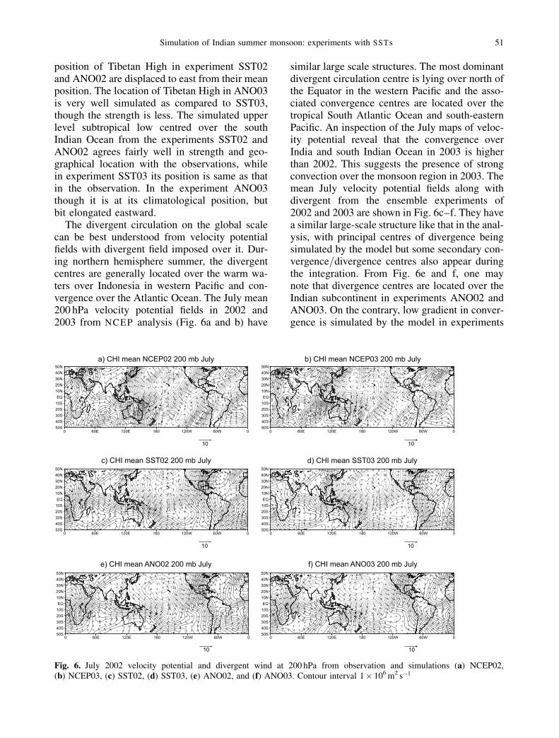
position of Tibetan High in experiment SST02and ANO02 are displaced to east from their meanposition. The location of Tibetan High in ANO03is very well simulated as compared to SST03,though the strength is less. The simulated upperlevel subtropical low centred over the southIndian Ocean from the experiments SST02 andANO02 agrees fairly well in strength and geo-graphical location with the observations, whilein experiment SST03 its position is same as thatin the observation. In the experiment ANO03though it is at its climatological position, butbit elongated eastward.

The divergent circulation on the global scalecan be best understood from velocity potentialfields with divergent field imposed over it. Dur-ing northern hemisphere summer, the divergentcentres are generally located over the warm wa-ters over Indonesia in western Pacific and con-vergence over the Atlantic Ocean. The July mean200 hPa velocity potential fields in 2002 and2003 from NCEP analysis (Fig. 6a and b) have

similar large scale structures. The most dominantdivergent circulation centre is lying over north ofthe Equator in the western Pacific and the asso-ciated convergence centres are located over thetropical South Atlantic Ocean and south-easternPacific. An inspection of the July maps of veloc-ity potential reveal that the convergence overIndia and south Indian Ocean in 2003 is higherthan 2002. This suggests the presence of strongconvection over the monsoon region in 2003. Themean July velocity potential fields along withdivergent from the ensemble experiments of2002 and 2003 are shown in Fig. 6c–f. They havea similar large-scale structure like that in the anal-ysis, with principal centres of divergence beingsimulated by the model but some secondary con-vergence=divergence centres also appear duringthe integration. From Fig. 6e and f, one maynote that divergence centres are located over theIndian subcontinent in experiments ANO02 andANO03. On the contrary, low gradient in conver-gence is simulated by the model in experiments

Fig. 6. July 2002 velocity potential and divergent wind at 200 hPa from observation and simulations (a) NCEP02,(b) NCEP03, (c) SST02, (d) SST03, (e) ANO02, and (f) ANO03. Contour interval 1� 106 m2 s�1

Simulation of Indian summer monsoon: experiments with SSTs 51

SST02 (Fig. 6c) and SST03 (Fig. 6d) over thisregion. The difference of velocity potential andcorresponding divergent wind from NCEP, ob-served SST experiments and persisted SSTA for2002 and 2003 are shown in Fig. 8a–c. One maynotice that divergent centre is located over Indiain observed SST experiments, as in NCEP anal-ysis but convergent is located in persisted SSTA

differences, showing inter-annual variation be-tween 2002 and 2003. Thus, the fraction of thevariance explained by the model seasonal fore-cast appears to be limited when only the SST

data are used for forcing the simulations. In otherwords, prescribing SST alone may not be justsufficient for successful seasonal forecasts; more-over, it underscores the importance of otherfeedbacks especially arising from the vegetationcover as the simulations reported here use onlybare soil. However, this proposition needs to beexamined further by using appropriate vegetationcover in the model. These investigations havebeen left for the future. One can also notice inFig. 6c and d, that model simulates a large gradientin divergent field in the equatorial Pacific Ocean in

Fig. 7. July 2002 velocity potential anomaly and divergent wind at 200 hPa from observation and simulations (a) NCEP02,(b) NCEP03, (c) SST02, and (d) SST03. Contour interval 1� 106 m2 s�1

Fig. 8. July 2002 velocity potential and divergent wind difference (a) NCEP03–NCEP02, (b) SST03–SST02, and(c) ANO03–ANO02. Contour interval 2� 106 m2 s�1

52 S. K. Deb et al

July 2003 and 2002 but fails to do so in experi-ments ANO02 (Fig. 6e) and ANO03 (Fig. 6f).The strong overturning associated with the east–west circulation (Krishnamurti, 1971) over mon-soon region in experiments SST02 and SST03resembles the observed overturning, while it isnot so strong in experiments ANO02 and ANO03.From the above discussion, it may be concludedthat the model has satisfactorily reproduced theaverage features of large-scale circulation in thesimulations. Next, the most sensitive parameterrainfall is analyzed with the help of mean fieldsand the empirical orthogonal functions analysis.

3.3 Observed and simulated mean rainfall

The mean July observed rainfall anomaly fromGPCP for the years 2002 and 2003 are shown inFig. 9a and b, respectively. From an inspection

the July 2002 mean rainfall anomaly (Fig. 9a)shows a vertical split in the rainfall pattern about80 E, poor rainfall region to its west and rela-tively good rainfall to its east with a maximumin its distribution occurring over the West Bengaland head Bay of Bengal region. On the otherhand, rainfall anomaly is homogeneously distrib-uted over most parts of India during July 2003.This is evident from the Fig. 9c showing thedifference of mean rainfall for the month of July2003 and 2002. The mean July summer monsoonrainfall anomaly from SST02 and SST03 areshown in Fig. 9d and e. The mean rainfallanomaly in experiment SST02 (Fig. 9d) showsa fair correspondence over land with observa-tions (Fig. 9a), with poor precipitation over thenorthwestern part of India and appreciable rain-fall over West Bengal, the head Bay region andTripura. But the model simulates unrealistically

Fig. 9. July rainfall anomaly (mm=day): (a) GPCP 2002 (Observed), (b) GPCP 2003 (Observed), (c) DIFF GPCP(2003–2002), (d) SST02, (e) SST03, (f) SST03–SST02, (g) ANO02, (h) ANO03, and (i) ANO03–ANO02

Simulation of Indian summer monsoon: experiments with SSTs 53

higher rainfall amounts over the Arabian Seawith another maximum lying west of WesternGhats. In the persisted SSTA experiment forANO02 the model simulated rainfall resembleswith observations with less rainfall over Indiansubcontinents. The July rainfall from the experi-ment SST03 (Fig. 9e) has a good correspondencewith July 2003 GPCP mean rainfall (Fig. 9b)over most parts of India except Western Ghats,where negative anomaly is present in the simula-tion. However, there is a strong maximum in therainfall over equator about 70 E, which is presentin GPCP rainfall (Fig. 9b), but bit weaker. Thus,the model produces reasonably well the distribu-tion and rainfall amounts for July 2003, but itdoes not happen for July 2002. An inspection ofthe July mean rainfall from experiment SST02reveals that the model has failed to simulate theobserved pattern (Fig. 9c), and one may note someprincipal deficiencies in the model simulation: atongue of dry region over northwest India includ-ing parts of Gujarat and relatively heavy rainfallover Himalaya and equatorial central IndianOcean. This tongue is not visible in 2002 experi-ments but clearly visible in 2003. In both SST03and ANO03 the rainfall over Western Ghats isnot simulated well. This may be due to the poorhorizontal resolution viz. 3.8� lon and 2.5� lat(Sabre et al, 2000) and non-inclusion of veg-etation in the model. It is also note that in thepresent simulation climatological soil-moisture,sea-ice and albedo are used, as we all know theimportance of evolving soil-moisture and relatedland-surface parameters for monsoon simulations(Douville et al, 2001; 2002; 2003).

Moreover, there is a striking similarity in themorphology of simulated rainfall from experi-ments ANO02 (Fig. 9g) and ANO03 (Fig. 9h)which is largely attributed to the similarity ofApril SST during two monsoon years. On theother hand, simulations forced with observedSST show resemblance in the rainfall over landregions in 2002 (Fig. 9d) with only minor differ-ences near Western Ghats. It has been found froman inspection of the weekly SST that there wereno significant differences in its evolution during2002 and 2003 and even the onset of these twomonsoons were of similar nature (Flatau et al,2003). But in reality there were huge differencesin the mean July rainfall between 2002 and 2003seasonal and inter-annual variations. This clearly

shows in the difference of observed rainfall forthese two years (Fig. 9c), which is not simulatedvery well in all the experiments (Fig. 9f andFig. 9i), though the observed SST experimentshas produced better picture as compared to theSSTA experiments. The mean July 2002 ob-served and simulated rainfall and their corre-sponding anomaly (Fig. 12) using 29th May 2002as initial condition are showing the sensitivity ofheat source over equatorial Indian Ocean in June2002. Heat source over Indian Ocean has im-proved the simulation quite a lot in July 2002.Figure 12g also shows the difference of July rain-fall over Indian subcontinent with and withoutusing heat source. Therefore, it is a very challeng-ing problem for modellers to identify the mech-anisms that cause such intense variations in themonsoon system and to understand the extent oftheir coupling (Krishnamurthy and Shukla, 2000;Sperber et al, 2000; Goswami and Ajaya Mohan,2001) which may also be responsible for theobserved variability both at intra-seasonal andinter-annual scales. In a recent paper, Molteniet al (2003) have examined the impact of SST

anomalies on inter-annual and intra-seasonal var-iations by performing several predictability ex-periments for the Asian summer monsoon. Theirfindings, though of mixed nature, shows a highcorrelation between observed and simulatedSVD-2 index (related to all-India rainfall index)is very encouraging for the prospects of numer-ical seasonal forecasting. We believe that vegeta-tion in conjunction with observed SST also playsan important role in modulating the intra-season-al variations of summer monsoon; however thisneeds to be quantified from a long series ofnumerical simulations with the model. A vegeta-tion model due to Ducoudre et al (1993) will beincorporated in the model for future investiga-tions on seasonal forecasting.

Further evaluation of simulations is done bycalculating the all-India rainfall time series fromthe June and July rainfall by comparing it withGPCP data ( Figs. 10 and 11) for all members ofthe ensemble experiments viz. one 10 membersand two 5 members ensembles consisting offive initial conditions each from April and Mayrespectively. The 5 members ensembles are de-noted by SSTapr02, SSTmay02, ANOapr02 andANOmay02 for SST02 and ANO02, respectively,and similar index for 2003 also. It is found that

54 S. K. Deb et al

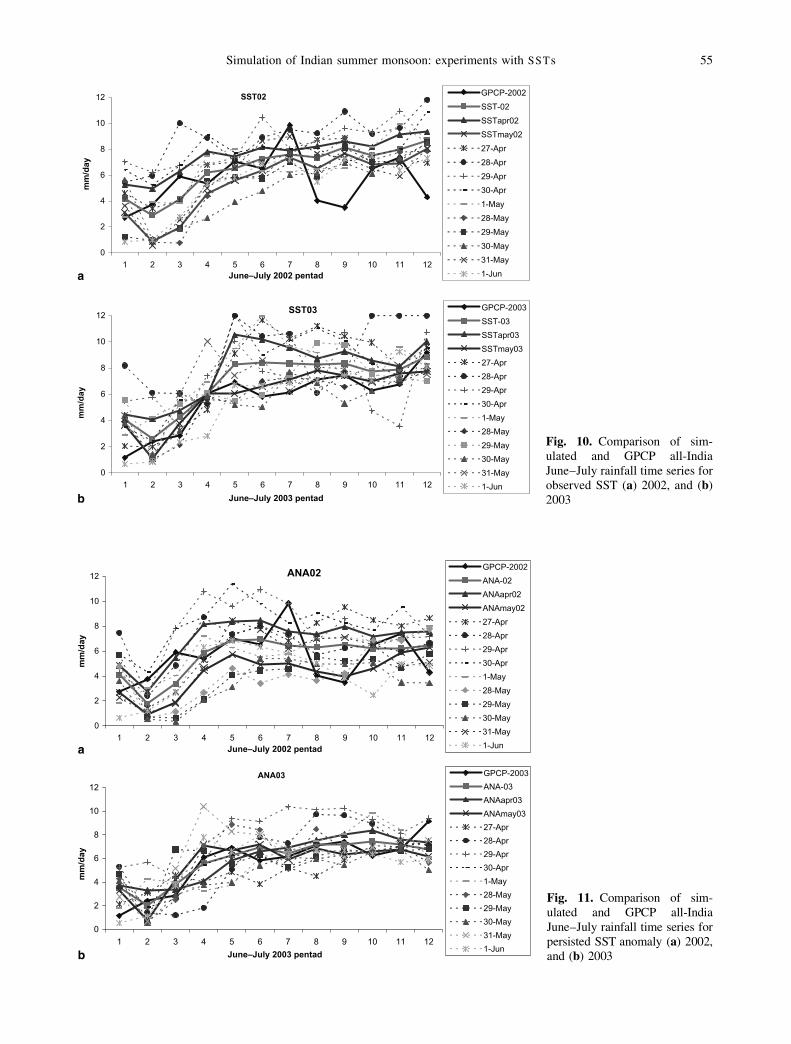
Fig. 11. Comparison of sim-ulated and GPCP all-IndiaJune–July rainfall time series forpersisted SST anomaly (a) 2002,and (b) 2003

Fig. 10. Comparison of sim-ulated and GPCP all-IndiaJune–July rainfall time series forobserved SST (a) 2002, and (b)2003

Simulation of Indian summer monsoon: experiments with SSTs 55

the rainfall time series are wide spread in thepersisted SST anomaly experiments as comparedto observed SST experiments for both the year.One may easily notice that the ensemble meanfrom the May initial condition come more closerto the observation as compared to the April en-semble mean in all experiments for both theyears. It is also notice that in 2002 model hasnot been able to capture the intra-seasonal vari-ability in July. Over a larger part of the givenperiod, except at its beginning and ending por-

tions, all three curves have a very close resem-blance in 2003. This is good news for the model,since it has reproduced very accurately the all-India rainfall time variations of the 2003 summermonsoon. Unfortunately, this has not happenedfor July 2002 summer monsoon, as it has notbeen able to simulate the large oscillation in July2003, which is a bad news for the model. Fur-thermore, the two sets of simulations only differin the specification of SST yet the all-India rain-fall is largely spread with persisted SSTA and

Fig. 12. 2002 July mean observed and simulated (29 May 2002 as IC) rainfall and its anomaly (a) GPCP, (b) Normal,(c) Heating, (d) Anomaly GPCP, (e) Anomaly normal, (f) Anomaly heating, (g) Heating normal

56 S. K. Deb et al

less with actual SST, it seems plausible to inferthat it is mostly caused by deficiencies in theconvective parameterization which affect theoverall quality of model simulations. This kindof observation has also been made by Molteniet al (2003) for the ECMWF model from pre-dictability experiments for the summer mon-soons. But Fig. 13 shows both pentad and dailyJune–July 2002 all-India rainfall time series for aparticular experiment in 2002 where equatorialheat source over Indian Ocean has been appliedand compared it with the experiment where noheat source has been added and with observedGPCP. It is found that application of heat sourceover Indian Ocean has able to capture the strongintra-seasonal oscillation in July 2002, but it hasunderestimated the June 2002 rainfall quite a bit.Nevertheless, the use of dynamical models forseasonal forecasting does get some vital supportfrom this mixed outcome about the behavior ofvariations in the simulated all-India summermonsoon rainfall. The all India cumulative rain-fall for the month of June and July for 2002 and2003 from all members of the ensemble andGPCP are shown in Table 2. From the Table

2a, it is evident that so far as cumulative Julyrainfall are concerned, the total rainfall simulatedin ANO02 and ANO03 are close to GPCP but inSST02 and SST03 it is overestimated. For June2002 (Table 2b) it is found that cumulative rain-fall by SST02 is a exactly match with GPCP, butin ANO02 it is underestimated by 13 mm forGPCP. In June 2003 both SST03 and ANO03have overestimated as compared to GPCP. Onemajor difficulty in evaluating the ensemble eva-luation arises due to large differences betweenthe GPCP and IMD rainfall (not given). TheGPCP only presents the average large-scale field.So it is appropriate to compare the model resultswith GPCP.

3.4 The principal components of observedrainfall

The empirical orthogonal functions of the GPCP

rainfall are calculated over the Indian regionwhich encompasses 56 model grid points. Theirtime series are also been normalized. The firstfour EOFs of the pentad rainfall series representmost part of the intra-seasonal variability of ISM

Fig. 13. Comparison of simulated and GPCPall-India June–July rainfall time series for2002 from two different simulation (with andwithout using heat source over equatorialIndian Ocean) (a) Pentad, and (b) Daily

Simulation of Indian summer monsoon: experiments with SSTs 57

Table

2a.

July

20

02

and

20

03

All

Ind

iaC

um

ula

tive

rain

fall

July

20

02

All

Ind

iaC

um

ula

tive

rain

fall

(mm

)

E-1

(27

apr)

E-2

(28

apr)

E-3

(29

apr)

E-4

(30

apr)

E-5

(01

may

)E

-6(2

8m

ay)

E-7

(29

may

)E

-8(3

0m

ay)

E-9

(31

may

)E

-10

(01

jun

)E

NS

-10

OB

S(G

PC

P)

SS

T0

22

30

.74

30

1.5

72

75

.46

24

7.4

02

29

.28

23

3.3

22

17

.97

20

5.1

22

1.9

22

05

.52

23

6.8

31

78

AN

O0

22

48

.99

19

1.9

12

28

.97

24

9.9

62

08

.28

16

7.1

41

55

.38

13

6.6

41

83

.66

13

4.9

01

90

.58

17

8

July

20

03

All

Ind

iaC

um

ula

tive

rain

fall

(mm

)

SS

T0

32

97

.47

32

5.3

52

15

.90

28

2.1

12

60

.46

21

3.1

82

44

.59

20

7.1

12

20

.67

22

9.0

82

49

.59

21

4.7

AN

O0

31

82

.87

25

0.5

72

87

.97

19

2.0

12

32

.80

19

8.2

61

90

.33

17

9.3

92

08

.20

91

87

.19

21

0.9

62

14

.7

Table

2b.

Jun

e2

00

2an

d2

00

3A

llIn

dia

Cu

mu

lati

ve

rain

fall

Jun

e2

00

2A

llIn

dia

Cu

mu

lati

ve

rain

fall

(mm

)

E-1

(27

apr)

E-2

(28

apr)

E-3

(29

apr)

E-4

(30

apr)

E-5

(01

may

)E

-6(2

8m

ay)

E-7

(29

may

)E

-8(3

0m

ay)

E-9

(31

may

)E

-10

(01

jun

)E

NS

-10

OB

S(G

PC

P)

SS

T0

21

44

.73

23

1.2

62

22

.86

21

6.8

21

61

.54

10

9.5

71

32

.07

59

9.6

21

34

.58

11

3.2

51

56

.63

15

6.7

AN

O0

21

28

.03

19

3.8

02

29

.78

23

9.2

41

39

.72

86

.07

88

.66

75

.32

12

9.7

11

20

.02

14

3.0

31

56

.7

Jun

e2

00

3A

llIn

dia

Cu

mu

lati

ve

rain

fall

(mm

)

SS

T0

31

64

.50

27

3.9

31

99

.81

20

4.3

82

10

.26

12

5.6

67

14

7.7

41

22

.46

18

6.4

69

9.9

81

73

.52

12

6.3

AN

O0

31

12

.61

11

3.3

31

97

.94

13

3.9

61

15

.66

15

8.9

31

53

.72

10

3.7

61

76

.50

13

8.7

81

40

.52

12

6.3

58 S. K. Deb et al

Fig. 14. Four leading EOFs ofJune–July GPCP pentad rainfallfor 2002 (a–d), and 2003 (e–h)

Simulation of Indian summer monsoon: experiments with SSTs 59

that arises from its inherent oscillations or dueto the passage of advective=convective systemsthrough this region. The first EOF of GPCP pen-tad rainfall (Fig. 14a) in 2002 explains a signifi-cant part (56%) of the total variance, while thesecond, third and fourth EOFs (Fig. 14b–d)jointly put together explain 28% (12%, 10%and 6%, respectively) of the total variance ofthe monsoon rainfall. Thus the first four EOFsexplain 84% of the total variance of the rain-

fall. However, the first four EOFs explain 86%(Fig. 14e–h) of the variance of June–July mon-soon rainfall. Most importantly, the leading EOF

in 2003 is far more dominant as it explains 71%of the variance as compared to 56% by the samein the preceding year. Obviously rainfall wasfairly homogenous over the entire country andthe effect of model variations on seasonal meanrainfall was much smaller because the varianceof rainfall in 2003 explained by second, third and

Fig. 15. Time series principalcomponents of GPCP 2002,SST02 and ANO02 (left panel)and GPCP 2003, SST03 andANO03 (right panel)

60 S. K. Deb et al

fourth EOFs is only 6%, 5% and 4% respec-tively; implying the dominance of active intra-seasonal variations on the rainfall in this year,while the opposite is true in 2002 monsoon(Kripalani et al, 2004). This evidently gives riseto a strong signal of inter-annual variability in ob-served monsoon rainfall of two successive years,where intra-seasonal variations have played a keyrole. The strong role of intra-seasonal variationsin determining the seasonal-mean variability of themonsoon has been earlier stressed by Goswamiand Ajay Mohan (2001). The EOF1 of eachmonsoon has a unimodal pattern with a maxi-mum in correlations (þ0.9). The region of max-imum correlations is oriented northeast and liesover West Bengal and Bangladesh during 2002,where as it practically covers entire India in 2003.The homogeneous pattern of EOF1 is associatedwith increased or decreased precipitation. Thestructure of the first EOF1 for 2002 has a verysimilar pattern to that is shown in a study byShukla (1987), there also a zone of higher valuesof correlations of the first function is noted overthe northeast India. He argued that higher valuesof the EOF1 are confined to those regions ofIndia, which show large correlations with theSouthern Oscillation. This is difficult to verifyhere with only two monsoon year data and a lon-ger time series is necessary. The correspondingtime series (PC1) of EOF1 of GPCP rainfall(Fig. 15a, e) of two monsoons represent the prog-ress of mean precipitation over India during eachyear and one may note the contrast in rainfallthere. Moreover, there is also a large variationin amplitude of PC1 (Fig. 15a) during July 2002due to the long break conditions in the monthof July; on the contrary amplitude of the PC1 of2003 (Fig. 15e) gradually increases and peaksduring the month of July which depicts the actualbehaviour of observed rainfall.

The second, third and fourth EOFs of precipi-tation for 2002 and 2003 also present some in-teresting results even though they explain muchlower proportion of the variance. EOF2 (Fig. 15b)for 2002 divides ISM region just into two parts,with strong positive correlations (þ0.6) in thewestern part and negative correlations (�0.3) inthe around the eastern part of India. This clearlyshows an east–west oscillation of the summerrains arising from the intra-seasonal variations ofthe summertime circulation. The time series PC2

(Fig. 15b) shows high frequency variations in themonth of July 2002. The EOF2 (Fig. 14f) for2003 divides India into three parts with positivecorrelations in the southern and northern region,and negative correlations lying in between them.This type of pattern in rainfall occurs over Indiaafter the onset of a break in monsoon; Fig. 14fshows its amplitude. This is still not a dominantmode since it explains a much smaller (6%) pro-portion of the variance. The EOF3 map (Fig. 15c)for 2002 indicates the presence of north–southoscillations in rainfall. The corresponding timeseries PC3 (Fig. 15c) possesses an oscillation ofhigh amplitude during first week of July. Themaps of EOF4 in 2002 and 2003 show the con-tribution of weather-scale disturbances (lows anddepression etc) to rainfall variability. The timeseries of EOF4 (Fig. 15d, h) is apparently com-posed of rapid oscillations as compared to thetime series of other EOFs. In what follows, therainfall from model ensembles is analyzed interms of the aforementioned leading components.

3.5 Analysis of simulated rainfallfrom model ensembles

The simulated precipitation from each modelensemble is projected on the EOFs of the GPCP

pentad rainfall discussed above. Hence the ob-served and model simulated rainfall anomalieshave common spatial structures defined by theEOFs (of observed rainfall) and consequently,the differences between these two fields shallappear in the corresponding expansion coeffi-cients or the principal component time series ofeach mode. It then becomes much easier to com-pare mode wise essential differences over theentire region from expansion coefficients timeseries of these two fields. The elegant mathemat-ical foundation of a projection method makes itone of the novel methods of evaluating a largebody of numerical simulations with greater easeand reliability. This procedure is robust andwhich could help in identifying the model defi-ciencies as well. The expansion coefficients se-ries of EOFs of the GPCP and simulated rainfallanomalies will be referred in the text as PCs(observed) and PCs (simulated), respectively. Ina recent study, Molteni et al (2003) have usedthe singular value decomposition (SVD) modeson which the model anomalies were projected

Simulation of Indian summer monsoon: experiments with SSTs 61

to analyze 850 hPa winds and precipitation.Bretherton et al (1992) have presented severalmethods and their intercomparison for finding thecoupled patterns in meteorological data whichcould be used effectively for evaluating the mod-el performance. Moreover, several authors haveapplied SVD to projections of meteorologicalfields on suitable subspaces spanned by dominantEOFs for studying the coupled patterns.

The pentad averages of precipitation are cal-culated from daily stored values in the simula-tions and subsequently the precipitation anomaliesare calculated. The two curves (Fig. 15a) of PC1(simulated) from the experiments SST02 andANO02 resemble the corresponding PC1 (ob-served) in 2002, except in July 2002 simulatedPC1 in both experiments have not been able tocapture the long break condition as like in PC1(observed). The time series of expansion coeffi-cients obtained by projecting the simulated rain-fall anomalies from experiments SST02 andANO02 on EOF2 (Fig. 15b) is showing an outof phase relationship with PC2 (observed) duringJuly 2002. Interestingly, the curves of PC3 (sim-ulated) from experiments SST02 and ANO02(Fig. 15c) show greater resemblance with the cor-responding curve of PC3 (observed). On the con-trary, it may be seen from the curves (Fig. 15d)of PC4 (simulated) that they do not show oscilla-tions of the kind, which are present in the PC4(observed). In a similar manner, the simulatedrainfall anomaly values from model ensemblesfor 2003 were projected on to the EOFs of the2003 GPCP rainfall. The curves (Fig. 15e) ofexpansion coefficients series from experimentsSST03 and ANO03 show very good resemblewith PC1 (observed) for 2003 monsoon (Fig. 15e).PC2 (observed) and PC2 (simulated) has alsovery good agreement with each other (Fig. 15f).The curve (Fig. 15g) of PC3 (observed) showsonly one oscillation. Notably, the PC3 (simu-lated) of experiments SST03 and ANO03 agreewith observations in June but in July they are outof phase. The PC4 (simulated) resemble eachother (Fig. 15h) to some extent with PC4 (ob-served), which possesses high frequency oscilla-tions (Fig. 15h). From the above discussion, itmay be inferred that PC1 (simulated) and PC2(simulated) resemble very well to PC1 (ob-served) and PC2 (observed) in 2003 and in 2002PC2 (simulated) agrees well with PC2 (observed).

4. Conclusions

The seasonal hindcasting of Indian summer mon-soons of 2002 and 2003 has been studied fromensemble experiments that have been performedusing a general circulation model by changingSSTs for different experiments. The model couldserve as a tool for seasonal forecasting becausecertain parameters of interest like precipitation,the low level and upper level features of thelarge-scale circulation are satisfactorily repro-duced in the simulations. The simulated ISM pre-cipitation values in model forced by persistedSSTA, are generally wide spread in comparisonto those produced in numerical experiments withprescribed SST. Moreover, the model simulatesa tongue of dry region in northwestern part ofIndia, in contravention to observations, in allsimulations and has a tendency to produce higherrainfall over Himalaya. This is indicative of cer-tain deficiencies in the parameterization of con-vection, which has to be looked upon. Fivemembers ensemble from May initial conditionhas come very close to the observed as comparedto the other five member ensemble from Aprilinitial condition in all experiment. This showsthat initial condition plays a significant role inthe seasonal forecasting simulation. Thus, theprobability of a useful seasonal forecast froma model is higher if the summer monsoon isgoing to be good, possibly because the strongcorrelations between ISM rainfall and SST arereproduced in the simulations. However, if intra-seasonal oscillations dominate, then model pro-duced rainfall variations may depend on otherfactors besides SST, which is evident from SST02and ANO02 experiment where model fails toproduce the long break condition in July 2002.But equatorial heat source over Indian Ocean issuccessful in producing the long break conditionin July 2002 over India, as compared to anymember of SST02. This concludes that July2002 rainfall over India was strongly modulatedby the heating over equatorial Indian Ocean.Nevertheless, the observed SST model ensemblesdo provide a signal about the overall expectedbehavior of the monsoon.

It has been observed that the time series ofexpansion coefficients (PCs) obtained by project-ing the simulated rainfall on observed EOFs alsoprovide a framework for comparing model simu-

62 S. K. Deb et al

lations and their evaluation with observed data.It has been observed that PC1 (simulated) andPC2 (simulated) resemble reasonably well to PC1(observed) and PC2 (observed) for 2003 and PC3(simulated) and PC3 (observed) for 2002. PC2appears to be very sensitive to the specificationof the SST in the model in 2002. In other words,PC2 may serve as a parameter to design an ap-propriate measure to evaluate a seasonal forecast.This appears to be a major problem with themodel, but requires a separate study based onseveral monsoon years. A study on the relation-ship of rainfall of each year with SST of that yearis very much warranted. In conclusion, it maybe mentioned that seasonal forecasting fromAGCMs has a very bright prospect.

Acknowledgement

The research has been supported by the Council for Scien-tific and Industrial Research (CSIR), New Delhi underthe project ‘‘Adoption, development and evaluation of a vari-able AGCM (VRAM) for monsoon region’’ under NMITLI

scheme. Laurent Fairhead (LMD) and Marie-Angile Filiberti(IPSL) are acknowledged for providing ECMWF initial andboundary conditions data to make this study possible.

References

Arakawa A (1966) Computational design for long-termnumerical integrations of the equations of atmosphericmotion. J Comput Phys 1: 119–143

Barnston AG, Mason SJ, Goddard L, DeWitt DG, Ziebiak S(2003) Multimodel ensembling in seasonal forecasting atIRI. Bull Am Meteor Soc 8(4): 1783–1796

Bedi HS, Bindra MMS (1980) Principal components ofmonsoon rainfall. Tellus 32: 296–298

Brankovic C, Palmer TN (2000) Seasonal skill and pre-dictability of ECMWF PROVOST ensembles. Q J RoyMeteorol Soc 126: 2035–2067

Bretherton CS, Smith C, Wallace JM (1992) An intercom-parison of methods for finding coupled patterns in climatedata. J Climate 5: 541–560

Charney JG, Shukla J (1981) Predictability of monsoons.In: Monsoon dynamics (Lighthill J, Pearce RP, eds).Cambridge University Press, pp 99–109

Douville H (2002) Influence of soil moisture on the Asianand African monsoons. Part 2: Inter-annual variability.J Climate 15: 701–720

Douville H (2003) Assessing the influence of soil moistureon seasonal climate variability with AGCMs. J HydroMeteorol 4: 1044–1066

Douville H, Chauvin F, Broqua H (2001) Influence of soilmoisture on the Asian and African monsoons. Part 1. Meanmonsoon and daily precipitation. J Climate 14: 2381–2403

Ducoudre N, Laval K, Perrier A (1993) SECHIBA, a newset of parameterizations of hydrologic exchanges at the

land=atmosphere within LMD atmospheric general cir-culation model. J Climate 6: 284–273

Flatau MK, Flatau PJ, Daniel Rudnick (2001) The dynamicsof double monsoon onsets. J Climate 14: 4130–4146

Flatau MK, Flatau PJ, Schmidt J, Kiladis GN (2003) De-layed onset of the 2003 Indian monsoon. Geophys ResLett 30(14): 1768 (DOI: 10.1029=2003GL017424)

Fouquart Y, Bonnel B (1980) Computations of solar heatingof the earth’s atmosphere: a new parameterization. BeitrPhys Atmos 53: 35–62

Gadgil S, Vinayachandran PN, Francis PA (2003) Droughtsof the Indian summer monsoon: Role of clouds over theIndian Ocean. Curr Sci 85(12): 1713–1719

Goddard L, Mason SJ (2002) Sensitivity of seasonal climateforecasts to persisted SST anomalies. Climate Dyn 19:619–631

Goswami BN, Ajai Mohan RS (2001) Intra-seasonal oscilla-tions and inter-annual variability of the Indian summermonsoon. J Climate 14: 1180–1198

Hourdin F, Armengaud A (1999) On the use of finite volumemethods for atmospheric advection of trace species: I.Test of various formulations in a general circulationmodel. Mon Wea Rev 127: 822–837

Ji M, Behringer DW, Leetmma A (1998) An improvedcoupled model for ENSO prediction and implicationsfor ocean initialization, Part 2: The coupled model.Mon Wea Rev 126: 1022–1034

Kripalani RH, Kulkarni A, Sabade SS, Revadekar JV,Patwardhan SK, Kulkarni JR (2004) Intra-seasonal oscil-lations during monsoon 2002 and 2003. Curr Sci 87(3):325–331

Krishnamurti TN (1971) Tropical east–west circulationsduring northern summer. J Atmos Sci 28: 1342–1347

Krishnamurti TN, Bhalme HN (1976) Oscillations of amonsoon system. Part 1: Observational aspects. J AtmosSci 33: 1937–1954

Krishnamurti TN, Kishtawal CM, LaRow T, Bachiochi D,Zhang Z, Williford CE, Gadgil S, Surendran S (1999)Improved skills for weather and seasonal climate forecastsfrom multi-model superensemble. Science (September 3)

Krishnamurti TN, Kishtawal CM, LaRow T, Bachiochi D,Zhang Z, Williford CE, Gadgil S, Surendran S (2000)Multi-model superensemble forecasts for weather andseasonal climate. J Climate 13: 4196–4216

Krishnamurthy V, Shukla J (2000) Intra-seasonal andinter-annual variability of rainfall over India. J Climate13: 4366–4377

Krishnan R, Majumder M, Vaidya V, Ramesh KV, Satyan V(2003) The abnormal Indian summer monsoon of 2000.J Climate 16: 1177–1194

Kumar A, Hoerling MP (1995) Prospects and limitationsof seasonal atmospheric GCM predictions. Bull AmerMeteor Soc 76: 335–345

Le Treut H, Li ZX, Forichon M (1994) Sensitivity study ofLMD GCM to green house forcing associated with twodifferent cloud water parameterization. J Climate 7:1827–1841

Lott F, Miller M (1997) A new subgrid scale orographic dragparameterization: its testing in the ECMWF model. Q JRoy Meteorol Soc 123: 101–127

Simulation of Indian summer monsoon: experiments with SSTs 63

Madden RA, Julian PR (1994) Observations of 40–50-daytropical oscillations – a review. Mon Wea Rev 122: 814–836

Molteni F, Corti S, Ferranti L, Slingo JM (2003) Predict-ability experiments for the Asian summer monsoon:Impact of SST anomalies on inter-annual and intra-sea-sonal variability. J Climate 16: 4001–4021

Morcrette JJ, Fouquart Y (1985) On systematic errors inparameterized calculations of long wave radiation trans-fer. Q J Roy Meteorol Soc 111: 691–708

Palmer TN, Brankovic C, Molteni F, Tibaldi S (1990)Extended range predictions with ECMWF models:Inter-annual variability in operational model integrations.Q J Roy Meteorol Soc 116: 799–834

Palmer TN, Brankovic C, Viterbo P, Miller MJ (1992)Modelling inter-annual variations of summer monsoons.J Climate 5: 399–417

Palmer TN, Alessandri A, Andersen U, Cantelaube P, DaveyM, Deque M, Diez E, Doblas-Reyes FJ, Feddersen H,Graham R, Gualdi S, Gueremy J-F, Hagedorn R,Hoshen M, Keenlyside N, Latif M, Lazar A, MaisonnaveE, Marletto V, Morse AP, Orfila B, Rogel P, Terres J-M,Thomson MC (2004) Development of a European multi-model ensemble system for seasonal to inter-annualprediction (DEMETER). Bull Amer Meteor Soc 85(6):853–872

Rasmusson EM, Carpenter TH (1983) The relationshipbetween eastern equatorial Pacific sea-surface temperatureand rainfall over India and Sri Lanka. Mon Wea Rev 111:517–528

Rowell DP (1998) Assessing potential seasonal predictabil-ity with an ensemble of multidecadal GCM simulations.J Climate 11: 109–120

Sabre M, Hodges K, Laval K, Polcher J, Desalmand F (2000)Simulation of monsoon disturbances in the LMD GCM.Mon Wea Rev 128: 3752–3771

Sadourny R, Laval K (1984) January and July performancesof LMD general circulation model: In new perspectivein climate modelling (Berger AL, Nicolis C, eds). ElsevierPress, pp 173–198

Sharma OP, Le Treut H, Seze G, Fairhead L, Sadourny R(1998) Inter-annual variations of summer monsoons: Sen-sitivity to cloud radiative forcing. J Climate 11: 1883–1905

Sharma OP, Upadhyaya HC, Harzallah A, Sadourny R(2003) Preparing area averaged rainfall on a regular grid

from scattered rain gauge data. J Comp Meth Sci Engg(in press)

Shukla J (1987) Inter-annual variability of monsoon. InMonsoons (Fein JS, Stephens PL, eds). New York: Wiley,pp 399–463

Sikka DR (2003) Evaluation of monitoring and forecastingof summer monsoon over India and a review of monsoondrought of 2002. Proc Indian Natl Sci Acad 69(A-5):479–504

Soman MK, Slingo JM (1997) Sensitivity of the Asiansummer monsoon to aspects of the sea-surface tempera-ture anomalies in the tropical Pacific Ocean. Q J RoyMeteorol Soc 123: 309–336

Sperber KR, Palmer TN (1996) Interannual tropical rainfallvariability in general circulation model simulations asso-ciated with the AMIP. J Climate 11: 2727–2750

Sperber KR, Slingo JM, Annamalai H (2000) Predictabilityand the relationship between subseasonal and interannualvariability during the Asian summer monsoon. Q J RoyMeteorol Soc 126: 2545–2574

Tiedtke M (1989) A comprehensive mass flux scheme forcumulus parameterization in large-scale models. MonWea Rev 17: 1779–1800

Van Leer B (1977) Towards the ultimate conservative dif-ference scheme IV: A new approach to numerical con-vection. J Comput Phys 23: 276–299

Van Leer B (1979) Towards the ultimate conservative dif-ference scheme: V: A second-order sequel to Godunov’smethod. J Comput Phys 32: 101–136

Walker GT (1923) Correlations of seasonal variations ofweather. VIII: A preliminary study of world weather.Mem India Meteor Dept 24: 75–131

Watanabe M, Shinoda M (1996) Long-term variability ofAsian summer monsoon rainfall, during 1946–1988.J Meteor Soc Japan 74: 923–931

Xie P, Janowiak JE, Arkin PA, Adler R, Gruber A, Ferraro R,Huffman GJ, Curtis S (2003) GPCP pentad precipitationanalyses: an experimental data set based on gauge obser-vations and satellite estimates. J Climate 16: 2197–2214

Corresponding author’s address: Sanjib Kumar Deb,Centre for Atmospheric Sciences, I. I. T. Delhi, NewDelhi-110016, India (E-mail: sanjib_deb@rediffmail.com;deb_sk2001@yahoo.co.in)

64 S. K. Deb et al: Simulation of Indian summer monsoon: experiments with SSTs