Sea surface temperature associations with the late Indian summer monsoon

P. Terray Æ P. Delecluse Æ S. Labattu Æ L. Terray

Sea surface temperature associations with the late Indian summermonsoon

Received: 15 January 2003 / Accepted: 18 August 2003 / Published online: 23 October 2003� Springer-Verlag 2003

Abstract Recent gridded and historical data are used inorder to assess the relationships between interannualvariability of the Indian summer monsoon (ISM) andsea surface temperature (SST) anomaly patterns over theIndian and Pacific oceans. Interannual variability ofISM rainfall and dynamical indices for the traditionalsummer monsoon season (June–September) are stronglyinfluenced by rainfall and circulation anomalies ob-served during August and September, or the late Indiansummer monsoon (LISM). Anomalous monsoons arelinked to well-defined LISM rainfall and large-scalecirculation anomalies. The east-west Walker and localHadley circulations fluctuate during the LISM ofanomalous ISM years. LISM circulation is weakenedand shifted eastward during weak ISM years. Therefore,we focus on the predictability of the LISM.Strong (weak) (L)ISMs are preceded by significant po-sitive (negative) SST anomalies in the southeasternsubtropical Indian Ocean, off Australia, during borealwinter. These SST anomalies are mainly linked to southIndian Ocean dipole events, studied by Besera andYamagata (2001) and to the El Nino-Southern Oscillation(ENSO) phenomenon. These SST anomalies are highlypersistent and affect the northwestward translation ofthe Mascarene High from austral to boreal summer. Thesoutheastward (northwestward) shift of this subtropicalhigh associated with cold (warm) SST anomalies offAustralia causes a weakening (strengthening) of thewhole monsoon circulation through a modulation of thelocal Hadley cell during the LISM. Furthermore, it issuggested that the Mascarene High interacts with the

underlying SST anomalies through a positive dynamicalfeedback mechanism, maintaining its anomalous posi-tion during the LISM. Our results also explain why astrong ISM is preceded by a transition in boreal springfrom an El Nino to a La Nina state in the Pacific andvice versa. An El Nino event and the associated warmSST anomalies over the southeastern Indian Oceanduring boreal winter may play a key role in the devel-opment of a strong ISM by strengthening the localHadley circulation during the LISM. On the other hand,a developing La Nina event in boreal spring and summermay also enhance the east–west Walker circulationand the monsoon as demonstrated in many previousstudies.

1 Introduction

The Asian summer monsoon is a dominant feature ofthe boreal summer atmospheric circulation. The Asianmonsoon region may be defined as the areas where boththe atmospheric circulation and associated precipitationregime reverse with season. However, it is now recog-nized that three major subcomponents can be identifiedin the Asian monsoon system: the Indian summermonsoon (ISM), the East Asian summer monsoon(EASM) and the western North Pacific summer mon-soon (WNPSM). The interested readers are referred tothe works of Lau et al. (2000) and Wang et al. (2001) forfurther details. Prediction of the Asian summermonsoon, particularly the ISM, is one of the majorchallenges of climate research (Webster et al. 1998).

In the context of ENSO-monsoon relationships, theWNPSM and EASM seem more predictable than theISM since WNPSM and EASM rainfall anomalies aresignificantly correlated with Nino3.4 sea surface tem-perature (SST) anomaly in the preceding winter. On theother hand, many investigators have found it very dif-ficult to interpret lead-lag relationships between the ISM

P. Terray (&) Æ P. Delecluse Æ S. LabattuLaboratoire d�Oceanographie Dynamique et de Climatologie,Paris, FranceE-mail: [email protected]

P. TerrayUniversite Paris 7, Paris, France

L. TerrayCERFACS, Toulouse, France

Climate Dynamics (2003) 21: 593–618DOI 10.1007/s00382-003-0354-0

and ENSO, given that both are phase-locked to theannual cycle (Webster and Yang 1992). A strong (weak)ISM often occurs in the developing phase of La Nina (ElNino) events (Wang et al. 2001; Meehl and Arblaster2002a). Thus, attempts to ascribe cause and effect toeither ENSO or the ISM are not likely to be very illu-minating. The ‘‘boreal spring barrier’’ in ENSO indices(Torrence and Webster 1998) explains why these indicesare not good predictors for the ISM, though manystudies have attempted to use ENSO as a base predictor(Webster et al. 1998). Despite a very long history ofresearch, the potential predictability of the ISM is stillthe subject of much debate and investigation both withnumerical (coupled) models and observational analysis.However, up to now, the statements of Normand (1953)with regard to the ISM are still valid: ‘‘The Indianmonsoon therefore stands out as an active, not a passivefeature in world weather, more efficient as a broadcast-ing tool than an event to be forecast’’.

Despite the pessimistic conclusion of Normand(1953) some recent studies have suggested that ISMrainfall variability consists of a large-scale persistentrainfall anomaly and an independent fluctuating intra-seasonal component (Webster et al. 1998, Krishnamur-thy and Shukla 2000). In this conceptual framework,predictability of the ISM depends on the relative con-tributions of these two components. The mechanismsresponsible for this persistent rainfall anomaly are notwell understood. Furthermore, other studies suggest thatISM rainfall interannual variability is primarily the re-sult of different manifestations of the intraseasonalvariability associated with the duration/intensity of ac-tive cycles during the monsoon season (Palmer 1994;Annamalai et al. 1999; Lawrence and Webster 2001).Consequently, a first step toward achieving a betterunderstanding of ISM predictability is to characterizethe influences of the various surface boundary conditions(SST, snow cover and mass, soil moisture) on the ISMsubsystem as suggested by Charney and Shukla (1981).

The relationship between tropical SST and the ISMhas been the subject of many studies in the past decades.Due to its close proximity and the importance of boththe land-sea meridional thermal contrast and the SST-convection relationship for the strength of the ISM, theIndian Ocean may play a role in ISM interannual vari-ability. Historically, however, the Indian Ocean has beenviewed as a passive element of the ISM system (Websteret al. 1998). Most previous observational studies haveconcluded that the Indian Ocean has no significantinfluence on ISM interannual variability, due to the lackof a significant relationship between various ISM indicesand Indian Ocean SST (Shukla 1987; Webster et al.1998). On the other hand, a number of recent modelingstudies have demonstrated that Indian Ocean SSTanomalies in certain areas under certain conditions cansignificantly affect the ISM variability (Chandrasekarand Kitoh 1998; Meehl and Arblaster 2002b). However,most of the previous studies have focused either onnorthern or equatorial Indian Ocean SST and their

relationships with convection during boreal summer.Very few studies have drawn attention to the southernIndian Ocean and its relationships to the ISM variabilitysince earlier studies by Krishnamurti and Bhalme (1976),Cadet (1983) and Meehl (1987) that have suggested ashift of the Mascarene High in association with mon-soon strength.

In the present study, we will reassess the relativeimportance of Indian Ocean SST on ISM variability inlight of recent advances in Indian Ocean climate research(Webster et al. 1999; Saji et al. 1999; Behera andYamagata 2001). The focus is on the interannual vari-ability and predictability of ISM rainfall and circulation.We are primarily concerned with the nature of predict-ability and its link to local (IndianOcean) and remote SSTforcing.Ourmost important result is that southern IndianOcean SST anomaly is a major precursory signal for theISM. This result is fundamental to the predictability ofISMrainfall since the IndianOcean SST anomaly appearsone or two seasons before the ISM onset.

The datasets and methods used in this study are de-scribed in Sect. 2. Section 3 depicts the temporal andspatial structures of ISM rainfall and circulation vari-ability. Observational analysis of the ISM-SST relation-ships is presented in Sect. 4, with conclusions in Sect. 5.

2 Data and methods

The monthly (June–September) area weighted rainfall series foreach of the 29 Indian meteorological subdivisions and the areaweighted monthly rainfall series for all India, for the period 1871–1998, have been used in this study in order to describe ISMrainfall variability over the Indian subcontinent (Parthasarathyet al. 1995).

The circulation associated with ISM rainfall has been examinedby using National Centers for Environmental Prediction (NCEP)reanalysis datasets (Kalnay et al. 1996). Monthly mean sea levelpressure (SLP), winds and stream function at standard pressurelevels from the reanalysis data for the period January 1948 toDecember 1999 were used in most calculations, though streamfunction data were only available from 1958. The empiricalorthogonal function (EOF) reconstructed SST analysis of Smithet al. (1996) during the period 1950–1998 (hereinafter referred to asthe Reynolds SST analysis) are used to study lead-lag relationshipsbetween the ISM and Indo-Pacific SST.

We also examine the surface wind and SST data from theComprehensive Ocean–Atmosphere Data Set (COADS) in order tovalidate our findings. The COADS data used here cover the period1948–1992. The noisy nature of the COADS data was partiallyovercome by averaging the observations over different key areas.The monthly time series for the different areas were determined asfollows:

1. First, the 1950–1980 interval was used as a reference period incalculating a climatology for each calendar month and each 2�box from the COADS dataset, provided that data for at least10 years with more than five observations per month wereavailable in the period. The monthly means for each i grid pointand j month were computed as a weighted average

�Xij ¼X1980

k¼1950WijkXijk

!=

X1980

k¼1950Wijk

!

where Wijk ¼ 1� expð�Nijk=5Þ

594 Terray et al.: Sea surface temperature associations with the late Indian summer monsoon

Here Xijk is the value computed for the ith box, jth month andkth year. Nijk is the number of ship-observations used incomputing Xijk . Wijk is in the neighborhood of 1 if Nijk > 10and near 0.5 if Nijk equals 5.

2. After this first step, time monthly anomaly series for each 2�box during the 1950–1980 period were computed by simplysubtracting from each value this climatology, provided thatneither the datum nor the climatology were missing. Theseanomalies were then spatially averaged over the selected areasby using the same weighting scheme (e.g., Wijk) as used in thecomputation of the climatology.

Various ENSO indices (SST Nino3, SLP Darwin and Tahititime series) are finally adapted from the NCEP website (http://www.cpc.ncep.noaa.gov/). From the SLP Tahiti and Darwin timeseries, a Southern Oscillation Index (SOI) was simply derived as thedifference of the monthly (or seasonally) standardized values (zeromean and unit variance) at both stations (Tahiti minus Darwin).

Composite and correlation analyses have been performed tohighlight the space-time structure of ISM variability and thecomplex SST-ISM relationships. For all correlations computed inthis study the statistical significance of the result has been assessedwith a classical two tail t-test without taking into account the serialcorrelation of the time series. This is justified by the fact that all thecorrelations are based on yearly sampled series (a large timeincrement) showing white noise spectra and insignificant lag-1autocorrelations. When computing a correlation with a time seriesfrom COADS, the standardized anomalies for the other time seriesare always computed with respect to a climatology computedfrom the 1950–1980 period. A new method was used in order toreplace the more common (and inappropriate) Student�s t-test toestablish the significance of our composites. The procedure wasadapted from French statistical literature (Lebart et al. 1995, pp.181–182) and is described in Appendix 1. As designed, the proce-dure aims at determining the aspects of our composites that aresignificantly distinct from the background variability in the avail-able data, not in a hypothetical population. This procedure isappropriate for exploratory studies and tries to cure some of theproblems raised by Nicholls (2001) on the insignificance of signif-icance testing in climate research. All the critical probabilitiesassociated with our composites are calculated with this method.Note finally that various significance levels (0.1, 1, 10%) are plottedon the figures in agreement with the suggestions of Nicholls (2001).

Wavelet analysis (Torrence and Compo 1998) has been used toreveal the temporal structure of the various time series. Morletwavelet transforms display the variance of a time series as a con-tinuous function of time and frequency. In addition, a globalwavelet spectrum can be deduced from the wavelet spectrum. Sig-nificance testing using a white noise background has been donefollowing Torrence and Compo (1998) for most time series.

3 Dominant modes of seasonal variationsin the Indian summer monsoon

To discuss the interannual variability of the ISM, ameasure of ISM strength must be defined. There haverecently been considerable investigations on the defini-tion of valuable rainfall or dynamical monsoon indices.Wang and Fan (1999) compared a variety of dynamicalindices computed from the NCEP reanalysis and con-cluded that large discrepancies still exist during someyears between convection/rainfall and dynamical indicesfor the ISM. Annamalai et al. (1999) studied thebehavior of the ISM using ERA and NCEP reanalysesand suggested that the All India Rainfall Index (AIRI)defined by Parthasarathy et al. (1995) is currently themost accurate measure of rainfall over the Indian

subcontinent. Consequently, we first reexamine themonthly and seasonal AIRI in order to describe themain features of ISM rainfall variability over India.

Table 1 presents basic statistics (means and standarddeviations) of the monthly AIRI. The correlationsamong the monthly AIRI during boreal summer as wellwith the seasonal AIRI are also given in Table 1. Allthese statistics have been computed during the 1871–1998 period. India experiences a maximum in precipi-tation in July, with a rapid decline in September. Thelatter is related to the fact that the monsoon has alreadywithdrawn from the northern parts of India in Septem-ber (Krishnamurthy and Shukla 2000). However, theinterannual variability of the seasonal AIRI is alsolinked to the interannual variability of the late Indiansummer monsoon (LISM), during August and Septem-ber. Both standard deviations of the monthly AIRI andthe correlation of these indices with the seasonal AIRIincrease from the onset (June) to the withdrawal of theISM (September). It is noteworthy that the correlationbetween the June and seasonal AIRI is only 0.38, whilethe correlation between the September and seasonalAIRI is as high as 0.64. Another interesting feature isthat correlations between succeeding monthly AIRI alsoincrease during the boreal summer. This supports thenotion of a seasonally persistent rainfall anomaly pat-tern, at least for the months of the LISM (Webster et al.1998; Krishnamurthy and Shukla 2000). The precedingresults also suggest that the mechanisms sustaining ISMinterannual variability are somewhat different during theearly and late ISM (Ailikun and Yasunari 2001).

In order to further investigate these aspects of ISMvariability, EOF analysis of the seasonal rainfallanomalies over the 29 meteorological Indian subdivi-sions during the 1871–1998 period has been performed.The EOFs and the associated principal components arecomputed from the correlation matrix of the anomalies.The first three EOFs of the standardized seasonalanomalies are shown in Fig. 1. The spatial loadingsassociated with each EOF can be interpreted as corre-lation coefficients between the corresponding principalcomponent (PC) and the ISM rainfall time series of the

Table 1 Means, standard-deviations of monthly AIR indices andcross-correlations among seasonal (AIRI) and monthly (AIRI6,AIRI7, AIRI8, AIRI9) AIR indices during the 1871–1998 period.Statistical significance has been assessed with a classical two tailt-test. See the text for the definition of the indices

AIRI6 AIRI7 AIRI8 AIRI9

Mean 163.3 273.9 243.6 171.1STD 36.4 36.5 38.2 37.7

Correlations

AIRI 0.38*** 0.59*** 0.59*** 0.65***AIRI6 1AIRI7 –0.01 1AIRI8 –0.05 0.10 1AIRI9 –0.06 0.24** 0.24** 1

*:P < 0.05; **:P < 0.01; ***:P < 0.001

Terray et al.: Sea surface temperature associations with the late Indian summer monsoon 595

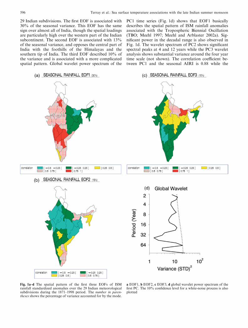
29 Indian subdivisions. The first EOF is associated with30% of the seasonal variance. This EOF has the samesign over almost all of India, though the spatial loadingsare particularly high over the western part of the Indiansubcontinent. The second EOF is associated with 13%of the seasonal variance, and opposes the central part ofIndia with the foothills of the Himalayas and thesouthern tip of India. The third EOF described 10% ofthe variance and is associated with a more complicatedspatial pattern. Global wavelet power spectrum of the

PC1 time series (Fig. 1d) shows that EOF1 basicallydescribes the spatial pattern of ISM rainfall anomaliesassociated with the Tropospheric Biennial Oscillation(TBO; Meehl 1997; Meehl and Arblaster 2002a). Sig-nificant power in the decadal range is also observed inFig. 1d. The wavelet spectrum of PC2 shows significantspectral peaks at 4 and 12 years while the PC3 waveletanalysis shows substantial variance around the four yeartime scale (not shown). The correlation coefficient be-tween PC1 and the seasonal AIRI is 0.88 while the

Fig. 1a–d The spatial pattern of the first three EOFs of ISMrainfall standardized anomalies over the 29 Indian meteorologicalsubdivisions during the 1871–1998 period. The number in paren-theses shows the percentage of variance accounted for by the mode.

a EOF1, b EOF2, c EOF3, d global wavelet power spectrum of thefirst PC. The 10% confidence level for a white-noise process is alsoplotted


correlation coefficient between PC2 and the seasonalAIRI is only –0.16 and is insignificant at the 5% level.Interestingly, PC3 has also a high and significant cor-relation (0.42) with the AIRI. In summary, these resultssuggest that EOF1 is associated with the dominant modeof ISM rainfall interannual variations over India. Fur-ther substantiating this finding, we note that the spatialpattern depicted by EOF1 shows striking similarities tothe flood or drought ISM rainfall composites presentedby Terray (1995) or Krishnamurthy and Shukla (2000).

The atmospheric circulation associated with thedominant modes of ISM rainfall variations is nowexamined using the NCEP-NCAR reanalysis and theCOADS dataset. We have used three dynamical mon-soon indices from the NCEP-NCAR reanalysis in orderto link the rainfall variability to the broad-scale ISMcirculation in this study. The three dynamical indices are:

1. The Indian Monsoon Index 1 (IMI1) suggested byWang et al. (2001), defined as the difference of thestandardized zonal wind anomalies at 850 hPa be-tween a southern region of 5�–15�N, 40�–80�E and anorthern region of 20�–30�N, 70�–90�E. Thisdynamical index reflects the intensity of the westerlyflow over the Arabian Sea and the lower tropo-spheric vorticity anomalies associated with theRossby wave response to the ISM trough and con-vective heating.

2. In summer, southwesterlies at the surface andnortheasterlies at upper levels prevail over the Asianregion. At 1000 hPa, the flow of the SouthernHemisphere crosses the Equator mainly near theAfrican coast and forms the Somali jet. At 200 hPa,the most outstanding feature is a huge anticycloniccirculation, the Tibetan Plateau High, centered overthe southern part of the Tibetan Plateau. At thislevel, the cross-equatorial flow from the NorthernHemisphere to the Southern Hemisphere is mainlyconcentrated along the southeastern periphery ofthe Tibetan High. Therefore, another ISM dynam-ical index may be defined as the difference betweenthe standardized wind anomaly on the southwest–northeast axis at 1000 hPa, area-averaged over theregion 43�E–55�E, 5�S–11�N (hereafter Somali jetarea), and the standardized wind anomaly on thesouthwest–northeast axis at 200 hPa area-averagedover the region 70�E–110�E, 5�N–30�N (hereafterthe Tibetan High area). Hereafter, this time series isreferred to as the Indian Monsoon Index 2 (IMI2).

3. Finally, the Indian Ocean meridional wind shearindex (VSI) is defined as the difference between thestandardized meridional wind anomalies at 1000and 200 hPa area-averaged over the same regionsused to define IMI2. The VSI is similar to theMonsoon Hadley Index proposed by Goswami et al.(1999), although the 1000 hPa and 200 hPa meridi-onal wind time series have been standardized beforecomputing the difference and the meridional wind atlow levels is only averaged over the Somali jet area.

This index intends to quantify the cross-equatorialHadley circulation over the Indian Ocean duringboreal summer.

Various surface wind indices have also been com-puted from the COADS dataset with the techniqueexplained in Sect. 2:

– The wind anomaly on the southwest-northeast axisarea-averaged over the Somali jet area (hereafterWSOMAI).

– The zonal wind anomaly area-averaged over the westArabian Sea area (7�–21�N, 51�–63�E). Hereafter, thistime series is referred to as the zonal wind WestArabian Sea Index (UWARAI).

– The wind anomaly on the southwest–northeast axisarea-averaged over the east Arabian Sea area (7�–21�N, 63�–75�E). Hereafter, this time series is referredto as the wind east Arabian Sea Index (WEARAI).

Table 2 presents the correlation coefficients betweenthe seasonal AIRI, the first three PCs of ISM rainfalland the seasonal dynamical indices constructed from theNCEP reanalysis and COADS dataset. The correlationcoefficients have been computed during the 1948–1998and 1948–1992 periods for the NCEP and COADSindices, respectively. All the seasonal ISM circulationindices show high and significant correlations withrainfall ISM PC1 and AIRI, particularly IMI1 andIMI2. On the other hand, no significant correlations arefound with rainfall PC2, except for IMI1. In addition, ifthe monthly dynamical indices are correlated with theseasonal rainfall PC1 (Table 3), a systematic display ofmonthly correlations is found. The monthly correlationsgradually increase during the ISM and reach theirmaximum during the LISM. These systematic relation-ships suggest that the dominant mode of ISM rainfallvariations is associated with large-scale circulationanomalies in the Asian monsoon region and that theseanomalies are much more pronounced during the LISM.Both the zonal wind shear and the cross-equatorialHadley circulation during the LISM are significantlylinked to the seasonal rainfall anomalies over the Indiansubcontinent. Additionally, wavelet analysis of the

Table 2 Cross-correlations between the seasonal AIRI, the firstthree PCs of seasonal ISM rainfall and seasonal dynamical indicesconstructed from the NCEP reanalysis and COADS dataset. Thecorrelation coefficients have been computed during the 1948–1998and 1948–1992 periods for NCEP and COADS indices, respec-tively. Statistical significance has been assessed with a classical twotail t-test. See the text for the definition of the indices

Variable AIRI PC1 PC2 PC3

IMI1 0.70*** 0.70*** –0.39** 0.07IMI2 0.58*** 0.51*** –0.10 0.23VSI 0.46** 0.31* –0.22 0.28*WSOMAI 0.20 0.30* 0.09 –0.01UWARAI 0.29* 0.32* –0.06 0.11WEARAI 0.51*** 0.41** –0.30* 0.26

*:P < 0.05; **:P < 0.01; ***:P < 0.001


LISM (August and September) IMI1 shows substantialvariance in the 2–3-year period range during most of thedata record (Fig. 2). Similar results are obtained withIMI2 or VSI (not shown). Thus, the TBO appears to bea fundamental characteristic of dynamical indices duringthe LISM.

To further identify the atmospheric patterns associ-ated with strong and weak ISM years, rainfall, wind and

stream function composites were constructed for theperiod 1948–1998 from the NCEP reanalysis. Using thecriterion that years with seasonal AIRI anomaliesgreater than 1 standard deviation are categorized asstrong monsoons and years associated with anomalies ofless than –1 standard deviation are considered weakmonsoons, there are eight strong ISM years and 11 weakISM years during the recent 51 years. The strong ISMyears are 1956, 1959, 1961, 1970, 1975, 1983, 1988 and1994. The weak ISM years are 1951, 1965, 1966, 1968,1972, 1974, 1979, 1982, 1985, 1986 and 1987. The 850and 200 hPa seasonal wind composites with respect tostrong and weak ISMs (not shown) are almost identicalto those based on IMI1 presented by Wang et al. (2001).The results verify the findings that the upper-levelmonsoon circulation is coupled with the low-levelmonsoon circulation and that both reflect the rainfallanomalies associated with the monsoon trough over theIndian subcontinent. However, composite analysis ofmonthly dynamical and rainfall indices with respect tostrong and weak ISM years again reveals that ISM in-terannual variability is strongly influenced by the LISMcirculation and rainfall anomalies (Tables 4 and 5).Moreover, the significance of the results increases fromJune to September for most of indices, particularly forthe indices related to the Hadley circulation, the Somalijet and the low-level monsoon winds.

The 200 hPa stream function composites for strongand weak ISM years during the early and late ISMs,

Fig. 2a, b Wavelet modulus analysis of the LISM IMI1. a The timeseries of LISM IMI1 b the local wavelet power spectrum of a usingthe Morlet wavelet. The left axis is the period (in years). The bottomaxis is time (in years). Contours indicate the total variance at aparticular frequency explained at a particular time in the timeseries. The thick contour encloses regions of greater than 10%confidence level for a white-noise process. Cross-hatched regions oneither end indicate the cone of influence where edge effects becomeimportant. Methods used are described in Torrence and Compo(1998)

Table 3 Cross-correlations between PC1 of the seasonal ISMrainfall and monthly dynamical indices constructed from theNCEP reanalysis and COADS dataset. The correlation coefficientshave been computed during the 1948–1998 and 1948–1992 periodsfor NCEP and COADS indices, respectively. Statistical significancehas been assessed with a classical two tail t-test. See the text for thedefinition of the indices

Variable/month June July August September

IMI1 0.24 0.25 0.40** 0.66***IMI2 0.04 0.26 0.40** 0.65***VSI –0.07 0.16 0.27* 0.48***WSOMAI –0.13 0.09 0.33* 0.48***UWARAI –0.19 –0.04 0.26 0.64***WEARAI 0.05 0.01 0.16 0.67***

*:P < 0.05; **:P < 0.01; ***:P < 0.001

Table 4 Composite standardized monthly anomalies of rainfalland dynamical indices for 8 strong ISMs during the period 1948–1998. The strong ISMs are defined with the help of the ISM AIRI.Critical probabilities are computed by the method explained inAppendix 1. All the indices have been computed from NCEPreanalysis, including WSOMAI, UWARAI and WEARAI whichare defined at 1000 hPa

Var/month June July August September

AIRI 0.83* 0.89** 0.75* 1.02***IMI1 0.74* 0.49 0.79* 0.86**IMI2 0.26 0.08 0.63 0.85**VSI 0.12 0.09 0.60 0.91**WSOMAI 0.15 –0.04 0.57 0.85**UWARAI 0.39 –0.08 0.77* 1.07***WEARAI 0.38 0.43 0.38 1.02**

*:P < 0.05; **:P < 0.01; ***:P < 0.001

Table 5 Same as Table 4, but for 11 weak ISMs extracted from theobservations during the period 1948–1998

Var/month June July August September

AIRI –0.67* –0.94*** –1.15*** –1.02***IMI1 –0.49 –0.74** –0.74** –0.82**IMI2 –0.21 –0.75** –0.70** –0.95***VSI –0.02 –0.77** –0.68* –0.55*WSOMAI –0.23 –0.64* –0.65* –0.70**UWARAI –0.11 –0.45 –0.63* –0.84**WEARAI –0.11 –0.37 –0.40 –0.89***

*:P < 0.05; **:P < 0.01; ***:P < 0.001


presented in Fig. 3, illustrate these facts and show an-other remarkable feature of the circulation patternsassociated with anomalous ISM years. Positive (nega-tive) values of the stream function denote clockwise(anticlockwise) motions. It can be noticed immediatelythat in the upper troposphere, both the Tibetan Plateauand Mascarene Highs are strengthened (weakened)during the LISM of the flood (drought) years. Fur-thermore, it may be deduced from the composite mapsthat the tropical easterly jet is stronger (weaker) and thatboth anticyclones are shifted westward (eastward) dur-ing LISM of flood (drought) years. This verifies anearlier result of Chen and Van Loon (1987) with a muchlarger dataset. Significant teleconnection patterns withextratropical latitudes in both hemispheres are alsonotable during LISM. Interestingly, the 200 hPa streamfunction composite standardized anomalies during theearly ISM (June and July) are much less defined and arenot significant at the 10% confidence level over the In-dian region excepted for areas around Madagascarduring weak early ISMs.

All the results presented suggest that changes in thethree-dimensional monsoon system are involved duringthe flood and drought years. However, what is verystriking is that the anomalous signal is particularlystrong and significant during the LISM. Therefore, thetraditional ISM season could be divided into two sub-periods June–July and August–September. These resultsare important to the predictability of ISM rainfall, sincethey suggest that the dominant mode of ISM variabilitymay be an integral part of a low-frequency coupledocean–atmosphere-land fluctuation which is dominantduring the LISM.

4 Observed SST relationships

We now examine the lead-lag relationships between theISM and Indo-Pacific SST. The focus is on precursorysignals of rainfall and circulation variability associatedwith both ISM and LISM. We are particularly con-cerned with potential predictability of the (L)ISM andits link to local (Indian Ocean) and remote (Pacific) SSTforcing.

4.1 (L)ISM-Indo-Pacific SST relationships

We first illustrate the role of Pacific and Indian SST onISM circulation anomalies with a composite analysis ofthe Reynolds SST dataset based on ISM AIRI. Thestrong and weak ISM years used to construct thecomposites are the same as those used in the precedingsection. Composite standardized SST anomalies overthe Indo-Pacific areas during January, February andMarch preceding the weak ISM years are shown inFig. 4.

A weak LISM is preceded in northern winter by coldSST anomalies over the tropical Indian Ocean and a

SST dipole pattern in the subtropical southern IndianOcean with a positive anomaly to the south-east ofMadagascar and a negative anomaly to the west ofAustralia (positive south dipole event hereafter). Thisdipole pattern strengthens from January to March, andboth the positive and negative anomalies become sig-nificant in March. The extent and significance of the coldSST anomalies are, however, much more distinct. Thisdipole pattern is similar to the SST dipole events studiedrecently by Behera and Yamagata (2001). We will referto this SST dipole as the south Indian Ocean SST dipoleto avoid confusion with the tropical Indian Ocean dipoleof Saji et al. (1999). Inspection of the composite windand latent heat flux anomalies shows that during themature phase of positive south dipole events, the sub-tropical Mascarene High is strengthened and shiftedsouthward (not shown). This is followed by the ampli-fication of the southeasterlies along the eastern edge ofthis anticyclone associated with enhanced evaporationand upper ocean mixing off Australia. A decrease in thelatent heat loss due to reduced evaporation in the wes-tern subtropical Indian Ocean is also observed duringaustral summer. From January to February of weakISM years, the SST anomalies in the equatorial Pacificalso resemble a decaying La Nina state with cold SSTanomalies in the central–eastern equatorial Pacific andpositive SST anomalies in the western equatorial Pacific,though this pattern is not significant. Inspection of thecomposite fields for the years preceding weak ISM yearscorroborates the fact that cold SST anomalies in theequatorial eastern Pacific and the Indian Ocean can betraced back to the preceding winter. The strong ISMSST composites are presented in Fig. 5. These compos-ites approximately reverse the structure seen in the weakISM SST composites, particularly in the southern sub-tropical Indian Ocean and the tropical Pacific. Forexample, in February–March preceding strong ISMyears, significant warm SST anomalies are observed inthe eastern part of the southern Indian Ocean off Aus-tralia, and are associated with negative SST anomaliessouth of Madagascar (negative south dipole eventshereafter). From January to February of strong ISMyears, a decaying El Nino state is also observed in thePacific, with warm SST anomalies in the central-easternequatorial Pacific and tropical Indian Ocean, negativeSST anomalies in the subtropical mid-Pacific, and po-sitive SST anomalies in the eastern North Pacific. Thestrong ISM SST composites are, however, less definedthan the corresponding weak composites in terms ofsignificant features.

Composites of SST based on early and late ISM AIRindices have also been formed in order to elucidate therole of SST boundary forcing on the ISM. Using thecriteria that years with early (late) ISM AIRI anomaliesgreater than 1 standard deviation are categorized asstrong early (late) ISM years and that years associatedwith early (late) ISM AIRI anomalies less than –1standard deviation are considered weak early (late) ISMyears, there are 6 (8) strong and 6 (9) weak early (late)


ISM years during the recent 51 years. The strong earlyISM years are 1956, 1961, 1971, 1977, 1990 and 1994.On the other hand, the strong LISM years are 1955,1958, 1961, 1970, 1973, 1975, 1983 and 1988. The weakearly ISM years are 1965, 1972, 1974, 1979, 1987 and1992. Finally, the weak LISM years are 1951, 1952,1965, 1966, 1968, 1972, 1979, 1986 and 1991. Compositestandardized SST anomalies over the Indo-Pacific areasduring February–March preceding the weak/strongearly and late ISM years are shown in Fig. 6. The SSTcomposites for the early and late ISMs are strikinglydifferent suggesting that the SST boundary forcingassociated with the early and late ISMs is reversed.Moreover, the significance of the SST anomalies overthe Indian and Pacific oceans is only marginal for theearly ISM composites. However, inspection of the earlyISM SST composites during April–May suggests a sig-nificant influence of a developing El Nino (La Nina)during weak (strong) early ISM years (not shown). Onthe other hand, positive (negative) dipole events in thesouthern Indian Ocean are significant precursors ofweak (strong) LISM years as for the weak (strong) ISMyears (Figs. 4, 5). Interestingly, another SST dipole isestablished over the central and eastern North Pacific forweak (strong) LISM years, resembling that occurringduring the decay phase of La Nina (El Nino) events(Larkin and Harrison 2001). This North Pacific dipolefades away during boreal spring preceding weak orstrong LISM years (not shown). Thus, the LISM SSTcomposites emphasize the role of extratropical SSTanomalies onto LISM variability. The symmetry of thestrong and weak LISM SST composites, both in termsof anomaly patterns and significant features, is alsoremarkable compared to the strong and weak ISM SSTcomposites.

The main conclusion we can draw from the previouscomposite analyses is the large signal found in the sub-tropical southern Indian Ocean and North Pacific bothfor ISM and LISM. This corroborates the existence ofkey regions for (L)ISM prediction and TBO transitions,outside the equatorial Pacific (Meehl 1997; Meehl andArblaster 2002a). These hypotheses deserve furtherexploration in the next sections. Due to the strongsimilarity between the ISM and LISM SST composites,we focus particularly on the LISM in the rest of thepaper.

4.2 (L)ISM-ENSO relationships

We now analyze the lead-lag relationships betweenvarious ENSO indices and interannual variability of the(L)ISM in more details.

The lag-correlations of ISM and LISM AIR indiceswith Nino3 SST anomalies in the preceding and fol-lowing months are plotted in Fig. 7a. This figure illus-trates the complexity of the relationship between theISM AIRI and Nino3 SST anomalies used as an ENSOindex. The Nino3 SST anomalies in January and Feb-ruary before the ISM have a weak positive correlationwith ISM rainfall. From February to June, the correla-tions become gradually negative and significant. Finally,highly significant negative correlations occur in latesummer, fall and winter, suggesting that anomalousmonsoons provide very favorable conditions for trig-gering cold/warm events in the Pacific during the fol-lowing winter, or at least for enhancing an ongoingwarm/cold event (Kirtman and Shukla 2000). On theother hand, Nino3 SST anomalies in the previous winterdo not seem to help in forecasting the intensity of thefollowing ISM as a whole. This illustrates the problem ofthe predictability barrier that affects ENSO indicesduring boreal spring (Torrence and Webster 1998).However, the correlations of winter (January and Feb-ruary) Nino3 SST anomalies with the LISM AIRI aresignificant at the 5% level (Fig. 7a). This suggests thatthe LISM will be strong (weak) after El Nino (La Nina)-like conditions during the preceding winter. These SSTanomalies decay and switch sign in boreal spring, as forthe full ISM. The cooling (warming) continues until thefollowing winter.

Lead-lag relationships between Southern Oscillationindices (SOI and Darwin SLP) and (L)ISM dynamicalindices (IMI1, IMI2, VSI) have also been investigated(Fig. 7b, c). The results suggest the existence of a long-range potential predictability of LISM dynamical indi-ces related to the interhemispheric Hadley circulationover the Indian Ocean based on SO indices (Fig. 7c).This is consistent with Fig. 7a in showing that the LISMAIRI is more predictable than the ISM AIRI. On theother hand, the LISM IMI1 is no more predictable thanthe ISM IMI1 in the context of ENSO-monsoon rela-tionships (Fig. 7b). Another conspicuous feature inFig. 7b is the higher observed correlation between theSOI and the LISM IMI1 after the ISM onset as com-pared to the correlation between the SOI and the ISMIMI1.

A strong ISM is preceded by a transition from an ElNino state to a La Nina state and vice versa (Wang et al.2001). These relationships which are inherent in the TBOtransitions during northern spring (Meehl and Arblaster2002a) corroborate the earlier finding of Shukla andPaolino (1983) who have suggested that the trend ofENSO indices in the preceding spring is a better pre-dictor of the ISM than the indices themselves. However,Fig. 7a shows that all these features are mainly associ-ated with the LISM and not with the whole ISM. Sec-

Fig. 3a–l Composite analysis of ISM 200 hPa stream functionfields with respect to strong and weak ISMs during June–July andAugust–September. The strong and weak ISMs are defined with thehelp of ISM AIRI. See text for more details. a June–July composite200 hPa stream function means for strong ISMs. b June–Julycomposite 200 hPa stream function standardized anomalies forstrong ISMs. c Probability maps showing critical probabilitiesassociated with the composite maps in b. Only the 10, 1, 0.1%confidence levels are plotted. d, e, f Same as a, b, c, but for August–September of strong ISMs. g, h, i Same as a, b, c, but for June–Julyof weak ISMs. j, k, l Same as a, b, c, but for August–September ofweak ISMs

b


ondly, the fact that the LISM is more affected by theanomalous state of ENSO in the previous winter thanthe ISM as a whole, seems to be linked to the Hadleycirculation over the Indian Ocean.

4.3 (L)ISM-Southern Indian Ocean SST relationships

To further substantiate the importance of the south di-pole mode in the southern Indian Ocean, we havecomputed area-averaged SST monthly anomalies fortwo key regions in the subtropical Indian Ocean. Theregions are the eastern (71�–121�E, 5�–25�S) and western(50�–75�E, 35�–45�S) southern Indian Ocean. Hereafterthe corresponding SST time series are referred to as thesoutheast Indian Ocean Index (SEIOI) and the south-west Indian Ocean Index (SWIOI), respectively. Finally,we define a south dipole mode (SDM) time series as thedifference between the monthly (or seasonally) stan-dardized SWIO and SEIO indices. The different timeseries have been computed both from COADS andReynolds datasets in order to demonstrate the robust-ness of the results.

The wavelet spectra of the winter (January–March)SST SEIO and SDM indices from the Reynolds datasethave a leading energy peak at a period of 30 months,significant at the 90% confidence level against a white(or red) noise spectrum (SDM is shown in Fig. 8). Thetime series computed from COADS give similar results.Winter SST SDM indices fluctuate with a quasi-biennialrhythm, similar to the (L)ISM rainfall and dynamicalindices. In addition, the cross-correlations betweenthe winter SEIOI time series and the (L)ISM rainfalland dynamical indices are very high and significant(Table 6). It is interesting to observe that the lag-corre-lations increase significantly using the LISM indices,particularly for the meridional wind shear index (VSI).This suggests that the SST anomalies over the SEIO mayplay a key role in the interannual variability of theinterhemispheric Hadley cell and more generally withthe variability of the entire ISM circulation system,since the lag-correlations are statistically significant withall the (L)ISM indices. In order to confirm these results,we have computed the lag-correlations between thewinter SEIOI and monthly wind anomalies in selectedISM key areas from the COADS SST and wind data(Fig. 9). The key-areas are the same as used in Sect. 3:the Somali jet area, the west and east Arabian Sea. Thecorrelations increase substantially and are highly sig-nificant for the LISM, particularly for the meridional

wind along the east coast of tropical Africa and thezonal wind over the east Arabian Sea. The results ob-tained from the COADS dataset again suggest that thestrength of the cross-equatorial surface flow during theLISM is predictable using the winter SEIOI.

However, a necessary condition for a winter SEIOSST anomaly influence on the next LISM is the persis-tence of these winter SST anomalies through late sum-mer. To investigate this feature, the lag-correlationsbetween SEIOI, SWIOI and SDM in each month andSEIOI, SWIOI and SDM in the preceding winter (Jan-uary, February, March) have been computed, as shownin Fig. 10. A similar analysis has been performed withthe Nino3 SST index and SOI in order to illustrate theremarkable persistence of the SDM SST indices innorthern spring and summer. A strong persistency isseen from winter to the succeeding spring, summer andfall for the SDM SST indices, particularly for the SEIOI.In contrast, the auto-correlation of the ENSO indicesdecay rapidly, and no significant lag-correlations arefound after spring. This lack of persistence in northernspring is a common feature of many ENSO indices andis generally attributed to the phase locking of ENSO tothe annual cycle (Torrence and Webster 1998). However,the main point is that SEIOI transitions do not occurduring northern spring, but later in boreal fall (Nicholls1984; Saji et al. 1999, Webster et al. 1999; Meehl andArblaster 2002a). Surprisingly, SWIOI and SDM alsoshow some persistence until the end of the next ISM.Similar results are obtained with SDM SST indicescomputed from the COADS data.

At this point, it is worthwhile describing our workinghypotheses for the influence of the SEIO SST anomalieson ISM variability. There are two competing ways ISMvariability could be affected by SEIO SST anomalies.First, the cross-equatorial flow may bring in additionalmoisture due to the increase in local evaporation whenpositive SST anomalies occur over the SEIO. As thesouthern tropical Indian Ocean supplies about two-thirds of the moisture that accounts for ISM precipita-tion (Hastenrath and Greischar 1993), a larger moisturecontent over the SEIO could lead to increased moistureconvergence in the monsoon trough, thereby enhancingthe whole monsoon system. The second scenario in-volves the fact that the LISM is strongly linked tofluctuations of the interhemispheric Hadley cell and thelow-level cross-equatorial gyre over the Indian Oceanthat connects the monsoon trough to the MascareneHigh at the surface. Both circulation features are partlylinked to the strength or position of the MascareneHigh in the southern Indian Ocean and we proposethat the SEIO SST anomalies may exert an influence onthe LISM through a modulation of the position of theMascarene High during boreal summer. Colder (war-mer) than normal SST in the SEIO from spring to fallmay be postulated to increase (decrease) surface pressureand wind divergence and provide a remote forcing forthe ISM atmospheric circulation by delaying the sea-sonal transition of the Mascarene High and shifting to

Fig. 4a–f Composite analysis of monthly SST fields with respect toweak ISMs. The weak ISMs are defined with the help of the ISMAIRI. a, b, c Composite SST standardized anomalies over theIndian and Pacific Oceans for January, February and March beforethe weak ISMs. d, e and f Probability maps showing criticalprobabilities associated with the composite maps in a, b and c,respectively. Only the 10, 1, 0.1% confidence levels are plotted. Seetext for more details

b


the east (west) the position of this anticyclone duringboreal summer.

In order to test the validity of these two postulates,Fig. 11 shows the lead-lag correlations between monthlySDM SST indices and LISM dynamical and rainfallindices. The persistence of the positive correlation be-tween monthly SEIO SSTs and the LISM VSI isremarkable. This result is in agreement with the role ofthe SEIO SST anomaly on the Hadley circulationmentioned above. However, the most striking feature inFig. 11 is that the magnitude of the correlation coeffi-cients increases in August. This suggests a local atmo-spheric response to the SEIO SST anomaly that may actas a positive dynamical feedback on the SDM SST.Further insight into the validity of our two postulates isprovided by composites of wind, SLP, latent heat fluxand SST with respect to weak and strong LISM years.Figures 12 and 13 show the wind and SLP composites,respectively. Associated with a strong LISM are stronglow-level westerly and southwesterly flows over theArabian Sea. The circulation pattern suggests anenhancement of the monsoon low-level interhemisphericgyre circulation. Worth noting is the reduced southerlyflow into the Bay of Bengal. Only one branch of cross-equatorial flow, along the east coast of Africa, can beidentified during strong LISMs. Another conspicuousfeature during strong LISMs is the existence of signifi-cant circulation anomalies over the southern IndianOcean (south of 10�S). Significant anticlockwise circu-lation anomalies are apparent around Madagascar whileclockwise circulation anomalies are prominent between70�E and Australia. These anomalous circulations sug-gest a westward shift of the Mascarene High duringstrong LISMs and support the second postulate. Thestrong LISM SLP composite (Fig. 13) is in agreementwith this conclusion since it shows a tilted band ofnegative SLP anomalies stretching from the north Ara-bian Sea to the SEIO with significant negative SLPanomalies observed over the north Arabian Sea and offAustralia (Fig. 13). This leads to a stronger interhemi-spheric pressure gradient in the western Indian Ocean,resulting in a stronger Somali jet. Furthermore, anothereffect of the anomalous position of the Mascarene Highis a weaker interhemispheric flow into the Bay of Bengal(Fig. 12) associated with a weaker interhemisphericpressure gradient in the eastern Indian Ocean. The re-verse wind and SLP patterns are observed during weakLISMs (Figs. 12, 13). Moreover, the wind anomalies inthe southern Indian Ocean reach the 0.1% significancelevel in the weak LISM wind composite. These windanomalies suggest a significant southeastward shift ofthe Mascarene High during weak LISMs. The weakLISM SLP composite corroborates again this hypothesisthough the statistical significance of the SLP anomaliesis lower than for the strong LISM SLP composite(Fig. 13). Another interesting feature of the weak LISM

wind composite is a significant teleconnection pattern inthe Northern Hemisphere. A key feature of the wind andSLP composites shown in Figs. 12 and 13 is thus theshift of the Mascarene High in association with mon-soon strength. This feature was documented as far backas Krishnamurti and Bhalme (1976) and led these au-thors to advance the notion of ISM circulation system.However, the possible association between the shift ofthe Mascarene High and the southern Indian Ocean SSTanomalies was not documented by Krishnamurti andBhalme (1976) and we explore this relationship now.

The latent heat flux and SST composites are shown inFigs. 14 and 15, respectively. Positive values indicateheat loss from the ocean and vice versa for the latentheat flux composites. Higher (lower) latent heat loss inthe eastern (western) southern Indian Ocean regioncontributes to the amplification of the positive SDMpattern during weak LISM years (Figs. 11, 15). This isagain consistent with the southeastward shift of theMascarene High during weak LISM years. In contrast,during strong LISM years, the latent heat loss is stron-ger (lower) in the western (eastern) southern IndianOcean and produces colder (warmer) SST in the centraland western (eastern) southern Indian Ocean (Figs. 14,15). This strengthens the negative SDM pattern (Fig. 11)and is again in agreement with the second postulate. Ifthe first postulate were true, we would expect a dampingof the SST anomalies through latent heat loss anomaliesassociated with stronger trade winds over the SEIOduring strong LISM years and vice versa. However, theobserved results show the reverse with amplified SDMSST anomalies during the LISM (Fig. 11) sustained by apositive wind-evaporation feedback (Figs. 14, 15). Thisfeature is inconsistent with the first postulate. Anotherinteresting feature in Fig. 15 is the absence of significantSST anomalies in the northern or equatorial IndianOcean both for strong and weak LISMS.

Weak (strong) (L)ISMs typically occur during theonset and maturing stages of El Nino (La Nina) asillustrated in Fig. 7. Thus, it may be argued that it isunclear to what extent SEIO SST anomalies actuallyforce anomalies in ISM rainfall and circulation ascompared to SST anomalies directly associated withENSO. Furthermore, the maximum effect of ENSO isnoted during LISM (Slingo and Annamalai 2000; seealso Fig. 7b) and ENSO also influences the MascareneHigh intensity (Lau and Nath 2000), thus obfuscatingthe role of local or remote forcing on ISM variability.On the other hand, SEIO SST anomalies emerge beforethe onset of El Nino or La Nina events in the Pacificwhich peak at the end of the year (Fig. 6). This isinconsistent with the hypothesis that the observed SSTanomalies during boreal summer are solely a conse-quence of an ongoing ENSO. The analysis of Beheraand Yamagata (2001) is also in agreement with thisinterpretation. Composites of (L)ISM rainfall, wind andstream function with respect to winter (January–March)SEIO SST anomalies are now formed in order to eluci-date the role of local forcing (SEIO SST) for producing

Fig. 5 Same as in Fig. 4, but for the strong ISMs

b


the observed evolution of anomalous LISMs displayedin Figs. 12 and 13. Warm/cold years are defined in termsof winter SEIOI exceeding +/–0.75 standard deviationrelative to the long-term mean. Warm years are 1958,1959, 1964, 1970, 1978, 1983, 1988, 1992, 1995, 1998.Cold years are 1951, 1952, 1953, 1956, 1960, 1965, 1966,1968, 1971, 1974, 1976, 1982. Out of the 10 warm SSTSEIO years, only one is a deficient LISM rainfall year(negative LISM rainfall anomaly) and six years haveLISM rainfall in excess of 0.75 standard-deviation abovethe long-term mean. Out of the 12 cold SST SEIO years,only three are excess LISM rainfall years (positive LISMrainfall anomaly) and six years have LISM rainfall lessthan 0.75 standard-deviation below the long-term mean.

Table 7 shows the results of the composite analysis ofthe (L)ISM rainfall and dynamical indices with respectto warm and cold SEIO SST years. These statisticsindicate a robust link between (L)ISM rainfall and cir-culation features and SEIO SST anomalies. The rela-tionship is particularly strong and significant for LISMrainfall and circulation indices related to the localHadley circulation of warm SEIO SST years. The LISMcomposite rainfall anomaly associated with the coldSEIO SST years is also remarkable.

Rainfall composites were also prepared from theLISM rainfall series of the 29 Indian subdivisions(Fig. 16). The ISM rainfall composites have a similarstructure but are little less significant (not shown).Deficient (heavy) rainfall over most of the Indian sub-continent observed during the cold (warm) years isaccompanied by anomalies of the opposite sign for thenortheastern part of India. Overall, the structures of thewarm (cold) SEIOI rainfall composites have strikingresemblances to the strong (weak) AIRI rainfall com-posites (Terray 1995; Krishnamurthy and Shukla 2000).In order to further investigate the influence of SEIO SSTon monsoon circulation and the whole ENSO-monsoonsystem, the anomalous wind patterns at 850 hPa duringthe LISM for warm and cold winter SEIO SST anom-alies are shown in Fig. 17. There is an opposite windpattern in the Asian monsoon region for warm and coldSEIO SSTs. The structure of the warm SEIO SST windcomposite indicates that an enhanced low-level cross-equatorial flow in the Somali jet area, a deeper ISMtrough and a westward shift of the Mascarene High aresignificant characteristics of warm SEIO SST years(Fig. 17a). The spatial wind anomaly pattern over Indiaand adjacent oceanic areas also reflects the intensity of

the lower tropospheric vorticity anomalies associatedwith the Rossby wave response to the positive ISMrainfall and convective heating anomalies during warmSEIO SST years. Meanwhile, the cross-equatorial flowinto the Bay of Bengal is reduced during the LISM of thewarm SST years. The reverse structure is observed and issignificant for the cold SEIO SST anomalies (Fig. 17d).Overall, the wind composite pattern of Fig. 17a (17d)for the Indian Ocean bears a strong resemblance to thestrong (weak) LISM wind composite in Fig. 12a (12d).Inspection of the stream function composites confirmsthat the whole three-dimensional LISM system isstronger (weaker) during warm (cold) SST years (notshown). Another interesting feature in Fig. 17 is the verysignificant wind anomalies observed over the Pacificsuggesting that the SST SEIO anomalies may also play asignificant role in the evolution of El Nino or La Ninaevents and in TBO transitions of the coupled tropicalsystem. The detailed analysis of these interesting featuresis beyond the scope of this study. However, this signif-icant relationship contradicts the idea that SST anom-alies in the southern Indian Ocean are just the responseto ENSO forcing and have no role to play in the ENSO-monsoon system.

While the determination of the relative role of SEIOSST and ENSO on the evolution of ISM can probablyonly be addressed with careful GCM experiments, theprevious results together suggest that SEIO SST anom-alies which are set up during boreal winter are a signif-icant precursor for both the broad-scale LISMcirculation and the ENSO evolution in the Pacific.

5 Summary and discussion

The principal purpose of this study has been to investi-gate the impact of Indo-Pacific SST anomalies on theISM. Special emphasis has been given to Indian OceanSST variability. Several investigators have addressed thisproblem before and contradictory results have beenobtained for the Indian Ocean. However, most of thesestudies investigated the atmospheric response to SSTanomalies over the equatorial or northern Indian Ocean.Only a few studies considered southern Indian OceanSST anomalies. In this work, we have shifted ourattention away from the northern and equatorial IndianOcean and found that well-defined precursory signals forthe ISM exist in the Southern Indian Ocean.

The ISM exhibits considerable interannual and in-traseasonal variability. However, our analysis of obser-vations indicates that strong and weak monsoons arestrongly linked to persistent and well-defined rainfalland large-scale circulation anomalies during the LISM.During the LISM of the strong (weak) years, both theTibetan Plateau and Mascarene Highs are strengthened(weakened) and shifted westward (eastward) at 200 hPa.At the surface, the Somali jet and the zonal wind overthe Arabian Sea are strengthened (weakened) during theLISM of the strong (weak) years, suggesting an en-

Fig. 6a–h. Composite analysis of February–March SST fields withrespect to strong/weak EISMs and LISMs. The strong and weakEISMs (LISMs) are defined with the help of the EISM (LISM)AIRI. a composite SST standardized anomalies over the Indianand Pacific oceans for February–March before the strong EISMs.b probability map showing critical probabilities associated with thecomposite map in a. Only the 10, 1, 0.1% confidence levels areplotted. See text for more details. c, d Same as a, b, but for thestrong LISMs. e, f Same as a, b, but for the weak EISMs. g, h sameas a, b, but for the weak LISMs

b


hanced (decreased) cross-equatorial monsoon flow nearthe coast of East Africa. The whole three-dimensionalmonsoon fluctuates during the LISM of the anomalousyears. It is difficult to explain why LISM is differentfrom the beginning of ISM (in June and July). Onepossible reason is that the IntraSeasonal Oscillation(ISO) of ISM is strongest during the early ISM and thatthis ISO activity is highly variable from year to year(Lawrence and Webster 2001). Moreover, summertimeISO activity is uncorrelated to SST variability accordingto Lawrence and Webster (2001). Another possible

Fig. 8 a,b Wavelet modulus analysis of the winter (January,February, March) SST SDM time series. Same conventions as inFig. 2

Fig. 7 a Lead/lag correlations between (L)ISM AIR indices andthe monthly Nino3 SST anomaly. b Lead/lag correlations between(L)ISM IMI1 and the monthly SOI. c Lead/lag correlations of(L)ISM VSI with monthly SOI and Darwin SLP anomaly. Alsoshown are the 5% confidence levels. The correlations are computedduring the period 1948–1998. See text for the definition of theindices

Table 6 Cross-correlations between late winter (January, Februaryand March) SST SEIOI from COADS and Reynolds datasets and(L)ISM rainfall and dynamical indices. The correlation coefficientshave been computed during the 1948–1998 and 1948–1992 periodsfor Reynolds and COADS SST indices, respectively. Statisticalsignificance has been assessed with a classical two tail t-test. See thetext for the definition of the indices

Variable SEIOI(Reynolds) SEIOI(COADS)

AIRI (6–9) 0.37** 0.43**AIRI (8–9) 0.48*** 0.54***PC1 0.47*** 0.50***IMI1 (6–9) 0.38** 0.40**IMI1 (8–9) 0.38** 0.43**IMI2 (6–9) 0.35* 0.38**IMI2 (8–9) 0.40** 0.43**VSI (6–9) 0.36** 0.47***VSI (8–9) 0.47*** 0.54***

*:P < 0.05; **:P < 0.01; ***:P < 0.001


reason is that statistics computed from June and Julymay be strongly dependent on the date of the ISM onset,which is also uncorrelated with seasonal ISM rainfall

(Rao and Goswami 1988). Both reasons may contributeto mask the low-frequency signal during June and July.A final possible reason is that ENSO is strongly linkedto the LISM as illustrated in Sect. 4.b and by manyothers (Slingo and Annamalai 2000). This questionwarrants further investigation. However, due to the well-defined and broad-scale circulation anomalies associatedwith the LISM of anomalous years, we focused on thepredictability of the LISM in this study.

One important finding is that the Indian Ocean SSTacts as a major boundary forcing for the LISM system.We found that SSTs over the southeastern Indian Oceanare significantly lower (higher) during the boreal winterof weak (strong) (L)ISM years. These SST anomaliesresult from a variety of physical processes. Among them,two factors seem most important. First, as has been welldocumented, our analysis shows that SST anomalies inthe Indian Ocean tend to be in phase with those in thecentral and eastern Pacific, while those in the westernPacific tend to be out of phase, particularly duringboreal winter. The eastern Pacific SST anomaly nor-mally reaches a maximum (or a minimum) in borealwinter during El Nino (or La Nina) events. Thus, cold(warm) SST anomalies during boreal winter in thesoutheastern Indian Ocean off Australia are stronglyassociated with La Nina (El Nino) events in the Pacific(Kidson and Renwick 2002). Second, these cold (warm)SST anomalies are considerably amplified in weak(strong) LISM years by positive (negative) south IndianOcean dipole events, recently studied by Behera andYamagata (2001). Positive south Indian Ocean dipole

Fig. 9 Lagged correlations of winter (January, February, March)SEIO SST anomaly with monthly meridional wind index over theSomali jet area (VSOMAI) and monthly zonal wind indices overthe west (UWARAI) and east (UEARAI) Arabian Sea in thepreceding/following months. The 5% confidence level is alsoplotted. The wind time series are computed from the COADSdataset using the method described in Sect. 2

Fig. 10 Auto-correlations of winter (January, February, March)SST SDM indices and ENSO indices with monthly SST SDMindices and ENSO indices, respectively. The 5% confidence level isalso plotted. See text for the definition of the indices

Fig. 11 Lead/lag correlations of monthly SST SDM indices withLISM rainfall and dynamical indices during the year of ISM. Therow axis labels indicate which monthly SST SDM indices arecorrelated with the LISM indices. Also shown are 5% confidencelevels. See text for the definition of the indices


Fig. 12 a, d, composite mapsof LISM wind anomaly overthe Indian region with respectto the 8 strong and 9 weakLISM years, respectively. Theanomalous LISMs are definedwith the help of the LISMAIRI. b, c and e, f, the criticalprobability maps associatedwith the zonal (U) andmeridional (V) wind compositesfor the strong and weak LISMyears, respectively. Only the 10,1, 0.1% confidence levels areplotted


events are associated with a strengthening and south-eastward shift of the Mascarene High during late australsummer. Southeasterlies west of Australia are enhancedand cold SST anomalies in the southeastern IndianOcean are significantly amplified due to increasedevaporation and upper ocean mixing during positive

south dipole events. The reverse situation is observedduring negative south dipole events. The SST anomaliesset up by these various physical processes are highlypersistent and are seen until the end of the followingISM. From austral summer to boreal summer, theMascarene High normally migrates slightly northwest-ward. Our results suggest that the cold (warm) SSTanomalies set up during late austral summer over the

Fig. 13a–d Same as in Fig. 12, but for SLP


southeastern Indian Ocean affect this northwestwardmovement of the subtropical high. SLP and wind fieldsfrom NCEP reanalysis show a southeastward (north-westward) shift of the subtropical high at the surfaceduring weak (strong) LISMs. The same pattern is

observed during cold (warm) SEIO SST years. Thissoutheastward (northwestward) shift causes a weakening(strengthening) of the whole monsoon circulationthrough a modulation of the interhemispheric Hadleycell during the LISM. Corresponding to positive (nega-tive) SEIO SST anomalies, both the Somali jet and thezonal wind over the Arabian Sea are strengthened

Fig. 14a–d Same as in Fig. 12, but for latent heat flux


(weakened), suggesting an enhanced (reduced) cross-equatorial monsoon flow near the coast of East Africa.

The westward (eastward) shift of the Mascarene Highduring strong (weak) LISMs is associated with a coldSST anomaly in the western (eastern) part of thesouthern Indian Ocean through a wind-evaporation

mechanism. Overall, these SST anomalies enhance thepersisting SST dipole pattern in the southern IndianOcean. The Mascarene High may also further interactwith the underlying cold SST anomalies through a po-sitive feedback mechanism that maintains its westward(eastward) position during wet (dry) LISMs. Namely,during LISM, a westward (eastward) shift of theMascarene High may enhance the negative (positive)

Fig. 15a–d Same as in Fig. 12, but for SST


SDM SST, which in turn may reinforce the anticyclone.The exact process of this interaction remains an unan-swered question and must be addressed with some GCMexperiments.

The aforementioned scenario may also help ourunderstanding of why weak ISMs are preceded in borealspring by a transition from La Nina to El Nino, and viceversa. A developing El Nino in boreal spring and sum-mer may influence the transverse large-scale monsoonthrough modulation of the geographical position of theInter Tropical Convergence Zone over the eastern In-dian Ocean and the western Pacific (Ju and Slingo 1995;Ailikun and Yasunari 2001). On the other hand, a LaNina event in boreal winter and the associated cold SSTanomalies over the SEIO may also play a key role in thedevelopment of weak ISM years through a modulationof the intensity of the lateral monsoon, since the SST

Table 7 Composite standardized anomalies of (L)ISM rainfall anddynamical indices for 12 cold and 10 warm winter SEIO SST yearsextracted from the observations during the period 1950–1998. Theanomalous years are defined with the help of winter SEIOI SST(winter SEIO SST anomalies below –0.75 or above 0.75 standard-deviation). Critical probabilities are computed by the methodexplained in Appendix 1

Variable cold SEIO SST warm SEIO SST

AIRI (6–9) –0.46 0.56*AIRI (8–9) –0.64** 0.83**IMI1 (6–9) –0.46 0.84**IMI1 (8–9) –0.49 0.94***IMI2 (6–9) –0.50* 0.49IMI2 (8–9) –0.47 0.68*VSI (6–9) –0.52* 0.38VSI (8–9) –0.50* 0.73**

*:P < 0.05; **:P < 0.01; ***:P < 0.001

Fig. 16 a, c Composite maps of LISM rainfall standardizedanomaly for 29 meteorological subdivisions over India with respectto the 10 warm and 12 cold winter SEIO SST years, respectively.The anomalous SEIO SST years are defined with the help of the

winter SEIOI. b, d The critical probability maps associated with therainfall composites for warm and cold years, respectively. Only the10, 1, 0.1% confidence levels are plotted


anomalies over the SEIO are highly persistent and affectthe position of the Mascarene High during the nextLISM. However, the relationship between Indian Ocean

SDM events and ENSO should be investigated in moredetail in order to elucidate the relative contribution ofremote and local forcing onto ISM variability.

Fig. 17 a, d Composite maps of LISM wind anomaly over theIndo-Pacific region with respect to the 10 warm and 12 cold winterSEIO SST years. b, c, e, f The critical probability maps associated

with the zonal (U) and meridional (V) wind composites for warmand cold years, respectively. Only the 10, 1, 0.1% confidence levelsare plotted


It is clear from our results that ISM interannualvariability, particularly its relationship with the TBO,should be recast in a cross-equatorial context. More-over, a thorough understanding of the interannual cli-mate variability in the Indo-Pacific region or the TBOmust take into account the southern Indian Ocean var-iability. Recent studies emphasize the role of the trans-verse monsoon and the tropical east–west circulation forthe ISM interannual variability (Ju and Slingo 1995; Lauand Nath 2000). However, our principal result indicatesthat high quality SST precursory signals of the LISM orthe TBO exist over the subtropical southeastern IndianOcean in the preceding winter. A strong (weak) LISM isassociated with a westward (eastward) shift of theMascarene High, a modulation of the local Hadley cir-culation and a SEIO SST anomaly that may be tracedback to the previous winter well before the onset of LaNina or El Nino events in the Pacific.

We have concentrated on the relationship betweenthe ISM and Indian Ocean SST. However, our analysissuggests that LISM variability over India is also moreassociated, during the preceding winter, with events inthe North-Pacific mid-latitudes than over the equatorialPacific. Though the reason for this significant associa-tion is not clear and deserves further study, this resultagain shows that LISM variability is significantly af-fected by SST boundary forcing.

To what extent the SEIO and North Pacific SSTanomalies exert an influence on the whole ENSO-mon-soon system is an interesting question to be investigatedin a future paper. Another important related task is todetermine the role of SEIO SST anomalies and SDMevents during the austral summer in the TBO (Meehland Arblaster 2002a, b). Finally, it is well-known thatsignificant long-term changes in the distribution oftropical Pacific and Indian oceans SST have occurredaround 1976–77 (e.g. Nitta and Yamada 1989; Terray1994). This climatic shift has altered the SST-ISM andENSO-ISM relationships (Clark et al. 2000; Kinter et al.2002). How these interdecadal changes may affect theinterannual SEIO SST-LISM relationship will be an-other important focus of our future work.

Acknowledgements Thanks to A. Fischer and G. Reverdin forhelpful comments and suggestions during the course of this re-search. Sebastien Masson provided graphical software for plottingthe results. The comments of the editor (J.-C. Duplessy) and threeanonymous reviewers are greatly appreciated.

Appendix 1

The goal of composite analysis is to highlight the space-timeevolution of a time series or a gridded dataset according to thevariations of some index time series. The first step of the methodconsists in defining groups of years according to the values of theindex time series. The second step involves the description of eachgroup of years with the help of the gridded dataset or other timeseries. Usually, this description is obtained by computing compos-ite means for each group of years. As the years used in thecomposite means are restricted to those years belonging to eachgroup, the resulting maps may be useful to describe the spatial

variability associated with each group of years identified by theindex time series. While it is easy to compute composite means,assessing the significance of these composite maps is a moredifficult task. This is often done with the help of a classicalStudent�s two sample t-test (Morrison 1990), where one sampleconsists of the years belonging to one group and the second sampleof the other years (or the years belonging to another group). In theusual context of statistical inference, this procedure is used to testthe hypothesis of equal population means on the basis of tworandom samples independently drawn from two normal popula-tions with a common variance s2, but possibly different means. Theassumptions of random selection and normality are essential forthe validity of the test. As noted by Brown and Hall (1999), thisclassical test cannot be used for statistical inference in compositeanalysis since composite means are computed from groups of yearswhich are not randomly selected but rather by the value of theindex time series. The assumption of normality is also difficult toverify and inappropriate here since the data distribution in eachcomposite is unknown even if the original data distribution is as-sumed to be Gaussian. Finally, the Student�s t-test is inappropriatein exploratory studies which are very common in climate research(Nicholls 2001). Therefore, we need an alternative procedure forsignificance testing of our composites. In order to overcome thedrawbacks of the Student�s t-test, we suggest the following ap-proach to assess chance of occurrence of the composite maps.Letx1, x2, …, xn be the raw time series of one grid point X in thedataset observed during the n years included in the compositeanalysis. �x and s are the sample mean and the sample standard-deviation calculated on these n values. Suppose now that the nyears are classified by means of an index time series into k groupsand let C1, C2, …, Ck be the k groups of years. In commonapplications k is less than or equal to 3. Finally, let n1, n2, …, nk bethe number of years in each group and �x1; x2; . . . ; �xk be the meanscomputed from the years belonging to each group. Suppose nowthat we want to assess if the nj values for the grid point X observedduring the years in class Cj are significantly different from thevalues observed on all the years.

This problem can be treated as the statistical testing of anhypothesis. The null hypothesis H0, as usually stated, is that thesenj values were allocated in class Cj at random and withoutreplacement among the population of the n years included in thecomposite analysis. In order to test this hypothesis, we may com-pare the actual mean �xj with the expected value of the mean,assuming the null hypothesis H0 is true. More precisely, it may beshown with the help of the theory of random sampling withoutreplacement in a finite population, that �x is the expected value ofthe mean for the years in class Cj and

ffiffiffiffiffiffiffiffiffiffiffiffiffiffiffiffiffiffiffiffiffiffiffiffiffiffiffiffiffiffiffiffiffiffiffiffiffiffiffiffiffiffiffiffiffiffiffiffiffiðn� njÞ=ðnj � ðn� 1ÞÞ

p� s

is the standard-error of the mean for the years in class Cj if the nullhypothesis H0 is true. In order to assess the validity of this nullhypothesis, we may then compute the following sample criterionfor each grid-point X in the dataset:

UðX Þ ¼ ð�xj � �xÞ=sj

with sj ¼ffiffiffiffiffiffiffiffiffiffiffiffiffiffiffiffiffiffiffiffiffiffiffiffiffiffiffiffiffiffiffiffiffiffiffiffiffiffiffiffiffiffiffiffiffiðn� njÞ=ðnj � ðn� 1Þ

q� s

ð1Þ

In statistical terms, large absolute values of this statistic indicate astrong departure from the null hypothesis. For example, U(X) = 8means that the overall mean �xj in class Cj deviates from the samplemean �x by over 8 standard-deviations under the null hypothesis of arandom selection of years in group Cj in the finite population of then years.

Finally, the statistic U may be used to compute critical proba-bility, that is to say, the probability that, under the null hypothesisof a random selection of group Cj in the finite population, thestatistic U takes values more discordant than the observed sampledcriterion U(X). More precisely, this critical probability is

PROBðabsðUÞ > absðUðX ÞÞÞ if H0 true ð2Þ

For this purpose, we need to find the null distribution of theU statistic. This null distribution may be estimated by means ofsimulation, as in bootstrapping techniques and (approximate)


randomisation tests (Noreen 1989), or approximated since it ispossible to demonstrate that U(X) is approximately distributed as aGaussian distribution with mean zero and standard-deviation unityif H0 is true by the use of an extension of the central limit theorem.This is the approximation which is used here since simulationsindicate that this approximation is good enough if at least 5 or 6observations belong to the class Cj.In other words, the statistic U(X) may be compared with a

critical value ka based on the theory of random sampling in a finitepopulation to determine whether the null hypothesis H0 is to beretained or rejected as in a classical statistical test. This criticalvalue corresponds to the value of the criterion U which would beexceeded by chance with some specified and small probability a(say 0.01 or 0.05) if the null hypothesis is true. a represents thesignificance level of the test. Intuitively, this significance level is therisk of erroneously rejecting the null-hypothesis (statistical type Ierror) as in a formal statistical test.The procedure outlined may be applied to each grid-point in the

dataset and to each group of years defined in the composite anal-ysis in order to assess the significance of the composite maps.Finally, it should be noted that if there is only two groups in thecomposite analysis, our test procedure may also be used to test thedifference between the means in the two groups. In other words,testing the significance of the mean in one group is the same astesting the mean in the other group, or the difference between thetwo group means in this case. Finally, it should be mentioned thatour procedure does not solve the problem of multiple tests since theprocedure is applied separately to each group in the compositeanalysis rather than to all the groups together.

References

Ailikun B, Yasunari T (2001) ENSO and Asian summer monsoon:persistence and transitivity in the seasonal march. J MeteorolSoc Japan 79: 145–159

Annamalai H, Slingo JM, Sperber KR, Hodges K (1999) The meanevolution and variability of the Asian summer monsoon:comparison of ECMWF and NCEP/NCAR reanalysis. MonWeather Rev 127: 1157–1186

Besera SK, Yamagata T (2001) Subtropical SST dipole events inthe southern Indian Ocean. Geophys Res Lett 28: 327–330

Brown TJ, Hall BL (1999) The use of t values in composite anal-yses. J Clim 12: 2941–2944Cadet D (1983) The monsoon over the Indian Ocean during

summer 1975. Part II: Break and active monsoons. MonWeather Rev 111: 95–108

Chandrasekar A, Kitoh A (1998) Impact of localized sea surfacetemperature anomalies over the equatorial Indian Ocean on theIndian summer monsoon. J Meteorol Soc Japan 76: 841–853

Chang C-P, Zhang Y, Li T (2000) Interannual and interdecadalvariations of the East Asian summer monsoon and the tropicalsea-surface temperatures. Part I: Roles of the subtropical ridge.J Clim 13: 4310–4325

Charney JG, Shukla J (1981) Predictability of monsoon. In:Lighthill J, Pierce RP (eds) Monsoon dynamics. CambridgeUniversity Press, Cambridge, UK, pp 99–108

Chen TC, Van Loon H (1987) Interannual variation of the tropicaleasterly jet. Mon Weather Rev 115: 1739–1759

Clark CO, Cole JE, Webster PJ (2000) Indian Ocean SST andIndian summer rainfall: predictive relationships and their dec-adal variability. J Clim 13: 2503–2519

Goswami BN, Krishnamurty V, Annamalai H (1999) A broad-scale circulation index for the interannual variability of theIndian summer monsoon. Q J R Meteorol Soc 125: 611–633

Hastenrath S, Greischar L (1993) The monsoonal heat budget ofthe hydrosphere–atmosphere system in the Indian Ocean sector.J Geophys Res 98: 6869–6881

Ju J, Slingo J (1995) The Asian summer monsoon and ENSO. Q JR Meteorol Soc 121: 1133–1168

Kalnay E, Coauthors (1996) The NCEP/NCAR 40-year reanalysisproject. Bull Am Meteorol Soc 77: 437–471

Kidson JW, Renwick JA (2002) The Southern hemisphere evolu-tion of ENSO during 1981–99. J Clim 15: 847–863

Kinter JL, Miyakoda K, Yang S (2002) Recent change in theconnection from the Asian Monsoon to ENSO. J Clim 15:1203–1215

Kirtman BP, Shukla J (2000) Influence of the Indian summermonsoon on ENSO. Q J R Meteorol Soc 126: 213–239

Krishnamurti TN, Bhalme HN (1976) Oscillations of a monsoonsystem. Part I. Observational aspects. J Atmos Sci 33: 1937–1954

Krishnamurthy V, Shukla J (2000) Intraseasonal and interannualvariability of rainfall over India. J Clim 13: 4366–4377

Larkin NK, Harrison DE (2001) Tropical Pacific ENSO coldevents, 1946–1995: SST, SLP, and surface wind compositeanomalies. J Clim 14: 3904–3931

Lau K-M, Kim K-M, Yang S (2000) Dynamical and boundaryforcing characteristics of regional components of the Asiansummer monsoon. J Clim 13: 2461–2482

Lau NC, Nath MJ (2000) Impact of ENSO on the variability of theAsian–Australian monsoons as simulated in GCM experiments.J Clim 13: 4287–4309

Lawrence DM, Webster PJ (2001) Interannual variations of in-traseasonal convection in the South Asian monsoon region.J Clim 14: 2910–2922

Lebart L, Morineau A, Piron M (1995) Statistique exploratoiremultidimensionnelle. Dunod, pp 439

Meehl GA (1987) The annual cycle and interannual variability inthe tropical Indian and Pacific Ocean regions. Mon WeatherRev 115: 27–50

Meehl GA (1997) The South Asian monsoon and the troposphericbiennial oscillation. J Clim 10: 1921–1943

Meehl GA, Arblaster JM (1998) The Asian–Australian Monsoonand El Nino-Southern Oscillation in the NCAR Climate SystemModel. J Clim 11: 1356–1385

Meehl GA, Arblaster J (2002a) The tropospheric biennial oscilla-tion and the Asian–Australian monsoon rainfall. J Clim 15:722–744

Meehl GA, Arblaster J (2002b) Indian monsoon GCM sensitivityexperiments testing tropospheric biennial oscillation transitionconditions. J Clim 15: 923–944

Morrison DF (1990) Multivariate statistical methods. 3rd edn,MacGraw Hill, New York

Nicholls N (1984) The Southern Oscillation and Indonesian seasurface temperature. Mon Weather Rev 112 424–432

Nicholls N (2001) The insignificance of significance testing. BullAm Meteorol Soc 81: 981–986

Nitta T, Yamada S (1989) Recent warming of tropical sea surfacetemperature and its relationship to the northern hemispherecirculation. J Meteorol Soc Japan 67: 375–383

Noreen EW (1989) Computer-intensive methods for testinghypotheses: an introduction. John Wiley & Sons, New York

Normand C (1953) Monsoon seasonal forecasting. Q J R MeteorolSoc 79: 463–473

Palmer TN (1994) Chaos and the predictability in forecasting themonsoons. Proc Indian Natn Sci Acad Part A 60: 57–66

Parthasarathy B, Munot AA, Kothawale DR (1995) All Indiamonthly and seasonal rainfall series: 1871–1993. Theor ApplClimatol 49: 217–224

Rao KG, Goswami BN (1988) Interannual variations of sea surfacetemperature over the Arabian Sea and the Indian monsoon: anew perspective. Mon Weather Rev 116: 558–568

Saji NH, Goswami BN, Vinayachandran PN, Yamagata T (1999)A dipole mode in the tropical Indian Ocean. Nature 401: 360–363

Shukla J (1987) Interannual variability of monsoons. In: Fein JS,Stephens PL (eds) Monsoons. Wiley, Chichester, pp 399–464

Shukla J, Paolino DA (1983) The Southern Oscillation and long-range forecasting of the summer monsoon rainfall over India.Mon Weather Rev 111: 1830–1837


Slingo JM, Annamalai H (2000) 1997: the El Nino of the centuryand the Response of the Indian summer monsoon. MonWeather Rev 128: 1778–1797

Smith TM, Reynolds RW, Livezey RE, Stokes DC (1996) Recon-struction of historical sea surface temperatures using empiricalorthogonal functions. J Clim 9: 1403–1420

Terray P (1994) An evaluation of climatological data in the IndianOcean area. J Meteorol Soc Japan 72: 359–386

Terray P (1995) Space/Time structure of monsoons interannualvariability. J Clim 8: 2595–2619

Torrence C, Compo P (1998) A practical guide to Wavelet Anal-ysis. Bull Am Meteorol Soc 79: 61–78

Torrence C, Webster PJ (1998) The annual cycle of persistence inthe El Nino/Southern Oscillation. Q J R Meteorol Soc 124:1985–2004

Wang B, Fan Z (1999) Choice of South Asian summer monsoonindices. Bull Am Meteorol Soc 80: 629–638

Wang B, Wu R, Lau K-M (2001) Interannual Variability of theAsian Summer Monsoon: contrasts between the Indian and thewestern North Pacific–east Asian monsoons. J Clim 14: 4073–4090

Webster PJ, Yang S (1992) Monsoon and ENSO: selectivelyinteractive systems. Q J R Meteorol Soc 118: 877–926

Webster PJ, Magana VO, Palmer TN, Shukla J, Tomas RA, YanaiM, Yasunari T (1998) Monsoons: processes, predictability andthe prospects for prediction. J Geophys Res 103(C7): 14,451–14,510

Webster PJ, Moore AM, Loschnigg JP, Leben RR (1999) Coupledocean–atmosphere dynamics in the Indian Ocean during 1997–98. Nature 401: 356–360

Xie P, Arkin PA (1997) Global precipitation: a 17-year monthlyanalysis based on gauge observations, satellite estimatesand numerical model outputs. Bull Am Meteorol Soc 78: 2539–2558


Sea surface temperature associations with the late Indian summer monsoon

Documents

Transcript of Sea surface temperature associations with the late Indian summer monsoon