Subatomic mechanism of the oscillatory magnetoresistance in ...
Pergamon Mathl. Comput. Modelling Vol. 25, No. 10, pp. 9-27, 1997
Copyright@1997 Elsevier Science Ltd Printed in Great Britain. All rights reserved
PII: s0895-7177(97)00071-x 0895-7177/97 $17.00 + 0.00
Periodic and Nonperiodic Oscillatory Behavior in a Model for Activated Sludge Reactors
A. AJBAR* AND G. IBRAHIM Department of Chemical Engineering, King Saud University
P.O. Box 800, Riyedh 11421, Saudi Arabia f45k002QKSU.EDU.SA
(Received and accepted March 1997)
Abstract-A dynamic model for an activated sludge process is proposed to investigate the stability and bifurcation characteristics of thii industrially important unit. The model is structured upon two processes: an intermediate particulate product formation and sctive biomass synthesis processes The growth kinetics expressions are bssed on substrate inhibition and noncompetitive inhibition of the intermediate product. The bifurcation analysis of the process model shows static ss well es periodic behavior over a wide range of model parameters. The model also exhibits other interesting stability characteristics, including bistability and transition from periodic to nonperiodic behavior through period doubling and torus bifurcations. For some range of the reactor residence time the model exhibits chaotic behavior ss well. Practical criteria are also derived for the effects of feed conditions and purge fraction on the dynamic characteristics of the bioreactor model.
Keywords-Activated sludge process, Inhibition, Structured models, Bifurcation, Oscillations.
NOMENCLATURE
intermediate product inhibition constant (mg/l)
substrate saturation constant (mg/l)
saturation constant for biomass growth rate (mg/l)
volumetric flow rate (l/h)
substrate concentration (mg/l)
reactor volume (1)
sludge withdrawal fraction
biomass concentration (mg/l)
intermediate particulate product concentration (mg/l)
GREEK SYMBOL.S
a inverse of substrate inhibition constant (l/mg)
e resctor residence time (hr)
~1 specific rate for conversion of substrate to intermediate product (hr-‘)
~2 specific rate for conversion of intermediate product to active biomsss (hr-‘)
p,,, maximum specific rate (hr-*)
.%JBSCRIPTS
f feed stream
R recycle stream
*Author to whom all correspondence should be addressed.
9
10 A. AJBAR AND G. IBRAHIM
ABBREVIATIONS
HB Hopf bifurcation point
SLP static limit point
PD period doubling bifurcation
TR torus bifurcation
INTRODUCTION
The heterogeneity and the complexity of activated sludge processes pose a continuous challenge to developing models that can incorporate all the necessary levels of information concerning the process, and be accurate enough for the adequate control and safe operation of the bioreactor. The complete quantification of the microbiological system on the other hand, requires the un- derstanding of the complex biological and physicochemical interactions in the process and the measurement of a large number of reaction rates, which is often beyond the scope of reasonable measurement techniques. This task is particularly complicated when dynamic modeling is sought. While simple, and often unstructured, steady-state models are sufficient for the purpose of plant design, these models are generally inadequate for dynamic simulations and control of the process, since they often fail to predict accurately the effects of process disturbances [1,2]. Structured models on the other hand, with different degrees of complexity can supplement the inadequacies of unstructured models. Structured models take into account the inevitable changes in the cell population composition, since the model microbial kinetics are constructed on the basis of at least some of the knowledge accumulated in the vast repository of fundamental biochemistry and microbiology. Structured models, however, may sometimes suffer from over-detailed information that cannot be verified, making them inappropriate for practical use. A good structured model should have a reasonable number of parameters to provide it with some levels of flexibility [3,4].
Besides predicting the effects of external disturbances, a good dynamic model should also be able to predict the different dynamic behavior the autonomous process may exhibit. Activated sludge reactors have long been known to exhibit a variety of dynamic behavior depending on the process operating conditions [5-71. DiBiasio et al. [8] for instance, examined both theoretically and experimentally the occurrence of steady-state multiplicity and hysteresis in activated sludge reactors, confirming the experimental findings reported in earlier works [6,7]. Bertucoo et al. [9] on the other hand, examined the stability and bifurcation characteristics of the activated sludge reactors with solids recycle, and showed the existence of steady-state multiplicity for some range of operating parameters.
In this paper, the dynamic characteristics of a flexible model of activated sludge process with solids recycle are studied. The proposed model is a simplified version of a structured model used by Andrews and his colleagues [HI-121 for the dynamic simulation and control of activated sludge processes. The model is structured upon substrate and intermediate component growth depending processes. The model kinetics are based, on the other hand, on substrate and inter- mediate product inhibitory effects. A static and dynamic bifurcation analysis is carried out for the evidently nonlinear model using continuation methods. It is known that a nonlinear system can exhibit complex dynamic behavior depending on the values of the model parameters. A non- linear system has often point attractors. It can also exhibit periodic, quasiperiodic, and even a chaotic behavior. The use of principles of bifurcation theory coupled with continuation methods allows, in general, an in-depth investigation of the dynamic characteristics of the model including eventual periodic, and nonperiodic behavior.
The present work has then two objectives. The first objective is to carry out a static and dynamic bifurcation analysis of the model, and to show how principles of bifurcation theory can be used to classify different branching phenomena in a realistic model of activated sludge process. It is shown that the proposed model can predict within a wide range of physically realistic param- eters phenomena ranging from hysteresis, periodic behavior to bistability and chaotic behavior.
Activated Sludge Reactora 11
The second objective of this work is to analyze the performances of the reactor when operated in different regions of static, periodic, and nonperiodic behavior. Practical strategies are suggested for obviating oscillatory behavior or to determine if such oscillations can be of beneficial use.
PROCESS MODEL
The proposed model
Substrate (S) 4 Particulate product (Xs) 4 Biomass (Xa)
is structured upon two processes:
(1) formation of an intermediate particulate product (X,) depending on substrate; (2) active biomass (Xa) synthesis.
The model is a simplified version of the original Andrews model [lo-121 for activated sludge process where the decay rate is being assumed negligible. This assumption is acceptable when operating at low cell residence time.
The substrate S is converted to a slowly biodegradable particulate product following the rate expression:
p1 = (S+$CrS2)Y (1)
where ~1 is the specific rate. This kinetic expression accounts for the well-known phenomenon of substrate inhibition. The Haldane expression has been used for this purpose. The equation requires only three parameters: the specific growth rate pm, the substrate saturation constant K,, and the substrate inhibition constant l/a. The Haldane equation is accurate enough to be favored over more complicated inhibitory kinetics models [13]. Substrate inhibition has been extensively studied both in batch reactors and in chemostats, and it was shown that substrate inhibition models are fundamental in predicting the stability characteristics in activated sludge reactors (with or without solids recycle), such as the occurrence of steady-state multiplicity and the hysteresis phenomenon [14,15].
Besides the direct inhibitory effects due to the substrate, a delayed inhibitory effect caused by the intermediate product is also assumed. This inhibition effect is assumed to be noncompetitive, i.e., the growth of the intermediate product affects negatively the maximum growth rate pL,, given
by
where Ki is the inhibition constant. The biomass growth rate on the other hand, depends on the intermediate product following
the common Monod behavior: !J77bX,
“= K,+X,' (3)
where ~2 is the specific growth rate and K, is the half saturation constant for biomass synthesis. The intermediate product inhibition affects then both the substrate uptake rate and the biomass growth rate through the term CL,,,. This is in agreement with the observations made in [16] on the influence of particulate intermediate products on the performances of microbial cultures.
Equations [l-3] form then the model kinetics. In the following section, the unsteady state component balance equations around the reactor-settler, shown in Figure 1, are written for the different species.
l Substrate S. The substrate is consumed to produce the uct X#. The unsteady state component balance yields
intermediate particulate prod-
W)S + v$$ (4)

12 A. AJBAR AND G. IBRAHIM
Q(R) Figure 1. Schematic diagram of the bioreactor with solids recycle.
with Yzls is the yield coefficient assumed constant. Equation (4) is also equivalent to
s,--s-epx,=e$ X/S
(5)
where 0 = V/Q is the reactor residence time. l Particulate intermediate product X,. The particulate product X, is consumed to produce
the biomass. A component balance yields, then
Q-&f + QR-&R + V(p2 - pi)-& = QW& + Q(1 + R - W)& + Vf$. (6)
The assumed ideal conditions in the settler allows the following simple relation between the recycle XsR and the effluent X, concentrations
x,R=x (l+R-W) 8 R ’ (7)
Equation (6) is then equivalent to
xsj - wx, + e(p2 - pl)xa = edt. (8)
l Active biomass X,. The component balance equation for biomass is
QXaj + QRX,R + Vp2Xa = QWX, + Q(l + R - W)Xa + V$$. (9)
Similarly to the intermediate product (equation (7)), Xa~ and the effluent X, biomass concentrations
X,,=X (l+R-W) 0 R *
Equation (9) is equivalent then to
a simple relation links the recycle
(19)
X dXa a j - WXa + @2X, = 8~. 01)
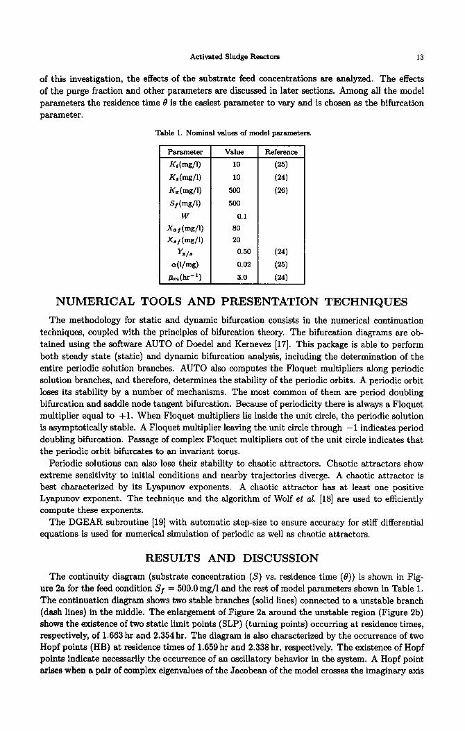
Equations [5,8,11] form the autonomous model of the bioreactor. The three-dimensional model includes a large number (nine) of parameters. Besides the reactor operating parameters, i.e., feed conditions and purge fraction, the nominal values of the other model parameters are given in Table 1. These nominal values (as shown in the table) are taken from realistic ranges given in literature. The bifurcation analysis consists in studying the branching phenomena in the model when its parameters (or a subset of them) are varied around the nominal values. In the first part
Activated Sludge Reactors 13
of this investigation, the effects of the substrate feed concentrations are analyzed. The effects of the purge fraction and other parameters are discussed in later sections. Among all the model parameters the residence time 0 is the easiest parameter to vary and is chosen as the bifurcation parameter.
Table 1. Nominal values of model parameters.
Parameter
Mm0
KS (mg/l)
Kc (ma
sj (mg/U
W
X&%/l)
X.f(w/l)
Y x/s
4ed
Pm(hrsl)
Value
10
10
500
500
0.1
80
20
0.50
0.02
3.0
Reference
(25)
(24)
(26)
(24)
(25)
(24)
NUMERICAL TOOLS AND PRESENTATION TECHNIQUES
The methodology for static and dynamic bifurcation consists in the numerical continuation techniques, coupled with the principles of bifurcation theory. The bifurcation diagrams are ob- tained using the software AUTO of Doedel and Kernevez [17]. This package is able to perform both steady state (static) and dynamic bifurcation analysis, including the determination of the entire periodic solution branches. AUTO also computes the Floquet multipliers along periodic solution branches, and therefore, determines the stability of the periodic orbits. A periodic orbit loses its stability by a number of mechanisms. The most common of them are period doubling bifurcation and saddle node tangent bifurcation. Because of periodicity there is always a Floquet multiplier equal to +l. When Floquet multipliers lie inside the unit circle, the periodic solution is asymptotically stable. A Floquet multiplier leaving the unit circle through -1 indicates period doubling bifurcation. Passage of complex Floquet multipliers out of the unit circle indicates that the periodic orbit bifurcates to an invariant torus.
Periodic solutions can also lose their stability to chaotic attractors. Chaotic attractors show extreme sensitivity to initial conditions and nearby trajectories diverge. A chaotic attractor is best characterized by its Lyapunov exponents. A chaotic attractor has at least one positive Lyapunov exponent. The technique and the algorithm of Wolf et al. [18] are used to efficiently compute these exponents.
The DGEAR subroutine [19] with automatic step-size to ensure accuracy for stiff differential equations is used for numerical simulation of periodic as well ss chaotic attractors.
RESULTS AND DISCUSSION
The continuity diagram (substrate concentration (S) vs. residence time (0)) is shown in Fig- ure 2a for the feed condition Sf = 500.0 mg/l and the rest of model parameters shown in Table 1. The continuation diagram shows two stable branches (solid lines) connected to a unstable branch (dash lines) in the middle. The enlargement of Figure 2a around the unstable region (Figure 2b) shows the existence of two static limit points (SLP) (turning points) occurring at residence times, respectively, of 1.663 hr and 2.354 hr. The diagram is also characterized by the occurrence of two Hopf points (HB) at residence times of 1.659 hr and 2.338 hr, respectively. The existence of Hopf points indicate necessarily the occurrence of an oscillatory behavior in the system. A Hopf point arises when a pair of complex eigenvalues of the Jacobean of the model crosses the imaginary axis

A. AJBARAND G. TBRAHIM
-100 I I I I
0. 1.
Resic2ncetim* b (hr)
4. 3.
(a) Continuity diagram (substrate concentration vs. residence time) for Sf = 500 mg/l and the rest of parameters of Table 1.
2@Q
-58 LPI t I I I 1 I I 1 I \
1.M 1.6B 1.70 1.8s 1.98 2.M 2.1. 2.29 2.3B 2.41) 2.58
Residence time 0 (hr) (b) Enlargement of (a) showing the locations of the limit points (LP) and the Hopf points (HB).
Figure 2. Solid line is a stable branch; dash line is an unstable branch.
transversally. Oscillations are then expected in the reactor for any residence time in the range of the two EIopf points (1,659 hr, 2.338 hr). The nature itself of these oscillations is analyzed in a later section.
The existence of static limit points (SLP) along Hopf points (HIS) in the continuation diagram indicates a potential richness in the stability characteristics of the model. It is known from bifurcation theory (20,211 that interactions between a SLP and HB point may lead to a variety of behavior ranging from simple periodicity to complex periodic behavior. In the beginning of this analysis it is helpful to build an overall picture of the possible bifurcation mechanisms that the
Activated Sludge Reactors
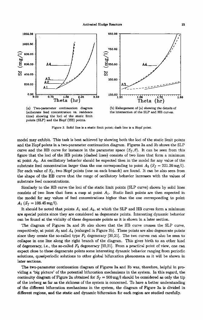
(a) Two-parameter continuation diagram (substrate feed concentration vs. residence time) showing the loci of the static limit points (SLP) and the Hopf (HB) points.
750.00 -
?
J550.00 i
(b) Enlargement of (a) showing the details of the intersection of the SLP and HB curves.
15
Figure 3. Solid line is a static limit point; dash line is a Hopf point.
model may exhibit. This task is best achieved by showing both the loci of the static limit points
and the Hopf points in a two-parameter continuation diagram. Figures 3a and 3b shows the SLP
curve and the HB curve for instance in the parameter space (Sf,B). It can be seen from this
figure that the loci of the HB points (dashed lines) consists of two lines that form a minimum
at point AZ. An oscillatory behavior should be expected then in the model for any value of the
substrate feed concentration larger than the one corresponding to point AZ (Sf = 221.20 mg/l).
For each value of Sf, two Hopf points (one on each branch) are found. It can be also seen from
the shape of the HB curve that the range of oscillatory behavior increases with the values of
substrate feed concentrations.
Similarly to the HB curve the loci of the static limit points (SLP curve) shown by solid lines
consists of two lines that form a cusp at point AI. Static limit points are then expected in
the model for any values of feed concentrations higher than the one corresponding to point
Al (Sf = 108.45mg/l).
It should be noted that points A1 and Ax, at which the SLP and HB curves form a minimum
are special points since they are considered as degenerate points. Interesting dynamic behavior
can be found at the vicinity of these degenerate points as it is shown in a later section.
The diagram of Figures 3a and 3b also shows that the HB curve crosses the SLP curve,
respectively, at point As and A4 (enlarged in Figure 3b). These points are also degenerate points
since they create the so-called type Fl degeneracy [20,21]. The two curves can also be seen to
collapse in one line along the right branch of the diagram. This gives birth to an other kind
of degeneracy, i.e., the so-called Fz degeneracy [20,21]. From a practical point of view, one can
expect close to these degenerate points some interesting dynamic behavior ranging from periodic
solutions, quasiperiodic solutions to other global bifurcation phenomena as it will be shown in
later sections.
The two-parameter continuation diagram of Figures 3a and 3b was, therefore, helpful in pro-
viding a ‘big picture’ of the potential bifurcation mechanisms in the system. In this regard, the
continuity diagram of Figure 2a obtained for Sf = 500 mg/l should be considered as only the tip
of the iceberg as far as the richness of the system is concerned. To have a better understanding
of the different bifurcation mechanisms in the system, the diagram of Figure 3a is divided in
different regions, and the static and dynamic bifurcation for each region are studied carefully.
16 A. AJBAR AND G. IBRAHIM 3e
-10
e. 1 I I I
I. Resi&ce titne~ (hr) l .
5.
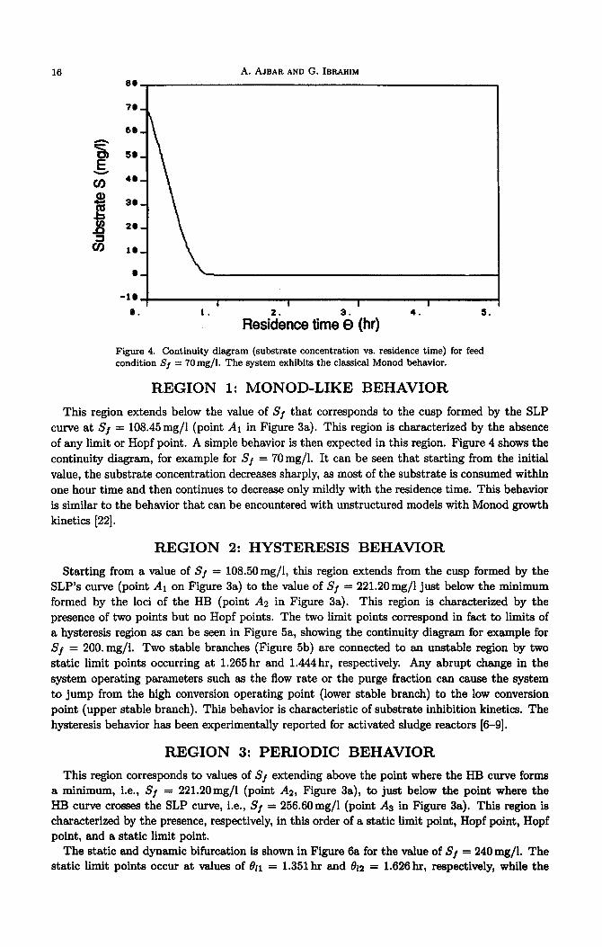
Figure 4. Continuity diagram (substrate concentration vs. residence time) for feed condition Sf = 7Omg/l. The system exhibits the classical Monod behavior.
REGION 1: MONOD-LIKE BEHAVIOR
This region extends below the value of Sj that corresponds to the cusp formed by the SLP curve at Sj = 108.45mg/l (point A1 in Figure 3a). This region is characterized by the absence of any limit or Hopf point. A simple behavior is then expected in this region. Figure 4 shows the continuity diagram, for example for Sj = 70mg/l. It can be seen that starting from the initial value, the substrate concentration decreases sharply, ss most of the substrate is consumed within one hour time and then continues to decrease only mildly with the residence time. This behavior is similar to the behavior that can be encountered with unstructured models with Monod growth kinetics [22].
REGION 2: HYSTERESIS BEHAVIOR
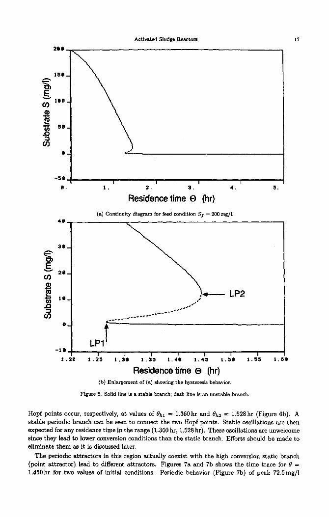
Starting from a value of Sj = 108.5Omg/l, this region extends from the cusp formed by the SLP’s curve (point A1 on Figure 3a) to the value of Sj = 221.2Omg/l just below the minimum formed by the loci of the HB (point A2 in Figure 3a). This region is characterized by the presence of two points but no Hopf points. The two limit points correspond in fact to limits of a hysteresis region as can be seen in Figure 5a, showing the continuity diagram for example for Sj = 200.mg/l. Two stable branches (Figure 5b) are connected to an unstable region by two static limit points occurring at 1.265 hr and 1.444 hr, respectively. Any abrupt change in the system operating parameters such 8s the flow rate or the purge fraction can cause the system to jump from the high conversion operating point (lower stable branch) to the low conversion point (upper stable branch). This behavior is characteristic of substrate inhibition kinetics. The hysteresis behavior has been experimentally reported for activated sludge reactors [6-g].
REGION 3: PERIODIC BEHAVIOR
This region corresponds to values of Sj extending above the point where the HB curve forms a minimum, i.e., Sj = 221.20mg/l (point As, Figure 3a), to just below the point where the HB curve crosses the SLP curve, i.e., Sj = 256.60 mg/l (point AJ in Figure 3a). This region is characterized by the presence, respectively, in this order of a static limit point, Hopf point, Hopf point, and a static limit point.
The static and dynamic bifurcation is shown in Figure 6a for the value of Sj = 24Omg/l. The static limit points occur at values of 811 = 1.351 hr and 012 = 1.626hr, respectively, while the
Activated Sludge Reactors
20@n
-58 1 I I I I
8. 1. Residence . 4. 5.
time ‘0
(hr)
46
(a) Continuity diagram for feed condition Sf = 200mg/l. -
38,
29,
LO_ ,’
_.c- .?- -0’
__---
___*.+- _ ___-----
0,
LPI t -I@
I I I I I I i 1.21 1.25 1.39 1.35 1.4@ 1.45 1.50 1.55 1.
17
Residence time 0 (hr) (b) Enlargement of (a) showing the hysteresis behavior.
Figure 5. Solid line is a stable branch; dash line is an unstable branch.
Hopf points occur, respectively, at values of &r = 1.360 hr and &s = 1.528 hr (Figure 6b). A stable periodic branch can be seen to connect the two Hopf points. Stable oscillations are then expected for any residence time in the range (1.360 hr, 1.528 hr). These oscillations are unwelcome since they lead to lower conversion conditions than the static branch. Efforts should be made to eliminate them as it is discussed later.
The periodic attractors in this region actually coexist with the high conversion static branch (point attractor) lead to different attractors. Figures 7a and 7b shows the time trace for B = 1.450 hr for two values of initial conditions. Periodic behavior (Figure 7b) of peak 72.5mg/l

18 A. AJBAR AND G. IBRAHIM
250
200
f
150
0
-50 1 I I I I
0. 1 . 2. 3. 4. 5;
Residence time 0 (hr)
(a) Continuity diagram for feed condition Sf = 24Omg/l. Two Hopf points are connected by stable periodic branches.
100
-25 1
1 .20 I I I I
1 .30 1.40 1.50 1.60 1.’
Residence time 0 (hr) (b).Enlargement of (a) showing the location of the limit points (LP) and the Hopf points (HB).
Figure 6. Solid line ls a stable branch; dash line is an unstable branch; filled circle ls a stable periodic branch; empty circle is an unstable periodic branch.
and period 17.30 hr coexist with a high conversion point attractor (Figure 7a) acting actually as a blackhole. The periodic behavior in this region is not orbitally stable since different initial conditions can break the periodic attractor and push it out of its domain of attraction into the blackhole, resulting in the annihilation of the oscillations.
As the substrate feed concentration moves down to the the degenerate point (St = 221.20 mg/l) the two Hopf move close to each other giving birth to periodic oscillations of small amplitude as it

Activated Sludge Reactors 19
0.68 z, I
6°*oo *
0.68
z70.64
2 9.62
fa 0.60
0.58
. . . . . . . . . . . . . . . . . . . . . . . . . . . . . . . . . . . . ..I 10.00 I . I . . I I 80.00 120.00 160.00 200.00
4omoo Time (hr) 0. 0
(a) Point attractor obtained with initial con- (b) Periodic attractor obtained with initial
ditions (S = 0.67mg/l, Xa = 38.5mg/l, conditions (S = 63.0 mg/l, XS = 290.0 mg/l,
x, = 2150 mg/l). X, = 1600mg/l).
Figure 7. Time traces showing bistability in Figure 6a, for 6 = 1.450 hr.
0.68
3-8, 2.
0.60 m
0.58
0.52 , . I . . a . . 0.00 10
(a) Point attractor obtained with initial con- (b) Periodic attractor obtained with initial
ditions (S = 0.54mg/l, X, = 31.82mg/l, conditions (S = 46.0 mg /l, XS = 330.0 mg/l,
X, = 2070 mg/l). X, = 154Omg/l).
00
Figure 8. Time traces showing bistability as the two HB points collapse near point A2 (Figure 38). Oscillations become smaller in amplitude.
can be seen in Figures 8a and 8b. Small oscillations of period 17.10 hr and ranging in amplitude
from 45.30 mg/l to 46.90 mg/l coexist with the high conversion static branch.
REGION 4: ORBITALLY STABLE OSCILLATIONS
This region extends from the first intersection of the SLP and the HB curves at Sf =
256.66mg/l (point A3 of Figure 3a) until the second intersection at Sf = 555.0mg/l (point Ad, Figure 3a). Here the system is characterized by the presence in this order of a Hopf point, a static
limit point, Hopf point, and a static limit point. The continuation diagram is shown in Figure 9a
for the value of Sf = 350mg/l. The diagram enlarged in Figure 9b shows two limit points LPr
and LPz occurring, respectively, at 8~1 = 1.520 hr and 0l2 = 2.013 hr, and two Hopf points HBr
and HBz occurring, receptively, at 19hr = 1.509 hr and &z = 1.978 hr. The relative positioning
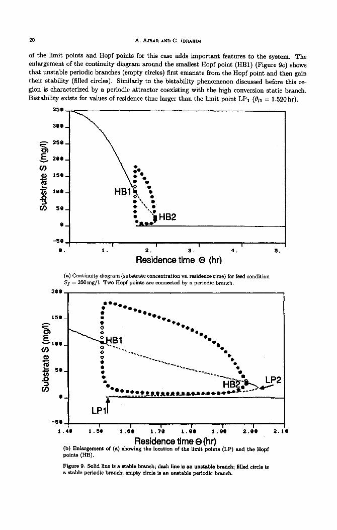
20 A. AJBAR AND G. IBRAHIM
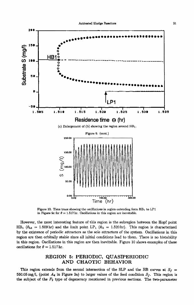
of the limit points and Hopf points for this case adds important features to the system. The enlargement of the continuity diagram around the smallest Hopf point (HBl) (Figure 9c) shows that unstable periodic branches (empty circles) first emanate from the Hopf point and then gain their stability (filled circles). Similarly to the bistability phenomenon discussed before this re- gion is characterized by a periodic attractor coexisting with the high conversion static branch. Bistability exists for values of residence time larger than the limit point LPr (011 = 1.520 hr).
-59
0. I I I I
1.
Reiidence timi 0 (hr) 4. s.
(a) Continuity diagram (substrate concentration vs. residence time) for feed condition Sf = 35Omg/l. Two Hopf points are connected by a periodic branch.
-so 1 I I I I I I
1.4. 1 .5# 1 .b@ 1.70 1.86 1.W 2.0. 2.
Residence time 0 (hr) (b) Enlargement of (a) showing the location of the limit points (LP) and the Hopf points (HB).
Figure 9. Solid line is a stable branch; dash line is an unstable branch; filled circle is a stable periodic branch; empty circle is an unstable periodic branch.
Activated Sludge Reactors
t LPI
15 1410 1.:15 1 , 5’20 1 .5’25 1430 1.
Residence time o (hr) (c) Enlargement of (b) showing the region around HBI.
Figure 9. (cont.)
2oo’oo 3
21
Figure 10. Time trace showing the oscillations in region extending form HBl to LPl in Figure 9c for 6 = 1.517 hr. Oscillations in this region are inevitable.
However, the most interesting feature of this region is the subregion between the Hopf point
HBr (0~ = 1.509hr) and the limit point LPI (&I = 1.520hr). This region is characterized by the existence of periodic attractors as the sole attractors of the system. Oscillations in this region are then orbitally stable since all initial conditions lead to them. There is no bistability in this region. Oscillations in this region are then inevitable. Figure 10 shows examples of these oscillations for 8 = 1.517 hr.
REGION 5: PERIODIC, QUASIPERIODIC AND CHAOTIC BEHAVIOR
This region extends from the second intersection of the SLP and the HB curves at S, = 550.05mg/l, (point Aa in Figure 3a) to larger values of the feed condition Sf. This region is the subject of the Fz type of degeneracy mentioned in previous sections. The two-parameter
22 A. AJBAR AND G. IBRAHIM
continuation diagram is characterized by the occurrence, in this order, of a static limit point,
Hopf point, Hopf point, and a static limit point.
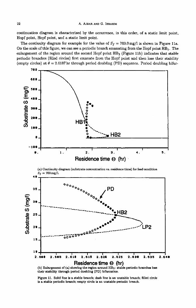
The continuity diagram for example for the value of Sf = 700.0mg/l is shown in Figure lla.
On the scale of this figure, we can see a periodic branch emanating from the Hopf point HBr. The
enlargement of the region around the second Hopf point HBs (Figure llb) indicates that stable
periodic branches (filled circles) first emanate from the Hopf point and then lose their stability
(empty circles) at 0 = 2.6187 hr through period doubling (PD) sequence. Period doubling bifur-
600
0 HB2
-100 1 I I I I
8. 1 . 2. 3. 4. 5.
Residence time o (hr)
(a) Continuity diagram (substrate concentration vs. residence time) for feed condition Sf = 7OOmg/l.
4e _
I I I I I I I
2.690 2.605 2.61Q 2.615 2.620 2.625 2.630 2.635 2.1
Residence time 0 (hr) (b) Enlargement of (a) showing the region around HB2: stable periodic branches lose their stability through period doubling (PD) bifurcation.
Figure 11. Solid line is a stable branch; dash line ls an unstable branch; filled circle is a stable periodic branch; empty circle is an unstable periodic branch.
23 Activated Sludge Reactors
LPI t
1 . 78 1.75 1.80 1.qs I. 00 1.05
Residence time 0 (hr) 2.0. 2. es 2.10
(c) Enlargement of (a) showing the region around HB1: stable periodic branches lose their stability through torus (TR) bifurcation and regain stability through torus.
Figure 11. (cont.)
cation occurs when one of the Floquet multipliers crosses the unit circle at -1 on the real axis,
while the other multipliers remain inside the unit circle. In this phenomenon, one starts with a
system with a periodic motion then as the bifurcation parameter 0 is varied the system undergoes
a secondary bifurcation to a periodic motion twice the period of the original solution.
Figure 12a shows the dynamics of the system for the value of B = 2.62 hr just before the
occurrence of period doubling. These regular oscillations of period 23.10 hr also coexist with the
high conversion static branch (not shown in the time trace). Figure 12b shows, on the other
hand, time trace for the value of 0 = 2.6179 hr corresponding to the region of instability just
after the occurrence of the period doubling bifurcation. The oscillations are clearly not periodic.
In fact, they correspond to a chaotic behavior. The Lyapunov exponents for this attractor are
(0.0595,0.000, -1.1563). The maximum exponent is positive confirming the chaotic nature of the
attractor. The oscillations are also shown in phase plane (Figure 12~).
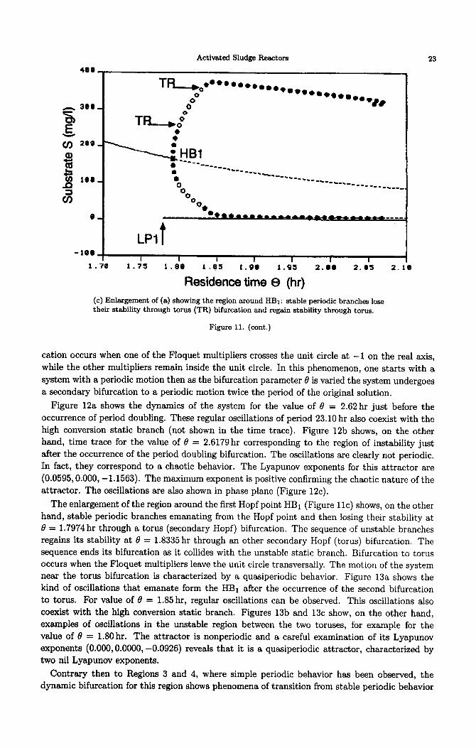
The enlargement of the region around the first Hopf point HBi (Figure llc) shows, on the other
hand, stable periodic branches emanating from the Hopf point and then losing their stability at
8 = 1.7974 hr through a torus (secondary Hopf) bifurcation. The sequence of unstable branches
regains its stability at 0 = 1.8335 hr through an other secondary Hopf (torus) bifurcation. The
sequence ends its bifurcation as it collides with the unstable static branch. Bifurcation to torus
occurs when the Floquet multipliers leave the unit circle transversally. The motion of the system
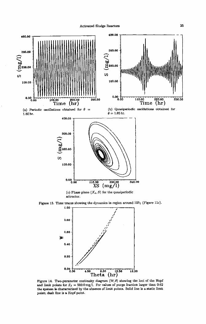
near the torus bifurcation is characterized by a qussiperiodic behavior. Figure 13a shows the
kind of oscillations that emanate form the HBi after the occurrence of the second bifurcation
to torus. For value of 0 = 1.85 hr, regular oscillations can be observed. This oscillations also
coexist with the high conversion static branch. Figures 13b and 13c show, on the other hand,
examples of oscillations in the unstable region between the two toruses, for example for the
value of 8 = 1.80 hr. The attractor is nonperiodic and a careful examination of its Lyapunov
exponents (0.000, 0.0000, -0.0926) reveals that it is a quasiperiodic attractor, characterized by
two nil Lyapunov exponents.
Contrary then to Regions 3 and 4, where simple periodic behavior has been, observed, the
dynamic bifurcation for this region shows phenomena of transition from stable periodic behavior

24 A. AJBAR AND G. IBRAHIM
-24.00
co
22.00
18.00 - I I I . I . I
0.60 3od.00 ioX+ii~~ ’ f%&jf ’ ’ ’ ’ ’ ’ ’
(a) Periodic oscillations obtained for 0 = (b) Chaotic oscillations obtained for 0 = 2.6179 hr. i.620 hr.
(c) Phase plane (X,,S) for the chaotic
attractor.
50
Figure 12. Time traces showing the dynamics in the region around HB2 (Figure llb).
to unstability through two fundamental mechanisms that are period doubling and torus. These mechanisms of transition can be quite complicated and their detailed analysis is left to a future work.
EFFECTS OF THE PURGE FRACTION
The effects of the purge fraction W on the stability characteristics of the bioreactor are shown in Figure 14, showing the static limit point curve and the Hopf curve for the feed condition
Sf = 500mg/l. The diagram shows that the two curves join in different points creating also potential degeneracies and richness in the model. Interestingly enough, as the purge fraction increases beyond the value of W = 0.62, the continuity diagram is characterized by the existence of two Hopf points but no limit points. The practical relevance of this feature is that orbitally stable periodic attractors are the only attractors to the system in the region between the two Hopf points. The maximum value of the purge fraction at which only Hopf points, i.e., periodic behavior are found depends obviously on the values of the other operating parameters such as feed concentrations of substrate and biomass. Figure 15 shows the continuity diagram for the important case of no solids recycle, i.e., W = 1. The diagram features two Hopf points
Activated Sludge Reactors 25
Time (hr)
o.oo’..,.,,,,,,,,,.,.,,.., .II.IIIII.
0.60 UJ
110.00 2 d.00
f
330100 Time hr)
(a) Periodic oscillations obtained for 0 = 1.80 hr.
(b) Quasiperiodic oscillations obtained for 6 = 1.85 hr.
0.00 0.00 m
(c) Phase plane (X,, S) for the quasiperiodic attractor.
Figure 13. Time traces showing the dynamics in region around HBr (Figure 11~).
:.i;;:;:’
0.60 /I
/I
b I
/ /
0.40 / / 1~ /
0.20
,*
Figure 14. Two-parameter continuity diagram (W, 0) showing the loci of the Hopf and limit points for Sf = 5OO.Omg/l. For values of purge fraction larger than 0.62 the system is characterized by the absence of limit points. Solid line is a static limit point; dash line is a Hopf point.
26 A. AJBAR AND G. IBRAHIM
-G E ‘2:
0.39
0.26
0.17
0.06
12.5. 12.75 13.a. 13.25 13.5. 13.75 1
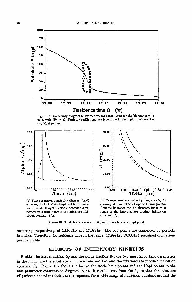
Residence time Q (hr) Figure 15. Continuity diagram (substrate vs. residence time) for the bioreactor with
no recycle (W = 1). Periodic oscillations are inevitable in the region between the
two Hopf points.
-0.05-1...~..... 1.50
,......*..I.‘...,... I
Gleta (2) 2.70
(a) Two-parameter continuity diagram ((Y, 0) showing the loci of the Hopf and limit points for Sf = 500.0mg/l. Periodic behavior is ex- pected for a wide range of the substrate inhi- bition constant l/a.
6.00 --,I III*,. *. ,,., .,,,,. , , ,,,, 0.40 oh3 oh LB4 l.d2
Theta (hr) 1.
(b) Two-parameter continuity diagram (Ki, 0) showing the loci of the Hopf and limit points. Periodic behavior can be observed for a wide range of the intermediate product inhibition
constant Kc.
D
Figure 16. Solid line is a static limit point; dash line is a Hopf point.
occurring, respectively, at 12.992 hr and 13.083 hr. The two points are connected by periodic branches. Therefore, for residence time in the range (12.992 hr, 13.083 hr) sustained oscillations are inevitable.
EFFECTS OF INHIBITORY KINETICS
Besides the feed condition Sf and the purge fraction W, the two most important parameters in the model are the substrate inhibition constant l/a and the intermediate product inhibition constant Ki. Figure 16a shows the loci of the static limit points and the Hopf points in the two parameter continuation diagram (a, 0). It can be seen from the figure that the existence of periodic behavior (dash line) is expected for a wide range of inhibition constant around the

Activated Sludge Reactors 27
nominal value (Y = O.O2l/mg. As (Y takes on small values a Monod-type behavior is expected, characterized by the absence of any limit or Hopf points.
Figure 16b shows, on the other hand, the SLP and HB curve in the two-parameter dia- gram (Ki, 0). Again it can be observed that periodic behavior is expected for values of Ki
in a wide range around the nominal value Ki = lOmg/l. As Ki takes on large values both the SLP and HB points became close to each other and eventually collapse as the maximum growth rate pLm reaches a constant value pm (equation (2)) independent of the intermediate product concentration.
CONCLUDING REMARKS
An investigation of the static and dynamic bifurcation of a model of activated sludge processes was carried out in this paper. The model exhibits rich stability characteristics ranging from simple Monod-like behavior and hysteresis, to periodic and chaotic behavior. The investigation shows that for some range of model parameters, the system is characterized by the presence of periodic oscillations coexisting with high conversion static points over some range of the residence time. Elimination of these oscillations is possible by choosing the appropriate initial conditions. However, for some range of model parameters oscillations in the bioreactor are orbitally stable and are independent of the initial conditions. Oscillations in this case can be eliminated by choosing the residence time outside the region of periodic behavior. Quasiperiodic and chaotic behavior were also observed for some range of the model parameters. These different dynamic behavior were observed for a wide range of the parameters, providing the proposed model with a good deal of flexibility.
REFERENCES
1. J. Nielsen, K. Nikolajsen and J. Villedsen, Biotcchnol. Bioeng. 38, 1, (1991). 2. A.A. Esener, T. Veerman, J.A. RoeIs and N.W.F. Kossen, Biotechnol. Bioeng. 24, 1749, (1982). 3. M.S. Sheffer, M. Hiraoka and K. Tsumura, War. Sci. Tech. 17, 247, (1984). 4. A. Harder and J.A. Roeis, Adu. B&hem. Eng. 21, 55, (1982). 5. J.F. Andrews, Biotechnol. Bioeng. 10, 707, (1968). 6. U. Pawlowsky and J.A. Howell, Bioteehnol. Bioeng. 15, 887, (1973). 7. U. Pawlowsky, J.A. Howell and C.T. Chi, Biotechnol. Bioeng. 15, 905, (1973). 8. D. DiBiasio, H.C. Lim and W.A. Weigand, AIChEJ 27, 284, (1981). 9. A. Bertucco, P. Volpe, H.E. Klei, T.F. Anderson and D.W. Sundstrom, Water. Res. 56, 9, (1989).
10. J.F. Andrews, War. Res. 8, 261, (1974). 11. J.B. Bubsy and J.F. Andrews, Water Pollut. Control Fed. 47, 1055, (1975). 12. J.B. Bubsy and J.F. Andrews, Water Pollut. Control Assoc. 47, 1067, (1975). 13. A. Mulchandani and J.H.T. Luong, Enzyme Microbial. Technol. 11, 66, (1989). 14. A.F. Rozich and A.F. Gaudy, Water Poll&. Control Fed. 57, 795, (1985). 15. A.N. Godrej and J.H. Sherrard, Water Pollut. Control Fed. 60,221, (1988). 16. B.E. Rittman, W. Bae, E. Namkung and C.J. Lu, Wut. Sci. Technol. 19, 517, (1987). 17. E.J. Doedel and J.P. Kerneves, AUTO: Software for Continuation and Bij+cution Problems in ordinary
Differential Equations, California Institute of Technology, Pasadena, CA, (1986). 18. A. Wolf, J.B. Swift, H.L. Swinney and J.A. Vastano, Physics 16D, 285, (1985). 19. Math/PC-Library, IMSL Library, Microsoft, (1992). 20. S. Wiggins, Introduction to Applied Nonlinear Dynamical Systems and Chaos, Springer-Velag, New York,
(1990). 21. J. Guckenheimer and P. Hohns, Nonlinear Oscillations, Dynamical Systems and Bifurcntion of Vector Fields,
Springer, New York, (1983). 22. J.E. Bailey and D.F. Ollis, Biochemical Engineering Fktndamentals, McGraw-Hill, New York, (1986). 23. G. Ibrahim and A.E. Abasaeed, Wat. Res. 29, 1761, (1995). 24. M. Henee, C.P.L. Grady, Jr, W. Gujer, G.V.R. Marais and T. Matsuo, Wat. Res. 21, 505, (1987). 25. P.D. D’Adamo, A.F. Rosich and A.F. Gaudy, Biotechnol. Bioeng. 26, 397, (1984). 26. R.W. Dennis and R.L. Irvine, Wat. Res. 15, 1363, (1981).
Copyright © 2022 FDOKUMEN