Performance of Prewhitening Beamforming in MEG Dual Experimental Conditions

Performance of Prewhitening Beamforming in MEG DualExperimental Conditions

Kensuke Sekihara*,Department of Systems Design and Engineering, Tokyo Metropolitan University, Asahigaoka 6-6,Hino, Tokyo 191-0065, Japan

Kenneth E. Hild II [Senior Member, IEEE],Department of Radiology, University of California, San Francisco, CA 94143 USA

Sarang S. Dalal, andDepartment of Radiology, University of California, San Francisco, CA 94143 USA

Srikantan S. Nagarajan [Senior Member, IEEE]Department of Radiology, University of California, San Francisco, CA 94143 USA

AbstractThis paper presents an analysis on the performance of the prewhitening beamformer when appliedto magnetoencephalography (MEG) experiments involving dual (task and control) conditions. Wefirst analyze the method’s robustness to two types of violations of the prerequisites for theprewhitening method that may arise in real-life two-condition experiments. In one type of violation,some sources exist only in the control condition but not in the task condition. In the other type ofviolation, some signal sources exist both in the control and the task conditions, and that they changeintensity between the two conditions. Our analysis shows that the prewhitening method is very robustto these nonideal conditions. In this paper, we also present a theoretical analysis showing that theprewhitening method is considerably insensitive to overestimation of the signal-subspacedimensionality. Therefore, the prewhitening beamformer does not require accurate estimation of thesignal subspace dimension. Results of our theoretical analyses are validated in numerical experimentsand in experiments using a real MEG data set obtained during self-paced hand movements.

KeywordsAdaptive beamforming; brain noise; interference removal; magnetoencephalography (MEG);neuromagnetic source reconstruction; prewhitening

I. IntroductionONE MAJOR problem with magnetoencephalography (MEG) measurements is that themeasured MEG data contain not only signals from brain regions of interest, but also largeinterfering magnetic fields generated from spontaneous brain activities all over the brain. Suchbackground interference degrades the quality of source reconstruction results, and often makesinterpreting the results difficult. Such background interference is sometimes referred to as brainnoise or physiological noise.

© 2008 IEEE*K. Sekihara is with the Department of Systems Design and Engineering, Tokyo Metropolitan University, Asahigaoka 6-6, Hino, Tokyo191-0065, Japan.

NIH Public AccessAuthor ManuscriptIEEE Trans Biomed Eng. Author manuscript; available in PMC 2009 December 10.

Published in final edited form as:IEEE Trans Biomed Eng. 2008 March ; 55(3): 1112–1121. doi:10.1109/TBME.2008.915726.

NIH

-PA Author Manuscript

NIH


NIH


A common strategy for extracting the signal of interest from measurements overlapped with alarge amount of interference is to design experiments with dual (control and task) conditions.Subtraction between the reconstruction results obtained under these two conditions is acommon procedure to reconstruct signal sources of interest [1]. (This subtraction is oftenperformed as a part of calculating pseudo-t statistics, which is used for statistically evaluatingthe source configuration difference between the two conditions.) However, when the sourcereconstruction is performed with adaptive spatial filter methods [2]-[4], such subtraction-basedmethods cannot effectively remove the influence of the background interference [5]. This isbecause the influence of the background activity is not simply additive. It involves spatial blurand source location bias, as will be shown in our computer simulation in Section V.

Recently, we have proposed a novel prewhitening method suitable for reconstructing sourcesfrom evoked measurements overlapped with large background interference [6]. The goal ofthis paper is to show that the prewhitening method can also be effective for measurementsinvolving task and control conditions. We first analyze the prewhitening method’s robustnessto two types of violations of the prerequisites for the prewhitening method that may arise inreal-life two-condition experiments. We refer to these two types violations as the control-onlysource scenario and the modulating source scenario in this paper. In the control-only-sourcescenario, some sources appear only in the control measurements and that they do not appearin the task measurements. In the modulating-source scenario, some signal sources of interestexist both in the control and the task measurements, and they change intensity between the twoconditions. In real-life measurements, one or both of these scenarios may arise. In this paperwe demonstrate that the prewhitening method is still effective under these scenarios.

This paper also presents an analysis on the influence caused by the overestimation of the signalsubspace dimensionality, and it shows that the method is considerably insensitive to suchoverestimation. Therefore, the accurate determination of the signal subspace dimension is notessential for implementing the prewhitened beamformer, and an intentionally large value canbe used for the signal subspace dimension.

Section II briefly reviews the prewhitening method that has already been proposed in [6].Section III presents our theoretical analysis on the method’s performance under two realisticscenarios with dual-condition experiments. Section IV shows the effects of overestimation ofthe signal subspace dimension. The arguments in Sections III–IV are validated first bynumerical experiments in Section V and by an application to real MEG data collected duringself-paced finger flection in Section VI. Throughout this paper, plain italics indicate scalars,lower-case boldface italics indicate vectors, and upper-case boldface italics indicate matrices.The eigenvalues are numbered in decreasing order.

II. Prewhitening Beamforming Under an Ideal ScenarioWe use a model for measurements b(t) expressed as

(1)

where bs(t) is the magnetic field generated by signal sources of interest, bI(t) is the magneticfield generated by background activity, and n(t) is the additive sensor noise. These vectors areM × 1 column vectors where M is the number of sensors. The covariance matrix of themeasurements is denoted R such that R = ⟨b(t)bT(t)⟩ where ⟨·⟩ indicates an expectation operator.We define the covariance matrix of the signal magnetic field as Rs, such that

. We assume that the signal is low rank, i.e., the rank of Rs is Q, which issmaller than M, the number of sensors. We also define the interference-plus-sensor-noise

Sekihara et al.

IEEE Trans Biomed Eng. Author manuscript; available in PMC 2009 December 10.

NIH


NIH


NIH


https://www.researchgate.net/publication/13937409_Localization_of_Brain_Electrical_Activity_via_Linearly_Constrained_Minimum_Variance_Spatial_Filtering?el=1_x_8&enrichId=rgreq-596da27da2889cae547c00093f641625-XXX&enrichSource=Y292ZXJQYWdlOzU1MTg2NTQ7QVM6MTAxNjQ4MzQ5MjcwMDIwQDE0MDEyNDYyNjMzNzY=

https://www.researchgate.net/publication/6846614_A_novel_adaptive_beamformer_for_MEG_source_reconstruction_effective_when_large_background_brain_activities_exist?el=1_x_8&enrichId=rgreq-596da27da2889cae547c00093f641625-XXX&enrichSource=Y292ZXJQYWdlOzU1MTg2NTQ7QVM6MTAxNjQ4MzQ5MjcwMDIwQDE0MDEyNDYyNjMzNzY=


https://www.researchgate.net/publication/8192754_Improving_permutation_test_power_for_group_analysis_spatically_filtered_MEG_data?el=1_x_8&enrichId=rgreq-596da27da2889cae547c00093f641625-XXX&enrichSource=Y292ZXJQYWdlOzU1MTg2NTQ7QVM6MTAxNjQ4MzQ5MjcwMDIwQDE0MDEyNDYyNjMzNzY=

covariance matrix Ri+n, such that Ri+n = ⟨[bI(t) + n(t)][bI(t) + n(t)]T⟩. Note that this Ri+n is apositive definite matrix, because we assume that the sensor noise is the white Gaussian noiseuncorrelated between different channels. Under the assumption that the signal source activityis uncorrelated with the background interferences and sensor noise, the relationship

(2)

holds. In the conventional (nonprewhitened) minimum-variance spatial filter, the source powerreconstruction Φ̂(r) is obtained using this covariance matrix R such that

(3)

where l(R) is an M × 1 column vector representing the sensor lead field in the estimated sourcedirection1 at location r. Equation (3) indicates that the influence of the additive interference isnot simply additive, but it affects the final source-reconstruction results through Ri+n in a highlynonlinear manner. The influence actually involves spatial blur and source location bias, as willbe shown in our computer simulation in Section V.

We next explain the prewhitening method of estimating the signal covariance matrix Rs; themethod was first reported in [6]. We here assume the ideal scenario, in which control-statemeasurements bc(t) contain only the interference and sensor noise, i.e.,

and the interference-plus-noise covariance matrix Ri+n can be obtained from such control-statemeasurements. Namely, defining the covariance matrix from the control measurements as

Rc, i.e., , the relationship

(4)

holds. To estimate the signal covariance matrix, we first calculate the prewhitenedmeasurement covariance matrix , which is defined as . Thus, from (4), wehave the relationship

(5)

where

(6)

We define the eigenvalues and eigenvectors of an M × M matrix as γ1, . . . , γM and u1, . . . ,uM. Since Rs is a positive semidefinite matrix with rank Q and is a nonsingular matrix,

1The method of estimating the source orientation at each voxel location is presented in [7] and [8].

Sekihara et al.


NIH


NIH


NIH



is also a positive semidefinite matrix with rank Q. Thus, the eigenvalues γ1, . . . , γQ arepositive and the other eigenvalues γQ+1, . . . , γM are zero. (Here, we assume that the eigenvaluesare ordered in a decreasing manner.) Namely, we have

(7)

Therefore, the eigendecomposition of can be expressed as

(8)

The above equation indicates that the Q largest eigenvalues of are greater than 1 and thecorresponding eigenvectors are the same as those for the nonzero eigenvalues of . Theeigenvalues of greater than 1 are referred to as the signal-level eigenvalues and theircorresponding eigenvectors as the signal-level eigenvectors. Equation (8) indicates that it ispossible to retrieve from the signal-level eigenvalues and their corresponding eigenvectorsof . That is, defining a matrix US as US = [u1 , . . . , uQ], the signal covariance matrix, Rs,can be obtained using

(9)

In actual cases, the covariance matrices R and Rc are unknown, and instead we should use thesample covariance matrices, which are obtained using

(10)

where t1, . . . , tK are the time points contained in a certain time window. We define such

that . Using (9), the estimate of the signal covariance matrix can beobtained using

(11)

where ÛS = [û1, . . . , ûQ], and û1, . . . , û>Q are the signal-level eigenvectors of . Given theestimate of the signal covariance matrix R̂s, a reasonable estimate of the signal-plus-sensor-noise covariance matrix, R̂s+n, can be obtained using

Sekihara et al.


NIH


NIH


NIH


(12)

where μ is the regularization constant that should be set close to the variance of the sensor noise. (Actually, since the noise variance is unknown, an appropriate value of μ should be

determined from the measured data, and some empirical methods, such as that of using theminimum-eigenvalue of R, are employed to determine μ.) Consequently, using the minimum-variance spatial filter, the prewhitening source power reconstruction free from the influenceof the background activity, can be obtained using

(13)

III. Prewhitening Beamforming Under Nonideal ScenariosIn this section, we analyze the performance of the prewhitening method under two kinds ofnonideal scenarios that may arise in real-life task and control-type measurements. In thescenario argued first, there are some sources that appear only in the control state and do notappear in the task state. Such sources are called the control-only sources in this paper, and thisscenario is referred to as the control-only-source scenario. In the scenario argued next, thesignal sources of interest are active in the control state as well as in the task state but theychange their intensities between the two states. Such sources are called the modulating sourcesin this paper, and this scenario is referred to as the modulating-source scenario.

A. Control-Only Source ScenarioIn the control-only-source scenario, we assume that there are P sources that exist only in thecontrol state and do not appear in the task state. We also assume that the observed signal spaceis still low-rank, i.e., Q+P < M. When such control-only sources exist, the control statemeasurements bc(t) can be expressed as

(14)

where bΔ(t) indicates the magnetic field generated by control-only sources. The covariancematrix relationships are then expressed as

(15)

where

(16)

In deriving (15), we assume that the activity of control-only sources is uncorrelated with theinterference and sensor noise. Using (15), we have

(17)

Sekihara et al.


NIH


NIH


NIH


and thus

(18)

where . Since Rδ is a nonnegative definite matrix with rank P and is a nonsingular matrix, is a nonnegative definite matrix with rank P. Thus, isdecomposed as

(19)

where βj, (j = 1, . . . , P) are P nonzero eigenvalues of , and vj are the correspondingeigenvectors. Substituting (7) and (19) into (18), we have

(20)

When the control-only sources are well separated from the signal sources of interest, therelationship

(21)

approximately holds. Under this assumption, we will show that a set of vectors

(22)

are the eigenvectors of , where {d1, . . . , dM - P - Q} are the orthonormal basis set of the

subspace , which is defined as .

We first show that the relationship

(23)

holds. That is, we show that the vectors ui (where i = 1, . . . , Q) are the eigenvectors of andtheir corresponding eigenvalues are γi + 1. To show this, we calculate the right multiplicationof ui (i = 1, . . . , Q) to , and using (20) this multiplication results in

(24)

Sekihara et al.


NIH


NIH


NIH


The first term in the right-hand side becomes γiui. The second term becomes ui, because therelationship

(25)

holds. The validity of (25) is shown in the Appendix. The third term in the right-hand side of(24) vanishes due to the orthogonality assumption in (21). Therefore, we can derive therelationship in (23), i.e., we can show that the vectors ui (where i = 1, . . . , Q) are the eigenvectorsof .

Next, we show that the relationship

(26)

holds. That is, we show that the vectors di (i = 1, . . . , M - P - Q) are the eigenvectors of andthe corresponding eigenvalues are equal to 1. To show this relationship, we calculate the rightmultiplication of di to , which is equal to

(27)

Since di is orthogonal to both the subspace spanned by uj (j = 1, . . . , Q) and that spanned byvj (j = 1, . . . , P), the only nonzero term in the right-hand side is the second term, which is equalto di, because di ∈ span {vP+1, . . . , vM}. Thus, we have proved (26).

Finally, we calculate the right multiplication of vi (i = 1, . . . , P) to , which produces that

(28)

On the right-hand side, the first term becomes zero due to the orthogonality assumption in (21)and the second term becomes zero due to the orthogonality relationship between the signal andthe noise subspaces. Thus, we have

(29)

Therefore, vi (i = 1, . . . , P) are eigenvectors of and the corresponding eigenvalues are 1 -βi. We can also show that these eigenvalues are positive but less than 1, i.e., 0 < 1 - βj < 1,although we do not include the proof here. In summary, we have shown that the vectors

Sekihara et al.


NIH


NIH


NIH


are the eigenvectors of . The corresponding eigenvalues, in a decreasing order, are

(30)

Here, the largest Q eigenvalues γ1 + 1, . . . , γQ + 1 are greater than 1, and therefore, (9) is stilleffective at retrieving Rs, even when the control-only sources exist.

In general, however, the subspace angle between span{u1, . . . , uQ} and span{v1, . . . , vP}may not be so large and the assumption that these two subspaces are orthogonal may not besatisfied. In such cases, (23) is changed to

(31)

This equation shows that ui (i = 1, . . . , Q) is no longer the eigenvector of and the secondterm on the right-hand side of (31) indicates the error term. Thus, if the relationship

(32)

holds, the error term is negligibly smaller than the first term, and ui are still approximately thesignal-level eigenvectors of . Conversely, when the error term is not small, the signal-covariance estimate obtained from (9) could be erroneous.

B. Modulating-Source ScenarioWe next examine the modulating-source scenario. We define the covariance matrix of thesignal activity in the control state as . Then we have the relationship

(33)

Thus, we have

(34)

We consider a general case where some signal sources have their intensities greater in thecontrol state than in the task state, but others have their intensities smaller in the control statethan in the task state. The power of the jth signal source in the task and the control conditions

are denoted, respectively, and . We assume that the signal sources with j = 1, . . . ,

Sekihara et al.


NIH


NIH


NIH


Qp have the relationship of , and that the signal sources with j = Qp+1, . . . , Q have

the relationship . Therefore, defining , we have

(35)

where

(36)

(37)

Therefore, we have

(38)

and thus

(39)

where

Because both and are the positive semidefinite matrices, (39) is in principle the sameas (18), and exactly the same arguments hold as those in Section III-A. Therefore, we canestimate Dp by using

(40)

where ÛS = [û1, . . . , ûQp] is a matrix containing Qp eigenvectors of . We

can estimate Dn by changing the role of R̂ and R̂c. That is, we first calculate such that

, and then obtain an estimate of Dn using

(41)

Sekihara et al.


NIH


NIH


NIH


In the equation above, is defined as , which is a matrix containing Qn

(where Qn = Q - Qp) signal-level eigenvectors of . The prewhitening method in which theroles of R̂ and R̂c are reversed is referred to as the “flipped” prewhitening method in this paper.Therefore, the sources that are stronger in the task state than in the control state can bereconstructed using

(42)

The sources that are stronger in the control state than in the task state can be reconstructedusing the flipped prewhitening, i.e.,

(43)

IV. Overestimation of Signal-Subspace DimensionalityThe prewhitening method requires us to determine Q, the dimension of the signal subspace ofR (or the rank of Rs). This determination is usually performed by counting the number ofdistinctively large eigenvalues of data covariance matrix R̂. In actual MEG measurements,however, it is often problematic to accurately determine Q because the eigenvalue spectrumdoes not have a clear separation between these two subspaces. Here, we presents an analysison the influence caused by the overestimation of the signal subspace dimensionality, and weshow that the prewhitening method is very insensitive to such over-estimation. Therefore, theaccurate determination of Q is not needed and we can use an intentionally large Q to implementthe prewhitening method.

In the following, we discuss the influence caused when the dimension of the signal-subspaceof is overestimated. We assume the ideal scenario in this section. Let us assume that thesignal subspace dimension is overestimated as Q + Qε and define Uε as Uε = [uQ+1, . . . ,uQ+Qε]. Ideally, the prewhitened data covariance matrix, , has Q signal-level eigenvaluesgreater than 1 and M - Q eigenvalues equal to 1. Therefore, according to (9), the overestimationof Q does not affect the signal covariance estimate R̂s because the relationship

holds. However, the prewhitened covariance matrix is usually estimatedfrom finite time samples, and in such cases, the noise-level eigenvalues are generally not equalto 1. We denote the noise-level eigenvalues of the estimated prewhitened covariance matrix

as δj + 1 and assume δj ≥ 0 for j = Q + 1, . . . , Qε. Then, the estimated signal covariancematrix, R̂s, is expressed in this case as

(44)

The second term on the right-hand side of the above equation indicates the error term causedby the overestimation. The error term, R̂ε, is expressed as

Sekihara et al.


NIH


NIH


NIH


(45)

where .

Let us define the signal and noise subspaces of the measuremnt covariance matrix R, as εS andεN, i.e.,

where ej is the jth eigenvector of Rs. Then, assuming that , we can expand R̂susing ej such that

(46)

where . On the righthand side of (46), the first term is the signalsubspace component and the second term is the noise subspace component. To obtain the sourcereconstruction in (13), we need to calculate the signal-plus-sensor-noise convariance matrix.The estimate of the signal-plus-sensor-noise convariance matrix, R̂s+n, is in this case given by

(47)

where λi is the ith eigenvalue of Rs, and we assume that λi ≫ Δλi for i = 1, . . . , Q.

The equation above indicates that the influence of the over-estimation is mainly an increase ofthe regularization constant. The regularization in the minimum variance beamformer, knownas diagonal loading, has been widely used and a significant increase of the regularizationconstant is known to cause a spatial blur in the reconstruction results [5]. Therefore, theoverestimation of the signal subspace dimension should cause a spatial blur. However, the blurshould not be large if Qε and the resultant Δλi are small. In Section V, examples are presentedin which the prewhitening method can still provide successful reconstruction, even when thesignal subspace dimension is significantly overestimated. In the analysis presented in thissection, we assume the ideal scenario. Considering the fact that large eigenvalues are the samein the ideal and the nonideal scenarios, it is obvious that the arguments here are also valid forthe nonideal scenarios.

V. Computer SimulationA. Data Generation

A computer simulation was performed to demonstrate the validity of the arguments in thepreceding sections. In our experiments, we used a sensor alignment of the 275-sensor array

Sekihara et al.


NIH


NIH


NIH


from the Omega™ (VMS Medtech, Coquitlam, Canada) neuromagnetometer. Three sourceswere assumed to exist on a single plane (x = 0 cm), and their (y,z) coordinates were (−2.1,9.5)cm, (2.6,10.5) cm, and (1.4,7.5) cm, respectively. The source-sensor configuration and thecoordinate system are depicted in Fig. 1(a). The spherical homogeneous conductor model[10] with the sphere origin set as (0,0,4) cm was used for the forward calculation. The powersof the three sources were set equal in the sensor-domain, i.e., the relationship,

, held where rj, , and l(rj) were the location, the power,and the lead field vector of the jth source, respectively. Multiepoch measurements weresimulated.

Each epoch had two sets of data: the task and the control data sets. The task and the controldata sets in the ℓth epoch are denoted B(ℓ) and , respectively, and they are expressed as

B(ℓ) = [b(ℓ)(t1, . . . , b(ℓ)(tK)], and , where K is the number of timepoints. Since K was set at 600 in our computer simulation, B(ℓ) and resulted in 275 × 600spatio-temporal data matrices. To calculate B(ℓ)(tk) and , we assumed uncorrelatedsinusoidal time courses for the three sources; the source time course for the jth source and for

the ℓth epoch is expressed as , where ΔT is the timewindow equal to tK - t1, and the constant Aj controls the frequency, which was set at 6.3 for

the first source, 9.1 for the second source, and 13.1 for the third source. The phase offset was generated using the random number between 0 and 2π, and different random number was

used for depending on j, ℓ, and the two conditions. We therefore simulated induced sourceactivities, which are elicited by the stimulus but not phase-locked to it.

B. Simulation for the Control-Only-Source ScenarioWe first check the performance of the prewhitening method under the existence of a control-only source. In this computer simulation, the first source is the control-only source, and thesecond and the third sources are the signal sources, which appear only in the task state. Namely,

contains the magnetic field from the second and the third sources, and containsthe magnetic field from the first source. Real spontaneous MEG was used as the interference

, and the signal-to-interference ratio (SIR) was set equal to 0.3. That is, values of the

source power were determined in order for the SIR defined as

to be equal to 0.3. A total of 96 epochs of and B(ℓ)

(ℓ = 1, . . . , 96) were generated. The representative examples of and B(ℓ) are shown inFig. 1(b). The sample covariance matrices R̂c and R̂ were calculated using

and where Le indicates the numberof epochs, which is equal to 96 in this computer simulation. The total covariance matrix wascalculated for later use, using

(48)

The conventional beamformer source reconstruction was performed for the control and the

task data, using and Φ̂(r) = 1/ [lT(r)R̂−1lT(r)] where Φ̂C(r) andΦ̂C(r) are the source power reconstruction for the control and the task states, respectively. The

Sekihara et al.


NIH


NIH


NIH


results are shown in Fig. 2(a) and (b). These results contain severe blur due to the interferenceinherent in the task and the control data. The source reconstruction was next performed withthe prewhitening estimate of the signal covariance matrix R̂s, using (13). The prewhiteningestimate of RΔ, R̂Δ, was also obtained from the flipped prewhitening method using

, and the source reconstruction was performed using (13) with R̂s replacedby R̂Δ. The results of prewhitening and flipped prewhitening source reconstructions are shownin Fig. 2(c) and (d). Compared to the results in Fig. 2(a) and (b), the results in Fig. 2(c) and (d)show that the signal and the control-only sources were reconstructed at the correct locationswith much higher spatial resolution, demonstrating that the prewhitening method is stilleffective in the control-only-source scenario.

C. Simulation for the Modulating-Source ScenarioIn this computer simulation, the intensity of the first source was decreased by 30% from thecontrol to the task conditions, while the intensity of the third source was increased by 30%from the control to the task conditions. The intensity of the second source remained the samebetween the two conditions. The SIR was set equal to 0.3.

The existing method of processing this type of data calculates the following pseudo-F image[3], such that F(r) = (Φ̂(r) - Φ̂(C(r))/Φ̂(r), where Φ̂C(r) and Φ̂(r) are obtained using Φ̂C(r) =wTR̂cw, and Φ̂(r) = wTR̂w, and where the beamformer weight is obtained using

(49)

In the above expression, the total covariance matrix R̂total is calculated using (48). The resultsof calculating Φ̂(r), Φ̂C(r) and F (r) are shown in Fig. 3(a)-(c), respectively. In the pseudo-Fimage in (c), the third source forms a positive peak, and the first source forms a negative peak.Although these peaks are blurred and the peak locations are biased, the pseudo-F image F (r)can at least detect these two sources. Next, the methods of prewhitening and flippedprewhitening source reconstruction were performed, and the results are shown in Fig. 3(d) and(e). In these results, the signal source and the control-only source form clear peaks around thecorrect locations of these sources, although a small bias of the reconstructed source locationcan be observed, particularly for the third source.

To compare the source localization biases for the pseudo-F and the prewhitening results, weperformed a Monte Carlo-type computer simulation in which 40 data sets, each containingB(ℓ) and , were generated and 40 sets of reconstruction results were obtained.In each set of the results, the distance between the peak location and the true location of thethird source was calculated as the source locatization bias. The mean and the standard deviationof the 40 sets of the source-bias results are plotted for four SIR values in fig. 4. (The values of1/SIR were set to 1, 2, 3, and 4.) According to these results, the amount of the source bias isalmost the same for the prewhitening and pseudo-F results when the SIR is moderately high(1/SIR ≤ 2). However. When the SIR is low (1/SIR > 2), the prewhitening results have asignificantly smaller source bias. These results demonstrate the effectiveness and superiorityof the prewhitening method in the modulating-source scenario.

Finally, we show the robustness of the prewhitening method to the overestimation of the signal-

subspace dimension Q. The eigenvalue spectrum of for obtaining the results in Fig. 3(d) isshown in Fig. 5(a). This spectrum indicates that there is no clear separation between the noise-and the signal-level eigen-values, and there should be some ambiguity when determining the

Sekihara et al.


NIH


NIH


NIH


signal subspace dimension. When obtaining the results in Fig. 3(d), the signal subspacedimension was set to 15. The reconstruction results obtained with the signal subspacedimension set to 30 are shown in Fig. 5(b). Results almost identical to those in Fig. 3(d) wereobtained in spite of the fact that the signal subspace dimension was significantly overestimatedin this case.

VI. ExperimentThe effectiveness of the prewhitening method is further demonstrated using real MEG datacollected during finger flection. The measurement was performed using the 275-channelOmega-275™ whole-cortex biomagnetometer installed at the Biomagnetic ImagingLaboratory, University of California, San Francisco. Here, a subject was asked to press a buttonwith his right-index finger every 3–4 s. The onset of the movement was indicated by a buttonpress and defined as the time-origin. A total of 200 epochs were acquired at a 1-kHz samplingrate.

We set two time windows for covariance matrix estimation: the first from 1000–1300 ms, andthe second from −300–0 ms. The fourier transforms of the ℓth epoch data in the first and the

second time windows are respectively denoted and . The frequency-domainsample covariance matrices for the first and the second time windows, Ω ̂1 and Ω ̂2, are obtainedusing

(50)

where l = 1 and 2. In this equation, ℓ is the epoch index and the notation indicates thesummation over a specific frequency band Fw, and Fw was set to the beta-band region between15 and 25 Hz inour experiments. In these experiments, Ω ̂1 and Ω ̂2 were used as the task andthe control covariance matrices.

It is well-known that the intensity of the magnetic field in the beta-band spectral regiondecreases preceding and during the button-press finger movements [11]. Therefore, thesemeasurements represent the modulating-source scenario where signal sources are present bothin the task and control conditions but modulated in their amplitudes. First, we calculated thepseudo-F map F (r) with the results shown in Fig. 6(a). Although the Pseudo-F map was ableto detect source activities in the left temporal region, the results are considerably blurry. Wenext applied the prewhitening source reconstruction and the results are shown in Fig. 6(b). Wecan see that the proposed method can reconstruct a clear, localized source in the left temporalregion. The MRI overlay of these results in shown in Fig 6(c). The overlay shows that thecenter of the reconstructed activity is located in contralateral hand-cortex. The results in Fig.6(b) and (c) demonstrate the effectiveness of the prewhitening source reconstruction for thisdata set.

We again check the sensitivity of the prewhitening method to the overestimation of the signal

subspace dimension. The eigenvalue spectrum of is shown in fig. 6(d). We can see that thereis no clear separation between the noise and the signal level eigenvalues and that there wouldbe some abiguity when determining the signal-subspace dimension. When obtaining the resultsin Fig. 6(b), the signal-subspace dimension was set to 15. (This value was determined by ourcomputer algorithm that detects a point where the spectrum starts to rise above th noise slope.)The reconstruction results obtained with the dimension set at 25 are shown in Fig. 6(e). These

Sekihara et al.


NIH


NIH


NIH


https://www.researchgate.net/publication/285833494_Event-related_EEG-MEG_synchronization_and_desynchronization_Basic_principles?el=1_x_8&enrichId=rgreq-596da27da2889cae547c00093f641625-XXX&enrichSource=Y292ZXJQYWdlOzU1MTg2NTQ7QVM6MTAxNjQ4MzQ5MjcwMDIwQDE0MDEyNDYyNjMzNzY=

results are almost identical to those in Fig. 6(b), demonstrating that results from theprewhitening method are largely insensitive to the overestimation of the signal subspacedimension.

AcknowledgmentsThis work was supported in part by Grants-in-Aid from the Ministry of Education, Science, Culture and Sports inJapan under Grant C16500296 to K. Sekihara and supported in part by grants from the Whitaker Foundation and theNational Institute of Health (R01-DC004855-01A1 and NS006435) to S. Nagarajan.

AppendixThis appendix presents the proof of (25). We first point out that the following relationshipholds:

(51)

where ∅ indicates the empty set. Although we do not provide the formal proof, it is easy toprove this relationship. Because this relationship holds, we can then show uj (j = 1, . . . , Q) ∈span{v1, . . . , vp}. That is, uj (j = 1, . . . , Q) belongs to the complementary subspace of span{v1, . . . , vp}, which is equal to span{vQ+1, . . . , vM}, i.e., uj ∉ span{vQ+1, . . . , vM}. Therefore,

because is the projector onto sapn{vQ+1, . . . , vM}, the application of this projectorto ui results in

which is (25).

Biographies

Kensuke Sekihara received the M.S. and Ph.D. degrees from the Tokyo Institute ofTechnology, Tokyo, Japan, in 1976 and 1987, respectively.

From 1976 to 2000, he worked with Central Research Laboratory, Hitachi, Ltd., Tokyo. Hewas a Visiting Research Scientist at Stanfrod University, Stanford, CA from 1985 to 1986, andat Basic Development, Siemens Medical Engineering, Erlangen, Germany from 1991 to 1992.From 1996 to 2000, He worked with “Mind Articulation,” a research project sponsored by theJapan Science and Technology Corporation. He is currently a Professor at the Department ofSystems Design and Engineering, Tokyo Metropolitan University, Tokyo. His research

Sekihara et al.


NIH


NIH


NIH


interests include neuromagnetic source reconstruction and statistical signal processing,especially its application to functional neuroimaging.

Dr. Sekihara is a member of IEEE Medicine and Biology Society and the IEEE SignalProcessing Society.

Kenneth E. Hild, II (M’90-SM’05) received the B.S. and M.Sc. degrees in electricalengineering, with emphasis in signal processing, communications, and controls, from theUniversity of Oklahoma, Norman, in 1992 and 1996, respectively, and the Ph.D. degree inelectrical engineering from the University of Florida, Gainesville, in 2003, where he studied

Sekihara et al.


NIH


NIH


NIH


information-theoretic learning and blind source separation in the ComputationalNeuroEngineering Laboratory. Dr. Hild has also studied biomedical informatics at StanfordUniversity, Palo Alto.

From 1995 to 1999 he was employed at Seagate Technologies, Inc., where he served as anAdvisory Development Engineer in the Advanced Concepts group. From 2000 to 2003 hetaught several graduate-level classes on adaptive filter theory and stochastic processes at theUniversity of Florida. He is currently employed at the Biomagnetic Imaging Laboratory in theDepartment of Radiology, University of California at San Francisco, where he is applyingvariational Bayesian techniques for biomedical signal processing of encephalographic andcardiographic data.

Dr. Hild is a member of Tau Beta Pi, Eta Kappa Nu, and the International Society for BrainElectromagnetic Topography.

Sarang S. Dalal was born in Hayward, CA, in 1978. He received the B.S. degree in biomedicalengineering, with a concentration in electrical engineering and a minor in psychology, fromThe Johns Hopkins University, Baltimore, MD, in 2000 and the Ph.D. degree in bioengineering,jointly with the University of California, San Francisco (UCSF) and the University ofCalifornia, Berkeley in the laboratory of Dr. Srikantan Nagarajan, in 2007.

His research interests include neuromagnetic source reconstruction, time-frequency analyses,cortical connectivity, and auditory/language processing. He is currently a Postdoctoral Scholarwith the Mental Processes and Brain Activation Lab, INSERM U821, Bron, France.

Dr. Dalal is a member of the IEEE Engineering in Medicine and Biology Society. He receivedthe Young Investigator Award from the International Conference on Biomagnetism in 2004,the Ruth L. Kirschstein National Research Service Award from the National Institute onDeafness and Other communication Disorders, and the Chateaubriand Fellowship from theEmbassy of France in the U.S.

Srikantan S. Nagarajan (S’90-M’91-SM’07) received the M.S. and Ph.D. degrees inbiomedical engineering from Case Western Reserve University (CWRU), Cleveland, OH.

His research career began at the Applied Neural Control Laboratory, CWRU. After graduateschool, he did a postdoctoral fellowship at the Keck Center for Integrative Neuroscience,

Sekihara et al.


NIH


NIH


NIH


University of California, San Francisco (UCSF), under the mentorship of Drs. MichaelMerzenich and Christoph Schreiner. Subsequently, he was a tenure-track faculty member inthe Department of Bioengineering, University of Utah. Currently, he is the Director of theBiomagnetic Imaging Laboratory, an Associate Professor in Residence in the Department ofRadiology, and a member in the UCSF/University of California, Berkeley Joint GraduateProgram in Bioengineering. His research interests are in the area of neural engineering wherehis goal is to better understand dynamics of brain networks involved in processing, andlearning, of complex human behaviors such as speech, through the development of functionalbrain imaging technologies.

References[1]. Chau W, McIntosh AR, Robinson SE, Schulz M, Pantev C. Improving permutation test power for

group analysis of spatially filtered MEG data. NeuroImage 2004;23:983–996. [PubMed: 15528099][2]. Sekihara K, Nagarajan SS, Poeppel D, Marantz A, Miyashita Y. Application of an MEG eigenspace

beamformer to reconstructing spatio-temporal activities of neural sources. Human Brain Mapping2002;15:199–215. [PubMed: 11835609]

[3]. Robinson, SE.; Vrba, J. Functional neuroimaging by synthetic aperture magnetometry (SAM). In:Yoshimoto, T., et al., editors. recent Advances in Biomagnetism. Tohoku Univ. Press; Sendai,Japan: 1999. p. 302-305.

[4]. van Veen BD, van Drongelen W, yuchtman M, Suzuki A. Localization of brain electrical activity vialinearly constrained minimum variance spatial filtering. IEEE Trans. Biomed. Eng 1997;44:867–880. [PubMed: 9282479]

[5]. Sekihara, K.; Hild, KE., II; Nagarajan, SS. influence of high-rank background interference onadaptive beamformer source reconstruction; Proc. 5th Int. Conf. Bioelectromagnetism and 5th Int.Symp. Noninvasive Functional Source Imaging within the Human Brain and Heart; Minneapolis,MN. May 2005;

[6]. Sekihara K, Hild KE II, Nagarajan SS. A novel adaptive beamformer for MEG source reconstructioneffective when large background brain activities exist. IEEE Trans. Biomed. Eng 2006;53:1755–1764. [PubMed: 16941831]

[7]. Sekihara, K.; Scholz, B.; Aine, CJ., et al., editors. Generalized Wiener estimation of three-dimensional current distribution from biomagnetic measurements; Biomag 96: Proceedings of the10th Int. Conf. Biomagnetism; New York. 1996; p. 338-341.

[8]. Sekihara K, Nagarajan SS, Poeppel D, Marantz A. Asymptotic SNR of scalar and vector minimum-variance beamformers for neuromagnetic source reconstruction. IEEE Trans. Biomed. Eng2004;51:1726–1734. [PubMed: 15490820]

[9]. Carlson BD. Covariance matrix estimation errors and diagonal loading in adaptive arrays. IEEETrans. Aerosp. Electron. Syst 1988;24:397–401.

[10]. Sarvas J. Basic mathematical and electromagnetic concepts of the biomagnetic inverse problem.Phys. Med. Biol 1987;32:11–22. [PubMed: 3823129]

[11]. Pfurtscheller G, Silva F. H. L. d. Event-related EEG/MEG synchronization and desynchronization:Basic principles. Clin. Neurophysiol 1999;110:1842–1857. [PubMed: 10576479]

Sekihara et al.


NIH


NIH


NIH








https://www.researchgate.net/publication/8225841_Asymptotic_SNR_of_Scalar_and_Vector_Minimum-Variance_Beamformers_for_Neuromagnetic_Source_Reconstruction?el=1_x_8&enrichId=rgreq-596da27da2889cae547c00093f641625-XXX&enrichSource=Y292ZXJQYWdlOzU1MTg2NTQ7QVM6MTAxNjQ4MzQ5MjcwMDIwQDE0MDEyNDYyNjMzNzY=



https://www.researchgate.net/publication/11524497_Application_of_an_MEG_Eigenspace_Beamformer_to_reconstructing_spatio-temporal_activities_of_neural_sources?el=1_x_8&enrichId=rgreq-596da27da2889cae547c00093f641625-XXX&enrichSource=Y292ZXJQYWdlOzU1MTg2NTQ7QVM6MTAxNjQ4MzQ5MjcwMDIwQDE0MDEyNDYyNjMzNzY=



https://www.researchgate.net/publication/19339066_Basic_Mathematical_and_Electromagnetic_Concepts_of_the_Biomagnetic_Inverse_Problem?el=1_x_8&enrichId=rgreq-596da27da2889cae547c00093f641625-XXX&enrichSource=Y292ZXJQYWdlOzU1MTg2NTQ7QVM6MTAxNjQ4MzQ5MjcwMDIwQDE0MDEyNDYyNjMzNzY=

https://www.researchgate.net/publication/19339066_Basic_Mathematical_and_Electromagnetic_Concepts_of_the_Biomagnetic_Inverse_Problem?el=1_x_8&enrichId=rgreq-596da27da2889cae547c00093f641625-XXX&enrichSource=Y292ZXJQYWdlOzU1MTg2NTQ7QVM6MTAxNjQ4MzQ5MjcwMDIwQDE0MDEyNDYyNjMzNzY=



https://www.researchgate.net/publication/299966242_Generalized_Wiener_Estimation_of_Three-Dimensional_Current_Distribution_from_Biomagnetic_Measurements?el=1_x_8&enrichId=rgreq-596da27da2889cae547c00093f641625-XXX&enrichSource=Y292ZXJQYWdlOzU1MTg2NTQ7QVM6MTAxNjQ4MzQ5MjcwMDIwQDE0MDEyNDYyNjMzNzY=





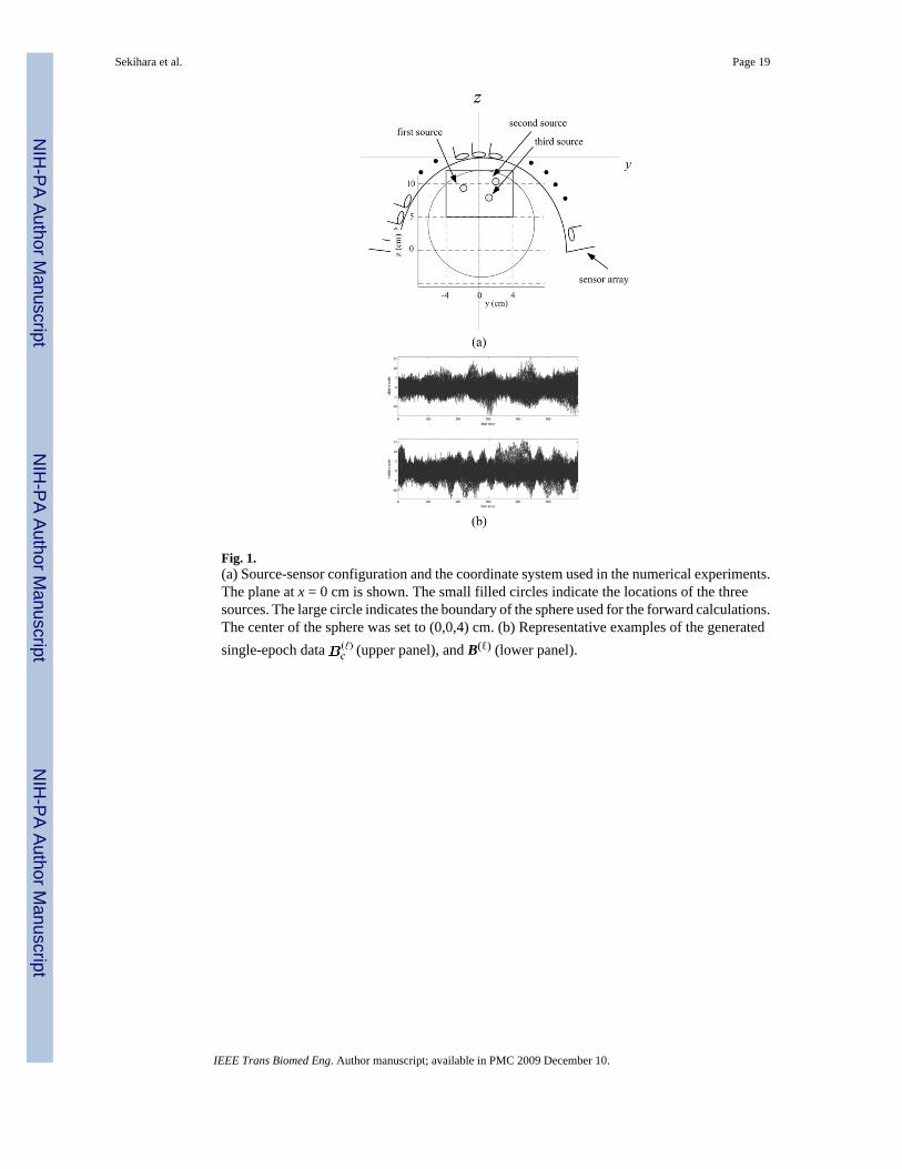
Fig. 1.(a) Source-sensor configuration and the coordinate system used in the numerical experiments.The plane at x = 0 cm is shown. The small filled circles indicate the locations of the threesources. The large circle indicates the boundary of the sphere used for the forward calculations.The center of the sphere was set to (0,0,4) cm. (b) Representative examples of the generatedsingle-epoch data (upper panel), and B(ℓ) (lower panel).

Sekihara et al.


NIH


NIH


NIH


Fig. 2.Results of the source reconstruction experiments simulating the control-only-source scenario.(a) Results of conventional reconstruction for the task condition, Φ̂(r). (b) Results ofconventional reconstruction for the control condition, Φ̂C(r). (c) Results of the prewhiteningsource reconstruction. (d) Results of the flipped prewhitening source reconstruction.

Sekihara et al.


NIH


NIH


NIH


Fig. 3.Results of the source reconstruction experiments simulating the modulating-source scenario.(a) Results of conventional reconstruction for the task condition, Φ̂(r). (b) Results ofconventional reconstruction for the control condition, Φ̂C(r). (c) Results of calculating thepseudo-F image F (r). (d) Results of applying the prewhitening source reconstruction. Thesignal subspace dimension was set to 15. (e) Results of the Flipped prewhitening sourcereconstruction.

Sekihara et al.


NIH


NIH


NIH


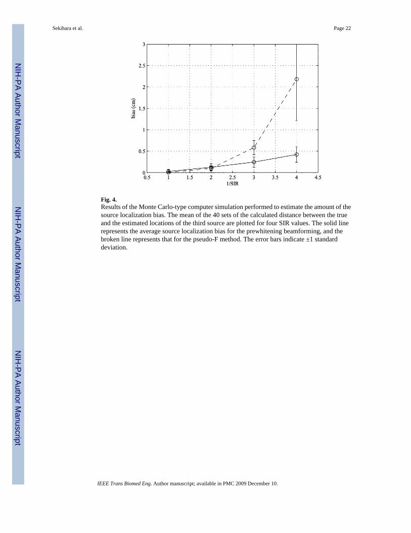
Fig. 4.Results of the Monte Carlo-type computer simulation performed to estimate the amount of thesource localization bias. The mean of the 40 sets of the calculated distance between the trueand the estimated locations of the third source are plotted for four SIR values. The solid linerepresents the average source localization bias for the prewhitening beamforming, and thebroken line represents that for the pseudo-F method. The error bars indicate ±1 standarddeviation.

Sekihara et al.


NIH


NIH


NIH


Fig. 5.

(a) Eigenvalue spectrum of used for reconstruction in Fig. 3(d). (b) The results of theprewhitening source reconstruction obtained with the signal subspace dimension set to 30.

Sekihara et al.


NIH


NIH


NIH


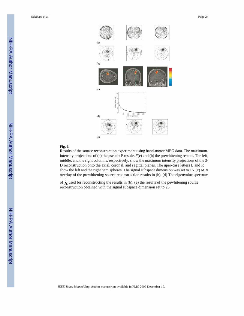
Fig. 6.Results of the source reconstruction experiment using hand-motor MEG data. The maximum-intensity projections of (a) the pseudo-F results F(r) and (b) the prewhitening results. The left,middle, and the right columns, respectively, show the maximum intensity projections of the 3-D reconstruction onto the axial, coronal, and sagittal planes. The uper-case letters L and Rshow the left and the right hemispheres. The signal subspace dimension was set to 15. (c) MRIoverlay of the prewhitening source reconstruction results in (b). (d) The eigenvalue spectrum

of used for reconstructing the results in (b). (e) the results of the pewhitening sourcereconstruction obtained with the signal subspace dimension set to 25.

Sekihara et al.


NIH


NIH


NIH


Performance of Prewhitening Beamforming in MEG Dual Experimental Conditions

Documents

Transcript of Performance of Prewhitening Beamforming in MEG Dual Experimental Conditions