performance of c-shaped structural concrete - CORE
412
PERFORMANCE OF C-SHAPED STRUCTURAL CONCRETE WALLS SUBJECTED TO BI-DIRECTIONAL LOADING BY ANDREW W. MOCK DISSERTATION Submitted in partial fulfillment of the requirements for the degree of Doctor of Philosophy in Civil Engineering in the Graduate College of the University of Illinois at Urbana-Champaign, 2018 Urbana, Illinois Doctoral Committee: Professor Billie F. Spencer, Chair Professor Daniel A. Kuchma, Tufts University, Director of Research Professor Laura N. Lowes, University of Washington Professor John S. Popovics
-
Upload
khangminh22 -
Category
Documents
-
view
2 -
download
0
Transcript of performance of c-shaped structural concrete - CORE

PERFORMANCE OF C-SHAPED STRUCTURAL CONCRETE
WALLS SUBJECTED TO BI-DIRECTIONAL LOADING
BY
ANDREW W. MOCK
DISSERTATION
Submitted in partial fulfillment of the requirements
for the degree of Doctor of Philosophy in Civil Engineering
in the Graduate College of the
University of Illinois at Urbana-Champaign, 2018
Urbana, Illinois
Doctoral Committee:
Professor Billie F. Spencer, Chair
Professor Daniel A. Kuchma, Tufts University, Director of Research
Professor Laura N. Lowes, University of Washington
Professor John S. Popovics
ii
ABSTRACT
Reinforced concrete walls are commonly used as the lateral force resisting system for mid-rise
buildings in regions of low and high seismicity. Wall geometries in buildings are generally
complex configurations to accommodate architectural constraints during new construction or
existing conditions in seismic retrofit applications. A typical configuration for seismic regions is
the concrete core-wall system in which coupling beams link a pair of C-shaped walls. While a
prevalent structural system, few experimental research programs have examined this wall type and
codes of practice have focused on design provisions for planar walls which do not fully account
for the effects of non-planar geometry and multi-directional loading.
To improve the understanding of the three-dimensional and asymmetric response of coupled
core walls, an experimental testing program of C-shaped walls subjected to uni-directional and bi-
directional cyclic loading was completed. Three C-shaped walls representative of a ten-story core
wall building were tested at the University of Illinois Newmark Structural Engineering Laboratory.
Each wall test was subjected to progressively complex loading conditions, and a new stiffness-
based loading algorithm was developed to conduct the experiment. Analysis of the experimental
data studied the energy dissipation, progression of yielding, components of deformation to total
wall drift, base deformations, strain fields generated from displacement field data, and overall
displacement profiles of the prototype ten-story building. Subsequent evaluations using prior
experimental tests of planar, coupled and non-planar walls identified the aspects of behavior
unique to C-shaped walls.
The experimental tests exhibited a ductile failure resulting from loss of boundary element
confinement, bar buckling, and rupture of the longitudinal bars. However, the ductile failure
mechanism was precipitated by increased shear deformation and undesirable shear related damage
of base sliding and web crushing. The onset of damage mechanisms, propagation of damage, and
drift capacity at failure was identified to be path dependent, and bi-directional loading decreased
drift capacity. Effective flexural and shear stiffness values for the elastic analysis of non-planar
walls were recommended for design. Design variables and demand to capacity ratios were
parametrically studied for non-planar walls as a means to correlate drift capacity and ductility. To
supplement the experimental data, a series of non-linear finite element analyses were conducted
using a layered shell element model with comprehensive constitutive models capturing the cracked
response of reinforced concrete in cyclic biaxial loading conditions. Model validation is conducted

iii
using reinforced concrete panel tests, and the impact of crack spacing on prediction is quantified.
The resulting analytical models of the C-shaped walls provide a validation of the experimental
results and a characterization of shear stress distribution as a function of drift level for strong axis
and weak axis loading.

iv
In memory of Donald Wickens

v
ACKNOWLEDGMENTS
This dissertation would not have been possible without the support of my research advisor,
doctoral committee, collaborating faculty members, laboratory staff, and prior graduate students.
First and foremost, I acknowledge my research advisor, Dr. Daniel Kuchma. He provided me
with the opportunity to take a leadership role in an advanced research project and taught me how
to conduct large-scale experimental tests. His subsequent mentorship, guidance, and expertise not
only supported the completion of this dissertation, but impacted my intellectual development and
appreciation for the field of structural engineering and the behavior of concrete structures.
I extend my gratitude to Dr. Laura Lowes and Dr. Dawn Lehman at the University of
Washington. Their support and expertise were instrumental to the experimental testing effort, the
analysis of the data, and the documentation of the work. I also acknowledge and thank Dr. Lowes
for her time and involvement dedicated to my doctoral committee.
I express my appreciation to the doctoral committee for their support, guidance, and advice
throughout the completion of this dissertation. I thank Dr. Bill Spencer for serving as the chair of
my committee and for the years of insight provided while working in the Newmark Structural
Engineering Laboratory. I thank Dr. John Popovics for serving on the committee and his helpful
perspective in reviewing this dissertation. I also acknowledge Dr. David Lange and Dr. Arif
Masud for serving on my preliminary examination committee.
The experiments supporting this dissertation involved many graduate students and laboratory
staff. In particular, I acknowledge former students: Dr. Anahid Behrouzi, Dr. Anna Birely, and
Dr. Christopher Hart for their contributions and shared experiences on the Complex Walls research
project. I also specifically acknowledge Michael Bletzinger and Dr. Chia-Ming Chang for their
assistance with the laboratory control and instrumentation methods.
Finally, I acknowledge that the research was supported by the National Science Foundation
under Grant No. CMMI-0421577, the Graduate Research Fellowship Program, and the Graduate
Research Opportunities Worldwide Program. Additional support for this project was provided by
the Charles Pankow Foundation through Grant No. CPF 03-09. Any opinions, findings, and
conclusions or recommendations expressed in this dissertation are those of myself and do not
necessarily reflect the views of the National Science Foundation or the Charles Pankow
Foundation.
vi
TABLE OF CONTENTS
LIST OF SYMBOLS .................................................................................................. vii
CHAPTER 1: INTRODUCTION............................................................................... 1
CHAPTER 2: LITERATURE REVIEW .................................................................... 6
CHAPTER 3: EXPERIMENTAL TESTING OF C-SHAPED WALLS ............... 115
CHAPTER 4: QUALITATIVE EXPERIMENTAL OBSERVATIONS ............... 181
CHAPTER 5: DATA ANALYSIS OF C-SHAPED WALL EXPERIMENTS ..... 214
CHAPTER 6: NON-PLANAR WALL PERFORMANCE .................................... 257
CHAPTER 7: FINITE ELEMENT ANALYSIS OF C-SHAPED WALLS .......... 319
CHAPTER 8: CONCLUSIONS AND FUTURE WORK ..................................... 376
REFERENCES .......................................................................................................... 387
vii
LIST OF SYMBOLS
cA area of concrete
cvA area of concrete for shear design per ACI 318
effA effective area of concrete for a single reinforcing bar
gA gross sectional area
D diameter
cE elastic modulus of concrete
1cE , 2cE secant stiffness for net concrete principal stress-strain
rE elastic modulus of reloading
sE elastic modulus of steel
shE elastic modulus of steel strain hardening
12cG secant stiffness for net concrete shear stress-strain
cG elastic shear modulus of concrete
fG fracture energy released per unit area
H wall height
effI effective moment of inertia considering the effects of cracking
gI gross section moment of inertia
K strength enhancement factor for Kent-Park model
coupleL coupling length between geometric centroids of wall piers
rL characteristic length for cracking
M moment
,b baseM M base moment
crM sectional cracking moment
nM nominal moment strength
N Ramberg-Osgood power term
P applied load
viii
coupleP axial force due to coupling on wall pier
gravityP axial force due to gravity load on wall pier
V shear
baseV base shear
flV shear resisted in wall flange
nV nominal shear strength
webV shear resisted in wall web
mZ slope of the descending branch of the Kent-Park model
a maximum aggregate size
c sectional depth of compression at nominal
cc clear cover
yieldc sectional depth of compression at yield
bd reinforcing bar diameter
'cf 28-day compressive strength
' *cf compressive strength at time of testing
1cf first principal concrete stress
2cf second principal concrete stress
crf concrete cracking stress
,cx cyf f net concrete normal stress in coordinate directions
mf maximum historic stress
rf concrete modulus of rupture
sf steel stress
,sx syf f steel stresses in coordinate directions
tf tensile stress
uf steel ultimate stress
,x yf f normal stress in coordinate directions
ix
yf yield stress
eh effective height
r
eh average height of row of elements
sh specimen height
10h ten-story height
i increment
j iteration
k bond ratio for crack spacing models
e length of the element
fl length of the flange
w length of the web
m bond parameter for tension stiffening model
s bond slip deformation
s mean crack spacing perpendicular to principal strain
,mx mys s mean crack spacing in coordinate directions
rms mean crack spacing
wt wall thickness
cw crack width
avgw average crack width
flex effective flexural stiffness ratio
shear effective shear stiffness ratio
compressive softening scaling factor
d compressive damage parameter for cyclic modeling
t tensile damage parameter for cyclic modeling
s average shear slip
1 first principal strain
2 second principal strain
x
'c nominal compressive strain
o
c initial or elastic strain offset in concrete
p
c plastic strain offset in concrete
cm maximum principal concrete strain of cycle during cyclic loading
cr concrete cracking strain
,cx cy net concrete strain in coordinate directions
cu concrete ultimate (crushing) strain
m maximum historic strain
rec recovered strain during cyclic loading
ro strain at the end of reloading during cyclic loading
o
s initial or elastic strain offset in steel
p
s plastic strain offset in steel
sh steel strain hardening strain
,sx sy steel strains in coordinate directions
t tensile strain at sectional nominal strength
p
t plastic offset in concrete tension model
ts terminal strain where the concrete tensile distribution becomes zero
,x y average strain in coordinate directions
,s s
x y average slip strain in coordinate directions
y steel yield strain
u steel ultimate strain
cxy net shear strain in concrete
s shear strain at crack interface
xy average shear strain
s
xy average slip shear strain
load increment parameter
xi
N axial load ratio
ductility ratio
civ shear stress at crack interface
cxyv net concrete shear stress
dv shear stress resisted by dowel action
xyv average shear stress
uv ultimate shear stress
12 21, Poisson’s ratio
rotation
c orientation of net concrete stress
eff rotation of wall at the effective height of loading
orientation of total strain
be boundary element reinforcement ratio
con lateral confining steel reinforcement ratio at boundary element
ef effective reinforcement ratio for crack spacing models
h horizontal reinforcement ratio
total total reinforcement ratio of section
,x y reinforcing ratio in coordinate directions
bond stress
bm mean bond stress
, ,,x flexure y flexure contribution of flexural deformation to total lateral displacement
, ,,x shear y shear contribution of shear deformation to total lateral displacement
u displacement increment
p load increment
rotation lag between average principal stress and strain
eff displacement at the effective height of loading
xii
roof wall roof level displacement
r
avg average curvature of row of elements
n curvature at sectional nominal strength
y curvature at sectional yield
B element strain-displacement matrix
D global element stiffness matrix
cD global element concrete stiffness matrix
s iD global element smeared steel reinf. stiffness matrix for each component
cD
local concrete secant stiffness matrix
si
D
local smeared steel reinf. secant stiffness matrix for each component
F force vector
histF experimentally measured force history matrix
measF experimentally measured force vector
targetF proposed force target for load-control
G Jacobian gain matrix for load control
K stiffness matrix
P reference force vector
R unbalanced force vector
cT element transformation matrix for concrete
s iT element transformation matrix for each rebar component
u displacement vector
histu experimentally measured displacement history matrix
targetu incremental displacement to reach target displacement
optimization vector
1
CHAPTER 1: INTRODUCTION
Reinforced concrete walls are commonly used as the lateral force resisting system for buildings
around the world in regions of low and high seismicity. Wall geometries in buildings are generally
complex configurations to accommodate architectural constraints during new construction or
existing conditions in seismic retrofit applications. The plan layout of walls often results in non-
planar wall configurations with walls that are interconnected by beams and floor slabs.
Furthermore, these walls often include openings in elevation to accommodate architectural and
mechanical equipment needs. In combination, the resulting wall configurations are complex and
believed to induce three-dimensional effects, unintended coupling between walls, and reduced
ductility due to bi-directional loadings. Observations of damage after earthquakes, large-scale
experimental testing, and numerical modeling provide opportunities to improve the understanding
of how wall and building behavior are influenced by these effects.
Earthquake damage to structural walls has resulted in an evolution of building code provisions
throughout their history (Massone et al. 2012). Modern detailing of walls in seismic regions often
requires confined boundary elements and constraints on the maximum reinforcement ratios with a
desire for high stiffness during service loading and a ductile response in seismic events (Lowes et
al. 2013). However, limited test data exists for these types of structural walls to validate the design
stipulations that exist in our codes of practice. Furthermore, recent earthquakes have resulted in
severe damage to concrete structures that were designed and built consistent with modern codes
of practice. In 2011, a magnitude 6.2 earthquake in Christchurch, New Zealand resulted in damage
to more than 130 structural concrete buildings (Kam and Pampanin 2011). In 2010, a magnitude
8.8 earthquake in Maule, Chile resulted in severe damage to more than 40 structural concrete
buildings (Maffei et al. 2014). In particular, building configuration issues including vertical
discontinuities, geometric changes and unintended coupling of walls through slabs, beams, and
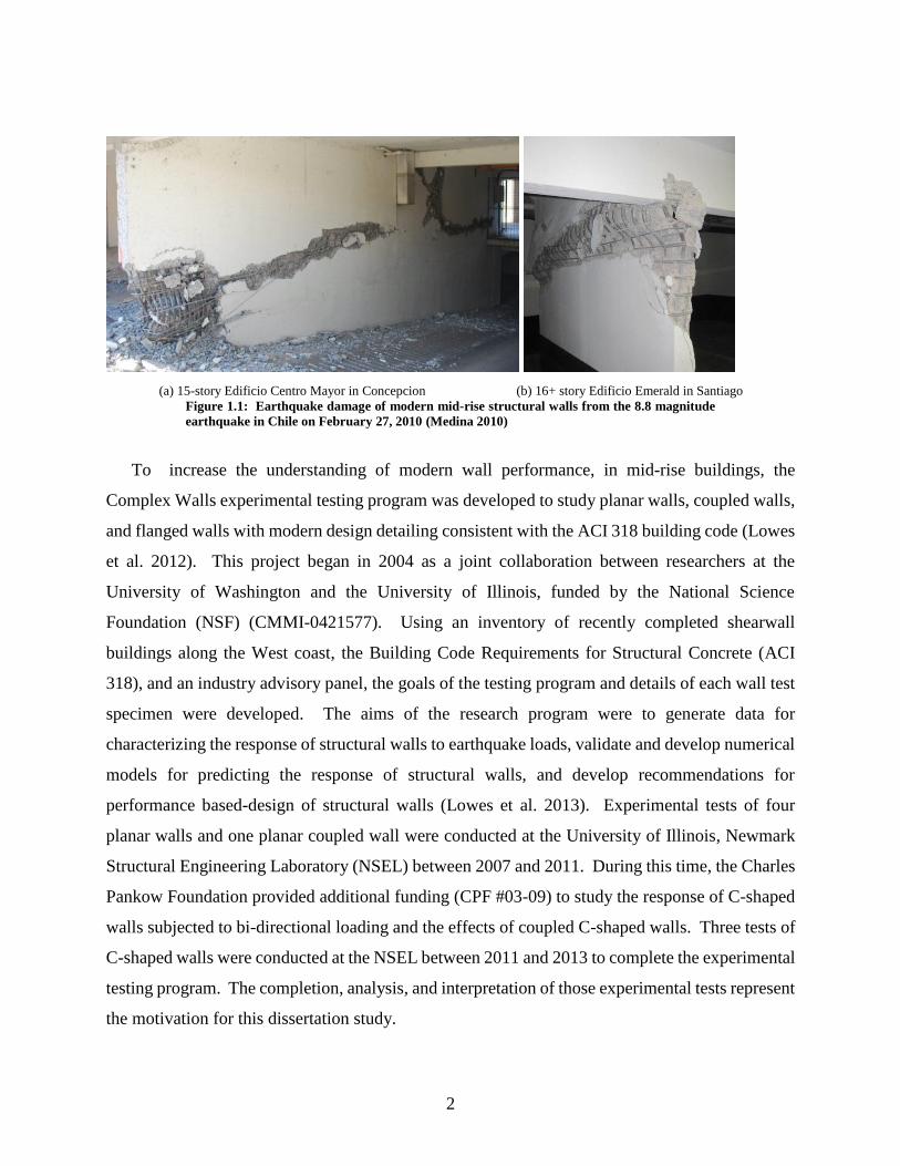
non-structural components were present in the damaged buildings (Wallace et al. 2012). Figure
1.1 provides an example of the earthquake damage to structural walls in Chile. The evident
damage in modern walled buildings reinforces the need for continued evolution of the building
code and design practices.
2
(a) 15-story Edificio Centro Mayor in Concepcion (b) 16+ story Edificio Emerald in Santiago
Figure 1.1: Earthquake damage of modern mid-rise structural walls from the 8.8 magnitude
earthquake in Chile on February 27, 2010 (Medina 2010)
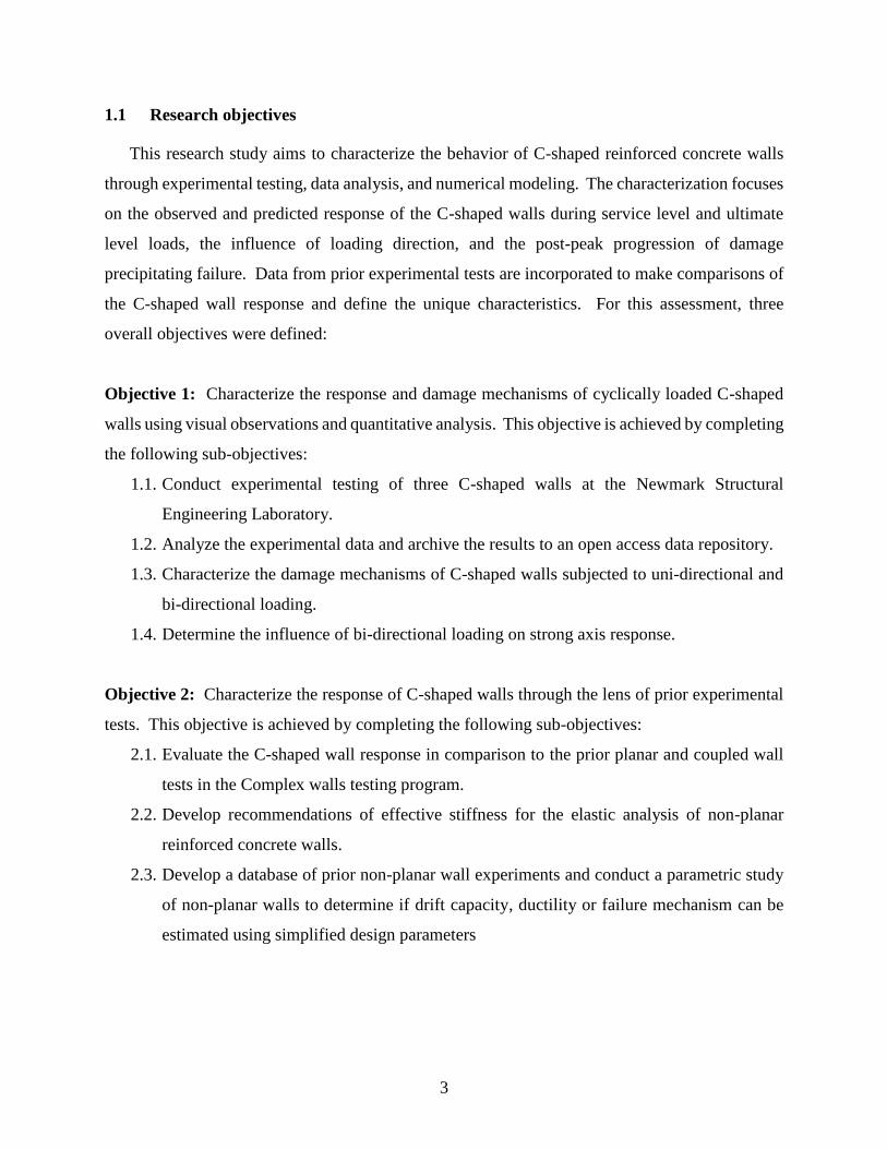
To increase the understanding of modern wall performance, in mid-rise buildings, the
Complex Walls experimental testing program was developed to study planar walls, coupled walls,
and flanged walls with modern design detailing consistent with the ACI 318 building code (Lowes
et al. 2012). This project began in 2004 as a joint collaboration between researchers at the
University of Washington and the University of Illinois, funded by the National Science
Foundation (NSF) (CMMI-0421577). Using an inventory of recently completed shearwall
buildings along the West coast, the Building Code Requirements for Structural Concrete (ACI
318), and an industry advisory panel, the goals of the testing program and details of each wall test
specimen were developed. The aims of the research program were to generate data for
characterizing the response of structural walls to earthquake loads, validate and develop numerical
models for predicting the response of structural walls, and develop recommendations for
performance based-design of structural walls (Lowes et al. 2013). Experimental tests of four
planar walls and one planar coupled wall were conducted at the University of Illinois, Newmark
Structural Engineering Laboratory (NSEL) between 2007 and 2011. During this time, the Charles
Pankow Foundation provided additional funding (CPF #03-09) to study the response of C-shaped
walls subjected to bi-directional loading and the effects of coupled C-shaped walls. Three tests of
C-shaped walls were conducted at the NSEL between 2011 and 2013 to complete the experimental
testing program. The completion, analysis, and interpretation of those experimental tests represent
the motivation for this dissertation study.
3
1.1 Research objectives
This research study aims to characterize the behavior of C-shaped reinforced concrete walls
through experimental testing, data analysis, and numerical modeling. The characterization focuses
on the observed and predicted response of the C-shaped walls during service level and ultimate
level loads, the influence of loading direction, and the post-peak progression of damage
precipitating failure. Data from prior experimental tests are incorporated to make comparisons of
the C-shaped wall response and define the unique characteristics. For this assessment, three
overall objectives were defined:
Objective 1: Characterize the response and damage mechanisms of cyclically loaded C-shaped
walls using visual observations and quantitative analysis. This objective is achieved by completing
the following sub-objectives:
1.1. Conduct experimental testing of three C-shaped walls at the Newmark Structural
Engineering Laboratory.
1.2. Analyze the experimental data and archive the results to an open access data repository.
1.3. Characterize the damage mechanisms of C-shaped walls subjected to uni-directional and
bi-directional loading.
1.4. Determine the influence of bi-directional loading on strong axis response.
Objective 2: Characterize the response of C-shaped walls through the lens of prior experimental
tests. This objective is achieved by completing the following sub-objectives:
2.1. Evaluate the C-shaped wall response in comparison to the prior planar and coupled wall
tests in the Complex walls testing program.
2.2. Develop recommendations of effective stiffness for the elastic analysis of non-planar
reinforced concrete walls.
2.3. Develop a database of prior non-planar wall experiments and conduct a parametric study
of non-planar walls to determine if drift capacity, ductility or failure mechanism can be
estimated using simplified design parameters

4
Objective 3: Conduct finite element modeling of the C-shaped wall experiments for validation
and exploration of the wall response in shear. This objective is achieved by completing the
following sub-objectives:
3.1. Develop a database of reinforced concrete panel tests and conduct an element level
validation of the constitutive models with a focus on the influence of crack spacing.
3.2. Recommend a crack spacing model for continuum analysis of reinforced concrete in which
cracks form non-orthogonal to the reinforcement.
3.3. Conduct non-linear finite element analyses simulating the cyclic response of the C-shaped
wall in both axes to validate the model performance and characterize the shear stress
distribution.
1.2 Organization
Chapter 2 provides a literature review to support the research effort. Prior experimental tests
of non-planar walls, as well as the prior experimental tests in the Complex Walls testing program,
are reviewed to create a context for the C-shaped wall response and damage patterns. For the
application of loading during the experimental testing, nonlinear solution methods are reviewed.
To support the interpretation of behavior and numerical modeling effort, an overview of the
relevant behavior of reinforced concrete, associated constitutive models, approaches to the
numerical modeling the response of structural concrete in a continuum, and prior finite element
studies of non-planar concrete walls are developed.
Chapter 3 provides the experimental testing methodology for the three C-shaped walls. The
specimen design and construction are detailed. The loading protocol for each test and laboratory
methodology for applying mixed displacements and loads is described. A bi-directional loading
algorithm for testing the third C-shaped wall as part of a simulated coupled core wall system is
developed.
Chapter 4 provides an overview of the key qualitative observations and progression of damage
in each of the three experimental tests. Based on the visual observations, a comparison of the walls
is made to understand the damage progression and key damage states. The demand and capacity
response of each wall is tabulated.
Chapter 5 provides a comprehensive quantitative analysis of the C-shaped wall experiments
comparing and contrasting the impact of loading history on wall response. An overview of the

5
data processing and subsequent data archival to the NHERI Design-Safe cyberinfrastructure is
provided. The data is post-processed to evaluate the energy dissipation of the walls, progression
of reinforcing yielding, base deformations, strain fields using non-contact displacement
measurements, drift contributions, and displacement profiles.
Chapter 6 extends the comparison of the C-shaped walls to prior planar, coupled and non-
planar walls. A parametric study of design parameters for structural walls is conducted to identify
trends in damage patterns, drift capacity, and ductility. The results of the parametric study are
subsequently applied to a recently proposed drift capacity equation for structural concrete walls
and evaluated. Finally, recommendations of effective stiffness values for the elastic analysis of
non-planar walls are developed.
Chapter 7 describes the non-linear finite element analysis of C-shaped walls conducted for
model validation and the characterization of shear demand associated with flanged walls. The
finite element analysis is conducted using layered shell elements with smeared cracking and
reinforcement in a continuum. To validate the choice of constitutive models utilized in the shell
element analysis, an element level study of the constitutive models is validated against
experimentally tested reinforced concrete panels. Six different models for predicting crack spacing
are studied as part of the model validation. The resulting finite element models of the C-shaped
walls are used to assess the shear distribution in the web and flanges for monotonic and reverse
cyclic loading.
Chapter 8 provides a summary of the individual conclusions and recommendations on how
non-planar wall geometry and complex loading history influence the wall response. Future work
stemming from these efforts is described.
6
CHAPTER 2: LITERATURE REVIEW
2.1 Prior experimental tests of non-planar walls
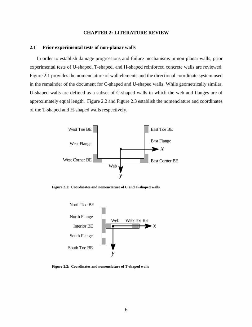
In order to establish damage progressions and failure mechanisms in non-planar walls, prior
experimental tests of U-shaped, T-shaped, and H-shaped reinforced concrete walls are reviewed.
Figure 2.1 provides the nomenclature of wall elements and the directional coordinate system used
in the remainder of the document for C-shaped and U-shaped walls. While geometrically similar,
U-shaped walls are defined as a subset of C-shaped walls in which the web and flanges are of
approximately equal length. Figure 2.2 and Figure 2.3 establish the nomenclature and coordinates
of the T-shaped and H-shaped walls respectively.
Figure 2.1: Coordinates and nomenclature of C and U-shaped walls
Figure 2.2: Coordinates and nomenclature of T-shaped walls
x
y
North Flange
North Toe BE
South Flange
South Toe BE
Web Toe BEWeb
Interior BE
x
y
East Corner BE
East Toe BE
East FlangeWest Flange
Web
West Corner BE
West Toe BE

7
Figure 2.3: Coordinates and nomenclature of H-shaped walls
2.1.1 Dimensionless datasets for comparisons of test data
The load-deformation response is presented using dimensionless ratios to facilitate comparison
of data from different tests. The deformation is presented as the drift ratio at the effective height
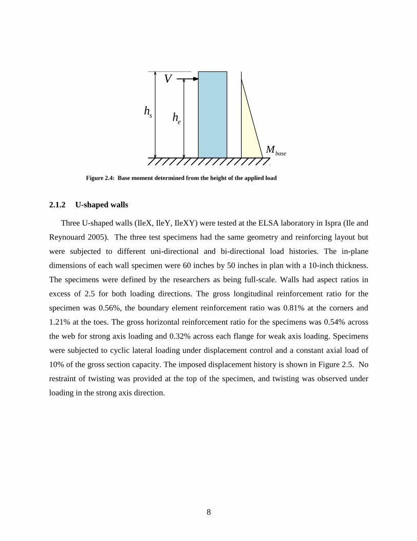
of the imposed load as shown in Figure 2.4. The effective height is defined as the inflection point
of the moment diagram. The base moment is defined as the product of the shear and effective
height:
base eM V h= (2.1)
The effective height is typically different from the specimen height due to the loading apparatus.
The load is presented as the moment developed at the base of the wall divided by the predicted
nominal flexural strength. Nominal flexural strength was taken as the maximum strength predicted
from section analysis using the Response2000 software (Bentz 2000) which can consider the
impact of shear on section response using the modified compression field theory (see Section
2.5.2.2). The maximum strength corresponds to the predicted failure mechanism of concrete
crushing ( 0.003cu = − per ACI 318, or first rupture of a longitudinal bar or stirrup.
x
y
Southwest Toe BE
West Interior BE
Northwest Toe BE
Southeast Toe BE
East Interior BE
Northeast Toe BE
Web
8
Figure 2.4: Base moment determined from the height of the applied load
2.1.2 U-shaped walls
Three U-shaped walls (IleX, IleY, IleXY) were tested at the ELSA laboratory in Ispra (Ile and
Reynouard 2005). The three test specimens had the same geometry and reinforcing layout but
were subjected to different uni-directional and bi-directional load histories. The in-plane
dimensions of each wall specimen were 60 inches by 50 inches in plan with a 10-inch thickness.
The specimens were defined by the researchers as being full-scale. Walls had aspect ratios in
excess of 2.5 for both loading directions. The gross longitudinal reinforcement ratio for the
specimen was 0.56%, the boundary element reinforcement ratio was 0.81% at the corners and
1.21% at the toes. The gross horizontal reinforcement ratio for the specimens was 0.54% across
the web for strong axis loading and 0.32% across each flange for weak axis loading. Specimens
were subjected to cyclic lateral loading under displacement control and a constant axial load of
10% of the gross section capacity. The imposed displacement history is shown in Figure 2.5. No
restraint of twisting was provided at the top of the specimen, and twisting was observed under
loading in the strong axis direction.
ehsh
baseM
V
9
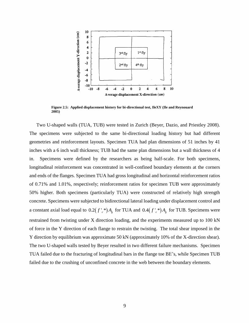
Figure 2.5: Applied displacement history for bi-directional test, IleXY (Ile and Reynouard
2005)
Two U-shaped walls (TUA, TUB) were tested in Zurich (Beyer, Dazio, and Priestley 2008).
The specimens were subjected to the same bi-directional loading history but had different
geometries and reinforcement layouts. Specimen TUA had plan dimensions of 51 inches by 41
inches with a 6 inch wall thickness; TUB had the same plan dimensions but a wall thickness of 4
in. Specimens were defined by the researchers as being half-scale. For both specimens,
longitudinal reinforcement was concentrated in well-confined boundary elements at the corners
and ends of the flanges. Specimen TUA had gross longitudinal and horizontal reinforcement ratios
of 0.71% and 1.01%, respectively; reinforcement ratios for specimen TUB were approximately
50% higher. Both specimens (particularly TUA) were constructed of relatively high strength
concrete. Specimens were subjected to bidirectional lateral loading under displacement control and
a constant axial load equal to ( )0.2 ' *c gf A for TUA and ( )0.4 ' *c gf A for TUB. Specimens were
restrained from twisting under X direction loading, and the experiments measured up to 100 kN
of force in the Y direction of each flange to restrain the twisting. The total shear imposed in the
Y direction by equilibrium was approximate 50 kN (approximately 10% of the X-direction shear).
The two U-shaped walls tested by Beyer resulted in two different failure mechanisms. Specimen
TUA failed due to the fracturing of longitudinal bars in the flange toe BE’s, while Specimen TUB
failed due to the crushing of unconfined concrete in the web between the boundary elements.

10
Figure 2.6: Graphical representation of displacement history for specimen TUA and TUB
(Beyer, Dazio, and Priestley 2008)
Table 2.1: Summary of U-shaped wall test specimen geometry and reinforcement
Reference: (Beyer, Dazio, and Priestley 2008) (Ile and Reynouard 2005)
Specimen ID TUA TUB UW1 / UW2 / UW3
Scale 1:2 1:2 1:1
Shear span (M/V) 2.95m / 3.35m 2.95m / 3.35m 3.90m
Spear span ratio (h/lw) 2.81 / 2.58 2.81 / 2.58 3.12 / 2.60
Axial Load 169k (750kN) 175k (780kN) 477k (2120kN)
Axial load ratio 0.02 0.04 0.1-0.12
Compressive Strength
at time of testing, f’c* 11.3 ksi (78 MPa) 8 ksi (55 MPa) 3.5 ksi (24 MPa)
Compactness ratios
lweb/tw 8.7 13 6
lfl/tw 7 10.5 5
Vertical reinforcement ratios
total 0.71% 1.01% 0.56%
corner BE's 0.84% 1.88% 0.81%
toe BE's 2.11% 2.45% 1.21%
Horizontal reinforcement ratios
web 0.30% 0.45% 0.54%
flanges 0.30% 0.45% 0.32%
Beyer et al. (2008): Specimen TUA and TUB
The load-deformation response of each specimen under strong-axis, weak-axis, and diagonal
loading are given in Figure 2.7 and Figure 2.9. The damage states and influence of bi-directional
loading on the test response are detailed in the following sections.
x
y

11
Specimen TUA damage narrative
Specimen TUA was loaded bidirectional with cyclic displacements about the strong-axis,
weak-axis and in a diagonal pattern. Load-deformation response histories for the different loading
directions are shown in Figure 2.7. After reaching theoretical yield around 0.25% drift, spalling
initiated during cycles to 1% drift (All plots: DS1) and became widespread during cycles to 1.25%
drift (All plots: DS2). During cycles to 1.8% drift in X-direction, 2% drift in the positive weak
axis, and 2% drift in the negative weak axis, sliding along the interface, buckling of the
longitudinal bars in the flange toe BE’s, and minor spalling in the unconfined regions of the web
adjacent to the corner BE’s was observed (All plots: DS3). The last cycle in the strong axis
fractured the longitudinal bars in the West flange (Strong-Axis: Failure). The positive-weak axis
failed due to the fracture of previously buckled bars in the flange toe BE’s (Weak-Axis: Failure).
A significant loss in load-carrying capacity was observed under subsequent loading in the diagonal
direction. The last cycle in the negative diagonal direction caused fracture of previously buckled
web bars (Strong-Diagonal, Weak-Diagonal: DS4). After load reversal to the positive diagonal,
all remaining bars in the West flange web fractured as well as three additional longitudinal bars in
the West flange toe BE (Strong-Diagonal, Weak-Diagonal: Failure).
Boundary elements at the toes of flanges exhibited extensive spalling and rupture of the end
boundary element bars. However, concrete within the toe boundary elements remained well
confined, and no concrete crushing was observed. Sliding was observed at large displacements,
even with shear keys used in the design of the specimens. One of the shear keys was observed to
have sheared off; other shear keys were not visible. Some compressive damage was visible along
the web between the corner boundary elements and on the east flange web, although the researchers
did not observe an impact on the failure mechanism from this damage.

12
(a) Strong axis normalized moment vs. drift (b) Weak axis normalized moment vs. drift
(c) Diagonal axis normalized moment (square root of the sum of the squares) vs. drift
Figure 2.7: Specimen TUA load-deformation response
Specimen TUA strength and ductility
The load-deformation response for strong-axis loading TUA shows a well-defined yield
plateau with minimal cyclic strength degradation. Some pinching of the hysteretic response is
observed, becoming pronounced as early as 1% drift. The specimen reached a maximum strength
equal to approximately 83% of simulated nominal strength; drift capacity was 2.5%. While no
cyclic strength degradation is observed because of the bidirectional loading, the shortcoming to
the predicted strength could be a consequence of the bi-directional loading.
The weak-axis hysteresis in the positive direction (web in compression) has a defined yield
plateau and ductile response reaching approximately 86% of the nominal moment capacity and a
maximum drift of 3.5%. After unloading in the positive direction, significant residual deformation

13
was observed at zero force after cycles to 1% drift. The negative weak-axis direction (toe in
compression) presents a slightly stiffer response with smaller energy dissipating loops. The
nominal moment strength is achieved and reaches a maximum drift of 2.8%.
The hystereses of the diagonal loading path present reduced ductility, strength, and energy
dissipation. Both directions achieve less than 2% drift and have a strength loss of 20-25% when
compared to the uni-directional response in each direction. The positive diagonal (East flange
corner in compression) performs marginally better than the negative diagonal (West flange toe in
compression) which can be attributed to the smaller compressive region in the toe BE and
consequential damage occurring.
Specimen TUB damage narrative
Specimen TUB was loaded with the same bidirectional pattern as specimen TUA with cyclic
displacements about the strong-axis, weak-axis and in a diagonal pattern. The hystereses are
shown in Figure 2.9. After reaching theoretical yield around 0.4% drift, spalling initiated during
cycles to 1.25% drift (All plots: DS1). The spalling exposed longitudinal reinforcement during
cycles to 1.65% drift (All plots: DS2). Spalling spread into the unconfined web regions during
subsequent cycles resulting in a significant loss of sectional width in some unconfined areas. The
web’s ability to carry compression across the damaged unconfined regions failed during the cycles
at 2.5% drift in the strong axis. The web-crushing failure resulted in a new load path for the lateral
shear. A frame mechanism developed to transfer the shear through bending of the corner boundary
elements and transverse shear across the flange in compression. The frame mechanism is shown
in Figure 2.8. Bar buckling was observed in the West flange toe BE during the final cycles. No
loss of confinement or crushing in the BE’s was observed. No reinforcing bars fractured and the
maximum sliding displacement was 4.4% of the total drift.

14
(a) Photo of interior of U-shaped wall web (b) Photo of exterior of U-shaped wall web
Figure 2.8: Web crushing of specimen TUB (Beyer, Dazio, and Priestley 2008)
(a) Strong axis normalized moment vs. drift (b) Weak axis normalized moment vs. drift
(c) Diagonal axis normalized moment (square root of the sum of the squares) vs. drift
Figure 2.9: Specimen TUB load-deformation response

15
Specimen TUB strength and ductility
Specimen TUB presented a similar load-deformation response to TUA prior to failure. The
strong axis response has a defined yield plateau and no strength degradation reaching 86% of the
nominal capacity and a maximum drift of 2.5%. The weak-axis hysteresis in the positive direction
(web in compression) reaches a higher strength at approximately 91% of the nominal moment
capacity and a maximum drift of 3%. Unloading from the positive direction resulted in significant
residual deformations at zero force after cycles to 1.5% drift. The negative weak-axis direction
(toe in compression) presents more considerable energy dissipating loops, surpasses the nominal
moment strength, and reaches a maximum drift of 2.8%.
Ile and Reynouard (2005): Specimen IleX, IleY and IleXY
The three identical U-shaped walls tested by Ile and Reynouard under varying uni-directional
and bi-directional loadings allowed the influence of bi-directional loading to be directly compared
to the uni-directional response. The load-deformation response of each specimen in the strong-
axis (lleX and IleXY) and the weak-axis (IleY and IleXY) are given in Figure 2.12 to Figure 2.12.
The damage states and influence of bi-directional loading on the test response are detailed in the
following sections.
Specimen IleX damage narrative
Specimen IleX was loaded uni-directionally about the strong axis. Theoretical yield was
identified at 0.43% drift. Damage initiated during cycles to 2% drift with bar buckling at the toe
BE’s of the flanges (IleX: DS1). After two cycles to 3% drift, the damage was characterized by
severe bar buckling, rupture of BE stirrups and longitudinal BE bars at the ends of both flanges
and the corners (IleX: DS2). In the final cycle to 3% drift, failure resulted from rupture of
previously buckled longitudinal bars in the flange.
16
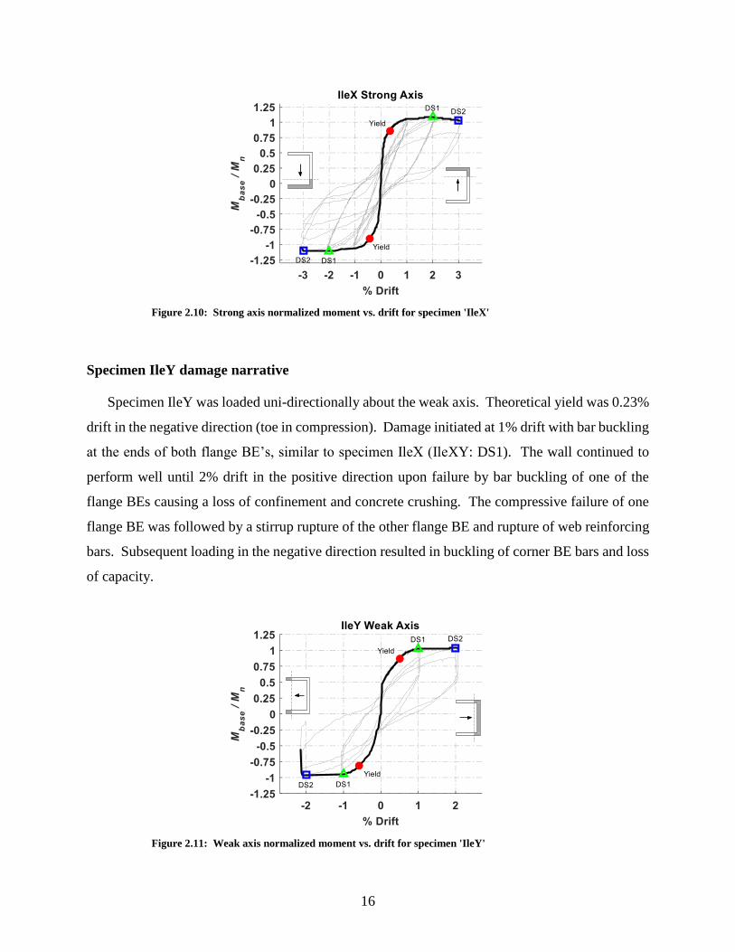
Figure 2.10: Strong axis normalized moment vs. drift for specimen 'IleX'
Specimen IleY damage narrative
Specimen IleY was loaded uni-directionally about the weak axis. Theoretical yield was 0.23%
drift in the negative direction (toe in compression). Damage initiated at 1% drift with bar buckling
at the ends of both flange BE’s, similar to specimen IleX (IleXY: DS1). The wall continued to
perform well until 2% drift in the positive direction upon failure by bar buckling of one of the
flange BEs causing a loss of confinement and concrete crushing. The compressive failure of one
flange BE was followed by a stirrup rupture of the other flange BE and rupture of web reinforcing
bars. Subsequent loading in the negative direction resulted in buckling of corner BE bars and loss
of capacity.
Figure 2.11: Weak axis normalized moment vs. drift for specimen 'IleY'

17
Specimen IleXY damage narrative
Specimen IleXY was loaded bi-directionally in a butterfly pattern. Damage became
widespread by the first cycle to 2% drift with extensive spalling, bar buckling and fracture
occurring (IleXY: DS1). The specimen failed in the last cycle while at 2% drift in the strong axis
and 2% drift in the negative weak axis (East flange toe in compression). Failure was caused by
the fracture of three previously buckled BE bars on the West flange followed by a shear failure of
the flange (IleXY: Failure).
(a) Strong axis normalized moment vs. drift (b) Weak axis normalized moment vs. drift
Figure 2.12: Load-deformation response for specimen ‘IleXY’
Strength and ductility of Ile test specimens
The IleXY test displays a reduction in strength, stiffness, and ductility as a result of the bi-
directional loading path. In the uni-directional tests, minimal strength degradation is observed for
both the strong and weak axis tests until nearing failure, while the bi-directional loading causes
significant cyclic stiffness degradation in the strong axis and negative weak axis at 1% drift and
2% drift in the positive weak axis direction. The negative weak axis bending (toe in compression)
shows the most substantial degradation as a result of the increased demand on the toe BE region.
The initiation of damage at the toe BE degrades the subsequent strong and weak axis performance.
Significant relaxation is observed in the weak axis response of the bi-directional test after
reaching 1% drift. The residual lateral force required to reach zero displacement is dissipated
IleXY Strong Axis
18
during the subsequent loading about the strong axis with no change in weak axis displacement.
This phenomenon was not observed for the strong axis.
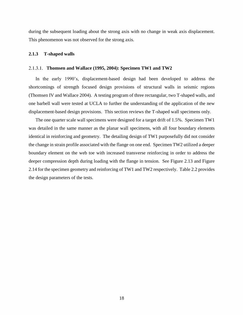
2.1.3 T-shaped walls
Thomsen and Wallace (1995, 2004): Specimen TW1 and TW2
In the early 1990’s, displacement-based design had been developed to address the
shortcomings of strength focused design provisions of structural walls in seismic regions
(Thomsen IV and Wallace 2004). A testing program of three rectangular, two T-shaped walls, and
one barbell wall were tested at UCLA to further the understanding of the application of the new
displacement-based design provisions. This section reviews the T-shaped wall specimens only.
The one quarter scale wall specimens were designed for a target drift of 1.5%. Specimen TW1
was detailed in the same manner as the planar wall specimens, with all four boundary elements
identical in reinforcing and geometry. The detailing design of TW1 purposefully did not consider
the change in strain profile associated with the flange on one end. Specimen TW2 utilized a deeper
boundary element on the web toe with increased transverse reinforcing in order to address the
deeper compression depth during loading with the flange in tension. See Figure 2.13 and Figure
2.14 for the specimen geometry and reinforcing of TW1 and TW2 respectively. Table 2.2 provides
the design parameters of the tests.
19
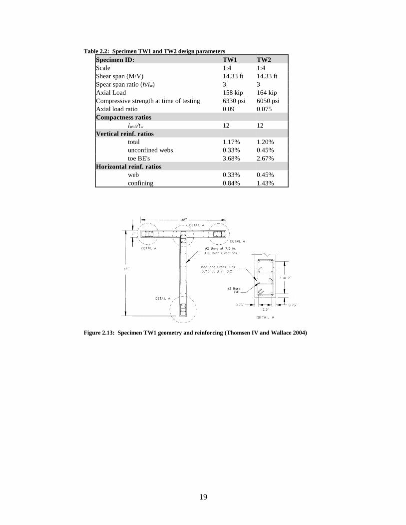
Table 2.2: Specimen TW1 and TW2 design parameters
Specimen ID: TW1 TW2
Scale 1:4 1:4
Shear span (M/V) 14.33 ft 14.33 ft
Spear span ratio (h/lw) 3 3
Axial Load 158 kip 164 kip
Compressive strength at time of testing 6330 psi 6050 psi
Axial load ratio 0.09 0.075
Compactness ratios
lweb/tw 12 12
Vertical reinf. ratios
total 1.17% 1.20%
unconfined webs 0.33% 0.45%
toe BE's 3.68% 2.67%
Horizontal reinf. ratios
web 0.33% 0.45%
confining 0.84% 1.43%
Figure 2.13: Specimen TW1 geometry and reinforcing (Thomsen IV and Wallace 2004)

20
Figure 2.14: Specimen TW2 geometry and reinforcing (Thomsen IV and Wallace 2004)
The test specimens were subjected to a constant axial load using a hydraulic jack with a
resulting axial load ratio of about ( )0.08 ' *c gf A . A reverse cyclic lateral displacement history
was imposed using an actuator mounted perpendicular to the top of the wall specimen. The
resulting load-deformation histories given in terms of drift and normalized base moment are
presented in Figure 2.15.
The complete progression of cracking and damage for the wall specimens is given by Thomsen
and Wallace (1995). For specimen TW1, flexural cracking initiated at 0.25% and shear cracking
at 0.50% drift cycles. Vertical splitting cracks in the web toe boundary element were observed
during the cycle at -0.75% drift (noted as DS1). At the cycle to -1% drift, extensive vertical
splitting cracks and minor crushing of the concrete over the bottom 12 inches were observed (noted
as DS2). Failure of the wall specimen was observed during the cycle to -1.25% drift resulting
from a brittle buckling failure of the web toe boundary element. The resulting damage to the
bottom 36 inches of the web is shown in Figure 2.16.

21
(a) (b)
Figure 2.15: (a) Specimen TW1 and (b) Specimen TW2 Load-Deformation Response for
loading parallel to the web of the wall versus percent drift. Positive drift represents the
flange in compression and negative drift represents the web toe in compression.
For specimen TW2, flexural cracking initiated at 0.25% and shear cracking at 0.50% drift
cycles. Vertical splitting cracks in the web toe boundary element were observed during the first
cycle at -0.9% drift (noted as DS1). The cycles to -1.3% (noted as DS2) resulted in cover spalling
of the web toe boundary element over the bottom 12 inches. During the cycle to -1.8% drift, the
cover spalling extended an additional 12 inches up the boundary element, but the core remained
intact. Core crushing and failure of confining reinforcement were observed during the cycle at -
2.25% drift (noted as DS3). After positive displacement to 2.5% drift, the wall failure at -0.75%
drift due to an out-of-plane buckling of the web boundary element as shown in Figure 2.17.
Figure 2.16: Specimen TW1 web failure (Thomsen IV and Wallace 2004)

22
Figure 2.17: Specimen TW2 web failure (Thomsen IV and Wallace 2004)
Brueggen (2009): Specimen NTW1 and NTW2
Two tests of T-shaped walls subjected to complex multi-directional loading were carried out
at the University of Minnesota (Brueggen 2009). Prior experimental tests of T-shaped walls had
utilized uni-directional loading only due to laboratory constraints. Multi-directional testing is a
necessity to understand how wall damage during loading in one direction affects wall performance
in other directions. These tests of T-shaped walls also evaluated modern design detailing for the
confinement region when subjected to non-orthogonal loading. Both test specimens represented a
six-story prototype building; however, specimen NTW1 was a four-story sub-assemblage, and
specimen NTW2 was a two-story sub-assemblage. Each of the sub-assemblies was subjected to a
moment and axial load at the top of the wall in order to simulate the demands associated with the
six-story building. See Figure 2.18 (a) and (b) for the specimen geometry and reinforcing of
NTW1 and NTW2 respectively. Table 2.3 provides the design parameters of the tests.

23
Table 2.3: Specimen NTW1 and NTW2 design parameters
Specimen ID: NTW1 NTW2
Scale 1:2 1:2
Shear span (M/V) 26 ft 26 ft
Spear span ration (h/lw) 3.47 (web) /
4.33 (flange)
3.47 (web) /
4.33 (flange)
Axial Load 186.5kip 186.5kip
Compressive strength at time of testing 6833 psi 6178 psi
Axial load ratio 0.03 0.03
Compactness ratios
lweb/tw 15 15 lfl/tw 12 12
Vertical reinf. ratios
total 2.51% 2.16% unconfined webs 0.59% uniform corner BE's no BEs uniform toe BE's 3.78% uniform
Horizontal reinf. ratios
web 0.26% 0.41% flanges 0.26% 0.41% confining
(a) Specimen NTW1 (b) Specimen NTW2
Figure 2.18: Specimen NTW1 and NTW2 geometry and reinforcing (Brueggen 2009)
The load-deformation response of specimen NWT1 is given in Figure 2.19. Shear and flexural
cracking of the specimen initiated during the first cycle to 25% yield in the web direction. After
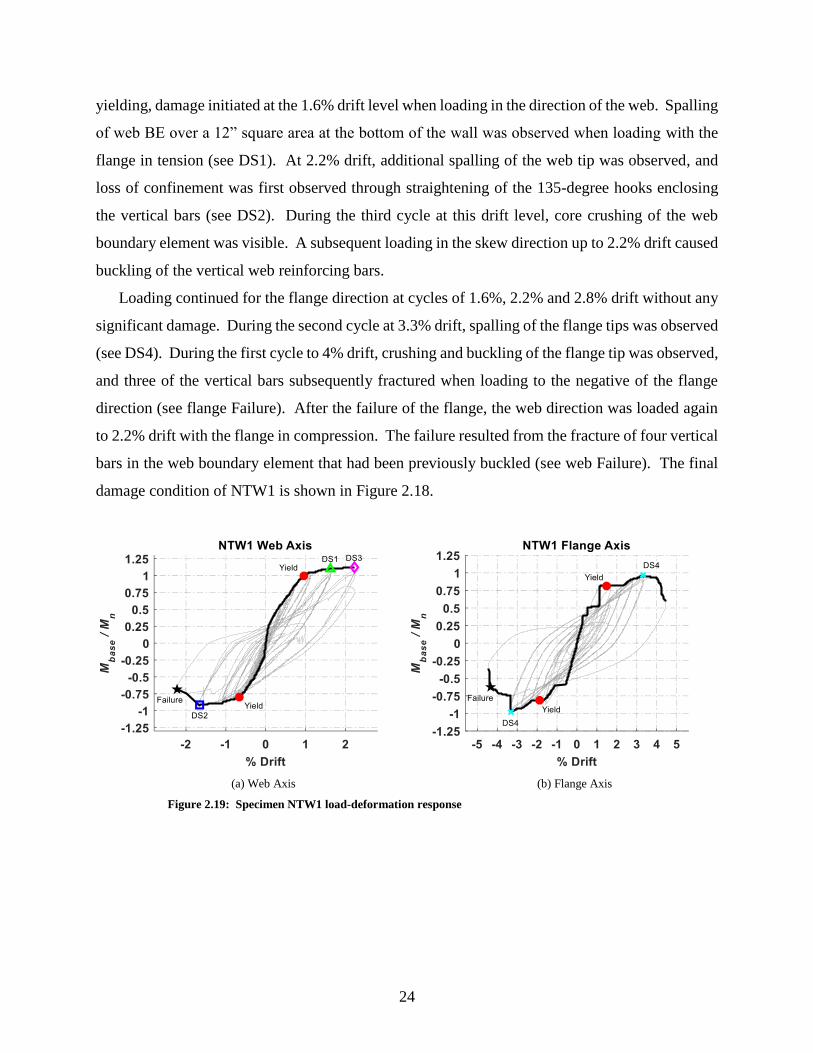
24
yielding, damage initiated at the 1.6% drift level when loading in the direction of the web. Spalling
of web BE over a 12” square area at the bottom of the wall was observed when loading with the
flange in tension (see DS1). At 2.2% drift, additional spalling of the web tip was observed, and
loss of confinement was first observed through straightening of the 135-degree hooks enclosing
the vertical bars (see DS2). During the third cycle at this drift level, core crushing of the web
boundary element was visible. A subsequent loading in the skew direction up to 2.2% drift caused
buckling of the vertical web reinforcing bars.
Loading continued for the flange direction at cycles of 1.6%, 2.2% and 2.8% drift without any
significant damage. During the second cycle at 3.3% drift, spalling of the flange tips was observed
(see DS4). During the first cycle to 4% drift, crushing and buckling of the flange tip was observed,
and three of the vertical bars subsequently fractured when loading to the negative of the flange
direction (see flange Failure). After the failure of the flange, the web direction was loaded again
to 2.2% drift with the flange in compression. The failure resulted from the fracture of four vertical
bars in the web boundary element that had been previously buckled (see web Failure). The final
damage condition of NTW1 is shown in Figure 2.18.
(a) Web Axis (b) Flange Axis
Figure 2.19: Specimen NTW1 load-deformation response

25
(a) Web (b) Flange
Figure 2.20: Specimen NTW1 after failure (Brueggen 2009)
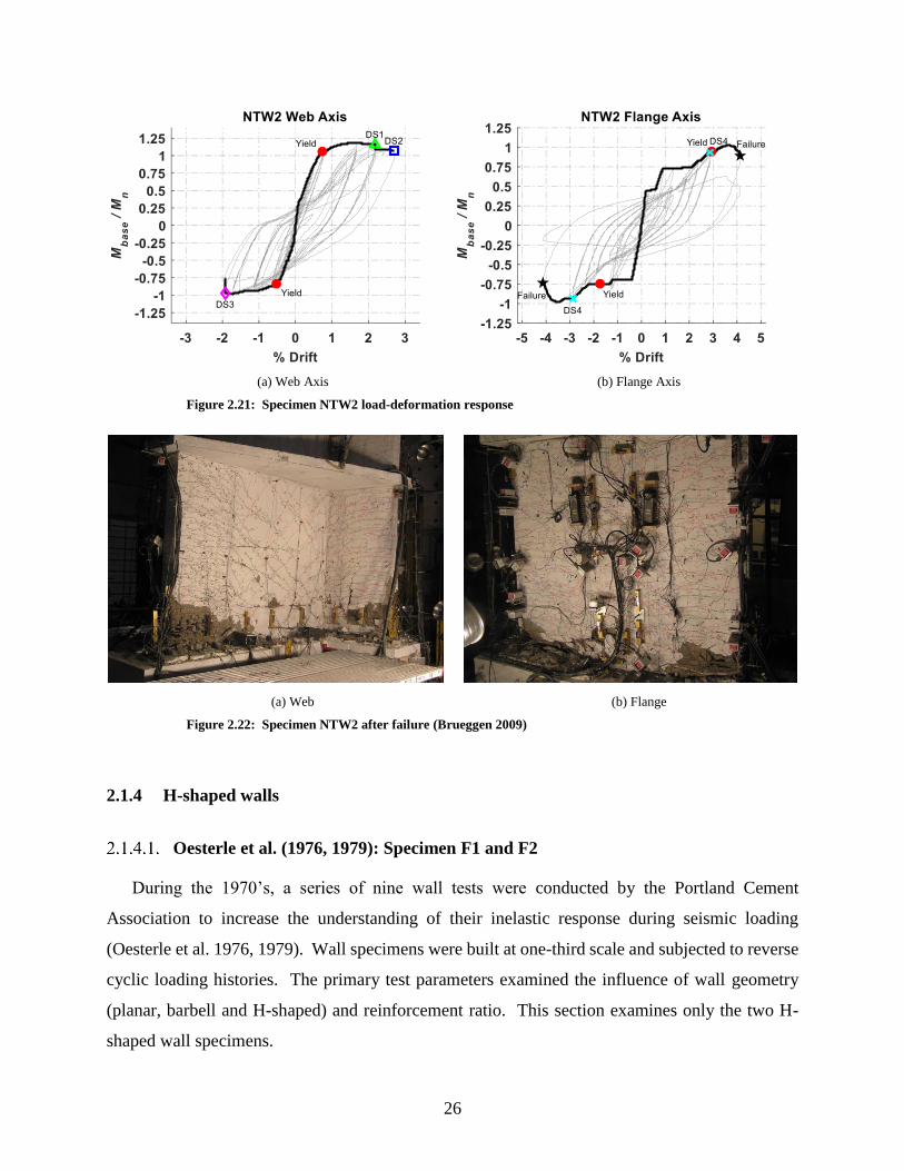
The load-deformation response of specimen NWT2 is given in Figure 2.21. After yielding,
damage initiated at the 2.2% drift level when loading in the direction of the web with spalling of
the web BE (see DS1). Subsequently, skew loading of the specimen to 2.2% drift in the web
direction and 0.66% in the skew direction resulted in additional spalling of the web BE and minor
flaking/spalling was observed along shear cracks in the unconfined web. A sliding deformation
of 1/8” was noted. At 2.7% drift, loss of confinement and fracture of the confinement hoops
occurred. Four longitudinal bars in the web tip buckled (see DS2). Upon loading in the opposite
direction with flange in compression at -1.9% drift, the four previously buckled bars fractured (see
DS3). Load carrying capacity was less than 50% of nominal upon reloading with the web tip in
compression.
Loading continued for the flange direction at cycles up to 2.3% drift without any significant
damage. During the cycle at 2.8% drift, spalling of the flange tips was observed (see DS4). During
the cycle to 4.1% drift, fracture of one BE bar occurred in the South tip and two BE bars in the
North tip (see flange Failure). The subsequent cycle at 4.1% drift resulted in additional fractures
and loss of load carrying capacity. The final damage condition of NTW2 is shown in Figure 2.22.
26
(a) Web Axis (b) Flange Axis
Figure 2.21: Specimen NTW2 load-deformation response
(a) Web (b) Flange
Figure 2.22: Specimen NTW2 after failure (Brueggen 2009)
2.1.4 H-shaped walls
Oesterle et al. (1976, 1979): Specimen F1 and F2
During the 1970’s, a series of nine wall tests were conducted by the Portland Cement
Association to increase the understanding of their inelastic response during seismic loading
(Oesterle et al. 1976, 1979). Wall specimens were built at one-third scale and subjected to reverse
cyclic loading histories. The primary test parameters examined the influence of wall geometry
(planar, barbell and H-shaped) and reinforcement ratio. This section examines only the two H-
shaped wall specimens.
27
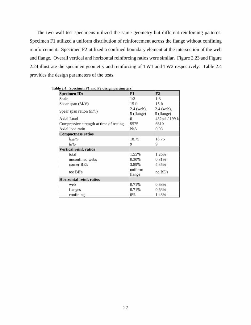
The two wall test specimens utilized the same geometry but different reinforcing patterns.
Specimen F1 utilized a uniform distribution of reinforcement across the flange without confining
reinforcement. Specimen F2 utilized a confined boundary element at the intersection of the web
and flange. Overall vertical and horizontal reinforcing ratios were similar. Figure 2.23 and Figure
2.24 illustrate the specimen geometry and reinforcing of TW1 and TW2 respectively. Table 2.4
provides the design parameters of the tests.
Table 2.4: Specimen F1 and F2 design parameters
Specimen ID: F1 F2
Scale 1:3 1:3
Shear span (M/V) 15 ft 15 ft
Spear span ration (h/lw) 2.4 (web),
5 (flange)
2.4 (web),
5 (flange)
Axial Load 0 482psi / 199 k
Compressive strength at time of testing 5575 6610
Axial load ratio N/A 0.03
Compactness ratios lweb/tw 18.75 18.75 lfl/tw 9 9
Vertical reinf. ratios total 1.55% 1.26% unconfined webs 0.30% 0.31% corner BE's 3.89% 4.35%
toe BE's uniform
flange no BE's
Horizontal reinf. ratios web 0.71% 0.63% flanges 0.71% 0.63% confining 0% 1.43%

28
Figure 2.23: Specimen F1 geometry and reinforcing (Oesterle et al. 1976)
Figure 2.24: Specimen F2 geometry and reinforcing (Oesterle et al. 1979)
29
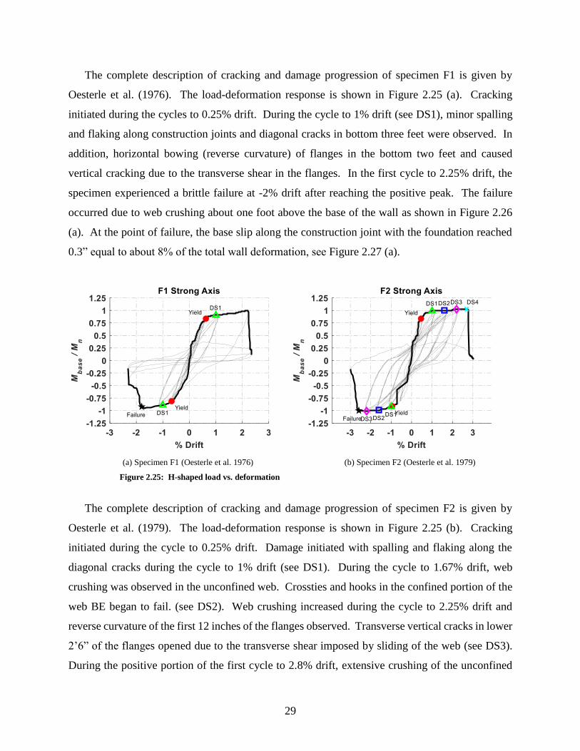
The complete description of cracking and damage progression of specimen F1 is given by
Oesterle et al. (1976). The load-deformation response is shown in Figure 2.25 (a). Cracking
initiated during the cycles to 0.25% drift. During the cycle to 1% drift (see DS1), minor spalling
and flaking along construction joints and diagonal cracks in bottom three feet were observed. In
addition, horizontal bowing (reverse curvature) of flanges in the bottom two feet and caused
vertical cracking due to the transverse shear in the flanges. In the first cycle to 2.25% drift, the
specimen experienced a brittle failure at -2% drift after reaching the positive peak. The failure
occurred due to web crushing about one foot above the base of the wall as shown in Figure 2.26
(a). At the point of failure, the base slip along the construction joint with the foundation reached
0.3” equal to about 8% of the total wall deformation, see Figure 2.27 (a).
(a) Specimen F1 (Oesterle et al. 1976) (b) Specimen F2 (Oesterle et al. 1979)
Figure 2.25: H-shaped load vs. deformation
The complete description of cracking and damage progression of specimen F2 is given by
Oesterle et al. (1979). The load-deformation response is shown in Figure 2.25 (b). Cracking
initiated during the cycle to 0.25% drift. Damage initiated with spalling and flaking along the
diagonal cracks during the cycle to 1% drift (see DS1). During the cycle to 1.67% drift, web
crushing was observed in the unconfined web. Crossties and hooks in the confined portion of the
web BE began to fail. (see DS2). Web crushing increased during the cycle to 2.25% drift and
reverse curvature of the first 12 inches of the flanges observed. Transverse vertical cracks in lower
2’6” of the flanges opened due to the transverse shear imposed by sliding of the web (see DS3).
During the positive portion of the first cycle to 2.8% drift, extensive crushing of the unconfined

30
region of the flange occurred (see DS4). On the negative loading to 2.8% drift, the lower portion
of the web experienced a brittle crushing failure. The compression flange sheared and a horizontal
failure plane developed across the web with a fracture of one horizontal bar as shown in Figure
2.26 (b). While specimen F2 experienced base slip similar to F1, the magnitude of slip was less
than one-third of that experienced by specimen F1, see Figure 2.27 (b). The confined boundary
elements may have contributed to the increased resistance to base slip.
(a) Specimen F1 (Oesterle et al. 1976) (b) Specimen F2 (Oesterle et al. 1979)
Figure 2.26: H-shaped wall failure due to web crushing
(a) Specimen F1 (Oesterle et al. 1976) (b) Specimen F2 (Oesterle et al. 1979)
Figure 2.27: H-shaped wall shear vs. base slip deformation
Of the conclusions from the testing program, three key conclusions are noted here: (1) the
presence of a horizontal construction joint in the plastic hinge region for walls may limit inelastic
31
response in walls subjected to high shear stress, (2) boundary elements in walls behave similar to
dowels, increasing resistance to base slip and shear distortion, and (3) shear deformation is a
significant portion of the overall non-planar wall displacement (Oesterle et al. 1976).
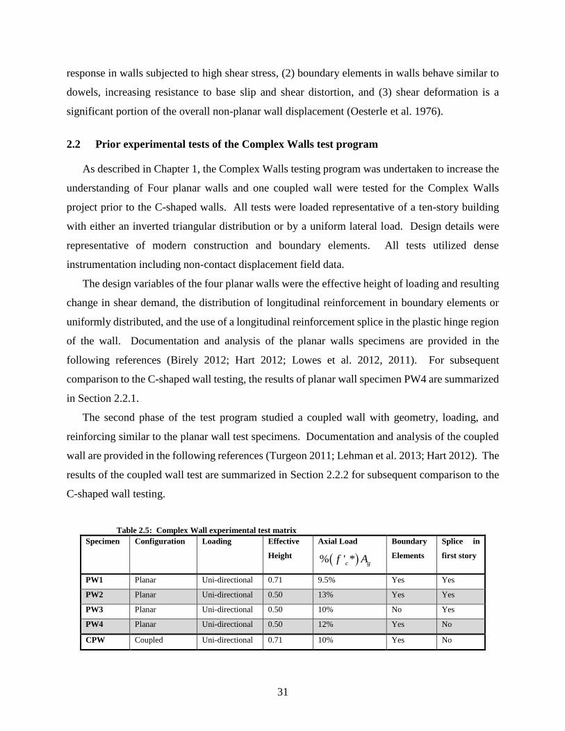
2.2 Prior experimental tests of the Complex Walls test program
As described in Chapter 1, the Complex Walls testing program was undertaken to increase the
understanding of Four planar walls and one coupled wall were tested for the Complex Walls
project prior to the C-shaped walls. All tests were loaded representative of a ten-story building
with either an inverted triangular distribution or by a uniform lateral load. Design details were
representative of modern construction and boundary elements. All tests utilized dense
instrumentation including non-contact displacement field data.
The design variables of the four planar walls were the effective height of loading and resulting
change in shear demand, the distribution of longitudinal reinforcement in boundary elements or
uniformly distributed, and the use of a longitudinal reinforcement splice in the plastic hinge region
of the wall. Documentation and analysis of the planar walls specimens are provided in the
following references (Birely 2012; Hart 2012; Lowes et al. 2012, 2011). For subsequent
comparison to the C-shaped wall testing, the results of planar wall specimen PW4 are summarized
in Section 2.2.1.
The second phase of the test program studied a coupled wall with geometry, loading, and
reinforcing similar to the planar wall test specimens. Documentation and analysis of the coupled
wall are provided in the following references (Turgeon 2011; Lehman et al. 2013; Hart 2012). The
results of the coupled wall test are summarized in Section 2.2.2 for subsequent comparison to the
C-shaped wall testing.
Table 2.5: Complex Wall experimental test matrix
Specimen Configuration Loading Effective
Height
Axial Load
( )% ' *c gf A
Boundary
Elements
Splice in
first story
PW1 Planar Uni-directional 0.71 9.5% Yes Yes
PW2 Planar Uni-directional 0.50 13% Yes Yes
PW3 Planar Uni-directional 0.50 10% No Yes
PW4 Planar Uni-directional 0.50 12% Yes No
CPW Coupled Uni-directional 0.71 10% Yes No

32
2.2.1 Planar wall test specimen PW4
The fourth planar wall test specimen, PW4, was distinguished from the prior tests primarily by
the lack of vertical reinforcing bar lap splice in the first story. At one-third scale, the planar wall
specimen was 10’-0” long and 6” thick. A heavily reinforced boundary element was detailed over
the last 1’-8” of each end of the wall. The story height was 4’-0” and the total specimen height
was 12’-0” to represent the bottom three stories of the ten-story building. The specimen geometry
and detailing are shown in Figure 2.28.
Figure 2.28: Cross-section and boundary element detail of PW4 (Hart 2012)
As previously noted, the imposed loads on the top of the third story were representative of the
ten-story building through the application of overturning moment and axial load. The imposed
axial load was 360 kips or 11.7% of the gross compressive strength at time of testing. The effective
height of loading was at mid-height of the ten-story building, so ancillary actuators were provided
at the top of the first and second floor in order to provide a uniform shear applied at each floor.
The resulting load-deformation response for base shear (left) and base moment (right) is given in
Figure 2.29.
L = 80L = 20
t =
6
A
be wL = 20
be
20
6
12
21
1 3 3 3 3 3 3 1
Detail A
#2 bar @ 6" o.c. e.f.
#2 bar @ 6" o.c. e.f.
(3)7 - #4 @ 3" o.c.
Confinement
Hoops & Ties
#2 @ 2" o.c.
L = 120
0.5" clear cover
Note: All units ininches unlessotherwise noted
L =
80
L =
20
t = 6
A
be
wL =
20
be
20
6
1 2 2 1
13
33
33
31
Detail A
#2 b
ar @
6" o
.c. e
.f.
#2 b
ar @
6" o
.c. e
.f.
(3)7
- #4 @
3" o
.c.
Confin
em
ent
Hoops &
Tie
s
#2 @
2" o
.c.
L =
120
0.5
" cle
ar c
over
Note
: All u
nits
inin
ches u
nle
ss
oth
erw
ise n
ote
d

33
Figure 2.29: PW4 Load-deformation response (Birely 2012)
For the damage progression, horizontal and diagonal cracking initiated at 0.06% and 0.07%
drift respectively. Yielding was first realized in compression of the extreme vertical boundary
element bars at 0.19% drift. Tensile yield of the same bars was noted at 0.30% drift. Vertical
splitting cracking in the boundary element compression region was observed during the cycle to
0.50% drift and followed by spalling of the concrete cover in the same cycle. As spalling extended,
the vertical boundary element reinforcing became fully exposed at the cycle to 0.75% drift. In the
third cycle at 0.75% drift, the vertical boundary element bars began to buckle followed by evident
core crushing inside the boundary element. During the second cycle to 1.0% drift, extensive bar
buckling and core crushing in the right boundary element at the bottom of the wall resulted in
failure and loss of load-carrying capacity. The resulting cracking and damage pattern are indicated
in Figure 2.30.
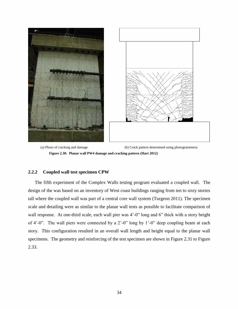
34
(a) Photo of cracking and damage (b) Crack pattern determined using photogrammetry
Figure 2.30: Planar wall PW4 damage and cracking pattern (Hart 2012)
2.2.2 Coupled wall test specimen CPW
The fifth experiment of the Complex Walls testing program evaluated a coupled wall. The
design of the was based on an inventory of West coast buildings ranging from ten to sixty stories
tall where the coupled wall was part of a central core wall system (Turgeon 2011). The specimen
scale and detailing were as similar to the planar wall tests as possible to facilitate comparison of
wall response. At one-third scale, each wall pier was 4’-0” long and 6” thick with a story height
of 4’-0”. The wall piers were connected by a 2’-0” long by 1’-0” deep coupling beam at each
story. This configuration resulted in an overall wall length and height equal to the planar wall
specimens. The geometry and reinforcing of the test specimen are shown in Figure 2.31 to Figure
2.33.

35
Figure 2.31: Elevation of coupled wall test specimen (Turgeon 2011)
Figure 2.32: Coupled wall coupling beam detail (Turgeon 2011)
Confinement
Ties & Hoops
#2 @ 2" o.c.
#4 bar @ 2" o.c. e.f.
#2 bar @ 3" o.c. e.f. (1st Floor)
#2 bar @ 6" o.c. e.f. (2nd & 3rd Floor)
#2 bar @
6" o.c. e.f.
LVL 3
LVL 2
LVL 1
LVL 0
5'-6" 1' 5'-6"
3'
4'
4'
4'
1'
2'-6"
18'-6"
4' Typ. 2'
PRODUCED BY AN AUTODESK EDUCATIONAL PRODUCT
PR
OD
UC
ED
BY
AN
AU
TO
DE
SK
ED
UC
AT
ION
AL
PR
OD
UC
T
PRODUCEDBYANAUTODESKEDUCATIONALPRODUCT
PR
OD
UC
ED
BY
AN
AU
TO
DE
SK
ED
UC
AT
ION
AL
PR
OD
UC
T
Detail B
BB
19
°
2'
2.5
"T
yp
.
1'-4''
2" Typ.
#2 bars
4-#4
bars
PRODUCED BY AN AUTODESK EDUCATIONAL PRODUCT
PR
OD
UC
ED
BY
AN
AU
TO
DE
SK
ED
UC
AT
ION
AL
PR
OD
UC
T
PRODUCEDBYANAUTODESKEDUCATIONALPRODUCT
PR
OD
UC
ED
BY
AN
AU
TO
DE
SK
ED
UC
AT
ION
AL
PR
OD
UC
T
Detail B
12''
6''
1'' 2'' 2'' 1''
1''
2.5
"1''
2.5
''2.5
''2.5
''
(2)4-#4 bar @ 3/4" x 2"
19° angle
ConfinementHoops & Ties
#2 @ 2" o.c.
12-#2 bar @ 2.5" o.c.
PRODUCED BY AN AUTODESK EDUCATIONAL PRODUCT
PR
OD
UC
ED
BY
AN
AU
TO
DE
SK
ED
UC
AT
ION
AL
PR
OD
UC
T
PRODUCEDBYANAUTODESKEDUCATIONALPRODUCT
PR
OD
UC
ED
BY
AN
AU
TO
DE
SK
ED
UC
AT
ION
AL
PR
OD
UC
T
Detail B
BB
19
°
2'
2.5
"T
yp
.
1'-4''
2" Typ.
#2 bars
4-#4
bars
PRODUCED BY AN AUTODESK EDUCATIONAL PRODUCT
PR
OD
UC
ED
BY
AN
AU
TO
DE
SK
ED
UC
AT
ION
AL
PR
OD
UC
T
PRODUCEDBYANAUTODESKEDUCATIONALPRODUCT
PR
OD
UC
ED
BY
AN
AU
TO
DE
SK
ED
UC
AT
ION
AL
PR
OD
UC
T
Detail B
12''
6''
1'' 2'' 2'' 1''
1''
2.5
"1''
2.5
''2.5
''2.5
''
(2)4-#4 bar @ 3/4" x 2"
19° angle
ConfinementHoops & Ties
#2 @ 2" o.c.
12-#2 bar @ 2.5" o.c.
PRODUCED BY AN AUTODESK EDUCATIONAL PRODUCT
PR
OD
UC
ED
BY
AN
AU
TO
DE
SK
ED
UC
AT
ION
AL
PR
OD
UC
T
PRODUCEDBYANAUTODESKEDUCATIONALPRODUCT
PR
OD
UC
ED
BY
AN
AU
TO
DE
SK
ED
UC
AT
ION
AL
PR
OD
UC
T
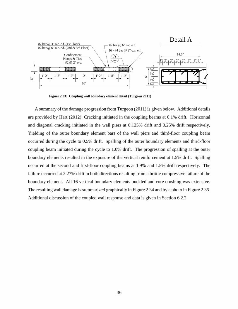
36
Figure 2.33: Coupling wall boundary element detail (Turgeon 2011)
A summary of the damage progression from Turgeon (2011) is given below. Additional details
are provided by Hart (2012). Cracking initiated in the coupling beams at 0.1% drift. Horizontal
and diagonal cracking initiated in the wall piers at 0.125% drift and 0.25% drift respectively.
Yielding of the outer boundary element bars of the wall piers and third-floor coupling beam
occurred during the cycle to 0.5% drift. Spalling of the outer boundary elements and third-floor
coupling beam initiated during the cycle to 1.0% drift. The progression of spalling at the outer
boundary elements resulted in the exposure of the vertical reinforcement at 1.5% drift. Spalling
occurred at the second and first-floor coupling beams at 1.9% and 1.5% drift respectively. The
failure occurred at 2.27% drift in both directions resulting from a brittle compressive failure of the
boundary element. All 16 vertical boundary elements buckled and core crushing was extensive.
The resulting wall damage is summarized graphically in Figure 2.34 and by a photo in Figure 2.35.
Additional discussion of the coupled wall response and data is given in Section 6.2.2.
16 - #4 bar @ 2" o.c. e.f.
#2 bar @ 6" o.c. e.f.
ConfinementHoops & Ties
#2 @ 2" o.c.
#2 bar @ 3" o.c. e.f. (1st Floor)#2 bar @ 6" o.c. e.f. (2nd & 3rd Floor)
A
10'
1'-2" 1'-8" 1'-2" 1'-2" 1'-8" 1'-2"2'
6"
PRODUCED BY AN AUTODESK EDUCATIONAL PRODUCT
PR
OD
UC
ED
BY
AN
AU
TO
DE
SK
ED
UC
AT
ION
AL
PR
OD
UC
T
PRODUCEDBYANAUTODESKEDUCATIONALPRODUCT
PR
OD
UC
ED
BY
AN
AU
TO
DE
SK
ED
UC
AT
ION
AL
PR
OD
UC
T
Detail A
14.0''
6''
1''
2''
2''
1''
1'' 2'' 2'' 2'' 2'' 2'' 2'' 1''
PRODUCED BY AN AUTODESK EDUCATIONAL PRODUCTP
RO
DU
CE
DB
YA
NA
UT
OD
ES
KE
DU
CA
TIO
NA
LP
RO
DU
CT
PRODUCEDBYANAUTODESKEDUCATIONALPRODUCT
PR
OD
UC
ED
BY
AN
AU
TO
DE
SK
ED
UC
AT
ION
AL
PR
OD
UC
T
16 - #4 bar @ 2" o.c. e.f.
#2 bar @ 6" o.c. e.f.
ConfinementHoops & Ties
#2 @ 2" o.c.
#2 bar @ 3" o.c. e.f. (1st Floor)#2 bar @ 6" o.c. e.f. (2nd & 3rd Floor)
A
10'
1'-2" 1'-8" 1'-2" 1'-2" 1'-8" 1'-2"2'
6"
PRODUCED BY AN AUTODESK EDUCATIONAL PRODUCT
PR
OD
UC
ED
BY
AN
AU
TO
DE
SK
ED
UC
AT
ION
AL
PR
OD
UC
T
PRODUCEDBYANAUTODESKEDUCATIONALPRODUCT
PR
OD
UC
ED
BY
AN
AU
TO
DE
SK
ED
UC
AT
ION
AL
PR
OD
UC
T
Detail A
14.0''
6''
1''
2''
2''
1''
1'' 2'' 2'' 2'' 2'' 2'' 2'' 1''
PRODUCED BY AN AUTODESK EDUCATIONAL PRODUCT
PR
OD
UC
ED
BY
AN
AU
TO
DE
SK
ED
UC
AT
ION
AL
PR
OD
UC
T
PRODUCEDBYANAUTODESKEDUCATIONALPRODUCT
PR
OD
UC
ED
BY
AN
AU
TO
DE
SK
ED
UC
AT
ION
AL
PR
OD
UC
T

37
Figure 2.34: Final regions of damage identified at the end of the coupled wall experiment
(Lehman et al. 2013)
Figure 2.35: Photograph of the bottom story of the coupled wall failure at the end of the test
2.3 Nonlinear solution techniques
The goal of all nonlinear solution techniques in finite element methods is to find the load-
displacement relationship of a structure. A load and/or displacement is applied to the structure
and iterations are then performed to find a convergent solution marking a single point on the load-
deformation solution path. All methods aim to solve static equilibrium u F=K after each
increment of load or displacement in order to match the external forces of the system to the internal
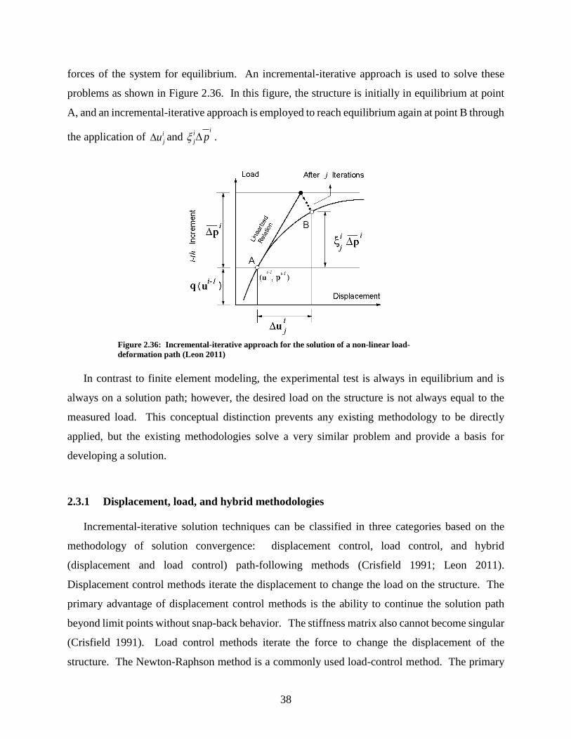
38
forces of the system for equilibrium. An incremental-iterative approach is used to solve these
problems as shown in Figure 2.36. In this figure, the structure is initially in equilibrium at point
A, and an incremental-iterative approach is employed to reach equilibrium again at point B through
the application of i
ju and i
i
j p .
Figure 2.36: Incremental-iterative approach for the solution of a non-linear load-
deformation path (Leon 2011)
In contrast to finite element modeling, the experimental test is always in equilibrium and is
always on a solution path; however, the desired load on the structure is not always equal to the
measured load. This conceptual distinction prevents any existing methodology to be directly
applied, but the existing methodologies solve a very similar problem and provide a basis for
developing a solution.
2.3.1 Displacement, load, and hybrid methodologies
Incremental-iterative solution techniques can be classified in three categories based on the
methodology of solution convergence: displacement control, load control, and hybrid
(displacement and load control) path-following methods (Crisfield 1991; Leon 2011).
Displacement control methods iterate the displacement to change the load on the structure. The
primary advantage of displacement control methods is the ability to continue the solution path
beyond limit points without snap-back behavior. The stiffness matrix also cannot become singular
(Crisfield 1991). Load control methods iterate the force to change the displacement of the
structure. The Newton-Raphson method is a commonly used load-control method. The primary

39
disadvantage of the load-control method is the failure at limit points where the stiffness matrix
becomes singular as well as the inability to trace the solution path beyond the limit point as shown
in Figure 2.37.
Figure 2.37: Divergence of a load-control methodology at a limit point of the load-
deformation path (Crisfield 1991)
The decision to use load or displacement-based control is dependent primarily upon the
structure being evaluated, and the loads applied to that structures. To address a wider variety of
structural problems with one solution, path-following methodologies where the displacement and
force are iterated upon were developed. A widely used path following method is known as the
arc-length method using a spherical arc-length constraint as proposed by Crisfield (1981). Bergan
(1980), Crisfield (1991) and Leon (2011; 2012) provide a more comprehensive evaluation of these
methods and their applications.
The load and displacement of the ith increment of the jth iteration can be characterized by the
following equations and by Table 2.6.
1
i i i
j j ju u u− = + (2.2)
1
i i i
j j jp p p− = + (2.3)
Table 2.6: Summary of control methodologies
Displacement control Load control Arc-length control
1j = 2j 1j = 2j 1j = 2j
i
ju prescribed 0 prescribed iterated prescribed iterated
i
jp prescribed iterated prescribed 0 prescribed iterated
The testing control methodology described in Section 3.3 falls somewhere between a true load
control method and a true arc-length methodology. The initial iteration will command the lateral

40
displacement with an axial force and overturning moments. The load will then be iterated as
needed without a change in displacement until convergence.
2.3.2 Stiffness measurement methodology
The tangent or secant stiffness measurement of the solution method can be done every iteration
(standard stiffness update) or only on the first iteration of the increment (constant stiffness update).
Crisfield illustrates the two stiffness methods in Figure 2.38 and Figure 2.39 in the case of a load-
control method. In both figures, two increments on the solution path are completed denoted by ft1
and ft2. The standard stiffness update shows a tangent stiffness measurement after each point of
convergence providing an increasing accurate stiffness to reach convergence of the increment in
less iteration. In the Newton method, the standard stiffness updates provide quadratic convergence
on the solution (Crisfield 1991). In contrast, the constant stiffness update shows a tangent stiffness
measured at the first iteration of the increment; however, the stiffness is not updated again until
after the increment is converged. The constant stiffness update could result in significantly more
iterations in a region of nonlinearity. However, if the increment is sufficiently small, the initial
tangent stiffness will be a reasonable value to use for the entire increment and reduce the
computational cost of stiffness updating (Crisfield 1991). The primary disadvantage and danger
of constant stiffness updates are the inability to correct for nonlinearities that occur during the
increment causing a significant change in stiffness.
Figure 2.38: Example of standard stiffness update at each iteration using a tangent stiffness
measurement (Crisfield 1991)
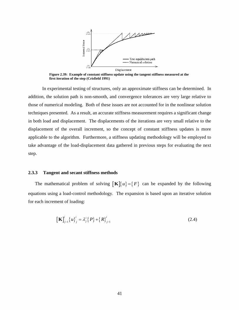
41
Figure 2.39: Example of constant stiffness update using the tangent stiffness measured at the
first iteration of the step (Crisfield 1991)
In experimental testing of structures, only an approximate stiffness can be determined. In
addition, the solution path is non-smooth, and convergence tolerances are very large relative to
those of numerical modeling. Both of these issues are not accounted for in the nonlinear solution
techniques presented. As a result, an accurate stiffness measurement requires a significant change
in both load and displacement. The displacements of the iterations are very small relative to the
displacement of the overall increment, so the concept of constant stiffness updates is more
applicable to the algorithm. Furthermore, a stiffness updating methodology will be employed to
take advantage of the load-displacement data gathered in previous steps for evaluating the next
step.
2.3.3 Tangent and secant stiffness methods
The mathematical problem of solving u F=K can be expanded by the following
equations using a load-control methodology. The expansion is based upon an iterative solution
for each increment of loading:
11
i i ii
jj jju P R
−−= +K (2.4)
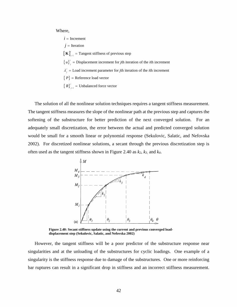
42
Where,
1
Increment
Iteration
Tangent stiffness of previous step
Displacement increment for th iteration of the th increment
Load increment parameter for th iteration of the th increment
Refe
i
j
i
j
i
j
u j i
j i
P
i
j
−
=
=
=
=
=
=
K
1
rence load vector
Unbalanced force vectori
jR
−=
The solution of all the nonlinear solution techniques requires a tangent stiffness measurement.
The tangent stiffness measures the slope of the nonlinear path at the previous step and captures the
softening of the substructure for better prediction of the next converged solution. For an
adequately small discretization, the error between the actual and predicted converged solution
would be small for a smooth linear or polynomial response (Sekulovic, Salatic, and Nefovska
2002). For discretized nonlinear solutions, a secant through the previous discretization step is
often used as the tangent stiffness shown in Figure 2.40 as k2, k3, and k4.
Figure 2.40: Secant stiffness update using the current and previous converged load-
displacement step (Sekulovic, Salatic, and Nefovska 2002)
However, the tangent stiffness will be a poor predictor of the substructure response near
singularities and at the unloading of the substructures for cyclic loadings. One example of a
singularity is the stiffness response due to damage of the substructures. One or more reinforcing
bar ruptures can result in a significant drop in stiffness and an incorrect stiffness measurement.

43
Figure 2.41 illustrates the discretized solution path with a sudden reduction in stiffness. The
dashed line represents the secant stiffness through that step.
Figure 2.41: Example of sudden drop in tangent stiffness between increments resulting from
damage (i.e. reinforcing bar fracture)
A pure secant stiffness method measures the stiffness or each step relative to force and
displacement at the initial or starting point on the nonlinear path. The secant stiffness method does
not have any convergence issues with singularities but will always overpredict the response. Drops
in stiffness do not significantly affect the predicted response of the next increment. Figure 2.42
illustrates the secant stiffness method.
Figure 2.42: Secant stiffness method using a current and initial or predefined converged
load-displacement point (Sekulovic, Salatic, and Nefovska 2002)
A tangent stiffness measured by a secant approximation of the last discretized step would best
characterize the changing stiffness of the test structure. This type of stiffness measurement, falling
into the class of ‘Quasi-Newton’ methods, will be further explored to determine its application to
the problem.
{u}
{F}
44
2.3.4 Secant stiffness updating
“Quasi-Newton methods” identify the class of nonlinear solution techniques that use the
Newton-Raphson method with an approximate Jacobian stiffness matrix as opposed to
mathematically forming and decomposing a tangent stiffness matrix (Crisfield 1981). The secant
approach described in 2.3.3 is commonly used.
2.3.5 Broyden update
The approximate tangent stiffness will be updated at each step to reflect the changing stiffness
of the structure. The aim is to update the Jacobian stiffness as little as possible while still
maintaining the prescribed relationship given the load-deformation of the last step. Fittingly, this
minimization calls the method a “least change secant update.” Mathematically prescribed as:
Find a solution to the stiffness K:
( ) ( )1 1
0 0 0 00
i i i i iu u F F
− −− = −K
(2.5)
While minimizing its solution:
1
0 0min
i i−−K K
(2.6)
The derivation of the solution is given by Broyden (1965) as well as Dennis and Schnabel
(1979). The solution results stiffness will be a fully populated square matrix with the number of
columns and rows equal to the number of prescribed degrees of freedom. The solution is:
( ) ( )
( )
11 1 1
0 0 001
0 0 1 1
0 0
Tii i i
measi i
Ti i
F u
u
−− − −
−
− −
− = +
KK K
(2.7)
45
0
1
0
1 1 2
0 0 0
,
approximated tangential stiffness for the next increment
approximated tangential stiffness used in the last step
change in internal force during the previously comp
i
i
i i i
meas
Where
F F F
−
− − −
=
=
= −
K
K
1 1 2
0 0 0
1
0
leted increment
change in displacement during the previously completed increment
"vector chosen to optimize the performance of the iteration method"
i i i
i
u u u
− − −
−
= − =
=
Broyden proposed that the optimization vector, psi, be equal to the change in displacement
(Crisfield 1991; Dennis and Schnabel 1979):
1 1
0 0
i iu
− −= (2.8)
The resulting solution hereafter referred to as the “Broyden update” is given by:
( ) ( )
( )
11 1 1
0 0 001
0 0 1 1
0 0
Tii i i
measi i
Ti i
F u
u
−− − −
−
− −
− = +
KK K
(2.9)
2.3.6 Davidon-Fletcher-Powell update
A refinement of the Broyden method was found by applying a weighting factor pre and post-
multiplied to the stiffness update. The weighting factor is chosen to represent the natural scaling
of the problem, providing an update the better represents the actual tangential stiffness.
Application of the weighting factor resulting in an updated minimization:
( ) ( )( )1 11 11
0 00 0min
i ii i− −− −−
− K K K K (2.10)
The derivation of the weighting factor and solution was completed by Davidon (1991) Fletcher
and Powell (1963). The resulting solution is given as:

46
( ) ( ) ( ) ( )
( )
( )
( )
1
0 0
1 11 1 1 1 1 1
0 0 0 0 0 00 0
1 1
0 0
11 1 1
0 0 00 1 1
2 0 01 1
0 0
i i
TTi ii i i i i i
meas meas
Ti i
ii i i
Tmeas i i
Ti i
F u u u F u
u u
F u uu u
u u
−
− −− − − − − −
− −
−− − −
− −
− −
=
− + − +
− −
K K
K K
K
(2.11)
The solution is hereafter referred to as the Davidon-Fletcher-Powell (DFP) update. For the
specialized case of using the stiffness matrix to predict forces as opposed to displacements, no
inversion of the stiffness matrix is required for either method of stiffness approximation.
2.4 Behavior and constitutive modeling of structural concrete
Detailed finite element modeling of structural concrete first requires an understanding of the
physical behavior or each independent material as well as the interactions between the two
materials. The approximations and applicability of constitutive models designed to represent the
physical phenomena of structural concrete must also be understood to evaluate the output of any
finite element analysis properly. This section provides a brief overview of the relevant phenomena
observed in concrete, steel, and their interaction.
2.4.1 Cracking
Concrete is inherently weak in tension relative to its compressive capacity and exhibits quasi-
brittle fracturing. Cracking occurs in concrete from time-dependent effects such as shrinkage, but
will primarily be considered from a mechanically induced tensile stress that exceeds the tensile
capacity of the concrete. Cracking generally refers to macro-cracking, cracks that are visible to
the naked eye (thousandth of an inch and larger). However, macro-cracks are in fact the result of
the propagation and coalescence of many micro-cracks that previously formed under lower levels
of stress.
Concrete is a heterogeneous material consisting of aggregates of varying sizes (fine and
coarse), a cement paste, and voids of air or water. For normal strength concretes, the aggregates
are typically higher strength than the paste, and micro-cracks form in the paste between and around
aggregates. Higher strength concrete exhibits a more uniform strength distribution, and micro-
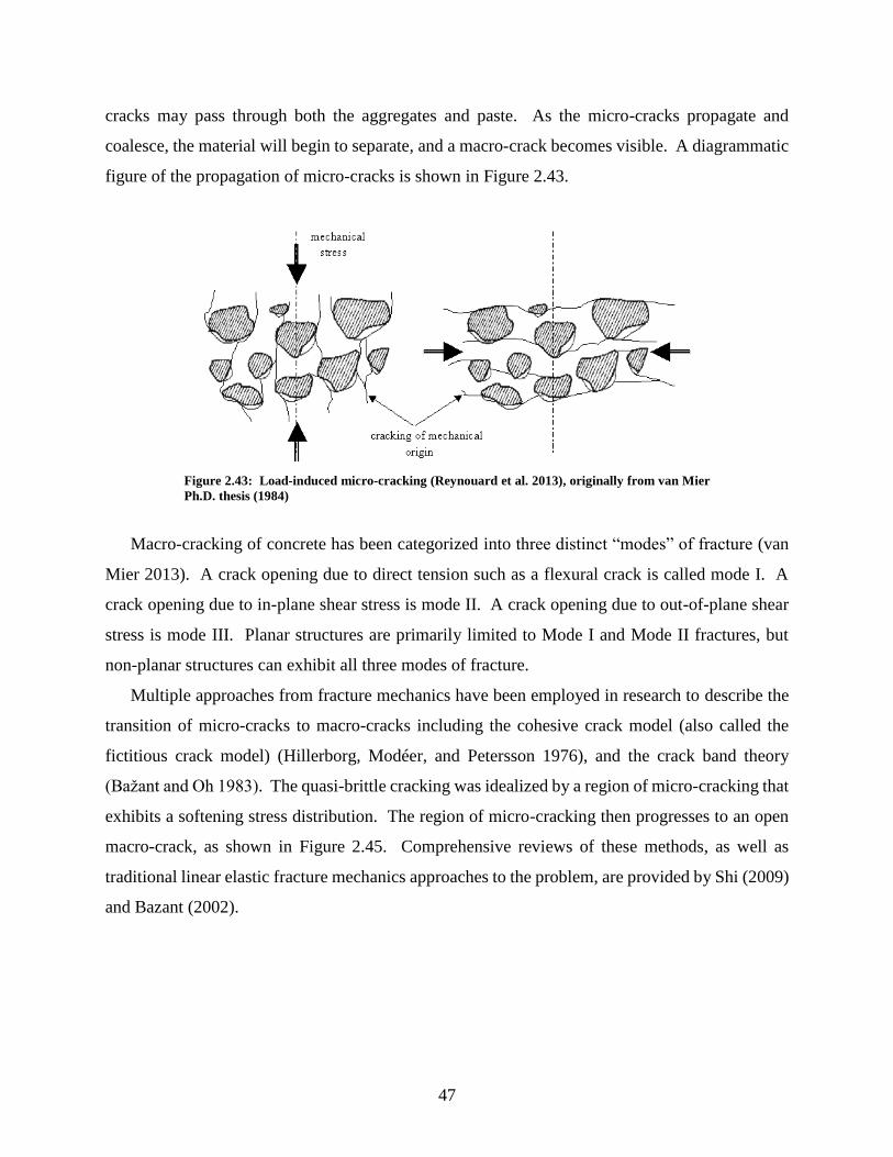
47
cracks may pass through both the aggregates and paste. As the micro-cracks propagate and
coalesce, the material will begin to separate, and a macro-crack becomes visible. A diagrammatic
figure of the propagation of micro-cracks is shown in Figure 2.43.
Figure 2.43: Load-induced micro-cracking (Reynouard et al. 2013), originally from van Mier
Ph.D. thesis (1984)
Macro-cracking of concrete has been categorized into three distinct “modes” of fracture (van
Mier 2013). A crack opening due to direct tension such as a flexural crack is called mode I. A
crack opening due to in-plane shear stress is mode II. A crack opening due to out-of-plane shear
stress is mode III. Planar structures are primarily limited to Mode I and Mode II fractures, but
non-planar structures can exhibit all three modes of fracture.
Multiple approaches from fracture mechanics have been employed in research to describe the
transition of micro-cracks to macro-cracks including the cohesive crack model (also called the
fictitious crack model) (Hillerborg, Modéer, and Petersson 1976), and the crack band theory
(Bažant and Oh 1983). The quasi-brittle cracking was idealized by a region of micro-cracking that
exhibits a softening stress distribution. The region of micro-cracking then progresses to an open
macro-crack, as shown in Figure 2.45. Comprehensive reviews of these methods, as well as
traditional linear elastic fracture mechanics approaches to the problem, are provided by Shi (2009)
and Bazant (2002).
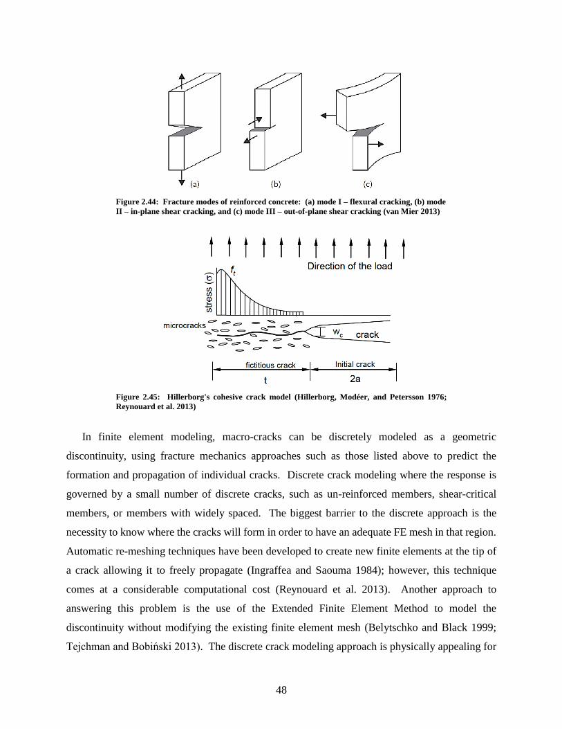
48
Figure 2.44: Fracture modes of reinforced concrete: (a) mode I – flexural cracking, (b) mode
II – in-plane shear cracking, and (c) mode III – out-of-plane shear cracking (van Mier 2013)
Figure 2.45: Hillerborg's cohesive crack model (Hillerborg, Modéer, and Petersson 1976;
Reynouard et al. 2013)
In finite element modeling, macro-cracks can be discretely modeled as a geometric
discontinuity, using fracture mechanics approaches such as those listed above to predict the
formation and propagation of individual cracks. Discrete crack modeling where the response is
governed by a small number of discrete cracks, such as un-reinforced members, shear-critical
members, or members with widely spaced. The biggest barrier to the discrete approach is the
necessity to know where the cracks will form in order to have an adequate FE mesh in that region.
Automatic re-meshing techniques have been developed to create new finite elements at the tip of
a crack allowing it to freely propagate (Ingraffea and Saouma 1984); however, this technique
comes at a considerable computational cost (Reynouard et al. 2013). Another approach to
answering this problem is the use of the Extended Finite Element Method to model the
discontinuity without modifying the existing finite element mesh (Belytschko and Black 1999;
Tejchman and Bobiński 2013). The discrete crack modeling approach is physically appealing for

49
modeling the discontinuities of cracking; however, the computational complexity in modeling
specimens with widespread distributed cracking remains a significant barrier. An alternative
approach known as smeared crack modeling has proven successful in predicting members with
widespread cracking. The smeared crack modeling approach is treated in detail in Section 2.5
2.4.2 Compressive response of concrete
Concrete subjected to uniaxial compression exhibits a softening response up to a peak
compressive stress denoted as 'cf . The concrete exhibits a linear elastic behavior up to
approximately one-third the peak compressive stress. Nonlinear softening of the response
gradually increases due to the formation of micro-cracks. After reaching a peak compressive
stress, macro-cracks develop and propagate reducing the stress capacity of the material until
reaching a splitting failure.
Biaxial response of concrete and compressive softening
The biaxial response of concrete exhibits a dependency of the compressive strength on the
transverse loading. The response of concrete to biaxial compression, compression-tension, and
biaxial compression were evaluated experimentally by Kupfer (1969). The key conclusions of
these experiments are central themes to models of the constitutive response of concrete.
For a state of biaxial compression, the compressive stress capacity increases as shown in Figure
2.46. A proportional compressive loading resulted in about a 16% increase in capacity. The peak
increase in capacity of about 25% is realized for a non-proportional loading with a compressive
stress ratio of 2:1. Furthermore, biaxial compression resulted in an increased tensile ductility in
the out-of-plane direction and a consequent increase in compressive strain ductility. For a state of
biaxial tension, the response was not distinctly different from a uniaxial response. For a state of
biaxial compression and tension, the compressive stress capacity and ductility decrease as shown
in Figure 2.47. The experimental results revealed a nearly linear relationship between decreasing
compressive capacity and increasing tensile stress (Chen 1982). The reduction of compressive
capacity is often referred to as compression softening.

50
Figure 2.46: Plot of normalized compressive strength versus normal strains on an element of
plain concrete subjected to uniaxial and biaxial compression (Kupfer, Hilsdorf, and Rüsch
1969)
Figure 2.47: Plot of normalized compressive strength versus normal strains on an element of
plain concrete subjected to uniaxial compression and biaxial tension (Kupfer, Hilsdorf, and
Rüsch 1969)

51
Pre-peak compressive response of concrete
The base curve of the concrete stress-strain relationship for the initial linear regime and
nonlinear softening up to the peak compressive stress was first approximated using a parabolic
relationship by Hognestad (1955). The peak compressive strength is limited by a maximum stress
given as a function of the transverse tension on the element to base upon the effect of compression
softening.
(2.12)
While the parabolic relationship is a commonly utilized assumption, it does not fit compressive
response test data as well as some later methods. Smith and Young (1956) proposed the following
exponential model,
(2.13)
Subsequent experiments through the work of Thorenfeldt (1987), Popovics (1973), Collins and
Porasz (1989) developed a model applicable to normal and high-strength concretes as follows.
The model is shown in Figure 2.48 and the relationship given as,
(2.14)
Where 2,maxcf is the softened peak compressive stress for the biaxial strain state and the
modification parameters are,
For normal strength concrete,
( )2,max
1
c
c c p
En
E f
k
=
−
=
(2.15)
For high strength concrete,
( )2,max MPa
0.8017
cfn = + (2.16)
f fc c
o o
2 2
2 2
2
2,max
f fc c
c c
2 2
2 21,max'
exp'
f fn
nc c
c c
nk2 2
2
21,max
' '

52
(2.17)
Based upon the finite element modeling of 21 structural walls, Palermo and Vecchio (2007)
recommended the following concrete models: For compressive strength greater than 45 MPa (6.53
ksi), the high-strength modified Popovics (Equations (2.14) and (2.16)). For compressive strength
between 22 to 45 MPa (3.2 to 6.53 ksi), the normal-strength Popovics (Equations (2.14) and (2.15)
). In addition, for concretes with compressive strength less than 22 MPa (3.2 ksi), the Smith-
Young base curve was recommended (Equation (2.14)).
Figure 2.48: Base curve of modified Popovics high-strength concrete constitutive model (from
Selby (1997) with modified variable names)
Compressive softening
The first experimental investigation of the effect of compression softening response was
completed by Robinson and Demorieux (1977). This investigation tested slender panels that were
loaded in compression in one axis and in tension in the transverse axis. Reinforcement was
provided in the transverse direction and was used the means of applying tension to the specimen.
Reinforcement was examined for the orthogonal and skewed configuration. A 14% reduction in
kk
f
p
c
p
1 0
0 6762
2
2
2
for
MPafor.
,max
2
2,max
c
c
f
f
2 'c

53
compressive strength was observed when the panel was pulled in tension in the transverse direction
up to the yield strength of the bars (Nielsen 2011).
The softened peak compressive stress, 2,maxcf is defined by a scaling parameter, . A variety
of empirical models have been developed to quantify this scaling factor for describing the strength
and stiffness prior to reaching the peak compressive stress. A review, comparison, and
recommendation of up to eight different compression softening models based on the ten years of
experimental data from both universities were completed by Vecchio and Collins (1993). Based
upon the experimental data of 116 panel tests, the work concluded that the most important factor
influencing compression softening was the principal tensile strain followed by the concrete
strength. The test data of these panels is shown in Figure 2.50. Two models were proposed from
the statistical analysis of the results defined by the influence of transverse straining ( )sK and the
concrete strength ( )fK (Vecchio and Collins 1993). Model A” is a two-parameter model based
on the biaxial strain state and compressive strength:
(2.18)
Where, n and k are defined in (2.15) and (2.16)
( )1 2
1,
1.0c c
c f
fnK K
= =+
(2.19)
'0.1825 1.0f cK f= (2.20)
0.80
1
2
0.35 0.28 1.0cc
c
K
−= −
(2.21)
f f
n
n
c c
c
co
c
co
nk2
2
21
,max
' for
for
for
c co
c co c co
c base
f
f
2
2
2
'
, c co2
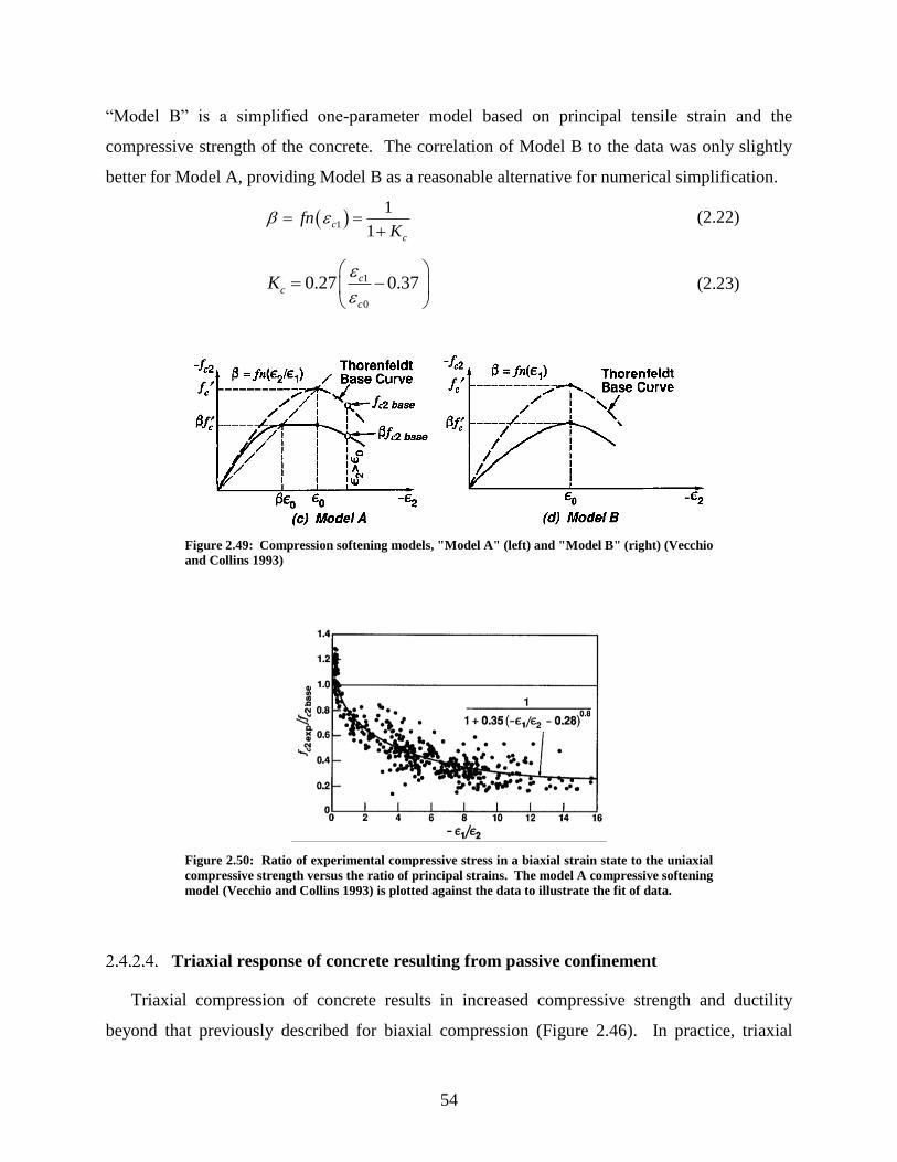
54
“Model B” is a simplified one-parameter model based on principal tensile strain and the
compressive strength of the concrete. The correlation of Model B to the data was only slightly
better for Model A, providing Model B as a reasonable alternative for numerical simplification.
( )1
1
1c
c
fnK
= =+
(2.22)
1
0
0.27 0.37cc
c
K
= −
(2.23)
Figure 2.49: Compression softening models, "Model A" (left) and "Model B" (right) (Vecchio
and Collins 1993)
Figure 2.50: Ratio of experimental compressive stress in a biaxial strain state to the uniaxial
compressive strength versus the ratio of principal strains. The model A compressive softening
model (Vecchio and Collins 1993) is plotted against the data to illustrate the fit of data.
Triaxial response of concrete resulting from passive confinement
Triaxial compression of concrete results in increased compressive strength and ductility
beyond that previously described for biaxial compression (Figure 2.46). In practice, triaxial

55
compression is most prevalent in structure within soils, rock, and water due to lateral earth
pressures and hydrostatic pressures that “actively” confine the structure. However, confinement
can also be provided by taking advantage of the Poisson’s effect and restricting the lateral
expansion of the concrete when it is subjected to uniaxial compression. This “passive”
confinement can be provided in compressive members with closely spaced longitudinal and
transverse steel, usually used in columns and boundary elements of walls. A separate constitutive
relationship of the stress-strain relationship is then desired to describe the increased strength and
ductility of a region with longitudinal and confining steel.
The Modified Kent-Park model (Scott, Park, and Priestley 1982) was developed using
experimental tests on square columns with a variety of reinforcement layouts at low and high strain
rates. A strength enhancement factor, K , is used to describe the peak compressive stress and
corresponding strain. Modifying Equation (2.14) to reflect the strength enhancement (where the
compression softening factor is one), the pre-peak confined response is,
(2.24)
From the paper of Scott (1982), the post-peak response and parameters are defined as follows,
( ) ( ) ( )2 2 2' 1 ' 0.2 ' for 'c c m c c cf K f Z K K f = − − (2.25)
1'
s yh
c
fK
f
= + (2.26)
( )
( )
0.5
3 0.29 ' MPa 3 '''
145 ' MPa 1000 4
m
c
s c
c b
Zf h
Kf s
=+
+ −−
(2.27)
Where, s is the ratio of confining steel to the gross volume contained by the confining steel
including the area up to the outside edge of the confining steel, ''h is the width of the confined
area of concrete measured to the outside edge of the confining steel, and bs is the center-to-center
spacing of the confining steel.
f K fK
n
n Kc c
c c
nk c2
2
2
2
1'
' ''for

56
Figure 2.51: Modified Kent and Park model of passive confinement (from Selby (1997) with
modified variable names)
2.4.3 Tensile response of concrete
As concrete is a heterogeneous material, it is weak in tension due to the limited bond strength,
existing micro-cracks from shrinkage and hardening, as well as flaws that form during casting of
the concrete. The tensile strength of concrete is typically between 8 to 15% of its compressive
capacity (Shi 2009). In engineering practice, the tensile response is often considered negligible;
however, it will be important to consider the tensile stresses in the concrete when aiming to
describe the complete response of a structure. Prior to cracking, the tensile response is considered
to behave linear elastic. From Hooke’s law, the response is defined as,
1 1 1 for 0c c c c crf E = (2.28)
crcr
c
f
E = (2.29)
Where, cr and crf are the strain and stress at cracking respectively. The value of crf and the
initial elastic modulus, cE , will be prescribed as a function of the material properties and the
desired criterion for cracking.
After the complete development of a crack in the concrete, the tensile stress of the concrete
will be zero. However, due to the quasi-brittle cracking process as previously described in Section
2.4.1, the reduction from the stress at cracking to zero stress is not instantaneous. For small crack
widths, the concrete is still able to resist some direct tensile stress across the crack for a width of
the crack termed the “fracture process zone” (FPZ). Figure 2.52 (a) shows the transition of the
fracture process zone with two idealized regions. The region of “bridging” refers to the arrest of
'cK
'cKf
2cf
0.2 'cf
2
'm cZ f

57
the developing crack by the aggregates that ‘bridge’ the crack. The degrading tensile stress across
the FPZ is shown in Figure 2.52 (b), and this inelastic phenomenon is referred to as tension
softening (Shi 2009).
(a)
(b)
Figure 2.52: Concept of tension softening from fracture mechanics, (a) illustrates the presence
of microcracking around the tip of the open crack and associated fracture process zone (FPZ),
and (b) the approximation of the fracture process zone using a tension softening model (Shi
2009)
Experimental uniaxial tension tests conducted at Delft University of Technology (Cornelissen,
Hordijk, and Reinhardt 1986; Hordijk 1991) developed constitutive relationships for the tension
softening observed in normal weight and lightweight concrete. The relationship of best fit from
the experiments of normal weight concrete is shown in Figure 2.53. It provided the following
relationship as a function of the current crack width, W , with adaptation from Wong (Cornelissen,
Hordijk, and Reinhardt 1986; Wong, Vecchio, and Trommels 2013),
(2.30)
f f cW
Wc
W
W
W
Wcc cr
c c c
1 1
3
2 1
31 1exp exxp c2

58
1 3c = (2.31)
2 6.93c = (2.32)
5.136 f
c
cr
GW
f= (2.33)
Where, fG is the fracture energy released per unit area in the cracking process. From Figure 2.52
(b) the fracture energy can be defined by Equation (2.34) (Shi 2009), although it is commonly
assumed to be 75 N/m (Wong, Vecchio, and Trommels 2013)
( )0
cW
f nG W dW= (2.34)
Figure 2.53: Plot of the ratio of tensile stress to nominal tensile strength versus the ratio of
principal tensile displacement. Solid line represents the correlation of test data for the
nonlinear tension softening model (Cornelissen, Hordijk, and Reinhardt 1986).
2.4.4 Reinforcement response
The Seckin (1981) and Menegotto-Pinto (1973) both proposed hysteretic models for steel
reinforcement that include the Bauschinger effect are considered in this study. The Bauschinger
effect results in a reduction of the compressive capacity after load reversal when the bar has
undergone plastic straining. Both models are based upon an elastic-plastic base curve of the stress-
strain response with linear or nonlinear strain hardening. The primary difference between the two
models is the Seckin model is a function of the maximum historical stress/strain point, and the
Menegotto-Pinto is a function of the stress-strain response in the previous cycle. A comparison of
the two hysteretic models is shown in Figure 2.54 followed by their numerical implementation.
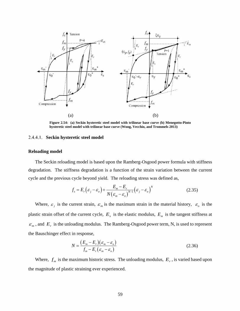
59
(a) (b)
Figure 2.54: (a) Seckin hysteretic steel model with trilinear base curve (b) Menegotto-Pinto
hysteretic steel model with trilinear base curve (Wong, Vecchio, and Trommels 2013)
Seckin hysteretic steel model
Reloading model
The Seckin reloading model is based upon the Ramberg-Osgood power formula with stiffness
degradation. The stiffness degradation is a function of the strain variation between the current
cycle and the previous cycle beyond yield. The reloading stress was defined as,
( )( )
( )1
Nm r
s r j o j oN
m o
E Ef E
N
−
−= − + −
− (2.35)
Where, j is the current strain, m is the maximum strain in the material history, o is the
plastic strain offset of the current cycle, sE is the elastic modulus, mE is the tangent stiffness at
m , and rE is the unloading modulus. The Ramberg-Osgood power term, N, is used to represent
the Bauschinger effect in response,
( ) ( )
( )m r m o
m r m o
E EN
f E
− −=
− − (2.36)
Where, mf is the maximum historic stress. The unloading modulus, rE , is varied based upon
the magnitude of plastic straining ever experienced.

60
(2.37)
Unloading model
The unloading relationship is linear and based upon the elastic modulus of the steel.
( )( 1) 1s s j r j jf f E − −= + − (2.38)
2.4.5 Buckling of reinforcement in compression
Dhakal and Maekawa (2002a) examined the buckling response of bars in compression using a
parametric study by finite element using previous experimental results. The parametric study
identified the response to be sensitive to the effective length and the yield strength of the bar. The
effective length is defined as the quotient of the “unbraced” length of the bar and its diameter. As
the yield strength and diameter are known, the problem becomes determining the effective length.
The test results revealed that an unsupported length to diameter ratio exceeding 5.0 would induce
buckling beyond the compressive yield, and if the ratio is less than 5.0, the response is consistent
with that of the local stress-strain. The tests also revealed the decreasing compressive capacity
with increasing strain was approximately equal to 2% of the bar modulus. The model assumes this
stiffness starting from an intermediate stress-strain point ( )* *, that signifies the onset of
buckling. The intermediate stress point is defined as,
*
*55 2.3 / 7100
ys
s y
y
f L
D
= − (2.39)
,
,
,
1.1 0.016 0.2100
s avg y
s avg y
s local
f f Lf f
f D = −
(2.40)
Where, the local stress-strain refers to the material response, i.e. elastic-plastic or trilinear. The
model is then defined as follows,
E
E
Er
s m o y
s
m o
y
for
for1 05 0 05. .
for
y m o y
s y m oE
4
4

61
*
, , *
* *
, ,
1 1s avg s avg s y
y s s
s local s local s y
f f
f f
−= − − −
(2.41)
( )* *
, , 0.02 0.2s avg s avg s s s y s yf f E f = − − (2.42)
The model is shown in Figure 2.55. A hysteretic implementation of this model is based on the
Menegotto-Pinto model (Dhakal and Maekawa 2002b). The model was validated against
monotonic and cyclic experimental results for multiple L/D ratios.
Figure 2.55: Stress-strain response of reinforcing bars in compression utilizing the post-yield
buckling model (Dhakal and Maekawa 2002b)
Determination of L/D ratio from elastic buckling analysis
An elastic buckling analysis will be carried out to determine the effective buckling length of
the #4 boundary element bars based on the work of Maekawa (2003). Each determination is
dependent on the stiffness of the longitudinal bar, the stiffness of the lateral tie, and the spacing of
the lateral ties, all of which are known with the assumption of elasticity and the measured material
properties. The “buckling mode” defined as the number of bar spacings that buckling will occur
over is the unknown of the problem. Buckling the bar over a short distance requires high lateral
tie stiffness while buckling the bar over a longer distance decreases the required stiffness in each
tie. The buckling modes are iterated upon until the required spring stiffness for the current
buckling mode is less than or equal to the provided tie stiffness. The elastic buckling analysis is
summarized in Figure 2.56.
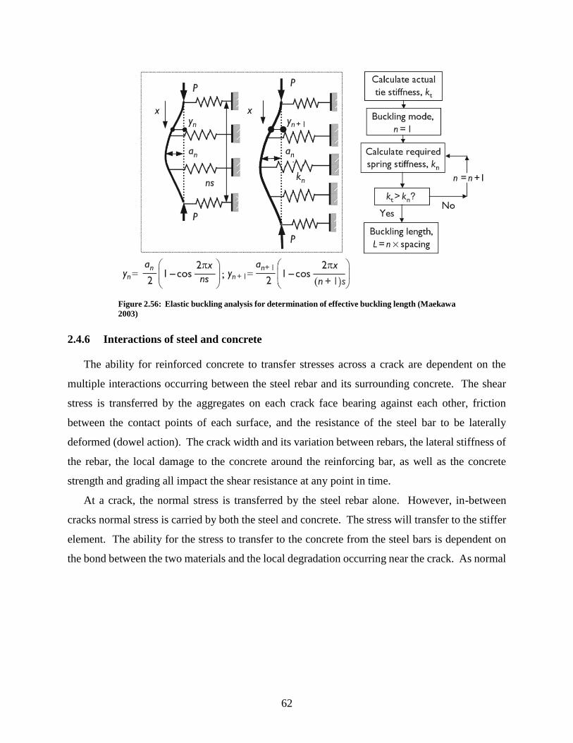
62
Figure 2.56: Elastic buckling analysis for determination of effective buckling length (Maekawa
2003)
2.4.6 Interactions of steel and concrete
The ability for reinforced concrete to transfer stresses across a crack are dependent on the
multiple interactions occurring between the steel rebar and its surrounding concrete. The shear
stress is transferred by the aggregates on each crack face bearing against each other, friction
between the contact points of each surface, and the resistance of the steel bar to be laterally
deformed (dowel action). The crack width and its variation between rebars, the lateral stiffness of
the rebar, the local damage to the concrete around the reinforcing bar, as well as the concrete
strength and grading all impact the shear resistance at any point in time.
At a crack, the normal stress is transferred by the steel rebar alone. However, in-between
cracks normal stress is carried by both the steel and concrete. The stress will transfer to the stiffer
element. The ability for the stress to transfer to the concrete from the steel bars is dependent on
the bond between the two materials and the local degradation occurring near the crack. As normal

63
stress increases, the rebar will begin to pull out of the concrete due to bond degradation and crack
dilatancy.
Figure 2.57: Deformations and forces at a reinforcing of a crack interface (Maekawa 2003)
Bond between steel and concrete
Chemical bond, mechanical bearing, and friction between the concrete and steel resist the
tensile stress in a reinforcing bar. For the case of deformed bars, the lugs mechanically bear on
the surrounding concrete and are the primary resistance to bar slip (Figure 2.58 (a)). As demand
increases, the concrete surrounding each lug will begin to crush, and the resistance by mechanical
bearing degrades. The compressive stress developed in the concrete from bearing is equilibrated
by radial tensile stresses (Figure 2.58 (b)). As demand increases, cracks will open and propagate
around the bar lugs. If the cover concrete is thin, the splitting cracks can propagate through to the
exterior surface (Figure 2.58 (c)). A splitting failure results in decreased bond strength capacity.
If significant cover is provided or if the concrete is subject to a confining pressure, the cracks will
not propagate, and the concrete will crush between the bar lugs and the primary resistance
mechanism becomes friction (Figure 2.58 (d)). In the case of reversed cyclic loading, the
degradation of concrete around the bar lugs is more severe, and splitting cracks will form in both
directions. Both results in lower bond strengths (Lowes, Moehle, and Govindjee 2004).

64
Figure 2.58: Bond stresses and failure mechanisms in reinforced concrete, (a) the mechanical
resistance to bond slip from the lugs on deformed bar reinforcement, (b) the radial tensile
stresses (hoop stresses) resulting from compressive stresses bearing on the lugs, (c) the
degradation of bond due to splitting cracks through the concrete cover, and (d) the crushing of
concrete between lugs when reinforcement is sufficiently confined (ACI Committee 408 2003)
Many numerical bond models have been developed for monotonic and cyclic loading
applications based on experimental tests. The primary variables are the concrete compressive
strength, bar spacing and diameter, concrete clear cover, and confinement condition (Cervenka,
Jendele, and Cervenka 2007). The CEB-FIP Model Code (1993) proposes a bond model that
smears the resistive effects together based and is suitable only for monotonic loading conditions
(Figure 2.59 (a)). A more general model was proposed by Lowes (2004) that considers the
individual contributions of mechanical bearing and friction to the total bond resistance as well as
the effects of cyclic loading (Figure 2.59 (b)).

65
(a) (b)
Figure 2.59: (a) Simplified monotonic model of bond (Comité euro-international du béton
1993) (b) Cyclic bond model proposed by Lowes et al. (2004)
Crack dilatancy, friction, and aggregate interlock
Aggregate interlock is the resistance of at a crack interface to resist slip by bearing of the
aggregates. Aggregate can only be assumed for a “rough” crack in the concrete, one that has
propagated naturally as opposed to a crack at a geometric discontinuity or construction joint. The
experimental work of Walraven (1981) characterized the shear, civ , vs. slip, a
s , relationship as
a function of the crack width, w , and the concrete compressive strength. The average shear strain,
a
s , is then calculated as the ratio of total slip to the average crack spacing. The shear slip
relationship was developed based upon monotonic loadings of rough cracks and does not consider
the degradation of aggregate interlock during cyclic loadings nor does it consider smooth
interfaces.
( )0.8 0.7071.8 0.234 0.20 '
a cis
c
v
w w f
− −=
+ − (2.43)
a
a ss
s
= (2.44)
Rough cracks resisting an imposed shear stress tend to increase the crack width as the
aggregates slide over each other, referred to as crack dilatancy. Crack dilatancy has been found to
have different relationships for plain and reinforced concrete and is largely dependent on the crack
roughness (Maekawa 2003). The result of crack dilatancy is an increase in the normal stress that
must be carried by the steel bars and a consequent increase of bar pull out at the interface. A study
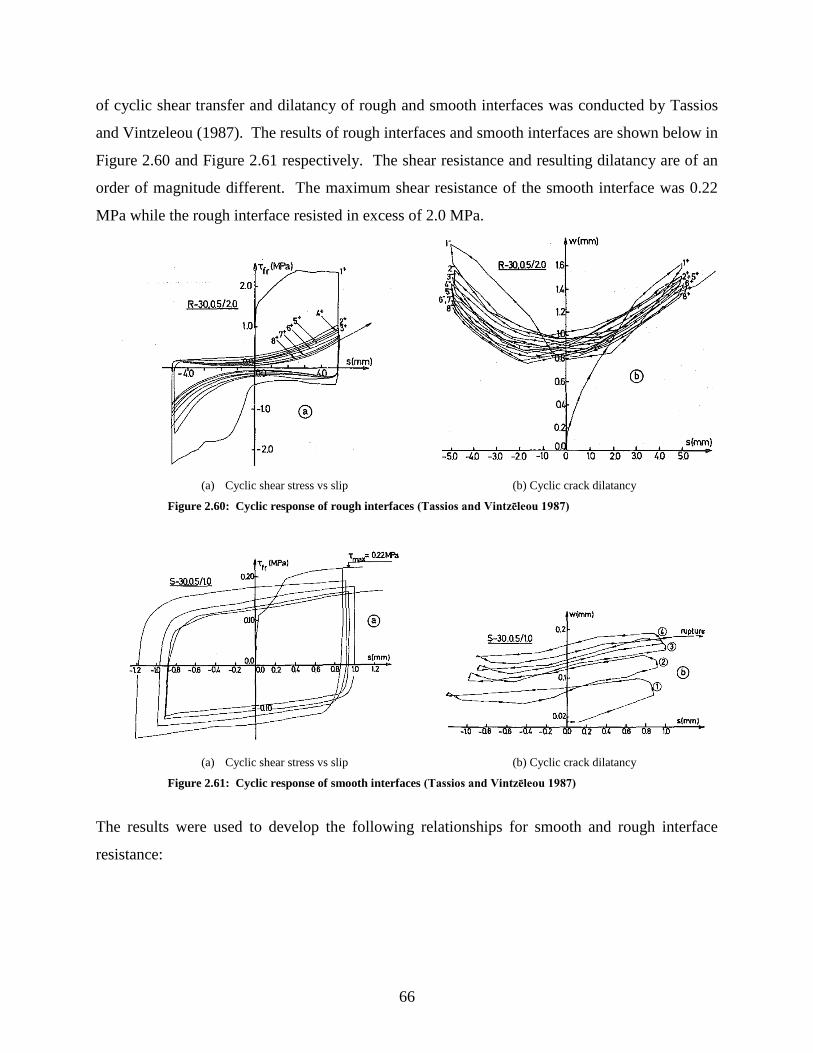
66
of cyclic shear transfer and dilatancy of rough and smooth interfaces was conducted by Tassios
and Vintzeleou (1987). The results of rough interfaces and smooth interfaces are shown below in
Figure 2.60 and Figure 2.61 respectively. The shear resistance and resulting dilatancy are of an
order of magnitude different. The maximum shear resistance of the smooth interface was 0.22
MPa while the rough interface resisted in excess of 2.0 MPa.
(a) Cyclic shear stress vs slip (b) Cyclic crack dilatancy
Figure 2.60: Cyclic response of rough interfaces (Tassios and Vintzēleou 1987)
(a) Cyclic shear stress vs slip (b) Cyclic crack dilatancy
Figure 2.61: Cyclic response of smooth interfaces (Tassios and Vintzēleou 1987)
The results were used to develop the following relationships for smooth and rough interface
resistance:

67
(2.45)
Where, n = the cycle number, cif = normal stress across the interface, ns is the slip of the nth
cycle, us is the maximum slip in the displacement history. A hysteretic model for this relationship
is shown in
Figure 2.62: Hysteretic model for shear transfer by aggregate interlock (Tassios and
Vintzēleou 1987)
The same researchers carried out an experimental investigation to characterize the shear resistance
by dowel action and the mechanisms of failure by dowel action (Tassios and Vintzēleou 1986).
The study identified failure due to crushing of the concrete and yielding of the bar, or by side-
splitting of the concrete for sections where inadequate concrete cover is available to develop the
full strength when bearing against the cover. For this experimental study, the first failure mode
will be the controlling case in general. The cyclic dowel response was characterized by the
following relationship, similar to that for aggregate interlock:
, ,1
11 1
7d n dv v n
= − −
(2.46)
Where, the monotonic response is,
( )2 '
,1d b c syv k d f f= (2.47)
Where, k is an experimental parameter to fit the data. This factor was set as 1.3 in the
experimental data of Rasmussen (1963). The hysteretic model developed for the dowel action is
v
f n s
v
ci n
ci n u
c
,
.0 40 11
71 for smooth interfaces if s
ii
ci
c
n
u
nf
f
s
s, '
/
.1
1 1 3
1 0 002 1 for rough interfaces
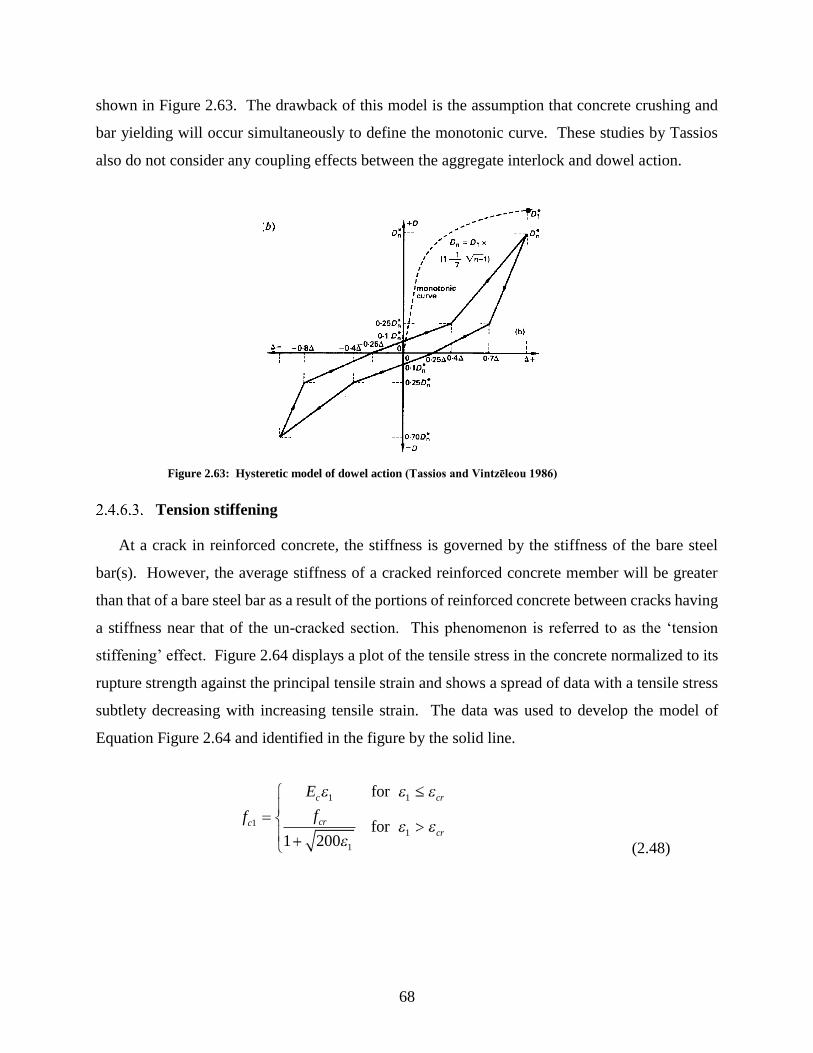
68
shown in Figure 2.63. The drawback of this model is the assumption that concrete crushing and
bar yielding will occur simultaneously to define the monotonic curve. These studies by Tassios
also do not consider any coupling effects between the aggregate interlock and dowel action.
Figure 2.63: Hysteretic model of dowel action (Tassios and Vintzēleou 1986)
Tension stiffening
At a crack in reinforced concrete, the stiffness is governed by the stiffness of the bare steel
bar(s). However, the average stiffness of a cracked reinforced concrete member will be greater
than that of a bare steel bar as a result of the portions of reinforced concrete between cracks having
a stiffness near that of the un-cracked section. This phenomenon is referred to as the ‘tension
stiffening’ effect. Figure 2.64 displays a plot of the tensile stress in the concrete normalized to its
rupture strength against the principal tensile strain and shows a spread of data with a tensile stress
subtlety decreasing with increasing tensile strain. The data was used to develop the model of
Equation Figure 2.64 and identified in the figure by the solid line.
(2.48)
f
E
fc
c cr
cr
cr1
1 1
1
11 200
for
for

69
Figure 2.64: Plot of the ratio of average principal tensile stress to tensile stress at a crack versus
the principal tensile strain. Solid line indicates the correlation of the 1986 tension stiffening
model (Vecchio and Collins 1986)
Bentz (2000) evaluated a series of tension stiffening models developed from experimental test
data at the University of Toronto and the University of Houston. While the individual expressions
were observed to fit the data at each institution, a substantial variation was observed when
evaluated against the experimental data of both institutions. Bentz recognized that the tension
stiffening effect is largely influenced by the bond transfer length on each side of an open crack.
To account for the effect of bond, the parameter, m , was introduced to represent the relative
changes in bond characteristics based on the ratio of perimeter bar area in contact with concrete to
the total area of concrete:
c
b
Am
d =
(2.49)
The resulting expression incorporating the bond parameter is given as:
(2.50)
While this expression increases the spread of data relative to the individual panels, the overall
fit of data between both institutions and all available data sets increased substantially (Bentz 2000).
This relationship was modified by Sato and Vecchio (2003) to account for the inclination of
principal strain relative to the orientation of each reinforcing bar.
f
E
f
m
c
c cr
cr
cr1
1 1
1
11 3 6
for
for.

70
The tensile behavior is dominated by either tension softening or tension, two distinctly different
phenomena. Tension softening models the reduction in tensile strength due to the fracture process
zone, while tension stiffening models the increased tensile strength on average due to smearing
the cracked and un-cracked portions of the element. The stiffness of the continuum element is
controlled by the smaller value predicted from either model but is not a function of both
phenomena. For coarse mesh discretization, the tension stiffening model dominates the response
because many cracks exist over the large element size. For fine mesh discretization, single cracks
will exist in only selected elements, and elements without cracks will exist in-between cracked
elements. In this case, the tension stiffening relationship is captured without a constitutive model,
and the cracked element stiffness is based on the tension softening model.
2.5 Numerical analysis of structural concrete
Treating cracked concrete as a continuous orthotropic material was first proposed by Rashid
(1968). To describe the response of reinforced concrete in a continuum, the phenomena associated
with cracking and the nonlinear material response of the concrete and steel are smeared together
in a single material model. This approach is commonly referred to as a “smeared crack” model.
For the continuum approach, an element of reinforced concrete can only be solved globally in
terms of average stresses and strains. The local stresses and strains in each material, at cracks and
in-between cracks, are determined based on the features of the constitutive models for the concrete
and steel.
The primary advantage of smeared crack modeling is the ability to adopt continuum mechanics
approaches for finite element analyses. The primary disadvantage is the requirement that all the
nonlinear interactions of an element of structural concrete be “lumped” together, including the
effect of cracking on stiffness, strength and the ductility of the element (Fédération internationale
du béton and Task Group 4.4 2008). As the stress-strain state increases during the loading of a
structure, the discontinuities imposed at cracks as well as the damage and yielding of the materials
locally increases. Predicting the damaged conditions of structural concrete in a continuum has
been based primarily on empirical relationships and is thus limited in scope (Comité euro-
international du béton 1996). Consequently, the continuum modeling approach becomes “further
from reality” as the demand increases to the post-peak response.
71
The section describes the general formulation of reinforced concrete for a 2-D continuum
followed by a summary of total strain and strain decomposition models developed for NLFEA.
2.5.1 Membrane element formulation for reinforced concrete
A membrane element is defined as a 2-D continuum element of a single material subjected to
in-plane normal and shear stresses. In general, these stresses are assumed to act uniformly along
the mid-plane of each edge of the element. The out-of-plane normal and shear stresses are assumed
negligible. Furthermore, strains and stresses across the thickness are assumed uniform. The
principle of stress transformation provides the ability to describe the stress state or strain state of
any element in multiple coordinate systems, commonly achieved using Mohr’s circle for graphical
analysis (Mohr 1882). The stress transformation is used here to convert an element’s configuration
in a finite element mesh to the configuration of principal stresses or principal strains.
A membrane element of reinforced concrete is assumed as a two-part composite consisting of
concrete as an isotropic material and a grid of orthogonal uniformly distributed reinforcing bars.
The reinforcing bars are assumed to have axial stiffness only. Based on these assumptions, the
following variables exist,
Reinforcement ratios .................................... ,
Total stresses................................................. , ,
Total strains...................................................
x y
x y xy
x
f f v
, ,
Net concrete stresses..................................... , ,
Net concrete strains....................................... , ,
Net steel stresses..................................
y xy
cx cy cxy
cx cy cxy
f f v
.......... ,
Net steel strains............................................. ,
Orientation of net concrete stress/strain.........
Orientation of total stress/strain.....................
sx sy
sx sy
c
f f
The development of continuum models for reinforced concrete is based on equilibrium of the
element in-plane shear and normal stresses by the concrete and steel, strain compatibility whereby
the concrete and steel components are subjected to the same strain states throughout the element,
and the use of appropriate constitutive relationships for the steel and concrete components. For

72
analyzing an element, the reinforcing ratios are known, and the total stress to be carried by the
element would have been determined from a global analysis. Therefore, the known variables are,
, , , ,x y x y xyf f v
The fifteen (15) unknown variables are,
, , , , , , , , , , , , , ,x y xy cx cy cxy cx cy cxy sx sy sx sy cf f v f f
For strain compatibility, perfect bond is assumed to exist between the concrete and reinforcing
bars (no slip) providing that the average strains in the concrete and average strains in the steel must
be equal.
x cx sx = = (2.51)
xy cxy = (2.52)
With equal strains in the two materials, Mohr’s circle of strain was used to derive relationships
between the normal, shear and principal strains as shown in Figure 2.65.
Figure 2.65: Mohr’s circle for total strains (left) and net concrete strains (right)
2
1 2
2
tan
1 tanx
+=
+ (2.53)
2
1 2 2
2
tan
1 tany
+ +=
+ (2.54)
( )22
tan
x
xy
−= (2.55)
,2
xy
y
,2
cxy
cy
2 c2c 1c
,2
cxy
cx
12
,2
xy
x
2

73
11
tan2
xy
x y
−
= − (2.56)
Similarly, equations (2.53) to (2.56) can be produced for the net concrete strains.
Three equations of equilibrium were derived for the cracked reinforced concrete element
pictured in Figure 2.66. The first equation of equilibrium relates the shear stress to the two
principal stresses. The second equation of vertical equilibrium relates the applied normal and shear
stresses to the first principal stress and the stress in the vertical reinforcement. The third equation
of horizontal equilibrium relates the applied normal and shear stresses to the second principal stress
and the stress in the horizontal reinforcement.
1cotx sx x xy cf f f = + − (2.57)
1tany sy y xy cf f f = + − (2.58)
( )2 1 tan cotc c xyf f = − + (2.59)
Figure 2.66: Equilibrium of the RC membrane element
The fifteen unknown variables have now been reduced to only six:
1 2, , , , and c c sx sy cf f f f
This problem remained unsolved until the development of the Compression Field Theory
(CFT) (Collins and Mitchell 1980). Drawing from the much earlier work of Wagner (1929) for
thin-webbed steel members, this work produced the needed compatibility equation for solving the
orientation of the compression strut based on the assumption that concrete had no tensile strength:
( )
( )22
2
tanx
y
−=
− (2.60)
xf
yf
xy
x
y
xf
yf
sxf
syf

74
The remaining five relationships required are the constitutive models for relating the stresses and
strains of the concrete and steel.
For un-cracked concrete, the constitutive relationships for steel and concrete can be defined by
Hooke’s law and the orientation of total strain and net concrete strains will be coincident. For
cracked concrete, the response becomes nonlinear for both materials. The steel will still be
described by Hooke’s law, but the modulus will be considered a function of the strain to capture
the nonlinear stress-strain response:
sx s sxf E = (2.61)
sy s syf E = (2.62)
As the principal tensile stress of the un-cracked concrete reaches its capacity, a crack will form
perpendicular to the angle of principal tensile stress. After cracking, the angle between principal
concrete stress and principal stress of the element will not remain coincident when the element is
non-proportionally reinforced (x y ) and/or when subsequent loadings are not increased
proportionally. Subsequent cracks may form at different angles than the initial crack. In all these
cases, shear stress in the concrete develops along the crack interfaces that must be included in the
equilibrium equations. Multiple theories have emerged to address how the angle of cracking, the
angle of principal stress of the element, and the angle of principal concrete stress are related.
Fixed crack model
The first theory is called the ‘fixed crack’ model which assumes the orientation of a crack is
fixed upon the first fracture and remains unchanged for all subsequent loadings (Darwin 1974).
The orientation of principal stresses becomes fixed to the orientation of total strain at the time of
fracturing:
( )at fracture
c = (2.63)
The fixed angle of cracking based on the loading history directly affects the behavior of the element
to all subsequent loads. Subsequent loading after cracking results in the development of shear and
normal forces across the crack plane because the principal stress and strain are no longer
coincident. In the fixed crack model, strains are decomposed into the elastic strain and the strain
at the crack. The stresses and strains are thus evaluated based on the stress-strain response of the
un-cracked material and on the stress-strain response of each crack. These models often have

75
multiple cracks with varying angles. The stress-strain response at each crack is then transformed
to the global coordinates to evaluate the global stress and strain in the cracked reinforced concrete
element.
For the fixed crack approach, the assumption that only a single crack can form in the element
is rarely applicable to members with cyclic loads. For reversed cyclic loadings, cracks will often
form in at least two planes at opposing orientations. A common assumption is that second crack
forms orthogonal (90˚), or quasi-orthogonal (90˚ ± 22.5˚) to the first crack (Maekawa 2003). For
multi-directional cyclic loadings or cyclic loadings with large changes in the orientation of
principal stresses after cracking, cracks may form in many different planes. The two-way quasi-
orthogonal crack model was extended by Maekawa have a second co-ordinate frame for a total of
four distinct cracks, referred to as a four-way fixed crack model (Maekawa 2003).
Rotating crack model
For the “rotating crack” theory (Vecchio and Collins 1986), the principal stress and strain state
are coincident (same orientation and coordinate frame) resulting in no shear stress development
over the element on average. Therefore,
c = (2.64)
The rotating crack model is further broken down into the “rotating angle” and “fixed angle”
models.
The rotating angle model assumes the principal concrete stress remains coincident with the
principal stress of the element so that no shear stress develops in the concrete. The constitutive
matrix for the rotating angle theory in terms of the net concrete stresses and strains,
(2.65)
The shear modulus is shown as approximately equal to zero. In some numerical implementations,
the shear modulus is given a very small value to provide numerical stability (Hsu and Mo 2010).
The fixed angle model assumes that the principal concrete stress and principal element stress
are no longer coincident but separated by a fixed deviation angle. The deviation angle is based on
the distribution of reinforcement in each direction. This deviation results in the development of
shear stresses along the crack interfaces. Experimental tests have indicated that the deviation angle
f
f
E
E
c
c
c
c
1
2
1
2
1
2
0
0 0
0 0
0 0 0 0

76
between principal concrete stress and principal stress will decrease as loading increases and
subsequent cracks form (Hsu and Mo 2010). This can be attributed to increasing crack widths and
increasing stress demands softening the shear stress-shear slip relationship along the crack. At
ultimate load, Hsu and Mo observed the deviation angle to be only one half of the theoretical value.
In the case that the element is orthogonally reinforced with equal reinforcing ratios in each
direction, the deviation angle will be zero and the fixed angle model will be equal to the rotating
angle model. The constitutive matrix for the fixed angle theory in terms of the net concrete stresses
and strains,
(2.66)
2.5.2 Total strain models
A total strain model of reinforced concrete is defined to have only one state of stress for each
state of strain. The total strain approach has been the most widely adopted approach in professional
practice because of its conceptual simplicity, implementation, and success in predicting the
response of a variety of structures. The approach allows defining separate constitutive relationship
between the compressive and tensile response. The constitutive models can be considered as
simple uniaxial relationships or more complex biaxial relationships that consider the nonlinear
response, compression softening, tension stiffening, confinement, and other behavior.
Compression Field Theory (CFT) / Mohr Compatibility Truss Model (MCTM)
The Compression Field Theory (CFT) applied to reinforced concrete (Collins and Mitchell
1980) was originally developed for modeling the shear and torsional response of beams. The
model has also been referred to as the Mohr Compatibility Truss Model (MCTM) by Hsu (1993).
In the context of continuum analysis, the CFT is a rotating crack approach with uniaxial
constitutive models. For solving equilibrium of the model, the CFT assumes the concrete to act
as plain concrete in compression and to have zero capacity in tension. All biaxial phenomena are
neglected. The constitutive relationships for the steel and concrete can be any linear or nonlinear
relationship assuming they are a function only of the uniaxial strain:
( ) 0c c c cf E = (2.67)
f
f
v
E
E
G
c
c
c
c
c
c
1
2
12
1
2
12
1
2
12
0 0
0 0
0 0 2

77
( )s s s sf E = (2.68)
Modified Compression Field Theory (MCFT)
An experimental study conducted at the University of Toronto (Vecchio 1982) subjected
slender reinforced concrete panels to various combinations of in-plane shear and normal stresses
and found that the concrete did not behave as assumed in the CFT. In particular, the experiments
showed that tensile stresses exist in the un-cracked regions of concrete between cracks. The tensile
concrete stresses significantly increase the overall stiffness of the panel and should not be
neglected. The Modified Compression Field Theory (MCFT) (Vecchio and Collins 1986)
extended the CFT to use experimentally verified constitutive relationships that describe that tensile
response of the concrete as well as new constitutive relationships for the compressive response to
characterize the effect of compression softening.
Building on the previous models, the MCFT assumes there is only one state of stress for each
state of strain. Stresses and strains are considered as an average across the element, and the element
is taken over an area large enough to capture multiple cracks. Perfect bond is assumed between
the concrete and reinforcing bars, and the reinforcing bars are evenly distributed across the element
in both directions. Based on these assumptions, the MCFT is best applied to short-term, monotonic
loadings. Cyclic loading effects and loading history are not considered. Furthermore, the model
is less suited to lightly reinforced and/or widely spaced reinforcing bars where the response of a
single crack may govern the overall response.
The panel test data utilized in the development of the MCFT was evaluated in terms of the
angle of deviation between principal stress and strain. Figure 2.67 displays the data and resulting
deviations of up to ±10 degrees. The MCFT assumes the orientation of principal stresses and
strains to be coincident. This assumption restricts the ability for shear stress or shear deformation
(slip) to develop along a crack plane, and the crack plane orientation rotates with the direction of
principal stress. The total average strains equal the net average strains in the concrete.

78
Figure 2.67: Test data of the orientation of total stains and stresses of an element (Vecchio
and Collins 1986)
Constitutive models
Constitutive models relate the average strains to average stresses. Independent models are used
for steel reinforcing bars and the concrete. Simple constitutive models of the concrete in
compression and tension, and for the steel reinforcing bars are shown in Figure 2.68. The
compressive response of concrete was modeled by the Hognestad parabola, equation (2.12). The
concrete in tension is modeled using a linear elastic theory until cracking with a nonlinear tension
stiffened response, equation (2.48). The reinforcement was modeled as elastic-perfectly plastic.
(a) (b) (c)
Figure 2.68: Constitutive relationships of the MCFT, (a) non-linear compression, (b) non-
linear tension stiffening, and (c) elastic-plastic reinforcement response
2 1 ( , )s x y
( , )s x yf1f2f
yf
sE
o
2,maxcf
cE
crf
cr y
sE
cE
2cE1cE

79
In conjunction with modeling the effect of tension stiffening, the local stress variation at a
crack and between cracks must be considered in the equilibrium formulation. At the crack plane,
the local stresses in the steel reinforcing bars will be of greater magnitude than the average steel
stresses. Conversely, the concrete stresses will be zero at a crack but much greater than average
in-between cracks. The steel’s ability to transmit the local tension across a crack will be limited
by its material properties. Furthermore, local shear stress will develop at the crack plane outside
of the situation that the reinforcement orientation is coincident to the direction of principal tensile
stress. As stresses increase, the response of the element may be limited by the yielding of the
reinforcement locally at the crack. To maintain equilibrium, it is necessary to check that the
average tensile stress can be transmitted across the crack.
To enforce the first limitation, on the principal tensile stress in the concrete, the average stresses
in the element determined from equilibrium (Figure 2.66) are used to calculate the local stresses
that must be transmitted by the steel across the critical crack plane (assumed to be a plane in the
direction of the principal tensile strain). The average and local stresses at a crack must be statically
equivalent and are shown in Figure 2.69.
(a) Average stresses at crack (b) Local stresses at crack
Figure 2.69: (a) The average stresses at a crack interface, and (b) the local stresses at a crack
interface (Vecchio and Collins 1986)
The principal tensile stress developed from equilibrium of the average stresses must be
statically equivalent to the principal tensile stress developed from equilibrium of the local stresses
at the crack plane. This provides the following relationship,
( ) ( ) ( ) ( )2 2
1 , ,cos cosc x sx cr sx nx y sy cr sy nyf f f f f = − + − (2.69)

80
Where, nx and ny are the angles from the principal tensile stress to the horizontal and vertical
component of reinforcing, respectively. Using an elastic-plastic assumption of the reinforcing bar
response, the steel stress cannot exceed its yield stress,
, ,sx cr sx yieldf f (2.70)
, ,sy cr sy yieldf f (2.71)
Imposing this restraint into equation (2.69) provides a limit to the post-cracking concrete
tensile stress,
( ) ( ) ( ) ( )2 2
1 , ,cos cosc x sx yield sx nx y sy yield sy nyf f f f f − + − (2.72)
To enforce the second limitation on the shear stress, the shear stress in the concrete at the crack
plane was determined from static equivalency of the average and local stresses to provide the
following,
( ) ( ) ( ) ( ) ( ) ( ), ,cos sin cos sinci x sx cr sx nx nx y sy cr sy ny nyf f f f = − + − (2.73)
The MCFT assumes the shear stress is transmitted across a crack plane solely by interlock of
the aggregates in the concrete. The crack’s ability to transmit shear stress is thus limited by a
function of concrete strength, the crack width, and the maximum aggregate size, a. Based upon
experimental test data (Walraven 1981), the shear stress is limited by the following,
( )
( )'
for ,0.31 24 26
c
ci
fmm MPa
w a
+ + (2.74)
Where the crack width, w, is defined by the principal tensile strain and average crack spacing
in the current orientation,
1cw s= (2.75)
1
cos sin
mx my
s
s s
=
+
(2.76)
If the principal tensile stress of the concrete and/or the shear stress in the concrete is exceeded,
the strains state in the element must be iterated upon until a converged solution of lower stress is
found.

81
The reinforcing steel is modeled using an elastic-plastic assumption as shown in Figure 2.68
(c). The steel bars behave linear elastic until reaching the yield stress/strain. The response is
then plastic with no increase in stress for increasing strain,
(2.77)
The resulting performance of the MCFT indicated three distinct regions of behavior based on
the in-plane shear and normal stress interaction diagrams shown in Figure 2.70. The first region
is where high biaxial tension exists. In this region, the yielding of reinforcing bars at cracks
controls the response. The second region is where normal stresses are moderate and concrete shear
governs the response. In this region, it is important to note that the concrete fails at compressive
stresses significantly lower than the uniaxial compressive strength of the concrete, f’c. The third
region is where high biaxial compression exists. In this region, the failure is governed by the
principal compressive stress reaching the uniaxial compressive strength (or beyond due to the
strength enhancement of biaxial compression). The study indicated that the most difficult panels
to predict were those subjected to high shear demand with high levels of reinforcing because the
response was increasingly dependent on the constitutive model of the concrete.
Figure 2.70: In-plane shear stress and normal stress interaction diagram (Vecchio and
Collins 1986)
Modeling lateral expansion and confinement
Years after the publishing of the MCFT, additional test data from the University of Toronto
and University of Houston revealed that in concrete elements subjected to biaxial compression or
low tensile strains, the lateral expansion of the concrete during loading (Poisson’s effect) impacted
fE
Es
s s s y
s y y
for
for 1

82
the element response and should not be neglected (Vecchio 1992). In these cases, the strain due
to Poisson’s effect became a significant portion of the total strain, and furthermore as the
compressive stress demand increases the Poisson’s ration also increases and magnifies this effect.
To address this shortcoming, Vecchio expanded the formulation of the MCFT to include the effects
of lateral expansion.
In addition to the Poisson’s effect, for concrete subjected to biaxial compression or low tensile
strains, the presence of confinement steel will increase the compressive stress capacity. In the
same work, Vecchio extended the MCFT to permit modeling of triaxial stresses within the plane
stress formulation for confined concrete (Vecchio 1992). The out-of-plane concrete strain is
defined as a function of the initial and secant moduli of the concrete, the moduli and reinforcement
ratio of the confinement steel, the Poisson’s ratio of the concrete, and the imposed principal
stresses in the concrete. Prior to yielding of the confinement reinforcement, a linear elastic
response of the steel is assumed. After yielding of the confinement steel, the steel is assumed to
have a perfectly plastic response. Based on the elastic-plastic assumption, the following
definitions of the out-of-plane strain and stress result,
(2.78)
(2.79)
The out-of-plane concrete stress is then,
cz z szf f= − (2.80)
A constitutive model of concrete in the boundary element regions is used that represents in
the increased compressive stress available beyond 2,maxcf when passively confined. The model
implemented was presented by Mander, Priestly, and Park (1988). The strength enhancement
due to the passive pressure is based upon the experimental data of Kupfer (1969).
cz
c
c z sz
c
c
c
c
cz yz
z yz
E
E E
f
E
f
E
f
12
2
2
21
1
1
for
EE
f
E
f
Ec
c
c
c
c
cz yz12
2
2
21
1
1
for
fE
fsz
sz cz cz yz
yz cz yz
for
for

83
Softened Membrane Model (SMM)
The Softened Membrane Model (SMM) is a rotating crack model proposed Hsu and Zhu
(2002). The SMM differs primarily from the MCFT in its treatment of lateral expansion and by
the assumption of a fixed angle between the principal concrete stress and principal element stress.
In contrast to the MCFT, the SMM assigns a constitutive model to the reinforcing bars based on
their average response across and in-between cracks. Because the steel response is based on the
average, it is not possible to explicitly check the local equilibrium conditions at the crack in the
SMM. However, the SMM has provided good agreement with test data of panels up to 100 MPa
and reinforcing ratios from 0.6% to 5.24% in each direction.
The SMM directly includes the Poisson’s effect with the constitutive matrix becoming the
following:
(2.81)
Similar, to the previously described methods the moduli of the concrete in compression and tension
( )1 2,c cE E represent secant moduli of the biaxial nonlinear stress-strain relationships. The SMM
takes the shear modulus from Zhu, Hsu, and Lee (2001):
( )
12 1 2
1 212 / 2
cr cr cr
c c cc cr crcr
c cc
v f fG
−= =
− (2.82)
The Poisson’s ratios ( )12 21, present in (2.81) represent the smeared Poisson’s effect for the
element in an average sense. Due to the smeared cracks, these ratios may exceed 0.5. The authors
refer to these ratios as the “Hsu/Zhu ratios” which were developed from experimental panel test
data conducted at the University of Houston (Zhu and Hsu 2002).
f
f
v
E E
E E
G
c
cr
c
cr
c
cr
c c
c c
c
1
2
12
1 12 1
21 2 2
0
0
0 0
c
cr
c
cr
c
c
1
2
12 2

84
Figure 2.71: Hsu/Zhu ratios determined from panel test data, 12 (left),
21 (right) (Hsu and
Mo 2010)
From the results, the following relationships for the ratios were defined,
(2.83)
(2.84)
Where, sf corresponds to the steel strain in the bar that yielded first in the panel. This recognizes
the test data for a panel with orthogonal and skewed reinforcement layouts relative to the loading.
The constitutive matrix of Equation (2.81) represents the strains and material moduli based
upon the biaxial strain condition with the effect of the Hsu/Zhu ratios. By redefining the strain
state to the strain state without the effect of the Hsu/Zhu ratios, the constitutive matrix is rewritten
in terms of the material moduli without the effect of the Hsu/Zhu ratios. These material moduli
are denoted with a hat, 1
ˆcE ,
2ˆ
cE . In this context, the material moduli can be considered consistent
with the previous research and development of biaxial stress-strain relationships that did not
consider the smeared Poisson’s effect. The resulting constitutive matrix is,
(2.85)
12
0 2 850
1 9
.
.
sf sf y
sf y
21
0 2
0
. before cracking
after cracking
f
f
v
E E
c
cr
c
cr
c
cr
c c
1
2
12
1
12 21
12 1
12 21
21
1 10
^
E E
G
c c
c
c
cr
c
2
12 21
2
12 21
1
21 1
0
0 0
ccr
c
c
12 2
^
^ ^

85
Similarly, the constitutive matrix for the response of the steel bars is redefined resulting in the
following,
(2.86)
The tensile response of the concrete considered the effect of tension stiffening based on the
work of Belarbi and Hsu (1995). The compressive response of concrete was based on a parabolic
relationship with a two-parameter model of compression softening. For the fixed crack
assumption, the compression softening relationship was determined to be influenced by the
difference between the orientations of principal stress and principal strain, . The linear
relationship fitting the data follows and the plot of the fit to the experimental panel data is shown
in Figure 2.72.
( )1 o'1
5.8 1ˆ , 0.9 1
24ˆ1 400c
cc
fnf
= = − +
(2.87)
Figure 2.72: Increase of compression softening effect with increasing (Hsu and Mo 2010)
The experimental panel data identified that the average stress-strain response of the steel bar
did not behave in accordance with the expected bare-bar response. The bare bar response is only
sx sx
sy sy
sx sx
sy sy
f
f
E
E
0
0 0
0 0
0 0 0
^
^ssx
sy
sx sx cE
0
12 2
2^ cos sx sx c
sy sy c sy sy c
E
E E
^ sin
^ sin ^ c
21 1
2
12 2
2
21 1 oos2
0
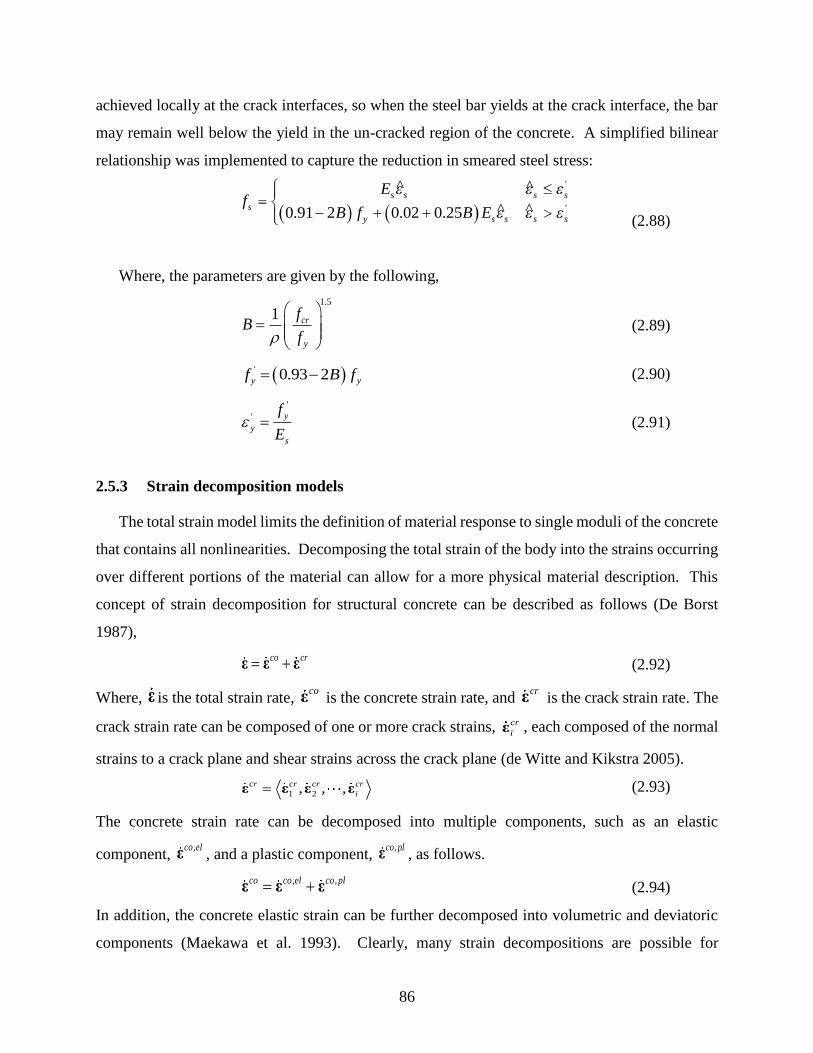
86
achieved locally at the crack interfaces, so when the steel bar yields at the crack interface, the bar
may remain well below the yield in the un-cracked region of the concrete. A simplified bilinear
relationship was implemented to capture the reduction in smeared steel stress:
(2.88)
Where, the parameters are given by the following,
1.5
1 cr
y
fB
f
=
(2.89)
( )' 0.93 2y yf B f= − (2.90)
'
' y
y
s
f
E = (2.91)
2.5.3 Strain decomposition models
The total strain model limits the definition of material response to single moduli of the concrete
that contains all nonlinearities. Decomposing the total strain of the body into the strains occurring
over different portions of the material can allow for a more physical material description. This
concept of strain decomposition for structural concrete can be described as follows (De Borst
1987),
co cr= +ε ε ε (2.92)
Where, ε is the total strain rate, coε is the concrete strain rate, and
crε is the crack strain rate. The
crack strain rate can be composed of one or more crack strains, cr
iε , each composed of the normal
strains to a crack plane and shear strains across the crack plane (de Witte and Kikstra 2005).
1 2, , ,cr cr cr cr
i=ε ε ε ε (2.93)
The concrete strain rate can be decomposed into multiple components, such as an elastic
component, ,co el
ε , and a plastic component, ,co pl
ε , as follows.
, ,co co el co pl= +ε ε ε (2.94)
In addition, the concrete elastic strain can be further decomposed into volumetric and deviatoric
components (Maekawa et al. 1993). Clearly, many strain decompositions are possible for
fE
B f B Es
s s s s
y s s s s
^
. . .
'
'0 91 2 0 02 0 25
^
^ ^

87
providing an open-ended framework for constitutive model definitions. The strain decomposition
allows combinations of elasticity, plasticity, and fracture mechanics to describe the material
response with one or more crack planes at multiple orientations. For this study, the decomposition
of concrete strain and crack strain is of greatest interest and will be taken in the context of total
strain models.
Distributed Stress Field Model (DSFM)
The Distributed Stress Field Model (DSFM) (Vecchio 2000, 2001) was an extension of the
MCFT developed to address deficiencies identified from experimental validations. Vecchio
identified that heavily reinforced sections, section subjected to biaxial compression and shear, as
well as sections subjected to proportional loadings, the principal stress, and strain fields had limited
rotation, and the MCFT underestimated their strength and stiffness due to excessive compressive
softening. In addition, sections with very light reinforcement and/or shear-critical members where
the slip along a crack plane was significant, the members exhibited a lag of the principal stress
fields relative to the principal strains. Figure 2.67 displayed the lag of compressive stress
orientation in a significant portion of the data points ( c = to o10c = + ). In these sections, the
MCFT overestimated the strength and stiffness. To address these shortcomings of the MCFT, the
DSFM abandoned the assumption that the principal stresses and strains are coincident but instead
have a lag between their orientations after cracking with a calculated shear slip at the critical crack
plane. The DSFM also overcame the necessity of limiting the local shear stress development at a
crack plane because the crack slip was now calculated. The resulting model is a hybrid of the
fixed-crack approach and the rotating crack approach. This hybrid formulation is subsequently
described.
Strain compatibility
The strain compatibility conditions of the DSFM are described in Figure 2.73. The total strain
of the element was redefined from the MCFT of Equation (2.140) to include a component of strain,
s , representing the shear slip along a crack,
s o p
c c c = + + + (2.95)

88
Figure 2.73(c) displays the Mohr’s circle construction of the apparent total strains on the
element defined at an orientation of, :
11
tan2
xy
x y
−
= − (2.96)
Figure 2.73(a) displays the Mohr’s circle construction of the net concrete strains on the element
defined at an orientation of, :
11
tan2
cxy
cx cy
−
= = − (2.97)
From this definition, the principal stresses “lag” the apparent principal strains defined by the
following,
= − (2.98)
Figure 2.73(b) displays the Mohr’s circle construction of the local strains at a crack. The
DSFM adds this compatibility condition of the slip at a crack plane defined as, s . The slip is
reduced to an average shear slip strain, s , relative to the average crack spacing:
ss
s
= (2.99)
The orthogonal components of the average shear slip strain, s , are defined by the Mohr’
( )1
sin 22
s
x s = (2.100)
( )1
sin 22
s
y s = − (2.101)
( )cos 2s
xy s = (2.102)
Furthermore, the orientation of concrete strains was related to the apparent total stains by the
following,
( ) ( ) ( )cos 2 sin 2s xy y x = + − (2.103)
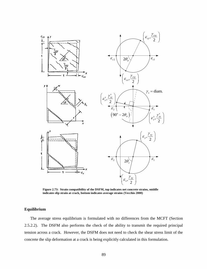
89
Figure 2.73: Strain compatibility of the DSFM, top indicates net concrete strains, middle
indicates slip strain at crack, bottom indicates average strains (Vecchio 2000)
Equilibrium
The average stress equilibrium is formulated with no differences from the MCFT (Section
2.5.2.2). The DSFM also performs the check of the ability to transmit the required principal
tension across a crack. However, the DSFM does not need to check the shear stress limit of the
concrete the slip deformation at a crack is being explicitly calculated in this formulation.
diam.s =
( )o90 2 −,
2
s
xys
y
,2
s
xys
x
2 1
,2
xy
y
,2
cxy
cy
2 2c 1c
,2
cxy
cx
12
,2
xy
x
2
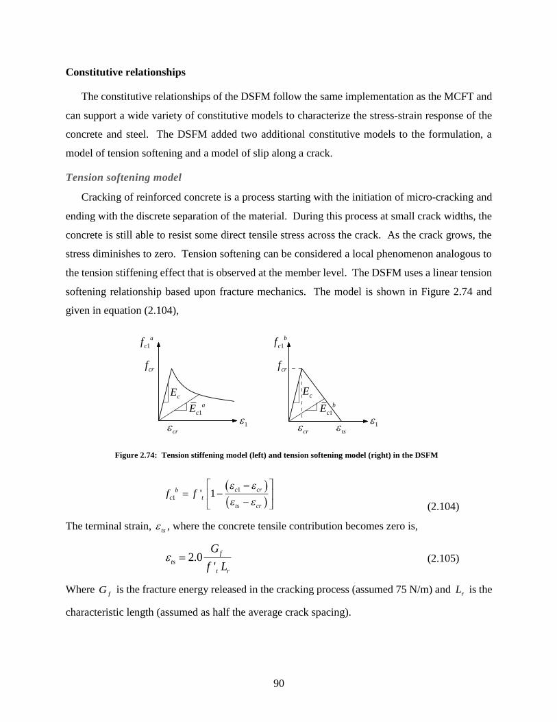
90
Constitutive relationships
The constitutive relationships of the DSFM follow the same implementation as the MCFT and
can support a wide variety of constitutive models to characterize the stress-strain response of the
concrete and steel. The DSFM added two additional constitutive models to the formulation, a
model of tension softening and a model of slip along a crack.
Tension softening model
Cracking of reinforced concrete is a process starting with the initiation of micro-cracking and
ending with the discrete separation of the material. During this process at small crack widths, the
concrete is still able to resist some direct tensile stress across the crack. As the crack grows, the
stress diminishes to zero. Tension softening can be considered a local phenomenon analogous to
the tension stiffening effect that is observed at the member level. The DSFM uses a linear tension
softening relationship based upon fracture mechanics. The model is shown in Figure 2.74 and
given in equation (2.104),
Figure 2.74: Tension stiffening model (left) and tension softening model (right) in the DSFM
(2.104)
The terminal strain, ts , where the concrete tensile contribution becomes zero is,
2.0'
f
ts
t r
G
f L = (2.105)
Where fG is the fracture energy released in the cracking process (assumed 75 N/m) and rL is the
characteristic length (assumed as half the average crack spacing).
f fc
b
t
c cr
ts cr
1
11'
1
b
cf1
a
cf
cE
crf
ts
1
b
cE
cr 111
a
cE
cr
crf
cE
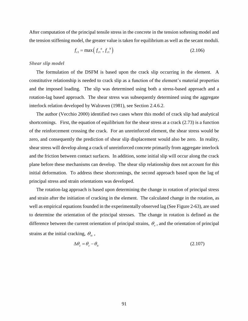
91
After computation of the principal tensile stress in the concrete in the tension softening model and
the tension stiffening model, the greater value is taken for equilibrium as well as the secant moduli.
( )1 1 1max ,a b
c c cf f f= (2.106)
Shear slip model
The formulation of the DSFM is based upon the crack slip occurring in the element. A
constitutive relationship is needed to crack slip as a function of the element’s material properties
and the imposed loading. The slip was determined using both a stress-based approach and a
rotation-lag based approach. The shear stress was subsequently determined using the aggregate
interlock relation developed by Walraven (1981), see Section 2.4.6.2.
The author (Vecchio 2000) identified two cases where this model of crack slip had analytical
shortcomings. First, the equation of equilibrium for the shear stress at a crack (2.73) is a function
of the reinforcement crossing the crack. For an unreinforced element, the shear stress would be
zero, and consequently the prediction of shear slip displacement would also be zero. In reality,
shear stress will develop along a crack of unreinforced concrete primarily from aggregate interlock
and the friction between contact surfaces. In addition, some initial slip will occur along the crack
plane before these mechanisms can develop. The shear slip relationship does not account for this
initial deformation. To address these shortcomings, the second approach based upon the lag of
principal stress and strain orientations was developed.
The rotation-lag approach is based upon determining the change in rotation of principal stress
and strain after the initiation of cracking in the element. The calculated change in the rotation, as
well as empirical equations founded in the experimentally observed lag (See Figure 2-63), are used
to determine the orientation of the principal stresses. The change in rotation is defined as the
difference between the current orientation of principal strains, , and the orientation of principal
strains at the initial cracking, ic ,
ic = − (2.107)

92
The observed lag ranged from 5˚ to 10˚ before yielding of the panels, and the author characterized
this constant lag, L , as follows:
(2.108)
The post-cracking rotation of the stress field, , is given as,
(2.109)
The orientation of principal stresses is then the sum of the orientation at initial cracking and
the post-cracking rotation, and then Equation (2.103) can determine the average crack shear strain.
ic = + (2.110)
The rotation lag-approach is limited by its basis on empirical evidence of the orientation lag as
well as the assumption of a constant orientation lag over the entire response. In reality, the
orientation will have escalating variations when subjected to higher demands.
The stress-based approach and rotation-lag approach have now provided two values of the
shear slip strain, s . By using both approaches, the deficiencies of both shear-slip methods can
be reduced, and the shear strain is taken as the maximum value,
( )max ,a b
s s s = (2.111)
The finite element implementation of the DSFM is based directly upon that of the MCFT
described in Section 2.5.3.3; however, complete treatment is given in the following references,
(Vecchio 2001; Wong, Vecchio, and Trommels 2013)
L
5
7 5
10
.
for biaxially reinforced
for uniaxially reeinforced
for un-reinforced
for
for
L
L L

93
Strain decomposition for hysteretic modeling
The simplest hysteretic model is to use the total strain relationship in loading and reloading
and for unloading to follow a secant line from the current stress-strain state to the undeformed
stress-strain state. In general, this is an underestimation of energy dissipation because some
residual deformation (plastic offset) will exist in the material after unloading. An improved model
considers the plastic straining in the material during the current load cycle or based upon the entire
load history. To achieve this, total strain models have been decomposed into the elastic and plastic
strain components. Empirical relationships have used to identify what plastic strain offset will
exist in the material after unloading as a function of the peak strain state imposed during the load
cycle. For the uni-axial case, test data as shown in Fig. 2.44 was used to associate the plastic strain
offset with the maximum principal compressive or tensile strain imposed during the load cycle.
The relationship between the current stress-strain state and the zero stress-plastic strain state has
been modeled linear, multi-linear and non-linear.
Figure 2.75 (a) shows the use of the monotonic loading base curve for any new strain state. A
secant unloading relationship to the plastic offset is utilized. The model reloads along a secant
line from the undeformed state to the previous stress-strain state achieved of the base curve.
Similarly, Figure 2.76 (b) shows the cyclic tensile model with no change except that the model
unloads along to secant to the undeformed configuration. Refined approaches based on this have
been completed with a multi-linear unloading and reloading relationship as shown in Figure 2.77
as well as with nonlinear unloading and linear reloading relationships. A detailed description of
one nonlinear unloading and reloading model and its determination of the plastic strain offset is
subsequently described based on the work of Palermo (2003).

94
Figure 2.75: Linear unloading and reloading for (a) concrete compression response, and (b)
concrete tension stiffened response (Vecchio 1999)
Figure 2.76: Multi-linear unloading and reloading for concrete in compression (Sittipunt 1994)
Nonlinear hysteretic model of concrete
A hysteretic model for the response of the concrete in a total strain format was proposed by
Palermo and Vecchio (2003, 2004). The model explicitly describes relationships for unloading
and reloading based upon quasi-static experimental data. The model uses a nonlinear unloading
relationship to improve the prediction of energy dissipated in each cycle and a linear reloading
relationship with stiffness degradation based upon a one-parameter scalar damage model. The
monotonic uniaxial response in compression and tension is used as a backbone curve for the model.
Consequently, the model does not predict any strength degradation due to cyclic loading. This
approach in reloading and unloading is used for both the compressive and tensile response of the
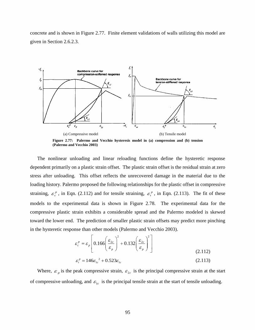
95
concrete and is shown in Figure 2.77. Finite element validations of walls utilizing this model are
given in Section 2.6.2.3.
(a) Compressive model (b) Tensile model
Figure 2.77: Palermo and Vecchio hysteresis model in (a) compression and (b) tension
(Palermo and Vecchio 2003)
The nonlinear unloading and linear reloading functions define the hysteretic response
dependent primarily on a plastic strain offset. The plastic strain offset is the residual strain at zero
stress after unloading. This offset reflects the unrecovered damage in the material due to the
loading history. Palermo proposed the following relationships for the plastic offset in compressive
straining, p
c , in Eqn. (2.112) and for tensile straining, p
t , in Eqn. (2.113). The fit of these
models to the experimental data is shown in Figure 2.78. The experimental data for the
compressive plastic strain exhibits a considerable spread and the Palermo modeled is skewed
toward the lower end. The prediction of smaller plastic strain offsets may predict more pinching
in the hysteretic response than other models (Palermo and Vecchio 2003).
(2.112)
2
1 1146 0.523p
t c c = + (2.113)
Where, p is the peak compressive strain, 2c is the principal compressive strain at the start
of compressive unloading, and 1c is the principal tensile strain at the start of tensile unloading.
c
p
p
c
p
c
p
0 166 0 1322
2
2
2
. .

96
(a) Compressive plastic strain model (b) Tensile plastic strain model
Figure 2.78: Palermo model for plastic strain offset (Palermo and Vecchio 2003)
Determination of plastic strains
The hysteretic response of the concrete and steel models presented are a function of the current
strains and plastic strain offsets, maximum historic strains and maximum historic stresses (Vecchio
1999). The plastic strain offsets are recorded in the element x,y, coordinate space. The changing
directions of the principal strains due to the rotating crack model requires the plastic strain offsets
to be transformed from the global coordinates to the current principal axes of the element. Mohr’s
circle of strain provides the transformation to principal plastic strains as follows,
( ) ( )1 cos 2 sin 22 2
p p p p
cx cy cx cyp p
c cxy
+ −= + + (2.114)
( ) ( )2 cos 2 sin 22 2
p p p p
cx cy cx cyp p
c cxy
+ −= − − (2.115)
For a load step of plastic straining, the plastic strain offsets in x,y space are updated as a
function of the incremental principal concrete strains and the previous plastic strain offsets:
( )( ) ( )( )1 2' 1 cos 2 1 cos 22 2
p pp p c c
cx cx
= + + + − (2.116)
( )( ) ( )( )1 2' 1 cos 2 1 cos 22 2
p pp p c c
cy cy
= + − + + (2.117)
( ) ( )1 2' sin 2 sin 2p p p p
cxy cxy c c = + − (2.118)
The maximum principal strains and principal stresses in the concrete are also desired for input
to hysteretic constitutive relationships. While the plastic strain offsets are an incremental function

97
of the strain history, the maximum stresses and strains represent only an envelope value of the
loading history. The maximum compressive strains
( )( ) ( )( )1 2' 1 cos 2 1 cos 22 2
cm cmcmx cmx
= + + + − (2.119)
( )( ) ( )( )1 2' 1 cos 2 1 cos 22 2
cm cmcmy cmy
= + − + + (2.120)
( ) ( )1 2' sin 2 sin 2cmxy cmxy cm cm = + − (2.121)
Using the Mohr’s circle and the incremental changes, the maximum tensile strains and as well
as the corresponding maximum tensile stresses and compressive stresses can be developed.
Reloading model in compression
The concrete stress of cyclic reloading is a function of a degrading Young’s modulus. The
degradation of stiffness is a function of the stress/strain state at the end of the last unloading curve.
The compressive stress in reloading, cf , and the associated degraded modulus, cmE + , are,
( )c ro cm c rof f E += + − (2.122)
d cm rocm
cm ro
f fE
+ −=
− (2.123)
Where, rof and ro are the principal stress/strain state at the end of unloading, cmf and cm
are the maximum principal stress and strain, and c is the current strain on the reloading path.
The damage parameter d and the recovered (or elastic) strain are,
(2.124)
rec cm ro = − (2.125)
Unloading model in compression
The elastic unloading relationship to the determined plastic strain offset is defined by the
Ramberg-Osgood (1943) power formulation. The initial unloading stiffness is the elastic modulus
d
rec p
c p
rec p
c
1
1 0 10
1
1 0 175
0 5
0 6
.
.
.
.
for
for p

98
of the concrete and reduces to 7.1% of the elastic modulus at the end of the unloading branch. The
compressive stress in unloading, cf , and the power term
cN were defined as,
( )( ) ( )
( )1
0.071 1 c
c
N
c c cm
c cm c c cm Np
c c cm
Ef f E
N
−
− −= + − +
− (2.126)
( ) ( )
( )0.071 1 p
c c cm
c p
cm c c cm
EN
f E
− −=
+ − (2.127)
Reloading model in tension
The tensile concrete stress of cyclic reloading is a function of a degrading Young’s modulus,
following a similar form to the reloading model in compression. The tensile stress in reloading,
cf , and the associated degraded modulus, tmE + , are,
( )c t tm tm tm cf f E += − − (2.128)
t tm rotm
tm ro
f fE
+ −=
− (2.129)
Where, tmf and tm are the maximum principal stress and strain. The tensile damage parameter
t and the recovered (or elastic) strain are,
( )
0.25
1
1 1.15t
rec
=+
(2.130)
rec cm ro = − (2.131)
Unloading model in tension
The unloading relationship in tension is also based on the Ramberg-Osgood (1943) power
formulation and calibrated to a set of experimental data. The compressive stress in unloading, cf
, the power term, cN , and the unloading modulus, f
cE , defined as,
( )( )( )
( )1
t
t
Nf
c c tm c
c tm c c tm Np
t tm c
E Ef f E
N
−
− −= + − +
− (2.132)
( )( )
( )
f p
c c tm c
t p
c tm c tm
E EN
E f
− −=
− − (2.133)
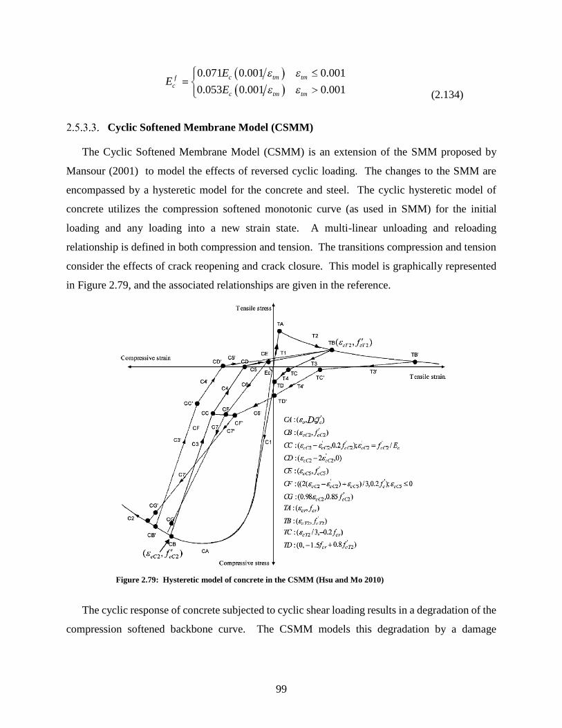
99
(2.134)
Cyclic Softened Membrane Model (CSMM)
The Cyclic Softened Membrane Model (CSMM) is an extension of the SMM proposed by
Mansour (2001) to model the effects of reversed cyclic loading. The changes to the SMM are
encompassed by a hysteretic model for the concrete and steel. The cyclic hysteretic model of
concrete utilizes the compression softened monotonic curve (as used in SMM) for the initial
loading and any loading into a new strain state. A multi-linear unloading and reloading
relationship is defined in both compression and tension. The transitions compression and tension
consider the effects of crack reopening and crack closure. This model is graphically represented
in Figure 2.79, and the associated relationships are given in the reference.
Figure 2.79: Hysteretic model of concrete in the CSMM (Hsu and Mo 2010)
The cyclic response of concrete subjected to cyclic shear loading results in a degradation of the
compression softened backbone curve. The CSMM models this degradation by a damage
EE
Ec
f c tm tm
c tm tm
0 071 0 001 0 001
0 053 0 001 0 001
. . .
. . .

100
parameter, D, that is a function of the maximum compression strain achieve in the stress-strain
history as follows,
max
1 1.0c
co
D
= − (2.135)
The value of is taken as 0.4 to fit the experimental cyclic shear stress-strain response of panels
(Mansour 2001). This damage parameter is applicable only in the compressive response.
The cyclic response of the steel bars is based upon the bilinear smeared stress relationship
developed for the SMM. That model is extended to hysteretic response to account for the
Bauschinger effect using a Ramberg-Osgood power formula (Yokoo and Nakamura 1977),
(2.136)
0.11.9 pA k −= (2.137)
0.210 pR k −= (2.138)
( )'
' '
ˆsi yp
p
y y
k
−= = (2.139)
Where, ˆsi , and sif represent the smeared-stress strain state at the point of load-reversal. The
value pk controls the magnitude of the Bauschinger effect. Increasing the magnitude of
pk
increases the Bauschinger effect, effectively increasing the size of the hysteretic loop with
increasing plastic strain after the steel bars have yielded.
2.5.4 Finite element implementations
The implementation of the aforementioned models to finite element analysis tools varies
widely with respect to the solution methodology and overall complexity. In general, NLFEA
methods have favored a tangent stiffness formulation as opposed to a secant stiffness formulation.
They have also favored higher order elements (such as those with additional nodes and polynomial
shape functions) instead of simpler elements in a larger quantity (Vecchio 1989). An international
competition to predict the behavior of cracked reinforced concrete elements (Collins, Vecchio, and
Mehlhorn 1985) indicated no direct correlation between analytical complexity and performance.
Instead, the performance was driven by the constitutive modeling of the cracked reinforced
s si
s si
s
R s si
y
R
f f
EA
f f
f1
1
^

101
concrete. As a result, researchers have focused on the constitutive models and utilized the finite
element implementation that has provided the best convergence and numerical stability (Vecchio
1990). In addition, the models have utilized triangular and rectangular plane stress elements with
linear shape functions. These element types provide a closed form solution for the element
stiffness matrices and do not require numerical integration. This section provides an overview of
the secant stiffness formulation utilized to implement the models of this study in finite element
analysis programs.
Secant stiffness formulation
The finite element implementation of the MCFT and its variants utilizes a secant stiffness
formulation (Vecchio and Collins 1986) including pre-strains (Vecchio 1990) and plastic strain
offsets (Vecchio 2000, 2001). The benefits of a secant stiffness formulation are numerical
simplicity and the ability to easily adapt a linear finite element analysis program to have nonlinear
capability.
The global coordinate frame sign convention is shown in Figure 2.80(a), the local coordinate
frame of the concrete and steel are given in (b) and (c) respectively.
Figure 2.80: Sign convention of the MCFT FE implementation (Vecchio 1990)
The total average strain on the element is then described by the summation of the net strains
due to imposed stress c , the stain due to initial or elastic offsets, o
c , and the strains due to
plastic deformation in the material p
c .
o p
c c c = + + (2.140)
102
And similarly, the steel strain of each reinforcement component is a function of the total strain,
initial offsets, and plastic offsets,
o p
s s si i i = + + (2.141)
The solution must then solve the nodal displacements as a function of the externally imposed
loads,
K u F= (2.142)
Determination of global stiffness
To describe the nonlinear response of a reinforced concrete element the stiffness matrix must
be updated as a function of the strain. The MCFT decomposes the global element stiffness of the
concrete and the contribution of smeared steel reinforcing in one or more directions.
1
n
c s ii
D D D=
= + (2.143)
The global stiffness contributions rewritten in terms of the local stiffness’s and the
transformation matrices becomes,
1
nT T
c c c s s si iii
D T D T T D T=
= + (2.144)
The transformation matrix is formed for the concrete and each contribution of smeared steel
reinforcing as follows,
(2.145)
(2.146)
The local stiffness matrix of the concrete is given in plane stress. The Poisson’s effect is
considered negligible in cracked reinforced concrete, and the corresponding terms of the stiffness
are dropped. The resulting stiffness given in terms of the secant moduli is,
(2.147)
T
cos sin cos sin
sin cos cos sin
cos sin cos si
2 2
2 2
2 2 nn cos sin2 2
for
for
T
T
c
i s i
D
E
E
G
c
c
c
c
2
1
0 0
0 0
0 0
103
The local stiffness matrix of each reinforcing bar is given with a uniaxial response in terms of
the reinforcement ratio in the given direction and the secant moduli of the steel.
(2.148)
The secant moduli are defined as follows and solved using the constitutive relationship defined
for each component,
11
1
cc
c
fE
= (2.149)
22
2
cc
c
fE
= (2.150)
1 2
1 2
c cc
c c
E EG
E E
=
+ (2.151)
sisi
si
fE
= (2.152)
After solution of the secant stiffness, the element stiffness is determined by,
Te
Ak t B D B dA= (2.153)
The independent components of the concrete and steel to the element stiffness can also be
evaluated,
Te
c cA
k t B D B dA= (2.154)
Te
s s ii Ak t B D B dA= (2.155)
The element stiffnesses are then assembled to form the global stiffness matrix,
1
eln
e
jjK k
= =
(2.156)
Determination of nodal load vector
The global stiffness matrix operates on a nodal load vector to solve the nodal displacements.
However, the nodal displacements include free strains due to elastic and plastic offsets. To impose
the externally applied forces to the displaced configuration, a ‘pseudo’ nodal load vector was
developed to represent the forces required to impose the free strains in the elements as a function
D
E
si
i si 0 0
0 0 0
0 0 0

104
of the current stiffness of the structure (Vecchio 2001). The pseudo nodal load vector is added to
the externally applied loads to solve the system.
The elastic and plastic strain offsets are described as follows,
(2.157)
(2.158)
The elastic and plastic offsets of the ith component of smeared steel are described in terms of
the angle, i , of the reinforcement relative to the x-axis.
(2.159)
(2.160)
The nodal displacements due to the strain offsets can subsequently be found from integrating
the strains over the element.
o o
c cA
u dA= (2.161)
p p
c cA
u dA= (2.162)
o o
s si iAu dA= (2.163)
p p
s si A iu dA= (2.164)
From the resulting displacements, the corresponding forces for the pseudo nodal load vector
can be evaluated,
( ) ( )1
*n
e o p e o p
c c c s s si iii
F k u u k u u=
= + + + (2.165)
The is then the sum of the externally applied loads and the pseudo nodal load vector,
c
o
cx
o
cy
o
cxy
o
cx
o
cy
o
0
c
p
cx
p
cy
p
cxy
p
s
o
i
sxi
o
syi
o
sxyi
o
si
o
i
si
o
1 2 2
1
cos
coos
sin
2 2
2
i
si
o
i
s
p
i
sxi
p
syi
p
sxyi
p
si
p
i
si
p
1 2 2
1
cos
coos
sin
2 2
2
i
si
p
i

105
*extF F F= + (2.166)
After solving the nodal displacements and strains, element stresses are evaluated by,
( ) ( )1
no p o p
c c c s s si i ii
f D D =
= − − + − − (2.167)
Tangent stiffness formulations of the MCFT
The tangent stiffness formulation for NLFEA is the solution methodology found in nearly all
commercial finite element programs, including those focused on the modeling of reinforced
concrete. The following provides a high-level review of the applicability of secant stiffness models
such as the MCFT to be solved using a tangent stiffness formulation.
The earliest known implementation of the MCFT using a tangent stiffness formulation was
completed by Adeghe (1986). The MCFT was utilized into the finite element program ADINA
developed by K. J. Bathe. It assumed uniaxial response in principal strain directions and the
tangent stiffness was based on the tangent stiffness for each principal strain direction using a
weighting scheme. The Broyden–Fletcher–Goldfarb–Shanno (BFGS) (Fletcher 1987) algorithm
was reported to provide better convergence than the modified Newton method.
A second implementation was completed by Stevens (1987; Stevens et al. 1991) as an
independent program using Fortran. This approach utilized a modified version of the MCFT.
High-powered (24 DOF) rectangular elements were selected so that a single element could
represent the full depth of a beam. The non-linear solution scheme utilized the Modified-Newton
method. An energy-based convergence criterion was found to require more accuracy at DOFs that
are sensitive to small load changes. The non-symmetry of the material stiffness resulted in
difficulties to solve the tangent stiffness. A non-symmetric solver with ‘frontal’ approach was
utilized including numerical integration on the full matrix. This approach more than doubled the
solution time, but reduced convergence time and solution time overall. The stress transfer at cracks
was reported to be destabilizing to the solution due to the large changes in tensile stiffness. The
crack check was eliminated from the MCFT to improved performance. Elimination of the crack
check requires the tensile response to consider the amount and distribution of reinforcing. An
empirical relation was developed based on the assumptions that the bond stress is proportional to
cracking stress and uniform steel distribution. Additional empirical factors were included model
the biaxial response for cracks non-orthogonal to the reinforcement. The model was calibrated to

106
achieve the best numerical stability even though it did not properly represent all test data
(unreinforced concrete and low reinforcement ratios). Consequently, this implementation did not
accurately predict panels subjected to biaxial compression and shear.
A third implementation was created by Cook (1987; Cook and Mitchell 1988). This approach
included the original features of the MCFT with the crack check. This approach utilized triangular
and rectangular elements up to nine nodes and evaluated with up to sixteen Gauss points and the
Newton-Raphson solution method. The tangent stiffness matrix was determined by incrementing
the existing strains to determine the corresponding changes in stress. Details of the incremental
solution were not provided in the literature. One shortcoming of this implementation was that the
post-peak compressive strength resulted in negative tangent stiffness terms an caused numerical
instability. As a workaround, a small positive stiffness was used for strains beyond the peak strain,
'c , equal to 10,000cE .
The final and most successful approach was completed by Aquino and Erdem (2007). The
authors acknowledge the previous approaches of Stevens and Cook and the necessity to eliminate
sharp changes in stiffness in order to achieve convergence in their implementations. Furthermore,
the primary challenge of calculating the material tangent stiffness matrix was implementing the
check for load transmission at the cracks. The approach of this paper included all features of the
MCFT in their original form and added the available compressive stress increase due to biaxial
compression (Vecchio 1992). The concrete contribution to the tangent stiffness matrix Jacobian is
solved using an iterative finite difference approach. Each strain is incremented forward and
backward solving the concrete stresses at each step. The relative change in stresses divided by the
total strain increment is used to define each column of the Jacobian. By incrementing each strain
component in sequence, each column of the Jacobian can be determined. The steel contribution
to the tangent stiffness is solved in a closed form based on an elastic-perfectly plastic material
model. The resulting stiffness matrix is generally non-symmetric and requires a non-symmetric
FE solver. A user-defined subroutine for the tangent stiffness was utilized within ABAQUS to
validate the approach. In general, the results are equal to the previously documented results of the
MCFT using secant stiffness solutions.

107
2.6 Numerical approaches to predicting the response of structural walls
Modeling the inelastic response of structural walls has been approached in three primary ways:
lumped plasticity models, sectional fiber analysis models, and finite element models. The lumped
plasticity models utilize a combination of elastic beam and column elements connected by plastic
rotational springs (hinges) (Figure 2.81 (a)). This type of model is termed “lumped plasticity”
because all the inelasticity is contained within these springs. Parameters of this model are the
effective stiffness values assigned to the elastic beam / column elements and the constitutive
relationship of the hinge. This simplified model is limited by its inability to capture cyclic effects,
any variation of axial or shear forces, and its dependence on the user-defined locations of the
plastic hinges (Pugh 2012).
A more comprehensive approach is the use of fiber elements to perform a sectional fiber
analysis at each discretized section of a wall (Figure 2.81 (b)). A sectional analysis splits the
section into fibers of concrete and steel each with an area defined by the discretization for the fiber
analysis and material properties. Uniaxial constitutive relationships for the steel and concrete are
defined to determine the resistance of the section to any imposed strain profile. This approach can
consider the effects of axial load, moment and shear. The sectional analysis assumes that plane
sections remain plane and a uniform strain distribution through the thickness of each fiber. These
assumptions can become unreasonable in non-planar or non-slender sectional geometries.
Nevertheless, a detailed study of finite line elements using fiber analysis by Pugh (2012)
successfully predicted the stiffness up to and beyond yielding and the ultimate strength of planar
and non-planar walls subjected to cyclic loadings. While not the focus of that effort, it is important
to note that this approach did not always capture the cyclic strength and stiffness degradation due
to damage, the energy dissipated in the hysteretic loops or the ultimate failure mode of the walls.
Finally, detailed finite element analyses have been employed to predict the response of walls.
The member can be discretized by plane, shell or solid elements each with increasing complexity.
An example of each type of discretization is shown in Figure 2.82. Static or dynamic analysis can
be carried out each for a wide variety of material definitions that can be provided for the concrete
and steel. A comprehensive overview of finite element analysis of structural concrete is provided
in the fib guide (Fédération internationale du béton and Task Group 4.4 2008). This study focuses
on the use of static nonlinear finite element analysis of structural concrete and will be subsequently
described in detail.

108
(a) (b)
Figure 2.81: (a) Lumped plasticity approach (b) sectional analysis approach (Moehle, Mahin,
and Bozorgnia 2010)
(a) (b) (c)
Figure 2.82: Finite element models of structural concrete (a) plane stress elements (b) shell
elements (Ile and Reynouard 2005) (c) solid elements (Maekawa and Fukuura 2010)
2.6.1 Nonlinear finite element analysis of structural concrete
Nonlinear finite element analysis (NLFEA) represents a set of methods to approximate the
response of structures with complex or irregular geometries that remain difficult or impossible to
solve with classical mechanics. Nonlinearity of a structure stems from the geometry of structures
undergoing large deformations and/or the material response exhibiting inelasticity under an
applied load. NLFEA is used in the analysis and design of many structures including, buildings,
bridges, automobiles, airplanes, as well as countless mechanical/industrial/electrical components.
NLFEA was first developed in the mid-1960s with its first application to structural concrete
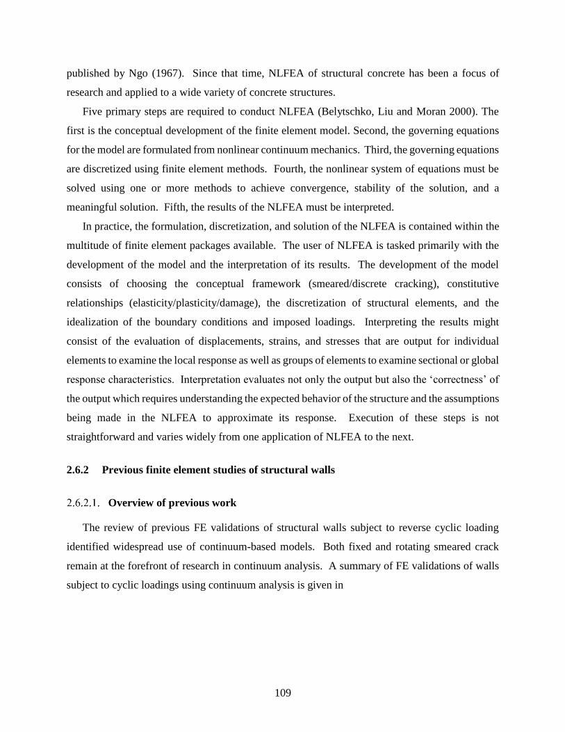
109
published by Ngo (1967). Since that time, NLFEA of structural concrete has been a focus of
research and applied to a wide variety of concrete structures.
Five primary steps are required to conduct NLFEA (Belytschko, Liu and Moran 2000). The
first is the conceptual development of the finite element model. Second, the governing equations
for the model are formulated from nonlinear continuum mechanics. Third, the governing equations
are discretized using finite element methods. Fourth, the nonlinear system of equations must be
solved using one or more methods to achieve convergence, stability of the solution, and a
meaningful solution. Fifth, the results of the NLFEA must be interpreted.
In practice, the formulation, discretization, and solution of the NLFEA is contained within the
multitude of finite element packages available. The user of NLFEA is tasked primarily with the
development of the model and the interpretation of its results. The development of the model
consists of choosing the conceptual framework (smeared/discrete cracking), constitutive
relationships (elasticity/plasticity/damage), the discretization of structural elements, and the
idealization of the boundary conditions and imposed loadings. Interpreting the results might
consist of the evaluation of displacements, strains, and stresses that are output for individual
elements to examine the local response as well as groups of elements to examine sectional or global
response characteristics. Interpretation evaluates not only the output but also the ‘correctness’ of
the output which requires understanding the expected behavior of the structure and the assumptions
being made in the NLFEA to approximate its response. Execution of these steps is not
straightforward and varies widely from one application of NLFEA to the next.
2.6.2 Previous finite element studies of structural walls
Overview of previous work
The review of previous FE validations of structural walls subject to reverse cyclic loading
identified widespread use of continuum-based models. Both fixed and rotating smeared crack
remain at the forefront of research in continuum analysis. A summary of FE validations of walls
subject to cyclic loadings using continuum analysis is given in

110
Table 2.7. Key conclusions regarding the approaches of these studies are summarized below
followed by some selected results of individual studies.
The conceptual approaches of nonlinear elasticity and elasto-plasticity were most common.
These conceptual approaches primarily used plane stress and fiber shell element formulations.
Only one study used a three-dimensional solid element. In 1993, Sittipunt and Wood identified a
700% increase of computational cost for the modeling of a C-shaped wall in-plane stress vs. fiber
shell elements. Since that time, massive increases in computing power and computational
robustness of finite element solution methods have eliminated the prohibitive nature of doing shell
and solid finite element analyses. A significant increase in 3-D formulations during the 2000’s is
identified in the table. However, the necessity of a full three-dimensional analysis over a plane
stress analysis for non-planar wall structures remains unclear.
The primary mechanism for modeling the hysteretic response is the inclusion of unloading and
reloading relationships with plastic offsets. Within this approach, cyclic stiffness degradation can
be captured in the reloading relationship defined often as a function of the plastic offset and
previously attained maximum stresses and strains. The use of linear or nonlinear unloading
relationships significantly affects the prediction of energy dissipation. However, energy
dissipation capability is generally unreliable because the unloading stiffness is not based on the
physics of the actual degradation of the material. Explicit modeling of material degradation using
damage mechanics in compression and fracture mechanics in tension was identified in only one
study based on the work of Maekawa (Kitada et al. 2007; Ono et al. 2001; Maekawa 2003).
The hysteretic response is also highly influenced by the choice of crack model. Rotating and
fixed crack approaches were both used. Fixed crack approaches included the orthogonal crack
models (cracks at right angles) as well as multiple non-orthogonal crack models. While the fixed
crack models are physically motivated, the significant rotations of cracks, cracks in multiple
directions, and transfer of shear stress across a crack greatly increase the complexity and reduce
the reliability of the model. Fixed crack models based upon shear retention require a degrading
response based on the cyclic shear degradation along a crack plane to prevent overprediction of
stiffness (Kwan and Billington 2001). Nevertheless, fixed crack models retain great potential to
better model the physics of the problem.
All models identified modeled the interface between the wall and footing with full fixity,
restraining horizontal and vertical displacement. The experimental results and earthquake

111
observations previously identified have invalidated this assumption due to sliding along this
interface as well as significantly greater crack width at the interface compared to other cracks.
Furthermore, strain penetration of the longitudinal steel bars into the footing cannot be captured
with an assumption of vertical fixity. One study explicitly identified that the assumption of no
interface deformations affected the predicted global response and deviation between the
experimental and analytical results (Ile and Reynouard 2005).
Model validation is limited to the global response and does not evaluate the element level
response. The deficiency of this approach was addressed by multiple authors including Sittipunt
(Sittipunt 1994) and Constantin (2012). In addition, the validation of global response is limited
primarily to the prediction through yielding and nominal strength. Evaluation of the failure mode
and damage states is limited and revealed unreliability in the ability to correctly predict the
mechanism of failure and degradation of the materials. Furthermore, each study typically only
evaluates the performance of a single model.
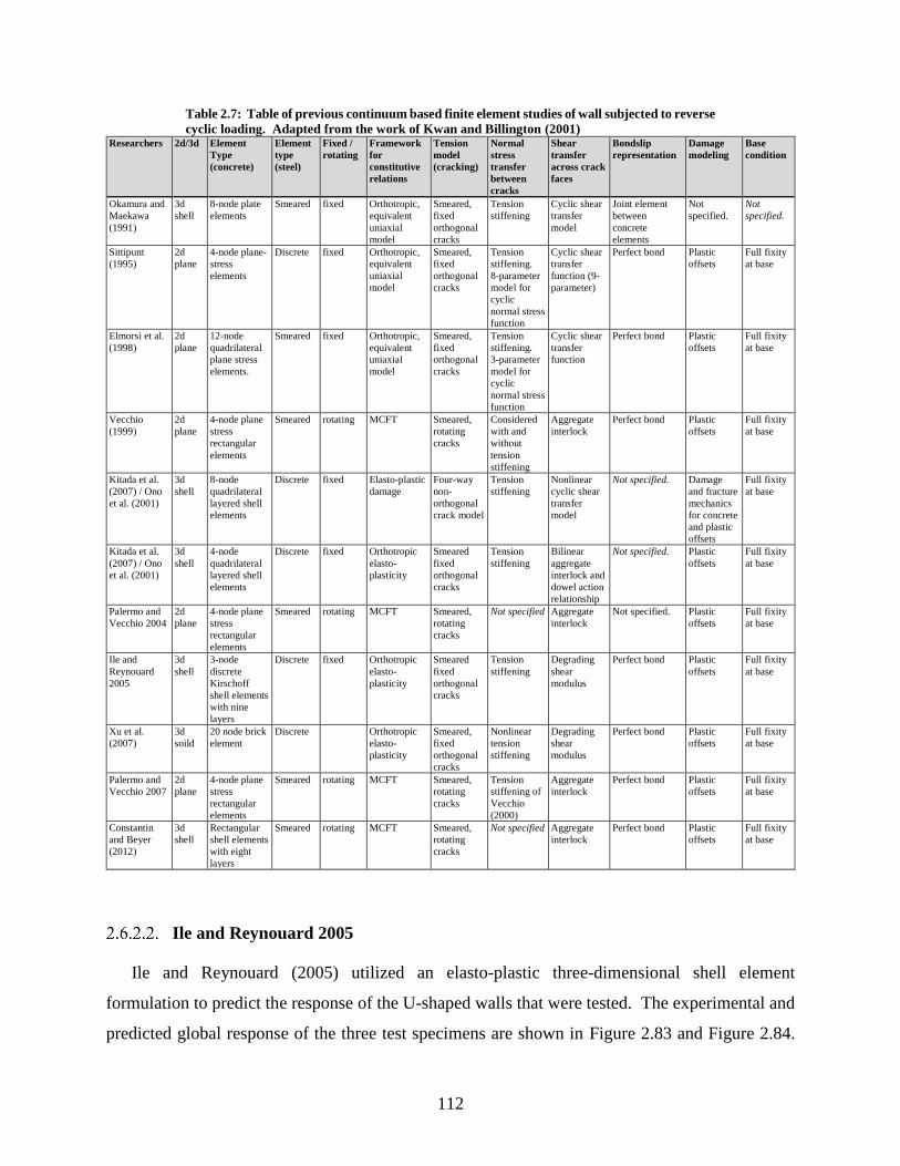
112
Table 2.7: Table of previous continuum based finite element studies of wall subjected to reverse
cyclic loading. Adapted from the work of Kwan and Billington (2001) Researchers 2d/3d Element
Type
(concrete)
Element
type
(steel)
Fixed /
rotating
Framework
for
constitutive
relations
Tension
model
(cracking)
Normal
stress
transfer
between
cracks
Shear
transfer
across crack
faces
Bondslip
representation
Damage
modeling
Base
condition
Okamura and
Maekawa
(1991)
3d
shell
8-node plate
elements
Smeared fixed Orthotropic,
equivalent
uniaxial
model
Smeared,
fixed
orthogonal
cracks
Tension
stiffening
Cyclic shear
transfer
model
Joint element
between
concrete
elements
Not
specified.
Not
specified.
Sittipunt
(1995)
2d
plane
4-node plane-
stress
elements
Discrete fixed Orthotropic,
equivalent
uniaxial
model
Smeared,
fixed
orthogonal
cracks
Tension
stiffening.
8-parameter
model for
cyclic
normal stress
function
Cyclic shear
transfer
function (9-
parameter)
Perfect bond Plastic
offsets
Full fixity
at base
Elmorsi et al.
(1998)
2d
plane
12-node
quadrilateral
plane stress
elements.
Smeared fixed Orthotropic,
equivalent
uniaxial
model
Smeared,
fixed
orthogonal
cracks
Tension
stiffening.
3-parameter
model for
cyclic
normal stress
function
Cyclic shear
transfer
function
Perfect bond Plastic
offsets
Full fixity
at base
Vecchio
(1999)
2d
plane
4-node plane
stress
rectangular
elements
Smeared rotating MCFT Smeared,
rotating
cracks
Considered
with and
without
tension
stiffening
Aggregate
interlock
Perfect bond Plastic
offsets
Full fixity
at base
Kitada et al.
(2007) / Ono
et al. (2001)
3d
shell
8-node
quadrilateral
layered shell
elements
Discrete fixed Elasto-plastic
damage
Four-way
non-
orthogonal
crack model
Tension
stiffening
Nonlinear
cyclic shear
transfer
model
Not specified. Damage
and fracture
mechanics
for concrete
and plastic
offsets
Full fixity
at base
Kitada et al.
(2007) / Ono
et al. (2001)
3d
shell
4-node
quadrilateral
layered shell
elements
Discrete fixed Orthotropic
elasto-
plasticity
Smeared
fixed
orthogonal
cracks
Tension
stiffening
Bilinear
aggregate
interlock and
dowel action
relationship
Not specified. Plastic
offsets
Full fixity
at base
Palermo and
Vecchio 2004
2d
plane
4-node plane
stress
rectangular
elements
Smeared rotating MCFT Smeared,
rotating
cracks
Not specified Aggregate
interlock
Not specified. Plastic
offsets
Full fixity
at base
Ile and
Reynouard
2005
3d
shell
3-node
discrete
Kirschoff
shell elements
with nine
layers
Discrete fixed Orthotropic
elasto-
plasticity
Smeared
fixed
orthogonal
cracks
Tension
stiffening
Degrading
shear
modulus
Perfect bond Plastic
offsets
Full fixity
at base
Xu et al.
(2007)
3d
soild
20 node brick
element
Discrete Orthotropic
elasto-
plasticity
Smeared,
fixed
orthogonal
cracks
Nonlinear
tension
stiffening
Degrading
shear
modulus
Perfect bond Plastic
offsets
Full fixity
at base
Palermo and
Vecchio 2007
2d
plane
4-node plane
stress
rectangular
elements
Smeared rotating MCFT Smeared,
rotating
cracks
Tension
stiffening of
Vecchio
(2000)
Aggregate
interlock
Perfect bond Plastic
offsets
Full fixity
at base
Constantin
and Beyer
(2012)
3d
shell
Rectangular
shell elements
with eight
layers
Smeared rotating MCFT Smeared,
rotating
cracks
Not specified Aggregate
interlock
Perfect bond Plastic
offsets
Full fixity
at base
Ile and Reynouard 2005
Ile and Reynouard (2005) utilized an elasto-plastic three-dimensional shell element
formulation to predict the response of the U-shaped walls that were tested. The experimental and
predicted global response of the three test specimens are shown in Figure 2.83 and Figure 2.84.

113
The IleX test adequately predicts the response up to nominal. In the damaged state, the model
clearly does not capture the cyclic strength degradation occurring in the final three cycles at the
same displacement level. In addition, the IleY and IleX models do not adequately predict the
pinching of the hysteretic loops as a consequence of the assumption of base fixity when significant
interface deformations were observed experimentally. The IleXY test illustrates that the 3-D
modeling with shell elements successfully captured the reduced strength and stiffness due to the
bi-directional loading. None of the predictions adequately captured the web crushing or bar
buckling that was observed experimentally.
(a) IleX response (b) IleY response
Figure 2.83: Predicted response of unidirectional tests IleX and IleY (Ile and Reynouard 2005)
Figure 2.84: Predicted response of bidirectional test IleXY (Ile and Reynouard 2005)

114
Palermo and Vecchio 2007
The MCFT and DSFM were extended to cyclic response based upon the work of Palermo and
Vecchio. Extending this effort, twenty-one previously experimentally tested structural walls of
various configurations subjected to reverse cyclic loading were simulated using the MCFT. This
selection included planar walls, barbell walls, and flanged walls of varying aspect ratios, but was
limited to uni-directional loading only. The objective of the study was to find evidence that the
smeared crack formulation of the MCFT in conjunction with low powered finite elements could
provide reasonable predictions of response at low computational cost. Indeed, their effort found
substantial agreement in the ability to predict strength, ductility, energy dissipation, and failure
mechanisms. The shortcomings identified were a common “flat-topped” response indicative of
predicting flexural yielding only, when in reality the experiments had a combination of concrete
damage and steel yielding in the post-peak regime. Along with this same idea, cyclic strength
degradation that is experimentally observed due to the concrete damage was not well predicted.
Furthermore, the mechanisms were not correctly predicted in all cases. These shortcomings are
apparent in the test results shown in Figure 2.85.
Figure 2.85: Experimental and predicted response using a hysteretic implementation of the
MCFT (Palermo and Vecchio 2007)
115
CHAPTER 3: EXPERIMENTAL TESTING OF C-SHAPED WALLS
3.1 Introduction
Chapter 3 summarizes the design, instrumentation, and loading of the three C-shaped walls
tested as part of the NSF and CPF funded study introduced in Chapter 1. The specimen design
and loading were based on a ten-story prototype structure representing a mid-rise structure with
central core wall construction. The test specimens represent the bottom three stories of the
prototype building at one-third scale. A plan of the prototype building is shown in Figure 3.1 with
the test specimen emphasized in red. In addition, an isometric of the prototype structure is shown
in Figure 3.2 with the test specimen similarly emphasized. To represent the ten-story building
experimentally, axial, shear and moment demands at the third story are imposed on the specimen
to simulate the loads from the upper seven stories of the structures. The detail of the specimen
design and construction are given in Section 3.2.
The first C-shaped wall test (CW1) was subjected the specimen to a uni-directional cyclic
loading history about the strong axis. The second C-shaped wall test (CW2) was subjected to a
cyclic cruciform bi-directional loading history in the plane of the strong and weak axis of the
specimen. The third C‐shaped wall test (CW3) investigated the bidirectional performance of the
test specimen when considered part of a coupled core wall system. Details of the loading
methodology and imposed displacement history are detailed in Section 3.3.
For CW3, the complexity of the bi-directional loading with coupled core wall simulation
required a new loading algorithm to be developed. The loading algorithm utilizes incremental
measurements of stiffness during the loading history to predict the target load of future steps. The
algorithm improves step convergence while minimizing unintended demands on the specimen.
The development and implementation of this loading algorithm are given in Section 3.4.
The wall specimens were densely instrumented with more than three hundred ninety channels
of data on each test. Global displacements of the test specimen were measured with displacement
transducers and string potentiometers. Global loads were measured from load cells in the
actuators. Local displacements were measured from an array of displacement transducers as well
as two non-contact measurement systems, the Metris Krypton system and the use of
photogrammetric methods. Local strains were measured with concrete surface strain gauges and
from steel strain gauges embedded in the wall on the longitudinal, horizontal, and confining steel

116
bars. High-resolution still cameras placed around the specimen capture the damage and cracking
patterns at each load step. A complete description of the wall instrumentation is detailed by
Behrouzi et al. (2015a). Conclusions on the resulting methodology for experimental testing are
summarized in Section 0.
Figure 3.1: Prototype building plan with prototype specimen shown in red
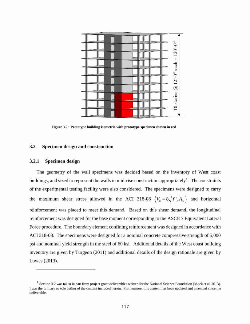
117
Figure 3.2: Prototype building isometric with prototype specimen shown in red
3.2 Specimen design and construction
3.2.1 Specimen design
The geometry of the wall specimens was decided based on the inventory of West coast
buildings, and sized to represent the walls in mid-rise construction appropriately1. The constraints
of the experimental testing facility were also considered. The specimens were designed to carry
the maximum shear stress allowed in the ACI 318-08 ( )8 'n c cvV f A= and horizontal
reinforcement was placed to meet this demand. Based on this shear demand, the longitudinal
reinforcement was designed for the base moment corresponding to the ASCE 7 Equivalent Lateral
Force procedure. The boundary element confining reinforcement was designed in accordance with
ACI 318-08. The specimens were designed for a nominal concrete compressive strength of 5,000
psi and nominal yield strength in the steel of 60 ksi. Additional details of the West coast building
inventory are given by Turgeon (2011) and additional details of the design rationale are given by
Lowes (2013).
1 Section 3.2 was taken in part from project grant deliverables written for the National Science Foundation (Mock et al. 2013).
I was the primary or sole author of the content included herein. Furthermore, this content has been updated and amended since the
deliverable.
10 s
tori
es @
12’-
0”
each
= 1
20’-
0”

118
The overall geometry and reinforcing of the C-shaped walls are shown in Figure 3.3. The
boundary element details are shown in Figure 3.4. It is noted that for CW1, the J-hook in the toe-
boundary element was inadvertently left out during the construction process. The boundary
element details of CW2 and CW3 were constructed as designed.
Figure 3.5 shows a schematic drawing of the wall footing design. The footing was 14 ft. by
8.75 ft. by 2 ft. and heavily reinforced with two horizontal mats of #4 bars and vertical #4 bars.
The footing was post-tensioned to the strong floor with approximately 100 kips per point of
anchorage. A void was left for each post-tensioning rod using PVC tubing with spiral
reinforcement in the surrounding concrete. In addition, two lifting ducts were left open through
the depth of the footing to allow the specimen to be lifted into place using an overhead crane.
The wall cap was constructed similarly to the footing using two heavily reinforced mats of #4
horizontal and vertical bars. To connect the cap to the loading device, PVC tubing was again used
to leave voids for post-tensioning rods. The wall cap is 18 inches high. A schematic drawing of
the cap is shown in Figure 3.6.
Figure 3.3: CW1/2/3 overall wall geometry and reinforcing
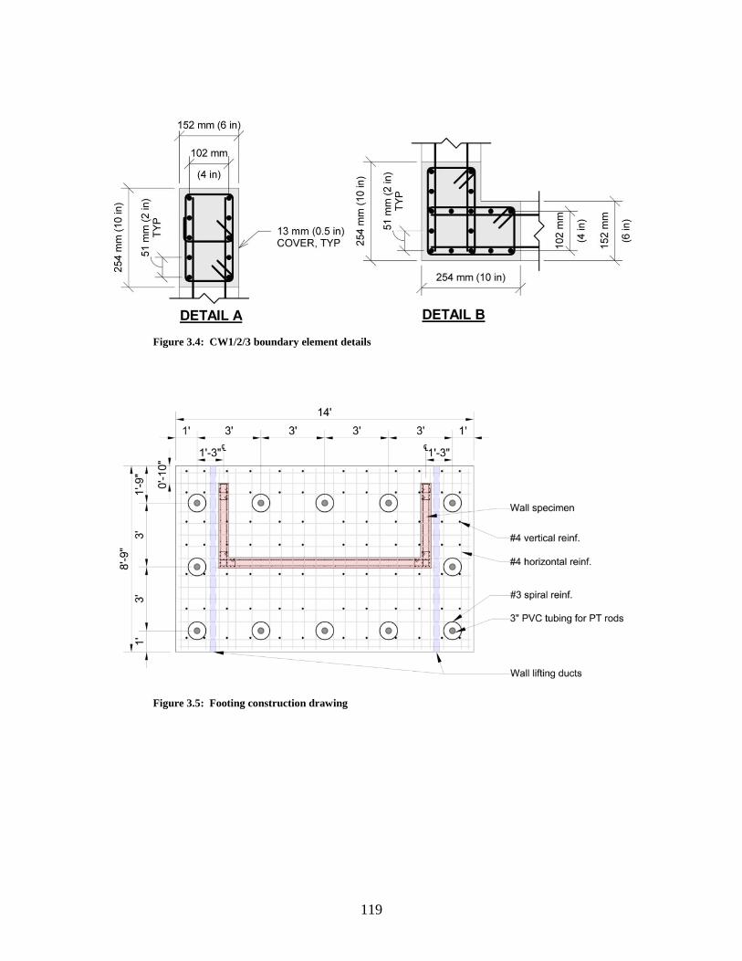
119
Figure 3.4: CW1/2/3 boundary element details
Figure 3.5: Footing construction drawing
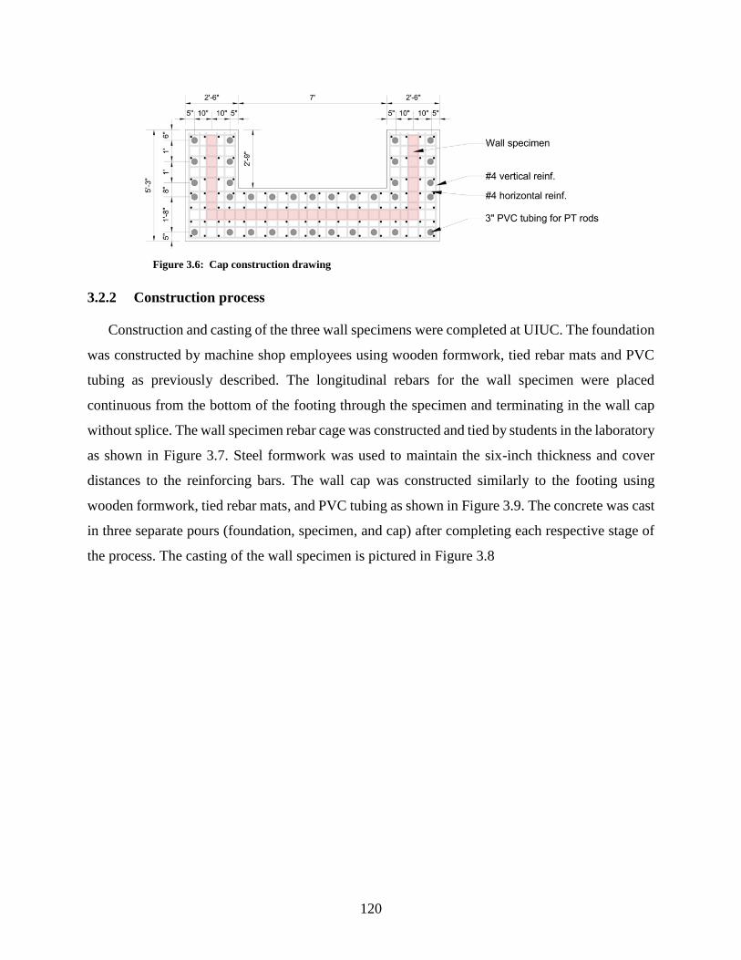
120
Figure 3.6: Cap construction drawing
3.2.2 Construction process
Construction and casting of the three wall specimens were completed at UIUC. The foundation
was constructed by machine shop employees using wooden formwork, tied rebar mats and PVC
tubing as previously described. The longitudinal rebars for the wall specimen were placed
continuous from the bottom of the footing through the specimen and terminating in the wall cap
without splice. The wall specimen rebar cage was constructed and tied by students in the laboratory
as shown in Figure 3.7. Steel formwork was used to maintain the six-inch thickness and cover
distances to the reinforcing bars. The wall cap was constructed similarly to the footing using
wooden formwork, tied rebar mats, and PVC tubing as shown in Figure 3.9. The concrete was cast
in three separate pours (foundation, specimen, and cap) after completing each respective stage of
the process. The casting of the wall specimen is pictured in Figure 3.8

121
Figure 3.7: Nearing completion of CW3 rebar cage
Figure 3.8: Casting of CW3 specimen

122
Figure 3.9: Rebar mats and completed formwork for CW2 cap
3.2.3 Material properties
Concrete Properties
A self-consolidating concrete mix design was selected for the C-shaped wall specimens attain
proper consolidation in the tightly reinforced boundary elements given the one-third scale design
of the test specimen (Lowes et al. 2013). The target strength was 5,000 psi, and coarse aggregates
were limited to 3/8” diameter also to accommodate the scale of the specimen. Higher cement
content, flyash, and fines were used in substitution of some coarse aggregate. A relatively high
water to cement ratio of 0.5 was needed to reach the design concrete strength. Table 3.1 shows
the material quantities of the concrete mix.
Table 3.1: Concrete mix design for C-shaped wall specimens
Material Quantity
Sand (FA-01) 1,383 lb
Coarse Aggregate (Chips CM-
16)
1,340 lb
Portland Cement 450 lb
Flyash 150 lb
Water 36.7 gal
Air 0.5 oz
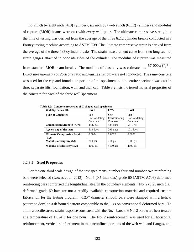
123
Four inch by eight inch (4x8) cylinders, six inch by twelve inch (6x12) cylinders and modulus
of rupture (MOR) beams were cast with every wall pour. The ultimate compressive strength at
the time of testing was derived from the average of the three 6x12 cylinder breaks conducted in a
Forney testing machine according to ASTM C39. The ultimate compressive strain is derived from
the average of the three 4x8 cylinder breaks. The strain measurement came from two longitudinal
strain gauges attached to opposite sides of the cylinder. The modulus of rupture was measured
from standard MOR beam breaks. The modulus of elasticity was estimated as 57,000 ' *cf
.
Direct measurements of Poisson's ratio and tensile strength were not conducted. The same concrete
was used for the cap and foundation portion of the specimen, but the entire specimen was cast in
three separate lifts, foundation, wall, and then cap. Table 3.2 lists the tested material properties of
the concrete for each of the three wall specimens.
Table 3.2: Concrete properties of C-shaped wall specimens
Wall Specimen ID: CW1 CW2 CW3
Type of Concrete: Self
Consolidating
Concrete
Self
Consolidating
Concrete
Self
Consolidating
Concrete
Compression Strength (f'c*): 4937 psi 5254 psi 5119 psi
Age on day of the test: 513 days 296 days 101 days
Ultimate Compression Strain
(εcu):
0.0024 0.0022 0.0028
Modulus of Rupture (fr): 700 psi 711 psi 1009 psi
Modulus of Elasticity (Ec): 4000 ksi 4100 ksi 4100 ksi
Steel Properties
For the one third scale design of the test specimens, number four and number two reinforcing
bars were selected (Lowes et al. 2013). No. 4 (0.5 inch dia.) grade 60 (ASTM A706) deformed
reinforcing bars comprised the longitudinal steel in the boundary elements. No. 2 (0.25 inch dia.)
deformed grade 60 bars are not a readily available construction material and required custom
fabrication for the testing program. 0.25” diameter smooth bars were stamped with a helical
pattern to develop a deformed pattern comparable to the lugs on conventional deformed bars. To
attain a ductile stress-strain response consistent with the No. 4 bars, the No. 2 bars were heat treated
at a temperature of 1,024 F for one hour. The No. 2 reinforcement was used for all horizontal
reinforcement, vertical reinforcement in the unconfined portions of the web wall and flanges, and

124
the confining reinforcement of the boundary elements. Table 3.3 lists the measured material
properties of the No. 2 and No. 4 reinforcing bars used in all three C-shaped wall tests.
Table 3.3: Reinforcing bar properties of all C-shaped wall specimens
Type of Rebar: No. 2 No. 4
Diameter of Bar: 0.25 in 0.5 in
Area of bar: 0.0491 in2 0.20 in2
Yield Stress (fy): 75.7 ksi 63.8 ksi
Ultimate Stress (fu): 76.3 ksi 91.3 ksi
Yield Strain (εsy): 0.0026 0.00228
Strain Hardening (εsh): 0.015 0.00775
Ultimate Strain (εu): 0.058 0.16518
3.3 Test setup & loading protocol
3.3.1 Introduction
The University of Illinois at Urbana-Champaign (UIUC) houses the Multi-Axial Full-Scale
Sub-Structure Testing & Simulation (MUST-SIM) facility and conducts large-scale and small-
scale experimental testing in the Newmark Structural Engineering Laboratory (NSEL)2. The
UIUC site. The large-scale facility utilizes a unique loading system known as Load and Boundary
Condition Boxes (LBCBs) that allows control of load and displacement in all six degrees of
freedom. The LBCB pictured in Figure 3.10 consists of six actuators with one end attached to a
steel reaction frame and the other attached to a steel platen. The reaction frame is post-tensioned
to an L-shaped strong wall for support, and the test specimens are attached to the strong floor and
the movable steel platens. The strong floor consists of a 17 foot (5.2m) deep reinforced concrete
box girder that provides approximately 100 kips of anchorage capacity every three feet on center.
The L-shaped strong wall dimensions are 50 ft (15.2m) long x 30 ft (9.1m) wide x 28 ft (8.5m)
high x 5 ft (1.5m) deep. The strong wall has anchorage points at every two feet on center. The C-
shaped wall testing was conducted at the Northwest end of the strong wall along the long portion
2 Section 3.3 was taken in part from project grant deliverables written for the National Science Foundation (Mock et al. 2013).
I was the primary or sole author of the content included herein. Furthermore, this content has been updated and amended since the
deliverable.

125
of the L. To apply the six degree-of-freedom loading, two “Load and Boundary Condition Boxes”
(LBCB) were post-tensioned to the strong wall 22 feet above the floor. The LBCBs are spaced
approximately 36 inches apart. The test specimen was placed beneath the LBCBs, and a series of
steel connection plates and beams were utilized to attach the LBCB and wall specimen together.
Overall plan and sectional drawings of the experimental test setup are shown in Figure 3.11 to
Figure 3.13.
Figure 3.10: Load and boundary condition box used to apply displacements and measure
applied loads on the test specimen. Coordinate system and actuator nomenclature are
identified.
Steel reaction
box attached
to strong wall
Movable steel
platen attached
to test specimen
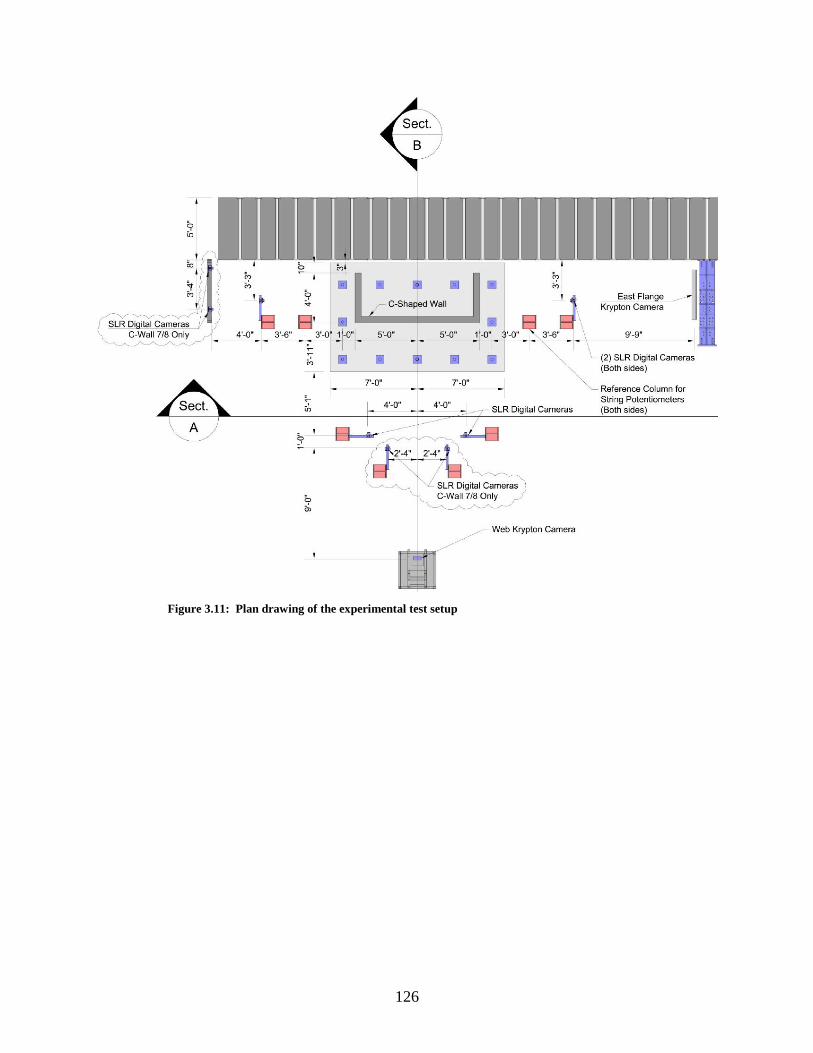
126
Figure 3.11: Plan drawing of the experimental test setup
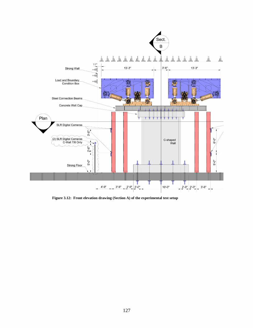
127
Figure 3.12: Front elevation drawing (Section A) of the experimental test setup

128
Figure 3.13: Cross-sectional drawing (Section B) of the experimental test setup
3.3.2 Connection beams description
The footing of the wall specimen was post-tensioned to the strong floor using (12) 2” diameter
rods with approximately 100 kips of clamping force in each rod. An assembly of steel beams and
plates are used to mate the wall specimen cap to the LBCB platens. Three wide flange beams
(W14x211) are connected to the LBCB platens using (84) 1” diameter high-strength bolts, each
with a clamping force of approximately 40 kips. The beams are connected to 2” thick steel plates
using (60) 1” diameter high-strength bolts, each with a clamping force of approximately 40 kips.
The plates were countersunk to allow the bolt heads to lay flush with the face of the plate. To
complete the connection, the plates are connected to the specimen wall cap using (34) 1.5”
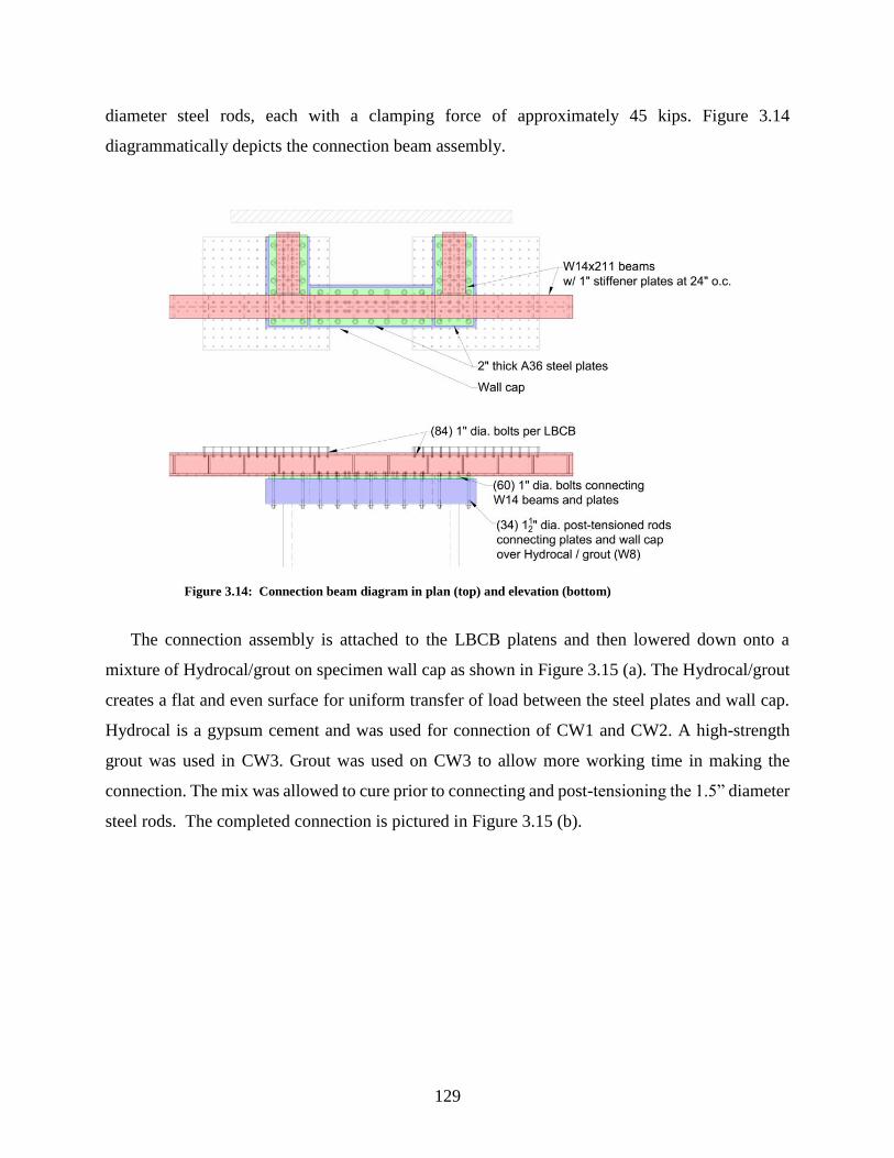
129
diameter steel rods, each with a clamping force of approximately 45 kips. Figure 3.14
diagrammatically depicts the connection beam assembly.
Figure 3.14: Connection beam diagram in plan (top) and elevation (bottom)
The connection assembly is attached to the LBCB platens and then lowered down onto a
mixture of Hydrocal/grout on specimen wall cap as shown in Figure 3.15 (a). The Hydrocal/grout
creates a flat and even surface for uniform transfer of load between the steel plates and wall cap.
Hydrocal is a gypsum cement and was used for connection of CW1 and CW2. A high-strength
grout was used in CW3. Grout was used on CW3 to allow more working time in making the
connection. The mix was allowed to cure prior to connecting and post-tensioning the 1.5” diameter
steel rods. The completed connection is pictured in Figure 3.15 (b).

130
(a) Pouring Hydrocal for connection of CW2 (b) Completed connection of CW2
Figure 3.15: Connection process of C-shaped wall specimens
3.3.3 Application of loading
The LBCB described introduced in Section 3.3.1 is a six DOF loading device that imposes the
displacements on the test specimen. The LBCB consists of six 330 kip actuators attached to a steel
reaction frame (blue) and steel platen (orange) shown in Figure 3.10. Each actuator has a linear
displacement transducer and load cell that provides that position and force carried in each of the
six actuators. Mathematical transformation allows the six DOF position of the platen to be
determined in Cartesian coordinates from the displacement transducer readings. Similarly, the
forces and moments being imposed by the platen can also be determined in the six DOF Cartesian
coordinates from the load cell readings. The Cartesian force and moment readings are the sole
means of determining the loads imposed on the test specimen. Figure 3.10 shows the LBCB platen
and each of the six actuators identified as “X1” and “X2” for the X-direction, “Y1” for the Y-
direction, and “Z1”, “Z2”, and “Z3” for the Z-direction.
The Operations Manager (OM) software written in Labview provides the controlled six degree-
of-freedom movements of the steel platen at any point in Cartesian space. This transformation of
actuator displacements and forces allows the test specimen to be displaced in all six DOFs about
a control point defined by the researcher as well as providing the measured forces and moments
applied to the specimen at that point. The OM provides “mixed-mode” control allowing the ability
to command displacements and forces to the test specimen simultaneously. This enables the
control of a selection of the six DOFs to be in displacement control and other DOFs in force
control. Since the actuators are controlled by displacement, the OM uses small iterative
displacements in conjunction with a measured stiffness of the test set up to achieve the commanded
force or moment on the specimen. Additional description of these capabilities is described in
131
section 3.4.2 and Nakata et al. (2007). While the OM software is utilized to apply the target loads
and displacements, the target loads and displacements are sent from the LbcbPlugin software.
The LbcbPlugin software was also written at UIUC performing many functions for the
coordinated stepwise testing of structures. In the case of cyclic displacement histories, the operator
defines an input file of displacement and load steps. Advanced loading protocols can be
implemented into the LbcbPlugin to generate a target load protocol based on the measured loads
and deformations of the structure to be achieved at each step. The LbcbPlugin also coordinates
the data acquisition from all systems for each step. The adaptability of this software to generate
advanced loadings specific to an experimental test and its response were utilized for testing the C-
shaped walls.
3.3.4 Loading protocol
The loading protocol for all three C-shaped wall specimens was based on the prototype ten-
story core-wall system subjected to the ASCE 7-05 equivalent lateral force (ELF) distribution for
design for earthquake loading and gravity load. The test specimens represent the bottom three
stories of this ten-story prototype structure at one-third scale. The performance of the upper stories
of the wall was assumed non-critical to the global system performance, and thus the upper stories
were not tested in the laboratory. The effects of the gravity and lateral loads acting on the upper
seven stories of the wall were simulated in the laboratory through the application of an overturning
moment, shear force and axial force on the top of the test specimen.
Each specimen was subjected to a quasi-static cyclic displacement history along one or both
horizontal principal axes of the test specimen. Each step of the displacement history included the
application of a lateral translation as well as an axial force and overturning moment. The target
axial force and overturning moment were a function of the measured lateral shear from the applied
displacement, thus requiring an incremental-iterative approach for determining the converged state
of the wall at the end of each step. The displacement history was discretized into thousands of
displacement steps to facilitate convergence at each step. The displacement step size varied from
approximately five thousands of an inch (0.005 in.) in the elastic range to four-hundredths of an
inch (0.04 in.) in the post-yielding regime. The loading rate also varied but did not exceed one-
hundredth of an inch per second (0.01 in/sec).
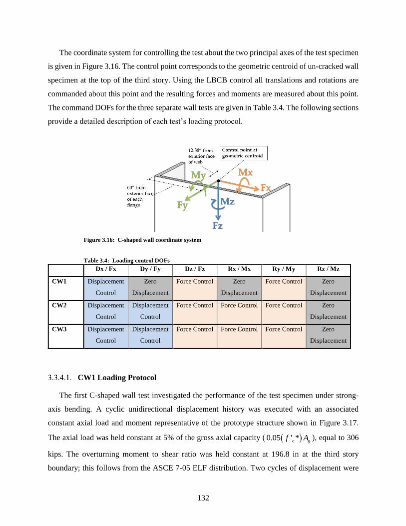
132
The coordinate system for controlling the test about the two principal axes of the test specimen
is given in Figure 3.16. The control point corresponds to the geometric centroid of un-cracked wall
specimen at the top of the third story. Using the LBCB control all translations and rotations are
commanded about this point and the resulting forces and moments are measured about this point.
The command DOFs for the three separate wall tests are given in Table 3.4. The following sections
provide a detailed description of each test’s loading protocol.
Figure 3.16: C-shaped wall coordinate system
Table 3.4: Loading control DOFs
Dx / Fx Dy / Fy Dz / Fz Rx / Mx Ry / My Rz / Mz
CW1 Displacement
Control
Zero
Displacement
Force Control Zero
Displacement
Force Control Zero
Displacement
CW2 Displacement
Control
Displacement
Control
Force Control Force Control Force Control Zero
Displacement
CW3 Displacement
Control
Displacement
Control
Force Control Force Control Force Control Zero
Displacement
CW1 Loading Protocol
The first C-shaped wall test investigated the performance of the test specimen under strong-
axis bending. A cyclic unidirectional displacement history was executed with an associated
constant axial load and moment representative of the prototype structure shown in Figure 3.17.
The axial load was held constant at 5% of the gross axial capacity ( ( )0.05 ' *c gf A ), equal to 306
kips. The overturning moment to shear ratio was held constant at 196.8 in at the third story
boundary; this follows from the ASCE 7-05 ELF distribution. Two cycles of displacement were

133
completed at each drift level in the x-direction, which corresponded to strong axis bending as
shown in Figure 3.18. Maximum displacement demands for displacement cycles were intended to
target limit states of concrete cracking, yielding of longitudinal reinforcement, nominal flexural
strength, concrete spalling and subsequent damage states. The displacement history is shown in
Table 3.5 and Figure 3.19.
Figure 3.17: CW1 loading with the ten-story test with triangular load-distribution (left) and
the three-story test specimen with equivalent loading (right)
Figure 3.18: Strong axis unidirectional displacement pattern for CW1

134
Table 3.5: CW1 Displacement History
Target Limit State Disp(in) Disp (% Drift) # of Cycles
Elastic 0.02 0.014% 1
Cracking 0.04 0.028% 1
25% Yield 0.1 0.069% 2
50% Yield 0.2 0.139% 2
75% Yield 0.3 0.208% 2
100% Yield 0.5 0.347% 2
150% Yield 0.72 0.5% 2
Nominal 1.08 0.75% 2
Damage 1.44 1% 2
Damage 2.16 1.5% 2
Damage 3.24 2.25% 2
Pushover 5.057 3.512% +X only
Figure 3.19: CW1 plot of displacement history in x- and y-directions
CW2 Loading Protocol
The second C-shaped wall test investigated the bidirectional performance of the test specimen.
A cyclic cruciform displacement history was executed with an associated constant axial load and
constant moment-to-shear ratio as shown in Figure 3.20. The axial load was held constant at 5%
of the gross axial capacity ( ( )0.05 ' *c gf A ), equal to 306 kips. The overturning moment to shear
ratio was held constant at 196.8 in., which follows from the ASCE 7-05 ELF distribution, in both
principal directions.
For most of the test, two displacement cycles were completed in each direction at each drift
level following the cruciform history shown in Figure 3.21. Following this cruciform history,
cycles 1 and 3 displace the wall in the direction of the web of the wall, which is the x-direction
and activates strong-axis bending of the wall; cycles 2 and 4 displace the wall in the directions of
the flanges, which is the y-direction and activates weak-axis bending of the wall. Towards the end

135
of the test, the displacement capacity of the loading apparatus was reached in the positive and
negative y-directions. To enable application of increasing demand on the boundary elements of
the wall, which are severely loaded under weak-axis / y-direction loading, the cruciform
displacement history was replaced with the bi-directional displacement history shown in Figure
3.22. This displacement pattern consisted of a full displacement cycle in x-direction while
maintaining a constant y-direction displacement. Maximum displacement demands for
displacement cycles in both the x- and y-directions were intended to target limit states of concrete
cracking, yielding of longitudinal reinforcement, nominal flexural strength, concrete spalling and
subsequent damage states. The displacement history is shown in Table 3.6 and Figure 3.23.
Figure 3.20: CW2 bi-directional loading with the ten-story test with triangular load-
distribution (left) and the three-story test specimen with equivalent loading (right)
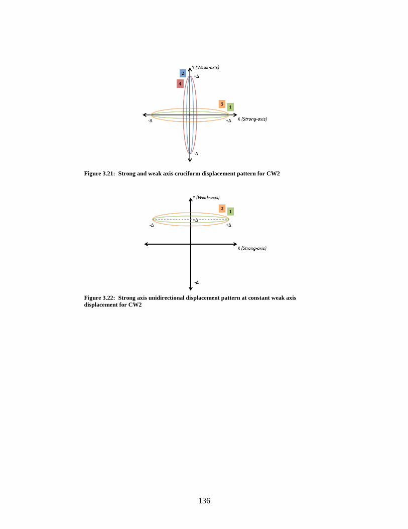
136
Figure 3.21: Strong and weak axis cruciform displacement pattern for CW2
Figure 3.22: Strong axis unidirectional displacement pattern at constant weak axis
displacement for CW2

137
Table 3.6: CW2 Displacement History
Target Limit
State
Loading
Pattern
Dx
(in)
+Dy
(in)
-Dy
(in)
Dx
(% drift)
+Dy
(% drift)
-Dy
(% drift)
# of
Cycles
Elastic Cruciform ±0.02 0.02 -0.02 0.014% 0.014% -0.014% 1
Cracking Cruciform ±0.04 0.08 -0.12 0.028% 0.056% -0.083% 2
Cruciform ±0.1 0.2 -0.3 0.069% 0.14% -0.21% 2
50% Yield Cruciform ±0.2 0.4 -0.6 0.14% 0.28% -0.42% 2
75% Yield Strong Axis ±0.3 --- --- 0.21% --- --- 1
100% Yield Cruciform ±0.5 0.6 -0.9 0.35% 0.42% -0.63% 2
1/2 Nominal Cruciform ±0.72 1.8 -1.05 0.50% 1.25% -0.73% 2
Nominal Cruciform ±1.08 3.24 -1.22 0.75% 2.25% -0.85% 1
Cruciform ±1.08 3.24 -2.14 0.75% 2.25% -1.49% 1
Damage 1 Cruciform ±1.44 3.24 -2.14 1% 2.25% -1.49% 1
Strong Axis ±1.44 --- --- 1% --- --- 1
Damage 2 Constant Dy ±1.44 2.88 --- 1% 2% --- 1
Constant Dy ±1.44 --- -1.584 1% --- -1.1% 1
Damage 3 Strong Axis ±2.16 --- --- 1.5% --- --- 1
Damage 4 Constant Dy ±2.16 2.88 --- 1.5% 2% --- 1
Pushover +X Constant Dy 2.81 2.88 --- 1.95% 2% --- 1
Figure 3.23: CW2 plot of displacement history in x- and y-directions
CW3 Loading Protocol
The third C-shaped wall test investigated the bidirectional performance of the test specimen
when considered part of a coupled core wall system. A cyclic cruciform displacement history was
executed with axial load and moment applied at the top of the specimen determined from the ASCE
7-05 ELF and gravity loads applied to the complete coupled core-wall system as shown in Figure
3.24. For displacement cycles in the x-direction, parallel to the webs of the c-shaped walls,
coupling beams are not activated, and the response of the c-shaped walls is essentially identical to

138
the response of an isolated c-shaped wall. Thus, for displacement cycles in the x-direction, a
constant axial load equal to 5% of the gross axial capacity ( ( )0.05 ' *c gf A ), equal to 306 kips, was
applied and a constant moment-to-shear ratio of 196.8 in., which follows from the ASCE 7-05
ELF distribution was used.
Lateral loading of the core wall system in the y-direction, parallel to the flanges of the c-shaped
walls, activates coupling beams resulting in “coupling” of the c-shaped walls. The flexural
response of the coupling beams results in tensile loads being applied to one of the c-shaped walls,
identified as the tension pier, and compression loads being applied to the other c-shaped wall,
identified as the compression pier. These tension/compression loads affect the flexural stiffness
and strength of the c-shaped walls and result in the individual wall piers developing different
internal moments and shears at each story. To simulate this in the laboratory test, axial load and
moment applied to the top of the specimen were varied for displacement cycles in the y-direction.
The following is a detailed discussion of the process employed to determine an appropriate
protocol for y-direction loading of the test specimen.
Figure 3.24: CW2 bi-directional loading with the ten-story test with triangular load-
distribution (left) and the three-story test specimen with equivalent loading (right)

139
Details of y-direction loading and simulation of demands resulting from coupling
Specification of the y-direction loading protocol comprised specification of (1) the ratio of
shear, axial and moment demand to be applied to the specimen for loading in the positive and
negative y-directions and (2) the maximum displacement demands in the positive and negative y-
directions for each cycle. The following paragraphs explain the process employed to develop these
specifications as well as the control logic employed to implement these specifications in the
laboratory.
Y-direction loading activates coupling between the wall piers resulting in the individual wall
piers carrying significantly different shear, axial load and moment at each story. The distribution
of total story shear, axial load and moment between the individual wall piers, and thus the ratio of
shear, axial and moment demand for an individual wall pier, varies as a function of wall stiffness.
Numerical analyses of the ten-story prototype core-wall system subjected to the increasing lateral
load and constant gravity load were conducted to establish appropriate demand ratios (i.e., the ratio
of shear, axial and moment demand) for use in testing. The demand ratio versus roof drift
developed from these analyses was simplified for application to experimental testing; ultimately,
seven different ratios were used at different stages of the test. Demand ratios were varied during
the test on the basis of measured response quantities and observed damage.
It should be noted that the laboratory test specimen represents the bottom three stories of one
c-shaped wall pier without coupling beams. Without coupling beams, the demands that develop in
a c-shaped wall in the coupled core-wall system cannot be simulated in the laboratory specimen
over the entire three-story height of the laboratory specimen. Consequently, demands were applied
at the top of the laboratory specimen to achieve representative demands in the critical first story of
the specimen. This is illustrated in a free-body-diagram of the coupled walls individual and system
demands in Figure 3.25.

140
Figure 3.25: Coupled core wall free body diagram for the system (left) and individual wall
piers acting as the test specimen (right)
Analysis results indicated that under lateral loading of the core-wall system, lateral
displacements for the individual wall piers differed due to axial elongation of coupling beams.
Initially, it was assumed that this difference in wall displacements could be ignored and
displacement demands in the positive and negative y-directions could be of equal magnitude. As
testing progressed, the stiffness of the specimen under positive y-direction loading began to differ
substantially from the stiffness of the specimen under negative y-direction loading (this would be
analogous to the stiffness of the compression wall pier in the coupled wall system differing
substantially from the stiffness of the tension wall pier), and it was observed that the loads applied
at the maximum and minimum y-direction displacement demands did not, when combined,
represent an equilibrium state for the core-wall system. In the core-wall system, loads applied to
the specimen under positive and negative y-direction loading would be applied simultaneously to
the individual wall piers; thus, applied loads, when combined, should approximately represent an

141
equilibrium state for the core-wall system. Thus, for subsequent displacement cycles, a force-based
approach was used to determine maximum displacements in the positive and negative y-directions.
Numerical analyses indicated that for moderate to large displacement demands, the
compression pier determines core-wall strength. This is because at these displacement demands
the tension pier has minimal stiffness relative to the compression pier and carries relatively little
shear and moment relative to the compression pier. Given this, a force-based approach to
determining displacement demands was developed in which (1) the test specimen was first loaded
to a target drift demand in the positive y-direction, such that it became the compression pier, (2)
the axial force and moment demands at the target drift demand were recorded, and (3) the specimen
was loaded in the negative y-direction until the axial force and moments required for equilibrium
of the core-wall system were achieved. No consideration was given to the magnitude of the shear
force applied at the peak displacement in the negative y-direction; thus, this loading protocol did
not maintain the moment-to-shear ratio associated with the ASCE 7-05 ELF distribution for the
core-wall system.
The displacement history for CW3 is given in Table 3.7, and Figure 3.26; Table 3.7 also lists
the moment, shear, and axial load ratios for the pier walls, where
,base CompRatioV = Portion of system base shear to the compression pier
,base TensRatioV = Portion of system base shear to the tension pier
,base CompRatioM = Portion of system moment to the compression pier
,base TensRatioM = Portion of system moment to the tension pier
,base CoupleRatioM = Portion of system moment to coupling

142
Table 3.7: CW3 Displacement History
Target
Limit State
Loading
Pattern
Dx
(in)
Dy
(in)
Dx
(%
drift)
Dy
(%
drift)
# of
Cycles
Mbase
Couple
Ratio
MbaseC
Ratio
MbaseT
Ratio
VbaseT
Ratio
Vbase
CRatio
Elastic Cruciform ±0.02 ±0.02 0.027% 0.027% 1 0.65 0.25 0.1 0.35 0.65 Cracking Cruciform ±0.04 ±0.04 0.027% 0.027% 2 "" "" "" "" ""
Cruciform ±0.1 ±0.1 0.067% 0.067% 2 0.65 0.25 0.1 0.2 0.8
50% Yield Cruciform ±0.2 ±0.2 0.14% 0.14% 2 "" "" "" "" "" 75% Yield Cruciform ±0.35 ±0.35 0.24% 0.24% 1 "" "" "" "" ""
Weak axis 0 ±0.44 0% 0.30% 2 "" "" "" "" ""
100%
Yield
Cruciform ±0.5 ±0.65 0.35% 0.35% 2 "" "" "" "" ""
+Y only 0 0.711 0% 0.49% 1 "" "" "" "" ""
Weak axis 0 ±0.8 0% 0.55% 1 0.6 0.32 0.08 0.3 0.7
Logic change to force target for tension pier
1/2
Nominal
Strong Axis ±0.72 0 0.50% 0% 1 0.6 0.33 0.07 0.15 0.65
Comp. Pier 0 0.8 0% 0.55% 1 "" "" "" "" "" Tension Pier 0 -0.178 0% -0.12% 1 "" "" "" "" "" Strong Axis ±0.72 0 0.50% 0% 1 "" "" "" "" "" Comp. Pier 0 1.2 0% 0.83% 1 "" "" "" "" "" Tension Pier 0 -0.14 0% -0.09% 1 "" "" "" "" ""
Nominal Strong Axis ±1.08 0 0.75% 0% 1 "" "" "" "" "" Comp. Pier 0 1.2 0% 0.83% 1 "" "" "" "" "" Comp. Pier 0 1.6 0% 1.11% 1 0.6 0.28 0.12 0.25 0.65 Tension Pier 0 0.067 0% 0.05% 1 "" "" "" "" "" Comp. Pier 0 1.6 0% 1.11% 1 "" "" "" "" "" Tension Pier 0 -0.4 0% -0.28% 1 "" "" "" "" ""
Damage 1 Strong Axis ±1.44 0 1.0% 0% 1 "" "" "" "" "" Comp. Pier 0 1.6 0% 1.11% 1 "" "" "" "" "" Tension Pier 0 -0.223 0% -0.16% 1 "" "" "" "" "" Comp. Pier 0 2.4 0% 1.67% 1 "" "" "" "" "" Tension Pier 0 -0.168 0% -0.11% 1 "" "" "" "" ""
Damage 2 Strong Axis ±2.16 0 1.5% 0% 1 "" "" "" "" "" Comp. Pier 0 2.84 0% 1.94% 1 "" "" "" "" "" Tension Pier
-2.84 0% 1.94% 1 0.6 0.28 0.26 0.6 0.65
Damage 3 Strong Axis ±2.56 0 1.777% 0% 1 "" "" "" "" "" Comp. Pier 0 2.84 0% 1.97% 1 "" "" "" "" "" Tension Pier 0 -3.01 0% -2.09% 1 0.6 0.28 0.24 0.6 0.65
Damage 4 Comp. Pier 0 2.95 0% 2.05% 1 0.6 0.2 0.24 0.6 0.8 Tension Pier 0 -3 0% -2.08% 1 0.6 0.2 0.23 0.6 0.8
Damage 5 Comp. Pier 0 2.95 0% 2.05% 1 Fz = 1,000 kips
Tension Pier 0 -2.745 0% -1.91% 1 Fz = -250 kips Comp. Pier 0 2.33 0% 1.62% 1 Fz = 1,000 kips
Figure 3.26: CW3 plot of displacement history
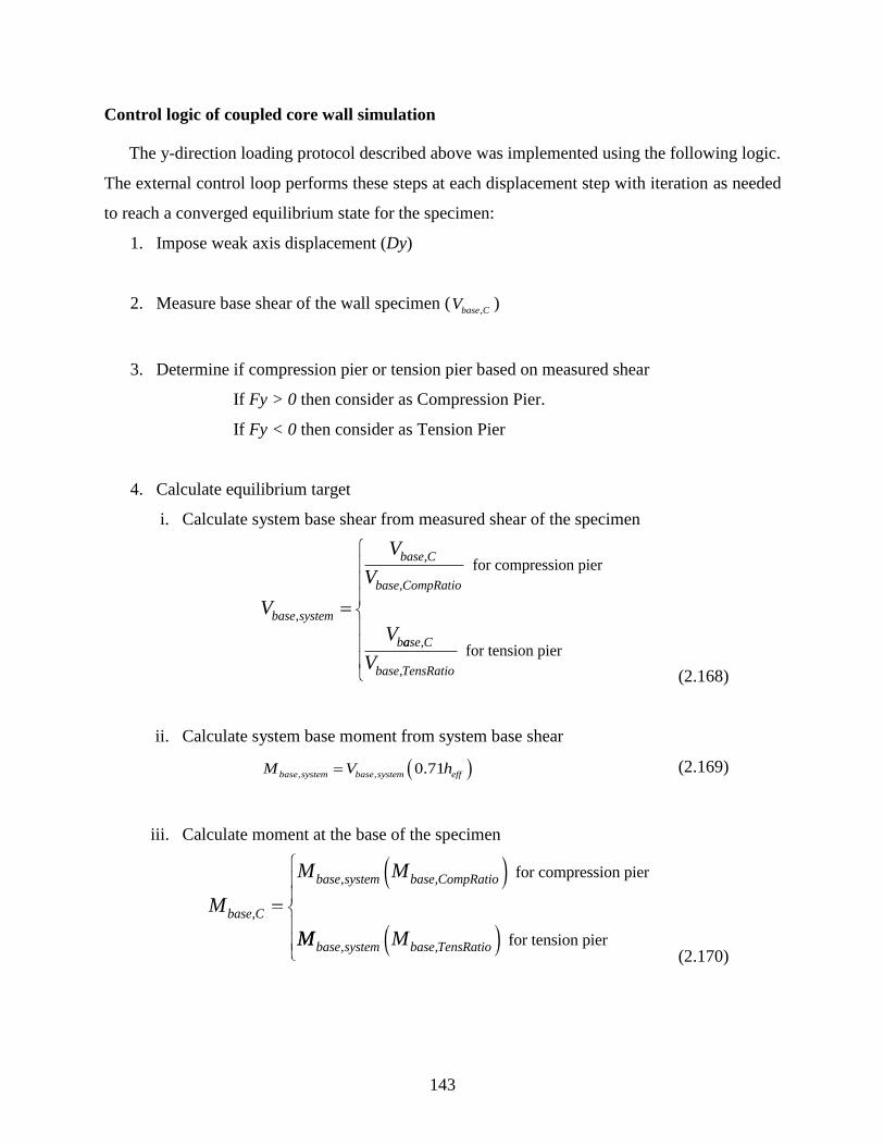
143
Control logic of coupled core wall simulation
The y-direction loading protocol described above was implemented using the following logic.
The external control loop performs these steps at each displacement step with iteration as needed
to reach a converged equilibrium state for the specimen:
1. Impose weak axis displacement (Dy)
2. Measure base shear of the wall specimen (,base CV )
3. Determine if compression pier or tension pier based on measured shear
If Fy > 0 then consider as Compression Pier.
If Fy < 0 then consider as Tension Pier
4. Calculate equilibrium target
i. Calculate system base shear from measured shear of the specimen
(2.168)
ii. Calculate system base moment from system base shear
( ), , 0.71base system base system effM V h= (2.169)
iii. Calculate moment at the base of the specimen
(2.170)
V
V
V
Vbase system
base C
base CompRatio
b
,
,
,
for compression pier
aase C
base TensRatioV
,
,
for tension pier
M
M M
base C
base system base CompRatio
,
, , for compression pier
MM Mbase system base TensRatio, ,
for tension pier

144
iv. Calculate moment due to the coupling
( ), , ,base couple base system base CoupleRatioM M M= (2.171)
v. Calculate axial load from moment due to the coupling
,
,
base couple
base couplecouple
MP
L= (2.172)
vi. Calculate total axial force from gravity and coupling
, ,top C gravitybase couple
PP P= + (2.173)
vii. Calculate total moment to be applied at the third story
( ), , , specimentop C base C base CM M V h= − (2.174)
5. Impose calculated ,top CP and
,top CM on the specimen
3.4 Development of a bi-directional loading algorithm
During the testing for CW1 and CW2, two shortcomings in the procedure for applying the
loading to each test specimen were identified. The first shortcoming identified was the variation
in loading that occurred in-between converged load steps. The second shortcoming was the
difficulty to achieve convergence for the target load step when controlling multiple degrees of
freedom that are interdependent. Section 3.4 explores the source of each of these shortcomings,
and a new loading algorithm is developed that considers the load-deformation curve of a reinforced
concrete structure. Small-scale testing was conducted to validate the proposed algorithm prior to
testing in the large-scale laboratory to ensure the proposed algorithm was conservative and
sufficiently robust. After successful testing in the small-scale laboratory, the algorithm was
implemented for testing CW3. A final validation was conducted during elastic testing of CW3,
and the algorithm subsequently conducted the remainder of the test.

145
3.4.1 Motivation and background
As described in Section 3.3.4.3, the loading protocol for the final C-shaped wall test consists
of a cruciform cyclic displacement history with a varying axial force and overturning moment in
each direction. The variable axial force simulates a coupled core wall system in the weak-axis
direction. The cyclic displacement history for the test is discretized into a series of equal
displacement steps. Each step commands a lateral translation with an axial force and overturning
moments. The axial force and overturning moment are a function of the lateral shear response
from the applied displacement as given by Lowes (2012). The overturning moment in each
direction is a function of the measured shear in each direction:
( ) ( )( ), ,M x y C V x y= (2.175)
Where,
( )
( )
, overturning moments corresponding to both lateral translations and
, shear forces corresponding to both lateral translations and
constant moment-to-shear ratio,
zero if top of specimen
M x y x y
V x y x y
C
=
=
=
is equal to top of building
non-zero if simulating building structure above being subjected to lateral force
As a direct function of the lateral shears, the prediction of overturning moment also requires
the prediction of the lateral shears resulting from the displacement. The stiffness of the test
structure and displacement step size determine how well the commanded axial force and
overturning moment relationships are maintained during the test. Within the mixed mode control
algorithm of the OM, the displacements are commanded first and independently of the forces and
moments. As a result, the size of the lateral translation has a direct impact on the level of error
between the initial and subsequently converged axial force and overturning moments. In addition,
the correction of the moment based on the prescribed moment to shear ratio is completed after the
displacement has occurred and the resulting shear has been measured. The test structure is stiffer
when displaced without rotation (conceptually a fixed-fixed condition) resulting in a lateral shear
that is larger than the lateral shear after the moment to shear ratio solution has converged. Figure
3.27 plots the overshoot of lateral shear resulting from this problem using the data of the first C-
shaped wall test (CW1).

146
Figure 3.27: Scatter plot of CW1 shear force overshoots (kips) versus displacement step size
(inches)
This constantly changing shear and applied moment have physical implications of the inelastic
response of the test structure. To reduce the error between the actual and idealized forces and
moments, each step can be discretized into substeps of smaller displacements. The force
relationships can then be converged at each substep of displacement as opposed to only at the end
of the step. Figure 3.28 illustrates substep discretization and points of load control convergence.
Figure 3.28: Breakdown of displacement step into substeps and subsequent breakdown of
substeps into iterative steps to converge on the target displacement
The substep can be considered to have three phases: one initial displacement command, any
number of correction steps of setup deformation (correcting for deformations that occur in any
element outside of the test specimen), and any number of correction steps of the overturning
moment. The number of correction steps due to setup deformation, axial force correction, and
overturning moment correction has a direct impact on the efficiency of the test and the
minimization of error between the idealized and actual forces. The ideal substep would require no
0 0.02 0.04 0.06 0.08 0.1 0.12 0.14 0.160
10
20
30
40
50
60
Step Size (in)
Fo
rce
Ov
ers
ho
ot
(kip
s)
Shear Force Overshoots - All Steps
Substep, i+1
Step, i {u}
Substep, i Substep, i+2
Initial displacement
Correction steps
Converged substep
Converged and
completed step

147
correction steps. Eliminating correction steps requires predicting both the setup deformation that
will occur during the step as well as the change in lateral shear relative to the change in
displacement to predict the axial force and overturning moment. In this ideal case, the initial
displacement command of the substep will command the displacement of the step combined with
the setup deformation that will occur with that displacement, the axial force resulting after the
lateral translation, and the overturning moment that will correspond to the lateral shear measured
after the lateral translation. The workflow of this process is given in the flowchart in Figure 3.29.
Figure 3.29: Flowchart of displacement step convergence using substeps and correction steps
Axial force and
overturning moments
within tolerance?
Calculate target moment for next substep
Perform substep in OM
Perform correction step in OM using
M/V ratios and Fz calc.
No
Yes
Step Complete
Substep disp. equal to
step disp?
No
Yes
Start of step
Discretize step into substeps
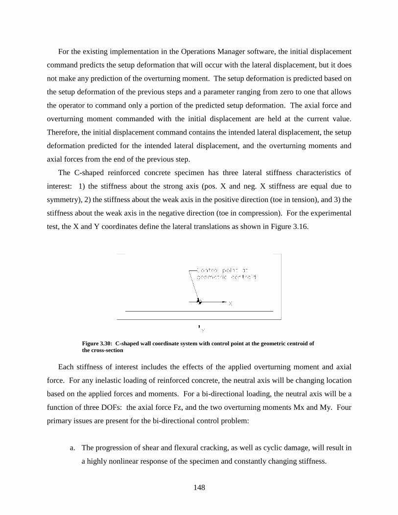
148
For the existing implementation in the Operations Manager software, the initial displacement
command predicts the setup deformation that will occur with the lateral displacement, but it does
not make any prediction of the overturning moment. The setup deformation is predicted based on
the setup deformation of the previous steps and a parameter ranging from zero to one that allows
the operator to command only a portion of the predicted setup deformation. The axial force and
overturning moment commanded with the initial displacement are held at the current value.
Therefore, the initial displacement command contains the intended lateral displacement, the setup
deformation predicted for the intended lateral displacement, and the overturning moments and
axial forces from the end of the previous step.
The C-shaped reinforced concrete specimen has three lateral stiffness characteristics of
interest: 1) the stiffness about the strong axis (pos. X and neg. X stiffness are equal due to
symmetry), 2) the stiffness about the weak axis in the positive direction (toe in tension), and 3) the
stiffness about the weak axis in the negative direction (toe in compression). For the experimental
test, the X and Y coordinates define the lateral translations as shown in Figure 3.16.
Figure 3.30: C-shaped wall coordinate system with control point at the geometric centroid of
the cross-section
Each stiffness of interest includes the effects of the applied overturning moment and axial
force. For any inelastic loading of reinforced concrete, the neutral axis will be changing location
based on the applied forces and moments. For a bi-directional loading, the neutral axis will be a
function of three DOFs: the axial force Fz, and the two overturning moments Mx and My. Four
primary issues are present for the bi-directional control problem:
a. The progression of shear and flexural cracking, as well as cyclic damage, will result in
a highly nonlinear response of the specimen and constantly changing stiffness.
149
b. For control of multiple DOFs, the coupling terms of the measured stiffness matrix
cannot be determined. As a result, the influence of each DOF on the other is unknown,
and the combined actions on the specimen must be applied in an incremental-iterative
approach for convergence.
c. The current inability to command the lateral translation with the corresponding rotation
and vertical translation required for the axial force and overturning moment
simultaneously results in a non-smooth solution path. In addition, the required error
tolerances for solution convergences along the path will cause further deviations to the
smoothness of the solution path.
d. Stiffness components in a bi-directional loading cannot be considered additive (Beyer,
Dazio, and Priestley 2008). The stiffness of the specimen is a direct function of the
direction in which it is being displaced requiring each cycle to be considered
independently of any previous history.
To expand on point c, data from the second C-shaped wall test is used as an example. This test
used a control methodology as described in Section 3.3.4.2. In this test, the bi-directional moment
was commanded, but the axial force remained constant. Figure 3.31 shows the iterative,
incremental approach for a portion of a displacement cycle post-yielding. The displacement
increment was approximately 0.04” followed by iterative load control to find convergence. The
spikes of the “iterations” path correspond to the overshoots in lateral shear previously described.
The key observation of this figure is that the solution path (identified by the “Increments” line) is
not smooth. The solution path generally observed to be non-smooth when looking at the data from
any part of the inelastic loading.

150
Figure 3.31: Plot of shear force (kip) versus displacement (inch) during strong axis loading
indicating converged and non-converged steps
Figure 3.32 shows the same approach during the unloading phase of the same cycle. The initial
unloading step is accompanied by a significant drop in stiffness. Because the current approach
maintains the applied moment of the previous converged step (the shear at 173 kips) with the initial
displacement increment, the deviation between the converged solution (151 kips) and the start of
the step (134 kips) is large. The non-smooth solution path and change in stiffness for unloading
must both be accounted for in the proposed algorithm.
Figure 3.32: Plot of shear force (kip) versus displacement (inch) during strong axis unoading
indicating converged and non-converged steps
3.4.2 Existing control software methodology
The Operations Manager described in 3.3.3 employs the ability to command displacements and
forces to a test specimen known as ‘mixed-mode’ control. As previously described, force targets
are converted to displacements based upon a measured tangent stiffness. The displacement target
1.3 1.35 1.4 1.45 1.5 1.55 1.6 1.65 1.7
145
150
155
160
165
Dx (in)
Fx
(k
ip)
Dx vs. Fx
Iterations
Increments
2 2.05 2.1 2.15
130
140
150
160
170
180
Dx (in)
Fx
(k
ip)
Dx vs. Fx
Iterations
Increments

151
is achieved by the LBCBs, and the resulting force is compared to the force target. Prescribed error
tolerance for each DOF is used to compare the resulting force to the force target. If the force is
within the prescribed tolerance, the force command is complete; otherwise, multiple iterations are
completed until the resulting force is within the tolerance.
The OM employs the Broyden update (see Section 2.3.5) to maintain the approximate
tangential stiffness of each DOF. Currently, the force control works with only one DOF at a time,
and each column of the stiffness matrix is updated only when new information about the load-
displacement history is available. Each column is updated after it has been commanded a
displacement to achieve a force target and all other columns are left unchanged.
A series of features were added to the force control to add robustness to the solution technique:
1. Stiffness bounding – an upper and lower bound of the stiffness matrix is employed to
prevent a poor approximation of the tangential stiffness causing the solution to be a large
undesirable value.
2. Maximum increment – the maximum increment limits the magnitude of change in any one
iteration.
3. Jacobian gain – the gain is a factor applied to the target to assume some loss of stiffness
with each step as well as accounting for some error in the approximate stiffness. The gain
for each DOF forms the diagonal of the ‘gain’ matrix, [G], applied to the displacement
solution as follows:
( ) ( )1
1 1
0 0 0 00
ii i i iu u F F
−− −
= + −KG (2.176)
Figure 3.33 shows the implementation of these features in the interface of the operations
manager. Furthermore, a complete description and methodology of the Operations Manager force
control can be found in the work of Nakata et al. (2007).
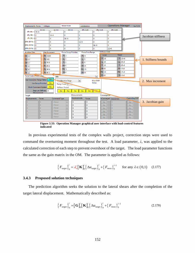
152
Figure 3.33: Operation Manager graphical user interface with load-control features
indicated
In previous experimental tests of the complex walls project, correction steps were used to
command the overturning moment throughout the test. A load parameter, λ, was applied to the
calculated correction of each step to prevent overshoot of the target. The load parameter functions
the same as the gain matrix in the OM. The parameter is applied as follows:
( )1
target target 000 0 for any 0,1
i ii i
meas
i
oF u F −
= + K (2.177)
3.4.3 Proposed solution techniques
The prediction algorithm seeks the solution to the lateral shears after the completion of the
target lateral displacement. Mathematically described as:
1
target target 00 00 0
i ii i i
measF u F−
= +G K (2.178)
Jacobian stiffness
1. Stiffness bounds
3. Jacobian gain
2. Max increment
153
The stiffness matrix will be approximated using two primary techniques: least change secant
updates from the literature as well as straight line linear regression proposed in this study. See the
following:
1. The Broyden least change secant update per section 2.3.5
2. The Davidon-Fletcher-Powell least change secant update per section 2.3.6
3. The straight-line linear regression methods proposed in section 3.4.3.1
Methodology of line fitting
The least change secant updates are highly sensitive to the load-deformation data of the
previous increment (substep). The sensitivity can cause the predictions to be poor if the data is
non-smooth. An example of non-smooth data points is illustrated in Figure 3.34 by the diamond
points connected by dashed lines. To better address the non-smooth data, a linear fit can be
implemented to capture the stiffness based on a history of converged loads and deformation from
previous substeps. The next point on the load-deformation can then be predicted using the line
fitting as shown by the example in Figure 3.34.
Since the load-deformation path is highly nonlinear, it might seem justifiable to use a curve
fitting method with a higher order polynomial or sine wave approximation. Curve fitting solutions,
in general, do not have a closed form solution requiring iteration to minimize the residuals (S. L.
Meyer 1975). This adds significant computational cost, complexity to the solution, and a
consequent loss of robustness. A brief simulation performed using curve fitting methods within
MATLAB showed that a significant history of data points might be required to ensure the curve is a
negative quadratic for the loading and positive quadratic unloading. The added complexity in
Where
FFx
Fy
i
i
,
target
target
target
Predicted shear0
0
forces resulting from target displacement of increment i
FFFx
Fymeas
i meas
meas
i
0
1
0
1
Measured forces of previious increment
targetuDx
Dy
i input file
input file0
00 0
1i
input file
input file
iDx
DyChange in displacemeent of increment
Approximate tangential stiffness
i
iK
0mmeasured from previous increment
Jacobian gain matriG0
ixx

154
providing the constraints to properly bound the solution eliminated this method as a reasonable
option. Furthermore, the straight-line fitting will be adequate to predict the next step with a small
error only if the discretization of the load-deformation is small enough. The implementation of
prediction only with small substeps will allow the test to meet this criterion.
Figure 3.34: Example of line fitting to predict the future load-displacement point using prior
converged steps in the load-deformation history
Load-deformation history
The linear regression requires a history of data points to fit a line to. The number of points
used for the history will influence the robustness of the solution as well as defining how well the
line approximates the tangent stiffness. Using a large number of data points will result in a poorer
approximation of a nonlinear load-deformation path but a more robust solution as it will have a
reduced sensitivity to irregular data points. Fewer data points will provide a closer approximation
of the load-deformation path but with a higher sensitivity to irregular data points. The number of
data points used is expected to be critical to the success of a line fitting technique. From three to
six or more steps of history are used in the simulations to determine the influence of history on the
fitting of the data.
22
23
24
25
26
27
28
29
0.25 0.35 0.45 0.55 0.65
Fo
rce
(kip
)
Displacement (in)
Linear fit of load-deformation history
History
Predicted
Linear (History)
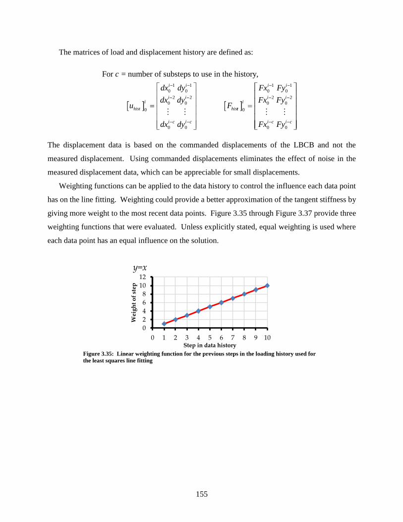
155
The matrices of load and displacement history are defined as:
The displacement data is based on the commanded displacements of the LBCB and not the
measured displacement. Using commanded displacements eliminates the effect of noise in the
measured displacement data, which can be appreciable for small displacements.
Weighting functions can be applied to the data history to control the influence each data point
has on the line fitting. Weighting could provide a better approximation of the tangent stiffness by
giving more weight to the most recent data points. Figure 3.35 through Figure 3.37 provide three
weighting functions that were evaluated. Unless explicitly stated, equal weighting is used where
each data point has an equal influence on the solution.
Figure 3.35: Linear weighting function for the previous steps in the loading history used for
the least squares line fitting
For = number of substeps to use in the history,c
uhist
i
0
dx
dx
dx
dy
dy
dy
F
i
i
i c
i
i
i c
his
0
1
0
2
0
0
1
0
2
0
tt
i
i
i
i c
i
i
i c
Fx
Fx
Fx
Fy
Fy
Fy
0
0
1
0
2
0
0
1
0
2
0
0
2
4
6
8
10
12
0 1 2 3 4 5 6 7 8 9 10
Wei
gh
t o
f st
ep
Step in data history
y=x

156
Figure 3.36: Quadratic weighting function for the previous steps in the loading history used
for the least squares line fitting
Figure 3.37: Inverse hyperbolic cosine weighting function for the previous steps in the
loading history used for the least squares line fitting
Least squares line fitting
Straight-line fitting requires a solution of the parameters for a first-order polynomial:
y b mx= + (2.179)
If more than two data points are used to fit a line, the system of equations is over-determined and
requires a minimization approach to find the best solution. The least squares minimization is one
approach to solving the problem. The least squares method minimizes the sum of the squared
residuals. As a topic of extensive study, many forms of the least squares method exist with
variations on what variables are minimized and the corresponding mathematics as well as using
weighting functions on the residuals.
The most common form is the “Ordinary Least Squares” (OLS) which seeks to minimize the
error in the Y variable (S. L. Meyer 1975). Mathematically given by:
0
20
40
60
80
100
120
0 1 2 3 4 5 6 7 8 9 10W
eig
ht
of
step
Step in data history
y=x2
0
1
2
3
4
5
0 1 2 3 4 5 6 7 8 9 10
Wei
gh
t o
f st
ep
Step in data history
y=arcosh(x)+1
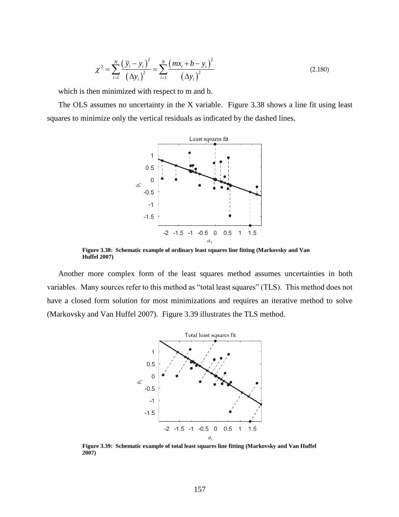
157
( )
( )
( )
( )
2 2
2
2 21 1
N Ni i i i
i ii i
y y mx b y
y y
= =
− + −= =
(2.180)
which is then minimized with respect to m and b.
The OLS assumes no uncertainty in the X variable. Figure 3.38 shows a line fit using least
squares to minimize only the vertical residuals as indicated by the dashed lines.
Figure 3.38: Schematic example of ordinary least squares line fitting (Markovsky and Van
Huffel 2007)
Another more complex form of the least squares method assumes uncertainties in both
variables. Many sources refer to this method as “total least squares” (TLS). This method does not
have a closed form solution for most minimizations and requires an iterative method to solve
(Markovsky and Van Huffel 2007). Figure 3.39 illustrates the TLS method.
Figure 3.39: Schematic example of total least squares line fitting (Markovsky and Van Huffel
2007)

158
For this study, the X variable is the displacement for which we do not have uncertainty. The
only uncertainty of the problem is the load at each displacement; therefore, only ordinary least
squares methodologies are further investigated.
Four methods of least squares lines fitting were evaluated for the algorithm: ordinary least
squares (OLS), weighted least squares, robust ordinary least squares, and weighted robust ordinary
least squares. OLS is described in 3.4.3.3. The weighted least squares approach has only one
mathematical change to OLS. A weight, wi, for each data point is used when calculating the
residual of that data point. Mathematically given as:
( )
( )
2
2
21
Ni i
i i
i
mx b yw
y
=
+ −=
(2.181)
In the OLS the weight is equal for all points and consequently falls out of the equation. The
weighted least squares use weights to give more or less priority to the data points for the fitting.
Applicable weighting functions to this study are given in 3.4.3.2. The robust OLS is used to reduce
the sensitivity of the algorithm to outlying data points. The implementation uses a weighted least
squares approach with a weight defined by the magnitude of residual to the fitted line (Holland
and Welsch 1977). The robust solution requires iteration to find a solution. The weighted robust
OLS combines the previous two methods. A weight is applied based on the residual of the point
as well as a weighting factor based upon a given weighting function.
3.4.4 Unloading stiffness model
For cyclic loading of reinforced concrete, a distinct change in stiffness occurs between the
loading and unloading of the specimen, particularly for inelastic loadings. In the linear elastic
regime, the loading stiffness could be used as the unloading stiffness with no undesirable result.
However, beyond the limit point of the structure, the stiffness is negative (load decreases with
increasing displacement) and using the loading stiffness would actually increase the load on the
unloading step due to the negative tangent stiffness. This example illustrates the importance of
accounting for the unloading stiffness to predict.

159
Figure 3.40: Idealized reinforced concrete hysteresis (C. Meyer 1998)
An idealized behavior of reinforced concrete is shown in Figure 3.40. The inelastic loading
stiffness reduces from the elastic loading stiffness on each cycle of displacement. The inelastic
unloading represents a much larger stiffness than that of the inelastic loading. From this, we can
say with certainty that the inelastic loading will exhibit stiffness less than the maximum inelastic
unloading. This idea is employed in the compressive model of concrete given by Mander (1988)
shown in Figure 3.41. The model uses the initial tangent stiffness of the cycle (Ec) as equivalent
to the initial unloading stiffness of the cycle (Eu).
Figure 3.41: Mander and Park (1988) stress-strain response of concrete during unloading
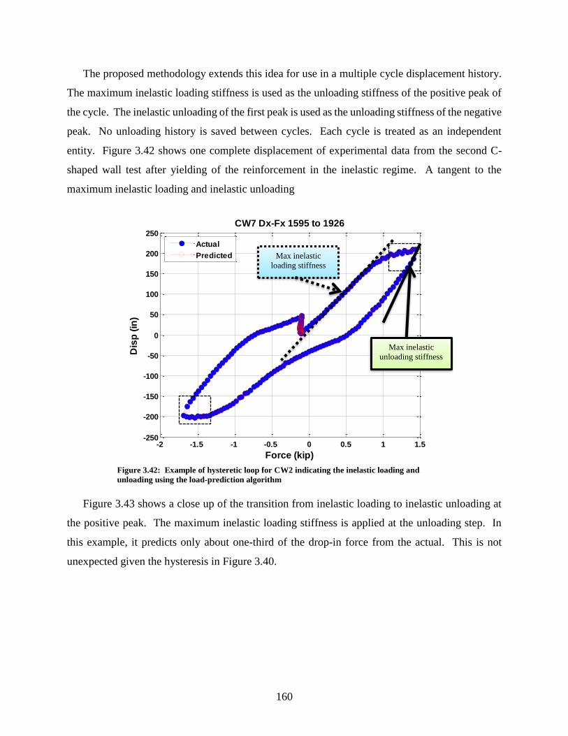
160
The proposed methodology extends this idea for use in a multiple cycle displacement history.
The maximum inelastic loading stiffness is used as the unloading stiffness of the positive peak of
the cycle. The inelastic unloading of the first peak is used as the unloading stiffness of the negative
peak. No unloading history is saved between cycles. Each cycle is treated as an independent
entity. Figure 3.42 shows one complete displacement of experimental data from the second C-
shaped wall test after yielding of the reinforcement in the inelastic regime. A tangent to the
maximum inelastic loading and inelastic unloading
Figure 3.42: Example of hysteretic loop for CW2 indicating the inelastic loading and
unloading using the load-prediction algorithm
Figure 3.43 shows a close up of the transition from inelastic loading to inelastic unloading at
the positive peak. The maximum inelastic loading stiffness is applied at the unloading step. In
this example, it predicts only about one-third of the drop-in force from the actual. This is not
unexpected given the hysteresis in Figure 3.40.
-2 -1.5 -1 -0.5 0 0.5 1 1.5-250
-200
-150
-100
-50
0
50
100
150
200
250
Force (kip)
Dis
p (
in)
CW7 Dx-Fx 1595 to 1926
Actual
Predicted Max inelastic
loading stiffness
Max inelastic
unloading stiffness
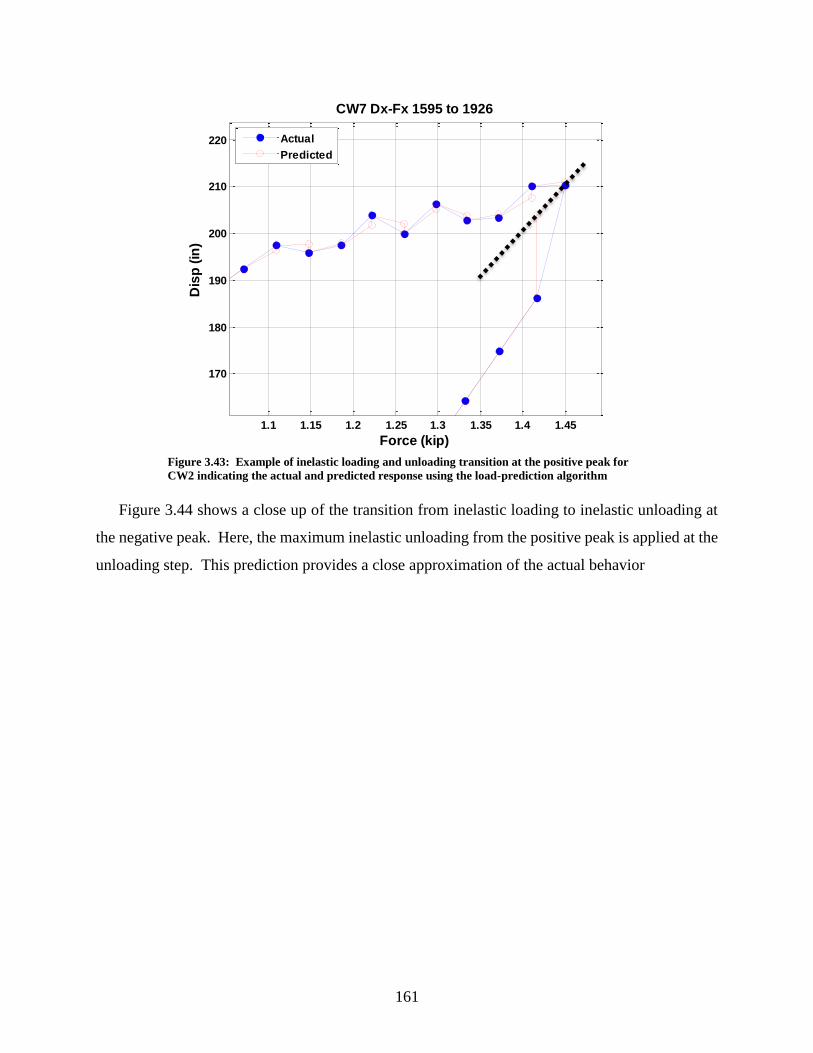
161
Figure 3.43: Example of inelastic loading and unloading transition at the positive peak for
CW2 indicating the actual and predicted response using the load-prediction algorithm
Figure 3.44 shows a close up of the transition from inelastic loading to inelastic unloading at
the negative peak. Here, the maximum inelastic unloading from the positive peak is applied at the
unloading step. This prediction provides a close approximation of the actual behavior
1.1 1.15 1.2 1.25 1.3 1.35 1.4 1.45
170
180
190
200
210
220
Force (kip)
Dis
p (
in)
CW7 Dx-Fx 1595 to 1926
Actual
Predicted

162
Figure 3.44: Example of inelastic loading and unloading transition at the negative peak for
CW2 indicating the actual and predicted response using the load-prediction algorithm
3.4.5 Testing and results
Numerical testing
The experimental test data from the first and second C-shaped wall test provides an ideal data
set to use for simulating the performance of the prediction methods. A Matlab script was written
for performing the simulation of the prediction algorithm utilizing these datasets with the ability
to vary the length of displacement history that is used. The experimental dataset consisted of the
target deformations of each step, the commanded displacement at each step, and the measured load
at each step. Simulations were performed on both CW1 and CW2 data sets, and all nine methods
were run for each dataset. Methods one through six iterated through four maximum history lengths
for the fitting: 3 steps, 4 steps, 5 steps, and 6 steps. Methods seven and eight used a nonlinear
weighting function and employed the entire available load-displacement history.
-1.7 -1.65 -1.6 -1.55 -1.5 -1.45 -1.4 -1.35
-210
-200
-190
-180
-170
-160
-150
Force (kip)
Dis
p (
in)
CW7 Dx-Fx 1595 to 1926
Actual
Predicted

163
Table 3.8: Summary of simulated methods
# Method Weighting function Max. load-def. history
1 Broyden update n/a 3, 4, 5 or 6 steps
2 Davidon-Fletcher-Powell update n/a 3, 4, 5 or 6 steps
3 Ordinary Least Squares n/a 3, 4, 5 or 6 steps
4 Weighted Least Squares linear 3, 4, 5 or 6 steps
5 Robust Least Squares n/a 3, 4, 5 or 6 steps
6 Weighted Robust Least Squares linear 3, 4, 5 or 6 steps
7 Weighted Robust Least Squares quadratic no limit
8 Weighted Robust Least Squares inverse hyperbolic cosine no limit
A qualitative and quantitative evaluation of the proposed methods of moment prediction is
presented and examined in this section based on the numerical simulations utilizing the previous
C-shaped wall test data.
Quantitative analysis of all methods
The quantitative evaluation utilizes the data from all steps of each method using experimental
test data from both the first and second C-shaped wall test for both lateral translations. The first
series of bar plots show the relative errors of each method for each data set.
( )errors > 5 kips
%total # of steps
error =
(2.182)
Figure 3.45 illustrates the success of the least squares methods using only a short history of
load-displacement data. In addition, the percentage of errors in the CW2 test is significantly lower
than the errors from the CW1 test. The difference is a direct result of the displacement step size.
The step size in CW1 exceeded fifteen-hundredths of an inch in the strong axis direction while the
CW2 test was limited to approximately five-hundredths of an inch. Figure 3.46 shows the error in
the weak-axis direction yielding the same result. CW1 was a unidirectional test, so the weak axis
response is limited to the CW2 dataset only.

164
Figure 3.45: Bar plot of % error in strong axis shear as predicted using each method
Figure 3.46: Bar plot of % error in weak axis shear as predicted using each method
A closer inspection of the percentage of errors in the least squares methods is shown in Figure
3.47. While the methods are performed at a similar level, some distinct trends and expectations
are realized. For all four methods, the smallest history of load-deformation steps results in the best
performance of each method. If the data is well conditioned using fewer steps will better
approximate the tangent stiffness of the structure. It also appears that the weighted least squares
0.0%
10.0%
20.0%
30.0%
40.0%
50.0%
60.0%
Percentage of steps with Fx errors greater than 5 kips
C-Wall 6
C-Wall 7
0
0.01
0.02
0.03
0.04
0.05
0.06
0.07
0.08
0.09
Percentage of steps with Fy errors greater than 5 kips
C-Wall 7

165
provided slightly better performance than the ordinary least squares. The robust OLS and robust
WLS showed no significant improvement in performance.
Figure 3.47: Bar plot of % error in strong axis shear as predicted using methods 3-6
The errors greater than 5 kips are broken into smaller categories in Figure 3.48 for CW1 and
Figure 3.49 for CW2. All prediction errors greater than five kips could significantly affect the
experimental test. The CW1 data shows errors exceeding twenty kips but with the majority under
10 kips. CW2 has a similar result but also shows that the errors above 10 kips are essentially
constant for all four prediction methods. In both cases, the weighted least squares reduce the errors
as compared to the constant weighting OLS.
0.0%
2.0%
4.0%
6.0%
8.0%
10.0%
12.0%
Percentage of steps with Fx errors greater than 5 kips
C-Wall 6
C-Wall 7

166
Figure 3.48: Bar plot of CW1 force error (kips) as predicted using each method
Figure 3.49: Bar plot of CW2 force error (kips) as predicted using each method
This level of detail requires the graphical qualitative evaluation to determine the sources of the
errors greater than 10 kips. Nearly all of the errors greater than 5 kips for CW2 will be a result of
three things: test restarts, the first step of the history (no prediction as there is no history), and the
initial unloading step. The unloading stiffness model presented in section 3.4.4 shows that it does
05
101520253035404550
# o
f st
eps
CW1 - Breakdown of Fx errors greater than 5 kips
5 to 10 kips
10 to 15 kips
15 to 20 kips
Over 20 kips
0
50
100
150
200
250
# o
f st
eps
CW2 - Breakdown of Fx errors greater than 5 kips
Series1
Series2
Series3
Series4
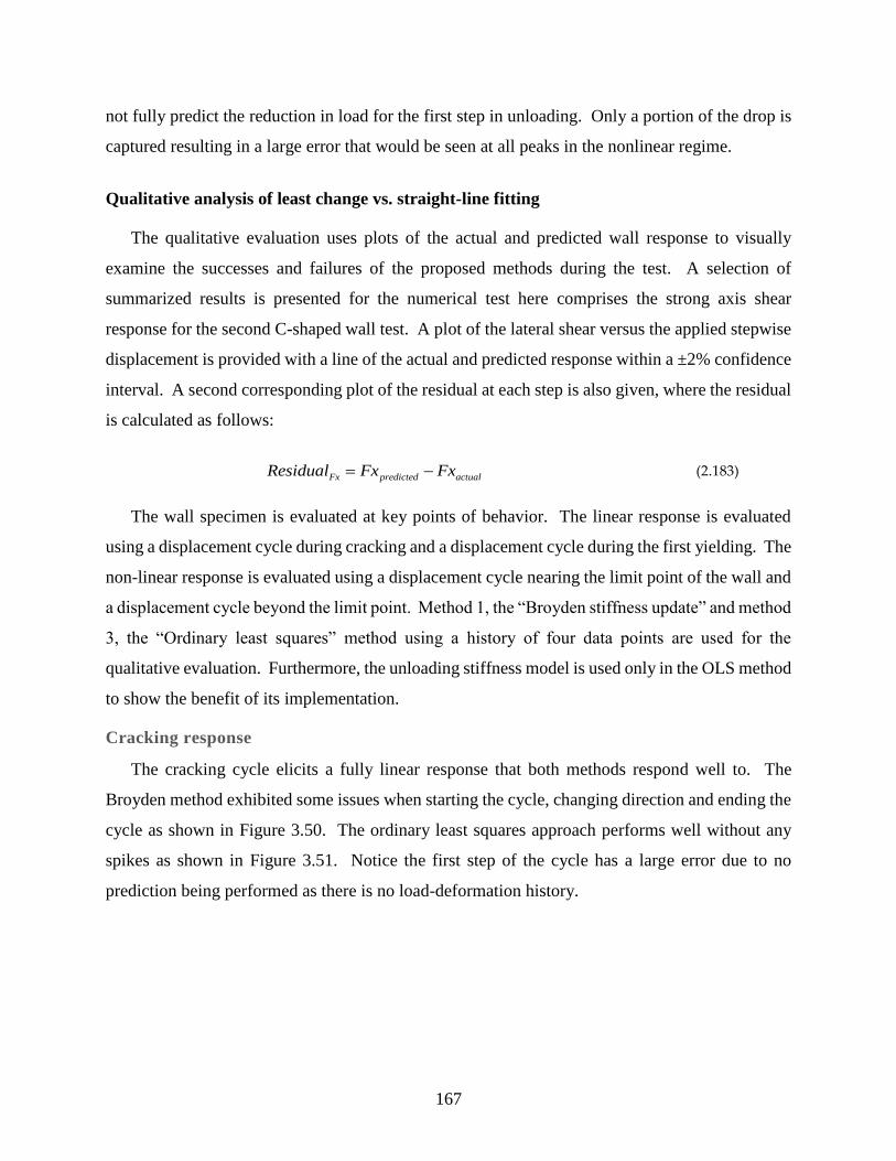
167
not fully predict the reduction in load for the first step in unloading. Only a portion of the drop is
captured resulting in a large error that would be seen at all peaks in the nonlinear regime.
Qualitative analysis of least change vs. straight-line fitting
The qualitative evaluation uses plots of the actual and predicted wall response to visually
examine the successes and failures of the proposed methods during the test. A selection of
summarized results is presented for the numerical test here comprises the strong axis shear
response for the second C-shaped wall test. A plot of the lateral shear versus the applied stepwise
displacement is provided with a line of the actual and predicted response within a ±2% confidence
interval. A second corresponding plot of the residual at each step is also given, where the residual
is calculated as follows:
Fx predicted actualResidual Fx Fx= − (2.183)
The wall specimen is evaluated at key points of behavior. The linear response is evaluated
using a displacement cycle during cracking and a displacement cycle during the first yielding. The
non-linear response is evaluated using a displacement cycle nearing the limit point of the wall and
a displacement cycle beyond the limit point. Method 1, the “Broyden stiffness update” and method
3, the “Ordinary least squares” method using a history of four data points are used for the
qualitative evaluation. Furthermore, the unloading stiffness model is used only in the OLS method
to show the benefit of its implementation.
Cracking response
The cracking cycle elicits a fully linear response that both methods respond well to. The
Broyden method exhibited some issues when starting the cycle, changing direction and ending the
cycle as shown in Figure 3.50. The ordinary least squares approach performs well without any
spikes as shown in Figure 3.51. Notice the first step of the cycle has a large error due to no
prediction being performed as there is no load-deformation history.

168
Figure 3.50: Broyden method cracking response
Figure 3.51: Ordinary least squares cracking response
45 50 55 60 65 70 75 80 85-50
0
50
Fx
(k
ip)
CW7 Fx Step 43 to 85
Fx Actual
98% CI
102% CI
Fx Predicted
45 50 55 60 65 70 75 80 85
0
10
20
30
Step
Re
sid
ua
l (k
ip)
45 50 55 60 65 70 75 80 85
-30
-20
-10
0
10
Fy
(k
ip)
CW7 Fy Step 43 to 85
Fy Actual
98% CI
102% CI
Fy Predicted
45 50 55 60 65 70 75 80 85
-10
0
10
20
Step
Re
sid
ua
l (k
ip) 45 50 55 60 65 70 75 80 85
-50
0
50
Fx
(k
ip)
CW7 Fx Step 43 to 85
Fx Actual
98% CI
102% CI
Fx Predicted
45 50 55 60 65 70 75 80 85
-15-10-505
Step
Re
sid
ua
l (k
ip)
45 50 55 60 65 70 75 80 85
-30
-20
-10
0
10
Fy
(k
ip)
CW7 Fy Step 43 to 85
Fy Actual
98% CI
102% CI
Fy Predicted
45 50 55 60 65 70 75 80 85
-6-4-2024
Step
Re
sid
ua
l (k
ip)
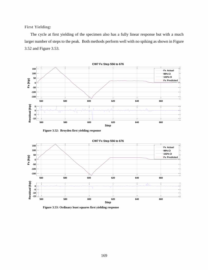
169
First Yielding:
The cycle at first yielding of the specimen also has a fully linear response but with a much
larger number of steps to the peak. Both methods perform well with no spiking as shown in Figure
3.52 and Figure 3.53.
Figure 3.52: Broyden first yielding response
Figure 3.53: Ordinary least squares first yielding response
560 580 600 620 640 660
-150
-100
-50
0
50
100
150
Fx
(k
ip)
CW7 Fx Step 556 to 676
Fx Actual
98% CI
102% CI
Fx Predicted
560 580 600 620 640 660
-10
-5
0
5
Step
Re
sid
ua
l (k
ip)
560 580 600 620 640 660
-60
-40
-20
0
20
Fy
(k
ip)
CW7 Fy Step 556 to 676
Fy Actual
98% CI
102% CI
Fy Predicted
560 580 600 620 640 660
-10
0
10
Step
Re
sid
ua
l (k
ip) 560 580 600 620 640 660
-150
-100
-50
0
50
100
150
Fx
(k
ip)
CW7 Fx Step 556 to 676
Fx Actual
98% CI
102% CI
Fx Predicted
560 580 600 620 640 660
-15
-10
-5
0
Step
Re
sid
ua
l (k
ip)
560 580 600 620 640 660
-60
-40
-20
0
20
Fy
(k
ip)
CW7 Fy Step 556 to 676
Fy Actual
98% CI
102% CI
Fy Predicted
560 580 600 620 640 660
-10
-5
0
5
Step
Re
sid
ua
l (k
ip)

170
Approaching the limit point:
As the response reached the nominal strength, the majority of vertical rebars have yielded, and
the response has flattened. The residuals graph indicates significant errors near the peak
displacements for the Broyden method as shown in Figure 3.54. The ordinary least squares
approach is shown in Figure 3.55. A close up on each peak will provide a better understanding of
the prediction.
Figure 3.54: Broyden approaching limit point response
Figure 3.55: Ordinary least squares approaching limit point response
1600 1650 1700 1750 1800 1850 1900-200
-100
0
100
200
Fx
(k
ip)
CW7 Fx Step 1595 to 1926
Fx Actual
98% CI
102% CI
Fx Predicted
1600 1650 1700 1750 1800 1850 1900
-20
0
20
Step
Re
sid
ua
l (k
ip)
1600 1650 1700 1750 1800 1850 1900-80
-60
-40
-20
0
20
40
Fy
(k
ip)
CW7 Fy Step 1595 to 1926
Fy Actual
98% CI
102% CI
Fy Predicted
1600 1650 1700 1750 1800 1850 1900
-10
0
10
Step
Re
sid
ua
l (k
ip)
1600 1650 1700 1750 1800 1850 1900-200
-100
0
100
200
Fx
(k
ip)
CW7 Fx Step 1595 to 1926
Fx Actual
98% CI
102% CI
Fx Predicted
1600 1650 1700 1750 1800 1850 1900-10
0
10
Step
Re
sid
ua
l (k
ip)
1600 1650 1700 1750 1800 1850 1900-80
-60
-40
-20
0
20
40
Fy
(k
ip)
CW7 Fy Step 1595 to 1926
Fy Actual
98% CI
102% CI
Fy Predicted
1600 1650 1700 1750 1800 1850 1900
-10
0
10
Step
Re
sid
ua
l (k
ip)

171
The peak response shows a non-smooth solution path that causes clear issues for the Broyden
method as shown in Figure 3.56. As the stiffness update directly reflects the previous step, the
update becomes erroneous if the solution path is non-smooth. The use of multiple data points in
the OLS continues to provide a good approximation as shown in Figure 3.57.
In addition, the unloading step in the nonlinear causes a significant error for the Broyden
method. The unloading stiffness model employed in the OLS method reduces the error in the
initial unloading step.
Figure 3.56: Broyden approaching limit point peak response
Figure 3.57: Ordinary least squares approaching limit point peak response
1620 1625 1630 1635 1640
170
180
190
200
210
Fx
(k
ip)
CW7 Fx Step 1595 to 1926
Fx Actual
98% CI
102% CI
Fx Predicted
1620 1625 1630 1635 1640
-20
0
20
Step
Re
sid
ua
l (k
ip)
1775 1780 1785 1790 1795 1800 1805 1810 1815
35
40
45
50
55
Fy
(k
ip)
CW7 Fy Step 1595 to 1926
Fy Actual
98% CI
102% CI
Fy Predicted
1775 1780 1785 1790 1795 1800 1805 1810 1815
-10
0
10
Step
Re
sid
ua
l (k
ip)
1620 1625 1630 1635 1640
170
180
190
200
210
Fx
(k
ip)
CW7 Fx Step 1595 to 1926
Fx Actual
98% CI
102% CI
Fx Predicted
1620 1625 1630 1635 1640-10
0
10
Step
Re
sid
ua
l (k
ip)
1775 1780 1785 1790 1795 1800 1805 1810 1815
35
40
45
50
55
Fy
(k
ip)
CW7 Fy Step 1595 to 1926
1775 1780 1785 1790 1795 1800 1805 1810 1815
-10
0
10
Step
Re
sid
ua
l (k
ip)

172
Beyond limit point:
Post-peak, the observed behavior is similar to the response at the limit point. The solution path
continues to be non-smooth around the peak responses causing significant errors in the Broyden
stiffness update as shown in Figure 3.58 and Figure 3.60. The OLS continues to perform well with
spikes at only the initial cycle step and the unloading step as shown in Figure 3.59 and Figure 3.61.
Figure 3.58: Broyden beyond limit point response
Figure 3.59: Ordinary least squares beyond limit point response
2800 2850 2900 2950 3000 3050 3100 3150 3200
-100
-50
0
50
100
150
Fx
(k
ip)
CW7 Fx Step 2760 to 3221
Fx Actual
98% CI
102% CI
Fx Predicted
2800 2850 2900 2950 3000 3050 3100 3150 3200
-10
0
10
20
Step
Re
sid
ua
l (k
ip)
2800 2850 2900 2950 3000 3050 3100 3150 3200
-20
-10
0
10
20
30
40
Fy
(k
ip)
CW7 Fy Step 2760 to 3221
Fy Actual
98% CI
102% CI
Fy Predicted
2800 2850 2900 2950 3000 3050 3100 3150 3200
-10
0
10
Step
Re
sid
ua
l (k
ip)
2800 2850 2900 2950 3000 3050 3100 3150 3200
-100
-50
0
50
100
150
Fx
(k
ip)
CW7 Fx Step 2760 to 3221
Fx Actual
98% CI
102% CI
Fx Predicted
2800 2850 2900 2950 3000 3050 3100 3150 3200
-505
1015
Step
Re
sid
ua
l (k
ip)
2800 2850 2900 2950 3000 3050 3100 3150 3200
-20
-10
0
10
20
30
40
Fy
(k
ip)
CW7 Fy Step 2760 to 3221
Fy Actual
98% CI
102% CI
Fy Predicted
2800 2850 2900 2950 3000 3050 3100 3150 3200
-10
-5
0
5
Step
Re
sid
ua
l (k
ip)

173
Figure 3.60: Broyden beyond limit point peak response
Figure 3.61: Ordinary least squares beyond limit point peak response
3085 3090 3095 3100 3105 3110 3115 3120
60
70
80
90
100
110
120
Fx
(k
ip)
CW7 Fx Step 2760 to 3221
Fx Actual
98% CI
102% CI
Fx Predicted
3085 3090 3095 3100 3105 3110 3115 3120
-10
0
10
20
Step
Re
sid
ua
l (k
ip)
2780 2785 2790 2795 2800 2805 2810 2815 2820 2825
25
30
35
40
45
Fy
(k
ip)
CW7 Fy Step 2760 to 3221
Fy Actual
98% CI
102% CI
Fy Predicted
2780 2785 2790 2795 2800 2805 2810 2815 2820 2825
-5
0
5
Step
Re
sid
ua
l (k
ip)
3085 3090 3095 3100 3105 3110 3115 3120
60
70
80
90
100
110
120
Fx
(k
ip)
CW7 Fx Step 2760 to 3221
Fx Actual
98% CI
102% CI
Fx Predicted
3085 3090 3095 3100 3105 3110 3115 3120
-505
1015
Step
Re
sid
ua
l (k
ip)
2780 2785 2790 2795 2800 2805 2810 2815 2820 2825
25
30
35
40
45
Fy
(k
ip)
CW7 Fy Step 2760 to 3221
Fy Actual
98% CI
102% CI
Fy Predicted
2780 2785 2790 2795 2800 2805 2810 2815 2820 2825
-10
-5
0
5
Step
Re
sid
ua
l (k
ip)
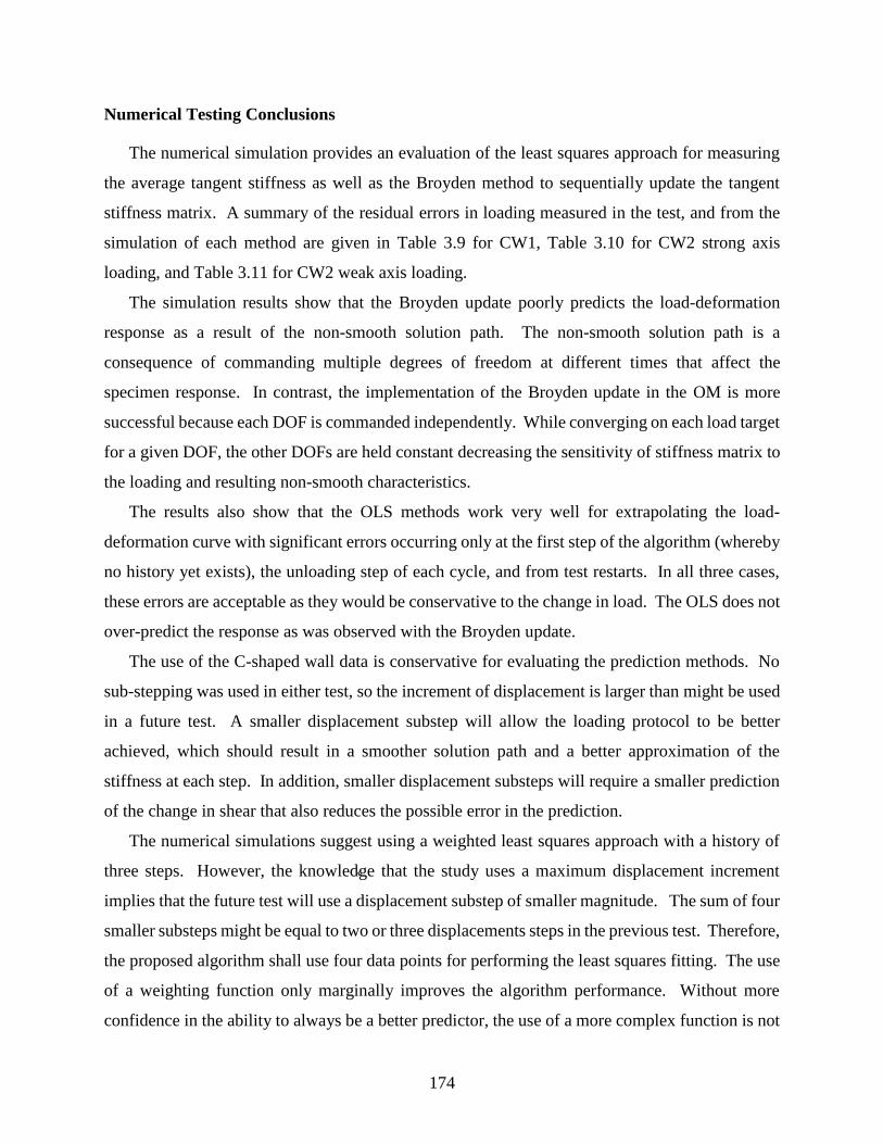
174
Numerical Testing Conclusions
The numerical simulation provides an evaluation of the least squares approach for measuring
the average tangent stiffness as well as the Broyden method to sequentially update the tangent
stiffness matrix. A summary of the residual errors in loading measured in the test, and from the
simulation of each method are given in Table 3.9 for CW1, Table 3.10 for CW2 strong axis
loading, and Table 3.11 for CW2 weak axis loading.
The simulation results show that the Broyden update poorly predicts the load-deformation
response as a result of the non-smooth solution path. The non-smooth solution path is a
consequence of commanding multiple degrees of freedom at different times that affect the
specimen response. In contrast, the implementation of the Broyden update in the OM is more
successful because each DOF is commanded independently. While converging on each load target
for a given DOF, the other DOFs are held constant decreasing the sensitivity of stiffness matrix to
the loading and resulting non-smooth characteristics.
The results also show that the OLS methods work very well for extrapolating the load-
deformation curve with significant errors occurring only at the first step of the algorithm (whereby
no history yet exists), the unloading step of each cycle, and from test restarts. In all three cases,
these errors are acceptable as they would be conservative to the change in load. The OLS does not
over-predict the response as was observed with the Broyden update.
The use of the C-shaped wall data is conservative for evaluating the prediction methods. No
sub-stepping was used in either test, so the increment of displacement is larger than might be used
in a future test. A smaller displacement substep will allow the loading protocol to be better
achieved, which should result in a smoother solution path and a better approximation of the
stiffness at each step. In addition, smaller displacement substeps will require a smaller prediction
of the change in shear that also reduces the possible error in the prediction.
The numerical simulations suggest using a weighted least squares approach with a history of
three steps. However, the knowledge that the study uses a maximum displacement increment
implies that the future test will use a displacement substep of smaller magnitude. The sum of four
smaller substeps might be equal to two or three displacements steps in the previous test. Therefore,
the proposed algorithm shall use four data points for performing the least squares fitting. The use
of a weighting function only marginally improves the algorithm performance. Without more
confidence in the ability to always be a better predictor, the use of a more complex function is not
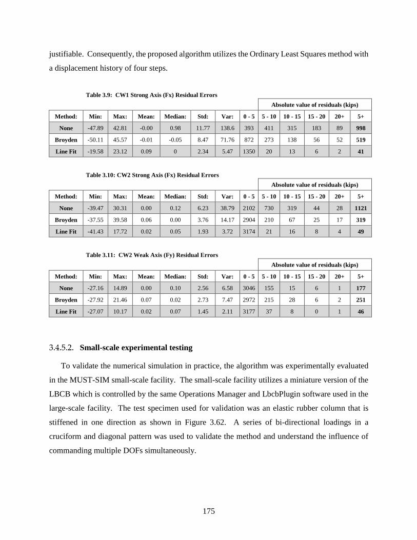
175
justifiable. Consequently, the proposed algorithm utilizes the Ordinary Least Squares method with
a displacement history of four steps.
Table 3.9: CW1 Strong Axis (Fx) Residual Errors
Absolute value of residuals (kips)
Method: Min: Max: Mean: Median: Std: Var: 0 - 5 5 - 10 10 - 15 15 - 20 20+ 5+
None -47.89 42.81 -0.00 0.98 11.77 138.6 393 411 315 183 89 998
Broyden -50.11 45.57 -0.01 -0.05 8.47 71.76 872 273 138 56 52 519
Line Fit -19.58 23.12 0.09 0 2.34 5.47 1350 20 13 6 2 41
Table 3.10: CW2 Strong Axis (Fx) Residual Errors
Absolute value of residuals (kips)
Method: Min: Max: Mean: Median: Std: Var: 0 - 5 5 - 10 10 - 15 15 - 20 20+ 5+
None -39.47 30.31 0.00 0.12 6.23 38.79 2102 730 319 44 28 1121
Broyden -37.55 39.58 0.06 0.00 3.76 14.17 2904 210 67 25 17 319
Line Fit -41.43 17.72 0.02 0.05 1.93 3.72 3174 21 16 8 4 49
Table 3.11: CW2 Weak Axis (Fy) Residual Errors
Absolute value of residuals (kips)
Method: Min: Max: Mean: Median: Std: Var: 0 - 5 5 - 10 10 - 15 15 - 20 20+ 5+
None -27.16 14.89 0.00 0.10 2.56 6.58 3046 155 15 6 1 177
Broyden -27.92 21.46 0.07 0.02 2.73 7.47 2972 215 28 6 2 251
Line Fit -27.07 10.17 0.02 0.07 1.45 2.11 3177 37 8 0 1 46
Small-scale experimental testing
To validate the numerical simulation in practice, the algorithm was experimentally evaluated
in the MUST-SIM small-scale facility. The small-scale facility utilizes a miniature version of the
LBCB which is controlled by the same Operations Manager and LbcbPlugin software used in the
large-scale facility. The test specimen used for validation was an elastic rubber column that is
stiffened in one direction as shown in Figure 3.62. A series of bi-directional loadings in a
cruciform and diagonal pattern was used to validate the method and understand the influence of
commanding multiple DOFs simultaneously.

176
Figure 3.62: Small-scale facility rubber test specimen
The commanded displacement history shown in Figure 3.63 consisted of a cruciform
displacement pattern followed by a diagonal displacement pattern. The x-direction loading utilized
a constant axial load and moment to shear ratio. The Y-direction loading utilized a variable axial
load consistent with the coupling procedure described in Section 3.3.4.3. The displacement
magnitude was two-tenths of an inch in both directions.
Figure 3.63: Rubber specimen displacement history
100 120 140 160 180 200 220-0.2
-0.1
0
0.1
0.2
Step Index
Dis
p (
in)
StepIndex vs. Dx and Dy
Dx
Dy

177
The measured shear forces, axial force, and moments are plotted in Figure 3.64, Figure 3.65,
Figure 3.66 respectively. One hundred twenty displacement steps were imposed, and eleven
correction steps were required. Each step averaged 27 seconds in duration. The performance of
the algorithm was excellent with minimal errors between the measured and predicted forces. The
largest deviations are observed at the unloading step and the initial loading step.
Figure 3.64: Rubber specimen measured shear force (lb)
Figure 3.65: Rubber specimen measured axial force (lb)
100 120 140 160 180 200 220
0
2
4
6
Step Index
Sh
ea
r (k
ip)
StepIndex vs. Fx
Meas
Predicted
100 120 140 160 180 200 220
-6
-4
-2
0
2
Step Index
Sh
ea
r (k
ip)
StepIndex vs. Fy
Meas
Predicted
100 120 140 160 180 200 220
30
40
50
Step Index
Fo
rce
(k
ip)
StepIndex vs. Fz
Meas
Calc
Prop

178
Figure 3.66: Rubber specimen measured moments (lb-in)
Large-scale testing results
After successful completion of small-scale testing, the algorithm was implemented in the large-
scale laboratory for testing specimen CW3. The initial elastic loading cycles were utilized to verify
the algorithm again before proceeding with inelastic loading. The load-step history and predicted
stiffness values are shown in Figure 3.67 and Figure 3.68. The dashed green boxes indicate where
the prediction was performed. The measured response is smooth, and the corrections steps have
been reduced. The algorithm initiates during the unloading steps after the first peak. There are
two requirements for the simultaneous movement to be performed: 1) it must have enough
converged data points (the data history resets at peaks and the start of new cycles) and 2) the
displacement history must be greater than a prescribed delta to ensure the history of converged
data points are meaningful. The measured stiffness indicates where the algorithm was allowed to
run and predict the forces for the combined movements. Only a limited number of steps were
predicted during this trial based on the number of steps in the load cycle (40 in Dx, 20 in Dy).
Cycles with more steps between the onset of loading and peak loading will benefit more from the
algorithm.
100 120 140 160 180 200 220
-40
-20
0
20
Step Index
Mo
me
nt
(kip
-in
)
StepIndex vs. Mx
Meas
Prop
100 120 140 160 180 200 220
-40
-20
0
Step Index
Mo
me
nt
(kip
-in
)
StepIndex vs. My
Meas
Prop

179
Figure 3.67: Predicted strong axis and weak axis stiffness during intial loading of CW3
Figure 3.68: Impact of load-prediction algorithm for strong axis response (top) and weak axis
response (bottom) during intial loading of CW3
5 10 15 20 25 30 35 400
500
1000
StepIndex
Sti
ffn
es
s (
kip
/in
)
StepIndex vs. Predicted Stiffness
Fx
Fy
5 10 15 20 25 30 35 40
-20
0
20
StepIndex
Mo
me
nt
(kip
-in
)
StepIndex vs. Predicted Fx
Meas
Predicted
5 10 15 20 25 30 35 40
-10
-5
0
5
StepIndex
Mo
me
nt
(kip
-in
)
StepIndex vs. Predicted Fy
Meas
Predicted
180
3.5 Conclusions
Chapter 3 summarizes the development of the specimen design, construction and loading
methodology for the C-shaped wall experiments. Three one-third scale test specimens were
constructed for testing at the Newmark Structural Engineering Laboratory. The loading protocol
utilized the six DOF capability of two Load and Boundary Condition Boxes to impose mixed
displacements and loads that simulated the upper seven stories of a ten-story building acting on
the test specimen. A loading methodology and displacement history for uni-directional loading,
bi-directional loading, and a coupled core-wall system in bi-directional loading were outlined.
To conduct the coupled core wall simulation, the ability to predict mixed-mode displacements
in multiple degrees of freedom simultaneously was evaluated. The existing methods for
application of loading resulted in increased shear demand prior to the convergence of the load step.
Furthermore, the convergence of the load step took many iterations when the load target was
dependent on the specimen response. To address these shortcomings, a stiffness-based loading
algorithm was developed, tested and implemented in the laboratory. The algorithm recommended
measurement of the tangent stiffness of each degree of freedom using a least squares line fitting of
previous points on the load-deformation history. The hysteretic aspects of response were
considered by measurement of the stiffness during loading and unloading to improve predictions
at changes in the loading direction. The algorithm yielded a 94% reduction in shear force
overshoot and enhanced convergence to improve testing efficiency based on numerical testing.

181
CHAPTER 4: QUALITATIVE EXPERIMENTAL OBSERVATIONS
4.1 Introduction
Chapter 43 presents a qualitative damage narrative of the response from each of the C-shaped
wall tests. Observations of key limit and damage states are described including cracking, yielding,
nominal strength, spalling, buckling, rupture, and failure. Section 4.2, 4.3, and 4.4 summarize the
experimental response for CW1, CW2, and CW3 respectively. All three walls ultimately lost load
carrying capacity due to rupture of the BE reinforcing bars that had been previously buckled in
compression as a consequence of the cyclic loading. Section 4.5 provides a comparison of the
wall damage states identifies the key damage states leading to failure. A quantitative comparison
is made of the strength and drift capacities as well as the drift levels corresponding to each limit
state. Conclusions of the qualitative evaluation are given in Section 4.6.
4.2 CW1 Experimental results
4.2.1 Overall observations
The first C-shaped wall test provides insight into the strong axis behavior of the specimen. The
response was governed by flexure as the loss in load carrying capacity was precipitated by rupture
of the longitudinal #4 bars in the boundary elements. Nearly all longitudinal #2 bars in the web
and center of each flange are believed to have been ruptured. After the rupture of #2 bars, a
significant portion of the deformation was observed to be carried by sliding along the web. The
sliding component is clearly visible in the load-deformation hysteresis and is responsible for
significant damage to the centers of each flange and a very large separation between the web and
corner boundary element.
3 Sections 4.2 through 4.5 were taken in part from project grant deliverables written for the National Science Foundation
(Mock et al. 2013). I was the primary or sole author of the content included herein. Furthermore, this content has been updated
and amended since the deliverable.
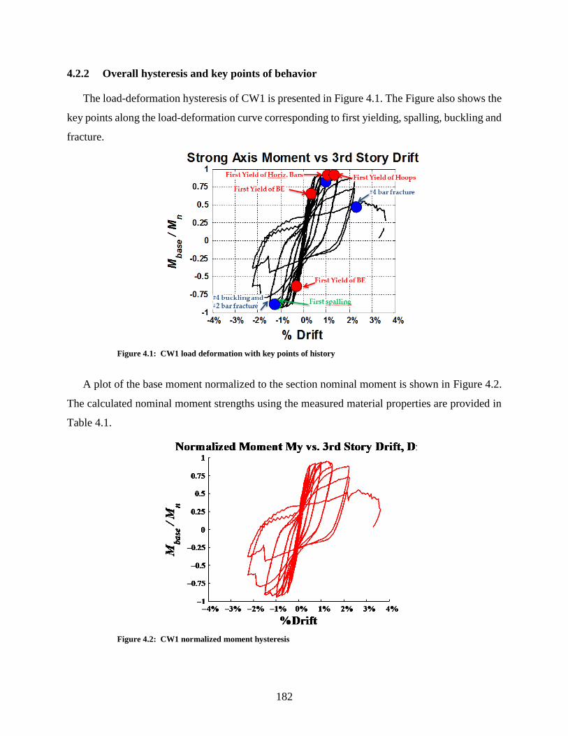
182
4.2.2 Overall hysteresis and key points of behavior
The load-deformation hysteresis of CW1 is presented in Figure 4.1. The Figure also shows the
key points along the load-deformation curve corresponding to first yielding, spalling, buckling and
fracture.
Figure 4.1: CW1 load deformation with key points of history
A plot of the base moment normalized to the section nominal moment is shown in Figure 4.2.
The calculated nominal moment strengths using the measured material properties are provided in
Table 4.1.
Figure 4.2: CW1 normalized moment hysteresis

183
4.2.3 Damage narrative and photos
Substantial Yield
Dx = 0.5” (0.35%), Shear, Fx = 177 kips, Base Moment, My = 4,979 kip-ft
The cracking pattern developed primarily in the cycles up to yielding. Cracking was initiated
by flexural cracks in the first and second stories of the flanges. Inclined shear cracking then
developed shortly after as well as additional uniformly spaced flexural cracks along the boundary
elements in the web. The 0.35% drift cycle marked yielding of multiple #4 bars in the boundary
elements in each direction as well as #2 bars in the flanges.
Figure 4.3: CW1 substantial yield hysteresis
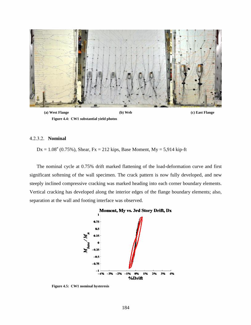
184
(a) West Flange (b) Web (c) East Flange
Figure 4.4: CW1 substantial yield photos
Nominal
Dx = 1.08” (0.75%), Shear, Fx = 212 kips, Base Moment, My = 5,914 kip-ft
The nominal cycle at 0.75% drift marked flattening of the load-deformation curve and first
significant softening of the wall specimen. The crack pattern is now fully developed, and new
steeply inclined compressive cracking was marked heading into each corner boundary elements.
Vertical cracking has developed along the interior edges of the flange boundary elements; also,
separation at the wall and footing interface was observed.
Figure 4.5: CW1 nominal hysteresis

185
(a) West Flange (b) Web (c) East Flange
Figure 4.6: CW1 nominal photos
Onset of Spalling
Dx = 2.16” (1.5%), Shear, Fx = 201 kips, Base Moment, My = 5,765 kip-ft
The cycle to 1.5% drift was highlighted by numerous ruptures of #2 vertical reinforcing bars
along the web and centers of the flanges. Some loss of strength was associated with these ruptures.
A significant component of the deformation was observed as sliding along the web and a
pronounced separation between the web and Southwest boundary element. The horizontal bars
ruptured along this separation. Significant spalling of the clear cover was removed along both
corner boundary elements; at this point #4 bars have begun to buckle in the East flange boundary
element

186
Figure 4.7: CW1 onset of spalling hysteresis
(a) West Flange (b) Web (c) East Flange
Figure 4.8: CW1 onset of spalling photos
Bar buckling and rupture
Dx = 3.24” (2.25%), Shear, Fx = 198 kips, Base Moment, My = 5,612 kip-ft
The cycle at 2.25% drift marked the rupturing of #4 longitudinal bars and a failure of the
specimen on the second cycle in the negative X direction. Continued buckling of longitudinal rebar
in the spalled portions of the corner boundary elements and some loss of confinement was
observed. New vertical compressive cracking is marked along the flanges flowing into the corner
boundary elements. The spalled cover was removed at the boundary element toes and along the

187
web. Significant sliding along the web resulted in spalling along the middle of the flanges due to
out of plane shear. On the second cycle of 2.25% drift in the negative direction, a large number of
#4 bars were ruptured in the East flange resulting in a significant drop in lateral load carrying
capacity.
Figure 4.9: CW1 bar buckling and rupture hysteresis
(a) West Flange (b) Web (c) East Flange
Figure 4.10: CW1 bar buckling and rupture photos

188
Pushover failure
Dx = 5.1” (3.52%)
After observing a failure in the negative X-direction during the second cycle at 2.25% drift, a
pushover was performed in the positive X-direction until reaching failure at 3.5% drift. The
separation between the web and Southwest boundary element grew large enough to see through
the specimen with all horizontal bars ruptured in the bottom foot of the wall. The sliding behavior
is evident in the offset between the bottom and top portion of fractured #2 bars along this diagonal
opening. The wall exhibited severe buckling of longitudinal rebars along the East flange and a loss
of confinement in both the corner and toe boundary elements. Successive rupturing of longitudinal
rebars in the West flange resulted in the loss of load carrying capacity.
Figure 4.11: CW1 failure hysteresis

189
(a) West Flange (b) Web (c) East Flange
Figure 4.12: CW1 failure photos
4.3 CW2 Experimental results
4.3.1 Overall observations
The second C-shaped wall test provides great insight into the bidirectional behavior of the
specimen. The response was governed again by flexure with the loss in load carrying capacity
precipitated by the rupture of longitudinal #4 bars in the boundary elements. Nearly all longitudinal
#2 bars in the web and center of each flange are believed to have been ruptured. The specimen
exhibited less ductility in the X-direction due to the Y-direction loading and the fact that the
boundary elements were subjected to twice as many cycles of loading as compared to the first test.
4.3.2 Overall hysteresis and key points of behavior
The load-deformation hysteresis of CW2 is presented in Figure 4.1. The figure also shows the
key points along the load-deformation curve corresponding to first yielding, spalling, buckling and
fracture.

190
(a) Strong Axis (b) Weak Axis
Figure 4.13: CW2 load deformation with key points of history
A plot of the base moment normalized to the section nominal moment is shown for each
direction in Figure 4.14. The calculated nominal moment strengths using the measured material
properties are provided in Table 4.1.
(a) Strong Axis (b) Weak Axis
Figure 4.14: CW2 normalized moment overall hysteresis

191
4.3.3 Damage narrative and photos
Substantial Yield
Dx = 0.5” (0.35%), +Dy = 0.6” (0.42%), -Dy = -0.9” (-0.63%)
The cracking pattern developed primarily in the cycles up to yielding. Cracking was initiated
by flexural cracks in the lower two floors of the flanges in the X-direction. The cracking pattern
in both Y-directions consisted of reopening of X-direction flexural cracks. The 0.35% drift cycle
marked yielding of multiple #4 bars in the lower two floors of the boundary elements in each
direction as well as #2 bars in the flanges and web. Separation at the wall and footing interface
across the entire span of the web was observed.
(a) Strong Axis (b) Weak Axis
Figure 4.15: CW2 substantial yield hysteresis

192
(a) West Flange (b) Web (c) East Flange
Figure 4.16: CW2 substantial yield photos
Nominal
Dx = 1.08” (0.75%), Dy = +3.24” (2.25%), -Dy = -2.135” (-1.49%)
The nominal cycle at 0.75% drift marked flattening of the load-deformation curve in the X-
direction and positive Y-direction, but no significant flattening in negative Y-direction. Significant
softening of the wall specimen was observed in both directions. The nominal cycle resulted in
spalling on both toes of the flanges at approximately two feet from the base. Some #2 bar buckling
noted at the rear of the wall resulting in spalling of cover.
(a) Strong Axis (b) Weak Axis
Figure 4.17: CW2 nominal hysteresis

193
(a) West Flange (b) Web (c) East Flange
Figure 4.18: CW2 nominal photos
Bar buckling and rupture
Dx = 1.44” (1.0%), Dy = +2.88” (2.0%), -Dy = -1.584” (-1.1%)
Due to reaching displacement capacity in the Y-direction, a cycle in the X-direction was
completed at a constant Dy of 2.0% drift and a second cycle at a constant Dy of -1.1% drift. The
goal of these cycles was to increase the demand on the corner and toe boundary elements. During
the X-direction cycle, the separation between the flanges and the footing increased. There was also
significant spalling on the corner boundary elements during the cycle at positive Dy. Additional
spalling was also observed on the toes of the flanges during the cycle at negative Dy, particularly
on the East flange. Furthermore, this cycle showed significantly less stiffness than when
completing at zero Dy and positive Dy. Rupturing of #2 bars observed along the center of the web,
and buckling began to occur in the vertical bars of the boundary elements. Sliding of the web at
the interface between wall and footing was noted when evaluating Krypton displacement readings.

194
(a) Strong Axis (b) Weak Axis
Figure 4.19: CW2 bar buckling and rupture hysteresis
(a) West Flange (b) Web (c) East Flange
Figure 4.20: CW2 bar buckling and rupture photos
Pushover failure
Dx = 2.80” (1.9%), Dy = +2.88” (2.0%)
The X-direction pushover held at the positive 2% drift in the Y and resulted in the additional
rupture of approximately five #4 bars in the West flange boundary elements as well as additional
spalling on the East flange. Minimal confined concrete remained in the corner boundary elements,
and the vertical rebar was extensively buckled. One of the ties in the Northeast corner boundary
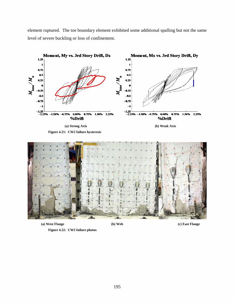
195
element ruptured. The toe boundary element exhibited some additional spalling but not the same
level of severe buckling or loss of confinement.
(a) Strong Axis (b) Weak Axis
Figure 4.21: CW2 failure hysteresis
(a) West Flange (b) Web (c) East Flange
Figure 4.22: CW2 failure photos
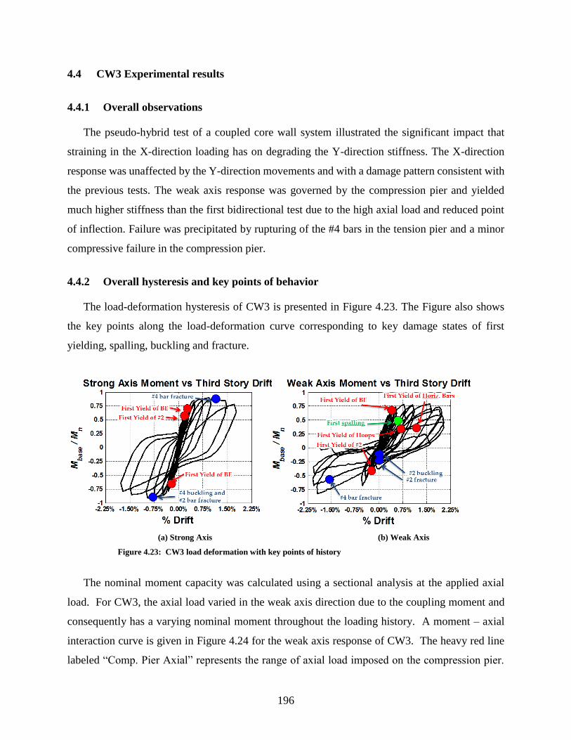
196
4.4 CW3 Experimental results
4.4.1 Overall observations
The pseudo-hybrid test of a coupled core wall system illustrated the significant impact that
straining in the X-direction loading has on degrading the Y-direction stiffness. The X-direction
response was unaffected by the Y-direction movements and with a damage pattern consistent with
the previous tests. The weak axis response was governed by the compression pier and yielded
much higher stiffness than the first bidirectional test due to the high axial load and reduced point
of inflection. Failure was precipitated by rupturing of the #4 bars in the tension pier and a minor
compressive failure in the compression pier.
4.4.2 Overall hysteresis and key points of behavior
The load-deformation hysteresis of CW3 is presented in Figure 4.23. The Figure also shows
the key points along the load-deformation curve corresponding to key damage states of first
yielding, spalling, buckling and fracture.
(a) Strong Axis (b) Weak Axis
Figure 4.23: CW3 load deformation with key points of history
The nominal moment capacity was calculated using a sectional analysis at the applied axial
load. For CW3, the axial load varied in the weak axis direction due to the coupling moment and
consequently has a varying nominal moment throughout the loading history. A moment – axial
interaction curve is given in Figure 4.24 for the weak axis response of CW3. The heavy red line
labeled “Comp. Pier Axial” represents the range of axial load imposed on the compression pier.
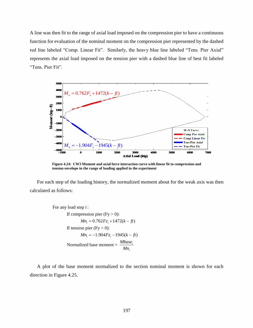
197
A line was then fit to the range of axial load imposed on the compression pier to have a continuous
function for evaluation of the nominal moment on the compression pier represented by the dashed
red line labeled “Comp. Linear Fit”. Similarly, the heavy blue line labeled “Tens. Pier Axial”
represents the axial load imposed on the tension pier with a dashed blue line of best fit labeled
“Tens. Pier Fit”.
Figure 4.24: CW3 Moment and axial force interaction curve with linear fit to compression and
tension envelope in the range of loading applied in the experiment
For each step of the loading history, the normalized moment about for the weak axis was then
calculated as follows:
For any load step :
If compression pier (Fy > 0):
0.762 1472( )
If tension pier (Fy < 0):
1.904 1945( )
Normalized base moment =
i i
i i
i
i
i
Mn Fz k ft
Mn Fz k ft
Mbase
Mn
= + −
= − − −
A plot of the base moment normalized to the section nominal moment is shown for each
direction in Figure 4.25.
0.762 1472( )n zM F k ft= + −
1.904 1945( )n zM F k ft= − − −

198
(a) Strong Axis (b) Weak Axis
Figure 4.25: CW3 normalized moment overall hysteresis
4.4.3 Damage narrative and photos
Substantial Yield
Dx = 0.5” (0.35%), +Dy = 0.65” (0.45%), -Dy = -0.65” (-0.45%)
Yielding across the flange boundary element vertical reinforcement was reached at the 0.35%
drift level in the X and 0.45% drift in the Y. Higher strains were achieved in the X-direction cycle
than the Y-direction. Yield was reached in the #2 bars in the web prior to yielding the boundary
elements. The cracking pattern developed primarily in the cycles up to yielding, initiated primarily
by horizontal and diagonal cracking from the X-direction loading. The cracking pattern in the
positive Y-direction consisted of reopening of X-direction flexural cracks as well as new diagonal
cracking.

199
(a) Strong Axis (b) Weak Axis
Figure 4.26: CW3 substantial yield hysteresis
(a) West Flange (b) Web (c) East Flange
Figure 4.27: CW3 substantial yield photos
Nominal
Dx = 1.08” (0.75%), Dy = +1.6” (1.11%), -Dy = -0.4” (-0.28%)
The nominal cycle at 0.75% drift marked reaching the yield plateau of the load-deformation
curve in the X-direction, but no significant flattening in Y-direction. Significant softening of the
wall specimen was observed in both directions. New inclined compressive and diagonal cracking
was marked in the positive Dy cycle as well as the initiation of diagonal cracking in the negative

200
Dy. Minor spalling was also observed on the Southeast corner boundary element where the
concrete cover had been patched.
(a) Strong Axis (b) Weak Axis
Figure 4.28: CW3 nominal hysteresis
(a) West Flange (b) Web (c) East Flange
Figure 4.29: CW3 nominal photos
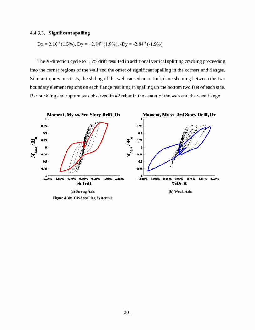
201
Significant spalling
Dx = 2.16” (1.5%), Dy = +2.84” (1.9%), -Dy = -2.84” (-1.9%)
The X-direction cycle to 1.5% drift resulted in additional vertical splitting cracking proceeding
into the corner regions of the wall and the onset of significant spalling in the corners and flanges.
Similar to previous tests, the sliding of the web caused an out-of-plane shearing between the two
boundary element regions on each flange resulting in spalling up the bottom two feet of each side.
Bar buckling and rupture was observed in #2 rebar in the center of the web and the west flange.
(a) Strong Axis (b) Weak Axis
Figure 4.30: CW3 spalling hysteresis
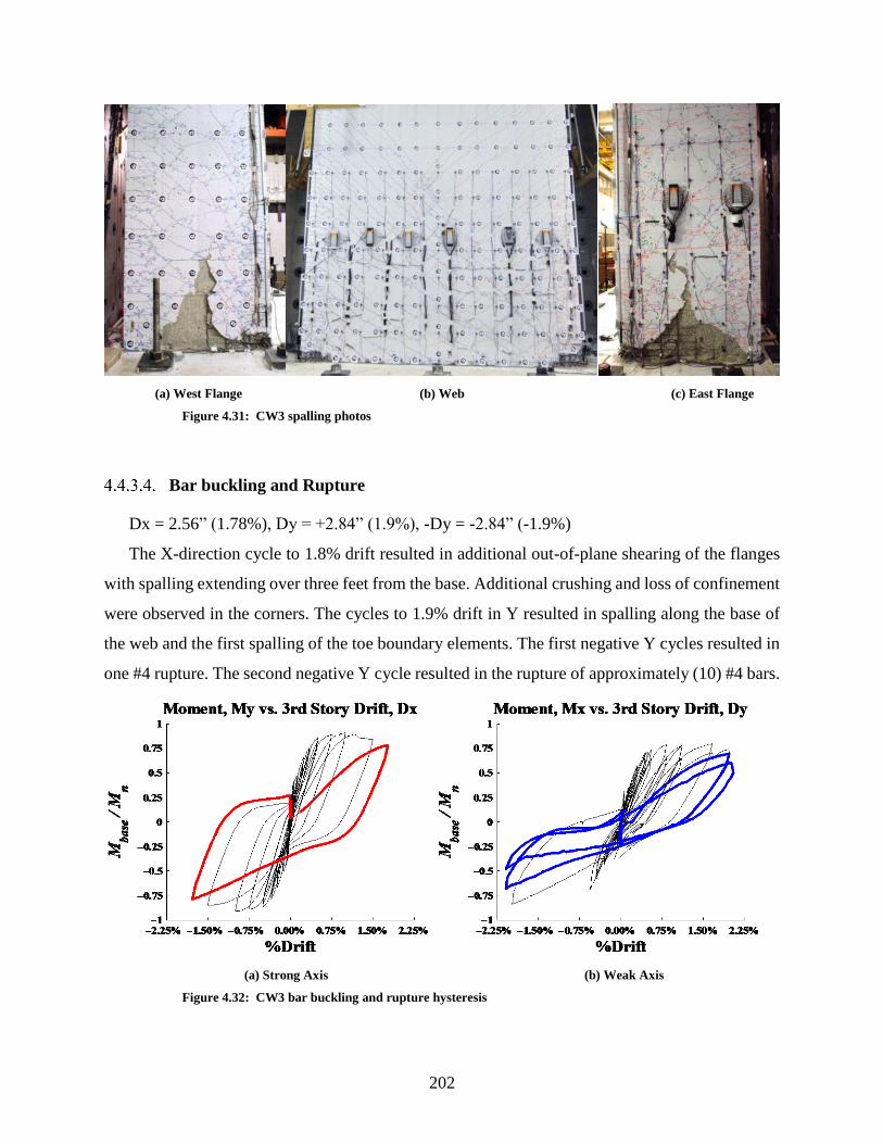
202
(a) West Flange (b) Web (c) East Flange
Figure 4.31: CW3 spalling photos
Bar buckling and Rupture
Dx = 2.56” (1.78%), Dy = +2.84” (1.9%), -Dy = -2.84” (-1.9%)
The X-direction cycle to 1.8% drift resulted in additional out-of-plane shearing of the flanges
with spalling extending over three feet from the base. Additional crushing and loss of confinement
were observed in the corners. The cycles to 1.9% drift in Y resulted in spalling along the base of
the web and the first spalling of the toe boundary elements. The first negative Y cycles resulted in
one #4 rupture. The second negative Y cycle resulted in the rupture of approximately (10) #4 bars.
(a) Strong Axis (b) Weak Axis
Figure 4.32: CW3 bar buckling and rupture hysteresis

203
(a) West Flange (b) Web (c) East Flange
Figure 4.33: CW3 bar buckling and rupture photos
Failure
Dy = +2.3” (1.62%), -Dy = -2.75” (-1.9%)
The final cycles in the positive Y direction were completed at a constant axial load of 1000
kips. The positive Y direction cycles resulted in widespread spalling along the face of the web and
further loss of confinement and core crushing in the corner regions. In-plane shearing was observed
in the center of both flanges causing further spalling and splitting up the height of the flange. The
negative Dy cycle was completed with an axial tension of up to 250 kips. At -1.53% drift multiple
#4 bars ruptured along the East flange, and the specimen could no longer carry the full axial
tension. The final positive cycle ended at 1.62% drift where the specimen exhibited a minor
compressive failure dropping 133 kips of the axial load and 20 kips of shear.
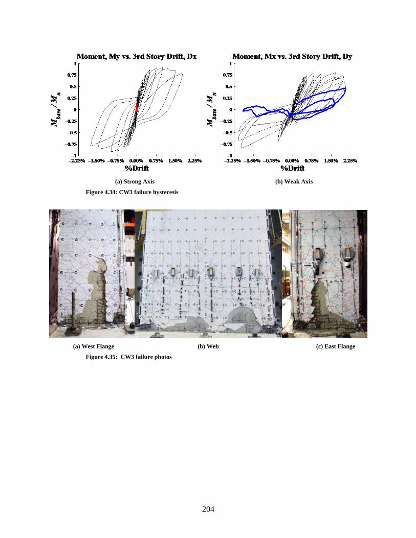
204
(a) Strong Axis (b) Weak Axis
Figure 4.34: CW3 failure hysteresis
(a) West Flange (b) Web (c) East Flange
Figure 4.35: CW3 failure photos
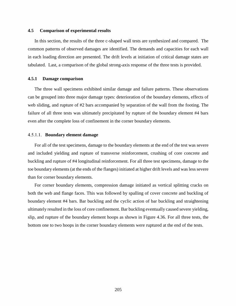
205
4.5 Comparison of experimental results
In this section, the results of the three c-shaped wall tests are synthesized and compared. The
common patterns of observed damages are identified. The demands and capacities for each wall
in each loading direction are presented. The drift levels at initiation of critical damage states are
tabulated. Last, a comparison of the global strong-axis response of the three tests is provided.
4.5.1 Damage comparison
The three wall specimens exhibited similar damage and failure patterns. These observations
can be grouped into three major damage types: deterioration of the boundary elements, effects of
web sliding, and rupture of #2 bars accompanied by separation of the wall from the footing. The
failure of all three tests was ultimately precipitated by rupture of the boundary element #4 bars
even after the complete loss of confinement in the corner boundary elements.
Boundary element damage
For all of the test specimens, damage to the boundary elements at the end of the test was severe
and included yielding and rupture of transverse reinforcement, crushing of core concrete and
buckling and rupture of #4 longitudinal reinforcement. For all three test specimens, damage to the
toe boundary elements (at the ends of the flanges) initiated at higher drift levels and was less severe
than for corner boundary elements.
For corner boundary elements, compression damage initiated as vertical splitting cracks on
both the web and flange faces. This was followed by spalling of cover concrete and buckling of
boundary element #4 bars. Bar buckling and the cyclic action of bar buckling and straightening
ultimately resulted in the loss of core confinement. Bar buckling eventually caused severe yielding,
slip, and rupture of the boundary element hoops as shown in Figure 4.36. For all three tests, the
bottom one to two hoops in the corner boundary elements were ruptured at the end of the tests.

206
(a) Southwest corner (b) Southeast corner
Figure 4.36: CW2 ruptured and buckled bars in corner boundary elements
For all three tests, the toe boundary elements at the ends of the flanges were not as severely
damaged as the corner boundary element but still sustained yielding of hoops, crushing of core
concrete, and buckling and rupture of #4 longitudinal reinforcement. Damage to the toe boundary
elements was most severe in the CW1 test; Figure 4.37 shows the toe boundary elements for CW1
at the end of the test. This result is due to the larger drift demands achieved in the strong axis
loading of CW1. Figure 4.37(a) shows the four ruptured #4 bars in the boundary element at the
toe of the west flange that resulted in the loss of load carrying capacity for the specimen. Figure
4.37(b) shows the outward buckling of the #4 longitudinal reinforcement and crushing of core
concrete in the boundary element at the toe of the east flange.
(a) West flange toe (b) East flange toe
Figure 4.37: CW1 ruptured and buckled bars in toe boundary elements

207
Rupture of #2 bars along the web and flanges
For all three tests, it is believed that all of longitudinal #2 bars in the web and flanges of the
walls had ruptured at or near the footing and wall interface. Rupture of this reinforcement resulted
in a large separation between the wall and footing. For the flanges, the separation between the wall
and footing was most pronounced when the wall was subjected to displacement demands in the x-
direction activating strong-axis bending; for CW2, measured separation of the East flange and
footing exceeded one-half inch (Figure 4.38(a)). For the web of the c-shaped walls, the separation
between the wall and footing was most pronounced when the wall was subjected to displacement
demands in the negative y-direction. For CW3, displacement in the negative y-direction included
the application of tensile axial loading, and the separation between the wall and footing exceeded
one inch (Figure 4.38(b)).
(a) CW2 East flange base separation (b) CW3 web separation
Figure 4.38: Interface separation at base
Outward buckling of the vertical and horizontal bars and cover spalling followed the rupture
of the #2 longitudinal reinforcement. However, for all of the tests, the interior concrete of the web
remained largely intact throughout the test. For CW3, displacement in the positive y-direction,
which put the web of the c-shaped wall in compression, was accompanied by the application of an
axial load reaching 1000 kips. Even after core crushing and complete loss of confinement in the
boundary elements, the largely intact web of CW3 was able to carry this large compressive load.
A picture of CW3 near the end of the test (Figure 4.39) indicates the resulting damage to the web.
For all of the tests, while the web of the wall remained largely intact, the interior of the flanges did
not due to the out-of-plane shearing discussed in Section 4.5.1.3.
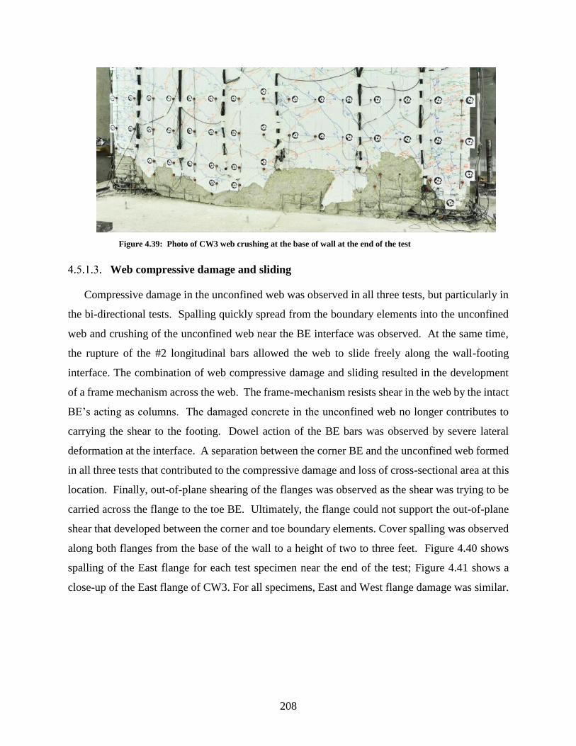
208
Figure 4.39: Photo of CW3 web crushing at the base of wall at the end of the test
Web compressive damage and sliding
Compressive damage in the unconfined web was observed in all three tests, but particularly in
the bi-directional tests. Spalling quickly spread from the boundary elements into the unconfined
web and crushing of the unconfined web near the BE interface was observed. At the same time,
the rupture of the #2 longitudinal bars allowed the web to slide freely along the wall-footing
interface. The combination of web compressive damage and sliding resulted in the development
of a frame mechanism across the web. The frame-mechanism resists shear in the web by the intact
BE’s acting as columns. The damaged concrete in the unconfined web no longer contributes to
carrying the shear to the footing. Dowel action of the BE bars was observed by severe lateral
deformation at the interface. A separation between the corner BE and the unconfined web formed
in all three tests that contributed to the compressive damage and loss of cross-sectional area at this
location. Finally, out-of-plane shearing of the flanges was observed as the shear was trying to be
carried across the flange to the toe BE. Ultimately, the flange could not support the out-of-plane
shear that developed between the corner and toe boundary elements. Cover spalling was observed
along both flanges from the base of the wall to a height of two to three feet. Figure 4.40 shows
spalling of the East flange for each test specimen near the end of the test; Figure 4.41 shows a
close-up of the East flange of CW3. For all specimens, East and West flange damage was similar.
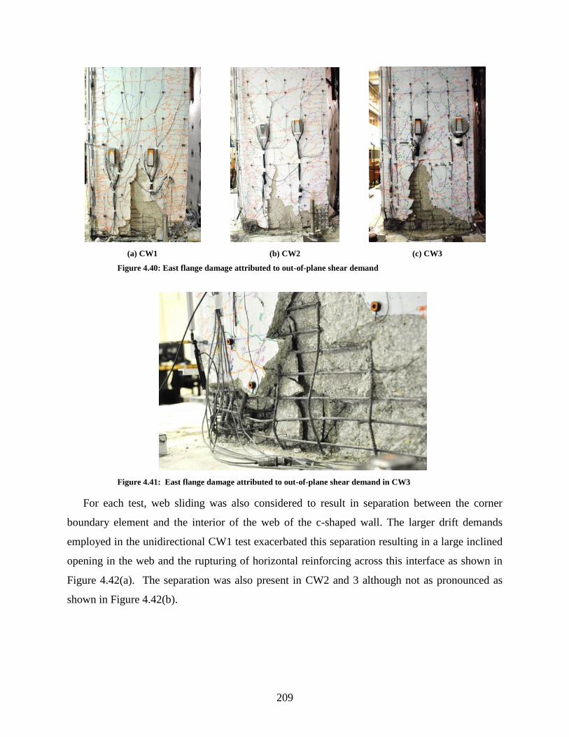
209
(a) CW1 (b) CW2 (c) CW3
Figure 4.40: East flange damage attributed to out-of-plane shear demand
Figure 4.41: East flange damage attributed to out-of-plane shear demand in CW3
For each test, web sliding was also considered to result in separation between the corner
boundary element and the interior of the web of the c-shaped wall. The larger drift demands
employed in the unidirectional CW1 test exacerbated this separation resulting in a large inclined
opening in the web and the rupturing of horizontal reinforcing across this interface as shown in
Figure 4.42(a). The separation was also present in CW2 and 3 although not as pronounced as
shown in Figure 4.42(b).

210
(a) CW1 (b) CW3
Figure 4.42: Boundary element and web separation
4.5.2 Evaluation of demand and capacity
The shear and moment strengths were calculated per ACI 318 and compared with the maximum
shear and moment applied to each c-shaped wall specimen. Given the geometry of the specimen,
three capacities/demands can be compared: strong axis response (loading in the x-direction), weak
axis response with toe in tension (loading in the positive y-direction), and weak axis response with
toe in compression (loading in the negative y-direction). The comparison is tabulated in Table
4.1Table 4.3, Table 4.2, and Table 4.3 respectively.
Table 4.1: Strong axis demands and capacities
Specimen
ID
ACI shear
strength, VnA
Max shear demand,
VmaxA
Vmax/
Vn
Design
strength,
Mn, k -ft (kN m)
Max moment,
Mbase, k -ft (kN
m)
Mbase/Mn
CW1 10.0√f'c*Acv (0.83√f'cAcv) 4.3√f'c*Acv(0. 36√f'cAcv) 0.43 6414 6080 0.95
CW2 9.7√f'c*Acv (0.81√f'cAcv) 4.0√f'c*Acv (0.33√f'cAcv) 0.41 6426 5949 0.93
CW3 9.8√f'c*Acv (0.82√f'cAcv) 4.0√f'c*Acv (0.33√f'cAcv) 0.41 6421 5851 0.91
A Units: f'c in psi (f'c in MPa)
Table 4.2: Weak axis (+Y, toe in tension) demands and capacities
Specimen
ID
ACI shear
strength, VnA
Max shear demand,
VmaxA
Vmax/
Vn
Design strength,
Mn, k -ft (kN m)
Max moment,
Mbase, k -ft (kN
m)
Mbase/Mn
CW2 9.7√f'c*Acv (0.81√f'cAcv) 2.6√f'c*Acv (0.22√f'cAcv) 0.27 1733 1525 0.88
CW3 9.8√f'c*Acv (0.82√f'cAcv) 8.2√f'c*Acv (0.68√f'cAcv) 0.84 2048 B 1613 B 0.79 B A Units: f'c in psi (f'c in MPa)
B Axial load = 746 kip compression
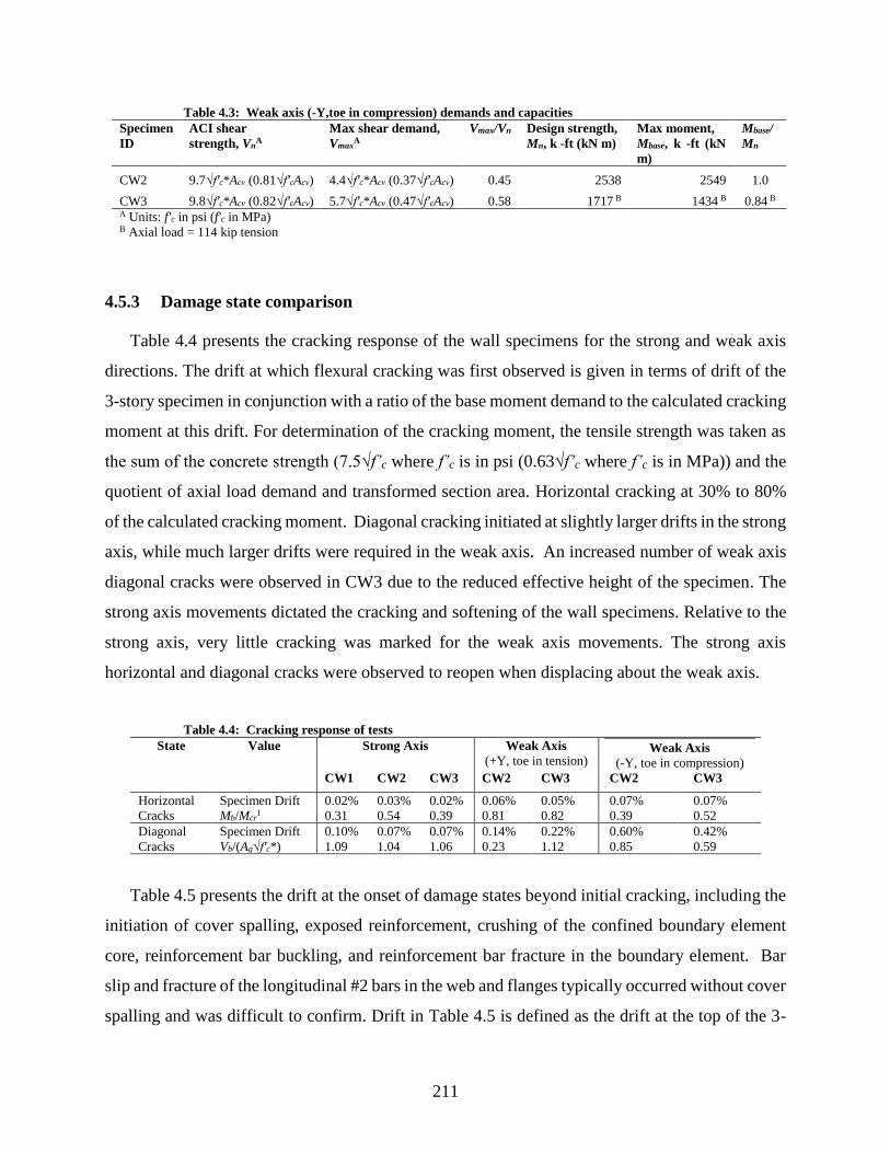
211
Table 4.3: Weak axis (-Y,toe in compression) demands and capacities
Specimen
ID
ACI shear
strength, VnA
Max shear demand,
VmaxA
Vmax/Vn Design strength,
Mn, k -ft (kN m)
Max moment,
Mbase, k -ft (kN
m)
Mbase/
Mn
CW2 9.7√f'c*Acv (0.81√f'cAcv) 4.4√f'c*Acv (0.37√f'cAcv) 0.45 2538 2549 1.0
CW3 9.8√f'c*Acv (0.82√f'cAcv) 5.7√f'c*Acv (0.47√f'cAcv) 0.58 1717 B 1434 B 0.84 B A Units: f'c in psi (f'c in MPa)
B Axial load = 114 kip tension
4.5.3 Damage state comparison
Table 4.4 presents the cracking response of the wall specimens for the strong and weak axis
directions. The drift at which flexural cracking was first observed is given in terms of drift of the
3-story specimen in conjunction with a ratio of the base moment demand to the calculated cracking
moment at this drift. For determination of the cracking moment, the tensile strength was taken as
the sum of the concrete strength (7.5√f’c where f’c is in psi (0.63√f’c where f’c is in MPa)) and the
quotient of axial load demand and transformed section area. Horizontal cracking at 30% to 80%
of the calculated cracking moment. Diagonal cracking initiated at slightly larger drifts in the strong
axis, while much larger drifts were required in the weak axis. An increased number of weak axis
diagonal cracks were observed in CW3 due to the reduced effective height of the specimen. The
strong axis movements dictated the cracking and softening of the wall specimens. Relative to the
strong axis, very little cracking was marked for the weak axis movements. The strong axis
horizontal and diagonal cracks were observed to reopen when displacing about the weak axis.
Table 4.4: Cracking response of tests
State Value Strong Axis Weak Axis
(+Y, toe in tension) Weak Axis
(-Y, toe in compression) CW1 CW2 CW3 CW2 CW3 CW2 CW3
Horizontal Specimen Drift 0.02% 0.03% 0.02% 0.06% 0.05% 0.07% 0.07%
Cracks Mb/Mcr1 0.31 0.54 0.39 0.81 0.82 0.39 0.52
Diagonal
Cracks
Specimen Drift 0.10% 0.07% 0.07% 0.14% 0.22% 0.60% 0.42%
Vb/(Ag√f'c*) 1.09 1.04 1.06 0.23 1.12 0.85 0.59
Table 4.5 presents the drift at the onset of damage states beyond initial cracking, including the
initiation of cover spalling, exposed reinforcement, crushing of the confined boundary element
core, reinforcement bar buckling, and reinforcement bar fracture in the boundary element. Bar
slip and fracture of the longitudinal #2 bars in the web and flanges typically occurred without cover
spalling and was difficult to confirm. Drift in Table 4.5 is defined as the drift at the top of the 3-

212
story specimen. The drifts provide in Table 4.5 are the drifts at the first occurrence of each damage
state in any of the three loading directions; the loading direction is provided.
Table 4.5: Damage response of tests
Damage State Value CW1 CW2 CW3
Cover Spalling Drift 1.49% X 1.44% -Y 0.75% +Y 1
Exposed Reinforcement Drift 1.49% X 1% X and 2% +Y 1.50% +X
Bar buckling Drift 1.49% X 2.25% +Y 1.50% +X
Core crushing Drift 2.19% X 1.50% X 1.98% +Y
Boundary Element Bar fracture Drift 2.19% X 2.50% X 1.64% -Y 1 Spalling occurred in a patched area
4.6 Conclusions
Three C-shaped walls were successfully tested using the methods and loading criteria outlined
in Chapter 3. This chapter has summarized the global load-deformation response of each test and
progression of cracking, yielding, damage states, and failure. While the walls ultimately failed in
a ductile manner, the damage mechanisms leading to failure were precipitated by shear associated
damage of base sliding and web crushing. Based on the visual observations, the damage
mechanism progression was concluded to be the following:
• The onset of sliding and rupture of web vertical reinforcing bars result in a loss of shear
resistance along the web.
• The loss of web shear resistance shifts the load path to the corner boundary element
and compression flange. As a result, the unconfined concrete of the web adjacent to
the corner boundary elements begins to spall and crush.
• As base slip increases, visible deformation and lateral buckling of the longitudinal bars
was observed at the interface of the corner boundary elements and foundation. In
addition, base slip deformation creates out-of-plane shear in the flanges that ultimately
results in vertical cracking and splitting up the height of the first story.
• Significant core crushing of the unconfined web resulted in loss of section and
separation of the web from the corner boundary elements.
• The increasing demand on the corner boundary elements and lateral buckling resulted
in failure of the confinement ties and extensive core crushing.

213
• The vertical and lateral buckling of the longitudinal reinforcing bars in the corner
boundary elements is followed by straightening when loading in the opposite direction.
This cycle of plastic deformation results in fracture and loss of load-carrying capacity.
Regarding the behavior of the uni-directionally loaded test versus the bi-directionally loaded
tests, the following conclusions are made:
• For the strong axis response, all three C-shaped walls reached 91 to 95% of the nominal
moment strength and 41 to 43% of the nominal shear strength. The bi-directional
loading did not impact the strong axis response prior to nominal.
• The damage mechanisms observed were the same for all three tests independent of the
specific changes in loading direction and axial loading; however, bi-directional loading
results in earlier onset of damage and reduced drift capacity.

214
CHAPTER 5: DATA ANALYSIS OF C-SHAPED WALL EXPERIMENTS
5.1 Introduction
Chapter 5 presents the data processing and analytical evaluation of the C-shaped wall tests.
Section 5.2 summarizes the processing and structuring of the raw data from the experimental tests.
Using the processed data, Sections 5.3 to 5.5 describe the data analysis and results for
displacements profiles of the ten-story specimen, spread of reinforcement yielding, and cumulative
energy dissipation of the wall at failure. Section 5.6 analyzes the non-contact displacement field
measurements of the web and flange to produce strain fields of the wall in each direction of
loading. Section 5.7 presents the deformation of each wall test in each axis through the relative
contributions of shear, flexure, base slip, and base rotation to the total wall deformation at each
story over the course of the loading history. The test specimen represented the bottom three stories
of the ten-story building, so the measured deformations do not capture the upper seven stories of
the simulation. Section 5.8 describes the determination of the ten-story displacements using a
model of beam theory for the upper stories, and Section 5.9 utilizes the ten-story displacements to
evaluate the global-load deformation response of the full wall height.
5.2 Data processing
The C-shaped wall experiments were densely instrumented and produced more than 390
channels of data output. Data was measured through three sources: the mixed-mode control
software for application of the loading, the data acquisition system for the physical instruments,
and the Metris Krypton system for non-contact measurements of the wall. Data from each source
was captured at each step of the loading protocol and output to individual tab-delimited text files.
Combining the step data for all instruments of all three walls results in a dataset of approximately
5 million data points. In order to manage this data, the text files were input into a series of data
structures using Matlab. Metadata for each instrument is added to the data structure to identify the
sources, location, and changes to the data. Furthermore, the metadata is used to create relationships
between groups of instruments to aid in the analysis of the overlapping and adjacent instruments.
The data is subsequently processed to remove errors and non-pertinent data.

215
5.2.1 Raw data processing
The raw test data is imported from the text files into the data structure using Matlab in
combination with the metadata associated with each instrument. The instrument type, channel
name, three-dimensional coordinate position, units of measure, and zero step/offset are saved in
the data structure for each instrument imported. A similar data structure was utilized by Birely
(2012) and Turgeon (2011) for the planar and coupled wall experiments; however, the C-shaped
wall tests required key changes to this structure to accommodate the three-dimensional geometry
of the specimens as well as the multi-directional loading history applied. Instrument positions
were recorded in three-dimensions and associated to each flange or the web of the wall as well as
the story. Relationships between adjacent instruments are recorded to accommodate future
evaluations of data measurements at the same location. A graphical representation of the wall
instruments in the resulting data structure is shown in Figure 5.1.

216
Figure 5.1: Graphical representation of wall instruments in the data structure. Dotted lines
represent the extents of the wall, foundation, and cap. Solid dots and lines indicate
instrument locations plotted in 3-D coordinates. Coordinates shown are in inches.
After the initial import of data and metadata, the instruments are processed to remove errors in
the data acquisition, steps associated with starting and stopping the test, and invalid sensor data
from malfunctions before or during the test. Before starting the test, approximately 20% of the
steel strain gauges for each test were not functional. These gauges were likely damaged as a result
of the wall construction through tieing adjacent reinforcing bars, the placement of concrete, or
damage to wires or wire splices. In addition, the inclinometers were found to be non-functional
and produced erroneous data after analysis of CW1 data. The sensors could not be repaired;
consequently, inclinometers were excluded from CW2 and CW3. Furthermore, a number of
Krypton LEDs were determined to have erroneous data during post-processing associated with the
limitations of Krypton camera volume. Despite these shortcomings, over 92% of instrument
channels were maintained for each test. During the course of testing, some instruments become

217
compromised due to wall damage associated with the loading history. The data associated with
these instruments after being compromised is identified in the data and removed to prevent
erroneous results in future analyses. A summary of the instrument processing was documented
for the project deliverable to the data repository (Mock 2013).
To measure the relative changes in displacement from the start of the test, all instruments are
set with a zero-offset value. String potentiometer, linear potentiometer, linear variable
displacement transducer, and Metris Krypton LED readings are zeroed at the first step of loading.
The zero step of each sensor and the corresponding offset value are recorded with each sensor’s
metadata. Concrete strain gauges are zeroed before the specimen is connected to the loading units
in order to capture straining during the connection process and are already represented in the
unprocessed data. Similarly, steel strain gauges are zeroed after connection and just prior to the
initial loading within the data acquisition software.
A data verification document (Mock, Birely, and Turgeon 2013a, 2013b, 2013c) containing
the response of each instrument and its associated metadata was produced to verify and examine
the data for errors prior to performing subsequent analyses. An example of the data document
output shown in Figure 5.2.

218
Figure 5.2: Example of data verification document indicating the metadata for the
instrument and measured loading history with key drift levels of the test notated.
5.2.2 Data archival
The complete dataset of each test was archived on the Design Safe Cyber-Infrastructure
initiative for use by future researchers (Birely et al. 2014; Behrouzi et al. 2014; Mock et al. 2014).
The archived data included the raw unprocessed data, the processed data, and metadata of each
instrument. In addition, drawings of wall geometry, reinforcing, and instrument locations were
provided as well as material test results for the concrete and steel. An example of the metadata to
associate the data with the physical instruments is shown in Figure 5.3. Photographs, videos, and
testing notes associated with each data of testing were also uploaded. In total, more than 850 GB
of data were archived.

219
Figure 5.3: Metadata example of LEDs for data archival
5.3 Energy dissipation
Hysteretic energy dissipation is a measure of the structural wall’s ability to absorb energy
through inelastic deformations (Elnashai and Di Sarno 2008). Energy dissipation is measured as
the total area contained inside the hysteric loop of base shear versus third-story displacement. For
U.S. customary units, the resulting measure of energy is kip-inches. The energy dissipation is
measured for each direction of loading and each load cycle independently. The energy dissipation
is measured cumulatively throughout the loading history to assess the total inelastic response of
the wall. Figure 5.4 provides the cumulative strong axis energy dissipation at each drift level.
Figure 5.5 provides the cumulative weak axis energy dissipation at each drift level. Figure 5.6
provides the combined cumulative energy dissipation for the bi-directional loading history per
strong axis drift level.
Observing the strong axis response in Figure 5.4, the unidirectional test CW1 exhibits 50% to
100% greater energy dissipation than CW2 and CW3 respectively. The bi-directional loading of
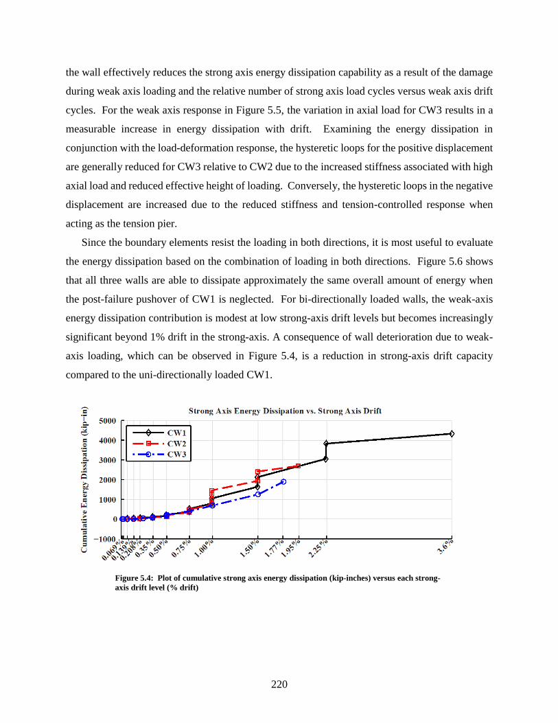
220
the wall effectively reduces the strong axis energy dissipation capability as a result of the damage
during weak axis loading and the relative number of strong axis load cycles versus weak axis drift
cycles. For the weak axis response in Figure 5.5, the variation in axial load for CW3 results in a
measurable increase in energy dissipation with drift. Examining the energy dissipation in
conjunction with the load-deformation response, the hysteretic loops for the positive displacement
are generally reduced for CW3 relative to CW2 due to the increased stiffness associated with high
axial load and reduced effective height of loading. Conversely, the hysteretic loops in the negative
displacement are increased due to the reduced stiffness and tension-controlled response when
acting as the tension pier.
Since the boundary elements resist the loading in both directions, it is most useful to evaluate
the energy dissipation based on the combination of loading in both directions. Figure 5.6 shows
that all three walls are able to dissipate approximately the same overall amount of energy when
the post-failure pushover of CW1 is neglected. For bi-directionally loaded walls, the weak-axis
energy dissipation contribution is modest at low strong-axis drift levels but becomes increasingly
significant beyond 1% drift in the strong-axis. A consequence of wall deterioration due to weak-
axis loading, which can be observed in Figure 5.4, is a reduction in strong-axis drift capacity
compared to the uni-directionally loaded CW1.
Figure 5.4: Plot of cumulative strong axis energy dissipation (kip-inches) versus each strong-
axis drift level (% drift)
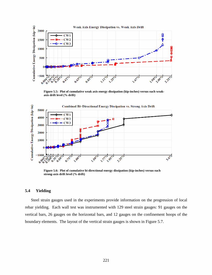
221
Figure 5.5: Plot of cumulative weak axis energy dissipation (kip-inches) versus each weak-
axis drift level (% drift)
Figure 5.6: Plot of cumulative bi-directional energy dissipation (kip-inches) versus each
strong-axis drift level (% drift)
5.4 Yielding
Steel strain gauges used in the experiments provide information on the progression of local
rebar yielding. Each wall test was instrumented with 129 steel strain gauges: 91 gauges on the
vertical bars, 26 gauges on the horizontal bars, and 12 gauges on the confinement hoops of the
boundary elements. The layout of the vertical strain gauges is shown in Figure 5.7.

222
Figure 5.7: Vertical steel strain gauge layout
As noted in Section 5.2.1, about 20% of the strain gauges were not functional at the time of
testing. For the functional gauges, the strains were measured at each load step. a constitutive
model was thn applied to the strain history to evaluate the stress response. The hysteretic stress-
strain relationship of the reinforcing bars is based upon the cyclic bar model developed by Hoehler
and Stanton (2006). Example results for a strain gauge in the toe BE of the West flange at 15
inches above the base for CW2 are shown in Figure 5.8 and Figure 5.9.

223
Figure 5.8: Total strain and decomposed strain components determined from the Hoehler-
Stanton model using data from specimen CW2
Figure 5.9: Stress-strain history determined from Hoehler-Stanton model using data from
specimen CW2
The resulting yield of vertical reinforcing bars is plotted at the nominal strength in the strong
axis (0.75% drift) in Figure 5.10 and Figure 5.11. Figure 5.10 shows the progression of tension
yielding, strain hardening, and gauges which yielded in compression prior to yielding in tension.
Similarly, Figure 5.11 shows the progression of compression yielding, strain hardening, and
gauges which yielded in tension prior to yielding in compression. The same plots are provided for
the yield progression after significant damage in Figure 5.12 and Figure 5.13. For the comparison
of the yield progression after damage, CW1 and CW3 are plotted at the end of the tests but prior
to the pushover, and CW2 is plotted at the end of the standard cyclic loading but prior to the
simultaneous loading the strong and weak axis directions (see Section 3.3.4.2).
For a direct comparison of yielding relative to drift level, the strain gauge history is considered
first at the point of nominal strength. At this point, tension yielding is widespread across the entire

224
first floor and the boundary element of the second floor. In addition, strain hardening in tension
was observed primarily in the boundary element at the first floor. When comparing CW1 to CW2
to assess the impact of bi-directional loading, additional yielding and strain hardening is observed
in both the East and West flanges and toe boundary elements. Compression yielding after yielding
in tension is also observed in the toe boundary elements in CW2 that was not present in CW1. For
the impact of axial loading, CW3 does not reveal a significant difference in yield progression. In
fact, CW3 exhibits reduced yielding overall when compared to CW1 and CW2 which is believed
to be a result of the reduced number of strong axis load cycles prior to reaching the nominal
strength.
At the end of the standard loading protocol, tension yielding is observed for the majority of
gauges in the bottom two floors for all three tests. Strain hardening along the boundary elements
has spread, but the general yield pattern is not significantly different from the pattern at nominal
strength. However, the pattern of compression yielding progressed during the damage cycles of
the wall loading. Post-peak, a majority of the boundary elements gauges in first-floor yield in
compression after having yielded in tension for all three tests. Comparing CW1 to CW2, the web
of CW1 exhibits increased compression yielding as a result of the larger drift demands imposed.
The sliding and compression damage of the unconfined web is evident with the addition of yielded
gauges adjacent to the corner boundary elements. Comparing CW3 to CW1 and CW2, the vertical
bars along the center of the web have yielded in compression as a result of the increased axial load
when acting as the tension pier.
For the strain gauges on the horizontal reinforcing bars, four bars in the web yielded in tension
for CW1, no bars yielded in tension for CW2, and three bars in the web one bar on the East flange
yielded in tension for CW3. For the strain gauges on the confinement hoops, yielding in tension
was observed in the corner boundary elements for CW3 only consistent with high axial load and
extensive crushing observed during the test.
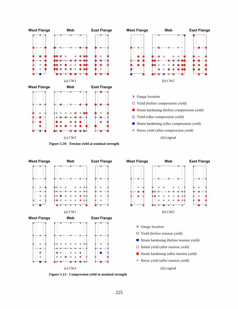
225
(a) CW1 (b) CW2
(c) CW3 (d) Legend
Figure 5.10: Tension yield at nominal strength
(a) CW1 (b) CW2
(c) CW3 (d) Legend
Figure 5.11: Compression yield at nominal strength
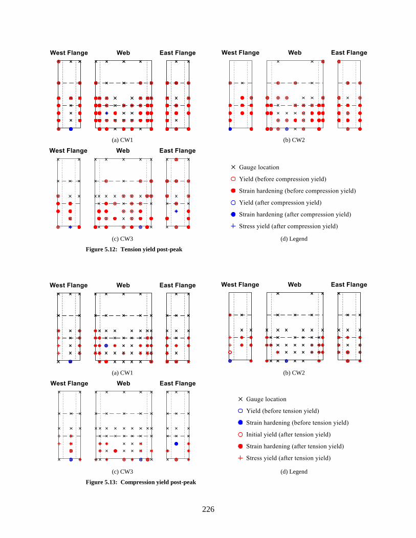
226
(a) CW1 (b) CW2
(c) CW3 (d) Legend
Figure 5.12: Tension yield post-peak
(a) CW1 (b) CW2
(c) CW3 (d) Legend
Figure 5.13: Compression yield post-peak

227
5.5 Base slip
The experimental tests indicated that base slip accounted for a significant portion of the total
deformation post-peak. The base slip was measured using string potentiometers at each end of the
wall and by a row or Krypton LEDs along the base of the web and East flange. The base slip
measured from each source varied as a result of the local damage occurring where the individual
instruments were anchored.
The Krypton LED measurements were averaged across the length of the wall; however, the
LEDs attached to the corner boundary elements became compromised after the onset of spalling.
As spalling progressed, the measurement of base slip using the Krypton LEDs becomes limited to
those attached to the unconfined web only. As shown in Figure 4.42, the base sliding resulted in
a separation between the boundary elements and the unconfined web. This results in a base slip
measurement along the unconfined web that is significantly larger than the base slip at the
boundary elements. While this measurement of slip between the boundary elements is an
important local damage phenomenon, the global displacement of the wall is limited by the
boundary elements acting as dowels to the foundation. Consequently, the Krypton LEDs provide
information on the global base slip only up to the point of spalling.
String potentiometers were anchored into the corner boundary elements at each end of the web
wall for measuring the strong axis base slip. A single string potentiometer at each toe boundary
element was provided for measuring the weak axis base slip. These instruments became
compromised during core crushing of the boundary elements at which point the anchorage was
dislodged. As the string potentiometers provided a more stable measurement of the base slip for
a longer duration of the tests, these instruments were utilized for assessing the global base slip.
The average base slip, as well as the base slip at each end of the web, is plotted by step for CW1,
CW2, and CW3 in Figure 5.14, Figure 5.15, and Figure 5.16 respectively.

228
Figure 5.14: CW1 Base slip measured by string potentiometers
Figure 5.15: CW2 Base slip measured by string potentiometers
Figure 5.16: CW3 Base slip measured by string potentiometers
-2.5
-2
-1.5
-1
-0.5
0
0.5
1
1.5
2
2.5
0 200 400 600 800 1000 1200 1400 1600
Dis
pla
cem
en
t (i
n)
Step
West Web String Pot East Web String Pot Average
-1.5
-1
-0.5
0
0.5
1
1.5
0 500 1000 1500 2000 2500 3000
Dis
pla
cem
en
t (i
n)
Step
West Web String Pot East Web String Pot Average
-1.5
-1
-0.5
0
0.5
1
1.5
0 500 1000 1500 2000
Dis
pla
cem
en
t (i
n)
Step
West Web String Pot East Web String Pot Average

229
The base slip measured pre-peak is small, and there is not a meaningful difference between the
base slip measured at each end of the wall. However, as the wall becomes damaged post-peak, the
base slip measurements begin to deviate from each other indicating a lateral elongation between
the instruments. Elongation of structural concrete is a known phenomenon resulting from inelastic
deformations in the plastic hinge zone. Vertical elongation associated with flexural response and
lateral elongation associated with shear response has been observed in prior tests of structural walls
(Palermo and Vecchio 2002). In these C-shaped wall tests, the elongation is a result of the dowel
action occurring in the corner boundary elements with the foundation. While loading in one
direction, the boundary element bars buckle in the direction of the sliding; however, these same
bars straighten in tension after load reversal, and minimal slip is observed. Thus, a larger measure
of base slip is observed in the boundary element in compression when compared to the boundary
element in tension. While this second order phenomenon does not directly impact the global
response of the wall, it is a representative measure of the damage the precipitates the loss of load
carrying capacity (buckling-rupture failure). The average base slip maintains a value of
approximately zero at the points of zero displacement throughout the loading. For subsequent
evaluations considering base slip, the average measurement of the string potentiometers is utilized.
The resulting hystereses of base versus base slip for each wall test are shown in Figure 5.17.

230
(a) CW1 Base Shear vs. Base Slip (b) CW2 Base Shear vs. Base Slip
(c) CW3 Base Shear vs. Base Slip (d) Envelope of Base Shear vs. Base Slip
Figure 5.17: C-Wall Base Shear versus Base Slip
5.6 Strain fields
The high-resolution measurements collected using the Nikon Metrology/Krypton system
enabled the calculation of average strain fields for the lower two floors of both the web and east
flange. Three-dimensional displacement data were measured at 155 discrete points on the bottom
two stories of the web and East flange of each specimen for each load step. The coordinate
positions are shown in Figure 5.3. The grid of displacements points is analogous to a finite element
mesh and can be analyzed in a similar manner.
-1 -0.5 0 0.5 1
-200
-150
-100
-50
0
50
100
150
200
Slip (in)
Sh
ea
r (k
ips
)
CW6 Base Shear vs. Base Slip
-1 -0.5 0 0.5 1
-200
-150
-100
-50
0
50
100
150
200
Slip (in)
Sh
ea
r (k
ips
)
CW7 Base Shear vs. Base Slip
-1 -0.5 0 0.5 1
-200
-150
-100
-50
0
50
100
150
200
Slip (in)
Sh
ea
r (k
ips
)
CW8 Base Shear vs. Base Slip
-1 -0.5 0 0.5 1
-200
-150
-100
-50
0
50
100
150
200
Slip (in)
Sh
ea
r (k
ips
)
C-Wall Envelope Base Shear vs. Base Slip
CW6
CW7
CW8

231
The initial position was measured for each LED prior to loading and the relative displacement
of each LED during the loading history was measured at each step. Using this displacement data,
the average strains across each region is determined using a bilinear quadrilateral finite element
(Hughes 2000). A similar approach was utilized by Birely (2012) and Turgeon (2011) for the
planar and coupled wall experiments; however, the C-shaped walls required consideration of the
two separate planes of LED targets with a three-dimensional coordinate system. The bilinear
element formulation is utilized to produce measurements of the horizontal, vertical, and shear
strain for each region. Subsequently, the principal strains and maximum shear strain are
determined:
( )2
2
1,22 2
x z x zxz
+ − = +
(4.1)
( )2
2
max2
x zxz
− = +
(4.2)
The finite element mesh is coarse relative to the dimensions of the test specimen. As a result,
significant discontinuities of the strain field are observed between elements. In order to provide a
continuous strain field, the data is smoothed by averaging the measures of strain at each node from
the surrounding elements. A weighting is applied to the individual measurements corresponding
to the tributary area of the area of each element from which the strains were determined.
A comparison of the principal compressive strain during strong axis loading in the uni-
directional test (CW1) versus the bi-directional test (CW3) is given in Figure 5.18. The
comparison at 0.75% drift reveals increased compressive stress demand in the corner boundary
element of the web as well as a more non-linear strain distribution across the flange. The formation
of compressive struts across the web are apparent in both walls. The comparison at 1.50% drift
reveals significantly lower compressive stress demands in CW3 overall due to the loss of load
carrying capacity at this point in the loading history. Loss of confinement and crushing of the
corner boundary element (BE) in CW3 results in the compressive stress being carried in the
unconfined web and toe boundary element of the flange. While the compressive strain demand
across the flange of CW1 remains largely uniform, the demand across the flange of CW3 is
increasingly nonlinear as a result of the bi-directional loading.

232
(a) CW1 at 0.75% drift (b) CW3 at 0.75% drift
(c) CW1 at 1.50% drift (d) CW3 at 1.50% drift
Figure 5.18: Plot of second principal strain during strong axis loading. Color-bar ranges
from zero millistrain (grey) to negative six millistrain (purple).
A comparison of the vertical strain during weak axis loading with the web in compression for
CW2 and CW3 is given in Figure 5.19. The comparison at ~1.2% drift reveals relatively uniform
vertical strain distribution across the web for both walls. The comparison at ~2.0% drift reveals a
non-linear strain distribution across the web for both walls as a result of the damage during bi-
directional loading. CW2 indicates increased compressive stress to the left corner BE after the
right corner BE experienced damage. Similarly, the loss of confinement and crushing of the corner
boundary element on both sides of CW3 results in demand being carried in the unconfined web
between the boundary elements.
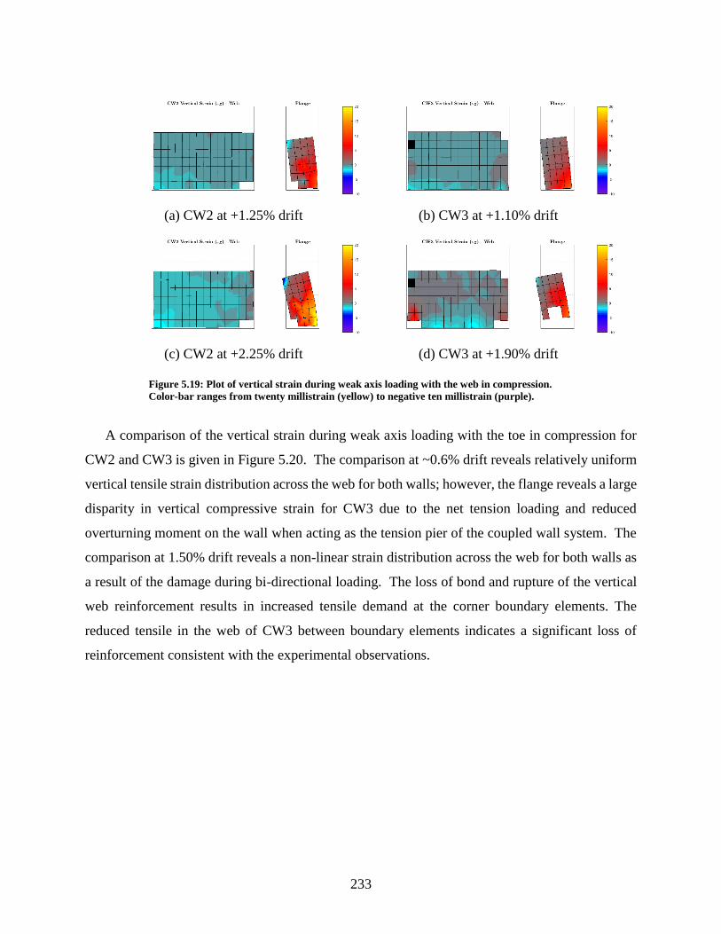
233
(a) CW2 at +1.25% drift (b) CW3 at +1.10% drift
(c) CW2 at +2.25% drift (d) CW3 at +1.90% drift
Figure 5.19: Plot of vertical strain during weak axis loading with the web in compression.
Color-bar ranges from twenty millistrain (yellow) to negative ten millistrain (purple).
A comparison of the vertical strain during weak axis loading with the toe in compression for
CW2 and CW3 is given in Figure 5.20. The comparison at ~0.6% drift reveals relatively uniform
vertical tensile strain distribution across the web for both walls; however, the flange reveals a large
disparity in vertical compressive strain for CW3 due to the net tension loading and reduced
overturning moment on the wall when acting as the tension pier of the coupled wall system. The
comparison at 1.50% drift reveals a non-linear strain distribution across the web for both walls as
a result of the damage during bi-directional loading. The loss of bond and rupture of the vertical
web reinforcement results in increased tensile demand at the corner boundary elements. The
reduced tensile in the web of CW3 between boundary elements indicates a significant loss of
reinforcement consistent with the experimental observations.

234
(a) CW2 at -0.75% drift (b) CW3 at -0.56% drift
(c) CW2 at -1.50% drift (d) CW3 at -1.50% drift
Figure 5.20: Plot of vertical strain during weak axis loading with the toe in compression.
Color-bar ranges from twenty millistrain (yellow) to negative ten millistrain (purple).
There are several observations that can be made by comparing the aforementioned C-shaped
wall tests to planar walls from Birely (2012). First, vertical strain fields indicate that for all C-
shaped wall specimens, and particularly the bi-directionally loaded CW2 and 3, the neutral axis
depth when loaded in the strong-axis direction is considerably shallower than for the planar walls,
especially at higher drift levels. Second, the onset of substantial compressive straining occurs at a
lower drift demand for the planar walls compared to the C-shaped wall web. The differences in
response between planar and C-shaped wall types can be attributed to the contribution of the flange
in carrying compressive demand.
From the strain fields the following conclusions can be drawn for the C-shaped wall tests:
• The wall flanges contribute to carrying a rather significant portion of the compression
demand thus reducing the demand on the wall web. As a result, the overall wall failure
is tension-controlled rather than compression-controlled as observed in the planar
walls;
• There is significant shear demand in the wall web, particularly in tension regions. With
increasingly drift level, the shear demand in the flange becomes more significant along
the base of the wall and in the boundary elements. Nonlinear strain distribution in the
flanges appears to have a more rapid onset and greater magnitude in the bi-directionally
loaded walls.

235
• The stiffness discontinuity in transitioning from a lightly-reinforced web to boundary
element/flange results in a region of tensile straining (and high shear straining) along
the edge of the compression boundary element.
5.7 Components of deformation
Another metric to evaluate the wall response is to compare the individual contributions of base
slip, base rotation, shear deformation, and flexural deformation to the total deformation throughout
the loading history. The non-contact displacement data from the Krypton system in conjunction
with an array of linear potentiometers on the back face of the wall are utilized to determine these
components of deformation. Methods of measuring the rotations, flexural deformations and shear
deformations using these instruments are described herein and compared. The resulting
components of deformation are produced for each wall experiment and compared.
5.7.1 Rotations
Rotations at each floor of the wall were determined using the measured vertical displacements
at various points on the wall. Vertical displacements were measured by the Krypton system on
the bottom two stories of the web and East flange. Rotations were determined from the slope of a
line of best fit to the vertical displacement measurements across the web or flange. Vertical
displacements were also measured by an array of nine vertical linear potentiometers located at key
locations around the wall geometry as shown in Figure 5.21. Considering the small angle
approximation, the rotation, , is measured from the linear potentiometers as the difference in
vertical displacement, ( )1 2,V V , across the panel divided by the panel length, :
1 2V V
−
=
(4.3)

236
Figure 5.21: Vertical linear potentiometer positions at each story of the C-shaped wall
specimen
The prior tests of the planar walls also utilized Krypton measurements and linear
potentiometers for measuring rotation (Birely 2012); however, the C-shaped walls proved more
challenging due to the non-symmetric geometry and shallow depth of compression associated with
a flanged wall. The third method of rotation calculation was devised to take advantage of all nine
measures of vertical displacement. A planar surface was fit to the data using the three-dimensional
plan positions and vertical displacements of each discrete point. The slope of the surface in the X-
direction and Y-direction are used as the measure of rotation in the strong axis and weak axis
loading respectively. Figure 5.22 illustrates an example of the surface fitting to the nine
displacement measures.
Figure 5.22: Plane of best fit for vertical displacement measurements
For a comparison of the measurements using each method, Figure 5.23 plots the first-floor
rotation at 0.75% drift in the strong axis and similar magnitudes of rotations in the weak axis
(0.83% drift for CW2 and 1.24% drift for CW3). The traditional method of measurement using
the linear potentiometers does not consistently match the measurements of the Krypton nor the
plane rotation. This is particularly true for the bi-directionally loaded tests in which there are some
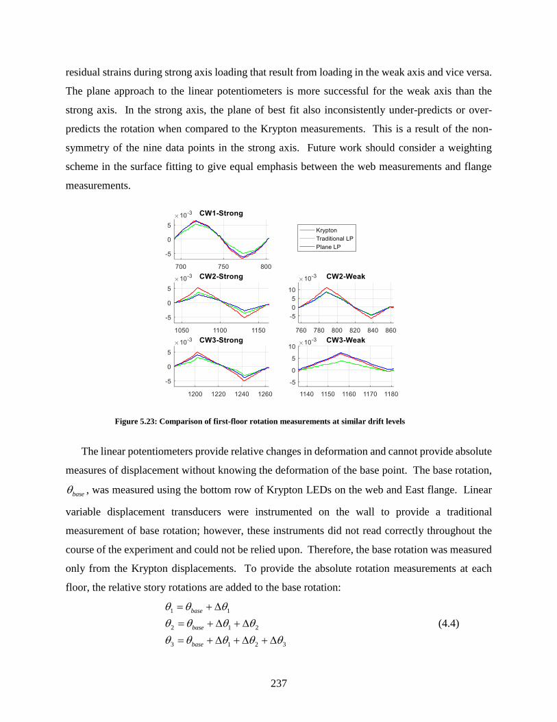
237
residual strains during strong axis loading that result from loading in the weak axis and vice versa.
The plane approach to the linear potentiometers is more successful for the weak axis than the
strong axis. In the strong axis, the plane of best fit also inconsistently under-predicts or over-
predicts the rotation when compared to the Krypton measurements. This is a result of the non-
symmetry of the nine data points in the strong axis. Future work should consider a weighting
scheme in the surface fitting to give equal emphasis between the web measurements and flange
measurements.
Figure 5.23: Comparison of first-floor rotation measurements at similar drift levels
The linear potentiometers provide relative changes in deformation and cannot provide absolute
measures of displacement without knowing the deformation of the base point. The base rotation,
base , was measured using the bottom row of Krypton LEDs on the web and East flange. Linear
variable displacement transducers were instrumented on the wall to provide a traditional
measurement of base rotation; however, these instruments did not read correctly throughout the
course of the experiment and could not be relied upon. Therefore, the base rotation was measured
only from the Krypton displacements. To provide the absolute rotation measurements at each
floor, the relative story rotations are added to the base rotation:
1 1
2 1 2
3 1 2 3
base
base
base
= +
= + +
= + + +
(4.4)

238
An example of the resulting base rotation and rotations for each floor are shown for CW3 in Figure
5.24.
Figure 5.24: CW3 absolute floor rotations using linear potentiometers
5.7.2 Flexural and shear deformations
Using the strain data from the Krypton displacement measurements (see Section 5.6), the shear
deformation from each row of finite elements can be determined by a summation of the average
shear strain in the element integrated over each element’s area. The total shear deformation of a
story is then defined by the from the base of the wall up to the height at which the shear deformation
is desired. Using the four-node quadrilateral approach, the shear strain of a row is defined by the
summation of the product of shear strain in each finite element and ratio of element length to wall
length.
#
1
colsr r cavg c
c tot
=
=
(4.5)
The shear deformation of each row is determined by the average shear deformation of the row
multiplied by the height of the elements in the row. The total shear deformation of the story is
obtained by the summation of shear deformation in each row of elements.
#
,
1
rowsr r
x shear avg e
r
h=
= (4.6)

239
Similarly, the flexural deformation can be determined by integrating the average curvature of the
cross section over the height of interest. The average curvature and flexural deformation are
obtained by,
#
1
colsr r cavg c
c tot
=
=
(4.7)
#
,
1
rowsr r
x flexure avg e
r
h=
= (4.8)
For the second and third story of the wall specimens, the Krypton LEDs did not extend over
the full height of those stories. As a result, the Krypton could only be used to determine shear and
flexural deformations in the first story. The upper two stories utilized the array of vertical and
diagonal displacement transducers along the backside of the web and flange as shown in Figure
5.25.
Figure 5.25: Array of linear potentiometers utilized for determining shear and flexural
deformations in the second and third story of the wall specimen
The determination of shear and flexural deformations using linear potentiometers has
historically neglected the interaction of shear and flexure on the displacement measurements.
Figure 5.26 indicates the idealized flexural and shear deformation of a given panel of vertical and
diagonal displacement transducers.

240
(a) Flexure (b) Shear
Figure 5.26: Idealized shear and flexural deformation (adapted from Massone and Wallace
(2004))
The flexural deformation is determined as the product of the story rotation and height. The story
rotation is considered to be the difference in vertical deformation divided the panel length using
the small angle approximation:
1 2
,flex original
V Vh h
− = =
(4.9)
The average shear deformation across the panel is determined using the change in length of the
diagonals and the height of the panel:
( ) ( )2 2
2 2
1 2
,2
shear shear
shear original
D h D h− − − =
(4.10)
Two problems are observed for this approach, first the flexural deformation assumes a uniform
distribution of curvature over the height of the panel. The uniform distribution is generally a false
assumption in the plastic hinge region of reinforced concrete wall. Second, the measurement of
displacement in the diagonal transducers will include a component of the vertical deformation
associated with flexure. To account for these issues, a correction factor, alpha, was introduced
(Massone and Wallace 2004).
The correction factor represents the normalized distance from the top of the story to the
centroid of curvature. A value of 0.5 indicates a uniform curvature distribution while a value of
0.67 indicates a triangular distribution. For reinforced concrete outside the elastic range, the
neutral axis depth will be shallow and triangular distribution is a better approximation of the

241
curvature. Massone and Wallace (2004) conducted a parametric study of the value of the
correction factor to verify that the value 0.67 is appropriate in slender concrete walls. Utilizing a
uniform curvature distribution was observed to overestimate shear deformations. After
introducing the correction factor, the corrected measures of shear and flexural deformations are
given by the following equations:
( ),flex flex original =
(4.11)
1 2
,
1
2shear shear original
V Vh
− = + −
(4.12)
5.7.3 Results
For evaluating the drift contributions, the Krypton data was only available for measuring the
base deformations and first-floor deformations. The Krypton LEDs on the second floor only
covered the bottom 36 inches of the 48-inch story height. At the second floor and third floor, shear
and flexure components are calculated using the linear potentiometers previously described.
Figure 5.27, Figure 5.28, and Figure 5.29 display the resulting deformation components of the
walls up to 1% drift. The components of deformation during the initial phases of loading do not
equal the total deformation due to instrumentation’s limitations of measuring small displacements
measured during elastic and cracking phases of the wall loading. Similarly, the components do
not equal the total deformation after wall damage compromises the anchorage of the instruments
into the wall which is observed in CW3 between the 0.5% and 1.0% drift level.
A general comparison of strong axis response in Figure 5.27 reveals that shear and flexural
deformations contribute nearly equally up to about 0.5% drift. During yielding of the
reinforcement and up to the nominal strength at 0.75% drift, the flexural deformation of the first
floor begins to dominate the response. Shear deformations remain relatively constant throughout
the loading history tapering off only marginally during the formation of the plastic hinge in the
first floor. In addition, the base slip and base rotation begin increasing around the nominal strength
and have become a significant portion (20%) of the deformation at 1% drift.
When comparing the uni-directional test to the bi-directional tests, increased base slip and base
rotation are observed in CW3. The tensile loading to the tension pier of the coupled wall system
creates increased demand on the vertical reinforcement of the wall web leading to an earlier
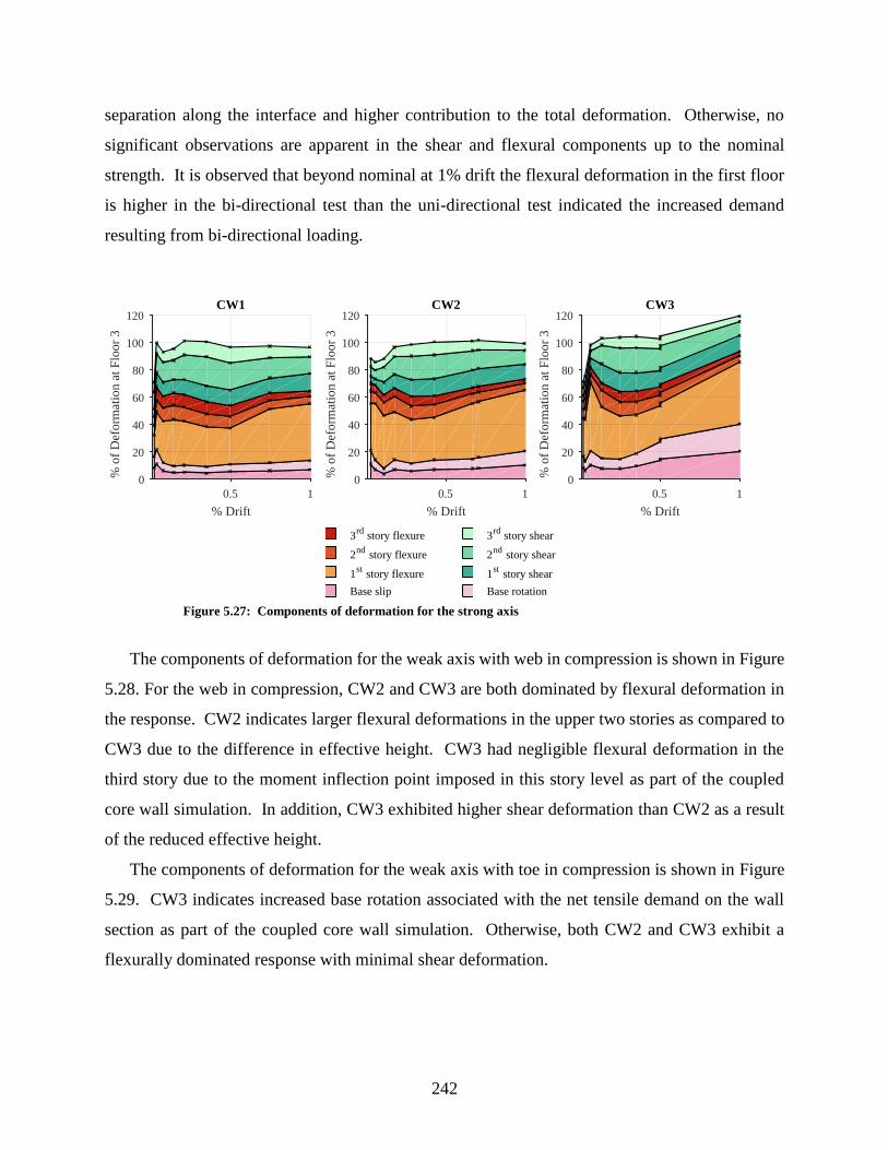
242
separation along the interface and higher contribution to the total deformation. Otherwise, no
significant observations are apparent in the shear and flexural components up to the nominal
strength. It is observed that beyond nominal at 1% drift the flexural deformation in the first floor
is higher in the bi-directional test than the uni-directional test indicated the increased demand
resulting from bi-directional loading.
Figure 5.27: Components of deformation for the strong axis
The components of deformation for the weak axis with web in compression is shown in Figure
5.28. For the web in compression, CW2 and CW3 are both dominated by flexural deformation in
the response. CW2 indicates larger flexural deformations in the upper two stories as compared to
CW3 due to the difference in effective height. CW3 had negligible flexural deformation in the
third story due to the moment inflection point imposed in this story level as part of the coupled
core wall simulation. In addition, CW3 exhibited higher shear deformation than CW2 as a result
of the reduced effective height.
The components of deformation for the weak axis with toe in compression is shown in Figure
5.29. CW3 indicates increased base rotation associated with the net tensile demand on the wall
section as part of the coupled core wall simulation. Otherwise, both CW2 and CW3 exhibit a
flexurally dominated response with minimal shear deformation.
CW1
0.5 1
% Drift
0
20
40
60
80
100
120
%o
fD
efo
rmat
ion
atF
loo
r3
CW2
0.5 1
% Drift
0
20
40
60
80
100
120
%o
fD
efo
rmat
ion
atF
loo
r3
CW3
0.5 1
% Drift
0
20
40
60
80
100
120
%o
fD
efo
rmat
ion
atF
loo
r3
Base slip
1st
story flexure
2nd
story flexure
3rd
story flexure
Base rotation
1st
story shear
2nd
story shear
3rd
story shear
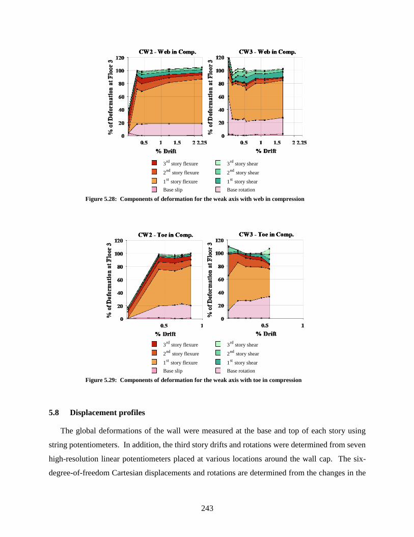
243
Figure 5.28: Components of deformation for the weak axis with web in compression
Figure 5.29: Components of deformation for the weak axis with toe in compression
5.8 Displacement profiles
The global deformations of the wall were measured at the base and top of each story using
string potentiometers. In addition, the third story drifts and rotations were determined from seven
high-resolution linear potentiometers placed at various locations around the wall cap. The six-
degree-of-freedom Cartesian displacements and rotations are determined from the changes in the
Base slip
1st
story flexure
2nd
story flexure
3rd
story flexure
Base rotation
1st
story shear
2nd
story shear
3rd
story shear
Base slip
1st
story flexure
2nd
story flexure
3rd
story flexure
Base rotation
1st
story shear
2nd
story shear
3rd
story shear

244
length of the seven sensors relative to the control point indicated in Figure 3.16. Furthermore, the
non-contact displacement measurements from the Krypton system are utilized to supplement and
validate the displacement fields at each story and in-between.
Since the experimental load-displacement history is available only for the bottom three stories,
the load-displacement history of the upper seven stories is determined using Timoshenko beam
theory based on the work of Birely (2012) for the planar walls. From the experimentally measured
base moment and base shear, the ASCE 7 Equivalent Lateral Force distribution can be back-
calculated to determine the theoretical load distribution imposed over the ten-story building, as
shown in Figure 5.30 (a). From statics, the resulting shears and moments at each story are
determined and shown in Figure 5.30 (b) and (c) respectively.
The imposed theoretical shear and moment distribution are used to approximate the
displacements of the upper seven stories from beam theory. The fixed-end (interface) deformations
and the deformations in the bottom three stories are known from the experimental measurements.
The base slip is considered a rigid-body motion of the structure and is not included in the beam
theory formulation. After calculation, the base slip is added to each of the calculated displacements
of the upper seven stories. The upper seven stories are considered as a cantilever beam extending
from the deformed configuration of the third story with the theoretically imposed shear and
moment distribution. Figure 5.30 (d) reveals the displacement when considered as a rigid member,
the additional flexural displacement when evaluated with Euler-Bernoulli beam theory, and the
additional shear displacement when evaluated with the Timoshenko beam theory.

245
(a) (b) (c) (d)
Figure 5.30: Example of displacement profile determination (Specimen CW2 at 0.35% drift)
The use of beam theory depends upon the selected flexural and shear stiffness values for the
cross-section. The use of gross section properties would underestimate the deflection due to the
presence of cracking. Various values of flexural and shear stiffness for the upper seven stories
were compared to select ratios of these values from the gross section properties (Birely 2012). A
comparison of two ratios and their representative effects on the ten-story drifts for the normalized
moment envelope is given in Figure 5.31 for each wall specimen. The plot reveals a negligible
difference between these selections, consistent with the previous work of Birely for the planar
walls. Subsequent use of the ten-story drifts is based upon using 35% of the gross flexural stiffness
and 15% of the gross shear stiffness.
0 0.5 1 1.5 20
1
2
3
4
5
6
7
8
9
10
Disp. (in)
Rigid
Euler
Timoshenko
Meas.(0-3)
0 50 100 150 2000
1
2
3
4
5
6
7
8
9
10
Shear (kip)
Theo
Meas
0 2000 4000 60000
1
2
3
4
5
6
7
8
9
10
Moment (kip-ft)
Theo
Meas
3.2
6.4
9.6
13
16
19
23
26
29
32
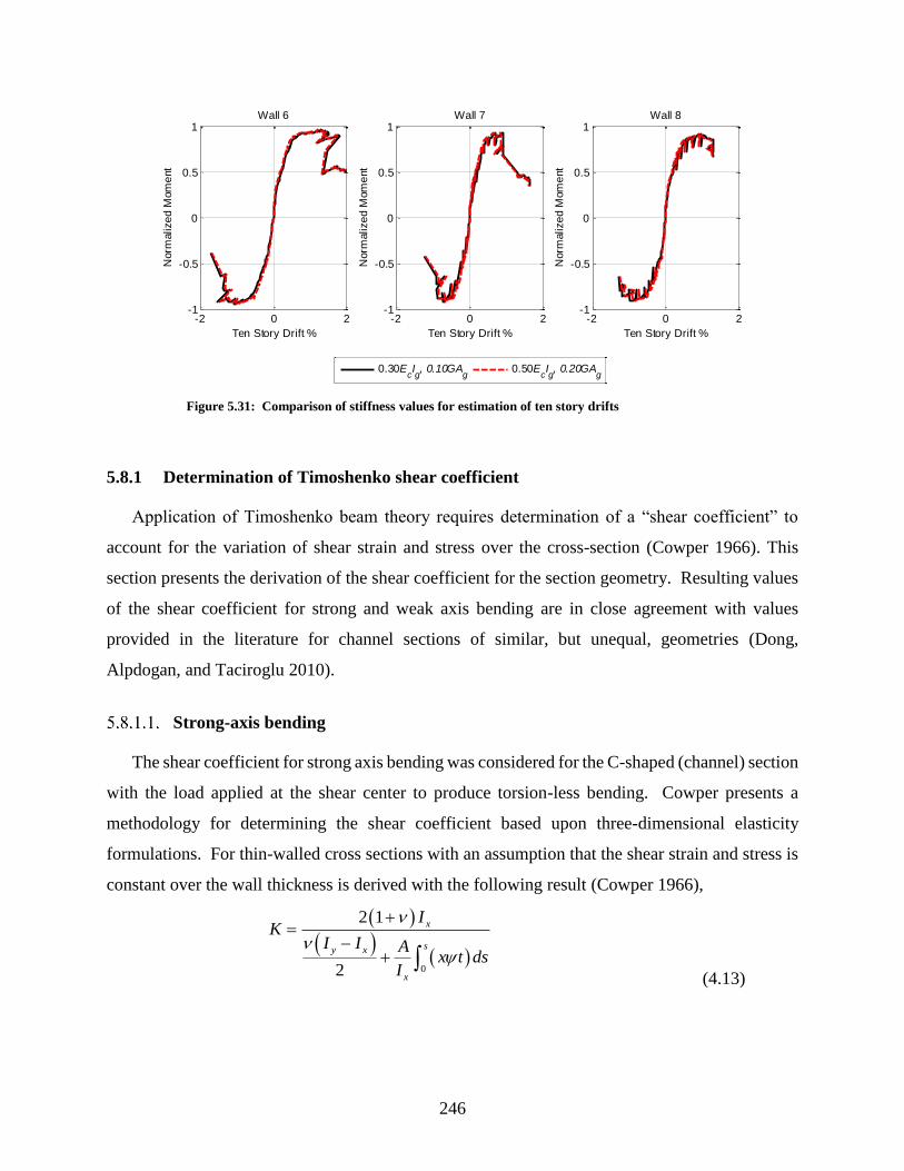
246
Figure 5.31: Comparison of stiffness values for estimation of ten story drifts
5.8.1 Determination of Timoshenko shear coefficient
Application of Timoshenko beam theory requires determination of a “shear coefficient” to
account for the variation of shear strain and stress over the cross-section (Cowper 1966). This
section presents the derivation of the shear coefficient for the section geometry. Resulting values
of the shear coefficient for strong and weak axis bending are in close agreement with values
provided in the literature for channel sections of similar, but unequal, geometries (Dong,
Alpdogan, and Taciroglu 2010).
Strong-axis bending
The shear coefficient for strong axis bending was considered for the C-shaped (channel) section
with the load applied at the shear center to produce torsion-less bending. Cowper presents a
methodology for determining the shear coefficient based upon three-dimensional elasticity
formulations. For thin-walled cross sections with an assumption that the shear strain and stress is
constant over the wall thickness is derived with the following result (Cowper 1966),
( )
( )( )
0
2 1
2
x
sy x
x
IK
I I Ax t ds
I
+=
−+
(4.13)
-2 0 2-1
-0.5
0
0.5
1
Ten Story Drift %
Norm
alize
d M
om
ent
Wall 6
-2 0 2-1
-0.5
0
0.5
1
Ten Story Drift %
Norm
alize
d M
om
ent
Wall 7
0.30EcIg, 0.10GA
g0.50E
cIg, 0.20GA
g
-2 0 2-1
-0.5
0
0.5
1
Ten Story Drift %
Norm
alize
d M
om
ent
Wall 8
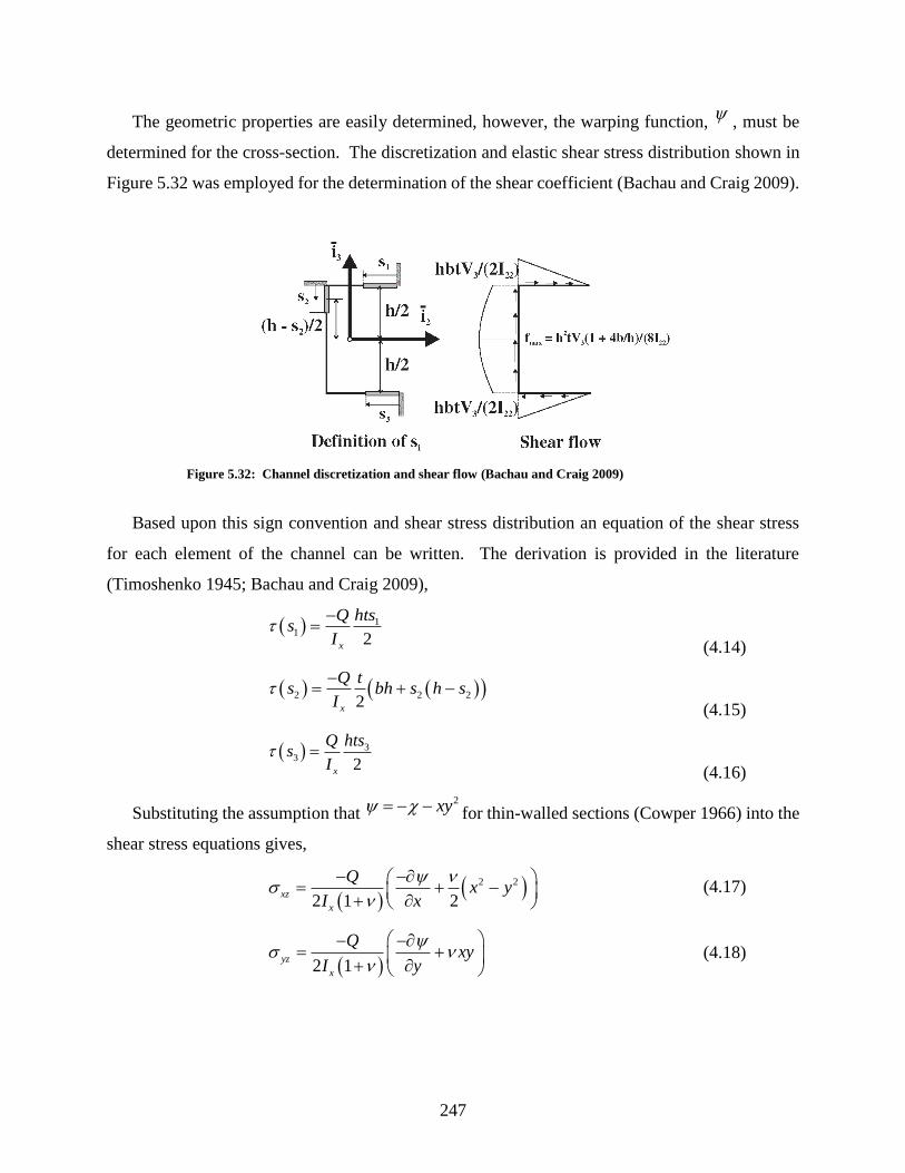
247
The geometric properties are easily determined, however, the warping function,
, must be
determined for the cross-section. The discretization and elastic shear stress distribution shown in
Figure 5.32 was employed for the determination of the shear coefficient (Bachau and Craig 2009).
Figure 5.32: Channel discretization and shear flow (Bachau and Craig 2009)
Based upon this sign convention and shear stress distribution an equation of the shear stress
for each element of the channel can be written. The derivation is provided in the literature
(Timoshenko 1945; Bachau and Craig 2009),
( ) 11
2x
Q htss
I
−=
(4.14)
( ) ( )( )2 2 22x
Q ts bh s h s
I
−= + −
(4.15)
( ) 33
2x
Q htss
I =
(4.16)
Substituting the assumption that 2xy = − − for thin-walled sections (Cowper 1966) into the
shear stress equations gives,
( )
( )2 2
2 1 2xz
x
Qx y
I x
− − = + −
+ (4.17)
( )2 1
yz
x
Qxy
I y
− −= +
+ (4.18)
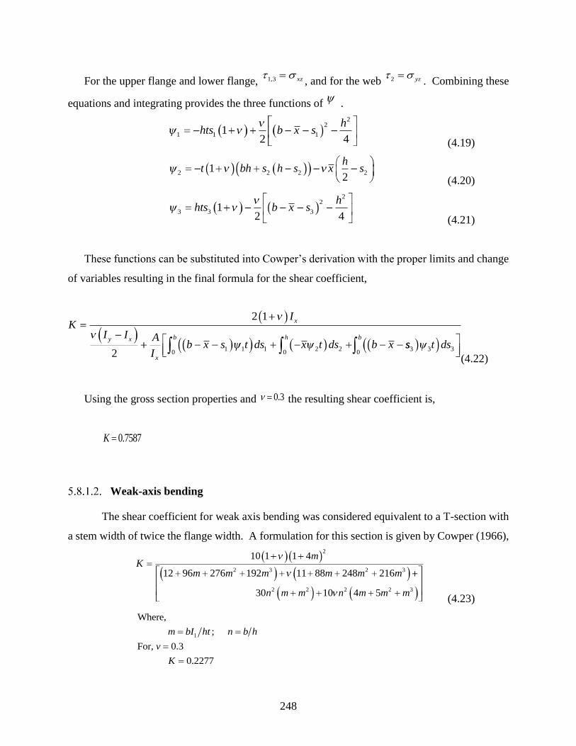
248
For the upper flange and lower flange, 1,3 xz =, and for the web 2 yz =
. Combining these
equations and integrating provides the three functions of
.
(4.19)
(4.20)
(4.21)
These functions can be substituted into Cowper’s derivation with the proper limits and change
of variables resulting in the final formula for the shear coefficient,
(4.22)
Using the gross section properties and 0.3 = the resulting shear coefficient is,
0.7587K =
Weak-axis bending
The shear coefficient for weak axis bending was considered equivalent to a T-section with
a stem width of twice the flange width. A formulation for this section is given by Cowper (1966),
(4.23)
1
Where,
;
For, 0.3
0.2277
m bI ht n b h
v
K
= =
=
=
1 1 1
22
12 4
hts b x sh
2 2 2 212
t bh s h s xh
s
3 3 3
22
12 4
hts b x sh
KI
I I A
Ib x s t ds x t ds b x
x
y x
x
h
2 1
21 1 1 2 2
0ss t ds
bb
3 3 300
Km
m m m m m m
10 1 1 4
12 96 276 192 11 88 248 216
2
2 3 2 3
30 10 4 52 2 2 2 3n m m n m m m
249
5.8.2 Displacement profiles of the ten-story building
Displacement profiles for the ten-story building are assembled by combining the measured
base deformations and story deformations up to the third floor with the extrapolated story
deformations up to the tenth floor using beam theory as described in Section 5.8. For the measured
deformations up to the third floor, the base slip was determined from the string potentiometer data
described in Section 5.5. The base rotations were determined from the Krypton data as described
in Section 5.7.1. First story and second story displacement were directly measured using string
potentiometers. The third story displacement was measured using high-resolution linear
potentiometers. At low-level displacements, the test specimen has not fully developed the crack
pattern and remains relatively stiff. For the procedure used to determine the deformations in the
upper seven stories of the wall specimen, it is assumed that those stories are cracked, and a reduced
flexural and shear stiffness is applied. Consequently, the ten-story displacement profile is invalid
at low displacement levels where the test specimen is stiffer than the upper seven stories. For this
reason, displacement profiles shown have been limited to drift levels after cracking starting at
approximately 0.25% drift in both strong and weak axes.
The resulting displacement profiles for the strong axis response of each wall test are presented
in Figure 5.33 through Figure 5.35 for each drift level. Drift levels are given in terms of the
imposed third-story drifts. The displacement profiles from 0.21% to 0.5% indicate a relatively
uniform progression of the deformation over the height of the wall. This correlates with the
minimal change in relative contributions of shear and flexural deformations given in Figure 5.27.
After 0.5% drift, the yielding results in the formation of the plastic hinge in the first story which
progressively dominates the wall response as drift increases. The cycle to 1.0% drift for CW1,
0.75% drift for CW2, and 0.75% drift for CW3 represents this turning point in the response. After
reaching the nominal strength, the sliding deformation at the base becomes apparent in the
displacement profiles and substantially changes the ten-story drifts. Sliding becomes apparent in
the 2.25% drift cycle for CW1, 1.5% drift for CW2 and 1.0% drift for CW3. As a consequence of
the base sliding, the rotation at the third story is reduced when compared to the same deformation
without sliding. Consequently, the displacement profile of the upper seven stories is reduced and
the ten-story displacement actually is reduced with the increasing drift levels. For example, at the
1.5% drift cycle of CW2, the approximate sliding displacement of 1” at the base results in a tenth-
story displacement that is approximately the same as the 0.75% drift cycle.
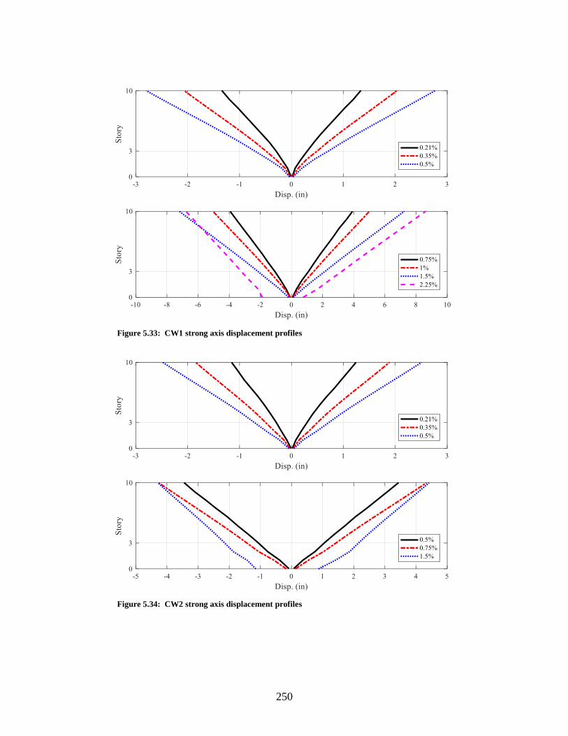
250
Figure 5.33: CW1 strong axis displacement profiles
Figure 5.34: CW2 strong axis displacement profiles
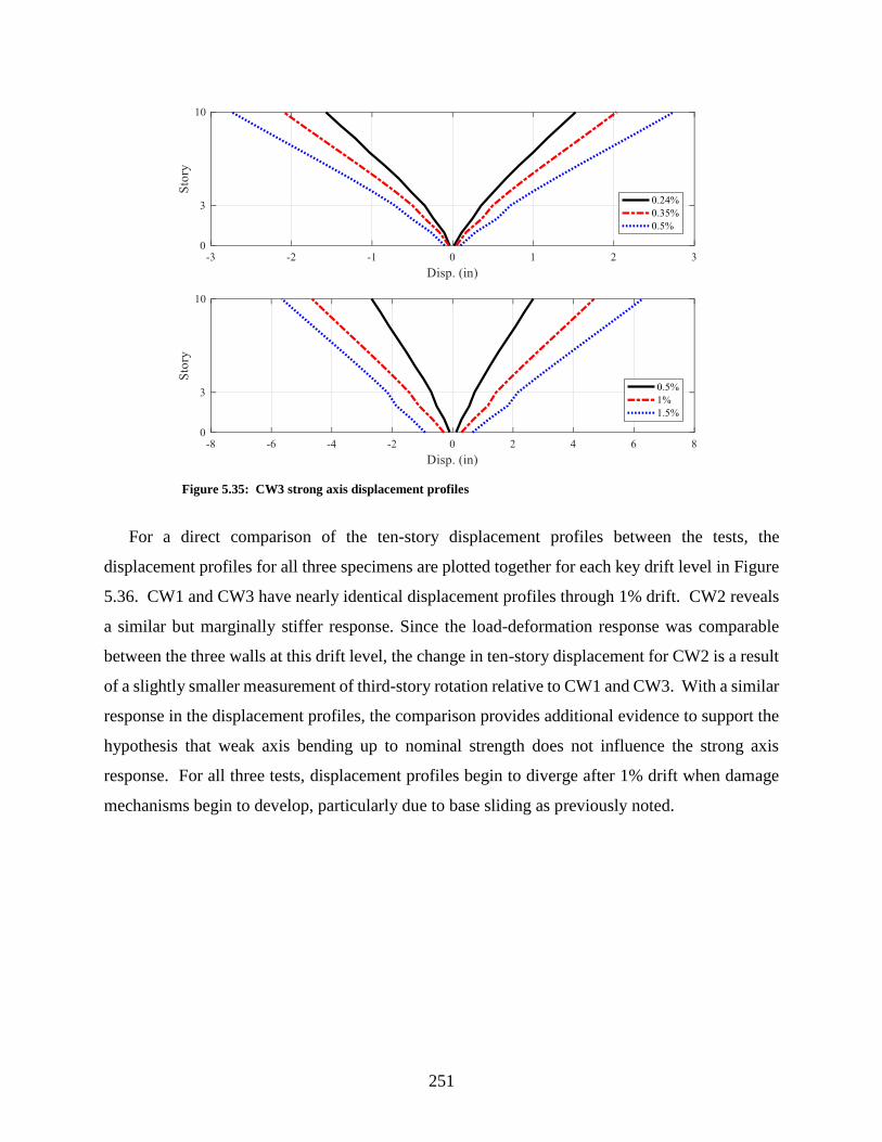
251
Figure 5.35: CW3 strong axis displacement profiles
For a direct comparison of the ten-story displacement profiles between the tests, the
displacement profiles for all three specimens are plotted together for each key drift level in Figure
5.36. CW1 and CW3 have nearly identical displacement profiles through 1% drift. CW2 reveals
a similar but marginally stiffer response. Since the load-deformation response was comparable
between the three walls at this drift level, the change in ten-story displacement for CW2 is a result
of a slightly smaller measurement of third-story rotation relative to CW1 and CW3. With a similar
response in the displacement profiles, the comparison provides additional evidence to support the
hypothesis that weak axis bending up to nominal strength does not influence the strong axis
response. For all three tests, displacement profiles begin to diverge after 1% drift when damage
mechanisms begin to develop, particularly due to base sliding as previously noted.

252
Figure 5.36: Comparison of displacement profiles for strong axis bending
The displacement profiles for the weak axis loading of CW2 is shown in Figure 5.37. For
reference, the positive displacement corresponds to loading with the web in compression while
negative displacement corresponds to loading with the toe in compression. The displacement
profiles for CW2 indicate that the web in compression loading develops a flexural dominated
response with the formation of a plastic hinge in the first story after 0.5% drift. As previously
indicated by the components of deformation in Figure 5.28, the base slip is negligible, and the
shear deformations are small for loading this direction. The displacement profiles for the toe in
compression reveal a relatively stiffer response consistent the global load-deformation. While the
CW1 CW2 CW3

253
first floor contains the majority of the deformation, additional inter-story drift is visible at the
second and third floors consistent with the components of deformation.
The displacement profiles for the weak axis loading of CW3 is shown in Figure 5.38. The
displacement profiles for loading with the toe in compression is difficult to ascertain due to the
change in loading logic described in Section 3.3.4.3. For loading with the web in compression,
the displacement profiles are also difficult to interpret because the change in loading logic resulted
in a variation in the effective height of loading and relative moment to shear demand for different
drift levels.
Figure 5.37: CW2 weak axis displacement profiles
Figure 5.38: CW3 weak axis displacement profiles

254
5.9 Global response of ten-story building
The hysteretic response of the building given in Chapter 4 used the third-story drift of the
building rather than the ten-story drift of the prototype structure. For comparison of the test results
to other experiments, the hysteretic response is evaluated based on both the effective height of the
structure and the top of the tenth story of the prototype building. The resulting hystereses of the
strong axis response and weak axis response are given in Figure 5.39 and Figure 5.40 respectively.
In general, the response is not noticeably different from the third story drift for the majority of the
experiments; however, the drift begins to deviate after 1% strong axis drift due to the sliding. As
the base of the wall slides, the rotation at the top of the wall decreases for the same third story
deformation. With reduced rotation at the third story, the rigid-body rotation in the upper seven
stories is also reduced.
Figure 5.39: Strong-axis ten-story drift versus normalized base moment for CW1 (left), CW2
(middle), and CW3 (right)
Figure 5.40: Weak-axis ten-story drift versus normalized base moment for CW1 (left), CW2
(middle), and CW3 (right)
-2 -1 0 1 2
% Drift, Strong Axis
-1
-0.5
0
0.5
1
No
rm.
Ba
seM
om
ent
CW1
-2 -1 0 1 2
% Drift, Strong Axis
-1
-0.5
0
0.5
1
No
rm.
Ba
seM
om
ent
CW2
-2 -1 0 1 2
% Drift, Strong Axis
-1
-0.5
0
0.5
1
No
rm.
Ba
seM
om
ent
CW3
-3 -1.5 0 1.5 3
% Drift, Weak Axis
-1
-0.5
0
0.5
1
No
rm.
Ba
seM
om
ent
CW1
-3 -1.5 0 1.5 3
% Drift, Weak Axis
-1
-0.5
0
0.5
1
No
rm.
Ba
seM
om
ent
CW2
-3 -1.5 0 1.5 3
% Drift, Weak Axis
-1
-0.5
0
0.5
1
No
rm.
Ba
seM
om
ent
CW3

255
5.10 Conclusions
This chapter presents a summary of the quantitative analysis of the three C-shaped wall
experiments. To perform the analysis, more than 390 channels of raw data and 850 GB of
photographs, videos, and data files were processed, cleaned and archived for use in this project
and future projects by other researchers. The complete dataset for each test was archived to the
NHERI Design Safe Cyber-Infrastructure with accompanying metadata to describe each
instrument and the organization of the data. The subsequent analysis of the C-shaped wall
experiments studied the energy dissipation of the walls, the progression of yielding, the
components of deformation to total wall drift including an analysis of base slip, strain fields
generated from displacement field data, and overall displacement profiles of the prototype ten-
story building. From this work, the following conclusions are made:
1. The energy dissipation capacity of the uni-directionally loaded and bi-directionally
loaded walls is approximately equivalent for equal levels of damage to the boundary
elements. This conclusion builds on the idea that the individual damage and tension-
compression cycles to each boundary element precipitates the failure of the wall as a
whole irrespective of loading direction.
2. The bi-directionally loaded test indicates tension yielding and strain hardening in the
flanges and toe boundary elements that were not present in the uni-directional test.
However, there is no evidence that the increased demand in the toe-boundary elements
directly impacts the strong axis response.
3. Prior to reaching the nominal strength at 0.75% drift, the base slip deformation is
negligible; however, beyond 1% drift post-peak the base slip deformation becomes
significant and is one mechanism of damage that results in the loss of load carrying
capacity. This conclusion provides confirmation of the visually observed sliding during
the test and rupture of vertical reinforcing bars in the unconfined web.
4. The bi-directional loading and variation in axial load during weak axis loading do not
change the relative drift contributions of the strong axis response prior to reaching the
nominal strength. Up to 0.75% drift, the strong axis response of the three tests is nearly
the same with approximately 40% of the total deformation in the bottom three stories
to be shear deformation.
256
5. While all three tests developed a concentration of the flexural deformation in the first
floor (plastic hinge), the bi-directionally loaded tests developed the plastic hinge at
earlier drift levels than the uni-directionally loaded test.
6. For the coupled core wall simulation, increased base slip and base rotation were
observed in the drift contributions beyond 0.5% drift. The increased tensile demand on
the web of the wall associated with loading in the negative weak axis direction as the
tension pier of the simulation resulted in increased yielding and earlier rupture of the
vertical reinforcement. The increased yielding in the web of CW3 relative to the prior
tests was also observed in the strain gauges. As noted in the visual observations, the
yielding and rupture of the vertical web reinforcing precipitated the interface separation
between the wall and foundation element that causes web sliding and damage to the
unconfined web.
7. An analysis of the displacement profiles of the ten-story building reveals that the
response at the effective height of loading is not significantly different from the
response at the top of the third story up to 1% drift. After 1% drift, sliding in the strong
axis impacts the response of the ten-story building because the third-story rotation with
base sliding is reduced when compared to the rotation at the same level of displacement
without base sliding.

257
CHAPTER 6: NON-PLANAR WALL PERFORMANCE
6.1 Introduction
Chapter 6 presents a comparative study of the C-shaped wall tests to prior experiments in order
to validate conclusions that are specific to C-shaped walls or that are generally applicable to non-
planar walls of different geometries. Section 6.2 evaluates the impact of non-planar wall geometry
on response using the prior experiments of the Complex Walls testing program described in the
literature review, Section 2.2. Section 6.3 conducts a study of effective stiffness values for the
elastic analysis of non-planar walls during design. Section 6.4 utilizes the planar wall drift capacity
equation that has been proposed for inclusion to the ACI 318 to evaluate its ability to predict drift
capacity in non-planar walls. Section 6.6 provides a parametric study of non-planar walls
identified in the literature review in conjunction with the C-shaped wall data. The study evaluates
design and demand parameters of the walls with respect to drift capacity and ductility. Trends are
also evaluated with respect to wall shape and failure mechanism.
6.2 Comparison of wall geometry
A unique contribution of the Complex Wall testing program described in Section 2.2 is the
ability to directly compare the performance of different wall types with similar geometries,
reinforcing and loading. This section evaluates the strong axis response of the first C-shaped wall
with the fourth planar wall experiment. This evaluation highlights the impact of the flange on the
wall response. Similarly, the weak axis response of the coupled C-shaped wall is compared to the
planar coupled wall test. This evaluation highlights the influence of the web and also serves as a
metric for the performance of the coupled core wall simulation.
6.2.1 Planar wall versus C-shaped wall
The four planar wall tests utilized the same geometry but different reinforcement, splicing, and
loading distribution. Planar wall test specimen, PW4, was selected for comparison to the C-shaped
wall. The length of the web and wall thickness were the same for both walls. Both walls contained
confined boundary elements; however, the length and shape of the boundary element differed. The
planar wall utilized a 1’-8” by 6” rectangular boundary element while CW1 utilized an L-shaped
boundary element extending 10” each direction. While both tests intended to represent the bottom
258
three stories of a ten-story building, the axial load ratio and lateral loading distribution differed.
The axial load ratio was ( )0.12 ' *c gf A for PW4 and ( )0.05 ' *c gf A in CW1. While a significant
difference in axial load ratio, the actual magnitude of the axial load was similar with an applied
force of 360 kips for PW4 and 306 kips for CW1. The effective height of loading differed as well.
PW4 utilized an effective height of 50% of the overall wall height, simulating a uniform lateral
load distribution. Two ancillary actuators were utilized at the top of the first floor and second floor
during testing to apply the shear at each story in conjunction with the LBCBs. Conversely, CW1
utilized an effective height of 71% of the wall height, simulating a triangular load distribution.
Load-deformation response
The load-deformation responses of PW4 and CW1 are shown in Figure 6.1. The drifts at the
onset of each cracking and damage state are summarized in Table 6.1. The stress demands at
nominal strength summarized in Table 6.2. Both tests approximately achieved the nominal
moment strength of the section. While the nominal moment strength of PW4 was approximately
50% less than CW1, the shear demand on the walls was nearly the same due to the reduced
effective height of loading in PW4 (uniform load distribution). The area of web concrete and
compressive strength of concrete were nearly the same, but the shear reinforcing was spaced at
2.25” on center for CW1 and 6” on center for PW4. The resulting shear demand on PW4 was
approximately twice that of CW1. The damage patterns in both tests included spalling of the
boundary element concrete, bar buckling, and core crushing; however, the onset of each damage
state occurs at significantly larger drifts in the C-shaped wall. The planar wall failed due to a
brittle compression failure of the boundary element at 1.0% drift. The C-shaped wall failed due
to a ductile buckling-rupture mechanism of the corner boundary elements at 2.25% drift. This
response concludes that a C-shaped wall of similar geometry and loading demand exhibits more
ductile response with increased drift capacity.
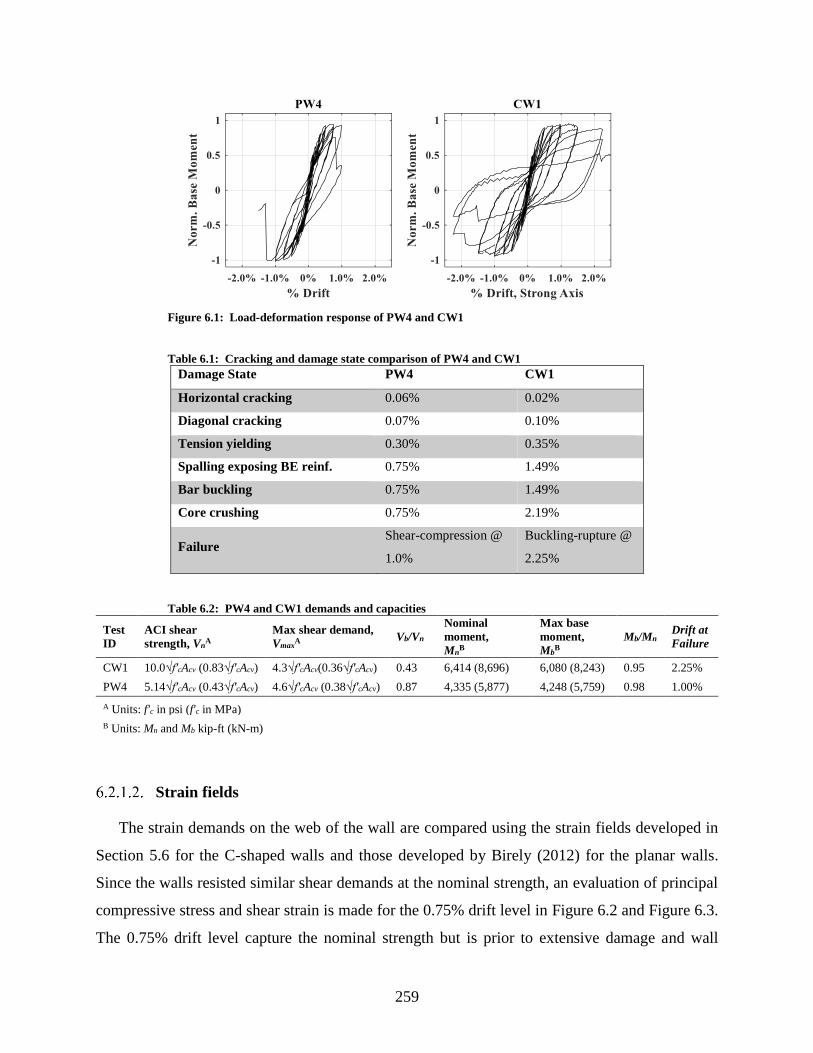
259
Figure 6.1: Load-deformation response of PW4 and CW1
Table 6.1: Cracking and damage state comparison of PW4 and CW1
Damage State PW4 CW1
Horizontal cracking 0.06% 0.02%
Diagonal cracking 0.07% 0.10%
Tension yielding 0.30% 0.35%
Spalling exposing BE reinf. 0.75% 1.49%
Bar buckling 0.75% 1.49%
Core crushing 0.75% 2.19%
Failure Shear-compression @
1.0%
Buckling-rupture @
2.25%
Table 6.2: PW4 and CW1 demands and capacities
Test
ID
ACI shear
strength, VnA
Max shear demand,
VmaxA
Vb/Vn
Nominal
moment,
MnB
Max base
moment,
MbB
Mb/Mn Drift at
Failure
CW1 10.0√f'cAcv (0.83√f'cAcv) 4.3√f'cAcv(0.36√f'cAcv) 0.43 6,414 (8,696) 6,080 (8,243) 0.95 2.25%
PW4 5.14√f'cAcv (0.43√f'cAcv) 4.6√f'cAcv (0.38√f'cAcv) 0.87 4,335 (5,877) 4,248 (5,759) 0.98 1.00%
A Units: f'c in psi (f'c in MPa)
B Units: Mn and Mb kip-ft (kN-m)
Strain fields
The strain demands on the web of the wall are compared using the strain fields developed in
Section 5.6 for the C-shaped walls and those developed by Birely (2012) for the planar walls.
Since the walls resisted similar shear demands at the nominal strength, an evaluation of principal
compressive stress and shear strain is made for the 0.75% drift level in Figure 6.2 and Figure 6.3.
The 0.75% drift level capture the nominal strength but is prior to extensive damage and wall

260
failure. The vertical strain profiles at the same drift level are also provided in Figure 6.4.
Similarities and differences between the planar wall and C-shaped wall are summarized below:
• The largest compressive strain demand for both walls is located at the end of the web
and along the base of the wall; however, the compressive strain demand in the planar
wall is nearly twice that of the C-shaped wall.
• Based on the vertical strain profile, the depth of compression in the C-shaped wall is
shallow compared to the planar wall with a corresponding uniform compressive strain
distribution across the flange.
• With a shallow depth of compression, the compressive strain demand in the web of the
C-shaped wall is due primarily to shear since it occurs in the tension region of the wall.
The shear strain demand and compressive strain demand show a direct correlation
across the web of the C-shaped wall.
• Conversely, the planar wall exhibits distributed compressive strain in the web
extending up the height of the boundary element and beyond the length of the boundary
element from a combination of moment and shear demand.
• The shear strain in the tension region of the planar wall does correlate with compressive
strain in the web; however, distinct compressive struts across the web are not apparent
as they are for the c-shaped wall. In addition, the overall magnitude and average
magnitude of shear strain across the web is higher for the C-shaped wall.
In conclusion, it is observed that the ability of the C-shaped wall to distribute and re-distribute
compressive stress across the flange increases the drift capacity of the wall and provides the
opportunity for a ductile failure mechanism. The C-shaped wall exhibits increased shear strain
demand and the formation of compressive struts across the web that are not apparent in the planar
wall.

261
(a) PW4 (b) CW1 web (c) CW1 flange Legend
Figure 6.2: Comparison of second principal strain during strong axis loading at 0.75% drift.
Color-bar ranges from zero millistrain (grey) to negative six millistrain (purple).
(a) PW4 (b) CW1 web (c) CW1 flange Legend
Figure 6.3: Comparison of pure shear strain during strong axis loading at 0.75% drift.
Color-bar ranges from six millistrain (orange) to zero millistrain (grey).
(a) PW4 (b) CW1 web (c) CW1 flange Legend
Figure 6.4: Comparison of vertical strain during strong-axis loading at 0.75% drift. Color-
bar ranges from twenty millistrain (yellow) to negative ten millistrain (purple).
Drift components
The drift contributions of base slip, base rotation, flexure and shear for PW4 and CW1 are
compared in Figure 6.5. The C-shaped wall drift contributions provided in Section 5.7 are
262
compared to those of the planar wall developed by Birely (2012). The similarities and differences
are summarized below:
• Base slip in both walls represents less than 10% of the overall deformation up to the
nominal strength; however, during the post-peak response the C-shaped wall exhibits
significant base slip that was not observed in the planar wall.
• Base rotation represented ~25% of the planar wall deformation, but only 5-10% of the
C-shaped wall deformation. This is attributed to the ability of the C-shaped wall to
distribute the tension demand across the flange. In addition, the C-shaped wall activates
a greater portion of the web vertical reinforcing bars due to the shallow depth of
compression.
• The flexural component of deformation represents ~50% of the planar wall deformation
and C-shaped wall deformation. Both walls exhibit increasing flexural deformation in
the first story as drift increases corresponding to the idea of plastic hinge formation in
the first story.
• The shear deformation represents approximately 40% of the C-shaped wall deformation
but only 20% of the planar wall deformation. This corresponds to the prior observation
of increased shear strain demand across the web of the CW1 when compared to PW4.
In conclusion, the shear deformation of the C-shaped wall is nearly twice that of the planar
wall when subjected to the same shear demand. This is present even when the planar wall was
tested with a lower moment to shear ratio than the C-shaped wall.

263
Figure 6.5: Components of deformation for the planar wall, PW4, and strong-axis response
of CW1
6.2.2 Planar coupled wall versus coupled C-shaped wall
The planar coupled wall test of the Complex Walls testing program described in Section 2.2.2
is compared to the third C-shaped wall experiment that simulated a coupled core wall system as
described in Section 3.3.4.3. The coupled wall utilized two 4’-0” by 6” thick wall piers separated
by a 2’-0” long coupling beam. The overall pier width of 4’-0” and thickness matched that of the
C-shaped wall flanges. Both walls contained confined boundary elements; however, the length
and shape of the boundary element differed. The coupled wall utilized a 1’-2” by 6” rectangular
boundary element at each end of each wall pier while CW1 utilized an L-shaped boundary element
extending 10” each direction at the corner and 10” by 6” boundary element at the toe. The constant
axial load was higher for the coupled wall with a ratio of ( )0.1 ' *c gf A as compared to
( )0.05 ' *c gf A in CW1. The loading of the coupled wall and coupled core wall system were the
same, utilizing an effective height of 71% of the total wall height for triangular load distribution.
The specific application of loading to the top of the wall and wall piers varied due to the
simulation of the upper seven stories for both tests and the opposing C-shaped wall for the coupled
core wall test. In addition, the C-shaped wall simulation did not include the coupling beams at
each story as part of the experiment. The loading simulation was created to simulate the correct
demands in the first story only, anticipating that the demands in the upper two stories would not
control the overall wall response. The subsequent comparison of response focuses on the first
CW1
0.5 1
% Drift
0
20
40
60
80
100
120
%o
fD
efo
rmat
ion
atF
loo
r3
PW4
0.5 1
% Drift
0
20
40
60
80
100
120
%o
fD
efo
rmat
ion
atF
loo
r3
Base slip
1st
story flexure
2nd
story flexure
3rd
story flexure
Base rotation
1st
story shear
2nd
story shear
3rd
story shear

264
floor. The details of these loading simulation procedures are described by Turgeon (2011) for the
coupled wall and in Section 3.3.4.3 for the C-shaped wall.
Load-deformation response
The load-deformation responses of CPW and CW3 are shown in Figure 6.6. The load-
deformation response is plotted in terms of system base shear. For the coupled wall, the system
base shear is directly measured but the shear resisted by each pier is estimated using instruments.
For the coupled core wall, the shear resisted by the pier is directly measured, and the system base
shear is estimated based on the assumed degree of coupling and shear distribution. The drift
capacity of both tests is comparable, reaching 2.2% for the coupled wall and 2.0% for the C-shaped
wall. While the coupled wall appears to have greater drift capacity, the drift capacity of the C-
shaped wall experiment is impacted by the bi-directional loading which was not present in the
coupled wall. Prior observations in Chapter 4 indicate that the bi-directional loading reduced the
drift capacity as a result of the combined cycles of tension and compression on the boundary
elements.
Figure 6.6: Load-deformation response of CPW and CW3
The drifts at the onset of each cracking and damage state are summarized in Table 6.3.
Reported drifts for the coupled wall damage correspond to the onset of damage in the wall pier.
Damage onset initiated in the coupling beams at earlier drifts, but a comparison cannot be made
because coupling beams were not present in the C-shaped wall. The coupled wall failed at 2.27%
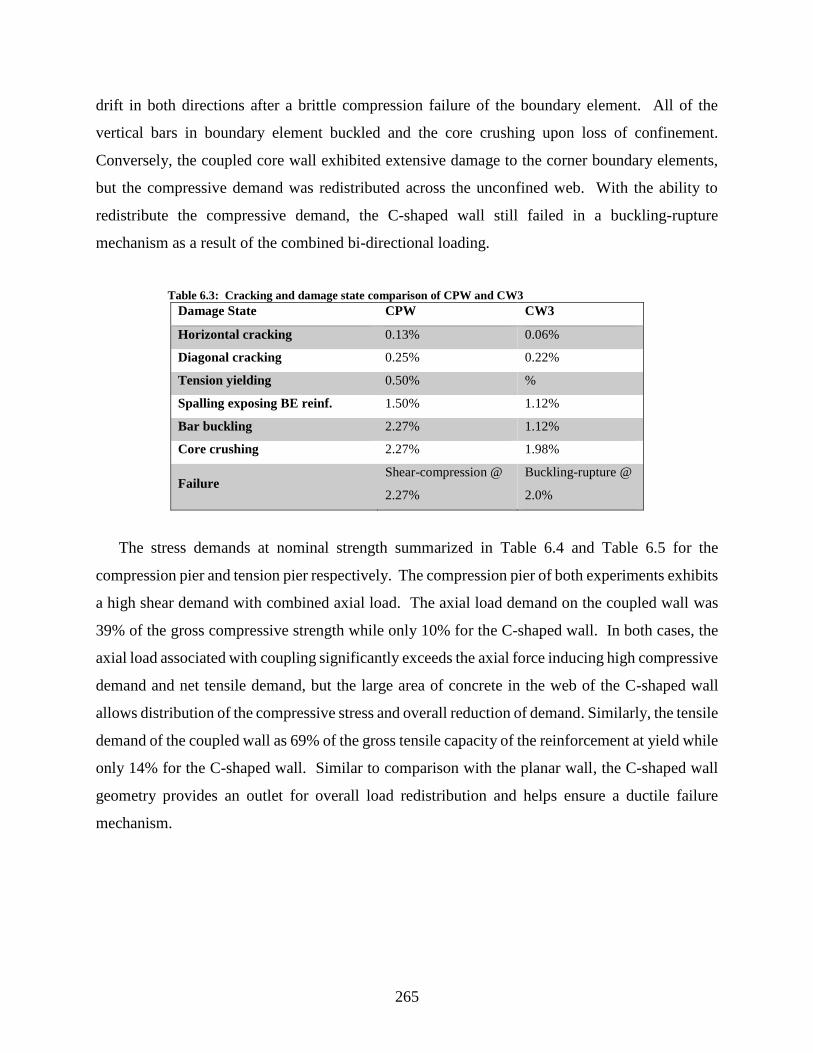
265
drift in both directions after a brittle compression failure of the boundary element. All of the
vertical bars in boundary element buckled and the core crushing upon loss of confinement.
Conversely, the coupled core wall exhibited extensive damage to the corner boundary elements,
but the compressive demand was redistributed across the unconfined web. With the ability to
redistribute the compressive demand, the C-shaped wall still failed in a buckling-rupture
mechanism as a result of the combined bi-directional loading.
Table 6.3: Cracking and damage state comparison of CPW and CW3
Damage State CPW CW3
Horizontal cracking 0.13% 0.06%
Diagonal cracking 0.25% 0.22%
Tension yielding 0.50% %
Spalling exposing BE reinf. 1.50% 1.12%
Bar buckling 2.27% 1.12%
Core crushing 2.27% 1.98%
Failure Shear-compression @
2.27%
Buckling-rupture @
2.0%
The stress demands at nominal strength summarized in Table 6.4 and Table 6.5 for the
compression pier and tension pier respectively. The compression pier of both experiments exhibits
a high shear demand with combined axial load. The axial load demand on the coupled wall was
39% of the gross compressive strength while only 10% for the C-shaped wall. In both cases, the
axial load associated with coupling significantly exceeds the axial force inducing high compressive
demand and net tensile demand, but the large area of concrete in the web of the C-shaped wall
allows distribution of the compressive stress and overall reduction of demand. Similarly, the tensile
demand of the coupled wall as 69% of the gross tensile capacity of the reinforcement at yield while
only 14% for the C-shaped wall. Similar to comparison with the planar wall, the C-shaped wall
geometry provides an outlet for overall load redistribution and helps ensure a ductile failure
mechanism.

266
Table 6.4: Weak axis compression pier demands and capacities
Specimen
ID
ACI shear
strength, VnA
Max shear demand,
VmaxA
Vmax/Vn Axial Demand
CPW 7.5√f'cAcv (0.63√f'cAcv) 7.3√f'cAcv (0.61√f'cAcv) B 0.97 641k (0.39 f'cAg)
CW3 9.8√f'cAcv (0.82√f'cAcv) 8.2√f'cAcv (0.68√f'cAcv) 0.84 746k (0.10 f'cAg) A Units: f'c in psi (f'c in MPa)
B Shear resisted by comp. pier equal to 90% of system base shear
Table 6.5: Weak axis tension pier demands and capacities
Specimen
ID
ACI shear
strength, VnA
Max shear demand,
VmaxA
Vmax/Vn Axial Demand
CPW 7.5√f'cAcv (0.63√f'cAcv) 0.9√f'cAcv (0.07√f'cAcv) B 0.12 304 kips (0.69 ∑AsFy)
CW3 9.8√f'cAcv (0.82√f'cAcv) 5.7√f'cAcv (0.47√f'cAcv) 0.58 114 kips (0.14 ∑AsFy) A Units: f'c in psi (f'c in MPa)
B Shear resisted by tens. pier equal to 10% of system base shear
Strain fields
To compare the strain demands, the strain fields developed in Section 5.6 for the C-shaped
walls are compared to the coupled wall strain fields developed by Turgeon (2011). A comparison
is made at the 1.0% drift level to capture the response at nominal strength prior to extensive
damage. A comparison is also made at the 1.5% drift level to capture how the strain field change
as damage progression increases prior to reaching failure. A comparison of the principal
compressive strain at 1.0% and 1.5% drift is given in Figure 6.7 and Figure 6.8 for the purpose of
comparing the wall response when acting as the compression pier. Similarities and differences
between the compression pier of the coupled wall and C-shaped wall are summarized below:
• The compressive strain demand in the coupled wall extends up the height of the
boundary element with a deep neutral axis located at approximately half the depth of
the wall pier (Turgeon 2011). The compressive strain demand is a combination of axial
coupling, moment in the wall pier, and shear demand resisted primarily by the
compression pier. Compressive strain demand in the boundary element approaches
the crushing strain up the height of the wall.
• Conversely, the compressive strain demand in the C-shaped wall is well distributed
primarily across the web of the wall with modest strain demands. Locally higher
compressive strain demand in the bottom corner of the flange and web in the corner
boundary elements is associated primarily with the shear demand resisted by the
flanges.

267
• At the 1.50% drift level, the corner boundary elements have been damaged as a result
of the bi-directional loading. The compressive strain field indicates a redistribution of
the compressive strain to the unconfined web. In the case of the coupled wall, the
compressive strain field is not remarkably different in distribution, but the magnitude
of strain has increased to equal or exceeds the crushing strain. This is a precursor to
the subsequent brittle compressive failure of the coupled wall.
(a) CW3 Web (b) CW3 Flange (c) CPW (d) Legend
Figure 6.7: Comparison of second principal strain at 1.00% drift. Color-bar ranges from
zero millistrain (grey) to negative six millistrain (purple).
(a) CW3 Web (b) CW3 Flange (c) CPW (d) Legend
Figure 6.8: Comparison of second principal strain at 1.50% drift. Color-bar ranges from
zero millistrain (grey) to negative six millistrain (purple).
A comparison of the vertical strain at 1.0% and 1.5% drift is given in Figure 6.9 and Figure
6.10 for the purpose of comparing the wall response when acting as the tension pier. For the
tension pier of the coupled core simulation, the load target was set based upon the imposed
demands on the system during loading of the compression pier. This logic maintained the
equilibrium of the overall system demand but resulted in unequal drift demands. The strain fields

268
given are based on the drift demand of the compression pier with an equal target load on the tension
pier. Further details of this logic are described in Section 3.3.4.3. Similarities and differences
between the tension pier of the coupled wall and C-shaped wall are summarized below:
• The tensile strain demand is nearly uniformly distributed across the C-shaped wall web
and flange. The tensile strain demand of the coupled wall is well distributed across the
tension pier, but a moment gradient is visible with higher tensile strains at the outer
boundary element. In both cases, the vertical strain on the tension pier is all in the
tensile direction corresponding to the net tensile stress demand resulting from the
coupling.
• As drift level increases, the overall distribution does not notably change for either wall
test. The overall magnitude of tensile strain remains similar between the coupled wall
and coupled core wall tension piers.
The comparison indicates that the demands imposed on the tension pier of the coupled core
wall simulation are representative of those imposed on the coupled wall, and the C-shaped wall
does activate the entire width of the web and flanges to resist the tensile load associated with
coupling. The lack of coupling beams presents inconsistencies for comparing drift demand of the
tension pier as well as the shear demand in the tension pier.
(a) CW3 Web (b) CW3 Flange (c) CPW (d) Legend
Figure 6.9: Comparison of vertical strain at 1.00% drift (0.28% CW3 equivalent). Color-bar
ranges from twenty millistrain (yellow) to negative ten millistrain (purple).

269
(a) CW3 Web (b) CW3 Flange (c) CPW (d) Legend
Figure 6.10: Comparison of vertical strain at 1.50% drift (0.12% CW3 equivalent). Color-bar
ranges from twenty millistrain (yellow) to negative ten millistrain (purple).
Drift components
The drift contributions of base slip, base rotation, flexure and shear for CPW and CW3 are
compared in Figure 6.11 for the compression pier and Figure 6.12 for the tension pier. The C-
shaped wall drift contributions provided in Section 5.7 are compared to those of the coupled wall
developed by Turgeon (2011). The similarities and differences are summarized below:
• Neither wall pier of either test exhibited a measured base slip.
• Base rotation represented ~15-20% of the overall deformation of the coupled wall
compression pier and ~25-30% of the C-shaped wall compression pier. The increase
in the base rotation for the C-shaped wall is attributed to the shallow depth of
compression resulting from the distribution of the compressive strain across the web of
the wall.
• Base rotation represented ~20-30% of the overall deformation of the coupled wall and
C-shaped wall tension pier. The C-shaped wall exhibits slightly higher base rotation.
• The overall flexural deformation and shear deformation of the coupled wall and C-
shaped wall compression and tension piers were similar. The C-shaped wall exhibited
higher flexural deformation in the first story but reduced flexural deformation in the
second story when acting as the compression pier. Conversely, the C-shaped wall
exhibited lower shear deformation in the upper two stories than the coupled wall. These
variations in deformation distribution between the stories may be significant or may be
a consequence of the C-shaped wall lacking coupling beams in the experiment.

270
In conclusion, the drift contributions of the wall piers are remarkably similar providing
validation to the approach to the coupled core wall simulation. However, direct conclusions are
limited with respect to the variations in shear and flexural demand in the upper stories due to the
lack of coupling beams in the C-shaped wall experiment.
Figure 6.11: Components of deformation for the coupled wall compression pier
Figure 6.12: Components of deformation for the coupled wall tension pier
Base slip
1st
story flexure
2nd
story flexure
3rd
story flexure
Base rotation
1st
story shear
2nd
story shear
3rd
story shear
Base slip
1st
story flexure
2nd
story flexure
3rd
story flexure
Base rotation
1st
story shear
2nd
story shear
3rd
story shear
271
6.3 Effective stiffness of walls
Analyses to determine component demands for seismic design of concrete buildings often
employ elastic models in which reduced component stiffnesses are used to account for additional
flexibility resulting from concrete cracking4. Accurate representation of component stiffness is
required to ensure accurate estimation of earthquake demand, drifts and accurate modeling of load
distribution within the structure. This section investigates the stiffness of non-planar walls
subjected to varying load histories. Existing recommendations for defining the effective flexural,
shear and axial stiffness of concrete walls are reviewed, and data from recently completed
experimental tests are employed to compute effective stiffness values. The results of this study
include recommendations for defining the effective stiffness of walls for use in seismic design.
6.3.1 Review of existing recommendations and past research
Elastic analysis remains the most common method of analysis for determining the demands
and deformations of a structure. Because reinforced concrete behaves inelastically under service-
level loading, the section properties will differ significantly from the gross uncracked section
properties. Effective stiffness values are prescribed reductions to the gross section properties to
account for the inelastic response of the section and can be applied to the flexural, shear, and axial
stiffness. Proper application of effective stiffness values to an elastic model can provide a more
accurate representation of load distribution for determining demands as well as the expected
deformation of the structure. While the application of effective stiffness values is analytically
straightforward, the rational selection of effective stiffness values has been a research focus within
experimental tests of a wide variety of building components.
Codes of practice and research publications typically include recommended effective stiffness
values for use in the design of concrete members. Table 6.6 lists the flexural, shear and axial
stiffness recommendations for walls included in eight selected publications. Recommended
effective stiffness values typically represent the onset of yielding in the wall and prescribe a
reduction of the flexural rigidity only. Five of the recommended flexural stiffness included in Table
4 Section 6.3 was taken in part from project grant deliverables written for the Charles Pankow Foundation (Mock et al. 2015).
I was the primary or sole author of the content included herein. Furthermore, this content has been updated and amended since the
deliverable.

272
6.6 are given as a function of the axial to account for the increase in stiffness associated with
increasing axial load. An axial load of ( )0.05 ' *c gf A was applied to the C-shaped walls tested as
part of this study; the effective flexural stiffness values corresponding to this axial load are shown
in Table 6.6. Most codes of practice acknowledge the presence of shear deformations but do not
provide recommendations for reduced shear stiffness; only PEER/ATC-72-1 (2010) and Birely
(2012) include a recommendation for effective shear stiffness. Only the CSA A23.3 (2004)
addresses axial stiffness; a reduction in axial stiffness equal to the reduction in flexural stiffness
based on the upper bound relationship of Adebar (2007) is recommended.
Specific recommendations are not made for planar or non-planar walls. Non-planar walls are
prescribed to determine the moment of inertia based upon the effective flange width requirements
of ACI 318 (2016). Similarly, the shear area is prescribed based upon the guidance of ACI 318.
Table 6.6: Effective stiffness values for walls ASCE
41
(2007)
NZS:
3101
(2006)
PEER/AT
C-72-1
(2010)
CSA
A23.3
(2004)
Paulay
(2002)
FIB 27
(2003)
ACI
318-14
(2016)
Birely
(2012)
Flexure 0.5EcIg1 0.32EcIg
1 0.33EcIg1,2 0.65EcIg
1,3 0.29EcIg1 0.3EcIg 0.35EcIg 0.35EcIg
Shear 0.1GcAcv 0.15GcAcv
Axial 0.65EcAg
Notes: 1. Adebar lower-bound relationship. 2. Adebar upper-bound relationship
6.3.2 Previous research addressing effective stiffness
Recommendations for effective stiffnesses for use in analysis of concrete walls and walled
buildings has been addressed by researchers at the University of Washington as part of the on-
going research program. Brown (2008) developed an effective flexural stiffness model based on
previous experimental tests of planar walls. The experimental data exhibited a wide scatter of data
points and a rapid drop in effective stiffness for low drift levels, so the model a constant effective
flexural stiffness for low drift levels up to 0.3% drift. The constant stiffness was based upon the
average flexural stiffness for all data points less than 0.3% drift. Subsequently, an exponential
relationship was calibrated to fit the data points beyond 0.3% drift. Brown proposed the following
nonlinear relationship:
(5.1)
E IH
E I E Ic eff
roof
c g c g0 3 1 2 0 3 0 3. exp . . .

273
Two shortcomings of the nonlinear relationship proposed by Brown were the underprediction
of stiffness for very low drift levels and a stiffness nearing zero at large drift levels (beyond 3%).
Doepker (2008) examined shake table and quasi-static test results of walls and observed a stiffness
not reducing below 0.05EcIg. Doepker proposed the following relationship for an effective
flexural stiffness to address both shortcomings:
(5.2)
6.3.3 Determination of effective stiffness values
Effective stiffness values for the planar and non-planar walls were determined from the
experimental data using a Timoshenko beam model. The effective flexural and shear stiffness
values from Timoshenko beam theory are given below. A complete derivation of these is given
by Birely (2012).
Effective flexural stiffness:
(5.3)
eff
flex
g
EI
EI =
(5.4)
Effective shear stiffness:
(5.5)
eff
shear
cv
GA
GA =
(5.6)
The planar and c-shaped wall test program utilized experimental specimens that represented
the bottom three stories of a ten-story building as described in Section 0. A combination of shear,
moment and axial force was applied at the top of the third story to simulate the upper seven stories
of the building. For this reason, the experimental data set provided measurements of story
displacements and rotations from only the base of the wall to the third story. The story
displacements and rotations from the fourth story to the tenth story are then extrapolated from the
E IH H
Ec eff
roof roof
c0 8 0 05 0 7
0 2
. exp . .
.
IIg
EI M hV h
eff
top bot
bot
bot1
2
2
GAV h
hEI
M h V heff
bot
top bot bot
eff
bot bot
1
1
2 6
2 3
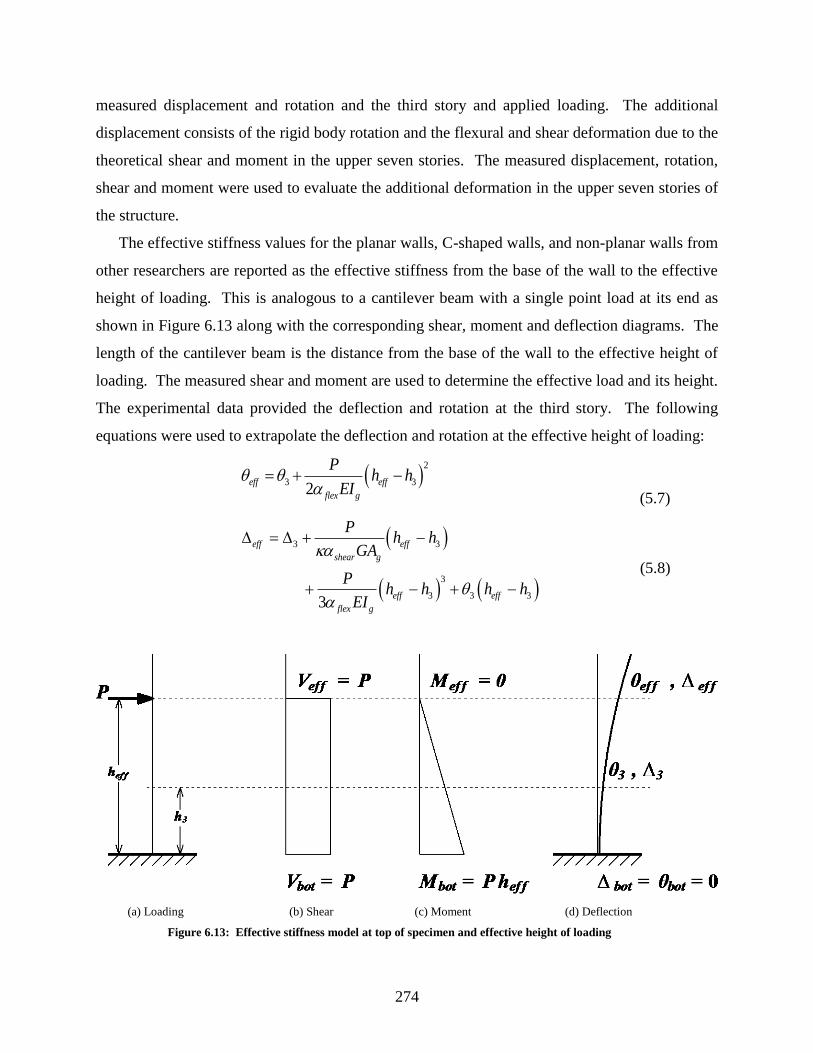
274
measured displacement and rotation and the third story and applied loading. The additional
displacement consists of the rigid body rotation and the flexural and shear deformation due to the
theoretical shear and moment in the upper seven stories. The measured displacement, rotation,
shear and moment were used to evaluate the additional deformation in the upper seven stories of
the structure.
The effective stiffness values for the planar walls, C-shaped walls, and non-planar walls from
other researchers are reported as the effective stiffness from the base of the wall to the effective
height of loading. This is analogous to a cantilever beam with a single point load at its end as
shown in Figure 6.13 along with the corresponding shear, moment and deflection diagrams. The
length of the cantilever beam is the distance from the base of the wall to the effective height of
loading. The measured shear and moment are used to determine the effective load and its height.
The experimental data provided the deflection and rotation at the third story. The following
equations were used to extrapolate the deflection and rotation at the effective height of loading:
( )2
3 32
eff eff
flex g
Ph h
EI
= + −
(5.7)
( )
( ) ( )
3 3
3
3 3 3 3
eff eff
shear g
eff eff
flex g
Ph h
GA
Ph h h h
EI
= + −
+ − + −
(5.8)
(a) Loading (b) Shear (c) Moment (d) Deflection
Figure 6.13: Effective stiffness model at top of specimen and effective height of loading

275
Various ratios of the flexural stiffness, flex, and shear stiffness, shear
, used in the above
equations for the stiffness of the upper seven stories were evaluated separately for the planar walls
and the C-shaped walls. A comparison of two given ratios and their representative effects on the
ten-story drifts for the normalized moment envelope of the C-shaped walls is given in Figure 6.14.
The flexural and shear stiffness of the upper stories are shown to have a small influence on the
total story deformation. The primary component of deformation in the upper stories is the rigid-
body rotation. Therefore, subsequent evaluations of the drifts above the third-story are determined
using 50% of the gross flexural stiffness and 20% of the gross shear stiffness (0.50flex =
,
0.20shear =).
Figure 6.14: Comparison of stiffness values for drift computation
6.3.4 Effective stiffnesses computed from C-shaped wall test data
The effective stiffness values of the C-shaped walls were determined separately for each
direction of strong and weak axis loading for all drift levels. The story stiffnesses were evaluated
at each story and at the effective height determined using the methodology previously described.
Attention is given to the stiffness values in the first story which contains the initial cracking,
yielding, damage, and failure. Attention is also given to the stiffness at the effective height of
loading to provide an average stiffness up the height of the cracked wall. The experimental
-2 0 2-1
-0.5
0
0.5
1
Ten Story Drift %
Norm
alize
d M
om
ent
Wall 6
-2 0 2-1
-0.5
0
0.5
1
Ten Story Drift %
Norm
alize
d M
om
ent
Wall 7
0.30EcIg, 0.10GA
g0.50E
cIg, 0.20GA
g
-2 0 2-1
-0.5
0
0.5
1
Ten Story Drift %
Norm
alize
d M
om
ent
Wall 8
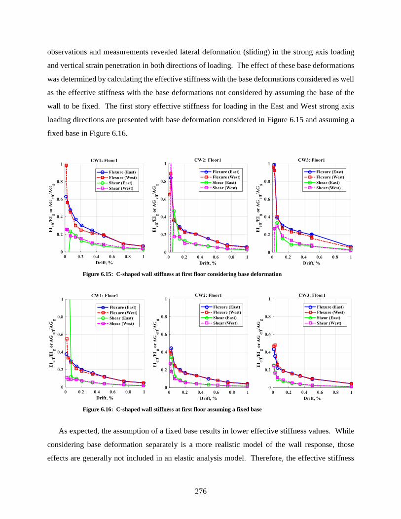
276
observations and measurements revealed lateral deformation (sliding) in the strong axis loading
and vertical strain penetration in both directions of loading. The effect of these base deformations
was determined by calculating the effective stiffness with the base deformations considered as well
as the effective stiffness with the base deformations not considered by assuming the base of the
wall to be fixed. The first story effective stiffness for loading in the East and West strong axis
loading directions are presented with base deformation considered in Figure 6.15 and assuming a
fixed base in Figure 6.16.
Figure 6.15: C-shaped wall stiffness at first floor considering base deformation
Figure 6.16: C-shaped wall stiffness at first floor assuming a fixed base
As expected, the assumption of a fixed base results in lower effective stiffness values. While
considering base deformation separately is a more realistic model of the wall response, those
effects are generally not included in an elastic analysis model. Therefore, the effective stiffness

277
values are subsequently presented based upon the assumption of a fixed base to include the effects
of base deformation in the elastic analysis. In addition, the effective flexural and shear stiffness
values from these plots showed no significant variations between the East and West directions for
all three tests. Subsequent values of strong axis stiffness are presented as an average of the East
and West directions at each drift level. The average effective flexural and shear stiffness values
at the first story and effective height of loading are presented in Figure 6.17 and Figure 6.18
respectively.
Figure 6.17: Averaged effective flexural stiffness values for C-shaped walls
Figure 6.18: Averaged effective shear stiffness values for C-shaped walls
A comparison of the average effective stiffness values at the effective height of loading for
each wall and direction of loading are presented with the ATC 72 and CSA A23.3 code
recommendations and the non-linear models proposed by Brown and Doepker in Figure 6.19.
With respect to the flexural stiffness, the strong axis response and weak axis response for the web
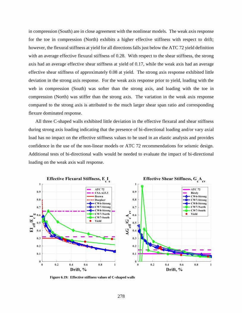
278
in compression (South) are in close agreement with the nonlinear models. The weak axis response
for the toe in compression (North) exhibits a higher effective stiffness with respect to drift;
however, the flexural stiffness at yield for all directions falls just below the ATC 72 yield definition
with an average effective flexural stiffness of 0.28. With respect to the shear stiffness, the strong
axis had an average effective shear stiffness at yield of 0.17, while the weak axis had an average
effective shear stiffness of approximately 0.08 at yield. The strong axis response exhibited little
deviation in the strong axis response. For the weak axis response prior to yield, loading with the
web in compression (South) was softer than the strong axis, and loading with the toe in
compression (North) was stiffer than the strong axis. The variation in the weak axis response
compared to the strong axis is attributed to the much larger shear span ratio and corresponding
flexure dominated response.
All three C-shaped walls exhibited little deviation in the effective flexural and shear stiffness
during strong axis loading indicating that the presence of bi-directional loading and/or vary axial
load has no impact on the effective stiffness values to be used in an elastic analysis and provides
confidence in the use of the non-linear models or ATC 72 recommendations for seismic design.
Additional tests of bi-directional walls would be needed to evaluate the impact of bi-directional
loading on the weak axis wall response.
Figure 6.19: Effective stiffness values of C-shaped walls
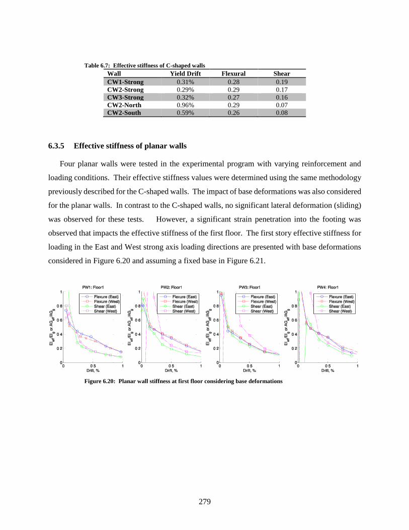
279
Table 6.7: Effective stiffness of C-shaped walls
Wall Yield Drift Flexural Shear
CW1-Strong 0.31% 0.28 0.19
CW2-Strong 0.29% 0.29 0.17
CW3-Strong 0.32% 0.27 0.16
CW2-North 0.96% 0.29 0.07
CW2-South 0.59% 0.26 0.08
6.3.5 Effective stiffness of planar walls
Four planar walls were tested in the experimental program with varying reinforcement and
loading conditions. Their effective stiffness values were determined using the same methodology
previously described for the C-shaped walls. The impact of base deformations was also considered
for the planar walls. In contrast to the C-shaped walls, no significant lateral deformation (sliding)
was observed for these tests. However, a significant strain penetration into the footing was
observed that impacts the effective stiffness of the first floor. The first story effective stiffness for
loading in the East and West strong axis loading directions are presented with base deformations
considered in Figure 6.20 and assuming a fixed base in Figure 6.21.
Figure 6.20: Planar wall stiffness at first floor considering base deformations

280
Figure 6.21 : Planar wall stiffness at first floor assuming a fixed base
The assumption of a fixed base results in lower flexural and shear stiffness values. For all
four walls, the flexural stiffness is similar in both directions of loading. The first planar wall that
was subjected to the ASCE 7 load distribution, in accordance with the C-shaped walls, had a shear
stiffness of similar magnitude between the two directions of loading. However, the second, third
and fourth planar walls which were subjected to a uniform lateral load distribution show some
variation in the shear stiffness between the two directions of loading. The variation in the shear
stiffness is attributed to the increased shear demand and associated cracking that occurs in one
direction before the other. The average effective flexural and shear stiffness values for each wall
are plotted with the non-linear models and ATC 72 and CSA A23.3 code recommendations in
Figure 6.22. The average effective stiffness values at yield are presented in Table 6.8.

281
Figure 6.22: Effective stiffness values of planar walls
Table 6.8: Effective stiffness of planar walls
Wall Yield Drift Flexural Shear
PW1 0.35% 0.42 0.15
PW2 0.42% 0.39 0.13
PW3 0.17% 0.44 0.21
PW4 0.19% 0.45 0.20
6.3.6 Effective stiffness of non-planar walls
A select number of other researchers in the literature measured and provided the experimental
displacements and rotations of non-planar walls. The C-shaped walls of this study were compared
the U-shaped walls tested by Beyer, Dazio, and Priestley (2008) and the H-shaped walls tested by
Oesterle (1976, 1979), see Section 2.1.2.1 and 2.1.4.1 respectively for details of these experiments.
The effective stiffness values were determined from the provided experimental data using the same
methodology described for the planar and C-shaped walls. The effective stiffness values were
calculated at all drift points provided in each direction of loading. The presented values are an
average of the effective stiffness values measured at each drift level. For symmetric directions of
loading (i.e., strong-axis loading of C-shaped walls and planar walls), the effective stiffness values
were also averaged between the two directions of loading. Effective stiffness values of walls
0 0.2 0.4 0.6 0.8 10
0.1
0.2
0.3
0.4
0.5
0.6
0.7
0.8
0.9
1
Effective Flexural Stiffness, EcIe
Drift, %
EI e
ff/E
cI g
ATC 72
CSA A23.3
Brown
Doepker
PW1
PW2
PW3
PW4
Yield
0 0.2 0.4 0.6 0.8 10
0.1
0.2
0.3
0.4
0.5
0.6
0.7
0.8
0.9
1
Effective Shear Stiffness, GcA
cv
Drift, %A
Ge
ff/G
cA
cv
ATC 72
Birely
PW1
PW2
PW3
PW4
Yield

282
loaded in directions of asymmetry were reported independently. The results are provided in Figure
6.23, and the corresponding values of effective stiffness at first yielding are presented in Table 6.9.
The strong-axis response of the C-shaped walls and the strong axis response of the U-shaped
wall TUA provide nearly identical effective flexural and shear stiffness values beyond 0.5% drift.
The weak axis response of all C-shaped and U-shaped walls was stiffer than the strong axis
response indicating that shear span ratio may influence effective stiffness estimation. In addition,
the PCA H-shaped walls which also had shallower shear span ratios provided higher effective
flexural stiffness ratios. However, the PCA tests provided limited test measurements and
resolution for making this evaluation. In contrast to the flexural stiffness, the shear stiffness
dropped to approximately 25% or less by 0.5% drift and subsequently to 10% or less by 1% drift
for most tests.
Figure 6.23: Effective stiffness values of non-planar walls
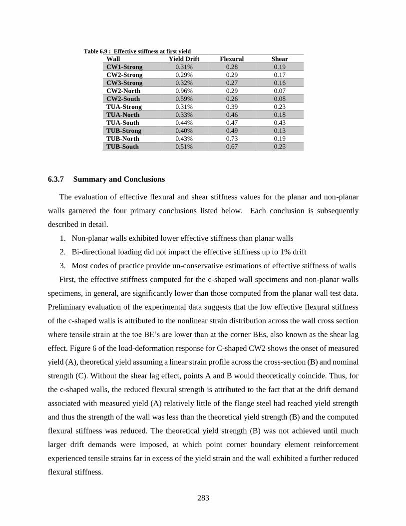
283
Table 6.9 : Effective stiffness at first yield
Wall Yield Drift Flexural Shear
CW1-Strong 0.31% 0.28 0.19
CW2-Strong 0.29% 0.29 0.17
CW3-Strong 0.32% 0.27 0.16
CW2-North 0.96% 0.29 0.07
CW2-South 0.59% 0.26 0.08
TUA-Strong 0.31% 0.39 0.23
TUA-North 0.33% 0.46 0.18
TUA-South 0.44% 0.47 0.43
TUB-Strong 0.40% 0.49 0.13
TUB-North 0.43% 0.73 0.19
TUB-South 0.51% 0.67 0.25
6.3.7 Summary and Conclusions
The evaluation of effective flexural and shear stiffness values for the planar and non-planar
walls garnered the four primary conclusions listed below. Each conclusion is subsequently
described in detail.
1. Non-planar walls exhibited lower effective stiffness than planar walls
2. Bi-directional loading did not impact the effective stiffness up to 1% drift
3. Most codes of practice provide un-conservative estimations of effective stiffness of walls
First, the effective stiffness computed for the c-shaped wall specimens and non-planar walls
specimens, in general, are significantly lower than those computed from the planar wall test data.
Preliminary evaluation of the experimental data suggests that the low effective flexural stiffness
of the c-shaped walls is attributed to the nonlinear strain distribution across the wall cross section
where tensile strain at the toe BE’s are lower than at the corner BEs, also known as the shear lag
effect. Figure 6 of the load-deformation response for C-shaped CW2 shows the onset of measured
yield (A), theoretical yield assuming a linear strain profile across the cross-section (B) and nominal
strength (C). Without the shear lag effect, points A and B would theoretically coincide. Thus, for
the c-shaped walls, the reduced flexural strength is attributed to the fact that at the drift demand
associated with measured yield (A) relatively little of the flange steel had reached yield strength
and thus the strength of the wall was less than the theoretical yield strength (B) and the computed
flexural stiffness was reduced. The theoretical yield strength (B) was not achieved until much
larger drift demands were imposed, at which point corner boundary element reinforcement
experienced tensile strains far in excess of the yield strain and the wall exhibited a further reduced
flexural stiffness.
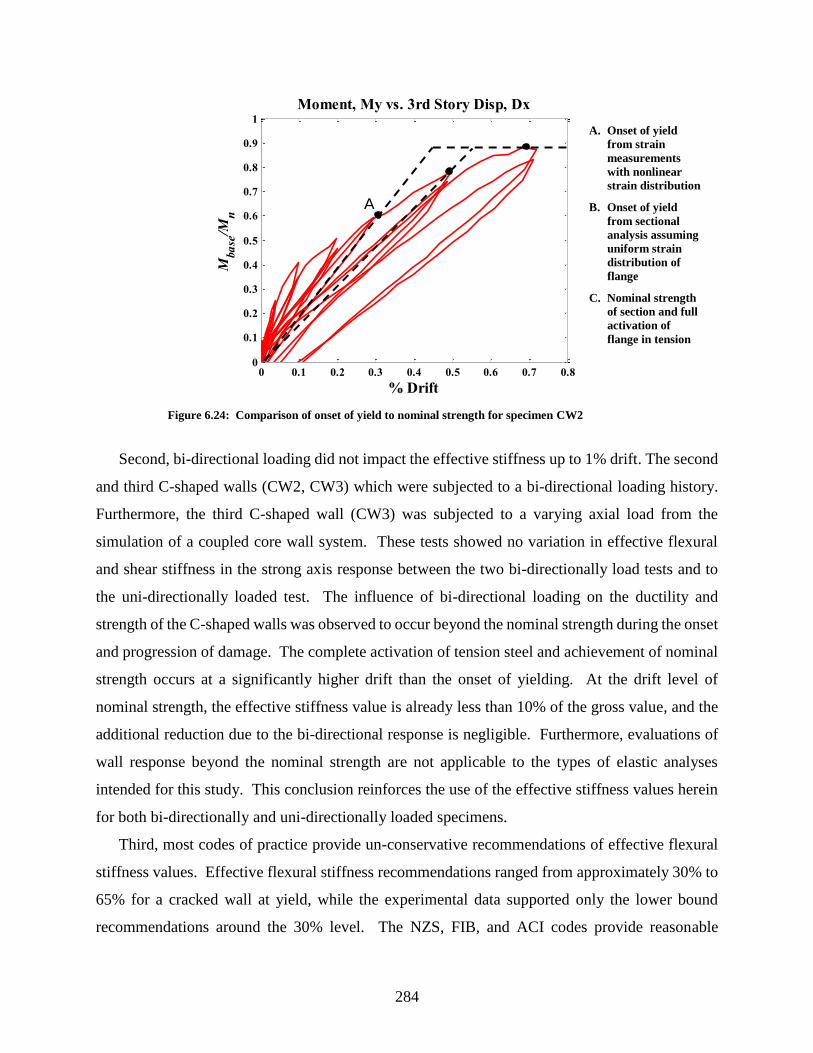
284
Figure 6.24: Comparison of onset of yield to nominal strength for specimen CW2
Second, bi-directional loading did not impact the effective stiffness up to 1% drift. The second
and third C-shaped walls (CW2, CW3) which were subjected to a bi-directional loading history.
Furthermore, the third C-shaped wall (CW3) was subjected to a varying axial load from the
simulation of a coupled core wall system. These tests showed no variation in effective flexural
and shear stiffness in the strong axis response between the two bi-directionally load tests and to
the uni-directionally loaded test. The influence of bi-directional loading on the ductility and
strength of the C-shaped walls was observed to occur beyond the nominal strength during the onset
and progression of damage. The complete activation of tension steel and achievement of nominal
strength occurs at a significantly higher drift than the onset of yielding. At the drift level of
nominal strength, the effective stiffness value is already less than 10% of the gross value, and the
additional reduction due to the bi-directional response is negligible. Furthermore, evaluations of
wall response beyond the nominal strength are not applicable to the types of elastic analyses
intended for this study. This conclusion reinforces the use of the effective stiffness values herein
for both bi-directionally and uni-directionally loaded specimens.
Third, most codes of practice provide un-conservative recommendations of effective flexural
stiffness values. Effective flexural stiffness recommendations ranged from approximately 30% to
65% for a cracked wall at yield, while the experimental data supported only the lower bound
recommendations around the 30% level. The NZS, FIB, and ACI codes provide reasonable
0 0.1 0.2 0.3 0.4 0.5 0.6 0.7 0.80
0.1
0.2
0.3
0.4
0.5
0.6
0.7
0.8
0.9
1
% Drift
Mbase/Mn
Moment, My vs. 3rd Story Disp, Dx
A. Onset of yield
from strain
measurements
with nonlinear
strain distribution
B. Onset of yield
from sectional
analysis assuming
uniform strain
distribution of
flange
C. Nominal strength
of section and full
activation of
flange in tension
A
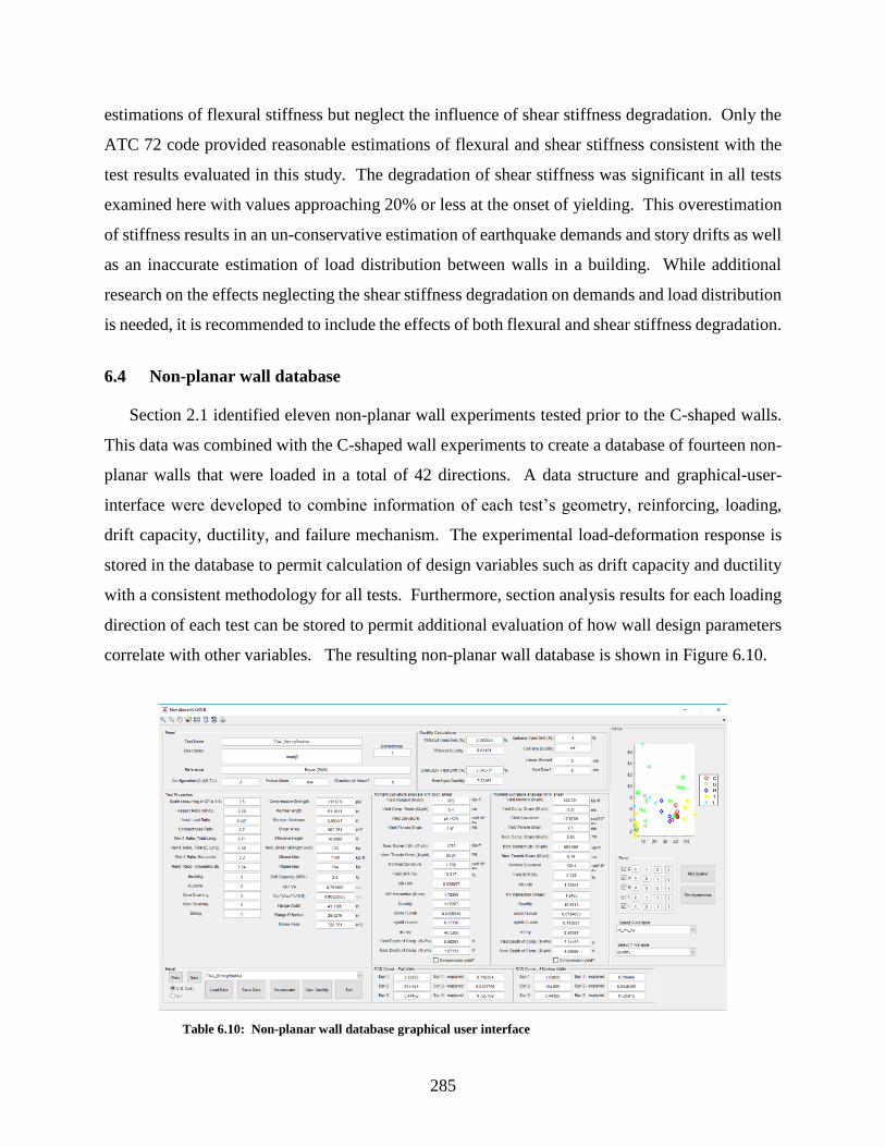
285
estimations of flexural stiffness but neglect the influence of shear stiffness degradation. Only the
ATC 72 code provided reasonable estimations of flexural and shear stiffness consistent with the
test results evaluated in this study. The degradation of shear stiffness was significant in all tests
examined here with values approaching 20% or less at the onset of yielding. This overestimation
of stiffness results in an un-conservative estimation of earthquake demands and story drifts as well
as an inaccurate estimation of load distribution between walls in a building. While additional
research on the effects neglecting the shear stiffness degradation on demands and load distribution
is needed, it is recommended to include the effects of both flexural and shear stiffness degradation.
6.4 Non-planar wall database
Section 2.1 identified eleven non-planar wall experiments tested prior to the C-shaped walls.
This data was combined with the C-shaped wall experiments to create a database of fourteen non-
planar walls that were loaded in a total of 42 directions. A data structure and graphical-user-
interface were developed to combine information of each test’s geometry, reinforcing, loading,
drift capacity, ductility, and failure mechanism. The experimental load-deformation response is
stored in the database to permit calculation of design variables such as drift capacity and ductility
with a consistent methodology for all tests. Furthermore, section analysis results for each loading
direction of each test can be stored to permit additional evaluation of how wall design parameters
correlate with other variables. The resulting non-planar wall database is shown in Figure 6.10.
Table 6.10: Non-planar wall database graphical user interface
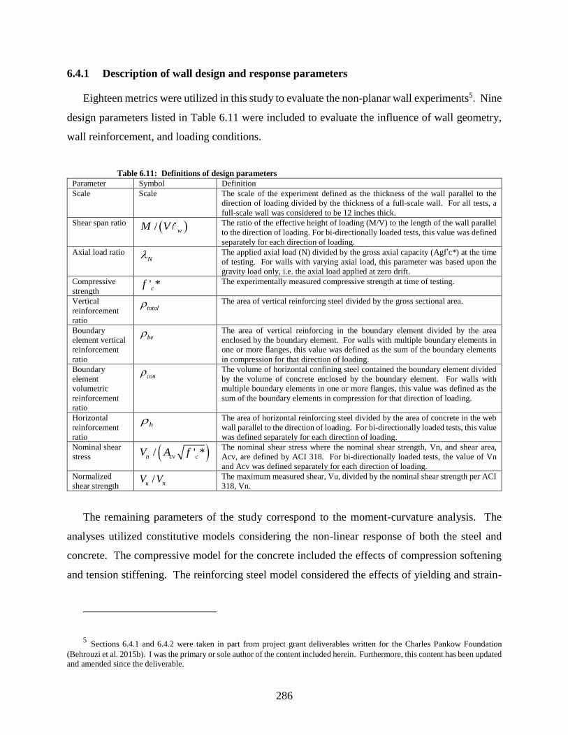
286
6.4.1 Description of wall design and response parameters
Eighteen metrics were utilized in this study to evaluate the non-planar wall experiments5. Nine
design parameters listed in Table 6.11 were included to evaluate the influence of wall geometry,
wall reinforcement, and loading conditions.
Table 6.11: Definitions of design parameters
Parameter Symbol Definition
Scale Scale The scale of the experiment defined as the thickness of the wall parallel to the
direction of loading divided by the thickness of a full-scale wall. For all tests, a
full-scale wall was considered to be 12 inches thick.
Shear span ratio ( )/ wM V The ratio of the effective height of loading (M/V) to the length of the wall parallel
to the direction of loading. For bi-directionally loaded tests, this value was defined
separately for each direction of loading.
Axial load ratio N The applied axial load (N) divided by the gross axial capacity (Agf’c*) at the time
of testing. For walls with varying axial load, this parameter was based upon the
gravity load only, i.e. the axial load applied at zero drift.
Compressive
strength ' *cf The experimentally measured compressive strength at time of testing.
Vertical
reinforcement
ratio
total The area of vertical reinforcing steel divided by the gross sectional area.
Boundary
element vertical
reinforcement
ratio
be The area of vertical reinforcing in the boundary element divided by the area
enclosed by the boundary element. For walls with multiple boundary elements in
one or more flanges, this value was defined as the sum of the boundary elements
in compression for that direction of loading.
Boundary
element
volumetric
reinforcement
ratio
con The volume of horizontal confining steel contained the boundary element divided
by the volume of concrete enclosed by the boundary element. For walls with
multiple boundary elements in one or more flanges, this value was defined as the
sum of the boundary elements in compression for that direction of loading.
Horizontal
reinforcement
ratio
h The area of horizontal reinforcing steel divided by the area of concrete in the web
wall parallel to the direction of loading. For bi-directionally loaded tests, this value
was defined separately for each direction of loading.
Nominal shear
stress ( )/ ' *n cv cV A f The nominal shear stress where the nominal shear strength, Vn, and shear area,
Acv, are defined by ACI 318. For bi-directionally loaded tests, the value of Vn
and Acv was defined separately for each direction of loading.
Normalized
shear strength /u nV V The maximum measured shear, Vu, divided by the nominal shear strength per ACI
318, Vn.
The remaining parameters of the study correspond to the moment-curvature analysis. The
analyses utilized constitutive models considering the non-linear response of both the steel and
concrete. The compressive model for the concrete included the effects of compression softening
and tension stiffening. The reinforcing steel model considered the effects of yielding and strain-
5 Sections 6.4.1 and 6.4.2 were taken in part from project grant deliverables written for the Charles Pankow Foundation
(Behrouzi et al. 2015b). I was the primary or sole author of the content included herein. Furthermore, this content has been updated
and amended since the deliverable.

287
hardening with a trilinear approximation. In the aim of a simplified analysis, the influence of
confinement, cyclic loading, bi-directional loading, and shear-flexure interaction were not
considered in the models. Table 6.12 contains the parameters drawn from the results of the
moment-curvature analysis. For these parameters, the nominal moment strength was the strength
at which the strain in the extreme compression fiber was -0.003 consistent with ACI 318. The
results of the moment-curvature analysis for each experiment and loading direction in the database
is given in Table 6.13.
Table 6.12: Definitions of moment-curvature parameters
Parameter Symbol Definition
Normalized
moment strength /u nM M The maximum measured shear, Mu, divided by the nominal moment strength.
Compressive
strain at yield c Strain in extreme concrete compression fiber at first measured yield extreme tensile
reinforcement.
Depth of
compression at
yield
yield wc The depth of compression at first measured yield of the extreme tensile
reinforcement divided by the length of the wall parallel to the direction of loading.
Curvature at
yield y The curvature at the first measured yield of the extreme tensile reinforcement.
Tensile strain at
nominal t Strain in the extreme tensile reinforcement at the nominal moment strength of the
analysis.
Normalized
tensile strain at
nominal
t y The tensile strain at nominal divided by the reported yield strain of the reinforcing
bars.
Depth of
compression at
nominal
wc The depth of compression at the nominal moment strength divided by the length of
the wall parallel to the direction of loading.
Curvature at
nominal n The curvature at nominal moment strength.
These metrics were compared to the drift capacity of the walls. Drift capacity was defined as
the drift at which the experiment dropped in strength to 80% of its maximum or the maximum drift
measured if a strength loss was not present. However, drift capacity was found to be a poor metric
for comparison due to the wide variety of wall geometries and loading conditions present. The
study was revised to utilize ductility as the metric of comparison. The ductility ratio was
calculated from the experimental data using two different methods.

288
Table 6.13: Non-planar wall moment-curvature analysis
Researcher Name Mu/
Mn
Vu/
Vn
εt
(ms) εt/εy c / lweb
φNom
(rad)
εc
(ms)
cyield /
lweb
φYield
(rad)
TUA_Strong 0.92 0.78 88.87 46.529 0.033 1.79E-03 0.40 0.173 4.52E-05
Beyer et al.
(2008)
TUA_WeakPositive 0.91 0.41 83.36 42.531 0.035 2.09E-03 0.40 0.169 5.72E-05
TUA_WeakNegative 1.04 0.47 24.07 15.529 0.111 6.55E-04 0.75 0.326 5.56E-05
TUB_Strong 0.98 0.99 76.29 38.726 0.038 1.55E-03 0.51 0.206 4.84E-05
TUB_WeakPositive 0.95 0.48 68.55 34.797 0.042 1.73E-03 0.46 0.189 6.93E-05
TUB_WeakNegative 1.03 0.57 12.84 7.598 0.189 3.78E-04 1.05 0.383 8.74E-05
IleX_Strong 1.11 0.68 26.86 13.297 0.100 4.94E-04 0.67 0.249 5.65E-05
Ile and
Reynouard
(2005)
IleY_WeakPositive 1.13 0.45 25.72 11.431 0.104 5.81E-04 0.68 0.232 6.73E-05
IleY_WeakNegative 1.11 0.50 9.18 4.613 0.246 2.25E-04 1.22 0.380 8.17E-05
IleXY_Strong 1.05 0.65 24.51 11.956 0.109 4.65E-04 0.70 0.255 5.72E-05
IleXY_WeakPositive 1.08 0.44 23.34 10.327 0.114 5.54E-04 0.71 0.239 6.80E-05
IleXY_WeakNegative 0.83 0.37 8.15 4.137 0.269 2.14E-04 1.28 0.394 8.25E-05
CW1_Strong 1.00 0.43 74.45 40.027 0.039 6.45E-04 0.57 0.235 2.02E-05
Lowes et al.
(2013)
CW2_Strong 0.97 0.41 77.24 41.751 0.037 6.69E-04 0.55 0.229 2.00E-05
CW2_WeakPositive 1.01 0.06 67.08 36.656 0.043 1.46E-03 0.34 0.157 4.70E-05
CW2_WeakNegative 1.03 0.10 6.42 3.508 0.318 1.96E-04 1.45 0.442 6.84E-05
CW3_Strong 0.95 0.41 76.09 41.353 0.038 6.59E-04 0.56 0.233 2.00E-05
NTW1_WebPositive 1.12 0.69 8.15 4.075 0.269 1.24E-04 1.46 0.422 3.85E-05
Brueggen
(2009)
NTW1_WebNegative 0.92 0.36 111.3 57.412 0.026 1.27E-03 0.31 0.138 2.50E-05
NTW1_Flange 0.97 0.63 6.20 3.316 0.326 1.28E-04 1.27 0.404 4.36E-05
NTW2_WebPositive 1.19 0.74 7.39 3.469 0.289 1.15E-04 1.53 0.418 4.07E-05
NTW2_WebNegative 0.98 0.41 98.91 48.724 0.029 1.13E-03 0.33 0.140 2.62E-05
NTW2_Flange 1.04 0.58 5.99 3.169 0.334 1.25E-04 1.24 0.396 4.36E-05
Oesterle et al.
(1976, 1979)
F1_Strong 0.99 1.02 76.19 34.475 0.038 1.06E-03 0.57 0.205 3.71E-05
F2_Strong 1.03 1.19 53.25 26.894 0.053 7.50E-04 0.75 0.275 3.65E-05
Thomsen and
Wallace
(1995)
TW1_WebPositive 0.74 0.86 4.37 2.441 0.407 1.54E-04 1.80 0.501 7.48E-05
TW1_WebNegative 0.99 0.58 81.82 47.570 0.035 1.77E-03 0.38 0.181 4.36E-05
TW2_WebPositive 0.94 0.89 3.85 2.127 0.438 1.43E-04 1.88 0.509 7.69E-05
TW2_WebNegative 0.97 0.46 77.97 50.630 0.037 1.69E-03 0.36 0.189 3.96E-05
The two ductility methods considered are based upon a bilinear elastic/plastic approximation
of the wall response from the experimental hysteresis. The plastic portion of the curve is taken as
a horizontal tangent to the point of maximum load. The methods then differ in the determination
of the linear elastic response from zero load to yield. The first method, as shown in Figure 6.25
(a) is to form a secant line between zero and the point in the force envelope where 75% of the
maximum experimental force applied. The second method, as shown in Figure 6.25 (b), is to
determine the line for which the elastic energy (the area above the secant line and below the force
envelope) is equal to the plastic energy (area below the secant line and above the force envelope).
An iterative method was utilized to solve the slope of this secant line. The two methods were
found to provide similar results with good agreement to the experimentally measured yield drifts.
Neither method was statistically more accurate in predicting the experimental yield. Therefore,
the 75% method was utilized due to the simplicity of its calculation.

289
(a) 75% Method (b) Energy Equivalence Method
Figure 6.25: Comparison of Ductility Methods
6.4.2 Failure mechanisms of non-planar walls
The failure mechanism of each non-planar was determined by examination of the researchers’
photos and damage narratives. A failure mechanism was only assigned for directions of loading
in which a 20% strength loss was measured in the experimental hysteresis. Three primary failure
mechanisms were classified as “buckling-rupture,” “crushing-buckling,” and “shear-
compression.” In addition, three secondary failure mechanisms that were observed to contribute
significantly to the failure were classified as “framing action,” “sliding,” and “stirrup slip.” These
mechanisms are subsequently described in detail.
Primary failure mechanisms
Buckling-rupture (BR)
The buckling-rupture failure is characterized by the rupture of BE vertical reinforcing bars
during straightening after being buckled in compression in the opposite direction of loading. The
BR failure may or may not exhibit compressive crushing in the BE. For this failure, the loss of
load carrying capacity is a direct result of the reinforcing bar fractures. An example of the buckling
of vertical BE reinforcing bars followed by rupture during straightening in shown in Figure 6.26.
0 0.5 1 1.5 2 2.50
200
400
600
800
1000
1200
1400
1600
75% Method
0 0.5 1 1.5 2 2.50
200
400
600
800
1000
1200
1400
1600
Energy Equivalence

290
Figure 6.26: Example of buckling-rupture failure from Specimen TUA (Constantin and
Beyer 2016)
Crushing-buckling (CB)
The crushing-buckling failure is characterized by crushing of the BE core and buckling of the
vertical BE reinforcing bars. The CB failure is typically preceded by the loss of confinement in
the boundary element due to rupture or slip of the confining stirrup(s). Two examples of a CB
failure are shown in Figure 6.27
(a) Paulay and Goodsir (1985) (b) Brueggen (2009) - Specimen NTW2
Figure 6.27: Examples of crushing-buckling failures
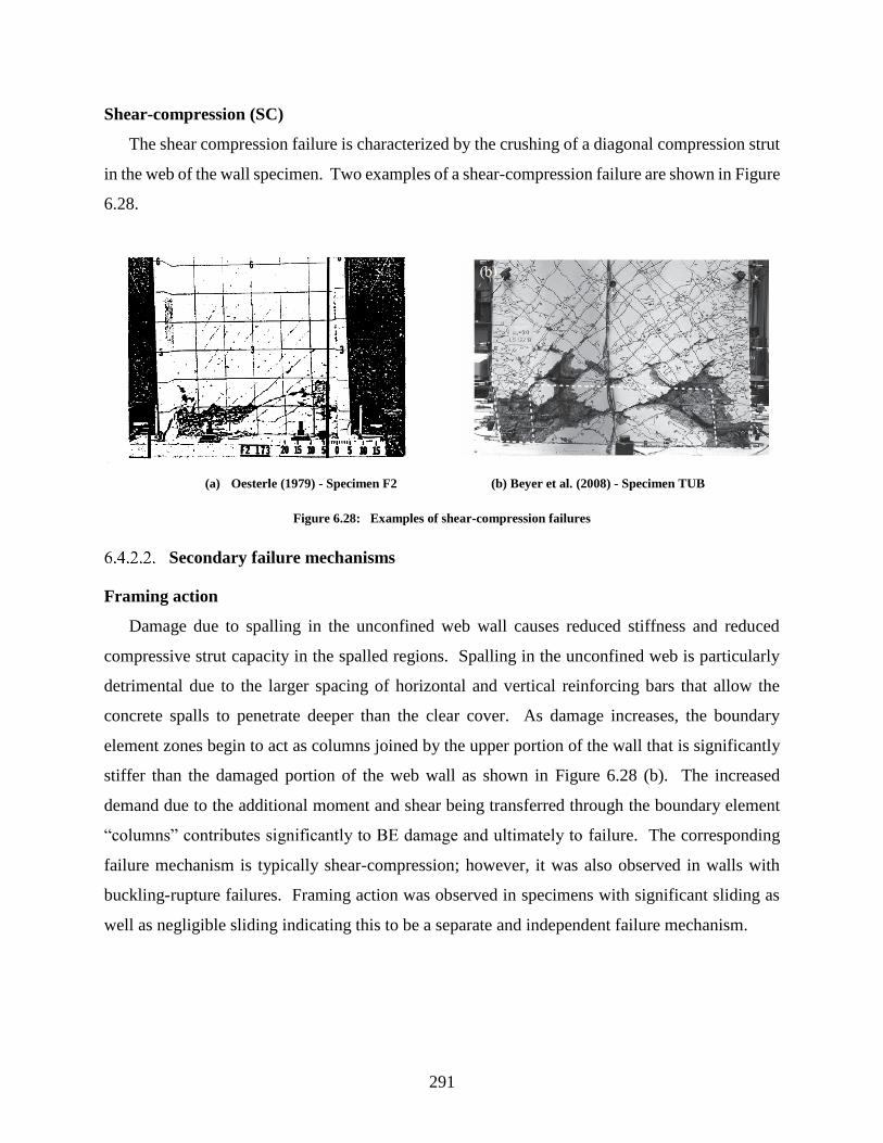
291
Shear-compression (SC)
The shear compression failure is characterized by the crushing of a diagonal compression strut
in the web of the wall specimen. Two examples of a shear-compression failure are shown in Figure
6.28.
(a) Oesterle (1979) - Specimen F2 (b) Beyer et al. (2008) - Specimen TUB
Figure 6.28: Examples of shear-compression failures
Secondary failure mechanisms
Framing action
Damage due to spalling in the unconfined web wall causes reduced stiffness and reduced
compressive strut capacity in the spalled regions. Spalling in the unconfined web is particularly
detrimental due to the larger spacing of horizontal and vertical reinforcing bars that allow the
concrete spalls to penetrate deeper than the clear cover. As damage increases, the boundary
element zones begin to act as columns joined by the upper portion of the wall that is significantly
stiffer than the damaged portion of the web wall as shown in Figure 6.28 (b). The increased
demand due to the additional moment and shear being transferred through the boundary element
“columns” contributes significantly to BE damage and ultimately to failure. The corresponding
failure mechanism is typically shear-compression; however, it was also observed in walls with
buckling-rupture failures. Framing action was observed in specimens with significant sliding as
well as negligible sliding indicating this to be a separate and independent failure mechanism.

292
Sliding
Sliding is the interface slip occurring between the base of the wall and wall foundation.
Typically, this interface is a cold-joint in the concrete making it susceptible to a large crack at this
location. Furthermore, the separate concrete pours result in little to no aggregate interlock across
this interface. The shear resistance at this interface is provided primarily through friction and
dowel action of the vertical reinforcing bars. Therefore, the onset of sliding in a web wall increases
the shear demand to the BE zones and transverse flanges, if present. Dowel action at the BE results
in an increased deformation of the vertical bars with an evident reverse curvature in the bottom
few inches above the interface. The cyclic loading history results in the dowel action reversing
directions and degrading the concrete around the vertical BE bars. The degraded concrete around
the vertical bars causes a loss of confinement, reduces the buckling capacity of the bars, and
ultimately contributes to a BR or CB failure at the boundary element(s). An example of sliding
is shown in Figure 6.29.
(a) Dowel action of the BE bars (b) Transverse shear in flange
Figure 6.29: Examples of damage due to sliding
Confinement hoop damage
The secondary failure mechanism of damage to the confinement hoops at boundary elements
results in a loss of confinement, unrestrained bar buckling, and core crushing. After spalling of
the concrete and high compressive demand in the boundary element, the confinement hoops were

293
observed to deform outward with the buckling of the reinforcement. This was particularly notable
where vertical bars were not individually restrained with a hook or corner of a tie. Compromised
confining hoops also resulting from sliding of the wall section dislodging the concrete inside and
around the boundary element at the interface. As the concrete became loose, the bond of the
confinement hoops and their hooks became compromised and failed.
(a) Deformed confinement hoops (b) Post-test evaluation of hoops (Brueggen 2009)
Figure 6.30: Example of confinement hoop damage
Summary of failure mechanisms
Each experiment was classified to have the primary and secondary failure mechanisms using
the definitions of Section 6.4.2. The classifications for each test are summarized in Table 6.14.
Table 6.14: Non-planar wall failure mechanisms
Researcher Specimen Primary
Mechanism
Secondary Mechanisms
Beyer et al. TUA BR Sliding
TUB SC Frame mech.
Ile and
Reynouard
IleX BR
IleY BR
IleXY BR
CW1 BR Sliding, frame mech., stirrup slip
Lowes et al. CW2 BR Sliding, frame mech., stirrup slip
CW3 BR Sliding, frame mech., stirrup slip
Brueggen NTW1 CB Stirrup slip
NTW2 CB Stirrup slip
Oesterle et al. F1 SC Sliding, frame mech.
F2 SC Sliding, frame mech.
Thomsen and
Wallace
TW1 CB
TW2 CB
294
6.5 Non-planar wall drift capacity prediction
Section 6.5 utilizes the non-planar wall database to evaluate proposed equations of drift
capacity for reinforced concrete structural wall with special boundary elements in accordance with
ACI 318-14. A recent parametric study of planar walls conducted by Abdullah and Wallace
(2018a) completed using the UCLA RC Wall Database (Abdullah and Wallace 2018b) determined
that planar wall drift capacity was primarily a function of the:
• Ratio of wall length to wall thickness, w b
• Wall neutral axis depth to wall thickness, c b
• Level of wall shear stress, ( )/ 'u cv cV A f
For comparison to that study, the same parameters and resulting drift capacity equations are studied
for non-planar walls with C-shaped, U-shaped, T-shaped, and H-shaped geometries. The tests
included in the UCLA RC Wall Database were screened on the basis of nine different criteria as
noted below to narrow the database to a selection of 164 experiments. The non-planar wall
database of 14 non-planar wall tests loaded in a total of 42 directions was evaluated against the
same criteria for the comparative study. The results are described below and shown in Table 6.15.
Non-compliant values are highlighted in red text.
Non-planar wall test compliance with UCLA RC Wall Database criteria:
a) Quasi-static reversed cyclic loading
• All walls included in the non-planar wall database complied.
b) Measured concrete compressive strength ≥ 3 ksi (20 MPa)
• All walls included in the non-planar wall database complied.
c) Width of compression zone, b ≥ 3.5” (90 mm)
• All walls included in the non-planar wall database complied.
d) Specimens with a rectangular compression zone
• All walls included in the non-planar wall database complied. For non-planar
walls with a flange or web in compression, the boundary elements are often
non-rectangular; however, the predicted depth of compression from the
sectional analysis was less than the flange wall thickness for all walls in the
non-planar wall database resulting in a rectangular compression zone.

295
e) At least two curtains of web vertical and horizontal reinforcement
• All walls included in the non-planar wall database complied.
f) No shear failure (i.e., diagonal tension, diagonal compression, or sliding at the base) or
splice failure
• 27 of 42 loading direction included in the non-planar wall database complied.
The 15 non-compliant loading directions exhibited shear sliding and/or
crushing of the unconfined web. These damage patterns were observed in the
strong axis loading of the C-shaped, U-shaped and H-shaped walls. Web
crushing was also observed for the T-shaped wall specimen with the web toe in
compression.
g) Ratio of ultimate to yield stress of boundary longitudinal reinforcement 1.2u yF F
• All walls included in the non-planar wall database complied.
h) Ratio of provided-to-required boundary transverse reinforcement required
, , 0.7sh provided sh requiredA A
• 33 of 42 loading directions included in the non-planar wall database complied.
The 9 non-compliant loading directions had a mean ratio of 0.53 with a
minimum value of 0.28.
i) Ratio of vertical spacing of hoops/crossties of boundary transverse reinforcement to
boundary longitudinal bar diameter 7.0v bs d
• 31 of 42 loading directions included in the non-planar wall database complied.
The 11 non-compliant loading directions had a mean ratio of 7.9 with a
maximum value of 10.7.
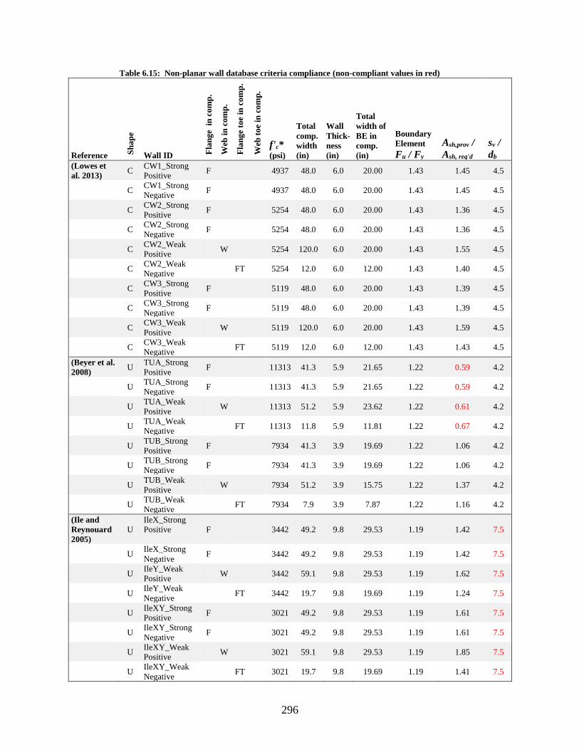
296
Table 6.15: Non-planar wall database criteria compliance (non-compliant values in red)
Reference Sh
ap
e
Wall ID Fla
ng
e i
n c
om
p.
Web
in
com
p.
Fla
ng
e to
e in
co
mp
.
Web
to
e in
co
mp
.
f'c* (psi)
Total
comp.
width
(in)
Wall
Thick-
ness
(in)
Total
width of
BE in
comp.
(in)
Boundary
Element
Fu / Fy
Ash,prov /
Ash, req'd
sv /
db
(Lowes et
al. 2013) C
CW1_Strong
Positive F 4937 48.0 6.0 20.00 1.43 1.45 4.5
C
CW1_Strong
Negative F 4937 48.0 6.0 20.00 1.43 1.45 4.5
C
CW2_Strong
Positive F 5254 48.0 6.0 20.00 1.43 1.36 4.5
C
CW2_Strong
Negative F 5254 48.0 6.0 20.00 1.43 1.36 4.5
C
CW2_Weak
Positive W 5254 120.0 6.0 20.00 1.43 1.55 4.5
C
CW2_Weak
Negative FT 5254 12.0 6.0 12.00 1.43 1.40 4.5
C
CW3_Strong
Positive F 5119 48.0 6.0 20.00 1.43 1.39 4.5
C
CW3_Strong
Negative F 5119 48.0 6.0 20.00 1.43 1.39 4.5
C
CW3_Weak
Positive W 5119 120.0 6.0 20.00 1.43 1.59 4.5
C
CW3_Weak
Negative FT 5119 12.0 6.0 12.00 1.43 1.43 4.5
(Beyer et al.
2008) U
TUA_Strong
Positive F 11313 41.3 5.9 21.65 1.22 0.59 4.2
U
TUA_Strong
Negative F 11313 41.3 5.9 21.65 1.22 0.59 4.2
U
TUA_Weak
Positive W 11313 51.2 5.9 23.62 1.22 0.61 4.2
U
TUA_Weak
Negative FT 11313 11.8 5.9 11.81 1.22 0.67 4.2
U
TUB_Strong
Positive F 7934 41.3 3.9 19.69 1.22 1.06 4.2
U
TUB_Strong
Negative F 7934 41.3 3.9 19.69 1.22 1.06 4.2
U
TUB_Weak
Positive W 7934 51.2 3.9 15.75 1.22 1.37 4.2
U
TUB_Weak
Negative FT 7934 7.9 3.9 7.87 1.22 1.16 4.2
(Ile and
Reynouard
2005)
U
IleX_Strong
Positive F 3442 49.2 9.8 29.53 1.19 1.42 7.5
U
IleX_Strong
Negative F 3442 49.2 9.8 29.53 1.19 1.42 7.5
U
IleY_Weak
Positive W 3442 59.1 9.8 29.53 1.19 1.62 7.5
U
IleY_Weak
Negative FT 3442 19.7 9.8 19.69 1.19 1.24 7.5
U
IleXY_Strong
Positive F 3021 49.2 9.8 29.53 1.19 1.61 7.5
U
IleXY_Strong
Negative F 3021 49.2 9.8 29.53 1.19 1.61 7.5
U
IleXY_Weak
Positive W 3021 59.1 9.8 29.53 1.19 1.85 7.5
U
IleXY_Weak
Negative FT 3021 19.7 9.8 19.69 1.19 1.41 7.5

297
Table 6.15 cont’d.
Reference Sh
ap
e
Wall ID Fla
ng
e i
n c
om
p.
Web
in
com
p.
Fla
ng
e to
e in
co
mp
.
Web
to
e in
co
mp
.
f'c* (psi)
Total
comp.
width
(in)
Wall
Thick-
ness
(in)
Total
width of
BE in
comp.
(in)
Boundary
Element
Fu / Fy
Ash,prov /
Ash, req'd
sv /
db
(Brueggen
2009) T
NTW1_Web
Positive WT 7260 6.0 6.0 6.00 1.45 1.14 3.0
T
NTW1_Web
Negative F 7260 72.0 6.0 39.00 1.45 0.76 3.5
T
NTW1_Flange
Positive FT 7260 6.0 6.0 6.00 1.45 0.91 3.5
T
NTW1_Flange
Negative FT 7260 6.0 6.0 6.00 1.45 0.91 3.5
T
NTW2_Web
Positive WT 6570 6.0 6.0 6.00 1.51 1.53 3.2
T
NTW2_Web
Negative F 6570 72.0 6.0 40.25 1.51 1.24 3.7
T
NTW2_Flange
Positive FT 6570 6.0 6.0 6.00 1.51 1.53 3.7
T
NTW2_Flange
Negative FT 6570 6.0 6.0 6.00 1.51 1.53 3.7
(Thomsen
and Wallace
1995)
T
WallaceTW1_
WebPositive WT 6330 4.0 4.0 4.00 1.48 0.60 8.0
T
WallaceTW1_
WebNegative F 6330 48.0 4.0 19.00 1.48 0.59 8.0
T
WallaceTW2_
WebPositive WT 6050 4.0 4.0 4.00 1.48 1.26 4.0
T
WallaceTW2_
WebNegative F 6050 48.0 4.0 19.00 1.48 0.28 10.7
(Oesterle et
al. 1976) H
F1_Strong
Positive F 5575 36.0 4.0 36.0 1.59 0.42 7.0
H F1_Strong
Negative F 5575 36.0 4.0 36.0 1.59 0.42 7.0
(Oesterle et
al. 1979) H
F2_Strong
Positive F 6610 36.0 4.0 14.0 1.68 1.06 2.7
H F2_Strong
Negative F 6610 36.0 4.0 14.0 1.68 1.06 2.7
Using the resulting non-planar wall database, each parameter considered to impact the drift
capacity ( w b , c b , and ( )/ 'u cv cV A f ) is plotted against the measured drift capacity in Figure
6.31 and Figure 6.32. Drift capacity was defined as the drift at which 20% of the peak strength is
lost in each loading direction.

298
(a) (b)
Figure 6.31: Non-planar wall parameters, (a) Drift vs. (lw / b), (b) Drift vs. (c / b)
(a) (b)
Figure 6.32: Non-planar wall parameters, (a) Drift vs. (lwc / b2), (b) Drift vs. (Vu / (Acv√f'c))
While these parameters were found to be representative of drift capacity in planar walls, the
same relationship is not observed for the non-planar walls as indicated in Figure 6.31 (a) and (b).
In particular, the large width of compression combined with the shallow depth of compression
present in flanged walls causes the c b parameter to become very small. The shear stress
parameter ( )/ 'u cv cV A f also does not indicate a direct correlation with drift capacity.
The results of the UCLA RC Wall Database parametric study were utilized to develop
empirical equations for predicting the drift capacity of planar walls as a function of the wall
0
2
4
6
8
10
12
14
16
0 1 2 3 4 5
l w/
b
Experimental Drift Capacity (%)
C
U
H
T0.01
0.1
1
10
0 1 2 3 4 5
c /
b
Experimental Drift Capacity (%)
C
U
H
T
0.001
0.01
0.1
1
10
100
0 2 4 6
l wc
/ b
2
Experimental Drift Capacity (%)
C
U
H
T0
1
2
3
4
5
6
7
8
9
10
0 2 4 6
Vu
/ (A
cv√f'
c)
Experimental Drift Capacity (%)
C
U
H
T

299
thickness, wall length, neutral axis depth, and shear stress demand. The first proposed equation
given in terms of % drift:
Drift Capacity Equation 1: ( )2
% 3.8550 8 '
c w u
w c cv
l c V
h b f A
= − − (5.9)
The first term of the equation is an upper bound on the drift prediction. The second term represents
the wall material properties, axial and moment demand, geometry, and longitudinal reinforcing.
The third term represents the impact of wall shear stress. The predicted drift capacity from
Equation 1 plotted against the experimental drift capacity is given in Figure 6.33 (a). The ratio of
predicted drift from Equation 1 to experimental drift plotted against the experimental drift capacity
is given in Figure 6.33 (b).
(a) (b)
Figure 6.33: Drift Capacity Equation 1: ( )2
% 3.8550 8 '
c w u
w c cv
l c V
h b f A
= − −
The results of Figure 6.33(a) indicate there is no direct correlation between the predicted drift
capacity and experimental drift capacity for Drift Capacity Equation 1. For walls with a
flange/web in compression (b >> t), the second term of the equation approaches zero as a result
of the square of the compression width (b) in the denominator. Consequently, the second term of
the equation becomes negligible and the drift capacity becomes a function of only the shear
stress demand on the web only. Furthermore, Figure 6.33(b) indicates that the equation
overpredicts the drift capacity for nearly all walls. The only walls with an underpredicted drift
0
1
2
3
4
0 1 2 3 4 5
Pre
dic
ted
Dri
ft C
ap
aci
ty (
%)
Experimental Drift Capacity (%)
C U H T0
0.5
1
1.5
2
2.5
0 1 2 3 4 5
Pre
dic
ted
/
Exp
erim
enta
l
Experimental Drift Capacity (%)
C U H T

300
capacity are the T-shaped walls with the toe of the web in compression or the toe of the flange in
compression.
For further comparison of this subset of tests to the UCLA RC Wall Database, a reduced dataset
including only the cases of non-planar walls with a toe in compression is given in Figure 6.34.
These walls contain lwc / b2 ratios consistent with the tests of the UCLA database.
(a) (b)
Figure 6.34: Drift Capacity Equation 1 for walls with toe in compression only
The results of the reduced dataset still indicate no direct correlation between the predicted drift
capacity and experimental drift capacity for Drift Capacity Equation 1. While the dimensions of
the compression zone may be representative of the planar wall database, the effects of loading
history and non-planar wall geometry in tension impact the drift capacity and are not represented
in Equation 1.
The second proposed equation given in terms of % drift:
Drift Capacity Equation 2: ( )2 2 '10
% 1.55c cvc
w w u
f Ab
h l c V
= + + (5.10)
Drift Capacity Equation 2 utilizes a lower bound on the drift prediction in the first term. The
second term represents the wall material properties, axial and moment demand, geometry, and
longitudinal reinforcing but in an inverse form to Equation 1. The third term represents the impact
of wall shear stress but again using the inverse of Equation 1. The predicted drift capacity from
0
1
2
3
4
0 1 2 3 4
Pre
dic
ted
D
rift
Ca
pa
city
(%
)
Experimental Drift Capacity (%)
C U T0
0.5
1
1.5
2
2.5
0 1 2 3 4
Pre
dic
ted
/
Exp
erim
enta
l
Experimental Drift Capacity (%)
C U T

301
Equation 2 plotted against the experimental drift capacity is given in Figure 6.35 (a). The ratio of
predicted drift from Equation 2 to experimental drift plotted against the experimental drift capacity
is given in Figure 6.35 (b).
(a) (b)
Figure 6.35: Drift Capacity Equation 2: ( )2 2 '10
% 1.55c cvc
w w u
f Ab
h l c V
= + +
The results of Figure 6.35 indicate there is no direct correlation between the predicted drift
capacity and experimental drift capacity for Drift Capacity Equation 2. For walls with a
flange/web in compression (b >> t), the second term of the equation becomes very large as a
result of the square of the compression width (b) in the numerator. Consequently, the second
term of the equation overwhelms the other terms and produces unrealistic drift capacities.
The third proposed equation given in terms of % drift is:
Drift Capacity Equation 3: ( )2
% 2.575 12 '
c w u
w c cv
l c V
h b f A
= − − (5.11)
The third equation is similar in form to Equation 1. The upper bound on the drift capacity is
reduced from 3.85% to 2.5%. The scalar multipliers in the denominator of the second and third
term have been increased 50% from 50 and 8 to 75 and 12 respectively. The predicted drift
capacity from Equation 3 plotted against the experimental drift capacity is given in Figure 6.36
0
400
800
1200
1600
0 1 2 3 4 5
Pre
dic
ted
Dri
ft C
ap
aci
ty (
%)
Experimental Drift Capacity (%)
C U H T
0
200
400
600
800
0 2 4 6P
red
icte
d
/ E
xp
erim
enta
lExperimental Drift Capacity (%)
C U H T

302
(a). The ratio of predicted drift from Equation 1 to experimental drift plotted against the
experimental drift capacity is given in Figure 6.36 (b).
(a) (b)
Figure 6.36: Drift Capacity Equation 3: ( )2
% 2.575 12 '
c w u
w c cv
l c V
h b f A
= − −
Similar to Equation 1, the results of Figure 6.36 indicate there is no direct correlation between
the predicted drift capacity and experimental drift capacity for Drift Capacity Equation 3. The
reduction in the upper bound of the drift equation to 2.5% does shift the data down, reducing the
ratio of predicted drift to experimental drift. Figure 6.36 (b) indicates that the equation
underpredicts the drift capacity of the majority of walls. The primary outlier is the bi-
directionally loaded C-shaped walls which remain overpredicted by up to 50%. While the drift
ratios are more reasonable for Equation 3, the results do not capture the variations in geometry,
reinforcing, and loading as the second term approaches zero for large widths of compression.
In conclusion, the drift capacity of non-planar walls cannot be reliably predicted using the same
parameters as planar walls proposed by the ACI 318H drift capacity equations. Furthermore, the
experimental drift capacity of non-planar walls subjected to bi-directional loading is further
reduced by the cumulative damage associated with the loading history. Further research is needed
to develop recommended drift capacity recommendations for non-planar walls.
0
0.5
1
1.5
2
2.5
3
0 1 2 3 4 5
Pre
dic
ted
Dri
ft C
ap
aci
ty (
%)
Experimental Drift Capacity (%)
C U H T0
0.2
0.4
0.6
0.8
1
1.2
1.4
1.6
0 1 2 3 4 5
Pre
dic
ted
/
Exp
erim
enta
l
Experimental Drift Capacity (%)
C U H T

303
6.6 Parametric study of non-planar walls
Section 6.3 developed recommendations for the effective stiffness of non-planar walls for
elastic analysis; however, these recommendations do not provide an estimate of the drift capacity
or ductility ratio of the wall being designed. Section 6.4 developed a database of non-planar walls
containing the experimental data, metadata, and moment-curvature analysis results. Section 6.5
evaluated proposed drift capacity equations using the non-planar wall databased, but those
expressions were found to be inadequate. This section utilizes the full range of parameters in the
non-planar wall database to determine if information about the strength, ductility and failure
mechanism of a non-planar wall could be ascertained from wall design parameters and/or a
simplified moment-curvature analysis6.
The influence of cyclic loading damage, increasingly non-linear strain distribution in non-
planar walls, as well as the effects of bi-directionally loading provide uncertainty to the
applicability and limitations of using simplified engineering analyses in the design of these walls.
A moment-curvature analysis was conducted for each experimental test in each direction of
loading. The results of the analyses for all experimental tests in the study were evaluated in terms
of the wall shape, failure mechanism, and uni/bi-directional loading history. These results were
then compared to a previous study of moment-curvature analyses of cyclically loaded planar walls
to further identify the limitations of these analyses specific to non-planar and/or bi-directionally
loaded walls.
6.6.1 Shear span ratio
The non-planar walls examined in this study had shear span ratios between two and four. The
data points with larger aspect ratios corresponded to the weak axis loading of the T and C-shaped
wall tests subjected to bi-directional loading. The planar walls examined had an aspect ratio
between two and four. These walls exhibited a relationship between increasing drift capacity and
increasing aspect ratio as shown in plot (f) of Figure 6.37. The non-planar walls subjected to uni-
directional loading history show a weak correlation between increasing ductility with increasing
6 Sections 6.6 was taken in part from project grant deliverables written for the Charles Pankow Foundation (Behrouzi et al.
2015b). I was the primary or sole author of the content included herein. Furthermore, this content has been updated and amended
since the deliverable.

304
aspect ratio as shown in plot (c). However, the non-planar walls subjected to bi-directional loading
showed no relationship between ductility and aspect ratio. The reduced ductility is believed to be
a result of the damage and failure of the wall specimen due to loading in other directions indicating
an important limitation in our predictions of wall response.
(a) Shape (b) Failure Mode
(c) Loading History (d) Bi-directional Failure Mode
Figure 6.37: Shear span ratio versus drift & ductility, figures (e) and (f) from Birely et al.
(2011)

305
Figure 6.37 cont.
(e) All Planar Walls (f) ACI Compliant Planar Walls
6.6.2 Axial load
The non-planar walls examined in the study had axial load ratios between 0.2 and 3%. The
planar walls had axial loads between 0 and 1.3%. Both data-sets indicate that specimens with
lower axial load exhibit greater ductility. They also indicate that the tests with higher axial load
and reduced ductility had compressive failure mechanisms. Nearly all of the walls with crushing-
buckling failures occurred in walls with higher levels of axial load, 1%f’cAg or more, with ductility
ratios less than five. The two outlying CB failures were T-shaped walls subjected to a bi-
directional loading history.
(a) Shape (b) Failure Mode
Figure 6.38: Axial load ratio versus drift & ductility, figures (e) and (f) from Birely et al. (2011)

306
Figure 6.38 cont.
(c) Loading History (d) Bi-directional Failure Mode
(e) All Planar Walls (f) ACI Compliant Planar Walls
6.6.3 Boundary element reinforcing
A strong correlation between boundary element reinforcing and ductility was observed for the
non-planar walls in the directions of failure, shown in Figure 6.39 (b). Increasing boundary
element vertical reinforcing corresponded to decreasing ductility as well as the probability of a
compressive failure mechanism.

307
(a) Shape (b) Failure Mode
(c) Loading History (d) Bi-directional Failure Mode
(e) All Planar Walls (f) ACI Compliant Planar Walls
Figure 6.39: Boundary element reinforcing ratio versus drift & ductility, figures (e) and (f)
from Birely et al. (2011)

308
6.6.4 Volumetric BE reinforcing
The evaluation of volumetric boundary element reinforcing does not indicate a significant trend
in the data for the non-planar walls or planar walls as shown in Figure 6.40. Increasing
confinement reinforcement theoretically helps to resist compressive stress and reduce the
likelihood of compressive failure; however, in practice, it appears that the other damage
mechanisms in non-planar walls take precedence over confining reinforcement. In conjunction,
damage mechanisms such as sliding might compromise the boundary elements regardless of
confining reinforcement ratio.
(a) Shape (b) Failure Mode
(c) Loading History (d) Bi-directional Failure Mode
Figure 6.40: Boundary element confinement reinforcement ratio versus drift & ductility,
figures (e) and (f) from Birely et al. (2011)

309
Figure 6.40 cont.
(e) All Planar Walls (f) ACI Compliant Planar Walls
6.6.5 Normalized shear strength
The planar wall study indicated a strong correlation between increasing shear demand and
decreasing drift capacity. The plot of failure mechanisms in Figure 6.41 (b) correlates compressive
failures with low ductility to walls with high shear demand. The more ductile buckling-rupture
failures corresponded to walls with an imposed shear demand between 0.5 and 0.75 Vn. It is also
observed that the uni-directionally loaded walls exhibit a weak trend between increasing shear
demand and decreasing drift capacity similar to the planar walls; however, the bi-directionally
loaded specimens show no trend.
(a) Shape (b) Failure Mode
Figure 6.41: Normalized shear strength versus drift & ductility, figures (e) and (f) from Birely
et al. (2011)
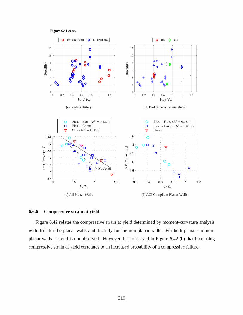
310
Figure 6.41 cont.
(c) Loading History (d) Bi-directional Failure Mode
(e) All Planar Walls (f) ACI Compliant Planar Walls
6.6.6 Compressive strain at yield
Figure 6.42 relates the compressive strain at yield determined by moment-curvature analysis
with drift for the planar walls and ductility for the non-planar walls. For both planar and non-
planar walls, a trend is not observed. However, it is observed in Figure 6.42 (b) that increasing
compressive strain at yield correlates to an increased probability of a compressive failure.

311
(a) Shape (b) Failure Mode
(c) Loading History (d) Bi-directional Failure Mode
(e) All Planar Walls (f) ACI Compliant Planar Walls
Figure 6.42: Compressive strain at yield versus drift & ductility, figures (e) and (f) from
Birely et al. (2011)
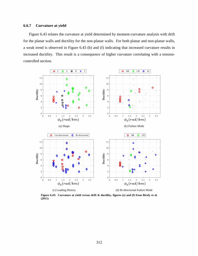
312
6.6.7 Curvature at yield
Figure 6.43 relates the curvature at yield determined by moment-curvature analysis with drift
for the planar walls and ductility for the non-planar walls. For both planar and non-planar walls,
a weak trend is observed in Figure 6.43 (b) and (f) indicating that increased curvature results in
increased ductility. This result is a consequence of higher curvature correlating with a tension-
controlled section.
(a) Shape (b) Failure Mode
(c) Loading History (d) Bi-directional Failure Mode
Figure 6.43: Curvature at yield versus drift & ductility, figures (e) and (f) from Birely et al.
(2011)

313
Figure 6.43 cont.
(e) All Planar Walls (f) ACI Compliant Planar Walls
6.6.8 Tensile strain at nominal
Figure 6.44 relates the ratio of tensile strain at nominal to tensile strain at yield as determined
by moment-curvature analysis with drift for the planar walls and ductility for the non-planar walls.
The planar walls indicated that a high ratio of tensile strain correlated with greater drift capacity,
but a low ration of tensile strain was inconclusive. For the non-planar walls, the same trend is not
observed. In fact, small and large ratios of tensile strain were observed with small and large
ductility ratios.
(a) Shape (b) Failure Mode
Figure 6.44: Ratio of tensile strain at nominal to yield versus drift & ductility, figures (e) and
(f) from Birely et al. (2011)

314
Figure 6.44 cont.
(c) Loading History (d) Bi-directional Failure Mode
(e) All Planar Walls (f) ACI Compliant Planar Walls
6.6.9 Nominal curvature
Figure 6.45 relates the curvature at nominal strength determined by moment-curvature analysis
with drift for the planar walls and ductility for the non-planar walls. For both planar and non-
planar walls, a weak trend is observed in Figure 6.45 (a) and (f) indicating that increased curvature
results in increased ductility. Similar to the curvature at yield, this correlates a tension-controlled
section. In contrast to the curvature at yield, the data points for failure directions only in Figure
6.45 (b) does not indicate the same correlation.

315
(a) Shape (b) Failure Mode
(c) Loading History (d) Bi-directional Failure Mode
(e) All Planar Walls (f) ACI Compliant Planar Walls
Figure 6.45: Curvature at nominal versus drift & ductility, figures (e) and (f) from Birely et
al. (2011)
316
6.6.10 Recommendations
The planar and non-planar walls indicate that walls with compressive failures exhibited less
ductility than walls with tensile failures. While some direct relationships between design
parameters and ductility were observed for the planar walls, these relationships were weak to non-
existent for the non-planar walls. However, this general conclusion leads to the idea that certain
design parameters can indicate a higher or lower probability of a tensile or compressive failure
mechanism in the non-planar walls that can then be attributed to a more or less ductile design.
In contrast to the planar walls and uni-directionally load non-planar walls, the bi-directionally
loaded walls show less correlation between the design or analysis parameters and ductility. The
increased scatter of data is attributable to damage and failures occurring in other directions of
loading. This conclusion is reinforced by the test programs for which one wall geometry was
subjected to uni-directional and bi-directional loading histories that resulted in reduced ductility
when the specimen was subjected to bi-directional loading.
A strong trend between increasing boundary element vertical reinforcement ratio with
decreasing ductility was observed in non-planar walls subjected to both uni-directional and bi-
directional loading. This trend was not observed in the planar walls. From the damage narratives
the experiments, the loss of strength (and limit of drift capacity) corresponded to the progression
of damage in the boundary elements.
6.7 Conclusions
This chapter presents a summary of the quantitative analysis of the three C-shaped wall
experiments from the perspective of prior experimental tests. The experiments were compared to
the planar wall and coupled wall experiments previously completed in the Complex Wall testing
program to inform how wall geometry affects response. Comparisons were made utilizing the
dense dataset available for each test including strain fields and components of deformation. The
experiments were also compared to eleven prior experimental tests of U-shaped, H-shaped and T-
shaped walls to inform how the C-shaped walls are unique among non-planar walls and to inform
how non-planar walls can be characterized in general. Comparisons were made through a
parametric study of wall design and demand parameters as well as through the development of
effective stiffness values for non-planar walls. From this work, the following conclusions are
made:

317
• A C-shaped wall of similar geometry and loading demand to a planar wall exhibits
more ductile strong axis response with increased drift capacity. The increased drift
capacity is a result of lower compressive stress demand and the ability to redistribute
compressive stress along the flange as the corner boundary element becomes damaged.
• For both the planar wall and coupled wall, the failure mechanism was non-ductile with
shear-compression damage to the boundary element. While C-shaped walls
experienced similar demands, the failure mechanism was ductile resulting from cyclic
buckling and rupture of the vertical reinforcing bars.
• A C-shaped wall exhibits reduced flexural deformation and base rotation, but nearly
twice the shear deformation when compared to a planar wall. The strain field of the C-
shaped wall indicates increased shear strain and principal compressive stress in the
tension zone of the wall. The combination of shear in the tension zone of the wall
causes increased shear slip along cracks and an overall increase in shear deformation
when compared to the planar wall.
• Bi-directional loading does not impact effective stiffness recommendations for the
elastic analysis of non-planar walls during yielding up to 1% drift. This conclusion is
consistent with the load-deformation response and visual observations described in
Chapter 4 and the quantitative analysis of the data in Chapter 5.
• Codes of practice generally provide un-conservative recommendations of effective
flexural stiffness values. Effective flexural stiffness recommendations in codes of
practice ranged from approximately 30% to 65% for a cracked wall at yield, while the
experimental data supported only the lower bound recommendations around the 30%
level. An effective flexural stiffness of 35%EcIg was recommended for design.
• Codes of practice generally do not provide recommendations of effective shear stiffness
values; however, the degradation of shear stiffness was significant in all tests examined.
Effective shear stiffness values approached 20% or lower at the onset of yielding. An
effective shear stiffness of 15%GcAcv was recommended for design.
• Drift capacity of non-planar walls cannot be estimated using the same design
parameters as planar walls. Specifically, the ratio of wall length to wall thickness, w b
318
, the wall neutral axis depth to wall thickness, c b , and the level of wall shear stress,
( )/ 'u cv cV A f were not found to be statistically significant for non-planar walls.
• A parametric study of eighteen design parameters for non-planar walls found that
ductility is a better metric for estimating wall performance than drift capacity. Ductility
was determined using both the 75% method and energy equivalence method with
comparable results. The 75% method is recommended for ductility calculations due to
its simplicity.
• For non-planar walls, increasing the reinforcement ratio of the boundary elements
results in reduced ductility, a trend which was not observed in planar walls. This
conclusion reinforces the idea that non-planar wall ductility is ultimately a function of
the damage to the individual boundary elements in cycles of tension and compression.
• The drift capacity and ductility of bi-directionally loaded non-planar walls cannot be
estimated using design parameters and moment-curvature analysis alone, a more
detailed evaluation considering the three-dimensional geometry and loading history is
required.
319
CHAPTER 7: FINITE ELEMENT ANALYSIS OF C-SHAPED WALLS
7.1 Introduction
Concrete structures do not exhibit a linear relationship between load and deformations due to
the inelastic response of concrete in compression, the cracking of concrete in tension, the yielding
and strain-hardening of reinforcements, path-dependent effects, and damage. The effective design
of concrete structures for all levels of performance, particularly for structures in regions of high
seismicity, makes it critically important to be able to predict the complete inelastic response of
these structures. The prior chapters concluded that the shear demand in non-planar walls,
particularly C-shaped walls, significantly affects wall response as compared to planar wall tests of
similar geometry and reinforcing. Prior experimental tests also concluded that the shear response
impacted the behavior; however, a true understanding of how shear is distributed in a C-shaped
wall after cracking, yielding and damage was not well understood. Chapter 7 seeks to improve the
understanding of shear distribution in C-shaped walls.
Finite element analysis methods that can account for geometric and material non-linearity
provide the most versatile approach to predicting the response of C-shaped walls. The flexibility
of FEA methods has enabled the incorporation of different conceptual theories, behavioral models,
and constitutive relationships for cracked reinforced concrete. Choosing from the wide array of
NLFEA approaches for a specific structure requires an understanding of the underlying
assumptions, the experimental data from which each model was calibrated, and the expected
behavior of the member being analyzed. Section 7.2 summarizes the constitutive modeling
approach for the finite element study based on the literature review conducted in Section 2.4.
Section 7.3 validates the selected constitutive models at the element level using a database of
reinforced concrete panel tests. In conjunction with the element level validation, the impact of
crack spacing on model performance is evaluated. Section 7.4 describes the finite element
modeling approach using a three-dimensional layered shell element. The results of the analysis
for strong axis and weak axis loading are compared to the experimental response. Section 7.5
studies the results of the finite element analysis to determine the shear distribution in the C-shaped
walls and a parametric study of the ratio of flange to web length is conducted.

320
7.2 Constitutive modeling
Structural concrete is a highly anisotropic material and exhibits an inelastic response at even
service level loading for most structures. Section 2.4 illustrated that inelasticity results from the
cracking of concrete in tension, the nonlinear response of concrete in compression, and the
interactions between the concrete and steel. Anisotropy is the dependence of the material response
to the direction of loading, and is a consequence of the reinforcement layout and cracking of the
concrete. Selected challenges to the numerical modeling of structural concrete include:
• the heterogeneous material structure of concrete
• the discontinuities induced by the cracking of concrete,
• the local interactions of the two materials at cracks and in-between cracks,
• the non-perfect bond between concrete and reinforcement
• load path dependency,
• the effects of cyclic and/or non-proportional loadings,
• and, the precipitation of failure due to local damage.
While extensive progress has been made in addressing these challenges, many deficiencies still
exist that have limited the widespread use of NLFEA for the design and analysis of concrete
structures.
As evidence of these challenges and to provide guidance in addressing them, an international
competition for the blind prediction of the response of structural concrete was conducted in the
mid-1980s. Predicting structural concrete elements subjected to a variety of in-plane shear and
normal stresses revealed a wide disparity in numerical model predictions (Collins, Vecchio, and
Mehlhorn 1985). Of twenty-seven entries, the entries had an average error of 15% from the
experimentally observed values. The authors found no correlation between the complexity of an
analytical model and the accuracy of its prediction. Failure loads and deformations prior to
yielding were generally overestimated. The effects of non-proportional loading history were not
well understood or predicted in the numerical models. Moreover, mathematically rigorous models
founded on theoretical basis did not always predict the actual concrete response. From this, the
authors recommended that all models support their theoretical basis with experimental test data.
Existing models for structural concrete in the literature number in the hundreds, and many of
those models available in commercial finite element analysis programs. As evidence, the theory
manuals for three NLFEA programs specific only to structural concrete are lengthy numbering
321
229p (Cervenka, Jendele, and Cervenka 2007), 347p (Wong, Vecchio, and Trommels 2013), and
534p (de Witte and Kikstra 2005). Theory manuals of general NLFEA tools applicable to many
materials have in excess of one thousand pages. The choice of model and implementation of the
model will each result in a different prediction of member response. This lack of unique
predictions and the unknown level of uncertainty associated with that prediction are undesirable
traits. Choosing from the wide array of models and their implementations requires understanding
their underlying assumptions, the experimental data for which each model was calibrated, and the
expected behavior of the member being analyzed before conducting any analysis. A
comprehensive assessment would parametrically study the influence of every model decision and
compare predictions from multiple nonlinear analyses (Lee 2009). The associated effort of such
an assessment and the required expertise create significant barriers to the adoption of NLFEA.
7.2.1 Selection of constitutive models
The constitutive models selected for the NLFEA were based upon the literature review in
Section 2.4. For compression response of the concrete, models were selected that capture the non-
linear stress-strain response, effects of confinement, biaxial strength enhancement, compression
softening and hysteretic effects. These models and their corresponding description in the literature
review are summarized below:
• The pre-peak concrete compression response is modeled using the stress-strain
response proposed by Popovics (1973) described in Section 2.4.2.2. This model was
selected because of its wide applicability to capture the variation in stress-strain
response for low, medium and high-strength concretes.
• The post-peak response is based on the modified Kent-Park model (Park, Priestley, and
Gill 1982) described in Section 2.4.2.4 in order to capture the increase in strength
associated with passive confinement in the boundary elements.
• The compression softening response utilizes the type B model proposed by Vecchio
and Collins (1993) described in Section 2.4.2.3. The type B model was selected
because of its numerical simplicity over the type A model and performance against a
wide array of experimental panel tests.
• The strength enhancement associated with biaxial loading was considered based on the
work of Kupfer described in Section 2.5.2.2.

322
• The hysteretic response of the concrete considers the plastic strain offsets associated
with damage and the non-linear unloading and reloading curves to capture the cyclic
load response. This model is described in Section 2.5.3.2.
For the response of concrete in tension, models were selected that capture the effects of tension
stiffening, tension softening, and the behavior of shear and tension across open cracks. These
models and their corresponding description in the literature review are summarized below:
• The tension stiffening response is based on the work of Bentz (2000) described in
Section 2.4.6.3 as modified by Wong et al. (2013) to include the effect of principal
stress inclination relative to the reinforcing bar angle.
• The tension softening response is based on the work of Cornelissen, Hordijk, and
Reinhardt (1986) described in Section 2.4.3. While the tension softening relationship
is included, the expected mesh discretization is not expected to sufficiently small such
that the tension softening relationship would control the response.
• The transmission of stress across a crack is modeled consistently with the MCFT and
DSFM described in Section 2.5.2.2 and 2.5.3.1.
For the response of the steel reinforcement, models were selected that capture the non-linear
stress-strain response, hysteretic effects, and bar buckling. These models and their corresponding
description in the literature review are summarized below:
• The hysteretic non-linear stress-strain response is based on the work of Seckin (1981)
described in Section 2.4.4.1.
• Analytically, the bond between the concrete and reinforcing is not explicitly
considered. The average strain in the concrete is equal to the average strain in the
reinforcement. However, the effect of bond degradation is implicitly considered in the
constitutive model of tension stiffening. The effect of bond degradation is also captured
in the constitutive model for determination of crack width.
• Bar buckling is considered based on the work of Dhakal and Maekawa described in
Section 2.4.5
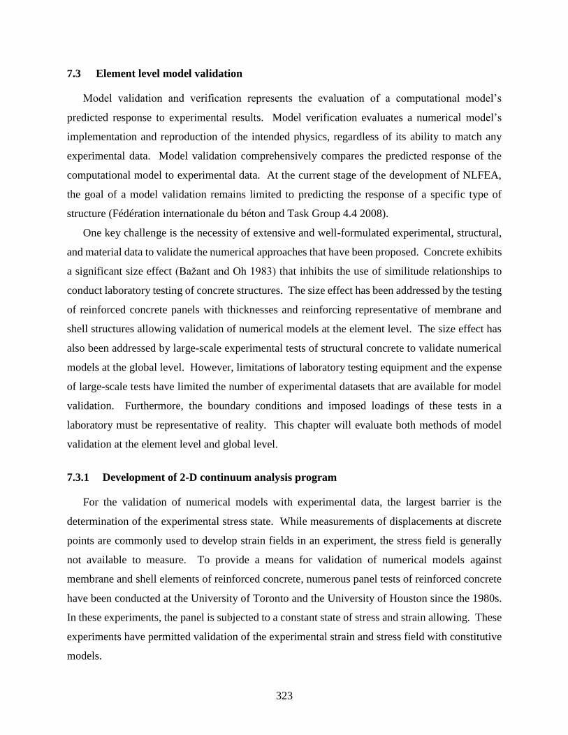
323
7.3 Element level model validation
Model validation and verification represents the evaluation of a computational model’s
predicted response to experimental results. Model verification evaluates a numerical model’s
implementation and reproduction of the intended physics, regardless of its ability to match any
experimental data. Model validation comprehensively compares the predicted response of the
computational model to experimental data. At the current stage of the development of NLFEA,
the goal of a model validation remains limited to predicting the response of a specific type of
structure (Fédération internationale du béton and Task Group 4.4 2008).
One key challenge is the necessity of extensive and well-formulated experimental, structural,
and material data to validate the numerical approaches that have been proposed. Concrete exhibits
a significant size effect (Bažant and Oh 1983) that inhibits the use of similitude relationships to
conduct laboratory testing of concrete structures. The size effect has been addressed by the testing
of reinforced concrete panels with thicknesses and reinforcing representative of membrane and
shell structures allowing validation of numerical models at the element level. The size effect has
also been addressed by large-scale experimental tests of structural concrete to validate numerical
models at the global level. However, limitations of laboratory testing equipment and the expense
of large-scale tests have limited the number of experimental datasets that are available for model
validation. Furthermore, the boundary conditions and imposed loadings of these tests in a
laboratory must be representative of reality. This chapter will evaluate both methods of model
validation at the element level and global level.
7.3.1 Development of 2-D continuum analysis program
For the validation of numerical models with experimental data, the largest barrier is the
determination of the experimental stress state. While measurements of displacements at discrete
points are commonly used to develop strain fields in an experiment, the stress field is generally
not available to measure. To provide a means for validation of numerical models against
membrane and shell elements of reinforced concrete, numerous panel tests of reinforced concrete
have been conducted at the University of Toronto and the University of Houston since the 1980s.
In these experiments, the panel is subjected to a constant state of stress and strain allowing. These
experiments have permitted validation of the experimental strain and stress field with constitutive
models.

324
For the reinforced concrete panels, the loading is applied to create a uniform state of stress on
average permitting the resulting data to include measured average stresses and strains in the
concrete and steel. While the literature identified more than 70 panel tests, the data set herein
includes only those with reported crack widths at each step of loading to facilitate the evaluation
of crack prediction. The data from these panel tests and others were the primary basis for the
development of the constitutive relationships implemented in the total strain models described in
Section 2.5. The wide array of material properties, reinforcing and loading conditions creates an
opportunity to determine the successes and shortcomings of the different analytical models.
To perform this element level validation, a database of 25 experimentally tested reinforced
concrete panels (Chan 1989; Aspiotis 1993; Zhang 1995; Xie 2009) was compiled and summarized
in Table 7.1. The panel database contains panels with reinforcement ratios varying from zero to
5.98%. In addition, the reinforcing ratios in 21 of the 25 panels utilized non-orthogonal reinforcing
with a minimum reinforcing ratio to maximum ratio ranging from zero to one half. The concrete
compressive strength varied from 24 to 103 MPa and the panels were subjected to various
configurations of in-plane shear and normal stresses applied in a monotonic loading pattern. A
summary of the design parameters of each panel test included is given in Table 7.1.
Table 7.1: Panel test database
Reference Panel ID Nx Ny Vxy f'c (MPa) ρx (%) ρy (%) ρmin / ρmax
Zhang (1995) VA1 0 0 1 95.10 1.20 1.20 1.00
Zhang (1995) VA2 0 0 1 98.20 2.39 2.39 1.00
Zhang (1995) VA3 0 0 1 94.60 3.59 3.59 1.00
Zhang (1995) VA4 0 0 1 103.10 5.24 5.24 1.00
Zhang (1995) VB1 0 0 1 98.20 2.39 1.20 0.50
Zhang (1995) VB2 0 0 1 97.60 3.59 1.20 0.33
Zhang (1995) VB3 0 0 1 102.30 5.98 1.20 0.20
Zhang (1995) VB4 0 0 1 96.90 1.80 0.60 0.33
Aspiotis (1993) PA1 0 0 1 49.90 1.65 0.82 0.50
Aspiotis (1993) PA2 0 0 1 43.00 1.65 0.82 0.50
Aspiotis (1993) PHS1 0 0 1 72.20 3.23 0.00 0.00
Aspiotis (1993) PHS2 0 0 1 66.10 3.23 0.41 0.13
Aspiotis (1993) PHS4 0.25 0.25 1 68.50 3.23 0.82 0.25
Aspiotis (1993) PHS5 0.25 0.25 1 52.10 3.23 0.41 0.13
Aspiotis (1993) PHS8 0 0 1 55.90 3.23 1.24 0.38
Aspiotis (1993) PHS9 -0.25 -0.25 1 56.00 3.23 0.41 0.13

325
Table 7.1 cont.
Reference Panel ID Nx Ny Vxy f'c (MPa) ρx (%) ρy (%) ρmin / ρmax
Chan (1989) PC1A 0 0 1 27.91 1.65 0.82 0.50
Chan (1989) PC4 -0.39 -0.39 1 24.89 1.65 0.82 0.50
Chan (1989) PC7 0.32 0.32 1 28.73 1.65 0.82 0.50
Xie (2009) PL1 -2 0 1 38.50 1.57 0.18 0.12
Xie (2009) PL2 -1 0 1 38.20 1.58 0.19 0.12
Xie (2009) PL3 1 0 1 42.00 1.57 0.18 0.12
Xie (2009) PL4 -2.8 0 1 43.10 1.65 0.19 0.12
Xie (2009) PL5 0 0 1 38.10 1.58 0.18 0.12
Xie (2009) PL6 3 0 1 43.50 1.58 0.19 0.12
A continuum analysis program was developed to evaluate and validate the choice of
constitutive models for predicting the response of the reinforced concrete panels. The overall
workflow of the program consists of taking tabulated experimental data in the literature that was
imported to excel and importing that data into a Matlab data structure. The data structure contains
the geometry, material properties, reinforcing, and loading parameters for each panel test as well
as stepwise data for the experimental response and analytical simulations. The response data
includes all strains, concrete stresses, reinforcement stresses and cracking information. To
maximize the number of constitutive models available for analysis, two pre-existing finite element
analysis programs, VecTor2 (Wong, Vecchio, and Trommels 2013) and OpenSees (McKenna,
Fenves, and Scott 2000) were incorporated to perform the analysis of each panel. The analytical
model for each program is automatically generated based upon the panel parameters defined in the
data structure. After running an analysis, the output data files are imported back into the data
structure and organized in the same manner as the experimental data. This approach allows the
ability to perform a large number of numerical analyses efficiently and subsequently perform
statistical analyses as part of a parametric study. The overall workflow is depicted in Figure 7.1.
A snapshot of the continuum analysis program input and output is shown in Figure 7.2.
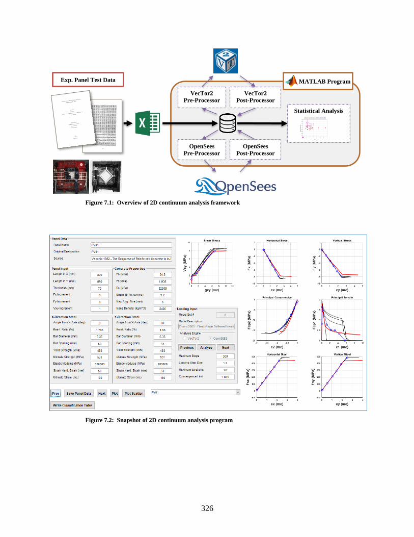
326
Figure 7.1: Overview of 2D continuum analysis framework
Figure 7.2: Snapshot of 2D continuum analysis program
Exp. Panel Test Data
Statistical Analysis
VecTor2
Pre-Processor
VecTor2
Post-Processor
MATLAB Program
OpenSees
Pre-Processor
OpenSees
Post-Processor

327
7.3.2 Parameters for evaluating model performance
The parameters utilized in the panel database analysis are summarized in Table 7.2 and Table
7.3. The design parameters in Table 7.2 represent the input variables to crack spacing models that
are independent of the predicted response. The response parameters in Table 7.3 represent the
ability of the analytical prediction to capture the experimental response at key points along the
entire load-deformation history.
Table 7.2: Definitions of design parameters
Parameter Symbol Definition
Clear Cover cc The clear cover is the distance from the face of concrete to outside face of rebar. The
clear cover is subject to construction tolerances and the layering of reinforcing bars.
A common representation of the clear cover is to use 1.5 times the maximum
aggregate size.
Bar Diameter bd The diameter of the reinforcing bar. Each direction is considered separately.
Compressive
strength at testing ' *cf The experimentally measured compressive strength at the time of testing.
Tensile strength 'tf The experimentally measured direct tensile strength, in the absence of test data this
value is taken as 4 'cf .
Effective
reinforcement ratio ef The area of vertical reinforcing steel divided by the effective area of concrete.
Mean bond stress bm The nominal shear stress where the nominal shear strength, Vn, and shear area, Acv,
are defined by ACI 318. For bi-directionally loaded tests, the value of Vn and Acv
was defined separately for each direction of loading.
Bond ratio k The ratio of mean bond stress to direct tensile strength of the concrete.
Table 7.3: Definitions of response parameters
Parameter Symbol Definition
Shear stress at
cracking crv The shear stress at onset of cracking given in megapascals.
Shear strain at
cracking cr The shear strain at onset of cracking given in millistrain.
Shear stress at
25% yield 25 yv The shear stress at first 25% yield of the reinforcing bars in either direction based
upon the average stress in the reinforcing bars given in megapascals.
Shear strain at
25% yield 25 y The shear strain at first 25% yield of the reinforcing bars in either direction based
upon the average stress in the reinforcing bars given in millistrain.
Secant stiffness at
25% yield 25 yE The ratio of stress at 25% yield and strain at 25% yield given in megapascals.
Shear stress at
50% yield 50 yv The shear stress at first 50% yield of the reinforcing bars in either direction based
upon the average stress in the reinforcing bars given in megapascals.
Shear strain at
50% yield 50 y The shear strain at first 50% yield of the reinforcing bars in either direction based
upon the average stress in the reinforcing bars given in millistrain.

328
Table 7.3 cont.
Parameter Symbol Definition
Secant stiffness at
50% yield 50 yE The ratio of stress at 50% yield and strain at 50% yield given in megapascals.
Shear stress at
75% yield 75 yv The shear stress at first 75% yield of the reinforcing bars in either direction based
upon the average stress in the reinforcing bars given in megapascals.
Shear strain at
75% yield 75 y The shear strain at first 75% yield of the reinforcing bars in either direction based
upon the average stress in the reinforcing bars given in millistrain.
Secant stiffness at
75% yield 75 yE The ratio of stress at 75% yield and strain at 75% yield given in megapascals.
Maximum shear
stress uv The maximum shear stress given in megapascals.
Shear strain at
peak stress u The shear strain at the maximum shear stress given in millistrain.
Secant stiffness at
peak stress uE The ratio of maximum stress and strain at maximum stress given in megapascals.
7.3.3 Crack spacing of reinforced concrete subjected to biaxial stress
The tensile response and shear response of cracked reinforced concrete are directly related to
the width and spacing of the cracks. For numerical modeling of reinforced concrete in a
continuum, the constitutive models are dependent on the width of cracks which is also dependent
on the distribution or spacing of those cracks. Consequently, the assumption of crack spacing
input to the numerical model can significantly impact the predicted response.
Prior research on cracking of reinforced concrete has focused on controlling crack width.
Crack width has been the focus due to the desire to limit crack width during service level loading
for appearance and durability (Beeby et al. 1985). Prior research and models of crack spacing
have indicated the primary variables to be the clear cover to reinforcing, the spacing of reinforcing
bars, the diameter of reinforcing bars, the effective reinforcing ratio of the section in tension, the
bond of the reinforcing bars to the concrete, and the mean tensile strength of the concrete. A state
of the art review of cracking conducted by Borosnyói and Balázs (2005) identified twenty-four
different models for crack spacing proposed from 1950 to the present utilizing these parameters in
various combinations. The models range from a single parameter to five parameters and include
both linear and non-linear functions of those parameters. One of the key findings of this study was
that there is not a universally accepted model for crack spacing in reinforced concrete.
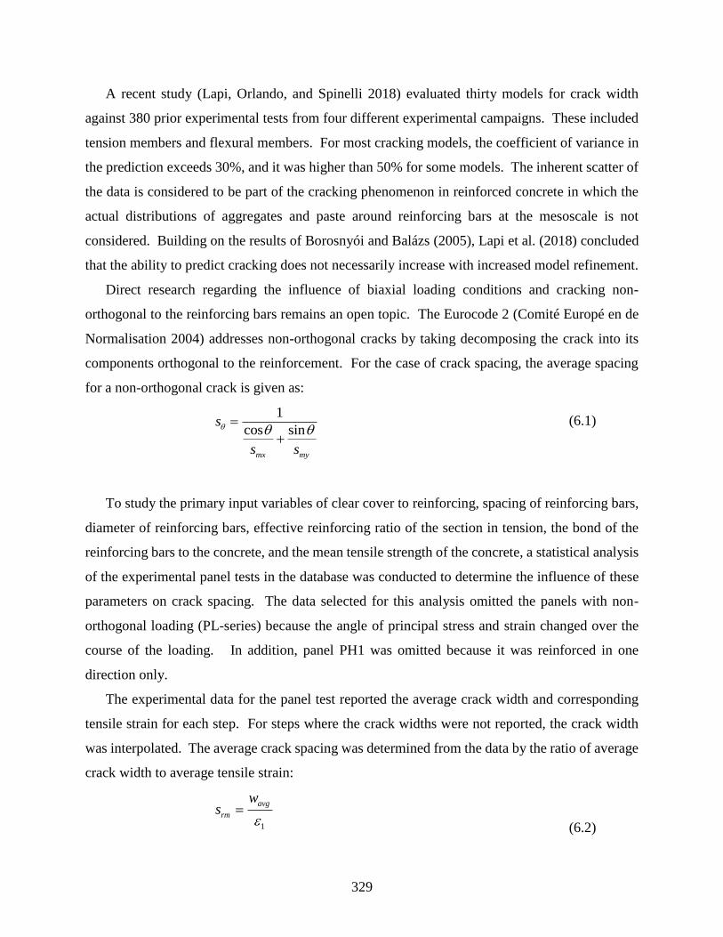
329
A recent study (Lapi, Orlando, and Spinelli 2018) evaluated thirty models for crack width
against 380 prior experimental tests from four different experimental campaigns. These included
tension members and flexural members. For most cracking models, the coefficient of variance in
the prediction exceeds 30%, and it was higher than 50% for some models. The inherent scatter of
the data is considered to be part of the cracking phenomenon in reinforced concrete in which the
actual distributions of aggregates and paste around reinforcing bars at the mesoscale is not
considered. Building on the results of Borosnyói and Balázs (2005), Lapi et al. (2018) concluded
that the ability to predict cracking does not necessarily increase with increased model refinement.
Direct research regarding the influence of biaxial loading conditions and cracking non-
orthogonal to the reinforcing bars remains an open topic. The Eurocode 2 (Comité Europé en de
Normalisation 2004) addresses non-orthogonal cracks by taking decomposing the crack into its
components orthogonal to the reinforcement. For the case of crack spacing, the average spacing
for a non-orthogonal crack is given as:
1
cos sin
mx my
s
s s
=
+
(6.1)
To study the primary input variables of clear cover to reinforcing, spacing of reinforcing bars,
diameter of reinforcing bars, effective reinforcing ratio of the section in tension, the bond of the
reinforcing bars to the concrete, and the mean tensile strength of the concrete, a statistical analysis
of the experimental panel tests in the database was conducted to determine the influence of these
parameters on crack spacing. The data selected for this analysis omitted the panels with non-
orthogonal loading (PL-series) because the angle of principal stress and strain changed over the
course of the loading. In addition, panel PH1 was omitted because it was reinforced in one
direction only.
The experimental data for the panel test reported the average crack width and corresponding
tensile strain for each step. For steps where the crack widths were not reported, the crack width
was interpolated. The average crack spacing was determined from the data by the ratio of average
crack width to average tensile strain:
1
avg
rm
ws
=
(6.2)
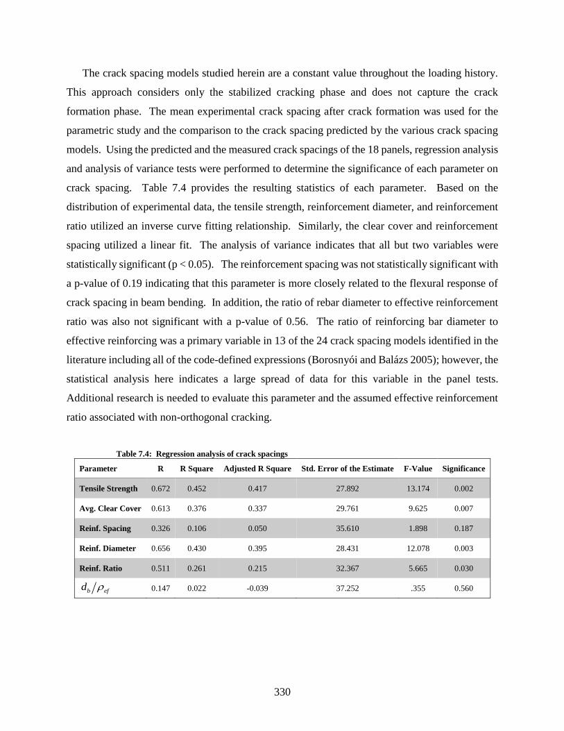
330
The crack spacing models studied herein are a constant value throughout the loading history.
This approach considers only the stabilized cracking phase and does not capture the crack
formation phase. The mean experimental crack spacing after crack formation was used for the
parametric study and the comparison to the crack spacing predicted by the various crack spacing
models. Using the predicted and the measured crack spacings of the 18 panels, regression analysis
and analysis of variance tests were performed to determine the significance of each parameter on
crack spacing. Table 7.4 provides the resulting statistics of each parameter. Based on the
distribution of experimental data, the tensile strength, reinforcement diameter, and reinforcement
ratio utilized an inverse curve fitting relationship. Similarly, the clear cover and reinforcement
spacing utilized a linear fit. The analysis of variance indicates that all but two variables were
statistically significant (p < 0.05). The reinforcement spacing was not statistically significant with
a p-value of 0.19 indicating that this parameter is more closely related to the flexural response of
crack spacing in beam bending. In addition, the ratio of rebar diameter to effective reinforcement
ratio was also not significant with a p-value of 0.56. The ratio of reinforcing bar diameter to
effective reinforcing was a primary variable in 13 of the 24 crack spacing models identified in the
literature including all of the code-defined expressions (Borosnyói and Balázs 2005); however, the
statistical analysis here indicates a large spread of data for this variable in the panel tests.
Additional research is needed to evaluate this parameter and the assumed effective reinforcement
ratio associated with non-orthogonal cracking.
Table 7.4: Regression analysis of crack spacings
Parameter R R Square Adjusted R Square Std. Error of the Estimate F-Value Significance
Tensile Strength 0.672 0.452 0.417 27.892 13.174 0.002
Avg. Clear Cover 0.613 0.376 0.337 29.761 9.625 0.007
Reinf. Spacing 0.326 0.106 0.050 35.610 1.898 0.187
Reinf. Diameter 0.656 0.430 0.395 28.431 12.078 0.003
Reinf. Ratio 0.511 0.261 0.215 32.367 5.665 0.030
b efd
0.147 0.022 -0.039 37.252 .355 0.560

331
(a) ( )( )
30050m
t
mmMPa
sf
= − + (b) ( ) ( )125 1.2m cmm mms c= −
Figure 7.3: Crack spacing as a function of (a) tensile strength and (b) clear cover
(a) Non-significant fit of data (b) ( )( )
2.75125m
b
mmmm
sd
= −
Figure 7.4: Crack spacing as a function of (a) reinf. spacing and (b) reinf. diameter

332
(a) ( )( )%
12530m
ef
mms
= + (b) Non-significant fit of data
Figure 7.5: Crack spacing as a function of (a) reinf. ratio and (b) db/ρ
7.3.4 Crack spacing models for reinforced concrete
The subsequent study utilizes the panel test data containing measured crack widths and load-
deformation response to evaluate the performance of six different crack spacing models identified
in the literature. Six models were selected with historical significance in the development of crack
spacing and/or are present in building codes or model codes of practice.
Saliger (1950)
One of the earliest empirical formulas for crack spacing was developed by Saliger (1950). The
approach utilized the product of the ratio of reinforcing bar diameter to effective reinforcing ratio
and the ratio of compressive strength to average bond stress:
'0.157
4
c b
rm
bm ef
f ds
=
(6.3)
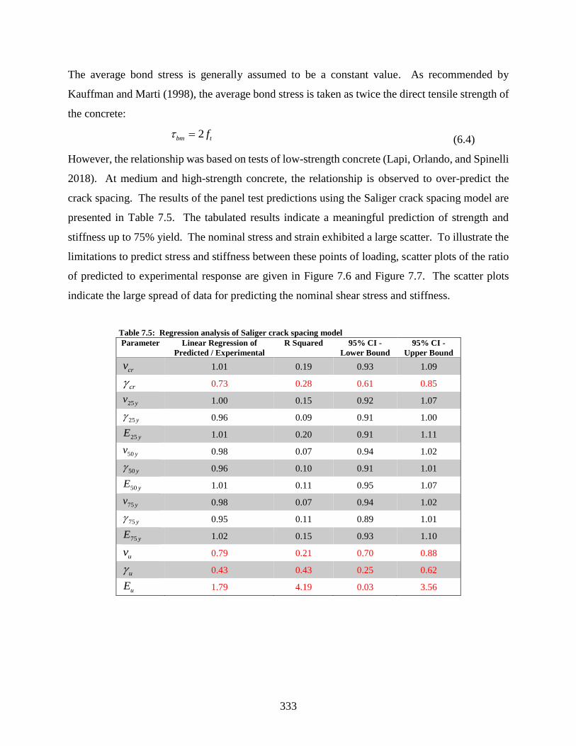
333
The average bond stress is generally assumed to be a constant value. As recommended by
Kauffman and Marti (1998), the average bond stress is taken as twice the direct tensile strength of
the concrete:
2bm tf =
(6.4)
However, the relationship was based on tests of low-strength concrete (Lapi, Orlando, and Spinelli
2018). At medium and high-strength concrete, the relationship is observed to over-predict the
crack spacing. The results of the panel test predictions using the Saliger crack spacing model are
presented in Table 7.5. The tabulated results indicate a meaningful prediction of strength and
stiffness up to 75% yield. The nominal stress and strain exhibited a large scatter. To illustrate the
limitations to predict stress and stiffness between these points of loading, scatter plots of the ratio
of predicted to experimental response are given in Figure 7.6 and Figure 7.7. The scatter plots
indicate the large spread of data for predicting the nominal shear stress and stiffness.
Table 7.5: Regression analysis of Saliger crack spacing model
Parameter Linear Regression of
Predicted / Experimental
R Squared 95% CI -
Lower Bound
95% CI -
Upper Bound
crv 1.01 0.19 0.93 1.09
cr 0.73 0.28 0.61 0.85
25 yv 1.00 0.15 0.92 1.07
25 y 0.96 0.09 0.91 1.00
25 yE 1.01 0.20 0.91 1.11
50 yv 0.98 0.07 0.94 1.02
50 y 0.96 0.10 0.91 1.01
50 yE 1.01 0.11 0.95 1.07
75 yv 0.98 0.07 0.94 1.02
75 y 0.95 0.11 0.89 1.01
75 yE 1.02 0.15 0.93 1.10
uv 0.79 0.21 0.70 0.88
u 0.43 0.43 0.25 0.62
uE 1.79 4.19 0.03 3.56
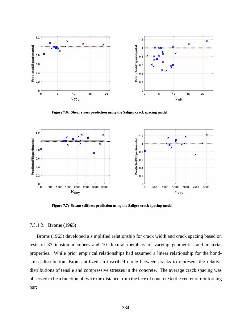
334
Figure 7.6: Shear stress prediction using the Saliger crack spacing model
Figure 7.7: Secant stiffness prediction using the Saliger crack spacing model
Broms (1965)
Broms (1965) developed a simplified relationship for crack width and crack spacing based on
tests of 37 tension members and 10 flexural members of varying geometries and material
properties. While prior empirical relationships had assumed a linear relationship for the bond-
stress distribution, Broms utilized an inscribed circle between cracks to represent the relative
distributions of tensile and compressive stresses in the concrete. The average crack spacing was
observed to be a function of twice the distance from the face of concrete to the center of reinforcing
bar:

335
22
b
rm c
ds c
= +
(6.5)
The model generally underpredicted the crack spacing at low steel stresses and overpredicted
the crack spacing at high steel stresses. The results of the panel test predictions using the Broms
crack spacing model are presented in Table 7.6. The tabulated results indicate a meaningful
prediction of strength up to nominal and stiffness up to 75% yield. To illustrate the limitations to
predict stress and stiffness between these points of loading, scatter plots of the ratio of predicted
to experimental response are given in Figure 7.8 and Figure 7.9. In general, the Broms crack
spacing model overpredicted the strength and stiffness by 10% on average.
Table 7.6: Analysis of Broms crack spacing model
Parameter Mean of Predicted /
Experimental
Root squared
mean error
Minimum
Value
Maximum
Value
crv 1.05 0.19 0.97 1.13
cr 0.77 0.29 0.65 0.90
25 yv 1.19 0.13 1.12 1.25
25 y 1.07 0.16 0.99 1.14
25 yE 1.08 0.19 0.99 1.16
50 yv 1.17 0.10 1.13 1.22
50 y 1.06 0.15 1.00 1.13
50 yE 1.08 0.15 1.02 1.15
75 yv 1.15 0.09 1.11 1.20
75 y 1.03 0.14 0.96 1.09
75 yE 1.09 0.17 1.02 1.17
uv 1.12 0.22 1.02 1.21
u 0.90 0.56 0.66 1.13
uE 1.15 3.61 0.38 2.67
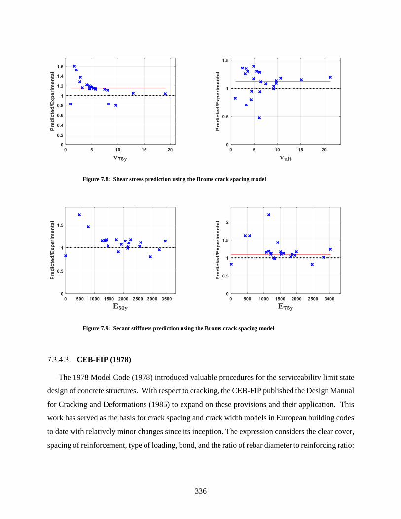
336
Figure 7.8: Shear stress prediction using the Broms crack spacing model
Figure 7.9: Secant stiffness prediction using the Broms crack spacing model
CEB-FIP (1978)
The 1978 Model Code (1978) introduced valuable procedures for the serviceability limit state
design of concrete structures. With respect to cracking, the CEB-FIP published the Design Manual
for Cracking and Deformations (1985) to expand on these provisions and their application. This
work has served as the basis for crack spacing and crack width models in European building codes
to date with relatively minor changes since its inception. The expression considers the clear cover,
spacing of reinforcement, type of loading, bond, and the ratio of rebar diameter to reinforcing ratio:

337
1 2210
b
rm
ef
dss c k k
= + + (6.6)
The first parameter, 1k , represents the change in bond strength associated with the bar surface.
For deformed bar reinforcing, this parameter is taken as 0.4. For plain bar reinforcing, this
parameter is taken as 0.8. All test specimens utilized deformed bars or mechanically imprinted
bars, so the value of 0.4 was used. The second parameter, 2k , represents the strain distribution in
the effective area of concrete. For bending, this parameter is taken as 0.125. For direct tension,
this parameter is taken as 0.25.
The results of the panel test predictions using the 1978 Model Code crack spacing model are
presented in Table 7.7. The tabulated results indicate a meaningful prediction of strength up to
nominal and stiffness up to 75% yield. To illustrate the limitations to predict stress and stiffness
between these points of loading, scatter plots of the ratio of predicted to experimental response are
given in Figure 7.10 and Figure 7.11.
Table 7.7: Regression analysis of 1978 CEB-FIP crack spacing model
Parameter Linear Regression of
Predicted / Experimental
R Squared 95% CI -
Lower Bound
95% CI -
Upper Bound
crv 1.02 0.19 0.94 1.10
cr 0.74 0.29 0.62 0.86
25 yv 1.06 0.16 0.99 1.14
25 y 1.01 0.13 0.95 1.07
25 yE 1.01 0.20 0.91 1.10
50 yv 1.04 0.08 1.00 1.08
50 y 0.99 0.13 0.93 1.05
50 yE 1.01 0.13 0.95 1.07
75 yv 1.03 0.08 1.00 1.07
75 y 0.98 0.14 0.91 1.04
75 yE 1.05 0.20 0.95 1.14
uv 0.93 0.15 0.87 0.99
u 0.59 0.42 0.41 0.77
uE 1.34 1.18 0.84 1.83

338
Figure 7.10: Shear stress prediction using the 1978 CEB-FIP crack spacing model
Figure 7.11: Secant stiffness prediction using the 1978 CEB-FIP crack spacing model
Noakowski (1985)
Noakowski (1985) utilized a nonlinear relationship for the crack spacing. The expression is a
function of the direct tensile strength of the concrete, average bond stress, effective reinforcing
ratio, and bar diameter. In contrast to most other models, this expression is not based on empirical
data. Instead, it was developed analytically using the differential equation of bond-slip in the
transfer length on each side of an open crack (Lapi, Orlando, and Spinelli 2018).

339
( )0.89
0.88
0.66
0.223.1
t ef
rm b
t
fs k d
f
= (6.7)
bm
t
kf
=
(6.8)
For analysis of the panel tests, this expression overpredicted the average crack spacing
measured experimentally by a factor of 4 to 10. The regression analysis of the Noakowski model
indicates a poor prediction of strength and deformation beyond 75% yielding as shown in Table
7.8. Figure 7.12 illustrates the model was unable to predict the nominal strength of the panel
reliably, and the prediction captured only 80% of the nominal strength on average. In addition,
Figure 7.13 indicates that the prediction of secant stiffness degrades beyond 50% yielding with a
wide scatter of data at 75%.
Table 7.8: Regression analysis of Noakowski crack spacing model
Parameter Linear Regression of
Predicted / Experimental
R Squared 95% CI -
Lower Bound
95% CI -
Upper Bound
crv 1.01 0.20 0.92 1.09
cr 0.73 0.29 0.61 0.85
25 yv 1.01 0.16 0.93 1.08
25 y 0.95 0.11 0.90 1.00
25 yE 1.01 0.20 0.91 1.10
50 yv 0.99 0.09 0.94 1.03
50 y 0.95 0.10 0.90 1.00
50 yE 1.01 0.14 0.94 1.08
75 yv 0.96 0.12 0.89 1.03
75 y 0.95 0.16 0.85 1.04
75 yE 1.01 0.24 0.87 1.15
uv 0.77 0.19 0.69 0.85
u 0.35 0.31 0.22 0.48
uE 2.82 3.20 1.47 4.17

340
Figure 7.12: Shear stress prediction using the Noakowski crack spacing model
Figure 7.13: Secant stiffness prediction using the Noakowski crack spacing model
CEB-FIP (1990)
The CEB-FIP Model Code 1990 simplified the expression given in the CEB-FIP Model Code
1978 expression to remove the dependence of clear cover, rebar spacing, and bond on crack
spacing:
2
3 3.6
b
rm
ef
ds
=
(6.9)
This simplified model has been observed to exhibit particularly poor performance when the clear
cover becomes large (Lapi, Orlando, and Spinelli 2018).

341
The results of the panel test predictions using the Model Code 1990 crack spacing expression
are presented in Table 7.9. The tabulated results indicate a meaningful prediction of strength up
to nominal and stiffness up to 75% yield. To illustrate the limitations to predict stress and stiffness
between these points of loading, scatter plots of the ratio of predicted to experimental response are
given in Figure 7.14 and Figure 7.15. While the simplified expression may reduce the accuracy
of the prediction, it also reduces the sensitivity of the model to material properties and geometry
outside the calibrated test data.
Table 7.9: Regression analysis of 1990 CEB-FIP crack spacing model
Parameter Linear Regression of
Predicted / Experimental
R Squared 95% CI -
Lower Bound
95% CI -
Upper Bound
crv 1.02 0.18 0.95 1.10
cr 0.74 0.28 0.63 0.86
25 yv 1.09 0.18 1.00 1.18
25 y 1.00 0.11 0.95 1.06
25 yE 1.01 0.21 0.91 1.11
50 yv 1.04 0.09 0.99 1.08
50 y 0.99 0.11 0.94 1.04
50 yE 1.02 0.13 0.96 1.08
75 yv 1.03 0.08 0.99 1.07
75 y 0.96 0.15 0.89 1.03
75 yE 1.06 0.21 0.96 1.16
uv 0.92 0.19 0.85 1.00
u 0.61 0.46 0.41 0.80
uE 1.31 3.73 -0.27 2.88
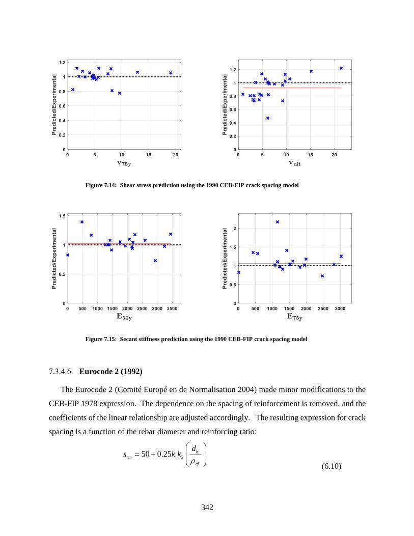
342
Figure 7.14: Shear stress prediction using the 1990 CEB-FIP crack spacing model
Figure 7.15: Secant stiffness prediction using the 1990 CEB-FIP crack spacing model
Eurocode 2 (1992)
The Eurocode 2 (Comité Europé en de Normalisation 2004) made minor modifications to the
CEB-FIP 1978 expression. The dependence on the spacing of reinforcement is removed, and the
coefficients of the linear relationship are adjusted accordingly. The resulting expression for crack
spacing is a function of the rebar diameter and reinforcing ratio:
1 250 0.25 b
rm
ef
ds k k
= +
(6.10)
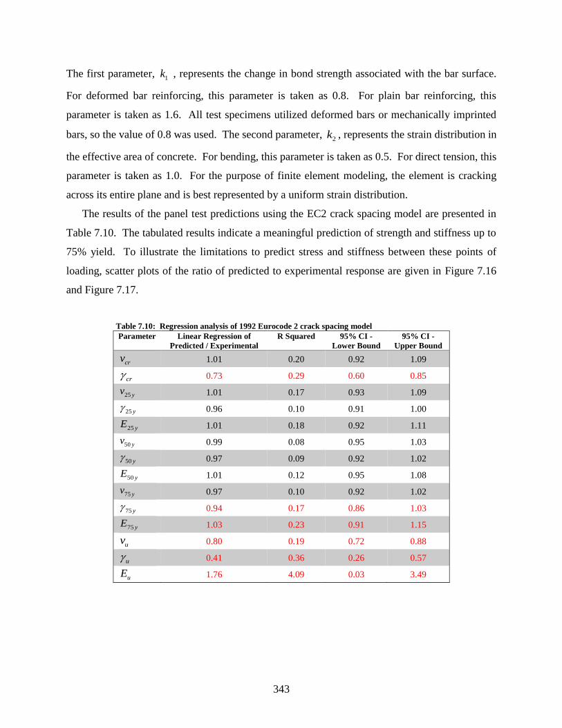
343
The first parameter, 1k , represents the change in bond strength associated with the bar surface.
For deformed bar reinforcing, this parameter is taken as 0.8. For plain bar reinforcing, this
parameter is taken as 1.6. All test specimens utilized deformed bars or mechanically imprinted
bars, so the value of 0.8 was used. The second parameter, 2k , represents the strain distribution in
the effective area of concrete. For bending, this parameter is taken as 0.5. For direct tension, this
parameter is taken as 1.0. For the purpose of finite element modeling, the element is cracking
across its entire plane and is best represented by a uniform strain distribution.
The results of the panel test predictions using the EC2 crack spacing model are presented in
Table 7.10. The tabulated results indicate a meaningful prediction of strength and stiffness up to
75% yield. To illustrate the limitations to predict stress and stiffness between these points of
loading, scatter plots of the ratio of predicted to experimental response are given in Figure 7.16
and Figure 7.17.
Table 7.10: Regression analysis of 1992 Eurocode 2 crack spacing model
Parameter Linear Regression of
Predicted / Experimental
R Squared 95% CI -
Lower Bound
95% CI -
Upper Bound
crv 1.01 0.20 0.92 1.09
cr 0.73 0.29 0.60 0.85
25 yv 1.01 0.17 0.93 1.09
25 y 0.96 0.10 0.91 1.00
25 yE 1.01 0.18 0.92 1.11
50 yv 0.99 0.08 0.95 1.03
50 y 0.97 0.09 0.92 1.02
50 yE 1.01 0.12 0.95 1.08
75 yv 0.97 0.10 0.92 1.02
75 y 0.94 0.17 0.86 1.03
75 yE 1.03 0.23 0.91 1.15
uv 0.80 0.19 0.72 0.88
u 0.41 0.36 0.26 0.57
uE 1.76 4.09 0.03 3.49

344
Figure 7.16: Shear stress prediction using the Eurocode crack spacing model
Figure 7.17: Secant stiffness prediction using the Eurocode 2 crack spacing model
Recommendation
The evaluation of crack spacing from experimental panel tests identified that the following
parameters were significant:
• Direct tensile strength
• Effective reinforcing ratio
• Bar diameter
• Clear cover

345
Five crack spacing models were selected that utilized these four variables. While not meeting
these criteria, the CEB-FIP 1978 model was also included due to its recommendation by prior
work and adoption in existing finite element software (Sato and Vecchio 2003; Wong, Vecchio,
and Trommels 2013). The six crack spacing models were evaluated with respect to their ability to
predict stress, strain and secant stiffness during cracking, yielding and ultimate load. A summary
of the performance of the different crack spacing models is given in Table 7.11.
Table 7.11: Summary of element prediction performance
Parameter R Squared Value
Saliger Broms CEB-FIP78 Noakowski CEB-FIP90 EC2
crv 0.19 0.19 0.19 0.2 0.18 0.2
cr 0.28 0.29 0.29 0.29 0.28 0.29
25 yv 0.15 0.13 0.16 0.16 0.18 0.17
25 y 0.09 0.16 0.13 0.11 0.11 0.1
25 yE 0.2 0.19 0.2 0.2 0.21 0.18
50 yv 0.07 0.1 0.08 0.09 0.09 0.08
50 y 0.1 0.15 0.13 0.1 0.11 0.09
50 yE 0.11 0.15 0.13 0.14 0.13 0.12
75 yv 0.07 0.09 0.08 0.12 0.08 0.1
75 y 0.11 0.14 0.14 0.16 0.15 0.17
75 yE 0.15 0.17 0.2 0.24 0.21 0.23
uv 0.21 0.22 0.15 0.19 0.19 0.19
u 0.43 0.56 0.42 0.31 0.46 0.36
uE 4.19 3.61 1.18 3.2 3.73 4.09
Mean 0.45 0.44 0.25 0.39 0.44 0.46
In general, the crack spacing models performed equally up to 50% yield. At 75% yield, the
prediction of stiffness begins to degrade. At the ultimate load, the models provided reasonable
predictions of stress but could not reliably predict the secant stiffness. The inability to predict the
strain at ultimate is a result of two factors: first, the constitutive models are not well suited to
failure conditions and damage in reinforced concrete, and second, the panels were analyzed in
loading control in order to match the experimental response. The use of load-control creates
numerical instability as the load-deformation response becomes flat or negative, and this prevents
the numerical model from capturing the peak and post-peak response. The specific analyses of the
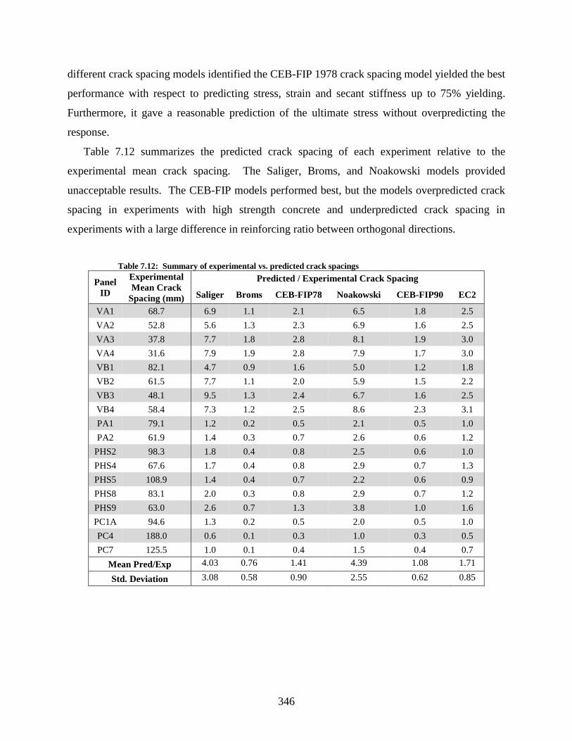
346
different crack spacing models identified the CEB-FIP 1978 crack spacing model yielded the best
performance with respect to predicting stress, strain and secant stiffness up to 75% yielding.
Furthermore, it gave a reasonable prediction of the ultimate stress without overpredicting the
response.
Table 7.12 summarizes the predicted crack spacing of each experiment relative to the
experimental mean crack spacing. The Saliger, Broms, and Noakowski models provided
unacceptable results. The CEB-FIP models performed best, but the models overpredicted crack
spacing in experiments with high strength concrete and underpredicted crack spacing in
experiments with a large difference in reinforcing ratio between orthogonal directions.
Table 7.12: Summary of experimental vs. predicted crack spacings
Panel
ID
Experimental
Mean Crack
Spacing (mm)
Predicted / Experimental Crack Spacing
Saliger Broms CEB-FIP78 Noakowski CEB-FIP90 EC2
VA1 68.7 6.9 1.1 2.1 6.5 1.8 2.5
VA2 52.8 5.6 1.3 2.3 6.9 1.6 2.5
VA3 37.8 7.7 1.8 2.8 8.1 1.9 3.0
VA4 31.6 7.9 1.9 2.8 7.9 1.7 3.0
VB1 82.1 4.7 0.9 1.6 5.0 1.2 1.8
VB2 61.5 7.7 1.1 2.0 5.9 1.5 2.2
VB3 48.1 9.5 1.3 2.4 6.7 1.6 2.5
VB4 58.4 7.3 1.2 2.5 8.6 2.3 3.1
PA1 79.1 1.2 0.2 0.5 2.1 0.5 1.0
PA2 61.9 1.4 0.3 0.7 2.6 0.6 1.2
PHS2 98.3 1.8 0.4 0.8 2.5 0.6 1.0
PHS4 67.6 1.7 0.4 0.8 2.9 0.7 1.3
PHS5 108.9 1.4 0.4 0.7 2.2 0.6 0.9
PHS8 83.1 2.0 0.3 0.8 2.9 0.7 1.2
PHS9 63.0 2.6 0.7 1.3 3.8 1.0 1.6
PC1A 94.6 1.3 0.2 0.5 2.0 0.5 1.0
PC4 188.0 0.6 0.1 0.3 1.0 0.3 0.5
PC7 125.5 1.0 0.1 0.4 1.5 0.4 0.7
Mean Pred/Exp 4.03 0.76 1.41 4.39 1.08 1.71
Std. Deviation 3.08 0.58 0.90 2.55 0.62 0.85

347
7.4 Finite element modeling of C-shaped wall specimens
To numerically study the C-shaped wall test specimen, a series of non-linear finite element
analyses are conducted using a three-dimensional layered shell element formulation. A true three-
dimensional analysis was required to capture the asymmetric response of the C-shaped wall. As
observed in the experimental data, the neutral is shallow, and a non-uniform stress/strain field is
expected to be present in the compression flange during strong axis loading and similarly in the
web during weak axis loading with the web in compression. A layered shell was selected in lieu
of a membrane element in order to capture this non-linear stress-strain response through the
thickness of the wall. The “VecTor4” software published by the University of Toronto was
selected to conduct the non-linear finite element analysis with the desired capabilities. The
VecTor4 software for the analysis of reinforced concrete shell elements has been in development
since the 1980s. An overview of the software’s development and most recent capabilities are
summarized by Hrynyk (2013). The key features relevant to this chapter are summarized below.
For generalized application to reinforced concrete shell structures, a formulation that could
predict the nonlinear response of both think and thick shells was desired. To accommodate both
types of structures, the Heterosis element developed by Hughes and Cohen (1978) on the basis of
Mindlin plate theory was implemented. The Heterosis element is a nine-node element where the
outer eight nodes have five degrees of freedom, and the central ninth node has two rotational
degrees of freedom. The resulting element has a total of 42 degrees of freedom. The element is
based on three-dimensional elasticity which allows the ability to include out-of-plane shear
reinforcement and deformations. A reduced integration scheme is utilized with 3x3 Gauss point
integration for bending and 2x2 Gauss point integration for shear. The reduced integration scheme
reduces zero-energy modes and the problem of shear locking. In addition, a total Lagrangian
formulation is used to model geometric nonlinearity. The first application of the MCFT in this
software introduced by Polak and Vecchio (1993). Since that time, a wide range of constitutive
models, including those described in Section 7.2.1 have been implemented.
The finite element mesh generation is defined by a parametric model of the C-shaped wall as
shown in Figure 7.18. The toe and corner boundary elements are defined by regions A, C and D
are defined by their length, thickness and orthogonal reinforcement in two layers. In addition, the
boundary elements include out-of-plane confining reinforcement. The unconfined webs are
defined by regions B and E in which there are two layers of orthogonal reinforcement. By utilizing

348
a parametric definition, a maximum element width and height is defined such that each region is
automatically meshed to meet the input geometry as well as the maximum element dimensions.
Similarly, the elevation of the wall is defined parametrically by its foundation, first three floors,
upper floors, and loading cap as indicated in Figure 7.19. The height of each element is defined,
and the maximum element sizes are used to generate the appropriate mesh.
Figure 7.18: Plan of parametric C-shaped wall FE model regions
Figure 7.19: Elevation of parametric C-shaped wall FE model regions

349
The assessment of drift contributions of the C-shaped walls in Section 5.7.3 revealed that the
base rotation was up to 20% of the total deformation. For inclusion of the base rotation in the
finite element analysis, the foundation is modeled and restrained such that the strain penetration
of the reinforcing bars into the footing can be captured in the analysis.
The application of loading and restraint of the finite element model in strong axis and weak
axis directions is shown in Figure 7.20. For both directions, the bottom row of nodes is fixed in
all three translational degrees of freedom. Above the bottom row, the nodes of the foundation are
fixed against horizontal translation but permit vertical translation. For strong axis loading, the
model is also restrained against out of plane displacement and rotation at the top of the third floor
and at the wall cap. The out-of-plane restraint mimics the displacement control procedure
described in Section 3.3.4. The impact of these restraints is further studied in Section 7.4.3.
Displacements are imposed at the center of the wall along the web for strong axis loading and each
flange for weak axis loading.
(a) Strong Axis Loading (b) Weak Axis Loading
Figure 7.20: Finite element model load application
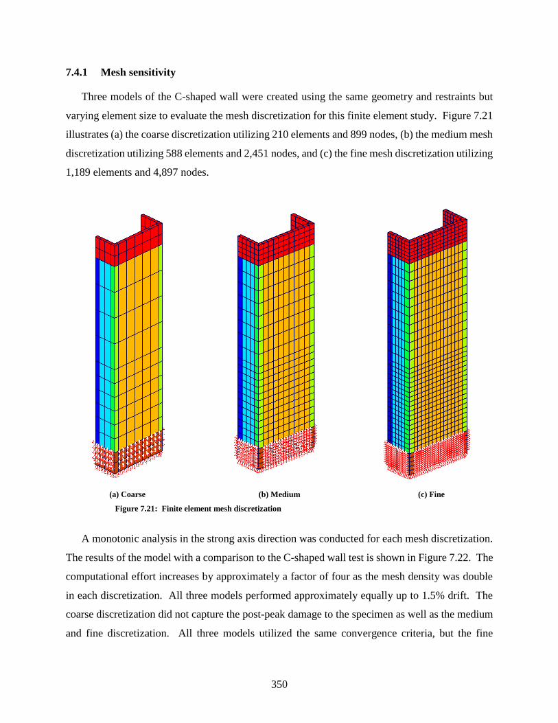
350
7.4.1 Mesh sensitivity
Three models of the C-shaped wall were created using the same geometry and restraints but
varying element size to evaluate the mesh discretization for this finite element study. Figure 7.21
illustrates (a) the coarse discretization utilizing 210 elements and 899 nodes, (b) the medium mesh
discretization utilizing 588 elements and 2,451 nodes, and (c) the fine mesh discretization utilizing
1,189 elements and 4,897 nodes.
(a) Coarse (b) Medium (c) Fine
Figure 7.21: Finite element mesh discretization
A monotonic analysis in the strong axis direction was conducted for each mesh discretization.
The results of the model with a comparison to the C-shaped wall test is shown in Figure 7.22. The
computational effort increases by approximately a factor of four as the mesh density was double
in each discretization. All three models performed approximately equally up to 1.5% drift. The
coarse discretization did not capture the post-peak damage to the specimen as well as the medium
and fine discretization. All three models utilized the same convergence criteria, but the fine

351
discretization encountered challenges in convergence prior to failure that were not observed in the
other models. The medium mesh discretization was selected for the subsequent analyses due to
its numerical stability and ability to capture the post-peak damage.
Figure 7.22: Shell element model mesh sensitivity
7.4.2 Effect of initial shrinkage cracking
Shrinkage strains associated with the placement and curing of the concrete are known to induce
microcracking resulting in an overall reduction of stiffness prior to loading. Cracking due to
shrinkage is most evident at interfaces of the concrete with relatively stiffer elements such as
between the wall and foundation element, and in heavily reinforced elements in which the
reinforcement restrains the concrete inducing cracking. Cracking of reinforced concrete due to
shrinkage is observed to increase the strains induced by loading and in conjunction with slightly
wider crack widths than estimated (Beeby et al. 1985). In general, the effects of shrinkage cracking
are not considered in finite element analyses; however, Palermo (2002) and Hart (2012) evaluated
the use of a pre-strain to simulate the effect of shrinkage cracking in finite element modeling of
concrete walls. Palermo (2002) recommended a pre-strain of 0.4 millistrain prior to loading on
the basis of experimental and analytical data. Hart (2012) validated the use of the same magnitude
of pre-strain for the planar wall test, PW4, in conjunction with the tension stiffening effect. The

352
C-shaped wall response was evaluated with and without an initial pre-strain to determine the effect.
Pre-strains were imposed in the VecTor4 analysis using a pseudo-temperature load.
(a) Planar wall (PW3) (Hart 2012) (b) C-shaped wall (CW2)
Figure 7.23: Effect of pre-strain and tension stiffening
Figure 7.23 (a) illustrates the impact of pre-strain and tension stiffening for the planar wall
specimen, PW3, based on the work of Hart (2012). Similarly, Figure 7.23 (b) illustrates the same
impact of the C-shaped wall specimen. The black line represents the backbone curve of the
experimental response. The red line indicates the predicted response including the effect of tension
stiffening but neglecting initial shrinkage cracking. The blue line represents the predicted response
including the effect of tension stiffening and an initial pre-strain of 4ms. Finally, the green line
represents the predicted response with an initial pre-strain but neglecting tension stiffening. In
both cases, the tension stiffened response overpredicts the experimental stiffness during yielding.
Conversely, the prediction without tension stiffening significantly underpredicts the stiffness
during yielding. The addition of pre-strain to represent the initial shrinkage cracking present in
the test specimen nearly corrected the response of the planar wall. The C-shaped wall prediction
is improved by considering a pre-strain for initial shrinkage cracking; however, the predicted
response remains stiffer than the experimental. Since the method of initial pre-strain to represent
the shrinkage cracking was inconclusive for the C-shaped walls, the subsequent analyses
considered the tension stiffening effect only. Furthermore, the empirical data used in the
development of the constitutive models is based on reinforced concrete panels that would have

353
inherently had shrinkage cracking prior to performing the experiment (Bentz 2007). In this
perspective, the tension models already account for the effects of shrinkage after cracking.
Additional research is needed to quantify and evaluate the methods of simulating initial shrinkage
cracking in non-planar walls.
7.4.3 Strong axis response
Non-Linear finite element analysis of the strong axis response of the C-shaped wall test
specimen was conducted using the parameters and constitutive models previously described in this
chapter. A reverse cyclic displacement history similar to that of the experimental test was imposed.
The exact displacement history is difficult to impose because the experimental displacements were
imposed at the third story and the displacement at the effective height was extrapolated from the
results. Conversely, the analytical model imposes the displacement at the effective height, and the
displacement at the third story is a result of the wall behavior. The resulting load-deformation
response is shown in Figure 7.24.
Overall, the analytical prediction provides a reasonable estimation of the strength, stiffness and
post-peak drift capacity. Regarding stiffness, the monotonic study of initial stiffness described in
Section 7.4.2 indicated that the stiffness during cracking and yielding is overpredicted. The reverse
cyclic analysis revealed the same overprediction. Regarding strength, the analytical model
predicted a base shear of 202 kips and base moment of 5,736 kip-ft. This represents 94%, 96%
and 98% of the nominal moment strength of CW1, CW2, and CW3 respectively. The strength of
the test upon reaching the yield plateau is nearly identical; however, the peak strength including
the effects of strain hardening is not fully captured in the analytical model. The monotonic model
had approximately the same strength as the experiment, so the difference in strength is believed to
be related to the treatment of hysteretic loading and plastic offsets in the reinforcing steel. The
unloading stiffness and reloading stiffness approximate that of the experimental study. Post-peak,
the pinching response of the hysteresis is slightly underpredicted by the analytical prediction. This
difference is due to the sliding present in the experiment that is not explicitly captured in the
analytical model. However, the elements at the interface of the foundation exhibit a very high
shear deformation in the analytical model indicating this same mode of deformation. Ultimately,
the model lost load carrying capacity and failed due to rupture of the longitudinal reinforcing and
failure of confining reinforcement in the boundary elements. This failure mechanism is consistent

354
with the analytical model. The drift capacity at loss of load carrying capacity was 1.25% and 1.5%
in the two loading directions for the analytical prediction and 1.5% for both directions of the
experiment (CW2).
Figure 7.24: Predicted strong axis response
For the strong axis loading protocol of the C-shaped wall experiments, Section 3.3.4 indicated
the out-of-plane displacement and twist of the specimen were restrained during the loading. This
application of loading effectively loaded the test specimen through the shear center. A
consequence of the out-of-plane restraint is the development of an out-of-plane shear force that is
resisted by the wall specimen. The prototype building shown in Figure 3.1 has two opposing C-
shaped walls surrounded by a floor slab at each level. This configuration would effectively load
the C-shaped walls about the shear center; however, a tension/compression force would be present
in the coupling beams between walls and/or floor slab to provide this restraint. This restraining
force has not been quantified by prior experiments and analytical studies.
To assess the impact of the out-of-plane restraint, a second NLFEA was conducted that
removed the out-of-plane restraints at the third floor and wall cap indicated in Figure 7.20. The
resulting response is evaluated in Figure 7.25. This figure provides the load-deformation of CW1
with the corresponding out-of-plane load-deformation response. The analytical prediction with
restraint (loading at shear center) is compared to the analytical prediction without restraint. CW1
had a maximum out-of-plane restraining force of 52 kips at 1.4% drift. Similarly, the analytical
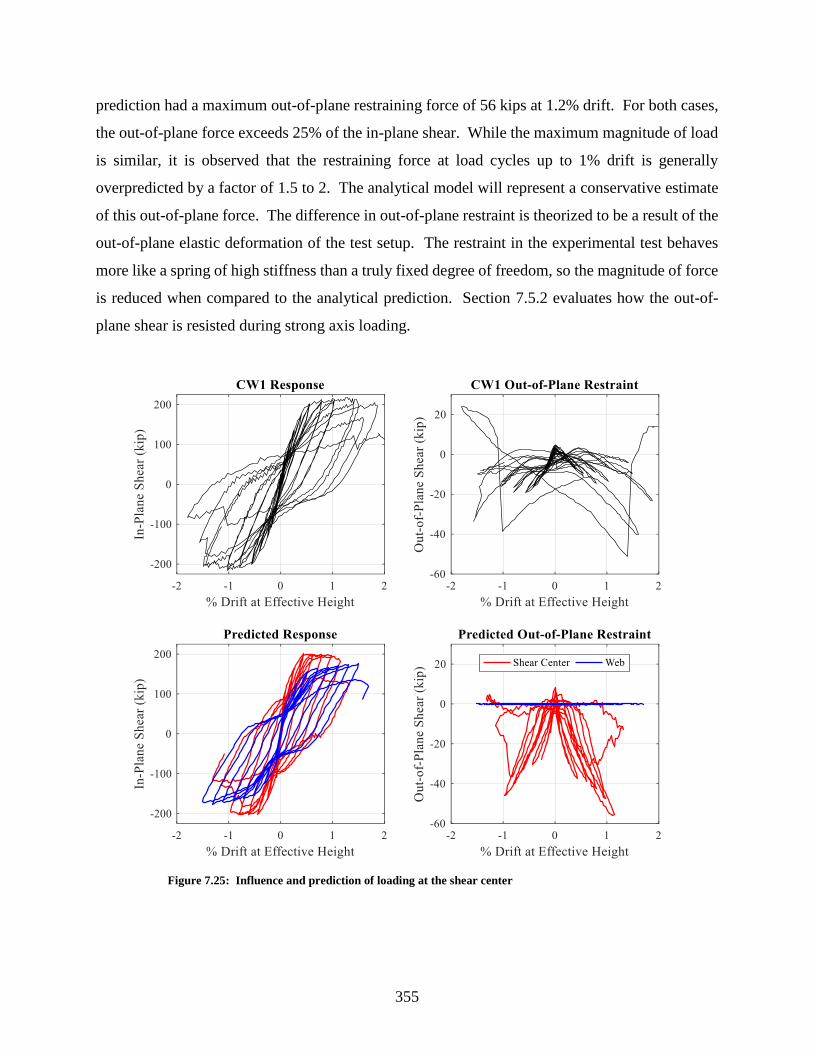
355
prediction had a maximum out-of-plane restraining force of 56 kips at 1.2% drift. For both cases,
the out-of-plane force exceeds 25% of the in-plane shear. While the maximum magnitude of load
is similar, it is observed that the restraining force at load cycles up to 1% drift is generally
overpredicted by a factor of 1.5 to 2. The analytical model will represent a conservative estimate
of this out-of-plane force. The difference in out-of-plane restraint is theorized to be a result of the
out-of-plane elastic deformation of the test setup. The restraint in the experimental test behaves
more like a spring of high stiffness than a truly fixed degree of freedom, so the magnitude of force
is reduced when compared to the analytical prediction. Section 7.5.2 evaluates how the out-of-
plane shear is resisted during strong axis loading.
Figure 7.25: Influence and prediction of loading at the shear center
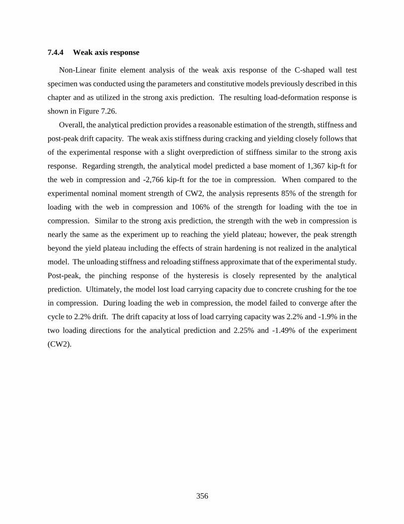
356
7.4.4 Weak axis response
Non-Linear finite element analysis of the weak axis response of the C-shaped wall test
specimen was conducted using the parameters and constitutive models previously described in this
chapter and as utilized in the strong axis prediction. The resulting load-deformation response is
shown in Figure 7.26.
Overall, the analytical prediction provides a reasonable estimation of the strength, stiffness and
post-peak drift capacity. The weak axis stiffness during cracking and yielding closely follows that
of the experimental response with a slight overprediction of stiffness similar to the strong axis
response. Regarding strength, the analytical model predicted a base moment of 1,367 kip-ft for
the web in compression and -2,766 kip-ft for the toe in compression. When compared to the
experimental nominal moment strength of CW2, the analysis represents 85% of the strength for
loading with the web in compression and 106% of the strength for loading with the toe in
compression. Similar to the strong axis prediction, the strength with the web in compression is
nearly the same as the experiment up to reaching the yield plateau; however, the peak strength
beyond the yield plateau including the effects of strain hardening is not realized in the analytical
model. The unloading stiffness and reloading stiffness approximate that of the experimental study.
Post-peak, the pinching response of the hysteresis is closely represented by the analytical
prediction. Ultimately, the model lost load carrying capacity due to concrete crushing for the toe
in compression. During loading the web in compression, the model failed to converge after the
cycle to 2.2% drift. The drift capacity at loss of load carrying capacity was 2.2% and -1.9% in the
two loading directions for the analytical prediction and 2.25% and -1.49% of the experiment
(CW2).

357
Figure 7.26: Predicted weak axis response
7.5 Shear distribution in C-shaped walls
The prior chapters concluded that the shear demand in non-planar walls, particularly C-shaped
walls, significantly affects wall response as compared to planar wall elements of similar geometry
and reinforcing. The relative proportion of shear deformation to flexural deformation is about
40% larger in the C-shaped walls than the planar walls. The presence of base sliding, crushing of
the unconfined web, and the formation of compressive struts across the web indicated in the strain
data are all indicative of high shear demand. Out-of-plane shear damage was also observed in the
wall flanges during strong axis loading post-peak resulting from the base sliding. Shear design in
the building code is based upon the wall in the area in the direction of loading only. The shear
design neglects any positive or negative interactions resulting from the presence of a wall flange
perpendicular to the direction of loading. To evaluate this assumption, this section characterizes
the shear stress distribution in the C-shaped walls as a function of wall height and drift level.
7.5.1 Integration of shear stresses
The finite element analysis provides a measurement of shear stress in each layer at each Gauss
point. For nine gauss points and n layers, each element has a total of 9n shear stress measurements.
To determine the average shear resisted across the element as a whole, these stresses must be

358
integrated appropriately. First, the shear stresses at each Gauss point are integrated over the
thickness of the layer and summed to determine the unit shear (kN/m) at each Gauss point.
/2
/212
nti i
xy xy xyt
i
tdz
−=
= = (6.11)
To determine the average element shear (kN), the unit shear is then average over the total element
by the summation of the product of the unit shear stress at each Gauss point with the normalized
gauss point weighting. The summation is multiplied by the length of the element to determine the
shear resisted across each element.
9
1
gp gp
xy e xy
gp
V w=
= (6.12)
The corresponding gauss point locations and weights for the nine-node shell element are given in
Figure 7.27.
(a) Gauss point locations (Hrynyk 2013) (b)Gauss point weights (Paulino 2012)
Figure 7.27: Shell element gauss point locations and weights
To validate the methodology of shear stress integration, the elastic response of the wall is
compared to the theoretical shear distribution in an open channel. The theoretical distribution of
shear stress for an open-channel loaded about the strong axis has a triangular distribution across
each flange and parabolic distribution across the web, refer to Figure 7.28. For an elastic loading
of the finite element model previously described, the element shear distribution and total shear
resisted at the top of the first floor is plotted in Figure 7.29. For this example, the applied shear
was 478 kN, and the shear measured by integration of shear stresses was 477 kN. Similarly, the
response in the weak axis response is validated in Figure 7.30 for positive weak axis loading and
Figure 7.31 for negative weak axis loading. The parabolic shear stress distribution is evident along

359
each flange with a linear distribution across the web. The sum of the flange shear is equal to the
total shear without a significant residual. For base cases, the difference between the applied and
measured shear is a negligible difference, so this methodology is utilized moving forward to assess
shear distribution during inelastic states.
(a)Theoretical shear stress distribution (Bachau and Craig 2009) (b)FE model shear stress elastic distribution
Figure 7.28: Elastic shear stress distribution
Figure 7.29: Validation of shear stress integration for strong axis elastic loading

360
Figure 7.30: Validation of shear stress integration for positive weak axis elastic loading
Figure 7.31: Validation of shear stress integration for negative weak axis elastic loading
7.5.2 Strong-axis response
The strong axis shear stress distribution as evaluated using the results of the model described
in Section 7.4.3. The shear stresses distribution was developed for each horizontal layer of
elements at each peak drift step. The resulting distributions are evaluated with respect to drift level
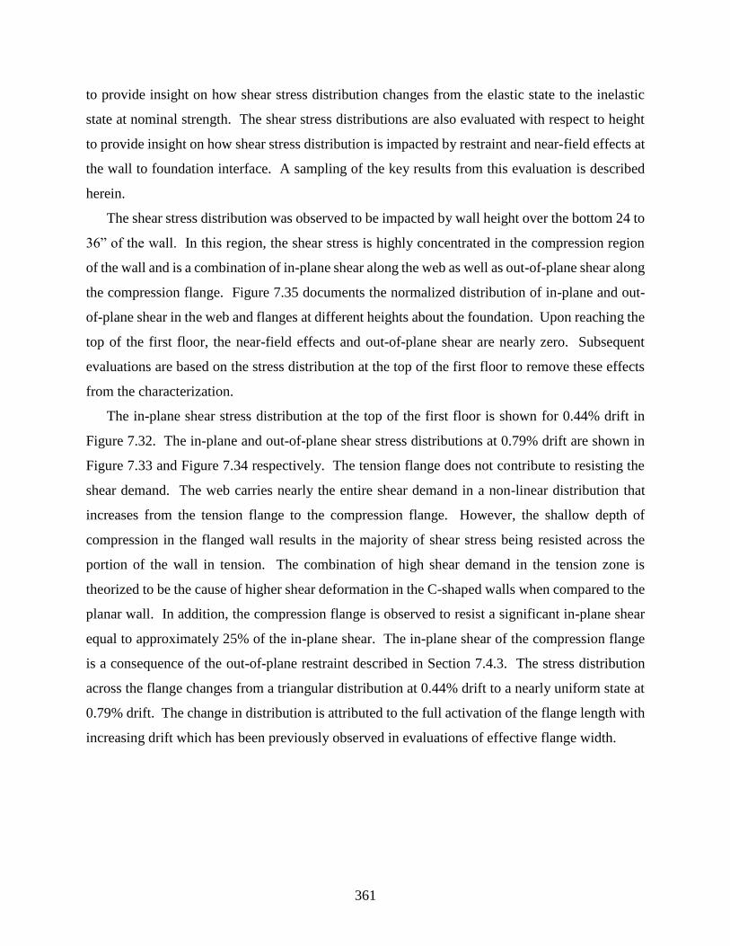
361
to provide insight on how shear stress distribution changes from the elastic state to the inelastic
state at nominal strength. The shear stress distributions are also evaluated with respect to height
to provide insight on how shear stress distribution is impacted by restraint and near-field effects at
the wall to foundation interface. A sampling of the key results from this evaluation is described
herein.
The shear stress distribution was observed to be impacted by wall height over the bottom 24 to
36” of the wall. In this region, the shear stress is highly concentrated in the compression region
of the wall and is a combination of in-plane shear along the web as well as out-of-plane shear along
the compression flange. Figure 7.35 documents the normalized distribution of in-plane and out-
of-plane shear in the web and flanges at different heights about the foundation. Upon reaching the
top of the first floor, the near-field effects and out-of-plane shear are nearly zero. Subsequent
evaluations are based on the stress distribution at the top of the first floor to remove these effects
from the characterization.
The in-plane shear stress distribution at the top of the first floor is shown for 0.44% drift in
Figure 7.32. The in-plane and out-of-plane shear stress distributions at 0.79% drift are shown in
Figure 7.33 and Figure 7.34 respectively. The tension flange does not contribute to resisting the
shear demand. The web carries nearly the entire shear demand in a non-linear distribution that
increases from the tension flange to the compression flange. However, the shallow depth of
compression in the flanged wall results in the majority of shear stress being resisted across the
portion of the wall in tension. The combination of high shear demand in the tension zone is
theorized to be the cause of higher shear deformation in the C-shaped walls when compared to the
planar wall. In addition, the compression flange is observed to resist a significant in-plane shear
equal to approximately 25% of the in-plane shear. The in-plane shear of the compression flange
is a consequence of the out-of-plane restraint described in Section 7.4.3. The stress distribution
across the flange changes from a triangular distribution at 0.44% drift to a nearly uniform state at
0.79% drift. The change in distribution is attributed to the full activation of the flange length with
increasing drift which has been previously observed in evaluations of effective flange width.
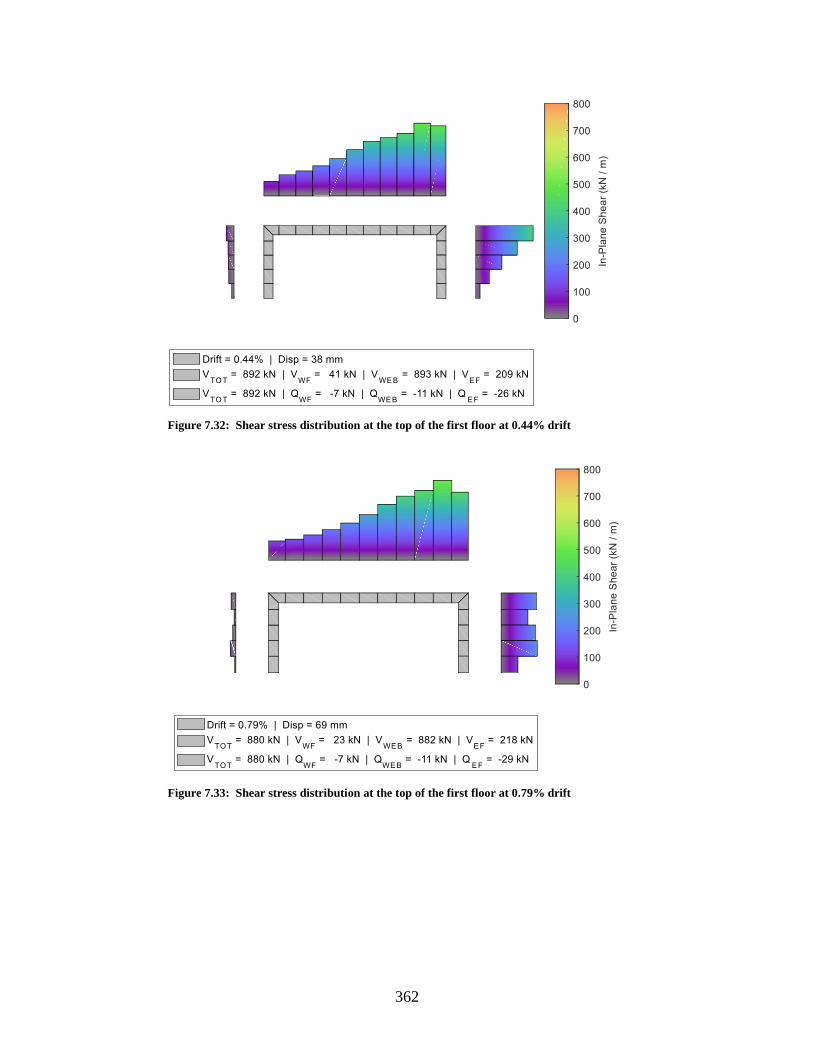
362
Figure 7.32: Shear stress distribution at the top of the first floor at 0.44% drift
Figure 7.33: Shear stress distribution at the top of the first floor at 0.79% drift
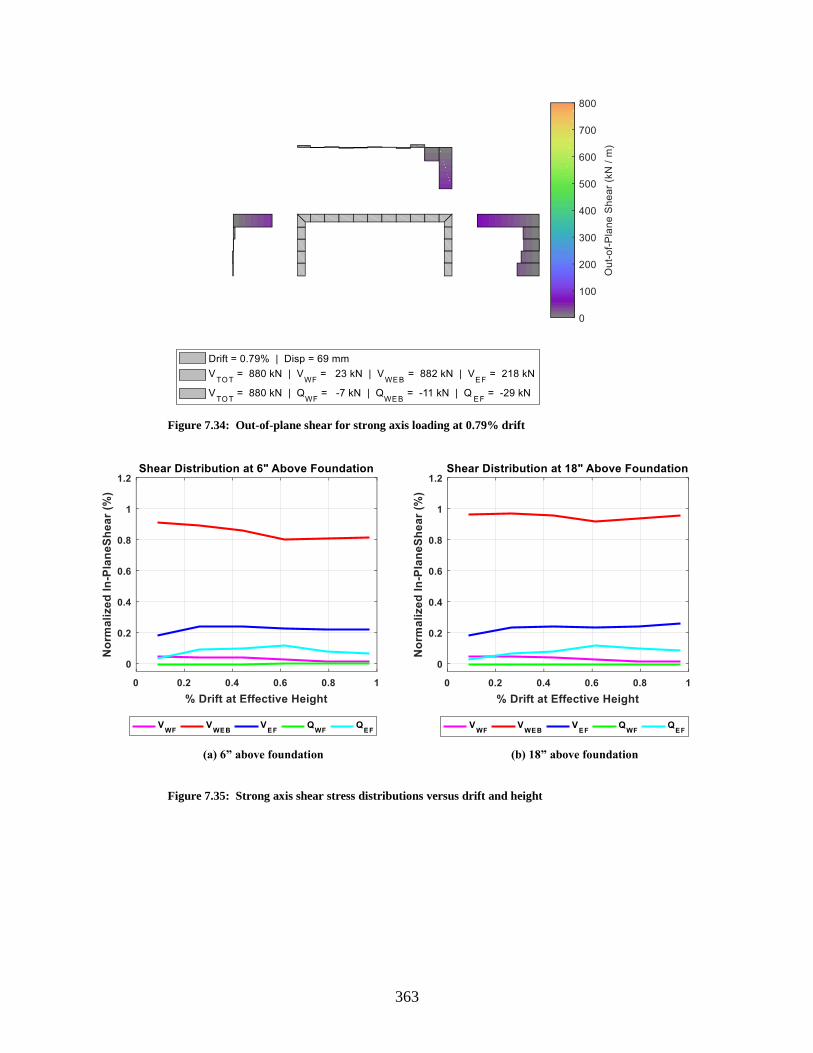
363
Figure 7.34: Out-of-plane shear for strong axis loading at 0.79% drift
(a) 6” above foundation (b) 18” above foundation
Figure 7.35: Strong axis shear stress distributions versus drift and height
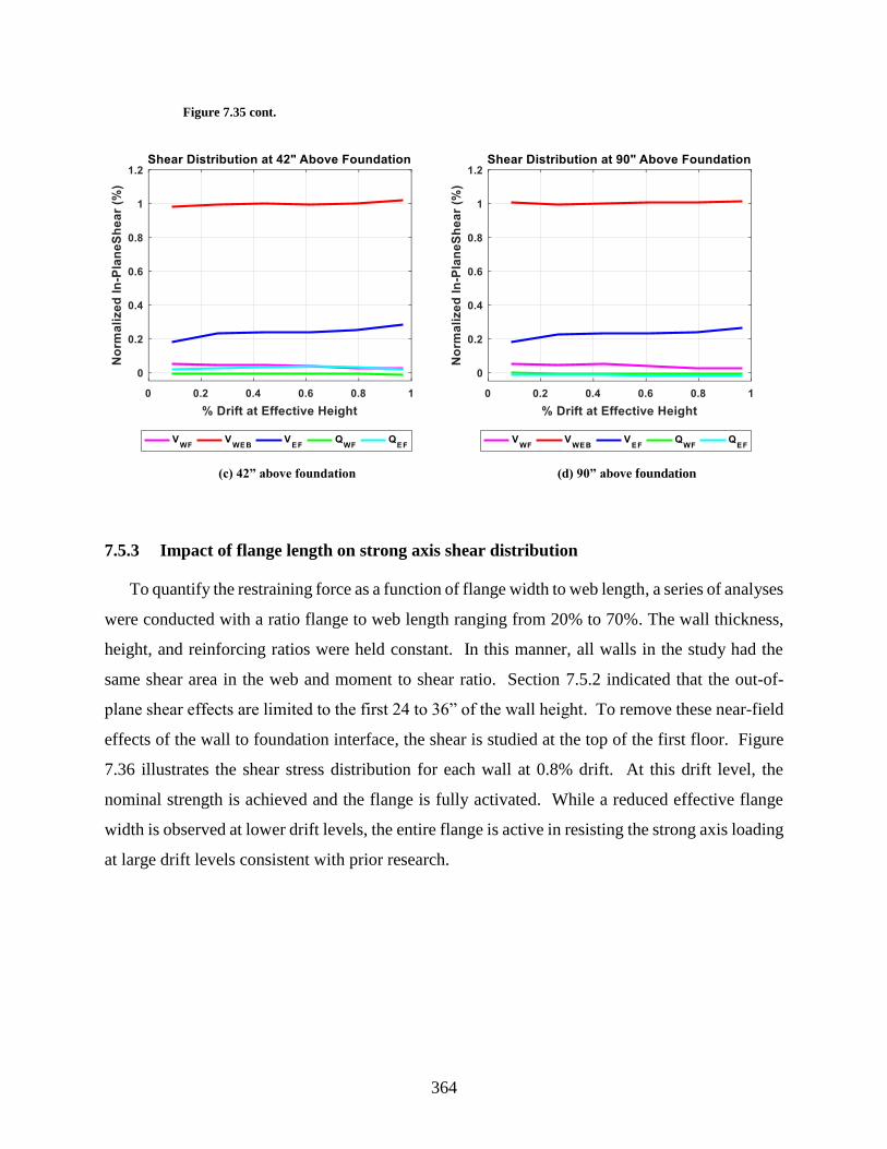
364
Figure 7.35 cont.
(c) 42” above foundation (d) 90” above foundation
7.5.3 Impact of flange length on strong axis shear distribution
To quantify the restraining force as a function of flange width to web length, a series of analyses
were conducted with a ratio flange to web length ranging from 20% to 70%. The wall thickness,
height, and reinforcing ratios were held constant. In this manner, all walls in the study had the
same shear area in the web and moment to shear ratio. Section 7.5.2 indicated that the out-of-
plane shear effects are limited to the first 24 to 36” of the wall height. To remove these near-field
effects of the wall to foundation interface, the shear is studied at the top of the first floor. Figure
7.36 illustrates the shear stress distribution for each wall at 0.8% drift. At this drift level, the
nominal strength is achieved and the flange is fully activated. While a reduced effective flange
width is observed at lower drift levels, the entire flange is active in resisting the strong axis loading
at large drift levels consistent with prior research.

365
(a) 0.2fl web= (b) 0.3fl web= (c) 0.4fl web=
(c) 0.5fl web= (d) 0.6fl web= (e) 0.7fl web=
Figure 7.36: Shear stress distribution at 0.8% drift at the top of first floor
Section 7.5.2 also indicated that the out-of-plane shear resisted across the compression flange
is approximately constant up the height of the wall to the point of restraint. Using the assumption
that the out-of-plane shear is independent of height but dependent on drift, the normalized ratio of
shear in the flanges to the web is plotted at the top of the first story for each wall in Figure 7.37.
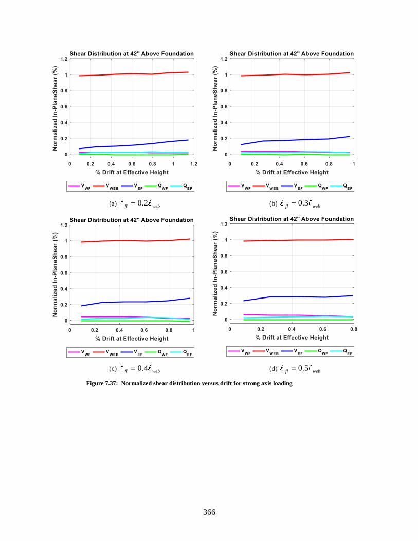
366
(a) 0.2fl web= (b) 0.3fl web=
(c) 0.4fl web= (d) 0.5fl web=
Figure 7.37: Normalized shear distribution versus drift for strong axis loading
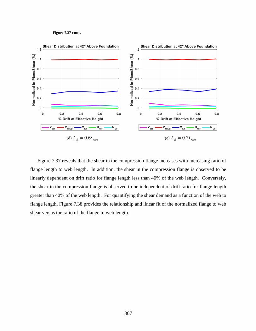
367
Figure 7.37 cont.
(d) 0.6fl web= (e) 0.7fl web=
Figure 7.37 reveals that the shear in the compression flange increases with increasing ratio of
flange length to web length. In addition, the shear in the compression flange is observed to be
linearly dependent on drift ratio for flange length less than 40% of the web length. Conversely,
the shear in the compression flange is observed to be independent of drift ratio for flange length
greater than 40% of the web length. For quantifying the shear demand as a function of the web to
flange length, Figure 7.38 provides the relationship and linear fit of the normalized flange to web
shear versus the ratio of the flange to web length.

368
Figure 7.38: Normalized flange to web shear versus the ratio of flange to web length
For a coupled C-shaped wall subjected to strong axis loading, the flange should be designed to
resist a minimum shear at all stories within the plastic hinge region given as:
0.6fl
fl web
web
V V
=
(6.13)
For structural walls utilizing the same horizontal and vertical reinforcement ratio in the flange as
the web, this requirement should be met inherently. However, the out-of-plane restraining force
can represent a significant load that needs to be considered in the load path through the coupling
beams at each slab level as well as the foundation. Additional research is needed to understand
how this load is realized in the coupling beams and whether it has an impact on the design and
performance of coupled C-shaped walls.
7.5.4 Weak-axis web in compression response
The weak axis shear stress distribution for the web in compression was evaluated using the
results of the model described in Section 7.4.4. The in-plane and out-of-plane shear stress
distribution are given in Figure 7.39 and Figure 7.40 respectively. While the flanges resist the
majority of shear stress, a complex stress state is observed in the web. The web resists a
meaningful component of out-of-plane shear that is dependent on wall height. As elevation
decreases, the component of out-of-plane shear increases. As noted in the strain field descriptions
in Section 5.6, the compression is carried across the entire web of the wall, and an effective flange
y = 0.5778x
R² = 0.9692
0.0%
5.0%
10.0%
15.0%
20.0%
25.0%
30.0%
35.0%
40.0%
45.0%
0 0.1 0.2 0.3 0.4 0.5 0.6 0.7 0.8
Vfl
/ V
web
ℓfl / ℓweb
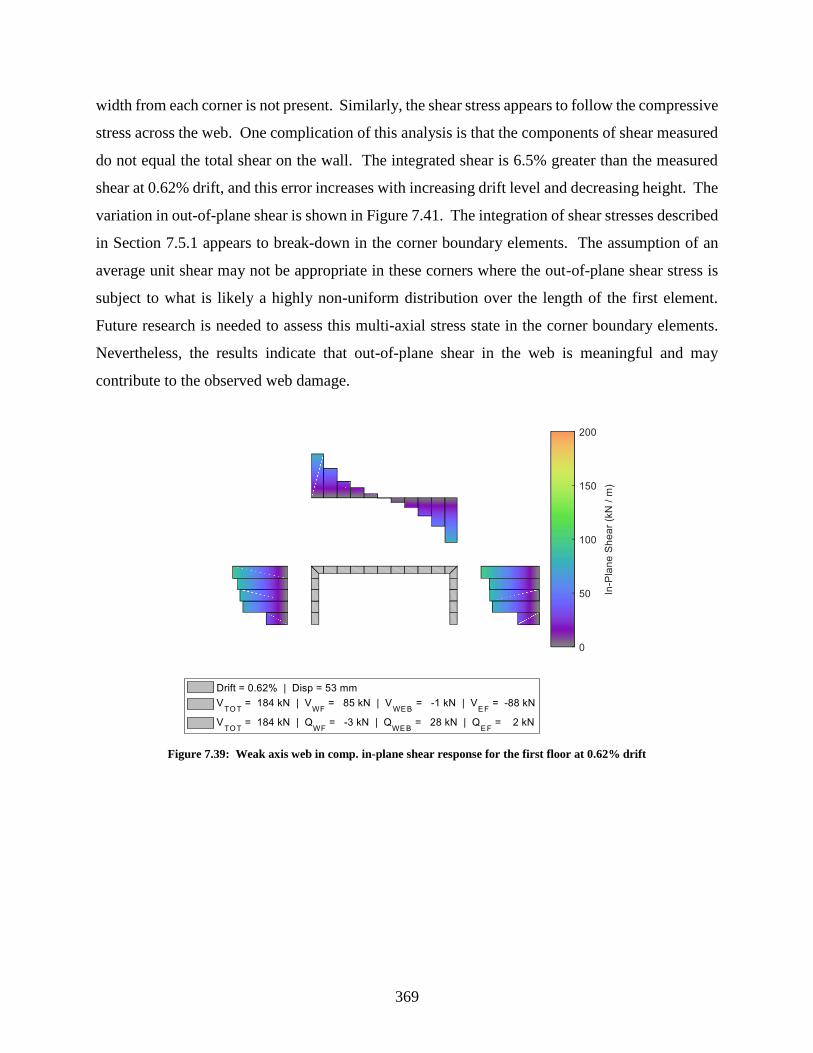
369
width from each corner is not present. Similarly, the shear stress appears to follow the compressive
stress across the web. One complication of this analysis is that the components of shear measured
do not equal the total shear on the wall. The integrated shear is 6.5% greater than the measured
shear at 0.62% drift, and this error increases with increasing drift level and decreasing height. The
variation in out-of-plane shear is shown in Figure 7.41. The integration of shear stresses described
in Section 7.5.1 appears to break-down in the corner boundary elements. The assumption of an
average unit shear may not be appropriate in these corners where the out-of-plane shear stress is
subject to what is likely a highly non-uniform distribution over the length of the first element.
Future research is needed to assess this multi-axial stress state in the corner boundary elements.
Nevertheless, the results indicate that out-of-plane shear in the web is meaningful and may
contribute to the observed web damage.
Figure 7.39: Weak axis web in comp. in-plane shear response for the first floor at 0.62% drift
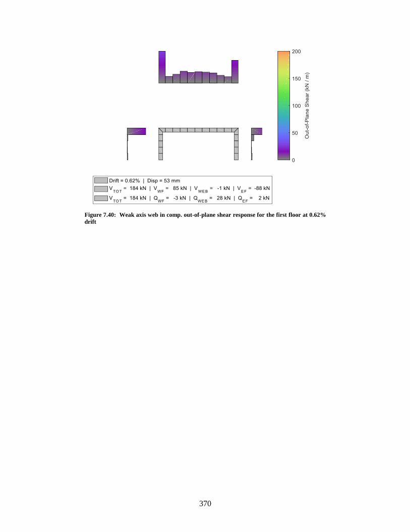
370
Figure 7.40: Weak axis web in comp. out-of-plane shear response for the first floor at 0.62%
drift
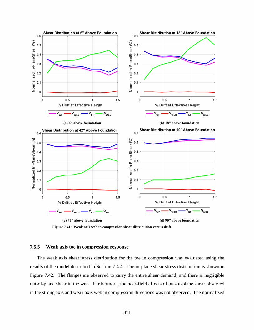
371
(a) 6” above foundation (b) 18” above foundation
(c) 42” above foundation (d) 90” above foundation
Figure 7.41: Weak axis web in compression shear distribution versus drift
7.5.5 Weak axis toe in compression response
The weak axis shear stress distribution for the toe in compression was evaluated using the
results of the model described in Section 7.4.4. The in-plane shear stress distribution is shown in
Figure 7.42. The flanges are observed to carry the entire shear demand, and there is negligible
out-of-plane shear in the web. Furthermore, the near-field effects of out-of-plane shear observed
in the strong axis and weak axis web in compression directions was not observed. The normalized

372
distribution of shear stress along the wall height is shown in Figure 7.43. In conclusion, for weak
axis loading with the toe in compression, the shear response is not influenced by the non-planar
wall geometry.
Figure 7.42: Weak axis toe in compression shear response for the first floor at 0.62% drift
(a) Shear distribution at interface (b) Shear distribution at first floor
Figure 7.43: Weak axis toe in compression shear distribution versus drift
373
7.6 Conclusions
This chapter supplements the experimental data of the C-shaped walls with non-linear finite
element analyses. This effort utilized a layered shell element model with comprehensive
constitutive models capturing the cracked response of reinforced concrete in cyclic biaxial loading
conditions. To validate the selection of constitutive models, a database of reinforced concrete
panel tests containing the complete experimental stress-strain response and cracking
measurements was compiled. The database is accessed through the development of a non-linear
continuum analysis program that allows comprehensive evaluation of the data against any number
of analytical predictions using varying constitutive models. The element level model validation
focused on the impact of crack spacing prediction on model performance. From this work, the
following conclusions are made regarding crack spacing:
• Empirical crack spacing models have been developed based on experimental tests of
tension members and beams where the cracks form perpendicular to the tension
reinforcement. Membrane/shell elements of reinforced concrete are subject to biaxial
loading conditions and crack formation non-orthogonal to the reinforcement which is
inconsistent with the tests used to develop the crack spacing models. To evaluate the
parameters used in crack spacing models, a parametric study of panel tests identified
that rebar diameter, clear cover, tensile strength (bond strength), and effective
reinforcing ratio had a significant impact on crack spacing. The reinforcement spacing
and ratio of bar diameter to effective reinforcing ratio were not statistically significant.
• Existing crack spacings models consistently overpredict of crack spacing in membrane
elements subjected to shear by a factor ranging from 1 to 4 indicating a deficiency in
the application of these models to finite element studies. Additional experimental data
and analytical evaluation are needed to develop a crack spacing model that inherently
considers the non-orthogonality of cracking.
• The predictions of stress and strain for the panel tests varied significantly on the basis
of the crack spacing model selected. However, the CEB-FIP 1978 crack spacing model
is recommended based on its consistent performance in predicting stress, strain and
secant stiffness up to 75% yielding. Furthermore, it gave a reasonable prediction of the
ultimate stress without overpredicting the response.

374
Using the recommended crack spacing model, subsequent NLFEA models of the C-shaped
walls provided a validation of the experimental results and a characterization of shear stress
distribution based on drift level for strong axis and weak axis loading. The following conclusions
are made regarding the results of the non-linear finite element analyses:
• For strong axis loading, the web carries nearly the entire shear demand in a non-linear
distribution that increases from the tension flange to the compression flange. The
shallow depth of compression in the flanged wall results in the majority of shear stress
being resisted across the portion of the wall in tension. This conclusion supports the
observed shear strain distribution in the experimental tests that resulted in an increased
shear deformation.
• For strong axis loading, the compression flange is also observed to resist an in-plane
shear of approximately 25% of the web shear due to the out-of-plane restraint of the C-
shaped wall. The in-plane shear stress distribution across the flange changes from a
triangular distribution at 0.44% drift to a nearly uniform distribution at 0.79% drift
indicating full activation of the flange length with increasing drift.
• A parametric study of flange width for strong axis loading indicated that the shear
demand in the compression flange increases with increasing ratio of flange length to
web length. In addition, the shear in the compression flange is observed to be linearly
dependent on drift ratio for flange length less than 40% of the web length.
• For a coupled C-shaped wall subjected to strong axis loading, the flange should be
designed to resist a minimum shear equal to: 0.6fl
fl web
web
V V
=
. This out-of-plane
restraining force should be considered in the load path through the coupling beams at
each slab level as well as the foundation. Future work is needed to evaluate how this
force is shared between floor levels and whether there is a meaningful impact on the
coupling beams.
• For weak axis loading with the web in compression, the non-planar geometry has a
significant impact of stress distribution. While the flanges resist the majority of shear
stress, the web resists a combination of in-plane and out-of-plane shear stress that varies
with elevation and drift level. As elevation decreases, the component of out-of-plane

375
shear increases. An effective flange width was not observed, and stresses are
distributed across the entire width of the web.
• For weak axis loading with the toe in compression, the shear response is not influenced
by the non-planar wall geometry. The flanges carry the entire shear demand, and there
is negligible out-of-plane shear in the web.
376
CHAPTER 8: CONCLUSIONS AND FUTURE WORK
8.1 Conclusions
The research presented in this dissertation provides insight into the performance of C-shaped
walls subjected to multi-directional loading through a combination of experimental testing, data
analysis, and numerical modeling. This effort has sought to improve the understanding of the
three-dimensional and asymmetric response of C-shaped walls during both service level and
ultimate loadings. Recommendations and procedures for the simplified analysis of C-shaped walls
using elastic analysis as well as the detailed analysis using non-linear finite elements were
provided for predicting the wall response up to the nominal strength. The impacts of bi-directional
loading and coupling on damage patterns, drift capacity, and ductility were quantified.
Furthermore, the limitations of existing numerical models and simplified predictions for non-
planar walls were identified. The tasks associated with the completion of this work are
summarized below:
1. The design, construction, instrumentation, and loading control for three C-shaped walls
specimens was developed and documented in Chapter 3. This effort included the
development and implementation of a new response-based loading algorithm for multi-
degree-of-freedom experimental testing. The experimental tests were completed at the
Newmark Structural Engineering Laboratory.
2. The experimental results were documented in Chapter 4. The complete progression of
cracking observations, damage progression, hysteretic response, failure mechanisms,
and final load-deformation response was described for each experiment.
3. The instrument data from each of the three experimental tests was processed and
cleaned to support additional analyses in Chapter 5. Accompanying metadata was
created to describe each set of instruments. All resulting data and documentation were
archived to the NHERI Design Safe Cyber Infrastructure where it is publicly available
to the design and research community. The processed data was utilized to
quantitatively evaluate the displacement profiles, yielding, energy dissipation, strain
fields, and deformation contributions of each wall test.
4. The C-shaped wall response was evaluated through the lens of prior planar, coupled
and non-planar wall tests in Chapter 6. The strong axis response was compared and

377
contrasted with the planar wall response. The weak axis response of the coupled core
wall simulation was similarly compared to the planar coupled wall response. A
database of non-planar wall tests was created wherein parametric studies of wall
geometry, reinforcing, loading, ductility, and sectional analysis metrics were
conducted. Derived measures of shear and flexural deformations for the C-shaped
walls as well as prior tests were used to develop effective stiffness recommendations
for the elastic analysis of non-planar concrete walls.
5. The experimental data of the C-shaped walls was supplemented with non-linear finite
element analyses in Chapter 7. The analytical model utilized a layered shell element
with comprehensive constitutive models capturing the cracked response of reinforced
concrete in cyclic biaxial loading conditions. The model was validated at the element
level using a database of reinforced concrete panel tests with a focus on the influence
of crack spacing on model prediction. The resulting non-linear finite element analyses
were used to characterize the shear distribution in C-shaped walls.
The resulting conclusions from these five tasks are summarized in Sections 8.1.1, 8.1.2, and 8.1.3
with respect to the objectives outlined in Section 1.1.
8.1.1 Conclusions of the testing and experimental response
The first objective of the research was to characterize the response and damage mechanisms of
cyclically loaded C-shaped walls using visual observations and quantitative analysis. The key
conclusions associated with each sub-objective of this work are described below:
1.1. Conduct experimental testing of three C-shaped walls at the Newmark Structural
Engineering Laboratory.
• Three C-shaped walls were successfully constructed, instrumented and tested using
the methods and loading criteria outlined in Chapter 3. The loading protocol utilized
the six DOF capability to impose mixed displacements and forces that simulated the
upper seven stories of ten-story building acting on the test specimen. The loading
protocol included a uni-directional test, bi-directional test, and a simulated coupled
core-wall system subjected to bi-directional loading.

378
• For conducting the coupled core wall simulation, the experiment required the efficient
application of multiple degrees of freedom in mixed-mode control simultaneously with
a load target that was dependent on the specimen response. In addition, the existing
methods for application of loading were observed to cause increased shear demand
prior to the convergence of the load step. Furthermore, the convergence of the load
step took many iterations when multiple force-based degrees of freedom were imposed
simultaneously. To address these shortcomings, a stiffness-based loading algorithm
was developed, tested and implemented in the small-scale and large-scale laboratory.
The algorithm recommended measurement of the tangent stiffness of each degree of
freedom using a least squares line fitting of previous points on the load-deformation
history. The hysteretic response of the reinforced concrete specimen is considered by
measurement of the peak stiffness during loading and unloading to improve
predictions at changes in the loading direction. The resulting algorithm yielded a 94%
reduction in shear force overshoot and enhanced convergence to improve testing
efficiency.
1.2. Analyze the experimental data and archive the results to an open access data
repository.
• The instrumentation of each C-shaped wall experiments included more than 390
channels of raw data as well as photographs and videos. These data files were
processed, cleaned and archived for subsequent analysis in this research work and for
future researchers.
• The complete dataset for each test was archived to the NHERI Design Safe Cyber-
Infrastructure. Accompanying metadata and drawings to describe each instrument and
their configuration were developed to inform the engineering and research community
on the use of the data.
• The subsequent analysis of the C-shaped wall experiments studied the energy
dissipation of the walls, the progression of yielding, the components of deformation to
total wall drift, strain fields generated from displacement field data, and overall
displacement profiles of the prototype ten-story building.

379
1.3. Characterize the damage mechanisms of C-shaped walls subjected to uni-directional
and bi-directional loading.
• The experimental tests exhibited a ductile failure resulting from loss of boundary
element confinement, bar buckling, and rupture of the longitudinal bars. However, the
ductile failure mechanism was precipitated by increased shear deformation and
undesirable shear related damage of base sliding and web crushing.
• The onset of sliding and rupture of web vertical reinforcing bars resulted in a loss of
shear resistance along the web. The loss of web shear resistance resulted in a
redistribution of shear demand to the corner boundary element and compression flange.
Subsequently, the unconfined concrete of the web adjacent to the corner boundary
elements spalled and crushed.
• As base slip increased beyond 1% drift, visible deformation and lateral buckling of the
longitudinal bars was observed at the interface of the corner boundary elements and
foundation. The base slip deformation created an out-of-plane shear in the flanges that
ultimately results in vertical cracking and spalling up the height of the first story.
• The increased demand on the corner boundary elements and lateral buckling resulted
in the failure of the confinement ties and extensive core crushing. The vertical and
lateral buckling of the longitudinal reinforcing bars in the corner boundary elements is
followed by straightening when loading in the opposite direction. This cycle of plastic
deformation results in fracture and loss of load-carrying capacity in each test.
1.4. Determine the influence of bi-directional loading on strong axis response.
• For the strong axis response, all three C-shaped walls reached 91 to 95% of the nominal
moment strength and 41 to 43% of the nominal shear strength. The bi-directional
loading did not impact the strong axis response prior to the nominal strength.
• The energy dissipation capacity of the uni-directionally loaded and bi-directionally
loaded non-planar walls were approximately equivalent for equal levels of damage to
the boundary elements. The damage and tension-compression cycles at each boundary
element precipitate the failure of the wall as a whole irrespective of loading direction.
• The damage mechanisms observed were the same for all three tests independent of the
specific changes in loading direction and axial loading; however, the bi-directional

380
loading results in earlier onset of damage and reduced drift capacity. CW2 exhibited a
strong axis drift capacity of only 1.5% when compared to a drift capacity of 2.25% for
CW1.
• The bi-directionally loaded test indicated tension yielding and strain hardening in the
flanges and toe boundary elements that were not present in the uni-directional test.
However, there was no evidence that the increased demand in the toe-boundary
elements directly impacted the strong axis response.
• The bi-directional loading and variation in axial load during weak axis loading do not
change the relative drift contributions of the strong axis response prior to reaching the
nominal strength. Up to 0.75% drift, the strong axis response of the three tests is nearly
the same with approximately 40% of the total deformation in the bottom three stories
to be shear deformation.
• For the coupled core wall simulation, increased base slip and base rotation were
observed in the drift contributions beyond 0.5% drift. The increased tensile demand
on the web of the wall associated with loading in the negative weak axis direction as
the tension pier of the simulation resulted in increased yielding and earlier rupture of
the vertical reinforcement.
8.1.2 Conclusions of the performance of non-planar walls
The second objective of the research was to characterize the response of C-shaped walls
through the lens of prior experimental tests. Chapter 6 described the research conducted to study
this objective. The research included a quantitative evaluation of the impact of wall geometry and
loading history through comparison of the planar wall tests, coupled wall test, and C-shaped wall
tests. The experimental data were analyzed to develop effective stiffness recommendations for the
elastic analysis of non-planar concrete walls. The C-shaped wall tests were also compared to
previous and subsequent non-planar wall tests identified in the literature review through the
development of a database of non-planar wall tests and parametric study of wall geometry,
reinforcing, loading, ductility, and sectional analysis metrics. The key conclusions associated with
each sub-objective of this work are described below:

381
2.1. Evaluate the C-shaped wall response in comparison to the prior planar and coupled
wall tests in the Complex walls testing program.
• A C-shaped wall of similar geometry and loading demand to a planar wall exhibits
increased ductility and increased drift capacity in the strong axis. The improved
performance is attributed to the lower compressive stress demand and ability to
redistribute compressive stress along the flange as the corner boundary element
becomes damaged. The planar wall does not have the same ability to redistribute
compressive stress and is more susceptible to non-ductile failure mechanisms.
• In both experiments of the planar wall and coupled wall, the failure mechanism was
non-ductile resulting from shear-compression damage to the boundary element. While
C-shaped walls experienced similar loading demands, the failure mechanism was
ductile resulting from cyclic buckling and rupture of the vertical reinforcing bars.
• The C-shaped wall exhibited reduced flexural deformation and base rotation, but nearly
twice the shear deformation of the planar wall. The strain field of the C-shaped wall
indicates increased shear strain and principal compressive stress in the tension zone of
the wall as compared to the planar. For shear demand in the tension zone across open
cracks, the shear slip along cracks is increased resulting in greater shear deformation.
2.2. Develop recommendations of effective stiffness for the elastic analysis of non-planar
reinforced concrete walls.
• The measured shear deformation, flexural deformation, and base deformations were
utilized to develop effective stiffness recommendations for the C-shaped walls. These
recommendations were evaluated against codes of practice and prior planar and non-
planar wall tests. The effective flexural stiffness recommendations in codes of practice
ranged from approximately 30% to 65% for a cracked wall at yield, while the
experimental data supported only the lower bound of these recommendations at the
30% level. An effective flexural stiffness of 35%EcIg was recommended for design.
• Codes of practice generally did not provide recommendations of effective shear
stiffness values; however, the degradation of shear stiffness was significant in all tests
examined. Effective shear stiffness values approached 20% at the onset of yielding.
An effective shear stiffness of 15%GcAcv was recommended for design.

382
• Bi-directional loading did not impact the effective stiffness values for the elastic
analysis of non-planar walls during yielding up to 1% drift. The effective stiffness
recommendations are applicable to both uni-directional and bi-directional loaded walls.
2.3. Develop a database of prior non-planar wall experiments and conduct a parametric
study of non-planar walls to determine if drift capacity, ductility or failure
mechanism can be estimated using simplified design parameters.
• The drift capacity of planar walls have been effectively characterized using the ratio of
wall length to wall thickness, w b , the wall neutral axis depth to wall thickness, c b ,
and the level of wall shear stress, ( )/ 'u cv cV A f and a resulting expression has been
proposed for the ACI 318 building code. The same parameters and drift capacity
expressions were applied to non-planar walls of C, U, H and T-shaped geometry. These
parameters were not statistically significant for non-planar walls, and the drift capacity
expression did not have a meaningful correlation with the drift capacity of the
experiments.
• A parametric study of eighteen design parameters for non-planar walls found that
ductility is a better metric for estimating non-planar wall performance than drift
capacity. Ductility was determined using both the 75% method and energy equivalence
method with comparable results. For simplicity, the 75% method is recommended for
ductility calculations.
• For non-planar walls, the parametric study indicated that increasing the reinforcement
ratio of the boundary elements results in reduced ductility. This trend is unique to non-
planar walls, and it reinforces the idea that non-planar wall ductility is ultimately a
function of the damage to the boundary elements.
• The drift capacity and ductility of bi-directionally loaded non-planar walls cannot be
reliably estimated using design parameters and moment-curvature analysis alone. The
three-dimensional geometry and path dependency of the post-peak response require a
more detailed evaluation using non-linear modeling tools.

383
8.1.3 Conclusions of the finite element analysis
The third objective of the research was to conduct finite element modeling of the C-shaped
wall experiments for validation and exploration of the wall response in shear.
3.1. Develop a database of reinforced concrete panel tests and conduct an element level
validation of the constitutive models with a focus on the influence of crack spacing.
• The literature review of crack spacing models identified that the majority of models are
empirically developed using experimental tests of tension members and beams where
the cracks form perpendicular to the tension reinforcement. Membrane/shell elements
of reinforced concrete are subject to biaxial loading conditions and crack formation
non-orthogonal to the reinforcement which is inconsistent with those tests. To evaluate
the parameters used in crack spacing models, a parametric study of crack spacing in
reinforced concrete panel tests identified that rebar diameter, clear cover, tensile
strength (bond strength), and effective reinforcing ratio had a significant impact on
crack spacing. The reinforcement spacing and ratio of bar diameter to effective
reinforcing ratio were not statistically significant.
• Existing crack spacings models consistently overpredict crack spacing in membrane
elements subjected to shear by a factor ranging from one to four. The overprediction
is consistent with prior observations of the panel tests, and it confirms a deficiency in
the application of these crack spacing models to finite element studies. Additional
experimental data and analytical evaluation are needed to develop a crack spacing
model that inherently considers the non-orthogonality of cracking in shear.
3.2. Recommend a crack spacing model for continuum analysis of reinforced concrete in
which cracks form non-orthogonal to the reinforcement.
• For finite element modeling, the effective reinforcement ratio input to the crack spacing
model should be evaluated for each layer using the specific bar diameter, spacing, clear
cover, and section thickness. For a single reinforcing bar in a section with two layers
of rebar each face, the effective area of concrete is recommended to be taken as a square
area around the bar with a width equal to lessor of the bar spacing and 15 bar diameters

384
and a height equal to the lesser of one half the section thickness and the sum of clear
cover and 7.5 bar diameters.
• The predictions of stress and strain for the panel tests varied significantly on the basis
of the crack spacing model selected; however, the CEB-FIP 1978 crack spacing model
is recommended based on its consistent performance in predicting stress, strain and
secant stiffness up to 75% yielding. Furthermore, it gave a reasonable prediction of the
ultimate stress without overpredicting the response. This model is also readily available
in existing finite element analysis software.
3.3. Conduct non-linear finite element analyses simulating the cyclic response of the C-
shaped wall in both axes to validate the model performance and characterize the
shear stress distribution.
• The analytical prediction of strong axis loading indicated that the web carried nearly
the entire shear demand in a parabolically shaped distribution with peak stress near the
compression flange. The shallow depth of compression in the flanged wall results in
the majority of shear stress being resisted across the portion of the wall in tension. The
combination of shear and vertical tensile strain results in increased shear slip along
cracks and increased shear deformation consistent with the experimental results.
• For strong axis loading, the compression flange resisted an in-plane shear of
approximately 25% of the web shear. The out-of-plane demand was a consequence of
the out-of-plane restraint of the C-shaped wall. The stress distribution across the flange
changes from a triangular distribution during yielding to a nearly uniform state at the
nominal strength indicating full activation of the flange length with increasing drift.
• A parametric study of flange width for strong axis loading indicated that the shear
demand in the compression flange increases with increasing ratio of flange length to
web length. The shear in the compression flange is observed to be linearly dependent
on drift ratio for flange length less than 40% of the web length but independent for
flange lengths greater than 40% of the web length.
• For a coupled C-shaped wall subjected to strong axis loading, the flange should be
designed to resist a minimum shear equal to: 0.6fl
fl web
web
V V
=
. The out-of-plane

385
restraining force should be considered in the load path through the coupling beams at
each slab level as well as the foundation. Future work is suggested to evaluate how this
force is shared between floor levels and whether there is a meaningful impact on the
coupling beam response.
8.2 Future Work
The experimental testing of C-shaped walls revealed a complex and interdependent structural
response. During service level loading and up to the nominal strength, shortcomings in the
prediction of cracking and stiffness were identified. The use of a continuum analysis with smeared
cracking and reinforcement inherently links these effects, and the empirically based constitutive
models utilized in this study do not separate these different aspects of the response. Future work
addressing the interdependence between cracking and stiffness is described below:
• The bond between the concrete and reinforcing bars was not explicitly considered, and
the analysis assumed the average strain in the concrete to be equal to the average strain
in the reinforcement. However, the effect of bond degradation is implicitly considered
in the constitutive models of tension stiffening and crack spacing. The interdependence
of bond on these parameters needs further evaluation. As part of this effort, the tension
chord model (Marti et al. 1998) should be included since it directly considers the bond
stress distribution and crack spacing with an analytical approach.
• The application of initial shrinkage cracking in non-planar walls to correct the initial
stiffness prior to loading was not successful. The straining and cracking pattern was
not consistent with the expected response due to the asymmetry of the specimen.
Additional research is needed to evaluate initial shrinkage effects on asymmetric
geometries. In conjunction with this challenge, prior research has estimated that the
inconsideration of time-dependent shrinkage in tension stiffening models can
overpredict the stiffening effect by up to a factor of two (Bischoff 2001). While these
effects do not generally control the peak and post-peak response, the prediction of
deformations at service level loading is critical for design engineering.
• The crack spacing models utilized were empirically developed using experimental tests
of tension members and beams where the cracks form perpendicular to the tension
reinforcement. The biaxial stress states and crack formation non-orthogonal to the

386
reinforcement in membrane/shell elements of reinforced concrete, and the evaluation
of those models against experimental data indicated a large scatter of results with
general overprediction of crack spacing. Prior research has also noted that the
formation of non-orthogonal cracks may be influenced by the location of transverse
reinforcement and local stress transmission across existing cracks (Bentz 2007).
Additional experimental data and analytical evaluation are needed to develop a crack
spacing model that inherently considers the non-orthogonality of cracking.
387
REFERENCES
Abdullah, Saman A., and John W. Wallace. 2018a. “Drift Capacity Prediction of RC Structural
Walls with Special Boundary Elements.” In Proceedings of the 11th National Conference
in Earthquake Engineering. Los Angeles, CA: Earthquake Engineering Research Institute.
———. 2018b. “UCLA-RCWalls Database for Reinforced Concrete Structural Walls.” In
Proceedings of the 11th National Conference in Earthquake Engineering. Los Angeles,
CA: Earthquake Engineering Research Institute.
ACI Committee 318. 2016. Building Code Requirements for Structural Concrete (ACI 318-14).
Farmington Hills: American Concrete Institute.
ACI Committee 408. 2003. Bond and Development of Straight Reinforcing Bars in Tension (ACI
408R-03). Detroit, Michigan: American Concrete Institute.
Adebar, Perry, Ahmed Ibrahim, and Michael Bryson. 2007. “Test of High-Rise Core Wall:
Effective Stiffness for Seismic Analysis.” ACI Structural Journal 104 (5): 549.
Adeghe, Louis N. 1986. “A Finite-Element Model for Studying Reinforced Concrete Detailing
Problems.” PhD diss., University of Toronto.
Applied Technology Council. 2010. “Modeling and Acceptance Criteria for Seismic Design and
Analysis of Tall Buildings.” PEER/ATC-72-1. Redwood City, CA: Pacific Earthquake
Engineering Research Center.
Aquino, Wilkins, and Ibrahim Erdem. 2007. “Implementation of the Modified Compression Field
Theory in a Tangent Stiffness-Based Finite Element Formulation.” Steel and Composite
Structures 7 (4): 263–78. https://doi.org/10.12989/scs.2007.7.4.263.
ASCE/SEI Seismic Rehabilitation Standards Committee. 2007. Seismic Rehabilitation of Existing
Buildings (ASCE/SEI 41-06). Reston, VA: American Society of Civil Engineers.
Aspiotis, James. 1993. “Compression Softening of High Strength Reinforced Concrete Elements
Subjected to In-Plane Stresses.” Master’s thesis, University of Toronto.
Bachau, Olivier A., and James I. Craig, eds. 2009. Structural Analysis. Heidelberg: Springer.
Bažant, Zdeněk P. 2002. “Concrete Fracture Models: Testing and Practice.” Engineering Fracture
Mechanics 69 (2): 165–205. https://doi.org/10.1016/S0013-7944(01)00084-4.
Bažant, Zdeněk P., and Byung H. Oh. 1983. “Crack Band Theory for Fracture of Concrete.”
Matériaux et Construction 16 (3): 155–77. https://doi.org/10.1007/BF02486267.
Beeby, A. W, R. Favre, M. Koprna, and J. P. Jaccoud, eds. 1985. CEB Design Manual on Cracking
and Deformations. Lausanne: Comité euro-international du béton.

388
Behrouzi, Anahid A., Andrew W. Mock, Anna C. Birely, Daniel A. Kuchma, Dawn E. Lehman,
and Laura N. Lowes. 2014. “Seismic Behavior of Modern Reinforced Concrete C-Shaped
Walls (Specimen UW7).” Dataset, DOI:10.4231/D37D2Q79C. Design-Safe Cyber
Infrastructure (distributor).
Behrouzi, Anahid A., Andrew W. Mock, Laura N. Lowes, Dawn E. Lehman, and Daniel A.
Kuchma. 2015a. “Summary of Large-Scale C-Shaped Reinforced Concrete Wall Tests.”
White Paper. Performance-Based Seismic Design of Concrete Walls. Charles Pankow
Foundation.
———. 2015b. “Summary of Large-Scale Nonplanar Reinforced Concrete Wall Tests.” White
Paper. Performance-Based Seismic Design of Concrete Walls. Charles Pankow
Foundation.
Belarbi, Abdeldjelil, and Thomas T. C. Hsu. 1995. “Constitutive Laws of Softened Concrete in
Biaxial Tension Compression.” ACI Structural Journal 92 (5): 562–73.
Belytschko, Ted, and Tom Black. 1999. “Elastic Crack Growth in Finite Elements with Minimal
Remeshing.” International Journal for Numerical Methods in Engineering 45 (5): 601–
620. https://doi.org/10.1002/(SICI)1097-0207(19990620)45:5<601::AID-
NME598>3.0.CO;2-S.
Bentz, Evan C. 2000. “Sectional Analysis of Reinforced Concrete Members.” PhD diss.,
University of Toronto.
———. 2007. “Closure to ‘Explaining the Riddle of Tension Stiffening Models for Shear Panel
Experiments’ by Evan Bentz.” Journal of Structural Engineering 133 (1): 151–151.
https://doi.org/10.1061/(ASCE)0733-9445(2007)133:1(151).
Bergan, Pal G. 1980. “Solution Algorithms for Nonlinear Structural Problems.” Computers &
Structures 12 (4): 497–509. https://doi.org/10.1016/0045-7949(80)90125-X.
Beyer, Katrin, Alessandro Dazio, and Nigel Priestley. 2008. “Quasi-Static Cyclic Tests of Two U-
Shaped Reinforced Concrete Walls.” Journal of Earthquake Engineering 12 (7): 1023–53.
https://doi.org/10.1080/13632460802003272.
Birely, Anna C. 2012. “Seismic Performance of Slender Reinforced Concrete Structural Walls.”
PhD diss., University of Washington.
Birely, Anna C., Laura N. Lowes, and Dawn E. Lehman. 2011. “Investigation of Performance of
Slender RC Structural Walls.” NEESR-SG: Seismic Behavior, Analysis, and Design of
Complex Wall Systems. University of Washington.
Birely, Anna C., Andrew W. Mock, Anahid A. Behrouzi, Daniel A. Kuchma, Dawn E. Lehman,
and Laura N. Lowes. 2014. “Seismic Behavior of Modern Reinforced Concrete C-Shaped
Walls (Specimen UW6).” Dataset, DOI:10.4231/D3C24QP0D. Design-Safe Cyber
Infrastructure (distributor).
389
Bischoff, Peter H. 2001. “Effects of Shrinkage on Tension Stiffening and Cracking in Reinforced
Concrete.” Canadian Journal of Civil Engineering 28 (3): 363–74.
https://doi.org/10.1139/l00-117.
Borosnyói, Adorjan, and György L. Balázs. 2005. “Models for Flexural Cracking in Concrete: The
State of the Art.” Structural Concrete 6 (2): 53–62.
Broms, Bengt B. 1965. “Crack Width and Crack Spacing In Reinforced Concrete Members.”
Journal of the ACI 62 (10): 1237–56. https://doi.org/10.14359/7742.
Brown, Peter C. 2008. “Probabilistic Earthquake Damage Prediction for Reinforced Concrete
Building Components.” Master’s thesis, University of Washington.
Broyden, Charles G. 1965. “A Class of Methods for Solving Nonlinear Simultaneous Equations.”
Mathematics of Computation 19 (92): 577–93. https://doi.org/10.2307/2003941.
Brueggen, Beth L. 2009. “Performance of T-Shaped Reinforced Concrete Structural Walls under
Multi-Directional Loading.” PhD diss., University of Minnesota.
Canadian Standards Association. 2004. Design of Concrete Structures. CAN/CSA-A23.3-04.
Mississauga, Ont.: Canadian Standard Association.
Cervenka, Vladimir, Libor Jendele, and Jan Cervenka. 2007. “ATENA Program Documentation
Part 1 Theory.” Cervenka Consulting.
Chan, Calvin. 1989. “Testing of Reinforced Concrete Membrane Elements with Perforations.”
Master’s thesis, University of Toronto.
Chen, Wai-Fah. 1982. Plasticity in Reinforced Concrete. New York: McGraw-Hill.
Collins, Michael P., and Denis Mitchell. 1980. “Shear and Torsion Design of Prestressed and Non-
Prestressed Concrete Beams.” PCI Journal 25 (5): 32–100.
Collins, Michael P., and A. Porasz. 1989. “Shear Design for High-Strength Concrete,” Comite
Euro-International du Beton, Bulletin d’Information, 193: 77–83.
Collins, Michael P., Frank J. Vecchio, and G. Mehlhorn. 1985. “An International Competition to
Predict the Response of Reinforced Concrete Panels.” Canadian Journal of Civil
Engineering 12 (3): 624–44. https://doi.org/10.1139/l85-070.
Comité euro-international du béton. 1978. CEB-FIP Model Code 1978 - Design Code. CEB
Bulletin d’Information No. 124/125. London: Thomas Telford.
———. 1993. CEB-FIP Model Code 1990. Lausanne: Thomas Telford.
———. 1996. RC Elements under Cyclic Loading: State of the Art Report. CEB Bulletin
d’Information No. 210. London: Thomas Telford.
390
Comité Europé en de Normalisation. 2004. Eurocode 2: Design of Concrete Structures, General
Rules and Rules for Buildings. ENV 1992-1-1:2004. Brussels: Comité Europé en de
Normalisation.
Constantin, Raluca, and Katrin Beyer. 2012. “Modelling of Reinforced Concrete Core Walls
Under Bi-Directional Loading.” In Proceedings of the 15th World Conference on
Earthquake Engineering. Lisboa: Sociedade Portuguesa de Engenharia Sismica.
———. 2016. “Behaviour of U-Shaped RC Walls under Quasi-Static Cyclic Diagonal Loading.”
Engineering Structures 106: 36–52. https://doi.org/10.1016/j.engstruct.2015.10.018.
Cook, William D. 1987. “Studies of Reinforced Concrete Regions Near Discontinuities.” PhD
diss., Canada: McGill University.
Cook, William D., and Denis Mitchell. 1988. “Studies of Disturbed Regions Near Discontinuities
in Reinforced Concrete Members.” ACI Structural Journal 85 (2): 206–16.
https://doi.org/10.14359/2772.
Cornelissen, Hans AW, Dirk A. Hordijk, and Hans W. Reinhardt. 1986. “Experimental
Determination of Crack Softening Characteristics of Normalweight and Lightweight
Concrete.” HERON 31 (2): 45–56.
Cowper, G. R. 1966. “The Shear Coefficient in Timoshenko’s Beam Theory.” Journal of Applied
Mechanics 33 (2): 335–40. https://doi.org/10.1115/1.3625046.
Crisfield, M. A. 1981. “A Fast Incremental/Iterative Solution Procedure That Handles ‘Snap-
Through.’” Computers & Structures 13 (1): 55–62. https://doi.org/10.1016/0045-
7949(81)90108-5.
———. 1991. Non-Linear Finite Element Analysis of Solids and Structures. New York: John
Wiley & Sons, Inc.
Davidon, William C. 1991. “Variable Metric Method for Minimization.” SIAM Journal on
Optimization 1 (1): 1–17. https://doi.org/10.1137/0801001.
De Borst, Rene. 1987. “Smeared Cracking, Plasticity, Creep, and Thermal Loading—A Unified
Approach.” Computer Methods in Applied Mechanics and Engineering 62 (1): 89–110.
Dennis, Jr., J., and R. Schnabel. 1979. “Least Change Secant Updates for Quasi-Newton Methods.”
SIAM Review 21 (4): 443–59. https://doi.org/10.1137/1021091.
Dhakal, Rajesh P., and Koichi Maekawa. 2002a. “Modeling for Postyield Buckling of
Reinforcement.” Journal of Structural Engineering 128 (9): 1139–47.
https://doi.org/10.1061/(ASCE)0733-9445(2002)128:9(1139).
———. 2002b. “Path-Dependent Cyclic Stress–Strain Relationship of Reinforcing Bar Including
Buckling.” Engineering Structures 24 (11): 1383–96. https://doi.org/10.1016/S0141-
0296(02)00080-9.

391
Doepker, Blake D. 2008. “Evaluation of Practical Methods for the Evaluation of Concrete Walls.”
Master’s thesis, University of Washington.
Dong, Stanley B., Can Alpdogan, and Ertugrul Taciroglu. 2010. “Much Ado about Shear
Correction Factors in Timoshenko Beam Theory.” International Journal of Solids and
Structures 47 (13): 1651–65. https://doi.org/10.1016/j.ijsolstr.2010.02.018.
Elmorsi, M., M. Reza Kianoush, and W. K. Tso. 1998. “Nonlinear Analysis of Cyclically Loaded
Reinforced Concrete Structures.” Structural Journal 95 (6): 725–39.
https://doi.org/10.14359/586.
Elnashai, Amr S., and Luigi Di Sarno. 2008. Fundamentals of Earthquake Engineering.
Chichester, UK: Wiley.
Fédération internationale du béton, and Task Group 4.4. 2008. Practitioners’ Guide to Finite
Element Modelling of Reinforced Concrete Structures: State-of-Art Report. Edited by
Stephen J. Foster, Koichi Maekawa, and Frank J. Vecchio. Lausanne, Switzerland:
International Federation for Structural Concrete.
Fédération internationale du béton, and Task Group 7.3. 2003. Seismic Design of Precast Concrete
Building Structures: State-of-Art Report. Bulletin 27. Lausanne: International Federation
for Structural Concrete.
Fletcher, Roger. 1987. Practical Methods of Optimization. 2nd ed. New York: John Wiley & Sons.
Fletcher, Roger, and Michael Powell. 1963. “A Rapidly Convergent Descent Method for
Minimization.” The Computer Journal 6 (2): 163–68.
https://doi.org/10.1093/comjnl/6.2.163.
Hart, Christopher R. 2012. “Cracking of Reinforced Concrete Structural Walls Subjected to Cyclic
Loading.” PhD diss., University of Illinois at Urbana-Champaign.
Hillerborg, Arne, Mats Modéer, and P. E. Petersson. 1976. “Analysis of Crack Formation and
Crack Growth in Concrete by Means of Fracture Mechanics and Finite Elements.” Cement
and Concrete Research 6 (6): 773–81. https://doi.org/10.1016/0008-8846(76)90007-7.
Hoehler, Matthew S., and John F. Stanton. 2006. “Simple Phenomenological Model for
Reinforcing Steel under Arbitrary Load.” Journal of Structural Engineering 132 (7): 1061–
69. https://doi.org/10.1061/(ASCE)0733-9445(2006)132:7(1061).
Hognestad, Eivind, N. W. Hanson, and Douglas McHenry. 1955. “Concrete Stress Distribution in
Ultimate Strength Design.” ACI Journal 27 (4): 455–79.
Holland, Paul W., and Roy E. Welsch. 1977. “Robust Regression Using Iteratively Reweighted
Least-Squares.” Communications in Statistics - Theory and Methods 6 (9): 813–27.
https://doi.org/10.1080/03610927708827533.
392
Hordijk, Dirk A. 1991. “Local Approach to Fatigue of Concrete.” PhD diss., Delft University of
Technology.
Hrynyk, Trevor D. 2013. “Behaviour and Modelling of Reinforced Concrete Slabs And Shells
Under Static And Dynamic Loads.” PhD diss., University of Toronto.
Hsu, Thomas T. C., and Yi-Lung Mo. 2010. Unified Theory of Concrete Structures. Chichester,
UK: John Wiley & Sons.
Hsu, Thomas T. C., and Ronnie R. H. Zhu. 2002. “Softened Membrane Model for Reinforced
Concrete Elements in Shear.” ACI Structural Journal 99 (4): 460–69.
Hughes, Thomas J. R. 2000. The Finite Element Method: Linear Static and Dynamic Finite
Element Analysis. Mineola, NY: Dover Publications.
Hughes, Thomas J. R., and Martin Cohen. 1978. “The ‘Heterosis’ Finite Element for Plate
Bending.” Computers & Structures 9 (5): 445–50. https://doi.org/10.1016/0045-
7949(78)90041-X.
Ile, Nicolae, and J. M. Reynouard. 2005. “Behaviour of U-Shaped Walls Subjected to Uniaxial
and Biaxial Cyclic Lateral Loading.” Journal of Earthquake Engineering 9 (1): 67–94.
https://doi.org/10.1080/13632460509350534.
Ingraffea, Anthony R., and Victor Saouma. 1984. “Numerical Modeling of Discrete Crack
Propagation in Reinforced and Plain Concrete.” In Fracture Mechanics of Concrete:
Structural Application and Numerical Calculation, edited by George C. Sih and Angelo
DiTommaso, 171–225. Engineering Application of Fracture Mechanics 4. Springer
Netherlands.
Kam, Weng Yuen, and Stefano Pampanin. 2011. “The Seismic Performance of RC Buildings in
the 22 February 2011 Christchurch Earthquake.” Structural Concrete 12 (4): 223–233.
https://doi.org/10.1002/suco.201100044.
Kaufmann, Walter, and Peter Marti. 1998. “Structural Concrete: Cracked Membrane Model.”
Journal of Structural Engineering 124 (12): 1467–75.
https://doi.org/10.1061/(ASCE)0733-9445(1998)124:12(1467).
Kitada, Yoshio, Takao Nishikawa, Katsuki Takiguchi, and Koichi Maekawa. 2007. “Ultimate
Strength of Reinforce Concrete Shear Walls under Multi-Axes Seismic Loads.” Nuclear
Engineering and Design 237 (12–13): 1307–14.
https://doi.org/10.1016/j.nucengdes.2006.10.014.
Kupfer, Helmut, Hubert K. Hilsdorf, and Hubert Rüsch. 1969. “Behavior of Concrete Under
Biaxial Stresses.” ACI Journal 66 (8): 656–66.
Kwan, Wing-Pin, and Sarah L. Billington. 2001. “Simulation of Structural Concrete under Cyclic
Load.” Journal of Structural Engineering 127 (12): 1391–1401.

393
Lapi, Massimo, Maurizio Orlando, and Paolo Spinelli. 2018. “A Review of Literature and Code
Formulations for Cracking in R/C Members.” Structural Concrete 19 (5): 1481–1503.
https://doi.org/10.1002/suco.201700248.
Lee, Heui Hwang. 2009. “Estimation of Uncertainties and Validation of Computational Models
for Structural Concrete.” PhD diss., University of Illinois.
Lehman, Dawn E., Jake Turgeon, Anna C. Birely, Christopher R. Hart, Kenneth P. Marley, Daniel
A. Kuchma, and Laura N. Lowes. 2013. “Seismic Behavior of a Modern Concrete Coupled
Wall.” Journal of Structural Engineering 139 (8): 1371–81.
https://doi.org/10.1061/(ASCE)ST.1943-541X.0000853.
Leon, Sofie E. 2011. “A Unified Library of Nonlinear Solution Schemes: An Excursion into
Nonlinear Computational Mechanics.” Master’s thesis, University of Illinois at Urbana-
Champaign.
Leon, Sofie E., Glaucio H. Paulino, Anderson Pereira, Ivan F. M. Menezes, and Eduardo N. Lages.
2012. “A Unified Library of Nonlinear Solution Schemes.” Applied Mechanics Reviews 64
(4): 040803-040803–26. https://doi.org/10.1115/1.4006992.
Lowes, Laura N. 2012. “Overview of Bi-Directional Testing Protocol for C-Shaped
Walls.” White Paper. University of Washington.
Lowes, Laura N., Dawn E. Lehman, Anna C. Birely, Daniel A. Kuchma, Christopher R. Hart, and
Kenneth P. Marley. 2011. “Analysis, and Design of Complex Wall Systems: Planar Wall
Test Program Summary Document.” University of Washington.
Lowes, Laura N., Dawn E. Lehman, Anna C. Birely, Daniel A. Kuchma, Kenneth P. Marley, and
Christopher R. Hart. 2012. “Earthquake Response of Slender Planar Concrete Walls with
Modern Detailing.” Engineering Structures 43: 31–47.
https://doi.org/10.1016/j.engstruct.2012.04.040.
Lowes, Laura N., Jack P. Moehle, and Sanjay Govindjee. 2004. “Concrete-Steel Bond Model for
Use in Finite Element Modeling of Reinforced Concrete Structures.” ACI Structural
Journal 101 (4): 501–11.
Maekawa, Koichi. 2003. Nonlinear Mechanics of Reinforced Concrete. London: Spon Press.
Maekawa, Koichi, and Naoyuki Fukuura. 2010. “Nonlinear Modeling of 3D Structural Reinforced
Concrete and Seismic Performance Assessment.” In Proceedings of International
Workshop on Infrastructure Systems for Nuclear Energy (IWISNE). National Center for
Research on Earthquake Engineering.
Maekawa, Koichi, Jun-ichi Takemura, Paulus Irawan, and Masa-aki Irie. 1993. “Continuum
Fracture in Concrete Nonlinearity under Triaxial Confinement.” Proceedings of JSCE 18
(460): 113–22.

394
Maffei, Joseph, Patricio Bonelli, Dominic Kelly, Dawn E. Lehman, Laura N. Lowes, Jack P.
Moehle, Karl Telleen, John W. Wallace, and Michael Willford. 2014. “Recommendations
for Seismic Design of Reinforced Concrete Wall Buildings Based on Studies of the 2010
Maule, Chile Earthquake.” NIST Grant/Contract Reports (NISTGCR) - 14-917-25.
Mander, John B., Michael J. N. Priestley, and R. Park. 1988. “Theoretical Stress‐Strain Model for
Confined Concrete.” Journal of Structural Engineering 114 (8): 1804–26.
https://doi.org/10.1061/(ASCE)0733-9445(1988)114:8(1804).
Mansour, Mohamad Y. 2001. “Behavior of Reinforced Concrete Membrane Elements under
Cyclic Shear: Experiments to Theory.” PhD diss., University of Houston.
Mansour, Mohamad Y., Jung-Yoon Lee, and Thomas T. C. Hsu. 2001. “Cyclic Stress-Strain
Curves of Concrete and Steel Bars in Membrane Elements.” Journal of Structural
Engineering 127 (12): 1402–11. https://doi.org/10.1061/(ASCE)0733-
9445(2001)127:12(1402).
Markovsky, Ivan, and Sabine Van Huffel. 2007. “Overview of Total Least-Squares Methods.”
Signal Processing, Special Section: Total Least Squares and Errors-in-Variables Modeling,
87 (10): 2283–2302. https://doi.org/10.1016/j.sigpro.2007.04.004.
Marti, Peter, Manuel Alvarez, Walter Kaufmann, and Viktor Sigrist. 1998. “Tension Chord Model
for Structural Concrete.” Structural Engineering International 8 (4): 287–98.
https://doi.org/10.2749/101686698780488875.
Massone, Leonardo M., Patricio Bonelli, René Lagos, Carl Lüders, Jack P. Moehle, and John W.
Wallace. 2012. “Seismic Design and Construction Practices for RC Structural Wall
Buildings.” Earthquake Spectra 28 (S1): S245–56. https://doi.org/10.1193/1.4000046.
Massone, Leonardo M., and John W. Wallace. 2004. “Load-Deformation Responses of Slender
Reinforced Concrete Walls.” ACI Structural Journal 101 (1): 103–13.
https://doi.org/10.14359/13003.
McKenna, Frank, Gregory L. Fenves, and Michael H. Scott. 2000. “Open System for Earthquake
Engineering Simulation.” University of California, Berkeley, CA.
Medina, Francisco. 2010. “Observations on Building Damage.” In Chile Earthquake
Clearinghouse. Earthquake Engineering Research Institute.
Menegotto, Marco, and Paolo E. Pinto. 1973. “Method of Analysis for Cyclically Loaded RC Plane
Frames Including Changes in Geometry and Non-Elastic Behavior of Elements under
Combined Normal Force and Bending.” In Proceedings of the IABSE Symposium on
Resistance and Ultimate Deformability of Structures Acted on by Well Defined Repeated
Loads, 15–22.
Meyer, Christian, ed. 1998. Modelling and Analysis of Reinforced Concrete Structures for
Dynamic Loading. CISM International Centre for Mechanical Sciences. Wien: Springer-
Verlag.
395
Meyer, Stuart L. 1975. Data Analysis for Scientists and Engineers. John Wiley & Sons, Inc.
Mier, Jan G. M. van. 2013. Concrete Fracture: A Multiscale Approach. Boca Raton, FL: CRC
Press.
Mock, Andrew W. 2013. “C-Shaped Wall Data Processing Summary Document.” White Paper.
NEESR-SG: Seismic Behavior, Analysis, and Design of Complex Wall Systems. Network
for Earthquake Engineering Simulation.
Mock, Andrew W., Anahid A. Behrouzi, Anna C. Birely, Daniel A. Kuchma, Dawn E. Lehman,
and Laura N. Lowes. 2014. “Seismic Behavior of Modern Reinforced Concrete C-Shaped
Walls (Specimen UW8).” Dataset, DOI:10.4231/D33N20F5M. Design-Safe Cyber
Infrastructure (distributor).
Mock, Andrew W., Anahid A. Behrouzi, Laura N. Lowes, Dawn E. Lehman, and Daniel A.
Kuchma. 2015. “Empirically Derived Effective Stiffness Expressions for Concrete Walls.”
White Paper. Performance-Based Seismic Design of Concrete Walls. Charles Pankow
Foundation.
Mock, Andrew W., Anna C. Birely, and Jacob A. Turgeon. 2013a. “C-Shaped Wall 6 Summary
of Data.” Internal Report. NEESR-SG: Seismic Behavior, Analysis, and Design of
Complex Wall Systems. University of Illinois at Urbana-Champaign.
———. 2013b. “C-Shaped Wall 7 Summary of Data.” Internal Report. NEESR-SG: Seismic
Behavior, Analysis, and Design of Complex Wall Systems. University of Illinois at
Urbana-Champaign.
———. 2013c. “C-Shaped Wall 8 Summary of Data.” Internal Report. NEESR-SG: Seismic
Behavior, Analysis, and Design of Complex Wall Systems. University of Illinois at
Urbana-Champaign.
Mock, Andrew W., Laura N. Lowes, Anahid A. Behrouzi, Dawn E. Lehman, and Daniel A.
Kuchma. 2013. “C-Shape Wall Summary Document.” White Paper. NEESR-SG: Seismic
Behavior, Analysis, and Design of Complex Wall Systems. Network for Earthquake
Engineering Simulation.
Moehle, Jack P., Stephen A. Mahin, and Yousef Bozorgnia. 2010. “Modeling and Acceptance
Criteria for Seismic Design and Analysis of Tall Buildings.” PEER/ATC-72-1. Applied
Technology Council.
Nakata, Narutoshi. 2007. “Multi-Dimensional Mixed-Mode Hybrid Simulation Control and
Applications.” NSEL-005. Newmark Structural Engineering Laboratory Report Series.
University of Illinois at Urbana-Champaign.
Ngo, D., and Alex C. Scordelis. 1967. “Finite Element Analysis of Reinforced Concrete Beams.”
ACI Journal 64 (3): 152–63.
396
Nielsen, Mogens P. 2011. Limit Analysis and Concrete Plasticity. 3rd ed. Boca Raton, FL: CRC
Press.
Noakowski, Piotr. 1985. “Verbundorientierte, kontinuierliche Theorie zur Ermittlung der
Rißbreite.” Beton- und Stahlbetonbau 80 (7): 185–90.
https://doi.org/10.1002/best.198500350.
Oesterle, R. G., J. D. Aristizabal-Ochoa, A. E. Fiorato, H. G. Russell, and W. G. Corley. 1979.
“Earthquake Resistant Structural Walls, Tests of Isolated Walls, Phase II.” Portland
Cement Association. Washington, DC: National Science Foundation.
Oesterle, R. G., A. E. Fiorato, L. S. Johal, J. E. Carpenter, and H. G. Russell. 1976. “Earthquake
Resistant Structural Walls, Tests of Isolated Walls.” Portland Cement Association.
Washington, DC: National Science Foundation.
Okamura, Hajime, and Kohichi Maekawa. 1991. Nonlinear analysis and constitutive models of
reinforced concrete. Tokyo: Gihodo.
Ono, Hideo, Manabu Yoshimura, Koichi Maekawa, Yoshio Kitada, and E. Oguro. 2001. “Pretest
Analysis of Shear Walls Subjected to Horizontal and Two-Directional Loading.” In
Proceedings of the SMiRT-16. Washington, DC: International & American Associations
for Structural Mechanics in Reactor Technology.
Palermo, Daniel, and Frank J. Vecchio. 2002. “Behavior of Three-Dimensional Reinforced
Concrete Shear Walls.” ACI Structural Journal 99 (1). https://doi.org/10.14359/11038.
———. 2003. “Compression Field Modeling of Reinforced Concrete Subjected to Reverse Cyclic
Loading: Formulation.” ACI Structural Journal 100 (5): 616–25.
———. 2004. “Compression Field Modeling of Reinforced Concrete Subjected to Reverse Cyclic
Loading: Verification.” ACI Structural Journal 101 (2): 155–64.
———. 2007. “Simulation of Cyclically Loaded Concrete Structures Based on the Finite-Element
Method.” Journal of Structural Engineering 133 (5): 728–38.
https://doi.org/10.1061/(ASCE)0733-9445(2007)133:5(728).
Park, Robert, Michael J. N. Priestley, and Wayne D. Gill. 1982. “Ductility of Square-Confined
Concrete Columns.” Journal of the Structural Division 108 (4): 929–50.
Paulay, Tom. 2002. “The Displacement Capacity of Reinforced Concrete Coupled Walls.”
Engineering Structures 24 (9): 1165–75. https://doi.org/10.1016/S0141-0296(02)00050-0.
Paulay, Tom, and William J. Goodsir. 1985. “The Ductility of Structural Walls.” Bulletin of the
New Zealand Society for Earthquake Engineering 18 (3): 250–69.
Paulino, G.H. 2012. “Numerical Integration: Gauss Quadrature.” Class Notes, CEE 570 Finite
Element Methods. University of Illinois at Urbana-Champaign.
397
Polak, M., and F. J. Vecchio. 1993. “Nonlinear Analysis of Reinforced‐Concrete Shells.” Journal
of Structural Engineering 119 (12): 3439–62. https://doi.org/10.1061/(ASCE)0733-
9445(1993)119:12(3439).
Popovics, Sandor. 1973. “A Numerical Approach to the Complete Stress-Strain Curve of
Concrete.” Cement and Concrete Research 3 (5): 583–99. https://doi.org/10.1016/0008-
8846(73)90096-3.
Pugh, Joshua S. 2012. “Numerical Simulation of Walls and Seismic Design Recommendations for
Walled Buildings.” PhD diss., University of Washington.
Ramberg, Walter, and William R. Osgood. 1943. “Description of Stress-Strain Curves by Three
Parameters.” Technical Note No. 902. Washington DC: National Advisory Committee For
Aeronautics.
Rashid, Y.R. 1968. “Ultimate Strength Analysis of Prestressed Concrete Pressure Vessels.”
Nuclear Engineering and Design 7 (4): 334–44. https://doi.org/10.1016/0029-
5493(68)90066-6.
Rasmussen, B. Højlund. 1963. “The Carrying Capacity of Transversely Loaded Bolts and Dowels
Embedded in Concrete.” Bygningsstatiske Meddelelser 34.
Reynouard, Jean-Marie, Jean-François Georgin, Khalil Haidar, and Gilles Pijaudier-Cabot. 2013.
“Modeling the Macroscopic Behavior of Concrete.” In Mechanical Behavior of Concrete,
edited by Jean-Michel Torrenti, Gilles Pijaudier-Cabot, and Jean-Marie Reynouard, 63–
120. Hoboken, NJ: John Wiley & Sons, Inc.
Robinson, J. R., and J. M. Demorieux. 1977. “Essai de Modeles d’ame de Poutre En Double Té.”
In Annales de l’lnstitut Technique Du Bâtiment et Des Traveaux Publics, 354:77–95.
Beton 172.
Saliger, Rudolf. 1950. Die Neue Theorie Des Stahlbetons Auf Grund Der Bildsamkeit Vor Dem
Bruch. Wien: Franz Deuticke.
Sato, Yuichi, and Frank J. Vecchio. 2003. “Tension Stiffening and Crack Formation in Reinforced
Concrete Members with Fiber-Reinforced Polymer Sheets.” Journal of Structural
Engineering 129 (6): 717–24. https://doi.org/10.1061/(ASCE)0733-
9445(2003)129:6(717).
Scott, Bryan D., Robert Park, and Michael J. N. Priestley. 1982. “Stress-Strain Behavior of
Concrete Confined by Overlapping Hoops at Low and High Strain Rates.” ACI Journal 79
(1).
Seckin, Mustafa. 1981. “Hysteretic Behaviour of Cast-in-Place Exterior Beam Column-Slab
Subassemblies.” PhD diss., University of Toronto.

398
Sekulovic, Miodrag, Ratko Salatic, and Marija Nefovska. 2002. “Dynamic Analysis of Steel
Frames with Flexible Connections.” Computers & Structures 80 (11): 935–55.
https://doi.org/10.1016/S0045-7949(02)00058-5.
Selby, Robert G., and Frank J. Vecchio. 1997. “A Constitutive Model for Analysis of Reinforced
Concrete Solids.” Canadian Journal of Civil Engineering 24 (3): 460–70.
Shi, Zihai. 2009. Crack Analysis in Structural Concrete: Theory and Applications. Burlington,
MA: Butterworth-Heinemann.
Sittipunt, Chadchart. 1994. “Finite Element Analysis of Reinforced Concrete Shear Walls.” PhD
diss., University of Illinois at Urbana-Champaign.
Smith, G. M., and L. E. Young. 1956. “Ultimate Flexural Analysis Based on Stress-Strain Curves
of Cylinders.” ACI Journal 53 (12): 597–609.
Standards New Zealand. 2006. Concrete Structures Standard. Vol. 1. 2 vols. NZS 3101:Part
1:2006. Wellington: Standards New Zealand.
Stevens, Nicholas J. 1987. “Analytical Modelling of Reinforced Concrete Subjected to Monotonic
and Reversed Loadings.” PhD diss., University of Toronto.
Stevens, Nicholas J., S. M. Uzumeri, Michael P. Collins, and G. T. Will. 1991. “Constitutive
Model for Reinforced Concrete Finite Element Analysis.” ACI Structural Journal 88 (1):
49–59.
Tassios, Theodossius P., and Elisabeth N. Vintzēleou. 1986. “Mathematical Models for Dowel
Action under Monotonic and Cyclic Conditions.” Magazine of Concrete Research 38
(134): 13–22. https://doi.org/10.1680/macr.1986.38.134.13.
———. 1987. “Concrete‐to‐Concrete Friction.” Journal of Structural Engineering 113 (4): 832–
49. https://doi.org/10.1061/(ASCE)0733-9445(1987)113:4(832).
Tejchman, Jacek, and Jerzy Bobiński. 2013. Continuous and Discontinuous Modelling of Fracture
in Concrete Using FEM. Berlin: Springer.
Thomsen IV, John H., and John W. Wallace. 1995. “Displacement-Based Design of Reinforced
Concrete Structural Walls: An Experimental Investigation of Walls with Rectangular and
T-Shaped Cross-Sections.” CU/CEE-95-06. Clarkson University.
———. 2004. “Displacement-Based Design of Slender Reinforced Concrete Structural Walls—
Experimental Verification.” Journal of Structural Engineering 130 (4): 618–630.
Thorenfeldt, E., A. Tornaszewicz, and J. J. Jensen. 1987. “Mechanical Properties of High-Strength
Cocnrete and Application in Design.” In Proceedings Symposium Utilization of High-
Strength Concrete. Stavanger, Norway: Tapir Trondheim.

399
Timoshenko, Stephen P. 1945. “Theory of Bending, Torsion and Buckling of Thin-Walled
Members of Open Cross Section.” Journal of the Franklin Institute 239 (5): 343–61.
https://doi.org/10.1016/0016-0032(45)90013-5.
Turgeon, Jacob A. 2011. “The Seismic Performance of Coupled Reinforced Concrete Walls.”
Master’s thesis, University of Washington.
Vecchio, Frank J. 1982. “The Response of Reinforced Concrete to In-Plane Shear and Normal
Stresses.” PhD diss., Toronto: University of Toronto.
———. 1989. “Nonlinear Finite Element Analysis of Reinforced Concrete Membranes.” ACI
Structural Journal 86 (1): 26–35.
———. 1990. “Reinforced Concrete Membrane Element Formulations.” Journal of Structural
Engineering 116 (3): 730–50. https://doi.org/10.1061/(ASCE)0733-
9445(1990)116:3(730).
———. 1992. “Finite Element Modeling of Concrete Expansion and Confinement.” Journal of
Structural Engineering 118 (9): 2390–2406. https://doi.org/10.1061/(ASCE)0733-
9445(1992)118:9(2390).
———. 1999. “Towards Cyclic Load Modeling of Reinforced Concrete.” ACI Structural Journal
96: 193–202.
———. 2000. “Disturbed Stress Field Model for Reinforced Concrete: Formulation.” Journal of
Structural Engineering 126 (9): 1070–77. https://doi.org/10.1061/(ASCE)0733-
9445(2000)126:9(1070).
———. 2001. “Disturbed Stress Field Model for Reinforced Concrete: Implementation.” Journal
of Structural Engineering 127 (1): 12–20. https://doi.org/10.1061/(ASCE)0733-
9445(2001)127:1(12).
Vecchio, Frank J., and Michael P. Collins. 1986. “The Modified Compression-Field Theory for
Reinforced Concrete Elements Subjected to Shear.” ACI Journal 83 (2): 219–31.
———. 1993. “Compression Response of Cracked Reinforced Concrete.” Journal of Structural
Engineering 119 (12): 3590–3610. https://doi.org/10.1061/(ASCE)0733-
9445(1993)119:12(3590).
Wallace, John W., Leonardo M. Massone, Patricio Bonelli, Jeff Dragovich, René Lagos, Carl
Lüders, and Jack P. Moehle. 2012. “Damage and Implications for Seismic Design of RC
Structural Wall Buildings.” Earthquake Spectra 28 (S1): S281–99.
https://doi.org/10.1193/1.4000047.
Walraven, Joost C. 1981. “Fundamental Analysis of Aggregate Interlock.” Journal of the
Structural Division 107 (11): 2245–70.
400
Witte, Frits C. de, and Wijtze P. Kikstra, eds. 2005. DIANA - Finite Element Analysis User’s
Manual. 9th ed. Delft: TNO DIANA.
Wong, P. S., Frank J. Vecchio, and Heather Trommels. 2013. VecTor2 & FormWorks User’s
Manual. 2nd ed. University of Toronto.
Xie, Liping. 2009. “The Influence of Axial Load and Prestress on The Shear Strength of Web-
Shear Critical Reinforced Concrete Elements.” PhD diss., University of Toronto.
Xu, Jim, Jinsuo Nie, Charles Hofmayer, and Syed Ali. 2007. “Finite Element Analyses of
JNES/NUPEC Seismic Shear Wall Cyclic and Shaking Table Test Data.” In Proceedings
of 2007 ASME Pressure Vessels and Piping Division Conference. San Antonio, TX:
Brookhaven National Laboratory.
Yokoo, Yoshitsura, and Tsuneyoshi Nakamura. 1977. “Nonstationary Hysteretic Uniaxial Stress-
Strain Relations of Wide-Flange Steel: Part II: Empirical Formulae.” Transactions of the
Architectural Institute of Japan 260: 71–82.
Zhang, Li-Xin. 1995. “Constitutive Laws of Reinforced Concrete Membrane Elements with High
Strength Concrete.” PhD diss., University of Houston.
Zhu, Ronnie R. H., and Thomas T. C. Hsu. 2002. “Poisson Effect in Reinforced Concrete
Membrane Elements.” ACI Structural Journal 99 (5): 631–40.
Zhu, Ronnie R. H., Thomas T. C. Hsu, and Jung-Yoon Lee. 2001. “Rational Shear Modulus for
Smeared-Crack Analysis of Reinforced Concrete.” ACI Structural Journal 98 (4): 443–50.