Precast concrete products — Concrete finishes — Identification
Upload
khangminh22Category
view
1download
0
To
Jean,
Charles (Anthony),
Chris and
Mark
Structural concrete Materials; mix design; plain, reinforced and prestressed concrete; design tables
C. B. Wilby, BSc, PhD, CEng, FICE, FIStructE Professor and Chairman of Undergraduate and Postgraduate Schools of Civil and Structural Engineering, University of Bradford, UK
Butterworths London Boston Durban Singapore Sydney Toronto Wellington

All rights reserved. No part of this publication may be reproduced or transmitted in any form or by any means, including photocopying and recording, without the written permission of the copyright holder, applications for which should be addressed to the Publishers. Such written permission must also be obtained before any part of this publication is stored in a retrieval system of any nature.
This book is sold subject to the Standard Conditions of Sale of Net Books and may not be re-sold in the UK below the net price given by the Publishers in their current price list.
First published 1983
© Butterworth & Co. (Publishers) Ltd 1983
British Library Cataloguing in Wilby,C. B.
Structural concrete. 1. Concrete construction I. Title 624.T834 TA681
ISBN 0-408-01170-X
Publication Data
Filmset by Northumberland Press Ltd, Gateshead, Tyne and Wear Printed in England by Page Bros Ltd, Norwich, Norfolk

Preface
This book includes: 1. The design and analysis of reinforced and prestressed concrete structural
components (or members or elements) and structures. 2. The basic theories required for (1). 3. The properties and behaviour of plain concrete, and of the steel used for
reinforcing and prestressing concrete. 4. Cement manufacture. 5. Properties of cement and fine and coarse aggregates. 6. The design of concrete mixes and properties of fresh (or wet) concrete. 7. Numerous design tables and graphs, both for general use and for aiding
design with British Standard CP 110. (These are listed in Appendix 1 to assist location.)
8. The use of limit state design and British Standard CP 110 in connection with the above.
9. Various British Standard CP 110 clauses, figures and tables used or referred to in the text, or otherwise useful, are given in Appendix 4. (The structural concrete engineer will undoubtedly acquire CP 110, Parts 1, 2 and 3, sometime in his career. However, Appendix 4 may be adequate for his needs as a student and save him the considerable expense of these documents.)
It has been written primarily as a good course for University (or C.N.A.A.) bachelor degree students of civil and/or structural engineering. It has everything and more than required by a bachelor degree student in architecture and by students on non-degree courses in civil and structural engineering, architecture and building. The book is also useful to a student on an M.Sc. or post-graduate diploma course in concrete technology or structural engineering, as a basis for his more advanced work (Chapters 4 and 8 may provide some of the course material).
The book should be a useful addition to the design offices of practising engineers, with its numerous design tables and graphs. It will help an experienced CP 114 designer to convert to CP 110 as it collects together the CP 110 clauses, figures and tables most useful for most designs, and gives the information required for designing concrete mixes.
IX
x Preface
A special feature which should appeal to students and practising engin-eers internationally is the explanation with the use of examples of Hillerborg's methods (particularly his advanced method) for designing any type of indeterminate slab (see later and Chapter 4). The method is lower bound and produces very sensible practical reinforcement systems.
A special feature which should appeal to students beginning design is that the author teaches the student how to create practical structures (see Chapter 7 and Section 2.5). Competitive books sometimes give designs of structures of known geometry, which check the strength of the given structure and design the reinforcement for those sections requiring the most. No explanation is given of how to decide upon the geometry of the structure, yet this is the first thing a beginner has to obtain. An example is given in this book of how to decide upon a reasonable structural system from a rectangular layout of column positions. This is usually the starting point as the architect will have planned his client's requirements to suit a certain layout of columns. The example (Chapter 7) shows speedily that all the members will meet with CP 110 requirements; in particular their sizes are adequate with regard to limit states and reasonably economic and adequate to contain practical reinforcement systems. Then a summary is given showing how to set out calculations in practice for submission for checking by other professionals.
With regard to two-way and flat slabs of complicated shapes which cannot be designed by the use of tables, this is the first book of its type to give useful design examples using Hillerborg's advanced method. They stand on their own and are completely explained. The many advantages of Hillerborg's methods are outlined. It is also the first book of its type (that is not a specialist book devoted to yield-line analysis only) to give useful examples using the equilibrium method of yield-line analysis and the most effective combined equilibrium and virtual-work method, topics which are, at best, scantily covered in most student texts. Yet lecturers often teach students these methods and the method of affine slab transformations (required for skew slabs, for example sometimes required for bridge decks). This method, generally omitted by competitive books, is included in this book, which also gives examples using the virtual-work method (the only method usually covered adequately by competitive books).
A history of the design and analysis of these slabs and a review of useful design tables put the various designs and analyses into perspective.
A very special feature of the book is the wide range of topics covered, and for this the author is indebted to the following for their assistance and comments. Thanks go to
(\) Mr W. Appleyard, Senior Lecturer in Civil and Structural Engineering, University of Bradford, for help with Example 4.5 and with the provision and solution of Examples 4.7 and 4.8:
(2) Dr Andrew W. Beeby, Research and Development Division, Cement and Concrete Association, for checking and commenting upon Chapters 1 and 8:
(3) Dr Ernest W. Bennett, Reader in Civil Engineering, University of Leeds, for checking and commenting upon Chapters 1 and 8:
(4) Dr J. C. Boot, Lecturer in Civil and Structural Engineering, University of Bradford, for checking and commenting upon Sections 2.3.9 to 2.6.9 inclusive:
(5) Professor John Christian, Chairman of Civil Engineering Programme,
Preface xi
Memorial University of Newfoundland, Canada, for checking and commenting upon Chapter 1:
(6) Mr A. T. Corish, Marketing Division, Blue Circle Cement, Portland House, London, for kindly checking Sections 2.1 to 2.3.8 inclusive:
(7) Mr P. Gregory, Esq., Lecturer in Civil and Structural Engineering, University of Bradford, for his comments upon Chapters 6 and 8:
(8) Professor Arne Hillerborg, Lund Institute of Technology, University of Lund, Sweden, for the solution to Example 4.15 and for personally tutoring the author on this solution and his advanced method. He kindly gave the author permission to use the problems of Examples 4.10 to 4.16 inclusive from his book. The author is also indebted to Hillerborg's publisher, Eyre & Spottiswoode Publications Ltd., for permission to reproduce these examples and to DrR.E. Rowe, Director General, Cement and Concrete Association, for his help in this respect as the book concerned was published by Viewpoint Publications, Cement and Concrete Association. Lastly Professor Hillerborg kindly checked and commented upon Chapter 4:
(9) Professor Leonard L. Jones, Professor of Structural Engineering, Loughborough University of Technology, for checking and commenting upon Chapter 4:
(10) Dr Imamuddin Khwaja, University College, Gal way, Ireland, for checking and commenting upon Chapters 2,4 and 8. He kindly lent the author the notes he gave to students at the University of Bradford on yield-line methods and permitted the author to use the problems and solutions of Examples 4.3 to 4.6 inclusive:
(11) Dr V. R. Pancholi, Honorary Visiting Research Fellow at the University of Bradford, for checking and commenting upon Chapter 5:
(12) Mr Derek Walker, Consultant Structural and Traffic Engineer and Town Planner, G. Alan Burnett & Partners, Chartered Architects, Leeds, for checking and commenting upon Chapters 1, 7 and 8.
In addition the author is indebted to the following graduates, in alphabeti-cal order, with useful industrial experience, each pursuing research for the degree of Ph.D. under the author's supervision at the University of Bradford.
(i) Andreas Dracos, for kindly checking and commenting upon Chapters 1, 3 5, 6 and Sections 2.1 to 2.3.8 inclusive:
(ii) David H. Schofield, for kindly checking and commenting upon Chapters 1 2, 3, 4, 5, 6, 7.
The author is indebted to his sons: Charles Anthony Wilby, Chris. B. Wilby and Mark Stainburn Wilby for discussions with regard to the styles of books and points liked by students.
The author is indebted to Mr Lionel Browne of the Publishers for his considerable enthusiasm and work in moulding the book into shape.
Extracts from the D.O.E.s Design of Normal Concrete Mixes included in Chapter 2 are contributed by courtesy of the Director, Building Research Establishment. Crown Copyright reproduced by permission of the Controller H.M.S.O., and extracts from CP 110 in Appendix 4 and elsewhere in this book, are included by kind permission of the British Standards Institution, 2 Park Street, London Wl A 2BS from whom complete copies of the documents can be obtained.
The author thanks Mrs H. Mahoney, Photographs Librarian, Cement and Concrete Association, for her efficient help and permission to reproduce the photographs in Chapter 7.

Chapter 1
Serviceability and safety
1.1 Serviceability and safety
A structure or any part of it, such as a beam, column, slab, etc., must be serviceable in use and safe against collapse. Serviceability requires that, at the kind of loads likely to occur during use, everything will be satisfactory, for example, deflections will be adequately small, vibrations will be toler-able, the maximum width of cracks will be no greater than specified, etc. For example, for prestressed concrete no cracks may be specified whatsoever, whilst for reinforced concrete design the maximum size of crack might be specified as small enough not to admit rainwater (about 0.25 mm) or, if inside a building, not to be visually unacceptable.
Safety requires that the strength of a structure or any part of it be adequate to withstand the kind of loads reasonably considered to be most critical as regards collapse.
In assessing the requirements for serviceability and safety just described, it is necessary to assess, for example, deflections and ultimate strengths which require assessments of Young's moduli and strengths for the concrete and reinforcement. These properties vary to some extent for any material used. For example, if one cast a large number of concrete cubes and endeavoured to make them identical so that they all had the same strength, on crushing these cubes one would obtain a result like the graph of Figure 2.4. One can hardly assume that this particular concrete can be assumed to have a strength equal to say its mean strength of 35N/mm2 as shown on this graph because one or two cubes out of this very large number have failed at near to 15N/mm2. Also it is not economic to try and assume this particular concrete to have the strength of the weakest cube tested. So a compromise based on experience, and involving a decision on chance with regard to safety, has to be made by any code committee. The tensile strength of specimens of steel reinforcement all thought to be the same, would give a graph similar to Figure 2.4 except that the range and standard deviation of the histogram would be very much less.
Again, in assessing the previously described requirements for service-ability and safety, it is necessary to decide upon loads which may have to be carried during use and occasionally sustained to prevent collapse. It may
1
2 Serviceability and safety
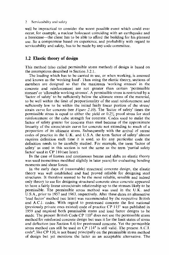
well be impractical to consider the worst possible event which could ever occur, for example, a nuclear holocaust coinciding with an earthquake and a hurricane—the client has to be able to afford the building for his planned use. So a compromise based on experience, and probability with regard to serviceability and safety, has to be made by any code committee.
1.2 Elastic theory of design
This method (also called permissible stress method) of design is based on the assumptions described in Section 3.2.1.
The loading which has to be carried in use, or when working, is assessed and known as the 'working load'. Then using the elastic theory, sections of members are designed so that the maximum 'working stresses' in the concrete and reinforcement are not greater than certain 'permissible stresses' or 'allowable working stresses'. A permissible stress is restricted by a 'factor of safety' to be sufficiently below the ultimate stress of the material, to be well within the limit of proportionality of the steel reinforcement and sufficiently low to be within the initial fairly linear portion of the stress/ strain curve for concrete (see Figure 2.10). The 'factor of safety' times the permissible stress is equal to either the yield or 0.2% proof stress for steel reinforcement or the cube strength for concrete. Codes used to make the factor of safety greater for concrete than steel because of the approximate linearity of the stress/strain curve for concrete not extending to much of a proportion of its ultimate stress. Subsequently with the arrival of recent codes of practice in the U.K. and U.S.A. the term 'factor of safety' almost requires definition each time it is used, so for any particular code the definition needs to be carefully studied. For example, the term 'factor of safety' as used in this section is not the same as the term 'partial safety factor' used in CP 110 (see later).
In the case of frames and continuous beams and slabs an elastic theory was used (sometimes modified slightly in later years) for evaluating bending moments and shear forces.
In the early days of (reasonable) structural concrete design, the elastic theory was well established and had proved reliable for designing steel structures. It therefore seemed to be the most reliable, sensible and indeed only theory to use for designing structural concrete since concrete appeared to have a fairly linear stress/strain relationship up to the stresses likely to be permissible. The permissible stress method was used in the U.K. and U.S.A., prior to 1957 and 1963, respectively. After these dates an alternative 'load factor' method (see later) was recommended by the respective British and A.C.I, codes. With regard to prestressed concrete the first national (previously private ones existed) code of practice CP 1151 was published in 1959 and required both permissible stress and load factor designs to be made. The present British Code CP HO2 does not use the permissible stress method for reinforced concrete design but uses it for the limit states of stress and deflection (see Section 8.4) for prestressed concrete. Yet the permissible stress method can still be used as CP 1143 is still valid. The present A.C.I. code4, like CP 110, is not based principally on the permissible stress method of design but yet mentions the latter as an acceptable alternative. The
Load factor method of design 3
British Code BS 5337 for designing water-retaining structures recommends permissible stress design and, as an alternative, a 'limit state design' (see later in this Chapter, Section 3.2.4 and Example 3.5).
Permissible stress design has certainly been very satisfactory for a long time.
1.3 Load factor method of design
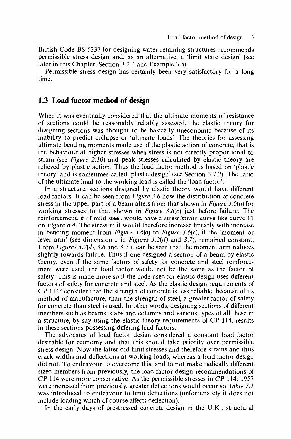
When it was eventually considered that the ultimate moments of resistance of sections could be reasonably reliably assessed, the elastic theory for designing sections was thought to be basically uneconomic because of its inability to predict collapse or 'ultimate loads'. The theories for assessing ultimate bending moments made use of the plastic action of concrete, that is the behaviour at higher stresses when stress is not directly proportional to strain (see Figure 2.10) and peak stresses calculated by elastic theory are relieved by plastic action. Thus the load factor method is based on 'plastic theory' and is sometimes called 'plastic design' (see Section 3.7.2). The ratio of the ultimate load to the working load is called the 'load factor'.
In a structure, sections designed by elastic theory would have different load factors. It can be seen from Figure 3.6 how the distribution of concrete stress in the upper part of a beam alters from that shown in Figure 3.6(a) for working stresses to that shown in Figure 3.6(c) just before failure. The reinforcement, if of mild steel, would have a stress/strain curve like curve 11 on Figure 8.4. The stress in it would therefore increase linearly with increase in bending moment from Figure 3.6(a) to Figure 3.6(c), if the 'moment or lever arm' (see dimension z in Figures 3.2(d) and 3.7), remained constant. From Figures 3.2(d), 3.6 and 3.7 it can be seen that the moment arm reduces slightly towards failure. Thus if one designed a section of a beam by elastic theory, even if the same factors of safety for concrete and steel reinforce-ment were used, the load factor would not be the same as the factor of safety. This is made more so if the code used for elastic design uses different factors of safety for concrete and steel. As the elastic design requirements of CP 1143 consider that the strength of concrete is less reliable, because of its method of manufacture, than the strength of steel, a greater factor of safety for concrete than steel is used. In other words, designing sections of different members such as beams, slabs and columns and various types of all these in a structure, by say using the elastic theory requirements of CP 114, results in these sections possessing differing load factors.
The advocates of load factor design considered a constant load factor desirable for economy and that this should take priority over permissible stress design. Now the latter did limit stresses and therefore strains and thus crack widths and deflections at working loads, whereas a load factor design did not. To endeavour to overcome this, and to not make radically different sized members from previously, the load factor design recommendations of CP 114 were more conservative. As the permissible stresses in CP 114: 1957 were increased from previously, greater deflections would occur so Table 7.1 was introduced to endeavour to limit deflections (unfortunately it does not include loading which of course affects deflection).
In the early days of prestressed concrete design in the U.K., structural

4 Serviceability and safety
concrete members were being made considerably smaller than ordinary reinforced concrete members and contained thin wires instead of robust bars. Prior to code CP 115 they were designed by the permissible stress method, sometimes without checking the load factor. When CP 115 was introduced it required a load factor of 2 but this could be less if the member would fail at a load not less than the sum of 1.5 times the dead load plus 2.5 times the imposed, or live, load. This introduced the concept of what has subsequently been called 'partial safety factors' for loads in CP 110. The imposed load may increase by accident. For example, a flat roof may be designed for occasional access but while a procession was passing by it might become packed tight with spectators. The dead load cannot increase unless, for example, the finishes to a roof or floor are renewed or changed, in which case the client would usually seek or encounter some building advice. Thus the load factor used for the imposed load part of the loading must be greater than that used for the dead load part of the loading.
The illogicality that existed after the publication of CP 114 was that, for example, individual ordinary reinforced concrete sections of a frame, or continuous beam or slab, could be designed to have a constant load factor but the distribution of bending moments was obtained by elastic analysis. The ideas of plastic collapse mechanisms (see Chapter 6), first developed for steelwork structures, had not been established well enough for inclusion in CP 114 in any greater way than allowing bending moments obtained by elastic analysis at supports to be increased or decreased by up to 15% provided that these modified moments were used for the calculation of the corresponding moments in the spans.
Still most analyses used would give bending moments at sections which would not increase in direct proportion to the loading towards failure, so to design sections of indeterminate structures with a constant load factor seemed pointless. Also the load factor method, with a general conservatism incorporated, only indirectly controlled crack widths and deflections com-pared to the permissible stress design method. Historically, however, a start presumably had to be made somewhere and somehow with the introduction of methods endeavouring to gain extra economy by the use of load factor methods.
To summarise, when the load factor method of CP 114 was used for sections, crack size was limited by incorporating conservatism into the formulae (in effect limiting the tensile stress in the reinforcement) and deflection was limited by the use of Table 7.1. Of course in important cases the designer could use the elastic methods of CP 114 and calculate deflections.
The book by Evans and Wilby5 gives considerable description and many examples on the elastic and plastic methods of CP 114 and the plastic method of the A.C.I.6 code of practice.
1.4 CP 110 philosophy of design
The European Concrete Committee (abbreviated to C.E.B., the initials of the Committee in French) introduced the concept of probability and used statistics in connection with the strengths of materials, loadings and safety and produced recommendations7 for a code of practice for reinforced

CP 110 philosophy of design 5
concrete. The underlying philosophy involved has been used as a basis for the present British CP HO2 and codes of practice in the U.S.A.4
With regard to concrete strength, the previous British practice was essentially to specify a minimum concrete strength below which no cubes should fail. This meant that the contractor needed to decide upon the quality of his control (see Table 2.2) to be able to calculate the average strength of the concrete he should endeavour to make. Then he designed his mix for this mean strength as in Section 2.3.10. When on the site, if any of the concrete cubes tested failed below the minimum strength then the concrete was either removed or cores of the concrete taken and tested or a load test was performed to see if the extra age had increased the strength and if the general monolithic construction (sometimes permitted to receive help from, for example, surrounding brickwork if any) was such that the construction could be considered to be safe. The CP 110 philosophy was to specify, not a minimum concrete strength as previously, but a strength which 5% of the cubes would not achieve, called the 'characteristic strength'. This involved the use of statistics and is explained in Section 2.3.9. The idea of accepting a strength below that at which some cubes would fail was hard for many British engineers to accept, because of their being brought up to think and desire that their designs should be very safe—failure was out of the question.
With regard to loading, the previous British practice was to assess the load which would be unlikely to be exceeded in use, and this would be called the 'working load'. Then if the CP 114 load factor method of design was used, sections would be designed to have a factor of safety of 1.8 against an ultimate load which would be taken as 1.8 times the working load. Now the CP 110 philosophy was not to assess the maximum load for the working load as previously but was to assess a load which, in effect, only 5% of occurrences of loading would exceed, called the characteristic load. This involved the use of statistics as is explained in Section 2.3.9. The idea of seemingly now accepting a working load which was planned to be sometimes exceeded was again hard for many British engineers to accept. Then, as if to make it more difficult for engineers to accept, CP 110 introduced the idea of probability of characteristic strengths and loads being variable.
British engineers had always prided themselves on designing structures which in their opinion could never fail. Well, of course, scientific reality cannot be ignored, materials do vary and probability does exist. Apart from negligence and natural catastrophes, the most likely cause of failure of a structure, or inadequacy at working loads (that is cracks or deflections being unacceptable), is the coincidental occurrence of both overload and excessive weakness at a critical section.
The probability of failure, for example, could involve the concept of an accident rate intuitively accepted for a given type of structure. For example, how often are crane gantries liable to fail by overload? The probability of failure could also involve economy, for example a reduced probability of failure will require a stronger structure at an increased cost.
Discussions of probability of failure become very emotive because of probable loss of life. A possible analogy is a motor coach full of passengers because if it crashes loss of life is also involved. There is a certain statistical

6 Serviceability and safety
level of probability of hitting a lamp standard or telegraph post, of running into a ditch or river, of rolling over, of hitting another vehicle head on, etc. The designers would not dream of designing the motor coach so that no lives would be lost, or even that no parts of the coach would fail, under all these eventualities. It would not be economically desirable even if possible with brilliant engineering design. On the other hand one would expect the coach floor not to fail due to a suitcase dropping from a luggage rack. One would expect the walls and floor not to fail due to unequal loading of passengers or even a fight amongst some passengers. So with structures a compromise has to be reached between practicality, economy and prob-ability of failure. A jetty designed for a certain use, namely a ship being piloted up to it by a skilled skipper cannot economically be designed to withstand the fairly remote probability of say a drunken skipper sailing a large ship at full speed at right angles to and into the side of the jetty. In such a case it would be argued that the damage and loss of life to anyone on the jetty was the responsibility of the skipper and it was not the re-sponsibility of the owners of the jetty to build it strong enough for this eventuality.
The CP 110 use of probability manifests itself in the use of 'partial safety factors'. The word 'partial' is used as each part of the problem may have a different safety factor. The characteristic strength of a material permits 5% of the control specimens to be inadequately strong. Dividing the character-istic strength by a partial safety factor (a number greater than unity) means that less specimens will be below the resulting 'design strength' used. The characteristic loading is such that it will only be exceeded on 5% of occasions. Multiplying the characteristic load by a partial safety factor (a number mainly greater than unity) means that the resulting 'design load' should be exceeded on less than 5% of occasions. Thus these partial safety factors are intended to reduce the probability of failure towards zero.
CP 110 also introduced the concept of 'limit state design'. In design everything that matters as regards the strength and serviceability of a structure is limited or restricted to a satisfactory amount. The condition of a structure or part of it, when it becomes unfit for use, is called a 'limit state'. We can categorise these limit states into two broad divisions, namely 'limit states of serviceability' and 'ultimate limit states'. 'Limit states of service-ability' include:
1. Deflection: This must not impair the appearance or efficiency of the structure—see clause 2.2.3.1 of CP 110 (Appendix 4 of this present book).
2. Cracking: Cracks must not adversely affect the durability or ap-pearance of a structure (see clause 2.2.3.2 of CP 110) although the latter does not seem to matter in some parts of the world. In Britain there is a practice of generally limiting cracks and this is often done no less for a hidden and protected member than for one that is seen in a building or exposed. This uneconomic and inefficient practice was established in pre-vious codes. The limit state design of CP 110 now gives opportunities of using different limit states for different members whereas CP 114 did not.
3. Vibration: This must not cause unpleasantness or alarm to the occupants, damage to fixtures, fittings and services (such as water pipes), etc. (see clause 2.2.3.3 of CP 110).

CP 110 philosophy of design 7
4. Other limit states: Clause 2.2.3.4 of CP 110 requires consideration of any other limit states considered necessary by the engineer.
'Ultimate limit state' requires that the strength of the structure should be adequate to withstand the design loads with due consideration being given where appropriate to buckling and the general overall stability (see clause 2.2.2 of CP 110). Ultimate limit states may need to be assessed for the following:
(A) Flexural or compression failure at any critical sections (B) Shear failure (C) Torsion failure (D) Bond or anchorage failure of reinforcement (E) Instability of a member (F) General instability (for example overturning) (G) Bearing failure at a support or under a concentrated load or at bends or
hooks in tension reinforcement (H) Bursting of prestressed concrete end blocks (I) Failure of connections (for example between precast concrete elements
or in composite construction).
TABLE 1.1. Partial safety factors for loads yf
Load combination Ultimate Serviceability limit state limit state
(1) Dead and imposed load: yf for dead load Gk
y( for imposed load Qk
(2) Dead and wind load: y{ for dead load Gk yf for wind load Wk
(3) Dead, imposed and wind load: yf for dead load Gk
y{ for imposed load Qk
y{ for wind load Wk
1.4 1.6
0.9 or 1.4* 1.4
1.2 1.2 1.2
1.0 1.0
1.0 1.0
1.0 0.8 0.8
* Use 0.9 when the dead load contributes to the stability, and 1.4 when the dead load assists the overturning of the structure.
Tables 1.1 and 1.2 summarise the partial safety factors for loads and strengths, respectively, as recommended by CP 110 clauses 2.3.3.1 and 2.3.4.1. For example from Table 1.1 if one is designing for the ultimate limit state and considers the combination of loading (1) then, using CP 110 symbols (Appendix 3)
Design load = sum of y{ times each characteristic load = 1.4Gk + 1.6Qk
The y{ is smaller for the dead load because there is less likelihood of the dead load being increased (for example, a small increase can be due to members being cast slightly oversize) whereas the y{ for the imposed load is greater because the imposed load can experience an overload.

8 Serviceability and safety
TABLE 1.2. Partial safety factors for material strength ym
Material
Concrete Steel
Ultimate limit state
1.5 1.15
Serviceability limit state
Deflection Cracking
1.0 1.3 1.0 1.0
Again from Table 1.1 if one is designing for serviceability limit state for the combination of loading (3) then
Design load = 1.0Gk 4- 0.8£>k + 0.8 Wk
The y{ is smaller for Qk and Wk because it is a fairly remote possibility that full imposed and wind loading will occur together.
For limit state of serviceability the partial safety factors are lower than for ultimate limit state as an overload in the former case may be temporary and although undesirable the excessive deflections and crack widths will reduce when the overload is reduced. But if the ultimate limit state is exceeded with an overload, failure may occur—an irreversible condition.
In Table 1.2 it will be noticed for example that ym is less for the ultimate limit state for steel than it is for concrete. This is because the control in the manufacture of steel is considered to be better than it is for concrete.
1.4.1 Summary of C? 110 philosophy of design
(a) A 'limit state' is a condition of a structure at which it ceases to function in the manner for which it was designed. Limit states can be classified as follows:
1. 'Ultimate limit state'refers to failure. 2. 'Serviceability limit states' refer to conditions in normal use. The main
ones are deflection, cracking, vibration, fatigue, durability and fire resistance. (b) Materials:
1. 'Characteristic strength' is the strength below which only 5% of test specimens will fail (see Figure 2.4).
2. 'Partial factor of safety', ym, is given by characteristic strength
'Design strength' = 7rr
and this is applied to each of concrete and steel, that is the parts involved. For example, ym is normally 1.5 for concrete and 1.15 for steel for assessing ultimate limit state. Refer to Table 1.2.
(c) Loads: 1. 'Characteristic load' is the load which is expected to be exceeded on, in
effect, only 5% of occasions. 2. 'Partial factor of safety' for loads, yf, is a factor by which each part (dead,
imposed, wind) of the loading is multiplied so as to obtain the 'design load',

CP 110 philosophy of design 9
that is the load to be designed against. The design load for limit state of serviceability is different and much less than the design load for ultimate limit state.
For example, for ultimate limit state, if wind load is not being considered, using Table 1.1, (design load) equals 1.4 times (dead load) plus 1.6 times (live load). Another example, for serviceability limit state, for all loads, again using Table LI, (serviceability load) equals 1.0 times (dead load) plus 0.8 times (imposed load) plus 0.8 times (wind load).
1.4.2 Simplified statement of CP 110 philosophy of design
An attempt to summarise the whole process of CP 110 design is now made. Essentially 'characteristic loads' are determined. There are usually three: namely for dead, imposed and wind loadings. These are then, for design, considered in what are thought to be the most critical combinations for causing failure ('ultimate limit state') and causing, say, excessive cracking and deflections in use ('serviceability limit states of cracking and deflection', respectively) by using multipliers ('partial safety factors'), to give various 'design loadings'.
The resistance to these various load combinations is calculated using 'design strengths' for concrete and steel obtained by dividing 'characteristic strengths' for concrete and steel by their respective 'partial safety factors'.
References
1. 'Code of Practice for the Structural Use of Prestressed Concrete in Buildings', CP 115, 1959, last reprint 1969, British Standards Institution, London
2. 'Code of Practice for the Structural Use of Concrete', CP 110: Part 1: Nov. 1972, British Standards Institution, London
3. 'Code of Practice for the Structural Use of Reinforced Concrete in Buildings', CP 114: Part 2: 1957, last reprint 1969, British Standards Institution, London
4. 'Building Code Requirement for Reinforced Concrete', A.C.I. 318-77, American Concrete Institute, Detroit, Michigan, U.S.A. (1977)
5. EVANS, R. H. and WILBY, C. B., Concrete-Plain, Reinforced, Prestressed and Shell, Edward Arnold (1963)
6. 'Building Code Requirements for Reinforced Concrete', A.C.I. 318-56, American Concrete Institute. Detroit, Michigan, U.S.A. (1956)
7. C.E.B., 'Recommendations for an International Code of Practice for Reinforced Concrete'. English edition. American Concrete Institute and Cement and Concrete Association (1964)

Chapter 2
Properties of materials and mix design
2.1 Cement
Cement is the most important and expensive ingredient of concrete, on a price per tonne of material basis (dependent upon the mix, the aggregates can sometimes cost more than the cement in a cubic metre of concrete). It was patented by J. Aspdin in the U.K. in 1824 and he called his product Portland Cement because the 'artificial stone' (concrete) made with it resembled Portland stone.
Portland cement is made by grinding together its principal raw materials, which are (a) argillaceous, for example silicates of alumina in the form of clays and shales, and (b) calcareous, for example calcium carbonate in the form of limestone, chalk, and marl which is a mixture of clay and calcium carbonate. The mixture is then burned in a rotary kiln (shaft kilns are still used for works with small outputs and there is an interest in their installation in developing countries) at a temperature between 1400 and 1500°C; pulverised coal, gas or oil is the fuel. The material partially fuses into a clinker which is taken from the kilns, cooled and then passed on to ball mills where gypsum is added and it is ground to the requisite fineness. The resulting cement is allowed to contain small strictly limited percentages of materials not required, some disadvantageous for some uses, such as iron oxide and sulphur trioxide. A general idea of the composition of cement is indicated by the following oxide composition ranges for Portland cements: lime (CaO) 60-67%, silica (Si02) 17-25%, alumina (A1203) 3-8%, iron oxide (Fe203) 0.5-6%, magnesia (MgO) 0.1-4%, sulphur trioxide (S03) 1-3%, soda (Na20) and/or potash (K20) 0.5-1.3%.
The constituents forming the raw materials used in the manufacture of Portland cement combine to form compounds, sometimes called Bogue1
compounds, in the finished product. The following four compounds are regarded as the major constituents of cement: tricalcium silicate (3CaO.Si02 or C3S), dicalcium silicate (2CaO.Si02 or C2S), tricalcium aluminate (3CaO.Al203 or C3A) and tetracalcium aluminoferrite (4CaO.Al203 .Fe203 or C4AF).
A cement works is usually sited near to its raw materials. These sites vary and consequently cements from different works vary within permissible 10

Cement 11
limitations. In the U.K. this variation seems to have an insignificant effect upon concrete. However, research by the author and others indicates that the asbestos cement manufacturing process is sensitive to the percentage of C3S, which varies significantly with cements from different works in the U.K. Examples of other sensitivities: pipe spinners sometimes request coarse ground cement, aerated block manufacturers sometimes request cements with high total silicates, roof tile manufacturers sometimes prefer cements with higher alkalis (for the associated high strengths at early ages), floor layers dislike cements with short or long setting times, etc.
High alumina cement was first made by J. Bied for the French Lafarge Company in 1908, and named Ciment Fondu. This discovery was made whilst searching for a cement which liberated no free hydrated lime upon setting. Portland cement liberates free hydrated lime upon hydration and this in the resulting concrete is very vulnerable to attack from mineral sulphates, dilute acids and other agents.
When cement is hydrated, lime and alumina are liberated. The lime combines with the alumina and in the case of Portland cement an excess of lime results, whereas in the case of high alumina cement an excess of alumina results. Bearing this in mind, the properties of these two fundamen-tally different cements can often be predicted. For example, when these cements are mixed together and hydrated, the respective excesses of lime and alumina react chemically with one another and a flash set (almost instantaneous setting) can result. This can be useful for caulking small leakages in cofferdams and water-retaining structures. The flash set phenom-enon is, however, a reason for new Ciment Fondu concrete not being suitable for jointing to new Portland cement concrete, and vice versa. Time limits have to elapse so that there is no danger of unhydrated Portland cement coming into contact with unhydrated high alumina cement. The concrete which is to be extended should be 24 hours old if it is Ciment Fondu concrete, 2 days old if rapid hardening Portland cement, and 7 days old if ordinary Portland cement.
When cement is hydrated the terms initial setting time, final setting time and rate of hardening are used, often loosely. However, the first two are defined for cement by BS 12, 915 and 1370. Other tests of cement for soundness, tensile and compressive strength, chemical composition, fine-ness of grinding, etc., are described in BS 12. The definitions of initial set and final set unfortunately bear no precise relationship to practice. They do, however, enable the properties of different cements to be compared for their setting qualities. It can loosely be said that it is good practice not to disturb concrete after its initial set, and the initial setting time is normally not less than half an hour. There are exceptions to this rule in practice, however, since such operations as the trowelling of concrete floors and granolithic finishes, for example, usually need to be performed after the initial set, but before the final set has taken place. The final setting time is not usually more than ten hours.
If one imagines say a sewn-up sheep's bladder (a colloidal membrane) containing a solution, immersed in a similar solution of greater dilution, then water travels through the very fine pores in the bladder so that a pressure (an osmotic pressure) is developed in the bladder. This pressure continues to increase until the solutions on either side of the colloidal
12 Properties of materials and mix design
membrane have the same dilution. This is a very simple description of colloidal chemistry relative to the hydration of cement. Upon hydration the surface of a small portion of cement forms crystalline substances, which can be observed with an electron microscope,2 with the water. These form a colloidal membrane, surrounding the portion of cement, called tobermorite gel3 (a calcium silicate hydrate). As indicated previously, water travels through the membrane to dilute the solution of hydrating cement com-pounds within the membrane. This causes a pressure inside the membrane and hence expansion of the concrete or mortar. Conversely, drying of the cement after hydration causes shrinkage of the concrete. However, the amount of shrinkage caused by complete drying out of hydrated cement paste is not completely recovered by subsequent wetting.
If water is in contact with concrete, for example the wall of a basement, water can travel through the concrete not only via any cracks, construction joints, or voids, but also via the colloidal membranes. The water passes through adjacent colloidal membranes, until all solutions surrounded by colloidal membranes have reached the same dilution. Thus water, or dampness, can be transmitted through a basement wall of sound concrete. Hence the desirability of 'tanking' (providing an impervious membrane) even if the concrete is very good.
The strength of a cement paste depends greatly upon the bonds formed between the very small particles of its cement gel. Generally the greater the number of these particles and the denser the gel structure, the stronger the gel mass.2 The water-to-cement ratio used for a cement paste is related to its strength.
There are several types of cement available to the engineer, for example, as follows:
1. Ordinary Portland cement. This is the most inexpensive cement and is consequently widely used.
2. Rapid hardening Portland cement. As the name implies, concrete made with this cement hardens more rapidly than concrete made with ordinary Portland cement. Such a property enables early stripping of concrete formwork, especially advantageous for precast work where repeated uses are made of the same shutter. Extra rapid hardening cements can be obtained for special purposes. These two cements are of the same material as ordinary Portland cement except more finely ground.
3. High alumina cement (H.A.C.). This cement is not classed as a Portland cement. It hardens much more rapidly than any other commercial cement, and it has the further advantage of being sufficiently immune, for practical purposes, to attack from several important chemicals. Some examples are: many of the sulphates present in subsoil waters and in sewage; sulphur compounds formed from the combustion of coal and oil; carbonic acid as experienced in subsoil waters from moorland areas; many of the chemicals contained in sea water; chemicals which attack Portland cement and which are present in important industries such as lactic acid (associated with milk), tar oil, cottonseed oil, beer, and sugar juices. H.A.C. was excluded from CP 110 by the August 1974 amendment, but was previously allowed to be used when high strength was required urgently, for

Cement 13
example on maritime structures when it was necessary to have a reasonably hard concrete before high tide; for the sealing of water leaks in emergencies when excavating in water-bearing ground; for structural work which required to be in use within, say, 24 hours; for structural work where formwork was required to be stripped early or where it was required to prop further shutters from the members cast as soon as possible; for prestressed concrete, especially pretensioned concrete, where economy re-quired release of the wires and removal of the members from the prestress-ing beds as early as the strength of the concrete permitted. The high early strength is obtained to some extent because the chemical reaction of the cement with water is very exothermic. To avoid the ills of overheating (see 7, page 15) it is desirable to have a low water-to-cement ratio (to reduce the rate of chemical activity), to cast at an ambient temperature of not more than about 20 °C, not to allow the internal temperature of the concrete to be more than 30 °C for more than 24 hours after casting, to cure with water or similar, and certainly not to steam cure.
The greatest disadvantage of high alumina cement was its cost, which made it prohibitive for many purposes. Another economic disadvantage was the necessity of curing with water or dampness. Concrete using this cement was nevertheless quoted as being more economical than steam cured Portland cement concrete for prestressed concrete work.
H.A.C. with suitable aggregate can be used as a refractory concrete or mortar for fireclay bricks and is suitable for temperatures up to about 1300°C. High climatic temperatures in combination with high humidities as experienced in the tropics were found to reduce the strength of concrete made with H.A.C. rather alarmingly.4 The chemical conversion of certain crystalline compounds having certain numbers of elements of water of crystallisation to other crystalline compounds with different numbers of elements of water of crystallisation could cause an internal volume change in the concrete with a consequent disruption and weakening of the concrete. The shape of crystals changes from hexagonal to cubic. Neville4 claimed that this chemical conversion could also eventually occur with aging in the cool damp U.K. climate, although CP 110 prior to the August 1974 amendment, regarded this effect as negligible for properly cured concrete. It might be thought that high alumina cement concrete could be used in structures protected from moisture, which is the case with many buildings, without worrying about chemical conversion. Yet even indoors, with central heating and solar gain through large glass windows, temperatures can be high and it is argued that there is always water in some form inside the concrete, and the humidity of the atmosphere can be high in the U.K. and this air is not normally dried before entering buildings. After full conversion, concrete strength increases with age.
Although the dangers of conversion became rather catastrophically expe-rienced about 1961, seemingly inadequate notice was taken of this sub-sequently, until about 1974 when there was considerable alarm concerning lack of reliable knowledge of when high alumina cement could be used. Inadequate notice was taken of work by Bolomey5 of France in 1927 and Davey5 in the U.K. in 1937; both demonstrated that high alumina cement concretes, hardened under good conditions, subsequently lost up to 40% of

14 Properties of materials and mix design
their strength permanently, due to curing in warm water, and experienced the colour change to yellow-brown, which we now know to be due to conversion.
In the case of the most publicised failure in the U.K., the prestressed concrete beams were over a swimming pool and experienced warmth, moisture from condensation and roof leaks, sulphate attack from the plaster, and possibly had poor concrete and support seatings. The other few failures in the U.K. seem to have had more than just conversion as a weakness. Subsequently most high alumina cement work has been tested in the U.K. and most of it found to be safe. Some structures have been strengthened against possible future weakness due to conversion. The author has tested roofs to a building with up to 95% conversion and found them very safe over several years. There is no doubt that steam constantly directed on to high alumina cement beams can cause them to disintegrate.
4. Cement for use in cold weather. Such cements (manufacture was discontinued in the U.K. some years ago) are usually achieved by adding about 1.5% of calcium chloride to rapid hardening Portland cement. The calcium chloride generates heat by reacting with the water used in mixing the concrete. This also enhances the rapid hardening qualities. Because of the heat evolved, these cements can very often be profitably used in cold weather to allow concreting operations to continue. The high early strength properties are advantageous for allowing early stripping, and, in the case of precast concrete, handling. The chloride ion aggravates the corrosion of steel (this is particularly so in the case of NaCl). Hence if water and oxygen ion can penetrate to the reinforcement through pores and/or cracks in the concrete, the calcium chloride will increase the rate of corrosion of this reinforcement. It is interesting that in the case of water-retaining structures and underground pipelines, if the water is in contact with concrete contain-ing very fine cracks which penetrate to the reinforcement, it is possible for corrosion to occur even though many would not imagine that air could penetrate through the crack. This is because the oxygen ion of air dissolved in the water is easily carried in the water penetrating the crack to the steel— refer to the theory of notch corrosion. CP 110 prohibited calcium chloride in prestressed pretensioned concrete, and restricted it to not more than 1.5% by weight of the cement in reinforced concrete. Subsequent amend-ments have effectively banned calcium chloride in reinforced concrete; theoretically a small amount can be used but this is too small to be effective practically as an accelerator. Non-chloride accelerators are now being used to some extent to aid winter working.
5. Sulphate-resisting cement. This cement is made specifically to resist the attack of sulphates. Underground structures can experience sulphate attack from the soil, back-fill or ground water. There is a cement known as super sulphated cement which is sometimes claimed to be better when the sul-phates are acid in nature.
6. Cements with a low coefficient of shrinkage can be specifically devised for highways, dams, water-retaining structures, etc., to reduce the magni-tude of cracks caused by shrinkage. Such a cement, which also had low beat of setting, was devised and used for the mass concreting to the Boulder Dam, U.S.A. There are cements which are claimed to expand, but they do not always do so if the concrete subsequently dries out.
Aggregates 15
7. 'Low heaf Portland cements generate less heat upon reacting with water than normally experienced with other cements and are thus suitable for mass concrete work. The heat generated with Portland cement in mass concrete work can literally boil off the water required for the necessary chemical reaction, the steam causing flash setting of some of the cement and also disruption and voids in the resulting concrete.
8. 'Portland-pozzolana cements'. Fly ash (pulverised fuel ash, P.F.A., or pozzolana) is sometimes substituted for 15-35% (one cement manufactured in the U.K. uses 28%) by mass of the ordinary Portland cement to achieve low heat of setting and reduced shrinkage without reducing the 28-day strength of the concrete, but the early rate of hardening is reduced. About 1970 this idea was used for a gravity dam in Yorkshire, and to help further, the concrete mix had a low cement content and used a large size of aggregate. Unfortunately fly ash contains a small amount of sulphate. CP 110 restricts the total sulphate content of a mix expressed as S 0 3 to not more than 4% by mass of the cement. So far, in the U.K., in practice fly ash has had no difficulty in complying with this restriction.
9. Coloured cements are used for reconstructed stones, renderings, and the like. Because of the high cost of these cements, coloured artificial stones usually have a facing about 38 mm thick made with the coloured cement, and a backing made with ordinary Portland cement. Coloured cements can be obtained by adding the following pigments to Portland cement: yellow ochre (yellow), brown oxide of iron (brown), green oxide of chromium (green), red oxide of iron (red), manganese black (black). The weight of the pigment should not exceed 10% of the weight of the cement, otherwise the strength will be impaired. White cements are popular and require to be specially manufactured. The colour of a concrete can be improved and will wear better if the aggregates also are of a colour similar to the coloured cement. Of recent years the manufacture of coloured cements has been discontinued in the U.K., except for white cement.
10. Portland blastfurnace cement is obtained by grinding granulated blast furnace slag with the clinker which is normally ground down to make ordinary Portland cement. It has a slightly lower heat of hydration than ordinary Portland cement, is slightly more resistant to sulphate attack, and is slower to develop its early strength.
11. Water-repellent cements. Certain ones are most effective in sealing leakages in water-retaining structures.
2.2 Aggregates
Aggregates are classed as fine aggregates and coarse aggregates. Generally, various sands are used as fine aggregates, and coarse aggregates are either water-worn gravels or crushed rocks. The aggregates chosen are usually the most inexpensive to give the requisite quality of concrete. The engineer must, however, be satisfied that the source selected will consistently supply the quality of aggregate which he has approved. This can be difficult for certain special requirements. Sometimes the engineer requires stockpiles at the suppliers' works to meet with his approval. These are then drawn upon exclusively for the concreting operations.

16 Properties of materials and mix design Aperture size (Imperial)
BS Sieve No.s Aperture size, in
300 1.20 2.40 4.76
mm
9.52 19.05
Aperture size (SI)
Figure 2.1
Aggregates for normal concreting work are a fairly inexpensive com-modity at the quarry and thus transport charges substantially influence their overall cost. Local aggregates are therefore generally employed, but an expensive type of aggregate may warrant greater transport costs if the necessary stone does not occur locally. Examples of more expensive stones are: granites for granolithic finishes; various types of coloured aggregates for artificial (reconstructed) stones (usually used for the surface layer of the stone only); and vermiculite (imported into the U.K.) for lightweight finishes.
Reference should be made to the British Standards 882, 1198, 1199, 1200 and 1201, which recommend various gradings of the particle sizes for both fine and coarse aggregates. These enable standardisation and control but are not necessarily ideal gradings for concrete. The standards quoted specify tests of other relevant qualities of the aggregates, namely specific gravity, water absorption, bulk density, organic impurities, and crushing strength. Figure 2.1 shows four gradings, upon which the mix designs of the D. S.I. R.Road Note No. 48 are based, for 19.05 mm (f in) and down aggregates, and one average grading curve for 9.52 mm (fin) aggregate. The grading of a 19.05 mm (fin) aggregate should lie within the curves 1 and 4 and preferably within the curves 2 and 3 if this method of mix design is to be used.
Coarse aggregates can be classified according to shape (BS 812) as follows:
1. Rounded aggregates, for example beach and other well worn gravels. 2. Irregular aggregates, for example water worn river gravels.

Concrete 17
3. Angular aggregates, for example crushed rock or manufactured ma-terials. These are commonly granites, limestones, basalts, quartzites, flints, pumice, broken bricks, foamed slag, blast furnace slag, sometimes a strong sandstone, vermiculite and duromit, etc.
The grading, shape, porosity and surface texture of the aggregates can affect the workability and consequently the strength of concrete.
When a concrete is required to be lightweight, to have a good resistance to heat transmission and impermeability to water, and a high strength is not required, special lightweight aggregates are often used, such as vermic-ulite, foamed slag, clinker, breeze, pumice, wood wool and expanded shales.
If water is added to 1 m3 of sand, the gross volume of this sand in-creases until it occupies about 1.25 m3. After this volume is attained the addition of further water decreases the gross or bulk volume until when the sand is finally saturated the volume has returned to 1 m3. When concrete is 'batched' by volume (that is the ingredients measured by volume) the water content of the sand greatly influences the quality of the resulting concrete. Consider a l(cement):2(sand):4(gravel) mix, the ratios referring to dry volumes of the respective materials (as is standard practice). If we were using a sand experiencing its maximum amount of 'bulking' of, say, 25%, then the mix actually produced in terms of dry volumes would be 1:2/1^:4 or 1:1.6:4.
If water is added to 1 kg of sand, the gross weight is increased by the weight of the water added to about 1.1kg upon saturation. Hence, if the batching of concrete were by weight, the water content of the sand would still be troublesome but not to as great an extent as by volume. Consider again a 1:2:4 mix and let the sand be increased in weight by its maximum amount of say 10% due to its water content. Then the mix actually produced in terms of dry volumes would be 1:2/1.1:4 or 1:1.818:4. For illustrative purposes it has been assumed that the bulk densities of the dry materials are the same. Thus the inaccuracy of batching by weight is basically not as great as batching by volume. This reasoning ignores the fact that the same phenomenon also affects coarse aggregates, but to a far lesser extent. Several devices are available for measuring the water content of the aggregates, so that the mix can be adjusted accordingly. The water content often varies from place to place in a stockpile. When a large concreting programme is being conducted, sometimes the stockpiles will be insufficient (especially on congested sites) and sand which arrives during the course of the concreting operations will have a different water content to the sand in stock. Aggregates are commonly exposed to the weather so that the water content will vary with the rainfall. One needs to be vigilant therefore to allow for the errors in batching caused by the water content of the aggregates.
2.3 Concrete
Coarse aggregate, fine aggregate, cement and water are mixed together in suitable proportions, and this mixture, placed and compacted wherever required, solidifies after a lapse of time into what is known as concrete.

18 Properties of materials and mix design
The mixes of concrete commonly used (CP 114) for structural purposes were 1 part (by dry volume) of cement: 2 parts (by dry volume) of fine aggregated parts (by dry volume) of coarse aggregate, and similarly, 1:1^:3 and 1:1:2. CP 110 calls such mixes 'prescribed mixes' and specifies them for various grades of concrete in terms of weights of cement and total dry aggregates with percentages by weight of fine aggregate in total dry aggregates. It is now more common to design mixes to specified grades or strengths.
Many investigators have proved that most of the qualities desired of concrete benefit by increased compressive crushing strength, for example, strength in tension, shear, and resistance to weathering, abrasion and wear, and impermeability. Exceptions to this rule are lightness (in density), and thermal insulation.
The factors which have the greatest effect upon the strength of concrete are the cement-to-aggregate ratio, the compaction, the water-to-cement ratio of the mix, and the method of curing.
It is easy to imagine that the strength of concrete depends upon the absence of voids, or in other words, upon the final density after setting and maturing. For example, 5% of air voids can give a loss in strength of 30%, 10% of voids can give a loss in strength of 60% and 25% of voids can give a loss in strength of 90%. Compaction of the concrete is therefore extremely important, and this is dependent upon the 'workability' of the concrete.
2.3.1 Workability
Workability is the ease with which concrete can be placed in moulds, compacted around reinforcement and screeded to a level. Many tests have been devised for measuring this property, and all have been subjected to much adverse criticism. The test which has possibly been condemned the most, namely the slump test, is the most commonly used in the U.K., and is referred to by CP 110. The nature and the grading of the aggregates con-siderably affect the slump. Thus specifying the slump can ensure uniformity in the consistency of concrete during the progress of work only if the materials are of constant quality.
Other tests of workability referred to by CP 110 are the compacting factor test and the VB consistometer test. The former was developed as an improvement upon the slump test in attempting to measure workability. The latter became useful in the U.K. when drier concretes than previously became necessary for prestressed concrete work, as it can distinguish between various concretes having virtually zero slump. It is also better for very dry mixes than the compacting factor test.
Table 2.1 recommends suitable approximate workabilities of concrete for various uses.
Good compaction of the concrete, and hence a high strength concrete with a good finish, can be obtained by manipulation of the grading and type of the aggregates, the use of additives to reduce the surface tension of the water, employment of vibration and/or pressure, and use of a high water content.
The additives are plasticisers and 'super-plasticisers' comprising soaps, detergents, or resins. Essentially they reduce the surface tension of the

Concrete 19
TABLE 2.1. Uses of concrete of different degrees of workability (Road Note No. 4)
Degree of workability
Very low
Low
Slump, mm
0-25
25-50
Compacting
Small apparatus
0.78
0.85
' factor
Large apparatus
0.80
0.87
Use for which
Vibrated concrete in roads or other large sections
Mass concrete foundations without vibration. Simple reinforced sections with vibration
Medium 50-100 0.92 0.935 Normal reinforced work without vibration and heavily reinforced sections with vibration
High 100-180 0.95 0.96 Sections with congested reinforcement. Not normally suitable for vibration
water, that is the water wets the particles more easily, increasing work-ability. They allow the water-to-cement ratio to be reduced for no decrease in workability, thus giving a stronger concrete. Some entrain finely disper-sed air bubbles sufficiently for the concrete to have increased frost resistance for little decrease of strength—used for roads in cold countries and called 'air entrained concrete'.
The use of a high water content must be avoided as much as possible as it also decreases the strength of the concrete, as explained later. It can however be used with advantage when combined with a vacuum process (see page 21). A high strength concrete requires to be as free from voids as possible. If water in excess of the amount required for the chemical reaction with the cement is present in the mix, this water remains in a free state and the concrete sets around the drops of water. Such particles of water form pores and voids in the concrete, resulting in weakness and permeability. Dependent upon curing conditions they may freeze and expand, cause corrosion and/or eventually evaporate into the atmosphere.
23.2 Water-to-cement ratio and strength of concrete
The important effect of the water-to-cement ratio, by weights, on the strength of concrete was realised in 1918 by D. Abrams of Chicago, who stated that the strength of any workable concrete was dependent upon the water-to-cement ratio alone, assuming the same cement and degree of compaction are used and the conditions of curing and age at comparison of strengths are constants. The types of aggregates used can be varied, provided the concrete does not fail by the fracture of such aggregates. The workabilities of different mixes having the same water-to-cement ratios would be considerably different; for example a lean (low proportion of cement) mix might need vibration to obtain the same compaction as a

20 Properties of materials and mix design
richer (in cement) mix placed by hand. The strength of concrete increases as the water-to-cement ratio decreases, provided the water present is sufficient to allow the full chemical reaction to occur with the cement. If the water is less than this amount, a decrease in strength is experienced. Figure 2.2 shows the relationship between the average ultimate compressive stress (or crushing strength) and the water-to-cement ratio for 150 mm cubes of fully compacted concrete for mixes of various proportions. In recent years U.K. manufacturers have altered ordinary Portland cement to rapid hardening cement by finer grinding.
Water-to-cement ratio by weight
Figure 2.2
Only the compressive strength of concrete has been considered so far. It is generally accepted that this is a fairly reliable guide to the tensile and shear strengths, the modulus of rupture, the resistance to abrasion and wear, durability to the weather, density, porosity and watertightness. For durability, cement content is also important and minima are specified for various conditions in CP 110.
2.3.3 Strength tests of concrete
BS 1881 specifies a standard compressive test, and also a standard test for the modulus of rapture. The latter flexural tensile test gives greater values than those obtained from tension tests made on standard briquettes (BS 12).

Concrete 21
The cross section of the briquette which is tested in tension is 25 mm square, the specimen being primarily designed for testing cements by determining the strengths of their cement/sand mortars. Larger specimens should be used for tension tests when the maximum size of the aggregate is greater than 9 mm. The cylinder splitting test has become popular as a tensile test of concrete. Unfortunately it is an indirect test of tension and assumes an elastic theory to calculate ultimate stress.
Shear in concrete beams is thought of in terms of diagonal tension and consequently the tensile strength of concrete is more relevant than the shearing strength. The shearing strength can be obtained from torsion tests of cylinders of concrete. The distribution of shear stress in such tests, however, is not the same as experienced in, say, a punching shear test.
With all the tests mentioned, size and shape of specimen matter, and thus empirical factors are usually required to relate these indicative control tests to the behaviour in the structural member.
2.3.4 Vacuum concrete
The concrete is made sufficiently wet to be placed and compacted easily and then the vacuum process removes water from the concrete, so that it finally has a low water-to-cement ratio. The water is extracted through mats placed in contact with the concrete. These mats are such that only water, and no cement, or fines (out of the aggregates) can be sucked from the concrete by the vacuum pump. Side shutters can usually be removed immediately afterwards if desired, as the concrete has almost zero slump. In the U.K. the vacuum concrete process is used by certain, but not all, firms making pavement flag stones.
2.3.5 Vibrated concrete and pressure compaction
Concretes with low water-to-cement ratios can be placed and compacted by internal or external vibrators. External vibrators usually consist of motors with heavy cams on their shafts, and are fastened to a mould. Internal vibrators are of a poker type and can be held in the hand and immersed in the concrete where required. They are the more efficient for compaction and do not require the strong moulds often necessary for the external vibrators. If sufficiently dry mixes are used, the sides of the moulds can be removed immediately after vibration. There are in fact beam-making machines where the concrete is compacted by vibration, the sides removed immediately, and the beam on its pallet dragged away along skids. Most block-making machines employ pressure as well as vibration. Here again, solid and hollow blocks can be removed immediately from block-making machines on their pallets.
Workmen, when not strictly supervised, tend to make concrete extremely wet. Vibration does not increase the workability of such concrete and can be detrimental by causing segregation of the constituents of the concrete, the gravel tending to sink to the bottom, and the sand and cement to float to the top of the concrete. Such segregation can also occur with dry mixes if the vibration is sustained for a long enough period. The vibration employed with an apparently dry mix should be only just sufficient to make the
22 Properties of materials and mix design
concrete flow into the sharp arrises of the mould and around the reinforce-ment. Poker vibrators should not be removed rapidly or they can leave voids behind them.
Essentially compaction by pressure and/or vibration enables drier con-cretes to be satisfactorily compacted to make stronger concretes.
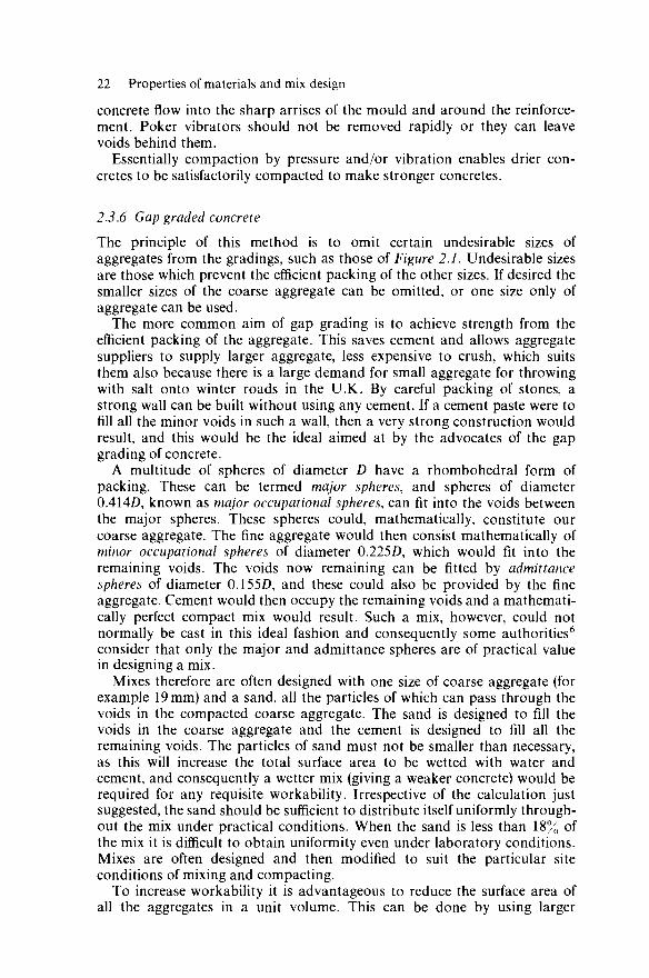
2.3.6 Gap graded concrete
The principle of this method is to omit certain undesirable sizes of aggregates from the gradings, such as those of Figure 2.1. Undesirable sizes are those which prevent the efficient packing of the other sizes. If desired the smaller sizes of the coarse aggregate can be omitted, or one size only of aggregate can be used.
The more common aim of gap grading is to achieve strength from the efficient packing of the aggregate. This saves cement and allows aggregate suppliers to supply larger aggregate, less expensive to crush, which suits them also because there is a large demand for small aggregate for throwing with salt onto winter roads in the U.K. By careful packing of stones, a strong wall can be built without using any cement. If a cement paste were to fill all the minor voids in such a wall, then a very strong construction would result, and this would be the ideal aimed at by the advocates of the gap grading of concrete.
A multitude of spheres of diameter D have a rhombohedral form of packing. These can be termed major spheres, and spheres of diameter 0.414D, known as major occupational spheres, can fit into the voids between the major spheres. These spheres could, mathematically, constitute our coarse aggregate. The fine aggregate would then consist mathematically of minor occupational spheres of diameter 0.225D, which would fit into the remaining voids. The voids now remaining can be fitted by admittance spheres of diameter 0.155Z), and these could also be provided by the fine aggregate. Cement would then occupy the remaining voids and a mathemati-cally perfect compact mix would result. Such a mix, however, could not normally be cast in this ideal fashion and consequently some authorities6
consider that only the major and admittance spheres are of practical value in designing a mix.
Mixes therefore are often designed with one size of coarse aggregate (for example 19 mm) and a sand, all the particles of which can pass through the voids in the compacted coarse aggregate. The sand is designed to fill the voids in the coarse aggregate and the cement is designed to fill all the remaining voids. The particles of sand must not be smaller than necessary, as this will increase the total surface area to be wetted with water and cement, and consequently a wetter mix (giving a weaker concrete) would be required for any requisite workability. Irrespective of the calculation just suggested, the sand should be sufficient to distribute itself uniformly through-out the mix under practical conditions. When the sand is less than 18% of the mix it is difficult to obtain uniformity even under laboratory conditions. Mixes are often designed and then modified to suit the particular site conditions of mixing and compacting.
To increase workability it is advantageous to reduce the surface area of all the aggregates in a unit volume. This can be done by using larger

Concrete 23
particles. The largest aggregate possible should therefore be used, consistent with the minimum clearances allowed.
Gap grading enables leaner and drier mixes to be used, the absence of many intermediate sizes of aggregates having reduced the specific surface area of the aggregates and therefore having increased workability. The lean mixes usually utilised, however, make vibration almost essential. Such concrete, being made of leaner and drier mixes than a conventional concrete of equivalent strength, will therefore experience less shrinkage and hence possess better weathering qualities. Compressive forces on the gap graded concrete described are ideally transmitted from particle to particle of the coarse aggregate and not through any cement and sand particles. Consequently the creep associated with such concrete is low. A coarse aggregate as used in a conventional mix experiences a fair amount of segregation during transportation, and pouring into and out of lorries, etc. Rain also helps segregation in stockpiles. Gap grading avoids these disad-vantages by requiring only single sizes of coarse aggregate.
Some advocate two different single sizes of coarse aggregates to be used with sand and cement in a mix. Gap graded concretes as lean as 1 (cement): 2.45(sand):6.59(gravel), with a water-to-cement ratio of 0.51, increase in strength with age in a similar fashion to conventional concretes.6 Because of the packing of the aggregate of a gap graded concrete, vertical shutters can often be removed immediately after casting. Walls and columns can then be trowelled if desired or sprayed with a light water jet to expose the aggregate.
One disadvantage of gap grading is that if the single-size aggregates supplied contain over 2.5% by weight of undesirable particles, this upsets the grading which is very sensitive to such intrusions. If however such irregularities are to be expected in the supply then the mix can be calculated accordingly to be of reduced efficiency.
2.3.7 No fines concrete
Coarse aggregate (gravel) is mixed with cement and the fine aggregate (sand) is omitted. No fines concrete is required to contain a multitude of voids to give good thermal insulation, and these voids need to be large enough to prevent the movement of water through the concrete by capillary attraction. In-situ no fines concrete walls have been used in the U.K. for housing, the idea being that good thermal insulation is achieved and that rain beating on a wall penetrates only a short horizontal distance before having dropped to the bottom of the wall, there being no capillary paths to conduct the water completely through the wall. It is, however, often desirable to render and paint exposed no fines concrete walls.
2.3.8 Curing of concrete
After setting or solidifying, concrete increases in strength with age (see Figure 2.3). The strength at a particular age can be further increased by suitable curing of the concrete whilst it is maturing. Such curing comprises the application of heat (not if CaCl2 is present or for high alumina cement or mass concrete) and/or the preservation of moisture within the concrete. The

24 Properties of materials and mix design
<N1
fc E z r O )
LO
CD
i
u
40
30
?0
1 0
0 1/ ■ ■ . . 0 3 7 28 90
Age, days
Figure 2.3
application of heat speeds up the chemical reaction and consequently rate of hardening of the concrete.
It can be imagined that preventing the escape of moisture from the concrete enables previously unwetted minute particles of cement to partic-ipate in the cementing action. If heat is applied to accelerate the hardening of the concrete it is therefore important not to expel the water held within the concrete. In other words, if heat is applied a high humidity is also desirable; steam is therefore a most suitable medium for this purpose. Steam curing can be done at atmospheric pressure or under pressure. The latter method is more effective but far more expensive, as pressure chambers are required. For example, the half-hour strength of concrete steam cured under pressure could equal the 28-day strength of an identical concrete maturing in air.
Increasing the strength of concrete by preventing the water used in mixing from escaping is usually done in one of the following ways:
1. Flooding or submerging the concrete in water. The floors of basements and reservoirs can fairly easily be flooded with water. Precast concrete units can be immersed in water in special tanks.
2. Treating the surface of the concrete so that it cannot dry out. Proprietary products exist for painting, or for applying coverings which adhere to the concrete.
3. Covering the concrete with damp sand or hessian fabrics, which are kept damp by watering periodically, or with thin polythene sheet.
2.3.9 Design of concrete mixes
Most commonly a concrete mix is designed to give the specified strength at the minimum cost. The cost depends upon the value of the materials, the labour required for batching, mixing, transporting, placing and trowelling, and the method of curing adopted.
Mix designs are fairly inaccurate due to the number of possible variables. The D.S.I.R. Road Note No. 48 of 1950 based a mix design method on the aggregate gradings shown in Figure 2.1. This method is simple and can be used by mixing one's sand and gravel in such proportions as to correspond to one or other of these grading zones. As the method is even then not very accurate, it can be improved upon by casting trial mixes, measuring their

Concrete 25
workabilities and cube crushing strengths, and then adjusting the mix accordingly. Much of this work can easily be performed in the laboratory. The part of the method with which Table 2.2 is concerned has of course to be established by co-operation with the site. Considerable creditable re-search since Road Note No. 48 has been faced with the inherent complexity of the problem and has not made this method obsolete as a useful simple method of designing a mix. All other methods can still be improved by studying trial mixes, as mentioned previously.
TABLE 2.2.
Conditions Minimum strength as percentage of average strength
Very good control with weight batching, moisture determinations on aggregates, etc.; constant supervision 75
Fair control with weight batching 60
Poor control; volume batching of aggregates 40
CP 114 used to specify concretes according to their minimum cube crushing strength at 7 and 28 days, and it is still possible for a designer to do this, but CP 110 has a more scientific approach—unfortunately more complicated. The mix design method presented in this book is based on the required average crushing strength. To design a mix with a certain specified minimum crushing strength, as for CP 114, we use Table 2.2 to obtain the requisite average crushing strength, and then design a mix for this average crushing strength.
CP 110 specifies a concrete with a characteristic strength. For example, in Table 47 it defines Grades 20, 25, 30, etc., of concrete as having character-istic strengths of 20, 25, 30, etc., N/mm2. If a large number of cubes of the same concrete (same age, curing, etc.) are tested the results can be plotted as shown in Figure 2.4. In statistics this figure is known as a histogram, and its shape is well known as a normal (gaussian) distribution. The average (or mean) cube strength is the value of cube strength corresponding to the centroid of this shape. As in this case we assume it to be a normal distribution, not skew7 (though in fact it is slightly skew), the average (or mean) strength corresponds to the centre line of the shape, as shown. Statistical theory gives the formula:
Characteristic strength = Mean strength — 1.64 x Standard deviation (2.1)
The number 1.64 is derived from the fact that CP 110 chooses character-istic strength as the value below which we can expect 5% of the cubes to fail (see Figure 2.4).
The breadth of the shape of Figure 2.4 gives an indication of the scatter of the results. For statistical purposes this is expressed as standard deviation, which can be obtained thus: if we make n cube tests and their crushing strengths are fcul,fcu2, • • -,/Cu« then the mean crushing strength is /cum = (Z/cui)/n a n d the standard deviation is VIX/cui -/CUm)2/(» ~ !)]•

26 Properties of materials and mix design
Normal curve
CP 110
characteristic strength
Mean strength
40 50
Strength, N / m m 2
Figure 2.4
If we are to design a concrete to a particular CP 110 characteristic strength then we must obtain the mean strength, that is Characteristic strength + 1.64 x Standard deviation. Hence, we need to know the standard deviation. Equation 2.1 can be expressed as:
Characteristic strength = Mean strength — Margin where
Margin = 1.64 x Standard deviation and thus
Characteristic strength Mean strength = 1 — 1.64 x (Coefficient of variation)
where
Coefficient of variation = Standard deviation
Mean strength
(2.2)
(2.3)
(2.4)
(2.5)
For concretes stronger than 20 N/mm2, CP 110 recommends (a) the stan-dard deviation can be obtained for cube tests on at least 100 separate batches of concrete produced over a period of not more than one year, provided the margin is not less than 3.75 N/mm2, or (b) the standard deviation can be obtained for cube tests on at least 40 separate batches of
Concrete 27
concrete produced over a period between 5 days and 6 months, providing the margin is not less than 7.5 N/mm2, or (c) if histograms have not been established as for (a) and (b), then the margin can be simply taken as 15 N/mm2.
2.3.10 Design of concrete mix of given mean (or average) strength
To design a concrete mix for industry the mean strength has first to be established as in Section 2.3.9. If however the mix is for a laboratory experiment then we design for the mean strength. The required water-to-cement ratio for the mean strength required is obtained from Figure 2.2, which assumes that the concrete is cured in air. Then a decision is made on the degree of workability, using Table 2.1 as a guide. Then the most suitable aggregate-to-cement ratio can be chosen from Table 2.3. This table gives such ratios for different gradings (as given in Figure 2.1), workabilities, water-to-cement ratios, and types of aggregates.
Then if durability is important because, say, the concrete is exposed to injurious elements, that is is not protected inside an office block or laboratory, Tables 48 and 49 of CP 110 should be consulted to see if we have sufficient cement in our mix. If not, we decrease the aggregate-to-cement ratio accordingly. If this has to be done we might perhaps then repeat our design, taking advantage of, say, an increased workability to assist compaction and ease, and therefore cost, of concreting.
Example 2.1. To design a concrete mix for a pretensioned prestressed beam to have a mean (or average) crushing strength of 47 N/mm2 at an age of 7 days.
The coarse aggregate to be used is a 19.05 mm (fin) and down, rounded aggregate with a grading curve approximating to Curve 2 on Figure 2.1. Vibration is to be employed and the prestressing wires cause little obstruction to the placing of the concrete. We shall assume however that the beam is of I-section with narrow flanges and web. Hence it is decided that a medium workability is desirable (see Table 2.1).
Using rapid hardening Portland cement and consulting Figure 2.2, the necessary water-to-cement ratio is 0.35.
From Table 2.3, the aggregate-to-cement ratio is therefore 3. To check that the cement content is adequate for durability in accordance with
CP 110, Tables 48 and 49 give the minimum mass of cement per m3 of the concrete. Hence it is necessary to calculate this quantity from Section 2.3.12.
2.3.11 Combining aggregates to obtain a grading for the mix design method
Available sands and gravels need to be combined in suitable proportions so that the resultant grading approximates to one of the curves of Figure 2.1, so that the method of mix design of Section 2.3.10 can be used. A graphical method is given for obtaining these proportions in Road Note No. 48, but the method of calculation, illustrated by the following example, is simpler to explain and understand and the calculations are trivial.
Example 2.2. The gradings of sand and two coarse aggregates kept in stock in the concrete laboratory at Bradford University are given in Columns (a), (b) and (c)

28 Properties of materials and mix design
&3
s
1
£ o
^
£
^ "b £
<> -**
^ 3 2!
T f
m
<N
-
^ f
m
( N
fr
m
CN
-
^t
m
CN
-
* -Si
IP ^
i n m
CN rn
so in CN m'
(N m*
OO sq (N rn
—< oo i n T f T^ l/-j
i n m H Tt i n so
oo r-~ m rt- in so
- ; vo (N vd ^d r^
oo TJ- os
CN r~-
so in m Tf' i n s o
IT) T}- T f
I Tf i n so CN oo
oo os CN rn
O CN rn ^
—« CN
q o s T f i i n i n r~ <
m m m i n so r-
m m m >ri so" K
I I
I I
1 in so so r«- in r^ oo'
CN «n
sq —-rn i n
oo m r<S in
CN in
i n m
r n i n
Os O CN i n t ^ oo
so © | so oo I
os <N , sd oo I
OO O ^ in K oo
so oo
i n m i
T t s d I
in so < rf SO (
I I
I I
I I
I I
I I
I I
I I
I
I i
o o o o o o o o
ft G ' 5
S S 2 *
-s: .00
5
5 3
^ *> *
^ 3
-2 ^ s- ^
■^
-3 53 -ie v. o £
^ S? S\j
^ £o <> q
•ofr
m
CN
~
^ f
m
CN
—
Ti-
e n
CN
-
T f
m
(N
—'
* <U
I s\> bo be a > bo ST
^ <3 v.
O
I os in —< r^ CN so ^ i (N m Tf Tf in in so
; rN os Tt os rf oo (N i rn rn Tt r t in in so
i^ (N OS ^ OO f N m r n T t T f
—> CN m X X X X X X
o s i n -H i r n T f i n
r N oo r f
I T f r t i n
sq —; SO in so so
o t o o SO so SO
^H OO t I
I TT Tf i n *
so m o so r- | ( N r n T t T f
—< rn r f
m o T t i n
sq ^t T t i n
oo i n
T f i n
oo i n
TT i n
O OS
i n i n
r - i n
i n s o
oo oo
i n s o
O <N so r^
r-i n
o sd
CN
SO
r N
sd
r^ sd
m r^
oo r^
rn oo
CM
sd
r-SO
os sd
oo so
T f
r^
o oo
so oo
TT
Os
oo so
rn r-'
i n
r^
T f
r~-*
o oo
1
1
i 1
1
T f
r-'
r-;
K
o oo
p oo'
1
1
1
1
1
1
1
1
s
o o o o o o o o
I an

Concrete 29
- .*> *
s 3
^ ^ ^
£ o ^
^ ^ ^ ^
^
<> -V
k.
o £ "$> ^ J^ !?0 > Q
TT
m
<N
*-*
Tf
m
<N
—
^t
m
<N
~
^f
m
(N
~"
* <X>
I *>-t>c So <3
^ t>o .c ^ ^3 *>■ O
fN rN rn ro r t r t T -' iri
<N r4 rn rn rt rf v-i io
rnOsmOs X X X X
<N ON V~) <N r-i en X X X X X
P ^ 15
" *~! ^ <"1 ^ °i ^ °i <N en en -rf -rf i/S U"i vO
^ 1 ^ ^ ^ (N r n r n ' t -<t
<N rn en ■*T rfr »/S iri v©
r ^ i o m o r ^ m o N T j -o i rn r t ir i v i vd vd r^
r » « / - > m o v q r n O N » o
0 ( N O O O \ 0 ( N M r n
o o o o o o o o
« 6 ^ o £
2 8 o 2
I B S .top a> <u
£ -5 £
30 Properties of materials and mix design
respectively of Table 2.4. Suppose that these are combined to approximate to Curve 1 of Figure 2.1, whose grading is listed in Column (i) of Table 2.4.
To 1 kg of sand we can only decide how many kgx of 9.52 mm (fin) gravel and how many kgy of 19.05mm (Jin) gravel to mix with it to obtain the grading of Curve 1. Two unknowns only need two equations. Hence we can only make Curve 1 correct for the percentages passing two chosen sieve sizes. Suppose we choose the percentages passing apertures 9.52 mm (fin) and 4.76 mm (i^in).
According to Curve 1, the percentage passing 9.52 mm (fin) aperture is 45%, hence using Table 2.4:
100 x 1 + 96x + \9y = 45(1 + x + y)
According to Curve 1, the percentage passing 4.76 mm (^in) aperture is 30%; hence using Table 2.4:
100 x 1 + 13x + y = 30(1+ x + y )
Solving these two equations, x = 0.1172, and y — 2.345. Thus the sand, 9.52 mm (fin) gravel and 19.05mm (Jin) gravel must be combined in the proportions 1:0.1172:2.345, respectively.
The grading of the combined aggregate is obtained by multiplying Columns (a), (b) and (c) of Table 2.4 by 1, 0.1172 and 2.345, respectively, the products being shown in Columns (d), (e) and (f), respectively. The values in these columns are added together to give the values in Column (g) and then divided by 1 + 0.1172 + 2.345 = 3.462 to give the values in Column (h), and this is the grading of the combined aggregate. Comparing this with Column (i) we have achieved the same percentages passing 9.52 mm and 4.76mm apertures, as calculated. Our error is mainly for percentages passing 1.20mm and 600 urn apertures. We could repeat the calculation say making the percentages passing apertures 9.52 mm and 1.20 mm equate in Columns (h) and (i). Mix design is not a very accurate science and this is probably not worth the trouble and its result would not really be known to be any better. Various sets of two percentages passing certain sizes could be made equal in Columns (h) and (i) by calculation and all the various results plotted on a graph such as Figure 2.1, and one could choose the combined grading which looks generally closest to the graph of Curve 1. Again it is extremely doubtful if this is worth doing.
2.3.12 Design of concrete mixes (further methods)
The Road Note No. 4s method described in Sections 2.3.9 to 2.3.11 inclusive has been followed by a Department of the Environment (D.O.E.) publication9
which is more comprehensive, more complicated to describe and requires more tables and figures than Road Note No. 4. Hughes7 presents an even more comprehensive and complex method than the two methods just mentioned. In the U.S.A. the A.C.I.1 0 recommends a different method.
As explained in Section 2.3.9 mix designs are not very accurate and need to be adjusted by making tests of trial mixes, but are naturally useful for determining the first trial mix. The Road Note No. 4 method described previously is the simplest of the above-mentioned methods to describe to students and to understand. It has been used for many years and is still used although the D.O.E. hope that their method will replace it. The other methods are easy to use without much understanding by following through the examples and using the tables and graphs given in the publications already cited.
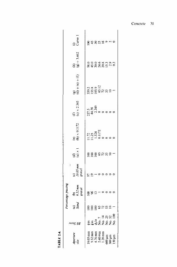
TA
BL
E 2
.4.
Ape
rtur
e si
ze
19.0
5 m
m
9.52
mm
4.
76 m
m
2.40
mm
1.2
0 m
m
600
irn
300
urn
150
urn
£1
CO
jin
£in
A in
N
o. 7
N
o. 1
4 N
o. 2
5 N
o. 5
2 N
o. 1
00
Per
cent
age
pass
ing
(a)
Sand
100
100
100 85
72
53
10 1
(b)
9.52
mm
gr
avel
100 96
13 1 0 0 0 0
(c)
19.0
5 m
m
grav
el
97
19 1 0 0 0 0 0
(d)
(a)x
1
100
100
100 85
72
53
10 1
(e)
(b)
x 0.
1172
11.7
2 11
.25
1.52
4 0.
1172
0 0 0 0
(0
(c)
x 2.
345
227.
5 44
.56
2.34
5 0 0 0 0 0
(g)
(d)
+ (e
) +
(f)
339.
2 15
5.8
103.
9 85
.12
72
53
10 1
(h)
(g)
- 3.
462
98.0
45
.0
30.0
24
.6
20.8
15
.3
2.9
0.3
(i)
Cur
ve 1
100 45
30
23
16 9 2 0
n
o
o
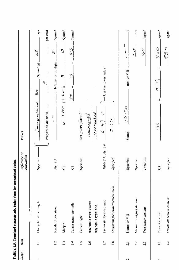
TA
BL
E 2
.5.
Com
plet
ed c
oncr
ete
mix
des
ign
form
for
unr
estr
icte
d de
sign
Stag
e It
em
Ref
eren
ce o
r ca
lcul
atio
n V
alue
s
1.1
Cha
ract
eris
tic s
treng
th
1.2
1.3
1.4
1.5
1.6
1.7
1.8
Stan
dard
dev
iatio
n
Mar
gin
Targ
et m
ean
stre
ngth
Cem
ent
type
Agg
rega
te t
ype:
coa
rse
Agg
rega
te t
ype:
fine
Free
-wat
er/c
emen
t ra
tio
Max
imum
fre
e-w
ater
/cem
ent
ratio
Spec
ified
-
Fig
. 2.
5
Cl
C2
Spec
ified
Tabl
e 2.
7. F
ig.
2.6
Spec
ified
N/m
m2 a
t.
Prop
ortio
n de
fect
ive.
JD
N/m
m2 o
r no
dat
a .
(k=
('&
^ )
t'
^ x
2 /?
OPC
/S^P
C/R
HPC
— U
se t
he l
ower
val
ue
■2J
? da
ys
per
cent
_ N
/mm
2
15
N/m
m2
V^3
N
/mm
2
2.1
Slum
p or
V-B
2.2
Max
imum
agg
rega
te s
ize
2.3
Free
-wat
er c
onte
nt
Spec
ified
Spec
ified
Tabl
e 2.
8
Slum
p _
/e>
-3©
m
m o
r V
-B .
SL<
?
ico
_kg/
m3
3.1
Cem
ent
cont
ent
3.2
Max
imum
ce
men
t co
nten
t
C3
Spec
ified
(bo
o ■
*l
3<t^
=>
55'o
_k
g/m
3
_kg/
m3

3.3
Min
imum
ce
men
t co
nten
t Sp
ecifi
ed
^K^
kg/m
3 — U
se if
gre
ater
tha
n Ite
m 3
.1
and
calc
ulat
e Ite
m 3
.4
3.4
Mod
ified
fre
e-w
ater
/cem
ent
ratio
4.1
Rel
ativ
e de
nsity
of
aggr
egat
e (S
SD)
4.2
Con
cret
e de
nsity
F
ig. 2
.7
4.3
Tota
l ag
greg
ate
cont
ent
C4
2L-
6 .
kfte
wfi/
assu
med
Jjd^
x=>
_ ^
cfo
_
(tx;
,
2^sc
C>
_ kg
/m3
H^
kg/m
3
5.1
Gra
ding
of
fine
aggr
egat
e
5.2
Prop
ortio
n of
fin
e ag
greg
ate
5.3
Fine
agg
rega
te c
onte
nt
5.4
Coa
rse
aggr
egat
e co
nten
t
BS8
82
Fig
. 2.8
-C5
Zone
_
r
_A
as
tv
So
l°[e
&
><**
.*
3/7
o.-z
^]
<3 <
X>
€<
$
>\5
\Z*S
per
cent
kg/m
3
kg/m
3
Qua
ntiti
es
Cem
ent
(kg)
W
ater
(k
g or
1)
Fine
agg
rega
te
(kg)
C
oars
e ag
greg
ate
(kg)
per
m3 (
to n
eare
st 5
kg)
per
trial
mix
of
m3
3^o
ho
i»
s-o
6^
r61
3^5
b\2
-
Item
s in
ital
ics
are
optio
nal
limiti
ng v
alue
s th
at m
ay b
e sp
ecifi
ed.
OPC
= o
rdin
ary
Port
land
cem
ent;
SRPC
= s
ulph
ate-
resi
stin
g Po
rtla
nd c
emen
t; R
HPC
= r
apid
-har
deni
ng P
ortla
nd c
emen
t. R
elat
ive
dens
ity =
spe
cific
gra
vity
. SS
D =
bas
ed o
n a
satu
rate
d su
rfac
e-dr
y ba
sis.
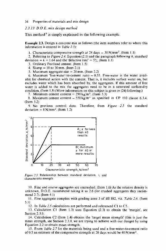
34 Properties of materials and mix design
2.3.13 D.O.E. mix design method
This method 9 is simply explained in the following example.
Example 2.3. Design a concrete mix as follows (the item numbers refer to where this information is entered in Table 2.5):
1. Characteristic compressive strength at 28 days = 30N/mm2. (Item 1.1) 2. Referring to Figure 2.4, Equation (2.1) and the paragraph following it, standard
deviation = /c = 1.64 and the 'defective rate' = 5%. (Item 1.1) 3. Ordinary Portland cement. (Item 1.5) 4. Slump = 10 to 30mm. (Item 2.1) 5. Maximum aggregate size = 20mm. (Item 2.2) 6. Maximum 'free-water'-to-cement ratio = 0.55. Free-water is the water avail-
able for chemical action with the cement. That is, it includes surface water on, but excludes water which has been absorbed by, the aggregates. If this amount of free water is added to the mix the aggregates need to be in a saturated surface-dry condition. (Item 1.8) (More information on this subject is given in (24) following.)
7. Minimum cement content = 290kg/m3. (Item 3.3) 8. Maximum cement content = 550 kg/m3 as specified in CP 110 clause 6.3.4.
(Item 3.2) 9. No previous control data. Therefore, from Figure 2.5 the standard
deviation = 8N/mm2. (Item 1.2)
A; s for I than 40 results
B; minimum s for 40 or more results
10 20 30 40 50 60
Characteristic strength, N/mm2
70
Figure 2.5 Relationship between standard deviation, s, and characteristic strength
10. Fine and coarse aggregates are uncrushed. (Item 1.6) As the relative density is unknown, D.O.E. recommend taking it as 2.6 (for crushed aggregates they recom-mend 2.7). (Item 4.1)
11. Fine aggregate complies with grading zone 3 of BS 882, viz. Table 2.6. (Item 5.1)
12. In Table 2.5 calculations are performed and referenced Cl to C5. 13. Calculation Cl (Item 1.3) uses Equation (2.3) to obtain the 'margin', see
Section 2.3.9. 14. Calculation C2 (Item 1.4) obtains the 'target mean strength' (this is just the
mean strength, see Section 2.3.9, we are trying to achieve with our design) by using Equation 2.2 to obtain mean strength.
15. From Table 2.7 for the materials being used and a free-water-to-cement ratio of 0.5 an estimate of the compressive strength at 28 days would be 40 N/mm2.
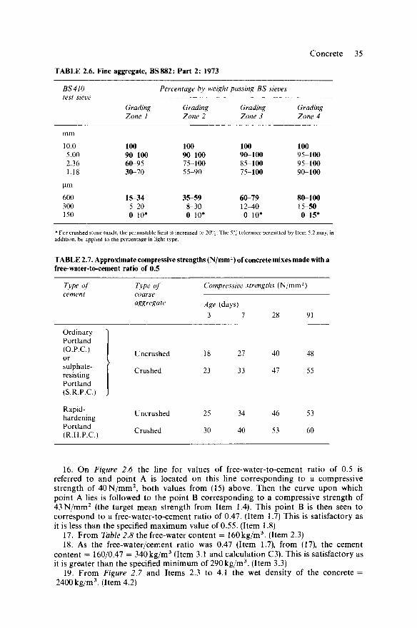
Concrete 35
TABLE 2.6. Fine aggregate, BS882: Part 2: 1973
BS410 test sieve
mm
10.0 5.00 2.36 1.18
urn
600 300 150
Grading Zone 1
100 90-100 60-95 30-70
15^34 5-20 0-10*
Percentage by weight
Grading Zone 2
100 90-100 75-100 55-90
35-59 8-30 0-10*
passing BS sieves
Grading Zone 3
100 90-100 85 100 75-100
60-79 12^0 0-10*
Grading Zone 4
100 95-100 95-100 90-100
80-100 15-50 0-15*
* For crushed stone sands, the permissible limit is increased to 20%. The 5% tolerance permitted by Item 5.2 may, in addition, be applied to the percentage in light type.
TABLE 2.7. Approximate compressive strengths (N/mm2) of concrete mixes made with a free-water-to-cement ratio of 0.5
Type of cement
Ordinary Portland (O.P.C.) or sulphate-resisting Portland (S.R.P.C.) J
Rapid-hardening Portland (R.H.P.C.)
Type of
aggregate
Uncrushed
> Crushed
Uncrushed
Crushed
Compressive s
Age
3
18
23
25
30
(days) 7
27
33
34
40
trengths (N/mm2)
28 91
40 48
47 55
46 53
53 60
16. On Figure 2.6 the line for values of free-water-to-cement ratio of 0.5 is referred to and point A is located on this line corresponding to a compressive strength of 40 N/mm2, both values from (15) above. Then the curve upon which point A lies is followed to the point B corresponding to a compressive strength of 43 N/mm2 (the target mean strength from Item 1.4). This point B is then seen to correspond to a free-water-to-cement ratio of 0.47. (Item 1.7) This is satisfactory as it is less than the specified maximum value of 0.55. (Item 1.8)
17. From Table 2.8 the free-water content = 160kg/m3. (Item 2.3) 18. As the free-water/cement ratio was 0.47 (Item 1.7), from (17), the cement
content = 160/0.47 = 340kg/m3 (Item 3.1 and calculation C3). This is satisfactory as it is greater than the specified minimum of 290kg/m3. (Item 3.3)
19. From Figure 2.7 and Items 2.3 to 4.1 the wet density of the concrete = 2400 kg/m3. (Item 4.2)
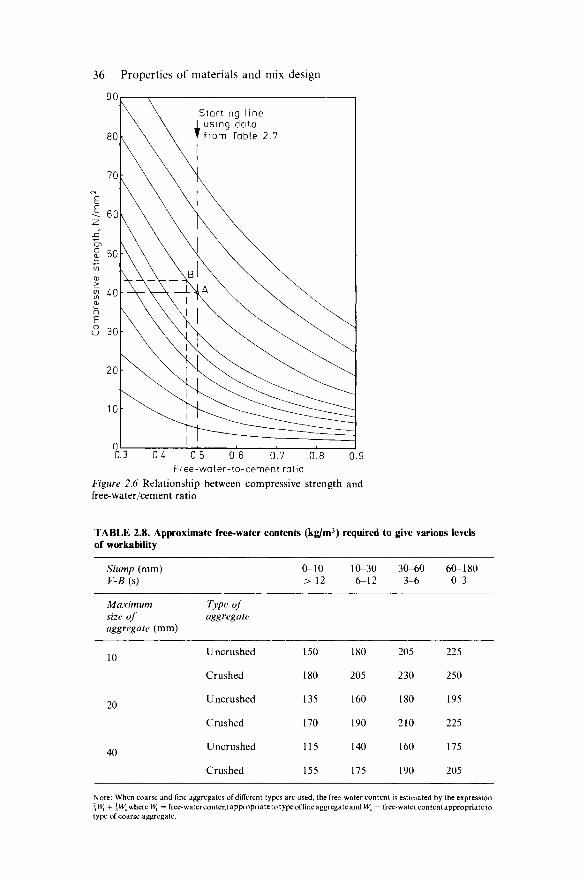
36 Properties of materials and mix design
0.3 (K 0.5 0.6 0.7 0.8 0.9 Free-water-to-cement ratio
Figure 2.6 Relationship between compressive strength and free-water/cement ratio
TABLE 2.8. Approximate free-water contents (kg/m3) required to give various levels of workability
Slump (mm) V-B (s)
Maximum size of aggregate (mm)
Type of aggregate
0-10 > 12
10-30 6-12
30-60 3-6
60-180 0-3
Uncrushed
Crushed
Uncrushed
Crushed
Uncrushed
Crushed
150
180
135
170
115
155
180
205
160
190
140
175
205
230
180
210
160
190
225
250
195
225
175
205
Note: When coarse and fine aggregates of different types are used, the free-water content is estimated by the expression \Wf + 5 Wc where Wf = free-water content appropriate to type of fine aggregate and Wc = free-water content appropriate to type of coarse aggregate.
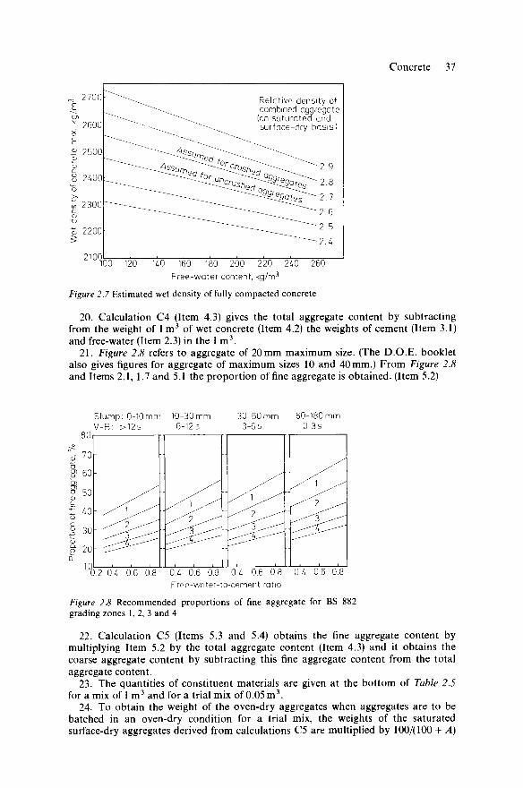
Concrete 37
Relative density of combined aggregate (on saturated and surface-dry basis
160 180 200 220 240
Free-water content, kg/m3
Figure 2.7 Estimated wet density of fully compacted concrete
20. Calculation C4 (Item 4.3) gives the total aggregate content by subtracting from the weight of 1 m3 of wet concrete (Item 4.2) the weights of cement (Item 3.1) and free-water (Item 2.3) in the 1 m3.
21. Figure 2.8 refers to aggregate of 20mm maximum size. (The D.O.E. booklet also gives figures for aggregate of maximum sizes 10 and 40 mm.) From Figure 2.8 and Items 2.1, 1.7 and 5.1 the proportion of fine aggregate is obtained. (Item 5.2)
80
«r 70 601
0 50
't 0 O
1 30 o 8" 20
Slump: 0-10mm V-B: >12s
10-30 mm 6-12s
30-60 mm 3-6 s
60-180 mm 0-3 s
1 Qj 0.2 0.4 0.6 Oi 0.4 0.6 0.8 0.4 0.6 0.8
Free-water-to-cement ratio 0.4 0.6 Oi
Figure 2.8 Recommended proportions of fine aggregate for BS 882 grading zones 1, 2, 3 and 4
22. Calculation C5 (Items 5.3 and 5.4) obtains the fine aggregate content by multiplying Item 5.2 by the total aggregate content (Item 4.3) and it obtains the coarse aggregate content by subtracting this fine aggregate content from the total aggregate content.
23. The quantities of constituent materials are given at the bottom of Table 2.5 for a mix of 1 m3 and for a trial mix of 0.05 m3.
24. To obtain the weight of the oven-dry aggregates when aggregates are to be batched in an oven-dry condition for a trial mix, the weights of the saturated surface-dry aggregates derived from calculations C5 are multiplied by 100/(100 + A)

38 Properties of materials and mix design
where A is the percentage by weight of water needed to bring the dry aggregates to a saturated surface-dry condition. The amount of mixing water should be increased by the weight of water absorbed by the aggregates to reach the saturated surface-dry condition. For example, if the absorption of the fine aggregate is 2% and of the coarse aggregate is 1%, then in the above trial mix:
Weight of oven-dry fine aggregate = 25.7 x 100/102 = 25.2 kg Weight of oven-dry coarse aggregate = 69.2 x 100/101 = 68.5 kg Water required for absorption = (25.7 - 25.2) + (69.2 - 68.5)
= 0.5+ 0.7 = 1.2kg
Thus, the quantities for the trial mix are: cement 17.0kg, water 9.2kg, fine aggregate 25.2 kg (oven-dry) and coarse aggregate 68.5 kg (oven-dry).
23.14 Quantities of materials required to make 1 m3 of concrete
A very simple method is illustrated in Example 2.4. This is useful for individual beams. If one needed considerable accuracy for a large quantity such as a dam, this can easily, and best, be established experimentally in the laboratory.
Example 2.4. Calculate the quantities of ingredients required for casting a beam and cubes in the laboratory having a total volume of 0.4 m3. The mix is to be in the proportions of 1 part cement to 0.87 parts sand to 0.10 parts 9.52 mm gravel to 2.03 parts 19.05 mm gravel by dry volumes with a water-to-cement ratio of 0.35 by masses.
Assume the bulk density of cement, sand and gravel to be 1440 kg/m3 (reasonably true if not using lightweight aggregates). Assume the density of the matured concrete to be 2400 kg/m3 (again reasonably true). The mass of the concrete is equal to the mass of its ingredients, except that much of the water will evaporate. Assume all the water vanishes—this will very slightly underestimate the cement, sand and gravel. Therefore:
lkg +0.87 kg + 0.10 kg +2.03 kg = 4 kg concrete cement sand small gravel large gravel
Mass of mature concrete = 0.4 x 2400 = 960kg. Therefore requirements are: 1 x 960/4 = 240 kg cement 0.87x960/4 = 208.8 kg sand 0.10 x 960/4 = 24 kg small aggregate 2.03 x 960/4 = 487.2 kg large aggregate 240x0.35 = 84 kg water
Then add 10% to these figures to allow for small underestimation and waste. This figure may need small adjustment according to experience of the concreting conditions, the particular mix and type of aggregates, etc.
23.15 Prescribed mixes
C P 110 gives prescribed mixes in Table 50 to replace the nominal mixes of C P 114. Generally these will give uneconomic concretes stronger than required. But they have the advantage that proper mix design procedures do not need to be established for the concreting plant.

Concrete 39
2.3.16 Shrinkage
When cement, sand, gravel and water are mixed together the gross volume decreases as the finer particles arrange themselves in the interstices of the larger particles. This shrinkage continues as the concrete is being worked into place. Evaporation of water in the mix also decreases the volume of such concrete. It is possible to fill a mould, for example a 150 mm cube, and observe the concrete retract into the mould. Shrinkage, when the concrete is in a fluid state, does not matter structurally because no internal stresses can be instigated. There is an inaccurately known point at which the concrete changes from a fluid to a solid and immature fragile material. The exact time when this occurs depends upon the water-to-cement ratio, the type of cement, and the ambient humidity and temperature. After this time, further shrinkage of the concrete will cause internal stresses and even cracks to occur. The time when the transition occurs from liquid to solid is not precisely determinable, and it is difficult to know exactly when to commence measuring the shrinkage of the concrete in its solid state.
Measurements of the coefficient of shrinkage are possibly commenced too late to be of real mathematical value in research, because such readings are often commenced just when the specimen is hard enough to strip and handle for the purposes of the test. On such a basis the shrinkage coefficient can be of the order of 0.0005 at an age of 12 months and a typical relationship between shrinkage and age is illustrated in Figure 2.9. Initially
0.04 r
Figure 2.9
the rate of shrinkage is high so that the error in not knowing the precise time to start measurements is quite appreciable. With the above coefficient, and supposing, for simplicity, the modulus of elasticity of concrete is 28 000 N/mm2, then if the concrete were restricted from shrinking the tensile stress induced in the concrete would be 0.0005 x 28000 = 14N/mm2. The concrete would certainly crack as its ultimate tensile strength would only be

40 Properties of materials and mix design
about 2.8 N/mm2. The coefficient of shrinkage is less for a lean mix than for a rich mix (in cement content). It is less for a low water-to-cement ratio than for a high one, is very sensitive to the method of curing, and is influenced to a lesser extent by all the other possible variables.
Shrinkage after the concrete has solidified continues as and when further water evaporates. The chemical reaction of cement with water, and thus the shrinkage, continues in the concrete seemingly indefinitely. A gel is formed which contracts upon desiccation and becomes very hard (see Section 2.1). If concrete is submerged in water this cement gel expands with considerable force, so that the whole mass of concrete expands. This expansion, however, can never equal the shrinkage which has already taken place. On drying the concrete in air shrinkage again occurs. Therefore, when concrete is sub-jected to continual wetting and drying, as for example due to tidal action, it experiences corresponding expansions and contractions. If concrete is cast beneath water then it does not shrink at all but expands, owing to the cement gel absorbing water.
If a mass of concrete shrinks (or expands) uniformly and its movement is not restricted by any external forces, then no internal stresses can be induced in the concrete. This seldom happens in practice; usually any movement of the concrete is restricted internally by reinforcement embed-ded in the concrete, and often externally by its surroundings. Also, the surface of concrete will often dry out (and therefore shrink) faster than the internal particles of concrete. When the concrete of a reinforced beam is in the solid state, as it shrinks it also bonds to the reinforcement. The resistance of the reinforcement to contraction opposes the shrinkage of the concrete. Thus the concrete near to the reinforcement is in tension, a bond stress is developed between the two, and the reinforcement is in com-pression. Shrinkage cracks often exist in reinforced concrete beams at inter-vals along the length of the reinforcement. These are sometimes too small to be observed with the instruments normally available. When a reinforced concrete beam is tested, cracks can usually be observed at a lighter loading than predicted from the modulus of rupture of the concrete, indicating that cracks or tensile stresses are already present due to shrinkage.
Designs concerning conventional reinforced concrete work do not usually attempt to estimate the quantitative effect of shrinkage, because such calculations cannot be made with any degree of confidence and the basic assumptions of any mathematical analysis can be adversely criticised. Prestressed concrete designers simply treat shrinkage as a loss' reducing the prestressing force. The ultimate strength of a beam is not altered by shrinkage because when cracks occur the initial internal stress systems are released, yet shrinkage affects the size of cracks and deflections at working loads.
The particles at the surface usually experience different conditions of curing to internal particles. Their rates of shrinkage thus differ and this 'differential shrinkage' can cause troublesome stresses, cracks and move-ments, for example the surface crazing of artificial stones and the warping of ground floor and road slabs. This effect can be reduced by endeavouring to cure the surfaces similarly to the internal fibres. The latter are fairly well sealed from the atmosphere so that to reduce differential shrinkage it is therefore desirable to seal the surfaces from the atmosphere. One way of achieving

Concrete 41
this is to immerse the concrete member in water for as long as possible. It is often more economical to cover with damp hessian sacks, sand, or water-proof sheets, or to spray periodically with water. A granolithic topping on a floor is very vulnerable to the detrimental effects of differential shrinkage and is usually kept damp for as long as practicable, and for at least seven days.
Shrinkage must always be borne in mind in the design and construction of structures. Whenever possible, concreting programmes aim at minimising the detrimental effects of shrinkage. For example, ground floor slabs on solid (placed over either suitable subsoil or suitably consolidated blinded hardcore), are often concreted in numerous independent portions each of about 4.5 m square, which are able to shrink before being joined together. Plain concrete roads are similarly constructed. This is not considered necessary when reinforcement is present. Numerous minute cracks are formed, but as the reinforcement resists shrinkage the overall contraction is negligible. Some engineers will attribute almost any serious crack in a structure solely to shrinkage. This is often a fallacy because the reinforce-ment of most structures has a considerable resistance to the forces exerted by the shrinkage of the concrete, so that shrinkage cracks in a long structure will take the form of very small cracks fairly regularly spaced throughout the length of the structure. A serious crack is more often caused by thermal expansion and contraction, and settlement.
2.3.17 Relationship between stress and strain for concrete
If a graph is plotted relating stress and strain, the shape of the curve obtained is very much influenced by the rate at which the stress is applied. It is also dependent upon the strength of the concrete under question and indeed to some degree upon all the other possible variables. Figure 2.10 shows a relationship OAF which is typical of a concrete specimen loaded at a uniform rate. If the stressing had been held at the point A the concrete would have continued to strain under this particular constant stress. After a
Strain
Figure 2.10
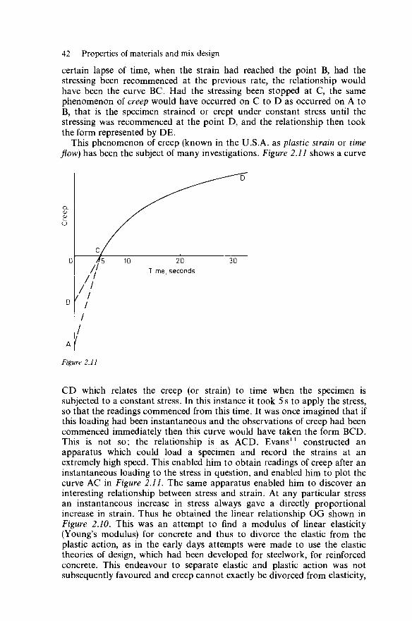
42 Properties of materials and mix design
certain lapse of time, when the strain had reached the point B, had the stressing been recommenced at the previous rate, the relationship would have been the curve BC. Had the stressing been stopped at C, the same phenomenon of creep would have occurred on C to D as occurred on A to B, that is the specimen strained or crept under constant stress until the stressing was recommenced at the point D, and the relationship then took the form represented by DE.
This phenomenon of creep (known in the U.S.A. as plastic strain or time flow) has been the subject of many investigations. Figure 2.11 shows a curve
c /
/ /
/ I
10 20 Time, seconds
^^—Ef
30
Figure 2.11
CD which relates the creep (or strain) to time when the specimen is subjected to a constant stress. In this instance it took 5 s to apply the stress, so that the readings commenced from this time. It was once imagined that if this loading had been instantaneous and the observations of creep had been commenced immediately then this curve would have taken the form BCD. This is not so; the relationship is as ACD. Evans11 constructed an apparatus which could load a specimen and record the strains at an extremely high speed. This enabled him to obtain readings of creep after an instantaneous loading to the stress in question, and enabled him to plot the curve AC in Figure 2.11. The same apparatus enabled him to discover an interesting relationship between stress and strain. At any particular stress an instantaneous increase in stress always gave a directly proportional increase in strain. Thus he obtained the linear relationship OG shown in Figure 2.10. This was an attempt to find a modulus of linear elasticity (Young's modulus) for concrete and thus to divorce the elastic from the plastic action, as in the early days attempts were made to use the elastic theories of design, which had been developed for steelwork, for reinforced concrete. This endeavour to separate elastic and plastic action was not subsequently favoured and creep cannot exactly be divorced from elasticity,

Concrete 43
shrinkage and other possible variables. Investigators generally agree that creep is mainly directly proportional to the constant stress causing it and proportional to a function of time. Various functions have been recom-mended for this.
It is thus distinctly noticeable that with regard to the relationship between stress and strain, concrete is comparable in behaviour to natural stones and timber, but certainly not to mild steel, because there is no period of proportionality, no marked elastic limit and no yield point. Apologies must therefore be made for using the term 'modulus of elasticity' for concrete. However, from the early days this has been done in connection with the elastic theory which still has its uses. Therefore some value or values must be attributed to a rather mythical modulus of elasticity. Figure 2.12 illustrates a typical stress-strain diagram for a concrete specimen and
0 Strain
Figure 2.12
shows various ideas which have been propounded for the modulus of elasticity. OT0 is tangential to the function at the origin and is called the initial tangent modulus. TPT' is a tangent at the point P and is known as the tangent modulus at this point. Similarly T J Q T J is the tangent modulus at point Q. The straight line PQ is called the chord modulus for the range P to Q. OP is the secant modulus for point P, and similarly OQ is the secant modulus for point Q. In Figure 2.10 the slope of the curve OG is Evans' short range or instantaneous modulus of elasticity. This modulus is suitable for use in predicting the stresses caused in concrete structures by shocks from bombing or earthquakes.
The maximum permissible compressive stress in bending at working loads is often specified, for designs based on elastic theory, to be about one third of the crushing strength. Up to such working stresses the relationship between stress and strain approximates with reasonable accuracy to a straight line and most engineers utilise a secant modulus of elasticity corresponding to the maximum allowable working stress. This is the modulus of elasticity implied when reference is subsequently made to the modulus of elasticity of concrete, unless stated otherwise.

44 Properties of materials and mix design
If points A and B in Figure 2.10 were at the allowable working stress of the concrete under investigation, then the moduli of elasticity at points A and B are obviously different. One can take the modulus of elasticity for A and then make a separate calculation for creep. The former depends on the speed of loading to A, and the latter relies on debatable methods. It is usual, and simpler, to take the secant modulus of elasticity of point B, or whatever point on A to B one considers relevant to the time creep has been occurring. For example, concrete at the age of one year can have a modulus of elasticity of about one third of its value at the age of one month. When creep tests are made, specimens are cast out of the same mix, for the purpose of measuring the shrinkage which occurs. The shortening due to shrinkage can then be deducted, to give the true creep over the period independently of the effect of shrinkage.
Concrete made with certain popular lightweight aggregates can have a modulus of elasticity of only two thirds of the value of a conventional type of concrete of the same ultimate compressive strength. For elastic design the modulus of elasticity has been related to the concrete strength, but then for simplicity CP 114 adopted a constant value of 14000N/mm2. For example, the modular ratio ae used by CP 114, is Young's modulus for steel 210000N/mm2 divided by 14000, which equals 15.
If a reinforced concrete beam is subjected to a loading test ae could be about 9 for use in calculations predicting deflection or stresses. If the load were maintained for say one year then ae would be about 15.
With time, creep causes beams to deflect more, causes compression steel to be more highly stressed, and causes long slender columns to increase their lateral deflection. This causes the bending moments to be higher and research by the author shows this to be a very important effect.
With regard to prestressed concrete, creep of steel (relaxation) and of concrete is calculated as a loss of prestressing force.
2.4 Types of reinforcement
Much reinforced concrete construction employs 'black' mild steel bars of circular cross section. In the early days, engineers often worried that such bars might not grip or 'bond' to the concrete. Consequently, numerous bars were devised with surface deformations. As knowledge advanced, it became accepted that a mild steel bar of circular cross section could grip adequately to the concrete to develop its full tensile strength, surface deformations on the bar being superfluous.
Engineers generally are now happy to use high tensile steel provided the bar mechanically bonds with the concrete. If a mild steel bar of square cross section is twisted, this cold working converts it into a high tensile steel bar which can mechanically grip to the concrete. Another type of bar is made by rolling a round mild steel bar with a slight patterning on its surface, then subjecting it to cold working by tensioning and twisting to give a high tensile bar with a mechanical bond. Another type of high tensile bar is a hot rolled high tensile steel bar with a deformed surface. These high tensile reinforcements are called high yield by CP 110 because it is the yield stress which is of interest in our theories for ultimate strength. Cold working, for
Types of reinforcement 45
example, can increase the yield stress of mild steel much more than its ultimate stress. The advantage of using high yield bars is that the mass of steel required is reduced, and even though its cost per kilogram is higher than mild steel the total cost of the reinforcement and its fixing can be reduced. This does not apply in the case of the nominal reinforcement, which is usually more economic in mild steel, in a structure. Square twisted bars are bulkier for detailing, concreting, etc., than round deformed bars of the same strength. This disadvantage is reduced for a square twisted bar with chamfered corners. Sometimes square twisted bars have the advantage of bulk per unit cost for use as 'spacer bars' in cylindrical shells—for keeping the fabrics apart and aiding concreting on the sloping surfaces. The appropriateness of a bar for a purpose and its cost and availability will usually decide which type of reinforcement to use. Mild steel is usually the most universally available and because more is required than high yield steel, say, as longitudinal tensile reinforcement in a cylindrical shell, then as Young's modulus is the same for both, the moment of inertia will be greater and hence the deflection less for shells with such mild steel. Also, the design has been elastic so that the lower strains of the mild steel do not conflict as much with the assumptions of the design. This also applies to frames which have their bending moments decided on elastic theory.
One should ascertain that any high yield reinforcement to be used bent does not have its strength seriously impaired by 'overstrain'. For example, the cold working of a bar introduces internal stresses in the bar. If the bar is then bent, further high stresses are superimposed on these stresses. It has been known for the fibres of steel on the inside of a bend to crush and for this not to be noticed until the bar was accidentally gently knocked, when the bar then came apart at the bend. Reference 12 explains this problem and establishes that for two particular high yield bars, at the time, over-strain was not a practical worry. One of these bars had less cold working than the same make of bar at an earlier time. The amount of cold working is very important and a certain bar can have this altered for policy reasons from time to time without the designer necessarily realising that this has happened. A disadvantage of high yield bars is that the percentage of longitudinal tensile reinforcement is reduced, and it has been proved by many that this reduces the strength of a beam in shear. Research shows that at a given stress in the reinforcement the cracks will be more numerous and smaller for a mechanically bonded bar than for a plain bar. Certain recommendations for the design of structures to resist bombing do not allow high yield steels to be stressed as highly as mild steel reinforcements, because they are more brittle than mild steel, so that their strength can be impaired by sudden shocks.
High yield wires are used to make fabrics for reinforcing slabs (BS 1221). Cross wires are welded to the main wires and enable the main high yield wires to be mechanically bonded to the concrete. The chief advantage of such fabric reinforcements is the speed and low cost of fixing. A disadvan-tage is the high cost of fabrics. Also, fabrics do not commonly allow comparable economies to those effected by bending up or curtailing alter-nate bars in slabs. The steel over the supports of continuous slabs is far more rigid for concreting purposes when bars are used as opposed to fabrics. The main steel in a slab is sometimes inadequately anchored into

46 Properties of materials and mix design
the supporting beams when fabrics are used. The cross wires of rectangular BS fabrics do not normally satisfy the recommendation of CP 110, to the effect that the high yield reinforcement in any direction should be not less than 0.12% of the gross cross-sectional area. Sometimes additional bars are laid on the fabric to supplement the area of the cross wires to comply with the recommendation, but quite often this has not been done. Such steel is important, however, when substantial temperature stresses are liable to occur or when the slab is of a substantial length (or width) in the direction of the cross wires.
In the U.K., wires commonly used for prestressed concrete are of 2, 5 and 7 mm diameter. Some are also available crimped or with indented surfaces. The wires usually need to be degreased before use either with carbon tetrachloride or by allowing them to rust very slightly and then removing any loose rust. Some favour the latter with plain wires (ones not provided with a mechanical bond) as the rust pitting can increase bond. The author consistently found both methods unsatisfactory for certain laboratory tests of beams with 2 mm diameter plain wires and reliably cured this trouble by using crimped wires. Strand is also very popular in the U.K.—this is essentially a wire rope. When stretched the wires tend to pull in laterally, resulting in a lower modulus of elasticity and also greater relaxation (creep) losses than with straight wires or bars. To reduce these disadvantages strand can be cold-drawn, which also makes it less bulky and stronger. Much work has also been done in the U.K. with high tensile steel bars having rolled-on threads. These threads do not weaken the bar like cut threads.
2.5 Practical use, creation and economics of structural concrete Concrete is a heavy structural material. The largest spans of bridges are steel suspension bridges, next largest are steel trusses, steel girders, rein-forced concrete arches, prestressed concrete girders, then reinforced con-crete girders. Concrete is very cheap per unit compressive strength. This strength is weak relative to steel, so that in compression it has larger sections and does not have buckling problems as limiting as do steel columns and beams. This explains its economy for columns, arches and prestressed concrete, all essentially concrete in compression. Also many columns, say in a building, are within reason more economic than few, as the columns are more economic than longer span beams.
The large sections cause members to be heavy. It is important for economy to minimise the weight of suspended floors and roofs. Slabs cannot be too thin because of cracks due to shrinkage and temperature and thus the danger of a miscellaneous point load punching through. A minimum floor thickness is about 125 mm. For lightness and economy a floor 125 mm thick can be spanned continuously as far as possible and supported by T-beams which use the slab as their flanges. If the spans required are greater, then this system of beams can be supported by main T-beams. With this system, for economy, the length-to-breadth of the slab panels should be ^ 2 : 1 . If less, then the slabs should be designed less economically to be two-way spanning. If because of supporting columns the grid of beams is required to be square, then 'two-way spanning slabs' will be
'Bond1 between concrete and steel 47
useful. If the overall floor thickness needs to be reduced then a 'flat-slab system' may be used. Because of its shallow depth the amount of reinforce-ment needed is high and it is a heavy construction as none of the concrete not required in flexural tension is eliminated. Economy is improved in this latter respect by having dropped panels, but these can only be used economically for thicker floors of more than about 220mm total thickness. Both types of flat slab have inexpensive shuttering but drop panels cause significantly more expense. As the self-weight is high they tend to be less economic for light loadings. 'Waffle floors' can help the economy of this type of construction, but if the minimum crown thickness is too low and inadequately reinforced they can crack noticeably due to shrinkage, and for some structures this can interfere with serviceability.
Similar considerations apply to reinforced concrete roofs. The weight can be reduced by using shell roofs, and weight reduction is more important because the superimposed load is very light—even with a shell roof only 63 mm thick the self-weight is often 60% of the total load. The minimum thickness of a roof slab would be about 110 mm, and this plus supporting beams is far heavier than a shell roof.
Hollow tile roofs and floors are economic for in-situ constructions where floors are required to be say ^ 200 mm thick, and they can have the advantage of continuity and can provide flanges for T-beams.
The previous remarks apply to in-situ concrete. Lightness and economy can be assisted by the use of precast concrete floor and roof units. Generally, they are less expensive than in-situ floors and roofs, but the supporting beams lose efficiency and generally the structure is less robust. The great advantage and economy of the continuity of beams and framing action of in-situ work is reduced.
Prestressed concrete tends to be economic mainly when the depth allowed is inadequate for reinforced concrete construction.
The weight problem when overcome in a design automatically gives other advantages in the final structure, such as high natural frequency, easily spread small point loads and damping of small vibrations. Other advan-tages automatically obtained are good fire resistance and durability.
The structure is often dictated by client layout requirements. Aesthetics have not been mentioned because there are so many claddings and finishes available, for example a beam and slab floor often has a suspended ceiling to accommodate services so that the final appearance can be the same as a flat slab. Structural concrete usually looks best when the prime aesthetics of the building are based on the structure as opposed to the cladding. Both truism and proportioning according to strength requirements have parts to play, for example a pseudo-reinforced concrete shell roof composed of rolled steel girders and a curved slab can look wrong and unattractive—the girders have constant depth, looking too much in some places and too little in others.
2.6 'Bond' between concrete and steel This is a most necessary requirement of reinforced concrete construction. If, for example, no 'bond' existed between the tension reinforcement of a beam and the surrounding concrete, then the system would behave in the same

48 Properties of materials and mix design
way as a carriage spring, having two leaves of different inertias and strengths, namely a relatively large concrete leaf (possibly with a modulus of rupture of only say 3.5N/mm2) and a comparatively small steel leaf (rela-tively strong with a maximum ultimate fibre stress in bending of, say, 520N/mm2). Under these conditions the stiller concrete member would resist most of the superimposed bending moment and its ultimate strength would very soon be realised, at such a load that the assistance of the reinforcement in resisting bending moment could be described as negligible. Thus for the reinforcement to be utilised satisfactorily it has to bond to the concrete so that a reinforced concrete beam bends as though it is a homogeneous member (the strain in the reinforcement being the same as the strain in the surrounding concrete fibres).
Pretensioned tendons must bond to the concrete which is cast around them. Otherwise when released after the concrete has adequately matured, no precompression would be induced in the concrete, the wires just sliding relative to the concrete.
Bond comprises two different actions. Firstly, there is the ability of the concrete to stick to the steel. This is usually referred to as adhesion. Secondly, there is the frictional resistance between the steel and the concrete, often called grip. When a bar is tending to pull out of its surrounding concrete the relative movement of the bar to such concrete is known as slip. A bond stress cannot exist without its coexistent strain, that is without slip. Adhesion is an initial resistance to bond and occurs when the slip is minute. With a smooth cylindrical bar for example, adhesion is often attributed to micromechanical locking (minute irregularities on the bar mechanically locking to the concrete). As soon as a small amount of slip occurs the adhesion is ruptured and takes no further part in the bond resistance. For such slips a bond resistance is developed by the friction between the bar and the surrounding concrete. This is aided by the shrinkage of the concrete upon setting, as this causes the concrete to exert a radial pressure on the reinforcing bar, thus increasing the frictional re-sistance between the two materials.
The frictional resistance can be assessed by multiplying such a pressure due to shrinkage by some suitable coefficient. Certain coefficients suggested by Armstrong13 illustrate the sensitivity of the frictional resistance to the grease and rust on the surface of a bar. Dilatancy is a resistance to slip resulting from the wedging action of the small particles of concrete loosened after an initial slip has occurred. This effect constitutes a part of the general frictional resistance mentioned previously. The frictional resistance is en-hanced at the locality of a crack where a tangential friction occurs because of the slight change in direction of the reinforcement bar.
Another contribution to the frictional resistance can be called wedge action. When the stress in a bar changes along its length due to its bond to the surrounding concrete, the effect of Poisson's ratio will cause a cor-responding change in its cross-sectional area. Thus, such a reinforcement bar becomes slightly tapered and hence the term wedge action. With non-prestressed reinforced concrete this effect is extremely small. For prestressed concrete where steel stresses are much greater the wedge action is a significant asset. To illustrate this point, Figure 2.13 exaggerates the effect; the pretensioned wire is unstressed after release at A and has therefore a

'Bond' between concrete and steel 49
Figure 2.13
larger diameter here than at B where the wire is in its fully stressed condition.
Both the adhesion and the frictional resistance are increased by mechan-ical locking, that is by using reinforcement bars with surface deformations which mechanically lock to the concrete.14
Bond therefore consists of firstly an adhesive resistance and then a frictional resistance. As a simple illustration, Figure 2.14 refers to a pull-out test of a steel rod from a concrete block. When the pull in the rod is P the portion of the graph AB represents the way in which the force in the rod is gradually transmitted to the concrete by frictional resistance. At the point B, the force still in the bar is insufficient to overcome the adhesive resistance of the remainder of the bar, and therefore BC represents the way in which the force in the rod is gradually transmitted to the concrete by adhesion. When the load in the bar is increased to P', the length of the bar slipping increases and the curve becomes A B C , A'B' being the frictional stage and B'C the adhesive stage.
-<L
■o d o —i
4 . 1 \ Face of / " ^ concrete
A
A * -
c c Distance along bar
Figure 2.14
When a reinforced concrete beam is subjected to bending, the tension reinforcement which is bonded to the concrete is such that both the steel and the concrete are in tension. This is a criticism of the above mentioned pull-out test in which the steel is in tension and its surrounding concrete is in compression. Tests15 of bond stress are therefore made by measuring the strain in the steel, and the strain in the concrete touching such steel, along the lengths of the bars provided as tension reinforcement in beams.
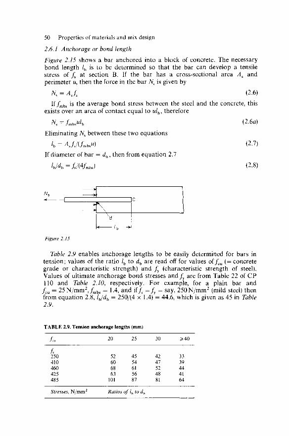
50 Properties of materials and mix design
2.6.1 Anchorage or bond length
Figure 2.15 shows a bar anchored into a block of concrete. The necessary bond length /b is to be determined so that the bar can develop a tensile stress of fs at section B. If the bar has a cross-sectional area As and perimeter u, then the force in the bar Ns is given by
K = AJS (2.6)
If/mbs is the average bond stress between the steel and the concrete, this exists over an area of contact equal to w/b, therefore
iVs=/mbsu/b (2.6a)
Eliminating Ns between these two equations
'b = AJJ(fmbsu) (2.7) If diameter of bar = dh, then from equation 2.7
lJdb=fJWmbs) (2.8)
Figure 2.15
Table 2.9 enables anchorage lengths to be easily determined for bars in tension; values of the ratio /b to dh are read off for values of/cu (= concrete grade or characteristic strength) and fy (characteristic strength of steel). Values of ultimate anchorage bond stresses and/y are from Table 22 of CP 110 and Table 2.10, respectively. For example, for a plain bar and
fcu = 25N/mm2,/mbs = 1.4, and if/s = / y = say, 250N/mm2 (mild steel) then from equation 2.8, lh/db = 250/(4 x 1.4) = 44.6, which is given as 45 in Table 2.9.
TABLE 2.9. Tension anchorage lengths (mm)
/ c u 20 25 30 ^40
fy 250 410 460 425 485
52 60 68 63 101
45 54 61 56 87
42 47 52 48 81
33 39 44 41 64
Stresses, N/mm2 Ratios of lh to db
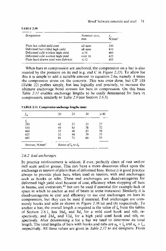
'Bond' between concrete and steel 51
TABLE 2.10
Designation
Plain hot rolled mild steel Deformed hot rolled high yield Deformed cold worked high yield Deformed cold worked high yield Plain hard drawn steel wire (fabrics)
Nominal sizes, mm
all sizes all sizes ^16 over 16 <12
/ y . N/mm2
250 410 460 425 485
When bars in compression are anchored, the compression on a bar is also resisted by the pressure on its end (e.g. end C in Figure 2.15). To allow for this it is simple to add a suitable amount to equation 2.6a, namely A times the compressive stress on the concrete. This was once done, but CP 110 (Table 22) prefers simply, but less logically and precisely, to increase the ultimate anchorage bond stresses for bars in compression. On this basis Table 2.11 enables anchorage lengths to be easily determined for bars in compression, similarly to Table 2.9 (see Section 2.6.5).
TABLE 2.11. Compression anchorage lengths (mm)
fcu 20 25 30 ^40
42 37 49 43 55 48 51 44 81 71
Ratios oflb to dh
33 38 43 39 64
27 32 36 33 53
2.6.2 End anchorages
In practice reinforcement is seldom, if ever, perfectly clean of rust and/or mill scale and/or grease. This can have a more disastrous effect upon the anchorage in tension of plain than of deformed bars. Hence it is good practice always to provide plain bars, when used in tension, with end anchorages such as hooks or nibs. These end anchorages are disadvantageous for deformed high yield steel because of cost, efficiency when stopping off bars in beams, and overstrain,12 but can be used if essential (for example lack of space in which to anchor at end of beam in some instances). Similarly it is disadvantageous in cost and efficiency to use end anchorages on bars in compression, but they can be used if essential. End anchorages are com-monly hooks and nibs as shown in Figure 2.16 (a) and (b) respectively. To anchor a bar, the overall length a required is the value of /b from the tables of Section 2.6.1, less 16db and 8db for a mild steel hook and nib, re-spectively, and 24dh and 12dh for a high yield steel hook and nib, re-spectively. After determining a for a bar we need to determine its total length. The total lengths of bars with hooks and nibs are ah + /b and an + Zn, respectively. All these values are given in Table 2.12 to aid designers. From
/y 250 410 460 425 485

52 Properties of materials and mix design
/ 1
((1 u
4c/b "1
^ Oh-c/b-c/h/2
Q=Qh *n
( a )
t
1
ldb
\ \
«*—
y^ v _
an-c/b-rn
a=an
^ (b)
Figure 2.16
the geometry of Figure 2.16(a), the total length of the bar
= ah + lh = (ah -db- 0.5dh) + 0.5n(dh + db) + 4dh
/ . /h = 3db - 0.54 + 0.57E(dh + dh) (2.9) From Figure 2.16(b), the total length of the bar
= an + ln = (an -db- rn) + 0.5;r(rn 4- 0.5db) + 4db
.\ ln = Mb - rn + 0.57r(rn + 0.5Jb) (2.10) From these equations: for mild steel dh = 4dh and rn = 2db, thus
/h = 8.85db, say 9db, and ln = 4.93db, say 5db; for high yield steel dh = 6db
and rn = 3 4 , thus /h = lldb and /n = 5.5db. Hooks are worth much more as an anchorage per unit length of material
than nibs and cost little more to produce. Tables 2.13 and 2.14 are based on Table 2.10 and fcu = 20N/mm2 and
should be useful for designers of in-situ concrete, because the weakest structural concrete is generally used for such work. If occasionally say
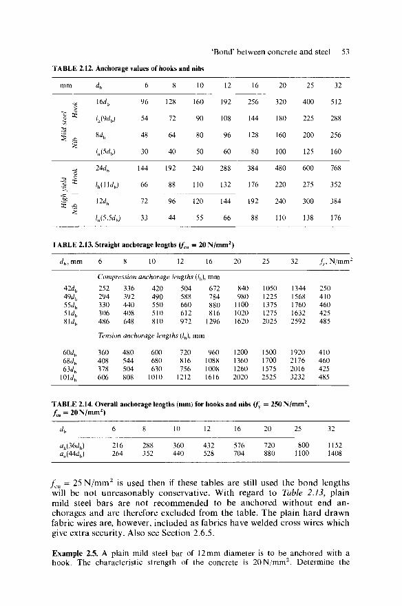
'Bond1 between concrete and steel 53
TABLE 2.12
mm
IS
*E
3 5 •Si
TABLE 2.13
4, mm
. Anchorage values of hooks and nibs
db
164
'h(Wb)
84
U54)
24db
'h(H^b)
I2dh
U5.5dh)
6
96
54
48
30
144
66
72
33
8
128
72
64
40
192
88
96
44
. Straight anchorage lengths (fcu
6 8 10 12
10
160
90
80
50
240
110
120
55
= 20N/
16
12
192
108
96
60
288
132
144
66
mm 2)
20
16
256
144
128
80
384
176
192
88
25
20
320
180
160
100
480
220
240
110
32
25
400
225
200
125
600
275
300
138
32
512
288
256
160
768
352
384
176
fy, N/mm:
42db
49db
554, 5ldb
8 U h
Compression anchorage lengths (/b), m m
252 336 420 504 672 840 1050 1344 250 294 392 490 588 784 980 1225 1568 410 330 440 550 660 880 1100 1375 1760 460 306 408 510 612 816 1020 1275 1632 425 486 648 810 972 1296 1620 2025 2592 485
Tension anchorage lengths (/b), m m
60db 360
68^b 408
634 378 1014 606
480 544 504
600 680 630 1010
720 816 756 1212
960 1088 1008 1616
1200 1360 1260 2020
1500 1700 1575 2525
1920 410 2176 460 2016 425 3232 485
TABLE 2.14. Overall anchorage lengths (mm) for hooks and nibs (fy = 250N/mm2, /cu = 20N/mm2)
db
ah(364) <U444)
6
216 264
8
288 352
10
360 440
12
432 528
16
576 704
20
720 880
25
800 1100
32
1152 1408
fcu = 25 N / m m 2 is used then if these tables are still used the bond lengths will be not unreasonably conservative. With regard to Table 2.13, plain mild steel bars are not recommended to be anchored without end an-chorages and are therefore excluded from the table. The plain hard drawn fabric wires are, however, included as fabrics have welded cross wires which give extra security. Also see Section 2.6.5.
Example 2.5. A plain mild steel bar of 12 mm diameter is to be anchored with a hook. The characteristic strength of the concrete is 20N/mm2. Determine the
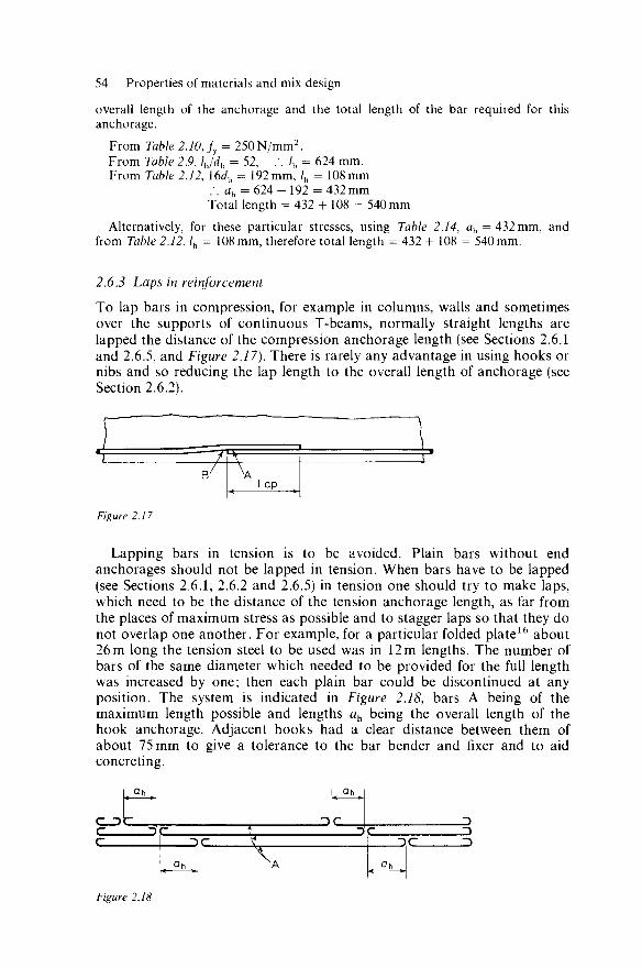
54 Properties of materials and mix design
overall length of the anchorage and the total length of the bar required for this anchorage.
From Table 2.10, fy = 250N/mm2. From Table 2.9, lh/dh = 52, .*. /b - 624 mm. From Table 2.12, I6dh = 192mm, /h - 108 mm
.-. ah = 624 -192 = 432mm Total length = 432 + 108 - 540 mm
Alternatively, for these particular stresses, using Table 2.14, ah = 432 mm, and from Table 2.12, lh = 108 mm, therefore total length = 432 + 108 = 540 mm.
2.6.3 Laps in reinforcement
To lap bars in compression, for example in columns, walls and sometimes over the supports of continuous T-beams, normally straight lengths are lapped the distance of the compression anchorage length (see Sections 2.6.1 and 2.6.5, and Figure 2.17). There is rarely any advantage in using hooks or nibs and so reducing the lap length to the overall length of anchorage (see Section 2.6.2).
m Lap
Figure 2.17
Lapping bars in tension is to be avoided. Plain bars without end anchorages should not be lapped in tension. When bars have to be lapped (see Sections 2.6.1, 2.6.2 and 2.6.5) in tension one should try to make laps, which need to be the distance of the tension anchorage length, as far from the places of maximum stress as possible and to stagger laps so that they do not overlap one another. For example, for a particular folded plate16 about 26 m long the tension steel to be used was in 12 m lengths. The number of bars of the same diameter which needed to be provided for the full length was increased by one; then each plain bar could be discontinued at any position. The system is indicated in Figure 2.18, bars A being of the maximum length possible and lengths ah being the overall length of the hook anchorage. Adjacent hooks had a clear distance between them of about 75 mm to give a tolerance to the bar bender and fixer and to aid concreting.
Qh
C-DC
Qh
D C
Qh
- D C
Qh
Figure 2.18
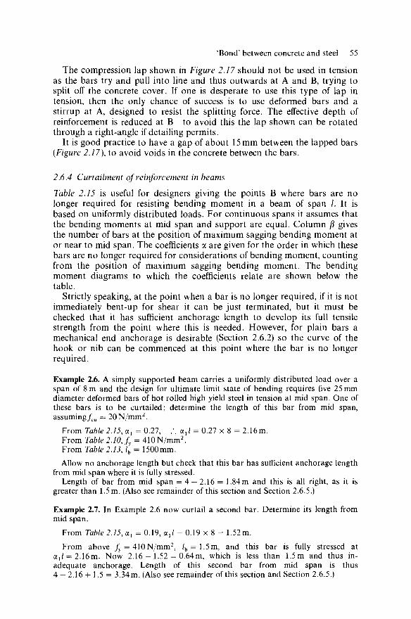
'Bond' between concrete and steel 55
The compression lap shown in Figure 2.17 should not be used in tension as the bars try and pull into line and thus outwards at A and B, trying to split off the concrete cover. If one is desperate to use this type of lap in tension, then the only chance of success is to use deformed bars and a stirrup at A, designed to resist the splitting force. The effective depth of reinforcement is reduced at B—to avoid this the lap shown can be rotated through a right-angle if detailing permits.
It is good practice to have a gap of about 15 mm between the lapped bars (Figure 2.17), to avoid voids in the concrete between the bars.
2.6.4 Curtailment of reinforcement in beams
Table 2.15 is useful for designers giving the points B where bars are no longer required for resisting bending moment in a beam of span /. It is based on uniformly distributed loads. For continuous spans it assumes that the bending moments at mid span and support are equal. Column /? gives the number of bars at the position of maximum sagging bending moment at or near to mid span. The coefficients a are given for the order in which these bars are no longer required for considerations of bending moment, counting from the position of maximum sagging bending moment. The bending moment diagrams to which the coefficients relate are shown below the table.
Strictly speaking, at the point when a bar is no longer required, if it is not immediately bent-up for shear it can be just terminated, but it must be checked that it has sufficient anchorage length to develop its full tensile strength from the point where this is needed. However, for plain bars a mechanical end anchorage is desirable (Section 2.6.2) so the curve of the hook or nib can be commenced at this point where the bar is no longer required.
Example 2.6. A simply supported beam carries a uniformly distributed load over a span of 8 m and the design for ultimate limit state of bending requires five 25 mm diameter deformed bars of hot rolled high yield steel in tension at mid span. One of these bars is to be curtailed; determine the length of this bar from mid span, assuming fcu = 20N/mm2.
From Table 2.15, ax = 0.27, .\ at/ = 0.27 x 8 = 2.16m. From Table 2.10, fy = 410N/mm2. From Table 2.13, lh = 1500mm. Allow no anchorage length but check that this bar has sufficient anchorage length
from mid span where it is fully stressed. Length of bar from mid span = 4 — 2.16 = 1.84m and this is all right, as it is
greater than 1.5 m. (Also see remainder of this section and Section 2.6.5.)
Example 2.7. In Example 2.6 now curtail a second bar. Determine its length from mid span.
From Table 2.15, ai = 0.19, aj = 0.19 x 8 = 1.52m. From above /y = 410N/mm2, /b = 1.5m, and this bar is fully stressed at
OLJ = 2.16m. Now 2.16 - 1.52 = 0.64m, which is less than 1.5m and thus in-adequate anchorage. Length of this second bar from mid span is thus 4 — 2.16 + 1.5 = 3.34m. (Also see remainder of this section and Section 2.6.5.)

TA
BL
E 2
.15.
p
al 1s
t 2n
d 3r
d 4t
h 5t
h 6t
h
a 2
1st
«3
Ord
er o
f st
oppi
ng-o
ff o
r be
ndin
g-up
bar
s 2n
d 3r
d 4t
h 5t
h 6t
h 1s
t 2n
d 3r
d 4t
h 5t
h 6t
h
a 4
1st
2nd
3rd
4th
5th
6th
o
O B
1 2 3 4 5 6 7 8
0 .15
.21
.25
.28
.30
.31
.32
0 .09
.15
.19
.21
.23
.25
0 .07
.12
.15
.17
.19
—
—
0 .05
.09
.12
.15
—
—
0 .04
.08
.10
—
—
—
0 .04
.07
.11
.24
.30
.33
.35
.37
.39
.40
.11
.19
.24
.28
.30
.32
.33
.11
.17
.21
.24
.26
.27
—
.11
.16
.19
.22
.24
—
.11
.14
.17
.20
—
—
.11
.14
.17
0 .13
.18
.22
.25
.27
.29
.30
0 .08
.13
.15
.18
.20
.22
0 .05
.09
.13
.15
.17
—
0 .04
.08
.11
.13
—
—
—
0 .03
.07
.09
—
—
—
—
0 .03
.05
.09
.21
.27
.30
.31
.33
.34
.35
.09
.16
.21
.24
.27
.29
.30
—
.09
.15
.18
.21
.23
.25
—
—
.09
.13
.16
.19
.21
—
—
—
.09
.12
.15
.18
—
—
—
.09
.12
.15
3 3 X a.
t/3
CTQ
Z3
a \
I ■
1/
J | 1 «
/i
r 1
iir
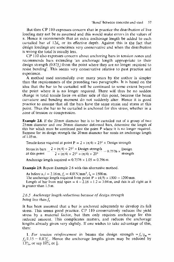
'Bond' between concrete and steel 57
But then CP 110 expresses concern that in practice the distribution of live loading may not be as assumed and this would make errors in the values of a. Hence it recommends that an extra anchorage length be added to each curtailed bar of I2dh or its effective depth. Against this is the fact that design loadings are sometimes very conservative and when the distribution is wrong the total is usually less.
CP 110 also expresses concern about anchoring bars in tension zones and recommends bars extending 4an anchorage length appropriate to their design strength (0.87/y) from the point where they are no longer required to resist bending'. This seems very conservative relative to past practice and experience.
A method used successfully over many years by the author is simpler than the requirements of the preceding two paragraphs. It is based on the idea that the bar to be curtailed will be continued to some extent beyond the point where it is no longer required. There will thus be no sudden change in total tensile force on either side of this point, because the beam curvature and bending moment do not suddenly alter. Hence it is good practice to assume that all the bars have the same strain and stress at this point. Thus the bar to be curtailed is anchored for this stress, whether in a zone of tension or compression.
Example 2.8. If the 20 mm diameter bar is to be curtailed out of a group of two 25 mm diameter and one 20 mm diameter deformed bars, determine the length of this bar which must be continued past the point P where it is no longer required. Suppose for its design strength the 20 mm diameter bar needs an anchorage length of 1.05 m.
Tensile force required at point P = 2 x (n/4) x 252 x Design strength Stress in bars 2 x (n/4) x 252 x Design strength ncn^ Design
= = =— = 0.7576 x . at this point 2 x (TT/4) X 252 + (TC/4) X 202 strength Anchorage length required = 0.7576 x 1.05 = 0.796 m.
Example 2.9. Repeat Example 2.6 with this alternative method. As before aj = 2.16m, fy = 410N/mm2, /b = 1500m. The anchorage length required from point P = (4/5) x 1500 = 1200 mm. Length of bar from mid span = 4 - 2.16 + 1.2 = 3.04m, and this is all right as it
is greater than 1.5 m.
2.6.5 Anchorage length reductions because of design strength being less thanfy
It has been assumed that a bar is anchored adequately to develop its full stress. This seems good practice. CP 110 conservatively reduces the yield stress by a material factor, but then only requires anchorage for this reduced amount. This complicates matters, and reduces the anchorage lengths already given very slightly. If one wishes to take advantage of this, then:
1. For tension reinforcement in beams the design strength =fy/ym = /y/1.15 = 0.87/y. Hence the anchorage lengths given may be reduced by 13%, or say 10% or i
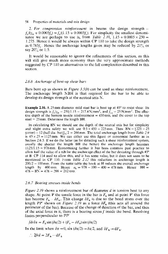
58 Properties of materials and mix design
2. For compression reinforcement in beams the design strength = fy/(ym + 0.0005/y) =/y /(1.15 + 0.0005/y). For simplicity the smallest denomi-nator we are perhaps to use is, from Table 2.10, 1.15 + 0 .0005x250 = 1.275. Hence it would be always within C P 110 to take the design strength as 0.785/y. Hence the anchorage lengths given may be reduced by 2 1 % or say 20% or 1/5.
It would be reasonable to ignore the refinements of this section, as this will still give much more economy than the very approximate methods suggested by C P 110 as alternatives to the full complexities described in this section.
2.6.6 Anchorage ofbent-up shear bars
Bars bent up as shown in Figure 3.5(b) can be used as shear reinforcement. The anchorage length N B H is that required for the bar to be able to develop its design strength at the neutral axis N .
Example 2.10. A 25 mm diameter mild steel bar is bent up at 45° to resist shear. Its design strength is/y/ym = 250/1.15 = 217.4N/mm2, and/ c u = 25N/mm2. The effec-tive depth of the bottom tensile reinforcement = 450 mm, and the cover to the top steel = 25 mm. Determine the length BH.
In calculating BN we should use the depth of the neutral axis but for simplicity and slight extra safety we will use 0.5 x 450 = 225 mm. Then BN = [225 — 25 (cover) — 12 (half dia. bar)]^2 = 266 mm. The total anchorage length from Table 2.9 is 45 x 25 = 1125 mm. We can either use this figure or economise further as in Section 2.6.5. If we do the latter (as for detailing such a shear reinforcement system, usually the shorter the length BH the better) the anchorage length becomes 1125/1.15 = 978mm. Economising further it has been common past practice to allow half the value of a nib for the anchorage effect of the bar deviating through 45° at B. CP 114 used to allow this, and it has some value, but it does not seem to be mentioned in CP 110. From Table 2.12 this reduction in anchorage length is 200/2 = 100 mm. From the same table the hook at H reduces the overall anchorage length by 400 mm. Hence ah = 978 - 100 - 400 = 478 mm. Hence BH = 478 - BN = 478 - 266 = 212 mm.
2.6.7 Bearing stresses inside bends
Figure 2.19 shows a reinforcement bar of diameter d in tension bent to any shape. At point P the tensile force in the bar is Fh and at point P ' this force has become Fh — SFh. This change SFb is due to the bond stress over the length PP ' shown on Figure 2.19 as a force SFh (this acts all around the perimeter of the bar). Because of the change of direction of the bar, and thus of the axial force in it, there is a bearing s t r e s s / inside the bend. Resolving forces perpendicular to P P '
fdrSoL = Fh sin (SOL/2) + (Fh - SFh) sin (SOL/2)
In the limit when doc -► 0, sin (SOL/2) -► Soc/2, and SFh -> dFh.
:. 2frd = 2Fh-dFh

'Bond' between concrete and steel 59
Figure 2.19
Now dFb is negligible (->0) in comparison to the size of the quantities 2frd and 2Fb.
:.f=FJ(rd) (2.11)
This stress at P does not need to be checked for the standard anchorage hooks and nibs of Section 2.6.2. CP 110 requires/ to be checked when the bar continues more than Ad after the bend and is still required for bond resistance—for example the bend at B in Figure 3.5(b) and at b' in Figure 2.21.
The same theory and equation (2.11) apply for bars in compression. In Figure 2.19 Fb would be in the opposite direction and / would be at the opposite side of the bar.
A dowel bar under the bend just transmits and concentrates the bearing stress to immediately below it, though it can help to spread this pressure transversely. CP 110 already does this considerably in its formula 3.11.6.8, and so such dowel bars are not considered helpful in reducing the bearing stresses inside bends.
Example 2.11. For Example 2.10 determine the minimum radius of curvature allowed at B. The beam is T-shaped and the bend B is in the wide flange.
Stress in bar at B = 217.4 x (978 - 266)/978 = 158.3 N/mm2. d = 25mm,Fh= 158.3 x (TT/4) x 252 = 77690N. The permissible/is, from CP 110 (formula 3.11.6.8), ah = GO, = (1.5 x 25)/(l + 2 x 25/oo) = 37.5 N/mm2
Hence from equation 2.11 r = FJ(fd) = 77 690/(37.5 x 25) - 82.87 mm
2.6.8 Anchorage of stirrups {or links)
CP 110 recommendation 3.11.6.4 conflicts with the CP 110 recommen-dations already referred to in this chapter regarding anchorage length and bearing stress inside bends. Its inadequacy in this respect might be justified
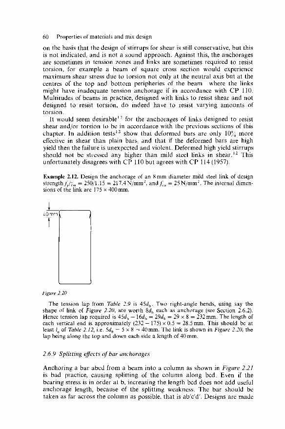
60 Properties of materials and mix design
on the basis that the design of stirrups for shear is still conservative, but this is not indicated, and is not a sound approach. Against this, the anchorages are sometimes in tension zones and links are sometimes required to resist torsion, for example a beam of square cross section would experience maximum shear stress due to torsion not only at the neutral axis but at the centres of the top and bottom peripheries of the beam—where the links might have inadequate tension anchorage if in accordance with CP 110. Multitudes of beams in practice, designed with links to resist shear and not designed to resist torsion, do indeed have to resist varying amounts of torsion.
It would seem desirable17 for the anchorages of links designed to resist shear and/or torsion to be in accordance with the previous sections of this chapter. In addition tests12 show that deformed bars are only 10% more effective in shear than plain bars, and that if the deformed bars are high yield then the failure is unexpected and violent. Deformed high yield stirrups should not be stressed any higher than mild steel links in shear.12 This unfortunately disagrees with CP 110 but agrees with CP 114 (1957).
Example 2.12. Design the anchorage of an 8 mm diameter mild steel link of design strength fy/ym = 250/1.15 = 217.4N/mm2, and/cu = 25N/mm2. The internal dimen-sions of the link are 175 x 400 mm.
L l AOmmk j
Figure 2.20
The tension lap from Table 2.9 is 45db. Two right-angle bends, using say the shape of link of Figure 2.20, are worth 8db each as anchorage (see Section 2.6.2). Hence tension lap required is 45db — 16dh = 29db = 29 x 8 = 232 mm. The length of each vertical end is approximately (232 — 175) x 0.5 = 28.5 mm. This should be at least /n of Table 2.12, i.e. 5dh = 5x8 = 40mm. The link is shown in Figure 2.20, the lap being along the top and down each side a length of 40 mm.
2.6.9 Splitting effects of bar anchorages
Anchoring a bar abed from a beam into a column as shown in Figure 2.21 is bad practice, causing splitting of the column along bed. Even if the bearing stress is in order at b, increasing the length bed does not add useful anchorage length, because of the splitting weakness. The bar should be taken as far across the column as possible, that is ab'c'd'. Designs are made
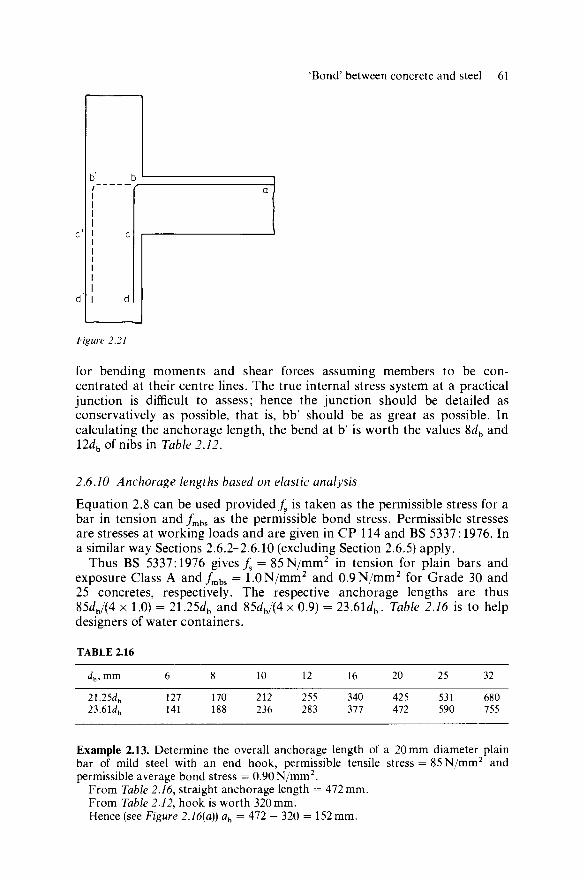
'Bond'between concrete and steel 61
b' b
c' l c
d' I d
Figure 2.21
for bending moments and shear forces assuming members to be con-centrated at their centre lines. The true internal stress system at a practical junction is difficult to assess; hence the junction should be detailed as conservatively as possible, that is, bb' should be as great as possible. In calculating the anchorage length, the bend at b' is worth the values 8db and \2dh of nibs in Table 2.12.
2.6.10 Anchorage lengths based on elastic analysis
Equation 2.8 can be used provided fs is taken as the permissible stress for a bar in tension and/m b s as the permissible bond stress. Permissible stresses are stresses at working loads and are given in CP 114 and BS 5337:1976. In a similar way Sections 2.6.2-2.6.10 (excluding Section 2.6.5) apply.
Thus BS 5337:1976 gives / s = 85 N/mm2 in tension for plain bars and exposure Class A and/m b s = l.ON/mm2 and 0.9N/mm2 for Grade 30 and 25 concretes, respectively. The respective anchorage lengths are thus 85rfb/(4 x 1.0) = 2l.25db and 85db/(4 x 0.9) = 23.61db. Table 2.16 is to help designers of water containers.
TABLE 2.16
db, m m
21.254 23.614
6
127 141
8
170 188
10
212 236
12
255 283
16
340 377
20
425 472
25
531 590
32
680 755
Example 2.13. Determine the overall anchorage length of a 20 mm diameter plain bar of mild steel with an end hook, permissible tensile stress = 85 N/mm2 and permissible average bond stress = 0.90N/mm2.
From Table 2.16, straight anchorage length = 472 mm. From Table 2.12, hook is worth 320mm. Hence (see Figure 2.16(a)) ah = All - 320 = 152 mm.

62 Properties of materials and mix design
References
1. BOGUE, R. H., Chemistry of Portland Cement, Reinhold, New York (1955) 2. TROXELL, G. E., DAVIS, H. E., and KELLY, J. W., Composition and Properties of
Concrete, McGraw-Hill, U.S.A. (1968) 3. BRUNAUER, S., Tobermorite Gel—The Heart of Concrete1, American Scientist, Mar.
(1962) 4. NEVILLE, A. M., Properties of Concrete, Pitman (1963 and 1973) 5. ROBSON, T. D., 'High Alumina Cements and Concretes', Contractors' Record (1962) 6. BATE, E. E. H., and STEWART, D. A., 'A Survey of Modern Concrete Technique', Proc.
I.C.E. Part 3, Dec. (1955) 7. HUGHES, B. P., Limit State Theory for Reinforced Concrete, Pitman (1971 and 1980) 8. Design of Concrete Mixes, D.S.I.R. Road Research Laboratory, Road Note No. 4,
H.M.S.O., London (1950) 9. TEYCHENNE, D. C , FRANKLIN, R. E., and ERNTROY, H. C , Design of Normal
Concrete Mixes, Department of the Environment, H.M.S.O., London (1975) 10. A.C.I. Committee 211, A.C.I. Standard 211.1-70: Recommended Practice for Selecting
Proportions for Concrete, American Concrete Institute, Detroit (1970) 11. EVANS, R. H., 'Effect of Rate of Loading on Some Mechanical Properties of Concrete',
Proceedings of the 1958 London Conference organised by the Mining Research Establishment of the N.C.B. in consultation with the Building Research Establishment, D.S.I.R., pp. 157-175
12. WILBY, C. B., 'Overstrain in High-tensile Reinforcing Bars at Bends and in Stirrups', Indian Concrete Journal, Jan. (1962)
13. ARMSTRONG, W. E. I., 'Bond in Prestressed Concrete', Journal of the Institute of Civil Engineers, 33, Nov. (1949)
14. REGAN, P. E., and YU, C. W., Limit State Design of Structural Concrete, Chatto and Windus(1973)
15. EVANS, R. H., and ROBINSON, G. W., 'Bond Stresses in Prestressed Concrete from X-ray Photographs', Paper No. 6025, Proceedings of the Institute of Civil Engineers, Part 1, Mar. (1953)
16. WILBY, C. B., Concrete for Structural Engineers, Newnes-Butterworths, London-Boston (1977)
17. EVANS, R. H., and WILBY, C. B., Concrete—Plain, Reinforced, Prestressed and Shell, Art. 5.7, Edward Arnold (1963)

Chapter 3
Reinforced concrete beams
3.1 Design
To design a reinforced concrete beam a reasonable procedure is as follows:
1. Estimate the dimensions of the beam. The overall depth can be taken as say a proportion of the 'effective span', 1/20 for simply supported, 1/25 for continuous, and 1/10 for cantilever beams. The breadth (or breadth of rib for, say, a T-beam) can be taken as j to \ of this depth.
2. For a rectangular beam, the ratio of the maximum distance between lateral restraints to breadth is ideal if less than 30, reasonable if between 30 and 40, and likely to be impracticable if more than 50. This is because of the possibility of narrow beams buckling sideways.
3. Check the strength in shear, and torsion if present, in the worst case, usually a section adjacent to a support. It may well be that reinforcement is required and this should not normally be greater than say 10 mm diameter stirrups (two, four or six arm according to width of beam) at 80 mm centres. The beam may well eventually be detailed with bent-up bars assisting the stirrups in the localities of maximum shear force.
4. Check the strength in bending. For a rectangular (or simply supported) beam this is best done first at the section subjected to maximum bending moment. For a continuous T-beam, mid span will normally be strong enough in bending if the supports are, because the beam is acting as a rectangular beam at the supports. If compression steel is required it might be desirable because of detailing to revise the design to eliminate the need for such steel—if this is not done it is useful practically for the area of the compression steel not to exceed 1% of the breadth (of rib for a T-beam) times the overall depth. Then determine the longitudinal tension reinforcement and see if it can be detailed reasonably in the beam. In the case of simply supported T-beams it is speedier to calculate the reinforcement before the compressive strength of the section.
The beam has now been reasonably well designed and it is now only a matter of checking the limit states of deflection and cracking, and then determining the bending and shear steel at critical sections.
63

64 Reinforced concrete beams
3.2 Elastic analysis for bending moments
At working loads the elastic analysis gives a reasonably accurate assessment of the (longitudinal) stresses in the concrete and reinforcement. It also gives a reasonable assessment of deflections experienced at modest loads in a loading test using a Young's modulus obtained from test of specimens of the concrete. For estimating the deflection of a member in practice, for, say, a CP 110 Grade 20 or 25 concrete, the elastic analysis is reasonable for design purposes if a Young's modulus of the concrete of say 14kN/mm2 is used for continuously sustained loading and 21kN/mm2 for loading of short duration.
CP114 allowed the design of beams to be based on elastic analysis, restricting stresses to within the elastic behaviour of the materials at working loads. Multitudes of structures which have lasted many years illustrate the safety of such designs. This method has been dispensed with by CP 110, but is still used for water-retaining structures (BS 5337: 1976).
For shell roofs the analysis for forces and bending moments is elastic, so it would seem logical and safe (because our experience is based on elastic design) to use elastic analysis for designing for these forces and moments. Where experimental evidence has not adequately ratified the methods of predicting ultimate bending moments, members can be designed by elastic theory with confidence, for example shells, or a beam with unsymmetrical section with skew loading.
For the above and other reasons the elastic analysis will be presented as concisely as possible, using only the moment of intertia of the equivalent concrete section method.
3.2.1 Assumptions made in the elastic design of reinforced concrete
Firstly, it is assumed that plane sections subjected to bending remain plane after bending (Bernoulli's theorem). This is found to be reasonably true by experiment, and means that the distribution of strain is linear across the section.
It is also assumed that stress is proportional to strain for both the steel and the concrete. This is accurately true for the steel up to the limit of proportionality, but only approximately true for the concrete as far as the allowable working stress (permissible stress), and is most inaccurate above this stress towards failure. The elastic method of design endeavours to compute the stresses at working loads, and limits these stresses to amounts below the yield stress of the steel and the crushing stress of the concrete. The respective factors of safety are obtained from experience in industry. It can therefore be appreciated that beams designed in such a fashion are safe but are not designed to have specific load factors against their ultimate strengths. Advocates of elastic design feel that stresses and therefore the size of cracks at working loads are controlled. Concerning the design of prestressed concrete beams in bending the 'modulus of elasticity for concrete in tension is assumed to be the same as the value of this modulus for concrete in compression'.
Perfect bond is assumed between the steel and the concrete. The concrete shrinks upon setting and therefore exerts a pressure upon the steel, which
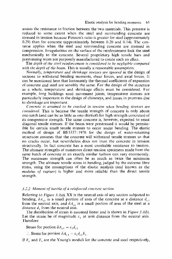
Elastic analysis for bending moments 65
assists the resistance to friction between the two materials. This pressure is reduced to some extent when the steel and surrounding concrete are stressed in tension because Poisson's ratio is greater for steel (approximately 0.29) than for concrete (approximately between 0.20 and 0.14). The con-verse applies when the steel and surrounding concrete are stressed in compression. Irregularities on the surface of the reinforcement lock the steel mechanically to the concrete. Several proprietary high tensile bars and prestressing wires are purposely manufactured to create such an effect.
The depth of the steel reinforcement is considered to be negligible compared with the depth of the beam. This is usually a reasonable assumption.
Normally, temperature and shrinkage stresses are ignored in the design of sections to withstand bending moments, shear forces, and axial forces. It can be mentioned here that fortunately the thermal coefficients of expansion of concrete and steel are sensibly the same. For the design of the structure as a whole, temperature and shrinkage effects must be considered. For example, long buildings need movement joints, temperature stresses are particularly important in the design of chimneys, and losses in prestress due to shrinkage are important.
Concrete is assumed to be cracked in tension when bending stresses are considered. This is because the tensile strength of concrete is only about one-tenth (and can be as little as one-thirtieth for high strength concretes) of its compressive strength. The same concrete is, however, expected to resist diagonal tensile stresses. If the beam were prestressed it would be permiss-ible for certain small tensile stresses to occur under bending. The elastic method of design of BS 5337:1976 for the design of water-retaining structures assumes that the concrete will withstand tensile stresses so that no cracks occur, but nevertheless does not trust the concrete in tension structurally. In fact concrete has a most unreliable resistance to tension. The ultimate strengths of numerous direct tension specimens made from the same batch of concrete in an exactly similar fashion can vary enormously. The maximum strength can often be as much as twice the minimum strength. The ultimate tensile stress in bending, judged by the extreme fibre stress, using the assumptions of the elastic analysis (and known as the modulus of rupture) is higher and more reliable than the direct tensile strength.
3.2.2 Moment of inertia of a reinforced concrete section
Referring to Figure 3.1(a), XX is the neutral axis of any section subjected to bending, SAcl is a small portion of area of the concrete at a distance dcl
from the neutral axis, and SAsl is a small portion of area of the steel at a distance d1 from the neutral axis.
The distribution of strain is assumed linear and is shown in Figure 3.1(b). Let the strain be of magnitude ex at unit distance from the neutral axis. Therefore
Strain for portion SAcl = sldcl
.'. Stress for portion SAcl = s1dclEc
If Ec and £s are the Young's moduli for the concrete and steel respectively,
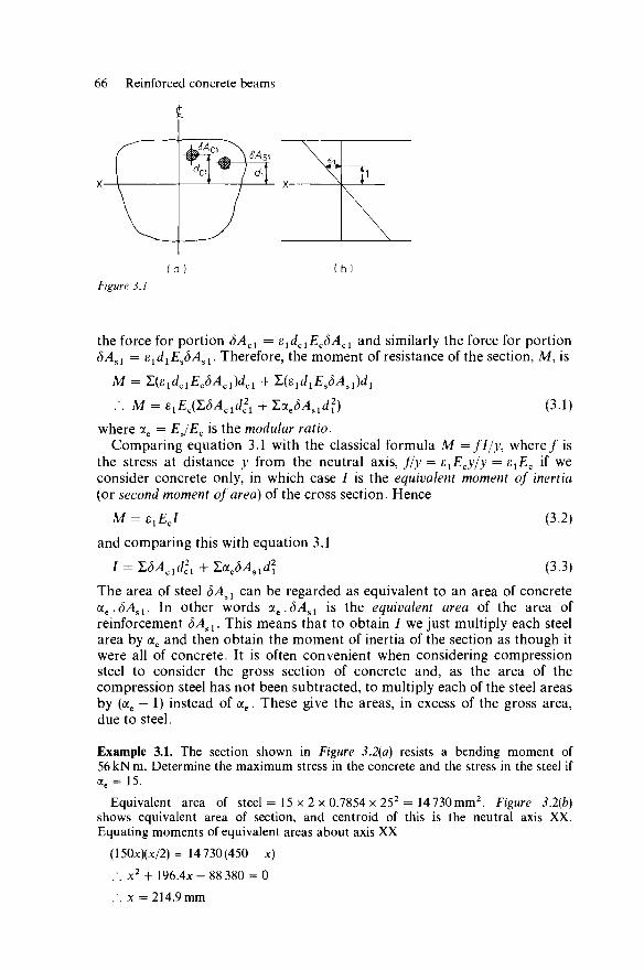
66 Reinforced concrete beams
(a ) (b) Figure 3.1
the force for portion SAcl = eldclEc3Acl and similarly the force for portion SAsi = eldlEs8Asl. Therefore, the moment of resistance of the section, M, is
M = Zie^EMciKi + ZMEMnWi .'. M = s.E^SA^d^ + T,oL,SAsldl) (3.1)
where ae = EJEC is the modular ratio. Comparing equation 3.1 with the classical formula M = fl/y, where/ is
the stress at distance y from the neutral axis, f/y = elEcy/y = e1Ec if we consider concrete only, in which case / is the equivalent moment of inertia (or second moment of area) of the cross section. Hence
M = exEcI (3.2)
and comparing this with equation 3.1
/ = ZSAcld2
cl + 2ae5i48ldf (3.3) The area of steel SAsl can be regarded as equivalent to an area of concrete ae.SAsl. In other words ae.SAsl is the equivalent area of the area of reinforcement SAsl. This means that to obtain / we just multiply each steel area by ae and then obtain the moment of inertia of the section as though it were all of concrete. It is often convenient when considering compression steel to consider the gross section of concrete and, as the area of the compression steel has not been subtracted, to multiply each of the steel areas by (ae — 1) instead of ae. These give the areas, in excess of the gross area, due to steel.
Example 3.1. The section shown in Figure 3.2(a) resists a bending moment of 56kNm. Determine the maximum stress in the concrete and the stress in the steel if ae = 15.
Equivalent area of steel = 15 x 2 x 0.7854 x 252 = 14 730mm2. Figure 3.2(b) shows equivalent area of section, and centroid of this is the neutral axis XX. Equating moments of equivalent areas about axis XX
(150x)(x/2)= 14 730(450 - x)
:. x2 + 196.4x- 88 380 = 0 .'. x = 214.9 mm

Elastic analysis for bending moments 67
Taking moments of (equivalent) area about XX
/ = (150x3/3) + 14 730 x (450 - x)2
= 1310 x 106mm4.
From equation 3.2
sl = M/(IEC) = 56/(1310£c) = 0.042 75/£c
Figure 3.2(c) gives distribution of strain and Figure 3.2(d) gives corresponding distribution of stress. Therefore
fc = E^x) = 0.042 75 x 214.9 = 9.187 N/mm2
and
fs = £^(450 - x) = 0.042 75 ae(450 - x) = 150.8 N/mm2
These last two equations are sometimes expressed as
fc = Mx/I and/ s = aeM(450 - x)/I (3.4)
Example 3.2. If the beam of Example 3.1 were simply supported over an (effective) span (/) of 9.75 m and all the loading was uniformly distributed (q), determine the central deflection. Assume that the bending moment of 56kNm was at mid span. Take Es = 200kN/mm2; then Ec = 200/ae = 13.33kN/mm2.
Central deflection at mid span = ax = (5/384)((?/4/£/) In this example M = ql2/8
.". q = (56 x 8)/9.752 = 4.713 kN/m (or N/mm)
5x4.713x9750 4
= 31.76 mm 384 x 13 330 x 1310 x 106
Example 3.3. Determine the moment of resistance of the section shown in Figure 3.2(a) if the permissible stresses (i.e. the stresses allowed at working loads) are 10.5 N/mm2 and 210 N/mm2 for the concrete and steel, respectively, and the modular ratio is 15.
From Example 3.1, x = 214.9 mm and / == 1310 x 106mm4. If concrete is the criterion, from equation 3.4
Moment of resistance =fc(I/x) = 10.5 x 1310 x 106/214.9Nmm
= 64.01 kNm
If steel is the criterion, from equation 3.4
/ s / 210 x 1310 xlO 6
Moment of resistance = = N mm ae (450 -x) 15(450-214.9)
= 78.01 kN m Therefore according to the assumptions of this design the moment of resistance of the beam is limited by the compressive strength of the concrete to 64.01 kN m.
3.2.3 Method for tabulating calculations for x and I
Table 3.1 illustrates the method. A is the equivalent area of a portion, y is the distance of the centroid of A from any chosen axis, say YY for Figure 3.3(a), In is the second moment of area for the portion about its neutral axis.
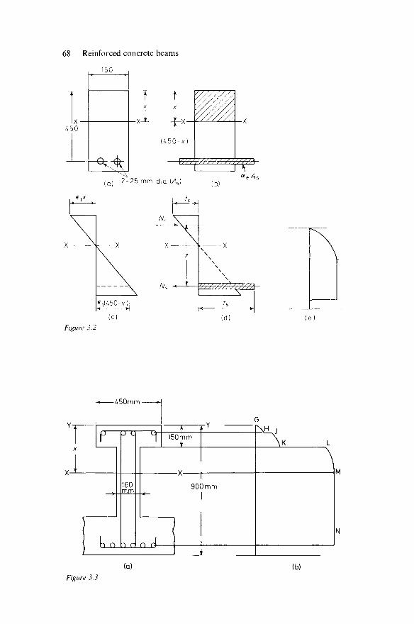
68 Reinforced concrete beams
150
(Q) 2-25 mm clia [As) (b)
L fc
Nc
Ns +- w/////?///,*?a X-
(d)
Figure 3.2
1 ,
y
>
<
[_
■* 450mm >■
f
kn
r H
160 mm
K ri
1 t \
150 mm
V ■" A " ■
90(
( „ A
' '
v , Y
)mm
'
^ H J ^ \ K L
\
Figure 3.3
(a) (b)

TAB
LE 3
.1.
Por
tion
Are
a A
y
Ay
Ay2
Con
cret
e C
oncr
ete
Com
pres
sion
ste
el
Tens
ile s
teel
(45
- 16
) x 1
5 =
435
16x
4x3.
142
= 12
.57
6 x
4.90
9 =
29.4
5
435
16x
(x 1
4=)
175.
9 (x
15=
) 44
1.8
7.5
0.5x
6 83
.7
3 26
3 8x2
1055
36
979
2447
0 4x3
6332
30
9500
0
29 x
153 /1
2 =
8156
16
x3 /12
= 1.
333x
3
—
—
Tota
ls
1053
38
030
3101
000
H
ST
16x
+ 8x
2+
5.33
3x2 +
§ P a B'
OQ
3 o
ON

70 Reinforced concrete beams
Then taking moments of area about YY
"LAy = x£A (3.5)
.'. x = XAy/ZA (3.6)
Second moment of area of whole section about YY
= Iy = XAy2 + Un (3.7)
If / is second moment of area of the whole section about its neutral axis XX, and x is depth of neutral axis below YY, then
Iy = x2XA + I (3.8)
From equations 3.7 and 3.8
/ = "LAy1 + I / n - x2I,A (3.9)
Supposing we wish to obtain the lever arm z. Then considering the tensile steel, area As, effective depth du the moment of resistance =fsAsz = / , W i - x)
:.z = I/lAs(dl-xft (3.10)
Example 3.4. The section shown in Figure 3.3 is through an external counterfort to a tank. The reinforcement bars comprise six of 25mm diameter in tension and four of 20 mm diameter in compression and have 50 mm cover of concrete, ae = 15, the permissible stresses (for BS 5337: 1976 strength calculations for Grade 25 concrete and Class A exposure for plain bars of steel) are: concrete in compression 9.15 N/mm2, and steel in tension 85N/mm2. Determine the moment of resistance of the section at working loads, and the stress in the compression steel.
Table 3.1 shows the calculation (dimensions are in centimetres for convenience). Then from equation 3.5
8x2 + 38 030 = 16x2 + 1053x
8x2 + 1053x- 38 030 = 0
.'. x = 29.50cm = 295.0mm
From equation 3.9
/ = 5.333x2 + 3 101000 - x2(16x + 1053)
= 3 101000 - 29.52(16 x 29.5 + 1048)
= 1.778 x 106cm4 = 17 780 x 106mm4
Referring to equations 3.4 17 780 x 106
Moment of resistance (concrete) = 9.15 x Nmm = 551.5 kNm 295
85 17 7 8 0 x l 0 6
Moment of resistance (steel) = — x N mm = 185.9 kN m 15 (837-295)
The latter is therefore the criterion, and the stress in the compression steel will be 185.9
= 15 x x (295 - 60) = 36.86 N/mm2
17 780 '
The latter is well within the permissible stress of 125 N/mm2 given by BS 5337, and 551.5 is much greater than 185.9, hence a designer might reduce the diameter of
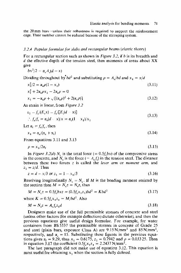
Elastic analysis for bending moments 71
(3.13)
the 20 mm bars—unless their robustness is required to support the reinforcement cage. Their number cannot be reduced because of the stirruping system.
3.2.4 Popular formulae for slabs and rectangular beams (elastic theory)
For a rectangular section such as shown in Figure 3.2, if b is its breadth and d the effective depth of the tension steel, then moments of areas about XX give
bx2/2 = (xeAs(d — x)
Dividing throughout by bd2 and substituting p = AJbd and xx = x/d
x2/2 = oiep(l-xl) (3.11)
x2 + 2aepx1 — 2aep = 0 *i = -* e P + VLKP)2 + 2(aep)] (3.12)
As strain is linear, from Figure 3.2
sl=fc/(Ecx)=fJ[Es(d-xn
.'• fjfc = *M ~ X)/X = M 1 - *l)/*l Let a f =/ s / / c , then
xl =ae/(ae + af) (3.14)
From equations 3.11 and 3.13
p = xJ2oLf (3.15) In Figure 3.2(d) Nc is the total force (= 0.5fcbx) of the compressive stress
in the concrete, and Ns is the force (= Asfs) in the tension steel. The distance between these two forces z is called the lever arm or moment arm, and zr = z/d. Thus
z = d — x/3 or Zj = 1 — x1/3 (3.16)
Resolving longitudinally Nc = Ns. If M is the bending moment resisted by the section then M = Ncz = Nsz, thus
M = Ncz = 0.5fcbxz = (O^x^Jbd2 = Kbd2 (3.17)
where K = 0.5fcxlZl = M/bd2. Also M = Nsz = AsfZld (3.18) Designers make use of the full permissible stresses of concrete and steel
(unless other factors (for example deflection) dictate otherwise), and then the previous equations give useful design formulae. For example, for water containers from BS 5337 the permissible stresses in concrete of Grade 25 and steel (plain bars, exposure Class A) are 9.15 N/mm2 and 85N/mm2, respectively, and ae = 15. Substituting these figures in the previous equa-tions gives Of = 9.29, thus xx = 0.6175, zx = 0.7942 and p = 0.033 25. Then in equation 3.17 the coefficient 0.5fGxlzl = 2.2437N/mm2.
The last paragraph did not make use of equation 3.12. This equation is most useful for obtaining xx when the section is fully defined.
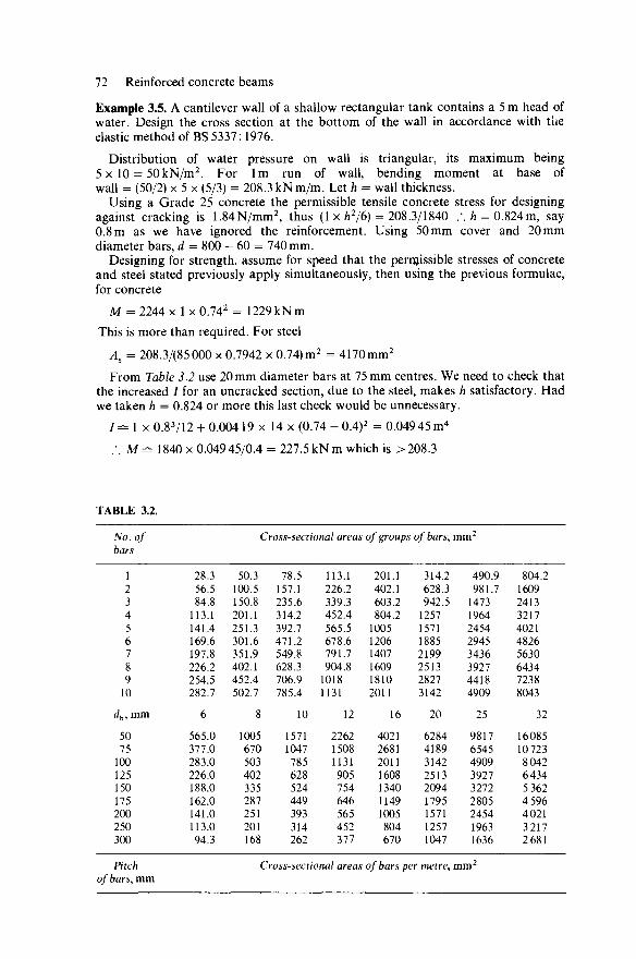
72 Reinforced concrete beams
Example 3.5. A cantilever wall of a shallow rectangular tank contains a 5 m head of water. Design the cross section at the bottom of the wall in accordance with the elastic method of BS 5337:1976.
Distribution of water pressure on wall is triangular, its maximum being 5 x 10 = 50kN/m2. For lm run of wall, bending moment at base of wall = (50/2) x 5 x (5/3) = 208.3 kNm/m. Let h = wall thickness.
Using a Grade 25 concrete the permissible tensile concrete stress for designing against cracking is 1.84N/mm2, thus (1 x h2/6) = 208.3/1840 /. h = 0.824m, say 0.8m as we have ignored the reinforcement. Using 50mm cover and 20mm diameter bars, d = 800 - 60 = 740 mm.
Designing for strength, assume for speed that the permissible stresses of concrete and steel stated previously apply simultaneously, then using the previous formulae, for concrete
M = 2244 x 1 x 0.742 = 1229 kNm This is more than required. For steel
As = 208.3/(85000 x 0.7942 x 0.74)m2 = 4170mm2
From Table 3.2 use 20 mm diameter bars at 75 mm centres. We need to check that the increased / for an uncracked section, due to the steel, makes h satisfactory. Had we taken h = 0.824 or more this last check would be unnecessary.
7 = 1 x0.8 3 /12+ 0.004 19 x 14 x (0.74 - 0.4)2 = 0.04945 m4
.-. M=^ 1840 x 0.04945/0.4 = 227.5kNm which is >208.3
TABLE 3.2.
No. of Cross-sectional areas of groups of bars, mm2
bars
1 2 3 4 5 6 7 8
28.3 56.5 84.8 113.1 141.4 169.6 197.8 226.2
50.3 100.5 150.8 201.1 251.3 301.6 351.9 402.1
78.5 157.1 235.6 314.2 392.7 471.2 549.8 628.3
113.1 226.2 339.3 452.4 565.5 678.6 791.7 904.8
201.1 402.1 603.2 804.2 1005 1206 1407 1609
314.2 628.3 942.5 1257 1571 1885 2199 2513
490.9 981.7 1473 1964 2454 2945 3436 3927
804.2 1609 2413 3217 4021 4826 5630 6434
9 254.5 452.4 706.9 1018 1810 2827 4418 7238
10 282.7 502.7 785.4 1131 2011 3142 4909 8043
dh,mm 6 8 10 12 16 20 25 32
50 565.0 1005 1571 2262 4021 6284 9817 16085 75 100 125 150 175 200 250 300
377.0 283.0 226.0 188.0 162.0 141.0 113.0 94.3
670 503 402 335 287 251 201 168
1047 785 628 524 449 393 314 262
1508 1131 905 754 646 565 452 377
2681 2011 1608 1340 1149 1005 804 670
4189 3142 2513 2094 1795 1571 1257 1047
6545 4909 3927 3272 2805 2454 1963 1636
10 723 8 042 6434 5 362 4 596 4021 3217 2681
Pitch Cross-sectional areas of bars per metre, mm2
of bars, mm
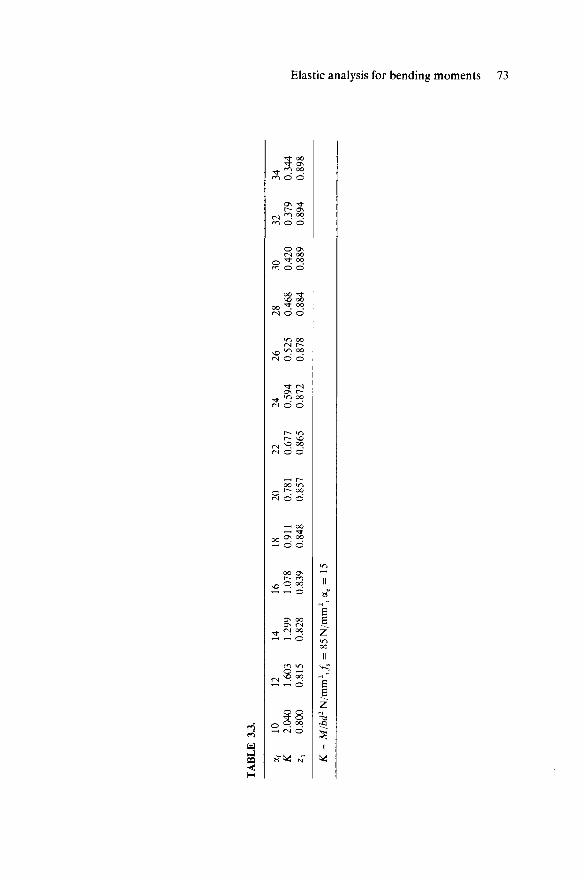
Elastic analysis for bending moments 73
" t OO
en oo
, m oo
O ON rs oo
. Tf OO
vo 00 oo °° (N O O
»o oo
, «/-> o o
ON r-, ^ OO
r- in , vo oo
OO »Ti
, r- oo
^H OO
, 0\ OO
oo ON
O oo
os oo G\ CM
. CM OO
O -H CS ^ OO -H -H O
8 ^ *
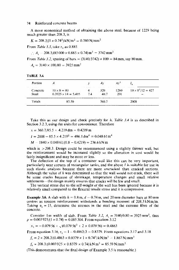
74 Reinforced concrete beams
A more economical method of obtaining the above steel, because of 1229 being much greater than 208.3, is
K = 208.3/(1 x 0.742)kN/m2 = 0.380N/mm2
From Table 3.3, take zx as 0.885
.". As = 208.3/(85 000 x 0.885 x 0.74)m2 = 3742mm2
From Table 3.2, spacing of bars = (3140/3742) x 100 = 84 mm, say 80mm.
As = 3140 x 100/80 = 3925 mm2
TABLE 3.4.
Portion
Concrete Steel
Totals
A
10 x 8 = 80 0.3925 x 14 = 5.495
85.50
y
4 7.4
Ay
320 40.7
360.7
Ay2
1280 291
In
10x83 /12 = 427
2008
Take this as our design and check precisely for h. Table 3.4 is as described in Section 3.2.3, using dm units for convenience. Therefore
x = 360.7/85.5 = 4.219 dm = 0.4219 m
/ = 2008 - 85.5 x 4.2192 = 486.1 dm4 = 0.048 61 m4
M = 1840 x 0.048 61/(0.8 - 0.4219) = 236.6kNm which is >208.3. Design could be recommenced using a slightly thinner wall, but the reinforcement would be increased slightly so the alteration in cost would be fairly insignificant and may be more or less.
The deflection of the top of a container wall like this can be very important, particularly near corners of rectangular tanks, and the above / is suitable for use in such elastic analyses because there are more uncracked than cracked sections. Although the value of h was determined so that the wall would not crack, there will be some cracks because of shrinkage, temperature changes and small relative settlements—the design mainly ensures that cracks will be few and small.
The vertical stress due to the self-weight of the wall has been ignored because it is relatively small compared to the flexural tensile stress and it is compressive.
Example 3.6. A slab with h = O.Sm, d = 0.74 m, and 20 mm diameter bars at 80 mm centres as tension reinforcement withstands a bending moment of 208.3 kNm/m. Taking ae = 15, determine the stresses in the steel and the extreme fibre of the concrete.
Consider lm width of slab. From Table 3.2, As = 3140/0.80 = 3925 mm2, thus p = 0.003 925/(1 x 0.74) = 0.005 304. From equation 3.12
X l = -0.079 56 + v(0.079 562 + 2 x 0.079 56) = 0.4863 From equation 3.16, zt = l - 0.4863/3 = 0.8379. From equations 3.17 and 3.18
fc = 2 x 208.3/(0.4863 x 0.8379 x 1 x 0.742)kN/m2 = 1.867 N/mm2
fs = 208.3/(0.003 925 x 0.8379 x 0.74)kNm2 = 85.59 N/mm2
(This demonstrates that the final design of Example 3.5 is reasonable.)
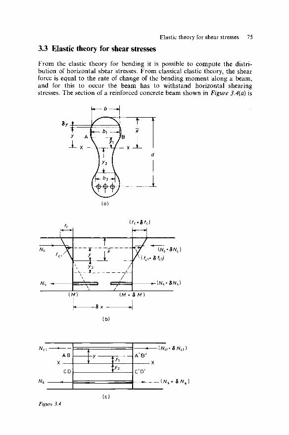
Elastic theory for shear stresses 75
3.3 Elastic theory for shear stresses
From the elastic theory for bending it is possible to compute the distri-bution of horizontal shear stresses. From classical elastic theory, the shear force is equal to the rate of change of the bending moment along a beam, and for this to occur the beam has to withstand horizontal shearing stresses. The section of a reinforced concrete beam shown in Figure 3.4(a) is
(NC + 8NC)
[Ns + 8Ns)
(b)
A/ci AB
CD ly2
A ' B '
C'D'
-INC]+8NC])
(Ns* 8 /V s
Figure 3.4
(c)

76 Reinforced concrete beams symmetrical about a vertical axis. The distributions of bending stresses for two sections distance Sx apart are shown in Figure 3.4(b), the bending moments causing the distributions between M and (M + 3M) respectively. The horizontal shear stress will now be determined at AB. The concrete stress on the small element of area bdy is given by
fcl = (M/I)y (3.19)
at one section of Figure 3.4(b) and at the other section by
fci+Sfci=l(M + 6M)/r\y (3.20)
Subtracting these quantities
Sfel = (SM/I)y (3.21)
Forces on strip at the two sections are
JVei =fdbSy (3.22) Ncl + 5Ncl = (fcl + Sfcl)bSy (3.23)
Subtracting these quantities
SNcl = Sfclb3y (3.24)
Figure 3.4(c) shows the same two sections as Figure 3.4(b). It can be seen that the plane ABA'B' has to resist shear stresses due to all such quantities as (Ncl + SNcl) — Ncl = SNcl. Hence the total shear stress resisted by plane ABA'B' is given by
v = {ZSN^yfaSx) (3.25)
Substituting from equations 3.24 and 3.21, equation 3.25 becomes
v = VL(6M/l)yb . Sy^b.Sx) (3.26)
Now from the well-known theory of bending, shear force
V = SM/Sx (3.27)
Therefore from equations 3.26 and 3.27
v = [I,(V5x/I)yb . Sy^b.Sx) = (V/IbJXby. Sy (3.28)
Or more precisely
v = (V/Ibi) by.dy (3.29) Jyi
This is the horizontal shearing stress at a point distance yx from the neutral axis XX. From classical theory of elasticity it is also the vertical shearing stress at this point. Equation 3.29 has been derived considering the rate of change of compressive stress in the concrete along the beam, and only concerns sections above the neutral axis. Considering a plane CDC'D' below the neutral axis, the horizontal shear stress resisted by this plane considering forces below it is given by
v = [(AT, + SNS) - ATJ/(fc25x) = (l/b2)(dNJSx) (3.30)
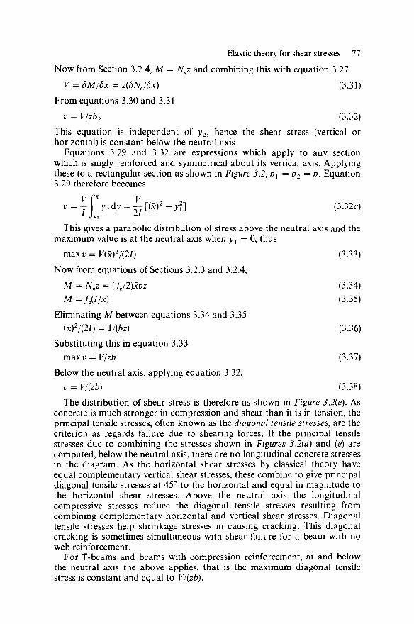
Elastic theory for shear stresses 77 Now from Section 3.2.4, M = Nsz and combining this with equation 3.27
V = SM/dx = z(SNJdx) (3.31)
From equations 3.30 and 3.31
v = V/zb2 (3.32) This equation is independent of y2, hence the shear stress (vertical or horizontal) is constant below the neutral axis.
Equations 3.29 and 3.32 are expressions which apply to any section which is singly reinforced and symmetrical about its vertical axis. Applying these to a rectangular section as shown in Figure 3.2,bl=b1 = b. Equation 3.29 therefore becomes
v = j{Xy.dy = ^ll(x)2-y2^ (3.32a)
This gives a parabolic distribution of stress above the neutral axis and the maximum value is at the neutral axis when yt = 0, thus
maxv = V(x)2/(2I) (3.33) Now from equations of Sections 3.2.3 and 3.2.4,
M = Ncz = (fJ2)xbz (3.34) M=fc(I/x) (3.35)
Eliminating M between equations 3.34 and 3.35 (x)2/(2I) = l/(bz) (3.36)
Substituting this in equation 3.33 max v = V/zb (3.37)
Below the neutral axis, applying equation 3.32, v = V/{zb) (3.38)
The distribution of shear stress is therefore as shown in Figure 3.2(e). As concrete is much stronger in compression and shear than it is in tension, the principal tensile stresses, often known as the diagonal tensile stresses, are the criterion as regards failure due to shearing forces. If the principal tensile stresses due to combining the stresses shown in Figures 3.2(d) and (e) are computed, below the neutral axis, there are no longitudinal concrete stresses in the diagram. As the horizontal shear stresses by classical theory have equal complementary vertical shear stresses, these combine to give principal diagonal tensile stresses at 45° to the horizontal and equal in magnitude to the horizontal shear stresses. Above the neutral axis the longitudinal compressive stresses reduce the diagonal tensile stresses resulting from combining complementary horizontal and vertical shear stresses. Diagonal tensile stresses help shrinkage stresses in causing cracking. This diagonal cracking is sometimes simultaneous with shear failure for a beam with no web reinforcement.
For T-beams and beams with compression reinforcement, at and below the neutral axis the above applies, that is the maximum diagonal tensile stress is constant and equal to V/(zb).

78 Reinforced concrete beams
Example 3.7. From the previous discussion the distribution of horizontal (or vertical) shear stress in the concrete for the section in Figure 3.3(a) of Example 3.4 is as shown in Figure 3.3(b), being parabolic for GH, JK and LM. Determine the shear stresses represented by points H, J, K, L, M and N, if the shear force is 60 kN.
For points M and N, that is maximum at neutral axis XX, using equation 3.29 (and figures from Example 3.4) it is simpler to consider the section below the neutral axis for the moment of area term
v = [0.06/(0.016 34 x 0.16)] x 0.044 18 x (0.847 - 0.3179) MN/m2
= 0.5365 N/mm2
As explained previously this is equal to V/(zb). Thus alternatively from equation 3.10
z = 1.634 x 10⁶/[441.8(84.7 - 31.79)] cm
= 699 mm
then
i? = 60000/(699 x 160)
= 0.5365 N/mm2
For approximate preliminary design one would perhaps have guessed that the centre of compression was at about half the depth of the T-flange giving z = 847 — 75 = 772 mm, about 10% error on the dangerous side. The following shear stresses are not needed by the designer but are of academic interest.
For point H, using equation 3.29
0.06 v = x 0.45 x 0.05(0.3179 - 0.025) MN/m2
0.016 34x0.45 '
= 0.053 78 N/mm2
For point J
0.06 v = 0.053 78 + x 0.017 59 x (0.3179 - 0.05)
0.016 34x0.45 = 0.053 78 + 0.03845 = 0.092 23 N/mm2
For point K 0.06
v = x 0.45 x 0.15 x (0.3179 - 0.075) + 0.038 45 0.016 34x0.45 ;
= 0.1722 N/mm2
For point L
v = 0.1722 x 0.45/0.16 = 0.4843 N/mm2
3.4 Shear reinforcement
Generally speaking experimental research1 shows that if design is based on ultimate strength in shear with suitable load factors, then diagonal crack widths at working loads are acceptable. The ultimate shear forces carried by
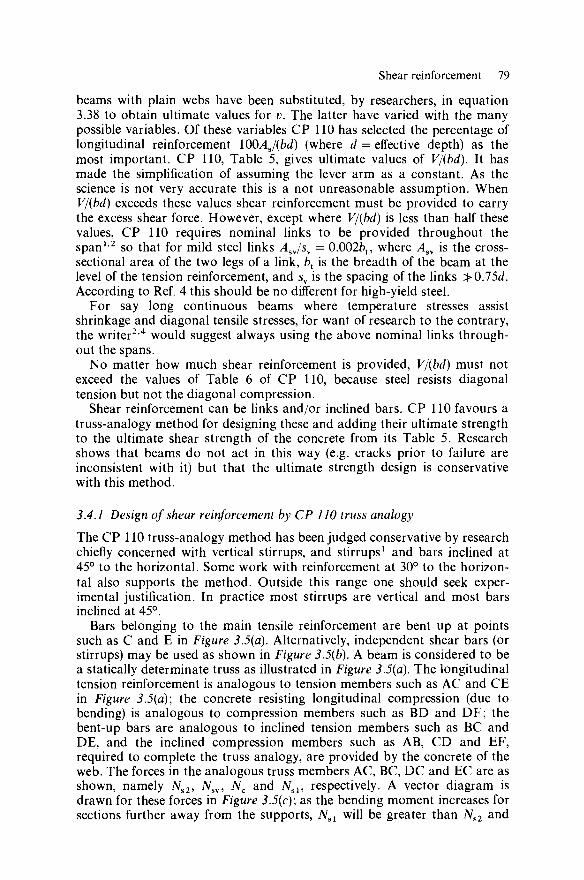
Shear reinforcement 79
beams with plain webs have been substituted, by researchers, in equation 3.38 to obtain ultimate values for v. The latter have varied with the many possible variables. Of these variables CP 110 has selected the percentage of longitudinal reinforcement 100AJ(bd) (where d = effective depth) as the most important. CP 110, Table 5, gives ultimate values of V/(bd). It has made the simplification of assuming the lever arm as a constant. As the science is not very accurate this is a not unreasonable assumption. When V/(bd) exceeds these values shear reinforcement must be provided to carry the excess shear force. However, except where V/(bd) is less than half these values, CP 110 requires nominal links to be provided throughout the span1,2 so that for mild steel links AsJsy = 0.002fot, where ^ s v is the cross-sectional area of the two legs of a link, bt is the breadth of the beam at the level of the tension reinforcement, and sv is the spacing of the links >0.75d. According to Ref. 4 this should be no different for high-yield steel.
For say long continuous beams where temperature stresses assist shrinkage and diagonal tensile stresses, for want of research to the contrary, the writer2,4 would suggest always using the above nominal links through-out the spans.
No matter how much shear reinforcement is provided, V/(bd) must not exceed the values of Table 6 of CP 110, because steel resists diagonal tension but not the diagonal compression.
Shear reinforcement can be links and/or inclined bars. CP 110 favours a truss-analogy method for designing these and adding their ultimate strength to the ultimate shear strength of the concrete from its Table 5. Research shows that beams do not act in this way (e.g. cracks prior to failure are inconsistent with it) but that the ultimate strength design is conservative with this method.
3.4.1 Design of shear reinforcement by CP 110 truss analogy
The CP 110 truss-analogy method has been judged conservative by research chiefly concerned with vertical stirrups, and stirrups1 and bars inclined at 45° to the horizontal. Some work with reinforcement at 30° to the horizon-tal also supports the method. Outside this range one should seek exper-imental justification. In practice most stirrups are vertical and most bars inclined at 45°.
Bars belonging to the main tensile reinforcement are bent up at points such as C and E in Figure 3.5(a). Alternatively, independent shear bars (or stirrups) may be used as shown in Figure 3.5(b). A beam is considered to be a statically determinate truss as illustrated in Figure 3.5(a). The longitudinal tension reinforcement is analogous to tension members such as AC and CE in Figure 3.5(a); the concrete resisting longitudinal compression (due to bending) is analogous to compression members such as BD and DF; the bent-up bars are analogous to inclined tension members such as BC and DE, and the inclined compression members such as AB, CD and EF, required to complete the truss analogy, are provided by the concrete of the web. The forces in the analogous truss members AC, BC, DC and EC are as shown, namely Ns2, Nsv, Nc and Nsl, respectively. A vector diagram is drawn for these forces in Figure 3.5(c); as the bending moment increases for sections further away from the supports, Ns l will be greater than Ns2 and

80 Reinforced concrete beams
Top reinforcement
Bottom reinforcement
(b)
Figure 3.5
(d)

Shear reinforcement 81
their difference is represented by the vector KM; forces Nc and Afsv are represented by the vectors LK and LM respectively. If the area of tensile reinforcement which is analogous to member CE is As, and the area of the bars bent up is \j/As, and if the bent-up bars are required to develop their full stress /sv, then Nsy = ij/Asfsy. At the same time, if the stresses in the members CA and CE are not to exceed fs, they are designed so that Nsi = Asfs and Ns2 = (As — ij/As)fs. Hence, referring to Figure 3.5(c) the vector LM = ^4S/8V and the vector KM = Asfs - (As - ij/As)fs = \//Asfs. In the case of mild steel reinforcement, fsy=fs and therefore LM = KM; consequently in the vector diagram LKM,
OL = OLX (3.39)
For high-yield steel,4 using/sv = 250N/mm2 (CP 110 would say 425) and fs = say 460N/mm2, LM = 250$ As and KM = 460$ As,
a n d f r o m t h e vector diagram
sin a/sin a t = LM/KM = 250/460 (3.40)
The inclined compression members are assumed to be sufficiently strong for all requirements. They are safeguarded by compliance with Table 6 of CP 110. By Ritter's Method of Sections, assume the truss to be cut at the section xx shown in Figure 3.5(a). Then resolving vertically for, say, the left-hand side of this section
Nsv sin p = Shear force at xx = V (3.41)
The principle of the superposition of trusses can be applied. For example, the system shown in Figure 3.5(d), where sv = AC/2, is assumed to be twice as strong as the system of Figure 3.5(a); hence from equation 3.41
V = 2NsysinP (3.42)
The inclined bars shown in Figures 3.5(a) and (d) are sometimes described as being in single-shear and double-shear, respectively. Extending this principle of superposition for any value of sv in Figure 3.5(d), equation 3.42 becomes
V = (AC/sy)Ns,sinP (3.43)
From triangle ABC AC = z(cota + cot£) (3.44)
This is traditional international truss analogy, but CP 110 says z = d
. . AC = d(cot a + cot p) (3.44a)
Hence equation 3.43 becomes
V = (Nsvd/sv) sin 0(cot a + cot P) (3.45)
Applying equation 3.45 to mild steel reinforcement and hence using the equation 3.39, also from triangle KLM in Figure 3.5(c),
a + a i + i S - 180° (3.46)

82 Reinforced concrete beams
Therefore from equation 3.39
a = 90°-03/2) (3.47)
Substituting this in equation 3.45
V = (iVsvd/5v) sin j8[tan(j8/2) + cot p]
= (Nsv^/sv)[2sin2(jS/2) + cosiS]
.'. V = Nsvd/sv (3.48) Applying equation 3.45 to high tensile reinforcement, and hence using
equation 3.40
sina = (250/460) sin a t
Therefore from equation 3.46
sin a = (250/460) sin(180° - fi - a)
.'. 1.84 sin a = sin p cos a + cos (5 sin a
.'. cot a = (1.84-cos jS)/sinj8 (3.49)
Substituting this in equation 3.45
V = (Nsyd/sy)(l .84 - cos fi + cos /?) = 1M(Nsyd/sv) (3.50)
For inclined bars CP 110 recommends the truss analogy as described, but using a < 45°. For stirrups CP 110 assumes that x = d and a = 45°, so that equation 3.45 becomes
V = (Nsvd/sv)(sin fi + cos P) (3.51)
From equation 3.51 and substituting Afsv = AsvfyJym = /lsv0.87/yv
^svAv = K/[0.87/yv(sin p + cos P)d~] (3.52)
For vertical stirrups P = 90°, thus
AJsy = F/(0.87/yvd) (3.53)
Table 3.5 (upper half) is useful for designers, uses equation 3.53, and refers to mild steel stirrups with /yv = 250N/mm2, from Table 2.10. According to Ref. 4 this also applies to all other stirrups. However, for those who wish to use CP 110 for cold deformed hot-rolled high-yield steel stirrups, fyy = 410N/mm2, the lower half of Table 3.5 is provided. This would be reasonable also for the use of deformed cold-worked high-yield steel stirrups, because CP 110 limits/yv to 425 (only 3.7% more than 410).
For mild steel bars bent up at 45°, from equation 3.39, a = CLX = 67.5°. Table 3.6 gives shear resistances for single-shear systems for single bars, using equation 3.41 and l/ym = 0.87. Ref. 4 would use/yv = 250N/mm2 for all other bars. CP 110 allows /yv = 410-425 N/mm2 for deformed high-yield steel bars and Table 3.6 gives shear resistances for/yv = 410 N/mm2 which is all right for all deformed high-yield bars.
Example 3.8. A beam of T-section has a rib of breadth 250 mm, d = 600 mm and 100AJ(bd) = 1.2. Design links to resist an ultimate shear force of 200 kN if the characteristic strength of concrete = 25 N/mm2.

Shear reinforcement 83
S
a oa H
i S
< <■
O ON ON (N m 00
r - i n CN co co r-» ON Tf r- CN *—'
m o m r- co o
—i CN
CN i n r - r^ Tf -H ON r - NO o co" Tf Tf OO r o OO T f CN
—i - H CN
r^ CN oo so t o ON ON ON OO m Tf
-H CN
i n co oo ' ©
ON co CN —i ON O © ON © NO o r » © r - oo
CO ON CN m ON rsj © '*" »n r - CN ON _ .
O oo oo i n ^ i n r s ' t n i ^ Tf ON co oo Tf CN co co r-
- ^ CN ^ H CN co
OO Tf ON t—
p r co 00 CN —•
co
CN
NO
Tf co
NO
r-;
© CN
NO oo 00 Tf CN T>
vo co od © in NO co »n
r - ON NO •^H Tf NO
o ON
o OO
NO CN ON co Tf r— »H rN n
r- co »-H co co r-in r- CN —1 CN Tf
Tf OO CN CN ON CN CN CO NO
—( CN Tf CN OO © m Tf © CN T> r-
O i n i n ON *-H i—t
3 H i n ON i n
—t CN Tf
i n CN oo r - *-> oo ~H CO T f
oo oo r -NO r - TT CN T t r-~
CN COi Tf OO CN © O O H O CN i n oo
CN r^ oo NO c-»' co' co ON co co in ON
O co co Tf CN NO NO r - co Tf CO OO CN Tf s o
co r- o
§ £ 2
NO OO O NO OO O

84 Reinforced concrete beams
TABLE 3.6.
Single bars in single shear
/ y v , N / m m 2 i m m 10
250 K, kN 12.08
410 KkN 19.81
at 45°, 1/7
12
17.39
28.53
m = 0.87
16
30.92
50.71
20
48.29
79.24
25
75.49
123.8
32
123.7
202.9
V/(bd) = 0.2/(0.25 x 0.6)MN/m2 = 1.333 N/mm2, which is satisfactory from Table 6 of CP 110 (see Section 3.4). From Table 5 of CP 110 (see Section 3.4) shear resistance provided by concrete web alone
= [0.65 + (1.2 - 1.0)(0.85 - 0.65)] x 250 x 600N = 103.5 kN. Hence shear reinforcement is required and it has to resist 200 — 103.5 = 96.5 kN. Using stirrups the V/d required is 96.5/0.6 kN/m = 160.8 N/mm. From Table 3.5 use 6 mm diameter mild steel two-arm stirrups at 75 mm centres (164 > 160.8).
Example 3.9. A beam of rectangular cross section has b = 300 mm, d = 700 mm, and \00AJ(bd) = 1.87. The ultimate shear force it has to resist is 642kN. Design a suitable shear reinforcement system. Assume characteristic strength of concrete in compression = 20 N/mm2.
V/bd = 0.642/(0.3 x 0.7) MN/m2 = 3.06 N/mm2, which is satisfactory from Table 6 of CP 110 (see Section 3.4).
From Table 5 of CP 110 (see Section 3.4) shear resistance provided by concrete web alone
= [0.8 + (0.8 - 0.6) x (1.87 - 1.0)] x 300 x 700N = 204.5 kN. Hence shear reinforcement is required and it has to resist 642 — 204.5 = 437.5 kN. According to CP 110 the shear force taken by bent-up bars must not exceed 0.5 x 437.5 = 218.8kN. Using pairs of 20mm diameter bent-up mild steel bars in double shear, from Table 3.6 this is worth 48.29 x 4 = 193.2 kN (< 218.8). Thus the amount to be resisted by stirrups is 437.5 -193.2 = 244.3 kN, giving V/d = 244.3/700 kN/mm = 349 N/mm. Using mild steel links with two arms, from Table 3.5, 10mm diameter links at 90mm centres give V/d = 379.6 N/mm (> 349).
3.5 Bond' stresses due to shear (or flexural bond)
The theory expounded concerning shear stresses (Section 3.3) assumes perfect adhesion of the concrete to the tensile reinforcement, and therefore involves 'bond stresses' being developed between the steel and the concrete. Referring to Figure 3.4(b), the change of force in the tensile reinforcement between the sections shown is (Ns + SNS) — Ns = SNS. This can only be resisted by bond stresses which act on the contact area between the steel and the concrete of Sxl,us. Hence the bond stress at this locality is given by
/bs = dNJ(dxXus) = (l/Lu^dNJdx) (3.54) where Xus = sum of the perimeters of bars of tensile steel. Now
V = dM/dx = (d/dx)(Nsz) = z(dNJdx) (3.55)

Torsion 85
Hence from equations 3.54 and 3.55
/bs = V/(zZus) = V/(ZldXus) (3.56)
These bond stresses are known as local bond stresses and ultimate values of V/(dI,us) = z1fhs are recommended for various types of concrete in Table 21 of CP 110, even though/bs is derived from the elastic theory. Research on ultimate values has been related to F/(ZZMS), however, and as the results are not very precise it is not unreasonable for CP 110 to take zx as constant. Designs need to ensure that ultimate local bond stresses are nowhere exceeded and this is the only requirement in this connection; such bond stresses are local effects and do not for instance require any anchorage.
Example 3.10. The maximum tensile reinforcement in a beam consists of four 25 mm diameter plain bars, and d = 600 mm. The maximum ultimate shear force im-mediately adjacent to a support is 140kN. If the ultimate local bond stress of Table 21 of CP 110 is 2N/mm2 (= Zj/JJ, what is the least number of the reinforcement bars which must continue through to the support? Note that CP 110 calls our z{fhs just/bs.
Applying equation 3.56, Zws = 140000/(2 x 600) = 116.7 mm. The circumference of one 25mm diameter bar = n x 25 = 78.5mm. Number of bars required to continue through to support = 116.7/78.5 = 2, to nearest integer.
3.6 Torsion
Torques are usually calculated assuming a structure to be elastic and uncracked. This is true neither at working nor at ultimate loads, but there is no reliable alternative to this procedure. The monolithic nature of in-situ construction means that most sections inevitably experience torques, even if only very small, at some time or other. The experience of the designer usually enables him to provide for minor torques when detailing the reinforce-ment. For example, the external beams to a floor might be given nominal stirruping of say 10 mm diameter at 230 mm centres, as opposed to say 6 mm diameter at 300 mm centres for the internal beams (assuming the possibility of torques on the internal beams is negligible, that is a low ratio of live to dead load). This practice is obviously satisfactory in that torsional failures are extremely rare, yet the majority of structures are never over-loaded and have been designed to more conservative past codes. CP 110 indicates that where torsional resistance of members can be ignored in analysis of an indeterminate structure, only nominal shear reinforcement (Section 3.4) is required for torsion. If torsional resistance needs assessing, CP 110 requires the torsional rigidity, G x C, of a member to be such that G = 0.4£c and C, the torsional moment of inertia, equal to half polar second moment of area based on the gross concrete sections. This makes some allowance for the fact that plane cross sections warp under torsion, and the classical theory assumes plane sections remain plane. Torsion failures are very inconsistent and this leads to divergent views upon design by various researchers. In practice, torques often occur simultaneously with shear forces and bending moments, thus complicating the problem still

86 Reinforced concrete beams
further, especially as the design of members in shear is a difficult problem in itself. In this respect it is good practice to create structural systems so that torsion is always a subsidiary and negligible effect.
Design has been based on the classical work of St. Vernant5 modified in the light of experimentation. The maximum shear stress due to torsion for a rectangular section is at the middle of the longer sides5 according to St. Vernant, whereas CP 110 assumes a plastic stress distribution, that is a uniform shear stress given by
^ = 6r/[^ i n(3/ I m a x- / l m i n)] (3.57)
where T is the torsional moment due to ultimate loads, hmin is the smaller dimension of the section, and /imax is the larger dimension of the section.
T-, L- or I-sections may be treated by dividing them into their com-ponent rectangles, so as to maximise the function ^(h^inhmax) which will generally be achieved if the widest rectangle is made as long as possible. The torsion shear stress carried by each component rectangle can be calculated by treating them as rectangular sections subjected to a torsional moment of
T T ^ A a x A ^ m i A a x ) ]
Where the torsion shear stress, i?t, exceeds the value vt from Table 7 of CP 110, reinforcement should be provided. In no case should the sum of the shear stresses resulting from shear force and torsion (v + vt) exceed the value vtu from Table 7 of CP 110 nor, in the case of small sections (yl < 550 mm), should the torsion shear stress, vt9 exceed vtuy1/550, where yl is the larger dimension of a link in mm.
Torsion reinforcement should consist of rectangular closed links together with longitudinal reinforcement. CP 110 requires this reinforcement to be additional to any requirements for shear or bending and to be such that:
0.87/yv(Asv/5v) ^ T/(0.*xiyi) (3.58)
Asl ^ (AJsJfMixt + yi) = [TAO.Sx^^CUi + *i)/0.87/yl] (3.59)
where Asv is the area of the legs of closed links at a section, Asl is the area of longitudinal reinforcement, /yv is the characteristic strength of the links, fyl
is the characteristic strength of the longitudinal reinforcement, sv is the spacing of the links, xx is the smaller dimension of the links, and y{ is the larger dimension of the links.
In the above formulae fyy and fyl are not to be taken as greater than 425N/mm2. (Ref. 4 would say 250N/mm2.)
Example 3.11. Design links for the section shown in Figure 3.2, hmax = 488 mm, to resist an ultimate torsional moment of 3 kN m combined with an ultimate vertical shear force of 60kN. Concrete is of Grade 25, cover is 25 mm (xx = 100mm, and y^ = 438mm), and /yv = 250N/mm2. If fyl = 425N/mm2, what extra longitudinal reinforcement is required?
From equation 3.57, t?t = (6x 0.003)/[0.152(3 x 0.488 - 0.15)] MN/m2 = 0.6088 N/mm2.

Torsion 87
From Table 7 of CP 110, this is >0.33 so that torsional reinforcement is required.
V/(bd) = 0.06/(0.15 x 0.45) MN/m2 = 0.8889 N/mm2
vx + V/(bd) = 1.498
This is in order, as Table 7 of CP 110 limits this to 3.75. As yx < 550mm, vt must not exceed 3.75 x 438/550 = 2.99N/mm2, which is all
right as vt = 0.6088 N/mm2.
From equation 3.58,
0.87/yv(yl8V/sv) = 3/(0.8 x 0.1 x 0.438)kN/m = 85.62 N/mm
Using Table 3.2, W0AJ(bd) = (100 x 982)/(150 x 450) = 1.455. From Table 5 of CP 110, V/(bd) = 0.65 + 0.2 x 0.455 = 0.741 N/mm2.
Hence shear reinforcement (two-arm links) is required to resist a value of V/(bd) = 0.8889 - 0.741 = 0.1479 N/mm2.
Also from Table 6 of CP 110, 0.741 < 3.75 and is therefore satisfactory.
V/d = 0.1479 x b = 0.1479 x 150 = 22.19 N/mm
Total V/d = 85.62 (see equation 3.53) + 22.19 = 107.8
From Table 3.5, use 8 mm diameter two-arm links at 200mm centres. From equation 3.59,
Asl = 85.62(100 + 438)/(0.87 x 425) = 124.6mm2
Refer to CP 110, as yl > 300 mm, use two bars in the top corners of the stirrups, two at hall depth (of y{) of stirrup (wired to inside of stirrup) and two in the bottom corners of the stirrups. The latter cannot be catered for by just increasing the size of the tension steel in this case, as the cover would be inadequate. Neither can a bar be placed between these tension bars because of the spacing required between bars (assuming /i = 19 mm). The bottom two bars for torsion will therefore be placed above the tension bars, a clear distance of 19 x 2/3 = 13 mm above them. Thus, using Table 3.2, six 6 mm diameter bars will be used as the longitudinal torsion bars.
Example 3.12. An L-shaped beam has: depth and overall breadth of top flange 120 mm and 300 mm, respectively, thickness and overall depth of web 100 mm and 600 mm, respectively. The ultimate vertical and horizontal shear forces are 20 kN and 10 kN, respectively and the ultimate torque is 2kNm. Determine the reinforce-ment required for resisting shear and torsion. Concrete is of Grade 30. Cover to longitudinal steel is 20 mm.
Taking the gross web as one rectangle,
2*iiAn« = l3 x 6 + 1.23 x (3 - 1) = 9.46dm4
Taking the gross flange as one rectangle
^miAiax = 1.23 x 3 + l3 x (6 - 1.2) = 5.184 + 4.8 = 9.984dm4
Hence the latter is the way to consider the section as two rectangles. For the gross flange, torque = 2 x 5.184/9.984 = 1.038 kNm. For the web, torque = 2 - 1.038 = 0.962kNm. From equation 3.57:
6x0.001038 0.122(3x 0.3 - 0 . 1 2 ) '
6x0.000962
for gross flange vt = A i l 2 n r> i—AT^T M N / m 2 = 0.5545 N/mm2
for web v. = — " " "' ~— MN/m2 = 0.4307 N/mm2
1 0.12(3x 0.48 -0 .1 ) '

88 Reinforced concrete beams
From Table 7 of CP 110, these are >0.37 so that torsional reinforcement is required for both gross flange and web.
For gross flange V/(bd) = 0.01/(0.12 x 0.27) = 0.3086N/mm2 (assuming d = 300 - 30 = 270mm). For web V/(bd) = 0.02/(0.1 x 0.57) = 0.351 N/mm2 (assuming d = 600 - 30 = 570mm). For gross flange vt+ V/{bd) = 0.8631 N/mm2. For web vt+ V/{bd) = 0.782 N/mm2.
These are in order as Table 7 of CP 110 limits this value to 4.1. For gross flange yl = 300-40 = 260mm. For web yt =600-40 = 560 mm. As yl < 550 for the gross flange, vt for it must not exceed 4.1 x 260/550 =
1.938 N/mm2, which is all right as vt = 0.5545 N/mm2. The design is continued, treating the gross flange and web, respectively, as in
Example 3.11, as though each were an independent member.
3.7 Plastic analysis
A material is in a plastic condition when stresses cause permanent defor-mations, that is when stress is no longer directly proportional to strain (as in Hooke's law). A section of a beam experiences such conditions when realising its ultimate moment of resistance. The plastic method of design predicts the ultimate moment of resistance, and this is required to equal the ultimate bending moment derived from the working loads multiplied by suitable load factors, called the design loads by CP 110.
3.7.1 Assumptions of plastic design methods
Plastic design concerns two ideas. Firstly, with regard to the assessment of the bending moments in a redundant frame, plasticity is the ability of highly stressed sections to what might be termed yield, and allow a redistribution6
of the bending moments towards failure. Secondly, plastic design can be employed in the design of individual sections of structural members. In the latter instance the following assumptions are employed.
It is assumed that plane sections subjected to bending remain plane after bending, which means that the distribution of strain is linear. Some relationship is then assumed between this strain, and stress. This is where the methods differ. Concrete is assumed to have no resistance in flexural tension, perfect bond is assumed between the steel and the concrete, the depth of the steel reinforcement is assumed to be small compared with its effective depth, and normally temperature and shrinkage stresses are ig-nored in the stress analysis of sections.

Plastic analysis 89
3.7.2 Plastic design in bending
The term balanced design refers to the situation when the beam is designed to fail simultaneously in flexural compression and tension. Under-reinforced sections will fail in flexural tension and over-reinforced sections will fail in flexural compression. An under-reinforced section fails owing to yielding (or straining excessively in the case of high-yield steel) of the tensile reinforce-ment; this causes the cracks to open so that the depth of the beam available to resist flexural compression is reduced, and final collapse occurs by the crushing of the compression zone. This is not, however, a flexural compres-sion failure, since the failure has actually been precipitated by the in-adequacy of the tensile reinforcement and the final failure in apparent flexural compression is a secondary effect; it could be described as part of the disintegration of the beam after failure.
Figure 2.10 shows a typical relationship between stress and strain for concrete in compression. As described in Section 2.3.17, this will vary in shape according to the speed of loading, the strength of the concrete, etc. Considerable plasticity is experienced towards failure, i.e. stress is not linearly proportional to strain near failure. It is assumed that the distri-bution of strain due to bending is linear. The strain is therefore pro-portional to the distance from the neutral axis. Curves such as those illustrated in Figure 2.10 can therefore be plotted on the axes O/and Oy as shown in Figure 3.6. For example Figure 3.6(a) illustrates the elastic stress distribution at working loads at a section where there is a crack. For higher loads the stress distribution becomes as shown in Figure 3.6(b), and just before failure the stress distribution will be as shown in Figure 3.6(c). The point denoted by g is at the same position on all of Figures 2.10, 3.6(a), (b) and (c). Different scales are used for the strains plotted on the axes Oy. The diagrams ehgO in Figure 3.6 are termed stress blocks.
yocc y y >
e
0
h
3r^^
,
e
0/ /
/ /
7
/
k
h
/ /
>
e
0
h
X ( a ) ( b ) ( c )
Figure 3.6
For estimating the ultimate moments of resistance of beams, the shape of the stress block just before failure must be known. This is assessed empirically, and shapes suggested for the stress block just before failure have included parabolas, cubic parabolas, trapeziums, ellipses, and many unusual shapes; some theories have even assumed that part of the concrete just below the neutral axis resists tensile stresses. This idea is not justified by experiments, because the cracks penetrate too far so as to reduce the compression zones at the critical sections. C. S. Whitney, in 1937, suggested
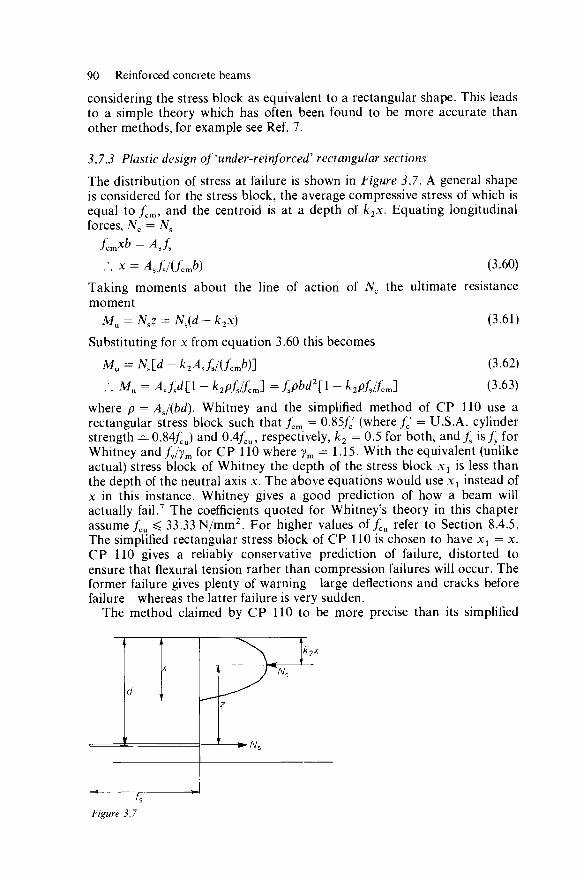
90 Reinforced concrete beams considering the stress block as equivalent to a rectangular shape. This leads to a simple theory which has often been found to be more accurate than other methods, for example see Ref. 7.
3.7.3 Plastic design of 'under-reinforced' rectangular sections
The distribution of stress at failure is shown in Figure 3.7. A general shape is considered for the stress block, the average compressive stress of which is equal t o / c m , and the centroid is at a depth of k2x. Equating longitudinal forces, Nc = Ns
Jem*" = ASJS
.-. x = AsfJ(fcmb) (3.60) Taking moments about the line of action of Nc the ultimate resistance moment
Mu = Nsz = Ns(d-k2x) (3.61)
Substituting for x from equation 3.60 this becomes
Mu = J V s [ ( i - M . / s / 0 ] .'. Mu = AMI - k2pfjfcm\ =fpbd\\ - k2pfjfcm]
where p = AJ(bd). Whitney and the simplified method of CP 110 use a rectangular stress block such that/ c m = 0.85/c' (where /c ' = U.S.A. cylinder strength ^ 0.84/cu) and 0.4/cu, respectively, k2 = 0.5 for both, and/ s is /y for Whitney and/y/ym for CP 110 where ym = 1.15. With the equivalent (unlike actual) stress block of Whitney the depth of the stress block xx is less than the depth of the neutral axis x. The above equations would use xx instead of x in this instance. Whitney gives a good prediction of how a beam will actually fail.7 The coefficients quoted for Whitney's theory in this chapter assume fcu ^ 33.33 N/mm2. For higher values of/cu refer to Section 8.4.5. The simplified rectangular stress block of CP 110 is chosen to have x{ = x. CP 110 gives a reliably conservative prediction of failure, distorted to ensure that flexural tension rather than compression failures will occur. The former failure gives plenty of warning—large deflections and cracks before failure—whereas the latter failure is very sudden.
The method claimed by CP 110 to be more precise than its simplified
(3.62) (3.63)
\k7X
A/c
Figure 3.7

Plastic analysis 91
r~ i
- — € , — >
/ > /
/
F
k
/ ' / X
- £ o *
/
/
t ■ 1
A
(G )
-« /
(b)
i *
G
t k2x
, 1 ^ c
B
1 j E D
Figure 3.8
method uses a stress block as shown in Figure 3.8(b) and the distribution of strain shown in Figure 3.8(a), where el = 0.0035. Tests over many years show that the maximum extreme fibre compressive strain realised before failure in flexure is about this figure. CP 110 specifies e0 = {y/fcu}/5000, fl = 0.45/cu and curve AB as a parabola. Thus, considering the shape ABD, its area is AD x BD/3, C is its centroid and CE = BD/4. The compression force Nc is
fcmxb - (area ABGF)fo
•'• /cm* = a r e a ADGF — area ADB = / 1 x —/iX0/3
.'. fcm = / i [ l - *0/(3x)] = / i [ l ~ fi0/(3fii)]
.". /c« = 0.45/cu[l - {V(/cu)}/52.5] (3.64) Taking moments for compression force about F Nck2x = b[(area ADGF)0.5x - (area ADB)(x - CE)] fcmxk2x = O.S^x2 - (/iX0/3Xx - x0/4) • '. k2 = (fJLJlO.5 - {X0/(3X)}{1 - x0/(4x)}]
= {0.45/cu/(2/cm)}[l - {280/(3£l)}{l - e0/(4£l)}] .-. k2 = (0.225fJfcJll - {(V/CU)/26.25}[1 - (V/c»)/70]] (3.65) Equations 3.64 and 3.65 are the same as given on page v, Appendix A of
Part 2 of CP 110, and are the basis of the design charts.
3.7.4 'Balanced' plastic design of rectangular sections
The equations of Section 3.7.3 apply. With these equations, as As increases x increases and Mu increases, but experimentally we find that x cannot

92 Reinforced concrete beams
increase beyond a certain amount and increasing the reinforcement further gives no increase in Mu, the section being known as over-reinforced. When x has its maximum value, and As corresponds to this, the section is in its 'balanced design' condition, the maximum flexural compression being bal-anced by the minimum i4s to give a maximum Mu for the section.
For balanced design Whitney gives x1 = 0.537d, and CP 110, for design purposes, gives x = 0.5d. Using the simplified CP 110 method, from Section 3.7.3, equation 3.60 becomes
0.5<* = AJJ(0Afcub), :. p = 0.2(/cu//s) (3.66)
Equation 3.61 becomes
Mu = AJs(d - 0.5 x 0.5d) = 0.15Asfsd (3.67)
and substituting for pfs from equation 3.66
Mu = 0J5pfsbd2 = 0A5fcubd2 = K,bd2 (3.68)
TABLE 3.7.
/ v ,
N/mm2
250 410 460 425 485
* i >
/., N/mm2
217 357 400 370 422
N/mm2
20
1.843 1.120 1.000 1.081 0.948
3.0
25
2.304 1.401 1.250 1.351 1.185
3.75
/ c u ,N/mm
30
2.765 1.681 1.500 1.622 1.422
4.5
2
40
3.687 2.241 2.000 2.162 1.896
6.0
50
4.608 2.801 2.500 p% 2.703 2.370
7.5
Equations 3.66 and 3.68 are used for design Table 3.7. Without tables, equation 3.68 is usually used to decide the size of the member as limited by the strength of the concrete. Then As is often obtained from equation 3.67 thus:
Mu Muym 1.15MU 1.533MU A
u u / m u u /T f£\\
O.lSdf, 0.754/, 0.754/, dfy
Example 3.13. A slab 160 mm thick is reinforced in tension with 16 mm diam-eter bars having 30 mm cover. Determine the spacing of the reinforcement if the slab is designed in accordance with CP 110 for an ultimate resistance mo-ment of 27.6 kNm, and if fcu = 25 N/mm2 = 25 000kN/m2, fy = 250 N/mm2 = 250000kN/m2 and ym for the steel = 1.15.
Using simplified CP 110 method, from equation 3.68 considering lm width of slab, for balanced design
Mu = 0.15 x 25 000 x 1 x (0.160 - 0.038)2
= 0.15 x 25 000 x0.1222
= 55.82kNm

Plastic analysis 93
This is greater than 27.6kNm, hence section is under-reinforced. From equation 3.62 (or 3.63), using/s = 250000/1.15 = 217400kN/m2
27.6 = 217400/4S[0.122 - 0.5 x 217400As/(0.4 x 25 000 x 1)]
.'. As = 0.001161m2 = 1161mm2
From Table 3.2, use 16 mm diameter bars at 150mm centres.
Example 3.14. Repeat Example 3.13 using the method preferred by CP 110.
Equations 3.64 and 3.65 give
fcm = 0.45 x 25[1 - {(V25)/52.5}] = 10.18 N/mm2
k2 = (0.225 x 25/10.18)[l - [{(V25)/26.25}{1 - (V25)/70}]] = 0.4548
From equations 3.60 and 3.62 for 1 m width of slab for balanced design
0.5 x 122 = ^217.4/(10.18 x 1000)
Mu = As x 217.4[122 - 0.4548/ls217.4/(10.18 x 1000)]
/ . Mu = 61 x 10180(122 - 0.4548 x 61)Nmm = 58.53kNm
This is >27.6, hence section is under-reinforced. Hence from equation 3.62
27.6 = 217400AS[0.122 - 0.4548 x 217400/4S/(10 180 x 1)]
.'. As = 0.001145 m2 = 1145 mm2
From Table 3.2, use 16 mm diameter bars at 175 mm centres. (Page ix of CP 110, Part 2, obtains the same answer by using the design charts.)
Example 3.15. The slab of Example 3.13 is reinforced in flexural tension with 16 mm diameter bars at 175 mm centres (that is, As = 1149 mm2 per metre) and is to be tested to destruction. Predict its ultimate resistance moment using Whitney's theory.7
To determine whether it is under- or over-reinforced, apply equation 3.60 (referring also to Sections 3.7.3 and 3.7.4).
x, = [1149 x 250/(0.85(0.84 x 25) x 1000}] = 16.09 mm
For balanced design xx = 0.537 x 122 = 65.5 mm, hence section is under-reinforced. Hence applying equation 3.62
Mu = 1149 x 250[122 - 0.5 x 1149 x 250/(0.85(0.84 x 25) x 1000}] N mm = 32.73 kNm
This is considerably greater than the 27.6kNm used in Example 3.14, indicating the conservativeness built into the CP 110 design method.
Example 3.16. Design a section of a beam, using the simplified CP 110 method, to have an ultimate resistance moment of 200kNm, using fcu = 20N/mm2, fy = 250N/mm2 and ym for steel = 1.15.
From equation 3.68,
200 xlO 6 = 0 . 1 5 x 2 0 M 2
.'. bd2 = 66.67 x 10⁶

94 Reinforced concrete beams
If b^0.5d say, then d3 = 133.3 x 10⁶ and d = 5li. So 6 = 255, say, choose b = 250mm. Then d = V(66.67 x 10⁶/250) = 516mm. From equation 3.69 (or 3.66 or 3.67)
As = 1.533 x 200 x 106/(516 x 250) = 2377 mm2
From Table 3.2 use three 32 mm diameter bars.
Example 3.17. Repeat Example 3.16 using Table 3.7.
From Table 3.7, K1 = 3N/mm2 and p = 1.843%. Using equation 3.68, bd2 = 200 x 106/3 = 66.67 x 10⁶. As in Example 3.15, choose b = 250mm, then d = 516mm. Then As = 0.018 43 x 250 x 516 = 2377mm2. From Table 3.2 use three 32 mm diameter bars.
3.7.5 Plastic design of any shape of'under-reinforced' section
For the section of Figure 3.4(a), using a rectangular concrete stress block of average stress fcm (see Section 3.7.3), equating longitudinal forces
/cnA = Asf (3.70) where Ac = area of concrete in compression. Taking moments about the line of action of Nc
Mu = Asfsz (3.71) where z = lever arm = distance between lines of action of Nc and Ns. Nc
acts at centroid of Ac. Whitney specifies fcm = 0.85/c' ^ 0 . 8 5 x 0.84/cu = 0.714/cu as before. CP
110 specifies fcm = 0Afcu for simplified design method.
3.7.6 'Balanced' plastic design of any shape of section
For balanced design (see Section 3.7.4) the depth of the stress block xx ob-tained from equation 3.70 is 0.537d for Whitney's theory and 0.5d for CP 110.
Example 3.18. A T-beam has a flange of breadth 750 mm and depth 130 mm. The width of its rib or web is 300 mm and the tensile reinforcement comprises one layer of five 25 mm diameter bars having an effective depth of 500 mm. Determine its ultimate resistance moment from the simplified design method of CP 110, assuming /cu = 20N/mm2,/y = 425N/mm2 and ym = 1.15 for the reinforcement.
From equation 3.70 and Table 3.2,
0.4 x 20[300x + (750 - 300) x 130] = 2455 x (425/1.15) .'. x = 183 mm As 0.5 x 500 = 250 the section is under-reinforced. Also x > depth of flange,
hence beam is designed as a T-beam and not a rectangular beam. If depth of centroid of Ac is k2x then taking area moments about the top of the
beam for Ac
Ack2x = 300x2/2 + (750 - 300) x (1302/2) .'. k2x = [8 826000/{300x + (750 - 300) x 130}] = 77.8 mm From equation 3.71 Mu = 2455 x (425/1.15) x (500 - 77.8)N mm = 383.1 kNm

Plastic analysis 95
3.7.7 Plastic design of any shape of 'under-reinforced' section containing com-pression steel
It might be said that compression reinforcement is only required in a beam when the balanced design condition applies. Whilst this is often true, there are cases where compression steel is available even though not required to assist flexural compression, for example sometimes at the supports of con-tinuous beams. In such cases the compression steel can increase the ultimate bending moment of the section and sometimes economises in tensile steel.
For a section like Figure 3.4(a) but including compression steel in the top, using a rectangular concrete stress block (see Section 3.7.3):
Compression force for gross area of concrete in compression = Acfcm
Compression force for compression steel over and above that included at this position above = A's(fsc -fcm)
Therefore equating longitudinal forces
AJcm + 4(/ , c -fcJ = AJS (3.72) where As = gross area of concrete in compression, A's = area of compression steel and fsc = stress in compression steel (usually characteristic strength because the strain is high in the concrete and thus the steel as flexural concrete failure occurs). Taking moments about the line of action of Nc
M^AJsZ^AJ^d-k.x,) (3.73)
Whitney specifies /cm —0.714/cu as before. CP 110 specifies fcm = 0.4/cu for simplified design method. Whitney gives /sc as yield stress of compression steel and CP 110 gives /sc as 2000/y/(2000ym +/y), where ym = 1.15, which it suggests can be simplified to 0.72/y for ease of calculation. There is no need to make this simplification if use is made of Table 3.8. These comments on
TABLE 3.8.
/ y ,N/mm 2
2000^/(2300 +/y), N/mm2
0.72/y,N/mm2
250
196.1
180.0
410
302.6
295.2
460
333.3
331.2
425
311.9
306.0
485
348.3
349.2
fsc depend upon the strain in the compression steel being at least that corresponding to its yield stress. The strain at the level of the compression steel needs to be assessed and related to the stress-strain relationship for the steel (for example CP 110, Fig. 2)—see Section 3.7.10. Note k2x1 is the depth to the total compression force resulting from concrete and compres-sion steel forces.
3.7.8 'Balanced' plastic design for any shape of section containing compression steel
For balanced design (see Sections 3.7.4 and 3.7.6) the depth of the stress block x1 is 0.531d for Whitney's theory and 0.5d for CP 110.
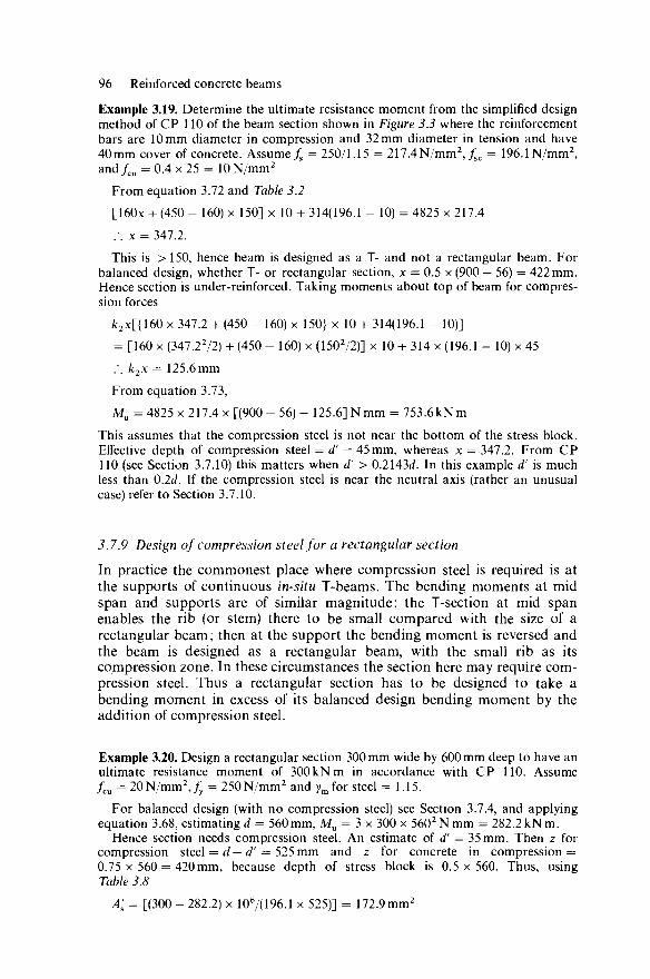
96 Reinforced concrete beams
Example 3.19. Determine the ultimate resistance moment from the simplified design method of CP 110 of the beam section shown in Figure 3.3 where the reinforcement bars are 10 mm diameter in compression and 32 mm diameter in tension and have 40mm cover of concrete. Assume fs = 250/1.15 = 217.4N/mm2,/sc = 196.1N/mm2, and/cu = 0.4 x 25 = 10N/mm2
From equation 3.72 and Table 3.2
[160x + (450 - 160) x 150] x 10 + 314(196.1 - 10) = 4825 x 217.4
.'. x = 347.2.
This is >150, hence beam is designed as a T- and not a rectangular beam. For balanced design, whether T- or rectangular section, x = 0.5 x (900 — 56) = 422 mm. Hence section is under-reinforced. Taking moments about top of beam for compres-sion forces
/c2x[{160 x 347.2 + (450 - 160) x 150} x 10 + 314(196.1 - 10)]
= [160 x (347.22/2) + (450 - 160) x (1502/2)] x 10 + 314 x (196.1 - 10) x 45
.'. k2x = 125.6mm
From equation 3.73,
Mu = 4825 x 217.4 x [(900 - 56) - 125.6] N mm = 753.6kNm
This assumes that the compression steel is not near the bottom of the stress block. Effective depth of compression steel = d' = 45 mm, whereas x = 347.2. From CP 110 (see Section 3.7.10) this matters when d' > 0.2143d. In this example d' is much less than 0.2d. If the compression steel is near the neutral axis (rather an unusual case) refer to Section 3.7.10.
3.7.9 Design of compression steel for a rectangular section
In practice the commonest place where compression steel is required is at the supports of continuous in-situ T-beams. The bending moments at mid span and supports are of similar magnitude; the T-section at mid span enables the rib (or stem) there to be small compared with the size of a rectangular beam; then at the support the bending moment is reversed and the beam is designed as a rectangular beam, with the small rib as its compression zone. In these circumstances the section here may require com-pression steel. Thus a rectangular section has to be designed to take a bending moment in excess of its balanced design bending moment by the addition of compression steel.
Example 3.20. Design a rectangular section 300 mm wide by 600 mm deep to have an ultimate resistance moment of 300kNm in accordance with CP 110. Assume fcu = 20N/mm2,/y = 250N/mm2 and ym for steel = 1.15.
For balanced design (with no compression steel) see Section 3.7.4, and applying equation 3.68, estimating d = 560mm, Mu = 3 x 300 x 5602Nmm = 282.2kNm.
Hence section needs compression steel. An estimate of d' = 35 mm. Then z for compression steel = d — d' — 525 mm and z for concrete in compression = 0.75 x 560 = 420 mm, because depth of stress block is 0.5x560. Thus, using Table 3.8
A's = [(300 - 282.2) x 106/(196.1 x 525)] = 172.9 mm2

Limit state of deflection 97 From Table 3.2 use say two 12mm diameter bars. Resolving forces longitudinally (that is using equation 3.72),
(250/1.15) xAs = 300 x 0.5 x 560 x 0.4 x 20 + 172.9 x (196.1 - 0.4 x 20) .'. As = 3241mm2. From Table 3.2 use say seven 25 mm diameter bars. These will need to be in two
layers, say five in the bottom and two in the layer above. Using 19 mm down coarse aggregate the vertical distance between the layers of bars = 13 mm, say 15mm. This will mean that, using 25 mm cover to the tension steel, an estimate of d — 550 mm (the accurate value necessitates the calculation of the position of the centroid of these bars). Using 25 mm cover for the compression reinforcement, d' = 31mm. This design can be repeated with these more accurate values of d and d', but it should not alter the results as the reinforcement is on the generous side because of the limitation of bar sizes, and the initial estimates of d and d' were not too inaccurate. d' > 0.2143d, hence (see Section 3.7.10) the stress we have taken in the compression steel does not need reducing.
3.7A0 Compression steel near to neutral axis
In practice this can hardly ever arise, as when compression steel is required it is placed as far from the neutral axis as possible for economic reasons. At failure in flexure the maximum strain in the concrete is about 0.0035 and the distribution of strain is approximately linear. Hence the strain at the level of the compression steel is 0.0035 (x — d')/x. According to Fig. 2 of CP 110, if this strain is less than 0.002 then the stress-strain curve of Fig. 2 should be used to determine the design stress in the compression reinforce-ment. Hence for CP 110 we do not have to concern ourselves in Sections 3.7.7, 3.7.8 and 3.7.9 with reducing the stress in the compression steel if (x — d')/x < 20/35, that is x < 2333d'. In the case of balanced design x = 0.5d, and this becomes 0.5d < 2.333d', that is d' > 0.2143d (CP 110 calls this 0.2d).
3.7.11 Further points about compression steel
Compression steel, even if available in a section, should not be relied upon in design if not prevented by adequate anchoring from buckling out of the faces of the member; each bar should be anchored at right-angles to the outer surface of the concrete according to CP 114, but CP 110 has reduced this requirement in its Clause 3.11.4.3. Both codes specify diameter and spacing of suitable stirrups. For example, framing bars in a beam are not always suitably anchored for compression steel when evaluating ultimate resistance moment.
Compression steel, even if available in a section, should not be relied upon in design without adequate compression laps. For example, steel in the bottom of a continuous T-beam over a support with nominal lapping can only be used to the strength of the lapping in compression.
3.8 Limit state of deflection
Deflections can be calculated as in Example 3.2. This assumes the gross concrete section to be homogeneous and the deflection is obtained with
98 Reinforced concrete beams
elastic theory. The value assumed for Ec or ae (as Ec = EJoce) can vary considerably (see Section 2.3.15). For accurate work it is best to obtain Ec
from laboratory tests on specimens of the concrete. In loading tests on in-situ buildings with say Grade 20 (CP 110) concrete perhaps about 2-3 months old, the writer has experienced ae of about 10, that is due to the live load applied. In design it is useful to divorce the live and dead loadings and take ae = 8 for strong concretes to 10 for weak concretes for calculating deflections due to live loads (that is of short duration; not developing much creep), and take ae = 15 for deflections due to dead loading (this will be realised over several years of creep).
Ignoring the reinforcement and including concrete in tension, which at the positions of cracks will not exist, is usual practice. In the writer's experience troubles with deflection arising from design are usually due to no calculations of deflections, on at least these lines, being made. In the laboratory, obtaining Ec and Es from tests of specimens of the concrete and steel respectively, and allowing concrete to take tensile stresses and allowing for reinforcement to obtain /, deflections of beams can be predicted very accurately1 before cracks about 0.01mm wide occur. For greater loads the deflection often approaches the deflection calculated in the same way but excluding concrete in tension. Just before failure it often becomes greater than this calculated amount.
For a beam (span /) carrying uniformly distributed loading q and if the breadth is a constant proportion of its depth and if Ec is constant, then maximum deflection ~ql4/bd3 ~ qf/d*. Thus the l/d ratio can be a guide to deflection, but only in conjunction with q. The tables restricting l/d in CP 114 for beams and slabs were inadequate in that q was ignored. Tables 8 and 9 of CP 110 are similar but require modification by factors given in Tables 10 and 11, but whose derivation and justification are not given. For example, for a constant l/d the greater q the greater the deflection (even though the reinforcement will be increased slightly). Now from Table 10 the greater the reinforcement the less the factor, which reduces the allowable l/d ratio, so indirectly some allowance is made for q. Table 11 has similar logic but also allows for the fact that when compression steel is present it restrains the tendency of the shrinkage in this location to increase deflections.
Deflections must be limited so as not to cause trouble to internal partitions and finishes. Beams obviously sagging are aesthetically un-desirable—the deflection can be calculated and the beam given an upward camber of at least this amount. Slightly hogging beams are aesthetically acceptable. Consideration should be given to each particular case, and CP 110 gives general guidance on limitation of deflection.
3.9 Limit state of cracking
Research has indicated that water cannot penetrate to the reinforcement to cause corrosion if cracks are not greater than 0.25 mm wide. This figure can vary with the concrete grade, cover, etc., and CP 110 uses a figure of 0.3 mm, specifying other figures for various exposures. CP 110 considers that its reinforcement detailing recommendations take care of undesirable
Limit state of cracking 99
cracking. For example, smaller diameter bars at closer centres resist cracks much better than the converse. When this problem is of particular impor-tance because, say, of severe exposure, or where groups of bars are used, an empirical formula is given in Appendix A of CP 110 for assessing crack widths.
References
1. WILBY, C. B., Strength of Reinforced Concrete Beams in Shear, Ph.D. Thesis, University of Leeds(1949)
2. WILBY, C. B., 'Permissible Shear Stresses of the 1957 British Code of Practice1, Journal of the American Concrete Institute, June (1958)
3. 'Lessons from Failures of Concrete Structures', A.C.I. Monograph No. I (1965) 4. WILBY, C. B., 'Overstrain in High-tensile Reinforcing Bars at Bends and in Stirrups', Indian
Concrete Journal, Jan. (1962) 5. EVANS, R. H., and WILBY, C. B., Concrete—Plain, Reinforced, Prestressed and Shell,
Edward Arnold (1963) 6. WILBY, C. B., and PANDIT, C. P., Tnelastic Behaviour of Reinforced Concrete Single Bay
Portal Frames', Civil Engineering and Public Works Review, Mar. (1967) 7. EVANS, R. H., The Plastic Theories for the Ultimate Strength of Reinforced Concrete
Beams', Journal of the Institute of Civil Engineers, Dec. (1943)

Chapter 4
Reinforced concrete slabs
4.1 Slabs spanning 'one way'
These are designed per unit width as rectangular beams (see examples in Chapter 3).
One-way spanning slabs have always been designed as beams of consider-able width. This involves secondary distribution reinforcement being pro-vided which has been specified as various amounts by different codes of practice over the years. The specifications have been based on practical experience. This 'distribution reinforcement' is provided to distribute tem-perature and shrinkage effects, to assist in fixing and spacing the main steel, and to act as distribution steel for concentrated loads.
4.2 Slabs spanning 'two ways'
These are, for example, in-situ rectangular slabs supported on four, three or two adjacent sides. Originally they were designed by ascertaining bending moments and shear forces by elastic theory and then designing sections for these by elastic theory (Sections 3.2.4 and 3.3). Subsequently it was possible (CP 114) alternatively to design the resistance to bending moments by plastic theory (Section 3.7.2). This seems to have been satisfactory, but is very illogical, as towards failure the distribution of the bending moments will be different to that given by the elastic theory.
Bending moments from elastic theory can be calculated from simple formulae in CP 110 for rectangular slabs carrying uniformly distributed loads. These together with formulae for slabs with triangularly distributed loadings (for walls of tanks) and with concentrated loads are given in Reynolds' Handbook.
A later step has been to design slabs by assessing the bending moments at collapse by Johansen's yield-line1 or Hillerborg's strip method.2
Generally shear stresses are low and usually found to be satisfactory when checked. Slab thicknesses are often dictated by deflection consider-ations and sometimes slabs have to have a minimum practical thickness 100
Slabs spanning 'two ways' 101
of preferably 125 mm. Deflections may be calculated from elastic theory but are more simply dealt with using Tables 8, 9 and 10 of CP 110. Cracks can be controlled at working loads by attention to detailing (see CP 110).
4.2.1 General discussion of design2* of two-way spanning slabs
British Standard CP 114, 1957 gave bending moment coefficients for two-way spanning rectangular slabs with simply supported edges in its Table 16. These coefficients were determined from Grashof-Rankine formulae (de-veloped independently by Grashof in Germany and Rankine in the U.K.), which were derived by equating the central deflections of two strips of slab, each of unit width, at right-angles to each other, and each bisecting the slab. Ref. 3 claimed that this method gives greater bending moments than exist. The problem of corners tending to lift was considered complex. The neglect of torsion at the corners was justification for over-estimating bending moments. Ref. 3 also considered that test results justified the omission of corner reinforcement.
Table 17 of CP 114, 1957 gave bending moment coefficients for slabs restrained along all edges; with hinged (discontinuous) and fixed (con-tinuous) edge conditions. These coefficients were obtained from U.S.A. regulations based on a mathematical analysis by Westergaard4,5 and sup-ported by test data. Some plastic redistribution of bending moments was assumed to occur to reduce the number of coefficients to a minimum to help designers. At corners where at least one of the two sides meeting was discontinuous, reinforcement was specified by CP 114.
CP 114, 1957 allowed an alternative method to the above to be used, namely a 'purely theoretical analysis' based on the elastic theory with Poisson's ratio = 0, provided the sections were designed elastically using a modular ratio = 1 5 . The basis of the exact elastic theory of plates spanning in two directions was established by Lagrange and Navier in the nineteenth century, but most of the problems having practical importance have been solved in the past sixty-five years or so, when the names of Neuber, Bubnov, Timoshenko, Galerkin, Vlassov, Kalmanok and Girkmann have been in-separably associated with the fundamentals of the classical theory of plates. These analyses, prior to the availability to designers of computers and finite element and other methods suitable for the computer, were considered to be out of the question for designers of reinforced concrete slabs. Thus Ref. 3 recommends the use of Marcus's6 method (proposed and used in Germany) which is similar to the Grashof-Rankine method but includes a simple correction to allow for restraint at corners and for assistance given by torsion. The results of Marcus's method were considered3 to deviate by only 1-2% from a rigorous elastic analysis based on the elastic theory of plates. Marcus's method was also used by the German reinforced concrete regulations. Bending moments in continuous panels were determined by a method provided by Loser7 based on Marcus's method. Ref. 3 gives design tables using Loser's method for various ratios of dead to live load. Prior to CP 114, 1957 Reynolds' Reinforced Concrete Designer's Handbook of 1948 recommended the same as the above except Pigeaud's method instead of Westergaard's method. CP 114, 1957 allowed a further alternative method

102 Reinforced concrete slabs
of design to the above two methods, namely Johansen's8'9 yield-line method. A load factor of 1.8 was recommended but a restriction was placed on using the full concrete cube strength for extra safety. However Ref. 3 expressed worries about the 'upper bound' (see Section 4.4.3) nature of yield-line designs and the method's inability to give 'stress conditions away from the yield lines and hence information on how to distribute reinforce-ment'. Ref. 3, however, anticipated that the yield-line method might be popular for 'complex slab systems for which computations according to the elastic theory are impracticable'. Alongside the British practice just de-scribed, Westergaard4,5 was a pioneer in elastic analysis of two-way rein-forced concrete slabs in the U.S.A. In Ref. 5 Westergaard recommended moment coefficients that gave considerable weight to the non-elastic (plas-tic) readjustments in slab moments which take place before failure. In recognition of these favourable adjustments, his recommended coefficients were established at 28% below strictly elastic values. The A.C.I. Standard Building Code Requirements for Reinforced Concrete (ACI 318-63) 1963 recommended three alternative designs. Two fundamentally stemmed from Westergaard although work by Van Buren, Di Stassio10 and Berlin11 was also recognised, whilst the other was based on the work of Marcus.
It will be noticed that the yield-line method was permitted by the British code in 1957 but not by the U.S.A. code of 1963. It was not permitted by the A.C.I. Building Code of 1971 but permitted by the Code of 1977. In 1962 Ref. 12 was published in the English language. This gave formulae for cal-culating the ultimate bending moment at collapse for many differently-shaped slabs.
In 1964 Ref. 13 was published in the Czech language. A German and English edition was published in 1969 and an enlarged German/English edition was published in 1971. This work gave about 600 pages of tables of coefficients for bending moments, shear forces, and deflections at many points of square, rectangular and skew slabs with many combinations of restraint and free edge conditions, and of reactions at various points along the supports.
About 1960 many bridges were beginning to be designed for a large programme of motorways in the U.K. There was considerable demand for methods of designing two-way deck slabs of rectangular and sometimes skew shapes. Computers were not easily available, nor easy to use by most designers of reinforced concrete slabs. The Grashof-Rankine method was extended by some so that a slab analysis was considered as a grillage analogy. Then the grillage could be analysed by the method of Hendry and Jaeger,14 or later the method of Bares and Massonnet,15 prior to computers and then eventually by computers and computer packages. Also a great interest in both research and design developed concerning Johansen's yield-line method. Subsequently, and to date, finite difference and finite element methods for elastic design have been developed con-siderably for use with computers. CP 110:1972 allows 'elastic analysis' for bending moments (and shear forces) as in CP 114. Likewise it again allows the use of Johansen's yield-line method. It now also allows Hillerborg's strip method to be used. However, it now restricts these methods with the proviso that 'the ratios between support and span mo-ments are similar to those obtained by the use of elastic theory; values

Slabs spanning 'two ways' 103
between 1.0 and 1.5 are recommended'. This requires some sort of elastic analysis to be made as well as the ultimate strength analysis. This mitigates against the advantage of ultimate collapse mechanism analysis previously quoted; that is its advantage when elastic analyses are complex and a computer program is not available.
CP 110 recommends the use of the coefficients in its Table 12 for two-way spanning slabs which are simply supported along their edges, and have inadequate torsional resistance at their corners to prevent them lifting. This table is derived from the Grashof-Rankine formulae previously mentioned. It recommends the use of the coefficients in its Table 13 for slabs which are rectangular and cast monolithically with their supports. These coefficients have been derived from yield-line analysis and calculated from values given by Taylor et al}6.
Hillerborg's method for designing for ultimate strength was published in Sweden (in Swedish) in 1956 and 1959. It received much more attention after a critical analysis of the method and a comparison of it with tests were published by Wood and Armer17,18,19 in 1968. They found (mathemati-cally) that the 'strip' method did not suffer from the disadvantage of being 'upper bound' as did Johansen's method. The strip method gave the designer wide freedom of choice in his design approach. It is easier to curtail reinforcement than is the case with Johansen's method. Wood and Armer pointed out that a design using moments approaching those from elastic analysis was an efficient design and to be preferred. The suitability of the method for slabs with openings is a strong point in its favour.
The most difficult slabs for this method are those supported on columns. For such cases Hillerborg developed what Crawford20 calls the advanced strip method, using a rectangular element (in lieu of a strip) carrying load in two directions to a support at one corner of the element. Wood and Armer report that they could not prove a mathematical basis for this type of element even though they devoted a considerable time to this investigation. For irregular shapes the advanced Hillerborg method also uses elements of triangular shape. An alternative to Hillerborg's advanced method is Kemp's21 method, which is also much easier to understand.
The methods just mentioned, namely Hillerborg (strip and advanced) and Kemp can, particularly in the hands of an inexperienced designer, produce designs which are very unsatisfactory for limit state of deflection and cracking. The less the design departs from elastic theory the more efficient the design in these respects as mentioned by Wood and Armer (see previously). As regards the design of an individual strip with one or both ends fixed, the distribution of bending moments obtained from an elastic analysis can be altered to say increase or decrease the mid-span moment in accordance with the plastic theory but not making this alteration can still be considered as one possible plastic analysis. That is this one particular plastic analysis choice does not conflict with elastic analysis and thus helps to control stresses (thus cracks) and deflections at working loads. Thus the method of Fernando and Kemp22 was developed to control the freedom of choice of Kemp's21 method so as not to depart too greatly from the elastic method of matching up the deflections of an element in the two directions at right-angles; this is similar to the method of Grashof-Rankine for elastic theory, but more rigorous, complicated and difficult (requiring computer

104 Reinforced concrete slabs
assistance) than Grashof-Rankine in that deflections of all elements are dealt with, whereas Grashof-Rankine dealt only with the central point. In some ways the Fernando and Kemp method is similar to using a beam-analogy method for a slab and solving as a grillage with a computer program but ignoring torsional resistance of the beams. In this case normal flexibility coefficients would be used. These are simpler to derive than the special flexibility coefficients needed for the Fernando and Kemp method and which deal with short loads instead of point loads.
Wilby23 wrote computer programs (which are essential) for using the strip-deflection method,22 for any size of rectangular slab with any type of support conditions, loading and any number of strips taken in each direction. These programs were used to produce many design tables.24 As the equations given in Ref. 22 are mainly incorrect they are fully developed in Ref. 24.
4.2.2 Design tables15 for two-way slabs
Various design tables which have been in use over approximately the past decade are listed below. Many of these tables are still in use. They are all based on the limit state of ultimate strength, except for those based on CP 114 and even these are modified because of ultimate strength considerations.
1. Taylor, S. R., Hayes, B. and Mohamedbhai, G. T. G.16 The coefficients presented are derived from the yield-line theory and apply to the full width of the slab. It is recommended16 that the loading used should be the design load of 1.4 times the dead load plus 1.6 times the live load, as given in CP 110. It is also suggested16 that although in theory the full width of the slab should be used, in practice only a middle strip (three-quarters of the width) of the slab might be reinforced in accordance with the moments produced from these coefficients, and similarly for the length of the slab. In the derivation of the coefficients, yield lines have been extended to the corners of the slab and corner levers (see later) have been ignored.
2. CP 110 Coefficients in Table 13 of CP 110 are based on work done by Taylor, Hayes and Mohamedbhai16 but have been modified to some extent. They give coefficients for the full width of the slab with a suggestion of reinforcing only a middle strip (see 1. previously). Similarly, CP 110 defines a middle strip of three-quarters of the full width of the slab and states that the steel area, obtained from the moments calculated from the moment coefficients, is used only to reinforce this middle strip. Edge strips are then reinforced by using the minimum area of steel given in clause 3.11.4.1 of CP 110.
3. Thakkar, M. C. and Rao, J. K. S.26 In this method the average moment distribution per unit width of the slab is derived for uniform orthotropic reinforcement throughout the whole width of the slab. That is, the slab is analysed by Hillerborg's strip method and then the average of the moments for all strips along each edge is taken and this value is the moment per metre width quoted by the tables.
4. CP 114 These tables have been obtained from a theoretical elastic analysis and adjusted in the light of experimental data. This code separates each direction of the slab into a middle strip, of width three-quarters the

Yield-line theory of slab analysis 105
width of the slab, and edge strips one-eighth of the width of the slab. Where slabs have aspect ratios greater than four the middle strip in the short direction could be taken to have a width of ly — lx and each edge strip a width of /x/2, where /x and ly are the short and long spans of the slab, respectively. The coefficients given in the table are used for the middle strip of the slab only.
5. Wilby, C. B. Wilby has produced tables24,27 with his computer program for the strip-deflection22 method for eight strips in each of two mutually perpendicular directions, namely length and width. To obtain coefficients for comparison with the previously mentioned tables, the mean values for the full widths of the slabs of bending moment per unit length have been taken. As the methods compare reasonably well these tables may be used in lieu of those in CP 110 and they consider cases not considered by CP 110. Also they give deflections.
43 Flat slabs
These are slabs without beams supported only by columns. Flared column heads usefully reduce the high shear stresses in the slabs around the column heads. Flat slabs generally give a heavier construction than beam and slab systems; they require more concrete and steel but the shuttering is much less expensive. For longer spans of flat slabs dropped panels are sometimes used to make the construction lighter in weight. This usually means dropping the soffits of rectangular portions of slab around the column heads. Flat slabs are described further in Section 7.3 which also describes 'waffle' slabs.
Design has been based on empirical formulae which are limited to systems with rectangular panels, length-to-width not exceeding 4/3, with at least three continuous spans in both directions. Such formulae are given in CP 110 and are simple to use. The alternative method allowed by CP 110 is more arduous but is useful when the empirical formulae do not apply. It consists of dividing the structure longitudinally and transversely into frames consisting of columns and the connecting strips of the slabs, and then elastically analysing these frames for bending moments and shear forces. This is well enunciated in CP 110. More recently they might be designed using Johansen's yield-line1 or Hillerborg's strip method.2
4.4 Yield-line theory of slab analysis
Having read the previous Sections 4.2 to 4.3 the reader might still ask, 'Why use the yield-line instead of the elastic theory?' Even though the basic equations of the theory of elasticity are simple enough, it can be extremely difficult to solve these equations for complex structural formations. This difficulty can also apply to finite element methods. Also the yield-line theory gives a more realistic representation of the behaviour of slabs at ultimate limit states than the elastic theory.
There are two different methods of yield-line analysis, perhaps most simply introduced by the following two examples.
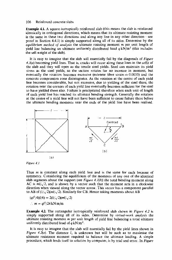
106 Reinforced concrete slabs
Example 4.1. A square isotropically reinforced slab (this means the slab is reinforced identically in orthogonal directions, which means that its ultimate resisting moment is the same in these two directions and along any line in any other direction—see proof in Section 4.4.1) is simply supported along all of its sides. Determine by the equilibrium method of analysis the ultimate resisting moment m per unit length of yield line balancing an ultimate uniformly distributed load <jkN/m2 (this includes the self-weight of the slab).
It is easy to imagine that the slab will essentially fail by the diagonals of Figure 4.1(a) becoming yield lines. That is, cracks will occur along these lines in the soffit of the slab and they will open as the tensile steel yields. Steel can maintain its yield stress as the steel yields, so the section rotates for no increase in moment, but eventually the rotation becomes excessive (extreme fibre strain =^ 0.0035) and the concrete compression zone disintegrates. As the rotation at the centre of each yield line becomes considerable, but not excessive, due to yielding of the steel there, the rotation near the corners of each yield line eventually becomes sufficient for the steel to have yielded there also. Failure is precipitated therefore when each unit of length of each yield line has reached its ultimate bending strength. Generally the rotation at the centre of a yield line will not have been sufficient to cause failure there before the ultimate bending moments near the ends of the yield line have been realised.
k / H Centroid
(a)
Figure 4.1
Thus m is constant along each yield line and is the same for each because of symmetry. Considering the equilibrium of the moments of any one of the identical slab segments about the support (see Figure 4.1(b)) the total bending moment along AC is m//v
/2, and is shown by a vector such that the moment acts in a clockwise direction when viewed along the vector arrow. This vector has a component parallel to AB of (1/V2XW//V2). Similarly for CB. Hence taking moments about AB
(ql2/4W6) = 2(l/V2Xm//V2) / . m = g/2/24kNm/m
Example 4.2. The rectangular isotropically reinforced slab shown in Figure 4.2 is simply supported along all of its sides. Determine by virtual-work analysis the ultimate resisting moment m per unit length of yield line balancing a total ultimate uniformly distributed load of qkN/m2.
It is easy to imagine that the slab will essentially fail by the yield lines shown in Figure 4.2(a). The distance lx is unknown but will be such as to maximise the ultimate resistance moment required to balance the ultimate loading. A simple procedure, which lends itself to solution by computer, is by trial and error. In Figure
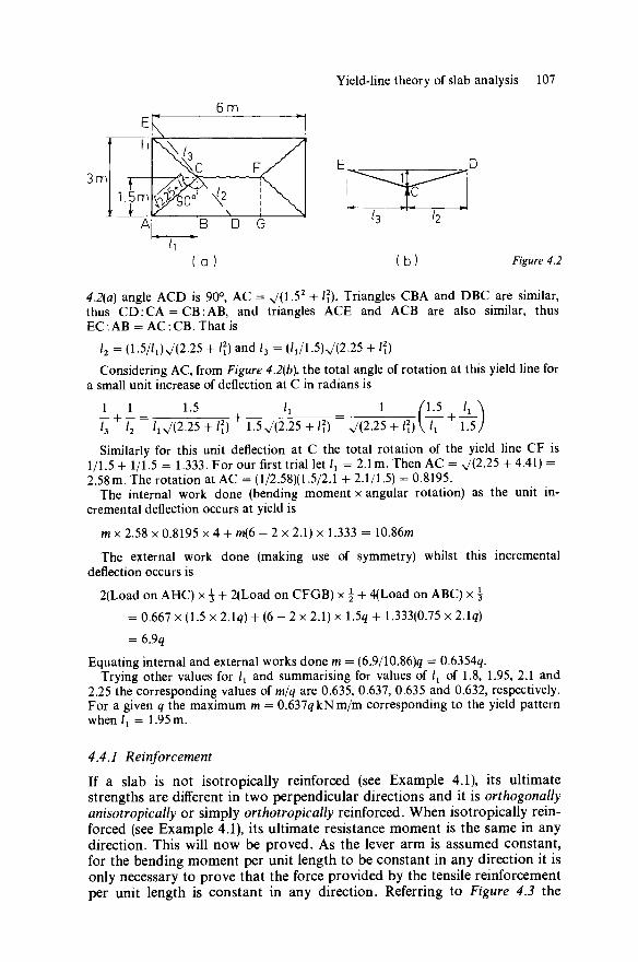
Yield-line theory of slab analysis 107
( Q ) ( b ) Figure 4.2
4.2(a) angle ACD is 90°, AC = V(l-52 + '?)• Triangles CBA and DBC are similar, thus CD: CA = CB: AB, and triangles ACE and ACB are also similar, thus EC:AB = AC:CB.Thatis
l2 = {1.5/1^(225 + l\) and /3 = (/1/1.5)V(2.25 + l\)
Considering AC, from Figure 4.2(b), the total angle of rotation at this yield line for a small unit increase of deflection at C in radians is
1 1 1.5 I, _ 1 /1.5 _^_\ T3
+ T2 ~ /lv/(2.25 + /?) + 1.5 V(2.25 + l\) " V(2.25 + l\) \ h + 1.5/ Similarly for this unit deflection at C the total rotation of the yield line CF is
1/1.5 + 1/1.5 = 1.333. For our first trial let lx = 2.1m. Then AC = V(2.25 + 4.41) = 2.58m. The rotation at AC = (1/2.58)(1.5/2.1 + 2.1/1.5) = 0.8195.
The internal work done (bending moment x angular rotation) as the unit in-cremental deflection occurs at yield is
m x 2.58 x 0.8195 x 4 + m(6 - 2 x 2.1) x 1.333 = 10.86m The external work done (making use of symmetry) whilst this incremental
deflection occurs is 2(Load on AHC) x £ + 2(Load on CFGB) x \ + 4(Load on ABC) x £
= 0.667 x (1.5 x 2.I4) + (6 - 2 x 2.1) x 1.5q + 1.333(0.75 x 2.1q)
= 6.9q
Equating internal and external works done m = (6.9/10.86)^ = 0.6354<j. Trying other values for lx and summarising for values of lx of 1.8, 1.95, 2.1 and
2.25 the corresponding values of m/q are 0.635, 0.637, 0.635 and 0.632, respectively. For a given q the maximum m = 0.637<? kN m/m corresponding to the yield pattern when /x = 1.95 m.
4.4.1 Reinforcement
If a slab is not isotropically reinforced (see Example 4.1), its ultimate strengths are different in two perpendicular directions and it is orthogonally anisotropically or simply orthotropically reinforced. When isotropically rein-forced (see Example 4.1), its ultimate resistance moment is the same in any direction. This will now be proved. As the lever arm is assumed constant, for the bending moment per unit length to be constant in any direction it is only necessary to prove that the force provided by the tensile reinforcement per unit length is constant in any direction. Referring to Figure 4.3 the
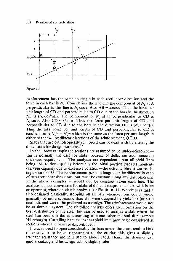
108 Reinforced concrete slabs
Figure 4.3
reinforcement has the same spacing s in each rectilinear direction and the force in each bar is Ns. Considering the line CD the component of Ns at A perpendicular to this line is Ns cos a. Also AB = s/cosa. Thus the force per unit length of CD and perpendicular to CD due to the bars in the direction AE is (Ns cos2a)/s. The component of Ns at D perpendicular to CD is N ssina. Also CD = s/sina. Thus the force per unit length of CD and perpendicular to CD due to the bars in the direction DF is (Ns sin2a)/s. Thus the total force per unit length of CD and perpendicular to CD is (cos2 a + sin2a)iVs/s = NJs which is the same as the force per unit length in either of the two rectilinear directions of the reinforcement, Q.E.D.
Slabs that are orthotropically reinforced can be dealt with by altering the dimensions for design purposes.28
In the above example the sections are assumed to be under-reinforced— this is normally the case for slabs, because of deflection and minimum thickness requirements. The analyses are dependent upon all yield lines being able to develop fully before say the initial portion loses its moment-carrying capacity due to excessive rotation—the extreme fibre strain reach-ing about 0.0035. The reinforcement per unit length can be different in each of two rectilinear directions, but must be constant along any line, otherwise in the above examples m would not be constant along each line. The analysis is most convenient for slabs of difficult shapes and slabs with holes or openings, where an elastic analysis is difficult. R. H. Wood2 says that a slab designed elastically, stopping off all bars whenever one could, would generally be more economic than if it were designed by yield line (or strip method), and was to be preferred as a design. The reinforcement would not be so simple a system. The yield-line analysis offers no information on the best distribution of the steel, but can be used to analyse a slab where the steel has been distributed according to some other method (for example Hillerborg's). Curtailing bars means that yield lines have to be considered at sections where the bars are discontinued.
If cracks need to open considerably the bars across the crack tend to kink to endeavour to be at right-angles to the cracks; this gives a slightly stronger resistance moment (up to about 14%). Hence the designer can ignore kinking and his design will be slightly safer.
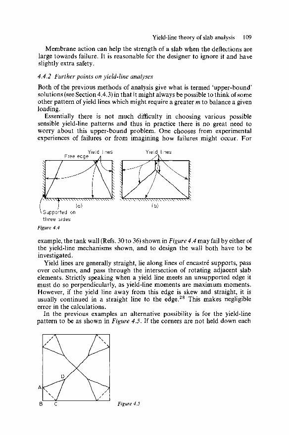
Yield-line theory of slab analysis 109
Membrane action can help the strength of a slab when the deflections are large towards failure. It is reasonable for the designer to ignore it and have slightly extra safety.
4.4.2 Further points on yield-line analyses
Both of the previous methods of analysis give what is termed 'upper-bound' solutions (see Section 4.4.3) in that it might always be possible to think of some other pattern of yield lines which might require a greater m to balance a given loading.
Essentially there is not much difficulty in choosing various possible sensible yield-line patterns and thus in practice there is no great need to worry about this upper-bound problem. One chooses from experimental experiences of failures or from imagining how failures might occur. For
\ Supported on three sides
Figure 4.4
example, the tank wall (Refs. 30 to 36) shown in Figure 4.4 may fail by either of the yield-line mechanisms shown, and to design the wall both have to be investigated.
Yield lines are generally straight, lie along lines of encastre supports, pass over columns, and pass through the intersection of rotating adjacent slab elements. Strictly speaking when a yield line meets an unsupported edge it must do so perpendicularly, as yield-line moments are maximum moments. However, if the yield line away from this edge is skew and straight, it is usually continued in a straight line to the edge.28 This makes negligible error in the calculations.
In the previous examples an alternative possibility is for the yield-line pattern to be as shown in Figure 4.5. If the corners are not held down each
B C Figure 4.5

110 Reinforced concrete slabs
corner element such as ABCD will rotate about AC lifting B from the support. If the corners are held down, at each corner, lines such as AC will become yield lines. In this case reinforcement is required perpendicularly to lines such as AC in the top of such a slab. The slab spans between AD and CD, and AB and BC, and sometimes supplementary reinforcement is desired to take care of this, the bars being parallel to the direction AC and in the bottom of the slab. The yield lines at corners are called 'corner levers'. Although their effect is adverse they are often neglected in yield-line analyses for simplicity. For right-angled corners this causes an error of about 9% with bottom steel only and much less when there is top as well as bottom steel. The error is particularly high37 for acute angles with free edges, about 26% with bottom steel only and 14% when there is top and bottom steel.
For non-rectangular shapes Ref. 12 is useful.
4.4.3 'Upper-bound' and 'lower-bound' solutions
Most engineering analyses or designs make approximations which cause them to give conservative solutions. In yield-line terminology these are called 'lower-bound' solutions. The yield-line theory as developed to date gives only 'upper-bound' solutions which are dangerous.
It was of course a worry, which delayed the acceptance of yield-line analysis for design, that one might consider a reasonably sensible yield-line pattern for failure and then the solution should turn out to be upper bound and one might sometimes wonder with a complicated slab how many crack patterns one might need to consider to obtain a solution at least felt to be insignificantly upper bound. Nevertheless the same com-plicated slabs may well be more difficult to analyse elastically.
The critical pattern was easy to obtain in Example 4.2 by varying one parameter, namely ll9 to obtain a maximum value of m/q. Had one of the short sides been fixed (or encastre) then there would have been a second similar variable locating the distance of F from one of the shorter sides. Had two adjacent sides been fixed then using a similar crack pattern there would have been four variables, namely the co-ordinates locating C and F. If one programmed the analysis on say a microcomputer then one could make many trials of various combinations of guessed values of the four co-ordinates and this would be a speedy and easy way of obtaining a solution, which could be difficult without the computer.
In Example 4.2 the maximised or critical yield-line pattern with lx = 1.95 m still gives an upper-bound solution because other patterns, often for example with a greater number of yield lines, will give solutions which are less upper bound. (NB The trials with /x not equal to 1.95 m do not satisfy equilibrium and are therefore invalid.)
4.4.4 Further consideration of the 'equilibrium method'
This has been introduced by giving Example 4.1 for a simple symmetrical case. For a less symmetrical case, suppose a region of a slab enclosed by yield lines is as shown in Figure 4.6. Each arrow along each edge indicates vectorially the bending moment for the yield line. Each arrow perpendicular

Yield-line theory of slab analysis 111
Figure 4.6
to each edge and in the plane of this region of the slab indicates vectorially the twisting moment for this yield line. Along each edge there will be a resultant shear force normal to the plane of the slab.
Johansen considered that for each edge the total twisting moment and the total shear force could be replaced by two forces (normal to the plane of the slab), one at each end of this edge. These forces are referred to as 'nodal forces'. For equilibrium it can be shown5 that:
1. If several yield lines converge to a point called a 'node' then all the nodal forces at this node must vectorially add up to zero.
2. When three yield lines meet at a point (that is a node) and the reinforcement is isotropic (that is identical in orthogonal directions) the nodal force for each yield line at this point is zero.
3. When a yield line intersects a free edge (see Figure 4.7) and the reinforcement is orthotropic and the m-moment key lines are as shown, then the nodal (or knot or edge) forces are as shown in Figure 4.7 and are given by
Kl2 = +nmcotij/ (4.1)
and K3l = — \im cot i// (4.2)
\m y
1 X^^^Yield line jum /
Free edge
Figure 4J
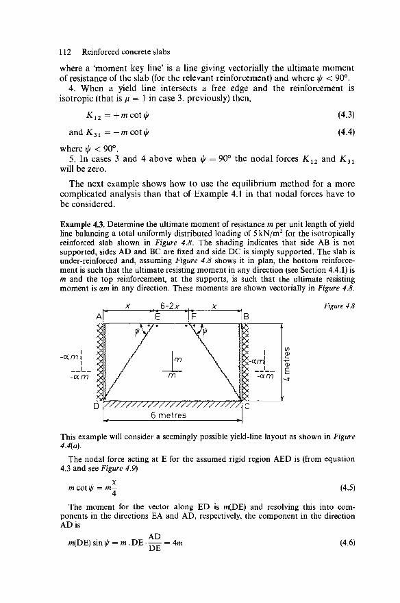
112 Reinforced concrete slabs
where a 'moment key line' is a line giving vectorially the ultimate moment of resistance of the slab (for the relevant reinforcement) and where \j/ < 90°.
4. When a yield line intersects a free edge and the reinforcement is isotropic (that is \i = 1 in case 3. previously) then,
K12 = +mcoti/^
and K3l = —mcotij/
(4.3)
(4.4)
where \\J < 90°. 5. In cases 3 and 4 above when \\i = 90° the nodal forces Kl2 and K3l
will be zero. The next example shows how to use the equilibrium method for a more
complicated analysis than that of Example 4.1 in that nodal forces have to be considered.
Example 4.3. Determine the ultimate moment of resistance m per unit length of yield line balancing a total uniformly distributed loading of 5 kN/m2 for the isotropically reinforced slab shown in Figure 4.8. The shading indicates that side AB is not supported, sides AD and BC are fixed and side DC is simply supported. The slab is under-reinforced and, assuming Figure 4.8 shows it in plan, the bottom reinforce-ment is such that the ultimate resisting moment in any direction (see Section 4.4.1) is m and the top reinforcement, at the supports, is such that the ultimate resisting moment is am in any direction. These moments are shown vectorially in Figure 4.8.
-Ot/77 1 I I
-am
x ,,6-2x x
\ 'IE I F '1
vy777777777777777777777777\ I 6 metres C
Figure 4.8
This example will consider a seemingly possible yield-line layout as shown in Figure 4.4(a).
The nodal force acting at E for the assumed rigid region AED is (from equation 4.3 and see Figure 4.9)
m cot \jj = m— (4.5)
The moment for the vector along ED is m(DE) and resolving this into com-ponents in the directions EA and AD, respectively, the component in the direction AD is
AD m(DE) sin ij/ = m. DE • —— = Am (4.6)
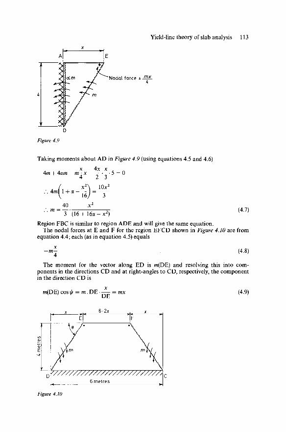
Yield-line theory of slab analysis 113
Nodal force = -02*. 1*
Figure 4.9
Taking moments about AD in Figure 4.9 (using equations 4.5 and 4.6)
x 4x x 4m + 4am — m—x — — • — • 5
4 2 3
A / x 2 \ 10x2
.• .4m^l + a--j = —
40 x2
• m = ■=-
= 0
3 (16 + 1 6 a - x 2 ) (4.7)
Region FBC is similar to region ADE and will give the same equation. The nodal forces at E and F for the region EFCD shown in Figure 4.10 are from
equation 4.4; each (as in equation 4.5) equals
x - m -
(4.8)
The moment for the vector along ED is m(DE) and resolving this into com-ponents in the directions CD and at right-angles to CD, respectively, the component in the direction CD is
m(DE) cos if/ = m. DE DE
6-2*
(4.9)
Y///////////////////////////A 6 metres
Figure 4.10

114 Reinforced concrete slabs
For region EFCD, moments about CD (see Figure 4. JO) give
x 5 = 0 mx 1 4 2mx + 2 4 - ( 6 - 2 x ) x 4 x 2 + 2 x - x 4 x x x -
20 / 9 - 2 x \ ■■■m = T{—) , 4 - 1 0 )
Equating the values of m in equations 4.7 and 4.10 gives
9x2 + 32(1 + a)x - 144(1 + a) = 0 (4.11) Exactly the same equation can be obtained by using the virtual-work analysis (see
Example 4.4), but not as simply and directly as a differentiation is involved to obtain the maximum value of m.
Equation 4.11 only applies to the yield-line pattern considered and which can only exist if x ^ 3, that is half the length of AB. From equation 4.11
- 32(1 + a) + V[322(l + a)2 4- 36 x 144(1 + a)] 18
(4.12)
Now a is positive and it can be seen that in equation 4.12 the square root is of a larger amount than 322(1 + a)2 and so it will give x as positive which of course it is. It can also be seen that increasing the value of a increases the value of x. Therefore, the greatest value of a for this yield-line layout is when x is a maximum for it, namely 3. Putting x = 3 in equation 4.11, gives a = 0.687. If a ^ 0.687 then the yield-line pattern just considered can be used. If, however, a > 0.687 then we are outside the range of this pattern and we shall need to consider a yield pattern the same as shown in Figure 4.9.
The above has been treated algebraically. For computer use it is better generally to analyse one yield pattern at a time and repeat the calculation by altering a relevant variable. In this case a would be chosen, a value of x guessed, and then m calculated from equations 4.7 and 4.10. The difference in these values is obtained. Then other values of x are chosen until the difference just mentioned is considered to be negligible.
4.4.5 Further consideration of the virtual-work method
The problem of Example 4.3 will now be solved using the virtual-work method in the following example.
Example 4.4. Consider unit displacement, normal to the plane ABCD in Figure 4.8, at E and F. The expenditure of energy by applied loading is as follows:
1. Portion AED (same as BFC by symmetry)
( i x 4 x x ) x 5 x | = f x
2. Portion EFCD
2 x ( x x x 4) x 5 x ^ + {(6 - 2x) x 4} x 5 x | = 60 - ^ x The internal energy held in yield lines is as follows: (a) Yield line AD (same as BC by symmetry)
angular rotation for unit displacement at E = 1/x radians moment = 4am energy = 4am/x
(b) Yield line ED (same as FC by symmetry) For convenience the moment vector along ED can be obtained by vectorially adding its components in directions parallel to DC and AD, respectively.
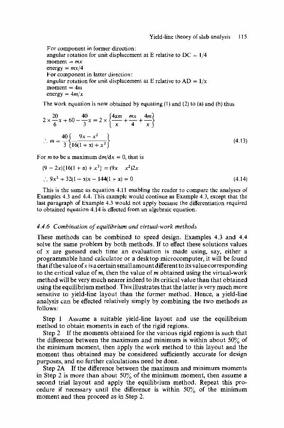
Yield-line theory of slab analysis 115
For component in former direction: angular rotation for unit displacement at E relative to DC = 1/4 moment = mx energy = mx/4 For component in latter direction: angular rotation for unit displacement at E relative to AD = 1/x moment = 4m energy = 4m/x
The work equation is now obtained by equating (1) and (2) to (a) and (b) thus
^ 2 0 40 f4am mx 4m) 2x— x + 6 0 - — x = 2x< + — + — > 6 3 [ x 4 x J
40f ■ 9x-x2 } " w - j { i 6 ( i + ,) + *»} (4'13)
For m to be a maximum dm/dx = 0, that is
(9 - 2x){16(l + a) + x2} = (9x - x2)2x
.". 9x2 + 32(1 + a)x - 144(1 + a) = 0 (4.14)
This is the same as equation 4.11 enabling the reader to compare the analyses of Examples 4.3 and 4.4. This example would continue as Example 4.3, except that the last paragraph of Example 4.3 would not apply because the differentiation required to obtained equation 4.14 is effected from an algebraic equation.
4.4.6 Combination of equilibrium and virtual-work methods
These methods can be combined to speed design. Examples 4.3 and 4.4 solve the same problem by both methods. If to effect these solutions values of x are guessed each time an evaluation is made using, say, either a programmable hand calculator or a desktop microcomputer, it will be found that if the value of x is a certain small amount different to its value corresponding to the critical value of m, then the value of m obtained using the virtual-work method will be very much nearer indeed to its critical value than that obtained using the equilibrium method. This illustrates that the latter is very much more sensitive to yield-line layout than the former method. Hence, a yield-line analysis can be effected relatively simply by combining the two methods as follows:
Step 1 Assume a suitable yield-line layout and use the equilibrium method to obtain moments in each of the rigid regions.
Step 2 If the moments obtained for the various rigid regions is such that the difference between the maximum and minimum is within about 50% of the minimum moment, then apply the work method to this layout and the moment thus obtained may be considered sufficiently accurate for design purposes, and no further calculations need be done.
Step 2A If the difference between the maximum and minimum moments in Step 2 is more than about 50% of the minimum moment, then assume a second trial layout and apply the equilibrium method. Repeat this pro-cedure if necessary until the difference is within 50% of the minimum moment and then proceed as in Step 2.
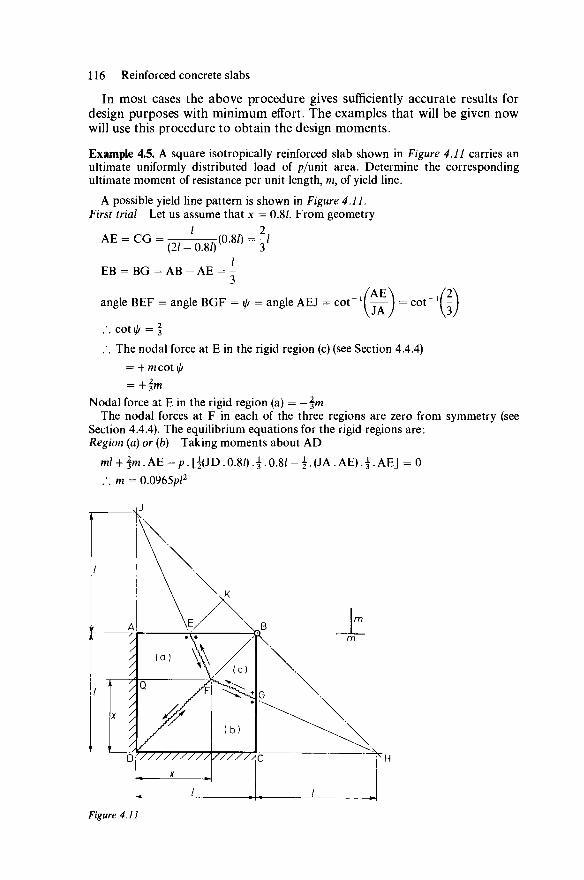
116 Reinforced concrete slabs
In most cases the above procedure gives sufficiently accurate results for design purposes with minimum effort. The examples that will be given now will use this procedure to obtain the design moments.
Example 4.5. A square isotropically reinforced slab shown in Figure 4.11 carries an ultimate uniformly distributed load of p/unit area. Determine the corresponding ultimate moment of resistance per unit length, m, of yield line.
A possible yield line pattern is shown in Figure 4.11. First trial Let us assume that x = 0.8/. From geometry
AE = CG = (21
-(0.8/) = - / -0.8/) 3
EB = BG = AB - AE
angle BEF = angle BGF = \jj = angle AEJ = cot" AE JAT
= cot"
.'. COtl/f = §
.*. The nodal force at E in the rigid region (c) (see Section 4.4.4) = + m cot \ff = +fm
Nodal force at E in the rigid region (a) = — fm The nodal forces at F in each of the three regions are zero from symmetry (see
Section 4.4.4). The equilibrium equations for the rigid regions are: Region (a) or (b) Taking moments about AD
m/ + f m . A E - p . [ ^ J D . 0 . 8 / ) . i . 0 . 8 / -.'. m = 0.0965p/2
■i.(JA.AE).£.AE] = 0
Figure 4.11

Yield-line theory of slab analysis 117
Region (c) Referring to Figure 4.12, vector moments in the directions EF and FG added together give a vector moment which can be resolved into vector moments in the directions EB and BG added together. Taking moments about BE,
pi(a / 2 I /
m- - -m.BG - p- (area RBNF)— + (area FNG) 3 3
= 0
. ml
.-. m = 0.0745p/2
10
- ' •G
1 1 2 \ 1 / - + - - . / + (area ERF)----
/ / 1 / 2 11 1 / 2/ / 5 5'T0 + 2*5'T5 '45 + 2 ' 5 * T 5 l 5
Nodal force
Nodal force - 1m
Figure 4.12
The difference in yield-line moments obtained from regions (a), or (b), and (c) is (0.0965 - 0.0745)p/2 = 0.022p/2 which is about 30% of the lesser value, 0.0745p/2. Therefore, referring to Step 2A, as this is less than 50%, we can apply the work equation to this layout.
For Figure 4.11, taking the vertical deflection of F as unity
Slope of (a) normal to AD = 1 5
Slope of (c) normal to EG
QF 4/ 1
BF ~ 1
B D - F D 5
TJ2 The arrows show the directions of the yield-line moments vectorially.
Portion (a) rotates about an axis AD but not at all about an axis at right-angles to AD (for example in the direction AE). The moment vectors EF and FD give a resultant ED which can be resolved into EA and AD, in other words one can travel from E to D via F or A. The vector component AE does not rotate but the vector AD rotates by the slope of (a) just given. Therefore, the energy absorbed at the yield lines for portion (a) (or portion (b) from symmetry)
5 5 = (m. AD) x — = -m
4/ 4
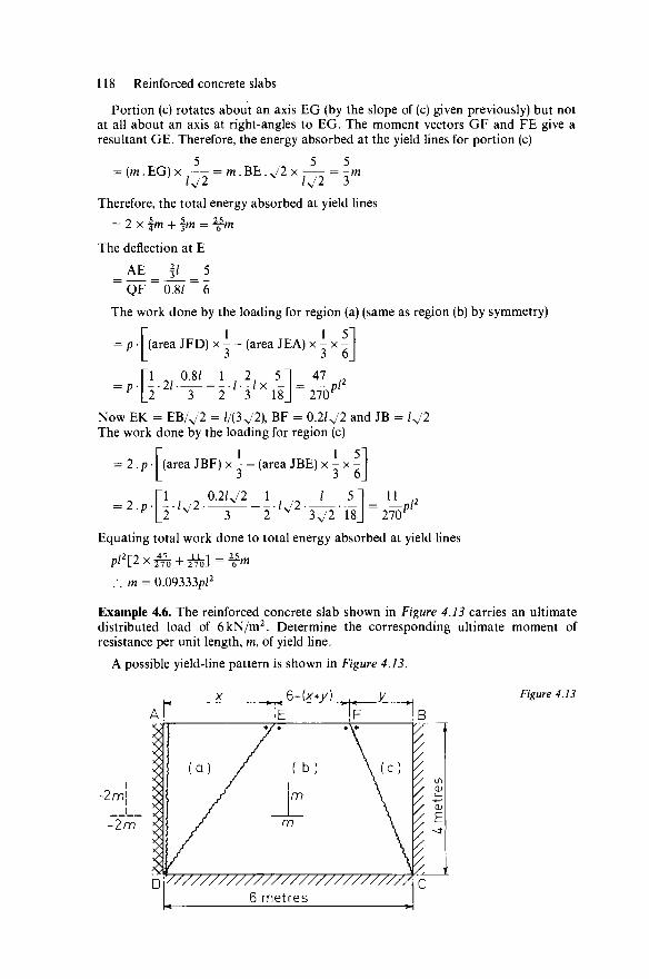
118 Reinforced concrete slabs
Portion (c) rotates about an axis EG (by the slope of (c) given previously) but not at all about an axis at right-angles to EG. The moment vectors GF and FE give a resultant GE. Therefore, the energy absorbed at the yield lines for portion (c)
= ( m . E G , x ^ = m . B E . V 2 x ^ = ^
Therefore, the total energy absorbed at yield lines
= 2 x f m + § m = ^m
The deflection at E _ AE _ §/ _ 5 ~ Q F ~ 0 8 / ~ 6
The work done by the loading for region (a) (same as region (b) by symmetry)
1 p • (area JFD) x - — (area JEA) x
- L
1 5] - x -3 6j
2 3
1 / 2i 5 " ■ - • / • - / x —
2 3 18 27(r
Now EK = EB/V2 = 1/(3 y/2), BF = 0.2/^2 and JB The work done by the loading for region (c)
ly/2
= 2 . p | i (area JBF) x - — (area JBE) x - x -
■ly/2 0.2/V2
2 ' / ^ 2 ' 3 x / 2 ' l 8 j 11
270 Pi2
2 v 3 Equating total work done to total energy absorbed at yield lines
.'. m = 0.09333p/2 m
Example 4.6. The reinforced concrete slab shown in Figure 4.13 carries an ultimate distributed load of 6kN/m2. Determine the corresponding ultimate moment of resistance per unit length, m, of yield line.
A possible yield-line pattern is shown in Figure 4.13.
-2m\
-2m
X 5-(x+y) ,. y . ' E "!F
< ♦ / • «Vf
(a) / ( b ) \ ( c )
/ m \
\ / m \
Y \ y/////////////////////////// 6 metres h« >■
B
V '/ '/ in / -
1Z 3
Figure 4.13
I
'

Yield-line theory of slab analysis 119
First trial Guess/estimate x = 4 and y = 1
mx Nodal force at E (see Section 4.4.4) = — = m
my m Nodal force at F = —- = —
4 4
For region (a), taking moments about AD: for yield line AD, 2m x 4 = 8m for yield line DE, vector ED can be resolved into vectors EA and AD, m. AD = 4m for nodal force at E, — m. x = — 4m for loading, - 6 x f x 4 x § = — 64 .". 8m + 4m - 4m - 64 = 0, .'. m = 8
For region (c), taking moments about BC: for yield line FC, vector FC can be resolved into vectors FB and BC, m. BC = 4m
for nodal force at F, — • v = — 4 4
for loading, — 6 x { x 4 x j = - 4
.'. 4m + — - 4 = 0 4
. . m — 17 For region (b), taking moments about DC:
for yield line ED, mx = Am for yield line FC, my = m
for nodal forces at E and F, I m + — 1 • 4 = 5m
for loading, - 6 x [ | x 4 x 4 x f + l x 4 x f + | x 4 x l x f ] = 128 / . 4m + m + 5m = 128 / . m = 12.8 These results indicate that regions (a) and (b) have been chosen too large and
region (c) too small. A reduction in area (a) increases area (b) whilst an increase in area (c) reduces area (b). Because of the large difference in the value of m for regions (b) and (c) it is highly unlikely that the yield-line pattern shown in Figure 4.13 could give the same value of m for the three regions. Hence the alternative pattern shown in Figure 4.14 will now be considered. Let us guess/estimate x = 4 and y = 1. The nodal forces for the regions (a) and (c) at points F and E will be zero (see rules 2 and 3 in Section 4.4.4). The equilibrium equations for the regions (a), (b) and (c) are: For region (a), taking moments about AD:
for yield line AD, (2m). AD = 8m for yield line EFD, vectors EF and FD add up to a resultant ED which can be resolved into vectors EA and AD, m. AD = 4m
[ XX X I
^ • y ^ + x- (4- )>)— =— 96 .'. 8m + 4m - 96 = 0 .'. m = 8

120 Reinforced concrete slabs
x = 4
r ' E 'i i • $ •
( c )
I / n \ F •}• y^\
y (b) \
B
'7, \ /, A /, " A H A 1 7, t A 1 << /< / / 4 H / K / / \
D
Figure 4. 14
For region (b), taking moments about DC: for yield line DFC, vectors DF and FC have a resultant vector DC, m. DC 6m
for loading, — 6
0
6 (4 2
-y)2
3 -54
/. 6m-54 .'. m = 9
For region (c), taking moments about BC: for yield line EFC, vectors EF and FC add up to a resultant EC which can be resolved into vectors EB and BC, m. BC = 4m
for loading, — 6 • [,& - x ) 2 | (4-y) (6-x)2
= - 2 4
.*. 4m - 24 = 0
.'. m = 6 The maximum value of m, namely 9, does not exceed a 50% increase in the
minimum value of m, namely 6, so from Step 2A previously, we can use the work equation for this yield-line pattern.
Taking the vertical deflection of line EF as unity, the slope of region (a) normal to AD is 1/4, the slope of (b) normal to DC is 1/3 and the slope of (c) normal to BC is 1/2.
Work done by loading for region (a)
r i x = 6|x.,.- + - . ( 4-y){ = 24
Work done by loading for region (b)
r 6 n «6.[(4-,).-.-_
= 18
Work done by loading for region (c)
= 6U6-x).yl- (6-x) 2
(4-y). 1]-12
Energy absorbed at the yield lines: For portion (c), it rotates about an axis BC only, an amount 1/2, see above. The resultant of the moment vectors CF and EF can be resolved into the moment
Yield-line theory of slab analysis 121
vectors CB and BE. Hence energy absorbed at yield lines = (m.CB).(l/2) = 2m
For portion (b), it rotates about an axis DC only, an amount 1/3, see above. The resultant of the moment vectors DF and FC is moment vector DC. Hence energy absorbed at yield lines
= (m.DC).(l/3) = 2m For portion (a), it rotates about an axis AD only, an amount 1/4, see above. The energy absorbed at yield line AD
= (2m.AD).(l/4) = 2m The resultant of the moment vectors DF and EF is DE and this can be resolved into the moment vectors DA and AE. Hence energy absorbed at yield lines DF and FE
= (m.DA).(l/4) = m Equating energy absorbed to work done: 2m + 2m + 2m + m = 24 + 18 + 12 .". m = 7.714
With the increased use of computers a hand-held or desktop microcom-puter might be programmed to solve this example by the method of equilibrium, or virtual work. Then various sets of x and y can be guessed until the solution has adequate accuracy. This was done for the yield-line pattern of Figure 4.14 and the results were x = 3.804, y = 1.215 and m = 7.754. So the above result of 7.714 has an error of only 0.52% supporting the effectiveness of the combined method advocated in this section.
4.4.7 Affine slab transformations
There are affinity theorems by Johansen for transforming certain slab problems into equivalent simpler ones to analyse (by the methods already described in this chapter). An affine slab and loading is devised to cor-respond to a given real slab and loading and the results for the former apply to the latter. These theorems1 are summarised as follows.
Affinity theorem for orthotropic reinforcement (the reinforcement in one direction gives an ultimate resisting moment, m, and in the other direction fim):
1. Multiply all relevant dimensions (defining slab shape or load position) in the direction of the \im reinforcement by 1/VM-
2. Multiply each total load by 1/VM-Affinity theorem for skew reinforcement (the angle between the reinforce-
ment in two directions being 0): 1. Define all relevant points by co-ordinates relative to axes parallel to
the reinforcement. 2. Replot these points to orthogonal axes. 3. Multiply each total load by cosec (p.
In both the above cases, the support conditions are the same for the affine as the real slab.

122 Reinforced concrete slabs
Example 4.7. The slab shown in Figure 4.15(a) carries the point load WkN, a uniformly distributed load gkN/m2 and a line load wkN/m. The reinforcement in the direction of dimension 'a' is obtained from the bending moment \im. Give details of the affine slab.
Figure 4.15(b) shows the affine slab where, from the above a' = a/y/n W = W/y/fi q'a'l = qa\j^J\i .'. q' = q
y'i = yiNv-length of line load w = L = J[(y2 - yj2 + (*2 - *i)2] length of line load w' = L = J[(y'2 - y\)2 + (x2 - *i)2] w'L = wL/y/11
wL
Uy/H
k
0
T
A
\a'
T
"<
/ /
*3
~J—\
V/A
»■■
!M/ / / /1 jum
/ /v/1
//A V/A
*'
/ /
*2
*3
/ ,. !
/ V / j
y/A *'
•<. * 2
m >
A s
b
m
m
^'
vvV^
».
,
i
J /2
' r \
^3
1
,
' '1
( a )
J
J
* 1
k
' 2
' 1
( b
1
' i
'
) Figure 4.15
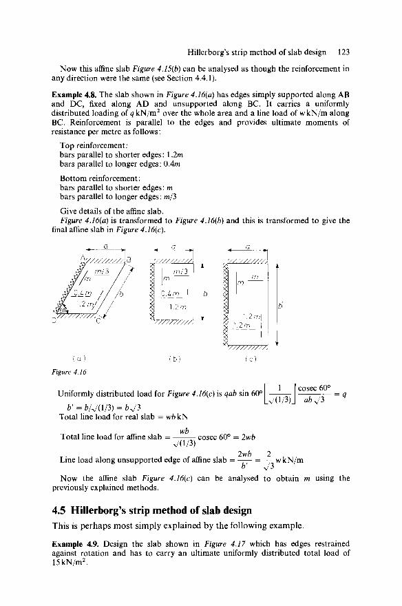
Hillerborg's strip method of slab design 123
Now this affine slab Figure 4.15(b) can be analysed as though the reinforcement in any direction were the same (see Section 4.4.1).
Example 4.8. The slab shown in Figure 4.16(a) has edges simply supported along AB and DC, fixed along AD and unsupported along BC. It carries a uniformly distributed loading of q kN/m2 over the whole area and a line load of w kN/m along BC. Reinforcement is parallel to the edges and provides ultimate moments of resistance per metre as follows:
Top reinforcement: bars parallel to shorter edges: 12m bars parallel to longer edges: 0.4m
Bottom reinforcement: bars parallel to shorter edges: m bars parallel to longer edges: m/3
Give details of the affine slab. Figure 4.16(a) is transformed to Figure 4.16(b) and this is transformed to give the
final affine slab in Figure 4.16(c).
(c)
Figure 4.16
Uniformly distributed load for Figure 4.16(c) is qab sin 60°
b' = b/y/(l/3) = bJ3 Total line load for real slab = wb kN
Vd/3). cosec 60°
ab^3
Total line load for affine slab wb
7(1/3) cosec 60° = 2wb
Line load along unsupported edge of affine slab = —— = —vvkN/m
Now the affine slab Figure 4.16(c) can be analysed to obtain m using the previously explained methods.
4.5 Hillerborg's strip method of slab design This is perhaps most simply explained by the following example.
Example 4.9. Design the slab shown in Figure 4.17 which has edges restrained against rotation and has to carry an ultimate uniformly distributed total load of 15 kN/m2.
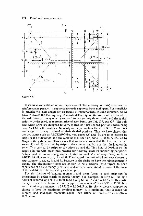
124 Reinforced concrete slabs
0.9m
0.9m
6m
0.9m
0.9m
♦ N
0.9m
■<f ZZ3Z3
1 0.9m
1 Jw
0.36mg [T7|
n 0.72mT W
_ _
/ V/M/\
1.05m
:B)
No. 7 f m L ' Jp.36mi
z ^ p 0.45m
4 .5m
| X d~ i —
Figure 4.17
It seems sensible (based on our experience of elastic theory, or tests) to reduce the reinforcement parallel to supports towards supports from mid span. For simplicity in practice we shall design for six bands of reinforcement in each direction, so we have to divide the loading to give constant loading for the width of each band. In the x-direction, from symmetry we need to design only three bands, and the typical strips to be designed, as representative of each band, are LM, NP, and QR. The only load these strips are designed to carry is that on their shaded portions, there being none on LM in this instance. Similarly in the ^-direction the strips ST, UV and WX are designed to carry the load on their shaded portions. Thus we have chosen that the two zones such as ABCDEFGHA, now called (A) and (B), are to be carried by strips in the x-direction and the remainder of the slab, zone (C), is to be carried by strips in the ^-direction. This means that we have chosen that the load on the two zones (A) and (B) is carried by strips to the edges ac and bd, and that the load on the zone (C) is carried by strips to the edges ab and dc. This kind of loading on the edges is in line with much past practice for deciding loads on supporting peripheral beams, and is more recognisable if the internal discontinuity lines, such as ABCDEFGH, were ae, ec, bf and fd. The stepped discontinuity lines were chosen to approximate to ae, ec, bf and fd, because of the desire to have the reinforcement in bands. The discontinuity lines are chosen to be a sensible (with regard to one's experience of elastic theory, yield line, and/or experimentation) division of the areas of the slab likely to be carried by each support.
The distribution of bending moments and shear forces in each strip can be determined by either elastic or plastic theory. For example, for strip ST, taking a nominal breadth of lm, the total load along ST is 15 x 4.5 = 67.5 kN. By elastic theory, it is a fixed beam, so each support moment is 67.5 x 4.5/12 = 25.31 kNm and the mid-span moment is 25.31/2 = 12.66kNm. By plastic theory, suppose we choose to keep the maximum bending moment to a minimum, that is make the support and mid-span moments equal, then either of these = 67.5 x 4.5/16 = 18.98 kNm.

CP 110 and yield-line and strip methods 125
4.5.1 Further points on Hillerborg's strip method
This method involves a tremendous amount of plastic action. If one's experience of elastic analysis, yield line or tests is severely gone against in deciding discontinuity lines and points of contraflexure of strips, then a very undesirable slab can be obtained, with regard to cracking. It is also possible that such a slab might not pass the British Standard loading test because of lack of recovery of deflection due to high plasticity, even though the ultimate strength might be satisfactory.
If the strips are designed elastically then the method is very illogical, in that deflections of strips are not matched up, as was done years ago by Grashof-Rankine.
In the past decade at least, there has been a tendency to use computers to design structures more accurately, so in one sense the strip method seems a retrograde step. It is the kind of method one has not been proud to use in design offices when precise elastic analyses38 have been too difficult to attempt in the time available. But there are more computer packages available today.
The great advantage of the method is that it is easy to use and apply to any shape. It is probably best when there is not an elastic analysis available.
For skew slabs the strips are taken as beams cranked in plan and the geometry involves different portions of a strip having different widths.29
It is an easy method to apply to slabs containing holes.29
It is generally accepted37 that Hillerborg's strip method is not upper bound which is a concern with yield-line analyses. If yield lines are chosen to be disposed where one would imagine from experience of tests or from common engineering sense then the analysis should not be significantly upper bound; however it will generally be the latter. For the strip method it is best to choose the discontinuity lines from thoughts (probably based on experience of elastic theories) of which areas would be sensibly carried by which supports.
Hillerborg's strip and advanced (see Section 4.7) methods are very economical in that generally each portion of loading is carried only once. This contrasts with methods used over the past half century in design offices where beams are formed within the slab thickness and a portion of loading is, for example, carried twice by slab and this then by a beam.
4.6 CP 110 and yield-line and strip methods
CP 110 recommends that yield-line and strip methods can be used provided that the ratio between support and span moments is between 1:1 and 1.5:1. This helps to safeguard against designing a slab which may crack badly at working loads.
Certain plastic methods used2 choose the positions of the points of inflection or contraflexure at 0.2 of the span from each support for strips such as ST, 0.4 of the length of the loaded area from each support for strips such as UV and WX, 0.5 of the length of the loaded area from each support for strips such as NP and QR (strip LM having no loading). These points are marked with an asterisk in Figure 4.17. On this basis Figure 4.18(a)
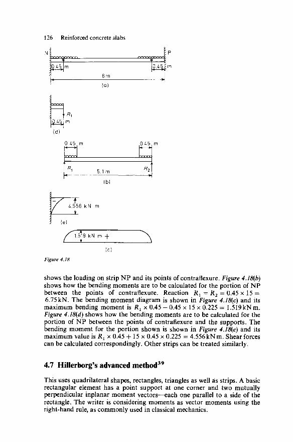
126 Reinforced concrete slabs
d0./,5jm 0.4 w 6 m
0.45 m ,0.45
5.1 m
4.556 kN m 4_
(e)
/^1.5*19 kN m + " X
Figure 4.18
shows the loading on strip NP and its points of contraflexure. Figure 4.18(b) shows how the bending moments are to be calculated for the portion of NP between the points of contraflexure. Reaction Rt = R2 = 0.45 x 15 = 6.75 kN. The bending moment diagram is shown in Figure 4.18(c) and its maximum bending moment is Rx x 0.45 — 0.45 x 15 x 0.225 = 1.519kNm. Figure 4.18(d) shows how the bending moments are to be calculated for the portion of NP between the points of contraflexure and the supports. The bending moment for the portion shown is shown in Figure 4.18(e) and its maximum value is Rx x 0.45 + 15 x 0.45 x 0.225 = 4.556 kNm. Shear forces can be calculated correspondingly. Other strips can be treated similarly.
4.7 Hillerborg's advanced method39
This uses quadrilateral shapes, rectangles, triangles as well as strips. A basic rectangular element has a point support at one corner and two mutually perpendicular inplanar moment vectors—each one parallel to a side of the rectangle. The writer is considering moments as vector moments using the right-hand rule, as commonly used in classical mechanics.

Hillerborg's advanced method 127
Example 4.10. The slab shown in Figure 4.19(a) carries a uniformly distributed load q. Suggest a design solution using Hillerborg's methods.
Consider the rectangular element AGFE. It is in equilibrium as follows: a point support upwards at A, a loading q. AG. AE downwards, a moment vector FG and a moment vector EF. From external considerations: the reactions at A and B are the same from symmetry; the total of these reactions is the same as the total reaction
a/2 a/ 2
J—T-?
i *
bll
b/2
-f I 4-E H Fj
-7/3 7/3 | 7/3 -7/3
U7/3 [27/3 I27/3 U7/3 ; IJ * IK \ I ♦ .
D y////v///x////f///\ c
N ( a )
h+ ■ »■ ■* »■ aM a Ik
H-< H
1
blk
blL
1
1 1
t
II 1 MM Mill 1 11II11 Qb2 \ qb2 12 T
j |
7 i:
7a2
6
n2
2
m i i i i i i i i i i i
] 7 ] 4
3 2
8
(b)
(c )
v////////////////; Figure 4.19

128 Reinforced concrete slabs
due to the line-load support DC from symmetry considerations. Thus the shear forces on sections GK and EN are zero. Considering the whole slab
Reaction at A = RA — qab/4
Therefore the element must be of the area shown so that resolving vertically for it: the downward load = qab/4 which equals the value of RA above and which is therefore correct. For the element take moments about GF, then the vector moment GF
/a\ a b fa\ qa2b
So the vector moment GF per unit length
qa2b fb\ qa2
Now it is sensible, bearing in mind serviceability conditions, to have a stronger strip of slab near to the free edge AB; hence the bending moment for design along GF is distributed as in Figure 4.19(b): the half nearer the edge is allocated a moment qa2/6 per unit length and the other half a moment qa2/\2, so that the average moment per unit length is qa2/S as required above.
Again for the element take moments about EF, then the vector moment EF
b\ a b fb\ qab2
q-K2) " 2 2 \4J 16
So the vector moment FE per unit length
qab2 fa\ qb2
16 " \2
It is sensible, bearing in mind serviceability conditions, to have a stronger strip of slab near to the free edge AD so we halve EF, use a moment qb2/6 per unit length for the outer half and a moment qb2/12 per unit length for the other half. These then average qb2/S per unit length for FE.
As DC is a line-load support it should be split into several portions. In this case four portions are taken. The rectangular element EHJD is supported by a line load along DJ, there are vector moments EH and HJ and it carries a loading q. EH . ED. In Figure 4.17 each portion of loading was carried in either one direction of two mutually perpendicular directions. But with both Hillerborg's strip method and his advanced method any portion of loading can be carried by one proportion of it being carried in one direction and the remainder carried in the other direction. Furthermore one proportion can be greater than one so that the remainder is negative. In the case of a vertically downwards portion of loading if one proportion is greater than unity then the negative remainder would be positively upwards.
Suppose for the loading q on element EHJD its proportion carried in the DE direction is ql. Then taking moments about DJ for the element:
qb2
6
. . q
a
T = 4i
4q
' 3
a
4 b
2 ft u
Therefore the proportion of the loading q carried in the DJ direction is

Hillerborg's advanced method 129
q — qx =—q/3 (that is an upwards loading). Now the element EHJD is not the proper Hillerborg rectangular element described at the beginning of this section, because there is not one corner load but a line load along DJ and therefore moments cannot be taken about HJ for this element. But ENCD can be treated as a strip spanning from ED to NC just as for the Hillerborg strip method of Section 4.5. This strip spans from end to end ignoring the support DC just as in Figure 4.17 strip WX spans from end to end ignoring the support bd. The main point with Hillerborg's methods is to carry towards collapse all loads and portions of loads somehow or other, no matter how badly cracked the slab is.
Suppose for the loading q on element HFKJ its proportion carried in the JH direction is q2. Then taking moments about JK for the element:
qb2 a a b /b\
72~*4 = ^ 2 ' 4 ' 2 W
Therefore the proportion of the loading q carried in the JK direction is q-q2 = 4/3.
Now for the Hillerborg strip ENCD the moment vector FK
q a b S3 \ q a b /a\
_qa2b
~~96~ So the vector moment FK per unit length
qa2b /b\ qa2
= ~96~""" \ 2 / ~48~
The bending moments per unit length and the directions with arrows of the way in which loading is carried are shown in Figure 4.19(b) and (a) respectively. Figure 4.20(a) shows the loading diagram for strip ENCD with corresponding shear force and bending moment diagrams in Figure 4.20 (b) and (c), respectively.
Alternatively to the above, if one did not like distributing the bending moment vectors along GF and FE in an arbitrary fashion, then AGFE could have been split into four rectangular elements to obtain a similar result. Furthermore a greater number of rectangular elements could be used for this area and the rest of the slab. For this present example Hillerborg suggests using fewer elements for practical design as shown in Figure 4.19(c) and then distributing the moments along the edges of the rectangle in a reasonable way. He justifies this by saying 'that different theoretical solutions give somewhat different distributions of moments and that a reinforcing bar in practice is efficient in resisting moments occurring within a considerable relative distance from the bar itself. The writer's comment on this would be that the greater the number of sensible (that is bearing in mind servi-ceability, viz. how it tends to act elastically at working loads) elements the better the solution, and the extra work involved is quite reasonable when Hillerborg's methods are solving problems outside existing design tables and which would be tremen-dously formidable by other analyses.
Hillerborg states Tor practical design the main condition is that the equilibrium is fulfilled for the elements as a whole and that the lateral distribution of moments chosen is reasonable'.
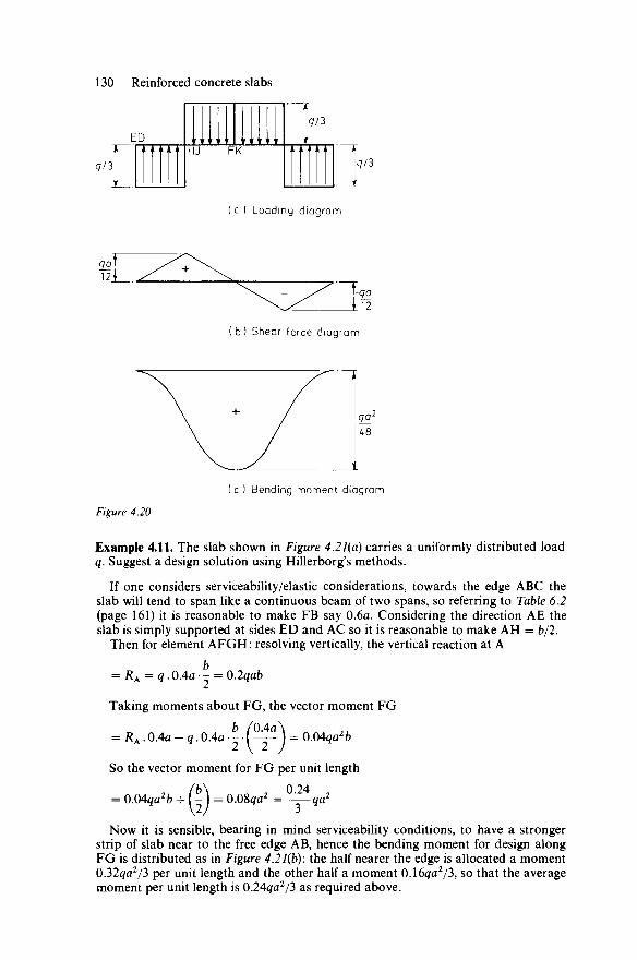
130 Reinforced concrete slabs
<7/3 r ED
l , 1 t A A 1 r i l l
HJ ' I f f ? ? ? FK
Tqr/3
1 A A A t t 1, <7/3
( a ) Loading diagram
Figure 4.20
( b ) Shear force diagram
( c ) Bending moment diagram
Example 4.11. The slab shown in Figure 4.21(a) carries a uniformly distributed load q. Suggest a design solution using Hillerborg's methods.
If one considers serviceability/elastic considerations, towards the edge ABC the slab will tend to span like a continuous beam of two spans, so referring to Table 6.2 (page 161) it is reasonable to make FB say 0.6a. Considering the direction AE the slab is simply supported at sides ED and AC so it is reasonable to make AH = b/2.
Then for element AFGH: resolving vertically, the vertical reaction at A
b = RA = q.0Aa- = Q.2qab
= RA. 0.4a - q . 0.4a • 0 - 04qa2b
Taking moments about FG, the vector moment FG
b /0.4aN
So the vector moment for FG per unit length
= 0.04qa2b -=- f - ) = 0.08aa2 = — g a 2
\2) 3 Now it is sensible, bearing in mind serviceability conditions, to have a stronger
strip of slab near to the free edge AB, hence the bending moment for design along FG is distributed as in Figure 4.21(b): the half nearer the edge is allocated a moment 0.32ga2/3 per unit length and the other half a moment 0.16<?a2/3, so that the average moment per unit length is 0.24ga2/3 as required above.
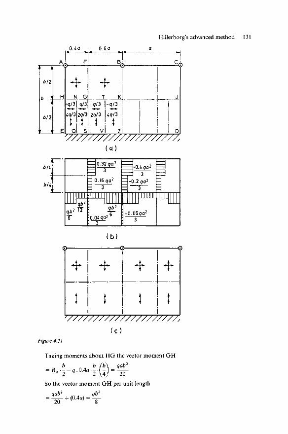
Hillerborg's advanced method 131
0.4a 0.6a
J i
b/2
P -
b/2
Y 1
> *
f H i
'. E 777777777777777777777,
(a )
6M
6/4
M *i T
j c
mill
6 F
=J0.32 9a2 [
H 3
Jo. 16 9a2 [
H 3 t '"" [
<7*>2 [ 0.04 9Q2 6 [
-0.4 9a 2
= 3 3 H-0.2 9a2
H 3
1 1 1 1 1
- 0 . 059a 2
3
H
I M | | | |
(b)
0 j —
ki — i -1 1
t ! 1 i
+ t
i -1-
1 1 i i
—
t
T
t 1
777777777777777777777, ( c )
Figure 4.21
Taking moments about HG the vector moment GH b ~ . b fb\ 1ab2
= RA.--q.0Aa- (-) = ?—-A 2 H 2 \4J 20
So the vector moment GH per unit length
20 v ; 8

132 Reinforced concrete slabs
It is sensible, bearing in mind serviceability conditions, to have a stronger strip of slab near to the free edge AE so HG is halved and a moment qb2/6 per unit length used for the outer half and a moment qb2/12 per unit length used for the other half. These then average qb2/S per unit length for GH.
Now the vector moment FG for element AFGH is equal to the vector moment GF for element FBKG. Hence for this latter element, taking moments about BK the vector moment KB
= q. 0.6a • - • (0.3a) - 0.04qa2b = 0.05qa2b
So the vector moment for KB per unit length
Similarly to before it is sensible to have a stronger strip of slab near to the free edge AB so BK is halved and a moment 0Aqa2/3 per unit length used for the outer half and a moment 0.2qa2/3 per unit length used for the other half. These then average qa2/10 per unit length for KB. The ratio of moments per unit length between the halves of FG and BK is kept the same, namely 2 to 1 as chosen for FG. These are shown in Figure 4.21(b).
Again for element FBKG, taking moments about FB the vector moment KG
So the vector moment for KG per unit length
= l,flfc^(0.6«) = l ^
(NB The vector moment KG is a pure moment and has the same moment about any line parallel to KG, for example FB in this case.)
It is sensible, bearing in mind serviceability conditions, to have a stronger strip near to the support B so GK is halved and a moment qb2/6 per unit length used for the half nearest to BK and a moment qb2/12 per unit length used for the other half. These then average 3qb2/24 per unit length, as required above, for KG.
For element HNQE, if the portion of q to be carried in the HE direction is ql then taking moments about EQ
qb2 b (b\ Y'0.2a-^.0.2a--- - =0
(NB Vector moment GH for element AFGH is equal and opposite to vector moment HG for element HGSE.)
.'. <h = 4*/3 Therefore the portion of q to be carried in the EQ direction is q — qt = — q/3. For element NGSQ, if the portion of q to be carried in the NQ direction is q2,
then taking moments about QS
qb2 b /b\ ^0.2a-q2.0.2a-l-\ = 0
2<1
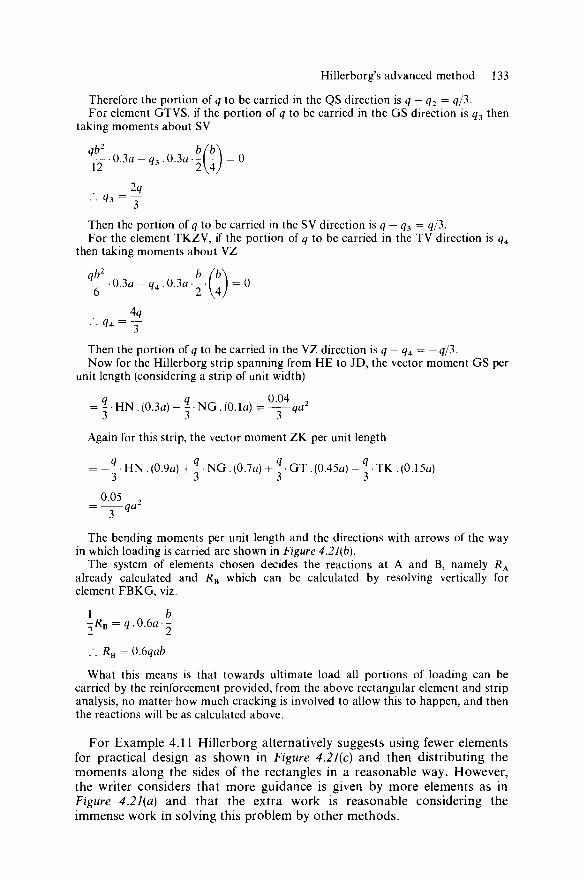
Hillerborg's advanced method 133
Therefore the portion of q to be carried in the QS direction is q — q2 = q/3. For element GTVS, if the portion of q to be carried in the GS direction is q3 then
taking moments about SV
qb2 b(b\ — • 0.3a-<?3 .0.3a-- ( - 1 = 0 12 H3 2\4J
2a
Then the portion of q to be carried in the SV direction is q — q3 = q/3. For the element TKZV, if the portion of q to be carried in the TV direction is qA
then taking moments about VZ
= 0 qb2
6 ■0.3a-
4a U = ~3
q4 .0.3a b
Y a Then the portion of q to be carried in the VZ direction is q — q4 = — q/3. Now for the Hillerborg strip spanning from HE to JD, the vector moment GS per
unit length (considering a strip of unit width)
= - • HN . (0.3a) - - • NG . (0.1a) = -^— qa2
Again for this strip, the vector moment ZK per unit length
= - - • HN . (0.9a) + I • NG . (0.7a) + | • GT. (0.45a) - | • TK . (0.15a)
0.05 , = — q a
The bending moments per unit length and the directions with arrows of the way in which loading is carried are shown in Figure 4.21(b).
The system of elements chosen decides the reactions at A and B, namely RA
already calculated and RB which can be calculated by resolving vertically for element FBKG, viz.
1 b -RB = q.0.6a-
.'. RB = 0.6qab
What this means is that towards ultimate load all portions of loading can be carried by the reinforcement provided, from the above rectangular element and strip analysis, no matter how much cracking is involved to allow this to happen, and then the reactions will be as calculated above.
For Example 4.11 Hillerborg alternatively suggests using fewer elements for practical design as shown in Figure 4.21(c) and then distributing the moments along the sides of the rectangles in a reasonable way. However, the writer considers that more guidance is given by more elements as in Figure 4.21(a) and that the extra work is reasonable considering the immense work in solving this problem by other methods.

134 Reinforced concrete slabs
6m
Ac A C
H
y
r ' *
3 3
E i
» P = |60kNT
J
4-K
<7 = 4kN/m 2
-f .,.,_. C. -6 (a )
24
1U
rf 24
A E ?C7 = ^ l<N/m2H2^
-f H12
H J
( c )
Figure 4.22
4- 90
13.33 6.67
(e)
Example 4.12. The slab shown in Figure 4.22(a) carries a uniformly distributed load of 4kN/m2 and a point load P = 60kN. Suggest a design solution using Hillerborg's methods.
For element AEJH, taking moments about AE, the vector moment JH
„ (5 - y)2 60
2 2
(NB The vector moment JH is a pure moment and has the same moment about any line parallel to JH, for example AE in this case.)
For element HJGD, taking moments about DG, the vector moment HJ
y2
= 4 x 3 x —

Hillerborg's advanced method 135
The above two vector moments are equal and opposite; equating them gives
6 x (5 - y)2 + 30 = 6y2
Solving this quadratic equation gives y = 3m. So for element HJGD the vector moment HJ = 54 kN m and per unit length
54 = — = 18kNm/m
3 '
It is desirable, see previous examples, to have a stronger strip near the outer edge AD, so we choose to distribute this moment as shown in Figure 4.22(b).
For element HJGD, taking moments about HD, the vector moment JG
32
= 4 x — xy = 54kNm 2
So the vector moment JG per unit length
54 = — = 18kNm/m
y It is desirable, see previous examples, to have a stronger strip near the outer edge
DC, so we choose to distribute this moment as shown in Figure 4.22(b). Again it is desirable to have a stronger strip near the outer edge AB particularly
because of the proximity of the point load to this edge. One way Hillerborg suggests dealing with this desirability is to consider separately the uniformly distributed loading and the point load. For the former, taking moments about AH for element AEJH, the vector moment EJ per unit length
32
= 4 x — = 18kNm/m 2
This is distributed sensibly as shown in Figure 4.22(c). Figure 4.22(d) shows elements for carrying the point load. Elements AESQ and
EBTS each carry half of the point load at their corners at S as shown. For element AESQ, taking moments about AQ, the vector moment ES per unit length
= 3 0 x 3 = 90kNm/m Taking moments about AE, the vector moment SQ per unit length
= 30x 1/3 = lOkNm/m
These moments are shown in Figure 4.22(e), the lOkNm/m being distributed sensibly. Figure 4.22(c) and (e) combined give the resultant distribution of moment along EJ and this is shown in Figure 4.22(b) which now gives the complete solution.
Example 4.13. The slab shown in Figure 4.23(a) carries a uniformly distributed load q. Suggest a design solution using Hillerborg's methods.
Hillerborg39 recommends the use of triangular corner-supported elements with reinforcement parallel to the diagonals and analysing the slab as in Figure 4.23(b), as if it were supported at only two corners.
For triangular element ABE: Taking moments about AE, the vector moment AE
_qa2 EB
So the vector moment AE per unit length
_qa^ EB _qa2
~ 4 ' 3 ^ b A " 12
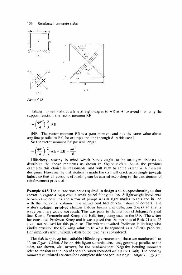
136 Reinforced concrete slabs
A k - - - Q — - - ^ B v\ it
Figure 4.23
Taking moments about a line at right-angles to AE at A, to avoid involving the support reaction, the vector moment BE
(NB The vector moment BE is a pure moment and has the same value about any line parallel to BE, for example the line through A in this case.)
So the vector moment BE per unit length
Hillerborg, bearing in mind which bands ought to be stronger, chooses to distribute the above moments as shown in Figure 4.23(c). As in the previous examples this choice is 'reasonable' and will vary to some extent with different designers. However the distribution is made the slab will crack accordingly towards failure so that all portions of loading can be carried according to the distribution of reinforcement provided.
Example 4.15. The author was once required to design a slab approximating to that shown in Figure 4.24(a) over a small petrol filling station. A lightweight kiosk was between two columns and a row of pumps was at right angles to this and in line with the individual column. The actual roof had curves instead of corners. The writer's solution involved shallow hidden beams and deflection checks so that a wavy periphery would not result. This was prior to the methods of Johansen's yield line, Kemp, Fernando and Kemp and Hillerborg being used in the U.K. The writer has consulted Professor Kemp and it was agreed that the methods of Refs. 21 and 22 could not be used for this problem. The writer consulted Professor Hillerborg who kindly provided the following solution to what he regarded as a difficult problem. For simplicity unit uniformly distributed loading is considered.
The slab is split up into suitable Hillerborg elements and these are numbered 1 to 13 on Figure 4.24(a). Also on this figure suitable directions, generally parallel to the sides, are shown, with arrows, for the reinforcement. Negative bending moments refer to tension in the top of the slab, when recorded on Figure 4.24(b). The bending moments calculated are each for a complete side not per unit length. Angle a = 15.37°.

Hillerborg's advanced method 137
1.4m 0.3
Figure 4.24(a)
Figure 4.24(b)
Element No. 1: Taking moments about HJ, the vector moment HJ
1.32
= 1.4 x = 1.183 2
Taking moments about BJ, the vector moment JB 1.42
= 1.3 x 1.274 2
Element No. 2: Taking moments about JS, the vector moment SJ 1.42
= 0.3 x — = 0.294 2
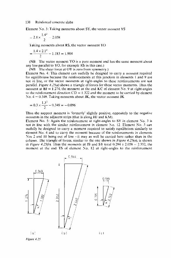
138 Reinforced concrete slabs
Element No. 3: Taking moments about SY, the vector moment YS
1.42
= 2.1x = 2.058 2
Taking moments about RS, the vector moment YO
1.4 x 2.12
= 1.183 = 1.904 2
(NB The vector moment YO is a pure moment and has the same moment about any line parallel to YO, for example RS in this case.)
(NB The shear force at OY is zero from symmetry.) Element No. 4: This element can usefully be designed to carry a moment required for equilibrium because the reinforcements at this junction in elements 1 and 9 are not in line, or the vector moments at right-angles to these reinforcements are not parallel. Figure 4.25(a) shows a triangle of forces for these vector moments. Thus the moment at BJ = 1.274, the moment at the end KC of element No. 9 at right-angles to the reinforcement direction CD = 1.322 and the moment to be carried by element No. 4 = 0.349. Taking moments about JK, the vector moment JK
1.32
= 0.3 x 0.349 = -0.096 2
Thus the support moment is 'formerly' slightly positive, oppositely to the negative moments in the adjacent strips (that is along HJ and KM). Element No. 5: Again the reinforcement at right-angles to SY in element No. 3 is not in line with the similar reinforcement in element No. 12. Element No. 5 can usefully be designed to carry a moment required to satisfy equilibrium similarly to element No. 4 and to carry the moment because of the reinforcements in elements Nos 2 and 11 being out of line—it may as well be carried here rather than in the column. The triangle of forces, similar to the one shown in Figure 4.25(a), is shown in Figure 4.25(b). Thus the moments at JS and SY total 0.294 + 2.058 = 2.352, the moment at the end TS of element No. 12 at right-angles to the reinforcement
0.6U
( a ) ( b ) ( c )
Figure 4.25

Hillerborg's advanced method 139
direction TV = 2.440 and the moment to be carried by element No. 5 = 0.644. Taking moments about ST, the vector moment ZY
2.12
= 0.3 x - — + 0.644 + 0.096 (from element No. 4)
= 1.402
Element No. 6: Taking moments about FP, the vector moment FP
1.42
= 0.59x + (1.01 2
1.4 1.4 0.59) x — x — = 0.715
2 3
Taking moments about PQ, the vector moment PQ
0.42
= 0.458
0.592
= 1.4 x — h (1.01 1.4 - 0.59) x — x 2
0.59 +
Element No. 7: Taking moments about PW, the vector moment PW
1.42
= 0.3 x = 0.294 2
Element No. 8: Again the reinforcement at right-angles to FP in element No. 6 is not in line with the similar reinforcement in element No. 10. Element No. 8 can usefully be designed to carry a moment required to satisfy equilibrium similarly to element No. 4. The triangle of forces, similar to the one shown in Figure 4.25(a), is shown in Figure 4.25(c). Taking moments about NP, the vector moment NP
0.3 / 1 .10+1 .01 \ 2
= — x( ) +0.196 0.363
Element No. 9: From element No. 4 the vector moment at the end KC of element No. 9 at right-angles to the reinforcement direction CD is 1.322. Taking moments about end KC the vector moment at right-angles to the reinforcement direction CD at end DM (assuming DM has been chosen so that the shear force at DM is zero)
T 4.252 4.25 4.25 = 1.2x — + (1.3-1.2)x — x —
= 9.416
cos a — 1.322
Taking moments about end KM, the vector moment at right-angles to the reinforcement in direction CK at end KM
1.2) x 1.2 + 0.1 T 1.22 4.25 = 4.25 X - — + — - x (1.3-
|_ 2 2 = 3.202
Element No. 10: From Figure 4.25(c) the vector moment at the end EN of element No. 10 at right-angles to the reinforcement direction DE is 0.742. Taking moments about end EN the vector moment at right-angles to the reinforcement direction DE at end DM
1.2 x 4.252 (1.2 1.1) 4.252
x •cos a — 0.742
9.415

140 Reinforced concrete slabs
(assuming DM has been chosen so that the shear force at DM is zero). This value needs to agree with the corresponding value for element No. 9, namely 9.416 earlier. This agreement is satisfactory. If the difference were more than 10% then the position of DM would have to be changed, that is an alteration would be required in the relative sizes of elements Nos 9 and 10. If the two values have a difference of less than 10% then they are averaged to give the design moment at this location.
Taking moments about end MN the vector moment at right-angles to the reinforcement direction DM at end MN
4 4 . 2 5 x l £ + ^ x < 1 . 2 - l . l ) x ( u + f ~
= 2.711
Elements Nos 11 and 12: These can usefully be taken together when considering vector moments at right-angles to the reinforcement in the TV direction. From Figure 4.25(b) and earlier the vector moment for these two elements at end KZ at right-angles to the reinforcement in the direction TV is 2.440. Taking moments about end KZ, the vector moment at right-angles to the reinforcement direction TV at end LU
0 3.862 (2.4-1.378) 3.862
1.378 x + - - x
9.903
•cosa -2 .440
(assuming LU has been chosen so that the shear force at LU is zero). The vector moment at right-angles to the reinforcement in direction CK at end TV, from element No. 9, is 3.202. Taking moments, for element No. 12 about end TV, the vector moment at right-angles to the reinforcement in direction ZT at end ZU
1.0782 3.86 3.86 x + x (2.1 - 1.078)
2 2 1.078 +
1.022 •cosa - 3.202
= 1.658
(NB The shear force at ZU is zero from symmetry.) Element No. 13: From element No. 7 the vector moment at the end NI of element No. 13 at right-angles to the reinforcement direction LN
0.294 2 cos a
0.152
Taking moments about end NI the vector moment at right-angles to the reinforce-ment direction LN at end LU
4.642 4.642
0.15 x —— + (1.378 - 0.15) x •cosa — 0.152
= 9.921
(assuming LU has been chosen so that the shear force at LU is zero). This should agree with the corresponding value from elements Nos 11 and 12, namely 9.903. These are within a 10% difference so average these values giving 9.912. Had the difference been greater than 10% then the position of line LVU would have needed altering.
From element No. 10 the vector moment at the end LN of element No. 13 at right-angles to the reinforcement direction LU is 2.711. Taking moments about UI,
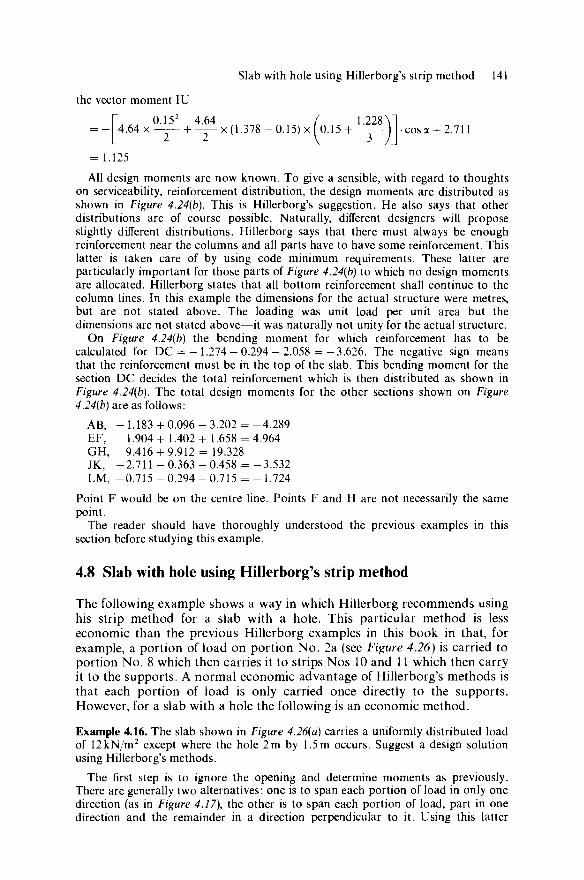
Slab with hole using Hillerborg's strip method 141
the vector moment IU
0.152 4.64 / 1.228 , , 4.64 x —— + — x (1.378 - 0.15) x I 0.15 + ) | cos a + 2.711
= 1.125
All design moments are now known. To give a sensible, with regard to thoughts on serviceability, reinforcement distribution, the design moments are distributed as shown in Figure 4.24(b). This is Hillerborg's suggestion. He also says that other distributions are of course possible. Naturally, different designers will propose slightly different distributions. HiUerborg says that there must always be enough reinforcement near the columns and all parts have to have some reinforcement. This latter is taken care of by using code minimum requirements. These latter are particularly important for those parts of Figure 4.24(b) to which no design moments are allocated. HiUerborg states that all bottom reinforcement shall continue to the column lines. In this example the dimensions for the actual structure were metres, but are not stated above. The loading was unit load per unit area but the dimensions are not stated above—it was naturally not unity for the actual structure.
On Figure 4.24(b) the bending moment for which reinforcement has to be calculated for DC = — 1.274 - 0.294 - 2.058 = -3.626. The negative sign means that the reinforcement must be in the top of the slab. This bending moment for the section DC decides the total reinforcement which is then distributed as shown in Figure 4.24(b). The total design moments for the other sections shown on Figure 4.24(b) are as follows:
AB, -1 .183+ 0.096-3.202 = -4.289 EF, 1.904 + 1.402 + 1.658 = 4.964 GH, 9.416 + 9.912 = 19.328 JK, - 2 . 7 1 1 - 0 . 3 6 3 - 0 . 4 5 8 = -3.532 LM, -0.715 - 0.294 - 0.715 = - 1.724
Point F would be on the centre line. Points F and H are not necessarily the same point.
The reader should have thoroughly understood the previous examples in this section before studying this example.
4.8 Slab with hole using Hillerborg's strip method
The following example shows a way in which HiUerborg recommends using his strip method for a slab with a hole. This particular method is less economic than the previous HiUerborg examples in this book in that, for example, a portion of load on portion No . 2a (see Figure 4.26) is carried to portion No . 8 which then carries it to strips Nos 10 and 11 which then carry it to the supports. A normal economic advantage of Hillerborg's methods is that each portion of load is only carried once directly to the supports. However, for a slab with a hole the following is an economic method.
Example 4.16. The slab shown in Figure 4.26(a) carries a uniformly distributed load of 12kN/m2 except where the hole 2 m by 1.5 m occurs. Suggest a design solution using Hillerborg's methods.
The first step is to ignore the opening and determine moments as previously. There are generally two alternatives: one is to span each portion of load in only one direction (as in Figure 4.17), the other is to span each portion of load, part in one direction and the remainder in a direction perpendicular to it. Using this latter

142 Reinforced concrete slabs
4 of T
11 2^ 11 />WSAAVSA<VWYV
H^li3
1 * 2 <?6
12
4a HE
.prn 8 .rTTT^ 9 n^ 9
<?6 <?6
Figure 4.26
5a
(c)
method Hillerborg suggests discontinuity lines as shown in Figure 4.26(b) and carrying the loads in the directions shown with arrows.
For strip No. 2, the strip spanning from EF to KJ, the writer would probably calculate the maximum moments from Table 7.2 (page 179): span 12 x 52/14.2 = 21.13 kNm/m and support — 12 x 52/8 = — 37.5kNm/m. Alternatively a position for the point of contraflexure can be chosen. For this example Hillerborg chooses this at 3.8 m from the free edge; this then gives a maximum span moment
= 12x3.82/8 = 21.7 kNm/m and a maximum support moment
= - 12 x 1.9 x (5 - 3.8) - ^ x (5 - 3.8)2 = - 3 6 k N m / m
Hillerborg has guessed, by his experience, a point of contraflexure which gives a similar solution to the elastic theory used above. With plasticity this departure from

Slab with hole using Hillerborg's strip method 143
elastic theory is naturally permissible. If Hillerborg has a choice he normally prefers to increase the elastic support moment slightly whereas detailers normally prefer the support and span moments to be equal.
For strip No. 4-2-5, the strip spanning from NL to GH, Hillerborg chooses a point of contraflexure lm from GH. This makes the simple span between NL and the point of contraflexure symmetrically loaded and the reaction is 12 x 1 = 12kN/m and maximum span moment
= 12 x l - 1 2 x l2/2 = 6kNm/m Then the support moment
= - 1 2 x l - 1 2 x l2/2 = - 1 8 k N m / m In this case an elastic analysis gives a slightly lesser span moment. For portions 1, 3, 6 and 7 Hillerborg, because they are corner portions, allows half
the loading to be taken in each direction. Then for strips 1-2-3 and 6-2-7 the bending moments are half those of strip 4-2-5, and are therefore: maximum span moment = 6/2 = 3kNm/m and support moment = — 18/2 = —9kNm/m.
Then for either strip 1-4-6 or 3-5-7 Hillerborg chooses the point of contra-flexure 0.6 m from the fixed support. This makes the calculation simple in that the simply supported span between this point of contraflexure and the edge AB is symmetrically loaded and the end reaction
= 6x0.95 = 5.7kN/m The maximum span moment is the same all along the central portion and
= 5.7 x 0.95 - 6 x 0.952/2 = 2.7kN m/m
The support moment, at edge DC, = - 5 . 7 x 0 . 6 - 6 x0.62/2 = -4 .5kNm/m
Edge strips bounding the hole are shown in Figure 4.26(c) and the directions in which the loading will be carried in portions Nos 2a, 2b, 4a and 5a are shown with arrows. These portions are within the portions Nos 2, 4 and 5 shown in Figure 4.26(b).
Edge strip No. 8 supports portion No. 2a with a uniformly distributed reaction qx
as shown in Figure 4.26(c). Taking moments about edge EF
4J.0.5X 1.25 = 12 x 1.5x0.75 .'. qx =21.6kN/m2
Then the reaction at the support (EF)
= 12 x 1.5 - 21.6 x 0.5 = 7.2kN/m The distance from this support to the point of zero shear (that is maximum
moment)
= 7.2/12 = 0.6 m
Then the maximum span moment = 7.2 x 0.6 - 12 x 0.62/2 = 2.16 kN m/m
Edge strip No. 9 supports portion No. 2b with a uniformly distributed reaction q2
as shown in Figure 4.26(c). Taking moments about edge KJ the support moment = 4 2 .0 .5x 1 . 7 5 - 1 2 x 2 x 1 = 0.875.q2 - 2 4
Now if this moment = — 24 then q2 is zero. The basic case (that is ignoring the hole) gave a moment at this support of — 36 kN m/m. To maintain this value would give a

144 Reinforced concrete slabs
negative value of q2 meaning that portion No. 9 would not be supporting portion No. 2b but dragging down on it. Then portion No. 9 would be lifting portions Nos 10 and 11. The general idea was that portion No. 9 would support portion No. 2b and that portions Nos 10 and 11 would support portion No. 9. In this case Hillerborg decided not to allow q2 to be negative and yet allow the support moment to be as near to —36 as possible. Thus this support moment is taken as —24kNm/m and then q2 is zero. The portions Nos 2b and 9 of the slab thus cantilever from the support (KJ).
Edge strip No. 10 supports portion No. 4a with a uniformly distributed reaction q3 as shown in Figure 4.26(c). Taking moments about edge NL
1 2 x 1 x 0 . 5 ^ 1 X T / 2 fr= n< ?-)< =3.7kN/m 2
0.5 x 3.25
The maximum span moment will be much less than the basic of 6 kN m/m, see earlier. Hillerborg takes this latter figure.
Edge strip No. 11 supports portion No. 5a with a uniformly distributed reaction q4 as shown in Figure 4.26(c). Taking moments about GH the support moment
= < j 4 . 0 . 5 x 2 . 2 5 - 1 2 x 2 x 1 = 1.125.^ — 24
If this is made —18 to agree with the basic case, see earlier, then
<?4 = 6/1.125 = 5.3kN/m2
Half of edge strip No. 8 is carried on edge strip No. 10 (and half on edge strip No. 11), see Figure 4.26(c), therefore
<?5.0.5x0.5 = ^ . 0 . 5 x 1.0 .-. q5 =2q{ = 43.2kN/m2
and the moment at mid span for edge strip No. 8 (taking moments about the mid span)
= 0 . 5 . 4 5 . 1 . 2 5 - 1 . 0 . ^ . 0 . 5 = 16.2 kN m/m
Half of edge strip No. 9 is carried on edge strip No. 10 (and half on edge strip No. 11), see Figure 4.26(c), therefore
4 6 .0 .5x0.5 = <af2.0.5.1.0 .'. <?6 = 2q2 = zero
and the moment at mid span for edge strip No. 9 (taking moments about the mid span)
= 0.5. q6.1.25-1.0. q2.0.5 = 0
For strip No. 10, taking moments about edge KJ, the support moment
= 5R, - 43.2 x 0.5 x 3.75 - 3.7 x 1.5 x 2.75 = 5Rl-963
Hillerborg chooses this moment as — 24kNm/m. Then
R, = (96.3 - 24)/5 = 14.5 kN/m
The distance from the free edge to the point of zero shear force (that is maximum moment)
= (14.5/43.2)+1 = 1.336m
Then the maximum span moment
= 14.5 x 1.336-43.2.(1.336-l)2 /2 = 16.9 kN m/m

Traditional U.K. design office methods 145
Figure 4.27
For strip No. 11, taking moments about edge KJ, the support moment per metre run
= 5R2 - 43.2 x 0.5 x 3.75 - 5.3 x 1.5 x 2.75 = 5R2 - 102.8 Hillerborg chooses this moment as -24kNm/m because he chose this for
portion No. 10, see earlier. Then R2 = (102.8 - 24)/5 = 15.8 kN/m The distance from the free edge to the point of zero shear force (that is maximum
moment) = (15.8/43.2) +1 = 1.366m
Then the maximum span moment = 15.8 x 1.366-43.2.(1.366-l)2/2= 18.7kNm/m In Figure 4.27 the distribution of moments is shown, calculated by adding the
moments of the basic case and the moments in the edge strip around the hole.
4.9 Traditional U.K. design office methods
Prior to Johansen's and Hillerborg's methods and since, slabs have been designed using code tables (see Section 4.2.1). When shapes did not allow this, then main, secondary etc. beams were formed with reinforcement within the slab depth and everything designed simply for adequate strength against bending moments and shear forces. This kind of design is incon-sistent with the satisfying of deflection considerations of the various internal beam and slab members. The individual sections of the conceived con-stituent members are designed by code methods based formerly on elastic theory but now on plastic theory.
The problem of holes is dealt with by pushing aside the reinforcement, which would have traversed the holes, to form narrow beams at the sides of the holes. Then nominal corner bars are placed at the corners to reduce cracking there because from photo-elastic tests high stresses are known to occur at these corners. Away from the hole this impairs the reinforcement
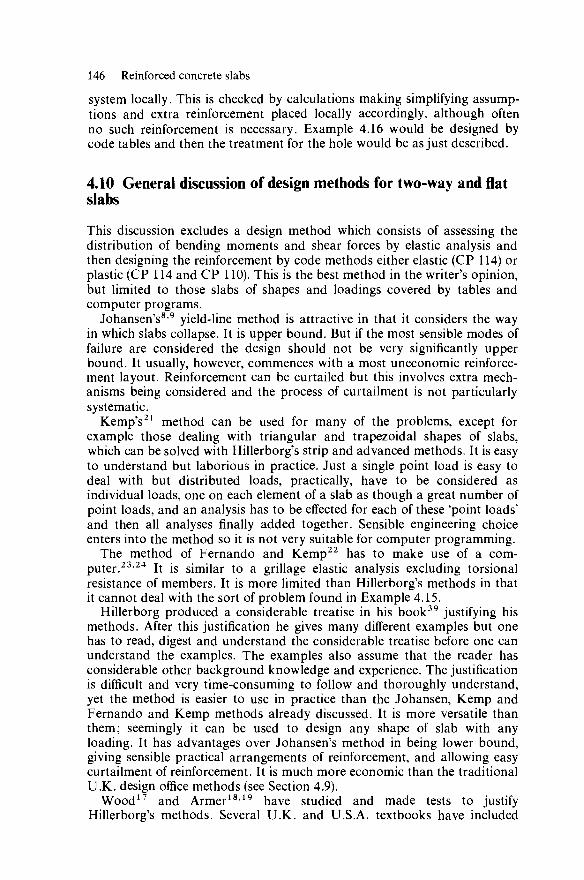
146 Reinforced concrete slabs
system locally. This is checked by calculations making simplifying assump-tions and extra reinforcement placed locally accordingly, although often no such reinforcement is necessary. Example 4.16 would be designed by code tables and then the treatment for the hole would be as just described.
4.10 General discussion of design methods for two-way and flat slabs
This discussion excludes a design method which consists of assessing the distribution of bending moments and shear forces by elastic analysis and then designing the reinforcement by code methods either elastic (CP 114) or plastic (CP 114 and CP 110). This is the best method in the writer's opinion, but limited to those slabs of shapes and loadings covered by tables and computer programs.
Johansen's8'9 yield-line method is attractive in that it considers the way in which slabs collapse. It is upper bound. But if the most sensible modes of failure are considered the design should not be very significantly upper bound. It usually, however, commences with a most uneconomic reinforce-ment layout. Reinforcement can be curtailed but this involves extra mech-anisms being considered and the process of curtailment is not particularly systematic.
Kemp's21 method can be used for many of the problems, except for example those dealing with triangular and trapezoidal shapes of slabs, which can be solved with Hillerborg's strip and advanced methods. It is easy to understand but laborious in practice. Just a single point load is easy to deal with but distributed loads, practically, have to be considered as individual loads, one on each element of a slab as though a great number of point loads, and an analysis has to be effected for each of these 'point loads' and then all analyses finally added together. Sensible engineering choice enters into the method so it is not very suitable for computer programming.
The method of Fernando and Kemp22 has to make use of a com-puter.23 '24 It is similar to a grillage elastic analysis excluding torsional resistance of members. It is more limited than Hillerborg's methods in that it cannot deal with the sort of problem found in Example 4.15.
Hillerborg produced a considerable treatise in his book39 justifying his methods. After this justification he gives many different examples but one has to read, digest and understand the considerable treatise before one can understand the examples. The examples also assume that the reader has considerable other background knowledge and experience. The justification is difficult and very time-consuming to follow and thoroughly understand, yet the method is easier to use in practice than the Johansen, Kemp and Fernando and Kemp methods already discussed. It is more versatile than them; seemingly it can be used to design any shape of slab with any loading. It has advantages over Johansen's method in being lower bound, giving sensible practical arrangements of reinforcement, and allowing easy curtailment of reinforcement. It is much more economic than the traditional U.K. design office methods (see Section 4.9).
Wood17 and Armer18 '19 have studied and made tests to justify Hillerborg's methods. Several U.K. and U.S.A. textbooks have included

General discussion of design methods for two-way and flat slabs 147
Hillerborg's strip method. A very few have seemingly outlined Hillerborg's advanced method from the scientific works just quoted of Wood and Armer, and certainly are not written for students. None of the books, which the author could find from a considerable search, gives any examples of how to use Hillerborg's advanced method.
The author has given examples, covering most types of loading and a very difficult shape in Example 4.15, completely explained as they are pursued. They are best attempted in the sequence given and some syllabi may exclude Example 4.15, which the author found difficult to explain. After understanding these examples the reader may find he can understand many of the further examples given in Hillerborg's book.39
If the elastic analyses described in the first paragraph of this section are not available then Hillerborg's methods seem to offer the best solution to any problem.
References
1. JONES, L. L., and WOOD, R. H., Yield-Line Analysis of Slabs, Thames and Hudson and Chatto and Windus, London (1967)
2. WOOD, R. H., and ARMER, G. S. T., The Theory of the Strip Method for Design of Slabs', Proceedings of the Institute of Civil Engineers, Oct. (1968)
2a.WILBY, C. B., "Design of Reinforced Concrete Slabs', Civil Engineering, August (1980) 3. SCOTT, W. L., GLANVILLE, W. H., and THOMAS, F. G., Handbook on B.S. Code
CP 114 (1957-65), Concrete Publications Ltd. 4. WESTERGAARD, H. M., and SLATER, W. A., "Moments and Stresses in Slabs', A.C.I.
Proceedings, 17, p. 415 (1921) 5. WESTERGAARD, H. M., 'Formulas for the Design of Rectangular Floor Slabs and the
Supporting Girders', A.C.I. Proceedings, 22, p. 26 (1926) 6. MARCUS, H., Die Theorie Elastischer Gewebe und Hire Anwendung auf die Berchnung
biegsaner Platten, 2nd edn, p. 362, Julius Springer, Berlin 7. LOSER, B., Bernessungsverfahren, W. Ernst und Sohn, Berlin 8. JOHANSEN, K. W., Pladeformler, Polyteknish Forening, Copenhagen, 2nd edn (1949) 9. JOHANSEN, K. W., Pladeformler: Formelsamling, Polyteknish Forening, Copenhagen, 2nd
edn (1954) 10. DI STASSIO, J., and VAN BUREN, M. P., "Slabs Supported on Four Sides', A.C.I., 7,
No. 3, Jan.-Feb. (1936); Proceedings, 32, p. 350 11. BERTIN, R. L., DI STASSIO, J., and VAN BUREN, M. P., 'Slabs Supported on Four
Sides', A.C.I., 16, No. 6, June (1945); Proceedings, 41, p. 537 12. European Committee for Concrete, Information Bulletin No. 35, English Translation issued
by Cement and Concrete Association, London (1962) 13. BARES, R., Tables for the Analysis of Plates, Slabs and Diaphragms Based on the Elastic
Theory, Bauverlag, Germany (1971) 14. HENDRY, A. W., and JAEGER, L. G., The Analysis of Grid Frameworks and Related
Structures, Chatto and Windus, London (1958) 15. BARES, R., and MASSONNET, C. Analysis of Beam Grids and Orthotropic Plates by the
Guyon-Massonnet-Bares Method, Crosby Lockwood, London (1968). Earlier non-English edition, Prague (1966)
16. TAYLOR, R., HAYES, B., and MOHAMEDBHAI, G. T. G., Coefficients for the Design of Slabs by the Yield-Line Theory', Concrete, 3, No. 5, p. 171, May (1969)
17. WOOD, R. H., and ARMER, G. S. T., The Theory of the Strip Method for Design of Slabs, Proceedings of the Institute of Civil Engineers, 41, p. 287, Oct. (1968)
18. ARMER, G. S. T., 'Ultimate Load Tests of Slabs Designed by the Strip Method', Proceedings of the Institute of Civil Engineers, 41, p. 313, Oct. (1968)
19. ARMER, G. S. T., 'The Strip Method: A New Approach to the Design of Slabs', Concrete, 2, No. 9, p. 358, Sept. (1968)

148 Reinforced concrete slabs
20. CRAWFORD, R. L., 'Limit Design of Reinforced Concrete Slabs', Proceedings of the American Society of Civil Engineers, Engineering Mechanics Division, EM5, p. 321, Oct. (1964)
21. KEMP, K. O., 'A Strip Method of Slab Design with Concentrated Loads or Supports', Structural Engineer, 49, No. 12, Dec. (1971)
22. FERNANDO, J. S. and KEMP, K. O., A Generalized Strip Deflexion Method of Reinforced Concrete Slab Design', Proceedings oj the Institute of Civil Engineers, Part 2, 65, Mar. (1978)
23. WILBY, C. B., 'Computation of the Strip Deflection Method', Proceedings of the Institute of Civil Engineers, Part 2, TN244, June (1980)
24. WILBY, C. B., 'The Strip Deflection Method of Reinforced Concrete Slab Design', B.Eng.(Tech.) major project, University of Wales Institute of Science and Technology (1979)
25. WILBY, C. B., 'Design Tables for Two-Way Spanning Slabs', The Structural Engineer, Oct. (1981) (Synopsis on p. 337)
26. THAKKAR, M. C , and RAO, J. K. S., 'Design of Two-Way Reinforced Concrete Rectangular Slabs by Modified Hillerborg's Strip Method', Indian Concrete Journal, April (1970)
27. WILBY, C. B., 'Design Tables for Slabs using Strip Deflection Method', Indian Concrete Journal (mi)
28. DUNHAM, C. W., Advanced Reinforced Concrete, McGraw-Hill, U.S.A. (1964) 29. FERGUSON, P. M., Reinforced Concrete Fundamentals, John Wiley, U.S.A. (1973) 30. WILBY, C. A., The Plastic and Elastic Design and Analysis of Reinforced Concrete
Containers', M.Sc. Thesis, University of Oxford (1976) 31. WILBY, C. A., 'Structural Analysis of Reinforced Concrete Tanks', Journal of Structural
Division, Proceedings of the American Society of Civil Engineers, May (1977) 32. WILBY, C. A., 'General Optimisation of the Design of Rectangular Containers', Indian
Concrete Journal, May (1977) 33. WILBY, C. A., 'Optimization of Design of Circular Tanks', Proceedings of the Institute of
Civil Engineers, Part 2, TNI70, Dec. (1977) 34. WILBY, C. A., 'Optimization of Design of Tanks of Regular Polygonal Shape', Indian
Concrete Journal, May-June (1978) 35. WILBY, C. A., 'Application of the Strip Method to the Design of Tanks', Indian Concrete
Journal, April (1979) 36. WILBY, C. A., 'Rectangular Tanks', Civil Engineering, July (1979) 37. HUGHES, B. P., Limit State Theory for Reinforced Concrete, Pitman, London (1971) 38. WILBY, C. B., and NAQVI, M. M., 'Deflections of Rectangular Plates Supported
Elastically', Proceedings of the Institute of Civil Engineers, Paper 7411, August (1971) 39. HILLERBORG, A., Strip Method of Design, A Viewpoint Publication, London (1975)
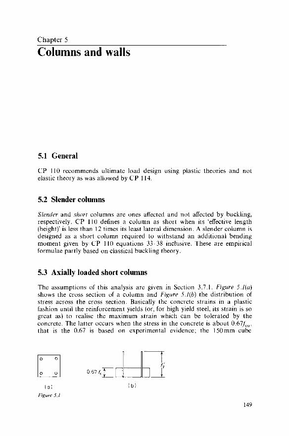
Chapter 5
Columns and walls
5.1 General
CP 110 recommends ultimate load design using plastic theories and not elastic theory as was allowed by CP 114.
5.2 Slender columns
Slender and short columns are ones affected and not affected by buckling, respectively. CP 110 defines a column as short when its 'effective length (height)' is less than 12 times its least lateral dimension. A slender column is designed as a short column required to withstand an additional bending moment given by CP 110 equations 33-38 inclusive. These are empirical formulae partly based on classical buckling theory.
5.3 Axially loaded short columns
The assumptions of this analysis are given in Section 3.7.1. Figure 5.1(a) shows the cross section of a column and Figure 5.1(b) the distribution of stress across the cross section. Basically the concrete strains in a plastic fashion until the reinforcement yields (or, for high yield steel, its strain is so great as) to realise the maximum strain which can be tolerated by the concrete. The latter occurs when the stress in the concrete is about 0.67/cu, that is the 0.67 is based on experimental evidence; the 150mm cube
I—. f?
Figure 5.1
149

150 Columns and walls
strength is affected by nearness of loading platens because of friction between concrete and platens restricting movement associated with Poisson's ratio. Hence resolving vertically
Ultimate axial load = 0.67/cuAc +fJAsc (5.1) where Ac = area of concrete, 4SC = area of compression steel, fcu = characteristic strength of concrete and fy' = characteristic strength of steel in compression. Refer to Section 3.7.7, which explains that for design, CP 110 approximates/y'/ym to 0.72/y./cu is divided by a ym of 1.5 so the ultimate axial load for CP 110 design purposes
= (0.67/1.5)/cu/lc + 0.72/y.4sc
= 0A5fcuAc + 0.12fyAsc
where fy is the characteristic tensile strength of the steel. As loads in practice are rarely axial, to allow for an eccentricity up to 0.05 x least lateral dimension, CP 110 recommends for design an ultimate axial load
= 0.4/clA + 0.61 AsJy (5.2)
Example 5.1. Design a short reinforced concrete column for an ultimate axial load of 2900 kN.
Suppose fcu = 25 N/mm2 and fy = 250 N/mm2 and assume say 2% of reinforce-ment, then
Asc = 0.02(AC + AJ, .'. Asc = 0.0204\AC
From equation 5.2, 2900 = 0.4 x 25 000 xAc + 0.67 x 250000 x 0.0204MC
Therefore Ac = 0.2161 m2 and Asc = 0.02041 x 0.2161 = 0.004411m2
Gross cross sectional area of column = 0.2161 + 0.0044 = 0.2205 m2. Use a column 470mm square with (see Table 3.2) four 32 mm diameter and four 20mm diameter bars.
5.4 Plastic analysis for eccentrically loaded short columns
This is a column required to be designed for an ultimate axial load N combined with an ultimate bending moment M where M = Ne. Figure 5.2(a) shows the cross-section of a column of any shape, Figure 5.2(b) the distribution of stress assumed by CP 110 for design purposes, and Figure 5.2(c) the distribution of strain. The 0.4/cu should really be (0.67/1.5)/cu = 0.45/cu but this is reduced to 0.4/cu to give slightly less chance of failure as a concrete compression failure is sudden and thus undesirable.
Resolving vertical forces N = Nc + Nsc — Ns where Nc is the force in the concrete over the gross area in compression, and Nsc and Ns are forces in the steel in compression and tension, respectively. CP 110 ignores the fact

Plastic analysis for eccentrically loaded short columns 151
0.4/cu
Figure 5.2
that concrete does not exist over the cross-sectional areas of steel-generally a useful and satisfactory assumption. Thus
N = 0AfGUAc + Ascfsc - Asfs (5.3)
where Ac = area of concrete in compression, Asc and As = areas of steel in compression and tension respectively, k2x is the distance to the line of action of Nc (that is to the centroid of AG), and fsc and fs = design strengths (stresses) of compression and tension steels, respectively. Taking moments for convenience about the line of action of JV_
N(e + d - x) = Nc(d - k2x) + NJd - d!) (5.4)
For large eccentricities, failure is initiated by the tension steel yielding or straining excessively (for high-yield steel) causing the value of x to be
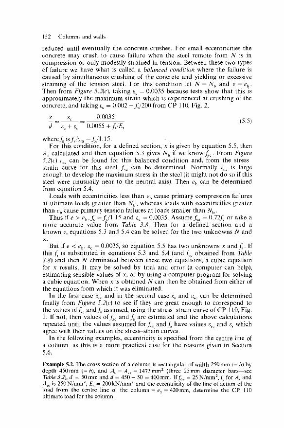
152 Columns and walls
reduced until eventually the concrete crushes. For small eccentricities the concrete may crush to cause failure when the steel remote from N is in compression or only modestly strained in tension. Between these two types of failure we have what is called a balanced condition where the failure is caused by simultaneous crushing of the concrete and yielding or excessive straining of the tension steel. For this condition let N = Nb and e = eh. Then from Figure 5.2(c), taking ec = 0.0035 because tests show that this is approximately the maximum strain which is experienced at crushing of the concrete, and taking es = 0.002 +/s/200 from CP 110, Fig. 2,
x _ ec 0.0035 1 " e c + £ s ~ 0.0055 +fJEs
where/ sis/y/ym=/y/1.15. For this condition, for a defined section, x is given by equation 5.5, then
Ac calculated and then equation 5.3 gives Nb if we know/ s c . From Figure 5.2(c) esc can be found for this balanced condition and, from the stress-strain curve for this steel, /sc can be determined. Normally esc is large enough to develop the maximum stress in the steel (it might not do so if this steel were unusually near to the neutral axis). Then eb can be determined from equation 5.4.
Loads with eccentricities less than eh cause primary compression failures at ultimate loads greater than Nb, whereas loads with eccentricities greater than eb cause primary tension failures at loads smaller than Nb.
Thus if e > eh,fs =/y/1.15 and ec = 0.0035. Assume fsc = 0.72/y or take a more accurate value from Table 3.8. Then for a defined section and a known e, equations 5.3 and 5.4 can be solved for the two unknowns N and x.
But if e < eb, £c = 0.0035, so equation 5.5 has two unknowns x and/ s . If this/ s is substituted in equations 5.3 and 5.4 (and/sc obtained from Table 3.8) and then N eliminated between these two equations, a cubic equation for x results. It may be solved by trial and error (a computer can help), estimating sensible values of x, or by using a computer program for solving a cubic equation. When x is obtained N can then be obtained from either of the equations from which it was eliminated.
In the first case £sc and in the second case es and esc can be determined finally from Figure 5.2(c) to see if they are great enough to correspond to the values of/sc and/s assumed, using the stress-strain curve of CP 110, Fig. 2. If not, then values of/sc and/ s are estimated and the above calculations repeated until the values assumed for/sc and/ s have values £sc and £s which agree with their values on the stress-strain curves.
In the following examples, eccentricity is specified from the centre line of a column, as this is a more practical case for the reasons given in Section 5.6.
Example 5.2. The cross section of a column is rectangular of width 250 mm (= b) by depth 450 mm (= h), and As = Asc = 1473 mm2 (three 25 mm diameter bars—see Table 3.2), d' = 50mm and d = 450 - 50 = 400mm. If/cu = 25N/mm2,/y for As and Asc is 250 N/mm2, Es = 200 kN/mm2 and the eccentricity of the line of action of the load from the centre line of the column = el = 420 mm, determine the CP 110 ultimate load for the column.
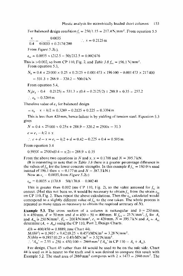
Plastic analysis for eccentrically loaded short columns 153
For balanced design condition^ = 250/1.15 = 217.4N/mm2. From equation 5.5
x 0.0035 . n o i - _ . . x = 0.2125m 0.4 0.0055 + 0.2174/200
From Figure 5.2(c),
£sc = 0.0035 x (212.5 - 50)/212.5 = 0.002 676
This is >0.002, so from CP 110, Fig. 2, and Table 3.8 fsc = 196.1 N/mm2. From equation 5.3,
Nh = 0.4 x 25 000 x 0.25 x 0.2125 + 0.001 473 x 196 100 - 0.001 473 x 217400
= 531.3 + 288.9 - 320.2 = 500.0kN
From equation 5.4,
Nh(eh + 0.4 - 0.2125) = 531.3 x (0.4 - 0.2125/2) + 288.9 x 0.35 = 257.2
.'. eh = 0.3269 m
Therefore value of e{ for balanced design
= eh-x + h/2 = 0.3269 - 0.2125 + 0.225 = 0.3394 m
This is less than 420mm, hence failure is by yielding of tension steel. Equation 5.3 gives
N = 0.4 x 25 000 x 0.25x + 288.9 - 320.2 - 2500x - 31.3
e — ex — h/2 + x
:. e + d-x = el-h/2 + d = 0.42 - 0.225 + 0.4 = 0.595 m.
From equation 5.4
0.595N = 2500x(0.4 - x/2) + 288.9 x 0.35
From the above two equations in N and x, x = 0.1708 and N = 395.7 kN. (It is interesting to note that in Table 3.8 there is a greater percentage difference in
the values of/sc for the lower concrete strengths. In this example if/sc = 180.0 is used instead of 196.1 then x = 0.177m and N = 387.5 kN.)
Now as £c = 0.0035, from Figure 5.2(c)
esc = 0.0035 x (170.8 - 50)/170.8 = 0.00248
This is greater than 0.002 (see CP 110, Fig. 2), so the value assumed for /sc is correct. (Had this not been so, it would be necessary to obtainfsc from the strain £sc on CP 110, Fig. 2. Then repeat the above calculations. Then the £sc calculated would correspond to a slightly different value of/sc to the one taken. The whole process is repeated as many times as necessary to obtain the required accuracy of N).
Example 5.3. The cross section of a column is rectangular and b = 250 mm, h = 450 mm, d' = 50 mm and d = 450 - 50 = 400 mm. If fcu = 25 N/mm2, fy for As
and Asc is 250N/mm2, Es = 200kN/mm2, ex = 420mm, TV = 395.7 kN and As = Asc
determine (As + Asc) using the CP 110, Part 2, Design Charts. d/h = 400/450 = 0.8889, (use Chart 44). M/(bh2) = 0.3957 x 0.42/(0.25 x 0.452)MN/m2 = 3.28 N/mm2. N/(bh) = 0.3957/(0.25 x 0.45) MN/m2 = 3.52N/mm2. .'. 'AJ = 2.55 x 250 x 450/100 = 2869 mm2 ('AJ in CP 110 = As + AJ.
For design, Chart 45 rather than 44 would be used to be on the safe side. Chart 44 is used as it is nearer to the truth and it was desired to compare this result with Example 5.2. The steel area of 2869mm2 compares with 2 x 1473 = 2946mm2. The

154 Columns and walls
small difference between the Charts and Example 5.2 is due to the fact that (a) the stress blocks are slightly different, (b) the charts do not use the correct value of d/h.
It is interesting to note that linearly interpolating between Charts 44 and 45 gives 2890 mm2, which is within 2% of 2946 mm2.
Example 5.4. Repeat Example 5.2, only using ex = 180mm.
As before, the value of el for the balanced design condition = 0.3394 m. This is greater than 0.18 m, hence failure is by compression of concrete. Equations 5.3, 5.4 and 5.5 become
N = 0.4 x 25 000 x 0.25x + 288.9 - 0.001 473/s (5.6)
e + d-x = el-h/2 + d = 0A&- 0.225 + 0.4 = 0.355 m
0.355N = 2500x(0.4 - x/2) + 288.9 x 0.35 (5.7) Assuming/, is on the first portion of the stress-strain curve of CP 110, Fig. 2, then
from Figure 5.2(c)
x _ 0.0035 0 4 " 0.0035 +/s/200000000 ( 5 ' 8 )
One way of solving these equations is to assume that/s is say 217 400kN/m2 (that is 250/1.15 N/mm2), then calculate x from the last equation. With these values calculate values of N from the previous two equations. These wifl normally differ. Adjust the value of fs and start again. Repeat until the values of N from the two equations are sufficiently in agreement. Alternatively the equations can be algebraic-ally reduced to 1250x3 — 112.5x2 + 361 Ax — 146.4 = 0. It is then very easy and rapid to solve this with an electronic hand programmable calculator and guessing values of x, or with a computer library program. The former method gave x = 0.3191m, / s = 177 500kN/m2, and N = 825.2 kN. From Figure 5.2(c)
£sc = 0.0035 x (319.1 - 50)/319.1 = 0.002 952
This is > 0.002 (see CP 110, Fig. 2), so our assumption for/sc is correct. Also from Figure 5.2(c)
0.0035 x (400-319.1) _ _ o £s = = 0.000 887 3 319.1
Referring to CP 110, Fig. 2,
0.8/y/ym = 0.8 x 217.4 = 173.9 N/mm2
and the corresponding strain is
0.1739/200 = 0.000869 5
Thus the strain in this steel appears to be within the second linear portion of the stress-strain curve. The co-ordinates of two points connected by this line are (0.000 869 5, 173 900) and (0.002, 196 100). Thus for any point on this line
(es - 0.000 869 5)/(/s - 173 900) = (0.002 - 0.000 869 5)/(196100 - 173 900) .-. /s = 19 640000es + 156 800 (5.9)
Thus the previous assumption that fs was on the first portion of the stress-strain curve is incorrect and equation 5.8 becomes
x/0.4 = 0.0035/[0.0035 + (/s - 156800)/19640000] (5.10) From equation 5.9 the value of fs corresponding to £s = 0.000 887 3 can be
obtained. The above calculations for N, x, £sc and £s are then repeated. The whole

Reinforced concrete walls 155
process can be repeated until the value of N has sufficient accuracy. It converges rapidly. To reduce the arithmetic one might like to plot the above mentioned line of the stress-strain curve so that the values of fs for various values of £s can be read graphically. Alternatively, by direct calculation the above equations can be algebraic-ally reduced to 1250x3 - 112.5x2 - 44.6x - 14.38 = 0.
It is very easy and rapid to program this on an electronic hand programmable calculator and solve by trial and error as x is known to be near to 0.3191. This gave x = 0.3170, fs = 174800kN/m2, and N = 823.9kN. Had we guessed initially that the second portion of the stress-strain curve was relevant, not the first portion as in equation 5.8, then we would have used equation 5.10 instead of equation 5.8 and saved considerable time and effort. As x is now different to when £sc was previously checked, esc will be rechecked. From Figure 5.2(c).
£sc = 0.0035 x (317 - 50)/317 = 0.002 948 This is > 0.002 (see CP 110, Fig. 2), so our assumption for/sc is still correct.
Example 5.5. Repeat Example 5.3, only using e{ = 180mm, and N = 823.9kN. d/h = 400/450 = 0.889 (use Chart 44). M/{bh2) = 0.8239 x 0.18/(0.25 x 0.452)MN/m2 = 2.929N/mm2. N/(bh) = 0.8239/(0.25 x 0.45) MN/m2 = 7.324N/mm2. kAJ = 2.2 x 250 x 450/100 = 2475 mm2. Comparing this example with Example 5.4, the steel area of 2475 mm2 compares
with 2946 mm2. The difference is due to the fact that (a) the stress blocks are slightly different, (b) the charts do not use the correct value of d/h.
It is interesting to note that if the preceding analysis is repeated using the more complicated stress block of Fig. 3, CP 110, Part 2, and if linear interpolation is used between the Charts 44 and 45 of CP 110, Part 2, then the answer given by the calculation is within 1% of the answer given by the Charts.
5.4.1 Design of eccentrically loaded columns
To be in accordance with CP 110 it is probably best to choose columns from the Charts of Parts 2 and 3 of CP 110. If a column section cannot be obtained in these Charts then the Charts can give guidance in estimating approximately the dimensions of, and steel in, the column. Then it has to be checked as in Section 5.4.
5.5 Reinforced concrete walls
Load-bearing reinforced concrete walls are designed as columns, but if any structural reliance is made on the reinforcement, such reinforcement needs to have ties across the wall to prevent the bars buckling outwards. Such ties are highly undesirable in practice, causing much trouble to both the steelfixer and concretor. It is therefore usually more economical to design the wall as though it contained no reinforcement. It would not, however, be built without any reinforcement because differential settlement, shrinkage and temperature expansion or contraction could all cause cracking, which would be most noticeable on a concrete surface. Such small movements also cause hair cracks between the bricks of brickwork walls, but even if occasional bricks are cracked the cracks blend with the pattern of the wall

156 Columns and walls and are not noticeable to the layman. Cracks in concrete surfaces tend to concentrate into a few of large size, rather than many of a small size, and ramble in various directions in an unsightly way. Consequently horizontal and vertical reinforcement is placed in both faces of a reinforced concrete wall, whether the wall is load bearing or not, the horizontal reinforcement usually being nearer the surface than the vertical reinforcement. In practice, the vertical bars are usually made of at least 12 mm diameter, except in the case of very thin walls, as these have to support the horizontal reinforce-ment. The construction of walls may be very difficult if light reinforcement fabrics are used.
5.6 Design of columns to frameworks
In accordance with CP 110, frameworks are analysed using elastic theory for forces and bending moments, assuming the members to be concentrated at their centre lines (see Chapter 7). The designer may then choose to redistribute these bending moments as described in Chapter 6. Each column section then needs to be designed for a bending moment about its centre line and an axial force whose line of action is through this centre line. It will be appreciated from Section 5.4 and its examples that a direct design calculation is difficult because of decisions as to whether primary compres-sion or tension failures or balanced design conditions are relevant. The designer will often desire the column to be as large as possible to aid detailing of column and interconnecting beam reinforcement, to avoid long column instability, and for economy as the concrete is a more economic material than steel with regard to the carrying of compression forces. However, the larger the column the more it restricts circulation space in the building, and for this reason and aesthetic considerations the architect will often want columns to be as few and as slender as possible. The designer often chooses the size of a column using these considerations, and an assessment of strength. To assess the size of the column and its reinforce-ment to carry the load required a very approximate design is usually made. This can then be checked more accurately by using the design charts of CP 110, or analytically, similar to the method of Section 5.4 if the section is not included in the design charts. If the approximate design is inadequate or uneconomic then this design is altered accordingly and the above procedure repeated until the designer is satisfied. This is a long process if charts, or a computer program, are not used. For the initial approximate design the gross cross-sectional area can be obtained by dividing the ultimate axial load by 0.42/cu if the line of action of the eccentric load is outside and 0.45/cu if within the section. These figures are for rectangular or square cross sections. For circular cross sections the figures would be 0.39/cu and 0.42/cu, respectively. In all cases the amount of longitudinal reinforcement, fy = 250N/mm2, can be taken to be 2.0% of the gross cross-sectional area.
Example 5.6. Make an approximate initial design for a circular column required to withstand a design ultimate moment of 153 kNm and an axial load of 2400 kN for fcu = 50N/mm2 and/y - 425N/mm2.

Design of columns to frameworks 157
Eccentricity of load = 153/2400 = 0.0638 m. The size of the column is not yet known. Assume that the line of action of the
axial load is inside the section, and check this later. Cross-sectional area required
= 2400/(0.42 x 50000) = 0.1143m2
Diameter of column
= V(0.1143/0.7854) = 0.3815 m, say 400 mm
The line of action of the axial load is within the section. Total area of steel reinforcement
= 0.02 x 0.1143 x (425/250) m2 = 3886 mm2
Example 5.7. Check the previous design using CP 110 Design Charts. From Table 3.2, the steel would be eight 25 mm diameter bars. From CP 110,
Table 19, suppose that the cover to the links needs to be 25 mm. Again guided by CP110, suppose that the links are of 8 mm diameter. Then the cover to the main steel is 33 mm. Referring to CP 110, Part 3, hjh = (400 - 2 x 33 - 25)/400 = 0.7725. To be on the safe side use Chart 137 rather than 136. Now
M/h3 = 0.153/0.43 MN/m2 = 2.39 N/mm2
and N/h2 = 2 A/0 A2 = 15.0 N/mm2
hence 100 'AJ/AC = 2.6
Therefore 'AJ = 0.026 x 0.7854 x 4002 = 3276 mm2
Eight reinforcement bars allow a system of rectangular stirrups, which are much better for construction purposes than helices. If the reinforcement is to be reduced it means choosing say either eight, six or twelve bars, for rectangular stirrups. No practical economy can therefore be made in the reinforcement (see Table 3.2) if the bars are all kept of the same diameter. Using two diameters, six 25 mm diameter and six 10 mm diameter bars can be used together in a symmetrical arrangement giving ?. steel area of 3416 mm2 < 3927 mm2 (eight 25 mm diameter bars). These will be positioned on a circle of diameter hs = 309 mm. Thus spacing of bars will be
n x 309/12-80.9 mm
If bars are alternate then distance between two consecutive bars
= 8 0 . 9 - 1 2 . 5 - 5 = 63.4mm This is satisfactory if the size of coarse aggregate is less than 63 — 5 = 58 mm (see CP 110). It will probably be 25 mm and down aggregate because of steel from beams framing into this column, say. This column is similar to the one designed in CP 110, Part 3.
Example 5.8. Make an approximate initial design for a rectangular column required to withstand a design ultimate moment of 91 kNm and an axial load of 2460 kN for fcu = 50N/mm2 and/y = 425N/mm2. Then check the design using CP 110 Design Charts.
Eccentricity of load = 91/2460 = 0.037 m. Assume that the line of action of the axial load is inside the section and check this
later. Cross-sectional area required = 2460/(0.45 x 50000) = 0.1093 m2. If one dimension is 450 mm, the other needs to be
0.1093/0.45 m = 243 mm, say 250 mm

158 Columns and walls
Thus the line of action of the axial load is within the section, as assumed. Total area of steel reinforcement = 0.02 x 0.1093 x (250/425) m2 = 1286 mm2
Use four 20mm diameter bars. Using 30 mm cover to these bars, d = 450 - 3 0 -10 = 410mm and d/h = 410/450 -0.91
UseCP 110, Chart 88. Then M/{bh2) = 0.091/(0.25 x 0.452) MN/m2 = 1.798 N/mm2
N/bh = 2.46/(0.25 x 0.45) MN/m2 = 21.87 N/mm2
and'AJ = 1.0 x 0.25 x 0.45/100m2 = 1125mm2
Hence the steel and size of section chosen are in order. This column is similar to the one designed in CP 110, Part 2.
5.7 Very slender columns
Since 1968 the author and Dr V. R. Pancholi have conducted research for the S.R.C. (now S.E.R.C.) at the University of Bradford, with the assistance of A. Dracos and D. H. Schofield, into very slender columns with length to least lateral dimension ratios of 30 to 79, mainly 30 to 60, see Refs. 1 and 2. Occasionally very slender columns have been used for important structures, for example supports to bridge decks for (a) the bridge across the River Derwent at Hobart, Tasmania, and (b) the approaches to the main span of the Almo bridge, Sweden.
Our tests show that the columns fail by instability when the maximum concrete strain is well below the 0.0035 used by CP 110 (and a similar figure used by the A.C.I, code), for example often no more than 0.001. Thus the codes mentioned are incorrect in using theories based on material failure for very slender columns.
The instability failure experienced manifests itself in that the column collapses due to excessive lateral deflection. In a practical structure, if the column ends were still secure and the collapse loading was not redistributed to other members, the column would eventually fold up under a lower load than caused the initial instability failure. This 'disintegration' after initial failure is irrelevant but at this stage the basic code theories (that is maximum strain of 0.0035) should apply.
References
1. PANCHOLI, V. R., The Instability of Slender Reinforced Concrete Columns', Ph.D. Thesis, University of Bradford (1978)
2. WILBY, C. B., and PANCHOLI, V. R., Design oi Very Slender Reinforced Concrete Columns', Civil Engineering, London (1978)

Chapter 6
Reinforced concrete frames and continuous beams and slabs
6.1 Introduction
Although this chapter is really part of, and its contents are used in, Chapter 7, it is useful for it to be separated for clarity and easy reference as it contains Tables 6.1 and 6.2 which designers refer to considerably, even though it makes a very short chapter. The author wrote Chapters 6 and 7 because a lecturer complained that many books considered elements, for example beams, slabs, columns, in isolation and not as a complete structure, and of course one great advantage of reinforced concrete has always been its use in monolithic constructions, which have many advantages—stability, inherent strength, economy, etc.
6.2 Frames
CP 110 accepts frames being designed for bending moments and shear forces obtained by elastic analysis. The second moments of areas are not usually varied according to the disposition of reinforcement. It is common practice to calculate the second moments of areas of the gross concrete cross sections only, ignoring reinforcement. The individual sections are then designed for ultimate limit states of bending moment and shear force. The disposition of this reinforcement influences the distribution of bending moments towards plastic collapse of a frame.
Much research has been done (for example the author has supervised the work of Refs. 1, 2, 3) with regard to the plastic redistribution of bending moments towards collapse. The fear is that if a designer chooses to make the resistance moment of a section excessively weak, then the section might fail by the extreme concrete fibre strain trying to exceed 0.0035 (the maximum amount experienced before concrete crushing), or fail in shear, before the other sections of the collapse mechanism have realised their full resistance moments. To allow reasonable plastic redistribution of moments but to safeguard against the above, CP 110 says The ultimate resistance moment provided at any section of a member must not be less than 70% of the moment at that section obtained from an elastic maximum moments
159

160 Reinforced concrete frames and continuous beams and slabs
diagram covering all appropriate combinations of ultimate loads, and the elastic moment at any section in a member due to a particular combination of ultimate loads should not be reduced by more than 30% of the numerically largest moment given anywhere by the elastic maximum mo-ments diagram for that particular member, covering all appropriate com-binations of ultimate loads.' Then CP 110 is concerned that the sections should be reasonably under-reinforced (because of the fear of concrete compression failure, which occurs suddenly). Where, as a result of re-distribution, the ultimate resistance moment at a section is reduced, it therefore restricts the neutral axis depth to be not greater than (0.6 — fi)d, where d is the effective depth and fi is the ratio of the reduction in resistance moment, to the numerically largest moment given anywhere by the elastic maximum moments diagram for that particular member, covering all appropriate combinations of ultimate loads. Also, for buildings of more than four storeys CP 110 more cautiously allows elastic moments to be reduced by only 10%, not 30% as mentioned previously.
Design in accordance with the first paragraph of this chapter is com-mendable, in that it automatically gives good control of crack widths and deflections (limit states of serviceability). Design in accordance with the second paragraph endeavours to give increased economy and reinforcement systems which are easier to detail and assist in concreting. For example, the steel required over the supports is often reduced to help detailing, particu-larly when there are two continuous beams at right-angles to one another joining a column at the same place and the architect has requested that the column should have a small cross-section.
6.3 Continuous beams and slabs
The previous section deals with frames, but applies similarly to continuous beams and slabs. Tables 6.1 and 6.2 are most useful for designers. Table 6.1 gives bending moment coefficients for continuous beams or slabs whose spans are equal, or do not vary by more than say 10%, carrying uniformly distributed loads. For live loads the coefficients are for complete spans
TABLE 6.1
Dead load
0.125 A0.071A0.07f
0.100 0.100
0.080*0.025*0.080*
0.107 0.072 0.107
0.077 0.036 0.036 0.077 0105 0.080 0080 0.105
▲ "A A A A A
[ 0.078 0.033 0.0^6 0.033 0.078
Live load
0.125
0.096 0.096
0.117 0.117 A A A A
0.101 0.075 0.101
0.121 0.107 0.121 0.099 0.081 0.081 0.099
0.120 0.111 0.111 0.120 A A A A A A
0.100 0.080 0.086 0.080 0.100

TABLE 6.2
Cont inuous beams and slabs 161
Dead load
038 0.62 z z z
062 038
0X0 0.50 0.60 z z z z
0.60 0.50 0X0
0.39 0.5£ 0X6 0.61 z z z z z
0.61 0X6 0.54 0.39 0X0 0.53 0.50 0X7 0.60
z z z z z z 0.60 0X7 0.50 0.53 0X0
Live load
0.U 0.62 z z z
0.62 OW 0X5 058 062
z z z z 0.62 0.58 0X5
0X5 060 057 062 £ Z 1 1 Z
062 057 060 0X5
0X5 060 059 058 062 Z Z Z Z Z Z
0.62 058 059 060 0X5
loaded in the worst possible arrangement. The elastic bending moment at either support or span = Coefficient x Total load on span x Span. Similarly, Table 6.2 gives coefficients for shear forces. The elastic shear force at a support = Coefficient x Total load on span.
References
1. WILBY, C. B., and PANDIT, T., Tnelastic Behaviour of Reinforced Concrete Single-bay Portal Frames' Civil Engineering and Public Works Review, Mar. (1967)
2. NOOR, F. A., 'Elastic and Inelastic Behaviour of Reinforced Concrete Frames', Ph.D. Thesis, University of Bradford (1970)
3. CHAPMAN, B. C , 'Flexural Behaviour of Redundant Reinforced Concrete Frames', Ph.D. Thesis, University of Bradford (1973)
Chapter 7
Design of structures
7.1 Introduction
Some other books give designs which check the adequacy and design of, and design the reinforcement for, beams, slabs and columns, whose sizes and layouts are given without any explanation of derivation. In other words the essential speedy creation (which a designer has to perform) of the design, giving layout and sizes of members, is not done. The beginner following such designs naturally asks, 'How were this layout and these sizes chosen?' These books might be thought useful for designers of sufficient experience as not to need guidance on determination of layout and sizes, but then such designers do not need the information which the books give—unless they are experienced with CP 114 and trying to convert their skills to CP 110, in which case they probably will find the books most useful.
The beginner needs to be able to create/design suitable structural systems and the sizes of the beams, slabs and columns involved, with the knowledge that the reinforcement will properly fit in the sections upon subsequent detailing and that more comprehensive or accurate design will not require revision of the outline drawings. The self-weight of reinforced concrete members is very significant in their structural design and is unknown until layout and sizes, which it affects, have been determined. As speed is important for economy in design, it is therefore necessary to determine the adequacy of the layout and outlines from simple (approximate), basic, reliable and rapid calculations considering the most influential design requirements first. For example, it is certainly not unknown for a beginner to have inadequate guidance and to design a continuous T-beam by firstly concentrating on making full use of the flange in flexural compression at mid span and then finding that this needs to be revised radically several times because of other design requirements (such as concerning considerations of shear and flexural compression at the supports, and the practicality of detailing reinforcement etc.) which, for efficiency and speed of design, should have been considered previously.
This present chapter, therefore, takes the beginner through the system of creating/designing a beam and slab layout (from merely a column layout required by the architect planning the client's requirements), obtaining the 162

Introduction 163
7m
LO
7 m J
Figure 7.1
sizes and checking the practicality of the main practical design problems (for example, that reinforcement can be detailed in sections) in the sequence in which a professional designer has to rapidly perform this operation. Continuous T-beams, mentioned previously, are designed for layout, size and reinforcement in a speedy practical sequence. The reader is able to follow the mind of the professional designer through this present Section 7.1 and its sub-sections 7.1.1 to 7.1.5 inclusive. Following the designer's mind in creating a structure is not the same as submitting tidy calculations justifying one's creations, to checkers of the designs, for structural ade-quacy. In Section 7.1.6, therefore, the designs are set out in a suitable way for submission to others who wish to check general structural adequacy. These could be: one's supervisor in the design concern or an outside supervisory authority (local, national or consultant working for one or other of these). This setting out of the calculations also acts as a summary to the designs in the previous sub-sections.
Chapter 6 belongs to Chapter 7 but has been separated for clarity of the very useful design tables it contains—these are used where required in Chapter 7.
Figure 7.1 shows a layout of columns, which has been determined to be sympathetic to the arrangement of the windows and layout of internal requirements (for example, partition walls, equipment, machinery). The building is four 7 m bays wide and ten 5 m bays long. Table 7.1 gives a very approximate guide for preliminary design proportioning. If there were no
TABLE 7.1.
Ratios of span to overall depth
Simply supported beams
Continuous beams
Cantilever beams
Slabs spanning in one direction, simply supported
Slabs spanning in one direction, continuous
Slabs spanning in two directions, simply supported
Slabs spanning in two directions, continuous
Cantilever slabs
20
25
10
30
35
35
40
12

164 Design of structures
intermediate beams and the floor slabs were designed as 7 m x 5 m two-way spanning they would be, from Table 7.1, say about 7/40m = 175 mm thick. This is a rather thick slab. Intermediate beams reduce it considerably so that the total amount of concrete and reinforcement is less, and the load on the supporting beams, columns and foundations is less. Also the shuttering does not need to be as strong. The intermediate beams can be as shown in Figure 7.1 and from Table 7.1 the slab is about 2.5/35 m = 71 mm say 125 mm thick as this is about a minimum floor thickness for practical reasons, and for deflection in this example, see later. Otherwise they could have been at right-angles to these, giving two-way spanning slabs 5m x 3.5m, of thickness, from Table 7.1, approximately 5/40m = 125mm say 150 mm for practical reasons. If these two schemes are compared the first is favoured as the shorter beams carry a greater proportion of the load on each 7 m x 5 m panel.
7.1.1 Floor slab
This is therefore a 125 mm thick one-way slab, continuous for 20 bays, each of 2.5 m span. Suppose the floor carries bedrooms for a hotel or hospital. CP 3 requires the floor to be designed for a uniformly distributed load of 2kN/m2. As the slab was made thicker than required for practical reasons the concrete will only need to be weak but as it is a slab and not very thick we do not want the cover to be very great. Considering mild exposure in CP 110 Table 19, we choose Grade 25 concrete so that we can have 20 mm cover—not 25 mm as with Grade 20—so as not to reduce the effective depth of the reinforcement. Referring to CP 110 Table 56, the slab will have \\ hours fire resistance and we assume that this is satisfactory. The floor will carry lightweight partitions and there will be floor finishes, perhaps tiles on the floor, and either plaster or a suspended ceiling and minor services below; assume all this weighs 1.5kN/m2. The self-weight of the floor (taking the weight density of reinforced concrete as 23.6kN/m3) = 0.125 x 23.6 = 2.95 kN/m2.
Thus characteristic dead load = 2.95 + 1.5 = 4.45 kN/m2. The building is wide and long enough compared to its height for wind forces to be neglected (see CP 3). From CP 110 clause 2.3.3.1, design load = 1A x 4.45 + 1.6 x 2 = 9.43 kN/m2.
From CP 110 Table 4, maximum bending moment is at the first interior support and
= 9.43 x 2.52/9 = m per metre 6.55 kN width of slab.
Using/y = 460N/mm2 and CP 110 Design Chart No. 4, and (guessing 8 mm diameter bars and thus d = 125 — 24 = 101 mm)
M/(bd2) = 0.006 55/0.1012 MN/m2 - 0.6421 N/mm2
then 100 AJ(bd) = 0.165 .-. As = 0.165 x 0.101/100 = 0.000 166 7m2/m From Table 3.2 use 8 mm diameter bars at 300 mm centres. This is
reasonable for detailing. The steel at other locations can be obtained pro rata to the bending moments of CP 110 Table 4. For example the smallest
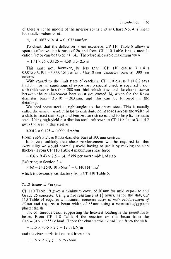
Introduction 165
of these is at the middle of the interior spans and as Chart No. 4 is linear for smaller values of M,
As = 0.1667 x 9/14 = 0.1072 mm2/ni
To check that the deflection is not excessive, CP 110 Table 8 allows a span-to-effective-depth ratio of 26 and from CP 110 Table 10 the modifi-cation factor can be taken as 1.41. Therefore allowable maximum span
= 1.41 x 26 x 0.125 = 4.58m > 2.5m
This must not, however, be less than (CP 110 clause 3.11.4.1) 0.0015x0.101 =0.0001515m2 /m. Use 8mm diameter bars at 300mm centres.
With regard to the limit state of cracking, CP 110 clause 3.11.8.2 says that for normal conditions of exposure no special check is required if our slab thickness is less than 200mm thick which it is; and the clear distance between the reinforcement bars must not exceed 3d, which for the 8 mm diameter bars = 3 x 101 = 303 mm, and this can be followed in the detailing.
We need some steel at right-angles to the above steel. This is usually called distribution steel; it helps to distribute point loads across the width of a slab, to resist shrinkage and temperature stresses, and to help fix the main steel. Using high-yield distribution steel, reference to CP 110 clause 3.11.4.2 gives the area of this steel as
0.0012 x 0.125 = 0.00015 m2/m
From Table 3.2 use 8 mm diameter bars at 300mm centres. It is very unlikely that shear reinforcement will be required (in this
eventuality we would normally avoid having to use it by making the slab thicker). From CP 110 Table 4 maximum shear force
= 0.6 x 9.43 x 2.5 = 14.15 kN per metre width of slab Referring to Section 3.4
V/bd = 14.15/0.101 kN/m2 = 0.1401 N/mm2
which is obviously satisfactory from CP 110 Table 5.
7.1.2 Beams of 7 m span
CP 110 Table 19 gives a minimum cover of 20 mm for mild exposure and Grade 25 concrete. Using a fire resistance of \\ hours, as for the slab, CP 110 Table 54 requires a minimum concrete cover to main reinforcement of 15 mm and requires a beam width of 85 mm using a vermiculite/gypsum plaster finish.
The continuous beam supporting the heaviest loading is the penultimate beam. From CP 110 Table 4 the reaction on this beam from the slab = (0.6 + 0.55) x load. Hence the characteristic dead load from the slab
= 1.15 x 4.45 x 2.5 = 12.79 kN/m and the characteristic live load from slab
= 1.15 x 2 x 2.5 = 5.75kN/m

166 Design of structures
From Table 7.1 the overall depth of the beam required is approximately 7/25 = 0.28 m. Within reason the greater the depth the more economic and easy the design, detailing and fixing of the reinforcement. A small amount of extra vertical shuttering (which does not alter scaffolding costs) and of concrete can save expensive reinforcement and its fixing and reduce concret-ing costs of placing concrete around high percentages of reinforcement. Architects often require the overall depths of beams to be a reasonable minimum for reasons of asesthetics. Deeper beams increase the heights of buildings where strict use is made of minimum headrooms, but we are only talking about altering the depth of beams by perhaps about 0.1 m or so to increase the economy and speed of the reinforced concrete construction. In this example suppose the architect for aesthetic reasons does not desire a beam with overall depth deeper than 0.4 m. The breadth of the rib of a beam will often be about j to y of the overall depth with a minimum sufficient to accommodate three 25 mm diameter bars. Using 19 mm down coarse aggregate the horizontal distance between bars, from CP 110, must be greater than 19-I-5 = 24 mm, say, 25 mm. Hence width of rib to accommodate three 25 mm diameter bars = 5 x 25 + 2 x 25 (that is covers) = 175mm. Hence use a beam of overall depth 0.4m and breadth of rib of 0.2 m. The effective depth, assuming 25 mm diameter bars with 25 mm cover at mid span, will be approximately 400 — 25 — 25/2 = 362 mm and then the span-to-effective-depth ratio = 7000/362 = 19.3. This is less than 26 from CP 110 Table 8 so limit state of deflection is satisfied.
Then characteristic self-weight of rib
= (0.4 - 0.125) x 0.2 x 23.6 = 1.30kN/m
and the total characteristic dead load is
12.79+ 1.3 = 14.09 kN/m
The design ultimate load is then
1.4 x 14.09 + 1.6 x 5.75 = 28.93 kN/m
If the support moments can be carried, and the reinforcement will practically fit in the sections, then the spans should be adequate to resist flexural compression; there is a considerable area of the T-flange available, whereas there is only the rib to take compression at the supports, and the bending moments at mid spans and supports are similar in magnitude.
It is also important to know if the maximum shear force can be carried by the rib with suitable reinforcement if necessary—sometimes being able to practically detail the shear reinforcement can be the critical problem to overcome with the design, necessitating a larger rib.
From CP 110 Table 4, maximum bending moment at a support (and anywhere)
= 28.93 x 72/9 = 157.5 kN/m
and the maximum shear force (adjacent to the inner support of either end span)
= 0.6 x 28.93 x 7 = 121.5kN

Introduction 167
At this support the beam is cracked in flexure in the top and acts as a rectangular beam. The overall depth of the beam is 0.4 m. The slab has top main steel up to 8 mm diameter with 20 mm cover. The main beam steel over the support must be beneath this slab steel; hence, assuming it is of 25 mm diameter bars its effective depth
= 4 0 0 - 2 8 - 1 2 . 5 = 359 mm Using the same type of reinforcement as for the slab, from CP 110 Table
3 fy = 425 N/mm2, then using CP 110 Part 2 Design Chart No. 3 M/bd2 = 157.5/(0.2 x 0.3592)kN/m2 = 6.11 N/mm2
This is beyond the range of the Chart, so compression steel is required. So using Chart 33,
As = 2.0 x 200 x 359/100 = 1436 mm2
and
A's = 1.0 x 200 x 359/100 = 718 mm2
From Table 3.2 use three 25 mm diameter bars as tension steel and two 25 mm diameter bars as compression steel.
V/bd = 121.5/(0.2 x 0.359) kN/m2 = 1.692 N/mm2
< 3.75 of CP 110 Table 6. Then see Example 3.8. At support As
provided = 1473 mm2 and
.'. 100AJ(bd) = 100 x 1473/(200 x 359) = 2.05
From CP 110 Table 5 shear resistance provided by concrete alone
= (0.85 + 0.05 x 0.05) x 200 x 359 N = 61.2 kN
Hence shear reinforcement is required and has to resist 121.5 — 61.2 = 60.3 kN. Using stirrups the V/d required is 60.3/0.359 = 168 N/mm. From Table 3.5, using steel with/yv = 250 N/mm2, use 8 mm diameter two-arm stirrups at 125 mm centres.
There are significant bending moments and shear forces because of the ends not being pin-jointed to the external columns. This reduces the maximum shear forces and bending moments used above. Hence this beam is capable of being designed and detailed with regard to ultimate limit state from the above.
The maximum span bending moment is in the end span and from CP 110 Table 4
28.93 x 72
= = 128.9 kN/m
Assuming 25 mm diameter bars will be used (two of these need to carry through the supports to provide compression steel there) and using 25 mm cover to them, the effective depth
= 4 0 0 - 2 5 - 1 2 . 5 = 362 mm
The whole of the large slab portion of the T-beam is unlikely to be required in compression, so the centre of the compression force is unlikely
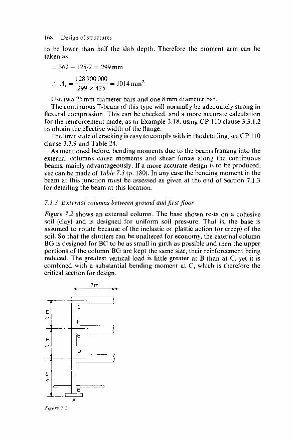
168 Design of structures to be lower than half the slab depth. Therefore the moment arm can be taken as
= 362-125/2 = 299 mm
128 900000 A =
299 x 425 = 1014mm2
Use two 25 mm diameter bars and one 8 mm diameter bar. The continuous T-beam of this type will normally be adequately strong in
flexural compression. This can be checked, and a more accurate calculation for the reinforcement made, as in Example 3.18, using CP 110 clause 3.3.1.2 to obtain the effective width of the flange.
The limit state of cracking is easy to comply with in the detailing, see CP 110 clause 3.3.9 and Table 24.
As mentioned before, bending moments due to the beams framing into the external columns cause moments and shear forces along the continuous beams, mainly advantageously. If a more accurate design is to be produced, use can be made of Table 7.3 (p. 180). In any case the bending moment in the beam at this junction must be assessed as given at the end of Section 7.1.3 for detailing the beam at this location.
7.1.3 External columns between ground and first floor
Figure 7.2 shows an external column. The base shown rests on a cohesive soil (clay) and is designed for uniform soil pressure. That is, the base is assumed to rotate because of the inelastic or plastic action (or creep) of the soil. So that the shutters can be unaltered for economy, the external column BG is designed for BC to be as small in girth as possible and then the upper portions of the column BG are kept the same size, their reinforcement being reduced. The greatest vertical load is little greater at B than at C, yet it is combined with a substantial bending moment at C, which is therefore the critical section for design.
h *+-
i
E CO
, E
en
'
E
'
k
r
) \
, | G
|F
IE
|D ( )
[C
|B F 1 1
Figure 7.2

Introduction 169
Considering durability (mild exposure) and fire resistance (1^ hours) CP 110 Tables 19 and 59 mean that the cover of Grade 25 concrete to the links needs to be 20 mm and the minimum dimension of the concrete needs to be 150 mm, using vermiculite/gypsum plaster.
The vertical loads can be accurately obtained from the shear forces of the beams framing into the columns and estimating the self-weight of the columns. The 5 m long beams should therefore be designed in a similar way (NB CP 110 Table 4 cannot be used for point loads) to that given in Section 7.1.2 before the columns are designed. Assume that the vertical load at C comprises a characteristic dead load of 665 kN and a maximum characteristic live load of 166 kN. To estimate the size of the column assume it is axially loaded, ignore the strength of its reinforcement, and increase the cross-sectional area by about 30%. The design ultimate load
= 1.4 x 665 + 1.6 x 166 = 1197kN
Then the cross-sectional area of column required (see equation 5.2)
= 1.3 x 1197 000/(0.4x25)= 155 600 mm2, say 350 mm by 450 mm
Second Moment of Area for the column
= 350 x 4503/12 = 2658 x 106mm4
The stiffnesses of columns DE and CB, respectively, are 2658 x 106/3000 = 886000 mm3 and 2658 x 106/4000 = 664 500 mm3, respectively. The Second Moment of Area of the beam poses a problem as the beam is a T-beam at mid span but a rectangular beam in effect at the location of cracks near the supports. The writer considers the former as the more accurate assumption, as did Scott and Glanville, and many structures have been designed on this basis in the past. However, the latter assumption is easier for calculation, gives higher moments in the columns, and is favoured in books by Allen (1974) and Higgins and Hollington (1973) of the Cement and Concrete Association. Using this latter assumption the Second Moment of Area for the beam
= 200 x 4003/12 = 1067 x 106mm4
and the stiffness
= 1067 x 106/7000 = 152400 mm3
For this beam the total design ultimate load = 28.93 kN/m, and if it were fixed the end moment (from Table 7.2)
= 28.93 x 72/12 = 118.1 kNm.
The bending moment at C, from CP 110 clause 3.5.2, is
H8.1 x ——— 6 6c
4 ' 5 ,^ AlfS = 48.24kNm. 664.5 + 886 + 152.4/2
As A in Figure 7.2 is assumed to be in effect a hinge, it would be more accurate to reduce the stiffness of CB, but CP 110 does not suggest this, and thus gives a higher moment at C.
There are walls between the external columns, various internal walls and the overall height of the building compared to its horizontal dimensions is

170 Design of structures
sufficiently low for lateral wind forces to be ignored. It can be assumed therefore that the beam column junctions will not move laterally, that is the columns can be considered as 'braced' as defined by CP 110 clause 3.5.1.3. From CP 110 Table 15 take the effective height of column CB as the length CB = 3.7m guessing AB as 0.3 m. Then 3.7/0.35 = 10.57 which is less than 12; hence column can be treated as a short column (see Section 5.2).
From CP 110 clause 3.5.5 the minimum design ultimate bending moment
= 1197 x 0.05 x 0.45 = 26.9 kNm < 48.24kNm,
hence design for this latter. If the links are 8 mm diameter this means that the cover to the main steel is 28, say, 30 mm. Suppose 25 mm bars are to be used in a single layer at each side of the column then effective depth = 450 - 43 = 407 mm and d/h = 407/450 = 0.90. Thus for /cu = 25N/mm2 and/y = 425N/mm2 use Design Chart 76 of CP 110 Part 2.
N/bh = 1.197/(0.35 x 0.45) MN/m2 - 7.6N/mm2
M/bh = 0.048 24/(0.35 x 0.452) MN/m2 = 0.6806 N/mm2
therefore no reinforcement is required. But the percentage of reinforcement should not be less than one (see CP 110 clause 3.11.4.1), hence the area of reinforcement required
= loo x 350 x 450 = 1575 mm2
Then from Table 3.2, four 25 mm diameter bars can be used. For junctions with beams higher up the external column, bending
moments will be similar but the vertical loadings much less. The column is kept the same size all the way to economise on shuttering. A greater predominance of bending moment relative to axial load could require greater reinforcement so it would be precipitous to redesign this portion CB of the column to be smaller with more reinforcement just because the reinforcement required is fairly modest, although four 25 mm diameter bars are quite good for detailing purposes particularly at the junctions with the beams.
With the present design the bending moment in the beam framing into the column at its support is the sum of the bending moments in the columns at C and D, that is
664.5 4- 886 ° " ' U * 664.5 + 886 + .52.4/2 = " " " - " °
It was mentioned at the end of Section 7.1.2 that this bending moment would be calculated here. Its effect can be assessed along the continuous beam using Table 7.3.
7.1.4 Bases
From Section 7.1.3 the design ultimate vertical load at C was 1197kN and AB the thickness of the base was guessed to be 0.3 m. The characteristic self-weight of the column BC can be taken as
0.450 x 0.350 x (4.0 - 0.3) x 23.6 = 13.75 kN

Introduction 171
The design ultimate vertical load at B is therefore
13.75 x 1.4 +1197 = 1215kN The weight of the base gives a characteristic pressure on the soil of
0.3 x 23.6 = 7.08 kN/m2 and an ultimate design pressure of 1.4 x 7.08 = 9.91 kN/m2. As mentioned before, the soil is cohesive and is considered to give a uniform pressure beneath the base. Assume the soil beneath the base can safely withstand a pressure of 217kN/m2. Using a load factor of say 1.8 the ultimate pressure on the soil can be 217 x 1.8 = 390kN/m2. Then the area of the base needs to be
1215/(390-9.91)-3.2m 2
Making it square to save shuttering it needs to be 1.8 m x 1.8 m. From CP 110 Table 19 cover to reinforcement for moderate exposure
(buried concrete) = 40 mm. If 16 mm diameter bars are to be used to form a square mesh, then the effective depth for the bars in the upper layer = 300 - 40 - 24 = 236 mm.
For shear using CP 110 clause 3.10.4.2 condition (1): ultimate design uniform pressure on base = 1215/1.82 = 375 kN/m2, shear force on section distance 1.5 times effective depth (= 1.5 x 236 = 354 mm) from face of column
= 375 x 1.8 x (1.8/2 - 0.35/2 - 0.354) = 250.4 kN
V/bd = 0.2504/(1.8 x 0.236) MN/m2 = 0.59 N/mm2
Condition (2): critical shear perimeter is 1.5 x slab thickness = 1.5 x 300 = 450 mm away from the faces of the column and is
= 2 x 350 + 2 x 450 + 2TI x 450 = 4427 mm area enclosed by this perimeter
= 350 x 450 + 2 x 450 x 350 + 2 x 450 x 450 + n x 4502
= 1514000 mm2
shear on perimeter
= 1215-1.514 x 375 = 647kN
shear stress on perimeter
= 0.647/(4.427 x 0.236) MN/m2 = 0.619 N/mm2
From CP 110 Tables 5, 6 and 14, these shear stresses are satisfactory if the longitudinal reinforcement is slightly greater than
This is to be so for bending considerations later. Using clause 3.10.3 of CP 110 the maximum bending moment is at a
section passing completely across the base at the face of the column and
375 / 1 . 8 - 0 . 3 5 V = — x ( I =98.55kNm/m

172 Design of structures For fcu = 25 N/mm2 and/y = 250N/mm2 use CP 110 Design Chart 1
M 0.09855 —=- —=- MN/m2 = 1.769 N/mm2
bd2 0.2362 ' '
.-. A, = 0.9% of M = ^ x 1000 x 236 = 2124mm2/m
From Table 3.2 use, say, 16 mm diameter bars at 90mm centres. With regard to limit state of cracking, from CP 110, clause 3.11.8.2, the
clear distance between bars should not exceed 300 mm so the 90 mm centres suggested are satisfactory.
CP 110, clause 3.10.5, says that limit state of deflection can be ignored for bases. Deflections would not be unsightly underground; also the greater proportion of the loading is dead not live so the deflection due to the latter would not normally result in undesirable springiness of the base.
The local bond stresses associated with the shear forces above need to be checked for adequacy. Assuming the reinforcement is not reduced in effectiveness by curtailment where either of these shear forces occur:
perimeter of bars per unit length of base = n x 16/0.09 = 558.5 mm/m
from Table 21, ultimate local bond stress = 2N/mm2; from formula 43 of CP 110 (or Section 3.5 of this book) this gives an ultimate shear force
= 0.002 x 558.5 x 236 = 263.6kN/m
where this occurs it corresponds to an ultimate shear stress
MN/m2 = 0.6205 N/mm2
1.8 x 0.236 This is satisfactory as it is greater than 0.59 and 0.619 previously.
The reinforcement must be able to develop adequate anchorage length, within the size of the base, from the position of the maximum bending moment. The distance from the face of the column, where the maximum bending moment was calculated to the periphery of the base = (1.8 — 0.35)/2 = 0.725 m. Using an end cover of 40mm this gives a possible overall bar length of 0.725 — 0.040 = 0.685 m available for anchorage. Referring to Table 2.9 (and see Example 2.4)
Jb = 45db = 45 x 16 = 720 mm
If hooks are used as anchors to the bars, from Table 2.12 a. hook is equivalent to an anchorage length of 256 mm. Hence the overall anchorage length required = 720 — 256 = 464 mm, so 685 mm is satisfactory.
It is interesting that the CP 110 calculation for bending moment gives the same result as using Johansen's method with a yield-line pattern as shown in Figure 7.3(a), and as using Hillerborg's methods for strips and elements as shown in Figure 7.3(b). Applying Johansen's method to the yield-line pattern of Figure 7.3(b) gives an upper-bound solution to that using Figure 7.3(a) as a yield-line pattern.
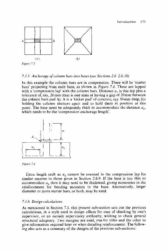
Introduction 173
m
Figure 7.3
7.1.5 Anchorage of column bars into bases {see Sections 2.6-2.6.10)
In this example the column bars are in compression. There will be 'starter bars' projecting from each base, as shown in Figure 7.4. These are lapped with a 'compression lap' with the column bars. Distance ax is this lap plus a tolerance of, say, 20 mm (that is one aims at having a gap of 20 mm between the column bars pad A). A is a 'kicker pad' of concrete, say 50 mm deep, for holding the column shutters apart and to hold them in position at this point. The base must be adequately thick to accommodate the distance a2, which needs to be the 'compression anchorage length'.
r-^\ Figure 7.4
Extra length such as a3 cannot be counted in the compression lap for similar reasons to those given in Section 2.6.9. If the base is too thin to accommodate a2 then it may need to be thickened, giving economies in the reinforcement for bending moments in the base. Alternatively, larger diameter or more starter bars, or both, may be used.
7.1.6 Design calculations
As mentioned in Section 7.1, this present sub-section sets out the previous calculations, in a style used in design offices for ease of checking by one's supervisor, or an outside supervisory authority, wishing to check general structural adequacy. Two margins are used, one for titles and the other to give information required later or when detailing reinforcement. The follow-ing also acts as a summary of the designs of the previous sub-sections:
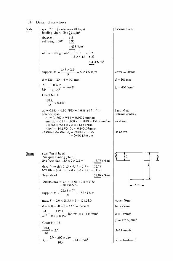
174 Design of structures
Slab
Beam
span 2.5 m (continuous 20 bays) loading (char.): live 2kN/m2
finishes self-weight, SW
1.5 2.95
4.45 kN/m2
ultimate design load: 1.6x2 =3 .2 1.4x4.45 = 6.23
9.43 kN/m2
support M 9.43 x 2.52
= 6.55kNm/m
d = 1 2 5 - 2 0 - 4 M 0.006 55
M 2 " 0.1012
Chart No. 4, 100,4.
: 0.165
101mm
= 0.6421
bd
As = 0.165 x 0.101/100 = 0.000 166 7 m2/m Interior span
As = 0.1667 x 9/14 = 0.1072 mm2/m min. As = 0.15 x 1000 x 101/100 = 151.5mm2/m V= 0.6 x 9.43 x 2.5 = 14.15 kN/m V/(bd) = 14.15/0.101 = 0.1401 N/mm2
Distribution steel As = 0.0012 x 0.125 = 0.00015 m2/m
span 7 m (4 bays) 7 m span loading (char.) live from slab 1.15 x 2 x 2.5 = 5.75 kN/m
dead from slab 1.15 x 4.45 x 2.5 = 12.79 SW rib = (0.4 - 0.125) x 0.2 x 23.6 = 1.30
Total dead 14.09 kN/m
Design load = 1.4 x 14.09 -f 1.6 x 5.75 = 28.93 kN/m
28.93 x 72
support M = = 157.5 kN m
max. V= 0.6 x 28.93 x 7 = 121.5 kN d = 400 - 20 - 8 - 12.5 = 359 mm M _ 157.5
bd* ~ 0.2 x 0.3592
Chart No. 33
100/1.
rkN/m2 = 6.11 N/mm2
bd 2.7
2.0 x 200 x 359 A, = = 1436 mm2
100
125 mm thick
cover = 20 mm
d = 101mm
fy = 460N/m2
8 mm # at 300 mm centres
as above
as above
cover 20 mm
bars 25 mm
d = 359 mm
fy = 425 N/mm2
3-25 mm <P
AK = 1474 mm2
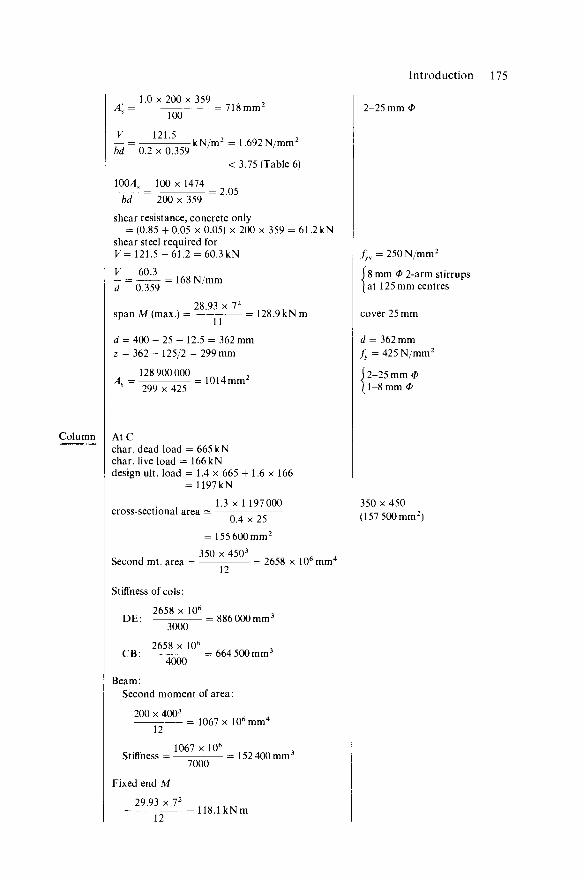
Introduction 175
1 .0x200x359 A' = = 718mm2
100
V _ 121.5 W ~ 0 . 2 x 0.359
kN/m2 = 1.692 N/mm2
< 3.75 (Table 6)
10O4, 100 x 1474 bd 200 x 359
= 2.05
shear resistance, concrete only = (0.85 + 0.05 x 0.05) x 200 x 359 = 61.2kN
shear steel required for V= 121.5-61.2 = 60.3 kN
60.3 : 0.359
168 N/mm
28.93 x 72
span M (max.) = = 128.9 kN m
d = 400 - 25 - 12.5 = 362mm z = 362 -125/2 = 299 mm
128 900000 As = = 1014 mm2
s 299 x 425
AtC char, dead load = 665 kN char, live load = 166 kN design ult. load = 1.4 x 665 + 1.6 x 166
= 1197kN
cross-sectional area : 1.3 x 1197 000
Second mt. area ■
0.4 x 25 = 155 600 mm2
350 x 4503
12 2658 x 106mm4
Stiffness of cols:
2658 x 106
DE: 3000
= 886000 mm3
2658 x 106
CB: = 664 500 mm3
4000
Beam: Second moment of area:
200 x 4003
12 = 1067 x 106mm4
1067 x 106
Stiffness = — - = 152400 mm3
7000
Fixed end M
_ 29.93 x 72
= 12 = 118.1 kNm
2-25 mm <P
/yv = 250 N/mm2
8 mm <P 2-arm stirrups at 125 mm centres
cover 25 mm
d = 362 mm fy = 425 N/mm2
2-25 mm <P 1-8 mm ^
350 x 450 (157 500 mm2)
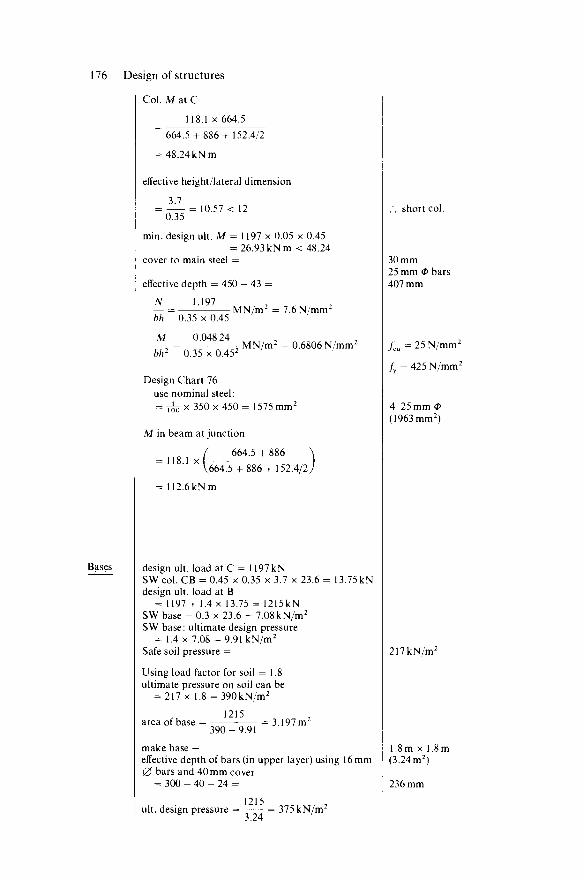
176 Design of structures
Col. M at C
118.1 x 664.5
Bases
664.5 + 886 + 152.4/2
= 48.24 kNm
effective height/lateral dimension
3.7 = = 10.57 < 12
0.35
min. design ult. M = 1197 x 0.05 x 0.45 = 26.93 k N m < 48.24
cover to main steel =
effective depth = 450 - 43 =
N 1.197 bh 0.35 x 0.45
M 0.048 24 bit 0.35 x 0.452
MN/m2 = 7.6 N/mm2
MN/m2 = 0.6806 N/mm2
Design Chart 76 use nominal steel: = jfe x 350 x 450 = 1575 mm2
M in beam at junction
664.5 + 886 118.1 x
V664.5 + 8 8 6 + 152.4/2
= 112.6kNm
design ult. load at C = 1197kN SW col. CB = 0.45 x 0.35 x 3.7 x 23.6 = 13.75kN design ult. load at B
= 1197 + 1.4 x 13.75 = 1215kN SW base - 0.3 x 23.6 = 7.08 kN/m2
SW base: ultimate design pressure = 1.4 x 7.08 = 9.91 kN/m2
Safe soil pressure =
Using load factor for soil = 1.8 ultimate pressure on soil can be
= 217 x 1.8 = 390 kN/m2
area of base = 1215
390-9 .91 = 3.197m2
make base — effective depth of bars (in upper layer) using 16 mm 0 bars and 40 mm cover
= 300 - 40 - 24 =
ult. design pressure = 1215 124 : : 375 kN/m2
.'. short col.
30 mm 25 mm # bars 407 mm
/cu = 25N/mm2
/ = 425 N/mm2
4 25 mm <P (1963 mm2)
217 kN/m2
1.8m x 1.8m (3.24 m2)
236 mm
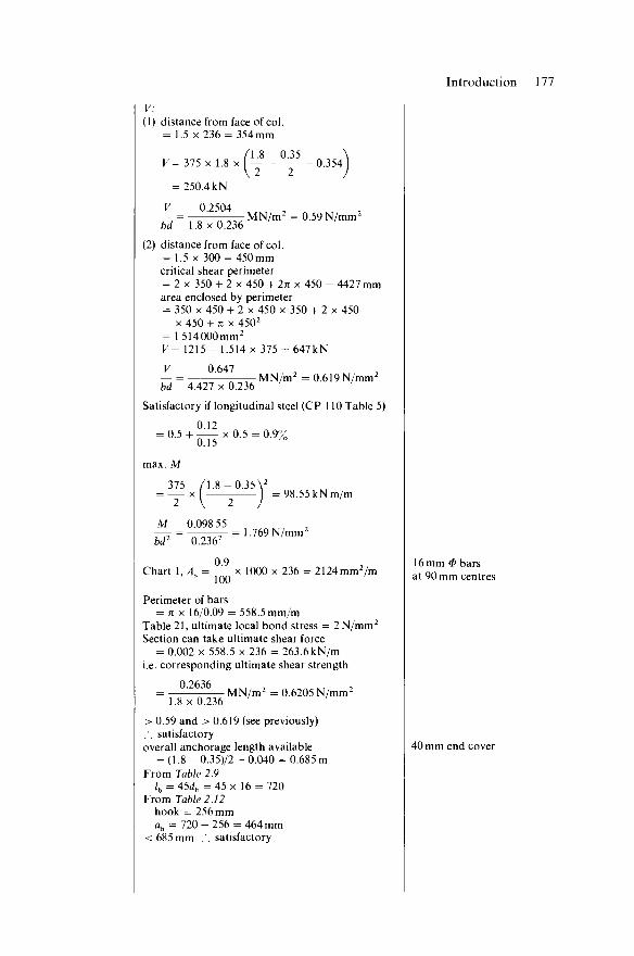
Introduction 177
(1) distance from face of col. = 1.5 x 236 = 354 mm
V=315 x 1.8 x
= 250.4 kN
V 0.2504
0.354
bd 1.8x0.236
0.35
MN/m2 =0.59 N/mm2
(2) distance from face of col. = 1.5 x 300 = 450mm critical shear perimeter = 2 x 350 + 2 x 450 + 2TT x 450 = 4427 mm area enclosed by perimeter = 350 x 450 + 2 x 450 x 350 + 2 x 450
x 450 + 7i x 4502
= 1514000mm2
V= 1215 - 1.514 x 375 = 647kN
0.647 MN/m2 =0.619 N/mm2
bd 4.427 x 0.236
Satisfactory if longitudinal steel (CP 110 Table 5)
0.12 :0 .5+ x 0 . 5 :
0.15 : 0.9%
max. M
_ 375 ~ ~ 2 ~ " \ 2 M _ 0.098 55
bd~~
1.8-0 .35V : 98.55 kNm/m
Chart 1, /L
0.2362
0.9
= 1.769 N/mm2
100 x 1000x236 = 2124mm2/m
Perimeter of bars = 7T x 16/0.09 = 558.5 mm/m
Table 21, ultimate local bond stress = 2 N/mm2
Section can take ultimate shear force = 0.002 x 558.5 x 236 = 263.6 kN/m
i.e. corresponding ultimate shear strength
0.2636 1.8 x 0.236
MN/m2 = 0.6205 N/mm2
> 0.59 and > 0.619 (see previously) .'. satisfactory overall anchorage length available
= (1.8 - 0.35)/2 - 0.040 = 0.685 m From Table 2.9
lh = 454 = 45 x 16 = 720 From Table 2.12
hook E= 256 mm ah = 7 2 0 - 2 5 6 = 464 mm
< 685 mm ..satisfactory
16 mm <P bars at 90 mm centres
40 mm end cover
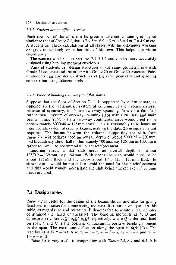
178 Design of structures
7.1.7 Student design office exercise
Each member of the class can be given a different column grid layout similar to that of Figure 7.1, that is 7 x 5 m, 6.9 x 5 m, 6.8 x 5 m, 7 x 4.9 m etc. A student can check calculations at all stages, with his colleagues working on grids immediately on either side of his own. This helps supervision enormously.
The exercise can be as in Sections 7.1-7.1.6 and can be more accurately designed using bending moment envelopes.
Pairs of students can design structures of the same geometry, one with Grade 25 concrete and the other with Grade 20 or Grade 30 concrete. Pairs of students can also design structures of the same geometry and grade of concrete but using different steels.
7.1.8 Floor of building (two-way and fiat slabs)
Suppose that the floor of Section 7.1.1 is supported by a 5m square, as opposed to the rectangular, system of columns. It then seems natural, because of symmetry, to choose two-way spanning slabs or a flat slab, rather than a system of one-way spanning slabs with subsidiary and main beams. Using Table 7.1 the two-way continuous slabs would need to be approximately 5000/40 = 125mm thick. This is reasonably thin; hence an intermediate system of crucifix beams, making the slabs 2.5 m square, is not required. The beams between the columns supporting the slab, from Table 7.1, will perhaps need an overall depth of about 5000/25 = 200 mm, and breadth say about half of this, namely 100 mm, say 125 mm as 100 mm is rather too small to accommodate beam reinforcement.
Ignoring shear, a flat slab needs an overall depth of about 125/0.9 = 139mm, say 150mm. With drops the slab would need to be about 125 mm thick and the drops about 1.4 x 125 = 175 mm thick. In either case it would be normal to avoid the need for shear reinforcement and this would usually necessitate the slab being thicker even if column heads are used.
7.2 Design tables
Table 7.2 is useful for the design of the beams shown and also for giving fixed end moments for commencing moment distribution analyses. In this table, as regards the end restraints, F denotes free to rotate and C denotes constrained (i.e. fixed or encastre). The bending moments at A, B and C, respectively, are aAQ/, aBg/, acQl respectively, where Q is the total load on span /, and C is the position of maximum positive bending moment in the span. The maximum deflection along the span is /3Ql3/{EI). The reaction at A is P = yQ. Also OL1 = 1 — a, a2 = 2 — a, a3 = 3 — a and a1 = 1 + a - a2/2.
Table 7.3 is very useful in conjunction with Tables 7.2, 6.1 and 6.2. It is

TABLE 7.2.
Design tables 179
Loading
A B nrr>mr>nn
iL
^ A
! /
A^rrrTTtl
\r ^
A T" , c t \p
t
r
B
I ItmtKB
• l
J B i
1
End restraint
A
F
C
C
F
C
C
F
C
C
F
C
C
B
F
F
C
F
F
C
F
F
C
F
F
C
Coefficients bending moment
« A
- 1 / 8
-1 /12
-1/5.33
- 1 / 8
—
- 1/6.4
-1/9.6
—
aa1a2/2
— aa2
ac
1/8
1/14.2
1/24
1/4
1/6.4
1/8
1/6
1/9.51
1/16
(X(Xl
a2a!a3/2
2a2a2
aB
—
-1 /12
"
- 1 / 8
—
—
- 1/9.6
—
— a2a t
Deflection
P
1/76.8
1/185
1/384
1/48
1/107.3
1/192
1/60
1/139.5
1/274.3
a2a2/3
P
y
1/2
0.625
1/2
1/2
0.688
1/2
1/2
0.656
1/2
<*i
o^a1
a2(l + 2a)
for continuous beams of spans AB, BC, CD, etc. The first section is for a unit bending moment applied at A, whilst the second section is for unit bending moments applied simultaneously at A and the other end of the continuous beam. The bending moment at any support is the applied bending moment M at the end (or ends) times the coefficient. The shear force next to any support is M x Shear force coefficient divided by the span; EF is always the end span, otherwise the spans read consecutively from left to right (that is AB, BC, CD, etc.). The use of Table 73 is described in Sections 7.1.3 and 7.1.2.
Table 74 gives the weights (for 0 = 9.8O7m/s2) of various building materials.

TAB
LE 7
.3.
Ben
ding
mom
ent
coef
ficie
nts
No.
of
—
span
s A
Shea
r fo
rce
coef
ficie
nts
B
D
AB
BA
BC
C
B
CD
D
C
DE
ED
EF
FE
-1.0
0 +0
.25
—
—
+0.2
5 -1
.00
+0.2
67
—
—
-0.0
67
-1.0
0 +0
.268
-0
.071
—
+0
.018
-1
.00
+0.2
68
-0.0
72
+0.0
19
-0.0
05
—
+0.5
00
—
+0.2
00
—
+0.2
86
-0.0
53
+0.2
63
1.00
1.00
1.00
1.00
+ 0.
500
+ 0.
200
+ 0.
286
+ 0.
263
—
—
-0.1
43
-0.0
53
■1.00
1.0
0 1.0
0 -1
.00
+ 1.2
50
-1.2
50
+ 1.2
67
-1.2
67
+ 1.2
68
-1.2
68
+ 1.2
68
-1.2
68
+ 1.5
00
+ 1.2
00
+ 1.2
86
+ 1.2
63
-1.5
00
-1.2
00
-1.2
86
-1.2
63
-0.3
33
-0.3
39
-0.3
40
0 -0.4
29
-0.3
16
+ 0.
333
+ 0.
339
+ 0.
340
0 +
0.42
9 +
0.31
6
+ 0.
089
-0.0
89
+ 0.
091
-0.0
91
+ 0.
429
0 -0
.429
0
-0.0
24
+0.0
24
+ 0.
316
-0.3
16
-0.2
50
+0.2
50
+ 0.
067
-0.0
67
-0.0
18
+0.0
18
+ 0.
005
-0.0
05
-1.5
00
+1.5
00
-1.2
00
+1.2
00
-1.2
86
+1.2
86
-1.2
63
+1.2
63

Creation (design or selection) of structural system 181
TABLE 7.4. Weights of materials
Aluminium Ashes (dry) Asphalt Brickwork, cement mortar
common brick pressed brick
Cement loose bags bulk
Coal solid crushed washed crushed unwashed
Concrete plain or reinforced granolithic or terrazzo foamed slag non-structural foamed slag structural aerated
Cork Copper Fibreboard Fibreboard, compressed Glass Iron Lead Lime plaster Macadam Mortar (set)
cement screeds lime screeds
Plasterboard Rubber Steel (cast or mild) Tarmacadam Vermiculite/cement screed Wood paving Wood wool/cement slabs Woodwork
red pine teak pitch pine greenheart
kN/m3
27.0 6.3
20.4
19 23
11.8-13.3 11.0-12.6 12.6-14.1
12.8 9.0 9.3
23.6 23.6 13-15 21
8.5-9.4 2.4
85.9 2.9 5.0
24^27 70.6
112 18.8 21
22.6 15.7-17.3 9.3 9.6
77 23
5.8 8.7 5.8-7.2
4.8-7.2 6.4-8.8 6.6-7.2
10-12
Concrete hollow tile slabs 125 mm thick 150 mm thick 190 mm thick
Corrugated sheeting galvanised iron asbestos-cement
Doors N-light roof glazing Roofing felt (two-layer built up) Windows
kN/m2
2.14 2.38 2.68
0.144 0.156 0.384 0.264 0.048 0.240
7.3 Creation (design or selection) of structural system
The designer has to initially decide which type of construction to use. Of course he could design and obtain prices from contractors for many different alternative schemes. Generally the time available for, and the cost of, design and pricing or estimating mitigate against this procedure. The structural designer in conjunction with the architect has therefore generally
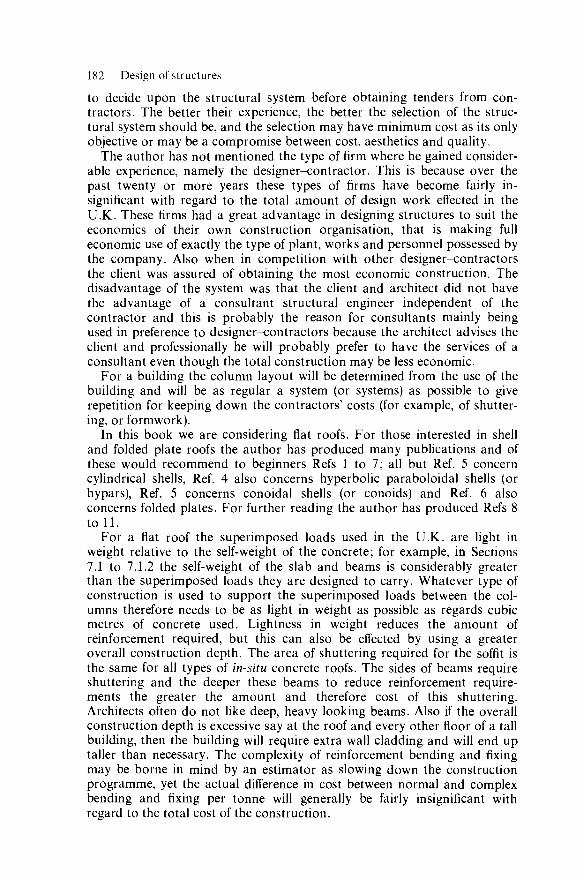
182 Design of structures to decide upon the structural system before obtaining tenders from con-tractors. The better their experience, the better the selection of the struc-tural system should be, and the selection may have minimum cost as its only objective or may be a compromise between cost, aesthetics and quality.
The author has not mentioned the type of firm where he gained consider-able experience, namely the designer-contractor. This is because over the past twenty or more years these types of firms have become fairly in-significant with regard to the total amount of design work effected in the U.K. These firms had a great advantage in designing structures to suit the economics of their own construction organisation, that is making full economic use of exactly the type of plant, works and personnel possessed by the company. Also when in competition with other designer-contractors the client was assured of obtaining the most economic construction. The disadvantage of the system was that the client and architect did not have the advantage of a consultant structural engineer independent of the contractor and this is probably the reason for consultants mainly being used in preference to designer-contractors because the architect advises the client and professionally he will probably prefer to have the services of a consultant even though the total construction may be less economic.
For a building the column layout will be determined from the use of the building and will be as regular a system (or systems) as possible to give repetition for keeping down the contractors' costs (for example, of shutter-ing, or formwork).
In this book we are considering flat roofs. For those interested in shell and folded plate roofs the author has produced many publications and of these would recommend to beginners Refs 1 to 7; all but Ref. 5 concern cylindrical shells, Ref. 4 also concerns hyperbolic paraboloidal shells (or hypars), Ref. 5 concerns conoidal shells (or conoids) and Ref. 6 also concerns folded plates. For further reading the author has produced Refs 8 to 11.
For a flat roof the superimposed loads used in the U.K. are light in weight relative to the self-weight of the concrete; for example, in Sections 7.1 to 7.1.2 the self-weight of the slab and beams is considerably greater than the superimposed loads they are designed to carry. Whatever type of construction is used to support the superimposed loads between the col-umns therefore needs to be as light in weight as possible as regards cubic metres of concrete used. Lightness in weight reduces the amount of reinforcement required, but this can also be effected by using a greater overall construction depth. The area of shuttering required for the soffit is the same for all types of in-situ concrete roofs. The sides of beams require shuttering and the deeper these beams to reduce reinforcement require-ments the greater the amount and therefore cost of this shuttering. Architects often do not like deep, heavy looking beams. Also if the overall construction depth is excessive say at the roof and every other floor of a tall building, then the building will require extra wall cladding and will end up taller than necessary. The complexity of reinforcement bending and fixing may be borne in mind by an estimator as slowing down the construction programme, yet the actual difference in cost between normal and complex bending and fixing per tonne will generally be fairly insignificant with regard to the total cost of the construction.

Creation (design or selection) of structural system 183
A flat slab will not therefore usually provide a very economic roof because although there are no beam sides to shutter, the construction is heavy (meaning large quantities of concrete and stronger soffit shutters) and shallow in overall depth. Thus large quantities of reinforcement are re-quired because of both the heavy self-weight and the small overall depth. For example the roof slab may be 200 mm thick for a flat slab roof whereas the slab of an alternative design with beams and slab might well be 125 mm thick. The flat slab can be made lighter by having 'dropped-panels', that is the area around each column is made thicker than the remainder of the slab. This involves the expense of shuttering the vertical periphery of each drop panel. Hollow tiles have also been incorporated in flat slabs to reduce weight but this will generally be found to be uneconomic.
Apart from systems with either or both thicker slabs and/or larger columns, flat slabs are usually supported by columns with heads flared out each in the shape of an inverted pyramid or cone to reduce the high shear stress in the slab around the periphery of each column. The term 'punching shear stress' used to be used in this connection, the scenario being that of columns punching through a flat slab. The term was used and a check was made of the slab tearing in shear on a plane vertically above the periphery of the column. Tests show that this never happens and that the failure in shear, characterised by an inclined crack basically due to diagonal tension but also affected by bending moment etc., occurs a short distance away from the periphery of the column. For example CP 110 says in effect that the critical section for calculating shear should be taken on a perimeter 1.5 times the overall depth of the slab, from the boundary of the supported area.
Flat slabs can be made more economic by reducing the amount and thus the weight of the concrete by introducing voids of minimum shuttering cost. For example a 'waffle slab' uses say standard glass fibre moulds (for lightness and ease of stripping) as shown in position in Figure 7.5 with the idea that the tremendous repetition of use which each of these moulds can sustain will make this shuttering very inexpensive. More recently this idea has been extended using larger voids, see Figures 7.6 and 7.7, these giving more of a standardised two-way spanning slab supported by beams to the column arrangement.
Continuing our discussion of roofs (the flat slab discussion having led to regular systems of two-way spanning slab arrangements just mentioned) after flat slabs the next in-situ arrangements would be those of beams supporting either one-way or two-way spanning slabs. If the column arrangement is square in plan or of up to say 1.5 to 1.0 length-to-width ratio then two-way spanning slabs may well be useful. Again for a roof it is desirable to keep the thickness of the slab to a minimum of say 125 mm. Panel sizes can be designed on this basis. If they are too large for a suitable division of the distances between columns with a suitable beam system, then the thickness can be kept the same for smaller panels and economies made in the amount of reinforcement required, because the depth is then greater than the minimum requirement.
For more rectangular column layouts one-way spanning slabs of mini-mum thickness, say, 125 mm would be used in preference to two-way spanning slabs.
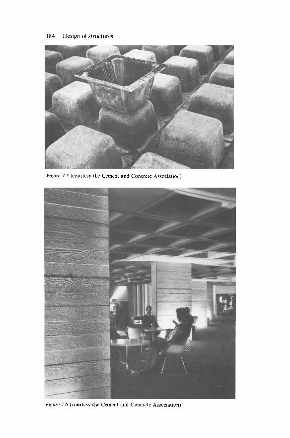
184 Design of structures
Figure 7.5 (courtesy the Cement and Concrete Association)
"1?
Figure 7.6 (courtesy the Cement and Concrete Association)

Creation (design or selection) of structural system 185
Figure 7.7 (courtesy the Cement and Concrete Association)
The beam layouts for these beam/slab systems sometimes involve main beams supporting secondary beams. This can cause enormous weight on the main beams which may need to be of shorter span and greater depth than the secondary beams.
Figure 7.8 shows one of many types of precast concrete roofs. The type shown incorporates voids to keep the weight down. Generally the beam units of these types of roofs (and floors) can be of ordinary or prestressed reinforced concrete. An alternative type commonly used is such that each unit is in effect a hollow beam. The author has been concerned with units which comprise halves of these, and patented for his employer a system using such halves either together or as singles or in pairs between hollow blocks making three types of floor from a machine-produced block and a machine-produced half hollow beam unit. Generally it has been the author's experience that precast slabs are less expensive than in-situ slabs mainly because of the shuttering cost. If a slab is at a height then there is

186 Design of structures
Figure 7.8 (courtesy the Cement and Concrete Association)
also an advantage with precast units in the saving of considerable scaffold-ing costs for the shuttering.
Generally in-situ slabs are of better quality than precast slabs. For example they are more robust, that is they do not have thin (for example 30 mm thick) unreinforced members supporting the top surfaces, although the top surfaces of precast floors are often strengthened, for example, with 25 mm thick screeds. Still an in-situ slab is more robust against, say, a blow from a sledge hammer, a load being accidentally dropped on the floor, say, on one of its corners (that is an impact point load), and so on.
Precast units have to sit on beams and be fastened to them. This causes clumsy detailing problems. If the units simply sit on the beams then the overall depth is unnecessarily high. Beams sometimes have their sides provided with seatings for the precast units; the beams are then rectangular and cannot benefit from being T-beams as in in-situ construction. Supporting beams sometimes have their top part cast after the precast units are in place so that the beams can be T-beams but then the beams have to be propped whilst the units are placed, unless the T action is only for subsequent live load.
The units are sometimes filled in with in-situ reinforced concrete over the supports to gain the advantage which in-situ floors automatically have, that is of continuity.
Creation (design or selection) of structural system 187
The type of roof shown in Figure 7.8 can be made with the beam unit supporting the blocks incomplete and requiring supporting until finally completed with in-situ concrete. Apart from the disadvantages of this system one advantage is being able to make a very standard and lightweight beam unit. One such system used burnt clay tiles with grooves in them for accommodating prestressing wires for fabricating the beam units.
Previously in this section the discussion has concentrated on roofs. Similar considerations apply to floors, particularly for those carrying lightweight superimposed loads. For floors supporting heavy superimposed loads, the self-weight of the concrete is a smaller proportion of the total weight of the construction than for roofs and it is therefore not so important to try and reduce the self-weight as described previously for roofs.
Flat slabs supported by columns with flared heads will not be economic for small spans because of the size and therefore cost of these heads.
Precast frames1213 are economic for single-storey buildings commonly of column layouts 9 m by 4.5 m to 6 m. The author1 2 1 3 has designed and constructed many of these and exceptionally designed for a column layout of 15 m by 9.3 m—the doubly-pitched portal frames in this case carried overhead cranes and needed to be post-tensioned.
With precast frames, joints are the weakness and the problem. The author in Ref. 14 describes a joint suitable for use in multi-storey buildings.
References
1. EVANS, R. H., and WILBY, C. B., Concrete—Plain, Reinforced, Prestressed and Shell, Edward Arnold, London (1963)
2. WILBY, C. B., and BELLAMY, N. W., Elastic Analysis of Shells by Electronic Analogy, Edward Arnold, London (1962)
3. WILBY, C. B., 'A Proposed "Exact" Theory for Analysing Shells, and its Solution with an Analogue Computer,' Proceedings of the Institute of Civil Engineers, July (1962)
4. WILBY, C. B., and KHWAJA, I., Concrete Shell Roofs, Applied Science Publishers Ltd., Amsterdam, London, New York (1977)
5. WILBY, C. B., and NAQVI, M. M., Reinforced Concrete Conoidal Shell Roofs—Flexural Theory, Design Tables, Cement and Concrete Association, London (1973)
6. WILBY, C. B., Concrete for Structural Engineers, Newnes-Butterworths, London (1977) 7. WILBY, C. B., Design Graphs for Concrete Shell Roofs, Applied Science Publishers, London
(1980) 8. WILBY, C. B., and BELLAMY, N. W., Analysis Elastico de Cascarones por la Analogia
Electronica, Compania Editorial Continental, S.A., Mexico (1963) 9. WILBY, C. B., 'A Method of Designing North-Light Shell Roofs', Indian Concrete Journal,
Jan.(1961) 10. WILBY, C. B., Elastic Stability of Post-tensioned Prestressed Concrete Members, Edward
Arnold, London (1964) 11. WILBY, C. B., 'Shell Roofs', Handbook of Structural Concrete, Editors Kong and Evans,
Chapter 32, Pitman Books Ltd., London (1982) 12. WILBY, C. B., A Warehouse with Continuous Precast Frames', Concrete & Constructional
Engineering, Jan. (1958) 13. WILBY, C. B., 'Precast Concrete Framed Roofs—Design of Joints and Post-tensioning',
Indian Concrete Journal, Feb. (1960) 14. WILBY, C. B., 'Structural Behaviour of a Special Type of Joint for Connecting Precast
Concrete Members of Industrialised Buildings', Proceedings R1LEM -CEBC1B Symposium, University of Athens (1978)
Chapter 8
Prestressed concrete
8.1 Prestressing
Prestressing consists of initially applying loads to a member to counteract the effects of the working loads to which it will eventually be subjected. Concrete is relatively weak in tension compared with compression, so the prestressing forces are used to compress zones which will subsequently be required to carry tension. Prestressing forces are usually applied in one of the following ways:
1. Stretching wires, cables or bars on a bed, concreting the member around such wires, and then releasing the wires when the concrete is sufficiently hard. When the wires are released, they shorten, and compress the concrete member, the line of action of such compression for each wire being the profile of the wire in the beam. This procedure is known as pretensioning.
2. A member is concreted and a duct is formed in the member either with a metal sheath or an inflatable tube. A tendon, consisting of either a bar, cable (for example Strand) or groups of wires, is threaded through the duct and tensioned when the concrete is sufficiently hard, and anchored to the concrete member, so that the concrete member is compressed by this tendon. The procedure is known as post-tensioning, and it is usual sub-sequently to fill the duct surrounding the cable with grout. A grout of cement, with no more than sufficient water for the workability required, is suitable. Sand is not recommended.1'2 Special plasticisers3,4 are recom-mended to give better quality grouting. Air entrainers4 can be used instead of or in addition to plasticisers. It is vitally important not to trap pockets of water in ducts, as they have frozen in winter and caused trouble. Soroka and Geddes5 report 'the ultimate moment and pattern of cracking are hardly influenced by grout quality'. Szilard6 reports particular concern with regard to the adequacy of the strength of the grout and its corrosion resisting properties. Refs. 5 and 6 list 75 and 103 references respectively on this subject. The author has experience of a special polyester material which would seem to be excellent for strength and workability for use in even damp ducts, though its rapid setting time would be its greatest disadvantage in use and some 188
Prestressing 189 development in this respect would be necessary. Epoxy resins3 are affected by water, as in the experience of the author the hardeners react chemically with water.
3. A variation on method 2 is to place the tendon in the sheath before concreting. It is usually easier to thread the tendon in the sheath before concreting than in the duct after concreting. This does not, of course, allow inflatable tubes to be used for forming the duct. This latter method appears to be cheaper from the point of view of forming the duct, but on the whole, in the U.K., when the extra cost of positioning the inflatable tubes and threading the ducts they form is considered, it is usually more economical to place the tendon in the expendable tubing before casting.
4. Another variation on method 2 is to make the concrete member in precast portions which are placed together on the site, the joints between such members being dry packed with cement: sand mortar, usually after the tendons have been threaded through the blocks. An alternative material for jointing is polyester resin. The author devotes Chapter 16 of Ref. 7 to 'Beams Consisting of Segments—Joint Efficiency'.
5. A variation7 on method 4 is to cast each portion against the previous portion, sometimes post-tensioning each portion to the previous one, and then finally post-tensioning all portions together.
6. Prestressing forces can be exerted on structures in suitable places by jacks. For example, hydraulic jacks have been used in the abutments of dams arched in plan, to exert known forces in favourable directions and achieve economies in the amounts of concrete required in the dams.
8.1.1 Advantages and disadvantages of prestressing
The chief advantages of prestressed concrete are in reducing the quantities of steel and concrete required and in eliminating or reducing the widths of cracks. The disadvantages are the extra labour costs connected with the stressing of the tendons, and with other items.
Prestressing strengthens a beam in shear and can give a useful saving in shear reinforcement, useful with regard to cost and sometimes especially with regard to facility of detailing. The author has on occasions post-tensioned jointed precast structures solely because of the weakness of the joints in shear.
In the U.K., if a member can be equally well constructed in prestressed or ordinary reinforced concrete, then the latter is usually more economical. When, however, large spans are required with shallow depths, for example for bridges, precast floors and so on, and the ordinary reinforced concrete is structurally unacceptable, then prestressed concrete is the only answer in concrete, and, if there is a reasonable repetition in the making of members (to reduce shuttering costs), in the U.K. it is sometimes more economical than structural steelwork. If a factory is highly organised in the manufac-ture of prestressed flooring units it is sometimes found that units which could be of ordinary reinforced concrete can be made shallower in pre-stressed concrete and can thus be less expensive overall by making savings in transportation, handling and stacking. When the spans of bridges are sufficiently short to make prestressing cheaper than steelwork, prestressed

190 Prestressed concrete
concrete has the great advantages over steelwork of relative freedom from maintenance, and fire resistance.
Prestressed concrete construction is often more expensive to design than ordinary reinforced concrete work. In post-tensioned in-situ structures, prestressing procedures have to be carefully planned because tensioning one cable makes previously tensioned cables deficient in stress and can cause undesirable stresses to develop due to the eccentricity of the prestressing force; this eccentricity will usually be eliminated when the prestressing is satisfactorily completed. Sometimes this planning involves larger amounts of structures to be shuttered or alternatively supported before prestressing than would be necessary if the structure were of ordinary reinforced concrete. In such circumstances prestressing sometimes slows down the speed of construction and increases the shuttering required for a contract.
Members designed with prestressed concrete can be very flexible and the designer must be particularly careful that deflections, cambers and flexibil-ities are satisfactory.
It is conceivable even to pay more for prestressed concrete structures than for ordinary reinforced concrete structures when resistance to cor-rosion is important; the life of the prestressed structure can be greater because of the absence of cracks. Structures such as docks, wharfs and jetties which are exposed to sea water, exposed structures at gas works, bridges exposed to pollution, structural work in dairies exposed to lactic acid, are common examples of concrete structures exposed to corrosive elements and can benefit from prestressing.
8.2 Materials
Prestressed concrete uses highly stressed steel and concrete, and good materials and workmanship are most important. Failures have occurred due to corrosion of tendons. The concrete and grouting materials must be non-corrosive to the steel and dense for strength and for resistance against water or corrosive liquids endeavouring to come into contact with the steel. Calcium chloride is detrimental in concrete that allows water to contact the steel (see Chapter 2). Generally the quantities of chlorides and sulphates should be strictly limited in the concrete materials. The corrosion of tendons is due to pitting and hydrogen embrittlement as well as stress corrosion; Ref. 6 is useful.
If high alumina cement is to be used, refer to Section 2.1.
8.2.1 Stress corrosion
This is a very important problem. There have been failures due to stress corrosion, and there has been much research, particularly in connection with prestressed concrete bridges, and also because the strands used for tendons are also used for cables of suspension and cable-stayed bridges and funicular mountain railways. The author has seen considerable research in progress in stress corrosion in Paris and Zurich. Leonhardt3 establishes conditions which must exist for stress corrosion of prestressing wires. The author understands that British steel has always been manufactured not to experience this problem.
Losses of prestress 191
8.3 Losses of prestress
The stress initially effected in the tendons is reduced by the following losses. (For examples of how CP 110 deals with these losses, see Example 8.5.)
1. Relaxation (creep) of steel. The high stresses used in the tendons mean that the steel is sometimes stressed slightly beyond its limit of pro-portionality. Hence, after anchorage the strain in the steel can correspond to a lower stress as creep occurs. With pretensioned members, this loss can be greatly reduced by tensioning say in the afternoon and then suitably increasing the strain in the tendons next morning before casting. This is an operation which interferes with progress and increases labour costs, and for overall economy it is usually better not to try to eliminate creep but to consider it as a loss in prestress. A rise of temperature helps the steel to creep and can thus increase creep loss. The relaxation loss depends on the type of tendon and the magnitude of the stress it experiences.
2. Elastic deformation (strain) of concrete. When pretensioned wires are released they compress the concrete, the concrete strains, and thus reduces the strain and hence the stress in the wires. This is known as loss of prestress due to strain (or elastic deformation). A post-tensioned member with only one tendon does not, in theory, experience a strain loss because as the jack strains the tendon it compresses the concrete. When more than one tendon is used, then as each tendon is strained the jack increases the strain in the concrete; this reduces the strain in the tendons already anchored; that is strain losses occur in all but the last tendon to be stressed. All these losses total less than those experienced with pretensioned concrete. When pretensioned wires are released they will shorten owing to the concrete becoming strained and stressed (that is prestressed). The shortening of the wires divided by their length is the loss in strain of the wires, say sl. This shortening must be the same for the concrete immediately in contact with the wires and this is unstressed before the shortening and then stressed due to the shortening. Hence the strain in the concrete is also el. Applying Hooke's law, the loss of stress in the wires is Essl and the gain of stress in the concrete is Ecel. Hence loss of stress in wires = Ese1 = Es (Stress in concrete/£c) = ae (Stress in concrete). This is most important and will be summarised as follows: For pretensioning:
. . shortening of wires Loss of strain in wires = ——
length = gain of strain in concrete = sx
. . . . stress in concrete Gain in strain in concrete = = e1
£c /stress in concrete\
Loss of stress in wires = £_et = £s x
= ae x (stress in concrete)
3. Shrinkage of concrete. Shrinkage is discussed in Chapter 2. As concrete shrinks after the tendons have been anchored to the concrete, the concrete
192 Prestressed concrete member shortens and hence so does the tendon, thus releasing some stress in the tendon. In the case of pretensioned concrete, the shrinkage effect begins as soon as the concrete is cast, but with post-tensioned concrete the concrete is able to shrink before the tendon is stressed. If there were no longitudinal reinforcement the shrinkage would be restricted only by fric-tion with moulds, etc., and most of the shrinkage would occur before stressing. Humidity and temperature also affect shrinkage. For practical design CP 110 gives suitable recommendations for calculating the loss of prestress due to shrinkage of the concrete (see Example 8.5).
4. Creep in concrete. Creep has already been explained in Chapter 2. As the concrete creeps it reduces the strain and hence the stress in the prestressing tendons. With prestressed concrete, creep is not under a constant stress, as considered in Chapter 2, because the stress in the concrete is reducing as the concrete creeps. The creep loss may be estimated by reference to CP 110. The loss is greater for pretensioned than for post-tensioned members. Pretensioned tendons rely upon their bond to the concrete for anchorage and in time this releases (or creeps) slightly; this creep of bond stress is not counted as a separate loss, so is accounted for as an increase in creep loss.
5. Slip of anchorage. This refers to the tendons losing stress after anchorage due to the anchorage device slipping; for example wedges are pulled forward in their jaws as the stress is taken up by the anchorage. This should be assessed for the particular system used. For prestressing over short distances it is preferable that this allowance should be as small as possible, as the greater the allowance the greater the probable error in the reliability of this quantity. For this reason the author8 found certain bars useful for prestressing over short lengths; the relative movement between the nuts and threads of the system caused only very little loss of stress.
6. Friction in jack and anchorage system. In pretensioning, if the extension of the wire is measured directly then the friction in the jack is not a loss to be deducted from this prestress measurement. If, however, in pretensioning, and mostly in post-tensioning, the prestress is measured say on the body of the jack with a vernier recording the movement of the movable part relative to the stationary part, then as there will be friction in the jack, this frictional force will be included in our measurement of the force in the tendon using the oil pressure gauge on the jack. The difference between the forces measured in a tendon by these two methods depends upon the type of jack used. This difference should be reasonable for the particular type of jack as excessive oil pressure would indicate that the jack had seized up and further stressing would damage it. Certain jacking equipment can incorporate a strain gauge load cell. In post-tensioning systems where the tendons are deviated just before the final anchorage, indeed deviated to effect the final anchorage because of the space required by jacks and anchorages, there is a frictional loss related to the pressure of the tendons on the sides of the deviating device used by the particular system. This must be allowed for in determining the prestressing force in the tendons and it depends upon the particular system.
7. Friction along duct in post-tensioning. With regard to a straight tendon it will normally be detailed not to touch its duct, but in practice, because of lack of straightness of tendon and duct, there will be some contact between
Limit state design of members 193
a tendon and its duct. The duct will tend to deviate the tendon, perhaps in some kind of wobble along the duct. Because of this deviation there must be pressure between tendon and duct and thus frictional forces between the two when the tendon is being stressed. When a tendon is taken round a bend, the tendon exerts pressure on the duct, or concrete tank wall, etc., and there is friction associated with this pressure on tensioning the tendon.
CP 110 recommends the following formula which has been justified by tests:
Px = P 0 exp [ -Kx- ( / i x / r p s ) ] (8.1) which for small values of Kx and fix/rps can be approximated to
Px = P0ll-Kx-(iix/rpsn (8.2) where
P0 = Prestressing force in a tendon at the jacking end. Px = Prestressing force at any distance x from the jack. K is a constant depending on how much the duct is likely to deviate, that
is how rigid the sheath is, how often it is supported, how much vibration is used for the concrete.
H is the coefficient of friction between the tendon and the duct surface, or surface of concrete tank wall, etc.
rps = Radius of curvature. e =2.718.
In the case of tendons which are not to be finally bonded to the member, they can be lubricated, and some tendons can be purchased enclosed in polythene sheaths packed with suitable grease. The author has used the latter on the outside of a dome which required strengthening as an emergency measure—the polythene and grease have good weather resistance.
The author in Ref. 7 devotes Chapter 5 to friction describing methods of assessment, giving derivation of formulae (such as equations 8.1 and 8.2) and suggesting a different approach. It gives K and ji values for normal work and, in a Table 5.1, for both mastic coated and pregreased tendons which are used to reduce friction in the U.S.A. Then Appendix 1.6 in the book gives K and \i values used in many different countries for many various types of tendons and ducts.
8. Steam curing. This can interfere with the losses due to creep and shrinkage of the concrete, and relaxation of the steel.
8.4 Limit state design of members
Members must be designed for the following, according to CP 110:
1. Limit state of cracking, due to flexure. 2. Ultimate limit state, due to flexure. 3. Prestressing requirements; losses; maximum initial prestress; end-
block design or transmission length requirements. 4. Ultimate limit state; shear. 5. Limit state of deflection. 6. Considerations affecting design details. 7. Torsion.
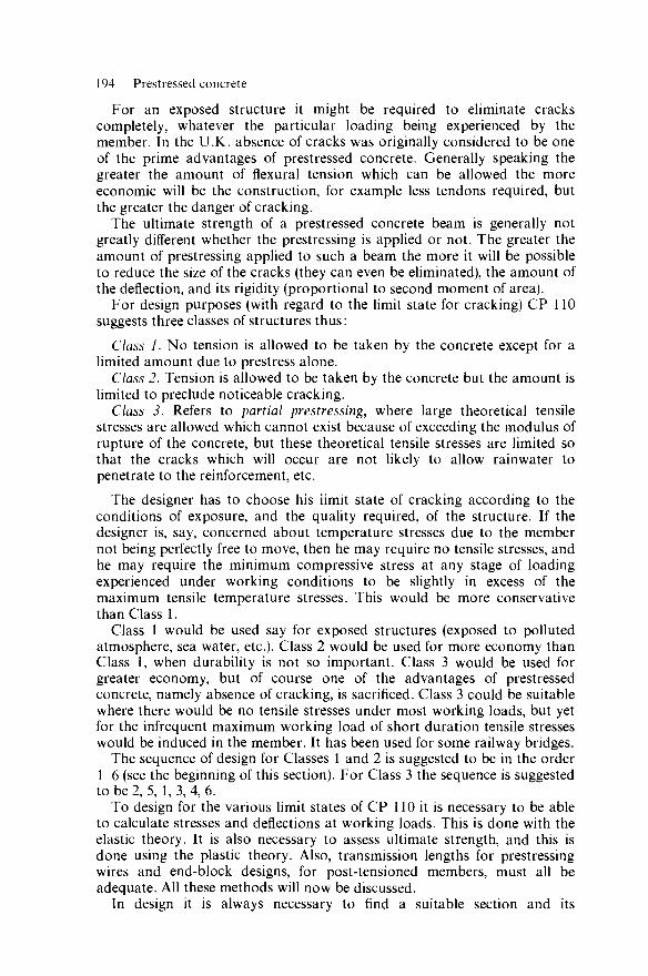
194 Prestressed concrete
For an exposed structure it might be required to eliminate cracks completely, whatever the particular loading being experienced by the member. In the U.K. absence of cracks was originally considered to be one of the prime advantages of prestressed concrete. Generally speaking the greater the amount of flexural tension which can be allowed the more economic will be the construction, for example less tendons required, but the greater the danger of cracking.
The ultimate strength of a prestressed concrete beam is generally not greatly different whether the prestressing is applied or not. The greater the amount of prestressing applied to such a beam the more it will be possible to reduce the size of the cracks (they can even be eliminated), the amount of the deflection, and its rigidity (proportional to second moment of area).
For design purposes (with regard to the limit state for cracking) CP 110 suggests three classes of structures thus:
Class 1. No tension is allowed to be taken by the concrete except for a limited amount due to prestress alone.
Class 2. Tension is allowed to be taken by the concrete but the amount is limited to preclude noticeable cracking.
Class 3. Refers to partial prestressing, where large theoretical tensile stresses are allowed which cannot exist because of exceeding the modulus of rupture of the concrete, but these theoretical tensile stresses are limited so that the cracks which will occur are not likely to allow rainwater to penetrate to the reinforcement, etc.
The designer has to choose his limit state of cracking according to the conditions of exposure, and the quality required, of the structure. If the designer is, say, concerned about temperature stresses due to the member not being perfectly free to move, then he may require no tensile stresses, and he may require the minimum compressive stress at any stage of loading experienced under working conditions to be slightly in excess of the maximum tensile temperature stresses. This would be more conservative than Class 1.
Class 1 would be used say for exposed structures (exposed to polluted atmosphere, sea water, etc.). Class 2 would be used for more economy than Class 1, when durability is not so important. Class 3 would be used for greater economy, but of course one of the advantages of prestressed concrete, namely absence of cracking, is sacrificed. Class 3 could be suitable where there would be no tensile stresses under most working loads, but yet for the infrequent maximum working load of short duration tensile stresses would be induced in the member. It has been used for some railway bridges.
The sequence of design for Classes 1 and 2 is suggested to be in the order 1-6 (see the beginning of this section). For Class 3 the sequence is suggested to be 2, 5, 1, 3, 4, 6.
To design for the various limit states of CP 110 it is necessary to be able to calculate stresses and deflections at working loads. This is done with the elastic theory. It is also necessary to assess ultimate strength, and this is done using the plastic theory. Also, transmission lengths for prestressing wires and end-block designs, for post-tensioned members, must all be adequate. All these methods will now be discussed.
In design it is always necessary to find a suitable section and its

Limit state design of members 195
reinforcement, before all the checks of the adequacy of 1-6 (previously in this section) are ascertained with adequate precision. With experience the original estimate of the section may need little or no alteration as a result of these checks. For optimisation one would program the procedure so that the computer can keep modifying the original estimate of the section to satisfy the various checks as economically as possible. This is simply a matter of programming the procedures of design which follow in this chapter.
8.4.1 Simple assessment of size of prestressed members
As previously mentioned, experience helps this procedure. One can be guided by observing sizes of members of similar jobs from publications, etc. Alternatively, or in addition, one can choose the type of concrete to be used—one which is not too difficult to achieve with the methods to be used and standard of product required—and proceed as follows.
Example 8.1. An initial estimate is required of a suitable I-shaped cross section for a prestressed concrete beam which has to resist a total bending moment at mid span at working loads of 870 kN m (inclusive of its self-weight), and is to be designed for a limit state of cracking of Class 1.
It is fairly easy for the manufacturer to obtain a concrete of characteristic cube strength at 28 days (when we assume the structure may need to withstand its working load) of 40 N/mm2, and this concrete can be made of early enough strength for the requirements at transfer.
Referring to Table 32 of CP 110, and because we are considering concrete stresses ym = 1.3, but as an allowance has been made for this in the table, the allowable compressive stress is
0.33 x 40 = 13.2N/mm2 = 13 200kN/m2.
If the tendons are to be straight then the bending moment due to the weight of the member will reduce the prestressing at mid span, but not at the supports, and thus the supports are the critical sections for deciding the amount of prestressing. At these sections at working loads the prestressing could be as Figure 8.1(a). This would also be the prestressing at the mid-span section, because of the straight tendons. The total bending moment at mid span can therefore give a stress distribution as Figure 8.1(b), which is superimposed upon (a) to give (c) in Figure 8.1, assuming the section to have its neutral axis at mid depth of the section. The section can hence be designed as for Figure 8.1(b)\ thus the section modulus needs to be
870/13 200 = 0.065 91m2.
Try the section shown in Figure 8.2. Its second moment of area is
[(0.45 x 1.13)/12] - [(0.3 x 0.83)/12] = 0.037 11m4
and its section modulus is therefore
0.037 11/0.55 = 0.067 48 m3.
This section will therefore be suitable. The bending moment used included an allowance for the self-weight of the member. This had to be estimated and should be checked against the section now obtained. If the estimate is found to be wrong then the section we have just designed gives a good clue to a revised estimate of the self-weight of the beam for use in a revised design.
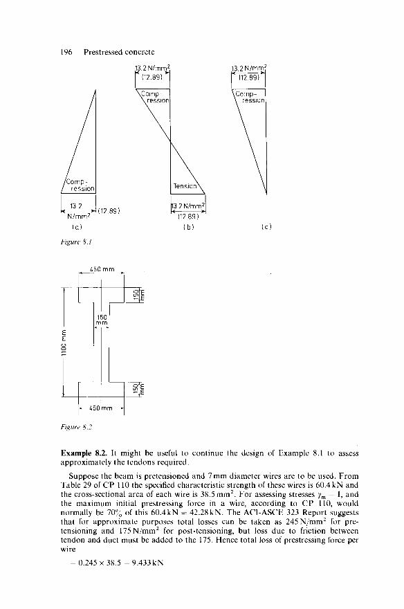
196 Prestressed concrete
13.2 N/mm2.
12.89)
,13.2 N/mm2
l l2 iJ9f
Figure 8.1
450 mm
150 mm
?I
—it
k i50mm *►]
Figure 8.2
Example 8.2. It might be useful to continue the design of Example 8.1 to assess approximately the tendons required.
Suppose the beam is pretensioned and 7 mm diameter wires are to be used. From Table 29 of CP 110 the specified characteristic strength of these wires is 60.4 kN and the cross-sectional area of each wire is 38.5 mm2. For assessing stresses ym = 1, and the maximum initial prestressing force in a wire, according to CP 110, would normally be 70% of this 60.4kN = 42.28kN. The ACI-ASCE 323 Report suggests that for approximate purposes total losses can be taken as 245 N/mm2 for pre-tensioning and 175 N/mm2 for post-tensioning, but loss due to friction between tendon and duct must be added to the 175. Hence total loss of prestressing force per wire
= 0.245x38.5 - 9.433 kN
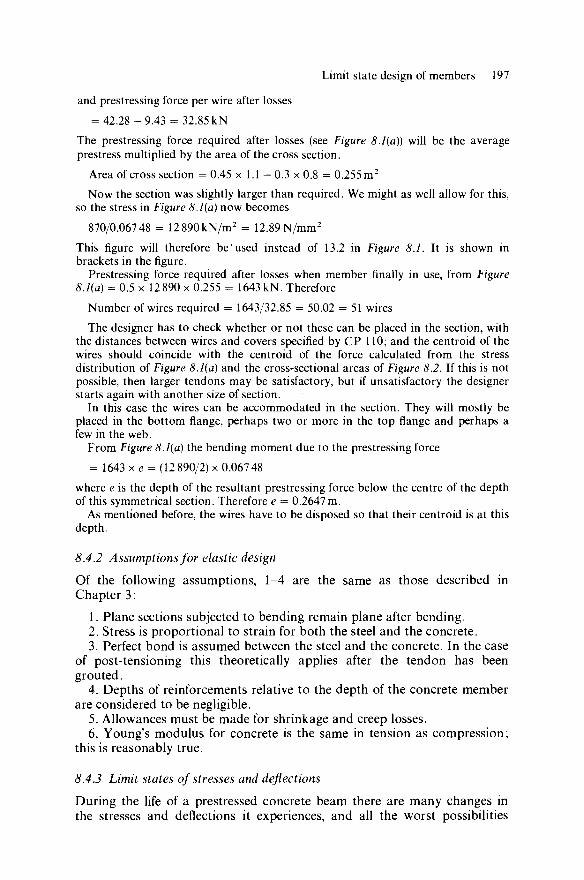
Limit state design of members 197
and prestressing force per wire after losses = 42.28-9.43 = 32.85 kN
The prestressing force required after losses (see Figure 8.1(a)) will be the average prestress multiplied by the area of the cross section.
Area of cross section = 0.45 x 1.1 - 0.3 x 0.8 = 0.255 m2
Now the section was slightly larger than required. We might as well allow for this, so the stress in Figure 8.1(a) now becomes
870/0.06748 = 12 890kN/m2 = 12.89 N/mm2
This figure will therefore be*used instead of 13.2 in Figure 8.1. It is shown in brackets in the figure.
Prestressing force required after losses when member finally in use, from Figure 8.1(a) = 0.5 x 12 890 x 0.255 = 1643 kN. Therefore
Number of wires required = 1643/32.85 = 50.02 = 51 wires The designer has to check whether or not these can be placed in the section, with
the distances between wires and covers specified by CP 110; and the centroid of the wires should coincide with the centroid of the force calculated from the stress distribution of Figure 8.1(a) and the cross-sectional areas of Figure 8.2. If this is not possible, then larger tendons may be satisfactory, but if unsatisfactory the designer starts again with another size of section.
In this case the wires can be accommodated in the section. They will mostly be placed in the bottom flange, perhaps two or more in the top flange and perhaps a few in the web.
From Figure 8.1(a) the bending moment due to the prestressing force = 1643 x e = (12 890/2) x 0.06748
where e is the depth of the resultant prestressing force below the centre of the depth of this symmetrical section. Therefore e = 0.2647 m.
As mentioned before, the wires have to be disposed so that their centroid is at this depth.
8.4.2 Assumptions for elastic design
Of the following assumptions, 1-4 are the same as those described in Chapter 3:
1. Plane sections subjected to bending remain plane after bending. 2. Stress is proportional to strain for both the steel and the concrete. 3. Perfect bond is assumed between the steel and the concrete. In the case
of post-tensioning this theoretically applies after the tendon has been grouted.
4. Depths of reinforcements relative to the depth of the concrete member are considered to be negligible.
5. Allowances must be made for shrinkage and creep losses. 6. Young's modulus for concrete is the same in tension as compression;
this is reasonably true.
8.4.3 Limit states of stresses and deflections
During the life of a prestressed concrete beam there are many changes in the stresses and deflections it experiences, and all the worst possibilities

198 Prestressed concrete
should be investigated. When all this has been evaluated, if anything is wrong then one has to return to the beginning and re-estimate the size of the section. Hence one has to concentrate on the most likely worst cases first, so that if re-design is necessary one finds this out as soon as possible.
Essentially a member has to be designed for stresses at transfer of prestress from tendons to concrete. This is an important limit state, as the concrete is often not very old and hence not as strong as it will be when in the final structure; also, the tendons have not experienced losses as great as they will experience in the final structure.
Then the member, if not in situ, will be handled, stacked, loaded, transported, unloaded, perhaps stacked and then lifted into position. All these operations, if not skilfully performed, could impose many adverse stresses. It is usually best, for prestressed concrete, to have spreaders for slings of cranes and to use lorries with long backs so that beams are always supported at their ends as they have been at transfer, and will be in the final structure. Then adverse stresses can be eliminated, and there is no need to design for this limit state of handling, transportation, erection, etc.
A member must also, of course, be designed for its limit states of stresses and deflection when in its final position in the structure.
8.4.4 Simplified elastic design of prestressed concrete beams
The simplification is by way of ignoring the steel reinforcement in calculat-ing the cross-sectional area, depth of neutral axis and second moment of area of the concrete section. This reduces the work of the calculations considerably, as for very accurate calculations various different sectional properties are required. For example, when pretensioning, the areas of the wires and the concrete they displace should be included in the calculations of the sectional properties and different modular ratios should be used for transfer and final serviceability. For post-tensioning, at transfer, the tendon and duct should be excluded, but any other steel included, in calculations of sectional properties. On the other hand, for limit state of serviceability (that is after the duct has been grouted) all the concrete (including grout), tendons and any other reinforcements should be included in the calculations of sectional properties, these reinforcements having different modular ratios to those used at transfer.
The simplified method is adequate for many purposes, as the percentage of steel in the cross section is generally low enough to cause little error, and this error tends to cause excess safety.
The losses are firstly taken as percentages of the initial prestressing tendon forces. This enables the concrete stresses to be obtained and then the losses can be obtained more accurately from these stresses. If it is then found that the original estimate of losses was not good enough, an adjustment is made and the design repeated. The process can be repeated until the designer is satisfied—it can quite simply be programmed for a computer. However, with experience a designer often does not need to alter his first estimate, as he will have slightly overestimated so as not to have the trouble of re-design; the computer is of course useful for optimisation here. The method is illustrated in the following examples.

Limit state design of members 199
Example 8.3. Continue the design of the beam of Example 8.1. Having approxi-mately checked the stresses it might now be best approximately to check the limit states of deflection in case we have to alter the section on this count.
When we are interested in the maximum deflection in service, the concrete then has a characteristic strength of 40N/mm2, and ym for concrete is unity, so from Table 1 of CP 110 Ec = 31kN/mm2. Shrinkage and creep have been allowed for in the losses assumed. When we consider deflection at transfer we will assume that the concrete has a characteristic strength of 30 N/mm2, and ym for concrete is unity, so from Table 1 ofCP 110,
Ec = 28 kN/mm2
Assuming the beam is simply supported over a span of 22 m and that all loading is uniformly distributed (q\ then
(g/8) x 222 = 870, .'. q = 14.38 kN/m
From CP 110, clause 2.2.3, the limit states of deflection are as follows:
1. If finishes are to be applied the span-to-total-upward-deflection ratio should exceed 300. This refers chiefly to floor and roof units which can have varying cambers, often because of releasing the wires when the concrete is not strong enough on the prestressing beds—the indicative cubes are sometimes compacted very much more thoroughly and sometimes cured more favourably than most of the concrete in a member and, under these bad circumstances, are misleading. The less the upward deflection, the less the problem and hence this limitation suggestion of CP 110.
At transfer the losses will not be as great as finally. For pretensioning they can be very approximately 10-15% (assuming the relaxation losses of the steel are kept modest). Supposing we take 10% to be on the safe side. At transfer the smaller losses give greater concrete stresses, which are usually the most limiting consideration at transfer. (Note that a safe and not excessively conservative figure for post-tensioned concrete would be just the steel relaxation loss if the tendons are stressed simul-taneously and there are no excessive losses due to severe curvature, such as for a circular tank or dome.)
Prestressing force of 1643 kN was based on losses of
(9.43/42.28) x 100 = 22.3%
Then at transfer prestressing force after losses
= " 4 3 x (100-10) 100 - 22.3
The bending moment due to this prestressing force
= 1903 x 0.2647 = 503.7 kNm
The deflection upwards due to this constant bending moment (the span on the prestressing bed is the overall length of the beam, say 23 m)
503.7 x23 2 _ _ = 0.0321m 8 x 2 8 x 106x 0.037 11
This is reduced by the downwards deflection due to the self-weight of the beam which is
5 x 6 . 0 1 8 x 2 3 4 „ _ ■ = 0.0211m 3 8 4 x 2 8 x l 0 6 x 0 . 0 3 7 1 1

200 Prestressed concrete
where the self-weight of the beam, assuming the weight density of prestressed concrete is 23.6 kN/m3 (mass density of prestressed concrete = 2400 kg/m3), is
0.255 x 23.6 = 6.018 kN/m
At transfer, therefore, the total upward deflection
= 32.1-21.1 = 11.0mm
This gives a span-to-deflection ratio of 2091, which is greater than 300 and therefore satisfactory should the member be used in this way. (In this particular example it was not necessary to calculate the 21.1, as the 32.1 without the reduction of 21.1 would still have been satisfactory for the span-to-deflection ratio of 300, but this will not always be the case.)
2. The final span-to-deflection ratio should exceed 250, the deflection being measured below the level of the supports. In the present example the deflection downwards
5 x 14.38 x 224 _ „ 0.03813 m 384x31x 106x 0.037 11
The bending moment due to the prestressing force
= 1643 x 0.2647 = 434.9 kNm
The deflection upwards due to this constant bending moment
434.9 x 222
= 0.022 87 m 8 x 3 1 x 106x 0.037 11
Hence the deflection below the supports is
38.13-22.87 = 15.26 mm
This gives a span-to-deflection ratio of 1442, which is satisfactory as it exceeds 250. 3. Partitions and finishes, either above or below, if the beam is in a building, can
be damaged by excessive deflections. CP 110 generally suggests limiting the de-flection to 20 mm and to a span-to-deflection ratio greater than 350. These deflection calculations are for deflections after the fixing of the partitions and the applications of the finishes. We can therefore assume the concrete to be at least 28 days old and we are essentially interested in the subsequent deflection due to live load. However, if say glass partitions are built up to the soffit of the beam, then no live load deflection is tolerable and details have to be devised to, for example, allow a beam to slide past rather than bear on to a partition.
In the present example, the self-weight of the beam, from 1 above, is 6.018 kN/m, hence the live load is
14.38-6.018 = 8.362kN/m
and the deflection due to this
= (8.362/14.38) x 38.13 = 22.17 mm
The span-to-deflection ratio is 992.3, which is greater than 350 and therefore satisfactory.
The deflection is, however, greater than 20 mm and therefore not as recommended by CP 110. If this is acceptable practically then the design does not need revision to reduce this deflection. Thus in the present example the beam might not be suitable in a building.
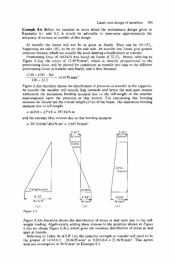
Limit state design of members 201
Example 8.4. Before we examine in more detail the preliminary design given in Examples 8.1 and 8.2, it would be advisable to determine approximately the adequacy of stresses at transfer of this design.
At transfer the losses will not be as great as finally. They can be 10-15%. Supposing we take 10% to be on the safe side. At transfer less losses give greater concrete stresses, which are usually the most limiting consideration at transfer.
Prestressing force of 1643 kN was based on losses of 22.3%. Hence, referring to Figure 8.1(a), the stress of 12.89 N/mm2, which is directly proportional to the prestressing force, will be altered for conditions at transfer pro rata to the different prestressing forces at transfer and finally, and it thus becomes
12.89 x (100-10) 100-22.3
14.93 N/mm2
Figure 8.3(a) therefore shows the distribution of prestress at transfer at the supports. At transfer the member will usually hog upwards and hence the mid-span section withstands the maximum bending moment due to the self-weight of the member superimposed upon the prestress at this section. For calculating this bending moment we should use the overall length (23 m) of the beam. The maximum bending moment due to self-weight
= (6.018 x 232)/8 = 397.9 kNm
and the extreme fibre stresses due to this bending moment
= 397.9/0.067 48 kN/m2 = 5.897 N/mm2
5.897 "< * N/mm'
\Comp ression
Tension
5.897 N/mm7
(b)
5.897 < it-, N/mm2
/Comp-ression
9.033 N/mm2
( c )
Figure 8.3(b) therefore shows the distribution of stress at mid span due to the self-weight loading. Algebraically adding these stresses to the prestress shown in Figure 8.3(a) we obtain Figure 8.3(c), which gives the resultant distribution of stress at mid span at transfer.
Referring to Table 36 of CP 110, the concrete strength at transfer will need to be the greater of 14.93/0.5 = 29.86N/mm2 or 9.033/0.4 = 22.58N/mm2. This agrees with our assumption of 30 N/mm2 in Example 8.3.
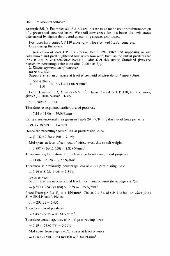
202 Prestressed concrete
Example 8.5. In Examples 8.1, 8.2, 8.3 and 8.4 we have made an approximate design of a prestressed concrete beam. We shall now check for this beam the limit states determined by elastic theory and concerning stresses and losses.
For these limit states CP 110 gives ym = 1 for steel and 1.3 for concrete. Considering the losses:
1. Relaxation of steel. CP 110 refers us to BS 2691, 1969, and supposing we use cold drawn and prestraightened low relaxation wire, then, as the initial prestress we took is 70% of characteristic strength, Table 6 of this British Standard gives the maximum percentage relaxation after lOOOh as 2%.
2. Elastic deformation of concrete (a) At transfer Support: stress in concrete at level of centroid of wires (from Figure 8.3(a))
550 + 264.7 = x 14.93 = 11.06 N/mra2
1100 '
From Example 8.3, Ec = 28kN/mm2. Clause 2.4.2.4 of CP 110, for the wires, gives Es = 200kN/mm2. Hence
ae - 200/28 = 7.14
Therefore, as explained earlier, loss of prestress
= 7.14x 11.06 = 79.0 N/mm2
Using cross-sectional area given in Table 29 of CP 110, the loss of force per wire
= 79.0 x 38.5 N = 3.042kN
Hence the percentage loss of initial prestressing force
= (3.042/42.28) x 100 = 7.19%
Mid span: at level of centroid of wires, stress due to self-weight
= 5.897 x (264.7/550) = 2.838 N/mm2
Therefore resultant stress at this level due to self-weight and prestress
= 11.06-2.838 = 8.22 N/mm2
Therefore, as previously, percentage loss of initial prestressing force
= 7.19 x (8.22/11.06) = 5.34%
(b) In service Support: stress in concrete at level of centroid of wires (from Figure 8.1(a))
= {(550 + 264.7)/l 100} x 12.89 = 9.55 N/mm2
From Example 8.3, Ec = 31kN/mm2. Clause 2.4.2.4 of CP 110 for the wires gives Es = 200 kN/mm2. Hence
ae = 200/31 = 6.452
Therefore loss of prestress
= 6.452 x 9.55 = 61.61 N/mm2
Therefore percentage loss of initial prestressing force
= 7.19 x (61.61/79) = 5.61%
Mid span: from Figure 8.1(c) stress at level of wires
= 12.89 x (550 - 264.6)/1100 = 3.344 N/mm2
Limit state design of members 203
Therefore percentage loss of prestress
= 5.61 x (3.344/9.55) = 1.96% 3. Shrinkage of concrete. Supposing the beam is cured in effect in water—say by
covering with wet hessian cloth which is covered with polythene sheet; there will then be no shrinkage loss at transfer. Table 41 of CP 110 gives concrete shrinkage values for pretensioning between three and five days after casting, curing at exposures of 90% and 70% relative humidity respectively as far as transfer. Let us assume that we cure after transfer at normal exposure until it is in use, then, guided by Figure 2.9, take the maximum shrinkage per unit length as 0.04%. Taking the shortening movement of the tendon as the same as the concrete shrinkage, then strain loss in tendon due to shrinkage
= 400x 10" 6
Hence corresponding loss of stress
- 400 x 10"6 x 200 x 103 = 80N/mm2
Therefore percentage loss of prestress (finally)
= (80/79) x 7.19 = 7.28%
4. Creep of concrete. At transfer, creep has had negligible time to take place, hence we take this loss as zero. The stress in the concrete at transfer will cause subsequent creep, and it is upon this stress that the final creep is based. Referring to clause 4.8.2.5 of CP 110, as cube strength at transfer is 30N/mm2, creep per unit length is
48 x 10"6 x (40/30) = 64 x 10"6 per N/mm2
According to CP 110, if the maximum stress at transfer exceeds 3- x Cube strength at transfer
= ^ x 3 0 = 10 N/mm2
then the creep loss should be increased. At transfer Figure 8.3(a) gives the stresses at each support and Figure 8.3(c) gives the stresses at mid span. At mid span the stresses do not exceed 10 N/mm2 so the creep loss is satisfactory. At each support, as the maximum stress is approximately half the cube strength, the creep per unit length from CP 110 is
1.25 x 64 x 10"6 = 80 x 10"6 per N/mm2
The stress causing creep will depend upon whether the beam is supporting its own weight only or its full load most of its life. At the level of the centroid of the wires the former gives a stress of 11.06 N/mm2 at support and 8.22 N/mm2 at mid span, whilst the latter, from Figure 8.3(a) and Figure 8.1(b), gives 11.06 N/mm2 at support and
11.06-(264.7/1100) x 12.89 = 7.96 N/mm2
at mid span. Supposing the imposed load is rarely applied, so that we take the worst of the cases just mentioned. When in use therefore the creep per unit length is
(a) 11.06 x 80 x 10"6 = 885 x 10"6 at the support and (b) 8.22 x 64 x 10"6 = 526 x 10"6 at mid span
As the movement of the concrete is assumed to be the same as that of the tendon, then the loss of stress in the tendon is
(a) 885 x 10"6 x 200 x 103 = 177N/mm2 at the support and (b) 526 x 10"6 x 200 x 103 = 105.2 N/mm2 at mid span

204 Prestressed concrete
These can be expressed as (a) (177/61.61) x 5.61 = 16.12% at support and (b) (105.2/61.61) x 5.61 = 9.58% at mid span 5. Slip of anchorage. Suppose the wedges at each end pull in 3 mm and our system
is one where we jack the movable wire anchorage block away from the prestressing bed, which has a length of say 75 m; then this loss, if not allowed for when stressing, would be
(6/75 000) x 200 x 103 = 16N/mm2
But we will allow for this when stressing and extend the movable anchorage block 6mm more than its required amount.
6. Friction in jack and anchorage system. This is nil because of the way we are pretensioning; see 5 above and also Section 8.3, para. 6.
Summarising the losses: at transfer total loss at mid span
= 2(1) + 5.34(2) = 7.34% and at a support
= 2(1)+ 7.19(2) = 9.19% Finally, in use total loss at mid span
= 2(1) + 1.96(2) + 7.28(3) + 9.58(4) = 20.82% and at a support
= 2(1) + 5.61(2) + 7.28(3) + 16.12(4) = 31.01% At transfer we took the losses as 10%, so for greater accuracy we could now try
9.1% for support sections and 7.3% for mid-span sections and repeat the above design. Further such repetitions can then be made until the desired degree of accuracy is achieved. When in use we took the losses as 22.3%. For greater accuracy we would repeat the above design and use losses of 20% for mid span and 31% for support sections. Also for more accurate design, we would repeat the example, considering losses for the wires at their respective levels. We have considered them all as though concentrated at their centroid and this is slightly erroneous. For normal purposes our present accuracy in this problem could be considered satisfac-tory and hence our design is justified.
8.4.5 Ultimate limit state due to flexure (bonded tendons)
If a member has been designed as shown previously, then if the tendons are arranged so that most have a reasonably generous effective depth, checking the ultimate limit state is almost a formality. The exception to this is in the case of CP 110, Class 3, structures (partially prestressed)—see Section 8.4. These could be designed for ultimate limit state first, then deflections at working loads checked before checking the stress systems at working loads and transfer.
In the case of a rectangular beam with one tendon, this is required at about j of the height of the beam. Hence when cracking occurs due to overloading, the effective depth of this tendon is small, so the tendon does not control the crack widths very well at the soffit. In a case like this the ultimate limit state might not be satisfactory so additional non-prestressed reinforcement might be used and placed as near to the soffit as possible.

Limit state design of members 205
Likewise in the case of a pole of circular cross section, when the bending moment can be in any direction; if the tendons are arranged around the periphery then the ultimate limit state will most probably be all right, but not if there is say just one tendon down the centre.
As in Chapter 3 the equivalent rectangular stress block due to C. S. Whitney is favoured9 for predicting actual ultimate resistance moments,
that is, fcm = (<x/2j8)/c' and x, = 2/lx
where (taking/; = 0.84/cu)
a = 0.72 for/cu ^ 33N/mm2
and decreases by 0.04 for every 8.21 N/mm2 above 33 N/mm2
and p = 0.425 for /cu < 33 N/mm2
and decreases by 0.025 for every 8.21 N/mm2 above 33 N/mm2
Thus for /cu ^ 33 N/mm2,
/cm = 0.85/; = 0.714/cu and x{ = 0.85x It is generally used in the U.S.A. and is the basis of the CP 110 simplified method and many other codes internationally. Towards failure in bending a prestressed concrete beam cracks and behaves like a non-prestressed rein-forced concrete beam apart from:
1. The strain in the tendon was not zero at zero loading, as in the reinforcement of the reinforced concrete beam. At zero loading the strain ^p in a tendon corresponds to the force in the tendon after losses (that is, the losses which have occurred up to the time of loading to failure) divided by the cross-sectional area of the tendon and its Young's modulus. Strain in the tendon caused by the loading adds to ep. The strain due to the prestress in the concrete can be ignored, as it is negligible compared to ep and the strains at failure.
2. The stress-strain relationships for tendons are different to those for a reinforcement bar (see Figure 8.4). The ultimate resistance moment for an under-reinforced prestressed beam can be obtained as in Example 3.15 for under-reinforced sections, provided the ultimate tensile strength (stress) of the tendons is used f o r / in equations 3.60 and 3.62. To determine if the section is under-reinforced we need to calculate the maximum concrete strain corresponding to the tensile reinforcement strain when ultimate steel stress (or a suitable proof stress) is reached (see Figures 8.4 and 8.6) to check that this is less than the maximum known to be possible from experiments, namely 0.003 according to Whitney (0.0035 is used by CP 110). Figures 8.5(a) and (b) show the distribution of stress across the cross section and the corresponding distribution of strain, respectively.
From similar triangles in Figure 8.5(b), the maximum concrete strain
If this is greater than 0.003 (Whitney) then it is an over-reinforced pre-stressed concrete beam and its ultimate resistance moment cannot be
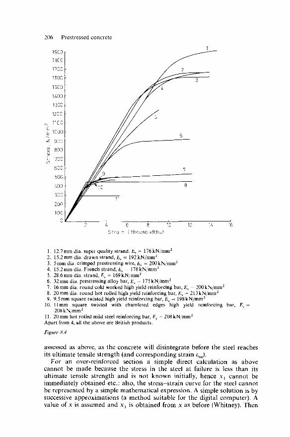
206 Prestressed concrete
A 6 8 10 S t ra in ( thousandths)
12 16
1. 2. 3. 4. 5. 6. 7. 8. 9.
10.
11.
12.7 mm dia. super quality strand, Es = 176kN/mm2
15.2 mm dia. drawn strand, £s = 192kN/mm2
5 mm dia. crimped prestressing wire, Es = 200kN/mm2
15.2 mm dia. French strand, £s = 178kN/mm2
28.6mm dia. strand, £s = 169kN/mm2
32 mm dia. prestressing alloy bar, Es = 175kN/mm2
16 mm dia. round cold worked high yield reinforcing bar, Es = 200kN/mm2
20 mm dia. round hot rolled high yield reinforcing bar, Es = 213kN/mm2
9.5 mm square twisted high yield reinforcing bar, Es = 198kN/mm2
11mm square twisted with chamfered edges high yield reinforcing bar, 208kN/mm2
20 mm hot rolled mild steel reinforcing bar, Es = 208kN/mm2
EK =
Apart from 4, all the above are British products.
Figure 8.4
assessed as above, as the concrete will disintegrate before the steel reaches its ultimate tensile strength (and corresponding strain esu).
For an over-reinforced section a simple direct calculation as above cannot be made because the stress in the steel at failure is less than its ultimate tensile strength and is not known initially, hence xx cannot be immediately obtained etc.; also, the stress-strain curve for the steel cannot be represented by a simple mathematical expression. A simple solution is by successive approximations (a method suitable for the digital computer). A value of x is assumed and x{ is obtained from x as before (Whitney). Then
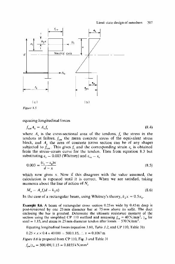
Limit state design of members 207
(a) Figure 8.5
equating longitudinal forces
fcmAQ = AJS (8.4)
where As is the cross-sectional area of the tendons, / s the stress in the tendons at failure, fcm the mean concrete stress of the equivalent stress block, and Ac the area of concrete (cross section can be of any shape) subjected to fcm. This gives fs and the corresponding strain es is obtained from the stress-strain curve for the tendon. Then from equation 8.3 but substituting ec = 0.003 (Whitney) and esu = es
0.003 = d — x
(8.5)
which now gives x. Now if this disagrees with the value assumed, the calculation is repeated until it is correct. When we are satisfied, taking moments about the line of action of Nc
Mu = AJs(d-k2x) (8.6) In the case of a rectangular beam, using Whitney's theory, k2x = O^Xj.
Example 8.6. A beam of rectangular cross section 0.25 m wide by 0.45 m deep is post-tensioned by one 25 mm diameter bar at 75 mm above its soffit. The duct enclosing the bar is grouted. Determine the ultimate resistance moment of the section using the simplified CP 110 method and assuming fcu = 40N/mm2, ym for steel = 1.15, and stress in 25 mm diameter tendon after losses = 570N/mm2.
Equating longitudinal forces (equation 3.60, Table 3.2, and CP 110, Table 31) 0.25 x x x 0.4 x 40000 = 500/1.15, .'. x = 0.1087m
Figure 8.6 is prepared from CP 110, Fig. 3 and Table 31 fjym = 500/491/1.15 = 0.8855 kN/mm2
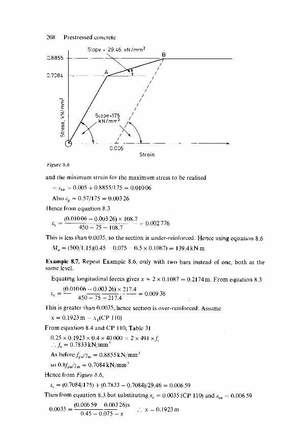
208 Prestressed concrete
Slope = 29.46 kN/mm2
0.8855
0.7084
0.005 Strain
Figure 8.6
and the minimum strain for the maximum stress to be realised
= £su = 0.005 + 0.8855/175 = 0.01006
Also £p = 0.57/175 = 0.003 26
Hence from equation 8.3
(0.01006-0.003 26) x 108.7 £< = 4 5 0 - 7 5 - 1 0 8 . 7 = ° - 0 0 2 7 7 6
This is less than 0.0035, so the section is under-reinforced. Hence using equation 8.6
Mu = (500/1.15)(0.45 - 0.075 - 0.5 x 0.1087) = 139.4kN m
Example 8.7. Repeat Example 8.6, only with two bars instead of one, both at the same level.
Equating longitudinal forces gives x = 2 x 0.1087 = 0.2174m. From equation 8.3
(0.01006-0.003 26) x 217.4 *< = 4 5 0 - 7 5 - 2 1 7 . 4 = ° 0 0 9 3 8
This is greater than 0.0035, hence section is over-reinforced. Assume x = 0.1923m = xx(CP 110)
From equation 8.4 and CP 110, Table 31 0.25 x 0.1923 x 0.4 x 40000 = 2 x 491 x/ s .\fs = 0.7833 kN/mm2
As before fpJym = 0.8855 kN/mm2
so 0.8/pU/ym = 0.7084 kN/mm2
Hence from Figure 8.6,
es = (0.7084/175) + (0.7833 - 0.7084)/29.46 = 0.006 59
Then from equation 8.3 but substituting ec = 0.0035 (CP 110) and esu = 0.006 59
« ^ r (0.006 59 - 0.003 26)x 0 0 0 3 5 = 0.45- 0.075 J •■•* = 0.1923m

Limit state design of members 209
This is in order, the estimate of x being correct. Normally several attempts would be required. Although this trial and error method is favoured by others, and by the writer when using real stress-strain curves for the tendons, the writer prefers direct calculation when using the simplified stress-strain curves of CP 110. To illustrate this, instead of assuming x as before, assume that the strain in the tendons is in the range AB of Figure 8.6. Then from equation 8.4 and CP 110, Table 31
0.25 x x x 0.4 x 40000 = 2 x 491/s .'. fs = 4.073x
From Figure 8.6,
(0.7084/175) + (4.073*- 0.7084) £s = — = 0.1383* - 0.02
Using this for esu and £c = 0.0035 in equation 8.3
(0.1383* - 0 . 0 2 - 0.003 26)x 0.0035 = —
0.375 -x
:. x = 0.1923 m and / s = 4.073x = 0.7833 kN/mm2
Hence fs does lie in range AB and the calculation is satisfactory. If/S had been in range AO then one would assume it in this range and make a similar but simpler calculation to the above. Then from equation 8.6
Mu = (0.7833 x 2 x 491X0.375 - 0.5 x 0.1923) = 214.5 kN m
Example 8.8. Repeat Example 8.6 using CP 110, Table 37.
Using Table 31,
f ^ = 5 0 ° = 01333 fcubd 40000x0.25x0.375
Therefore from Table 37,
/pb/0.87/pu = 1.0, and x = 0.290 x 0.375 = 0.1088 m
From CP 110, equation 44 and Table 31,
Mu = 0.81fpuAps(d - 0.5 x 0.1088) = 0.87 x 500 x 0.3206 = 139.5 kNm
Example 8.9. Repeat Example 8.7 using CP 110, Table 37.
Using Table 31, ^ - 2x500 = 0 . 2 6 6 7
fcubd 40000x0.25x0.375 For larger amounts of tendons, Table 37 empirically assumes slightly less reliance
on the grouting of post-tensioned tendons. Thus to compare with Example 8.7 we should take the figures for pretensioning in Table 37. Thus /pb/0.87/pu = 1.0, and x = 0.580 x 0.375 = 0.2175 m. From CP 110, equation 44 and Table 31,
Mu = 0.81fpuAps{d - 0.5 x 0.2175) = 0.87 x 1000 x 0.27 = 231.6kNm
This disagrees with 214.5 because Table 37 has an experimental basis. CP 110 Chart 140 gives 220kNm which disagrees with 214.5 because it uses a CP 110 Fig. 1 stress block.
Using the post-tensioning suggestions of Table 37
/Pb/0.87/pu = 0.883
and x = 0.511 x 0.375 = 0.1916m

210 Prestressed concrete
From CP 110, equation 44 and Table 31 Mu = 0.883 x 870 x (0.375 - 0.5 x 0.1916) = 214.5 kN m
8.4.6 Additional untensioned steel (bonded tendons)
If the ultimate resistance moment is inadequate, and the other limit states satisfactory, sometimes extra untensioned steel is added. This has negligible effect on the other limit states, and thus saves re-design. This extra steel might be extra prestressing tendons which are not stressed, or reinforcement bar. This steel is placed with maximum effective depth.
Additional untensioned steel is sometimes necessary for crack control when post-tensioned bonded tendons are located at some distance from the tensile face of the concrete.
Example 8.10. Repeat Example 8.7 but add two 12mm diameter bars, with 25 mm concrete cover, in the bottom of the beam. Assume f = 460N/mm2 for these bars.
Equating longitudinal forces, using Table 3.2
0.25 x x x 0.4 x 40000 = 2 x 500/1.15 + 226 x 0.46/1.15 .'. x = 0.24m For tendons, from Example 8.6, £su = 0.01066 and ep = 0.003 26. Hence from
equation 8.3, £c = (0.01006 - 0.003 26) x 0.24/(0.375 - 0.24) = 0.0121 Using distribution of strain diagram and similar triangles, strain in 12 mm
diameter bars = 0.0121 x (419 - 240)/240 = 0.009025
so that maximum stress can be realised in these bars (see CP 110, Fig. 2), that is strain greater than
0.002 + 460/(1.15 x 200000) = 0.004 As ec is greater than 0.0035, section is over-reinforced. Equating longitudinal forces
0.25 x x x 0.4 x 40000 = 2 x 491 x/s + 226 x 0.46/1.15 . \ / s = 4.073x- 0.09206
From Figure 8.6,
£s = (0.7084/175) + (/s - 0.7084)/29.46 = 0.1383x - 0.023 12 Using this for £su and £c = 0.0035 in equation 8.3
(0.1383x - 0.023 12 - 0.003 26)x 0.0035 = —
0.375-x .'. x = 0.2105 m, and/s = 0.7654kN/mm2
As fs lies in the range AB in Figure 8.6, the calculation is satisfactory. We have assumed the strain in the 12 mm diameter bars is large enough for them to develop their maximum stress. Strain in bars
= (0.0035/210.5) x (450 - 25 - 6 - 210.5) = 0.003467 Referring to CP 110, Fig. 2, this strain is less than 0.004, so the maximum stress is
not quite realised. If we reassess this design stress/sl, then repeat the calculation, we
Limit state design of members 211
should improve the result. If this is done a few times the accuracy becomes adequate. Then Mu is determined by taking moments about the line of action of Nc.
Mu = 2 x 491 x/s(0.375 - 0.5x) + 226 x/8l x (0.419 - 0.5x) Had the 12 mm diameter high-yield bars been replaced by bars of an equivalent
strength in mild steel then the strain would have only needed to have exceeded
0.002 + 250 0.003 087 (CP 110, Fig. 2) 1.15x200000
for its design yield stress to have been realised, that is mild steel for additional unprestressed steel is likelier to simplify the design. In the above design, because the additional steel was not fully stressed a certain amount of trial and error is used, but convergence is very rapid. Some might prefer to guess x to avoid solving the quadratic equation and continue by trial and error as indicated in Example 8.7, but this is slower to converge.
8.4.7 Compression steel
Wires or handling reinforcement placed in the top of a beam are usually too inadequately anchored against buckling (see CP 110) to be included in the ultimate resistance moment calculations. If compression steel is to be included in these calculations, it is included in the previous calculations in the same way as given in Chapter 3.
8.4.8 Ultimate limit moment due to flexure {unbonded tendons)
In this instance Sections 8.4.5-8.4.7 apply, except that CP 110 reduces the force which can be developed in the tendons. The problem is that as loading is applied, instead of the force imposed in the tendon decreasing towards the support as with bonded tendons or reinforcement bars, the force in the tendon is always the same from end to end in an unbonded tendon. Towards failure the first crack occurs at the position of maximum bending moment. At this crack, instead of the tendon being highly stressed locally and anchored on either side of the crack so that its extension is limited (as would be the case if the tendons were bonded to the concrete), when the tendon is unbonded, this high stress extends along its whole length. The whole length thus extends pro rata and the extension is considerable, allowing the first crack to open excessively (few if any extra cracks form towards failure), precipitating earlier failure than occurs with a beam with a bonded tendon.
The normal theories treat post-tensioning as if it were pretensioning and just modify the ultimate resistance moment for unbonded tendons as previously and bonded tendons as described in Example 8.9. However, the problem is basically different at pretensioning, working loads and ul-timately. References 7 and 10 deal at length with this problem at tensioning and at working loads. They take account of pressures between tendons and their surrounding concrete, which can give high stress concentrations in the concrete.7'11 (A failure has been reported where these pressures were considered to be too high and the concrete was under-strength.) Tendons

212 Prestressed concrete
cannot be deflected say vertically by beams without such forces existing and the theories of Refs. 7 and 10 calculate stresses and deflections for beams with tendons of various profiles.
Example 8.11. Repeat Example 8.7, only assuming the tendons are unbonded. See Example 8.9 but using CP 110, Table 38, instead of Table 37, and supposing
l/d = 20. From Example 8.6, /pe = 570N/mm2; thus, using Table 31,
! ^ = 0.57x2x491 fcubd 40000x0.25x0.375 From Table 38,/pb//pe = 1.20 and x = 0A6d. Then using CP 110, equation 44, Mu = 1.2 x 0.57 x 2 x 491(0.375 - 0.5 x 0.46 x 0.375) = 193.9kNm
Compare this result with the 214.5 kN m for bonded tendons in Example 8.9.
8.4.9 Prestressed columns
It is rarely economical or necessary to prestress columns. One example of prestressing columns (designed by the author) is in the case of large span pitched-roofed portal frames; in this instance, however, the columns ex-perience very small direct stresses relative to the bending stresses.
8.4.10 Prestressed ties
Prestressed ties7 are often extremely useful for space frames, arches, hyper-bolic paraboloids, gable ties to barrel vault and folded plate roofs, suspen-ders to tied arch bridges and ties beneath prestressing beds. Extensions of ties are often desired to be as small as possible. This means a low strain is desirable in a tie, hence a steel tie or a prestressed concrete tie is designed, using a low stress. If the steel tie needs to be clad to resist fire or corrosion then the prestressed tie is often a more economical solution. One objection to unprotected steel ties to concrete structures is that their life and fire resistance is far less than that of the concrete members and if they fail a heavy structure collapses. Pretensioning was favoured for ties because the long slender members were considered to buckle as Euler's theory when post-tensioned. Refs. 7,11 and 12 show that the tendons restrain such buckling and a position of static equilibrium can be obtained when post-tensioning, so that if a certain unnoticeable curvature is allowed then the post-tensioned member can be designed accordingly and very economically. Post-tensioned ties have the economic advantage that they can easily be effected on site from existing scaffolding to shells, arched bridges, etc., when required. Pretensioned ties have to be delivered on time and threaded amongst the scaffolding and provided with special end attachments. Designs of pretensioned and steel ties are compared in Ref. 13 and post-tensioned ties are designed in Refs. 7,11 and 12.
8.4.11 Shear resistance of prestressed concrete beams
At working loads for CP 110 Class 1 and 2 structures, beams are considered as uncracked and hence principal stresses can be calculated in the usual manner by combining stresses due to prestressing, bending and shear. The

Limit state design of members 213
concrete is usually well able to resist the principal compressive stresses, and can usually resist the principal tensile stresses; if it cannot, then the section or the amount of prestressing has to be altered, or shear reinforcement in the form of inclined tendons, or vertical or inclined stirrups, or vertical prestressing, has to be introduced. The principal stresses can be calculated from the well known expression
/ = 0.5{/h +fv ± V/[(A -D2 + 4»2]} (8.7)
where fh and fv are horizontal and vertical direct stresses (tensile positive) and v = shear stress.
In the early days of prestressed concrete it was only necessary to limit the principal tensile stress to zero or a small amount, say 0.5 N/mm2 at working loads. This can still be done for a preliminary design. Research in shear generally shows that, with the kind of load factors used, if a beam is satisfactory with regard to its ultimate shear resistance then the diagonal cracks at working loads for reinforced concrete beams are adequately narrow and they are narrower still for prestressed concrete beams because of the prestressing forces tending to close such cracks. CP 110 therefore regulates only the ultimate shear resistance and equation 8.7 is used for sections not cracked in bending on the basis that when the principal stresses become great enough to cause cracking this can be regarded as correspond-ing to ultimate failure in shear. CP 110 treats sections experiencing cracks due to bending differently in shear (see Example 8.12). Research concerning ultimate shear strength,1415 as with non-prestressed concrete, is incon-clusive and appears inconsistent; hence empirical formulae have to be agreed for codes and these have to err greatly on the side of safety in some instances, because of the erratic nature and sensitivity to many variables of shear failures.
Example 8.12. Consider the CP 110 design of the beam of Example 8.7 in shear. At a support where the section is not cracked in bending and the shear force is a
maximum, suppose f = 7 N/mm2, then from CP 110 Table 39 Vco = 2.2 x 250 x 450 N = 247.5 kN
Then CP 110 is concerned about sections where there is likely to be a bending crack towards failure reducing the shear strength of the beam. The C. and C.A. Handbook on CP 110 suggests considering such a crack at a distance of half the effective depth from the point of maximum bending moment. Suppose for such a section
V/M = 0.032 m " l and ft = 11 N/mm2
0.25 x 0.453
Now / = = 0.001 898 m4
12 0.8 x 11000x0.001898 hence M0 = = 91.42kNm 0 0.375-0.1923
For Table 5 100/1, 100 x 2 x 491 _
bd 250 x 375 thus vc = 0.75 + 0.2 x 0.047 = 0.759 N/mm2
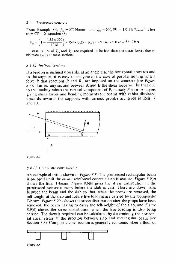
214 Prestressed concrete
From Example 8.6, /pe = 570N/mm2 and /pu = 500/491 = 1.018 kN/mm2. Thus from CP 110, equation 46:
Vcr = M _ °-55 X 5 7° j x 759 x 0.25 x 0.375 + 91.42 x 0.032 = 52.17 kN
These values of Vco and Vcr are required to be less than the shear forces due to ultimate loads at these sections.
8.4.12 Inclined tendons
If a tendon is inclined upwards, at an angle a to the horizontal, towards and to the support, it is easy to imagine in the case of post-tensioning with a force P that reactions P and Rx are imposed on the concrete (see Figure 8.7); thus for any section between A and B the shear force will be that due to the loading minus the vertical component of P, namely P sin a. Analyses giving shear forces and bending moments for beams with cables displaced upwards towards the supports with various profiles are given in Refs. 7 and 10.
^ p
*r
R
Figure 8.7
8.4.13 Composite construction
An example of this is shown in Figure 8.8. The prestressed rectangular beam is propped until the in-situ reinforced concrete slab is mature. Figure 8.9(a) shows the final T-beam. Figure 8.9(b) gives the stress distribution in the prestressed concrete beam before the slab is cast. There are dowel bars between the beam and the slab so that, when the props are removed, the self-weight of the slab and future live loading are carried by the 'composite' T-beam. Figure 8.9(c) shows the stress distribution after the props have been removed, the beam having to carry the self-weight of the slab, and Figure 8.9(d) shows the stress distribution when the live loading is also being carried. The dowels required can be calculated by determining the horizon-tal shear stress at the junction between slab and rectangular beam (see Section 3.3). Composite construction is generally economic when a floor or
* H i i h | i i = I
Figure 8.8
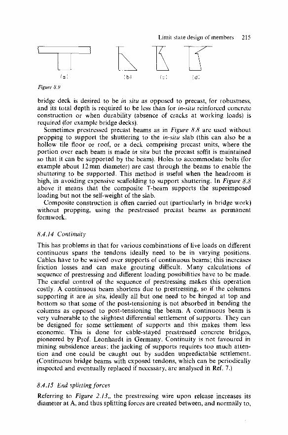
Limit state design of members 215
X IT ( a ) ( b ) ( c ) ( d )
Figure 8.9
bridge deck is desired to be in situ as opposed to precast, for robustness, and its total depth is required to be less than for in-situ reinforced concrete construction or when durability (absence of cracks at working loads) is required (for example bridge decks).
Sometimes prestressed precast beams as in Figure 8.8 are used without propping to support the shuttering to the in-situ slab (this can also be a hollow tile floor or roof, or a deck comprising precast units, where the portion over each beam is made in situ but the precast soffit is maintained so that it can be supported by the beam). Holes to accommodate bolts (for example about 12 mm diameter) are cast through the beams to enable the shuttering to be supported. This method is useful when the headroom is high, in avoiding expensive scaffolding to support shuttering. In Figure 8.8 above it means that the composite T-beam supports the superimposed loading but not the self-weight of the slab.
Composite construction is often carried out (particularly in bridge work) without propping, using the prestressed precast beams as permanent formwork.
8.4.14 Continuity
This has problems in that for various combinations of live loads on different continuous spans the tendons ideally need to be in varying positions. Cables have to be waived over supports of continuous beams; this increases friction losses and can make grouting difficult. Many calculations of sequence of prestressing and different loading possibilities have to be made. The careful control of the sequence of prestressing makes this operation costly. A continuous beam shortens due to prestressing, so if the columns supporting it are in situ, ideally all but one need to be hinged at top and bottom so that some of the post-tensioning is not absorbed in bending the columns as opposed to post-tensioning the beam. A continuous beam is very vulnerable to the slightest differential settlement of supports. They can be designed for some settlement of supports and this makes them less economic. This is done for cable-stayed prestressed concrete bridges, pioneered by Prof. Leonhardt in Germany. Continuity is not favoured in mining subsidence areas; the jacking of supports requires too much atten-tion and one could be caught out by sudden unpredictable settlement. (Continuous bridge beams with exposed tendons, which can be periodically inspected and eventually replaced if necessary, are analysed in Ref. 7.)
8.4.15 End splitting forces
Referring to Figure 2.13,, the prestressing wire upon release increases its diameter at A, and thus splitting forces are created between, and normally to,

216 Prestressed concrete a line between A and B. Designers have sometimes been unaware of this problem and have experienced splitting cracks in pretensioned members along the line between A and B. Other end splitting forces are caused by the end anchorages of tendons being, in effect, a system of irregularly distri-buted point loads on the end of a member. Each point load causes splitting forces normal to its line of action. Again failures have occurred.
This problem should be considered by the designer and CP 110 gives simple empirical guidance.
8.4.16 Prestressed concrete tanks, pipes, domes, shells and piles
For circular tanks and pressure pipes, circular prestressing is provided to counteract the circumferential tension due to the loading. A residual circumferential compression can ensure no cracks developing, due to shrinkage and temperature change, and this increases the watertightness. The pipes also need longitudinal prestressing for handling purposes. The writer has been consulted concerning troubles with certain prestressed concrete pipes. From his considerable literature searches he would recommend Ref. 16 for determining soil pressures on pipes and Ref. 17 for guidance on the design of prestressed concrete pipes. Some recent research supervised by the author on this problem is given in Ref. 18.
With rectangular tanks the walls must be free at the base, otherwise the corners act rigidly as folded plates and prevent the post-tensioning impos-ing stresses along the walls (a very able designer overlooked this point). Prestressing is useful for providing the ring tension to domes. The writer has rectified a dome, failing due to inadequate ring steel, by prestressing around the periphery.
Prestressed concrete piles are used for longer piles when handling stresses are a problem; end reinforcement details are important. Prestressing is useful for normal and North Light barrel vault roofs longer than about 36 m and 27 m, respectively, assuming that the ratio of width to length is about 1:2.
8.4.17 Torsional resistance
The ultimate limit state for torsion is dealt with in the same way as for non-prestressed beams (see Chapter 3).
8.5 Load balancing
This method of design19 helps suitable profiles for tendons of simply supported and continuous beams to be rapidly determined.
References
1. WALZ, K., 'Requirements Concerning the Grout for Prestressed Concrete Elements', Bau und Bauindustrie (Diisseldorf), 8, 16, p. 468 (1957) (in German)
2. LEONHARDT, F., 'On the Injection of the Grout into the Ducts1, Proceedings of the Third Congress of the Federation Internationale de la Precontrainte (Berlin, 1958), Cement and Concrete Association, pp. 323-336 (1958) (in German)

Load-balancing 217
3. LEONHARDT, F., Prestressed Concrete for the Practice, Wilhelm Ernst und Sohn, 2nd edn, p. 45, Berlin (1966) (in German)
4. BENZ, G. H., Grout for the Ducts of Prestressed Concrete, Sittler and Federman, Illertissen, Germany (1965) (in German)
5. SOROKA, I., and GEDDES, J. D., 'Cement Grouts and the Grouting of Post-tensioned Prestressed Concrete', Bulletin No. 26, University of Newcastle-upon-Tyne, Dept. of Civil Engineering, June (1966)
6. SZILARD, R., 'A Survey of the Art—Corrosion and Corrosion Protection of Tendons in Prestressed Concrete Bridges', Journal of the American Concrete Institute, Jan. (1969)
7. WILBY, C. B., Post-tensioned Prestressed Concrete, Applied Science Publishers Ltd., London (1981)
8. WILBY, C. B., 'Precast Concrete Framed Roofs—Design of Joints and Use of Post-tensioning', Indian Concrete Journal, Feb. (1960)
9. WINTER, G., and NILSON, A. H., Design of Concrete Structures, McGraw-Hill, U.S.A. (1973)
10. WILBY, C. B., Prestressed Concrete Beams, Elsevier Publishing, Amsterdam, London, New York; Applied Science Publishers, London (1969)
11. WILBY, C. B., 'Design of Post-tensioned Prestressed Concrete Ties for Bridges and Shell Roofs', Civil Engineering and Public Works Review, Apr. (1972)
12. WILBY, C. B., Elastic Stability of Post-tensioned Prestressed Concrete Members, Edward Arnold (1964)
13. EVANS, R. H., and WILBY, C. B., Concrete—Plain, Reinforced, Prestressed and Shell, Edward Arnold (1963)
14. WILBY, C. B., and NAZIR, C. P., 'Shear Strength of Uniformly Loaded Prestressed Concrete Beams', Civil Engineering and Public Works Review, Apr. (1964)
15. WILBY, C. B., and INMAN, P., 'The Structural Behaviour of Jointed Prestressed Concrete Beams', Proceedings of the Institute of Civil Engineers, Sept. (1972)
16. CLARKE, N. W. B., Buried Pipelines: a Manual of Structural Design and Installation, Maclaren (1968)
17. SWANSON, H. V., 'Design of Prestressed Concrete Pressure Pipe', Journal Prestressed Concrete Institute, Chicago, Illinois, 10, Aug. (1965)
18. JOHNSON, P., Structural Design of Buried Pipes, M.Sc. Thesis, University of Bradford, U.K.(1973)
19. LIN, T. Y., Design of Prestressed Concrete Structures, John Wiley, New York (1963)
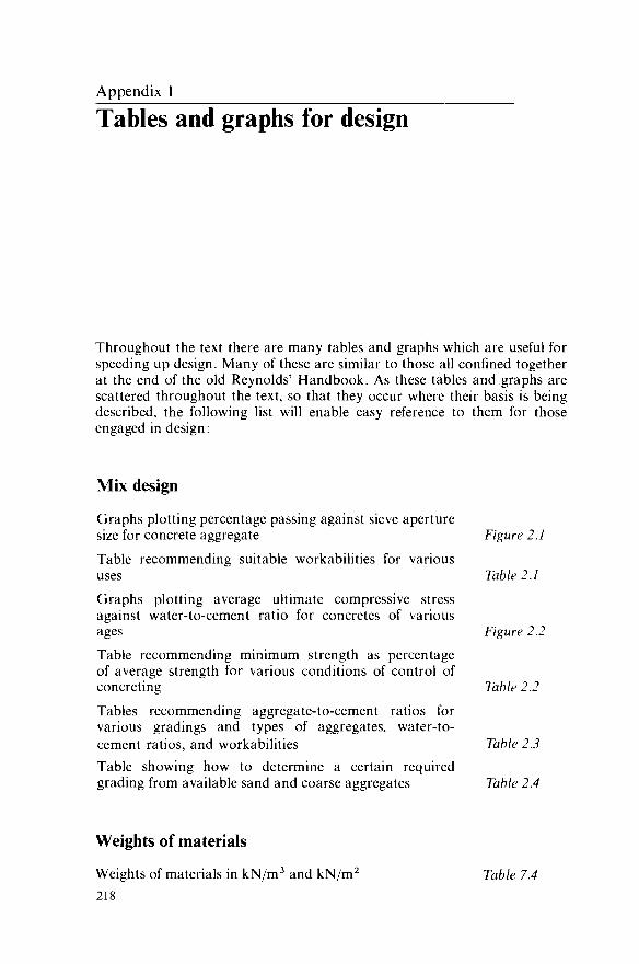
Appendix 1 Tables and graphs for design
Throughout the text there are many tables and graphs which are useful for speeding up design. Many of these are similar to those all confined together at the end of the old Reynolds' Handbook. As these tables and graphs are scattered throughout the text, so that they occur where their basis is being described, the following list will enable easy reference to them for those engaged in design:
Mix design
Graphs plotting percentage passing against sieve aperture size for concrete aggregate Figure 2.1
Table recommending suitable workabilities for various uses Table 2.1
Graphs plotting average ultimate compressive stress against water-to-cement ratio for concretes of various ages Figure 2.2
Table recommending minimum strength as percentage of average strength for various conditions of control of concreting Table 2.2
Tables recommending aggregate-to-cement ratios for various gradings and types of aggregates, water-to-cement ratios, and workabilities Table 2.3
Table showing how to determine a certain required grading from available sand and coarse aggregates Table 2.4
Weights of materials
Weights of materials in kN/m3 and kN/m2 Table 7.4
218
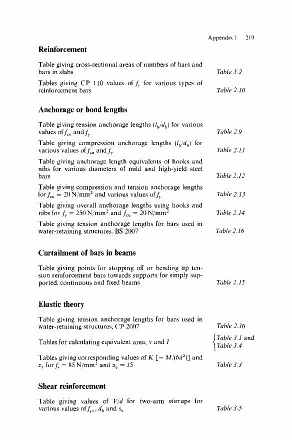
Appendix 1 219
Reinforcement
Table giving cross-sectional areas of numbers of bars and bars in slabs Table 3.2
Tables giving CP 110 values of/y for various types of reinforcement bars Table 2.10
Anchorage or bond lengths
Table giving tension anchorage lengths (lb/dh) for various values of/cu and/y
Table giving compression anchorage lengths (ljdh) for various values of/cu and/y
Table giving anchorage length equivalents of hooks and nibs for various diameters of mild and high-yield steel bars
Table giving compression and tension anchorage lengths for/cu = 20N/mm2 and various values of/y
Table giving overall anchorage lengths using hooks and nibs for fy = 250 N/mm2 and /cu = 20 N/mm2
Table giving tension anchorage lengths for bars used in water-retaining structures, BS 2007
Curtailment of bars in beams
Table giving points for stopping off or bending up ten-sion reinforcement bars towards supports for simply sup-ported, continuous and fixed beams Table 2.15
Elastic theory
Table giving tension anchorage lengths for bars used in water-retaining structures, CP 2007
Tables for calculating equivalent area, x and /
Tables giving corresponding values of K [= M/(bd2)~\ and zl for/s = 85 N/mm2 and ae = 15
Shear reinforcement
Table 2.9
Table 2.11
Table 2.12
Table 2.13
Table 2.14
Table 2.16
Table 2.16
Table 3.1 and Table 3.4
Table 3.3
Table giving values of V/d for two-arm stirrups for various values of/yv, dh and sv Table 3.5

220 Tables and graphs for design
Table giving values of V for single bars bent up at 45° in single shear for various values off and db Table 3.6
Plastic design of sections for bending moments
Table giving, for balanced design, values of Kx
[= MJ{bd2j] and p% [= l0OAJ(bd)] for various values of /y>/ sand/c u Table 3.7
Strength of steel in compression
Table giving /sc (design ultimate compressive stress) for various values ofjfy for compression steel Table 3.8
Figure giving CP 110, Fig. 3, stress-strain curve for 25 mm diameter alloy bar Figure 8.6
Design of beams and slabs
Table to assist in the preliminary design of depths of beams and slabs of various spans Table 7.1
Continuous beams and slabs
Tables giving bending moments and shear forces in con-tinuous beams and slabs carrying dead and imposed f Table 6.1 and loadings [Table 6.2
Table giving bending moments and shear forces in con-tinuous beams and slabs subjected to unit bending mo-ment at one and both ends Table 7.3
Single-span beams with fixed and free end supports
Table giving bending moments, support reactions and deflections for beams with various loadings Table 7.2

Appendix 2
Units and Greek symbols
For the purpose of being absolutely clear internationally about the units used in this book, the following conversions (which should prove useful anyway to engineers internationally) are given.
British Imperial 1 ton 20001b 0.9843 ton
l ib 10001b 1 inch lfoot 1000 lb in 1000 lb/in 1 lb/in2
1000 lb/in2
1 lb/ft2
1 ton/ft2
1 lb/ft 1 ton/ft 1 lb/ft3
145.0 lb/in2
U.S.A. 1 long ton 1 short ton 0.9843 long tons
l ib l k i p 1 inch lfoot 1 kip in 1 kip/in lpsi
( 1 kip/in2
(1000 psi 1 lb/ft2
1 long ton/ft2
1 lb/ft 1 long ton/ft 1 lb/ft3
l P a
Metric 1016.0kg 907.1kg
\1 tonne [1000 kg
0.4536 kg 453.6 kg 2.54 cm 30.48 cm 1.152kgcm 178.6 kg/cm 0.070 309 kg/cm2
70.309 kg/cm2
4.882 kg/m2
10940kg/m2
1.488 kg/m 3333 kg/m 16.02 kg/m3
10.20 kg/cm2
SI 9.964 kN 8.896 kN 9.807 kN
4.448 N 4.448 kN 25.4 mm 0.3048 m 0.1130 kNm 175.1 kN/m 6.895 kN/m2
6.895 N/mm2
0.047 88 kN/m2
107.3 kN/m2
0.014 59 kN/m 32.69 kN/m 0.157 07 kN/m3
lN /m 2
Notes 1. The terms 'force' and 'mass' have not been used above, and acceleration
due to gravity = 9.807 m/s2
2. p.s.i. = psi = lb/in2 = pounds per square inch 3. kip = 10001b = 1000 pounds 4. kip/in2 = 1000 psi = 1000 pounds per square inch 5. Pa = pascal
221
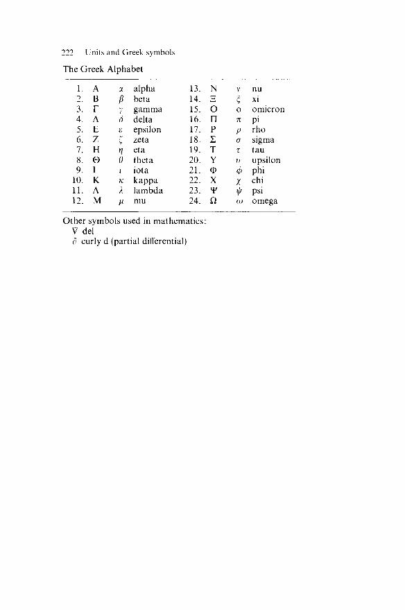
222 Units and Greek symbols
The Greek Alphabet
1. 2. 3. 4. 5. 6. 7. 8. 9.
10. 11. 12.
A B r A E Z H 0 I K A M
(X
P y s £
c n e i
K
X V
alpha beta gamma delta epsilon zeta eta theta iota kappa lambda mu
13. 14. 15. 16. 17. 18. 19. 20. 21. 22. 23. 24.
N ^ O n p 2 T Y 0 X ¥ Q
V
z o n P a T
V
4> i •A CD
nu xi omicroi Pi rho sigma tau upsilon phi chi psi omega
Other symbols used in mathematics: V del d curly d (partial differential)

Appendix 3
Nomenclature used in British Standard CP 110
Symbols for CP 110 were agreed internationally and are used, for example, by the latest A.C.I, code of practice used in the U.S.A. They are generally used in this present book. The symbols conform to an internationally agreed system of constructing symbols which can be used in creating further symbols.
4 1
Ac 4,1
4 a a!
Area of concrete Area of effective concrete flange Area of prestressing tendons Area of compression reinforcement Area of compression reinforcement in the more highly com-pressed face Area of tension reinforcement Area of reinforcement in other face (see 3.5.5.3) Area of longitudinal reinforcement (for columns) Cross-sectional area of longitudinal reinforcement provided for torsion Area of tension reinforcement provided Area of tension reinforcement required Cross-sectional area of the two legs of a link Deflection Distance from compression face to the point at which the crack width is being calculated Distance between bars Distance of the centroid of the concrete flange from the centroid of the composite section Distance from the point (crack) considered to the surface of the nearest longitudinal bar Distance of the centroid of the steel from the centroid of the net concrete section Distance between the line of action of the load and the face of the supporting member Width of section Breadth of compression face
223

224 Nomenclature used in British Standard CP 110
be Width of contact surface (between in situ and precast components)
bl Breadth of section at level of tension reinforcement bw Breadth of web or rib of a member C Torsional constant (see 3.3.7) cmin Minimum cover to tension steel Dc Density of concrete at time of test d Effective depth of tension reinforcement d' Depth to compression reinforcement dc Depth of concrete in compression dQ Depth to additional reinforcement to resist horizontal loading dt Effective depth in shear (see 4.3.5.3) d2 Depth to reinforcement (see 3.5.5.3) Ec Static secant modulus of elasticity of concrete Ecf Modulus of elasticity of flange concrete Ecq Dynamic tangent modulus of elasticity of concrete Es Modulus of elasticity of steel e Eccentricity e Base of Napierian logarithms ea Additional eccentricity due to deflections in walls ex Resultant eccentricity of load at right angles to plane of wall exl Resultant eccentricity calculated at top of wall ex2 Resultant eccentricity calculated at bot tom of wall F Ultimate load Fh Anchorage value of reinforcement Fbst Tensile bursting force Fb t Tensile force due to ultimate loads in a bar or group of bars Fh Horizontal component of a load Fk Characteristic load Ft Tie force Fv Maximum vertical ultimate load Fw Horizontal force on stiffened section of wall /bs Bond stress fci Concrete strength at (initial) transfer fco Stress in concrete at the level of the tendon due to initial
prestress and dead load / c p Compressive stress at the centroidal axis due to prestress fcu Characteristic concrete cube strength fk Characteristic strength fph Tensile stress in tendons at (beam) failure /pe Effective prestress (in tendon) f t Stress due to prestress (see 4.3.5.2) fpu Characteristic strength of prestressing tendons fs Service stress fs2 Stress in reinforcement (see 3.5.5.3) ft Maximum principal tensile stress fy Characteristic strength of reinforcement fyl Characteristic strength of longitudinal reinforcement /yv Characteristic strength of link reinforcement G Shear modulus
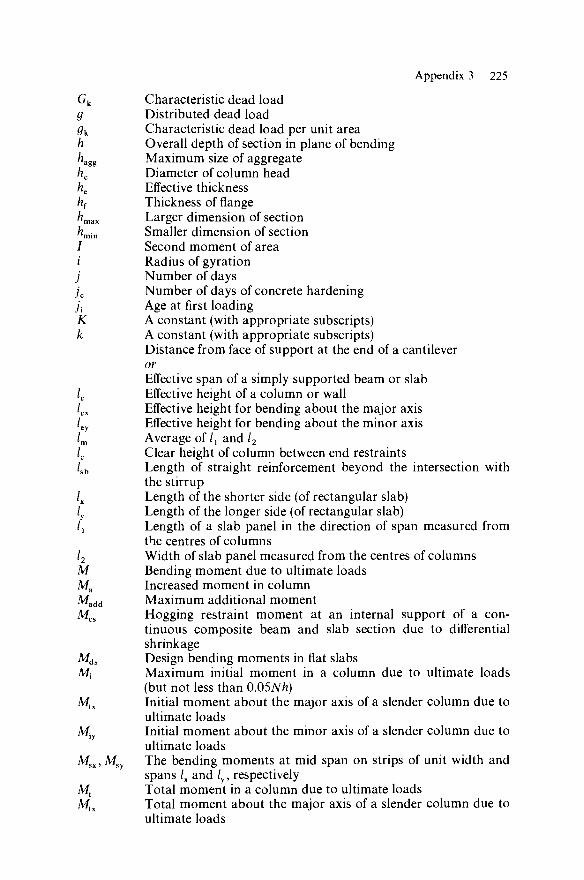
Appendix 3 225
Gk Characteristic dead load g Distributed dead load gk Characteristic dead load per unit area h Overall depth of section in plane of bending /zagg M a x i m u m size of aggrega te hc Diameter of column head he Effective thickness /zf Thickness of flange /imax Larger dimension of section hmin Smaller dimension of section / Second moment of area i Radius of gyration j Number of days jc Number of days of concrete hardening ji Age at first loading K A constant (with appropr ia te subscripts) k A constant (with appropr ia te subscripts)
Distance from face of support at the end of a cantilever or Effective span of a simply supported beam or slab
/e Effective height of a column or wall /ex Effective height for bending about the major axis /ey Effective height for bending about the minor axis /m Average of lx a n d l2
lc Clear height of column between end restraints /sb Length of straight reinforcement beyond the intersection with
the stirrup /x Leng th of the shor te r side (of rec tangula r slab) ly Length of the longer side (of rectangular slab) lx Length of a slab panel in the direction of span measured from
the centres of columns l2 Width of slab panel measured from the centres of columns M Bending moment due to ultimate loads Ma Increased moment in column Ma d d Maximum additional moment Mcs Hogging restraint moment at an internal support of a con-
t inuous composite beam and slab section due to differential shrinkage
Mds Design bending moments in flat slabs M{ Maximum initial moment in a column due to ultimate loads
(but not less than 0.05Nh) Mix Initial moment about the major axis of a slender column due to
ultimate loads Miy Initial moment about the minor axis of a slender column due to
ultimate loads M sx , Msy The bending moments at mid span on strips of unit width and
spans lx and ly, respectively Mt Total moment in a column due to ultimate loads M tx Total moment about the major axis of a slender column due to
ultimate loads
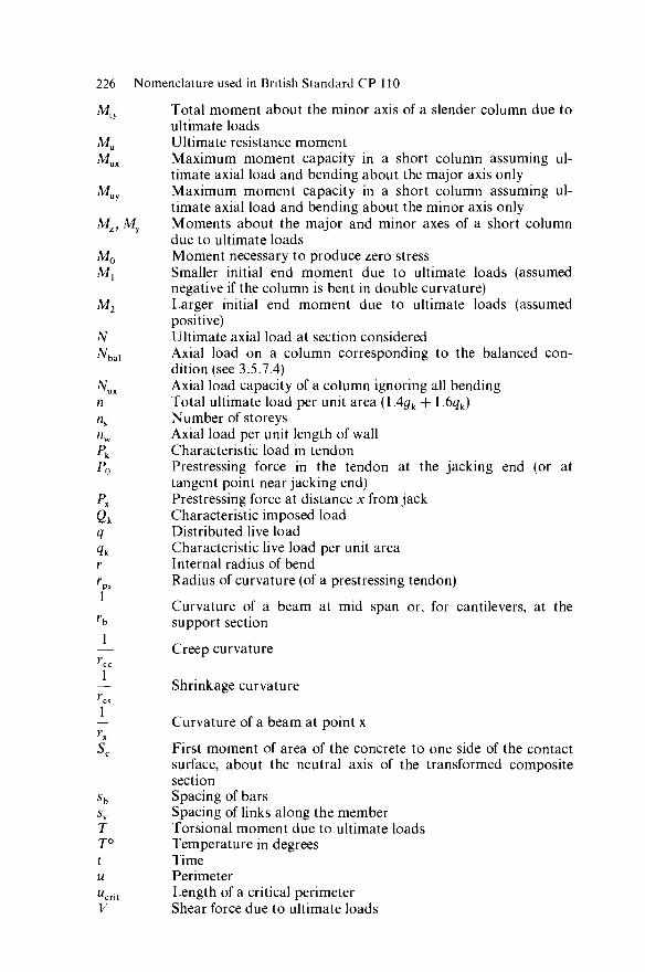
226 Nomenclature used in British Standard CP 110
Mt Total moment about the minor axis of a slender column due to ultimate loads
Mu Ultimate resistance moment Mux Maximum moment capacity in a short column assuming ul-
timate axial load and bending about the major axis only Muy Maximum moment capacity in a short column assuming ul-
timate axial load and bending about the minor axis only M z , My Moments about the major and minor axes of a short column
due to ultimate loads M0 Moment necessary to produce zero stress M1 Smaller initial end moment due to ultimate loads (assumed
negative if the column is bent in double curvature) M2 Larger initial end moment due to ultimate loads (assumed
positive) N Ultimate axial load at section considered Nb a l Axial load on a column corresponding to the balanced con-
dition (see 3.5.7.4) Nux Axial load capacity of a column ignoring all bending n Total ultimate load per unit area (\Agk + 1.6gk) ns Number of storeys nw Axial load per unit length of wall Pk Characteristic load in tendon P0 Prestressing force in the tendon at the jacking end (or at
tangent point near jacking end) Px Prestressing force at distance x from jack Qk Characteristic imposed load q Distributed live load qk Characteristic live load per unit area r Internal radius of bend rps Radius of curvature (of a prestressing tendon)
— Curvature of a beam at mid span or, for cantilevers, at the rb support section
— Creep curvature
— Shrinkage curvature r
cs
— Curvature of a beam at point x rx Sc First moment of area of the concrete to one side of the contact
surface, about the neutral axis of the transformed composite section
sb Spacing of bars sv Spacing of links along the member T Torsional moment due to ultimate loads T° Temperature in degrees t Time u Perimeter wcrit Length of a critical perimeter V Shear force due to ultimate loads

Appendix 3 227
Vc Ultimate shear resistance of concrete Vco U l t ima t e shear resis tance of a sect ion unc racked in flexure (see
4.3.5.1) VCT Ultimate shear resistance of a section cracked in flexure Vd Total vertical shear due to design service load v Shear stress vc Ultimate shear stress in concrete vh Horizontal shear stress per unit area of contact surface vt Torsional shear stress vtu Ultimate torsional shear stress Wk Characteristic wind load x Neutral axis depth *! Smaller dimension of a link y0 Half the side of end block ypo Half the side of loaded area yx Larger dimension of a link z Lever arm ac A ratio of the sum of column stiffnesses to the sum of beam
stiffnesses a c l Value of ac at lower end of column ac2 Value of ac at upper end of column acmin Minimum value of a c l and ac2 ae Modular ratio af Angle of internal friction for concrete interfaces an Coefficient as a function of column axial loading ax x ,ax y Bending moment coefficients for slabs with no provision to
resist torsion at the corners or to prevent the corners from lifting
jSb Ra t io of b e a m m o m e n t s with respect to service stress in b e a m s (see 3.3.8.1)
jScc Ratio of total creep to elastic deformation /} r e d Ratio of reduction in resistance moment /?sx,j8sy Bending moment coefficients for slabs with provision to resist
torsion and to prevent corners from lifting /?! Ratio of the longer to shorter base sides yf Partial safety factor for load ym Partial safety factor for strength Sm Degree of hardening at moment of loading ecs Shrinkage strain ecl Strain in concrete at the level of the tendon at time of loading sc2 Strain in concrete at the centroid of the section at time of
loading ediff Differential shrinkage strain em Average strain ex Strain at the level considered rj Relaxation coefficient 6S Angle between the compress ion face a n d the tens ion re-
inforcement A w Coefficient for walls dependent upon dimensions and concrete
used
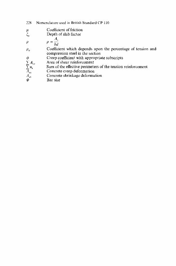
228 Nomenclature used in British Standard CP 110
[i Coefficient of friction £s Depth of slab factor
pQ Coefficient which depends upon the percentage of tension and compression steel in the section
0 Creep coefficient with appropriate subscripts £ ,4SV Area of shear reinforcement £ us Sum of the effective perimeters of the tension reinforcement Acc Concrete creep deformation Acs Concrete shrinkage deformation <P Bar size

Appendix 4
Extracts from British Standard CP 110: Part 1:1972
Throughout this present book references are often made to parts of CP 110. These are generally reproduced in essence in this Appendix. If a part of CP 110 is given to some extent, or completely, in the text then usually a note of this is given in this Appendix. Points in CP 110 which come from previous sources are sometimes not quoted in this Appendix.
Headings and references to sections, figures and tables set in bold type are from CP 110. All other references relate to this book.
2.2.3 Serviceability limit states
2.2.3.1 Deflection. Refer to Example 8.3, p. 199.
2.2.3.2 Cracking. Cracking of concrete should not adversely affect the appearance or durability of the structure.
The engineer must satisfy himself that any cracking will not be excessive, having regard to the requirements of the particular structure but, as a guide, the following may be regarded as reasonable limits.
1. Reinforced concrete. An assessment of the likely behaviour of a reinforced concrete structure should show that the surface width of cracks would not, in general, exceed 0.3 mm. Where members are exposed to particularly aggressive environments such as the very severe category in Table 19, the assessed surface widths of cracks at points nearest to the main reinforcement should not, in general, exceed 0.004 times the nominal cover to the main reinforcement. It should be recognised that in a reinforced concrete structure, under the effects of load and environment, the actual widths of cracks will vary between wide limits, and the prediction of an absolute maximum width is not possible; the possibility of some cracks being wider than the above must be accepted unless special precautions are taken.
2. Prestressed concrete. Refer to Section 8.4. 2.2.3.3 Vibration. Refer to Section 1.4(c)
2.2.3.4 Other limit states. Refer to Section 1.4(d)
229

230 Extracts from British Standard C P 110
2.3.3 Values for the ultimate limit state.
2.3.3.1 Loads. Refer to Table 1.1
2.3.3.2 Materials. Refer to Table 1.2
2.3.4 Values for a serviceability limit state
2.3.4.1 Loads. Refer to Table 1.1
2.3.4.2 Materials. Refer to Table 1.2
2.4.2.2 Elastic modulus: concrete. In the absence of better information, for normal-weight concrete the short-term elastic modulus, relevant to the serviceability limit states, may be taken from Table 1.
TABLE 1. Values of modulus of elasticity of concrete
Cube strength of concrete at the Modulus of elasticity appropriate age or stage considered, of concrete, N/mm2 kN/mm2
20 25 25 26 30 28 40 31 50 34 60 36
2.4.2.4 Elastic modulus: steel. For reinforcement, the elastic modulus for all types of loading may be taken as Es = 200 kN/mm2.
For prestressing tendons, the short-term elastic modulus may be taken as £s = 200 kN/mm2 for wire and small diameter strand, Es = 175 kN/mm2 for alloy bars and large diameter strand.
For sustained loading conditions, appropriate allowance for relaxation should be made.
2.4.3.2 Analysis of sections. The strength of a section should be assessed by inelastic analysis based on short-term stress-strain curves derived from the design strengths of materials given in 2.3.3.2, and from Figures 1 to 4.
3.1.4.3 Characteristic strength of reinforcement. Table 3: refer to Table 2.10
3.2.2.3 Redistribution of moments. Refer to Section 6.2
3.3.4 Moments and forces in continuous beams: uniform loading and equal spans. Provided the charactersic imposed load does not exceed the charac-teristic dead load, for beams which support substantially uniformly distrib-uted loads over three or more spans which do not differ by more than 15% of the longest, the ultimate bending moments and shear forces used in design may be obtained from Table 4.

Appendix 4 231
0__8_/y./?m_
/ / /
^y/*m Tension
Compression
.. . . r
^200kN/mm 2 /
0.002
Note: fy in N/mm 2
rm+ 2000
Strain
Figure A4.2 Short-term design stress-strain curve for reinforcement
(For Figure A4.1 Short-term design stress-strain curve for normal weight concrete see Figure 3.8(b) of this book)
0.005
200kN/mm 2 for wire to B5 2691 sections 2 and 3 and strand to BS 3617 sections 2 and 3 175 k N / m m 2 for al loy bars to BS U 8 6 and 19-wire strand to BS 4757 section 3
Strain
Figure A4.3 Short-term design stress-strain curve for nor-mal and low relaxation products
TABLE 4. Ultimate bending moments and shear forces
At outer support
Near middle of end span
At first interior support
At middle of interior spans
At interior supports
Moment
Shear
0
0.45F
Fl
IT —
-Fl
~9~
0.6F
Fl
14 —
-Fl
~io~ 0.55F
In Table 4, / is the effective span and F is the total ultimate load (1.4Gk + 1.6<2k). No redistribution of the moments found from Table 4 should be made.
3.3.5.1 Analysis of sections. Refer to Section 3.7 and its sub-sections.
3.3.6.1 Shear stresses and shear reinforcement in beams. Where the shear stress exceeds the appropriate value of vc from Table 5, shear reinforcement in the
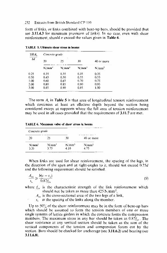
232 Extracts from British Standard C P 110
form of links, or links combined with bent-up bars, should be provided (but see 3.11.4.3 for minimum provision of links). In no case, even with shear reinforcement, should v exceed the values given in Table 6.
TABLE 5. Ultimate shear stress in beams
100/4S
bd
0.25 0.50 1.00 2.00 3.00
Concrete
20
N/mm2
0.35 0.45 0.60 0.80 0.85
grade
25
N/mm2
0.35 0.50 0.65 0.85 0.90
30
N/mm2
0.35 0.55 0.70 0.90 0.95
40 or more
N/mm2
0.35 0.55 0.75 0.95 1.00
The term As in Table 5 is that area of longitudinal tension reinforcement which continues at least an effective depth beyond the section being considered except at supports where the full area of tension reinforcement may be used in all cases provided that the requirements of 3.11.7 are met.
TABLE 6. Maximum value of shear stress in beams
Concrete grade
20 25 30 40 or more
N/mm2 N/mm2 N/mm2 N/mm2
3.35 3.75 4.10 4.75
When links are used for shear reinforcement, the spacing of the legs, in the direction of the span and at right-angles to it, should not exceed 0.75<i and the following requirement should be satisfied.
A^ > b(v - vc) 5V ^ 0.87/yv
l ;
where /yv is the characteristic strength of the link reinforcement which should not be taken as more than 425 N/mm2,
,4SV is the cross-sectional area of the two legs of a link, 5V is the spacing of the links along the member.
Up to 50% of the shear reinforcement may be in the form of bent-up bars which should be assumed to form the tension members of one or more single systems of lattice girders in which the concrete forms the compression members. The maximum stress in any bar should be taken as 0.87/yv. The shear resistance at any vertical section should be taken as the sum of the vertical components of the tension and compression forces cut by the section. Bars should be checked for anchorage (see 3.11.6.2) and bearing (see 3.11.6.8).
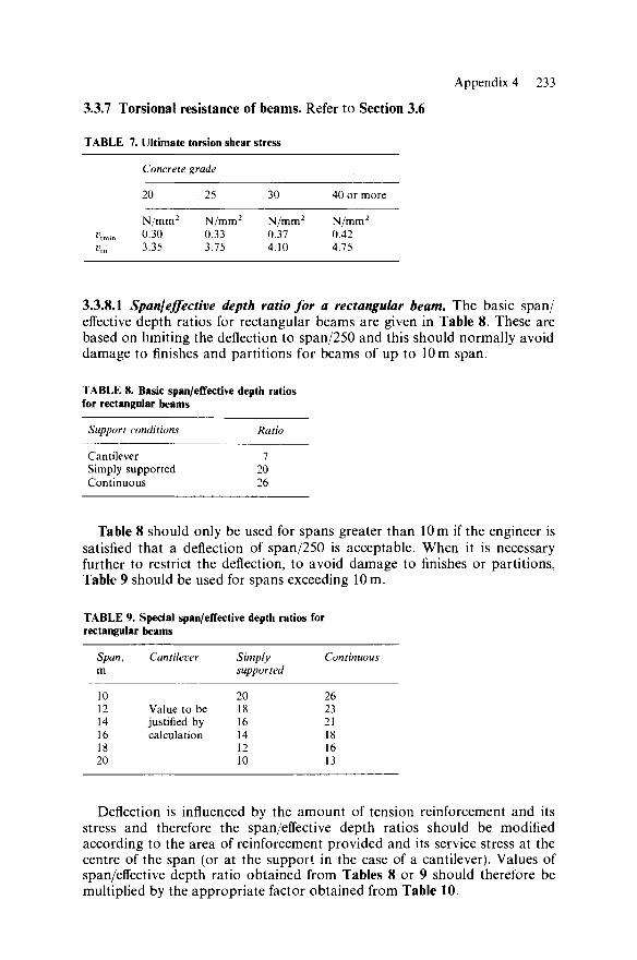
Appendix 4 233
3.3.7 Torsional resistance of beams. Refer to Section 3.6
TABLE 7. Ultimate torsion shear stress
Concrete grade
20 25 30 40 or more
N/mm2 N/mm2 N/mm2 N/mm2
vtmin 0.30 0.33 0.37 0.42 vtu 3.35 3.75 4.10 4.75
3.3.8.1 Span/effective depth ratio for a rectangular beam. The basic span/ effective depth ratios for rectangular beams are given in Table 8. These are based on limiting the deflection to span/250 and this should normally avoid damage to finishes and partitions for beams of up to 10 m span.
TABLE 8. Basic span/effective depth ratios for rectangular beams
Support conditions Ratio
Cantilever 7 Simply supported 20 Continuous 26
Table 8 should only be used for spans greater than 10 m if the engineer is satisfied that a deflection of span/250 is acceptable. When it is necessary further to restrict the deflection, to avoid damage to finishes or partitions, Table 9 should be used for spans exceeding 10 m.
TABLE 9. Special span/effective depth ratios for rectangular beams
Span, Cantilever Simply Continuous m supported
10 20 26 12 Value to be 18 23 14 justified by 16 21 16 calculation 14 18 18 12 16 20 10 13
Deflection is influenced by the amount of tension reinforcement and its stress and therefore the span/effective depth ratios should be modified according to the area of reinforcement provided and its service stress at the centre of the span (or at the support in the case of a cantilever). Values of span/effective depth ratio obtained from Tables 8 or 9 should therefore be multiplied by the appropriate factor obtained from Table 10.
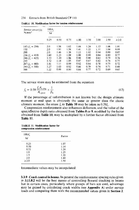
234 Extracts from British Standard CP 110
TABLE 10. Modification factor for tension reinforcement
Service stress (fs), N/mm2
145 (fy = 250) 150 200 238 (fy = 410) 246 (fy = 425) 250 267 (fy = 460) 290 (fy = 500) 300
100,4S
bd
0.25
2.0 2.0 2.0 1.60 1.55 1.52 1.41 1.27 1.22
0.50
1.98 1.91 1.46 1.23 1.20 1.18 1.11 1.03 0.99
0.75
1.62 1.58 1.26 1.09 1.06 1.05 0.99 0.92 0.90
1.00
1.44 1.41 1.15 1.00 0.98 0.97 0.92 0.86 0.84
1.50
1.24 1.22 1.02 0.90 0.88 0.87 0.84 0.79 0.77
2.00
1.13 1.11 0.94 0.84 0.83 0.82 0.78 0.74 0.72
2.50
1.06 1.04 0.89 0.80 0.79 0.78 0.75 0.71 0.69
^3.0
1.01 0.99 0.85 0.77 0.76 0.75 0.72 0.68 0.67
The service stress may be estimated from the equation
/ s = 0 . 5 8 ^ ^ 1 1 (13)
If the percentage of redistribution is not known but the design ultimate moment at mid span is obviously the same or greater than the elastic ultimate moment, the stress fs in Table 10 may be taken as 0.58/y.
Compression reinforcement also influences deflection, and the value of the span/effective depth ratio obtained from Tables 8 or 9, modified by the factor obtained from Table 10, may be multiplied by a further factor obtained from Table 11.
TABLE 11. Modification factor for compression reinforcement
100A'S
bd
0.25 0.50 0.75 1.0 1.5 2.0
^3.0
Factor
1.07 1.14 1.20 1.25 1.33 1.40 1.50
Intermediate values may be interpolated.
3.3.9 Crack control in beams. In general the reinforcement spacing rules given in 3.11.8.2 will be the best means of controlling flexural cracking in beams but in certain cases, particularly where groups of bars are used, advantage may be gained by calculating crack widths (see Appendix A) under service loads and comparing them with the recommended values given in Section 2.

Appendix 4 235 3.4.5.1 Shear stresses in solid slabs: general. No shear reinforcement is required when the stress v is less than £svc
where £s has the value shown in Table 14 and vc is obtained from Table 5.
TABLE 14. Values of $s
Overall slab depth, mm «.
300 or more 275 250 225 200 175 150 or less
1.00 1.05 1.10 1.15 1.20 1.25 1.30
The shear stress v in solid slabs less than 200 mm thick should not exceed £svc.
3.4.5.2 Shear stresses in solid slabs under concentrated loads. Refer to Section 7.3
3.5.1.3 Braced and unbraced columns: definitions. Refer to Section 7.1.3
3.5.1.4 Effective height of a column.
TABLE 15. Effective column height
Type of column Effective column height
Braced column properly restrained in direction at both ends
Braced column imperfectly restrained in direction at one or both ends
Unbraced or partially braced column, properly restrained in direction at one end but imperfectly restrained in direction at the other end
0.75/o
A value intermediate between 0.75/o and /0 depending upon the efficiency of the directional restraint
A value intermediate between /0 and 2/0 depending upon the efficiency of the directional restraint and bracing
3.5.2 Moments and forces in columns. Refer to Section 7.1.3
3.5.5 Short columns resisting moments and axial forces. Any short column may be designed in accordance with the following recommendations pro-vided the moment at any cross-section is not taken to be less than that produced by considering the ultimate axial load as acting at an eccentricity of 0.05/zmin, where hmin is the minimum depth of cross-section.

236 Extracts from British Standard CP 110
3.11.2 Concrete cover to reinforcement. The nominal cover should always be at least equal to the size of the bar and in the case of bundles of three or more bars, should be equal to the size of a single bar of equivalent area.
Table 19 gives the nominal cover of dense natural aggregate concrete which should be provided to all reinforcement, including links, when using the indicated grade of concrete under particular conditions of exposure.
3.11.4 Minimum areas of reinforcement in members.
3.11.4.1 Minimum area of main reinforcement. The area of tension reinforce-ment in a beam or slab should not be less than 0.15%btd when using high yield reinforcement, or 0.25%btd when mild steel reinforcement is used, where bt is the breadth of the section and d is the effective depth. For a box, T- or I -section, bt should be taken as the average breadth of the concrete below the upper flange.
The minimum number of longitudinal bars provided in a column should be four in rectangular columns and six in circular columns and their size should not be less than 12 mm. Except for lightly loaded columns (see 3.5.1.1) the total cross-sectional area of these bars should not normally be less than 1% of the cross section of the column.
A wall cannot be considered as a reinforced concrete wall unless the percentage of vertical reinforcement provided is at least 0.4%. This vertical reinforcement may be in one or two layers.
It should be noted that for fire resistance purposes, a wall containing less than 1.0% of vertical reinforcement is classed as a plain concrete wall.
3.11.4.2 Minimum area of secondary reinforcement. In a solid concrete suspended slab, the amount of reinforcement provided at right-angles to the main reinforcement, expressed as a percentage of the gross cross section, should not be less than 0.12% of high yield reinforcement or, alternatively, not less than 0.15% of mild steel reinforcement. In either case, the distance between bars should not exceed five times the effective depth of the slab.
In a flanged beam the amount of reinforcement provided over the top surface and across the full effective width of the flange, expressed as a percentage of the longitudinal cross-sectional area of the flange, should not be less than 0.3%.
Where in a wall the main vertical reinforcement is used to resist compres-sion, at least 0.25% in the case of high yield or 0.3% in the case of mild steel of horizontal reinforcement of not less size than one-quarter of the size of the vertical bars and not less than 6mm should be provided. It may also be necessary to provide links in the thickness of the wall (see 3.11.4.3).
3.11.4.3 Minimum area of links. When in a beam or column part or all of the main reinforcement is required to resist compression, links or ties at least one-quarter the size of the largest compression bar should be provided at a maximum spacing of twelve times the size of the smallest compression bar. Links should be so arranged that every corner and alternate bar or group in an outer layer of reinforcement is supported by a link passing round the bar and having an included angle of not more than 135°. All other bars or groups within a compression zone should be within 150 mm of a restrained bar. For circular columns, where the longitudinal reinforcement is located
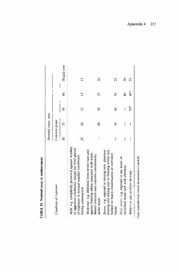
TA
BL
E 1
9. N
omin
al c
over
to
rein
forc
emen
t
Con
ditio
n of
exp
osur
e
Nom
inal
cov
er, m
m
Con
cret
e gr
ade
20
25
30
40
50 a
nd o
ver
Mil
d: e
.g. c
ompl
etel
y pr
otec
ted
agai
nst
wea
ther
, or
agg
resi
ve c
ondi
tions
, exc
ept
for
brie
f pe
riod
of e
xpos
ure
to n
orm
al w
eath
er c
ondi
tions
du
ring
cons
truc
tion
Mod
erat
e: e
.g.
shel
tere
d fro
m s
ever
e ra
in a
nd
agai
nst
freez
ing
whi
lst
satu
rate
d w
ith w
ater
. B
urie
d co
ncre
te a
nd c
oncr
ete
cont
inuo
usly
un
der
wat
er
Seve
re:
e.g.
exp
osed
to
driv
ing
rain
, al
tern
ate
wet
ting
and
dryi
ng a
nd t
o fre
ezin
g w
hils
t w
et.
Subj
ect
to h
eavy
con
dens
atio
n or
cor
rosi
ve
fum
es
Ver
y se
vere
: e.
g. e
xpos
ed t
o se
a w
ater
or
moo
rlan
d w
ater
and
with
abr
asio
n
Subj
ect
to s
alt
used
for
de-i
cing
25
20
40
50
15
30
40
50*
15
25
30
60
40*
15
20
25
50
25
* O
nly
appl
icab
le if
the
conc
rete
has
ent
rain
ed a
ir (s
ee 6
.3.6
).
> a 3 a-

238 Extracts from British Standard CP 110
round the periphery of a circle, adequate lateral support is provided by a circular tie passing round the bars or groups.
When in a wall the percentage of vertical reinforcement resisting compre-ssion exceeds 2%, links at least 6 mm or one quarter of the size of the largest compression bar should be provided through the thickness of the wall. The spacing of these links should not exceed twice the wall thickness in either the horizontal or vertical directions and in the vertical direction should be not greater than 16 times the bar size. Any vertical compression bar not enclosed by a link should be within 200 mm of a restrained bar.
In all beams except those of minor structural importance (for example lintels) or where the maximum shear stress, calculated in accordance with 3.3.6, is less than half the recommended value, nominal links should be provided throughout the span such that:
for high yield links
for mild steel links
where Asy is the cross-sectional area of the two legs of a link, bt is the breadth of the beam at the level of the tension
reinforcement, sv is the spacing of the links.
The spacing of links should not exceed 0.75 times the effective depth of the beam, nor should the lateral spacing of the individual legs of the links exceed this figure. Links should enclose all tension reinforcement.
3.11.6.1 Local bond. Critical sections for local bond occur at the faces of simply supported ends of members, at points where tension bars stop and at points of contraflexure. However, points where tension bars stop and points of contraflexure need not be considered if the anchorage bond stresses in the continuing bars do not exceed 0.8 times the value given in 3.11.6.2.
TABLE 21. Ultimate local bond stresses
Bar type
Plain bars Deformed bars
Concrete grade
20
N/mm2
1.7 2.1
25
N/mm2
2.0 2.5
30
N/mm2
2.2 2.8
40 or more
N/mm2
2.7 3.4
Where there would be an advantage, and the deformed reinforcement to be used is Type 2, as defined in E.l of Appendix E, the values of bond stress for deformed bars may be increased by 20%.
3.11.6.2 Anchorage bond.
Where there would be an advantage, and the deformed reinforcement to be used is Type 2, as defined in E.l of Appendix E, the values of bond stress for deformed bars may be increased by 30%.
- ^ = 0.0012bt
^ = 0.002fct
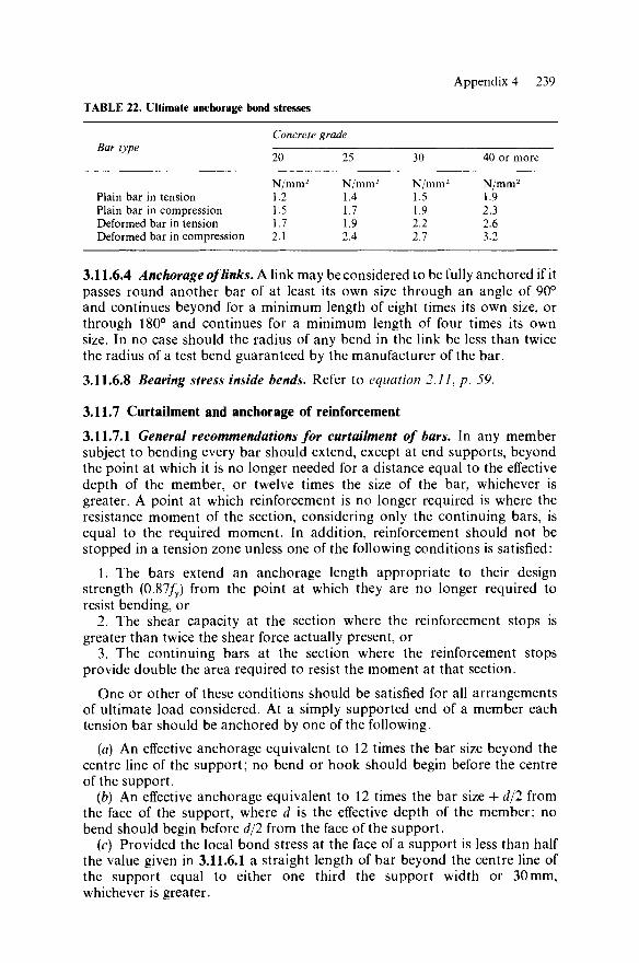
Appendix 4 239
TABLE 22. Ultimate anchorage bond stresses
Bar type
Plain bar in tension Plain bar in compression Deformed bar in tension Deformed bar in compression
Concrete grade
20
N/mm2
1.2 1.5 1.7 2.1
25
N/mm2
1.4 1.7 1.9 2.4
30
N/mm2
1.5 1.9 2.2 2.7
40 or more
N/mm2
1.9 2.3 2.6 3.2
3.11.6.4 Anchorage of links. A link may be considered to be fully anchored if it passes round another bar of at least its own size through an angle of 90° and continues beyond for a minimum length of eight times its own size, or through 180° and continues for a minimum length of four times its own size. In no case should the radius of any bend in the link be less than twice the radius of a test bend guaranteed by the manufacturer of the bar.
3.11.6.8 Bearing stress inside bends. Refer to equation 2.11, p. 59.
3.11.7 Curtailment and anchorage of reinforcement
3.11.7.1 General recommendations for curtailment of bars. In any member subject to bending every bar should extend, except at end supports, beyond the point at which it is no longer needed for a distance equal to the effective depth of the member, or twelve times the size of the bar, whichever is greater. A point at which reinforcement is no longer required is where the resistance moment of the section, considering only the continuing bars, is equal to the required moment. In addition, reinforcement should not be stopped in a tension zone unless one of the following conditions is satisfied:
1. The bars extend an anchorage length appropriate to their design strength (0.87/y) from the point at which they are no longer required to resist bending, or
2. The shear capacity at the section where the reinforcement stops is greater than twice the shear force actually present, or
3. The continuing bars at the section where the reinforcement stops provide double the area required to resist the moment at that section.
One or other of these conditions should be satisfied for all arrangements of ultimate load considered. At a simply supported end of a member each tension bar should be anchored by one of the following.
(a) An effective anchorage equivalent to 12 times the bar size beyond the centre line of the support; no bend or hook should begin before the centre of the support.
(b) An effective anchorage equivalent to 12 times the bar size + d/2 from the face of the support, where d is the effective depth of the member; no bend should begin before d/2 from the face of the support.
(c) Provided the local bond stress at the face of a support is less than half the value given in 3.11.6.1 a straight length of bar beyond the centre line of the support equal to either one third the support width or 30 mm, whichever is greater.

240 Extracts from British Standard CP 110 3.11.7.2 Simplified rules for curtailment of bars in beams. As an alternative to 3.11.7.1 for beams which support substantially uniformly distributed loads, the following simplified rules may be applied.
1. Simply supported beams. At least 50% of the tension reinforcement provided at mid span should extend to the supports and have an effective anchorage of 12$ past the centre of the support. The remaining 50% should extend to within 0.08/ of the support.
2. Cantilever beams. At least 50% of the tension reinforcement provided at the support should extend to the end of the cantilever. The remaining 50% should extend a distance of 1/2 or 45 times the bar size, whichever is the greater, from the support.
3. Continuous beams of equal span where the characteristic imposed load does not exceed the characteristic dead load, and which are designed in accordance with 3.3.4.
(a) At least 20% of the reinforcement in tension over the supports should be made effectively continuous through the spans. Of the remainder, half should extend to a point not less than 0.25/ from the support, and the other half to a point not less than 0.15/ from the support, but no bar should stop at a point less than 45 times its own size from the support.
(b) At least 30% of the reinforcement in tension at mid span should extend to the supports. The remainder should extend to points not less than 0.15/ from interior supports, and not less than 0.1/ from exterior supports.
(c) At a simply supported end, the detailing should be as given in (1) above for a simply supported beam. 3.11.7.3 Simplified rules for curtailment of bars in slabs. As an alternative to 3.11.7.1 for solid slabs spanning one way which support substantially uniformly distributed loads, the following simplified rules may be applied.
1. Simply supported slabs. At least 50% of the tension reinforcement provided at mid span should extend to the supports and have an effective anchorage of 12# past the centre of the support. The remaining 50% should extend to within 0.08/ of the support.
2. Cantilever slabs. At least 50% of the tension reinforcement provided at the support should extend to the end of the cantilever. The remaining 50% should extend a distance of 1/2 or 45 times the bar size, whichever is the greater, from the support.
3. Continuous slabs of approximately equal span where the characteristic imposed load does not exceed the characteristic dead load, and which are designed in accordance with 3.3.4. All tension reinforcement over supports should extend a distance of 0.1/ or 45 times the bar size, whichever is the greater, and at least 50% should extend 0.3/ into the span.
The tension reinforcement at mid span of a slab should extend to within 0.2/ of internal supports and within 0.1/ of external supports and at least 50% should extend into the support.
Where at an end support there is a monolithic connection between the slab and its supporting beam or wall, provision should be made for the negative moment which may arise. The negative moment to be assumed in this case depends on the degree of fixity, but it will generally be sufficient to provide tension reinforcement, equal to half that provided at mid span, ex-tending 0.1/ or 45 times the bar size, whichever is the greater, into the span.

Appendix 4 241 3.11.8 Spacing of reinforcement
3.11.8.1 Minimum distance between bars. These recommendations are not related to bar sizes but when a bar exceeds the maximum size of coarse aggregate by more than 5 mm, a spacing smaller than the bar size should generally be avoided. A pair of bars in contact or a bundle of three or four bars in contact should be considered as a single bar of equivalent area when assessing size.
The spacing of bars should be suitable for the proper compaction of concrete and when an internal vibrator is likely to be used, sufficient space should be left between reinforcement to enable the vibrator to be inserted. Minimum reinforcement spacing is best determined by experience or proper works tests but in the absence of better information, the following may be used as a guide.
1. Individual bars. Except where bars form part of a pair or bundle (see (2) and (3)) the horizontal distance between bars should not be less than /iagg + 5 mm, where /iagg is the maximum size of the coarse aggregate. Where there are two or more rows:
(a) the gaps between corresponding bars in each row should be vertically in line;
(b) the vertical distance between bars should be not less than | / ia g g . 2. Pairs of bars. Bars may be arranged in pairs either touching or closer
than in (1) above, in which case: (a) the gaps between corresponding pairs in each row should be vertically
in line and of width not less than /iagg -I- 5 mm; (b) when the bars forming the pair are one above the other, the vertical
distance between pairs should not be less than § /iagg. (c) when the bars forming the pair are side by side, the vertical distance
between pairs should be not less than hagg + 5 mm. 3. Bundled bars. Horizontal and vertical distances between bundles
should be not less than /zagg + 15mm and the gaps between the rows of bundles should be vertically in line.
3.11.8.2 Maximum distance between bars in tension. Unless the calculation of crack widths (see Appendix A) shows that a greater spacing is acceptable, the following rules should be applied to beams in normal internal or external conditions of exposure.
1. In the application of these rules any bar with a diameter less than 0.45 times the diameter of the maximum bar size in the section should be ignored except when considering those in the side faces of beams. Bars placed in the side face of beams to control cracking should be of a size not less than yf(shb/fy\ where sb is the spacing of the bars and b the breadth of the section at the point considered.
2. The clear horizontal distance between adjacent bars, or groups, near the tension face of a beam should not be greater than the value given in Table 24 depending on the amount of redistribution carried out in analysis and the characteristic strength of the reinforcement.
3. The clear distance from the corner of a beam to the surface of the nearest longitudinal bar should not be greater than half the clear distance given in Table 24.
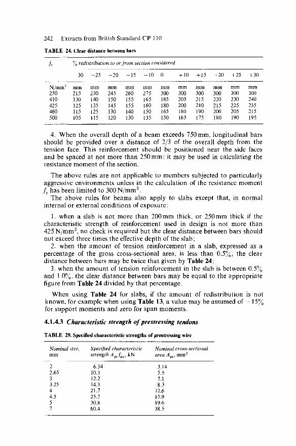
242 Extracts from British Standard C P 110
TABLE 24. Clear distance between bars
/ % redistribution to or from section considered
N/mm2
250 410 425 460 500
- 3 0
mm 215 130 125 115 105
- 2 5
mm 230 140 135 125 115
- 2 0
mm 245 150 145 130 120
- 1 5
mm 260 155 155 140 130
- 1 0
mm 275 165 160 150 135
0
mm 300 185 180 165 150
+ 10
mm 300 205 200 180 165
+ 15
mm 300 215 210 190 175
+20
mm 300 220 215 200 180
+ 25
mm 300 230 225 205 190
+ 30
mm 300 240 235 215 195
4. When the overall depth of a beam exceeds 750 mm, longitudinal bars should be provided over a distance of 2/3 of the overall depth from the tension face. This reinforcement should be positioned near the side faces and be spaced at not more than 250 mm; it may be used in calculating the resistance moment of the section.
The above rules are not applicable to members subjected to particularly aggressive environments unless in the calculation of the resistance moment /y has been limited to 300N/mm2.
The above rules for beams also apply to slabs except that, in normal internal or external conditions of exposure:
1. when a slab is not more than 200 mm thick, or 250 mm thick if the characteristic strength of reinforcement used in design is not more than 425 N/mm2, no check is required but the clear distance between bars should not exceed three times the effective depth of the slab;
2. when the amount of tension reinforcement in a slab, expressed as a percentage of the gross cross-sectional area, is less than 0.5%, the clear distance between bars may be twice that given by Table 24;
3. when the amount of tension reinforcement in the slab is between 0.5% and 1.0%, the clear distance between bars may be equal to the appropriate figure from Table 24 divided by that percentage.
When using Table 24 for slabs, if the amount of redistribution is not known, for example when using Table 13, a value may be assumed of —15% for support moments and zero for span moments.
4.1.4.3 Characteristic strength of prestressing tendons
TABLE 29. Specified characteristic strengths of prestressing wire
Nominal size, mm
2 2.65 3 3.25 4 4.5 5 7
Specified characteristic strength Apsfpu,kN
6.34 10.3 12.2 14.3 21.7 25.7 30.8 60.4
Nominal cross-sectional area A^, mm2
ps '
3.14 5.5 7.1 8.3
12.6 15.9 19.6 38.5

Appendix 4 243
TABLE 30. Specified characteristic strengths of prestressing strand
Number of wires
7
19
Nominal size, mm
6.4 7.9 9.3
10.9 12.5 15.2
18 25.4 28.6 31.8
Specified characteristic strength A]
44.5 69.0 93.5
125 165 227
370 659 823 979
ps./pu • , kN Nominal cross-sectional area Aps, mm2
24.5 37.4 52.3 71.0 94.2
138.7
210 423 535 660
TABLE 31. Specified characteristic strengths of prestressing bars
Nominal size, mm
20* 22 25* 28 32* 35 40*
Specified characteristic strength /4ps/pu , kN
325 375 500 625 800 950
1250
Nominal cross-sectional area Aps, mm2
314 380 491 615 804 961
1257
" Preferred sizes.
4.3.3.2 Stress limitations under service conditions
4.3.3.2.1 Compressive stresses
TABLE 32. Compressive stresses in concrete for serviceability limit states
Nature of loading Allowable compressive stresses
Design load in bending
Design load in direct compression
0.33/cu In continuous beams and other statically indeterminate structures this may be increased to 0.4/cu within the range of support moments 0.25/cu
4.3.3.3 Stress limitations at transfer
4.3.3.3.1 Compressive stresses
TABLE 36. Allowable compressive stresses at transfer
Nature of stress distribution Allowable compressive stresses
Triangular or near triangular distribution of prestress 0.5/cl Uniform or near uniform distribution of prestress 0Afcl
where fcl is the concrete strength at transfer.

244 Extracts from British Standard CP 110
4.3.4 Ultimate limit state: flexure
4.3.4.1 Section analysis. Refer to Section 8.4 and its sub-sections
4.3.4.3 Design formula. In the absence of an analysis based on the assumptions given in 4.3.4.1, the resistance moment of a rectangular beam, or of a flanged beam in which the neutral axis lies within the flange, may be obtained from equation 44.
Mu=fphAps(d-0.5x) (44) Values for fph and x are given in Table 37 for pretensioned members and
for post-tensioned members with effective bond between the concrete and tendons. The effective prestress after all losses should not be less than 0.45/pU. Prestressing tendons and additional reinforcement in the compres-sion zone should be ignored in strength calculations when using this method. TABLE 37. Conditions at the ultimate limit state for rectangular beams with pretensioned tendons or with post-tensioned tendons having effective bond
-/pu^ps
fcubd
0.025 0.05 0.10 0.15 0.20 0.25 0.30 0.40
Stress in tendons the design
as a proportion of strength /pb/0.87/pu
Pretensioning
1.0 1.0 1.0 1.0 1.0 1.0 1.0 0.9
Post-tensioning with effective bond
1.0 1.0 1.0 1.0 0.95 0.90 0.85 0.75
Ratio of depth of neutral axis to that of the centroid of the tendons in the tension zone x/d
Pretensioning
0.054 0.109 0.217 0.326 0.435 0.542 0.655 0.783
Post-tensioning with effective bond
0.054 0.109 0.217 0.326 0.414 0.488 0.558 0.653
For rectangular beams and flanged beams in which the neutral axis lies within the flange, the stress in the tendons at failure where unbonded tendons are used may be derived from Table 38.
TABLE 38. Conditions at the ultimate limit state for post-tensioned rectangular beams having unbonded tendons
Stress in tendons as a proportion of Ratio of depth of neutral axis to that /pu^ps effective prestress fph/fpu for values of of the centroid of the tendons in the ~T~bd~ ' (effective sPan \ tension zone x/d for values of
d [effective depth) U effective span \ d \effective depth/
30 20 10 30 20 10
0.025 1.23 1.34 1.45 0.10 0.10 0.10 0.05 1.21 1.32 1.45 0.16 0.16 0.18 0.10 1.18 1.26 1.45 0.30 0.32 0.36 0.15 1.14 1.20 1.36 0.44 0.46 0.52 0.20 1.11 1.16 1.27 0.56 0.58 0.64

Appendix 4 245
In Table 38 the following assumptions have been made:
1. the effective prestress after all losses have occurred (fpc) does not exceed 0.6/pu,
2. the compression block is rectangular with a uniform stress of 0.4/cu, 3. the tendons are either in ducts or, if they are free as in hollow sections,
diaphragms are provided to prevent a reduction of the effective depth, 4. the effective depth is determined by assuming that the tendons are in
contact with the top of the duct or the soffit of the diaphragms.
4.3.5.1 Sections uncracked in flexure. The ultimate shear resistance of a section uncracked in flexure, Fco, corresponds to the occurrence of a maximum principal tensile stress, at the centroidal axis of the section, of / = 0.24V/C11.
In the calculation of Vco, the value of prestress at the centroidal axis, should be taken as 0.8/cp. The value of Vco is given by
Vco = 0.67frM/t2 + 0 . 8 / ^ ) (45) where ft is 0.24V/Cu> taken as positive,
fcp is the compressive stress at the centroidal axis due to prestress, taken as positive,
b is the breadth of the member which for T-, I- and L-beams should be replaced by the breadth of the rib few,
h is the overall depth of the member.
Values of VJbh obtained from equation (45) are given in Table 39.
TABLE 39. Values of VJbh
Jcp
N/mm2
2 4 6 8
10 12 14
Concrete grade
30
N/mm2
1.30 1.65 1.90 2.15 2.35 2.55 2.70
40
N/mm2
1.45 1.80 2.10 2.30 2.55 2.75 2.95
50
N/mm2
1.60 1.95 2.20 2.50 2.70 2.95 3.15
60
N/mm2
1.70 2.05 2.35 2.65 2.85 3.10 3.30
In flanged members where the centroidal axis occurs in the flange the principal tensile stress should be limited to 0.24y/fcu at the intersection of the flange and web; in this calculation, 0.8 of the stress due to prestress at this intersection should be used in calculating Vco.
For a section uncracked in flexure and with inclined tendons or vertical prestress, the component of prestressing force normal to the longitudinal axis of the member may be added to Vco. 4.3.5.2 Sections cracked in flexure. The ultimate shear resistance of a section cracked in flexure, Fcr, may be calculated using equation 46:
. / p e Y . , , , . , V VCI = I 1 - 0.55 ^ I vcbd + M0~ (46)

246 Extracts from British Standard C P 110
where d is the distance from the extreme compression fibre to the centroid of the tendons at the section considered,
M0 is the moment necessary to produce zero stress in the concrete at the depth d.
M0 = 0.8/pt - where /p t is the stress due to prestress only at
depth d and distance y from the centroid of the concrete section which has second moment of area /,
/ p e is the effective prestress after all losses have occurred. For the purposes of this equation / p e shall not be put greater t han0 .6 / p u ,
vc is obtained from Table 5, Kand M are the shear force and bending moment, respectively, at
the section considered due to ultimate loads, Vcr should be taken as not less than 0Abdyffcu.
The value of Vcr calculated using equation 46 at a particular section may be assumed to be constant for a distance equal to rf/2, measured in the direction of increasing moment, from that particular section.
For a section cracked in flexure and with inclined tendons, the com-ponent of prestressing force normal to the longitudinal axis of the member should be ignored.
4.8.1. Maximum initial prestress. The jacking force should not normally exceed 70% of the characteristic strength of the tendon but may be increased to 80%, provided that additional consideration is given to safety, to the stress-strain characteristics of the tendon and to the assessment of the friction losses.
4.8.2.4 Loss of prestress due to shrinkage of the concrete. The loss of prestress in the tendons due to shrinkage of the concrete may be calculated from the modulus of elasticity for the tendons given in 2.4.2.4, assuming the values for shrinkage per unit length given in Table 41.
TABLE 41. Shrinkage of concrete
System Shrinkage per unit length
Humid exposure Normal exposure (90% r.h.) (70% r.h.)
Pre-tensioning: transfer at between 3 days and 5 days after concreting 100 x 10" 6 300 x 10" 6
Post-tensioning: transfer at between 7 days and 14 days after concreting 70 x 10"6 200 x 10" 6
4.8.2.5 Loss of prestress due to creep of the concrete. The loss of prestress in the tendons due to creep of the concrete should be calculated on the assump-tion that creep is proportional to the stress in the concrete for stresses of up to one-third of the cube strength at transfer. The loss of prestress is obtained from the product of the modulus of elasticity of the tendon (see

Appendix 4 247
2.4.2.4) and the creep of the concrete adjacent to the tendons. Usually it is sufficient to assume, in calculating this loss, that the tendons are located at their centroid.
For pre-tensioning at between 3 days and 5 days after concreting and for humid or dry conditions of exposure where the required cube strength at transfer is greater than 40.0 N/mm2, the creep of the concrete per unit length should be taken as 48 x 10~6 per N/mm2. For lower values of cube strength at transfer the creep per unit length should be assumed to be 48 x 10"6 x 40.0//ci per N/mm2.
For post-tensioning at between 7 days and 14 days after concreting and for humid or dry conditions of exposure where the required cube strength at transfer is greater than 40.0 N/mm2, the creep of the concrete per unit length should be taken as 36 x 10~6 per N/mm2. For lower values of cube strength at transfer the creep per unit length should be taken as 36 x 10~6 x 40.0//ci per N/mm2.
Where the maximum stress anywhere in the section at transfer exceeds one-third of the cube strength of the concrete the value for the creep per unit length used in calculations should be increased. When the maximum stress at transfer is half the cube strength, the values for creep are 1.25 times the values given above; at intermediate stresses, the values should be interpolated linearly.
The values in the preceding paragraphs relate to the ultimate creep after a period of years. When it is necessary to determine the deformation of the concrete due to creep at some earlier stage, it may be assumed that half the total creep takes place in the first month after transfer and that three-quarters of the total creep takes place in the first six months after transfer.
4.9.2 Size and number of prestressing tendons. The size and number of prestressing tendons should be such that cracking of the concrete would precede failure of the beam.
This requirement will be satisfied for under-reinforced beams, where failure would be due to fracture of the tendons, if the percentage of reinforcement, calculated on an area equal to the width of the beam soffit multiplied by its overall depth, is not less than 0.15. For over-reinforced beams, where failure would be due to crushing of the concrete, the maximum number and size of tendons will be governed by strain com-patibility considerations (see 4.3.4.1).
4.9.3 Cover to prestressing tendons. The cover to prestressing tendons will generally be governed by considerations of durability or fire resistance and the recommendations of 3.11.2 concerning cover to reinforcement may be taken to be applicable to tendons also. The ends of individual pre-tensioned tendons do not normally require concrete cover and should preferably be cut off flush with the end of the concrete member.
In post-tensioning systems, particularly with large or wide ducts, pre-cautions should be taken to ensure a dense concrete cover. Where the tendons are located outside the structural concrete, as defined in 8.8.3, and are to be protected by dense concrete added subsequently, the thickness of this cover should be not less than that required for tendons inside the structural concrete under similar conditions.

248 Extracts from British Standard CP 110
4.9.4 Spacing of prestressing tendons. In all prestressed members, there should be sufficient gaps between the tendons or groups of tendons to allow the largest size of aggregate used to move, under vibration, to all parts of the mould.
Where curved tendons are used in post-tensioning, the positioning of the tendon ducts and the sequence of tensioning should be such as to prevent:
1. bursting of the cover at the sides of ducts in thin members, 2. bursting of the cover where the tendons run close to and approx-
imately parallel with the soffit of the member, 3. crushing of the concrete separating tendons in the same vertical plane.
If necessary, reinforcement should be provided between ducts.
In pretensioned members, where anchorage is achieved by bond, the spacing of the wires or strands in the ends of the members should be such as to allow the transmission lengths given in 4.8.4 to be developed. In addition, if the tendons are positioned in two or more widely spaced groups, the possibility of longitudinal splitting of the member should be considered.
6.3.2 Grade designation
TABLE 47. Grades of concrete
Grade
7 10 15 20 25 30 40 50 60
Characteristic strength,
7.0 10.0 15.0 20.0 25.0 30.0 40.0 50.0 60.0
N/mm2 Lowest grade for compliance with appropriate use
plain concrete
reinforced concrete with lightweight aggregate reinforced concrete with dense aggregate
concrete with post-tensioned tendons concrete with pre-tensioned tendons
6.3.3 Minimum cement content. One of the main characteristics influencing the durability of any concrete is its permeability. With strong, dense aggregates, a suitably low permeability is achieved by having a sufficiently low water-to-cement ratio, by ensuring complete compaction of the con-crete, and by ensuring sufficient hydration of the cement through proper curing methods. Therefore, for given aggregates the cement content should be sufficient to provide adequate workability with a low water-to-cement ratio so that the concrete can be completely compacted with the means available.
Table 48 gives the minimum cement content required, when using a particular size of aggregate in a Portland cement concrete, to provide acceptable durability under the appropriate conditions of exposure. The reduced minimum cement contents given in Table 48 should only be used when trial mixes (see 6.5.3) have verified that a concrete with a maximum free-water-to-cement ratio not greater than that given for the particular condition, can be consistently produced and that it is suitable for the conditions of placing and compaction.

TA
BL
E 4
8. M
inim
um c
emen
t co
nten
t re
quir
ed i
n P
ortl
and
cem
ent
conc
rete
to
ensu
re d
urab
ility
und
er s
peci
fied
cond
itio
ns o
f ex
posu
re
Exp
osur
e
Rei
nfor
ced
conc
rete
P
rest
ress
ed c
oncr
ete
Pla
in c
oncr
ete
Nom
inal
max
imum
siz
e of
agg
rega
te,
Nom
inal
max
imum
siz
e of
agg
rega
te,
Nom
inal
max
imum
siz
e of
agg
rega
te,
mm
m
m
mm
40
20
14
10
40
20
14
10
40
20
14
10
kg/m
3 kg
/m3
kg/m
3 kg
/m3
kg/m
3 kg
/m3
kg/m
3 kg
/m3
kg/m
3 kg
/m3
kg/m
3 kg
/m3
Mil
d: e
.g. c
ompl
etel
y pr
otec
ted
agai
nst
wea
ther
, or
aggr
essi
ve c
ondi
tions
, exc
ept f
or a
br
ief
perio
d of
exp
osur
e to
nor
mal
wea
ther
co
nditi
ons
duri
ng c
onst
ruct
ion.
22
0 25
0 27
0 29
0 30
0 30
0 30
0 30
0 20
0 22
0 25
0 27
0
Mod
erat
e: e
.g. s
helte
red
from
sev
ere
rain
and
ag
ains
t fre
ezin
g w
hils
t sa
tura
ted
with
wat
er.
Bur
ied
conc
rete
and
con
cret
e co
ntin
uous
ly
unde
r w
ater
. 26
0 29
0 32
0 34
0 30
0 30
0 32
0 34
0 22
0 25
0 28
0 30
0
Seve
re:
e.g.
exp
osed
to
sea
wat
er,
moo
rlan
d w
ater
, dr
ivin
g ra
in, a
ltern
ate
wet
ting
and
dryi
ng a
nd t
o fre
ezin
g w
hils
t w
et.
Subj
ect
to
heav
y co
nden
satio
n or
cor
rosi
ve f
umes
.
Subj
ect
to s
alt
used
for
de-i
cing
(see
6.3
.7)
320
260
360
290
390
320
410
340
320
300
360
300
390
320
410
340
270
240
310
280
330
310
360
330
Whe
n th
e m
axim
um f
ree-
wat
er-to
-cem
ent
ratio
can
be
stric
tly c
ontro
lled
(see
6.3
.3)
thes
e va
lues
may
be
redu
ced
to:
Exp
osur
e
Mild
M
oder
ate
Seve
re
Salt
used
for
de-
Rei
nfor
ced
conc
rete
Nom
inal
max
imum
siz
e of
ag
greg
ate,
mm
40
kg/m
3
200
240
290
-icin
g 24
0
20
kg/m
3
230
260
330
260
14
kg/m
3
250
290
350
290
10
kg/m
3
260
310
370
310
Max
. fr
ee-
wat
er-t
o-ce
men
t ra
tio
0.65
0.
55
0.45
0.
55
Pre
stre
ssed
con
cret
e
Nom
inal
max
imum
siz
e of
ag
greg
ate,
mm
40
kg/m
3
300
300
300
300
20
kg/m
3
300
300
330
300
14
kg/m
3
300
300
350
300
10
kg/m
3
300
310
370
310
Max
. fr
ee-
wat
er-t
o-ce
men
t ra
tio
0.65
0.
55
0.45
0.
55
Pla
in c
oncr
ete
Nom
inal
max
imum
siz
e of
ag
greg
ate,
mm
40
kg/m
3
180
200
240
220
20
kg/m
3
200
230
280
250
14
kg/m
3
220
250
300
280
10
kg/m
3
240
270
320
300
Max
. fr
ee-
wat
er-t
o-ce
men
t ra
tio
0.70
0.
60
0.50
0.
55

250 Extracts from British Standard CP 110
6.3.4 Maximum cement content. Refer to Table 2.5, pp. 32-33.
8.1 Specification
Prestressing tendons should comply with the requirements of BS 2691, BS 3617, BS 4486 and BS 4757.
10.2 Beams
The fire resistance of a reinforced or prestressed concrete beam depends on the amount of protective cover, consisting of concrete with or without an insulating encasement, provided to the reinforcement or tendons.
TABLE 54. Fire resistance of reinforced concrete beams
Description
1. Siliceous aggregate concrete: (a) average concrete cover to main reinforcement (b) beam width
Dimension of concrete tc resistance in hours, mm
4
65* 280
3
55* 240
2
45* 180
> give
H
35 140
afire
1
25 110
i
15 80
2. As (1) with cement or gypsum plaster 15 mm thick on light mesh reinforcement: (a) average concrete cover to main reinforcement (b) beam width
3. As (1) with vermiculite/gypsum plasterf or sprayed asbestos:} 15 mm thick: (a) average concrete cover to main reinforcement (b) beam width
50* 150
40 210
30 170
20 110
15 85
15 70
25 170
15 145
15 125
15 85
15 60
15 60
* Supplementary reinforcement, to hold the concrete cover in position, may be necessary. Reference should be made to 10.2. t Vermiculite/gypsum plaster should have a mix ratio in the range of 1^-2: 1 by volume. % Sprayed asbestos should conform to BS 3590.
10.3 Floors
TABLE 56. Fire resistance of reinforced concrete floors (siliceous or calcareous aggregate)
Floor construction
Minimum dimension to give fire resistance in hours, mm
li 1. Solid slab Average cover to
reinforcement 25 25 20 20 15 15 Depth, overallf 150 150 125 125 100 100
t Non-combustible screeds and finishes may be included in these dimensions.

10.5 Columns
TABLE 59. Fire resistance of concrete columns
Type of construction
1. Siliceous aggregate concrete: (a) without additional protection (b) with cement or gypsum plaster 15 mm thick on light mesh reinforcement (c) with vermiculite/gypsum plaster* or sprayed asbestosf 15 mm thick
* Vermiculite/gypsum plaster should have a mix ratio in the t Sprayed asbestos should conform to BS 3590.
Appendix 4 251
1 faces exposed)
Dimension of concrete to give fire resistance in hours, mm
4 3 2 1± 1 i
450 400 300 250 200 150
300 275 225 150 150 150
275 225 200 150 120 120
of l f -2 : 1 by volume.
Appendix A CP 110: Part 2:1972 (see Figure 3.8(b), p. 91)

Index
Adhesion 48, 49 Advanced method, Hillerborg's, see Slabs Age of concrete 20, 24, 39 Aggregate: cement ratio 27 Aggregates 15-17,28,29
combining 27 fine, coarse 15 gradings 16, 27-30 lightweight, shape 16, 17 rounded, irregular, angular 16, 17
Air entrained concrete 19 Anchorage 47-54, 239, 240
end 51-54 failure 7 splitting effects of 60
Anchorage lengths 51-53, 57-59, 60, 61, 219 elastic theory 61
Anchorage of column bars into bases 173 Anchorage of shear bars 58 Anchorage of stirrups 57, 58 Arches 212 Asbestos cement 11
Balanced design 89, 94, 95 Basement wall 12 Bases 170-173, 176, 177 Batching concrete by volume and weight 17,18 Beams
breadth 63 continuous 2, 160, 161, 163, 165-168,
220, 230 depth 63, 65, 98, 233 elastic theory formulae 71 T- 63, 96
Bearing failure 7 Bearing stresses inside bends 58, 239 Bending moments, redistribution 159, 160 Bogue compounds 10 Bond 47-53, 64 Bond failure 7
Bond stress 50, 51, 84,238 Briquettes for tension test 20 Bulk volume 17
Calcium chloride 14, 190 Cement 10-15
chemical composition 10 extra rapid hardening 12 for cold weather 14 high alumina (H.A.C.) 11, 12, 13 minimum content 248, 249 Portland 10 Portland blast furnace 15 rapid: hardening 12, 20 sulphate-resisting 14 super sulphated 14 testing of 21 water-repellant 15 with low coefficient of shrinkage 14 with low heat of setting 15
Characteristic load 8 Characteristic strength 5, 8, 9, 25, 26, 34, 230,
242, 243, 248 Chemical conversion 13, 14 Ciment Fondu 11 Coloured cements 14 Columns 149-158,251
circular 156 eccentrically loaded 150-155 short 149, 150,235 slender 149, 158
Compacting factor 18 Composite construction 214, 215 Compression steel 95-97, 211 Compression steel near neutral axis 97 Concrete 17, 44
age of 20, 24, 39 air-entrained 19 curing of 23 design of mixes 24-38, 218
253

254 Index
Concrete (cont'd) grades 25, 248 mixes 18,24,27 no fines 23 quantities of materials 38 strength 18 use of 19 vacuum 21 vibrated 16,21,22 voids in 18
Connections 7 Continuous beams, see Beams Continuous slabs, see Slabs Corrosion of tendons 190 Cover of concrete 236, 237, 247 Cracks, cracking 4, 6, 8, 9, 98, 101, 193, 229,
234 Creation of structures 181-187 Creep 41-44, 192,203 Curing of concrete 23 Curtailment of reinforcement 55, 56, 219, 239,
240 Cylinder splitting test 21
Deflection 6, 8, 9, 97, 101, 193, 197, 222 Design calculations 173-177 Design load 7, 8 Design of
bases 170-173 beams 63, 220 columns 156-158, 168-170 compression steel 95, 96 concrete mixes 24-38, 218 floor of building 162-168, 174, 175 frames 156, 159, 160, 168-170 prestressed concrete members 193-216 shear reinforcement 78-84, 165, 167, 174,
175,213,231,232 slabs 220 structures 162-187
Design philosophy (CP 110) 4. 5, 8, 9 Design strength 8, 9 Designers1 tables
anchorage lengths 219 areas of bars 219 areas of bars for slabs 219 balanced design values Kx and p 220 bending moments and shear forces in
continuous beams and slabs 179, 180, 220
bending moments, support reactions and deflections for beams with fixed and free supports 178-179
bent-up bars 220 curtailment of bars 219 hooks and nibs 219 ratios of span to overall depth, beams and
slabs 163,233,234 stirrups 219 stress in compression steel 220
two-way spanning slabs 104, 105 values of zx and K — M/(bd2) for elastic
theory 219 weights of materials 218
Diagonal tensile stresses 77, 79 Dilatency 48 D.O.E. mix design method 34 Ducts 188 Durability 8, 20
Economics 46, 47 Elastic modulus 230 Elastic theory/analysis/design 2, 3, 4, 64, 197,
198,219 Elastic theory formulae for slabs and beams 71 Elastic theory of plates 101 End anchorages 51-54 End blocks 7 Epoxy resin 189 Equivalent area 66 Extra rapid hardening cement 12
Factor of safety 2, 5 Factor yf 7 Factor ym 8 Fatigue, 8 Fire resistance 8, 250, 251 Flash set 11 Flat slabs 105, 146, 178, 183
dropped panels 105 Flexural compression failure 7 Flexural bond 84 Fly ash 15 Frames 156-160 Frost resistance 19, 188
Gap-graded concrete 22, 23 Grades of concrete 25, 248 Grading, combining aggregates 27-30 Granolithic 16 Gravity, acceleration due to 221 Greek alphabet 222 Grip 48 Grouting ducts 188
Hardening, rate of 11 High alumina cement (H.A.C.) 11, 12, 13 Hillerborg's strip/advanced methods, see Slabs Hooks 219
Instability 7
Laps in reinforcement 54, 55 Limit state design 6, 193-212

Index 255
Links 236 Load
dead 7, 8 factor 3, 4 imposed 7, 8 wind 7, 8
Loading tests 125
Mean strength 25, 26, 27 Mix design 24-38, 218 Modular ratio 66, 67, 70, 71-74 Modulus of elasticity 43, 65, 66, 230 Modulus of rupture 65 Moment of inertia 65 Moment of resistance 67
Neutral axis 65-67 Nibs 51-53 No fines concrete 23 Nomenclature 223-228
Over-reinforced 89, 205, 208
Partial factor of safety 6, 7, 8, 9 Partial prestressing 194 Permissible stresses 2 Philosophy of design (CP 110) 4, 5, 8, 9 Plastic analysis 88 Plastic analysis assumptions 88 Plastic collapse mechanisms 4 Plastic design in bending 89-97 Plasticisers 18 Poisson's ratio 65 Polyester 189 Portland blast furnace cement 15 Portland cement 10
ordinary 20 rapid hardening 12
Portland-pozzolana cement 15 Post-tensioning 188 Post-tensioning for shear 189 Precast concrete floors and roofs 185-187 Prescribed mixes 18, 38 Prestress, losses due to
creep 192, 203 elastic deformation 191, 192, 202 friction 192, 193,204 relaxation (creep) of steel 191, 202 slip of anchorage 192, 204 shrinkage 191, 203 steam curing 193
Prestressed concrete 188-217 additional untensioned steel 210-211 advantages and disadvantages 189-190 classes of structures 194 columns 212 composite construction 214, 215
compression steel 211 continuity 215 end splitting forces 215-216 inclined tendons 214 limit states of deflections and stresses
197-201 load balancing 216 losses 191-193,246 materials 190 shear resistance 212 stress corrosion 190 tanks, pipes, domes, shells and piles 216 tendons 242-244, 248 ties 212-214 torsional resistance 216 ultimate limit state due to flexure 193 unbonded tendons 211, 244
Prestressing beds 212 Prestressing dams 189 Pressure compaction 21, 22 Pretensioning 188 Probability 4, 6 Proof stress 2
Rapid hardening cement 12, 20 Reinforcement 44-46, 107, 108, 219, 236, 241
areas 72 Relaxation 46, 191,202 Road Note No 4, 16, 19, 24, 25, 27, 30
Safety 1 Serviceability limit state 1, 229 Set: initial, final 11 Setting time: initial, final 11 Shear failure 7 Shear reinforcement 78-84, 219, 231, 232 Shear strength 232 Shear stresses (elastic) 78 Shrinkage 39-41, 203 Shrinkage stresses 65, 77, 79 Slabs
affine, transformations 121 continuous 2, 160, 161, 164, 165, 220 design of 220 elastic theory formulae 71 flat 105, 146, 178, 183 Hillerborg's advanced method 127-141, 146 Hillerborg's strip method 100, 102, 103,
123-125, 141-146 holes in 108, 125, 141-145 isotropically reinforced 106 Johansen's yield line 100, 102, 103, 105-123 orthogonally anisotropically reinforced 107 orthotropically reinforced 107 shear stresses 235 skew 121, 123, 125 spanning one way 100 spanning two ways 100, 101, 146, 178, 183

256 Index
Slabs (cont'd) traditional U.K. design office methods 145 waffle 183, 184
Slip 48, 192,204 Slump test 18 Space frames 212 Statistics 4, 5, 25 Steam curing 14, 24, 193 Stopping-off bars, order of 56 Strand 46, 206 Strength tests 20, 21 Stress-block 89-91 Stress: strain relationship 41, 205-206 Strip method, Hillerborg's, see Slabs
discontinuity lines 124 Sulphate-resisting cement 14 Super-plasticisers 18 Super sulphated cement 14
Ultimate limit state 7, 8, 9, 204, 211 Under-reinforced 89, 108, 208 Units, conversion British Imperial, U.S.A.,
metric and S.I. 221
Vacuum concrete 21 Variation, coefficient of 26 VB consistometer test 18 Vibrated concrete 16, 21, 22 Vibration 6, 8, 229
Waffle slabs 183, 184
Walls 149, 155, 156 Water-repellant cements 15 Water-retaining structures 3, 56, 59, 60, 71 Water-to-cement ratio 19, 20, 36, 37 Wedge action 41 Weights of materials 181, 218 Workability 21, 36 Working loads 2, 5 Working stress 2
Yield line, Johansen's, see Slabs affine slab transformations 121 combination of equilibrium and virtual-
work methods 115 corner levers 110 design of bases 133, 134 equilibrium method of analysis 106,110,115 kinking of reinforcement 105 lower-bound solutions 110 membrane action 105 upper-bound solutions 110 virtual-work method of analysis 106, 114,
115
T-beams 63,96,97, 162-163,214,215,236, 245 Tables for designers, see Designers tables Tank for water 72 Tanking 12 Temperature stresses 65 Tobermorite gel 12 Torsion 85-88, 193 Torsion failure 7 Torsion test 21 Truss-analogy 79
Copyright © 2022 FDOKUMEN