Performance of a multi-RCM ensemble for South EasternSouth America

A. F. Carril • C. G. Menendez • A. R. C. Remedio • F. Robledo • A. Sorensson • B. Tencer •

J.-P. Boulanger • M. de Castro • D. Jacob • H. Le Treut • L. Z. X. Li • O. Penalba • S. Pfeifer •

M. Rusticucci • P. Salio • P. Samuelsson • E. Sanchez • P. Zaninelli

Received: 17 May 2011 / Accepted: 16 October 2012 / Published online: 31 October 2012

� Springer-Verlag Berlin Heidelberg 2012

Abstract The ability of four regional climate models to

reproduce the present-day South American climate is

examined with emphasis on La Plata Basin. Models were

integrated for the period 1991–2000 with initial and lateral

boundary conditions from ERA-40 Reanalysis. The

ensemble sea level pressure, maximum and minimum

temperatures and precipitation are evaluated in terms of

seasonal means and extreme indices based on a percentile

approach. Dispersion among the individual models and

uncertainties when comparing the ensemble mean with

different climatologies are also discussed. The ensemble

mean is warmer than the observations in South Eastern

South America (SESA), especially for minimum winter

temperatures with errors increasing in magnitude towards

the tails of the distributions. The ensemble mean

reproduces the broad spatial pattern of precipitation, but

overestimates the convective precipitation in the tropics

and the orographic precipitation along the Andes and over

the Brazilian Highlands, and underestimates the precipita-

tion near the monsoon core region. The models overesti-

mate the number of wet days and underestimate the daily

intensity of rainfall for both seasons suggesting a pre-

mature triggering of convection. The skill of models to

simulate the intensity of convective precipitation in sum-

mer in SESA and the variability associated with heavy

precipitation events (the upper quartile daily precipitation)

is far from satisfactory. Owing to the sparseness of the

observing network, ensemble and observations uncertain-

ties in seasonal means are comparable for some regions and

seasons.

A. F. Carril (&) � C. G. Menendez � A. Sorensson � P. Salio �P. Zaninelli

Centro de Investigaciones del Mar y la Atmosfera (CIMA),

CONICET-UBA, Ciudad Universitaria, Ciudad Autonoma

de Buenos Aires, Int. Guiraldes 2160, Pabellon 2, Piso 2,

C1428EGA Buenos Aires, Argentina

e-mail: carril@cima.fcen.uba.ar

A. F. Carril � C. G. Menendez � F. Robledo � B. Tencer �O. Penalba � M. Rusticucci � P. Salio

Departamento de Ciencias de la Atmosfera y los Oceanos

(DCAO), FCEN, Universidad de Buenos Aires,

Buenos Aires, Argentina

A. F. Carril � C. G. Menendez � A. Sorensson � O. Penalba �M. Rusticucci � P. Salio � P. Zaninelli

UMI IFAECI/CNRS, Buenos Aires, Argentina

A. R. C. Remedio � D. Jacob � S. Pfeifer

Max Planck Institute for Meteorology (MPI-M),

Hamburg, Germany

J.-P. Boulanger

LOCEAN, UMR CNRS/IRD/UPMC, Paris, France

M. de Castro � E. Sanchez

Universidad de Castilla-La Mancha (UCLM),

Toledo, Spain

H. Le Treut � L. Z. X. Li

Laboratoire de Meteorologie Dynamique (LMD), Institut-Pierre-

Simon-Laplace et Ecole Doctorale, Sciences de l’Environnement

en Ile de France, Paris, France

P. Samuelsson

Swedish Meteorological and Hydrological Institute (SMHI),

Norrkoping, Sweden

123

Clim Dyn (2012) 39:2747–2768

DOI 10.1007/s00382-012-1573-z

Keywords Regional climate models � Multi-RCM

ensemble validation � South Eastern South America �South America

1 Introduction

In the last Intergovernmental Panel on Climate Change

(IPCC) Report, global coupled climate models are gener-

ally able to capture the main features of the large scale

circulation (Randall et al. 2007), but their performance

deteriorates at regional scales (e.g., Vera et al. 2006;

Christensen et al. 2007a; Silvestri and Vera 2008; Vera and

Silvestri 2009; Rusticucci et al. 2010; Marengo et al.

2010a). In particular, the South American continent needs

to be resolved with the highest resolution possible due to

the influence by a number of local and regional atmo-

spheric phenomena and circulations such as mesoscale

convective systems (Velasco and Fritsch 1987), the South

American low level jet (Vernekar et al. 2003), and the

Chaco Low (Seluchi and Marengo 2000).

Global circulation models (GCMs) perform numerical

simulations at coarse horizontal resolution up to around

100 km (Meehl et al. 2007). On one hand, this resolution

limits the representation of the local forcings. Both the

complex physiographic features of South America and the

explicit simulation of the small scale processes, which

impact on the representation of the heat and momentum

fluxes, are poorly simulated at a typical GCM resolution.

The complex topography includes the narrow and sharp

Andes Mountains along the entire west coast and the

Brazilian plateau. On the other hand, model resolution

determines the nature and the extent to which the param-

eterizations are needed. However, due to high computa-

tional cost, climate integrations of GCMs at higher

horizontal resolution are still not quite feasible.

Regional climate models (RCMs) are complementary

tools that allow detailed simulations of regional and local

processes. The essential principles, potential and limita-

tions of RCMs are summarized in Rummukainen (2010).

RCMs integrated at horizontal resolution of about

20–50 km is expected to have the ability to generate added

value especially in regions where local processes dominate

(e.g., Rocha et al. 2009; Seth et al. 2007). Several research

groups have been working with RCMs over South Amer-

ica. A number of studies are for short-term integrations

ranging from several months of continuous simulations,

monthly reinitialized simulations, case studies, idealized

experiments and sensitivity to the model physics (e.g.,

Figueroa et al. 1995; Berbery and Collini 2000; Menendez

et al. 2001; Chou et al. 2002; Nicolini et al. 2002; Misra

et al. 2003; Seth and Rojas 2003; Rojas and Seth 2003;

Seth et al. 2004; Fernandez et al. 2006; Solman and

Pessacg 2011; Sorensson and Menendez 2011). Over the

years, the approach for dynamical downscaling has been

changed from reinitialization into continuous long-term

experiments i.e., from decadal to multi-decadal (e.g., Sol-

man et al. 2008; Silvestri et al. 2009; Nunez et al. 2009;

Marengo et al. 2009, 2011; Alves and Marengo 2010;

Pesquero et al. 2010; Sorensson et al. 2010; Chou et al.

2011). Recently, an example of dynamical downscaling

over South America using a hydrostatic atmospheric global

model (AGCM) integrated at a very high resolution of

about 20 km has been documented by Kitoh et al. (2011).

Transferability studies highlight the difficulties in sim-

ulating the regional climate over South America. Results by

Meinke et al. (2007) and Rockel and Geyer (2008) suggest

that the largest precipitation biases in RCMs are found

within the South American domain. Dynamic downscaling

experiments are expected to have a greater skill if a multi-

model ensemble approach is used (Palmer and Shukla

2000). The first coordinated regional climate experiment

over South America was documented by Roads et al.

(2003). They analyzed an ensemble of four RCMs driven by

the NCEP/NCAR I global reanalysis and concluded that

regional models did not provide significant improvement

over large-scale analyses. A second effort was made in the

framework of CREAS regional program (Marengo et al.

2010b) in which three RCMs (Eta CCS, RegCM3 and

HadRM3P) were nested within the HadAM3P global

model, to simulate regional present and future climate.

Nowadays, a new set of coordinated RCM simulations over

South America is available in the framework of CLARIS-

EU, A Europe South America Network for Climate Change

Assessment and Impact Studies Project (Boulanger et al.

2010). First initiatives analyzing these integrations were

reported in Menendez et al. (2010a, b). They have evaluated

the capability of a multi-model ensemble to reproduce

3 month-long case-studies (January 1971, November 1986

and July 1996) characterized by anomalous climate condi-

tions in the southern La Plata Basin (LPB), emphasizing the

representation of the precipitation.

In view of the growing need of regional climate pro-

jections, other various international projects have produced

coordinated dynamical downscaling experiments for

assessing climate variability, climate change, impacts and

vulnerability focusing on diverse regional domains: PRU-

DENCE and ENSEMBLES from Europe (pru-

dence.dmi.dk, Christensen et al. 2007b, Gao et al. 2006,

ensembles-eu.metoffice.com, Hewitt 2005); NARCCAP

from North America (www.narccap.ucar.edu, Mearns et al.

2009); ARCMIP from the Arctic region (curry.eas.ga-

tech.edu/ARCMIP/, Curry and Lynch 2002); RMIP from

Asia (Fu et al. 2005); and WAMME from Africa (wam-

me.geog.ucla.edu, Xue et al. 2010, Druyan et al. 2010). At

present the European Commission is funding the second

2748 A. F. Carril et al.

123

stage of CLARIS for La Plata Basin (EU FP7 CLARIS-

LPB, www.claris-eu.org), and complementary coordinated

experiments for studies of climate change over South

America have been performed.

The objective of this paper is to document the ability of

the CLARIS models and the multi-model ensemble mean

to simulate the present climate, which are integrations done

with so-called perfect boundary conditions (Christensen

et al. 1997) with emphasis on the representation of the

surface fields over Southeastern South America. The multi-

model multi-year simulation presented in this paper was

briefly introduced by Menendez et al. (2010b). As society

urgently needs reliable climate change information to

develop adaptation strategies, this work aims to contribute

to the development of a high quality regional system for

climate simulations. The data and methods used in the

coordinated experiment data are described in Sect. 2.

Sections 3 and 4 assess the models in terms of the mean

conditions of temperature (maximum and minimum) and

precipitation as well as their capability to represent indices

of extremes based on a percentile approach. In particular,

we discuss the spread among the individual models, the

added value of considering a multi-model ensemble and the

uncertainties. Section 5 concludes the study.

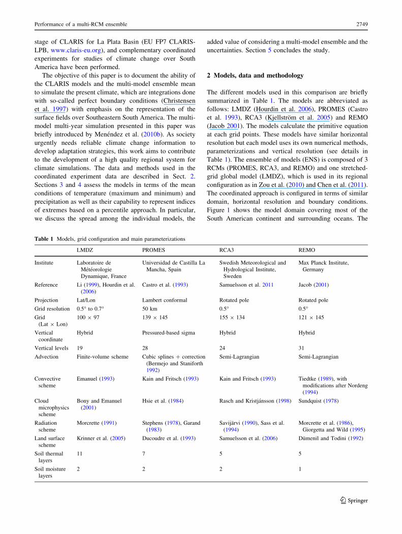
2 Models, data and methodology

The different models used in this comparison are briefly

summarized in Table 1. The models are abbreviated as

follows: LMDZ (Hourdin et al. 2006), PROMES (Castro

et al. 1993), RCA3 (Kjellstrom et al. 2005) and REMO

(Jacob 2001). The models calculate the primitive equation

at each grid points. These models have similar horizontal

resolution but each model uses its own numerical methods,

parameterizations and vertical resolution (see details in

Table 1). The ensemble of models (ENS) is composed of 3

RCMs (PROMES, RCA3, and REMO) and one stretched-

grid global model (LMDZ), which is used in its regional

configuration as in Zou et al. (2010) and Chen et al. (2011).

The coordinated approach is configured in terms of similar

domain, horizontal resolution and boundary conditions.

Figure 1 shows the model domain covering most of the

South American continent and surrounding oceans. The

Table 1 Models, grid configuration and main parameterizations

LMDZ PROMES RCA3 REMO

Institute Laboratoire de

Meteorologie

Dynamique, France

Universidad de Castilla La

Mancha, Spain

Swedish Meteorological and

Hydrological Institute,

Sweden

Max Planck Institute,

Germany

Reference Li (1999), Hourdin et al.

(2006)

Castro et al. (1993) Samuelsson et al. 2011 Jacob (2001)

Projection Lat/Lon Lambert conformal Rotated pole Rotated pole

Grid resolution 0.5� to 0.7� 50 km 0.5� 0.5�Grid

(Lat 9 Lon)

100 9 97 139 9 145 155 9 134 121 9 145

Vertical

coordinate

Hybrid Pressured-based sigma Hybrid Hybrid

Vertical levels 19 28 24 31

Advection Finite-volume scheme Cubic splines ? correction

(Bermejo and Staniforth

1992)

Semi-Lagrangian Semi-Lagrangian

Convective

scheme

Emanuel (1993) Kain and Fritsch (1993) Kain and Fritsch (1993) Tiedtke (1989), with

modifications after Nordeng

(1994)

Cloud

microphysics

scheme

Bony and Emanuel

(2001)

Hsie et al. (1984) Rasch and Kristjansson (1998) Sundquist (1978)

Radiation

scheme

Morcrette (1991) Stephens (1978), Garand

(1983)

Savijarvi (1990), Sass et al.

(1994)

Morcrette et al. (1986),

Giorgetta and Wild (1995)

Land surface

scheme

Krinner et al. (2005) Ducoudre et al. (1993) Samuelsson et al. (2006) Dumenil and Todini (1992)

Soil thermal

layers

11 7 5 5

Soil moisture

layers

2 2 2 1

Performance of a multi-RCM ensemble 2749

123

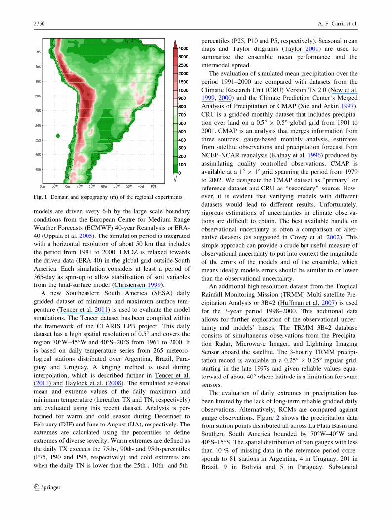
models are driven every 6-h by the large scale boundary

conditions from the European Centre for Medium Range

Weather Forecasts (ECMWF) 40-year Reanalysis or ERA-

40 (Uppala et al. 2005). The simulation period is integrated

with a horizontal resolution of about 50 km that includes

the period from 1991 to 2000. LMDZ is relaxed towards

the driven data (ERA-40) in the global grid outside South

America. Each simulation considers at least a period of

365-day as spin-up to allow stabilization of soil variables

from the land-surface model (Christensen 1999).

A new Southeastern South America (SESA) daily

gridded dataset of minimum and maximum surface tem-

perature (Tencer et al. 2011) is used to evaluate the model

simulations. The Tencer dataset has been compiled within

the framework of the CLARIS LPB project. This daily

dataset has a high spatial resolution of 0.5� and covers the

region 70�W–45�W and 40�S–20�S from 1961 to 2000. It

is based on daily temperature series from 265 meteoro-

logical stations distributed over Argentina, Brazil, Para-

guay and Uruguay. A kriging method is used during

interpolation, which is described further in Tencer et al.

(2011) and Haylock et al. (2008). The simulated seasonal

mean and extreme values of the daily maximum and

minimum temperature (hereafter TX and TN, respectively)

are evaluated using this recent dataset. Analysis is per-

formed for warm and cold season during December to

February (DJF) and June to August (JJA), respectively. The

extremes are calculated using the percentiles to define

extremes of diverse severity. Warm extremes are defined as

the daily TX exceeds the 75th-, 90th- and 95th-percentiles

(P75, P90 and P95, respectively) and cold extremes are

when the daily TN is lower than the 25th-, 10th- and 5th-

percentiles (P25, P10 and P5, respectively). Seasonal mean

maps and Taylor diagrams (Taylor 2001) are used to

summarize the ensemble mean performance and the

intermodel spread.

The evaluation of simulated mean precipitation over the

period 1991–2000 are compared with datasets from the

Climatic Research Unit (CRU) Version TS 2.0 (New et al.

1999, 2000) and the Climate Prediction Center’s Merged

Analysis of Precipitation or CMAP (Xie and Arkin 1997).

CRU is a gridded monthly dataset that includes precipita-

tion over land on a 0.5� 9 0.5� global grid from 1901 to

2001. CMAP is an analysis that merges information from

three sources: gauge-based monthly analysis, estimates

from satellite observations and precipitation forecast from

NCEP–NCAR reanalysis (Kalnay et al. 1996) produced by

assimilating quality controlled observations. CMAP is

available at a 1� 9 1� grid spanning the period from 1979

to 2002. We designate the CMAP dataset as ‘‘primary’’ or

reference dataset and CRU as ‘‘secondary’’ source. How-

ever, it is evident that verifying models with different

datasets would lead to different results. Unfortunately,

rigorous estimations of uncertainties in climate observa-

tions are difficult to obtain. The best available handle on

observational uncertainty is often a comparison of alter-

native datasets (as suggested in Covey et al. 2002). This

simple approach can provide a crude but useful measure of

observational uncertainty to put into context the magnitude

of the errors of the models and of the ensemble, which

means ideally models errors should be similar to or lower

than the observational uncertainty.

An additional high resolution dataset from the Tropical

Rainfall Monitoring Mission (TRMM) Multi-satellite Pre-

cipitation Analysis or 3B42 (Huffman et al. 2007) is used

for the 3-year period 1998–2000. This additional data

allows for further exploration of the observational uncer-

tainty and models’ biases. The TRMM 3B42 database

consists of simultaneous observations from the Precipita-

tion Radar, Microwave Imager, and Lightning Imaging

Sensor aboard the satellite. The 3-hourly TRMM precipi-

tation record is available in a 0.25� 9 0.25� regular grid,

starting in the late 1997s and given reliable values equa-

torward of about 40� where latitude is a limitation for some

sensors.

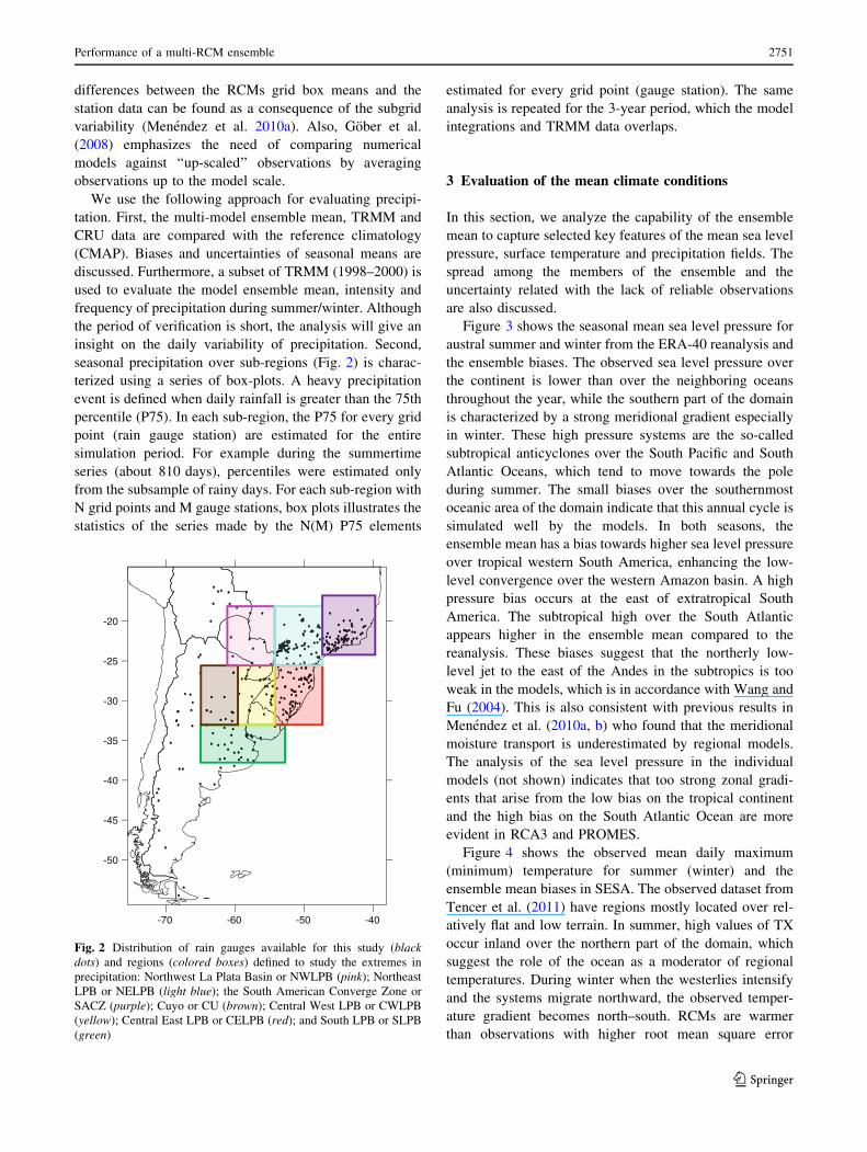
The evaluation of daily extremes in precipitation has

been limited by the lack of long-term reliable gridded daily

observations. Alternatively, RCMs are compared against

gauge observations. Figure 2 shows the precipitation data

from station points distributed all across La Plata Basin and

Southern South America bounded by 70�W–40�W and

40�S–15�S. The spatial distribution of rain gauges with less

than 10 % of missing data in the reference period corre-

sponds to 81 stations in Argentina, 4 in Uruguay, 201 in

Brazil, 9 in Bolivia and 5 in Paraguay. Substantial

Fig. 1 Domain and tospography (m) of the regional experiments

2750 A. F. Carril et al.

123

differences between the RCMs grid box means and the

station data can be found as a consequence of the subgrid

variability (Menendez et al. 2010a). Also, Gober et al.

(2008) emphasizes the need of comparing numerical

models against ‘‘up-scaled’’ observations by averaging

observations up to the model scale.

We use the following approach for evaluating precipi-

tation. First, the multi-model ensemble mean, TRMM and

CRU data are compared with the reference climatology

(CMAP). Biases and uncertainties of seasonal means are

discussed. Furthermore, a subset of TRMM (1998–2000) is

used to evaluate the model ensemble mean, intensity and

frequency of precipitation during summer/winter. Although

the period of verification is short, the analysis will give an

insight on the daily variability of precipitation. Second,

seasonal precipitation over sub-regions (Fig. 2) is charac-

terized using a series of box-plots. A heavy precipitation

event is defined when daily rainfall is greater than the 75th

percentile (P75). In each sub-region, the P75 for every grid

point (rain gauge station) are estimated for the entire

simulation period. For example during the summertime

series (about 810 days), percentiles were estimated only

from the subsample of rainy days. For each sub-region with

N grid points and M gauge stations, box plots illustrates the

statistics of the series made by the N(M) P75 elements

estimated for every grid point (gauge station). The same

analysis is repeated for the 3-year period, which the model

integrations and TRMM data overlaps.

3 Evaluation of the mean climate conditions

In this section, we analyze the capability of the ensemble

mean to capture selected key features of the mean sea level

pressure, surface temperature and precipitation fields. The

spread among the members of the ensemble and the

uncertainty related with the lack of reliable observations

are also discussed.

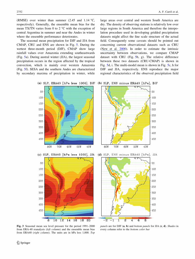
Figure 3 shows the seasonal mean sea level pressure for

austral summer and winter from the ERA-40 reanalysis and

the ensemble biases. The observed sea level pressure over

the continent is lower than over the neighboring oceans

throughout the year, while the southern part of the domain

is characterized by a strong meridional gradient especially

in winter. These high pressure systems are the so-called

subtropical anticyclones over the South Pacific and South

Atlantic Oceans, which tend to move towards the pole

during summer. The small biases over the southernmost

oceanic area of the domain indicate that this annual cycle is

simulated well by the models. In both seasons, the

ensemble mean has a bias towards higher sea level pressure

over tropical western South America, enhancing the low-

level convergence over the western Amazon basin. A high

pressure bias occurs at the east of extratropical South

America. The subtropical high over the South Atlantic

appears higher in the ensemble mean compared to the

reanalysis. These biases suggest that the northerly low-

level jet to the east of the Andes in the subtropics is too

weak in the models, which is in accordance with Wang and

Fu (2004). This is also consistent with previous results in

Menendez et al. (2010a, b) who found that the meridional

moisture transport is underestimated by regional models.

The analysis of the sea level pressure in the individual

models (not shown) indicates that too strong zonal gradi-

ents that arise from the low bias on the tropical continent

and the high bias on the South Atlantic Ocean are more

evident in RCA3 and PROMES.

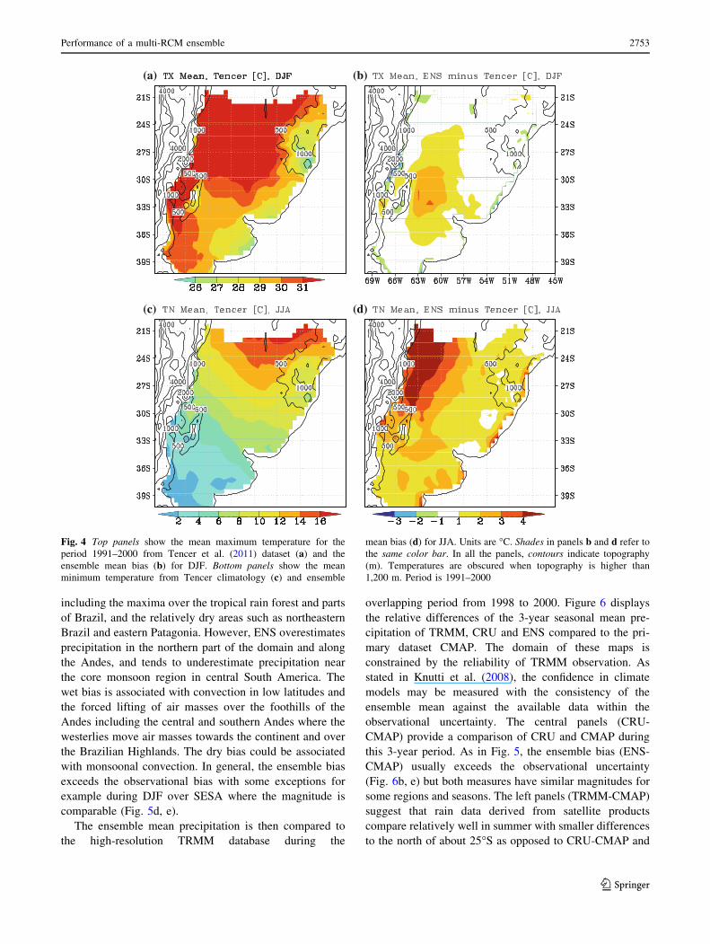
Figure 4 shows the observed mean daily maximum

(minimum) temperature for summer (winter) and the

ensemble mean biases in SESA. The observed dataset from

Tencer et al. (2011) have regions mostly located over rel-

atively flat and low terrain. In summer, high values of TX

occur inland over the northern part of the domain, which

suggest the role of the ocean as a moderator of regional

temperatures. During winter when the westerlies intensify

and the systems migrate northward, the observed temper-

ature gradient becomes north–south. RCMs are warmer

than observations with higher root mean square error

-70 -60 -50 -40

-50

-45

-40

-35

-30

-25

-20

Fig. 2 Distribution of rain gauges available for this study (blackdots) and regions (colored boxes) defined to study the extremes in

precipitation: Northwest La Plata Basin or NWLPB (pink); Northeast

LPB or NELPB (light blue); the South American Converge Zone or

SACZ (purple); Cuyo or CU (brown); Central West LPB or CWLPB

(yellow); Central East LPB or CELPB (red); and South LPB or SLPB

(green)

Performance of a multi-RCM ensemble 2751

123

(RMSE) over winter than summer (2.45 and 1.14 �C,

respectively). Generally, the ensemble mean bias for the

mean TX/TN varies from 0 to 2 �C with the exception of

central Argentina in summer and near the Andes in winter

where the ensemble performance deteriorates.

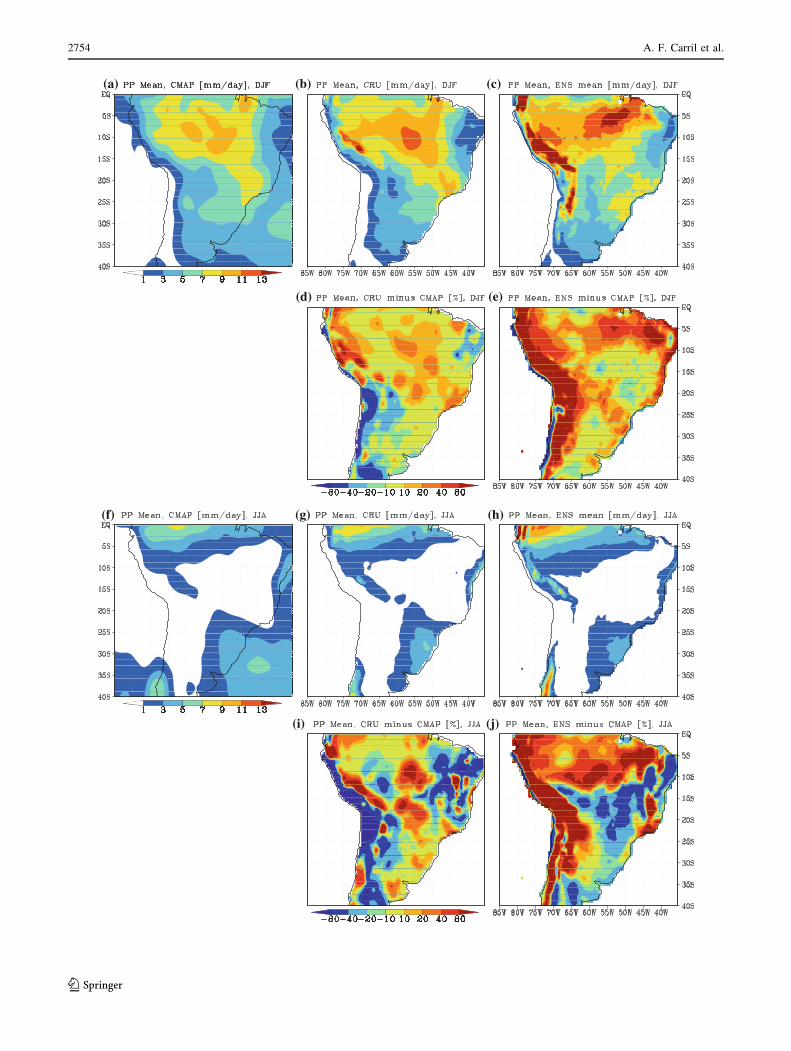
The seasonal mean precipitation for DJF and JJA from

CMAP, CRU and ENS are shown in Fig. 5. During the

wettest three-month period (DJF), CMAP show large

rainfall values over Amazonia extending southeastwards

(Fig. 5a). During austral winter (JJA), the largest seasonal

precipitation occurs in the region affected by the tropical

convection, which is mainly over western Amazonia

(Fig. 5f). SESA and the southern Andes are characterized

by secondary maxima of precipitation in winter, while

large areas over central and western South America are

dry. The density of observing stations is relatively low over

large regions in South America and therefore the interpo-

lation procedure used in developing gridded precipitation

datasets might affect the fine scale structure of the actual

field. Consequently some caveats should be pointed out

concerning current observational datasets such as CRU

(New et al. 2000). In order to estimate the intrinsic

uncertainty between observations, we compare CMAP

dataset with CRU (Fig. 5b, g). The relative difference

between these two datasets (CRU-CMAP) is shown in

Fig. 5d, i. The multi-model mean is shown in Fig. 5c, h for

DJF and JJA, respectively. ENS reproduce the major

regional characteristics of the observed precipitation field

(a) (b)

(c) (d)

Fig. 3 Seasonal mean sea level pressure for the period 1991–2000

from ERA-40 reanalysis (left column) and the ensemble mean bias

from ERA40 (right column). The units are in hPa less 1,000. Top

panels are for DJF (a, b) and bottom panels for JJA (c, d). Shades in

every column refer to the bottom color bar

2752 A. F. Carril et al.

123

including the maxima over the tropical rain forest and parts

of Brazil, and the relatively dry areas such as northeastern

Brazil and eastern Patagonia. However, ENS overestimates

precipitation in the northern part of the domain and along

the Andes, and tends to underestimate precipitation near

the core monsoon region in central South America. The

wet bias is associated with convection in low latitudes and

the forced lifting of air masses over the foothills of the

Andes including the central and southern Andes where the

westerlies move air masses towards the continent and over

the Brazilian Highlands. The dry bias could be associated

with monsoonal convection. In general, the ensemble bias

exceeds the observational bias with some exceptions for

example during DJF over SESA where the magnitude is

comparable (Fig. 5d, e).

The ensemble mean precipitation is then compared to

the high-resolution TRMM database during the

overlapping period from 1998 to 2000. Figure 6 displays

the relative differences of the 3-year seasonal mean pre-

cipitation of TRMM, CRU and ENS compared to the pri-

mary dataset CMAP. The domain of these maps is

constrained by the reliability of TRMM observation. As

stated in Knutti et al. (2008), the confidence in climate

models may be measured with the consistency of the

ensemble mean against the available data within the

observational uncertainty. The central panels (CRU-

CMAP) provide a comparison of CRU and CMAP during

this 3-year period. As in Fig. 5, the ensemble bias (ENS-

CMAP) usually exceeds the observational uncertainty

(Fig. 6b, e) but both measures have similar magnitudes for

some regions and seasons. The left panels (TRMM-CMAP)

suggest that rain data derived from satellite products

compare relatively well in summer with smaller differences

to the north of about 25�S as opposed to CRU-CMAP and

(a) (b)

(c) (d)

Fig. 4 Top panels show the mean maximum temperature for the

period 1991–2000 from Tencer et al. (2011) dataset (a) and the

ensemble mean bias (b) for DJF. Bottom panels show the mean

minimum temperature from Tencer climatology (c) and ensemble

mean bias (d) for JJA. Units are �C. Shades in panels b and d refer to

the same color bar. In all the panels, contours indicate topography

(m). Temperatures are obscured when topography is higher than

1,200 m. Period is 1991–2000

Performance of a multi-RCM ensemble 2753

123

(a) (b) (c)

(d) (e)

(f) (g) (h)

(i) (j)

2754 A. F. Carril et al.

123

ENS-CMAP. Comparing the left panels (TRMM-CMAP)

with the right panels (ENS-CMAP), similar features can be

found in terms of magnitude and sign of the differences e.g.

in the tropical and subtropical Andes throughout the year,

northern South America (0–10�S) in JJA, and the shores of

the Rio de la Plata in DJF. This suggests that the bias of the

ensemble may be lower in these regions if taken as refer-

ence TRMM climatology instead of CMAP.

The biases in temperature and precipitation are not

independent of each other. The model ensemble tends to

simulate too warm climate in summer over areas of SESA

corresponding to a dry bias as can be seen by comparing

Fig. 4b with Fig. 5e. This correlation suggests the occur-

rence of a drying phenomenon i.e. positive feedback of soil

moisture drying over areas of southern La Plata Basin. The

models especially in the RCA3 tend to overestimate

maximum temperature on areas with negative bias of pre-

cipitation. The drying out of the soil does not only depend

on deficient rainfall, but also on the soil properties and

physiographic factors affecting evapotranspiration and heat

fluxes in the regional models such as roughness length,

vegetation fraction, leaf area index, albedo, rooting depth.

In addition, SESA has been identified as a hotspot of strong

coupling between land and atmosphere in summer

(Sorensson and Menendez 2011). Thus, a realistic repre-

sentation of the land–atmosphere interaction would be

particularly critical for this region. Another factor to con-

sider is cloudiness as it has a radiative influence on the

surface energy balance. During summer in SESA, all

models except RCA3 underestimate the total cloud cover

(compared to CRU data, not shown). So the positive tem-

perature bias could also be induced by decreased cloudi-

ness, causing an increase in insolation reaching the land’s

surface.

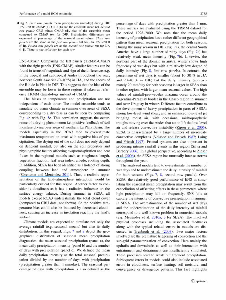
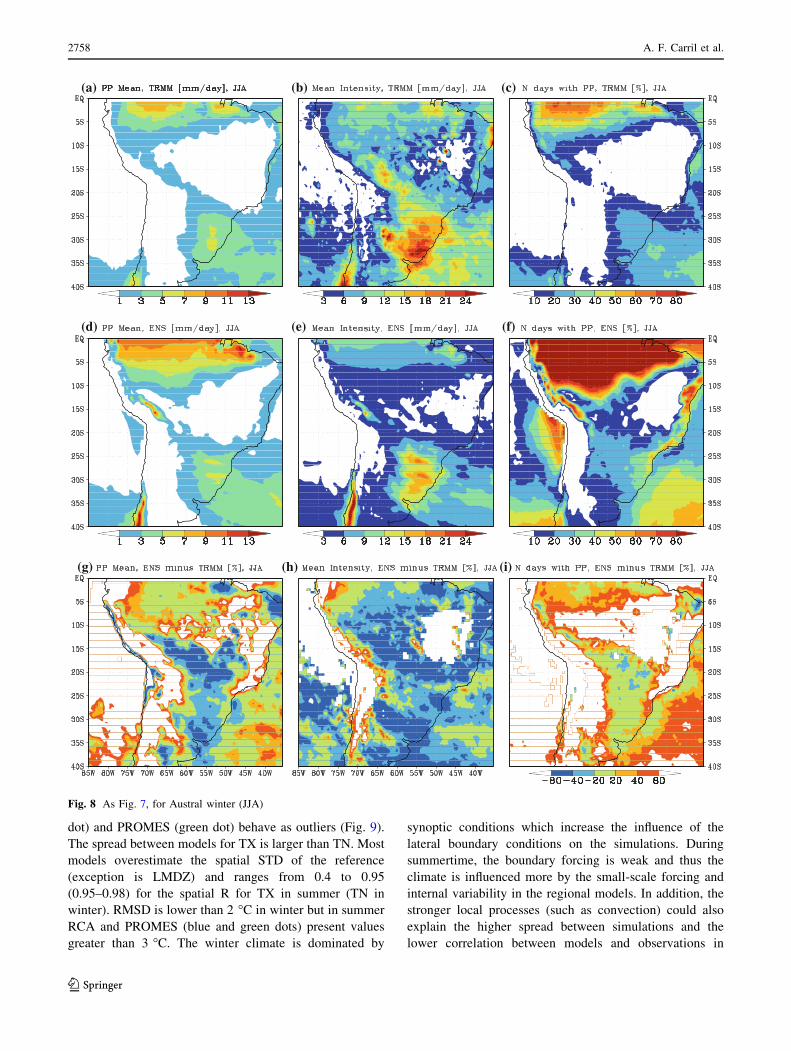
Climate models are expected to simulate not only the

average rainfall (e.g. seasonal means) but also its daily

distribution. In this regard, Figs. 7 and 8 depict the geo-

graphical distribution of seasonal mean precipitation

diagnostics: the mean seasonal precipitation (panel a), the

mean daily precipitation intensity (panel b) and the number

of days with precipitation (panel c). We defined the mean

daily precipitation intensity as the total seasonal precipi-

tation divided by the number of days with precipitation

(precipitation greater than 1 mm/day). The seasonal per-

centage of days with precipitation is also defined as the

percentage of days with precipitation greater than 1 mm.

These metrics are evaluated using the TRMM dataset for

the period 1998–2000. We note that the mean daily

intensity of precipitation has a rather different geographical

pattern than mean seasonal precipitation for both seasons.

During the rainy season in DJF (Fig. 7a), the central South

America have a large number of rainy days (Fig. 7c) but

relatively weak mean intensity (Fig. 7b). Likewise, the

northern part of the domain in austral winter shows high

frequency of wet days but with a relatively low degree of

daily intensity (Fig. 8, first row panels). In contrast, the

percentage of wet days is smaller (about 10–30 % in JJA

and 20–40 % in DJF) but the daily intensity (approxi-

mately 20 mm/day for both seasons) is larger in SESA than

in other regions with larger mean seasonal values. The high

values of rainfall-per-wet-day maxima occur around the

Argentina-Paraguay border in the Chaco region in summer

and over Uruguay in winter. Different factors contribute to

the development of heavy precipitation in parts of SESA:

strong low-level wind shear, and an enhanced low-level jet

bringing moist air, with occasional midtropospheric

troughs moving over the Andes that act to lift the low-level

air and release convective instability (Zipser et al. 2006).

SESA is characterized by a large number of mesoscale

convective complexes (Velasco and Fritsch 1987; Laing

and Fritsch 1997). Frontal systems are also important in

producing intense rainfall events in this region (Silva and

Berbery 2006). In a global perspective, according to Zipser

et al. (2006), the SESA region has unusually intense storms

throughout the year.

The analyzed models tend to overestimate the number of

wet days and to underestimate the daily intensity of rainfall

for both seasons (Figs. 7, 8, second row panels). Over

SESA, the relatively good performance of ENS in simu-

lating the seasonal mean precipitation may result from the

cancellation of offsetting effects in these parameters where

light precipitation may fall too frequently. ENS fails to

capture the intensity of convective precipitation in summer

in SESA. The overestimation of the number of wet days

and the underestimation of the daily intensity of rainfall

correspond to a well-known problem in numerical models

(e.g. Menendez et al. 2010a, b for SESA). The involved

physical processes including the associated feedbacks

along with the typical related errors in models are dis-

cussed in Trenberth et al. (2003). Two major factors

involved are the premature triggering of convection and the

sub-grid parameterization of convection. Here mainly the

updrafts and downdrafts as well as their interaction with

entrainment and detrainment are insufficiently simulated.

These processes lead to weak but frequent precipitation.

Subsequent errors in models could also include associated

errors in cloudiness, surface heating, soil moisture, and

convergence or divergence patterns. This fact highlights

Fig. 5 First row panels mean precipitation (mm/day) during DJF

1991–2000: CMAP (a), CRU (b) and the ensemble mean (c). Secondrow panels CRU minus CMAP (d), bias of the ensemble mean

compared to CMAP (e), for DJF. Precipitation differences are

expressed in percentage of the seasonal mean values. Third rowpanels are the same as the first row panels but for JJA 1991–2000

(f–h). Fourth row panels are as the second row panels but for JJA

(i–j). There is one color bar for each row

b

Performance of a multi-RCM ensemble 2755

123

two points. First, the ‘‘triggers’’ as well as the life-cycles in

parameterizing convection in models must be better sim-

ulated. Second, a good agreement with the observations for

the mean climate over a given region does not necessarily

imply a good depiction of the climate variability and/or a

correct representation of involved physical processes.

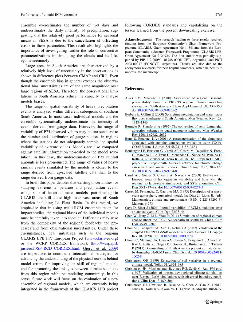
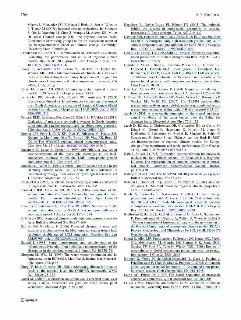
We now analyze how consistent are the geographical

patterns of precipitation anomalies and daily maximum and

minimum temperature anomalies from the four individual

models and the ensemble. Figures 9 and 10 provide a sta-

tistical summary of how well the simulated patterns of

precipitation and daily maximum and minimum tempera-

ture anomalies match the reference climatology in terms of

root mean square difference (RMSD), correlation coeffi-

cients (R) and standard deviation (STD) using Taylor

diagrams (Taylor 2001). These diagrams provide a visual

framework to easily compare results between models and

gridded observations. The radial distance from the origin is

proportional to STD, the radial distance from the reference

climatology (point REF) is proportional to the RMSD and

the correlation between the single model/ensemble and

REF is given by the azimuthal position of the tested field.

The Taylor diagram for temperature/precipitation is

calculated over the SESA/full South American domain

(Figs. 9, 10). As mentioned before, CMAP and the Tencer

dataset are used as the reference data sets for precipitation

and temperature, respectively. All the statistics are calcu-

lated after removing the spatial mean value of each dataset.

In general, ENS (red point) has a good performance rela-

tive to each individual model. It is further away from the

outlier point and near to the cluster of best models. The

outliers in these diagrams are points lying far away from

the verification data (point REF). This result suggests that

combining the models in a multi-model ensemble gives in

general a good climate depiction independently of the

variable and season, which corroborates previous outcomes

(e.g. Menendez et al. 2010a, Hagedorn et al. 2005). In the

case of precipitation (Fig. 10), note that the spread between

CMAP and CRU could compromise the assessment of the

model quality. However, the models are clustered among

(a) (b) (c)

(d) (e) (f)

Fig. 6 Bias of the seasonal mean precipitation (%) for the 3-year

period 1998–2000. Left column bias of TRMM compared to CMAP;

middle column bias of CRU compared to CMAP; right column bias of

the ensemble mean compared to CMAP. Precipitation biases are

expressed in percentage of the seasonal mean values. Top (bottom)

panels are for DJF (JJA)

2756 A. F. Carril et al.

123

each other except for PROMES (green dot), which has the

largest values for STD and lowest values for R during

summer and winter.

In general, models and the ensemble mean are more

accurate in simulating the temperature anomaly patterns of

TN in winter than those of TX in summer where RCA (blue

(a) (b) (c)

(d) (e) (f)

(g) (h) (i)

Fig. 7 Top panels Austral summer (DJF) mean precipitation (mm/

day) (a), mean daily intensity of precipitation (mm/day) (b), and

percentage of number of days with precipitation greater than 1 mm/

day (c) from TRMM climatology, for 1998–2000. Middle panels are

the same as the top panels but for the ensemble mean. Bottom panels

are the bias of the ensemble mean compared to TRMM to reproduce

the DJF mean precipitation (g), the intensity of precipitation (h) and

the number of days with precipitation (i), for the same 3-year period.

Bottom panels refer to the same color bar

Performance of a multi-RCM ensemble 2757

123

dot) and PROMES (green dot) behave as outliers (Fig. 9).

The spread between models for TX is larger than TN. Most

models overestimate the spatial STD of the reference

(exception is LMDZ) and ranges from 0.4 to 0.95

(0.95–0.98) for the spatial R for TX in summer (TN in

winter). RMSD is lower than 2 �C in winter but in summer

RCA and PROMES (blue and green dots) present values

greater than 3 �C. The winter climate is dominated by

synoptic conditions which increase the influence of the

lateral boundary conditions on the simulations. During

summertime, the boundary forcing is weak and thus the

climate is influenced more by the small-scale forcing and

internal variability in the regional models. In addition, the

stronger local processes (such as convection) could also

explain the higher spread between simulations and the

lower correlation between models and observations in

(a) (b) (c)

(d) (e) (f)

(g) (h) (i)

Fig. 8 As Fig. 7, for Austral winter (JJA)

2758 A. F. Carril et al.

123

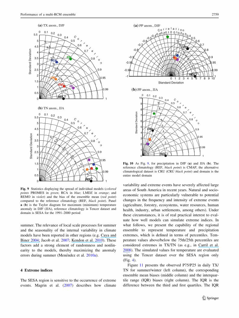
summer. The relevance of local scale processes for summer

and the seasonality of the internal variability in climate

models have been reported in other regions (e.g. Caya and

Biner 2004; Jacob et al. 2007; Kendon et al. 2010). These

factors add a strong element of randomness and nonlin-

earity to the models, thereby maximizing the anomaly

errors during summer (Menendez et al. 2010a).

4 Extreme indices

The SESA region is sensitive to the occurrence of extreme

events. Magrin et al. (2007) describes how climate

variability and extreme events have severely affected large

areas of South America in recent years. Natural and socio-

economic systems are particularly vulnerable to potential

changes in the frequency and intensity of extreme events

(agriculture, forestry, ecosystems, water resources, human

health, industry, urban settlements, among others). Under

these circumstances, it is of real practical interest to eval-

uate how well models can simulate extreme indices. In

what follows, we present the capability of the regional

ensemble to represent temperature and precipitation

extremes, which is defined in terms of percentiles. Tem-

perature values above/below the 75th/25th percentiles are

considered extremes in TX/TN (as e.g., in Carril et al.

2008). The simulated values for temperature are evaluated

using the Tencer dataset over the SESA region only

(Fig. 4).

Figure 11 presents the observed P75/P25 in daily TX/

TN for summer/winter (left column), the corresponding

ensemble mean biases (middle column) and the interquar-

tile range (IQR) biases (right column). The IQR is the

difference between the third and first quartiles. The IQR

0 1

2 3

4 5

6 7

8 9

0 1 2 3 4 5 6 7 8 9 101

0.99

0.95

0.9

0.8

0.70.6

0.50.40.30.20.10-0.1-0.2-0.3-0.4

-0.5-0.6

-0.7

-0.8

-0.9

-0.95

-0.99

-1

Standard Deviation

Co r r e l a t i o n(a) PP anom., DJF

REF

CRU

0

1

2

3

4

5

6

7

8

9

0

1

2

3

4

5

6

7

8

9

10

1

0.99

0.95

0.9

0.8

0.7

0.6

0.50.4

0.30.20.10

Sta

ndar

d D

evia

tion

Co

rr

el

at

io

n

(b) PP anom., JJA

REF

CRU

Fig. 10 As Fig. 9, for precipitation in DJF (a) and JJA (b). The

reference climatology (REF, black point) is CMAP, the alternative

climatological dataset is CRU (CRU black point) and domain is the

entire model domain

0

0.5 1

1.5 2

2.5 3

3.5 4

4.5 5

0

0.5

1

1.5

2

2.5

3

3.5

4

4.5

5

5.5

1

0.99

0.95

0.9

0.8

0.7

0.6

0.50.4

0.30.20.10

Sta

nd

ard

De

via

tion

Co

rr

el

at

io

n

(a) TX anom., DJF

(b) TN anom., JJA

REF

ENS

LMD

PRRCA

RE

0 0

.5 1

1.5

2 2

.5 3

3.5

4 4

.5 5

0

0.5

1

1.5

2

2.5

3

3.5

4

4.5

5

5.5

1

0.99

0.95

0.9

0.8

0.7

0.6

0.50.4

0.30.20.10

Sta

nd

ard

De

via

tion

Co

rr

el

at

io

n

REF

Fig. 9 Statistics displaying the spread of individual models (coloredpoints PROMES in green; RCA in blue; LMDZ in orange; and

REMO in violet) and the bias of the ensemble mean (red point)compared to the reference climatology (REF, black point). Panel

a (b) is the Taylor diagram for maximum (minimum) temperature

anomaly in DJF (JJA), reference climatology is Tencer dataset and

domain is SESA for the 1991–2000 period

Performance of a multi-RCM ensemble 2759

123

bias is a measure of how models (ENS) capture the

observed range of daily variability. In comparison with

Fig. 4, the observed pattern of the P75/P25 for TX/TN

fields displays east–west/north–south gradients and the

ENS biases remain positive almost everywhere. The main

difference between the bias in extreme thresholds and bias

in mean temperatures is that the errors increase in magni-

tude as analysis moves to the tails of the distributions. The

ENS mean bias for the index P75 of daily TX varies from 0

to 4 �C. The error magnitude in the P90 of TX (P10 of TN)

increases further to 6 �C (8 �C) while the pattern of the

error remains almost invariant (figure not shown). The right

column in Fig. 11 presents a measure of the statistical

dispersion. The IQR of the ensemble mean for TX is higher

than the observed one (Fig. 11c), which suggests that the

simulation of TX presents a platykurtic distribution (i.e., a

flatter peak around its mean, which causes thin tails within

the distribution due to its large variability). However, TN

values behave somewhat differently. Although the

ensemble mean overestimates the mean values of TN in

SESA as shown in Fig. 4, the IQR northward of 35�S is

underestimated (Fig. 11f), which suggest a leptokurtic

distribution (i.e., data is highly concentrated around its

mean value).

In order to quantify the spread of the ensemble mem-

bers, Fig. 12 presents the Taylor diagrams estimated for the

indexes P75/P25 in TX/TN. In this case, we analyze how

consistent are the geographical patterns of the indices of

daily maximum and minimum temperature extremes from

the four individual models and the ensemble. The ENS (red

point) performs better than each individual model however

each model is more accurate in simulating the P25 of daily

TN during winter than daily TX during summer. Some

models have large RMSE during summer but offsetting

errors cancel each other (figures not shown). As in the

simulation of the mean TX and TN, RCA (blue) and

PROMES (green) models behave as outliers in summer.

Results are almost invariant when considering indices for

extremes at higher/lower (e.g., TX P90/TN P10)

percentiles.

(a) (b) (c)

(d) (e) (f)

Fig. 11 Top panels 75th percentile of daily maximum temperature

from Tencer et al. (2011) climatology (a), the ensemble mean bias

(b) and the ensemble mean bias to simulate the interquartile range

(c) in DJF. Bottom panels the same as the top panels but for 25th

percentile of daily minimum temperature in JJA. Units are �C

2760 A. F. Carril et al.

123

In the case of precipitation, only the surplus values

based on the index P75 is discussed. The simulated pre-

cipitation values like all other grid values should not be

considered as representing the weather conditions at the

exact location of the grid point but as a time–space average

within the grid box (Gober et al. 2008). Consequently, we

expect that heavy rainfall values (P75) from station data are

higher than those from models representing the mean

precipitation over an area determined by the models’ res-

olution. With this in mind, we verify how the individual

models and the ensemble are able to capture the range of

variability of P75 values in different regions in SESA.

For each individual model, we evaluate the upper

quartile of daily precipitation at every grid point in each

region defined in Fig. 2. The range of values representing

the highest 25 % daily precipitation is an estimate of the

variability of extreme precipitation in each model at sub-

regions. Figures 13, 14, 15 and 16 display basic statistical

information of these quantities (median, maximum and

minimum values, and the 25th and 75th quartiles). The IQR

estimates the spatial variability of heavy precipitation

events within each region. We repeat the calculation for the

observed station data. These boxplot figures compare ran-

ges of P75 grid point values with both the rain gauge and

TRMM observational datasets. We consider a simulation as

‘‘satisfactory’’ if its IQR intersects at least part of the

corresponding IQR of the observations. This criterion is

stricter than just comparing the min–max ranges.

The majority of models and the ensemble do not match

the IQR of the observed P75 values for most regions and in

both seasons (Figs. 13, 14). In general, models thoroughly

underestimate the intensity of observed strong or heavy

precipitation events. The exception is PROMES that match

at least part of the observed IQR in various situations.

However, PROMES is an outlier as shown in the Taylor

diagrams (Fig. 10) and its seasonal mean rainfall shows

significant differences from either CMAP or CRU (map not

shown). The spatial variability of the precipitation is much

higher for PROMES than for the other models and obser-

vational data (Fig. 10). This finding is also consistent with

Figs. 13 and 14 in which PROMES generally has an IQR

greater than the other models. So even though PROMES

seems to capture the intense precipitation events better than

other models in these regions, this could be a reflection of a

general noisy simulated precipitation field.

The models’ deviation from the observations is larger

for summer as more severe events have to be simulated

(e.g. CWLPB in summer), and becomes less significant for

winter especially in regions with relatively small precipi-

tation amounts (e.g. CU). Although the ensemble mean P75

values in both seasons are found outside the observed IQR

for all regions, during JJA at least part of the ensemble

range (i.e., maximum minus minimum value) often match

part of the corresponding observed range. Nevertheless, as

already mentioned, models simulate grid box means

whereas observations (station data) are point values.

Within the grid box, the precipitation amounts can assume

quantities well above or below the box mean especially in

the case of severe weather events. Thus, substantial dif-

ferences are expected between grid box means and point

values depending on the subgrid-scale variability (Men-

endez et al. 2010a).

Some studies underline the imperative to compare

models’ grid-box means against up-scaled observation (e.g.

Gober et al. 2008). However, we have compared models

0

0.5 1

1.5 2

2.5 3

3.5 4

4.5 5

0

0.5

1

1.5

2

2.5

3

3.5

4

4.5

5

5.5

1

0.99

0.95

0.9

0.8

0.7

0.6

0.50.4

0.30.20.10

Sta

ndar

d D

evia

tion

Co

rr

el

at

io

n

(b) P25 TN, JJA

REF

0

0.5 1

1.5 2

2.5 3

3.5 4

4.5 5

0

0.5

1

1.5

2

2.5

3

3.5

4

4.5

5

5.5

1

0.99

0.95

0.9

0.8

0.7

0.6

0.50.4

0.30.20.10

Sta

ndar

d D

evia

tion

Co

rr

el

at

io

n

(a) P75 TX, DJF

REF

Fig. 12 Statistics displaying the spread of individual models (coloredpoints PROMES in green, RCA in blue, LMDZ in orange, REMO in

violet) and the bias of the ensemble mean (red point) compared to the

reference climatology (REF, black point). Panel a (b) is the Taylor

diagram for the 75th (25th) percentile of daily maximum (minimum)

tesmperature in DJF (JJA). Reference climatology is Tencer dataset

and domain is SESA for the 1991–2000 period

Performance of a multi-RCM ensemble 2761

123

with point observations (Figs. 13, 14) because the network

of gauges is not sufficiently dense in the region of interest.

We repeated the box plots but including the high-resolution

satellite information (TRMM) up-scaled to the models

resolution. TRMM data were interpolated from the 0.25�native resolution to the 0.5� models grid using a triangle-

Fig. 13 Box plots showing the

distribution of daily

precipitation (mm/day) in heavy

rainy days (defined as the 75th

percentile series of the daily

precipitation for every grid

point/station data, see text for

details). Every panel is for a

particular region. Every boxstands for a specific dataset (an

individual model, the ensemble

mean and the observed

climatology) and represents the

interquartile distance (IQD,

25–75th percentiles); the

median is indicated by the redline inside the box and the mean

by the stars inside box. Values

farther from the median more

than 1.5 times the IQD

(horizontal bars outside boxes)

are considered outliers (littleblue crosses). Calculations are

for DJF 1992–2000 period

2762 A. F. Carril et al.

123

based cubic interpolation (Demaria et al. 2010). As we

have only 3 years of TRMM data, we recalculated the

statistics for each model and the station observations for

the period 1998–2000. Figure 15 shows an example of the

box plots for the SLPB region in summer and winter. In

general, the underestimation of P75 rainfall amounts is

Fig. 14 As Fig. 13, for JJA

Performance of a multi-RCM ensemble 2763

123

reduced when comparing against up-scaled observations

instead of precipitation gauge measurements. However, the

simulated IQR do not fully intersect the observed IQR or at

least the observed minimum to maximum range. In contrast

to SLPB, the NWLPB region has a lesser density of rain

gauge stations (Fig. 2). The uncertainty of the observations

is then illustrated by calculating the statistics of the refer-

ence dataset (OBS3) when the observation network is less

dense (Fig. 16). Statistics of the observations in the left

panel are estimated considering a low density network

(only 10 stations) while the OBS3 in the right panel has a

denser network (60 stations) available for the 3-year per-

iod. Although the results depend on the variability of the

precipitation in the selected region, Fig. 16 evidences how

the variability can increase when finer scales are

considered.

5 Conclusions

Regional climate simulations over South American are

carried out by four regional models forced by the ERA-40

reanalysis for the period 1991–2000. The models have been

evaluated with focus on near surface minimum and maxi-

mum temperatures and precipitation. We used several

observational datasets from Tencer et al. (2011) for tem-

perature, and from CRU, CMAP, upscaled TRMM and rain

gauge observations for precipitation.

Overall, the model ensemble depicts the regional cli-

mate better in comparison to individual ensemble member.

This result is independent of the variable and the season,

stressing the benefit of combining models in a multi-model

ensemble. However, the ensemble mean tends to be too

warm over large areas of SESA with the greatest seasonal

mean biases in minimum temperature during winter and the

smallest in maximum temperature during summer. Using

the Taylor diagrams to compare the geographical patterns

of daily temperature for the individual models, the

ensemble and the Tencer climatology, results show a rel-

atively large spread between models in summer but with

offsetting errors in the ensemble. It is also noted that errors

are generally larger at the tails of the probability distribu-

tion (e.g. P25 and P75) than in the mean field, especially in

summer.

The large-scale precipitation is reproduced in the

ensemble mean but models overestimate the convective

precipitation near the equator, the orographic precipitation

along the Andes and over the Brazilian Highlands, and

underestimate the precipitation near the core monsoon

region in central South America. The multi-model

Fig. 15 As Figs. 13 and 14 for

the region S-LPB, but period of

estimations is 1998–2000. A

box for the TRMM climatology

is included

Fig. 16 As Fig. 13 for the NW-

LPB region, but period of

estimations is 1998–2000. A

box for the TRMM climatology

is included. Difference between

both panels is the density of

precipitation stations considered

to estimate the statistics of

OBS3 boxes. In the right panel(b) statistics are from a

particularly high density of rain

gauges available over the 3-year

period

2764 A. F. Carril et al.

123

ensemble overestimates the number of wet days and

underestimates the daily intensity of precipitation, sug-

gesting that the relatively good performance for seasonal

means in SESA is due to the cancellation of offsetting

errors in these parameters. This result also highlights the

importance of investigating further the role of convective

parameterizations in simulating the clouds and its life-

cycles accurately.

Large areas in South America are characterized by a

relatively high level of uncertainty in the observations as

shown in difference plots between CMAP and CRU. Even

though the ensemble bias in general exceeds the observa-

tional bias, uncertainties are of the same magnitude over

large regions of SESA. Therefore, the observational limi-

tations in South America reduce the capacity to analyze

models biases.

The range of spatial variability of heavy precipitation

events is analyzed within different subregions of southern

South America. In most cases individual models and the

ensemble systematically underestimate the intensity of

events derived from gauge data. However, the range of

variability of P75 observed values may be too sensitive to

the number and distribution of gauge stations in regions

where the stations do not adequately sample the spatial

variability of extreme values. Models are also compared

against satellite information up-scaled to the model reso-

lution. In this case, the underestimation of P75 rainfall

amounts is less pronounced. The range of values of heavy

rainfall events simulated by the models is closer to the

range derived from up-scaled satellite data than to the

range derived from gauge data.

In brief, this paper denotes that existing uncertainties for

studying extreme temperature and precipitation events

using state-of-the-art climate models participating in

CLARIS are still quite high over vast areas of South

America including La Plata Basin. In this regard, we

emphasize that in using multi-RCM ensemble mean for

impact studies, the regional biases of the individual models

must be carefully taken into account. Difficulties may arise

from the complexity of the regional feedbacks and pro-

cesses and from observational uncertainties. Under these

circumstances, new initiatives such as the ongoing

CLARIS LPB FP7 European Project (www.claris-eu.org)

or the WCRP CORDEX framework (http://wcrp.ipsl.

jussieu.fr/SF_RCD_CORDEX.html, Giorgi et al. 2009)

are imperative to coordinate international strategies for

advancing the understanding of the physical reasons behind

model errors, for improving the skill of regional models

and for promoting the linkages between climate scientists

from this region with the modeling community. In this

sense, future work will focus on the evaluation of a new

ensemble of regional models, which are currently being

integrated in the framework of the CLARIS LPB project

following CORDEX standards and capitalizing on the

lesson learned from the present downscaling exercise.

Acknowledgments The research leading to these results received

funding from the European Community’s Sixth Framework Pro-

gramme (CLARIS, Grant Agreement No 1454) and from the Euro-

pean Community’s Seventh Framework Programme (CLARIS-LPB,

Grant Agreement No 212492). The first author was partially sup-

ported by PIP 112-200801-01788 (CONICET, Argentina) and PICT

2008-00237 (FONCYT, Argentina). Thanks are also due to the

anonymous reviewers for their helpful comments, which helped us to

improve the manuscript.

References

Alves LM, Marengo J (2010) Assessment of regional seasonal

predictability using the PRECIS regional climate modeling

system over South America. Theor Appl Climatol 100:337–350.

doi:10.1007/s00704-009-0165-2

Berbery E, Collini E (2000) Springtime precipitation and water vapor

flux over southeastern South America. Mon Weather Rev 128:

1328–1346

Bermejo R, Staniforth A (1992) The conversion of semi-Lagrangian

advection schemes to quasi-monotone schemes. Mon Weather

Rev 120(11):2622–2632

Bony S, Emanuel KA (2001) A parameterization of the cloudiness

associated with cumulus convection; evaluation using TOGA-

COARE data. J Atmos Sci 58(21):3158–3183

Boulanger J-P, Brasseur G, Carril AF, Castro M, Degallier N, Ereno

C, Marengo J, Le Treut H, Menendez C, Nunez M, Penalba O,

Rolla A, Rusticucci M, Terra R (2010) The European CLARIS

project: a Europe-South America network for climate change

assessment and impact studies. Clim Change 98(3):307–329.

doi:10.1007/s10584-009-9734-8

Carril AF, Gualdi S, Cherchi A, Navarra A (2008) Heatwaves in

Europe: areas of homogeneous variability and links with the

regional to large-scale atmospheric and SSTs anomalies. Clim

Dyn 30(1):77–98. doi:10.1007/s00382-007-0274-5

Castro M, Fernandez C, Gaertner MA (1993) Description of a meso-

scale atmospheric numerical model. In: Diaz JI, Lions JL (eds)

Mathematics, climate and environment (ISBN: 2-225-84297-3),

Masson, p 273

Caya D, Biner S (2004) Internal variability of RCM simulations over

an annual cycle. Clim Dyn 22:33–46

Chen W, Jiang Z, Li L, Yiou P (2011) Simulation of regional climate

change under the IPCC A2 scenario in southeast China. Clim

Dyn 36:491–507

Chou SC, Tanajura CA, Xue Y, Nobre CA (2002) Validation of the

coupled Eta/CPTEC/SSiB model over South America. J Geophys

Res 107(D20). doi:10.1029/2000JD000270

Chou SC, Marengo JA, Lyra AA, Sueiro G, Pesquero JF, Alves LM,

Kay G, Betts R, Chagas DJ, Gomes JL, Bustamante JF, Tavares

P (2011) Downscaling of South America present climate driven

by 4-member HadCM3 runs. Clim Dyn. doi:10.1007/s00382-011-

1002-8

Christensen OB (1999) Relaxation of soil variables in a regional

climate model. Tellus 51A:674–685

Christensen JH, Machenhauer B, Jones RG, Schar C, Ruti PM et al

(1997) Validation of present-day regional climate simulations

over Europe: LAM simulations with observed boundary condi-

tions. Clim Dyn 13:489–506

Christensen JH, Hewitson B, Busuioc A, Chen A, Gao X, Held I,

Jones R, Kolli RK, Kwon W-T, Laprise R, Magana Rueda V,

Performance of a multi-RCM ensemble 2765

123

Mearns L, Menendez CG, Raisanen J, Rinke A, Sarr A, Whetton

P, Tignor M (2007a) Regional climate projections. In: Solomon

S, Qin D, Manning M, Chen Z, Marquis M, Averyt KB, Miller

HL (eds) Climate change 2007: the physical science basis.

Contribution of working group i to the 4th assessment report of

the intergovernmental panel on climate change. Cambridge

University Press, Cambridge

Christensen JH, Carter TR, Rummukainen M, Amanatidis G (2007b)

Evaluating the performance and utility of regional climate

models: the PRUDENCE project. Clim Change 81:1–6. doi:

10.1007/s10584-006-9211-6

Covey C, AchutaRao KM, Fiorino M, Gleckler PJ, Taylor KE,

Wehner MF (2002) Intercomparison of climate data sets as a

measure of observational uncertainty. Report no. 69, Program for

climate model diagnosis and intercomparison, Livermore, CA

94550, USA, 38 pp

Curry JA, Lynch AH (2002) Comparing arctic regional climate

models. EOS Trans Am Geophys Union 83:87

da Rocha RP, Morales CA, Cuadra SV, Ambrizzi T (2009)

Precipitation diurnal cycle and summer climatology assessment

over South America: an evaluation of Regional Climate Model

version 3 simulations. J Geophys Res 114:D10108. doi:10.1029/

2008JD010212

Demaria EMC, Rodriguez DA, Ebert EE, Salio P, Su F, Valdes JB (2011)

Evaluation of mesoscale convective systems in South America

using multiple satellite products and an object-based approach.

J Geophys Res 116:D08103. doi:10.1029/2010JD015157

Druyan LM, Feng J, Cook KH, Xue Y, Fulakeza M, Hagos SM,

Konare0 A, Moufouma-Okia W, Rowell DP, Vizy EK, Ibrah SS

(2010) The WAMME regional model intercomparison study.

Clim Dyn 35:175–192. doi:10.1007/s00382-009-0676-7

Ducoudre N, Laval K, Perrier A (1993) SECHIBA, a new set of

parameterizations of the hydrologic exchanges at the land-

atmosphere interface within the LMD atmospheric general

circulation model. J Clim 6:248–273

Dumenil L, Todini E (1992) A rainfall–runoff scheme for use in the

Hamburg climate model. In: O’Kane JP (ed) Advances in

theoretical hydrology. EGS series of hydrological sciences, vol

1. Elsevier, Amsterdam, pp 129–157

Emanuel KA (1993) A scheme for representing cumulus convection

in large-scale models. J Atmos Sci 48:2313–2335

Fernandez JPR, Franchito SH, Rao VB (2006) Simulation of the

summer circulation over South America by two regional climate

models. Part I: mean climatology. Theor Appl Climatol

86:247–260. doi:10.1007/s00704-005-0212-6

Figueroa S, Satyamurti P, Silva Dias PL (1995) Simulation of the

summer circulation over the South American region with an eta

coordinate model. J Atmos Sci 52:1573–1584

Fu C et al (2005) Regional climate model intercomparison project for

Asia. Bull Am Meteorol Soc 86:257–266

Gao X, Pal JS, Giorgi F (2006) Projected changes in mean and

extreme precipitation over the Mediterranean region from a high

resolution double nested RCM simulation. Geophys Res Lett

33:L03706. doi:10.1029/2005GL024954

Garand L (1983) Some improvements and complements to the

infrared emissivity algorithm including a parameterization of the

absorption in the continuum region. J Atmos Sci 40:230–244

Giorgetta M, Wild M (1995) The water vapour continuum and its

representation in ECHAM4, Max Planck Institut fuer Meteorol-

ogie report, 162, p 38

Giorgi F, Jones C, Asrar GR (2009) Addressing climate information

needs at the regional level: the CORDEX framework. WMO

Bull 58(3):175–183

Gober M, Zsoter E, Richardson DS (2008) Could a perfect model ever

satisfy a naıve forecaster? On grid box mean versus point

verification. Meteorol Appl 15:359–365

Hagedorn R, Doblas-Reyes FJ, Palmer TN (2005) The rationale

behind the success of multi-model ensembles in seasonal

forecasting. I. Basic concept. Tellus A57:219–233

Haylock MR, Hofstra N, Klein Tank AMG, Klok EJ, Jones PD, New

M (2008) A European daily high-resolution gridded data set of

surface temperature and precipitation for 1950–2006. J Geophys

Res 113:D20119. doi:10.1029/2008JD010201

Hewitt CD (2005) The ENSEMBLES project: providing ensemble-

based predictions of climate changes and their impacts. EGGS

Newsletter 13:22–25

Hourdin F, Musat I, Bony S, Braconnot P, Codron F, Dufresne J-L,

Fairhead L, Filiberti M-A, Friedlingstein P, Grandpeix J-X,

Krinner G, LeVan P, Li Z-X, Lott F (2006) The LMDZ4 general

circulation model: climate performance and sensitivity to

parametrized physics with emphasis on tropical convection.

Clim Dyn 27:787–813

Hsie EY, Anthes RA, Keyser D (1984) Numerical simulation of

frontogenesis in a moist atmosphere. J Atmos Sci 41:2581–2594

Huffman GJ, Adler RF, Bolvin DT, Gu G, Nelkin EJ, Bowman KP,

Stocker EF, Wolff DB (2007) The TRMM multi-satellite

precipitation analysis: quasi-global, multi-year, combined-sensor

precipitation estimates at fine scale. J Hydrometeorol 8:33–55

Jacob D (2001) A note on the simulation of the annual and inter-

annual variability of the water budget over the Baltic Sea

drainage basin. Meteorol Atmos Phys 77:61–73

Jacob D, Barring L, Christensen OB, Christensen JH, de Castro M,

Deque M, Giorgi F, Hagemann S, Hirschi M, Jones R,

Kjellstrom E, Lenderink G, Rockel B, Sanchez E, Schar C,

Seneviratne SI, Somot S, van Ulden A, van den Hurk B (2007)

An intercomparison of regional climate models for Europe:

design of the experiments and model performance. Clim Change,

31–52. doi:10.1007/s10584-006-9213-4

Kain J, Fritsch J (1993) Convective parameterization for mesoscale

models: the Kain–Fritsch scheme. In: Emanuell KA, Raymond

DJ (eds) The representation of cumulus convection in numer-

ical models. American Meteorological Society, Boston,

pp 165–170

Kalnay E et al (1996) The NCEP/NCAR 40-year reanalysis project.

Bull Am Meteorol Soc 77:437–472

Kendon EJ, Jones RG, Kjellstrom E, Murphy JM (2010) Using and

designing GCM–RCM ensemble regional climate projections.

J Clim 23:6485–6503

Kitoh A, Kusunoki S, Nakaegawa T (2011) Climate change

projections over South America in the late 21st century with

the 20 and 60 km mesh Meteorological Research Institute

atmospheric general circulation model (MRI-AGCM). J Geophys

Res 116:D06105. doi:10.1029/2010JD014920

Kjellstrom E, Barring L, Gollvik S, Hansson U, Jones C, Samuelsson

P, Rummukainen M, Ullerstig A, Willen U, Wyser K (2005) A

140-year simulation of European climate with the new version of

the Rossby Centre regional atmospheric climate model (RCA3).

Reports Meteorology and Climatology No 108, SMHI, SE-60176

Norrkoping, Sweden

Knutti R, Allen MR, Friedlingstein P, Gregory JM, Hegerl GC, Meehl

GA, Meinshausen M, Murphy JM, Plattner G-K, Raper SCB,

Stocker TF, Stott PA, Teng H, Wigley TML (2008) Review of

uncertainties in global temperature projections over the twenty-

first century. J Clim 21:2651–2663

Krinner G, Viovy N, de-Noblet-Ducoudre N, Ogee J, Polcher J,

Friedlingstein P, Ciais P, Sitch S, Prentice C (2005) A dynamic

global vegetation model for studies of the coupled atmosphere–

biosphere system. Glob Change Biol 19:1015–1048

Laing AG, Fritsch JM (1997) The global population of mesoscale

convective complexes. Q J R Meteorol Soc 123:389–405

Li ZX (1999) Ensemble atmospheric GCM simulation of climate

interannual variability from 1979 to 1994. J Clim 12:986–1001

2766 A. F. Carril et al.

123

Magrin G, Gay Garcıa C, Cruz Choque D, Gimenez JC, Moreno AR,

Nagy GJ, Nobre C, Villamizar A (2007) In: Parry ML, Canziani

OF, Palutikof JP, van der Linden PJ, Hanson CE (eds) Climate

change 2007: impacts, adaptation and vulnerability. Contribution

of working group II to the 4th assessment report of the

intergovernmental panel on climate change. Cambridge Univer-

sity Press, Cambridge, pp 581–615

Marengo JA, Jones R, Alvesa LM, Valverdea MC (2009) Future

change of temperature and precipitation extremes in South

America as derived from the PRECIS regional climate modeling

system. Int J Climatol. doi:10.1002/joc.1863

Marengo JA, Rusticucci M, Penalba O, Renom M (2010a) An

intercomparison of observed and simulated extreme rainfall and

temperature events during the last half of the twentieth century:

part 2: historical trends. Clim Change 98:509–529. doi:

10.1007/s10584-009-9743-7

Marengo JA, Ambrizzi T, da Rocha RP, Alves LM, Cuadra SV,

Valverde MC, Torres RR, Santos DC, Ferraz SET (2010b)

Future change of climate in South America in the late twenty-

first century: intercomparison of scenarios from three regional

climate models. Clim Dyn. doi:10.1007/s00382-009-0721-6

Marengo JA, Chou SC, Kay G, Alves LM, Pesquero JF, Soares WR,

Santos DC, Lyra AA, Sueiro G, Betts R, Chagas DJ, Gomes JL,

Bustamante JF, Tavares P (2011) Development of regional

future climate change scenarios in South America using the Eta

CPTEC/HadCM3 climate change projections: climatology and

regional analyses for the Amazon, Sao Francisco and the Parana

River basins. Clim Dyn. doi:10.1007/s00382-011-1155-5

Mearns LO, Gutowski W, Jones R, Leung R, McGinnis S, Nunes A,

Qian Y (2009) A regional climate change assessment program

for North America. EOS Trans Am Geophys Union 90(36):311.

doi:10.1029/2009EO360002

Meehl GA, Stocker TF, Collins WD, Friedlingstein P, Gaye AT et al

(2007) Global climate projections. In: Solomon S, Qin D,

Manning M, Chen Z, Marquis M et al (eds) Climate change

2007: the physical science basis. contribution of working group I

to the 4th assessment report of the intergovernmental panel on

climate change. Cambridge University Press, Cambridge

Meinke I, Roads J, Kanamitsu M (2007) Evaluation of RSM-

simulated precipitation during 317 CEOP. J Meteorol Soc Jpn

85A:145–166

Menendez CG, Saulo AC, Li Z-X (2001) Simulation of South

American wintertime climate with a nesting system. Clim Dyn

17:219–231

Menendez CG, de Castro M, Boulanger J-P, D’Onofrio A, Sanchez E,

Sorensson AA, Blazquez J, Elizalde A, Jacob D, Le Treut H, Li

Z-X, Nunez MN, Pessacg N, Pfeiffer S, Rojas M, Rolla A,

Samuelsson P, Solman SA, Teichmann C (2010a) Downscaling

extreme month-long anomalies in southern South America. Clim

Change 98:379–403. doi:10.1007/s10584-009-9739-3

Menendez CG, de Castro M, Sorensson AA, Boulanger J-P,

Participating CLARIS Modeling Groups (2010b) CLARIS

project: towards climate downscaling in South America. Mete-

orol Z 19:357–362. doi:10.1127/0941-2948/2010/0459

Misra V, Dirmeyer P, Kirtman B (2003) Dynamic downscaling of

seasonal simulations over South America. J Clim 16:103–117

Morcrette J–J (1991) Radiation and cloud radiative properties in the

ECMWF operational weather forecast model. J Geophys Res

96D:9121–9132

Morcrette J–J, Smith L, Fourquart Y (1986) Pressure and temperature

dependance of the absorption in longwave radiation parameter-

izations. Beitr Phys Atmos 59:455–469

New MG, Hulme M, Jones PD (1999) Representing twentieth-century

space time climate variability. Part I. Development of a

1961–1990 mean monthly terrestrial climatology. J Clim

12:829–856

New MG, Hulme M, Jones PD (2000) Representing twentieth-century

space time climate variability. Part II. Development of a

1901–1996 mean monthly terrestrial climatology. J Clim

13:2217–2238

Nicolini M, Salio P, Katzfey J, McGregor JL, Saulo AC (2002)

January and July regional climate simulation over South Amer-

ica. J Geophys Res 107(D20). doi:10.1029/2001JD000736

Nordeng TE (1994) Extended versions of the convective parametri-

zation scheme at ECMWF and their impact on the mean and

transient activity of the model in the tropics. ECMWF technical

Memorandum no 206. European Centre for Medium Range

Weather Forecasts, Reading, UK, p 41

Nunez MN, Solman SA, Cabre MF (2009) Regional climate change

experiments over southern South America. II: climate change

scenarios in the late twenty-first century. Clim Dyn 32:1081–

1095. doi:10.1007/s00382-008-0449-8

Palmer TN, Shukla J (2000) Editorial to DSP/PROVOST special

issue. Q J R Meteorol Soc 126:1989–1990

Pesquero JF, Chou SC, Nobre CA, Marengo JA (2010) Climate

downscaling over South America for 1961–1970 using Eta

model. Theor Appl Climatol 99:75–93. doi:10.1007/s00704-

009-0123-z

Randall DA, Wood RA, Bony S, Colman R, Fichefet T, Fyfe J,

Kattsov V, Pitman A, Shukla J, Srinivasan J, Stouffer RJ, Sumi

A, Taylor KE (2007) Climate models and their evaluation. In:

Solomon S, Qin D, Manning M, Chen Z, Marquis M, Averyt KB,

Tignor M, Miller HL (eds) Climate change 2007: the physical

science basis. Contribution of working group I to the 4th

assessment report of the intergovernmental panel on climate

change. Cambridge University Press, Cambridge

Rasch PJ, Kristjansson JE (1998) A comparison of the CCM3 model

climate using diagnosed and predicted condensate parameter-

izations. J Clim 11:1587–1614

Roads J, Chen S, Cocke S, Druyan L, Fulakeza M, LaRow T,

Lonergan P, Qian J-H, Zebiak S (2003) International Research

Institute/Applied Research Centers (IRI/ARCs) regional model

intercomparison over South America. J Geophys Res

108(D14):4425. doi:10.1029/2002JD003201

Rockel B, Geyer B (2008) The performance of the regional climate

model CLM in different climate regions, based on the example

of precipitation. Meteorol Z 12:487–498

Rojas M, Seth A (2003) Simulation and sensitivity in a nested

modeling system for South America. Part II: GCM boundary

forcing. J Clim 16:2454–2471

Rummukainen M (2010) State-of-the-art with regional climate

models. WIREs Clim Change 1:82–96. doi:10.1002/wcc.008

Rusticucci M, Marengo J, Penalba O, Renom M (2010) An

intercomparison of model-simulated in extreme rainfall and

temperature events during the last half of the twentieth century.

Part 1: mean values and variability. Clim Change 98:493–508.

doi:10.1007/s10584-009-9742-8

Samuelsson P, Gollvik S, Ullerstig A (2006) The land-surface scheme

of the Rossby Centre regional atmospheric climate model (RCA3).

Rep Meteorol 122, SMHI SE-601 76. Norrkoping, Sweden

Samuelsson P, Jones C, Willen U, Ullerstig A, Gollvik S, Hansson U,

Jansson C, Kjellstrom E, Nikulin G, Wyser K (2011) The Rossby

Centre Regional Climate Model RCA3: model description

and performance. Tellus 63A. doi:10.1111/j.1600-0870.2010.

00478.x

Sass BH, Rontu L, Savijarvi H, Raisanen P (1994) HIRLAM-2

Radiation scheme: documentation and tests. Hirlam technical

report no 16, SMHI. SE-601 76 Norrkoping, Sweden, 43 pp

Savijarvi H (1990) A fast radiation scheme for mesoscale model and

short-range forecast models. J Appl Meteorol 29:437–447

Seluchi ME, Marengo JA (2000) Tropical-midlatitude exchange of air

masses during summer and winter in South America: climatic

Performance of a multi-RCM ensemble 2767

123

aspects and examples of intense events. Int J Climatol

20:1167–1190

Seth A, Rojas M (2003) Simulation and sensitivity in a nested

modeling system for South America. Part I: reanalyses boundary

forcing. J Clim 16:2437–2453

Seth A, Rojas M, Liebmann B, Qian J-H (2004) Daily rainfall

analysis for South America from a regional climate model and

station observations. Geophys Res Lett 31:L07213. doi:

10.1029/2003GL019220

Seth A, Rauscher SA, Camargo SJ, Qian J-H, Pal JS (2007) RegCM3

regional climatologies for South America using reanalysis and

ECHAM global model driving fields. Clim Dyn 28:461–480.

doi:10.1007/s00382-006-0191-z

Silva VBS, Berbery EH (2006) Intense rainfall events affecting the La

Plata basin. J Hydrometeorol 7:769–787

Silvestri G, Vera C (2008) Evaluation of the WCRP-CMIP3 model

simulations in the La Plata basin. Meteorol Appl 15:497–502.

doi:10.1002/met.98

Silvestri G, Vera C, Jacob D, Pfeifer S, Teichmann C (2009) A high-

resolution 43-year atmospheric hindcast for South America

generated with the MPI regional model. Clim Dyn 32:693–709.

doi:10.1007/s00382-008-0423-5

Solman SA, Pessacg NL (2011) Regional climate simulations over

South America: sensitivity to model physics and to the treatment

of lateral boundary conditions using the MM5 model. Clim Dyn.

doi:10.1007/s00382-011-1049-6

Solman SA, Nunez MN, Cabre MF (2008) Regional climate change

experiments over southern South America. I: present climate.

Clim Dyn 30:533–552. doi:10.1007/s00382-007-0304-3

Sorensson AA, Menendez CG (2011) Summer soil-precipitation

coupling in South America. Tellus 63A:56–68

Sorensson AA, Menendez CG, Ruscica R, Alexander P, Samuelsson

P, Willen U (2010) Projected precipitation changes in South

America: a dynamical downscaling within CLARIS. Meteorol Z

19:347–355. doi:10.1127/0941-2948/2010/0467

Stephens GL (1978) Radiation profiles in extended water clouds: II.

Parameterization schemes. J Atmos Sci 35:2123–2132

Sundquist H (1978) A parameterization scheme for non-convective

condensation including precipitation including prediction of

cloud water content. Q J R Meteorol Soc 104:677–690

Taylor KE (2001) Summarizing multiple aspects of model perfor-

mance in a single diagram. J Geophys Res 106:7183–7192

Tencer B, Rusticucci M, Jones P, Lister D (2011) A Southeastern

South American daily gridded dataset of observed surface

minimum and maximum temperature for 1961–2000. Bull Am

Meteorol Soc 92:1339–1346

Tiedtke M (1989) A comprehensive mass flux scheme for cumulus

parameterization in large scale models. Mon Weather Rev

117:1779–1800

Trenberth KE, Dai A, Rasmussen RM, Parsons DB (2003) The

changing character of precipitation. Bull Am Meteorol Soc

84:1205–1217

Uppala SM et al (2005) The ERA-40 re-analysis. Q J R Meteorol Soc

131:2961–3012. doi:10.1256/qj.04.176

Velasco I, Fritsch JM (1987) Mesoscale convective complexes in the

Americas. J Geophys Res 92(D8):9591–9613

Vera C, Silvestri G (2009) Precipitation interannual variability in

South America from the WCRP-CMIP3 multi-model dataset.

Clim Dyn 32:1003–1014. doi:10.1007/s00382-009-0534-7

Vera C, Silvestri G, Liebmann B, Gonzalez P (2006) Climate change

scenarios for seasonal precipitation in South America from

IPCC-AR4 models. Geophys Res Lett 33:L13707. doi:

10.1029/2006GL025759

Vernekar AD, Kirtman BP, Fennessy MJ (2003) Low-level jets and

their effects on the South American summer climate as simulated

by the NCEP ETA model. J Clim 16:297–311

Wang H, Fu R (2004) Influence of cross-Andes flow on the South

American low-level jet. J Clim 17:1247–1262

Xie P, Arkin PA (1997) Global precipitation: a 17-year monthly

analysis based on gauge observations, satellite estimates, and

numerical model outputs. Bull Am Meteorol Soc 78:2539–2558

Xue Y, De Sales F, Lau WK-M, Boone A, Feng J, Dirmeyer P, Guo

Z, Kim K-M, Kitoh A, Kumar V, Poccard-Leclercq I, Mahowald

N, Moufouma-Okia W, Pegion P, Rowell DP, Schemm J,

Schubert SD, Sealy A, Thiaw WM, Vintzileos A, Williams SF,

Wu M-LiC (2010) Intercomparison and analyses of the clima-

tology of the West African Monsoon in the West African

Monsoon Modeling and Evaluation project (WAMME) first

model intercomparison experiment. Clim Dyn. doi:10.1007/

s00382-010-0778-2

Zipser EJ, Cecil DJ, Liu C, Nesbitt SW, Yorty DP (2006) Where are

the most intense thunderstorms on earth? Bull Am Meteorol Soc

87:1057–1071

Zou LW, Zhou TJ, Li L, Zhang J (2010) East China Summer rainfall

variability of 1958–2000: dynamical downscaling with a vari-

able-resolution AGCM. J Clim 23:6394–6408

2768 A. F. Carril et al.

123