CLIMATE RESEARCHClim Res

Vol. 57: 201–220, 2013doi: 10.3354/cr01165

Published online October 8

1. INTRODUCTION

The climate over regions characterized by com-plex topographical and land-ocean features exhibitsfine scale structure that can be captured only byRegional Climate Models (RCMs) (Gao et al. 2006).Therefore, high-resolution climate information pro-

vided by RCMs is required for the assessment of theregional im pacts of climate variability and change.This work focuses on the Iberian Peninsula (IP), asan ex ample of a topographically complex region,and characterizes the ability of a new set of RCMsimulations in reproducing the observed climate ata regional scale.

© Inter-Research 2013 · www.int-res.com*Email: pedro.jimenezguerrero@um.es

Mean fields and interannual variability in RCM simulations over Spain: the ESCENA project

P. Jiménez-Guerrero1,*, J. P. Montávez1, M. Domínguez2, R. Romera2 , L. Fita3, J. Fernández4, W. D. Cabos4, G. Liguori4, M. A. Gaertner5

1Department of Physics, Regional Campus of International Excellence ‘Campus Mare Nostrum’, University of Murcia, 30100 Murcia, Spain

2Environmental Science Institute, Universidad de Castilla la Mancha, 45071 Toledo, Spain3Grupo de Meteorología, Dept. Applied Mathematics and Computer Science, Universidad de Cantabria, 39005 Santander, Spain

4Department of Physics, Climate Physics Group, Universidad de Alcalá de Henares, 28805 Madrid, Spain5Environmental Science Faculty, Universidad de Castilla la Mancha, 45071 Toledo, Spain

ABSTRACT: The ESCENA (2008 to 2012) project is a Spanish initiative, which applies the dynam-ical downscaling technique to generate climate change scenarios based on an ensemble ofRegional Climate Models (RCMs) consisting of PROMES, WRF, MM5 or REMO over PeninsularSpain and the Balearic and Canary Islands using a high resolution of 25 km. We describe the meanfields and interannual variability for temperature and precipitation in an ensemble of simulationsforced by the high resolution ERA-Interim reanalysis (1990 to 2007) and compare them to theSpain02 observed data set. Maximum surface air temperature shows seasonal cold biases upto –2.5K in all models and it is clearly underestimated during the coldest seasons, but less so dur-ing summertime (JJA). Generally, there is a better agreement between observed and simulatedminimum surface air temperature, which is slightly overestimated (up to +2K) especially duringwintertime (DJF). Regarding precipitation, all models except PROMES tend to show low drybiases during all seasons, especially for autumn on the Mediterranean coast of the Iberian Penin-sula. With respect to the interannual variability, the PROMES simulations overestimate the stan-dard deviation of maximum surface air temperature, while the remaining models tend to slightlyunderestimate it, and most models tend to underestimate the standard deviation of precipitation.The results highlight the ability of these RCMs to reproduce the mean fields and the interannualvariability in a very complex terrain such as the Iberian Peninsula, showing a great diversity of cli-matic behavior. The evaluation of the ensemble results indicates a great improvement in the tem-poral correlation and the representation of the spatial patterns of temperature and precipitationfor all seasons with respect to the individual models.

KEY WORDS: Regional climate models · Spain · Interannual variability · Present climate ·Spain02 gridded dataset

Resale or republication not permitted without written consent of the publisher

FREEREE ACCESSCCESS

Clim Res 57: 201–220, 2013202

The IP presents a large climate heterogeneity be -cause of its position with respect to the North Atlanticcirculation and its complex orography. The regionexhibits a wide range of precipitation and tempera-ture regimes. This heterogeneity necessitates the useof RCMs to simulate the regional climate detailsunder present, past or future climate change condi-tions. Thus, the IP is an ideal test area for studyingthe accuracy of RCMs (see e.g. Jacob et al. 2007,Gómez-Navarro et al. 2010). There is also a greatdeal of RCM sensitivity experiments over the area.For instance, Fernández et al. (2007) showed the sen-sitivity of the climatology (mean temperature andprecipitation) to the changes in the model physics.More recent studies have shown the influence ofland-surface model choice on the reproduction ofobserved climate (Jerez et al. 2010). Most of the pre-vious studies considered a single RCM. The relativeperformance of RCMs over the region has been com-pared only recently (e.g. Herrera et al. 2010).

The climate simulated by an RCM suffers fromuncertainties arising from a variety of sources such asinternal variability, different model formulations, andimperfections in the boundary conditions. Suchuncertainties can be explored by running an ensem-ble of simulations, varying the source of the uncer-tainty. For example, the uncertainty associated withimperfections in the model formulation can beaddressed by running a multi-model ensemble. Cli-mate signals common to all models are usually givenmore confidence. This reasoning relies on the inde-pendence of the errors of the different models, eventhough this is not fully justified due to the commonbuilding blocks of the diverse models (Fernández etal. 2009, Knutti et al. 2010).

A recent series of EU-funded projects exploitedthis multi-model ensemble approach to provide anestimation of the uncertainties of regional climatechange over Europe. The latest projects in this serieswere PRUDENCE (Christensen & Christensen 2007)and ENSEMBLES (Van der Linden & Mitchell 2009).In PRUDENCE (2001 to 2004), 2 SRES emission sce-narios (A2 and B2) were analyzed for the last 3 de -cades of this century (2071 to 2100) with an ensembleof 11 RCMs at a spatial resolution of 50 km. Most ofthe simulations were forced with the same GeneralCirculation Model (GCM) (HadCM3). The main ob-jective of the subsequent ENSEMBLES project (2004to 2009) was to generate an objective probabilisticestimate of uncertainty in future climate scenarios.Several combinations of 13 RCMs and 7 GCMs wereapplied to the SRES emissions scenarios A1B and A2,with a finer horizontal resolution (25 km). All RCMs

simulated a common period extending over the firstdecades of the century, up to 2050. Additionally, EN-SEMBLES included RCM evaluation simulationsnested into ‘perfect’ boundary conditions taken fromthe ERA-40 Reanalysis (Uppala et al. 2005).

Unfortunately, the Spanish territory is not well covered in these pan-European multi-model experi-ments. For this reason, the Spanish governmentfunded a strategic action to generate high-resolutiondownscaled scenarios over Spain, complementingthose produced within ENSEMBLES. The ESCENAproject is in charge of generating downscaled scenar-ios using nested RCMs, including perfect-boundaryevaluation simulations, which are analyzed in thisstudy. The simulations produced within ESCENAand, in particular, those described in this work, arepublicly available at http:// proyectoescena. uclm.es.

Compared to ENSEMBLES, ESCENA uses improved(PROMES) or additional RCMs (MM5, WRF), newGCM/RCM combinations, and a larger set of emis-sion scenarios (A1B, A2 and B1), with the target do-main centered over the IP and covering parts of theAtlantic Ocean, including the Canary Islands. One ofthe RCMs (WRF) has been run with 2 different con-figurations of the boundary layer scheme. Addition-ally, the evaluation runs in ESCENA are forced bythe higher resolution ERA-Interim reanalysis, insteadof the ERA-40 reanalysis used in ENSEMBLES.

Several previous studies analyzed the performanceof an ensemble of RCM simulations forced by perfectboundaries and focused on the IP or included the IPin their analyses. The main source for those analyseshas been the ENSEMBLES RCM database. In partic-ular, Herrera et al. (2010) validated the mean andextreme precipitation regimes simulated by theENSEMBLES RCMs over the IP. They used theSpain02 gridded observational data set (Herrera etal. 2012), which is also used in our study. Our workextends that of Herrera et al. (2010) by including theanalysis of maximum and minimum temperature andconsidering the ability of reproducing the inter -annual variability. We also performed a seasonalanalysis, given that the climate in the IP exhibits amarked intra-anual variability.

A number of references provide a measure of cur-rent state-of-the-art RCM seasonal biases. Forinstance, Christensen et al. (2010) explored differentmetrics in order to weight the RCM simulations fromENSEMBLES. They showed seasonal temperatureand precipitation climatologies all over Europe, butdid not find compelling evidence of an improveddescription of mean climate states using perform-ance-based weights in comparison to the use of equal

Jiménez-Guerrero et al.: RCM simulations over Spain

weights. Coppola et al. (2010) indicate a wide vari-ability in the performance across models included inan ensemble of ENSEMBLES-project simulationsfor the European region, mostly deriving from the mag nitude/ sign of precipitation-based functionalme trics. The authors indicate that weighting leads toan overall improvement of the performance of theensemble especially over topographically complexregions. Lastly, Kjellström et al. (2011) use an ensem-ble of 16 regional climate model simulations to indi-cate that the spread of the results and the biases inthe 1961–1990 period are strongly related to the rep-resentation of the large-scale circulation in the GCMs.

Thus, the objectives of the present study were to(1) characterize the ability of a multi-model ensem-ble of RCMs to reproduce the observed regional cli-mate over peninsular Spain and the Balearic Islands;(2) quantify the performance of the RCMs, focusingon the mean seasonal climate. not only on the cli-matology, but particularly on the interannual vari-ability, which usually receives little attention (Giorgiet al. 2004); (3) compare the performance of theensemble mean with that of the individual models;and (4) compare the model-to-model variability withthe intra-model variability induced by the use of alocal and a non-local planetary boundary layer(PBL) scheme. The present work focuses on themean climate and interannual variability, while acompanion paper by Domínguez et al. (2013) char-acterizes the ability of this new set of model simula-tions in reproducing the extreme climatic situationsover the region.

2. METHODOLOGY AND DATA

2.1. RCM description

This study involved 4 different RCMs: PROMES,WRF, MM5 and REMO. The WRF model was runwith 2 different physical parameterization configura-tions in order to compare the model-to-model vari-ability with the variability induced by changing thephysical scheme within the same RCM. All simula-tions cover a present-day 18 yr period (1990 to 2007)and were driven by ECMWF/ERA-Interim reanalysis(Section 2.2). The simulations cover most of Europe,with domains centered in the IP (Fig. 1). Some modeldomains (PROMES, WRF and REMO) were rotated inorder to include the area of the Canary Islands (forthe ESCENA project) with a domain smaller than theunrotated one used by MM5. The different domainsizes and locations may bring additional uncertainty

to the model results. All models were run with a hor-izontal resolution of ~25 km and set the top verticallayer at 10 hPa using a different number of verticallevels (see Table 1). A lateral boundary relaxationzone of 5 to 10 additional grid points was used by thedifferent models. A brief description of each modelconfiguration is provided in the following sectionsand is summarized in Table 1.

2.1.1. PROMES

The regional climate model PROMES (Castro et al.1993) has been developed by MOMAC (Model i za -ción para el Medio Ambiente y el Clima) researchgroup at the Complutense University of Madrid(UCM) and the University of Castilla-La Mancha(UCLM). PROMES has been applied over many dif-ferent simulation domains: IP (Gaertner et al. 2001,Arribas et al. 2003), Europe (Gaertner et al. 2007,Sánchez et al. 2009), West Africa (Domínguez et al.2010, Gaertner et al. 2010) and South Ameri -ca (Boulanger et al. 2010). The PROMES versionused in this work includes several improvements tothe physical parameterizations which have beenintroduced during the last years. The resolved-scalecloud formation and its associated precipitation pro-cesses are modeled according to Hong et al. (2004).This scheme in cludes ice microphysics processes.The sub-grid scale convective clouds and their pre -cipi tation are simulated with the Kain-Fritsch para -meterization (Kain & Fritsch 1993). The shortwave

203

−20˚W 0˚ 20˚E

20˚20˚

40˚N40˚ N

MM5

REMOPROMES

WRF

Fig. 1. Simulation domains used in the models used in theESCENA project. Color shades: topography of domain. Re-laxation zone, where the regional climate model output is

relaxed towards the reanalysis, is excluded

Clim Res 57: 201–220, 2013

and longwave radiation parameterizations describedin ECMWF (2004) are used, and the clouds-radiationinteraction is simulated with a fractional cloud coverpara meterization (Chaboureau & Bechtold 2002,2005). The turbulent vertical ex change in the PBL ismodeled following Cuxart et al. (2000). PROMES hasbeen coupled to the land surface model ORCHIDEE(Organizing Carbon and Hydrology in Dynamic Eco-systEms, Krinner et al. 2005) with the aim of improv-ing the land surface-atmosphere coupling. A contourband of 10 points is used to relax the model variablesfollowing Davies (1976). The method for the verticalinterpolation of the large scale variables to modellevels is described in Gaertner & Castro (1996).

2.1.2. WRF

The Weather Research and Forecasting (WRF)model is a state-of-the-art limited area model devel-oped in a collaboration between the National Centerfor Atmospheric Research (NCAR; Boulder, CO,USA) and a number of research institutions in theUnited States. In this study we used the AdvancedResearch WRF (ARW) core (version 3.1.1), which isthe research version of the model and incorporatesthe latest advances in the physics schemes. The ARWsolver (Klemp et al. 2007, Skamarock et al. 2008) inte-grates the non-hydrostatic fully compressible Eulerequations in flux form, using a conservative schemeover a staggered (Arakawa-C) horizontal grid and avertical mass coordinate. The WRF model simulations

were run by the Santander Meteorology Group(SMG) of the University of Cantabria (Fita et al. 2010)through the WRF4G execution workflow (Fernández-Quiruelas et al. 2010), and represent the first WRFsimulations available over the IP, together with thework of Argüeso et al. (2012). The main physicalschemes used were the Grell & Devenyi (2002; GD)cumulus ensemble scheme, the WRF single-moment5-class microphysics (WSM5; Hong & Lin 2006) andthe Community Atmospheric Model (CAM) 3.0 radia-tion scheme (Collins et al. 2006). The simulationsused 2 different configurations (labeled WRF-A andWRF-B in Table 1), which only differ in the PBLscheme. WRF-A uses a local scheme (Mellor- Yamada-Janjic; MYJ), whereas WRF-B uses a non-local scheme(Yonsei University; YSU). The non-local schemetreats vertical mixing of the entire PBL, meanwhilein the local scheme, vertical mixing is computed suc-cessively between contiguous vertical layers. As withthe MM5 model, the Noah LSM was used to solve thesoil processes on 4 layers to a depth of 2 m (Chen & Dudhia 2001a,b).

2.1.3. MM5

MM5 consists of a climatic version developed at theUniversity of Murcia (Gómez-Navarro et al. 2011,Jerez et al. 2012a, 2013) of the Fifth-GenerationPennsylvania State University-NCAR MesoscaleModel (Dudhia 1993, Grell et al. 1994). MM5 hasbeen extensively used in a number of regional cli-

204

Model Geo. Vert. Horiz. Physics parameterizations proj. level resol. Microphysics Cumulus Radiation PBL LSM

PROMES Lambert 37 25 km Includes ice Kain & ECMWF (2004) Cuxart et ORCHIDEE processes Fritsch with fractional al. (2000) LSM (Krinner (Hong et al. (1993) cloud cover et al. 2005) 2004) (Chaboureau & Bechtold 2002, 2005)

WRF-A Lambert 33 25 km WSM5 GD CAM MYJ Noah

WRF-B Lambert 33 25 km WSM5 GD CAM YSU Noah

MM5 Lambert 30 25 km Simple ice Grell RRTM MRF Noah

REMO Rotated 31 0.22° Roeckner Tiedkte Morcrette et Higher-order Bucket scheme lat-lon et al. (1996) (1989) with al. (1986) with closure scheme for hydrology; modifications modifications (Brinkop & 5 layers for after Nordeng after Giorgetta & Roeckner thermal (1994) Wild (1995) 1995) processes

Table 1. Configurations used in each of the models run in this study. Columns: model name, geographical projection (Geo.proj), number of vertical levels (Vert. level), horizontal resolution (Horiz. resol.), and physical parameterizations for convectiveclouds and precipitation (Cumulus), resolved cloud microphysics, radiation, planetary boundary layer (PBL) and land surface

models (LSM). See Section 2.1 for details; Fig. 1 shows domain covered by each model

Jiménez-Guerrero et al.: RCM simulations over Spain

mate simulations under different configurations (e.g.Boo et al. 2006, Nunez et al. 2009, Gómez-Navarro etal. 2010, among others). The physical configurationhas been chosen in order to minimize the computa-tional cost, since none of the tested configurationsprovides the best performance for all kinds of synop-tic events and regions (Fernández et al. 2007, Jerezet al. 2012a). The physical options used were Grellcumulus parameterization (Grell 1993), Simple Icefor microphysics (Dudhia 1989), rapid radiative trans-fer model (RRTM) radiation scheme (Mlawer et al.1997) and medium-range forecast scheme (MRF) forplanetary boundary layer (Hong & Pan 1996). TheNoah Land-Surface model (Chen & Dudhia 2001a,b)has been used in summer over the southern part ofthe IP, as it simulates the climate more accurately,especially in dry areas (Jerez et al. 2012b).

2.1.4. REMO

REMO is a hydrostatic, three-dimensional regionalclimate atmospheric model developed at the Max-Planck-Institute for Meteorology in Hamburg. It isbased on the Europa Model, a former numericalweather prediction model of the German WeatherService and is described in Jacob et al. (2001). REMOuses the physical package of the global circulationmodel ECHAM4 (Roeckner et al. 1996). In the verti-cal, variations of the prognostic variables are repre-sented by a hybrid vertical coordinate system (Sim-mons & Burridge 1981). The relaxation schemeaccording to Davies (1976) is applied.

2.2. Driving data

All the simulations were forced at the boundariesby the latest reanalysis product from the ECMWF:ERA-Interim (Dee et al. 2011). ERA-Interim has sev-eral differences with respect to ERA-40 (Uppala et al.2005), such as variational bias correction of satelliteradiance data, improvements in model physics andnew humidity analysis, among others. The ERA-Interim atmospheric model and reanalysis systemuses cycle 31r2 of ECMWF’s Integrated Forecast Sys-tem (IFS), which was introduced operationally inSeptember 2006, configured for the following spatialresolution: (1) 60 levels in the vertical, with the toplevel at 0.1 hPa; (2) T255 spherical-harmonic repre-sentation for the basic dynamical fields; (3) a reducedGaussian grid with approximately uniform 79 kmspacing for surface and other grid-point fields. In the

study, all models have used boundary and initial con-ditions from ERA-Interim every 6 h with a spatial resolution of 0.7° × 0.7°.

With respect to the forcings along the ERA-Interimperiod, all models use a sea surface temperatureinterpolated from ERA-Interim data and updatedevery 6 h. Aerosols in PROMES follow the GADS cli-matology (d’Almeida et al. 1991, Koepke et al. 1997),while the rest of the models do not include aerosols intheir forcing for regional climate simulations. Forgreenhouse gases, REMO uses trends in the amountsof specified radiatively active gases (CO2, CH4, N2O,CFC-11, CFC-12) according to the ones used to gen-erate the ERA reanalysis (Houghton et al. 1996).PROMES, WRF and MM5 use constant values ofgreenhouse gases.

2.3. Observational database

We used the Spain02 precipitation and tempera-ture database (Herrera et al. 2012). Spain02 is a dailygridded dataset developed using surface station datafrom a set of 2756 quality-controlled stations overpeninsular Spain and the Balearic islands. This dataset covers the period 1950–2008, with a daily fre-quency and 0.2° × 0.2° resolution. A 2-step interpola-tion procedure was used: firstly, the monthly meanswere interpolated using thin-plate splines, and sec-ondly, daily departures from the monthly meanswere interpolated using a kriging methodology. Inthe case of precipitation, occurrence and amountsare interpolated through indicator and ordinary krig-ing, respectively. The interpolation procedure forprecipitation is similar to that of the E-OBS Europeandatabase (Haylock et al. 2008), except for theabsence of the elevation-dependent splines ap pliedto the E-OBS database, which was not used inSpain02 since the topography is well represented bythe large amount of stations. For temperature, theSpain02 database applied a more stringent filter tothe station data in order to provide a product bettersuited for trend analyses (Herrera et al. 2012). Unlikethe precipitation product, where the maximum num-ber of available stations at a given day were used, thetemperature data set was built from a reduced set ofonly those stations with a record longer than 40 yrand <1% of missing data, leaving 186 stations. Thesestations were gridded using the same methodologyas E-OBS, the only difference being the better qual-ity and higher number of stations over spain.

The large number of stations used in this productcompared with the ECA database provides a better

205

Clim Res 57: 201–220, 2013206

representation of precipitation (Herrera et al. 2010)and temperature variability (Herrera et al. 2012) overSpain.

2.4. Validation methodology

The Spain02 regular latitude-longitude grid hasbeen used as the reference for validation. Thus, allRCM data have been bilinearly interpolated onto theSpain02 grid. Since the resolution of the RCMs issimilar to that of Spain02 and we are interested in themean climate, the interpolation procedure is notexpected to significantly alter any of our results.

All the statistical measures are calculated at indi-vidual grid points. Only land grid points over penin-sular Spain and the Balearic islands are considered inthe analysis. Since this work focuses on mean cli-mate, we only worked with monthly averaged data.Thus, we will use the notation for a variablefrom model k at grid point i, in year y = 1990, …, 2007and month m = 1, …, 12. If we use bracket notationfor an average over a given index (e.g. for anaverage over all years and months, i.e. a time aver-age), we can express the bias (b) at a given grid pointas:

(1)

where Oiym is the value observed. The model bias isthe simplest measure of model performance.

The ensemble mean, � �k, is usually consideredas an additional simulation that compensates theerrors of the different ensemble members. Eventhough this is a very simplistic view of the ensemble(which should be considered from a probabilisticpoint of view), it can be useful to reinforce the com-mon signal of the different models in our analysis ofthe mean climate. Notice, however, that the ensem-ble mean is not a physical realization of any of themodels, but just a statistical average of different non-linear trajectories (Knutti et al. 2010).

For seasonal analyses, the seasons were defined aswinter (DJF), spring (MAM), summer (JJA) andautumn (SON). Seasonal biases can be defined byaveraging over months in a specific season, e.g.

.The seasonal cycle was calculated as follows:

(2)

Then, the interannual variability was assessed onthe series without considering their annual cycle( ). The averaged monthly annual cycle wasremoved from each corresponding monthly value:

(3)

The ability to represent the interannual variabilitycan be decomposed into (1) the ability to represent itssize, which can be represented by the standard devi-ation (SD) of the deseasonalized series as:

(4)

and (2) can be compared to that of the observationsSD[O]i, and (3) the ability to represent the year-to-year variations, which can be represented by thelinear correlation coefficient with the observations:

(5)

The latter ability can only be expected on RCMsimulations nested into ‘perfect’ boundary conditionssuch as those considered in this study.

Finally, pattern agreement between simulated andobserved seasonal climatologies was quantified bymeans of the spatial correlation and the ratio be -tween simulated and observed SDs, , as:

(6)

(7)

This information can be summarized in a Taylor(2001) diagram, which is a polar plot, with radialcoordinate sk and angular coordinate related to rk.

3. RESULTS

3.1. Bias

Seasonal model biases in representing the climatol-ogy of maximum and minimum temperature and pre-cipitation are represented in Figs. 2 & 3 and summa-rized in Table 2a by their spatial averages, along withthe average annual bias. The ensemble average isalso displayed as if it were an additional simulation.

Annual maximum temperatures are cold-biased(Table 2a) in most models (ranging from –2.43K inMM5 to –1.74K in PROMES). REMO is the onlyexception and shows a warm bias (+0.64K). Themodels keep in all seasons the same bias sign as theannual values: REMO shows warm biases in all sea-sons and the other models show cold biases. Themodels show similar bias spatial patterns (Fig. 2). For

Viymk

ym⟨⋅⟩

b V Oik

iymk

iym ym= ⟨ − ⟩

Viymk

b V Oik

iymk

iym y m⟨ − ⟩=,DJF , =DJF

V Vimk

iymk

y⟨ ⟩=

Viymkˆ

V V Viymk

iymk

imk−ˆ =

V Vik

iymk

ym( )⟨ ⟩SD[ ] = ˆ 2

V O

V Oik iym

kiym ym

iymk

ym iym ym( ) ( )ρ

⟨ ⟩

⟨ ⟩ ⟨ ⟩=

ˆ ˆ

ˆ ˆ2 2

V Vik

iymk

ym⟨ ⟩=

rV V O O

V V O O

k ik

ik

i i i i i

ik

ik

i i i i i i

( )

( )

( )

( )

⟨ − ⟨ ⟩ − ⟨ ⟩ ⟩

⟨ − ⟨ ⟩ ⟩ ⟨ − ⟨ ⟩ ⟩=

2 2

sV VO O

k ik

ik

i i

i i i i

( )( )

⟨ − ⟨ ⟩ ⟩⟨ − ⟨ ⟩ ⟩

=2

2

Jiménez-Guerrero et al.: RCM simulations over Spain 207

instance, all models overestimate maximum temper-ature during summertime over the southern IP andsome areas along the Mediterranean coast.

For minimum temperature (Table 2a), REMO isagain strongly warm biased (+2.63K) compared withthe other models, which range from –0.37 (WRF-A) to+0.79K (WRF-B). Two configurations of the samemodel provide a wide range of minimum tempera-tures. Regarding minimum temperature, the differ-ence between different PBL parameterizations in asingle model is larger than between completely dif-ferent models in the ensemble (e.g. MM5 andPROMES), except in the case of REMO. Again, thespatial patterns (Fig. 2) of the different models arevery similar. The topographical characteristics ofminimum temperatures are well captured by themodels, but they all show overestimations overmountainous areas and slight underestimations else-where. Note that these tend to partly compensateeach other in the spatially averaged biases shown inTable 2a.

For precipitation, only those cells over land withobserved precipitation >0.25 mm d−1 (monthly aver -age) have been selected for comparisons. Annualbiases (Table 2a) range from –0.38 (WRF-A) to+0.44 mm d−1 (PROMES). In this case, the spatialpattern of seasonal biases (Fig. 3) are presented asa relative difference (in %), since larger absolutebiases tend to occur over areas with larger precipi-tation. The threshold chosen (0.25 mm d−1) is espe-cially noticeable for summertime in the south andsoutheastern Mediterranean coast. In autumn, mostmodels show a large precipitation underestimationin southern and eastern peninsular Spain andthe Bale aric Islands, where torrential precipitationoccurs. PROMES shows a different behaviour compared with the rest of the models, since it over-estimates seasonal precipitation, especially duringspring.

Table 2a and Figs. 2 & 3 include the biases of theensemble mean, considered as an additional modelsimulation. As expected, the ensemble mean showsan intermediate behaviour, which in most cases leadsto reduced biases. However, common biases, such asthe cold-biased maximum temperature or the com-mon pattern in minimum temperature, remain in theensemble mean, although the most extreme biasesare attenuated. For precipitation, the ensemble meanshows the smallest absolute bias compared to theindividual simulations.

An especially remarkable result is the high spreadof the simulated bias, despite the small amount ofmodels used in this study. It is crucial to work with an

Tm

ax(K

)

T

min

(K)

P

reci

pit

atio

n (

mm

d–1

)

D

JF

MA

M

JJA

SO

N

A

nn

ual

D

JF

M

AM

JJA

SO

N

AN

NU

AL

DJF

MA

M

J

JA

S

ON

A

nn

ual

(a)

PR

OM

ES

−

2.08

−

2.07

−

0.62

−

2.20

−1.

70

0.

51

0.

06

0.27

0.53

0.

34

0.

30

0.

65

0.52

0.38

0.

44W

RF

-A

−

2.48

−

2.33

−

2.31

−

2.49

−2.

40

0.

03

−0.

42

−

0.59

−

0.45

−0.

37

−0.

48

−0.

25

0.01

−

0.80

−0.

38W

RF

-B

−

1.80

−

2.27

−

2.44

−

2.00

−2.

13

1.

25

0.

67

0.60

0.65

0.

79

−0.

29

−0.

17

−

0.07

−

0.71

−0.

31M

M5

−

1.72

−

2.59

−

2.99

−

2.44

−2.

43

0.

79

−0.

21

−

0.15

0.09

0.

13

−0.

07

−0.

13

0.00

−

0.22

−0.

10R

EM

O

0.30

0.26

1.01

0.98

0.

64

2.

34

2.

10

3.21

2.87

2.

63

−0.

17

0.

21

0.14

−

0.24

−0.

25E

NS

EM

BL

E

−1.

56

−1.

80

−1.

47

−1.

63

−

1.61

0.98

0.44

0.

67

0.

74

0.71

−

0.14

0.06

0.

12

−0.

32

−

0.08

(b)

Sp

ain

02

1.

64

1.

86

1.

86

1.

80

1.81

1.83

1.26

1.

20

1.

59

1.50

0.92

0.74

1.

07

0.

74

0.87

PR

OM

ES

−

0.07

0.33

0.32

0.22

0.

21

−0.

09

0.

11

−

0.04

0.07

0.

00

0.

04

0.

16

0.28

0.04

0.

29W

RF

-A

0.07

−

0.00

−

0.02

0.04

0.

02

−0.

33

−0.

04

0.06

−

0.12

−0.

13

−0.

23

−0.

18

−

0.26

−

0.28

−0.

21W

RF

-B

−

0.11

−

0.16

−

0.12

−

0.06

−0.

12

−0.

36

−0.

18

0.01

−

0.20

−0.

20

−0.

19

−0.

14

−

0.34

−

0.23

−0.

17M

M5

−

0.27

−

0.38

−

0.20

−

0.12

−0.

24

−0.

38

−0.

16

−

0.02

−

0.01

−0.

16

−0.

06

−0.

08

−

0.15

−

0.07

0.

00R

EM

O

−

0.08

−

0.15

−

0.17

−

0.01

−0.

10

−0.

60

−0.

21

0.08

−

0.19

−0.

25

−0.

05

0.

03

−

0.07

−

0.05

0.

02E

NS

EM

BL

E

−0.

09

−0.

07

−0.

04

−0.

01

–

0.05

−

0.35

−

0.10

0.

02

−0.

09

−

0.15

−

0.09

−

0.04

−0.

10

−0.

11

−

0.01

Tab

le 2

. Sp

atia

lave

rag

e of

(a) t

he

mea

n b

ias

and

(b) i

nte

ran

nu

al v

aria

bil

ity

for

max

imu

m (T

max

) an

d m

inim

um

(Tm

in) t

emp

erat

ure

an

d p

reci

pit

atio

n in

the

mod

els

incl

ud

edin

ES

CE

NA

an

d t

he

ense

mb

le o

f si

mu

lati

ons.

Dat

a in

(b

): S

D f

or t

emp

erat

ure

, CV

for

pre

cip

itat

ion

. Sea

son

s: w

inte

r (D

JF),

sp

rin

g (

MA

M),

su

mm

er (

JJA

), a

utu

mn

(S

ON

)

Clim Res 57: 201–220, 2013208

Fig. 2. Seasonal maximum (Tmax) and minimum (Tmin) temperature (°C; top row) for Spain02 and biases (K) for models. Columns: winter (DJF) and summer (JJA) values

Jiménez-Guerrero et al.: RCM simulations over Spain 209

0.25

DJF MAM JJA SON

0.5 1 2 3 4 5 7 10

–80 –70 –50 50 70–30 30–10 10–60 –40 40 60 80–20 20

Seasonal precipitation (mm d–1)

Bias (%)

Spain02

PROMES

WRF-A

WRF-B

MM5

REMO

Ensemble

Fig. 3. Seasonal precipitation for Spain02 (mm d−1, top row) and biases (%) for models. Columns (left to right): winter (DJF),spring (MAM), summer (JJA) and autumn (SON) values. Grey shading: areas where biases are not shown (ocean and

precipitation <0.25 mm d−1)

Clim Res 57: 201–220, 2013210

Fig. 4. Standard deviation (SD) of seasonal maximum (Tmax) and minimum (Tmin) temperature for Spain02 (K; top row) and SD biases (K) for models. Columns: winter (DJF) and summer (JJA) values

Jiménez-Guerrero et al.: RCM simulations over Spain 211

0.4

DJF MAM JJA SON

0.6 0.8 1 1.2 1.4 1.6 1.8 2 2.2 2.4 2.6

–1 –0.8 –0.6 0.6 0.8–0.3 0.3–0.1 0.1–0.7 –0.5 0.5 0.7 1–0.2 0.2

CV of precipitation

Bias CV

Spain02

PROMES

WRF-A

WRF-B

MM5

REMO

Ensemble

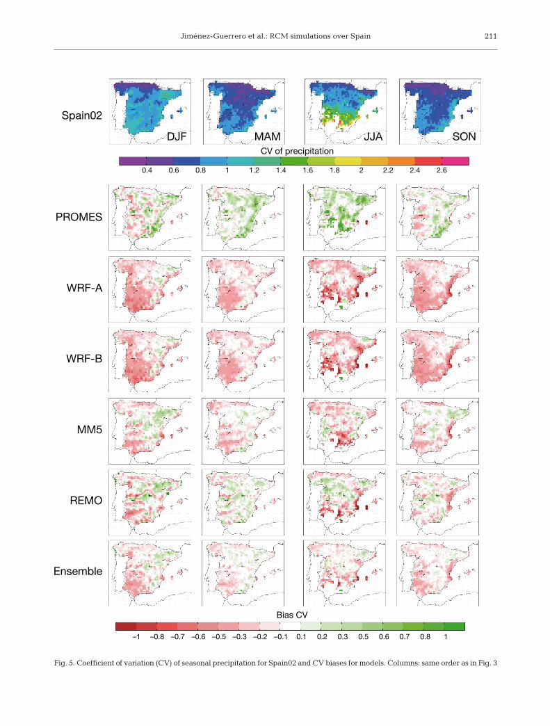
Fig. 5. Coefficient of variation (CV) of seasonal precipitation for Spain02 and CV biases for models. Columns: same order as in Fig. 3

Clim Res 57: 201–220, 2013

ensemble of regional climate models instead of oneindividual model to get more robust future climateprojections, for a better assessment of uncertaintiesdue to the dynamical downscaling process. These cli-mate projections have already been carried out in theESCENA project. An important issue, which we donot address here but will be considered in futurestages of the ESCENA project, is the relationship be -tween past and future performance of models (asevaluated by Whetton et al. 2007 and Abe et al. 2009,among others). As stated by Annan & Hargreaves(2010), climate models have already been tuned tosome extent to the recent climate data and thereforeaccurately reproduce present-day climate conditions.It would be interesting to further test the reliability ofthe ensemble in other ways, for example consideringsimulations of other epochs or other climatic observa-tions that are less widely used during model con-struction and tuning.

3.2. Interannual variability

For precipitation, SD is normalized by the periodaverage, therefore by obtaining a coefficient of vari-ation (CV). This is done because the SD of precipita-tion is typically related to the mean (Giorgi et al.2004), so that the CV is a more independent measureof interannual variability.

Table 2b shows the spatially averaged seasonaland annual interannual variability biases for maxi-mum and minimum temperature and the spatiallyaveraged CV biases for precipitation. The seasonalspatial distribution of the mentioned statistics arerepresented in Figs. 4 & 5, for maximum and mini-mum temperature and precipitation, respectively.

All models except for PROMES and WRF-A tend toslightly underestimate the interannual SD of maxi-mum temperature (Fig. 4). Similar values and re -sponses from models are observed for different sea-sons. In winter, the biases of maximum temperatureSD vary be tween –0.27K in MM5 to +0.07K inWRF-A (Table 2b). The biases range from –0.38(MM5) to +0.33K (PROMES) in spring, and –0.20(MM5) to +0.32K (PROMES) during summer; mean-while for autumn MM5 once more provides thelargest underestimation of the SD (–0.12K) andPROMES the highest overestimation (+0.22K). Therest of the models show an intermediate behavior forrepresenting the interannual SD, with the best skillsduring the autumn season.

For minimum temperature (Fig. 4), the results aresimilar to maximum temperature, but in this case it is

REMO which tends to provide the largest biases inthe minimum temperature variability (Table 2b). TheSD is generally underestimated by all models, espe-cially during winter over the highest mountain chainsof the IP. In this season, biases vary between –0.60(REMO) and –0.09K (PROMES). All models predictspring variability better than for wintertime (–0.21Kin REMO and 0.11K in PROMES during springtime).However, in summer all the models show valuesclose to Spain02.

Regarding precipitation, the models (exceptPROMES) pervasively underestimate the interannualvariability over the domain, especially in southwest-ern Spain in winter, and the Mediterranean coast andthe Balearic Islands during summer and autumn(Fig. 5). The biases of the CV range from +0.04 (win-ter and autumn) to +0.28 (summer) in the case ofPROMES, to underestimations in WRF-A (–0.28 inautumn to –0.18 in spring). MM5 and REMO presentthe smallest average biases, ranging from –0.15 to0.03.

The multi-model ensemble mean outperforms mostof the individual models in all seasons, showing theadded value of using an ensemble of RCMs toimprove the amount of interannual variability. How-ever, common model deficiencies still remain (e.g.the low precipitation variability in autumn on theMediterranean coast).

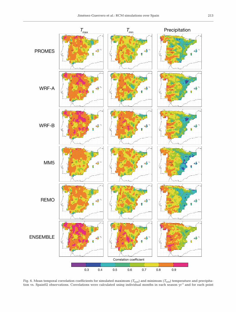
The temporal correlation (ρ) between simulatedand observed deseasonalized series is shown inFig. 6 for maximum and minimum temperature andprecipitation. Maximum temperatures show thehighest correlations (>0.85) over most of the domain,especially over the river valleys of northern Spain.The fact that the lowest correlations (~0.4) are foundin northeastern Spain for all models may point to (1)problems with the quality of raw observed data usedto create the Spain02 database or (2) to local climaticfeatures that the models are unable to capture at theselected resolution. For minimum temperature, ρ isgenerally slightly lower than for maxima. The spatialstructure of the correlation presents common minimain all models, and this points to a relation with topog-raphy, since the lowest correlation coefficients (ρ <0.5) are located in the highest mountain chains inSpain, such as the Pyrenees, Sistema Ibérico or SierraNevada, from north to south of the domain. On theother hand, the highest correlations for minimumtemperatures are observed over the Central Plateausand the river valleys. The precipitation correlationsshow a strong east-west gradient reaching the lowestvalues (~0.30 to 0.50) towards the Ebro Valley andthe southeastern IP (Fig. 6).

212

Jiménez-Guerrero et al.: RCM simulations over Spain 213

Correlation coefficient

Tmax Tmin Precipitation

0.3 0.4 0.5 0.6 0.7 0.8 0.9

PROMES

WRF-A

WRF-B

MM5

REMO

ENSEMBLE

Fig. 6. Mean temporal correlation coefficients for simulated maximum (Tmax) and minimum (Tmin) temperature and precipita-tion vs. Spain02 observations. Correlations were calculated using individual months in each season yr-1 and for each point

Clim Res 57: 201–220, 2013

In order to discriminate the seasonal behavior ofthis temporal correlation, Table 3 represents spatiallyaveraged correlations for maximum and minimumtemperature and precipitation. Maximum tempera-ture shows the highest correlations and they presenta low seasonal variability. Spring has slightly highercorrelations than the rest of the seasons. In general,there is also a low model-to-model variability. OnlyWRF shows somewhat higher correlations (mostly>0.8). REMO, unlike the rest of the models, presentsa value <0.70 in summer, indicating a lower capabil-ity to capture maximum temperature variability insummer. For minimum temperatures, correlationsare, in general, lower than for maximum temperatureand they exhibit a clearer seasonal variability, withhigher correlations in winter and autumn. In thiscase, spring shows the lowest correlations, and sev-eral models show correlations <0.7 in different sea-sons. Only WRF-B is above this threshold throughoutthe year and performs best on average. For this vari-able, WRF-A is more similar to other models, such asMM5, than to WRF-B. Lastly, for precipitation thecorrelations are generally much lower than for tem-perature, and the seasonal dependence is verystrong. As expected, higher correlation coefficientsare at tained during winter (0.77 to 0.80), when syn-optic systems, well captured in the reanalysis data,drive precipitation. During summer, the synopticactivity is lower and precipitation is mostly driven byconvective systems, less constrained by the boundaryconditions; therefore, the lowest correlations areattained (0.42 to 0.55). An intermediate behaviour isshown in the transition seasons.

The most noticeable aspect regarding correlation(Fig. 6), is the large improvement achieved whenconsidering the ensemble mean. Spatially (Fig. 6),there are areas where correlations are above any ofthe component members; most noticeably in precipi-tation over the eastern coast, where a common RCMdefect is improved by the ensemble, softening thestrong gradient present in each individual model.Also, after spatial averaging (Table 3), the ensemblemean performs at least as well as the best member,and in most cases shows better correlation than any ofthe members. This is true especially for precipitation.

3.3. Spatial variability

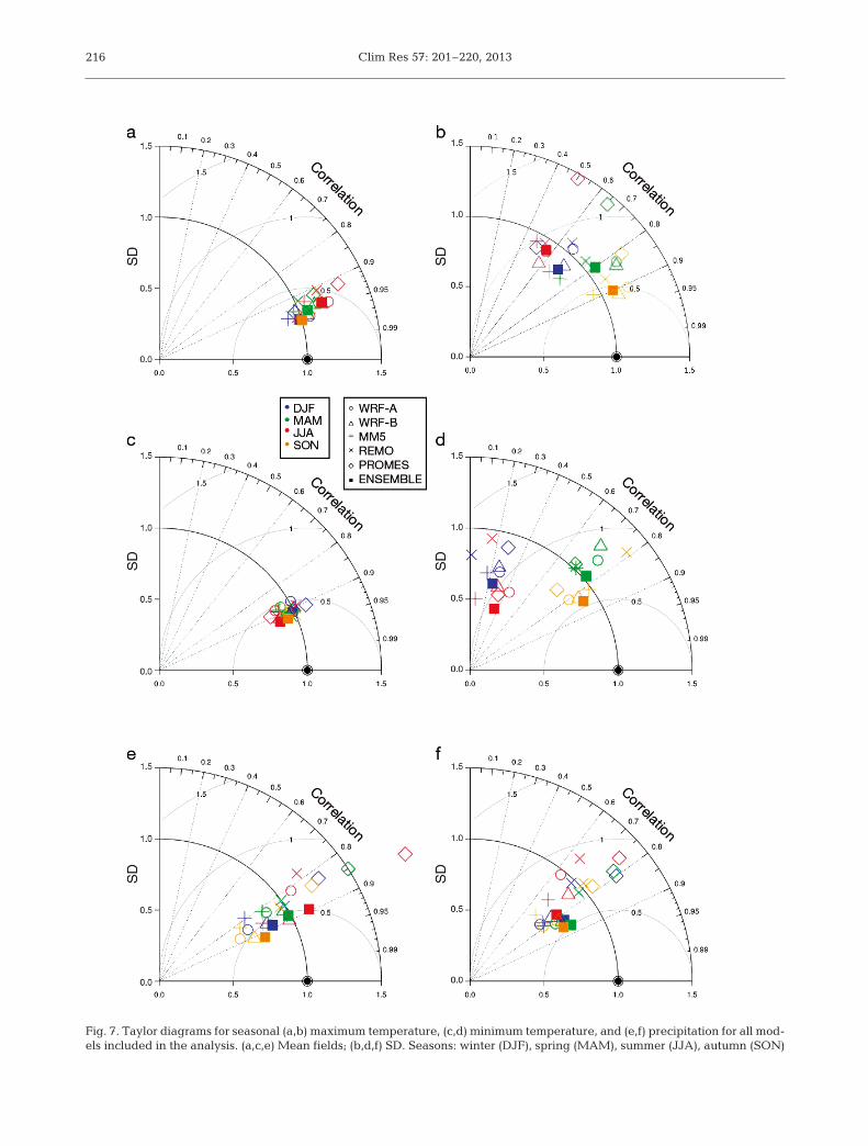
Here, we focus on the ability of the models to rep-resent the observed spatial variability by using Tay-lor diagrams (Taylor 2001), which enable an easycomparison between the spatial and temporal pat-

terns of 2 fields. In our diagrams (Fig. 7), the statisticsdisplayed are the relative spatial SD (radial distancefrom the origin) and the correlation (cosine of theangular coordinate). Better models, in terms of cen-tered root mean squared error (RMSE), are locatedcloser to the black circle shown in Fig. 7, which cor-responds to Spain02. Centered RMSE increases withdistance from this point.

With respect to the mean field of maximum temper-ature (Fig. 7a), all models perform well, especially forwinter, with very high spatial correlations and a normalized SD close to observations. However,PROMES and REMO represent excessive spatialvariability during summertime. The spatial variabil-ity of the interannual SD (Fig. 7b), as well as its spa-tial mean (Table 2) is strongly overestimated byPROMES in spring and summer, providing highervalues of spatial patterns of variability. There is astrong variation in the skill of the models as a func-tion of the season of the year, with better correlationvalues during spring and autumn.

In the simulation of the mean minimum tempera-ture (Fig. 7c), the models perform very similarly witheach other, showing a high spatial correlation withthe observations, but in most cases with a smallunderestimation of the spatial variability, except for

214

(a)

DJF MAM JJA SON Annual

PROMES 0.77 0.79 0.77 0.80 0.78WRF-A 0.78 0.85 0.83 0.84 0.83WRF-B 0.80 0.86 0.83 0.84 0.84MM5 0.77 0.83 0.74 0.80 0.78REMO 0.78 0.83 0.69 0.83 0.79Ensemble 0.81 0.87 0.83 0.86 0.84(b)PROMES 0.67 0.74 0.77 0.76 0.73WRF-A 0.76 0.69 0.74 0.80 0.75WRF-B 0.82 0.74 0.74 0.82 0.78MM5 0.81 0.70 0.73 0.79 0.76REMO 0.78 0.66 0.68 0.78 0.72Ensemble 0.82 0.74 0.77 0.83 0.79(c)PROMES 0.79 0.68 0.55 0.60 0.67WRF-A 0.78 0.68 0.52 0.62 0.68WRF-B 0.80 0.69 0.53 0.63 0.69MM5 0.77 0.64 0.44 0.62 0.66REMO 0.77 0.67 0.42 0.64 0.66Ensemble 0.85 0.77 0.63 0.73 0.77

Table 3. Time-correlation for modeled (a) maximum and (b)minimum temperature, and (c) precipitation vs. Spain02 ob-servations for all seasons and diverse models included in ES-CENA. Seasons: winter (DJF), spring (MAM), summer (JJA),autumn (SON). Light to dark shading indicates low to high

correlation coefficients, respectively

Jiménez-Guerrero et al.: RCM simulations over Spain 215

the cold season. The models do not capture the spa-tial structure of the variability during summer andwintertime (Fig. 7d). This variability is pervasivelyunderpredicted for winter and summer, when spatialcorrelation does not ex ceed 0.45. Both for maximumand minimum temperature, the diverse models (andseasons) present a high spread in the representationof the spatial structure of the SD.

The mean precipitation pattern (Fig. 7e) is capturedworse than those of temperature. This is ex pected,since the temperature patterns are strongly related tothe orography. PROMES tends to provide a higherspatial variability than observations, especially forsummertime (see red diamond outside the Taylor dia-gram in 7e), but with a high correlation (>0.88). Inthis case, REMO tends to better capture the field vari-ability. For the SD pattern (Fig. 7f), a similar analysiscan be performed, with PROMES tending to overesti-mate the SD of the spatial variability.

In this case, the added value of considering theensemble mean is not clear for the maximum temper-ature (the ensemble mean outperforms most but notall models), albeit it generally improves the skill ofmost models. For minimum temperature and, overall,precipitation, the ensemble mean outperforms theindividual models in all seasons, although it some-what underestimates the variance of the SD patterns.

4. DISCUSSION AND CONCLUSIONS

In this work we have analyzed the RCM evaluationsimulations of the ESCENA project over peninsularSpain and the Balearic Islands. This work evaluates,for the first time over a European region, the MM5and WRF open-source, US-developed models alongwith European RCMs (PROMES and REMO). Thisstudy is also one of the earliest works using ERA-Interim as boundary conditions over Europe. As aninitial evaluation of the ESCENA simulations, weused simple, widely used metrics to enable the com-parison of the model performance with earlier stud-ies. Also, we focused on the mean climate and inter-annual variability, therefore relying on monthly data.

As an indication of the quality of the simulations,we can compare the spatial correlation values forprecipitation deduced from Fig. 7 with those ob -tained for RCMs in ENSEMBLES included in Herreraet al. (2010). That work classified the RCMs into 2groups, according to a gap in the spatial correlationof precipitation. According to this classification, allindividual RCMs in ESCENA would be in the groupof the ‘best’ models. Also, the ensemble mean in

ESCENA is similar to the best ensemble in the afore-mentioned work. Therefore, the ability to reproduceprecipitation within ESCENA is high, at least in thisaspect, when compared to Herrera et al. (2010) andreferences therein. The temperature results can bequalitatively compared to the bias maps shown byChristensen et al. (2010), which show typical biaseswithin ENSEMBLES of the order of 2K in this region,similar to those found in ESCENA. Temperature-out-lier models in ENSEMBLES show biases much largerthan those in ESCENA. Therefore, overall, the 5regional climate simulations included in ESCENAshow good quality in reproducing the climatology ofthe IP, even though these models are based on completely different approaches and physical para-meterizations.

WRF was used in 2 different settings, which differonly in the representation of the PBL. WRF-A used alocal closure scheme, which has been reported todevelop shallower, colder, and moister PBLs thanWRF-B, which used a non-local closure scheme (García-Díez et al. 2013). The weaker low-level mix-ing in WRF-A leads to colder nighttime (i.e. mini-mum) temperatures. Therefore, the largest differ-ences be tween the WRF ensemble members appearin the minimum temperature. Remarkably, MM5 isthe only other model in the ensemble using a non-local closure PBL scheme, but the results are closer toWRF-A. It seems that biases arising from other com-ponents (model dynamics, numerics or other parame-terizations) are compensating the expected summerwarm bias.

Regarding the inherent uncertainties of model validation methodologies, climate models here areassessed on their capacity to reproduce present cli-mate conditions, which in turn are established bycomparing the output of climate simulations withobservational datasets including gridded products(here, Spain02 dataset). However, due to the natureof the procedures to obtain observations and the sta-tistical techniques employed to extrapolate this infor-mation onto reference gridded databases, they con-tain important uncertainties which may compromisethe evaluation process. A recent work by Gómez-Navarro et al. (2012) indicates that, even in areascovered by dense monitoring networks such asSpain, uncertainties in the observations are compara-ble to the uncertainties within state-of-the-art RCMsdriven by reanalysis, such as those used in ESCENA.Therefore, some of the common deficiencies found,can probably be traced to problems in the observa-tional database. For instance, the warm biased mini-mum temperatures over northeastern Spain are a

Clim Res 57: 201–220, 2013216

Fig. 7. Taylor diagrams for seasonal (a,b) maximum temperature, (c,d) minimum temperature, and (e,f) precipitation for all mod-els included in the analysis. (a,c,e) Mean fields; (b,d,f) SD. Seasons: winter (DJF), spring (MAM), summer (JJA), autumn (SON)

Jiménez-Guerrero et al.: RCM simulations over Spain

candidate to a misrepresentation in the observationaldatabase, since (1) the problem is common to allmodels, (2) there are no complex topographic fea-tures over that area, and (3) the problem does notarise in any other variable.

No single model outperforms the rest of the modelsfor all the variables analyzed. Depending on the vari-able and season, different models stand out. Forexample, REMO stands out for temperature (espe-cially minimum temperature), PROMES shows a wetbias when the rest tend to be drier than observed,and WRF is also especially dry during autumn.Regarding the inclusion of US-developed models inthe ensemble, we found no ‘home court advantage’(Takle et al. 2007) for the European models. Unlikeshown in other recent studies over north America(Mearns et al. 2012), the use of RCMs out of their‘home’ domain did not lead to poorer performance.

The different performance of the RCMs in differentseasons and variables encourages the use of thewhole ensemble of simulations, taking the range ofbiases as an indicator of model uncertainty. The sim-plest way of considering the ensemble of RCMs isthrough the use of the ensemble mean as an addi-tional simulation. The results show that the ensemblemean is usually less biased than the individual mem-bers or is close to the best member. Remarkably, theensemble of simulations is able to correct the prob-lems associated with the interannual variability forprecipitation, showing substantially higher temporalcorrelation than the best individual model. These re -sults are in accordance with previous works (Gleckleret al. 2008, Coppola et al. 2010, Kjellström et al.2011). As stated by Annan & Hargreaves (2011), onehypothesis for the improvement of the ensemblemean when compared to the performance of the indi-vidual models is the paradigm of models being con-sidered as independent samples from some distribu-tion that is centered on the truth, as in this case theensemble mean could be expected to converge to thetruth as more models are added to the ensemble(Tebaldi & Knutti 2007). However, this hypothesishas been refuted by Knutti et al. (2010). Annan &Hargreaves (2010, 2011) defend the point that thestatistically indistinguishable paradigm provides areasonable basis for explanation of the properties ofthe CMIP3 ensemble. However, their results are onlydirectly applicable to their specific comparisons anda convincing explanation for the outperformance ofthe ensemble mean is still an open question in cli-mate science.

We can, therefore, conclude that the use of ensem-ble simulations in this kind of study substantially

improves the representativity of the climatologies,and we also expect that studies of future climates, byusing ensemble methodologies, will provide morerobust climate projections and a valuable estimationof the associated uncertainty. As shown, these datacan be complementary to other European projectssuch as ENSEMBLES over the Iberian Peninsula andsurrounding areas. The data from this study are pub-licly available on the ESCENA project server (http://proyectoescena.uclm.es). The analyses shown arejust an initial evaluation that needs to be extended inforthcoming studies by the climate and impact communities in the Iberian Peninsula, who are en -couraged to use the whole RCM ensemble, therebypropagating the uncertainties found.

Acknowledgements. The Spanish R+D Programme of theMinistry of the Environment (Ministerio de Medio Ambientey Rural y Marino) is acknowledged for the funding providedfor the ESCENA project (Ref: 200800050084265). P.J.G. alsothanks the Ramón y Cajal Programme of the Spanish Ministryof Science and Technology. This ministry is also acknowl-edged for the financial support through grants CGL2008-05112-C02-02, CGL2010-18013 and CGL2010-22158-C02(this latter also funded by the European Fund for RegionalDevelopment [FEDER]. The authors also acknowledge the 5anonymous reviewers for their valuable comments.

LITERATURE CITED

Abe M, Shiogama H, Hargreaves J, Annan J, Nozawa T,Emori S (2009) Correlation between inter-model similar-ities in spatial pattern for present and projected futuremean climate. SOLA 5: 133–136

Annan JD, Hargreaves JC (2010) Reliability of the CMIP3en semble. Geophys Res Lett 37: L02703, doi: 10. 1029/2009GL041994

Annan JD, Hargreaves JC (2011) Understanding the CMIP3multimodel ensemble. J Clim 24: 4529−4538

Argüeso D, Hidalgo-Muñoz JJ, Gamiz-Fortis SR, Esteban-Parra MJ, Castro-Diez Y (2012) Evaluation of WRF meanand extreme precipitation over Spain: present climate(1970–1999). J Clim 25: 4883–4897

Arribas A, Gallardo C, Gaertner MA, Castro M (2003) Sensi-tivity of Iberian Peninsula climate to land degradation.Clim Dyn 20: 477−489

Boo KO, Kwon WT, Baek HJ (2006) Change of extremeevents of temperature and precipitation over Korea usingregional projection of future climate change. GeophysRes Lett 33: L01791, doi: 10.1029/2005GL023378

Boulanger JP, Brasseur G, Carril AF, de Castro M and others(2010) A Europe-South America network for climatechange assessment and impact studies. Clim Change 98: 307−329

Brinkop S, Roeckner E (1995) Sensitivity of a general circu-lation model to parameterizations of cloud-turbulenceinteractions in the atmospheric boundary layer. Tellus A47(2): 197–220

Castro M, Fernández C, Gaertner MA (1993) Description ofa mesoscale atmospheric numerical model. In: Díaz JI,

217

Clim Res 57: 201–220, 2013

Lions JL (eds) Mathematics, climate and environment.Rech Math Appl Ser 27, Masson, Paris, p 230–253

Chaboureau JP, Bechtold P (2002) A simple cloud parameter-ization derived from cloud resolving model data: diagnos-tic and prognostic applications. J Atmos Sci 59: 2362−2372

Chaboureau JP, Bechtold P (2005) Statistical representationof clouds in a regional model and the impact on the diur-nal cycle of convection during tropical convection, cirrusand nitrogen oxides (TROCCINOX). J Geophys Res 110: D17103, doi: 10.1029/2004JD005645

Chen F, Dudhia J (2001a) Coupling an advanced land surface-hydrology model with the Penn State-NCARMM5 modeling system. I. Model implementation andsensitivity. Mon Weather Rev 129: 569–585

Chen F, Dudhia J (2001b) Coupling an advanced land sur-face-hydrology model with the Penn State-NCAR MM5modeling system. II. Preliminary model validation. MonWeather Rev 129:587–604

Christensen JH, Christensen OB (2007) A summary of thePRUDENCE model projections of changes in Europeanclimate by the end of this century. Clim Change 81: 7−30

Christensen JH, Kjellström E, Giorgi F, Lenderink G, Rum-mukainen M (2010) Weight assignment in regional cli-mate models. Clim Res 44: 179−194

Collins WD, Rasch PJ, Boville DA, Hack JJ, McCaa JR,Williamson DK, Briegleb BP (2006) The formulation andatmospheric simulation of the Community AtmosphereModel. J Clim 19: 2144−2161

Coppola E, Giorgi F, Rauscher SA, Piani C (2010) Modelweighting based on mesoscale structures in precipitationand temperature in an ensemble of regional climatemodels. Clim Res 44: 121–134

Cuxart J, Bougeault P, Redelsperger JL (2000) A turbulencescheme allowing for mesoscale and large-eddy simula-tions. Q J R Meteorol Soc 126: 1−30

d’Almeida GA, Koepke P, Shettle EP (1991) Atmosphericaerosols: global climatology and radiative characteris-tics. A Deepak Publ, Hampton, VA

Davies HC (1976) A lateral boundary formulation for multi-level prediction models. Q J R Meteorol Soc 102: 405−418

Dee DP, Uppsala SM, Simmons AJ, Berrisford P and others(2011) The ERA-Interim reanalysis: configuration and per-formance of the data assimilation system. Q J R MeteorolSoc 137: 553−597

Domínguez M, Gaertner MA, de Rosnay P, Losada T (2010)A regional climate model simulation over West Africa: parameterization tests and analysis of land-surfacefields. Clim Dyn 35: 249−265

Domínguez M, Romera R, Sánchez E, Fita L and others(2013) Present climate precipitation and temperatureextremes over Spain from a set of high resolution RCM.Clim Res (in press) doi: 10. 3354/ cr01186

Dudhia J (1989) Numerical study of convection observedduring the winter monsoon experiment using amesoscale two-dimensional model. J Atmos Sci 46: 3077−3107

Dudhia J (1993) A nonhydrostatic version of the Penn StateNCAR mesoscale model: validation tests and simulationof an Atlantic cyclone and cold front. Mon Weather Rev121: 1493−1513

ECMWF (2004) IFS Documentation CY28r1, Chapter 4: physical processes, Section 2: radiation. Available atwww. ecmwf.int/research/ifsdocs/CY28r1/index.html

Fernández J, Montávez JP, Saenz J, Gonzalez-Rouco JF,Zorita E (2007) Sensitivity of the MM5 mesoscale model

to physical parameterizations for regional climate stud-ies: annual cycle. J Geophys Res 112(D4): D04101, doi: 10.1029/ 2005JD006649

Fernández J, Primo C, Cofiño AS, Gutiérrez JM, RodríguezMA (2009) MVL spatiotemporal analysis for model inter-comparison in EPS: application to the DEMETER multi-model ensemble. Clim Dyn 33: 233−243

Fernández-Quiruelas V, Fita L, Fernández J, Cofiño A(2010) WRF workflow on the Grid with WRF4G. Proc11th WRF Users’ Workshop, Boulder, CO

Fita L, Fernández J, García-Díez M (2010) CLWRF: WRFmodifications for regional climate simulation under futurescenarios. Proc 11th WRF Users’ Workshop, Boulder, CO

Font-Tullot I (2000) Climatología de España y Portugal, 2ndedn. Universidad de Salamanca, Salamanca

Gaertner MA, Castro M (1996) A new method for verticalinterpolation of the mass field. Mon Weather Rev 124: 1596−1603

Gaertner MA, Christensen OB, Prego JA, Polcher J, Gal-lardo C, Castro M (2001) The impact of deforestation onthe hydrological cycle in the western Mediterranean: anensemble study with two regional climate models. ClimDyn 17: 857−873

Gaertner MA, Jacob D, Gil V, Domínguez M, Padorno E,Sánchez E, Castro M (2007) Tropical cyclones over theMediterranean Sea in climate change simulations. Geo-phys Res Lett 34:L14711, doi: 10.1029/2007GL029977

Gaertner MA, Domínguez M, Garvert MA (2010) Modellingcase-study of soil moisture-atmosphere coupling. Q J RMeteorol Soc 136: 483−495

Gallardo C, Arribas A, Prego JA, Gaertner MA, de Castro M(2001) Multi-year simulations using a regional-climatemodel over the Iberian Peninsula: current climate anddoubled CO2 scenario. Q J R Meteorol Soc 127: 1659−1682

Gao X, Pal JS, Giorgi F (2006) Projected changes in meanand extreme precipitation over the Mediterraneanregion from a high resolution double nested RCM simu-lation. Geophys Res Lett 33: L03706, doi: 10.1029/2005 GL024954

García-Díez M, Fernández J, Fita L, Yagüe C (2013) Seasonaldependence of WRF model biases and sensitivity to PBLschemes over Europe. Q J R Meteorol Soc 139: 501–514

Giorgi F, Bi X, Pal JS (2004) Mean, interannual variabilityand trends in a regional climate change experiment overEurope. I. Present-day climate (1961–1990). Clim Dyn22: 733−756

Gleckler P, Taylor K, Doutriax C (2008) Performance metricsfor climate models. J Geophys Res 113: D06104, doi: 10.1029/ 2007JD008972

Gómez-Navarro JJ, Montávez JP, Jiménez-Guerrero P,Jerez S, García-Valero JA, González-Rouco JF (2010)Warming patterns in regional climate projections overthe Iberian Peninsula. Met Zeit (Hambg) 19: 275−285

Gómez-Navarro JJ, Montávez JP, Jerez S, Jiménez-Guer-rero P, Lorente-Plazas R, González-Rouco JF, Zorita E(2011) A regional climate simulation over the IberianPeninsula for the last millennium. Clim Past 7: 451−472

Gómez-Navarro JJ, Montávez JP, Jerez S, Jiménez-Guer-rero P, Zorita E (2012) What is the role of the observa-tional dataset in the evaluation and scoring of climatemodels? Geophys Res Lett 39: L24701, doi: 10. 1029/ 2012GL 054206

Grell GA (1993) Prognostic evaluation of assumptions usedby cumulus parameterizations. Mon Weather Rev 121: 764–787

218

Jiménez-Guerrero et al.: RCM simulations over Spain

Grell GA, Dévényi D (2002) A generalized approach to para-meterizing convection combining ensemble and dataassimilation techniques. Geophys Res Lett 29(14), doi: 10.1029/2002GL015311

Grell GA, Dudhia J, Stauffer DR (1994) A description of thefifth-generation PennState/NCAR mesoscale model(MM5). NCAR Tech Note NCAR/TN-398+STR, NCAR,Boulder, CO. Available at www.mmm.ucar.edu/mm5

Haylock MR, Hofstra N, Klein Tank AMG, Klok EJ, JonesPD, New M (2008) A European daily high-resolutiongridded data set of surface temperature and precipitationfor 1950–2006. J Geophys Res 113: D20119, doi: 10.1029/2008JD010201

Herrera S, Fita L, Fernández J, Gutiérrez J (2010) Evaluationof the mean and extreme precipitation regimes from theENSEMBLES regional climate multimodel simulationsover Spain. J Geophys Res 115: D21117, doi: 10.1029/ 2010JD013936

Herrera S, Gutiérrez JM, Ancell R, Pons MR, Frías MD, Fer-nández J (2012) Development and analysis of a 50-yearhigh-resolution daily gridded precipitation dataset overSpain (Spain02). Int J Climatol 32: 74–85

Hong SY, Lin JOJ (2006) The WRF Single-Moment 6-ClassMicrophysics Scheme (WSM6). J Korean Meteorol Soc42: 129−151

Hong SY, Pan HL (1996) Comparison of NCEP/NCARReanalysis with 1987 FIFE data. Mon Weather Rev 124: 1480−1498

Hong SY, Dudhia J, Chen S (2004) A revised approach toice microphysical processes for the bulk parameteriza-tion of cloud and precipitation. Mon Weather Rev 132: 103−120

Houghton JT, Meira Filho LG, Callander BA, Harris N, Kat-tenberg A, Maskell K (eds) (1996) Climate change 1995.The science of climate change. Cambridge UniversityPress, Cambridge

Jacob D, Van den Hurk BJJM, André U, Elgered G and oth-ers (2001) A comprehensive model inter-comparisonstudy investigating the water budget during the BAL-TEX-PIDCAP period. Meteorol Atmos Phys 77: 19−43

Jacob D, Bärring L, Christensen OB, Christensen JH andothers (2007) An intercomparison of regional climatemodels for Europe: model performance in present-dayclimate. Clim Change 81: 31−52

Jerez S, Montávez JP, Gomez-Navarro JJ, Jiménez-Guer-rero P, Jiménez J, González-Rouco JF (2010) Tempera-ture sensitivity to the land-surface model in MM5 climatesimulations over the Iberian Peninsula. Met Zeit 19: 363−374

Jerez S, Montávez JP, Jiménez-Guerrero P, Gómez-Navarro JJ, Lorente-Plazas R, Zorita E (2012a) A multi-physics ensemble of present-day climate regional simulations over the Iberian Peninsula. Clim Dyn 40:3023–3046

Jerez S, Montávez JP, Gómez-Navarro JJ, Jiménez PA,Jiménez-Guerrero P, Lorente R, González-Rouco JF(2012b) The role of the land-surface model for climatechange projections over the Iberian Peninsula. J Geo-phys Res 117: D01109, doi: 10.1029/2011JD016576

Jerez S, Montávez JP, Gómez-Navarro JJ, Lorente-Plazas R,García-Valero JA, Jiménez-Guerrero P (2013) A multi-physics ensemble of regional climate change projectionsover the Iberian Peninsula. Clim Dyn 41: 1749–1768

Kain JS, Fritsch JM (1993) Convective parameterization formesoscale models: the Kain-Fritsch scheme. The repre-

sentation of cumulus convection in numerical models.Meteor Monogr 24: 165−170

Kjellström E, Nikulim F, Hanson U, Strandberg G, UllerstigA (2011) 21st century changes in the European climate: uncertainties derived from an ensemble of regional cli-mate model simulations. Tellus 63A: 24–40

Klemp JB, Skamarock WC, Dudhia J (2007) Conservativesplit-explicit time integration methods for the compressi-ble non-hydrostatic equations. Mon Weather Rev 135: 2897−2913

Knutti R, Furrer R, Tebaldi C, Cermak J, Meehl GA (2010)Challenges in combining projections from multiple cli-mate models. J Clim 23: 2739–2758

Koepke P, Hess M, Schult I, Shettle EP (1997) Global aerosoldata set. Rep 243, Max Planck Inst Meteorol, Hamburg.Available at http: //opac.userweb. mwn.de/ radaer/ gads.html

Krinner G, Viovy N, Noblet-Ducoudre N, Ogee J and others(2005) A dynamic global vegetation model for studies ofthe coupled atmosphere-biosphere system. Global Bio-geochem Cycles 19: BG1015, doi: 10.1029/2003GB002199

Mearns LO, Arritt R, Biner S, Bukovsky MS and others(2012) The North American Regional Climate ChangeAssessment Program: overview of phase I results. BullAm Meteorol Soc 93:1337–1362

Mlawer EJ, Taubman SJ, Brown PD, Iacono MJ, Clough SA(1997) Radiative transfer for inhomogeneous atmospheres: RRTM, a validated correlated-k model for the longwave.J Geophys Res 102: 16663−16682

Morcrette J, Smith L, Fourquart Y (1986) Pressure and temperature dependence of the absorption in longwaveradiation parameterizations. Beitr Phys Atmos 59: 455–469

Nordeng T (1994) Extended versions of the convectiveparametrization scheme at ECMWF and their impacton the mean and transient activity of the model in thetropics. Res Dep, Tech Memo 206, ECMWF, Reading

Nunez MN, Solman SA, Cabre MF (2009) Regional climatechange experiments over southern South America. II.Climate change scenarios in the late twenty-first century.Clim Dyn 32: 1081−1095

Roeckner E, Arpe K, Bengtsson L, Christoph M and others(1996) The atmospheric general circulation modelECHAM4: model description and simulation of present-day climate. Rep 218, Max Planck Inst Meteorol, Hamburg

Sánchez E, Romera R, Gaertner MA, Gallardo C, Castro M(2009) A weighting proposal for an ensemble of regionalclimate models over Europe driven by 1961–2000 ERA40based on monthly precipitation probability density func-tions. Atmos Sci Lett 10: 241−248

Simmons AJ, Burridge DM (1981) An energy and angular-momentum conserving vertical finite-difference schemeand hybrid vertical coordinates. Mon Weather Rev 109: 758−766

Skamarock WC, Klemp JB, Dudhia J, Gill DO, Barker DM,Duda MG (2008) A description of the Advanced ResearchWRF version 3. NCAR Tech Note NCAR/ TN 20201 c475+STR, available at www.mmm. ucar. edu/ wrf/ users/ docs/arw _ v3.pdf

Takle ES, Roads J, Rockel WJ, Gutowski WJ and others(2007) Transferability intercomparison. Bull Am MeteorolSoc 88: 375−384

Taylor KE (2001) Summarizing multiple aspects of modelper formance in a single diagram. J Geophys Res 106: 7183−7192

219

Clim Res 57: 201–220, 2013

Tebaldi C, Knutti R (2007) The use of the multi-model ensem-ble in probabilistic climate projections. Philos Trans R SocLond A 365: 2053−2075

Tiedtke M (1989) A comprehensive mass flux scheme forcumulus parameterization in large–scale models. MonWeather Rev 117(8): 1779–1800

Uppala SM, Kallberg PW, Simmons AJ, Andrae U and others(2005) The ERA-40 re-analysis. Q J R Meteorol Soc 131: 2961−3012

Van der Linden P, Mitchell JFB (2009) ENSEMBLES: climatechange and its impacts: summary of research and resultsfrom the ENSEMBLES project. Met Office Hadley Cen-tre Tech Rep, Exeter

Whetton P, Macadam I, Bathols J, O’Grady J (2007) Assess-ment of the use of current climate patterns to evaluateregional enhanced greenhouse response patterns of cli-mate models. Geophys Res Lett 34: L14701, doi: 10. 1029/2007GL030025

220

Editorial responsibility: Filippo Giorgi, Trieste, Italy

Submitted: July 29, 2011; Accepted: April 24, 2013Proofs received from author(s): September 26, 2013