
Improving pan-european hydrological simulation of extreme events through statistical bias correction...
22
Hydrol. Earth Syst. Sci., 15, 2599–2620, 2011 www.hydrol-earth-syst-sci.net/15/2599/2011/ doi:10.5194/hess-15-2599-2011 © Author(s) 2011. CC Attribution 3.0 License. Hydrology and Earth System Sciences Improving pan-European hydrological simulation of extreme events through statistical bias correction of RCM-driven climate simulations R. Rojas 1 , L. Feyen 1 , A. Dosio 2 , and D. Bavera 1 1 Land Management and Natural Hazards Unit, Institute for Environment and Sustainability (IES), Joint Research Centre (JRC), European Commission (EC), Ispra, Italy 2 Climate Change & Air Quality Unit, Institute for Environment and Sustainability (IES), Joint Research Centre (JRC), European Commission (EC), Ispra, Italy Received: 1 April 2011 – Published in Hydrol. Earth Syst. Sci. Discuss.: 19 April 2011 Revised: 29 June 2011 – Accepted: 12 August 2011 – Published: 24 August 2011 Abstract. In this work we asses the benefits of removing bias in climate forcing data used for hydrological climate change impact assessment at pan-European scale, with emphasis on floods. Climate simulations from the HIRHAM5-ECHAM5 model driven by the SRES-A1B emission scenario are cor- rected for bias using a histogram equalization method. As target for the bias correction we employ gridded interpolated observations of precipitation, average, minimum, and max- imum temperature from the E-OBS data set. Bias removal transfer functions are derived for the control period 1961– 1990. These are subsequently used to correct the climate simulations for the control period, and, under the assump- tion of a stationary error model, for the future time win- dow 2071–2100. Validation against E-OBS climatology in the control period shows that the correction method performs successfully in removing bias in average and extreme statis- tics relevant for flood simulation over the majority of the European domain in all seasons. This translates into con- siderably improved simulations with the hydrological model of observed average and extreme river discharges at a ma- jority of 554 validation river stations across Europe. Proba- bilities of extreme events derived employing extreme value techniques are also more closely reproduced. Results indi- cate that projections of future flood hazard in Europe based on uncorrected climate simulations, both in terms of their magnitude and recurrence interval, are likely subject to large errors. Notwithstanding the inherent limitations of the large- Correspondence to: R. Rojas ([email protected]) scale approach used herein, this study strongly advocates the removal of bias in climate simulations prior to their use in hydrological impact assessment. 1 Introduction and scope Europe has experienced heavy floods over the last decades, which have affected thousands of people and caused millions of Euros worth of damage. Even though it is yet impossi- ble to link recent flooding events to global warming, climate projections indicate that in the future we can expect more extreme weather events triggering flooding. Managing risks from extreme flood events will be a crucial component of cli- mate change adaptation. It is therefore of utmost importance to develop and implement techniques that enhance the con- fidence in projecting future trends in flood occurrence and intensity. The basis for the definition of potential impacts of global warming are climate predictions. To date the most advanced tools to obtain those predictions are coupled Atmosphere- Ocean General Circulation Models (AOGCMs or in short GCMs) (Giorgi, 2005). Owing mainly to their coarse hor- izontal resolution (ca. 100–300km), however, downscaling procedures are required to feed small-scale impact mod- els and to guarantee a correct representation of the hydro- logic processes at a much finer spatial resolution (Fowler and Kilsby, 2007). Possible strategies to achieve this include sta- tistical or dynamical downscaling. The former develops sta- tistical relationships between large-scale climate information Published by Copernicus Publications on behalf of the European Geosciences Union.
-
Upload
independent -
Category
Documents
-
view
2 -
download
0
Transcript of Improving pan-european hydrological simulation of extreme events through statistical bias correction...
Hydrol. Earth Syst. Sci., 15, 2599–2620, 2011www.hydrol-earth-syst-sci.net/15/2599/2011/doi:10.5194/hess-15-2599-2011© Author(s) 2011. CC Attribution 3.0 License.
Hydrology andEarth System
Sciences
Improving pan-European hydrological simulation of extreme eventsthrough statistical bias correction of RCM-driven climatesimulations
R. Rojas1, L. Feyen1, A. Dosio2, and D. Bavera1
1Land Management and Natural Hazards Unit, Institute for Environment and Sustainability (IES),Joint Research Centre (JRC), European Commission (EC), Ispra, Italy2Climate Change & Air Quality Unit, Institute for Environment and Sustainability (IES), Joint Research Centre (JRC),European Commission (EC), Ispra, Italy
Received: 1 April 2011 – Published in Hydrol. Earth Syst. Sci. Discuss.: 19 April 2011Revised: 29 June 2011 – Accepted: 12 August 2011 – Published: 24 August 2011
Abstract. In this work we asses the benefits of removing biasin climate forcing data used for hydrological climate changeimpact assessment at pan-European scale, with emphasis onfloods. Climate simulations from the HIRHAM5-ECHAM5model driven by the SRES-A1B emission scenario are cor-rected for bias using a histogram equalization method. Astarget for the bias correction we employ gridded interpolatedobservations of precipitation, average, minimum, and max-imum temperature from the E-OBS data set. Bias removaltransfer functions are derived for the control period 1961–1990. These are subsequently used to correct the climatesimulations for the control period, and, under the assump-tion of a stationary error model, for the future time win-dow 2071–2100. Validation against E-OBS climatology inthe control period shows that the correction method performssuccessfully in removing bias in average and extreme statis-tics relevant for flood simulation over the majority of theEuropean domain in all seasons. This translates into con-siderably improved simulations with the hydrological modelof observed average and extreme river discharges at a ma-jority of 554 validation river stations across Europe. Proba-bilities of extreme events derived employing extreme valuetechniques are also more closely reproduced. Results indi-cate that projections of future flood hazard in Europe basedon uncorrected climate simulations, both in terms of theirmagnitude and recurrence interval, are likely subject to largeerrors. Notwithstanding the inherent limitations of the large-
Correspondence to:R. Rojas([email protected])
scale approach used herein, this study strongly advocates theremoval of bias in climate simulations prior to their use inhydrological impact assessment.
1 Introduction and scope
Europe has experienced heavy floods over the last decades,which have affected thousands of people and caused millionsof Euros worth of damage. Even though it is yet impossi-ble to link recent flooding events to global warming, climateprojections indicate that in the future we can expect moreextreme weather events triggering flooding. Managing risksfrom extreme flood events will be a crucial component of cli-mate change adaptation. It is therefore of utmost importanceto develop and implement techniques that enhance the con-fidence in projecting future trends in flood occurrence andintensity.
The basis for the definition of potential impacts of globalwarming are climate predictions. To date the most advancedtools to obtain those predictions are coupled Atmosphere-Ocean General Circulation Models (AOGCMs or in shortGCMs) (Giorgi, 2005). Owing mainly to their coarse hor-izontal resolution (ca. 100–300 km), however, downscalingprocedures are required to feed small-scale impact mod-els and to guarantee a correct representation of the hydro-logic processes at a much finer spatial resolution (Fowler andKilsby, 2007). Possible strategies to achieve this include sta-tistical or dynamical downscaling. The former develops sta-tistical relationships between large-scale climate information
Published by Copernicus Publications on behalf of the European Geosciences Union.
2600 R. Rojas et al.: Hydrological simulation and statistical bias correction
and regional variables (Wilby et al., 1999), whereas the lat-ter considers the application of Regional Climate Models(RCMs) driven by boundary conditions obtained from GCMs(Fowler et al., 2007). Advantages and drawbacks of bothdownscaling techniques have been widely discussed in lit-erature (see, e.g.Wilby and Wigley, 1997; Murphy, 1999;Hellstrom et al., 2001; Haylock et al., 2006; Schmidli et al.,2007) and, hence, they will not be repeated here. For ex-cellent discussions of downscaling techniques with focus onhydrological applications the reader is referred toWood et al.(2004) andFowler et al.(2007). In this paper, the dynamicaldownscaling approach is employed.
Despite the fact that hydrological components (e.g. sur-face and subsurface runoff) can be directly obtained fromRCMs at lateral resolutions that agree with meso-scale catch-ments (e.g. 25× 25 km or 50× 50 km), these components arehardly ever used to assess the local hydrology. This is mainlydue to the poor representation of the land surface processes,which results in a poor agreement between the surface runoffsimulated by the RCMs and observations (Giorgi et al., 1994;Evans, 2003). Instead, the detailed climate information ob-tained from the coupled GCM-RCM is typically employedto force off-line hydrological models and, thus, to obtainmore accurate representations of meso- and small-scale hy-drologic processes. In recent years, several studies have ap-peared that implement this technique to assess the impacts ofclimate change on hydrological extremes, either at the local(e.g.Middelkoop et al., 2001; Etchevers et al., 2002; Prud-homme et al., 2003; Kleinn et al., 2005; Wilby et al., 2006;Steele-Dunne et al., 2008; Thorne, 2011), regional (e.g.Gra-ham et al., 2007) or continental (e.g.Lehner et al., 2006;Dankers and Feyen, 2008, 2009) scale.
Notwithstanding RCMs have considerably advanced in re-producing regional and local climate, they are known to fea-ture systematic errors (see, e.g.Jacob et al., 2007; Lenderink,2010; Suklitsch et al., 2010). These biases are likely ex-plained by model errors caused by imperfections in the cli-matic model conceptualization, discretization and spatial av-eraging within cells, and uncertainties conveyed from theGCM to the RCM (Teutschbein and Seibert, 2010). Particu-larly, small-scale patterns of precipitation are highly depen-dent on climate model resolution and parametrization. At thesame time, some RCMs show systematic biases with a cleartendency to enhance these biases in more extreme cold orwarm conditions (van der Linden and Mitchell, 2009). In apan-European context, it has been noticed that climate mod-els tend to overestimate warm summers in south-eastern Eu-rope whereas precipitation in winter is too abundant in north-ern Europe (Jacob et al., 2007; Christensen et al., 2008). Ithas also been found that areas with a warm bias during win-ter generally exhibit a wet bias, whereas areas with a coldwinter bias show a dry bias (Jacob et al., 2007). At the sametime, Kjellstrom et al.(2010) found a clear tendency towarda warm bias in northern Europe for daily minimum tempera-ture. This potentially has a significant impact on the simula-
tion of hydrological processes such as spring-flooding eventsdriven by snow melting. A tendency to simulate too much(daily) precipitation by different RCMs, with this tendencybeing more pronounced for the upper-end percentiles (i.e. ex-treme precipitation events), has also been noticed (Kjellstromet al., 2010; Lenderink, 2010). Also a persistent overestima-tion of the wet day frequency is generally observed (see, e.g.Leander and Buishand, 2007; Piani et al., 2010b). It shouldbe highlighted that these biases can in part be explained byerrors in the observational data set employed for comparison(Lenderink, 2010).
The presence of biases in the forcing data seriously limitsits use in hydrological impact assessments (see, e.g.Woodet al., 2004) and it can result in unwanted uncertainty regard-ing projected climate change (van der Linden and Mitchell,2009). More specifically, RCM outputs not corrected forbiases tend to produce inaccurate probabilities for extremeevents, thus rendering the extreme value analysis less reli-able (Durman et al., 2001). Hence, some form of prior biascorrection of the forcing data is required if a realistic descrip-tion of the hydrology is sought. This procedure should aimat correcting climate simulated by the RCM during a controlperiod to properly reflect the spatio-temporal patterns of theobserved climate and, subsequently, use the “transfer func-tion” between climate observations and simulations obtainedfor the control period to correct future climate simulations(Piani et al., 2010a).
In recent literature, the presence of bias in dynamicallydownscaled outputs has been amply recognized (see, e.g.Shabalova et al., 2003; Lenderink et al., 2007; van Pelt et al.,2009; Hurkmans et al., 2010). As a result, several techniquesto correct potential bias in precipitation and temperature havebeen developed. Some use (a) monthly correction factorsbased on the ratio between present-day simulated values andobserved values (Durman et al., 2001), (b) linear or non-linear transformation functions which consider changes inthe mean and the variance of the observed and simulated timeseries (Horton et al., 2006; Leander and Buishand, 2007; Le-ander et al., 2008), (c) probability distribution transfer func-tions derived from observed and simulated cumulative distri-bution functions (cdfs), which is also referred to as “quantilemapping” or “histogram equalization” (Deque, 2007; Blocket al., 2009; Piani et al., 2010a,b), and (d) empirical factors totailor the RCM outputs considering normalization, tuning ofthe standard deviation and calculation of residuals (Engen-Skaugen, 2007). Themeßl et al.(2011) evaluated an ensem-ble of seven empirical-statistical methods to correct bias indaily precipitation of a high-resolution regional climate hind-cast for the Alpine region. They found that quantile mappingshows the best performance, particularly at high quantiles,which is favourable for applications related to extreme pre-cipitation events such as flooding. For a recent review of biascorrection techniques with focus on hydrological applica-tions the reader is referred toTeutschbein and Seibert(2010).
Hydrol. Earth Syst. Sci., 15, 2599–2620, 2011 www.hydrol-earth-syst-sci.net/15/2599/2011/
R. Rojas et al.: Hydrological simulation and statistical bias correction 2601
Most of the above bias removal techniques have been ap-plied at the local catchment scale, where dense networks ofmeteorological stations are available to reconstruct recent cli-mate. With the exception of the regional study ofGrahamet al.(2007), all large-scale hydrological assessments to datehave lacked a consistent bias correction step aimed at ensur-ing a correct spatio-temporal description of observed presentclimatic conditions. We note that there have been applica-tions of the delta-approach at pan-European scale (see, e.g.Lehner et al., 2006), where for the control period the hy-drological model has been forced by observed climate andfor future climate projections the climate signal is added tocurrent climate, hereby avoiding the need for bias correc-tion. However,Lehner et al.(2006) used monthly time seriesof observed climate at 0.5◦ lat-long resolution (New et al.,2000) and only accounted for long-term trends and averagechanges in seasonal climate, neglecting a potential change inclimate variability and extreme events.
The main reason advocated to skip bias correction in pan-European impact studies has been the lack of a high-qualityand high-resolution meteorological data set with sufficientobservation length with which to confront climate simula-tions of present climate. In this regard, the meteorologi-cal observations data set E-OBS (seeHaylock et al., 2008),recently developed in the European project ENSEMBLES(van der Linden and Mitchell, 2009), provides the oppor-tunity to create fully consistent bias corrected time seriesof precipitation and temperatures to force pan-European hy-drological models. It consists of European land-only dailyhigh-resolution gridded data for precipitation and minimum,maximum and mean surface temperature. This data set im-proves on previous products in its spatial resolution and ex-tent, time period, number of contributing stations and atten-tion to finding the most appropriate method for spatial inter-polation of daily climate observations (Haylock et al., 2008).Also newly available is the global dataset of observed mete-orological forcing data (Weedon et al., 2010) of the last 50yr from the EU project WATCH (http://www.eu-watch.org).The data are derived from the ERA-40 reanalysis product viasequential interpolation to 0.5◦ lat-long resolution, elevationcorrection and monthly-scale adjustments based on CRU andGPCC monthly observations combined with new correctionsfor varying atmospheric aerosol-loading and separate precip-itation gauge corrections for rainfall and snowfall.
Based on the recently established pan-European andglobal meteorological datasetsPiani et al.(2010a,b) haveproposed a “statistical bias correction” method based onquantile mapping that corrects daily values of mean, max-imum, and minimum temperatures and precipitation, withthe latter respecting the original precipitation-to-snow ratio.This technique works by fitting pre-defined “transfer func-tions” between climate observations and simulations for agiven control period. A clear advantage of this techniqueis the flexibility of the fitting procedure by reaching a trade-off between robustness and goodness-of-fit of the alternative
“transfer functions”, and the preservation of seasonal statis-tics even if the bias correction is performed daily. To date,this technique has not been applied in any pan-European hy-drological impact assessment.
This work presents an assessment of the benefits of cor-recting the bias in regional climate simulations for hydro-logical impact assessments at pan-European scale, with anemphasis on hydrological extreme events. To this end, weemploy the bias correction method recently developed byPi-ani et al.(2010b). This method corrects for errors not onlyin the mean but also in the shape of the distribution.Dosioand Paruolo(2011) recently showed that this method is alsocapable of correcting the high-end percentiles of the distri-bution of precipitation for an ensemble of RCMs for Europe.It is therefore capable to correct for errors in the variabilityas well, which is crucial for extreme event analysis. As tar-get for the bias correction we make use of the E-OBS data set(Haylock et al., 2008). We correct daily RCM fields of mean,maximum and minimum temperatures, as well as daily pre-cipitation. The uncorrected and bias-corrected climate dataare evaluated against observed climate with respect to av-erage and extreme statistics relevant for flood simulation.The original and bias-corrected climate data are then usedto force the hydrological model LISFLOOD. This spatially-distributed model has been developed for operational floodforecasting at European scale (van der Knijff et al., 2010) andhas recently been applied in pan-European climate changeimpact assessments (Dankers and Feyen, 2008, 2009; Feyenand Dankers, 2009). Employing extreme value analysis tech-niques, the probability of extreme discharges is estimatedand compared to results derived from long time observed dis-charge series at 554 stations in Europe.
The remainder of this paper is arranged as follows. Sec-tion 2 provides details on the data and methodology used inthis work. This includes a description of the observed and cli-mate data, the bias correction method, the hydrological mod-elling framework and the extreme value analysis for evaluat-ing changes in hydrological extremes. We report our resultsin Sect.3, provide a more in-depth discussion in Sect.4 andoffer concluding thoughts in Sect.5.
2 Data and methods
2.1 Observed and simulated climate
Climate simulations are assessed on the basis of the high-resolution gridded E-OBS data set (v3.0) (Haylock et al.,2008) (publicly available fromhttp://eca.knmi.nl/). The aimof the E-OBS data set is to represent daily areal valuesin alternative grid-boxes (i.e. 0.5◦ and 0.25◦ regular lon-latgrids, and 0.44◦ and 0.22◦ rotated-pole grids). The data setcovers the same spatial extent as RCMs in ENSEMBLESfor the time period 1950–2006. The station network usedfor interpolation in E-OBS comprises ca. 3000 stations for
www.hydrol-earth-syst-sci.net/15/2599/2011/ Hydrol. Earth Syst. Sci., 15, 2599–2620, 2011
2602 R. Rojas et al.: Hydrological simulation and statistical bias correction
precipitation and ca. 1900 stations for temperature, spread(unevenly) over Europe. A robust three-step process to inter-polate daily observations was employed; first, interpolationof monthly precipitation totals and monthly mean tempera-ture, second, interpolation of daily anomalies for precipita-tion and temperature and, third, combination of monthly anddaily estimates (Haylock et al., 2008). The E-OBS data sethas been specially designed to represent grid box estimates,instead of point values. This is essential to enable a directcomparison with results obtained from RCMs (see, e.g.Chenand Knutson, 2008).
Daily climate simulations are obtained from the RCMHIRHAM5 (Christensen et al., 2007) of the Danish Mete-orological Institute (DMI), driven by the GCM ECHAM5(Roeckner et al., 2003) of the Max Planck Institute for Mete-orology (MPI), downloaded from the FP6 project ENSEM-BLES website (http://ensemblesrt3.dmi.dk/). In the frame-work of ENSEMBLES, the HIRHAM5-ECHAM5 modelwas run for the period 1961–2100 with a lateral resolutionof ca. 25 km (0.22◦ rotated-pole grids) and forced accordingto the SRES-A1B scenario of the Intergovernmental Panelon Climate Change (IPCC) (Nakicenovic and Swart, 2000).We selected this climate model, on the basis of a prelimi-nary evaluation of a large number of regional climate simu-lations from the ENSEMBLES project. In that context, theHIRHAM5-ECHAM5 model showed to be one of the mostdeficient in reproducing present climate conditions in theperiod 1961–1990 (defined as control period in this study)when compared to the E-OBS data set.
2.2 Statistical bias correction
The bias correction method employed in this work fallswithin the category “histogram equalization” and it has beendescribed in detail inPiani et al.(2010a,b). In this technique,the corrected variable(xcor) is a function of the simulated(xsim) counterpart given asxcor= f (xsim). The functionf isdefined such that the intensity histograms of both corrected(xcor) and observed(xobs) variables match. As demonstratedby Piani et al.(2010a), the functionf (also referred to as“transfer function”) can be obtained by estimating the cu-mulative distribution functions (cdfs) ofxobs andxsim and,subsequently, associating to each value ofxsim the value ofxobs such that cdfsim(xsim) = cdfobs(xobs).
Following Piani et al.(2010b), two functional forms areused to perform the bias correction of precipitation at thegrid-cell level,
xcor= a+bxsim (1)
xcor= (a+bxsim)×(1−e−(xsim−x0)/τ ), (2)
wherea, b, x0, andτ are parameters of the function to befitted. In Eq. (1) (linear case),a corresponds to an additivecorrection factor whereasb is a multiplicative factor.Piani
et al.(2010b) suggest that in some regions the transfer func-tion is well approximated by a linear function at high inten-sities, but a systematic change of slope occurs at the lowestintensities. Based on this, they suggest Eq. (2), which rep-resents an exponential tendency to an asymptote. Here, theasymptote is given by the linear factor (a +bxsim), whereasτ defines the rate at which the asymptote is approached andx0 is the “dry day correction” factor (value of precipitationbelow whichxsim is set to zero), defined here as−a/b. Inaddition to Eqs. (1) and (2), Piani et al.(2010b) also pro-posed a logarithmic fit, which however turned out to be lesssuitable due to fit errors.
From a global analysis,Piani et al.(2010b) concluded thatany of these two functions may do a good job in correct-ing climate simulations, usually showing little improvementwhen moving from a two-parameter function (Eq.1) to afour-parameter function (Eq.2). They noted, however, thatwhere fitting errors were high for Eq. (1), Eq. (2) performedbetter. As a consequence, the linear model is generally usedin most cases resorting to the exponential tendency to anasymptote model (Eq.2) when the performance of the linearmodel is unsatisfactory, i.e. a trade-off between robustnessand goodness-of-fit.
To perform the bias correction of precipitation, series ofsimulated and observed daily values within a “constructionperiod” (Y ) of lengthn years are selected for every monthm
and for each grid cell. That is,xmsim (xm
obs) for monthm (m =
1,...,12) is given by{xm
sim(xmobs) : x ∈ Yi,m ; i = 1,...,n
}(for
sake of clarity we are ignoring the spatial index). Subse-quently, Eq. (1) or (2) are fitted usingxm
sim and xmobs and
monthly correction transfer functions are obtained for eachgrid cell. Daily precipitation values are then obtained byinterpolating monthly transfer functions into daily transferfunctions, using as reference points the middle-day of eachmonth. When the estimated transfer functions for two con-secutive months are both linear or both exponential-type, thedaily transfer functions are obtained by a linear interpolationof the parameters of both monthly transfer functions. On thecontrary, when monthly transfer functions are of a differenttype, an interpolation scheme is implemented that preservesthe characteristics of both linear and exponential-type trans-fer functions. For a detailed description of this interpolationscheme the reader is referred toPiani et al.(2010b).
Following Piani et al.(2010b), only wet days (i.e. dayswith more than 1 mm of precipitation) are considered to per-form the fitting of one of the two proposed transfer func-tions (Eqs.1 or 2) through ordinary least squares (OLS) ornon-linear least squares (NLS), respectively. If the numberof wet days is less than 20 in the observed record, or if themean observed precipitation value is less than 0.01 mmd−1,then a simple additive correction factor equal to the differ-ence in the means between simulated and observed series isapplied. In turn, if the number of wet days is greater than20, and the mean observed precipitation value is greater than0.01 mmd−1, the linear transfer function (Eq.1) is fitted. The
Hydrol. Earth Syst. Sci., 15, 2599–2620, 2011 www.hydrol-earth-syst-sci.net/15/2599/2011/

R. Rojas et al.: Hydrological simulation and statistical bias correction 2603
exponential-type transfer function (Eq.2) is selected to per-form the bias correction under two conditions. First, if forthe linear fita > 0, which is interpreted as the corrected pre-cipitation being always greater or equal than zero (xcor≥ 0),i.e. ignoring dry days entirely; and, second, when the multi-plicative factor (slope of Eq.1) is too extreme, with arbitraryvalues defined in the rangeb < 0.2 andb > 5.
For temperature, series of observed and simulated daily(mean, maximum and minimum) temperatures within a“construction period” for every month are employed to fitthe monthly linear transfer functions.Piani et al.(2010b)suggest that independently correcting the mean, maximumand minimum temperature results in large relative errors inthe daily temperature range (Tmax−Tmin) and in the skew-ness (Tmean−Tmin/Tmax−Tmin) of the corrected series. Forthat reason, the fitting of the monthly linear transfer func-tions is performed on the mean (Tmean), temperature range(Trg) and temperature skewness (Tsk). Subsequently, dailytransfer functions are obtained by a weighted linear interpo-lation of the parameters of the contributing monthly lineartransfer functions for each variableTmean, Trg andTsk. Us-ing the daily transfer functions the corrected mean tempera-ture(T c
mean) is directly obtained whereas minimum and max-imum temperatures are obtained from daily corrected val-ues ofT c
rg and T csk as T c
min = T cmean−T c
rg ×T csk and T c
max =
T cmean+T c
rg×(1−T csk), respectively.
Given the availability of observed gridded data for dailyprecipitation, average, maximum, and minimum temperaturein the E-OBS data set, the bias correction was performedfor these four forcing variables. As “construction period”to build the transfer functions we defined the control period1961–1990, i.e. 30 yr of daily data. We employed two se-ries for each month (observed values from the E-OBS dataset and simulated values from the HIRHAM5-ECHAM5 cli-mate model) of ca. 900 values each to build the monthlytransfer functions. The transfer functions obtained in this pe-riod were then applied to correct control (1961–1990) and fu-ture (2071–2100) climate simulations from the HIRHAM5-ECHAM5 model. In a parallel work,Dosio and Paruolo(2011) validated the transfer functions obtained in the controlperiod for an independent (validation) period between 1991–2000 using an ensemble of 11 RCMs over Europe. We notehere the important assumption ofstationarity, which meansthat the corresponding form of the transfer function and itsassociated parameters are invariant over time. As a result,the transfer function estimated for present climate conditionsis assumed to remain valid to correct biases in future climatesimulations. As highlighted byChristensen et al.(2008),however, the stationarity assumption could be violated as bi-ases can grow under climate change conditions and they de-pend on the values of the variables to be corrected.
2.3 Hydrological simulation
LISFLOOD is a GIS-based spatially-distributed hydrologi-cal rainfall-runoff model, which includes a one-dimensionalhydrodynamic channel routing model (van der Knijff et al.,2010). Driven by meteorological forcing data (precipitation,temperature, potential evapotranspiration, and evaporationrates for open water and bare soil surfaces), LISFLOOD cal-culates a complete water balance at every (daily) time stepand every grid cell defined in the modelled domain. Pro-cesses simulated for each grid cell include snowmelt, soilfreezing, surface runoff, infiltration into the soil, preferentialflow, redistribution of soil moisture within the soil profile,drainage of water to the groundwater system, groundwaterstorage, and groundwater base flow. Runoff produced for ev-ery grid cell is routed through the river network using a kine-matic wave approach. Although this model has been devel-oped aiming at operational flood forecasting at pan-Europeanscale, recent applications demonstrate that it is well suited forassessing the effects of land-use change and climate changeon hydrology (see, e.g.de Roo et al., 2001; Feyen et al.,2007; Dankers and Feyen, 2008, 2009).
The current pan-European setup of LISFLOOD uses a5 km grid and spatially variable input parameters and vari-ables obtained from European databases when available. Soilproperties were obtained from the European Soil Geograph-ical Database (King et al., 1994) whereas porosity, saturatedhydraulic conductivity and moisture retention properties fordifferent texture classes were obtained from the HYPRESdatabase (Wosten et al., 1999). Vegetative properties andland use cover were obtained from the CORINE2000 data set(EEA, 2002) while elevation data and river properties wereobtained from the Catchment Information System (Hiedererand de Roo, 2003). Parameters controlling snowmelt rates,overland and river flows, infiltration, and residence timesin the soil and subsurface reservoirs have been calibratedagainst historical records of river discharge in 258 Euro-pean catchments and sub-catchments. The calibration pe-riod varied for different catchments but all spanned at least4 yr between the period 1995–2002. It may be argued thatthe selection of four years is too short for long-term appli-cations, however, the selection of this period responded toa trade-off between computational time and the use of reli-able and recent available information on discharges. Even ifthe calibration period is restricted to 4 yr, it must be stressedthat LISFLOOD was calibrated having a particular inter-est in correctly reproducing the timing and magnitude offlooding events. The meteorological variables used to forceLISFLOOD during the calibration were obtained from theMeteorological Archiving and Retrieving System (MARS)database (Rijks et al., 1998) and interpolated using an inverseweighted distance method over the 5 km grid. For catch-ments where discharge measurements were not availablesimple regionalization techniques (regional averages) wereapplied to obtain the parameters. The algorithm implemented
www.hydrol-earth-syst-sci.net/15/2599/2011/ Hydrol. Earth Syst. Sci., 15, 2599–2620, 2011
2604 R. Rojas et al.: Hydrological simulation and statistical bias correction
for calibration corresponded to the Shuffled Complex Evolu-tion (SCE) (Duan et al., 1992). A more detailed descrip-tion of the hydrological processes and parameters included inLISFLOOD are given byvan der Knijff et al.(2010) whereasFeyen et al.(2007, 2008) discuss the calibration of LIS-FLOOD for different European catchments.
To drive the LISFLOOD model, the HIRHAM5-ECHAM5 daily simulations of temperature, precipitation,solar and thermal radiation, albedo, dewpoint temperature,humidity and wind speed were re-gridded to the 5 km gridused by LISFLOOD employing a nearest neighbour ap-proach on the basis of the centre points of the 25 km grid cellsof the HIRHAM5-ECHAM5 model. This resulted in forcingdata on a grid fully consistent with the one employed to runLISFLOOD at pan-European scale. Two sets of forcing datawere generated, one based on uncorrected regional climatesimulations, and another based on the bias corrected fieldsof precipitation and temperature (avg, min and max). Dailyinformation on solar and thermal radiation, albedo, dew-point temperature, average, maximum and minimum tem-peratures, humidity and wind speed were used to calculatereference evapotranspiration employed by LISFLOOD us-ing the Penman-Monteith model (Allen et al., 1998). Sub-sequently, fields of precipitation, average temperatures andPenman-Monteith-based evapotranspiration fields were usedto force LISFLOOD in the control and future period. As aresult, time series of daily discharge for each river pixel inthe modelled domain (depicted in Fig.1) were obtained forboth bias corrected and uncorrected forcing data.
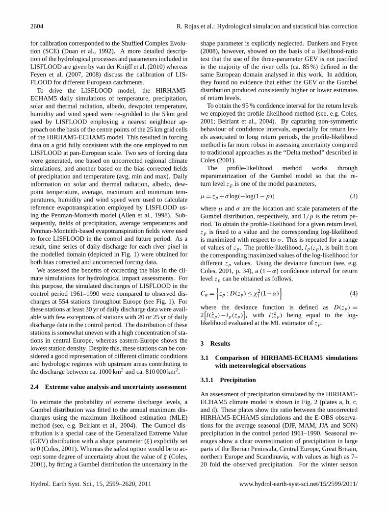
We assessed the benefits of correcting the bias in the cli-mate simulations for hydrological impact assessments. Forthis purpose, the simulated discharges of LISFLOOD in thecontrol period 1961–1990 were compared to observed dis-charges at 554 stations throughout Europe (see Fig.1). Forthese stations at least 30 yr of daily discharge data were avail-able with few exceptions of stations with 20 or 25 yr of dailydischarge data in the control period. The distribution of thesestations is somewhat uneven with a high concentration of sta-tions in central Europe, whereas eastern-Europe shows thelowest station density. Despite this, these stations can be con-sidered a good representation of different climatic conditionsand hydrologic regimes with upstream areas contributing tothe discharge between ca. 1000 km2 and ca. 810 000 km2.
2.4 Extreme value analysis and uncertainty assessment
To estimate the probability of extreme discharge levels, aGumbel distribution was fitted to the annual maximum dis-charges using the maximum likelihood estimation (MLE)method (see, e.g.Beirlant et al., 2004). The Gumbel dis-tribution is a special case of the Generalized Extreme Value(GEV) distribution with a shape parameter (ξ ) explicitly setto 0 (Coles, 2001). Whereas the safest option would be to ac-cept some degree of uncertainty about the value ofξ (Coles,2001), by fitting a Gumbel distribution the uncertainty in the
shape parameter is explicitly neglected.Dankers and Feyen(2008), however, showed on the basis of a likelihood-ratiotest that the use of the three-parameter GEV is not justifiedin the majority of the river cells (ca. 85 %) defined in thesame European domain analysed in this work. In addition,they found no evidence that either the GEV or the Gumbeldistribution produced consistently higher or lower estimatesof return levels.
To obtain the 95 % confidence interval for the return levelswe employed the profile-likelihood method (see, e.g.Coles,2001; Beirlant et al., 2004). By capturing non-symmetricbehaviour of confidence intervals, especially for return lev-els associated to long return periods, the profile-likelihoodmethod is far more robust in assessing uncertainty comparedto traditional approaches as the “Delta method” described inColes(2001).
The profile-likelihood method works throughreparametrization of the Gumbel model so that the re-turn levelzp is one of the model parameters,
µ = zp +σ log(−log(1−p)) (3)
whereµ andσ are the location and scale parameters of theGumbel distribution, respectively, and 1/p is the return pe-riod. To obtain the profile-likelihood for a given return level,zp is fixed to a value and the corresponding log-likelihoodis maximized with respect toσ . This is repeated for a rangeof values ofzp. The profile-likelihood,lp(zp), is built fromthe corresponding maximized values of the log-likelihood fordifferent zp values. Using the deviance function (see, e.g.Coles, 2001, p. 34), a (1−α) confidence interval for returnlevel zp can be obtained as follows,
Cα =
{zp : D(zp) ≤ χ2
1(1−α)}
(4)
where the deviance function is defined asD(zp) =
2[l(zp)− lp(zp)
], with l(zp) being equal to the log-
likelihood evaluated at the ML estimator ofzp.
3 Results
3.1 Comparison of HIRHAM5-ECHAM5 simulationswith meteorological observations
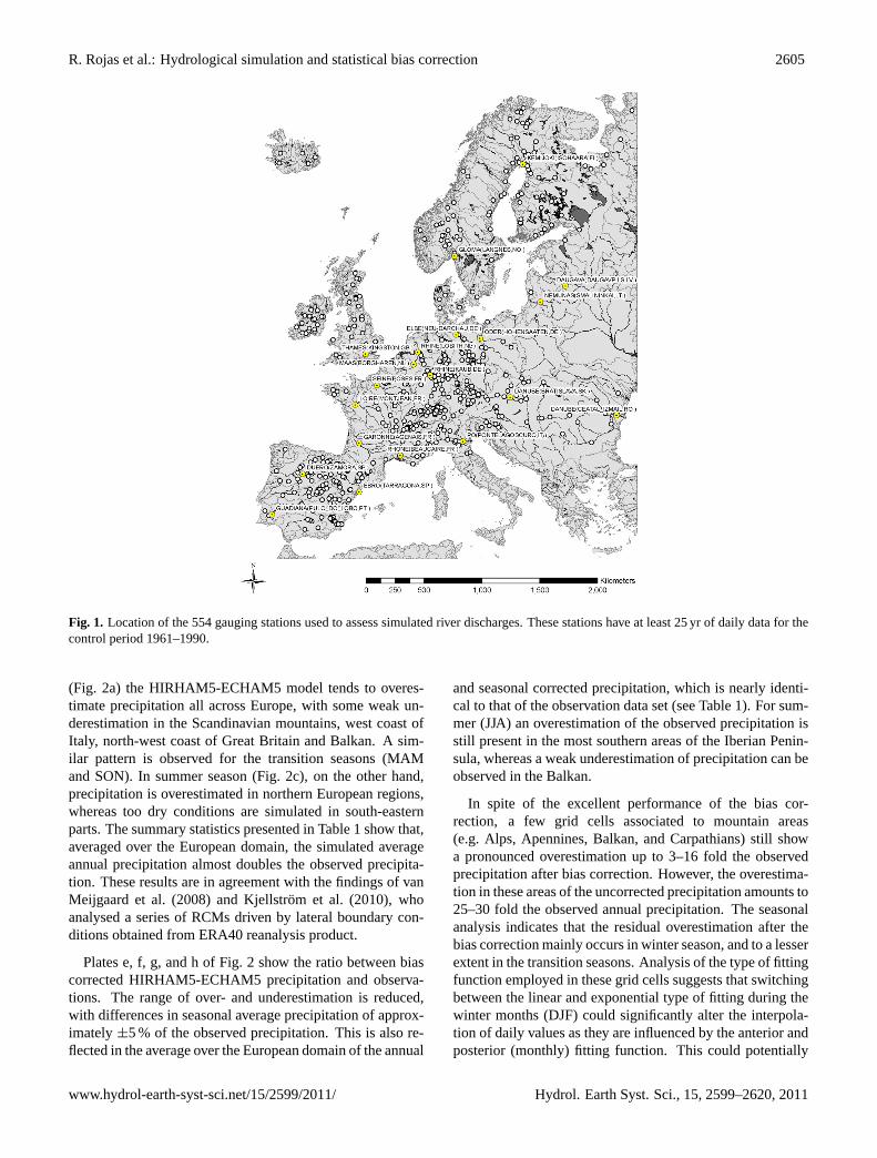
3.1.1 Precipitation
An assessment of precipitation simulated by the HIRHAM5-ECHAM5 climate model is shown in Fig.2 (plates a, b, c,and d). These plates show the ratio between the uncorrectedHIRHAM5-ECHAM5 simulations and the E-OBS observa-tions for the average seasonal (DJF, MAM, JJA and SON)precipitation in the control period 1961–1990. Seasonal av-erages show a clear overestimation of precipitation in largeparts of the Iberian Peninsula, Central Europe, Great Britain,northern Europe and Scandinavia, with values as high as 7–20 fold the observed precipitation. For the winter season
Hydrol. Earth Syst. Sci., 15, 2599–2620, 2011 www.hydrol-earth-syst-sci.net/15/2599/2011/
R. Rojas et al.: Hydrological simulation and statistical bias correction 2605
Fig. 1. Location of the 554 gauging stations used to assess simulated river discharges. These stations have at least 25 yr of daily data for thecontrol period 1961–1990.
(Fig. 2a) the HIRHAM5-ECHAM5 model tends to overes-timate precipitation all across Europe, with some weak un-derestimation in the Scandinavian mountains, west coast ofItaly, north-west coast of Great Britain and Balkan. A sim-ilar pattern is observed for the transition seasons (MAMand SON). In summer season (Fig.2c), on the other hand,precipitation is overestimated in northern European regions,whereas too dry conditions are simulated in south-easternparts. The summary statistics presented in Table1 show that,averaged over the European domain, the simulated averageannual precipitation almost doubles the observed precipita-tion. These results are in agreement with the findings ofvanMeijgaard et al.(2008) and Kjellstrom et al.(2010), whoanalysed a series of RCMs driven by lateral boundary con-ditions obtained from ERA40 reanalysis product.
Plates e, f, g, and h of Fig.2 show the ratio between biascorrected HIRHAM5-ECHAM5 precipitation and observa-tions. The range of over- and underestimation is reduced,with differences in seasonal average precipitation of approx-imately±5 % of the observed precipitation. This is also re-flected in the average over the European domain of the annual
and seasonal corrected precipitation, which is nearly identi-cal to that of the observation data set (see Table1). For sum-mer (JJA) an overestimation of the observed precipitation isstill present in the most southern areas of the Iberian Penin-sula, whereas a weak underestimation of precipitation can beobserved in the Balkan.
In spite of the excellent performance of the bias cor-rection, a few grid cells associated to mountain areas(e.g. Alps, Apennines, Balkan, and Carpathians) still showa pronounced overestimation up to 3–16 fold the observedprecipitation after bias correction. However, the overestima-tion in these areas of the uncorrected precipitation amounts to25–30 fold the observed annual precipitation. The seasonalanalysis indicates that the residual overestimation after thebias correction mainly occurs in winter season, and to a lesserextent in the transition seasons. Analysis of the type of fittingfunction employed in these grid cells suggests that switchingbetween the linear and exponential type of fitting during thewinter months (DJF) could significantly alter the interpola-tion of daily values as they are influenced by the anterior andposterior (monthly) fitting function. This could potentially
www.hydrol-earth-syst-sci.net/15/2599/2011/ Hydrol. Earth Syst. Sci., 15, 2599–2620, 2011
2606 R. Rojas et al.: Hydrological simulation and statistical bias correction
Fig. 2. Ratio between HIRHAM5-ECHAM5 simulations and observations of seasonal average precipitation for the control period 1961–1990. First row, uncorrected seasonal precipitation; second row, bias corrected seasonal precipitation.
Table 1. Summary statistics of precipitation (mmd−1) for the control period 1961–1990.
Statistics
Observed Bias corrected Uncorrected
Average annual precipitation 1.9 1.9 3.4Average annual max precipitation 28.3 30.6 47.83-d annual max precipitation 47.6 48.8 78.55-d annual max precipitation 59.1 60.0 97.97-d annual max precipitation 68.5 69.5 114.499th percentile precipitation 23.9 25.5 37.3Average seasonal precipitation (DJF) 1.8 1.8 3.8Average seasonal precipitation (MAM) 1.6 1.6 3.2Average seasonal precipitation (JJA) 2.0 2.0 2.8Average seasonal precipitation (SON) 2.1 2.1 3.9
modify the monthly statistics. A similar problem has beenrecognized byPiani et al.(2010b) in their global analysis.Aside from model deficiencies, the pronounced overestima-tion at high altitudes can in part be explained by the fact thatobserved precipitation typically underestimates true precipi-tation, especially in winter, due to poor station network den-
sity (see, e.g.Hofstra et al., 2010; Lenderink, 2010) that doesnot allow to fully capture orographic effects on precipitation.Hence, the bias-corrected precipitation in these areas maymore closely correspond to true precipitation amounts thanthe comparison with observed precipitation suggests here.
Hydrol. Earth Syst. Sci., 15, 2599–2620, 2011 www.hydrol-earth-syst-sci.net/15/2599/2011/
R. Rojas et al.: Hydrological simulation and statistical bias correction 2607
50°40°30°
20°
20°
10°
10°
0°
0°-10°-20°-30°
60° 60°
50° 50°
40° 40°
50°40°30°
20°
20°
10°
10°
0°
0°-10°-20°-30°
60° 60°
50° 50°
40° 40°
mean: 36.19; std: 34.60; min: -177.47; max: 166.03 mean: -6.83; std: 6.59; min: -44.03; max: 59.43a b
-5 +40+5 +30+10 +15 +20 +50-10-15-20
Difference wet days frequency
Uncorrected Bias corrected
>+100-30-40<-50
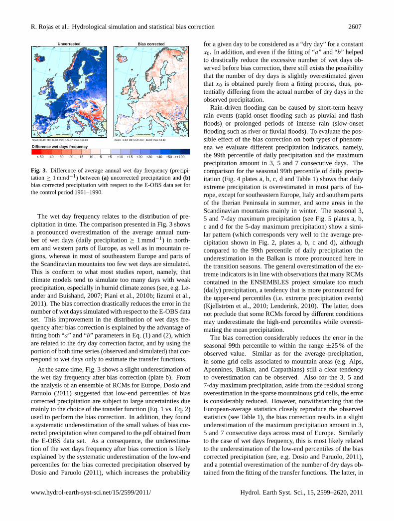
Fig. 3. Difference of average annual wet day frequency (precipi-tation ≥ 1 mmd−1) between(a) uncorrected precipitation and(b)bias corrected precipitation with respect to the E-OBS data set forthe control period 1961–1990.
The wet day frequency relates to the distribution of pre-cipitation in time. The comparison presented in Fig.3 showsa pronounced overestimation of the average annual num-ber of wet days (daily precipitation≥ 1 mmd−1) in north-ern and western parts of Europe, as well as in mountain re-gions, whereas in most of southeastern Europe and parts ofthe Scandinavian mountains too few wet days are simulated.This is conform to what most studies report, namely, thatclimate models tend to simulate too many days with weakprecipitation, especially in humid climate zones (see, e.g.Le-ander and Buishand, 2007; Piani et al., 2010b; Iizumi et al.,2011). The bias correction drastically reduces the error in thenumber of wet days simulated with respect to the E-OBS dataset. This improvement in the distribution of wet days fre-quency after bias correction is explained by the advantage offitting both “a” and “b” parameters in Eq. (1) and (2), whichare related to the dry day correction factor, and by using theportion of both time series (observed and simulated) that cor-respond to wet days only to estimate the transfer functions.
At the same time, Fig.3 shows a slight underestimation ofthe wet day frequency after bias correction (plate b). Fromthe analysis of an ensemble of RCMs for Europe,Dosio andParuolo(2011) suggested that low-end percentiles of biascorrected precipitation are subject to large uncertainties duemainly to the choice of the transfer function (Eq.1 vs. Eq.2)used to perform the bias correction. In addition, they founda systematic underestimation of the small values of bias cor-rected precipitation when compared to the pdf obtained fromthe E-OBS data set. As a consequence, the underestima-tion of the wet days frequency after bias correction is likelyexplained by the systematic underestimation of the low-endpercentiles for the bias corrected precipitation observed byDosio and Paruolo(2011), which increases the probability
for a given day to be considered as a “dry day” for a constantx0. In addition, and even if the fitting of “a” and “b” helpedto drastically reduce the excessive number of wet days ob-served before bias correction, there still exists the possibilitythat the number of dry days is slightly overestimated giventhat x0 is obtained purely from a fitting process, thus, po-tentially differing from the actual number of dry days in theobserved precipitation.
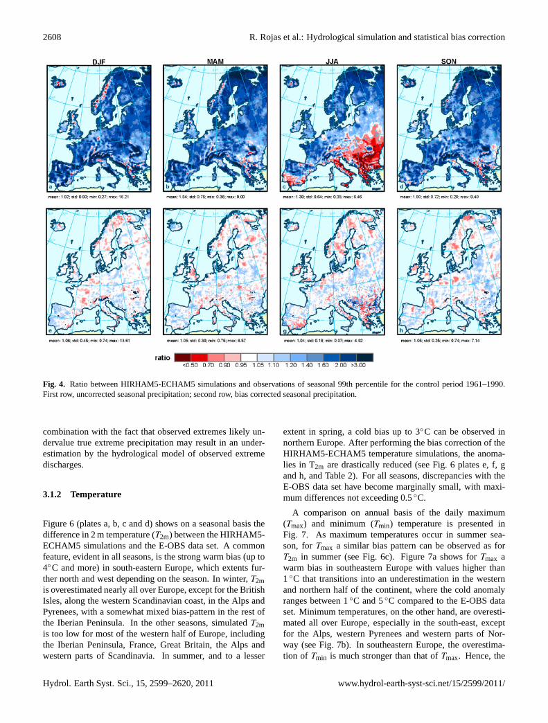
Rain-driven flooding can be caused by short-term heavyrain events (rapid-onset flooding such as pluvial and flashfloods) or prolonged periods of intense rain (slow-onsetflooding such as river or fluvial floods). To evaluate the pos-sible effect of the bias correction on both types of phenom-ena we evaluate different precipitation indicators, namely,the 99th percentile of daily precipitation and the maximumprecipitation amount in 3, 5 and 7 consecutive days. Thecomparison for the seasonal 99th percentile of daily precip-itation (Fig.4 plates a, b, c, d and Table1) shows that dailyextreme precipitation is overestimated in most parts of Eu-rope, except for southeastern Europe, Italy and southern partsof the Iberian Peninsula in summer, and some areas in theScandinavian mountains mainly in winter. The seasonal 3,5 and 7-day maximum precipitation (see Fig.5 plates a, b,c and d for the 5-day maximum precipitation) show a simi-lar pattern (which corresponds very well to the average pre-cipitation shown in Fig.2, plates a, b, c and d), althoughcompared to the 99th percentile of daily precipitation theunderestimation in the Balkan is more pronounced here inthe transition seasons. The general overestimation of the ex-treme indicators is in line with observations that many RCMscontained in the ENSEMBLES project simulate too much(daily) precipitation, a tendency that is more pronounced forthe upper-end percentiles (i.e. extreme precipitation events)(Kjellstrom et al., 2010; Lenderink, 2010). The latter, doesnot preclude that some RCMs forced by different conditionsmay underestimate the high-end percentiles while overesti-mating the mean precipitation.
The bias correction considerably reduces the error in theseasonal 99th percentile to within the range±25 % of theobserved value. Similar as for the average precipitation,in some grid cells associated to mountain areas (e.g. Alps,Apennines, Balkan, and Carpathians) still a clear tendencyto overestimation can be observed. Also for the 3, 5 and7-day maximum precipitation, aside from the residual strongoverestimation in the sparse mountainous grid cells, the erroris considerably reduced. However, notwithstanding that theEuropean-average statistics closely reproduce the observedstatistics (see Table1), the bias correction results in a slightunderestimation of the maximum precipitation amount in 3,5 and 7 consecutive days across most of Europe. Similarlyto the case of wet days frequency, this is most likely relatedto the underestimation of the low-end percentiles of the biascorrected precipitation (see, e.g.Dosio and Paruolo, 2011),and a potential overestimation of the number of dry days ob-tained from the fitting of the transfer functions. The latter, in
www.hydrol-earth-syst-sci.net/15/2599/2011/ Hydrol. Earth Syst. Sci., 15, 2599–2620, 2011
2608 R. Rojas et al.: Hydrological simulation and statistical bias correction
Fig. 4. Ratio between HIRHAM5-ECHAM5 simulations and observations of seasonal 99th percentile for the control period 1961–1990.First row, uncorrected seasonal precipitation; second row, bias corrected seasonal precipitation.
combination with the fact that observed extremes likely un-dervalue true extreme precipitation may result in an under-estimation by the hydrological model of observed extremedischarges.
3.1.2 Temperature
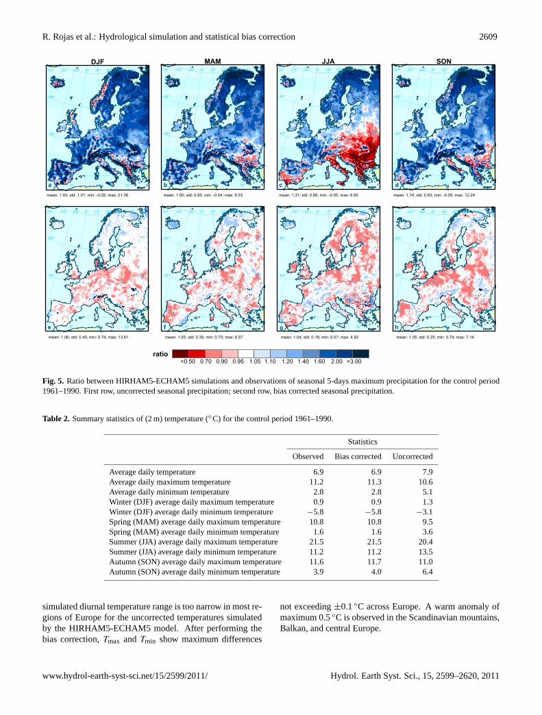
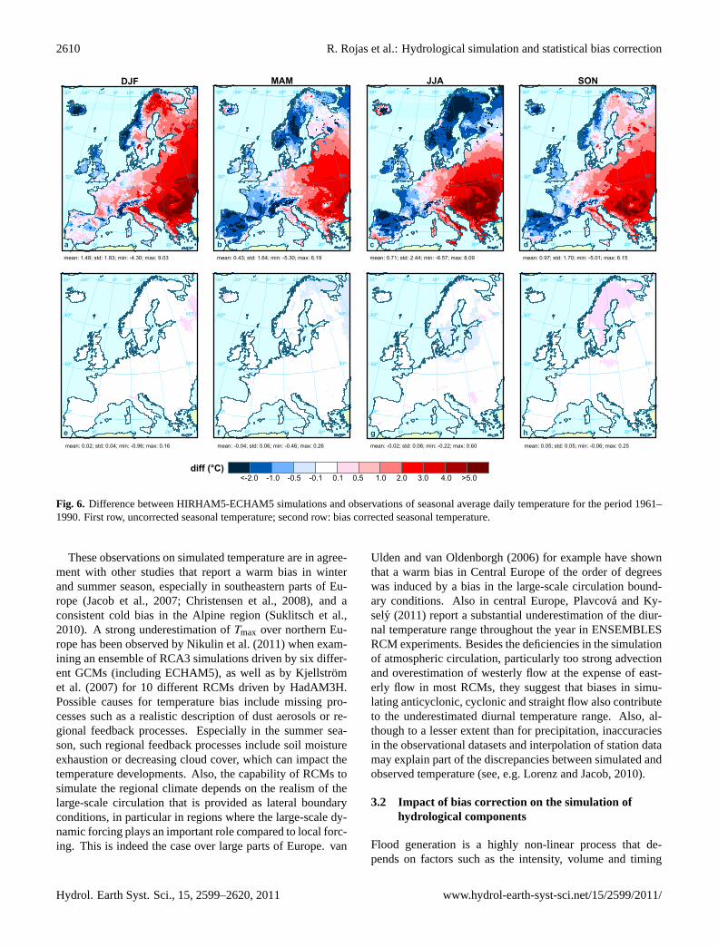
Figure6 (plates a, b, c and d) shows on a seasonal basis thedifference in 2 m temperature (T2m) between the HIRHAM5-ECHAM5 simulations and the E-OBS data set. A commonfeature, evident in all seasons, is the strong warm bias (up to4◦C and more) in south-eastern Europe, which extents fur-ther north and west depending on the season. In winter,T2mis overestimated nearly all over Europe, except for the BritishIsles, along the western Scandinavian coast, in the Alps andPyrenees, with a somewhat mixed bias-pattern in the rest ofthe Iberian Peninsula. In the other seasons, simulatedT2mis too low for most of the western half of Europe, includingthe Iberian Peninsula, France, Great Britain, the Alps andwestern parts of Scandinavia. In summer, and to a lesser
extent in spring, a cold bias up to 3◦C can be observed innorthern Europe. After performing the bias correction of theHIRHAM5-ECHAM5 temperature simulations, the anoma-lies in T2m are drastically reduced (see Fig.6 plates e, f, gand h, and Table2). For all seasons, discrepancies with theE-OBS data set have become marginally small, with maxi-mum differences not exceeding 0.5◦C.
A comparison on annual basis of the daily maximum(Tmax) and minimum (Tmin) temperature is presented inFig. 7. As maximum temperatures occur in summer sea-son, forTmax a similar bias pattern can be observed as forT2m in summer (see Fig.6c). Figure7a shows forTmax awarm bias in southeastern Europe with values higher than1◦C that transitions into an underestimation in the westernand northern half of the continent, where the cold anomalyranges between 1◦C and 5◦C compared to the E-OBS dataset. Minimum temperatures, on the other hand, are overesti-mated all over Europe, especially in the south-east, exceptfor the Alps, western Pyrenees and western parts of Nor-way (see Fig.7b). In southeastern Europe, the overestima-tion of Tmin is much stronger than that ofTmax. Hence, the
Hydrol. Earth Syst. Sci., 15, 2599–2620, 2011 www.hydrol-earth-syst-sci.net/15/2599/2011/
R. Rojas et al.: Hydrological simulation and statistical bias correction 2609
50°40°30°
20°
20°
10°
10°
0°
0°-10°-20°-30°
60° 60°
50° 50°
40° 40°
50°40°30°
20°
20°
10°
10°
0°
0°-10°-20°-30°
60° 60°
50° 50°
40° 40°
50°40°30°
20°
20°
10°
10°
0°
0°-10°-20°-30°
60° 60°
50° 50°
40° 40°
50°40°30°
20°
20°
10°
10°
0°
0°-10°-20°-30°
60° 60°
50° 50°
40° 40°
50°40°30°
20°
20°
10°
10°
0°
0°-10°-20°-30°
60° 60°
50° 50°
40° 40°
50°40°30°
20°
20°
10°
10°
0°
0°-10°-20°-30°
60° 60°
50° 50°
40° 40°
50°40°30°
20°
20°
10°
10°
0°
0°-10°-20°-30°
60° 60°
50° 50°
40° 40°
b
hgfe
dc
50°40°30°
20°
20°
10°
10°
0°
0°-10°-20°-30°
60° 60°
50° 50°
40° 40°
amean: 1.93; std: 1.01; min: -0.02; max: 21.38 mean: 1.31; std: 0.68; min: -0.05; max: 6.99mean: 1.80; std: 0.85; min: -0.04; max: 9.53 mean: 1.74; std: 0.83; min: -0.05; max: 12.24
mean: 1.04; std: 0.18; min: 0.07; max: 4.92 mean: 1.05; std: 0.25; min: 0.74; max: 7.14mean: 1.06; std: 0.45; min: 0.74; max: 13.61 mean: 1.05; std: 0.30; min: 0.75; max: 6.57
1.05 1.10 1.20 1.40 1.60 2.00 >3.000.950.900.70<0.50ratio
DJF SONJJAMAM
Fig. 5. Ratio between HIRHAM5-ECHAM5 simulations and observations of seasonal 5-days maximum precipitation for the control period1961–1990. First row, uncorrected seasonal precipitation; second row, bias corrected seasonal precipitation.
Table 2. Summary statistics of (2 m) temperature (◦C) for the control period 1961–1990.
Statistics
Observed Bias corrected Uncorrected
Average daily temperature 6.9 6.9 7.9Average daily maximum temperature 11.2 11.3 10.6Average daily minimum temperature 2.8 2.8 5.1Winter (DJF) average daily maximum temperature 0.9 0.9 1.3Winter (DJF) average daily minimum temperature −5.8 −5.8 −3.1Spring (MAM) average daily maximum temperature 10.8 10.8 9.5Spring (MAM) average daily minimum temperature 1.6 1.6 3.6Summer (JJA) average daily maximum temperature 21.5 21.5 20.4Summer (JJA) average daily minimum temperature 11.2 11.2 13.5Autumn (SON) average daily maximum temperature 11.6 11.7 11.0Autumn (SON) average daily minimum temperature 3.9 4.0 6.4
simulated diurnal temperature range is too narrow in most re-gions of Europe for the uncorrected temperatures simulatedby the HIRHAM5-ECHAM5 model. After performing thebias correction,Tmax andTmin show maximum differences
not exceeding±0.1◦C across Europe. A warm anomaly ofmaximum 0.5◦C is observed in the Scandinavian mountains,Balkan, and central Europe.
www.hydrol-earth-syst-sci.net/15/2599/2011/ Hydrol. Earth Syst. Sci., 15, 2599–2620, 2011
2610 R. Rojas et al.: Hydrological simulation and statistical bias correction
50°40°30°
20°
20°
10°
10°
0°
0°-10°-20°-30°
60° 60°
50° 50°
40° 40°
50°40°30°
20°
20°
10°
10°
0°
0°-10°-20°-30°
60° 60°
50° 50°
40° 40°
50°40°30°
20°
20°
10°
10°
0°
0°-10°-20°-30°
60° 60°
50° 50°
40° 40°
50°40°30°
20°
20°
10°
10°
0°
0°-10°-20°-30°
60° 60°
50° 50°
40° 40°
50°40°30°
20°
20°
10°
10°
0°
0°-10°-20°-30°
60° 60°
50° 50°
40° 40°
50°40°30°
20°
20°
10°
10°
0°
0°-10°-20°-30°
60° 60°
50° 50°
40° 40°
50°40°30°
20°
20°
10°
10°
0°
0°-10°-20°-30°
60° 60°
50° 50°
40° 40°
b
hgfe
dc
50°40°30°
20°
20°
10°
10°
0°
0°-10°-20°-30°
60° 60°
50° 50°
40° 40°
amean: 1.48; std: 1.83; min: -4.30; max: 9.03 mean: 0.71; std: 2.44; min: -8.57; max: 8.09mean: 0.43; std: 1.64; min: -5.30; max: 6.19 mean: 0.97; std: 1.70; min: -5.01; max: 6.15
mean: -0.02; std: 0.06; min: -0.22; max: 0.60 mean: 0.05; std: 0.05; min: -0.06; max: 0.25mean: 0.02; std: 0.04; min: -0.96; max: 0.16 mean: -0.04; std: 0.06; min: -0.46; max: 0.26
0.1 0.5 1.0 2.0 3.0 4.0 >5.0-0.1-0.5-1.0<-2.0diff (°C)
DJF MAM JJA SON
Fig. 6. Difference between HIRHAM5-ECHAM5 simulations and observations of seasonal average daily temperature for the period 1961–1990. First row, uncorrected seasonal temperature; second row: bias corrected seasonal temperature.
These observations on simulated temperature are in agree-ment with other studies that report a warm bias in winterand summer season, especially in southeastern parts of Eu-rope (Jacob et al., 2007; Christensen et al., 2008), and aconsistent cold bias in the Alpine region (Suklitsch et al.,2010). A strong underestimation ofTmax over northern Eu-rope has been observed byNikulin et al. (2011) when exam-ining an ensemble of RCA3 simulations driven by six differ-ent GCMs (including ECHAM5), as well as byKjellstromet al. (2007) for 10 different RCMs driven by HadAM3H.Possible causes for temperature bias include missing pro-cesses such as a realistic description of dust aerosols or re-gional feedback processes. Especially in the summer sea-son, such regional feedback processes include soil moistureexhaustion or decreasing cloud cover, which can impact thetemperature developments. Also, the capability of RCMs tosimulate the regional climate depends on the realism of thelarge-scale circulation that is provided as lateral boundaryconditions, in particular in regions where the large-scale dy-namic forcing plays an important role compared to local forc-ing. This is indeed the case over large parts of Europe.van
Ulden and van Oldenborgh(2006) for example have shownthat a warm bias in Central Europe of the order of degreeswas induced by a bias in the large-scale circulation bound-ary conditions. Also in central Europe,Plavcova and Ky-sely (2011) report a substantial underestimation of the diur-nal temperature range throughout the year in ENSEMBLESRCM experiments. Besides the deficiencies in the simulationof atmospheric circulation, particularly too strong advectionand overestimation of westerly flow at the expense of east-erly flow in most RCMs, they suggest that biases in simu-lating anticyclonic, cyclonic and straight flow also contributeto the underestimated diurnal temperature range. Also, al-though to a lesser extent than for precipitation, inaccuraciesin the observational datasets and interpolation of station datamay explain part of the discrepancies between simulated andobserved temperature (see, e.g.Lorenz and Jacob, 2010).
3.2 Impact of bias correction on the simulation ofhydrological components
Flood generation is a highly non-linear process that de-pends on factors such as the intensity, volume and timing
Hydrol. Earth Syst. Sci., 15, 2599–2620, 2011 www.hydrol-earth-syst-sci.net/15/2599/2011/
R. Rojas et al.: Hydrological simulation and statistical bias correction 2611
50°40°30°
20°
20°
10°
10°
0°
0°-10°-20°-30°
60° 60°
50° 50°
40° 40°
50°40°30°
20°
20°
10°
10°
0°
0°-10°-20°-30°
60° 60°
50° 50°
40° 40°
50°40°30°
20°
20°
10°
10°
0°
0°-10°-20°-30°
60° 60°
50° 50°
40° 40°
50°40°30°
20°
20°
10°
10°
0°
0°-10°-20°-30°
60° 60°
50° 50°
40° 40°
mean: -0.60; std: 3.25; min: -8.15; max: 99.6a
mean: 2.36; std: 2.86; min: -4.27; max: 94.72
b
mean: 0.10; std: 2.60; min: -0.94; max: 1.02
cmean: 0.10; std: 2.44; min: -0.31; max: 0.95
d
Tmax Tmin
-0.1 >5.04.03.02.00.5 1.00.1-0.5-1.0<-2.0diff (°C)
Unc
orre
cted
Bia
s co
rrec
ted
Fig. 7. Differences for daily maximum (Tmax) and minimum (Tmin)temperature simulated by HIRHAM5-ECHAM5 and the E-OBSdata set for the control period 1961–1990. First row, uncorrectedannual temperature; second row: bias corrected annual temperature.
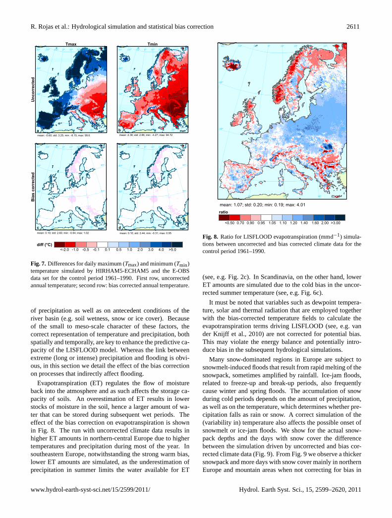
of precipitation as well as on antecedent conditions of theriver basin (e.g. soil wetness, snow or ice cover). Becauseof the small to meso-scale character of these factors, thecorrect representation of temperature and precipitation, bothspatially and temporally, are key to enhance the predictive ca-pacity of the LISFLOOD model. Whereas the link betweenextreme (long or intense) precipitation and flooding is obvi-ous, in this section we detail the effect of the bias correctionon processes that indirectly affect flooding.
Evapotranspiration (ET) regulates the flow of moistureback into the atmosphere and as such affects the storage ca-pacity of soils. An overestimation of ET results in lowerstocks of moisture in the soil, hence a larger amount of wa-ter that can be stored during subsequent wet periods. Theeffect of the bias correction on evapotranspiration is shownin Fig. 8. The run with uncorrected climate data results inhigher ET amounts in northern-central Europe due to highertemperatures and precipitation during most of the year. Insoutheastern Europe, notwithstanding the strong warm bias,lower ET amounts are simulated, as the underestimation ofprecipitation in summer limits the water available for ET
50°40°30°
20°
20°
10°
10°
0°
0°-10°-20°-30°
60° 60°
50° 50°
40° 40°
mean: 1.07; std: 0.20; min: 0.19; max: 4.01
1.05 1.10 1.200.95 1.40 1.60 2.00 >3.000.900.70<0.50
ratio
Fig. 8. Ratio for LISFLOOD evapotranspiration (mmd−1) simula-tions between uncorrected and bias corrected climate data for thecontrol period 1961–1990.
(see, e.g. Fig.2c). In Scandinavia, on the other hand, lowerET amounts are simulated due to the cold bias in the uncor-rected summer temperature (see, e.g. Fig.6c).
It must be noted that variables such as dewpoint tempera-ture, solar and thermal radiation that are employed togetherwith the bias-corrected temperature fields to calculate theevapotranspiration terms driving LISFLOOD (see, e.g.vander Knijff et al., 2010) are not corrected for potential bias.This may violate the energy balance and potentially intro-duce bias in the subsequent hydrological simulations.
Many snow-dominated regions in Europe are subject tosnowmelt-induced floods that result from rapid melting of thesnowpack, sometimes amplified by rainfall. Ice-jam floods,related to freeze-up and break-up periods, also frequentlycause winter and spring floods. The accumulation of snowduring cold periods depends on the amount of precipitation,as well as on the temperature, which determines whether pre-cipitation falls as rain or snow. A correct simulation of the(variability in) temperature also affects the possible onset ofsnowmelt or ice-jam floods. We show for the actual snow-pack depths and the days with snow cover the differencebetween the simulation driven by uncorrected and bias cor-rected climate data (Fig.9). From Fig.9 we observe a thickersnowpack and more days with snow cover mainly in northernEurope and mountain areas when not correcting for bias in
www.hydrol-earth-syst-sci.net/15/2599/2011/ Hydrol. Earth Syst. Sci., 15, 2599–2620, 2011
2612 R. Rojas et al.: Hydrological simulation and statistical bias correction
50°40°30°
20°
20°
10°
10°
0°
0°-10°-20°-30°
60° 60°
50° 50°
40° 40°
50°40°30°
20°
20°
10°
10°
0°
0°-10°-20°-30°
60° 60°
50° 50°
40° 40°
mean: 602.9; std: 6111.8; min: -615.4; max: 221704.0 mean: 3.5; std: 30.2; min: -353.1; max: 303.9a b
snowpack depth (mm SWE) days with snow cover
3-7 -3 >112845628147-14
<-75
<-28
-50 -25 -10 10 100755025 250 >500diff. mm SWE
diff. days
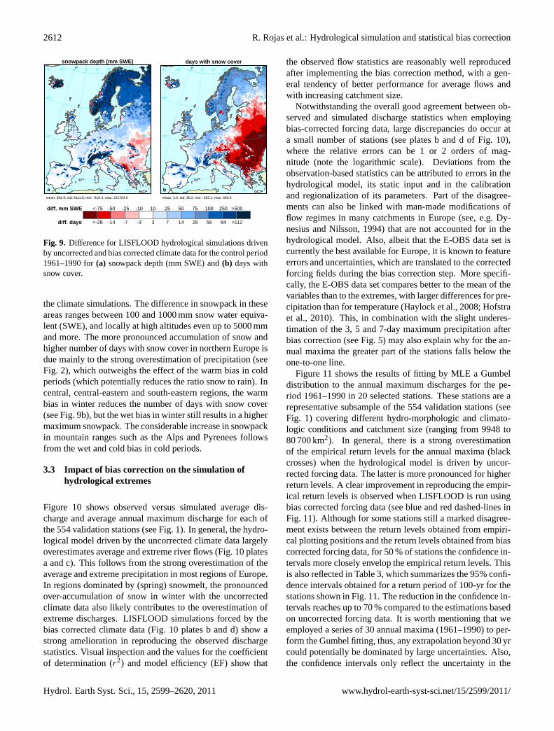
Fig. 9. Difference for LISFLOOD hydrological simulations drivenby uncorrected and bias corrected climate data for the control period1961–1990 for(a) snowpack depth (mm SWE) and(b) days withsnow cover.
the climate simulations. The difference in snowpack in theseareas ranges between 100 and 1000 mm snow water equiva-lent (SWE), and locally at high altitudes even up to 5000 mmand more. The more pronounced accumulation of snow andhigher number of days with snow cover in northern Europe isdue mainly to the strong overestimation of precipitation (seeFig. 2), which outweighs the effect of the warm bias in coldperiods (which potentially reduces the ratio snow to rain). Incentral, central-eastern and south-eastern regions, the warmbias in winter reduces the number of days with snow cover(see Fig.9b), but the wet bias in winter still results in a highermaximum snowpack. The considerable increase in snowpackin mountain ranges such as the Alps and Pyrenees followsfrom the wet and cold bias in cold periods.
3.3 Impact of bias correction on the simulation ofhydrological extremes
Figure 10 shows observed versus simulated average dis-charge and average annual maximum discharge for each ofthe 554 validation stations (see Fig.1). In general, the hydro-logical model driven by the uncorrected climate data largelyoverestimates average and extreme river flows (Fig.10platesa and c). This follows from the strong overestimation of theaverage and extreme precipitation in most regions of Europe.In regions dominated by (spring) snowmelt, the pronouncedover-accumulation of snow in winter with the uncorrectedclimate data also likely contributes to the overestimation ofextreme discharges. LISFLOOD simulations forced by thebias corrected climate data (Fig.10 plates b and d) show astrong amelioration in reproducing the observed dischargestatistics. Visual inspection and the values for the coefficientof determination (r2) and model efficiency (EF) show that
the observed flow statistics are reasonably well reproducedafter implementing the bias correction method, with a gen-eral tendency of better performance for average flows andwith increasing catchment size.
Notwithstanding the overall good agreement between ob-served and simulated discharge statistics when employingbias-corrected forcing data, large discrepancies do occur ata small number of stations (see plates b and d of Fig.10),where the relative errors can be 1 or 2 orders of mag-nitude (note the logarithmic scale). Deviations from theobservation-based statistics can be attributed to errors in thehydrological model, its static input and in the calibrationand regionalization of its parameters. Part of the disagree-ments can also be linked with man-made modifications offlow regimes in many catchments in Europe (see, e.g.Dy-nesius and Nilsson, 1994) that are not accounted for in thehydrological model. Also, albeit that the E-OBS data set iscurrently the best available for Europe, it is known to featureerrors and uncertainties, which are translated to the correctedforcing fields during the bias correction step. More specifi-cally, the E-OBS data set compares better to the mean of thevariables than to the extremes, with larger differences for pre-cipitation than for temperature (Haylock et al., 2008; Hofstraet al., 2010). This, in combination with the slight underes-timation of the 3, 5 and 7-day maximum precipitation afterbias correction (see Fig.5) may also explain why for the an-nual maxima the greater part of the stations falls below theone-to-one line.
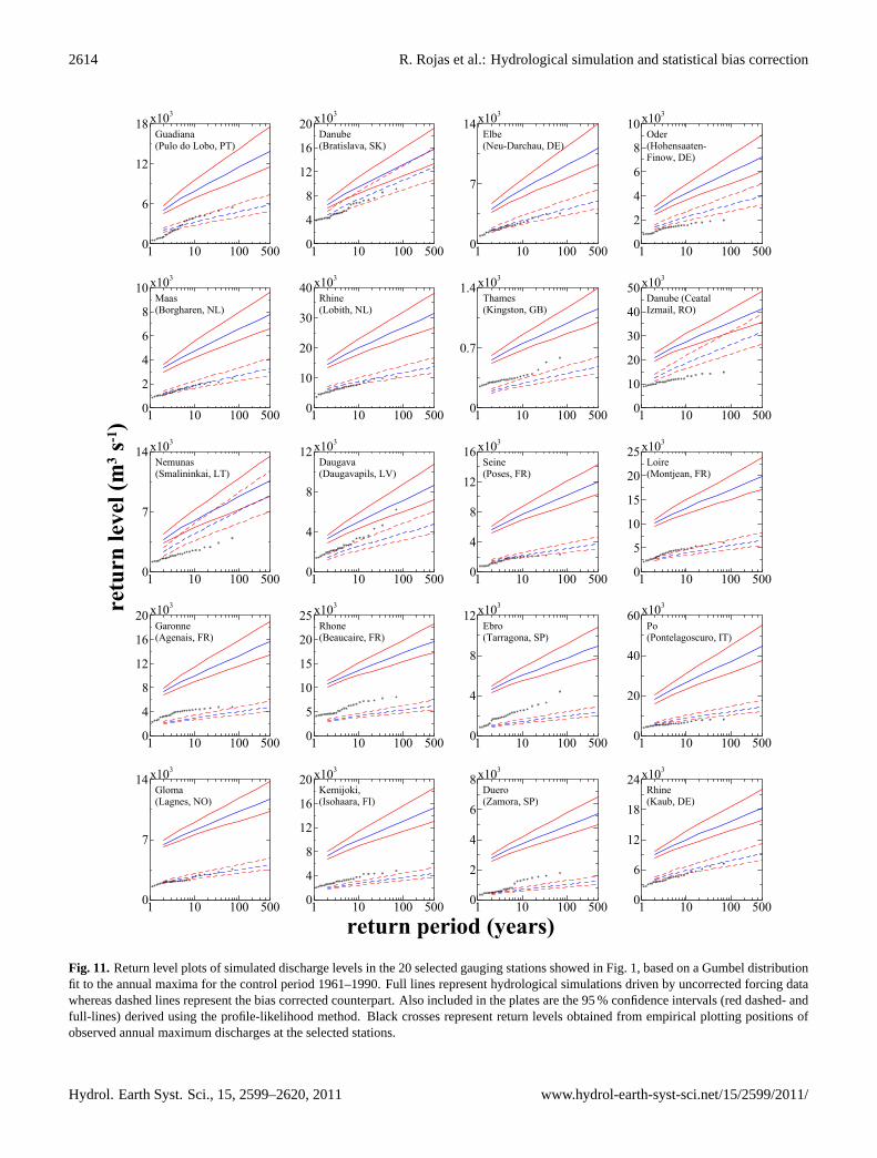
Figure11 shows the results of fitting by MLE a Gumbeldistribution to the annual maximum discharges for the pe-riod 1961–1990 in 20 selected stations. These stations are arepresentative subsample of the 554 validation stations (seeFig. 1) covering different hydro-morphologic and climato-logic conditions and catchment size (ranging from 9948 to80 700 km2). In general, there is a strong overestimationof the empirical return levels for the annual maxima (blackcrosses) when the hydrological model is driven by uncor-rected forcing data. The latter is more pronounced for higherreturn levels. A clear improvement in reproducing the empir-ical return levels is observed when LISFLOOD is run usingbias corrected forcing data (see blue and red dashed-lines inFig. 11). Although for some stations still a marked disagree-ment exists between the return levels obtained from empiri-cal plotting positions and the return levels obtained from biascorrected forcing data, for 50 % of stations the confidence in-tervals more closely envelop the empirical return levels. Thisis also reflected in Table3, which summarizes the 95% confi-dence intervals obtained for a return period of 100-yr for thestations shown in Fig.11. The reduction in the confidence in-tervals reaches up to 70 % compared to the estimations basedon uncorrected forcing data. It is worth mentioning that weemployed a series of 30 annual maxima (1961–1990) to per-form the Gumbel fitting, thus, any extrapolation beyond 30 yrcould potentially be dominated by large uncertainties. Also,the confidence intervals only reflect the uncertainty in the
Hydrol. Earth Syst. Sci., 15, 2599–2620, 2011 www.hydrol-earth-syst-sci.net/15/2599/2011/

R. Rojas et al.: Hydrological simulation and statistical bias correction 2613
Table 3. 95 % confidence intervals obtained using the profile-likelihood method for a return period of 100-yr for the gauging stationsdepicted in Fig.1 for the control period 1961–1990. Observed column corresponds toQ100 obtained from a Gumbel distribution fitted fromthe observations. All values in m3s−1 (values in parentheses show the percentage reduction).
Forcing input data
Stations Country Observed Uncorrected Bias corrected(Gumbel fitting)
Guadiana, Pulo do Lobo PT 4521 [9598–14 239] [4027–6008] (57.3 %)Danube, Bratislava SK 7435 [11 356–15 957] [8951–12 973] (12.6 %)Elbe, Neu-Darchau DE 3038 [7742–11 343] [3373–5109] (51.8 %)Oder, Hohensaaten-Finow DE 1933 [5058–7394] [2730–4055] (43.3 %)Maas, Borgharen NL 2105 [5610–7938] [2260–3352] (53.1 %)Rhine, Lobith NL 9336 [23 190–31 827] [10 105–13 985] (55.1 %)Thames, Kingston GB 500 [866–1172] [341–490] (51.3 %)Danube, Ceatal Izmail RO 13 825 [31 519–41 268] [22 430-31 932] (2.5 %)Nemunas, Smalininkai LT 2963 [7290–10 901] [5678–9260] (0.8 %)Daugava, Daugavapils LV 3887 [6033–8782] [3156–4842] (38.7 %)Seine, Poses FR 2296 [8940–12 041] [2598–3798] (61.3 %)Loire, Montjean FR 5715 [15 116–20 099] [4664–6724] (58.7 %)Garonne, Agenais FR 5143 [11 612–15 898] [3490–4804] (69.3 %)Rhone, Beaucaire FR 7142 [15 366–19 898] [4753–6269] (66.6 %)Ebro, Tarragona SP 3245 [6839–9199] [1687–2400] (69.8 %)Po, Pontelagoscuro IT 8280 [31 623–45 357] [10 338–14 659] (68.5 %)Gloma, Langnes NO 2982 [9172–11 838] [3090–4092] (62.4 %)Kemijoki, Isohaara FI 4222 [11 396–15 591] [3193–4418] (70.8 %)Duero, Zamora SP 1340 [4323–5778] [841–1275] (70.2 %)Rhine, Kaub DE 5975 [13 781–18 590] [6782–9358] (46.4 %)
101 102 103 104 105
observed (m3 s-1)
101
102
103
104
105
sim
ulat
ed (m
3 s-1
)
100 101 102 103 104 105
observed (m3 s-1)
100
101
102
103
104
105
sim
ulat
ed (m
3 s-1
)
a
d
r2 = -0.93EF = -0.39
r2 = -0.92EF = -0.89
100 101 102 103 104 105
observed (m3 s-1)
100
101
102
103
104
105
sim
ulat
ed (m
3 s-1
)
b
r2 = -0.99EF = -0.99
101 102 103 104 105
observed (m3 s-1)
101
102
103
104
105
sim
ulat
ed (m
3 s-1)
c
r2 = -0.87EF = -1.89
Uncorrected Bias corrected
Ave
rage
dis
char
geA
vera
ge a
nnua
l max
ima
Fig. 10. Observed versus simulated average discharge(a, b) and average annual maximum discharge(c, d) for each of the 554 stationsdepicted in Fig.1 for the control period 1961–1990. Left and right columns show hydrological simulations driven by uncorrected and biascorrected climate data, respectively.
www.hydrol-earth-syst-sci.net/15/2599/2011/ Hydrol. Earth Syst. Sci., 15, 2599–2620, 2011
2614 R. Rojas et al.: Hydrological simulation and statistical bias correction
1 10 1000
6
12
18 x103
500 1 10 1000
4
8
12
16
20 x103
500 1 10 1000
7
14 x103
500 1 10 1000
2
4
6
8
10 x103
500
1 10 1000
2
4
6
8
10 x103
500 1 10 1000
10
20
30
40 x103
500 1 10 1000
0.7
1.4 x10³
500 1 10 1000
10
20
30
40
50 x103
500
1 10 1000
7
14 x103
500 1 10 1000
4
8
12 x103
500 1 10 1000
4
8
12
16 x103
500 1 10 1000
5
10
15
20
25 x103
500
1 10 1000
4
8
12
16
20 x103
500 1 10 1000
5
10
15
20
25 x103
500 1 10 1000
4
8
12 x103
500 1 10 1000
20
40
60 x103
500
1 10 1000
7
14 x103
500 1 10 1000
4
8
12
16
20 x103
500 1 10 1000
2
4
6
8 x10³
500 1 10 1000
6
12
18
24 x103
500
return period (years)
retu
rn le
vel (
m3 s
-1)
Guadiana (Pulo do Lobo, PT)
Danube(Bratislava, SK)
Elbe(Neu-Darchau, DE)
Oder(Hohensaaten-Finow, DE)
Maas(Borgharen, NL)
Rhine(Lobith, NL)
Thames(Kingston, GB)
Danube (CeatalIzmail, RO)
Nemunas(Smalininkai, LT)
Daugava(Daugavapils, LV)
Seine(Poses, FR)
Loire(Montjean, FR)
Garonne(Agenais, FR)
Rhone(Beaucaire, FR)
Ebro(Tarragona, SP)
Po(Pontelagoscuro, IT)
Gloma(Lagnes, NO)
Kemijoki,(Isohaara, FI)
Duero(Zamora, SP)
Rhine(Kaub, DE)
Figure 1: Return level plots of simulated discharge levels in the 20 selected gauging stations showedin Fig. 1, based on a Gumbel distribution fit to the annual maxima for the control period 1961–1990.Full lines represent hydrological simulations driven by uncorrected forcing data whereas dashed linesrepresent the bias corrected counterpart. Also included in the plates are the 95% confidence intervals(red dashed- and full-lines) derived using the profile-likelihood method. Black crosses represent returnlevels obtained from empirical plotting positions of observed annual maximum discharges at the selectedstations.
4
Fig. 11.Return level plots of simulated discharge levels in the 20 selected gauging stations showed in Fig.1, based on a Gumbel distributionfit to the annual maxima for the control period 1961–1990. Full lines represent hydrological simulations driven by uncorrected forcing datawhereas dashed lines represent the bias corrected counterpart. Also included in the plates are the 95 % confidence intervals (red dashed- andfull-lines) derived using the profile-likelihood method. Black crosses represent return levels obtained from empirical plotting positions ofobserved annual maximum discharges at the selected stations.
Hydrol. Earth Syst. Sci., 15, 2599–2620, 2011 www.hydrol-earth-syst-sci.net/15/2599/2011/
R. Rojas et al.: Hydrological simulation and statistical bias correction 2615
50°40°30°
20°
20°
10°
10°
0°
0°-10°-20°-30°
60° 60°
50° 50°
40° 40°
mean: 2.47; std: 1.70; min: 0.14; max: 44.86
0.950.90 >3.002.001.601.401.10 1.201.050.70<0.50
ratio
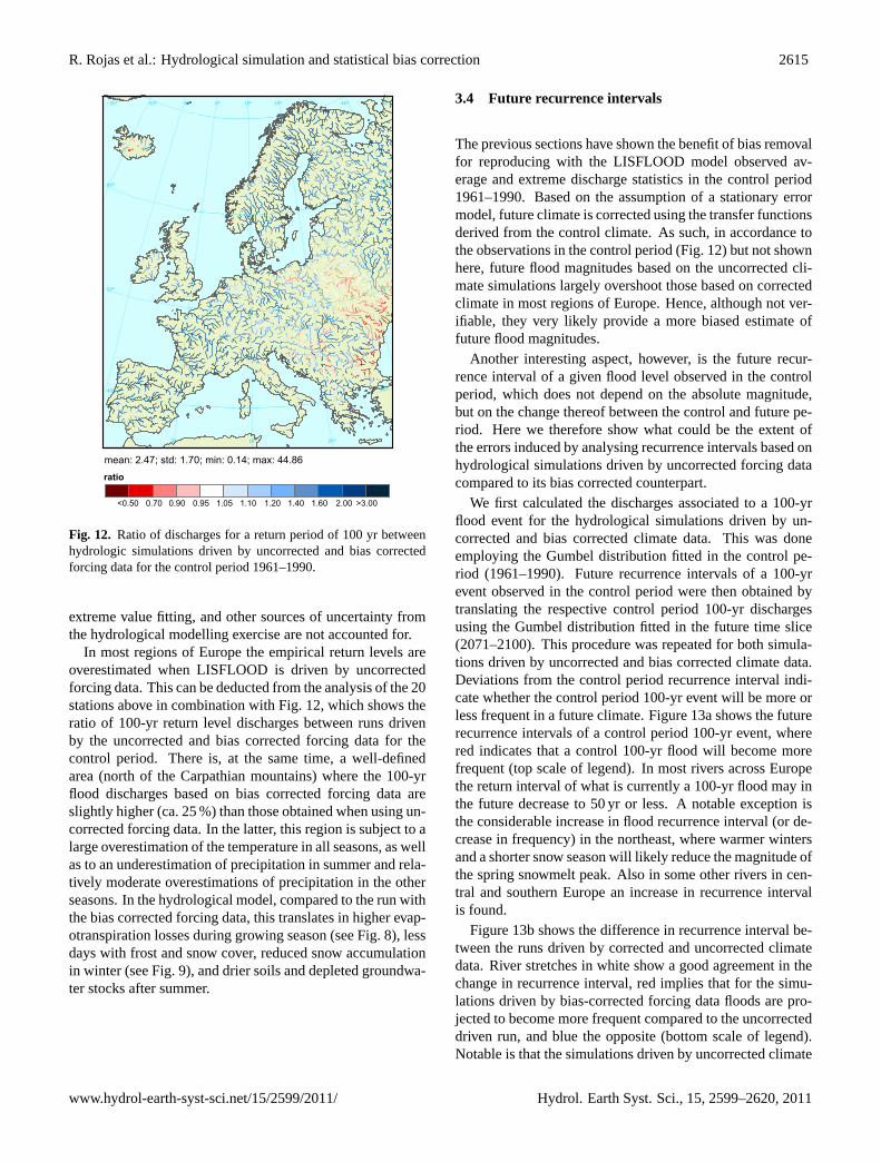
Fig. 12. Ratio of discharges for a return period of 100 yr betweenhydrologic simulations driven by uncorrected and bias correctedforcing data for the control period 1961–1990.
extreme value fitting, and other sources of uncertainty fromthe hydrological modelling exercise are not accounted for.
In most regions of Europe the empirical return levels areoverestimated when LISFLOOD is driven by uncorrectedforcing data. This can be deducted from the analysis of the 20stations above in combination with Fig.12, which shows theratio of 100-yr return level discharges between runs drivenby the uncorrected and bias corrected forcing data for thecontrol period. There is, at the same time, a well-definedarea (north of the Carpathian mountains) where the 100-yrflood discharges based on bias corrected forcing data areslightly higher (ca. 25 %) than those obtained when using un-corrected forcing data. In the latter, this region is subject to alarge overestimation of the temperature in all seasons, as wellas to an underestimation of precipitation in summer and rela-tively moderate overestimations of precipitation in the otherseasons. In the hydrological model, compared to the run withthe bias corrected forcing data, this translates in higher evap-otranspiration losses during growing season (see Fig.8), lessdays with frost and snow cover, reduced snow accumulationin winter (see Fig.9), and drier soils and depleted groundwa-ter stocks after summer.
3.4 Future recurrence intervals
The previous sections have shown the benefit of bias removalfor reproducing with the LISFLOOD model observed av-erage and extreme discharge statistics in the control period1961–1990. Based on the assumption of a stationary errormodel, future climate is corrected using the transfer functionsderived from the control climate. As such, in accordance tothe observations in the control period (Fig.12) but not shownhere, future flood magnitudes based on the uncorrected cli-mate simulations largely overshoot those based on correctedclimate in most regions of Europe. Hence, although not ver-ifiable, they very likely provide a more biased estimate offuture flood magnitudes.
Another interesting aspect, however, is the future recur-rence interval of a given flood level observed in the controlperiod, which does not depend on the absolute magnitude,but on the change thereof between the control and future pe-riod. Here we therefore show what could be the extent ofthe errors induced by analysing recurrence intervals based onhydrological simulations driven by uncorrected forcing datacompared to its bias corrected counterpart.
We first calculated the discharges associated to a 100-yrflood event for the hydrological simulations driven by un-corrected and bias corrected climate data. This was doneemploying the Gumbel distribution fitted in the control pe-riod (1961–1990). Future recurrence intervals of a 100-yrevent observed in the control period were then obtained bytranslating the respective control period 100-yr dischargesusing the Gumbel distribution fitted in the future time slice(2071–2100). This procedure was repeated for both simula-tions driven by uncorrected and bias corrected climate data.Deviations from the control period recurrence interval indi-cate whether the control period 100-yr event will be more orless frequent in a future climate. Figure13a shows the futurerecurrence intervals of a control period 100-yr event, wherered indicates that a control 100-yr flood will become morefrequent (top scale of legend). In most rivers across Europethe return interval of what is currently a 100-yr flood may inthe future decrease to 50 yr or less. A notable exception isthe considerable increase in flood recurrence interval (or de-crease in frequency) in the northeast, where warmer wintersand a shorter snow season will likely reduce the magnitude ofthe spring snowmelt peak. Also in some other rivers in cen-tral and southern Europe an increase in recurrence intervalis found.
Figure13b shows the difference in recurrence interval be-tween the runs driven by corrected and uncorrected climatedata. River stretches in white show a good agreement in thechange in recurrence interval, red implies that for the simu-lations driven by bias-corrected forcing data floods are pro-jected to become more frequent compared to the uncorrecteddriven run, and blue the opposite (bottom scale of legend).Notable is that the simulations driven by uncorrected climate
www.hydrol-earth-syst-sci.net/15/2599/2011/ Hydrol. Earth Syst. Sci., 15, 2599–2620, 2011
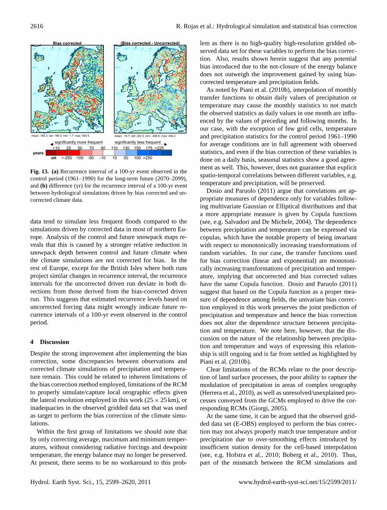
2616 R. Rojas et al.: Hydrological simulation and statistical bias correction
Bias corrected
significantly more frequent significantly less frequent
(Bias corrected - Uncorrected)
amean: 185.2; std: 188.3; min: 1.7; max: 500.5
bmean: -19.7; std: 202.5; min: -498.6; max: 494.2
50°40°30°
20°
20°
10°
10°
0°
0°-10°-20°-30°
60° 60°
50° 50°
40° 40°
50°40°30°
20°
20°
10°
10°
0°
0°-10°-20°-30°
60° 60°
50° 50°
40° 40°
<10 25 50 70 90 110 130 150 175 >225
<-250 -100 -50 -10 10 50 100 >250years
diff.
a b
Fig. 13. (a)Recurrence interval of a 100-yr event observed in thecontrol period (1961–1990) for the long-term future (2070–2099),and(b) difference (yr) for the recurrence interval of a 100-yr eventbetween hydrological simulations driven by bias corrected and un-corrected climate data.
data tend to simulate less frequent floods compared to thesimulations driven by corrected data in most of northern Eu-rope. Analysis of the control and future snowpack maps re-veals that this is caused by a stronger relative reduction insnowpack depth between control and future climate whenthe climate simulations are not corrected for bias. In therest of Europe, except for the British Isles where both runsproject similar changes in recurrence interval, the recurrenceintervals for the uncorrected driven run deviate in both di-rections from those derived from the bias-corrected drivenrun. This suggests that estimated recurrence levels based onuncorrected forcing data might wrongly indicate future re-currence intervals of a 100-yr event observed in the controlperiod.
4 Discussion
Despite the strong improvement after implementing the biascorrection, some discrepancies between observations andcorrected climate simulations of precipitation and tempera-ture remain. This could be related to inherent limitations ofthe bias correction method employed, limitations of the RCMto properly simulate/capture local orographic effects giventhe lateral resolution employed in this work (25× 25 km), orinadequacies in the observed gridded data set that was usedas target to perform the bias correction of the climate simu-lations.
Within the first group of limitations we should note thatby only correcting average, maximum and minimum temper-atures, without considering radiative forcings and dewpointtemperature, the energy balance may no longer be preserved.At present, there seems to be no workaround to this prob-
lem as there is no high-quality high-resolution gridded ob-served data set for these variables to perform the bias correc-tion. Also, results shown herein suggest that any potentialbias introduced due to the not-closure of the energy balancedoes not outweigh the improvement gained by using bias-corrected temperature and precipitation fields.
As noted byPiani et al.(2010b), interpolation of monthlytransfer functions to obtain daily values of precipitation ortemperature may cause the monthly statistics to not matchthe observed statistics as daily values in one month are influ-enced by the values of preceding and following months. Inour case, with the exception of few grid cells, temperatureand precipitation statistics for the control period 1961–1990for average conditions are in full agreement with observedstatistics, and even if the bias correction of these variables isdone on a daily basis, seasonal statistics show a good agree-ment as well. This, however, does not guarantee that explicitspatio-temporal correlations between different variables, e.g.temperature and precipitation, will be preserved.
Dosio and Paruolo(2011) argue that correlations are ap-propriate measures of dependence only for variables follow-ing multivariate Gaussian or Elliptical distributions and thata more appropriate measure is given by Copula functions(see, e.g.Salvadori and De Michele, 2004). The dependencebetween precipitation and temperature can be expressed viacopulas, which have the notable property of being invariantwith respect to monotonically increasing transformations ofrandom variables. In our case, the transfer functions usedfor bias correction (linear and exponential) are monotoni-cally increasing transformations of precipitation and temper-ature, implying that uncorrected and bias corrected valueshave the same Copula function.Dosio and Paruolo(2011)suggest that based on the Copula function as a proper mea-sure of dependence among fields, the univariate bias correc-tion employed in this work preserves the joint prediction ofprecipitation and temperature and hence the bias correctiondoes not alter the dependence structure between precipita-tion and temperature. We note here, however, that the dis-cussion on the nature of the relationship between precipita-tion and temperature and ways of expressing this relation-ship is still ongoing and is far from settled as highlighted byPiani et al.(2010b).
Clear limitations of the RCMs relate to the poor descrip-tion of land surface processes, the poor ability to capture themodulation of precipitation in areas of complex orography(Herrera et al., 2010), as well as unresolved/unexplained pro-cesses conveyed from the GCMs employed to drive the cor-responding RCMs (Giorgi, 2005).
At the same time, it can be argued that the observed grid-ded data set (E-OBS) employed to perform the bias correc-tion may not always properly match true temperature and/orprecipitation due to over-smoothing effects introduced byinsufficient station density for the cell-based interpolation(see, e.g.Hofstra et al., 2010; Boberg et al., 2010). Thus,part of the mismatch between the RCM simulations and
Hydrol. Earth Syst. Sci., 15, 2599–2620, 2011 www.hydrol-earth-syst-sci.net/15/2599/2011/
R. Rojas et al.: Hydrological simulation and statistical bias correction 2617
observational dataset might actually not be related to modelerrors, but instead to errors in the observed gridded data set(Lenderink, 2010). In the bias correction, this can potentiallycorrupt properly simulated temperature or precipitation in ar-eas with low station densities. Also, using an alternative ob-served gridded data set (e.g. CRU TS1.2 seeMitchell et al.,2004) can lead to different transfer functions. The latter,however, is expected to have limited influence as alternativeobserved data sets often present similar climatology despitedifferences in horizontal extent or station density (see, e.g.Rauscher et al., 2010).
Notwithstanding the considerable improvement in repro-ducing observed discharge statistics after implementing thebias correction, some notable discrepancies between simu-lated and observed average annual maxima are still presentat a number of river stations. Several factors may contributeto this mismatch. Part of the disagreement can be attributedto the remaining error in the meteorological forcing fields af-ter the bias correction.
The disagreement is in part also attributable to not ac-counting for river regulation in the current LISFLOOD setup.The main reason is a deplorable lack of relevant data at Eu-ropean scale, as well as the large uncertainty regarding futureriver regulation and land-use changes. As a consequence, re-sults are likely to underestimate the human influence on highflows, and, for future climate, rather reflect the impact of cli-mate change on natural flows.
Errors in the conceptualization and parametrization of thehydrological model further affect the simulated discharges.We do not make an attempt to account for hydrological un-certainty, as it is outside the scope of this study. Several otherstudies (e.g.Wilby, 2005) showed, however, that this layer ofuncertainty is generally much lower than the uncertainty ofthe climate input to the hydrological model.
The relative contribution of these factors is difficult toquantify because observed events cannot be compared on anindividual basis with simulations for the control climate, asit does not reproduce the historical weather.
5 Conclusions
In this work we assessed the benefits of removing bias in cli-mate forcing data for pan-European hydrological impact as-sessment, with emphasis on extreme events. Results showthat the bias correction method employed performed verywell in removing bias in average, maximum and minimumtemperatures. Even though daily maximum and minimumtemperatures were corrected for indirectly, and the dailytransfer functions were obtained on a monthly basis, ob-served annual and seasonal statistics were fully preserved.
For precipitation, the bias correction method was able todrastically reduce the strong overestimation generally ob-served across Europe. Only in certain mountain areas, e.g.Alps, Apennines, and Carpathian, a persistent overestimation
remained, mainly in winter. This is likely due to the alter-nation between linear and exponential fitting-type functionsduring winter months in these areas, which can significantlyalter the interpolation of daily values based on the anteriorand posterior (monthly) fitting functions.
Validation of simulated discharge statistics at 554 gaug-ing stations showed that LISFLOOD simulations driven byuncorrected forcing data strongly overestimated average andextreme discharge statistics at the majority of stations. Sim-ulations with corrected climate simulations were more con-sistent with historical discharge records. A strong improve-ment was observed not only in average discharges but alsoin the annual maxima and the probability of flood levels de-rived by extreme value analysis. For the extremes, however,we observed a slight tendency to underestimate observedflow statistics. This can in part be explained by errors inthe E-OBS data set used as target in the bias correction. Inthe latter, gridded extreme precipitation may undervalue trueextremes due to under-catch of precipitation, especially inmountain stations, as well as to the over-smoothing effect inthe grid-based interpolation in areas with low station den-sity. Despite this, the E-OBS data set is currently the bestavailable at pan-European scale. In small-scale studies suchproblems may be alleviated by using more dense data sets toreconstruct historical climate.
At a number of stations, the bias-correction could not(fully) remove the (sometimes considerable) discrepanciesbetween observed and simulated discharge statistics. Thissuggests that they relate to other limitations of the hydrologi-cal modelling exercise, such as not accounting for river regu-lation, or errors in the conceptualization and parametrizationof the hydrological model.
In accordance to the results for the control period, futureflood magnitudes for the hydrological simulations driven byuncorrected climate data largely exceed those based on cor-rected climate. Although strictly not verifiable, this suggeststhat projections of future flood magnitude based on uncor-rected climate simulations are likely unreliable. Moreover,results show that the recurrence interval of a 100-yr floodevent observed in the control period, which depends on thechange in flood magnitude rather than on the absolute valuethereof, can substantially vary in both directions from itscorrected-based counterpart.
This research has shown the benefits of bias removal in cli-mate simulations for hydrological impact assessment at pan-European scale. Despite the potential limitations in the ap-proach employed, the considerable improvement in the sim-ulation of extreme events and their probability of occurrencein the control period 1961–1990 increases the confidence inthe projections of future flood hazard. Our next steps in-volve the implementation of this technique to the full ensem-ble of climate simulations available in the FP6 ENSEMBLESproject, and the hydrological impact assessment using fullyconsistent and bias corrected climate simulations for an en-semble of climate models.
www.hydrol-earth-syst-sci.net/15/2599/2011/ Hydrol. Earth Syst. Sci., 15, 2599–2620, 2011
2618 R. Rojas et al.: Hydrological simulation and statistical bias correction
Acknowledgements.We thank past and present collaborators at theJRC who have for several years assisted in developing and cali-brating LISFLOOD. We would like to thank Claudio Piani (ICTP,Trieste) and Jan Haerter (MPI, Hamburg) for providing the bias-correction algorithms and assisting in implementing the codes. Thiswork received funding from the EU-FP7 project ClimateCost (FullCosts of Climate Change, Grant Agreement 212774,http://www.climatecost.cc/). Data used in this work was funded by the EU-FP6 project ENSEMBLES (Contract number 505539). We thankAlessandra Bianchi for managing the data set in netCDF format.We acknowledge the data providers in the ECA&D project (http://eca.knmi.nl), the Global Runoff Data Centre (GRDC) (Germany),CEDEX-IEH (Spain), Banque HYDRO (France), and ARPA EmiliaRomagna (Italia).
Edited by: T. Elliot
References
Allen, R., Pereira, L., Raes, D., and Smith, M.: Crop evapotran-spiration – Guidelines for computing crop water requirements,vol. FAO irrigation and drainage paper 56, FAO, 1998.
Beirlant, J., Goegebeur, Y., Segers, J., Teugels, J., De Waal, D., andFerro, C.: Statistics of extremes – Theory and applications, Wi-ley series in probability and statistics, Wiley, Chichester, 1 Edn.,2004.
Block, P., Filho, F., Sun, L., and Kwon, H.: A streamflow fore-casting framework using multiple climate and hydrological mod-els, Journal of the American Water Association, 45, 828–843,doi:10.1111/j.1752-1688.2009.00327.x, 2009.
Boberg, F., Berg, P., Thejil, P., Gutowski, J., and Chris-tensen, J.: Improved confidence in climate change projectionsof precipitation further evaluated using daily statistics fromENSEMBLES models, Clim. Dynam., 35(7–8), 1509–1520,doi:10.1007/s00382-009-0683-8, 2010.
Chen, C. and Knutson, T.: On the verification and comparison of ex-treme rainfall indices from climate models, J. Climate, 21, 1605–1621,doi:10.1175/2007JCLI1494.1, 2008.
Christensen, J., Boberg, F., Christensen, O., and Lucas-Picher, P.:On the need for bias correction of regional climate change pro-jections of temperature and precipitation, Geophys. Res. Lett.,35, L20709,doi:10.1029/2008GL035694, 2008.
Christensen, O., Drews, M., Christensen, J., Dethloff, K., Ketelsen,K., Hebestadt, I., and Rinke, A.: The HIRHAM Regional Cli-mate Model Version 5 (beta), Tech. Rep. 06-17, Danish Meteo-rological Institute, 2007.
Coles, S.: An introduction to statistical modeling of extreme values,Springer series in statistics, Springer, London, 1 Edn., 2001.
Dankers, R. and Feyen, L.: Climate change impact onflood hazard in Europe: An assessment based on high–resolution climate simulations, J. Geophys. Res., 113, D19105,doi:10.1029/2007JD009719, 2008.
Dankers, R. and Feyen, L.: Flood hazard in Europe in an ensembleof regional climate scenarios, J. Geophys. Res., 114, D16108,doi:10.1029/2008JD011523, 2009.
de Roo, A., Odijk, M., Shcmuck, G., Koster, E., and Lucieer, A.:Assessing the effects of land use changes on floods in the Meuseand Oder catchments, Phys. Chem. Earth, Part B, 26, 593–599,doi:10.1016/S1464-1909(01)00054-5, 2001.
Deque, M.: Frequency of precipitation and temperature extremesover France in an anthropogenic scenario: Model results and sta-tistical correction according to observed values, Global Planet.Change, 57, 16–26,doi:10.1016/j.gloplacha.2006.11.030, 2007.
Dosio, A. and Paruolo, P.: Bias correction of the ENSEMBLEShigh resolution climate change projections for use by impactmodels: evaluation on the present cimate, J. Geophys. Res., 116,D16106,doi:10.1029/2011JD015934, 2011.
Duan, Q., Sorooshian, S., and Gupta, H.: Effective and efficientglobal optimization fro conceptual ranfall – runoff models, WaterResour. Res., 28, 1015–1031,doi:10.1029/91WR02985, 1992.
Durman, C., Gregory, J., Kassell, D., Jones, R., and Murphy, J.:A comparison of extreme European daily precipitation simu-lated by a global and a regional climate model for present andfuture climates, Q. J. Roy. Meteorol. Soc., 127, 1005–1015,doi:10.1002/qj.49712757316, 2001.
Dynesius, M. and Nilsson, C.: Fragmentation and flow regulationof river systems in the northern third of the world, Science, 266,753–762,doi:10.1126/science.266.5186.753, 1994.
EEA: Corine Land Cover 2000, Tech. Rep. 89, European Commis-sion, European Environment Agency (EEA), available at:http://dataservice.eea.europa.eu/, 2002.
Engen-Skaugen, T.: Refinement of dynamically downscaled pre-cipitation and temperature scenarios, Climatic Change, 84, 365–382,doi:10.1007/s10584-007-9251-6, 2007.
Etchevers, P., Golaz, C., Habets, F., and Noilhan, J.: Impact of aclimate change on the Rhone river catchment hydrology, J. Geo-phys. Res., 107, 4293,doi:10.1029/2001JD000490, 2002.
Evans, J.: Improving the characteristics of streamflow mod-eled by regional climate models, J. Hydrol., 284, 211–227,doi:10.1016/j.jhydrol.2003.08.003, 2003.
Feyen, J., Kalas, M., and Vrugt, J.: The value of semi-distributed parameters for large-scale streamflow simulationusing global optimization, Hydrolog. Sci. J., 53, 293–308,doi:10.1623/hysj.53.2.293, 2008.
Feyen, L. and Dankers, R.: Impact of global warming on stream-flow drought in Europe, J. Geophys. Res., 114, D17116,doi:10.1029/2008JD011438, 2009.
Feyen, L., Vrugt, J.,O Nuallain, B., van der Knijff, J., and de Roo,A.: Parameter optimization and uncertainty assessment for large-scale streamflow simulation with the LISFLOOD model, J. Hy-drol., 332, 276–289,doi:10.1016/j.jhydrol.2006.07.004, 2007.
Fowler, H. and Kilsby, C.: Using regional climate model data tosimulate historical and future river flows in northwest England,Climatic Change, 80, 337–367,doi:10.1007/s10584-006-9117-3, 2007.
Fowler, H., Blenkinsop, S., and Tebaldi, C.: Linking climate changemodelling to impacts studies: Recent advances in downscal-ing techniques for hydrological modelling, Int. J. Climatol., 27,1547–1578,doi:10.1002/joc.1556, 2007.
Giorgi, F.: Climate change prediction, Climatic Change, 73, 239–265,doi:10.1007/s10584-005-6857-4, 2005.
Giorgi, F., Hostetler, S., and Shields Brodeur, C.: Analysis of thesurface hydrology in a regional climate model, Q. J. Roy. Mete-orol. Soc., 120, 161–183,doi:10.1002/qj.49712051510, 1994.
Graham, L., Hagemann, S., Jaun, S., and Beniston, M.: On in-terpreting hydrological change from regional climate models,Climatic Change, 81, 97–122,doi:10.1007/s10584-006-9217-0,2007.
Hydrol. Earth Syst. Sci., 15, 2599–2620, 2011 www.hydrol-earth-syst-sci.net/15/2599/2011/

R. Rojas et al.: Hydrological simulation and statistical bias correction 2619
Haylock, M., Cawley, G., Harpham, C., Wilby, R., and Good-ess, C.: Downscaling heavy precipitation over the UnitedKingdom: a comparison of dynamical and statistical methodsand their future scenarios, Int. J. Climatol., 26, 1397–1415,doi:10.1002/joc.1318, 2006.
Haylock, M., Hofstra, N., Klein, A., Klok, E., Jones, P., and New,M.: A European daily high – resolution gridded data set of sur-face temperature and precipitation for 1950–2006, Geophys. Res.Lett., 113,doi:10.1029/2008JD010201, 2008.
Hellstrom, C., Chen, D., Achberger, C., and Raisanen, J.: Compar-ison of climate change scenarios for Sweden based on statisticaland dynamical downscaling of monthly precipitation, Clim. Res.,19, 44–55,doi:10.3354/cr019045, 2001.
Herrera, S., Fita, L., Fernandez, J., and Gutierrez, J.: Evaluation ofthe mean and extreme precipitation regimes from the ENSEM-BLES regional climate multimodel simulations over Spain, J.Geophys. Res., 115, D21117,doi:10.1029/2010JD013936, 2010.
Hiederer, R. and de Roo, A.: A European flow network and catch-ment data set, Tech. rep., Joint Research Centre, European Com-mission, 2003.
Hofstra, N., New, M., and McSweeney, C.: The influence of in-terpolation and station network density on the distributions andtrends of climate variables in gridded daily data, Clim. Dynam.,35, 841–858,doi:10.1007/s00382-009-0698-1, 2010.
Horton, P., Schaefli, B., Mezghani, A., Benoıt, H., and Musy,A.: Assessment of climate–change impacts on alpine dischargeregimes with climate model uncertainty, Hydrol. Process., 20,2091–2109,doi:10.1002/hyp.6197, 2006.
Hurkmans, R., Terink, W., Uijlenhoet, R., Torfs, P., Jacob, D., andTroch, P.: Changes in streamflow dynamics in the Rhine basinunder three high–resolution regional climate scenarios, J. Cli-mate, 23, 679–699,doi:10.1175/2009JCLI3066.1, 2010.
Iizumi, T., Nishimori, M., Dairaku, K., Adachi, S., and Yokozawa,M.: Evaluation and intercomparison of downscaled daily pre-cipitation indices over Japan in present-day climate: Strengthsand weaknesses of dynamical and bias correction-type statis-tical downscaling methods, J. Geophys. Res., 116, D01111,doi:10.1029/2010JD014513, 2011.
Jacob, D., Barring, L., Christensen, O., Christensen, J., de Castro,M., Deque, M., Giorgi, F., Hagemann, S., Hirschi, M., Jones, R.,Kjellstrom, E., Lenderink, G., Rockel, B., Sanchez, E., Schar, C.,Seneviratne, S., Somot, S., Ulden, A., and Hurk, B.: An inter–comparison of regional climate models for Europe: Model per-formance in present – day climate, Climatic Change, 81, 31–52,doi:10.1007/s10584-006-9213-4, 2007.
King, D., Daroussin, J., and Tavernier, R.: Development of a soilgeographic database from the Soil Map of the European Com-munities, Catena, 21, 37–56,doi:10.1016/0341-8162(94)90030-2, 1994.
Kjellstrom, E., Barring, L., Jacob, D., Jones, R., Lenderink, G., andSchar, C.: Modelling daily temperature extremes: recent climateand future changes over Europe, Climatic Change, 81, 249–265,doi:10.1007/s10584-006-9220-5, 2007.
Kjellstrom, E., Boberg, F., Castro, M., Chirstensen, J., Nikulin, G.,and Sanchez, E.: Daily and monthly temperature and precipi-tation statistics as performance indicators for regional climatemodels, Clim. Res., 44, 135–150,doi:10.3354/cr00932, 2010.
Kleinn, J., Frei, C., Gurtz, J., Luthi, D., Vidale, P., and Schar,C.: Hydrologic simulations in the Rhine basin driven by
a regional climate model, J. Geophys. Res., 110, D04102,doi:10.1029/2004JD005143, 2005.
Leander, R. and Buishand, T.: Resampling of regional climatemodel output for the simulation of extreme river flows, J. Hy-drol., 332, 487–496,doi:10.1016/j.jhydrol.2006.08.006, 2007.
Leander, R., Buishand, T., van den Hurk, B., and de Wit, M.: Esti-mated changes in flood quantiles of the river Meuse from resam-pling of regional climate model output, J. Hydrol., 351, 331–343,doi:10.1016/j.jhydrol.2007.12.020, 2008.
Lehner, B., Doll, P., Alcamo, J., Henrichs, T., and Kaspar, F.: Esti-mating the impact of global change on flood and drought risks inEurope: A continental integrated analysis, Climatic Change, 75,273–299,doi:10.1007/s10584-006-6338-4, 2006.
Lenderink, G.: Exploring metrics of extreme daily precipitation ina large ensemble of regional climate model simulations, Clim.Res., 44, 151–166,doi:10.3354/cr00946, 2010.
Lenderink, G., Buishand, A., and van Deursen, W.: Estimates offuture discharges of the river Rhine using two scenario method-ologies: direct versus delta approach, Hydrol. Earth Syst. Sci.,11, 1145–1159,doi:10.5194/hess-11-1145-2007, 2007.
Lorenz, P. and Jacob, D.: Validation of temperature trends in theENSEMBLES regional climate model runs driven by ERA40,Climatic Change, 44, 167–177,doi:10.3354/cr00973, 2010.
Middelkoop, H., Daamen, K., Gellens, D., Grabs, W., Kwadijk, J.,Lang, H., Parmet, B., Schadler, B., Schulla, J., and Wilke, K.:Impact of climate change on hydrological regimes and water re-sources management in the Rhine basin, Climatic Change, 49,105–128,doi:10.1023/A:1010784727448, 2001.
Mitchell, T., Carter, T., Jones, P., Hulme, M., and New, M.: A com-prehensive set of high-resolution grids of monthly climate forEurope and the globe: the observed record (1901–2000) and 16scenarios (2001–2100), Tech. rep., Tyndall Centre for ClimateResearch, Norwich, UK, 2004.
Murphy, J.: An evaluation of statistical and dynamical techniquesfor downscaling local climate, J. Climate, 12, 2256–2284,doi:10.1175/1520-0442(1999)012¡2256:AEOSAD¿2.0.CO;2,1999.
Nakicenovic, N. and Swart, R. (Eds.): IPCC Special Report onEmissions Scenarios, Cambridge University Press, Cambridge,UK, 2000.
New, M., Hulme, M., and Jones, P.: Representing twentieth-century space-time climate variability. Part II: Develop-ment of 1901–96 monthly grids of terrestrial surface cli-mate, J. Climate, 13(13), 2217–2238,doi:10.1175/1520-0442(2000)013¡2217:RTCSTC¿2.0.CO;2, 2000.
Nikulin, G., Kjellstrom, E., Hansson, U., Strandberg, G., andUllerstig, A.: Evaluation and future projections of tempera-ture, precipitation and wind extremes over Europe in an en-semble of regional climate simulations, Tellus A, 63, 41–55,doi:10.1111/j.1600-0870.2010.00466.x, 2011.
Piani, C., Haerter, J., and Coppola, E.: Statistical bias correctionfor daily precipitation in regional climate models over Europe,Theor. Appl. Climatol., 99, 187–192,doi:10.1007/s00704-009-0134-9, 2010a.
Piani, C., Weedon, G., Best, M., Gomes, S., Viterbo, P., Hage-mann, S., and Haerter, J.: Statistical bias correction of globalsimulated daily precipitation and temperature for the appli-cation of hydrological models, J. Hydrol., 395, 199–215,doi:10.1016/j.jhydrol.2010.10.024, 2010b.
www.hydrol-earth-syst-sci.net/15/2599/2011/ Hydrol. Earth Syst. Sci., 15, 2599–2620, 2011
2620 R. Rojas et al.: Hydrological simulation and statistical bias correction
Plavcova, E. and Kysely, J.: Evaluation of daily temperatures inCentral Europe and their links to large-scale circulation in an en-semble of regional climate models, Tellus A, 63(4), 763–781,,doi:10.1111/j.1600-0870.2011.00514.x, 2011.
Prudhomme, C., Jakob, D., and Svensson, C.: Uncertainty and cli-mate change impact on the flood regime of small UK catchments,J. Hydrol., 277, 1–23,doi:10.1016/S0022-1694(03)00065-9,2003.
Rauscher, S., Coppola, E., PIani, C., and Girogi, F.: Reso-lution effects on regional climate model simulations of sea-sonal precipitation over Europe, Clim. Dynam., 35, 685–711,doi:10.1007/s00382-009-0607-7, 2010.
Rijks, D., Terres, J., and Vossen, P.: Agrometeorological applica-tions for regional crop monitoring and production assessment,Tech. Rep. EUR 17735, European Commission, Joint ResearchCentre, Ispra, Italy, 1998.
Roeckner, E., Bauml, G., Bonaventura, L., Brokopf, R., Esch,M., Giorgetta, M., Hagemann, S., Kirchner, I., Kornblueh, L.,Manzini, E., Rhodin, A., Sclese, U., Schulzweida, U., and Tomp-kins, A.: The atmospheric general circulation model ECHAM5Part I: Model description, Tech. Rep. 349, Max Planck Institutefor Meteorology, 2003.
Salvadori, G. and De Michele, C.: Frequency analysis via copu-las: Theoretical aspects and applications to hydrological events,Water Resour. Res., 40, W12511,doi:10.1029/2004WR003133,2004.
Schmidli, J., Goodess, C., Frei, C., Haylock, M., Hundecha, Y.,Ribalaygua, J., and Schmith, T.: Statistical and dynamical down-scaling of precipitation: An evaluation and comparison of sce-narios for the European Alps, J. Geophys. Res., 112, D04105,doi:10.1029/2005JD007026, 2007.
Shabalova, M., van Deursen, W., and Buishand, T.: Assessing fu-ture discharge of the river Rhine using regional climate modelintegrations and a hydrological model, Clim. Res., 23, 233–246,doi:10.3354/cr023233, 2003.
Steele-Dunne, S., Lynch, P., McGrath, R., Semmler, T., Wang,S., Hanafin, J., and Nolan, P.: The impacts of climatechange on hydrology in Ireland, J. Hydrol., 356, 28–45,doi:10.1016/j.jhydrol.2008.03.025, 2008.
Suklitsch, M., Gobiet, A., Truhetz, H., Awan, N., Gottel, H., andJacob, D.: Error characteristics of high resolution regional cli-mate models over the Alpine area, Clim. Dynam., 37(1), 377–390,doi:10.1007/s00382-010-0848-5, 2010.
Teutschbein, C. and Seibert, J.: Regional climate models for hy-drological impact studies at the catchment scale: A reviewof recent model strategies, Geography Compass, 4, 834–860,doi:10.1111/j.1749-8198.2010.00357.x, 2010.
Themeßl, M., Gobiet, A., and Leuprecht, A.: Empirical-statisticaldownscaling and error correction of daily precipitation from re-gional climate models, International J. Climatol., 31(10), 1530–1544,doi:10.1002/joc.2168, 2011.
Thorne, R.: Uncertainty in the impacts of projected climate changeon the hydrology of a subarctic environment: Liard River Basin,Hydrol. Earth Syst. Sci., 15, 1483–1492,doi:10.5194/hess-15-1483-2011, 2011.
van der Knijff, J., Younis, J., and de Roo, A.: LISFLOOD: aGIS-based distributed model for river basin scale water bal-ance and flood simulation, Int. J. Geogr. Inf. Sci., 24, 189–212,doi:10.1080/13658810802549154, 2010.
van der Linden, P. and Mitchell, J.: ENSEMBLES: Climatechange and its impacts: Summary of research and resultsfrom the ENSEMBLES project, Tech. rep., Met Office hadleyCentre, available at:http://ensembles-eu.metoffice.com/docs/Ensemblesfinal reportNov09.pdf, 2009.
van Meijgaard, E., van Ulft, L., van de Berg, W., Bosveld, F., vanden Hurk, B., Lenderink, G., and Siebesma, A.: The KNMI re-gional atmospheric climate model RACMO, version 2.1, Tech.Rep. TR-302, KNMI, De Bilt, The Netherlands, 2008.
van Pelt, S. C., Kabat, P., ter Maat, H. W., van den Hurk, B. J. J. M.,and Weerts, A. H.: Discharge simulations performed with a hy-drological model using bias corrected regional climate model in-put, Hydrol. Earth Syst. Sci., 13, 2387–2397,doi:10.5194/hess-13-2387-2009, 2009.
van Ulden, A. P. and van Oldenborgh, G. J.: Large-scale atmo-spheric circulation biases and changes in global climate modelsimulations and their importance for climate change in CentralEurope, Atmos. Chem. Phys., 6, 863–881,doi:10.5194/acp-6-863-2006, 2006.
Weedon, G., Gomes, S., Viterbo, P., Osterle, H., Adam, J., Bellouin,N., Boucher, O., and Best: The WATCH forcing data 19582001:a meteorological forcing dataset land-surface and hydrological-models, Tech. rep., WATCH project, Technical Report Nr. 22,2010.
Wilby, R.: Uncertainty in water resource model parameters used forclimate change impact assessment, Hydrol. Process., 19, 3201–3219,doi:10.1002/hyp.5819, 2005.
Wilby, R. and Wigley, T.: Downscaling general circulation modeloutput: a review of methods and limitations, Progr. Phys. Geog.,21, 530–548,doi:10.1177/030913339702100403, 1997.
Wilby, R., Hay, L., and Leavesley, G.: A comparison of downscaledand raw GCM output: implications for climate change scenariosin the San Juan River basin, Colorado, J. Hydrol., 225, 67–91,doi:10.1016/S0022-1694(99)00136-5, 1999.
Wilby, R., Whitehead, P., Wade, A., Butterfield, D., Davis,R., and Watts, G.: Integrated modelling of climate changeimpacts on water resources and quality in a lowland catch-ment: River Kennet, UK, J. Hydrol., 330, 204–220,doi:10.1016/j.jhydrol.2006.04.033, 2006.
Wood, A., Leung, L., Sridhar, V., and Lettenmaier, D.: Hydrologicimplications of dynamical and statistical approaches to down-scaling climate model outputs, Climatic Change, 62, 189–216,doi:10.1023/B:CLIM.0000013685.99609.9e, 2004.
Wosten, J., Lilly, A., and Le Bas, C.: Development and use of adatabase of hydraulic properties of European soils, Geoderma,90, 169–185,doi:10.1016/s0016-7061(98)00132-3, 1999.
Hydrol. Earth Syst. Sci., 15, 2599–2620, 2011 www.hydrol-earth-syst-sci.net/15/2599/2011/