Climate-driven interannual variability of water scarcity in food production: a global analysis

HESSD10, 6931–6962, 2013

Climate-driveninterannual variability

of water scarcity infood production

M. Kummu et al.

Title Page

Abstract Introduction

Conclusions References

Tables Figures

J I

J I

Back Close

Full Screen / Esc

Printer-friendly Version

Interactive Discussion

Discussion

Paper

|D

iscussionP

aper|

Discussion

Paper

|D

iscussionP

aper|

Hydrol. Earth Syst. Sci. Discuss., 10, 6931–6962, 2013www.hydrol-earth-syst-sci-discuss.net/10/6931/2013/doi:10.5194/hessd-10-6931-2013© Author(s) 2013. CC Attribution 3.0 License.

EGU Journal Logos (RGB)

Advances in Geosciences

Open A

ccess

Natural Hazards and Earth System

Sciences

Open A

ccess

Annales Geophysicae

Open A

ccess

Nonlinear Processes in Geophysics

Open A

ccess

Atmospheric Chemistry

and Physics

Open A

ccess

Atmospheric Chemistry

and Physics

Open A

ccess

Discussions

Atmospheric Measurement

Techniques

Open A

ccess

Atmospheric Measurement

Techniques

Open A

ccess

Discussions

Biogeosciences

Open A

ccess

Open A

ccess

BiogeosciencesDiscussions

Climate of the Past

Open A

ccess

Open A

ccess

Climate of the Past

Discussions

Earth System Dynamics

Open A

ccess

Open A

ccess

Earth System Dynamics

Discussions

GeoscientificInstrumentation

Methods andData Systems

Open A

ccess

GeoscientificInstrumentation

Methods andData Systems

Open A

ccess

Discussions

GeoscientificModel Development

Open A

ccess

Open A

ccess

GeoscientificModel Development

Discussions

Hydrology and Earth System

Sciences

Open A

ccess

Hydrology and Earth System

Sciences

Open A

ccess

Discussions

Ocean Science

Open A

ccess

Open A

ccess

Ocean ScienceDiscussions

Solid Earth

Open A

ccess

Open A

ccess

Solid EarthDiscussions

The Cryosphere

Open A

ccess

Open A

ccessThe Cryosphere

Discussions

Natural Hazards and Earth System

Sciences

Open A

ccess

Discussions

This discussion paper is/has been under review for the journal Hydrology and Earth SystemSciences (HESS). Please refer to the corresponding final paper in HESS if available.

Climate-driven interannual variability ofwater scarcity in food production:a global analysis

M. Kummu1, D. Gerten2, J. Heinke2, M. Konzmann2, and O. Varis1

1Water & Development Research Group (WDRG), Aalto University, Espoo, Finland2Potsdam Institute for Climate Impact Research (PIK), Potsdam, Germany

Received: 17 May 2013 – Accepted: 26 May 2013 – Published: 3 June 2013

Correspondence to: M. Kummu ([email protected])

Published by Copernicus Publications on behalf of the European Geosciences Union.

6931

http://www.hydrol-earth-syst-sci-discuss.net

http://www.hydrol-earth-syst-sci-discuss.net/10/6931/2013/hessd-10-6931-2013-print.pdf

http://www.hydrol-earth-syst-sci-discuss.net/10/6931/2013/hessd-10-6931-2013-discussion.html

http://creativecommons.org/licenses/by/3.0/

HESSD10, 6931–6962, 2013



M. Kummu et al.

Title Page



Tables Figures

J I

J I

Back Close

Full Screen / Esc



Discussion

Paper

|D

iscussionP

aper|

Discussion

Paper

|D

iscussionP

aper|

Abstract

Interannual climatic and hydrologic variability has been substantial during the pastdecades in many regions. While climate variability and its impacts on precipitation andsoil moisture have been rather intensively studied, less is known on its impacts onfreshwater availability and further implications for global food production. In this paper5

we quantify effects of hydroclimatic variability on global “green” and “blue” water avail-ability and demand in agriculture. Analysis is based on climate forcing data for the past30 yr with demography, diet composition and land use fixed to constant reference con-ditions. We thus assess how observed interannual hydroclimatic variability impacts onthe ability of food production units (FPUs) to produce a given diet for their inhabitants,10

here focused on a benchmark for hunger alleviation (3000 kilocalories per capita perday, with 80 % vegetal food and 20 % animal products). We applied the LPJmL vege-tation and hydrology model to calculate spatially explicitly the variation in green-bluewater availability and the water requirements to produce that very diet. An FPU wasconsidered water scarce if its water availability was not sufficient to produce the diet15

(neglecting trade from elsewhere, i.e. assuming food self-sufficiency). We found thataltogether 24 % of the global population lives in areas under chronic scarcity (i.e. wa-ter is scarce every year) while an additional 19 % live under occasional water scarcity(i.e. water is scarce in some years). Of these 2.6 billion people under some degreeof scarcity, 55 % would have to rely on international trade to reach the reference diet20

while for 24 % domestic trade would be enough (assuming present cropland extent andmanagement). For the remaining 21 % of population under scarcity, local food storageand/or intermittent trade would be enough secure the reference diet over the occasionaldry years.

6932





HESSD10, 6931–6962, 2013



M. Kummu et al.

Title Page



Tables Figures

J I

J I

Back Close

Full Screen / Esc



Discussion

Paper

|D

iscussionP

aper|

Discussion

Paper

|D

iscussionP

aper|

1 Introduction

Climatic and hydrologic conditions vary significantly around the globe, both spatiallyand temporally (Zachos et al., 2001; Trenberth et al., 2007). The importance of interan-nual hydroclimatic variability has been reported for many ecologic (e.g. Notaro, 2008)and societal functions (Brown and Lall, 2006; Brown et al., 2010). Although the global5

interannual variabilities of precipitation (e.g. Fatichi et al., 2012; Sun et al., 2012), tem-perature (Sakai et al., 2009) and surface wetness (Ma and Fu, 2007) are rather wellunderstood, less is known on variability in runoff or river discharge at global scale.The runoff mainly determines the available blue water resources (i.e. freshwater inrivers and aquifers) for aquatic ecosystems and human societies. It is thus crucial to10

understand its variations at global and smaller scales. Dettinger and Diaz (2000) andWard et al. (2010) have assessed the variability based on observed discharge data,but due to low data coverage in various parts of the world, they could not cover thewhole globe. Recently, global hydrological models have enabled to assess averageconditions, variabilities and trends in global runoff and discharge with greater spatial15

coverage (Hirabayashi et al., 2005; Piao et al., 2007; Gerten et al., 2008; Haddelandet al., 2011), though interannual variability was not their focus, and model results mayin some regions disagree with observed variations and trends (Dai et al., 2009). Fur-thermore, meteorological and hydrological droughts have been assessed globally, yetbasically constrained to a hydroclimatological perspective (Sheffield et al., 2009; Dai,20

2011). To our knowledge, no global assessment is available on interannual variabilityin water availability for food production.

Sufficiency of blue water to meet certain demands can be measured with simplescarcity indices (Falkenmark et al., 1989; Falkenmark, 1997; Vörösmarty et al., 2000;Alcamo et al., 2003; Arnell, 2004; Oki and Kanae, 2006; Kummu et al., 2010). Although25

blue water and irrigation are crucial for global food production, still around 60 % of foodis produced with green water (i.e. naturally infiltrated rain, attached to soil particlesand accessible on roots) resources on rainfed land (Rockström et al., 2009). This has

6933





HESSD10, 6931–6962, 2013



M. Kummu et al.

Title Page



Tables Figures

J I

J I

Back Close

Full Screen / Esc



Discussion

Paper

|D

iscussionP

aper|

Discussion

Paper

|D

iscussionP

aper|

led to a quest for integrated green-blue water (GBW) scarcity indicators. Rockström etal. (2009) found a global GBW shortage by referring to a threshold of available GBWresources that is needed to produce a diet of 1300 m3 cap−1 yr−1. Gerten et al. (2011)developed a locally specific GBW scarcity indicator by taking explicitly into account thewater productivity, i.e. the amount of GBW resources needed to produce a benchmark5

for hunger alleviation (3000 kcal cap−1 day−1, assumed to consist of 80 % vegetal foodand 20 % animal products).

All of these have focused on water scarcity under long-term average climate condi-tions. Besides, recent global studies are available that have focused on average sea-sonal (i.e. intra-annual) blue water scarcity (Wada et al., 2011; Hoekstra et al., 2012).10

The interannual variability of water scarcity has remained, however, tenuously quanti-fied at global scale. We argue that it would be imperative to understand the frequency ofwater scarcity in food production, as in agricultural systems under occasional scarcityrequires essentially different adaptation measures as compared to chronic scarcity.Thus, quantitative knowledge of average water scarcity, assessed for example over15

30 yr (Gerten et al., 2011) or 10 yr (Rockström et al., 2009), might not reveal the areasthat suffer water scarcity occasionally during dry years, and on the other hand it mightclassify areas to be water scarce although the scarcity is not present every year.

In this paper we quantify the impact of interannual climatic variability on global GBWavailability and requirements for food production, using the GBW scarcity index intro-20

duced by Gerten et al. (2011). Our analysis is based on climate forcing data for thepast 30 yr (1977–2006) while diet composition, population and land cover settings arefixed to specific reference conditions. We thus assess how the hydroclimatic variabilityimpacts on food producing units’ (FPUs) ability to produce a given diet for their inhabi-tants. Moreover, we quantify whether the variability has changed over time by compar-25

ing two time periods (1947–1976 and 1977–2006). All calculations are performed withthe LPJmL vegetation and hydrology model (Bondeau et al., 2007; Rost et al., 2008).

6934





HESSD10, 6931–6962, 2013



M. Kummu et al.

Title Page



Tables Figures

J I

J I

Back Close

Full Screen / Esc



Discussion

Paper

|D

iscussionP

aper|

Discussion

Paper

|D

iscussionP

aper|

2 Data and methods

In this study we kept the land cover, population, diet composition and agricultural man-agement options constant in order to trace the sole impact of climate variability ongreen-blue water scarcity. We used year 2000 as a reference year, as for that year themost detailed and accurate data is available for all the needed datasets. Below the5

used methodologies and data to conduct the study are introduced.

2.1 LPJmL model and data

The process-based, dynamic global vegetation and water balance model LPJmL(Bondeau et al., 2007; Rost et al., 2008) simulates – among other processes – cropwater requirements, crop water productivities, and green and blue water availabilities10

at a daily time step and on a global 0.5×0.5 degree spatial grid. It computes thegrowth, production and phenology of 9 natural vegetation types, of grazing land, andof crops as classified into 12 “crop functional types” (CFTs). The fractional coverage ofgrid cells with CFTs was prescribed here using datasets of the reference (around year2000) cropland distribution (Ramankutty et al., 2008) and maximum monthly irrigated15

and rainfed harvested areas (Portmann et al., 2010). Seasonal phenology of CFTs issimulated based on meteorological conditions. Crop management is calibrated for theperiod around 2000 so as to ensure that simulated yields best match those reportedby FAOSTAT (see Fader et al., 2010 for details).

In LPJmL carbon fluxes and pools as well as water fluxes are modelled in direct20

coupling with vegetation dynamics. Effects of atmospheric CO2 concentration on plantgrowth and water use efficiency can be included in the simulations, but atmosphericCO2 concentration was held constant here at 370 ppm, corresponding approximatelyto the year 2000 level. Water requirements, water consumption (i.e. evapotranspira-tion, distinguished into transpiration, evaporation and interception loss) and crop wa-25

ter productivity (water consumption per unit of biomass produced) are calculated forboth irrigated and rainfed systems. On rainfed areas, all consumed water is green

6935





HESSD10, 6931–6962, 2013



M. Kummu et al.

Title Page



Tables Figures

J I

J I

Back Close

Full Screen / Esc



Discussion

Paper

|D

iscussionP

aper|

Discussion

Paper

|D

iscussionP

aper|

per definition, whereas on areas equipped for irrigation, we distinguish the fractionsof green water and blue water (withdrawn from rivers, reservoirs, lakes and shallowaquifers to the extent required by crops and unfulfilled by green water, consideringcountry-specific irrigation efficiencies). We assume that the irrigation water require-ments of each CFT can always be met, implicitly assuming contributions from fossil5

groundwater, river diversions or other large-scale water transports (details in Rost etal., 2008; Konzmann et al., 2013). River flow directions are determined as in Haddelandet al. (2011), and reservoir distribution and management as in Biemans et al. (2011).

The areal distribution of CFTs and grazing land, the calibration parameters and theirrigation efficiencies are held constant at the year 2000 level throughout the simulation10

period. Thus, we disregard any effects of crop management and cropland expansion.Monthly values of temperature and fraction of cloud cover are taken from CRU TS 3.1(Mitchell and Jones, 2005) and linearly interpolated to daily values. Monthly precipita-tion totals are taken from GPCC v5 (Rudolf et al., 2010; extended to cover the full CRUgrid) and the number of monthly precipitation days is derived using the method from15

Heinke et al. (2012). Daily precipitation values are calculated from these two parame-ters by a statistical weather generator (Gerten et al., 2005).

2.2 Analysis and reporting scales

The model results, with resolution of 0.5◦, are aggregated primarily to the FPU scale.FPUs divide the world into 281 sub-areas, being a hybrid between river basin and20

economic regions (Cai and Rosegrant, 2002; Rosegrant et al., 2002; De Fraiture, 2007)modified here as in Kummu et al. (2010). The final FPU set used includes 309 unitswith an average size of 467×103 km2 and an average population of 19.6 million. Wefocus on FPUs, as they are at a hydro-political scale where the demand for water canassumed to be managed (Kummu et al., 2010).25

We introduce another three reporting scales to further analyse and present our re-sults, namely countries, administrative regions, and hydrobelts. The administrative re-gions divide the world into 12 regions (see Fig. S1a in the Supplement) based on

6936





HESSD10, 6931–6962, 2013



M. Kummu et al.

Title Page



Tables Figures

J I

J I

Back Close

Full Screen / Esc



Discussion

Paper

|D

iscussionP

aper|

Discussion

Paper

|D

iscussionP

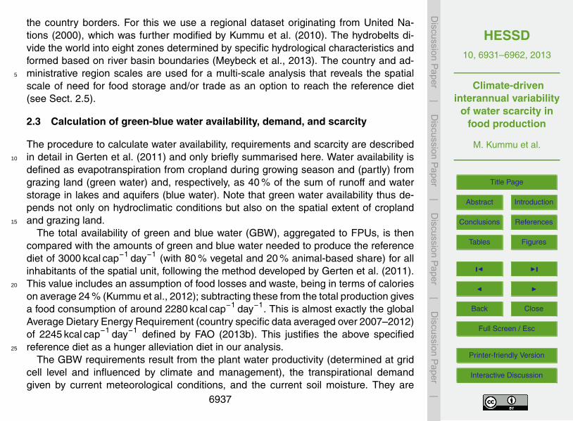
aper|

the country borders. For this we use a regional dataset originating from United Na-tions (2000), which was further modified by Kummu et al. (2010). The hydrobelts di-vide the world into eight zones determined by specific hydrological characteristics andformed based on river basin boundaries (Meybeck et al., 2013). The country and ad-ministrative region scales are used for a multi-scale analysis that reveals the spatial5

scale of need for food storage and/or trade as an option to reach the reference diet(see Sect. 2.5).

2.3 Calculation of green-blue water availability, demand, and scarcity

The procedure to calculate water availability, requirements and scarcity are describedin detail in Gerten et al. (2011) and only briefly summarised here. Water availability is10

defined as evapotranspiration from cropland during growing season and (partly) fromgrazing land (green water) and, respectively, as 40 % of the sum of runoff and waterstorage in lakes and aquifers (blue water). Note that green water availability thus de-pends not only on hydroclimatic conditions but also on the spatial extent of croplandand grazing land.15

The total availability of green and blue water (GBW), aggregated to FPUs, is thencompared with the amounts of green and blue water needed to produce the referencediet of 3000 kcal cap−1 day−1 (with 80 % vegetal and 20 % animal-based share) for allinhabitants of the spatial unit, following the method developed by Gerten et al. (2011).This value includes an assumption of food losses and waste, being in terms of calories20

on average 24 % (Kummu et al., 2012); subtracting these from the total production givesa food consumption of around 2280 kcal cap−1 day−1. This is almost exactly the globalAverage Dietary Energy Requirement (country specific data averaged over 2007–2012)of 2245 kcal cap−1 day−1 defined by FAO (2013b). This justifies the above specifiedreference diet as a hunger alleviation diet in our analysis.25

The GBW requirements result from the plant water productivity (determined at gridcell level and influenced by climate and management), the transpirational demandgiven by current meteorological conditions, and the current soil moisture. They are

6937





HESSD10, 6931–6962, 2013



M. Kummu et al.

Title Page



Tables Figures

J I

J I

Back Close

Full Screen / Esc



Discussion

Paper

|D

iscussionP

aper|

Discussion

Paper

|D

iscussionP

aper|

computed from both the water requirements to produce the vegetal calorie share onpresent cropland (represented by the CFTs) and from a provisional livestock sec-tor. Contributions from the latter come from both grazing land and cropland (i.e. theshares used for feed production, assigned according to the scheme used in Gertenet al., 2011). The water requirements from grazing land are computed slightly differ-5

ently as compared to Gerten et al. (2011): here we weigh the green water availableon each country’s/FPU’s grazing land according to its water productivity, while Gertenet al. (2011) uses a water productivity relative to the global average for grass. GBWscarcity is given by the ratio between the GBW availability and the GBW requirementsfor producing the reference diet.10

2.4 Methods for analysing the variability and change in variability

As GBW scarcity is assessed on the basis of GBW requirements and GBW availability,it is important to understand the impact of climate variation on both and, moreover, theresulting GBW scarcity. To quantify this variability we use the coefficient of variation(CV; i.e. standard deviation divided by mean) that is comparable between different15

areas, and also between the three variables. Further, we measure the frequency ofyears when an FPU in question is under GBW scarcity (i.e. when it does not haveenough water to produce the reference diet). With this frequency analysis we are ableto classify the FPUs into three main groups of which occasional GBW scarcity is furtherdivided into four sub-groups:20

1. no GBW water scarcity (enough GBW to produce the reference diet in 100 % ofthe years);

2. occasional GBW water scarcity:

a. sporadic GBW scarcity (GBW scarcity in 1–25 % of the years);

b. medium frequent GBW scarcity (GBW scarcity in 25–50 % of the years);25

c. highly frequent GBW scarcity (GBW scarcity in 50–75 % of the years);6938





HESSD10, 6931–6962, 2013



M. Kummu et al.

Title Page



Tables Figures

J I

J I

Back Close

Full Screen / Esc



Discussion

Paper

|D

iscussionP

aper|

Discussion

Paper

|D

iscussionP

aper|

d. recurrent GBW scarcity (GBW scarcity in 75–99 % of the years);

3. chronic GBW scarcity (GBW scarcity in 100 % of the years).

Moreover, we analyse the average GBW scarcity for each FPU using the average val-ues of GBW requirements and GBW availability over the study period of 30 yr. Thisreveals whether the area in question can produce enough food with available water5

resources under long-term average climate conditions – assuming the reference diet,and the extent of agricultural land and management practices around year 2000.

We also investigate whether there have been changes over time in GBW scarcity, asaffected by changes in both the CV and average conditions. In so doing, we first testwith a one-way ANOVA whether the mean values of these two parameters are equal10

in two 30 yr periods (1947–1976 and 1977–2006). Moreover, we analyse the changesin variability of GBW requirements and GBW availability within both 30 yr periods. Weuse the Brown-Forsythe Levene’s test for equality of variances (Brown and Forsythe,1974) to assess whether there is a difference in group variances between these two pe-riods. All statistical tests are performed with SPSS v20. We also perform the frequency15

analysis of GBW scarcity for both periods and compare those.

2.5 Response options and stress drivers: multi-scale analysis and GBW matrix

We further conduct a multi-scale scenario analysis to scrutinise possible responsemeasures on how each FPU under GBW scarcity could theoretically reach the refer-ence diet of 3000 kcal cap−1 day−1. The results from GBW scarcity analyses are used20

at FPU, country and regional scale to identify the possible response measures as fol-lows (see also Table 2 in Sect. 3.3):

– Perennial food self-sufficiency: the FPUs that do not suffer from any degree ofGBW scarcity are classified as FPUs that do not need any response measure toreach local food self-sufficiency.25

6939





HESSD10, 6931–6962, 2013



M. Kummu et al.

Title Page



Tables Figures

J I

J I

Back Close

Full Screen / Esc



Discussion

Paper

|D

iscussionP

aper|

Discussion

Paper

|D

iscussionP

aper|

– Need of local food storage and/or intermittent trade: if an FPU has some degree ofoccasional scarcity but is self-sufficient under average climate conditions it wouldneed to store food in excess years to overcome the deficit years and/or import(export) food in deficit (excess) years.

– Need of domestic trade: in cases where an FPU is not self-sufficient under av-5

erage climate conditions, but the country in which the FPU is located is self-sufficient, an FPU would need domestic trade to overcome the deficit years.

– Regional and inter-regional trade: if however a country in question is not self-sufficient under average climate conditions, an FPU is classified to need eitherregional trade (if the region of FPU in question is self-sufficient) or inter-regional10

trade (if it is not).

3 Results

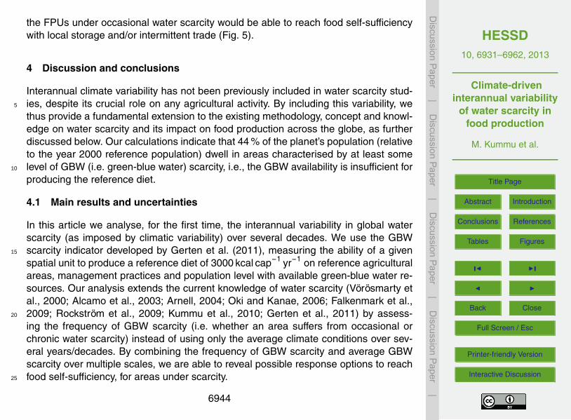
3.1 Interannual variability of GBW scarcity

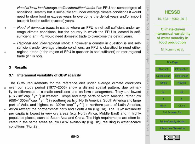
The GBW requirements for the reference diet under average climate conditionsover our study period (1977–2006) show a distinct spatial pattern, due primar-15

ily to differences in climatic conditions and on-farm management. They are lowest(< 650 m3 cap−1 yr−1) in western Europe and large parts of North America, rather low(650–1300 m3 cap−1 yr−1) in southern parts of North America, South America and largepart of Asia, and highest (> 1300 m3 cap−1 yr−1) in northern parts of Latin America,Africa (except the northernmost part) and South Asia (Fig. 1a). The GBW availability20

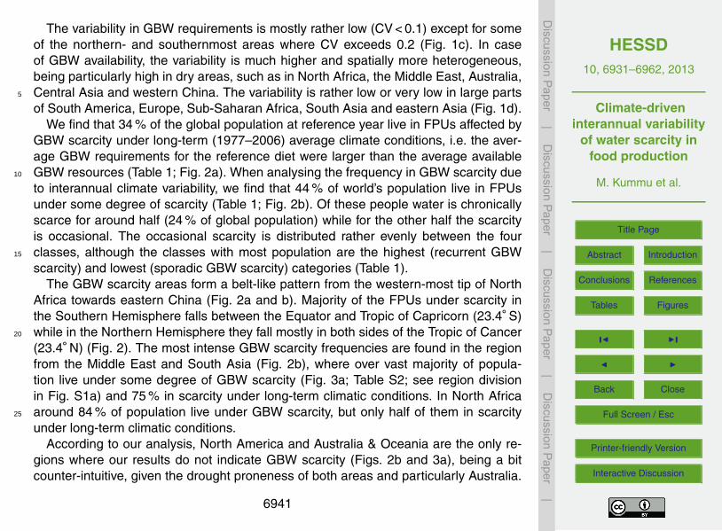
per capita is lowest in very dry areas (e.g. North Africa, Middle East) and in highlypopulated places, such as South Asia and China. The high requirements are often lo-cated in the same areas as low GBW availability (Fig. 1b), resulting in water-scarceconditions (Fig. 2a).

6940





HESSD10, 6931–6962, 2013



M. Kummu et al.

Title Page



Tables Figures

J I

J I

Back Close

Full Screen / Esc



Discussion

Paper

|D

iscussionP

aper|

Discussion

Paper

|D

iscussionP

aper|

The variability in GBW requirements is mostly rather low (CV < 0.1) except for someof the northern- and southernmost areas where CV exceeds 0.2 (Fig. 1c). In caseof GBW availability, the variability is much higher and spatially more heterogeneous,being particularly high in dry areas, such as in North Africa, the Middle East, Australia,Central Asia and western China. The variability is rather low or very low in large parts5

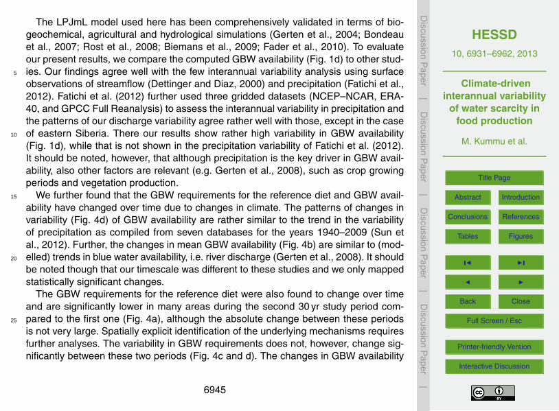
of South America, Europe, Sub-Saharan Africa, South Asia and eastern Asia (Fig. 1d).We find that 34 % of the global population at reference year live in FPUs affected by

GBW scarcity under long-term (1977–2006) average climate conditions, i.e. the aver-age GBW requirements for the reference diet were larger than the average availableGBW resources (Table 1; Fig. 2a). When analysing the frequency in GBW scarcity due10

to interannual climate variability, we find that 44 % of world’s population live in FPUsunder some degree of scarcity (Table 1; Fig. 2b). Of these people water is chronicallyscarce for around half (24 % of global population) while for the other half the scarcityis occasional. The occasional scarcity is distributed rather evenly between the fourclasses, although the classes with most population are the highest (recurrent GBW15

scarcity) and lowest (sporadic GBW scarcity) categories (Table 1).The GBW scarcity areas form a belt-like pattern from the western-most tip of North

Africa towards eastern China (Fig. 2a and b). Majority of the FPUs under scarcity inthe Southern Hemisphere falls between the Equator and Tropic of Capricorn (23.4◦ S)while in the Northern Hemisphere they fall mostly in both sides of the Tropic of Cancer20

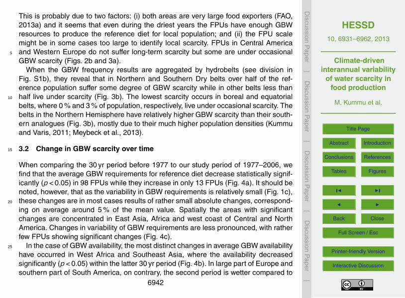
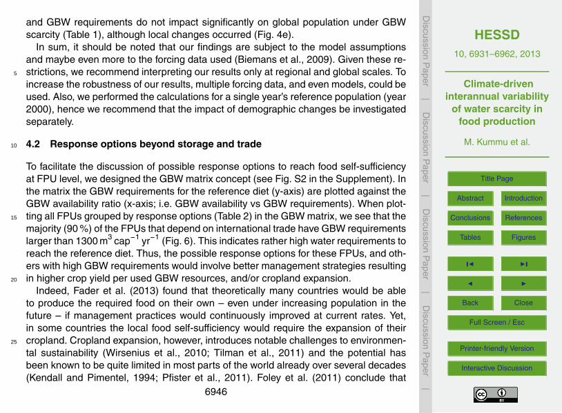
(23.4◦ N) (Fig. 2). The most intense GBW scarcity frequencies are found in the regionfrom the Middle East and South Asia (Fig. 2b), where over vast majority of popula-tion live under some degree of GBW scarcity (Fig. 3a; Table S2; see region divisionin Fig. S1a) and 75 % in scarcity under long-term climatic conditions. In North Africaaround 84 % of population live under GBW scarcity, but only half of them in scarcity25

under long-term climatic conditions.According to our analysis, North America and Australia & Oceania are the only re-

gions where our results do not indicate GBW scarcity (Figs. 2b and 3a), being a bitcounter-intuitive, given the drought proneness of both areas and particularly Australia.

6941





HESSD10, 6931–6962, 2013



M. Kummu et al.

Title Page



Tables Figures

J I

J I

Back Close

Full Screen / Esc



Discussion

Paper

|D

iscussionP

aper|

Discussion

Paper

|D

iscussionP

aper|

This is probably due to two factors: (i) both areas are very large food exporters (FAO,2013a) and it seems that even during the driest years the FPUs have enough GBWresources to produce the reference diet for local population; and (ii) the FPU scalemight be in some cases too large to identify local scarcity. FPUs in Central Americaand Western Europe do not suffer long-term scarcity but some are under occasional5

GBW scarcity (Figs. 2b and 3a).When the GBW frequency results are aggregated by hydrobelts (see division in

Fig. S1b), they reveal that in Northern and Southern Dry belts over half of the ref-erence population suffer some degree of GBW scarcity while in other belts less thanhalf live under scarcity (Fig. 3b). The lowest scarcity occurs in boreal and equatorial10

belts, where 0 % and 3 % of population, respectively, live under occasional scarcity. Thebelts in the Northern Hemisphere have relatively higher GBW scarcity than their south-ern analogues (Fig. 3b), mostly due to their much higher population densities (Kummuand Varis, 2011; Meybeck et al., 2013).

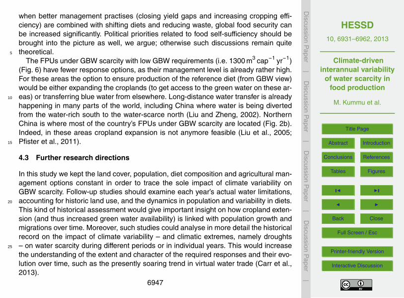
3.2 Change in GBW scarcity over time15

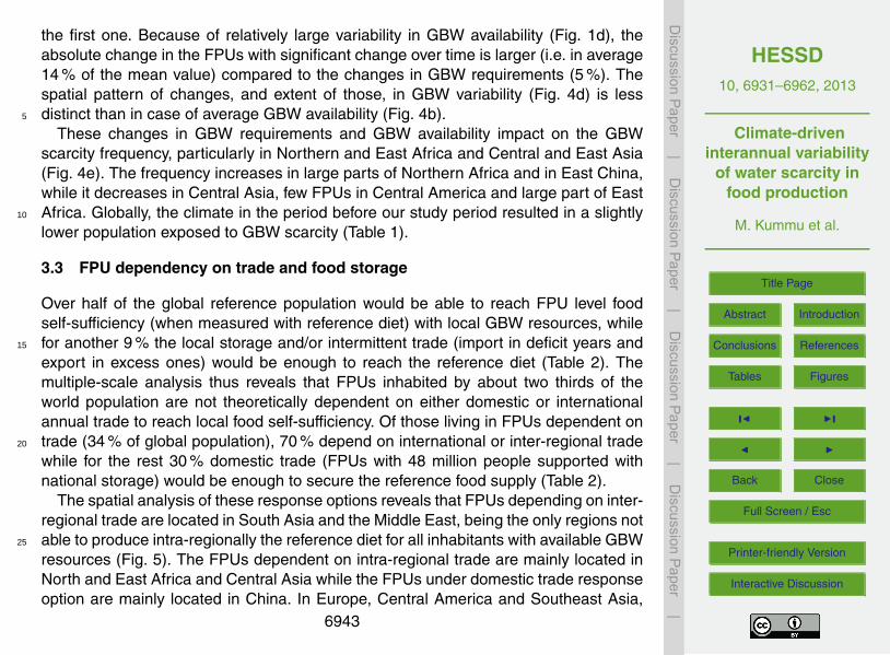
When comparing the 30 yr period before 1977 to our study period of 1977–2006, wefind that the average GBW requirements for reference diet decrease statistically signif-icantly (p< 0.05) in 98 FPUs while they increase in only 13 FPUs (Fig. 4a). It should benoted, however, that as the variability in GBW requirements is relatively small (Fig. 1c),these changes are in most cases results of rather small absolute changes, correspond-20

ing on average around 5 % of the mean value. Spatially the areas with significantchanges are concentrated in East Asia, Africa and west coast of Central and NorthAmerica. Changes in variability of GBW requirements are less pronounced, with ratherfew FPUs showing significant changes (Fig. 4c).

In the case of GBW availability, the most distinct changes in average GBW availability25

have occurred in West Africa and Southeast Asia, where the availability decreasedsignificantly (p< 0.05) within the latter 30 yr period (Fig. 4b). In large part of Europe andsouthern part of South America, on contrary, the second period is wetter compared to

6942





HESSD10, 6931–6962, 2013



M. Kummu et al.

Title Page



Tables Figures

J I

J I

Back Close

Full Screen / Esc



Discussion

Paper

|D

iscussionP

aper|

Discussion

Paper

|D

iscussionP

aper|

the first one. Because of relatively large variability in GBW availability (Fig. 1d), theabsolute change in the FPUs with significant change over time is larger (i.e. in average14 % of the mean value) compared to the changes in GBW requirements (5 %). Thespatial pattern of changes, and extent of those, in GBW variability (Fig. 4d) is lessdistinct than in case of average GBW availability (Fig. 4b).5

These changes in GBW requirements and GBW availability impact on the GBWscarcity frequency, particularly in Northern and East Africa and Central and East Asia(Fig. 4e). The frequency increases in large parts of Northern Africa and in East China,while it decreases in Central Asia, few FPUs in Central America and large part of EastAfrica. Globally, the climate in the period before our study period resulted in a slightly10

lower population exposed to GBW scarcity (Table 1).

3.3 FPU dependency on trade and food storage

Over half of the global reference population would be able to reach FPU level foodself-sufficiency (when measured with reference diet) with local GBW resources, whilefor another 9 % the local storage and/or intermittent trade (import in deficit years and15

export in excess ones) would be enough to reach the reference diet (Table 2). Themultiple-scale analysis thus reveals that FPUs inhabited by about two thirds of theworld population are not theoretically dependent on either domestic or internationalannual trade to reach local food self-sufficiency. Of those living in FPUs dependent ontrade (34 % of global population), 70 % depend on international or inter-regional trade20

while for the rest 30 % domestic trade (FPUs with 48 million people supported withnational storage) would be enough to secure the reference food supply (Table 2).

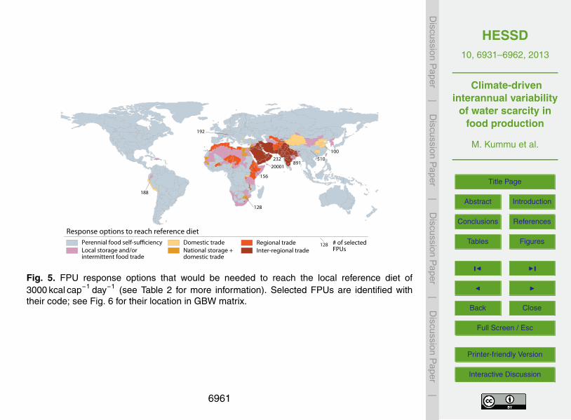
The spatial analysis of these response options reveals that FPUs depending on inter-regional trade are located in South Asia and the Middle East, being the only regions notable to produce intra-regionally the reference diet for all inhabitants with available GBW25

resources (Fig. 5). The FPUs dependent on intra-regional trade are mainly located inNorth and East Africa and Central Asia while the FPUs under domestic trade responseoption are mainly located in China. In Europe, Central America and Southeast Asia,

6943





HESSD10, 6931–6962, 2013



M. Kummu et al.

Title Page



Tables Figures

J I

J I

Back Close

Full Screen / Esc



Discussion

Paper

|D

iscussionP

aper|

Discussion

Paper

|D

iscussionP

aper|

the FPUs under occasional water scarcity would be able to reach food self-sufficiencywith local storage and/or intermittent trade (Fig. 5).

4 Discussion and conclusions

Interannual climate variability has not been previously included in water scarcity stud-ies, despite its crucial role on any agricultural activity. By including this variability, we5

thus provide a fundamental extension to the existing methodology, concept and knowl-edge on water scarcity and its impact on food production across the globe, as furtherdiscussed below. Our calculations indicate that 44 % of the planet’s population (relativeto the year 2000 reference population) dwell in areas characterised by at least somelevel of GBW (i.e. green-blue water) scarcity, i.e., the GBW availability is insufficient for10

producing the reference diet.

4.1 Main results and uncertainties

In this article we analyse, for the first time, the interannual variability in global waterscarcity (as imposed by climatic variability) over several decades. We use the GBWscarcity indicator developed by Gerten et al. (2011), measuring the ability of a given15

spatial unit to produce a reference diet of 3000 kcal cap−1 yr−1 on reference agriculturalareas, management practices and population level with available green-blue water re-sources. Our analysis extends the current knowledge of water scarcity (Vörösmarty etal., 2000; Alcamo et al., 2003; Arnell, 2004; Oki and Kanae, 2006; Falkenmark et al.,2009; Rockström et al., 2009; Kummu et al., 2010; Gerten et al., 2011) by assess-20

ing the frequency of GBW scarcity (i.e. whether an area suffers from occasional orchronic water scarcity) instead of using only the average climate conditions over sev-eral years/decades. By combining the frequency of GBW scarcity and average GBWscarcity over multiple scales, we are able to reveal possible response options to reachfood self-sufficiency, for areas under scarcity.25

6944





HESSD10, 6931–6962, 2013



M. Kummu et al.

Title Page



Tables Figures

J I

J I

Back Close

Full Screen / Esc



Discussion

Paper

|D

iscussionP

aper|

Discussion

Paper

|D

iscussionP

aper|

The LPJmL model used here has been comprehensively validated in terms of bio-geochemical, agricultural and hydrological simulations (Gerten et al., 2004; Bondeauet al., 2007; Rost et al., 2008; Biemans et al., 2009; Fader et al., 2010). To evaluateour present results, we compare the computed GBW availability (Fig. 1d) to other stud-ies. Our findings agree well with the few interannual variability analysis using surface5

observations of streamflow (Dettinger and Diaz, 2000) and precipitation (Fatichi et al.,2012). Fatichi et al. (2012) further used three gridded datasets (NCEP–NCAR, ERA-40, and GPCC Full Reanalysis) to assess the interannual variability in precipitation andthe patterns of our discharge variability agree rather well with those, except in the caseof eastern Siberia. There our results show rather high variability in GBW availability10

(Fig. 1d), while that is not shown in the precipitation variability of Fatichi et al. (2012).It should be noted, however, that although precipitation is the key driver in GBW avail-ability, also other factors are relevant (e.g. Gerten et al., 2008), such as crop growingperiods and vegetation production.

We further found that the GBW requirements for the reference diet and GBW avail-15

ability have changed over time due to changes in climate. The patterns of changes invariability (Fig. 4d) of GBW availability are rather similar to the trend in the variabilityof precipitation as compiled from seven databases for the years 1940–2009 (Sun etal., 2012). Further, the changes in mean GBW availability (Fig. 4b) are similar to (mod-elled) trends in blue water availability, i.e. river discharge (Gerten et al., 2008). It should20

be noted though that our timescale was different to these studies and we only mappedstatistically significant changes.

The GBW requirements for the reference diet were also found to change over timeand are significantly lower in many areas during the second 30 yr study period com-pared to the first one (Fig. 4a), although the absolute change between these periods25

is not very large. Spatially explicit identification of the underlying mechanisms requiresfurther analyses. The variability in GBW requirements does not, however, change sig-nificantly between these two periods (Fig. 4c and d). The changes in GBW availability

6945





HESSD10, 6931–6962, 2013



M. Kummu et al.

Title Page



Tables Figures

J I

J I

Back Close

Full Screen / Esc



Discussion

Paper

|D

iscussionP

aper|

Discussion

Paper

|D

iscussionP

aper|

and GBW requirements do not impact significantly on global population under GBWscarcity (Table 1), although local changes occurred (Fig. 4e).

In sum, it should be noted that our findings are subject to the model assumptionsand maybe even more to the forcing data used (Biemans et al., 2009). Given these re-strictions, we recommend interpreting our results only at regional and global scales. To5

increase the robustness of our results, multiple forcing data, and even models, could beused. Also, we performed the calculations for a single year’s reference population (year2000), hence we recommend that the impact of demographic changes be investigatedseparately.

4.2 Response options beyond storage and trade10

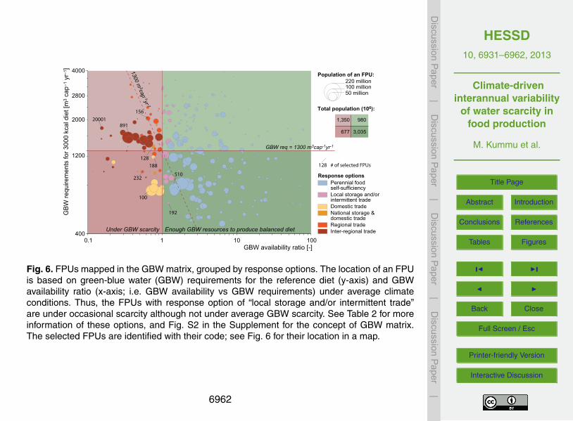
To facilitate the discussion of possible response options to reach food self-sufficiencyat FPU level, we designed the GBW matrix concept (see Fig. S2 in the Supplement). Inthe matrix the GBW requirements for the reference diet (y-axis) are plotted against theGBW availability ratio (x-axis; i.e. GBW availability vs GBW requirements). When plot-ting all FPUs grouped by response options (Table 2) in the GBW matrix, we see that the15

majority (90 %) of the FPUs that depend on international trade have GBW requirementslarger than 1300 m3 cap−1 yr−1 (Fig. 6). This indicates rather high water requirements toreach the reference diet. Thus, the possible response options for these FPUs, and oth-ers with high GBW requirements would involve better management strategies resultingin higher crop yield per used GBW resources, and/or cropland expansion.20

Indeed, Fader et al. (2013) found that theoretically many countries would be ableto produce the required food on their own – even under increasing population in thefuture – if management practices would continuously improved at current rates. Yet,in some countries the local food self-sufficiency would require the expansion of theircropland. Cropland expansion, however, introduces notable challenges to environmen-25

tal sustainability (Wirsenius et al., 2010; Tilman et al., 2011) and the potential hasbeen known to be quite limited in most parts of the world already over several decades(Kendall and Pimentel, 1994; Pfister et al., 2011). Foley et al. (2011) conclude that

6946





HESSD10, 6931–6962, 2013



M. Kummu et al.

Title Page



Tables Figures

J I

J I

Back Close

Full Screen / Esc



Discussion

Paper

|D

iscussionP

aper|

Discussion

Paper

|D

iscussionP

aper|

when better management practises (closing yield gaps and increasing cropping effi-ciency) are combined with shifting diets and reducing waste, global food security canbe increased significantly. Political priorities related to food self-sufficiency should bebrought into the picture as well, we argue; otherwise such discussions remain quitetheoretical.5

The FPUs under GBW scarcity with low GBW requirements (i.e. 1300 m3 cap−1 yr−1)(Fig. 6) have fewer response options, as their management level is already rather high.For these areas the option to ensure production of the reference diet (from GBW view)would be either expanding the croplands (to get access to the green water on these ar-eas) or transferring blue water from elsewhere. Long-distance water transfer is already10

happening in many parts of the world, including China where water is being divertedfrom the water-rich south to the water-scarce north (Liu and Zheng, 2002). NorthernChina is where most of the country’s FPUs under GBW scarcity are located (Fig. 2b).Indeed, in these areas cropland expansion is not anymore feasible (Liu et al., 2005;Pfister et al., 2011).15

4.3 Further research directions

In this study we kept the land cover, population, diet composition and agricultural man-agement options constant in order to trace the sole impact of climate variability onGBW scarcity. Follow-up studies should examine each year’s actual water limitations,accounting for historic land use, and the dynamics in population and variability in diets.20

This kind of historical assessment would give important insight on how cropland exten-sion (and thus increased green water availability) is linked with population growth andmigrations over time. Moreover, such studies could analyse in more detail the historicalrecord on the impact of climate variability – and climatic extremes, namely droughts– on water scarcity during different periods or in individual years. This would increase25

the understanding of the extent and character of the required responses and their evo-lution over time, such as the presently soaring trend in virtual water trade (Carr et al.,2013).

6947





HESSD10, 6931–6962, 2013



M. Kummu et al.

Title Page



Tables Figures

J I

J I

Back Close

Full Screen / Esc



Discussion

Paper

|D

iscussionP

aper|

Discussion

Paper

|D

iscussionP

aper|

It should be noted that many FPUs that are today under GBW scarcity, or are ap-proaching that, are facing rapid population growth and thus, the situation can be ex-pected to become even more challenging in the near future (Gerten et al., 2011; Faderet al., 2013; Suweis et al., 2013). Or it might actually already be so since 13 yr havepassed since the conditions of our population reference year. The projected climate5

change, as well as demographic growth, thus adds another extra stress dimensions,particularly in regions such as the Middle East, northern and southern Africa, and partsof Australia. Therefore, it would be important to assess how the projected increase inhydroclimatic variability in the future (e.g. Boer, 2009; Wetherald, 2010) might impacton frequency of GBW scarcity. As the future climate would concur with population pro-10

jections, showing rapid growth in many areas under water scarcity (UN, 2011), muchmore FPUs would turn from water abundant to water scarce (as suggested by Arnell,2004; Arnell et al., 2011 for the river basin scale). Thus, it would be desirable to in-vestigate the impact of climate variability in the future, in order to extend the currentknowledge of adaptation options to secure the food supply to everyone.15

The policies related to food self-sufficiency should also be systematically investigatedwithin the context of studies such as ours. Our analysis reveals the theoretical potentialof FPUs to reach perennial or potential food self-sufficiency, or if self-sufficiency can-not be reached, the dependence level on either domestic or international food trade.We strongly encourage the linking of our study and approach to investigations on na-20

tional and regional food policies across the globe in order to bridge the calculations oftheoretical potentials to actual policy level priorities for meeting the demand for food.

Supplementary material related to this article is available online at:http://www.hydrol-earth-syst-sci-discuss.net/10/6931/2013/hessd-10-6931-2013-supplement.pdf.25

6948





http://www.hydrol-earth-syst-sci-discuss.net/10/6931/2013/hessd-10-6931-2013-supplement.pdf



HESSD10, 6931–6962, 2013



M. Kummu et al.

Title Page



Tables Figures

J I

J I

Back Close

Full Screen / Esc



Discussion

Paper

|D

iscussionP

aper|

Discussion

Paper

|D

iscussionP

aper|

Acknowledgements. We thank our colleagues at Aalto University and the Potsdam Institute forClimate Impact Research for their support and helpful comments. This work was partly fundedby the Maa-ja vesitekniikan tuki ry, the postdoctoral funds and core funds of Aalto University,and the European Communities’ project CLIMAFRICA (grant no. 244240).

References5

Alcamo, J., Döll, P., Henrichs, T., Kaspar, F., Lehner, B., Rösch, T., and Siebert, S.: Globalestimates of water withdrawals and availability under current and future “business-as-usual”conditions, Hydrolog. Sci. J., 48, 339–348, 2003.

Arnell, N. W.: Climate change and global water resources: SRES emissions and socio-economic scenarios, Global Environ. Change, 14, 31–52, 2004.10

Arnell, N. W., van Vuuren, D. P., and Isaac, M.: The implications of climate policy for the im-pacts of climate change on global water resources, Global Environ. Change, 21, 592–603,doi:10.1016/j.gloenvcha.2011.01.015, 2011.

Biemans, H., Hutjes, R. W. A., Kabat, P., Strengers, B. J., Gerten, D., and Rost, S.: Effects ofPrecipitation Uncertainty on Discharge Calculations for Main River Basins, J. Hydrometeo-15

rol., 10, 1011–1025, doi:10.1175/2008JHM1067.1, 2009.Biemans, H., Haddeland, I., Kabat, P., Ludwig, F., Hutjes, R. W. A., Heinke, J., von Bloh, W.,

and Gerten, D.: Impact of reservoirs on river discharge and irrigation water supply during the20th century, Water Resour. Res., 47, W03509, doi:10.1029/2009WR008929, 2011.

Boer, G. J.: Changes in Interannual Variability and Decadal Potential Predictability under Global20

Warming, J. Climate, 22, 3098–3109, doi:10.1175/2008JCLI2835.1, 2009.Bondeau, A., Smith, P., Zaehle, S., Schaphoff, S., Lucht, W., Cramer, W., Gerten, D., Lotze-

Campen, H., Müller, C., Reichstein, M., and Smith, B.: Modelling the role of agriculture forthe 20th century global terrestrial carbon balance, Global Change Biol., 13, 679–706, 2007.

Brown, C. and Lall, U.: Water and economic development: The role of variability and25

a framework for resilience, Nat. Resour. Forum, 30, 306–317, doi:10.1111/j.1477-8947.2006.00118.x, 2006.

Brown, C., Meeks, R., Ghile, Y., and Hunu, K.: An Empirical Analysis of the Effects of ClimateVariables on National Level Economic Growth, The World Bank, 29, 2010.

6949





http://dx.doi.org/10.1016/j.gloenvcha.2011.01.015

http://dx.doi.org/10.1175/2008JHM1067.1

http://dx.doi.org/10.1029/2009WR008929

http://dx.doi.org/10.1175/2008JCLI2835.1

http://dx.doi.org/10.1111/j.1477-8947.2006.00118.x

http://dx.doi.org/10.1111/j.1477-8947.2006.00118.x

http://dx.doi.org/10.1111/j.1477-8947.2006.00118.x

HESSD10, 6931–6962, 2013



M. Kummu et al.

Title Page



Tables Figures

J I

J I

Back Close

Full Screen / Esc



Discussion

Paper

|D

iscussionP

aper|

Discussion

Paper

|D

iscussionP

aper|

Brown, M. B. and Forsythe, A. B.: Robust tests for equality of variances, J. Am. StatisticalAssoc., 69, 364–367, 1974.

Cai, X. and Rosegrant, M.: Global water demand and supply projections. Part 1: A modelingapproach, Water Int., 27, 159–169, 2002.

Carr, J. A., D’Odorico, P., Laio, F., and Ridolfi, L.: Recent History and Geography of Virtual5

Water Trade, PLoS ONE, 8, e55825, doi:10.1371/journal.pone.0055825, 2013.Dai, A.: Drought under global warming: a review, WIREs Climate Change, 2, 45–65, 2011.Dai, A., Qian, T., Trenberth, K. E., and Milliman, J. D.: Changes in Continental Freshwater Dis-

charge from 1948 to 2004, J. Climate, 22, 2773–2792, doi:10.1175/2008JCLI2592.1, 2009.De Fraiture, C.: Integrated water and food analysis at the global and basin level. An application10

of WATERSIM, Water Resour. Manag., 21, 185–198, 2007.Dettinger, M. D. and Diaz, H. F.: Global Characteristics of Stream Flow Seasonality and Vari-

ability, J. Hydrometeorol., 1, 289–310, doi:10.1175/1525-7541(2000)001<0289:GCOSFS>2.0.CO;2, 2000.

Fader, M., Rost, S., Müller, C., and Gerten, D.: Virtual water content of temperate cereals and15

maize: Present and potential future patterns, J. Hydrol., 384, 218–231, 2010.Fader, M., Gerten, D., Krause, M., Lucht, W., and Cramer, W.: Spatial decoupling of agricultural

production and consumption: quantifying dependences of countries on food imports dueto domestic land and water constraints, Environ. Res. Lett., 8, 014046, doi:10.1088/1748-9326/8/1/014046, 2013.20

Falkenmark, M.: Meeting water requirements of an expanding world population, Philos. T. R.Soc Lond. B, 352, 929–936, doi:10.1098/rstb.1997.0072, 1997.

Falkenmark, M., Lundqvist, J., and Widstrand, C.: Macro-scale water scarcity requires micro-scale approaches, Nat. Resour. Forum, 13, 258–267, 1989.

Falkenmark, M., Rockström, J., and Karlberg, L.: Present and future water requirements for25

feeding humanity, Food Security, 1, 59–69, doi:10.1007/s12571-008-0003-x, 2009.FAO: FAOSTAT – FAO database for food and agriculture, Food and agriculture Organisation of

United Nations (FAO), Rome, 2013a.FAO: Food security indicators, Food and Agriculture Organization of the United Nations

(FAO), Rome, available at: http://www.fao.org/economic/ess/ess-fs/ess-fadata/en/ (last ac-30

cess: 19 April 2013), 2013b.

6950





http://dx.doi.org/10.1371/journal.pone.0055825


http://dx.doi.org/10.1175/1525-7541(2000)001<0289:GCOSFS>2.0.CO;2



http://dx.doi.org/10.1088/1748-9326/8/1/014046

http://dx.doi.org/10.1088/1748-9326/8/1/014046

http://dx.doi.org/10.1088/1748-9326/8/1/014046

http://dx.doi.org/10.1098/rstb.1997.0072

http://dx.doi.org/10.1007/s12571-008-0003-x

http://www.fao.org/economic/ess/ess-fs/ess-fadata/en/

HESSD10, 6931–6962, 2013



M. Kummu et al.

Title Page



Tables Figures

J I

J I

Back Close

Full Screen / Esc



Discussion

Paper

|D

iscussionP

aper|

Discussion

Paper

|D

iscussionP

aper|

Fatichi, S., Ivanov, V. Y., and Caporali, E.: Investigating Interannual Variability of Precipitationat the Global Scale: Is There a Connection with Seasonality?, J. Climate, 25, 5512–5523,doi:10.1175/JCLI-D-11-00356.1, 2012.

Foley, J. A., Ramankutty, N., Brauman, K. A., Cassidy, E. S., Gerber, J. S., Johnston, M.,Mueller, N. D., O’Connell, C., Ray, D. K., West, P. C., Balzer, C., Bennett, E. M., Car-5

penter, S. R., Hill, J., Monfreda, C., Polasky, S., Rockstrom, J., Sheehan, J., Siebert, S.,Tilman, D., and Zaks, D. P. M.: Solutions for a cultivated planet, Nature, 478, 337–342,doi:10.1038/nature10452, 2011.

Gerten, D., Schaphoff, S., Haberlandt, U., Lucht, W., and Sitch, S.: Terrestrial vegetation andwater balance – hydrological evaluation of a dynamic global vegetation model, J. Hydrol.,10

286, 249–270, doi:10.1016/j.jhydrol.2003.09.029, 2004.Gerten, D., Lucht, W., Schaphoff, S., Cramer, W., Hickler, T., and Wagner, W.: Hy-

drologic resilience of the terrestrial biosphere, Geophys. Res. Lett., 32, L21408,doi:10.1029/2005GL024247, 2005.

Gerten, D., Rost, S., von Bloh, W., and Lucht, W.: Causes of change in 20th century global river15

discharge, Geophys. Res. Lett., 35, L20405, doi:10.1029/2008GL035258, 2008.Gerten, D., Heinke, J., Hoff, H., Biemans, H., Fader, M., and Waha, K.: Global water

availability and requirements for future food production, J. Hydrometeorol., 12, 885–899,doi:10.1175/2011JHM1328.1, 2011.

Haddeland, I., Clark, D. B., Franssen, W., Ludwig, F., Voß, F., Arnell, N. W., Bertrand, N., Best,20

M., Folwell, S., Gerten, D., Gomes, S., Gosling, S. N., Hagemann, S., Hanasaki, N., Harding,R., Heinke, J., Kabat, P., Koirala, S., Oki, T., Polcher, J., Stacke, T., Viterbo, P., Weedon, G.P., and Yeh, P.: Multimodel Estimate of the Global Terrestrial Water Balance: Setup and FirstResults, J. Hydrometeorol., 12, 869–884, doi:10.1175/2011JHM1324.1, 2011.

Heinke, J., Ostberg, S., Schaphoff, S., Frieler, K., Müller, C., Gerten, D., Meinshausen, M.,25

and Lucht, W.: A new dataset for systematic assessments of climate change impacts as afunction of global warming, Geosci. Model Dev. Discuss., 5, 3533–3572, doi:10.5194/gmdd-5-3533-2012, 2012.

Hirabayashi, Y., Kanae, S., Struthers, I., and Oki, T.: A 100-year (1901–2000) global retro-spective estimation of the terrestrial water cycle, J. Geophys. Res.-Atmos., 110, D19101,30

doi:10.1029/2004JD005492, 2005.

6951





http://dx.doi.org/10.1175/JCLI-D-11-00356.1

http://dx.doi.org/10.1038/nature10452

http://dx.doi.org/10.1016/j.jhydrol.2003.09.029

http://dx.doi.org/10.1029/2005GL024247

http://dx.doi.org/10.1029/2008GL035258



http://dx.doi.org/10.5194/gmdd-5-3533-2012



http://dx.doi.org/10.1029/2004JD005492

HESSD10, 6931–6962, 2013



M. Kummu et al.

Title Page



Tables Figures

J I

J I

Back Close

Full Screen / Esc



Discussion

Paper

|D

iscussionP

aper|

Discussion

Paper

|D

iscussionP

aper|

Hoekstra, A. Y., Mekonnen, M. M., Chapagain, A. K., Mathews, R. E., and Richter, B. D.: GlobalMonthly Water Scarcity: Blue Water Footprints versus Blue Water Availability, PLoS ONE, 7,e32688, doi:10.1371/journal.pone.0032688, 2012.

Kendall, H. W. and Pimentel, D.: Constraints on the Expansion of the Global Food Supply,Ambio, 23, 198–205, 1994.5

Konzmann, M., Gerten, D., and Heinke, J.: Climate impacts on global irrigation requirementsunder 19 GCMs, simulated with a vegetation and hydrology model, Hydrolog. Sci. J., 58,1–18, 2013.

Kummu, M. and Varis, O.: The World by latitudes: a global analysis of human population, devel-opment level and environment across the north-south axis over the past half century, Appl.10

Geogr., 31, 495–507, doi:10.1016/j.apgeog.2010.10.009, 2011.Kummu, M., Ward, P. J., de Moel, H., and Varis, O.: Is physical water scarcity a new phe-

nomenon? Global assessment of water shortage over the last two millennia, Environ. Res.Lett., 5, 034006, doi:10.1088/1748-9326/5/3/034006, 2010.

Kummu, M., de Moel, H., Porkka, M., Siebert, S., Varis, O., and Ward, P. J.: Lost food, wasted15

resources: global food supply chain losses and their impacts on freshwater, cropland, andfertiliser use, Sci. Total Environ., 438, 477–489, doi:10.1016/j.scitotenv.2012.08.092, 2012.

Liu, C. and Zheng, H.: South-to-north Water Transfer Schemes for China, Int. J. Water Resour.Dev., 18, 453–471, doi:10.1080/0790062022000006934, 2002.

Liu, X., Wang, J., Liu, M., and Meng, B.: Spatial heterogeneity of the driving forces of cropland20

change in China, Sci. China Ser. D, 48, 2231–2240, 2005.Ma, Z. and Fu, C.: Global aridification in the second half of the 20th century and its relationship

to large-scale climate background, Sci. China Ser. D, 50, 776–788, doi:10.1007/s11430-007-0036-6, 2007.

Meybeck, M., Kummu, M., and Dürr, H. H.: Global hydrobelts and hydroregions: im-25

proved reporting scale for water-related issues?, Hydrol. Earth Syst. Sci., 17, 1093–1111,doi:10.5194/hess-17-1093-2013, 2013.

Mitchell, T. D. and Jones, P. D.: An improved method of constructing a database of monthlyclimate observations and associated high-resolution grids, Int. J. Climatol., 25, 693–712,doi:10.1002/joc.1181, 2005.30

Notaro, M.: Response of the mean global vegetation distribution to interannual climate variabil-ity, Clim. Dynam., 30, 845–854, doi:10.1007/s00382-007-0329-7, 2008.

6952





http://dx.doi.org/10.1371/journal.pone.0032688

http://dx.doi.org/10.1016/j.apgeog.2010.10.009

http://dx.doi.org/10.1088/1748-9326/5/3/034006

http://dx.doi.org/10.1016/j.scitotenv.2012.08.092

http://dx.doi.org/10.1080/0790062022000006934

http://dx.doi.org/10.1007/s11430-007-0036-6

http://dx.doi.org/10.1007/s11430-007-0036-6

http://dx.doi.org/10.1007/s11430-007-0036-6

http://dx.doi.org/10.5194/hess-17-1093-2013

http://dx.doi.org/10.1002/joc.1181

http://dx.doi.org/10.1007/s00382-007-0329-7

HESSD10, 6931–6962, 2013



M. Kummu et al.

Title Page



Tables Figures

J I

J I

Back Close

Full Screen / Esc



Discussion

Paper

|D

iscussionP

aper|

Discussion

Paper

|D

iscussionP

aper|

Oki, T. and Kanae, S.: Global Hydrological Cycles and World Water Resources, Science, 313,1068–1072, doi:10.1126/science.1128845, 2006.

Pfister, S., Bayer, P., Koehler, A., and Hellweg, S.: Projected water consumption in futureglobal agriculture: Scenarios and related impacts, Sci. Total Environ., 409, 4206–4216,doi:10.1016/j.scitotenv.2011.07.019, 2011.5

Piao, S., Friedlingstein, P., Ciais, P., de Noblet-Ducoudré, N., Labat, D., and Zaehle, S.: Changesin climate and land use have a larger direct impact than rising CO2 on global river runofftrends, P. Natl. Acad. Sci., 104, 15242–15247, doi:10.1073/pnas.0707213104, 2007.

Portmann, F. T., Siebert, S., and Döll, P.: MIRCA2000 – Global monthly irrigated and rainfedcrop areas around the year 2000: A new high-resolution data set for agricultural and hydro-10

logical modeling, Global Biogeochem. Cy., 24, GB1011, doi:10.1029/2008gb003435, 2010.Ramankutty, N., Evan, A. T., Monfreda, C., and Foley, J. A.: Farming the planet: 1. Geo-

graphic distribution of global agricultural lands in the year 2000, Global Biogeochem. Cy.,22, GB1003, doi:10.1029/2007GB002952, 2008.

Rockström, J., Falkenmark, M., Karlberg, L., Hoff, H., Rost, S., and Gerten, D.: Future water15

availability for global food production: The potential of green water for increasing resilienceto global change, Water Resour. Res., 45, W00A12, doi:10.1029/2007WR006767, 2009.

Rosegrant, M., Cai, X., and Cline, S.: World Water and Food to 2025. Dealing with Scarcity,International Food Policy Research Institute (IFPRI), Washington DC, USA, 2002.

Rost, S., Gerten, D., Bondeau, A., Lucht, W., Rohwer, J., and Schaphoff, S.: Agricultural green20

and blue water consumption and its influence on the global water system, Water Resour.Res., 44, W09405, doi:10.1029/2007WR006331, 2008.

Rudolf, B., Becker, A., Schneider, U., Meyer-Christoffer, A., and Ziese, M.: GPCC Status ReportDecember 2010, Global Precipitation Climatology Centre (GPCC), 2010.

Sakai, D., Itoh, H., and Yukimoto, S.: Changes in the Interannual Surface Air Temperature25

Variability in the Northern Hemisphere in Response to Global Warming, J. Meteorol. Soc.Jpn., 87, 721–737, doi:10.2151/jmsj.87.721, 2009.

Sheffield, J., Andreadis, K. M., Wood, E. F., and Lettenmaier, D. P.: Global and Con-tinental Drought in the Second Half of the Twentieth Century: Severity–Area–DurationAnalysis and Temporal Variability of Large-Scale Events, J. Climate, 22, 1962–1981,30

doi:10.1175/2008JCLI2722.1, 2009.Sun, F., Roderick, M. L., and Farquhar, G. D.: Changes in the variability of global land precipi-

tation, Geophys. Res. Lett., 39, L19402, doi:10.1029/2012GL053369, 2012.

6953





http://dx.doi.org/10.1126/science.1128845

http://dx.doi.org/10.1016/j.scitotenv.2011.07.019

http://dx.doi.org/10.1073/pnas.0707213104

http://dx.doi.org/10.1029/2008gb003435

http://dx.doi.org/10.1029/2007GB002952

http://dx.doi.org/10.1029/2007WR006767

http://dx.doi.org/10.1029/2007WR006331

http://dx.doi.org/10.2151/jmsj.87.721


http://dx.doi.org/10.1029/2012GL053369

HESSD10, 6931–6962, 2013



M. Kummu et al.

Title Page



Tables Figures

J I

J I

Back Close

Full Screen / Esc



Discussion

Paper

|D

iscussionP

aper|

Discussion

Paper

|D

iscussionP

aper|

Suweis, S., Rinaldo, A., Maritan, A., and D’Odorico, P.: Water-controlled wealth of nations, P.Natl. Acad. Sci., 110, 4230–4233, doi:10.1073/pnas.1222452110, 2013.

Tilman, D., Balzer, C., Hill, J., and Befort, B. L.: Global food demand and the sustainable intensi-fication of agriculture, P. Natl. Acad. Sci., 108, 20260–20264, doi:10.1073/pnas.1116437108,2011.5

Trenberth, K. E., Jones, P. D., Ambenje, P., Bojariu, R., Easterling, D., Klein Tank, A., Parker, D.,Rahimzadeh, F., Renwick, J. A., Rusticucci, M., Soden, B., and Zhai, P.: Observations: sur-face and atmospheric climate change, in: Climate Change 2007: The Physical Science Basis.Contribution of Working Group I to the Fourth Assessment Report of the IntergovernmentalPanel on Climate Change, edited by: Solomon, S., Qin, D., Manning, M., Chen, Z., Marquis,10

M., Averyt, K. B., Tignor, M., and Miller, H. L., Cambridge University Press, Cambridge andNew York, 235–336, 2007.

UN: World Population Prospects: The 2010 Revision, Population Division of the Departmentof Economic and Social Affairs of the United Nations (UN) Secretariat, available at: http://esa.un.org/wpp/ (last access: March 2012), 2011.15

Vörösmarty, C. J., Green, P., Salisbury, J., and Lammers, R. B.: Global Water Resources: Vul-nerability from Climate Change and Population Growth, Science, 289, 284–288, 2000.

Wada, Y., van Beek, L. P. H., Viviroli, D., Dürr, H. H., Weingartner, R., and Bierkens, M. F. P.:Global monthly water stress: 2. Water demand and severity of water stress, Water Resour.Res., 47, W07518, doi:10.1029/2010WR009792, 2011.20

Ward, P. J., Beets, W., Bouwer, L. M., Aerts, J. C. J. H., and Renssen, H.: Sensitivity of riverdischarge to ENSO, Geophys. Res. Lett., 37, L12402, doi:10.1029/2010GL043215, 2010.

Wetherald, R.: Changes of time mean state and variability of hydrology in response to a dou-bling and quadrupling of CO2, Climatic Change, 102, 651–670, doi:10.1007/s10584-009-9701-4, 2010.25

Wirsenius, S., Azar, C., and Berndes, G.: How much land is needed for global food productionunder scenarios of dietary changes and livestock productivity increases in 2030?, Agr. Syst.,103, 621–638, doi:10.1016/j.agsy.2010.07.005, 2010.

Zachos, J., Pagani, M., Sloan, L., Thomas, E., and Billups, K.: Trends, Rhythms,and Aberrations in Global Climate 65 Ma to Present, Science, 292, 686–693,30

doi:10.1126/science.1059412, 2001.

6954







http://esa.un.org/wpp/



http://dx.doi.org/10.1029/2010WR009792

http://dx.doi.org/10.1029/2010GL043215

http://dx.doi.org/10.1007/s10584-009-9701-4

http://dx.doi.org/10.1007/s10584-009-9701-4

http://dx.doi.org/10.1007/s10584-009-9701-4

http://dx.doi.org/10.1016/j.agsy.2010.07.005

http://dx.doi.org/10.1126/science.1059412

HESSD10, 6931–6962, 2013



M. Kummu et al.

Title Page



Tables Figures

J I

J I

Back Close

Full Screen / Esc



Discussion

Paper

|D

iscussionP

aper|

Discussion

Paper

|D

iscussionP

aper|

Table 1. Global population (in millions) under green-blue water (GBW) scarcity. Frequency ofscarcity over the period (1977–2006) and over the 30 yr period before that (1947–1976). Bottomrow (“average scarcity”) represents the GBW scarcity under average climate conditions withinthose periods. See also Figs. 2 and 4e. Note that the calculations were made for constantreference population (year 2000 situation) but varying climate within the indicated time periods.

Population under GBW scarcity (in millions)

Frequency 1977–2006 % of total 1947–1976 % of total

0 % 3,471 57.4 % 3524 58.3 %0–25 % 332 5.5 % 247 4.1 %25–50 % 197 3.3 % 240 4.0 %50–75 % 212 3.5 % 198 3.3 %75–100 % 375 6.2 % 370 6.1 %100 % 1456 24.1 % 1463 24.2 %

Total 6042 6042

Average scarcity 2027 33.6 % 1,885 31.2 %

6955





HESSD10, 6931–6962, 2013



M. Kummu et al.

Title Page



Tables Figures

J I

J I

Back Close

Full Screen / Esc



Discussion

Paper

|D

iscussionP

aper|

Discussion

Paper

|D

iscussionP

aper|

Table 2. Response options for FPUs, depending on the ability of to reach reference diet of3000 kcal cap−1 yr−1 (see map in Fig. 5 and FPUs in GBW matrix in Fig. 6). Scarcity frequencyrefers to the frequency of GBW scarcity (see Fig. 2b) and average scarcity on GBW scarcityunder average climate conditions (see Fig. 2a) over our study period of 1977–2006.

FPU Country Region Population

Scarcity frequency 0 % > 0 % > 0 % 0 % > 0 % > 0 %Average scarcity No no yes no no yes no yes 106 %

No response needed × 3471 57.4 %Local food storage and/or intermittent trade × 544 9.0 %Domestic trade × × 563 9.3 %National storage & domestic trade × × 48 0.8 %Regional trade × × × 266 4.4 %Inter-regional trade × × × 1163 19.0 %

6956





HESSD10, 6931–6962, 2013



M. Kummu et al.

Title Page



Tables Figures

J I

J I

Back Close

Full Screen / Esc



Discussion

Paper

|D

iscussionP

aper|

Discussion

Paper

|D

iscussionP

aper|

2000 - 27001300 - 2000

> 34002700 - 3400

650 - 1300< 650

2000 - 27001300 - 2000

> 34002700 - 3400

650 - 1300< 650

0 - 0.050.05 - 0.1

0.1 - 0.150.15 - 0.2

0.2 - 1.1 0 - 0.050.05 - 0.1

0.1 - 0.150.15 - 0.2

0.2 - 0.75

A. GBW requirements for reference diet (m3cap–1yr–1) B. GBW availability (m3cap–1yr–1)

C. Variability in GBW requirements for reference diet (coefficient of variation) D. Variability in GBW availability (coefficient of variation)

Fig. 1. Green-blue water (GBW) requirements for reference diet and GBW availability. (A) Aver-age GBW requirements over 30 yr study period; (B) average GBW availability over 30 yr studyperiod; (C) variability in GBW requirements measured with coefficient of variation (CV); and(D) variability in GBW availability measured with CV.

6957





HESSD10, 6931–6962, 2013



M. Kummu et al.

Title Page



Tables Figures

J I

J I

Back Close

Full Screen / Esc



Discussion

Paper

|D

iscussionP

aper|

Discussion

Paper

|D

iscussionP

aper|

No scarcity Under scarcity

Never under scarcity 0 - 25%25 - 50%

50 - 75% of years under scarcity75-100%

Every year under scarcity

0°

23.4°N

23.4°S

0°

23.4°N

23.4°S

A. GBW scarcity under average climate conditions

B. Frequency of GBW scarcity due to interannual climate variability

Fig. 2. Green-blue water (GBW) scarcity mapped by FPUs. (A) GBW scarcity under averageclimate conditions over 30 yr study period; and (B) frequency of GBW scarcity due to interan-nual climate variability. The marked latitudes represent Tropic of Cancer (23.4◦ N), Equator (0◦),and Tropic of Capricorn (23.4◦ S).

6958





HESSD10, 6931–6962, 2013



M. Kummu et al.

Title Page



Tables Figures

J I

J I

Back Close

Full Screen / Esc



Discussion

Paper

|D

iscussionP

aper|

Discussion

Paper

|D

iscussionP

aper|

Boreal

Northern Mid Latitude

Northern Dry

Northern Sub-Tropical

Equator

Southern Sub-Tropical

Southern Dry

Southern Mid Latitude

0% 25% 50% 75% 100%

0% 25% 50% 75% 100%

Australia and Oceania

Central America

Eastern Asia

Eastern Europe and Central Asia

South Asia

Latin America

Middle and Southern Africa

Middle East

North Africa

North America

Southeastern Asia

Western Europe

A. Frequency of GBW scarcity by administrative regions

B. Frequency of GBW scarcity by hydrobelts


50 - 75% of years under scarcity75-100% Every year under scarcity


50 - 75% of years under scarcity75-100% Every year under scarcity

Fig. 3. Frequency of green-blue water (GBW) scarcity aggregated by (A) administrative regions,and (B) hydrobelts. See maps of the administrative regions and hydrobelts in the Supplement(Fig. S1a and b, respectively).

6959





HESSD10, 6931–6962, 2013



M. Kummu et al.

Title Page



Tables Figures

J I

J I

Back Close

Full Screen / Esc



Discussion

Paper

|D

iscussionP

aper|

Discussion

Paper

|D

iscussionP

aper|

p < 0.01p < 0.05p < 0.1

p < 0.01p < 0.05p < 0.1

2nd 30-yr period lower than 1st 2nd 30-yr period higher than 1st

–38 - –20–20 - –10–2 - –10

20 - 4810 - 202 - 10


p < 0.01p < 0.05p < 0.1

p < 0.01p < 0.05p < 0.1


p < 0.01p < 0.05p < 0.1

p < 0.01p < 0.05p < 0.1

2nd 30-yr period lower than 1st 2nd 30-yr period higher than 1st p < 0.01p < 0.05p < 0.1

p < 0.01p < 0.05p < 0.1


E. Change in frequency of GBW scarcity in percentage-points (1st vs 2nd 30-yr period)

C. Change in variance of GBW requirements for reference diet (1st vs 2nd 30-yr period) D. Change in variance of GBW availability (1st vs 2nd 30-yr period)

A. Change in average GBW requirements for reference diet (1st vs 2nd 30-yr period) B. Change in average GBW availability (1st vs 2nd 30-yr period)

no change

No change(–2 - 2)

no change

no change no change

Fig. 4. Comparison of two 30 yr periods (i.e. model forced by hydrometeorological data of 1947–1976 vs. 1977–2006). (A) Change in average green-blue water (GBW) requirements for thereference diet; (B) change in average GBW availability; (C) change in variance of GBW re-quirements; (D) change in variance of GBW availability; and (E) change in frequency of GBWscarcity. The change assessment in average values was conducted with One-way ANOVA andthe change assessment in variability was conducted with the Leven type Brown-Forsythe test.

6960





HESSD10, 6931–6962, 2013



M. Kummu et al.

Title Page



Tables Figures

J I

J I

Back Close

Full Screen / Esc



Discussion

Paper

|D

iscussionP

aper|

Discussion

Paper

|D

iscussionP

aper|

Perennial food self-sufficiency

Response options to reach reference diet

Local storage and/orintermittent food trade

Domestic tradeNational storage + domestic trade

Regional tradeInter-regional trade

# of selectedFPUs

100510

891232

20001

156

128

128

188

192

Fig. 5. FPU response options that would be needed to reach the local reference diet of3000 kcal cap−1 day−1 (see Table 2 for more information). Selected FPUs are identified withtheir code; see Fig. 6 for their location in GBW matrix.

6961





HESSD10, 6931–6962, 2013



M. Kummu et al.

Title Page



Tables Figures

J I

J I

Back Close

Full Screen / Esc



Discussion

Paper

|D

iscussionP

aper|

Discussion

Paper

|D

iscussionP

aper|

50 million100 million220 million

Population of an FPU:

1300 m3cap -1yr -1

400

1200

2000

2800

4000

0.1 1 10

GB

W re

quire

men

ts fo

r 300

0 kc

al d

iet [

m3 c

ap–1

yr–

1 ]

100

GBW req = 1300 m3cap-1yr-1

Total population (106):

677

1,350

3,035

980

GBW availability ratio [-]

Under GBW scarcity Enough GBW resources to produce balanced diet

Perennial food self-sufficiency

Response options

Local storage and/orintermittent tradeDomestic tradeNational storage & domestic tradeRegional tradeInter-regional trade

# of selected FPUs

100

232

128188

510

192

891

15620001

128

Fig. 6. FPUs mapped in the GBW matrix, grouped by response options. The location of an FPUis based on green-blue water (GBW) requirements for the reference diet (y-axis) and GBWavailability ratio (x-axis; i.e. GBW availability vs GBW requirements) under average climateconditions. Thus, the FPUs with response option of “local storage and/or intermittent trade”are under occasional scarcity although not under average GBW scarcity. See Table 2 for moreinformation of these options, and Fig. S2 in the Supplement for the concept of GBW matrix.The selected FPUs are identified with their code; see Fig. 6 for their location in a map.

6962





Climate-driven interannual variability of water scarcity in food production: a global analysis

Documents

Transcript of Climate-driven interannual variability of water scarcity in food production: a global analysis