Dublin Institute of TechnologyARROW@DIT

Conference Papers School of Civil and Building Services Engineering

2009-06-03

Performance Monitoring of Cover-Zone ConcreteNiall HolmesDublin Institute of Technology, niall.holmes@dit.ie

John McCarterHeriot-Watt University

Malcolm ChrispHeriot-Watt University

Gerry StarrsHeriot-Watt University

Sreejith NanukuttanQueen's University - Belfast

See next page for additional authors

This Conference Paper is brought to you for free and open access by theSchool of Civil and Building Services Engineering at ARROW@DIT. It hasbeen accepted for inclusion in Conference Papers by an authorizedadministrator of ARROW@DIT. For more information, please contactyvonne.desmond@dit.ie, arrow.admin@dit.ie.

Recommended CitationHolmes, N., McCarter, J., Chrisp, M., Starrs, G., Nanukuttan, S., Basheer, L., Basheer, M.: Performance Monitoring of Cover-ZoneConcrete. Proceedings of Concrete in Aggressive Aqueous Environments, Vol.2, pp.523-531. Toulouse, France, June 3-4th, 2009.

AuthorsNiall Holmes, John McCarter, Malcolm Chrisp, Gerry Starrs, Sreejith Nanukuttan, Lulu Basheer, NiallHolmes, and Muhammed Basheer

This conference paper is available at ARROW@DIT: http://arrow.dit.ie/engschcivcon/6

1

PERFORMANCE MONITORING OF COVER-ZONE CONCRETE

John McCarter(1)

, Malcolm Chrisp(1)

, Gerry Starrs(1)

, Sreejith Nanukuttan(2)

, Lulu

Basheer(2)

and Muhammed Basheer(2)

(1) Heriot Watt University, School of the Built Environment, Edinburgh, Scotland, U.K.

(2) Queen's University, School of Planning, Architecture and Civil Engineering, Belfast, N.

Ireland, U.K.

Abstract

The concrete cover-zone is a major factor governing the degradation of concrete structures

as it provides the only barrier to aggressive agents which initiate corrosion of the

reinforcement. Knowledge of the protective qualities of cover-zone concrete is critical in

attempting to make predictions as to the in-service performance of the structure with regard

to likely deterioration rates for a particular exposure condition and compliance with specified

design life. To this end, a multi-electrode array was used to study the surface 50mm of

concrete specimens thereby allowing a detailed picture of the response of the covercrete to

the changing environment. In the current work, CEM I, CEM II/B-V and CEM III/A cements

were used and comprised field studies representing a range of exposure conditions.

1. INTRODUCTION

The concrete cover-zone (covercrete) provides the only barrier to aggressive agents and

hence has a major influence on the deterioration of concrete structures. Knowledge of the

protective qualities of cover-zone concrete is an absolute necessity in attempting to make

realistic predictions as to the in-service performance of the structure with regard to likely

deterioration rates for a particular exposure condition and compliance with specified design

life. Virtually all concrete deterioration processes such as chloride-induced corrosion, freeze-

thaw damage, alkali-silica reaction, carbonation and sulphate attack require the presence of

water and it is the permeation characteristics of the covercrete that are of interest; strength,

per se, is not a requirement although strength is normally associated with durability.

Regarding the permeation properties of the covercrete, terms such as diffusion, permeability

and sorptivity have been used in this respect.

Since the flow of water under a pressure differential (hence permeability) or the movement

of ions under a concentration gradient (hence diffusion) is analogous to the flow of current

under a potential difference (hence electrical resistance) then the measurement of the

electrical properties of concrete could be of practical significance as a simple methodology

for assessing cover-zone performance. Furthermore, once passivity is lost, research indicates

that the single most important factor affecting the corrosion rate of the reinforcing steel is the

electrical conductivity of the surrounding concrete [1].

This paper employs a multi-electrode array embedded within the cover-zone of concrete

specimens to allow monitoring of the temporal and spatial variation of electrical conductivity

within the cover-zone. This gives a detailed picture of the response of the covercrete to the

changing environment.

2

2. EXPERIMENTAL PROGRAMME

2.1 Electrical measurements

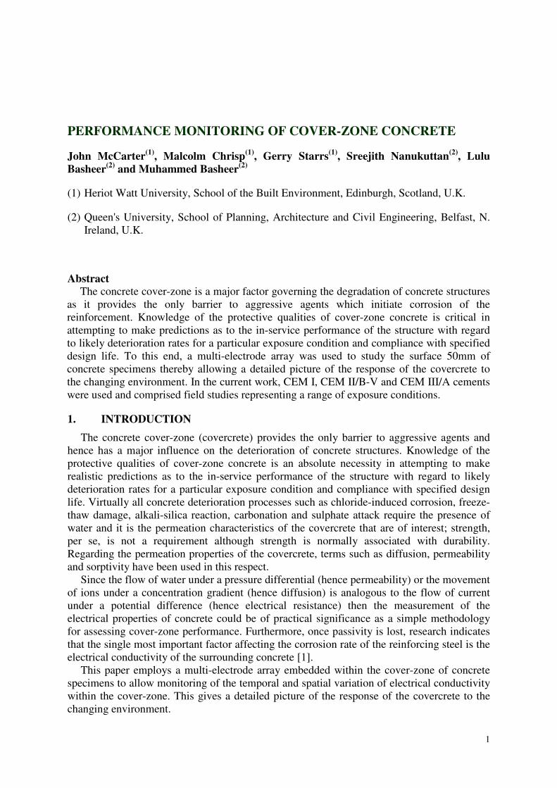
Resistance measurements were obtained at

discrete points within the cover zone of

concrete samples by embedding an electrode

array in the surface region of reinforced

concrete specimens. The array comprised 8

electrode pairs mounted on a plastic former;

each electrode consisted of a stainless steel pin

(1.2mm in diameter) which was sleeved to

expose a 5mm tip; in each electrode pair the

pins had a (horizontal) centre to centre spacing

of 5mm. The pairs of electrodes were

positioned at discrete depths from the exposed

surface ranging from 5mm-75mm. The former was secured onto stainless steel bars as shown

in Figure 1. The complete module could then be secured to the reinforcement with cable ties.

Four thermistors were also mounted on the former thereby allowing monitoring of the

temperature distribution through the covercrete (also required for temperature standardisation

of resistance measurements). Prior to installation, the electrode arrays were calibrated in

solutions of known conductivity enabling the measured resistance, R (in ohms), to be

converted to conductivity, σ (in Siemens/m), viz,

σ = R

k (S/m) (1)

where k is the calibration constant for the electrode array. An average value of k was

evaluated to give an overall constant for the array.

2.2 Materials, Samples and Curing

Table 1 presents the concrete mix details, together with the mean 28-day compressive

strength (F28) determined on 100mm cubes. These mixes were chosen as they satisfy the

requirements for virtually all exposure conditions specified in [2] and [3]. Dredged river

gravel and matching fine aggregate was used throughout; the binders comprised ordinary

Portland cement (CEM I to EN197-1:2000), ground granulated blast-furnace slag (GGBS to

EN15167-1:2006) and pulverised fuel ash (PFA to EN450-1:2005).

Table 1: Concrete mixes (w/b = water-binder ratio)

CEM I 42.5N CEM III/A 42.5N CEM II/B-V 42.5N

OPC (kg/m3) 460 270 370

PFA (kg/m3) - - 160

GGBS (kg/m3) - 180 -

20mm (kg/m3) 700 700 695

10mm (kg/m3) 350 375 345

Fine (kg/m3) 700 745 635

Plasticiser (l/m3) 1.84 3.60 2.65

w/b 0.4 0.44 0.39

Slump (mm) 105 140 110

F28 (MPa) 70 53 58

3

Samples took the form of 300×300×200mm (depth) blocks cast in plywood formwork and

an array, described above, was placed at the plan centre of each slab. All cabling was colour

coded and taken into a watertight reinforced plastic box embedded into the face opposite to

the working face. A 37-pin, multi-pole female socket was used to terminate all wires from the

electrode array and thermistors. On demoulding, the samples were wrapped with damp

hessian and polythene and left in the laboratory (15-20°C) for a period of 7 days. All

surfaces, apart from the surface cast against the formwork which was the exposed 'working'

surface, were sealed with several coats of an epoxy-based paint to ensure uniaxial moisture

movement. A total of 54 blocks (18 per mix) were fabricated.

In parallel with this, nine concrete monoliths - three per mix in Table 1 - of dimensions

2000(high)×400×400mm were fabricated in plywood formwork. The monoliths were lightly

reinforced over their full length. An electrode array, similar to that described above, was

positioned within the cover-zone of each monolith and secured to main reinforcement at mid-

height in all four vertical faces and also at 1.5 and 0.5m above the base of each monolith on

the roadside face (see below). All cabling from the arrays was ducted through the base of

each monolith to a central communications box.

2.3 Exposure Sites

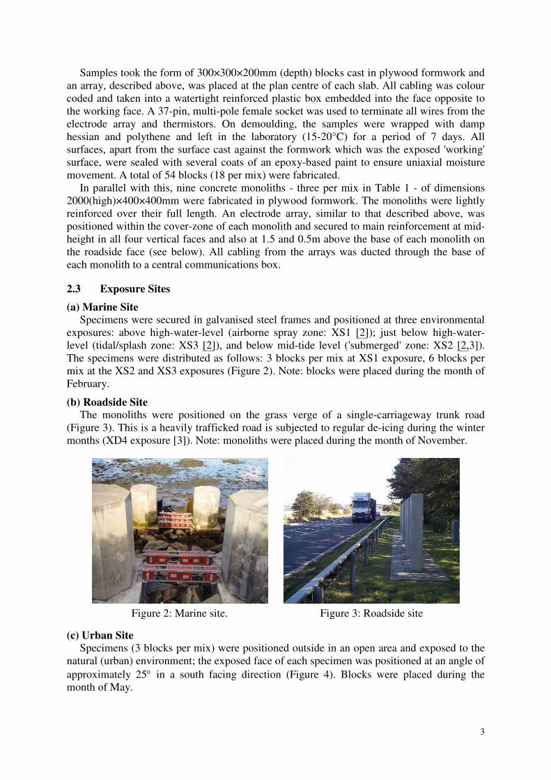
(a) Marine Site

Specimens were secured in galvanised steel frames and positioned at three environmental

exposures: above high-water-level (airborne spray zone: XS1 [2]); just below high-water-

level (tidal/splash zone: XS3 [2]), and below mid-tide level ('submerged' zone: XS2 [2,3]).

The specimens were distributed as follows: 3 blocks per mix at XS1 exposure, 6 blocks per

mix at the XS2 and XS3 exposures (Figure 2). Note: blocks were placed during the month of

February.

(b) Roadside Site

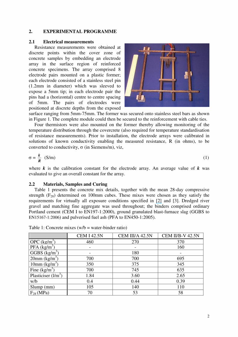
The monoliths were positioned on the grass verge of a single-carriageway trunk road

(Figure 3). This is a heavily trafficked road is subjected to regular de-icing during the winter

months (XD4 exposure [3]). Note: monoliths were placed during the month of November.

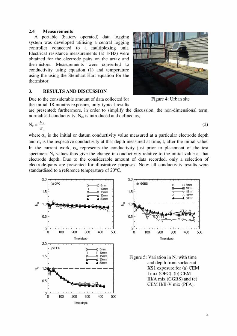
(c) Urban Site

Specimens (3 blocks per mix) were positioned outside in an open area and exposed to the

natural (urban) environment; the exposed face of each specimen was positioned at an angle of

approximately 25° in a south facing direction (Figure 4). Blocks were placed during the

month of May.

Figure 2: Marine site. Figure 3: Roadside site

4

2.4 Measurements

A portable (battery operated) data logging

system was developed utilising a central logging

controller connected to a multiplexing unit.

Electrical resistance measurements (at 1kHz) were

obtained for the electrode pairs on the array and

thermistors. Measurements were converted to

conductivity using equation (1) and temperature

using the using the Steinhart-Hart equation for the

thermistor.

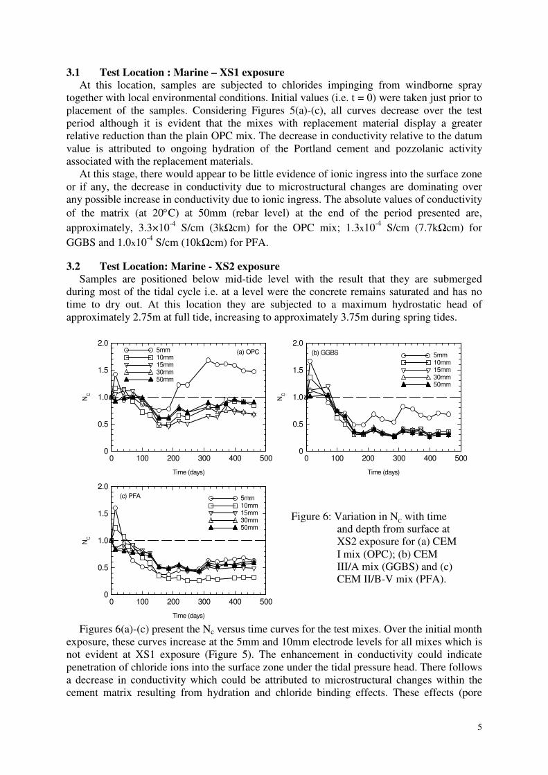
3. RESULTS AND DISCUSSION

Due to the considerable amount of data collected for

the initial 18-months exposure, only typical results

are presented; furthermore, in order to simplify the discussion, the non-dimensional term,

normalised-conductivity, Nc, is introduced and defined as,

Nc = o

t

σ

σ (2)

where σo is the initial or datum conductivity value measured at a particular electrode depth

and σt is the respective conductivity at that depth measured at time, t, after the initial value.

In the current work, σo represents the conductivity just prior to placement of the test

specimen. Nc values thus give the change in conductivity relative to the initial value at that

electrode depth. Due to the considerable amount of data recorded, only a selection of

electrode-pairs are presented for illustrative purposes. Note: all conductivity results were

standardised to a reference temperature of 20°C.

Figure 4: Urban site

0

0.5

1.0

1.5

2.0

0 100 200 300 400 500

5mm10mm15mm30mm50mm

(a) OPC

Time (days)

NC

0

0.5

1.0

1.5

2.0

0 100 200 300 400 500

5mm10mm15mm30mm50mm

(b) GGBS

Time (days)

NC

0

0.5

1.0

1.5

2.0

0 100 200 300 400 500

5mm10mm15mm30mm50mm

(c) PFA

Time (days)

NC

Figure 5: Variation in NC with time

and depth from surface at XS1 exposure for (a) CEM

I mix (OPC); (b) CEM

III/A mix (GGBS) and (c) CEM II/B-V mix (PFA).

5

3.1 Test Location : Marine – XS1 exposure

At this location, samples are subjected to chlorides impinging from windborne spray

together with local environmental conditions. Initial values (i.e. t = 0) were taken just prior to

placement of the samples. Considering Figures 5(a)-(c), all curves decrease over the test

period although it is evident that the mixes with replacement material display a greater

relative reduction than the plain OPC mix. The decrease in conductivity relative to the datum

value is attributed to ongoing hydration of the Portland cement and pozzolanic activity

associated with the replacement materials.

At this stage, there would appear to be little evidence of ionic ingress into the surface zone

or if any, the decrease in conductivity due to microstructural changes are dominating over

any possible increase in conductivity due to ionic ingress. The absolute values of conductivity

of the matrix (at 20°C) at 50mm (rebar level) at the end of the period presented are,

approximately, 3.3×10-4

S/cm (3kΩcm) for the OPC mix; 1.3x10-4

S/cm (7.7kΩcm) for

GGBS and 1.0x10-4

S/cm (10kΩcm) for PFA.

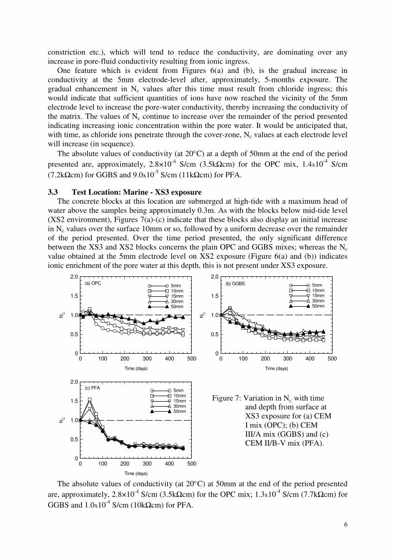
3.2 Test Location: Marine - XS2 exposure

Samples are positioned below mid-tide level with the result that they are submerged

during most of the tidal cycle i.e. at a level were the concrete remains saturated and has no

time to dry out. At this location they are subjected to a maximum hydrostatic head of

approximately 2.75m at full tide, increasing to approximately 3.75m during spring tides.

Figures 6(a)-(c) present the Nc versus time curves for the test mixes. Over the initial month

exposure, these curves increase at the 5mm and 10mm electrode levels for all mixes which is

not evident at XS1 exposure (Figure 5). The enhancement in conductivity could indicate

penetration of chloride ions into the surface zone under the tidal pressure head. There follows

a decrease in conductivity which could be attributed to microstructural changes within the

cement matrix resulting from hydration and chloride binding effects. These effects (pore

0

0.5

1.0

1.5

2.0

0 100 200 300 400 500

5mm10mm15mm30mm50mm

(a) OPC

Time (days)

NC

0

0.5

1.0

1.5

2.0

0 100 200 300 400 500

5mm10mm15mm30mm50mm

(b) GGBS

Time (days)

NC

0

0.5

1.0

1.5

2.0

0 100 200 300 400 500

5mm10mm15mm30mm50mm

(c) PFA

Time (days)

NC

Figure 6: Variation in NC with time

and depth from surface at

XS2 exposure for (a) CEM

I mix (OPC); (b) CEM III/A mix (GGBS) and (c) CEM II/B-V mix (PFA).

6

constriction etc.), which will tend to reduce the conductivity, are dominating over any

increase in pore-fluid conductivity resulting from ionic ingress.

One feature which is evident from Figures 6(a) and (b), is the gradual increase in

conductivity at the 5mm electrode-level after, approximately, 5-months exposure. The

gradual enhancement in Nc values after this time must result from chloride ingress; this

would indicate that sufficient quantities of ions have now reached the vicinity of the 5mm

electrode level to increase the pore-water conductivity, thereby increasing the conductivity of

the matrix. The values of Nc continue to increase over the remainder of the period presented

indicating increasing ionic concentration within the pore water. It would be anticipated that,

with time, as chloride ions penetrate through the cover-zone, Nc values at each electrode level

will increase (in sequence).

The absolute values of conductivity (at 20°C) at a depth of 50mm at the end of the period

presented are, approximately, 2.8×10-4

S/cm (3.5kΩcm) for the OPC mix, 1.4x10-4

S/cm

(7.2kΩcm) for GGBS and 9.0x10-5

S/cm (11kΩcm) for PFA.

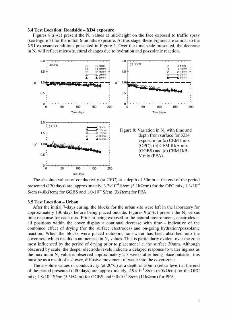
3.3 Test Location: Marine - XS3 exposure

The concrete blocks at this location are submerged at high-tide with a maximum head of

water above the samples being approximately 0.3m. As with the blocks below mid-tide level

(XS2 environment), Figures 7(a)-(c) indicate that these blocks also display an initial increase

in Nc values over the surface 10mm or so, followed by a uniform decrease over the remainder

of the period presented. Over the time period presented, the only significant difference

between the XS3 and XS2 blocks concerns the plain OPC and GGBS mixes; whereas the Nc

value obtained at the 5mm electrode level on XS2 exposure (Figure 6(a) and (b)) indicates

ionic enrichment of the pore water at this depth, this is not present under XS3 exposure.

The absolute values of conductivity (at 20°C) at 50mm at the end of the period presented

are, approximately, 2.8×10-4

S/cm (3.5kΩcm) for the OPC mix; 1.3x10-4

S/cm (7.7kΩcm) for

GGBS and 1.0x10-4

S/cm (10kΩcm) for PFA.

0

0.5

1.0

1.5

2.0

0 100 200 300 400 500

5mm10mm15mm30mm50mm

(a) OPC

Time (days)

NC

0

0.5

1.0

1.5

2.0

0 100 200 300 400 500

5mm10mm15mm30mm50mm

(b) GGBS

Time (days)

NC

0

0.5

1.0

1.5

2.0

0 100 200 300 400 500

5mm10mm15mm30mm50mm

(c) PFA

Time (days)

NC

Figure 7: Variation in NC with time

and depth from surface at

XS3 exposure for (a) CEM

I mix (OPC); (b) CEM III/A mix (GGBS) and (c) CEM II/B-V mix (PFA).

7

3.4 Test Location: Roadside – XD4 exposure

Figures 8(a)-(c) present the Nc values at mid-height on the face exposed to traffic spray

(see Figure 3) for the initial 6-months exposure. At this stage, these Figures are similar to the

XS1 exposure conditions presented in Figure 5. Over the time-scale presented, the decrease

in Nc will reflect microstructural changes due to hydration and pozzolanic reaction.

The absolute values of conductivity (at 20°C) at a depth of 50mm at the end of the period

presented (170 days) are, approximately, 3.2×10-4

S/cm (3.1kΩcm) for the OPC mix; 1.3x10-4

S/cm (4.8kΩcm) for GGBS and 1.0x10-4

S/cm (3kΩcm) for PFA.

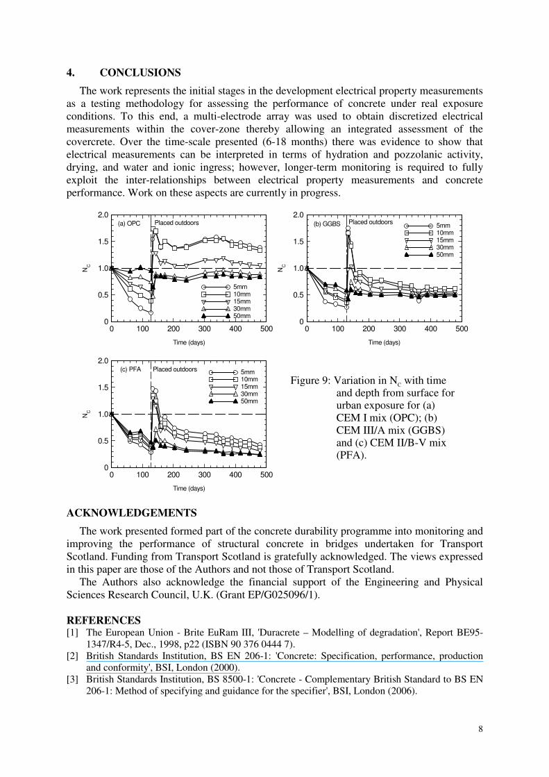
3.5 Test Location – Urban

After the initial 7-days curing, the blocks for the urban site were left in the laboratory for

approximately 130-days before being placed outside. Figures 9(a)-(c) present the Nc versus

time response for each mix. Prior to being exposed to the natural environment, electrodes at

all positions within the cover display a continual decrease with time - indicative of the

combined effect of drying (for the surface electrodes) and on-going hydration/pozzolanic

reaction. When the blocks were placed outdoors, rain-water has been absorbed into the

covercrete which results in an increase in Nc values. This is particularly evident over the zone

most influenced by the period of drying prior to placement i.e. the surface 30mm. Although

obscured by scale, the deeper electrode levels indicate a delayed response to water ingress as

the maximum Nc value is observed approximately 2-3 weeks after being place outside - this

must be as a result of a slower, diffusive movement of water into the cover-zone.

The absolute values of conductivity (at 20°C) at a depth of 50mm (rebar level) at the end

of the period presented (480 days) are, approximately, 2.9×10-4

S/cm (3.5kΩcm) for the OPC

mix; 1.8x10-4

S/cm (5.5kΩcm) for GGBS and 9.0x10-5

S/cm (11kΩcm) for PFA.

0

0.5

1.0

1.5

2.0

0 50 100 150 200

5mm10mm15mm30mm50mm

(a) OPC

Time (days)

NC

0

0.5

1.0

1.5

2.0

0 50 100 150 200

5mm10mm15mm30mm50mm

(b) GGBS

Time (days)

NC

0

0.5

1.0

1.5

2.0

0 50 100 150 200

5mm10mm15mm30mm50mm

(c) PFA

Time (days)

NC

Figure 8: Variation in NC with time and

depth from surface for XD4

exposure for (a) CEM I mix (OPC); (b) CEM III/A mix (GGBS) and (c) CEM II/B-V mix (PFA).

8

4. CONCLUSIONS

The work represents the initial stages in the development electrical property measurements

as a testing methodology for assessing the performance of concrete under real exposure

conditions. To this end, a multi-electrode array was used to obtain discretized electrical

measurements within the cover-zone thereby allowing an integrated assessment of the

covercrete. Over the time-scale presented (6-18 months) there was evidence to show that

electrical measurements can be interpreted in terms of hydration and pozzolanic activity,

drying, and water and ionic ingress; however, longer-term monitoring is required to fully

exploit the inter-relationships between electrical property measurements and concrete

performance. Work on these aspects are currently in progress.

ACKNOWLEDGEMENTS

The work presented formed part of the concrete durability programme into monitoring and

improving the performance of structural concrete in bridges undertaken for Transport

Scotland. Funding from Transport Scotland is gratefully acknowledged. The views expressed

in this paper are those of the Authors and not those of Transport Scotland.

The Authors also acknowledge the financial support of the Engineering and Physical

Sciences Research Council, U.K. (Grant EP/G025096/1).

REFERENCES [1] The European Union - Brite EuRam III, 'Duracrete – Modelling of degradation', Report BE95-

1347/R4-5, Dec., 1998, p22 (ISBN 90 376 0444 7).

[2] British Standards Institution, BS EN 206-1: 'Concrete: Specification, performance, production

and conformity', BSI, London (2000).

[3] British Standards Institution, BS 8500-1: 'Concrete - Complementary British Standard to BS EN

206-1: Method of specifying and guidance for the specifier', BSI, London (2006).

0

0.5

1.0

1.5

2.0

0 100 200 300 400 500

5mm10mm15mm30mm50mm

(a) OPC Placed outdoors

Time (days)

NC

0

0.5

1.0

1.5

2.0

0 100 200 300 400 500

5mm10mm15mm30mm50mm

Placed outdoors(b) GGBS

Time (days)

NC

0

0.5

1.0

1.5

2.0

0 100 200 300 400 500

5mm10mm15mm30mm50mm

(c) PFA Placed outdoors

Time (days)

NC

Figure 9: Variation in NC with time

and depth from surface for urban exposure for (a) CEM I mix (OPC); (b) CEM III/A mix (GGBS) and (c) CEM II/B-V mix (PFA).