pdf - Repositorio CEPAL
192
-
Upload
khangminh22 -
Category
Documents
-
view
1 -
download
0
Transcript of pdf - Repositorio CEPAL
REV
IEW
ECONOMIC COMMISSION FOR
LATIN AMERICA ANDTHE CARIBBEAN


121NO
APRIL • 2017
REV
IEW
ECONOMIC COMMISSION FOR
LATIN AMERICA ANDTHE CARIBBEAN
Osvaldo SunkelChairman of the Editorial Board
Miguel TorresTechnical Editor
ISSN 0251-2920
Alicia BárcenaExecutive Secretary
Antonio PradoDeputy Executive Secretary
Alicia BárcenaExecutive Secretary
Antonio PradoDeputy Executive Secretary
Osvaldo SunkelChair of the Editorial Board
Miguel TorresTechnical Editor
The CEPAL Review was founded in 1976, along with the corresponding Spanish version, Revista CEPAL, and it is published three times a year by the Economic Commission for Latin America and the Caribbean (ECLAC), which has its headquarters in Santiago. The Review has full editorial independence and follows the usual academic procedures and criteria, including the review of articles by independent external referees. The purpose of the Review is to contribute to the discussion of socioeconomic development issues in the region by offering analytical and policy approaches and articles by economists and other social scientists working both within and outside the United Nations. The Review is distributed to universities, research institutes and other international organizations, as well as to individual subscribers.
The opinions expressed in the articles are those of the authors and do not necessarily reflect the views of ECLAC.
The designations employed and the way in which data are presented do not imply the expression of any opinion whatsoever on the part of the United Nations concerning the legal status of any country, territory, city or area or its authorities, or concerning the delimitation of its frontiers or boundaries.
To subscribe, please visit the Web page: http://ebiz.turpin-distribution.com/products/197587-cepal-review.aspx
The complete text of the Review can also be downloaded free of charge from the ECLAC website (www.eclac.org).
This publication, entitled CEPAL Review, is covered in theSocial Sciences Citation Index (SSCI), published by Thomson
Reuters, and in the Journal of Economic Literature (JEL),published by the American Economic Association
United Nations publication ISSN: 0251-2920 ISBN: 978-92-1-121950-0 (print) ISBN: 978-92-1-058587-3 (pdf) LC/PUB.2017/8-P Distribution: General Copyright © United Nations, April 2017All rights reservedPrinted at United Nations, Santiago S.16-01252
Requests for authorization to reproduce this work in whole or in part should be sent to the Economic Commission for Latin America and the Caribbean (ECLAC), Publications and Web Services Division, [email protected]. Member States of the United Nations and their governmental institutions may reproduce this work without prior authorization, but are requested to mention the source and to inform ECLAC of such reproduction.

Contents
Disasters, economic growth and fiscal response in the countries of Latin America and the Caribbean, 1972-2010
Omar D. Bello . . . . . . . . . . . . . . . . . . . . . . . . . . . . . . . . . . . . . . . . . . . . . . . . . . . . . . . . . 7
Nicaragua: trend of multidimensional poverty, 2001-2009
José Espinoza-Delgado and Julio López-Laborda . . . . . . . . . . . . . . . . . . . . . . . . . . . . . . 31
Determinants of non-farm employment and non-farm earnings in Ecuador
Cristian Vasco and Grace Natalie Tamayo . . . . . . . . . . . . . . . . . . . . . . . . . . . . . . . . . . . 53
Innovation and productivity in services and manufacturing firms: the case of Peru
Mario D. Tello . . . . . . . . . . . . . . . . . . . . . . . . . . . . . . . . . . . . . . . . . . . . . . . . . . . . . . . . 69
Santiago Chile: city of cities? Social inequalities in local labour market zones
Luis Fuentes, Oscar Mac-Clure, Cristóbal Moya and Camilo Olivos . . . . . . . . . . . . . . . 87
Thoughts on the inequality of opportunities: new evidence
Wallace Patrick Santos de Farias Souza, Ana Cláudia Annegues and Victor Rodrigues de Oliveira . . . . . . . . . . . . . . . . . . . . . . . . . . . . . . . . . . . . . . . . . 103
How did Costa Rica achieve social and market incorporation?
Juliana Martínez Franzoni and Diego Sánchez-Ancochea . . . . . . . . . . . . . . . . . . . . . . 123
Ecuador: why exit dollarization?
Gonzalo J. Paredes . . . . . . . . . . . . . . . . . . . . . . . . . . . . . . . . . . . . . . . . . . . . . . . . . . . . 139
The political economy of the fiscal deficit in nineteenth-century Chile
Roberto Pastén . . . . . . . . . . . . . . . . . . . . . . . . . . . . . . . . . . . . . . . . . . . . . . . . . . . . . . . 157
The determinants of foreign direct investment in Brazil: empirical analysis for 2001-2013
Eduarda Martins Correa da Silveira, Jorge Augusto Dias Samsonescu and Divanildo Triches . . . . . . . . . . . . . . . . . . . . . . . . . . . . . . . . . . . . . . . . . . . . . . . . . 171
Guidelines for contributors to the CEPAL Review . . . . . . . . . . . . . . . . . . . . . . . . 185

Explanatory notes
- Three dots (...) indicate that data are not available or are not separately reported.- A dash (-) indicates that the amount is nil or negligible.- A full stop (.) is used to indicate decimals.- The word “dollars” refers to United States dollars, unless otherwise specified.- A slash (/) between years (e.g. 2013/2014) indicates a 12-month period falling between the two years.- Individual figures and percentages in tables may not always add up to the corresponding total because of rounding.
Disasters, economic growth and fiscal response in the countries of Latin America and the Caribbean, 1972-2010Omar D. Bello1
Abstract
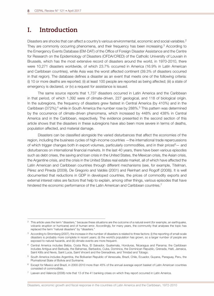
The aim of this study is to estimate the impact of geological and climate-related disasters on the per capita growth rates of gross domestic product (GDP) and fiscal expenditure in Latin American and Caribbean countries. The results show that the effects vary by type of disaster and by subregion. In the Caribbean countries, the per capita GDP growth rate has typically responded negatively to climate disasters, whereas the response to a geological disaster has generally not been statistically significant. In Central American countries, the response of the per capita GDP growth rate was found to be negative in the first year and positive in the third year in the case of climate disasters, but positive in the second and third years for disasters of geological origin.
Keywords
Natural disasters, economic growth, gross domestic product, public expenditure, Latin America and the Caribbean
JEL classification
Q54, L6, L7, L8
Author
Omar D. Bello is coordinator of the Sustainable Development and Disaster Unit of the Economic Commission for Latin America and the Caribbean (ECLAC) subregional headquarters for the Caribbean, Port of Spain. [email protected]
1 The author is grateful for comments and suggestions from Jean Acquatella, Adriana Arreaza, Carlos de Miguel, Leda Peralta and Omar Zambrano, and also for excellent research assistance provided by Ignacio Cristi LeFort and Viviana Rosales Salinas. As usual, all opinions, errors or omissions are the author’s exclusive responsibility.
8 CEPAL Review N° 121 • April 2017
Disasters, economic growth and fiscal response in the countries of Latin America and the Caribbean, 1972-2010
I. Introduction
Disasters are shocks that can affect a country’s various environmental, economic and social variables.2 They are commonly occurring phenomena, and their frequency has been increasing.3 According to the Emergency Events Database (EM-DAT) of the Office of Foreign Disaster Assistance and the Centre for Research on the Epidemiology of Disasters (OFDA/CRED) of the Catholic University of Louvain in Brussels, which has the most extensive record of disasters around the world, in 1970-2010, there were 10,271 disasters worldwide, of which 23.7% occurred in America (16.9% in Latin American and Caribbean countries), while Asia was the worst affected continent (39.3% of disasters occurred in that region). The database defines a disaster as an event that meets one of the following criteria: (i) 10 or more deaths are reported; (ii) at least 100 people are reported as being affected; (iii) a state of emergency is declared, or (iv) a request for assistance is issued.
The same source reports that 1,737 disasters occurred in Latin America and the Caribbean in that period, of which 1,392 were of climate-driven, 227 geological, and 118 of biological origin. In the subregions, the frequency of disasters grew fastest in Central America (by 410%) and in the Caribbean (372%);4 while in South America the number rose by 288%.5 This pattern was determined by the occurrence of climate-driven phenomena, which increased by 448% and 438% in Central America and in the Caribbean, respectively. The evidence presented in the second section of this article shows that the disasters in these subregions have also been more severe in terms of deaths, population affected, and material damage.
Disasters can be classified alongside the varied disturbances that affect the economies of the region, including the business cycles of high-income countries —the international trade repercussions of which trigger changes both in export volumes, particularly commodities, and in their prices6— and disturbances on international financial markets. In the last 40 years, there have been various episodes such as debt crises, the saving and loan crisis in the United States, the Mexican crisis, the Asian crisis, the Argentine crisis, and the crisis in the United States real estate market, all of which have affected the Latin American and Caribbean countries through different mechanisms (see, for example, Titelman, Pérez and Pineda (2009), De Gregorio and Valdés (2001) and Reinhart and Rogoff (2008)). It is well documented that reductions in GDP in developed countries, the prices of commodity exports and external interest rates are factors that help to explain, among other things, various episodes that have hindered the economic performance of the Latin American and Caribbean countries.7
2 This article uses the term “disasters,” because these situations are the outcome of a natural event (for example, an earthquake, volcanic eruption or hurricane) and of human error. Accordingly, for many years, the community that analyses the topic has replaced the term “natural disasters” by “disasters.”
3 According to Stromberg (2007), the increase in the number of disasters is related to three factors: (i) the reporting of small-scale disasters is probably more complete in recent years; (ii) the world’s population has grown, so a larger number of people are exposed to natural hazards, and (iii) climate events are more frequent.
4 Central America includes Belize, Costa Rica, El Salvador, Guatemala, Honduras, Nicaragua and Panama; the Caribbean includes Antigua and Barbuda, the Bahamas, Barbados, Cuba, Dominica, the Dominican Republic, Grenada, Haiti, Jamaica, Saint Kitts and Nevis, Saint Lucia, Saint Vincent and the Grenadines, and Trinidad and Tobago.
5 South America includes Argentina, the Bolivarian Republic of Venezuela, Brazil, Chile, Ecuador, Guyana, Paraguay, Peru, the Plurinational State of Bolivia and Suriname.
6 Except for Mexico and Brazil, in 2000-2010 more than 45% of the annual average export basket of Latin American countries consisted of commodities.
7 Laeven and Valencia (2008) note that 13 of the 41 banking crises on which they report occurred in Latin America.
9CEPAL Review N° 121 • April 2017
Omar D. Bello
From the economic standpoint, disasters produce both effects and impacts. The former involve damage to assets and changes in flows, which are the additional losses and costs. The impacts are consequences of the effects on different social and economic variables, such as family incomes, unemployment, GDP growth and the fiscal deficit, among others.8 It is therefore to be expected that the destruction of assets by a disaster will temporarily interrupt production flows and affect the public finances, for example through the reduction in tax revenue and the additional costs that the emergency may generate.
This article estimates the impacts of different types of disaster on two variables: the per capita GDP growth rate and the rate of growth of per capita fiscal spending in Latin American and Caribbean countries, and in the two subregions most intensively affected by these events, the Caribbean and Central America.
The article is organized as follows: section II presents the stylized facts of the disasters that have occurred in Latin America and the Caribbean; section III contains a review of the literature on the impact of disasters on economic activity, public finances and social variables; section IV sets out the estimation methodology and the variables used; section V discusses the estimated impulse-response functions of the per capita growth rates of GDP and government spending, in response to shocks in the variables studied. The final section contains a number of evaluations of the results.
II. Stylized facts on the disasters that have occurred in Latin America and the Caribbean
This section analyses the trend of disasters and some of the measures of intensity generally used, such as deaths, population affected and damage. The emphasis is placed on disasters occurring in Latin America and the Caribbean.
1. Number of disasters
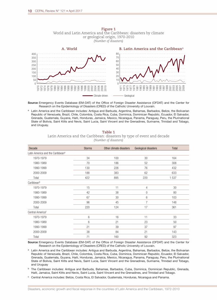
The frequency of disasters, of all types, has increased in all continents during the period analysed,9
although those of climate origin have increased the most (see figure 1).10 Climate-driven disasters can be classified as follows: (i) storms, and (ii) other climate disasters, including floods, droughts and wet mass movements. Table 1 reports the dynamic of these events by decade in Latin America and the Caribbean, showing that both storms and other climate-related disasters have grown steadily.11
Between the 1970s and the 2000 decade, climate disasters increased by 326%, owing to the frequency of storms, which increased by 453%. In the Caribbean and Central American subregions, storm frequency rose by 540% and 533%, respectively, while the frequency of other climate disasters increased by 309% and 425%.
8 See ECLAC (2014).9 See Stromberg (2007).10 The classification used follows Skidmore and Toya (2002).11 To reduce the noise that might be caused by considering individual disasters, the information is presented by decade,
specifically the four decades spanning 1970-1999.
10 CEPAL Review N° 121 • April 2017
Disasters, economic growth and fiscal response in the countries of Latin America and the Caribbean, 1972-2010
Figure 1 World and Latin America and the Caribbean: disasters by climate
or geological origin, 1970-2010(Number of disasters)
A. World B. Latin America and the Caribbeana
050
100150200250300350400
1970
1972
1974
1976
1978
1980
1982
1984
1986
1988
1990
1992
1994
1996
1998
2000
2002
2004
2006
2008
2010
Climate-driven Geological
01020304050607080
1971
1973
1975
1977
1979
1981
1983
1985
1987
1989
1991
1993
1995
1997
1999
2001
2003
2005
2007
2009
Source: Emergency Events Database (EM-DAT) of the Office of Foreign Disaster Assistance (OFDAT) and the Center for Research on the Epidemiology of Disasters (CRED) of the Catholic University of Louvain.
a Latin America and the Caribbean includes: Antigua and Barbuda, Argentina, Bahamas, Barbados, Belize, the Bolivarian Republic of Venezuela, Brazil, Chile, Colombia, Costa Rica, Cuba, Dominica, Dominican Republic, Ecuador, El Salvador, Grenada, Guatemala, Guyana, Haiti, Honduras, Jamaica, Mexico, Nicaragua, Panama, Paraguay, Peru, the Plurinational State of Bolivia, Saint Kitts and Nevis, Saint Lucia, Saint Vincent and the Grenadines, Suriname, Trinidad and Tobago, and Uruguay.
Table 1 Latin America and the Caribbean: disasters by type of event and decade
(Number of disasters)
Decade Storms Other climate disasters Geological disasters Total
Latin America and the Caribbeana
1970-1979 34 100 30 164
1980-1989 70 186 52 308
1990-1999 130 226 76 432
2000-2009 188 383 62 633
Total 422 895 220 1 537
Caribbeanb
1970-1979 15 11 4 30
1980-1989 42 38 0 80
1990-1999 67 30 6 103
2000-2009 96 45 7 148
Total 220 124 17 361
Central Americac
1970-1979 6 16 11 33
1980-1989 6 21 23 50
1990-1999 21 39 37 97
2000-2009 38 84 21 143
Total 71 160 92 323
Source: Emergency Events Database (EM-DAT) of the Office of Foreign Disaster Assistance (OFDAT) and the Center for Research on the Epidemiology of Disasters (CRED) of the Catholic University of Louvain.
a Latin America and the Caribbean includes: Antigua and Barbuda, Argentina, Bahamas, Barbados, Belize, the Bolivarian Republic of Venezuela, Brazil, Chile, Colombia, Costa Rica, Cuba, Dominica, Dominican Republic, Ecuador, El Salvador, Grenada, Guatemala, Guyana, Haiti, Honduras, Jamaica, Mexico, Nicaragua, Panama, Paraguay, Peru, the Plurinational State of Bolivia, Saint Kitts and Nevis, Saint Lucia, Saint Vincent and the Grenadines, Suriname, Trinidad and Tobago, and Uruguay
b The Caribbean includes: Antigua and Barbuda, Bahamas, Barbados, Cuba, Dominica, Dominican Republic, Grenada, Haiti, Jamaica, Saint Kitts and Nevis, Saint Lucia, Saint Vincent and the Grenadines, and Trinidad and Tobago.
c Central America includes: Belize, Costa Rica, El Salvador, Guatemala, Honduras, Nicaragua and Panama.

11CEPAL Review N° 121 • April 2017
Omar D. Bello
2. Deaths
Of the various measures of disaster intensity, mortality is the most affected by specific events. In 1970-2010, a total of 3,450,255 people died worldwide as a result of disasters.12 Of that total, 498,030 deaths occurred in Latin America and the Caribbean, and 73.1% of those deaths occurred as a result of five events:13 (i) the earthquake in Chimbote (Peru, 1970); (ii) the earthquake in Guatemala City (1976); (iii) the eruption of the Nevado del Ruiz Volcano (Colombia, 1985); (iv) the landslide in Vargas (Bolivarian Republic of Venezuela, 1999), and (v) the earthquake in Port-au-Prince (Haiti, 2010).14 Table 2 shows the trend of the deaths per 1,000 inhabitants by decade. During the course of these decades, the number of deaths in Latin America and the Caribbean fluctuated, but disaster mortality rates in the Caribbean and in Central America outpaced the entire region in every decade studied.
Table 2 Latin America and the Caribbean: disaster-related deaths, by decade
(Number of deaths per 1,000 inhabitants)
Decade Latin America and the Caribbeana Caribbeanb Central Americac
1970-1979 0.063 0.011 0.452
1980-1989 0.014 0.007 0.015
1990-1999 0.017 0.008 0.065
2000-2009 0.004 0.021 0.012
2010-2011 0.403 8.914 0.014
Source: Emergency Events Database (EM-DAT) of the Office of Foreign Disaster Assistance (OFDAT) and the Center for Research on the Epidemiology of Disasters (CRED) of the Catholic University of Louvain.
a Latin America and the Caribbean includes: Antigua and Barbuda, Argentina, Bahamas, Barbados, Belize, the Bolivarian Republic of Venezuela, Brazil, Chile, Colombia, Costa Rica, Cuba, Dominica, Dominican Republic, Ecuador, El Salvador, Grenada, Guatemala, Guyana, Haiti, Honduras, Jamaica, Mexico, Nicaragua, Panama, Paraguay, Peru, the Plurinational State of Bolivia, Saint Kitts and Nevis, Saint Lucia, Saint Vincent and the Grenadines, Suriname, Trinidad and Tobago, and Uruguay.
b The Caribbean includes: Antigua and Barbuda, Bahamas, Barbados, Cuba, Dominica, Dominican Republic, Grenada, Haiti, Jamaica, Saint Kitts and Nevis, Saint Lucia, Saint Vincent and the Grenadines, and Trinidad and Tobago.
c Central America includes: Belize, Costa Rica, El Salvador, Guatemala, Honduras, Nicaragua and Panama.
In the 1970s and 1980s, 81% of fatalities were caused by geological disasters. In contrast, in 1990-2009, 80.1% of the losses of human life were a result of climate-related disasters. This pattern is very likely to reverse in the current decade owing to the number of deaths caused by the 2010 earthquake in Haiti.
In Central America, climate events caused 49.2% of disaster-related deaths, whereas geological events caused 48.9%. In that region, there were fatalities in 65% of climate-related disasters, with an average of 216 deaths in each event. In the Caribbean, geological events caused 92.2% of the deaths, while climate events accounted for 5.4%. Fatalities occurred in 56.6% of climate events, with 63 people dying on average. The number of deaths per 1,000 inhabitants caused by geological disasters increased sharply in 2010-2011, as a result of the 2010 earthquake in Haiti, which was the single event that caused most deaths in the region.
12 Throughout this article, mention of “disaster” refers to the occurrence of a disaster in one country. If an event, such as Hurricane Mitch, affects several countries, an observation is made for each of the countries affected.
13 Worldwide, 10 disasters caused 53.8% of all of these fatalities. The only disaster occurring in Latin America and the Caribbean included among them is the Port-au-Prince earthquake of 2010.
14 Cavallo and Noy (2010) claim that 96% of the deaths caused by disasters in 1970-2008 occurred in Africa, Latin America and the Caribbean, and Asia, which jointly account for 75% of the world’s population. Stromberg (2007) argues that in 1980-2004, for every death caused by disasters in high-income countries, there were 12 deaths in low-income countries. These results stem from the four events that caused most of the fatalities: the 1984 droughts in Sudan and Ethiopia, the 1991 cyclone in Bangladesh and the 2004 tsunami in the Indian Ocean.
12 CEPAL Review N° 121 • April 2017
Disasters, economic growth and fiscal response in the countries of Latin America and the Caribbean, 1972-2010
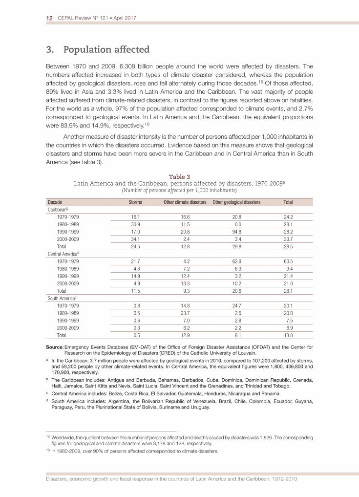
3. Population affected
Between 1970 and 2009, 6.308 billion people around the world were affected by disasters. The numbers affected increased in both types of climate disaster considered, whereas the population affected by geological disasters, rose and fell alternately during those decades.15 Of those affected, 89% lived in Asia and 3.3% lived in Latin America and the Caribbean. The vast majority of people affected suffered from climate-related disasters, in contrast to the figures reported above on fatalities. For the world as a whole, 97% of the population affected corresponded to climate events, and 2.7% corresponded to geological events. In Latin America and the Caribbean, the equivalent proportions were 83.9% and 14.9%, respectively.16
Another measure of disaster intensity is the number of persons affected per 1,000 inhabitants in the countries in which the disasters occurred. Evidence based on this measure shows that geological disasters and storms have been more severe in the Caribbean and in Central America than in South America (see table 3).
Table 3 Latin America and the Caribbean: persons affected by disasters, 1970-2009a
(Number of persons affected per 1,000 inhabitants)
Decade Storms Other climate disasters Other geological disasters TotalCaribbeanb
1970-1979 16.1 16.6 20.8 24.2
1980-1989 30.9 11.5 0.0 28.1
1990-1999 17.0 20.8 94.8 28.2
2000-2009 34.1 2.4 3.4 33.7
Total 24.5 12.8 29.8 28.5
Central Americac
1970-1979 21.7 4.2 62.9 60.5
1980-1989 4.6 7.2 6.3 9.4
1990-1999 14.9 12.4 3.2 21.4
2000-2009 4.9 13.3 10.2 21.0
Total 11.5 9.3 20.6 28.1
South Americad
1970-1979 0.8 14.8 24.7 20.1
1980-1989 0.5 23.7 2.5 20.8
1990-1999 0.6 7.0 2.8 7.5
2000-2009 0.3 6.2 2.2 6.9
Total 0.5 12.9 8.1 13.8
Source: Emergency Events Database (EM-DAT) of the Office of Foreign Disaster Assistance (OFDAT) and the Center for Research on the Epidemiology of Disasters (CRED) of the Catholic University of Louvain.
a In the Caribbean, 3.7 million people were affected by geological events in 2010, compared to 107,200 affected by storms, and 59,200 people by other climate-related events. In Central America, the equivalent figures were 1,800, 436,800 and 170,900, respectively.
b The Caribbean includes: Antigua and Barbuda, Bahamas, Barbados, Cuba, Dominica, Dominican Republic, Grenada, Haiti, Jamaica, Saint Kitts and Nevis, Saint Lucia, Saint Vincent and the Grenadines, and Trinidad and Tobago.
c Central America includes: Belize, Costa Rica, El Salvador, Guatemala, Honduras, Nicaragua and Panama.d South America includes: Argentina, the Bolivarian Republic of Venezuela, Brazil, Chile, Colombia, Ecuador, Guyana,
Paraguay, Peru, the Plurinational State of Bolivia, Suriname and Uruguay.
15 Worldwide, the quotient between the number of persons affected and deaths caused by disasters was 1,826. The corresponding figures for geological and climate disasters were 3,178 and 128, respectively.
16 In 1980-2009, over 90% of persons affected corresponded to climate disasters.
13CEPAL Review N° 121 • April 2017
Omar D. Bello
4. Damage
In 1970-2011, the damage caused by climate-related disasters represented 72.9% of global disaster damage, whereas that caused by geological disasters accounted for 27%.17 Storms caused 53.4% of climate-related damage, while other climate-driven disasters caused 46.6%. Of total damage, 9.1% occurred in Latin America and the Caribbean.
Despite being the most comprehensive database of disasters in the world, EM-DAT underestimates disaster damage, because it only records damage in 32.1% of the events registered.18 If this figure is broken down by the type of threat causing them, damage is recorded in just 32.3% of geological disasters, 50.8% of storms and 29.3% of other climate-related disasters. Two factors seem to explain the preponderance of damage caused by climate disasters: the increase in this type of event worldwide compared to those of geological origin, and the larger proportion of events of this type with a record of damage. Nonetheless, the average damage per geological event exceeded the average per climate event. A similar result was obtained by Bello, Ortiz and Samaniego (2014) using a database containing estimates of natural disaster impacts in Latin America, which was maintained by ECLAC for internal use between 1972 and 2010.
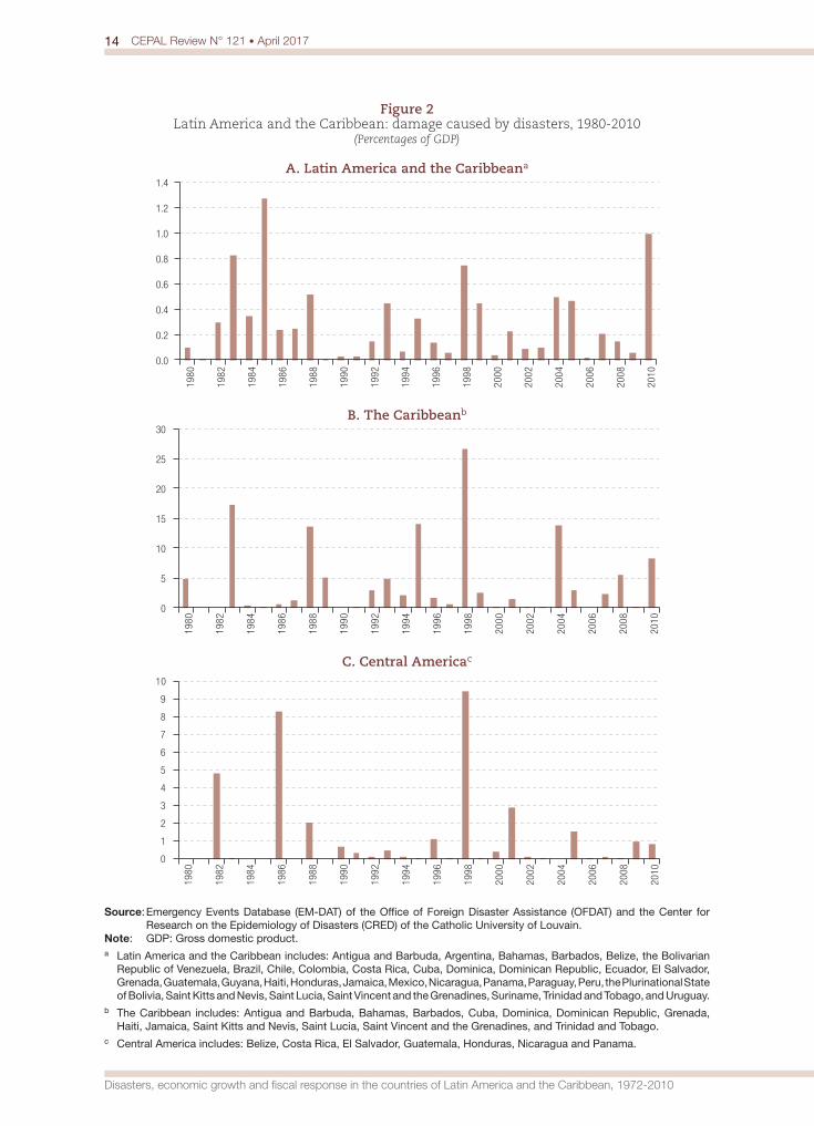
Instead of absolute values, damage is better expressed as percentages of GDP of the countries affected by disasters in each region and in each year. The Caribbean is the region in which disaster damage, on average, has represented the largest share of GDP, surpassing 8% seven times. It is followed by Central America, where disaster damage exceeded 8% of GDP twice. In Latin America and the Caribbean, this indicator reached at least 1% of GDP of the countries affected on just two occasions.
In short, the Caribbean and Central America are the two subregions most affected by disasters, in terms of both population and material effect. Compared to South America and Mexico, they are smaller territories and have few inhabitants. A characteristic of disasters is that in most cases they only affect one area, one region, or one specific department of a country. The exception is the Caribbean, where some of the small islands have been overwhelmed by hurricanes. As described in Albala-Bertrand (1993), disasters are generally confined to a specific space, and indirectly affect the rest of the economy through the links between the local and national systems. The stronger these links are, the greater the potential for transmission. When the effect of the disaster is measured in terms of a national economic indicator, such as GDP, this does not express its true extent in the regional economy, which in practice is likely to suffer the greatest impact; but in large countries, the regional may be minimized, as shown in figure 2A.
17 The question that arises from this evolution is “how much of this is attributable to climate change?" An answer was provided in the Special Report of the Intergovernmental Panel on Climate Change (IPCC) of 2012. This panel states that until now the trends of disaster damage, adjusted for wealth and population, are not attributable to climate change.
18 This percentage has been similar in the four decades considered: 35.4%, 29.9%, 39.4% and 28.1%, respectively. In the case of Latin America and the Caribbean, the proportions were 38.7%, 31.1%, 34.0% and 25.8%, respectively.
14 CEPAL Review N° 121 • April 2017
Disasters, economic growth and fiscal response in the countries of Latin America and the Caribbean, 1972-2010
Figure 2 Latin America and the Caribbean: damage caused by disasters, 1980-2010
(Percentages of GDP)
A. Latin America and the Caribbeana
0.0
0.2
0.4
0.6
0.8
1.0
1.2
1.419
80
1982
1984
1986
1988
1990
1992
1994
1996
1998
2000
2002
2004
2006
2008
2010
B. The Caribbeanb
0
5
10
15
20
25
30
1980
1982
1984
1986
1988
1990
1992
1994
1996
1998
2000
2002
2004
2006
2008
2010
C. Central Americac
0
1
2
3
4
5
6
7
8
9
10
1980
1982
1984
1986
1988
1990
1992
1994
1996
1998
2000
2002
2004
2006
2008
2010
Source: Emergency Events Database (EM-DAT) of the Office of Foreign Disaster Assistance (OFDAT) and the Center for Research on the Epidemiology of Disasters (CRED) of the Catholic University of Louvain.
Note: GDP: Gross domestic product.a Latin America and the Caribbean includes: Antigua and Barbuda, Argentina, Bahamas, Barbados, Belize, the Bolivarian
Republic of Venezuela, Brazil, Chile, Colombia, Costa Rica, Cuba, Dominica, Dominican Republic, Ecuador, El Salvador, Grenada, Guatemala, Guyana, Haiti, Honduras, Jamaica, Mexico, Nicaragua, Panama, Paraguay, Peru, the Plurinational State of Bolivia, Saint Kitts and Nevis, Saint Lucia, Saint Vincent and the Grenadines, Suriname, Trinidad and Tobago, and Uruguay.
b The Caribbean includes: Antigua and Barbuda, Bahamas, Barbados, Cuba, Dominica, Dominican Republic, Grenada, Haiti, Jamaica, Saint Kitts and Nevis, Saint Lucia, Saint Vincent and the Grenadines, and Trinidad and Tobago.
c Central America includes: Belize, Costa Rica, El Salvador, Guatemala, Honduras, Nicaragua and Panama.
15CEPAL Review N° 121 • April 2017
Omar D. Bello
III. Economic impacts of disasters
As noted above, disasters are a shock that can affect various economic variables, such as GDP, public finances and prices, as well as social variables such as the poverty index. The impact on the first of these variables has been studied extensively.19 A pioneering analysis of the subject is made by Albala-Bertrand (1993), who studies the short-term impacts of disasters. This author used data from 28 disasters of different origin occurring in 26 countries between 1960 and 1979, and found that there was a positive impact on GDP growth of 0.4%.20 Rasmussen (2004) used a similar methodology to analyse a sample of 12 major disasters that occurred in the countries of the Eastern Caribbean Currency Union in 1970-2002, and noted a negative impact on GDP in the year in which the disaster occurs. In terms of the fiscal accounts, the fiscal balance deteriorated owing to a fall in revenue and a spike in expenditure.21 Similar criticisms have been made of each of these studies: the samples are small and the conclusions are not based on a formal statistical method.
In response to these misgivings, a set of research projects arose that use both a broader database, namely EM-DAT, and formal statistical methods.
These studies include Noy (2007), who uses the three-stage Hausman-Taylor estimation method on a database that includes a sample of developed and developing countries in 1970-2003. The study found that disasters have an adverse impact on the GDP growth rate in the short run. Following a disaster of similar magnitude, developing countries, particularly the smallest ones, suffer steeper falls than developed countries. A better institutional framework and easier credit conditions in developed countries might explain this result, along with the fact that disasters are more likely to assume national proportions in small countries, such as those of the Caribbean.
Other studies have analysed the impacts of different disasters on economic activity in the short and long terms. Raddatz (2009) uses panel time series techniques (autoregressive distributed lag (ARDL) and autoregressive vector (VAR) models) to estimate the short- and long-term GDP effects of climate disasters, controlling for other variables. The sample includes countries that have suffered at least one major climate disaster since 1950. This author concludes that disasters have statistically significant impacts on output, causing a 1% drop in per capita GDP —greater than the typical impact of terms-of-trade shocks (which are considered major sources of fluctuation). The cumulative effect of a climate disaster is 0.6 percentage points of per capita GDP (0.5 points in the first year). In contrast, geological disasters do not generate statistically significant impacts on that variable. This result, like those of other studies, shows that treating disasters as a single aggregate can be misleading.
Loayza and others (2009), using a dynamic panel estimator (generalized method of moments (GMM)) on a sample of 94 developing and developed countries in 1961-2005, found that: (i) a generalized indicator of disasters does not affect the GDP growth rate; but, if different types of disaster are considered separately, only the impact of floods was statistically significant and positive, and (ii) in the case of growth rates in specific sectors such as agriculture, manufacturing and services, droughts and storms negatively affected the first, while floods had a positive effect.22 There are no statistically significant impacts of any type of disaster on manufacturing GDP. Growth in the commerce sector responded positively to flooding. In the sample of developing countries, the only types of disaster that
19 For a detailed review of all economic aspects of the topic of disasters see Cavallo and Noy (2010).20 Includes earthquakes, tsunamis, cyclones, floods and droughts; mainly considers African, Asian and Latin American countries,
with one European country; the impact estimates used by the author show that there was damage, in other words destruction of assets.
21 Dos Reis (2004) cites the aggregate costs for the countries of the Eastern Caribbean Currency Union in 1970-2000, as justification for a fiscal insurance mechanism in the countries of that region.
22 For a discussion on the sectoral effects of the different types of disasters in terms of methodological concepts of damage and loss, see Bello, Ortiz and Samaniego (2014).
16 CEPAL Review N° 121 • April 2017
Disasters, economic growth and fiscal response in the countries of Latin America and the Caribbean, 1972-2010
affected the GDP growth rate were droughts (negatively) and floods (positively). These results hold for the GDP growth rates of both manufacturing and agriculture. Moreover, in the case of manufacturing GDP, storms and earthquakes also had a positive growth effect. Lastly, no type of disaster had a statistically significant impact on the services sector.
Similarly, Jaramillo (2009), who estimated regressions of the type used by Islam (1995) to analyse disasters classified by incidence, concludes that disasters, particularly those caused by climate events, have a short-term impact lasting between two and five years. The author also establishes that only a small group of countries (those that have been negatively affected by disasters) suffer permanent impacts to the per capita GDP growth rate.
In their study on growth collapses, Hausmann, Rodríguez and Wagner (2006) conclude that disasters are not statistically significant in explaining the likelihood that a country will suffer a temporary reversal in its per capita GDP. Other events, such as wars, political transitions, exports collapses or sudden stops in capital flows, were statistically significant in determining that variable. A key study on this point is that of Cavallo and others (2010), which uses the comparative event study methodology. These authors conclude that even in the case of major disasters, there is still no long-term impact on economic growth. In the only cases which displayed long-term impacts —Nicaragua and the Islamic Republic of Iran— the result was associated with major political changes occurring a few years after the event, which led to a regime change. These authors do not establish a causality relation between the two disasters considered and the political changes that occurred.23
Other studies on this subject include Cuaresma, Hlouskova and Obersteiner (2008) and Raddatz (2007). The first estimated a gravity model for a sample of 49 countries, and observed that only countries with a certain development level succeed in improving their capital stock following a disaster. Raddatz (2007), using a VAR model with panel data, estimated the effect of exogenous shocks on GDP in 40 countries classified as low-income by the World Bank in 1965-1997. Apart from disasters, the exogenous shocks considered were fluctuations in commodity prices, international interest rates, and the economic activity level in the developed countries. The results show that, although these external shocks have a small but significant impact on per capita GDP in low-income countries, they can only explain a small portion of the total variance of per capita GDP in those countries. Even in the long run, they explain no more than 11% of the variance. The remaining 89% reflects factors outside the set of exogenous variables considered, in other words domestic factors such as conflicts, political instability and economic mismanagement.
In short, in the literature there is no consensus on the sign of the short-term impact of disasters, or any subset of them on the GDP growth rate.24 In the long run, the evidence shows that disasters do not have impacts on GDP growth. If this is true, disasters cannot be considered the cause of some countries’ poor secular economic performance.
With regard to other variables that might be affected by disasters, Cavallo, Cavallo and Rigobón (2013), using real-time data, studied two typical impacts: interruptions to goods supply and prices.25 The study in question considered two events: the earthquake that occurred in Chile on 27 February 2010, and the earthquake off the Pacific coast that affected Japan on 11 March 2011. The authors found that, the number of goods available for sale fell by 32% in Chile and by 17% in Japan. These estimations were based on the lowest supply point, which occurred 61 and 18 days
23 Rodrik (1998) suggests that domestic social conflicts are a key to understanding why some countries have experienced reductions in their growth rates since the mid-1970s. In particular, he suggests that the explanation is associated more with the way in which domestic social conflicts interact with external shocks (such as natural hazards), and the extent to which local institutions are capable of managing these conflicts.
24 The literature referred to here focuses on geological or climate-driven disasters. For other types of disaster, see Olaberría (2009), which focuses on epidemiological disasters.
25 The data used in this study come from the Billion Prices Project of the Massachusetts Institute of Technology (MIT). See [online] http://bpp.mit.edu.
17CEPAL Review N° 121 • April 2017
Omar D. Bello
after the earthquakes, respectively. Volpe and Blyde (2013) analyse the effect of a specific event, the 2010 Chilean earthquake, on that country’s exports. Using the differences-in-differences estimator, they identify a negative effect on that variable, for which the transmission channel is damage to road infrastructure.
In the case of public finances, Melecky and Raddatz (2011) estimate the impact of disasters on fiscal sustainability. They analyse how fiscal expenditure and revenues respond to different types of disaster, and how these responses are related governments’ ability to borrow and the availability of private financing sources for private and public reconstruction. The results show that the three categories of disaster considered cause GDP to fall, but these effects are not statistically significant. Nonetheless, they do detect clear consequences on fiscal policy following a climate disaster.
The economic impact of a disaster is likely to be reflected in social variables. The empirical evidence seems to indicate that disasters have a negative effect on overcoming poverty. Using data on rural households in Kenya, Christiaensen and Subbarao (2005) find that the inhabitants of arid zones are more vulnerable, in other words they are more likely to be poor than those in fertile zones, owing to the variability of rainfall. Elbers, Gunning and Kinsey (2002), using longitudinal data from Zimbabwe, and Lybbert and others (2004) and Dercon (2005), using longitudinal data from Ethiopia, find that disasters partly explain why individuals fail to overcome poverty. These studies use household panel data, which can introduce a number of econometric problems associated with the mean error or the reduction of the longitudinal sample. To overcome these problems, Rodríguez-Oreggia and others (2013) use municipal data from Mexico and find that, municipalities that experience disasters display lags in certain social indicators, such as the human development index and several poverty measures. These conclusions are based on the differences-in-differences indicator.
IV. Estimation methodology
Following the methodology used by Raddatz (2007) and by Melecky and Raddatz (2011), this analysis estimates the impact of disasters on the per capita GDP growth rate adjusted for purchasing power parity (PPP), and on the growth rate of per capita central government expenditure (GG), of the countries of Latin America and the Caribbean, based on annual data spanning 1970-2010.26 The aim is to measure the magnitude and duration of the response to a disaster, by economic activity and a policy variable such as fiscal expenditure.27 These estimates controlled for other variables also expressed in the form of growth rates, calculated from logarithmic differences, such as the GDP of high-income countries (PIBPAI) and the Deaton-Miller (DM) terms-of-trade index. The international interest rate (R) was also used. The estimate was made using a panel-data autoregressive vector model (PVAR).
PPP-adjusted real per capita GDP was obtained from the Penn World Tables (version 7.0), whereas per capita government spending was obtained from World Development Indicators (WDI) published by the World Bank.
Disasters are measured by country and by year, and are classified as follows: (i) geological (GEO), which includes storms, landslides, volcanic eruptions and tsunamis; (ii) storms (TOR), and (iii) other hydro-climatic disasters (OT), which include floods, droughts and extreme temperatures. In each category, the disasters are measured as a dummy variable. The criterion used to define it, in other words when it takes the value 1, is as follows: when considering all disasters in a given category in a
26 It is important to bear in mind that the estimates made in this research only cover the countries of Latin America and the Caribbean, a smaller sample than that used in the studies cited in the third section of this article, which are based on global data, so they will have a greater variance.
27 The variable “Per capita public spending” was preferred to other fiscal variables such as revenue or public debt, because it better reflects the government reaction to shocks such as a disaster.
18 CEPAL Review N° 121 • April 2017
Disasters, economic growth and fiscal response in the countries of Latin America and the Caribbean, 1972-2010
single year, the total number of fatalities is greater than 1 per 10,000 inhabitants; or the percentage of persons affected is greater than 5% of the population; or the total damage is greater than 5% of GDP.
The other variables used in the estimate aim to control for other shocks that could affect the countries of Latin America and the Caribbean, such as the performance of the global economy, the evolution of the terms of trade and the behaviour of the international financial market. As regards the first of these, the growth rate of (log) GDP of high-income countries, as defined in the World Bank’s World Development Indicators database was used. For the evolution of the terms of trade, the Deaton-Miller index was constructed for each country, using the methodology described in Deaton and Miller (1996), which captures fluctuations in the prices of the most important commodities for the economy of each country. Commodity prices were obtained from the data series supplied by the United Nations Conference on Trade and Development (UNCTAD), while each country’s foreign trade statistics were obtained from the United Nations Commodity Trade Statistics Database (COMTRADE). Lastly, the interest rate on United States government bonds was used as a proxy for international financial conditions.
For a country i, the structural model can be expressed as follows:
A x t A x, , ,i t i i j i t jj
qi t0 1
a b f= + + +−=/ (1)
where
x z y, ,
',
'i t i t i t= ,S X
(2)
, , , , ,z TOR OT GEO PIBPAI DM R,'
, , , ,i t i t i t i t t i t t= R W (3)
,y PIB GG,
', ,i t i t i t= R W (4)
Expressions (3) and (4) are the vectors of the model’s exogenous and endogenous variables, respectively. Six variables, TOR, OT, GEO, DM, PIB and GG, have sub-indices i and t because they correspond to country i and vary through time t. The other two variables PIBPAI and R, only have the subindex t because they are common to all countries in the sample, and the variation occurs through time.
The main identification assumption used in this study is that the variables of the vector Z do not respond to the variables in the vector Y with any lag, which is equivalent to imposing a block diagonal structure on the matrices A. This means that the occurrence of disasters, the GDP of high-income countries, the terms of trade and the international interest rate are not influenced by the past economic performance of the Latin American and Caribbean countries or by per capita government spending; but all of these variables probably exert contemporary or lagged effects on economic performance.
The assumption that the A matrices are block diagonal, enables us to identify the effect of each variable in the vector Z on the variables in the vector Y; but identifying the impact of the variables on vector Z requires stronger assumptions. Firstly, it is assumed that the occurrence of disasters is completely exogenous; in other words, not only is it unrelated to the variables in the vector Y, it is also unrelated to the other variables in the vector Z, for which a lower triangular structure is imposed on matrix A. The specification proposed assumes that the order goes from the GDP of the high-income countries to the terms of trade, and to the international interest rate.
The dynamic of this model, represented by the matrices A, is assumed common to all units of the cross-section, in other words to each country. The reason for this assumption is that, given the
19CEPAL Review N° 121 • April 2017
Omar D. Bello
size of the time dimension of the data, it is impossible to estimate specific dynamics for each country without considerably reducing the number of exogenous variables or the number of lags considered. The contrasts used to determine the optimal number of lags gave a result of between two and three. Given the size of the database, a lag of two was used in the estimations of the PVAR model.28
With all of these assumptions, impulse-response functions (IRFs) were estimated for the per capita GDP growth rate and rate of growth of per capita government spending, in response to changes in each of the variables contained in the vector Z. The IRFs are calculated for a five-year period. Estimations were performed for three samples: (i) for all countries of Latin America and the Caribbean (the full sample); (ii) for the countries of the Caribbean, and (iii) for the Central American countries.29
V. Estimations
1. Impulse-response functions of the per capita GDP growth rate
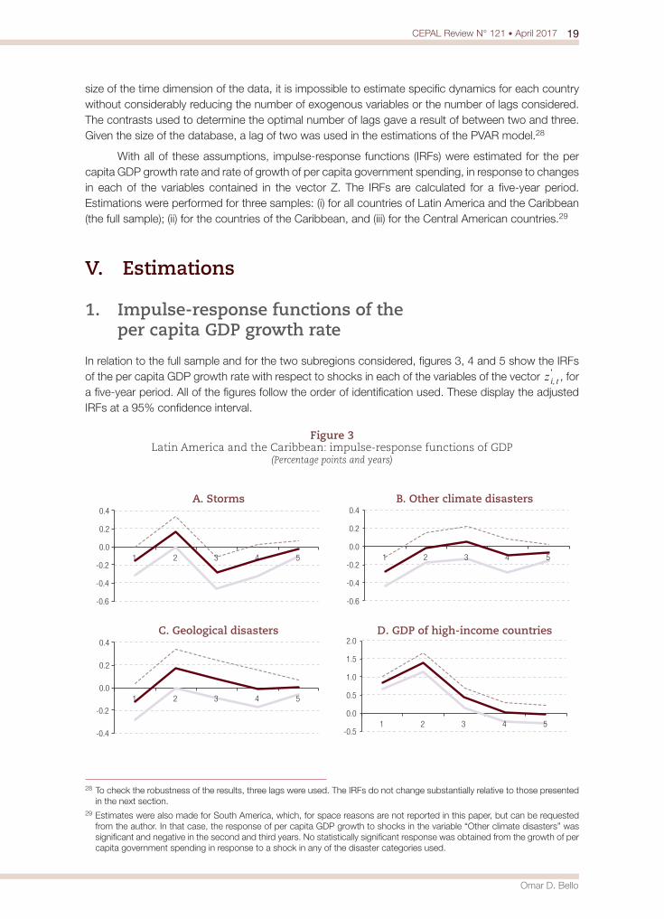
In relation to the full sample and for the two subregions considered, figures 3, 4 and 5 show the IRFs of the per capita GDP growth rate with respect to shocks in each of the variables of the vector z ,
'i t , for
a five-year period. All of the figures follow the order of identification used. These display the adjusted IRFs at a 95% confidence interval.
Figure 3 Latin America and the Caribbean: impulse-response functions of GDP
(Percentage points and years)
-0.6
-0.4
-0.2
0.0
0.2
0.4
1 2 3 4 5
A. Storms
-0.6
-0.4
-0.2
0.0
0.2
0.4
1 2 3 4 5
B. Other climate disasters
-0.4
-0.2
0.0
0.2
0.4
1 2 3 4 5
C. Geological disasters
-0.5
0.0
0.5
1.0
1.5
2.0
1 2 3 4 5
D. GDP of high-income countries
28 To check the robustness of the results, three lags were used. The IRFs do not change substantially relative to those presented in the next section.
29 Estimates were also made for South America, which, for space reasons are not reported in this paper, but can be requested from the author. In that case, the response of per capita GDP growth to shocks in the variable “Other climate disasters” was significant and negative in the second and third years. No statistically significant response was obtained from the growth of per capita government spending in response to a shock in any of the disaster categories used.
20 CEPAL Review N° 121 • April 2017
Disasters, economic growth and fiscal response in the countries of Latin America and the Caribbean, 1972-2010
-0.2
0.0
0.2
0.4
0.6
0.8
1.0
1 2 3 4 5
E. Terms of trade
-0.6
-0.4
-0.2
0.0
0.2
1 2 3 4 5
F. International interest rate
Source: Prepared by the author.
Figure 4 The Caribbean: impulse-response functions of GDP
(Percentage points and years)
0.0
0.5
1 2 3 4 5
A. Storms
-0.6
-0.4
-0.2
0.0
0.2
1 2 3 4 5
B. Other climate disasters
0.0
0.2
0.4
0.6
1 2 3 4 5
C. Geological disasters
-1.5
-1.0
-0.5
0.0
0.5
1.0
1.5
1 2 3 4 5
D. GDP of high-income countries
0.0
0.5
1.0
1.5
1 2 3 4 5
E. Terms of trade
-1.0
-0.5
0.0
0.5
1.0
1 2 3 4 5
F. International interest rate
-1.5
-1.0
-0.5
-0.6
-0.4
-0.2
-0.5
Source: Prepared by the author.
Figure 3 (concluded)
21CEPAL Review N° 121 • April 2017
Omar D. Bello
Figure 5 Central America: impulse-response functions of GDP
(Percentage points and years)
-1.5
-1.0
-0.5
0.0
0.5
1.0
1 2 3 4 5
A. Storms
-0.8
-0.3
0.2
0.7
1 2 3 4 5
B. Other climate disasters
-0.4
-0.2
0.0
0.2
0.4
0.6
0.8
1 2 3 4 5
C. Geological disasters
0.0
0.5
1.0
1.5
2.0
1 2 3 4 5
D. GDP of high-income countries
-0.4
-0.2
0.0
0.2
0.4
0.6
0.8
1 2 3 4 5
E. Terms of trade
-1.0
-0.5
0.0
0.5
1 2 3 4 5
F. International interest rate
Source: Prepared by the author.
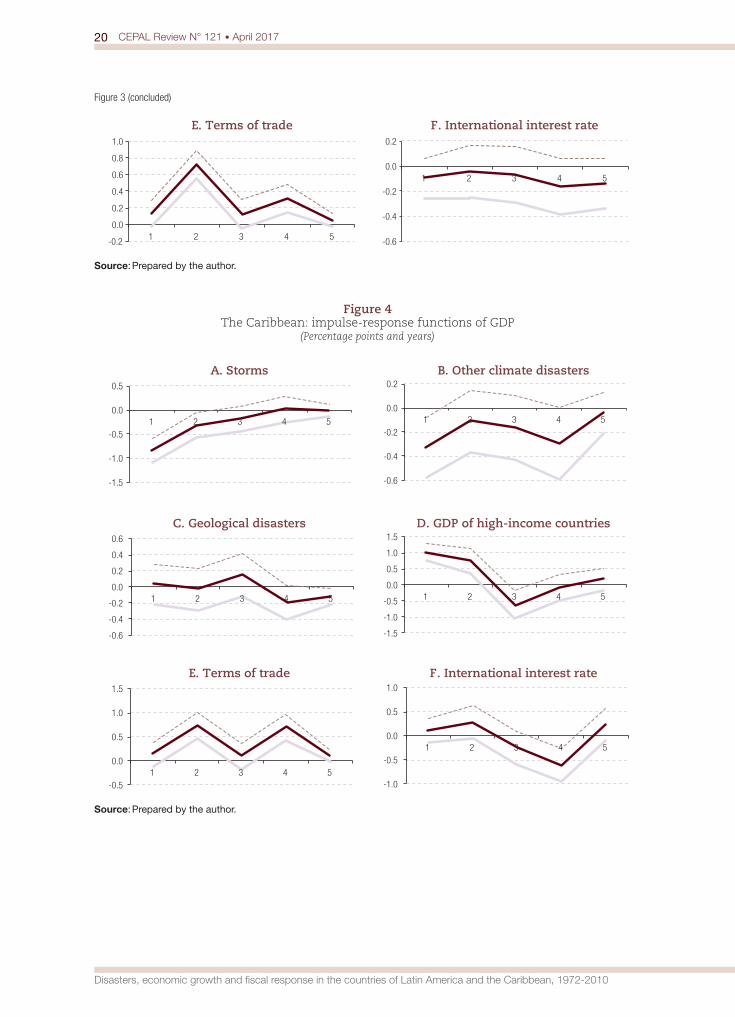
In Latin America and the Caribbean, the variable “Storms” has a first-year negative impact on the per capita GDP growth rate of roughly 0.16 percentage points, which is reversed in the second year, with an impact of 0.2 percentage points. The variable “Other climate disasters” has a statistically significant impact on the per capita GDP growth rate of roughly -0.24 percentage points, but only for one year. In the case of the variable “Geological disasters,” the impact is positive, of 0.18 percentage points in the second year (see figures 3 A, 3 B and 3 C). The two variables whose shocks most affect the per capita GDP growth rate are GDP growth in high-income countries and the rate of variation in the terms-of-trade index (see figures 3 D and 3 E). A shock to the GDP growth rate of high-income countries has a positive effect on GDP growth: in the first year, this is around 0.8 percentage points, rising to 1.4 percentage points in the second year, and roughly 0.5 points in the third year. As from the fourth year, the effect converges to zero. In contrast, a positive shock to the rate of change of the terms of trade has positive impact lasting for four years. As would be expected, in the first year the GDP growth effect is positive at around 0.1 percentage points; and this is followed by even stronger impact in the second year, of roughly 0.7 percentage points. In the third year, the growth effect declines to
22 CEPAL Review N° 121 • April 2017
Disasters, economic growth and fiscal response in the countries of Latin America and the Caribbean, 1972-2010
around 0.1 points before rising to 0.3 percentage points. As from the fifth year, the per capita GDP growth impact converges to zero. Lastly, the effect of an international interest rate shock does not have a statistically significant effect on the per capita GDP growth rate.
The estimates for the Caribbean show stronger evidence of the impact of climate disasters on the per capita GDP growth rate. A shock in the variable “Storms” causes a statistically significant negative response in the first two years, of roughly 0.7 and 0.3 percentage points, respectively (see figure 4 A). A shock in the variable “Other climate disasters” has a negative and significant effect of around 0.3 percentage points for one year only (see figure 4 B). Shocks caused by geological disasters do not have a significant impact on GDP in this region. In terms of the shock to the per capita GDP growth rate of the high-income countries, and in the region as a whole, the greatest effect is on the per capita GDP growth rate of the Caribbean countries, which display responses of around 1 and 0.8 percentage points in the first two years, respectively. As from the third year, the effect ceases to be statistically significant (see figure 4 D). In the case of a terms-of-trade shock, there are positive effects in the first two years of 0.1 and 0.7 percentage points, respectively; and again in the fourth year of 0.7 percentage points (see figure 4 E). Lastly, the regional result is repeated in respect of a variation in the international interest rate.
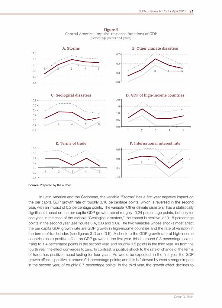
In the case of Central America, shocks in the variables “Storms” and “Other climate disasters” generate the same response pattern in the per capita GDP growth rate: a decrease in the first year of roughly 0.8 and 0.5 percentage points, respectively; and in both cases, a recovery of around 0.45 points in the third year (see figures 5 A and 5 B). Geological disasters did not produce a significant effect in the first year; but in the second and third years, there was an upturn of around 0.4 percentage points (see figure 5 C). In all three types of disaster, convergence occurs in the fourth year. In the IRFs of other variables, similar results are obtained, in other words the most important variable in terms of the magnitude of effect on the GDP growth rate of the Central American countries is a growth shock in the high-income economies. That impact does not fully dissipate in five years.30
2. Impulse-response functions of the growth rate of per capita government spending
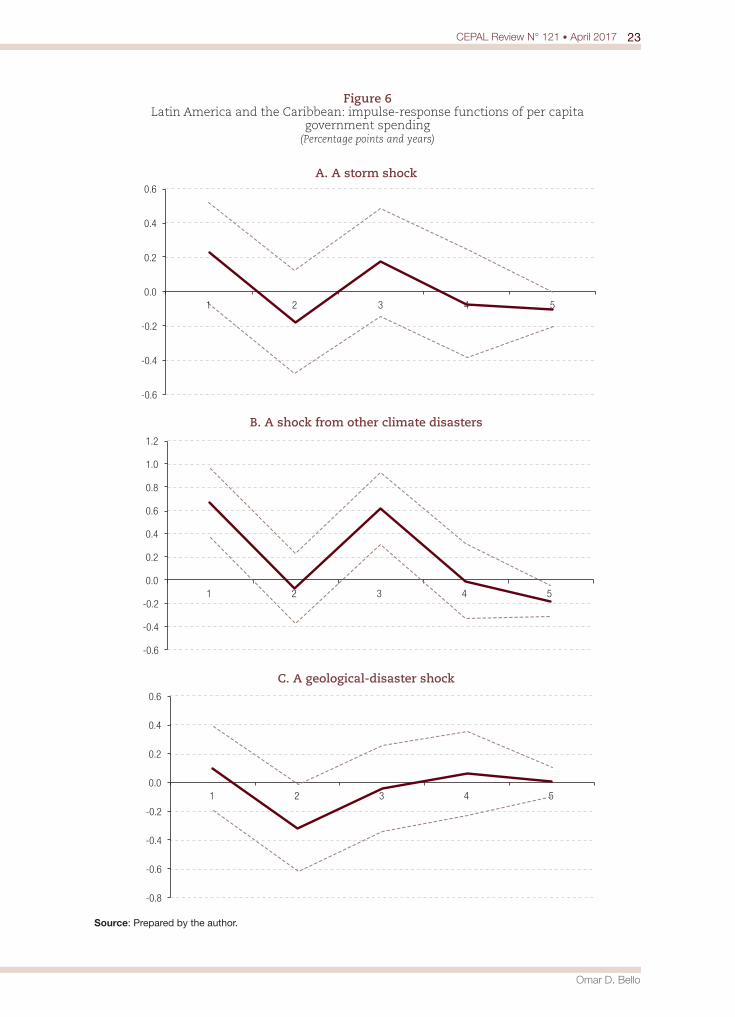
In this case, the analysis focuses on the response of the rate of growth of per capita government spending to shocks in the disaster variables, and only the IRFs corresponding to those events are presented, as shown in figures 6, 7 and 8. In the case of Latin America and the Caribbean, shocks in the variable “Storms” did not have a statistically significant effect on per capita government expenditure, whereas shocks in the variable “Other climate disasters” produced a positive and statistically significant response in the first three years, of 0.5, 0.6 and 0.5 percentage points, respectively.
30 The effect of this shock converges to zero in eight years.
23CEPAL Review N° 121 • April 2017
Omar D. Bello
Figure 6 Latin America and the Caribbean: impulse-response functions of per capita
government spending (Percentage points and years)
-0.6
-0.4
-0.2
0.0
0.2
0.4
0.6
1 2 3 4 5
A. A storm shock
-0.6
-0.4
-0.2
0.0
0.2
0.4
0.6
0.8
1.0
1.2
1 2 3 4 5
B. A shock from other climate disasters
-0.8
-0.6
-0.4
-0.2
0.0
0.2
0.4
0.6
1 2 3 4 5
C. A geological-disaster shock
Source: Prepared by the author.
24 CEPAL Review N° 121 • April 2017
Disasters, economic growth and fiscal response in the countries of Latin America and the Caribbean, 1972-2010
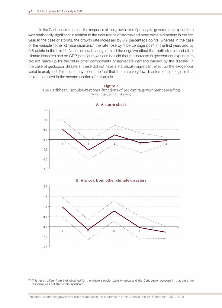
In the Caribbean countries, the response of the growth rate of per capita government expenditure was statistically significant in relation to the occurrence of storms and other climate disasters in the first year. In the case of storms, the growth rate increased by 0.7 percentage points, whereas in the case of the variable “other climate disasters,” the rate rose by 1 percentage point in the first year, and by 0.8 points in the third.31 Nonetheless, bearing in mind the negative effect that both storms and other climate disasters had on GDP (see figure 4) it can be said that the increase in government expenditure did not make up for the fall in other components of aggregate demand caused by the disaster. In the case of geological disasters, these did not have a statistically significant effect on the exogenous variable analysed. This result may reflect the fact that there are very few disasters of this origin in that region, as noted in the second section of this article.
Figure 7 The Caribbean: impulse-response functions of per capita government spending
(Percentage points and years)
-1.5
-1.0
-0.5
0.0
0.5
1.0
1.5
1 2 3 4 5
A. A storm shock
-1.0
-0.5
0.0
0.5
1.0
1.5
2.0
1 2 3 4 5
B. A shock from other climate disasters
31 This result differs from that obtained for the whole sample (Latin America and the Caribbean), because in that case the response was not statistically significant.

25CEPAL Review N° 121 • April 2017
Omar D. Bello
-0.8
-0.6
-0.4
-0.2
0.0
0.2
0.4
0.6
0.8
1 2 3 4 5
C. A geological-disaster shock
Source: Prepared by the author.
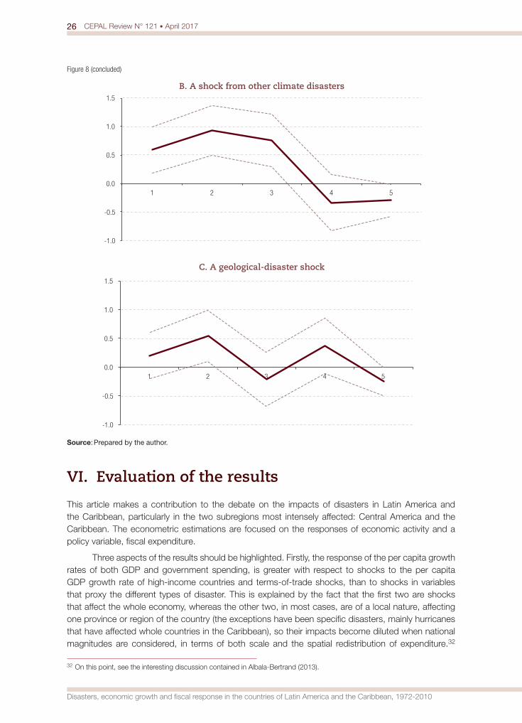
In the case of Central America, the IRFs of the growth rate of per capita government expenditure in response to a shock in the variable “Storms” shows that the statistically significant impact lasts two years. As a result of this shock, the rate of growth of per capita government spending rose by 0.6 percentage points in the first year and by 0.8 percentage points in the second. As in the Caribbean countries, this result differs from that displayed by the sample as a whole. In the case of other climate disasters, the statistically significant impact lasts three years, with increases of roughly 0.6, 0.9 and 0.8 percentage points during the period. As with the Caribbean countries, this expenditure growth was not enough to compensate for the reduction in other flows, and the final result was a drop in the GDP growth rate. In the case of geological disasters, there was a statistically significant effect in the first two years, of roughly 0.5 and 0.6 percentage points, respectively.
Figure 8 Central America: impulse-response functions of per capita government spending
(Percentage points and years)
-1.0
-0.5
0.0
0.5
1.0
1.5
1 2 3 4 5
A. A storm shock
Figure 7 (concluded)
26 CEPAL Review N° 121 • April 2017
Disasters, economic growth and fiscal response in the countries of Latin America and the Caribbean, 1972-2010
-1.0
-0.5
0.0
0.5
1.0
1.5
1 2 3 4 5
B. A shock from other climate disasters
-1.0
-0.5
0.0
0.5
1.0
1.5
1 2 3 4 5
C. A geological-disaster shock
Source: Prepared by the author.
VI. Evaluation of the results
This article makes a contribution to the debate on the impacts of disasters in Latin America and the Caribbean, particularly in the two subregions most intensely affected: Central America and the Caribbean. The econometric estimations are focused on the responses of economic activity and a policy variable, fiscal expenditure.
Three aspects of the results should be highlighted. Firstly, the response of the per capita growth rates of both GDP and government spending, is greater with respect to shocks to the per capita GDP growth rate of high-income countries and terms-of-trade shocks, than to shocks in variables that proxy the different types of disaster. This is explained by the fact that the first two are shocks that affect the whole economy, whereas the other two, in most cases, are of a local nature, affecting one province or region of the country (the exceptions have been specific disasters, mainly hurricanes that have affected whole countries in the Caribbean), so their impacts become diluted when national magnitudes are considered, in terms of both scale and the spatial redistribution of expenditure.32
32 On this point, see the interesting discussion contained in Albala-Bertrand (2013).
Figure 8 (concluded)
27CEPAL Review N° 121 • April 2017
Omar D. Bello
Thus, assistance to deal with the emergency caused by the disaster can be largely obtained in other provinces or departments, so sectoral activity, despite suffering regional upheavals, may not suffer at the national level. By not capturing the local nature of the disaster, measurement of the aggregate impact alone would be shrouding the effect on the regional economy (see ECLAC, 2014). In many cases, highlighting the local dimension is limited by data availability; so, the correct measurement of the impact of the disaster, to make the effects on the local economies of the country visible, should make use of subnational accounts, which have been developed in some countries of the region.33 It is worth reiterating that, while a disaster might not have a major macroeconomic impact, it may have one at the local level, seriously affecting the lives of the inhabitants of territories where the event occurred. Hence the need to develop disaster risk management policies that are inclusive of local governments and communities.
Secondly, with respect to the results obtained from the disasters themselves, it should be noted that the longest duration of their impact is three years. In other words, a disaster apparently does not affect long-term per capita GDP growth or per capita fiscal spending in the economies of Latin America and the Caribbean. Nonetheless, this is an average, and the result also reflects the PVAR model used, which assumes that the dynamic is the same for all countries. Lastly, given the size of the sample, the robustness of this result cannot be verified, considering only the largest disasters.34 For example, Loayza and others (2009) observed nonlinear disaster-intensity effects.
In terms of more specific results, in the Latin American and Caribbean countries, the IRFs of the per capita GDP growth rate with respect to each of the disaster types considered show that there are differentiated effects between them —negative in the case of storms and other climate disasters and positive in the case of the variable that proxies for geological disasters. The response to the first was statistically significant for three years, but only for one year in the other two cases. An assumption of the PVAR model used is that the same dynamic is being attributed to each country, which might be questionable given the heterogeneity of production patterns in Latin America and the Caribbean. For that reason, estimations were made for groups of countries displaying greater similarities, such as those of Central America and the Caribbean, which are also the two subregions most intensely affected by disasters.
When the Caribbean and Central America are analysed, the conclusions change. In the Caribbean countries, the response of the per capita GDP growth rate to shocks in the variables “Storms” and “Other climate disasters” was negative, lasting for two years in the first case and one year in the second. The response to a geological disaster was not statistically significant. In the Central American countries, the response of the per capita GDP growth rate to storms and other climate disasters was similar, negative in the first year positive in the third; and whereas it was not compensated in the first case it was in the second. The response to a disaster of geological origin was positive in the second and third years. These results show that, in both subregions, the two types of climate disaster, which are the disaster types that have grown most in the last few decades, in all cases had a statistically significant negative response in per capita GDP growth in the first year, accumulating a negative response in three out of four cases. This could be evidence that processes to rebuild or repair the damage caused by those disasters may have been insufficient. Cuaresma, Hlouskova and Obersteiner (2008) observed that, following a disaster, only countries with a certain level of development succeeded rebuilding and achieving improvements relative to the situation prior to the event.
33 Thus far, seven Latin American countries have this type of subnational account: Brazil, Chile, Colombia, Ecuador, Mexico, Peru and the Plurinational State of Bolivia.
34 The database used here only included countries from Latin America and the Caribbean, so it is a lot smaller than that used in other studies, such as Loayza and others (2009), Jaramillo (2009) and Raddatz (2007 and 2009), among others, which used global data.
28 CEPAL Review N° 121 • April 2017
Disasters, economic growth and fiscal response in the countries of Latin America and the Caribbean, 1972-2010
In the case of the growth rate of real per capita public spending, the IRF corresponding to the Latin American and Caribbean countries was statistically significant only for a shock in the variable “Other climate disasters” in the first and third years. In the Caribbean countries, that response was statistically significant and positive only for climate disasters —in the first year in the case of storms, and in the first and third years for other climate disasters. In the Central American countries, the response to shocks in the variables of all types of disaster was positive and statistically significant. The response lasted for the first two years in the case of storms, but extended to three for other climate disasters. For geological disasters, the response lasted a year. In short, the results show that the rate of growth of per capita government spending increased as a consequence of a disaster in six out of nine cases. Nonetheless, the results obtained for per capita GDP suggest that this reaction was insufficient to prevent a fall in the growth rate of this indicator. It could be that the reaction has been affected by institutional constraints in each country or by the amount of fiscal slack existing before the event. This constitutes a strong argument in favour of countries enhancing the institutional consolidation of their disaster-risk reduction policy, to incorporate it into public investment policies.
BibliographyAlbala-Bertrand, J. (2013), Disasters and the Networked Economy, New York, Routledge.
(1993), The Political Economy of Large Natural Disasters, Oxford, Clarendon Press.Bello, O., L. Ortiz and J.L. Samaniego (2014), “La estimación de los efectos de los desastres en América
Latina, 1972-2010”, Medio Ambiente y Desarrollo series, No. 157 (LC/L.3899), Santiago, Economic Commission for Latin America and the Caribbean (ECLAC).
Cavallo, A., E. Cavallo and R. Rigobón (2013), “Prices and supply disruptions during natural disasters”, NBER Working Paper, No. 19474, Cambridge, Massachusetts, National Bureau of Economic Research.
Cavallo, E. and I. Noy (2010), “The economics of natural disasters: a survey”, IDB Working Paper Series, No. 124, Washington, D.C., Inter-American Development Bank.
Cavallo, E. and others (2010), “Catastrophic natural disasters and economic growth”, IDB Working Paper Series, No. 183, Washington, D.C., Inter-American Development Bank.
Christiaensen, L. and K. Subbarao (2005), “Towards an understanding of household vulnerability in rural Kenya”, Journal of African Economies, vol. 14, No. 4, Centre for the Study of African Economies.
Cuaresma, J., J. Hlouskova and M. Obersteiner (2008), “Natural disasters as creative destruction? Evidence from developing countries”, Economic Inquiry, vol. 46, No. 2.
De Gregorio, J. and R. Valdés (2001), “Crisis transmission: evidence from the debt, tequila and Asian flu crises”, World Bank Economic Review, vol. 25, No. 2, Oxford University Press.
Deaton, A. and R. Miller (1996), “International commodity prices, macroeconomic performance and politics in Sub-Saharan Africa”, Journal of African Economies, vol. 5, No. 3, Centre for the Study of African Economies.
Dercon, S. (2005), “Growth and shocks: evidence from rural Ethiopia”, Journal of Development Economics, vol. 74, No. 2, Amsterdam, Elsevier.
Dos Reis, L. (2004), “A fiscal insurance scheme for the Eastern Caribbean Currency Union” [online] http://www.iadb.org/WMSFiles/products/research/files/pubS-242.pdf.
ECLAC (Economic Commission for Latin America and the Caribbean) (2014), Handbook for Disaster Assessment (LC/L.3691), Santiago.
Elbers, C., J. Gunning and B. Kinsey (2002), “Convergence, shocks and poverty”, Discussion Paper, No. 2002-035/2, Amsterdam, Tinbergen Institute.
Hausmann, R., F. Rodríguez and R. Wagner (2006), “Growth collapses”, CID Working Paper, No. 136, Cambridge, Massachusetts, Harvard University.
IPCC (Intergovernmental Panel on Climate Change) (2012), Managing the Risks of Extreme Events and Disasters to Advance Climate Change Adaptation, Cambridge University Press.
Islam, N. (1995), “Growth empirics: a panel data approach”, Quarterly Journal of Economics, vol. 110, No. 4, Oxford University Press.
Jaramillo, C. (2009), “Do natural disasters have long-term effects on growth?”, Documentos CEDE, No. 24, Bogota, University of the Andes.
29CEPAL Review N° 121 • April 2017
Omar D. Bello
Laeven, L. and F. Valencia (2008), “Systemic banking crises: a new database”, IMF Working Paper, No. 224, Washington, D.C., International Monetary Fund.
Loayza, N. and others (2009), “Natural disasters and growth - going beyond the averages”, Policy Research Working Paper Series, No. 4980, Washington, D.C., World Bank.
Lybbert, T. and others (2004), “Stochastic wealth dynamics and risk management among a poor population”, Economic Journal, vol. 114, No. 498.
Melecky, M. and C. Raddatz (2011), “How do governments respond after catastrophes? Natural-disaster shocks and the fiscal stance”, Policy Research Working Paper Series, No. 5564, Washington, D.C., World Bank.
Noy, I. (2007), “The macroeconomic consequences of disasters”, Working Paper, No. 7, Honolulu, University of Hawaii.
Olaberría, E. (2009), “Economic impacts of epidemics”, unpublished.Raddatz, C. (2009), “The wrath of God: macroeconomic costs of natural disasters”, Policy Research Working
Paper Series, No. 5039, Washington, D.C., World Bank.(2007), “Are external shocks responsible for the instability of output in low-income countries?”, Journal of Development Economics, vol. 84, No. 1, Amsterdam, Elsevier.
Rasmussen, T. (2004), “Macroeconomic implications of natural disasters in the Caribbean”, IMF Working Paper, No. 04/24, Washington, D.C., International Monetary Fund.
Reinhart, C. and K. Rogoff (2008), “This time is different: a panoramic view of eight centuries of financial crises”, NBER Working Paper, No. 13882, Cambridge, Massachusetts, National Bureau of Economic Research.
Rodríguez-Oreggia, E. and others (2013), “Natural disasters, human development and poverty at the municipal level in Mexico”, Journal of Development Studies, vol. 49, No. 3, Taylor & Francis.
Rodrik, D. (1998), “Where did all the growth go? External shocks, social conflict, and growth collapses”, NBER Working Papers, No. 6350, Cambridge, Massachusetts, National Bureau of Economic Research.
Skidmore, M. and H. Toya (2002), “Do natural disasters promote long-run growth?”, Economic Inquiry, vol. 40, No. 4.
Stromberg, D. (2007), “Natural disasters, economic development, and humanitarian aid”, Journal of Economic Perspectives, vol. 21, No. 3, Nashville, Tennessee, American Economic Association.
Titelman, D., E. Pérez and R. Pineda (2009), “The bigness of smallness: The financial crisis, its contagion mechanisms and its effects in Latin America”, CEPAL Review, No. 98 (LC/G.2404-P), Santiago, Economic Commission for Latin America and the Caribbean (ECLAC).
Volpe, C. and J.S. Blyde (2013), “Shaky roads and trembling exports: assessing the trade effects of domestic infrastructure using a natural experiment”, Journal of International Economics, vol. 90, No. 1, Amsterdam, Elsevier.

Nicaragua: trend of multidimensional poverty, 2001-2009José Espinoza-Delgado and Julio López-Laborda
Abstract
This paper estimates multidimensional poverty in Nicaragua between 2001 and 2009, using data from the three most recent standard of living surveys that are available (2001, 2005 and 2009), and mainly following the methodology proposed by Alkire and Foster (2007 and 2011). For that purpose, 10 dimensions and three weighting systems are used: equal-weightings and two other systems based on the data themselves, one based on the first principal component scores, and the other based on the relative frequencies of dimensional deprivations (both of these systems are new to Nicaragua). Overall, the results show that the incidence, intensity and severity of multidimensional poverty in Nicaragua declined in 2001-2009, and particularly so between 2001 and 2005.
Keywords
Poverty, standard of living, measurement, household surveys, statistical methodology, Nicaragua
JEL classification
D31, I32, O15.
Authors
José Espinoza-Delgado is a research assistant with the Department of Economics, Chair of Development Economics, at the University of Göttingen, Germany. [email protected]
Julio López-Laborda is a professor with the Department of Economic Structure, Economic History and Public Economics, at the University of Zaragoza, Spain. [email protected]
32 CEPAL Review N° 121 • April 2017
Nicaragua: trend of multidimensional poverty, 2001-2009
I. Introduction
The conceptual understanding of poverty has been improved and deepened notably in the last three decades, thanks to the seminal work of Amartya Sen and his theoretical framework of capabilities and functionings (Thorbecke, 2008, p. 3).1 There is currently a broad consensus that poverty is a multidimensional phenomenon and that its analysis cannot be confined to the study of a monetary dimension (Sen, 1985 and 2000; Atkinson, 2003; Kakwani and Silber, 2008; Stiglitz, Sen and Fitoussi, 2009a and 2009b) —whether per capita income or per capita consumption expenditure, as suggested by the traditional or monetary approach to measuring poverty. In this context, a broader poverty measure, which considers other attributes apart from income (Atkinson, 2003, p. 51), is a key and necessary input for the design, monitoring and evaluation of poverty-reduction policies.
Taking Sen’s ideas as a conceptual base, and returning to previous work by Espinoza-Delgado and López-Laborda (2015), this study measures poverty in Nicaragua from a multidimensional standpoint, using the data from the last three available editions of the National Household Survey on Living Standards Measurement (EMNV, 2001, 2005 and 2009) and applying the measurement methodology proposed by Alkire and Foster (2007 and 2011). Specifically, the measures H, M0, M1 and M2 proposed by Alkire and Foster are estimated; and the trend of the first two is compared with the headcount ratio obtained by applying the official methodology used to measure poverty in Nicaragua, which basically follows a monetary approach. Before calculating these measures, a global measure is estimated that follows some of the ideas of the fuzzy poverty measurement proposed by Cerioli and Zani (1990), which is also compared against the official poverty estimates. This global measure could also be used as an anchor to approximate the second cut-off (or multidimensional poverty threshold) required by the Alkire and Foster methodology to identify individuals who are multi-dimensionally poor (Alkire and Foster, 2011, p. 478), and to obtain a specific estimation based on this methodology, which is not done in this paper. The analysis considers 10 dimensions which are then aggregated by using three alternative weighting systems. Apart from equal weights, two weighting systems are obtained from the data themselves: one based on the first principal component scores, and the other based on the relative frequencies of deprivations in the different dimensions.
In general, the literature contains few studies on poverty in Nicaragua, and even fewer have analysed poverty from a multidimensional perspective, beyond the unsatisfied basic needs (UBN) approach, of long tradition in the region (ECLAC, 2009; Boltvinik, 2013). This situation is not peculiar to Nicaragua; studies on multidimensional poverty are very few and far between in all of Latin America (Roche and Santos, 2012, p. 4; Battiston and others, 2013, p. 292), and the monetary approach has dominated the studies undertaken, particularly in Central America (ECLAC, 2009, p. 17).2
One of the earliest attempts —if not the first— to measure multidimensional poverty in Nicaragua (and also in other Central American countries) can be found in the ECLAC study on poverty and social vulnerability of December 2003. This applies the “integrated poverty measure” proposed by Kaztman (1989), which jointly considers the incidence of income and unsatisfied basic needs (ECLAC, 2003, p. 19). Although this paper was innovative at the time, its suggested approach has several methodological weaknesses: it accords a major protagonist role to income (ECLAC, 2009, p. 49) and does not take account of the dimensional deficits, an issue raised by Bourguignon and Chakravarty (2003, p. 27). Another ECLAC study (ECLAC, 2009) uses a variety of methodologies, apart from the Kaztman measure —the Alkire and Foster methodology, principal components and cluster analysis—
1 See, for example, Sen (1985, 1992, 2000 and 2008).2 ECLAC (2009) summarizes the different studies that have used different methodologies to measure multidimensional poverty in
Latin America, and particularly in Central America (ECLAC, 2009, pp. 19 ff). For the specific case of Nicaragua, there are only two references: Del Carpio and Castro (2007), which uses a subjective approximation of well-being, and ECLAC (2003), which uses the integrated poverty measurement.

33CEPAL Review N° 121 • April 2017
José Espinoza-Delgado and Julio López-Laborda
to estimate multidimensional poverty in Mexico and Central America (including Nicaragua). Like the Katzman paper, this ECLAC study makes a joint analysis of per capita income and seven dimensions of UBN (housing, overcrowding, water, sanitation, education, electricity, and household consumption capacity). It also applies the Alkire and Foster methodology to the case of Nicaragua for the first time and estimates H and M0 using data from the 2005 EMNV. The results show that 84.3% of the Nicaraguan population was suffering from deprivation in at least one dimension in 2005, and that 0.1% suffered deprivation in all of the dimensions; estimations for M0 range from 30.7% to 0.1% (ECLAC, 2009, p. 38).
This was followed by the Alkire and Santos (2010) study, which includes estimations of multidimensional poverty in Nicaragua, in relation to the proposed multidimensional poverty index (MPI). This adheres to the mathematical structure of one of the measures of the Alkire and Foster methodology (M0) and considers 10 indicators representing the three dimensions that are used to calculate the Human Development Index (HDI) published by the United Nations Development Programme (UNDP). According to this study, data from the 2001 Nicaraguan Demography and Health Survey show that 40.7% of the Nicaraguan population was living in conditions of multidimensional poverty (H); and the country was ranked 64th out of a total of 104 developing countries, with an M0 of 0.211 (Alkire and Santos, 2010, p. 75). It is worth noting that the index proposed by Alkire and Santos (2010) has been adopted by UNDP; and since 2010 it has formed part of the Human Development Report (UNDP, 2010). Nonetheless, as it is an acute poverty index, it gives relatively lower estimations for Nicaragua, and even for all of Latin America; so its results are not very relevant to the reality of the country and region as a whole (Roche and Santos, 2012). Then, the National Human Development Report for 2011, prepared by the UNDP Office in Nicaragua (UNDP, 2011), puts forward the Youth Multidimensional Poverty Index (IPMJ), which incorporates four dimensions (education, employment, health, and household conditions). This index also uses the M0 measurement of the Alkire and Foster methodology, and focuses on the Nicaraguan population aged between 13 and 29 years. This report, using data from the 2001 and 2005 EMNV and the 2009 Household Survey for poverty measurement of the International Foundation for the Global Economic Challenge (FIDEG), concludes, among other things, that the proportion of young people and adolescents who were multidimensionally poor declined by 8.3 percentage points between 2001 and 2009 (UNDP, 2011, p. 82).3 Lastly, Roche and Santos (2012) analyses the results of the IPM for 18 Latin American and Caribbean countries, including Nicaragua, and proposes a number of amendments to the index to better reflect multidimensional poverty in the region, and to make the estimations more relevant.
Thus, as far as the authors are aware, this study, together with the earlier work by Espinoza-Delgado and López-Laborda (2015), represents the first attempt to measure and determine the trend of multidimensional poverty in Nicaragua, at the national level and for the population as a whole, using data from the last three available EMNVs, which the Government of Nicaragua uses to measure poverty (INEC, 2002a, 2002b and 2003; INIDE, 2007 and 2011a). The surveys also have the advantage of including information on the income and expenditure of Nicaraguan households, which makes it possible, among other things, to compare the trend of monetary and multidimensional poverty. This study is also the first attempt to measure the intensity and severity of multidimensional poverty in Nicaragua —two aspects of poverty that are not estimated in the literature that deals with the measurement of multidimensional poverty in Nicaragua and elsewhere, perhaps owing to the nature of the data. Naturally, the intention is not to propose the multidimensional poverty measurement, but to provide empirical evidence for adopting a broader approach to measuring poverty in the country, which complements the official estimations and helps to reduce the deficit in the specialized literature on Nicaragua and the region.
3 See [online] www.fideg.org.

34 CEPAL Review N° 121 • April 2017
Nicaragua: trend of multidimensional poverty, 2001-2009
Section II describes the data and methodological issues (multidimensional poverty measures, the choice and justification of the dimensions and indicators, dimensional poverty lines and weightings). Section III presents the main results obtained. Section IV addresses issues relating to the bilateral correlations and overlaps in identifying the poor; and section V sets out a number of conclusions.
II. Data and methodological issues
The data analysed are obtained from the last three EMNVs (2001, 2005, 2009) conducted by the National Information and Development Institute (INIDE) of Nicaragua, with support from the World Bank.4 The sample encompassed 4,191 households (22,810 people) in 2001; 6,882 households (36,612 people) in 2005; and 6,515 households (30,432 people) in 2009. Given the aim of this study, the household is the unit of analysis chosen to identify the poor.5 Nonetheless, information pertaining to individuals is also incorporated, and related to the household in question; and the results are presented in population terms using the survey expansion factors.
1. Multidimensional poverty measures
According to Sen, two problems need to be addressed when measuring poverty: the identification of the poor in the wider population, and the construction of a poverty index that uses the available information on the poor (Sen, 1976, p. 219). To resolve these two issues, in a multidimensional context for Nicaragua, this paper follows the Alkire and Foster (2007 and 2011) methodology, which consists of an identification method (rho-k), which expands the traditional approaches of union and intersection, and a family of measures, Mα, which resolves the second issue.6 The identification method uses two cut-offs: one within each dimension (dimensional cut-off) to determine whether the unit of analysis is deprived in that specific dimension; and a second cut-off between the dimensions (k), which identifies the poor by counting the dimensions in which the unit of analysis is deprived. Alkire and Foster (2011, p. 478) suggest setting the value of k at some intermediate point between the two extremes that represent the traditional approaches, which is controversial and arbitrary. This study follows the principles of the dominance approach for analysing poverty, and uses a wide range of k-values (Duclos, Sahn and Younger, 2008, p. 246). The Mα measures, meanwhile, are based on the Foster-Greer-Thorbecke (FGT) family of measures, suitably adjusted to take account of multi-dimensionality. This study, apart from the multidimensional headcount ratio (H), calculates the adjusted headcount ratio (M0), the adjusted poverty gap (M1) and the adjusted FGT measure (M2).7 Accordingly, it addresses the three important aspects of poverty —incidence, intensity and inequality— which have been called the “three Is” of poverty (Jenkins and Lambert, 1997, p. 319).
4 Previously, INIDE was the National Institute of Statistics and Censuses (INEC).5 This is a normative decision making it possible to appropriately compare the estimations made in this study with the official
figures and with estimations of the multidimensional poverty index for Nicaragua. In addition, the household represents the unit observation of the surveys used (INEC, 2006, p. 4; INIDE, 2011b, p. 4).
6 The union approach classifies a household as poor if it suffers deprivation in at least one dimension. At the other extreme, the intersection approach requires the household to suffer deprivation in all of the dimensions to be considered poor (see Atkinson, 2003).
7 H measures the fraction of the population that is multidimensionally poor; M0 (which is sensitive to the frequency and amplitude of multidimensional poverty) is obtained by multiplying H by the average proportion of deprivations suffered by the multidimensionally poor (A); M1 is the product of M0 and the average poverty gap (G); M2 is the product of M0 and the average severity index (S), and it is sensitive to the inequality with which deprivations are distributed among the poor (Alkire and Foster, 2011, p. 479).
35CEPAL Review N° 121 • April 2017
José Espinoza-Delgado and Julio López-Laborda
Before calculating the measures referred to above, the study estimates a measure that follows the structure of the fuzzy poverty index proposed by Cerioli and Zani (1990), which is also used to approximate the second cut-off required by the Alkire and Foster (2011) identification method. This measure (Cerioli and Zani, 1990, p. 282) is defined as:
P n i1A
i
n
1
n==
R W/ (1)8
where μA(i) denotes, for each household, a degree of belonging to the subset of multidimensionally deprived persons, and it is constructed according to the following expression:
, , ...,Pr
iw
wi n1 2A
jj
d
j ijj
d
1
1n = =
=
=R RW W//
(2)
where wj represents the weighting of dimension j and Prij reflects the deprivation of household i in dimension j. Thus, Prij will take the value 1 if the ith household is deprived in dimension j, and 0 otherwise. So, μA(i) = 0 if the ith household does not suffer deprivation in any dimension, which would mean that it was clearly not poor; μA(i) = 1 if the ith household suffers deprivation in all dimensions, which would make it clearly a multidimensionally poor household; and 0< μA(i) < 1 if the ith household is deprived in some but not all of the dimensions.
2. Choice and justification of the dimensions and indicators
Following Alkire and Santos (2010, p. 11), the choice of the relevant dimensions is a value judgement rather than a technical exercise; and it is a crucial step in defining a multidimensional poverty measure (Battiston and others, 2013, p. 294). Bearing this in mind, and based on the UBN approach and guided also by the Millennium Development Goals, this study considers a set of dimensions and indicators that certainly reflect important aspects of the well-being of Nicaraguan households and are directly related to specific basic capabilities (Klasen, 2000, p. 38). Table 1 shows the dimensions, indicators and scores associated with each achievement.
Considering the attainments, as described by the selected indicators, as a matter of degree rather than an “all or nothing” condition (Chiappero Martinetti, 2006, p. 100), and taking advantage of the information available on them, the study has scored each indicator on a scale of 1 to 5. A score of 5 represents the best possible standard or condition; a score of 3 represents a basic level of well-being; and a score of 1 represents the worst condition, or severe deprivation. With this scoring structure, the differences in the levels of achievement are interpreted on a cardinal basis: an achievement that obtains a score of 4 is interpreted as being twice as good as one that scores 2. Although this is arguable, in most cases the scoring is quite intuitive and it is unlikely to cause much debate. Moreover, the cardinal interpretation is a good approximation of the differences in the achievements (Klasen, 2000, p. 39).
8 P represents the proportion of individuals that belong, in a fuzzy-set sense, to the subset of poor; and it provides an effective measure of the full extent of poverty in the population (Cerioli and Zani, 1990, p. 282).
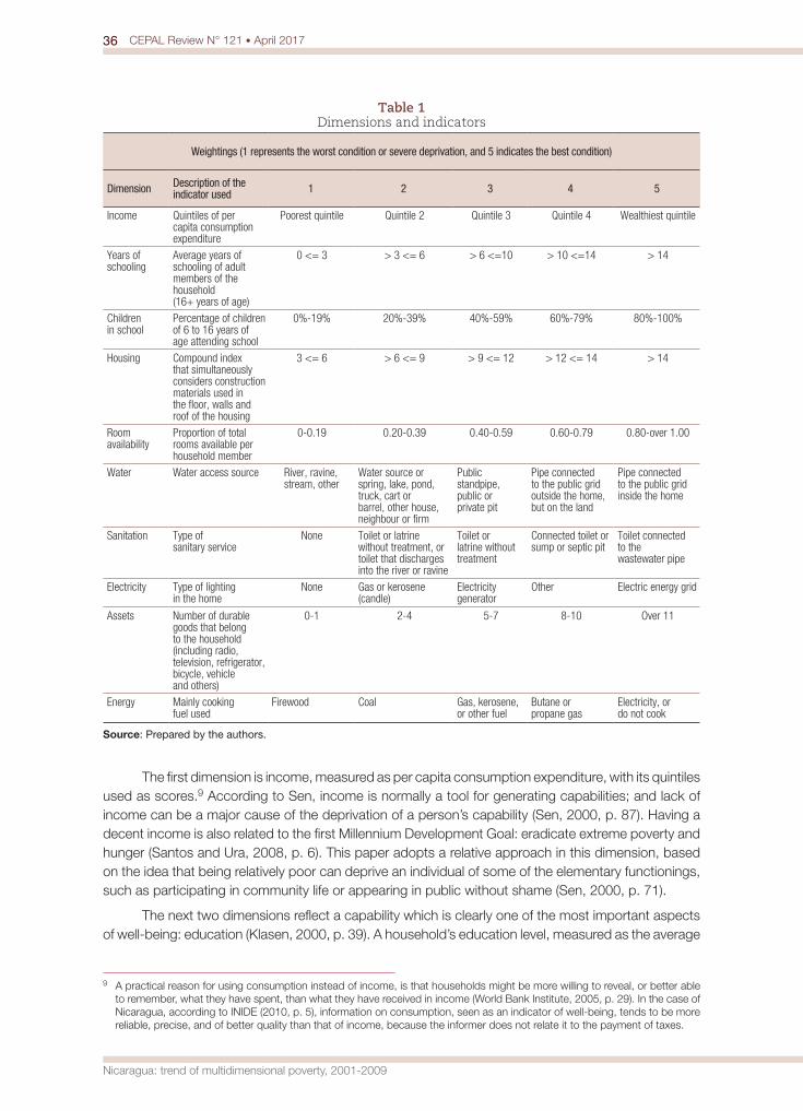
36 CEPAL Review N° 121 • April 2017
Nicaragua: trend of multidimensional poverty, 2001-2009
Table 1 Dimensions and indicators
Weightings (1 represents the worst condition or severe deprivation, and 5 indicates the best condition)
Dimension Description of the indicator used 1 2 3 4 5
Income Quintiles of per capita consumption expenditure
Poorest quintile Quintile 2 Quintile 3 Quintile 4 Wealthiest quintile
Years of schooling
Average years of schooling of adult members of the household (16+ years of age)
0 <= 3 > 3 <= 6 > 6 <=10 > 10 <=14 > 14
Children in school
Percentage of children of 6 to 16 years of age attending school
0%-19% 20%-39% 40%-59% 60%-79% 80%-100%
Housing Compound index that simultaneously considers construction materials used in the floor, walls and roof of the housing
3 <= 6 > 6 <= 9 > 9 <= 12 > 12 <= 14 > 14
Room availability
Proportion of total rooms available per household member
0-0.19 0.20-0.39 0.40-0.59 0.60-0.79 0.80-over 1.00
Water Water access source River, ravine, stream, other
Water source or spring, lake, pond, truck, cart or barrel, other house, neighbour or firm
Public standpipe, public or private pit
Pipe connected to the public grid outside the home, but on the land
Pipe connected to the public grid inside the home
Sanitation Type of sanitary service
None Toilet or latrine without treatment, or toilet that discharges into the river or ravine
Toilet or latrine without treatment
Connected toilet or sump or septic pit
Toilet connected to the wastewater pipe
Electricity Type of lighting in the home
None Gas or kerosene (candle)
Electricity generator
Other Electric energy grid
Assets Number of durable goods that belong to the household (including radio, television, refrigerator, bicycle, vehicle and others)
0-1 2-4 5-7 8-10 Over 11
Energy Mainly cooking fuel used
Firewood Coal Gas, kerosene, or other fuel
Butane or propane gas
Electricity, or do not cook
Source: Prepared by the authors.
The first dimension is income, measured as per capita consumption expenditure, with its quintiles used as scores.9 According to Sen, income is normally a tool for generating capabilities; and lack of income can be a major cause of the deprivation of a person’s capability (Sen, 2000, p. 87). Having a decent income is also related to the first Millennium Development Goal: eradicate extreme poverty and hunger (Santos and Ura, 2008, p. 6). This paper adopts a relative approach in this dimension, based on the idea that being relatively poor can deprive an individual of some of the elementary functionings, such as participating in community life or appearing in public without shame (Sen, 2000, p. 71).
The next two dimensions reflect a capability which is clearly one of the most important aspects of well-being: education (Klasen, 2000, p. 39). A household’s education level, measured as the average
9 A practical reason for using consumption instead of income, is that households might be more willing to reveal, or better able to remember, what they have spent, than what they have received in income (World Bank Institute, 2005, p. 29). In the case of Nicaragua, according to INIDE (2010, p. 5), information on consumption, seen as an indicator of well-being, tends to be more reliable, precise, and of better quality than that of income, because the informer does not relate it to the payment of taxes.
37CEPAL Review N° 121 • April 2017
José Espinoza-Delgado and Julio López-Laborda
number of years of schooling of its adult members (aged 16 years or older), approximates to the level of knowledge and understanding of household members, and can be seen as a relatively good proxy variable for the functioning is that education requires: reading, writing, numeracy, understanding of information, and others. Although it does not reflect the quality of education or the level of knowledge or skills attained, it is a robust and widely used indicator (Alkire and Santos, 2010, p. 14). The dimension of children in school records the attendance of children at educational institutions. The indicator used in this paper is the percentage of children aged 6-16 years (both inclusive) who are attending school, in line with the second Millennium Development Goal of achieving universal primary education (Santos and Ura, 2008, p. 8), based on the UBN approach.10 Although, again, school attendance does not reflect the quality of the educational institution or the skills acquired, it is the best possible indicator to indicate whether or not school-age children are being exposed to a learning environment; and it is considered a good enough proxy for educational functionings (Alkire and Santos, 2010, p. 14).
Housing and room availability are the fourth and fifth dimensions, respectively. Housing is a simple compound index, formed by three variables that reflect the type of material that is mainly used in the floor, walls and roof, which proxies for the quality of the home in which the household lives.11 For various intrinsic and instrumental reasons, the quality of the home is a key indicator of well-being. An instrumental reason is that housing quality involves factors that are important for health and safety; so, intrinsically, it has a direct influence on the well-being of its occupants (Klasen, 2000, p. 41).12 The room availability dimension, measured by the proportion of the total number of rooms available per household member (excluding kitchen, bathroom, passageways, and garage) is related to the quality of the home, and is also an important dimension of well-being. Crowding directly affects well-being, since it is a key factor in the transmission of diseases and does not contribute to a healthy environment (Elender, Bentham and Langford, 1998; Cage and Foster, 2002).
Water and sanitation are the next two dimensions. Both are included in target 7.C of the Millennium Development Goals (halve, by 2015, the proportion of the population without sustainable access to safe drinking water and basic sanitation), and they have considerable instrumental and intrinsic importance (Klasen, 2000, p. 41). Drinking water is necessary for health and well-being (Jain, 2012, p. 1), and is also considered a human right (Noga and Wolbring, 2013, p. 1878). Moreover, access to water generates time savings that can be used in other activities (Boone, Glick and Sahn, 2011, p. 1826). Sanitation is also an important component of well-being, since it is essential for good health and prevents various diseases (Mara and others, 2010, p. 1); and it is normally considered in the UBN approach (Battiston and others, 2013, p. 295).
Electricity is the eighth dimension, for which the indicator used in this study is the type of lighting in the home. This dimension is directly related to the seventh Millennium Development Goal: ensure environmental sustainability. Increasing access to electricity is one of the key objectives pursued by this target, because it will not only improve living conditions, particularly among the rural population, but will also reduce the proportion of inhabitants who use solid fuels, thereby improving air quality (Santos and Ura, 2008, p. 8). Electricity is generally also a safer form of lighting (Alkire and Santos, 2010, p. 16).
The measure developed in this study also includes the assets dimension, which considers the equipment available to the household, in the form of utensils, bicycles, vehicles and other durable goods, given their instrumental importance in facilitating work in the household, improving health, and
10 Households with no children between 6 and 16 years of age have been assigned a proportion of 100% and, therefore, a score of 5, because they would not be suffering deprivation in this dimension.
11 Previously, each of these three variables was recodified to the scoring scale of 1 to 5 and were added together, with equal weightings, to obtain a joint indicator of the three. Lastly, this joint indicator was recodified to the scale of 1 to 5 to obtain the dimension.
12 Living in a house with non-precarious wall materials is generally included in the UBN approach (Santos and others, 2010, p. 9).
38 CEPAL Review N° 121 • April 2017
Nicaragua: trend of multidimensional poverty, 2001-2009
helping the household to maintain contact with the world outside (Klasen, 2000, p. 42). The indicator used is the number of consumer goods that belong to the household, prepared from a list of 29 items (radio, television, cooker, refrigerator, washing machine, bicycle, vehicle and others) included in the section on household equipment of the databases used.
The last dimension is energy, which reflects the type of fuel used by the household for cooking. This dimension is also included because of its intrinsic and instrumental importance, in addition to being related to the Millennium Development Goals, having clear implications for health and living standards, and particularly affecting women. A clean fuel for cooking prevents respiratory diseases, contributes to a healthy environment in the home (Alkire and Santos, 2010, p. 16) and reduces accidents in the home (Klasen, 2000, p. 41). Its importance is therefore clear.
3. Dimensional poverty lines and weightings
All of the dimensional poverty thresholds were set at 3, except for “children in school,” which is set at 5. A household that scores under three in a given dimension (or less than five) is considered deprived in that dimension; as are all of its members. The rationales for these poverty lines are the same as used in forming the dimensions, as discussed above: a weighting of 3 implies a minimum acceptable level of well-being. In the children-in-school dimension, a relatively stricter approach is taken given its nature, requiring at least 80% of children to be attending school. All of the poverty lines coincide with what is generally reported in the empirical literature, although the indicators used have been formed dichotomously.13
Weighting the dimensions involves value judgements with clear normative implications (Decancq and Lugo, 2013, p. 9). This study uses three weighting systems. The first, widely used in the literature (see, for example, Alkire and Santos, 2010 and 2014; Batana, 2013; Battiston and others, 2013; Whelan, Nolan and Maître, 2014), assumes that all the dimensions are equally important; so it assigns an equal weight to each of them (1/10). This makes it possible to study the trend of multidimensional poverty in Nicaragua between 2001 and 2009; and it also makes the index easy to interpret (Atkinson and others, 2002, p. 25). In addition, two alternative weighting systems are proposed, derived from the data themselves, which makes it possible to illustrate the sensitivity of the measures to variations in the parameters, in this case the weightings, and to some extent test the robustness of the estimations. For the first of these systems, principal components analysis is used, a data reduction technique that is widely employed in exercises of this type (see, for example, Noorbakhsh, 1998; Klasen, 2000; Cahill and Sánchez, 2001; Ray and Sinha, 2015). The coefficients matrix is used to calculate the scores in the first principal component. Then, the coefficients are normalized to a range of [0, 1], by dividing them, firstly, between the standard deviation of the original indicator and then, between the sum of the previous coefficients. The advantage of this method is that it empirically reveals the commonalities between the individual dimensions and bases their weightings on the strength of the empirical relation between the poverty measure and the individual dimensions. The drawback is that it implicitly assumes that only the components that have a strong correlation are relevant, which could be debatable (Klasen, 2000, p. 39). Nonetheless, this method is less arbitrary than the first one. The second alternative system uses the relative frequencies of the deprivations in each dimension. In the context of multidimensional poverty analysis, some researchers assume that there should be an inverse relation between the frequency of deprivation in a given dimension and the weight assigned to that dimension: more frequent deprivations obtain a lower weighting (see, for example, Cerioli and Zani, 1990; Cheli and Lemmi, 1995; Deutsch and Silber, 2005). This reflects the idea that people attach greater importance to shortcomings in dimensions in which most people are not deprived; a
13 See, for example, Santos and Ura (2008), Santos and others (2010), Alkire and Santos (2010).
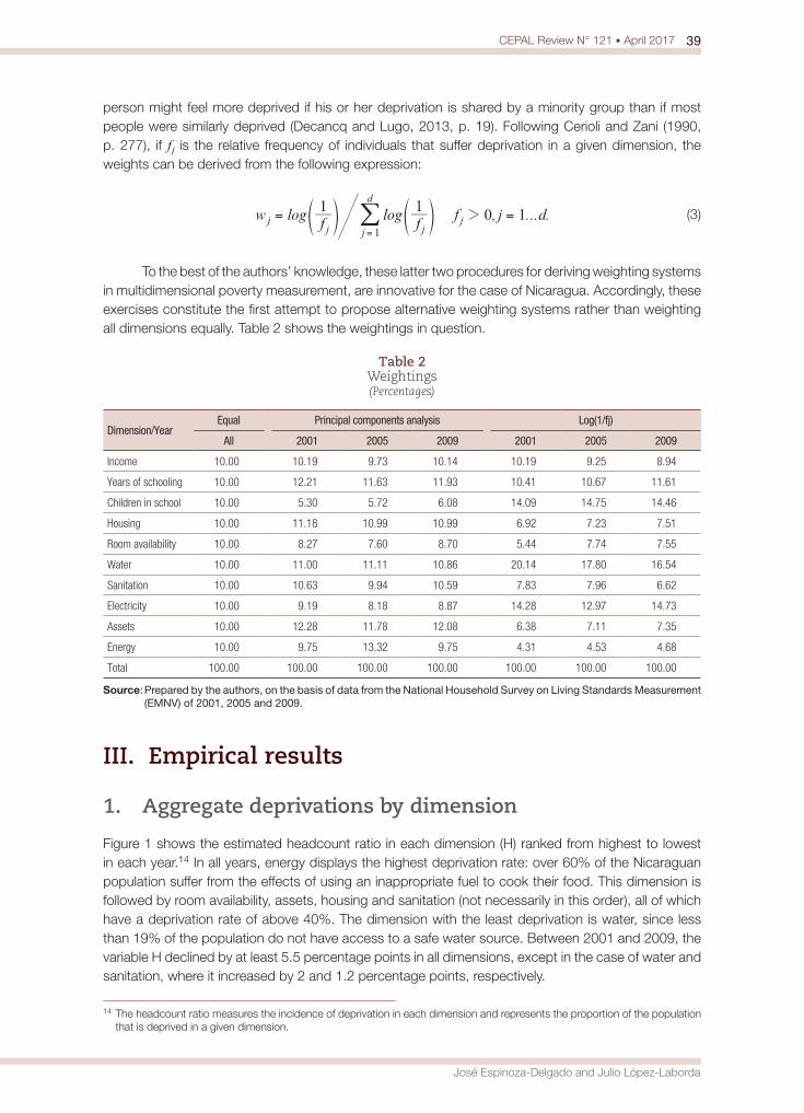
39CEPAL Review N° 121 • April 2017
José Espinoza-Delgado and Julio López-Laborda
person might feel more deprived if his or her deprivation is shared by a minority group than if most people were similarly deprived (Decancq and Lugo, 2013, p. 19). Following Cerioli and Zani (1990, p. 277), if fj is the relative frequency of individuals that suffer deprivation in a given dimension, the weights can be derived from the following expression:
, ... .log logwf f
f j d1 1 0 1jj jj
d
j1
2= ==
U UZ Z/ (3)
To the best of the authors’ knowledge, these latter two procedures for deriving weighting systems in multidimensional poverty measurement, are innovative for the case of Nicaragua. Accordingly, these exercises constitute the first attempt to propose alternative weighting systems rather than weighting all dimensions equally. Table 2 shows the weightings in question.
Table 2 Weightings (Percentages)
Dimension/YearEqual Principal components analysis Log(1/fj)
All 2001 2005 2009 2001 2005 2009
Income 10.00 10.19 9.73 10.14 10.19 9.25 8.94
Years of schooling 10.00 12.21 11.63 11.93 10.41 10.67 11.61
Children in school 10.00 5.30 5.72 6.08 14.09 14.75 14.46
Housing 10.00 11.18 10.99 10.99 6.92 7.23 7.51
Room availability 10.00 8.27 7.60 8.70 5.44 7.74 7.55
Water 10.00 11.00 11.11 10.86 20.14 17.80 16.54
Sanitation 10.00 10.63 9.94 10.59 7.83 7.96 6.62
Electricity 10.00 9.19 8.18 8.87 14.28 12.97 14.73
Assets 10.00 12.28 11.78 12.08 6.38 7.11 7.35
Energy 10.00 9.75 13.32 9.75 4.31 4.53 4.68
Total 100.00 100.00 100.00 100.00 100.00 100.00 100.00
Source: Prepared by the authors, on the basis of data from the National Household Survey on Living Standards Measurement (EMNV) of 2001, 2005 and 2009.
III. Empirical results
1. Aggregate deprivations by dimension
Figure 1 shows the estimated headcount ratio in each dimension (H) ranked from highest to lowest in each year.14 In all years, energy displays the highest deprivation rate: over 60% of the Nicaraguan population suffer from the effects of using an inappropriate fuel to cook their food. This dimension is followed by room availability, assets, housing and sanitation (not necessarily in this order), all of which have a deprivation rate of above 40%. The dimension with the least deprivation is water, since less than 19% of the population do not have access to a safe water source. Between 2001 and 2009, the variable H declined by at least 5.5 percentage points in all dimensions, except in the case of water and sanitation, where it increased by 2 and 1.2 percentage points, respectively.
14 The headcount ratio measures the incidence of deprivation in each dimension and represents the proportion of the population that is deprived in a given dimension.

40 CEPAL Review N° 121 • April 2017
Nicaragua: trend of multidimensional poverty, 2001-2009
Figure 1 Headcount ratio in each dimension (H), 2001, 2005 and 2009
(Percentages)
67.9
61.3
56.4
53.7
49.4
40.0 39.2
28.2 27.7
16.4
0
40
60
80
Ener
gy
Room
ava
ilabi
lity
Asse
ts
Hous
ing
Sani
tatio
n
Inco
me
Year
s of
sch
oolin
g
Child
ren
in s
choo
l
Elec
trici
ty
Wat
er
2001
63.8
49.4 48.946.4 45.4
40.0
34.7
27.7
23.2
17.1
Ener
gy
Asse
ts
Hou
sing
Room
ava
ilabi
lity
Sani
tatio
n
Inco
me
Year
s of
sch
oolin
g
Elec
trici
ty
Child
ren
in s
choo
l
Wat
er
2005
61.9
50.7
47.0 46.3 46.1
40.0
30.4
22.7 22.1
18.3
Ener
gy
Sani
tatio
n
Asse
ts
Hous
ing
Room
ava
ilabi
lity
Inco
me
Year
s of
sch
oolin
g
Child
ren
in s
choo
l
Elec
trici
ty
Wat
er
2009
20
0
40
60
80
20
0
40
60
80
20
Source: Prepared by the authors, on the basis of data from the National Household Survey on Living Standards Measurement (EMNV) of 2001, 2005 and 2009.
These results show that the proportion of the population suffering deprivation in each dimension decreases by more, between 2001 and 2005 than in 2005-2009 and in both absolute and relative terms, except in the years-of-schooling and electricity dimensions. In contrast, official reports suggest the incidence of poverty in Nicaragua increased between 2001 and 2005 (by 2.5 percentage points) and declined in 2005-2009 (by 5.7 points) (INIDE, 2007 and 2011a). Consequently, these initial results cast doubt on the appropriateness of the official approach used to measure and monitor poverty in Nicaragua, and they confirm that poverty is more than monetary deprivation.
2. Measurement and trend of multidimensional poverty
(a) Proportion of multidimensionally poor (P)
Table 3 reports the proportion of multidimensionally poor people (P), estimated by equation (1) of section II.1, for each of the three years of the study, under each weighting system. The results show that the proportion of multidimensionally poor in Nicaragua declined between 2001 and 2009, irrespective of the weighting system used, owing, above all, to the reduction achieved in 2001-2005. In terms of the number of poor people, between 2001 and 2009, using equal weights, just over 76,000 people ceased to be multidimensionally poor. Nonetheless, in 2005-2009, the number of people living in poverty actually increased by over 180,000, which sounds an alarm bell for policymakers.
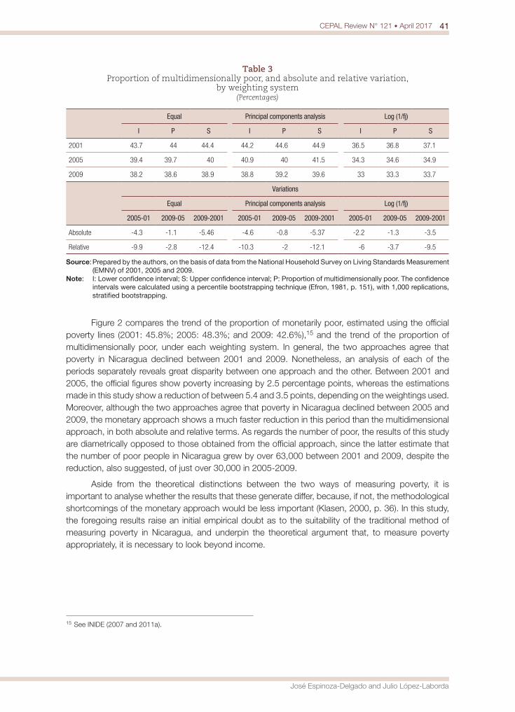
41CEPAL Review N° 121 • April 2017
José Espinoza-Delgado and Julio López-Laborda
Table 3 Proportion of multidimensionally poor, and absolute and relative variation,
by weighting system(Percentages)
Equal Principal components analysis Log (1/fj)
I P S I P S I P S
2001 43.7 44 44.4 44.2 44.6 44.9 36.5 36.8 37.1
2005 39.4 39.7 40 40.9 40 41.5 34.3 34.6 34.9
2009 38.2 38.6 38.9 38.8 39.2 39.6 33 33.3 33.7
Variations
Equal Principal components analysis Log (1/fj)
2005-01 2009-05 2009-2001 2005-01 2009-05 2009-2001 2005-01 2009-05 2009-2001
Absolute -4.3 -1.1 -5.46 -4.6 -0.8 -5.37 -2.2 -1.3 -3.5
Relative -9.9 -2.8 -12.4 -10.3 -2 -12.1 -6 -3.7 -9.5
Source: Prepared by the authors, on the basis of data from the National Household Survey on Living Standards Measurement (EMNV) of 2001, 2005 and 2009.
Note: I: Lower confidence interval; S: Upper confidence interval; P: Proportion of multidimensionally poor. The confidence intervals were calculated using a percentile bootstrapping technique (Efron, 1981, p. 151), with 1,000 replications, stratified bootstrapping.
Figure 2 compares the trend of the proportion of monetarily poor, estimated using the official poverty lines (2001: 45.8%; 2005: 48.3%; and 2009: 42.6%),15 and the trend of the proportion of multidimensionally poor, under each weighting system. In general, the two approaches agree that poverty in Nicaragua declined between 2001 and 2009. Nonetheless, an analysis of each of the periods separately reveals great disparity between one approach and the other. Between 2001 and 2005, the official figures show poverty increasing by 2.5 percentage points, whereas the estimations made in this study show a reduction of between 5.4 and 3.5 points, depending on the weightings used. Moreover, although the two approaches agree that poverty in Nicaragua declined between 2005 and 2009, the monetary approach shows a much faster reduction in this period than the multidimensional approach, in both absolute and relative terms. As regards the number of poor, the results of this study are diametrically opposed to those obtained from the official approach, since the latter estimate that the number of poor people in Nicaragua grew by over 63,000 between 2001 and 2009, despite the reduction, also suggested, of just over 30,000 in 2005-2009.
Aside from the theoretical distinctions between the two ways of measuring poverty, it is important to analyse whether the results that these generate differ, because, if not, the methodological shortcomings of the monetary approach would be less important (Klasen, 2000, p. 36). In this study, the foregoing results raise an initial empirical doubt as to the suitability of the traditional method of measuring poverty in Nicaragua, and underpin the theoretical argument that, to measure poverty appropriately, it is necessary to look beyond income.
15 See INIDE (2007 and 2011a).
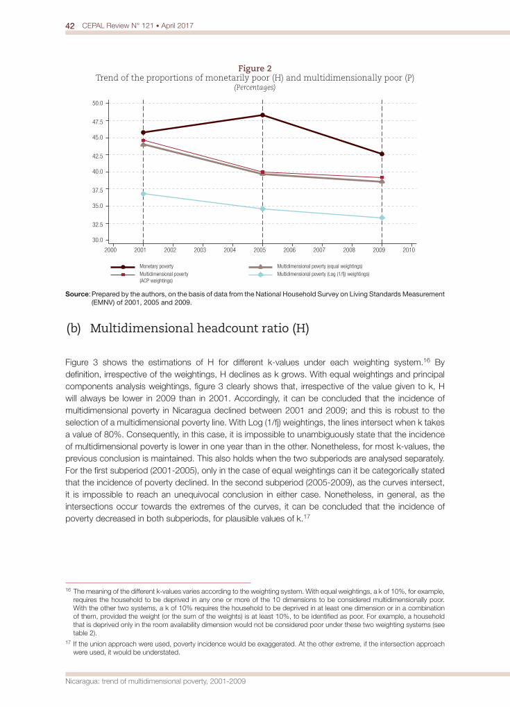
42 CEPAL Review N° 121 • April 2017
Nicaragua: trend of multidimensional poverty, 2001-2009
Figure 2 Trend of the proportions of monetarily poor (H) and multidimensionally poor (P)
(Percentages)
30.0
32.5
35.0
37.5
40.0
42.5
45.0
47.5
50.0
2000 2001 2002 2003 2004 2005 2006 2007 2008 2009 2010
Monetary poverty Multidimensional poverty (equal weightings)Multidimensional poverty (ACP weightings)
Multidimensional poverty (Log (1/fj) weightings)
Source: Prepared by the authors, on the basis of data from the National Household Survey on Living Standards Measurement (EMNV) of 2001, 2005 and 2009.
(b) Multidimensional headcount ratio (H)
Figure 3 shows the estimations of H for different k-values under each weighting system.16 By definition, irrespective of the weightings, H declines as k grows. With equal weightings and principal components analysis weightings, figure 3 clearly shows that, irrespective of the value given to k, H will always be lower in 2009 than in 2001. Accordingly, it can be concluded that the incidence of multidimensional poverty in Nicaragua declined between 2001 and 2009; and this is robust to the selection of a multidimensional poverty line. With Log (1/fj) weightings, the lines intersect when k takes a value of 80%. Consequently, in this case, it is impossible to unambiguously state that the incidence of multidimensional poverty is lower in one year than in the other. Nonetheless, for most k-values, the previous conclusion is maintained. This also holds when the two subperiods are analysed separately. For the first subperiod (2001-2005), only in the case of equal weightings can it be categorically stated that the incidence of poverty declined. In the second subperiod (2005-2009), as the curves intersect, it is impossible to reach an unequivocal conclusion in either case. Nonetheless, in general, as the intersections occur towards the extremes of the curves, it can be concluded that the incidence of poverty decreased in both subperiods, for plausible values of k.17
16 The meaning of the different k-values varies according to the weighting system. With equal weightings, a k of 10%, for example, requires the household to be deprived in any one or more of the 10 dimensions to be considered multidimensionally poor. With the other two systems, a k of 10% requires the household to be deprived in at least one dimension or in a combination of them, provided the weight (or the sum of the weights) is at least 10%, to be identified as poor. For example, a household that is deprived only in the room availability dimension would not be considered poor under these two weighting systems (see table 2).
17 If the union approach were used, poverty incidence would be exaggerated. At the other extreme, if the intersection approach were used, it would be understated.
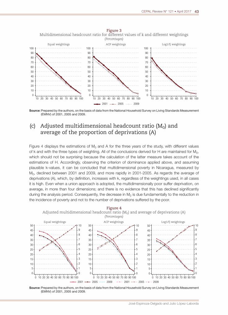
43CEPAL Review N° 121 • April 2017
José Espinoza-Delgado and Julio López-Laborda
Figure 3 Multidimensional headcount ratio for different values of k and different weightings
(Percentages)
0
10
20
30
40
50
60
70
80
90
100
0
10
20
30
40
50
60
70
80
90
100
0
10
20
30
40
50
60
70
80
90
100
10 20 30 40 50 60 70 80 90 100
2001 2005 2009
Equal weightings
10 20 30 40 50 60 70 80 90 100
ACP weightings
10 20 30 40 50 60 70 80 90 100
Log1/fj weightings
Source: Prepared by the authors, on the basis of data from the National Household Survey on Living Standards Measurement (EMNV) of 2001, 2005 and 2009.
(c) Adjusted multidimensional headcount ratio (M0) and average of the proportion of deprivations (A)
Figure 4 displays the estimations of M0 and A for the three years of the study, with different values of k and with the three types of weighting. All of the conclusions derived for H are maintained for M0, which should not be surprising because the calculation of the latter measure takes account of the estimations of H. Accordingly, observing the criterion of dominance applied above, and assuming plausible k-values, it can be concluded that multidimensional poverty in Nicaragua, measured by M0, declined between 2001 and 2009, and more rapidly in 2001-2005. As regards the average of deprivations (A), which, by definition, increases with k, regardless of the weightings used, in all cases it is high. Even when a union approach is adopted, the multidimensionally poor suffer deprivation, on average, in more than four dimensions; and there is no evidence that this has declined significantly during the analysis period. Consequently, the decrease in M0 is due fundamentally to the reduction in the incidence of poverty and not to the number of deprivations suffered by the poor.
Figure 4 Adjusted multidimensional headcount ratio (M0) and average of deprivations (A)
(Percentages)
0
1
2
3
4
5
6
7
8
9
10
0
5
10
15
20
25
30
35
40
45
50
0 10 20 30 40 50 60 70 80 90 100
2001 2005 2009 2001 2005 2009
Equal weightings
0 10 20 30 40 50 60 70 80 90 100
ACP weightings
0 10 20 30 40 50 60 70 80 90 100
Log1/fj weightings
0
5
10
15
20
25
30
35
40
45
50
0
5
10
15
20
25
30
35
4040
45
50
0
1
2
3
4
5
6
7
8
9
10
0
1
2
3
4
5
6
7
8
9
10
Source: Prepared by the authors, on the basis of data from the National Household Survey on Living Standards Measurement (EMNV) of 2001, 2005 and 2009.
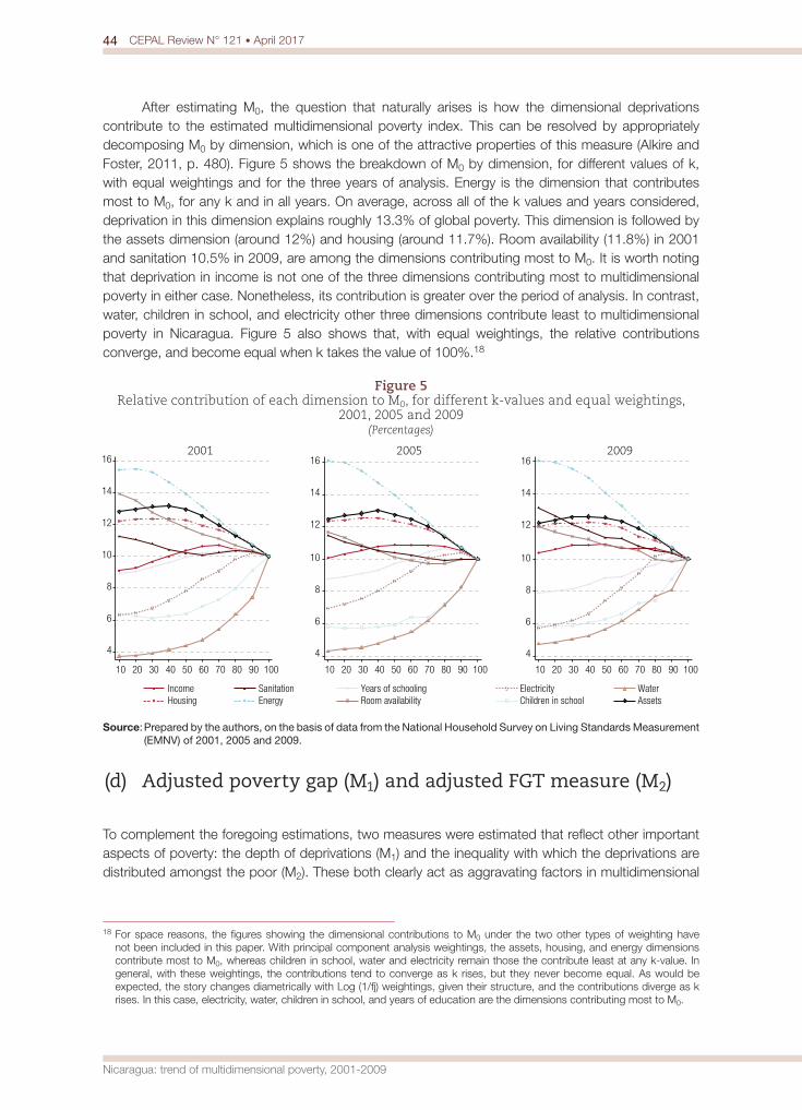
44 CEPAL Review N° 121 • April 2017
Nicaragua: trend of multidimensional poverty, 2001-2009
After estimating M0, the question that naturally arises is how the dimensional deprivations contribute to the estimated multidimensional poverty index. This can be resolved by appropriately decomposing M0 by dimension, which is one of the attractive properties of this measure (Alkire and Foster, 2011, p. 480). Figure 5 shows the breakdown of M0 by dimension, for different values of k, with equal weightings and for the three years of analysis. Energy is the dimension that contributes most to M0, for any k and in all years. On average, across all of the k values and years considered, deprivation in this dimension explains roughly 13.3% of global poverty. This dimension is followed by the assets dimension (around 12%) and housing (around 11.7%). Room availability (11.8%) in 2001 and sanitation 10.5% in 2009, are among the dimensions contributing most to M0. It is worth noting that deprivation in income is not one of the three dimensions contributing most to multidimensional poverty in either case. Nonetheless, its contribution is greater over the period of analysis. In contrast, water, children in school, and electricity other three dimensions contribute least to multidimensional poverty in Nicaragua. Figure 5 also shows that, with equal weightings, the relative contributions converge, and become equal when k takes the value of 100%.18
Figure 5 Relative contribution of each dimension to M0, for different k-values and equal weightings,
2001, 2005 and 2009(Percentages)
4
6
8
10
12
14
16
10 20 30 40 50 60 70 80 90 100
Income Years of schoolingChildren in schoolHousing Room availability
WaterSanitation ElectricityAssetsEnergy
2001
10 20 30 40 50 60 70 80 90 100
2005
10 20 30 40 50 60 70 80 90 100
2009
4
6
8
10
12
14
16
4
6
8
10
12
14
16
Source: Prepared by the authors, on the basis of data from the National Household Survey on Living Standards Measurement (EMNV) of 2001, 2005 and 2009.
(d) Adjusted poverty gap (M1) and adjusted FGT measure (M2)
To complement the foregoing estimations, two measures were estimated that reflect other important aspects of poverty: the depth of deprivations (M1) and the inequality with which the deprivations are distributed amongst the poor (M2). These both clearly act as aggravating factors in multidimensional
18 For space reasons, the figures showing the dimensional contributions to M0 under the two other types of weighting have not been included in this paper. With principal component analysis weightings, the assets, housing, and energy dimensions contribute most to M0, whereas children in school, water and electricity remain those the contribute least at any k-value. In general, with these weightings, the contributions tend to converge as k rises, but they never become equal. As would be expected, the story changes diametrically with Log (1/fj) weightings, given their structure, and the contributions diverge as k rises. In this case, electricity, water, children in school, and years of education are the dimensions contributing most to M0.

45CEPAL Review N° 121 • April 2017
José Espinoza-Delgado and Julio López-Laborda
poverty. As far as the authors are aware, this study is the first attempt to measure these two features of poverty in Nicaragua in a multidimensional framework. Figure 6 shows the estimations of these two measures for different k-values, with the three weighting systems and for the three years of interest.
Figure 6 Adjusted poverty gap (M1) and adjusted FGT measure (M2), for different k-values
and different weightings(Percentages)
1
4
710
13
16
19
22
10 20 30 40 50 60 70 80 90 100
Equal weightings
10 20 30 40 50 60 70 80 90 100
ACP weightings
10 20 30 40 50 60 70 80 90 100
Log 1/fj weightings
0
2
4
6
8
10
12
10 20 30 40 50 60 70 80 90 100
2001 2005 2009
Equal weightings
10 20 30 40 50 60 70 80 90 100
ACP weightings
10 20 30 40 50 60 70 80 90 100
Log 1/fj weightings
A. Adjusted poverty gap (M1)
B. Adjusted FGT measure (M2)
1
4
7
10
13
16
19
22
1
4
710
13
16
19
22
0
2
4
6
8
10
12
0
2
4
6
8
10
12
Source: Prepared by the authors, on the basis of data from the National Survey of Household Living Standards (EMNV) of 2001, 2005 and 2009.
As figure 6 shows, irrespective of the weightings used and where the poverty line is set, M1 and M2 both declined between 2001 and 2009. An analysis of each of the period separately also shows a reduction in both measures between 2001 and 2005 and in 2005-2009, except when k takes the value of 100%, with principal component analysis weightings, in this second period.
Lastly, figure 7 shows the estimations of the average poverty gap (G) and the average severity of deprivations (S) for the different k-values and with the three weighting systems. It can be clearly seen that G and S declined between 2001 and 2009, irrespective of the weightings adopted and the value defined for k.
The results of this study thus show that the incidence, intensity and severity of multidimensional poverty in Nicaragua declined between 2001 and 2009, and fell faster in the first half of that period (2001-2005). This conclusion is robust to the choice of a multidimensional poverty line; and, in the vast majority of cases, it also holds with alternative weighting systems.
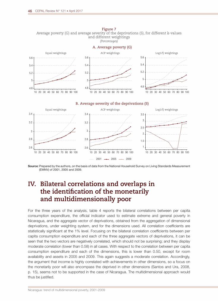
46 CEPAL Review N° 121 • April 2017
Nicaragua: trend of multidimensional poverty, 2001-2009
Figure 7 Average poverty (G) and average severity of the deprivations (S), for different k-values
and different weightings(Percentages)
4.8
5
5.2
5.4
5.6
10 20 30 40 50 60 70 80 90 100
Equal weightings
10 20 30 40 50 60 70 80 90 100
ACP weightings
10 20 30 40 50 60 70 80 90 100
Log1/fj weightings
A. Average poverty (G)
2.6
2.8
3
3.2
3.4
10 20 30 40 50 60 70 80 90 100
2001 2005 2009
Equal weightings
10 20 30 40 50 60 70 80 90 100
ACP weightings
1
1.5
2
2.5
3
3.5
10 20 30 40 50 60 70 80 90 100
Log1/fj weightings
B. Average severity of the deprivations (S)
4.8
5
5.2
5.4
5.6
4.8
5
5.2
5.4
5.6
2.6
2.8
3.2
3.4
3
Source: Prepared by the authors, on the basis of data from the National Household Survey on Living Standards Measurement (EMNV) of 2001, 2005 and 2009.
IV. Bilateral correlations and overlaps in the identification of the monetarily and multidimensionally poor
For the three years of the analysis, table 4 reports the bilateral correlations between per capita consumption expenditure, the official indicator used to estimate extreme and general poverty in Nicaragua, and the aggregate vector of deprivations, obtained from the aggregation of dimensional deprivations, under weighting system, and for the dimensions used. All correlation coefficients are statistically significant at the 1% level. Focusing on the bilateral correlation coefficients between per capita consumption expenditure and each of the three aggregate vectors of deprivations, it can be seen that the two vectors are negatively correlated, which should not be surprising; and they display moderate correlation (lower than 0.58) in all cases. With respect to the correlation between per capita consumption expenditure and each of the dimensions, this is lower than 0.50, except for room availability and assets in 2005 and 2009. This again suggests a moderate correlation. Accordingly, the argument that income is highly correlated with achievements in other dimensions, so a focus on the monetarily poor will also encompass the deprived in other dimensions (Santos and Ura, 2008, p. 15), seems not to be supported in the case of Nicaragua. The multidimensional approach would thus be justified.
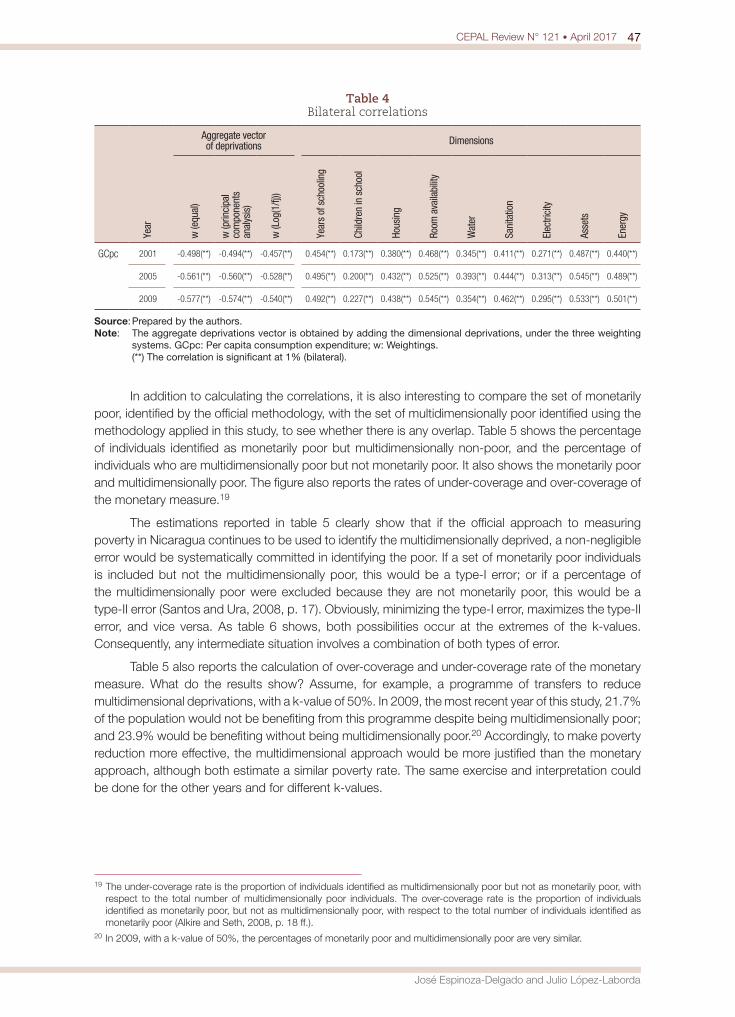
47CEPAL Review N° 121 • April 2017
José Espinoza-Delgado and Julio López-Laborda
Table 4 Bilateral correlations
Aggregate vector of deprivations Dimensions
Year
w (e
qual
)
w (p
rinci
pal
com
pone
nts
anal
ysis
)
w (L
og(1
/fj))
Year
s of
sch
oolin
g
Child
ren
in s
choo
l
Hous
ing
Room
ava
ilabi
lity
Wat
er
Sani
tatio
n
Elec
trici
ty
Asse
ts
Ener
gy
GCpc 2001 -0.498(**) -0.494(**) -0.457(**) 0.454(**) 0.173(**) 0.380(**) 0.468(**) 0.345(**) 0.411(**) 0.271(**) 0.487(**) 0.440(**)
2005 -0.561(**) -0.560(**) -0.528(**) 0.495(**) 0.200(**) 0.432(**) 0.525(**) 0.393(**) 0.444(**) 0.313(**) 0.545(**) 0.489(**)
2009 -0.577(**) -0.574(**) -0.540(**) 0.492(**) 0.227(**) 0.438(**) 0.545(**) 0.354(**) 0.462(**) 0.295(**) 0.533(**) 0.501(**)
Source: Prepared by the authors.Note: The aggregate deprivations vector is obtained by adding the dimensional deprivations, under the three weighting
systems. GCpc: Per capita consumption expenditure; w: Weightings. (**) The correlation is significant at 1% (bilateral).
In addition to calculating the correlations, it is also interesting to compare the set of monetarily poor, identified by the official methodology, with the set of multidimensionally poor identified using the methodology applied in this study, to see whether there is any overlap. Table 5 shows the percentage of individuals identified as monetarily poor but multidimensionally non-poor, and the percentage of individuals who are multidimensionally poor but not monetarily poor. It also shows the monetarily poor and multidimensionally poor. The figure also reports the rates of under-coverage and over-coverage of the monetary measure.19
The estimations reported in table 5 clearly show that if the official approach to measuring poverty in Nicaragua continues to be used to identify the multidimensionally deprived, a non-negligible error would be systematically committed in identifying the poor. If a set of monetarily poor individuals is included but not the multidimensionally poor, this would be a type-I error; or if a percentage of the multidimensionally poor were excluded because they are not monetarily poor, this would be a type-II error (Santos and Ura, 2008, p. 17). Obviously, minimizing the type-I error, maximizes the type-II error, and vice versa. As table 6 shows, both possibilities occur at the extremes of the k-values. Consequently, any intermediate situation involves a combination of both types of error.
Table 5 also reports the calculation of over-coverage and under-coverage rate of the monetary measure. What do the results show? Assume, for example, a programme of transfers to reduce multidimensional deprivations, with a k-value of 50%. In 2009, the most recent year of this study, 21.7% of the population would not be benefiting from this programme despite being multidimensionally poor; and 23.9% would be benefiting without being multidimensionally poor.20 Accordingly, to make poverty reduction more effective, the multidimensional approach would be more justified than the monetary approach, although both estimate a similar poverty rate. The same exercise and interpretation could be done for the other years and for different k-values.
19 The under-coverage rate is the proportion of individuals identified as multidimensionally poor but not as monetarily poor, with respect to the total number of multidimensionally poor individuals. The over-coverage rate is the proportion of individuals identified as monetarily poor, but not as multidimensionally poor, with respect to the total number of individuals identified as monetarily poor (Alkire and Seth, 2008, p. 18 ff.).
20 In 2009, with a k-value of 50%, the percentages of monetarily poor and multidimensionally poor are very similar.
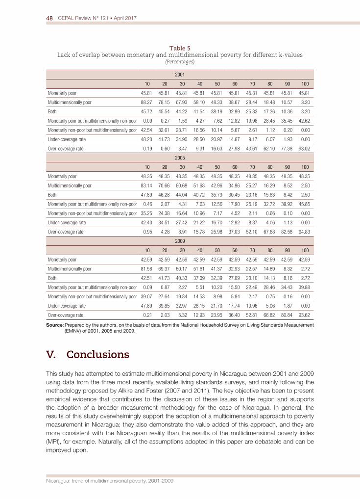
48 CEPAL Review N° 121 • April 2017
Nicaragua: trend of multidimensional poverty, 2001-2009
Table 5 Lack of overlap between monetary and multidimensional poverty for different k-values
(Percentages)
2001
10 20 30 40 50 60 70 80 90 100
Monetarily poor 45.81 45.81 45.81 45.81 45.81 45.81 45.81 45.81 45.81 45.81
Multidimensionally poor 88.27 78.15 67.93 58.10 48.33 38.67 28.44 18.48 10.57 3.20
Both 45.72 45.54 44.22 41.54 38.19 32.99 25.83 17.36 10.36 3.20
Monetarily poor but multidimensionally non-poor 0.09 0.27 1.59 4.27 7.62 12.82 19.98 28.45 35.45 42.62
Monetarily non-poor but multidimensionally poor 42.54 32.61 23.71 16.56 10.14 5.67 2.61 1.12 0.20 0.00
Under-coverage rate 48.20 41.73 34.90 28.50 20.97 14.67 9.17 6.07 1.93 0.00
Over-coverage rate 0.19 0.60 3.47 9.31 16.63 27.98 43.61 62.10 77.38 93.02
2005
10 20 30 40 50 60 70 80 90 100
Monetarily poor 48.35 48.35 48.35 48.35 48.35 48.35 48.35 48.35 48.35 48.35
Multidimensionally poor 83.14 70.66 60.68 51.68 42.96 34.96 25.27 16.29 8.52 2.50
Both 47.89 46.28 44.04 40.72 35.79 30.45 23.16 15.63 8.42 2.50
Monetarily poor but multidimensionally non-poor 0.46 2.07 4.31 7.63 12.56 17.90 25.19 32.72 39.92 45.85
Monetarily non-poor but multidimensionally poor 35.25 24.38 16.64 10.96 7.17 4.52 2.11 0.66 0.10 0.00
Under-coverage rate 42.40 34.51 27.42 21.22 16.70 12.92 8.37 4.06 1.13 0.00
Over-coverage rate 0.95 4.28 8.91 15.78 25.98 37.03 52.10 67.68 82.58 94.83
2009
10 20 30 40 50 60 70 80 90 100
Monetarily poor 42.59 42.59 42.59 42.59 42.59 42.59 42.59 42.59 42.59 42.59
Multidimensionally poor 81.58 69.37 60.17 51.61 41.37 32.93 22.57 14.89 8.32 2.72
Both 42.51 41.73 40.33 37.09 32.39 27.09 20.10 14.13 8.16 2.72
Monetarily poor but multidimensionally non-poor 0.09 0.87 2.27 5.51 10.20 15.50 22.49 28.46 34.43 39.88
Monetarily non-poor but multidimensionally poor 39.07 27.64 19.84 14.53 8.98 5.84 2.47 0.75 0.16 0.00
Under-coverage rate 47.89 39.85 32.97 28.15 21.70 17.74 10.96 5.06 1.87 0.00
Over-coverage rate 0.21 2.03 5.32 12.93 23.95 36.40 52.81 66.82 80.84 93.62
Source: Prepared by the authors, on the basis of data from the National Household Survey on Living Standards Measurement (EMNV) of 2001, 2005 and 2009.
V. Conclusions
This study has attempted to estimate multidimensional poverty in Nicaragua between 2001 and 2009 using data from the three most recently available living standards surveys, and mainly following the methodology proposed by Alkire and Foster (2007 and 2011). The key objective has been to present empirical evidence that contributes to the discussion of these issues in the region and supports the adoption of a broader measurement methodology for the case of Nicaragua. In general, the results of this study overwhelmingly support the adoption of a multidimensional approach to poverty measurement in Nicaragua; they also demonstrate the value added of this approach, and they are more consistent with the Nicaraguan reality than the results of the multidimensional poverty index (MPI), for example. Naturally, all of the assumptions adopted in this paper are debatable and can be improved upon.
49CEPAL Review N° 121 • April 2017
José Espinoza-Delgado and Julio López-Laborda
Both the monetary and the multidimensional approach agree that the proportion of poor people in Nicaragua declined between 2001 and 2009. Nonetheless, an analysis of each of the subperiods separately reveals great disparity between one approach and the other. Between 2001 and 2005, the official figures suggest a 2.5 percentage point increase in poverty, whereas the estimations made in this study suggest a reduction of between 5.4 and 3.5 points, depending on the weightings used. Moreover, although both approaches agree that poverty declined in Nicaragua between 2005 and 2009, the monetary approach shows faster progress in this period than the multidimensional approach, in both absolute and relative terms. As regards the number of poor, the results of this study are diametrically opposed to those obtained under the official approach, because the latter estimated that the number of poor people in Nicaragua grew by over 63,000 between 2001 and 2009, despite a reduction of just over 30,000 in 2005-2009. In contrast, with equal weightings, our estimations suggest that between 2001 and 2009, just over 76,000 people ceased to be multidimensionally poor. Nonetheless between 2005 and 2009 the number of poor people grew by over 180,000, which should serve as a warning for policy-makers.
In the context of the Alkire and Foster methodology, the results of this study suggest, robustly, that the incidence, intensity and severity of multidimensional poverty in Nicaragua declined between 2001 and 2009, and more intensively in the first half of this period. The fact that this again is diametrically contrary to what is suggested by the official figures raises doubts about the official measure (and methodology).
Moreover, a breakdown of M0 shows that income deprivation is in no way among the largest contributors to global multidimensional poverty, which reaffirms the belief that income is not everything. In addition, the results of the study reveal that if the traditional measurement approach is used to identify the multidimensionally deprived, a non-negligible error would be committed, either of type-I or of type-II.
Consequently, the recommendation is that the design, evaluation and monitoring of poverty reduction policies should not be exclusively based on a monetary approach, but should be supported with a broader measure that incorporates other important dimensions of the well-being of the Nicaraguan population. The results of the study also show that, to be more effective, policies and programmes should not only be targeted on increasing income, but they should also aim to promote clean domestic energy and a structural and competitive improvement in housing.
BibliographyAtkinson, A.B. (2003), “Multidimensional deprivation: contrasting social welfare and counting approaches”,
Journal of Economic Inequality, vol. 1, No. 1, Springer. Atkinson, A.B. and others (2002), Social Indicators. The EU and Social Inclusion, Oxford, Oxford University Press.Alkire, S. and J. Foster (2011), “Counting and multidimensional poverty measurement”, Journal of Public
Economics, vol. 95, No. 7-8, Amsterdam, Elsevier.(2007), “Counting and multidimensional poverty measurement”, OPHI Working Paper, No. 7, Oxford, Oxford Poverty and Human Development Initiative, University of Oxford.
Alkire, S. and M.E. Santos (2014), “Measuring acute poverty in the developing world: robustness and scope of the Multidimensional Poverty Index”, World Development, vol. 59, Amsterdam, Elsevier.(2010), “Acute multidimensional poverty: a new index for developing countries”, OPHI Working Paper, No. 38, Oxford, Oxford Poverty and Human Development Initiative, University of Oxford.
Alkire, S. and S. Seth (2008), “Measuring multidimensional poverty in India: a new proposal”, OPHI Working Paper, No. 15, Oxford, Oxford Poverty and Human Development Initiative, University of Oxford.
Batana, Y. (2013), “Multidimensional measurement of poverty among women in sub-Saharan Africa”, Social Indicators Research, vol. 112, No. 2, Springer.
Battiston, D. and others (2013), “Income and beyond: multidimensional poverty in six Latin American countries”, Social Indicators Research, vol. 112, No. 2, Springer.
50 CEPAL Review N° 121 • April 2017
Nicaragua: trend of multidimensional poverty, 2001-2009
(2009), “Income and beyond: multidimensional poverty in six Latin American countries”, OPHI Working Paper, No. 17, Oxford, Oxford Poverty and Human Development Initiative, University of Oxford.
Boltvinik, J. (2013), “Medición multidimensional de pobreza. América Latina de precursora a rezagada”, Revista Sociedad & Equidad, No. 5.
Boone, C., P. Glick and D. Sahn (2011), “Household water supply choice and time allocated to water collection: evidence from Madagascar”, The Journal of Development Studies, vol. 47, No. 12, Taylor & Francis.
Bourguignon, F. and S. Chakravarty (2003), “The measurement of multidimensional poverty”, Journal of Economic Inequality, vol. 1, No. 1, Springer.
Cage, R.A. and J. Foster (2002), “Overcrowding and infant mortality: a tale of two cities”, Scottish Journal of Political Economy, vol. 49, No. 2, Wiley.
Cahill, M. and N. Sánchez (2001), “Using principal components to produce an economic and social development index: an application to Latin America and the U.S.”, Atlantic Economic Journal, vol. 29, No. 3, Springer.
Cerioli, A. and S. Zani (1990), “A fuzzy approach to the measurement of poverty”, Income and Wealth Distribution, Inequality and Poverty, C. Dagum and M. Zenga (eds.), New York, Springer-Verlag.
Cheli, B. and A. Lemmi (1995), “Totally fuzzy and relative approach to the multidimensional analysis of poverty”, Economic Notes, vol. 21, Banca Monte dei Paschi di Siena.
Chiappero Martinetti, E. (2006), “Capability approach and fuzzy set theory: description, aggregation and inference issues”, Fuzzy Set Approach to Multidimensional Poverty Measurement, A. Lemmi and G. Betti (eds.), New York, Springer.
Decancq, K. and M.A. Lugo (2013), “Weights in multidimensional indices of wellbeing: an overview”, Econometric Reviews, vol. 32, No. 1, Taylor & Francis.
Del Carpio, X. and V. Castro (2007), “Voices of Nicaragua: a qualitative and quantitative approach to viewing poverty in Nicaragua”, Background Paper for World Bank Country Assessment, Managua.
Deutsch, J. and J. Silber (2005), “Measuring multidimensional poverty: an empirical comparison of various approaches”, Review of Income and Wealth, vol. 51, No. 1, Wiley.
Duclos, J.-Y., D. Sahn and S. Younger (2008), “Using an ordinal approach to multidimensional poverty analysis”, Quantitative Approaches to Multidimensional Poverty Measurement, N. Kakwani and J. Silber (eds.), New York, Palgrave Macmillan.
ECLAC (Economic Commission for Latin America and the Caribbean) (2009), Income Poverty and Unsatisfied Basic Needs (LC/MEX/L.949), Mexico City, ECLAC Subregional Headquarters in Mexico [online] http://www.eclac.cl/publicaciones/xml/0/38190/L949.pdf.(2003), Pobreza y vulnerabilidad social: mercado de trabajo e inversión social en el Istmo Centroamericano a inicios del Milenio, Santiago [online] http://www.eclac.org/publicaciones/xml/9/13909/L586-1.pdf.
Efron, B. (1981), “Nonparametric standard errors and confidence intervals”, The Canadian Journal of Statistics, vol. 9, No. 2, Statistical Society of Canada.
Elender, F., G. Bentham and I. Langford (1998), “Tuberculosis mortality in England and Wales during 1982-1992: its association with poverty, ethnicity and AIDS”, Social Science & Medicine, vol. 46, No. 6, Amsterdam, Elsevier.
Espinoza-Delgado, J.L. and J. López-Laborda (2015), “Evolución de la pobreza multidimensional en Nicaragua, 2001-2009”, Documento de Trabajo, No. 762, Funcas [online] http://www.funcas.es/publicaciones/Sumario.aspx?IdRef=7-05762.
INEC (National Institute of Statistics and Censuses) (2006), Encuesta Nacional de Hogares sobre Medición de Nivel de Vida 2005. Informe de metodología y operaciones, Managua [online] http://siteresources.worldbank.org/INTLSMS/Resources/3358986-1181743055198/3877319-1221830002534/InforMetod_EMNV05.pdf.(2003), Perfil comparativo de la pobreza en Nicaragua 1993-1998-2001 [online] http://www.inide.gob.ni/bibliovirtual/publicacion/comppobreza.pdf.(2002a), Perfil y características de los pobres en Nicaragua 2001 [online] http://www.inide.gob.ni/bibliovirtual/publicacion/perfil01.pdf.(2002b), Informe general. Encuesta Nacional sobre Medición de Nivel de Vida, 2001 [online] http://www.inide.gob.ni/bibliovirtual/publicacion/infgeneral.pdf.
INIDE (National Information and Development Institute) (2011a), Encuesta de Hogares sobre Medición del Nivel de Vida 2009 (EMNV’2009). Principales resultados: pobreza, consumo, ingreso, Managua [online] http://www.inide.gob.ni/Emnv/Informe%20EMNV%202009.pdf.(2011b), Encuesta de Hogares sobre Medición del Nivel de Vida 2009 (EMNV 2009). Aspectos metodológicos, Managua [online] http://www.inide.gob.ni/Emnv09/Aspectos_Metodologicos.pdf.
51CEPAL Review N° 121 • April 2017
José Espinoza-Delgado and Julio López-Laborda
(2010), Encuesta Nacional de Hogares sobre Medición de Niveles de Vida 2009, EMNV’09. Manual del usuario de la base de datos, Managua [online] http://www.inide.gob.ni/Emnv09/MANUAL_EMNV09.pdf.(2007), Perfil y características de los pobres en Nicaragua (Encuesta de Hogares sobre Medición de Nivel de Vida 2005), Managua.
Jain, R. (2012), “Providing safe drinking water: a challenge for humanity”, Clean Technologies and Environmental Policy, vol. 14, No. 1, Springer.
Jenkins, S. and P. Lambert (1997), “Three ‘I’s of poverty curves, with an analysis of UK poverty trends", Oxford Economic Papers, vol. 49, No. 3, Oxford University Press.
Kakwani, N. and J. Silber (2008), The Many Dimensions of Poverty, London, Palgrave Macmillan.Kaztman, R. (1989), “The heterogeneity of poverty: the case of Montevideo”, CEPAL Review, No. 37
(LC/G.1547-P), Santiago, Economic Commission for Latin America and the Caribbean (ECLAC).Klasen, S. (2000), “Measuring poverty and deprivation in South Africa”, Review of Income and Wealth,
vol. 46, No. 1, Wiley.Mara, D. and others (2010), “Sanitation and health”, PLOS Medicine, vol. 7, No. 11. Noga, J. and G. Wolbring (2013), “Perceptions of water ownership, water management, and the responsibility
of providing clean water”, Water, vol. 5, No. 4.Noorbakhsh, F. (1998), “The Human Development Index: some technical issues and alternative indices”,
Journal of International Development, vol. 10, No. 5, Wiley.Ray, R. and K. Sinha (2015), “Multidimensional deprivation in China, India and Vietnam: a comparative study
on micro data”, Journal of Human Development and Capabilities, vol. 16, No. 1, Taylor & Francis.Roche, J.M. and M.E. Santos (2012), “In search of a Multidimensional Poverty Index for Latin America” [online]
http://www.ecineq.org/ecineq_bari13/FILESxBari13/CR2/p170.pdf.Santos, M.E. and K. Ura (2008), “Multidimensional poverty in Bhutan: estimates and policy implications”, OPHI
Working Paper, No. 15, Oxford, Oxford Poverty and Human Development Initiative, University of Oxford.Santos, M.E. and others (2010), “Refining the basic needs approach: a multidimensional analysis of poverty
in Latin America”, Research on Economic Inequality, vol. 18, Emerald.Sen, A. (2008), “The economics of happiness and capability”, Capability and Happiness, L. Bruni, F. Comim
and M. Pugno (eds.), New York, Oxford University Press.(2000), Development as Freedom, New York, Anchor Books.(1992), Inequality Reexamined, Cambridge, Massachusetts, Harvard University Press.(1985), Commodities and Capabilities, Amsterdam, North-Holland.(1976), “Poverty: an ordinal approach to measurement”, Econometrica, vol. 44, No. 2, New York, The Econometric Society.
Stiglitz, J., A. Sen and J.-P. Fitoussi (2009a), Report by the Commission on the Measurement of Economic Performance and Social Progress [online] http://www.stiglitz-sen-fitoussi.fr/documents/rapport_anglais.pdf.(2009b), “The measurement of economic performance and social progress revisited - reflections and overview”, Working Papers [online] http://www.stiglitz-sen-fitoussi.fr/documents/overview-eng.pdf.
Thorbecke, E. (2008), “Multidimensional poverty: conceptual and measurement issues”, The Many Dimensions of Poverty, N. Kakwani and J. Silber (eds.), London, Palgrave Macmillan.
UNDP (United Nations Development Programme) (2011), Informe nacional sobre desarrollo humano 2011. Las juventudes construyendo Nicaragua, Managua [online] http://hdr.undp.org/sites/default/files/reports/245/nicaragua_indh_2011.pdf.(2010), Informe sobre desarrollo humano, 2010, New York [online] http://hdr.undp.org/es/content/informe-sobre-desarrollo-humano-2010.
Whelan, C., B. Nolan and B. Maître (2014), “Multidimensional poverty measurement in Europe: an application of the adjusted headcount approach”, Journal of European Social Policy, vol. 24, No. 2, SAGE.
World Bank Institute (2005), Poverty Manual, Washington, D.C. [online] http://siteresources.worldbank.org/PGLP/Resources/PovertyManual.pdf.

Determinants of non-farm employment and non-farm earnings in EcuadorCristian Vasco and Grace Natalie Tamayo
Abstract
This article analyses the determinants of both participation in non-farm employment and non-farm earnings in Ecuador. Using the Dubin-McFadden two-step estimation method, the results show that women are more likely than men to engage in non-farm self-employment but earn significantly less than men employed in the non-farm sector. Non-farm wage employment is a common choice among more educated individuals in landless households, while farm wage employment seems to be the only source of employment for uneducated landless people. Participation in non-farm work is more likely in areas located near medium-sized cities with dynamic economies. Finally, there are regional differences in employment patterns which appear to be associated with both the availability and the quality of land. This information is relevant in relation both to rural population growth and to the continuous process of land fragmentation in rural Ecuador.
Keywords
Rural employment, income, rural areas, mathematical analysis, econometric models, Ecuador
JEL classification
P25, R11, R58
Authors
Cristian Vasco is a full professor at the Faculty of Agricultural Sciences of the Central University of Ecuador. [email protected]
Grace Natalie Tamayo is an academic coordinator at the Faculty of Management and Economic Sciences of the Indoamérica Technological University, Ecuador. [email protected]
54 CEPAL Review N° 121 • April 2017
Determinants of non-farm employment and non-farm earnings in Ecuador
I. Introduction
Rural non-farm employment (RNFE) is important for the livelihoods of rural people in developing countries. In Latin America, it generates more than 40% of rural households’ income and employs about 35% of the rural adult population (Köbrich and Dirven, 2007).
RNFE is widely associated with poverty reduction (Elbers and Lanjouw, 2001; Lanjouw and Lanjouw, 2001), risk reduction (Ellis, 2000; Haggblade, Hazell and Reardon, 2010), higher income (Haggblade, Hazell and Reardon, 2010) and reduced pressure on natural resources (Ellis, 1993). Therefore, understanding the nature and patterns of participation in RNFE is a first step towards assessing its potential as a rural development tool.
A number of empirical studies have analysed the drivers of participation in RNFE in Latin America. In Chile, Berdegué and others (2001) found that female-headed households with good education and access to credit were more likely to participate in non-farm work. Laszlo (2005) found the same for Peruvian households in districts with more population centres and a more developed tourism sector. In Nicaragua, Isgut (2004) determined that off-farm wage labour was principally undertaken by men with a low level of education. In contrast, non-farm self-employment was common among women, while non-farm wage employment was carried out mainly by the well-educated. Ferreira and Lanjouw (2001) studied the determinants of non-farm work in north-east Brazil, finding that well-educated men were more likely to engage in well-paid non-farm work, whereas women engaged in low-income non-farm jobs. Also in Brazil, Jonasson and Helfand (2010) found that the likelihood of participation in RNFE was higher near population centres.
Few studies have examined the determinants of participation in and returns to non-farm employment in Ecuador. Using data from the 1995 Living Standards Measurement Survey, Elbers and Lanjouw (2001) found that RNFE was undertaken mainly by well-educated women from non-cultivating households. Nevertheless, the picture changed for high-productivity non-farm jobs, which were mainly carried out by men. Lanjouw (1999) found that educated households which did not farm and had access to electricity and a telephone were more likely to own rural businesses. However, the extent to which RNFE has changed and evolved since the 1990s is a question that remains to be answered.
Using data from the 2010 National Survey of Employment, Unemployment and Underemployment (ENEMDU), this paper analyses the determinants of non-farm employment and non-farm income in Ecuador. In distinction to former research in Ecuador and Latin America, it relies on a Dubin-McFadden two-step estimation method which controls for both simultaneity in decisions regarding a person’s principal source of income and potential selection bias in earning regressions. To anticipate some of the findings, non-farm employment is the principal source of income for an important fraction (36%) of Ecuador’s rural population. Well-educated individuals from wealthier households prefer to engage in non-farm wage employment. Conversely, farm wage employment is the (only) choice for uneducated individuals from poor households. Lack of land appears to be a push factor driving the rural population into non-farm employment. Women are more likely to obtain their income from non-farm self-employment but have lower earnings than men. Non-farm employment flourishes in areas near medium-sized towns with a dynamic agricultural sector. The rest of this paper is structured as follows. Section II presents the theoretical framework. Section III introduces the data and the variables. Section IV describes the empirical strategy. Section V then presents and discusses the results, and section VI concludes.
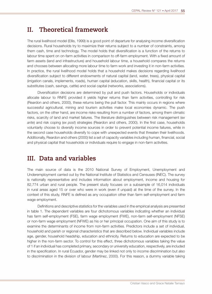
55CEPAL Review N° 121 • April 2017
Cristian Vasco and Grace Natalie Tamayo
II. Theoretical framework
The rural livelihood model (Ellis, 1999) is a good point of departure for analysing income diversification decisions. Rural households try to maximize their returns subject to a number of constraints, among them cash, time and technology. The model holds that diversification is a function of the returns to labour time spent on on-farm activities in comparison to off-farm employment. With a fixed amount of farm assets (land and infrastructure) and household labour time, a household compares the returns and chooses between allocating more labour time to farm work and investing it in non-farm activities. In practice, the rural livelihood model holds that a household makes decisions regarding livelihood diversification subject to different endowments of natural capital (land, water, trees), physical capital (irrigation canals, implements, roads), human capital (education, skills, health), financial capital or its substitutes (cash, savings, cattle) and social capital (networks, associations).
Diversification decisions are determined by pull and push factors. Households or individuals allocate labour to RNFE provided it yields higher returns than farm activities, controlling for risk (Reardon and others, 2000), these returns being the pull factor. This mainly occurs in regions where successful agricultural, mining and tourism activities make local economies dynamic. The push factors, on the other hand, are income risks resulting from a number of factors, among them climatic risks, scarcity of land and market failures. The literature distinguishes between risk management (ex ante) and risk coping (ex post) strategies (Reardon and others, 2000). In the first case, households voluntarily choose to diversify income sources in order to prevent potential income failures, while in the second case households diversify to cope with unexpected events that threaten their livelihoods. Additionally, Reardon and others (2000) list a set of capacity variables including human, financial, social and physical capital that households or individuals require to engage in non-farm activities.
III. Data and variables
The main source of data is the 2010 National Survey of Employment, Unemployment and Underemployment carried out by the National Institute of Statistics and Censuses (INEC). The survey is nationally representative and includes information about employment, income and housing for 82,774 urban and rural people. The present study focuses on a subsample of 16,014 individuals in rural areas aged 15 or over who were in work (even if unpaid) at the time of the survey. In the context of this study, RNFE is defined as any occupation other than farm self-employment and farm wage employment.
Definitions and descriptive statistics for the variables used in the empirical analysis are presented in table 1. The dependent variables are four dichotomous variables indicating whether an individual has farm self-employment (FSE), farm wage employment (FWE), non-farm self-employment (NFSE) or non-farm wage employment (NFWE) as his or her principal occupation. One aim of this study is to examine the determinants of income from non-farm activities. Predictors include a set of individual, household and parish or regional characteristics that are described below. Individual variables include age, gender, household headship, education and ethnicity. Returns to education are expected to be higher in the non-farm sector. To control for this effect, three dichotomous variables taking the value of 1 if an individual has completed primary, secondary or university education, respectively, are included in the specification. In rural Ecuador, gender may be linked not only to income discrimination but also to discrimination in the division of labour (Martínez, 2000). For this reason, a dummy variable taking
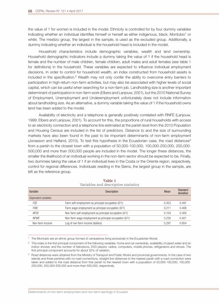
56 CEPAL Review N° 121 • April 2017
Determinants of non-farm employment and non-farm earnings in Ecuador
the value of 1 for women is included in the model. Ethnicity is controlled for by four dummy variables indicating whether an individual identifies himself or herself as either indigenous, black, Montubio1 or white. The mestizo group, the largest in the sample, is used as the excluded group. Additionally, a dummy indicating whether an individual is the household head is included in the model.
Household characteristics include demographic variables, wealth and land ownership. Household demographic indicators include a dummy taking the value of 1 if the household head is female and the number of male children, female children, adult males and adult females (see table 1 for definitions) in the household. These variables are expected to influence individual employment decisions. In order to control for household wealth, an index constructed from household assets is included in the specification.2 Wealth may not only confer the ability to overcome entry barriers to participation in high-return non-farm activities, but may also be associated with higher levels of social capital, which can be useful when searching for a non-farm job. Landholding size is another important determinant of participation in non-farm work (Elbers and Lanjouw, 2001), but the 2010 National Survey of Employment, Unemployment and Underemployment unfortunately does not include information about landholding size. As an alternative, a dummy variable taking the value of 1 if the household owns land has been added to the model.
Availability of electricity and a telephone is generally positively correlated with RNFE (Lanjouw, 1999; Elbers and Lanjouw, 2001). To account for this, the proportions of rural households with access to an electricity connection and a telephone line estimated at the parish level from the 2010 Population and Housing Census are included in the list of predictors. Distance to and the size of surrounding markets have also been found in the past to be important determinants of non-farm employment (Jonasson and Helfand, 2010). To test this hypothesis in the Ecuadorian case, the road distances3
from a parish to the closest town with a population of 50,000-100,000, 100,000-250,000, 250,000-500,000 and more than 500,000 people are included in the model. The longer these distances, the smaller the likelihood of an individual working in the non-farm sector should be expected to be. Finally, two dummies taking the value of 1 if an individual lives in the Costa or the Oriente region, respectively, control for regional differences. Individuals residing in the Sierra, the largest group in the sample, are left as the reference group.
Table 1 Variables and descriptive statistics
Variable Description Mean Standard deviation
Dependent variables
FSE Farm self-employment as principal occupation (0/1) 0.453 0.497
FWE Farm wage employment as principal occupation (0/1) 0.211 0.408
NFSE Non-farm self-employment as principal occupation (0/1) 0.104 0.305
NFWE Non-farm wage employment as principal occupation (0/1) 0.230 0.421
Non-farm income Log of non-farm income (dollars) 5.297 0.854
1 The Montubio are an ethnic group formed of campesinos living exclusively in the Ecuadorian littoral.2 This index is the first principal component of the following variables: home and car ownership, availability of piped water and an
indoor shower, and the number of televisions, DVD players, radios, computers, mobile phones, refrigerators and stoves. The first principal component accounts for about 32% of variation.
3 Road distances were obtained from the Ministry of Transport and Public Works and provincial governments. In the case of two islands and three parishes with no road connections, straight-line distances to the nearest parish with a road connection were taken and added to the road distance from that parish to the nearest town with a population of 50,000-100,000, 100,000-250,000, 250,000-500,000 and more than 500,000, respectively.
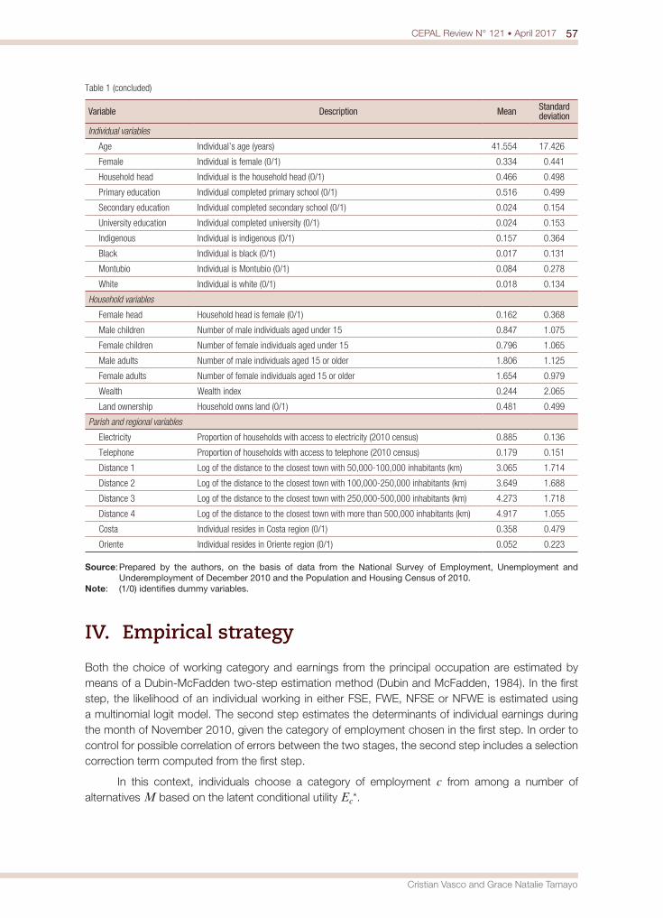
57CEPAL Review N° 121 • April 2017
Cristian Vasco and Grace Natalie Tamayo
Variable Description Mean Standard deviation
Individual variables
Age Individual’s age (years) 41.554 17.426
Female Individual is female (0/1) 0.334 0.441
Household head Individual is the household head (0/1) 0.466 0.498
Primary education Individual completed primary school (0/1) 0.516 0.499
Secondary education Individual completed secondary school (0/1) 0.024 0.154
University education Individual completed university (0/1) 0.024 0.153
Indigenous Individual is indigenous (0/1) 0.157 0.364
Black Individual is black (0/1) 0.017 0.131
Montubio Individual is Montubio (0/1) 0.084 0.278
White Individual is white (0/1) 0.018 0.134
Household variables
Female head Household head is female (0/1) 0.162 0.368
Male children Number of male individuals aged under 15 0.847 1.075
Female children Number of female individuals aged under 15 0.796 1.065
Male adults Number of male individuals aged 15 or older 1.806 1.125
Female adults Number of female individuals aged 15 or older 1.654 0.979
Wealth Wealth index 0.244 2.065
Land ownership Household owns land (0/1) 0.481 0.499
Parish and regional variables
Electricity Proportion of households with access to electricity (2010 census) 0.885 0.136
Telephone Proportion of households with access to telephone (2010 census) 0.179 0.151
Distance 1 Log of the distance to the closest town with 50,000-100,000 inhabitants (km) 3.065 1.714
Distance 2 Log of the distance to the closest town with 100,000-250,000 inhabitants (km) 3.649 1.688
Distance 3 Log of the distance to the closest town with 250,000-500,000 inhabitants (km) 4.273 1.718
Distance 4 Log of the distance to the closest town with more than 500,000 inhabitants (km) 4.917 1.055
Costa Individual resides in Costa region (0/1) 0.358 0.479
Oriente Individual resides in Oriente region (0/1) 0.052 0.223
Source: Prepared by the authors, on the basis of data from the National Survey of Employment, Unemployment and Underemployment of December 2010 and the Population and Housing Census of 2010.
Note: (1/0) identifies dummy variables.
IV. Empirical strategy
Both the choice of working category and earnings from the principal occupation are estimated by means of a Dubin-McFadden two-step estimation method (Dubin and McFadden, 1984). In the first step, the likelihood of an individual working in either FSE, FWE, NFSE or NFWE is estimated using a multinomial logit model. The second step estimates the determinants of individual earnings during the month of November 2010, given the category of employment chosen in the first step. In order to control for possible correlation of errors between the two stages, the second step includes a selection correction term computed from the first step.
In this context, individuals choose a category of employment c from among a number of alternatives M based on the latent conditional utility Ec*.
Table 1 (concluded)
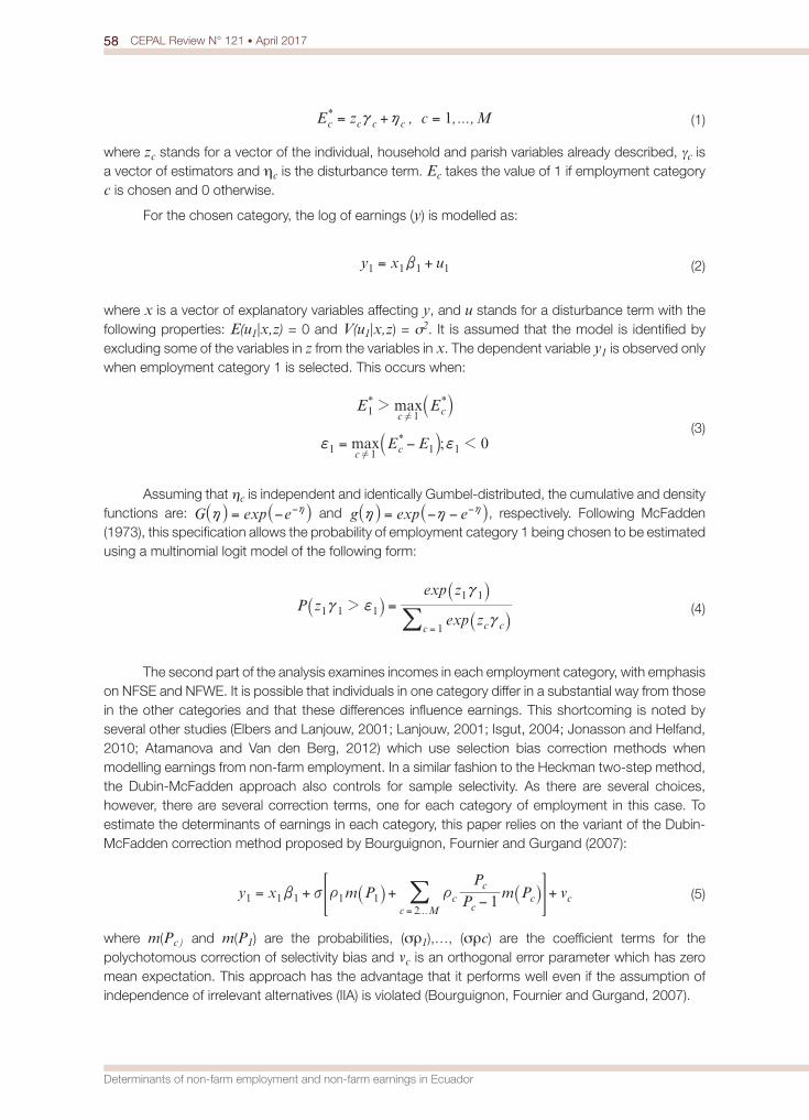
58 CEPAL Review N° 121 • April 2017
Determinants of non-farm employment and non-farm earnings in Ecuador
, , ...,E z c M1*c c c cc h= + = (1)
where zc stands for a vector of the individual, household and parish variables already described, γc is a vector of estimators and ηc is the disturbance term. Ec takes the value of 1 if employment category c is chosen and 0 otherwise.
For the chosen category, the log of earnings (y) is modelled as:
y x u1 1 1 1b= + (2)
where x is a vector of explanatory variables affecting y, and u stands for a disturbance term with the following properties: E(u1|x,z) = 0 and V(u1|x,z) = σ2. It is assumed that the model is identified by excluding some of the variables in z from the variables in x. The dependent variable y1 is observed only when employment category 1 is selected. This occurs when:
maxE E* *
c c1 12
!S X
(3)
max ;E E 0*
c c1 1 1 1 1f f= −!
S X
Assuming that ηc is independent and identically Gumbel-distributed, the cumulative and density functions are: expG eh = − h−R RW W and expg eh h= − − h−R RW W, respectively. Following McFadden (1973), this specification allows the probability of employment category 1 being chosen to be estimated using a multinomial logit model of the following form:
exp
expP z
z
z
c cc
1 1 1
1
1 12c f
c
c=
=
RR
RW
W
W/ (4)
The second part of the analysis examines incomes in each employment category, with emphasis on NFSE and NFWE. It is possible that individuals in one category differ in a substantial way from those in the other categories and that these differences influence earnings. This shortcoming is noted by several other studies (Elbers and Lanjouw, 2001; Lanjouw, 2001; Isgut, 2004; Jonasson and Helfand, 2010; Atamanova and Van den Berg, 2012) which use selection bias correction methods when modelling earnings from non-farm employment. In a similar fashion to the Heckman two-step method, the Dubin-McFadden approach also controls for sample selectivity. As there are several choices, however, there are several correction terms, one for each category of employment in this case. To estimate the determinants of earnings in each category, this paper relies on the variant of the Dubin-McFadden correction method proposed by Bourguignon, Fournier and Gurgand (2007):
y x m P PP
m P v1...
cc
cc
c Mc1 1 1 1 1
2
b v t t= + +−
+=
R RW W# &/ (5)
where m(Pc) and m(P1) are the probabilities, (σρ1),…, (σρc) are the coefficient terms for the polychotomous correction of selectivity bias and vc is an orthogonal error parameter which has zero mean expectation. This approach has the advantage that it performs well even if the assumption of independence of irrelevant alternatives (IIA) is violated (Bourguignon, Fournier and Gurgand, 2007).
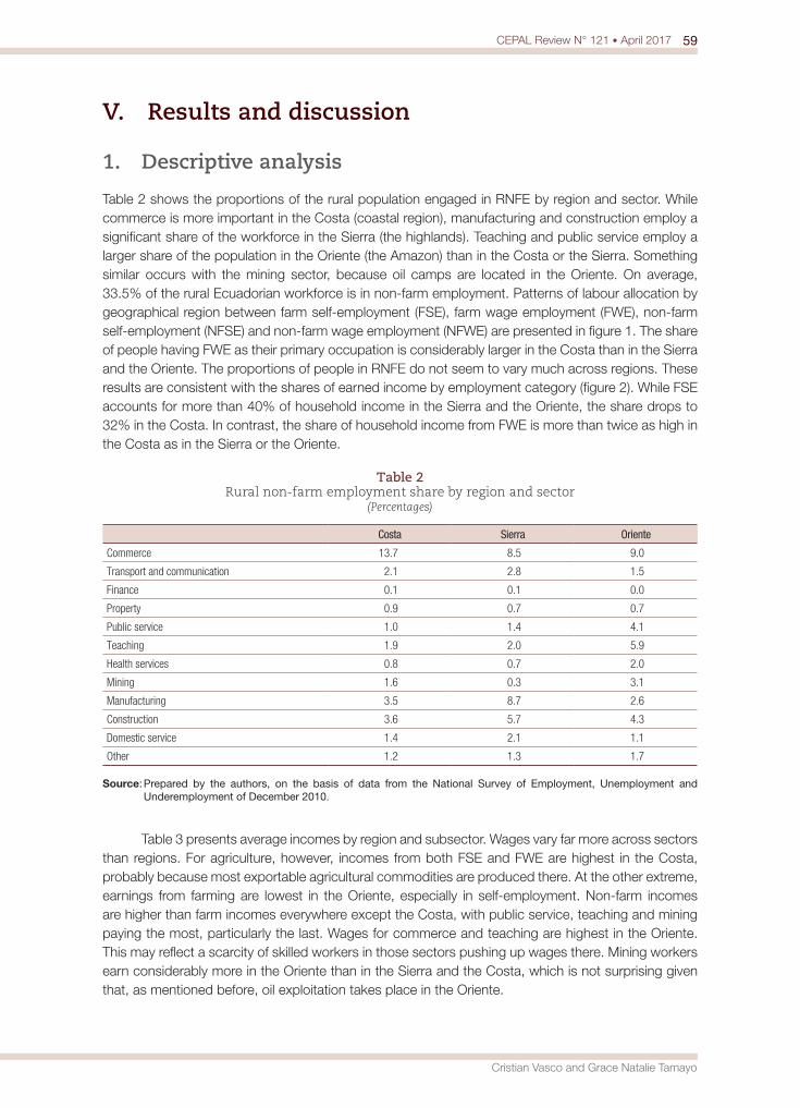
59CEPAL Review N° 121 • April 2017
Cristian Vasco and Grace Natalie Tamayo
V. Results and discussion
1. Descriptive analysis
Table 2 shows the proportions of the rural population engaged in RNFE by region and sector. While commerce is more important in the Costa (coastal region), manufacturing and construction employ a significant share of the workforce in the Sierra (the highlands). Teaching and public service employ a larger share of the population in the Oriente (the Amazon) than in the Costa or the Sierra. Something similar occurs with the mining sector, because oil camps are located in the Oriente. On average, 33.5% of the rural Ecuadorian workforce is in non-farm employment. Patterns of labour allocation by geographical region between farm self-employment (FSE), farm wage employment (FWE), non-farm self-employment (NFSE) and non-farm wage employment (NFWE) are presented in figure 1. The share of people having FWE as their primary occupation is considerably larger in the Costa than in the Sierra and the Oriente. The proportions of people in RNFE do not seem to vary much across regions. These results are consistent with the shares of earned income by employment category (figure 2). While FSE accounts for more than 40% of household income in the Sierra and the Oriente, the share drops to 32% in the Costa. In contrast, the share of household income from FWE is more than twice as high in the Costa as in the Sierra or the Oriente.
Table 2 Rural non-farm employment share by region and sector
(Percentages)
Costa Sierra Oriente
Commerce 13.7 8.5 9.0
Transport and communication 2.1 2.8 1.5
Finance 0.1 0.1 0.0
Property 0.9 0.7 0.7
Public service 1.0 1.4 4.1
Teaching 1.9 2.0 5.9
Health services 0.8 0.7 2.0
Mining 1.6 0.3 3.1
Manufacturing 3.5 8.7 2.6
Construction 3.6 5.7 4.3
Domestic service 1.4 2.1 1.1
Other 1.2 1.3 1.7
Source: Prepared by the authors, on the basis of data from the National Survey of Employment, Unemployment and Underemployment of December 2010.
Table 3 presents average incomes by region and subsector. Wages vary far more across sectors than regions. For agriculture, however, incomes from both FSE and FWE are highest in the Costa, probably because most exportable agricultural commodities are produced there. At the other extreme, earnings from farming are lowest in the Oriente, especially in self-employment. Non-farm incomes are higher than farm incomes everywhere except the Costa, with public service, teaching and mining paying the most, particularly the last. Wages for commerce and teaching are highest in the Oriente. This may reflect a scarcity of skilled workers in those sectors pushing up wages there. Mining workers earn considerably more in the Oriente than in the Sierra and the Costa, which is not surprising given that, as mentioned before, oil exploitation takes place in the Oriente.
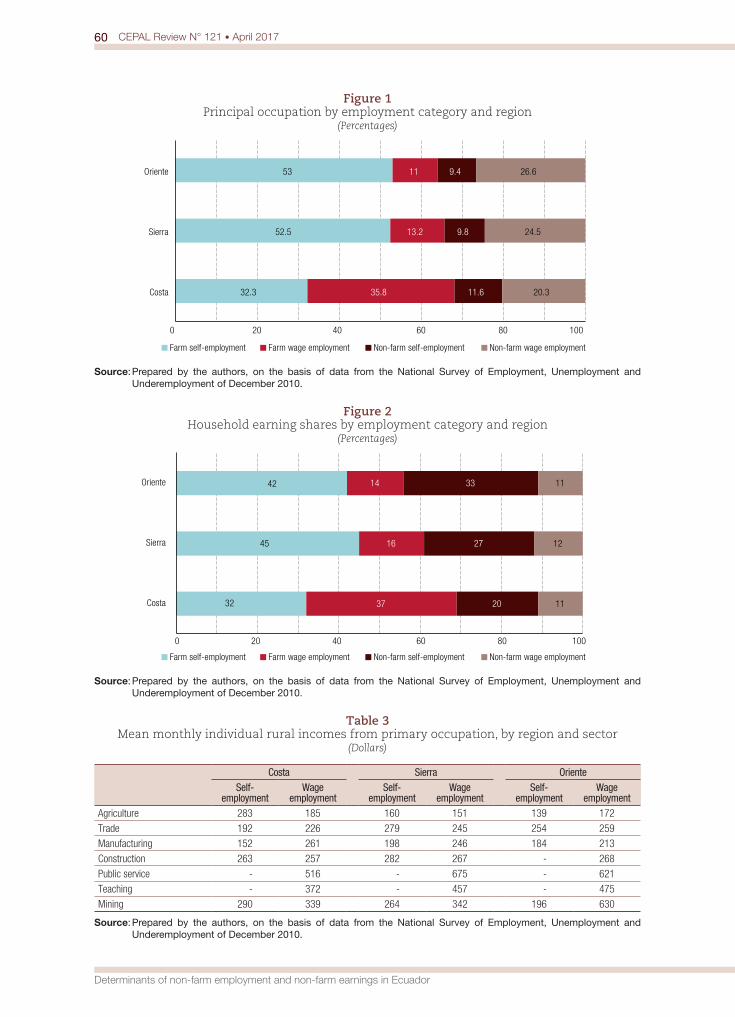
60 CEPAL Review N° 121 • April 2017
Determinants of non-farm employment and non-farm earnings in Ecuador
Figure 1 Principal occupation by employment category and region
(Percentages)
35.8
13.2
11
32.3
52.5
53
11.6
9.8
9.4
20.3
24.5
26.6
Costa
Sierra
Oriente
Farm self-employment Farm wage employment Non-farm self-employment Non-farm wage employment
0 20 40 60 80 100
Source: Prepared by the authors, on the basis of data from the National Survey of Employment, Unemployment and Underemployment of December 2010.
Figure 2 Household earning shares by employment category and region
(Percentages)
37
16
14
20
27
33
11
12
11
Costa
Sierra
Oriente
0 20 40 60 80 100
32
45
42
Farm self-employment Farm wage employment Non-farm self-employment Non-farm wage employment
Source: Prepared by the authors, on the basis of data from the National Survey of Employment, Unemployment and Underemployment of December 2010.
Table 3 Mean monthly individual rural incomes from primary occupation, by region and sector
(Dollars)
Costa Sierra OrienteSelf-
employmentWage
employmentSelf-
employmentWage
employmentSelf-
employmentWage
employmentAgriculture 283 185 160 151 139 172
Trade 192 226 279 245 254 259
Manufacturing 152 261 198 246 184 213
Construction 263 257 282 267 - 268
Public service - 516 - 675 - 621
Teaching - 372 - 457 - 475
Mining 290 339 264 342 196 630
Source: Prepared by the authors, on the basis of data from the National Survey of Employment, Unemployment and Underemployment of December 2010.
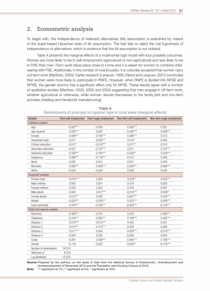
61CEPAL Review N° 121 • April 2017
Cristian Vasco and Grace Natalie Tamayo
2. Econometric analysis
To begin with, the independence of irrelevant alternatives (IIA) assumption is examined by means of the suest-based Hausman tests of IIA assumption. The test fails to reject the null hypothesis of independence of alternatives, which is evidence that the IIA assumption is not violated.
Table 4 presents the marginal effects of a multinomial logit model with four possible outcomes. Women are more likely to be in self-employment (agricultural or non-agricultural) and less likely to be in FWE than men. Farm work takes place close to home and it is easier for women to combine child-rearing with FSE. Additionally, in the context of rural Ecuador, it is culturally accepted that women carry out farm work (Martínez, 2000). Earlier research (Lanjouw, 1999; Elbers and Lanjouw, 2001) concluded that women were more likely to participate in RNFE. However, when RNFE is divided into NFSE and NFWE, the gender dummy has a significant effect only for NFSE. These results agree with a number of qualitative studies (Martínez, 2000, 2002 and 2004) suggesting that men engage in off-farm work, whether agricultural or otherwise, while women devote themselves to the family plot and non-farm activities (retailing and handicraft manufacturing).
Table 4 Determinants of principal occupation type in rural areas (marginal effects)
Variable Farm self-employment Farm wage employment Non-farm self-employment Non-farm wage employmentIndividual variables
Age -0.007*** -0.000 0.006*** 0.001
Age squared 0.000*** 0.000 -0.000*** -0.000***
Female 0.094*** -0.165*** 0.086*** 0.015
Household head 0.017 -0.025*** 0.012* -0.004
Primary education -0.017* -0.018*** 0.011** 0.010
Secondary education -0.031 -0.127*** 0.011 0.147***
University education -0.329*** -0.164*** -0.026** 0.520***
Indigenous 0.089*** -0.119*** -0.015 0.046
Black -0.005 -0.012 -0.021 0.040
Montubio 0.069*** 0.028*** -0.032*** -0.064***
White -0.030 -0.024 0.029 0.025
Household variablesFemale head -0.070*** 0.008 0.019** 0.042***
Male children 0.002 0.001 0.016 -0.005
Female children 0.002 0.003 0.016 -0.007
Male adults -0.002 0.017*** -0.010*** -0.009**
Female adults -0.013*** 0.000 -0.007*** 0.020***
Wealth -0.033*** -0.029*** 0.023*** 0.038***
Land ownership 0.374*** -0.162*** -0.024*** -0.142***
Parish and regional variablesElectricity -0.488*** -0.374 0.033 0.492***
Telephone -0.416*** -0.065*** 0.100*** 0.382***
Distance 1 0.010*** -0.015*** 0.003 0.001
Distance 2 0.010*** -0.010*** 0.000 0.000
Distance 3 0.011*** 0.004 -0.005*** -0.010***
Distance 4 -0.004 0.000 -0.000 0.004
Costa -0.291 0.059*** 0.065*** 0.166***
Oriente -0.119 -0.023 0.033** 0.110***
Number of observations 16 014
Wald test χ2 9 076
Log likelihood -15 670
Source: Prepared by the authors, on the basis of data from the National Survey of Employment, Unemployment and Underemployment of December 2010 and the Population and Housing Census of 2010.
Note: *** significant at 1%; ** significant at 5%; * significant at 10%.

62 CEPAL Review N° 121 • April 2017
Determinants of non-farm employment and non-farm earnings in Ecuador
As expected, education is negatively correlated with the likelihood of having FWE as the principal occupation. Individuals who have completed primary, secondary or higher education are less likely to be agricultural wage earners. The effects of education on NFSE are as expected. While the likelihood of participating in NFSE is greater for individuals who have completed primary school than for those with no education, it drops dramatically for those who hold a university degree, as expected. This reflects the relatively low education endowments required by the NFSE sector. The likelihood of partaking in NFWE increases for those who have completed either secondary or higher education, reflecting the fact that, in rural Ecuador, returns to education are found only in NFWE.
The results also show that household heads are less likely to become agricultural wage earners. On the other hand, being indigenous increases the likelihood of having FSE as the main source of income and reduces the odds of being a wage labourer. This agrees with previous research (Vasco, 2013a and 2014) concluding that indigenous peoples mainly rely on reciprocal labour to meet their workforce requirements. Belonging to the Montubio ethnic group increases the odds of participating in FSE and FWE, on the one hand, while reducing the likelihood of partaking in either form of non-farm employment, on the other. These findings are not surprising given that this group has traditionally engaged in agriculture.
Individuals from households with more adult men are more likely to be agricultural wage earners. This may be because members of households with labour flexibility diversify their income by engaging in FWE. Conversely, individuals from households with more adult men are less likely to take part in NFSE and NFWE. The number of adult women in a household is negatively correlated with the likelihood of participation in FSE and NFSE and positively correlated with the odds of being a non-agricultural wage earner. Having more women to enter either FSE or NFSE allows other household members to engage in NFWE.
Individuals from wealthier households are less likely to take part in agricultural work but more likely to engage in non-agricultural activities. Wealthier households are in a better position than their poorer peers to overcome the entry barriers (licence fees, equipment acquisition, etc.) that participation in RNFE often entails (Reardon and others, 2000). Land availability is positively correlated with the likelihood of engaging in off-farm work (agricultural and non-agricultural). Overall, these results indicate that lack of land is a push factor driving the rural population into off-farm activities, whether agricultural or otherwise. More educated people can access better paid non-farm jobs, while FWE is the choice for the landless uneducated population.
Availability of electricity or a telephone is negatively correlated with the likelihood of partaking in FSE and FWE, which is not surprising given that these services are mostly available in urban areas. In contrast, individuals residing in parishes where electricity and telephony are available are more likely to engage in NFSE and NFWE. This is consistent with earlier research concluding that infrastructure plays a crucial role in facilitating non-farm job opportunities in rural areas (Elbers and Lanjouw, 2001; Vasco, 2013b).
As expected, FSE is more common in remote population centres, with the exception of towns of more than 500,000 inhabitants. In the case of FWE, only Distance 1 (distance to the nearest town with 50,000-100,000 people) and Distance 2 (distance to the nearest town with 100,000-250,000 people) were significant and had the expected negative sign. These results indicate that the bulk of farms able to hire labour, and thus the most dynamic agricultural labour markets, are concentrated near small cities rather than big cities. For non-farm employment (both NFSE and NFWE), Distance 3 (distance to towns of 250,000-500,000 people) is significant and has the expected negative sign. A possible explanation for this finding is that the group of Distance 3 towns includes three medium-sized cities, among them Santo Domingo de los Tsachilas (368,000 people) and Ambato (330,000 people). Albeit with different patterns, these cities have three common characteristics: they have relatively large populations, advantageous geographical locations and close links with the agricultural sector.
63CEPAL Review N° 121 • April 2017
Cristian Vasco and Grace Natalie Tamayo
Ambato is the capital of the province of Tungurahua and is considered a model of successful RNFE in the otherwise deprived central Sierra (North and Cameron, 2000). Tungurahua’s advantageous location in the centre of the country has been favourable for trade in agricultural goods with both Quito and Guayaquil, the country’s largest cities (Ospina, 2010). Moreover, Ambato’s hinterland contains a concentration of small-scale and family-based leather, textile and woodworking factories that employ a significant share of Tungurahua’s rural population. Santo Domingo de los Tsachilas is a subtropical city which connects Quito, the country’s capital, with the biggest cities in the Costa, among them Guayaquil. Cattle ranching and the production of palm oil, bananas and cacao, among other tropical crops, have impelled the local and regional economies. These findings are consistent with the claim in Reardon and others (2000) that non-farm employment grows in tandem with a dynamic agricultural sector, and also with Jonasson and Helfand’s (2010) argument that the size of markets, as well as distance to them, matters for participation in non-farm activities.
Residents of the Costa are more likely to work as farm wage labourers. This finding is consistent with that for the Montubios. As mentioned earlier, the large-scale production of tropical cash crops (bananas, oil palm, sugar cane and cocoa) absorbs a big share of the rural population in the region. Individuals living in the Costa and the Oriente are more likely to obtain their income from non-farm sources than those settled in the Sierra. In the case of the Costa, the difference may be associated with land ownership patterns. Whereas 53% of households in the Sierra own land, this share drops to 31% for the Costa. Land concentration seems to play a determining role in driving rural people in the Costa into FWE and RNFE in general.
The case of the Oriente is somewhat different, with landless households making up 45% of the sample for this region. Why are people more likely to engage in RNFE in a region which was relatively recently colonized4 and where land concentration appears not to be as acute as it is in the Costa? The answer to this question may be related to land quality. The Ecuadorian Amazon, locally known as the Oriente, is one of the world’s biodiversity hotspots (Myers and others, 2000). Nevertheless, soils are very fragile and become depleted soon after vegetation is removed (Hicks and others, 1990). Under such conditions, returns to agriculture are low, as shown in table 3, and alternative income sources are needed. In any event, this finding is consistent with earlier research reporting significant growth in the share of people engaged in off-farm work in the Oriente provinces (Bilsborrow, Barbieri and Pan, 2004; Vasco Pérez, Bilsborrow and Torres, 2015). According to these authors, this is linked both to the shrinking size of farms because of continuous subdivision and to the growth of employment opportunities in urban areas.
Table 5 shows the results of the second stage of the Dubin-McFadden correction method. Following several other studies (Isgut, 2004; Jonasson and Helfand, 2010; Atamanova and Van den Berg, 2012), the identifying variables used to construct the selection correction terms are the sex of the household head and the household composition variables. Studies of this type assume that these variables do not influence earnings from each category of employment.
Being a woman reduces earnings from FSE, FWE, NFSE and NFWE by 34%, 20%, 48% and 26%, respectively. In the case of non-farm work, this finding is consistent with prior research (Elbers and Lanjouw, 2001) reporting that women are concentrated in low-income non-farm jobs. Returns to education are found only for FWE (primary and secondary education) and NFWE (secondary and university education). Having completed either secondary or higher education increases earnings from NFWE by 17% and 60%, respectively. Conversely, no education dummy had any significant effect on earnings from NFSE.5 This finding supports the contention that, other things being equal, NFSE does
4 Sustained colonization flows from the Costa and especially from the Sierra to the Oriente started during the 1970s following the discovery of oil in 1967.
5 The effects of education remain non-significant even when the education dummies are replaced by the number of years of formal education and its squared term.

64 CEPAL Review N° 121 • April 2017
Determinants of non-farm employment and non-farm earnings in Ecuador
not call for high education endowments. Overall, household heads earn more than other household members in all categories of employment. Where ethnicity variables are concerned, black people who have FSE as their principal occupation earn 23% less than their mestizo counterparts, and Montubio people earn 11% less than their mestizo peers from FWE even though they are more likely to engage in it. There are no significant differences between ethnic groups when it comes to non-farm earnings.
Wealth is positively correlated with higher earnings for all employment categories. Wealthier households are in a better position to access agricultural technology (e.g., chemical fertilizers, irrigation and mechanization), which increases yields and thence earnings. Similarly, individuals from wealthier households have the means to overcome the entry barriers that NFSE involves, such as the need for start-up capital and the cost of licence fees and machinery. In the case of wage employment, this finding may reflect the fact that members of wealthier households have more social capital and thus are able to access better-paid non-farm jobs (Jonasson and Helfand, 2010). A similar effect may exist with land ownership, which is associated with higher earnings for non-farm workers. As stated by Lanjouw and Stern (1998), access to attractive non-farm jobs may be determined by wealth, which in turn may be associated with landholding.
Table 5 Earnings by employment category in rural areas (log)
Variable Farm self-employment Farm wage employment Non-farm self-employment Non-farm wage employmentIndividual variables
Age 0.018*** 0.014*** 0.038*** 0.028***
Age squared -0.000*** -0.000*** -0.000*** -0.000***
Female -0.340*** -0.225*** -0.659*** -0.303***
Household head 0.233*** 0.170*** 0.165** 0.203***
Primary education 0.112*** -0.150 -0.030 -0.031
Secondary education 0.450*** 0.049 0.226 0.161***
University education 0.335 -0.380 0.310 0.470***
Indigenous 0.000 -0.105 -0.191 -0.044
Black -0.231*** 0.017 -0.161 -0.117
Montubio 0.007 -0.107*** -0.023 0.039
White 0.083 0.065 -0.074 -0.056
Household variablesWealth 0.104*** 0.065*** 0.133*** 0.059***
Land ownership 0.240* -0.010 0.128 0.156***
Parish and regional variablesElectricity -0.860*** 0.417*** 0.576* 0.034
Telephone -0.365* -0.051 -0.398 -0.021
Distance 1 -0.035*** -0.009 -0.002 0.002
Distance 2 0.005 -0.018*** 0.009 0.012**
Distance 3 0.008 -0.022*** -0.017 0.014**
Distance 4 -0.111*** -0.014 0.021 -0.011
Costa 0.162 0.310*** 0.136 0.022
Oriente -0.079 0.201*** 0.251* 0.217***
m1 0.119 -0.109 -0.045 0.185
m2 -0.535 -0.053 -0.086 -0.126
m3 -0.918 -0.090 -0.214** 0.097
m4 0.321 0.099 -0.289 -0.216
F-statistics 57.50*** 25.13*** 26.07*** 56.11***
R2 0.252 0.158 0.292 0.292
Source: Prepared by the authors, on the basis of data from the National Survey of Employment, Unemployment and Underemployment of December 2010 and the Population and Housing Census of 2010.
Note: m1, m2, m3 and m4 are the selection correction terms estimated from the selection model. *** significant at 1%; ** significant at 5%; * significant at 10%.
65CEPAL Review N° 121 • April 2017
Cristian Vasco and Grace Natalie Tamayo
Higher proportions of access to electricity are associated with lower earnings from FSE, which may reflect the fact that larger family farms and farmers entirely depending on FSE are normally found in places where service availability is low. In contrast, higher earnings from FWE are associated with higher proportions of access to electricity. This may be related to the fact that labour-intensive commodity production (e.g., flower production) is also intensive in electricity. Income from NFSE is greater in parishes with higher proportions of electricity access, with a 10% increase in this value raising self-employment earnings by 6%. Non-significance in the case of NFWE may indicate that access to electricity is an essential condition for the functioning of businesses big enough to hire labour, and so it does not play any role in determining wages.
FSE is higher near Distance 1 and Distance 4 towns. In the case of Distance 1, this may be because small towns are the main market for small-scale farmers selling their produce to traders. In the case of Distance 4, profit is higher for those farmers who are able to market their produce in the large cities included in this category. FWE is better paid in areas near Distance 2 and Distance 3 towns. A possible explanation for these findings is that more developed agricultural companies, which offer better wages than small-scale farms, are located in such areas. The further away Distance 2 and Distance 3 towns are, the higher the earnings from NFWE. A possible explanation for this finding is that competition for jobs in larger urban areas may be greater, keeping wages lower than in areas further from large cities.
Wages for agricultural labourers are higher in the Costa and the Oriente. These findings agree with the figures presented in table 3. All else being equal, earnings from non-farm employment are higher in the Oriente than in the Sierra. As mentioned earlier, oil companies, which pay the highest non-farm wages, are located in the Oriente.
VI. Conclusions
Non-farm employment is an important source of income for rural people in Ecuador, accounting for 36% of households’ income and employing roughly 33% of the country’s rural labour force. This study has examined the determinants of both participation in non-farm employment and non-farm income. The empirical analysis shows that women are more likely than men to participate in NFSE. However, they earn significantly less than men in both NFSE and NFWE. Participation in NFWE is more common among educated people, who usually also have the physical capital to overcome the entry barriers that RNFE involves. There is a marked tendency for landless people to engage in RNFE. The results also show, as expected, that participation in NFSE does not require high education endowments, which is evidence that the NFSE sector is still incipient.
Special emphasis has been placed on locational and geographical variables. The results suggest that RNFE blooms in areas near medium-sized towns with a dynamic agricultural sector. The likelihood of participating in non-farm work is higher in both the Costa and the Oriente than in the Sierra. There are different reasons for this, with land concentration appearing to be a major factor in the Costa and land quality in the Oriente.
There are regional variations in the wage differential between farm and non-farm income. While farm earnings are considerably lower than those from non-farm employment in the Sierra and the Oriente, those who have farm self-employment as their principal occupation in the Costa earn more than most non-farm self-employed workers. Essentially, though, non-farm wage employment offers better earnings than any form of agricultural labour, which indicates its potential for rural poverty alleviation. Nevertheless, participation in RNFE in general and well-paid RNFE in particular demands high human and physical capital endowments which are rarely available to the poor. Policy interventions
66 CEPAL Review N° 121 • April 2017
Determinants of non-farm employment and non-farm earnings in Ecuador
to address this should focus on providing rural people with education, training and credit to overcome the entry barriers that prevent the poor from engaging in non-farm employment.
Since participation in non-farm employment is shaped not only by distance to markets but also by market size and the local economic environment, policies should also be oriented towards supporting the development of medium-sized towns which, as shown earlier, have the potential to absorb the rural labour surplus. Investments in rural infrastructure, the promotion of agriculture and tourism and tax incentives for enterprises willing to relocate in deprived rural areas could be helpful in achieving that goal.
BibliographyAtamanova, A. and M. Van den Berg (2012), “Participation and returns in rural nonfarm activities: evidence
from the Kyrgyz Republic”, Agricultural Economics, vol. 43, No. 4, International Association of Agricultural Economists.
Berdegué, J. and others (2001), “Rural nonfarm employment and incomes in Chile”, World Development, vol. 29, No. 3, Amsterdam, Elsevier.
Bilsborrow, R., A. Barbieri and W. Pan (2004), “Changes in population and land use over time in the Ecuadorian Amazon”, Acta Amazonica, vol. 34, No. 4.
Bourguignon, F., M. Fournier and M. Gurgand (2007), “Selection bias corrections based on the multinomial logit model: Monte Carlo comparisons”, Journal of Economic Surveys, vol. 21, No. 1, Wiley.
Dubin, J.A. and D.L. McFadden (1984), “An econometric analysis of residential electric appliance holdings and consumption”, Econometrica, vol. 52, No. 2, New York, The Econometric Society.
Elbers, C. and P. Lanjouw (2001), “Intersectoral transfer, growth and inequality in rural Ecuador”, World Development, vol. 29, No. 3, Amsterdam, Elsevier.
Ellis, F. (2000), “The determinants of rural livelihood diversification in developing countries”, Journal of Agricultural Economics, vol. 51, No. 2, Agricultural Economics Society.(1999), “Rural livelihood diversity in developing countries: evidence and policy implications”, Natural Resource Perspectives, No. 40, Overseas Development Institute.(1993), Peasant Economics: Farm Households and Agrarian Development, Cambridge, Cambridge University Press.
Ferreira, F. and P. Lanjouw (2001), “Rural nonfarm activities and poverty in the Brazilian Northeast”, World Development, vol. 29, No. 3, Amsterdam, Elsevier.
Haggblade, S., P. Hazell and T. Reardon (2010), “The rural non-farm economy: prospects for growth and poverty reduction”, World Development, vol. 38, No. 10, Amsterdam, Elsevier.
Hicks, J.F. and others (1990), Ecuador’s Amazon Region Development Issues and Options, Washington, D.C., World Bank.
Isgut, A. (2004), “Non-farm income and employment in rural Honduras: assessing the role of locational factors”, Journal of Development Studies, vol. 40, No. 3, Taylor & Francis.
Jonasson, E. and S.M. Helfand (2010), “How important are locational characteristics for rural non-agricultural employment? Lessons from Brazil”, World Development, vol. 38, No. 5, Amsterdam, Elsevier.
Köbrich, C. and M. Dirven (2007), “Características del empleo rural no agrícola en América Latina con énfasis en los servicios”, Desarrollo Productivo series, No. 174 (LC/L.2659-P), Santiago, Economic Commission for Latin America and the Caribbean (ECLAC).
Lanjouw, P. (2001), “Nonfarm employment and poverty in rural El Salvador”, World Development, vol. 29, No. 3, Amsterdam, Elsevier.(1999), “Rural nonagricultural employment and poverty in Ecuador”, Economic Development and Cultural Change, vol. 48, No. 1, Chicago, The University of Chicago Press.
Lanjouw, J.O. and P. Lanjouw (2001), “The rural non-farm sector: issues and evidence from developing countries”, Agricultural Economics, vol. 26, No. 1, International Association of Agricultural Economists.
Lanjouw, P. and N. Stern (1998), A Kind of Growth: Palanpur 1957-1993, Oxford, Oxford University Press.Laszlo, S. (2005), “Self-employment earnings and returns to education in rural Peru”, Journal of Development
Studies, vol. 41, No. 7, Taylor & Francis.
67CEPAL Review N° 121 • April 2017
Cristian Vasco and Grace Natalie Tamayo
Martínez, L. (2004), “El campesino andino y la globalización a fines de siglo (una mirada sobre el caso ecuatoriano)”, European Review of Latin American and Caribbean Studies, No. 77.(2002), Economía política de las comunidades indígenas, Quito, Latin American Institute for Social Science Research (ILDIS).(2000), “La especificidad del empleo rural”, Antología de estudios rurales, A. Torres (eds.), Quito, FLACSO Ecuador/Latin American Institute for Social Science Research (ILDIS).
McFadden, D. (1973), “Conditional logit analysis of qualitative choice behavior”, Frontiers in Econometrics, P. Zarembka (eds.), New York, Academic Press.
Myers, N. and others (2000), “Biodiversity hotspots for conservation priorities”, Nature, No. 403.North, L.L. and J.D. Cameron (2000), “Grassroots-based rural development strategies: Ecuador in comparative
perspective”, World Development, vol. 28, No. 10, Amsterdam, Elsevier.Ospina, P. (2010), “Tungurahua rural: el territorio de senderos que se bifurcan”, Ecuador Debate, vol. 81,
No. 3, Quito, Andean Centre for Population Action.Reardon, T. and others (2000), “Household income diversification into rural nonfarm activities”, Transforming
the Rural Nonfarm Economy, S. Haggblade, P. Hazell and T. Reardon (eds.), Baltimore, Johns Hopkins University Press.
Vasco, C. (2014), “Reciprocal and wage labour in rural Ecuador. A quantitative analysis”, Journal of Agriculture and Rural Development in the Tropics and Subtropics, vol. 115, No. 1.(2013a), “Factores determinantes del trabajo recíproco y del uso de mano de obra salariada en el Ecuador rural”, Eutopía, No. 4, Quito, FLACSO-Ecuador.(2013b), “Migration, remittances and entrepreneurship: the case of rural Ecuador”, Migraciones Internacionales, vol. 7, No. 1, Mexico City, El Colegio de la Frontera Norte.
Vasco Pérez, C., R. Bilsborrow and B. Torres (2015), “Income diversification of migrant colonists vs. indigenous populations: contrasting strategies in the Amazon”, Journal of Rural Studies, vol. 42, Amsterdam, Elsevier.


Innovation and productivity in services and manufacturing firms: the case of Peru1
Mario D. Tello
Abstract
This article analyses the relationship between investment decisions, investment intensity, innovation outcomes and labour productivity for a sample of services and manufacturing firms from Peru in 2004, on the basis of an adjusted CDM model (Crepon, Duguet and Mairesse, 1998). The estimates of the model indicate that firm size was a key factor in the investment decision. Firm size and investment intensity were also key determinants in increasing, respectively, the probability of producing technological and non-technological innovation outputs and labour productivity across services and manufacturing sectors. By contrast, public financial support seemed to have a stronger effect in terms of investment inducement than in terms of investment intensity in services and low-tech manufacturing firms. These results suggest that horizontal science, technology and innovation (STI) policies that encourage firms to increase STI investment intensity may well produce some gains in firms’ labour productivity.
Keywords
Service industries, manufacturing enterprises, investments, science and technology, technological innovations, productivity, Peru
JEL classification
L8, O31
Author
Mario D. Tello is a professor in the Department of Economics at the Catholic University of Peru. [email protected]
1 This paper is a revised and shortened version of a paper presented under the project Innovation and Productivity in Services in Latin American Countries and was completed while the author was a CAF visiting fellow in the Latin American Centre at the University of Oxford. The author thanks Gustavo Crespi, Fernando Vargas, Diego Aboal, Esequiel Tacsir, Sylvia Dohnert and the participants of the seminars conducted under the project for their helpful comments, as well as Carla Solis for her excellent research assistance.
70 CEPAL Review N° 121 • April 2017
Innovation and productivity in services and manufacturing firms: the case of Peru
I. Introduction
Despite the importance of the services sector2 in many developing economies in terms of real value and employment,3 studies of the sector and its innovation activities in the Peruvian economy are scant. Most work in this area has concerned the analysis of services exports, in particular in the tourism sector.4 A handful of descriptive studies have been carried out on innovation, with an emphasis on the analysis of science, technology and innovation (STI) activities, information and communications technology (ICT), tools (e.g. CONCYTEC/INEI, 2005b; Kuramoto, 2008; Tello, 2010 and 2011) and economic policy (e.g. Comisión Consultiva para la Ciencia, Tecnología e Innovación, 2012; Kuramoto and Díaz, 2010 and 2011; Kuramoto, 2007; Tello, 2010; Sagasti, 2011; and UNCTAD/ECLAC, 2011).
In this regard and on the basis of a survey of STI activities at the firm level conducted by the National Council of Science, Technology and Technological Innovation (CONCYTEC) and the National Institute of Statistics and Informatics (INEI), this paper’s main contribution is an analysis, for the first time, of the relationship between firms’ investment in STI, innovation results and productivity for the services sector of Peru in 2004 through an adjusted standard Crepon, Duguet and Mairesse (CMD) model (1998). For purposes of comparison, this paper also analyses the same relationship for firms in the manufacturing sector.
The analysis below contains five sections. In section II, the literature is summarized briefly. Section III is describes the data sample drawn from the National Science and Technology Survey of 2004 (ENCYT-04) (INEI, 2005). Section IV formulates the structural model of innovation and productivity, and section V presents the results of the estimation. Lastly, section VI outlines the article’s main conclusions and provides some reflections on policy to foster STI activities.
II. Brief literature review
In the last two decades, literature on the innovation process, its restrictions and its effects on firms’ performance in Latin American countries has emerged5 as a consequence of surveys undertaken on STI and ICT at the firm level. Contributions6 focused on developed and some developing economies are listed in Mairesse and Sassenou (1991), OECD (2009), Mairesse and Mohnen (2010), Crespi and Zúñiga (2010) and Hall (2011). The dominant methodology in most of these is that proposed by Crepon, Duguet and Mairesse (1998), referred to as the CDM model.7 The two main features of the CDM model are, first, the specification of a structural model in which variables such as research and development (R&D) expenditures, innovation outputs and firms’ (labour) productivity are interrelated and, second, the use of econometric techniques to deal with selection and simultaneity biases and some statistical features of the available data.
2 This sector includes electricity and water; financial and insurance services; government services, households and enterprise services; transport, telecommunications, private health and education services; and hotels and restaurants.
3 According to the World Bank (2013), the services sector accounted, on average, for 59% of gross domestic product (GDP) in 2000-2010 and 77% of total formal employment in 2000-2009.
4 Services exports account for about 3% of GDP, meaning that services in Peru are mainly a domestic-oriented industry (Tello, 2012a).
5 For example, Crespi and Zúñiga (2010) use six data sets from STI surveys in Argentina (covering the period 1998-2001), Chile (2004-2005), Colombia (2004), Uruguay (2006) and Costa Rica (2008) to analyse the effects of innovation on firms’ productivity. Balboni, Rovira and Vergara (2011) use ICT surveys to analyse the effects of ICT on manufacturing firms’ performance in Chile, Argentina, Uruguay, Colombia and Peru.
6 Pioneers of this literature are the studies of Griliches (1979) and Griliches and Pakes (1980).7 The alternative methodology is based on estimations of total factor productivity (TFP) or labour productivity using panel and/or
cross sectional data.
71CEPAL Review N° 121 • April 2017
Mario D. Tello
Crespi and Zúñiga (2010) point out that CDM models consists of four stages: a firm’s decision to invest in innovation activities;8 firms’ decisions about the amount of the investment; the production of technological (TI) and non-technological (NTI) knowledge as a result of this investment and the effect of innovation on productivity. These authors also report a list of relevant empirical results concerning the factors included in these four stages. Among others is the fact that firm size, market share and diversification seem to increase the probability of investing in STI activities. Demand pull and technology are push forces that also increase such a probability. Second, firm productivity seems to be correlated positively with innovation output, even after controlling for the skill composition of labour. Third, technological innovation (in products or processes) may lead to increased firm productivity, sales and profits (see Mohnen and Röller (2005) for this conclusion in European firms). Lastly, firms that invest more intensively in R&D are more likely to develop innovations —products, process innovation or patents— after correcting for endogeneity and controlling for firm characteristics such as size, affiliation with a group, or type of innovation strategies (i.e. externalization, collaboration in R&D, and so on).
Evidence with regard to the ability of firms in developing countries to transform R&D into innovation is less clear, however, than in the case of firms in industrialized economies. The results with respect to the impact of innovation on labour productivity are inconclusive for Latin American firms. The failure of R&D to correlate significantly with innovation outcomes and productivity in developing countries could be explained by the fact that firms in developing countries are too far from the technological frontier and incentives to invest in innovation are weak or absent. In many Latin American economies, firms’ innovations consist basically of incremental changes with little or no impact on international markets and are based mostly on imitation and technology transfer, such as the acquisition of machinery and equipment, and disembodied technology purchasing. R&D investment is, in many cases, prohibitive (in terms of both financial costs and the human capital needed), and owing to the cumulative effects, it could require longer time horizons to demonstrate results.9
In addition to firm characteristics, CDM models also include external forces acting concurrently on firms’ innovation decisions. These are traditionally indicators of demand-driven innovation (such as environmental, health and safety regulation), technological push (such as scientific opportunities), innovation policy (including R&D subsidies), and spillovers.
One force pointed out by Álvarez and Crespi (2011) is financial constraints. That credit constraints could severely harm innovation is a longstanding conjecture in the field of the economics of innovation. Innovation is the result of knowledge investments, and there are at least four specific attributes of knowledge that may have important effects on the financing of innovation. The first attribute is the semipublic-good nature of knowledge that prevents innovating firms from excluding others from using the innovations they create. This attribute may explain not only why firms underinvest in innovation but also the constraint on financing innovation. The second attribute is that knowledge investments produce an intangible asset —linked to the human capital (e.g. engineers and technicians) working
8 Consistently with the available survey data for Peru, instead of investment in R&D, investment in science, technology and innovation (STI) is used in this paper. This includes expenditures on science and technological (ST) activities (such as research and experimental development, formation of human resources in science and technology and scientific and technological services) and innovation activities (such as research and development, capital investment, hardware and software designed to produce innovation in products, process, organization and commercialization). ST activities are related to the generation, production, dissemination and application of scientific and technical knowledge in all the fields of science and technology. Innovation activities are actions taken by firms with the aim of implementing new concepts, ideas and methods to acquire, assimilate or incorporate new knowledge.
9 Raffo, Lhuillery and Miotti (2008) also provide a comparative study of innovation in manufacturing firms from Latin America (Argentina, Brazil and Mexico) and European countries (France, Spain, and Switzerland). They find both structural differences between Europe and Latin America and heterogeneity within each region. In particular, firms tend to engage in innovation activities in order to achieve better economic performance on a similar basis, but their interaction with national systems is weaker in developing countries. Further, subsidiaries of foreign multinationals have a heterogeneous effect on innovation, leading to increased productivity in every country.
72 CEPAL Review N° 121 • April 2017
Innovation and productivity in services and manufacturing firms: the case of Peru
in the firm— that might be very difficult to use as collateral. Banks prefer physical assets for securing loans, however, and might be reluctant to lend when the project involves the accumulation of intangible assets, partially embodied in the human capital of firms’ employees, that can be lost when they leave the organization. The third attribute is that knowledge investments have tacit components that are idiosyncratic to a firm. That means that a potentially substantial share of investments in STI is sunk and cannot be easily deployed in other activities. The fourth attribute is the uncertainty associated with its outputs. The uncertainty in this case relates to the lack of a well-defined probability distribution of potential effects. In this context, knowledge investments are akin to options, to the extent that some projects with very small probabilities of great success may be worth pursuing even if they do not pass an ex ante cost-benefit analysis. All these attributes may have important effects on financing innovation.
Another relevant issue identified in the innovation and productivity literature is the specificity of the productive activities analysed. As pointed out by Tacsir and others (2011), services are not viewed as activities very disposed to innovation, and policymakers from developing economies do not usually treat services as a strategic area in their quest to achieve sustainable growth. This is not the case for developed economies, which increasingly recognize services as a powerful growth-driving sector and a leading job provider (Gallouj and Weinstein, 1997; Gallouj, 2002; Evangelista and Savona, 2003; Cainelli, Evangelista, and Savona, 2006; Crespi and others, 2006; Gallouj and Savona, 2009; Gallouj and Djellal, 2008 and 2010; and European Commission, 2011).
Theoretical, conceptual and empirical analysis of innovation in services in developed countries is reported in Gallouj and Savona (2009), Gallouj and Djellal (2008 and 2010), and Mothe and Nguyen Thi (2010), among others. In their theoretical and conceptual approach, Gallouj and Savona (2009) and Mothe and Nguyen Thi (2010) distinguish between a technologist or assimilation approach (either innovation in services is the adoption and use of technology or services are similar to manufacturing); a service-oriented differentiation or demarcation approach (highlighting the specificities in the service product and production processes whereby service innovation requires specific theories); and the integrative or synthesizing approach (wherein innovation can occur in both services and manufacturing and, given the trend of convergence between manufactured goods and services, supports the development of a common conceptual framework). In this regard, the CDM model applied to services seems to be best aligned with the synthesizing approach.
Turning to the empirical literature on innovation in services (Gallouj and Djellal, 2010; Carayannis, Varblane and Roolaht, 2012), the studies indicate that, first, R&D plays only a marginal role in some services and that services firms seldom use patents to protect their innovative output from imitation. Second, a large group of sectors that rely heavily on ICT expenditures are the most innovative after the science-based sectors. These sectors cooperate actively with client industries and firms positioned downstream along the value chain (retail and financial services). Third, a set of poor innovators that aim to introduce cost-cutting and rationalized hardware technologies, which involve ICTs to a small extent, are included in the most traditional service sectors (public services). Fourth, the characteristics of service products and production and delivery processes (as well as firm size), in terms of degree of standardization, were the main variables affecting the propensity to innovate and the type of innovation introduced. Fifth, service firms tend to cooperate and establish “open modes” of innovation and rely on high-level skills and a particular type of human capital, that is, they tend to arise from the humanities and soft disciplines. Finally, despite great sectoral and firm heterogeneity in the service sector, innovation plays a significant role in affecting productivity gains at firm level.
Results of comparative studies on innovation between services and manufactures reported in Tether (2005), Rubalcaba, Gago and Gallego (2010) and Masso and Vahter (2011) point out that firms in services activities do in fact innovate, although it is not clear if their innovation intensity is greater or less than that of manufacturing firms. In contrast to manufacturing, innovation in services seems to be oriented towards organizational change, use collaboration with customers and suppliers,
73CEPAL Review N° 121 • April 2017
Mario D. Tello
acquire external intellectual property and emphasize the skills and professionalism of their workforces. Innovation is frequent in knowledge-intensive business services (KIBS) and product innovation is strongly correlated with higher productivity. As in manufacturing, the main determinant of innovation in services is formal knowledge resulting from R&D or from acquisition of equipment, patents or licences. However, as an input in the innovation process, R&D tends to play a much smaller role, on average, in the service sector overall than it does in manufacturing. This may be explained by the fact that in services, R&D is often carried out on a more informal basis.
These studies seem to agree that, notwithstanding large disparities between goods and services, differences between these two sectors overall are, to a certain extent, smaller than the differences among some pairwise service sectors arising from the heterogeneity of service activities.
Interactive aspects of innovation between clients and suppliers are gaining ground within all economic sectors (including services and manufacturing). Evidence in European countries shows that clients may play a highly significant role in the quality impact of services, unlike in goods industries. This growing integration between goods and services opens the door to an interpretation of services-innovation-related studies and policies that considers peculiarities, goes beyond the differences, and focuses on commonalities across all productive activities. Thus, horizontal policy measures may also be used to promote a service-friendly policy, based on treating services innovation as a systemic dimension of any innovative system.
Unlike for advanced economies, literature and empirical evidence on innovation in services for Latin American countries are limited. The literature that does exist indicates the increasing importance of innovation in services (e.g. Garrido, 2009) and that Latin American service firms do innovate, sometimes even more than their manufacturing peers. Further, they often face burdensome financial constraints when seeking to innovate, and these constraints can sometimes be more binding in the service sector than in the manufacturing sector (Llisteri and García-Alba, 2008). This work attempts to fill a gap in this literature by focusing on the interrelationship between innovation and productivity for both manufacturing and services firms in Peru using two CDM models. These models are presented in the following section.
III. Data description
The main data source at the firm level used in this article is the National Survey of Science, Technology and Technological Innovation of 2004 (ENCYT-04) conducted by CONCYTEC and INEI between October and November 2004 (CONCYTEC/INEI, 2005a).10 ENCYT-04 provides information on science, technology and technological innovation activities for 4,898 firms from 44 sectors of the International Standard Industrial Classification (ISIC Rev. 3). Table 1 summarizes a set of key indicators for a sample of 3,888 firms in the services (2,732) and manufacturing (1,156) sectors.
The estimation of the CDM model is based upon the figures shown in table 1. Services sector firms are divided into KIBS and traditional services and manufacturing firms into high-tech and low-tech firms.11
10 These institutions recently conducted another survey similar to ENCYT-04, gathering data for 2012 but for manufacturing firms only. 11 KIBS include ISIC code 6, such as transport (by land, water and air), auxiliary transport activities, post and telecommunications,
financial intermediation, and insurance and pension funding, as well as code 7, such as computer and related activities, R&D, and other business activities. Traditional services include ISIC branches from codes 3 to 9, such as recycling, electricity, water, wholesale and retail trade, hotels and restaurants, real estate, renting of machinery, health and social work, sewage and refuse disposal, membership organizations, and recreational activities. High-tech manufacturing firms include ISIC codes 2 and 3, such as chemicals, machinery and equipment, electrical machinery, communication equipment, medical and precision instruments, and vehicles and other transport. Low-tech manufacturing firms include ISIC codes 1, 2 and 3, such as food products, beverages, tobacco products, textiles, clothing, leather and footwear, wood, paper, recorded media, refined petroleum, rubber, non-metallic mineral products, base metals, other transport equipment, fabricated metal products and furniture.
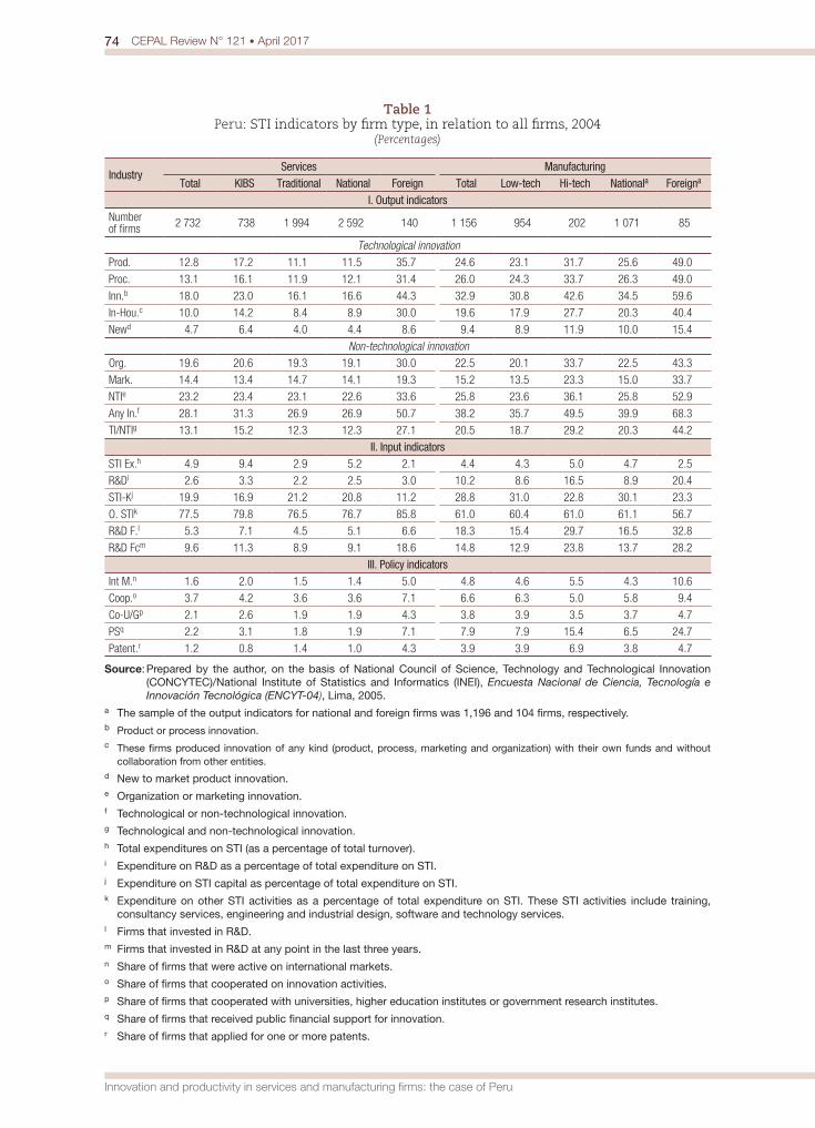
74 CEPAL Review N° 121 • April 2017
Innovation and productivity in services and manufacturing firms: the case of Peru
Table 1 Peru: STI indicators by firm type, in relation to all firms, 2004
(Percentages)
IndustryServices Manufacturing
Total KIBS Traditional National Foreign Total Low-tech Hi-tech Nationala Foreigna
I. Output indicators Number of firms 2 732 738 1 994 2 592 140 1 156 954 202 1 071 85
Technological innovationProd. 12.8 17.2 11.1 11.5 35.7 24.6 23.1 31.7 25.6 49.0
Proc. 13.1 16.1 11.9 12.1 31.4 26.0 24.3 33.7 26.3 49.0
Inn.b 18.0 23.0 16.1 16.6 44.3 32.9 30.8 42.6 34.5 59.6
In-Hou.c 10.0 14.2 8.4 8.9 30.0 19.6 17.9 27.7 20.3 40.4
Newd 4.7 6.4 4.0 4.4 8.6 9.4 8.9 11.9 10.0 15.4
Non-technological innovationOrg. 19.6 20.6 19.3 19.1 30.0 22.5 20.1 33.7 22.5 43.3
Mark. 14.4 13.4 14.7 14.1 19.3 15.2 13.5 23.3 15.0 33.7
NTIe 23.2 23.4 23.1 22.6 33.6 25.8 23.6 36.1 25.8 52.9
Any In.f 28.1 31.3 26.9 26.9 50.7 38.2 35.7 49.5 39.9 68.3
TI/NTIg 13.1 15.2 12.3 12.3 27.1 20.5 18.7 29.2 20.3 44.2
II. Input indicatorsSTI Ex.h 4.9 9.4 2.9 5.2 2.1 4.4 4.3 5.0 4.7 2.5
R&Di 2.6 3.3 2.2 2.5 3.0 10.2 8.6 16.5 8.9 20.4
STI-Kj 19.9 16.9 21.2 20.8 11.2 28.8 31.0 22.8 30.1 23.3
O. STIk 77.5 79.8 76.5 76.7 85.8 61.0 60.4 61.0 61.1 56.7
R&D F.l 5.3 7.1 4.5 5.1 6.6 18.3 15.4 29.7 16.5 32.8
R&D Fcm 9.6 11.3 8.9 9.1 18.6 14.8 12.9 23.8 13.7 28.2
III. Policy indicatorsInt M.n 1.6 2.0 1.5 1.4 5.0 4.8 4.6 5.5 4.3 10.6
Coop.o 3.7 4.2 3.6 3.6 7.1 6.6 6.3 5.0 5.8 9.4
Co-U/Gp 2.1 2.6 1.9 1.9 4.3 3.8 3.9 3.5 3.7 4.7
PSq 2.2 3.1 1.8 1.9 7.1 7.9 7.9 15.4 6.5 24.7
Patent.r 1.2 0.8 1.4 1.0 4.3 3.9 3.9 6.9 3.8 4.7
Source: Prepared by the author, on the basis of National Council of Science, Technology and Technological Innovation (CONCYTEC)/National Institute of Statistics and Informatics (INEI), Encuesta Nacional de Ciencia, Tecnología e Innovación Tecnológica (ENCYT-04), Lima, 2005.
a The sample of the output indicators for national and foreign firms was 1,196 and 104 firms, respectively. b Product or process innovation. c These firms produced innovation of any kind (product, process, marketing and organization) with their own funds and without
collaboration from other entities.d New to market product innovation.e Organization or marketing innovation.f Technological or non-technological innovation.g Technological and non-technological innovation. h Total expenditures on STI (as a percentage of total turnover).i Expenditure on R&D as a percentage of total expenditure on STI.j Expenditure on STI capital as percentage of total expenditure on STI.k Expenditure on other STI activities as a percentage of total expenditure on STI. These STI activities include training,
consultancy services, engineering and industrial design, software and technology services.l Firms that invested in R&D. m Firms that invested in R&D at any point in the last three years.n Share of firms that were active on international markets.o Share of firms that cooperated on innovation activities.p Share of firms that cooperated with universities, higher education institutes or government research institutes. q Share of firms that received public financial support for innovation. r Share of firms that applied for one or more patents.
75CEPAL Review N° 121 • April 2017
Mario D. Tello
These firms’ real value added12 (at 1994 prices) represented 31.9% of total value added for both sectors in 2004: 33.3% for the services sector and 27.4% for manufacturing.13 The main features of the figures in table 1 are the following: first, the share of the number of firms that innovate (either technological and non-technological innovation or both) was greater for manufacturing firms (38.2%) than for services (28.1%). However, services firms did have a greater share of NTI innovation than TI innovation. The opposite was true of manufacturing firms.
The share of foreign-owned firms (i.e. those with more than 10% of capital foreign-owned) that innovate was greater than that of nationally owned firms in both sectors. Second, firms’ investment intensity ratio (measured as the share of expenditure on STI activities out of total sales) was slightly higher for services (4.9%) than for manufacturing (4.4%). KIBS and high-tech manufacturing had the highest ratios (9.4% and 5%, respectively). Further, national firms’ STI investment ratios were higher than foreign firms in both the manufacturing and services sectors. On the other hand, the share of firms that performed innovation on a continuous basis in manufacturing (14.8%) was higher than in services (9.6%). More than 50% of the total STI expenditures in both sectors went to STI activities related to training, consultancy services, engineering and industrial design, software and technology services.
Third, and from the policy standpoint, firms in general did not collaborate with other entities for innovation purposes. In any case, the share of manufacturing firms that did collaborate (6.1%) was higher than the respective share for services firms (3.7%). The same low shares apply for firms’ international exposure, with manufacturing firms showing a higher share (4.8%) than services firms (1.6%). Similar figures are obtained for the share of firms that held patents. A higher share of foreign than domestic firms collaborated with respect to patent applications and international exposure in both sectors. Finally, the share of firms receiving public financial support for innovation was higher for manufacturing (7.9%) than for services (2.2%). Unexpectedly, the share of foreign firms receiving public financial support was greater than the respective share of domestic firms in both sectors.
Summing up, the 2004 figures for firms’ STI activities are consistent with Peru’s low STI investment indicators, even for 2012. Although a third of the interviewed firms in the sample do not perform STI activities, the average amount spent on these activities per worker in both sectors was US$ 2,353 (in constant 1994 dollars), which is less than US$ 6.5 dollars per day per worker. The extent to which this small amount affects firms’ performances (such as labour productivity) is investigated in the following sections.
IV. CDM models and estimation strategy
The CDM model to be estimated has the following equations:
ID*i=X1i.b1+a1.FCi+e1i; where if ID*i > μi then DIDi=1; otherwise DIDi=0; (1)
IE*i=X2i.b2+α2.FCi+e2i; where IE*i=IEi si ID*i ≥ μi; i.e., DIDi=1; otherwise IE*i=0; (2)
TI*i=d.IE*i+X3i.b3+e3i; where DTIi=1 si TI*i >0, DTIi=0 otherwise DTIi is zero; (3)
NTI*i=d.IE*i +X4i.b4+e4i; where DTIi=1 si TI*i >0, DNIi=0 otherwise DTIi is zero; (4)
lnProdi=j1.TI*i+ j2.NTIi+j3. IE*i+X5i.b5+e5i (5)
12 Firms’ value added comes from sales data. These are obtained using the average ratio of value added over value of production of the respective ISIC sector from the input output tables of 1994 and 2007 provided on a preliminary basis by INEI.
13 For the four ISIC groups, the shares of the real value of the firms out of the respective real value of the universe were: for KIBS, 21.19%; for traditional services, 43.79%; for high-tech firms, 22.44%; and for low-tech firms, 27.37%. In the case of formal employment, the figures are KIBS, 12.53%; traditional services, 18.87%; low-tech manufacturers, 24.25%; and high-tech manufacturers, 23.56%.
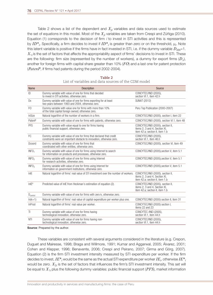
76 CEPAL Review N° 121 • April 2017
Innovation and productivity in services and manufacturing firms: the case of Peru
Table 2 shows a list of the dependent and Xji variables and data sources used to estimate the set of equations in this model. Most of the Xji variables are taken from Crespi and Zúñiga (2010). Equation (1) corresponds to the decision of firm i to invest in STI activities and this is represented by ID*i. Specifically, a firm decides to invest if ID*i is greater than zero or on the threshold, μi. Note this latent variable is positive if the firms have in fact invested in STI, i.e. if the dummy variable DIDi=1. X1i is the set of factors that affects the appropriability aspect of firms’ decisions to invest in STI. These are the following: firm size (represented by the number of workers), a dummy for export firms (Dx), another for foreign firms with capital share greater than 10% (FO) and a last one for patent protection (PatenP, if firms had patents during the period 2002-2004).
Table 2 List of variables and data sources of the CDM model
Name Description Source
ID Dummy variable with value of one for firms that decided to invest in STI activities, otherwise zero.
CONCYTEC/INEI (2005), section VI.1, item 42.h
Dx Dummy variable with value of one for firms exporting for at least two years between 1993 and 2004, otherwise zero.
SUNAT (2012)
FO Dummy variable with value one for firms with more than 10% of the total capital foreign owned; otherwise zero.
Peru Top Publication (2000-2007)
lnSize Natural logarithm of the number of workers in a firm. CONCYTEC/INEI (2005), section I, item 22
PatenP Dummy variable with value of one for firms with patents, otherwise zero. CONCYTEC/INEI (2005), section VI.1, item 48
PFS Dummy variable with value equal to one for firms having public financial support, otherwise zero.
CONCYTEC/INEI (2005), section II, items 2, 3 and 4, Section XI, item 42.a; section II, item 1.b
FC Dummy variable with value of one for firms that declared that credit constraints were an important obstacle to innovation, otherwise zero.
CONCYTEC/INEI (2005), section VI.1, item 46.h
Dcoord Dummy variable with value of one for firms that coordinated with other entities, otherwise zero.
CONCYTEC/INEI (2005), section VI, item 49
INFO1 Dummy variable with value of one for firms using Internet to search for information on products and processes, otherwise zero.
CONCYTEC/INEI (2005),section V, item 5.1
INFO2 Dummy variable with value of one for firms using Internet for research activities, otherwise zero.
CONCYTEC/INEI (2005),section V, item 5.1
INFO3 Dummy variable with value of one for firms using Internet for information on government institutions, otherwise zero.
CONCYTEC/INEI (2005),section V, item 5.1
lnIE Natural logarithm of firms’ real value of STI investment over the number of workers. CONCYTEC/INEI (2005), section II, items 2, 3 and 4, Section XI, item 42.a; section II, item 1.b
lnIEe Predicted value of lnIE from Heckman’s estimation of equation (2). CONCYTEC/INEI (2005), section II, items 2, 3 and 4, Section XI, item 42.a; section II, item 1.b
Dcontrol Dummy variable with value of one for firms with zero k, otherwise zero.
ln(k+1) Natural logarithm of firms’ real value of capital expenditure per worker plus one. CONCYTEC/INEI (2005) section II, item 31
lnProd Natural logarithm of firms’ real value per worker. CONCYTEC/INEI (2005) section I, items 22 and 23
TI Dummy variable with value of one for firms having technological innovation, otherwise zero.
CONCYTEC /INEI (2005), section VI.1, item 44.h
NTI Dummy variable with value of one for firms having non-technological innovation, otherwise zero.
CONCYTEC/INEI (2005), section VI.1, item 44.h
Source: Prepared by the author.
These variables are consistent with several arguments considered in the literature (e.g. Crepon, Duguet and Mairesse, 1998; Braga and Willmore, 1991; Kumar and Aggarwal, 2005; Álvarez, 2001; Cohen and Klepper, 1996; Benavente, 2006; Crespi and Peirano, 2007; Girma and Görg, 2007). Equation (2) is the firm STI investment intensity measured by STI expenditure per worker. If the firm decides to invest, IE*i would be the same as the actual STI expenditure per worker IEi, otherwise IE*i would be zero. X2i is the set of factors that influences the firm’s STI investment intensity. This set will be equal to X1i plus the following dummy variables: public financial support (PFS), market information
77CEPAL Review N° 121 • April 2017
Mario D. Tello
sources (INFO1), scientific information sources (INFO2), government institutions information INFO3) and the degree of coordination, cooperation, or collaboration between firm i and other entities (Dcoord).
Such factors are found in several studies for Latin America, for example, for Mexico and Argentina (Raffo, Lhuillery and Miotti, 2008). Although arguments based on size (for example, exploitation of scale and scope economies) point out that size affects the investment intensity equation, empirical evidence demonstrates that it may affect investment decisions but not the intensity of STI investment. For that reason and for identification purposes, in this paper, size is included in equation (1) and excluded from equation (2). The Peruvian evidence shown below for the marginal effects of both equations supports these changes. Finally, the analysis of financial constraints supports the inclusion of this constraint in both equations (1) and (2).
Equations (3) and (4) represent the outcomes of the technological (TI*i) and non-technological (NTI*i) innovation process or the expected returns on innovation. The latent variables TI*i and NTI*i are positive if firms, in fact, have innovation outputs, i.e. if the dummy variable DTIi=1 or DNTIi=1.14 Both outputs are determined by IE*i and the set of factors X3i=X4i. The variables of this set include size and the two dummy variables of exports and foreign ownership. Hahn and Park (2010), Hanley and Monreal-Pérez (2011) and Ito (2011) present the argument for and evidence of a relationship between exports and innovation; evidence of the other two factors, foreign ownership and size, is provided by Crespi and Zúñiga (2010).
Equation (5) is the labour productivity of a firm (measured by firms’ real value added per worker) determined by both technological (TI) and non-technological innovation (NTI) outputs, investment in STI, and X4i, which includes size and the ratio capital stock per worker, lnki (in natural logarithm). Although the measurement of productivity has a variety of shortcomings, not only in products (Tybout, Katayama and Lu, 2009; Syverson, 2011) but also in services (Dean and Kunze, 1992; Griliches, 1992; Crepon, Duguet and Mairesse, 1998; Gallouj and Djellal, 2008; Gallouj and Savona, 2009; Crespi and Zuñiga, 2010; Biege and others, 2011), in this work, labour productivity was measured as the real value added (or net sales)15 per worker.16
In the estimations, quantity variables such as size, productivity and investment expenditure are transformed into natural logarithms. The rest of the variables (which are binary) are not transformed. In addition, branch heterogeneity of the four ISIC (Revision 3) groups is introduced through a binary variable ISICn, where n is the first digit of the ISIC branch. Note that for each group of firms, one ISIC branch is included in the constant to avoid problems of collinearity.
Given these transformations and dummy variables, the econometric strategy is composed of the following steps: first, investment decision and intensity equations are estimated using a generalized Tobit model estimation (or Heckman maximum likelihood estimation, assuming a normal joint distribution for the error terms of both equations). For the purposes of robustness, the two-step Heckman procedure or Heckit estimator (which assumes conditional normal distributions for the error term) was estimated, although this is not reported owing to space limitations. The size variable included in the ID* equation and excluded in IE* equation allows identification of both equations. In addition PPS, Dcoord and the set of information variables reinforce the identifications of the parameters of both equations. Further,
14 NTI is a dummy variable equal to one if firms show innovation output results on commercialization and organization, otherwise zero.
15 Value added is obtained using the average ratio of value added over the value of production of the respective ISIC sector of the input output table for 1994 and 2007, which is provided on a preliminary basis to INEI.
16 The common problems associated with productivity and output measures are related to the relevant price deflators for computing real values and measures of product quality. In the services sector, measures of output will be restricted to the amount in value (sales or value added) of the transaction (following Griliches, 1992, and Gallouj and Savona, 2009). The characteristics of services output represented by the so called IHIP-criteria (intangibility, I; heterogeneity, H; inseparability, I; and perishability, P) and other considerations (for example in KIBS) pointed out by Biege and others (2011) (such as the innovativeness of the output; the “internal output”, input figures and knowledge) will not be taken into account due to restrictions in the data.
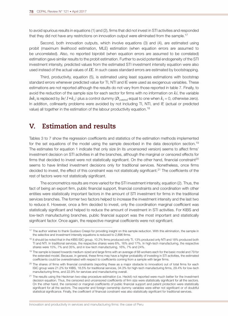
78 CEPAL Review N° 121 • April 2017
Innovation and productivity in services and manufacturing firms: the case of Peru
to avoid spurious results in equations (1) and (2), firms that did not invest in STI activities and responded that they did not have any restrictions on innovation output were eliminated from the sample.17
Second, both innovation outputs, which involve equations (3) and (4), are estimated using probit (maximum likelihood estimation, MLE) estimation (when equation errors are assumed to be uncorrelated). Also, no reported biprobit (when equation errors are assumed to be correlated) estimation gave similar results to the probit estimation. Further to avoid potential endogeneity of the STI investment intensity, predicted values from the estimated STI investment intensity equation were also used instead of the actual values of IE. In such cases standard errors are estimated by bootstrapping.
Third, productivity, equation (5), is estimated using least squares estimations with bootstrap standard errors whenever predicted value for TI, NTI and IE were used as exogenous variables. These estimations are not reported although the results do not vary from those reported in table 7. Finally, to avoid the reduction of the sample size for each sector for firms with no information on ki, the variable lnki is replaced by ln(1+ki) plus a control dummy (Dcontrol equal to one when ki = 0, otherwise zero). In addition, collinearity problems were avoided by not including TI, NTI, and IE (actual or predicted value) all together in the estimation of the labour productivity equation.18
V. Estimation and results
Tables 3 to 7 show the regression coefficients and statistics of the estimation methods implemented for the set equations of the model using the sample described in the data description section.19
The estimates for equation 1 indicate that only size (in its uncensored version) seems to affect firms’ investment decision on STI activities in all the branches, although the marginal or censored effects for firms that decided to invest were not statistically significant. On the other hand, financial constraint20
seems to have limited investment decisions only for traditional services. Nonetheless, once firms decided to invest, the effect of this constraint was not statistically significant.21 The coefficients of the rest of factors were not statistically significant.
The econometrics results are more varied for the STI investment intensity, equation (2). Thus, the fact of being an export firm, public financial support, financial constraints and coordination with other entities were statistically important factors in the amount of STI investment for firms in the traditional services branches. The former two factors helped to increase the investment intensity and the last two to reduce it. However, once a firm decided to invest, only the coordination marginal coefficient was statistically significant and helped to reduce the amount of investment in STI activities. For KIBS and low-tech manufacturing branches, public financial support was the most important and statistically significant factor. Once again, the respective marginal coefficients were not significant.
17 The author wishes to thank Gustavo Crespi for providing insight on this sample reduction. With this elimination, the sample in the selective and investment intensity equations is reduced to 2,896 firms.
18 It should be noted that in the KIBS ISIC group, 10.2% firms produced only TI, 13% produced only NTI and 18% produced both TI and NTI. In traditional services, the respective shares were 6%, 16% and 17%. In high-tech manufacturing, the respective shares were 15%, 7% and 35%, and in low-tech manufacturing, 16%, 7% and 24%.
19 The sample is biased towards medium-sized and large firms with an average of 68 workers each for the basic model and 79 for the extended model. Because, in general, these firms may have a higher probability of investing in STI activities, the estimated coefficients could be overestimated with respect to coefficients coming from a sample with larger firms.
20 The shares of firms with financial constraints (reporting these as a major obstacle to innovation) out of total firms for each ISIC group were 21.2% for KIBS, 18.5% for traditional services, 34.3% for high-tech manufacturing firms, 29.4% for low-tech manufacturing firms, and 22.9% for services and manufacturing overall.
21 The results using the Heckman two-step procedure estimation (i.e. Heckit) not reported were much better for the investment decision equation. Thus, the censored and uncensored coefficients of firm size were statistically significant for all the sectors. On the other hand, the censored or marginal coefficients of public financial support and patent protection were statistically significant for all the sectors. The exporter and foreign ownership dummy variables were either not significant or of doubtful statistical significance. Finally, the coefficient of financial constraint was also statistically significant for traditional services.
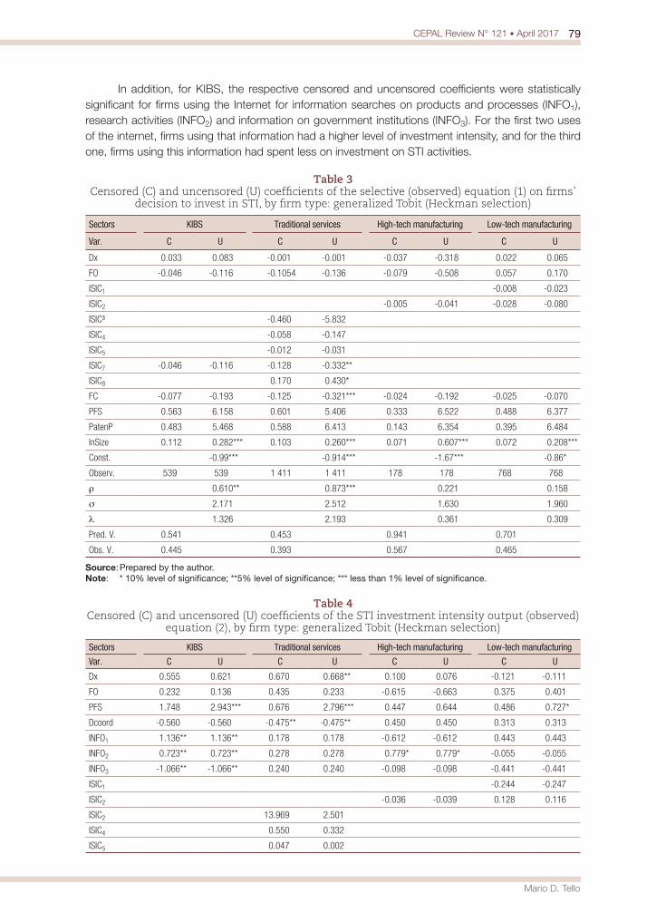
79CEPAL Review N° 121 • April 2017
Mario D. Tello
In addition, for KIBS, the respective censored and uncensored coefficients were statistically significant for firms using the Internet for information searches on products and processes (INFO1), research activities (INFO2) and information on government institutions (INFO3). For the first two uses of the internet, firms using that information had a higher level of investment intensity, and for the third one, firms using this information had spent less on investment on STI activities.
Table 3 Censored (C) and uncensored (U) coefficients of the selective (observed) equation (1) on firms’
decision to invest in STI, by firm type: generalized Tobit (Heckman selection)
Sectors KIBS Traditional services High-tech manufacturing Low-tech manufacturing
Var. C U C U C U C U
Dx 0.033 0.083 -0.001 -0.001 -0.037 -0.318 0.022 0.065
FO -0.046 -0.116 -0.1054 -0.136 -0.079 -0.508 0.057 0.170
ISIC1 -0.008 -0.023
ISIC2 -0.005 -0.041 -0.028 -0.080
ISIC³ -0.460 -5.832
ISIC4 -0.058 -0.147
ISIC5 -0.012 -0.031
ISIC7 -0.046 -0.116 -0.128 -0.332**
ISIC8 0.170 0.430*
FC -0.077 -0.193 -0.125 -0.321*** -0.024 -0.192 -0.025 -0.070
PFS 0.563 6.158 0.601 5.406 0.333 6.522 0.488 6.377
PatenP 0.483 5.468 0.588 6.413 0.143 6.354 0.395 6.484
lnSize 0.112 0.282*** 0.103 0.260*** 0.071 0.607*** 0.072 0.208***
Const. -0.99*** -0.914*** -1.67*** -0.86*
Observ. 539 539 1 411 1 411 178 178 768 768
ρ 0.610** 0.873*** 0.221 0.158
σ 2.171 2.512 1.630 1.960
l 1.326 2.193 0.361 0.309
Pred. V. 0.541 0.453 0.941 0.701
Obs. V. 0.445 0.393 0.567 0.465
Source: Prepared by the author.Note: * 10% level of significance; **5% level of significance; *** less than 1% level of significance.
Table 4 Censored (C) and uncensored (U) coefficients of the STI investment intensity output (observed)
equation (2), by firm type: generalized Tobit (Heckman selection)
Sectors KIBS Traditional services High-tech manufacturing Low-tech manufacturing
Var. C U C U C U C U
Dx 0.555 0.621 0.670 0.668** 0.100 0.076 -0.121 -0.111
FO 0.232 0.136 0.435 0.233 -0.615 -0.663 0.375 0.401
PFS 1.748 2.943*** 0.676 2.796*** 0.447 0.644 0.486 0.727*
Dcoord -0.560 -0.560 -0.475** -0.475** 0.450 0.450 0.313 0.313
INFO1 1.136** 1.136** 0.178 0.178 -0.612 -0.612 0.443 0.443
INFO2 0.723** 0.723** 0.278 0.278 0.779* 0.779* -0.055 -0.055
INFO3 -1.066** -1.066** 0.240 0.240 -0.098 -0.098 -0.441 -0.441
ISIC1 -0.244 -0.247
ISIC2 -0.036 -0.039 0.128 0.116
ISIC2 13.969 2.501
ISIC4 0.550 0.332
ISIC5 0.047 0.002
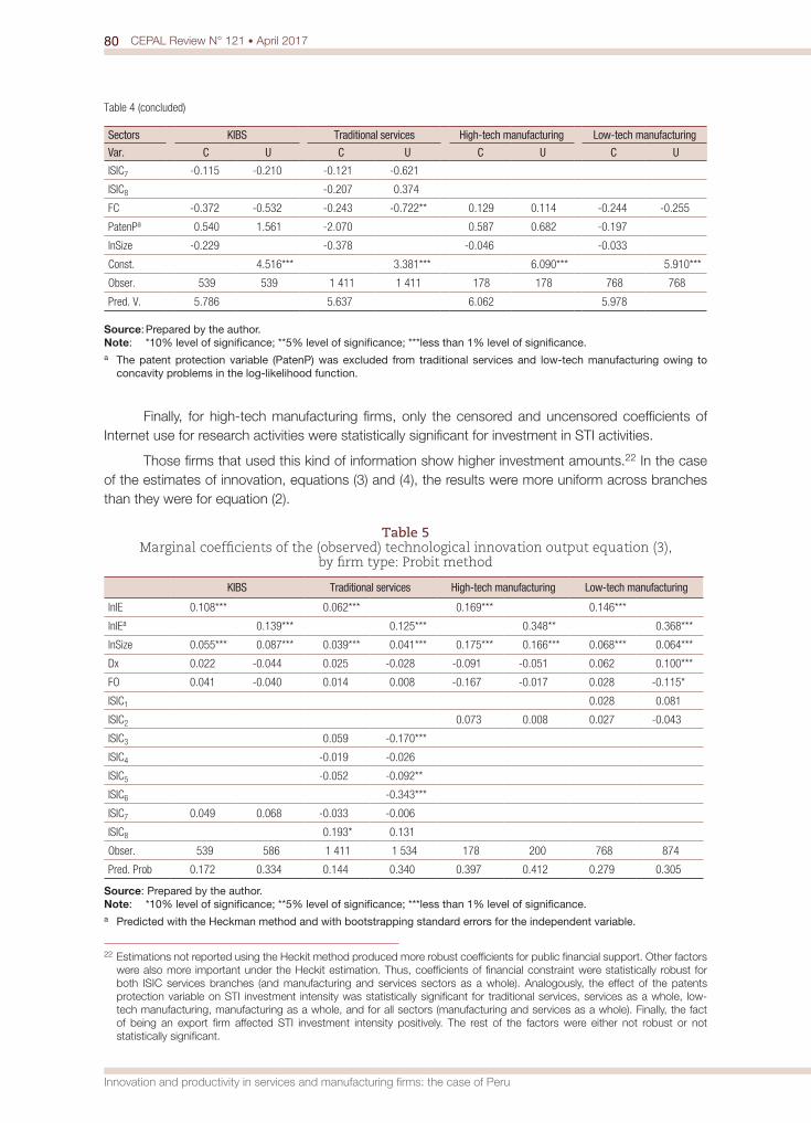
80 CEPAL Review N° 121 • April 2017
Innovation and productivity in services and manufacturing firms: the case of Peru
Sectors KIBS Traditional services High-tech manufacturing Low-tech manufacturing
Var. C U C U C U C U
ISIC7 -0.115 -0.210 -0.121 -0.621
ISIC8 -0.207 0.374
FC -0.372 -0.532 -0.243 -0.722** 0.129 0.114 -0.244 -0.255
PatenPa 0.540 1.561 -2.070 0.587 0.682 -0.197
lnSize -0.229 -0.378 -0.046 -0.033
Const. 4.516*** 3.381*** 6.090*** 5.910***
Obser. 539 539 1 411 1 411 178 178 768 768
Pred. V. 5.786 5.637 6.062 5.978
Source: Prepared by the author.Note: *10% level of significance; **5% level of significance; ***less than 1% level of significance. a The patent protection variable (PatenP) was excluded from traditional services and low-tech manufacturing owing to
concavity problems in the log-likelihood function.
Finally, for high-tech manufacturing firms, only the censored and uncensored coefficients of Internet use for research activities were statistically significant for investment in STI activities.
Those firms that used this kind of information show higher investment amounts.22 In the case of the estimates of innovation, equations (3) and (4), the results were more uniform across branches than they were for equation (2).
Table 5 Marginal coefficients of the (observed) technological innovation output equation (3),
by firm type: Probit method
KIBS Traditional services High-tech manufacturing Low-tech manufacturing
lnIE 0.108*** 0.062*** 0.169*** 0.146***
lnIEa 0.139*** 0.125*** 0.348** 0.368***
lnSize 0.055*** 0.087*** 0.039*** 0.041*** 0.175*** 0.166*** 0.068*** 0.064***
Dx 0.022 -0.044 0.025 -0.028 -0.091 -0.051 0.062 0.100***
FO 0.041 -0.040 0.014 0.008 -0.167 -0.017 0.028 -0.115*
ISIC1 0.028 0.081
ISIC2 0.073 0.008 0.027 -0.043
ISIC3 0.059 -0.170***
ISIC4 -0.019 -0.026
ISIC5 -0.052 -0.092**
ISIC6 -0.343***
ISIC7 0.049 0.068 -0.033 -0.006
ISIC8 0.193* 0.131
Obser. 539 586 1 411 1 534 178 200 768 874
Pred. Prob 0.172 0.334 0.144 0.340 0.397 0.412 0.279 0.305
Source: Prepared by the author. Note: *10% level of significance; **5% level of significance; ***less than 1% level of significance.a Predicted with the Heckman method and with bootstrapping standard errors for the independent variable.
22 Estimations not reported using the Heckit method produced more robust coefficients for public financial support. Other factors were also more important under the Heckit estimation. Thus, coefficients of financial constraint were statistically robust for both ISIC services branches (and manufacturing and services sectors as a whole). Analogously, the effect of the patents protection variable on STI investment intensity was statistically significant for traditional services, services as a whole, low-tech manufacturing, manufacturing as a whole, and for all sectors (manufacturing and services as a whole). Finally, the fact of being an export firm affected STI investment intensity positively. The rest of the factors were either not robust or not statistically significant.
Table 4 (concluded)
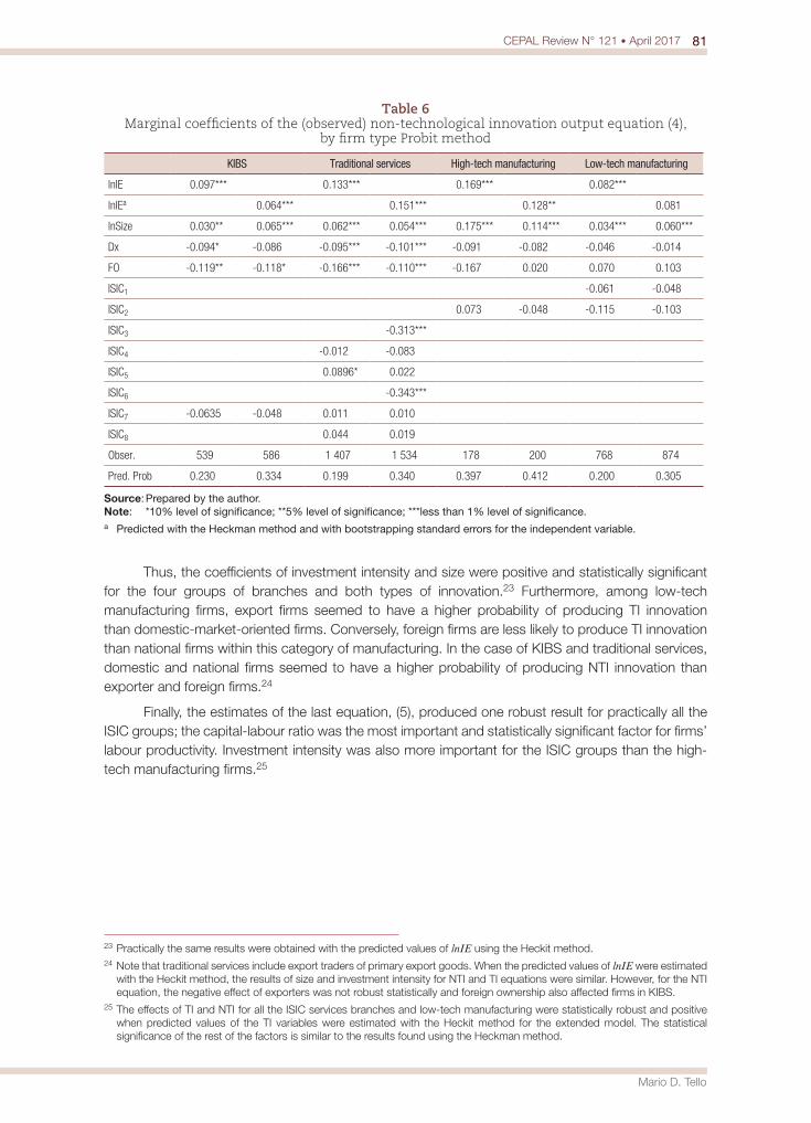
81CEPAL Review N° 121 • April 2017
Mario D. Tello
Table 6 Marginal coefficients of the (observed) non-technological innovation output equation (4),
by firm type Probit method
KIBS Traditional services High-tech manufacturing Low-tech manufacturing
lnIE 0.097*** 0.133*** 0.169*** 0.082***
lnIEa 0.064*** 0.151*** 0.128** 0.081
lnSize 0.030** 0.065*** 0.062*** 0.054*** 0.175*** 0.114*** 0.034*** 0.060***
Dx -0.094* -0.086 -0.095*** -0.101*** -0.091 -0.082 -0.046 -0.014
FO -0.119** -0.118* -0.166*** -0.110*** -0.167 0.020 0.070 0.103
ISIC1 -0.061 -0.048
ISIC2 0.073 -0.048 -0.115 -0.103
ISIC3 -0.313***
ISIC4 -0.012 -0.083
ISIC5 0.0896* 0.022
ISIC6 -0.343***
ISIC7 -0.0635 -0.048 0.011 0.010
ISIC8 0.044 0.019
Obser. 539 586 1 407 1 534 178 200 768 874
Pred. Prob 0.230 0.334 0.199 0.340 0.397 0.412 0.200 0.305
Source: Prepared by the author. Note: *10% level of significance; **5% level of significance; ***less than 1% level of significance. a Predicted with the Heckman method and with bootstrapping standard errors for the independent variable.
Thus, the coefficients of investment intensity and size were positive and statistically significant for the four groups of branches and both types of innovation.23 Furthermore, among low-tech manufacturing firms, export firms seemed to have a higher probability of producing TI innovation than domestic-market-oriented firms. Conversely, foreign firms are less likely to produce TI innovation than national firms within this category of manufacturing. In the case of KIBS and traditional services, domestic and national firms seemed to have a higher probability of producing NTI innovation than exporter and foreign firms.24
Finally, the estimates of the last equation, (5), produced one robust result for practically all the ISIC groups; the capital-labour ratio was the most important and statistically significant factor for firms’ labour productivity. Investment intensity was also more important for the ISIC groups than the high-tech manufacturing firms.25
23 Practically the same results were obtained with the predicted values of lnIE using the Heckit method.24 Note that traditional services include export traders of primary export goods. When the predicted values of lnIE were estimated
with the Heckit method, the results of size and investment intensity for NTI and TI equations were similar. However, for the NTI equation, the negative effect of exporters was not robust statistically and foreign ownership also affected firms in KIBS.
25 The effects of TI and NTI for all the ISIC services branches and low-tech manufacturing were statistically robust and positive when predicted values of the TI variables were estimated with the Heckit method for the extended model. The statistical significance of the rest of the factors is similar to the results found using the Heckman method.
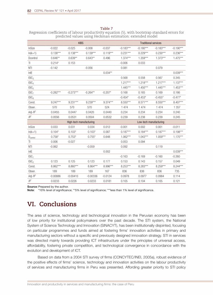
82 CEPAL Review N° 121 • April 2017
Innovation and productivity in services and manufacturing firms: the case of Peru
Table 7 Regression coefficients of labour productivity equation (5), with bootstrap standard errors for
predicted values using Heckman estimation: extended model
KIBS Traditional services
lnSize -0.022 -0.025 -0.008 -0.037 -0.183*** -0.180*** -0.183*** -0.190***
ln(k+1) 0.138*** 0.138*** 0.139*** 0.119*** 0.231*** 0.229*** 0.230*** 0.236***
Dcontrol 0.646** 0.639** 0.643** 0.496 1.374*** 1.359*** 1.373*** 1.475***
TI 0.214* 0.153 -0.006 0.033
NTI -0.142 -0.056 0.081 0.079
lnIE 0.034** 0.039***
ISIC3 0.568 0.558 0.567 0.345
ISIC4 1.217*** 1.218*** 1.217*** 1.137***
ISIC5 1.445*** 1.450*** 1.445*** 1.453***
ISIC7 -0.282*** -0.273*** -0.264** -0.207* 0.168 0.165 0.169 0.186
ISIC8 -0.454* -0.453* -0.455* -0.477*
Const. 9.247*** 9.231*** 9.239*** 9.374*** 8.550*** 8.571*** 8.550*** 8.407***
Obser. 570 570 570 524 1 474 1 474 1 474 1 357
Adj-R2 0.0455 0.0447 0.0420 0.0440 0.234 0.234 0.234 0.240
R2 0.0556 0.0531 0.0504 0.0532 0.239 0.238 0.239 0.245
High-tech manufacturing Low-tech manufacturing
lnSize 0.033 0.031 0.034 0.012 -0.001 0.002 0.001 -0.011
ln(k+1) 0.104* 0.103* 0.103* 0.087 0.187*** 0.184*** 0.187*** 0.198***
Dcontrol 0.758* 0.753* 0.755* 0.648 1.062*** 1.043*** 1.059*** 1.170***
TI 0.006 -0.027 0.053 0.094
NTI -0.062 -0.059 0.092 0.119
lnIE 0.002 0.039***
ISIC1 -0.163 -0.169 -0.160 -0.260
ISIC2 0.123 0.125 0.123 0.177 0.153 0.143 0.157 0.049
Const. 8.862*** 8.860*** 8.864*** 8.996*** 8.253*** 8.283*** 8.259*** 8.244***
Obser. 189 189 189 167 836 836 836 735
Adj-R2 -0.00886 -0.00410 -0.00336 -0.0124 0.0978 0.0977 0.0984 0.114
R2 0.0233 0.0226 0.0233 0.0181 0.105 0.104 0.105 0.121
Source: Prepared by the author. Note: *10% level of significance; **5% level of significance; ***less than 1% level of significance.
VI. Conclusions
The area of science, technology and technological innovation in the Peruvian economy has been of low priority for institutional policymakers over the past decade. The STI system, the National System of Science Technology and Innovation (SINACYT), has been institutionally disjointed, focusing on particular programmes and funds aimed at fostering firms’ innovation activities in primary and manufacturing sectors without a specific and previously designed innovation strategy. STI in services was directed mainly towards providing ICT infrastructure under the principles of universal access, affordability, fostering private competition, and technological convergence in concordance with the evolution and development of ICT.
Based on data from a 2004 STI survey of firms (CONCYTEC/INEI, 2005a), robust evidence of the positive effects of firms’ science, technology and innovation activities on the labour productivity of services and manufacturing firms in Peru was presented. Affording greater priority to STI policy
83CEPAL Review N° 121 • April 2017
Mario D. Tello
and its effective implementation in Peru could thus improve the poor performance of the past decade and spur productivity growth (Tello, 2012b). Two CDM models were estimated with methods that overcome selection and endogeneity problems.
The statistical results in general partially support some of the hypotheses found in the literature. Specifically, firm size seems to be a key determinant for decisions to invest in STI activities in all the seven ISIC groups considered in the analysis. However, for those firms motivated to invest, patent protection, particularly for manufacturing firms, was a determining factor for effective investment. At the same time, financial constraints influenced firms’ decisions to invest or not in STI activities only in the traditional services ISIC group. Further, for those firms that decided to invest in STI activities, the statistical significance of financial constraints vanished, implying that the financial factor was a major restraint only for firms that ultimately did not invest. Second, although public financial support seems to increase the latent variable of firms’ investment intensity for most of the ISIC groups (with the exception of firms from high-tech manufacturing branches), the effect on the actual investment intensity (measured through the expenditures on STI activities per worker) was not statistically significant for firms that invested in STI activities. This means that public support policies seem to have more of an inducement effect (making non-spending firms spend) than an intensive margin effect (increasing intensity by firms already spending). The same result is obtained for financial constraints in the traditional services ISIC group. The effect of other factors on firms’ STI investment intensity was also statistically robust for some ISIC groups. Specifically, Internet information on products and processes for KIBS and services as whole and for all (manufacturing and services) firms in the sample; Internet information on research activities for KIBS, high-tech manufacturing, traditional services and both sectors (services and manufacturing) overall; and firms’ coordination with other entities on innovation purposes for traditional services and total services.
Third, across all the ISIC groups, firm size and investment intensity were the key determinants for producing both technological and non-technological innovation outputs. In some ISIC groups (such as services and low-tech manufacturing), domestic-market-oriented and national firms had a higher probability of producing technological and non-technological innovation outputs than did exporters and foreign-owned firms. This result may indicate a greater need to produce technological changes in order to compete with export and foreign firms in the first group of firms. Last, capital per worker and STI investment intensity affected the labour productivity of firms positively for most of ISIC groups (with the exception of the high-tech manufacturing group).
From the perspective of economic policy, these results suggest that horizontal STI policies (at least for services and manufacturing branches) that encourage firms to increase their STI investment intensity may well produce some gains in firms’ labour productivity. However, given that innovation outputs showed no statistical effect on productivity, it appears necessary to conduct a detailed, micro-level analysis of what firms consider innovation output and to obtain information about the kinds of innovation outputs that can increase labour productivity. Finally, the fact that most firms’ STI activities are undertaken in an isolated fashion —i.e. production of innovation of any kind, whether product, process, marketing or organizational, is carried out with firms’ own funds and without collaboration from other entities— and the statistical non-significance of the effect of firms’ coordination with other entities on STI investment intensity indicate the need to exploit firms’ interactions with other firms, research institutions and government in order to increase the probability of producing innovation26 and reducing firms’ STI expenditure per worker.
26 See this result in Tello (2011).
84 CEPAL Review N° 121 • April 2017
Innovation and productivity in services and manufacturing firms: the case of Peru
BibliographyÁlvarez, R. (2001), “External sources of technological innovation in Chilean manufacturing industry”, Estudios
de Economía, vol. 28, No. 1, Santiago, University of Chile.Álvarez, R. and G. Crespi (2011), “Financing Gaps, Innovation Gaps? New Evidence from Chile”, unpublished.Balboni, M., S. Rovira and S. Vergara (eds.) (2011), ICT in Latin America: A Micro-Data Analysis (LC/R.2172),
Santiago, Economic Commission for Latin America and the Caribbean (ECLAC).Benavente M.J. (2006), “The role of research and innovation in promoting productivity in Chile”, Economics
of Innovation and New Technology, vol. No. 4-5, Taylor & Francis.Biege, S. and others (2011), “Challenges of measuring service productivity in innovative, knowledge-intensive
business services”, Karlsruhe, Fraunhofer Institute for Systems and Innovation Research (ISI). Braga, H. and L. Willmore (1991), “Technological imports and technological effort: an analysis of their
determinants in Brazilian firms”, Journal of Industrial Economics, vol. 39, No. 4, Wiley.Cainelli, G., R. Evangelista and M. Savona (2006), “Innovation and economic performance in services: a firm-
level analysis”, Cambridge Journal of Economics, vol. 30, No. 3, Oxford University Press. Carayannis, E., U. Varblane and T. Roolaht (2012), “Innovation systems in small catching-up economies. New
perspectives on practice and policy”, Innovation, Technology, and Knowledge Management, vol. 15, Springer.Cohen, W. and S. Klepper (1996), “Firm size and the nature of innovation within industries: the case of process
and product R&D”, The Review of Economics and Statistics, vol. 78, No. 2, Cambridge, Massachusetts, The MIT Press.
Comisión Consultiva para la Ciencia, Tecnología e Innovación (2012), “Nueva política e institucionalidad para dinamizar la CTI peruana” [online] http://franciscosagasti.com/descargas/eventos/ff-informe-comision-consultiva-cti.pdf.
CONCYTEC/INEI (National Council of Science, Technology and Technological Innovation/National Institute of Statistics and Informatics) (2005a), Encuesta Nacional de Ciencia, Tecnología e Innovación Tecnológica (ENCYT-04), Lima.(2005b), “Análisis de la Encuesta Nacional de Ciencia, Tecnología e Innovación Tecnológica, 2004”, Lima, unpublished.
Crepon, B., E. Duguet and J. Mairesse (1998), “Research, innovation and productivity: an econometric analysis at the firm level”, Economics of Innovation and New Technology, vol. 7, No. 2, Taylor & Francis.
Crespi, G. and P. Zúñiga (2010), “Innovation and productivity: evidence from six Latin American countries”, IDB Working Paper Series, No. IDB-WP-218, Washington, D.C., Inter-American Development Bank.
Crespi, G. and others (2006), “Measuring and understanding productivity in UK market services”, Oxford Review of Economic Policy, vol. 22, No. 4, Oxford University Press.
Crespi, G. and F. Peirano. (2007), “Measuring innovation in Latin America what we did where we are and what we want to do”, paper prepared for the Conference on Micro Evidence on Innovation in Developing Countries, Maastricht.
Dean, E. and K. Kunze (1992), “Productivity measurement in service industries”, Z. Griliches (ed.), Output Measurement in the Service Sectors, Chicago, University of Chicago Press.
European Commission (2011), “Policies in support of service innovation”, Global Review of Innovation Policy Sytudies INNO-Grips, INNO-Grips Policy Brief, No. 3, Budapest, ICEG European Center.
Evangelista, R. and M. Savona (2003), “Innovation, employment and skills in services: firm and sectoral evidence”, Structural Change and Economic Dynamics, vol. 14, No. 4, Amsterdam, Elsevier.
Gallouj, F. (2002), Innovation in the Service Economy: The New Wealth of Nations. Northampton, Edward Elgar Publishing.
Gallouj, F. and F. Djellal (2010), The Handbook of Innovation and Services, Northampton, Edward Elgar Publishing.(2008), Measuring and Improving Productivity in Services. Issues, Strategies and Challenges, Cheltenham, Edward Elgar Publishing.
Gallouj, F. and M. Savona (2009), “Innovation in services: a review of the debate and a research agenda”, Journal of Evolutionary Economics, vol. 19, No. 2, Springer.
Gallouj, F. and O. Weinstein (1997), “Innovation in services”, Research Policy, vol. 26, No. 4–5, Amsterdam, Elsevier.Garrido, C. (2009), “La innovación en los servicios: aspectos generales y los casos de los servicios de
telecomunicaciones, turismo y bancario y bancario”, Project Document (LC/W.286), Santiago, Economic Comission for Latin America and the Caribbean (ECLAC).
Girma S. and H. Görg (2007), “The role of the efficiency gap for spillovers from FDI: evidence from the UK electronics and engineering sectors”, Open Economies Review, vol. 18, No. 2, Springer.
85CEPAL Review N° 121 • April 2017
Mario D. Tello
Griliches Z. (1992), Output Measurement in the Service Sectors, Chicago, The University of Chicago Press.(1979), “Issues in assessing the contribution of research and development to productivity growth”, Bell Journal of Economics, vol. 10, No. 1, The RAND Corporation.
Griliches, Z. and A. Pakes (1980), “Patents and R&D at the firm level: a first look”, NBER Working Paper, No. 561, Cambridge, Massachusetts, National Bureau of Economic Research.
Hahn, C. and C. Park (2010), “Direction of causality in innovation-exporting linkage: evidence on Korean manufacturing”, ERIA Discussion Paper, No. 2012-07.
Hall, B. (2011), “Innovation and productivity”, NBER Working Paper, No. 17178, Cambridge, Massachusetts, National Bureau of Economic Research.
Hanley, A. and J. Monreal-Pérez (2011), “Are newly exporting firms more innovative? Findings from matched Spanish innovators”, Kiel Working Paper, No. 1735, Kiel, Kiel Institute of World Economics.
INEI (National Institute of Statistics and Informatics) (2005), “Encuesta económica anual. 2005: estadística manufacturera”, Lima.
Ito, K. (2011), “Sources of learning-by-exporting effects: does exporting promote innovation?”, RIETI Discussion Papers Series, No. 11066.
Kumar, N. and A. Aggarwal (2005), “Liberalization, outward orientation and in-house R&D activity of multinational and local firms: a quantitative exploration for Indian manufacturing”, Research Policy, vol. 34, No. 4, Amsterdam, Elsevier.
Kuramoto, J. (2008), “Propuesta de Agenda de Investigación para el Programa de Ciencia y Tecnología– FINCYT”, Lima [online] http://www.innovateperu.gob.pe/fincyt/doc/CIES/Propuesta-Agenda-Investigacion.pdf.(2007), “Retos del Plan Nacional de Ciencia, Tecnología e Innovación Tecnológica para la Competitividad y Desarrollo Humano”, unpublished.
Kuramoto, J. and J. Díaz (2011), “Aportes para el gobierno peruano 2011-2016: Políticas de ciencia, tecnología e innovación”, Elecciones 2011 Perú: centrando el debate electoral, No. 14, Lima.(2010), Evaluación de políticas de apoyo a la innovación en el Perú, Lima, Group for the Analysis of Development (GRADE).
Llisteri, J. and J. García-Alba (2008), “High-growth SMEs in Latin American emerging economies”, Technical Notes, No. IDB-TN-133, Washington, D.C., Inter-American Development Bank.
Masso, J. and P. Vahter (2011), The Link Between Innovation and Productivity in Estonian Service Sector, University of Tartu.
Mairesse, J. and P. Mohnen (2010), Using Innovations Surveys for Econometric Analysis, NBER Working Paper, No. 15857, Cambridge, Massachusetts, National Bureau of Economic Research.
Mairesse, J. and M. Sassenou (1991), “R&D and productivity: a survey of econometric studies at the firm level”, Science-Technology-Industry Review, No. 8, Paris, Organization for Economic Cooperation and Development (OECD).
Mohnen, P. and L.H. Röller (2005), “Complementarities in innovation policy”, European Economic Review, vol. 49, No. 6, Amsterdam, Elsevier.
Mothe, C. and T.U. Nguyen Thi (2010.) “The impact of non-technological innovation on technological innovation: do services differ from manufacturing? An empirical analysis of Luxembourg firms”, CEPS/Instead Working Paper, No. 2010-01.
OECD (Organization for Economic Cooperation and Development) (2009), Innovation in Firms: A Microeconomic Perspective, Paris.
Peru Top Publications (2002-2007), Peru: The Top 10,000 Companies, Lima.SUNAT (Office of the National Superintendent of Tax Administration) (2012), Series estadísticas de
exportaciones, Lima. Raffo, J., S. Lhuillery and L. Miotti (2008), “Northern and Southern innovativity: a comparison across European
and Latin American countries”, European Journal of Development, vol. 20, No. 2, Taylor & Francis.Rubalcaba, L., D. Gago and J. Gallego (2010), “On the differences between goods and services innovation”,
Journal of Innovation Economics & Management, vol. 1, No. 5. Sagasti, F. (2011), En Busca del Tiempo Perdido: Ciencia, tecnología e innovación en el Perú, Lima, Foro
Nacional Internacional.Syverson, C. (2011), “What determines productivity?”, Journal of Economic Literature, vol. 49, No. 2, Nashville,
Tennessee, American Economic Association. Tacsir, E. and others (2011), “Innovation in services: the hard case for Latin America and the Caribbean”, IDB
Discussion Paper, No. IDB-DP-203, Washington, D.C., Inter-American Development Bank.
86 CEPAL Review N° 121 • April 2017
Innovation and productivity in services and manufacturing firms: the case of Peru
Tello, M.D. (2012a), “Balance y agenda de investigación en tema de la inserción de la economía internacional”, Balance y agenda de investigación en el Perú, Lima, CIES.(2012b), “Productividad total factorial en el sector manufacturero: un análisis a nivel de firmas del Perú, 2002-2007”, Economía, vol. 35, No. 70, Lima, Catholic University of Peru.(2011), “Science and technology, ICT and profitability in the manufacturing sector in Peru”, ICT in Latin America: A Micro-Data Analysis (LC/R.2172), M. Balboni, S. Rovira and S. Vergara (eds.), Santiago, Economic Commission for Latin America and the Caribbean (ECLAC).(2010), Políticas de tecnologías de información y comunicación en el Perú, 1990-2010”, Documentos de Trabajo, No. 335, Lima, Catholic University of Peru.
Tether, B.S. (2005), “Do services innovate (differently)? Insights from the European Innobarometer Survey”, Industry and Innovation, vol. 12, No. 2, Taylor & Francis.
Tybout, J., H. Katayama and S. Lu (2009), “Firm-level productivity studies: illusions and a solution”, International Journal of Industrial Organization, vol. 27, No. 3, Amsterdam, Elsevier.
UNCTAD/ECLAC (United Nations Conference on Trade and Development/Economic Commission for Latin America and the Caribbean) (2011), Science, Technology and Innovation Policy Review: Peru (UNCTAD/DTL/STICT/2010/2), Geneva.
World Bank (2013), World Development Indicators [online] http://data.worldbank.org/data-catalog/world-development-indicators.

Santiago Chile: city of cities? Social inequalities in local labour market zones1
Luis Fuentes, Oscar Mac-Clure, Cristóbal Moya and Camilo Olivos
Abstract
This article seeks to define and characterize the urban structure of Santiago, Chile, based on the relation between its inhabitants’ places of residency and work, which form local labour market zones. The article explains the criteria and methodological procedures used to define these zones, and it describes them on the basis of this functional definition, to determine the extent to which they underpin the social inequalities prevailing in the city. It also makes a spatial analysis of income inequality, access to education and the composition of the social classes.
Keywords
Cities, labour market, employment, domicile and residence, social classes, equality, income, education, socioeconomic indicators, Chile
JEL classification
J60, D63, Z13
Authors
Luis Fuentes is an academic at the Institute of Urban and Territorial Studies and a researcher at the Centre for Sustainable Urban Development (CEDEUS) of the Pontificia Universidad Católica de Chile. [email protected]
Oscar Mac-Clure is an academic at the Centre for Regional Development and Public Policy Studies (CEDER) at Universidad de Los Lagos, Chile. [email protected]
Cristóbal Moya teaches at the School of Sociology at Universidad Diego Portales, Chile. [email protected]
Camilo Olivos is a research assistant at the Institute of Urban and Territorial Studies of the Pontificia Universidad Católica de Chile. [email protected]
1 This article was produced with funding from the National Fund for Scientific and Technological Development of Chile (FONDECYT), under projects Nos. 1141157 and 1150808, and from the National Commission on Scientific and Technological Research (CONICYT) through CONICYT/FONDAP project No. 15110020.

88 CEPAL Review N° 121 • April 2017
Santiago Chile: city of cities? Social inequalities in local labour market zones
I. Introduction
Globalization has given rise to various transformations of world economic geography, in which cities have served to articulate the internationalization of domestic economies (Sassen, 2001). Latin American cities have not been immune from this process (De Mattos, 2010). The Chilean capital, Santiago, is a special case, owing to the country’s early integration into the global economy, and consequent changes in the function, morphology, and socio-spatial structure of the city over different periods.
Recent trends in the urban growth of Santiago have made its structure more complex, owing to processes that have been analysed in specific studies. Nonetheless, as will be seen below, further progress needs to be made in understanding the functional modalities, general characteristics, and inequalities displayed by the city. In this regard, the questions addressed in this paper relate to the spatial configuration of the relation between place of residency and work. Specifically, what is the functional structure of the city; and to what extent, and through what mechanisms, is this linked to urban inequalities? The specific aim is to identify possibilities for characterizing and analysing the evolution of the functional structure of the city and the trends that explain urban inequalities in recent years.
Based on the conclusions reached by various studies and the analysis of the varied dimensions of urban evolution, the article aims to contribute to the debate on the structure of Santiago, based on a classification of the social spaces using criteria related to place of work and residency, so as to define the boundaries of the city on an aggregate scale. In addition, labour market zones are defined by the relation between supply and demand for labour in the city space. To validate this methodology, its contribution to the characterization of the city is tested from the standpoint of social inequalities in income, education, classes and other relevant indicators.
We postulate that a spatial configuration based on the residency-work relation offers an overall image of the structure and functioning of a large city such as Santiago; and it has the advantage of helping to elucidate the social inequalities that exist within it. This is because each of the zones considered displays specific characteristics in terms of the basic socioeconomic indicators, the level and distribution of income, and the composition of the social classes. The study thus demonstrates that socioeconomic inequalities are accentuated in some zones, and that there are major differences between some of them. Assuming the existence of a two-way relation between the spatial configuration and urban inequalities, the approach used prioritizes the influence of the social space on those inequalities.
Section II of the article describes the academic debate on the structure of the city and the methodological approach focused on local labour market zones. Section III gives details of the method applied in this study to identify and define the boundaries of such zones in Santiago. Section IV analyses the make-up of the labour market zones and characterizes their socioeconomic inequalities and social composition. Lastly, the article analyses conclusions relating to the spatial configuration of the city and its capacity to add value to the analysis of intra-urban social inequalities.
II. General framework of the urban spaces
1. Studies of the territorial structure of Santiago
This article considers the labour markets that exist in Santiago as a key factor for understanding the city’s heterogeneity. Several studies on this and other Latin American cities have highlighted the growing structural complexity generated by new urban growth processes. A study by Dockendorff and others
89CEPAL Review N° 121 • April 2017
Luis Fuentes, Oscar Mac-Clure, Cristóbal Moya and Camilo Olivos
(1990), which describes the socioeconomic and spatial structure of Greater Santiago, concluded that the constant distinctive feature was social segmentation between boroughs (comunas).
More recent studies have paid special attention to various urban dynamics, including residential shifts and internal migration (De Mattos, Fuentes and Link, 2014; Ortiz and Escolano, 2013; Ortiz and Morales, 2002); recent phenomena whereby business districts and jobs are relocating (Escolano and Ortiz, 2005; Rodríguez, 2012; Truffello and Hidalgo, 2015); the transformation of residential segregation patterns (Agostini, 2010; Sabatini, Cáceres and Cerda, 2001) and the new morphology generated by the financial system in the housing sector (Cattaneo, 2012).
Some of the studies mentioned have attempted to classify and characterize different functional zones of Santiago, by analysing poly-centrality from the standpoint of commercial density and mobility. Truffello and Hidalgo (2015) note that Santiago has a poly-centric business sector, although it also displays mono-centric features, since its central business district continues to play a predominant role. Taking account of variables such as the distribution of jobs and commercial nuclei (“centralities”), Rodríguez (2012) concludes that an incipient process of emerging sub-centralities coexists with the persistence of the historical business district, which makes studying the spatial dimension of the labour market even more relevant. On this point, it is difficult to find analysis of the territorial configuration of Santiago’s labour markets which go beyond the general studies on the metropolis (De Mattos, 2002; Pollack and Uthoff, 1987; Riffo, 2004) in which its characteristics or trends are linked to social stratification, poverty and residential segregation.
In terms of the socioeconomic inequalities prevailing in Santiago, Agostini (2010) finds that, despite an improvement in living standards in recent years, there are sharp differences in income between its inhabitants and the residents of boroughs elsewhere in the country. Based on a review of borough-level Gini coefficients, this author studies income heterogeneity and homogeneity in the wealthiest and poorest boroughs, and concludes that the widespread belief that the former are more homogeneous and the latter more heterogeneous is mistaken.
Arriagada (2010) argues that segregation intensified in Chile following the application of a social policy in certain zones of the city, and the concentration of urban infrastructure in comfortable zones of the eastern sector, compounded by the vertiginous rate of expansion towards outlying neighbourhoods with insufficient facilities.
Internal segmentation has been analysed by Sabatini, Cáceres and Cerda (2001), who define the eastern cone of Santiago as a socially heterogeneous area, and the peripheries of other sectors of the city as stigmatized places in which social problems accumulate. Taking account of multiple variables, including income and education, a description has been made of the formation of zones that display the existing social segmentation (Heinrichs and others, 2011).
With the aim of conducting technical studies on the urban transport system, the Transport Planning Secretariat has divided the city into macro-zones, between which journeys occur, which are quantified in origin and destination surveys (SECTRA, 1992). In addition, a study on the distribution of power and governance (Orellana and Fuentes, 2007) also developed a classification of the boroughs of Santiago.
The literature contains studies on specific issues, such as commuting to and from work and the transition from mono-centrality to poly-centrality; and others focused on narrowly defined problems, such as segregation and the lack of governance of the city. Based on the conclusions reached in the analyses of those aspects of urban evolution, the present article aims to supplement the previous studies and contribute to a debate on the urban structure of Santiago as a whole. In the authors’ opinion, before making a socioeconomic characterization, or one based on other variables, the basic distinction of local labour market zones facilitates an understanding of the social inequalities that exist in the city, which, in the final analysis, have been the focus of most of the studies.
90 CEPAL Review N° 121 • April 2017
Santiago Chile: city of cities? Social inequalities in local labour market zones
2. Studies of local labour market zones
The basic purpose of this article is to contribute to the debate on the territorial dimension of the labour market, through an analysis of work-motivated journeys similar to research undertaken in the United States (Singelmann and Deseran, 1993; Tolbert and Sizer, 1996), in Spain (Casado-Díaz, 2003), in Germany (Russo and others, 2011) and in other countries (Casado-Díaz and Coombes, 2011; OECD, 2002).2 These spaces have been conceptualized in different ways. In the United Kingdom, a study was made of the zones within which workers have to travel for work reasons (Coombes and Bond, 2008); in Italy, the local employment systems (ISTAT, 2005), and in France, the living spaces, “bassins de vie”, and inhabited territories (Vallès, 2004). It is important to have a comparative research agenda on labour market zones at the international level, since one of the difficulties faced by the regionalization process over the last several years has been the definition of the most important territories for national public policies. Moreover, to respond more effectively to the globalization of economy and society, it is useful to establish zones that are comparable between countries (Casado-Díaz and Coombes, 2011).
One of the first studies to consider the territorial dimension of labour markets, conducted in the United States in 1940, posited the existence of zones in which workers could change job without moving house (Casado-Díaz and Coombes, 2011). Based on those initial studies, this concept started to be defined as the area covering both the place of residency and the workplace of a given local population (Tolbert and Sizer, 1996). Thus, most of the current definitions of labour market zones accord special importance to the relation between the place of residency and place of work, and their connection through daily journeys. From the spatial standpoint, this has led to zones being defined by two key criteria: the nexus of the supply of and demand for labour, and the zone that defines the interaction between the place of residency and the place of work. These criteria are used to study the proximity between various municipalities,3 which involves a new analysis and, in the long run, the adoption of new administrative divisions that replace the traditional ones.
One of the salient features of research into local labour markets undertaken in Latin America, to which this article is an addition, is its contribution to the study of social and spatial inequalities. In the case of the metropolitan zone of the Valley of Mexico, research has revealed the complexity of the urban structure, resulting from growth processes associated with the mobility of firms and individuals (Casado, 2012). As in this article, the Casado study examines the interior of the city, to analyse the urban structure in terms of the geographic configuration of basic economic and social relations. The metropolitan zone of the Valley of Mexico is divided into 12 local labour market zones that are more or less autonomous in terms of the relation between residency and work, but which display a considerable concentration of employment in the business district, which extends beyond the traditional boundaries of the city centre.
Application of a similar methodology in Chile has contributed to the study of new dynamics in the rural world and inequities that affect different types of rural territory (Berdegué and others, 2011). This methodology has also been used to test whether there is a network of intermediate cities in the south of the country (Maturana and Arenas, 2012). As well as distinguishing labour market zones in Chile (Mac-Clure and Calvo, 2013), they have been linked with the distribution of income and the composition of the social classes in the country’s various territories (Mac-Clure, Barozet and Maturana, 2014). This article makes a study of the city of Santiago, Chile, which, like other large cities of Latin America, is characterized by accentuated inequalities.
2 The methodology used to define local labour market zones in various countries and studies is generally similar to that applied in this study. Casado-Díaz and Coombes (2011) provide a full description of the main procedures used.
3 Smaller zones can also be considered as units of analysis, depending on the availability of statistical data.
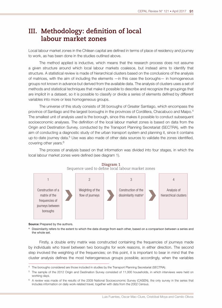
91CEPAL Review N° 121 • April 2017
Luis Fuentes, Oscar Mac-Clure, Cristóbal Moya and Camilo Olivos
III. Methodology: definition of local labour market zones
Local labour market zones in the Chilean capital are defined in terms of place of residency and journey to work, as has been done in the studies outlined above.
The method applied is inductive, which means that the research process does not assume a given structure around which local labour markets coalesce, but instead aims to identify that structure. A statistical review is made of hierarchical clusters based on the conclusions of the analysis of matrices, with the aim of including the elements —in this case the boroughs— in homogeneous groups not known in advance but derived from the available data. The analysis of clusters uses a set of methods and statistical techniques that make it possible to describe and recognize the groupings that are implicit in a dataset, so it is possible to classify or divide a series of elements defined by different variables into more or less homogeneous groups.
The universe of this study consists of 38 boroughs of Greater Santiago, which encompass the province of Santiago and the largest boroughs in the provinces of Cordillera, Chacabuco and Maipo.4 The smallest unit of analysis used is the borough, since this makes it possible to conduct subsequent socioeconomic analyses. The definition of the local labour market zones is based on data from the Origin and Destination Survey, conducted by the Transport Planning Secretariat (SECTRA), with the aim of conducting a diagnostic study of the urban transport system and planning it, since it contains up-to-date journey data.5 Use was also made of other data sources to validate the zones identified, covering other years.6
The process of analysis based on that information was divided into four stages, in which the local labour market zones were defined (see diagram 1).
Diagram 1 Sequence used to define local labour market zones
1
Construction of a
matrix of the
frequencies of
journeys between
boroughs
2
Weighting of the
flow of journeys
3
Construction of the
dissimilarity matrixa
4
Analysis of
hierarchical clusters
Source: Prepared by the authors.a Dissimilarity refers to the extent to which the data diverge from each other, based on a comparison between a series and
the whole set.
Firstly, a double entry matrix was constructed containing the frequencies of journeys made by individuals who travel between two boroughs for work reasons, in either direction. The second step involved the weighting of the frequencies; on this point, it is important to bear in mind that the cluster analysis defines the most heterogeneous groups possible; accordingly, when the variables
4 The boroughs considered are those included in studies by the Transport Planning Secretariat (SECTRA).5 The sample of the 2012 Origin and Destination Survey consisted of 11,000 households, in which interviews were held on
working days.6 A review was made of the results of the 2009 National Socioeconomic Survey (CASEN), the only survey in the series that
includes information on daily work-related travel, together with data from the 2002 Census.
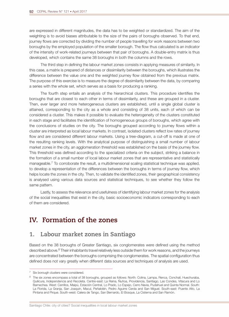
92 CEPAL Review N° 121 • April 2017
Santiago Chile: city of cities? Social inequalities in local labour market zones
are expressed in different magnitudes, the data has to be weighted or standardized. The aim of the weighting is to avoid biases attributable to the size of the pairs of boroughs observed. To that end, journey flows are corrected by dividing the number of people travelling for work reasons between two boroughs by the employed population of the smaller borough. The flow thus calculated is an indicator of the intensity of work-related journeys between that pair of boroughs. A double-entry matrix is thus developed, which contains the same 38 boroughs in both the columns and the rows.
The third step in defining the labour market zones consists in applying measures of similarity. In this case, a matrix is prepared of distances or dissimilarity between the boroughs, which illustrates the difference between the value one and the weighted journey flow obtained from the previous matrix. The purpose of this exercise is to measure the degree of dissimilarity between the data, by comparing a series with the whole set, which serves as a basis for producing a ranking.
The fourth step entails an analysis of the hierarchical clusters. This procedure identifies the boroughs that are closest to each other in terms of dissimilarity, and these are grouped in a cluster. Then, ever larger and more heterogeneous clusters are established, until a single global cluster is attained, corresponding to the city as a whole and consisting of 38 units, each of which can be considered a cluster. This makes it possible to evaluate the heterogeneity of the clusters constituted in each stage and facilitates the identification of homogeneous groups of boroughs, which agree with the conclusions of studies on the city. The boroughs grouped according to journey flows within a cluster are interpreted as local labour markets. In contrast, isolated clusters reflect low rates of journey flow and are considered different labour markets. Using a tree-diagram, a cut-off is made at one of the resulting ranking levels. With the analytical purpose of distinguishing a small number of labour market zones in the city, an agglomeration threshold was established on the basis of the journey flow. This threshold was defined according to the specialized criteria on the subject, striking a balance in the formation of a small number of local labour market zones that are representative and statistically manageable.7 To corroborate the result, a multidimensional scaling statistical technique was applied, to develop a representation of the differences between the boroughs in terms of journey flow, which helps locate the zones in the city. Then, to validate the identified zones, their geographical consistency is analysed using various data sources and statistical techniques, to see whether they follow the same pattern.
Lastly, to assess the relevance and usefulness of identifying labour market zones for the analysis of the social inequalities that exist in the city, basic socioeconomic indicators corresponding to each of them are considered.
IV. Formation of the zones
1. Labour market zones in Santiago
Based on the 38 boroughs of Greater Santiago, six conglomerates were defined using the method described above.8 Their inhabitants travel relatively less outside them for work reasons, and the journeys are concentrated between the boroughs comprising the conglomerates. The spatial configuration thus defined does not vary greatly when different data sources and techniques of analysis are used.
7 Six borough clusters were considered.8 The six zones encompass a total of 38 boroughs, grouped as follows: North: Colina, Lampa, Renca, Conchalí, Huechuraba,
Quilicura, Independencia and Recoleta. Centre-east: La Reina, Ñuñoa, Providencia, Santiago, Las Condes, Vitacura and Lo Barnechea. West: Cerrillos, Maipú, Estación Central, Lo Prado, Lo Espejo, Cerro Navia, Pudahuel and Quinta Normal. South: La Florida, La Granja, San Joaquín, Macul, Peñalolén, Pedro Aguirre Cerda and San Miguel. South-east: Puente Alto, La Pintana and Pirque. South-west: Calera de Tango, San Bernardo, El Bosque, La Cisterna and San Ramón.
93CEPAL Review N° 121 • April 2017
Luis Fuentes, Oscar Mac-Clure, Cristóbal Moya and Camilo Olivos
As an illustration, the centre-eastern zone is a destination of work-related journeys originating in all boroughs of the city; the frequency of journeys between the boroughs that form the zone is high, while a relatively small proportion of its residents travel to work outside those boroughs. The resulting zones are not closed spaces, but are integrated into the broader labour market of the city, whose inhabitants commute between multiple points, although mostly within the limits of the identified zones. Map 1 shows the six zones defined using the methodology described above, corresponding to the local labour markets of the city of Santiago.
Map 1 Santiago, Chile: definition and basic characteristics of the local labour market zonesa
0 5 Km
8 boroughs996 726 persons260 077 homes
7 boroughs1 232 432 persons
471 904 homes
7 boroughs1 217 925 persons
326 902 homes
3 boroughs816 249 persons213 748 homes
5 boroughs693 099 persons166 388 homes
8 boroughs1 487 520 persons
389 343 homes
NORTH
CENTRE-EAST
SOUTH
SOUTH-EASTSOUTH-WEST
WEST
N
Lampa
Colina
Pirque
Maipú
Lo Barnechea
Pudahuel
S´an Bernardo
Las Condes
Puente Alto
La Florida
Quilicura
Peñalolén
Calera de Tango
Renca
Huechuraba
Vitacura
La Pintana
La ReinaSantiago
Ñuñoa
Macul
Cerrillos
Recoleta
El Bosque
Conchalí
Providencia
La Granja
Cerro Navia
Estación Central
La Cisterna
San Miguel
Lo Espejo
Quinta Normal
Lo Prado
San Joaquín
San Ramón
Independencia
Pedro Aguirre Cerda
Source: Prepared by the authors, on the basis of data from the 2012 Origin-Destination Survey and the 2012 Census.a The zones indicated on the map are those used by the Transport Planning Secretariat.
In general, the configuration of the labour market zones of Santiago shows a clear geographic pattern, whereby the boroughs are grouped in differentiated and independent areas. The clearest departures from that pattern include the cases of the centre-east zone, which “takes over” the borough of Santiago, and the southern zone, a conglomerate of boroughs that are projected towards the western sector of the city. In themselves, these are relevant conclusions, since most of the articles consulted analyse the configuration of local labour markets in aggregate spatial structures, whereas this study also aims to determine the internal structure of the city.
94 CEPAL Review N° 121 • April 2017
Santiago Chile: city of cities? Social inequalities in local labour market zones
It is interesting to compare these conclusions with those reported in the study of the metropolitan zone of the Valley of Mexico, which used a similar methodology (Casado, 2012). The author identified a structure consisting of 12 zones, which display a radial spatial pattern, unlike that of Santiago; the latter also differs from the representations of the structure of the city in the form of concentric rings.
This geographic configuration is the spatial expression of the analysis of the tree-diagram and multidimensional scaling. The initial levels of agglomeration in the tree-diagram distinguish the centre-east zone, the south zone and the south-west zone, which are more homogeneous groupings than the others which have more porous boundaries.
The zones do not have the same number of boroughs or, therefore, of inhabitants and homes. For example, the zone with the fewest boroughs and inhabitants, located in the south-east of the city, comprises Puente Alto, La Pintana and Pirque, which have a total of 800,000 inhabitants. In contrast, the west zone —the most heavily populated and the one with the largest number of boroughs and homes— encompasses eight boroughs in which over 1.4 million people live (see map 1).
Apart from these differences, it is important to analyse the zones according to two key concepts: the level of self-containment and porosity. The former refers to the percentage of employed people who live in the same zone as that in which they work, and do not need to leave the zone to go to work. The second refers to the capacity to attract inhabitants from other labour market zones for work reasons. Table 1 summarizes this relation.
Table 1 Santiago, Chile: workers resident in labour market zones, 2009a
(Percentages and number of persons)
Area of residencyWorkers who live and work in the
same zone
Persons who go to work outside the area of residency
Total
To the centre-east zone To another zone Number of people Percentage of
the whole city
North 56% 32% 11% 373 963 15.3%
Centre-east 81% - 19% 582 403 23.9%
South 35% 45% 21% 447 107 18.3%
South-East 29% 39% 32% 285 155 11.7%
West 45% 39% 17% 510 937 21.0%
South-West 48% 24% 29% 232 882 9.5%
Total 2 432 449 100%
Source: Prepared by the authors, on the basis of data from the 2012 Origin-Destination Survey.a Only includes cases for which journey data exist.
The second column of this table shows the percentage of employed persons who work and live in the same zone. The lowest rate of self-containment is 29%, which validates the characterization of the zones as endogenous labour markets, despite displaying sharp differences. For example, as the approximate average level of self-containment is 49%, there are clearly sharp deviations. Areas that are above average include the centre-east zone, which has an 81% self-containment rate, more than double the rates in the south and south-east zones, which have the lowest values.
Table 1 also reveals the exogenous nature of the employment of workers residing in all zones, except for the centre-east, since the proportion of work-related journeys to that zone is high. In fact, a high percentage of workers from the two zones with the strongest exogenous relation between place of residency and place of work travel to the centre-east zone, and in some cases this exceeds the level of self-containment.
95CEPAL Review N° 121 • April 2017
Luis Fuentes, Oscar Mac-Clure, Cristóbal Moya and Camilo Olivos
The data of table 1 show that porosity is greatest in the centre-east zone, which is the destination of numerous journeys that start elsewhere, exceeding those that occur between the other zones. Moreover, the sum of the percentages of self-containment and journeys to the centre-east zone show that in most cases the proportion of work-related journeys to that zone is above 75%, but generally low in relation to the others.
The frequency of work-related journeys between labour market zones shows that for the inhabitants of the centre-east zone —followed, to a lesser extent, by the north zone— this is basically endogenous, whereas it is exogenous in the others and is centred on the first. In addition, the centre-east zone displays the highest level of porosity, since it receives a large number of external workers. Accordingly, similar to the finding in the study of the metropolitan zone of the Valley of Mexico (Casado, 2012), while it is possible to distinguish different local labour market zones, which in Santiago, Chile, display a non-radial configuration, the existence of a zone with great capacity to concentrate jobs gives rise to a territorial structure dependent on a broad centre, as occurs in the centre-east zone. Nonetheless, in general, the city of Santiago is a broad labour market, which is distinguished from the zone surrounding it and from neighbouring cities, and which encompasses zones with a relatively high level of self-containment.
2. Analysis of socioeconomic inequalities
In Latin America’s large cities, characterized by a high degree of socioeconomic inequality, the definition of labour market zones can add value to the analysis of inequalities, so the following paragraphs consider its validity from this standpoint in the case of Santiago.
Income inequality, a fundamental element of socioeconomic inequalities, is clearly seen in the classification of the labour market zones by income quintiles (see table 2).
Table 2 Santiago, Chile: classification of labour market zones by workers’ income quintiles,a 2013
(Percentages)
I II III IV V
Centre-east 3 7 8 20 63
West 12 23 29 24 12
South 13 17 26 27 18
South-west 17 24 25 24 10
North 15 25 29 23 8
South-east 21 23 26 26 5
Total 13 19 22 23 23
Source: National Socioeconomic Survey (CASEN), 2013.a The distribution represents regional autonomous income (measured using the new survey methodology).
A comparison between the zones reveals clear differences: particularly a greater concentration of the upper quintile in the centre-east zone, and of the lowest quintile in the south-east. The prevalence of the highest quintile in the centre-east zone is accompanied by a general income level that is substantially lower than in the other zones. In fact, this displayed a median autonomous income of US$ 1,260 equivalent per month in 2013,9 whereas, in the other zones, the median varied between US$ 533 equivalent in the west zone and around US$ 478 in the south-west, north, and south. Within the zones, even in the centre-east, there are variations that are not adequately reflected in median
9 According to the exchange rate prevailing in June 2015 (627 pesos per dollar).
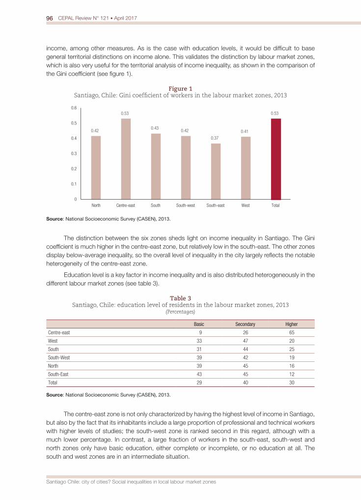
96 CEPAL Review N° 121 • April 2017
Santiago Chile: city of cities? Social inequalities in local labour market zones
income, among other measures. As is the case with education levels, it would be difficult to base general territorial distinctions on income alone. This validates the distinction by labour market zones, which is also very useful for the territorial analysis of income inequality, as shown in the comparison of the Gini coefficient (see figure 1).
Figure 1 Santiago, Chile: Gini coefficient of workers in the labour market zones, 2013
0.42
0.53
0.43 0.42
0.37
0.41
0.53
0
0.1
0.2
0.3
0.4
0.5
0.6
North Centre-east South South-west South-east West Total
Source: National Socioeconomic Survey (CASEN), 2013.
The distinction between the six zones sheds light on income inequality in Santiago. The Gini coefficient is much higher in the centre-east zone, but relatively low in the south-east. The other zones display below-average inequality, so the overall level of inequality in the city largely reflects the notable heterogeneity of the centre-east zone.
Education level is a key factor in income inequality and is also distributed heterogeneously in the different labour market zones (see table 3).
Table 3 Santiago, Chile: education level of residents in the labour market zones, 2013
(Percentages)
Basic Secondary Higher
Centre-east 9 26 65
West 33 47 20
South 31 44 25
South-West 39 42 19
North 39 45 16
South-East 43 45 12
Total 29 40 30
Source: National Socioeconomic Survey (CASEN), 2013.
The centre-east zone is not only characterized by having the highest level of income in Santiago, but also by the fact that its inhabitants include a large proportion of professional and technical workers with higher levels of studies; the south-west zone is ranked second in this regard, although with a much lower percentage. In contrast, a large fraction of workers in the south-east, south-west and north zones only have basic education, either complete or incomplete, or no education at all. The south and west zones are in an intermediate situation.
97CEPAL Review N° 121 • April 2017
Luis Fuentes, Oscar Mac-Clure, Cristóbal Moya and Camilo Olivos
The clear definition of the zones comprising the city’s socio-territorial space makes it easier to understand the gradual differences in terms of income and education. The analysis based on labour market zones affords a better understanding of other territorial inequalities in domains such as housing. The approximate value of real estate can be calculated from Property Tax data.10 According to data from the Internal Revenue Service for 2014, in the centre-east zone, 90% of properties are liable for this tax, whereas in the other zones the percentage is less and varies between 25% in the north and 8% in the south-east; other properties are exempt from the tax. On average, in the zone studied, 31% of properties are liable for the tax; this percentage is tripled in the centre-east zone, followed by the south zone, in which the proportion is slightly above average. The sharp differences reflect the value of properties in each of the zones and, therefore, reflect inequality in real estate assets. The average fiscal valuation varies considerably from one zone to another; in the centre-east sector it is 1.5 times higher than the city average, and 3.5 times higher than in the south-east zone, which has the lowest average valuation of all.
3. Composition of the zones by social classes
The composition of the labour market zones by social classes largely explains the differences present in this domain, both between zones and within each of them. Social classes are large groups defined generally by the place they occupy in the social hierarchy and relation with other conglomerates in terms of possession of usable or productive assets, prestige, and other social or symbolic assets (Mac-Clure, Barozet and Maturana, 2014). To analyse the social structure of the zones considered, the EGP classification is applied (Erikson and Goldthorpe, 1993),11 one of the most widely used internationally and also in several studies undertaken in Chile (Espinoza, Barozet and Méndez, 2013; Mac-Clure, 2012; Mac-Clure, Barozet and Maturana, 2014; Torche and Wormald, 2004). This classification applies criteria relating to ownership and control of productive assets, autonomy, type of activity of the workers (manual or non-manual) and their skill level. Table 4 shows the composition by social classes of the labour market zones of the city of Santiago.
Table 4 Santiago, Chile: social classes by labour market zones, 2013
(Percentages)
ClassZone
Centre-east West South South-West North South-East Total
High-level services 29 6 8 6 5 2 11
Low-level services 30 10 15 10 10 8 16
High-level non-manual routine occupations 9 12 11 11 11 12 11
Low-level non-manual routine operations 9 15 15 13 12 13 12
Small-scale entrepreneurs 1 1 1 1 1 1 1
Self-employed workers 9 16 16 18 18 18 15
Skilled manual workers 4 15 11 17 14 17 12
Unskilled manual workers 10 25 23 23 29 28 22
Farm workers 0 1 1 1 2 1 1
Farmers 0 0 0 1 1 0 0
Source: National Socioeconomic Survey (CASEN), 2013.
10 The fiscal valuation on which the property tax is based is roughly equivalent to 50% of the commercial valuation. Non-agricultural residential properties valued at less than US$ 3,500 (according to the June 2015 exchange rate) are not subject to this tax.
11 The variable “Social classes”, based on the EGP scheme applied to Chile, was obtained from the CASEN surveys, using a syntax developed by Vicente Espinoza. The authors are grateful for his contribution.
98 CEPAL Review N° 121 • April 2017
Santiago Chile: city of cities? Social inequalities in local labour market zones
As table 4 shows, the composition of the social classes in Santiago is dominated by unskilled manual workers, followed in smaller proportions by the low-level services class, consisting mainly of technicians, the self-employed (including nonprofessional own-account workers), the low-level manual routine occupations class (wage-earners working as sales persons or service providers) and skilled manual workers. The third group of social classes, which has slightly lower percentages, corresponds to the high-level services class, consisting of professionals with a university degree, and the high-level non-manual routine occupations class, which includes middle-level administrative employees. Lastly, the classes with the smallest share are small-scale entrepreneurs, farm labourers and farmers. This classification of the social classes present in Santiago does not include the socioeconomic elite, since they are generally not represented in household surveys, and they concentrate much of the country’s social, economic and political power. The high-level services class, described above, occupies positions closer to the elite.
The territorial distribution of the classes in the different zones varies considerably, with the high and low-level service classes being over-represented in the centre-east. The concentration of members of the high-level service class in this zone is consistent with its high level of income inequality, with income levels differing considerably from those in the other social classes and large internal dispersion. The services class is also represented in the south zone although to a lesser extent, and especially by intermediate level technicians and professionals. Here, as in the west zone, there is a high percentage of administrative employees and sales people in the low-level routine operations class. Manual workers are a larger proportion in the west, south west, north, and south-east zones, mostly unskilled in the latter two zones. Unlike the centre-east, in these four zones the services class is generally under-represented.
In the long run, and from the standpoint of intergenerational social mobility, the social classes within each zone are differentiated according to the origin of their members, parents’ education and a variable that is generally not considered in the studies: place of birth. Members of the high-level services class who live in the centre-east zone, in which they are more numerous than in the other zones, come from families in which the father generally did not pursue higher studies, and was born in a borough from another zone. Consequently, the centre-east zone is a labour market in which the higher strata of the middle class represent the outcome of an intense process of social mobility and considerable inter-generational territorial migration.
Between 1996 and 2013, there was a rapid increase in the proportion of workers from the service classes residing in the centre-east zone, and a reduction in the share of manual workers. The latter was partly due to the fact that the children of the inhabitants of boroughs in this zone frequently cannot choose to continue living there owing to the rise in land prices, which pushes up house prices and leads to the construction of social housing in the outlying boroughs of the city, where the price is lower. Unlike what happens in the centre-east zone, elsewhere the share of the non-manual routine operations classes, both high and low level, and skilled and unskilled manual workers, remains unchanged. All this suggests that the upward social mobility process is concentrated in that zone.
Presumably, the multiple inequalities that exist in the labour market zones reflect social differences. In addition, the presence of the various social classes in these zones allows for a better understanding of varied preferences and subjective perceptions.
The heterogeneity of the city in terms of facilities, which affects the quality of life of its inhabitants (Orellana, 2014), drives migration towards certain zones. The centre-east, which has a high concentration of fixed assets, accounted for 40% of building permits and 68% of the constructions undertaken in the Metropolitan Region between 2000 and 2012 (data on construction from the National Institute of Statistics). This greater endowment of fixed assets —along with better services, including health, education, and security— would provide an economic-interest explanation of both the preference of members of the high- and low-level services classes to live in the centre-east zone and
99CEPAL Review N° 121 • April 2017
Luis Fuentes, Oscar Mac-Clure, Cristóbal Moya and Camilo Olivos
the strategy of real estate firms to selectively target this zone. The way in which the real estate market operates facilitates upward residential mobility (Sabatini, 2006), particularly among the members of those classes, who migrate to the centre-east zone.
A preference for one zone of residency or another (Sabatini and others, 2012) also reflects subjective motivations, including those of the upper strata of the middle classes who live in the centre-east zone, related to a desire to increase their cultural and social capital through social distinction mechanisms (Bourdieu, 2012). Residents in the other zones —and those less favoured in the centre-east zone— must use other means to maintain or improve their social status. According to recent studies based on methodologies inspired in game theory (Barozet and Mac-Clure, 2014; Mac-Clure, Barozet and Moya, 2015), from a subjective point of view, the members of the less privileged segments of the middle classes consider that there are three decisive factors in income growth: personal effort, which is applied to the limited access to pre-existing economic resources; development of cultural capital, associated with education; and social capital linked to the family and the close circle. In particular, they attribute fundamental importance to educational and labour effort, which in their opinion is more important than accumulated or inherited economic capital, which they lack, and the symbolic value and resources embodied in fixed assets such as those existing in the centre-east zone, while criticizing the “discriminations” associated with their original borough of residency.
To summarize the socioeconomic characterization of the labour market zones of the city of Santiago from the analysis performed above, the centre-east zone is mainly inhabited by a high-income upper-middle stratum, but also displays considerable economic inequality among its residents. Most of them have higher university or technical education and, from the occupational standpoint, belong to the services classes, consisting particularly of high-level service-class professionals, whose preference for this zone reflects the value they accord to it as a symbol of upward social mobility. The inhabitants of the west and south zones belong to the middle strata, dominated by lower-middle income employees and salespeople of the non-manual routine occupations class. In these, internal inequality is moderate compared to the centre-east zone, and there is an aspiration for social mobility based on work and education effort. Nonetheless, both display specific distinguishing features: most of the inhabitants of the west zone have secondary education, whereas those in the south have a slightly higher proportion of individuals with higher level studies; in the latter case, there is also a larger percentage of middle-level technical and professional workers belonging to the low-level services class.
In terms of social hierarchies, manual workers predominate in the south-west, north, and south-east zones, where over half of the city’s inhabitants live. In these zones, the population’s income is low, and economic inequality is moderate —even relatively low in the south-east zone. Education levels are lower than in zones inhabited mainly by members of the middle classes, but whereas the population with secondary education predominates in the south-west and north zones, the south-east has a high proportion of residents with only basic education. Although the south-west and north zones have similarities, the former has a larger proportion of skilled manual workers than the latter, where there is a clear predominance of the unskilled manual workers class. In general, the social economic status of these zones does not vary, in contrast to the upward mobility that occurs in the residency zones of the middle classes, particularly the centre-east.
V. Conclusions
In short, this study shows the relevance of a methodological approach based on the analysis of local labour markets defined by inter-borough travel flows, to analyse large cities such as Chilean capital, Santiago. The criteria and methodological procedures described make it possible to distinguish six labour market zones in the city’s Metropolitan Area.
100 CEPAL Review N° 121 • April 2017
Santiago Chile: city of cities? Social inequalities in local labour market zones
According to the socioeconomic indicators analysed, the greatest differences seen in the city occur in the centre-east zone and other labour markets. Moreover, it was found that the centre-east displays the sharpest social inequalities, which are manifested, among other things, in a high Gini coefficient. In the centre-east zone, numerous inhabitants from the two extremes of the social ranking coexist: the high-level services class and the unskilled manual workers class. The first of these is predominant; so, in terms of social categories, this zone is the most polarized of all. Consequently, social inequality in the city of Santiago is eminently spatial, and fundamentally reflects the heterogeneity of the centre-east zone, and the differences between this and the city’s other labour market zones. The social inequalities existing in the other zones are more moderate and determined by the high proportion of members of the manual workers class living in them, except for the south-west, where there is a larger presence of middle-income strata corresponding to the low-level services classes, and high- and low-level manual routine occupations.
The conclusions set forth confirm the relevance of applying a territorial approach based essentially on the configuration of labour market zones, to the study of social inequalities in a metropolitan area. Labour markets shape geographic inequalities in the city of Santiago, which are expressed spatially through substantial differences between zones in terms of income, access to education and the composition of the social classes. Mechanisms of social distinction and subjective factors related to cultural and social capital also operate within the zones. In the case of Santiago, the spatial nature of the inequalities is manifested twice over, both between the metropolitan space as a whole and the rest of the country and also within the city, consisting of various local labour market zones. This conclusion affords a better understanding of urban spaces, since the analysis performed shows that labour market zones are characterized by a socioeconomic and social class configuration, and not only as sociodemographic phenomena linked exclusively to the place of residency and work-related journeys.
This article provides specific elements to help understand the city of Santiago, particularly in relation to under-studied aspects of the formation and transformation of the socio-territorial structure. The marked differences that exist between labour market zones show that Santiago is a city in which several cities seem to coexist. To some extent, the social differences between the various zones of Latin American metropolitan areas and other regions are habitual; the novelty of the analysis presented in this article is the application of a method for defining and describing those urban spaces, based on which one can discern that the trajectory of the social classes in the labour market zones of Santiago, over the last decade, tends to accentuate and consolidate the social differences displayed in the city, instead of reducing them. A consideration of the specifics of the zones makes it possible to apply the concept of “city of cities,” evoked by Nel.Lo (2002) to refer to Barcelona, and expand it from a perspective related to the socio-spatial configuration of a large cities such as Santiago.
BibliographyAgostini, C.A. (2010), “Pobreza, desigualdad y segregación en la Región Metropolitana”, Estudios Públicos,
No. 117, Santiago, Centre for Public Studies.Arriagada, C. (2010), “Segregación residencial según dos modelos de urbanización y bienestar: estudio
comparado de las áreas metropolitanas del Gran Santiago, Toronto y Vancouver”, Notas de Población, vol. 37, No. 91 (LC/G.2484-P), Santiago, Economic Commission for Latin America and the Caribbean (ECLAC).
Barozet, E. and O. Mac-Clure (2014), “Nombrar y clasificar: aproximación a una epistemología de las clases sociales”, Cinta de Moebio. Revista de Epistemología de Ciencias Sociales, No. 51, Santiago, Faculty of Social Sciences, University of Chile.
Berdegué, J. and others (2011) “Territorios funcionales en Chile”, Documento de Trabajo, No. 102, Santiago, Latin American Centre for Rural Development.
Bourdieu, P. (2012), La distinción. Criterio y bases sociales del gusto, Madrid, Taurus.
101CEPAL Review N° 121 • April 2017
Luis Fuentes, Oscar Mac-Clure, Cristóbal Moya and Camilo Olivos
Casado, J.M. (2012), “La estructura policéntrica de los mercados laborales locales de la Zona Metropolitana del Valle de México”, Investigaciones Geográficas, No. 79, Mexico City, National Autonomous University of Mexico.
Casado-Díaz, J. (2003), “The use of commuting data to define local labour market zones and urban zones in Spain”, paper presented at the NECTAR Conference “A New Millenium. Are Things The Same? Innovation, Sustainability and Efficiency in Communication and Transportation Systems”, Umeå, Sweden, Umeå University.
Casado-Díaz, J. and M. Coombes (2011), “The delineation of 21st century local labour market zones: a critical review and a research agenda”, Boletín de la Asociación de Geógrafos Españoles, No. 57.
Cattaneo, R. (2012), La fabrique de la ville: promoteurs immobiliers et financiarisation de la filière du logement à Santiago du Chili, Paris, Université Paris 8.
Coombes, M. and S. Bond (2008), Travel-to-Work Areas: the 2007 Review, London, Office for National Statistics.De Mattos, C. (2010), Globalización y metamorfosis urbana en América Latina, Quito, Latin American and
Caribbean Organization of Historic Centers.(2002), “Mercado metropolitano de trabajo y desigualdades sociales en el Gran Santiago: ¿Una ciudad dual?”, EURE, vol. 28, No. 85, Santiago, Catholic University of Chile.
De Mattos, C., L. Fuentes and F. Link (2014), “Tendencias recientes del crecimiento metropolitano en Santiago de Chile. ¿Hacia una nueva geografía urbana?”, Revista INVI, vol. 29, No. 81, Santiago, Faculty of Architecture and Town Planning, University of Chile.
Dockendorff, E. and others (1990), Santiago, dos ciudades: análisis de la estructura socio-económica espacial del Gran Santiago, Santiago, Centre for Development Research.
Erikson, R. and J.H. Goldthorpe (1993), The Constant Flux, Oxford, Oxford University Press.Escolano, S. and J. Ortiz (2005), “La formación de un modelo policéntrico de la actividad comercial en el
Gran Santiago (Chile)”, Revista de Geografía Norte Grande, No. 34, Santiago, Catholic University of Chile.Espinoza, V., E. Barozet and M.L. Méndez (2013), “Estratificación y movilidad social bajo un modelo neoliberal:
el caso de Chile”, Lavboratorio, No. 25, Buenos Aires, Gino Germani Institute/University of Buenos Aires.Heinrichs, D. and others (eds.) (2011), Risk Habitat Megacity, Heidelberg, Springer.ISTAT (National Institute for Statistics) (2005), I sistema locali del lavoro. Censimento 2001. Dati definitivi
[online] http://dawinci.istat.it/daWinci/jsp/MD/download/sll_comunic_solo_testo.pdf.Mac-Clure, O. (2012), “Chile’s new middle classes: a cohort analysis”, CEPAL Review, No. 108 (LC/G.2549-P),
Santiago, Economic Commission for Latin America and the Caribbean (ECLAC).Mac-Clure, O. and R. Calvo (2013), “Desigualdades sociales y tipos de territorios en Chile”, Polis, No. 34,
Osorno, Chile, Los Lagos University.Mac-Clure, O., E. Barozet and V. Maturana (2014), “Desigualdad, clase media y territorio en Chile: ¿clase
media global o múltiples mesocracias según territorios?”, EURE, Santiago, vol. 40, No. 121, Santiago, Catholic University of Chile.
Mac-Clure, O., Barozet, E. and C. Moya (2015), “Juicios de las clases medias sobre la élite económica: ¿crítica a las desigualdades en Chile?”, Polis, No. 41, Osorno, Chile, Los Lagos University.
Maturana, F. and F. Arenas (2012), “El policentrismo en Chile: medición exploratoria para el sistema de ciudades de las regiones de La Araucanía, de Los Ríos y de Los Lagos”, Revista de Geografía Norte Grande, No. 52, Santiago, Catholic University of Chile.
Nel.Lo, O. (2002), Cataluña, ciudad de ciudades, Lleida, Editorial Milenio.OECD (Organization for Economic and Development Cooperation) (2002), Redefining Territories: Functional
Regions, Paris, OECD Publishing.Orellana, A. (2014), Indicador de calidad de vida ciudades chilenas (ICVU), Santiago, Estudios Urbanos UC/
Chilean Chamber of Construction.(2009), “La gobernabilidad metropolitana de Santiago: la dispar relación de poder de los municipios”, EURE, vol. 35, No. 104, Santiago, Catholic University of Chile.
Orellana, A. and L. Fuentes (2007), "El arco, el cono y el cluster: Geometrías espaciales para la gobernabilidad metropolitana y local de Santiago", Arenas, ciudad, poder y gobernanza, G. Yáñez and others (eds.), Santiago, Geolibros.
Ortiz, J. and S. Escolano (2013), “Movilidad residencial del sector de renta alta del Gran Santiago (Chile): hacia el aumento de la complejidad de los patrones socioespaciales de segregación”, EURE, vol. 39, No. 118, Santiago, Catholic University of Chile.
Ortiz, J. and S. Morales (2002), “Impacto socioespacial de las migraciones intraurbanas en entidades de centro y de nuevas periferias del Gran Santiago”, EURE, vol. 28, No. 85, Santiago, Catholic University of Chile.

102 CEPAL Review N° 121 • April 2017
Santiago Chile: city of cities? Social inequalities in local labour market zones
Pollack, M. and A. Uthoff (1987), “Pobreza y mercado de trabajo en el Gran Santiago: 1969-1985”, Documento de Trabajo, No. 299, Santiago, Regional Employment Programme for Latin America and the Caribbean (PREALC).
Riffo, L. (2004), “Los impactos de la globalización sobre los mercados de trabajo metropolitanos: el caso de Santiago de Chile en la década de los noventa”, Santiago en la globalización ¿una nueva ciudad?, C. de Mattos and others (eds.), Santiago, Ediciones SUR.
Rodríguez, J. (2012), “¿Policentrismo o ampliación de la centralidad histórica en el Área Metropolitana del Gran Santiago? Evidencia novedosa proveniente de la encuesta Casen 2009”, EURE, vol. 38, No. 114, Santiago, Catholic University of Chile.
Russo, G. and others (2011), “Commuter effects on local labour markets: a German modelling study”, Tinbergen Institute Discussion Papers, No. 11-114/3, Tinbergen Institute.
Sabatini, F. (2006), “La segregación social del espacio en las ciudades de América Latina”, Working Paper, Washington, D.C., Inter-American Development Bank.
Sabatini, F., G. Cáceres and J. Cerda (2001), “Segregación residencial en las principales ciudades chilenas: Tendencias de las tres últimas décadas y posibles cursos de acción”, EURE, vol. 27, No. 82, Santiago, Catholic University of Chile.
Sabatini, F. and others (2012), “¿Es posible la integración residencial en las ciudades chilenas? Disposición de los grupos medios y altos a la integración con grupos de extracción popular”, EURE, vol. 38, No. 115, Santiago, Catholic University of Chile.
Sassen, S. (2001), The Global City, Princeton, Princeton University Press.SECTRA (Transport Planning Secretariat) (1992), Estudio encuesta origen destino de viajes del Gran Santiago,
1991, Santiago.Singelmann, J. and F. Deseran (eds.) (1993), Inequalities in Labor Market Areas, Boulder, Colorado,
Westview Press.Tolbert, C. and M. Sizer (1996), “U.S. commuting zones and labor market zones. A 1990 update”, Staff Paper,
No. AGES-9614, Washington, D.C., United States Department of Agriculture.Torche, F. and G. Wormald (2004), “Estratificación y movilidad social en Chile: entre la adscripción y el logro”,
Políticas Sociales Series, No. 98 (LC/L.2209-P), Santiago, Economic Commission for Latin America and the Caribbean (ECLAC).
Truffello, R. and R. Hidalgo (2015), “Policentrismo en el Área Metropolitana de Santiago de Chile: reestructuración comercial, movilidad y tipificación de subcentros”, EURE, vol. 41, No. 122, Santiago, Catholic University of Chile.
Vallès, V. (2004), “Bassins de vie: au centre de la vie quotidienne”, La Lettre, No. 14, Paris, National Institute for Statistics and Economic Studies (INSEE).
Thoughts on the inequality of opportunities: new evidenceWallace Patrick Santos de Farias Souza, Ana Cláudia Annegues and Victor Rodrigues de Oliveira
Abstract
This article evaluates the effects of a set of variables on the inequality of opportunities in Brazil, using the method developed by Li, Chen and Gao (2011) and combining data from the National Household Survey (PNAD) and Finanças do Brasil (FINBRA) on the Brazilian states for 1995-2012. The results show that economic growth has become less important in that debate than other conditioning factors over the last few years. The current pattern of education spending contributes to the maintenance of social vulnerability, thereby making it harder for individuals to participate fully in society. In contrast, increases in formal education and formalization have made opportunities less unequal.
Keywords
Macroeconomics, economic growth, equality of opportunities, measurement, econometric models, Brazil
JEL classification
D63, C14, C23
Authors
Wallace Patrick Santos de Farias Souza is a PhD student in applied economics on the Postgraduate Programme in Economics of the Federal University of Rio Grande do Sul (UFRGS), Brazil. [email protected]
Ana Cláudia Annegues is a PhD student in applied economics on the Postgraduate Programme in Economics of the Federal University of Rio Grande do Sul, Brazil. [email protected]
Victor Rodrigues de Oliveira is a PhD student in applied economics on the Postgraduate Programme in Economics of the Federal University of Rio Grande do Sul, Brazil. [email protected]
104 CEPAL Review N° 121 • April 2017
Thoughts on the inequality of opportunities: new evidence
I. IntroductionThe freedom to choose the quantity of one’s working hours automatically entails that
differential earnings will follow from choices for which one is personally responsible. Responsibility is a necessary consequence of any substantial amount of freedom and is
therefore part and parcel of any free society.
Fleurbaey (2008, p. 1)
Inequality can have many dimensions. In general, economists focus specifically on its monetary dimension, measuring the inequality of individual or family incomes. Nonetheless, inequality can also be understood more broadly as the outcome of unequal access to opportunities for work, education, happiness, health, a longer life expectancy, assets and social mobility, among other things. Modern inequality theory, as expressed in the key texts of Rawls (1971) and Roemer (1998), includes those dimensions in its analysis.1
This approach focuses less on the final distribution of resources than on the intermediate process by which they are allocated, since this will depend on the factors that determine individual economic gains. Those factors are: individual effort, measured by variables that agents can control; and circumstances, such as race or colour, socioeconomic origin, and others, which they cannot control. According to the concept of equality of opportunities, the inequality of total income comprises inequality originating in differential effort, and inequality stemming from circumstantial factors beyond individual control. Only the latter would be considered objectively unfair and should therefore be the target of public policies.2
Equality of opportunities and its measurement are relevant not only from the normative standpoint. Firstly, a growing body of empirical evidence shows that preferences in terms of redistribution and policy orientation are tempered by equity concerns. For example, Alesina and Angeletos (2005) showed that, in the United States, individuals who believe that personal economic success is related more to effort than luck have weaker preferences for redistribution. Moreover, based on data obtained from the World Values Survey, Alesina and La Ferrara (2005) found that perceptions of justice are related to individuals’ political orientation: when people believe that effort is the key determinant of economic advantages, redistribution and taxes are low; whereas in societies where people believe that the initial conditions (birth and connections established from then on) are the main determinants of economic success, taxes and redistribution will be higher. Secondly, as the determinants of economic inequality (circumstances and effort) influence individual incentives, those determinants are related to aggregate economic outcomes such as economic growth. In World Development Report 2006, the World Bank argues that income inequality owing to circumstances can produce a suboptimal accumulation of human capital and, therefore, a lower rate of economic growth; whereas income inequality owing
1 The theoretical literature indicates that the notion of equality of opportunities incorporates two basic principles: the principle of compensation, which requires the elimination of inequalities arising from circumstances; and the principle of reward, which refers to the way in which efforts between individuals with identical circumstances are rewarded. The compensation principle allows for an ex post or an ex ante perspective. The first analyses the real income of the individual and relates to the differences in income between individuals with the same responsibility characteristics and different circumstances. The ex ante approach, in contrast, focuses on prospects, for there to be equality of opportunities if individuals face different opportunity sets (or different value sets) owing to their circumstances. In the case of the principle of reward, the literature distinguishes between liberal reward and utilitarian reward. In the first case, it is argued that the government should not redistribute income between those that share the same characteristics of circumstance, because their income differences are exclusively due to differences in effort. In the second case, it is argued that one should not worry about what only arises from differences in effort. For a more detailed analysis of these points, see Ramos and Van De Gaer (2012).
2 Schokkaert and Devooght (2003), Gaertner and Schwettmann (2007) and Cappelen, Sorenson and Tungodden (2010) provided solid evidence that, judging by the income distribution, individuals clearly distinguish circumstances and effort, as suggested by the theories of equality of opportunities. For example, Cappelen, Sorenson and Tungodden (2010) proposed an exercise to evaluate the elements for which individuals feel responsible. The authors noted that the vast majority of participants did not attribute individual responsibility for the price determined on a random basis, an impersonal factor that is beyond the control of the individual; but they did hold them responsible for their choice of work time.

105CEPAL Review N° 121 • April 2017
Wallace Patrick Santos de Farias Souza, Ana Cláudia Annegues and Victor Rodrigues de Oliveira
to individual responsibility variables can encourage people to invest in human capital and make the greatest possible effort (World Bank, 2005).
Over the last few decades, inequality indices in Brazil have fallen steadily, although it is still on the list of the most unequal countries in the world (Barros and others, 2007).3 In the social sphere, programmes to combat poverty and misery were adopted in a modest way in 1995, but with greater emphasis as from 2003.4 Public policies on universal access to education5 and basic health care also play a key role in reducing Brazilian disparities.6 Apart from growth and closer targeting of social programmes, the macroeconomic reforms implemented in the country as from the first half of the 1990s, such as monetary stabilization and trade liberalization, may also have helped reduce income inequality in Brazil. Since the introduction of the Real Plan, there has been a steady rise in the minimum wage, which has a direct effect on family welfare, particularly among the poorest. Albeit to a limited extent, the combination of those factors shows that Brazil has high rates of income concentration and wide regional disparities; and economic growth has had varied effects on reducing income inequality, poverty and the inequality of opportunities in different historical periods.
Although the macroeconomic environment plays a major role from the social standpoint, studies on Brazil have paid little attention to that topic, preferring to focus more on the impact of social programmes such as the Bolsa Família family subsidy scheme.7 That debate has been ongoing in the international literature for some time, with an increasing number of studies investigating the effects of macroeconomic factors on social indicators. The most widely studied macroeconomic variables are economic growth and inflation.
The debate on the relation between inequality and economic growth begins with the theoretical formulation of the Kuznets curve (1955), which postulated a non-linear relation between the two variables, described by an inverted “U” shaped curve. The idea is that the income distribution is likely to worsen in the initial stages of development; but, later, productivity increases can be expected to spread domestically and, thus, inequality would tend to diminish. Since then, the literature has failed to reach a conclusion on the true nature of that relation. Alesina and Rodrik (1994) regressed the annual average growth rate against initial inequality measured by the Gini coefficient, based on cross-sectional data for different countries. The results show that income inequality is inversely related to subsequent economic growth. Li and Zou (1998) and Forbes (2000) used panel data with fixed effects to find that income inequality was positively related to economic growth. Other approaches highlight the positive effects of growth through economic agents’ access to the labour market (Nolan, 1987); and, more recently, Ravallion (2012) has shown that initial poverty levels are likely to be associated with low rates of economic growth.
In the case of inflation, the argument is that its adverse effect on income inequality is due to price rises, which have a major effect on the poorest population groups. Some theoretical studies attempt to systemize this argument by developing general-equilibrium models, such as in Erosa and Ventura (2002) and Cysne, Maldonado and Monteiro (2005). Some results are inconclusive and depend on the origin of the inflationary process: if price rises reflect supply-side pressures, inequality is likely to
3 The list of factors that contribute to variations in income inequality include education, race, social programmes, region and spatial demographics (Neri, 2011).
4 A detailed analysis of current poverty reduction programmes and future strategies can be found in Rocha (2007).5 The main changes in Brazilian public education include the decentralization of educational resources and the expansion
of enrolment as from 1996, which culminated in the creation of the Fund for the Maintenance and Development of Basic Education and the Upgrading of Teaching Staff (FUNDEF).
6 Menezes-Filho, Fernandes and Picchetti (2007) argued that, as from 1997, with a rapid increase in the proportion of young people in secondary education, the composition effect and the compression effect (wage differential) started to reduce income inequality.
7 Avila, Bagolin and Comim (2012, p. 461) question the validity of transfer programmes, showing that, at least in segments with a certain (low) level of income, monetary increases do not necessarily lead to an improvement in individuals’ multidimensional conditions; in other words, monetary incomes alone are insufficient to characterize human deprivations.

106 CEPAL Review N° 121 • April 2017
Thoughts on the inequality of opportunities: new evidence
decline; but if inflation is being driven by demand, inequality will worsen (Blinder and Esaki, 1978; Buse, 1982).
This study adds a set of variables to the list of determinants of inequality generated by circumstances, some of which are based on the empirical analysis performed by Marrero and Rodríguez (2010). Although social programmes attract greater attention when inequality reduction policies are discussed, the economic environment plays a major role (even determining the viability or otherwise of the social policy measures), so it is advisable to empirically measure the impact of the variables comprising it.
Unfair inequality is measured by estimating a model in which income depends on circumstance and effort variables. The logarithm of real wages is used as the dependent variable (as a proxy for individual income), along with a set of explanatory variables that represent specific characteristics of individuals, including the decision to migrate. As the migratory process is self-selective, the method proposed by Nelsen (2006)8 is used to avoid biased wage estimates. The components of total inequality are then calculated on the basis of the model’s adjusted incomes, holding constant variables of circumstance (inequality of effort) and effort (inequality of circumstance). In this stage, indices of the inequality of opportunities are calculated using the Gini coefficient.
The indices thus calculated are used to construct a data panel spanning 1996-2012, with state-level information. Then, a set of variables is used to verify the impact on inequality of circumstances constructed as described above, which is considered the only part of inequality that is socially undesirable.
The variables used follow the approaches previously discussed in the literature: real per capita gross domestic product (GDP) as an indicator of growth; per capita health and education expenditure; the average number of years of schooling among men and women; and the degree of informality of the economy. The method proposed by Li, Chen and Gao (2011) is used to estimate the impact of those variables on the level of inequality. This method makes it possible to deal with the problem, because it involves a nonparametric approach, which does not impose any specific functional form to describe the behaviour of the data. It is also appropriate for using panel data, because it eliminates the fixed effects without the need to express the variables in first-difference form.
This article is divided into four sections in addition to the Introduction. Section II presents the empirical procedures adopted, and section III describes the databases. Section IV provides justification for the variables used and discusses the results of the estimations. Section V concludes the study with some final thoughts.
II. Empirical strategy
To evaluate how the variables defined above are related to the inequality of opportunities, the method proposed by Li, Chen and Gao (2011) is used. Although the literature on panel data is wide-ranging, the parametric specifications can result in under- specified models and, consequently, inconsistent estimators. Various studies have been made to overcome that problem (Ullah and Roy, 1998; Fan and Li, 2004; Henderson, Carroll and Li, 2008; Zhang, Fan and Sun, 2009). At the same time, a line of research has emerged in the last few years that aims to model non-stationary time series. Gao and Hawthorne (2006) showed that the models in which the linear trend is obtained through a parametric specification do not display good fit. One of the main characteristics of the nonparametric models is that the data “speak for themselves.” In this connection, Gao and Hawthorne (2006) and Atak, Linton
8 For applications to the international and national cases, respectively, see Meng (2001) and Ramalho and Queiroz (2011).
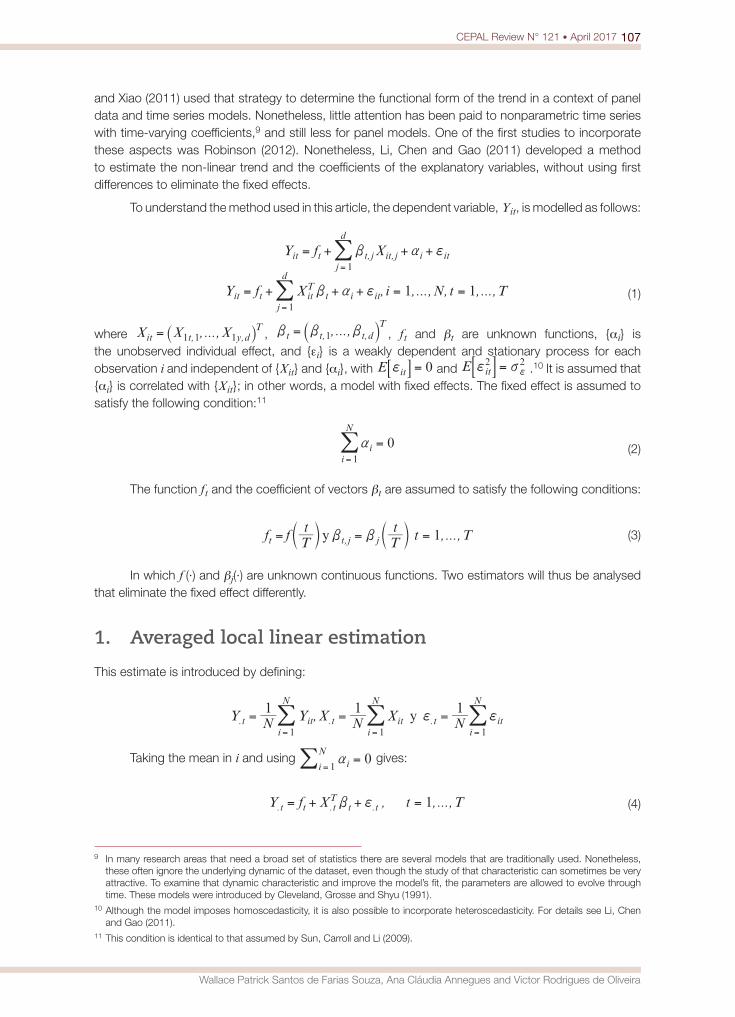
107CEPAL Review N° 121 • April 2017
Wallace Patrick Santos de Farias Souza, Ana Cláudia Annegues and Victor Rodrigues de Oliveira
and Xiao (2011) used that strategy to determine the functional form of the trend in a context of panel data and time series models. Nonetheless, little attention has been paid to nonparametric time series with time-varying coefficients,9 and still less for panel models. One of the first studies to incorporate these aspects was Robinson (2012). Nonetheless, Li, Chen and Gao (2011) developed a method to estimate the non-linear trend and the coefficients of the explanatory variables, without using first differences to eliminate the fixed effects.
To understand the method used in this article, the dependent variable, Yit, is modelled as follows:
Y f X, ,it t t j it jj
d
i it1
b a f= + + +=
/
, , ..., , , ...,Y f X i N t T1 1it t itT
tj
d
i it1
b a f= + + + = ==
/ (1)
where , ...,X X X, ,it t y dT
1 1 1= R W , , ...,, ,t t t dT
1b b b= S X , ft and bt are unknown functions, {αi} is the unobserved individual effect, and {ei} is a weakly dependent and stationary process for each observation i and independent of {Xit} and {αi}, with E 0itf =" % and E it
2 2f v= f" % .10 It is assumed that {αi} is correlated with {Xit}; in other words, a model with fixed effects. The fixed effect is assumed to satisfy the following condition:11
0ii
N
1
a ==
/ (2)
The function ft and the coefficient of vectors bt are assumed to satisfy the following conditions:
f y , ...,f Tt
Tt t T1,t t j jb b= = =T TY Y (3)
In which f (·) and bj(·) are unknown continuous functions. Two estimators will thus be analysed that eliminate the fixed effect differently.
1. Averaged local linear estimation
This estimate is introduced by defining:
y,Y N Y X N X N1 1 1
. . .t it ti
N
iti
N
t iti
N
1 1 1
f f= = == = =
/ / /
Taking the mean in i and using 0ii
N
1a =
=/ gives:
, , ...,Y f X t T1. . .t t tT
t tb f= + + = (4)
9 In many research areas that need a broad set of statistics there are several models that are traditionally used. Nonetheless, these often ignore the underlying dynamic of the dataset, even though the study of that characteristic can sometimes be very attractive. To examine that dynamic characteristic and improve the model’s fit, the parameters are allowed to evolve through time. These models were introduced by Cleveland, Grosse and Shyu (1991).
10 Although the model imposes homoscedasticity, it is also possible to incorporate heteroscedasticity. For details see Li, Chen and Gao (2011).
11 This condition is identical to that assumed by Sun, Carroll and Li (2009).

108 CEPAL Review N° 121 • April 2017
Thoughts on the inequality of opportunities: new evidence
In which the individual effects αi’s, are eliminated. Defining the following notations:
, ...,Y Y Y. . .t TT
1= R W , , ...,f f fTT
1= R W , , , ...,B X X X. .T
TT
TT
1 1b b b=R SW X and , ...,. .TT
1f f f= R W , model (4) can be rewritten as follows:
,Y f B X b f= + +R W (5)
The formulation of the local linear estimator proposed by Fan and Gijbels (1996) is used to estimate f. . , . , ..., .* d
T1b b b=R S R R RW W W WX .
For a 0<τ<1 given,
M
X
X
ThT
ThT T
ThT
ThT T
X
X
1
1
1 1.
.
.
.
T
TT
T
TT
1 1
h h h h hx
x
x
x
x=
−
−
−
−
J
L
KKKKKKKKKKK
R
N
P
OOOOOOOOOOO
W (6)
and
, ...,W diag KTh
TK
ThT T1
xx x
=− −R U TW Z Y# & (7)
where K is the Kernel function and h is the bandwidth.
Assuming b*(·) has continuous derivatives up to the second order, the Taylor expansion gives:
Tt
Tt O T
t* * *
'2
b b x b x x x= + − + −T R R T TY W W Y Y# & (8)
where 0<τ<1, and .*'b R W is the derivative of b*(·). Based on the approximation established by (8), the
local linear estimator of .*Tb R W is
,I O M W M M W Y* d d
T1 1
1 1b x x x x x x= + +
− −t R R R R R RW W W W W W" "% %
(9)
in which Id+1 is a identity matrix, (d+1)x(d+1) and 0d+1 is a null matrix (d+1)x(d+1). The bandwidth is selected by cross validation.
2. Local linear dummy variable approach
Li, Chen and Gao (2011) defined an alternative estimator that displays a faster rate of convergence. For that purpose, model (1) is rewritten as follows:
,Y f B X Db a f= + + +u u u u uR W (10)where
, ..., , , ..., ,Y Y Y Y Y YTNT T
i i iTT
1 1= =u S RX W
N Tr r, ,= =, ...,f I f f IT
Nr ,IT1
u R W
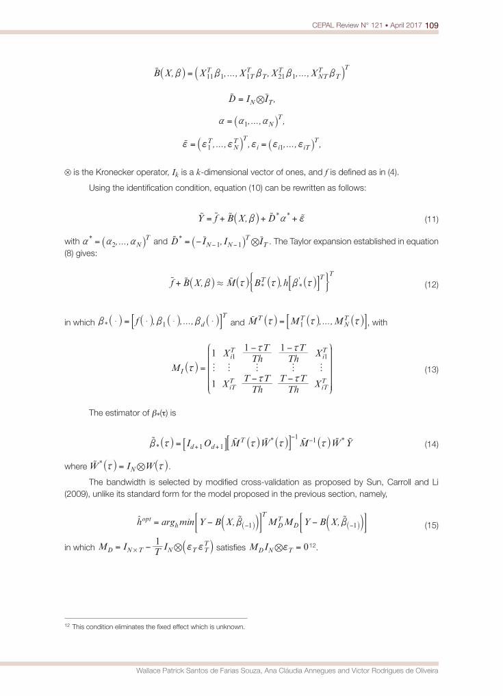
109CEPAL Review N° 121 • April 2017
Wallace Patrick Santos de Farias Souza, Ana Cláudia Annegues and Victor Rodrigues de Oliveira
, , ..., , , ...,B X X X X XTT
TT
TNTT
TT
11 1 1 21 1b b b b b=u R SW X
,D I IN T,=u r
, ..., ,NT
1a a a= R W
, ..., , , ..., ,TNT T
i i iTT
1 1f f f f f f= =u S RX W
⊗ is the Kronecker operator, Ik is a k-dimensional vector of ones, and f is defined as in (4).
Using the identification condition, equation (10) can be rewritten as follows:
,Y f B X D* *b a f= + + +u u u u uR W (11)
with , ...,*N
T2a a a= R W and ,D I I I*
N NT
T1 1 ,= − − −u r rR W . The Taylor expansion established in equation
(8) gives:
, ,f B X M B h* *'T T T
.b x x b x+u u uR R R RW W W W" %G J (12)
in which f , , ...,* dT
1$ $ $ $b b b=R R R RW W W W" % and , ...,M M MT TNT
1x x x=r R R RW W W" %, with
M
X
X
ThT
ThT T
ThT
ThT T
X
X
1
1
1 1
I
iT
iTT
iT
iTT
1 1
h h h h hx
x
x
x
x=
−
−
−
−
J
L
KKKKKKKKKKK
R
N
P
OOOOOOOOOOO
W (13)
The estimator of b*(τ) is
I O M W M W Y** *
d dT
1 1
1 1b x x x x= + +
− −u u u u u uR R R RW W W W" "% % (14)
where W I W*N,x x=u R RW W.
The bandwidth is selected by modified cross-validation as proposed by Sun, Carroll and Li (2009), unlike its standard form for the model proposed in the previous section, namely,
, ,arg minh Y B X M M Y B Xopth
T
DT
D1 1b b= − −− −t u uS SR RX XW W# #& & (15)
in which M I T I1D N T N T T
T, f f= −# S X satisfies M I 0D N T,f = 12.
12 This condition eliminates the fixed effect which is unknown.
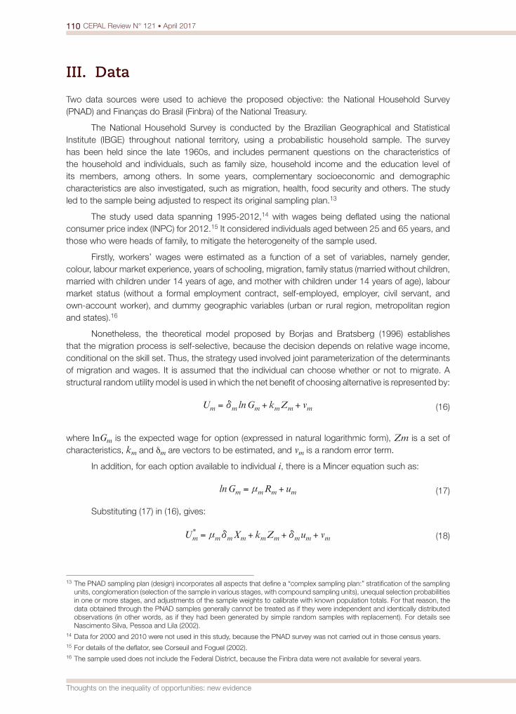
110 CEPAL Review N° 121 • April 2017
Thoughts on the inequality of opportunities: new evidence
III. Data
Two data sources were used to achieve the proposed objective: the National Household Survey (PNAD) and Finanças do Brasil (Finbra) of the National Treasury.
The National Household Survey is conducted by the Brazilian Geographical and Statistical Institute (IBGE) throughout national territory, using a probabilistic household sample. The survey has been held since the late 1960s, and includes permanent questions on the characteristics of the household and individuals, such as family size, household income and the education level of its members, among others. In some years, complementary socioeconomic and demographic characteristics are also investigated, such as migration, health, food security and others. The study led to the sample being adjusted to respect its original sampling plan.13
The study used data spanning 1995-2012,14 with wages being deflated using the national consumer price index (INPC) for 2012.15 It considered individuals aged between 25 and 65 years, and those who were heads of family, to mitigate the heterogeneity of the sample used.
Firstly, workers’ wages were estimated as a function of a set of variables, namely gender, colour, labour market experience, years of schooling, migration, family status (married without children, married with children under 14 years of age, and mother with children under 14 years of age), labour market status (without a formal employment contract, self-employed, employer, civil servant, and own-account worker), and dummy geographic variables (urban or rural region, metropolitan region and states).16
Nonetheless, the theoretical model proposed by Borjas and Bratsberg (1996) establishes that the migration process is self-selective, because the decision depends on relative wage income, conditional on the skill set. Thus, the strategy used involved joint parameterization of the determinants of migration and wages. It is assumed that the individual can choose whether or not to migrate. A structural random utility model is used in which the net benefit of choosing alternative is represented by:
lnU G k Z vm m m m m md= + + (16)
where lnGm is the expected wage for option (expressed in natural logarithmic form), Zm is a set of characteristics, km and dm are vectors to be estimated, and vm is a random error term.
In addition, for each option available to individual i, there is a Mincer equation such as:
ln G R um m m mn= + (17)
Substituting (17) in (16), gives:
U X k Z u v*m m m m m m m m mn d d= + + + (18)
13 The PNAD sampling plan (design) incorporates all aspects that define a “complex sampling plan:” stratification of the sampling units, conglomeration (selection of the sample in various stages, with compound sampling units), unequal selection probabilities in one or more stages, and adjustments of the sample weights to calibrate with known population totals. For that reason, the data obtained through the PNAD samples generally cannot be treated as if they were independent and identically distributed observations (in other words, as if they had been generated by simple random samples with replacement). For details see Nascimento Silva, Pessoa and Lila (2002).
14 Data for 2000 and 2010 were not used in this study, because the PNAD survey was not carried out in those census years.15 For details of the deflator, see Corseuil and Foguel (2002).16 The sample used does not include the Federal District, because the Finbra data were not available for several years.
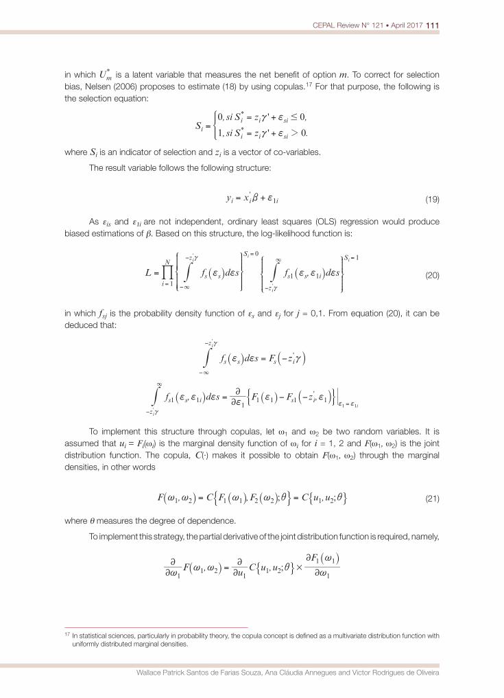
111CEPAL Review N° 121 • April 2017
Wallace Patrick Santos de Farias Souza, Ana Cláudia Annegues and Victor Rodrigues de Oliveira
in which U*m is a latent variable that measures the net benefit of option m. To correct for selection
bias, Nelsen (2006) proposes to estimate (18) by using copulas.17 For that purpose, the following is the selection equation:
, ' ,
, ' .S
si S z
si S z
0 0
1 0
*
*ii i si
i i si 2
#c f
c f=
= +
= +G
where Si is an indicator of selection and zi is a vector of co-variables.
The result variable follows the following structure:
y x'i i i1b f= + (19)
As eis and e1i are not independent, ordinary least squares (OLS) regression would produce biased estimations of b. Based on this structure, the log-likelihood function is:
,L f d s f d ss s
zS
s s i
z
S
i
N0
1 1
1
1
'
'
ii
i
i
f f f f f=3
3c
c−
−=
−
=
=R RW W
Z
[
\
]]]]]]]]]]
Z
[
\
]]]]]]]]
_
`
a
bbbbbbbbbb
_
`
a
bbbbbbbb
% # # (20)
in which fsj is the probability density function of es and ej for j = 0,1. From equation (20), it can be deduced that:
f d s F z's s
z
s i
'i
f f c= −3
c
−
−
R SW X#
, ,f d s F F z's s i
z
s i1 11
1 1 1 1'i
i1 122
f f ff
f f= − −
3
cf f
−=
R R SW W XG J#
To implement this structure through copulas, let ω1 and ω2 be two random variables. It is assumed that ui = Fi(ωi) is the marginal density function of ωi for i = 1, 2 and F(ω1, ω2) is the joint distribution function. The copula, C(·) makes it possible to obtain F(ω1, ω2) through the marginal densities, in other words
; ;, , ,F C F F C u u1 2 1 1 2 2 1 2~ ~ ~ ~ i i= =R R RW W WF FI I (21)
where θ measures the degree of dependence.
To implement this strategy, the partial derivative of the joint distribution function is required, namely,
;, ,F u C u uF
11 2
11 2
1
1 1#
22
22
2
2
~~ ~ i
~
~=R
RW
WF I
17 In statistical sciences, particularly in probability theory, the copula concept is defined as a multivariate distribution function with uniformly distributed marginal densities.
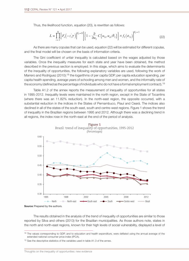
112 CEPAL Review N° 121 • April 2017
Thoughts on the inequality of opportunities: new evidence
Thus, the likelihood function, equation (20), is rewritten as follows:
;,L F z u C u u f1's i
S
i si i
S
i
N 0
11 1 1 1
1
1
ii
#22
c i f= − −= =
=
S RX W# #& &G F IJ% (22)
As there are many copulas that can be used, equation (22) will be estimated for different copulas, and the final model will be chosen on the basis of information criteria.
The Gini coefficient of unfair inequality is calculated based on the wages adjusted by those variables. Once the inequality measures for each state and year have been obtained, the method described in the previous section is employed. In this stage, which aims to evaluate the determinants of the inequality of opportunities, the following explanatory variables are used, following the work of Marrero and Rodríguez (2010):18 the logarithms of per capita GDP, per capita education spending, per capita health spending, average years of schooling among men and women, and the informality rate of the economy (defined as the percentage of individuals who do not have a formal employment contract).19
Table A1.2 of the annex reports the measurement of inequality of opportunities for all states in 1995-2012. Inequality levels were maintained in the north region, except in the State of Tocantins (where there was an 11.82% reduction). In the north-east region, the opposite occurred, with a substantial reduction in the indices in the States of Pernambuco, Piauí and Ceará. The indices also declined in all of the states of the south-east, south and centre-west regions. Figure 1 shows the trend of inequality in the Brazilian regions between 1995 and 2012. Although there was a declining trend in all regions, the index rose in the north-east at the end of the period of analysis.
Figure 1 Brazil: trend of inequality of opportunities, 1995-2012
(Percentages)
0.30
0.35
0.40
0.45
0.50
0.55
0.60
1995 1998 2002 2005 2008 2012
North North-east South-east South Centre-west Brazil
Source: Prepared by the authors.
The results obtained in the analysis of the trend of inequality of opportunities are similar to those reported by Silva and others (2013) for the Brazilian municipalities. As those authors note, states in the north and north-east regions, known for their high levels of social vulnerability, displayed a level of
18 The values corresponding to GDP, and to education and health expenditure, were deflated using the annual average of the extended national consumer price index (IPCA).
19 See the descriptive statistics of the variables used in table A1.3 of the annex.
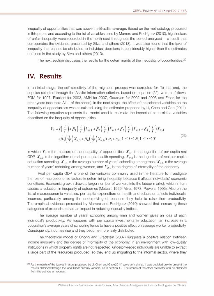
113CEPAL Review N° 121 • April 2017
Wallace Patrick Santos de Farias Souza, Ana Cláudia Annegues and Victor Rodrigues de Oliveira
inequality of opportunities that was above the Brazilian average. Based on the methodology proposed in this paper, and according to the list of variables used by Marrero and Rodríguez (2010), high indices of unfair inequality were recorded in the north-east throughout the period analysed —a result that corroborates the evidence presented by Silva and others (2013). It was also found that the level of inequality that cannot be attributed to individual decisions is considerably higher than the estimates obtained in the study by Silva and others (2013).
The next section discusses the results for the determinants of the inequality of opportunities.20
IV. Results
In an initial stage, the self-selectivity of the migration process was corrected for. To that end, the copulas selected through the Akaike information criterion, based on equation (22), were as follows: FGM for 1997, Plackett for 2003, AMH for 2007, Gaussian for 2002 and 2005 and Frank for the other years (see table A1.1 of the annex). In the next stage, the effect of the selected variables on the inequality of opportunities was calculated using the estimator proposed by Li, Chen and Gao (2011). The following equation represents the model used to estimate the impact of each of the variables described on the inequality of opportunities.
, ,
Y f Tt
Tt X T
t X Tt X T
t X
Tt X T
t X i N t T1 1
, , , ,
, ,
it it it it it
it it i it
1 1 2 2 3 3 4 4
5 5 6 6 # # # #
b b b b
b b a f
=
+ +
+ + + +
+ +
T
T
T
T
T T TY
Y
Y
Y
Y Y Y (23)
in which Yit is the measure of the inequality of opportunities, Xit,1 is the logarithm of per capita real GDP, Xit,2 is the logarithm of real per capita health spending, Xit,3 is the logarithm of real per capita education spending, Xit,4 is the average number of years’ schooling among men, Xit,5 is the average number of years’ schooling among women, and Xit,6 is the degree of informality of the economy.
Real per capita GDP is one of the variables commonly used in the literature to investigate the role of macroeconomic factors in determining inequality, because it affects individuals’ economic conditions. Economic growth draws a larger number of workers into the labour market, which in turn causes a reduction in inequality of outcomes (Metcalf, 1969; Mirer, 1973; Powers, 1995). Also on the list of macroeconomic variables, per capita expenditure on health and education affects individuals’ incomes, particularly among the underprivileged, because they help to raise their productivity. The empirical evidence presented by Marrero and Rodríguez (2010) showed that increasing these categories of expenditure had an impact in reducing inequality indices.
The average number of years’ schooling among men and women gives an idea of each individual’s productivity. As happens with per capita investments in education, an increase in a population’s average years of schooling tends to have a positive effect on average worker productivity. Consequently, incomes rise and they become more fairly distributed.
The theoretical model of Chong and Gradstein (2007) suggests a positive relation between income inequality and the degree of informality of the economy. In an environment with low-quality institutions in which property rights are not respected, underprivileged individuals are unable to extract a large part of the resources produced, so they end up migrating to the informal sector, where they
20 As the results of the two estimators proposed by Li, Chen and Gao (2011) were very similar, it was decided only to present the results obtained through the local linear dummy variable, as in section II.2. The results of the other estimator can be obtained from the authors on request.
114 CEPAL Review N° 121 • April 2017
Thoughts on the inequality of opportunities: new evidence
can retain all of the fruits of their production. As productivity in the informal market is lower than in the formal sector, this would generate a higher degree of income inequality in the economy.
Figure 2 shows the effects of the variables mentioned through the estimator of the local linear dummy variable. The figure consists of six graphs which show how each of the variables impacts on the inequality of opportunities. Figure 2A shows the correlation between per capita GDP and the inequality index. Although the graph seems to suggest a positive relation, the estimated coefficient is negative. This shows that, at the start of the period of analysis, income conditions have a significant weight in reducing inequality. But, after that period, and given the buoyancy of the Brazilian economy since 2003, other factors started to become more important in explaining the trend of the inequality of opportunities, and the primacy of economic growth declined. Using Markov transition matrices, Magalhães and Miranda (2009) showed that per capita income displays a severe process of divergence in Brazil, in which most municipalities fall into one or other of just two groups: the rich club —formed mainly by the municipalities of the south, centre west and south-east, with a per capita income of between 1.27 and 1.68 times above the average of all municipalities— and the poor club —consisting of the municipalities of the north and north-east, with a per capita income of up to 0.55 of that average. Boueri and others (2007) showed that the ergodic distribution in the following period starts to suggest a convergent trend. Lastly, in the most recent decade, the long-term results show a concentration of municipalities and population in the intermediate classes of the distribution.
Figure 2 Estimation of inequality by different variables and Gini coefficient, 1995-2012
-1.0E-05-8.0E-06-6.0E-06-4.0E-06-2.0E-060.0E+002.0E-064.0E-066.0E-068.0E-061.0E-05
1995 1998 2002 2005 2008 2012-1.0E-05
-8.0E-06
-6.0E-06
-4.0E-06
-2.0E-06
0.0E+00
2.0E-06
4.0E-06
1995 1998 2002 2005 2008 2012-3.5E -05
-3.0E -05
-2.5E -05
-2.0E -05
-1.5E -05
-1.0E -05
-5.0E -06
0.0E+00
5.0E -06
1.0E -05
1995 1998 2002 2005 2008 2012
9.9E-039.9E-039.9E-039.9E-039.9E-039.9E-039.9E-039.9E-039.9E-039.9E-039.9E-039.9E-03
1995 1998 2002 2005 2008 2012-1.1E -02
-1.1E -02
-1.1E -02
-1.1E -02
-1.1E -02
-1.1E -02
-1.1E -02
-1.1E -02
-1.1E -02
1995 1998 2002 2005 2008 20120.12
0.13
0.14
0.15
0.16
0.17
0.18
0.19
0.20
0.21
1996 1999 2003 2006 2009
A. Correlation between the inequality index and per
capita GDP
B. Correlation between unfair inequality and health expenditure
C. Correlation between unfair inequality and
education expenditure
D. Correlation between inequality of opportunities
and years of schooling among men
E. Correlation between inequality of opportunities
and years of schooling among women
F. Correlation between inequality of opportunities and the informality rate of
the economy
Source: Prepared by the authors.Note: The values shown on the vertical axis represent the impact of a variable with a much higher scale unit than that of
the inequality of opportunities. GDP: Gross domestic product.
115CEPAL Review N° 121 • April 2017
Wallace Patrick Santos de Farias Souza, Ana Cláudia Annegues and Victor Rodrigues de Oliveira
The relation between economic growth and the reduction of inequality of opportunities is both complex and important. For that reason, it is necessary to understand the channels through which economic growth acts on individuals. It should not be forgotten that progress in terms of welfare, ultimately depends on economic growth and the way individuals take advantage of its benefits. Nonetheless, the characteristics of the economic growth are important, because it can act neutrally, in favour of, or against individuals. Consequently, strategies to reduce the inequality of opportunities cannot be exclusively based on economic growth, but must be combined with income redistribution policies and adequate public expenditure.
Figures 2B and 2C show the correlation between unfair inequality and expenditure on health and education, respectively.
The characteristics of the health sector and changes in the age structure and mortality and morbidity patterns in Brazil have consequences for the costs and use of medical and ambulatory services. In addition, transformations in health systems —the reorganization of care models— and the incorporation of new technologies, among other factors, have also changed the way those services are used. Those dynamics have modified the pattern of health expenditure in recent years. Changes in this sector can be analysed under a microeconomic approach. From the individual standpoint, the consumption of health goods and services directly affects welfare, insofar as health status determines the level of individual happiness. Similarly, from a macroeconomic point of view, the provision of health services affects economic growth, because it restores the human capital stock and determines the economy’s productive capacity. Thus the relation between them can be seen both in the labour market, since it is a labour-intensive sector for low- and medium-complexity services, and in production, since it is also technology-intensive in the case of high-complexity services. Thus, the importance of investment in health, whatever its focus, can be seen in terms of social well-being. Accordingly, these changes have repercussions for resource allocation and for the organization of health service infrastructure, which shows the importance of providing these goods and services and their effects on individual opportunities. Figure 2B shows that the relation is negative throughout the period analysed, so investments in health play a major role in equalizing opportunities between individuals.
Figure 2C reports a positive relation between per capita education expenditure and the inequality of opportunities. This result stems largely from inefficient use of accountability policies. These have become important in the debate on the management of public expenditure, albeit on an incipient basis, but they did not attain the targets or bring equity to the education system. In that regard, the failure of Brazilian education, both in terms of direct investments and in the quality of teaching provided, contributes to that result. These factors serve to maintain a situation of social vulnerability that makes it harder for individuals to fully integrate into society.
Figures 2D and 2E show how the trend of years of formal schooling among men and women, respectively, affects individuals’ opportunities. There is a clear and direct relation between those variables. Figure 3 shows that the states in which the inequality of opportunities has decreased by most were those that in general had the highest growth rates of formal education among men and women. That result shows that an increase in average years of schooling allowed for wage increases (directly), while a reduction in the rate of depreciation of the health stock (indirectly) also contributes positively to income in the labour market. The sum of those two factors affords individuals greater access to opportunities and, thus, the effect of circumstances is compensated through individual effort. It should be stressed that the monetary dimension of the inequality of opportunities, captured by the Gini coefficient, is a partial and limited approach. Although insufficient, the income-based approach to inequality of opportunities should not be rejected, however, because income deprivation is one of the main causes of reduced access to adequate education and health and security conditions, among other factors.
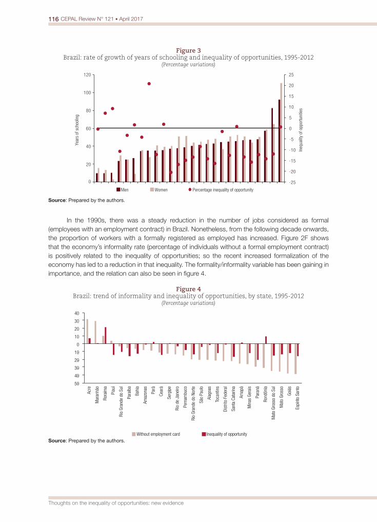
116 CEPAL Review N° 121 • April 2017
Thoughts on the inequality of opportunities: new evidence
Figure 3 Brazil: rate of growth of years of schooling and inequality of opportunities, 1995-2012
(Percentage variations)
-25
-20
-15
-10
-5
0
5
10
15
20
25
0
20
40
60
80
100
120
Ineq
ualit
y of
opp
ortu
nitie
s
Year
s of
sch
oolin
g
Men Women Percentage inequality of opportunity
Source: Prepared by the authors.
In the 1990s, there was a steady reduction in the number of jobs considered as formal (employees with an employment contract) in Brazil. Nonetheless, from the following decade onwards, the proportion of workers with a formally registered as employed has increased. Figure 2F shows that the economy’s informality rate (percentage of individuals without a formal employment contract) is positively related to the inequality of opportunities; so the recent increased formalization of the economy has led to a reduction in that inequality. The formality/informality variable has been gaining in importance, and the relation can also be seen in figure 4.
Figure 4 Brazil: trend of informality and inequality of opportunities, by state, 1995-2012
(Percentage variations)
-50
-40
-30
-20
-10
0
10
20
30
40
Acre
Mar
anhã
o
Rora
ima
Piau
í
Rio
Gran
de d
o Su
l
Para
íba
Bahi
a
Amaz
onas
Pará
Cear
á
Serg
ipe
Rio
de J
anei
ro
Pern
ambu
co
Rio
Gran
de d
o No
rte
São
Paul
o
Alag
oas
Toca
ntin
s
Dist
rito
Fede
ral
Sant
a Ca
tarin
a
Amap
á
Min
as G
erai
s
Para
ná
Rond
ônia
Mat
o Gr
osso
do
Sul
Mat
o Gr
osso
Goiá
s
Espí
rito
Sant
o
Without employment card Inequality of opportunitySource: Prepared by the authors.
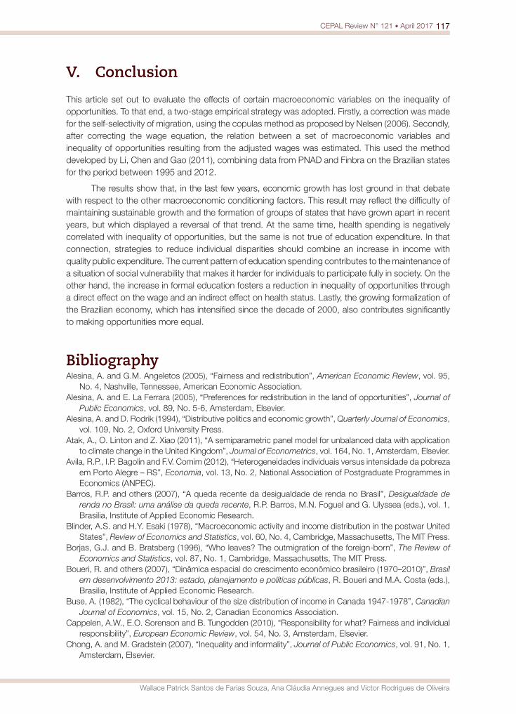
117CEPAL Review N° 121 • April 2017
Wallace Patrick Santos de Farias Souza, Ana Cláudia Annegues and Victor Rodrigues de Oliveira
V. Conclusion
This article set out to evaluate the effects of certain macroeconomic variables on the inequality of opportunities. To that end, a two-stage empirical strategy was adopted. Firstly, a correction was made for the self-selectivity of migration, using the copulas method as proposed by Nelsen (2006). Secondly, after correcting the wage equation, the relation between a set of macroeconomic variables and inequality of opportunities resulting from the adjusted wages was estimated. This used the method developed by Li, Chen and Gao (2011), combining data from PNAD and Finbra on the Brazilian states for the period between 1995 and 2012.
The results show that, in the last few years, economic growth has lost ground in that debate with respect to the other macroeconomic conditioning factors. This result may reflect the difficulty of maintaining sustainable growth and the formation of groups of states that have grown apart in recent years, but which displayed a reversal of that trend. At the same time, health spending is negatively correlated with inequality of opportunities, but the same is not true of education expenditure. In that connection, strategies to reduce individual disparities should combine an increase in income with quality public expenditure. The current pattern of education spending contributes to the maintenance of a situation of social vulnerability that makes it harder for individuals to participate fully in society. On the other hand, the increase in formal education fosters a reduction in inequality of opportunities through a direct effect on the wage and an indirect effect on health status. Lastly, the growing formalization of the Brazilian economy, which has intensified since the decade of 2000, also contributes significantly to making opportunities more equal.
BibliographyAlesina, A. and G.M. Angeletos (2005), “Fairness and redistribution”, American Economic Review, vol. 95,
No. 4, Nashville, Tennessee, American Economic Association.Alesina, A. and E. La Ferrara (2005), “Preferences for redistribution in the land of opportunities”, Journal of
Public Economics, vol. 89, No. 5-6, Amsterdam, Elsevier.Alesina, A. and D. Rodrik (1994), “Distributive politics and economic growth”, Quarterly Journal of Economics,
vol. 109, No. 2, Oxford University Press.Atak, A., O. Linton and Z. Xiao (2011), “A semiparametric panel model for unbalanced data with application
to climate change in the United Kingdom”, Journal of Econometrics, vol. 164, No. 1, Amsterdam, Elsevier.Avila, R.P., I.P. Bagolin and F.V. Comim (2012), “Heterogeneidades individuais versus intensidade da pobreza
em Porto Alegre – RS”, Economia, vol. 13, No. 2, National Association of Postgraduate Programmes in Economics (ANPEC).
Barros, R.P. and others (2007), “A queda recente da desigualdade de renda no Brasil”, Desigualdade de renda no Brasil: uma análise da queda recente, R.P. Barros, M.N. Foguel and G. Ulyssea (eds.), vol. 1, Brasilia, Institute of Applied Economic Research.
Blinder, A.S. and H.Y. Esaki (1978), “Macroeconomic activity and income distribution in the postwar United States”, Review of Economics and Statistics, vol. 60, No. 4, Cambridge, Massachusetts, The MIT Press.
Borjas, G.J. and B. Bratsberg (1996), “Who leaves? The outmigration of the foreign-born”, The Review of Economics and Statistics, vol. 87, No. 1, Cambridge, Massachusetts, The MIT Press.
Boueri, R. and others (2007), “Dinâmica espacial do crescimento econômico brasileiro (1970–2010)”, Brasil em desenvolvimento 2013: estado, planejamento e políticas públicas, R. Boueri and M.A. Costa (eds.), Brasilia, Institute of Applied Economic Research.
Buse, A. (1982), “The cyclical behaviour of the size distribution of income in Canada 1947-1978”, Canadian Journal of Economics, vol. 15, No. 2, Canadian Economics Association.
Cappelen, A.W., E.O. Sorenson and B. Tungodden (2010), “Responsibility for what? Fairness and individual responsibility”, European Economic Review, vol. 54, No. 3, Amsterdam, Elsevier.
Chong, A. and M. Gradstein (2007), “Inequality and informality”, Journal of Public Economics, vol. 91, No. 1, Amsterdam, Elsevier.

118 CEPAL Review N° 121 • April 2017
Thoughts on the inequality of opportunities: new evidence
Cleveland, W.S., E. Grosse and W.M. Shyu (1991), “Local regression models”, Statistical Models in S., J. Chambers and T.J. Hastie (eds.), Pacific Grove, Wadsworth & Brooks.
Corseuil, C.H. and M.N. Foguel (2002), “Uma sugestão de deflatores para rendas obtidas a partir de algumas pesquisas domiciliares do IBGE”, Texto para Discussão, No. 897, Rio de Janeiro, Institute of Applied Economic Research.
Cysne, R.P., W. Maldonado and P.K. Monteiro (2005), “Inflation and income inequality: a shopping-time approach”, Journal of Development Economics, vol. 78, No. 2, Amsterdam, Elsevier.
Erosa, A. and G. Ventura (2002), “On inflation as a regressive consumption tax”, Journal of Monetary Economics, vol. 49, No. 4, Amsterdam, Elsevier.
Fan, J. and I. Gijbels (1996), Local Polynomial Modelling and Its Applications, London, Chapman and Hall.Fan, J. and R. Li (2004), “New estimation and model selection procedures for semiparametric modeling in
longitudinal data analysis”, Journal of the American Statistical Association, vol. 99, No. 467, Taylor & Francis.Fleurbaey, M. (2008), Fairness, Responsibility, and Welfare, New York, Oxford University Press.Forbes, K. (2000), “A reassessment of the relationship between inequality and growth”, American Economic
Review, vol. 90, No. 4, Nashville, Tennessee, American Economic Association.Gaertner, W. and L. Schwettmann (2007), “Equity, responsibility and the cultural dimension”, Economica,
vol. 74, No. 296, Wiley.Gao, J. and K. Hawthorne (2006), “Semiparametric estimation and testing of the trend of temperature series”,
Econometrics Journal, vol. 9, No. 2, Wiley.Henderson, D., R.J. Carroll and Q. Li (2008), “Nonparametric estimation and testing of fixed effects panel
data models”, Journal of Econometrics, vol. 144, No. 1, Amsterdam, Elsevier.Kuznets, S. (1955), “Economic growth and income inequality”, American Economic Review, vol. 45, No. 1,
Nashville, Tennessee, American Economic Association.Li, D., J. Chen and J. Gao (2011), “Non-parametric time-varying coefficient panel data models with fixed
effects”, Econometrics Journal, vol. 14, No. 3, Wiley.Li, H. and H. Zou (1998), “Income inequality is not harmful for growth: theory and evidence”, Review of
Development Economics, vol. 2, No. 3, Wiley.Magalhães, J.C. and R.B. Miranda (2009), “Dinâmica da renda per capita, longevidade e educação nos
municípios brasileiros”, Estudos econômicos, vol. 39, No. 3, São Paulo.Marrero, A.G. and J.G. Rodríguez (2010), “Inequality of opportunity and growth”, Working Papers,
No. 154, ECINEQ.Menezes-Filho, N., R. Fernandes and P. Picchetti (2007), “Educação e queda recente da desigualdade no
Brasil”, Desigualdade de renda no Brasil: uma análise da queda recente, R.P. Barros, M.N. Foguel and G. Ulyssea (eds.), vol. 2, Brasilia, Institute of Applied Economic Research.
Meng, X. (2001), “The informal sector and rural-urban migration - a Chinese case study”, Asian Economic Journal, vol. 15, No. 1, Wiley.
Metcalf, C.E. (1969), “The size distribution of personal income during the business cycle”, American Economic Review, vol. 59, No. 4, Nashville, Tennessee, American Economic Association.
Mirer, T.W. (1973), “The effects of macroeconomic fluctuation on the distribution of income”, Review of Income and Wealth, vol. 19, No. 4, Wiley.
Nascimento Silva, P.L., D.G.C. Pessoa and M.F. Lila (2002), “Statistical analysis of data from PNAD: incorporating the sample design”, Ciência & Saúde Coletiva, vol. 7, No. 4, Rio de Janeiro, Brazilian Association of Collective Health.
Nelsen, R.B. (2006), An Introduction to Copulas, New York, Springer. Neri, M. (2011), Desigualdade de renda na década, Rio de Janeiro, FGV Editora.Nolan, B. (1987), “Cyclical fluctuations in factor shares and the size distribution of income”, Review of Income
and Wealth, vol. 33, No. 2, Wiley.Powers, E. (1995), “Inflation, unemployment, and poverty revisited”, Economic Review, No. 2, Cleveland,
Federal Reserve Bank of Cleveland.Ramalho, H.M.B. and V.S. Queiroz (2011), “Migração interestadual de retorno e autosseleção: evidências para
o Brasil”, Pesquisa e Planejamento Econômico, vol. 41, No. 3, Institute of Applied Economic Research.Ramos, X. and D. Van De Gaer (2012), “Empirical approaches to inequality of opportunity: principles, measures,
and evidence”, IZA Discussion Paper, No. 6672, Institute for the Study of Labour (IZA).Ravallion, M. (2012), “Why don’t we see poverty convergence?”, American Economic Review, vol. 102, No. 1,
Nashville, Tennessee, American Economic Association.Rawls, J. (1971), A Theory of Justice, Cambridge, Harvard University Press.

119CEPAL Review N° 121 • April 2017
Wallace Patrick Santos de Farias Souza, Ana Cláudia Annegues and Victor Rodrigues de Oliveira
Robinson, P.M. (2012), “Nonparametric trending regression with cross-sectional dependence”, Journal of Econometrics, vol. 169, No. 1, Amsterdam, Elsevier.
Rocha, S. (2007), “Os ‘novos’ programas de transferências de renda: impactos possíveis sobre a desigualdade no Brasil”, Desigualdade de renda no Brasil: uma análise da queda recente, R.P. Barros, M.N. Foguel and G. Ulyssea (eds.), vol. 2, Brasilia, Institute of Applied Economic Research.
Roemer, J.E. (1998), Equality of Opportunity, Cambridge, Massachusetts, Harvard University Press.Schokkaert, E. and K. Devooght (2003), “Responsibility-sensitive fair compensation in different cultures”,
Social Choice and Welfare, vol. 21, No. 2, Springer.Silva, V. and others (2013), “Uma proposta para mensuração dos índices de desigualdade de oportunidade
municipais” [online] http://www.ccsa.ufpb.br/ppge/arquivos/ensaios/td15_2013.pdf.Sun, Y., R.J. Carroll and D. Li (2009), “Semiparametric estimation of fixed effects panel data varying coefficient
models”, Advances in Econometrics, vol. 25, Emerald.Ullah, A. and N. Roy (1998), “Nonparametric and semiparametric econometrics of panel data”, Handbook of
Applied Economics and Statistics, A. Ullah and D.E.A. Giles (eds.), New York, Marcel Dekker.World Bank (2005), World Development Report 2006: Equity and Development, Washington, D.C.Zhang, W., J. Fan and Y. Sun (2009), “A semiparametric model for cluster data”, Annals of Statistics, vol. 37,
No. 2, Institute of Mathematical Statistics.

120 CEPAL Review N° 121 • April 2017
Thoughts on the inequality of opportunities: new evidence
Annex A1Table A1.1
Results of the use of copulas to correct for the self-selectivity of migration, 1995-2012
YearAkaike information criterion Selected
copulaa θGaussian FGM Plackett AMH Frank Clayton Gumbel Joe
1995 48 059.71 48 056.75 48 053.76 48 047.60 48 044.45 48 059.28 48 114.64 48 187.19 Frank 0.27
1996 47 520.12 47 502.70 47 523.15 47 521.48 47 490.60 47 513.63 47 508.93 47 647.91 Frank 0.33
1997 51 717.29 51 680.52 51 713.59 51 681.52 51 715.23 51 714.77 51 750.27 51 897.91 FGM -0.89
1998 50 574.84 50 573.07 50 575.04 50 573.10 50 571.26 50 574.59 50 734.43 50 739.76 Frank 0.08
1999 51 681.11 51 672.20 51 647.59 51 639.06 51 615.59 51 676.01 51 715.85 51 893.31 Frank 0.41
2001 58 775.96 58 773.69 58 773.95 58 773.64 58 773.12 58 773.99 58 842.08 59 007.08 Frank 0.02
2002 62 605.30 62 606.21 62 606.21 62 606.20 62 608.21 62 608.21 62 707.29 62 818.08 Gaussian 0.04
2003 59 862.64 59 862.11 59 854.56 59 862.11 59 861.94 59 862.19 60 001.84 60 081.74 Plackett 0.17
2004 62 795.18 62 772.10 62 781.08 62 789.63 62 762.61 62 798.06 62 911.15 63 044.55 Frank 0.35
2005 30 236.94 30 237.76 30 237.74 30 237.76 30 237.37 30 237.68 30 345.47 30 325.17 Gaussian -0.05
2006 69 608.50 69 579.25 69 619.57 69 575.62 69 548.41 69 630.96 69 791.28 69 691.63 Frank 0.40
2007 67 346.47 67 343.70 67 346.40 67 338.88 67 344.33 67 343.86 67 446.72 67 602.64 AMH -0.06
2008 71 689.75 71 685.56 71 690.11 71 688.38 71 683.67 71 690.03 71 786.05 71 870.61 Frank 0.08
2009 71 421.38 71 416.94 71 394.93 71 405.32 71 392.06 71 422.50 71 558.94 71 661.80 Frank 0.32
2011 57 894.80 57 855.66 57 895.93 57 894.48 57 852.15 57 893.46 57 962.15 58 066.96 Frank -0.40
2012 59 163.44 59 161.87 59 163.91 59 161.87 59 153.91 59 163.03 59 313.24 59 361.31 Frank -0.31
Source: Prepared by the authors.a For details of the copula functions and calculation of θ, see Kendall in Nelsen (2006).
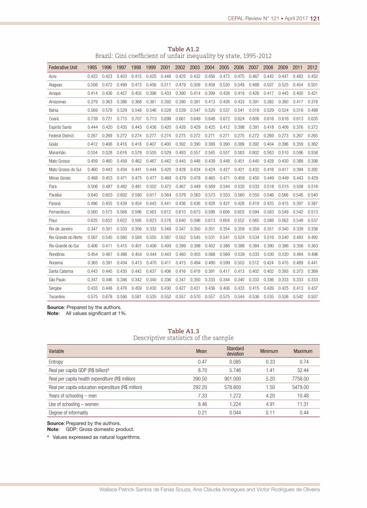
121CEPAL Review N° 121 • April 2017
Wallace Patrick Santos de Farias Souza, Ana Cláudia Annegues and Victor Rodrigues de Oliveira
Table A1.2 Brazil: Gini coefficient of unfair inequality by state, 1995-2012
Federative Unit 1995 1996 1997 1998 1999 2001 2002 2003 2004 2005 2006 2007 2008 2009 2011 2012
Acre 0.422 0.423 0.403 0.415 0.425 0.448 0.425 0.432 0.456 0.473 0.475 0.467 0.442 0.447 0.483 0.452
Alagoas 0.508 0.472 0.499 0.473 0.456 0.511 0.479 0.508 0.458 0.530 0.549 0.488 0.507 0.525 0.454 0.501
Amapá 0.414 0.436 0.457 0.455 0.396 0.433 0.390 0.414 0.399 0.426 0.419 0.426 0.417 0.445 0.400 0.421
Amazonas 0.379 0.363 0.386 0.368 0.361 0.392 0.390 0.391 0.413 0.426 0.433 0.391 0.382 0.380 0.417 0.378
Bahia 0.569 0.578 0.529 0.548 0.546 0.528 0.539 0.547 0.520 0.537 0.541 0.518 0.529 0.524 0.518 0.498
Ceará 0.739 0.721 0.715 0.707 0.713 0.698 0.661 0.649 0.648 0.672 0.624 0.606 0.616 0.616 0.613 0.635
Espírito Santo 0.444 0.420 0.435 0.443 0.436 0.420 0.426 0.429 0.425 0.412 0.398 0.391 0.418 0.406 0.376 0.372
Federal District 0.267 0.269 0.272 0.274 0.277 0.274 0.275 0.272 0.271 0.271 0.275 0.272 0.269 0.273 0.267 0.265
Goiás 0.412 0.406 0.416 0.418 0.407 0.400 0.392 0.390 0.389 0.390 0.389 0.392 0.404 0.396 0.359 0.362
Maranhão 0.554 0.528 0.616 0.579 0.555 0.529 0.493 0.557 0.545 0.557 0.563 0.602 0.563 0.510 0.596 0.558
Mato Grosso 0.459 0.460 0.458 0.462 0.467 0.442 0.445 0.448 0.439 0.448 0.451 0.440 0.428 0.430 0.388 0.398
Mato Grosso do Sul 0.460 0.443 0.434 0.441 0.444 0.420 0.428 0.434 0.424 0.427 0.421 0.432 0.416 0.417 0.394 0.392
Minas Gerais 0.488 0.453 0.471 0.475 0.477 0.469 0.479 0.478 0.465 0.471 0.459 0.450 0.449 0.449 0.443 0.429
Pará 0.506 0.487 0.482 0.481 0.502 0.472 0.467 0.449 0.569 0.544 0.535 0.533 0.518 0.515 0.508 0.516
Paraíba 0.640 0.603 0.602 0.590 0.617 0.564 0.578 0.563 0.573 0.553 0.560 0.550 0.546 0.566 0.546 0.540
Paraná 0.486 0.455 0.439 0.454 0.443 0.441 0.436 0.436 0.428 0.437 0.428 0.419 0.425 0.415 0.397 0.387
Pernambuco 0.560 0.573 0.568 0.596 0.563 0.612 0.610 0.673 0.598 0.606 0.603 0.594 0.583 0.549 0.542 0.513
Piauí 0.625 0.652 0.622 0.595 0.623 0.578 0.640 0.596 0.613 0.604 0.552 0.565 0.588 0.562 0.549 0.537
Rio de Janeiro 0.347 0.351 0.333 0.356 0.332 0.348 0.347 0.350 0.351 0.354 0.359 0.359 0.351 0.340 0.339 0.336
Rio Grande do Norte 0.567 0.545 0.560 0.584 0.555 0.587 0.552 0.545 0.531 0.541 0.524 0.534 0.516 0.540 0.493 0.492
Rio Grande do Sul 0.406 0.411 0.415 0.401 0.406 0.409 0.399 0.398 0.402 0.388 0.388 0.384 0.390 0.386 0.356 0.363
Rondônia 0.454 0.467 0.486 0.454 0.444 0.443 0.460 0.455 0.568 0.569 0.539 0.533 0.530 0.530 0.484 0.496
Roraima 0.365 0.391 0.434 0.413 0.470 0.411 0.415 0.494 0.490 0.599 0.503 0.512 0.424 0.470 0.489 0.441
Santa Catarina 0.443 0.440 0.430 0.442 0.437 0.406 0.416 0.418 0.391 0.417 0.413 0.402 0.402 0.393 0.373 0.369
São Paulo 0.347 0.346 0.346 0.342 0.340 0.336 0.347 0.350 0.333 0.344 0.340 0.333 0.336 0.333 0.333 0.333
Sergipe 0.433 0.448 0.476 0.459 0.430 0.430 0.427 0.431 0.436 0.406 0.433 0.415 0.426 0.425 0.413 0.437
Tocantins 0.575 0.678 0.590 0.581 0.535 0.552 0.557 0.570 0.557 0.575 0.544 0.536 0.535 0.526 0.542 0.507
Source: Prepared by the authors.Note: All values significant at 1%.
Table A1.3 Descriptive statistics of the sample
Variable Mean Standard deviation Minimum Maximum
Entropy 0.47 0.085 0.33 0.74
Real per capita GDP (R$ billion)a 8.70 5.746 1.41 32.44
Real per capita health expenditure (R$ million) 390.50 901.000 5.20 7758.00
Real per capita education expenditure (R$ million) 292.20 578.800 1.50 5479.00
Years of schooling – men 7.33 1.272 4.20 10.48
Use of schooling – women 8.46 1.224 4.91 11.31
Degree of informality 0.21 0.044 0.11 0.44
Source: Prepared by the authors. Note: GDP: Gross domestic product.a Values expressed as natural logarithms.

How did Costa Rica achieve social and market incorporation?Juliana Martínez Franzoni and Diego Sánchez-Ancochea
Abstract
In 1980, just before the debt crisis and in contrast with the experience of the rest of Latin America, almost all Costa Ricans had formal jobs and high-quality social services. To explain this double social and market incorporation, the present article calls into question the role of land distribution, high-quality public institutions and democracy. Instead of these, it focuses on the State-building process whereby a small emerging elite of business owners and urban professionals, drawing on and adapting international ideas, used public policy to deal with social conflict and expand their own economic opportunities. Looking beyond Costa Rica, this analysis is particularly germane at a time of growing emphasis on the political economy of public policy and the still inadequate attention paid to the elites involved in designing it.
Keywords
Economic conditions, social conditions, social welfare, employment, social security, social policy, Costa Rica
JEL classification
I3, O54
Authors
Juliana Martínez Franzoni is a full professor at the Institute for Social Research of the University of Costa Rica. [email protected]
Diego Sánchez-Ancochea is an associate professor at Oxford University (United Kingdom)and director of the Latin American Centre at the same university. [email protected]
124 CEPAL Review N° 121 • April 2017
How did Costa Rica achieve social and market incorporation?
I. Introduction1
People’s welfare depends simultaneously on proper participation in the labour market and protection against the great volatility of that market. In the first place, they need to be able to rely on a stable income so that they can increase their consumption and meet the needs of their households. As Banerjee and Duflo (2011, p. 227) stress in their latest book, Poor Economics: A Radical Rethink of the Way to Fight Poverty, everywhere they asked they found that the most common dream of the poor was that their children become civil servants, which suggests a desire for stability; this shows the importance of high-quality jobs. In the second place, people also want to receive certain services independently of the market as part of their citizen rights and as a way of securing themselves against external volatility and crises.
To explore this twofold goal of public policy, whose urgency has been emphasized by institutions such as the United Nations Research Institute for Social Development (see UNRISD, 2010), we have proposed the concepts of market incorporation and social incorporation (Martínez Franzoni and Sánchez-Ancochea, 2012).2 By incorporation we mean people’s participation over a long historical period in two key resource-allocating institutions: formal labour markets and public social services. Market incorporation means stable access to monetary commerce, which in turn requires the creation of a sufficient number of well-paid formal jobs in the private and public sectors. Social incorporation takes place when people are able to secure their well-being independently of the cash nexus.3
The notion of double incorporation in this article is thus a normative one: it does not mean just any participation in labour markets and social services, as necessarily entailed by urbanization, but the attainment of a “floor” of cash, labour and social protection and services for most.
Unfortunately, few countries in the South have achieved social and market incorporation simultaneously. In Latin America, for example, market incorporation was incomplete and social incorporation segmented for most of the twentieth century. In the period after the Second World War, low agricultural productivity resulted in rapid migration to urban areas, where the new capital-intensive industries could not create enough jobs. Levels of informality and unemployment remained high (albeit less so in Argentina, Chile and Uruguay than in Brazil or the Andean countries), and in 1980 two fifths of Latin American jobs were informal (Tokman, 2001). Social incorporation reflected occupational segmentation under contributory systems organized by formal employment type, which excluded the poor population (Seekings, 2008). In the early 1970s, for example, Chilean social security had 160 different programmes with asymmetrical benefits for different occupational groups (Mesa-Lago, 1978). Civil servants, professionals and other formal urban workers were the first to be incorporated into social security and enjoyed greater benefits than self-employed and informal workers (Filgueira, 2005). In Argentina, social security programmes for “less influential and organized groups, particularly rural and domestic workers, were largely ineffective in enrolling affiliates and the benefits they offered were usually minimal” (Lewis and Lloyd-Sherlock, 2009, p. 116).
Costa Rica was an exception, however, not only in the region but in the whole developing world: between 1950 and 1980, unemployment and underemployment were low, the formal sector
1 This article is based on the argument presented in the book Good Jobs and Social Services: How Costa Rica Achieved the Elusive Double Incorporation (Martínez Franzoni and Sánchez-Ancochea, 2013a), which had only appeared in Spanish until this issue of the CEPAL Review.
2 In using the idea of incorporation, we are preceded by a fruitful tradition of social research. In their now classic work, Collier and Collier (1991) explain how incorporation (into the political arena in this case) replaced the repression of the working class as a political actor.
3 Reygadas and Filgueira (2010) argue that Latin America currently faces a second social incorporation crisis. Instead of the formal working class that was at the forefront of the previous incorporation crisis, those badly in need of incorporation are now the millions of informal workers lacking minimum services. The wave of left-wing and centre-left parties in government partly reflects this population’s demand for incorporation.
125CEPAL Review N° 121 • April 2017
Juliana Martínez Franzoni and Diego Sánchez-Ancochea
grew steadily and a set of universal social programmes expanded.4 By the early 1980s, most Costa Ricans had access to relatively well-paid jobs and to high-quality health care, education and pensions (Sandbrook and others, 2007). Costa Rica actually performed better in some ways than the countries of East Asia. Although these experienced employment and economic “miracles,” they had low social spending and underdeveloped public social security networks (Goodman and Peg, 1996), while social protection was mainly organized around firms and left out a large proportion of the population (ILO, 2007).
What accounts for Costa Rica’s success? Long-term market and social incorporation was not so much the result of a particular ideology as the consequence of the economic preferences of a new elite whose goal was to build the State. An emerging class of small and medium-sized business owners and urban professionals grouped around the National Liberation Party (PLN) came to the fore and used the State to deal with issues as concrete as obtaining credit to expand their economic opportunities. By adapting international ideas (a variable usually overlooked in economics debates), these actors also used public policy to reduce social conflict and weaken the opposition.
Thus, the analysis presented here is of relevance beyond the Costa Rican case, contributing to some of the most significant current debates in political economy. First, the work of Acemoglu, Robinson and their collaborators has brought growing attention in mainstream economics to the role played by the power of elites and their influence on the institutional fabric (Acemoglu and Robinson, 2012; Amsden, Di Caprio and Robinson, 2012). However, few of these studies properly address the issue of who the elites are and why they need the State. This article, on the other hand, highlights the importance of those leading the State-building process and of interactions between the elite, the bureaucracy and international ideas. Second, considering both the importance of these groups and their relationship with the State can yield a better understanding of the opportunities and best strategies for creating new compacts for equality and achieving double incorporation in Latin America, which is one of the key goals of recent work by ECLAC (2014).
The second section will discuss the explanations given hitherto for Costa Rica’s success in achieving the twofold feat of social and market incorporation between 1950 and 1980, and their limitations. The third section will present an argument based on the State-building role played by the emerging elite. The fourth section will briefly analyse the validity of the two key variables presented here to explain why Costa Rica has been struggling to sustain this double incorporation since the 1980s. The fifth section concludes by drawing attention to the theoretical and political implications for the present.
II. The explanations so far given for Costa Rica’s success
The explanations usually given for Costa Rica’s success focus on the existence of relatively equitable patterns of land and income distribution creating conditions as early as colonial times for the subsequent consolidation of democracy and creation of State capacities. Despite its name, Costa Rica lacked natural resources or a large indigenous workforce, and was a long way from the centre of Spanish political authority in Guatemala. As a result, land distribution was less unequal and social divides narrower than in other Central American countries (Hall, 1982; Torres-Rivas, 1975). On this mainstream view, the relative weakness of the oligarchy and the strength of the rural middle class
4 Pribble’s (2011) analysis identifies Costa Rica along with Argentina, Chile and Uruguay as countries with a strong performance in risk prevention and management. However, her analysis concentrates exclusively on the present and does not disaggregate the unequal incorporation of social groups within each country. Sandbrook and others (2007), on the other hand, stress how exceptional Costa Rica is and identify the country as the one example of social democracy in Latin America before the 1990s.
126 CEPAL Review N° 121 • April 2017
How did Costa Rica achieve social and market incorporation?
helped create a more active State and governments that were more sensitive to social demands from the very outset of the republican era (Rueschemeyer, Huber and Stephens, 1992). Echoing the literature on inequality in Latin America (World Bank, 2003; Engerman and Sokoloff, 1997) and the increasingly influential literature on institutions and growth (Acemoglu, Johnson and Robinson, 2005), these explanations look to the colonial period and subsequent institutional development for the key to Costa Rican success.5
While it is true that Costa Rica benefited from a less unequal economic structure than other countries in Latin America, the empirical data cast doubt on the validity of this historical explanation. Between 1935 and 1937, infant mortality was higher in Costa Rica, at 159 children per 1,000, than in Ecuador (145), El Salvador (137) or México (135) (Hytrek, 1999). Although income distribution may have been somewhat more equitable than in the neighbouring countries, inequality was nonetheless very high (Bowman and Baker, 2007). Given that 40 years later Costa Rica’s mortality indices were among the lowest and its life expectancy among the highest in the world, the signs are that the second half of the twentieth century saw significant changes that can clearly not be explained by the colonial inheritance alone.
Alternative explanations for Costa Rican success emphasize the quality of State institutions. The evidence available for the superior performance of Costa Rica’s civil service relative to those of its neighbours would seem to support the theory of bureaucratic capabilities: in the late 1990s, Costa Rica scored best in Latin America and tenth overall among the 35 countries considered by Evans and Rauch (1999) in their evaluation of the quality of bureaucracies. However, State capacity-building did not precede but coincided with the implementation of the policies which made the double incorporation possible. Thus, the constitutional reforms to the civil service of 1946 and 1949 and the Public Administration Act of 1953 were approved in parallel with the changes that were to strengthen employment and create a more highly developed social policy. Again, State capacity in itself cannot explain double incorporation in a comparative perspective: it is significant that in the likes of the Republic of Korea and Taiwan Province of China, sound institutions were not necessarily matched by high levels of social incorporation.
Sandbrook and others (2007) consider Costa Rica’s success to have derived from the existence of a developmental State, a term coined to refer to States capable of disciplining the private sector and making it meet certain performance criteria (Amsden, 2001; Evans, 1995). This definition of the developmental State does not apply to the Costa Rican State: although it did succeed in expanding formal employment, it failed to create new and more dynamic comparative advantages or a competitive industrial sector. It was an expanding social State rather than a developmental State capable of directing the economy along a path of innovation and technological learning.
Of the explanations available, the most influential has been the one concerning the role of democracy in promoting human development. The most generally accepted idea is that, after the civil war of 1948, democratic institutions gave rise to the expansion of a social democratic party that strengthened the bureaucracy and expanded social policy (Huber, 2005; Garnier and Hidalgo, 1991; Itzigsohn, 2000). A second argument stresses the nature of political institutions (Gutierrez-Saxe and Straface, 2008; Lehoucq, 2010; Wilson, 1998). Specifically, the approval of new electoral rules meant that political actors could trust elections, which thus became the only route to power (Lehoucq, 1998; Wilson, 1998). The two-party system and the expectation of alternation in power permitted the consolidation of policies aimed at the median voter (Straface, 2008). In turn, the fact that much public policy was entrusted to independent bodies reduced the influence of electoral and party competition in key policy areas and ensured policy continuity (Lehoucq, 2010; Straface, 2008). The combination of institutional autonomy and alternation of parties in power strengthened public policy.
5 This explanation predominated in the interviews we conducted in Costa Rica in July and August 2011. See also Bodenheimer (1970).

127CEPAL Review N° 121 • April 2017
Juliana Martínez Franzoni and Diego Sánchez-Ancochea
Institutional dynamics have unquestionably been important, particularly in explaining the historical legacies that have operated during the most recent neoliberal period, which is not studied in detail here but is examined in Martínez Franzoni and Sánchez-Ancochea (2013a). However, other countries, with enduring democracies, such as Chile and Uruguay before 1970 in Latin America and others in different parts of the world, have been less successful in securing the double incorporation. In the case of Costa Rica, the institutional explanation is not enough in itself to account for social and market incorporation since the 1950s. For one thing, the autonomous institutions were never strictly autonomous, as the political parties sought to influence them directly and indirectly. In the early 1950s, for example, social actors close to the PLN, such as the Rerum Novarum Workers’ Confederation, participated actively in the appointment of the management boards of banks and the Costa Rican Electricity Institute (Brenes, 1990). For another, the PLN was the only party to put up candidates in all presidential elections, the only one always to have a parliamentary majority (Hernández, 2009; Rovira, 1987) and the real driving force behind the creation of most of the autonomous institutions. Thirdly, particularly between 1950 and 1980, the separation between political parties and the State bureaucracy was not at all clear-cut. Many of those appointed to top positions in the autonomous institutions were sympathizers of the PLN and supported its political project (Denton, 1969). In sum, the evidence points to the PLN and its membership being the key actor behind the expansion of the State in general and public institutions in particular.
Democracy undoubtedly opened up spaces for public debate and forced the political elite to respond at least in part to social demands. However, the direct role of formal democracy in the expansion of the State could be less important than is usually believed, and it was by no means a sufficient condition for success. For one thing, many of the most radical economic changes were made by the victors of the 1948 civil war in a de facto government with little democratic legitimacy per se.6 For another, in 1951 (the year of its foundation), the PLN was a small electoral force that had just been defeated twice over in elections to the legislature and the Constitutional Assembly.7 The PLN was surrounded at that time by a large array of opposition forces, from the coffee-growing oligarchy to the communists. In the 1953 elections, however, its presidential candidate, José “Pepe” Figueres, won 65% of the vote (Hernández, 2009). In a very short period, the brand-new PLN became the dominant political force by combining repression of opposition leaders, a ban on the pro-oligarchy military, specific policy measures during the Junta’s period of government, and electoral promises.
The idea that Costa Rica was fully democratic for most of this period is also questionable. During the 1950s, party leaders from the opposition and trade union activists were exiled or imprisoned. Between 1949 and 1975, the Costa Rican political system maintained anti-democratic exclusions. The second paragraph of article 98 of the Constitution established that the Legislative Assembly could ban political parties deemed undemocratic. Although the scope and severity of exclusion diminished towards the end of the period, it meant that a group of citizens did not have the same freedom of thought and organization or the same voting options as the rest of the population.8
Between 1950 and 1980, in short, democratic consolidation took place simultaneously with economic and social transformations (State of the Nation Program, 2001; Vargas-Cullell, Rosero-Bixby and Seligson, 2005). Broadly speaking, electoral competition simultaneously prompted and impeded changes in social policy, and went hand in hand with other factors such as bureaucratic initiative and the role of international organizations (McGuire, 2010).
6 The fact that the PLN has presented itself as the champion of democracy since its creation does not change the fact that it was its most emblematic leaders who triggered the civil war, abrogated constitutional powers, governed under a Junta and took 18 months to hand over power to the president-elect.
7 The social democrats had 4 of 45 representatives in the Constitutional Assembly of 1949 (Rovira, 1987). That same year they won 3 of 45 seats in the legislature in ordinary elections to renew half the Congress.
8 Rovira (1990) dates democratic consolidation to 1958, when party alternation took place. In this article we date it to 1970, when the Communist Party was legalized.
128 CEPAL Review N° 121 • April 2017
How did Costa Rica achieve social and market incorporation?
III. The emerging elite and the double incorporation
We argue that the double incorporation rested on a rapid expansion of the State presence in the economy and social provision, which in turn was driven by the interests of an emerging elite formed of different segments of the middle class. Grouped around the PLN, this elite used the State for its own benefit, specifically to: (i) support economic activities in which it had interests; (ii) increase its base of social support by expanding public-sector employment, and (iii) manage and suppress conflict.
Again, many of the policies pursued by the PLN can only be understood in the context of ideas that were internationally available. Politicians, and techno-politicians in particular, selectively took up different ideas and adapted them to the country’s conditions and their own political goals. Before the 1980s, these policies centred on the importance of import substitution, on universal social security and, later, on social assistance.
We shall now describe how this emerging elite came to power, how State-building in the interests of specific groups contributed to social and market incorporation, and how international ideas shaped policies.
1. The new elite and the expansion of the State between 1950 and 1970
The main goal of the PLN from its beginnings was to create economic opportunities for small and medium-sized proprietors and urban professionals (Bodenheimer, 1970). This required the party to become a dominant electoral force, something Figueres achieved with his crushing victory in 1953. Once in government, Figueres expanded public-sector employment (which rose from 6% to 10% of the active labour force between 1950 and 1958), introduced the thirteenth annual wage for public servants (as an explicit mechanism for distributing the budget surplus) and promoted pro-PLN unions.9
Because small and medium-sized proprietors like Figueres had great need of financing, the PLN also expanded credit and pursued agricultural sector modernization. In the late 1950s, over a third of all lending in the country was going to the agricultural sector, and the production of staple grains like beans, rice and maize was actively promoted by the National Production Council (Brenes, 1990). The increasing interventions directly benefited the group close to Figueres. A number of PLN leaders had growing interests in cattle ranching and received abundant cheap credit (Aguilar and Solís, 1988). Figueres himself and his brother owned one of the country’s largest coffee estates, located in Turrialba (Winson, 1989). Although the traditional elite also benefited from State support for the modernization of coffee production, the State demanded more from it in return. In 1954, for example, came the introduction of a new tax whereby “the ninety largest companies in the country would see their taxes increase from five million colones a year to fourteen and a half million colones a year” (Bowman and Baker, 2007, p. 38).
With the passing of the Industrial Protection and Development Act in 1959 and the accession of Costa Rica to the Central American Common Market (CACM) in 1963, the centre of economic policy shifted from agriculture to industrial promotion. Both measures were promoted by the PLN elite, which
9 Between 1950 and 1980, the Costa Rican political system had two blocs, the PLN and conservative groups that sometimes managed to build successful anti-PLN coalitions. Between 1951 and 1978, the conservatives won two presidential elections but never obtained a majority in parliament. Before 1970, the PLN did not face an electoral threat from the left because the Communist Party was outlawed.
129CEPAL Review N° 121 • April 2017
Juliana Martínez Franzoni and Diego Sánchez-Ancochea
saw an opportunity to expand its economic base.10 This economic strategy was fiercely opposed by the traditional agro-export oligarchy. These groups, which were in government in the early 1960s, refused to sign the agreement constituting the CACM, so that the accession of Costa Rica took place only after the PLN election victory of 1962.
Both loan subsidies and protection for the domestic market generated large corporate rents, in the sense of opportunities to earn more than would be the case in a free market system (Akyuz and Gore, 1996). González-Vega (1990, p. 21), for example, estimates that in 1974 preferential access to cheap credit translated into “an implicit subsidy of 30% a year.” That author also shows that in agriculture the implicit transfer from public-sector banks was equivalent to about a fifth of total value added. Although most of the data available on the level of protection are for the late 1970s and early 1980s, tariffs were already high during the 1960s. In 1980, the effective rate of protection for the industrial sector as a whole was 139%, with variance of from 45% to 388%, depending on the activity. Textile and leather products received particularly generous protection, as did furniture and wood products (Salazar, 1990). According to calculations by Monge González and González-Vega (1995, p. 134), transfers from consumers to producers were equivalent to 16% of gross domestic product (GDP) in 1996 and probably even more in previous decades.11
Of course, numerous governments set about creating rents that swelled corporate profits during this period (Amsden, 2001). Like many others, Costa Rica’s was not very successful in seeing that these rents turned into new comparative advantages and systematic productivity growth in the manufacturing sector (Brenes, 1990; Lizano, 1999). What was special and successful in Costa Rica was the way these rents were distributed. Although much public investment went to a small part of the new elite, small and medium-sized producers throughout the country benefited as well. In 1952, for example, the National Bank of Costa Rica, acting through its rural councils for economic development, granted 20,000 loans whose recipients totalled a quarter of all agricultural producers, and in 1976 over 24,000 loans were made (González-Vega, 1990). Much lending also went to public institutions which thereupon expanded rapidly and created a large number of jobs throughout the country. Protectionism likewise led to the creation of new firms. In the late 1970s, indeed, 40% of industrial business owners were people whose parents had not owned their own firms (Garnier and Hidalgo, 1991). In short, the economic policies pursued by the PLN during this period helped to buttress the new elite and, in doing so, facilitated the market incorporation of a growing middle class composed of public-sector employees and owners of small businesses in all sectors of the economy (Rodríguez, 1997).
Where social policy is concerned, it must be recognized that this was less of a priority than economic modernization for the PLN during the 1950s and 1960s. Indeed, “much of the social welfare infrastructure had been established before the Revolution of 1948” and there were “no radical innovations” in this period (Bodenheimer, 1970, p. 71; see also Winson, 1989). Even so, social spending and service coverage gradually increased because of three different factors. First, the PLN used social programmes as a tool to expand its base of support. This is clear, for example, from the way the law universalizing social security was passed in 1961. According to the law’s main sponsor, a deputy called Enrique Obregón Valverde, the PLN, then in opposition but with a majority in the legislature, supported it to take credit for the consolidation of social security, thus making up for the fact that the institution had been created by the Social Christians in the 1940s.12 Second, the bureaucracy in charge of pension and health policies demanded that new financing mechanisms be created to ensure
10 Thanks to these provisions and other protection measures, the Chamber of Industries, whose member firms depended on public subsidy, became a fervent supporter of the PLN. A survey conducted in the late 1970s showed that over two thirds of the Chamber’s board members supported the PLN (Vega, 1982).
11 Although the economic assumptions used to calculate these transfers are very questionable (see Ocampo and Taylor, 1998), they give an idea of the scale of the subsidies received by many producers.
12 Interview with Obregón Valverde on 10 August 2011.
130 CEPAL Review N° 121 • April 2017
How did Costa Rica achieve social and market incorporation?
that social security could be sustained and expanded (Rosemberg, 1983). Third, the few new social initiatives promoted by the PLN during this period, although aimed at economic transformation, also contributed to social incorporation. This was true of housing programmes and, still more clearly, of the National Learning Institute (INA).
The creation of the INA in 1965 was meant to support industrialization by providing training for the working class. Law 3506 under which it was created was tabled by the Minister of Labour, Alfonso Carro Zúñiga, with advice from the International Labour Organization (ILO) and Israeli experts (Congreso Constitucional, 1965). The PLN wanted to increase the productive capabilities of the workforce, particularly in manufacturing, and expand job opportunities for the young and low-income population. At the same time, the INA was meant to boost corporate earnings and thence also increase the party’s social base among the better-off sections of society. The law was supported enthusiastically by the Chamber of Industries, the media and Congress.
The expansion of public-sector employment was another crucial instrument for increasing the PLN support base. Whereas in 1960 less than 10% of the economically active population was in public-sector employment, 20 years later the figure had risen to about 18%, with an absolute increase from 30,000 to 150,000 public-sector jobs (CLAD, 2007). Unfortunately, the PLN also used other, less democratic methods to reduce conflicts and minimize opposition to its modernization project, coopting and repressing unions in particular. Because there was no law protecting their leaders from being dismissed as an anti-union measure, private-sector unions were systematically repressed (Castro Méndez and Martínez Franzoni, 2010). By the mid-1970s, only 5% of private-sector employees were unionized. In the public sector, there was a mixture of repression and cooptation. In 1971, the Minister of Labour admitted that “union freedoms as such” did not exist (Aguilar, 1989, p. 174). When the right to strike was established, the bar was set so high (strikes had to be supported by 60% of the workers concerned, for instance) that its exercise was severely restricted in practice and virtually all strikes ended up being illegal (Castro Méndez and Martínez Franzoni, 2010). Of the 182 strikes recorded between 1972 and 1983 and the 159 called between 1990 and 1998, just 5 were deemed legal (Donato and Rojas Bolaños, 1987; State of the Nation Program, 2001). Somewhat later, in 1984, with the support of the business chambers, the government passed the Solidarity Associations Act, which created mutual saving and loan organizations with workers’ membership and employer participation. Although formally these solidarity organizations complemented unions, in practice they became a powerful tool of anti-union policy, as repeated efforts were made to give them a role in representing workers’ employment interests (Castro Méndez, 2014).
2. The renewal of State initiative in the 1970s
While in power between 1970 and 1978, the PLN tried to cope with the international economic crisis of the early 1970s and growing constraints on manufacturing by giving the public sector a new role. Expanding the economic function of the State became more important than promoting opportunities for private accumulation. The creation of the Costa Rican Development Corporation (CODESA) in 1972 was the first step in this new market incorporation strategy. CODESA was originally expected to promote investment in new sectors of the economy and stimulate public-private partnerships. Its board was made up of representatives of business associations, including the Chamber of Industries, and it did not initially compete with the private sector.13 In 1975, though, CODESA expanded into a growing number of sectors, including sugar, cotton and cement, and also into the stock market. It also received ample loan support: in 1983, lending by the Central Bank of Costa Rica to CODESA represented half of all credit to the private sector and 18% of total domestic lending.
13 August 2011 interview with the technical and political advisor assisting President Oduber.
131CEPAL Review N° 121 • April 2017
Juliana Martínez Franzoni and Diego Sánchez-Ancochea
With the creation of CODESA and an increased role for the State, the PLN was pursuing a twofold objective. First, it sought to create a “bourgeois bureaucracy” comprising party members who progressively increased their power and wealth (Sojo, 1984). Second, it succeeded in expanding public-sector employment at a particularly difficult time in the labour market. It should not be surprising, then, that the private sector opposed the expansion of CODESA almost from the start and became increasingly critical of the PLN (Vega, 1980).
In the case of social policy, during the 1970s the PLN elite sought to enhance the role of the State while at the same time altering its approach. Up until then, actions to increase social and market incorporation had focused on the Central Valley and mainly benefited the middle class. Between 1963 and 1973, for example, the income received by people in the middle of the social structure (deciles 4 to 8) rose from 30% to 40%. However, the income share of the lowest-income 20% of the population declined slightly, from 6.0% to 5.4% (OFIPLAN, 1982).14 Efforts to redistribute land during the 1960s failed and landless campesinos living outside the Central Valley continued to be excluded from the modernization process (Seligson, 1980).15
The PLN faced a growing social conflict in the early 1970s: between 1971 and 1974, 2,240 families illegally occupied over 91,000 hectares of land (Cortés and León, 2008). Much of the protest was channelled by progressive movements with links to the still illegal Communist Party and other left-wing parties whose presence in rural areas increased considerably.16 To cope with the conflict, the PLN introduced new social programmes oriented towards the poor, especially in rural areas. In 1970, Figueres created the Joint Institute for Social Aid (IMAS) to transfer subsidies to people living in extreme poverty. More significant still was the 1974 creation of the Fund for Social Development and Family Allowances (FODESAF) under Oduber’s government. In its first year of operation, FODESAF received 1.4% of GDP (Trejos, cited in Rovira, 1987). This fund was groundbreaking in Latin America, focused as it was on financing services for hitherto excluded people via existing public services and public institutions that catered to the non-poor population. FODESAF also created new programmes, including non-contributory pensions, primary health care and school meals, implemented by institutions with a universal character.17
3. The role of international ideas between 1950 and 1980
While the interests of the PLN elite help to explain the general thrust of public policy, they are not enough to account for its specific features. For this, it is necessary to consider the role and origin of ideas and analyse how these changed over time. Specifically, we argue that international actors and the ideas promoted by them were extremely important for public policymaking.
By way of example, the social and labour market reforms of the 1940s were implemented in a setting that was heavily influenced by the anti-communist reformism of the New Deal brought in by President Roosevelt in the United States (Acuña, 1995). The system of health insurance created in 1941 was likewise strongly influenced by international recommendations that occupation-stratified regimes should be avoided in favour of unified systems for all (Martínez Franzoni and Sánchez-Ancochea, 2012; Seekings, 2010).
14 The data are based on nominal monthly household incomes and should be interpreted with caution, since the reliability of the surveys conducted at that time is unknown.
15 By the mid-1970s, the new institution responsible for land distribution had transferred just 3% of arable land and benefited 1.7% of landless campesino families (Seligson, 1984).
16 Social protests against foreign investment projects also intensified in urban areas, the most emblematic case being Alcoa.17 August 2011 interview with Kyra del Castillo, who was involved in the design and start-up of FODESAF.
132 CEPAL Review N° 121 • April 2017
How did Costa Rica achieve social and market incorporation?
Over the next three decades, regional and international paradigms moulded different economic and social policies. By contrast with the pioneering countries of South America, where the production structure changed prior to any explicit import substitution policies being applied (Thorp, 1998), protectionist and industrial policies in Central America were a response to international ideas whose goal was to transform the economic structure, not the other way round. Via CACM, ECLAC and the Government of the United States played a fundamental role in the implementation of import substitution. Something similar happened with social security, set up without the pressure from the working class that had been the driving force in the Southern Cone. Instead, the combination of other countries’ experience (particularly that of Chile) and ILO policy prescriptions encouraged less advanced countries like Costa Rica to catch up with the models of social incorporation considered desirable at the time.
In the 1950s, ECLAC promoted industrialization under a system known as “limited integration with reciprocity” (Bulmer-Thomas, 1987). Specifically, it proposed that State-regulated regional monopolies should be set up to distribute new industries equitably between member countries. Underlying the Multilateral Treaty on Free Trade and Central American Economic Integration was the ECLAC model excluding numerous agricultural products such as staple grains, cotton, coffee and sugar from the free market. Central American economic integration also reflected the thinking of the Government of the United States. Specifically, the Eisenhower administration favoured free trade between all member countries and promoted the idea of planning regional monopolies. This thinking was behind the Tripartite Agreement of February 1960 that became the basis for the General Treaty on Central American Economic Integration, approved in December that year by El Salvador, Guatemala, Honduras and Nicaragua and joined three years later by Costa Rica.
International ideas about import substitution had markedly different practical repercussions in each of the Central American countries. Costa Rica was more successful than the rest for at least two reasons. First, industrial protection contributed to a gradual expansion of social policy based on payroll taxes. Most firms could take a relaxed view of the high labour costs that resulted because they were not competing internationally (Lizano, 1999). Agro-exporters were not so comfortably placed, but many of them (particularly those recruiting temporary workers, including coffee producers) were exempt from this tax. In contrast to East Asia, where labour-intensive manufacturing exports made governments and firms resistant to social security regimes that would raise labour costs (Haggard and Kaufman, 2008, p. 9), import substitution industrialization in Costa Rica facilitated the expansion of public spending. Second, industrialization policy benefited not only large companies but also small and medium-sized enterprises and cooperatives, which made the country an outlier in Latin America.
International ideas also played an important role in the formation of social assistance programmes in the mid-1970s. Following the example of France, Uruguay and other countries, together with what were by then well-established ILO policy recommendations, Figueres and his Minister of Labour, Jiménez Veiga, proposed the creation of family allowances, i.e., an income per child transferred to low-income formal workers. However, this programme came at a time of growing influence for the ideas of social transformation that followed the Cuban revolution of 1959. These ideas stressed the need to go further than cash transfers and include services as part of an integrated, multidimensional response to poverty. This vision was reflected in Kennedy’s Alliance for Progress, in Johnson’s War on Poverty, in the new interventions based on the basic needs approach promoted by the World Bank and in the thinking of ECLAC and the Socialist International. President Oduber (1974-1978) and his Vice-President Castillo were more attuned to these ideas than Figueres. Oduber had been Vice-President of the Socialist International and Castillo had worked for ECLAC and for the Central American Integration System. After winning the February 1974 elections, the two of them successfully sought to turn the original project into a social development fund.
133CEPAL Review N° 121 • April 2017
Juliana Martínez Franzoni and Diego Sánchez-Ancochea
IV. The ups and downs of double incorporation
Incorporation can diminish and exclusion increase if inappropriate policies are applied at times of crisis. Costa Rica has struggled in recent decades to maintain the double incorporation achieved previously. Partly because of the new open export-oriented model, the Costa Rican workforce has increasingly divided between people with well-paid formal jobs in dynamic sectors of the economy, such as tourism, finance and high-technology assembly, and those who only have access to unskilled, low-technology informal jobs in other areas, mainly serving the domestic market. The informal sector employed 35% of the working population in 2006, as against 20% in the early 1980s. Between 1984 and 2009, the average minimum wage rose at an average annual rate of just 0.7% in real terms and wage inequality increased considerably (State of the Nation Program, 2011). As regards social incorporation, near-universal health-care coverage and very high pension coverage have been maintained, as have high primary and secondary school enrolment rates, albeit with growing quality problems and huge pressure to privatize service provision (Martínez Franzoni and Sánchez-Ancochea, 2013b).
Many of the problems have arisen precisely because the contribution to market and social incorporation of the two independent variables presented here (the composition and interests of the elite and international ideas) has weakened. In the first place, the Costa Rican elite responsible for the earlier success has fragmented, and much of it depends less and less on an expanding domestic market. The divisions within the PLN caused by disagreements about the optimum development model were already there in the second half of the 1970s, but intensified in the early 1980s (Lizano, 1999). New leaders such as Oscar Arias (the country’s President in 1986-1990 and 2006-2010), Eduardo Lizano (chairman of the Central Bank of Costa Rica on several occasions) and others worked for a quantitative and qualitative change in the State’s involvement in economic affairs. The strains arose in relation to the advisability or otherwise of having State-owned enterprises directly involved in production and maintaining an exclusively public banking system. These leaders largely represented the interests of business groups allied with the PLN that had been growing and collaborating with transnational enterprises during the 1970s and no longer had an interest in supporting the traditional Costa Rican economic model.
The divisions within the elites have been deepening ever since, and the power of groups interested in promoting exports and finance has grown steadily. The PLN agenda, which has been moving closer and closer to that of the Social Christian opposition (Rovira, 2004), has increasingly centred on creating better conditions for foreign investors, expanding the linkages between these and Costa Rican firms and using social policy to compensate those left behind. Outside the PLN, emerging business groups are more interested in strengthening their ties to foreign firms and expanding in the regional market than in trying to increase the consumption capacity of the Costa Rican population (Bull and Kasahara, 2013; Sánchez-Ancochea, 2003; Segovia, 2005).
In the second place, shifts in international thinking also help to explain the direction of policy in Costa Rica. The Washington Consensus called traditional social democratic ideas into question globally and provided a theoretical justification for trade liberalization and financial deregulation. Simultaneously, countries such as Ireland and Singapore turned into powerful examples of how to attract foreign firms and provide incentives to particular sectors of the economy to the detriment of others (Mortimore and Vergara, 2004; Sánchez-Ancochea, 2009). Following these experiences, the PLN committed decisively to promoting foreign high-technology investment, a policy that increased competitiveness but did relatively little for market incorporation in the aggregate.
134 CEPAL Review N° 121 • April 2017
How did Costa Rica achieve social and market incorporation?
V. Implications
Despite the changes of recent decades, the Costa Rican case furnishes important lessons, both theoretically and for policy purposes. Theoretically, it shows the need to pay serious attention to the composition of the elite and its incentives when taking up the task of State-building. The analysis presented here shows that the problem for incorporation is not that the elite seeks to control the State for its own benefit: it may happen that these groups do seek their own benefit and yet still help to bring about positive results in terms of double incorporation, something that authors such as Acemoglu and Robinson (2012) do not seem to consider. For example, the promotion of public-sector employment, small and medium-sized firms and cooperatives before the 1980s in Costa Rica reflects precisely the ability of various segments of the middle class to build a State that suits their own interests.
Likewise, the study presented here shows that the incentives for the elite to pursue labour market transformation and social incorporation are not necessarily aligned: there is no reason to expect a State focused on structural change to arise out of the same process that produces universal social policies, or vice versa. What makes the Costa Rican case particularly interesting is the convergence between a productive transformation that has created good jobs and an expanding social policy.
The main public policy implications of this study are the importance of understanding who the elites are and what they want (particularly from the State) and of considering innovations within an international public policy context. Placing the stress on elites provides a grasp of the structural possibilities and limitations that exist for the double incorporation (on this subject, see Schneider, 2012). Meanwhile, international ideas have a crucial role in legitimizing reforms and mapping out the range of possible options at different times, and considerably influence the specific characteristics of the programmes shaping the State.
If the analysis in this article is correct, then the emphasis placed on both industrial policy (UNRISD, 2010) and universal social policies (Mkandawire, 2006; Filgueira and others, 2006) in the region since the 2000s represents a valuable opportunity for countries with a history of limited social and market incorporation to pursue public policy changes. Again, if countries are to place the State at the service of the double incorporation, these ideas need actors who believe in them and can adapt them and give them substance in public policy decisions. It is necessary, then, to know whether and how far countries have emerging elites willing to embark on this new development path.
BibliographyAcemoglu, D., S. Johnson and J. Robinson (2005), “Institutions as fundamental cause of long-run growth”,
Handbook of Economic Growth, Ph. Aghion and S. Durlauf (eds.), Amsterdam, Elsevier.Acemoglu, D. and J. Robinson (2012), Why Nations Fail: The Origins of Power, Prosperity and Power, New
York, Crown Business.Acuña, M. (1995), Clays, Ivonne: Testigo de la neurosis de una administración, San Jose.Aguilar, M. (1989), Clase trabajadora y organización sindical en Costa Rica, 1943-1971, San Jose, Costa
Rican Institute of Social Studies/Editorial Porvenir.Aguilar, I. and M. Solís (1988), La élite ganadera en Costa Rica, San Jose, Editorial de la Universidad de
Costa Rica.Akyuz, Y. and Ch. Gore (1996), “The investment-profits nexus in East Asian industrialization”, World Development,
vol. 24, No. 3, Amsterdam, Elsevier.Amsden, A. (2001), The Rise of the Rest. Challenges to the West from Late-Industrializing Economies, New
York, Oxford University Press.Amsden, A., A. di Caprio and J. Robinson (2012), The Role of Elites in Economic Development, Oxford,
Oxford University Press.
135CEPAL Review N° 121 • April 2017
Juliana Martínez Franzoni and Diego Sánchez-Ancochea
Banerjee, A. and E. Duflo (2011), Poor Economics: A Radical Rethink of the Way to Fight Poverty, New York, Public Affairs.
Bodenheimer, S. (1970), “The social democratic ideology in Latin America: the case of Costa Rica’s Partido Liberación Nacional”, Caribbean Studies, vol. 10, No. 3.
Bowman, K. and S. Baker (2007), “Noisy regimes, causal processes, and democratic consolidation: the case of Costa Rica”, The Latin Americanist, vol. 50, No. 2.
Brenes, L. (1990), La nacionalización bancaria en Costa Rica. Un juicio histórico, San Jose, Latin American Faculty of Social Sciences (FLACSO).
Bull, B. and Y. Kasahara (2013), “The transformation of Central American economic elites: from local tycoons to transnational business groups”, Handbook of Central American Governance, D. Sánchez-Ancochea and S. Martí i Puig (eds.), London, Routledge.
Bulmer-Thomas, V. (1987), The Political Economy of Central America since 1920, Cambridge, Cambridge University Press.
Castro Méndez, M. (2014), “Arreglos directos y comités permanentes de trabajadores desde la perspectiva de la libertad sindical en Costa Rica”, Revista de la Sala Segunda de la Corte Suprema de Justicia de Costa Rica, No. 11, San Jose.
Castro Méndez, M. and J. Martínez Franzoni (2010), “Un modelo exitoso en la encrucijada: límites del desencuentro entre régimen laboral y de bienestar en Costa Rica”. Revista Centroamericana de Ciencias Sociales, vol. 7, No. 1.
CLAD (Latin American Centre for Development Administration) (2007), “Evolución del empleo en el sector público de Costa Rica (1950-1987)” [online] www.clad.org.ve/siare/tamano/deca1980/80cua51.hml.
Collier, R. and D. Collier (1991), Shaping the Political Arena: The Incorporation of the Labor Movement in Latin America, Princeton, Princeton University Press.
Congreso Constitucional (1965), “Ley de Creación del Instituto Nacional de Aprendizaje: Ley No. 3506”, May.Cortés, A. and A. León (2008), “Costa Rica: conflictividad social y distribución, 1950-2005”, Research Report,
Policy Regime and Poverty Reduction, Costa Rican Case, Geneva, United Nations Research Institute for Social Development (UNRISD).
Denton, Ch. (1969), “Bureaucracy in an immobilist society: the case of Costa Rica”, Administrative Science Quarterly, vol. 14, No. 3, Sage Publications.
Donato, E. and M. Rojas Bolaños (1987), Sindicatos y política económica, 1972-1986, San Jose, Alma Mater. ECLAC (Economic Commission for Latin America and the Caribbean) (2014), Compacts for Equality: Towards
a Sustainable Future (LC/G.2586(SES.35/3)), Santiago.Engerman, S. and K. Sokoloff (1997), “Factor endowments, institutions, and differential paths of growth
among new world economies: a view from economic historians of the United States”, How Latin America Fell Behind, S. Haber (ed.), Stanford, Stanford University Press.
Evans, P. (1995), Embedded Autonomy: States and Industrial Transformation, Princeton, Princeton University Press.Evans, P. and J. Rauch (1999), “Bureaucracy and growth: a cross-national analysis of the effects of
‘Weberian’ state structures on economic growth”, American Sociological Review, vol. 64, No. 5, American Sociological Association.
Filgueira, F. (2005), “Welfare and democracy in Latin America: the development, crises and aftermath of universal, dual and exclusionary welfare states”, Working Paper, Geneva, United Nations Research Institute for Social Development (UNRISD).
Filgueira, F. and others (2006), “Universalismo básico: una alternativa posible y necesaria para mejorar las condiciones de vida”, Universalismo básico. Una nueva política social para América Latina, C.G. Molina (ed.), Washington, D.C., Inter-American Development Bank (IDB).
Garnier, L. and R. Hidalgo (1991), “El Estado necesario y la política de desarrollo”, Costa Rica: entre la ilusión y la desesperanza, R. Hidalgo and others (eds.), San Jose, Ediciones Guayacán.
González Vega, C. (1990), “Política de intermediación financiera en Costa Rica: cuatro décadas de evolución”, Políticas económicas en Costa Rica, vol. 2, C. González Vega and E. Camacho Mejía (eds.), San Jose, Academia de Centroamérica.
Goodman, R. and I. Peg (1996), “The East Asian welfare state: peripatetic learning, adaptive change and nation-building”, Welfare States in Transition. National Adaptations in Global Economies, G. Esping-Andersen (ed.), London, Sage Publications.
Gutierrez-Saxe, M. and F. Straface (2008), “Antecedentes: política y economía en la Costa Rica de los últimos 50 años”, Democracia estable ¿alcanza? Análisis de la gobernabilidad en Costa Rica, M. Gutierrez-Saxe and F. Straface (eds.), Washington, D.C., Inter-American Development Bank (IDB).
136 CEPAL Review N° 121 • April 2017
How did Costa Rica achieve social and market incorporation?
Haggard, S. and R. Kaufman (2008), Development, Democracy, and Welfare States: Latin America, East Asia, and Eastern Europe, New Jersey, Princeton University Press.
Hall, C. (1982), El café y el desarrollo histórico-geográfico de Costa Rica, San Jose, Editorial de Costa Rica.Hernández, G. (2009), Reseña de las elecciones de 1974, San Jose, Institute for Social Research (IIS)-
University of Costa Rica (UCR).Hidalgo, R. and others (1991), Costa Rica: entre la ilusión y la desesperanza, San Jose, Ediciones Guayacán. Huber, E. (2005), “Inequality and the State in Latin America” [online] http://citeseerx.ist.psu.edu/viewdoc/do
wnload?doi=10.1.1.550.6064&rep=rep1&type=pdf.Hytrek, G. (1999), “Insurgent labour, economic change and social development: Costa Rica 1900–1948”,
Journal of Historical Sociology, vol. 12, No. 1, Wiley.ILO (International Labour Organization) (2007), Equality at Work: Tackling the Challenge, Ginebra. Itzigsohn, J. (2000), Developing Poverty: The State, Labor Market Deregulation, and the Informal Economy in
Costa Rica and the Dominican Republic, University Park, Pennsylvania, Pennsylvania State University Press.Lehoucq, F. (2010), “Political competition, constitutional arrangements and the quality of public choices in
Costa Rica”, Latin American Politics and Society, vol. 52, No. 4, Wiley.(1998), Instituciones democráticas y conflictos políticos en Costa Rica, Heredia, Editorial Universidad Nacional Autónoma.
Lewis, C. and P. Lloyd-Sherlock (2009), “Social policy and economic development in South America: an historical approach to social insurance”, Economy and Society, vol. 38, No. 1, Taylor & Francis.
Lizano, E. (1999), Ajuste y crecimiento en la economía de Costa Rica 1982-1994, San Jose, Academia de Centroamérica.
Martínez Franzoni, J. and D. Sánchez-Ancochea (2013a), Good Jobs and Social Services: How Costa Rica Achieved the Elusive Doble Incorporation, Palgrave.(2013b), “Can Latin American production regimes complement universalistic welfare regimes? Implications from the Costa Rican case”, Latin American Research Review, vol. 48, No. 2, Latin American Studies Association (LASA).(2012), “Inroads towards universalism: how Costa Rica informs theory”, Working Paper, Notre Dame, Kellogg Institute for International Studies.
McGuire, J. (2010), Wealth, Health and Democracy in East Asia and Latin America, New York, Cambridge University Press.
Mesa-Lago, C. (1978), Social Security in Latin America: Pressure Groups, Stratification and Inequality, Pittsburgh, University of Pittsburgh Press.
Mkandawire, T. (2006), “Targeting and universalism in poverty reduction”, Social Policy and Development Programme Paper, No. 23, Geneva, United Nations Research Institute for Social Development (UNRISD).
Monge González, R. and C. González-Vega (1995), Exportaciones tradicionales en Costa Rica, San Jose, Academia de Centroamérica.
Mortimore, M. and S. Vergara (2004), “Targeting winners: can foreign direct investment policy help developing countries industrialize?”, European Journal of Development Research, vol. 16, No. 3, Taylor & Francis.
Ocampo, J.A. and L. Taylor (1998), “Trade liberalisation in developing economies: modest benefits but problems with productivity growth, macro prices, and income distribution”, Economic Journal, vol. 108, No. 450, Wiley.
OFIPLAN (National Planning Office) (1982), Evolución socioeconómica de Costa Rica 1950-1980, San Jose, Editorial de la Universidad Estatal a Distancia (EUNED).
Pribble, J. (2011), “World apart: social policy regimes in Latin America”, Studies in Comparative International Development, vol. 46, No. 2, Springer.
Reygadas, L. and F. Filgueira (2010), “Inequality and the incorporation crisis: the left’s social policy toolkit”, Latin America’s Left Turns: Politics, Policies, and Trajectories of Change, C. Maxwell and E. Hershberg (eds.), Boulder, Lynne Rienner.
Rodríguez, C. (2007), “Estratificación y movilidad socio ocupacional en Costa Rica en la segunda mitad del siglo XX”, Transformaciones en la estructura social en Costa Rica: estratos sociocupacionales, educación y trabajo, C. Castro and others (eds.), San Jose, Institute for Social Research.(1997), “Los efectos del ajuste. Estratificación y movilidad ocupacional en Costa Rica en el período 1950-1995”, thesis, Mexico City, El Colegio de México.
Rosemberg, M. (1983), Las luchas por el seguro social en Costa Rica, San Jose, Editorial Costa Rica.
137CEPAL Review N° 121 • April 2017
Juliana Martínez Franzoni and Diego Sánchez-Ancochea
Rovira, J. (2004), “El nuevo estilo de desarrollo nacional de Costa Rica 1984-2003 y el TLC”, TLC con Estados Unidos: contribuciones para el debate. ¿Debe Costa Rica aprobarlo?, M.F. Flórez-Estrada and G. Hernández (eds.), San Jose, University of Costa Rica.(1990), “Costa Rica: elecciones, partidos políticos y régimen democrático”, Polémica, No. 11. (1987), Costa Rica en los años 80, San Jose, Porvenir.
Rueschemeyer, D., E. Huber and J. Stephens (1992), Capitalist Development and Democracy, Chicago, University of Chicago Press.
Salazar, J.M. (1990), “El Estado y el ajuste en el sector industrial”, Políticas económicas en Costa Rica, vol. 2, C. González Vega and E. Camacho Mejía (eds.), San Jose, Academia de Centroamérica.
Sánchez-Ancochea, D. (2009), “Are North-South trade agreements good for FDI-led development? The case of DR-CAFTA”, Transnational Corporations and Development Policy: Critical Perspectives, E. Rugraff, D. Sánchez-Ancochea and A. Sumner (eds.), London, Palgrave Macmillan.
Sánchez-Ancochea, D. (2009), “Are North-South trade agreements good for FDI-led development? The case of DR-CAFTA”, Transnational Corporations and Development Policy: Critical Perspectives, E. Rugraff, D. Sánchez-Ancochea and A. Sumner (eds.), London, Palgrave Macmillan.(2003), “Globalization and inequality in the developing world: potential benefits with real costs”, New York, The New School.
Sandbrook, R. and others (2007), Social Democracy in the Global Periphery: Origins, Challenges, Prospects, Cambridge, Cambridge University Press.
Schneider, A. (2012), State-building and Tax Regimes in Central America, Cambridge, Cambridge University Press.Seekings, J. (2010), The ILO and Social Protection in the Global South, 1919-2005, Geneva, International
Institute for Labour Studies.(2008), “Welfare regimes and redistribution in the South”, Divide and Deal: The Politics of Distribution in Democracies, I. Shapiro, P. Swenson and D. Donno (ed.), New York, New York University Press.
Segovia, A. (2005), Integración real y grupos de poder económico en América Central: Implicaciones para el desarrollo y la democracia de la región, San Jose, Friedrich Ebert Foundation.
Seligson, M. (1984), El campesino y el capitalismo agrario de Costa Rica, San Jose, Editorial de Costa Rica.(1980), Peasants of Costa Rica and the Development of Agrarian Capitalism, Wisconsin, University of Wisconsin Press.
Sojo, A. (1984), Estado empresario y lucha política en Costa Rica, San Jose, Editorial Universitaria Centroamericana. State of the Nation Program (2011), Estado de la nación en desarrollo humano sostenible. Decimoséptimo
Informe, San Jose.(2001), Estado de la nación en desarrollo humano sostenible. Séptimo informe, San Jose.
Straface, F. (2008), “Gobernabilidad democrática en Costa Rica: ¿’hipergradualismo’, cansancio reformista o desacuerdo sobre el modelo deseado?”, Democracia estable ¿alcanza? Análisis de la gobernabilidad en Costa Rica, M. Gutierrez-Saxe and F. Straface (eds.), Washington, D.C., Inter-American Development Bank.
Taylor-Dormond, M. (1991), “The State and poverty in Costa Rica”, CEPAL Review, No. 43 (LC/G.1654-P), Santiago, Economic Commission for Latin America and the Caribbean (ECLAC).
Thorp, R. (1998), Progress, Poverty and Exclusion: an Economic History of Latin America in the 20th Century, Washington, D.C., Inter-American Development Bank.
Tokman, V. (2001), De la informalidad a la modernidad, Santiago, International Labour Organization (ILO).Torres-Rivas, E. (1975), Centroamérica hoy, Mexico City, Siglo XXI. UNRISD (United Nations Research Institute for Social Development) (2010), Combating Poverty and Inequality:
Structural Change, Social Policy and Politics, New York.Vargas-Cullell, J., L. Rosero-Bixby and M. Seligson (2005), La cultura política de la democracia en Costa
Rica, 2004, San Jose, Central American Population Centre of the University of Costa Rica.Vega, M. (1982), El Estado costarricense de 1974 a 1978: CODESA y la fracción industrial, San Jose,
Editorial Hoy.(1980), “El Estado Costarricense de 1974 a 1978. CODESA y la fracción industrial”, tesis, San Jose, University of Costa Rica.
Wilson, B. (1998), “When social democrats choose neoliberal economic policies: the case of Costa Rica”, Comparative Politics, vol. 26, No. 2.
Winson, A. (1989), Coffee and Democracy in Modern Costa Rica, Toronto, Between the Lines.World Bank (2003), Inequality and Poverty in Latin America: Breaking with History?, Washington, D.C., World
Bank Group.

Ecuador: why exit dollarization?Gonzalo J. Paredes
Abstract
Dollarization is a monetary regime that is detrimental to sustained growth and the ability to cope with successive external shocks. Setting out from this premise, the present paper sets forth five reasons why Ecuador would be well advised to end dollarization. Studies such as those of Naranjo and Naranjo (2011), Acosta (2004), Correa (2004a and 2004b), Naranjo (2004) and Jameson (2003) made valuable and distinctive contributions to this discussion, but the oil boom and the change in the mode of development over the past decade have tended to leave the debate increasingly void. This article makes reference to regulation theory and the Argentine crisis of 2001. It concludes that dollarization has been maintained because of a transformation in the mode of regulation that opened the way to a different accumulation regime, but that the country needs to restore its own currency if it is to consolidate the new mode of development.
Keywords
Dollar, monetary systems, monetary policy, economic growth, Ecuador
JEL classification
E510, F45, O54
Author
Gonzalo J. Paredes is a doctoral candidate at the Faculty of Economic Sciences of the National University at Córdoba (Argentina), a researcher with the Institute of Economic and Political Research of the University of Guayaquil and a professor at the Catholic University of Santiago de Guayaquil (Ecuador). [email protected]
140 CEPAL Review N° 121 • April 2017
Ecuador: why exit dollarization?
I. Introduction1
After 15 years of dollarization, Ecuador’s monetary system has become untouchable. The financial and economic establishment insists that the economic stability experienced by Ecuadorian society has been due to the dollar being kept as the country’s currency. However, advances in the economic sciences that have made human beings the measure of society, and the experience of one of the greatest failures of neoliberalism in Latin America, have shown how insubstantial this claim is.
In Argentina, convertibility meant that no domestic currency other than the dollar was available, and it was the essential cause of the long recession and growing debt that weighed on the Argentine economy, to the point of destroying the country’s domestic production systems. This was an experience analogous to that of an Ecuador lacking its own currency.
According to Keifman (2004), the lessons of the Argentine experience are as follows: (i) rigid monetary regimes are unsustainable; (ii) while they last, all they ensure is price stability; (iii) they have high social costs; (iv) the longer they last, the higher these costs are, and (v) the distributive effects of a chaotic exit can be very great.
The idea that dollarization in Ecuador is nothing like the Argentine currency board system has been disseminated successfully in the media, politics and academia. A country experiencing its second oil boom and trying to re-establish rapid development has revived the nostrum of the Buenos Aires financial centre of the 1990s that “the regime is untouchable.” This can be expected to mean an identical outcome at the end of the road. On the most orthodox economic view, dollarization is only sustainable if public spending grows at a very low (and constant) rate and the State spends no more than a fifth of gross domestic product (GDP). An excessive fixation with some policy goal, the preservation of the dollar as the country’s currency being an example, often leads to this becoming an economic priority that crowds out other equally important aspects of development.
In the 2000s, enlisting favourable external conditions in the service of Ecuador’s long-delayed economic development was not a matter of choice but an obligation for a social process driven by an excruciating reality. To re-establish exchange-rate and monetary policy was to strengthen this social process and the path to development. For this reason, the arguments for an exit from dollarization are manifold. As Carrera (2004) points out, only regulation theory with its multidisciplinary character can shed light on the pitfalls and collapses that threaten. Classical theory, with its conception of money as neutral, has not succeeded in explaining the Argentine crisis of 2001, and nor would it suffice to demonstrate that Ecuador’s unstable economic growth in the 2000s (including the recession the country is in at the time of writing) is due to this insistence on keeping the dollar as the country’s currency.
This article is structured as follows: following the Introduction, section II analyses the political economy of the loss of monetary sovereignty, while section III discusses five reasons to abandon dollarization in Ecuador. Lastly, section IV offers a number of conclusions and closing reflections.
1 The author is grateful to Noemí Brenta (Faculty of Economic Sciences of the University of Buenos Aires), to Marina Mero (Faculty of Economic Sciences of the University of Guayaquil) and to M. Teresa Alcívar and M. Josefina Alcívar (Faculty of Business Specialities of the Catholic University of Santiago de Guayaquil) for their valuable contributions to this study.
141CEPAL Review N° 121 • April 2017
Gonzalo J. Paredes
II. The political economy of the loss of monetary sovereignty
In the late twentieth century, Ecuador suffered one of the deepest crises in its history, a bank failure stemming from application of the General Law of Financial System Institutions, which was actuated by two types of rivalry, one geographical, the other a struggle for monopoly power in the banking sector and beyond.
The law was presented as one that would restructure the banking business as a whole, but it ended up creating the conditions for a purge within the sector. By liberalizing banking, handicapping the Superintendency of Banks in its oversight work, formalizing financial groups and permitting linked credit of up to 60% of the technical equity of lenders, it helped make the whole financial system more susceptible to corruption (Falconí and Oleas, 2004; Miño, 2008).
Banks that did not resort to harmful practices and that at the same time strove to capture a larger market share, being classified as medium-sized, were “rewarded” with the power not only to form a deposit and investment oligopoly but also to control monetary liquidity via the loss of monetary sovereignty.2
On the way to this rationalization in the sector, one of the main characteristics of the system established during the rise of neoliberalism in Ecuador was abolished: the independence of the Central Bank of Ecuador. This independence was enshrined in the country’s 1998 constitution and subsequently in the Organic Law on the Monetary Regime and State Bank. However, temporary provision no. 42 of the same constitution established that the central bank could “provide credits to financial institutions to secure stability and solvency, and credits to secure the preference right of natural persons holding deposits at institutions going into liquidation.” In this way, moral hazard was enshrined in the constitution and central bank independence destroyed (Oleas, 2001).
Stiglitz (2012) asks how it is possible for financial sectors to get so much wealth and answers that part of the answer is simple: they helped write a set of rules that allows them to do well, even in the crises that they have helped create. This reflects the purpose of the General Law of Financial System Institutions. This law, which allowed the sector to conduct an internal purge, moved the country’s financial and geographic hub from Guayaquil to Quito. Financial institutions classified as medium-sized and small came to dominate the banking business and, with dollarization, the so-called monetary liquidity of the economy as well (see figure 1).3
2 According to figures from the Superintendency of Banks, the banks classed as large as of December 1993 were Filanbanco and Banco del Pacífico, with 13.81% and 13.21% of total assets, respectively. The medium-sized banks were Banco Pichincha, Banco del Progreso and Banco Guayaquil, with 10.2%, 7.62% and 5.34%, respectively. The small banks were La Previsora and Produbanco. By December 1998, Banco del Pacífico had lost ground in the sector to Banco del Progreso, which less than three months later would be mired in corruption problems.
3 In his opinion column of 11 August 2013 in El Universo newspaper, Walter Spurrier wrote: “The effects of the banking crisis can be seen in the production figures. In the late twentieth century, Guayaquil was the undisputed financial capital. Now, one of the biggest gaps between the two is that financial value added in Quito is 46.2%, more than twice that of Guayaquil, where it is 21.2%” (Spurrier, 2013). See [online] http://www.eluniverso.com/opinion/2013/08/11/nota/1269991/economias-guayaquil-quito. It should be enough to point out that Banco Pichincha had 10.86% of total assets in December 1998 and 27% in December 2002, at which time Produbanco had 10.81% of total system assets, whereas in December 1998 it was a small bank with 3.84% of assets.

142 CEPAL Review N° 121 • April 2017
Ecuador: why exit dollarization?
Figure 1 Ecuador: total liquidity, January 2007 to April 2016a
(Millions of dollars)
17 461.1 16 871.4
35 051.1
40 104.4 40 593.1
8 000
13 000
18 000
23 000
28 000
33 000
38 000
43 000
48 000
Jan
2007
May
200
7
Sept
200
7
Jan
2008
May
200
8
Sept
200
8
Jan
2009
May
200
9
Sept
200
9
Jan
2010
May
201
0
Sept
201
0
Jan
2011
May
201
1
Sept
201
1
Jan
2012
May
201
2
Sept
201
2
Jan
2013
May
201
3
Sept
201
3
Jan
2014
May
201
4
Sept
201
4
Jan
2015
May
201
5
Sept
201
5
Jan
2016
Source: Prepared by the author, on the basis of Central Bank of Ecuador, Información Estadística Mensual, No. 1971, Quito, 2016.
a Total liquidity or broad money includes the money supply and near money.
The monetary base, which before January 2000 originated from and was managed by the Central Bank of Ecuador as issuer, now comes from the external sector and is administered by the banking sector in its role as intermediary. Furthermore, the fact that there is no central bank with the ability to run monetary, credit and financial policy has left the private-sector banking system wholly in charge of creating bank money.
The 1999 banking crisis and the loss of monetary sovereignty opened the way to a new stage in the thinking dominant in Ecuador during the 1990s, namely the new neoliberal dispensation, which did everything possible to convince people of the virtues of dollarization and the risks that abandoning it would involve. It also fostered conditions that could not be bettered for the banking business, characterized by a rising oil price, increasing migrant remittance flows, a State that had a large social debt and was administratively and fiscally disorganized to the highest degree, and self-regulation.
The 1999 crisis forced a number of reforms to be made to banking supervision. Nonetheless, the sector retained intact its ability to fix the prices of lending and deposit operations and of financial services, to create its own “liquidity fund” in banks abroad, to decide the orientation and allocation of credit and, particularly, to continue transferring currency freely in and out of the country. In this exceptional situation, throughout the dollarization period, banks have made large profits that have turned this into one of the most profitable and prosperous sectors in the Ecuadorian economy.
III. Five reasons to abandon dollarization in Ecuador
1. The background to currency policy in Ecuador
In both its course and its outcome, the Argentine crisis of 2001 was an experience analogous to that of an Ecuador lacking monetary sovereignty.4 The currency board system and dollarization belong to
4 A few weeks after the currency board system was abandoned in Argentina, warnings were ignited in debates and forums in Ecuador. In February 2002, issue no. 92 of Gestión magazine, which specializes in social and economic issues, gave central place to the question of whether dollarization was a time bomb.
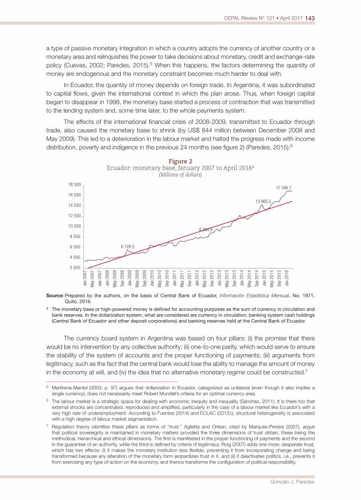
143CEPAL Review N° 121 • April 2017
Gonzalo J. Paredes
a type of passive monetary integration in which a country adopts the currency of another country or a monetary area and relinquishes the power to take decisions about monetary, credit and exchange-rate policy (Cuevas, 2002; Paredes, 2015).5 When this happens, the factors determining the quantity of money are endogenous and the monetary constraint becomes much harder to deal with.
In Ecuador, the quantity of money depends on foreign trade. In Argentina, it was subordinated to capital flows, given the international context in which the plan arose. Thus, when foreign capital began to disappear in 1998, the monetary base started a process of contraction that was transmitted to the lending system and, some time later, to the whole payments system.
The effects of the international financial crisis of 2008-2009, transmitted to Ecuador through trade, also caused the monetary base to shrink (by US$ 844 million between December 2008 and May 2009). This led to a deterioration in the labour market and halted the progress made with income distribution, poverty and indigence in the previous 24 months (see figure 2) (Paredes, 2015).6
Figure 2 Ecuador: monetary base, January 2007 to April 2016a
(Millions of dollars)
2 500
4 500
6 500
8 500
10 500
12 500
14 500
16 500
18 500
Jan
2007
May
200
7
sep
2007
Jan
2008
May
200
8
Sep
2008
Jan
2009
May
200
9
Sep
2009
Jan
2010
May
201
0
Sep
2010
Jan
2011
May
201
1
Sep
2011
Jan
2012
May
201
2
Sep
2012
Jan
2013
May
201
3
Sep
2013
Jan
2014
May
201
4
Sep
2014
Jan
2015
May
201
5
Sep
2015
Jan
2016
6 128.3
8 264.9
13 665.5
17 346.7
Source: Prepared by the authors, on the basis of Central Bank of Ecuador, Información Estadística Mensual, No. 1971, Quito, 2016.
a The monetary base or high-powered money is defined for accounting purposes as the sum of currency in circulation and bank reserves. In the dollarization system, what are considered are currency in circulation, banking system cash holdings (Central Bank of Ecuador and other deposit corporations) and banking reserves held at the Central Bank of Ecuador.
The currency board system in Argentina was based on four pillars: (i) the promise that there would be no intervention by any collective authority; (ii) one-to-one parity, which would serve to ensure the stability of the system of accounts and the proper functioning of payments; (iii) arguments from legitimacy, such as the fact that the central bank would lose the ability to manage the amount of money in the economy at will, and (iv) the idea that no alternative monetary regime could be constructed.7
5 Martirena-Mantel (2003, p. 97) argues that dollarization in Ecuador, categorized as unilateral (even though it also implies a single currency), does not necessarily meet Robert Mundell’s criteria for an optimal currency area.
6 The labour market is a strategic space for dealing with economic inequity and inequality (Sánchez, 2011). It is there too that external shocks are concentrated, reproduced and amplified, particularly in the case of a labour market like Ecuador’s with a very high rate of underemployment. According to Fuentes (2014) and ECLAC (2012c), structural heterogeneity is associated with a high degree of labour market segmentation.
7 Regulation theory identifies these pillars as forms of “trust.” Aglietta and Orléan, cited by Marques-Pereira (2007), argue that political sovereignty is maintained in monetary matters provided the three dimensions of trust obtain, these being the methodical, hierarchical and ethical dimensions. The first is manifested in the proper functioning of payments and the second in the guarantee of an authority, while the third is defined by criteria of legitimacy. Roig (2007) adds one more: desperate trust, which has two effects: (i) it makes the monetary institution less flexible, preventing it from incorporating change and being transformed because any alteration of the monetary form jeopardizes trust in it, and (ii) it deactivates politics, i.e., prevents it from exercising any type of action on the economy, and thence transforms the configuration of political responsibility.
144 CEPAL Review N° 121 • April 2017
Ecuador: why exit dollarization?
In this context, the inability of the State to find effective instruments to keep the economy operating at full capacity, the false promises of one-to-one parity, the notion that inflation was a purely monetary phenomenon and the political strength that enabled the financial and economic ruling class to impose its ideas led Argentina, South America’s second-largest economy, into a deep recession that caused severe intergenerational social harm.
Economic growth and income recovery between 1990 and 1994 were inequitable, with the real income of the top decile higher than it was in 1980. Developments subsequent to 1994 were clearly regressive. The incomes of the lowest-income 60% of households declined and those of the top three deciles improved. In other words, the distributive situation at the end of the twentieth century represented a substantial regression in real terms from that of 1980 (Altimir, Beccaria and González, 2002).
According to the Permanent Household Survey (EPH) of the National Institute of Statistics and Censuses (INDEC) of Argentina, 26.2% of households in 28 conurbations were below the poverty line in May 2001. A year later, in May 2002, the figure had risen to 41.4%, showing the profound effects caused in this period by the severe adjustments in the economic policy run by the then minister Cavallo and his team of advisors to maintain parity with the dollar. In Greater Buenos Aires, the incidence of household poverty was 23.5% during the period stated. A year later it was 37.7%. If the largest cities are included, the number of households affected by poverty was greater, showing that income distribution clearly regressed much more sharply in the provinces. Social conditions reflected the behaviour of the labour market, the deterioration of public goods such as health care and education, and the disruption of the production and social fabric, mainly in the large urban centres.8
For this reason, Carrera (2004) claims that convertibility brought a radical transformation in the behaviour of the labour market: the old pattern of the 1980s, with unemployment rates holding fairly steady while real wages fluctuated greatly, was replaced in the 1990s by one with exactly the opposite characteristics. In the same way, convertibility produced highly disparate results: an exceptional performance for growth and inflation, but poor performances for the external sector, the labour market and income distribution.
Given all this, the question must be why economic agents are so convinced that convertibility is viable in the long run. Three reasons have been given. In the first place, Boyer (2007) writes that the model gained traction in a consistent institutional and ideological framework that, according to Wainer (2010), formed part of the interlinkages between the different bourgeois factions under the hegemony of financial capital.
In the second place, Galiani, Heymann and Tomassi (2003), Heymann (2000) and Conesa (1996) propose a hypothesis of the expected effects of “contractual density.” Strict adherence to the existing monetary rule (via an elaborate system of contracts, most of them denominated in dollars) was identified with stability and predictability. To this end, the government (by issuing dollar-denominated bonds) and the private sector (by building up large dollar debts and assets) ensured that their solvency would depend on the exchange rate being maintained. The set of promises seemed to be such that they had to be either all kept together or all broken together. Any departure from the status quo of one peso for one dollar would create a shock with unpredictable consequences.
Thirdly and lastly, Roig (2007) developed a hypothesis for the way the production of knowledge, and particularly economic knowledge, affected the functioning of convertibility and the crisis in it,9
8 Ferrer (2004) defines this situation as one of “structural heterogeneity” and uses the concept of “national density.”9 Roig (2007) writes that logics of authorization can be found in all professions and disciplines, but take on a particular dimension
in the economic sciences. Of all the sciences close to “power,” this is the one that is most respected, has a truth status that validates authorization, and is most widely disseminated in society through education and the media.
145CEPAL Review N° 121 • April 2017
Gonzalo J. Paredes
making it possible to construct a specific form of trust dubbed “desperate” around the currency, based on the impossibility of exiting the established monetary regime. The author argues that this impossibility stemmed not only from the assertion that it was so, but mainly from the discrediting of the possibility that there might be alternatives.
The three reasons for viability given are not mutually divergent but quite the opposite. The sense of impossibility was underpinned by the “fear of floating” that resulted from the elaborate contractual form of convertibility and the institutional and ideological consistency so widely proclaimed by the media and academia. Convergence was possible because the monetary regime created increased scope for rent-seeking.
2. The strict monetary constraint is highly vulnerable to persistent external shocks
Money operates as a medium in relationships of exchange where it is used for this purpose. This is what is known as the monetary constraint. From this idea it follows that commodity realization is subject to the availability of money in the economy (Aglietta, 1979).
The dependence of capitalism on commodity circulation is expressed by equivalence relationships in exchange. The monetary constraint is not a permanent and absolute yardstick, but depends on how the general equivalent is formed. Banks experience the monetary constraint relative to society as a whole because they are required to convert the different bank moneys into commodity money on demand and without any limitation whatever. This general and permanent conversion is the proof that bank money has the attributes of its general equivalent.
For Aglietta (1979), any crisis in the realization of exchange value takes on a global character and presents as a financial crisis. This concerns all types of financial circulation, but the epicentre of the crisis is necessarily the banking system, which is where private debts are mobilized. Thus, the role of the central bank is to organize the bank money convertibility process by manipulating the issuance of its own money.
The implementation of the currency board system coincided with an upsurge of capital flows into emerging countries. These flows were the main underpinning of this regime in the early years and went mainly to the financial system, the result being quite intensive processes of bank money creation that systematically outpaced the money supply. When these flows went into reverse, two adjustment mechanisms came into action: one was automatic (contraction of the monetary base) and the other was applied when the first failed to work (fiscal adjustment).
However, when capital flows were not positive (they turned negative because of capital flight) and loans could not be obtained from international organizations (the International Monetary Fund suspended support to Argentina, instituting the Krueger-Rogoff approach of non-intervention in financial crises to avoid moral hazard), higher interest rates were not enough to incentivize international investors. It was then that fiscal adjustment was brought into action in an effort to remedy the absence of external capital by means of a greater economic contraction that would lead to higher interest rates (to encourage capital to return) and lower labour costs so that tradable goods could be produced more cheaply.
The “adjustment to the adjustment” carried out during the government of President De la Rúa did not succeed in incentivizing the return of capital flows, since the economic imbalances created by the currency board were becoming increasingly evident. The idea of generating a fiscal surplus to service the external debt by way of ever-larger cuts to current spending simply did not work (IMF, 2004, p. 43 and 2001, pp. 29 to 33).
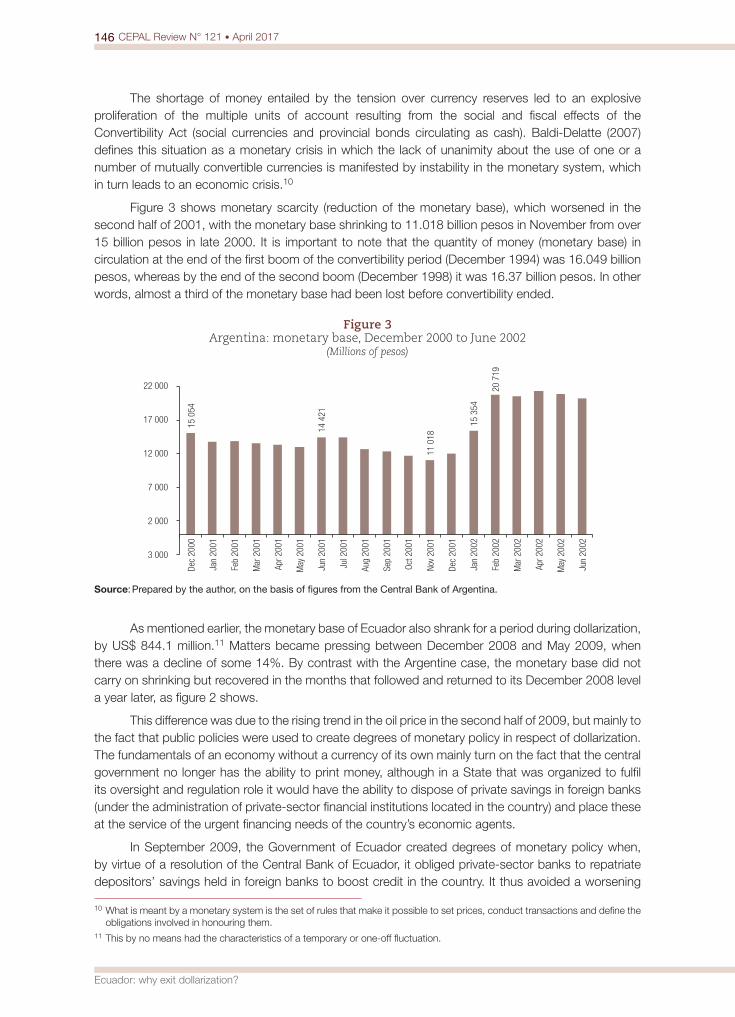
146 CEPAL Review N° 121 • April 2017
Ecuador: why exit dollarization?
The shortage of money entailed by the tension over currency reserves led to an explosive proliferation of the multiple units of account resulting from the social and fiscal effects of the Convertibility Act (social currencies and provincial bonds circulating as cash). Baldi-Delatte (2007) defines this situation as a monetary crisis in which the lack of unanimity about the use of one or a number of mutually convertible currencies is manifested by instability in the monetary system, which in turn leads to an economic crisis.10
Figure 3 shows monetary scarcity (reduction of the monetary base), which worsened in the second half of 2001, with the monetary base shrinking to 11.018 billion pesos in November from over 15 billion pesos in late 2000. It is important to note that the quantity of money (monetary base) in circulation at the end of the first boom of the convertibility period (December 1994) was 16.049 billion pesos, whereas by the end of the second boom (December 1998) it was 16.37 billion pesos. In other words, almost a third of the monetary base had been lost before convertibility ended.
Figure 3 Argentina: monetary base, December 2000 to June 2002
(Millions of pesos)
15 0
54
14 4
21
11 0
18
15 3
54
20 7
19
3 000
2 000
7 000
12 000
17 000
22 000
Dec
2000
Jan
2001
Feb
2001
Mar
200
1
Apr 2
001
May
200
1
Jun
2001
Jul 2
001
Aug
2001
Sep
2001
Oct 2
001
Nov
2001
Dec
2001
Jan
2002
Feb
2002
Mar
200
2
Apr 2
002
May
200
2
Jun
2002
Source: Prepared by the author, on the basis of figures from the Central Bank of Argentina.
As mentioned earlier, the monetary base of Ecuador also shrank for a period during dollarization, by US$ 844.1 million.11 Matters became pressing between December 2008 and May 2009, when there was a decline of some 14%. By contrast with the Argentine case, the monetary base did not carry on shrinking but recovered in the months that followed and returned to its December 2008 level a year later, as figure 2 shows.
This difference was due to the rising trend in the oil price in the second half of 2009, but mainly to the fact that public policies were used to create degrees of monetary policy in respect of dollarization. The fundamentals of an economy without a currency of its own mainly turn on the fact that the central government no longer has the ability to print money, although in a State that was organized to fulfil its oversight and regulation role it would have the ability to dispose of private savings in foreign banks (under the administration of private-sector financial institutions located in the country) and place these at the service of the urgent financing needs of the country’s economic agents.
In September 2009, the Government of Ecuador created degrees of monetary policy when, by virtue of a resolution of the Central Bank of Ecuador, it obliged private-sector banks to repatriate depositors’ savings held in foreign banks to boost credit in the country. It thus avoided a worsening
10 What is meant by a monetary system is the set of rules that make it possible to set prices, conduct transactions and define the obligations involved in honouring them.
11 This by no means had the characteristics of a temporary or one-off fluctuation.
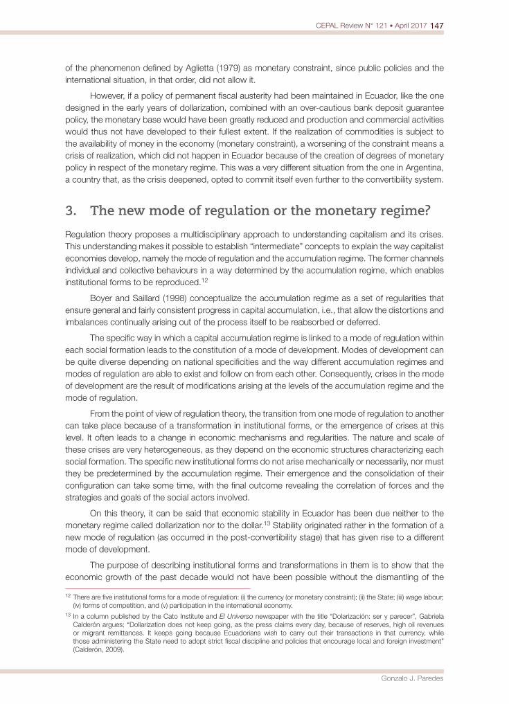
147CEPAL Review N° 121 • April 2017
Gonzalo J. Paredes
of the phenomenon defined by Aglietta (1979) as monetary constraint, since public policies and the international situation, in that order, did not allow it.
However, if a policy of permanent fiscal austerity had been maintained in Ecuador, like the one designed in the early years of dollarization, combined with an over-cautious bank deposit guarantee policy, the monetary base would have been greatly reduced and production and commercial activities would thus not have developed to their fullest extent. If the realization of commodities is subject to the availability of money in the economy (monetary constraint), a worsening of the constraint means a crisis of realization, which did not happen in Ecuador because of the creation of degrees of monetary policy in respect of the monetary regime. This was a very different situation from the one in Argentina, a country that, as the crisis deepened, opted to commit itself even further to the convertibility system.
3. The new mode of regulation or the monetary regime?
Regulation theory proposes a multidisciplinary approach to understanding capitalism and its crises. This understanding makes it possible to establish “intermediate” concepts to explain the way capitalist economies develop, namely the mode of regulation and the accumulation regime. The former channels individual and collective behaviours in a way determined by the accumulation regime, which enables institutional forms to be reproduced.12
Boyer and Saillard (1998) conceptualize the accumulation regime as a set of regularities that ensure general and fairly consistent progress in capital accumulation, i.e., that allow the distortions and imbalances continually arising out of the process itself to be reabsorbed or deferred.
The specific way in which a capital accumulation regime is linked to a mode of regulation within each social formation leads to the constitution of a mode of development. Modes of development can be quite diverse depending on national specificities and the way different accumulation regimes and modes of regulation are able to exist and follow on from each other. Consequently, crises in the mode of development are the result of modifications arising at the levels of the accumulation regime and the mode of regulation.
From the point of view of regulation theory, the transition from one mode of regulation to another can take place because of a transformation in institutional forms, or the emergence of crises at this level. It often leads to a change in economic mechanisms and regularities. The nature and scale of these crises are very heterogeneous, as they depend on the economic structures characterizing each social formation. The specific new institutional forms do not arise mechanically or necessarily, nor must they be predetermined by the accumulation regime. Their emergence and the consolidation of their configuration can take some time, with the final outcome revealing the correlation of forces and the strategies and goals of the social actors involved.
On this theory, it can be said that economic stability in Ecuador has been due neither to the monetary regime called dollarization nor to the dollar.13 Stability originated rather in the formation of a new mode of regulation (as occurred in the post-convertibility stage) that has given rise to a different mode of development.
The purpose of describing institutional forms and transformations in them is to show that the economic growth of the past decade would not have been possible without the dismantling of the
12 There are five institutional forms for a mode of regulation: (i) the currency (or monetary constraint); (ii) the State; (iii) wage labour; (iv) forms of competition, and (v) participation in the international economy.
13 In a column published by the Cato Institute and El Universo newspaper with the title “Dolarización: ser y parecer”, Gabriela Calderón argues: “Dollarization does not keep going, as the press claims every day, because of reserves, high oil revenues or migrant remittances. It keeps going because Ecuadorians wish to carry out their transactions in that currency, while those administering the State need to adopt strict fiscal discipline and policies that encourage local and foreign investment” (Calderón, 2009).
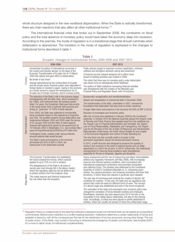
148 CEPAL Review N° 121 • April 2017
Ecuador: why exit dollarization?
whole structure designed in the new neoliberal dispensation. When the State is radically transformed, there are chain reactions that also affect all other institutional forms.14
The international financial crisis that broke out in September 2008, the constraints on fiscal policy and the total absence of monetary policy would have taken the economy deep into recession. According to this premise, the mode of regulation is in a transitional stage that should culminate when dollarization is abandoned. The transition in the mode of regulation is expressed in the changes to institutional forms described in table 1.
Table 1 Ecuador: changes in institutional forms, 2000-2006 and 2007-2015
2000-2006 2007-2015
Curre
ncy
Unrestricted circulation of international currencies in the country and transfer abroad, on the basis of the Economic Transformation of Ecuador Act of 13 March 2000 (the statute that gave effect to dollarization).No lender of last resort.Savings administered by the Central Bank of Ecuador and the private-sector financial system were deposited in foreign banks or invested in paper. Saving in the economy as a whole served to support the development not of Ecuador but of foreign countries, and to increase profits.
Public policies sought to maximize currency repatriation, minimize outflows and strengthen domestic saving and investment.A financial security network designed not to affect moral hazard in banking activities was created in 2008.The notion that there was no monetary policy under dollarization was shown to be an ideologically driven falsehood.The system of State institutions overseeing financial activities was strengthened with the creation of the Monetary and Financial Policy and Regulation Board, with 54 functions.
Stat
e tra
nsfo
rmat
ion
The reduction of the State’s role in the economy began simultaneously with the debt crisis, which worsened in the 1990s, and continued when the banking system failed. For years, the Ecuadorian State gave less priority to the social sector than to external debt servicing and acting as “guarantor” of 100% of bank deposits.From 2000, the State was subjected to innumerable fiscal constraints based on the experience of Argentina and Chile. The greatest austerity during dollarization was implemented between 2003 and 2005 under the decree of 22 January 2003 and the letter of intent (special drawing right agreement) signed by the government on 10 February 2003 in Washington, D.C. (see [online] http://www.imf.org/external/np/loi/2003/ecu/01/index.htm).Contingency funds, created under various statutes, ensured external debt would be paid.The State’s share and presence in the economy diminished (20.42% of GDP in 2004, the lowest point in the dollarization period).
Bureaucratic reorganization and reinstitutionalization.Default and renegotiation of commercial debt in December 2008.The transformation of the State, undertaken in 2007, removed the foundations that dollarization had been built on (chain reactions).A larger State share and presence in the economy (44.04% of GDP in 2013).Recovery of sovereignty over economic policy.After the oil funds were abolished in February 2008 by the Constituent Assembly, in October 2010 the National Assembly passed the Organic Code of Planning and Public Finance that repealed laws from the neoliberal era: the Organic Law on Financial Administration and Oversight, the Organic Law on Fiscal Responsibility, Stabilization and Transparency, the Organic Law for the Recovery of the Use of State Oil Resources and Administrative Rationalization of Borrowing, the Public-Sector Budget Act and chapter I of the Economic Regulation and Control of Public Spending Act.The only fiscal rule that currently exists in Ecuador is that permanent expenditure should not exceed permanent revenue.In 2015, a tariff structure was designed to preserve the quantity of money in the economy in the event of external shocks such as dollar appreciation or a fall in the oil price. In 2016, furthermore, the institutional arrangements for reducing fiscal avoidance were strengthened, especially for the tax on bequests, legacies and donations.
Wag
e la
bour
The Economic Transformation Act established the hourly employment format, which could be applied to up to 75% of a firm’s workers.The disappearance of the State in all areas of society was most strongly felt in the labour market, where the regulatory agencies lost all ability to act to protect workers from the employer class.This made insecure and informal employment the rule rather than the exception.
Hourly employment and the rise of outsourcing and labour intermediation (without any regulatory framework until May 2006), with increasingly insecure and informal working conditions, were inconsistent with international employment conventions and prevented unionization and collective hiring. This situation was addressed by the Constituent Assembly of 2008 in Constituent Mandate no. 8, comprising seven articles, four general provisions, five temporary provisions and three final provisions, in which these two statutes in particular were repealed.The new way of conceiving work involved the creation of decent, fair conditions for workers. To this end, the State acts via regulations and actions that create the basis for different forms of work. The concept of a decent wage was established and work in the home recognized.The restoration of the State and sovereignty over economic policy have changed the correlation of forces between workers and employers. Nonetheless, emphasis has been placed since 2015 not only on the inequalities in the capital-labour relationship, but also on the working class. Accordingly, a ceiling has been placed on profits distributed to workers, which can usually not exceed 24 times the unified basic wage.
14 Regulation theory is underpinned by the idea that institutions represent social commitments that can be treated as sociopolitical commitments. Behind every institution is a conflict seeking resolution. Institutions determine a certain relationship of forces and establish a hierarchy, with all the consequences this has for the distribution of income and power, among other things. The role of public action, of the State, may consist in favouring or otherwise the emergence of certain commitments. See Amable (2007) for a more in-depth study of institutional complementarity.

149CEPAL Review N° 121 • April 2017
Gonzalo J. Paredes
Inte
rnat
iona
lDependence of the fiscal and external sector on one State asset, oil. In 2004, this accounted for 30.08% of total central government revenue and 54.61% of total exports.The trade channel prevailed over the financial channel. Changes in tradable goods prices influenced the fiscal sector and the external sector more than international interest rates did.Import growth averaged 21.20% during the period.Fuel imports rose from US$ 243.84 million to US$ 2.54 billion.
In 2013, oil accounted for 22.93% of total central government revenue and 56.78% of total exports. At the end of 2015, the figures were 11.13% and 36.33%, respectively. A trade agreement with the European Union may be in prospect, given that Colombia and Peru have free trade treaties with that regional bloc and with the United States.Inward foreign direct investment (FDI) has been very low by the standards of the region (ECLAC, 2012b). Inflows of FDI in strategic sectors have been identified since 2014.Import growth averaged 12.31% up to 2013. The effects of the tariff structure mentioned earlier were reflected in a 22.64% fall in imports between 2014 and 2015. Between January and April 2016, the reduction was 36.46% on the same period the year before.Fuel imports rose from US$ 2.54 billion to US$ 6.62 billion. In 2015, these imports totalled US$ 4.17 billion.
Form
of c
ompe
titio
n
There was an “incestuous relationship” between the banks, the media and large business groups that was exposed by the crisis at the end of the century.The lack of regulation and oversight policies meant that the new financial and geographical axis began to become heavily concentrated as private-sector banks in particular forged close links with importers, with the media that monopolized public opinion and communication and with the State.
The constituent process that began in November 2007 forced the financial sector to cut its ties to firms in other sectors. Similarly, the approval of question 3 in the referendum and the popular consultation of 7 May 2011 impacted the media.A higher tax on bequests, legacies and donations is being debated.
Source: Prepared by the author, on the basis of data from Central Bank of Ecuador, Información Estadística Mensual, No. 1971, Quito, 2016; and Economic Commission for Latin America and the Caribbean (ECLAC), Foreign Direct Investment in Latin America and the Caribbean 2011 (LC/G.2538-P), Santiago, 2012.
In seeking to understand these changes, Marconi (2001, p. 11) argued that “dollarization is not simply an alternative management model that can be studied with conventional tools […] but must be interpreted mainly from the standpoint of political economy, since its conception, its methods of application and the people chosen to implement it are clearly determined by the interests of well-known business groupings with strong ties to the political and social spheres and the media.”
On this view, it was not the monetary regime that provided the conditions of economic stability needed for per capita incomes to increase and for the country to avoid the greatest crisis of capitalism since the Great Depression. There are two reasons for this: first, economic policymakers during the new neoliberal dispensation created three “contingency” funds that inhibited economic growth and made fiscal policy unusable in possible recessions, whether due to domestic or external factors.15 Second, dollarization in itself has inhibited economic growth, since it leaves the country without a monetary and exchange-rate policy to mobilize domestic saving, expand exports and replace imports, and deal with external shocks.
Trade is the main channel of transmission for these shocks.16 This could happen in two scenarios: a fall in the oil price and a slump or boom in the United States economy. Together or separately, these scenarios would cut short Ecuador’s rapid development of recent years. The current monetary regime means that the effect of outside shocks can be transmitted more directly and far more quickly.
A slump in the United States economy would have deep repercussions in the global economy, as it would cut trade flows between developed and developing countries and depress demand for
15 They were called “contingency” funds because their intended purpose was to cushion the kind of external shocks that send the business cycle into a downturn. Nonetheless, the way these funds were allocated did not live up to their name, as 70% of the resources from the sale of heavy crude (the second oil fund was set up on 25 March 2002, while the first, drawing on sales of light crude, had been set up under the Economic Transformation Act of 13 March 2000) were used to repurchase external public debt at market value (Paredes, 2015).
16 According to Coq (2007), the Convertibility Plan depended on capital flows because external trade to the United States accounted for just 16% of the total (in 2007 the figure was 7.44%). In other words, the financial channel prevailed over the trade channel. The effects of external shocks on the passive monetary integration carried out by Ecuador and Argentina differ in their transmission channels. The announcement that the Ecuadorian currency was being abandoned was made in an international context where capital flows were leaving emerging countries because of the successive financial crises of the late 1990s. When a country cedes sovereignty over its monetary policy, it creates a leader-follower relationship.
Table 1 (concluded)
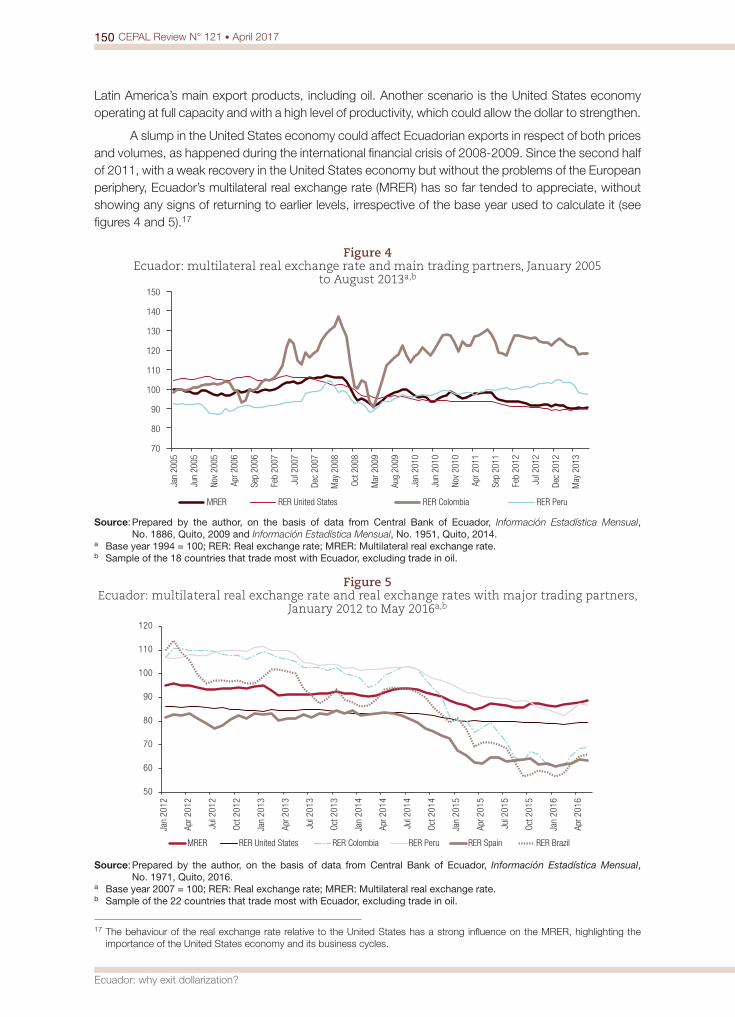
150 CEPAL Review N° 121 • April 2017
Ecuador: why exit dollarization?
Latin America’s main export products, including oil. Another scenario is the United States economy operating at full capacity and with a high level of productivity, which could allow the dollar to strengthen.
A slump in the United States economy could affect Ecuadorian exports in respect of both prices and volumes, as happened during the international financial crisis of 2008-2009. Since the second half of 2011, with a weak recovery in the United States economy but without the problems of the European periphery, Ecuador’s multilateral real exchange rate (MRER) has so far tended to appreciate, without showing any signs of returning to earlier levels, irrespective of the base year used to calculate it (see figures 4 and 5).17
Figure 4 Ecuador: multilateral real exchange rate and main trading partners, January 2005
to August 2013a,b
70
80
90
100
110
120
130
140
150
Jan
2005
Jun
2005
Nov
2005
Apr 2
006
Sep
2006
Feb
2007
Jul 2
007
Dec
2007
May
200
8
Oct 2
008
Mar
200
9
Aug
2009
Jan
2010
Jun
2010
Nov
2010
Apr 2
011
Sep
2011
Feb
2012
Jul 2
012
Dec
2012
May
201
3
MRER RER United States RER Colombia RER Peru
Source: Prepared by the author, on the basis of data from Central Bank of Ecuador, Información Estadística Mensual, No. 1886, Quito, 2009 and Información Estadística Mensual, No. 1951, Quito, 2014.
a Base year 1994 = 100; RER: Real exchange rate; MRER: Multilateral real exchange rate.b Sample of the 18 countries that trade most with Ecuador, excluding trade in oil.
Figure 5 Ecuador: multilateral real exchange rate and real exchange rates with major trading partners,
January 2012 to May 2016a,b
50
60
70
80
90
100
110
120
Jan
2012
Apr 2
012
Jul 2
012
Oct 2
012
Jan
2013
Apr 2
013
Jul 2
013
Oct 2
013
Jan
2014
Apr 2
014
Jul 2
014
Oct 2
014
Jan
2015
Apr 2
015
Jul 2
015
Oct 2
015
Jan
2016
Apr 2
016
MRER RER United States RER Colombia RER Peru RER Spain RER Brazil
Source: Prepared by the author, on the basis of data from Central Bank of Ecuador, Información Estadística Mensual, No. 1971, Quito, 2016.
a Base year 2007 = 100; RER: Real exchange rate; MRER: Multilateral real exchange rate.b Sample of the 22 countries that trade most with Ecuador, excluding trade in oil.
17 The behaviour of the real exchange rate relative to the United States has a strong influence on the MRER, highlighting the importance of the United States economy and its business cycles.
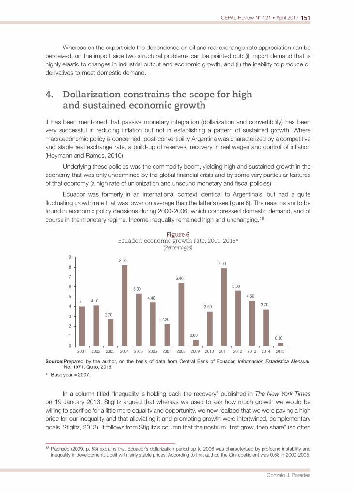
151CEPAL Review N° 121 • April 2017
Gonzalo J. Paredes
Whereas on the export side the dependence on oil and real exchange-rate appreciation can be perceived, on the import side two structural problems can be pointed out: (i) import demand that is highly elastic to changes in industrial output and economic growth, and (ii) the inability to produce oil derivatives to meet domestic demand.
4. Dollarization constrains the scope for high and sustained economic growth
It has been mentioned that passive monetary integration (dollarization and convertibility) has been very successful in reducing inflation but not in establishing a pattern of sustained growth. Where macroeconomic policy is concerned, post-convertibility Argentina was characterized by a competitive and stable real exchange rate, a build-up of reserves, recovery in real wages and control of inflation (Heymann and Ramos, 2010).
Underlying these policies was the commodity boom, yielding high and sustained growth in the economy that was only undermined by the global financial crisis and by some very particular features of that economy (a high rate of unionization and unsound monetary and fiscal policies).
Ecuador was formerly in an international context identical to Argentina’s, but had a quite fluctuating growth rate that was lower on average than the latter’s (see figure 6). The reasons are to be found in economic policy decisions during 2000-2006, which compressed domestic demand, and of course in the monetary regime. Income inequality remained high and unchanging.18
Figure 6 Ecuador: economic growth rate, 2001-2015a
(Percentages)
4 4.10
2.70
8.20
5.30
4.40
2.20
6.40
0.60
3.50
7.90
5.60
4.60
3.70
0.30
0
1
2
3
4
5
6
7
8
9
2001 2002 2003 2004 2005 2006 2007 2008 2009 2010 2011 2012 2013 2014 2015
Source: Prepared by the author, on the basis of data from Central Bank of Ecuador, Información Estadística Mensual, No. 1971, Quito, 2016.
a Base year = 2007.
In a column titled “Inequality is holding back the recovery” published in The New York Times on 19 January 2013, Stiglitz argued that whereas we used to ask how much growth we would be willing to sacrifice for a little more equality and opportunity, we now realized that we were paying a high price for our inequality and that alleviating it and promoting growth were intertwined, complementary goals (Stiglitz, 2013). It follows from Stiglitz’s column that the nostrum “first grow, then share” (so often
18 Pacheco (2009, p. 53) explains that Ecuador’s dollarization period up to 2006 was characterized by profound instability and inequality in development, albeit with fairly stable prices. According to that author, the Gini coefficient was 0.58 in 2000-2005.
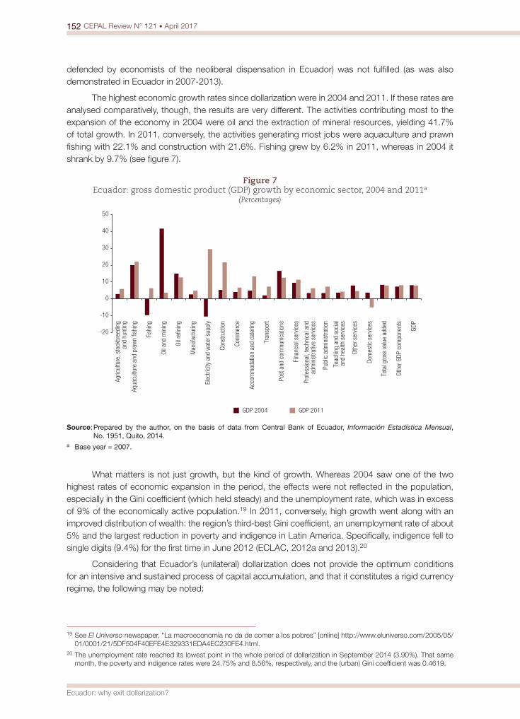
152 CEPAL Review N° 121 • April 2017
Ecuador: why exit dollarization?
defended by economists of the neoliberal dispensation in Ecuador) was not fulfilled (as was also demonstrated in Ecuador in 2007-2013).
The highest economic growth rates since dollarization were in 2004 and 2011. If these rates are analysed comparatively, though, the results are very different. The activities contributing most to the expansion of the economy in 2004 were oil and the extraction of mineral resources, yielding 41.7% of total growth. In 2011, conversely, the activities generating most jobs were aquaculture and prawn fishing with 22.1% and construction with 21.6%. Fishing grew by 6.2% in 2011, whereas in 2004 it shrank by 9.7% (see figure 7).
Figure 7 Ecuador: gross domestic product (GDP) growth by economic sector, 2004 and 2011a
(Percentages)
-20
-10
0
10
20
30
40
50
Agric
ultu
re, s
tock
bree
ding
and
hunt
ing
Aqua
cultu
re a
nd p
raw
n fis
hing
Fish
ing
Oil a
nd m
inin
g
Oil r
efini
ng
Man
ufac
turin
g
Elec
trici
ty a
nd w
ater
sup
ply
Cons
truct
ion
Com
mer
ce
Acco
mm
odat
ion
and
cate
ring
Tran
spor
t
Post
and
com
mun
icat
ions
Fina
ncia
l ser
vices
Prof
essi
onal
, tec
hnic
al a
ndad
min
istra
tive
serv
ices
Publ
ic a
dmin
istra
tion
Teac
hing
and
soc
ial
and
heal
th s
ervic
es
Othe
r ser
vices
Dom
estic
ser
vices
Tota
l gro
ss v
alue
add
ed
Othe
r GDP
com
pone
nts
GDP
GDP 2004 GDP 2011
Source: Prepared by the author, on the basis of data from Central Bank of Ecuador, Información Estadística Mensual, No. 1951, Quito, 2014.
a Base year = 2007.
What matters is not just growth, but the kind of growth. Whereas 2004 saw one of the two highest rates of economic expansion in the period, the effects were not reflected in the population, especially in the Gini coefficient (which held steady) and the unemployment rate, which was in excess of 9% of the economically active population.19 In 2011, conversely, high growth went along with an improved distribution of wealth: the region’s third-best Gini coefficient, an unemployment rate of about 5% and the largest reduction in poverty and indigence in Latin America. Specifically, indigence fell to single digits (9.4%) for the first time in June 2012 (ECLAC, 2012a and 2013).20
Considering that Ecuador’s (unilateral) dollarization does not provide the optimum conditions for an intensive and sustained process of capital accumulation, and that it constitutes a rigid currency regime, the following may be noted:
19 See El Universo newspaper, “La macroeconomía no da de comer a los pobres” [online] http://www.eluniverso.com/2005/05/01/0001/21/5DF504F40EFE4E329331EDA4EC230FE4.html.
20 The unemployment rate reached its lowest point in the whole period of dollarization in September 2014 (3.90%). That same month, the poverty and indigence rates were 24.75% and 8.56%, respectively, and the (urban) Gini coefficient was 0.4619.
153CEPAL Review N° 121 • April 2017
Gonzalo J. Paredes
(i) From the Research Department of the International Monetary Fund (IMF), Ghosh, Qureshi and Tsangarides (2013 and 2014) point out that fixed exchange rates impede external adjustment: external disequilibria (current account surpluses or deficits) are less persistent in floating exchange-rate regimes, which reduces the chances of dangerous imbalances building up and leading to a crisis. This argument was earlier developed by Milton Friedman in his 1953 essay “The Case for Flexible Exchange Rates.”
(ii) Rodrik (2008) demonstrates the correlation between growth and the real exchange rate. As Frenkel (2008) put it in relation to the effects of a stable and competitive real exchange rate (SCRER): “Although the scale and evolution of the SCRER effect on aggregate demand may be difficult to pinpoint, we do know that the higher growth experienced by economies which adopt an SCRER is partly due to this effect.”
(iii) Stress should be laid on the non-neutrality of money in the short and medium run as postulated since the 1930s by J.M. Keynes and the post-Keynesians, i.e., the link between the monetary and real spheres (Guttmann, 1996).
(iv) The concept of non-neutrality also appears to be valid in the long run. Blanchard (2003) argues that an active monetary policy has lasting effects on interest rates and thence unemployment. A steady rise in the real interest rate will lead to a high unemployment rate that, given its duration, the decline in capital accumulation and the effects on firms’ profit margins (higher financial outlays), will cause the natural rate of unemployment to rise. A sustained drop in the real interest rate will produce the opposite sequence.
The initiative of creating degrees of monetary policy in an economy without a currency of its own was based on what Blanchard (2003) has demonstrated. The repatriation of capital in Ecuador since 2009 (and the reduction in lending interest rates) shows that it not only helped the country avoid the shocks of the international financial crisis, but contributed to the reduction of the natural rate of unemployment. Depositors’ savings abroad that returned to the country did not serve to cushion a possible bank run but to expand private lending and galvanize production and employment.
5. The main condition for the new production matrix: the restoration of foreign exchange policy
The last reason to exit dollarization is to be able to construct a new production matrix. The experience of the Asian tigers (Hong Kong Special Administrative Region of China, Indonesia, Japan, Malaysia, the Republic of Korea, Singapore, Taiwan Province of China and Thailand) reveals the need for the exchange rate to be kept weak to promote exports, especially those of nascent industries.
Frenkel (2008) and Frenkel and Rapetti (2009) argue that a competitive exchange rate is what determines the incentives for the production of a wide range of internationally marketable products, with a view to selling them in the domestic or external markets. Another argument is that, unlike other incentive systems, this general policy of promoting marketable activities (over non-marketable ones) does not give rise to rent-seeking.
The insistence on keeping the dollar as the national currency would seem to entail a dependence on its being weak in the long run, which is very unlikely. The current disadvantage of Ecuador’s relative prices with its main trading partner (see figures 4 and 5) is a serious problem for the country’s export sector, considering that, as Falconí and Oleas (2004) put it, “dollarization suffers from a number of deep-seated problems, the most serious of which is structural with long-run effects on the country’s economy: productivity.”
154 CEPAL Review N° 121 • April 2017
Ecuador: why exit dollarization?
IV. Conclusions and closing reflections
Since the announcement and implementation of dollarization in Ecuador, the representatives and proponents of this monetary regime have used all possible means (economic, political and social) to bolster it.21 Their main instrument has been the creation in the social imaginary of the idea that it simply cannot be abandoned, since any attempt to cast doubt over this regime would leave the Ecuadorian economy in the worst of all worlds.
In Ecuador, the ultimate goal of economics has shifted in the last decade from the monetary regime to human beings as the core of society. This conceptual change was indirectly responsible for the survival of dollarization over time, since the economic structure designed during the 2000-2006 period would have brought about the collapse of the monetary regime because of the severe effects of the financial crisis in the central countries, transmitted through trade.
Between 2000 and 2006, the financial and economic ruling class of Ecuador created laws, regulations and ideas whose aim was that every effort of society’s should contribute to the survival of dollarization, even in downturns. Ensuring this meant high rates of return for sectors connected to this regime (and its policies), which is why people speak of a political economy of abandonment of the national currency.
Dollarization thus becoming an end in itself not only continued to set back the country’s economic development, but suppressed it to the point of turning this impaired development into a political process that came to seem irreversible from 2007. Ecuador’s suppressed development led to the mode of regulation being transformed via changes in its institutional forms and, subsequently, the accumulation regime.
Transformation of the mode of regulation began with the reorganization and reinstitutionalization of the State countrywide and continued with the other institutional forms. The accumulation regime and the workings of Ecuadorian capitalism were also transformed on the premise that human beings were the ultimate end of society. To prevent this change from being easily reversible, however, it is indispensable for dollarization to be abandoned. Economic development itself, which drove the transformation of the mode of regulation, requires the restoration of monetary sovereignty to entrench this transformation.
Dollarization has had structural impacts on the distribution of power in Ecuador. Abandoning it would have them too. The most advisable course would be to do it at a time when transformation of the State and employment relations were in a dominant position and in a context where a far-reaching progressive distribution of income was in progress. Otherwise, the way would be open, as Acosta (2004) very rightly points out, for the oligarchical groups that gained from dollarization to do so again and for the representatives of “orthodox, conservative and prudent” economics to seek an exit based on neoliberal principles.
21 The latest effort of this kind was made by the Inter-American Business Federation (FIE) in September 2014 when it proposed a public-private partnership law whose objective was to change the economic policy of the previous six years, with its focus on high public spending. Other business leaders rejected the proposal, arguing that the government ought to cut public spending without partnerships of any kind.
155CEPAL Review N° 121 • April 2017
Gonzalo J. Paredes
BibliographyAcosta, A. (2004), “Dolarización o desdolarización, esa no es toda la cuestión!”, Íconos, No. 19, Quito, Latin
American Faculty of Social Sciences (FLACSO). Aglietta, M. (1979), Regulación y crisis del capitalismo, Mexico City, Siglo XXI. Altimir, O., L. Beccaria and M. González (2002), “Income distribution in Argentina, 1974-2000”, CEPAL Review,
No. 78 (LC/G.2187-P), Santiago, Economic Commission for Latin America and the Caribbean (ECLAC). Amable, B. (2007), “Los cincos capitalismos: diversidad de sistemas económicos y sociales en la mundialización”,
Revista de Trabajo, No. 4, Buenos Aires. Baldi-Delatte, A. (2007), “La adhesión de los argentinos a la nueva regla monetaria: el peso vencedor del
dólar”, Salidas de crisis y estrategias alternativas de desarrollo, R. Boyer and J.C. Neffa (coord.), Buenos Aires, Miño y Dávila.
Blanchard, O. (2003), “Monetary policy and unemployment” [online] http://economics.mit.edu/files/731. Boyer, R. (2007), “Vigorosa recuperación… aunque incertidumbre sobre el nuevo régimen de crecimiento”,
Salidas de crisis y estrategias alternativas de desarrollo, R. Boyer and J.C. Neffa (coord.), Buenos Aires, Miño y Dávila.
Boyer, B. and T. Saillard (eds.) (1998), Teoría de la regulación: estado de los conocimientos, vols. 1, 2 and 3, Buenos Aires, Eudeba.
Calderón, G. (2009), “Dolarización: ser y parecer” [online] http://www.elcato.org/dolarizacion-ser-y-parecer.Carrera, J. (2004), “Las lecciones de la caja de conversión de Argentina”, La economía argentina y sus crisis
(1976-2001), R. Boyer and J.C. Neffa (coord.), Buenos Aires, Miño y Dávila. Central Bank of Ecuador (2016), Información Estadística Mensual, No. 1971, Quito.
(2014), Información Estadística Mensual, No. 1951, Quito.(2012), Cuentas Nacionales, No. 24, Quito.(2009), Información Estadística Mensual, No. 1886, Quito.
Conesa, E. (1996), Desempleo, precios relativos y crecimiento económico, Buenos Aires, Ediciones Depalma.Coq, D. (2007), “Los regímenes monetarios con paridades irrevocablemente fijas: algunas reflexiones de la
experiencia argentina”, Revista Principios, No. 7, Sevilla. Correa, R. (2004a), “Dolarización y desdolarización: más elementos para el debate. Comentarios al dossier
de Iconos 19”, Íconos, No. 20, Quito, Latin American Faculty of Social Sciences (FLACSO). (2004b), “De absurdas dolarizaciones a uniones monetarias”, paper presented at the Conference on Dollarization and Alternatives, Quito, Universidad Andina Simón Bolívar.
Cuevas, V. (2002), “Alternativas de integración monetarias entre México, Estados Unidos y Canadá”, Moneda y régimen cambiario en México, F.G. Chávez (coord.), Mexico City.
ECLAC (Economic Commission for Latin America and the Caribbean) (2013), Social Panorama of Latin America 2012 (LC/G.2557-P), Santiago.(2012a), Social Panorama of Latin America 2011 (LC/G.2514-P), Santiago. (2012b), Foreign Direct Investment in Latin America and the Caribbean 2011 (LC/G.2538-P), Santiago.(2012c), Structural Change for Equality: An Integrated Approach to Development (LC/G.2524(SES.34/3), Santiago.
El Universo (2005), “La macroeconomía no da de comer a los pobres” [online] http://www.eluniverso.com/2005/05/01/0001/21/5DF504F40EFE4E329331EDA4EC230FE4.html.
Falconí, F. and J. Oleas (comp.) (2004), Economía ecuatoriana, Quito, FLACSO-Ecuador. Ferrer, A. (2004), La economía argentina, Buenos Aires, Fondo de Cultura Económica (FCE). Frenkel, R. (2008), “The competitive real exchange-rate regime, inflation and monetary policy”, CEPAL Review,
No. 96 (LC/G.2396-P), Santiago.Frenkel, R. and M. Rapetti (2009), “Flexibilidad cambiaria y acumulación de reservas en América Latina”,
Lecturas, No. 50, Buenos Aires, Iniciativa para la Transparencia Financiera (ITF).Friedman, M. (1953), “The case for flexible exchange rates”, Essays in Positive Economics, Chicago, University
of Chicago Press.Fuentes, J.A. (ed.) (2014), Inestabilidad y desigualdad. La vulnerabilidad del crecimiento en América Latina
y el Caribe, Santiago, Economic Commission for Latin America and the Caribbean (ECLAC).Galiani, S., D. Heymann and M. Tomassi (2003), “Expectativas frustradas: el ciclo de la convertibilidad”,
Estudios y Perspectivas series, No. 16 (LC/BUE/L.185), Santiago, ECLAC Office in Buenos Aires. Ghosh, A., M. Qureshi and C. Tsangarides (2014), “Friedman Redux: external adjustment and exchange rate
flexibility”, IMF Working Paper, No. WP/14/146, Washington, D.C., International Monetary Fund. (2013), “Is the exchange rate regime really irrelevant for external adjustment?”, Economics Letters, vol. 118,
156 CEPAL Review N° 121 • April 2017
Ecuador: why exit dollarization?
No. 1, Amsterdam, Elsevier. Guttmann, R. (1996), “Moneda y crédito en la teoría de la regulación”, Teoría de la regulación: estado de los
conocimientos, R. Boyer and T. Saillard (eds.), vols. 1, 2 and 3, Buenos Aires, Eudeba.Heymann, D. (2000), “Políticas de reformas y comportamiento macroeconómico: la Argentina en los noventa”,
Reformas Económicas series, No. 61 (LC/L.1357), Santiago, Economic Commission for Latin America and the Caribbean (ECLAC).
Heymann, D. and A. Ramos (2010), “Una transición incompleta. Inflación y políticas macroeconómicas en la Argentina Post-convertibilidad”, Revista de Economía Política de Buenos Aires, year. 4, vol. 7-8, Buenos Aires.
IMF (International Monetary Fund) (2004), Report on the Evaluation of the Role of the IMF in Argentina, 1991-2001, Washington, D.C., Independent Evaluation Office. (2003), “Ecuador—Letter of Intent, Memorandum of Economic and Financial Policies, and Technical Memorandum of Understanding” [online] http://www.imf.org/external/np/loi/2003/ecu/01/index.htm. (2001), World Economic Outlook, Washington, D.C.
INDEC (National Institute of Statistics and Censuses) (various years), “Encuesta Permanente de Hogares (EPH)”, Buenos Aires.
Jameson, K. (2003), “Is it possible to de-dollarize?”, International Journal of Political Economy, vol. 33, No. 1, Taylor & Francis.
Keifman, S. (2004), “Auge y derrumbe de la convertibilidad argentina: lecciones para Ecuador”, Íconos, No. 19, Quito, Latin American Faculty of Social Sciences (FLACSO).
Marconi, S. (ed.) (2001), Macroeconomía y economía política en dolarización, Quito, Ediciones Abya-Yala/Latin American Institute for Social Research (ILDIS)/Universidad Andina Simón Bolívar.
Marques-Pereira, J. (2007), “Crecimiento, conflicto distributivo y soberanía monetaria en Argentina”, Salidas de crisis y estrategias alternativas de desarrollo, B. Boyer and J.C. Neffa (coords.), Buenos Aires, Miño y Dávila.
Martirena-Mantel, A. (2003), “Sobre la creación de áreas monetarias óptimas. El aporte de Robert Mundell”, Económica, vol. 40, Universidad Nacional de la Plata.
Miño, W. (2008), Breve historia bancaria del Ecuador, Quito, Corporación Editora Nacional.Naranjo, M. (2004), “Costos del abandono de la dolarización en el Ecuador”, Íconos, No. 19, Quito, Latin
American Faculty of Social Sciences (FLACSO). Naranjo, M. and L. Naranjo (2011), “Costos y escenarios de la salida de la dolarización oficial en el Ecuador”,
Revista de la Facultad de Economía de la PUCE, Quito, Catholic University of Ecuador. Oleas, J. (2001), “Del libertinaje financiero a la pérdida del signo monetario: una visión macroeconómica”,
Macroeconomía y economía política en dolarización, S. Marconi (eds.), Quito, Abya-Yala/Latin American Institute for Social Research (ILDIS)/Universidad Andina Simón Bolívar.
Pacheco, L. (2009), “El caso de Ecuador: la política económica del Gobierno de Rafael Correa”, Nuevas políticas económicas de izquierda en América Latina, S. Lichtensztejn (comp.), Veracruz, Biblioteca Universidad Veracruzana.
Paredes, G.J. (2015), Integraciones monetarias pasivas en Sudamérica, Buenos Aires, Ediciones Cooperativas. Rodrik, D. (2008), “The real exchange rate and economic growth”, Brookings Papers on Economic Activity,
vol. 39, No. 2, Washington, D.C., The Brookings Institution.Roig, A. (2007), “La confianza desesperada: discurso científico y crisis monetaria”, Salidas de crisis y
estrategias alternativas de desarrollo, B. Boyer and J.C. Neffa (coords.), Buenos Aires, Miño y Dávila.Sánchez, J. (2011), “Equidad y políticas sociales. Algunas reflexiones para el caso ecuatoriano”, ¡A (Re)
DISTRIBUIR!: Ecuador para todos, A. Serrano (coord.), Quito, National Secretariat of Planning and Development. Schuler, K. (2003), “¿Qué sucedió en Argentina?”, Washington D.C., Cato Institute [online] http://www.elcato.
org/que-sucedio-en-argentina.Spurrier, W. (2013), “Las economías de Guayaquil y Quito”, El Universo [online] http://www.eluniverso.com/
opinion/2013/08/11/nota/1269991/economias-guayaquil-quito.Stiglitz, J. (2013), “Inequality is holding back the recovery”, The New York Times, 19 January.
(2012), The Price of Inequality, Nueva York, W.W. Norton & Company.Wainer, A. (2010), “Clase dominante, hegemonía y modos de acumulación. La reconfiguración de las relaciones
de fuerza en el interior de la burguesía durante la crisis y salida de la convertibilidad (1998-2003)”, Ph.D. thesis, Buenos Aires, FLACSO-Argentina.
The political economy of the fiscal deficit in nineteenth-century ChileRoberto Pastén
Abstract
A structural shift in the trend toward higher deficits had emerged by the middle of the 1860s in Chile. For some authors, this was the result of increased spending owing to a fast-growing economy. Another common explanation is the higher spending required to finance and then recover from the war against Spain, which began in 1864. This article provides an alternative explanation for the country’s fiscal disarray during that period, suggesting that it was motivated largely by increased political turmoil at the beginning of the second half of the nineteenth century in Chile that ended with the ousting of President Balmaceda in 1891. That period represents a dramatic departure from the calmer and economically buoyant early years of the Republic. Thus, it is suggested that the beginning of President José Joaquín Pérez’s rule in 1861 marks both a major political realignment after the birth of the Republic and a structural shift in the trend toward higher deficits. This hypothesis is consistent with the idea that political instability tends to lead to a decoupling of taxes from spending, two elements which would be otherwise aligned as predicted by the tax smoothing theory. This essay is a factual description in support of this hypothesis.
Keyword
Fiscal policy, budget deficits, national budgets, economic history, Chile
JEL classification
H21, H62
Author
Roberto Pastén is a Third Environment Court judge and adjunct professor at the Economics Institute, Austral University of Chile, Valdivia, Chile. [email protected]
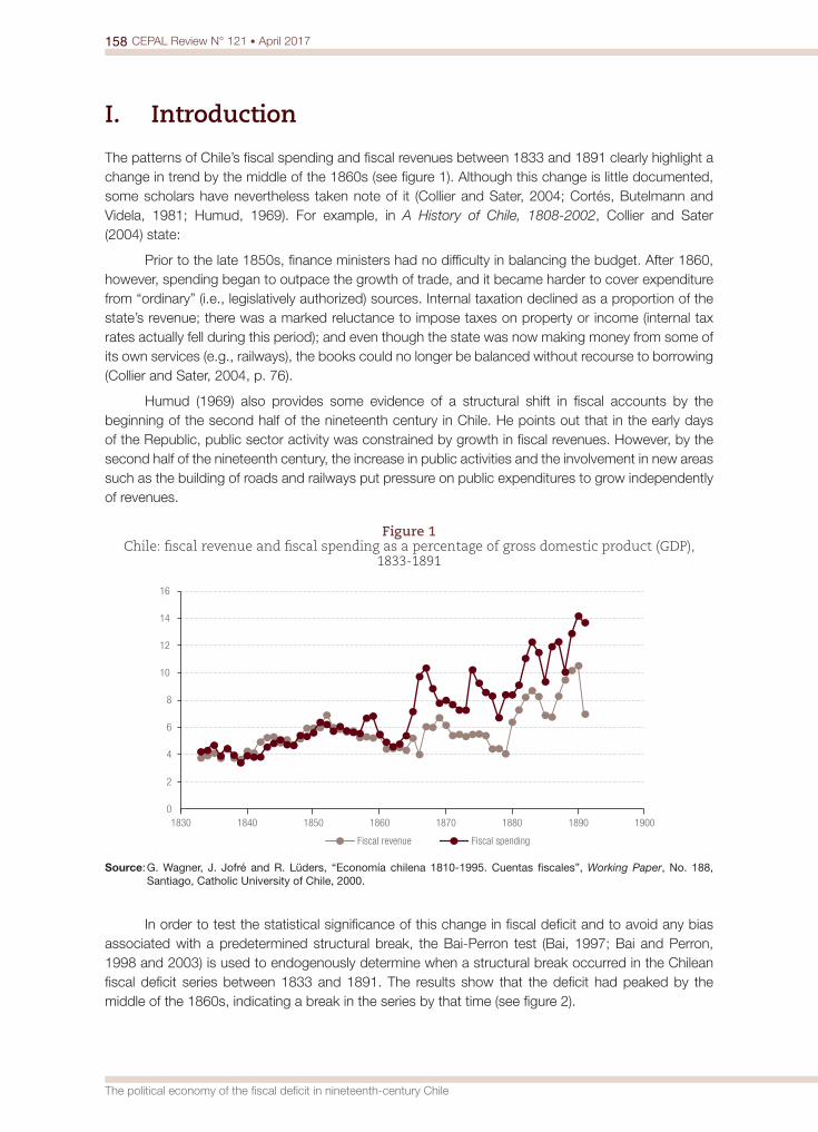
158 CEPAL Review N° 121 • April 2017
The political economy of the fiscal deficit in nineteenth-century Chile
I. Introduction
The patterns of Chile’s fiscal spending and fiscal revenues between 1833 and 1891 clearly highlight a change in trend by the middle of the 1860s (see figure 1). Although this change is little documented, some scholars have nevertheless taken note of it (Collier and Sater, 2004; Cortés, Butelmann and Videla, 1981; Humud, 1969). For example, in A History of Chile, 1808-2002, Collier and Sater (2004) state:
Prior to the late 1850s, finance ministers had no difficulty in balancing the budget. After 1860, however, spending began to outpace the growth of trade, and it became harder to cover expenditure from “ordinary” (i.e., legislatively authorized) sources. Internal taxation declined as a proportion of the state’s revenue; there was a marked reluctance to impose taxes on property or income (internal tax rates actually fell during this period); and even though the state was now making money from some of its own services (e.g., railways), the books could no longer be balanced without recourse to borrowing (Collier and Sater, 2004, p. 76).
Humud (1969) also provides some evidence of a structural shift in fiscal accounts by the beginning of the second half of the nineteenth century in Chile. He points out that in the early days of the Republic, public sector activity was constrained by growth in fiscal revenues. However, by the second half of the nineteenth century, the increase in public activities and the involvement in new areas such as the building of roads and railways put pressure on public expenditures to grow independently of revenues.
Figure 1 Chile: fiscal revenue and fiscal spending as a percentage of gross domestic product (GDP),
1833-1891
0
2
4
6
8
10
12
14
16
1830 1840 1850 1860 1870 1880 1890 1900
Fiscal revenue Fiscal spending
Source: G. Wagner, J. Jofré and R. Lüders, “Economía chilena 1810-1995. Cuentas fiscales”, Working Paper, No. 188, Santiago, Catholic University of Chile, 2000.
In order to test the statistical significance of this change in fiscal deficit and to avoid any bias associated with a predetermined structural break, the Bai-Perron test (Bai, 1997; Bai and Perron, 1998 and 2003) is used to endogenously determine when a structural break occurred in the Chilean fiscal deficit series between 1833 and 1891. The results show that the deficit had peaked by the middle of the 1860s, indicating a break in the series by that time (see figure 2).
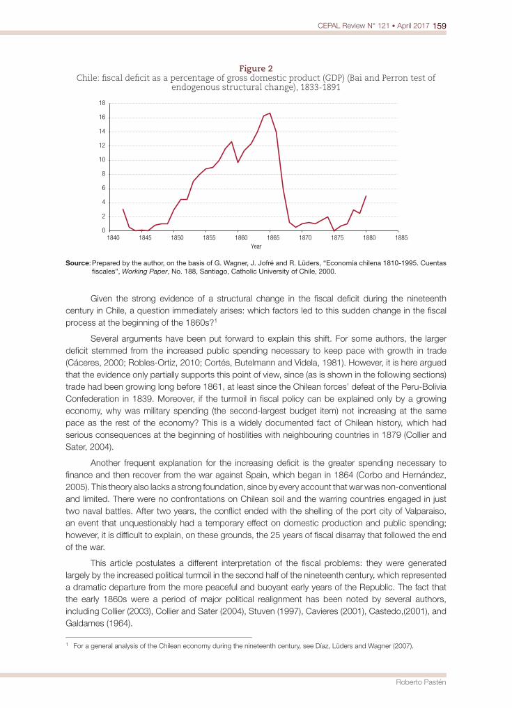
159CEPAL Review N° 121 • April 2017
Roberto Pastén
Figure 2 Chile: fiscal deficit as a percentage of gross domestic product (GDP) (Bai and Perron test of
endogenous structural change), 1833-1891
0
2
4
6
8
10
12
14
16
18
1840 1845 1850 1855 1860 1865 1870 1875 1880 1885 Year
Source: Prepared by the author, on the basis of G. Wagner, J. Jofré and R. Lüders, “Economía chilena 1810-1995. Cuentas fiscales”, Working Paper, No. 188, Santiago, Catholic University of Chile, 2000.
Given the strong evidence of a structural change in the fiscal deficit during the nineteenth century in Chile, a question immediately arises: which factors led to this sudden change in the fiscal process at the beginning of the 1860s?1
Several arguments have been put forward to explain this shift. For some authors, the larger deficit stemmed from the increased public spending necessary to keep pace with growth in trade (Cáceres, 2000; Robles-Ortiz, 2010; Cortés, Butelmann and Videla, 1981). However, it is here argued that the evidence only partially supports this point of view, since (as is shown in the following sections) trade had been growing long before 1861, at least since the Chilean forces’ defeat of the Peru-Bolivia Confederation in 1839. Moreover, if the turmoil in fiscal policy can be explained only by a growing economy, why was military spending (the second-largest budget item) not increasing at the same pace as the rest of the economy? This is a widely documented fact of Chilean history, which had serious consequences at the beginning of hostilities with neighbouring countries in 1879 (Collier and Sater, 2004).
Another frequent explanation for the increasing deficit is the greater spending necessary to finance and then recover from the war against Spain, which began in 1864 (Corbo and Hernández, 2005). This theory also lacks a strong foundation, since by every account that war was non-conventional and limited. There were no confrontations on Chilean soil and the warring countries engaged in just two naval battles. After two years, the conflict ended with the shelling of the port city of Valparaiso, an event that unquestionably had a temporary effect on domestic production and public spending; however, it is difficult to explain, on these grounds, the 25 years of fiscal disarray that followed the end of the war.
This article postulates a different interpretation of the fiscal problems: they were generated largely by the increased political turmoil in the second half of the nineteenth century, which represented a dramatic departure from the more peaceful and buoyant early years of the Republic. The fact that the early 1860s were a period of major political realignment has been noted by several authors, including Collier (2003), Collier and Sater (2004), Stuven (1997), Cavieres (2001), Castedo,(2001), and Galdames (1964).
1 For a general analysis of the Chilean economy during the nineteenth century, see Díaz, Lüders and Wagner (2007).
160 CEPAL Review N° 121 • April 2017
The political economy of the fiscal deficit in nineteenth-century Chile
The hypothesis that political instability is one of the possible causes of fiscal disarray is consistent with the conceptual framework developed by Pastén and Cover (2010, 2011 and 2015) based on the political determinants of tax smoothing and tax tilting, which they believe explain government budget deficits. Under tax smoothing (equivalent to a sustainable and efficient fiscal deficit), in order to minimize the distortionary social cost of taxes, deficits are efficient if they are the result of a policy decision not to vary the tax rate in response to transitory fluctuations in government spending. Tax tilting, conversely, occurs whenever the government has an incentive to discount the social cost of taxes at a higher rate than society discounts them; hence, it delays taxes or advances spending, triggering an upward trend in fiscal deficits. Pastén and Cover’s main point is that tax tilting is a positive function of political instability. The transmission mechanism is as follows: an increase in political instability, measured by the probability of losing power, increases the rate at which the government discounts future social costs; so, with tax tilting, a relatively more myopic fiscal government policy produces a trend toward higher fiscal deficits. Moreover, the authors show that the direction of causality is from politics (political instability) to deficits rather than the other way around (Pastén and Cover, 2010 and 2015).
Other authors have also suggested a link between tax tilting and political instability. Cashin, Haque and Olekalns (1999, p. 14) state that, “Tax tilting could occur, for example, if the current government is unsure of its re-election prospects and therefore favours higher current debt levels than are implied by tax smoothing.” For a similar view, see Cerda and Vergara (2008). For empirical evidence on Latin America, see Pastén and Cover (2015), and for evidence on Chile see Pastén and Cover (2010).
A closer look at figure 1 also seems to give some support to the hypothesis of political instability as a determinant of tax tilting. First, according to the graph, at least from 1851, fiscal revenues (as a percentage of gross domestic product (GDP)) start to fall prior to the break point postulated in this paper and before the crisis of 1873, which at first glance seems to be inconsistent with the hypothesis that fiscal disarray starts in the mid-1860s. However, figure 1 also shows clearly that not only taxes but also total spending fell at the beginning of the 1850s and they both continue to decrease for the most part, until the mid-1860s. This is consistent with the hypothesis outlined in this paper that in conditions of political stability, there are no tax tilting effects, and taxes and spending move together in the long run. Moreover, according to figure 1 spending only temporarily outpaces taxes in 1859, most likely due to a small civil war that year, at the end of President Manuel Montt’s term of office. That effect was transitory because, while taxes were kept relatively constant, spending increased briefly in order to finance the 1859 civil war, which is typical of tax smoothing but not of tax tilting. Also, after the mid-1860s, the chart shows that spending outpaces taxes dramatically, which is indeed characteristic of tax tilting.
Second, although Chile wrested control of nitrate-rich zones from Peru and Bolivia after the War of the Pacific (1879-1883), increasing the amount of revenues collected, the fiscal deficit problem persisted at least until 1891 (see again figure 1). This strongly supports the hypothesis proposed here, because even the higher revenues collected after the War of the Pacific were not enough to offset the increased fiscal expenditure which, according to this hypothesis, could be explained by the political weakness of a government desperate to bolster support in the run up to the 1891 civil war.
Lastly, starting from the mid-1860s, the higher deficits stemmed mainly from growth in spending; however, it is not clear which spending component fuelled this growth. Although the explanation is beyond the scope of this paper, Humud (1969) may shed some light on this change in composition, which is consistent with the hypothesis proposed here. Humud found that, before 1860, fiscal spending grew at a rate of 5.5% (compared with a 6.2% increase in tax revenues) mainly in order to finance conventional and administrative spending. However, spending then grew by 5.7% between 1860 and 1879, and by 3.4% from 1880 to 1900 (by comparison, revenues grew by 4.8% and 2.8%, respectively). This growth stemmed mainly from a group of emerging components of fiscal expenditure,
161CEPAL Review N° 121 • April 2017
Roberto Pastén
chief among them public works —particularly railroad construction— but also justice, education and war efforts. Spending on public works is a sign of patronage as postulated by Rogoff (1990) in his political business cycle models, where he describes the preference of governments for “projects with high immediate visibility.” González (2002) found similar political bias in Mexico, showing that the government manipulated fiscal policy for political purposes prior to all federal elections; infrastructure spending was the policy variable used.
In section II, we will show that, throughout Chile’s nineteenth-century history of politics and public finance, it is a reasonable hypothesis that the trend in fiscal deficits was affected by the political context. A brief, highly stylized description of the political and economic events that shaped the period between 1833 and 1860 is presented here, aiming to show that this was a time of sound fiscal policies and also of political stability. Section III describes the political and economic events of 1861-1891, a period characterized by fiscal crisis and intense and growing political uncertainty that climaxed with the civil war, which ended with the suicide of President José Manuel Balmaceda in 1891. Lastly, section IV concludes.
II. 1833-1860: a time of order and progress
As early as 1818, when Chile declared independence from Spain, two political movements with opposing views on society emerged. On one side, the liberals (pipiolos) most faithfully represented the liberal doctrines of Europe while, on the other, the conservatives (pelucones) were predominantly landowners and represented the country’s Spanish heritage.
Their differing views on how the new Republic should be organized led to constant clashes in the period immediately following independence from Spain. Following the Battle of Lircay (1830), the pelucones prevailed over the pipiolos, implementing a constitution that favoured a strong executive branch, in keeping with the ideas of Minister Diego Portales.
After the Battle of Lircay, Diego Portales emerged as a kind of Chilean Alexander Hamilton.2 In the joint posts of Minister of the Interior, Foreign Relations, and War, he designed and supported a centralist and presidential constitution. The Constitution of 1833 remained in effect for almost 100 years (until 1925), albeit with some modifications. It vested the president with two consecutive five-year terms that resulted, for example, in only four presidents being elected over a period of 40 years. The president controlled the cabinet, judiciary, public administration and armed forces, and also enjoyed emergency powers such as the authority to declare a state of siege in any part of the territory while the parliament was in recess. With these emergency powers, the president could suspend any constitutional guarantees in the affected territory. Also, because the Constitution of 1833 was strongly centralist, no federalist assemblies were allowed, provincial heads were appointed by the president, and the president had veto power over elected municipal councils.
The principal characteristics of this period (1833-1860) were the organization of a State of notable stability, efficacy and endurance; in addition, it was a period of sustained economic progress. Another feature was the electoral intervention that in practice allowed any government to elect the Congress and the presidential successor. The electorate was small (only owners of a certain amount of property were allowed to elect representatives) and military officers were able to influence the votes of their soldiers by retaining their electoral registration certificates until election day (Collier and Sater, 2004). Nevertheless, there was some opposition, mostly from deputies (representatives) who never held a majority in parliament. Conservative rule was more religious than secular and went
2 The similarities between the two men are remarkable. Each could have easily become president but neither sought the post. They both advocated a strong and centralized government and died tragically in their 40s.
162 CEPAL Review N° 121 • April 2017
The political economy of the fiscal deficit in nineteenth-century Chile
unchallenged during the first half of the nineteenth century. At least until the 1850s, there was no significant political resistance.3
The point of consensus between liberals and conservatives was a high regard for social order, which Minister Portales expressed eloquently when he said that: “The Republic should be a strong and centralized government that led citizens along the path of order and virtues.”4 Herein lies the justification for strict control over the press, the reshaping of the army and harsh public policies. In Portales’s view, order consisted primarily of public order and its ultimate goal was social order. He also believed in a union between the State and the (Catholic) Church as another precondition for social order.
For the liberals (who were more secular than confessional), the state of affairs imposed by the conservative regime was acceptable if the alternative was the anarchy that marked the early years of the Republic. Andrés Bello and other notable liberals were supportive of the conservative governments’ authoritarian rule. Any perceived opposition was quickly suppressed by the political class. For example, El Progreso (Santiago’s first daily newspaper) stated that: “In Chile [...] there is no national will to express, because there are no parties with conflicting points of view, or vital issues dividing society.”5
Regarding the prevailing consensus and the self-imposed limits on dissent, Collier and Sater (2004, p. 104) said that “liberalism as a coherent political force came close in these years [1833-1850] to being killed by kindness.”
1. A time of economic progress
After Chile’s independence from Spain in 1818, the Spanish monopoly ended and the flow of trade turned mostly to the United Kingdom and, to a lesser extent, France and Germany. The new trade pattern resulted in the installation of branches of British companies in Chile’s principal cities and ports. Nevertheless, it was the programme of economic reforms implemented by Portales’s Treasury Minister, Manuel Rengifo, that consolidated a development path based on openness to world trade by 1830.
The aim of Rengifo (who served as Minister of Finance from 1830 to 1835 and again from 1841 to 1844) was to balance the fiscal accounts. This was achieved in 1839 thanks to rising customs revenues.
From an economic standpoint, Rengifo’s policies were more neo-classical than neo-mercantilist. He favoured the expansion of trade. In 1834 commercial legislation reinforced the downward trend in the tariffs on imports in place since independence. The average tariff was 25% (Sutter and Sunkel, 1982).6
The reforms implemented by Minister Rengifo were consistent with an economy open to global trade and led to a spectacular increase in fiscal revenues. He eliminated most export duties, with the exception of a 4% duty on wheat and a 6% duty on minerals. However, the greatest stimulus to international trade was a measure that had been attempted by every government since 1813: public or bonded warehouse (almacén fiscal). Under this initiative, trading companies were allowed to store merchandise in the port of Valparaiso at low cost and then trade these goods when market conditions
3 In 7 of the 11 congressional elections held between 1833 and 1864, the opposition either abstained or scarcely bothered to run. It focused its efforts on the Chamber of Representatives, but only after 1860 were a handful of deputies elected (Collier, 2003).
4 Ernesto de la Cruz (editor), Epistolario de don Diego Portales (Santiago, Ediciones de la Biblioteca Nacional, 1936), p. 177; cited in Stuven, 1997, pp. 269-270.
5 El Progreso, 10 June 1844; cited by Stuven (1997, p. 280).6 Nonetheless, several studies show very different treatments behind the average tariff (Cortés, Butelmann and Videla, 1981;
Díaz and Wagner, 2004).
163CEPAL Review N° 121 • April 2017
Roberto Pastén
were favourable. In 1833, the time allowed for storage was increased from three to six years. At that point, Valparaiso became one of the most important ports in the South Pacific (second only to Callao in Peru) and the dominant port for ships rounding Cape Horn. Chile’s victory over Peru and Bolivia in the war with the Peru-Bolivia Confederation (1836-1839) consolidated Valparaiso’s position as the predominant port south of California. This period defines the expansion of foreign trade in Chile. By 1840, foreign trade tripled that of 1810 (Sutter and Sunkel, 1982).
In addition to opening up its economy, Chile was developing its focus on natural resources. In 1832, Juan Godoy discovered Chañarcillo, a silver mine that became the most spectacular mining discovery of the first half of the nineteenth century. Silver and subsequent copper mines helped increase the population of Chile’s Norte Chico region (a mining zone) and simultaneously created a new market for agricultural products from the southern part of the country. Nevertheless, fiscal revenues from natural resources never surpassed 10% of total revenues. Until the end of the War of the Pacific in 1883, customs duties and taxes rather than taxes on natural resources remained the largest component of total revenues.
The spectacular expansion of trade that began in 1833 allowed for the systematization of the tax system along with the simplification of customs rules and regulations and administrative organization. These conditions had a strong impact, resulting in increased revenue collection. Chile was able to pay back the loans incurred during colonial times and, furthermore, to generate large budget surpluses. Every conservative government from that of President José Joaquín Prieto in the early 1830s to that of President Manuel Montt in the early 1860s maintained the strict policy of keeping up with public debt payments. Chile’s creditworthiness under conservative rule was admirable (Edwards, 1932; Galdames, 1964; Collier and Sater, 2004).
2. An emerging crisis
As the memory of anarchy faded in Chile and foreign ideas arising from the events surrounding the French Revolution in 1848 gained ground among the liberals, the conservative regime began to face challenges (Stuven, 1997). Collier and Sater (2004, p. 104) accurately describe the incipient signs of a political realignment by the mid-nineteenth century:
It was unlikely that the Conservative settlement would survive indefinitely without alteration. In the middle years of the century a fierce and at times bloody battle was waged between the upholders of its initial authoritarian style and those who favored a more liberal and tolerant approach to the government.
The liberals used their constitutional authority for the first time in 1850, to delay the passing of the annual tax law in order to apply political pressure (this practice intensified in the early 1860s and was an important factor in the fall of President Balmaceda in the conflict of 1891).
The first significant uprising in republican history occurred on 20 April 1851. Government forces quashed the rebellion and those members of the army who led the revolt died in the confrontation. Later that year Manuel Montt became president (1851-1861). A hallmark of his government was its focus on material progress, with the construction of roads and railways, the opening up of new territories, the broadening of the frontier and other efforts. According to Collier and Sater (2004, p. 110):
Montt himself may have seen his emphasis on “material interest” as a means of distracting Chileans’ minds from political concerns.
Although President Montt did not swerve from this path of progress for almost his entire administration, by the end of his rule, there were signs of a profound change in Chilean politics. These events would reshape the political scenario in the years to come and put an end to the period of peace, order and progress imposed by the conservative governments.
164 CEPAL Review N° 121 • April 2017
The political economy of the fiscal deficit in nineteenth-century Chile
These political changes emerged because of a minor event in the late 1850s triggered by a conflict between the Catholic Church and the judiciary. In that instance, President Montt (in an unusual move given his conservative outlook) decided to support the judiciary because of his desire to uphold presidential power. As a result, for the first time in Chilean history, a crack appeared in the Conservative Party.
During the near-decade of President Montt’s rule, ideas of enlightened modernity and European liberalism were slowly absorbed by part of the political class. According to Domingo Santa María (a future liberal president, himself at odds with the Church) there were contradictions within the conservative settlement. Stuven (1997) argued that the political laziness of the time could be explained by presidential authoritarianism along with President Montt’s excessive kindness toward the Church.
However, the very notion of a confessional, conservative conglomerate was contrary to the idea of a strong presidential system. All of Chilean society was involved in the clash between the government and the Catholic Church. Starting from a minor conflict with the Church, the debate spread to other areas that had been previously overlooked by the public, including Catholic education and freedom of religion. The result was a bitter division of the president’s party into secular and confessional conservatives.
A strong new political force emerged from the ongoing conflict: a mix of liberals and conservatives unhappy with the president’s pro-clerical policies. At the end of President Montt’s term, a new (and bloodier) uprising against the government was suppressed. However, the period of conservative supremacy that had provided the country with stability (particularly fiscal stability) and economic progress had ended.
III. 1861-1891: a time of political turmoil
1. The turning point
Several authors have identified different structural changes in the republican period between 1833 and 1891. For some, 1876 was a major turning point, as a year in which the country experienced one of its deepest economic depressions. For others, the tide changed in 1879, when the War of the Pacific broke out. For still others (including this author), the most significant change in the nineteenth century in Chile occurred in the early 1860s, with the political realignment of the Conservative Party mentioned above. According to Collier and Sater (2004, p. 116):
The events of 1861 mark an important dividing line in Chilean political history. Later generations were to reflect more generously on Montt and Varas [President Montt’s Minister of the Interior], but the political class as a whole viewed their departure from office with undisguised relief. The new president’s style was very different. His tolerance may have stemmed, as was said at the time, from supreme indifference. José Manuel Balmaceda described him as “drunk on indolence.” Yet these qualities were precisely those needed to induce a mood of calm after the agitations of the previous decade. Admirers of strong government have often presented this elderly patrician in a poor light. In fact he deserves as much credit as any nineteenth-century president for consolidating the national “idiosyncrasy” of civilized politics.
As these authors point out, President José Joaquín Pérez’s rule (1861-1871) was anathema to believers in the strong governments that had characterized the early years of the Republic. His first term marks both the greatest political realignment since the birth of the Republic and a structural shift in the trend toward higher deficits (see figure 1).
165CEPAL Review N° 121 • April 2017
Roberto Pastén
During his tenure, President Pérez ruled mostly against the backdrop of the Liberal-Conservative Fusion. The departure from previous authoritarian regimes was evident in a number of proposed reforms to the Constitution of 1833 (some 34 articles of the Constitution were amendable in principle). Under the Constitution of 1833 only the next legislature could amend the Constitution, and as a result the elections of 1870 were hotly contested. The programme of reforms included electoral freedom, an expansion of individual liberties and an overall reduction of the president’s power. Nevertheless, the new Congress only adopted one (albeit historically significant) amendment: the prohibition of consecutive presidential terms, putting an end to the periods of decade-long rule by one president. This was the first amendment to the Constitution in 38 years.
The following president, Federico Errázuriz —in office from 1871 to 1876— took office in September. Like his predecessor, he began his term with support from the Liberal-Conservative Fusion; however, by the time he left office he had the support of the liberal coalition only. After that, presidential power shifted to the Liberal Party until Balmaceda’s deposition in 1891.
President Errázuriz’s term was marked by a much fiercer political struggle than any previous administration. At the beginning of his term, the conservative members of his government disagreed with public education’s prevailing tendency to afford great importance to the natural sciences; they regarded this as “contrary to religious belief and injurious to private morality” (Galdames, 1964). This conflict over theological issues prompted President Errázuriz to remove conservatives from his government. Thus, for the first time, conservatives became part of the opposition and began trying to broaden the electoral base to include formerly excluded Chileans (mostly Catholics), in an effort to diminish the president’s power. The electoral system was reformed to grant minority parties representation based on their number of qualified electors.
Meanwhile, 1870 ushered in a long period of declining export commodity prices, which affected mainly the wheat sector as crops became more productive and means of transportation for competitors more readily available in foreign markets (eliminating the advantageous position of Chile’s food export sector during the gold rush in California and Australia). Additionally, copper production decreased after 1872 and the price of silver fell at the same time. These events caused the deepest economic crisis experienced thus far by the new Republic and had some lasting effects on the economy. The development of the banking system around 1870 made it possible to monetize the economy (replacing the mandatory gold convertibility system with the use of paper notes). However, the inconvertibility of paper notes into gold resulted in the devaluation of the Chilean peso and increased its volatility, which also had political repercussions.7 Moreover, there is some evidence that inconvertibility was implemented in order to save some banks as well as to support the government (Millar, 1994).
By 1876 the global price of copper had fallen by 20% and Chile’s exports of this metal had declined by 16%. Silver exports were one third of the level seen in 1874. Severe weather in 1877 washed away roads and railroads and destroyed livestock and crops, causing wheat and flour exports to drop. About 300,000 workers lost their jobs, many businesses went bankrupt and food prices increased (Collier and Sater, 2004).
This economic downturn drastically reduced fiscal revenue collection. To remedy this, President Aníbal Pinto (1876-1881) added a 10% surcharge to prevailing tariffs. He also implemented unpopular measures such as laying off public employees, beaching naval vessels and discharging numerous army and navy units. The political crisis (the worst since independence) revealed an incipient social crisis.
In 1878, Congress passed a law modifying the tariff code. From that point on, a 35% tax was levied on luxury items and goods that competed with domestic products, while the tax applied to capital goods was just 15%. Other goods were subject to a 25% tax or a specific value-based tax.
7 The dispute between papeleros (who supported inconvertibility) and oreros (who advocated for convertibility to gold) became part of the political struggle for most of the Parliamentary Republic (1891-1925).
166 CEPAL Review N° 121 • April 2017
The political economy of the fiscal deficit in nineteenth-century Chile
There were also proposals to tax gifts and estate inheritances as well as income and investments, but these measures were ultimately rejected.
By 1870 deposits of sodium nitrate had been discovered in the Peruvian desert province of Tarapacá. The Bolivian silver mines in Caracoles were worked almost entirely by Chileans whose status on foreign soil, mainly in Bolivia, sparked an international crisis that led to the war between Chile and the allied forces of Peru and Bolivia in 1879. The War of the Pacific was to be the most traumatic experience for Chile since independence.
2. War and fiscal policy
As mentioned earlier, from the early years of independence until the crisis of the mid-1870s, the government’s budget was supported mostly by customs duties. However, the economic crisis halved these revenues. As a result, the main components of government revenue became estanco (trade licences), alcabala (transfer tax) and land tax (which had been proposed some years before by Rengifo). Nevertheless, just as these taxes were not enough to fund the fiscal budget during the economic crisis, they were unable to fund the war effort.
In 1879, under pressure owing to the international crisis, Congress passed the mobiliaria (income tax) that had been rejected the previous year. The government also tried to borrow money, but the country’s banks were unable to help, given the precarious situation of the banking system after the crisis of 1876. As a last resort, the government turned to printing paper notes that the public was forced to accept. Since printing money inevitably leads to inflation, something had to be done to prevent the government from relying indefinitely on this measure.
This problem was solved by Chile’s occupation of the resource-rich territories originally held by Peru and Bolivia at the beginning of the conflict. A new export tax was imposed in September 1879 (US$ 1.60 per quintal of nitrates), providing a sufficient flow of fiscal revenues to finance the government’s budget.
Although the Chilean government had the option of taxing nitrate production, the mines were still legally owned by the Peruvian government. This problem was solved by restoring the nitrate mines to their original owners, mostly British companies (who had previously been granted ownership by the Peruvian government). This policy enabled private entrepreneurs to take control of what became the main source of tax revenue during the next 50 years.
3. The deepening political crisis
The ongoing war did not stop the deterioration of the political situation in Chile (for example, in 1881 a group of deputies attempted to cut off funds for the war effort as a means of pressuring President Pinto into reshuffling his cabinet). This crisis was effectively ended by the significant revenues that began pouring in at the end of President Aníbal Pinto’s tenure and enabled several municipalities to undertake improvements. Meanwhile, the government itself embarked on a highway construction programme and completed a number of railroad lines.
The next President, Domingo Santa María (1881-1886), also a liberal, was faced with a Congress that was seeking to undermine the presidential system by eliminating the President’s veto power over the cabinet and promoting elections free of intervention. Since the President wished to maintain the prerogatives of his office, the relationship between the two branches of government was quite antagonistic. The President was also eager to reduce the powerful role of the Catholic Church in Chilean society. During his mandate, and amid a crisis over the right to appoint the archbishop of Santiago, he broke off relations with the Holy See.
167CEPAL Review N° 121 • April 2017
Roberto Pastén
After these events, laws concerning civil marriage and civil registry were passed. Secular cemeteries were created and, following protests from the clergy, a decree prohibiting private cemeteries was issued. “So great was the opposition made by the clergy that the country seemed on the verge of a revolution” (Galdames, 1964).
During this time of struggle between the president and the Church, the liberals (the President’s party) fought to restrict presidential power. A reform extended suffrage to every literate male (women were still not allowed to vote) over 25 years old. This reform was intended to reduce the President’s electoral influence, which had been quite strong since the conservative settlement. The Congressional elections of 1885 (the new Congress had the right to elect the next president) were the most violent in the country’s history (Collier and Sater, 2004).
When President José Manuel Balmaceda (a member of the Liberal Party) was inaugurated on 18 September 1886, the political environment had become highly polarized between those who supported the presidential system and its opponents. President Balmaceda conceived the idea of using the substantial revenues generated by nitrate produced in the new territories to finance an ambitious public works plan (the public works ministry was created in 1887 and by 1890 it accounted for one third of the fiscal budget).
This public works plan (unprecedented in Chile) could arguably be considered a way to uphold presidential power and undermine opposition. In fact, in the dangerous political climate of the time, Balmaceda’s public works projects were seen by the political opposition as a means of expanding presidential patronage.
This was clear to Valentín Letelier, one of the most prominent liberals of the time. In 1891, he presented a lecture on “Tyranny and the revolution” at the University of Chile’s School of Law, with the stated objective of “studying the dangerous politics of despotism and abuse by all parts of our administrative machine with which the government corrupts until it becomes the most horrible rot in the annals of the Republic.” He continued:
The exorbitant enrichment of the treasury, wrongly obtained through the increase in private wealth, transformed the executive into the strongest political power since O’Higgins.8
Never before has there been in Chile such large a number of employees, contractors, workers, engineers, architects and others whose subsistence and fortune depend directly and exclusively on the government.
The Ministry of Public Works determines the fate of hundreds of suppliers of wood, lime, brick, building stone, iron and other materials. And the construction of bridges, roads, railways, telegraph lines, schools, churches and prisons is linked so closely to the government that the most influential citizens of every province believe they are in debt to the President of the Republic for the works carried out thanks to his generosity and good grace (Cavieres, 2001).
President Balmaceda also allocated an unprecedented amount of resources to the modernization of the army and the navy. The traditional explanation for this is the threat presented by Chile’s neighbouring countries. However, it seems more plausible that the President was trying to win the loyalty of both entities of the armed forces in the event that the ongoing political conflict led to violence. This seems particularly reasonable given the increased presence of members of the army in high-level government posts and the incentives given to members of the navy who showed support for the government.9
8 Bernardo O’Higgins was Chile’s independence hero.9 Two years of wages for all crewmembers of a warship who renounced actions against the executive and a 25% wage increase
for members of the navy who did not participate in the uprising (Boletín de leyes y decretos de la dictadura 1891).
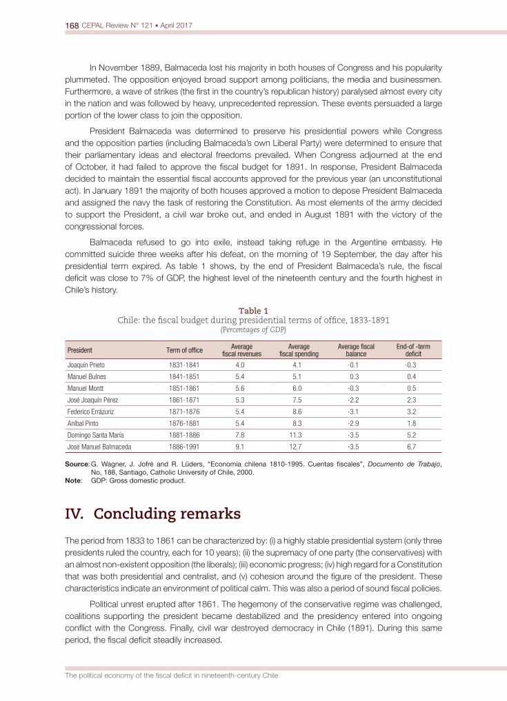
168 CEPAL Review N° 121 • April 2017
The political economy of the fiscal deficit in nineteenth-century Chile
In November 1889, Balmaceda lost his majority in both houses of Congress and his popularity plummeted. The opposition enjoyed broad support among politicians, the media and businessmen. Furthermore, a wave of strikes (the first in the country’s republican history) paralysed almost every city in the nation and was followed by heavy, unprecedented repression. These events persuaded a large portion of the lower class to join the opposition.
President Balmaceda was determined to preserve his presidential powers while Congress and the opposition parties (including Balmaceda’s own Liberal Party) were determined to ensure that their parliamentary ideas and electoral freedoms prevailed. When Congress adjourned at the end of October, it had failed to approve the fiscal budget for 1891. In response, President Balmaceda decided to maintain the essential fiscal accounts approved for the previous year (an unconstitutional act). In January 1891 the majority of both houses approved a motion to depose President Balmaceda and assigned the navy the task of restoring the Constitution. As most elements of the army decided to support the President, a civil war broke out, and ended in August 1891 with the victory of the congressional forces.
Balmaceda refused to go into exile, instead taking refuge in the Argentine embassy. He committed suicide three weeks after his defeat, on the morning of 19 September, the day after his presidential term expired. As table 1 shows, by the end of President Balmaceda’s rule, the fiscal deficit was close to 7% of GDP, the highest level of the nineteenth century and the fourth highest in Chile’s history.
Table 1 Chile: the fiscal budget during presidential terms of office, 1833-1891
(Percentages of GDP)
President Term of office Averagefiscal revenues
Averagefiscal spending
Average fiscalbalance
End-of -termdeficit
Joaquín Prieto 1831-1841 4.0 4.1 -0.1 -0.3
Manuel Bulnes 1841-1851 5.4 5.1 0.3 0.4
Manuel Montt 1851-1861 5.6 6.0 -0.3 0.5
José Joaquín Pérez 1861-1871 5.3 7.5 -2.2 2.3
Federico Errázuriz 1871-1876 5.4 8.6 -3.1 3.2
Aníbal Pinto 1876-1881 5.4 8.3 -2.9 1.8
Domingo Santa María 1881-1886 7.8 11.3 -3.5 5.2
José Manuel Balmaceda 1886-1991 9.1 12.7 -3.5 6.7
Source: G. Wagner, J. Jofré and R. Lüders, “Economía chilena 1810-1995. Cuentas fiscales”, Documento de Trabajo, No, 188, Santiago, Catholic University of Chile, 2000.
Note: GDP: Gross domestic product.
IV. Concluding remarks
The period from 1833 to 1861 can be characterized by: (i) a highly stable presidential system (only three presidents ruled the country, each for 10 years); (ii) the supremacy of one party (the conservatives) with an almost non-existent opposition (the liberals); (iii) economic progress; (iv) high regard for a Constitution that was both presidential and centralist, and (v) cohesion around the figure of the president. These characteristics indicate an environment of political calm. This was also a period of sound fiscal policies.
Political unrest erupted after 1861. The hegemony of the conservative regime was challenged, coalitions supporting the president became destabilized and the presidency entered into ongoing conflict with the Congress. Finally, civil war destroyed democracy in Chile (1891). During this same period, the fiscal deficit steadily increased.
169CEPAL Review N° 121 • April 2017
Roberto Pastén
The events of 1861-1891 seem to provide evidence that in periods of political turmoil, the fiscal deficit rises and as a result, can become unsustainable or at least suboptimal. At the same time, with political stability, there is no incentive to distort fiscal policy and therefore the officeholder plausibly follows an optimal fiscal policy.
Another fact apparent from this brief review of Chilean history and which is consistent with several types of political budget cycle (PBC) models is the attitude toward investment in public works during times of crisis (governments of Pinto, Santa María and, notably, Balmaceda). In his PBC model, Rogoff (1990) describes the preference of governments for “projects with high immediate visibility.” González (2002, p. 220) found similar political bias in Mexico. She states:
The findings presented in this paper have several interesting implications. First, the analysis shows that the Mexican government has, indeed, manipulated fiscal policy for political purposes prior to all federal elections; the policy variable used seems to be infrastructure spending. Some evidence suggests that a public investment boom starts relatively early in the political term (at least six quarters previous to the election), continues until at least the last quarter prior to the ballot, and then diminishes as the election quarter is reached.
BibliographyBai, J. (1997), “Estimation of a change point in multiple regression models”, Review of Economics and
Statistics, vol. 79, No. 4, Cambridge, Massachusetts, The MIT Press.Bai, J. and P. Perron (2003), “Computation and analysis of multiple structural change models”, Journal of
Applied Econometrics, vol. 18, No. 1, Wiley.(1998), “Estimating and testing linear models with multiple structural changes”, Econometrica, vol. 66, No. 1, New York, The Econometric Society.
Cáceres, J. (2000), “Guerra y finanzas públicas en Chile y Perú: 1860-1890”, Revista de Humanidades, No. 7, Santiago, Andrés Bello University.
Cashin, P.N. Haque and N. Olekalns (1999), “Spend now, pay later? Tax smoothing and fiscal sustainability in South Asia”, IMF Working Paper, No. WP/99/63, Washington, D.C., International Monetary Fund.
Castedo, L. (2001), Vida y muerte de la República Parlamentaria, Santiago, Editorial Sudamericana.Cavieres, E. (2001), “Anverso y reverso del liberalismo en Chile”, Historia, vol. 34, Santiago, Catholic University
of Chile.Cerda, R. and R. Vergara (2008), “Government subsidies and presidential election outcomes: evidence for
a development country”, World Development, vol. 36, No. 11, Amsterdam, Elsevier. Collier, S. (2003), Chile: the Making of a Republic, 1830-1865, New York, Cambridge University Press.Collier, S. and W.F. Sater (2004), A History of Chile 1808-2002, Cambridge, Cambridge University Press. Corbo, V. and L. Hernández (2005), “Ochenta años de historia del Banco Central de Chile”, Economía Chilena,
No. 3, Santiago, Central Bank of Chile.Cortés, D.H., A. Butelmann and P. Videla (1981), “Proteccionismo en Chile: una visión retrospectiva”, Cuadernos
de Economía, No. 54-55, Santiago, Catholic University of Chile. Díaz, J. and G. Wagner (2004), “Política comercial: instrumentos y antecedentes. Chile en los siglos XIX y XX”,
Documento de Trabajo, No. 223, Santiago, Catholic University of Chile.Díaz, J.R. Lüders and G. Wagner (2007), “Economía chilena 1810-2000. Producto total y sectorial. Una nueva
mirada”, Documento de Trabajo, No. 315, Santiago, Catholic University of Chile.Edwards, A. (1932), El gobierno de Don Manuel Montt 1851-1861, Santiago, Editorial Nascimento.Galdames, L. (1964), A History of Chile, New York, Russell and Russel Inc.González, M. (2002), “Do changes in democracy affect the political budget cycle? Evidence from Mexico”,
Review of Development Economics, vol. 6, No. 2, Wiley.Humud, C. (1969), “El sector público chileno entre 1830 y 1930”, thesis, Santiago, University of Chile.Millar, R. (1994), Políticas y teorías monetarias en Chile 1810-1925, Santiago, Gabriela Mistral University.Ortega, L.M. (1897), “Change and crisis in Chile’s economy and society, 1865-1879”, thesis, University
of London.
170 CEPAL Review N° 121 • April 2017
The political economy of the fiscal deficit in nineteenth-century Chile
Pastén, R. and J.P. Cover (2015), “Tax tilting and politics: some theory and evidence for Latin America”, Journal of Macroeconomics, vol. 44, Amsterdam, Elsevier.(2011), “Does the Chilean government smooth taxes? A tax-smoothing model with revenue collection from a natural resource”, Applied Economics Letters, vol. 18, No. 5, Taylor & Francis.(2010), “The political economy of unsustainable fiscal deficits”, Cuadernos de Economía, vol. 47, No. 136, Santiago, Catholic University of Chile.
Robles-Ortiz, C. (2010), “Ideología agraria y política económica en una economía exportadora: Chile 1860-1880”, Iberoamericana, vol. 10, No. 38.
Rogoff, K. (1990), “Equilibrium political budget cycles”, American Economic Review, vol. 80, No. 1, Nashville, Tennessee, American Economic Association.
Stuven, A. (1997), “Una aproximación a la cultura política de la elite chilena: concepto y valoración del orden social (1830-1860)”, Estudios Públicos, No. 66, Santiago, Centre for Public Studies.
Sutter, C.C. and O. Sunkel (1982), La historia económica de Chile 1830-1930: dos ensayos y una bibliografía, Madrid, Ediciones Cultura Hispánica del Instituto de Cooperación Iberoamericana.
Wagner, G., J. Jofré and R. Lüders (2000), “Economía chilena 1810-1995. Cuentas fiscales”, Documento de Trabajo, No. 188, Santiago, Catholic University of Chile.
The determinants of foreign direct investment in Brazil: empirical analysis for 2001-2013Eduarda Martins Correa da Silveira, Jorge Augusto Dias Samsonescu and Divanildo Triches
Keywords
Foreign direct investment, economic growth, productivity, agriculture, industry, tertiary sector, econometric models, Brazil
JEL classification
F23, L21, C22
Authors
Eduarda Martins Correa da Silveira is a PhD student in Economics on the Postgraduate Programme in Economics of the Federal University of Rio Grande do Sul (UFRGS) and holds a Masters Degree the University of Vale do Rio dos Sinos (UNISINOS), Brazil. [email protected]
Jorge Augusto Dias Samsonescu holds a Masters Degree in Economics from the University of Vale do Rio dos Sinos (UNISINOS), Brazil. [email protected]
Divanildo Triches holds a PhD in Economics from the Federal University of Rio Grande do Sul (UFRGS) and is a research fellow and professor on the Postgraduate Programme in Economics (PPGE) of the University of Vale do Rio dos Sinos (UNISINOS), Brazil. [email protected] and [email protected]
Abstract
This article aims to analyse the determinants of foreign direct investment (FDI) into Brazil between 2001 and 2013. It uses a vector error correction (VEC) model to analyse both the long-term function and the impulse-response function. The results show that levels of economic activity, wages and productivity are positively related to FDI inflows, which means that investors pursue market-seeking and efficiency-seeking strategies when targeting the Brazilian market. Although less important, the stability of the national economy and the exchange rate also proved statistically significant in explaining FDI inflows.
172 CEPAL Review N° 121 • April 2017
The determinants of foreign direct investment in Brazil: empirical analysis for 2001-2013
I. Introduction
From the 1990s onwards, foreign capital flows into Brazil in the form of foreign direct investment (FDI) have grown strongly, driven mainly by privatizations. Those investments also helped to reduce repetitive current account deficits (owing to the greater openness of the domestic economy to the international market) and to raise domestic productivity levels.
As noted by Lima Júnior (2005), throughout the 1990s most FDI was channelled into the tertiary sector, in response to the deregulation implemented by the Brazilian Government. Apart from alleviating balance-of-payments constraints, FDI capital inflows can stimulate economic growth and technological development in the receiving countries, particularly if the investments are made in export-oriented firms and thus increase export earnings.
With that backdrop, this study sets out to analyse the determinants of FDI flows into Brazil between 2001 and 2013 —a period in which they grew vigorously. The study also aims to identify the strategy adopted by foreign firms, based on the theoretical framework proposed by Dunning (1993), known as the “eclectic paradigm.” A vector error correction (VEC) model is used for this purpose, and its corresponding impulse-response function is presented.
As one of the objectives of this research is to identify the strategy pursued by multinational firms, gross domestic product (GDP) and the wage level are variables likely to be associated with a market-seeking strategy. In contrast, an efficiency-seeking strategy would be represented by the productivity, exchange rate, commodity prices and inflation variables; while a resource-seeking strategy would respond to wages and commodity prices. Given these pre-selected variables, one would expect FDI to be positively related to the degree of openness of the Brazilian economy, GDP, the exchange rate and productivity, and inversely related to the inflation rate. In the case of the commodity price index and wage variables, there is no a priori expected relation, since this will depend on the strategies adopted by the multinational firms, to be identified through the econometric model and the signs of the respective parameters. Empirical studies have been performed with a similar aim, relating to different time periods and, in most cases, using panel data or focusing only on statistical series obtained from the balance of payments. Consequently, a relatively large number of variables can be identified that prove significant, both for the Brazilian case and globally. Schneider and Frey (1985) identified political instability, country risk, vulnerability, GDP, per capita GDP, labour costs, labour skills, inflation and the balance of payments as determinants of FDI. Dunning (1988) emphasized efficiency, labour costs, the exchange rate and inflation; while Lélis (2010) highlighted the degree of openness of the receiving country and used a dummy variable for privatization.
Krugman and Obstfeld (2010) argue that the determinants of foreign investment are characterized by factor endowments and raw materials, the structure or costs of transport in the countries in question, or, ultimately, by comparative advantages. Other factors that help to attract FDI are technological attainment, vertically integrated production processes, market size and both institutional and macroeconomic stability.
Understanding the behaviour of FDI and its determinants is important, since, in addition to providing short-term balance-of-payments relief, FDI can help enhance the competitiveness and productivity of national production. On the other hand, this type of investment can also represent a constraint, by generating external imbalances when the invested capital is repatriated to the country of origin, or through profit remittances and interest payments. There is also a wide-ranging debate in the literature on the relation between FDI and certain indicators of well-being such as the Human Development Index (HDI), the Gini coefficient, and domestic consumption;1 while other
1 See De Groot (2014).
173CEPAL Review N° 121 • April 2017
Eduarda Martins Correa da Silveira, Jorge Augusto Dias Samsonescu and Divanildo Triches
studies consider productivity increases2 and technology transfer with a view to evaluating the quality of FDI.
The article is structured in five sections including this Introduction. Section II briefly reviews studies on the determinants of FDI flows, highlighting the product life-cycle theory proposed by Vernon, the industrial organization approach adopted by Hymer and the eclectic paradigm hypothesis put forward by Dunning. Section III discusses the methodological aspects of the estimation using vector autoregression models with vector error correction to evaluate the long-term parameters and the impulse-response function; and it discusses the definition of the statistical series. Section IV analyses the results, and section V sets forth the conclusions.
II. Review of the determinants of foreign direct investment
To explain the determinants of FDI, this study focuses on the product life-cycle theory defended by Vernon, the theory proposed by Hymer —who, according to Buckley (2010), pioneered the analysis of the behaviour of multinational enterprises based on industrial organization theory and market imperfections— and a third theoretical current developed by Dunning (1988), which encompasses the previous two and is known as the eclectic, or ownership, location and internalization (OLI) paradigm.3
According to Lélis (2010), product life-cycle theory defines three stages for a given product. The first stage corresponds to product launch: production is not standardized and is restricted to the launch region. In the second, known as the mature stage, the product starts to be consumed in other regions, particularly in countries with a high level of economic development, thereby initiating the process of standardizing production and the movement towards internalization. In the third stage, the author argues, a situation of production standardization is attained. Although demand in the economically developed regions declines, the product reaches a well organized international market, which makes the less-developed regions candidates to receive foreign investment and to host export platforms.
The theoretical approach to the behaviour of multinational enterprises based on market imperfections considers production internationalization theory separately from the theory of international trade and capital movements. The main source of market imperfections stems from the hypothesis of information asymmetry, which means that domestic firms know the local economic environment better than foreign ones, in terms of its legal and cultural aspects.
From the industrial organization standpoint, market imperfections can also originate in power gained by firms in an oligopolistic market structure to control the price and quantity supplied. For Hymer (1976), the two main reasons for firms to set up business abroad are: (i) the profitability obtained from controlling production in more than one country, probably related to the elimination of market competitors; and (ii) advantages in specific activities (ownership), which make it possible to obtain a higher return by exploiting factors such as lower capital costs, management with operational efficiency, technology, access to raw materials, economies of scale, bargaining power and political power.4
In terms of the eclectic paradigm, Castro, Fernandes and Campos (2013) argue that ownership advantages are exclusive to the firm, at least for a given time period. These include patents, technologies
2 See Bonelli (1999).3 The product life-cycle theory was developed by Vernon in 1966, the theory of multinational enterprises was put forward by
Hymer in 1960 (but according to Buckley (2010) it was only published in 1976) and the eclectic paradigm theory was proposed by Dunning in 1988.
4 The theoretical conception of FDI from the industrial organization standpoint can also be found in Buckley (2010), Dunning (1988), Kindleberger (1969), Lélis (2010) and Moosa (2002).
174 CEPAL Review N° 121 • April 2017
The determinants of foreign direct investment in Brazil: empirical analysis for 2001-2013
and organizational structure, among others; and they determine the firm’s superiority over its external competitors. According to these authors, location advantages arise from factors that are available in specific places, which would encourage multinational firms to invest in those areas. Natural resources, infrastructure and market size are examples of this. Internalization advantages stem from domestic exploitation of the intrinsic skills of the multinational firm, instead of allowing the market to exploit them through licensing agreements. According to the eclectic paradigm, the multinational will set up where it can benefit from those three advantages.
Dunning (1993) further elaborated the eclectic paradigm by showing that the actions of multinational firms are motivated by four different types of investment project: (i) market-seeking projects, which target the domestic market in the countries that receive the investment, promote import substitution and create trade when the subsidiary uses intermediate products from the country of origin of the FDI; (ii) efficiency-seeking projects, which aim to reduce production costs, and can serve both domestic and international markets, because they rationalize production in an international chain to benefit from economies of scope and scale, with unified management and geographically dispersed production activities; (iii) resource-seeking projects which seek access to raw materials and low-cost labour, with the aim of exporting products that make intensive use of the resources of the receiving countries, and (iv) those seeking strategic assets, by setting up manufacturing plants, or through mergers and acquisitions, or the operations of joint ventures that enable a joint ownership structure to act in regional or global markets.
In synthesis, Dunning and Lundan (2008) add that, although Vernon’s theory uses microeconomic concepts to explain a macroeconomic phenomenon without explicitly analysing market imperfections, the analysis focuses on the firm and, in particular, the location of its production. The product life-cycle theory is the first dynamic interpretation of the determinants and of the relation between international trade and production abroad.
The empirical literature has sought to identify the economic factors that determine the FDI flow. Amal and Seabra (2007) examined those factors in Latin America, to evaluate the relative importance of the macro- and microeconomic and institutional dimensions in the investment decision-making process of multinational firms in the region in a period spanning 1984-2001. Based on panel data and under the eclectic paradigm perspective, the authors conclude that the macroeconomic dimension is a central factor in the FDI decision and in the choice of its location. Investments by multinational enterprises target developing countries, initially in regions that display the best indices of the factors that traditionally determine FDI, such as market size, growth and economic stability.
Lélis (2010) studied Spanish direct investment in Latin America from the early 1990s until 2000. Using panel data, the author concludes that the driving factors identified on the basis of a positive and statistically significant relation with Spanish FDI were: market size, domestic absorption, productivity, a binary variable representing privatizations, the nominal exchange rate of the local currency against the euro, and degree of openness.
According to ECLAC (2015), transnational firms are key players in the Latin American economies, particularly Brazil, which has continental proportions. Nonetheless, those economies individually have very different structures from the standpoint of relative capital and labour endowments; these differences are partly reflected in the economic growth rate. Another factor that drives growth is the capacity to increase productivity, particularly through technological progress and innovation. According to ECLAC (2015), Brazil is way ahead of the other Latin American countries in terms of innovation capacity. The factors that contribute to this situation include research and development expenditure, expenditure on tertiary education and other forms of training, and the number of patent applications.
The fall in international commodity prices since the 2008 crisis has led to a substantial reduction in FDI entering the natural resources sector of the Latin American economies. Those investments were retargeted on the tertiary sector, particularly in countries with the largest markets.
175CEPAL Review N° 121 • April 2017
Eduarda Martins Correa da Silveira, Jorge Augusto Dias Samsonescu and Divanildo Triches
Foreign investment has also played a crucial role in accommodating the growing current account deficit of the region’s economies, which requires a large capital account surplus. Thus, at a time of slower economic growth owing to slacker global demand for exports, the Latin American countries increasingly need to attract FDI projects that can boost their production capacity and foster greater diversification.
Lima Júnior (2005) studied the main determinants of FDI flows to the Brazilian economy between 1996 and 2003, using a panel database for 49 sectors. The study shows that the size, output growth-rate and trade-openness coefficients tend to be the most important factors in attracting foreign investments into Brazil. In addition, the inflation rate, the performance of stock markets, and the existing FDI stock also affect the behaviour of FDI flows.
Costa (2002) also used a panel data model to analyse FDI flows in the 1990s, and showed that Brazil’s GDP and that of the investor countries were statistically significant, along with the exchange rate, wage costs, privatizations, geographic distance and the natural resource endowment.
The study by Castro, Fernandes and Campos (2013) sought to analyse the factors driving the attraction and concentration of FDI in the Brazilian and Mexican economies between 1990 and 2010. These authors also used the vector error correction model. The key results show that trade openness has been one of the key factors stimulating that type of investment in both countries. The main strategy of the multinational enterprises seems to be market-seeking (related to the attraction of the national market) in the case of Brazil, and efficiency-seeking in the case of Mexico. The relation found between international commodity prices and the FDI flow was inverse and significant in both countries, to the authors’ surprise.
Mattos, Cassuce and Campos (2007) also used a VEC model to analyse how FDI inflows in Brazil responded to changes in the levels of its main determinants in 1980-2004. The results show that FDI was most sensitive to country risk, trade openness and the Brazilian inflation rate. In contrast, it was relatively insensitive to changes in the pace of GDP and the exchange rate.
III. Methodological procedure and definition of variables
This study used a VEC model to evaluate the effects and identify the determinants of FDI in Brazil. This type of model allows for a system in which all variables have reciprocal influence, so they are considered endogenous and explained by their lagged values, following Enders (2010) and Patterson (2000). The estimation, in generalized form, is processed through variables in differences in the short run, and long-term information according to the error-correction mechanism, as in equation (1):
y y y x Dt t i t ii
n
i t ii
n
t t t0 11 1
r z r b c fD D D= + + + + +− −=
−=
/ / (1)
where Yt is the (n x 1) vector of endogenous variables; p0 is the (n x 1) vector of the intercept terms; f
is the (n x 1) cointegrating vector or the long-term adjustment coefficients of the model; pi is the
(n x n) matrix associated with the parameters of the model’s endogenous variables; bi is an (n x n) matrix associated with the parameters of the (n x 1) vector of the exogenous variable xt; γt is the (n x n) matrix associated with the parameters of the dummy variables, and Dt denotes the (n x 1) vector of the dummy variables, while et is the (n x 1) vector of the residuals or stochastic errors. The model further assumes that E 0tf =R W and E t
2f f v=xR W , for t = τ and E 0tf f =xR W for t ≠ τ.
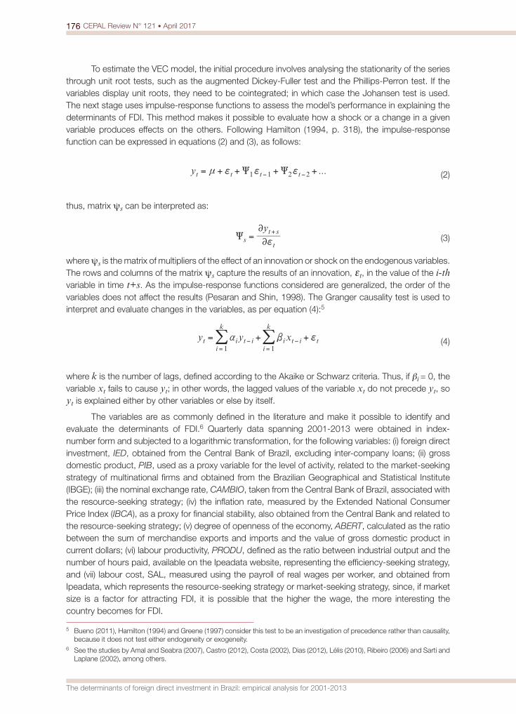
176 CEPAL Review N° 121 • April 2017
The determinants of foreign direct investment in Brazil: empirical analysis for 2001-2013
To estimate the VEC model, the initial procedure involves analysing the stationarity of the series through unit root tests, such as the augmented Dickey-Fuller test and the Phillips-Perron test. If the variables display unit roots, they need to be cointegrated; in which case the Johansen test is used. The next stage uses impulse-response functions to assess the model’s performance in explaining the determinants of FDI. This method makes it possible to evaluate how a shock or a change in a given variable produces effects on the others. Following Hamilton (1994, p. 318), the impulse-response function can be expressed in equations (2) and (3), as follows:
...yt t t t1 1 2 2n f f fW W= + + + +− − (2)
thus, matrix ys can be interpreted as:
y
st
t s
2
2
fW =
+ (3)
where ys is the matrix of multipliers of the effect of an innovation or shock on the endogenous variables. The rows and columns of the matrix ys capture the results of an innovation, et, in the value of the i-th variable in time t+s. As the impulse-response functions considered are generalized, the order of the variables does not affect the results (Pesaran and Shin, 1998). The Granger causality test is used to interpret and evaluate changes in the variables, as per equation (4):5
y y xt i t ii
k
i t ii
k
t1 1
a b f= + +−=
−=
/ / (4)
where k is the number of lags, defined according to the Akaike or Schwarz criteria. Thus, if bi = 0, the variable xt fails to cause yt; in other words, the lagged values of the variable xt do not precede yt, so yt is explained either by other variables or else by itself.
The variables are as commonly defined in the literature and make it possible to identify and evaluate the determinants of FDI.6 Quarterly data spanning 2001-2013 were obtained in index-number form and subjected to a logarithmic transformation, for the following variables: (i) foreign direct investment, IED, obtained from the Central Bank of Brazil, excluding inter-company loans; (ii) gross domestic product, PIB, used as a proxy variable for the level of activity, related to the market-seeking strategy of multinational firms and obtained from the Brazilian Geographical and Statistical Institute (IBGE); (iii) the nominal exchange rate, CAMBIO, taken from the Central Bank of Brazil, associated with the resource-seeking strategy; (iv) the inflation rate, measured by the Extended National Consumer Price Index (IBCA), as a proxy for financial stability, also obtained from the Central Bank and related to the resource-seeking strategy; (v) degree of openness of the economy, ABERT, calculated as the ratio between the sum of merchandise exports and imports and the value of gross domestic product in current dollars; (vi) labour productivity, PRODU, defined as the ratio between industrial output and the number of hours paid, available on the Ipeadata website, representing the efficiency-seeking strategy, and (vii) labour cost, SAL, measured using the payroll of real wages per worker, and obtained from Ipeadata, which represents the resource-seeking strategy or market-seeking strategy, since, if market size is a factor for attracting FDI, it is possible that the higher the wage, the more interesting the country becomes for FDI.
5 Bueno (2011), Hamilton (1994) and Greene (1997) consider this test to be an investigation of precedence rather than causality, because it does not test either endogeneity or exogeneity.
6 See the studies by Amal and Seabra (2007), Castro (2012), Costa (2002), Dias (2012), Lélis (2010), Ribeiro (2006) and Sarti and Laplane (2002), among others.
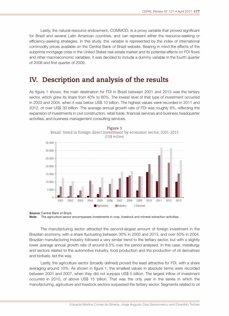
177CEPAL Review N° 121 • April 2017
Eduarda Martins Correa da Silveira, Jorge Augusto Dias Samsonescu and Divanildo Triches
Lastly, the natural-resource endowment, COMMOD, is a proxy variable that proved significant for Brazil and several Latin American countries, and can represent either the resource-seeking or efficiency-seeking strategies. In this study, this variable is represented by the index of international commodity prices available on the Central Bank of Brazil website. Bearing in mind the effects of the subprime mortgage crisis in the United States real estate market and its potential effects on FDI flows and other macroeconomic variables, it was decided to include a dummy variable in the fourth quarter of 2008 and first quarter of 2009.
IV. Description and analysis of the results
As figure 1 shows, the main destination for FDI in Brazil between 2001 and 2013 was the tertiary sector, which grew its share from 40% to 60%. The lowest level of that type of investment occurred in 2003 and 2004, when it was below US$ 10 billion. The highest values were recorded in 2011 and 2012, of over US$ 30 billion. The average annual growth rate of FDI was roughly 8%, reflecting the expansion of investments in civil construction, retail trade, financial services and business headquarter activities, and business management consulting services.
Figure 1 Brazil: trend in foreign direct investment by economic sector, 2001-2013
(US$ million)
0
5 000
10 000
15 000
20 000
25 000
30 000
35 000
2001 2002 2003 2004 2005 2006 2007 2008 2009 2010 2011 2012 2013
Agriculture Industry Services
Source: Central Bank of Brazil.Note: The agriculture sector encompasses investments in crop, livestock and mineral extraction activities.
The manufacturing sector attracted the second-largest amount of foreign investment in the Brazilian economy, with a share fluctuating between 30% in 2005 and 2013, and over 50% in 2004. Brazilian manufacturing industry followed a very similar trend to the tertiary sector, but with a slightly lower average annual growth rate of around 6.5% over the period analysed. In this case, metallurgy and sectors related to the automotive industry, food production and the production of oil derivatives and biofuels, led the way.
Lastly, the agriculture sector (broadly defined) proved the least attractive for FDI, with a share averaging around 10%. As shown in figure 1, the smallest values in absolute terms were recorded between 2001 and 2007, when they did not surpass US$ 5 billion. The largest inflow of investment occurred in 2010, of above US$ 15 billion. That was the only year in the series in which the manufacturing, agriculture and livestock sectors surpassed the tertiary sector. Segments related to oil
178 CEPAL Review N° 121 • April 2017
The determinants of foreign direct investment in Brazil: empirical analysis for 2001-2013
and natural gas extraction, mineral extraction and forestry production were the main destinations of FDI in the agriculture sector (broadly defined) in 2001-2013.
In terms of econometric procedures, the order of integration of the predefined variables was first verified as follows: CAMBIO, COMMOD, IPCA, PIB, PRODU, SAL and ABERT. This was done using the augmented Dickey-Fuller unit root test, as indicated in table A1.1 of the annex.7 The vast majority of the variables display a unit root in the two specifications, in other words, with a constant but without trend and with both constant and trend. The exceptions were IPCA, where the test indicated the acceptance of the null hypothesis, in other words, that it is stationary in levels for the two specifications at a 1% significance level; and the variables IED and COMMOD, which are also stationary with constant only and with trend at the 5% and 1% levels, respectively. The results of the augmented Dickey-Fuller unit root test showed that, with variables expressed as first differences, all of the series are stationary in the two specifications at a 1% significance level.
Next, the Granger test was performed to evaluate the statistical causality relation between each of the model’s endogenous variables and FDI. Table A1.2 of the annex reports the results of that test, which show that the hypothesis of “Granger causality” among the variables CAMBIO, PIB, PRODU and SAL for the FDI flow cannot be rejected —at the 1% level in the first three cases, and at 5% in the last. This means that movements in the exchange rate, GDP, productivity and labour cost precede, or “Granger cause,” movements in FDI. The Granger causality test also reveals the absence of any association between FDI and the economy’s degree of openness. In the case of international commodity prices, the hypothesis that IED (FDI) does not “Granger cause” COMMOD is rejected at a significance level of just over 10%.
Given the lack of causality with respect to the degree of external openness, the effect of this variable on FDI was evaluated through the impulse-response function. This procedure makes it possible to verify the short-run reaction of the IED variable (FDI) to a shock to the error term in the endogenous equation, in this case in the openness variable ABERT. The result was that the degree of openness of the Brazilian economy has a short-term negative effect on FDI —contrary both to expectations and to the results reported in the literature.8 This might be reflecting specific features of the empirical studies, which were concentrated mainly in the 1990s —a period marked by the adoption of the Real Plan, together with intensive foreign-capital inflows fuelled by privatization processes and an appreciation of the local currency against the dollar.
The degree of openness of the Brazilian economy was therefore excluded as a variable in the analysis, to reduce the chance of generating spurious relations. Bearing in mind that most of the series is integrated of order one, or I(1), the possibility of a cointegration relation between them needs to be assessed. To that end, the order of the vector autoregression was defined, identifying the number of lags of the model using the Schwarz and Akaike criteria, supported by the Lagrange multiplier test for residual autocorrelation and the White heteroscedasticity test for the model with two and three lags. The joint analysis of the tests, considering a 5% significance level and the criteria, selected the two-lag model as the best fit. In addition, as the inverse roots of the autoregressive characteristic polynomial were inside the unit circle, the model is consistent and susceptible to economic analysis.
The next procedure was the Johansen cointegration test, the results of which are shown in table A1.3 of the annex. The trace and maximum eigenvalue statistics show the existence of four cointegration relations at a 5% significance level, which makes it possible to validate the use of the VEC model.
7 Although the Philips-Perron test was also performed, the results did not report significant changes.8 Degree of openness has been considered important by Nonnenberg and Mendonça (2005), Lélis (2010), Laplane and
others (2001), Mattos, Cassuce and Campos (2007), Sarti and Laplane (2002) and Castro, Fernandes and Campos (2013), among others.
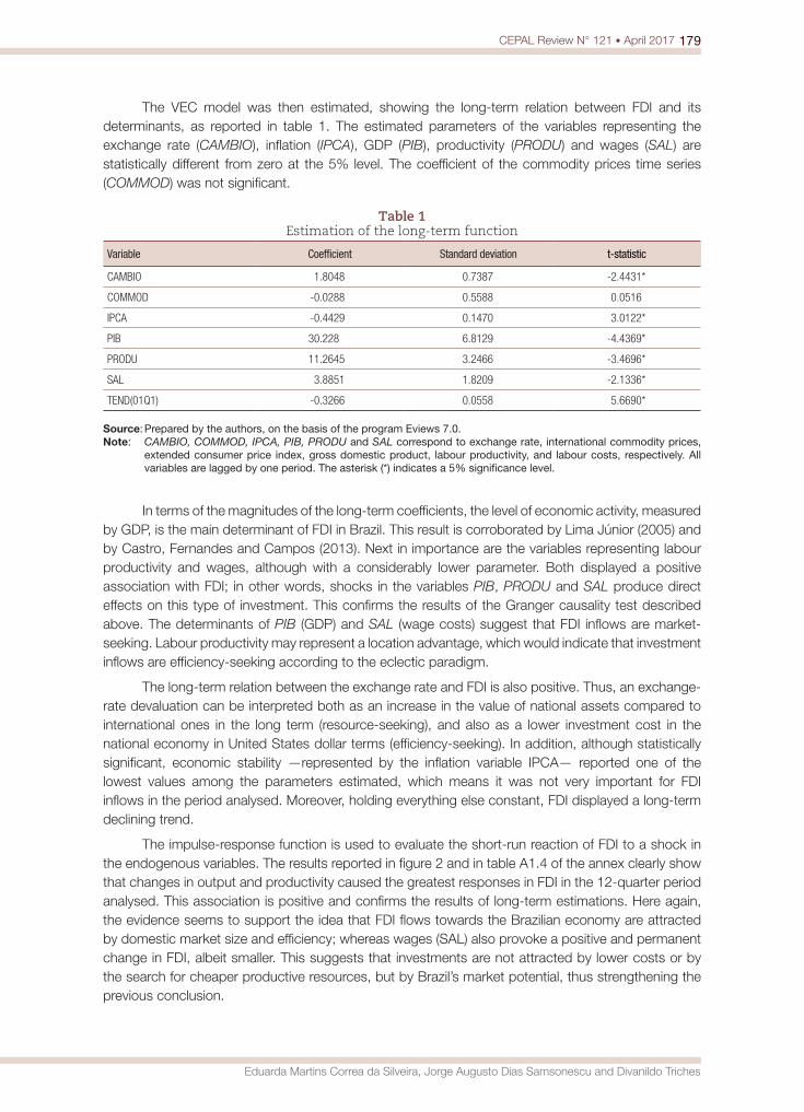
179CEPAL Review N° 121 • April 2017
Eduarda Martins Correa da Silveira, Jorge Augusto Dias Samsonescu and Divanildo Triches
The VEC model was then estimated, showing the long-term relation between FDI and its determinants, as reported in table 1. The estimated parameters of the variables representing the exchange rate (CAMBIO), inflation (IPCA), GDP (PIB), productivity (PRODU) and wages (SAL) are statistically different from zero at the 5% level. The coefficient of the commodity prices time series (COMMOD) was not significant.
Table 1 Estimation of the long-term function
Variable Coefficient Standard deviation t-statistic
CAMBIO 1.8048 0.7387 -2.4431*
COMMOD -0.0288 0.5588 0.0516
IPCA -0.4429 0.1470 3.0122*
PIB 30.228 6.8129 -4.4369*
PRODU 11.2645 3.2466 -3.4696*
SAL 3.8851 1.8209 -2.1336*
TEND(01Q1) -0.3266 0.0558 5.6690*
Source: Prepared by the authors, on the basis of the program Eviews 7.0.Note: CAMBIO, COMMOD, IPCA, PIB, PRODU and SAL correspond to exchange rate, international commodity prices,
extended consumer price index, gross domestic product, labour productivity, and labour costs, respectively. All variables are lagged by one period. The asterisk (*) indicates a 5% significance level.
In terms of the magnitudes of the long-term coefficients, the level of economic activity, measured by GDP, is the main determinant of FDI in Brazil. This result is corroborated by Lima Júnior (2005) and by Castro, Fernandes and Campos (2013). Next in importance are the variables representing labour productivity and wages, although with a considerably lower parameter. Both displayed a positive association with FDI; in other words, shocks in the variables PIB, PRODU and SAL produce direct effects on this type of investment. This confirms the results of the Granger causality test described above. The determinants of PIB (GDP) and SAL (wage costs) suggest that FDI inflows are market-seeking. Labour productivity may represent a location advantage, which would indicate that investment inflows are efficiency-seeking according to the eclectic paradigm.
The long-term relation between the exchange rate and FDI is also positive. Thus, an exchange-rate devaluation can be interpreted both as an increase in the value of national assets compared to international ones in the long term (resource-seeking), and also as a lower investment cost in the national economy in United States dollar terms (efficiency-seeking). In addition, although statistically significant, economic stability —represented by the inflation variable IPCA— reported one of the lowest values among the parameters estimated, which means it was not very important for FDI inflows in the period analysed. Moreover, holding everything else constant, FDI displayed a long-term declining trend.
The impulse-response function is used to evaluate the short-run reaction of FDI to a shock in the endogenous variables. The results reported in figure 2 and in table A1.4 of the annex clearly show that changes in output and productivity caused the greatest responses in FDI in the 12-quarter period analysed. This association is positive and confirms the results of long-term estimations. Here again, the evidence seems to support the idea that FDI flows towards the Brazilian economy are attracted by domestic market size and efficiency; whereas wages (SAL) also provoke a positive and permanent change in FDI, albeit smaller. This suggests that investments are not attracted by lower costs or by the search for cheaper productive resources, but by Brazil’s market potential, thus strengthening the previous conclusion.
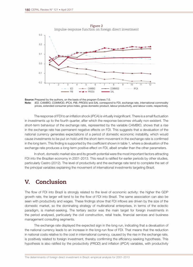
180 CEPAL Review N° 121 • April 2017
The determinants of foreign direct investment in Brazil: empirical analysis for 2001-2013
Figure 2 Impulse-response function on foreign direct investment
-0.2
-0.1
0.0
0.1
0.2
0.3
1 2 3 4 5 6 7 8 9 10 11 12
IED CAMBIO COMMOD IPCAPIB PRODU SAL
Source: Prepared by the authors, on the basis of the program Eviews 7.0.Note: IED, CAMBIO, COMMOD, IPCA, PIB, PRODU and SAL correspond to FDI, exchange rate, international commodity
prices, extended consumer price index, gross domestic product, labour productivity, and labour costs, respectively.
The response of FDI to an inflation shock (IPCA) is virtually insignificant. There is a small fluctuation in investments up to the fourth quarter, after which the response becomes virtually non-existent. The short-term behaviour of the exchange rate, represented by the variable CAMBIO, shows that a rise in the exchange rate has permanent negative effects on FDI. This suggests that a devaluation of the national currency generates expectations of a period of domestic economic instability, which would cause investments to be put on hold until the short-term movement in the exchange rate is confirmed in the long term. This finding is supported by the coefficient shown in table 1, where a devaluation of the exchange rate produces a long-term positive effect on FDI, albeit smaller than the other parameters.
In short, domestic market size and its growth potential were the most important factors attracting FDI into the Brazilian economy in 2001-2013. This result is ratified for earlier periods by other studies, particularly Castro (2012). The level of productivity and the exchange rate tend to complete the set of the principal variables explaining the movement of international investments targeting Brazil.
V. Conclusion
The flow of FDI into Brazil is strongly related to the level of economic activity: the higher the GDP growth rate, the larger will tend to be the flow of FDI into Brazil. The same association can also be seen with productivity and wages. These findings show that FDI inflows are driven by the size of the domestic market, so the dominating strategy of multinational enterprises, in terms of the eclectic paradigm, is market-seeking. The tertiary sector was the main target for foreign investments in the period analysed, particularly the civil construction, retail trade, financial services and business management consulting segments.
The exchange rate displayed the expected sign in the long run, indicating that a devaluation of the national currency leads to an increase in the long-run flow of FDI. That means that the reduction in national costs relative to the cost in international currency, caused by the rise in the exchange rate, is positively related to foreign investment, thereby confirming the efficiency-seeking hypothesis. This hypothesis is also ratified by the productivity (PROD) and inflation (IPCA) variables, with productivity
181CEPAL Review N° 121 • April 2017
Eduarda Martins Correa da Silveira, Jorge Augusto Dias Samsonescu and Divanildo Triches
reporting the second-largest estimated parameter. The stability of the national economy, represented by the inflation variable IPCA, reported a relatively lower coefficient, although statistically significant and negatively related to the FDI flow. This suggests that investors view the Brazilian economy as low-risk, or simply that they pay closer attention to the activity-level and productivity indicators. In any event, governments sought to maintain economic stability in the period analysed.
Although the prices of commodities (of which Brazil is a major producer) were very high on world markets in the period analysed, that variable was not significant for FDI inflows. In other words, the parameter cannot be considered different from zero at a 5% significance level.
Lastly, this research set out to identify the determinants of FDI in the Brazilian economy and how they relate to the strategies pursued by multinational enterprises. Although foreign currency inflows alleviate potential pressures on the balance of payments in the short run, economic policy-makers should take steps to create macroeconomic conditions that allow for a positive flow of that type of investment, since it is trending downwards. Although beyond the scope of this research, it is also important to analyse the impact of FDI on Brazil’s macroeconomic variables, such as the potential for multiplying domestic output and the virtue of improving the productivity and competitiveness of domestic products and fostering an improvement in social-welfare indicators.
BibliographyAmal, M. and F. Seabra (2007), “Determinantes do investimento direto externo na América Latina: uma
perspectiva institucional”, Revista de Economia, vol. 8, No. 2, Brasilia.Bonelli, R. (1999), “A note on foreign direct investment and industrial competitiveness in Brazil”, Oxford
Development Studies, vol. 27, No. 3, Taylor & Francis.Buckley, P. (2010), “Stephen Hymer: three phases, one approach?”, Foreign Direct Investment, China and
the World Economy, P. Buckley, Chippenham, Palgrave Macmillan. Bueno, R. de L. da S. (2011), Econometria de séries temporais, São Paulo, Cengage Learning. Castro, P.G. de (2012), “Os determinantes do investimento direto estrangeiro no Brasil e no México: uma
análise empírica para o período de 1990 a 2010, Brasil”, Federal University of Viçosa. Castro, P.G., E.A. Fernandes and A.C. Campos (2013), “Os determinantes do investimento direto estrangeiro
no Brasil e no México: uma análise empírica” [online] https://www.anpec.org.br/encontro/2013/files_I/i7-2bf472e0d97d8e932bc37c86feac6d31.pdf.
Costa, C.G. (2002), “Fatores de atração do investimento direto estrangeiro para a economia brasileira nos anos 90 e as repercussões sobre a especialização internacional no Brasil”, Informação Internacional: análise econômica e política, Ministry of the Environment of Portugal.
De Groot, O. (2014), Foreign Direct Investment and Welfare (LC/L.3800), Santiago, Economic Commission for Latin America and the Caribbean (ECLAC).
Dias, M.H.A. (2012), “Choques de produtividade e fluxos de investimentos estrangeiros para o Brasil”, Working Paper, No. 41 [online] http://www.bndes.gov.br/SiteBNDES/export/sites/default/bndes_pt/Galerias/Arquivos/produtos/download/pde/PDE2011_DiasUEM.pdf.
Dunning, J.H. (1993), Multinational Enterprises and the Global Economy, Reading, Massachusetts, Addison-Wesley.(1988), “Trade, location of economic activity and the multinational enterprise: a search for an eclectic approach”, Explaining International Production, J.H. Dunning, London, Unwin Hyman.
Dunning, J.H. and S. Lundan (2008), Multinational Enterprises and the Global Economy, London, Edward Elgar.ECLAC (Economic Commission for Latin America and the Caribbean) (2015), Foreign Direct Investment in
Latin America and the Caribbean, 2015 (LC/G.2641-P), Santiago.Enders, W. (2010), Applied Econometric Time Series, New York, Wiley. Greene, W.H. (1997), Econometric Analysis, Upper Saddle River, Prentice Hall.Hamilton, J.D. (1994), Time Series Analysis, Princeton, Princeton University Press.Hill, R.C., W.E. Griffiths and G.C. Lim (2011), Principles of Econometrics, Hoboken, Wiley.Hymer, S. (1976), The International Operations of National Firms: a Study of Direct Foreign Investment,
Cambridge, Massachusetts, The MIT Press.
182 CEPAL Review N° 121 • April 2017
The determinants of foreign direct investment in Brazil: empirical analysis for 2001-2013
IMF (International Monetary Fund) (n/d), “Balance of Payments Manual” [online] http://www.imf.org/external/pubs/ft/bopman/bopman.pdf.(n/d), “Glossary of foreign direct investment terms” [online] http://www.imf.org/external/np/sta/di/glossary.pdf.
Kindleberger, C.P. (1969), American Business Abroad: Six Lecture on Direct Investment, New Haven, Yale University Press.
Krugman, P.R. and M. Obstfeld (2010), Economia internacional: teoria e política, São Paulo, Pearson ABDR.Laplane, M. and others (2001), “La inversión extranjera directa en el MERCOSUR: el caso brasileño”, El
boom de inversión extranjera directa en el MERCOSUR, D. Chudnovsky (org.), Buenos Aires, Siglo XXI. Lélis, M.T.O. (2010), “Movimento recente do investimento espanhol na América Latina: condicionantes
macroeconômicos, Brasil”, thesis, Porto Alegre, Federal University of Rio Grande do Sul. Lima Júnior, A.J. (2005), “Determinantes do investimento direto estrangeiro no Brasil”, Belo Horizonte, Federal
University of Minas Gerais.Mattos, L.B. de, F.C. Cassuce and A.C. Campos (2007), “Determinantes dos investimentos diretos estrangeiros
no Brasil, 1980-2004”, Revista Economia Contemporânea, vol. 11, No. 1, Rio de Janeiro.MDIC (Ministry of Development, Industry and Commerce) (2014), “Acordos multilaterais: Organização Mundial
do Comércio (OMC)” [online] http://www.mdic.gov.br/sitio/interna/interna.php?area=5&menu=2530.Moosa, I.A. (2002), Foreign Direct Investment: Theory, Evidence and Practice, Wiltshire, Palgrave. Nonnenberg, M.J.B. and M.J.C. Mendonça (2005), “Determinantes dos investimentos diretos externos em
países em desenvolvimento”, Estudos Econômicos, vol. 35, No. 4, São Paulo, University of São Paulo. Patterson, K. (2000), An Introduction to Applied Econometrics: a Time Series Approach, New York, Palgrave
Macmillan.Pesaran, H.H. and Y. Shin (1998), “Generalized impulse response analysis in linear multivariate models”,
Economics Letters, vol. 58, No. 1, Amsterdam, Elsevier.Ribeiro, M.S. (2006), “Investimento estrangeiro direto e remessas de lucros e dividendos no Brasil: estratégia
microeconômica e determinantes macroeconômicos (2001-2004)”, tesis, Belo Horizonte, Federal University of Minas Gerais.
Sarti, F. and M.F. Laplane (2002), “Investimento direto estrangeiro e a retomada do crescimento sustentado nos anos 90”, Economia e Sociedade, vol. 8, Campinas, State University at Campinas (UNICAMP).
Schneider, F. and B. Frey (1985), “Economic and political determinants of foreign direct investment”, World Development, vol. 13, No. 2, Amsterdam, Elsevier.
Vernon, R. (1999), “International investment and international trade in the product cycle”, The Internalization of the Firm, P. Buckley and N. Ghauri, London, Thomson Learning.

183CEPAL Review N° 121 • April 2017
Eduarda Martins Correa da Silveira, Jorge Augusto Dias Samsonescu and Divanildo Triches
Annex A1Table A1.1
Augmented Dickey-Fuller unit root test
VariableLevels First differences
c c/t c c/t
ABERT -2.9016 -2.9133 -6.2652* -6.2187*
CAMBIO -1.2838 -1.9686 -5.0792 -5.0290*
COMMOD -2.2025 -3.5147** -4.8422* -4.8019*
IED -1.1155 -4.7242* -7.4540* -
IPCA -4.1764* -4.3265* - -
PIB -0.2528 -3.1692 -5.1135* -5.0583*
PRODU -1.2190 -3.1192 -6.9131* -6.8668*
SAL -1.3988 -3.1640 -4.2604* -6.7917*
Source: Prepared by the authors, on the basis of the program Eviews 7.0.Note: IED, CAMBIO, COMMOD, IPCA, PIB, PRODU, SAL and ABERT correspond to exchange rate, international
commodity prices, extended consumer price index, gross domestic product, labour productivity, labour costs and economic openness, respectively. The column heading c denotes the test with constant and without trend, and c/t the test with constant and trend. The asterisks (*, **) indicate rejection of the null hypothesis at the 1% and 5% significance levels, respectively.
Table A1.2 Results of the Granger causality test
Null Hypothesis F-statistic Prob.
ABERT does not cause IED 1.043 0.361
IED does not cause ABERT 0.427 0.655
CAMBIO does not cause IED 7.343* 0.002
IED does not cause CAMBIO 0.579 0.565
COMMOD does not cause IED 0.879 0.422
IED does not cause COMMOD 2.301 0.112
IPCA does not cause IED 0.871 0.426
IED does not cause IPCA 0.607 0.549
PIB does not cause IED 7.694* 0.001
IED does not cause PIB 0.985 0.382
PRODU does not cause IED 6.862* 0.003
IED does not cause PRODU 0.384 0.683
SAL does not cause IED 3.850** 0.029
IED does not cause SAL 0.379 0.687
Source: Prepared by the authors, on the basis of the program Eviews 7.0.Note: IED, CAMBIO, COMMOD, IPCA, PIB, PRODU, SAL and ABERT correspond to exchange rate, international
commodity prices, extended consumer price index, gross domestic product, labour productivity, labour costs and economic openness, respectively. The asterisks (*, **) indicate rejection of the null hypothesis at the 1% and 5% significance levels, respectively.

184 CEPAL Review N° 121 • April 2017
The determinants of foreign direct investment in Brazil: empirical analysis for 2001-2013
Table A1.3 Results of the Johansen cointegration test
Cointegrated equations Trace P-Value Maximum eigenvalue P-value
0 224.18 0.0000 65.99 0.0007
≤1 158.19 0.0000 46.50 0.0298
≤2 111.69 0.0004 38.50 0.0478
≤3 73.17 0.0067 31.36 0.0616
≤4 41.83 0.0640 26.48 0.0409
≤5 15.34 0.5460 10.69 0.5356
≤6 4.65 0.6465 4.65 0.6465
Source: Prepared by the authors, on the basis of the program Eviews 7.0.
Table A1.4 Response in FDI to generalized impulses of 1 standard deviation
Period IED CAMBIO COMMOD IPCA PIB PRODU SAL
1 0.2850 -0.0123 -0.0036 0.0365 0.0159 0.0380 0.0742
2 0.0797 -0.0614 -0.0566 0.0492 0.0725 0.0865 -0.0175
3 0.0885 -0.0843 -0.0306 0.0369 0.0750 0.0740 0.0650
4 0.1245 -0.1045 -0.0490 -0.0011 0.0674 0.1169 0.0487
5 0.0894 -0.1085 -0.0547 0.0167 0.1211 0.1187 0.0495
6 0.0617 -0.1396 -0.0714 0.0193 0.1240 0.1330 0.0545
7 0.0760 -0.1626 -0.0879 0.0028 0.1269 0.1671 0.0603
8 0.0709 -0.1561 -0.0853 0.0049 0.1431 0.1525 0.0618
9 0.0545 -0.1699 -0.0974 0.0051 0.1418 0.1621 0.0646
10 0.0568 -0.1838 -0.1003 0.0022 0.1512 0.1820 0.0647
11 0.0570 -0.1788 -0.0968 -0.0007 0.1558 0.1719 0.0685
12 0.0491 -0.1876 -0.1056 -0.0003 0.1578 0.1809 0.0687
Source: Prepared by the authors, on the basis of the program Eviews 7.0.Note: The period is expressed in quarters. IED, CAMBIO, COMMOD, IPCA, PIB, PRODU and SAL correspond to FDI,
exchange rate, international commodity prices, extended consumer price index, gross domestic product, labour productivity and labour costs, respectively.
In order to facilitate the submission, consideration and publication of articles, the editorial board of the cepal Review has prepared the following information and suggestions to serve as a guide for future contributors.
The submission of an article implies an undertaking by the author not to submit it simultaneously to other publications. The copyright to all articles published in the Review shall be owned by the United Nations.
Each article will be reviewed by the editorial board, which may decide to submit it to external referees.
Papers should be submitted in the original language (English, French, Portuguese or Spanish). They will be translated into the appropriate language by the relevant eclac services.
Each article must be accompanied by a summary, no more than 150 words in length, giving a brief description of its subject matter and main conclusions.
Each article must also carry three jel (Journal of Economic Literature) classification codes. The JEL Classification Codes Guide is available online at www.aeaweb.org/jel/jel_class_system.php.
Papers should be no longer than 10,000 words, including the summary, notes and bibliography. Shorter papers will also be considered.
Articles should be sent by e-mail to [email protected] in Word format. Papers in pdf format will not be accepted.
Style guide:
Titles should not be excessively long.
Footnotes
— It is recommended that footnotes be kept to a minimum.
— It is recommended that footnotes not be used to cite bibliographical references; such references should preferably be incorporated into the text.
— Footnotes should be numbered consecutively using superscript Arabic numerals.
Tables, figures and equations
— It is recommended that tables and figures be kept to a minimum, avoiding any redundancy with the text.
— Equations should be written using the Office equation editor “MathType”; they should not be inserted as “pictures”.
— Tables, figures and other elements should be inserted at the end of the text in the format in which they were designed; they should not be inserted as “pictures”. Figures in Excel should include the corresponding worksheets.
— The location of tables and figures in the body of the article should be indicated in the appropriate place as follows:
Insert figure 1
Insert table 1
— Tables and figures should include an explicit and complete reference to their sources.
— Tables should indicate the period covered at the end of the title, and should indicate the units in which the data are expressed in a subtitle (in italics and between brackets).
— The symbols referred to in the “Explanatory notes” which appear on the page preceding the table of contents should be taken into account in the preparation of tables and figures.
— Footnotes to tables and figures should be ordered consecutively using superscript lower-case letters.
— Figures should be prepared bearing in mind that they will be printed in black and white.
Acronyms and abbreviations
— Acronyms and abbreviations should not be used unless absolutely necessary, in which case the full name should be written out the first time it occurs in the article.
Bibliography
— Bibliographical references should be directly related to the content of the article and should not be excessively long.
— At the end of the article, under the title “Bibliography”, all the necessary information should be included accurately and in alphabetical order by author: name of author(s), year of publication, full name of article (if any) and publication (including any subtitle), city of publication, publisher and, in the case of a periodical, month of publication.
The editorial board of the Review reserves the right to make any necessary editorial changes in the articles, including their titles.
Authors will receive a one-year courtesy subscription to the Review, plus 30 offprints of their article in Spanish and 30 in English, at the time of publication in each language.
Guidelinesfor contributorsto the CEPAL Review

Publicaciones recientes de la CEPAL ECLAC recent publicationswww.cepal.org/publicaciones
Informes periódicos / Annual reportsTambién disponibles para años anteriores / Issues for previous years also available• Estudio Económico de América Latina y el Caribe 2016, 236 p. Economic Survey of Latin America and the Caribbean 2016, 232 p.
• La Inversión Extranjera Directa en América Latina y el Caribe 2016, 170 p. Foreign Direct Investment in Latin America and the Caribbean 2016, 164 p.
• Anuario Estadístico de América Latina y el Caribe 2016 / Statistical Yearbook for Latin America and the Caribbean 2016, 132 p.
• Balance Preliminar de las Economías de América Latina y el Caribe 2016, 132 p. Preliminary Overview of the Economies of Latin America and the Caribbean 2016, 124 p.
• Panorama Social de América Latina 2015, 226 p. Social Panorama of Latin America 2015, 222 p.
• Panorama de la Inserción Internacional de América Latina y el Caribe 2016, 174 p. Latin America and the Caribbean in the World Economy 2015, 170 p.
Libros y documentos institucionales / Institutional books and documents• ECLAC Thinking. Selected Texts (1948-1998), 2016, 520 p.
• La matriz de la desigualdad en América Latina, 2016, 96 p. The social inequality matrix in Latin America, 2016, 94 p.
• Autonomía de las mujeres e igualdad en la agenda de desarrollo sostenible, 2016, 184 p. Equality and women’s autonomy in the sustainable development agenda, 2016, 168 p. Autonomia das mulheres e igualdade na agenda de desenvolvimento sustentável. Síntese, 2016, 106 p.
• La Unión Europea y América Latina y el Caribe ante la Agenda 2030 para el Desarrollo Sostenible: el gran impulso ambiental, 2016, 112 p. The European Union and Latin America and the Caribbean vis-à-vis the 2030 Agenda for Sustainable Development: The environmental
big push, 2016, 112 p.
• Horizontes 2030: la igualdad en el centro del desarrollo sostenible, 2016, 176 p. Horizons 2030: Equality at the centre of sustainable development, 2016, 174 p. Horizontes 2030: a igualdade no centro do desenvolvimento sustentável, 2016, 176 p.
• 40 años de agenda regional de género, 2016, 130 p. 40 years of the regional gender agenda, 2016, 128 p.
• La nueva revolución digital: de la Internet del consumo a la Internet de la producción, 2016, 100 p. The new digital revolution: From the consumer Internet to the industrial Internet, 2016, 100 p.
• Panorama fiscal de América Latina y el Caribe 2016: las finanzas públicas ante el desafío de conciliar austeridad con crecimiento e igualdad, 2016, 90 p.
Fiscal Panorama of Latin America and the Caribbean 2016: Public finances and the challenge of reconciling austerity with growth and equality, 2016, 86 p.
• Reflexiones sobre el desarrollo en América Latina y el Caribe: conferencias magistrales 2015, 2016, 74 p.
• La nueva revolución digital: de la Internet del consumo a la Internet de la producción, 2015, 98 p. The new digital revolution: From the consumer Internet to the industrial Internet, 2015, 98 p.
• Pactos para la igualdad: hacia un futuro sostenible, 2014, 340 p. Covenants for Equality: Towards a sustainable future, 2014, 330 p.
Libros de la CEPAL / ECLAC books141 Brechas y transformaciones: la evolución del empleo agropecuario en América Latina, Jürgen Weller (ed.), 2016, 274 p.
140 Protección y formación: instituciones para mejorar la inserción laboral en América Latina y Asia, Alberto Isgut, Jürgen Weller (eds.), 2016, 428 p. Protection and training: Institutions for improving workforce integration in Latin America and Asia, Alberto Isgut, Jürgen Weller (eds.),
2016, 428 p.
139 Hacia una nueva gobernanza de los recursos naturales en América Latina y el Caribe, Hugo Altomonte, Ricardo J. Sánchez, 2016, 256 p.
138 Estructura productiva y política macroeconómica: enfoques heterodoxos desde América Latina, Alicia Bárcena, Antonio Prado, Martín Abeles (eds.), 2015, 282 p.
137 Juventud: realidades y retos para un desarrollo con igualdad, Daniela Trucco, Heidi Ullmann (eds.), 2015, 282 p.
136 Instrumentos de protección social: caminos latinoamericanos hacia la universalización, Simone Cecchini, Fernando Filgueira, Rodrigo Martínez, Cecilia Rossel (eds.), 2015, 510 p.
Páginas Selectas de la CEPAL / ECLAC Select Pages• Planificación y prospectiva para la construcción de futuro en América Latina y el Caribe. Textos seleccionados 2013-2016, Jorge Máttar
y Mauricio Cuervo (comps.), 2016, 222 p.
• Desarrollo inclusivo en América Latina. Textos seleccionados 2009-2016, Ricardo Infante (comp.), 2016, 294 p.
• Globalización, integración y comercio inclusivo en América Latina. Textos seleccionados 2010-2014, Osvaldo Rosales (comp.), 2015, 326 p.
• El desafío de la sostenibilidad ambiental en América Latina y el Caribe. Textos seleccionados 2012-2014, Carlos de Miguel, Marcia Tavares (comps.) 2015, 148 p.
Copublicaciones / Co-publications• El imperativo de la igualdad, Alicia Bárcena, Antonio Prado, CEPAL/Siglo Veintiuno, Argentina, 2016, 244 p.
• Gobernanza global y desarrollo: nuevos desafíos y prioridades de la cooperación internacional, José Antonio Ocampo (ed.), CEPAL/Siglo Veintiuno, Argentina, 2015, 286 p.
• Decentralization and Reform in Latin America: Improving Intergovernmental Relations, Giorgio Brosio and Juan Pablo Jiménez (eds.), ECLAC/Edward Elgar Publishing, United Kingdom, 2012, 450 p.
• Sentido de pertenencia en sociedades fragmentadas: América Latina desde una perspectiva global, Martín Hopenhayn y Ana Sojo (comps.), CEPAL/Siglo Veintiuno, Argentina, 2011, 350 p.
Coediciones / Co-editions• Perspectivas económicas de América Latina 2017: Juventud, Competencias y Emprendimiento, 2016, 338 p. Latin American Economic Outlook 2017: Youth, Skills and Entrepreneurship, 2016, 314 p.
• Desarrollo e integración en América Latina, 2016, 314 p.
• Hacia un desarrollo inclusivo: el caso del Uruguay, 2016, 174 p.
• Perspectivas de la agricultura y del desarrollo rural en las Américas: una mirada hacia América Latina y el Caribe 2015-2016, CEPAL/FAO/IICA, 2015, 212 p.
Documentos de proyecto / Project documents• El cambio tecnológico y el nuevo contexto del empleo: tendencias generales y en América Latina, Sebastian Krull, 2016, 48 p.
• Cambio climático, políticas públicas y demanda de energía y gasolinas en América Latina: un meta-análisis, Luis Miguel Galindo, Joseluis Samaniego, Jimy Ferrer, José Eduardo Alatorre, Orlando Reyes, 2016, 68 p.
• Estado de la banda ancha en América Latina y el Caribe 2016, 2016, 46 p.
Cuadernos estadísticos de la CEPAL44 Las cuentas de los hogares y el bienestar en América Latina. Más allá del PIB, 2016.
43 Estadísticas económicas de América Latina y el Caribe: Aspectos metodológicos y resultados del cambio de año base de 2005 a 2010
Series de la CEPAL / ECLAC SeriesAsuntos de Género / Comercio Internacional / Desarrollo Productivo / Desarrollo Territorial / Estudios Estadísticos / Estudios y Perspectivas (Bogotá, Brasilia, Buenos Aires, México, Montevideo) / Studies and Perspectives (The Caribbean, Washington) / Financiamiento del Desarrollo / Gestión Pública / Informes y Estudios Especiales / Macroeconomía del Desarrollo / Medio Ambiente y Desarrollo / Población y Desarrollo / Política Fiscal / Políticas Sociales / Recursos Naturales e Infraestructura / Seminarios y Conferencias.
Manuales de la CEPAL4 Territorio e igualdad: planificación del desarrollo con perspectiva de género, 2016, 84 p.
3 Manual de formación regional para la implementación de la resolución 1325 (2000) del Consejo de Seguridad de las Naciones Unidas relativa a las mujeres, la paz y la seguridad, María Cristina Benavente R., Marcela Donadio, Pamela Villalobos, 2016, 126 p.
2 Guía general para la gestión de residuos sólidos domiciliarios, Estefani Rondón Toro, Marcel Szantó Narea, Juan Francisco Pacheco, Eduardo Contreras, Alejandro Gálvez, 2016, 212 p.
Revista CEPAL / CEPAL ReviewLa Revista se inició en 1976, con el propósito de contribuir al examen de los problemas del desarrollo socioeconómico de la región. La Revista CEPAL se publica en español e inglés tres veces por año.
CEPAL Review first appeared in 1976, its aim being to make a contribution to the study of the economic and social development problems of the region. CEPAL Review is published in Spanish and English versions three times a year.
Observatorio demográfico / Demographic Observatory Edición bilingüe (español e inglés) que proporciona información estadística actualizada, referente a estimaciones y proyecciones de población de los países de América Latina y el Caribe. Desde 2013 el Observatorio aparece una vez al año.
Bilingual publication (Spanish and English) proving up-to-date estimates and projections of the populations of the Latin American and Caribbean countries. Since 2013, the Observatory appears once a year.
Notas de poblaciónRevista especializada que publica artículos e informes acerca de las investigaciones más recientes sobre la dinámica demográfica en la región. También incluye información sobre actividades científicas y profesionales en el campo de población. La revista se publica desde 1973 y aparece dos veces al año, en junio y diciembre.
Specialized journal which publishes articles and reports on recent studies of demographic dynamics in the region. Also includes information on scientific and professional activities in the field of population. Published since 1973, the journal appears twice a year in June and December.
Las publicaciones de la CEPAL están disponibles en:ECLAC publications are available at:
www.cepal.org/publicaciones
También se pueden adquirir a través de:They can also be ordered through:
www.un.org/publications
United Nations PublicationsPO Box 960
Herndon, VA 20172USA
Tel. (1-888)254-4286 Fax (1-800)338-4550
Contacto / Contact: [email protected] / Orders: [email protected]