Pdf - CEPAL
202
-
Upload
khangminh22 -
Category
Documents
-
view
1 -
download
0
Transcript of Pdf - CEPAL


REV
IEW
ECONOMIC COMMISSION FOR
LATIN AMERICA ANDTHE CARIBBEAN


116NO
AUGUST • 2015
REV
IEW
ECONOMIC COMMISSION FOR
LATIN AMERICA ANDTHE CARIBBEAN
Osvaldo SunkelChairman of the Editorial Board
André HofmanDirector
Miguel TorresTechnical Editor
ISSN 0251-2920
Alicia BárcenaExecutive Secretary
Antonio PradoDeputy Executive Secretary

This publication, entitled the cepal Review, is covered in the Social Sciences Citation Index (ssci), published by Thomson
Reuters, and in the Journal of Economic Literature (jel), published by the American Economic Association
The cepal Review was founded in 1976, along with the corresponding Spanish version, Revista cepal, and it is published three times a year by the United Nations Economic Commission for Latin America and the Caribbean (eclac), which has its headquarters in Santiago, Chile. The Review, however, has full editorial independence and follows the usual academic procedures and criteria, including the review of articles by independent external referees. The purpose of the Review is to contribute to the discussion of socioeconomic development issues in the region by offering analytical and policy approaches and articles by economists and other social scientists working both within and outside the United Nations. The Review is distributed to universities, research institutes and other international organizations, as well as to individual subscribers.
The opinions expressed in the signed articles are those of the authors and do not necessarily reflect the views of eclac.
The designations employed and the way in which data are presented do not imply the expression of any opinion whatsoever on the part of the secretariat concerning the legal status of any country, territory, city or area or its authorities, or concerning the delimitation of its frontiers or boundaries.
To subscribe, please visit the Web page: http://ebiz.turpin-distribution.com/products/197587-cepal-review.aspx
The complete text of the Review can also be downloaded free of charge from the eclac web site (www.eclac.org).
United Nations publicationISSN: 0251-2920ISBN: 978-92-1-121903-6 (Print)ISBN: 978-92-1-057232-3 (Pdf)LC/G. 2643-PCopyright © United Nations, August 2015. All rights reserved.Printed in Santiago, Chile
Requests for authorization to reproduce this work in whole or in part should be sent to the Secretary of the Publications Board. Member States and their governmental institutions may reproduce this work without prior authorization, but are requested to mention the source and to inform the United Nations of such reproduction. In all cases, the United Nations remains the owner of the copyright and should be identified as such in reproductions with the expression “© United Nations 2014”.

a r t i c l e s
The redistributive potential of taxation in Latin America 7Michael Hanni, Ricardo Martner and Andrea Podestá
Exchange-rate variations and the rate of inflation in emerging economies 27José García-Solanes and Fernando Torrejón-Flores
The People’s Republic of China and Latin America: the impact of Chinese economic growth on Latin American exports 47Daniel E. Perrotti
Climate change and carbon markets: implications for developing countries 61Carlos Ludeña, Carlos de Miguel and Andrés Schuschny
Education system institutions and educational inequalities in Uruguay 85Juan A. Bogliaccini and Federico Rodríguez
Systemic analysis of the health sector through the input-output matrix, 2000-2005 101Fernando Salgueiro Perobelli, Mônica Viegas Andrade, Edson Paulo Domingues, Flaviane Sousa Santiago, Joilson de Assis Cabral and Lucas Barbosa Rodrigues
The different faces of inclusion and exclusion 127Aldo Mascareño and Fabiola Carvajal
Is financial literacy an economic good? 143Rubén Castro and Andrés Fortunato
Do demand and profitability stimulate capital accumulation? An analysis for Brazil 159Henrique Morrone
The low predictive power of simple Phillips curves in Chile 171Pablo Pincheira and Hernán Rubio
Guidelines for contributors to the cepal Review 196

Explanatory notesThe following symbols are used in tables in the Review:… Three dots indicate that data are not available or are not separately reported.(–) A dash indicates that the amount is nil or negligible. A blank space in a table means that the item in question is not applicable.(-) A minus sign indicates a deficit or decrease, unless otherwise specified.(.) A point is used to indicate decimals.(/) A slash indicates a crop year or fiscal year; e.g., 2006/2007.(-) Use of a hyphen between years (e.g., 2006-2007) indicates reference to the complete period considered, including the beginning
and end years.The word “tons” means metric tons and the word “dollars” means United States dollars, unless otherwise stated. References to annual rates of growth or variation signify compound annual rates. Individual figures and percentages in tables do not necessarily add up to the corresponding totals because of rounding.

The redistributive potential of taxation in Latin America
Michael Hanni, Ricardo Martner and Andrea Podestá
ABSTRACT This study uses internationally comparable methodologies to analyse the distributional impact of income tax and public transfers in 17 countries of Latin America. The results indicate that fiscal policy plays a limited role in improving the distribution of disposable income; the Gini coefficient decreased by barely three percentage points after direct fiscal action. On average, 61% of this reduction was due to public cash transfers and the rest to direct taxes, reflecting the pressing need for personal income tax to be strengthened. Analysis of household surveys gives an indication of the potential effects of tax reforms aimed at increasing the average effective tax rate of the top income decile. Allocating this additional revenue to targeted transfers would produce significant results. Consequently, tax reforms must be evaluated bearing in mind how those resources are used.
KEYWORDS Taxation, income tax, income, income distribution, measurement, statistics, fiscal policy, Latin America
JEL CLASSIFICATION H22, H23, H24, H5, H55
AUTHORS Michael Hanni is an Associate Economic Affairs Officer with the Economic Development Division of eclac. [email protected]
Ricardo Martner is the Chief of the Fiscal Affairs Unit of the Economic Development division of eclac. [email protected]
Andrea Podestá is a consultant with the Economic Development Division of eclac. [email protected]

8 C E P A L R E V I E W 1 1 6 • A U G U S T 2 0 1 5
THE REDISTRIBUTIVE POTENTIAL OF TAXATION IN LATIN AMERICA • MICHAEL HANNI, RICARDO MARTNER AND ANDREA PODESTÁ
Even though inequality in Latin American countries is an incontrovertible fact, public policies, particularly fiscal policies, have not had sufficient impetus to tackle the issue. eclac (2008) has found that social spending has a considerable impact on the lowest income groups, but not on inequality measurements. Reduction in inequality over the past decade has mainly been the result of a better distribution of labour income, with a much lesser redistributive role being played by the State.
Despite methodological difficulties and reliability issues with available data, the impact of fiscal policy has been studied for at least three decades in the region (see Gómez Sabaini and Morán, 2013). During the first decade of the twenty-first century, a series of studies were carried out on the impact of fiscal policy on Central American, Andean and other South American countries.1 The results showed that value added tax (vat) had a modest redistributive, although regressive, effect, and that personal income tax was highly progressive, but had a very moderate redistributive effect, particularly when compared to the redistributive capacity of public social spending. It was thus concluded that fiscal policy overall was not playing a strong role in redistribution.
More recently, several papers have been published that examine the impact of spending and taxes on inequality and poverty in seven countries in the region: Argentina, Brazil, Mexico, Paraguay, Peru,
This paper is a summary of the first report on the draft eclac/International and Ibero-American Foundation for Administration and Public Policies (fiiapp) service contract as part of the eurosocial ii programme, component IV: “Recent tax and public spending reforms in Latin America: distributory effects”. The authors wish to thank Rodrigo Astorga and Ivonne González, as well as Xavier Mancero for his continued support in the analysis of household surveys, and Juan Pablo Jiménez, Michel Jorratt and an anonymous referee for their comments and suggestions. 1 These studies include the following countries: Plurinational State of Bolivia, Colombia, Ecuador, Peru and the Bolivarian Republic of Venezuela; Costa Rica, Dominican Republic, El Salvador, Guatemala, Honduras, Nicaragua and Panama; and Brazil, Chile, Paraguay and Uruguay. See the Inter-American Development Bank (idb) Fiscal Equity Series: Barreix, Roca and Villela (2006); Barreix, Bes and Roca (2009), and Jorratt (2010).
Plurinational State of Bolivia and Uruguay.2 These studies consider the effects of direct and indirect taxes, indirect subsidies and transfers in cash and in kind, based on household surveys.
As part of a project undertaken by the United Nations Development Programme (undp) and the Canadian International Development Research Centre (idrc), microsimulation models were developed (with and without behavioural changes) for five Latin American countries (Brazil, Chile, Guatemala, Mexico and Uruguay) with the aim of studying the impact of changes in direct and indirect taxes and social benefits on income distribution and poverty (Urzúa, 2012).
Similarly, the Organization for Economic Cooperation and Development (oecd) has published a series of studies on its member States. Joumard, Pisu and Bloch (2012) state that the redistributive impact of taxes and transfers depends on their size, mix and the progressivity of each component, and found that taxes and cash transfers reduced income inequality, as measured by the Gini index, by about 25% on average in oecd member countries towards 2010. In those countries, direct transfers reduce income dispersion more than taxes: three quarters of the reduction in inequality between market income and disposable income are due to transfers, the rest to taxes. Moreover, countries with a more unequal distribution of market income tend to redistribute more.
Against this backdrop, the first objective of this study is to calculate the impact of income tax and public cash transfers on the distribution of disposable income for a diverse group of 17 Latin American countries, using methodologies to obtain internationally comparable measurements. A second objective is to simulate the possible effects of potential reforms of tax systems, in order to demonstrate that tax instruments —and in particular that putting the resulting increase in revenue to good use— can have a significant impact on the distribution of disposable income.
This document has seven parts. Part II briefly describes the methodology used to measure the impact of fiscal policy. The results for both public cash transfers
2 See Lustig, Pessino and Scott (2013), and Higgins and others (2013).
IIntroduction

9C E P A L R E V I E W 1 1 6 • A U G U S T 2 0 1 5
THE REDISTRIBUTIVE POTENTIAL OF TAXATION IN LATIN AMERICA • MICHAEL HANNI, RICARDO MARTNER AND ANDREA PODESTÁ
IIMeasuring the impact of fiscal action
As in other studies available in the region, the methodology used consisted of applying a standard incidence analysis to determine how progressive or regressive the fiscal policy is and its effect on income redistribution. This type of static analysis does not take into account behavioural (for example, in the labour supply or in taxpayers’ evasion or avoidance strategies) or life-cycle or general equilibrium effects. Therefore, it does not consider the reaction functions of economic agents with regard to the introduction or modification of taxes and transfers.
Broadly speaking, these types of studies compare income distribution before and after the payment of taxes or public transfers, or both, and thus determine whether tax systems, transfers and fiscal policy overall are fulfilling their redistributive roles.
The data used was taken from the most recent survey of household income and expenditure available for each country. However, it is well known that income data from household surveys are often underestimated owing to various factors, including the failure to capture the incomes of top earners, item or unit non-response and underreporting of income (particularly at the top end of the income distribution scale).
In general, given that underreporting and non-response is a common issue in household surveys, the income data have been adjusted by the Statistics and Economic Projections Division of eclac. Thus, in adjusting for non-response bias, each individual is imputed the average income declared by similar individuals; while underreporting of income is adjusted by multiplying income from each source by a factor equal to the discrepancy with the per capita income figure indicated in the national accounts.3 This procedure increases average income figures and generally alters
3 For more details see the pioneering work of Altimir (1987).
their distribution too. In particular, it tends to yield higher values for inequality, chiefly owing to the fact that the capital income gap is imputed exclusively to the wealthiest quintile (eclac, 2012c).4
However, the adjustment for underreporting is not without its drawbacks and the availability and quality of data from national accounts varies depending on the country and period being studied. Countries also change their national accounts methodologies from time to time, changing either the base year of the series or the compilation methods. While these changes, which differ from country to country, undoubtedly improve the system of national accounts, they also affect household income and expenditure estimates to the extent that they alter some data sources, coverage of concepts and weightings between economic sectors and activities. Moreover, each new methodological approach is not just a simple rearrangement of the previous methodology; rather it modifies the treatment of certain items, incorporates new categories and eliminates old ones (eclac, 2012a).5
It is important to clarify some aspects of the methodology. The unit of analysis is the household and the well-being indicator is per capita income equivalent. The definition of income is that proposed by oecd (2008) so that the results are comparable across countries. Certain assumptions have been made with regard to the payment of taxes, since it is assumed that personal income tax is paid by the individual liable for the tax and that workers bear social security contributions in full, even if taxes are paid only in the formal sectors of the economy.
4 It was not possible to adjust for the underreporting of income in the following countries: Colombia, El Salvador, Honduras, Nicaragua and Uruguay.5 eclac is currently in the process of reviewing the income adjustment methodology for national accounts in order to make it more consistent and to improve the comparability of results across countries and over time.
and personal income tax are then analysed in part III. Part IV examines the redistributive effects of direct transfers disaggregated by population group. Part V assesses the progressivity and redistributive effects of personal
income tax on disposable income. Part VI simulates and evaluates the effects of certain changes on this type of tax. Lastly, part VII reflects upon the reforms needed to improve fiscal action overall.
10 C E P A L R E V I E W 1 1 6 • A U G U S T 2 0 1 5
THE REDISTRIBUTIVE POTENTIAL OF TAXATION IN LATIN AMERICA • MICHAEL HANNI, RICARDO MARTNER AND ANDREA PODESTÁ
BOX 1Progressivity and redistribution indicators
Income tax progressivity is determined on the basis of the tax payment share of each decile, the progression of average rates of tax and the Kakwani index.
The progression of average rates of tax indicates the amount of tax paid by each decile, expressed as a percentage of their income (effective tax rate). A tax is progressive when a higher income means that a greater proportion is paid in tax.
The Kakwani index compares the pre-tax Lorenz curve for income with the concentration curve for that tax, i.e.:
K = quasi-Gini (tax) - Gini (pre-tax income)
If K is greater (less) than zero, the tax is progressive (regressive) and inequality decreases (increases).The Reynolds-Smolensky index is an indicator of the redistributive capacity of the tax:
RS = Gini (pre-tax income) - Gini (post-tax income)
If RS is greater (less) than zero, it indicates that the tax has helped to reduce (increase) inequality.The Atkinson-Plotnick index is used to measure the reranking effect, i.e., to assess whether
individuals’ pre-tax and post-tax rankings are the same:
A - P = G(Y) - CX(Y)
where G(Y) is the Gini coefficient of post-tax income and CX(Y) is the Gini coefficient of post-tax income, but with individuals ranked according to pre-tax income. If the index is zero, it means that they were not reranked and if it is 1, the ranking has been completely inverted.
Source: Prepared by the authors.
IIIResults for 17 Latin American countries
It is important to start the analysis by considering a hallmark of inequality in the region: the large proportion of total income that goes to the top decile, or the wealthiest 10% of households (see figure 1). On average, this group receives 32% of total income, although in Brazil, Chile, Guatemala, Honduras and Paraguay the figure is 10 percentage points higher than that, while in the Bolivarian Republic of Venezuela and Uruguay it is 10 percentage points lower.
There follows an analysis of the effects of personal income tax, social security contributions and public cash transfers on distributive equity. The results of the impact analysis are presented separately for public pensions and other public cash transfers, while the next section
examines the redistributive effects of fiscal policy for people of working age and of retirement age.
The study considers 17 Latin American countries around 2011 and compares the results with oecd countries and, in particular, with the average for 15 European Union countries.
In addition, since personal income tax is an area in which the countries of the region are particularly weak, its impact on income distribution is analysed separately.
The results suggest that fiscal policy benefits lower income groups, mainly through public pensions and other direct cash transfers, since the effect resulting from income tax and social security contributions is more limited (see table 1 and figure 2).

11C E P A L R E V I E W 1 1 6 • A U G U S T 2 0 1 5
THE REDISTRIBUTIVE POTENTIAL OF TAXATION IN LATIN AMERICA • MICHAEL HANNI, RICARDO MARTNER AND ANDREA PODESTÁ
TABLE 1
Latin America (17 countries): Gini coefficients before and after taxes and public transfers, around 2011
CountryMarket income
(A)
Gross income with pensions only (B)
(B = A + public pensions)
Gross income (C) (C = B + public cash transfers)
Disposable income in cash (D)
(D = C - pit - ssc)
Argentina 0.536 0.490 0.484 0.469Bolivia (Plurinational State of) 0.502 0.493 0.491 0.487Brazil 0.573 0.528 0.518 0.502Chile 0.546 0.526 0.510 0.499Colombia 0.531 0.537 0.531 0.520Costa Rica 0.528 0.510 0.503 0.491Dominican Republic 0.560 0.555 0.551 0.545Ecuador 0.481 0.467 0.461 0.453El Salvador 0.442 0.445 0.443 0.430Hondurasa 0.551 … … 0.546Mexico 0.496 0.494 0.484 0.460Nicaragua 0.465 0.464 0.465 0.452Panama 0.546 0.524 0.519 0.504Paraguayb 0.523 0.524 0.523 0.520Peru 0.487 0.485 0.482 0.461Uruguay 0.449 0.411 0.400 0.381Venezuela (Bolivarian Republic of) 0.393 0.384 0.384 0.379
Source: Prepared by the authors, on the basis of household surveys.
Note: pit: Personal income tax; ssc: Social security contributions.a No information was obtained on the pensions and subsidies variables in the Honduras household survey, so their effect on the Gini coefficient
could not be calculated.b A simulation was used to calculate income tax in Paraguay based on the tax currently applicable.
FIGURE 1
Latin America (18 countries): income share by decile grouping, around 2012 a
(Percentages)
0
10
20
30
40
50
60
70
80
90
100
Arg
entin
ab
Bol
ivia
(P
lur.
Sta
te o
f)
Bra
zil
Chi
le
Col
ombi
a
Cos
ta R
ica
Ecu
ador
El S
alva
dor
Gua
tem
ala
Hon
dura
s
Mex
ico
Nic
arag
ua
Pana
ma
Para
guay
Peru
Dom
inic
an R
ep.
Uru
guay
Ven
ezue
la(B
ol. R
ep. o
f)
Lat
in A
mer
icac
Deciles 1 to 4 Deciles 5 to 7 Deciles 8 and 9 Decile 10
Source: Economic Commission for Latin America and the Caribbean (eclac), Social Panorama of Latin America 2013 (LC/G.2580), Santiago, 2013. United Nations publication, Sales No. E.14.II.G.6.a Data refer to 2012, except those for Chile, Panama, Paraguay and Plurinational State of Bolivia (2011), Honduras (2010), Nicaragua (2009)
and Guatemala (2006).b Urban areas.c Simple average.

12 C E P A L R E V I E W 1 1 6 • A U G U S T 2 0 1 5
THE REDISTRIBUTIVE POTENTIAL OF TAXATION IN LATIN AMERICA • MICHAEL HANNI, RICARDO MARTNER AND ANDREA PODESTÁ
As expected, the effectiveness of fiscal policy in reducing inequality varies from country to country. Argentina, Brazil and Uruguay stand out with personal income tax, social security contributions and public cash transfers (including pensions) together reducing inequality (as measured by the Gini coefficient) by around 13% on average.
Fiscal policy also reduced inequality by more than the regional average in Chile, Costa Rica, Mexico and Panama, primarily as a result of transfers and direct subsidies, such as the Oportunidades programme in Mexico, Chile Solidario (Solidarity Chile), Avancemos in Costa Rica or the Opportunities Network in Panama. An equalizing effect was also achieved by public pension programmes in Chile, Costa Rica and Panama, and by direct taxation in Mexico.
At the other end of the scale are Colombia and Paraguay, where public cash transfers and direct taxes have had only a small impact on income distribution,
FIGURE 2
Latin America (17 countries), oecd and 15 European Union countries: inequality of market income, gross income and disposable income, around 2011(Gini coefficients)
0.25
0.30
0.35
0.40
0.45
0.50
0.55
0.60
bra dom chl pan arg col cri pry bol mex per ecu nic ury slv ven lac oecd eu-15
Market income (A) Market income with pensions (B) (B = A + public pensions)
Gross income (C) (C = B + public cash transfers)
Dissposable income in cash (D) (D = C - PIT - SSC)
Source: Prepared by the authors, on the basis of household surveys for Latin America and oecd.Stat.
Note: pit: Personal income tax; ssc: Social security contributions.The figure for the Organization for Economic Cooperation and Development (oecd) is the average of 30 countries (excluding Chile and Mexico).eu-15: 15 European Union countries.oecd: Organization for Economic Cooperation and Development.lac: Latin America and the Caribbean.bra: Brazil; dom: Dominican Republic; chl: Chile; pan: Panama; arg: Argentina; col: Colombia; cri: Costa Rica; pry: Paraguay; bol: Plurinational State of Bolivia; mex: Mexico; per: Peru; ecu: Ecuador; nic: Nicaragua; ury: Uruguay; slv: El Salvador; ven: Bolivarian Republic of Venezuela.
since the Gini index decreases by less than 2% after fiscal action. These countries are also among those with the greatest market income inequality and those in which, accordingly, fiscal policy should in fact be more redistributive. Conversely, oecd countries with a more unequal market income distribution tend to redistribute more (Joumard, Pisu and Bloch, 2012). Brazil, Chile and Argentina have high pre-fiscal inequality, which is partly corrected through public pensions, transfer programmes and direct taxes.
Regardless of the differences between countries, in all cases public cash transfers (such as conditional transfer schemes and others) and personal income tax reduce income distribution inequality to varying degrees (see figure 3). In general, public pension systems also contribute to a more equal distribution, except in three countries where pensions increase inequality (Colombia, El Salvador and Paraguay).

13C E P A L R E V I E W 1 1 6 • A U G U S T 2 0 1 5
THE REDISTRIBUTIVE POTENTIAL OF TAXATION IN LATIN AMERICA • MICHAEL HANNI, RICARDO MARTNER AND ANDREA PODESTÁ
FIGURE 3
Latin America (17 countries): inequality reduction, by fiscal policy instrument, around 2011(Percentage points of the Gini coefficient)
7.1 6.8 6.8
4.7 4.2
3.7 3.7 3.2
2.7 2.7
1.5 1.5 1.4 1.4 1.2 1.1
0.3
-1
0
1
2
3
4
5
6
7
8
bra ury arg chl pan cri mex lac ecu per bol dom ven nic slv col pry
Public pensions Other public cash transfers pit and ssc
Source: Prepared by the authors, on the basis of household surveys.
Note: pit: Personal income tax; ssc: Social security contributions.lac: Latin America and the Caribbean.bra: Brazil; dom: Dominican Republic; chl: Chile; pan: Panama; arg: Argentina; col: Colombia; cri: Costa Rica; pry: Paraguay; bol: Plurinational State of Bolivia; mex: Mexico; per: Peru; ecu: Ecuador; nic: Nicaragua: ury: Uruguay; slv: El Salvador; ven: Bolivarian Republic of Venezuela.
On average, public cash transfers (including pensions) are responsible for 61% of the reduction in the Gini coefficient of market income and the rest of the decrease is the effect of income tax and the payment of social security contributions. This finding —that public transfers play a greater redistributive role than direct taxes— is consistent with those of other regional studies.
One advantage of the methodology used for these estimates is that it follows the oecd approach for the different definitions of income, which allows for comparison between the two groups of countries. Figure 2 illustrates the large difference in the role fiscal policy plays in reducing income inequality. The Gini coefficient of market income (i.e. before transfers and direct taxes) in Latin American countries is initially slightly higher than the oecd average (0.50 and 0.47, respectively). However, in oecd countries fiscal policy is important in reducing inequality, since the Gini coefficient drops 36% (39% on average in the 15 European Union countries) and stands at 0.30 (in absolute terms, the Gini coefficient decreases by 17 percentage points in oecd countries and 19 points in the 15 European Union countries). In contrast, inequality in Latin America and the Caribbean dropped by just 6% on average (or in absolute terms, by 3 Gini points for the 17 countries on average), bringing the Gini for disposable income to 0.47 on average (the same as the Gini coefficient for oecd market income).
The disparities between the two groups of countries can also be seen in figure 4, which charts the Gini coefficient before and after transfers and direct taxes. The vast majority of Latin American countries remain close to the 45° line, as fiscal policy has little effect on the Gini coefficient. Conversely, oecd countries are well below this line, which indicates that fiscal instruments have a much more significant impact.
One reason for this difference in the power of fiscal policy to improve income distribution is the lower tax burden in Latin America which, although it has improved in recent years, is still well below the levels of oecd countries.6 This lower tax burden limits the level of public and social spending and, therefore, the extent to which fiscal policy affects the income of the lowest strata. Not only is the tax burden different, but the tax structure is too: in the Latin American countries the structure relies heavily on indirect taxes, while in oecd countries a significant proportion of tax is levied directly, particularly through personal income tax, which has a greater redistributive impact. For example, the revenue raised by personal income tax averaged 8.4% of gross domestic product (gdp) in oecd, compared to just 1.4% in Latin America and the Caribbean.
6 See eclac (2013a) and oecd/eclac/ciat (2014).

14 C E P A L R E V I E W 1 1 6 • A U G U S T 2 0 1 5
THE REDISTRIBUTIVE POTENTIAL OF TAXATION IN LATIN AMERICA • MICHAEL HANNI, RICARDO MARTNER AND ANDREA PODESTÁ
FIGURE 4
Latin America, oecd and 15 European Union countries: inequality of market income and disposable income, around 2010 and 2011(Gini coefficients)
0.20
0.25
0.30
0.35
0.40
0.45
0.50
0.55
0.60
0.20 0.25 0.30 0.35 0.40 0.45 0.50 0.55 0.60
Market income Gini coef�cient (before transfers and direct taxes)
oecd
lac
eu-15Dis
posa
ble
inco
me
Gin
i coe
f�ci
ent
(aft
er tr
ansf
ers
and
dire
ct ta
xes)
Source: Prepared by the authors, on the basis of household surveys for Latin America and oecd.Stat.
Note: The lighter coloured triangle represents the average for oecd countries, the darker triangle is the average for the 15 European Union countries and the square is the average for Latin America. The circles represent Latin American and Caribbean countries, the diamonds oecd countries.eu-15: 15 European Union countries.oecd: Organization for Economic Cooperation and Development.lac: Latin America and the Caribbean.
The difference in social security coverage between countries of the region and oecd members is another factor in the different impact of fiscal policy. A significant percentage of older adults in countries with broad coverage receive a non-contributory pension: Uruguay with 11%; Argentina with 25%; Chile with 26%; and Brazil with 36% (Bosch, Melguizo and Pagés, 2013). The results reported here show that pensions have a stronger impact on inequality in those four countries and in Costa Rica than in other Latin American countries.
Another indicator used to assess the impact of transfers and direct taxes is the ratio between the average income of the top and bottom deciles, for the various categories of income (see table 2). This data can be used to supplement analysis of the Gini coefficients, because, as most public transfer programmes target the most vulnerable groups (the lower income deciles) and personal income tax is obtained mainly from the top two deciles, the distribution is largely unchanged.
According to this indicator, in several countries social security benefits increase the income of the top 10% more than the income of the bottom 10%,
making income distribution more uneven. The opposite happens with direct public transfers, which benefit in particular the lowest income decile and are thus the instrument with the greatest redistributive power. Brazil, Costa Rica, Mexico and Panama are among the countries whose transfer schemes have the strongest impacts, with larger drops in the income ratio. After payment of income tax and social security contributions, the ratio between the income of the top and bottom deciles drops again, with the most significant decreases occurring in Brazil, Chile, Costa Rica and Mexico.
The final average effect of tax action in the countries of the region indicates that the income of the top decile is 34 times that of the bottom decile for market income and 28 times for disposable monetary income (after transfers and direct taxes). While this implies a reduction in income inequality between the top and bottom deciles, the region falls far short of oecd and the European Union countries in this regard, where the average income for the top 10% is only eight times that of the bottom 10%, after taxes and direct transfers.

15C E P A L R E V I E W 1 1 6 • A U G U S T 2 0 1 5
THE REDISTRIBUTIVE POTENTIAL OF TAXATION IN LATIN AMERICA • MICHAEL HANNI, RICARDO MARTNER AND ANDREA PODESTÁ
TABLE 2
Latin America (17 countries): average per capita income ratio between the top and bottom deciles, around 2011(Multiples)
CountryMarket
income (A)
Market income with pensions (B)
(B = A + public pensions)
Gross income (C) (C = B + public cash transfers)
Disposable income in cash (D)
(D = C - pit - ssc)
Argentina 38.1 31.5 27.8 24.8Bolivia (Plurinational State of) 51.2 51.1 47.5 46.1Brasil 52.0 58.7 38.2 34.2Chile 33.1 31.6 27.7 24.7Colombia 34.6 39.1 36.1 33.7Costa Rica 39.8 36.9 32.4 29.5Dominican Republic 47.7 47.7 43.9 41.9Ecuador 28.4 25.2 23.3 21.9El Salvador 17.9 18.7 18.3 16.8Hondurasa 40.6 … … 39.2Mexico 27.9 28.6 24.1 20.8Nicaragua 21.8 22.2 22.3 20.7Panama 43.8 44.5 38.9 34.8Paraguayb 36.0 37.7 37.1 35.8Peru 35.1 36.5 33.3 29.0Uruguay 15.6 15.0 13.0 11.3Venezuela (Bolivarian Republic of) 13.8 14.4 14.3 13.8
Source: Prepared by the authors, on the basis of household surveys.
Note: pit: Personal income tax; ssc: Social security contributions.a No information was obtained on pensions and subsidies variables in the Honduras household survey, so their effect on the Gini coefficient
could not be calculated.b A simulation was used to calculate income tax in Paraguay based on the tax currently applicable.
It is useful to calculate the redistributive effect of fiscal action by population group, since this enables analysis of the impact on the working age population and on older people (see figure 5A and B).
In recent decades, several countries in the region have reformed their pensions systems and introduced private individual capitalization funds. These private models are relatively new, so, in general, most beneficiaries of old age pensions are covered by the public system and their pension is their main or only source of income. As a result, it is expected that the effects of public cash transfers will have a greater impact on people aged over 65.
In Latin America, as in oecd countries, cash transfers and direct taxes tend to reduce inequality among older
IVImpact of public cash transfers by population group
adults, with the Gini coefficient for this age group decreasing from 0.57 to 0.47 in Latin American countries and from 0.73 to 0.28 in oecd countries. However, with regard to the working-age population, inequality in market incomes is lower to start with, and the Gini coefficient drops considerably less: from 0.49 to 0.47 in Latin America and from 0.42 to 0.30 on average in oecd countries.
With regard to the results by country, in the case of the working-age population, transfers and direct taxes had the strongest impact in terms of reducing market income inequality in Uruguay, Brazil and Argentina, followed by Mexico, Panama, Chile and Costa Rica.

16 C E P A L R E V I E W 1 1 6 • A U G U S T 2 0 1 5
THE REDISTRIBUTIVE POTENTIAL OF TAXATION IN LATIN AMERICA • MICHAEL HANNI, RICARDO MARTNER AND ANDREA PODESTÁ
FIGURE 5
Latin America (16 countries), oecd and 15 European Union countries: inequality of market income, gross income and disposable income by age group, around 2011(Gini coefficient)
A. Retirement age population
0.25
0.35
0.45
0.55
0.65
0.75
arg cri dom bra pan ecu chl bol col per pry mex ury nic ven slv lac oecd eu-15
Market income (A)
Market income with pensions (B) (B = A + public pensions)
Gross income (C) (C = B + public cash transfers)
Disposable income in cash (D) (D = C - PIT - SSC)
B. Working age population
0.25
0.30
0.35
0.40
0.45
0.50
0.55
0.60
bra dom chl pan col pry cri arg bol mex per nic ecu slv ury ven lac oecd eu-15
Market income (A)
Market income with pensions (B) (B = A + public pensions)
Gross income (C) (C = B + public cash transfers)
Disposable income in cash (D) (D = C - PIT - SSC)
Source: Prepared by the authors, on the basis of household surveys.
Note: pit: Personal income tax; ssc: Social security contributions.The figure for the Organization for Economic Cooperation and Development (oecd) is the average for 30 countries (excluding Chile and Mexico).eu-15: 15 European Union countries.oecd: Organization for Economic Cooperation and Development.lac: Latin America and the Caribbean.bra: Brazil; dom: Dominican Republic; chl: Chile; pan: Panama; arg: Argentina; col: Colombia; cri: Costa Rica; pry: Paraguay; bol: Plurinational State of Bolivia; mex: Mexico; per: Peru; ecu: Ecuador; nic: Nicaragua; ury: Uruguay: slv: El Salvador; ven: Bolivarian Republic of Venezuela.

17C E P A L R E V I E W 1 1 6 • A U G U S T 2 0 1 5
THE REDISTRIBUTIVE POTENTIAL OF TAXATION IN LATIN AMERICA • MICHAEL HANNI, RICARDO MARTNER AND ANDREA PODESTÁ
BOX 2Pension scheme analysis in impact studies
Pension scheme analysis is a complex and controversial matter in these sorts of studies. In the countries of the region there are public pension systems and private ones, as well as contributory and non-contributory pensions. This can affect international comparisons, given that pensions could be considered market income or a public cash transfer.
For this study, we have followed the criterion used in oecd (2008), which includes occupational and private pensions in the definition of market income, while pensions from public social security systems are treated as cash transfers, i.e. as part of gross income. According to Lustig, Pessino and Scott (2013), there are arguments for treating contributory pensions as either part of market income, because they are deferred income, or a government transfer, especially in systems with a large subsidized component.
As far as the information available in surveys allows, additional impact analysis was carried out treating contributory pensions from public social security systems as part of market income. In this case, the effect of public transfers through pensions decreases considerably in Brazil and Uruguay (but not in Argentina). However, these countries are still among those with the most redistributive fiscal action, with a combined impact (under this alternative measurement) similar to that achieved in Chile and Mexico.
Source: Prepared by the authors.
Among the retirement age population, Brazil, Argentina, Uruguay and Chile stand out, with a drop in the Gini coefficient of 30% or more, while in Panama, Costa Rica, the Bolivarian Republic of Venezuela, Ecuador and the Plurinational State of Bolivia inequality decreases by between 15% and 23%. This highlights the strong influence of pension transfers on the difference between the market income and the disposable income Gini for those aged 65 and over, especially in countries with a high dependency rate of older adults, primarily in Argentina and Uruguay (see figure 6).
It is clear, then, that the degree of coverage of public pension systems has a high impact on the redistribution
of disposable income (although this also depends on each country’s dependency rate), and it is therefore not surprising that the impact of transfers is minimal in countries with low pension coverage (see Bosch, Melguizo and Pagés, 2013). Fiscal action clearly has a greater impact on income distribution in those countries where significant steps have been taken towards universal pension coverage, as most older adults lack substantial sources of income of their own.
However, such interventions will very likely be insufficient, given that inequality remains an unresolved issue for both the working age population and older people.

18 C E P A L R E V I E W 1 1 6 • A U G U S T 2 0 1 5
THE REDISTRIBUTIVE POTENTIAL OF TAXATION IN LATIN AMERICA • MICHAEL HANNI, RICARDO MARTNER AND ANDREA PODESTÁ
In order to assess the progressive or regressive nature of personal income tax, the average rates of tax paid by each decile must be calculated first. In general, the higher the income level (upper deciles), the higher the proportion of taxes paid, i.e. the personal income tax is progressive (see table 3). However, the progression curve of average rates does not always rise (for example, in the case of Colombia and Paraguay), so the Kakwani index is also calculated, which finds personal income tax to be progressive —with a positive value— in all the countries.
In most countries, 90% or more of income tax is levied on the 20% with the highest incomes, while the remaining 80% of lower income households do not contribute to tax revenue or do so to a very small extent.
Nevertheless, the effective rate of tax paid by individuals in the top decile is just 5.4% on average,
with the highest earners paying between 1% and 3% in tax on their gross income in some countries. Although the maximum legal rates for personal income tax range between 25% and 40%, the actual rates paid by the top decile are very low as a result of tax evasion and avoidance, exemptions, deductions and the preferential treatment afforded to capital income, which is taxed at a lower rate than labour income in some countries and not taxed at all in others.
Consequently, although the personal income tax is designed to be progressive in all countries, its redistributive impact is very limited owing to the low levels of collection. In other words, the action of personal income tax reduces the Gini coefficient by an average of 2% (or, in absolute terms, one percentage point of the Gini coefficient), with certain variations from country to country.
FIGURE 6
Latin America (16 countries): ratio between the decrease in the Gini coefficient as a result of public pensions and dependency rate of older persons (Retirement age population)
-0.05
0.00
0.05
0.10
0.15
0.20
0.25
0.30
6 8 10 12 14 16 18 20 22
ARG
URY
CHL
SLV
PAN
BRA
CRI
ECU
MEX
DOMPER
VEN
BOL
NIC PRY
COL
Dependency of older persons
R-S
inde
x of
mar
ket i
ncom
e pl
us
publ
ic p
ensi
ons
for
pers
ons
aged
ove
r 65
Source: Prepared by the authors, on the basis of household surveys and the Latin American and Caribbean Demographic Centre (celade)- Population Division, population database.
Note: r-s Reynolds Smolensky.bra: Brazil; dom: Dominican Republic; chl: Chile; pan: Panama; arg: Argentina; col: Colombia; cri: Costa Rica; pry: Paraguay; bol: Plurinational State of Bolivia; mex: Mexico; per: Peru; ecu: Ecuador; nic: Nicaragua; ury: Uruguay; slv: El Salvador; ven: Bolivarian Republic of Venezuela.
VProgressivity and redistributive impact of personal income tax

19C E P A L R E V I E W 1 1 6 • A U G U S T 2 0 1 5
THE REDISTRIBUTIVE POTENTIAL OF TAXATION IN LATIN AMERICA • MICHAEL HANNI, RICARDO MARTNER AND ANDREA PODESTÁ
BOX 3Impact of value added tax (vat) and tax systems overall
vat is widely known to be the main tax in all countries of the region, but its design and impact on income distribution varies from country to country, since some have standard rates (Chile, El Salvador), and others variable rates (Argentina, Colombia) and in still others, staple goods are exempt from vat (Mexico, Costa Rica, Dominican Republic) (for details on the different systems, see eclac, 2013a). Studies available for Latin America take into account the strong regressive nature of vat in countries such as Brazil, Chile, El Salvador, Guatemala, Paraguay, Plurinational State of Bolivia and Uruguay. In Uruguay, the study predates vat exemption measures for the beneficiaries of social programmes, which have been in force since 2012.
In countries that have data on the Gini coefficient before and after direct and indirect taxes, nowhere does the redistributive impact of tax systems overall exceed 1.5%, and the Reynolds-Smolensky index is between -0.008 and 0.009 in all cases. In other words, tax policy action does not change income distribution in the region significantly, in part owing to the low collection rate of income tax and in part because of the regressive nature of vat, which offsets the potentially progressive impact of personal income tax.
Source: Economic Commission for Latin America and the Caribbean (eclac), “Fiscal panorama of Latin America and the Caribbean: towards greater quality in public finance” (lc/l.3766), Santiago, 2014.
The Atkinson-Plotnick index is used to assess whether the distribution of income tax alters the ranking of individuals by income level. In the Bolivarian Republic of Venezuela, Ecuador, Honduras and Paraguay, the
ranking of taxpayers is practically unchanged. Conversely, individual ranking changes substantially as a result of personal income tax action in Argentina, Mexico and Uruguay.

20 C E P A L R E V I E W 1 1 6 • A U G U S T 2 0 1 5
THE REDISTRIBUTIVE POTENTIAL OF TAXATION IN LATIN AMERICA • MICHAEL HANNI, RICARDO MARTNER AND ANDREA PODESTÁ
TAB
LE
3
Latin
Am
eric
a (1
6 co
untr
ies)
: pro
gres
sivi
ty a
nd r
edis
trib
utiv
e im
pact
of p
erso
nal i
ncom
e ta
x, a
roun
d 20
11
Cou
ntry
Prog
ress
ion
of a
vera
ge r
ates
(p
erce
ntag
es o
f gr
oss
inco
me)
Kak
wan
i in
dex
Rev
enue
col
lect
ed
(per
cent
ages
)G
ini b
efor
e ta
xesc
Gin
i af
ter
pers
onal
in
com
e ta
xd
Rey
nold
s-
Smol
ensk
y in
dex
Atk
inso
n-Pl
otni
ck
inde
xd1
d2d3
d4d5
d6d7
d8d9
d10
Tota
lB
otto
m
40%
Top
20
%
Arg
entin
a0.
00.
00.
00.
00.
10.
10.
40.
92.
59.
13.
90.
420.
0096
.10
0.48
40.
467
0.01
70.
030
Bra
zila
0.0
0.0
0.0
0.0
0.0
0.0
0.1
0.2
0.7
6.6
2.8
0.43
0.00
99.2
00.
518
0.50
60.
012
0.00
6C
hile
0.0
0.0
0.0
0.0
0.0
0.1
0.1
0.3
0.9
7.1
3.2
0.44
0.00
98.5
00.
510
0.49
50.
014
0.00
4C
olom
bia
0.2
0.2
0.2
0.2
0.3
0.3
0.4
0.5
0.8
4.4
2.1
0.37
1.00
93.1
00.
531
0.52
30.
008
0.00
8C
osta
Ric
a0.
00.
00.
00.
00.
10.
10.
20.
51.
65.
32.
40.
400.
0096
.50
0.50
30.
493
0.01
00.
007
Dom
inic
an R
epub
lic0.
00.
00.
00.
00.
00.
00.
00.
10.
64.
32.
00.
390.
0099
.50
0.55
10.
543
0.00
80.
005
Ecu
ador
0.0
0.0
0.0
0.0
0.0
0.0
0.0
0.0
0.0
2.5
0.9
0.52
0.00
99.9
00.
461
0.45
70.
005
0.00
1E
l Sa
lvad
or0.
00.
00.
00.
10.
20.
40.
60.
91.
64.
82.
10.
410.
2089
.30
0.44
30.
434
0.00
90.
009
Hon
dura
s0.
00.
00.
00.
00.
00.
00.
00.
00.
42.
91.
30.
400.
0099
.80
0.55
10.
546
0.00
50.
002
Mex
ico
-2.1
-1.9
-1.4
-0.9
-0.2
0.6
1.4
2.6
4.7
10.6
5.0
0.44
-3.6
094
.70
0.48
40.
461
0.02
30.
057
Nic
arag
ua0.
00.
00.
00.
00.
00.
00.
10.
20.
54.
81.
80.
480.
0098
.20
0.46
50.
456
0.00
90.
004
Pana
ma
0.0
0.0
0.0
0.0
0.0
0.0
0.1
0.2
0.7
7.1
3.0
0.44
0.00
99.0
00.
519
0.50
60.
013
0.00
5Pa
ragu
ayb
0.0
0.0
0.0
0.0
0.0
0.1
0.0
0.1
0.1
1.2
0.5
0.43
0.10
96.8
00.
523
0.52
00.
002
0.00
1Pe
ru0.
00.
00.
00.
00.
10.
20.
40.
81.
55.
82.
50.
410.
1093
.70
0.48
20.
472
0.01
00.
007
Uru
guay
c0.
00.
00.
00.
10.
20.
50.
91.
83.
58.
43.
50.
450.
1089
.60
0.40
00.
384
0.01
60.
023
Ven
ezue
la (
Bol
ivar
ian
Rep
ublic
of)
0.0
0.0
0.0
0.0
0.0
0.0
0.1
0.1
0.3
2.3
0.7
0.54
0.10
96.2
00.
384
0.38
00.
004
0.00
2
Sour
ce:
Pre
pare
d by
the
aut
hors
, on
the
bas
is o
f ho
useh
old
surv
eys.
Not
e: d
: D
enot
es t
he d
ecil
e w
ith
its
corr
espo
ndin
g nu
mbe
r.a
Incl
udes
onl
y ta
xes
on l
abou
r in
com
e, s
ince
cap
ital
inco
me
was
agg
rega
ted
with
oth
er i
ncom
e in
the
sur
vey.
b Si
mul
atio
n ba
sed
on c
urre
nt t
ax r
ates
.
c G
ini
coef
ficie
nt o
f gr
oss
inco
me.
d G
ini
coef
ficie
nt o
f di
spos
able
inc
ome.

21C E P A L R E V I E W 1 1 6 • A U G U S T 2 0 1 5
THE REDISTRIBUTIVE POTENTIAL OF TAXATION IN LATIN AMERICA • MICHAEL HANNI, RICARDO MARTNER AND ANDREA PODESTÁ
As has been stressed in numerous documents and forums, the relative and absolute weakness of income tax is the main structural problem affecting tax systems in Latin America. Tax policy has prioritized efficiency, striving to ensure that income tax should have as little impact as possible on savings and investment decisions and, in some cases, moving towards a consumption base rather than the traditional income-based system.
In doing so, the attributes of fairness and simplicity have been sacrificed. The main issue undermining the fairness of income tax is the preferential treatment afforded to capital income, which leads to an asymmetry in respect of the taxation of labour income. The fairness of income tax is also undermined by its treatment of individuals rather than households as the unit of taxation, which encourages income splitting in order to reduce tax liabilities, and by income exemptions that benefit higher earners (see Jorratt, 2011).
In the past decade, several countries in the region have undertaken a series of tax reforms with a view to increasing receipts by raising rates, cutting exemptions, implementing dual taxation systems in some cases, modifying or introducing minimum rates and increasing oversight of the highest taxpayers.7 However, the impact of these reforms on inequality remains very limited in most countries, as recent studies by eclac have shown.8
In order to make tax significantly fairer, taxation on capital income and average effective rates of the top deciles or percentiles, which are comparatively low, must be increased.
It is therefore important to consider reforms from the perspective of a fair distribution of disposable income and, to that end, certain scenarios of personal income tax reform have been examined, as set out below:9
(i) Repeal the main tax expenditures that benefit natural persons, without changing the tax brackets or marginal rates. In other words, all earned income is taxed, including capital and transfers from any source. In
7 For a detailed description of the reforms implemented in the region between 2007 and 2013, see eclac (2014a and 2013a).8 Studies for Chile, Ecuador, El Salvador, Guatemala, Honduras, Peru and the Plurinational State of Bolivia show that the impact of income tax reforms on income distribution has been rather limited. 9 More details can be found in Jorratt (2011), who used similar simulations for some countries in the region.
countries where different rates of personal income tax are applied depending on income source, the brackets and progressive rates imposed on labour income will be applied to all types of income.
(ii) Family income tax10 where:• The taxation unit is the household rather than
the individual.• The same tax base as in scenario (i) is used, but
expressed as equivalent income and to which the current tax rate scale is applied.
• All the rate brackets are adjusted by the same factor, so that revenue is equal to that obtained under scenario (i).
(iii) Standard tax: the use in all countries of the same tax brackets on a broad tax base, without tax expenditures, in order to compare the redistributive potential of the tax in different countries. The same tax base as scenario (i) is used and the personal tax brackets of each country are replaced with a common scale.Of course the Gini coefficient barely moves in
simulations that marginally affect the income of the top or bottom deciles, as is the case in these exercises. In other words, from a tax point of view, instead of simulating detailed measures, it is also interesting to reverse the exercise, assuming that the average effective tax rates can be increased for the highest deciles —without specifying how—, in order to then calculate the impact on income distribution.11 Two additional simulations are therefore included:(iv) Based on scenario (i), the effective rate for the top
decile is increased to 20%. For this purpose, it is assumed that informal workers in the top decile pay personal income tax.
(v) In addition to applying an effective rate of 20% to decile 10, the tax burden on deciles 8 and 9 is increased to 10%, also on the basis of scenario (i).
10 While this measure may be difficult to apply in practice, as part of this study a series of exercises were carried out to assess a wide range of possible reforms, regardless of their legal feasibility. 11 This is far from a pointless exercise, for example, in Chile, the 2014 tax reform seeks to more than double the average effective tax rate for decile 10, by changing rates, phasing out of exemptions and introducing greater controls. The new effective rate of tax for that decile should be in excess of 20%, similar to the rate in the European Union (see document “Artículo 1, el corazón de la Reforma Tributaria” [online] http://reformatributaria.gob.cl/documentos.html).
VIPolicy simulations

22 C E P A L R E V I E W 1 1 6 • A U G U S T 2 0 1 5
THE REDISTRIBUTIVE POTENTIAL OF TAXATION IN LATIN AMERICA • MICHAEL HANNI, RICARDO MARTNER AND ANDREA PODESTÁ
In addition, the effect of redistributing the higher revenue raised through cash transfers was calculated for each of the five scenarios, compared to the current situation. As they are static simulations —which do not take into account second-round effects— there is no need to specify how these additional resources are allocated, since it is assumed that they would be distributed equally among individuals belonging to the three lowest income deciles.
The results indicate that there is ample room to improve the redistributive power of personal income tax in Latin America (see figure 7). Vertical and horizontal equity improves when the main tax expenditures of
income tax are phased out (even without considering the impact of redistributing additional revenue). Switching to a family tax regime, inequality decreases a little more.12 Applying a standard tax (scenario (iii)) in all countries, across a broad tax base, also improves the redistributive function of income tax, although it does change the ranking of individuals (Atkinson-Plotnick index) to a greater extent.
12 The greater redistributive effect of the family tax is in line with the results obtained by Jorratt (2011) in his simulations for Ecuador, Guatemala and Paraguay.
FIGURE 7
Average effective rate of tax of the top 10%, redistribution and reranking impact of personal income tax under different scenarios (Average for Latin America)
0
5
10
15
20
25
0.000
0.005
0.010
0.015
0.020
0.025
0.030
0.035
0.040
0.045
Current scenario Scenario (i) Scenario (ii) Scenario (iii) Scenario (iv) Scenario (v)
Ave
rage
eff
ectiv
e ra
te o
f ta
x of
top
10%
Reynolds-Smolensky
Rey
nold
s-Sm
olen
sky
and
Atk
inso
n-Pl
otni
ck
Atkinson-Plotnick Average effective rate of top 10%
Source: Prepared by the authors, on the basis of household surveys.
Note: Scenarios without redistributing additional revenue to the lower deciles. Scenarios: (i) Personal income tax without tax expenditures; (ii) Family tax; (iii) Standard tax; (iv) 20% tax rate on decile 10, and (v) 20% tax rate on decile 10 and 10% on deciles 8 and 9.
If the countries of the region managed to increase the effective tax rate for the top decile on the income scale up to 20%, the redistributive effect of personal income tax, measured by the Reynolds-Smolensky index, would increase considerably. This increase in the effective rate is achieved by eliminating the major tax expenditures, taxing capital income the same as labour income, and assuming no tax evasion. According to the study’s estimates, to achieve such an effect, the average statutory rate imposed on taxpayers in the top decile
would have to be between 20% and 30%, depending on the country. These values are below or close to the maximum rates provided for in national legislation, with the exception of Paraguay, which has a maximum statutory rate of 10%.
Taxing deciles 8 and 9 at an average effective rate of 10% also reduces inequality.
The results of the last two scenarios expose specific weaknesses in personal income tax in the countries of the region, in particular the high level of tax evasion

23C E P A L R E V I E W 1 1 6 • A U G U S T 2 0 1 5
THE REDISTRIBUTIVE POTENTIAL OF TAXATION IN LATIN AMERICA • MICHAEL HANNI, RICARDO MARTNER AND ANDREA PODESTÁ
and avoidance, tax structures that tend to leave some income untaxed and the high level of income that must be earned before the top rate of tax is applied.
Although in the first scenarios —which retain, in part or in full, the existing tax brackets and rates— broadening the tax base increases the average effective rates, particularly for the higher deciles, the rates remain relatively low (see figure 7). The reasons for this include the fact that, unlike oecd countries, the countries of the region have reduced their top marginal tax rates, bringing them in line with the rates for companies (Cetrángolo and Gómez Sabaini, 2007). This factor is exacerbated by the high income level from which these rates are applied. On average, the top rate in Latin America applies to incomes that are nine times per capita gdp, compared with 6.5 times in the group of middle-income countries overall (Ter-Minassian, 2012). The results of the last two scenarios and, to a lesser extent, scenario (iii) show that increasing average effective rates —overcoming certain weaknesses in the current tax structure by reducing tax evasion— would lead to greater income redistribution.
A common argument against reforms such as those simulated in this study, is that they could reduce tax progressivity, since the aim of the tax deductions permitted in most countries is to make the system more progressive. The decrease in the Kakwani index in the scenario where the main tax expenditures were eliminated appears to validate this argument (the indicator falls from an average of 0.44 to 0.37). However, according to Díaz de Sarralde, Garcimartín and Ruiz-Huerta (2010), Kakwani decomposition may not be suitable when analysing tax reforms which, like those examined here, increase revenue because, as the calculation of the Kakwani index is influenced by changes in the average effective rate, a drop in the index could indicate a decrease in tax progressivity or simply a change in the average effective rate, as is the case in these simulations. Thus, expanding the tax base leads to an increase in effective tax rates, particularly in the two highest income deciles, and the redistributive effect is greater than under the existing system (see figure 7).
In fact, in the scenarios under consideration, greater vertical equity was achieved by significantly increasing average effective rates. It should also be noted that the
increase in these rates is due to higher deciles paying a larger share of tax in relation to their income and that the differential between the rates paid by the upper and lower deciles widens as a result of these measures.
In turn, the effects on the Gini coefficient are relatively minor in the scenarios described above, where the resources generated by a higher tax take are not redistributed. It is often said that, on the basis of such exercises, the impact of tax systems —particularly income tax— on income distribution is relatively small, but it is important to calculate the overall effect, bearing in mind the end use of those resources.
The increase in effective rates, together with the subsequent redistribution of that revenue among the three lower deciles, would produce a reduction in the average Gini coefficient for the region ranging from 3 percentage points, in the case of family tax and taxation without tax expenditures, to 13 percentage points in the scenario of raising the effective rate for the three highest earning deciles (see figure 8). Thus, the Gini coefficient of average disposable income for the region would be between 0.45 and 0.36, depending on the policy scenario. The latter figure is quite close to the average rate for oecd countries or the 15 European Union countries considered, which stands at 0.30.
Since the income tax burden falls more heavily on the top decile, the income of that group drops, on average, from 29.5 to 27.9 times the income of the bottom decile in the current system for countries in the region (see figure 9). Eliminating the main deductions and exemptions and other policy options reduces this ratio to 26 or 27, depending on the scenario, while the simulations that increase the effective rate for the top decile to 20%, reduce the average income of that decile to 23.6 times that of the lowest decile.
The net effect of these policies, that is, when the additional revenue is redistributed among the lowest three deciles, places this ratio between 21 and 7 depending on the policy scenario used. The latter figure implies a significant decrease in income inequality between the highest and lowest deciles, and leaves the region with an income ratio similar to the average for oecd countries and the 15 European Union countries considered (whose ratios are 8.3 and 7.8, respectively).

24 C E P A L R E V I E W 1 1 6 • A U G U S T 2 0 1 5
THE REDISTRIBUTIVE POTENTIAL OF TAXATION IN LATIN AMERICA • MICHAEL HANNI, RICARDO MARTNER AND ANDREA PODESTÁ
FIGURE 8
Reduction in Gini coefficient due to personal income tax under different scenarios, average for Latin America(Reynolds-Smolensky index)
0.00
0.02
0.04
0.06
0.08
0.10
0.12
0.14
Current scenario Scenario (i) Scenario (ii) Scenario (iii) Scenario (iv) Scenario (v)
Without additional resource transfers With additional resource transfers to deciles 1, 2 and 3
Source: Prepared by the authors, on the basis of household surveys.
Note: Scenarios: (i) Personal income tax without tax expenditures; (ii) Family tax; (iii) Standard tax; (iv) 20% rate of tax on decile 10, and (v) 20% rate of tax on decile 10 and 10% on deciles 8 and 9.
FIGURE 9
Ratio of average per capita income between decile 10 and decile 1 under different scenarios, average for Latin America(Number of times)
0
5
10
15
20
25
30
Of grossincome
After currenttax
Scenario (i) Scenario (ii) Scenario (iii) Scenario (iv) Scenario (v)
Without additional resource transfers With additional resource transfers to deciles 1, 2 and 3
Source: Prepared by the authors, on the basis of household surveys.
Note: Scenarios: (i) Personal income tax without tax expenditures; (ii) Family tax; (iii) Standard tax; (iv) 20% rate of tax on decile 10, and (v) 20% rate of tax on decile 10 and 10% on deciles 8 and 9.

25C E P A L R E V I E W 1 1 6 • A U G U S T 2 0 1 5
THE REDISTRIBUTIVE POTENTIAL OF TAXATION IN LATIN AMERICA • MICHAEL HANNI, RICARDO MARTNER AND ANDREA PODESTÁ
In Latin America, fiscal policy still plays a limited role in improving the distribution of disposable income. While countries of the region are starting from market income inequality levels that are only slightly higher than those of oecd countries, fiscal policy in the latter plays a significant role in reducing inequality, as the Gini coefficient drops 36% after transfers and direct taxes, compared with only 6% in Latin American countries (in absolute terms, the Gini coefficient falls 17 percentage points in oecd countries and barely three points on average across 17 Latin American countries).
Regardless of the clear differences between countries that the foregoing calculations have illustrated, on average, 61% of the reduction in the Gini coefficient in Latin America is due to public cash transfers (including pensions) and the rest comes from personal income tax and social security contributions. This indicates that income tax is one of the main areas of fiscal policy that needs to be strengthened.
The simulations of possible personal income tax reforms demonstrate that there is scope to increase the redistributive power of this tax in the region. Vertical equity improves when the main tax expenditures are phased out, as well as when a family tax regime is introduced. Imposing a standard tax, on a broad tax base, further increases the redistributive role of the tax. In the hypothetical case that countries of the region raise the effective rate on the highest earning decile to 20%, the redistributive effect of personal income tax would increase considerably. If, in addition, the extra revenue raised is redistributed among lower deciles, the fiscal action would have a significant impact on the Gini coefficient.
Calculating the redistributive effect of these possible reforms reaffirms the importance of promoting measures to combat tax evasion and avoidance (particularly with regard to personal income tax); applying a similar treatment to capital income as that imposed on labour income; reducing preferential treatment; and lowering the threshold for the top rates of tax to be applied, consistently with the tax brackets in other regions.
Furthermore, if the additional revenue raised by these measures is used to supplement transfers received by the lower income deciles, it could triple the redistributive effect of fiscal policy.
In conclusion, the results of this study suggest that one of the major challenges still facing the region is improving the redistributive power of fiscal policy, in terms of both taxes and expenditure, in order to enhance equality in disposable income distribution and further reduce poverty. Broadening the study to examine transfers in kind (basically in education and health services) and applying it to different periods would help to establish a more complete picture of the impact of fiscal policy and its evolution over time.
As the distribution of “primary” income (before State intervention) is determined by a combination of legacies of tangible and material wealth and of human capital, the persistence of inequality also reflects the lack of policies capable of changing this situation in the region. Of course, as eclac has stressed in its equality trilogy (eclac, 2010, 2012b and 2014b), multiple initiatives must be deployed for structural change with equality. But redistributive fiscal policies must, undoubtedly, contribute to changing this regional stigma in the future.
VIIFinal remarks

26 C E P A L R E V I E W 1 1 6 • A U G U S T 2 0 1 5
THE REDISTRIBUTIVE POTENTIAL OF TAXATION IN LATIN AMERICA • MICHAEL HANNI, RICARDO MARTNER AND ANDREA PODESTÁ
Altimir, O. (1987), “Income distribution statistics in Latin America and their reliability”, Review of Income and Wealth, vol. 33, No. 2, New Haven, International Association for Research in Income and Wealth.
Barreix, A., M. Bes and J. Roca (2009), “Equidad fiscal en Centroamérica, Panamá y República Dominicana”, Washington, D.C., Inter-American Development Bank (idb)/eurosocial.
Barreix, A., J. Roca and L. Villela (2006), “La equidad fiscal en los países andinos”, Washington, D.C., Inter-American Development Bank (idb)/eurosocial.
Bosch, M., A. Melguizo and C. Pagés (2013), Better Pensions, Better Jobs: Towards Universal Coverage in Latin America and the Caribbean, Washington, D.C., Inter-American Development Bank (idb).
Cetrángolo, O. and J.C. Gómez Sabaini (2007), “La tributación directa en América Latina y los desafíos a la imposición sobre la renta”, Macroeconomía del Desarrollo series, No. 60 (LC/G.2838-P), Santiago, Economic Commission for Latin America and the Caribbean (eclac). United Nations publication, Sales No. S.07.II.G.159.
Díaz de Sarralde, S., C. Garcimartín and J. Ruiz-Huerta (2010), “The paradox of progressivity in low-tax countries: income tax in Guatemala”, cepal Review, No. 102 (LC/G.2468-P), Santiago.
eclac (Economic Commission for Latin America and the Caribbean) (2014a), “Panorama fiscal de América Latina y el Caribe: hacia una mayor calidad de las finanzas públicas” (LC/L.3766), Santiago.
(2014b), Compacts for Equality: Towards a Sustainable Future (LC/G.2586 (SES.35/3)), Santiago.
(2013a), “Panorama fiscal de América Latina y el Caribe: reformas tributarias y renovación del pacto fiscal” (LC/L.3580), Santiago.
(2013b), Social Panorama of Latin America 2013 (LC/G.2580), Santiago. United Nations publication, Sales No. E.14.II.G.6
(2012a), “La medición de los ingresos en la encuesta casen 2011-R2”, Santiago, August, preliminary version.
(2012b), Structural Change for Equality: An Integrated Approach to Development (LC/G.2524 (SES.34/3)), Santiago.
(2012c), Social Panorama of Latin America 2011 (LC/G.2514-P), Santiago. United Nations publication, Sales No. E.12.II.G.6.
(2010), Time for equality: closing gaps, opening trails (LC/G.2432 (SES.33/3)), Santiago.
(2008), Social Panorama of Latin America 2007 (LC/G.2351-P), Santiago. United Nations publication, Sales No. E.07.II.G.124.
Gómez Sabaini, J.C. and D. Morán (2013), “Política tributaria en América Latina: agenda para una segunda generación de reformas”, Macroeconomía del Desarrollo series, No. 133 (LC/L.3632), Santiago, Economic Commission for Latin America and the Caribbean (eclac).
Goñi, E., J. Lopéz and L. Servén (2011), “Fiscal redistribution and income inequality in Latin America”, World Development, vol. 39, No. 9, Amsterdam, Elsevier.
Higgins, S. and others (2013), “Social spending, taxes and income redistribution in Paraguay”, ceq Working Paper, No. 11.
Jorratt, M. (2011), “Evaluando la equidad vertical y horizontal en el impuesto al valor agregado y el impuesto a la renta: el impacto de reformas tributarias potenciales. Los casos del Ecuador, Guatemala y el Paraguay”, Macroeconomía del Desarrollo series, No. 113 (LC/L.3347), Santiago, Economic Commission for Latin America and the Caribbean (eclac).
(2010), “Equidad fiscal en Chile: un análisis de la incidencia distributiva de los impuestos y el gasto social”, Equidad Fiscal en Brasil, Chile, Paraguay y Uruguay, Washington, D.C., Inter-American Development Bank (idb).
Joumard, I., M. Pisu and D. Bloch (2012), “Less income inequality and more growth – Are they compatible? Part 3. Income redistribution via taxes and transfers across oecd countries”, oecd Economics Department Working Papers, No. 926, oecd Publishing.
Lustig, N., C. Pessino and J. Scott (2013), “The impact of taxes and social spending on inequality and poverty in Argentina, Bolivia, Brazil, Mexico, Peru and Uruguay: An overview”, ceq Working Paper, No. 13.
oecd (Organization for Economic Cooperation and Development) (2008), Growing Unequal? Income Distribution and Poverty in oecd Countries, Paris, oecd Publishing.
oecd/eclac/ciat (Organization for Economic Cooperation and Development/Economic Commission for Latin America and the Caribbean/Inter-American Center of Tax Administrations) (2014), Estadísticas tributarias de América Latina, oecd Publishing.
Ter-Minassian, T. (2012), “More than revenue: main challenges for taxation in Latin America and the Caribbean”, Policy Brief, No. idb-pb-175, Washington, D.C, Inter-American Development Bank (idb).
Urzúa, C.M. (ed.) (2012), Fiscal Inclusive Development: Microsimulation Models for Latin America, Mexico City, Monterrey Institute of Advanced Technological Studies.
Bibliography

Exchange-rate variations and the rate of inflation in emerging economies
José García-Solanes and Fernando Torrejón-Flores
ABSTRACT This paper develops a structural general equilibrium model to analyse the reactions of the nominal exchange rate and the domestic price level to three types of external shock in emerging economies that have limited access to world capital markets. Although the results depend crucially on the type of external shock, each of the two national balance-sheet parameters considered here —the risk premium and the ratio of external indebtedness— exacerbates the reactions of the two endogenous variables without altering the degree of exchange-rate pass-through (erpt). Moreover, flatter Phillips curves, as observed today in many economies, tend to increase erpt. On the basis of these results, the authorities of emerging economies seeking to stabilize markets and limit erpt are advised to minimize the two risk parameters by applying a flexible inflation-targeting regime.
KEYWORDS Foreign exchange rates, prices, capital markets, econometric models, macroeconomics, emerging markets
JEL CLASSIFICATION E52, F21, F33
AUTHORS José García-Solanes. Full Professor of Economic Analysis. University of Murcia, Spain. [email protected]
Fernando Torrejón-Flores. Professor of Economic Analysis. Catholic University of Murcia, Spain. [email protected]

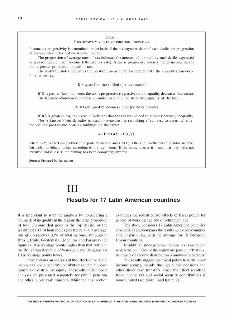
28 C E P A L R E V I E W 1 1 6 • A U G U S T 2 0 1 5
EXCHANGE-RATE VARIATIONS AND THE RATE OF INFLATION IN EMERGING ECONOMIES • JOSÉ GARCÍA-SOLANES AND FERNANDO TORREJÓN-FLORES
The literature on variations in exchange rates and prices in open economies has typically focused on exchange-rate pass-through (erpt), that is, the extent to which exchange-rate fluctuations are transmitted to domestic prices. In order to assess the pure erpt effects the analysis should be restricted to the initial impacts on import prices or, at most, to the first stages affecting domestic producer prices. If the analysis is extended to capture the short-run clearing of assets and goods markets, the final ratio of domestic price variations to exchange-rate variations gives a more indirect measure of erpt. The relationships between exchange rates and domestic prices are sensitive to the type of external shocks that trigger adjustments, as emphasized by Mishkin (2008).
Although it is generally held that low inflation rates, monetary policy credibility, and exchange-rate flexibility contribute to lower erpt,1 some authors have obtained estimates that contradict or call into question that consensus. For example, Nogueira (2007) found that the adoption of an inflation-targeting regime —thus strengthening monetary policy credibility— increased erpt in the Czech Republic and the Republic of Korea; and Coricelli, Jazbec and Masten (2004) discovered that exchange-rate flexibility magnified the erpt coefficient in four advanced transition economies. In a similar vein, Byrne, Chavali and Kontonikas (2010), Sek and Kapsalyamova (2008), and Korhonen and Wachtel (2006) found that erpt effects are, in fact, very heterogeneous and asymmetrical among countries. According to Mishkin (2008), those divergent findings may be explained by the fact that authors did not take into account the type of external shocks that hit the economies.
In this paper, we examine the erpt that occurs when exchange rates and domestic prices are adjusted in the short-run macroequilibrium. In order to address the
The authors acknowledge the financial support from the Seneca Foundation (project 15183/PHCS/10).1 Taylor (2000), Korhonen and Watchel (2006), Choundri and Hakura (2006), and Mihaljek and Klau (2008) found that low inflation environments reduce erpt. The ability of monetary policy credibility gains to reduce erpt were underlined by Mishkin and Savastano (2002), Vega and Winkelried (2005), Nogueira (2007) and Nogueira and León-Ledesma (2011), among others. Finally, Barhoumi (2006), Sek and Kapsalyamova (2008), and Takatoshi and Kiyotaka (2008) found that exchange rate flexibility pushes erpt down by increasing volatility in the exchange market and shrinking trade.
point raised by Mishkin (2008), we analyse separately the effects caused by three different external shocks. We further investigate the way in which four different features of emerging market economies affect adjustments: the degree of exchange-rate fixity, the level of country risk, country indebtedness, and the flattening of Phillips curves since the start of the Great Recession (2007-2012).2
To this end, we build a structural general equilibrium model centred on exchange-rate flexibility and balance-sheet effects. Compared with previous frameworks for emerging economies, our model incorporates two significant new features: first, on the production side we derive an aggregate supply function that includes inertia in price-setting in the spirit of the New Keynesian Phillips curve for open economies; second, we derive an optimal monetary policy function by assuming that central banks seek to minimize any intertemporal losses ensuing from output gaps or deviations from the inflation or nominal exchange-rate targets.
We calculate the deviations of the endogenous variables from their stationary level as functions of the exogenous parameters, and perform calibration exercises after assigning values to the parameters of the model that are generally accepted in the literature. Doing so allows us to clarify how the effects of exogenous shocks are transmitted through four channels before ultimately impacting on the exchange rate and the domestic producer price index. Since we are particularly interested in the implications of exchange-rate fixity, country risk, country indebtedness and the slope of the Phillips curve, we calibrate for different values for these parameters.
We obtain two key findings. First, exchange-rate fixity, macroeconomic stability —to the extent that it reduces the risk and indebtedness parameters— and flatter Phillips curves reduce the fluctuations of both the exchange rate and domestic prices when the shocks are variations in foreign prices and foreign output. But exchange-rate fixity and flatter Phillips curves exacerbate the fluctuations of the two endogenous variables when adjustments are provoked by variations in the foreign
2 imf (2013, chap. 3) provides a detailed account of the likely factors, including “menu costs”, that have made inflation much less volatile, and less responsive to changes in the output gap, than in the past.
IIntroduction

29C E P A L R E V I E W 1 1 6 • A U G U S T 2 0 1 5
EXCHANGE-RATE VARIATIONS AND THE RATE OF INFLATION IN EMERGING ECONOMIES • JOSÉ GARCÍA-SOLANES AND FERNANDO TORREJÓN-FLORES
real interest rate. Only macroeconomic stability can curb fluctuations in the two endogenous variables caused by any type of external shock. Second, after each external shock considered in the analysis, erpt increases with higher fixity in the exchange rate and with flatter Phillips curves, but is hardly affected by variations in the risk and indebtedness factors. The main implication is that reducing the risk and indebtedness parameters increases the ability of monetary policy to stabilize both exchange-rate variations and domestic inflation when the economy suffers any of the three shocks
considered in the analysis, without affecting the degree of erpt.
This paper is divided into four sections, including this Introduction. Section II presents the theoretical model and solves it for the selected endogenous variables. Section III evaluates the impact of changes in exogenous variables on both the nominal exchange rate and the domestic price index, and computes the erpt coefficients generated by each shock. Lastly, in section IV we conclude by considering some policy implications of our findings.
IIThe theoretical model
In this section we build and solve a structural general equilibrium model to analyse the impact of several external shocks on the nominal exchange rate and domestic prices in a small, open emerging economy that faces imperfections in the international financial markets. We expand on the work of Céspedes, Chang and Velasco (2003 and 2004), Fraga, Goldfajn and Minella (2003), and Tovar (2005).
Our economy has five types of agent: firms, households, entrepreneurs, governments and monetary authorities. There are a large number of firms that produce differentiated goods in a context of monopolistic competition. Firms obtain capital from entrepreneurs and labour from households. Entrepreneurs decide on the size of their investments, which they finance partly with their own resources (net worth) and partly with foreign debt denominated in strong foreign currency. Domestic households issue bonds expressed in strong foreign currency and optimize their actions by taking into account the intertemporal budget restrictions of the government. Governments levy lump sum taxes to finance their consumption expenditure. Monetary authorities are concerned with the stabilization of three variables: domestic output, the domestic inflation rate and the nominal exchange rate. This presupposes that, in response to external shocks, central banks take action to achieve an optimal combination of the three variables.
In the short term, we assume that prices adjust slowly, in the tradition of Calvo (1983). The number of firms that change prices in any given period is specified exogenously in this setting. The variables of the model are presented as linear deviations around their stationary
state, except for interest rates and risk premiums.3 The model is composed of the following equations:4
E w y w s s
w
21
ti
y t i s t i t iT
i
t iH
t iHT
2 2
0
2
b
r r
+ −
+ −
3
r
+ + +=
+ +
uu _ `
`
i j
j
;
E
(
2
/ (1)
re y y q
E
*t iH
r t i y t i y t i q t i
t t iH
t i1
*r m m m m
b r n
= + + +
+ +
+ + + + +
+ + +
u uu u
` j (2)
s h E s h E
s h bs
r s s
y s h E y q b
q s y s g
s h E g s s in
*
*
*
c t t c t
c b tc
ct q x
q bt c y t t t
t x t g t
c g t t c t in t
11 1
1
*
*
c h
z
− − + +
= + +
+ +
− + +
++ +
+
_ _ `
__
i i j
ii
(3)
r r E q q*t t t t t t1} g− = − ++_ i9 C (4)
3 Relative deviations from the stationary state are denoted with a lower case letter. For instance, for variable Xt, which has the stationary level XSS, relative deviation is defined as x X X Xt t
SS SS= −` j . Relative deviation may be expressed as a very approximate value by: x X= /` jln Xt t
SS . 4 These equations have been derived by assuming that all agents optimize their behaviour. A detailed explanation may be obtained from the authors upon request.

30 C E P A L R E V I E W 1 1 6 • A U G U S T 2 0 1 5
EXCHANGE-RATE VARIATIONS AND THE RATE OF INFLATION IN EMERGING ECONOMIES • JOSÉ GARCÍA-SOLANES AND FERNANDO TORREJÓN-FLORES
q in y de1 1t t t t t tg k c | k k | k| j= − + + − + + +_ _i i9 C (5)
in E y E q
q r1 1
1 1 1*
t t t t t
t t t
1 1
*c
c d
d g
=
− −
− + − −
+ − −
+ +_ _ _ __
i i i ii
99
CC (6)
Equation (1) is a central bank’s intertemporal loss function that penalizes deviations in output, the nominal exchange rate and the inflation rate from their targets. The log of the output gap ytu is calculated with respect to the long-run or potential output level .yt t
Ts_ i is the log of the target nominal exchange rate announced by the central bank, defined as the price of the foreign currency in units of the domestic currency. t
Tr is the target inflation rate. The inclusion of exchange-rate deviations from the target in the loss function of the central bank is justified for two reasons: first, in the open economies that we investigate, exchange-rate fluctuations are likely to have a significant effect on aggregate demand and supply; and, second, nominal exchange-rate volatility modifies the net wealth of entrepreneurs because their external borrowing is denominated in strong foreign currencies.
Although some authors have acknowledged the relevance of exchange-rate policy by including it in the monetary reaction function (for instance, Ball, 1999; Obstfeld and Rogoff, 1995; Svensson, 2000; Mishkin and Savastano, 2002; Caballero and Krishnamurthy, 2005; and Wollmershäuser, 2003), the model that we have built here is the first to incorporate the exchange rate in the loss function of the central bank. Edwards (2006) remarks that in many instances the exchange rate plays a significant role in the monetary policy reaction function (Taylor rules), even though central banks do not explicitly recognize it.
Et is the rational expectations operator in period t, b is the discount factor and wy stands for the relative weight attached to output variability. Our specification of the loss function allows us, as in Tovar (2005), to envisage a continuum of exchange-rate regimes depending on the relative weight assigned to exchange-rate stabilization.5
The parameters ws and wπ measure the relative weight accorded, respectively, to exchange-rate and inflation-rate variability.
Equation (2) is an aggregate supply in the spirit of the New Keynesian Phillips curve that incorporates
5 In Tovar’s model, the diversity of exchange-rate regimes follows from the different weights assigned to exchange rate stabilization by the Taylor rule.
inertia in price-setting. Our version includes two open economy variables: the log of the real exchange rate, which transmits external disturbances —such as increases in foreign prices— into domestic inflation, and the log of the foreign output gap y*tu` j. The real exchange rate is defined such that an increase denotes a real depreciation of the domestic currency. The rate of return on capital (ret) enters the equation as an additional cost-push factor. The conventional part of the equation may be derived by assuming —as in Calvo (1983)— that firms maximize the difference between their expected marginal revenue and unit costs, and that only a fraction of them adjust prices during each period. All coefficients ande y ym mu u, ,r q*m m are positive and proportional to parameter λ, which is linked to the probability of adjusting prices in the current period (1 - θ) with this expression: (λ = (1 - θ)(1 - θb)/θ). Thus, aggregate supply, as well as the implied Phillips curve, becomes flatter ( ymu goes down) as the probability of adjusting prices declines.6 Variable μt is an exogenous supply shock that pushes up inflation.
Equation (3) indicates that aggregate demand depends positively on the real exchange rate (expenditure switching mechanism), expected output (owing to consumption smoothing by households),7 the expected real exchange rate, the expected variation in the stock of foreign debt denominated in foreign currency ( b*t ), foreign output ( y*t ), government expenditure (gt), domestic investment (int) and a demand shock ( tz ). Aggregate demand decreases as the real interest rate (rt) and expected government expenditure rise.
Equation (4) is the uncovered interest rate parity condition expressed in real terms. The variable ξt is the country risk premium, which is endogenously determined according to equation (5). The last equation indicates that the risk premium unambiguously increases when the value of current investment rises and the real exchange rate deteriorates —real depreciation increases the value of debt repayments in cases of liability dollarization—. It also increases with the proportion of entrepreneurs’ debt denominated in foreign currency (det), and with a stochastic shock ( tj ). The risk premium decreases when domestic output rises, since output is associated with the income and net worth of capitalists. As can be observed, the incidence of all these determinants of the risk premium depends crucially on the value of
6 When the probability of adjusting prices is one, which means that all firms change their prices at every moment (full price flexibility), aggregate supply is represented by a completely vertical line (see, for instance, Woodford (2003, chap. 2)).7 See, for instance, Fraga, Goldfajn and Minella (2003).

31C E P A L R E V I E W 1 1 6 • A U G U S T 2 0 1 5
EXCHANGE-RATE VARIATIONS AND THE RATE OF INFLATION IN EMERGING ECONOMIES • JOSÉ GARCÍA-SOLANES AND FERNANDO TORREJÓN-FLORES
parameters ι and χ, which are, respectively, the semi-elasticity of the risk premium associated with the ratio of investment to net wealth of entrepreneurs and the ratio of external debt to net wealth.
Finally, equation (6) is the investment demand equation, which can be derived easily from the standard international arbitrage on rates of return. This relationship establishes that domestic investment decreases when the international cost of capital (the sum of the world interest rate and the risk premium) rises since entrepreneurs borrow abroad to finance investment. Domestic investment also decreases with the expected real exchange rate because, ceteris paribus, a higher expected qt today is associated with a higher expected real depreciation between today and tomorrow, and hence with a higher cost of foreign capital as that cost is measured in terms of domestic goods. Moreover, domestic investment depends positively on expected output and on the current real exchange rate because, ceteris paribus, a higher qt today is associated with a lower expected real depreciation. Parameters γ and δ stand for the preference for domestic goods in consumption (home bias) and the share of international flows of the home country in world international trade.
Combining (5) and (6), we arrive at the balance-of-payments (bp) curve, the locus of points (yt, int) for which financial markets are in equilibrium, everything else being constant:
in E y y
q
11
1
1
1
1 1 1
1
1 1 1
1 11
11*
t t t t
t t
t
t t t
1
1
k k
k |
k
c d
k
c d k c |
k
k|
k k
= + + +
+
+
+ − −
+
− − − − +
+ + +
+
+E−
q
de r j
+
− − −
__
_ __
_ _
ii
i ii
i i9 9C C (7)
The bp schedule illustrates how the degree of imperfection in capital markets (ι) and the international financial position of the country (χ) affect investment. In particular, as shown in Céspedes, Chang and Velasco (2003), investment may either rise or fall with the real exchange rate. When capital market imperfections and the inherited dollar debt are sufficiently high (large values of ι and χ), the balance-sheet effect prevails over the expenditure-shifting effect associated with coefficient γ. In that case, the coefficient of qt is negative and the economy becomes financially vulnerable. Compared with the framework put forward by Céspedes, Chang
and Velasco (2003), the coefficient of qt in our model reinforces the influence of the expenditure-shifting channel because we include the parameter δ < 1, which is equal to unity in the earlier model. An interesting particular case, also stressed by Céspedes, Chang and Velasco, is the one in which financial imperfections are absent (ι = 0), giving rise to a horizontal bp in the space (yt, int).
The solution of the model for the two endogenous variables relevant to the present study —the producer price level (pt
HE ) and the nominal exchange rate ( stE )—
is presented in the annex. The model has 14 exogenous variables: foreign output ( y*t ); potential foreign output ( y *
t ); supply cost-augmenting shock ( tn ); average productivity of production factors (state of the technology) (at); stock of bonds, denominated in foreign currency, issued by domestic residents and held by foreigners (stock of foreign debt) (b*t ); government expenditure (gt); demand shock in private consumption (ft); foreign real interest rate ( r*t ); rate of return on capital (ret); foreign price level ( p*t ); foreign debt of entrepreneurs (det); target nominal exchange rate (st
T ); target rate of domestic inflation ( t
HTr ); and shock to the risk premium ( tj ) Moreover, all exogenous variables —except st
T and t
HTr — are governed by stationary ar(1) processes:
, ,
, ,
, ,
, ,
, ,
,
y y y y
a a
b b g g
r r
re re p p
de de
* *,
* *,
, ,
* *, ,
,* *
,
,* *
,
, ,
t y t y t t y t y t
t t t t a t a t
t b t b t t g t g t
t t t t r t r t
t r t re t t p t p t
t de t de t t t t
1 1
1 1
1 1
1 1
1 1
1 1
* * * *
* *
* *
* *
tt f t f
n t n f t f
t f t f
z t z f t f
t f t f
t f j t j f
= + = +
= + = +
= + = +
= + = +
= + = +
= + = +
n n
z z
j j
- -
- -
- -
- -
- -
- -
r rr r
(8)
The equilibrium equations of the domestic price level and the nominal exchange rate, including the signs of the partial derivatives with respect to the exogenous parameters, can be found in the annex (equations (A7) and (A8)).
Before calibrating the model, let us discuss briefly the relative contribution of each channel in the transmission effects after the initial depreciating impact on the nominal exchange rate.8 The expenditure channel has expansionary effects on aggregate demand and
8 It is widely accepted that external shocks affect the stock markets first, including the foreign exchange market. The initial impact on the nominal exchange rate is subsequently transmitted to other variables, including the domestic price level, following a process of mutual interactions.
32 C E P A L R E V I E W 1 1 6 • A U G U S T 2 0 1 5
EXCHANGE-RATE VARIATIONS AND THE RATE OF INFLATION IN EMERGING ECONOMIES • JOSÉ GARCÍA-SOLANES AND FERNANDO TORREJÓN-FLORES
is composed of two elements in our model. The first reflects the effect of the initial pass-through: increases in the nominal exchange rate push up the aggregate price level which, in turn, increases the nominal value of domestic expenditures. The second is expenditure switching: depreciation increases net exports because it raises the relative price of imported goods and reduces the price of domestic exports in foreign markets. This strengthening of real net exports pushes up the demand for domestic goods.
The balance-sheet effect may have either sign. A positive result, associated with increases in the demand for domestic output, emerges when both the semi-elasticity of the risk premium with respect to the ratio of investment over net debt (ι) and the ratio of external debt over the net wealth of entrepreneurs (χ) are below certain thresholds. The monetary policy channel operates through the policy reaction of monetary authorities. Its
contribution to the expansion of aggregate demand for domestic output is directly related to the weight attached to fluctuations of the exchange rate in the loss function of the central bank (ws). The lower the value of ws, the less the exchange rate is permitted to fluctuate, reducing the impact of the exchange rate on aggregate demand. Finally, for a given expansion of aggregate demand, the final effects on the domestic price level depend on the slope of the aggregate supply. This is directly related to price rigidity (θ), which is, in turn, directly linked to the price elasticity of the aggregate supply schedule ( ymu ).
In order to obtain empirical results, we calibrate the model and derive responses of the endogenous variables to some specific exogenous shocks. To do so, we assign reasonable values to the parameters in line with the relevant literature. Table 1 summarizes the benchmark values that we adopt to implement empirical exercises and the original source, where applicable.
TABLE 1
Parameter values
Parameter Value Additional information
1 < θ < 0 0.75 Probability of not adjusting the price of domestic output (Fraga, Goldfajn and Minella, 2003).
b < 1 0.99 Intertemporal discount factor (Fraga, Goldfajn and Minella, 2003).
0 < a < 1 0.8 Output-labour elasticity (Fraga, Goldfajn and Minella, 2003).
0 < h < 1 0.2 Elasticity net exports-real exchange rate (Fraga, Goldfajn and Minella, 2003; Batini, Harrison and Millard, 2001).
γc > 1 2 Inverse value of the intertemporal elasticity of consumption (Céspedes and Soto, 2005).
γn > 1 1 Inverse value of the elasticity of labour with respect to the real wage (Céspedes and Soto, 2005).
0 < δ < 1 0.01 Share of domestic international trade in world international trade.
0 < γ < 1 0.6 Degree of preference for domestic goods in the consumer basket (home bias) (Tovar, 2005; Céspedes and Soto, 2005).
Wyu 0.03 Weight assigned to output stabilization in the loss function of the central bank. This value is higher than the one in Fraga, Goldfajn and Minella (2003).
Ws 0.0014
Wr 1
ι 0.51 Semi-elasticity of the risk premium with respect to the ratio of capital to net worth (Tovar, 2005).
NE
Q DESS
SS SS
| =1.25 Ratio of foreign debt of entrepreneurs to net worth of the stationary
state, measured in domestic currency and in nominal terms (Tovar, 2005).
scrY
Q C0 1SS
SS SS1
1 1=
c-_ i 0.65 Ratio of foreign debt of entrepreneurs to net worth of the stationary state, measured in domestic currency and in nominal terms (Tovar, 2005).

33C E P A L R E V I E W 1 1 6 • A U G U S T 2 0 1 5
EXCHANGE-RATE VARIATIONS AND THE RATE OF INFLATION IN EMERGING ECONOMIES • JOSÉ GARCÍA-SOLANES AND FERNANDO TORREJÓN-FLORES
sbrC
Q B1
*
SS
SS SS
2=
c_ i 0.63 Ratio of private consumption to domestic output in the stationary state. Both variables are measured in domestic currency.
sirY
Q I0 1SS
SS SS1
1 1= =
c-_ i 0.2 Ratio of private investment to domestic output in the stationary state. Both variables are measured in domestic currency.
sY
X0 1x SS
SS
1 1=0.26 Share of exports in domestic output in the stationary state.
sY
G0 1g SS
SS
1 1=0.14 Share of government consumption in domestic output in the
stationary state.
s scr0 1c1 1c= 0.6*0.65 = 0.39
s sir0 1in1 1c= 0.6*0.2 = 0.12
s s s0 1 1q c in1 1c= − +_ _i i 0.4*(0.39 + 0.12) = 0.204
hC
Yscr1
1y SS
SS
2= =1/0.65 = 1.538
hC
Gscr
s0 1g SS
SS g1 2= =
0.14/0.65 = 0.215
h sbr 0q 2c= 0.6*0.63 = 0.378
h sbr 0b* 2= 0.63
1y* 1t 0.90
1y* 1tu 0.90
1y* 1tr 0.98
11tn 0.95
1a 1t 0.95
1b* 1t 0.80
1g 1t 0.5
11tz 0.3
1r* 1t 0.5
1re 1t 0.7
1p* 1t 0.9
1de 1t 0.8
1sT 1t
1T 1tr
11
11tj 0.8
Source: Prepared by the authors.
Table 1 (concluded)

34 C E P A L R E V I E W 1 1 6 • A U G U S T 2 0 1 5
EXCHANGE-RATE VARIATIONS AND THE RATE OF INFLATION IN EMERGING ECONOMIES • JOSÉ GARCÍA-SOLANES AND FERNANDO TORREJÓN-FLORES
IIIThe effects of the external shocks
In this section we calculate and provide a graphical representation of the effects of changes in one standard deviation of three exogenous variables, p*t , y*t and r*t , on the two endogenous variables pt
H and St. More specifically, we quantify the value of the elasticities given by formulae (A9) to (A14) (see annex) for different values for the parameters of interest. Since we are looking for the specific incidence of exchange-rate fixity (related to (ws), the relative indebtedness of entrepreneurs (χ), the sensitivity of the country risk premium to relative investment (ι), and internal price fixity (θ), we make calculations using alternative values for these key parameters.
Table 2 reports the estimated erpt coefficients corresponding to the three shocks, and for alternative values for the exchange-rate fixity, risk and indebtedness indicators and the probability of not adjusting prices in the current period.
Figures 1, 2 and 3 show the impact of an increase in the degree of exchange-rate fixity. They depict the results for the elasticities of the two endogenous variables with respect to the foreign price (p*t ), foreign output ( y*t ) and foreign real interest rate (r*t ), respectively. Each figure presents the results for two alternative values of exchange-rate fixity, namely, ws = 0.0014 and ws = 0.0015.
TABLE 2
Exchange-rate pass-through coefficients p stH
tb l for shocks in variables p*t , y*t and
r*t and alternative values for parameters ws, ι, χ and θ
Shocks Baseline
for all parametersBaseline except for
ws = 0.0015Baseline except for
ι = 1.5Baseline except for
χ = 2.0Baseline except for
θ = 0.8
p*t 0.88 0.95 0.81 0.88 0.96
y*t 0.86 0.90 0.86 0.86 0.94
r*t 0.36 0.39 0.36 0.36 0.37
Source: Prepared by the authors using elasticities derived from the model: ws = 0.0014, ι = 0.51, χ = 1.25, θ = 0.75, γ = 0.6.
FIGURE 1
Response of endogenous variables ptH and st to shock p*t for two alternative
values of ws
pH
s
pH
s
0.0000
0.0050
0.0100
0.0150
0.0200
0.0250
0.0300
0.0350
0.0400
0.0450
0.0500
-1 0 1 2 3 4 5 6 7 8 9 10 11 12 13 14 15 16 17 18 19 20
y
y
γ = 0.6, χ = 1.25, ι = 0.51, ws = 0.0014, θ = 0.75γ = 0.6, χ = 1.25, ι = 0.51, ws = 0.0015, θ = 0.75
Source: Prepared by the authors using elasticities derived from the model.

35C E P A L R E V I E W 1 1 6 • A U G U S T 2 0 1 5
EXCHANGE-RATE VARIATIONS AND THE RATE OF INFLATION IN EMERGING ECONOMIES • JOSÉ GARCÍA-SOLANES AND FERNANDO TORREJÓN-FLORES
FIGURE 2
Response of endogenous variables ptH and st to shock y*t for two alternative
values of ws
γ = 0.6, χ = 1.25, ι = 0.51, ws = 0.0014, θ = 0.75γ = 0.6, χ = 1.25, ι = 0.51, ws = 0.0015, θ = 0.75
pH
s
pH.
s
0.0000
0.0100
0.0200
0.0300
0.0400
0.0500
0.0600
0.0700
0.0800
-1 0 1 2 3 4 5 6 7 8 9 10 11 12 13 14 15 16 17 18 19 20
Source: Prepared by the authors using elasticities derived from the model.
FIGURE 3
Response of endogenous variables ptH and st to shock r*t for two alternative
values of ws
γ = 0.6, χ = 1.25, ι = 0.51, ws = 0.0014, θ = 0.75γ = 0.6, χ = 1.25, ι = 0.51, ws = 0.0015, θ = 0.75
pH
s
pH
s
0.0000
0.0010
0.0020
0.0030
0.0040
0.0050
0.0060
-1 0 1 2 3 4 5 6 7 8 9 10 11 12 13 14 15 16 17 18 19 20
H
y
y
y
y
Source: Prepared by the authors using elasticities derived from the model.
Figures 1 to 3 and the numerical estimations in column three of table 2 reflect some common findings. First, shocks have a more intensive impact on the exchange rate than on domestic prices, confirming that erpt is only partial in the short run. Moreover, variation in foreign output causes the strongest effects on the two endogenous variables. Second, when the economy is shocked by increases in foreign output and foreign prices, greater fixity in the nominal exchange rate curtails
the two endogenous variables (the exchange rate and the domestic price level), but increases erpt. Similar results are obtained when the Phillips curve becomes flatter. However, when the external shock is an increase in the foreign real interest rate, the dampening effects are offset by additional flexibility in the exchange rate and more vertical Phillips curves, without altering erpt. In the current circumstances of economic slack and high unemployment, many central banks have assigned greater

36 C E P A L R E V I E W 1 1 6 • A U G U S T 2 0 1 5
EXCHANGE-RATE VARIATIONS AND THE RATE OF INFLATION IN EMERGING ECONOMIES • JOSÉ GARCÍA-SOLANES AND FERNANDO TORREJÓN-FLORES
weight to output stabilization (wy) than to exchange-rate stabilization (ws) in their social loss function in order to attenuate fluctuations in real domestic output and employment. According to our findings, this policy shift will also help to decrease erpt.
Figures 4 to 6 show the elasticities associated with each shock for two alternative values of the sensitivity
FIGURE 4
Response of endogenous variables ptH and st to shock p*t for two alternative
values of ι
γ = 0.6, χ = 1.25, ι = 0.51, ws = 0.0014, θ = 0.75γ = 0.6, χ = 1.25, ι = 1.5, ws = 0.0014, θ = 0.75
pH
s
pH
s
0.0000
0.0100
0.0200
0.0300
0.0400
0.0500
0.0600
-1 0 1 2 3 4 5 6 7 8 9 10 11 12 13 14 15 16 17 18 19 20
H
y
y
Source: Prepared by the authors using elasticities derived from the model.
FIGURE 5
Response of endogenous variables ptH and st to shock y*t for two alternative
values of ι
γ = 0.6, χ = 1.25, ι = 0.51, ws = 0.0014, θ = 0.75γ = 0.6, χ = 1.25, ι = 1.5, ws = 0.0015, θ = 0.75
pH
s
pH.
s
0.0000
0.0200
0.0400
0.0600
0.0800
0.1000
0.1200
0.1400
0.1600
0.1800
-1 0 1 2 3 4 5 6 7 8 9 10 11 12 13 14 15 16 17 18 19 20
Source: Prepared by the authors using elasticities derived from the model.
of the country risk premium to relative investment (ι). Again, it is apparent in each case that the nominal exchange rate reacts more markedly than the domestic price level. Moreover, an increase in ι exacerbates the reaction of both the nominal exchange rate and the internal price level without changing erpt. This applies to adjustments caused by any external shock.

37C E P A L R E V I E W 1 1 6 • A U G U S T 2 0 1 5
EXCHANGE-RATE VARIATIONS AND THE RATE OF INFLATION IN EMERGING ECONOMIES • JOSÉ GARCÍA-SOLANES AND FERNANDO TORREJÓN-FLORES
FIGURE 6
Response of endogenous variables ptH and st to shock r*t for two alternative
values of ι
γ = 0.6, χ = 1.25, ι = 0.51, ws = 0.0014, θ = 0.75γ = 0.6, χ = 1.25, ι = 1.5, ws = 0.0014, θ = 0.75
pH
s
pH
s
-0.0250
-0.0200
-0.0150
-0.0100
-0.0050
0.0000
0.0050
0.0100
-1 0 1 2 3 4 5 6 7 8 9 10 11 12 13 14 15 16 17 18 19 20
H
y
y
y
y
Source: Prepared by the authors using elasticities derived from the model.
However, the effects of an increase in the foreign real interest rate on the nominal exchange rate and on the domestic price level (see figure 6) are counter-intuitive for relatively high levels of ι. In fact, according to variations of the Mundell-Fleming model, an increase in the foreign interest rate triggers capital outflows that depreciate the domestic currency, thus stimulating domestic output. In our model, a rise in r*t increases the international cost of capital, which reduces domestic investment (equation (6)) because entrepreneurs borrow abroad to finance their investment expenditures. The decline in investment shrinks the risk premium. For the benchmark values of ι, χ and h assumed in our calibration, the increase in the foreign interest rate is greater than the impact on the risk premium, consequently giving rise to normal reactions of both the nominal exchange rate and the domestic price level. However, if the risk premium drops by more than the foreign interest rate
rises, financial capital inflows drive up the nominal exchange rate. Exchange-rate appreciation weakens the demand for domestic goods, causing reductions in both domestic prices and output. Those “abnormal” results are shown in figure 6, in which we assume that the risk parameter (ι) increases sufficiently. Finally, the central bank reacts by lowering the nominal interest rate in order to curb the fluctuations of both the nominal exchange rate and output. It is worth stressing that these abnormal reactions to shocks in the foreign real interest rate take place only for values of ι that exceed a certain threshold.
Figures 7 to 9 represent the elasticities for the three shocks and for two alternative values of the relative indebtedness of entrepreneurs (χ). As in previous cases, the nominal exchange rate reacts more strongly than the domestic price level after each shock. Furthermore, an increase in χ does not modify erpt.

38 C E P A L R E V I E W 1 1 6 • A U G U S T 2 0 1 5
EXCHANGE-RATE VARIATIONS AND THE RATE OF INFLATION IN EMERGING ECONOMIES • JOSÉ GARCÍA-SOLANES AND FERNANDO TORREJÓN-FLORES
FIGURE 7
Response of endogenous variables ptH and st to shock p*t for two alternative
values of χ
γ = 0.6, χ = 1.25, ι = 0.51, ws = 0.0014, θ = 0.75γ = 0.6, χ = 2.0, ι = 0.51, ws = 0.0014, θ = 0.75
pH
s
pH
s
0.0000
0.0100
0.0200
0.0300
0.0400
0.0500
0.0600
-1 0 1 2 3 4 5 6 7 8 9 10 11 12 13 14 15 16 17 18 19 20
H
y
y
Source: Prepared by the authors using elasticities derived from the model.
FIGURE 8
Response of endogenous variables ptH and st to shock y*t for two alternative
values of χ
γ = 0.6, χ = 1.25, ι = 0.51, ws = 0.0014, θ = 0.75γ = 0.6, χ = 2.0, ι = 0.51, ws = 0.0014, θ = 0.75
pH
s
pH.
s
0.0000
0.0200
0.0400
0.0600
0.0800
0.1000
0.1200
0.1400
-1 0 1 2 3 4 5 6 7 8 9 10 11 12 13 14 15 16 17 18 19 20
Source: Prepared by the authors using elasticities derived from the model.

39C E P A L R E V I E W 1 1 6 • A U G U S T 2 0 1 5
EXCHANGE-RATE VARIATIONS AND THE RATE OF INFLATION IN EMERGING ECONOMIES • JOSÉ GARCÍA-SOLANES AND FERNANDO TORREJÓN-FLORES
FIGURE 9
Response of endogenous variables ptH and st to shock r*t for two alternative
values of χ
γ = 0.6, χ = 1.25, ι = 0.51, ws = 0.0014, θ = 0.75γ = 0.6, χ = 2.0, ι = 0.51, ws = 0.0014, θ = 0.75
pH
s
pH
s
0.0000
0.0020
0.0040
0.0060
0.0080
0.0100
0.0120
-1 0 1 2 3 4 5 6 7 8 9 10 11 12 13 14 15 16 17 18 19 20
H
y
y
y
y
Source: Prepared by the authors using elasticities derived from the model.
Finally, figures 10 to 12 show the findings for the three shocks with respect to the probability of not adjusting prices in the current period θ. As can be seen, when the economy is hit by higher foreign prices and foreign output, a rise in price rigidity from 0.75 to 0.80 reins in the depreciation of the nominal
exchange rate and the increase in the domestic price level while pushing up erpt. However, when the economy is shocked by a higher foreign real interest rate, flatter Phillips curves exacerbate the reactions of the two endogenous variables and do not alter erpt.
FIGURE 10
Response of endogenous variables ptH and st to shock p*t for two alternative
values of θ
γ = 0.6, χ = 1.25, ι = 0.51, ws = 0.0014, θ = 0.75γ = 0.6, χ = 1.25, ι = 0.51, ws = 0.0014, θ = 0.80
pH
s
pH
s
0.0000
0.0050
0.0100
0.0150
0.0200
0.0250
0.0300
0.0350
0.0400
0.0450
0.0500
-1 0 1 2 3 4 5 6 7 8 9 10 11 12 13 14 15 16 17 18 19 20
H
y
y
Source: Prepared by the authors using elasticities derived from the model.

40 C E P A L R E V I E W 1 1 6 • A U G U S T 2 0 1 5
EXCHANGE-RATE VARIATIONS AND THE RATE OF INFLATION IN EMERGING ECONOMIES • JOSÉ GARCÍA-SOLANES AND FERNANDO TORREJÓN-FLORES
FIGURE 11
Response of endogenous variables ptH and st to shock y*t for two alternative
values of θ
γ = 0.6, χ = 1.25, ι = 0.51, ws = 0.0014, θ = 0.75γ = 0.6, χ = 1.25, ι = 0.51, ws = 0.0014, θ = 0.80
pH
s
pH
s
0.0000
0.0100
0.0200
0.0300
0.0400
0.0500
0.0600
0.0700
0.0800
-1 0 1 2 3 4 5 6 7 8 9 10 11 12 13 14 15 16 17 18 19 20
Source: Prepared by the authors using elasticities derived from the model.
FIGURE 12
Response of endogenous variables ptH and st to shock r*t for two alternative
values of θ
γ = 0.6, χ = 1.25, ι = 0.51, ws = 0.0014, θ = 0.75γ = 0.6, χ = 1.25, ι = 0.51, ws = 0.0014, θ = 0.80
pH
s
pH
s
0.0000
0.0010
0.0020
0.0030
0.0040
0.0050
0.0060
-1 0 1 2 3 4 5 6 7 8 9 10 11 12 13 14 15 16 17 18 19 20
H
y
y
y
Source: Prepared by the authors using elasticities derived from the model.
The results concerning variations in ι and χ are similar to those of Nogueira and León-Ledesma (2011), who use the Emerging Markets Bond Index Plus (embi+) and the real interest rate differential with the United States as a proxy for market perceptions of the national economic condition. In both cases, macroeconomic instability and increases in country risk lead to higher fluctuations in
the exchange rate and in the domestic price level, while simultaneously pushing up erpt. Consequently, our findings also indirectly support the general view that favourable macroeconomic environments, including those in which central banks apply an inflation-targeting regime, contribute decisively to controlling exchange-rate and domestic- price volatility and to decreasing the degree of erpt.

41C E P A L R E V I E W 1 1 6 • A U G U S T 2 0 1 5
EXCHANGE-RATE VARIATIONS AND THE RATE OF INFLATION IN EMERGING ECONOMIES • JOSÉ GARCÍA-SOLANES AND FERNANDO TORREJÓN-FLORES
In this paper we have built and applied a general equilibrium macroeconomic model to assess the sensitivity of the nominal exchange rate and the domestic price level to three types of exogenous shock, and to calculate the subsequent impact on gross erpt in emerging economies. The model includes two elements necessary to tackle the issue correctly in this type of economy. One is the degree of exchange-rate flexibility in the social loss function, which is needed to assess the influence of exchange-rate flexibility on erpt. The other is the inclusion of balance-sheet parameters in the transmission channel of erpt effects. Furthermore, the general equilibrium properties of the model allow us to verify the Mishkin (2008) proposition, according to which the degree of exchange-rate pass-through depends crucially on the external shock that hits the economy.
We obtain three significant findings. First, exchange-rate fixity decreases the volatility of the two endogenous variables and increases the erpt coefficient when the economy is shocked by variations in foreign output and the foreign price level. However, exchange-rate fixity exacerbates the fluctuations of the two endogenous variables when the economy is hit by variations in the foreign real interest rate. Second, an increase in the sources of macroeconomic instability, such as the sensitivity of the country risk premium to relative investment and the relative indebtedness of entrepreneurs, also makes the two endogenous variables more volatile, though it does not affect the degree of erpt. Those results confirm previous findings in the literature. Third, flatter
Phillips curves —as observed in many economies in the present context of economic crisis— help minimize adjustments to both the nominal exchange rate and the domestic price level, while pushing up erpt, when the economy is shocked by variations in foreign output and the foreign price level.
Some policy implications follow from our findings. First, authorities in emerging economies seeking to reduce the degree of erpt (with the aim of tackling inflation or making monetary policy more effective) should take very seriously the macroeconomic advantages provided by exchange-rate flexibility and a stable macroeconomic environment (that is one not dominated by indebtedness and economic risk). Second, since those elements are important pillars of an inflation-targeting regime, our findings confirm indirectly that inflation targeting stabilizes exchange rates and domestic prices, boosting the positive macroeconomic effects of such a regime in emerging economies, as demonstrated in some recent studies.9 Admittedly, central banks’ attempts to stabilize inflation under flatter Phillips curves could hurt economic growth, but central banks may address this problem by increasing the weight of output stabilization in their social loss functions.10
9 See, for instance, Vega and Winkelried (2005), and García-Solanes and Torrejón-Flores (2012).10 imf (2013) discusses other ways to tackle this issue.
IVConcluding remarks

42 C E P A L R E V I E W 1 1 6 • A U G U S T 2 0 1 5
EXCHANGE-RATE VARIATIONS AND THE RATE OF INFLATION IN EMERGING ECONOMIES • JOSÉ GARCÍA-SOLANES AND FERNANDO TORREJÓN-FLORES
To solve the model, we derive first the equation that specifies the equilibrium value of pt
HE using the undetermined coefficients method. The procedure is as
ANNEX
Mathematical resolution of the model
follows: minimize the loss function (1) subject to the aggregate supply (2) to derive the optimal trajectories for the domestic output gap and nominal exchange rate:
yw w w w w
w wre p p y E s* *
ty s q y s
y s
re t q t q tH
y t tH
t tHT
q tT
2 2 1*
m m
mm m m m b r n r m=
+ +− − + − − − + −
r r
r
+u uu u
u
u` `j j9 D (A1)
s
w w w w w
w wre
w w
w w ws* *
ty s q y s
q y
re t q t q tH
y t tH
t tHT
q y
s y y
tT
2 2 1
2
*m m
mm r n r
m
m=
+ +− − + +
+
r r
r
r
r
+p p y Em m m b− + uu u
u
uu
u u
` ``
j jj
R
T
SSSS
V
X
WWW
(A2)
Now, substitute the risk premium (5) into the uncovered interest rate parity (4), and insert the result into the aggregate demand (3). Then, combine the
resulting expression with the BP equation (7) and solve for y y yt t t= +u r . Insert (A1) and (A2) into the resulting expression and solve for E pt t
H2+` j.
We reach:
E p d E p d p C y C y C C a C b C g C C r
C re C p C de C s C C
* * * *
*
t tH
t tH
tH
y t y t t a t b t g t t r t
re t p t de t s tT
tHT
t
2 1 1 0 * * * *
* T HT
n z
r j
= + + + + + + + + +
+ + + + + +
n z
r j
+ + rr` `j j (A3)
Define:
p B y B y B B a B b B g B B r
B re B p B de B s B B
* * * *
*
tH
y t y t t a t b t g t t r t
re t p t de t s tT
tHT
t
* * * *
* T HT
n z
r j
= + + + + + + +
+ + + + + +
n z
r j
rr (A4)
E p B y B y B B a B b B g B B r
B re B p B de B s B B
* * * *
*
t tH
y y t y y t t a a t b b t g g t t r r t
re re t p p t de de t s tT
tHT
t
1 * * * * * * * *
* * T HT
t t t n t t t t z t
t t t r t j
= + + + + + + +
+ + + + + +
n n z z
r j j
+ rr r` j (A5)
E p B y B y B B a B b B g B B r
B r B p B de B s B B
* * * *
*
t tH
y y t y y t t a a t b b t g g t t r r t
r r t p p t de de t s tT
tHT
t
22 2 2 2 2 2 2 2
2 2 2 2
* * * * * * * *
* * T HT
t t t n t t t t z t
t t t r t j
= + + + + + + +
+ + + + + +
n n z z
r j j
+ rr r` j (A6)
Substitute equations (A4) to (A6) into (A3). On applying the undetermined coefficients methodology, we derive the coefficients of pt
HE (Bj), with:
Bd d
Cj
j j
j
21 0t t
=− −
Where j = y*, y*r , μ, a, b*, g, f, r*, re, p*, de, ϑ.
For sT and pHT, CB d d1jj 1 0= − −7 A.
For example, By* is the elasticity of the domestic price with respect to foreign output. With this information, on applying the parametric values (see table 1) that we explain below, we derive the signs of the partial derivatives in (A7):

43C E P A L R E V I E W 1 1 6 • A U G U S T 2 0 1 5
EXCHANGE-RATE VARIATIONS AND THE RATE OF INFLATION IN EMERGING ECONOMIES • JOSÉ GARCÍA-SOLANES AND FERNANDO TORREJÓN-FLORES
p B y B y B B a B b B g B B r
B re B p B de B s B B
* * * *
*
tHE
y t y t t a t b t g t t r t
re t p t de t s tT
tHT
t
* * * *
* T HT
n z
r j
= + + + + + + +
+ + + + + +
n z
r j
rr
+
+ + − − − −
+ + +− − − −/+ (A7)
To derive the equilibrium equation of the exchange rate, we apply a similar procedure as in the case of the domestic price level. Consequently,
' ' ' ' ' ' ' ' '
' ' ' ' ' '
E s d s C y C y C C a C b C g C C r
C re C p C de C s C C
* * * *
*
t t t y t y t t a t b t g t t r t
re t p t de t s tT
tHT
t
1 0 * * * *
* T HT
n z
r j
= + + + + + + + +
+ + + + + +
n z
r j
+ rr_ i (A3’)
We derive the coefficients of stHE (Sj), with:
'
'S
d
Cj
j
j
0t= −
Where: j = y*, y*r , μ, a, b*, g, f, r*, re, p*, de, ϑ.
For sT y p HT, ' 'CS d1jj 0= −7 A.
The result is:
y y a b g r
re p de s
s S S S S S S S S
S S S S S S
* * * *
*
tE
y t y t t a t b t g t t r t
re t p t de t s tT
tHT
t
* * * *
* T HT
n z
r j
= + + + + + + +
+ + + + + +
n z
r j
rr
+ + + −/+− − − −
+ + +− − −
(A8)
Taking into account the equations that specify the equilibrium values of the endogenous variables, it is easy to
derive the elasticity of each endogenous variable with respect to the three exogenous variables of interest, p*t , y
*t and r*t :
B FA w w P R w w M N M N1
pp
y q s p q y p p2
**
* * *m m t m t t=
− − + + +r ru u_ _i i9 C (A9)
B FA w w P R w w M N s1
yy
y y s y y q y y x*
*
* * * *m m t m m t=
− − + +r ru u u u_ _i i9 C (A10)
B F
s B1
rr
c
c
**
c k−
=
++_ i> H
(A11)
S N MA
w wB R P B N M1 1
pp
y s
p p q q p p
**
* * * *
t
mb t m m t
= − −
− + − − + − +ru _ _ _ _i i i i9 C& 0
(A12)

44 C E P A L R E V I E W 1 1 6 • A U G U S T 2 0 1 5
EXCHANGE-RATE VARIATIONS AND THE RATE OF INFLATION IN EMERGING ECONOMIES • JOSÉ GARCÍA-SOLANES AND FERNANDO TORREJÓN-FLORES
S N MA
w wB R P B N M s1
yy
y s
y y y y y y xq
**
* * * * * *
t
mb t m m t t
= − −
− + − − − + +ru
u_ _ _i i i9 C& 0 (A13)
S N M
A
w wB R P
s B1
1r
r
y s
r r q rc
c
**
* * *
t
mb t m t c k
= − −
− + − − ++
ru _ _ _i i i9 >C H& 0 (A14)
Where:
F RR A P w w w w N w w
M w w P w w
R
w N A M w M
1
1
j j y s q y s
q y y y s
q y
j j q q
2% %
% % %
%t b b m
b t t b m
m m m
m mm
= − + + +
− −+ − + +
r r r
r r r
` `
` `
j j
j j
&
&/ 0 (A15)
j = y*, r* and p*.
Moreover:
B ss
inc
c
c k= −< F
A w w w w wy s q y s2 2m m= + +r ru u` j
R s hB
1c yk
= ++_ i
N s hs
B 1
1 1 1c q
c
c
c }k
c d= − − +
+ − −_ _i i
Ms s
s s B1 1
1 1 1
c
c
c
cq xc } c k c | h
k
c d k c |= − − + + + +
− − − − ++_ _
_ _i i
i i9
9 9C
C C
RR A R w Nwy s y q
bm m= +u u9 C
Ps B
1 11c
ck | c k
= − + ++
_ _i i> H
M 1
1 1 11 k
c d= +
+ − −_ _i i
M1 1
1
12
c c
k
d k |− −= +
− − +_ _i i9 9C C

45C E P A L R E V I E W 1 1 6 • A U G U S T 2 0 1 5
EXCHANGE-RATE VARIATIONS AND THE RATE OF INFLATION IN EMERGING ECONOMIES • JOSÉ GARCÍA-SOLANES AND FERNANDO TORREJÓN-FLORES
Bibliography
Ball, L. (1999), “Policy rules for open economies”, Monetary Policy Rules, J. Taylor (ed.), Chicago, University of Chicago Press.
Barhoumi, K. (2006), “Differences in long run exchange rate pass-through into import prices in developing countries: an empirical investigation”, Economic Modelling, vol. 23, No. 6, Amsterdam, Elsevier.
Batini, N., R. Harrison and S.P. Millard (2001), “Monetary policy rules for an open economy”, Norges Bank Working Paper, No. 2001/4, Oslo, Norges Bank.
Byrne, J., A. Chavali and A. Kontonikas (2010), “Exchange rate pass-through to import prices: panel evidence from emerging market economies”, Business School – Economics Working Papers, No. 2010/19, Glasgow, University of Glasgow, June.
Calvo, G.A. (1983), “Staggered prices in a utility-maximizing framework”, Journal of Monetary Economics, vol. 12, No. 3, Amsterdam, Elsevier.
Caballero, R.J. and A. Krishnamurthy (2005), “Inflation targeting and sudden stops”, The Inflation-Targeting Debate, B.S. Bernanke and M. Woodford (eds.), Chicago, University of Chicago Press.
Céspedes, L.F. and C. Soto (2005), “Credibility and inflation targeting in Chile”, document prepared for the 9th Annual Conference of the Central Bank of Chile “Política monetaria bajo metas de inflación”, Santiago, 20-21 October.
Céspedes, L.F., R. Chang and A. Velasco (2004), “Balance sheets and exchange rate policy”, American Economic Review, vol. 94, No. 4, Nashville, Tennessee, American Economic Association.
(2003), “is-lm-bp in the Pampas”, imf Staff Papers, vol. 50, Washington, D.C., International Monetary Fund (imf).
Choundri, E.U. and D.S. Hakura (2006), “Exchange rate pass-through to domestic prices: does the inflationary environment matter?, Journal of International Money and Finance, vol. 25, No. 4, Amsterdam, Elsevier.
Coricelli, F., B. Jazbec and I. Masten (2004), “Exchange rate pass-through in acceding countries: the role of exchange rate regimes”, eui Working Paper, No. 2004/16, European University Institute.
Edwards, S. (2006), “The relationship between exchange rates and inflation targeting revisited”, nber Working Paper, No. 12163, Cambridge, Massachusetts, National Bureau of Economic Research (nber), April.
Fraga, A., I. Goldfajn and A. Minella (2003), “Inflation targeting in emerging market economies”, nber Working Paper, No. 10019, Cambridge, Massachusetts, National Bureau of Economic Research (nber).
García-Solanes, J. and F. Torrejón-Flores (2012), “Inflation targeting works well in Latin America”, cepal Review, No. 106 (LC/G.2518-P), Santiago.
imf (International Monetary Fund) (2013), World Economic Outlook: Hopes, Realities and Risks, Washington, D.C.
Korhonen, I. and P. Wachtel (2006), “A note on exchange rate pass-through in cis countries”, Research in International Business and Finance, vol. 20, No. 2, Amsterdam, Elsevier.
Mihaljek, D. and M. Klau (2008), “Exchange rate pass-through in emerging market economies: what has changed and why?”, bis Papers, No. 35, Bank for International Settlements.
Mishkin, F.S. (2008), “Exchange rate pass-through and monetary policy”, nber Working Paper, No. 13889, Cambridge, Massachusetts, National Bureau of Economic Research.
Mishkin, F.S. and M. Savastano (2002), “Monetary policy strategies for Latin America”, Journal of Development Economics, vol. 66, No. 2, Amsterdam, Elsevier.
Nogueira, R. (2007), “Inflation targeting and exchange rate pass-through”, Economía Aplicada, vol. 11, No. 2, São Paulo, University of São Paulo.
Nogueira, R. and M. León-Ledesma (2011), “Does exchange rate pass-through respond to measures of macroeconomic instability?”, Journal of Applied Economics, vol. 14, No. 1, Amsterdam, Elsevier.
Obstfeld, M. and K. Rogoff (1995), “The mirage of fixed exchange rates”, Journal of Economic Perspectives, vol. 9, No. 4, Nashville, Tennessee, American Economic Association.
Sek, S.K. and Z. Kapsalyamova (2008), “Exchange rate pass-through and volatility: impacts on domestic prices in four Asian countries”, mpra Working Paper, No. 11130, Munich, University Library of Munich, October.
Svensson, L. (2000), “Open-economy inflation targeting”, nber Working Paper, No. 6545, Cambridge, Massachusetts, National Bureau of Economic Research.
Takatoshi, I. and S. Kiyotaka (2008), “Exchange rate changes and inflation in post-crisis Asian countries: Vector Autorregression Analysis of the exchange rate pass-through”, Journal of Money, Credit and Banking, vol. 40, No. 7, Wiley.
Taylor, J. (2000), “Low inflation pass-through and the pricing power of firms”, European Economic Review, vol. 44, No. 4, Amsterdam, Elsevier.
Tovar, C.E. (2005), “The mechanics of devaluations and the output response in a dsge model: how relevant is the balance sheet effect?”, bis Working Papers, No. 192, Basel, Bank for International Settlements.
Vega, M. and D. Winkelried (2005), “Inflation targeting and inflation behavior: a successful story”, International Journal of Central Banking, vol. 1, No. 3.
Wollmershäuser, T. (2003), “Should central banks react to exchange rate movements? An analysis of the robustness of simple policy rules under exchange rate uncertainty”, document presented at the II Workshop on Macroeconomic Policy Research, Budapest, 2-3 October.
Woodford, M. (2003), Interest and Prices: Foundations of a Theory of Monetary Policy, Princeton, Princeton University Press.


The People’s Republic of China and Latin America: the impact of Chinese economic growth on Latin American exports
Daniel E. Perrotti
ABSTRACT The role of the People’s Republic of China in the world economy has grown substantially in recent decades, turning it into a strategic foreign trading partner for much of Latin America. Bilateral trade between the region and China totalled US$ 120 billion in 2009. This study analyses the income elasticity of the region’s exports to the country. The findings show that, assuming real gross domestic product (gdp) growth in China of about 7% a year, the value of Latin American exports to China (at 2005 prices) can be expected to increase by an average of about 10% a year between 2014 and 2019. In a more conservative scenario of 4.5% average annual growth in the Chinese economy over the period, exports would rise by about 7% a year.
KEYWORDS International trade, international economic relations, economic growth, exports, trade statistics, mathematical modelling, Latin America, China
JEL CLASSIFICATION F10, F17, F60
AUTHOR Daniel E. Perrotti is an official with the Latin American and Caribbean Institute for Economic and Social Planning (ilpes) of eclac and a regular associate professor with the Faculty of Economic Sciences of the University of Buenos Aires (uba), Argentina. [email protected]

48 C E P A L R E V I E W 1 1 6 • A U G U S T 2 0 1 5
THE PEOPLE’S REPUBLIC OF CHINA AND LATIN AMERICA: THE IMPACT OF CHINESE ECONOMIC GROWTH ON LATIN AMERICAN EXPORTS • DANIEL E. PERROTTI
This study estimates the income elasticity of Latin American exports to the People’s Republic of China1 for a set of 17 countries in the region, taking into account the dynamic aspects of exports while also considering the control variables customarily specified in the international trade literature.
The author is grateful for the comments and suggestions of René Hernández, an eclac staff member, and Rhys Jenkins, a professor at the University of East Anglia in the United Kingdom, and for the suggestions of an anonymous reviewer.1 Hereinafter simply China.
With this end in view, section II provides a brief description of the impact China is having on the world economy and its relationship with Latin America. Section III then reviews the literature in the light of the objectives of this study and touches on gravity models. Section IV presents the variables considered in the models, followed by the results of the two estimations carried out (for exports in general and by product type).
Lastly, section V offers some conclusions drawn from the findings of this study.
IIntroducción
IIThe Asian giant
The role of China in the world economy has increased substantially over the last three decades. In that time, it has achieved double-digit annual gross domestic product (gdp) growth, enabling it to increase per capita gdp tenfold and lift 500 million people out poverty.2 China has also become the world’s second-largest economy, if gdp is measured at purchasing power parity.
Not only does China account for an enormous share of global production, consumption and trade, but it is one of the most important actors in the global financial system, being the largest holder of United States Treasury Bonds. The country has even been promoting the yuan as an alternative international reserve currency (Rosales and Kuwayama, 2012).
The size and impact of China’s international trade can be appreciated in different ways. One is to consider that the country became the world’s largest goods exporter in 2009 (US$ 1.202 trillion dollars’ worth),3 accounting for 9.6% of world exports. It has also been
2 Growth and social inclusion have not led to improvements in the Gini coefficient, however, as inequalities between the seaboard and inland China have increased (Rosales and Kuwayama, 2012).3 China’s exports are clearly differentiated by province and city of origin. The four leading provinces (Guangdong, Jiangsu, Zhejiang and Shandong), together with the city of Shanghai, originated over 75% of the country’s total exports in 2007 (Rosales and Kuwayama, 2012).
playing a major role as an importer, being second in the world only to the United States, so that in 2009 it accounted for 8% of global imports (Rosales and Kuwayama, 2012).
Besides the export dynamic, another driver of the Chinese economy over the past decades has been the focus on investment as a driver of growth,4 to such an extent that the consumption to gdp ratio in China is among the lowest of any leading world economy. Over recent years, however, China has oriented its economic policy towards the goal of energizing domestic consumption.5
Where supply is concerned, the Chinese economy has continued to increase its agricultural output, which now exceeds even that of the United States and the European Union, and has expanded its share of the mining sector. China generates about 21% of the world’s agricultural value added, and its main agricultural products include cotton and rice (over 30% of the world total in both cases) and maize (over 20% of the world total). Its output of
4 Gross fixed capital formation (gfcf) represents about 40% of Chinese output, and the share rose in 2009 because of stimulus packages for infrastructure investment. The contribution of public consumption also grew (Rosales and Kuwayama, 2012).5 See, for example, “China vows to boost domestic consumption”, at [online] http://www.usatoday.com/story/money/business/2013/04/17/china-consumption/2089959/.
49C E P A L R E V I E W 1 1 6 • A U G U S T 2 0 1 5
THE PEOPLE’S REPUBLIC OF CHINA AND LATIN AMERICA: THE IMPACT OF CHINESE ECONOMIC GROWTH ON LATIN AMERICAN EXPORTS • DANIEL E. PERROTTI
soya meal and soya oil also exceeds 20% of the world total (Rosales and Kuwayama, 2012).
China is not just synonymous with the primary sector, however. On the contrary, it is one of the world’s main generators of manufacturing value added in sectors of differing technology intensity. There has also been substantial progress in the service sector, where China has increased its efficiency, especially in trade-related services (transport, physical infrastructure, communications and business and professional services, including financial services) (Rosales and Kuwayama, 2012).
The role of the Chinese economy as a major world consumer is also substantial: China buys 53% of all soybeans sold on the international market, 28% of soya oil and 23% of cotton, while it is the world’s leading consumer of coal, tin, zinc and copper. With regard to these last, its share of worldwide minerals and metals consumption in 2009 was about 40% for lead, nickel, tin, zinc, primary steel, refined copper and aluminium. That same year, it accounted for 10% of global crude oil consumption (Rosales and Kuwayama, 2012).
The relationship between China and Latin America
China represents a strategic partner for Latin America. Bilateral trade between the two increased greatly over the first decade of the twenty-first century, totalling US$ 120 billion in 2009. In addition to the other effects of rising trade volumes, some of the Latin American countries obtain revenues from export duties, which have played an important role in enabling them to sustain their fiscal accounts, hold down public borrowing and build up international reserves (Rosales and Kuwayama, 2012).
In bilateral trade, exports to China as a share of the total exported by the Latin America region rose from an average of 1.7% in the 1990s to 9.4% in the first decade of the twenty-first century (comtrade, undated).
This trade has mainly consisted in exports of commodities and minerals by Latin America (chiefly soya, metals and oil) and imports of manufactured goods from China. Regarding this trade pattern, Rosales and Kuwayama (2012) note that “one major challenge is to prevent the growing trade with China from reproducing and entrenching a centre-periphery trade pattern in which China emerges as a new centre and the countries of the Latin American and Caribbean region as a new periphery”.
China’s demand for Latin American commodities has resulted from its industrialization process, in which metals have played a preponderant part (Jenkins, 2011). The dynamism of this process has not only led to a rise
in the quantity of demand, but has also placed strong upward pressure on commodity and mineral prices, resulting in a substantial increase in the terms of trade for many countries of Latin America.
According to the study by Jenkins (2011), the “China effect”6 on global demand has been felt most strongly in the case of minerals and metals, since “China has reached a level of income at which metal use relative to gdp tends to rise significantly. This has been a result of the rapid industrialization process in China, which has become increasingly metal-intensive over time as production has shifted from labour-intensive goods (such as clothing) to more capital-intensive sectors (such as electrical and electronics). Demand for metals has also been driven by construction and other infrastructure projects,” as detailed in figure 1.7
A major drawback of the region’s export basket is that it competes directly with those of other countries and regions (such as Australia, Canada, New Zealand and the United States of America, and countries bordering China) to supply China with commodities and minerals (particularly mining, agriculture, fishery and forestry products), since China has considerably diversified its sources of supply (Rosales and Kuwayama, 2012).
Again, behaviour differs within Latin America, particularly between Central America, the Caribbean and Mexico, on the one hand, and South America, on the other. Whereas the latter region, being endowed with abundant natural and agricultural resources, has benefited most (excepting Paraguay) from trade with China and the resultant increase in the terms of trade because of the “China effect” (described in Jenkins, 2011), Central America, the Caribbean and Mexico have not been favoured in their trade with China, since their exports are substitutes for many Chinese exports (especially textiles and manufactures), while they are net importers of natural resources (such as oil).
In particular, Jenkins (2011) classifies countries by the impact of the “China effect” on them, highlighting the substantial benefits obtained by mineral-exporting economies in the region (Chile, Peru and the Plurinational
6 Effect calculated by estimating how much higher world commodity prices were in 2007 than they would have been had demand risen at the same rate in China as in the rest of the world between 2002 and 2007.7 In the hypothesis used by Jenkins (2011): “The counterfactual used to calculate the impact of China’s exceptional growth on commodity prices assumes that the other factors affecting prices […], such as shifts in supply curves, exchange-rate alterations and speculation, remain unchanged. In other words, we are interested in how much lower commodity prices would have been in 2007 had China’s share of world demand remained at the same level as in 2002, ceteris paribus.”

50 C E P A L R E V I E W 1 1 6 • A U G U S T 2 0 1 5
THE PEOPLE’S REPUBLIC OF CHINA AND LATIN AMERICA: THE IMPACT OF CHINESE ECONOMIC GROWTH ON LATIN AMERICAN EXPORTS • DANIEL E. PERROTTI
State of Bolivia). Next come oil exporters (the Bolivarian Republic of Venezuela, Ecuador and Mexico) and the region’s two most diversified economies (Argentina and Brazil). In last place are the countries of Central America and the Caribbean, affected by the rise in international commodity and mineral prices, and Mexico, disadvantaged by increased competition from Chinese manufactures in the United States market.
In the recent period, the economic slowdown of 2008-2009 led to an increase in the share of the
region’s exports going to China, with the share going to the United States diminishing accordingly. This was partly because the Government of China pursued a countercyclical stimulus programme worth US$ 586 billion during the 2009 international crisis (mainly in the form of infrastructure investment) and thereby managed to avoid any lasting effects from it, so much so that the Chinese economy grew by 9.1% in 2009, enabling foreign trade to recover rapidly after the initial negative impact (sela, 2010).
FIGURE 1
Estimated impact of Chinese demand on selected global commodity prices, 2007(Percentages) a
10.8
96
49.1 45.5
59.1
5.1
27.1
153.6
122.6
72.8
147.6
7.7
Oil Iron ore Copper Aluminium Zinc Soya
Low High
Source: Prepared by the author, on the basis of R. Jenkins, “The ‘China effect’ on commodity prices and Latin American export earnings”, cepal Review, No. 103 (LC/G.2487-P), Santiago, Chile, April 2011.a The chart shows how much higher global commodity prices were in 2007 than they would have been had demand risen at the same rate
in China as in the rest of the world between 2002 and 2007.
IIILiterature review
In consideration of the circumstances mentioned, which demonstrate the growing importance of China as a trading partner for Latin America and its role as a cornerstone of world trade, the present study, as noted in the Introduction, focuses on analysing the income elasticity of Latin American exports to the country, a subject that has been studied in two recent papers.
The first of these, prepared by Nomura (2013), analyses three channels through which a slowdown in the Chinese economy may be transmitted to the rest of the
world, namely exports, commodity prices and finance, for a set of 26 countries. After considering these three channels of transmission and comparing a base scenario with a high-risk one,8 the study finds that a drop of one percentage point in Chinese gdp would reduce economic growth outside the country by 0.3 percentage points of
8 For the estimates in this scenario, Nomura (2013) assumes a drop of between 20% and 30% for metal prices and between 15% and 20% for the oil price in 2014, taking the average for 2013 as the base.

51C E P A L R E V I E W 1 1 6 • A U G U S T 2 0 1 5
THE PEOPLE’S REPUBLIC OF CHINA AND LATIN AMERICA: THE IMPACT OF CHINESE ECONOMIC GROWTH ON LATIN AMERICAN EXPORTS • DANIEL E. PERROTTI
gdp. In the particular case of Latin America, the effect is found to be even larger, with a 0.5 percentage point drop for every percentage point decline in China’s gdp.
The same study notes that China’s import elasticity is 4.2, 5.7 and 0.2 for iron, crude oil and copper, respectively.9 However, these elasticities are derived from estimates arrived at with simple models that do not consider dynamic effects or other variables besides Chinese gdp growth, in addition to which only a small group of countries is made to stand for Latin America in the publication (Brazil, Colombia, Chile and Mexico).
A document by eclac (2012) analyses the impact of global demand and prices for Latin America and the Caribbean’s main export products by applying time series autoregressive integrated moving average (arima) models and gravity models.10 The study notes that the gravity model served as a basis for calculating the income elasticities of exports from each country in
9 Nomura (2013) states that the negative elasticity of copper may be attributed to the financial trade in the metal in China.10 The specifications given by the authors for these models are as follows: “For the arima model, monthly data for January 2006 to June 2012 on exports at current values and prices by product category were used to project export volumes for certain groups of products. For the gravity model, annual bilateral trade flows for 1995-2009 were used, together with a set of explanatory variables common to this type of model (gdp, distance, landlocked status, common language, existence of trade agreements)” (eclac, 2012, p. 60).
the region to their main destinations, including China. These elasticities were then used to estimate the volume of exports from the different countries11 in 2012-2015, assuming certain gdp projections for the economies of Latin America and the Caribbean and China.
This study employs the gravity model to conclude that the income elasticity of Latin American and Caribbean exports to China is 2.3, this being the weighted average of the elasticities calculated individually for each country, using exports by destination as weights. China and the rest of Asia have the highest income elasticity for Latin American and Caribbean exports of any region, as can be seen in table 1.
TABLE 1
Income elasticity of exports from Latin America and the Caribbean
Country or region Income elasticity
United States 1.7Europe 1.9People’s Republic of China 2.3Rest of Asia 2.3
Source: Economic Commission for Latin America and the Caribbean (eclac), Latin America and the Caribbean in the World Economy, 2011-2012 (LC/G.2547-P), Santiago, Chile, 2012. United Nations publication, Sales No. E.12.II.G.5.
11 The study does not list the countries included in the estimates.
The traditional literature on international trade models is based on so-called gravity models, which were originally introduced into economics by Tinbergen in 1962. They are called “gravity” models by analogy with physics, specifically Newton’s law of gravitation, whereby a mass of goods or production factors at a point of origin is attracted by a mass of demand at a point of destination (Anderson, 2010).
In their basic forms, these models set out from the theoretical assumption that trade flows are related directly to the size of the economies of the countries trading and inversely to the distance between them. In general terms, trade (X) is a function of economic “attractors” (m, the countries’ gdp), distance (d) and trade policies (p) (De Benedictis and Taglioni, 2011):
, ,X f m d p= _ iAs a rule, gravity models are estimated transversally,
i.e., by taking a diverse set of countries at a given point in time. The present study has departed from this tradition in that the focus of analysis has been placed solely on trade between Latin America and China over a long time period. Naturally, the distance variable has not been considered either, since this remains constant over time.
1. The variables considered
As mentioned in the Introduction, the data considered for the estimates include 17 countries in Latin America, namely Argentina, the Bolivarian Republic of Venezuela,
IVEstimates

52 C E P A L R E V I E W 1 1 6 • A U G U S T 2 0 1 5
THE PEOPLE’S REPUBLIC OF CHINA AND LATIN AMERICA: THE IMPACT OF CHINESE ECONOMIC GROWTH ON LATIN AMERICAN EXPORTS • DANIEL E. PERROTTI
Brazil, Chile, Colombia, Costa Rica, Ecuador, El Salvador, Guatemala, Honduras, Mexico, Nicaragua, Panama, Paraguay, Peru, the Plurinational State of Bolivia and Uruguay. Time information is annual and covers the period from 1990 to 2013.12
For the purpose of ascertaining the income elasticity of exports to China, use was made of a specification encompassing the following variables, which are traditional ones in the economic literature on international trade. In generic terms, the specification is as follows:
, , ,x f y tot rer r, , , ,i t t i t i t i t= _ i
+ + + − (1)where: (i) x represents exports valued at constant dollars from
country i to China in year t, as ascertained from the United Nations Commodity Trade Statistics Database (comtrade), following the Harmonized System (hs) nomenclature. The series have been deflated using each country’s foreign trade deflators (index base 2005 = 100) as obtained from cepalstat. Figure 2 shows that exports from the region to China grew by an annualized average of 19% a year between 1990 and 2013, with a particular surge in the first decade of the twenty-first century, when the annualized increase averaged 24%.
12 The period of the sample for the estimates was restricted for methodological reasons that are explained further on, but that stem from the particular concern of the author of this article to estimate elasticities for the period of the great upsurge in trade between Latin America and China in the first decade of the twenty-first century, as discussed by Rosales and Kuwayama (2012).
(ii) y is Chinese gdp, measured in billions of yuan at constant values, as ascertained from the World Development Indicators database of the World Bank. Figure 3 shows the uninterrupted growth in the Chinese economy over recent decades, averaging an annualized 10% between 1990 and 2013.
(iii) tot is the index for the ratio of trade prices and purchasing power for Latin American exports, measured from base 2005 = 100, as obtained from cepalstat. Figure 4 shows that, taking the simple average for the evolution of the terms of trade of all the countries in the sample, there has been a significant positive trend in the evolution of tot since 2003, with some reversals (which have not hitherto affected the trend, however), such as the 2009 crisis and the latest period observed (2012 and 2013), although the figures are still clearly higher than during the 1990s.
(iv) rer is the bilateral real exchange rate between China and country i (index base 2005 = 100), obtained from the bilateral nominal exchange rate (neri) deflated by the consumer price index of the country concerned (cpii) and indexed by the same price indicator for China (cpichina), as shown in the following equation:
brercpi
ner cpi,i t
ti
ti
tchina$
=
The series used to produce this indicator were obtained from the World Bank and cepalstat.
FIGURE 2
Exports from Latin America to China, 1990-2013(Millions of dollars at 2005 prices)
0
10 000
20 000
30 000
40 000
50 000
60 000
1990 1991 1992 1993 1994 1995 1996 1997 1998 1999 2000 2001 2002 2003 2004 2005 2006 2007 2008 2009 2010 2011 2012 2013
Source: Prepared by the author, on the basis of information from the United Nations Commodity Trade Statistics Database (comtrade).

53C E P A L R E V I E W 1 1 6 • A U G U S T 2 0 1 5
THE PEOPLE’S REPUBLIC OF CHINA AND LATIN AMERICA: THE IMPACT OF CHINESE ECONOMIC GROWTH ON LATIN AMERICAN EXPORTS • DANIEL E. PERROTTI
FIGURE 3
China: gross domestic product (gdp), 1990-2013(Billions of yuan at constant prices)
0
5 000
10 000
15 000
20 000
25 000
30 000
35 000
1990 1991 1992 1993 1994 1995 1996 1997 1998 1999 2000 2001 2002 2003 2004 2005 2006 2007 2008 2009 2010 2011 2012 2013
Source: Prepared by the author, on the basis of World Bank data.
FIGURE 4
Latin America: terms of trade, 1990-2013 (Simple averages, index base 2005 = 100)
85
90
95
100
105
110
115
120
125
1990 1991 1992 1993 1994 1995 1996 1997 1998 1999 2000 2001 2002 2003 2004 2005 2006 2007 2008 2009 2010 2011 2012 2013
Source: Prepared by the author, on the basis of cepalstat data.
Figure 5 shows that the bilateral real exchange rate of the Latin American countries (calculated as a simple average) was stronger in the first decade of the twenty-first century than in the previous decade. As with
real interest rates, which are presented below, reasons for this included the inflow of capital into the region (which strengthened the nominal exchange rate) and greater control of inflation.

54 C E P A L R E V I E W 1 1 6 • A U G U S T 2 0 1 5
THE PEOPLE’S REPUBLIC OF CHINA AND LATIN AMERICA: THE IMPACT OF CHINESE ECONOMIC GROWTH ON LATIN AMERICAN EXPORTS • DANIEL E. PERROTTI
(v) r is the real interest rate, as obtained from the World Bank database.13 Figure 6 shows that the relevant real interest rates in the countries dropped substantially in the latest period (2004 onward), reflecting greater global and regional liquidity, which in turn was contained by inflation rates that were significantly lower than the average for the 1990s.The purpose of including variables other than
Chinese gdp is to arrive at a correct specification of the underlying model. When these variables are considered, the relationships expected ex ante are as follows:
• An exogenous increase (decrease) in China’s gdp leads, other things being equal, to an increase (decrease) in the country’s demand for Latin American exports because income rises (falls).
13 With the exception of Ecuador and El Salvador, for which cepalstat data were used, as the World Bank series for these countries were incomplete.
• An exogenous increase (decrease) in Latin America’s terms of trade leads, other things being equal, to an increase (decrease) in Latin America’s exports to the country because there is a greater (lesser) incentive to export given the rise (fall) in export earnings and purchasing power.
• An exogenous weakening (strengthening) of the real exchange rate leads, other things being equal, to an increase (decrease) in Latin America’s exports to the country, as the competitiveness of products exported to China rises (falls).
• An exogenous increase (decrease) in the real interest rate leads, other things being equal, to a decrease (increase) in the amounts exported to China, owing to a rise (fall) in the opportunity cost.
In the estimations, given that the goal was to estimate elasticities, all variables other than the real interest rate (which has some negative values) have been expressed as logarithms.
FIGURE 5
Latin America’s bilateral real exchange rate with China, 1990-2013(Simple averages, index base 2005 = 100)
85
135
185
235
285
335
385
435
1990 1991 1992 1993 1994 1995 1996 1997 1998 1999 2000 2001 2002 2003 2004 2005 2006 2007 2008 2009 2010 2011 2012 2013
Source: Prepared by the author, on the basis of data from cepalstat and the World Bank.

55C E P A L R E V I E W 1 1 6 • A U G U S T 2 0 1 5
THE PEOPLE’S REPUBLIC OF CHINA AND LATIN AMERICA: THE IMPACT OF CHINESE ECONOMIC GROWTH ON LATIN AMERICAN EXPORTS • DANIEL E. PERROTTI
FIGURE 6
Latin America: real interest rates, 1990-2013 (Simple averages)
-3%
2%
7%
12%
17%
22%
1990 1991 1992 1993 1994 1995 1996 1997 1998 1999 2000 2001 2002 2003 2004 2005 2006 2007 2008 2009 2010 2011 2012 2013
Source: Prepared by the author, on the basis of data from the World Bank.
2. The estimation strategy
The estimation strategy chosen for modelling equation (1) was to use a methodology capable of encompassing the dynamic effect of exports to China. The importance of using methodologies of this type is that they yield long-term elasticities which take account of the autoregressive effect deriving from the existence of a degree of continuity in markets for exports between Latin America and China: once commitments have been established between the parties and exporting begins, these commitments usually remain in force for several years. Accordingly, the following specification was determined:
4 5a a+ +x x y tot rer r, , , , , ,i t i t t i t i t i t i t1 1 2 3a a a n= + + +- (2)
When models of this type are dealt with, the estimators for ordinary least squares (ols), fixed effects and random effects are skewed and inconsistent (Hsiao, 1986; Baltagi, 1995). Accordingly, use is made of the estimator developed by Arellano and Bond (1991), whereby the lags of the dependent variable are used as instruments for estimating it.
The Arellano-Bond estimator employs the generalized method of moments (gmm) to estimate a dynamic model of the form:
y y x, , ,i t i t i t it1a b n= + +- (3)
with ,it i i tn h f= + (4)
where yi,t is the variable of interest to be explained by its own lag and by other exogenous variables of interest χi,t. The error term μit is composed of two parts: one with an unobservable component of each cross-section unit (individual effects) hi and an idiosyncratic white noise error ei,t . It is used for long panels with short time periods, and requires there to be no autocorrelation in the idiosyncratic error. The estimator is constructed from first differences to remove the panel-level effects, using instruments to form the conditions of the different moments. The conditions of the moments are formed by the first differences of the error and the other instruments (lagged dependent variables, among others).
The requirement of this class of estimators as regards the size of the panel (i that are high relative to t) is directly connected with the intention of the author of the present article to obtain elasticities reflecting the recent boom period with the greatest certainty. Accordingly, while data are available from 1990 onward, the estimations using this methodology were carried out for the sampling period 2003-2013.14
In the estimations carried out, all the explanatory variables described in model (1) were considered a priori, although the estimation procedure consisted in progressively discarding those variables that did not evince
14 The decision to start the sampling period for the estimates in 2003 was based on two complementary criteria: the considerable dynamism that really began in that year (see Rosales and Kuwayama, 2012), and recovery from the major economic crisis that affected many countries in the Latin America region in 2002.

56 C E P A L R E V I E W 1 1 6 • A U G U S T 2 0 1 5
THE PEOPLE’S REPUBLIC OF CHINA AND LATIN AMERICA: THE IMPACT OF CHINESE ECONOMIC GROWTH ON LATIN AMERICAN EXPORTS • DANIEL E. PERROTTI
statistical significance at the usual levels. Consequently, the results presented below only show variables that displayed good statistical behaviour.
(a) Estimation for exports in generalFollowing the procedure described in the previous
subsection, model (2) was estimated. The results of the estimation, in which the logarithm of total exports from each Latin American country to China in real terms is taken as the dependent variable, are presented in table 2, where it can be seen that the autoregressive component has a very high statistical significance and a memory of 0.47 units for each unit exported in the previous period. Assuming this autoregressive component, the short-term income elasticity of exports is 0.79 percentage points for each percentage point change in Chinese gdp, while long-term elasticity15 is 1.51; in other words, for each 1% of additional growth in Chinese gdp, Latin American exports would grow by an average of 1.51%.
TABLE 2
General model estimation
(Dependent variable: lreal_expo)
Parameter z-statistic
lreal_expo (-1) 0.47 7.55 ***lgdp_ch 0.79 4.33 ***ltot - -lrer - -r - -
No. of observations 187No. of countries 17Estimation period 2003-2013
Source: Prepared by the author.
Note: *** Statistically significant at 1%.lreal_expo: Logarithm of exports.lgdp_ch: Logarithm of Chinese gdp.ltot: Logarithm of terms of trade.lrer: Logarithm of real exchange rate.r: Real interest rate.
The Sargan test was then carried out. This tests for overidentifying restrictions under the null hypothesis that the restrictions are valid, i.e., it is a test for the validity of the instrumental variables, checking that these are not correlated with the residuals, and thus that they are valid instruments. The results of this test for the above
15 This is given by: 1 1
2
a
a
−.
estimation are presented in table 3, where it can be seen that the model estimated does not reject the null hypothesis that the instruments are valid.
TABLE 3
Sargan test
Value
Chi-squared 170p-value 0.50
Source: Prepared by the author.
H0: Valid restrictions (valid instrumental variables).H1: Overidentification.
(b) Estimation by export product typeOne thing that needed to be studied were the
different elasticities of Latin America’s trade with China in relation to the type of export product basket. For this, constant value series were constructed for the following major aggregates: (i) agriculture, hunting, forestry and fisheries, (ii) mining and quarrying and (iii) manufacturing industry, these being baskets that match the major divisions in the nomenclature of the International Standard Industrial Classification of All Economic Activities (isic), second revision, as obtained from the Foreign Trade Data Bank for Latin America and the Caribbean (badecel) of eclac. These series were deflated using the eclac external sector commodity price indices,16 valued in 2005 dollars.
The countries to be included in each series had to meet both the following methodological criteria: a country belonged in the category if (i) its exports of types a, b and c represented a substantial share (≥10%) of total exports to China, and (ii) its exports represented at least 0.4% of total Latin American exports to China in the sector.
Figure 7 shows that virtually the entirety of the region’s exports to China during the 1990s came from manufacturing industry, as the sector had a share of 84% of the total for the three major divisions. This changed sharply with the commodity boom in the early years of the twenty-first century, when mining and quarrying exports and agricultural exports began to become very substantial, accounting between them for much the same share of trade as manufacturing.
16 The price indices were (1) agricultural products, (2) minerals and (3) energy, and they were used to deflate the following series, respectively: (i) agriculture, hunting, forestry and fisheries, (ii) mining and quarrying, and (iii) manufacturing industry.

57C E P A L R E V I E W 1 1 6 • A U G U S T 2 0 1 5
THE PEOPLE’S REPUBLIC OF CHINA AND LATIN AMERICA: THE IMPACT OF CHINESE ECONOMIC GROWTH ON LATIN AMERICAN EXPORTS • DANIEL E. PERROTTI
The methodology of Arellano and Bond (1991) was once again used in estimating equation (1) by major division. Table 4 presents the results, the main one being that agricultural products have the greatest long-term elasticity (1.60), followed by mining and
quarrying products (1.43) and, lastly, industrial products, with an income elasticity of less than 1 (0.82). Short-term elasticities maintain the characteristics of their long-term counterparts, with values of 0.95, 0.75 and 0.57, respectively.
FIGURE 7
Latin American exports to China by major division, 1990-2011(Millions of dollars at 2005 prices)
0
5 000
10 000
15 000
20 000
25 000
30 000
35 000
40 000
45 000
1990 1991 1992 1993 1994 1995 1996 1997 1998 1999 2000 2001 2002 2003 2004 2005 2006 2007 2008 2009 2010 2011
expo_agr_def expo_mq_def expo_ind_def
Source: Prepared by the author, on the basis of information from the Foreign Trade Data Bank for Latin America and the Caribbean (badecel).
Note: expo_agr_def: Agriculture, hunting, forestry and fisheries; expo_mq_def: Mining and quarrying; expo_ind_def: Manufacturing industry.
TABLE 4
Model estimations by type of products exported
Dependent variable: lexpo_agr_def
Dependent variable: lexpo_mq_def
Dependent variable: lexpo_ind_def
Parameter z-statistic Parameter z-statistic Parameter z-statistic
lexpo_x_def (-1) 0.41 3.74 *** 0.47 4.69 *** 0.30 2.74 ***lgdp_ch 0.95 3.23 *** 0.75 1.97 ** 0.57 2.05 **ltot - - - - - -lrer - - - -r - - -3.74 -2.80 *** - -
No. of observations 44 53 72No. of countries 5 7 8Estimation period 2003-2011
Source: Prepared by the author.
Note: ** Statistically significant at 5%; *** statistically significant at 1%.lexpo_x_def: Logarithm of exports.lexpo_agr_def: Logarithm of agriculture, hunting, forestry and fisheries exports.lexpo_mq_def: Logarithm of mining and quarrying exports.lexpo_ind_def: Logarithm of manufacturing industry exports. lgdp_ch: Logarithm of Chinese gdp.ltot: Logarithm of terms of trade.lrer: Logarithm of real exchange rate.r: Real interest rate.

58 C E P A L R E V I E W 1 1 6 • A U G U S T 2 0 1 5
THE PEOPLE’S REPUBLIC OF CHINA AND LATIN AMERICA: THE IMPACT OF CHINESE ECONOMIC GROWTH ON LATIN AMERICAN EXPORTS • DANIEL E. PERROTTI
The results of the estimates directly bear out what might have been expected ex ante in view of the degree of development attained by the Chinese economy during the period analysed and the needs deriving from this, which are consistent with a higher income elasticity for commodities and minerals required in the construction of large cities and as inputs for China’s own agricultural production, enabling it to feed the growing population that has been migrating from the rural sector to the new urban centres. Meanwhile, the lower income elasticity found in the estimates for Latin American manufactures shows how large and highly developed this production sector has become in China, and how Chinese manufactures have come to replace Latin American ones in this trade.
VConclusions
During the last decade (and particularly since 2003), Latin America’s trade with China has become strategic for several countries in the region. Along with other benefits from trade, income from duties on Latin American exports has been a major contributor to the region’s fiscal revenue and international reserves.
The first section of this document highlighted the strategic importance of China for Latin America as the recipient for a large share of the region’s exports.17 Because of this, there is now some concern about the impact China’s medium-run performance will have on the region, given that a number of experts have warned of a slowdown from the growth rates seen over the past two decades (Chivakul, 2014).
To respond to the possible impact of this slowdown in Latin America, the present study estimated the long-term income elasticity of the region’s exports to China, using dynamic panel data models that follow the methodology set out by Arellano and Bond (1991).
The results yielded by the estimates showed long-term elasticities of over 1 (except in the case of industrial products), albeit with moderate values. The estimates also proved robust to the choice of variables, something that was studied using the Sargan test.
17 This study has not analysed the geopolitical importance of China for the region, or other areas of economic influence, such as Chinese foreign direct investment (fdi) in Latin America.
When the results obtained are compared with those from other studies that have estimated income elasticities for Latin America’s trade with China, the following advances may be noted: the inclusion of a larger number of countries to represent the region (relative to Nomura, 2013) and the specification of an econometric model with dynamic panel data (an advance on eclac, 2012).
Looking ahead, the estimates of the International Monetary Fund for the Chinese economy over the next six years (2014-2019) are for average annual growth of 6.8%. If these projections were borne out, the estimates yielded by the general model indicate that the region’s exports to China would grow by about 10% a year on average. In a more conservative scenario of 4.5% average annual growth in China over the same period, Latin American exports to the country would grow by about 7% a year.
The likely dynamic of bilateral trade implies continuing infrastructure and logistics challenges that will have to be dealt with by governments. Some documents (eclac, 2010; Perrotti and Sánchez, 2011; Sánchez and Perrotti, 2012) have already warned about the problems of infrastructure shortfalls and their negative repercussions for trade. It is urgent, then, for the countries to make the infrastructure investments needed to avoid potential bottlenecks resulting from external trade in general, and that with China in particular.
As in the earlier estimate, the Sargan test was carried out to check for overidentification in the variables used. The test results, shown in table 5, do not reject the null hypothesis that the instruments are valid for the three models estimated.
TABLE 5
Sargan test
Values Model 1 Model 2 Model 3
Chi-squared 40 61 72p-value 0.58 0.14 0.43
Source: Prepared by the author.
H0: Valid restrictions (valid instrumental variables).H1: Overidentification.

59C E P A L R E V I E W 1 1 6 • A U G U S T 2 0 1 5
THE PEOPLE’S REPUBLIC OF CHINA AND LATIN AMERICA: THE IMPACT OF CHINESE ECONOMIC GROWTH ON LATIN AMERICAN EXPORTS • DANIEL E. PERROTTI
Bibliography
Anderson, J. (2010), “The gravity model”, nber Working Paper Series, No. 16576, Cambridge, Massachusetts, National Bureau of Economic Research.
Arellano, M. and S. Bond (1991), “Some tests of specification for panel data: Monte Carlo evidence and an application to employment equations”, Review of Economic Studies, vol. 58, No. 2, Wiley Blackwell.
Baltagi, B. (1995), Econometric Analysis of Panel Data, Wiley.Chivakul, M. (2014), “Economic health check: China would benefit
from slower but safer growth”, International Monetary Fund (imf), July [online] http://www.imf.org/external/pubs/ft/survey/so/2014/CAR073014A.htm.
comtrade (United Nations Commodity Trade Statistics Database) [online] http://comtrade.un.org/data/.
De Benedictis, L. and D. Taglioni (2011), “The gravity model in international trade” [online] http://works.bepress.com/cgi/viewcontent.cgi?article=1019&context=luca_de_benedictis.
eclac (Economic Commission for Latin America and the Caribbean) (2012), Latin America and the Caribbean in the World Economy, 2011-2012 (LC/G.2547-P), Santiago. United Nations publication, Sales No. S.12.II.G.5.
(2010), Time for equality: closing gaps, opening trails (LC/G.2432(SES.33/3)), Santiago.
(n/d), “cepalstat. Databases and Statistical Publications” [online] http://estadisticas.cepal.org/cepalstat/WEB_cepalstat/Portada.asp?idioma=i.
Hausman, J.A. (1978), “Specification tests in econometrics”, Econometrica, vol. 46, No. 6, New York, The Econometric Society.
Hsiao, C. (1986), Analysis of Panel Data, Cambridge, Cambridge University Press.
imf (International Monetary Fund) (2014), “The World Economic Outlook Databases” [online] http://www.imf.org/external/ns/cs.aspx?id=28.
Jenkins, R. (2011), “The ‘China effect’ on commodity prices and Latin American export earnings”, cepal Review, No. 103 (LC/G.2487-P), Santiago, April.
Kao, C. (1999), “Spurious regression and residual-based tests for cointegration in panel data”, Journal of Econometrics, vol. 90, No. 1, Amsterdam, Elsevier.
Mulder, N. (2006), “Aprovechar el auge exportador de productos básicos evitando la enfermedad holandesa”, Comercio Internacional series, No. 80 (LC/L.2627-P), Santiago, Economic Commission for Latin America and the Caribbean (eclac). United Nations publication, Sales No. S.06.II.G.151.
Nomura (2013), Global Markets Research. Anchor Report, July.Perrotti, D. and R. Sánchez (2011), “La brecha de infraestructura en
América Latina y el Caribe”, Recursos Naturales e Infraestructura series, No. 153 (LC/L.3342), Santiago, Economic Commission for Latin America and the Caribbean (eclac).
Rosales, O. and M. Kuwayama (2012), China and Latin America and the Caribbean: Building a Strategic Economic and Trade Relationship, eclac Books, No. 114 (LC/G.2519-P), Santiago, Economic Commission for Latin America and the Caribbean (eclac). United Nations publication, Sales No. E.12.II.G.12.
(2007), “Latin America meets China and India: prospects and challenges for trade and investment”, cepal Review, No. 93 (LC/G.2347-P), Santiago, December.
Sánchez, R. and D. Perrotti (2012), “Looking into the future: big full containerships and their arrival to South American Ports”, Maritime Policy and Management, vol. 39, No. 6, Taylor & Francis.
sela (Latin American Economic System) (2010), Evolución reciente de las relaciones económicas entre la República Popular China y América Latina y el Caribe. Mecanismos institucionales y de cooperación para su fortalecimiento (SP/CL/XXXVI.O/Di No. 12-10), Caracas, October.
Wooldridge, J. (2010), Econometric Analysis of Cross Section and Panel Data, Cambridge, Massachusetts, The mit Press.
World Bank (2014), “World Development Indicators Database” [online] http://data.worldbank.org/.


Climate change and carbon markets: implications for developing countries
Carlos Ludeña, Carlos de Miguel and Andrés Schuschny
ABSTRACT While the Kyoto Protocol provided a framework for reducing the greenhouse gas emissions of industrialized nations, current climate change negotiations envisage future commitments for major co2 emitters among developing countries. This document uses an updated version of the gtap-e general equilibrium model to analyse the economic implications of reducing carbon emissions under different carbon trading scenarios. The participation of developing countries such as China and India would reduce emissions trading costs. Impacts in Latin America would depend on whether a country is an energy exporter or importer and whether the United States reduces emissions. Welfare impacts might be negative depending on the carbon trading scheme adopted and a country’s trading partners.
KEYWORDS Climate change, environmental agreements, carbon dioxide, markets, tradable emission entitlements, economic aspects, environmental statistics, developing countries, Latin America
JEL CLASSIFICATION C68, D58, H23, Q52, Q54, Q56
AUTHORS Carlos Ludeña is a climate change economist with the Climate Change and Sustainability Division of the Inter-American Development Bank (idb). [email protected]
Carlos de Miguel heads the Policies for Sustainable Development Unit of the eclac Sustainable Development and Human Settlements Division. [email protected]
Andrés Schuschny is a staff member with the Natural Resources and Energy Unit of the eclac Natural Resources and Infrastructure Division. [email protected]

62 C E P A L R E V I E W 1 1 6 • A U G U S T 2 0 1 5
CLIMATE CHANGE AND CARBON MARKETS: IMPLICATIONS FOR DEVELOPING COUNTRIES • CARLOS LUDEÑA, CARLOS DE MIGUEL AND ANDRÉS SCHUSCHNY
Climate change is one of the greatest challenges facing humanity in the twenty-first century. The scientific community has reached a consensus that the planet is warming at the fastest rate in 10,000 years, and that this change in temperature has been caused by the increase in carbon dioxide (co2) and other greenhouse gases in the planet’s atmosphere, especially over the last 100 years. This increase is fundamentally due to anthropogenic activities. The level of greenhouse gases in the atmosphere is currently equivalent to almost 400 parts per million (ppm) of co2, compared with only 280 ppm before the Industrial Revolution, and is expected to rise by over 2 ppm per year if the current trend holds (Stern, 2007). On the basis of a doubling of pre-industrial levels of greenhouse gases, most climate models project a rise in global mean temperatures of something in the range of 2 ºC to 5 ºC over the next few decades. For example, a stabilization level of 450 ppm of co2 equivalent would mean a 78% likelihood of a temperature increase in excess of 2 ºC and an 18% likelihood of an increase of 3 ºC or over (Stern, 2007). Alterations in precipitation patterns, the reduction of the world’s ice masses and snow deposits, rising sea levels and changes in the intensity and frequency of extreme weather events are other expected consequences (ipcc, 2007). Climate change will significantly affect economic activity, the population and ecosystems and will play an essential part in determining the characteristics of economic development this century.
Limiting the probable rise in temperatures must involve stabilizing and reducing levels of co2 and other greenhouse gases. This reduction cannot be achieved by one nation or government alone, but requires a commitment from all governments around the world.
The United Nations Framework Convention on Climate Change (unfccc), the Kyoto Protocol and other treaties provide a framework that supports international cooperation on this issue. The Kyoto Protocol (unfccc, 1998) established a legal obligation for some industrialized countries (called Annex I countries) to reduce greenhouse gases (ghgs), as well as mechanisms such as emissions trading, the Clean Development Mechanism, and Joint Implementation to help these countries reduce their greenhouse gas emissions. Currently, there are 193 parties (192 States and 1 regional economic integration organization) to the Kyoto Protocol to the unfccc. The share of of Annex I parties’ ghg emissions varies from
35% to 40%, depending on whether land-use change and forestry are included.
Non-Annex I countries, including those of Latin America and the Caribbean, do not have any greenhouse gas emissions restrictions or commitments other than those enshrined in voluntary agreements. However, they do have financial incentives to develop projects that reduce greenhouse gas emissions in order to receive carbon credits, which they can then sell on to Annex I countries to help these achieve their greenhouse gas emissions targets. At the same time, the scale of the emissions cuts required means that any effective multilateral agreement would probably have to involve both developed and developing countries. Thus, there has been an expectation that recent and upcoming United Nations climate change conferences should provide an effective international response to climate change entailing further commitments from Annex I countries under the Kyoto Protocol and from unfccc countries generally.
Consequently, the negotiations for the second (post-2012) commitment period under the Protocol have been introducing variants into the global regime that are not only deepening the obligations of developed countries but may also give rise to commitments for different sectors or activities worldwide and for developing countries on the basis of the criteria of responsibility and capability (Samaniego, 2009). Stern (2008) estimates that a commitment to reducing emissions by 100% by 2050 will only be met if developing countries achieve a 28% cut in their per capita emissions by that year. Developing-country participation will also lower the cost of reducing emissions. De la Torre, Fajnzylber and Nash (2009) argue that a globally efficient solution is only possible if greenhouse gas reductions are achieved in low-cost reduction countries, and not necessarily in those countries with the highest greenhouse gas emissions. Springer (2003) shows that a common finding of all studies surveyed is that emissions trading lowers the cost of achieving the Kyoto Protocol commitments and also that the withdrawal of the United States from the Kyoto Protocol has large implications for its effectiveness and the emissions trading scheme that it implements. Zhang (2004), meanwhile, explores the extension of the Kyoto Protocol to developing countries, especially China, demonstrating that broad participation by developing countries would reduce Annex I countries’ compliance costs.
IIntroduction

63C E P A L R E V I E W 1 1 6 • A U G U S T 2 0 1 5
CLIMATE CHANGE AND CARBON MARKETS: IMPLICATIONS FOR DEVELOPING COUNTRIES • CARLOS LUDEÑA, CARLOS DE MIGUEL AND ANDRÉS SCHUSCHNY
Despite the extensive climate change economics modelling literature, there have been few studies with extensive coverage of Latin America. Medvedev and Van der Mensbrugghe (2010) try to link macro impacts to income distribution. They use results from a global general equilibrium model with an integrated climate module in tandem with a comprehensive compilation of household surveys to analyse within-country impacts in Latin America and the Caribbean. They find that, relative to their share of global emissions, the region’s countries are disproportionately affected by climate change damages. Although welfare declines for all households, agricultural households receive some benefit from rising food prices. Due to its low carbon intensity, the region stands to gain substantially from efficient mitigation or a cap-and-trade system.
The present study analyses the potential economic impacts of co2 emissions reduction in developing countries, with particular reference to Latin America. On the basis of an analysis of the interactions between the economy, energy and the environment, it assesses the economic and welfare effects of curbing greenhouse gas emissions under different trading schemes. Simulations of carbon trading markets model leading options under discussion in the climate change negotiations, including those involving contributions from major emitters in developing countries and those involving participation by developing countries in carbon trading without an obligation to mitigate.
The analysis focuses on two groups of developing countries. The first comprises major potential players in international carbon trading markets such as the Group of Five (g5), i.e., Brazil, China, India, Mexico and South Africa. Given their contribution to global emissions, put
at more than 30% (iea, 2010a), it is important for these countries to be included in any international effort to reduce co2 emissions. The analysis then goes on to consider Latin American and Caribbean countries, including Brazil and Mexico; while its current contribution to global co2 and greenhouse gas emissions is small (less than 6%, or around 8% when emissions associated with changes in land use are considered), the region is very vulnerable to climate change (eclac, 2009a and 2009b).
Latin America and the Caribbean does not speak with a single voice in international negotiations, something that may be accounted for by the heterogeneity of the region’s countries. Some, such as the Bolivarian Republic of Venezuela, Mexico and the Plurinational State of Bolivia, are energy exporters, while others, such as Brazil, Chile, Costa Rica and Mexico, are major players in the Clean Development Mechanism. Chile and Mexico are members of the Organization for Economic Cooperation and Development (oecd), while Brazil and Mexico are part of the g5. On the other hand, small island States in the Caribbean are extremely vulnerable to climate change. The present document makes an effort to address the economic implications of different emissions trading scenarios at the country level in this heterogeneous group.
Section II reviews the Kyoto Protocol and mechanisms for reducing greenhouse gas emissions, including carbon markets. Section III explains the methodology, including the general equilibrium model, the co2 emissions database and policy scenarios. Section IV describes the results for each set of scenarios evaluated, and section V draws some conclusions and discusses policy implications for developing countries.
IIThe Kyoto Protocol, the modelling framework and the scenarios simulated
The Kyoto Protocol was adopted in 1997, entering into force in 2005. In 2001, the Marrakesh Accords detailed its implementation. Under the Protocol, industrial countries agreed to cut greenhouse gas emissions by an average of 5.2% from 1990 levels by 2008-2012 (table 1).1 Under
1 The reduction targets cover emissions of the six main greenhouse gases: carbon dioxide, methane, nitrous oxide, hydrofluorocarbons,
Annex B of the Protocol, most Annex I countries are required to reduce their emissions, while some countries, in view of their 1990 emissions levels, are allowed to emit or not required to curb their emissions under the reduction scheme.
perfluorocarbons and sulphur hexafluoride, these last three being known as F-gases.

64 C E P A L R E V I E W 1 1 6 • A U G U S T 2 0 1 5
CLIMATE CHANGE AND CARBON MARKETS: IMPLICATIONS FOR DEVELOPING COUNTRIES • CARLOS LUDEÑA, CARLOS DE MIGUEL AND ANDRÉS SCHUSCHNY
The Kyoto Protocol has established three main market mechanisms for reducing greenhouse gases:(i) international emissions trading among participating
parties (Annex I countries) in the carbon market, where countries with emissions lower than their targets are able to sell those emissions to countries that are over their targets;
(ii) Joint Implementation, which allows Annex I countries to invest in projects that reduce greenhouse gas emissions in other Annex I countries and have the credits generated by those projects count towards their emissions reduction commitment; and
(iii) the Clean Development Mechanism, which allows Annex I countries to invest in emissions reduction projects in developing countries and have credits generated from those projects count towards their Kyoto Protocol commitments. The Kyoto Protocol and Marrakesh Accords established a system of emissions trading among 37 developed and transition economies that represented about 29% of all the world’s co2 emissions in 2004 (wri, 2008). With carbon markets, countries that have emissions
to spare (emissions permitted but not “used”) are able to sell this excess capacity to countries that are over their targets. In 2005, the European Union started its emissions trading system, regulating 10,000 facilities with a total value of US$ 50 billion in the international carbon market, or over 75% of the entire world carbon market in 2007 (Capoor and Ambrosi, 2008). This initiative continues. At the same time, there are domestic emission trading systems taking shape in other Annex I
countries, including Australia, Canada, Japan, New Zealand, Switzerland and the United States. For some countries, such as Canada, Japan and the United States, there are also subregional initiatives (Flachsland, Marschinski and Edenhofer, 2009).
Although the use of carbon taxes is relatively new in developing countries, many are implementing them, with or without trading schemes, as an independent instrument or alongside other carbon pricing instruments such as an energy tax (oecd, 2013). Furthermore, several are estimating the local co-benefits of co2 mitigation, while cap-and-trade systems, auction schemes and other pricing policies for specific activities are under study (eclac, 2009a; Johnson and others, 2009; iea, 2010b). The value of the carbon tax or its equivalent, as well as the co-benefits, depend on the system, activities involved, geographic coverage and year, among other things.
However, these regional or national markets are limited insofar as they may not include some countries that are particularly effective at reducing greenhouse gas emissions, such as certain developing countries, or are not able to benefit from the flexibility of wider and deeper markets. Thus, Evans (2003) argues that international emissions trading has the potential to lower the cost of reducing emissions and promote environmentally friendly investment in transition economies. De la Torre, Fajnzylber and Nash (2009) look beyond transition economies and argue that a global and cost-effective solution will only be achieved with the participation of countries that can reduce greenhouse gas emissions at low cost.
TABLE 1
Parties to the Kyoto Protocol: base year emission levels and emission limitations
Party Emission limitation or reduction commitment
(% of base year/period level)a, b
Base year for F-gases
Country’s total emissions in base year(tons of co2 equivalent)c
Australia 108 1990Austria 87 1990 79 049 657Belarusd 92e 1995Belgium 92.5 1995 145 728 763Bulgariad 92 1995 132 618 658Canada 94 1990 593 998 462Croatiad 95Czech Republicd 92 1995 194 248 218Denmark 79 1995 69 978 070Estoniad 92 1995 42 622 312European Union 92 1990 or 1995 4 265 517 719Finland 100 1995 71 003 509France 100 1990 563 925 328
Germany 79 1995 1 232 429 543

65C E P A L R E V I E W 1 1 6 • A U G U S T 2 0 1 5
CLIMATE CHANGE AND CARBON MARKETS: IMPLICATIONS FOR DEVELOPING COUNTRIES • CARLOS LUDEÑA, CARLOS DE MIGUEL AND ANDRÉS SCHUSCHNY
Party Emission limitation or reduction commitment
(% of base year/period level)a, b
Base year for F-gases
Country’s total emissions in base year(tons of co2 equivalent)c
Greece 125 1995 106 987 169Hungaryd 94 1995 115 397 149Iceland 110 1990 3 367 972Ireland 113 1995 55 607 836Italy 93.5 1990 516 850 887Japan 94 1995 1 261 331 418Latviad 92 1995 25 909 159Liechtenstein 92 1990 229 483Lithuaniad 92 1995 49 414 386Luxembourg 72 1995 13 167 499Monaco 92 1995 107 658Netherlands 94 1995 213 034 498New Zealand 100 1990 61 912 947Norway 101 1990 49 619 168Polandd 94 1995 563 442 774Portugal 127 1995 60 147 642Romaniad 92 1989 278 225 022Russian Federationd 100 1995 3 323 419 064Slovakiad 92 1990 72 050 764Sloveniad 92 1995 20 354 042Spain 115 1995 289 773 205Sweden 104 1995 72 151 646Switzerland 92 1990 52 790 957Ukrained 100 1990 920 836 933
United Kingdom 87.5 1995 779 904 144
Source: United Nations Framework Convention on Climate Change (unfccc) [online] http://unfccc.int/2860.php.
Note: F-gases are fluorinated gases: hydrofluorocarbons, perfluorocarbons and sulphur hexafluoride.a Targets under the European Union “burden-sharing” agreement are those shown in italics.b Annex I parties with a base year other than 1990 are Bulgaria (1988), Hungary (average of 1985-1987), Poland (1988), Romania (1989)
and Slovenia (1986).c The base year data are as determined during the initial review process.d A party undergoing the transition to a market economy (an eit party).e The amendment to the Kyoto Protocol with an emissions reduction target for Belarus has yet not entered into force.
IIIEconomic modelling for climate change and emissions trading: the gtap-e model
The economic literature devoted to modelling implementation of the Kyoto Protocol and carbon emissions trading has expanded since the signing of the Protocol. Springer (2003) has compiled the results from 25 models of the market for tradable greenhouse gas emission permits under the Kyoto Protocol. The models are categorized into five non-exclusive major groups (figure 1):
(i) integrated assessment models, which include physical and social processes and an economic component represented by one of the following models;
(ii) computable general equilibrium (cge) models;(iii) emissions trading models;(iv) neo-Keynesian macroeconomic models;(v) energy system models.
Table 1 (concluded)

66 C E P A L R E V I E W 1 1 6 • A U G U S T 2 0 1 5
CLIMATE CHANGE AND CARBON MARKETS: IMPLICATIONS FOR DEVELOPING COUNTRIES • CARLOS LUDEÑA, CARLOS DE MIGUEL AND ANDRÉS SCHUSCHNY
FIGURE 1
Model types for economic analysis of climate policy
cge models
edgeeppadem-e3greengtemms-mrtpacesgmwageworldscan
Macroeconomic models
g-cubed oxfordIntegrated assessment models
aim igsmgrape ricemerge
Energysystemmodels
ecn
poles
Emissions tradingmodels
macgem
Source: U. Springer, “The market for tradable ghg permits under the Kyoto Protocol: A survey of model studies”, Energy Economics, vol. 25, No. 5, Amsterdam, Elsevier, 2003.
Note: The gtap-e model is classified as a computable general equilibrium (cge) model.
General equilibrium models and neo-Keynesian macroeconomic models are top-down, since they use aggregate economic data on all sectors of the economy. On the other hand, energy system models offer more sectoral detail for the energy sector than cge and macroeconomic models, and are therefore called bottom-up models. For this study, we use an applied general equilibrium model, the gtap-e model, a modified version of the Global Trade Analysis Project (gtap) model, and the associated database. The gtap-e model (Burniaux and Truong, 2002; McDougall and Golub, 2009) is an extension of the gtap model (Hertel, 1997; Tsigas, Frisvold and Kuhn, 1997), which is a standard, static, multi-region, multi-sector applied general equilibrium model that includes explicit treatment of international trade and transport margins, global savings and investment, and price and income responsiveness across countries. It assumes perfect competition, constant returns to scale and the Armington specification for bilateral trade flows, which differentiates trade by origin.2 The gtap-e model was
2 Like any other, cge models present some limitations. These include their dependence on a large amount of statistical data and on high-quality parameters and elasticities (estimated outside the model), their poor representation of investment behaviour and the closure rules chosen for the simulations (O’Ryan, De Miguel and Miller, 2000; Schuschny, Durán and De Miguel, 2007).
used to analyse carbon emissions trading in Hamasaki and Truong (2001), Hamasaki (2004), Nijkamp, Wang and Kremers (2005), Dagoumas, Papagiannis and Dokopoulos (2006) and Houba and Kremers (2007).
The gtap-e model incorporates a modified treatment of energy demand that includes energy-capital substitution and inter-fuel substitution, co2 accounting, taxation, and emissions trading. It represents a top-down energy modelling approach which, given a detailed economic description at the macro level, estimates the demand for energy inputs in terms of demand for sectoral output. It estimates these two types of demand from aggregated production or cost functions.3
On the production side, the gtap-e model refines the standard gtap model with a new production system that has additional intermediate levels of nesting, incorporating energy into the value added nest (figure 2),
3 These capabilities provide flexibility in emissions reduction options following application of a carbon tax, quota or trading system, as countries and sectors are not limited to achieving their goals by curtailing gdp but can seek a new optimal solution in their production structure, capital-energy mix and consumption patterns. This may also involve energy efficiency options and changes in the composition of value added (including energy) via the value added-energy and capital-energy elasticities of substitution. The model does not allow alterations to technical coefficients between inputs or the relationship between valued added and inputs.

67C E P A L R E V I E W 1 1 6 • A U G U S T 2 0 1 5
CLIMATE CHANGE AND CARBON MARKETS: IMPLICATIONS FOR DEVELOPING COUNTRIES • CARLOS LUDEÑA, CARLOS DE MIGUEL AND ANDRÉS SCHUSCHNY
so that energy inputs are combined with capital to produce an energy-capital composite which is combined with other primary inputs in a value added-energy nest using a constant elasticity of substitution (ces) function. Energy commodities are also separated into electricity and non-electricity commodities (figure 3), with a level of substitution within the non-electricity group (σnely) and between the electricity and non-electricity commodity
groups (σener). This nesting continues with the separation of non-electricity into coal and non-coal, and of non-coal into gas, petroleum and petroleum products, with a substitution elasticity of σncol.
4
4 This production structure can be further modified to include biofuel production, as in Birur, Hertel and Tyner (2007).
FIGURE 2
gtap-e production structure
Output
Value added and energy(including energy inputs)
All other inputs (excluding energy inputs butincluding energy feedstock)
σVAE
σ = 0
σD
Capital-energy compositeLand Naturalresources
Skilled Unskilled
Labour
σLAB
Domestic Imports
Region 1 Region r
σM
Source: J.M. Burniaux and T.P. Truong, “gtap-e: An energy-environmental version of the gtap model”, gtap Technical Paper, No. 16, West Lafayette, Center for Global Trade Analysis, Purdue University, 2002.
FIGURE 3
Capital-energy composite
Electricity
Capital Energy
σKE
σENER
Non-electricity
Coal
σNELY
Gas
σNCOL
Petroleum productsPetroleum
Non-coal
Source: J.M. Burniaux and T.P. Truong, “gtap-e: An energy-environmental version of the gtap model”, gtap Technical Paper, No. 16, West Lafayette, Center for Global Trade Analysis, Purdue University, 2002.

68 C E P A L R E V I E W 1 1 6 • A U G U S T 2 0 1 5
CLIMATE CHANGE AND CARBON MARKETS: IMPLICATIONS FOR DEVELOPING COUNTRIES • CARLOS LUDEÑA, CARLOS DE MIGUEL AND ANDRÉS SCHUSCHNY
The gtap-e model also modifies private and government consumption (figures 4 and 5), separating energy from non-energy commodities. For government consumption, the substitution elasticities (σgenne = 0.5 and σgen = 1) allow for substitution between energy and non-energy commodities. However, if σgenne = σgen =
1, then the gtap-e structure reverts to the standard gtap model. Household consumption follows the standard gtap model, which uses the constant difference of elasticities (cde) functional form. The gtap-e model specifies the energy composite using a ces functional form with a substitution elasticity of σpen = 1.
FIGURE 4
gtap-e government consumption
Demand for composite
Energy composite Non-energy composite
Coal
σGEN
σGENNE
Petroleum productsGas Petroleum
σGNE
Electricity
Source: J.M. Burniaux and T.P. Truong, “gtap-e: An energy-environmental version of the gtap model”, gtap Technical Paper, No. 16, West Lafayette, Center for Global Trade Analysis, Purdue University, 2002.
FIGURE 5
gtap-e private household purchases
Household demand for private goods
Energy composite Non-energy products
Coal
σPEN
Petroleum productsGas PetroleumElectricity
cde
Source: J.M. Burniaux and T.P. Truong, “gtap-e: An energy-environmental version of the gtap model”, gtap Technical Paper, No. 16, West Lafayette, Center for Global Trade Analysis, Purdue University, 2002.
This study uses a new version of the gtap-e model (McDougall and Golub, 2009) which modifies the previous gtap-e model (Burniaux and Truong, 2002) by:(i) reinstating emissions trading with trading blocs;(ii) calculating carbon dioxide emissions from the
bottom up;
(iii) reinstating carbon taxation, without converting rates from specific to ad valorem;
(iv) reorganizing the production structure to group equations by nest and with a full set of technological change variables;
(v) revising the calculation of the contribution of net permit trading revenue to welfare change.

69C E P A L R E V I E W 1 1 6 • A U G U S T 2 0 1 5
CLIMATE CHANGE AND CARBON MARKETS: IMPLICATIONS FOR DEVELOPING COUNTRIES • CARLOS LUDEÑA, CARLOS DE MIGUEL AND ANDRÉS SCHUSCHNY
In this case, the gtap-e model includes emission permits and emissions trading by providing for trading blocs which trade emission permits within themselves. This allows bloc-level emissions and emission quotas to be the same. The model also allows for carbon taxation, relating the level of carbon emissions to a carbon tax rate.
1. Economic data, co2 emissions and parameters
The gtap-e modifies the standard gtap database by including co2 emissions by region, commodity and use. This paper uses version 6 of the gtap database, which covers 87 regions and has 2001 as its base year.5 For co2 emissions, data based on Lee (2008) were converted into a compatible gtap format (Ludeña, 2007). These carbon dioxide emissions data cover emissions from
5 We tried to use version 7 by transforming the co2 emissions data built up by Lee (2008) into the gtap format. Lee constructed co2 emissions data for version 7.0 of the gtap database with coverage of 113 regions and a base year of 2004. However, unlike the co2 emissions data for version 6.0 of the gtap database, the data did not differentiate between domestic and imported sources.
intermediate use and government and private consumption of both domestic and imported products. This paper thus improves on previous studies using the gtap-e model, as it employs a new version that corrects some shortcomings in Burniaux and Truong (2002), together with better economic and co2 emissions data.
As for parameters, the gtap-e model includes substitution elasticities for capital-energy subproduction (σke), energy subproduction (σener), non-electricity energy subproduction (σnely) and non-coal energy subproduction (σncol). It also modifies the substitution elasticity for primary factors (σvae), as it adds a regional dimension to this gtap parameter. In this paper, we use substitution parameters econometrically estimated by Beckman and Hertel (2009).
We aggregate the gtap database into 19 sectors and 25 regions (tables 2 and 3), with special attention to developing countries, including those of Latin America and the Caribbean. Sectoral aggregations focus on energy and energy-intensive sectors as well as carbon emissions-related sectors such as pulp and paper, chemical products, mineral products (concrete production) and metal products.
TABLE 2
Sectoral aggregations for all countries from the gtap database, version 6
No. Sector Description (57 commodities)
1 Crops Paddy rice, wheat, cereal grains, fruits and vegetables, oilseeds, sugar crops, plant-based fibres, other crops
2 Livestock Livestock, pigs, poultry, raw milk, wool3 Forestry Forestry4 Fishing Fishing5 Coal Coal extraction6 Crude oil Oil extraction7 Gas Gas extraction and distribution8 Mining Mining9 Light manufacturing Processed food (meat, vegetable oil and fats, dairy products, processed rice, sugar, etc.),
beverages and tobacco, textiles, wearing apparel, leather products, wood products10 Paper Paper products11 Processed oil products Petroleum and coal products12 Chemical products Chemical, rubber and plastic products13 Mineral products Glass, concrete and other mineral products14 Metal products Ferrous metals and other 15 Heavy manufacturing Metal products, motor vehicles and parts, transport equipment,
machinery and equipment, other manufactures16 Electricity Electricity17 Construction Construction18 Transport Land transport services, air and water transport services19 Other services Communication, financial services, insurance, business services,
recreation and other services, public administration, dwellings
Source: Prepared by the authors, on the basis of information from the gtap database.

70 C E P A L R E V I E W 1 1 6 • A U G U S T 2 0 1 5
CLIMATE CHANGE AND CARBON MARKETS: IMPLICATIONS FOR DEVELOPING COUNTRIES • CARLOS LUDEÑA, CARLOS DE MIGUEL AND ANDRÉS SCHUSCHNY
TABLE 3
Regional aggregations from the gtap database, version 6
No. Region/country Description (87 countries)
1 United States United States2 eu 15 Austria, Belgium, Denmark, Finland, France, Germany, Greece, Ireland, Italy, Luxembourg,
Netherlands, Portugal, Spain, Sweden, United Kingdom3 Japan Japan4 eu 12 Bulgaria, Cyprus, Czech Republic, Estonia, Hungary, Latvia, Lithuania, Malta, Poland,
Romania, Slovakia, Slovenia5 Other European Annex I Croatia, Russia, rest of former Soviet Union6 Rest of Annex I Australia, Canada, New Zealand, Norway, Switzerland, rest of European Free Trade
Association (efta)7 Rest of Europe Albania, rest of Eastern Europe, rest of Europe8 China China9 India India10 South Africa South Africa11 Energy exporters Indonesia, Malaysia, Vietnam, rest of South-East Asia, rest of Western Asia,
rest of North Africa, Central Africa, South-Central Africa, rest of Eastern Africa12 Argentina Argentina14 Bolivia (Plurinational State of) Plurinational State of Bolivia13 Brazil Brazil15 Chile Chile16 Colombia Colombia17 Ecuador Ecuador18 Mexico Mexico19 Paraguay Paraguay20 Peru Peru21 Uruguay Uruguay22 Venezuela (Bolivarian Republic of) Bolivarian Republic of Venezuela23 Central America Belize, Costa Rica, El Salvador, Guatemala, Honduras, Nicaragua, Panama24 Caribbean Cuba, Dominican Republic, Haiti, Jamaica, Puerto Rico, Trinidad and Tobago, etc.25 Rest of the world Rest of the world
Source: Prepared by the authors, on the basis of information from the gtap database.
2. Policy scenarios
Flachsland, Marschinski and Edenhofer (2009) analyse international emissions trading in the context of what they call “trading architectures,” with two options framed as top-down (unfccc-driven) and three as bottom-up (driven by individual countries or regions). These two approaches present trade-offs between political feasibility, the effectiveness of the trading system in curbing greenhouse gas emissions, and costs. We attempt to cover these different “trading architectures” by formulating several scenarios for carbon dioxide emissions reduction and trading, with and without the participation of developing countries.
gtap-e models emissions trading by dividing the world into trading blocs which trade emission permits within themselves. This makes it possible to formulate scenarios where there is no emissions trading and each region is its own bloc. In the Annex I trading scenario, Annex I countries alone form a trading bloc that excludes non-Annex I regions. In the global trading scenario, all regions trade carbon emission permits and the world
becomes a single trading bloc. On this basis, we formulate four primary scenarios:• Kyoto Protocol without emissions trading (Kyontr),• Kyoto Protocol with emissions trading between
Annex I countries (Kyotr),• Kyoto Protocol with emissions trading between Annex
I countries and participation by some developing countries (Kyotr3 and Kyotrla),
• Kyoto Protocol with worldwide emissions trading (Kyowtr).In the first (base) scenario, each Annex I country
must individually meet its Kyoto co2 emissions reduction target with no emissions trading across countries. In this case, Annex I countries meet their commitments individually without relying on flexibility mechanisms. The co2 emission constraints assumed for this study are shown in table 1. Although the United States has not ratified the Kyoto Protocol, for comparison purposes we have assumed a reduction target of 7% for that country.
In order to harmonize the Kyoto Protocol timing scheme with the baseline year of the gtap-e database, we assumed that Annex I countries would reduce

71C E P A L R E V I E W 1 1 6 • A U G U S T 2 0 1 5
CLIMATE CHANGE AND CARBON MARKETS: IMPLICATIONS FOR DEVELOPING COUNTRIES • CARLOS LUDEÑA, CARLOS DE MIGUEL AND ANDRÉS SCHUSCHNY
carbon emissions between 1990 and 2008-2012, the first commitment period of the Protocol, and considered co2 emission levels as of 2001 (the base year of the co2 data used in this study). To do this, we utilized aggregate anthropogenic co2 emissions for 1990 and 2000 (unfccc, 2007). Going by the average annual rate of change in emissions between 1990 and 2000, we extrapolated year
2000 data to estimate emissions levels for 2001. With these levels, we adjusted the emissions reduction targets based on 1990 figures to the year 2001 by comparing the emission levels targeted with those obtained for 2001. The estimated emission constraints are as follows: 21% for the United States, 6% for the eu 15, 12% for Japan and 16% for the Rest of Annex I category (see table 4).
TABLE 4
Selected countries and regions of the world: reduction in co2 emissions (1990 to 2008-2012) pending as of 2001(Percentages)
Region/country Description Change in co2 emissions
United States United States 20.78eu 15 European Union 15 -5.37Japan Japan -11.8eu 12 European Union (new members) 48.81Other European Annex I Other European Annex I countries 64.31Rest of Annex I Rest of Annex I countries -15.89Rest of Europe Rest of Europe 48.81
Source: Prepared by the authors, on the basis of United Nations Framework Convention on Climate Change (unfccc), “National greenhouse gas inventory data for the period 1990–2005” (fccc/sbi/2007/30), 2007 [online] http://unfccc.int/resource/docs/2007/sbi/eng/30.pdf.
Within the first scenario, we also tested a situation in which some developing countries, namely the g5 (Brazil, China, India, Mexico and South Africa), reduced emissions by 5%. We focused on these countries because they are most likely to contribute to emissions reduction in climate change negotiations. The emissions reduction amount is arbitrary, but can give us a measure of the potential impact of reduction by these countries.6
In the second scenario, we assumed emissions reductions by Annex I countries and emissions trading among these countries only. The emission constraints applied to Annex I countries are the same as in the first scenario, augmented by the amount of “hot air” from the former Soviet Union.7 “Hot air” refers to emission reduction in excess of the emissions requirements anticipated under the Kyoto Protocol, even in the absence of any limitation. co2 emissions from the eu 12 and the Other European Annex I category are assumed to remain unchanged (emissions reduction target of zero), given that these levels allow them to emit 49% and 64%
6 Anger (2008) also explores a scenario in which excess allowances are not allocated to installations in the former Soviet Union, as he questions whether this strategy will prevail in the future.7 The emission surplus originating in the economic recession in the former Soviet Union (often referred to as “hot air”) is enough to offset the reductions required in the remaining Annex I countries.
more than is permitted under the Protocol, respectively (see table 4). Regarding the issue of “hot air” from Eastern European and former Soviet Union countries, we explore several scenarios with and without “hot air”.8
The third scenario considers the participation of non-Annex I countries. First, we assume emissions trading between Annex I countries and major developing-country emitters, including Brazil, China, India, Mexico and South Africa (the g5). As in the first scenario, this group reduces emissions by 5%. We then focus on Latin American and Caribbean countries and their potential to participate in emissions trading, both with and without reductions by the United States. In this case, we do not assume any specific emissions reduction quota for these countries, and their emissions remain unchanged (neither increasing nor decreasing).
In a fourth scenario, finally, we focus on a true global cap-and-trade system of emissions trading between Annex I and non-Annex I countries. We formulate two scenarios. In the first, only Annex I countries reduce emissions, and “hot air” from former Soviet Union countries is factored in. The second scenario offers an alternative view, with Annex I countries and the g5 reducing emissions, but
8 If emissions trading is used, the emission surplus in the former Soviet Union can, in principle, be transferred to other Annex I parties at no cost.

72 C E P A L R E V I E W 1 1 6 • A U G U S T 2 0 1 5
CLIMATE CHANGE AND CARBON MARKETS: IMPLICATIONS FOR DEVELOPING COUNTRIES • CARLOS LUDEÑA, CARLOS DE MIGUEL AND ANDRÉS SCHUSCHNY
without “hot air.” For both scenarios, the co2 emissions quota constraints for all other countries, including developing countries, are set at zero.
Finally, within each of the four major scenarios, we tested situations in which the United States did and did not reduce emissions. In situations involving both emissions trading and a reduction in United States emissions, the United States participated in the emissions trading, while in situations where the Unites States did not reduce emissions, it was not a participant in carbon markets.
For the scenarios with emissions trading, countries that traded emissions were part of a trading bloc. For scenario 3, where non-Annex I countries also trade, we modified the gtap-e closure and parameter file to allow specific regions to trade with Annex I countries. As McDougall and Golub (2009) mention, in the standard closure with no emissions trading, emissions are always equal to the emissions quota, i.e., the quota is meaningless and follows emissions as if no emissions constraints were imposed. However, when regions trade, regional emissions and regional quotas are decoupled because
actual emissions become exogenous and the emissions quota endogenous.
A summary of the scenarios is given in table 5. The “usa” column shows whether the United States reduces co2 emissions. In the scenarios with emissions trading between Annex I countries but without emissions reduction by the United States, the country does not participate in emissions trading. The “fsu” column shows the scenarios in which we account for the “hot air” from countries in the former Soviet Union. The “g5” column shows scenarios where Brazil, China, India, Mexico and South Africa reduce emissions by 5%. These policy scenarios cover the emissions trading architectures described by Flachsland, Marschinski and Edenhofer (2009), with a combination of top-down and bottom-up approaches, i.e., global initiatives in combination with national or regional trading systems.9
9 For these scenarios, we assume a single price across trading blocs or countries, without any market imperfections such as monopolization of trading markets and with full price disclosure among trading countries.
TABLE 5
Emissions trading policy scenarios
No. Scenario Description usa fsu g5
1 Kyontr1a Kyoto without emissions trading, with United States ✓2 Kyontr1b Kyoto without emissions trading, without United States
3 Kyontr2a Kyoto without emissions trading, with United States and g5 (-5%) ✓ ✓4 Kyontr2b Kyoto without emissions trading, without United States but with g5 (-5%) ✓5 Kyotr0 Kyoto with Annex I countries trading emissions (fsu+emissions) ✓ ✓6 Kyotr1c Kyoto with Annex I emissions trading, with United States (fsu = 0) ✓7 Kyotr2a Kyoto with Annex I emissions trading, without United States (fsu = 0)
8 Kyotr3a Kyoto with Annex I emissions trading, with United States and g5 (-5%) ✓ ✓9 Kyotr3b Kyoto with Annex I emissions trading, without United States but with g5 (-5%) ✓10 Kyotrla1 Kyoto with Annex I emissions trading, with United States and Latin America ✓11 Kyotrla2 Kyoto with Annex I emissions trading, with United States and Latin America
12 Kyowtr1 Kyoto with worldwide emissions trading (fsu+emissions) ✓ ✓13 Kyowtr2 Kyoto with worldwide emissions trading (fsu+emissions) ✓ ✓
Source: Prepared by the authors.
Note: A tick in the “usa” column means that the United States reduces its emissions and participates in emissions trading (in scenarios where trading is allowed); a tick in the “fsu” column indicates that “hot air” from former Soviet Union countries is included; a tick in the “g5” column indicates scenarios with a 5% reduction in emissions from Brazil, China, India, Mexico and South Africa.

73C E P A L R E V I E W 1 1 6 • A U G U S T 2 0 1 5
CLIMATE CHANGE AND CARBON MARKETS: IMPLICATIONS FOR DEVELOPING COUNTRIES • CARLOS LUDEÑA, CARLOS DE MIGUEL AND ANDRÉS SCHUSCHNY
IVCarbon markets and the role of developing countries: the results
This effect, known as carbon leakage, is one of the problems of a system that lacks commitments at the global level, so that while some countries may reduce their emissions, others, without any binding constraints, may increase them. In the second scenario, where there is no reduction in United States emissions, the change in non-Annex I countries’ emissions is positive but lower than in scenario 1 (and is actually negative for India).
When selected developing countries (g5) voluntarily reduce their emissions by 5% (kyontr2a and kyontr2b), non-Annex I countries increase their emissions, and by more than in the first two scenarios, as the g5 countries reduce theirs, allowing extra room for increases in non-Annex I countries.11
The cost associated with these reductions is shown in table 8. The carbon tax equivalent (in dollars per ton) in scenario 1 ranges from US$ 9.72 for the EU 15 to US$ 36.2 for Japan. For the United States and the Rest of Annex I group, the carbon tax equivalent is close to US$ 22 per ton. It is important to note that it is cheaper for the g5 countries to reduce emissions by 5% than for any Annex I country. The cost is lowest for India (less than US$ 1 per ton), followed by China (US$ 1.5 to US$ 1.6 per ton) and South Africa (US$ 4). For the two Latin American countries, Brazil and Mexico, the cost is higher, being similar to that of the European Union at around US$ 7 to US$ 9 per ton. These results reflect developing countries’ advantage over developed countries in terms of reducing co2 emissions at lower cost, something that is analysed in more depth in later sections.
The impacts on gdp and welfare are shown in tables 9 and 10, respectively. For gdp, we focus on the sign of changes rather than their magnitude, which is less significant.12 As expected, reducing emissions has a marginal negative impact on gdp for Annex I countries
11 Since there is no trade, each country and region is its own bloc and the table 6 results are the same as those in table 7.12 Changes in gdp are quite small, mainly owing to the size of shocks and the static nature of the model itself, which does not capture the dynamics of carbon emissions reductions.
The set of scenarios analysed ranges from no trade to a global trading system, the aim being to measure the impacts on Latin America and the Caribbean. At the same time, this study seeks to measure the role that developing countries (including Latin American and Caribbean countries) can play within these trading structures. Our discussion focuses on the reduction in co2 emissions (tables 6 and 7) and the size of the carbon tax needed to achieve those reductions (table 8), as well as the effects on gdp (table 9) and welfare (tables 10 and 11).10 It is important to point out that the numerical values of the results are not as relevant as the signs of the impacts presented.
1. No emissions trading: the autarky scenario
We begin our discussion with the results from the various scenarios with no emissions trading, with and without United States participation and with the participation of developing countries in emissions reduction, namely Brazil, China, India, Mexico and South Africa. In this case, countries reduce their emissions, but without a system of emissions trading in place.
For emissions reductions, table 6 shows the percentage change in co2 emissions for all countries and regions from 2001 to 2008-2012. For Annex I countries, namely the eu 15, Japan, the Rest of Annex I category and the United States, the first two scenarios (kyontr1a and kyontr1b) represent the current status quo whereby only Annex I countries are required under the Kyoto Protocol to reduce emissions. The second scenario is the closest to the status quo, as the United States has not ratified the Kyoto Protocol but the rest of the Annex I countries are reducing their emissions.
In the first scenario, emissions reduction targets are met in Annex I countries, but emissions in all non-Annex I countries increase, in some case by almost 3%.
10 Changes in welfare only take into account the impacts derived from the scenarios simulated in this paper. The findings do not consider welfare effects from damages caused by climate change, adaptation options or other mitigation policies.

74 C E P A L R E V I E W 1 1 6 • A U G U S T 2 0 1 5
CLIMATE CHANGE AND CARBON MARKETS: IMPLICATIONS FOR DEVELOPING COUNTRIES • CARLOS LUDEÑA, CARLOS DE MIGUEL AND ANDRÉS SCHUSCHNY
under all scenarios. When the United States is outside Kyoto, even this negative impact on gdp disappears. It is also important to note that when the United States reduces its emissions, curtailing consumption of energy products, there are direct negative impacts on energy-exporting countries, in particular the Bolivarian Republic of Venezuela. Emissions cuts in Brazil, China, India, Mexico and South Africa have a marginal negative effect on gdp in all of them except India. As mentioned before, the cost to India of reducing emissions is the lowest of any of the developed and developing countries considered, which means that the gdp impact is minimal.
Where welfare changes are concerned, all non-trade scenarios predict welfare losses of between US$ 19 billion and US$ 20 billion a year, with these losses being smallest in scenarios without United States participation. In the first scenario, a third of welfare losses are borne by developing countries. Most of the countries affected are energy exporters (with a US$ 10 billion loss), which are worse affected than Japan or the Rest of Annex I group, and the bulk of their welfare losses derive from the terms of trade. For example, for the Bolivarian Republic of Venezuela, an energy exporter and the Latin American country with the largest welfare loss, practically the entire effect comes from changes in the terms of trade in the crude oil and petroleum products sectors. In the second scenario, where the United States does not reduce emissions, there is a direct effect on most developing
countries. There is a reduction in any potential welfare loss for energy-exporting countries, but this is offset by the effect on energy-importing countries such as Brazil, China and India, where any welfare gain is reduced. This effect on energy-importing countries derives from the terms of trade, with lower prices for energy commodities such as crude oil or petroleum products being forfeited. Nevertheless, welfare changes associated with carbon trading are positive for most developing countries, including when the g5 mitigates, unless the United States does not participate in the market. In this case, both Brazil and Mexico have fewer comparative advantages than China and India and might experience some welfare losses.
Lastly, when the g5 countries reduce their emissions, there is a negative effect on the welfare of Brazil, China and Mexico. The welfare losses vary with trading opportunities and United States participation. When the United States reduces co2 emissions, China, India and South Africa benefit because their mitigation opportunities give them comparative advantages relative to the United States, triggering positive impacts on welfare. Meanwhile, Brazil is unaffected and Mexico experiences larger welfare losses. The close ties between the Mexican and United States economies and Mexico’s role as a large energy exporter mean that emissions reduction commitments by the United States also impact Mexican welfare though the terms of trade channel, adding to the effect of Mexico’s own commitments.

75C E P A L R E V I E W 1 1 6 • A U G U S T 2 0 1 5
CLIMATE CHANGE AND CARBON MARKETS: IMPLICATIONS FOR DEVELOPING COUNTRIES • CARLOS LUDEÑA, CARLOS DE MIGUEL AND ANDRÉS SCHUSCHNY
TAB
LE
6
Sele
cted
cou
ntrie
s an
d re
gion
s: c
hang
es in
co
2 em
issi
ons,
200
1 to
200
8-20
12(P
erce
ntag
es)
Reg
ion
No
emis
sion
s tr
adin
gE
mis
sion
s tr
adin
gW
orld
wid
e em
issi
ons
trad
ing
Kyo
ntr1
aK
yont
r1b
Kyo
ntr2
aK
yont
r2b
Kyo
tr0
Kyo
tr1c
Kyo
tr2a
Kyo
tr3a
Kyo
tr3b
Kyo
trla
1K
yotr
la2
Kyo
wtr
1K
yow
tr2
Uni
ted
Stat
es-2
0.78
0.41
-20.
780.
480.
36-1
4.78
0.29
-9.3
40.
22-1
3.52
0.27
0-7
.94
eu 1
5-5
.37
-5.3
7-5
.37
-5.3
70.
20-7
.96
-4.6
7-4
.94
-2.3
7-7
.31
-3.8
20
-4.1
2Ja
pan
-11.
80-1
1.80
-11.
80-1
1.80
0.26
-5.2
6-3
.11
-3.2
4-1
.69
-4.8
0-2
.57
0-2
.74
eu 1
21.
540.
951.
631.
042.
19-1
6.93
-10.
22-1
1.57
-5.7
7-1
5.75
-8.6
40.
01-1
0.07
Oth
er E
urop
ean
Ann
ex I
0.98
0.58
1.06
0.65
0.27
-12.
58-6
.64
-7.7
2-3
.38
-11.
51-5
.42
0-6
.58
Res
t of
Ann
ex I
-15.
89-1
5.89
-15.
89-1
5.89
0.27
-11.
37-6
.31
-7.0
5-3
.23
-10.
19-5
.04
0-5
.84
Res
t of
Eur
ope
1.99
0.94
2.11
1.05
0.37
-15.
37-8
.56
-9.6
5-4
.40
-13.
93-6
.90
0-7
.95
Chi
na0.
630.
28-5
.00
-5.0
0-0
.02
0.69
0.23
-19.
71-1
0.41
0.46
0.14
0.01
-17.
32In
dia
0.09
-0.3
2-5
.00
-5.0
00.
000.
17-0
.08
-24.
59-1
3.73
0.22
-0.0
35.
32-2
2.23
Sout
h A
fric
a1.
730.
99-5
.00
-5.0
0-0
.05
2.07
0.86
-11.
53-5
.24
1.42
0.53
0-9
.34
Ene
rgy
expo
rter
s1.
260.
441.
340.
51-0
.03
1.39
0.41
1.04
0.29
1.16
0.32
0-5
.52
Arg
entin
a1.
020.
361.
150.
48-0
.03
1.13
0.35
0.91
0.27
-6.1
4-2
.91
0-3
.35
Bol
ivia
(Pl
urin
atio
nal
Stat
e of
) an
d E
cuad
or2.
720.
672.
900.
82-0
.06
2.53
0.56
1.89
0.43
-7.0
2-3
.69
0-3
.63
Bra
zil
1.90
0.63
-5.0
0-5
.00
-0.0
41.
900.
52-5
.97
-2.8
4-8
.73
-4.4
50
-5.0
2C
hile
0.39
0.22
0.44
0.27
-0.0
10.
370.
120.
330.
11-9
.05
-5.5
10.
01-6
.13
Col
ombi
a2.
670.
662.
830.
79-0
.06
2.43
0.54
1.76
0.39
-8.2
2-4
.28
0-4
.49
Mex
ico
1.43
0.34
-5.0
0-5
.00
-0.0
31.
280.
27-5
.23
-2.3
0-8
.19
-3.7
70
-4.3
5Pe
ru2.
200.
692.
370.
84-0
.05
2.19
0.58
1.68
0.44
-9.0
5-5
.51
0.01
-6.1
3U
rugu
ay1.
360.
301.
450.
38-0
.03
1.05
0.17
0.85
0.17
-9.0
5-5
.51
0.01
-6.1
3V
enez
uela
(B
oliv
aria
n
Rep
ublic
of)
1.98
0.55
2.14
0.68
-0.0
41.
850.
441.
480.
37-1
0.75
-5.4
30
-6.2
5
Res
t of
Sou
th A
mer
ica
2.47
0.85
2.67
1.03
-0.0
62.
630.
781.
940.
54-1
0.58
-6.2
70.
15-6
.6C
entr
al A
mer
ica
1.77
0.57
1.88
0.67
-0.0
41.
820.
501.
350.
35-5
.74
-2.8
90
-2.9
8C
arib
bean
1.52
0.74
1.67
0.87
-0.0
42.
070.
791.
490.
52-3
0.40
-22.
590.
2-2
4.57
Res
t of
the
wor
ld1.
080.
421.
190.
52-0
.03
1.16
0.36
1.00
0.31
0.95
0.27
0-5
.86
Sour
ce:
Pre
pare
d by
the
aut
hors
, on
the
bas
is o
f g
tap-
e si
mul
atio
ns.

76 C E P A L R E V I E W 1 1 6 • A U G U S T 2 0 1 5
CLIMATE CHANGE AND CARBON MARKETS: IMPLICATIONS FOR DEVELOPING COUNTRIES • CARLOS LUDEÑA, CARLOS DE MIGUEL AND ANDRÉS SCHUSCHNY
TAB
LE
7
Sele
cted
cou
ntrie
s an
d re
gion
s: c
hang
es in
co
2 em
issi
ons
quot
as, 2
001
to 2
008-
2012
(Per
cent
ages
)
Reg
ion
No
emis
sion
s tr
adin
gE
mis
sion
s tr
adin
gW
orld
wid
e em
issi
ons
trad
ing
Kyo
ntr1
aK
yont
r1b
Kyo
ntr2
aK
yont
r2b
Kyo
tr0
Kyo
tr1c
Kyo
tr2a
Kyo
tr3a
Kyo
tr3b
Kyo
trla
1K
yotr
la2
Kyo
wtr
1K
yow
tr2
Uni
ted
Stat
es-2
0.78
0.41
-20.
780.
480.
37-1
2.03
0.29
-10.
250.
22-1
1.01
0.27
0.23
-8.3
7eu
15
-5.3
7-5
.37
-5.3
7-5
.37
0.37
-12.
03-5
.65
-10.
25-5
.41
-11.
01-4
.87
0.23
-8.3
7Ja
pan
-11.
8-1
1.8
-11.
8-1
1.8
0.37
-12.
03-5
.65
-10.
25-5
.41
-11.
01-4
.87
0.23
-8.3
7eu
12
1.54
0.95
1.63
1.04
0.37
-12.
03-5
.65
-10.
25-5
.41
-11.
01-4
.87
0.23
-8.3
7O
ther
Eur
opea
n A
nnex
I0.
980.
581.
060.
650.
37-1
2.03
-5.6
5-1
0.25
-5.4
1-1
1.01
-4.8
70.
23-8
.37
Res
t of
Ann
ex I
-15.
89-1
5.89
-15.
89-1
5.89
0.37
-12.
03-5
.65
-10.
25-5
.41
-11.
01-4
.87
0.23
-8.3
7R
est
of E
urop
e1.
990.
942.
111.
050.
37-1
2.03
-5.6
5-1
0.25
-5.4
1-1
1.01
-4.8
70.
23-8
.37
Chi
na0.
630.
28-5
.00
-5.0
0-0
.02
0.69
0.23
-10.
25-5
.41
0.46
0.14
0.23
-8.3
7In
dia
0.09
-0.3
2-5
.00
-5.0
00.
000.
17-0
.08
-10.
25-5
.41
0.22
-0.0
30.
23-8
.37
Sout
h A
fric
a1.
730.
99-5
.00
-5.0
0-0
.05
2.07
0.86
-10.
25-5
.41
1.42
0.53
0.23
-8.3
7E
nerg
y ex
port
ers
1.26
0.44
1.34
0.51
-0.0
31.
390.
411.
040.
291.
160.
320.
23-8
.37
Arg
entin
a1.
020.
361.
150.
48-0
.03
1.13
0.35
0.91
0.27
-11.
01-4
.87
0.23
-8.3
7B
oliv
ia (
Plur
inat
iona
l St
ate
of)
and
Ecu
ador
2.72
0.67
2.90
0.82
-0.0
62.
530.
561.
890.
43-1
1.01
-4.8
70.
23-8
.37
Bra
zil
1.90
0.63
-5.0
0-5
.00
-0.0
41.
900.
52-1
0.25
-5.4
1-1
1.01
-4.8
70.
23-8
.37
Chi
le0.
390.
220.
440.
27-0
.01
0.37
0.12
0.33
0.11
-11.
01-4
.87
0.23
-8.3
7C
olom
bia
2.67
0.66
2.83
0.79
-0.0
62.
430.
541.
760.
39-1
1.01
-4.8
70.
23-8
.37
Mex
ico
1.43
0.34
-5.0
0-5
.00
-0.0
31.
280.
27-1
0.25
-5.4
1-1
1.01
-4.8
70.
23-8
.37
Peru
2.20
0.69
2.37
0.84
-0.0
52.
190.
581.
680.
44-1
1.01
-4.8
70.
23-8
.37
Uru
guay
1.36
0.30
1.45
0.38
-0.0
31.
050.
170.
850.
17-1
1.01
-4.8
70.
23-8
.37
Ven
ezue
la (
Bol
ivar
ian
R
epub
lic o
f)1.
980.
552.
140.
68-0
.04
1.85
0.44
1.48
0.37
-11.
01-4
.87
0.23
-8.3
7
Res
t of
Sou
th A
mer
ica
2.47
0.85
2.67
1.03
-0.0
62.
630.
781.
940.
54-1
1.01
-4.8
70.
23-8
.37
Cen
tral
Am
eric
a1.
770.
571.
880.
67-0
.04
1.82
0.5
1.35
0.35
-11.
01-4
.87
0.23
-8.3
7C
arib
bean
1.52
0.74
1.67
0.87
-0.0
42.
070.
791.
490.
52-1
1.01
-4.8
70.
23-8
.37
Res
t of
the
wor
ld1.
080.
421.
190.
52-0
.03
1.16
0.36
1.00
0.31
0.95
0.27
0.23
-8.3
7
Sour
ce:
Pre
pare
d by
the
aut
hors
, on
the
bas
is o
f g
tap-
e si
mul
atio
ns.
Not
e: F
or s
cena
rios
inv
olvi
ng e
mis
sion
s tr
adin
g, n
umbe
rs i
n it
alic
s re
pres
ent
chan
ges
in e
mis
sion
s in
the
tra
ding
blo
c as
a w
hole
, no
t fo
r in
divi
dual
cou
ntri
es.

77C E P A L R E V I E W 1 1 6 • A U G U S T 2 0 1 5
CLIMATE CHANGE AND CARBON MARKETS: IMPLICATIONS FOR DEVELOPING COUNTRIES • CARLOS LUDEÑA, CARLOS DE MIGUEL AND ANDRÉS SCHUSCHNY
TAB
LE
8
Sele
cted
cou
ntrie
s an
d re
gion
s: c
arbo
n ta
x eq
uiva
lent
, 200
1 to
200
8-20
12(D
olla
rs p
er to
n)
Reg
ion
No
emis
sion
s tr
adin
gE
mis
sion
s tr
adin
gW
orld
wid
e em
issi
ons
trad
ing
Kyo
ntr1
aK
yont
r1b
Kyo
ntr2
aK
yont
r2b
Kyo
tr0
Kyo
tr1c
Kyo
tr2a
Kyo
tr3a
Kyo
tr3b
Kyo
trla
1K
yotr
la2
Kyo
wtr
1K
yow
tr2
Uni
ted
Stat
es22
.40
022
.48
00
14.7
40
8.66
013
.31
00
7.35
eu 1
59.
728.
119.
888.
260
14.7
47.
058.
663.
5113
.31
5.7
07.
35Ja
pan
36.1
534
.03
36.3
934
.25
014
.74
7.05
8.66
3.51
13.3
15.
70
7.35
eu 1
20
00
00
14.7
47.
058.
663.
5113
.31
5.7
07.
35O
ther
Eur
opea
n A
nnex
I0
00
00
14.7
47.
058.
663.
5113
.31
5.7
07.
35R
est
of A
nnex
I21
.12
19.6
321
.25
19.7
50
14.7
47.
058.
663.
5113
.31
5.7
07.
35R
est
of E
urop
e0
00
00
14.7
47.
058.
663.
5113
.31
5.7
07.
35C
hina
00
1.63
1.53
00
08.
663.
510
00
7.35
Indi
a0
00.
890.
780
00
8.66
3.51
00
07.
35So
uth
Afr
ica
00
4.16
3.70
00
08.
663.
510
00
7.35
Ene
rgy
expo
rter
s0
00
00
00
00
00
07.
35A
rgen
tina
00
00
00
00
013
.31
5.7
07.
35B
oliv
ia (
Plur
inat
iona
l St
ate
of)
and
Ecu
ador
00
00
00
00
013
.31
5.7
07.
35
Bra
zil
00
8.04
6.57
00
08.
663.
5113
.31
5.7
07.
35C
hile
00
00
00
00
013
.31
5.7
07.
35C
olom
bia
00
00
00
00
013
.31
5.7
07.
35M
exic
o0
09.
027.
680
00
8.66
3.51
13.3
15.
70
7.35
Peru
00
00
00
00
013
.31
5.7
07.
35U
rugu
ay0
00
00
00
00
13.3
15.
70
7.35
Ven
ezue
la (
Bol
ivar
ian
R
epub
lic o
f)0
00
00
00
00
13.3
15.
70
7.35
Res
t of
Sou
th A
mer
ica
00
00
00
00
013
.31
5.7
07.
35C
entr
al A
mer
ica
00
00
00
00
013
.31
5.7
07.
35C
arib
bean
00
00
00
00
013
.31
5.7
07.
35R
est
of t
he w
orld
00
00
00
00
00
00
7.35
Sour
ce:
Pre
pare
d by
the
aut
hors
, on
the
bas
is o
f g
tap-
e si
mul
atio
ns.
Not
e: F
or s
cena
rios
inv
olvi
ng e
mis
sion
s tr
adin
g, c
arbo
n ta
x eq
uiva
lent
s ar
e th
e sa
me
for
all
trad
ing
bloc
par
tner
s.

78 C E P A L R E V I E W 1 1 6 • A U G U S T 2 0 1 5
CLIMATE CHANGE AND CARBON MARKETS: IMPLICATIONS FOR DEVELOPING COUNTRIES • CARLOS LUDEÑA, CARLOS DE MIGUEL AND ANDRÉS SCHUSCHNY
TAB
LE
9
Sele
cted
cou
ntrie
s an
d re
gion
s: e
ffect
s of
em
issi
ons
redu
ctio
n m
easu
res
on g
dp,
200
1 to
200
8-20
12(P
erce
ntag
e po
ints
ann
uall
y)
Reg
ion
No
emis
sion
s tr
adin
gE
mis
sion
s tr
adin
gW
orld
wid
e em
issi
ons
trad
ing
Kyo
ntr1
aK
yont
r1b
Kyo
ntr2
aK
yont
r2b
Kyo
tr0
Kyo
tr1c
Kyo
tr2a
Kyo
tr3a
Kyo
tr3b
Kyo
trla
1K
yotr
la2
Kyo
wtr
1K
yow
tr2
Uni
ted
Stat
es-0
.17
0-0
.17
00
-0.0
90
-0.0
40
-0.0
80
0-0
.03
eu 1
5-0
.03
-0.0
7-0
.02
-0.0
70
-0.0
9-0
.06
-0.0
3-0
.02
-0.0
7-0
.04
0-0
.01
Japa
n-0
.21
-0.2
1-0
.21
-0.2
10
-0.0
6-0
.03
-0.0
3-0
.01
-0.0
5-0
.03
0-0
.02
eu 1
20.
040.
010.
040.
020
-0.2
5-0
.1-0
.12
-0.0
4-0
.21
-0.0
70
-0.0
9O
ther
Eur
opea
n A
nnex
I-0
.05
-0.0
2-0
.06
-0.0
20
-0.7
6-0
.26
-0.3
6-0
.11
-0.6
7-0
.20
-0.3
1R
est
of A
nnex
I-0
.28
-0.2
8-0
.27
-0.2
80
-0.1
7-0
.08
-0.0
8-0
.04
-0.1
5-0
.06
0-0
.06
Res
t of
Eur
ope
0.22
0.08
0.24
0.09
0-0
.97
-0.4
9-0
.52
-0.2
2-0
.85
-0.3
70
-0.4
Chi
na0.
010
-0.0
3-0
.04
00.
010
-0.3
1-0
.10.
010
0-0
.25
Indi
a0.
060.
020.
050.
010
0.06
0.01
-0.1
7-0
.06
0.06
0.01
0-0
.13
Sout
h A
fric
a0.
070.
03-0
.05
-0.0
80
0.07
0.02
-0.2
6-0
.09
0.04
0.01
0-0
.2E
nerg
y ex
port
ers
-0.0
10
-0.0
10
00
00
00
00
-0.1
1A
rgen
tina
0.02
00.
020
00.
010
0.01
0-0
.09
-0.0
40
-0.0
4B
oliv
ia (
Plur
inat
iona
l St
ate
of)
and
Ecu
ador
0.05
0.01
0.05
0.01
00.
050.
010.
030.
010.
040.
020
-0.1
Bra
zil
0.02
0.01
-0.0
5-0
.05
00.
020.
01-0
.06
-0.0
2-0
.1-0
.04
0-0
.05
Chi
le0.
050.
020.
060.
030
0.05
0.02
0.05
0.01
-0.0
8-0
.04
0-0
.03
Col
ombi
a0.
020
0.02
00
0.01
00.
010
-0.1
5-0
.06
0-0
.08
Mex
ico
0.01
0-0
.02
-0.0
30
0.01
0-0
.03
-0.0
1-0
.05
-0.0
20
-0.0
2Pe
ru0.
060.
020.
060.
030
0.06
0.02
0.04
0.01
-0.0
8-0
.04
0-0
.03
Uru
guay
0.02
00.
020.
010
0.02
0.01
0.02
0-0
.08
-0.0
40
-0.0
3V
enez
uela
(B
oliv
aria
n
Rep
ublic
of)
-0.0
5-0
.01
-0.0
5-0
.01
0-0
.04
-0.0
1-0
.04
-0.0
1-0
.22
-0.0
90
-0.0
8
Res
t of
Sou
th A
mer
ica
0.06
0.04
0.07
0.05
00.
090.
040.
060.
02-0
.05
-0.0
20
0.03
Cen
tral
Am
eric
a0
00
00
00
00
-0.1
4-0
.06
0-0
.03
Car
ibbe
an0.
020
0.02
00
0.01
00.
010
0.02
0.01
0-0
.07
Res
t of
the
wor
ld0.
020
0.02
0.01
00.
020.
010.
010
-0.1
5-0
.04
0-0
.05
Sour
ce:
Pre
pare
d by
the
aut
hors
, on
the
bas
is o
f g
tap-
e si
mul
atio
ns.

79C E P A L R E V I E W 1 1 6 • A U G U S T 2 0 1 5
CLIMATE CHANGE AND CARBON MARKETS: IMPLICATIONS FOR DEVELOPING COUNTRIES • CARLOS LUDEÑA, CARLOS DE MIGUEL AND ANDRÉS SCHUSCHNY
TAB
LE
10
Sele
cted
cou
ntrie
s an
d re
gion
s: w
elfa
re c
hang
es, 2
001
to 2
008-
2012
(Mil
lion
s of
dol
lars
ann
uall
y)
Reg
ion
No
emis
sion
s tr
adin
gE
mis
sion
s tr
adin
gW
orld
wid
e em
issi
ons
trad
ing
Kyo
ntr1
aK
yont
r1b
Kyo
ntr2
aK
yont
r2b
Kyo
tr0
Kyo
tr1c
Kyo
tr2a
Kyo
tr3a
Kyo
tr3b
Kyo
trla
1K
yotr
la2
Kyo
wtr
1K
yow
tr2
Uni
ted
Stat
es-1
2 31
757
0-1
2 13
681
537
8-1
1 09
268
1-7
939
608
-10
446
745
3-6
623
eu 1
51
590
-3 9
252
111
-3 4
2720
-537
-2 8
171
054
-812
-188
-1 9
89-1
2 34
3Ja
pan
-5 2
86-7
053
-5 1
14-6
888
11-7
69-1
184
156
-335
-534
-829
065
4eu
12
372
126
399
151
-102
1 45
840
371
615
712
4829
4-1
606
Oth
er E
urop
ean
Ann
ex I
-1 6
92-7
15-1
774
-797
-404
227
-180
-674
-334
-374
-454
-4-1
204
Res
t of
Ann
ex I
-4 9
61-4
264
-5 0
26-4
332
119
-4 7
97-2
545
-3 0
83-1
356
-4 6
02-2
194
1-2
992
Res
t of
Eur
ope
9130
9736
-11
-52
-82
-58
-46
-54
-67
0-4
7C
hina
258
-129
-171
-527
-519
6-4
154
7-5
5021
5-2
022
0In
dia
838
212
815
193
-19
778
178
1 42
813
977
118
90
1 13
8So
uth
Afr
ica
8229
22-2
4-2
100
2189
-25
25-8
0-1
00E
nerg
y ex
port
ers
-10
067
-3 6
48-1
0 64
8-4
209
244
-10
519
-3 1
63-7
964
-2 2
55-9
825
-2 8
584
-8 0
65A
rgen
tina
-138
-46
-164
-69
3-1
40-4
2-1
25-4
0-3
25-1
350
-244
Bol
ivia
(Pl
urin
atio
nal
Stat
e of
) an
d E
cuad
or-1
22-3
1-1
33-4
13
-116
-28
-92
-23
-141
-44
0-1
13
Bra
zil
201
54-1
6-1
10-5
163
26-8
9-8
232
-66
0-1
49C
olom
bia
-291
-75
-307
-90
7-2
63-6
2-1
96-4
6-3
12-9
30
-238
Mex
ico
-861
-176
-1 1
10-3
7616
-709
-132
-700
-204
-549
-142
0-6
73V
enez
uela
(B
oliv
aria
n
Rep
ublic
of)
-1 1
87-2
57-1
260
-322
25-1
070
-223
-838
-189
-884
-192
0-7
89
Res
t of
Sou
th A
mer
ica
5939
6141
-289
3858
2187
340
54L
atin
Am
eric
an a
nd C
arib
bean
en
ergy
im
port
ers
200
8122
410
2-5
225
7118
455
153
270
97
Cen
tral
Am
eric
a36
136
1-1
344
232
5112
024
Car
ibbe
an14
127
154
38-3
114
1894
1863
817
10
308
Res
t of
the
wor
ld2
233
431
2 36
155
6-5
92
413
603
1 72
641
92
362
626
-11
944
Tota
l-3
0 81
9-1
8 71
8-3
1 57
9-1
9 27
820
8-2
4 26
7-8
454
-15
683
-4 8
76-2
2 65
0-6
974
2-1
3 84
7
Sour
ce:
Pre
pare
d by
the
aut
hors
, on
the
bas
is o
f g
tap-
e si
mul
atio
ns.

80 C E P A L R E V I E W 1 1 6 • A U G U S T 2 0 1 5
CLIMATE CHANGE AND CARBON MARKETS: IMPLICATIONS FOR DEVELOPING COUNTRIES • CARLOS LUDEÑA, CARLOS DE MIGUEL AND ANDRÉS SCHUSCHNY
TAB
LE
11
Sele
cted
cou
ntrie
s an
d re
gion
s: w
elfa
re c
hang
es d
ue to
car
bon
trad
ing,
200
1 to
200
8-20
12(M
illi
ons
of d
olla
rs a
nnua
lly)
Reg
ion
Em
issi
ons
trad
ing
Wor
ldw
ide
emis
sion
s tr
adin
g
Kyo
tr0
Kyo
tr1c
Kyo
tr2a
Kyo
tr3a
Kyo
tr3b
Kyo
trla
1K
yotr
la2
Kyo
wtr
1K
yow
tr2
Uni
ted
Stat
es36
1-5
262
0-5
906
0-5
749
03
-5 6
21eu
15
511
220
-159
-120
-338
826
-284
0-2
93Ja
pan
36-9
88-6
31-7
61-3
65-9
55-5
420
-683
eu 1
2-7
71
430
416
576
117
1 20
128
4-1
425
Oth
er E
urop
ean
Ann
ex I
-410
4 08
71
043
1 48
426
53
383
689
-41
075
Res
t of
Ann
ex I
49-7
08-7
20-8
13-4
73-8
05-6
590
-784
Res
t of
Eur
ope
-11
170
4663
1214
030
044
Chi
na0
00
3 62
454
30
00
2 57
5In
dia
00
01
627
295
00
01
213
Sout
h A
fric
a0
00
174
30
00
98E
nerg
y ex
port
ers
00
00
00
00
846
Arg
entin
a0
00
00
102
210
31B
oliv
ia (
Plur
inat
iona
l St
ate
of)
and
Ecu
ador
00
00
021
847
070
Bra
zil
00
024
-22
332
730
0C
olom
bia
00
00
099
260
37M
exic
o0
00
8-3
665
140
20V
enez
uela
(B
oliv
aria
n R
epub
lic o
f)0
00
00
415
820
-18
Res
t of
Sou
th A
mer
ica
00
00
028
60
8L
atin
Am
eric
an a
nd C
arib
bean
ene
rgy
impo
rter
s0
00
00
72
02
Cen
tral
Am
eric
a0
00
00
286
08
Car
ibbe
an0
00
00
631
202
028
2R
est
of t
he w
orld
00
00
00
00
653
Tota
l0
-50
-6-2
1-1
-34
-30
-11
Sour
ce:
Pre
pare
d by
the
aut
hors
, on
the
bas
is o
f g
tap-
e si
mul
atio
ns.

81C E P A L R E V I E W 1 1 6 • A U G U S T 2 0 1 5
CLIMATE CHANGE AND CARBON MARKETS: IMPLICATIONS FOR DEVELOPING COUNTRIES • CARLOS LUDEÑA, CARLOS DE MIGUEL AND ANDRÉS SCHUSCHNY
2. Emissions trading: Annex I and developing countries
This section analyses emissions trading between Annex I countries and includes participation by developing countries in the trading scheme, with a special focus on the g5 and Latin American countries. When Annex I countries reduce their emissions and “hot air” from the former Soviet Union countries (kyotr0) is accounted for, the change in co2 emissions across all countries is close to zero (table 6). The change in emissions at the bloc level for Annex I countries is 0.37% (table 7), i.e., the overall change in emissions when reductions by the United States, Japan, the EU 15 and other Annex I countries and the “hot air” from former Soviet Union countries are factored in is almost zero in a scenario of emissions trading among this set of countries. As a result, the effective cost of reducing emissions is close to zero (table 8). As the changes in emissions are close to zero, so too are the changes in gdp. For welfare, the world experiences a positive effect of US$ 208 million per year. Where welfare changes from carbon trading are concerned (table 11), the net effect is zero, with welfare gains for Annex I countries other than those of the former Soviet Union being offset by welfare losses for the latter. These welfare gains and the neutrality of carbon trading demonstrate the advantage of emissions trading versus no trading.
The second and third scenarios consider the case of emissions trading between Annex 1 countries (with and without the United States), but without “hot air” from the former Soviet Union countries. These two scenarios make it possible to test the case where the former Soviet Union countries keep their emissions quota unchanged. The findings show that the change in co2 emissions differs between the two scenarios (table 6). When the United States reduces its emissions, it also participates in the carbon market. The reduction in emissions for Annex I countries is larger when the United States participates than when it does not reduce emissions and does not participate. Also, the more that Annex I countries reduce their emissions, the more carbon leakage there is in developing countries.
The reduction at the bloc level is larger with United States participation in the carbon market (12%) than without (5.7%). This level of reduction is directly related to the level of the carbon tax necessary to reduce co2 emissions. The reduction in co2 emissions is larger when the United States participates in the carbon market, with a carbon tax equivalent of US$ 14.74 per ton. Conversely, when the United States does not participate in the carbon
market, both the reduction in co2 emissions and the level of carbon tax necessary to reduce emissions (US$ 7.05 per ton) are lower.
It is important to note that these carbon tax equivalents are lower than the taxes when there is no co2 emissions trading, which highlights the importance of having a carbon market. For welfare, as in the previous case, emissions reduction in the United States results in a loss of welfare that also directly affects energy-exporting countries. However, welfare losses are smaller than when there is no trade. As for welfare changes resulting from carbon trading, the results show that welfare gains for other Annex I countries are reduced when the United States does not participate in this, as the absence of the United States makes the market smaller.
The next four scenarios incorporate the participation of developing countries in carbon trading. The first two incorporate Brazil, China, India, Mexico and South Africa (g5), while the second two incorporate Latin American and Caribbean countries. The results show that participation by developing countries reduces the cost of the tax equivalent. The carbon tax equivalent is cut by almost half when the g5 countries are included and by about US$ 1 per ton when Latin American countries participate. This may be indicative of the weight of Latin American countries relative to other developing countries. The effect on welfare is the same, with larger positive welfare changes when developing countries participate. An important source of positive welfare changes is carbon trading, with China and India seeing positive welfare changes overall because they capture a large proportion of the market thanks to the low cost of reducing emissions there. As before, welfare gains are reduced when the United States does not reduce emissions and does not participate in emissions trading, as the carbon market is smaller. When there is worldwide emissions trading, costs are lower and market volume is smaller than in a scenario where only countries with quantified emission targets (Annex I countries) trade. At the same time, when all greenhouse gases in the analysis are included, costs and permit prices decrease relative to models that only consider co2 emissions. Thus, any limitation on participation would increase abatement costs.
On the other hand, participation by numerous developing countries reduces Annex I countries’ compliance costs, and the gains to oecd countries increase. Developing countries also benefit, as they gain additional financial resources and reduce their baseline carbon emissions. However, the gains for former Soviet Union countries decrease as developing-country participation

82 C E P A L R E V I E W 1 1 6 • A U G U S T 2 0 1 5
CLIMATE CHANGE AND CARBON MARKETS: IMPLICATIONS FOR DEVELOPING COUNTRIES • CARLOS LUDEÑA, CARLOS DE MIGUEL AND ANDRÉS SCHUSCHNY
rises, which might have important implications for rules and regulations governing the admission of new countries to emissions trading schemes.
3. Global emissions trading
With global emissions trading, the change in emissions under the first scenario (with reductions in Annex I countries and “hot air” from former Soviet Union countries) is close to zero, while at the bloc level emissions quotas rise by only 0.23%, with an equivalent carbon tax of zero. Given these small changes in emissions, there is almost no change in gdp or welfare. When we compare this scenario with the other two scenarios incorporating “hot air” (kyontr1a and kyotr0), we observe that, in contrast to the welfare losses in the autarky scenario, emissions trading reduces any negative economic impact that emissions cuts may have on developed and developing countries. Annex I countries are able to reduce their emissions without hampering economic growth or welfare, which reflects the effectiveness of a global trading system.
In the scenario where developing countries (g5) reduce their emissions and “hot air” is eliminated, non-inclusion of the emissions allowance of former Soviet Union countries in the accounts means that other countries around the world have to reduce their emissions. This shows the importance of the “hot air” assumption when carbon markets are modelled, as it enables the different
countries, and especially non-former Soviet Union Annex I countries, to meet their reduction commitments by trading with former Soviet Union countries. When this mechanism is eliminated, countries around the world have to reduce their collective emissions by almost 9% (table 7).
Both developed and developing countries therefore reduce their emissions by between 3% and 25%. Among developing countries, some of the largest reductions are in major players such as China (17%), India (22%) and South Africa (9%). All Latin American countries (but not those of the Caribbean) reduce their emissions by between 3% and 6%.
Where welfare is concerned, reducing emissions causes welfare losses in Annex I and energy-exporting countries. Developing countries such as China and India show welfare gains, as do Annex I countries such as Japan and the EU 15. However, it is important to note that carbon trading becomes a major source of welfare gains for China and India (table 11). China reports a US$ 2.6 billion welfare gain and India a US$ 1.2 billion gain. As discussed previously, it is cheaper to reduce emissions in China and India than in other developing countries, which might explain why they capture most of the welfare gains from carbon trading. For Latin American countries such as Brazil and Mexico, welfare gains from carbon trading are small and do not make up for possible welfare losses from other sources such as the terms of trade or resource allocation.
VConclusions and policy implications
Climate change is caused by anthropogenic emissions, so humankind needs to find solutions to prevent a continuous increase in the average global temperature, alterations in precipitation patterns and rising sea levels, among other things, that would irreversibly damage the resilience of the planet. The most likely scenarios have the average temperature climbing by between 1 °C and 4 °C during this century. Mitigation of greenhouse gas emissions to stabilize the climate appears to be essential and requires a global agreement. The efforts required represent a challenge to the current economic model and will have to go far beyond the commitments accepted under the Kyoto Protocol. Further commitments by developed countries and worldwide contributions to
mitigation will be imperative. Nevertheless, they could impose short-term costs. Mitigation will require a range of instruments of varying efficiency and flexibility, and the distribution of winners and losers around the world will be uneven. But the impacts of climate change in the absence of measures would be far costlier still, and the countries affected would have to be economically compensated for them.
This paper has simulated and analysed different scenarios for reducing carbon emissions and structures for trading co2 emissions (with their carbon tax equivalent), together with their impacts on the economies and welfare of both developed and developing countries, paying particular attention to Latin America and the

83C E P A L R E V I E W 1 1 6 • A U G U S T 2 0 1 5
CLIMATE CHANGE AND CARBON MARKETS: IMPLICATIONS FOR DEVELOPING COUNTRIES • CARLOS LUDEÑA, CARLOS DE MIGUEL AND ANDRÉS SCHUSCHNY
Caribbean. The results yield several stylized facts that are consistent with previous research. Firstly, the participation of the United States is crucial in lowering emissions around the world as well as in determining the cost of emissions reductions. It is therefore imperative for any carbon trading market to include the United States, which is the largest emitting country after China, and most developing countries would also benefit from improvements in competitiveness and participation in that emission-lowering trading scheme.
Secondly, the role of the former Soviet Union countries and their “hot air” is a major factor in the emissions trading market. In the short term, including this would reduce the cost of mitigation, assuming the co2 emissions reduction rates simulated in this paper. Given that this emissions surplus is insufficient in the long term, however, this “hot air” effect will not offer the same degree of latitude in trading schemes, because the countries benefiting from it will need to make mitigation efforts without emissions to spare.
Thirdly, the participation of developing countries is crucial for reducing co2 emission abatement costs. This effect is magnified when some of these developing countries also commit to mitigation (we simulated mitigation actions by Brazil, China, India, Mexico and South Africa), thus further lowering these mitigation costs.
The economic impact on developing countries, which is always very small, differs depending on whether the focus is on energy-exporting or energy-importing countries. The findings are also influenced by the participation of the United States in emissions reduction efforts. For energy-exporting countries, there are welfare losses that are mostly driven by a deterioration in the terms of trade, the reason being that Annex I countries cut their emissions mainly by decreasing consumption of energy commodities such as coal, gas, crude oil and petroleum products. This affects the terms of trade of energy-exporting countries, with prices for their energy commodity exports falling relative to their import prices. The terms-of-trade impact is greatest for Latin American energy-exporting countries such as Argentina, the Bolivarian Republic of Venezuela, Colombia and
Mexico, given their close relationship with the United States as a trading partner. Nevertheless, changes in welfare from participation in a carbon trading scheme are generally positive for Latin American countries (unless the United States does not participate), even when they have committed to reducing their own emissions. The Bolivarian Republic of Venezuela is the only one that might suffer from a worldwide system of carbon trading with commitments from all major polluters (Kyoto Protocol Annex I countries plus the g5).
The findings highlight the major role that developing countries can play in the carbon emissions market and the cost of emissions reduction. However, the study also finds that for some developing countries that are energy exporters, the impact of carbon emissions reductions may be negative, other things being equal, since demand for their commodities may decrease. However, it is also important to point out that this paper has not considered the Clean Development Mechanism, which may reduce some of these negative impacts for developing countries. Finally, it needs to be remarked that dynamic effects are not considered in this assessment, and the long-term incentives a carbon tax may create for investment allocation around the world and among economic sectors, and changes in future competitiveness, remain a matter for future reseach. Winners and losers from a trading scheme might change depending on countries’ ability to adapt their economies in a dynamic context. Nevertheless, the short-term costs are low enough to justify action, and trading schemes that provided flexibility would be beneficial.
As regards the policy implications that can be deduced from this analysis, developing countries should consider three things: (i) the potentially negative short-term impacts on their economies of any reduction in emissions by industrialized nations, and the mechanisms that might be used to reduce some of these impacts; (ii) the role they can play in international carbon markets as they negotiate at the unfccc Conferences of the Parties each year, and (iii) the potential role and benefits to developing countries of other flexible mechanisms envisioned in the Kyoto Protocol.

84 C E P A L R E V I E W 1 1 6 • A U G U S T 2 0 1 5
CLIMATE CHANGE AND CARBON MARKETS: IMPLICATIONS FOR DEVELOPING COUNTRIES • CARLOS LUDEÑA, CARLOS DE MIGUEL AND ANDRÉS SCHUSCHNY
Anger, N. (2008), “Emissions trading beyond Europe: linking schemes in a post-Kyoto world”, Energy Economics, vol. 30, No. 4, Amsterdam, Elsevier.
Beckman, J.F. and T.W. Hertel (2009), “Why previous estimates of the cost of climate mitigation are likely too low”, gtap Working Papers, No. 54, West Lafayette, Purdue University.
Birur, D., T.W. Hertel and W. Tyner (2007), “Impact of biofuel production on world agricultural markets: a computable general equilibrium analysis”, gtap Working Papers, No. 53, West Lafayette, Purdue University.
Burniaux, J.M. and T.P. Truong (2002), “gtap-e: an energy-environmental version of the gtap model”, gtap Technical Paper, No. 16, West Lafayette, Purdue University.
Capoor, K. and P. Ambrosi (2008), State and Trends of the Carbon Market 2008, Washington, D.C., World Bank, May.
Dagoumas, A.S., G.K. Papagiannis and P.S. Dokopoulos (2006), “An economic assessment of the Kyoto Protocol application”, Energy Policy, vol. 34, No. 1, Amsterdam, Elsevier.
De la Torre, A., P. Fajnzylber and J. Nash (2009), Low Carbon, High Growth: Latin American Responses to Climate Change-An Overview, Washington, D.C., World Bank.
eclac (Economic Commission for Latin America and the Caribbean) (2009a), Economics of Climate Change in Latin America and the Caribbean. Summary 2009 (LC/G.2425), Santiago, November.
(2009b), “La economía del cambio climático en Chile. Síntesis” (LC/W.288), Santiago.
Evans, M. (2003), “Emissions trading in transition economies: the link between international and domestic policy”, Energy Policy, vol. 31, No. 9, Amsterdam, Elsevier.
Flachsland, C., R. Marschinski and O. Edenhofer (2009), “Global trading versus linking: architectures for international emissions trading”, Energy Policy, vol. 37, No. 5, Amsterdam, Elsevier.
Hamasaki, H. (2004), “Japanese strategy on climate change to achieve the Kyoto Target with steady economic development-An investigation by using the dynamic version of gtap-e model”, document presented at the 7th Annual Conference on Global Economic Analysis, Washington, D.C.
Hamasaki, H. and T. Truong (2001), “The costs of green house gas emission reductions in the Japanese economy-An investigation using the gtap-e model”, document presented at the 4th Annual Conference on Global Economic Analysis, Purdue University.
Hertel, T.W. (ed.) (1997), Global Trade Analysis: Modeling and Applications, New York, Cambridge University Press.
Hertel, T.W. and others (2006), “The role of global land use in determining greenhouse gases mitigation costs”, gtap Working Papers, No. 2230, Purdue University.
Houba, H. and H. Kremers (2007), “Bargaining for an efficient and fair allocation of emissions permits to developing countries”, document presented at the gtap Conference, 7-9 June, Purdue University.
iea (International Energy Agency) (2010a), co2 Emissions from Fuel Combustion 2010-Highlights, Paris, Organization for Economic Cooperation and Development (oecd)/International Energy Agency (iea).
(2010b), Reviewing Existing and Proposed Emissions Trading Systems, Paris, Organization for Economic Cooperation and Development (oecd)/International Energy Agency (iea).
ipcc (Intergovernmental Panel on Climate Change) (2007), Climate Change 2007: The Physical Science Basis. Contribution of Working Group I to the Fourth Assessment Report of the ipcc, Cambridge, Cambridge University Press.
Johnson, T. and others (2009), Low-Carbon Development for Mexico, Washington, D.C., World Bank.
Lee, H. (2008), “An emissions data base for integrated assessment of climate change policy using gtap”, gtap Resources, No. 1143, West Lafayette, Purdue University.
Ludeña, C.E. (2007), “co2 Emissions by fuel and user for gtap-e”, gtap Resource, No. 2508, West Lafayette, Purdue University.
McDougall, R. and A. Golub (2009), “gtap-e release 6: a revised energy-environmental version of the gtap model”, gtap Research Memorandum, No. 15, West Lafayette, Purdue University.
Medvedev, D. and D. van der Mensbrugghe (2010), “Climate change in Latin America: impacts and mitigation policy options”, Modeling Public Policies in Latin America and the Caribbean, Carlos de Miguel and others (ed.), Santiago, Economic Commission for Latin America and the Caribbean (eclac)/Inter-American Development Bank (idb).
Nijkamp, P., S. Wang and H. Kremers (2005), “Modeling the impacts of international climate change policies in a cge context: the use of the gtap-e model”, Economic Modelling, vol. 22, No. 6, Amsterdam, Elsevier.
oecd (Organization for Economic Cooperation and Development) (2013), “Climate and carbon: aligning prices and policies”, oecd Environment Policy Paper, No. 01, October.
O’Ryan, R., C. de Miguel and S. Miller (2000), “Ensayo sobre equilibrio general computable: teoría y aplicaciones”, Documentos de Trabajo, No. 73, Santiago, Centre for Applied Economics.
Samaniego, J. (coord.) (2009), “Cambio climático y desarrollo en América Latina y el Caribe: una reseña” (LC/W.232), Santiago, Economic Commission for Latin America and the Caribbean (eclac), February.
Schuschny, A., J. Durán and C. de Miguel (2007), “El modelo gtap y las preferencias arancelarias en América Latina y el Caribe: reconciliando su año base con la evolución reciente de la agenda de liberalización regional”, Manuales series, No. 53 (LC/L.2679-P), Santiago, Economic Commission for Latin America and the Caribbean (eclac). United Nations publication, Sales No. S.07.II.G.29.
Springer, U. (2003), “The market for tradable ghg permits under the Kyoto Protocol: a survey of model studies”, Energy Economics, vol. 25, No. 5, Amsterdam, Elsevier.
Stern, N. (2008), “The economics of climate change”, American Economic Review, vol. 98, No. 2, Nashville, Tennessee, American Economic Association.
(2007), The Economics of Climate Change, London, Cambridge University Press.
Tsigas, M.E., G. Frisvold and B. Kuhn (1997), “Global climate change and agriculture”, Global Trade Analysis: Modeling and Applications, T.W. Hertel (ed.), New York, Cambridge University Press.
unfccc (United Nations Framework Convention on Climate Change) (2007), “National greenhouse gas inventory data for the period 1990-2005” (fccc/sbi/2007/30) [online] http://unfccc.int/resource/docs/2007/sbi/eng/30.pdf.
(1998), “Kyoto Protocol to the United Nations Framework Convention on Climate Change” [online] http://unfccc.int/resource/docs/convkp/kpspan.pdf.
wri (World Resources Institute) (2008), cait (Climate Analysis Indicators Tool) database [online] http://cait.wri.org.
Zhang, Z.X. (2004), “Meeting the Kyoto targets: the importance of developing country participation”, Journal of Policy Modeling, vol. 26, No. 1, Amsterdam, Elsevier.
Bibliography

Education system institutions and educational inequalities in Uruguay
Juan A. Bogliaccini and Federico Rodríguez
ABSTRACT This article shows how certain aspects at the secondary level of Uruguay’s public school system produce inequalities in student achievement. The 2006 edition of the Programme for International Student Assessment (pisa) (oecd, 2006a) points to three key aspects of the institutions that regulate secondary education that play a part in reproducing inequalities of origin, hindering the equalizing role that guides the education system. First, the teacher assignment mechanism has the dual effect of sending a revolving door of young and inexperienced teachers to schools in unfavourable sociocultural contexts as well as concentrating teachers with more experience in schools in favourable contexts. Second, the geography-based system for assigning students to schools reproduces the residential segregation process. Lastly, the centralized system for supplying educational and technological materials is inadequate to the needs of the schools.
KEYWORDS Education, secondary education, scholastic achievement, quality in education, evaluation, teaching corps, schools, instructional materials, Uruguay
JEL CLASSIFICATION I24, I28, D31
AUTHORS Juan A. Bogliaccini is assistant professor in the Social and Political Science Department at the Universidad Católica del Uruguay. [email protected]
Federico Rodríguez is the director of the Studies, Research and Indicators Unit of the National Institute of Education Assessment, Uruguay. [email protected]

86 C E P A L R E V I E W 1 1 6 • A U G U S T 2 0 1 5
EDUCATION SYSTEM INSTITUTIONS AND EDUCATIONAL INEQUALITIES IN URUGUAY • JUAN A. BOGLIACCINI AND FEDERICO RODRÍGUEZ
Uruguay has one of the highest indices of human development in Latin America and the region’s lowest inequality rate.1 However, in the second half of the 20th century, it entered a period of economic stagnation that led to a slow but steady deterioration of sociocultural conditions and higher rates of poverty and inequality. The capacity of the welfare State to respond to the new structure of social risks eroded (Filgueira and others, 2005). Secondary education is one of the public policy sectors that has proven least adept at responding to the new structure of risks, in part due to the political standoff that the sector has been experiencing for the past three decades. In effect, the representation of various corporate interests at the management levels, combined with an identity crisis as to the social purpose of secondary education, are the main battlegrounds.
This paper maintains that the causes of inequalities in education should be analysed at multiple levels. This is not a problem that can be explained solely by an analysis at the individual level (household) or at the system level. The individual level has been studied more closely in Uruguay beginning with the pioneering study by Rama (1993), and studies on the effect that a student’s home environment has on educational achievement are more prolific in the national literature. The purpose of this paper is to help understand the institutional roots of educational inequality.
1 With a Gini coefficient of 39.5, Uruguay has the lowest level of inequality in the region. For a full classification of global inequality levels, see World Bank, 2014.
The premise of this study is that Uruguay’s public education system, which educates 83% of all secondary school students in the country, has not succeeded in adapting its main organizational components in line with the country’s changing risk structure, which has exacerbated inequalities in educational achievement in two ways: through the exclusion of students from the system and through the segmentation of schools in terms of quality. With respect to discrepancies in quality, there are three main causes: the stability of teachers in schools; the type of relationship between teaching staff and central administration; and the mechanism used to assign students to schools.
The disconnect between the new social risks and the institutions regulating the education system has meant that a good part of the country’s educational indicators have stalled. This is more problematic at the secondary level, where the evidence indicates that the country has not managed to improve either completion rates for the basic cycle of secondary education among young people aged 15 to 20 years or advancement rates to the second cycle of secondary education (see figure 1).
This paper is organized as follows. Following the Introduction, section II explains the three mechanisms underpinning Uruguay’s education system that are failing to prevent socioeconomic inequalities from becoming educational inequalities. Section III presents the model prepared for the analysis of data and describes the variables included in it. Lastly, section IV presents the findings, and section V discusses the conclusions.
IIntroduction

87C E P A L R E V I E W 1 1 6 • A U G U S T 2 0 1 5
EDUCATION SYSTEM INSTITUTIONS AND EDUCATIONAL INEQUALITIES IN URUGUAY • JUAN A. BOGLIACCINI AND FEDERICO RODRÍGUEZ
1. Inequality and education: a difficult relationship
What role does education play in social equity? The working idea inherited from the old paradigm is that education is a factor in social integration and the main socializing agent. With the publication of the Coleman Report (Coleman, 1966), the notion that schools have very little to offer when it comes to building social equity took hold, and other levels of analysis of educational achievement began to emerge, such as the family, the neighborhood and the school itself. Regarding the specific role that teaching staff and the education system play in student achievement, Hanushek and Luque (2001) show the disproportionate contribution that the school makes to educational attainment in low-income countries, compared with the contribution made by the family. In the case of Latin America, Cueto (2004) shows how the school has a larger influence on student achievement than indicated in the Coleman Report.
The World Conference on Education for All (Jomtien, Thailand, 1990) and the World Education Forum (Dakar, Senegal, 2000) set global targets in three key areas: coverage, quality and equity in education. In the years since, efforts have been redoubled to measure educational outcomes and processes, in order to more effectively identify the policies to be followed and evaluate the role of the various aforementioned factors in educational attainment.
The prevailing approaches to the study of social inequalities focused on education as a vehicle for reducing inequality. These schools of thought —such as feminist theory (Abbott, Tyler and Wallace, 1990; Stromquist, 1990), the effective schools approach (Edmonds, 1986; Fernández, 1999; Hanushek, Link and Woessmann, 2012) and the school composition and peer effects theory (Wilkinson and others, 2002; Sacerdote, 2001; Graham, 2008; De Giorgi, Pellizzari and Redaelli, 2010)— were emerging and incorporating specific viewpoints that
IIRegulation and inequality: hypothesis on causal links
FIGURE 1
Uruguay: completion of the basic cycle of secondary education,a
by age group, 1991-2007(Percentages)
0
10
20
30
40
50
60
70
80
1991 1992 1993 1994 1995 1996 1997 1998 1999 2000 2001 2002 2003 2004 2005 2006 2007
Basic cycle completed: 15-17 years of age
Basic cycle completed: 18-20 years of age
Secondary education completed: 18-20 years of age
Secondary education completed: 21-23 years of age
Source: Prepared by the authors, on the basis of data from the Central Administrative Council of the National Public Education Administration.a 1st to 3rd year of secondary education.

88 C E P A L R E V I E W 1 1 6 • A U G U S T 2 0 1 5
EDUCATION SYSTEM INSTITUTIONS AND EDUCATIONAL INEQUALITIES IN URUGUAY • JUAN A. BOGLIACCINI AND FEDERICO RODRÍGUEZ
contributed to a better understanding of the inequalities present in society and how the educational environment either reflected them or offered a way to counter them. Of particular importance for this study were the findings reported by Hanushek and Woessmann (2010) on the relationship between educational performance and the type and quality of work obtained in the labour market. These authors noted the strength of this relationship across countries and regions, which underscores the policy importance of the question guiding this study.
Other works emphasize the importance of equality of opportunities (Roemer, 2005; Perera, Llambí and Messina, 2009; Méndez and Zerpa, 2009). Under this approach, which speaks more directly to the relationship between the regulations governing the education system and educational inequalities, giving individuals equal “opportunities of use” in line with their capacities is paramount. Thus, to minimize differences at the outset, the education system should level the playing field by ensuring that similarly talented individuals making the same degree of effort are able to achieve the same level of results, regardless of their family or social environment. According to this approach, institutional factors (educational conditions) are the key to more equitable outcomes (DiMaggio, 1982; Vélez, Schiefelbein and Valenzuela, 1994).
2. The case of Uruguay: regulation and inequality
Uruguay’s education system is centrally run and regulated by the State, basically through the system of inspections and the standardized curriculum.2 In the period 1995-1999, the Sanguinetti administration oversaw the most sweeping reform of the education system in 70 years, underpinned by strategies to ensure equity in resources (with a compensatory emphasis) and results with centralized models that combined targeting and universality in the allocation of resources.
From the start of this reform to the Vázquez presidency (2005-2009), there were a number of structural tensions that went unresolved between the existing and emerging models in the education system. The debate, which was driven by political and ideological differences, sparked ongoing battles between the educational authorities and the teachers’ unions, especially at the secondary level.
2 The main formal channel of communication between schools and the central administration takes the form of the inspector. The purpose of this position, which is competitively filled, is to evaluate teachers and principals, as well as to ensure the correct functioning of school facilities.
During the Vázquez administration, several of the changes introduced as part of the reform were reversed and others either slowed or stalled, and the most important educational innovations were run from outside the system, such as the ceibal Plan, which provides a personal computer to every student in the public schools (Martínez, Alonso and Díaz, 2009).
There are three aspects concerning the way in which the education system is currently run that are key to understanding the system’s failure to maintain high levels of coverage and prevent socioeconomic inequalities among the students from becoming educational inequalities. First, the mechanism for assigning teachers to schools has the dual effect of sending a revolving door of young and inexperienced teachers to schools with unfavourable and highly unfavourable sociocultural conditions and concentrating teachers with more experience in favourable schools. Second, the system by which students are assigned to schools based on geography reproduces the social segregation process. Lastly, the centralized system for supplying educational and technological materials is inadequate to the needs of the schools, leading to a parallel system in which materials are provided based on the ability of the students’ parents to meet those needs.
(a) Teacher distribution by school The mechanism for assigning teachers and principals
in the public school system stands in sharp contrast to its centralized model of administration. School selection rules give teachers the autonomy to select their preferred school, as well as to change schools at their discretion, within the framework of a hierarchical structure that gives seniority to the teachers who have worked the longest in the system. The hierarchically-based mechanism works as follows. Every year, the vacancies are announced. Once all open positions have been posted, a selection process is carried out in each department in the country. If a teacher wishes, he or she may register in up to two departments for the selection process. The current rules establish a complex mechanism governed by what is known as “order of precedence by grade in descending order.”3 Basically, this means that full teachers make their selection before interns and substitutes; teachers at higher professional grades choose before those at lower grades; and within each grade, teachers with more points choose before those with fewer points. The teachers choose their schools by order of precedence, but
3 See the Statutes on Teaching Personnel, particularly Articles 13 and 14. This same mechanism is set out in the rules for deconcentrated councils.

89C E P A L R E V I E W 1 1 6 • A U G U S T 2 0 1 5
EDUCATION SYSTEM INSTITUTIONS AND EDUCATIONAL INEQUALITIES IN URUGUAY • JUAN A. BOGLIACCINI AND FEDERICO RODRÍGUEZ
there is a complementary mechanism that allows them to subsequently resign their chosen position and select, on an interim basis, a better position that was left vacant by another teacher. These vacancies occur from time to time by teachers who are taking leave or transferring to jobs with the National Public Education Administration (anep) or another public agency.
Accordingly, the final distribution of teachers in the schools depends on the individual decisions made by each teacher under these conditions. Neither the authorities, nor the principals, nor the parents have any say in the matter.4 The only constraints on teachers as they make their selections are the selections of other teachers, or more precisely, the selections of teachers better positioned in the “order of precedence.”
This system favours teachers over students, inasmuch as it makes it impossible to incorporate into the system any type of strategic incentive or criteria in the distribution of teachers in schools. The most striking consequences are the segmentation of teachers by experience and chronic staffing instability in schools in more unfavourable areas. This, in turn, generates inequalities in two ways. First, teachers with more experience tend to be assigned to schools that are characterized by being located in more favourable neighborhoods and offering both cycles of secondary education (1st to 3rd years and 4th to 6th years, respectively). Second, the high turnover in schools located in less favourable areas diminishes their ability to coordinate, especially when it comes to following up with students who have significant learning challenges (Reimers, 2000; García Huidobro, 2003; Bogliaccini, 2003 and 2007). This leads to higher repeat and dropout rates (anep, 1999 and 2002; Filgueira, Fuentes and Rodríguez, 2006). The problem is worse at the secondary level and is consistent with the international evidence on good results, since a teacher selects positions in various schools, such that the last to choose must teach classes in different schools at some distance apart, which undermines the quality of the teaching and hinders coordination, increasing teacher absences (anep, 2005 and 2008).
(b) Geography-based assignment of students to schools Assigning students who live within a certain radius
of a school to that school, i.e. based on geographical proximity, in a society with relatively high levels of inequality and, even more importantly, with high levels
4 The anep authorities can act indirectly to eliminate, move or create positions.
of residential segregation by social class, creates a school segmentation problem (Kaztman, 1999 and 2001; Filgueira and Bogliaccini, 2004; Kaztman and Retamoso, 2006). In societies with high rates of inequality, there are two major sources of risk with respect to educational segregation: the geographic recruitment base and a segmented educational supply in terms of quality and costs. Educational segregation should be understood as the situation that arises when the educational experience of an individual, or a group of individuals within the society, tends to be essentially the same experience of other individuals of the same social background. This segregation works to the detriment not only of the civic development of individuals within society but also of learning and educational achievement (Kaztman, 2001; Kaztman and Filgueira, 2001; anep, 2002).
The geography-based assignment of students to schools impairs educational equity by weakening the “peer effect” within the system (García Huidobro, 2000; Reimers, 2000; anep, 2002). However, given the number of secondary schools and their geographic distribution, segmentation at this level tends to manifest in a different, even counterintuitive, way than at the primary level (which consists of six years). In the latter case, segmentation is created by the existence of schools in which the entire student body is poor, since each urban neighborhood in Uruguay has its own public school. Meanwhile, at the secondary level, because there are fewer schools, they tend not to be located in unfavourable neighborhoods.
This means that the burden of heterogeneity is not shared equally across social classes. On the contrary, students from better backgrounds do not contribute to a rising tide through the “peer effect,” and schools located in more unfavourable neighborhoods tend to receive a more heterogeneous student body from a larger radius, given that they must accept disadvantaged students from neighborhoods that do not have any or enough schools.5
This process of segmentation by “skimming” (Filgueira and Bogliaccini, 2004) worsens the inequalities in the system and is comparable to the process of residential segregation due to the development of private neighborhoods by social sectors with more resources. Over the past 30 years, these gated communities have sprung up rapidly in the region, a trend that has also
5 Unlike in the primary education system, where there has been an explicit policy for the past 20 years to build schools in the most critical neighborhoods, the process of expanding schools at the secondary level has been much slower.

90 C E P A L R E V I E W 1 1 6 • A U G U S T 2 0 1 5
EDUCATION SYSTEM INSTITUTIONS AND EDUCATIONAL INEQUALITIES IN URUGUAY • JUAN A. BOGLIACCINI AND FEDERICO RODRÍGUEZ
been seen in Uruguay though at a slower pace (Álvarez, 2007). Studies examining the effect of the school on performance include works by Formichella (2011) in Argentina; Oreiro and Valenzuela (2012) in Uruguay, and Fernández and Del Valle (2013) in Costa Rica.
(c) Provision of educational and technological materials Schools lack own resources for school furnishings
and supplies, with the exception of items provided by parent associations. Schools must put in requests with the central administration for the items they need, or otherwise solicit donations from parent associations and other occasional benefactors (Da Silveira and Queirolo, 1998; Filgueira and Martínez, 2001).
As a result, there are major differences between schools in terms of instructional materials and
technology, with two determining factors at play: the ability of school staff to negotiate with the central administration, and the economic capacity of the students’ parents. In an index of basic instructional materials and equipment that was constructed using data from the technical systems at anep (1999), 24% of schools in very unfavourable areas were found to have unmet needs, compared with just 2% of schools in favourable areas.
In summary, this article identifies three important factors in the institutional regulation of the school system that make it hard to correct performance inequalities: decentralized, teacher-driven decisions determining the distribution of teachers among schools, geography-based criteria for assigning students to schools and a nationally centralized system for supplying educational and technological resources.
IIIVariables and hypotheses
In order to test the three suggested hypotheses, a logit model is proposed using 2006 data from the Programme for International Student Assessment (pisa) on 15-year-olds enrolled in the basic cycle of secondary school. Table 2 summarizes the variables that were used in the model, as well as the suggested hypotheses.
pisa is an international tool that assesses educational performance based on a representative sample of 15-year-old secondary school students in each participating country. The assessment is conducted every three years, with each round focusing in depth on one cognitive area (science, reading or mathematics). In addition to the assessment, pisa administers three questionnaires to be completed by the students, their families and the school principals. In 2006, Uruguay also participated in the international option to assess a sample of students in the second year of the basic cycle of secondary school, regardless of age. A comparison of the findings from 2003 and 2006 points up some important changes: (i) coverage of 15-year-olds grew from 75% to 80%; (ii) the percentage of students who were behind grew, especially in the first year of secondary school; (iii) the participation of vocational schools grew by four percentage points, and (iv) the percentage of students attending schools in very unfavourable areas doubled. In short, “between 2003 and 2006, the trend in Uruguay was mixed: it maintained
its performance in mathematics but slipped in reading” (anep, 2007, p. 67).
The dependent variable is “scientific literacy,” a binary variable built using the pisa scale of proficiency in science.6 The pisa survey groups test scores by levels that indicate the proficiency that the student is demonstrated to possess. Students at level 6 have achieved the highest level of difficulty, and those at level 0 are unable to complete the most basic tasks (see table 1).7 Students at levels 0 and 1 have not attained scientific literacy. According to the pisa technical report, “at level 2, students have adequate scientific knowledge to provide possible explanations in familiar contexts or draw conclusions based on simple investigations. They are capable of direct reasoning and making literal interpretations of the results of scientific inquiry or technological problem solving” (oecd, 2006b, p. 294). As a point of reference, in 2006, 80.8% of students who completed the pisa test in the oecd countries placed at level 2 or higher.
6 The emphasis of the pisa assessment rotates between reading, mathematics and science. In 2006, the focus was on science. The same analysis could be repeated with either of the other two areas by consulting the database from other years (2003, 2009 or 2012).7 For more methodological information on how this variable is constructed, see oecd (2009, p. 134).

91C E P A L R E V I E W 1 1 6 • A U G U S T 2 0 1 5
EDUCATION SYSTEM INSTITUTIONS AND EDUCATIONAL INEQUALITIES IN URUGUAY • JUAN A. BOGLIACCINI AND FEDERICO RODRÍGUEZ
The dependent variable was selected for three reasons. First, it can be interpreted in substantive terms. As established in the conceptual framework for the pisa test, the skills that define the threshold of proficiency in science —as in reading and mathematics— are the minimum required to be able to reasonably participate in the knowledge society, advanced studies and the labour market.
TABLE 1
Proficiency scale in science
LevelsPorcentage of
studentsScientific literacy
0 15.3 Below the line(40.4 %)1 25.1
2 32.1
Above the line(59.6%)
3 18.54 7.45 1.56 0.1
Source: Prepared by the authors, on the basis of data from Organization for Economic Cooperation and Development (oecd), pisa 2006 Technical Report, Paris, oecd Publishing, 2006.
Secondly, in the case of Uruguay, it has been shown that when controlling for social and family background, it is virtually guaranteed that students who have not developed these competencies by 15 years of age will not finish secondary school and thus will not advance to higher education (Bucheli and Casacuberta, 2000; Kaztman and Retamoso, 2007; Fernández, 2009; Fernández and others, 2010). Moreover, their job prospects will be nearly entirely limited to performing manual labour in relatively low-paying jobs without protections (Fernández and others, 2010). This, in turn, has serious implications in terms of the development models to which the country can aspire based on the degree of specialization of the available human capital.
The third reason has to do with the problem of equity. The pisa test consists of a set of scalable activities reflecting a wide range of skills that can be hierarchically ordered from the most basic to the most complex, which are ultimately expressed in a value continuum scale. Intuitively, a system that produces less inequality could be thought of as one in which the range of student outcomes is narrower, which can easily be determined using classic indicators such as variance, coefficient of variation, percentile spread, or measures such as the Gini coefficient. Although these measures are statistically potent, another reasonable way to think about the problem is in terms of the capacity
of the education system to guarantee that all students have access to a standard set of lessons determined as necessary for the entire population.
In terms of the former approach, there are some cases in which high rates of equity can be normatively unacceptable, e.g. a system in which all students are below the proficiency threshold. The latter approach, which is the approach supported by this article, is less concerned about the prospect of an academic elite scoring far above the national average, instead focusing on the notion of universal access to a core set of skills and knowledge that school systems should guarantee. These approaches are not contradictory but rather complementary, inasmuch as the international empirical evidence shows that systems with higher performance levels are the same systems that succeed in minimizing gaps between their students (oecd, 2008).
The variable included in the model to measure the effect on literacy of the first factor considered that regulates the system is the “proportion of certified teachers at the school,” measured as the percentage of teachers with a teaching certificate out of the total number of teachers at the school (oecd, 2006b, p. 308). Given that all public schools in the country must either have a fully certified teaching corps or distribute the number of certified teachers equally across schools, this variable helps test the hypothesis that the system in place for assigning teachers to schools has a negative effect on educational equality.
Hypothesis 1: the teacher assignment mechanism means that less desirable schools must fill positions with uncertified teachers, teachers in their final year of training, or teachers in their first year following training.
The second factor considered is “heterogeneity of school,” measured as the standard deviation from the mean socioeconomic level of the student body.
Hypothesis 2: given the geographical distribution of secondary schools, those that are more heterogeneous will have a higher proportion of students falling below the “literacy” level.
The third factor considered is asymmetry in the distribution of technological and teaching resources among schools, as a result of the national centralisation of the system for supplying and repairing those resources. To capture this factor, two variables are used. “Shortages of technological resources” is a simple additive index of the shortages reported by the school principal of the number of computers available for instruction, software for those computers and audiovisual materials. The second variable is “shortages of instructional materials,” measured as a

92 C E P A L R E V I E W 1 1 6 • A U G U S T 2 0 1 5
EDUCATION SYSTEM INSTITUTIONS AND EDUCATIONAL INEQUALITIES IN URUGUAY • JUAN A. BOGLIACCINI AND FEDERICO RODRÍGUEZ
simple additive index of the shortages reported by the school principal of textbooks and library resources.8
Hypothesis 3: the greater the shortages of resources, in both cases, the smaller the percentage will be of students in the school who attain literacy levels.
Table 2 summarizes the descriptive statistics for the variables included in the analysis (table A.1 shows the statistics for each dependent variable group). The variables included as controls at the student level are as follows: “sex,” “socioeconomic level of the student,” and “age-grade delay status.” Previous studies in Uruguay have shown that in terms of “gender,” on average, girls perform better than boys (Perera, Llambí and Messina, 2009).9 Given that the dependent variable in this model is “literacy,” it is assumed that on average the proportion of proficiency above the literacy threshold will be greater
8 The pisa database offers an index of quality of school educational resources (scmatedu) that is computed from seven items that measure the school principal’s perceptions about the possible factors hindering instruction at the school. This study does not use the index on the understanding that it is important to make a conceptual distinction between shortages of technological resources and shortages of instructional materials.9 In general, with respect to the countries participating in the pisa survey, girls obtain higher scores than boys in reading, but boys score better in science and mathematics. However, the 2006 pisa A test in Uruguay did not yield any significant differences, as illustrated by the results of the statistical model.
among female students, but indicators are not available to put forth a hypothesis on the statistical importance of this difference in averages.
In relation to the “socioeconomic level of the student,” it is estimated —following the literature on the topic— that the literacy percentage will be higher among students with higher socioeconomic levels.
With respect to “age-grade delay of student,” the hypothesis is that this variable correlates inversely with the literacy rate. In this case, it should be noted that the pisa test is administered to 15-year-old students, so it is not possible to compare students who have repeated a grade against those who have not in the same level of secondary education (delayed students are enrolled in lower grades than the grade that corresponds to their age).
Also included are two school-level control variables: “socioeconomic context of the school” and “type of school,” either public or private.10 In the first case, the classification established by anep in 2006 was used, whereby schools were grouped into five categories ranging from a “very favourable” environment to a “very unfavourable” environment (anep, 2007). This classification has been used to test the importance that the
10 Schools are urban (there are virtually no schools in rural areas of Uruguay), and vocational schools were excluded from the analysis.
TABLE 2
Characteristics of independent variables
Variable
Operationalisation
Effect on literacy
MeanStandard deviation
Minimum value
Maximum value
Level of measure-
mentCategories
Sex Dummy variable
0 = female, 1 = male Negative 0.47 0.50 0 1
Context of student Interval Continuum, positive Positive 0.54 0.17 0 1
Age-grade delay of student Dummy 1 = delayed Negative 0.15 0.35 0 1
Proportion of certified teachers at the school
Interval Continuum Positive 61.91 18.61 20 100
Heterogeneity of school Interval Continuum Positive 0.92 0.20 0.9 2.3
Context of school Ordinal variable
1 = very unfavourable 5 = very favourable
Positive 3.00 1.23 1 5
Context of school Ordinal 0 = no shortages 6 = maximum shortages
Negative 3.20 1.95 0 6
Shortages of textbooks and library resources
Ordinal 0 = no shortages Negative 2.00 1.24 0 4
4 = maximum shortages 0.41
Type of school Nominal 0 = private, 1 = public Negative 0.84 0.49 0 1
Source: Prepared by the authors, on the basis of data from Organization for Economic Cooperation and Development (oecd), pisa 2006 Technical Report, Paris, oecd Publishing, 2006.

93C E P A L R E V I E W 1 1 6 • A U G U S T 2 0 1 5
EDUCATION SYSTEM INSTITUTIONS AND EDUCATIONAL INEQUALITIES IN URUGUAY • JUAN A. BOGLIACCINI AND FEDERICO RODRÍGUEZ
IVAnalytical technique and results
The model proposed for this analysis is a binomial logit model. The results are interpreted based on the analysis of the probability of change in the dependent variable (between 0 = illiterate and 1 = literate) given a change of one unit in the independent variable, with all other variables remaining constant at their mean values: Pr (Y = 1|x) (Gelman and Hill, 2007; Gujarati, 2004). The model includes robust standard errors to correct for heteroskedasticity.11 The number of observations in the model is 4,276, taken from the Uruguay data from the 2006 edition of the pisa test. The gross participation rate in the test was 98.2% of the schools in the sample (pisa
11 The tests for ruling out multicollinearity (variance inflation factor) and homoskedasticity from the errors (Breusch-Pagan/Cook-Weisberg test) can be found in tables A.3 and A.4.
requires a school participation rate of 85%). The rate of participation of students who completed both the test and the questionnaire was 83.16% of the effective sample (pisa requires a participation rate of at least 80%). Table 3 presents the results of the model.
1. Analysis of variables measured at the school level
The model required four iterations to converge. A first analysis conducted at the centre of the data, the point at which the slope of the logistic curve is most pronounced, revealed the maximum magnitude of the effect of each independent variable on literacy. Among the school-level variables, the most important as concerns aspects of educational inequality related to how the school
school environment has on student achievement, and it is clear that students perform better in a better environment (anep, 2007). As in the case of the individual context, the hypothesis is that this variable correlates positively with the literacy rate at the school.
Lastly, regarding the “type of school” and based on the work of Oreiro and Valenzuela (2012), the hypothesis is that private schools will have a smaller proportion of
literate students than will public schools. It is important to note that there are no private schools in the “very unfavourable” socioeconomic category and, conversely, no public schools in the “very favourable” category. Thus, the effect of “type of school” on literacy is determined by restricting the comparison to the “unfavourable,” “average,” and “favourable” categories, in which there are both public and private schools.
TABLE 3
Logit effect of selected variables on illiteracy
Iteration 1: pseudolikelihood log = -2 878.3Iteration 4: pseudolikelihood log = -2 250.6
b b /4 σ2 Robust Z Significance
Sex -0.048 -0.012 0.090 -0.53Context of student 2.579 0.645 0.327 7.89 ***Age-grade delay of student -2.155 -0.539 0.156 -13.82 ***Proportion of certified teachers at the school 0.009 0.002 0.003 3.49 ***Heterogeneity of school -1.168 -0.292 0.297 -3.93 ***Context of school 0.459 0.115 0.059 7.82 ***Shortages of technological resources -0.069 -0.017 0.036 -1.89 *Shortages of textbooks and library resources 0.061 0.015 0.048 1.27Type of school 0.514 0.129 0.181 2.84 **Intercept -1.524 -0.381 0.427 -3.56 ***
N = 4276; Wald chi2(9)=640; LR=1255; AIC=4521Code: * p(Z)<0.05; ** <0.1; *** <0.001 (a tail)
Source: Prepared by the authors.
94 C E P A L R E V I E W 1 1 6 • A U G U S T 2 0 1 5
EDUCATION SYSTEM INSTITUTIONS AND EDUCATIONAL INEQUALITIES IN URUGUAY • JUAN A. BOGLIACCINI AND FEDERICO RODRÍGUEZ
system is run —the proportion of certified teachers at the school, the homogeneity of the school, context of the school, shortages of technological resources and type of school— are statistically significant.
The proportion of certified teachers at the school is statistically significant in explaining illiteracy. An increase of 10% in that proportion at the centre of the data, with other variables remaining constant at their averages, causes the likelihood of obtaining literacy results to rise by 2%.
This finding supports the hypothesis put forth about the negative effect of the rules for filling teaching positions in the public sector, in which teacher preference is the only functionally strategic criterion. Individual teachers are limited only by the strategies of their colleagues exercising precedence in the selection process. This mechanism operates at the highest level of decentralisation (with the various levels identified as the central administration of the public school system, individuals schools and individual teachers), which does not allow for corrective measures in the system to improve equity in the distribution of resources among schools.
The effect is small but significant, which is to be expected given that the variable used as a proxy captures the difference in certification rates (and presumably teacher experience) but not the difference in the effect of teacher turnover.12 At any rate, the analysis of the model yields sufficient evidence to state definitively that this problem is a probable and important cause of educational inequality.
Heterogeneity at the school is also statistically significant and correlates negatively with the likelihood of rising out of the ranks of illiteracy. The less socioeconomically diverse the student body, the greater the likelihood will be that students will score above the literacy line. At the centre of the data, school heterogeneity in Uruguay is one (1) standard deviation from the mean of the context of the school. In this case, a onestep increase in school heterogeneity (from 0 to 1) leads to a 29% decrease in the likelihood of emerging from illiteracy.
These findings support the hypothesis that the mechanism for assigning students to schools based on geography has a regressive effect on the likelihood that a student will emerge from illiteracy. In a context of medium to high levels of residential segregation, the geography-based system segments the student body, preventing a distribution of students that would favour a positive “peer effect.”
12 pisa does not provide a better indicator, and the anep has not made systematic measurements of this phenomenon publicly available.
The variable included in the model to measure shortages of textbooks and library materials is not statistically significant as an explanation for literacy levels. However, the variable on shortage of technological resources is statistically significant. At the centre of the data, a one-step increase in terms of the shortage of technological resources causes a 1.7% decline in the likelihood that a student will test as literate.13
In short, the hypothesis on the negative effect on equality of centralised mechanisms for supplying educational materials is corroborated by the model presented in this paper only in the case of technological resources. This finding is extremely important for understanding the risks related to equity and integration of the individual in a society that is seeking to close the digital divide.
2. Analysis of three typical scenarios
To illustrate the effects of the variables introduced in the model, a series of scenarios are presented to examine, under a discrete set of conditions, the likelihood that a student will score above the threshold for scientific literacy (levels 2 to 6). For greater clarity with respect to the hypotheses guiding the study, the scenarios assume that student characteristics (average student in the system) remain constant while school characteristics vary, in order to observe changes in the likelihood that the average student will score above the literacy line, depending on whether he or she is enrolled in an average school, a school among the 25% with the worst conditions or a school among the 25% with the best conditions.
(a) Scenario 1In 2006, the average individual in the sample is a
female student from a middle socioeconomic background (category 3) who had no age-grade delays and was enrolled in an average school with the following characteristics: the school is public, the average student is also from a middle socioeconomic background, the heterogeneity of the school is also at the midpoint of the distribution (a standard deviation of 0.9), 62% of teachers are certified, there are shortages in at least two of the three categories included in the index of technological shortages and there are inadequate materials in at least one of category of instructional materials.
13 The 2006 pisa assessment was administered before President Vázquez’s government launched the ceibal Plan, which provides a personal computer to every student enrolled in a public school at the primary level.

95C E P A L R E V I E W 1 1 6 • A U G U S T 2 0 1 5
EDUCATION SYSTEM INSTITUTIONS AND EDUCATIONAL INEQUALITIES IN URUGUAY • JUAN A. BOGLIACCINI AND FEDERICO RODRÍGUEZ
The likelihood that this student will obtain a score on the pisa test that places her above the literacy line is 74%. In other words, 3 of every 4 hypothetical students will score above level 1 (see table 1). If the student has one year of age-grade delay, the likelihood that she scores as literate is just 25%. This figure is extremely important because of all the countries around the world participating in the pisa test, Uruguay is one of four with the highest rates of age-grade delays among 15-year-olds.14
(b) Scenario 2The same female student is assumed to attend a
school with conditions that place it among the best 25% of schools in the country. In this school, the average student is from a middle socioeconomic background (i.e. the peer effect remains constant in this comparison), there is less heterogeneity (a standard deviation of 0.72),
14 Uruguay has very high dropout rates among 15-year-olds and age-grade delays (14% of 15-year-olds who have remained in school). This is an inefficient solution to the problem created by the tension between coverage and quality that is always present in any school system.
73% of teachers are certified and there are technological shortages in just two of the three categories and shortages of instructional materials in just one. The likelihood that this same student will score above the literacy threshold is now 82% (compared with 74% in scenario 1). If the student has one year of age-grade delay, the likelihood drops to 34%.
(c) Scenario 3Lastly, the same student is assumed to attend a
school with conditions that place it among the worst 25% of schools in the country. In this school, the average student comes from an unfavourable sociocultural context, there is more heterogeneity (a standard deviation of 1.05), only 47% of teachers are certified and there are technological shortages in all three categories and shortages of instructional materials in both categories. The likelihood that this same student will score above the literacy threshold is just 58% (compared with 74% in scenario 1 and 82% in scenario 2). If the student has one year of agegrade delay, the likelihood drops to a mere 14%.
VConclusions
The analysis presented here demonstrates that the mechanisms for assigning teachers and students to schools and distributing instructional materials have an adverse effect, producing and reproducing educational inequalities. First, the mechanism for assigning teachers to schools leads to the segmentation in the distribution of teachers based on the sociocultural context of the respective schools, which reinforces inequalities of origin among the students. Second, the mechanism for assigning students to schools leads to homogeneity in the student body of schools with favourable conditions, and heterogeneity in the student body of schools with average, unfavourable and very unfavourable conditions. Lastly, the mechanism for the provision and maintenance of technological resources for educational use reinforces unequal access to these resources in favour of schools in more favourable contexts.
The effect that teacher assignment mechanisms have on the distribution of skills and capacities among schools and the ensuing inequalities in quality and equity raise the problem of how to stop operating according to
the “logic of the market” that the mechanism imposes. This is a clear “principalagent problem” in which the interests of the system diverge dramatically from those of the student body, begging the question as to what end is being served by allowing teachers to choose their school with no possibility for the system to intervene.
Assigning students who live within a certain radius of a school to that school reproduces patterns of residential segregation within the school and, thus, educational segmentation. During the 1995 education reform, some projects intended to break this dynamic were discussed, including a school busing policy that would have made it possible to transport students between districts, a proposal that was ultimately rejected for budgetary and political reasons. The risk of failing to implement policies to break this pattern is that school segmentation will become further entrenched, as the public school system expands through the construction of new schools in very unfavourable neighborhoods, generating a problem not unlike the one currently seen

96 C E P A L R E V I E W 1 1 6 • A U G U S T 2 0 1 5
EDUCATION SYSTEM INSTITUTIONS AND EDUCATIONAL INEQUALITIES IN URUGUAY • JUAN A. BOGLIACCINI AND FEDERICO RODRÍGUEZ
ANNEX
TABLE A.1
Descriptive statistics of the variables included in the analysis, by dependent variable category
VariableIlliterate Literate
Mean Standard deviation Mean Standard deviation
Sex 0.48 0.50 0.46 0.50Context of student 0.47 0.16 0.59 0.16Age-grade delay of student 0.33 0.47 0.03 0.17Proportion of certified teachers at the school 56.77 18.13 63.10 18.49Heterogeneity of school 0.96 0.18 0.89 0.21Context of school 2.00 1.00 3.02 1.19Shortages of technological resources 3.79 1.73 2.89 2.00Shortages of textbooks and library resources 2.24 1.15 1.77 1.26Type of school 0.92 0.27 0.71 0.46
Source: Prepared by the authors, on the basis of data from Organization for Economic Cooperation and Development (oecd), pisa 2006 Technical Report, Paris, oecd Publishing, 2006.
at the primary school level: the creation of cultural homogeneity in poor neighborhoods.
Signs of problems related to the highly centralised structure of the national school system are beginning to be seen in various aspects of how the system is run. The digital divide will clearly be a critical challenge in terms of overcoming inequality of opportunities in the years ahead, and Uruguay’s education system does not seem poised to tackle it. At the same time, the ceibal Plan has succeeded in reducing the technology gap by a wide margin in primary education and is on the path to accomplishing the same at the secondary level. However, the success of this solution should not be used to mask the root of the problem, which lies in the differential access that schools have to resources and the problem that this gap in access then creates by reinforcing inequalities at the origin. Nor should it go unrecognized that this plan was developed outside the national education system (and is run by an technology innovation agency), owing in part to internal conflicts and opposition to the policy, even in late 2010, by the teaching corps.
In conclusion, the institutional challenges that the national education system must face in order to overcome problems related to coverage, quality and equity will require actions at two levels. First, the
objectives of the secondary education cycle should be reformulated, followed by the institutional mechanisms in the service of those objectives. At present, instruction at the secondary level is not exclusively geared towards providing access to a university education, but rather also towards preparing students to enter the job market and vocational programs at post-secondary technical schools. The second area of action, which is related to the first, is for the education system to tackle problems related to sectoral corporatism, in order to advance towards the institutional changes needed to put student education above the interests of non-student actors in the system.
Lastly, the study presented here has its own limitations, namely the fact that is analyses only one category of the institutional aspects that can affect equity in educational achievement. In Uruguay, factors such as national exams, accountability, school choice and performance incentives have not been incorporated. As a result, the potential effect of these factors cannot be assessed. In addition, there are limitations in terms of the information available in the pisa databases and how to use the data to measures the desired concepts. Hopefully, future studies will be able to successfully transcend these limitations.

97C E P A L R E V I E W 1 1 6 • A U G U S T 2 0 1 5
EDUCATION SYSTEM INSTITUTIONS AND EDUCATIONAL INEQUALITIES IN URUGUAY • JUAN A. BOGLIACCINI AND FEDERICO RODRÍGUEZ
TABLE A.2
Description of variables used in the analysis
Variable Description
Sex Sex of the student.
Context of student Index of household economic, social and cultural status (iescs).
Age-grade delay of student This is defined as a delay of two or more years in the educational career of a student with respect to his/her cohorts.
Proportion of certified teachers at the school This variable is calculated by dividing the number of fully certified teachers by the total number of teachers.
Context of school This is established based on the iescs average for the student body at the school. It is a measure of the central trend.
Heterogeneity of school This is established based on the “context of school” variable, but it measures the internal heterogeneity of the respective school, regardless of its relative “context” position. It is a measure of dispersal.
Shortages of technological resources This is a simple additive index based on the school principal’s opinion about the shortages or inadequacy of computers available for instruction, the shortages or inadequacy of educational software for the computers and the shortages or inadequacy of audiovisual resources for instruction.
Shortages of textbooks and library resources This is a simple additive index based on the school principal’s opinion about the shortages or inadequacy of textbooks and library resources at the school.
Type of school A value of 1 is assigned when the school is private, and a value of 0 is assigned when the school is public.
Source: Prepared by the authors.
TABLE A.3
Variance inflation factor (vif) for the model
Variable vif 1/vif
Sex 2.58 0.387055Context of student 2.47 0.405523Age-grade delay of student 2.24 0.446160Proportion of certified teachers at the school 2.03 0.492614Heterogeneity of school 1.56 0.639929Context of school 1.24 0.804850Shortages of technological resources 1.17 0.851628Shortages of textbooks and library resources 1.06 0.941546Type of school 1.02 0.982756Mean vif 1.71
Source: Prepared by the authors, on the basis of data from Organization for Economic Cooperation and Development (oecd), pisa 2006 Technical Report, Paris, oecd Publishing, 2006.
TABLE A.4
Breusch-Pagan/Cook-Weisberg test for heteroskedasticity
Ho: Constant variance
Variables: Adjusted illiteracy values
χ2(1) = 9.27
P>χ2 = 0.0023
Source: Prepared by the authors, on the basis of data from Organization for Economic Cooperation and Development (oecd), pisa 2006 Technical Report, Paris, oecd Publishing, 2006.

98 C E P A L R E V I E W 1 1 6 • A U G U S T 2 0 1 5
EDUCATION SYSTEM INSTITUTIONS AND EDUCATIONAL INEQUALITIES IN URUGUAY • JUAN A. BOGLIACCINI AND FEDERICO RODRÍGUEZ
Bibliography
Abbott, W., P. Tyler and C. Wallace (1990), An Introduction to Sociology: Feminist Perspectives, New York, Routledge.
Álvarez, M.J. (2007), “Golden ghettos: gated communities and class residential segregation in Montevideo”, Environment and Planning A, vol. 39, No. 1.
anep (National Public Education Administration) (2008), Censo Nacional Docente, Montevideo.
(2007), Uruguay en pisa 2006, Montevideo. (2005), Uruguay en el Programa pisa. Boletín Informativo,
No. 5, Montevideo [online] http://www.anep.edu.uy/anep/ phocadownload/pisa/pisa2003/Boletines/Boletin%20informativo%2005%20-%202003.pdf.
(2002), “La repetición en la escuela pública en cifras”, Serie Estadística, No. 3, Montevideo.
(1999), Estudio de los factores institucionales y pedagógicos que inciden en los aprendizajes en escuelas primarias de contextos sociales desfavorecidos en el Uruguay, Montevideo.
Bogliaccini, J. (2007), “Primary education: changing mainstay of Uruguay”, International Handbook of Urban Education, G. Noblit and D. Pink (eds.), Springer.
(2003), “La autonomía del director de escuela”, Revista Umbral 2000, No. 11.
Bucheli, M. and C. Casacuberta (2000), “Asistencia escolar y participación en el mercado de trabajo de los adolescentes en Uruguay”, El Trimestre Económico, vol. 67, No. 267, Fondo de Cultura Económica.
Coleman, J. (1966), Equality of Educational Opportunity, Washington, D.C., Department of Education.
Cueto, S. (2004), “Factores predictivos del rendimiento escolar, deserción e ingreso a educación secundaria en una muestra de estudiantes de zonas rurales del Perú”.
Da Silveira, P. and R. Queirolo (1998), “Análisis organizacional: cómo funciona la educación pública en Uruguay”, Estudios, No. 6, Montevideo, Centre for Studies into Economic and Social Reality.
De Giorgi, G., M. Pellizzari and S. Redaelli (2010), “Identification of social interactions through partially overlapping peer groups”, American Economic Journal: Applied Economics, vol. 2, No. 2, Nashville, Tennessee, American Economic Association.
DiMaggio, P. (1982), “Cultural capital and school success: the impact of status culture participation on the grades of us high school students”, American Sociological Review, vol. 47, No. 2, American Sociological Association.
Edmonds, R. (1986), “Characteristics of effective schools”, The School Achievement of Minority Children: New Perspectives, U. Neisser (ed.), Routledge.
Fernández, T. (2009), “La desafiliación en la educación media en Uruguay. Una aproximación con base en el panel de estudiantes evaluados por pisa 2003”, Revista Iberoamericana sobre Calidad, Eficacia y Cambio en Educación (reice), vol. 7, No. 4.
(1999), “Análisis organizacional en educación”, Documento de Trabajo, No. 46, Montevideo, Social Sciences Faculty of the University of the Republic.
Fernández, T. and others (2010), La desafiliación en la Educación Media y Superior de Uruguay. Conceptos, estudios y políticas, Montevideo, University of the Republic.
Fernández, A. and R. del Valle (2013), “Inequality in education in Costa Rica: the gap between students in public and private schools. An analysis of the results of the Programme for International Student Assessment (pisa)”, cepal Review, No. 111 (LC/G.2597-P), Santiago.
Filgueira, F. and E. Martínez (2001), La reforma educativa en Uruguay: Desafíos y tendencias, “Alcance y resultados de las reformas educativas en Argentina, Chile y Uruguay” project, Buenos Aires, Inter-American Development Bank (idb).
Filgueira, F. and J.A. Bogliaccini (2004), “Las reformas educativas en Chile y Uruguay: descentralización orientada al mercado versus centralismo estatista”, Descentralización y políticas sociales en América Latina, R. Gomà and J. Jordana (eds.), Barcelona, Barcelona Centre for International Affairs (cidob).
Filgueira, C., A. Fuentes and F. Rodríguez (2006), “Viejos instrumentos de la inequidad educativa: repetición en primaria y su impacto sobre la equidad en Uruguay”, Educación y brechas de equidad en América Latina, S. Cueto (ed.), Santiago, Fondo de Investigaciones Educativas.
Filgueira, F. and others (2005), “Estructura de riesgo y arquitectura de protección social en el Uruguay actual: crónica de un divorcio anunciado”, Prisma, No. 21.
Formichella, M.M. (2011), “Do private schools in Argentina perform better because they are private?”, cepal Review, No. 107 (LC/G.2508-P), Santiago.
García Huidobro, J.E. (2003), “La buena escuela”, La centralidad de la escuela en la política educativa chilena de los 90, J.E. García Huidobro and C. Sotomayor, Santiago.
(2000), “La deserción y el fracaso escolar”, Educación, pobreza y deserción escolar, Santiago, United Nations Children’s Fund (unicef).
Gelman, A. and J. Hill (2007), Data Analysis Using Regression and Multilevel/Hierarchical models, Cambridge, Cambridge University Press.
Graham, B.S. (2008), “Identifying social interactions through conditional variance restrictions”, Econometrica, vol. 76, No. 3, New York, The Econometric Society.
Gujarati, D. (2004), Basic Econometrics, McGraw-Hill.Hanushek, E. and L. Woessmann (2010), “The economics of international
differences in educational achievement”, cesifo Working Papers Series, No. 3037, Munich, cesifo Group.
Hanushek, E., S. Link and L. Woessmann (2012), “Does school autonomy make sense everywhere? Panel estimates from pisa”, nber Working Paper, No. 17591, Cambridge, Massachusetts, National Bureau of Economic Research.
Hanushek, A. and J. Luque (2001), “Efficiency and equity in schools around the world”, Economics of Education Review, vol. 22, No. 5, Amsterdam, Elsevier.
Kaztman, R. (2001), “Seduced and abandoned: the social isolation of the urban poor”, cepal Review, No. 75 (LC/G.2150-P), Santiago.
(1999), Activos y estructura de oportunidades: estudios sobre las raíces de la vulnerabilidad social en Uruguay (LC/MVD/R.180), Montevideo, Economic Commission for Latin America and the Caribbean (eclac)/United Nations Development Programme (undp).
Kaztman, R. and F. Filgueira (2001), Panorama de la infancia y la familia en Uruguay, Montevideo, Catholic University of Uruguay.
Kaztman, R. and A. Retamoso (2007), “Effects of urban segregation on education in Montevideo”, cepal Review, No. 91 (LC/G.2333-P), Santiago.
(2006), Aprendiendo Juntos. Retos a la educación desde los procesos de segregación urbana, Montevideo, Catholic University of Uruguay.
Martínez, A.L. (coord.), S. Alonso and D. Díaz (2009), Monitoreo y evaluación de impacto social del Plan ceibal. Metodología y primeros resultados a nivel nacional, Montevideo [online] http://www.ceibal.org.uy.
Méndez, N. and M. Zerpa (2009), “Desigualdad en las capacidades educativas en Uruguay y Chile”, document presented at the First Seminar on Economics of Education, Montevideo, Faculty of Economics and Administration, University of the Republic.
oecd (Organization for Economic Cooperation and Development) (2009), pisa Data Analysis Manual. Second Edition, Paris, oecd Publishing.

99C E P A L R E V I E W 1 1 6 • A U G U S T 2 0 1 5
EDUCATION SYSTEM INSTITUTIONS AND EDUCATIONAL INEQUALITIES IN URUGUAY • JUAN A. BOGLIACCINI AND FEDERICO RODRÍGUEZ
(2008), Informe pisa 2006. Competencias científicas para el mundo del mañana, Santillana.
(2006a), “Database-pisa 2006” [online] http://pisa2006.acer.edu.au/.
(2006b), pisa 2006 Technical Report, Paris, oecd Publishing.Oreiro, C. and J.P. Valenzuela (2012), “Determinants of educational
performance in Uruguay, 2003-2006”, cepal Review, No. 107 (LC/G.2536-P), Santiago.
Perera, M., C. Llambí and P. Messina (2009), “Desigualdad de oportunidades y el rol del sistema educativo en los logros de los jóvenes uruguayos”, Documento de Trabajo, No. 4, Montevideo, Centre for Economic Research.
Rama, G. (1993), ¿Qué aprenden y quiénes aprenden en las escuelas públicas de Uruguay?, Montevideo, eclac office in Montevideo.
Reimers, F. (2000), Unequal Schools, Unequal Chances, Cambridge, Massachusetts, Harvard University Press.
Roemer, J. (2005), “Equality of opportunity”, The New Palgrave Dictionary of Economics. S.N. Durlauf and L.E. Blume (eds.), Palgrave Macmillan.
Sacerdote, B. (2001), “Peer effects with random assignment: results for Dartmouth roommates”, Quarterly Journal of Economics, vol. 116, No. 2, Oxford, Oxford University Press.
Stromquist, N.P. (1990), “Gender inequality in education: accounting for women’s subordination”, British Journal of Sociology of Education, vol. 11, No. 2, Taylor & Francis.
Vélez, E., E. Schiefelbein and J. Valenzuela (1994), “Factores que afectan el rendimiento académico en la educación primaria”, Revista Latinoamericana de Innovaciones Educativas, No. 17, Buenos Aires, Organization of Ibero-American States for Education, Science and Culture.
Wilkinson, I. and others (2002), “Discussion: modeling and maximizing peer effects in school”, International Journal of Educational Research, vol. 37, No. 5.
World Bank (2014), “Gini Index Ranking” [online] http://data.worldbank.org/.


Systemic analysis of the health sector through the input-output matrix, 2000-2005
Fernando Salgueiro Perobelli, Mônica Viegas Andrade, Edson Paulo Domingues, Flaviane Sousa Santiago, Joilson de Assis Cabral and Lucas Barbosa Rodrigues
ABSTRACT This article provides a systemic analysis of the health sector in Brazil, based on a study of its productive structure and its interactions with the other sectors of the economy. The article draws on unpublished data on the National Health Accounts provided by the Brazilian Geographical and Statistical Institute (ibge); and it proposes a methodology for harmonizing the System of National Accounts (input-output matrix) with the Health Satellite Accounts for 2000 and 2005. This sheds light on the relations that exist between the health sector and the other sectors the economy, through input-output indicators.
KEYWORDS Health, health services, input-output analysis, health economics, national accounts, macroeconomics, productivity, Brazil
JEL CLASSIFICATION I10, D57
AUTHORS Fernando Salgueiro Perobelli is an associate professor at the Federal University of Juiz de Fora, Brazil. [email protected]
Mônica Viegas Andrade is an associate professor at the Federal University of Minas Gerais, Brazil. [email protected]
Edson Paulo Domingues is an associate professor at the Federal University of Minas Gerais, Brazil. [email protected]
Flaviane Sousa Santiago is a research assistant at the Federal University of Minas Gerais, Brazil. [email protected]
Joilson de Assis Cabral is an assistant professor at the Rural Federal University of Rio de Janeiro, Brazil. [email protected]
Lucas Barbosa Rodrigues is an economics teacher at the Federal University of Juiz de Fora, Brazil. [email protected]

102 C E P A L R E V I E W 1 1 6 • A U G U S T 2 0 1 5
SYSTEMIC ANALYSIS OF THE HEALTH SECTOR THROUGH THE INPUT-OUTPUT MATRIX, 2000-2005 • FERNANDO SALGUEIRO PEROBELLI, MÔNICA VIEGAS ANDRADE, EDSON PAULO DOMINGUES, FLAVIANE SOUSA SANTIAGO, JOILSON DE ASSIS CABRAL AND LUCAS BARBOSA RODRIGUES
The authors are grateful for the funding received to carry out this work from the Foundation for Coordinating the Improvement of Staff in Higher Education (capes), within the framework of the National Programme for Academic Cooperation (procad) of the National Council for Scientific and Technological Development (cnpq).
The health sector has major effects on the level of social welfare. From the individual standpoint, the consumption of the goods and services produced by this sector affects well-being directly, since an individual’s health status determines the degree to which he/she feels completely well. From the macroeconomic perspective, the health sector affects economic growth, since it forms part of the stock of human capital and determines the economy’s productive capacity (who, 2001; Bloom, Canning and Sevilla, 2001). Over the last few years, health spending in both developed and developing economies has grown considerably in per capita terms (by 3% per year on average in the countries of the Organization for Economic Cooperation and Development (oecd) (oecd, 2010)). This increase is largely explained by the introduction of new technologies and changes in the population’s epidemiological profile, since a higher prevalence of chronic diseases results in more intensive use of hospital services. In Brazil, public and private health expenditure jointly account for roughly 8% of gross domestic product (gdp) —similar to the 8.9% average among oecd countries in 2009 —. In absolute terms, health expenditure in Brazil was equivalent to US$ 674 per capita at 2006 purchasing power parity (who, 2009), compared to a global per capita average of US$ 790. In sector-dynamic terms, health expenditure in Brazil has maintained a broadly constant share of gdp over the last few years (ibge, 2008). This relative stability partly reflects budgetary control by the government, which restrains public expenditure. In economies with health systems that are predominantly public, tighter control of health expenditure is normal.
Aside from the health sector’s importance in terms of gdp share, other characteristics provide insights into its dynamism and sectoral interaction in the economy at large. The delivery of health care, particularly in the case of low- and medium-complexity services, is a labour-intensive productive process that absorbs a large proportion of the employed population. Most
of the services in question cannot be provided on a commercial basis and respond to demand in the area of residence. In contrast, high-complexity health-sector activities, particularly diagnostic services and drug manufacturing, are technology-intensive. Consequently, those health subsectors are more interdependent with the external sector, either directly, for example through equipment purchase, or indirectly, through inputs to perform medical procedures. Technological-intensity varies between countries and seems to be related to the ways the services in question are financed and delivered in each country.
This article makes a systemic analysis of the health sector in Brazil, by studying its productive structure and interactions with the other sectors of the economy. It draws on unpublished data on the National Health Accounts, provided by the Brazilian Geographical and Statistical Institute (ibge), and it puts forward a methodology for harmonizing the System of National Accounts (input-output matrix) with the Health Satellite Accounts for 2000 and 2005.1 That harmonization helps to clarify the relations that exist between health and other sectors of the economy, and makes it possible to measure the effects of health policies on the macroeconomic aggregates using input-output indicators. The National Health Accounts System adopted in Brazil follows the international accounts model, which enables comparisons to be made between countries.
Input-output matrices are a suitable tool for analysing interdependence between the different sectors in an economy. Their main function is to make it possible to evaluate a sector’s production requirements to satisfy a given sectoral structure of final demand for goods and services. The input-output methodology has been used for analysis in different areas; and in Brazil there are applications relating to most of the industrial sectors —agriculture (Rodrigues and Guilhoto, 2004), transport (Toyoshima and Ferreira, 2002; Betarelli Junior, Bastos and Perobelli, 2008), income distribution (Azzoni and others, 2007; Moreira, 2007), energy (Perobelli, Mattos and Faria, 2007; Mattos and others, 2008) and
1 This article uses the tables of resources and uses for the health subsectors and the tables of uses of goods and services for those subsectors.
IIntroduction

103C E P A L R E V I E W 1 1 6 • A U G U S T 2 0 1 5
SYSTEMIC ANALYSIS OF THE HEALTH SECTOR THROUGH THE INPUT-OUTPUT MATRIX, 2000-2005 • FERNANDO SALGUEIRO PEROBELLI, MÔNICA VIEGAS ANDRADE, EDSON PAULO DOMINGUES, FLAVIANE SOUSA SANTIAGO, JOILSON DE ASSIS CABRAL AND LUCAS BARBOSA RODRIGUES
environmental issues (Hilgemberg and Guilhoto, 2006; Imori and Guilhoto, 2007), among others. Nonetheless, studies focusing specifically on the health sector are scarce. Most international research on this sector, using the input-output methodology, focuses mainly on intra-sectoral relations (Correa and Parker, 2005; Hongyi, 2009).
This study contributes to the input-output literature in Brazil and helps fill the gap in specific analyses of the health sector. With the epidemiological transition and population ageing processes that are unfolding in Brazil, health expenditure is likely to increase in the future; and this could have differentiated effects on the economy, according to the relations that exist between the health sector and other economic sectors. In that connection, the harmonization of the Brazilian
input-output matrix is an important tool allowing for a higher level of health sector disaggregation. Moreover, gaining a better understanding of inter-sectoral relations is fundamental for optimizing the planning of public health policies, in the context of consolidating and expanding the Brazilian health system, particularly its public-sector component.
The rest of this article is structured as follows: section II discusses the Brazilian health sector, and section III describes the harmonization of the National Health Accounts with the System of National Accounts. Section IV reviews descriptive statistics of the input-output matrix expanded to include subsectors of the health sector, while section V analyzes the other health subsectors based on the input-output model. Lastly, section VI concludes.
IIThe health sector in Brazil
This section describes the performance of the Brazilian health sector based on an extensive sample of oecd countries, including a number of Latin American ones. Three indicators are used: health sector expenditure as a proportion of gdp, life expectancy at birth, and health expenditure measured in purchasing-power-parity terms. Life expectancy at birth is generally used in the literature as an indicator of the population’s average health status, since it takes account of all age groups and all surviving cohorts (Robine, Romieu and Cambois, 1999; Almeida and others, 2000; Andrade, 2002; Camargo, Rodrigues and Machado, 2006; Terra and Queiroz, 2010). Although this indicator has a number of limitations, since it does not include the morbidity dimension or quality of life at the individual level, it is the best measure, particularly for making international comparisons. Indicators of expenditure as a proportion of gdp and expenditure at purchasing power parity are mutually complementary. The first relates to the allocation of health expenditure in the countries in question, while the second provides a measure of the level of expenditure per person. Two countries can allocate health spending in the same way, but at very different levels according to per capita income differences.
Figure 1 shows the relation between the proportion of gdp spent on health and gdp per capita in 2007. The shape of the curve reveals a monotonic relation
between health expenditure and per capita gdp, because the wealthier countries allocate a larger share of their gdp to the health sector. Although Brazil’s per capita gdp is low (US$ 7,185 at purchasing power parity), it is located on the curve, suggesting that the allocation of expenditure to the health sector in terms of relative share of output follows the same pattern as seen in the developed countries. It is interesting to note Brazil’s situation compared with that of other Latin American countries: while Mexico and Chile both have very similar per capita gdps to Brazil’s, they spend a much smaller share of gdp on health. Moreover, while gdp levels in Argentina and Cuba are below that of Brazil, their relative share of health expenditure is very similar to that seen in developed countries. Among the latter, the United States records the highest level of expenditure, close to 16% of gdp, and occupies a position well above the fitted curve of health expenditure against per capita gdp. Other developed countries, such as Germany (10.4%), Canada (10.1%) and France (11%) fit the curve well.
Figure 2 shows the relation between life expectancy at birth and per capita gdp. Life expectancy is a measure of economic welfare. The curve has a quadratic shape which suggests a positive relation but with life expectancy increasing at declining rates as per capita gdp grows. In other words, it suggests a concave health production function, which makes clear that health gains are greater

104 C E P A L R E V I E W 1 1 6 • A U G U S T 2 0 1 5
SYSTEMIC ANALYSIS OF THE HEALTH SECTOR THROUGH THE INPUT-OUTPUT MATRIX, 2000-2005 • FERNANDO SALGUEIRO PEROBELLI, MÔNICA VIEGAS ANDRADE, EDSON PAULO DOMINGUES, FLAVIANE SOUSA SANTIAGO, JOILSON DE ASSIS CABRAL AND LUCAS BARBOSA RODRIGUES
among the poorer countries. As the economy’s wealth grows, the health gains for individuals are ever smaller, bearing in mind the life-cycle dimension (mortality). Brazil’s location on the graph is well below the fitted curve, which suggests that Brazilian life expectancy is well below what would be expected in terms of the country’s wealth. It also probably reflects the high level
of child mortality in Brazil (close to 20 per 1,000 live births compared to the figures in developed countries, where rates are generally below 10 per 1,000 live births). According to the health economics literature, the Brazilian epidemiological profile reveals infectious/contagious diseases typical of less developed countries, coexisting with the chronic-degenerative diseases that are typical
FIGURE 1
Share of gdp spent on health and per capita gdp, selected countries 2007(us dollars at purchasing power parity)
GermanyArgentina
Brazil
Canada
Denmark
France
Portugal Sweden
United States
UnitedKingdom
Australia
Austria
Chile
Cuba
Spain FinlandIreland
Mexico
New Zealand
0
2
4
6
8
10
12
14
16
0 10 000 20 000 30 000 40 000 50 000 60 000
Perc
enta
ge o
f gd
p sp
ent o
n he
alth
Total per capita gdp
Total gdp spent on health Polynominal trend with quadratic �t
Italy
Switzerland
Source: World Health Organization (who), “Global health indicators”, World Health Statistics 2010, Geneva, 2010 [online] http://www.who.int/whosis/whostat/EN_WHS10_Full.pdf?ua=1; World Bank, “gdp per capita”, 2007 [online] http://data.worldbank.org/indicator/NY.GDP.PCAP.CD?order=wbapi_data_value_2007+wbapi_data_value&sort=asc.
FIGURE 2
Life expectancy at birth and per capita gdp, selected countries 2007(Years and us dollars)
Germany
Argentina
Brazil
Canada
Denmark
France
Italy
Portugal
Sweden
Switzerland
UnitedStates
UnitedKingdom
Australia
Austria
Chile
Cuba
Spain
Finland
Mexico
IrelandNew Zealand
70
72
74
76
78
80
82
0 10 000 20 000 30 000 40 000 50 000 60 000
Life expectancy at birth Polynominal trend with quadratic �t
Lif
e ex
pect
ancy
at b
irth
Per capita gdp
Source: World Health Organization (who), “Global health indicators”, World Health Statistics 2010, Geneva, 2010 [online] http://www.who.int/whosis/whostat/EN_WHS10_Full.pdf?ua=1; World Bank, “gdp per capita”, 2007 [online] http://data.worldbank.org/indicator/NY.GDP.PCAP.CD?order=wbapi_data_value_2007+wbapi_data_value&sort=asc.

105C E P A L R E V I E W 1 1 6 • A U G U S T 2 0 1 5
SYSTEMIC ANALYSIS OF THE HEALTH SECTOR THROUGH THE INPUT-OUTPUT MATRIX, 2000-2005 • FERNANDO SALGUEIRO PEROBELLI, MÔNICA VIEGAS ANDRADE, EDSON PAULO DOMINGUES, FLAVIANE SOUSA SANTIAGO, JOILSON DE ASSIS CABRAL AND LUCAS BARBOSA RODRIGUES
of developed countries (Luna, 2002; Schramm and others, 2004; Brazil, Ministry of Health, 2004 and 2010; Campelo, Gonçalves and Donadi, 2005).
Lastly, figure 3 corroborates the results of the previous figure, by analysing life expectancy in relation to total health expenditure calculated at purchasing power parity. The shape of the curve is the same as that obtained previously, thereby reinforcing the notion of a concave health-care production function. The relation in question makes it possible to rank countries in terms of technical efficiency, because the curve shows the life expectancy that would be predicted by the level of health expenditure. Brazil’s low position on the graph
reveals a degree of expenditure inefficiency (Marinho, Cardoso and Almeida, 2009; Ribeiro and Rodrigues Jr., 2006; Ribeiro, 2008). The authors of the present article believe this reflects the persistence of health problems that are typical of poorer countries, stemming above all from a lack of sanitation and basic public health services for certain segments of the population.
The indicators presented show Brazil’s relative position with respect to global health indicators and expenditure. To gain a better understanding of that position, the following sections analyse the structural characteristics of the health sector and how it integrates into the productive system.
FIGURE 3
Life expectancy at birth and per capita health expenditure, selected countries 2007(Years and us dollars at purchasing power parity)
Germany
Argentina
Brazil
New Zealand
Denmark
France
United States
Sweden
Switzerland
UnitedKingdom
Australia
FinlandIreland
Chile
Cuba
SpainCanada
Italy
Mexico
Austria
70
72
74
76
78
80
82
0.0 1.0 2.0 3.0 4.0 5.0 6.0 7.0 8.0 9.0 10.0
Lif
e ex
pect
ancy
at b
irth
Health expenditure
Life expectancy at birth Polynominal trend with quadratic �t
Portugal
Source: World Health Organization (who), “Global health indicators”, World Health Statistics 2010, Geneva, 2010 [online] http://www.who.int/whosis/whostat/EN_WHS10_Full.pdf?ua=1; World Bank, “gdp per capita”, 2007 [online] http://data.worldbank.org/indicator/NY.GDP.PCAP.CD?order=wbapi_data_value_2007+wbapi_data_value&sort=asc.
IIIHarmonization of the National Health Accounts with the System of National Accounts
This section describes the procedure used to harmonize Brazil’s input-output matrices with the aim of incorporating the breakdown of the economic activities of the health sector in 2000 and 2005. Two data systems were used: (i) the System of National Accounts of the ibge (2000 and 2005), which divides the Brazilian input-output
matrix into 55 sectors, and (ii) the National Health Accounts System, also published by the ibge, which reports five economic activities of the health sector in addition to those already existing. The new version of the input-output matrix proposed in this study thus comprises 60 sectors —the 55 original ones together

106 C E P A L R E V I E W 1 1 6 • A U G U S T 2 0 1 5
SYSTEMIC ANALYSIS OF THE HEALTH SECTOR THROUGH THE INPUT-OUTPUT MATRIX, 2000-2005 • FERNANDO SALGUEIRO PEROBELLI, MÔNICA VIEGAS ANDRADE, EDSON PAULO DOMINGUES, FLAVIANE SOUSA SANTIAGO, JOILSON DE ASSIS CABRAL AND LUCAS BARBOSA RODRIGUES
with the five health subsectors. As the structure of the input-output matrices is similar for all available years, the same procedure is adopted.
Tables 1 and 2 show the breakdown according to the technology of the activity and product in the System of National Accounts (original breakdown), and the respective breakdown in the National Health Accounts System. The first column shows the subsector or original output of the System of National Accounts; and the second shows the classification available in the National Health Accounts System proposed by the ibge. As can be seen, four subsectors and seven additional health-related products were created.
Three key tables were used from the System of National Accounts: the table of resources of goods and services, which shows their supply in the economy at current prices, and import values; the table of uses of goods and services at consumer prices, which provides
the economy’s value added; and the table of supply of and demand for production at basic prices, which specifies the values of intermediate consumption and final demand. The three tables originally encompass 110 products and 55 sectors, forming a 110x55 matrix.
From the National Health Accounts System, data on the total value of output was obtained from the resources of goods and services table; and these were combined with data on intermediate consumption and value added obtained from the uses of goods and services table.
Application of the input-output methodology requires the technology type (sector or product) under which the matrix will be constructed to be defined. This article chose an input-output model with sector-based technology, so that the final matrix is a 60x60 square matrix constructed from the market-share matrix. The procedures adopted in the harmonization are described in more depth in annex I.
TABLE 1
Description of the health subsectors in the System of National Accounts and National Health Accounts
Health subsector Other health subsectors
Pharmaceutical products Manufacture of pharmaceutical productsManufacture of apparatus for medical-hospital and dental use
Manufacture of apparatus for medical-hospital and dental use
Commerce Other commerce Trade in pharmaceutical, medical, orthopaedic and dental products
Financial intermediation and insurance Financial intermediation and other insurance Complementary medical care
Corporate health care Hospital care activities Other health-care-related activities Private social services
Source: Brazilian Geographical and Statistical Institute (ibge), Sistema de Contas Nacionais and Contas Nacionais em Saúde, 2005.
TABLE 2
Original product and breakdown of products in the System of National Accounts
Health product Health subproducts
Pharmaceutical products Pharmaco-chemical products Medicines for human use Medicines for veterinary use Materials for medical, hospital and dental use
Commerce Other commerce Trade in pharmaceutical, medical, orthopaedic and dental products
Financial intermediation and insurance Financial intermediation and other insurance Health plan —including health insurance
Corporate health care Hospital care activities Other health-care-related activities Private social services
Source: Brazilian Geographical and Statistical Institute (ibge), Sistema de Contas Nacionais and Contas Nacionais em Saúde, 2005.

107C E P A L R E V I E W 1 1 6 • A U G U S T 2 0 1 5
SYSTEMIC ANALYSIS OF THE HEALTH SECTOR THROUGH THE INPUT-OUTPUT MATRIX, 2000-2005 • FERNANDO SALGUEIRO PEROBELLI, MÔNICA VIEGAS ANDRADE, EDSON PAULO DOMINGUES, FLAVIANE SOUSA SANTIAGO, JOILSON DE ASSIS CABRAL AND LUCAS BARBOSA RODRIGUES
Table 3 shows the relative share of the other components of the health sector in gdp, employment and gross production value in the years 2000 and 2005, respectively. The health sector as a whole represented about 7% of gdp and 4% of total employment generated in Brazil. The other subsectors include public health and other related activities. The latter’s share in gdp and
employment reflects the importance of the unified health system in the delivery and financing of health services. Although the pharmaceutical and medical apparatus and instruments manufacturing subsectors generate few jobs, they account for a much larger share of gdp and gross production value, thereby indicating a high capital-output ratio.
IVDescriptive statistics of the input-output matrix expanded to incorporate subsectors of the health sector
TABLE 3
Brazil: relative share of the other health subsectors in gdp, employment and gross production value, 2000 and 2005(Percentages)
Subsectors gdp Employment
Gross production value
2000 2005 2000 2005 2000 2005
Manufacture of pharmaceutical products 0.71 0.61 0.05 0.04 0.70 0.58Medical-hospital, measurement and optical apparatus and instruments 0.32 0.33 0.12 0.13 0.29 0.28Trade in pharmaceutical, medical, orthopaedic and dental products 0.40 0.44 0.71 0.75 0.38 0.41Complementary medical assistance 0.26 0.19 0.06 0.07 0.33 0.22Hospital care activities 1.16 1.19 0.27 0.25 0.70 0.70Other health-care related activities 1.89 1.57 1.04 1.14 1.15 0.92Private social services 0.25 0.21 0.42 0.45 0.15 0.12Public health 2.47 2.73 1.37 1.40 1.45 1.55
Total 7.46 7.27 4.04 4.23 5.16 4.79
Source: Brazilian Geographical and Statistical Institute (ibge), Sistema de Contas Nacionais and Contas Nacionais em Saúde, 2000 and 2005.
To identify the linkage structure of the other components of the health sector, the typical input-output analysis statistics are presented for the years 2000 and 2005. Figures 4 and 5 show the distribution of the sales of the other health subsectors for intermediate consumption and components of final demand in 2000 and 2005, respectively. For comparison purposes, the composition of the sales of large aggregate sectors are included (agriculture, extractive industry, manufacturing, commerce and services). Families account for a very small proportion of the sales of the public health sector, which is mainly consumed by government. In practice, the family consumption of public health services is counted in government consumption, because, as a free-access public good, it is not paid for (directly) by the families.
The analysis of figures 4 and 5 reveals two intersectoral relation models associated with the other health subsectors. The first group, oriented more towards industrial activity, is headed by the complementary medical care branch, which has the largest share in sales for intermediate consumption. Much of the production of those subsectors is thus converted into productive inputs for the other sectors, potentially generating upstream linkages in the economy. That group consists of the other health subsectors: manufacture of pharmaceutical products, manufacture of apparatus for medical-hospital and dental use; trade in pharmaceutical, medical, orthopaedic and dental products; and complementary medical care. The latter is linked to consumption by the public administration sector, which represents the part financed by government.

108 C E P A L R E V I E W 1 1 6 • A U G U S T 2 0 1 5
SYSTEMIC ANALYSIS OF THE HEALTH SECTOR THROUGH THE INPUT-OUTPUT MATRIX, 2000-2005 • FERNANDO SALGUEIRO PEROBELLI, MÔNICA VIEGAS ANDRADE, EDSON PAULO DOMINGUES, FLAVIANE SOUSA SANTIAGO, JOILSON DE ASSIS CABRAL AND LUCAS BARBOSA RODRIGUES
FIGURE 4
Brazil: composition of total demand of the other health subsectors and sector aggregates by components of total absorption, 2000(R$ million)
0 10 000 20 000 30 000 40 000 50 000 60 000 70 000
Intermediateconsumption
Exports
Government
Families
Investment
Public health Private social services
Other health-care related activities Hospital care activities
Supplemenary medical care Trade in pharmaceutical, medical, orthopaedic and odontological products
Medical-hospital, measurement and optical apparatus and instruments Manufacture of pharmaceutical products
Source: Brazilian Geographical and Statistical Institute (ibge), Sistema de Contas Nacionais and Contas Nacionais em Saúde, 2000.
FIGURE 5
Brazil: composition of total demand of the other health subsectors and sector aggregates by components of total absorption, 2005(R$ million)
0 5 000 10 000 15 000 20 000 25 000 30 000 35 000 40 000 45 000
Intermediateconsumption
Exports
Government
Families
Investment
Public health Private social services
Other health-care related activities Hospital care activities
Supplemenary medical care Trade in pharmaceutical, medical, orthopaedic and odontological products
Medical-hospital, measurement and optical apparatus and instruments Manufacture of pharmaceutical products
Source: Brazilian Geographical and Statistical Institute (ibge), Sistema de Contas Nacionais and Contas Nacionais em Saúde, 2000.

109C E P A L R E V I E W 1 1 6 • A U G U S T 2 0 1 5
SYSTEMIC ANALYSIS OF THE HEALTH SECTOR THROUGH THE INPUT-OUTPUT MATRIX, 2000-2005 • FERNANDO SALGUEIRO PEROBELLI, MÔNICA VIEGAS ANDRADE, EDSON PAULO DOMINGUES, FLAVIANE SOUSA SANTIAGO, JOILSON DE ASSIS CABRAL AND LUCAS BARBOSA RODRIGUES
The second group of subsectors include activities related to the provision of medical care, consumed mainly by families. This group includes hospital-care activities, other health-care-related activities and private social services. The activities in question involve few upstream linkages, since they do not provide significant inputs for other sectors of the economy but basically represent final consumption services. Most of these activities are health services provided in the individual consumers’ area of residence. This intersectoral relation model is repeated in the two years analysed, as is corroborated by comparing the subsectors’ sales structure with that of the aggregate sectors. The first group’s share of intermediate consumption is similar to that reported for manufacturing industry and commerce. It should also be noted that the Brazilian health sector basically targets domestic demand, with a very small percentage of export sales.
Table 4 displays data on the cost structure of the disaggregated health subsectors, based on domestic intermediate consumption, value-added and imports, in 2000 and 2005. Imports account for a large proportion of the costs of health subsectors that engage in industrial activities, in other words, the manufacture of pharmaceutical products and the manufacture of apparatus
and instruments for medical-hospital and dental use. The share in question is similar to that seen in manufacturing industry in the two years analysed. Moreover, the share of those two subsectors in intermediate consumption is less than the industry average, which suggests few backward linkage effects in the productive structure. In addition, growth in the subsectors entails an increase in the demand for imports, which could have significant repercussions on the country’s balance of payments. The cost composition of the hospital-care activities subsector is the most similar to that of industry. This probably reflects the complexity of the services provided, which are intensive both in equipment and in various national services, and it needs relatively few imports. The cost structure of the other health subsectors is similar to that of the services sector generally, with a larger share of value-added and a smaller percentage of imports.
The indicators analysed in this section displayed some of the characteristics of the health subsectors in their direct inter-relation with the other sectors of the economy, in terms of purchases, sales and costs. A complementary analysis can be performed based on the input-output model resulting from the matrix constructed with the new health subsectors.
TABLE 4
Brazil: relative composition of purchases by the health subsectors and aggregate sectors, 2000 and 2005(Percentages)
Sectors
2000 2005
Intermediate consumption
Imports Value-addedIntermediate consumption
Imports Imports
Manufacture of pharmaceutical products 41.4 15.9 42.7 43 14.6 42.3Manufacture of apparatus 20.1 10.4 69.5 21.8 11.7 66.5Health-care commerce 30.8 0 69.2 30.5 0 69.5Complementary assistance 49.7 0 50.3 49.9 0 50.1Hospital activities 49.7 8.1 42.2 50 9.4 40.6Other health-related activities 30.8 5 64.2 36.1 6.8 57.1Private social services 44.4 7.2 48.4 39.5 7.5 53Public health 32.5 6.7 60.8 37 7.8 55.2
Agricultural 35.6 4.7 59.8 41.1 4.8 54.1Extractive 45.2 8.5 46.3 48.9 8.7 42.4Industry 55.6 12.1 32.2 57.6 12.1 30Commerce 24.8 5.1 70.1 24.9 5.2 69.9Services 31 4.6 64.4 30.9 5.2 63.9
Source: Brazilian Geographical and Statistical Institute (ibge), Sistema de Contas Nacionais and Contas Nacionais em Saúde, 2000.

110 C E P A L R E V I E W 1 1 6 • A U G U S T 2 0 1 5
SYSTEMIC ANALYSIS OF THE HEALTH SECTOR THROUGH THE INPUT-OUTPUT MATRIX, 2000-2005 • FERNANDO SALGUEIRO PEROBELLI, MÔNICA VIEGAS ANDRADE, EDSON PAULO DOMINGUES, FLAVIANE SOUSA SANTIAGO, JOILSON DE ASSIS CABRAL AND LUCAS BARBOSA RODRIGUES
VAnalysis of health subsectors based on the input-output model
Multiplier analysis is a traditional approach derived from the input-output model. Multipliers complement the analysis of the importance of a given sector in the economy, making it possible to evaluate the direct and indirect effects on the economic system of exogenous disturbances, particularly from final demand (Miller and Blair, 2009). This study uses the most common input-output indicators: production and employment multipliers, indices of backward and forward linkages and key sector. These indicators are constructed according to the methodology described in Miller and Blair (2009).
In short, production multipliers capture the effect on the economy’s production of a one-monetary-unit increase in the sector’s final demand. Thus, as the increase in final demand for the sector’s production implies a need for direct inputs, which in turn require more inputs, the indirect need of production is essential for satisfying that demand. The total coefficients of the Leontief inverse matrix capture that effect in all sectors, whereas summation along the rows measures the total multiplier effect of the sector in question. Similarly, assuming employment has a fixed-coefficient relation with the sectors’ production, the production multiplier effects would be reflected in employment multiplier effects. Lastly, the index of backward and forward linkage and the key sector are formulations based on the multipliers, where the aim is to identify the sectors that contribute by more than the economy-average in terms of multiplier effects on input purchases (backward linkage) and on the sale of their output (forward linkages). Annex II formalizes these indicators.
A complementary approach to key sector concept and linkage indices is the field of influence (Sonis and Hewings, 1992).
The field-of-influence concept relates directly to changes in the technical input-output coefficients, defined as follows:
A aij= is the direct coefficients matrix;
E eij= is the matrix of disturbances;
= −B I A b ij1=
-_ i is the inverse Leontief matrix before the effects of the disturbances;
B I A E bij1
ff == − −-_ _ _i i i is the inverse Leontief
matrix after the effects of the disturbances.Assume a small change e, in just one parameter, aij
of matrix A. For example, let i = 1 and j = 1, such that:
, ,
, ,E
s i j
s i j
e
e
1 1
0 1 1ij ! !
f=
= =* 4 (1)
According to Sonis and Hewings (1992), the field of influence stems from the following relation:
FB i B
ijij
jf f
f=
−_
_i
i9 C (2)
where F(eij) is the field of influence of the change in the input-output coefficient aij. According to Guilhoto (2004), to identify the coefficients with the largest field of influence, it would be necessary to associate each matrix F(eij) with a value equal to:
S fij kl ijl
n
k
n2
11
f===
_ i9 C// (3)
Thus, from the value Sij it is possible to develop a hierarchy of direct coefficients based on their respective fields of influence. In other words, the sectoral relations can be viewed in terms of their importance in the multiplier effect in the economy.

111C E P A L R E V I E W 1 1 6 • A U G U S T 2 0 1 5
SYSTEMIC ANALYSIS OF THE HEALTH SECTOR THROUGH THE INPUT-OUTPUT MATRIX, 2000-2005 • FERNANDO SALGUEIRO PEROBELLI, MÔNICA VIEGAS ANDRADE, EDSON PAULO DOMINGUES, FLAVIANE SOUSA SANTIAGO, JOILSON DE ASSIS CABRAL AND LUCAS BARBOSA RODRIGUES
VIResults
This section presents the results obtained from the analysis of the linkages of the health subsectors in the context of the Brazilian economy, using an input-output model and its usual indicators: (i) simple multipliers of production and employment; (ii) linkage indicators; (iii) key sector, and (iv) field of influence.
The forward and backward linkage indices can be used to evaluate the interaction between the subsectors, with respect to both the supply of intermediate inputs and the demand for them. As a result, key subsectors are considered those that have above-average linkages in both the purchase and the sale of their output to the rest of the national economy.
Annex III sets out the results of the forward and backward linkage indices and the identification of key sectors. Those results are illustrated in figures 6 and 7, which relate the forward and backward linkage indices to the specification of the key sectors in 2000 and 2005. The horizontal axis measures the forward linkage index in each sector, and the vertical axis indicates the backward linkage index.
Quadrant I of figures 6 and 7 shows the key sectors, in other words those with above-average input purchase and sale linkages to the rest of the economy. Quadrant II shows sectors that have above-average forward and
below-average backward linkages, in other words, while the sale of their products in money terms is greater than the average for the rest of the economy, their input purchases are below average. Quadrant III shows sectors that have a low level of production linkage, with few intersectoral relations in either the sale or the purchase of products on the domestic market. Lastly, although the sectors of quadrant IV purchase more than average amounts of domestic intermediate inputs, they are little used as production inputs themselves.
The results show that none of the health subsectors was a key sector of the economy, either in 2000 (see figure 6) or in 2005 (see figure 7). This result was expected, since the service sectors generally have few backward and forward linkages; they are more closely related to final demand (consumption by families and government), and make intensive use of imported inputs (pharmaceuticals sector).
The key sectors identified for the Brazilian economy were: (i) food and beverages; (ii) textiles; (iii) cellulose and paper products; (iv) oil refining; (v) chemical products; (vi) manufacture of resins and elastomers; (vii) articles of rubber and plastic; (viii) manufacture of steel and products of steel, and (ix) metal products, except machinery and equipment. There were no changes in the list of key sectors between the two periods.
FIGURE 6
Brazil: dispersion of backward and forward linkages, 2000
0.0
0.5
1.0
1.5
2.0
2.5
3.0
0.0 1.0 1.5 2.0 2.5 3.0
Health subsectors Other sectors
Strong forward linkage– Quadrant II
Weak linkage– Quadrant III
Strong backward linkage– Cuadrant IV
Key sector– Quadrant I
Forward
ForwardBackward
Backward
0.5
Source: Prepared by the authors.

112 C E P A L R E V I E W 1 1 6 • A U G U S T 2 0 1 5
SYSTEMIC ANALYSIS OF THE HEALTH SECTOR THROUGH THE INPUT-OUTPUT MATRIX, 2000-2005 • FERNANDO SALGUEIRO PEROBELLI, MÔNICA VIEGAS ANDRADE, EDSON PAULO DOMINGUES, FLAVIANE SOUSA SANTIAGO, JOILSON DE ASSIS CABRAL AND LUCAS BARBOSA RODRIGUES
FIGURE 7
Brazil: dispersion of backward and forward linkages, 2005
0.0
0.5
1.0
1.5
2.0
2.5
3.0
0.0 0.5 1.0 1.5 2.0 2.5 3.0
Strong forward linkage– Quadrant II
Weak linkage– Quadrant III
Backward
Backward
Forward
Key sector– Quadrant I
Strong backward linkage– Cuadrant IV
Forward
Health subsectors Other sectors
Source: Prepared by the authors.
A more detailed view of the health subsector multipliers reveals their lower-than-economy-average effect. The production multiplier corresponds to a direct and indirect variation in the total production of the economy (all sectors), stemming from an exogenous change of one monetary unit of final demand in a given sector. As a substantial part of the subsectors’ sales corresponds to final demand, and their intermediate purchase coefficients are small, one would expect these subsectors to rank low in terms of linkages.
Annex IV shows the results of the multipliers for Brazil in the period analysed (2000 and 2005). These figures are similar in the two years, because the input-output structure changes little through time. The simple production multipliers of the health subsectors (see table 5) displayed below-average values (1.88 in 2000 and 1.92 in 2005), compared to the other sectors of the economy (see annex IV). The services sectors generally have few upstream linkages, because their sales are destined mainly for final demand. Moreover, as explained in section III, the high import coefficients imply less multiplier effects on the national economy, which is characteristic of the pharmaceuticals manufacturing and hospital-care activities sectors, for example. Among the various health subsectors, hospital-care activities recorded the largest production multipliers in 2000 and 2005: 1.87 and 1.88, respectively (33rd and 35th in the ranking of the multiplier effects in the economy). In this case, an increase of one real in the production of hospital-care activities generates a 1.89 reais increase in final demand in the economy.
Associated with the production multipliers, the employment multipliers indicate the number of jobs created in the economy for each job created in the sector of interest, incorporating the direct and indirect effects of a variation in final demand.
Table 6 reports the employment multipliers of the health subsectors. An increase of one million reais in final demand produced an average of 59 jobs in 2000 and 38 in 2005. The employment multipliers fall in all sectors between 2000 and 2005, possibly reflecting productivity gains during the period (see annex IV). In the two years analysed, the multipliers of the private social services and health services trade sectors were above the national average. The private social services sector has the fourth largest sector employment multiplier, with 103 jobs created in the economy as a result of a change of R$1 million in final demand in 2005. This reflects the subsector’s high labour intensity. The health services trade and other health-related activities subsectors also generated jobs at a rate above the average for the Brazilian economy as a whole (see table 6).
The field of influence, as calculated in equation (3) defines the importance of each of the purchase and sale relations (input-output), both intersectoral and intrasectoral. Table 7 shows the field of influence of the input- output model corresponding to 2005. For ease of viewing, the results for each productive link are shown in grey scales, representing above-average fields of influence, in other words, the most important linkages for the economy in general. Those links were classified into four groups: (i) Group A: linkages that display one standard deviation

113C E P A L R E V I E W 1 1 6 • A U G U S T 2 0 1 5
SYSTEMIC ANALYSIS OF THE HEALTH SECTOR THROUGH THE INPUT-OUTPUT MATRIX, 2000-2005 • FERNANDO SALGUEIRO PEROBELLI, MÔNICA VIEGAS ANDRADE, EDSON PAULO DOMINGUES, FLAVIANE SOUSA SANTIAGO, JOILSON DE ASSIS CABRAL AND LUCAS BARBOSA RODRIGUES
above the mean (light grey); (ii) Group B: between one and two standard deviations above the mean (medium grey); (iii) Group C: between two and three standard deviations above the mean (dark grey); and (iv) Group D: more than three standard deviations above the mean (darker colour). Following the input-output structure, the rows correspond to the sectors that supply productive inputs, whereas the columns represent the destination of those inputs. The rows and columns labeled 18 and 19 refer to the health subsectors.
The results showed few significant links in health subsectors, compared with other sectors. The specific results in 2005 for the subsectors “Manufacture of pharmaceutical products (18)”, “Manufacture of apparatus for medical-hospital and dental use (19)” and “Complementary medical care (48)” are noteworthy. The results of the field of influence for 2000 repeat the pattern (see annex V). The sector “Manufacture of pharmaceutical products (18)” has close links with sectors from other areas of the economy, including the food and beverages (6), textiles (8), cellulose and paper products (12), oil and coke refining (14), and electricity and gas, water, sewerage and urban cleaning (41) sectors. The main upstream linkage of the health subsectors in the economy occurs through the purchases of the pharmaceuticals
subsector. In terms of intrasectoral interdependence, it is strongly linked with the subsector “Complementary medical care (48).”
In terms of the intensity of the linkages of the health subsectors:(i) The subsector “Manufacture of pharmaceutical
products (18)” displays seven above-average linkages with respect to the subsector’s purchases and 12 above-average linkages in relation to its sales.
(ii) The subsector “Manufacture of apparatus for medical-hospital and dental use” displays seven above-average linkages with respect to the subsector’s purchases and 10 above-average linkages in relation to its sales.
(iii) The subsector “Complementary medical care (48)” displays seven above-average linkages with respect to the subsector’s purchases and 14 above-average linkages with respect to its sales.
(iv) The intensity of the intersectoral linkages (within the group of subsectors that comprise the health sector) is not very strong, in terms of either sales or purchases. They are represented by lines 44, 48, 54, 55, 56 and 59, which show linkages with a below-average standard deviation. In some cases the linkages are below this pattern.
TABLE 6
Employment multipliers, 2000 and 2005
Health sectorsEmployment multiplier
2000 Rank 2005 Rank
Manufacture of pharmaceutical products 26 52 17 49Manufacture of apparatus 34 39 20 41Health services trade 89 13 54 15Complementary care 30 44 22 36Hospital care activities 44 27 27 28Other health-related activities 54 24 43 20Private social services 133 4 103 4Public health 58 22 36 23
General average 59 38
Source: Brazilian Geography and Statistical Institute (ibge), Sistema de Contas Nacionais and Contas Nacionais em Saúde, 2000.

114 C E P A L R E V I E W 1 1 6 • A U G U S T 2 0 1 5
SYSTEMIC ANALYSIS OF THE HEALTH SECTOR THROUGH THE INPUT-OUTPUT MATRIX, 2000-2005 • FERNANDO SALGUEIRO PEROBELLI, MÔNICA VIEGAS ANDRADE, EDSON PAULO DOMINGUES, FLAVIANE SOUSA SANTIAGO, JOILSON DE ASSIS CABRAL AND LUCAS BARBOSA RODRIGUES
TAB
LE
7
Fiel
d of
influ
ence
of t
he in
put-
outp
ut m
odel
, 200
5
12
34
56
78
910
1112
1314
1516
1718
1920
2122
2324
2526
2728
2930
3132
3334
3536
3738
3940
4142
4344
4546
4748
4950
5152
5354
5556
5758
5960
11.8
41.4
71.5
21.4
21.3
82.0
21.3
12.0
91.2
11.8
81.7
41.9
21.3
61.9
81.2
31.8
81.3
81.2
01.1
81.3
91.3
11.2
01.2
91.4
11.2
71.3
01.6
41.5
21.3
81.3
01.2
61.2
21.4
71.4
11.2
71.2
41.2
81.6
01.3
11.2
42.3
41.2
91.5
51.1
91.7
21.8
11.9
11.2
21.2
01.2
11.2
11.6
91.1
91.1
91.1
91.1
81.2
31.1
81.1
81.2
02
1.92
1.54
1.59
1.49
1.45
2.12
1.38
2.19
1.27
1.98
1.83
2.01
1 .42
2.08
1.29
1.97
1.45
1.26
1.24
1.46
1.38
1.26
1.35
1.48
1.33
1.36
1.72
1.59
1.45
1.37
1.32
1.28
1.54
1.48
1.33
1.30
1.35
1.67
1.38
1.30
2.46
1.35
1.63
1.25
1.81
1.89
2.00
1.28
1.26
1.27
1.27
1.77
1.25
1.24
1.24
1.24
1.29
1.24
1.24
1.26
31.6
91.3
51.4
01.3
11.2
71.8
61.2
11.9
21.1
11.7
31.6
01.7
61.2
51.8
21.1
31.7
31.2
71.1
01.0
91.2
81.2
11.1
01.1
91.3
01.1
71.1
91.5
11.4
01.2
71.2
01.1
61.1
31.3
51.2
91.1
71.1
41.1
81.4
71.2
11.1
42.1
51.1
91.4
31.0
91.5
81.6
61.7
51.1
21.1
01.1
11.1
11.5
51 .0
91.0
91.0
91.0
91.1
31.0
91.0
91.1
04
1.93
1.54
1.60
1.50
1.45
2.13
1.38
2.20
1.28
1.98
1.83
2.02
1.43
2.09
1.29
1.98
1.45
1.26
1.25
1.46
1.38
1.26
1.36
1.49
1.34
1.37
1.73
1.60
1.46
1.37
1.32
1.29
1.54
1.48
1.34
1.30
1.35
1.68
1.38
1.30
2.46
1.36
1.63
1.25
1.81
1.90
2.01
1.28
1.26
1.27
1.27
1.77
1.25
1.25
1.25
1.25
1.29
1.25
1.25
1.26
51.8
51.4
81.5
31.4
31.4
02.0
41.3
22.1
01.2
21.9
01.7
61.9
31.3
72.0
01.2
41.9
01.3
91.2
11.1
91.4
01.3
21.2
11.3
01.4
21.2
81.3
11.6
61.5
31.3
91.3
11.2
71.2
31 .4
81.4
21.2
81.2
51.2
91.6
11.3
21.2
52.3
61.3
01.5
61.2
01.7
41.8
21.9
21.2
31.2
11.2
21.2
21.7
01.2
01.1
91.1
91.1
91.2
31.1
91.1
91.2
16
2.55
2.04
2.11
1.97
1.92
2.81
1.82
2.89
1.68
2.61
2.42
2.66
1.88
2.75
1.70
2.61
1.92
1.67
1.64
1.93
1.82
1.66
1.79
1.96
1.76
1.80
2.28
2.11
1.92
1.81
1.75
1.70
2.04
1.95
1.76
1.72
1.78
2.21
1.82
1.72
3.25
1.79
2.15
1.65
2.39
2.50
2.65
1.69
1.67
1.68
1.67
2.34
1.65
1.65
1.65
1.64
1.70
1.64
1.64
1.66
71.9
11.5
31.5
81.4
81.4
42.1
11.3
72.1
71.2
61.9
61.8
12 .0
01.4
12.0
61.2
81.9
61.4
41.2
51.2
31.4
51.3
71.2
51.3
41.4
71.3
21.3
51.7
11.5
81.4
41.3
61.3
11.2
81.5
31.4
71.3
21.2
91.3
41.6
61.3
71.2
92.4
41.3
41.6
21.2
41.7
91.8
81.9
91.2
71.2
51.2
61.2
61.7
61.2
41.2
41.2
41.2
31.2
81.2
31.2
31.2
58
2.53
2.02
2.10
1.96
1.91
2.79
1.81
2.89
1.67
2.60
2.41
2.64
1.87
2.74
1.69
2.60
1.91
1.66
1.64
1.92
1.81
1.66
1.78
1.95
1.75
1.79
2.27
2.10
1.91
1.80
1.74
1.69
2.03
1.94
1.75
1.71
1.77
2.20
1.81
1.71
3.23
1.78
2.14
1.64
2.38
2.49
2.64
1.68
1.66
1.67
1.66
2.33
1.64
1.64
1.64
1.64
1.69
1.64
1.64
1.65
91.8
51.4
81.5
31.4
31.3
92.0
41.3
22.1
01.2
31.9
01.7
61.9
31.3
72.0
01.2
41.9
01.3
91.2
11.1
91.4
01.3
31.2
11.3
01.4
31.2
81.3
11.6
61.5
31.3
91.3
11.2
71.2
31.4
81.4
21.2
81.2
51.2
91.6
11.3
31.2
52.3
61.3
01.5
71.2
01.7
41.8
21.9
21.2
31.2
11.2
21.2
21.7
01.2
01.2
01.2
01.1
91.2
41.1
91.1
91.2
110
2.57
2.06
2.13
1.99
1.94
2.84
1.84
2.93
1.70
2.65
2.44
2.69
1.90
2.78
1.72
2.64
1.94
1.68
1.66
1.95
1.84
1.68
1.81
1.98
1.78
1.82
2.30
2.13
1.94
1. 83
1.76
1.72
2.06
1.97
1.78
1.74
1.80
2.24
1.84
1.74
3.28
1.81
2.18
1.67
2.42
2.53
2.68
1.71
1.68
1.69
1.69
2.37
1.67
1.66
1.66
1.66
1.72
1.66
1.66
1.68
112.3
11.8
51.9
11.7
91.7
42.5
51.6
52.6
31.5
32.3
72.2
02.4
11.7
12.4
91.5
42.3
71.7
41.5
11.4
91.7
51.6
51.5
11.6
21.7
81.6
01.6
32.0
71.9
11.7
41.6
41.5
81.5
41.8
51.7
71.6
01.5
61.6
22.0
11.6
51.5
62.9
51.6
21.9
51.5
02.1
72.2
72.4
01.5
41.5
11.5
21.5
22.1
21.5
01.4
91.4
91.4
91.5
41.4
91.4
91.5
112
2.49
1.99
2.06
1.93
1.88
2.75
1.78
2.83
1.65
2 .56
2.37
2.61
1.84
2.69
1.66
2.56
1.88
1.63
1.61
1.89
1.79
1.63
1.75
1.92
1.73
1.76
2.23
2.06
1.88
1.77
1.71
1.66
1.99
1.91
1.72
1.68
1.74
2.17
1.79
1.68
3.18
1.75
2.11
1.62
2.34
2.45
2.59
1.66
1.63
1.64
1.64
2.29
1.61
1.61
1.61
1.61
1.66
1.61
1.61
1.63
131.8
11.4
51.5
01.4
01.3
72.0
01.3
02.0
61.2
01.8
61.7
21.8
91.3
41.9
61.2
11.8
61.3
71.1
91.1
71.3
81.3
01.1
91.2
81.4
01.2
61.2
81.6
31.5
01.3
71.2
91.2
41.2
11.4
51.3
91.2
61.2
31.2
71.5
81.3
01.2
32.3
21.2
81.5
41.1
81.7
01.7
91.8
91.2
11.1
91 .1
91.1
91.6
71.1
81.1
71.1
71.1
71.2
11.1
71.1
71.1
814
2.63
2.11
2.18
2.04
1.99
2.91
1.89
3.00
1.74
2.71
2.50
2.75
1.95
2.85
1.76
2.70
1.98
1.72
1.70
2.00
1.89
1.72
1.85
2.03
1.83
1.87
2.36
2.18
1.99
1.87
1.81
1.76
2.11
2.02
1.82
1.78
1.84
2.29
1.89
1.78
3.36
1.85
2.23
1.71
2.47
2.59
2.74
1.75
1.72
1.74
1.73
2.42
1.71
1.70
1.70
1.70
1.76
1.70
1.70
1.72
151.9
01.5
21.5
71.4
71.4
32.1
01.3
62.1
61.2
61.9
51.8
11.9
91.4
12.0
51.2
71.9
51.4
31.2
41.2
31.4
41.3
61.2
41.3
41.4
71.3
21.3
51.7
01.5
81.4
31.3
51.3
01.2
71.5
21.4
61.3
21.2
81.3
31.6
51.3
61.2
92.4
31.3
41.6
11.2
31.7
91.8
71.9
81.2
61.2
41.2
51.2
51.7
51.2
31.2
31.2
31.2
31.2
71.2
31.2
31.2
416
2.03
1.63
1.68
1.58
1.53
2.24
1.46
2.31
1.35
2.09
1.93
2.12
1.50
2.20
1.36
2.09
1.53
1.33
1.31
1.54
1.46
1.33
1.43
1.57
1.41
1.44
1.82
1.69
1.53
1.45
1.40
1.36
1.63
1.56
1.41
1.37
1.42
1.77
1.46
1.37
2.60
1.43
1.72
1.32
1.91
2.00
2.12
1.35
1.33
1.34
1.34
1.87
1.32
1.32
1.32
1.31
1.36
1.31
1.31
1.33
172.1
21.7
01.7
61.6
41.6
02.3
41.5
22.4
11.4
02.1
82.0
12.2
21.5
72.2
91.4
22.1
81.6
01.3
91.3
71.6
11.5
21.3
91.4
91.6
41.4
71.5
01.9
01.7
61.6
01.5
11.4
61.4
21.7
01.6
31.4
71.4
31.4
81.8
51.5
21.4
32.7
11.4
91.8
01.3
81.9
92.0
92.2
11.4
11.3
91.4
01.3
91.9
51.3
81.3
71.3
71.3
71.4
21.3
71.3
71.3
818
1.61
1.29
1.33
1.24
1.21
1.77
1.15
1.83
1.06
1.65
1.53
1.68
1.19
1.74
1.07
1.65
1.21
1.05
1.04
1.22
1.15
1.05
1.13
1.24
1.11
1.14
1.44
1.33
1.21
1.14
1.10
1.07
1.29
1.23
1.11
1.09
1.13
1.40
1.15
1.09
2.05
1.13
1.36
1.04
1.51
1.58
1 .67
1.07
1.05
1.06
1.06
1.48
1.04
1.04
1.04
1.04
1.07
1.04
1.04
1.05
191.5
61.2
51.2
91.2
11.1
81.7
21.1
21.7
81.0
31.6
01.4
81.6
31.1
61.6
91.0
41.6
01.1
81.0
21.0
11.1
81.1
21.0
21.1
01.2
01.0
81.1
11.4
01.2
91.1
81.1
11.0
71.0
41.2
51.2
01.0
81.0
61.0
91.3
61.1
21.0
61.9
91.1
01.3
21.0
11.4
71.5
41.6
31.0
41.0
21.0
31.0
31.4
41.0
11.0
11.0
11.0
11.0
41.0
11.0
11.0
220
1.97
1.58
1.63
1.53
1.48
2.17
1.41
2.24
1.30
2.02
1.87
2.06
1.46
2.13
1.32
2.02
1.48
1.29
1.27
1.50
1.41
1.29
1.39
1.52
1.36
1 .39
1.76
1.63
1.49
1.40
1.35
1.32
1.58
1.51
1.36
1.33
1.38
1.71
1.41
1.33
2.52
1.39
1.67
1.28
1.85
1.94
2.05
1.31
1.29
1.30
1.30
1.81
1.28
1.27
1.27
1.27
1.32
1.27
1.27
1.29
211.7
91.4
31.4
81.3
91.3
51.9
81.2
82.0
41.1
91.8
41.7
01.8
71.3
31.9
41.2
01.8
41.3
51.1
71.1
61.3
61.2
91.1
71.2
61.3
81.2
41.2
71.6
11.4
91.3
51.2
71.2
31.2
01.4
31.3
81.2
41.2
11.2
51.5
61.2
81.2
12.2
91.2
61.5
21.1
61.6
81.7
61.8
71.1
91.1
71.1
81.1
81.6
51.1
61.1
61.1
61.1
61.2
01.1
61.1
61.1
722
1.66
1.33
1.38
1.29
1.25
1.83
1.19
1.89
1.10
1.71
1.58
1.74
1.23
1.80
1.11
1.71
1.25
1.09
1.07
1.26
1.19
1.09
1.17
1.28
1.15
1.18
1.49
1.38
1.25
1.18
1.14
1.11
1.33
1.28
1.15
1.12
1.16
1.45
1.19
1.12
2.12
1.17
1.41
1.08
1.56
1.64
1.73
1.11
1.09
1.10
1.09
1.53
1.08
1.08
1.08
1.07
1.11
1.07
1.07
1.09
231.7
51.4
01.4
51.3
61.3
21.9
31.2
51.9
91.1
61.8
01.6
61.8
31.3
01.8
91.1
71.8
01.3
21.1
51.1
31.3
31.2
61.1
51.2
41.3
51.2
11.2
41.5
71.4
51.3
21.2
51.2
01.1
71.4
01.3
41.2
11.1
81.2
31.5
21.2
61.1
82.2
41.2
31.4
81.1
41.6
51.7
21.8
21.1
71.1
51.1
51.1
51.6
11.1
41.1
31.1
31.1
31.1
71.1
31.1
31.1
424
1.95
1.56
1.62
1.51
1.47
2.16
1.40
2.22
1.29
2.01
1.86
2.04
1.45
2.11
1.31
2.01
1.47
1.28
1.26
1.48
1.40
1.28
1.38
1.51
1.35
1.38
1.75
1.62
1.47
1.39
1.34
1.31
1.56
1.50
1.35
1.32
1.37
1.70
1.40
1.32
2.50
1.38
1.65
1.27
1.84
1.92
2.03
1.30
1.28
1.29
1.29
1.80
1.27
1.26
1.26
1.26
1.31
1.26
1.26
1.28
251.7
41.3
91.4
41.3
51.3
11.9
21.2
51.9
81.1
51.7
91.6
51.8
21.2
91.8
81.1
61.7
91.3
11.1
41.1
31.3
21.2
51.1
41.2
31.3
41.2
11.2
31.5
61.4
41.3
11.2
41.1
91.1
61.3
91.3
41.2
11.1
81.2
21.5
21.2
51.1
82.2
21.2
31.4
71.1
31.6
41.7
11.8
11.1
61.1
41.1
51.1
51.6
01.1
31.1
31.1
31.1
21.1
61.1
21.1
21.1
426
1.77
1.42
1.47
1.37
1.34
1.96
1.27
2.02
1.17
1.82
1.69
1.85
1.31
1.92
1.19
1.82
1.34
1.16
1.15
1.35
1.27
1.16
1.25
1.37
1.23
1.26
1.59
1.47
1.34
1.26
1.22
1.19
1.42
1.36
1.23
1.20
1.24
1.54
1.27
1.20
2.27
1.25
1.50
1.15
1.67
1.75
1.85
1.18
1.16
1.17
1.17
1.63
1.15
1.15
1.15
1.15
1.19
1.15
1.15
1.16
272.0
41.6
31 .6
91.5
81.5
42.2
51.4
62.3
21.3
52.1
01.9
42.1
31.5
12.2
11.3
72.1
01.5
41.3
41.3
21.5
51.4
61.3
41.4
41.5
81.4
21.4
51.8
31.6
91.5
41.4
51.4
01.3
61.6
41.5
71.4
11.3
81.4
31.7
81.4
61.3
82.6
11.4
41.7
31.3
21.9
22.0
12.1
31.3
61.3
41.3
51.3
41.8
81.3
21.3
21.3
21.3
21.3
61.3
21.3
21.3
328
2.06
1.65
1.70
1.59
1.55
2.27
1.47
2.34
1.36
2.11
1.95
2.15
1.52
2.22
1.38
2.11
1.55
1.35
1.33
1.56
1.47
1.35
1.45
1.59
1.43
1.46
1.84
1.71
1.55
1.46
1.41
1.37
1.65
1.58
1.42
1.39
1.44
1.79
1.47
1.39
2.63
1 .45
1.74
1.33
1.93
2.03
2.14
1.37
1.35
1.36
1.35
1.89
1.33
1.33
1.33
1.33
1.37
1.33
1.33
1.34
291.8
61.4
81.5
41.4
41.4
02.0
51.3
32.1
11.2
31.9
11.7
61.9
41.3
72.0
11.2
41.9
01.4
01.2
11.2
01.4
11.3
31.2
11.3
11.4
31.2
91.3
11.6
61.5
41.4
01.3
21.2
71.2
41.4
91.4
21.2
81.2
51.3
01.6
21.3
31.2
52.3
71.3
11.5
71.2
01.7
41.8
31.9
31.2
31.2
21.2
21.2
21.7
11.2
01.2
01.2
01.2
01.2
41.2
01.2
01.2
130
1.77
1.41
1.46
1.37
1.33
1.95
1.27
2.01
1.17
1.82
1.68
1.85
1.31
1.91
1.18
1.81
1.33
1.16
1.14
1.34
1 .27
1.16
1.24
1.36
1.23
1.25
1.58
1.47
1.33
1.26
1.21
1.18
1.42
1.36
1.22
1.20
1.24
1.54
1.27
1.20
2.26
1.24
1.50
1.15
1.66
1.74
1.84
1.18
1.16
1.16
1.16
1.63
1.15
1.14
1.14
1.14
1.18
1.14
1.14
1.15
311.7
71.4
11.4
61.3
71.3
31.9
51.2
72.0
11.1
71.8
21.6
81.8
51.3
11.9
11.1
81.8
11.3
31.1
61.1
41.3
41.2
71.1
61.2
41.3
61.2
21.2
51.5
81.4
61.3
31.2
61.2
21.1
81.4
11.3
61.2
21.1
91.2
41.5
41.2
71.1
92.2
61.2
41.5
01.1
51.6
61.7
41.8
41.1
81.1
61.1
61.1
61.6
31.1
51.1
41.1
41.1
41.1
81.1
41.1
41.1
532
1.66
1.33
1.38
1.29
1.25
1.83
1.19
1.89
1.10
1.71
1.58
1.74
1.23
1.80
1.11
1.71
1.25
1.09
1.07
1.26
1.19
1.09
1.17
1.28
1.15
1.18
1.49
1.38
1.25
1.18
1.14
1.11
1.33
1.28
1.15
1.12
1.16
1.45
1.19
1.12
2.12
1.17
1.41
1.08
1.56
1.64
1.73
1.11
1.09
1.10
1.09
1.53
1.08
1.08
1.08
1.07
1.11
1.07
1.07
1.09
331.9
51.5
61.6
21.5
11.4
72.1
61.4
02.2
21.2
92.0
11.8
62.0
41.4
52.1
11.3
12.0
01.4
71.2
81.2
61.4
81.4
01.2
81.3
71.5
11.3
51.3
81.7
51.6
21.4
71.3
91.3
41.3
01.5
71.5
01.3
51.3
21.3
71.7
01.4
01.3
22.5
01.3
71.6
51.2
71.8
41.9
22.0
31.3
01.2
81.2
91.2
81.8
01.2
71.2
61.2
61.2
61.3
11.2
61.2
61.2
834
1.89
1.51
1.57
1.47
1.43
2.09
1.36
2.15
1.25
1.95
1.80
1.98
1.40
2.05
1.27
1.94
1.43
1.24
1.22
1.44
1.36
1.24
1.33
1.46
1.31
1.34
1.70
1.57
1.43
1.35
1.30
1.26
1.52
1.46
1.31
1.28
1.33
1.65
1.36
1.28
2.42
1.33
1.60
1.23
1.78
1.86
1.97
1.26
1.24
1.25
1.25
1.74
1.23
1.22
1.22
1.22
1.27
1.22
1.22
1.24
351.6
81.3
41.3
91.3
01.2
71.8
51.2
01.9
11.1
11.7
31.6
01.7
61.2
41.8
21.1
21.7
21.2
71.1
01 .0
91.2
71.2
01.1
01.1
81.3
01.1
61.1
91.5
11.3
91.2
71.1
91.1
51.1
21.3
51.2
91.1
71.1
41.1
81.4
61.2
01.1
42.1
51.1
81.4
21.0
91.5
81.6
51.7
51.1
21.1
01.1
11.1
11.5
51.0
91.0
91.0
91.0
91.1
21.0
91.0
91.1
036
1.73
1.38
1.43
1.34
1.31
1.91
1.24
1.97
1.15
1.78
1.64
1.81
1.28
1.87
1.16
1.78
1.30
1.13
1.12
1.31
1.24
1.13
1.22
1.34
1.20
1.23
1.55
1.43
1.31
1.23
1.19
1.16
1.39
1.33
1.20
1.17
1.21
1.51
1.24
1.17
2.21
1.22
1.47
1.12
1.63
1.70
1.80
1.15
1.13
1.14
1.14
1.59
1.12
1.12
1.12
1.12
1.16
1 .12
1.12
1.13
371.7
61.4
11.4
61.3
71.3
31.9
51.2
62.0
11.1
71.8
11.6
81.8
41.3
01.9
11.1
81.8
11.3
31.1
51.1
41.3
41.2
61.1
51.2
41.3
61.2
21.2
51.5
81.4
61.3
31.2
51.2
11.1
81.4
11.3
51.2
21.1
91.2
41.5
41.2
61.1
92.2
51.2
41.4
91.1
41.6
61.7
41.8
41.1
71.1
61.1
61.1
61.6
21.1
41.1
41.1
41.1
41.1
81.1
41.1
41.1
538
2.12
1.69
1.76
1.64
1.60
2.34
1.52
2.41
1.40
2.18
2.01
2.21
1.57
2.29
1.42
2.17
1.60
1.39
1.37
1.61
1.52
1.39
1.49
1.63
1.47
1.50
1.90
1.76
1.60
1.51
1.45
1.42
1.70
1.63
1.47
1.43
1.48
1.85
1.52
1.43
2.71
1.49
1.79
1.37
1.99
2.09
2.21
1.41
1.39
1.40
1.39
1.95
1.37
1.37
1.37
1.37
1.42
1.37
1.37
1.38
391.7
51.4
01.4
51.3
61.3
21.9
31.2
51.9
91.1
61.8
01.6
61.8
31.2
91.8
91.1
71.8
01.3
21.1
51.1
31.3
31.2
51.1
51.2
31.3
51.2
11.2
41.5
71.4
51.3
21.2
41.2
01.1
71.4
01.3
41.2
11.1
81.2
31.5
21.2
61.1
82.2
41.2
31.4
81.1
41.6
41.7
21.8
21.1
61.1
51.1
51.1
51.6
11.1
31.1
31.1
31.1
31.1
71.1
31.1
31.1
440
1.68
1.35
1.39
1.30
1.27
1.86
1.21
1.92
1.11
1.73
1.60
1.76
1.25
1.82
1.13
1 .73
1.27
1.10
1.09
1.28
1.21
1.10
1.19
1.30
1.17
1.19
1.51
1.40
1.27
1.20
1.16
1.12
1.35
1.29
1.17
1.14
1.18
1.47
1.21
1.14
2.15
1.19
1.43
1.09
1.58
1.66
1.75
1.12
1.10
1.11
1.11
1.55
1.09
1.09
1.09
1.09
1.13
1.09
1.09
1.10
412.7
62.2
12.2
92.1
42.0
83.0
41.9
83.1
41.8
32.8
42.6
22.8
82.0
42.9
81.8
42.8
32.0
81.8
11.7
82.0
91.9
81.8
11.9
42.1
31.9
11.9
52.4
72.2
92.0
81.9
61.8
91.8
42.2
12.1
21.9
11.8
71.9
32.4
01.9
81.8
73.5
31.9
42.3
41.7
92.5
92.7
22.8
71.8
41.8
11.8
21.8
22.5
41.7
91.7
81.7
81.7
81.8
41.7
81.7
81.8
042
1.72
1.37
1.42
1.33
1.30
1.90
1.23
1.96
1.14
1.77
1.63
1.80
1.27
1.86
1.15
1.76
1.29
1.13
1.11
1.30
1.23
1.12
1.21
1.33
1.19
1.22
1.54
1.42
1.30
1.22
1.18
1.15
1.38
1.32
1.19
1.16
1.20
1.50
1.23
1.16
2.20
1.21
1.45
1.11
1.61
1.69
1.79
1.14
1.13
1.13
1.13
1.58
1.11
1.11
1.11
1.11
1.15
1.11
1.11
1.12
431.6
61.3
31.3
71.2
81.2
51.8
31.1
91.8
91.1
01.7
01.5
81.7
31.2
31.7
91.1
11.7
01.2
51.0
91.0
71.2
61.1
91.0
91.1
71.2
81.1
51.1
71.4
91.3
71.2
51.1
81.1
41.1
11.3
31.2
71.1
51.1
21.1
61.4
41.1
91.1
22.1
21.1
71.4
11.0
81.5
61.6
31.7
31.1
01.0
91.0
91.0
91.5
31.0
81.0
71.0
71.0
71.1
11.0
71.0
71.0
844
1.58
1.27
1.31
1.23
1.19
1.75
1.13
1.80
1.05
1.63
1.50
1.65
1.17
1.71
1.06
1.62
1.19
1.04
1.02
1.20
1.14
1.04
1.11
1.22
1.10
1.12
1.42
1.31
1.19
1.13
1.09
1.06
1.27
1.22
1.10
1.07
1.11
1.38
1.14
1.07
2.02
1.11
1.34
1.03
1.49
1.56
1.65
1.05
1.04
1.04
1.04
1.46
1.03
1.02
1.02
1.02
1.06
1.02
1.02
1.03
451.8
91.5
11.5
71.4
61.4
32.0
91.3
52.1
51.2
51.9
41.8
01.9
81.4
02 .0
41.2
61.9
41.4
21.2
41.2
21.4
31.3
61.2
41.3
31.4
61.3
11.3
41.6
91.5
71.4
31.3
41.3
01.2
61.5
11.4
51.3
11.2
81.3
21.6
51.3
61.2
82.4
11.3
31.6
01.2
31.7
81.8
61.9
71.2
61.2
41.2
51.2
41.7
41.2
31.2
21.2
21.2
21.2
61.2
21.2
21.2
346
2.17
1.74
1.80
1.68
1.64
2.40
1.56
2.47
1.44
2.23
2.06
2.27
1.61
2.35
1.45
2.23
1.64
1.42
1.40
1.65
1.56
1.42
1.53
1.67
1.50
1.54
1.95
1.80
1.64
1.54
1.49
1.45
1.74
1.67
1.50
1.47
1.52
1.89
1.56
1.47
2.77
1.53
1.84
1.41
2.04
2.14
2.26
1.44
1.42
1.43
1.43
2.00
1 .41
1.40
1.40
1.40
1.45
1.40
1.40
1.42
472.2
11.7
61.8
31.7
11.6
62.4
31.5
82.5
11.4
62.2
72.0
92.3
01.6
32.3
81.4
72.2
61.6
61.4
41.4
21.6
71.5
81.4
41.5
51.7
01.5
31.5
61.9
81.8
31.6
61.5
71.5
11.4
71.7
61.6
91.5
31.4
91.5
41.9
21.5
81.4
92.8
21.5
51.8
71.4
32.0
72.1
72.3
01.4
71.4
41.4
51.4
52.0
31.4
31.4
31.4
31.4
21.4
71.4
21.4
21.4
448
1.74
1.39
1.44
1.35
1.31
1.92
1.24
1.98
1.15
1.79
1.65
1.81
1.29
1.88
1.16
1.78
1.31
1.14
1.12
1.32
1.25
1.14
1.22
1.34
1.20
1.23
1.56
1.44
1.31
1.24
1.19
1.16
1.39
1.33
1.20
1.17
1.22
1.51
1.25
1.17
2.22
1.22
1.47
1.13
1.63
1.71
1.81
1.16
1.14
1.14
1.14
1.60
1.13
1.12
1.12
1.12
1.16
1.12
1.12
1.13
491.5
61.2
41.2
91.2
11.1
71.7
21.1
11.7
71.0
31.6
01.4
81.6
31.1
51.6
81.0
41.6
01.1
71.0
21.0
11.1
81.1
21.0
21.1
01.2
01.0
81.1
01.3
91.2
91.1
71.1
11.0
71.0
41.2
51.1
91.0
81.0
51.0
91.3
51.1
21.0
51.9
91.1
01.3
21.0
11.4
61.5
31.6
21.0
41.0
21.0
31.0
21.4
31.0
11.0
11.0
11.0
11.0
41.0
01.0
01.0
250
1.59
1.27
1.32
1.23
1.20
1.76
1.14
1.81
1.05
1.64
1.51
1.66
1.18
1.72
1.06
1.63
1.20
1.04
1.03
1.21
1.14
1.04
1.12
1.23
1.10
1.13
1.43
1.32
1.20
1.13
1.09
1.06
1.28
1.22
1.10
1.08
1.12
1.39
1.14
1.08
2.03
1.12
1.35
1.03
1.50
1.57
1.66
1.06
1.04
1.05
1.05
1.47
1.03
1.03
1.03
1.03
1.06
1.03
1.03
1.04
511.8
11.4
51.5
01.4
01.3
72.0
01.3
02.0
61.2
01.8
61.7
21.8
91.3
41.9
61.2
11.8
61.3
71.1
91.1
71.3
81.3
01.1
91.2
81.4
01.2
61.2
81.6
31.5
01.3
71.2
91.2
41.2
11.4
51.3
91.2
61.2
31.2
71.5
81.3
01.2
32.3
21.2
81.5
41.1
81.7
01.7
91.8
91.2
11.1
91.2
01.2
01.6
71.1
81.1
71.1
71.1
71.2
11.1
71.1
71.1
852
1.86
1.48
1.54
1.44
1.40
2.05
1.33
2.11
1.23
1.91
1.76
1.94
1.37
2.01
1.24
1.90
1.40
1.22
1.20
1.41
1.33
1.21
1.31
1.43
1.29
1.31
1.66
1.54
1.40
1.32
1.27
1.24
1.49
1.42
1.29
1.25
1.30
1.62
1.33
1.25
2.37
1.31
1.57
1.20
1.74
1.83
1.93
1.23
1.22
1.22
1.22
1.71
1.20
1.20
1.20
1.20
1.24
1.20
1.20
1.21
531.5
91.2
71.3
11.2
31.2
01.7
51.1
41.8
11.0
51.6
31.5
11.6
61.1
71.7
21.0
61.6
31.2
01.0
41.0
31.2
01.1
41.0
41.1
21.2
21.1
01.1
21.4
21.3
21.2
01 .1
31.0
91.0
61.2
71.2
21.1
01.0
71.1
11.3
81.1
41.0
72.0
31.1
21.3
41.0
31.4
91.5
61.6
51.0
61.0
41.0
51.0
41.4
61.0
31.0
31.0
31.0
31.0
61.0
31.0
31.0
454
1.61
1.29
1.34
1.25
1.22
1.78
1.16
1.84
1.07
1.66
1.53
1.69
1.19
1.74
1.08
1.66
1.22
1.06
1.04
1.22
1.16
1.06
1.14
1.24
1.12
1.14
1.45
1.34
1.22
1.15
1.11
1.08
1.29
1.24
1.12
1.09
1.13
1.40
1.16
1.09
2.06
1.14
1.37
1.05
1.52
1.59
1.68
1.07
1.06
1.06
1.06
1.48
1.05
1.05
1.04
1.04
1.08
1.04
1.04
1.05
551.5
81.2
61.3
01.2
21.1
91.7
41.1
31.7
91.0
41.6
21.5
01.6
51.1
71.7
01.0
51.6
21.1
91.0
31.0
21.2
01.1
31.0
31.1
11.2
11.0
91.1
21.4
11.3
11.1
91.1
21.0
81.0
51.2
61.2
11.0
91.0
61.1
01.3
71.1
31.0
62.0
11.1
11.3
31.0
21.4
81.5
51.6
41.0
51.0
31.0
41.0
41.4
51.0
21.0
21.0
21.0
21.0
51.0
21.0
21.0
356
1.60
1.28
1.32
1.24
1.21
1.76
1.15
1.82
1.06
1.64
1.52
1.67
1.18
1.73
1.07
1.64
1.20
1.05
1.03
1.21
1.15
1.05
1.13
1.23
1.11
1.13
1.43
1.33
1.21
1.14
1.10
1.07
1.28
1.23
1.11
1.08
1.12
1.39
1.15
1.08
2.04
1.13
1.35
1.04
1.50
1.57
1.66
1 .06
1.05
1.05
1.05
1.47
1.04
1.03
1.03
1.04
1.07
1.03
1.03
1.04
571.6
21.3
01.3
41.2
61.2
21.7
91.1
61.8
51.0
71.6
71.5
41.6
91.2
01.7
51.0
81.6
61.2
21.0
61.0
51.2
31.1
61.0
61.1
41.2
51.1
21.1
51.4
51.3
41.2
21.1
51.1
11.0
81.3
01.2
51.1
21.1
01.1
41.4
11.1
61.1
02.0
71.1
41.3
71.0
51.5
21.6
01.6
91.0
81.0
61.0
71.0
71.4
91.0
51.0
51.0
51.0
51.0
91.0
51.0
51.0
658
1.56
1.25
1.29
1.21
1.18
1.72
1.12
1.77
1.03
1.60
1.48
1.63
1.15
1.69
1.04
1.60
1.17
1.02
1.01
1.18
1.12
1.02
1.10
1.20
1.08
1.10
1 .40
1.29
1.18
1.11
1.07
1.04
1.25
1.20
1.08
1.05
1.09
1.36
1.12
1.05
1.99
1.10
1.32
1.01
1.46
1.54
1.62
1.04
1.02
1.03
1.03
1.43
1.01
1.01
1.01
1.01
1.04
1.01
1.01
1.02
591.5
81.2
61.3
11.2
21.1
91.7
41.1
31.7
91.0
41.6
21.5
01.6
51.1
71.7
01.0
51.6
21.1
91.0
31.0
21.2
01.1
31.0
31.1
11.2
21.0
91.1
21.4
11.3
11.1
91.1
21.0
81.0
51.2
61.2
11.0
91.0
71.1
01.3
71.1
31.0
72.0
11.1
11.3
31.0
21.4
81.5
51.6
41.0
51.0
31.0
41.0
41.4
51.0
21.0
21.0
21.0
21.0
51.0
21.0
21.0
360
1.61
1.29
1.33
1.25
1.21
1 .78
1.15
1.83
1.06
1.65
1.53
1.68
1.19
1.74
1.08
1.65
1.21
1.05
1.04
1.22
1.15
1.05
1.13
1.24
1.12
1.14
1.44
1.33
1.21
1.14
1.10
1.08
1.29
1.24
1.11
1.09
1.13
1.40
1.15
1.09
2.06
1.13
1.36
1.04
1.51
1.58
1.68
1.07
1.05
1.06
1.06
1.48
1.04
1.04
1.04
1.04
1.08
1.04
1.04
1.05
Sour
ce:
Pre
pare
d by
the
aut
hors
, on
the
bas
is o
f th
e in
put-
outp
ut m
odel
.

115C E P A L R E V I E W 1 1 6 • A U G U S T 2 0 1 5
SYSTEMIC ANALYSIS OF THE HEALTH SECTOR THROUGH THE INPUT-OUTPUT MATRIX, 2000-2005 • FERNANDO SALGUEIRO PEROBELLI, MÔNICA VIEGAS ANDRADE, EDSON PAULO DOMINGUES, FLAVIANE SOUSA SANTIAGO, JOILSON DE ASSIS CABRAL AND LUCAS BARBOSA RODRIGUES
This article contributes to the study of health economics by constructing an input-output matrix with a subsector breakdown of the sectors analysed, thereby making it possible to evaluate their productive linkages. The harmonization and integration of the input-output matrix with the National Health Accounts System for the years 2000 and 2005 opens up a major research agenda in the field of health economics, by allowing for analysis and evaluation of public policies in that area. To better understand the reforms of the Brazilian health system, account needs to be taken of their macroeconomic effects on productive chains and job creation, bearing in mind the importance of the sector from the individual- and social-welfare standpoints.
This article’s broad characterization of the health sector, and its integration into the productive structure of the economy, produces a number of general results pertaining to the dynamic of the sector in Brazil. Firstly, intersectoral relations in the health subsectors are quite concentrated, since most of the sales represent final demand by families or intermediate consumption by the sector itself. This results in few backward and forward linkage effects. Two other characteristics of the sector’s productive structure are the highly intensive use of labour and orientation toward generating medical services as such. The subsectors linked to the production of pharmaceutical products and medical apparatus are an exception to the pattern, and are more similar to the industrial sectors. Accordingly, they are the health subsectors with the strongest domestic and external linkages.
Other structural characteristics of the health sector in 2000 and 2005 include the fact that the main destinations for the production of the pharmaceuticals manufacturing subsector are intermediate consumption and consumption by families; and this subsector requires a large amount of imported inputs compared to the other health subsectors. In the case of the employment multipliers, there are health subsectors with a high multiplier effect, such as private social services (ranked fourth), and also subsectors
with a low multiplier effect, such as the manufacture of pharmaceuticals (ranked 49th in 2005).
Lastly, another result concerns the productive linkage of the health subsectors. The field of influence showed that the pharmaceutical product manufacturing subsector, which has the strongest relation with the other sectors, has clear linkages with the food and beverages, textiles, cellulose and paper products, electricity and gas, water, sewerage and urban cleaning sectors. This result clarifies the productive chain of this health subsector and illustrates its likely repercussions on the productive sector of the economy as a result of policies to encourage the manufacture of pharmaceutical products, among other things.
From the standpoint of long-term sector policies, the results suggest that the effects of a general increase in health expenditure on Brazil’s productive structure are less intensive than the average of the other sectors of the economy, owing to the health sector’s low degree of backward and forward linkage. Those effects could be more important in the pharmaceuticals and hospital-care subsectors specifically. Population ageing will probably generate expenditure growth, particularly in those subsectors. This paper, based on the harmonization of the Brazilian input-output matrix, represents an important step enabling this type of research.
Thus, the systemic treatment of the health sector, in other words evaluating its interdependence with the productive fabric of an economy such as Brazil’s, constitutes a new research agenda in a country that is undergoing changes, such as the demographic transition and variations in the individuals’ consumption basket and in life expectancy, which could have repercussions for the behaviour of this sector. This study is seminal for the Brazilian economy because it provides a starting point for expanding the line of research in using the matrix developed here to calibrate computable general equilibrium models and, for example, perform a welfare analysis.
VIIFinal comments

116 C E P A L R E V I E W 1 1 6 • A U G U S T 2 0 1 5
SYSTEMIC ANALYSIS OF THE HEALTH SECTOR THROUGH THE INPUT-OUTPUT MATRIX, 2000-2005 • FERNANDO SALGUEIRO PEROBELLI, MÔNICA VIEGAS ANDRADE, EDSON PAULO DOMINGUES, FLAVIANE SOUSA SANTIAGO, JOILSON DE ASSIS CABRAL AND LUCAS BARBOSA RODRIGUES
The first step in the preparation of the data consisted of expanding the matrix of resources of goods and services to incorporate the health subsectors. A 110x60 matrix was obtained. For that purpose, the matrix of resources of goods and services of the National Health Accounts was used, assuming the same production technology for all of the products of a given industry. Under that hypothesis, the activity x product matrix was constructed (market share or D matrix), the coefficients of which are obtained by normalizing their values with respect to the total amount of each product produced. The resulting matrix provides data on the share of each product originating from the various sectors of economic activity.
The second stage was to expand the matrix of the supply of and demand for production at basic prices to incorporate the health subsectors; and the table of uses of goods and services of the satellite accounts for that sector were used for that purpose. As a result, a matrix of monetary flows with technology-product x sector (110x60) was obtained, along with intermediate consumption flows and final-demand values.
The final step consisted of transforming the matrix of supply and demand for production (constructed through the second stage) into a square matrix, using the following procedure: multiplication of the market-share matrix (constructed on the basis of the first step) transposed, in other words, a 60x110 matrix, by the matrix of supply and demand for production (constructed in B), in other words a 110x60 matrix. A 60x60 matrix was
thus obtained. Value added, obtained from the matrix of uses of goods and services at consumer prices, was incorporated into the 60x 60 input-output matrix. For the data on health-sector value-added, the uses of goods and services of the National Health Accounts was used. With respect to the closure of the matrix from the purchases standpoint, the value of imports was calculated as the difference between the total value of production and the sum of intermediate consumption and value-added.
The statistics available for the health sector in Brazil based on the satellite accounts are quite detailed. There are data on demand (final consumption, consumption of public administration, investment, government) and value-added, data relating to the use of domestic and imported inputs, tables on the production of the activities and a breakdown by margins and taxes.
This makes it possible to decompose the matrix and construct technical coefficients, taking account of the specifics of the products and sectors. Tables relating to the health sector in Brazil, obtained from the satellite accounts, make it possible to capture the orientation of the sales of products and sectors, for both intermediate and final consumption. This is of the utmost importance in this study, since the breakdown proposed presents a number of sectors that are oriented more towards intermediate consumption and others oriented towards final demand (for example private social services).
To gain a better idea of the structure of the accounts, an extract is reproduced below.
ANNEX I
Procedure adopted to harmonize Brazil’s input-output matrices

117C E P A L R E V I E W 1 1 6 • A U G U S T 2 0 1 5
SYSTEMIC ANALYSIS OF THE HEALTH SECTOR THROUGH THE INPUT-OUTPUT MATRIX, 2000-2005 • FERNANDO SALGUEIRO PEROBELLI, MÔNICA VIEGAS ANDRADE, EDSON PAULO DOMINGUES, FLAVIANE SOUSA SANTIAGO, JOILSON DE ASSIS CABRAL AND LUCAS BARBOSA RODRIGUES
TABLE A.1
Resources of goods and services
Product description
Output of the activities (previous year’s prices in R$ million)
Manufacture of pharmaceutical
products
Manufacture of apparatus for medical-hospital and dental use
Trade in pharmaceutical, m edical, orthopaedic
and dental products
Complementary medical care
Public health
Pharmaco-chemical products 310 0 0 0 0Medications for human use 12 307 0 0 0 13Medications for veterinary use 1 650 0 0 0 0Materials for medical, hospital and dental use 653 14 0 0 0
Apparatus and instruments for medical, hospital and dental use
3 2 644 0 0 0
Trade in pharmaceutical, medical, orthopaedic and dental products
0 0 7 541 0 0
Health plans —including health insurance 0 0 0 7 561 0Public health 0 0 0 0 29 506
Hospital care services 0 0 0 0 1 200Other health-care-related services 0 0 0 0 8Private social services 0 0 0 0 0Agriculture 0 0 0 0 0
Mining industry 0 0 0 0 0
Manufacturing industry 828 9 0 0 1Production and distribution of electricity, gas and water
0 0 0 0 0
Construction 0 0 3 0 0
Commerce 0 0 0 0 0Transport, storage and postal services 0 0 0 0 0Information services 0 0 0 0 0Financial intermediation, insurance and complementary pension saving
0 0 0 0 0
Real estate and rental activities 15 0 16 5 0Other services 0 0 0 0 0Public administration, health and education 0 0 0 0 0cif/fob adjustment - - - - -
Total 15 766 2 667 7 560 7 566 30 728

118 C E P A L R E V I E W 1 1 6 • A U G U S T 2 0 1 5
SYSTEMIC ANALYSIS OF THE HEALTH SECTOR THROUGH THE INPUT-OUTPUT MATRIX, 2000-2005 • FERNANDO SALGUEIRO PEROBELLI, MÔNICA VIEGAS ANDRADE, EDSON PAULO DOMINGUES, FLAVIANE SOUSA SANTIAGO, JOILSON DE ASSIS CABRAL AND LUCAS BARBOSA RODRIGUES
Product description
Output of the activities (previous year’s prices in R$ million)
Manufacture of pharmaceutical
products
Manufacture of apparatus for medical-hospital and dental use
Trade in pharmaceutical,
medical, orthopaedic and dental products
Complementary medical care
Public health
Pharmaco-chemical products 0 0 0 2 312Medications for human use 0 0 0 95 12 415Medications for veterinary use 0 0 0 245 1 895Materials for medical, hospital and dental use 0 0 0 6 673
Apparatus and instruments for medical, hospital and dental use
0 0 0 8 2 655
Trade in pharmaceutical, medical, orthopaedic and dental products
0 0 0 0 7 541
Health plans —including health insurance 0 0 0 0 7 561Public health 0 0 0 0 29 506
Hospital care services 13 590 0 0 281 15 071Other health-care-related services 0 22 783 0 0 22 791Private social services 0 0 1 464 0 1 464Agriculture 0 0 0 91 708 91 708
Mining industry 0 0 0 36 997 36 997Manufacturing industry 0 0 0 626 595 627 433Production and distribution of electricity, gas and water
0 0 0 64 030 64 030
Construction 0 0 0 110 119 110 122
Commerce 0 0 666 145 977 146 643Transport, storage and postal services 0 0 0 96 271 96 271Information services 0 0 0 76 606 76 606Financial intermediation, insurance and complementary pension saving
0 0 0 103 258 103 258
Real estate and rental activities 700 382 893 139 395 141 406Other services 0 0 0 226 185 226 185Public administration, health and education 0 0 0 193 210 193 210cif/fob adjustment - - - - -
Total 14 290 23 165 3 023 1 910 988 2 015 753
Source: Brazilian Geographical and Statistical Institute (ibge), Health Satellite Accounts.
Note: cif: Cost, insurance and freight; fob: Includes the value of the goods and expenses of transportation to the destination country.
The breakdown structure of the satellite accounts reveals differences in the production structure. To verify the technological differences, an extract of the inverse
Leontief matrix is shown below, with the health subsectors highlighted. The “technological” specifics of each sector can thus be viewed.
Table A.1 (concluded)
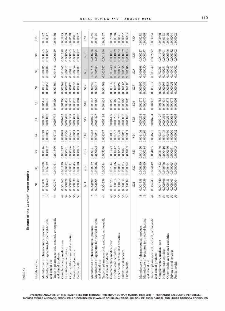
119C E P A L R E V I E W 1 1 6 • A U G U S T 2 0 1 5
SYSTEMIC ANALYSIS OF THE HEALTH SECTOR THROUGH THE INPUT-OUTPUT MATRIX, 2000-2005 • FERNANDO SALGUEIRO PEROBELLI, MÔNICA VIEGAS ANDRADE, EDSON PAULO DOMINGUES, FLAVIANE SOUSA SANTIAGO, JOILSON DE ASSIS CABRAL AND LUCAS BARBOSA RODRIGUES
TAB
LE
A.2
Extr
act o
f the
Leo
ntie
f inv
erse
mat
rix
Hea
lth s
ecto
rs
S1S2
S3S4
S5S6
S7S8
S9S1
0
Man
ufac
ture
of
phar
mac
eutic
al p
rodu
cts
180.
0034
310.
0274
080.
0001
460.
0002
180.
0003
650.
0064
320.
0018
100.
0008
050.
0003
650.
0013
72M
anuf
actu
re o
f ap
para
tus
for
med
ical
-hos
pita
l
and
dent
al u
se19
0.00
0869
0.00
6939
0.00
0037
0.00
0055
0.00
0092
0.00
1628
0.00
0458
0.00
0204
0.00
0092
0.00
0347
Tra
de i
n ph
arm
aceu
tical
, med
ical
, ort
hopa
edic
an
d de
ntal
pro
duct
s44
0.00
3274
0.00
4041
0.00
1979
0.00
2703
0.00
3737
0.00
5800
0.00
3360
0.00
4816
0.00
6629
0.00
6436
Com
plem
enta
ry m
edic
al c
are
480.
0013
650.
0011
500.
0012
770.
0030
480.
0016
230.
0017
000.
0022
680.
0016
650.
0012
880.
0018
95H
ospi
tal-
care
act
iviti
es54
0.00
0228
0.00
0252
0.00
0301
0.00
0366
0.00
0409
0.00
0439
0.00
0322
0.00
0312
0.00
0506
0.00
0409
Oth
er h
ealth
-car
e-re
late
d ac
tiviti
es55
0.00
0300
0.00
0331
0.00
0396
0.00
0481
0.00
0537
0.00
0577
0.00
0423
0.00
0411
0.00
0665
0.00
0538
Priv
ate
soci
al s
ervi
ces
560.
0000
390.
0000
430.
0000
520.
0000
630.
0000
710.
0000
760.
0000
560.
0000
540.
0000
870.
0000
71Pu
blic
hea
lth59
0.00
0002
0.00
0010
0.00
0005
0.00
0003
0.00
0002
0.00
0004
0.00
0003
0.00
0002
0.00
0002
0.00
0002
S11
S12
S13
S14
S15
S16
S17
S18
S19
S20
Man
ufac
ture
of
phar
mac
eutic
al p
rodu
cts
180.
0008
090.
0009
790.
0003
710.
0002
420.
0016
720.
0003
480.
0008
541.
0015
180.
0007
680.
0012
85M
anuf
actu
re o
f ap
para
tus
for
med
ical
-hos
pita
l
and
dent
al u
se19
0.00
0205
0.00
0248
0.00
0094
0.00
0061
0.00
0423
0.00
0088
0.00
0216
0.00
0384
1.00
0195
0.00
0325
Tra
de i
n ph
arm
aceu
tical
, med
ical
, ort
hopa
edic
an
d de
ntal
pro
duct
s44
0.00
4239
0.00
3744
0.00
3370
0.00
1597
0.00
2194
0.00
4634
0.00
4508
0.00
3787
0.00
1916
0.00
5167
Com
plem
enta
ry m
edic
al c
are
480.
0015
730.
0023
440.
0014
730.
0010
010.
0014
390.
0028
500.
0030
320.
0017
400.
0008
810.
0029
50H
ospi
tal-
care
act
iviti
es54
0.00
0314
0.00
0366
0.00
0412
0.00
0297
0.00
0222
0.00
0480
0.00
0378
0.00
0334
0.00
0169
0.00
0358
Oth
er h
ealth
-car
e-re
late
d ac
tiviti
es55
0.00
0412
0.00
0481
0.00
0542
0.00
0390
0.00
0292
0.00
0631
0.00
0497
0.00
0439
0.00
0222
0.00
0471
Priv
ate
soci
al s
ervi
ces
560.
0000
540.
0000
630.
0000
710.
0000
510.
0000
380.
0000
830.
0000
650.
0000
580.
0000
290.
0000
62Pu
blic
hea
lth59
0.00
0002
0.00
0002
0.00
0005
0.00
0004
0.00
0002
0.00
0003
0.00
0003
0.00
0006
0.00
0003
0.00
0003
S21
S22
S23
S24
S25
S26
S27
S28
S29
S30
Man
ufac
ture
of
phar
mac
eutic
al p
rodu
cts
180.
0013
380.
0006
300.
0011
200.
0011
060.
0002
540.
0002
770.
0001
920.
0001
980.
0002
270.
0002
38M
anuf
actu
re o
f ap
para
tus
for
med
ical
-hos
pita
l
and
dent
al u
se19
0.00
0339
0.00
0160
0.00
0284
0.00
0280
0.00
0064
0.00
0070
0.00
0049
0.00
0050
0.00
0057
0.00
0060
Tra
de i
n ph
arm
aceu
tical
, med
ical
, ort
hopa
edic
an
d de
ntal
pro
duct
s44
0.00
4943
0.00
4149
0.00
4065
0.00
4631
0.00
4634
0.00
4926
0.00
3014
0.00
3049
0.00
2992
0.00
3964
Com
plem
enta
ry m
edic
al c
are
480.
0018
400.
0018
220.
0021
660.
0022
470.
0021
260.
0017
810.
0026
360.
0022
610.
0019
600.
0029
60H
ospi
tal-
care
act
iviti
es54
0.00
0366
0.00
0376
0.00
0410
0.00
0403
0.00
0394
0.00
0436
0.00
0295
0.00
0251
0.00
0301
0.00
0373
Oth
er h
ealth
-car
e-re
late
d ac
tiviti
es55
0.00
0481
0.00
0494
0.00
0540
0.00
0530
0.00
0517
0.00
0573
0.00
0388
0.00
0329
0.00
0396
0.00
0490
Priv
ate
soci
al s
ervi
ces
560.
0000
630.
0000
650.
0000
710.
0000
700.
0000
680.
0000
750.
0000
510.
0000
430.
0000
520.
0000
64Pu
blic
hea
lth59
0.00
0004
0.00
0003
0.00
0003
0.00
0002
0.00
0003
0.00
0003
0.00
0002
0.00
0002
0.00
0002
0.00
0002

120 C E P A L R E V I E W 1 1 6 • A U G U S T 2 0 1 5
SYSTEMIC ANALYSIS OF THE HEALTH SECTOR THROUGH THE INPUT-OUTPUT MATRIX, 2000-2005 • FERNANDO SALGUEIRO PEROBELLI, MÔNICA VIEGAS ANDRADE, EDSON PAULO DOMINGUES, FLAVIANE SOUSA SANTIAGO, JOILSON DE ASSIS CABRAL AND LUCAS BARBOSA RODRIGUES
Hea
lth s
ecto
rs
S31
S32
S33
S34
S35
S36
S37
S38
S39
S40
Man
ufac
ture
of
phar
mac
eutic
al p
rodu
cts
180.
0004
750.
0001
460.
0003
490.
0002
270.
0024
500.
0005
350.
0003
730.
0003
680.
0002
780.
0004
77M
anuf
actu
re o
f ap
para
tus
for
med
ical
-hos
pita
l
and
dent
al u
se19
0.00
0120
0.00
0037
0.00
0088
0.00
0058
0.00
0620
0.00
0135
0.00
0094
0.00
0093
0.00
0070
0.00
0121
Tra
de i
n ph
arm
aceu
tical
, med
ical
, ort
hopa
edic
an
d de
ntal
pro
duct
s44
0.00
4625
0.00
6075
0.00
3669
0.00
5344
0.00
2403
0.00
7527
0.00
6818
0.00
5795
0.00
4777
0.00
4734
Com
plem
enta
ry m
edic
al c
are
480.
0022
800.
0014
080.
0020
220.
0024
840.
0014
230.
0025
060.
0026
200.
0025
650.
0020
700.
0014
07H
ospi
tal-
care
act
iviti
es54
0.00
0399
0.00
0379
0.00
0340
0.00
0400
0.00
0207
0.00
0450
0.00
0413
0.00
0373
0.00
0331
0.00
0334
Oth
er h
ealth
-car
e-re
late
d ac
tiviti
es55
0.00
0524
0.00
0498
0.00
0446
0.00
0526
0.00
0272
0.00
0592
0.00
0543
0.00
0491
0.00
0436
0.00
0439
Priv
ate
soci
al s
ervi
ces
560.
0000
690.
0000
650.
0000
590.
0000
690.
0000
360.
0000
780.
0000
710.
0000
640.
0000
570.
0000
58Pu
blic
hea
lth59
0.00
0003
0.00
0005
0.00
0002
0.00
0004
0.00
0002
0.00
0004
0.00
0004
0.00
0003
0.00
0003
0.00
0002
S41
S42
S43
S44
S45
S46
S47
S48
S49
S50
Man
ufac
ture
of
phar
mac
eutic
al p
rodu
cts
180.
0001
270.
0001
710.
0001
480.
0001
810.
0002
440.
0001
600.
0000
810.
0001
420.
0000
240.
0001
30M
anuf
actu
re o
f ap
para
tus
for
med
ical
-hos
pita
l
and
dent
al u
se19
0.00
0032
0.00
0043
0.00
0038
0.00
0046
0.00
0062
0.00
0041
0.00
0021
0.00
0036
0.00
0006
0.00
0033
Tra
de i
n ph
arm
aceu
tical
, med
ical
, ort
hopa
edic
an
d de
ntal
pro
duct
s44
0.00
1237
0.00
4013
0.00
1786
1.00
2186
0.00
3226
0.00
1619
0.00
0986
0.00
1722
0.00
0244
0.00
2243
Com
plem
enta
ry m
edic
al c
are
480.
0012
030.
0010
320.
0012
450.
0015
240.
0015
930.
0017
270.
0056
301.
0098
330.
0002
250.
0007
40H
ospi
tal-
care
act
iviti
es54
0.00
0175
0.00
0241
0.00
0525
0.00
0642
0.00
0277
0.00
0647
0.00
0209
0.00
0365
0.00
0077
0.00
0288
Oth
er h
ealth
-car
e-re
late
d ac
tiviti
es55
0.00
0230
0.00
0317
0.00
0690
0.00
0844
0.00
0364
0.00
0850
0.00
0275
0.00
0480
0.00
0101
0.00
0379
Priv
ate
soci
al s
ervi
ces
560.
0000
300.
0000
420.
0000
910.
0001
110.
0000
480.
0001
120.
0000
360.
0000
630.
0000
130.
0000
50Pu
blic
hea
lth59
0.00
0004
0.00
0002
0.00
0003
0.00
0004
0.00
0003
0.00
0005
0.00
0004
0.00
0007
0.00
0001
0.00
0001
S51
S52
S53
S54
S55
S56
S57
S58
S59
S60
Man
ufac
ture
of
phar
mac
eutic
al p
rodu
cts
180.
0022
600.
0001
270.
0014
870.
0346
710.
0250
140.
0274
010.
0006
610.
0016
260.
0525
160.
0039
40M
anuf
actu
re o
f ap
para
tus
for
med
ical
-hos
pita
l
and
dent
al u
se19
0.00
0572
0.00
0032
0.00
0376
0.00
8778
0.00
6333
0.00
6937
0.00
0167
0.00
0412
0.01
3296
0.00
0998
Tra
de i
n ph
arm
aceu
tical
, med
ical
, ort
hopa
edic
an
d de
ntal
pro
duct
s44
0.00
6520
0.00
1809
0.00
1545
0.00
3560
0.00
2569
0.00
2814
0.00
2169
0.00
1130
0.00
2291
0.00
1136
Com
plem
enta
ry m
edic
al c
are
480.
0010
380.
0012
350.
0005
320.
0013
300.
0009
600.
0010
510.
0006
440.
0002
690.
0005
340.
0051
73H
ospi
tal-
care
act
iviti
es54
0.00
0535
0.00
0310
0.00
0619
1.00
0555
0.00
0400
0.00
0438
0.00
0222
0.00
0371
0.00
0357
0.00
0449
Oth
er h
ealth
-car
e-re
late
d ac
tiviti
es55
0.00
0703
0.00
0408
0.00
0813
0.00
0729
1.00
0526
0.00
0576
0.00
0292
0.00
0487
0.00
0469
0.00
0591
Priv
ate
soci
al s
ervi
ces
560.
0000
920.
0000
540.
0001
070.
0000
960.
0000
691.
0000
760.
0000
380.
0000
640.
0000
620.
0000
78Pu
blic
hea
lth59
0.00
0002
0.00
0003
0.00
0005
0.00
0018
0.00
0013
0.00
0014
0.00
0003
0.00
0003
1.00
0025
0.00
0005
Sour
ce:
Pre
pare
d by
the
aut
hors
.
Tabl
e A
.2 (
conc
lude
d)

121C E P A L R E V I E W 1 1 6 • A U G U S T 2 0 1 5
SYSTEMIC ANALYSIS OF THE HEALTH SECTOR THROUGH THE INPUT-OUTPUT MATRIX, 2000-2005 • FERNANDO SALGUEIRO PEROBELLI, MÔNICA VIEGAS ANDRADE, EDSON PAULO DOMINGUES, FLAVIANE SOUSA SANTIAGO, JOILSON DE ASSIS CABRAL AND LUCAS BARBOSA RODRIGUES
ANNEX II
Formal construction of input-output indicators
The multipliers complement the analysis of the importance of a given sector in the economy, by making it possible to evaluate the short and long-term effects produced in a given economic system by exogenous disturbances (Miller and Blair, 2009).
The production multiplier measures the direct and indirect variation in the total production of an economy of all sectors and regions, caused by an exogenous variation of one monetary unit in the final demand of a given region or sector. In formal terms, the simple output multiplier for sector j, Oj, is given by:
O bj iji
n
1
==
/ (A.1)
where bij are the elements of the inverse Leontief matrix.The employment multiplier estimates the effects
of an exogenous change in final demand, in other words the number of jobs generated in the economy, either directly or indirectly, by a change in final demand that is sufficient to cause an increase in employment in sector j. Calculating the employment multiplier entails estimating the relation between the value of production of a given sector and employment in that sector. In formal terms:
ew X, jn j j1 =+ (A.2)
where ej represents personnel employed in sector j , and Xj is that sector’s gross production value.
For an economy with n sectors:
, , ,w w wW , , ,n n n nR 1 1 1 2 1g= + + +7 A (A.3)
So the simple employment multiplier is given by:
w bE ,n i ijji
n
11
= +=
/ (A.4)
where i represents a given sector of the economy and wn+1,i is the ratio between the number of employees and the value of production.
The matrix that results from that transformation (Ej) represents the sector capacity for generating employment per additional unit of final demand. The structure of the matrix Ej is similar to the structure of the matrices B (Leontief) and A (coefficients matrix). Consequently, for each sector j, the sum of the elements of each column represent the employment multiplier of sector j.
Rasmussen (1952) and Hirschman (1958) use backward and forward linkage indices to identify the sectors with the greatest linkage power in the economy. The backward linkages (power of dispersion) —Uj — determine how much a given sector demands from the other sectors of the economy, whereas the forward linkages (sensitivity of dispersion) —Ui — determine the degree to which that sector supplies demand from the other sectors the economy. The backward linkage index is defined as:
, , , ...,U n bn
b i j n1 1 1 2j iji ijji2= =_ i/ // (A.5)
The forward linkage index is defined as:
, , , ...,U n bn
b i j n1 1 1 2i ijj ijji2= =_ i/ // (A.6)
If Uj > 1, a unit variation in the final demand of sector j creates an above-average increase in the economy. If Ui > 1, a unit change in the final demand of all sectors creates an above average increase in the sector. Values above 1 in both indices identify key sectors in the economy. Those sectors have strong linkage effects in terms of the flow of goods and services, and make above-average contributions to the growth of the economy.

122 C E P A L R E V I E W 1 1 6 • A U G U S T 2 0 1 5
SYSTEMIC ANALYSIS OF THE HEALTH SECTOR THROUGH THE INPUT-OUTPUT MATRIX, 2000-2005 • FERNANDO SALGUEIRO PEROBELLI, MÔNICA VIEGAS ANDRADE, EDSON PAULO DOMINGUES, FLAVIANE SOUSA SANTIAGO, JOILSON DE ASSIS CABRAL AND LUCAS BARBOSA RODRIGUES
ANNEX III
TABLE A.3
Brazil: index of linkages and key sectors, 2000 and 2005
Economic sectorsBackward linkages Forward linkages Key sector
2000 2005 2000 2005 2000 2005
Agriculture, forestry, forestry management 0.8673 0.9086 1.6158 1.7715 - -Livestock and fishing 0.9629 1.0238 0.8550 0.8492 - -Oil and natural gas 0.9220 0.9692 1.3107 1.5526 - -Iron ore 1.0807 1.0224 0.6876 0.7293 - -Other extractive industry 1.0227 1.0500 0.8594 0.7967 - -Food and beverages 1.2718 1.2796 1.3742 1.4364 X XTobacco products 1.1258 1.2408 0.5625 0.5469 - -Textiles 1.0525 1.0254 1.1146 1.0826 X XGarments and accessories 1.0082 1.0241 0.5989 0.5657 - -Leather and footwear articles 1.2511 1.2159 0.6824 0.6822 - -Products onward except furniture 1.0114 1.1063 0.8078 0.8406 - -Cellulose and the likes of paper 1.0942 1.1403 1.2073 1.1404 X XNewspapers, magazines and discs 0.9844 0.9532 1.0359 0.8628 - -Oil and coke refining 1.2119 1.1900 1.9997 2.1330 X XAlcohol 1.0934 1.0238 0.7921 0.7015 - -Chemical products 1.1452 1.0975 1.9503 2.1663 X XManufacture of resins and elastomers 1.3315 1.2331 1.0811 1.1639 X XManufacture of pharmaceutical products 0.9313 0.9292 0.7023 0.6315 - -Manufacture of apparatus for medical-hospital and medical use 0.7266 0.7272 0.5637 0.5485 - -Pesticides 1.2635 1.1579 0.7379 0.7721 - -Perfume, hygiene and cleaning 1.0712 1.1283 0.7093 0.6286 - -Paints, varnishes, enamels and lacquers 1.1129 1.0757 0.6563 0.6185 - -Products and preparations of miscellaneous chemicals 1.0946 1.0787 0.8872 0.8494 - -Articles of rubber and plastic 1.2183 1.1675 1.2801 1.3594 X XCement 1.0467 1.1025 0.6274 0.6087 - -Other nonmetallic mineral products 1.1245 1.0734 0.7881 0.7804 - -Manufacture of steel and steel products 1.0944 1.0989 1.3294 1.6753 X XNon ferrous metallurgy 1.0882 1.0197 0.9302 0.8489 - -Products of metal, except machinery and equipment 1.0836 1.0515 1.1956 1.3435 X XMachinery and equipment, including maintenance and repairs 1.1059 1.1290 0.9712 0.9253 - -Electrical appliances 1.2088 1.2245 0.5708 0.5478 - -Office machinery and computer hardware 0.8997 0.9179 0.5525 0.5306 - -Electrical machines, apparatus and materials 1.0944 1.0729 0.9819 0.9758 - -Electronic material and communication equipment 1.0540 1.0635 0.7272 0.6465 - -Medical-hospital, measurement and optical apparatus and instruments
0.8435 0.8426 0.6242 0.6008 - -
Automobiles, trucks and utility vehicles 1.1507 1.2981 0.5815 0.5500 - -Trucks and buses 1.0829 1.1955 0.5731 0.5733 - -Parts and accessories for automotive vehicles 1.1286 1.2395 0.9680 1.2576 - -Other transport equipment 0.8862 1.1223 0.5860 0.6755 - -Furniture and products on various industries 1.0493 1.0252 0.6573 0.6066 - -Electricity and gas, water, sewerage and urban cleaning 0.9196 0.8993 2.2950 2.5283 - -Construction 0.9552 0.8919 0.7809 0.7343 - -Trade in other health services 0.7532 0.7443 2.4336 2.5043 - -Trade in pharmaceutical, medical, orthopaedic and dental products 0.8068 0.7945 0.6318 0.6322 - -Transport, storage and postal services 0.9298 0.9719 2.5105 2.5416 - -Information services 0.9017 0.8753 1.9773 1.9822 - -Financial intermediation and other insurance 0.8835 0.7574 2.2145 1.8974 - -Complementary medical care 0.9767 0.9343 0.6406 0.5811 - -Real estate and rental services 0.5732 0.5661 0.8905 0.8335 - -Maintenance and repair services 0.7837 0.7400 0.7956 0.6801 - -Hotel and restaurant services 1.0738 1.0632 0.7704 0.7014 - -Business services 0.8680 0.8112 2.4883 2.2097 - -Commercial education 0.8144 0.8221 0.5717 0.5511 - -Hospital-care activities 0.9960 0.9828 0.5443 0.5317 - -Other health-care-related activities 0.8197 0.8540 0.5513 0.5353 - -Private social services 0.9467 0.8858 0.5356 0.5223 - -Other services 0.8480 0.8188 0.8438 0.7459 - -Public education 0.6919 0.6963 0.5375 0.5233 - -Public health 0.8347 0.8441 0.5334 0.5205 - -Public administration and social security 0.8268 0.8008 0.7167 0.6672 - -
Source: Prepared by the authors.
Note: Health sectors shaded.

123C E P A L R E V I E W 1 1 6 • A U G U S T 2 0 1 5
SYSTEMIC ANALYSIS OF THE HEALTH SECTOR THROUGH THE INPUT-OUTPUT MATRIX, 2000-2005 • FERNANDO SALGUEIRO PEROBELLI, MÔNICA VIEGAS ANDRADE, EDSON PAULO DOMINGUES, FLAVIANE SOUSA SANTIAGO, JOILSON DE ASSIS CABRAL AND LUCAS BARBOSA RODRIGUES
AN
NE
X I
V
TAB
LE
A.4
Bra
zil:
prod
uctio
n an
d em
ploy
men
t mul
tiplie
rs, 2
000
and
2005
Eco
nom
ic s
ecto
rs
Prod
uctio
n m
ultip
liers
Em
ploy
men
t m
ultip
liers
2002
2005
2002
2005
Val
ueR
ank
Val
ueR
ank
Val
ueR
ank
Val
ueR
ank
Agr
icul
ture
, for
estr
y, f
ores
try
man
agem
ent
1.63
481.
7542
234
112
31
Liv
esto
ck a
nd fi
shin
g1.
8136
1.97
3119
53
113
2O
il an
d na
tura
l ga
s1.
7341
1.86
3720
5814
56Ir
on o
re2.
0323
1.96
3329
4715
54O
ther
ext
ract
ive
indu
stry
1.92
302.
0227
5225
3225
Food
and
bev
erag
es2.
392
2.46
211
98
698
Toba
cco
prod
ucts
2.11
112.
383
8517
689
Text
iles
1.97
271.
9728
7513
5614
Gar
men
ts a
nd a
cces
sori
es1.
8932
1.97
3011
15
955
Lea
ther
and
foo
twea
r ar
ticle
s2.
354
2.34
790
1059
11Pr
oduc
ts o
nwar
d ex
cept
fur
nitu
re1.
9031
2.13
1696
1461
10
Cel
lulo
se a
nd t
he l
ikes
of
pape
r2.
0518
2.19
1240
3231
26N
ewsp
aper
s, m
agaz
ines
and
dis
cs1.
8534
1.83
3839
2726
29O
il an
d co
ke r
efini
ng
2.27
62.
299
2357
1258
Alc
ohol
2.05
191.
9732
112
957
13C
hem
ical
pro
duct
s2.
159
2.11
1927
5316
51M
anuf
actu
re o
f re
sins
and
ela
stom
ers
2.50
12.
375
3046
1653
Man
ufac
ture
of
phar
mac
eutic
al p
rodu
cts
1.75
391.
7940
2652
1749
Man
ufac
ture
of
appa
ratu
s fo
r m
edic
al-h
ospi
tal
and
med
ical
use
1.36
581.
4058
3440
2041
Pest
icid
es2.
373
2.23
1138
3621
40Pe
rfum
e, h
ygie
ne a
nd c
lean
ing
2.01
252.
1714
3930
2927
Pain
ts, v
arni
shes
, ena
mel
s an
d la
cque
rs2.
0913
2.07
2133
3919
44Pr
oduc
ts a
nd p
repa
ratio
ns o
f m
isce
llane
ous
chem
ical
s2.
0515
2.07
2036
3422
34A
rtic
les
of r
ubbe
r an
d pl
astic
2.29
52.
2410
3933
2233
Cem
ent
1.96
292.
1217
2848
1847
Oth
er n
onm
etal
lic m
iner
al p
rodu
cts
2.11
122.
0622
6322
3822
Man
ufac
ture
of
stee
l an
d st
eel
prod
ucts
2.05
172.
1118
2555
1455
Non
fer
rous
met
allu
rgy
2.04
201.
9634
2850
1652
Prod
ucts
of
met
al, e
xcep
t m
achi
nery
and
equ
ipm
ent
2.03
212.
0226
4728
2530
Mac
hine
ry a
nd e
quip
men
t, in
clud
ing
mai
nten
ance
and
rep
airs
2.07
142.
1713
3638
2139
Ele
ctri
cal
appl
ianc
es2.
277
2.35
635
3721
38O
ffice
mac
hine
ry a
nd c
ompu
ter
hard
war
e1.
6944
1.76
4122
5416
50E
lect
rica
l m
achi
nes,
app
arat
us a
nd m
ater
ials
2.05
162.
0623
3342
1943

124 C E P A L R E V I E W 1 1 6 • A U G U S T 2 0 1 5
SYSTEMIC ANALYSIS OF THE HEALTH SECTOR THROUGH THE INPUT-OUTPUT MATRIX, 2000-2005 • FERNANDO SALGUEIRO PEROBELLI, MÔNICA VIEGAS ANDRADE, EDSON PAULO DOMINGUES, FLAVIANE SOUSA SANTIAGO, JOILSON DE ASSIS CABRAL AND LUCAS BARBOSA RODRIGUES
Eco
nom
ic s
ecto
rs
Prod
uctio
n m
ultip
liers
Em
ploy
men
t m
ultip
liers
2002
2005
2002
2005
Val
ueR
ank
Val
ueR
ank
Val
ueR
ank
Val
ueR
ank
Ele
ctro
nic
mat
eria
l an
d co
mm
unic
atio
n eq
uipm
ent
1.98
262.
0424
2845
1946
Med
ical
-hos
pita
l, m
easu
rem
ent
and
optic
al a
ppar
atus
and
ins
trum
ents
1.58
501.
6249
3044
1942
Aut
omob
iles,
tru
cks
and
utili
ty v
ehic
les
2.16
82.
491
3243
2235
Tru
cks
and
buse
s2.
0322
2.30
828
4919
45Pa
rts
and
acce
ssor
ies
for
auto
mot
ive
vehi
cles
2.12
102.
384
3641
2237
Oth
er t
rans
port
equ
ipm
ent
1.66
452.
1615
2156
1848
Furn
iture
and
pro
duct
s on
var
ious
ind
ustr
ies
1.97
281.
9729
6918
4718
Ele
ctri
city
and
gas
, wat
er, s
ewer
age
and
urba
n cl
eani
ng1.
7242
1.73
4317
5910
59C
onst
ruct
ion
1.79
371.
7144
7115
4817
Tra
de i
n ot
her
heal
th s
ervi
ces
1.41
571.
4356
9411
5912
Tra
de i
n ph
arm
aceu
tical
, med
ical
, ort
hopa
edic
and
den
tal
prod
ucts
1.51
551.
5354
8912
5415
Tra
nspo
rt, s
tora
ge a
nd p
osta
l se
rvic
es1.
7440
1.87
3657
2334
24In
form
atio
n se
rvic
es1.
6943
1.68
4638
3123
32Fi
nanc
ial
inte
rmed
iatio
n an
d ot
her
insu
ranc
e1.
6646
1.46
5525
5113
57C
ompl
emen
tary
med
ical
car
e1.
8335
1.80
3930
3522
36R
eal
esta
te a
nd r
enta
l se
rvic
es1.
0860
1.09
607
605
60M
aint
enan
ce a
nd r
epai
r se
rvic
es1.
4756
1.42
5792
778
7H
otel
and
res
taur
ant
serv
ices
2.01
242.
0425
126
680
6B
usin
ess
serv
ices
1.63
471.
5652
6019
4021
Com
mer
cial
edu
catio
n1.
5354
1.58
5060
2043
19H
ospi
tal-
care
act
iviti
es1.
8733
1.89
3544
2627
28O
ther
hea
lth-c
are-
rela
ted
activ
ities
1.54
531.
6447
5421
4320
Priv
ate
soci
al s
ervi
ces
1.78
381.
7045
133
410
34
Oth
er s
ervi
ces
1.59
491.
5751
156
210
93
Publ
ic e
duca
tion
1.30
591.
3459
7416
5016
Publ
ic h
ealth
1.57
511.
6248
5824
3623
Publ
ic a
dmin
istr
atio
n an
d so
cial
sec
urity
1.55
521.
5453
4129
2531
Med
ia1.
881.
9238
38
Sour
ce:
Pre
pare
d by
the
aut
hors
.
Not
e: H
ealt
h se
ctor
s sh
aded
.
Tabl
e A
.4 (
conc
lude
d)

125C E P A L R E V I E W 1 1 6 • A U G U S T 2 0 1 5
SYSTEMIC ANALYSIS OF THE HEALTH SECTOR THROUGH THE INPUT-OUTPUT MATRIX, 2000-2005 • FERNANDO SALGUEIRO PEROBELLI, MÔNICA VIEGAS ANDRADE, EDSON PAULO DOMINGUES, FLAVIANE SOUSA SANTIAGO, JOILSON DE ASSIS CABRAL AND LUCAS BARBOSA RODRIGUES
AN
NE
X V
TAB
LE
A.5
Fiel
d of
influ
ence
on
the
inpu
t-ou
tput
mod
el, 2
000
12
34
56
78
910
1112
1314
1516
1718
1920
2122
2324
2526
2728
2930
3132
3334
3536
3738
3940
4142
4344
4546
4748
4950
5152
5354
5556
5758
5960
11.
951.
541.
591.
481.
382.
391.
372.
421.
242.
221.
792.
001.
402.
171.
242.
241.
451.
421.
221.
441.
361.
221.
391.
481.
291.
331.
751.
561.
411.
441.
291.
471.
522.
381.
431.
381.
311.
862.
321.
312.
371.
321.
271.
211.
631.
881.
941.
241.
231.
231.
231.
751.
211.
211.
211.
201.
241.
201.
201.
222
2.07
1.65
1.70
1.58
1.47
2.56
1.46
2.58
1.32
2.37
1.91
2.13
1 .49
2.32
1.32
2.39
1.55
1.51
1.30
1.54
1.45
1.31
1.48
1.58
1.37
1.42
1.87
1.67
1.51
1.54
1.38
1.57
1.63
2.54
1.53
1.47
1.40
1.98
2.48
1.40
2.53
1.41
1.36
1.29
1.75
2.00
2.07
1.32
1.31
1.31
1.31
1.87
1.29
1.29
1.29
1.29
1.33
1.29
1.29
1.30
31.
741.
381.
431.
321.
232.
141.
232.
171.
111.
991.
601.
791.
251.
941.
112.
011.
301.
271.
091.
291.
221.
101.
241.
321.
151.
191.
571.
401.
261.
291.
161.
321.
362.
131.
281.
231.
181.
662.
081.
172.
121.
181.
141.
081.
461.
681.
741.
111.
101.
101.
101.
571.
081.
081.
081.
081.
111.
081.
081.
094
2.07
1.64
1.69
1.58
1.47
2.55
1.46
2.58
1.32
2.37
1.90
2.12
1.49
2.31
1.32
2.39
1.55
1.51
1.30
1.54
1.45
1.30
1.47
1.57
1.37
1.42
1.87
1.66
1.50
1.53
1.37
1.57
1.62
2.53
1.53
1.46
1.40
1.97
2.47
1.39
2.52
1.40
1.35
1.28
1.74
2.00
2.07
1.32
1.30
1.31
1.31
1.86
1.29
1.28
1.28
1.28
1.32
1.28
1.28
1.30
51.
831.
451.
501.
391.
302.
251.
292.
281.
172.
091.
681.
881.
312.
051.
172.
111.
371.
331.
151.
361.
281.
151.
301.
391.
211.
251.
651.
471.
331.
361.
221.
391.
432.
241.
351.
301.
241.
752.
191.
232.
231.
241.
201.
141.
541.
771.
831.
171.
151.
161.
161.
651.
141.
141.
141.
131.
171.
131.
131.
156
2.82
2.23
2.31
2.15
2.00
3.48
1.99
3.51
1.80
3.22
2.59
2.90
2.02
3.15
1.80
3.25
2.11
2.05
1.77
2.09
1.97
1.77
2.01
2.14
1.87
1.93
2.54
2.27
2.05
2.09
1.87
2.13
2.21
3.45
2.08
1.99
1.91
2.69
3.37
1.90
3.43
1.91
1.85
1.75
2.37
2.72
2.81
1.79
1.78
1.78
1.78
2.54
1.75
1.75
1.75
1.75
1.80
1.75
1.75
1.77
72.
071.
641.
691.
581.
472.
551.
462.
581.
322.
371.
902 .
131.
492.
321.
322.
391.
551.
511.
301.
541.
451.
301.
481.
581.
371.
421.
871.
671.
511.
531.
381.
571.
622.
541.
531.
471.
401.
982.
481.
392.
531.
411.
361.
291.
742.
002.
071.
321.
311.
311.
311.
871.
291.
291.
291.
281.
331.
281.
281.
308
2.79
2.21
2.29
2.13
1.98
3.45
1.97
3.49
1.78
3.20
2.57
2.87
2.01
3.13
1.78
3.23
3.60
2.09
2.04
1.76
2.08
1.96
1.76
1.99
2.13
1.85
1.91
2.52
2.25
2.03
2.07
1.86
2.12
2.19
3.42
3.82
2.06
1.98
1.89
2.67
3.34
1.88
3.41
1.90
1.83
1.74
2.35
2.70
2.79
1.78
1.76
1.77
1.77
2.52
1.74
1.73
1.73
1.73
1.79
1.73
1.73
1.75
92.
151.
711.
761.
641.
532.
661.
522.
691.
382.
471.
982.
221.
552.
411.
372.
491.
611.
571.
361.
601.
511.
361.
541.
641.
431.
481.
941.
741.
571.
601.
431.
631.
692.
641.
591.
531.
462.
062.
581.
452.
631.
461.
411.
341.
812.
082.
151.
371.
361.
361.
361.
941.
341.
341.
341.
341.
381.
341.
341.
3510
3.12
2.47
2.55
2.38
2.21
3.85
2.20
3.89
1.99
3.58
2.87
3.21
2.24
3.49
1.99
2.33
2.27
1.96
2.32
2.19
1.96
2.22
2.37
2.07
2.14
2.81
2.51
2.27
2.31
2 .07
2.36
2.44
2.30
2.21
2.11
2.98
3.73
3.38
2.10
3.80
2.12
2.04
1.94
2.62
3.01
3.12
1.99
1.97
1.97
1.97
2.81
1.94
1.94
1.94
1.93
2.00
1.93
1.93
1.96
112.
411.
911.
971.
841.
712.
971.
703.
011.
542.
762.
222.
481.
732.
701.
542.
781.
811.
761.
521.
791.
691.
521.
721.
841.
601.
652.
181.
941.
751.
791.
601.
831.
892.
961.
781.
711.
632.
302.
891.
622.
941.
641.
581.
502.
032.
332.
411.
541.
521.
521.
522.
171.
501.
501.
501.
501.
541.
501.
501.
5112
2.61
2.07
2.14
1.99
1.85
3.22
1.84
3.26
1.67
2.99
2 .40
2.69
1.88
2.92
1.67
3.02
1.96
1.91
1.64
1.94
1.83
1.65
1.86
1.99
1.73
1.79
2.36
2.11
1.90
1.94
1.74
1.98
2.05
3.20
1.93
1.85
1.77
2.50
3.13
1.76
3.19
1.78
1.71
1.62
2.20
2.53
2.61
1.67
1.65
1.65
1.65
2.36
1.63
1.62
1.62
1.62
1.67
1.62
1.62
1.64
131.
921.
521.
571.
461.
362.
371.
352.
391.
222.
201.
761.
971.
382.
151.
222.
221.
441.
401.
211.
431.
351.
211.
371.
461.
271.
311.
731.
551.
401.
421.
281.
451.
502.
351.
421.
361.
301.
832.
301.
292.
341.
301.
261.
191.
621.
861.
921.
221.
211 .
211.
211.
731.
191.
191.
191.
191.
231.
191.
191.
2014
2.82
2.24
2.31
2.15
2.00
3.48
1.99
3.52
1.80
3.23
2.59
2.90
2.03
3.16
1.80
3.26
2.11
2.06
1.78
2.10
1.98
1.78
2.01
2.15
1.87
1.93
2.55
2.27
2.05
2.09
1.88
2.14
2.21
3.46
2.08
2.00
1.91
2.70
1.90
3.44
1.92
1.85
1.75
2.37
2.73
2.82
1.80
1.78
1.78
1.78
2.54
1.76
1.75
1.75
1.75
1.81
1.75
1.75
1.77
151.
951.
551.
601.
491.
382.
411.
382.
431.
242.
231.
792.
011.
402.
181.
252.
251.
461.
421.
231.
451.
371.
231.
391.
491.
291.
341.
761.
571.
421.
451.
301.
481.
532.
391.
441.
381.
321.
862.
331.
312.
381.
331.
281.
211.
641.
891.
951.
241.
231.
231.
231.
761.
211.
211.
211.
211.
251.
211.
211.
2216
2.36
1.87
1.93
1.80
1.68
2.91
1.67
2.94
1.51
2.70
2.17
2.43
1.70
2.64
1.51
2.73
1.77
1.72
1.49
1.76
1.66
1.49
1.68
1.80
1.56
1.62
2.13
1.90
1.72
1.75
1.57
1.79
1.85
2.89
1.74
1.67
1.60
2.26
2.83
1.59
2.88
1.61
1.55
1.47
1.99
2.28
2.36
1.51
1.49
1.49
1.49
2.13
1.47
1.47
1.47
1.46
1.51
1.46
1.46
1.48
172.
111.
671.
731.
611.
502.
601.
492.
631.
342.
411.
942.
171.
512.
361.
352.
441.
581.
541.
331.
571.
481.
331.
501.
601.
401.
441.
901.
701.
531.
561.
401.
601.
652.
581.
561.
491.
432.
012.
521.
422.
571.
431.
381.
311.
772.
042.
111.
341.
331.
331.
331.
901.
311.
311.
311.
311.
351.
311.
311.
32
181.
911.
521.
571.
461.
362.
361.
352.
381.
222.
191.
761.
971.
372.
141.
222.
211.
431.
401.
201.
421.
341.
211.
361.
461.
271.
311.
731.
541.
391.
421.
271.
451.
502.
341.
411.
361.
291.
832.
291.
292.
331.
301.
251.
191.
611.
851.
911.
221 .
211.
211.
211.
721.
191.
191.
191.
191.
221.
191.
191.
2019
1.65
1.31
1.35
1.26
1.17
2.04
1.17
2.06
1.05
1.89
1.52
1.70
1.19
1.85
1.06
1.91
1.24
1.21
1.04
1.23
1.16
1.04
1.18
1.26
1.10
1.13
1.49
1.33
1.20
1.23
1.10
1.25
1.30
2.03
1.22
1.17
1.12
1.58
1.98
1.11
2.02
1.12
1.08
1.03
1.39
1.60
1.65
1.05
1.04
1.05
1.04
1.49
1.03
1.03
1.03
1.03
1.06
1.03
1.03
1.04
202.
081.
651.
711.
591.
482.
571.
472.
601.
332.
391.
922.
141.
502.
331.
332.
411.
561.
521.
311.
551.
461.
311.
491.
591.
381.
431.
881 .
681.
521.
551.
391.
581.
632.
551.
541.
481.
411.
992.
491.
402.
541.
421.
371.
301.
752.
022.
081.
331.
321.
321.
321.
881.
301.
291.
291.
291.
331.
291.
291.
3121
1.92
1.52
1.57
1.46
1.36
2.37
1.36
2.39
1.23
2.20
1.77
1.98
1.38
2.15
1.23
2.22
1.44
1.40
1.21
1.43
1.35
1.21
1.37
1.46
1.27
1.32
1.73
1.55
1.40
1.42
1.28
1.46
1.51
2.35
1.42
1.36
1.30
1.84
2.30
1.29
2.34
1.31
1.26
1.19
1.62
1.86
1.92
1.22
1.21
1.21
1.21
1.73
1.20
1.19
1.19
1.19
1.23
1.19
1.19
1.21
221.
801.
431.
471.
371.
282.
221 .
272.
241.
152.
061.
651.
851.
292.
011.
152.
081.
351.
311.
131.
341.
261.
141.
281.
371.
191.
231.
621.
451.
311.
331.
201.
361.
412.
211.
331.
271.
221.
722.
151.
212.
201.
221.
181.
121.
511.
741.
801.
151.
141.
141.
141.
621.
121.
121.
121.
121.
151.
121.
121.
1323
1.92
1.52
1.58
1.47
1.37
2.37
1.36
2.40
1.23
2.20
1.77
1.98
1.38
2.15
1.23
2.22
1.44
1.40
1.21
1.43
1.35
1.21
1.38
1.47
1.28
1.32
1.74
1.55
1.40
1.43
1.28
1.46
1.51
2.36
1.42
1.36
1.30
1.84
2.30
1.30
2.35
1.31
1.26
1.20
1.62
1 .86
1.92
1.23
1.21
1.22
1.22
1.73
1.20
1.19
1.19
1.19
1.23
1.19
1.19
1.21
242.
041.
621.
671.
561.
452.
521.
442.
551.
302.
341.
882.
101.
472.
291.
312.
361.
531.
491.
291.
521.
431.
291.
461.
561.
361.
401.
851.
651.
491.
521.
361.
551.
602.
511.
511.
451.
381.
952.
451.
382.
491.
391.
341.
271.
721.
982.
041.
301.
291.
291.
291.
841.
271.
271.
271.
271.
311.
271.
271.
2825
1.76
1.39
1.44
1.34
1.25
2.17
1.24
2.19
1.12
2.01
1.62
1.81
1.26
1.97
1.12
2.03
1.32
1.28
1.11
1.31
1.23
1.11
1.25
1.34
1 .17
1.20
1.59
1.42
1.28
1.30
1.17
1.33
1.38
2.15
1.30
1.25
1.19
1.68
2.10
1.18
2.14
1.19
1.15
1.09
1.48
1.70
1.76
1.12
1.11
1.11
1.11
1.58
1.09
1.09
1.09
1.09
1.13
1.09
1.09
1.10
261.
811.
431.
481.
381.
282.
231.
282.
251.
152.
071.
661.
861.
302.
021.
152.
091.
351.
321.
141.
341.
271.
141.
291.
381.
201.
241.
631.
461.
311.
341.
201.
371.
422.
221.
331.
281.
221.
732.
161.
222.
211.
231.
191.
121.
521.
751.
811.
151.
141.
141.
141.
631.
131.
121.
121.
121.
161.
121.
121.
1327
2.21
1.75
1.81
1.68
1.57
2.72
1.56
2.75
1.41
2.53
2.03
2.27
1.59
2.47
1.41
2.55
1.65
1.61
1.39
1.64
1.55
1.39
1.57
1.68
1.46
1.51
2.00
1.78
1.60
1.64
1.47
1.67
1.73
2.70
1.63
1.56
1.49
2.11
2.64
1.49
2.69
1.50
1.45
1.37
1.86
2.13
2.21
1.41
1.39
1.40
1.39
1.99
1.37
1.37
1.37
1.37
1.41
1.37
1.37
1.38
282.
131.
691.
741.
621.
512.
621.
502.
651.
362.
431.
962.
191.
532.
381.
362.
461.
591.
551.
341.
581.
491.
341.
521.
621.
411.
461.
921.
721.
551.
581.
411.
611.
672.
611.
571.
511.
442.
032.
541.
432.
601.
451.
391 .
321.
792.
062.
131.
361.
341.
351.
341.
921.
321.
321.
321.
321.
361.
321.
321.
3329
1.95
1.55
1.60
1.49
1.38
2.41
1.38
2.43
1.24
2.23
1.79
2.01
1.40
2.18
1.24
2.25
1.46
1.42
1.23
1.45
1.37
1.23
1.39
1.49
1.29
1.34
1.76
1.57
1.42
1.45
1.30
1.48
1.53
2.39
1.44
1.38
1.32
1.86
2.33
1.31
2.38
1.33
1.28
1.21
1.64
1.89
1.95
1.24
1.23
1.23
1.23
1.76
1.21
1.21
1.21
1.21
1.25
1.21
1.21
1.22
301.
941.
541.
591.
481.
372.
391.
372.
421.
242.
221.
781.
991.
392.
171.
242.
241.
451.
411.
221.
441.
361.
221.
381.
481.
281.
331.
751.
561.
411.
441.
291.
471.
522.
381.
431.
371.
311.
852.
321.
312.
361.
321.
271.
201.
631.
871.
941.
241.
221.
231.
221.
751.
211.
201.
201.
201.
241.
201.
201.
2231
1.90
1.50
1.55
1.44
1.34
2.34
1.34
2.36
1.21
2.17
1.74
1.95
1.36
2.12
1.21
2.19
1.42
1.38
1.19
1.41
1.33
1.19
1.35
1.44
1.26
1.30
1.71
1.53
1.38
1.41
1.26
1.44
1.49
2.32
1.40
1.34
1.28
1.81
2.27
1.28
2.31
1.29
1.24
1.18
1.60
1.83
1.89
1.21
1.20
1.20
1.20
1.71
1.18
1.18
1.18
1.18
1.21
1.18
1.18
1.19
322.
431.
931.
991.
851.
723.
001.
723.
031.
552.
782.
242.
501.
752.
721.
552.
811.
821.
771.
531.
811.
701.
531.
731.
851.
611.
672.
201.
961.
771.
801.
621.
851.
912.
981.
801.
721.
652.
322.
911.
642.
971.
651.
591.
512.
052.
352.
431.
551.
531.
541.
542.
191.
511.
511.
511.
511.
561.
511.
511.
5333
2.03
1.61
1.66
1.55
1.44
2.51
1.43
2.53
1.30
2.33
1.87
2.09
1.46
2.27
1.30
2.35
1.52
1.48
1.28
1.51
1.42
1.28
1.45
1.55
1.35
1.39
1.83
1.64
1.48
1.51
1.35
1.54
1.60
2.49
1.50
1.44
1.38
1.94
2.43
1.37
2.48
1.38
1.33
1.26
1.71
1.97
2.03
1.30
1.28
1.29
1.28
1.83
1.27
1.26
1.26
1.26
1.30
1.26
1.26
1.28
342.
802.
222.
302.
141.
993.
461.
983.
501.
793.
212.
582.
882.
023.
141.
793.
242.
102.
041.
762.
081.
971.
772.
002.
141.
861.
922.
532.
262.
042.
081.
862.
132.
203.
452.
071.
991.
902.
683.
361.
893.
421.
911.
841.
742.
362.
712.
801.
791.
771.
771.
772.
531.
751.
741.
741.
741.
801.
741.
741.
7635
1.95
1.54
1.59
1.48
1.38
2.40
1.37
2.43
1.24
2.23
1.79
2.00
1.40
2.18
1.24
2.25
1.46
1.42
1.22
1 .45
1.36
1.23
1.39
1.48
1.29
1.33
1.76
1.57
1.42
1.44
1.29
1.48
1.53
2.39
1.44
1.38
1.32
1.86
2.33
1.31
2.37
1.32
1.28
1.21
1.64
1.88
1.95
1.24
1.23
1.23
1.23
1.75
1.21
1.21
1.21
1.21
1.25
1.21
1.21
1.22
362.
111.
681.
731.
611.
502.
611.
492.
641.
352.
421.
942.
171.
522.
371.
352.
441.
581.
541.
331.
571.
481.
331.
511.
611.
401.
451.
911.
701.
541.
571.
411.
601.
662.
591.
561.
501.
432.
022.
531.
422.
581.
441.
391.
311.
782.
042.
111.
351.
331.
341.
341.
911.
321.
311.
311.
311.
351.
311.
311.
3337
2.03
1.61
1.66
1.54
1.44
2.50
1.43
2.52
1.29
2.32
1.86
2.08
1.46
2.27
1.29
2.34
1.52
1.48
1.27
1.51
1.42
1.28
1.44
1.54
1.34
1.39
1.83
1.63
1.47
1.50
1.35
1.54
1.59
2.48
1.50
1.44
1.37
1.94
2.42
1.36
2.47
1.38
1.33
1.26
1.71
1.96
2.02
1.29
1.28
1.28
1.28
1.83
1.26
1.26
1.26
1.26
1.30
1.26
1.26
1.27
382.
201.
751.
801.
681.
562.
721.
562.
751.
412.
522.
032.
271.
582.
471.
412.
551.
651.
611.
391.
641.
551.
391.
571.
681.
461.
511.
991.
781.
601.
631.
471.
671.
732.
701.
631.
561.
492.
112.
641.
482.
691.
501.
451.
371.
862.
132.
201.
401.
391.
391.
391.
991.
371.
371.
371.
371.
411.
371.
371.
3839
3.15
2.50
2.58
2.40
2.24
3.88
2.22
3.93
2.01
3.61
2.90
3.24
2.26
3.52
2.01
3.64
2.36
2.30
1.98
2.34
2.21
1.99
2.25
2.40
2.09
2.16
2.85
2.54
2.29
2.34
2.09
2.39
2.47
3.86
2.33
2.23
2.13
3.01
3.78
2.12
3.84
2.14
2.07
1.96
2.65
3.05
3.15
2.01
1.99
1.99
1.99
2.84
1.96
1.96
1.96
1.95
2.02
1.95
1.95
1.98
401.
821.
441.
491.
381.
292.
241.
282.
261.
162.
081.
671.
871.
312.
031.
162.
101.
361 .
321.
141.
351.
271.
141.
301.
381.
201.
241.
641.
461.
321.
351.
211.
381.
422.
231.
341.
291.
231.
742.
171.
232.
221.
231.
191.
131.
531.
761.
821.
161.
151.
151.
151.
641.
131.
131.
131.
131.
161.
131.
131.
1441
2.93
2.32
2.40
2.23
2.08
3.61
2.07
3.65
1.87
3.35
2.69
3.01
2.10
3.28
1.87
3.38
2.19
2.14
1.84
2.18
2.05
1.85
2.09
2.23
1.94
2.01
2.64
2.36
2.13
2.17
1.95
2.22
2.30
3.59
2.16
2.07
1.98
2.80
3.50
1.97
3.58
1.99
1.92
1.82
2.46
2.83
2.93
1.87
1.85
1.85
1.85
2.64
1.82
1.82
1.82
1.82
1 .87
1.82
1.82
1.84
421.
821.
441.
491.
391.
292.
251.
292.
271.
162.
081.
671.
871.
312.
041.
162.
101.
361.
331.
151.
351.
281.
151.
301.
391.
211.
251.
641.
471.
321.
351.
211.
381.
432.
231.
341.
291.
231.
742.
181.
232.
221.
241.
191.
131.
531.
761.
821.
161.
151.
151.
151.
641.
131.
131.
131.
131.
171.
131.
131.
1443
1.77
1.40
1.45
1.35
1.25
2.18
1.25
2.20
1.13
2.02
1.62
1.82
1.27
1.98
1.13
2.04
1.32
1.29
1.11
1.31
1.24
1.11
1.26
1.34
1.17
1.21
1.59
1.42
1.28
1.31
1.17
1.34
1.38
2.16
1.30
1 .25
1.20
1.69
2.11
1.19
2.15
1.20
1.16
1.10
1.49
1.71
1.76
1.13
1.11
1.12
1.12
1.59
1.10
1.10
1.10
1.09
1.13
1.09
1.09
1.11
441.
691.
341.
381.
291.
202.
081.
192.
111.
081.
931.
551.
741.
211.
891.
081.
951.
271.
231.
061.
261.
181.
061.
211.
291.
121.
161.
531.
361.
231.
251.
121.
281.
332.
071.
251.
201.
141.
612.
021.
142.
061.
151.
111.
051.
421.
631.
691.
081.
071.
071.
071.
521.
051.
051.
051.
051.
081.
051.
051.
06
452.
091.
651.
711.
591.
482.
581.
472.
601.
332.
391.
922.
151.
502.
341 .
332.
411.
561.
521.
311.
551.
461.
321.
491.
591.
381.
431.
891.
681.
521.
551.
391.
581.
642.
561.
541.
481.
412.
002.
501.
412.
551.
421.
371.
301.
762.
022.
091.
331.
321.
321.
321.
881.
301.
301.
301.
301.
341.
291.
301.
3146
2.27
1.80
1.86
1.73
1.61
2.80
1.60
2.83
1.45
2.60
2.09
2.33
1.63
2.54
1.45
2.62
1.70
1.65
1.43
1.69
1.59
1.43
1.62
1.73
1.50
1.55
2.05
1.83
1.65
1.68
1.51
1.72
1.78
2.78
1.68
1.61
1.54
2.17
2.72
1.53
2.77
1.54
1.49
1.41
1.91
2.20
2.27
1.45
1.43
1.44
1.43
2.05
1.41
1.41
1 .41
1.41
1.45
1.41
1.41
1.42
472.
351.
861.
921.
791.
672.
901.
662.
931.
502.
692.
162.
421.
692.
631.
502.
711.
761.
711.
481.
751.
651.
481.
681.
791.
561.
612.
121.
891.
711.
741.
561.
781.
842.
881.
731.
661.
592.
242.
811.
582.
871.
601.
541.
461.
982.
272.
351.
501.
481.
491.
482.
121.
461.
461.
461.
461.
501.
461.
461.
47
481.
801.
421.
471.
371.
272.
221.
272.
241.
152.
061.
651.
851.
292.
011.
152.
071.
351.
311.
131.
341.
261.
131.
281.
371.
191.
231.
621.
451.
311.
331.
191.
361.
412.
201.
331.
271.
221.
722.
151.
212.
191.
221.
181.
121.
511.
741.
801.
151.
131.
141.
141.
621.
121.
121.
121.
111.
151.
111.
111.
13
491.
621.
281.
331.
241.
152.
001.
142.
021.
031.
861.
491.
671.
171.
811.
031.
871.
211.
181.
021.
211.
141.
021.
161.
231.
071.
111.
461.
311.
181.
201.
081.
231.
271.
991.
201.
151.
101.
551.
941.
091.
981.
101.
061.
011.
361.
571.
621.
031.
031.
031.
021.
461.
011.
011.
011.
011.
041.
011.
011.
0250
1.69
1.34
1.38
1.29
1.20
2.08
1.19
2.10
1.08
1.93
1.55
1.74
1.21
1.89
1.08
1.95
1.26
1.23
1.06
1.26
1.18
1.06
1.20
1.29
1.12
1.16
1.52
1.36
1.23
1.25
1.12
1.28
1.32
2.07
1.25
1.20
1.14
1.61
2.02
1.14
2.06
1.15
1.11
1.05
1.42
1.63
1.69
1.08
1.07
1.07
1.07
1.52
1.05
1.05
1.05
1.05
1.08
1.05
1.05
1.06
512.
171.
721.
781.
661.
542.
681.
532.
711.
392.
492.
002.
231.
562.
431.
392.
511.
631.
581.
371.
621.
521.
371.
551.
651.
441.
491.
961.
751.
581.
611.
441.
651.
702.
661.
601.
541.
472.
082.
601.
462.
651.
481.
421.
351.
832.
102.
171.
391.
371.
371.
381 .
961.
351.
351.
351.
351.
391.
351.
351.
3652
1.94
1.54
1.59
1.48
1.38
2.39
1.37
2.42
1.24
2.22
1.78
1.99
1.39
2.17
1.24
2.24
1.45
1.41
1.22
1.44
1.36
1.22
1.38
1.48
1.29
1.33
1.75
1.56
1.41
1.44
1.29
1.47
1.52
2.38
1.43
1.37
1.31
1.85
2.32
1.31
2.37
1.32
1.27
1.21
1.63
1.88
1.94
1.24
1.22
1.23
1.23
1.75
1.21
1.20
1.20
1.20
1.24
1.20
1.20
1.22
531.
671.
321.
361.
271.
182.
061.
182.
081.
061.
911.
531.
711.
201.
861.
061.
921.
251.
221.
051.
241.
171.
051.
191.
271.
101.
141.
501.
341.
211.
241 .
111.
261.
312.
041.
231.
181.
131.
591.
991.
122.
031.
131.
091.
041.
401.
611.
671.
061.
051.
051.
051.
501.
041.
031.
031.
031.
071.
031.
031.
05
541.
711.
351.
401.
301.
212.
101.
202.
131.
091.
951.
571.
761.
231.
911.
091.
971.
281.
241.
071.
271.
201.
081.
221.
301.
131.
171.
541.
371.
241.
271.
131.
291.
342.
091.
261.
211.
161.
632.
041.
152.
081.
161.
121.
061.
441.
651.
711.
091.
081.
081.
081.
541.
061.
061.
061.
061.
091.
061.
061.
0755
1.65
1.31
1.35
1.26
1.17
2.04
1.16
2.06
1.05
1 .89
1.52
1.70
1.19
1.85
1.05
1.91
1.24
1.20
1.04
1.23
1.16
1.04
1.18
1.26
1.09
1.13
1.49
1.33
1.20
1.22
1.10
1.25
1.29
2.02
1.22
1.17
1.12
1.58
1.97
1.11
2.01
1.12
1.08
1.03
1.39
1.60
1.65
1.05
1.04
1.04
1.04
1.49
1.03
1.02
1.03
1.02
1.06
1.02
1.02
1.04
561.
691.
341.
381.
291.
202.
081.
192.
101.
081.
931.
551.
731.
211.
891.
081.
951.
261.
231.
061.
251.
181.
061.
201.
281.
121.
161.
521.
361.
231.
251.
121.
281.
322.
071.
251.
201.
141.
612.
021.
142.
061.
151.
111.
051.
421.
631.
691.
081.
061.
071.
071.
521.
051.
051.
051.
051.
081.
051.
051.
06
571.
711.
351.
401.
301.
212.
111.
212.
131.
091.
961.
571.
761.
231.
911.
091.
971.
281.
251.
081.
271.
201.
081.
221.
301.
131.
171.
541.
381.
241.
271.
141.
301.
342.
091.
261.
211.
161.
632.
041.
152.
081.
161.
121.
061.
441.
651.
711.
091.
081.
081.
081.
541.
061.
061.
061.
061.
101.
061.
061.
0758
1.63
1.29
1.33
1.24
1.15
2.01
1.15
2.03
1.04
1.86
1.50
1.67
1.17
1.82
1.04
1.88
1.22
1.19
1.02
1.21
1.14
1.03
1.16
1.24
1.08
1.11
1.47
1.31
1 .18
1.21
1.08
1.23
1.28
1.99
1.20
1.15
1.10
1.55
1.95
1.10
1.99
1.11
1.07
1.01
1.37
1.57
1.63
1.04
1.03
1.03
1.03
1.47
1.01
1.01
1.01
1.01
1.04
1.01
1.01
1.02
591.
661.
321.
361.
271.
182.
051.
172.
071.
061.
901.
531.
711.
201.
861.
061.
921.
251.
211.
051.
241.
171.
051.
191.
271.
101.
141.
501.
341.
211.
231.
111.
261.
302.
041.
231.
181.
131.
591.
991.
122.
031.
131.
091.
031.
401.
611.
661.
061.
051.
051.
051.
501.
041.
031.
031.
031.
071.
031.
031.
04
601.
691.
341.
381.
291.
202.
091.
192 .
111.
081.
941.
551.
741.
221.
891.
081.
951.
271.
231.
061.
261.
191.
071.
211.
291.
121.
161.
531.
361.
231.
251.
121.
281.
332.
071.
251.
201.
141.
622.
021.
142.
061.
151.
111.
051.
421.
641.
691.
081.
071.
071.
071.
521.
051.
051.
051.
051.
081.
051.
051.
06
Selling sectors
Purc
hasi
ng s
ecto
rs
One
sta
ndar
d de
viat
ion
abov
e th
e m
ean
Bet
wee
n on
e an
d tw
o st
anda
rd d
evia
tions
abo
ve th
e m
ean
Bet
wee
n tw
o an
d th
ree
stan
dard
dev
iatio
ns a
bove
the
mea
nM
ore
than
thre
e st
anda
rd d
evia
tions
abo
ve th
e m
ean
Sour
ce:
Pre
pare
d by
the
aut
hors
, on
the
bas
is o
f th
e in
put-
outp
ut m
odel
.

126 C E P A L R E V I E W 1 1 6 • A U G U S T 2 0 1 5
SYSTEMIC ANALYSIS OF THE HEALTH SECTOR THROUGH THE INPUT-OUTPUT MATRIX, 2000-2005 • FERNANDO SALGUEIRO PEROBELLI, MÔNICA VIEGAS ANDRADE, EDSON PAULO DOMINGUES, FLAVIANE SOUSA SANTIAGO, JOILSON DE ASSIS CABRAL AND LUCAS BARBOSA RODRIGUES
Almeida, C. and others (2000), “Health sector reform in Brazil: A case study of inequity”, International Journal of Health Services, vol. 30, No. 1, sage.
Andrade, M.V. (2002), “A saúde na pnad”, Texto para Discussão, No. 170, Belo Horizonte, Federal University of Minas Gerais/Centre for Regional Development and Planning.
Azzoni, C.R. and others (2007), “Social policies, personal and income inequality in Brazil: I-O analysis of the ‘Bolsa Família’ progam”, Anais do V Encontro Nacional da Associação Brasileira de Estudos Regionais e Urbanos, Pernambuco.
Betarelli Junior, A.A., S.Q.A. Bastos and F.S. Perobelli (2008), “As pressões das exportações setoriais sobre os modais de transporte: uma abordagem híbrida e intersetorial de insumo-produto”, Pesquisa e Planejamento Econômico, vol. 38, No. 3, Institute of Applied Economic Research (ipea).
Bloom, D., D. Canning and J. Sevilla (2001), “The effect of health on economic growth: Theory and evidence”, nber Working Paper, No. 8587, Cambridge, Massachusetts, National Bureau of Economic Research.
Brazil, Ministry of Health (2010), Doenças infecciosas e parasitárias, Brasilia.
(2004), Saúde Brasil 2004: uma análise da situação de saúde, Brasilia.
Camargo, M.C.S., R.N. Rodrigues and C.J. Machado (2006), “Expectativa de vida saudável para idosos brasileiros, 1998 e 2003”, Anais do XV Encontro Nacional de Estudos Populacionais, Caxambu, Minas Gerais.
Campelo, V., M.A.G. Gonçalves and E.A. Donadi (2005), “Mortalidade por doenças infecciosas e parasitárias no Município de Teresina-pi (Brasil), 1971-2000”, Revista Brasileira de Epidemiologia, vol. 8, No. 1, Brazilian Association of Collective Health.
Correa, H. and B. Parker (2005), “An application of organizational input-output analysis to hospital management”, Socio-Economic Planning Sciences, vol. 39, No. 4, Amsterdam, Elsevier.
Guilhoto, J.J.M. (2004), Análise de insumo-produto: teoria e fundamentos, São Paulo.
Guilhoto, J.J.M. and others (1994), “Índices de ligação e setores-chave na economia brasileira: 1959/80”, Pesquisa e Planejamento Econômico, vol. 24, No. 4, Institute of Applied Economic Research (ipea).
Hilgemberg, E.M. and J.M. Guilhoto (2006), “Uso de combustíveis e emissões de co2 no Brasil: um modelo inter-regional de insumo-produto”, Nova Economia, vol. 16, No. 1, Belo Horizonte.
Hirschman, A.O. (1958), The Strategy of Economic Development, New Haven, Yale University Press.
Hongyi, W. (2009), “The Analysis of Input-Output in Hospital and the Practical Application in Medicine Health Domain”, document presented at the 17th International Conference on Input- Output Techniques.
ibge (Brazilian Geographical and Statistical Institute) (2008), Economia da saúde: uma perspectiva macroeconômica 2000-2005, Rio de Janeiro.
(n/d), “Matriz de insumo-produto (2000 e 2005)” [online] http://www.ibge.gov.br/.
Imori, D. and J.J.M. Guilhoto (2007), “Estrutura produtiva brasileira e emissão de co2”, Anais do V Encontro da Associação Brasileira de Estudos Regionais e Urbanos, Recife.
Luna, E. (2002), “A emergência das doenças emergentes e as doenças infecciosas emergentes e reemergentes no Brasil”, Revista Brasileira de Epidemiologia, vol. 5, No. 3, Brazilian Association of Collective Health.
Marinho, A., S.S. Cardoso and V.V. Almeida (2009), “Brasil e ocde: avaliação da eficiência em sistemas de saúde”, Texto para Discussão, No. 1370, Institute of Applied Economic Research (ipea).
Bibliography
Mattos, R.S. and others (2008), “Integração de modelos econométricos e de insumo produto para previsões de longo prazo da demanda de energia no Brasil”, Estudos Econômicos, vol. 38, São Paulo, University of São Paulo.
Miller, R. and P. Blair (2009), Input-Output Analysis: Foundations and Extensions, New Jersey, Prentice-Hall.
Moreira, G. (2007), “Politicas sociais, desigualdades pessoais e regionais da renda no Brasil: uma analise de insumo-produto”, Luiz de Queiroz College of Agriculture.
oecd (Organization for Economic Cooperation and Development) (2010), “oecd Health Data 2010: Statistics and Indicators” [online] http://www.oecd.org.br.
Perobelli, F.S., R.S. Mattos and W.R. Faria (2007), “Interações energéticas entre o Estado de Minas Gerais e o restante do Brasil: uma análise inter-regional de insumo-produto”, Economia Aplicada, vol. 11, No. 1, São Paulo, University of São Paulo.
Rasmussen, P.N. (1952), Studies in Inter-Sectoral Relations, Amsterdam, North-Holland.
Ribeiro, M.B. (2009), “Eficiência do gasto público na América Latina: uma análise comparativa a partir do modelo semi-paramétrico com estimativa em dois estágios”, Gestión Pública series, No. 67 (LC/L.2883-P), Santiago, Economic Commission for Latin America and the Caribbean (eclac). United Nations publication, Sales No. P.08.II.G.28.
(2008), “Desempenho e eficiência do gasto público: uma análise comparativa entre o Brasil e um conjunto de países da América Latina”, Texto para Discussão, No. 1368, Brasilia, Institute of Applied Economic Research (ipea).
Ribeiro, M.B. and W. Rodrigues Jr. (2006), “Eficiência do gasto público na América Latina”, Boletim de Desenvolvimento Fiscal, No. 3, Institute of Applied Economic Research (ipea).
Robine, J.M., I. Romieu and E. Cambois (1999), “Health expectancy indicators”, Bulletin of the World Health Organization, Geneva, World Health Organization (who).
Rodrigues, R.L. and J.J.M. Guilhoto (2004), “Estrutura produtiva, relações intersetoriais e cooperativas agropecuárias no Paraná em 1980 e 1985”, Revista de Economia e Sociologia Rural, vol. 42, No. 2, Brazilian Society of Rural Sociology and Economics.
Schramm, J.N.A. and others (2004), “Transição epidemiológica e o estudo de carga de doença no Brasil”, Ciência & Saúde Coletiva, vol. 9, No. 4, Brazilian Association of Collective Health.
Sesso Filho, U.A. and others (2006), “Interações sinérgicas e transbordamento do efeito multiplicador de produção das grandes regiões do Brasil”, Economia Aplicada, vol. 10, No. 2, São Paulo, University of São Paulo.
Sonis, M. and G.J.D. Hewings (1992), “Coefficient changes in input-output models: theory and applications”, Economic Systems Research, vol. 4, No. 2.
Terra, L.P. and B.L. Queiroz (2010), “Qualidade de vida: qual é a esperança de vida feliz no Brasil?”, Anais do XVII Encontro Nacional de Estudos Populacionais, Caxambu, Minas Gerais.
Toyoshima, S. and M.J. Ferreira (2002), “Encadeamentos do setor de transportes na economia brasileira”, Planejamento e Políticas Públicas, No. 25, Institute of Applied Economic Research (ipea).
World Bank (2007), “pib per cápita” [online] http://datos.bancomundial.org/indicador/NY.GDP.PCAP.CD.
who (World Health Organization) (2010), “Global health indicators”, World Health Statistics 2010, Geneva [online] http://www.who.int/gho/publications/world_health_statistics/EN_WHS10_Full.pdf.
(2009), World Health Statistics 2009, Geneva [online] http://www.who.int/gho/publications/world_health_statistics/EN_WHS09_Full.pdf.
(2001), Macroeconomics and Health: Investing in Health for Economic Development. Report of the Commission on Macroeconomics and Health, Geneva.

The different faces of inclusion and exclusion
Aldo Mascareño and Fabiola Carvajal
ABSTRACT The notions of inclusion and exclusion have a long tradition in sociology, but have gained significant currency more recently in public policy analysis. However, a certain conceptual inflexibility arises when the distinction is applied to complex social situations. This article examines the main approaches to inclusion/exclusion in the sociological tradition, systems theory and the theory of new inequalities. On this basis, five interrelated situations of inclusion and exclusion are constructed: self-inclusion/self-exclusion, inclusion by risk/exclusion by danger, compensatory inclusion, inclusion in exclusion and sub-inclusion. They are illustrated with specific examples to refine an analytical approach to problems of inclusion and exclusion, with a view to contributing to sociological analysis and to assessing the consequences of public and private decisions.
KEYWORDS Social isolation, social integration, sociology, social structure, social policy
JEL CLASSIFICATION D63, D78, D81
AUTHORS Aldo Mascareño is a full professor with the School of Government of Adolfo Ibáñez University in Santiago, Chile. [email protected]
Fabiola Carvajal is a research assistant with the School of Government of Adolfo Ibáñez University in Santiago, Chile. [email protected]
128 C E P A L R E V I E W 1 1 6 • A U G U S T 2 0 1 5
THE DIFFERENT FACES OF INCLUSION AND EXCLUSION • ALDO MASCAREÑO AND FABIOLA CARVAJAL
This article forms part of the research activities of projects Redes 130008, National Fund for Scientific and Technological Development (fondecyt) 1140344, 1110437, and Núcleo Milenio Modelos de Crisis (NS130017), icm-Iniciativa Científica Milenio.
The concepts of inclusion and exclusion began to gain popularity in public policy analysis and practice in the 1990s, especially in Europe and in the work of international organizations. Programmes run by the International Labour Organization (ilo), the United Nations, commissions of the European Union and intersectoral bodies such as the Social Exclusion Unit of the Government of Tony Blair in the United Kingdom, built their social agendas around such concepts (MacPherson, 1997; Porter, 2000; Davies, 2005). Even before then, however, they had been used in French social policy (Lenoir, 1974) to refer to social groups warranting attention from government policy. The now widespread use of the inclusion/exclusion distinction in policy design reflects the fact that it introduces a readily understandable and broadly applicable strategic and political criterion: people fall within or outside specific social criteria, above or below certain limits which express difference.
Useful though this binary formula may be for policymaking, insofar as it provides concrete guidelines for deciding on measures and visualizing outcomes, from a sociological standpoint, drawing a sharp distinction between inclusion and exclusion is more of an artifice constructed for instrumental purposes than an actual observation of social circumstances. In its static form, the distinction transforms processes (for example, participation versus marginalization) into states (inclusion versus exclusion), attaches social categorizations to individuals (excluded versus included), and, by
demarcating boundaries, impedes the conception of paradoxical constellations in which different modalities of inclusion and exclusion are mingled (Goodin, 1996; Davies, 2005; Sánchez, 2012).
This article reviews the inclusion/exclusion distinction, aiming to overcome its limitations, reveal the paradoxes it masks and identify, conceptually, various forms of inclusion/exclusion that may refer to concrete situations. The hypothesis underlying this exercise is that social practices of different natures exist in modern societies, and these inevitably produce paradoxes that are hidden when the inclusion/exclusion distinction is applied in its static form. In order to address these paradoxes, it is first necessary to identify the conditions of inclusion within exclusion, and the conditions of exclusion within inclusion. This exercise should yield diverse constellations of inclusion/exclusion that take us beyond a static understanding of the distinction, which tends to entrench the very inclusion and exclusion conditions that we are trying to overcome.
To support this hypothesis, this Introduction is followed, in section II, with a reconstruction of the inclusion/exclusion distinction in sociological tradition (Simmel, Durkheim, Parsons), with an emphasis on the paradoxes that it reveals and hides. Section III continues with a systemic elaboration of the distinction (Luhmann, Stichweh), before discussing the proposal of the French school (Fitoussi, Rosanvallon) to show the limitations of the static version of the distinction inclusion/exclusion for addressing the emergence of new inequalities (section IV). On this basis, section V proposes an original classification of different constellations of inclusion/exclusion and illustrates them with specific examples. Section VI offers a summary of the main findings together with their conceptual and public policy implications.
IIntroduction

129C E P A L R E V I E W 1 1 6 • A U G U S T 2 0 1 5
THE DIFFERENT FACES OF INCLUSION AND EXCLUSION • ALDO MASCAREÑO AND FABIOLA CARVAJAL
In the history of sociological thought, the distinction inclusion/exclusion has been associated mostly with the functionalist tradition from Durkheim to Luhmann (Rawal, 2008; Braeckman, 2006; Allman, 2012). Nonetheless, it was Georg Simmel who originally noted the paradoxical nature of the inclusion/exclusion relationship. His essays on the stranger and on secrecy illustrate this point. The stranger is neither in nor out, or may be both at the same time. The stranger belongs to the social group, but comes from beyond; he develops charm and significance, but is not the “owner of soil,” either in a physical sense or in terms of social reference (Simmel, 1950a, p. 403). This ambiguity moves the group towards openness with the stranger, from confidence to confession, but at the same time the stranger maintains his freedom in practical terms. In other words, the stranger is not included or excluded; or is just as included as excluded.
Secrecy works in a more radical way: included are those who know; the rest are excluded. This binary use of distinction hides paradoxes, however. Secrecy involves a strong sense (expectation) of difference among persons, based on the possession of knowledge as inner property of the group (Simmel, 1950b). Inclusion in the secret develops the group’s identity and its boundaries. Yet there are inclusive groups (nations, creeds) for which the secret consists in “including everybody who is not explicitly excluded” (Simmel, 1950b, p. 369). In this case, Simmel gives the distinction a binary application: “The principle of including that which is not explicitly excluded is opposed by the principle of excluding that which is not explicitly included” (Simmel, 1992, p. 447). This masks the real paradoxes. In political matters, for example, inclusion by the State initially excludes members of other States (until they become “nationalized” or acquire some sort of formal citizenship): it excludes them in inclusion. And in religious matters, inclusion through tolerance means acceptance of the other who is nevertheless excluded as an equal. Inclusion and exclusion appear rather as interpenetrated forms.
In Durkheim’s work, the conceptualization of inclusion/exclusion must be reconstructed from the
author’s analysis of solidarity and anomy. Modern society implies an order of simultaneous inclusions and exclusions: inclusion as organic solidarity, exclusion as spheres outside the division of labour (Durkheim, 2001). This raises new issues of integration, which are reflected in types of suicide (Durkheim, 2002). Paradoxically, the egotistic and anomic suicide (lack of integration) encourages the suicidal to follow a social pattern of suicide by which he or she expresses denial of society (a lonely place, a means, a stage, a note). Also paradoxically, the suicidal must recognize him or herself as a member of society in order to reject the social, otherwise he would be a “death person,” not a “suicidal.” The suicide is thus included in his (last) exclusion. What Durkheim calls altruistic suicide (high integration) is a refusal of society in the name of society. Semantically, society elaborates such acts of self-sacrifice in terms of the martyr, the hero, the saint (Luhmann, 1993), affirming the act as desirable: exclusion is sustained (and viewed positively) as an act of inclusion.
Parsons goes further than Simmel and Durkheim by giving the inclusion/exclusion distinction explicit sociological meaning: “The process by which previously excluded groups attain full citizenship or membership in the societal community will, in this paper, be called inclusion” (Parsons, 1965, p. 1.015). In a more technical manner, Parsons details this definition as follows: “In view of the pluralistic structure of modem societies, it is quite possible for persons or other units which are in some respects ‘outsiders’ to be included with ‘locals’ in other respects […] inclusion is specifically because of the pluralistic structure of modern societies, not an either-or matter, but one of many partial components of membership and of ‘acceptance’” (Parsons, 2007, pp. 73 and 74).
Parsons attributes to inclusion the good, the expectable, the normal; while exclusion is the negative side. His empirical point of reference for this elaboration is what he called the “Negro situation in America” (Parsons, 1965). In that context, the concept of inclusion is predominantly used as a synonym for full citizenship.
IIParadoxes of inclusion/exclusion in sociological tradition: Georg Simmel, Émile Durkheim, Talcott Parsons

130 C E P A L R E V I E W 1 1 6 • A U G U S T 2 0 1 5
THE DIFFERENT FACES OF INCLUSION AND EXCLUSION • ALDO MASCAREÑO AND FABIOLA CARVAJAL
Parsons (1965, p. 1.026) understands this as a matter of “acceptance”, that is, “the capacity and opportunity for full participation without informal discrimination.” Exclusion defeats this goal. However, paradoxically, exclusion is seldom full exclusion: insofar as full citizenship is an ideal, real citizenship implies exclusions when compared with the ideal. For this reason, Parsons speaks of multiple partial components of membership and
acceptance, because ultimately inclusion is a cumulative and incremental outcome, which means that there are always exclusions to be overcome (Mascareño, 2012a).
The binary interpretation of the inclusion/exclusion distinction is thus rendered inadequate by the very reflection it invites. There can never be a single state of full inclusion or exclusion, only situations in which the two coexist.
IIIInclusion and exclusion in systemic sociology: Niklas Luhmann and Rudolf Stichweh
Contemporary systemic sociology takes a step forward in identifying complex situations of inclusion/exclusion, although it is still inclined to view the distinction in a binary manner, which again leads to the sublimation of certain paradoxes.
Luhmann’s analysis of inclusion/exclusion is precise and innovative: “Inclusion (and by analogy, exclusion) refers only to the way that humans are indicated, i.e. made relevant in communication” (Luhmann, 2005, p. 229). The author clarifies that “the societal system provides for persons and assigns them to positions in the framework of which they can act in keeping with expectations” (Luhmann, 2007a, p. 492). In Luhmann’s radical definition of the social in terms of communication, individuals as such are excluded from the social. They can participate in society only when they are engaged in communication. This is what Luhmann means by “indicating” and “made relevant”: social communication includes them as “people”. This can take different forms, depending on the communication system in question —people vote, buy, sell, are subjects of law, and fall in love, for example—. In all these cases there is inclusion. Inclusion is not a single thing, then; it is not a scheme of (up/down) class observation and is not only about welfare: subalterns are also included with reference to the possibility of subverting the order, and to that extent are observed and controlled. Debtors are also afforded an important place in economic communication, especially if they fall into arrears; and law-breakers may be excluded from multiple communications, but must be included at least in the penitentiary system.
What emerges from this system-related inclusion/exclusion concept is the affirmation that neither inclusion
nor exclusion of individuals is ever absolute: no one is fully included or fully excluded. True, one can always be included as a potential audience in a system in which one does not participate formally or professionally: museums, concerts, the arts in general, expect a larger audience at the weekends, but this participation is qualitatively different from that of the curator, the musician or the artist, and if both things are called “inclusion,” then the concept is too imprecise to capture the difference in real social operations. The audience cannot “touch”: it is included in the art’s exclusion of inclusion, and this is very different from being included or excluded as such.
Instead of opening the distinction to encompass these paradoxes, Luhmann (2005 and 2007a) emphasizes the radicalism of the distinction and speaks of the sphere of inclusion and the sphere of exclusion. The first has low integration, insofar as inclusion in one particular sphere does not imply inclusion in others; the second has high integration, because exclusion from one sphere can imply a chain of exclusions. This affirmation is logical when it is assumed that the principle of functional differentiation is almost fully predominant: having money does not necessarily imply having political power or more rights (low integration of inclusion); but lacking a job implies difficulties in gaining inclusion in education, health care, clothing and so on (high integration of exclusion). The problem is that this undervalues the potential that the social principles of stratification and segmentation retain to alter functional inclusions/exclusions.
Much of what is termed “factic power” is attributable to integrations of inclusion as a result of the persistence of stratification (money can buy votes and legal decisions);

131C E P A L R E V I E W 1 1 6 • A U G U S T 2 0 1 5
THE DIFFERENT FACES OF INCLUSION AND EXCLUSION • ALDO MASCAREÑO AND FABIOLA CARVAJAL
and the lack of formal work can be replaced by informal work (so that exclusion becomes decoupled from taxation and labour law) or by participation in informal networks that afford indirect access to functional outputs through segmentary groups (Mascareño, 2014). Referring to these spheres as “inclusion” and “exclusion” is to set up a binary distinction that is inconsistent with reality. This scheme is taken to an extreme when inclusion and exclusion are attributed to geographical areas: the “formal” sphere where the rule of law prevails and the favela (Luhmann, 2005, pp. 244 and 245).
The paradox is that Luhmann may observe these problems at both an empirical and a theoretical level, stating that the inclusion/exclusion difference never occurs empirically clearly enough for everyone to be unequivocally assigned to one side or the other (Luhmann, 2005, p. 246). The question, then, is why maintain the binary distinction at all as a scheme of observation. Why not, rather, deconstruct it in the terms required by the variety of forms of inclusion/exclusion present in modern society?1
Rudolf Stichweh (2005, pp. 20-41) attempts to do this by identifying various forms of inclusion by functional systems: inclusion through professional/client relations (health, education, law), voice/exit-options in politics, economy, the arts and the media, inclusion in the role of both producer of performances and public (intimate relationships), and indirect inclusion (for example, in science through training in the education system). All these call for determining the types of inclusion of publics. In most systems, the producers of functional outputs are also part of the system’s public: legislators also vote and are subject to the law, salespersons also buy. In law, in particular, there is another sort of inclusion of publics: the cooption of the accused, i.e. those who are obliged (expressly against their will) to participate in judicial communication. And in other spheres, publics are brought into secondary roles (voluntary services, science and amateur music, mass sports), i.e. they participate in
1 This was correctly anticipated by Robles (2005), although his proposal over-emphasizes individuation as a reference problem, and thus loses other sociological sources that place tension on inclusion and exclusion relations.
a restricted manner (local and non-specialized) in the system communication.
As is plain to see, none of these forms of inclusion involve any aspiration to fullness. Even inclusion as an exit option (i.e. the option of withdrawing from systemic participation) in politics, the arts and the media shows that inclusion can paradoxically occur as self-exclusion, i.e. when someone —having the opportunity to do otherwise— declines to vote, buy or sell, or be a spectator of an art or the public of the media. Indirect inclusion, meanwhile implies exclusion from the system itself only to be included in it through another —as in the inclusion of the sub-included in functional outputs through informal networks—. In the case of inclusion of publics, inclusion though cooption certainly involves exclusion from other options. And inclusion in secondary roles supposes exclusions from central operations of the system. These are forms of exclusion within systems, in other words inclusion in exclusion. People are thus neither included nor excluded, nor are they in an intermediate position; rather, in the concrete situation in which they operate, they are both included and excluded at the same time.
More recently, Stichweh (Stichweh and Windolf, 2009, pp. 38-40) reformulated this problem, addressing paradoxical situations of inclusion/exclusion using the distinction between including exclusion and excluding inclusion. The distinction thus re-enters itself and makes paradoxes easier to visualize: youth welfare institutions are an including exclusion insofar as they limit degrees of freedom with a view to “social resettlement” thereafter, while youth gangs function as excluding inclusion because the group is constructed through opposition to the expectations structure of the wider society. The same difference could be applied to organized protest groups (indigenous persons, environmentalists, students) that generate powerful communications of social exclusion to draw attention to their demands for inclusion (including exclusion), and terrorist groups that attract members by reinforcing the irrevocability and irreversibility of their operations of exclusion (excluding inclusion).
Systemic sociology thus takes a decisive step towards “visibilizing” the paradoxes in situations of inclusion/exclusion, and refines their conceptualization. However, the observation could be still more comprehensive.

132 C E P A L R E V I E W 1 1 6 • A U G U S T 2 0 1 5
THE DIFFERENT FACES OF INCLUSION AND EXCLUSION • ALDO MASCAREÑO AND FABIOLA CARVAJAL
IVInclusion and exclusion in the French school: Pierre Rosanvallon, Jean Paul Fitoussi
The inclusion/exclusion distinction has been widely applied in France. The popularity of the terms is apparent in the symbiosis between its uses in public discourse and in theory. In the first, the key figure is René Lenoir (1974), for whom the excluded consisted of those with any type of disability or mental illness, drug addicts, and even the elderly and single-parent families. Viewed thus, Lenoir’s proposal led to problems typical of binary application of the inclusion/exclusion distinction: dualization of society into the included and the excluded, transformation of processes into states, attribution of (discriminatory) categorizations to individuals, and concealment of the paradoxes of real-life constellations. The distinction helped to show the existence of a problem, but the schematic application prevented adequate description.
When Fitoussi and Rosanvallon (2010, p. 27) stated that “social dynamics cannot be reduced to those who are ‘in’ and those who are ‘out’” and added that “exclusion is the result of a process, not a given social state,” they were distancing themselves from a binary application of the distinction, making it necessary to determine to which social situations the distinction inclusion/exclusion now refers. The key to understanding this lies not in erasure of the classic modalities of stratification and prioritization (as Luhmann emphasized), but in strong individuation of their forms, which impedes reconstruction of a collective experience of social change. Whereas status used to allow recognition of inclusion in a group, class or community, today these references have become unstable, so the description of collective identities must be complemented by “individual trajectories and their variations over time” (Fitoussi and Rosanvallon, 2010, p. 31).
For Fitoussi and Rosanvallon, this affected the way in which individuals experience their relationships with others: (i) one who was previously an “equal” (same profession, same line of work, same area of residence), is now different: “An executive who has been unemployed for some time, for example, does not experience his situation solely in terms of reduced income: first of all he feels excluded from the world of executives” (Fitoussi and Rosanvallon, 2010, p. 74), and (ii) one who was previously different, is now an “unequal equal”: “Over
time, the Income differences between a small businessman who goes bankrupt, an unemployed executive and a wage earner with an unsteady job are likely to disappear, but they will still not form a homogenous category” (Fitoussi and Rosanvallon, 2010, p. 76). These authors call this new inequalities or dynamic inequalities (originating in technical, legal or economic developments) which are intertwined with the persistence of structural inequalities (of income, assets and education).
These authors’ theoretical strategy is to approach inclusion/exclusion in terms of equality/inequality, and so in the observation of specific situations equalities and inequalities can appear in both inclusion and exclusion. A first result of this strategy is to multiply the descriptive possibilities and visibilize real paradoxes: the included may be unequally included. This makes it possible to observe different degrees of exclusion in inclusion, as occurs in an education system whose quality is highly dependent on families’ monetary capacities (Repetto, 2011). Or, equally, the excluded may be the object of egalitarian inclusion through institutionally accepted inequalities that exclude others, as in the case of quotas for women’s political participation (Ríos, 2008).
A further result of this strategy is that the equality/inequality distinction introduces a normative standard into the inclusions/exclusions analysis: equality is favoured over inequality as a universal principle. This demands legitimization when inequality is inherent to the situation: inequality of professions (different professions), for example, is legitimate, but gender inequality (discrimination) is not, and since it is not, justified inequalities must be introduced in order to equalize (quotas in politics, flexibilities in employment, protection in the family). When this does not occur, inclusion in a particular category becomes exclusionary, because it differentiates (ranks) people who were previously equals without justification, treats equals as unequals, results in wage differences between men and women for the same work, and gives rise to different treatment by public services for people with different ethnic identities: “The action of dynamic inequalities generates differences in the immediate environment, and

133C E P A L R E V I E W 1 1 6 • A U G U S T 2 0 1 5
THE DIFFERENT FACES OF INCLUSION AND EXCLUSION • ALDO MASCAREÑO AND FABIOLA CARVAJAL
consequently, social non-belonging. What is occurring here is a rupture of perceived equality that is even more intolerable because it appears to be baseless” (Fitoussi and Rosanvallon, 2010, p. 103).
Underlying this perspective is the paradigm of solidarity present in French sociology since Durkheim. In this context, exclusion is a weakening of the bonds that keep society together, and inclusion denotes intentional efforts (especially by the State) to maintain that unity. According to Rosanvallon (2000), the combination of this perspective with the new inequalities is the new social question: “Two major problems appear in the wake of the crisis: the disintegration of the traditional principles of social solidarity, and the inadequacy of ‘social rights’ as a framework in which to resolve problems of social exclusion and fully legitimate assistance programmes” (Rosanvallon, 2000, p. 4).
The problem is this case is a passive welfare State resulting from the decoupling of welfare and labour. In the mid-twentieth century economy, workers could have a position in the labour structure in small niches of productivity. Their disadvantaged position was compensated for by the State. When the labour situation changed, with the market opening and competition of
the late twentieth century, workers lost their employment niches and were left reliant on State assistance: “They have become paid unemployed,” and welfare policies became “a system of subsidized exclusion” (Rosanvallon, 2000, pp. 61-63). This is what could be termed compensatory inclusion, which legitimizes different forms of exclusion.
To capture the novelty of this situation, the old paradigm of exclusion as a stable category must be abandoned, to address the “turning points, setbacks and failures that [individuals] have experienced, the divergences and differences that set them apart” (Rosanvallon, 2000, p. 98). The discussion must therefore address processes of exclusion, rather than states. Here, it becomes very important to understand exclusion in a context of global risk and act accordingly (Fitoussi and Stiglitz, 2009).
As may be appreciated, the French school strives to reveal the paradoxes in specific contemporary situations of inclusion/exclusion and to supply a dynamic conceptual framework for observing them.
Below, this framework is systematized through conceptual distinction of various constellations of inclusion/exclusion, bringing paradoxes into the light and helping to analyse them in more detail.
VConstellations of inclusion and exclusion in modern society
Whatever the forms and combinations of inclusion and exclusion considered, the theories examined suggest that two considerations are always relevant: (i) the first refers to the individuation of processes of inclusion/exclusion and explores people’s ability to chose among the options they consider best in relation to their view of their life; (ii) the second has to do with the general social contexts in which
processes of inclusion/exclusion take place, and the main issue is the extent to which different levels of social organization are capable of offering alternatives that are adequate in number and diversity, such that institutions can cover the range of options (in depth and breadth). Figure 1 offers a representation of these two macrovariables and the different constellations of inclusion/exclusion proposed.

134 C E P A L R E V I E W 1 1 6 • A U G U S T 2 0 1 5
THE DIFFERENT FACES OF INCLUSION AND EXCLUSION • ALDO MASCAREÑO AND FABIOLA CARVAJAL
FIGURE 1
Dimensions and situations of inclusion/exclusion
High
Low
Individuals Institutions
Medium
Range of selectivity
Sub-inclusion
Organizations
Self-inclusion/self-exclusion
Inclusion by risk/exclusion by danger
Compensatoryinclusion
Inclusionin exclusion
Source: Prepared by the authors.
• Self-inclusion/self-exclusion. A situation little considered in inclusion/exclusion theories is one in which individuals autonomously chose to participate or not in a particular social output. The clearest example of this is participation in religion. Those who consider themselves non-believers —36% worldwide, including the non-religious and atheists (win-Gallup International, 2012)— allow themselves self-exclusion from religious practice which, nevertheless, remains available for future inclusions. Viewed from the standpoint of religion, self-exclusion does not prevent (i) this individual being considered as included (as a brother, neighbour, child of God, or as an infidel, i.e. a form of inclusion through cooption in which the included party does not consent to the inclusion), or, furthermore, (ii) the operations of the system being geared towards his effective inclusion (through evangelization, compassion or the death of infidels —although the latter would be an extreme form of excluding inclusion, as in the case of the grouping known as Islamic State). Accordingly, the possibility of reverting self-exclusion through self-inclusion is always available: people can believe again or believe for the first time.
For situations of self-inclusion/self-exclusion to be possible, people must have the individual capacities
to identify and obtain the means to their ends (in classic terms: education and average income), and this must converge with different social contexts that must provide an environment of diversity and choice, so that if one option is not available, another equivalent will be, without implying substantial changes in individual’s life plans. In such a convergence of individual and social conditions, if someone leaves a job (self-exclusion) or even loses it, that person has access to a range of other possibilities in the form of eligible equivalent jobs (self-inclusion). Similarly, if a chosen place of study (self-inclusion) does not meet expectations, not only does the individual have the means (monetary and cognitive) to chose another, but society also provides the equivalent spaces.
In situations of lack of employment such as those described by Rosanvallon (“paid unemployed,” “subsidized exclusion”), and amid persistent structural inequalities, this possibility of self-exclusion /self-inclusion is limited to the upper strata of society. Only at this level can individuals expect to be communicationally relevant for social systems and to see this expectation realized by means of bank provision of saving and loan services, private health insurance, university scholarships or even a new and better job. This presupposes a

135C E P A L R E V I E W 1 1 6 • A U G U S T 2 0 1 5
THE DIFFERENT FACES OF INCLUSION AND EXCLUSION • ALDO MASCAREÑO AND FABIOLA CARVAJAL
high capacity for personal selection and decision and institutions capable of offering a range of alternatives. Self-inclusion/self-exclusion links people with the material and cognitive means to move within a varied institutional environment. Be this as it may, it does not mean a permanent state of inclusion. Ranges of individual selectivity can be rapidly and drastically reduced when a senior executive loses his job and the context of social crisis offers no alternatives at the same level. This triggers the high integration of exclusion described by Luhmann (2005). In a monetized social context, for example, long-lasting unemployment can mean mortgage foreclosure, moving children to a different school, changing health insurance and the destructuring of the identity references of those affected, which reintroduces the problem of new inequalities signalled by Fitoussi and Rosanvallon (2010).
• Inclusion by risk and exclusion by danger. Whereas self-inclusion/self-exclusion emphasizes the mobility of individual options in relation to social contingency, in the case of inclusion by risk/exclusion by danger the emphasis is on organizational decisions. The need to take a decision leads to a situation of growing complexity in which one of the alternatives must be chosen. But the unintended effects of organizational decisions are always amplified to levels that are hard to determine: extending high-risk (subprime) mortgages to local clients can unleash a global financial crisis; innovations in technological systems can be used to invade privacy; savings decisions in industrial facilities can cause environmental catastrophes; deficient fiscal policies can trigger long-term unemployment, drastically limit people’s plans or force mass migrations.
These events can leave a large number of people in highly ambiguous situations: they are excluded from organizational making of certain decisions that may affect them, but they are included in these decisions insofar as they may be affected by their consequences. This problem increases with the transnationalization of organizations, because the makers of decisions that may have local effects can be outside the jurisdiction of the authorities in the territory where their decisions cause dangers.2 At
2 This is exemplified by investment disputes between private corporations and States, or the prosecution of cybercrime (Mereminskaya, 2014; Shull, 2014).
the same time, technical decisions (whether to raise or lower interest rates, implement technological innovations, save on safety matters) have extensive normative consequences in terms of unsought changes in people’s life plans, or in terms of the associated political costs. Organizations can take the risk of making a decision, because it is assumed that it is the best decision from a strategic, technical or even political point of view, given the information available. They can even prepare for possible failures by means of policies to mitigate consequences (compensatory inclusion in the form of corporate social responsibility). But the person outside the decision-making process who is not consulted or in some way considered in a decision that will inevitably affect him, is beyond all possibility of avoidance or safeguarding from the consequences of the decision. This is no longer risk, because there is no selectivity option vis-à-vis the consequences; here the individual is subject to the potential danger of a risky decision taken by another (Luhmann, 2006).
In these terms, since risk is selection of one option among several by making a decision, social organizations and institutions design their policies from the point of view of inclusion in the risk of deciding. They may have mechanisms for consultation with those potentially affected (such as community plebiscites or user surveys) or procedures for including them in the actual decision-making (roundtables, participatory budgeting, community councils) (Mascareño, 2010). These mechanisms never reach all those potentially affected, however (Karlsson, 2012). There is always a group excluded from the decision, in other words, included in the danger of others’ decisions. This is a serious democratic problem, because exclusion by danger limits concretization of people’s right to consent on matters that may affect them, and this increases the new inequalities (Fitoussi and Rosanvallon, 2010). Affected persons are included in the consequences, but excluded from the decisions, for example, in the event of a unilateral change in the contractual conditions of commercial matters (in banking, retail and major department stores) (Ossandón, 2012), in the radical change of a public transport system, as occurred with the Transantiago system in Chile (Briones, 2009), or in the use of indigenous territories for forestry or industry without prior consultation as set forth in the provisions of the Indigenous and Tribal Peoples Convention, 1989

136 C E P A L R E V I E W 1 1 6 • A U G U S T 2 0 1 5
THE DIFFERENT FACES OF INCLUSION AND EXCLUSION • ALDO MASCAREÑO AND FABIOLA CARVAJAL
(No. 169) of the International Labour Organization (ilo) (Mereminskaya, 2011).
Those affected participate under a form of inclusion as cooption. In the sense of Stichweh (2005), they are included as a public, but without the voice/exit-options that would enable them to deliberate on issues that could affect them, or withdraw from the impacts that may occur. They are left in a kind of excluding inclusion: tied to the outcomes of a process which they have not explicitly sought or accepted.
• Compensatory inclusion. Compensatory inclusion is probably the most traditional form of inclusion and the most associated with the re-establishment of equality vis-à-vis unjustifiable (therefore illegitimate) contingent differences. Broadly defined, compensatory inclusion is carried out by social institutions (usually, but not always, public institutions), through public policies, subsidies, legislation or ad hoc actions, to balance situations which are assumed to be temporary: illness, short-term unemployment, welfare assistance in old age, poverty or catastrophe (Fitoussi and Rosanvallon, 2010).
Compensatory inclusion is both an including exclusion, insofar as it identifies a disadvantaged group, unequal to others, regarding whom an intervention is geared towards (re)inclusion. Since compensatory inclusion (especially by the State) assumes that the exclusions targeted are temporary situations, when these situations become permanent they tend to lead to demands for the compensation to be permanent, as well. This was the problem faced by welfare States in the second half of the twentieth century. The monetary cost of these State outputs was known as the crisis of the welfare State in the 1980s (Luhmann, 2007b; Offe, 2007), in which unemployment played a central role. Structural unemployment, as it was known (Standing, 1983; Rodríguez, 1993), produced structural exclusion which required structural compensation. But given that the costs of compensation grow increasingly high for the State, the quality of compensation becomes unsatisfactory for individuals. As unemployment becomes long-term, a chain of exclusions arise in other spheres (place of residence, education, health care), which then become further compensatory demands upon the State. Compensatory inclusion thus becomes an excluding inclusion, inasmuch as it includes those affected, but does so in inequality, i.e. it legitimizes and institutionalizes inequalities. For example, as in the case of Chile, people on low
and medium incomes have certain progressively restricted educational options compared with their higher-income compatriots (Torche, 2005). The State may offer compensatory policies such as subsidies or tax discounts for education (sii, 2013), but these are still not enough to balance out the selectivity ranges for interested parties and they stratify access to educational outputs of diverse quality. In other words, there is exclusion through progressive reduction of the range of individual (family) options, as well as a stratified inclusion in educational options of decreasing quality, or at least variable, quality. When this becomes routine and associated with semantics of discrimination, we are talking about inclusion in exclusion: there is inclusion, but it is stratified and stigmatized, that is, with structural and semantic exclusion at different levels.3
For reasons such as this, Rosanvallon (2000) prefers to change the welfare approach from the idea of compensation on the basis of social rights to the idea of risk. Because everyone faces different risks, the political justification for compensation becomes less relevant: “[The notion of risk] replaces the classical idea of justice, understood as conformity to nature or to an ethical or political norm, with the idea of a purely contractual justice (the system of compensation)” (Rosanvallon, 2000, p. 15). That is, compensation replaces political responsibility for a contractual compact. What Rosanvallon overlooks is that the State’s compensation operations also depend on decisions made excluding potential beneficiaries/affected parties and, thus, without consideration for possible future harm to them: compensatory inclusion puts them in danger of exclusion. Lengthy waiting periods for care for potentially serious illnesses are an example (Oliver and Mossialos, 2004); another is support for trade unions that lobby for universal access to work but exclude women who need flexible working conditions in order to enter stable employment (Abramo, 2006).
In these terms, compensatory inclusion functions with paradoxes that can be controlled when the exclusions it addresses are limited in time; by contrast, when the exclusions become permanent, the paradoxes multiply and it can no longer be certain that the State interventions are producing
3 We return to this in “inclusion in exclusion”.

137C E P A L R E V I E W 1 1 6 • A U G U S T 2 0 1 5
THE DIFFERENT FACES OF INCLUSION AND EXCLUSION • ALDO MASCAREÑO AND FABIOLA CARVAJAL
generalized welfare. A series of non-governmental institutions, national and transnational, address (and, in some cases, profit from) this problem, aiming to limit the chain of exclusions that can arise as a result of the systematic stratification of access caused by compensatory inclusion (community and church organizations, private welfare foundations, international development organizations). But, like the State, they too are subject to the paradoxes of compensatory inclusion.
A greater problem arises, however, when compensations (public or private, national or international) fail or become routine. In these cases, instances of inclusion in exclusion and sub-inclusion become entrenched. This is discussed next.
• Inclusion in exclusion. Inclusion in exclusion implies inclusion, but in a position of subordination compared with other social categories. Inclusion in exclusion supposes asymmetry between groups, generally justified in traditional or community terms. Group semantics and discourses play a preponderant role in this. Post-colonial theories refer to subalterns (Guha and Spivak, 1988): groups who suffer discrimination on the basis of ethnic origin, caste, class, gender, sexual orientation, language or religion. Without adopting that denomination or the political elements that go with it, it is nevertheless true that inclusion in exclusion is sustained by public discourses that: (i) form social categories on the basis of certain features that are understood to be shared by them, but do not necessarily form part of their self-description; (ii) public stabilization of that discourse leads the group to incorporate/adopt these externally formed categories, and (iii) the adoption of these categories situates the group in a position of subordination relative to the dominant discourse, which is reproduced by the same group to the extent that it assumes its hetero-categorization.
Probably the clearest example of this is gender categories. For Butler (2007, p. 49), the very category of woman is insufficient to capture “what one is […] because gender is not always constituted coherently or consistently across different historical contexts and it is interwoven with race, class, ethnic, sexual and regional modalities or discursively constituted identities.” From this it derives that even when the semantics of woman are used with emancipatory intent (activism), subordination flows from within the demand: every claim for woman is an actualization of that subordination. The struggle for inclusion excludes (Mascareño, 2013). But the problem is not
only expressed in terms of identification processes. It also has structural consequences in employment segregation by gender, in the concentration of women in the lower rungs of the occupational hierarchy, and in the wage gaps that result from these classifications (Mora, 2013; Uribe, 2008). Something similar occurs with migrants. Especially for lower-skilled migrant workers, the conditions of inclusion not only consist of precarious forms of employment (low-wage, sporadic, without a contract), but also involve ethnic discrimination, particularly, in Latin America, in the case of workers from Andean countries (Mora, 2009). Here, there is inclusion, although it has progressive and systematic restrictions on ranges of selectivity, which lead to different degrees of inclusion in exclusion.
A subtle, but equally illustrative, example of inclusion in exclusion is that of processes of cultural identification.4 In his critique of the essentialist concept of culture underlying positions of liberal multiculturalism, Sergio Costa (2012) argues that, by following this approach, the modern State legitimizes the protection of minorities by means of safeguards and limits within which identities can be reproduced without the risk of external intervention diluting them through assimilation. Liberal multiculturalism is thus based on paradoxical suppositions: that cultural identity does not change (because it has an immutable essential substrate), but it is assumed it needs to be protected from changing (protection against assimilation). On this dual basis, the guarantees enshrined in the Constitution of Brazil of 1988, which was created in a highly progressive political environment, included recognition of rural property for descendents of former slave communities (quilombos). Until 1988 there were no groups demanding such recognition, but the article in the Constitution encouraged political mobilizations that saw this as an opportunity to resolve land issues. These mobilizations also involved a series of “external” agents: anthropologists, members of religious orders, activists, agents of the State and the media.
4 The heavily criticized culture of poverty approach (Lewis, 1975) could also be considered inclusion in exclusion. In its original form, however, it was understood as an endogenous group production that was self-sustaining across generations. This limits its understanding as a relational problem to which certain features are attributed and then adopted as self-description by other groups, and which, moreover, conceals structural variables (especially relations of subordination) that determine the production of those identification processes (Harris, 2001).

138 C E P A L R E V I E W 1 1 6 • A U G U S T 2 0 1 5
THE DIFFERENT FACES OF INCLUSION AND EXCLUSION • ALDO MASCAREÑO AND FABIOLA CARVAJAL
In 2003, a presidential decree established that the procedure for declaring slave ascendancy would be based on self-identification. By late 2011, there were 3.524 communities descended from quilombos. One of them was the Mocambo community, which had always expressed a non-indigenous rural identity: “The legal advantages […] were persuasive, leading the Mocambo residents, after many discussions and political disputes, to publically accept themselves as a remnant quilombo community” (Costa, 2012, p. 150).
This example illustrates how the State set out originally to pursue inclusion (access to land), but for this it had to define a cultural identity that would be benefited by the inclusion. The symbolic relevance of that identity (associated with solving land issues) led to the exclusion of other possibilities, so that the group was subordinated to the form of identification constructed by the State.
Inclusion in exclusion reveals multiple paradoxes. It expands when we understand that it can combine with exclusion by danger (exclusion of discriminated groups from decision-making) or with compensated inclusion (limitations on inclusion on the basis of discriminatory discourse). Or when it heralds entry into sub-inclusion, as discussed below.
• Sub-inclusion. Sub-inclusion implies the lack of institutional conditions to fulfil fundamental rights, but the obligation to respond to a social order that exacts obedience (Neves, 2006). In other words, it is a denial of the rights that underlie any possibility of positive social inclusion (participation in institutional or organizational outputs), but a reaffirmation of obligations they include, and even the threat of physical force in response to deviation from the norm. There is much insistence on these obligations for such groups, because, unable to find an institutional way out of sub-inclusion, they may resort to violence, crime, illegality or subversion of the general order. However, often the main concern of the sub-included is sheer survival: refugees, migrants in war zones, victims of political persecution, the homeless, and the extremely poor. Certain groups suffer a convergence of discriminations that not only limit universal accessibility to institutional outputs, but also lead to the formation of areas in which the rule of law has no effective or symbolic application (slums, favelas) (Mascareño, 2012b and 2014), or groups that are systematically denied access to certain spaces or positions that are in principle universal (indigenous persons, gays, migrants).
In this sense, sub-inclusion is characterized by the denial of individual autonomy and the utmost restriction of degrees of selectivity.
For all those in a state of sub-inclusion, any aspiration to fulfil life plans through compensatory institutions is suspended. Historically, in Latin American sociology this has been termed marginality, hard poverty and extreme poverty (Nun, 2001; Kessler and Di Virgilio, 2008); governments have attempted to resolve it through compensatory policies which, so long as the poverty persists, must be considered to have failed. Given this failure, people seek alternatives in the informal sector to achieve some level of (sub)inclusion, for example, in community networks, occasional jobs or the informal market. The alternative of engaging with illegal rings (of crime, drug trafficking, corruption) may seem attractive, inasmuch as it promises access to otherwise inaccessible objects and resources (Dewey, 2012). What this produces is a sort of inclusion achieved through generally illegitimate means, which are thus not subject to bureaucratic restrictions, nor do they have any sort of social or legal protection. Those involved gain access to certain outputs they need for survival or to fulfil a modus vivendi through informal means, but at the cost of entering a milieu unprotected by the law or the formal institutions, and needless to say, at the risk of legal prosecution for any punishable action.
Undoubtedly sub-inclusion is not the only condition that motivates participation in informal networks or illegal rings. Indeed, those in a state of sub-inclusion lack the resources or contacts to organize such rings; they have to be formed already for sub-included individuals to be co-opted or to include themselves. But even those with the broadest ranges of selectivity (self-inclusion/self-exclusion) can diverge into illegal networks or rings (for purposes of tax evasion, market collusion, environmental bribes). The sphere of the State responsible for compensated inclusion is also vulnerable to this problem (corruption, political patronage, favours trading, unregulated lobbying). The difference is that the sub-included: (i) have illegality as the only alternative; (ii) are blamed as “responsible” when such rings are uncovered, and (iii) enable the upper echelons of the ring to continue operating and to regroup in due course. In that sense sub-inclusion, moreover, aids the particularistic (informal, but above all illegal) privileges of others, helping to reproduce and conceal them.

139C E P A L R E V I E W 1 1 6 • A U G U S T 2 0 1 5
THE DIFFERENT FACES OF INCLUSION AND EXCLUSION • ALDO MASCAREÑO AND FABIOLA CARVAJAL
VIConclusion
The difference between inclusion and exclusion is undeniably useful for sociological analysis and for public policies in complex societies. However, precisely that high degree of complexity prevents a simplistic analysis that attributes a state of inclusion to some and exclusion to others. The aim of this article has been to elaborate an analytical model of different situations in which inclusion and exclusion are intertwined, supported by illustrations and examples. A number of conclusions may be drawn from this exercise. Below are set forth conceptual conclusions, first, then conclusions with a bearing on policy design and implementation.
In conceptual terms, relations between inclusion and exclusion link individual expectations with organizational or institutional outputs with high, medium or low levels of selectivity. The broadest range of selectivity occurs when people may decide whether (and when) to participate in different social spheres. For example, high-income individuals can choose higher-cost private education or health care, or opt to save and use State alternatives. The level of selectivity decreases progressively for other situations of inclusion/exclusion. Without procedures for consultation with potential affected parties (exclusion by danger), organizational or institutional decisions affect people who have to deal with the consequences using their own resources, or wait for forms of compensatory inclusion (generally from public agencies), in which the range of selectivity available is institutionally predefined. Inclusion in exclusion discriminates culturally and leaves people subordinated to organizational or institutional contexts. Sub-inclusion, meanwhile, is associated with the narrowest range of individual selectivity. This both prevents the fulfilment of the fundamental rights of each individual and implies their submission to legally imposed obligations.
There may be permanent mobility between the different forms of inclusion and exclusion, especially on the boundaries between self-inclusion/self-exclusion and compensatory inclusion, or between inclusion in exclusion and sub-inclusion. Individuals move in a transitional space which can rarely be identified with permanent states. This may explain what Araujo and Martuccelli (2011, p. 168) term positional inconsistency in the social stratification: “The sense that anything can change at any time.” Even for the sub-included (those with the most limited selectivity), formal institutional
channels can offer a way out towards compensatory inclusion, where, nevertheless, they face the consequences of discriminatory discourses of inclusion in exclusion. At the same time, the broad capacity to decide conferred by self-inclusion/self-exclusion can be reduced by situational contingencies (financial crises, illness, accidents), by individual decisions (to save by switching to the public education or health system), or by third-party decisions (expropriations, a crisis in the firm where an individual is employed), which can lead people towards areas of compensatory inclusion in order to satisfy particular expectations. Complexity permanently deconstructs stratification, but does not eliminate it. Accordingly, differences in selectivity and inclusion may be identified, but not fixed in position. In other words, the distinction inclusion/exclusion cannot be applied in a binary fashion under highly complex social conditions.
This must be a key consideration for designing and implementing public policies: it is not possible to continue talking about inclusion and exclusion as if they were two separate worlds, as if only the sub-included were excluded, or only those with the capacity for self-inclusion and self-exclusion were included. Neither can exclusion be identified with extreme poverty and inclusion with crossing the poverty line: the first is a case of sub-inclusion, while the second is at least compensated inclusion. The binary formula of inclusion/exclusion is too rigid for this type of problem. Both mobility in borderline areas and the multiple social dimensions in which participation and non-participation occur in parallel, make this formula too simplistic, trivializing the objects of policies, distorting their effects and preventing a proper analysis of the problems in hand.
Finally, any measure, whether public or private, must be taken with awareness of its potential exclusionary outcomes. This is especially important when designing and implementing programmes based on technical models that do not consider those who will be affected in the future, and when programmes themselves reinforce the stratification of inclusion in exclusion. There can be no decision without consequences, especially when it comes to public organizations and institutions: it is not possible to precisely calculate the number of possible affected.
While it is true that synergy and complementarity between social programmes and broader public policies
140 C E P A L R E V I E W 1 1 6 • A U G U S T 2 0 1 5
THE DIFFERENT FACES OF INCLUSION AND EXCLUSION • ALDO MASCAREÑO AND FABIOLA CARVAJAL
are essential to bar possibilities of exclusion, it is also true that, whatever the policy framework, there will always be exclusion issues that will have to be treated with flexibility. For this it is necessary, first, to have sufficiently fine-tuned concepts to apply to case analysis and to assessment of the outcomes of each decision, whether
public or private. A broad distinction between inclusion and exclusion is confusing and oversimplifies problems that are by nature complex. The model presented here, on the basis of five interrelated situations of inclusion/exclusion, attempts to expand the sociological and policy capacity to observe and process this complexity.
Abramo, L. (ed.) (2006), Trabajo decente y equidad de género en América Latina, Santiago, International Labour Office.
Allman, D. (2012), “The Sociology of Social Inclusion”, sage Open [online] http://sgo.sagepub.com/content/3/1/2158244012471957.
Araujo, K. and D. Martuccelli (2011), “Positional inconsistency: a new concept in social stratification”, cepal Review, No. 103 (LC/G.2487-P), Santiago.
Braeckman, A. (2006), “Niklas Luhmann’s systems theoretical redescription of the inclusion/exclusion debate”, Philosophy & Social Criticism, vol. 32, No. 1, sage.
Briones, I. (2009), “Transantiago: un problema de información”, Estudios Públicos, No. 116, Santiago, Centre for Public Studies.
Butler, J. (2007), El género en disputa, Barcelona, Paidós.Costa, S. (2012), “Freezing differences. Politics, law, and the invention
of cultural diversity in Latin America”, Legitimization in World Society, A. Mascareño and K. Araujo (eds.), Surrey, Ashgate.
Davies, J. (2005), “The social exclusion debate: strategies, controversies and dilemmas”, Policy Studies, vol. 26, No. 1, London, Routledge.
Dewey, M. (2012), “Illegal police protection and the market for stolen vehicles in Buenos Aires”, Journal of Latin American Studies, vol. 44, No. 4, Cambridge University Press.
Durkheim, É. (2002), Suicide, London, Routledge. (2001), La división del trabajo social, Madrid, Akal.
Fitoussi, J.P. and P. Rosanvallon (2010), La nueva era de las desigualdades, Buenos Aires, Manantial.
Fitoussi, J.P. and J. Stiglitz (2009), “The ways out of the crisis and the building of a more cohesive world”, Document de Travail, No. 17, Centre de Recherche en Économie de Sciences Po.
Goodin, R. (1996), “Inclusion and exclusion”, European Journal of Sociology, vol. 37, No. 2, Cambridge, Cambridge University Press.
Guha, R. and G. Spivak (eds.) (1988), Selected Subaltern Studies, Oxford, Oxford University Press.
Harris, M. (2001), Antropología cultural, Madrid, Alianza.Karlsson, J. (2012), “The boundaries of transnational democracy:
alternatives to the all-affected principle”, Review of International Studies, vol. 38, No. 2, Cambridge, Cambridge University Press.
Kessler, G. and M.M. Di Virgilio (2008), “The new urban poverty: global, regional and Argentine dynamics during the last two decades”, cepal Review, No. 95 (LC/G.2382-P), Santiago.
Lenoir, R. (1974), Les exclus: un français sur dix, Paris, Seuil.Lewis, O. (1975), Five Families: Mexican Case Studies in the Culture
of Poverty, London, Basic Books.Luhmann, N. (2007a), La sociedad de la sociedad, Mexico City, Herder.
(2007b), Teoría política en el Estado de bienestar, Madrid, Alianza Editorial.
(2006), Sociología del riesgo, Mexico City, Ibero-American University.
(2005), “Inklusion und Exklusion”, Soziologische Aufklärung, No. 6, Wiesbaden, vs Verlag.
(1993), Gesellschaftsstruktur und Semantik, Band 3, Frankfurt, Suhrkamp.
MacPherson, S. (1997), “Social exclusion”, Journal of Social Policy, vol. 26, No. 4, Cambridge, Cambridge University Press.
Mascareño, A. (2014), “Grenzen der Kontrolle: Institutionalisierung und Informalisierung des Raums. Das Beispiel Lateinamerika”, Konstruktion und Kontrolle. Zur Raumordnung sozialer Systeme, P. Goeke, R. Lippuner and J. Wirths (eds.), Wiesbaden, Springer vs.
(2013), “Los varios rostros del género y sus fundamentos estructurales”, Desigualdad en Chile: la continua relevancia del género, C. Mora (ed.), Santiago, Ediciones Universidad Alberto Hurtado.
(2012a), “The many faces of justice and its structural foundations”, Legitimization in World Society, A. Mascareño and K. Araujo (eds.), Surrey, Ashgate.
(2012b), Die Moderne Lateinamerikas. Weltgesellschaft, Region und funktionale Differenzierung, Bielefeld.
(2010), “Social coordination through public policies: the Chilean case”, cepal Review, No. 101 (LC/G.2455-P), Santiago.
Mereminskaya, E. (2014), Arbitraje comercial internacional en Chile. Desafíos y desarrollo, Santiago, Thomson Reuters.
(2011), “El Convenio 169 de la oit sobre pueblos indígenas y tribales. Derecho internacional y experiencias comparadas”, Estudios Públicos, No. 121, Santiago, Centre for Public Studies.
Mora, C. (ed.) (2013), Desigualdad en Chile: la continua relevancia del género, Santiago, Ediciones Universidad Alberto Hurtado.
(2009), “Estratificación social y migración intrarregional: algunas caracterizaciones de la experiencia migratoria en Latinoamérica”, Universum, vol. 24, No. 1, Talca, University of Talca.
Neves, M. (2006), “Die Staaten im Zentrum und die Staaten an der Peripherie”, Soziale Systeme, vol. 12, No. 2, Stuttgart, Lucius & Lucius Verlag.
Nun, J. (2001), Marginalidad y exclusión social, Buenos Aires, Fondo de Cultura Económica.
Offe, C. (2007), Contradicciones en el Estado de bienestar, Madrid, Alianza.
Oliver, A. and E. Mossialos (2004), “Equity of access to health care: outlining the foundations for action”, Journal of Epidemiology and Community Health, vol. 58, No. 8.
Ossandón, J. (ed.) (2012), Destapando la caja negra. Sociologías de los créditos de consumo en Chile, Santiago, Instituto de Investigación en Ciencias Sociales (icso).
Parsons, T. (2007), American Society. A Theory of the Societal Community, Boulder, Paradigm Publishers.
(1965), “Full citizenship for the negro American? A sociological problem”, Daedalus, vol. 94, No. 4, Cambridge, Massachusetts, The mit Press.
Porter, F. (2000), “Social exclusion: what’s in a name?”, Development in Practice, vol. 10, No. 1, Taylor & Francis.
Rawal, N. (2008), “Social inclusion and exclusion: a review”, Dhaulagiri Journal of Sociology and Anthropology, vol. 2.
Repetto, A. (2011), “The effectiveness of private voucher education: evidence from structural switches”, Educational Evaluation and Policy Analysis, vol. 33, No. 2, June.
Ríos, M. (ed.) (2008), Mujer y política. El impacto de las cuotas de género en América Latina, Santiago, Catalonia.
Bibliography

141C E P A L R E V I E W 1 1 6 • A U G U S T 2 0 1 5
THE DIFFERENT FACES OF INCLUSION AND EXCLUSION • ALDO MASCAREÑO AND FABIOLA CARVAJAL
Robles, F. (2005), “Contramodernidad y desigualdad social: individualización e individuación, inclusión/exclusión y construcción de identidad. La necesidad de una sociología de la exclusión”, Revista Mad, No. 12.
Rodríguez, O. (1993), La teoría del subdesarrollo de la cepal, Buenos Aires, Siglo XXI.
Rosanvallon, P. (2000), The New Social Question. Rethinking the Welfare State, Princeton, Princeton University Press.
Sánchez, K. (2012), “Social exclusion, social cohesion: Defining narratives for development in Latin America”, Journal of International Development, vol. 24, No. 6, Hoboken, John Wiley & Sons.
Shull, A. (2014), “Global cybercrime: the interplay of politics and law”, Internet Governance Papers, No. 8, Centre for International Governance Innovation.
sii (Internal Revenue Service) (2013), “Rebaja de impuestos por gastos en educación” [online] http://www.sii.cl/pagina/intermedia/beneficio_educacion/beneficio_educacion.html.
Silver, H. (1994), “Social exclusion and social solidarity: three paradigms”, International Labour Review, vol. 133, No. 5/6, Geneva, International Labour Organization (ilo).
Simmel, G. (1992), Soziologie, Frankfurt, Suhrkamp. (1950a), “The stranger”, The Sociology of George Simmel,
K. Wolff (ed.), Glencoe, Illinois, The Free Press. (1950b), “The secret and the secret society”, The Sociology of
George Simmel, K. Wolff (ed.), Glencoe, Illinois, The Free Press.Standing, G. (1983), “The notion of structural unemployment”,
International Labour Review, vol. 122, No. 2, Geneva, International Labour Organization (ilo).
Stichweh, R. (2005), Inklusion und Exklusion. Studien zur Gesellschaftstheorie, Bielefeld, Verlag.
Stichweh, R. and P. Windolf (eds.) (2009), Inklusion und Exklusion: Analysen zur Sozialstruktur und sozialen Ungleichheit, Wiesbaden, vs Verlag.
Torche, F. (2005), “Privatization reform and inequality of educational opportunity: the case of Chile”, Sociology of Education, No. 78.
Uribe, V. (2008), “Inequidades de género en el mercado laboral: el rol de la división sexual del trabajo”, Cuaderno de Investigación, No. 35, Santiago, Directorate of Labour.
win-Gallup International (2012), “Global Index of Religiosity and Atheism” [online] http://www.wingia.com/web/files/news/14/file/14.pdf.


Is financial literacy an economic good?
Rubén Castro and Andrés Fortunato
ABSTRACT Financial literacy (fl) is generally regarded as an economic good which individuals choose whether or not to consume depending on how much of a contribution they expect it to make to the quality of their financial decision-making. This construct has not, however, been tested empirically. In this study we analyse variations in fl on the part of individuals who experience major life-cycle events that show up in the data and that can be assumed to have repercussions on their personal finances. The analysis of a panel made up of approximately 12,000 people indicates that there is a correlation between 13 of the 17 selected life events and financial decisions, but only one of those events (job training) is associated with a change in fl. This evidence casts doubt upon the conceptualization of fl as an economic good and is in line with a series of other studies that, for one reason or another, have questioned the soundness of the current conceptual approach to fl.
KEY WORDS Finance, consumption, consumer education, measurement, evaluation, mathematical analysis, Chile
JEL CLASSIFICATION A20, D14, G11, I20, J26
AUTHORS Rubén Castro is an associate professor with the Public Policy Institute of Diego Portales University, Santiago, Chile. [email protected]
Andrés Fortunato is a doctoral candidate in the School of Economics of the University of Chile, Santiago, Chile. [email protected]

144 C E P A L R E V I E W 1 1 6 • A U G U S T 2 0 1 5
IS FINANCIAL LITERACY AN ECONOMIC GOOD? • RUBÉN CASTRO AND ANDRÉS FORTUNATO
The authors are grateful for valuable assistance received for the project from Marcela Urbina, Olivia Mitchell, Ximena Quintanilla and Eduardo Fajnzylber.
Financial markets are becoming increasingly complex and are becoming accessible to more and more people. Because of this, individuals’ ability to optimize their finances is presumed to have a substantive influence on their well-being (see, for example, Hilgert, Hogarth and Beverly, 2003, and Campbell and others, 2011). This is the origin of the concept of “financial literacy” (fl) as a characteristic that has a decisive influence on an individual’s ability to optimize his or her financial standing position.
While the different empirical approaches used to measure people’s fl have come in for criticism, it can be argued that the levels of fl found in the general population are substantially lower than they should be (Hogarth and Hilgerth, 2002; Miles, 2004; Christelis, Jappelli and Padula, 2005; Lusardi and Mitchell, 2007a and 2007b; Lusardi, Mitchell and Curto, 2010; Landerretche and Martínez, 2011; Van Rooij, Lusardi and Alessie, 2011; Stone and Neumann, 2012, among others). This has consistently been found to be the case in all the countries for which data are available, and fl levels are particularly low among the poorer segments of the population and among women. It has been observed that this fl deficit not only has a detrimental impact on individuals but has also played a harmful role in markets and in recent global financial crises (Gerardi, Goette and Meier, 2010). Many countries have therefore begun to implement programmes designed to boost the population’s fl levels in the belief that the social benefits of this type of initiative will far outweigh its costs.
Analyses of such programmes’ impact on financial behaviour have not yielded straightforward results, however (see, for example, Lyons and others, 2006; Hathaway and Khatiwada, 2008; Servon and Kaestnert, 2008; Willis, 2009; Mandell and Klein, 2009). A number of authors attribute this to the fl literature’s lack of a sound conceptual framework (Mason and Wilson, 2000; Willis, 2008; Remund, 2010, and Huston, 2010).
In order to develop better policies and impact assessments in this area, a fuller understanding of the process of fl accumulation and decumulation (flad)
is needed. Thus far, only a very few in-depth studies (Delavande, Rohwedder and Willis, 2008, and Agarwal and others, 2009) have focused on how fl levels may change over people’s life cycles or over time or how they may be altered by changes in the surrounding environment.
There is no consensus in the literature regarding the conceptualization of fl (Huston, 2010). Mason and Wilson (2000) have looked into the meaning of “financial literacy”, while Remund (2010) says that experts and consumer advocates use the term “to describe the knowledge, skills, confidence and motivation necessary to effectively manage money.” Clearly, there are a number of different definitions of fl (based on such factors as numeracy, financial behaviour, knowledge and others) but very little clarity about the decision-making process and what role fl plays in that it.1
The approach most commonly taken in the literature is to treat fl as an economic good whose accumulation is optimized on the basis of its expected contribution to an individual’s decision-making process. This amounts to an implicit adoption of the model of fl as an “information good” (Bates, 1990), although some authors use a human capital model instead (see, for example, Delavande, Rohwedder and Willis, 2008). In both cases, the underlying idea is that fl is an economic good about which individuals arrive at optimization-based consumption decisions. flad patterns will therefore presumably be influenced by the expected benefit and expected cost of fl acquisition. If the expected benefit increases or the cost decreases, a person can be expected to acquire more fl. This is the origin of the idea that it is desirable to educate people about the importance of fl and to reduce the cost and effort involved in acquiring it. Here, this view will be referred to as the “economic model of fl.”
1 Van Rooij, Lusardi and Alessie (2011), for example, pose questions that allow them to measure numeracy and basic knowledge related to the working of inflation and interest rates, as well as questions designed to measure more advanced financial knowledge related to financial market instruments (stocks, bonds, and mutual funds). Lusardi and Mitchel (2006) and Stone and Neumann (2012) use a measurement of preparedness for retirement. Lusardi (2008) uses a measurement of knowledge about basic financial concepts, while Fajnzylber, Plaza and Reyes (2009) and Hastings and Tejeda-Ashton (2008) focus on variations in the amount of financial information provided to individuals or the format in which it is supplied.
IIntroduction

145C E P A L R E V I E W 1 1 6 • A U G U S T 2 0 1 5
IS FINANCIAL LITERACY AN ECONOMIC GOOD? • RUBÉN CASTRO AND ANDRÉS FORTUNATO
Yet, despite the fact that this approach is so widely used, no empirical assessments have been made of how well the fit between the economic model of fl and flad patterns is.
The main objective of this study is to arrive at just such an assessment. In the economic model of fl, the occurrence of an event that has long-term financial implications for a given person will raise the expected value of fl, since the incorporation of new information (the event) may make it necessary to take certain financial decisions. If the occurrence is exogenous to fl, then fl will be expected to increase in response to the event. The impact of events having financially significant implications on individuals’ fl was estimated using a representative sample of the Chilean population for the
period 2004-2009. The sample corresponds to that used in four rounds (2002, 2004, 2006 and 2009) of a panel survey (the Social Protection Survey); a fifth round was conducted in 2012, but the data from that round are not yet available. These longitudinal data include a module on financial knowledge and skills.
The results of this analysis indicate that there is no significant, consistent variation in fl when an event having substantial financial implications occurs. The study therefore concludes that fl does not behave like an economic good.
The following section covers the data, the selected events, the fl indicators and the statistical analyses used in this study. Sections III and IV report the results and present a discussion of the findings.
IIMethodology and data
In the economic model of fl, the benefit of fl is defined as its expected impact on financial decision-making. If the expected trends in people’s income and expenditure flows change, and they therefore have a strong reason to re-evaluate their financial situation, then the expected benefit of acquiring fl will rise. If, at the same time, the cost of acquiring fl remains constant, people would be expected to acquire more fl. A comparison of measurements of fl before and after a change in the expected trend of income and expenditure flows ought to reflect a positive effect under these circumstances.
For this study, we used survey data to select a series of observable events that can reasonably be supposed to trigger changes in people’s expected income and expenditure flows. These events are of a sort that has far-reaching, multidimensional effects on people’s lives and include changes in civil status, health, job training status and household composition. It is unlikely that changes in fl could be the factor that would bring about these transitions, and it is therefore reasonable to assume that they are exogenous to fl. It can also be reasonably assumed that, given the amount of time between one survey and the next (two years), most of the people concerned will have resolved the attendant time constraints and will have avoided paying a higher “price” to acquire fl. Under these assumptions, we should find
some extent of a positive correlation between the events in question and people’s financial behavior.
The methodology used for this study was based on the regression of an fl indicator with the occurrence of these events while controlling for fixed effects at the individual level and for variables that change over time. Panel data were used for a sample of approximately 14,000 people over a span of seven years. The events were selected beforehand and those that exhibited a correlation with changes in people’s financial portfolios were retained. In addition to fixed effects at the individual level, the econometric model incorporated variations in people’s incomes as a control variable, and an independent analysis was conducted of each age, sex and education-level subgroup.
Another reason for using the events that were selected for this study is that they are ones that usually involve coordination with government agencies, which facilitates the implementation of public policies dealing with personal finances. This is why it is so important to understand the fl patterns associated with these events, which can also create “teachable moments” (i.e., certain types of health and education learning opportunities) (Hansen, 1998; Syvertzen, Stout and Flanagan, 2009; Demark-Wahnefried and others, 2005; McBride, Emmons and Lipkus, 2003; McBride and Ostroff, 2003, among

146 C E P A L R E V I E W 1 1 6 • A U G U S T 2 0 1 5
IS FINANCIAL LITERACY AN ECONOMIC GOOD? • RUBÉN CASTRO AND ANDRÉS FORTUNATO
others) that may also be applied to the field of fl (Willis, 2008; gao, 2004; Mandell and Klein, 2007 and 2009). During these teachable moments, people are unusually receptive and are actively seeking out information.
1. Data
The data used in this study are drawn from the longitudinal Social Protection Survey, which is conducted roughly every two years in order to obtain information about the operation and development of the social protection system in Chile (Bravo and others, 2004). This study uses data from the last three rounds for which results are available (2004, 2006 and 2009). The questionnaire used in the previous round (2002) was substantially different from the one used in the following rounds, so the 2002 questionnaire could not be used to construct comparable measurements of variables such as income
and expenditure. A brief quantitative description of the database is given in table 1.
The first Social Protection Survey round, conducted in June 2002 and January 2003, used a representative nationwide sample of 17,246 persons registered with the country’s pension system. The second round (November 2004-May 2005) included a sample of approximately 3,000 people who were not covered by the pension system. In the third and fourth rounds (2006 and 2009), only people who had been surveyed in one of the previous rounds were covered. The 2006 round included a new module on financial knowledge and non- cognitive skills.
Balancing panel data from the last three rounds yields a sample with a total of 12,223 observations per round, with 5,905 men (48.3%) and 6,318 women (51.7%). The distribution of the sample by age group and level of education is shown in table 1.
TABLE 1
Number of observations per Social Protection Survey round, 2004-2009
2004 2006 2009
TotalCurrent
contributors to the pension system
TotalCurrent
contributors to the pension system
TotalCurrent
contributors to the pension system
Number % Number % Number % Number % Number % Number %
Men 5 905 48.3 4 346 54.6 5 905 48.3 4 200 55.1 5 905 48.3 4 442 54.5
Women 6 318 51.7 3 611 45.4 6 318 51.7 3 423 44.9 6 318 51.7 3 699 45.4
Age < 35 1 663 13.6 1 092 13.7 1 358 11.1 973 12.8 976 8 790 9.7
34 < age < 55 5 040 41.2 3 737 47 4 786 39.2 3 453 45.3 4 321 35.4 3 351 41.2
54 < age 5 522 45.2 3 130 39.3 6 081 49.8 3 198 41.9 6 928 56.7 4 002 49.1
Educ <= 12 9 990 81.7 6 122 76.9 9 935 81.3 5 765 75.6 9 951 81.4 6 177 75.9
12 < educ 2 235 18.3 1 837 23.1 2 290 18.7 1 859 24.4 2 274 18.6 1 966 24.1
Total 12 223 100 7 959 100 12 223 100 7 624 100 12 223 100 8 143 100
Source: Prepared by the authors, on the basis of data from the Social Protection Survey.

147C E P A L R E V I E W 1 1 6 • A U G U S T 2 0 1 5
IS FINANCIAL LITERACY AN ECONOMIC GOOD? • RUBÉN CASTRO AND ANDRÉS FORTUNATO
2. Selection of events
The events that were selected meet the following criteria: (i) they are presumably associated with a reassessment of people’s long-term financial positions; (ii) they are captured by the available data; and (iii) they exhibit a significant correlation with changes in the consumption of financial goods.
A number of such events were selected beforehand. For each of the consecutive rounds (2004-2006 and 2006-2009), each of these events was coded as 1 or 0, depending on whether or not it occurred. The initial list included 17 events:1. Birth of a child2. Retirement of a member of the household (other
than the interviewee)3. Marriage4. Divorce5. Widowed6. Award of a professional degree7. Award of a diploma8. Completion of a job training or in-service training
course9. Learning a trade10. Commencement of a person’s first permanent job11. Becoming unemployed12. Re-employment13. Retirement14. Disablement15. Termination of a period of disablement16. Deterioration in health status17. Improvement in health status
The frequencies of occurrence of each of these events for each consecutive pair of survey rounds and for each category are shown in table 2. These 17 events can be grouped into six categories: changes in household structure, changes in civil status, changes in level of education, training, changes in occupational status and changes in health status.
The next step is to confirm that these events actually are associated with a change in financial behaviour. In order to do so, we measured the correlation between the occurrence of these events and changes in four variables that entail some sort of interaction between the person concerned and the financial system. These variables are: (i) changes in savings rate; (ii) changes in total debt over income; (iii) changes in health insurance, and (iv) changes in the amount of insurance.
The econometric model used to find correlations was a linear fixed-effect model, since this allowed us to make sure that any omitted static variable that did not interact with the dynamic variables would not influence the results. The incidence of homogeneous phenomena caused by a round or time effect is partially captured by the constant:
+ +
incomeD D D= +Y X
d d
it j ijtj it1
17
34
b
d fDDhousehold_incomeit it+ + +=
/region it
(1)
where Y denotes the variable of interaction with the financial system, X corresponds to the vector of the 17 events and δ to the constant, i = 1…N indicates the individual concerned, d34 is a dummy variable that indicates whether the difference is in the 2006-2009 rounds rather than in the 2004-2006 rounds, dregion is a dummy that captures temporal heterogeneity by region, ∆income is the variation in the logarithm of the interviewee’s inter-round income, ∆income_household is the variation in the logarithm of the income of the rest of the household members and t = 1,2 corresponds to the periods 2004-2006 and 2006-2009, respectively. It is assumed that the variables for all the rest of the observables and unobservables are sufficiently fixed to be eliminated from the model or that they change over time in a similar way for all the individuals concerned and are therefore incorporated in the constant. The rest of the assumptions made by Liker, Augustyniak and Duncan (1985) are also used to obtain consistent, unbiased estimators.
The results of these regressions are shown in table 3. Each of the four variables that capture interaction with the financial system is analysed separately.
The criterion used to construct the definitive list of events was the existence of a correlation having a significance level of at least 10% between the event and one of the indicators of interaction with the financial market. This exercise allows us to immediately rule out four events: retirement of a household member, divorce, and the two types of changes in employment status.
In order to rule out the presence of multicollinearity, inter-event correlations were examined. All of these correlations were under 0.1 except in a few cases during the second period and, even in those cases, the correlation was barely above that figure.

148 C E P A L R E V I E W 1 1 6 • A U G U S T 2 0 1 5
IS FINANCIAL LITERACY AN ECONOMIC GOOD? • RUBÉN CASTRO AND ANDRÉS FORTUNATO
TAB
LE
2
Dis
trib
utio
n of
the
occu
rren
ce o
f the
sel
ecte
d ev
ents
, by
roun
d an
d ca
tego
ry, 2
004-
2009
(N
umbe
r of
obs
erva
tion
s)
Eve
ntR
ound
Tota
lM
enW
omen
You
ng p
eopl
eA
dults
Old
er a
dults
Edu
catio
n <
13
Edu
catio
n >
12
01
n.a.
01
n.a.
01
n.a.
01
n.a.
01
n.a.
01
n.a.
01
n.a.
01
n.a.
120
04-2
006
11 5
9259
932
5 58
130
123
6 01
129
89
1 16
119
42
4 55
022
49
5 87
918
121
9 46
644
621
1 99
514
610
2006
-200
911
655
534
345
620
260
256
035
274
982
814
52
4 13
018
64
6 69
720
328
9 54
038
623
1 97
214
110
220
04-2
006
10 9
1362
368
75
289
280
336
5 62
434
335
11
206
6784
4 49
498
193
5 21
345
841
08
881
475
577
1 91
014
010
120
06-2
009
10 6
9264
988
25
235
269
401
5 45
738
048
186
948
584
008
7423
85
815
527
586
8 72
650
871
51
834
135
154
320
04-2
006
11 6
7433
921
05
639
176
906
035
163
120
1 26
662
294
588
102
955
820
175
869
476
274
183
2 06
661
2420
06-2
009
11 3
8645
138
65
496
238
171
5 89
021
321
587
057
484
017
160
143
6 49
923
419
59
265
356
318
1 98
193
49
420
04-2
006
11 9
4073
210
5 78
431
906
156
4212
01
324
429
4 64
644
955
970
2586
9 69
852
183
2 10
621
2420
06-2
009
11 7
3410
338
65
691
4317
16
043
6021
592
16
484
124
5314
36
689
4419
59
545
7632
82
048
2649
520
04-2
006
11 9
2786
210
5 78
431
906
143
5512
01
325
329
4 67
416
955
928
6786
9 67
080
183
2 12
16
2420
06-2
009
11 7
2111
638
65
702
3217
11
019
8421
592
70
484
162
1514
36
632
101
195
9 51
310
832
82
070
449
620
04-2
006
12 1
4875
5
870
35
6 27
840
1
318
39
4 77
114
6
059
22
9 93
30
2
078
73
2006
-200
912
150
73
5 87
332
2
677
41
939
36
4 30
812
6
903
25
9 94
90
2
051
72
720
04-2
006
11 8
6727
383
5 73
214
132
6 13
513
251
1 30
248
74
637
111
375
928
114
399
682
182
692
050
8912
2006
-200
911
985
165
735
775
8842
6 21
077
3194
321
114
222
7226
6 82
072
369
795
104
502
054
5613
820
04-2
006
11 2
8585
583
5 37
350
032
5 91
235
551
1 21
313
77
4 35
039
837
5 72
232
039
9 40
845
669
1 75
138
812
2006
-200
911
736
414
735
640
223
426
096
191
3191
054
114
119
175
266
707
185
369
689
210
501
911
199
13
920
04-2
006
11 8
4829
283
5 74
712
632
6 10
116
651
1 29
555
74
617
131
375
936
106
399
647
222
692
071
6812
2006
-200
911
988
162
735
782
8142
6 20
681
3195
014
114
222
7226
6 81
676
369
772
127
502
078
3213
1020
04-2
006
11 7
1151
2
5 67
922
6
6 03
228
6
1 17
518
2
4 59
718
8
5 93
914
2
9 53
240
1
2 04
410
7
2006
-200
911
851
372
5
749
156
6
102
216
83
514
0
4 20
211
8
6 81
411
4
9 68
126
8
2 02
010
3
1120
04-2
006
11 1
631
060
5
472
433
5
691
627
1
200
157
4
341
444
5
622
459
9
024
909
2
019
132
20
06-2
009
11 2
5197
2
5 47
143
4
5 78
053
8
877
98
3 94
537
5
6 42
949
9
9 11
883
1
2 00
212
1
1220
04-2
006
11 6
4557
8
5 58
731
8
6 05
826
0
1 27
879
4
545
240
5
822
259
9
440
493
2
067
84
2006
-200
911
658
565
5
596
309
6
062
256
90
768
4
069
251
6
682
246
9
483
466
2
026
97
1320
04-2
006
11 8
5436
9
5 72
518
0
6 12
918
9
1 35
70
4
772
13
5 72
535
6
9 58
834
5
2 13
318
20
06-2
009
11 5
0671
7
5 54
635
9
5 96
035
8
975
0
4 30
713
6
224
704
9
274
675
2
087
36
1420
04-2
006
11 5
9161
319
5 60
728
711
5 98
432
68
1 33
719
14
639
138
85
615
456
109
363
555
152
096
523
2006
-200
911
615
554
545
616
261
285
999
293
2696
67
24
176
127
176
473
420
359
406
497
462
072
465
1520
04-2
006
11 8
0539
919
5 69
320
111
6 11
219
88
1 34
313
14
689
888
5 77
329
810
9 55
536
315
2 12
028
320
06-2
009
11 5
8858
154
5 59
728
028
5 99
130
126
962
112
4 20
210
117
6 42
446
935
9 37
752
646
2 07
147
5
1620
04-2
006
11 9
9322
46
5 82
480
16
169
144
51
351
6
4 69
291
25
950
127
49
719
209
52
140
11
2006
-200
911
989
226
85
803
100
26
186
126
696
87
4
252
653
6 76
915
45
9 73
720
48
2 10
419
1720
04-2
006
11 9
8223
56
5 78
611
81
6 19
611
75
1 32
334
4
692
912
5 96
911
04
9 72
220
65
2 12
328
20
06-2
009
12 0
3917
68
5 80
697
26
233
796
960
15
4 24
968
36
830
935
9 78
815
38
2 10
320
Sour
ce:
Pre
pare
d by
the
aut
hors
, on
the
bas
is o
f da
ta f
rom
the
Soc
ial
Pro
tect
ion
Sur
vey.

149C E P A L R E V I E W 1 1 6 • A U G U S T 2 0 1 5
IS FINANCIAL LITERACY AN ECONOMIC GOOD? • RUBÉN CASTRO AND ANDRÉS FORTUNATO
3. fl indicators
Two indicators are used to measure people’s stock of fl: their basic financial skills (bfs), which is determined on the basis of information drawn from the last two survey rounds, and their knowledge about the pension system (kps), which is determined on the basis of information from the last three rounds. This second indicator is intended to capture a different dimension of fl and to replicate the exercise conducted on the basis of bfs while extending it to include the 2004 round.
(a) Measurement of basic financial skills (bfs)The indicator used to measure bfs was calculated
for the 2006 and 2009 rounds on the basis of responses to six questions. These questions were grouped into a submodule whose purpose was to measure people’s ability to understand or perform basic mathematical and financial calculations. The questions were as follows:1. If the probability of falling ill is 10%, how many
people out of every 1,000 persons will fall ill?2. If five people have winning lottery tickets and the
jackpot is two million pesos, how much money will each person receive?
3. Suppose that you have $100 in a savings account. The account earns interest at a rate of 2% per year. If you keep the money in your account for five years, how much money will you have at the end of those five years? (four ranges of figures given).
4. Let’s say that you have $200 in a savings account. The account interest at a rate of 10% per year. How much will you have after two years?
5. Suppose that you have $100 in a savings account. The account earns interest at a rate of 1% per year. The rate of inflation is 2% per year. If you withdraw your money after one year, you will be able to buy something that costs: (i) more than $100; (ii) exactly $100; (iii) less than $100; (iv) don’t know or no response.
6. Is the following statement true or false?: “Using a given amount of money to buy shares in one company is less risky than using that same amount of money to buy shares in a number of different companies.”Each response is compared with the correct response
to arrive at binary variables (knows/does not know). A quantitative description of the responses given by the total sample to each question is shown in the upper portion of table 4. For all the questions in both rounds, men gave a larger number of correct answers than women did. Young people generally had more correct answers for all the questions except for the question about inflation in 2009, where adults scored higher. More educated people scored higher than their less educated counterparts, with the biggest differences (differentials of over 30%) corresponding to the first three questions. As for inter-round differences, the scores on questions 2, 4, 5 and 6 were generally better for the 2006 round, while the scores on questions 1 and 3 were higher for
TABLE 3
Regressions in first differences, indicators of interaction with financial markets in comparison to the preliminary selection of events, 2006-2009
ActivityEvent
Change in amount of insurance
Change in health insurance
Change in savings rate
Change in debt/income ratio
Birth of a child 0.089 0.053** 0.09 2.252*Retirement of household member 0.044 0.013 0.067 -0.637Marriage 0.115 0.054* 0.034 2.665***Divorce 0.358 0.044 0.031 1.847Widowed -0.086 -0.041*** 0.069 1.17Award of a professional degree 0.626 0.236** 0.461*** 6.645Award of a diploma 0.17 0.032 0.089 2.74***Job training 0.413*** 0.082*** -0.069 1.361Learning a trade 0.23* 0.005 -0.067 -0.191First permanent job -0.086 -0.011 -0.15*** 0.127Becoming unemployed -0.092 0.003 0.044 -0.441Re-employment -0.009 -0.022 0.279 -7.497Retirement of interviewee -0.156** -0.014 -0.129*** -0.624Disablement 0.048 -0.037*** 0.07 -0.855Termination of a period of disablement -0.086 -0.029*** 0.055 -0.163Improvement in health status 0.183 -0.026 -0.157*** 4.737Deterioration in health status -0.031 -0.06*** -0.168 0.558
Source: Prepared by the authors, on the basis of data from the Social Protection Survey.
Note: * Significant at 10%; ** significant at 5%; *** significant at 1%.

150 C E P A L R E V I E W 1 1 6 • A U G U S T 2 0 1 5
IS FINANCIAL LITERACY AN ECONOMIC GOOD? • RUBÉN CASTRO AND ANDRÉS FORTUNATO
the 2009 round; these differentials were generally less than 5%, however, except in the case of question 5 (on inflation), where the differential amounts to 7%.
The same information is given in the lower portion of table 4 for the subgroup of persons who were paying into the pension system at the time they were interviewed. In general, the differentials between rounds and categories are much the same as they were in the first case, but the scores are higher In all cases with the exception of the scores for more highly educated persons. This is no doubt due to the existence of a correlation between having a higher level of education and the probability that the person is paying into the pension system.
(b) Measurement of knowledge about the pension system (kps)The 2004, 2006 and 2009 rounds of the Social
Protection Survey included over 30 questions designed to measure people’s knowledge about the pension system. This makes it possible to construct a kps indicator that can be used in conjunction with the bfs indicator.
Because the wording of some of the questions differed from one round to the next, and given the findings of Lusardi, Mitchell and Curto (2012) regarding the ways
in which differences in the wording of questions can significantly influence the answers given, we decided to use only those questions which were worded in the same way in all three rounds. This left us with 11 questions:
1. Do you know what percentage of your taxable income is deducted (was deducted or would be deducted) each month for social security tax? [Between 11.1% and 13]
2. Do you know how the pension fund management boards (afps) calculate pension benefits? [On the basis of the balance in the individual pension account, retirement age or other factors]
3. Do you know about or have you heard about the Voluntary Retirement Savings (Ahorro Previsional Voluntario (apv)) system that has been in place since 2002?
4. Do you know how much you have in your individual pension account?
5. Do you know how much of a commission your afp charges for managing your funds?
6. Do you know about or have you heard about multi-funds?7. Do you know how many different types of funds
there are? [5]
TABLE 4
Basic financial skills: percentage of correct answers, by round and cohort(Percentages)
Question Round Total Men Women Age < 35 34 < age < 55 54 < age Educ <= 12 12 < educ
Total sample
1 2006 44.3 49.8 39.4 60.0 46.7 39.0 37.9 73.02009 44.4 50.0 39.0 65.4 48.0 39.2 37.7 76.0
2 2006 40.4 45.0 36.0 48.6 42.1 37.3 35.7 62.02009 38.4 43.1 34.0 51.9 41.8 34.5 33.2 63.6
3 2006 45.7 49.5 42.2 57.9 47.7 41.6 40.6 69.02009 47.1 51.1 43.2 63.5 50.8 42.5 41.5 72.9
4 2006 1.7 2.3 1.1 2.4 1.8 1.5 0.7 6.12009 1.3 2.0 0.6 2.2 1.4 1.0 0.5 4.9
5 2006 25.2 27.5 23.0 27.1 25.3 24.7 22.2 38.42009 17.8 20.0 15.8 17.8 19.5 16.8 15.3 30.3
6 2006 43.6 46.0 41.3 49.7 45.5 40.7 40.2 59.52009 40.4 43.2 37.7 48.3 45.1 36.4 37.1 55.9
Current contributors to the pension system only
1 2006 51.9 54.6 48.6 62.0 51.9 48.9 45.0 73.32009 52.3 55.9 48.0 67.7 51.8 49.9 45.2 76.7
2 2006 45.9 48.6 42.6 49.6 45.9 44.9 40.7 62.52009 44.5 47.0 41.5 53.4 45.2 42.3 38.9 63.8
3 2006 51.6 53.9 48.9 59.0 51.5 49.6 45.9 69.42009 54.9 56.8 52.6 66.5 55.1 52.6 49.0 74.3
4 2006 2.1 2.6 1.6 1.9 2.1 2.2 0.9 5.92009 1.6 2.3 0.8 2.2 1.7 1.5 0.6 4.9
5 2006 27.5 29.1 25.5 27.3 26.7 28.3 23.8 38.72009 20.2 21.8 18.3 18.4 20.9 19.9 17.2 30.2
6 2006 47.3 48.6 45.6 50.7 47.2 46.3 43.3 60.02009 44.9 46.3 43.2 48.1 47.4 42.2 41.5 55.9
Source: Prepared by the authors, on the basis of data from the Social Protection Survey.

151C E P A L R E V I E W 1 1 6 • A U G U S T 2 0 1 5
IS FINANCIAL LITERACY AN ECONOMIC GOOD? • RUBÉN CASTRO AND ANDRÉS FORTUNATO
8. Do you know what type of fund your pension contributions are in?
9. By law, at what age can a man begin to draw his pension? [65]
10. By law, at what age can a woman begin to draw her pension? [60]
11. Do you know what the different types of old-age pensions are? [Scheduled withdrawals, life annuities, fixed-term withdrawals with a deferred life annuity and immediate life annuities with scheduled withdrawals]The responses to questions 1, 2, 7, 9, 10 and 11 can
be checked, whereas the answers to the other questions consist of statements about the person’s knowledge. Bravo and others (2004, 2006 and 2008) report some discrepancies between self-reported knowledge and actual knowledge, but they nonetheless find a close correlation between the two. Chan and Huff (2003) find that responses regarding self-reported knowledge
provide supplementary data about the importance that people attribute to the information referred to in the question and about their degree of assurance in that regard. Landerretche and Martínez (2011) suggest that, in order to avoid overestimating the parameters in question, the results for these types of responses should be regarded as the upper limit for accurate results when the time comes to interpret them, with the assumption being that the actual value is lower.
It is very important to note that several of these questions are posed only to people who are paying into the pension system at the time that they were interviewed. The estimates discussed in the following section include this subsample so that the results for bfs and kps can be compared. As in the case of the bfs indicator, the responses are coded in order to obtain binary variables (correct/incorrect or knows/does not know). The percentages of correct answers in each round in each of the various categories are given in table 5.
TABLE 5
Knowledge about the pension system: percentage of correct answers, by round and cohort, 2006-2009(Percentages)
Question Round Total Men Women Age < 35 34 < age < 55 54 < age Educ <= 12 12 < educ
1 2004 22.5 24.0 20.8 26.8 22.3 21.3 19.4 33.02006 19.4 20.0 18.6 24.2 19.1 18.2 16.3 29.42009 16.5 17.5 15.3 23.0 16.5 15.2 13.2 27.7
2 2004 10.8 12.0 9.4 10.3 10.8 11.1 8.6 18.12006 11.4 11.9 10.8 10.9 10.8 12.2 9.5 17.62009 13.1 14.4 11.5 14.7 12.3 13.4 10.8 20.4
3 2004 55.8 56.3 55.2 53.3 57.4 54.7 49.0 78.42006 61.8 61.6 62.1 66.0 62.8 59.4 55.2 82.82009 44.3 44.3 43.6 44.8 45.8 42.9 37.3 67.3
4 2004 50.2 53.8 46.0 44.4 51.7 50.5 47.4 59.62006 50.1 53.1 46.3 41.3 52.0 50.6 47.5 58.42009 43.7 46.2 40.6 35.3 45.4 43.9 41.4 51.3
5 2004 3.1 4.0 1.9 2.3 3.2 3.2 2.2 5.82006 4.9 5.7 3.9 4.7 4.7 5.2 3.6 9.02009 5.1 5.8 4.3 5.8 4.9 5.2 3.8 9.3
6 2004 43.6 44.5 42.5 46.9 44.2 41.7 35.4 71.02006 40.9 42.8 38.6 42.3 41.5 39.8 32.7 67.22009 41.5 43.5 39.2 45.1 42.3 40.2 33.1 69.6
7 2004 17.9 18.8 16.9 17.6 18.4 17.5 12.6 36.02006 17.1 18.4 15.5 18.7 17.0 16.7 12.0 33.52009 24.5 26.2 22.4 27.1 24.5 23.9 17.6 46.9
8 2004 29.4 31.2 27.1 31.1 30.2 27.7 21.6 55.32006 30.2 32.6 27.2 31.4 30.5 29.4 22.7 53.82009 35.0 37.6 31.9 39.2 36.0 33.4 26.7 62.3
9 2004 82.9 83.8 81.8 76.6 83.3 84.7 81.5 87.72006 86.1 87.6 84.4 81.1 85.7 88.1 84.5 91.52009 86.8 90.6 80.4 79.3 85.9 89.0 85.6 90.7
10 2004 79.0 77.7 80.6 74.1 78.6 81.1 77.0 85.82006 81.6 81.4 82.4 77.6 81.6 82.8 78.8 90.72009 73.9 73.7 74.1 70.3 73.8 74.8 71.4 82.1
11 2004 1.1 1.3 0.8 0.5 1.2 1.2 0.6 2.92006 9.1 10.4 7.5 4.8 8.0 11.6 6.7 16.82009 0.9 1.1 0.8 0.5 0.7 1.3 0.4 2.6
Source: Prepared by the authors, on the basis of data from the Social Protection Survey.

152 C E P A L R E V I E W 1 1 6 • A U G U S T 2 0 1 5
IS FINANCIAL LITERACY AN ECONOMIC GOOD? • RUBÉN CASTRO AND ANDRÉS FORTUNATO
Here again, with the exception of the question about the age at which women can retire, men gave a larger percentage of correct answers to all of the questions in all of the rounds than women did. The ranking in terms of age group is not as clear here as it was in the preceding case. Young people seem to know more about the percentage that is deducted from their pay in the form of social security taxes and about how their funds are being invested, but older adults show themselves to be more knowledgeable about retirement ages and the different types of pension systems. Adults in the intermediate age group appear to know the most about how pension funds are calculated and about how much they have in their accounts. Level of education once again appears to be a significant differentiating factor in terms of the results, with the biggest differentials (around or slightly higher than 30%) being in the level of knowledge about the “solidarity insurance contribution” and about the different pension-fund investment options. The members of this group are the ones who know the least about retirement ages.
As far as inter-round differences are concerned, there does not, generally speaking, appear to be any clear-cut trend. People scored the highest on questions 1, 2, 4 and 6 in the 2004 round, the highest on questions 3, 10 and 11 in the 2006 round, and the highest on questions 5, 8 and 9 in the 2009 round. The differentials between consecutive rounds are below 5%, however, except for a 20% drop between the 2006 and 2009 rounds for
the question regarding knowledge about the Voluntary Retirement Savings system. These coefficients were obtained after the panel was balanced, so the same people were the respondents in all of the rounds.
(c) Principal Component Analysis of Ridit Scores (pridit) indicesIn order to obtain the bfs and kps indicators,
interviewees’ responses in each round were recoded using a psychometric methodology for analysing the principal score components (Lieberthal, 2008). A brief discussion concerning the pridit methodology can be found in annex 1. This is a non-parametric technique that has also been used by Lusardi, Mitchell and Curto (2012) in a similar context to reduce the restrictions associated with some of the assumptions that are implicit in the simple average. In particular, it makes it possible to give more weight to unusual responses in the final indicator (the ridit component) and to the responses to questions that appear to explain the responses given to other questions.
Table 6 provides a quantitative description of these indicators. It should be noted that the indicators constructed using this technique may take on negative values and that the values obtained are comparable only within their particular context (the bfs and kps indicators cannot be compared to one another). In order to provide a point of reference, the last two columns of table 6 show the overall average for each indicator for all the rounds and the corresponding standard deviation.
TABLE 6
Indicators of financial literacy: averages, by round and category, 2006-2009
Indicator bfs bfs (contributors only) kps
Round 2006 2009 2006 2009 2004 2006 2009
Total 0.0166 -0.0189 0.1406 0.1138 0.0918 0.1039 0.0324Men 0.0978 0.0710 0.1857 0.1648 0.1223 0.1410 0.0792Women -0.0634 -0.1050 0.0840 0.0521 0.0543 0.0571 -0.0237Age < 35 0.2332 0.2659 0.2611 0.3015 0.0871 0.1029 0.070434 < age < 55 0.0676 0.0617 0.1417 0.1319 0.0543 0.0571 -0.0237Age > 54 -0.0716 -0.1087 0.1025 0.0634 0.0767 0.0921 0.0109Educ < 13 -0.1007 -0.1296 0.0105 -0.0038 -0.0741 -0.0590 -0.1293Educ > 12 0.4562 0.4426 0.4967 0.4733 0.5706 0.5496 0.5270
Mean 0.0000 0.1277 0.0777Standard deviation 0.7052 0.6936 0.7513
Source: Prepared by the authors, on the basis of data from the Social Protection Survey.
Note: bfs: Basic financial skills; kps: Knowledge about the pension system.
As can be seen from the analysis of the responses to the survey questions, men tended to exhibit a greater extent of fl than women did. This finding is corroborated by all of the indicators, with differentials of between
approximately 0.10 and 0.25 standard deviations. The value of the bfs indicator appears to decline as people age, whereas the values of the kps indicator do not exhibit any clear-cut trend (see figure 1 (A and B)).

153C E P A L R E V I E W 1 1 6 • A U G U S T 2 0 1 5
IS FINANCIAL LITERACY AN ECONOMIC GOOD? • RUBÉN CASTRO AND ANDRÉS FORTUNATO
FIGURE 1
A. Average values for the bfs indicator, by age group, for each round(Confidence intervals of 10%)
-0.5
-0.4
-0.3
-0.2
-0.1
0
0.1
0.2
0.3
0.4
0.5
24
-26
27
-29
30
-32
33
-35
36
-38
39
-41
42
-44
45
-47
48
-50
51
-53
54
-56
57
-59
60
-62
63
-65
66
-68
69
-71
72
-74
75
-77
78
-80
81
-83
84
-86
87
-89
2006 2009
B. Average values for the kps indicator, by age group, for each round(Confidence intervals of 10%)
-0.3
-0.2
-0.1
0
0.1
0.2
0.3
0.4
0.5
24
-26
27
-29
30
-32
33
-35
36
-38
39
-41
42
-44
45
-47
48
-50
51
-53
54
-56
57
-59
60
-62
63
-65
66
-68
69
-71
72
-74
75
-77
78
-80
81
-83
84
-86
87
-89
2004 2006 2009
Source: Prepared by the authors, on the basis of data from the Social Protection Survey.
Note: bfs: Basic financial skills; kps: Knowledge about the pension system.The dotted lines indicate the confidence intervals.

154 C E P A L R E V I E W 1 1 6 • A U G U S T 2 0 1 5
IS FINANCIAL LITERACY AN ECONOMIC GOOD? • RUBÉN CASTRO AND ANDRÉS FORTUNATO
4. Statistical analysis
The statistical analysis focused on comparisons of the results for a given respondent as measured by the two fl indicators in consecutive rounds. The dependent variable is the change in the fl indicator and the independent variables are the occurrence or non-occurrence of the selected events. The 13 types of events are all included at one and the same time in the same regression.
Here too, a linear fixed-effect regression was used:
+ +
incomeD D D= +Y X
d d
it j ijtj it1
17
34
b
d fDDhousehold_incomeit it+ + +=
/region it
(2)
where Y corresponds to the knowledge indicator, X to the vector for the 13 teachable moments, δ to the constant that captures the linear time effect; ∆income and ∆income_household are the differentials in the logarithms for the income of the interviewee and for the rest of the household, respectively; dregion is a dichotomous variable, by region; d34 indicates whether the observation is for the period between 2006 and 2009; i = 1…N denotes the individual in question; and t = 1,2 corresponds to 2006 or 2009, respectively. It is assumed that the variables for all the rest of the observables and unobservables are sufficiently fixed to be eliminated from the model. The other assumptions are the same as they were for the preceding regressions.
IIIResults
An analysis of the sample as a whole yields results (shown in the first column of table 7) that generally hold true for the subsamples (see the remaining columns in table 7) as well: only 1 of the 13 events that were selected is clearly associated with variations in the fl indicator. This event —job training— has a significant impact on both basic financial skills (bfs) and knowledge about the pension system (kps), with coefficients of 0.271 and 0.630 for the pridit indicators of bfs and kps, respectively. This is far higher than the median for these indicators (around 0.10 in both cases). None of the other 12 events had a significant impact.
In the subsamples, the only education-related event that had an impact on fl was job training.
An analysis of the subsamples by sex, age and education yields some additional results but does not reflect any pattern that could be extrapolated to the overall sample. The most salient of these results have to do with the impact of changes in health status among women and among people below 54 years of age. In these subsamples, health-related events have a positive influence on bfs but a negative one on kps. The possible explanations for this may include the presence of divergent patterns in the appreciation and depreciation of individuals’ fl stocks or to movements into and out of the labour force.
In this study, all the regressions have been replicated using indicators calculated as simple averages rather than using principal components analysis of ridit scores (pridit). The two exercises yielded similar results.

155C E P A L R E V I E W 1 1 6 • A U G U S T 2 0 1 5
IS FINANCIAL LITERACY AN ECONOMIC GOOD? • RUBÉN CASTRO AND ANDRÉS FORTUNATO
TABLE 7
Results of the regressions
Subsample Total sample Men Women Age < 35 34 < age < 54 54 < age Educ <= 12 12 < educ
Event bfs indicator-total sample
Birth of a child 0.154*** 0.090 0.199*** 0.066 0.057 0.267*** 0.161** 0.018Marriage 0.053 0.086 0.013 -0.019 0.066 0.055 0.040 0.054Widowed -0.187 -0.461 -0.069 0.820*** -0.427 -0.149 -0.120 -0.130Award of a professional degree 0.180 0.045 0.274* 0.350** -0.220 -0.003 - -0.231*Award of a diploma 0.129* 0.055 0.162 -0.277 0.116 0.368** 0.195** -0.255**Job training 0.363*** 0.334*** 0.360*** 0.290** 0.288*** 0.470*** 0.297*** 0.081Learning a trade 0.034 0.211* -0.131 0.075 -0.032 0.130 0.024 -0.093Obtaining first permanent job -0.060 -0.030 -0.052 -0.096 -0.096 -0.083 -0.033 0.030Retirement -0.287*** -0.299 -0.253*** - -0.704*** -0.200*** -0.222*** -0.039Disablement -0.148** 0.008*** -0.255*** 0.059 -0.032 -0.174** -0.145** 0.128Termination of a period of disablement
-0.056 -0.030 -0.079 0.902*** 0.037 -0.068 0.002 -0.109
Improvement in health status 0.105 -0.331** 0.426*** 0.560*** 0.303** -0.125 0.181 0.450*Deterioration in health status 0.029 -0.032 0.042 0.024 -0.016 0.044 0.065 -0.110
Event bfs indicator-persons paying into the pension system only
Birth of a child 0.104* 0.052 0.139* 0.075 0.013 0.198** 0.114* 0.010Marriage 0.027 0.012 0.045 -0.140 0.099 0.009 0.005 0.027Widowed -0.389 -0.116 -0.493 0.758*** -0.918*** -0.509** -0.392 -0.256Award of a professional degree 0.196* 0.000 0.325*** 0.358** -0.334** 0.177 - -0.166Award of a diploma 0.059 0.019 0.083 -0.411*** 0.110 0.241 0.129 -0.273**Job training 0.271*** 0.263*** 0.274*** 0.212* 0.228*** 0.338*** 0.212*** 0.055Learning a trade -0.034 0.252** -0.248** -0.001 -0.141 0.138 -0.020 -0.121Obtaining first permanent job -0.066 -0.038 -0.067 -0.193 -0.063 -0.032 -0.073 0.101Retirement -0.280** -0.431*** 0.163 - -0.942*** -0.189* -0.195* -0.250Disablement 0.039 0.091 0.003 -0.031 0.120 -0.011 0.028 0.115Termination of a period of disablement
0.196** 0.188 0.225 0.776*** 0.205* 0.156 0.217** 0.241
Improvement in health status 0.057 -0.361** 0.325* 0.517*** 0.348** -0.305 0.142 0.432*Deterioration in health status 0.045 -0.089 0.163 0.091 0.008 0.041 0.051 0.020
Event kps indicator
Birth of a child 0.087 0.039 0.125 -0.026 0.058 0.249** 0.105 -0.020Marriage 0.124 0.116 0.105 0.207 -0.048 0.207 0.122 0.060Widowed -0.489 -0.227 -0.613** 0.988*** -0.735*** -0.635* -0.453 -0.594***Award of a professional degree -0.004 0.105 -0.062 -0.212 -0.166 0.256 - -0.444***Award of a diploma 0.392*** 0.546*** 0.259** 0.315* 0.336*** 0.585*** 0.341*** 0.184**Job training 0.630*** 0.646*** 0.623*** 0.709*** 0.624*** 0.607*** 0.609*** 0.301***Learning a trade 0.241*** 0.289** 0.188 0.001 0.161 0.468*** 0.249*** 0.138Obtaining first permanent job -0.214** -0.015 -0.325*** -0.141 -0.391*** -0.016 -0.226*** -0.023Retirement -0.209 -0.210 -0.155 - -0.743*** -0.155 -0.071 -0.436Disablement -0.211** -0.147 -0.308** -0.108 0.013 -0.431*** -0.224*** -0.108Termination of a period of disablement
-0.148 -0.130 -0.183 0.000 -0.239* -0.089 -0.132 0.042
Improvement in health status -0.343*** -0.407** -0.285* -0.861*** -0.349** -0.282 -0.206** -0.348Deterioration in health status 0.099 -0.067 0.232 0.537*** 0.168 -0.114 0.118 0.098
Source: Prepared by the authors, on the basis of data from the Social Protection Survey.
Note: bfs: Basic financial skills; kps: Knowledge about the pension system.* Significant at 10%; ** significant at 5%; *** significant at 1%.

156 C E P A L R E V I E W 1 1 6 • A U G U S T 2 0 1 5
IS FINANCIAL LITERACY AN ECONOMIC GOOD? • RUBÉN CASTRO AND ANDRÉS FORTUNATO
Given the importance that is generally ascribed to financial literacy (fl) in terms of its implications for people’s well-being, and in view of a number of studies that indicate that the population’s level of fl is quite low, various government programmes designed to increase the population’s level of fl have been introduced. There is, however, no consensus in the literature as to the effectiveness of these programmes or about the robustness of the current conceptual approach to fl.
According to the most prevalent way of thinking about fl (referred to here as the “economic model of fl”), people decide how much fl to acquire based on the expected benefits that it will yield in terms of decision-making. In this study, however, the economic model of fl did not fit the data very well, since the analysis did not turn up conclusive evidence of an increase in people’s fl when they experienced events that are associated with changes in financial status. This conclusion was reached by analysing two different indicators of fl, both in conjunction with one another and separately, on the basis of a panel of over 12,000 respondents who were surveyed up to four times within seven years. This sample was also divided up into several subsamples.
In short, it is not clear that the economic model is a good fit for fl. While some criticism might be aimed at this study in terms of the quality of the data or of the fl indicators or the validity of the empirical strategy that it has employed, the fact remains that it backs up a number of other studies that have, for one reason or another, cast doubt upon the soundness of the current construct of fl.
It is possible that fl cannot be reduced to a simple concept. Even in a more general context, information goods are quite complex (Bates, 1990; Rafaeli and Raban, 2003). It may also be that fl should be viewed as an individual trait which, like intelligence, does not change in the short run. A model of fluid intelligence versus crystalized intelligence has been proposed that may help us to come to grips with a possible association between fl and age (Agarwal and others, 2009). Or perhaps fl is more a matter of attitude than of knowledge per se. Yet another possibility, which would not preclude the preceding one, is that individuals update their fl in ways that cause it to appreciate and/or depreciate such that the net variation in fl is usually very small.
ANNEX 1
pridit
pridit (i.e., principal component analysis of ridit scores) is a non-parametric aggregation technique that involves using two different procedures to rank samples based on categorical observables (Lieberthal, 2008).
The ridit methodology has been developed to analyse categorical (in this case, binary) variables serving as proxies for unobservables (Lieberthal, 2008). The underlying reason for using the ridit methodology in this study is that an incorrect response may provide more information about a person’s level of fl than a correct one, and vice versa. This is because there are some questions that most people answer correctly and, in these cases, the incorrect answers allow us to identify a particular group of individuals; by the same token, when dealing with questions that most people get wrong, the correct answers provide us with more information.
Assigning ones and zeros to all correct and incorrect answers as a basis for constructing the indicator presupposes, first, that fl is metrically measurable —an assumption that we will not take exception to— and, second, that the metric can be scaled with equal intervals between responses for each survey question (Brockett and others, 2002). ridit deals with this problem by using sample information for each question to assign different values or weights to the responses (Lieberthal, 2008).
In line with Brockett and others (2002), the following algorithm was used to construct the ridit scores in this study: pti
t is the sample probability of obtaining answer i for question t, where i = 0,1 is the number of categories corresponding to answer t. ridit scores are therefore determined as follows:
R p pti tjj i
tjj i
= −1 2
t t/ /
IVDiscussion

157C E P A L R E V I E W 1 1 6 • A U G U S T 2 0 1 5
IS FINANCIAL LITERACY AN ECONOMIC GOOD? • RUBÉN CASTRO AND ANDRÉS FORTUNATO
Thus, rather than assigning zeros and ones, we assign Rt0 and Rt1 to the answers to each question t. This score rises monotonically in the different categories, with the original classification being maintained at the same time that E(Rt) = 0 is fulfilled. In the words of Brockett and others (2002), this method “eliminates the necessity of assigning integer values in an ad hoc fashion and improves the statistical characteristics of the resulting scored data for subsequent standard statistical analysis, whatever it is” (Brockett and others, 2002).
pridit: once the ridit scores for each question have been obtained, the principal component analysis weights the questions on the basis of how important a role the play in terms of the variance of the final scores. A convergent algorithm is used to compute the weightings, with the questions that are the least correlated with a linear combination of the other questions being given a greater weighting, since they are the ones that provide the most information. In other words, greater attention is devoted to the “strangest” answers when the time comes to compute the final scores (Lusardi, Mitchell and Curto, 2012).
Bibliography
Agarwal, S. and others (2009), “The age of reason: financial decisions over the life-cycle with implications for regulation”, Brookings Papers of Economic Activities, vol. 40, No. 2, Washington, D.C., The Brookings Institution.
Bates, B.J. (1990), “Information as an economic good: a re-evaluation of theoretical approaches”, Mediation, Information, and Communication. Information and Behavior, B.D. Ruben and L.A. Lievrouw (eds.), New Brunswick, Transaction Publishers.
Bravo, D. and others (2008), Determinantes del Ahorro Previsional Voluntario en Chile, Santiago, Microdata Centre, Department of Economics, University of Chile.
(2006), “Encuesta de Protección Social 2004: presentación general y principales resultados” [online] http://www.previsionsocial.gob.cl/subprev/?wpfb_dl=17.
(2004), Análisis y principales resultados. Primera Encuesta de Protección Social. Historia laboral y seguridad social, Santiago, University of Chile.
Brockett, P.L. and others (2002), “Fraud classification using principal component analysis of ridits”, The Journal of Risk and Insurance, vol. 69, No. 3, Wiley.
Campbell, J.Y. and others (2011), “Consumer financial protection”, Journal of Economic Perspectives, vol. 25, No. 1, Nashville, Tennessee, American Economic Association.
Chan, S. and A. Huff (2003), “What you don’t know can’t help you: pension knowledge and retirement decision making”, nber Working Paper, No. 10185, Cambridge, Massachusetts, National Bureau of Economic Research.
Christelis, D., T. Jappelli and M. Padula (2005), “Health risk, financial information and social interactions: the portfolio choice by European elderly households”, Working Paper, University of Salerno.
Delavande, A., S. Rohwedder and R. Willis (2008), “Preparation for retirement, financial literacy and cognitive resources”, Working Paper, No. 190, Michigan, University of Michigan.
Demark-Wahnefried, W. and others (2005), “Riding the crest of the teachable moment: promoting long-term health after the diagnosis of cancer”, Journal of Clinical Oncology, vol. 23, No. 24, New York, American Society of Clinical Oncology.
Fajnzylber, E., G. Plaza and G. Reyes (2009), “Better-informed workers and retirement savings decisions: impact evaluation of a personalized pension projection in Chile”, Working Paper, No. 31, Santiago, Chilean Pensions Supervisor.
gao (Government Accountability Office) (2004), “Highlights of a gao Forum: the Federal Government’s Role in Improving Financial Literacy” [online] http://www.gao.gov/products/gao-05-93SP.
Gerardi, K., L. Goette and S. Meier (2010), “Financial literacy and subprime mortgage delinquency: evidence from a survey matched to administrative data”, Working Paper Series, No. 2010-10, Atlanta, Federal Reserve Bank of Atlanta.
Hansen, E.J. (1998), “Creating teachable moments… and making them last”, Innovative Higher Education, vol. 23, No. 1, Springer.
Hastings, J. and L. Tejeda-Ashton (2008), “Financial literacy, information, and demand elasticity: survey and experimental evidence from Mexico”, nber Working Paper, No. 14538, Cambridge, Massachusetts, National Bureau of Economic Research.
Hathaway, I. and S. Khatiwada (2008), “Do financial education programs work?”, Working Paper, No. 08-03, Cleveland, Federal Reserve Bank of Cleveland.
Hilgert, M.A., J.M. Hogarth and S.G. Beverly (2003), “Household financial management: the connection between knowledge and behavior”, Federal Reserve Bulletin, vol. 89, No. 7.
Hogarth, J. and M. Hilgert (2002), “Financial knowledge, experience and learning preferences: preliminary results from a new survey on financial literacy”, Consumer Interests Annual, vol. 48, No. 1.
Huston, S.J. (2010), “Measuring financial literacy”, Journal of Consumer Affairs, vol. 44, No. 2, Wiley.
Landerretche, O. and C. Martínez (2011), “Voluntary savings, financial behavior and pension finance literacy: evidence from Chile”, Working Paper, No. 328, Santiago, Department of Economics, University of Chile.
Lieberthal, R.D. (2008), “Hospital quality: a pridit approach”, Health Services Research, vol. 43, No. 3, Chicago, Health Research & Educational Trust, June.
Liker, J.K., S. Augustyniak and G.J. Duncan (1985), “Panel data and models of change: a comparison of first difference and conventional two wave models”, Social Science Research, vol. 14, No. 1, Amsterdam, Elsevier.
Lusardi, A. (2008), “Financial literacy: an essential tool for informed consumer choice?”, cfs Working Paper Series, No. 19, Center for Financial Studies.
Lusardi, A. and O. Mitchell (2007a), “Baby boomer retirement security: the role of planning, financial literacy, and housing wealth”, Journal of Monetary Economics, vol. 54, No. 1, Amsterdam, Elsevier.
(2007b), “Financial literacy and retirement preparedness: evidence and implications for financial education”, Business Economics, vol. 42, No. 1.
(2006), “Financial literacy and planning: implications for retirement and wellbeing”, dnb Working Paper, No. 078, Netherlands Bank.

158 C E P A L R E V I E W 1 1 6 • A U G U S T 2 0 1 5
IS FINANCIAL LITERACY AN ECONOMIC GOOD? • RUBÉN CASTRO AND ANDRÉS FORTUNATO
Lusardi A., O. Mitchell and V. Curto (2012), “Financial sophistication in the older population”, nber Working Paper, No. 17863, Cambridge, Massachusetts, National Bureau of Economic Research.
(2010), “Financial literacy among the young”, Journal of Consumer Affairs, Special Issue on Financial Literacy, vol. 44, No. 2, Wiley.
Lyons, A.C. and others (2006), “Are we making the grade? A national overview of financial education and program evaluation”, Journal of Consumer Affairs, vol. 40, No. 2, Wiley.
Mason, C. and R. Wilson (2000), “Conceptualizing financial literacy”, Research Series Paper, No. 7, London, Business School, Laughborough University.
Mandell, L. and L.S. Klein (2009), “The impact of financial literacy education on subsequent financial behavior”, Journal of Financial Counseling and Planning, vol. 20, No. 1.
(2007), “Motivation and financial literacy”, Financial Services Review, vol. 16, No. 2.
McBride, C.M., K.M. Emmons and I.M. Lipkus (2003), “Understanding the potential of teachable moments: the case of smoking cessation”, Health Education Research, vol. 18, No. 2, Oxford, Oxford University Press.
McBride, C.M. and J.S. Ostroff (2003), “Teachable moments for promoting smoking cessation: the context of cancer care and survivorship”, Cancer Control, vol. 10, No. 4.
Miles, D. (2004), The uk Mortgage Market: Taking a Longer-Term View”, London, The Stationery Office.
Rafaeli, S. and D.R. Raban (2003), “Experimental investigation of the subjective value of information in trading”, Journal of the Association for Information Systems, vol. 4, No. 1.
Remund, D.L. (2010), “Financial literacy explicated: the case for a clearer definition in an increasingly complex economy”, Journal of Consumer Affairs, vol. 44, No. 2, Wiley.
Servon, L.J. and R. Kaestnert (2008), “Consumer financial literacy and the impact of online banking on the financial behavior of lower-income bank customers”, Journal of Consumer Affairs, vol. 42, No. 2, Wiley.
Stone, L.O. and B. Neumann (2012), “Gender differences in preparedness to meet retirement’s challenges”, Key Demographics in Retirement Risk Management, L. Stone (ed.), Springer.
Syvertzen, A.K., M.D. Stout and C.A. Flanagan (2009), “Using elections as teachable moments: a randomized evaluation of the student voices civic education programs”, American Journal of Education, vol. 116, No. 1, Chicago, University of Chicago Press.
Van Rooij, M., A. Lusardi and R. Alessie (2011), “Financial literacy and stock marker participation”, Journal of Financial Economics, vol. 101, No. 2, Amsterdam, Elsevier.
Willis, L.E. (2009), “Evidence and ideology in assessing the effectiveness of financial literacy education”, San Diego Law Review, vol. 46, San Diego, University of San Diego.
(2008), “Against financial-literacy education”, Iowa Law Review, vol. 94, Iowa.

Do demand and profitability stimulate capital accumulation? An analysis for Brazil
Henrique Morrone
ABSTRACT This article tests whether the profit share of gdp and capacity utilization affect capital accumulation in Brazil in the period 1950-2008 (in the sense of Granger causality). The methodology developed by Toda and Yamamoto (1995) is used to verify the Granger non-causality hypothesis. The results show that capacity utilization “Granger-causes” capital accumulation in the Brazilian economy and, also that the profit share of gdp does not “Granger-cause” the national investment-capital ratio. This corroborates the Kaleckian proposal based on the fundamental role of the accelerator, and suggests that the Brazilian economy can grow with either a concentration or a de-concentration of income, provided a suitable institutional arrangement is in place.
KEYWORDS Economic development, capital formation, economic growth, econometric models, Brazil
JEL CLASSIFICATION O1, B5, C1
AUTHOR Henrique Morrone is an assistant professor at the Federal University of Rio Grande do Sul (ufrgs), Brazil. [email protected]

160 C E P A L R E V I E W 1 1 6 • A U G U S T 2 0 1 5
DO DEMAND AND PROFITABILITY STIMULATE CAPITAL ACCUMULATION? AN ANALYSIS FOR BRAZIL • HENRIQUE MORRONE
Weak economic performance is a problem that affects many countries. A low level of economic activity can lead the economy into a vicious cycle of modest productivity. The reduction of effective demand is one of the factors explaining the mediocre economic performance of a group of countries. By contrast, robust demand growth can stimulate production in dynamic sectors and foster economies of scale, productivity growth, and economic expansion.
In that connection, redistributing income towards workers can fuel demand and economic activity in countries with large domestic markets. Redistribution can expand the domestic market and thus encourage considerable economies of scale. Moreover, if the redistribution of income towards the workers produces education and health improvements, these will also have positive effects on labour productivity and long-term economic growth. In some countries, this can even reduce political instability, thereby facilitating institutional reforms and promoting the supply of public goods.
For those reasons, it is crucial to analyse the growth regime of the Brazilian economy to determine whether redistributing income in favour of workers causes the economy’s output to expand. If the growth regime is wage-led, redistributing income will produce positive effects. By contrast, if the demand regime is
profit-led, redistribution will cause economic activity to contract.
The key objective of this paper is to verify whether the profit share of gdp and capacity utilization Granger-caused capital accumulation in the Brazilian economy in the period 1950-2008. In other words, the aim is to test whether variations in the profits-gdp ratio and capacity utilization precede variations in capital accumulation. Based on the ideas of Kalecki (1971) and Steindl (1952), the article will analyse the validity of the investment function for the case of Brazil and, consequently, will identify the economy’s growth regime (wage-led or profit-led). For the period under analysis, a data sample taken from ipea (2011) and Marquetti (2000) spanning 1950 to 2008 was used. The latter author’s database on national capital was used, extended to 2008; and the technique developed by Toda and Yamamoto (1995) was used to test causality between the time series for the variables capital accumulation, profits-gdp ratio, and capacity utilization.
This article has five sections following this Introduction. Section II briefly reviews the recent performance of the Brazilian economy; section III considers the relation between distribution and economic activity; section IV describes the methodology used and section V presents the results. Lastly, section VI concludes.
IIntroduction
IIThe Brazilian economy in the 2000 decade: a brief review
The Brazilian economy has grown vigorously since the middle of the 2000 decade. Between 2004 and 2010, gross domestic product (gdp) expanded at a rate of 4% per year, and per capita gdp rose by 2.8% per year, even after the effects of the international financial crisis that reached Brazil as from the fourth quarter of 2008. That performance almost doubled the growth recorded between 1980 and 2003, when the economy expanded at an average annual rate of 2.2%. It should be noted that
Brazil, which was included in the high-growth country group during the golden age of capitalist development (1950-1973), when gdp expanded by 7% per year, formed part of the low-growth group during the neoliberal capitalism period (1980-2007). Nonetheless, despite recovering a degree of dynamism, the country grew more slowly than in 1950-1973, and also more slowly than the developing economies generally between 2004 and 2010 (United Nations, 2010).

161C E P A L R E V I E W 1 1 6 • A U G U S T 2 0 1 5
DO DEMAND AND PROFITABILITY STIMULATE CAPITAL ACCUMULATION? AN ANALYSIS FOR BRAZIL • HENRIQUE MORRONE
A brief summary of the reasons for the recovery offers insight into the changes in the conduct of economic policy compared to the previous period and provides important elements for the analyses performed in this article.
The international panorama prevailing up to 2008 contributed to the results achieved in Brazil. The global economy grew rapidly, driven by China and India. In the first few years of the decade of 2000, the Brazilian economy benefited from export growth and highly favourable international prices. The country’s net external debt at the end of 2007 stood at US$ 49.3 billion, below that prevailing in 1980 in nominal terms. Brazil became less vulnerable to international crises, and it became a major recipient of net direct investment. When the international crisis hit, Brazil had a large volume of reserves and capacity to apply countercyclical policies.
A key feature of the expansion was the pursuit of a development programme based on the domestic market, with three key measures. The first was the adoption by the Brazilian government of a plan geared towards economic development. The Growth Acceleration Plan (pac) represented the recovery of the State’s role in economic planning and coordination of public investments and of State and private enterprises. As shown in figure 1, the investment rate recovered rapidly after the adoption of the pac, rising from 15.9% in 2005 to 19.5% in 2010.
The second measure was the implementation of redistributive policies, such as the Bolsa Família family
subsidy programme and real increases in the minimum wage, which were instrumental in boosting family consumption and stimulated economic activity. Figure 2 shows the trend of social spending in relation to gdp for 1994-2008. Economic policy changed course in the decade of 2000. One of the consequences of the redistribution was an improvement in the income distribution, with the Gini coefficient, which measures the degree of inequality in the economy, dropping from 0.61 in 1990 to 0.54 in 2009 (ipea, 2011), thereby indicating a reduction in the inequality of labour incomes.
The third measure was the expansion of credit supply across many segments of the financial market, with the State-owned banks leading the process. Thanks to increased lending from public and private banks, the amount of credit in relation to gdp grew considerably from 2000 to 2010.
One result of the domestic-market-led expansion policy was a fall in the unemployment rate, which dropped from 10.5% in December 2002 to 5.3% in December 2010. In addition, the increase in formal employment was fundamental for securing political and economic backing for the set of measures adopted by the Brazilian government.
Reducing inequality and improving living conditions among underprivileged population groups can stimulate growth, for two reasons. Firstly, these developments improve people’s nutrition in terms of both quality and quantity, which translates into labour productivity gains.
FIGURE 1
Brazil: investment rate, 1995-2010(Percentage of gdp)
12
14
16
18
20
22
1995 1996 1997 1998 1999 2000 2001 2002 2003 2004 2005 2006 2007 2008 2009 2010 2011
Perc
enta
ge
Source: Prepared by the author, on the basis of Brazilian Geographical and Statistical Institute (ibge), “Tabela de recursos e usos”, 2011 [online] http://www.ibge.gov.br/home/estatistica/economia/contasnacionais/2011.

162 C E P A L R E V I E W 1 1 6 • A U G U S T 2 0 1 5
DO DEMAND AND PROFITABILITY STIMULATE CAPITAL ACCUMULATION? AN ANALYSIS FOR BRAZIL • HENRIQUE MORRONE
Income redistribution reduces poverty, with positive effects on health and education (Deaton, 2003), which in turn increases labour productivity in the medium and long terms. Secondly, in egalitarian economies, it is easier to reach consensus to implement reforms, and this reduces political instability.
Throughout the period under analysis the goal of monetary policy was to control inflation, except at the peak of the international financial crisis between late 2008 and the first half of 2009. High interest rates have repercussions for fiscal policy and the cost of servicing the public debt. A reduction in real and nominal interest rates can make it possible to change the composition of public expenditure, reducing the cost of debt service and enabling increased investment and public spending, while lowering taxes.
Another significant effect is on the exchange rate. The spread between international interest rates and the yield on Brazilian government debt was a major factor in attracting financial resources and, consequently,
causing the real to appreciate. An overvalued exchange rate produces perverse effects on economic growth. Firstly, it increases the current account deficit and the need to attract foreign saving through the capital account, which generates additional external liabilities. Secondly, it reduces the competitiveness of industry, thereby speeding up the medium- and long-term de-industrialization process. Nonetheless, exchange-rate appreciation also makes it cheaper for the industrial sector to purchase machinery and equipment, which could generate productivity growth.
In fact, an appreciated exchange rate helps to restrain domestic inflation, which has positive effects on the real wage and, hence, on consumption. This can stimulate growth in large economies that have a broad domestic market. Thus, the net effect on the economy of exchange-rate overvaluation can be either expansionary or contractionary, depending on the specifics of each region.
Table 1 summarizes economic growth in Brazil between 1989 and 2008, which gathered pace after 2003.
FIGURE 2
Brazil: social spending, 1994-2008(Percentage of gdp)
0
5
10
15
20
25
30
1994 1995 1996 1997 1998 1999 2000 2001 2002 2003 2004 2005 2006 2007 2008
Perc
enta
ge
Source: Prepared by the author, on the basis of Brazilian Geographical and Statistical Institute (ibge), “Tabela de recursos e usos”, 2011 [online] http://www.ibge.gov.br/home/estatistica/economia/contasnacionais/2011 and Economic Commission for Latin America and the Caribbean (eclac).
TABLE 1
Brazil: rate of growth of gross domestic product (gdp), 1989-2008(Percentages)
Period gdp Net national capital
1989-2003 2.21 2.631989-1997 2.67 2.981997-2003 1.60 2.162003-2008 4.70 3.02
Source: Prepared by the author.

163C E P A L R E V I E W 1 1 6 • A U G U S T 2 0 1 5
DO DEMAND AND PROFITABILITY STIMULATE CAPITAL ACCUMULATION? AN ANALYSIS FOR BRAZIL • HENRIQUE MORRONE
Economic development is the outcome of profound structural shifts towards activities that generate greater value added and offer dynamic economies of scale.1 The interaction between supply and demand, and the distribution of the benefits obtained from the process of expanding the production surplus, play a significant role in explaining development. Accordingly, analysing certain aspects of the relation between the income distribution and the level of economic activity is crucial for gaining a better understanding of the economic growth process.
Analysis of whether redistributing income in favour of workers can induce growth in economic activity has been a constant in economics literature. The empirical and theoretical results are varied, and they highlight the complexity of the relationship between the two variables.
Some studies, including Berni, Marquetti and Kloeckner (2002) and Bagolin, Gabe and Ribeiro (2003), contain tests of the Kuznets curve for the southern region of Brazil. Kuznets (1966) argues that, irrespective of the initial level of inequality, economic growth can lead to equality of incomes in the long term. The author argues that in its initial stages, inequality would be pro-growth. The Kuznets curve, in the form of an inverted “U”, establishes strong empirical evidence that in the intermediate stages of development, a deepening of inequality would be a necessary and natural phenomenon. Although in the long run, egalitarian forms would predominate, this would be a natural consequence of the economic growth process. This argument is used to claim that an increase in the relative size of industry should lead to productivity growth, leading in turn to an increase in the pay of specialized workers. The shortage of skilled workers and capital would push up the remuneration of labour in the initial and intermediate stages of development; but, over time, the supply of skilled workers would increase, so their pay would tend to decline, thereby reducing the degree of inequality in the economy.
Nonetheless, studying inequality on a bidimensional basis is problematic; and the theoretical arguments in favour of equality need to be analysed. If income redistribution improves education and health levels, this will generate
1 Dynamic economies of scale are generated through technological progress, gains in learning, external economies, and the division of labour. The process of gains in learning can improve capacity to implement innovations.
economic growth because labour productivity is positively correlated with education and health in the long term. If the relation between absolute income and the level of health is concave, redistributing income towards workers will improve the population’s health (Deaton, 2003) which, in turn, will help keep it above the poverty line. Consequently, the effects on education and access to health care will stimulate long-term economic growth. In addition, in a wage-led economy, prosperity can be achieved through redistributive policies.
In an economy in which wages have a strong effect on growth, capital accumulation is encouraged by the remunerations paid to labour (and consumption). In that case, the demand effect (measured by the accelerator) would be an essential element explaining accumulation, while the share of profits in gdp would be a less important explanatory variable. For structuralists, the accelerator (demand effect) is the key to explaining accumulation, since its effect on investment is greater than that of profits in most developing countries (Taylor, 1983).
Redistribution towards workers can generate an economic expansion through various channels, including the reduction of political instability and credit constraints. Greater stability can stimulate industrial investment, which leads to productivity growth; whereas an easing of credit constraints can increase productivity through knowledge accumulation. Moreover, a reduction in instability can promote institutional reforms and the supply of public goods, which in turn promotes greater cohesion and facilitates consensus around a common direction and strategy for national development. Income redistribution also expands the domestic market and thereby generates considerable economies of scale. Ros (2000) suggests that equality can reduce incentives for economic agents to engage in rent-seeking activities.
A similar result can be reached through a microeconomic analysis. According to the utility approach, abandoning the hypothesis of exogenous preferences leads to the conclusion that the income distribution can maximize aggregate utility in the economy. This becomes clear when individual utility is treated as a function of the welfare of other individuals in the community (Bortis, 1997).
Accordingly, redistributing income towards workers can raise the aggregate utility level, because the utility gain in low- and middle-income segments compensates
IIIIncome inequality and economic activity

164 C E P A L R E V I E W 1 1 6 • A U G U S T 2 0 1 5
DO DEMAND AND PROFITABILITY STIMULATE CAPITAL ACCUMULATION? AN ANALYSIS FOR BRAZIL • HENRIQUE MORRONE
for the loss of utility among the upper-income brackets. In contrast, a concentration of income would act perversely. At least from the theoretical standpoint, an individual’s utility can be increased if other citizens receive a minimum quantity of goods. In that context, redistribution can be justified if preferences are endogenous and are interrelated.
The foregoing arguments show that the relation between inequality and the growth of economic activity is quite complex. Income inequality can stem from different factors, and it is important to discover
which of them is the predominant explanation. If the improvement in education and health levels among the population compensates for reduced domestic saving effects, then income redistribution will be crucial for expanding the economy. Consequently, it is important to ascertain the effects of inequality in a broad sense, including inequality in the political domain, inequality of income and unequal access to land. The next section describes the data sources and methodology used in this article.
IVData sources and the Toda and Yamamoto (1995) procedure
This article performs Granger non-causality tests on the Kaleckian investment function for Brazil in the period 1950-2008. In the original proposals made by Kalecki (1971) and Steindl (1952), the specification of the normalized investment function (g = i/k), includes the share of profits in gdp (profit-share) (π) and capacity utilization (u) as independent variables. In the case of π, this is calculated as the quotient between total profits and value-added. Capacity utilization is estimated through the ratio between value added and national capital, according to the neo-Kaleckian literature. The raw data used to calculate investment, national capital and the profit share of gdp were taken from statistics contained in ipea (2011) and Marquetti (2000). The latter author’s database on national capital extended to 2008 was used.
The series are annual, and constant 1995 values are used as the base. The econometric method chosen is the procedure developed by Toda and Yamamoto (1995) to test for Granger non-causality. All estimations were made with the programme.
The Granger non-causality test assumes steady-state variables. The traditional tests are not suitable in the presence of integrated variables, because they do not follow a standard distribution. To overcome that problem, unit root and co-integration tests are applied.
Nonetheless, the unit root econometric tests (the Dickey-Fuller test and the Phillips-Perron test) are ineffective with respect to the alternative hypothesis of steady-state variables, and are not reliable in the case of relatively small samples (Toda and Yamamoto, 1995, p. 226). The Johansen co-integration test suffers from
similar shortcomings, because its results are sensitive to the different specifications adopted. This increases uncertainty in the results of the causality test, owing to the presence of biased preliminary tests (Marquetti, Koshiama and Alencastro, 2009, p. 375).
The Toda and Yamamoto (1995) method does not have the shortcomings of the traditional procedures described above. This alternative method can be applied to co-integrated series, non-cointegrated series, or series with different orders of integration, without the need to perform unit root tests. It is also the most appropriate test for relatively small samples (Marquetti, Koshiama and Alencastro, 2009, p. 376; and Yamada and Toda, 1998).
The procedure developed by Toda and Yamamoto (1995) consists of applying a Wald test to verify the constraints on the parameters of an augmented vector autoregressive (var) model in levels and estimated by ordinary least squares (ols). Toda and Yamamoto (1995) showed that the application of the Wald test on the constraints on the parameters of an augmented var (k + emax) with variables in levels, follows an asymptotic chi-squared (χ2) distribution, irrespective of whether or not the system is cointegrated. The optimal number of lags is k, and emax is the maximum order of integration of the time series. Thus the Wald test is applied to the first k parameters to verify the validity of the hypothesis of Granger non-causality. The other lagged parameters are not tested, because they only serve to ensure the presence of an asymptotic χ2 distribution.
The procedure developed by Toda and Yamamoto (1995) to test for Granger non-causality has three steps.

165C E P A L R E V I E W 1 1 6 • A U G U S T 2 0 1 5
DO DEMAND AND PROFITABILITY STIMULATE CAPITAL ACCUMULATION? AN ANALYSIS FOR BRAZIL • HENRIQUE MORRONE
Firstly, the number of lags (k) must be defined along with a maximum order of integration of the system (emax). As in the original proposal by Toda and Yamamoto (1995), in this article the optimal number of lags will be chosen using the Schwartz information criterion (sic).2 It was found that the maximum order of integration of the system (emax) follows a first-order integrated process, since most of the economic variables are first-order integrated, I(1).
The next step consists of the direct estimation of a var(k + emax) in levels for the variables analysed. The details of the equations for the first specification are set out below:
g
g
c g u
u
aj jj
k
ajj
k
l al k
e
a ll k
e
a tl k
l
k
a j aj jj
k
11 1
1 11
11
11
1 1 11
a d
a d r b
r b x
+
+ + + +
= + += =
= + = + = +
=
_ _ _ _
_ _ _
i i i i
i i i
/ /
/ / /
/
c g u
g u
a j aj jj
k
aj jj
k
ajj
k
l a ll k
e
a ll k
e
a tl k
k
2 2 21
21 1
2 21
21
21
r a d r b
a d r b x
= + + +
+ + + +
= = =
= + = + = +
_ _ _ _
_ _ _
i i i i
i i i
/ / /
/ / / (1)
2 Although the Akaike information criterion (aic) could be used to define a maximum order of integration of the system, its application tends to select less parsimonious models.
u c g u
g u
a j aj jj
k
aj jj
k
ajj
k
l a ll k
e
a ll k
e
a tl k
k
3 3 31
31 1
3 31
31
31
a d r b
a d r b x
= + + +
+ + + +
= = =
= + = + = +
_ _ _ _
_ _ _
i i i i
i i i
/ / /
/ / /
where:g = accumulation rate (i/k);π = profit share of gdp;u = capacity utilization (y/k).
The last stage consists of performing the Wald constraints test on the first k parameters, to examine the hypothesis of Granger non-causality. Thus, the profit share of gdp Granger-causes the capital accumulation rate, if the hypothesis H0: δ1j = 0 is rejected. At the same time, installed capacity (u) Granger-causes accumulation if the hypothesis H0: b1j = 0 is rejected. In the tests developed to determine whether accumulation Granger-causes both the profit share of gdp and installed capacity, respectively, the procedure was analogous.
The procedure developed by Toda and Yamamoto (1995) to test the hypothesis of Granger non-causality between the variables, is thus a suitable method for identifying the variables that would affect the national rate of capital accumulation, and can provide elements to verify whether the economy is wage-led or profit-led. It should be stressed that the Granger non-causality test, on its own, indicates the time sequence between the variables under study and is predictor of future behaviour of the variables.
VResults
This section considers the main results obtained. Firstly, an analysis is performed of the order of integration of the variables studied. Then, the Toda and Yamamoto (1995) method is used to test the hypothesis of Granger non-causality between the variables.
Figure 3 shows the temporal behaviour of capital accumulation (g), the profit share of gdp (π) and capacity utilization (u) in the period spanning 1950 to 2008. The analysis in this study does not extend beyond 2008, because there are no estimates of national capital after that date; 1995 was taken as the base year for prices, as the series was annual.
The statements made above are confirmed, particularly in relation to the recovery of the capital accumulation
and investment rates as from 2003. In addition, the ratio between profits and gdp declines from 2003 on (Marquetti and Porsse, 2014), which highlights the wage growth during the period.
Table 2 shows the results of the unit root tests for the explanatory variables of the neo-Kaleckian accumulation function. The augmented Dickey-Fuller test was applied to verify the order of integration of the series.
An analysis of table 2 shows that the variables profits-gdp ratio (π) and capacity utilization (u) may have a unit root. Nonetheless, the results are not conclusive for those two variables, since they are sensitive to the specification adopted. It can also be seen that the “capital accumulation” variable has a unit root. The first

166 C E P A L R E V I E W 1 1 6 • A U G U S T 2 0 1 5
DO DEMAND AND PROFITABILITY STIMULATE CAPITAL ACCUMULATION? AN ANALYSIS FOR BRAZIL • HENRIQUE MORRONE
difference of the variables was tested, which indicated the stationarity of the series.
The Toda and Yamamoto (1995) procedure was applied to the neo-Kaleckian capital accumulation function to establish whether the series display Granger unidirectional or bidirectional causality. In the first stage of the test, the level of the augmented vector autoregressive var model must be defined; this means specifying the number of lags (k) and a maximum order of integration of the system (emax).
Further analysis of table 2 shows that the maximum order of integration of the system (emax) is 1. The number of lags (k) was obtained from the Schwartz test and proved equal to 2. Then, a var(3) in levels was estimated to test Granger non-causality, and a var(4)3
3 Tests were performed to verify the existence of autocorrelation in the residuals: the lm test and White heteroscedasticity test on the specification of the intensive-form investment function.
FIGURE 3
Brazil: temporal behaviour of the series on capital accumulation (g), investment rate, profit-gdp ratio (p ), and capacity utilization (u), 1950-2008
0
0.05
0.1
0.15
0.2
0.25
1950 1955 1960 1965 1970 1975 1980 1985 1990 1995 2000 2005 0.4
0.45
0.5
0.55
0.6
0.65
1950 1955 1960 1965 1970 1975 1980 1985 1990 1995 2000 2005
Capital accumulation (g) Pro�t share of gdp (p)
0.3
0.5
0.7
0.9
1.1
1.3
1.5
1.7
1.9
2.1
2.3
1950 1955 1960 1965 1970 1975 1980 1985 1990 1995 2000 2005 0
0.05
0.1
0.15
0.2
0.25
1950 1955 1960 1965 1970 1975 1980 1985 1990 1995 2000 2005
Capacity utilization (u) Investment rate
Source: Brazilian Geographical and Statistical Institute (ibge), “Tabela de recursos e usos”, 2011 [online] http://www.ibge.gov.br/home/estatistica/economia/contasnacionais/2011; Institute of Applied Economic Research (ipea), “Estatísticas sociais”, Ipeadata, 2011 [online] http://www.ipeadata.gov.br; and A.A. Marquetti, “Estimativa do estoque de riqueza tangível no Brasil, 1950-1998”, Nova Economia, vol. 10, No. 2, Minas Gerais, Federal University of Minas Gerais, 2000.
Note: Use was also made of the national capital database of Marquetti (2000) extended to 2008 and Marquetti and Porsse (2014). Capital accumulation was estimated through the ratio between investment and national capital. Capacity utilization was obtained by dividing output by national capital, in accordance with the neo-Kaleckian approach. Lastly, the investment rate is merely the ratio between investment and output.

167C E P A L R E V I E W 1 1 6 • A U G U S T 2 0 1 5
DO DEMAND AND PROFITABILITY STIMULATE CAPITAL ACCUMULATION? AN ANALYSIS FOR BRAZIL • HENRIQUE MORRONE
was estimated to verify the sensitivity of the results to the level of lags in the system.
The results for the neo-Kaleckian specification suggest that capacity utilization (u) precedes capital accumulation in time. In other words, installed capacity4
(whose coefficient in the equation is a measure of the accelerator) Granger-causes accumulation. The results are not sensitive to the number of lags chosen in the Granger test (for further details see table 3 and the annex).
Analysis of table 3 shows that the profits-gdp ratio does not Granger-cause capital accumulation. This result, together with the indication that capacity utilization (u) Granger-causes accumulation (which ratifies the central role of the accelerator in emerging
4 In general, there is a dispute between Marxian and neo-Kaleckian economists on the use of the output-capital ratio to proxy for installed capacity in the economy. Marxians do not consider the productivity of capital (the output-capital ratio) to be an adequate measure of installed capacity (Duménil and Lévy, 1999). Capital productivity would only be the technological component of the profit rate (r = (π/y)(y/k)), since it measures technical change in the economy and results from the distributive conflict. Marxians explain the Brazilian economic growth miracle (1968-1973) in terms of technological change and the high level of capital productivity in the period.
economies), is an indicator that income concentration and de-concentration processes would not necessarily determine the growth of the Brazilian economy in the period 1950-2008. Consequently, the economy could grow under policies of either redistribution or income concentration; but the institutional arrangement is an important explanatory component of the expansion.
In this connection, it is important to recall the ideas of Tavares and Serra (1972), who suggest that the exhaustion of the Brazilian growth model in the 1960s was caused by the weakening of investment. Those authors argue that the economy would require arrangements to secure new sources of financing to increase investment. Hence the need to re-concentrate income as a way to provide new sources of funding to increase capital accumulation. In short, Tavares and Serra (1972) believe that the paralysis or exhaustion of growth regimes are related to the system’s dynamic, which creates constraints that call for new social, economic and political arrangements.
Lastly, it is seen that there is no Granger-causality relation between gdp profit share and capacity utilization. In other words, there is no time precedence between the two series.
TABLE 3
Brazil: Granger-causality relations in the economy, 1950-2008
SpecificationCapacity utilization (u)
x Capital accumulation (g)
gdp profit share (π) x
Capital accumulation (g)
gdp profit share (π) x
Capacity utilization (u)
Specification
g = c + δπ + bu
u g
X π g
X π u
Source: Prepared by the author.
TABLE 2
Unit root test for the regression variables
Variables Test modality Number of lags Augmented Dickey-Fuller test p-value
Capital accumulation (g) Without constant 1 -0.95 0.30With constant 1 -1.59 0.47With constant and trend 1 -2.25 0.45
Profit-gdp ratio (π) Without constant 1 0.47 0.81With constant 3 -2.93 0.04**With constant and trend 3 -2.90 0.16
Installed capacity (u) Without constant 1 -2.48 0.01***With constant 1 -2.22 0.20With constant and trend 1 -1.29 0.87
Source: Prepared by the author.

168 C E P A L R E V I E W 1 1 6 • A U G U S T 2 0 1 5
DO DEMAND AND PROFITABILITY STIMULATE CAPITAL ACCUMULATION? AN ANALYSIS FOR BRAZIL • HENRIQUE MORRONE
This article aimed to establish whether there is Granger causality between the gdp profit-share, capacity-utilization and capital-accumulation variables. The results of the Granger non-causality test for the variables in the intensive-form investment function provide an indicator of the growth regime of the Brazilian economy in the period 1950-2008.
The results of the tests show that capacity utilization on its own Granger-causes capital accumulation. It was also found that the profit share of gdp does not Granger-cause accumulation. Thus the economy can have growth regimes that are either wage-led or profit-led, in certain periods. Wage-based regimes and profit-based regimes would explain the expansion processes only in the short and medium terms (Taylor, 1991).
Consequently, these results show that the growth of the Brazilian economy appears to be explained by the accelerator.
Specifically, the results show that the accelerator (the coefficient on the installed capacity variable in the regression) is the key parameter for explaining Brazilian
VIConclusions
capital accumulation. According to the neo-Kaleckian and structuralist literature, the accelerator is the main explanatory component of investment, since it has a greater effect than profits on investment in developing countries (Taylor, 1983). Other studies, such as Cuesta (1990) and Von Arnim and Rada (2011), obtained similar results using alternative methods for the study of other countries.
The results thus show that the accelerator tend to increase capital accumulation, thereby raising the level of economic activity. According to the estimations obtained, growth can be produced by either a concentration or a de-concentration of income. Periods of wage-led expansion in economies alternate with periods of profit-led expansion, as this is a short- or medium-term phenomenon. The main factors are found to be the accelerator effect and the institutional arrangement needed to stimulate growth. As growth regimes change through time, it is advisable to proceed cautiously and intensify research to determine the current regime of the Brazilian economy.
ANNEX
TABLE A.1
Vector autoregressive regression (var(3)), ordinary least squares (ols), 1950-2008(Dependent variable: capital accumulation (g))
Variable Coefficient Standard error t-statistic p-value
Constante 0.039638 0.037287 1.063054 0.2933g(-1) 0.954799 0.183519 5.202738 0.0000π(-1) -0.088970 0.087916 -1.011989 0.3168u(-1) 0.095541 0.048361 1.975580 0.0542g(-2) -0.093285 0.257331 -0.362509 0.7186π(-2) 0.095327 0.074971 1.271519 0.2099u(-2) 0.008393 0.070331 0.119337 0.9055g(-3) 0.105512 0.132798 0.794533 0.4310π(-3) -0.081704 0.078005 -1.047412 0.3004u(-3) -0.093466 0.054570 -1.712765 0.0935
R2 0.908229 Adjusted R2 0.890274S.E. of the regression 0.011322 Akaike criterion -5.963656Sum of the squares of the residuals 0.005897 Schwarz criterion -5.601986Durbin-Watson 1.958439 Prob. (F-statistic) 0.000000
Source: Prepared by the author.
Note: The regression variables are: capital accumulation (g), profit share of gdp (π) and capacity utilization (u).

169C E P A L R E V I E W 1 1 6 • A U G U S T 2 0 1 5
DO DEMAND AND PROFITABILITY STIMULATE CAPITAL ACCUMULATION? AN ANALYSIS FOR BRAZIL • HENRIQUE MORRONE
TABLE A.2
Wald test for the hypothesis that the variable profit share of gdp (p ) Granger-causes Brazilian capital accumulation (g)
Statistical test Value Degrees of freedom p-value
F-statistic 0.904804 (2.46) 0.4117χ2 1.809608 2 0.4046
Source: Prepared by the author.
TABLE A.3
Wald test of the hypothesis that the capacity-utilization variable (u) Granger-causes Brazilian capital accumulation (g)
Statistical test Value Degrees of freedom p-value
F-statistic 3.372944 (2.46) 0.0430χ2 6.745888 2 0.0343
Source: Prepared by the author.
TABLE A.4
Vector autoregressive (var(4)) regression, ordinary least squares (olc), 1950-2008(Dependent variable: capital accumulation (g))
Variable Coefficient Standard error t-statistic p-value
Constant 0.044792 0.035378 1.266118 0.2124g(-1) 0.968530 0.214332 4.518826 0.0000π(-1) -0.100200 0.092328 -1.085258 0.2840u(-1) 0.103160 0.047612 2.166659 0.0360g(-2) -0.072161 0.248043 -0.290920 0.7725π(-2) 0.096273 0.076167 1.263974 0.2132u(-2) 0.008107 0.074341 0.109053 0.9137g(-3) 0.047919 0.182107 0.263136 0.7937π(-3) 0.015815 0.105128 0.150432 0.8811u(-3) -0.127061 0.098793 -1.286133 0.2054g(-4) 0.020818 0.150357 0.138454 0.8905π(-4) -0.094231 0.076204 -1.236561 0.2231u(-4) 0.025055 0.068363 0.366495 0.7158
R2 0.907611 Adjusted R2 0.881214S.E. of the regression 0.011708 Akaike criterion -5.854008Sum of the squares of the residuals 0.005757 Schwarz criterion -5.379548Durbin-Watson 1.954304 Prob. (F-statistic) 0.00000
Source: Prepared by the author.
Note: The regression variables are: capital accumulation (g), profit share of gdp (π) and capacity utilization (u).
TABLE A.5
Wald test of the hypothesis that the variable profit share of gdp (p ) Granger-causes Brazilian capital accumulation (g)
Statistical test Value Degrees of freedom p-value
F-statistic 1.103795 (2.42) 0.3410χ2 2.207590 2 0.3316
Source: Prepared by the author.

170 C E P A L R E V I E W 1 1 6 • A U G U S T 2 0 1 5
DO DEMAND AND PROFITABILITY STIMULATE CAPITAL ACCUMULATION? AN ANALYSIS FOR BRAZIL • HENRIQUE MORRONE
TABLE A.6
Wald test for the hypothesis that capacity utilization variable (u) Granger-causes Brazilian capital accumulation (g)
Statistical test Value Degrees of freedom p-value
F-statistic 3.484320 (2.42) 0.0398χ2 6.968640 2 0.0307
Source: Prepared by the author.
The same results were obtained for Granger causality in the var(4), so they are not sensitive to the number of lags in the system. Analogously, a var was estimated in levels to verify whether the variables Granger-cause
capacity utilization and the profit share of gdp. The results showed that capital accumulation does not Granger-cause capacity utilization and the profit-gdp ratio. The full results of these tests can be obtained from the author on request.
Bibliography
Badhuri, A. and S. Marglin (1990), “Unemployment and real wage: The economic basis for contesting political ideologies”, Cambridge Journal of Economics, vol. 14, No. 4, Oxford, Oxford University Press.
Bagolin, I.P., J. Gabe and E.P. Ribeiro (2003), “Crescimento e desigualdade no Rio Grande do Sul: uma revisão da Curva de Kuznets para os municípios gaúchos (1970-1991)”, unpublished.
Berni, D.A., A.A. Marquetti and R. Kloeckner (2002), “A desigualdade econômica do Rio Grande do Sul: primeiras investigações sobre a Curva de Kuznets”, Anais do 1º Encontro de Economia Gaúcha, Porto Alegre.
Bortis, H. (1997), Institutions, Behaviour and Economic Theory: A Contribution to Classical-Keynesian Political Economy, Cambridge, Cambridge University Press.
Cuesta, J.L.L. (1990), “is-fm macroeconomics: general equilibrium linkages of the food market in Colombia”, Socially Relevant Policy Analysis: Structuralist Computable General Equilibrium Models for the Developing World, L. Taylor (ed.), Cambridge, Massachusetts, The mit Press.
Deaton, A. (2003), “Health, inequality, and economic development”, Journal of Economic Literature, vol. 41, No. 1, Nashville, Tennessee, American Economic Association.
Duménil, G. and D. Lévy (1999), “Being Keynesian in the short term and classical in the long term: The traverse to classical long-term equilibrium”, The Manchester School, vol. 67, No. 6, Wiley.
Dutt, A.K. (1984), “Stagnation, income distribution and monopoly power”, Cambridge Journal of Economics, vol. 8, No. 1, Oxford, Oxford University Press.
eclac (Economic Commission for Latin America and the Caribbean) (2012), “cepalstat” [online] http://estadisticas.cepal.org/cepalstat/WEB_CEPALSTAT/Portada.asp?idioma=i.
Furtado, C. (1972), Análise do modelo brasileiro, Rio de Janeiro, Civilização Brasileira.
_____ (1965), Subdesenvolvimento e estagnação na América Latina, Rio de Janeiro, Civilização Brasileira.
ibge (Brazilian Geographical and Statistical Institute) (2011), “Tabela de recursos e usos” [online] http://www.ibge.gov.br/home/estatistica/economia/contasnacionais/2011.
ilo (International Labour Organization) (2011), Studies on Growth with Equity. Brazil: An Innovative Income-led Strategy, Geneva, International Institute for Labour Studies.
ipea (Institute of Applied Economic Research) (2011), “Estatísticas sociais”, Ipeadata [online] http://www.ipeadata.gov.br.
Kalecki, M. (1971), Selected Essays on the Dynamics of the Capitalist Economy, Cambridge, Cambridge University Press.
Kuznets, S. (1966), Modern Economic Growth, New Haven, Yale University Press.
Marquetti, A.A. (2000), “Estimativa do estoque de riqueza tangível no Brasil, 1950-1998”, Nova Economia, vol. 10, No. 2, Minas Gerais, Federal University of Minas Gerais.
Marquetti, A.A., D. Koshiama and D. Alencastro (2009), “O aumento da lucratividade expande a acumulação de capital? Uma análise de causalidade de Granger para países da ocde”, Revista de Economia Contemporânea, vol. 13, No. 3, Rio de Janeiro, Institute of Economics, Federal University of Rio de Janeiro.
Marquetti, A.A. and M.C.S. Porsse (2014), “Patterns of technical progress in the Brazilian economy, 1952-2008”, cepal Review, No. 113 (LC/G.2614-P), Santiago, Economic Commission for Latin America and the Caribbean.
Ranis, G. and F. Stewart (2000), “Strategies for success in human development”, Journal of Human Development, vol. 1, No. 1, Taylor & Francis.
Ros, J. (2000), Development and the Economics of Growth, Ann Arbor, The University of Michigan Press.
Steindl, J. (1952), Maturity and Stagnation in American Capitalism, Oxford, Basil Blackwell.
Tavares, C. and J. Serra (1972), “Além da estagnação”, Da substituição de importações ao capitalismo financeiro, M.C. Tavares, Rio de Janeiro, Zahar Editores.
Taylor, L. (1991), Income Distribution, Inflation, and Growth: Lectures on Structuralist Macroeconomic Theory, Cambridge, Massachusetts, The mit Press.
_____ (1983), Structuralist Macroeconomics: Applicable Models for the Third World, New York, Basic Books.
Toda, H. and T. Yamamoto (1995), “Statistical inference in vector autoregressions with possibly integrated processes”, Journal of Econometrics, vol. 66, No. 1-2, Amsterdam, Elsevier.
United Nations (2010), World Economic Situation and Prospects 2010, New York.
Verbeek, M. (2008), A Guide to Modern Econometrics, John Wiley & Sons Ltd.
Von Arnim, R. and C. Rada (2011), “Labour productivity and energy use in a three-sector model: An application to Egypt”, Development and Change, vol. 42, No. 6, Wiley.
Yamada, H. and H. Toda (1998), “Inference in possibly integrated vector autorregresive models: Some finite sample evidence”, Journal of Econometrics, vol. 86, No. 1, Amsterdam, Elsevier.

The low predictive power of simple Phillips curves in Chile
Pablo Pincheira and Hernán Rubio
ABSTRACT This study uses some backward-looking versions of Phillips curves, estimated from both revised and real-time data, to explore the existence, robustness and size of the contribution that a variety of activity measures may make to the task of predicting inflation in Chile. The main results confirm the findings of the recent international literature: the predictive power of the activity measures considered here is episodic, unstable and of moderate size. This weak predictive contribution is robust to the use of final and real-time data.
KEYWORDS Economic conditions, inflation, economic forecasting, econometric modelling, evaluation, Chile
JEL CLASSIFICATION E47, E58, E43
AUTHORS Pablo Pincheira Brown is an assistant professor with the School of Business at Adolfo Ibáñez University, Santiago, Chile. [email protected]
Hernán Rubio Hurtado is an economic analyst with the Macroeconomic Analysis Department of the Central Bank of Chile. [email protected]

172 C E P A L R E V I E W 1 1 6 • A U G U S T 2 0 1 5
THE LOW PREDICTIVE POWER OF SIMPLE PHILLIPS CURVES IN CHILE • PABLO PINCHEIRA AND HERNÁN RUBIO
The authors are grateful for the judicious comments of an anonymous referee. They also wish to thank Carlos Medel and Ramón Cornejo for their valuable assistance and María Pilar Pozo for giving them access to part of the real-time database of the Monthly Indicator of Economic Activity (imacec). Their work has also benefited from the opinions expressed in the monetary policy management and price and wage dynamic workshops of the Central Bank of Chile, and in the economics seminars of the Central Bank of Argentina. Valuable comments by Luis Felipe Céspedes, Claudio Soto and Pablo García have also been incorporated into this study. The opinions expressed in this article do not necessarily represent the views of the Central Bank of Chile or its board.
Recent articles on the use of Phillips curves to predict inflation in the United States have shown their predictive capacity to be somewhat limited or, as Stock and Watson (2008) put it, “episodic.” In other words, Phillips curves, understood as models for predicting inflation from one or more activity variables, would appear to have predictive capacity only in certain specific periods, while in others they practically lose this capacity or do not outperform some simple competitors. Findings of this sort are obviously a cause for some surprise and concern, and they have been reported not only by Stock and Watson (2008) but also by Rossi and Sekhposyan (2010) and Clark and McCracken (2006), and implicitly too by Ciccarelli and Mojon (2010), among others.
Phillips curves, in their different versions, have been a feature of economic analysis for many years. However, the findings of Stock and Watson (2008), Rossi and Sekhposyan (2010) and Clark and McCracken (2006) call into question the predictive use that relationships of this kind may be put to in the economic literature.
The discussion abounds in subtle distinctions that can be important in gauging the predictive usefulness of a Phillips curve. First, the sheer variety of Phillips curves makes it practically impossible to assess them all in a single academic paper. Second, these curves portray a contemporaneous relationship between activity variables and inflation, so that strictly speaking they are consistency models and not projection models. This is true, for example, of the neo-Keynesian Phillips curve, which broadly speaking depicts a contemporaneous relationship between inflation, marginal costs and inflationary expectations (see, for example, Céspedes,
Ochoa and Soto, 2005). On the face of it, it is not clear that the modest predictive performance of Phillips curves also necessarily implies a weak contemporaneous relationship between activity measures and inflation.
Some hypotheses have been put forward to account for this evidence of weak predictive usefulness. For the case of the United States, in particular, it has been said that the inability of certain activity measures to predict inflation means not necessarily that there is no relationship between usual measures of activity and future inflation, but that there is a weak relationship between the two variables which, if linear, could be associated with a small and probably unstable parameter.1 This view is consistent with a number of studies that have reported a degree of instability in inflation model parameters for countries as diverse as the Bolivarian Republic of Venezuela (Pagliacci and Barráez, 2010), Canada (Hostland, 1995), Colombia (Melo and Misas, 1997) and the United States (Russell and Chowdhury, 2013).
It seems relevant, then, to explore this hypothesis for the relationship between usual measures of activity and future inflation in Chile. This study accordingly analyses whether some traditional activity measures have the capacity to contribute to the task of predicting inflation in the country. If the answer is affirmative, the stability of this predictive capacity will be studied.
In setting this goal, the intention is essentially pragmatic. The ultimate concern of the study is to determine whether the activity measures analysed here might inform economic policymaking by way of a sound inflation forecast. To this end, use is made of a real-time Monthly Indicator of Economic Activity (imacec) database, which at each moment in time t provides the historical series of this index as available at that time in the monthly bulletins of the Central Bank of Chile. This point is very important, especially considering that activity figures usually go through several rounds of revision before being finalized. These rounds can take years and, as this article shows, can result in large
1 This hypothesis was put forward by Michael McCracken at the Joint Statistical Meetings held in Washington, D.C., in August 2009.
IIntroduction

173C E P A L R E V I E W 1 1 6 • A U G U S T 2 0 1 5
THE LOW PREDICTIVE POWER OF SIMPLE PHILLIPS CURVES IN CHILE • PABLO PINCHEIRA AND HERNÁN RUBIO
alterations to the originally published figures. Using revised imacec figures to assess the predictive usefulness of activity measures would appear to be of little use when it comes to gauging the contribution of these variables to economic decision-making. If the difference between the figures originally published and the final ones were large, any analysis of this kind conducted with the final figures would be vitiated, as it would incorporate information that did not form part of the dataset available at the time decisions were actually being made. For this reason, the present article assigns an important role to real-time estimates, although estimates based on final figures are carried out in parallel with this to evaluate the potential differences that may be detected between analyses based on revised and real-time figures.
The main results obtained match those set out by Stock and Watson (2008), Rossi and Sekhposyan (2010) and Clark and McCracken (2006) for the United States: the evidence for predictability in Chile is episodic and unstable, and the coefficient for the different measures of activity is usually of moderate size. These findings may partly explain some of the results obtained in the out-of-sample exercise that was also carried out. In this exercise, the predictive contribution of the activity measures analysed was found to be minimal or non-existent in relation to the contribution of the inflation lags. From these empirical results it is concluded that, while the activity measures used here have some capacity to predict inflation, that capacity is unstable and modest compared to the contribution of trend and seasonal inflation components in Chile.
It is important to stress that the results of this study derive from a rigorous, basic econometric analysis centring on four simple versions of backward-looking Phillips curves, where the activity variable used enters each equation with no more lags than the latest activity
figure available.2 On the face of it, these results do not seem directly generalizable to other versions of Phillips curves incorporating forward-looking terms, other activity variables, additional lags of these or both. From this point of view, an interesting point to study in future is how far the results can be extrapolated to specifications of this type. Backward-looking Phillips curves were chosen for this paper because a large literature (cited in the following section) has studied them recently, and because a common way of instrumenting forward-looking terms is simply to add lags of the variable concerned, an expression that is ultimately fairly similar to a backward-looking specification. Lastly, it is important to clarify why only the latest activity measure figure available was included in this case, without lags. This was done because of the importance that seems to be given in the debate to the current state of economic activity in a country over the evolution of this activity. In particular, the approach here is based on the fact that the Phillips curve used (along with a traditional specification of a Taylor rule) by the so-called structural projection model of the Central Bank of Chile (2003) includes only the contemporaneous term of the output gap and no additional lags (Taylor, 1993).
The rest of the article is organized as follows. Section II presents a brief review of the recent literature on the predictability of inflation when Phillips curves are used. Section III describes the methodology adopted in this study. Section IV shows the results, section V carries out a brief robustness analysis and section VI sets forth the main conclusions from this study.
2 The present paper also contains a brief analysis of robustness inspired by the work of Hostland (1995), Melo and Misas (1997) and Pagliacci and Barráez (2010), in that the specifications are extended to allow for regime switching or incorporation of the annual rate of variation in the exchange rate as an extra control variable.
IILiterature review
It is now many years since a number of authors began to detect empirical relationships between economic activity and inflation, subsequently popularized under the name of Phillips curves, in reference to the work of Phillips (1958). Both that author and Fisher (1926) and Samuelson and Solow (1960) documented the existence of an inverse empirical relationship between some measure
of inflation and the unemployment rate. Since then, countless articles have debated and argued for and against the existence and the stability and usefulness, or both, of this type of relationship. The interested reader may be referred to the brief historical review of the literature on the subject compiled by Atkeson and Ohanian (2001). Also worth reviewing is the article by Stock and Watson

174 C E P A L R E V I E W 1 1 6 • A U G U S T 2 0 1 5
THE LOW PREDICTIVE POWER OF SIMPLE PHILLIPS CURVES IN CHILE • PABLO PINCHEIRA AND HERNÁN RUBIO
(2008), who provide a summary of the literature in which inflation predictions are evaluated with a pseudo out-of- sample methodology for the United States from 1993.
Although it would be over-ambitious to attempt in a few short paragraphs to cover the whole wealth of the vast literature analysing and employing different activity measures as a basis for inflation, a few lines may be devoted to some more or less recent contributions that specifically set out to use Phillips curves or activity measures to predict inflation.
Before going further with this literature review, it is worth highlighting what is something of a contradiction between different articles written in the last decade. To give an example of the way opinions have oscillated, reference will be made first of all to the articles of Stock and Watson (1999 and 2008). These authors state in the first of their articles that, among the methods used to predict inflation, Phillips curves are considered to provide stable and reliable forecasts. In that article, in fact, Stock and Watson (1999) devote part of their effort to evaluating the stability of a particular Phillips curve, which includes inflation lags and unemployment as predictors. Although they detect some instability in this equation, this is attributed primarily to the coefficients associated with the inflation lags, while the coefficients relating to economic activity measures are found to be relatively stable. At the same time, they provide evidence that activity measures other than unemployment can generate more accurate predictions than those which only use employment-related variables.3 Lastly, the authors conclude that Phillips curves are useful instruments for predicting inflation. Ten years on, the story seems to have changed, as in 2008 the same authors wrote an article stating that forecasts based on Phillips curves behaved in an “episodic” way, meaning that in some periods they were better than a good univariate benchmark, while in some others they were actually outperformed by these benchmarks.
Although the results published by Stock and Watson in that 10-year period do not contradict each other outright, they do seem to show a waning of their original enthusiasm regarding the usefulness of Phillips curves as a forecasting method.
Rather more drastic than Stock and Watson’s recent result is the one arrived at by Atkeson and Ohanian (2001), who note that a number of specifications of Phillips curves are unable to predict United States inflation a year ahead with any more accuracy than a simple random walk. This finding is a harsh reminder
3 The period of analysis runs from January 1959 to September 1997, with a monthly frequency.
of the devastating article by Meese and Rogoff (1983) in the field of exchange-rate forecasting literature.
Pursuing this parallel with the exchange-rate forecasting literature, Clark and McCracken (2006) claim to find evidence for the predictive capacity of Phillips curves when this predictability is evaluated by in-sample exercises, with mixed evidence for predictability when it is evaluated by out-of-sample exercises. In an attempt to reconcile these two somewhat contradictory results, the authors explore two possible explanations: instability in the parameters of the Phillips curve and the power of the out-of-sample tests. They conclude that the results might be due to the out-of-sample tests being less powerful than the in-sample tests. Although this lack of power might be amplified by a mooted instability in the parameters of the Phillips curve, they mention a number of articles suggesting stability rather than instability in the Phillips curve (see, for example, Stock and Watson, 1999; Rudebusch and Svensson, 1999; Estrella and Fuhrer, 2003).
Another interesting result, which also marks a kind of oscillation in the literature, is that contributed by Rossi and Sekhposyan (2010), who find that the predictive capacity of Phillips curves disappeared at the start of the period called the Great Moderation. This also goes against the findings of Stock and Watson (1999), Rudebusch and Svensson (1999) and Estrella and Fuhrer (2003), since it reflects a predictive instability in Phillips curves which, according to Clark and McCracken (2006), is not reported in these latter articles. Similarly, as noted in the Introduction, there is also evidence of instability in the parameters of some specifications for inflation in the Bolivarian Republic of Venezuela, Canada, Colombia and the United States as estimated by Hostland (1995), Melo and Misas (1997), Russell and Chowdhury (2013) and Pagliacci and Barráez (2010).
In the case of Chile, there seem to be few studies examining the ability of some variant of Phillips curves to predict inflation. The literature review carried out for the present paper turned up four studies: Nadal de Simone (2001), Aguirre and Céspedes (2004), Fuentes, Gredig and Larraín (2008) and Morandé and Tejada (2008). In the first, Nadal de Simone (2001) estimates a Phillips curve with variable parameters for Chile and finds, using an in-sample analysis, that all the coefficients are significant.4 Nonetheless, the evolution of the
4 Nadal de Simone (2001) also conducts an out-of-sample analysis, but only considers four inflation forecasts. Because of the small number of observations, the present study focuses on the conclusions from the in-sample analysis.

175C E P A L R E V I E W 1 1 6 • A U G U S T 2 0 1 5
THE LOW PREDICTIVE POWER OF SIMPLE PHILLIPS CURVES IN CHILE • PABLO PINCHEIRA AND HERNÁN RUBIO
coefficient associated with the output gap presented by the author is very striking. First, the coefficient starts off with negative values in the early 1990s before peaking positively around 1995 and then beginning a rapid decline towards the end of the decade that brings it to almost zero. This inverted “U” pattern is very striking, as it reveals a persistent trajectory encompassing positive and negative values before finally moving towards zero, an indication that if the gap was once significant as a predictor of inflation, this significance fell away towards the end of the sample period.
Another very interesting study is that of Aguirre and Céspedes (2004). These authors demonstrate that a Phillips curve augmented with dynamic factors in accordance with the out-of-sample methodology of Stock and Watson (1998) improves on the predictive capacity of a traditional Phillips curve over horizons of 6, 9 and 12 months. This augmented model also outperforms a univariate benchmark over horizons of 9 and 12 months. For their part, Fuentes, Gredig and Larraín (2008) evaluate the out-of-sample predictive capacity of a number of Phillips curves in what they call a “near” real-time prediction exercise. This exercise differs from a real-time one in that, among other things, it uses revised gross domestic product (gdp) figures and does not carry out real-time seasonal adjustment. With these considerations, the authors find that output gap measures have predictive capacity for inflation over horizons of 3 to 4 quarters. Lastly, Morandé and Tejada (2008) also estimate a Phillips curve with parameters that are variable over time, although without predictive goals. They also break down the evolution of the parameters
of this curve into periods of high and low volatility. Their findings indicate a sharp oscillation of the gap parameter associated with a state of marked instability in the economy. The parameter also seems to present a declining trend over time, at least in periods of stability, which would appear to indicate a diminishing capacity for the output gap to predict inflation.
It can be seen, then, that the evidence for predictability on the basis of Phillips curves for Chile is mixed. Both Aguirre and Céspedes (2004) and Fuentes, Gredig and Larraín (2008) show a predictive capacity, but Nadal de Simone (2001) and Morandé and Tejada (2008) show an unstable gap parameter, calling into question the predictive power of Phillips curves.
It is important to emphasize that most of these articles work with revised figures that can differ considerably from real-time figures. Chumacero and Gallego (2002) show that the difference between revised imacec series and initial indications can be great. More recently, Morandé and Tejada (2008) have drawn attention to major discrepancies between different gap estimates obtained in real time and with revised figures. Indeed, these authors point out that the literature has already suggested following monetary policy rules based on variables that are immune to this kind of uncertainty.
It is clear from the literature review that a real-time predictability analysis using Phillips curves that would make it possible to assess the true ability of these curves to provide decision makers with reliable inflation projections remains to be carried out in Chile. Just such an analysis is conducted in the following sections of this article.
IIIMethodology
1. Econometric specifications
The essential goal in this paper is to evaluate the capacity of certain activity measures to predict future inflation in Chile. Four simple linear models have been adopted for this, some of them very similar to those used by Aguirre and Céspedes (2004) and Fuentes, Gredig and Larraín (2008), and to the inflation models of Stock and Watson (2008). Thus, the following family of models will be considered:
Y Y
, ,
*t h t
i t i t hi
n
t t1
1 10
1 1 1 1r d r
{ r f
a c=
+ +
+ + −+
- +=
- -` j/ (1)
ln lnY Y100 *
, ,
t h t t t
i t i t hi
n
1 1
20
2 2 2
2
r d r
{ r f
a c=
+ +
+ + −+ - -
- +=
b l7 9A C/ (2)

176 C E P A L R E V I E W 1 1 6 • A U G U S T 2 0 1 5
THE LOW PREDICTIVE POWER OF SIMPLE PHILLIPS CURVES IN CHILE • PABLO PINCHEIRA AND HERNÁN RUBIO
ln lnY Y100
, ,
t h t t
i t i t hi
n
t1
0
3 3 3
3 3
13r d r
{ r f
a c=
+ +
+ + −+ -
- +=
-` j7 7A A/ (3)
ln lnY Y100
, ,
*t h t t t
i t i t hi
n
t1
0
4 4 4
4 4
1r r d r
{ r f
a c− =
+ +
+ + −+ -
- +=
-b l7 9A C/ (4)
where:
ln lnP P100t h t h t h 12r = −+ + + -_ _i i9 C
denotes the logarithmic approximation for cumulative 12-month inflation up to month t + h. This inflation is measured by the consumer price index (cpi).
Meanwhile, Yt-1 denotes the seasonally adjusted imacec using the x12-arima method. Yt-1 is a measure of economic activity available at time t - 1. It should be noted that this index is published with a month’s delay relative to inflation. Thus, in December 2009, for example, the inflation figure for November 2009 and the imacec for October 2009 were published. This is why the right-hand side of all the equations shows inflation at time t and the measure of activity at time t - 1. The results section of this article will graphically display some estimates of the parameters accompanying the activity variable in equations (1) to (4). This is done by estimating (1) to (4) both with final imacec figures and with real-time series, namely the imacec series reported each month in the monthly bulletin of the Central Bank of Chile.
Furthermore, the equations feature tr , which is defined as the inflation target announced by the Central Bank of Chile. Assuming perfect credibility, this term can also be taken as a proxy for inflation expectations.5
The variable Y*t 1- represents the trend of the
seasonally adjusted imacec at time t - 1. This trend is obtained by applying the Hodrick-Prescott filter.
Lastly, the variables ei,t+h represent shocks uncorrelated with the information available at t.
Depending on the number of lags for the inflation considered in each equation, and the inclusion or exclusion of the variable tr ,there will be a total of 2(n + 1) specifications associated with each equation. Generally speaking, this study will always work with at least the contemporaneous inflation term on the right
5 In point of fact, before Chile settled on a stable and constant inflation target of 3%, the target was variable, and in one sample period it was calculated to December each year rather than cumulative 12-month inflation being taken.
side, so that the possible specifications come down to 2n. The main goal is to determine the size, stability and statistical significance of the four gi parameters, with i = 1, 2, 3, 4. To obtain robust estimates for each of these parameters, i.e., estimates that do not depend on each of the 2n possible specifications for each equation, use will be made of traditional Bayesian model averaging (bma), as described by Brock and Durlauf (2001), among others, and also summarized in annex C of the article by Pincheira and Calani (2010).
2. Estimation, simultaneity and endogeneity
As noted earlier, this article uses the expression “Phillips curves” to denote a general relationship between inflation and one or more activity variables. As deployed in the economic literature, these relationships have two essential functions or objectives. First, equations that establish a relationship between inflation and activity typically form part of a set of simultaneous equations in general equilibrium models, which attempt to describe the mechanics of a number of macroeconomic variables taken as a whole. An example of this is the structural projection model of the Central Bank of Chile (2003), which uses an expression very similar to those employed in the present article, albeit extended so that it also includes an imported inflation term. A rather different example is found in Yeh (2009), who sets out not so much to prepare a general equilibrium model for the economy as to determine the causal relationship between growth and inflation and, conversely, between inflation and growth. This leads him to propose a model with two simultaneous equations, where both growth and inflation are endogenous variables. In this case, and in systems of simultaneous equations generally, Yeh (2009), and likewise Hansen (2014), shows that the ordinary least squares (ols) estimator of each equation generates inconsistent estimators for the structural parameters of the model. To deal with this drawback, additional information besides that contained in the equations themselves needs to be used if a constant estimation is to be obtained. For this, it is traditional to employ instrumental variables or strategies of identification by heteroskedasticity. Interesting applications of or variations on these methodologies can be found in Russell and Chowdhury (2013) and in García-Solanes and Torrejón-Flores (2012), as well as in the article by Yeh (2009) already cited, to mention just a few studies.
Secondly, another part of the literature employs a relationship between inflation and activity for prediction purposes. This is done in the present study and in the

177C E P A L R E V I E W 1 1 6 • A U G U S T 2 0 1 5
THE LOW PREDICTIVE POWER OF SIMPLE PHILLIPS CURVES IN CHILE • PABLO PINCHEIRA AND HERNÁN RUBIO
above-mentioned articles by Stock and Watson (2008), Rossi and Sekhposyan (2010), Clark and McCracken (2006) and Ciccarelli and Mojon (2010).
When the goal is predictive, it is usual to employ multi- or univariate single-equation models based on the following theoretical results:(i) The best predictor under quadratic loss for a
variable Yt+h based on the information available in a vector of variables Xt is given by the conditional expectation of Yt+h, given Xt, i.e., E Y Xt h t+_ i (see Hansen, 2014, for the demonstration).
(ii) The best linear predictor of a variable Yt+h based on the information available in the vector of variables Xt is given by X *
tTb , where b* is defined as
E X X E X Y*t t
Tt t h
1b =
-
+` _j i; E
and is denominated the best linear predictor under quadratic loss for Yt+h, based on the information available in a vector of variables Xt (see Hansen, 2014, for the demonstration).
(iii) The ols estimator between Yt+h and the vector of variables Xt consistently estimates the best linear predictor defined in the previous point (see Hamilton, 1994).The three results shown above are the basis on
which many predictive models have been constructed and estimated. What emerges from these results is that the traditional problem of endogeneity, arising when many economic relationships are being estimated, does not exist as a problem for prediction when the vector of parameters to be estimated is the best linear predictor b*, which is the goal of the present study, since the ols estimator provides a consistent estimate. Thus, the present study proceeds to estimate the four econometric specifications using the ols method, and this estimator is interpreted as an approximation to the best linear predictor.6
6 It is also interesting to note than when the shocks of the model are normal, the best predictor will have a linear form, so that in this particular case the best predictor is the same as the best linear predictor.
IVEmpirical results
1. Final and real-time imacec series
Activity figures, such as gdp and imacec series, undergo several rounds of revision after first being released. Accordingly, discrepancies are usually to be expected between the first release and the final figure for any of these variables. The whole process can take several years before the final figure (the one that will not be subject to further revisions) is arrived at, which could potentially be important for economic policymaking. Thus, if initial gdp indications, for example, significantly underestimated the final figure, economic agents’ decisions might not be optimal, since they would be working with skewed initial information. In Chile, there is now evidence that the differences between final and preliminary activity figures have been far from negligible. As noted earlier, Chumacero and Gallego (2002) show that the difference between revised imacec series and initial indications can be substantial. More recently, Morandé and Tejada (2008) have pointed out large discrepancies between different output gap estimates obtained in real time and
using revised figures. Lastly, Pincheira (2010) provides a table with near-final and preliminary figures for annual gdp growth in Chile, showing that first vintages have substantially underestimated near-final gdp, although the extent of this underestimation has diminished substantially over time.7
This subsection will depart from what has been done in the recent literature on Chile. Although it seems important to quantify the differences between final and preliminary figures, as is done by Chumacero and Gallego (2002) and, after a fashion, Pincheira (2010), the assumption followed will be that economic agents conduct their analyses on the basis of the most up-to-date activity series available at each point in time. Considering the most up-to-date imacec series available in December 2009, for example, it is very likely that
7 Near-final gdp growth is the latest growth figure published on a given basis. The near-final figure for gdp growth often matches the final figure that is no longer subject to any future revision. Pedersen (2013) is another recent study using a real-time imacec basis.

178 C E P A L R E V I E W 1 1 6 • A U G U S T 2 0 1 5
THE LOW PREDICTIVE POWER OF SIMPLE PHILLIPS CURVES IN CHILE • PABLO PINCHEIRA AND HERNÁN RUBIO
the latest figure will be a preliminary one, but it is also likely that the penultimate figure in the series will be on its second revision, and that the figure for December 2008 will be on its third or fourth revision. Again, the figure for December 2000 will probably be final. Thus, economic agents have to deal with heterogeneous time series, comprising a mix of final figures and figures that have been through different rounds of revision. An important question is whether this heterogeneity will result in some kind of noise or bias in the variables to be estimated. Morandé and Tejada (2008) answer this question affirmatively when calculating the output gap. This study will set out to evaluate differences in the ability of different activity measures to predict inflation. It will also seek to consider what differences there might potentially be in inflation forecasts as such. Nonetheless, before the issues of interest are directly evaluated in this way, it is advisable to carry out a graphic evaluation of whether the differences between real-time and final series are large. Figures 1 and 3 show sequences of time series illustrating the differences between those available in real time and those produced with final data. The panels of the charts differ in the base year taken to calculate the activity figures. Each panel within each chart represents the difference between the final imacec and the one published in the monthly bulletin of the Central Bank of Chile in March each year. These results are presented for a subsample of the period from 1997 to 2009. The shaded areas in the panels indicate that the values for that period include non-final data. What is calculated in these areas is the difference between the latest release available and the corresponding real-time figure.
Figure 1 analyses the curves only up to the month of December 1995. This is because from January 2006 onward there are no final imacec figures having 1986 as the base year, since subsequent rounds of revisions were carried out with 1996 as the base. To avoid comparing figures with different base years, it was considered preferable to focus on data available only up to December 1995. The first panel (with figures from the March 1996 monthly bulletin) shows a large revision between the real-time figures and the final ones. Consistently with the finding of Pincheira (2010), the final figures show the real-time ones to be significant underestimates, and the fewer rounds of revision they have been through, the larger the underestimate. The same pattern can be seen in the second panel of figure 1. Nonetheless, the next two panels show that there were virtually no revisions
in the publications of March 1998 onward for figures prior to January 1996. This indicates that the figures for December 1995 and earlier had been practically finalized by March 1998.
Figure 2 shows a very different situation to figure 1. It should be recalled that figure 2 compares series whose base year is 1996. For the reasons indicated in the previous paragraph, only figures up to December 2002 will be compared, since final imacec figures with base year 1996 are available up to that date. The four panels of figure 2 are very different to those of figure 1. First, there were continual revisions during the five years of evolution encompassed by figure 2, since all the panels show discrepancies between the final and real-time series. Second, the pattern of revisions in each panel is different to the one in the first panel of figure 1. There is no longer an upward trend in the panels, or such a strong bias towards underestimation relative to the final imacec as in figure 1. It is also striking that the revisions shown in figure 2 are medium-sized and present something of a seasonal pattern.
Figure 3 compares series constructed using base year 2003. Only the period between January 2003 and December 2006 is analysed. This period is chosen because data with base year 2003 are only available from January that year and because the latest finalized data are assumed to be those for December 2006.
The behaviour of revisions in figure 3 is different from that in figures 1 and 2; they are smaller and have a considerably less marked seasonal pattern than in figure 2.
The results of figures 1, 2 and 3 form an interesting picture where revisions follow very different processes, with size and bias tending to diminish over time, something that is wholly consistent with the analogous result shown by Pincheira (2010) for annual gdp growth. If the revision process continues to show this tendency towards diminishing size and bias, the uncertainty resulting from the non-availability of definitive real-time data will unquestionably tend to ease and perhaps disappear. Nonetheless, the same analysis carried out here suggests that this source of uncertainty has been considerable in the sample dealt with by the present study.8
8 To put a different perspective on the current size of revisions, the differences between the real-time and revised series were also calculated as 12-month changes. In some months, the differences between the two series exceeded 200 basis points, showing the size of revisions to be substantial.

179C E P A L R E V I E W 1 1 6 • A U G U S T 2 0 1 5
THE LOW PREDICTIVE POWER OF SIMPLE PHILLIPS CURVES IN CHILE • PABLO PINCHEIRA AND HERNÁN RUBIO
FIGURE 1
Evolution of the difference between the final and real-time imacec (fi - rti) (Index base year 1986 = 100)
-4
-2
0
2
4
6
8
10
12
14
16
Mar
-199
0
Sep-
1990
Mar
-199
1
Sep-
1991
Mar
-199
2
Sep-
1992
Mar
-199
3
Sep-
1993
Mar
-199
4
Sep-
1994
Mar
-199
5
Sep-
1995
-4
-2
0
2
4
6
8
10
12
14
16
Mar
-199
1
Sep-
1991
Mar
-199
2
Sep-
1992
Mar
-199
3
Sep-
1993
Mar
-199
4
Sep-
1994
Mar
-199
5
Sep-
1995
Mar
-199
6
Sep-
1996
-4
-2
0
2
4
6
8
10
12
14
16
Mar
-199
2
Sep-
1992
Mar
-199
3
Sep-
1993
Mar
-199
4
Sep-
1994
Mar
-199
5
Sep-
1995
Mar
-199
6
Sep-
1996
Mar
-199
7
Sep-
1997
-4
-2
0
2
4
6
8
10
12
14
16 M
ar-1
993
Sep-
1993
Mar
-199
4
Sep-
1994
Mar
-199
5
Sep-
1995
Mar
-199
6
Sep-
1996
Mar
-199
7
Sep-
1997
Mar
-199
8
Sep-
1998
Monthly bulletin for March 1996 Monthly bulletin for March 1997
Monthly bulletin for March 1998 Monthly bulletin for March 1999
Source: Central Bank of Chile.
FIGURE 2
Evolution of the difference between the final and real-time imacec (fi - rti) (Index base year 1996 = 100)
-4
-2
0
2
4
6
8
10
12
14
16
Mar
-199
6
Sep-
1996
Mar
-199
7
Sep-
1997
Mar
-199
8
Sep-
1998
Mar
-199
9
Sep-
1999
Mar
-200
0
Sep-
2000
Mar
-200
1
Sep-
2001
-4
-2
0
2
4
6
8
10
12
14
16
Mar
-199
7
Sep-
1997
Mar
-199
8
Sep-
1998
Mar
-199
9
Sep-
1999
Mar
-200
0
Sep-
2000
Mar
-200
1
Sep-
2001
Mar
-200
2
Sep-
2002
-4
-2
0
2
4
6
8
10
12
14
16
Mar
-199
8
Sep-
1998
Mar
-199
9
Sep-
1999
Mar
-200
0
Sep-
2000
Mar
-200
1
Sep-
2001
Mar
-200
2
Sep-
2002
Mar
-200
3
Sep-
2003
-4
-2
0
2
4
6
8
10
12
14
16
Mar
-199
9
Sep-
1999
Mar
-200
0
Sep-
2000
Mar
-200
1
Sep-
2001
Mar
-200
2
Sep-
2002
Mar
-200
3
Sep-
2003
Mar
-200
4
Sep-
2004
Monthly bulletin for March 2002 Monthly bulletin for March 2003
Monthly bulletin for March 2004 Monthly bulletin for March 2005

180 C E P A L R E V I E W 1 1 6 • A U G U S T 2 0 1 5
THE LOW PREDICTIVE POWER OF SIMPLE PHILLIPS CURVES IN CHILE • PABLO PINCHEIRA AND HERNÁN RUBIO
FIGURE 3
Evolution of the difference between the final and real-time imacec (fi - rti) (Index base year 2003 = 100)
-4
-2
0
2
4
6
8
10
12
14
16
Jan-
2003
Jul-
2003
Jan-
2004
Jul-
2004
Jan-
2005
Jul-
2005
Jan-
2006
Jul-
2006
Jan-
2007
-4
-2
0
2
4
6
8
10
12
14
16
Jan-
2003
Jul-
2003
Jan-
2004
Jul-
2004
Jan-
2005
Jul-
2005
Jan-
2006
Jul-
2006
Jan-
2007
Jul-
2007
Jan-
2008
-4
-2
0
2
4
6
8
10
12
14
16
Mar
-200
3
Sep-
2003
Mar
-200
4
Sep-
2004
Mar
-200
5
Sep-
2005
Mar
-200
6
Sep-
2006
Mar
-200
7
Sep-
2007
Mar
-200
8
Sep-
2008
Monthly bulletin for March 2007 Monthly bulletin for March 2008
Monthly bulletin for March 2009
Source: Central Bank of Chile.
-4
-2
0
2
4
6
8
10
12
14
16
Mar
-199
6
Sep-
1996
Mar
-199
7
Sep-
1997
Mar
-199
8
Sep-
1998
Mar
-199
9
Sep-
1999
Mar
-200
0
Sep-
2000
Mar
-200
1
Sep-
2001
-4
-2
0
2
4
6
8
10
12
14
16
Mar
-199
7
Sep-
1997
Mar
-199
8
Sep-
1998
Mar
-199
9
Sep-
1999
Mar
-200
0
Sep-
2000
Mar
-200
1
Sep-
2001
Mar
-200
2
Sep-
2002
-4
-2
0
2
4
6
8
10
12
14
16
Mar
-199
8
Sep-
1998
Mar
-199
9
Sep-
1999
Mar
-200
0
Sep-
2000
Mar
-200
1
Sep-
2001
Mar
-200
2
Sep-
2002
Mar
-200
3
Sep-
2003
-4
-2
0
2
4
6
8
10
12
14
16
Mar
-199
9
Sep-
1999
Mar
-200
0
Sep-
2000
Mar
-200
1
Sep-
2001
Mar
-200
2
Sep-
2002
Mar
-200
3
Sep-
2003
Mar
-200
4
Sep-
2004
Monthly bulletin for March 2002 Monthly bulletin for March 2003
Monthly bulletin for March 2004 Monthly bulletin for March 2005
Source: Central Bank of Chile.
Figure 2 (concluded)

181C E P A L R E V I E W 1 1 6 • A U G U S T 2 0 1 5
THE LOW PREDICTIVE POWER OF SIMPLE PHILLIPS CURVES IN CHILE • PABLO PINCHEIRA AND HERNÁN RUBIO
2. In-sample predictive evaluation: revised data
The first exercise carried out here consists in estimating equations (1) to (4) in 152 rolling windows of 71 observations each to get an idea of the evolution of the g parameter for each activity measure taken. The first window captures the monthly imacec data between January 1991 and November 1996. This first exercise is carried out with revised data available on the website of the Central Bank of Chile as of 2009. Even so, the imacec series has been seasonally adjusted and the output gap calculated using the Hodrick-Prescott filter in each estimation window, to avoid incorporating future information into the estimates. The assumption has been that the latest figure which will not undergo further revision is that for December 2006. Accordingly, the charts that follow are shaded from January 2007 onward to indicate that the values from that month include non-final data. Each model is estimated with eight variants. These variants take different numbers of inflation lags (from 1 to 4 lags), plus inclusion or exclusion of the “inflation target” variable. A robust estimate of the γ parameter is obtained by taking the Bayesian average for the eight variants of each model considered. To this end, the expressions shown in annex C of Pincheira and Calani (2010) are employed on the basis of heteroskedasticity and autocorrelation consistent (hac) estimates of the variances of the individual parameters of each model in according with the method of Newey and West (1987 and 1994). Also calculated are variances that are robust to model uncertainty in accordance with Bayesian averaging, and in this way asymptotically normal t-type statistics are constructed. The evolution of the γ parameter in models 1 and 3 for horizons of 1, 3, 6, 9 and 12 months, and that of its p values, can be seen in figures 4 and 5.
The thicker curve represents the robust estimate of the γ parameter associated with the activity variable being used. The thin line indicates the p value associated with the coefficient. The dotted straight line marks the 10% significance level. This means that the parameter estimated will be statistically significant, with a confidence level of 90% or more, whenever the thin line is below the dotted straight line. Graphs of the γ parameter for models 2 and 4 are omitted because they are very similar to those of figure 4 and do not add any information substantially different to that already shown.
Perhaps the most interesting thing about all the charts is that they show an “episodic” statistical significance for the parameter associated with the activity variable. In other words, the statistical significance of this parameter varies over time so that periods of high significance are
followed by periods of low significance. Furthermore, this alternation tends to occur repeatedly during the sample period. The only exception to this frequent alternation is seen in model 3, where the oscillation in statistical significance is considerably smaller. Table 1 illustrates the “episodic” character of the parameter associated with the activity variable by showing the percentage of estimation windows where this parameter is significant at 10%. It can be seen that this percentage varies depending on the model and the prediction horizon taken. In particular, it can be seen that the greatest frequency of statistical significance is concentrated at the prediction horizon of one month for all the models. This frequency oscillates between 57.9% and 84.2%. Conversely, the lowest frequency of significance is concentrated at the longer prediction horizons of 9 and 12 months. With those horizons, the activity variable is found to be statistically significant in less than half the rolling estimation windows. When the behaviour of the models is compared, what is striking is that the results of specifications 1 and 2 are very similar. Model 3, meanwhile, is distinguished by having the lowest frequency of significance at the first two horizons. In turn, model 4 is distinguished by having the highest frequency of significance in month-ahead projections and the lowest frequencies at horizons of 6, 9 and 12 months ahead.
TABLE 1
Rolling windows where the parameter associated with economic activity is significant at 10%a
(Percentages)
Model 1 Model 2 Model 3 Model 4
h = 1 73.0 71.1 57.9 84.2h = 3 50.0 52.6 43.4 44.1h = 6 46.1 46.7 41.4 17.1h = 9 36.2 34.2 33.6 16.4h = 12 44.1 42.8 35.5 15.1
Source: Prepared by the authors.a Final data: January 1991 to June 2009.
Lastly, it is also important to mention the size of the γ parameter estimate. It is seen that, in general, the estimate for γ has a moderate or small value. Although its largest positive value in all the charts is 1.34, not a negligible figure, the average for the estimates obtained in all the rolling windows, for each model and horizon, is no more than 0.23. These numbers, plus visual inspection of figures 4 and 5, suggest that the predictive contribution of the activity variable in equations (1) to (4) is moderate and unstable.

182 C E P A L R E V I E W 1 1 6 • A U G U S T 2 0 1 5
THE LOW PREDICTIVE POWER OF SIMPLE PHILLIPS CURVES IN CHILE • PABLO PINCHEIRA AND HERNÁN RUBIO
All this goes to form a situation where the coefficient associated with the activity variable is, in general, “episodic” in terms of statistical significance, and where the estimator of this parameter presents instability and is of moderate size. These results are consistent with the hypothesis attributed to Michael McCracken, presented in
the Introduction, and also with those results for the United States where no greater predictability was found with a series of Phillips curves. In particular, this result is very similar to that reported by Stock and Watson (2008), insofar as the predictability provided by the versions of Phillips curves analysed so far can also be described as “episodic.”
FIGURE 4
Evolution of the parameter and p-value associated with economic activity in the Phillips curve of model 1, 1997-2009(Final data)
0
10
20
30
40
50
60
70
80
-0.05
0.00
0.05
0.10
0.15
0.20
0.25
0.30
0.35
1997
1998
1999
2000
2001
2002
2003
2004
2005
2006
2007
2008
2009
Gamma p-value (%) Signi�cance at 10%
-20
-10
0
10
20
30
40
50
60
70
-0.05
0.00
0.05
0.10
0.15
0.20
0.25
0.30
0.35
0.40
1997
1998
1999
2000
2001
2002
2003
2004
2005
2006
2007
2008
2009
Gamma p-value (%) Signi�cance at 10%
-10
0
10
20
30
40
50
60
70
80
90
-0.10
0.00
0.10
0.20
0.30
0.40
0.50
0.60
0.70
0.80
0.90
1997
1998
1999
2000
2001
2002
2003
2004
2005
2006
2007
2008
2009
Gamma p-value (%) Signi�cance at 10%
-80
-60
-40
-20
0
20
40
60
80
100
-0.40
-0.20
0.00
0.20
0.40
0.60
0.80
1.00
1.20
1.40
1997
1998
1999
2000
2001
2002
2003
2004
2005
2006
2007
2008
2009
Gamma p-value (%) Signi�cance at 10%
0
20
40
60
80
100
120
-1.50
-1.00
-0.50
0.00
0.50
1.00
1.50
1997
1998
1999
2000
2001
2002
2003
2004
2005
2006
2007
2008
2009
Gamma p-value (%) Signi�cance at 10%
Perc
enta
ge
Perc
enta
ge
Perc
enta
ge
Perc
enta
ge
Perc
enta
ge
Horizon 1 Horizon 3
Horizon 6 Horizon 9
Horizon 12
Source: Prepared by the authors.

183C E P A L R E V I E W 1 1 6 • A U G U S T 2 0 1 5
THE LOW PREDICTIVE POWER OF SIMPLE PHILLIPS CURVES IN CHILE • PABLO PINCHEIRA AND HERNÁN RUBIO
FIGURE 5
Evolution of the parameter and p-value associated with economic activity in the Phillips curve of model 3, 1997-2009(Final data)
-80
-60
-40
-20
0
20
40
60
80
100
120
-0.08
-0.06
-0.04
-0.02
0.00
0.02
0.04
0.06
0.08
0.10
0.12
1997
1998
1999
2000
2001
2002
2003
2004
2005
2006
2007
2008
2009
Gamma p-value (%) Signi�cance at 10%
-150
-125
-100
-75
-50
-25
0
25
50
75
100
-0.30
-0.25
-0.20
-0.15
-0.10
-0.05
0.00
0.05
0.10
0.15
0.20
1997
1998
1999
2000
2001
2002
2003
2004
2005
2006
2007
2008
2009
Gamma p-value (%) Signi�cance at 10%
-60
-40
-20
0
20
40
60
80
100
-0.15
-0.10
-0.05
0.00
0.05
0.10
0.15
0.20
0.25
1997
1998
1999
2000
2001
2002
2003
2004
2005
2006
2007
2008
2009
Gamma p-value (%) Signi�cance at 10%
-100
-75
-50
-25
0
25
50
75
100
-0.60
-0.40
-0.20
0.00
0.20
0.40
0.60
0.80
1.00 19
97
1998
1999
2000
2001
2002
2003
2004
2005
2006
2007
2008
2009
Gamma p-value (%) Signi�cance at 10%
-90
-60
-30
0
30
60
90
120
-0.60
-0.40
-0.20
0.00
0.20
0.40
0.60
0.80
1997
1998
1999
2000
2001
2002
2003
2004
2005
2006
2007
2008
2009
Gamma p-value (%) Signi�cance at 10%
Perc
enta
ge
Perc
enta
ge
Perc
enta
ge
Perc
enta
ge
Perc
enta
ge
Horizon 1 Horizon 3
Horizon 6 Horizon 9
Horizon 12
Source: Prepared by the authors.

184 C E P A L R E V I E W 1 1 6 • A U G U S T 2 0 1 5
THE LOW PREDICTIVE POWER OF SIMPLE PHILLIPS CURVES IN CHILE • PABLO PINCHEIRA AND HERNÁN RUBIO
3. In-sample predictive evaluation: real-time data
The analysis carried out in this subsection is analogous to the one in the previous subsection, with the one great difference that this time the estimates are produced and the activity variable constructed with real-time data. This is done to assess whether the activity variables in the models (1 to 4) are useful for generating good inflation forecasts that can be employed by those required to take real-time decisions.
As in the analysis with revised data, figures 6 and 7 show “episodic” statistical significance for the parameter associated with the activity variable in models 1 and 3. The γ parameter is not charted for models 2 and 4 because the graphs are very similar to those of model 1 and do not add any information substantially different to that already shown. Table 2 is analogous to table 1 in that it shows the percentage of estimation windows in which this parameter is significant at 10%.
TABLE 2
Rolling windows where the parameter associated with economic activity is significant at 10%(Real-time data)
Model 1 Model 2 Model 3 Model 4
H = 1 65.8 65.1 73.0 73.0H = 3 65.8 63.8 44.7 56.6H = 6 63.2 60.5 39.5 39.5H = 9 53.9 55.3 38.2 35.5H = 12 48.7 50.0 40.8 28.9
Source: Prepared by the authors.
What stands out is that this percentage varies depending on the model and the prediction horizon taken, much as happened when final data were used. In particular, the highest frequency of statistical significance is once again found to be concentrated at the prediction horizon of one month for all the models. This frequency oscillates between 65.1% and 73%. Conversely, the lowest frequency of significance is once again concentrated at the longer prediction horizons of 9 and 12 months. At those horizons, the activity variable is found to be statistically significant in at most 55.3% of the rolling estimation windows. When the behaviour of the models is compared, it also transpires that the results of specifications (1) and (2) are very similar. Model 3, meanwhile, is no
longer distinguished by having the lowest frequency of significance at the first two horizons; in fact, it shares first place with model 4 for the frequency of statistical significance at the one-month horizon. Model 4 is also distinguished by having the lowest frequency of significance at horizons of 9 and 12 months.
Where the size of the γ parameter estimate is concerned, the results are also similar to those obtained with final data. In fact, figures 6 and 7 reveal a small or moderate γ estimation value, peaking at 1.25 but averaging out to a value of no more than 0.30 across the estimates obtained in all the rolling windows. These figures, plus visual inspection of figures 6 and 7, suggest that the predictive contribution of the activity variable in equations (1) to (4) is moderate and unstable when this variable is introduced with real-time data, in a result very similar to that obtained with final data.
What has been carried out so far is a general or global comparison between the results associated with the activity parameter in equations (1) to (4), when this estimation is conducted with final and real-time data. There have been found to be a number of general similarities between these two estimates. However, this should not be taken as affirming that the nature of the data used to estimate specifications (1) to (4) is irrelevant. In fact, there can be substantial differences in both the γ estimates and the inflation forecasts yielded by a single equation estimated in the same sample period but with real-time or final data. This is seen in figures 8 and 9, which show that for certain periods the γ parameter estimate and the 12-month inflation projections derived from equations (1) to (4) look very different depending on whether estimation is carried out with real-time or final data. Indeed, differences in inflation forecasts have on occasion exceeded 100 basis points, and it is quite common to see differences of 50 basis points or so, which, while not enormous, do not seem negligible either.
In summary, this analysis suggests that, on average, the marginal contribution of the activity variable to inflation forecasting is episodic, moderate in size and unstable over time. This conclusion is robust to the nature of the data used to estimate the Phillips curves in this study. Nonetheless, individual inflation forecasts, and likewise each estimation of the parameter accompanying the activity variable, can change significantly depending on whether the equation concerned is estimated with revised data or in real time.

185C E P A L R E V I E W 1 1 6 • A U G U S T 2 0 1 5
THE LOW PREDICTIVE POWER OF SIMPLE PHILLIPS CURVES IN CHILE • PABLO PINCHEIRA AND HERNÁN RUBIO
FIGURE 6
Real-time evolution of the parameter and p-value associated with economic activity in the Phillips curve of model 1a
(Percentages)
0
20
40
60
80
-0.02
0.03
0.08
0.13
0.18
1997
1998
1999
2000
2001
2002
2003
2004
2005
2006
2007
2008
2009
Gamma p-value (%) Signi�cance at 10%
-20
0
20
40
60
-0.20
0.00
0.20
0.40
0.60
1997
1998
1999
2000
2001
2002
2003
2004
2005
2006
2007
2008
2009
Gamma p-value (%) Signi�cance at 10%
0
20
40
60
80
100
0.00
0.20
0.40
0.60
0.80
1.00
1997
1998
1999
2000
2001
2002
2003
2004
2005
2006
2007
2008
2009
Gamma p-value (%) Signi�cance at 10%
0
20
40
60
80
-0.40
0.10
0.60
1.10
1.60
1997
1998
1999
2000
2001
2002
2003
2004
2005
2006
2007
2008
2009
Gamma p-value (%) Signi�cance at 10%
-20
0
20
40
60
80
100
-0.20
0.00
0.20
0.40
0.60
0.80
1.00
1997
1998
1999
2000
2001
2002
2003
2004
2005
2006
2007
2008
2009
Gamma p-value (%) Signi�cance at 10%
Perc
enta
ge
Perc
enta
ge
Perc
enta
ge
Perc
enta
ge
Perc
enta
ge
Horizon 1 Horizon 3
Horizon 6 Horizon 9
Horizon 12
Source: Prepared by the authors.a Data from January 1991 to June 2009.

186 C E P A L R E V I E W 1 1 6 • A U G U S T 2 0 1 5
THE LOW PREDICTIVE POWER OF SIMPLE PHILLIPS CURVES IN CHILE • PABLO PINCHEIRA AND HERNÁN RUBIO
FIGURE 7
Real-time evolution of the parameter and p-value associated with economic activity in the Phillips curve of model 3(Real-time data)
0
20
40
60
80
-0.10
-0.05
0.00
0.05
0.10
0.15
1997
1998
1999
2000
2001
2002
2003
2004
2005
2006
2007
2008
2009
Gamma p-value (%) Signi�cance at10%
0
20
40
60
80
100
-0.20
-0.15
-0.10
-0.05
0.00
0.05
0.10
0.15
0.20
0.25
1997
1998
1999
2000
2001
2002
2003
2004
2005
2006
2007
2008
2009
Gamma p-value (%) Signi�cance at10%
0
20
40
60
80
-0.30
-0.20
-0.10
0.00
0.10
0.20
0.30
0.40
0.50
0.60
1997
1998
1999
2000
2001
2002
2003
2004
2005
2006
2007
2008
2009
Gamma p-value (%) Signi�cance at10%
0
20
40
60
80
100
-0.50
-0.25
0.00
0.25
0.50
0.75
1997
1998
1999
2000
2001
2002
2003
2004
2005
2006
2007
2008
2009
Gamma p-value (%) Signi�cance at10%
0
20
40
60
80
100
-0.60
-0.30
0.00
0.30
0.60
0.90
1997
1998
1999
2000
2001
2002
2003
2004
2005
2006
2007
2008
2009
Gamma p-value (%) Signi�cance at10%
100
100
Perc
enta
ge
Perc
enta
ge
Perc
enta
ge
Perc
enta
ge
Perc
enta
ge
Horizon 1 Horizon 3
Horizon 6 Horizon 9
Horizon 12
Source: Prepared by the authors.

187C E P A L R E V I E W 1 1 6 • A U G U S T 2 0 1 5
THE LOW PREDICTIVE POWER OF SIMPLE PHILLIPS CURVES IN CHILE • PABLO PINCHEIRA AND HERNÁN RUBIO
FIGURE 8
Difference between γ estimates in the same equation estimated with final and real-time data
-0.5
-0.4
-0.3
-0.2
-0.1
0
0.1
0.2
0.3
0.4
0.5
Jan1997
Jan1998
Jan1999
Jan2000
Jan2001
Jan2002
Jan2003
Jan2004
Jan2005
Jan2006
Jan2007
Jan2008
Jan2009
Model 1 Model 2 Model 3 Model 4
Source: Prepared by the authors.
FIGURE 9
Difference between the 12-month inflation forecasts of the same equation estimated with final and real-time data
-1.75
-1.5
-1.25
-1
-0.75
-0.5
-0.25
0
0.25
0.5
0.75
Model 1 Model 2 Model 3 Model 4
Nov
-199
7
Jul-
1998
Mar
-199
8
Nov
-200
3
Jul-
2004
Mar
-200
4
Nov
-200
4
Jul-
2005
Mar
-200
5
Nov
-200
5
Jul-
2006
Mar
-200
6
Nov
-200
6
Jul-
2007
Mar
-200
7
Nov
-200
7
Jul-
2008
Mar
-200
8
Nov
-200
8
Mar
-200
9
Nov
-199
8
Jul-
1999
Mar
-199
9
Nov
-199
9
Jul-
2000
Mar
-200
0
Nov
-200
0
Jul-
2001
Mar
-200
1
Nov
-200
1
Jul-
2002
Mar
-200
2
Nov
-200
2
Jul-
2003
Mar
-200
3
Source: Prepared by the authors.

188 C E P A L R E V I E W 1 1 6 • A U G U S T 2 0 1 5
THE LOW PREDICTIVE POWER OF SIMPLE PHILLIPS CURVES IN CHILE • PABLO PINCHEIRA AND HERNÁN RUBIO
4. Complementary out-of-sample results
The results presented in the previous subsections were simple in-sample regressions. The “episodic” and unstable character of the estimator for the coefficient associated with the economic activity variable, and its moderate size, are an indication that in out-of-sample prediction exercises, the predictive contribution of economic activity measures should be minimal. Table 3 bears this out. The table shows the ratio of the root mean squared error for out-of-sample projection of each of the models (1 to 4), estimated with and without the activity variable over the five horizons that have been taken in this study: 1, 3, 6, 9 and 12 months ahead. The predictive exercise employs the same rolling windows of 71 observations as were used for the in-sample analysis. It should be noted that specifications with four lags for inflation were taken for this stage. Most of the figures in table 3 are found to be less than 1, an indication that including the activity variable impairs the predictive accuracy of the models in most cases. This is consistent with the instability detected in the parameters associated with the activity variable, its “episodic” character and its moderate size.
Table 4 supplements this analysis, comparing the root mean squared error of the Phillips curves with a prototype model proposed by Stock and Watson (2008) (see the annex for more details) and some simple time series models.9 It can be seen that the forecasts from the Phillips curves are less accurate than the best time series models taken over all horizons. Also interesting to highlight is that the difference in predictive accuracy between the models estimated with revised and real-time
9 The time series models considered are a random walk with constant and two sarima models similar to the airline model of Box and Jenkins (1970). These sarima models are described in great detail in Pincheira and García (2009) and in Pincheira and Medel (2015), with these studies also showing their excellent predictive capacity for inflation in Chile and a select group of countries. A brief summary with the sarima specifications used in this document can be found in the annex.
data is very small, something that is consistent with the minimal contribution usually made by the activity variables considered here, whose inclusion is actually detrimental in many cases.
There are two further observations about statistical inference exercises that the authors of the present article consider worth highlighting. First, it would appear that the application of predictive ability tests of the type used by Diebold and Mariano (1995), West (1996) and Giacomini and White (2006) does not constitute a major contribution for the purposes of this study, basically because the mean squared errors yielded by the models (1 to 4) have usually been found to be lower when they are estimated without the activity variable, ensuring that these tests cannot reject the null hypothesis of equal predictive ability in favour of the models that include activity variables. In other words, at worst, the null hypothesis cannot be rejected. While it is true that activity variables do reduce the root mean squared error in a few cases, the reduction is never greater than 2%. Even if reductions of this size were statistically significant, it would be hard to argue that they were economically significant, and there seems to be no point in implementing inference exercises considered unlikely a priori to be able to contribute significantly to the conclusions of this study.
Second, as discussed in Clark and West (2006 and 2007) and Pincheira (2013), this comparison of mean squared errors would not necessarily imply that the activity variables had no contribution to make to predicting inflation. This is because comparing mean squared errors between nested models usually favours the model with fewest parameters to be estimated. In this paper, however, not only has a mean squared error calculation been carried out, but the unstable and moderate predictive contribution of the activity variables has been seen in in-sample regressions too. In summary, both the in-sample and out-of-sample analyses indicate a weak contribution by the activity variables to the prediction of inflation, at least in the context of the models (1 to 4) used here.

189C E P A L R E V I E W 1 1 6 • A U G U S T 2 0 1 5
THE LOW PREDICTIVE POWER OF SIMPLE PHILLIPS CURVES IN CHILE • PABLO PINCHEIRA AND HERNÁN RUBIO
TABLE 3
Ratio of the root mean squared error in inflation projections with and without the activity variable a
(A value of less than 1 favours the specification without the activity variable)
Horizon
h = 1 h = 3 h = 6 h = 9 h = 12
Model 1 Real-time no target 0.98 0.94 0.93 0.90 0.97target 0.98 0.94 0.92 0.89 0.96
Corrected no target 0.97 0.95 0.94 0.90 0.96target 0.97 0.95 0.94 0.90 0.94
Model 2 Real-time no target 0.98 0.95 0.93 0.91 0.97target 0.98 0.94 0.93 0.90 0.96
Corrected no target 0.98 0.96 0.95 0.91 0.96target 0.98 0.96 0.94 0.90 0.95
Model 3 Real-time no target 1.00 0.99 0.99 0.97 1.02target 1.00 0.99 0.99 0.96 1.01
Corrected no target 0.98 0.99 1.00 0.97 0.97target 0.98 1.00 1.01 0.96 0.96
Model 4 Real-time no target 0.99 0.97 0.96 0.95 1.01target 0.99 0.97 0.96 0.95 1.00
Corrected no target 0.99 0.97 0.97 0.96 1.01target 1.00 0.97 0.97 0.95 0.99
Source: Prepared by the authors.a Out-of-sample exercise between November 1997 and June 2009.
TABLE 4
Root mean squared error in inflation projectionsa
(Hundredths of a basis point)
Horizon
h = 1 h = 3 h = 6 h = 9 h = 12
Random walk with constant 0.48 1.04 1.75 2.20 2.53sarima with constant 0.35 0.90 1.50 1.81 2.00sarima with constant and autoregressive term 0.34 0.90 1.51 1.82 2.01Stock-Watson with constant 0.39 1.04 1.79 2.26 2.55Stock-Watson without constant 0.39 1.03 1.73 2.18 2.45Phillips 1 with final activity 0.44 1.00 1.79 2.39 2.48Phillips 1 with real-time activity 0.44 1.01 1.81 2.40 2.43Phillips 2 with final activity 0.44 0.99 1.78 2.37 2.47Phillips 2 with real-time activity 0.44 1.00 1.81 2.39 2.44Phillips 3 with final activity 0.45 1.00 1.72 2.24 2.49Phillips 3 with real-time activity 0.44 1.01 1.75 2.24 2.38Phillips 4 with final activity 0.47 0.99 1.78 2.17 2.25Phillips 4 with real-time activity 0.47 0.99 1.79 2.17 2.23
Source: Prepared by the authors.a Out-of-sample exercise between November 1997 and June 2009.

190 C E P A L R E V I E W 1 1 6 • A U G U S T 2 0 1 5
THE LOW PREDICTIVE POWER OF SIMPLE PHILLIPS CURVES IN CHILE • PABLO PINCHEIRA AND HERNÁN RUBIO
1. Models including regime switching
As stated earlier, the goal of the present study is to assess whether certain measures of economic activity have the capacity to predict inflation in the context of simple backward-looking versions of Phillips curves, following in the wake of a fairly recent international literature exemplified in the studies of Stock and Watson (2008), Rossi and Sekhposyan (2010), Clark and McCracken (2006) and Ciccarelli and Mojon (2010).
Notwithstanding the above, it is clear that there are innumerable alternative specifications for predicting inflation, even within the category of Phillips curves itself. A line of research parallel to the one followed here has focused on using Markov regime switching models to characterize inflation. Examples of this include the studies by Hostland (1995), Melo and Misas (1997), Amisano and Fagan (2013) and Pagliacci and Barráez (2010). Of these, the closest to the present article are Pagliacci and Barráez (2010) and Amisano and Fagan (2013).
A cursory robustness analysis entails the employment of in-sample estimations of backward-looking Phillips curves, like those specified in this study, but with the option of endogenous regime switching along the lines of Hamilton (1989), in accordance with the following specifications:
RS1 model:
Y Y
, ,
*
is
t i t hi
n
t hs
ts s
t t
1 10
1 1 1 1 1
{ r f
r d r a c
+ +
= + + −
- +=
+ - -` j/ , s = 1,2
RS2 model:
ln lnY Y100 *
, ,
t t
is
t i t hi
n
t hs
ts s
1 1
0
2 2 2
2 2{ r f
r d r a c
+ +
= + + −- -
- +=
+ b l7 9A C/ , s = 1,2
RS3 model:
ln lnY Y100
, ,
t t
is
t i t hi
n
t hs
ts s
1 13
0
3 3 3
3 3{ r f
r d r a c
+ +
= + + −- -
- +=
+ ` j7 7A A/ , s = 1,2
RS4 model:
ln lnY Y100 *
, ,
t t
is
t i t hi
n
t h ts
ts s
1 1
0
4 4 4
4 4{ r f
r r d r a c
+ +
− = + + −- -
- +=
+ b l7 9A C/ , s = 1,2
These alternative specifications are a generalization of the original expressions (1) to (4), but allowing for two regimes for inflation.
Table 5 presents the results of the estimates when forecasting a month ahead. Exogenously incorporated into them is the possibility that two different regimes exist, differentiated by subscript s. The coefficient of the activity term is found to be small in all the specifications. Furthermore, only in the rs3 model is the activity variable found to have a statistically significant coefficient, something that occurs in regime 2. There is no statistical significance in any of the other cases. Generally speaking, in other words, the results are similar to those from the linear specifications: the activity terms only have an episodic predictive capacity. Interestingly, table 5 also provides a basis for conjecture about the characteristics that seem to differentiate one regime from the other. One regime appears to be characterized by a unit root, or at least by a process with a root close to 1, while the other seems to have considerably lower persistence. In any event, this is only a conjecture that would be worth evaluating in greater depth in future studies. The authors of the present study also think that it would be valuable to investigate the predictive out-of-sample behaviour of regime switching models, and this is likewise suggested for a future research agenda.
VA brief robustness analysis
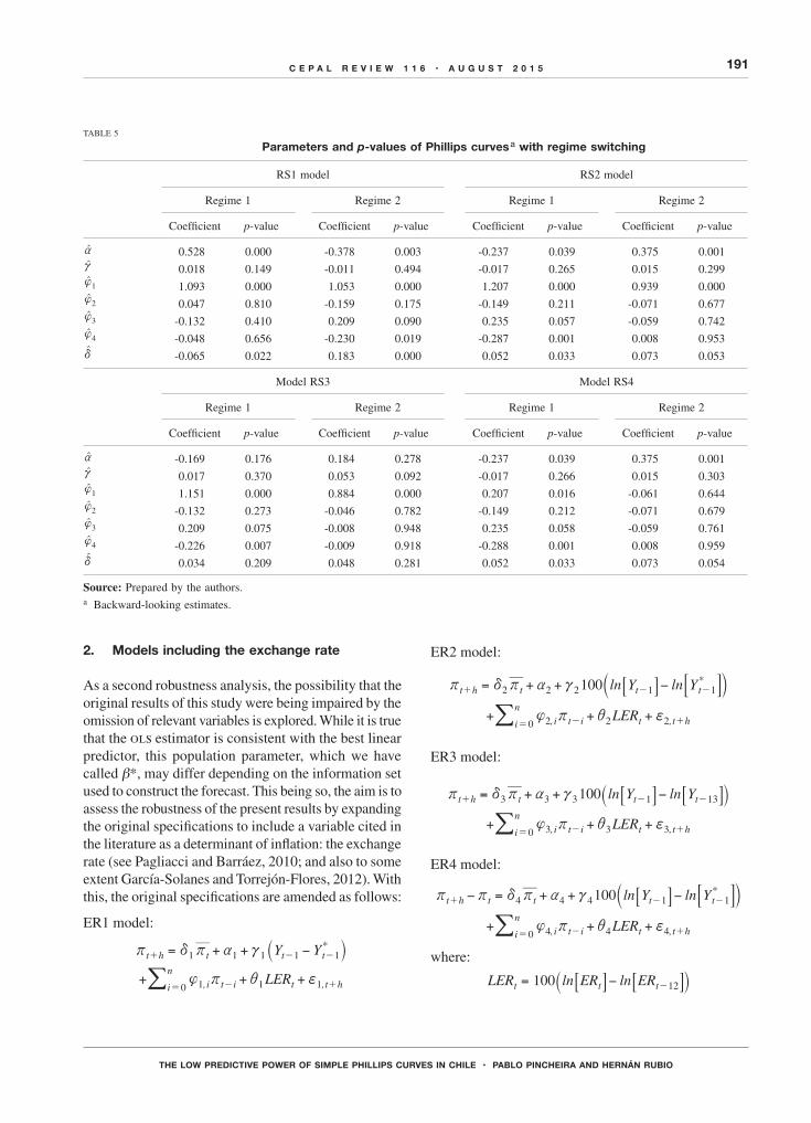
191C E P A L R E V I E W 1 1 6 • A U G U S T 2 0 1 5
THE LOW PREDICTIVE POWER OF SIMPLE PHILLIPS CURVES IN CHILE • PABLO PINCHEIRA AND HERNÁN RUBIO
TABLE 5
Parameters and p-values of Phillips curves a with regime switching
RS1 model RS2 model
Regime 1 Regime 2 Regime 1 Regime 2
Coefficient p-value Coefficient p-value Coefficient p-value Coefficient p-value
at 0.528 0.000 -0.378 0.003 -0.237 0.039 0.375 0.001ct 0.018 0.149 -0.011 0.494 -0.017 0.265 0.015 0.299
1{t 1.093 0.000 1.053 0.000 1.207 0.000 0.939 0.0002{t 0.047 0.810 -0.159 0.175 -0.149 0.211 -0.071 0.6773{t -0.132 0.410 0.209 0.090 0.235 0.057 -0.059 0.7424{t -0.048 0.656 -0.230 0.019 -0.287 0.001 0.008 0.953
dt -0.065 0.022 0.183 0.000 0.052 0.033 0.073 0.053
Model RS3 Model RS4
Regime 1 Regime 2 Regime 1 Regime 2
Coefficient p-value Coefficient p-value Coefficient p-value Coefficient p-value
at -0.169 0.176 0.184 0.278 -0.237 0.039 0.375 0.001ct 0.017 0.370 0.053 0.092 -0.017 0.266 0.015 0.303
1{t 1.151 0.000 0.884 0.000 0.207 0.016 -0.061 0.6442{t -0.132 0.273 -0.046 0.782 -0.149 0.212 -0.071 0.6793{t 0.209 0.075 -0.008 0.948 0.235 0.058 -0.059 0.7614{t -0.226 0.007 -0.009 0.918 -0.288 0.001 0.008 0.959
dt 0.034 0.209 0.048 0.281 0.052 0.033 0.073 0.054
Source: Prepared by the authors.a Backward-looking estimates.
2. Models including the exchange rate
As a second robustness analysis, the possibility that the original results of this study were being impaired by the omission of relevant variables is explored. While it is true that the ols estimator is consistent with the best linear predictor, this population parameter, which we have called b*, may differ depending on the information set used to construct the forecast. This being so, the aim is to assess the robustness of the present results by expanding the original specifications to include a variable cited in the literature as a determinant of inflation: the exchange rate (see Pagliacci and Barráez, 2010; and also to some extent García-Solanes and Torrejón-Flores, 2012). With this, the original specifications are amended as follows:
ER1 model:
i f+ +- +
Y Y
LER
*
, ,
t h t t t
i t i t t hi
n
1 1 1 1 1
1 1 10
r d r a c
{ r
= + + −
+
+ - -
=
` j/
ER2 model:
i f+ +- +
ln lnY Y
LER
100 *
, ,
t h t t t
i t i t t hi
n
1 1
0
2 2 2
2 2 2
r d r a c
{ r
= + + −
+
+ - -
=
b l7 9A C/
ER3 model:
i f- ++ +
ln lnY
LER
Y100
, ,
t h t t
i t i t t hi
n
t1
0
3 3 3
3 3 3
13r d r a c
{ r
= + + −
+
+ -
=
-` j7 7A A/
ER4 model:
i f- ++ +
ln lnY Y100
, ,
*t h t t t
i t i t t hi
n
t1
0
4 4 4
4 4 4
1r r d r a c
{ r
− = + + −
+
+ -
=
-b l7 9A C/ LER
where:
A At t= −7 7ln ln100 t 12-` jLER ER ER

192 C E P A L R E V I E W 1 1 6 • A U G U S T 2 0 1 5
THE LOW PREDICTIVE POWER OF SIMPLE PHILLIPS CURVES IN CHILE • PABLO PINCHEIRA AND HERNÁN RUBIO
while ert represents the observed exchange rate (Chilean pesos per United States dollar) reported by the Central Bank of Chile.
Thus, the aim is to analyse whether the episodic character of the parameters associated with the activity variables is altered or not when the annual rate of variation in the exchange rate is included as an additional predictor. To this end, the above equations are estimated in the same rolling windows as reported in section IV.2. Table 6 shows the percentage of these windows where the parameter associated with activity proved statistically significant with a confidence level of 90%. In other words, table 6 is analogous to table 1 above.
As can be seen in table 6, the episodic character of the parameter associated with the activity variable is maintained. It is clear that the percentage of windows where this parameter is statistically significant fluctuates between 11.8% and 64.5%. The general average of the percentages is 39.2% in table 6, while in table 1 it is 44.3%. In summary, incorporating the exchange rate as an additional predictor is not found to qualitatively alter the results. It could even be argued that including
the exchange rate diminishes the predictive capacity of activity, but on the whole, comparison of tables 1 and 6 shows that the results are dependent on the specification. In equations (1), (2) and (4), including the exchange rate somewhat diminishes the statistical significance of the activity variable parameter, while in specification (3) there is the opposite tendency.
TABLE 6
Rolling windows where the parameter associated with economic activity is significant at 10%a
(Percentages)
ER1 model
ER2 model
ER3 model
ER4 model
h = 1 50.0 50.0 64.5 57.9h = 3 46.7 46.1 41.4 28.3h = 6 40.1 40.8 56.6 11.8h = 9 23.0 23.7 55.9 17.8h = 12 30.9 28.3 44.1 25.7
Source: Prepared by the authors.a Final data: January 1991 to June 2009. Specifications with
exchange rate.
VISummary and conclusions
This study has considered four families of backward-looking Phillips curves for Chile with a monthly frequency and has assessed the capacity of these to predict inflation at horizons of 1, 3, 6, 9 and 12 months. All the specifications considered include an activity variable that is lagged relative to the latest inflation figure available, in order to emulate the availability of information in real time. It is done in this way because the imacec data used in this study to construct the activity variable are published with a month’s delay relative to the inflation figure. The predictability analysis is conducted both with revised figures and with figures available in real time, making it possible to evaluate the predictive economic relationship and the usefulness of these Phillips curves when it comes to generating projections for the use of decision makers.
The results obtained here indicate that the predictive capacity of these Phillips curves is limited and, furthermore, that the contribution made by the activity component to this predictability is moderate in size, often not
statistically significant, and fairly unstable. This holds true both for the real-time analysis and for the analysis with revised figures.
As a cursory analysis of robustness, the specifications were expanded to allow for the possibility of Markov-style regime switching, or the inclusion of the annual rate of variation in the exchange rate as an additional predictor. In-sample estimates of these expanded specifications are consistent with the results obtained in simpler linear specifications, since the statistical significance of the parameter associated with the activity variable continues to be occasional or episodic.
Part of the literature states that out-of-sample predictability assessments lack predictive power compared to in-sample assessments. It is for this reason that the present study has conducted exercises of both types, obtaining results that point in the same direction. Thus, it seems more plausible to attribute the lack of predictability to the unstable and moderate absolute

193C E P A L R E V I E W 1 1 6 • A U G U S T 2 0 1 5
THE LOW PREDICTIVE POWER OF SIMPLE PHILLIPS CURVES IN CHILE • PABLO PINCHEIRA AND HERNÁN RUBIO
value of the coefficient associated with the respective activity variables than to problems with the predictive power of out-of-sample statistical tests.
Although the results of this study are consistent with those of a number of articles dealing with the United
States, they are novel in that they demonstrate a lack of predictive power for backward-looking Phillips curves in Chile. It will be part of a future agenda to determine whether these interesting results continue to obtain with other versions of Phillips curves.
ANNEX
Stock and Watson (2008) methodology
For many years, the Phillips curve has been heavily used as a tool for predicting inflation. However, the empirical results provided by this paper, and by a substantial section of the literature, are not necessarily satisfactory if the comparison is made with models where only past inflation is considered. Stock and Watson (2008) present a prototype autoregressive model with the following specification:
t hh
th
ih
t ii
n
t hh1 1
0
r r a z r fD− = ++ -=
+_ _ _ _ _ _i i i i i i/
where: ln lnh
P P1200
th
t t hr = − -_ __ i ii 9 C
is annualized inflation accumulated over h periods from time t; t
1r_ i is annualized inflation accumulated over just one month; the variable t h
hf +_ i represents shocks
uncorrelated with the information available at t; and ha_ i is a constant that can vary depending on the inflation accumulation period used.
The exercise proposed here consists in estimating this prototype model, with and without constant, in 152 rolling windows of 71 observations apiece. The first window takes cpi data from January 1991 to November 1996. A number of models are estimated in each window, taking different numbers of lags for the inflation differential
t i1rD -_ i (from 0 to 12 lags). The Schwarz criterion was
used to determine the best model within each window. Once the model had been selected, with the number of lags already determined for the independent variable, projections were carried out at different horizons: 1, 3,
6, 9 and 12 months ahead. Since the predictive results yielded by these models are a function of inflation, simple algebraic steps give a forecast at different horizons for the target variable, which is cumulative 12-month inflation. The out-of-sample root squared error obtained with this methodology is presented in table 4.
sarima models
Apart from the Stock and Watson models detailed earlier, the time series models considered in table 4 of this study are a random walk with constant and two sarima models similar to the airline model of Box and Jenkins (1970). These sarima models are described in great detail in Pincheira and García (2009) and Pincheira and Medel (2015), with these articles also demonstrating their excellent predictive capacity for inflation in Chile and a select group of countries. In particular, the three models used here have the following specifications:
Random walk with constant: t t t1r a r f= + +-
sarima 1: t t t t t1 12 13r a f if jf jif= + − − +- - -
sarima 2: t t t t
t t
1 1
12 13
r a tr f if
jf jif
= + + −
− +- -
- -
where: i i= −_ _ln lnCPI CPI100t t t 12r -9 C
The model denominated sarima 1 corresponds to the model denominated “sarima with constant” in table 4. The sarima 2 model corresponds to the model denominated “sarima with constant and autoregressive term”, again in table 4.

194 C E P A L R E V I E W 1 1 6 • A U G U S T 2 0 1 5
THE LOW PREDICTIVE POWER OF SIMPLE PHILLIPS CURVES IN CHILE • PABLO PINCHEIRA AND HERNÁN RUBIO
Amisano, G. and G. Fagan (2013), “Money growth and inflation: a regime switching approach”, Journal of International Money and Finance, vol. 33(C), Amsterdam, Elsevier.
Aguirre, A. and L.F. Céspedes (2004), “Uso de análisis factorial dinámico para proyecciones macroeconómicas”, Economía Chilena, vol. 7, No. 3, Santiago, Central Bank of Chile.
Atkeson, A. and L. Ohanian (2001), “Are Phillips curves useful for forecasting inflation?”, Quarterly Review, vol. 25, No. 1, Minneapolis, Federal Reserve Bank of Minneapolis.
Box, G. and G. Jenkins (1970), Time Series Analysis: Forecasting and Control, San Francisco, Holden-Day.
Box, G. and G. Tiao (1973), Bayesian Inference in Statistical Analysis, New York, John Wiley and Sons.
Brock, W. and S. Durlauf (2001), “Growth empirics and reality”, The World Bank Economic Review, vol. 15, No. 2, Washington, D.C., World Bank.
Central Bank of Chile (2003), Modelos macroeconómicos y proyecciones del Banco Central de Chile 2003, Santiago.
Céspedes, L.F., M. Ochoa and C. Soto (2005), “The new Keynesian Phillips curve in an emerging market economy: the case of Chile”, Documento de Trabajo, No. 355, Santiago, Central Bank of Chile.
Chih-Chuan, Yeh (2009), “The Simultaneous Evolution of Growth and Inflation”, document presented at the International Conference on Applied Economics.
Chumacero, R. and F. Gallego (2002), “Trends and cycles in real-time”, Estudios de Economía, vol. 29, No. 2, Santiago, University of Chile.
Ciccarelli, M. and B. Mojon (2010), “Global inflation”, The Review of Economics and Statistics, vol. 92, No. 3, Cambridge, Massachusetts, The mit Press.
Clark, T. and K. West (2007), “Approximately normal tests for equal predictive accuracy in nested models”, Journal of Econometrics, vol. 138, No. 1, Amsterdam, Elsevier.
(2006), “Using out-of-sample mean squared prediction errors to test the martingale difference hypothesis”, Journal of Econometrics, vol. 135, No. 1-2, Amsterdam, Elsevier.
Clark, T. and M. McCracken (2006), “The predictive content of the output-gap for inflation: Resolving in-sample and out-of-sample evidence”, Journal of Money, Credit and Banking, vol. 38, No. 5, Columbus, Ohio, The Ohio State University Press.
Diebold, F. and R. Mariano (1995), “Comparing predictive accuracy”, Journal of Business and Economic Statistics, vol. 13, No. 3, American Statistical Association.
Estrella A. and J. Fuhrer (2003), “Monetary policy shifts and the stability of monetary policy models”, Review of Economics and Statistics, vol. 85, No. 1, Cambridge, Massachusetts, The mit Press.
Fisher I. (1973), “I discovered the Phillips curve”, Journal of Political Economy, vol. 81, No. 2, Chicago, University of Chicago Press.
(1926), “A statistical relationship between unemployment and price changes”, International Labour Review, vol. 13, No. 6, International Labour Organization (ilo), June.
Fuentes, R., F. Gredig and M. Larraín (2008), “La brecha de producto en Chile: medición y evaluación”, Economía Chilena, vol. 11, No. 2, Santiago, Central Bank of Chile.
García, M. and J.P. Medina (2008), “Efectos de primas financieras sobre la actividad agregada”, Economía Chilena, vol. 12, No. 3, Santiago, Central Bank of Chile.
García-Solanes, J. and F. Torrejón-Flores (2012), “Inflation targeting works well in Latin America”, cepal Review, No. 106 (LC/G.2518-P), Santiago.
Giacomini, R. and H. White (2006), “Tests of conditional predictive ability”, Econometrica, vol. 74, No. 6, New York, The Econometric Society.
Hamilton, J. (1994), Time Series Analysis, Princeton, Princeton University Press.
(1989), “A new approach to the economic analysis of nonstationary time series and the business cycle”, Econometrica, vol. 57, No. 2, New York, The Econometric Society.
Hansen, B. (2014), “Econometrics”, University of Wisconsin, Madison, unpublished.
Hostland, D. (1995), “Changes in the inflation process in Canada: evidence and implications”, Working Paper, No. 1995-5, Ottawa, Bank of Canada.
Lansing, K. (2002), “Can the Phillips curve help forecast inflation”, frbsf Economic Letter, No. 29, San Francisco, Federal Reserve Bank of San Francisco.
Meese, R. and K. Rogoff (1983), “Empirical exchange rate models of the seventies. Do they fit out-of-sample?”, Journal of International Economics, vol. 14, No. 1-2, Amsterdam, Elsevier.
Melo, L. and M. Misas (1997), “Análisis del comportamiento de la inflación trimestral en Colombia bajo cambios de régimen: Una evidencia a través del modelo ‘Switching’ de Hamilton”, Borradores de Economía, No. 86, Bogota, Bank of the Republic of Colombia.
Morandé, F. and M. Tejada (2008), “Fuentes de incertidumbre monetaria en la conducción de la política monetaria en Chile”, Economía Chilena, vol. 11, No. 3, Santiago, Central Bank of Chile.
Nadal de Simone, F. (2001), “Proyección de la inflación en Chile”, Economía Chilena, vol. 4, No. 3, Santiago, Central Bank of Chile.
Newey, W. and K. West (1994), “Automatic lag selection in covariance matrix estimation”, Review of Economic Studies, vol. 61, No. 4, Wiley Blackwell.
(1987), “A simple, positive, semi-definite, heteroskedasticity and autocorrelation consistent covariance matrix”, Econometrica, vol. 55, No. 3, New York, The Econometric Society.
Pagliacci, C. and D. Barráez (2010), “A Markov-switching model of inflation: looking at the future during uncertain times”, Análisis Económico, vol. 25, No. 59, Autonomous Metropolitan University.
Pedersen, M. (2013), “Extracting gdp signals from the monthly indicator of economic activity. Evidence from Chilean real-time data”, Journal of Business Cycle Measurement and Analysis, vol. 2013(1), oecd Publishing.
Phillips, A. (1958), “The relation between unemployment and the rate of change in money wage rates in the United Kingdom, 1861-1957”, Economica, vol. 25, Wiley, November.
Pincheira P. (2013), “Shrinkage based tests of predictability”, Journal of Forecasting, vol. 32, No. 4, Wiley.
(2010), “A real time evaluation of the Central Bank of Chile gdp growth forecasts”, Money Affairs, vol. 23, No. 1, Center for Latin American Monetary Studies.
Pincheira, P. and M. Calani (2010), “Communicational bias in monetary policy: can words forecast deeds?”, Economia, vol. 11, No. 1, Latin American and Caribbean Economic Association.
Pincheira, P. and A. García (2009), “En búsqueda de un buen benchmark predictivo para la inflación”, Documento de Trabajo, No. 514, Santiago, Central Bank of Chile.
Pincheira, P. and C. Medel (2015), “Forecasting inflation with a simple and accurate benchmark: The case of the us and a set of inflation targeting countries”, Czech Journal of Economics and Finance, vol. 65, No. 1.
Rossi, B. and T. Sekhposyan (2010), “Have economic models’ forecasting performance for us output changed over time, and when?”, International Journal of Forecasting, vol. 26, No. 4, Amsterdam, Elsevier.
Rudebusch, G. and L. Svensson (1999), “Policy rules for inflation targeting”, Monetary Policy Rules, J.B. Taylor (ed.), Chicago, University of Chicago Press.
Russell, B. and R. Chowdhury (2013), “Estimating United States Phillips Curves with expectations consistent with the statistical process of inflation”, Journal of Macroeconomics, vol. 35, Amsterdam, Elsevier.
Samuelson, P. and R. Solow (1960), “Analytical aspects of anti-Inflation policy”, American Economic Review, vol. 50, No. 2, Nashville, Tennessee, American Economic Association.
Bibliography

195C E P A L R E V I E W 1 1 6 • A U G U S T 2 0 1 5
THE LOW PREDICTIVE POWER OF SIMPLE PHILLIPS CURVES IN CHILE • PABLO PINCHEIRA AND HERNÁN RUBIO
Stock, J. and M. Watson (2008), “Phillips Curve inflation forecasts”, nber Working Paper, No. 14322, Cambridge, Massachusetts, National Bureau of Economic Research.
(1999), “Forecasting inflation”, Journal of Monetary Economics, vol. 44, No. 2, Amsterdam, Elsevier.
(1998), “Diffusion indexes”, nber Working Paper, No. 6702, Cambridge, Massachusetts, National Bureau of Economic Research.
Taylor, J.B. (1993), “Discretion versus policy rules in practice”, Carnegie-Rochester Conferences Series on Public Policy, vol. 39, No. 1, Amsterdam, Elsevier.
West, K. (2006), “Forecast evaluation”, Handbook of Economic Forecasting, G. Elliott, C.W.J. Granger and A. Timmerman (eds.), Amsterdam, Elsevier.
(1996), “Asymptotic inference about predictive ability”, Econometrica, vol. 64, No. 5, New York, The Econometric Society.
Yeh, C.C. (2009), “The Simultaneous Evolution of Growth and Inflation”, document presented at the International Conference on Applied Economics.

A U G U S T 2 0 1 5
C E P A L R E V I E W 1 1 6
In order to facilitate the submission, consideration and publication of articles, the editorial board of the cepal Review has prepared the following information and suggestions to serve as a guide for future contributors.
The submission of an article implies an undertaking by the author not to submit it simultaneously to other publications. The copyright to all articles published in the Review shall be owned by the United Nations.
Each article will be reviewed by the editorial board, which may decide to submit it to external referees.
Papers should be submitted in the original language (English, French, Portuguese or Spanish). They will be translated into the appropriate language by the relevant eclac services.
Each article must be accompanied by a summary, no more than 150 words in length, giving a brief description of its subject matter and main conclusions.
Each article must also carry three jel (Journal of Economic Literature) classification codes. The jel Classification Codes Guide is available online at www.aeaweb.org/jel/jel_class_system.php.
Papers should be no longer than 10,000 words, including the summary, notes and bibliography. Shorter papers will also be considered.
Articles should be sent by e-mail to [email protected] in Word format. Papers in pdf format will not be accepted.
Style guide:Titles should not be excessively long.
Footnotes
— It is recommended that footnotes be kept to a minimum.
— It is recommended that footnotes not be used to cite bibliographical references; such references should preferably be incorporated into the text.
— Footnotes should be numbered consecutively using superscript Arabic numerals.
Tables, figures and equations
— It is recommended that tables and figures be kept to a minimum, avoiding any redundancy with the text.
— Equations should be written using the Office equation editor “MathType”; they should not be inserted as “pictures”.
— Tables, figures and other elements should be inserted at the end of the text in the format in which they were designed; they should not be inserted as “pictures”. Figures in Excel should include the corresponding worksheets.
— The location of tables and figures in the body of the article should be indicated in the appropriate place as follows:
Insert figure 1 Insert table 1
— Tables and figures should include an explicit and complete reference to their sources.
— Tables should indicate the period covered at the end of the title, and should indicate the units in which the data are expressed in a subtitle (in italics and between brackets).
— The symbols referred to in the “Explanatory notes” which appear on the page preceding the table of contents should be taken into account in the preparation of tables and figures.
— Footnotes to tables and figures should be ordered consecutively using superscript lower-case letters.
— Figures should be prepared bearing in mind that they will be printed in black and white.
Acronyms and abbreviations
— Acronyms and abbreviations should not be used unless absolutely necessary, in which case the full name should be written out the first time it occurs in the article.
Bibliography
— Bibliographical references should be directly related to the content of the article and should not be excessively long.
— At the end of the article, under the title “Bibliography”, all the necessary information should be included accurately and in alphabetical order by author: name of author(s), year of publication, full name of article (if any) and publication (including any subtitle), city of publication, publisher and, in the case of a periodical, month of publication.
The editorial board of the Review reserves the right to make any necessary editorial changes in the articles, including their titles.
Authors will receive a one-year courtesy subscription to the Review, plus 30 offprints of their article in Spanish and 30 in English, at the time of publication in each language.
Guidelinesfor contributorsto the CEPAL Review

Publicaciones recientes de la CEPAL ECLAC recent publicationswww.cepal.org/publicaciones
Informes periódicos / Annual reportsTambién disponibles para años anteriores / Issues for previous years also available• Estudio Económico de América Latina y el Caribe 2014, 222 p. Economic Survey of Latin America and the Caribbean 2014, 214 p.
• La Inversión Extranjera Directa en América Latina y el Caribe 2015, 150 p. Foreign Direct Investment in Latin America and the Caribbean 2015, 140 p.
• Anuario Estadístico de América Latina y el Caribe 2014 / Statistical Yearbook for Latin America and the Caribbean 2014, 238 p.• Balance Preliminar de las Economías de América Latina y el Caribe 2014, 92 p. Preliminary Overview of the Economies of Latin America and the Caribbean 2014, 92 p.
• Panorama Social de América Latina 2014, 296 p. Social Panorama of Latin America 2014, 284 p.
• Panorama de la Inserción Internacional de América Latina y el Caribe 2014, 148 p. Latin America and the Caribbean in the World Economy 2014, 140 p.
Libros y documentos institucionales / Institutional books and documents• El desafío de la sostenibilidad ambiental en América Latina y el Caribe: textos seleccionados de la CEPAL 2012-2014, 2015, 148 p.• Panorama Fiscal de América Latina y el Caribe 2015: Dilemas y espacios de políticas, 2015, 130 p.
• La economía del cambio climático en América Latina y el Caribe: paradojas y desafíos del desarrollo sostenible, 2014, 98 p The economics of climate change in Latin America and the Caribbean: Paradoxes and challenges. Overview for 2014, 2014, 76 p.
• Los pueblos indígenas en América Latina: avances en el último decenio y retos pendientes para la garantía de sus derechos, 2014, 410 p.
• Pactos para la igualdad: hacia un futuro sostenible, 2014, 340 p. Covenants for Equality: Towards a sustainable future, 2014, 330 p.
• Integración regional: hacia una estrategia de cadenas de valor inclusivas, 2014, 226 p. Regional Integration: Towards an inclusive value chain strategy, 2014, 218 p. Integração regional: por uma estratégia de cadeias de valor inclusivas, 2014, 226 p.
• Reflexiones sobre el desarrollo en América Latina y el Caribe. Conferencias magistrales 2013-2014, 2014, 100 p.• Prospectiva y desarrollo: el clima de la igualdad en América Latina y el Caribe a 2020, 2013, 72 p.
• Comercio internacional y desarrollo inclusivo: construyendo sinergias, 2013, 210 p. International trade and inclusive development: Building synergies, 2013, 200 p.
• Cambio estructural para la igualdad: una visión integrada del desarrollo, 2012, 330 p. Structural Change for Equality: an integrated approach to development, 2012, 308 p.
• La hora de la igualdad: brechas por cerrar, caminos por abrir, 2010, 290 p. Time for Equality: closing gaps, opening trails, 2010, 270 p. A Hora da Igualdade: Brechas por fechar, caminhos por abrir, 2010, 268 p.

Libros de la CEPAL / ECLAC books135: Rising concentration in Asia-Latin American value chains: Can small firms turn the tide? Osvaldo Rosales, Keiji Inoue,
Nanno Mulder, 2015, 282 p.
134: Desigualdad, concentración del ingreso y tributación sobre las altas rentas en América Latina, Juan Pablo Jiménez (ed.), 2015, 172 p.
133: Desigualdad e informalidad: un análisis de cinco experiencias latinoamericanas, Verónica Amarante, Rodrigo Arim (eds.), 2015, 526 p.
132 Neoestructuralismo y corrientes heterodoxas en América Latina y el Caribe a inicios del siglo XXI, Alicia Bárcena, Antonio Prado (eds.),
2014, 452 p.
131 El nuevo paradigma productivo y tecnólogico: la necesidad de políticas para la autonomía económica de las mujeres, Lucía Scuro, Néstor Bercovich (eds.), 2014, 188 p.
130 Políticas públicas para la igualdad de género: un aporte a la autonomía de las mujeres, María Cristina Benavente, Alejandra Valdés, 2014, 134 p.
129 Prospectiva y política pública para el cambio estructural en América Latina y el Caribe, Javier Medina Vásquez, Steven Becerra y Paola Castaño, 2014, 338 p.
128 Inestabilidad y desigualdad: la vulnerabilidad del crecimiento en América Latina y el Caribe, Juan Alberto Fuentes Knight (ed.), 2014, 304 p.
Copublicaciones / Co-publications• Gobernanza global y desarrollo: nuevos desafíos y prioridades de la cooperación internacional, José Antonio Ocampo (ed.), CEPAL/Siglo Veintiuno,
Argentina, 2015, 286 p.• Decentralization and Reform in Latin America: Improving Intergovernmental Relations, Giorgio Brosio and Juan Pablo Jiménez (eds.),
ECLAC / Edward Elgar Publishing, United Kingdom, 2012, 450 p.• Sentido de pertenencia en sociedades fragmentadas: América Latina desde una perspectiva global, Martín Hopenhayn y Ana Sojo (comps.),
CEPAL / Siglo Veintiuno, Argentina, 2011, 350 p.
Coediciones / Co-editions• Perspectivas económicas de América Latina 2015: educación, competencias e innovación para el desarrollo, CEPAL/OCDE, 2014, 200 p. Latin American Economic Outlook 2015: Education, skills and innovation for development, ECLAC,/CAF/OECD, 2014, 188 p.• Regional Perspectives on Sustainable Development: Advancing Integration of its Three Dimensions through Regional Action,
ECLAC-ECE-ESCAP-ESCWA, 2014, 114 p.• Perspectivas de la agricultura y del desarrollo rural en las Américas: una mirada hacia América Latina y el Caribe 2014, CEPAL / FAO / IICA, 2013, 220 p.
Cuadernos de la CEPAL101 Redistribuir el cuidado: el desafío de las políticas, Coral Calderón Magaña (coord.), 2013, 460 p.101 Redistributing care: the policy challenge, Coral Calderón Magaña (coord.), 2013, 420 p.100 Construyendo autonomía: compromiso e indicadores de género, Karina Batthyáni Dighiero, 2012, 338 p.99 Si no se cuenta, no cuenta, Diane Alméras y Coral Calderón Magaña (coords.), 2012, 394 p.
Documentos de proyecto / Project documents• La economía del cambio climático en el Perú, 2014, 152 p.
• La economía del cambio climático en la Argentina: primera aproximación, 2014, 240 p.
• La economía del cambio climático en el Ecuador 2012, 2012, 206 p.
Cuadernos estadísticos de la CEPAL42 Resultados del Programa de Comparación Internacional (PCI) de 2011 para América Latina y el Caribe. Solo disponible en CD, 2015.41 Los cuadros de oferta y utilización, las matrices de insumo-producto y las matrices de empleo. Solo disponible en CD, 2013.
Series de la CEPAL / ECLAC SeriesAsuntos de Género / Comercio Internacional / Desarrollo Productivo / Desarrollo Territorial / Estudios Estadísticos / Estudios y Perspectivas (Bogotá, Brasilia, Buenos Aires, México, Montevideo) / Studies and Perspectives (The Caribbean, Washington) / Financiamiento del Desarrollo/ Gestión Pública / Informes y Estudios Especiales / Macroeconomía del Desarrollo / Manuales / Medio Ambiente y Desarrollo / Población y Desarrollo/ Política Fiscal / Políticas Sociales / Recursos Naturales e Infraestructura / Reformas Económicas / Seminarios y Conferencias.
Lista de Publicaciones Flagship JULIO 2015b.pdf 1 30-11-15 18:37

Revista CEPAL / CEPAL ReviewLa Revista se inició en 1976, con el propósito de contribuir al examen de los problemas del desarrollo socioeconómico de la región. La Revista CEPAL se publica en español e inglés tres veces por año.CEPAL Review first appeared in 1976, its aim being to make a contribution to the study of the economic and social development problems of the region. CEPAL Review is published in Spanish and English versions three times a year.
Observatorio demográfico / Demographic Observatory Edición bilingüe (español e inglés) que proporciona información estadística actualizada, referente a estimaciones y proyecciones de población de los países de América Latina y el Caribe. Desde 2013 el Observatorio aparece una vez al año.
Bilingual publication (Spanish and English) proving up-to-date estimates and projections of the populations of the Latin American and Caribbean countries. Since 2013, the Observatory appears once a year.
Notas de poblaciónRevista especializada que publica artículos e informes acerca de las investigaciones más recientes sobre la dinámica demográfica en la región. También incluye información sobre actividades científicas y profesionales en el campo de población. La revista se publica desde 1973 y aparece dos veces al año, en junio y diciembre.
Specialized journal which publishes articles and reports on recent studies of demographic dynamics in the region. Also includes information on scientific and professional activities in the field of population. Published since 1973, the journal appears twice a year in June and December.
Las publicaciones de la CEPAL están disponibles en:ECLAC publications are available at:
www.cepal.org/publicaciones
También se pueden adquirir a través de:They can also be ordered through:
www.un.org/publications
United Nations PublicationsPO Box 960
Herndon, VA 20172USA
Tel. (1-888)254-4286 Fax (1-800)338-4550
Contacto / Contact: [email protected] / Orders: [email protected]