Ozone and Nitrogen Dioxide Levels Monitored in an UrbanArea (Ciudad Real) in central-southern Spain

Pilar Martin & Beatriz Cabañas &

Florentina Villanueva & Maria Paz Gallego &

Inmaculada Colmenar & Sagrario Salgado

Received: 3 April 2009 /Accepted: 23 July 2009 /Published online: 25 August 2009# Springer Science + Business Media B.V. 2009

Abstract This work describes the evolution of NO2

and O3 levels from January to December of 2007,covering the four seasonal periods in the urban air ofCiudad Real in the central-southern Spain. Themeasurements were carried out by means of passivesamplers (Radiello® samplers). Eleven samples werecollected weekly, placed at different monitoring sitelocations. The data indicate that the mean levelsobtained during this period for O3 and NO2 were38.5±3.5 and 20.8±3.8 μg/m3, respectively. Thesemeasurements were compared with other studies inCiudad Real. Meteorological conditions (temperature,pressure, humidity relative, wind speed and direction)were also investigated.

Keyword Passive sampling . NO2 and O3 levels .

Urban and rural areas

1 Introduction

Urban air pollution problems are frequently associatedwith the products of combustion in industries, invehicles and for domestic purposes. Suspendedparticulate matter, carbon monoxide, sulphur diox-ide, nitrogen oxides and ozone (O3) are commonpollutants. Many large cities around the globeexhibit excessive levels of one or more of thesepollutants.

Hence, monitoring of air pollution is important andnecessary not only to comply with the environmentaldirectives and assess the effectiveness of emissioncontrol polices but also to understand the role of thedifferent physicochemical processes in the troposphere.

One of the main problems originated by the airpollution in urban areas is the pollution caused byphotochemical oxidants. Amongst these, the O3 andthe nitrogen dioxide (NO2) are important, which arecapable of causing adverse impacts on human healthand the environment (Lee et al. 1996; WHO 2000;Mazzeo and Venegas 2002, 2004). Nitrogen dioxideis considered to be an important atmospheric trace gaspollutant not only because of its effects on health butalso because (a) it absorbs visible solar radiation andcontributes to impaired atmospheric visibility, (b) asan absorber of visible radiation, it could play apotentially direct role in the change in the globalclimate if its concentrations were to become highenough (WHO 2000), (c) it is one of the major

Water Air Soil Pollut (2010) 208:305–316DOI 10.1007/s11270-009-0168-8

P. Martin (*) : B. Cabañas :M. P. Gallego : I. Colmenar :S. SalgadoDepartamento de Química Física, Facultad de CienciasQuímicas, Universidad de Castilla La Mancha,Avda Camilo José Cela 10,13071 Ciudad Real, Spaine-mail: mariapilar.martin@uclm.es

P. Martin : B. Cabañas : F. Villanueva :M. P. Gallego :I. Colmenar : S. SalgadoLaboratorio de Contaminación Atmosférica,ITQUIMA, UCLM,Avda. Camilo Jose Cela S/N,13071 Ciudad Real, Spain

sources of acid rain (Tang and Lau 1999), (d) it is,along with nitric oxide (NO), a chief regulator of theoxidising capacity of the free troposphere by control-ling the build-up and fate of radical species, includinghydroxyl radicals, and (e) it plays a critical role indetermining concentrations of O3, nitric acid (HNO3),nitrous acid (HNO2), organic nitrates such as PAN(CH3C(O)O2NO2), nitrate aerosols and other speciesin the troposphere. In fact, the photolysis of nitrogendioxide in the presence of volatile organic compoundsis the only key initiator of the photochemicalformation of ozone and photochemical smog, whetherin polluted or unpolluted atmospheres (WHO 2000;Varshney and Singh 2003).

Therefore, ozone mainly generated in the photo-chemical reactions mentioned above is a secondarypollutant. Normally, in polluted areas, it will reactwith NO and re-form NO2 and O2. However, thepresence of hydrocarbons (VOCs) in the atmospherewill interrupt this process by being more attractive tothe nitric oxide that the ozone molecule is contribut-ing to ozone accumulation. Ozone is also produced bynatural sources (trees and thunderstorms for example).It has been found out that the photochemical ozoneproduction in urban areas rises with the NOx

emissions and is less sensitive to the VOC emissions(Sillman and Samson 1995). In areas moderatelycontaminated, ozone sensitivity to emission of nitro-gen oxides depends on the season and on the emissionrates (Kleinman 1991).

Monitoring of NO2 and O3 is usually carried outusing continuous measurement techniques such aschemiluminescence (UNE-EN 14211:2005) and ultra-violet (UV) photometry (UNE-EN 14625: 2005),respectively, that are the reference methods, or activesampling using a pump. However, the continuousmeasurements are expensive and require continuousmaintenance, calibration and electric supply. On thecontrary, diffusive samplers for the measurements ofO3 and NO2 concentrations avoid the need for electricsupply or site calibration. Passive samplers are basedon free flow (according to the Fick’s first law ofdiffusion) of pollutant molecules from the sampledmedium to a collecting medium. These devices can bedeployed virtually anywhere, being them useful formean concentrations determinations.

In the work presented here, a field study of averageconcentrations of NO2 and ozone levels have beendeveloped using diffusive passive sampling (Radiello®

samplers) in an urban city of Spain, Ciudad Real,where no permanent air quality monitoring stationsexisted during measurement period.

The aims of this work have been, first, to determineaverage values obtained of NO2 and O3 concentrationsin the measurement period corresponding to differentmonitoring points covering almost all the city; second,to compare the results with previous ones determinedin the same city from 23 August 2000 to 25 September2000, using the differential optical absorption spec-troscopy (DOAS) technique; third, to establish arelationship between NOx and ozone levels measuredin each period and to relate this with biogenic volatilecompounds emissions (BVOCs), according to thephysicochemical principles operating in the atmo-sphere; fourth, to establish the influence of meteoro-logical variables on the measured concentrations and,finally, according to the mean values obtained in eachof the sampling points, we analyse the convenience ofthe situation of fixed monitoring stations in the futurein some of the studied zones.

2 Materials and Methods. Experimental Section

2.1 Area of Study

As indicated above, the study was carried out in theurban area of Ciudad Real (Spain). The city hasaround 65,000 inhabitants and is located in the heartof La Mancha region in central-southern Spain(38.59 N, 3.55 W, at approximately 628 m abovesea level) in a fairly flat area, 200 km south ofMadrid. With a low presence of industry, traffic islikely to be the most important source of air pollutionin this city. Meteorologically, the zone is characterisedby very hot and dry summer period with highinsulation, variable direction winds and by dry andcold winters, conditions that could play an importantrole in the evolution of the polluting agents.

In Fig. 1, a map of the city is shown, where thesituation of the 11 measurement points can be seen.Samples are sited in town centre (total sampling areaof 7.5 km2 approximately) with the exception ofpoints 6, 7 and 10 that correspond to rural zones, butin the case of point 10 in the influence zone of a smallairport under construction.

Industry next to the city is especially scarce, andthe zone is mainly surrounded by rural areas. There is

306 Water Air Soil Pollut (2010) 208:305–316

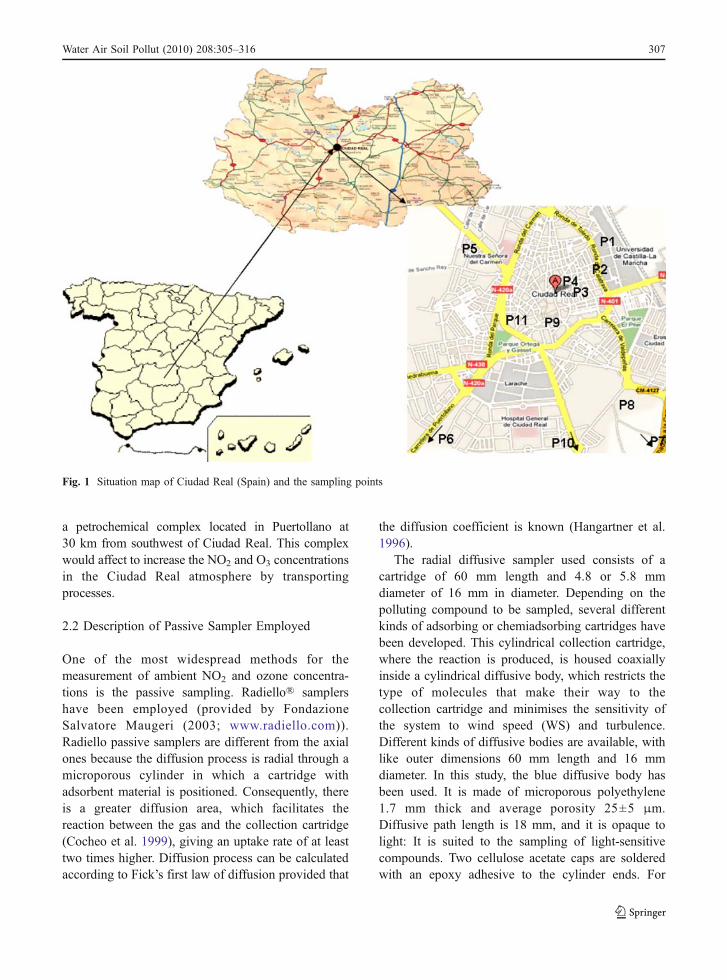
a petrochemical complex located in Puertollano at30 km from southwest of Ciudad Real. This complexwould affect to increase the NO2 and O3 concentrationsin the Ciudad Real atmosphere by transportingprocesses.

2.2 Description of Passive Sampler Employed

One of the most widespread methods for themeasurement of ambient NO2 and ozone concentra-tions is the passive sampling. Radiello® samplershave been employed (provided by FondazioneSalvatore Maugeri (2003; www.radiello.com)).Radiello passive samplers are different from the axialones because the diffusion process is radial through amicroporous cylinder in which a cartridge withadsorbent material is positioned. Consequently, thereis a greater diffusion area, which facilitates thereaction between the gas and the collection cartridge(Cocheo et al. 1999), giving an uptake rate of at leasttwo times higher. Diffusion process can be calculatedaccording to Fick’s first law of diffusion provided that

the diffusion coefficient is known (Hangartner et al.1996).

The radial diffusive sampler used consists of acartridge of 60 mm length and 4.8 or 5.8 mmdiameter of 16 mm in diameter. Depending on thepolluting compound to be sampled, several differentkinds of adsorbing or chemiadsorbing cartridges havebeen developed. This cylindrical collection cartridge,where the reaction is produced, is housed coaxiallyinside a cylindrical diffusive body, which restricts thetype of molecules that make their way to thecollection cartridge and minimises the sensitivity ofthe system to wind speed (WS) and turbulence.Different kinds of diffusive bodies are available, withlike outer dimensions 60 mm length and 16 mmdiameter. In this study, the blue diffusive body hasbeen used. It is made of microporous polyethylene1.7 mm thick and average porosity 25±5 μm.Diffusive path length is 18 mm, and it is opaque tolight: It is suited to the sampling of light-sensitivecompounds. Two cellulose acetate caps are solderedwith an epoxy adhesive to the cylinder ends. For

Fig. 1 Situation map of Ciudad Real (Spain) and the sampling points

Water Air Soil Pollut (2010) 208:305–316 307

exposition, these components are screwed onto aplane cellulose acetate equilateral triangle equippedwith an attaching clip.

The Radiello sampler for measuring nitrogendioxide and O3 is based on the principle that NO2

and O3 diffuse across the diffusive body towards theabsorbing material on the inner cartridge. NO2 and O3

in the atmosphere are captured in the sampler asnitrite (NO2

−) and 4-pyridylaldehyde, respectively.According to the Fick’s first law, the quantity of NO2

−

and 4-pyridylaldehyde in the sampler is proportionalto the concentration outside the sampler, the diffusioncoefficient, the dimensions of the sampler and thesampling time. Concentrations are calculated from thequantity of nitrite or 4-pyridylaldehyde captured inthe sampler by means of Eq. 1:

C mgm�3� � ¼ m� z

A� t � D¼ m

Qk � tð1Þ

where the sampling rate (Qk) is a constant:

Qk ¼ D� A

zð2Þ

where C represents the ambient air NO2 or O3

concentration measured by the passive sampler(micrograms per cubic metre), m is the quantity ofNO2

− or O3 captured in the sampler (micrograms) andz, A, t and D denote the diffusion length (metres),cross-sectional area (square metres), sampling time(seconds) and diffusion coefficient (square metres persecond), respectively. The theory of the passivesampling method is available in a number ofpublications (Palmes and Gunnison 1973; Posnerand Moore 1985; Harper and Purnell 1987; Krupaand Legge 2000; Gorecki and Namiesnik 2002).

How the diffusion coefficient of the pollutant in theair, the diffusion length and the cross-sectional areaare constant, the theoretical sampling rate should beconstant. Nevertheless, the diffusion coefficientdepends on certain environmental parameters such astemperature and pressure (Brown 2000). These varia-tions have been considered correcting the sampling rateQk according to Eq. 3:

QK ¼ Q298K

298

�7

ð3Þ

where K is the temperature and Q298 is the samplingrate at standard conditions.

For NO2, the sampling rate value Q298 at 298 K(25°C) and 1,013 hPa is 78 mL min−1. Only in the caseof NO2 is necessary to apply the Eq. 3 to the Eq. 1 tocalculate the concentration of nitrite in the ambient airbecause for O3, the sampling rate can be consideredlinear in the exposure range (10,000–4,000,000) μgm−3

min−1 and is not affected by humidity or wind speed.The value of Qk for O3 is 24.6 mL min−1 (http://www.radiello.com/english/index_en.html).

2.3 Extraction and Analysis of the Samples

Special care was taken when handling the passivesamplers. Before and after exposure, the cartridgeswere kept in airtight containers. After exposure, thesampler’s cartridges were transferred to a plastic tubeand kept in the refrigerator until the analysis.

2.3.1 Analysis of NO2 (R&P-Co 2001)

Exposure time was of 7 days. Five millilitres of ultra-pure water was added into the plastic tube with thecartridge inside. The solution was stirred vigorouslyby vortex for 2 min to allow the nitrite to dissolve in thewater. After stirring, the cartridges were removed fromthe solution. Of the nitrite solution, 0.5 mL was mixedalong with 5 mL of sulphanilamide reactive (10 g ofsulphanilamide in 100mL of concentratedHCl and diluteto 1 L with water) and stirred for 5 min. Then, 1 mL ofNEDA reactive (250 mg of N-(1-naphtyl) ethylenedi-amine dihydrochloride in 250 mL of water) was addedand stirred for 10 min.

The principle of working is the following: NO2 ischemiadsorbed in triethanolamine as nitrite ion (NO2

−).During the analysis in the laboratory, the nitrite reactswith sulphanilamide and forms a diazonium compoundwhich reacts with NEDA to form purple azodye whichis measured in an UV spectrophotometer at 537 nm(R&P-Co 2001). The concentration of the azodye isproportional to the amount of NO2 chemiadsorbed overthe sampling period (Cocheo et al. 1999). The mass ofnitrite in the cartridge is obtained by reference to alinear calibration derived from the spectrophotometricanalysis of standard solutions of sodium nitrite.

2.3.2 Analysis of O3 (R&P-Co 2001)

Exposure time was of 7 days. How the absorbingcartridge contains 1,2-di(4-pyridil)ethylene (DPE) and

308 Water Air Soil Pollut (2010) 208:305–316

it is light sensitive, the cartridge must be stored in aclosed tube in the dark. During exposure, the opaquediffusive body of Radiello sampler (of blue colour)protects the cartridge from the light. After theexposure time, the silica gel coated with DPEcontained in the cartridge is placed in a plastic tubefor extraction. A volume of 5 mL of 3-methyl-2-benzothiazolinone hydrazone (MBTH) solution (5 gMBTH with 5 mL of concentrated sulphuric acid in1 L of water) is added into a plastic tube containingthe silica gel. Then, the plastic tube is hermeticallysealed and shaken using a vortex shaker for 1 min. Toguarantee a complete reaction, this mixture is left forat least 60 min in the dark at room temperaturestirring from time to time before analysis.

The principle of working is as follows: The radialdiffusive cartridge used for ozone monitoring is filledwith silica gel coated with 1,2-di(4-pyridyl)ethylene.Ambient O3 diffuses through the porous membraneuntil the cartridge where it is trapped by reaction withDPE. Hauser and Bradley (1966) suggested theprobable absorption reaction between O3 and DPEto form an ozonure intermediate, which upon hydro-lysis yields 4-pyridylaldehyde (PA), amongst otherproducts. Later, MBTH reacts with PA to yield thecorresponding azide that is a yellow molecule. Theabsorbance of the solution is measured in the UVspectrophotometer at 430 nm. The mass of PA in thecartridge is obtained by reference to a linear calibra-tion derived from the spectrophotometric analysis ofstandard solutions of PA. Therefore, the amount of O3

can be calculated from the amount of PA taking intoaccount that 1 µg of PA correspond to 0.224 µg ofozone.

In all cases, tree unused cartridges belonging to thesame lot were treated in the same manner as thesamples. Then, it was subtracted by the average blankvalue from the absorbance values of the samples.

3 Results and Discussion

Tables 1 and 2 showed the results of the levels ofozone and NO2 measured during the campaign.

3.1 Seasonal Trend in Levels of Ozone and NO2

Figure 2 shows a plot of the mean levels of ozone andNO2 for all sampling points versus the sampling

period. Each period corresponds to a week ofexposure from February to December of 2007.

It can be seen as ozone levels vary throughout thedifferent seasons. In early spring, there are theabsolute higher ozone values (periods V and VI withvalues of 60.9 and 49.1 μg/m3, respectively) althoughthe maximum are typically achieved in summer. Onthe other hand, the minimum values of ozone wererecorded in December (period XL). This change hasalready been described in literature (Puxbaum et al.1991) where the increase of ozone concentration inspring is related to the transport of stratospheric ozonetowards the top of the troposphere. Other studies(Penkett 1986), however, consider that the peak in thespring season is due to the accumulation of ozoneprecursors during the winter, as a result of a lowerintensity of solar radiation. In spring, these precursorssuch as nitrogen oxides (NOx) and volatile organiccompounds react to give higher concentrations ofozone in this period. This second hypothesis issupported by the enormous variability of the seasonallifetime of NOx, that is, 20 times higher in spring(Lieu et al. 1987).

There are several studies concerning the role andcontribution of volatile organic compounds of bio-genic origin (BVOCs) in generating O3. Thus, inEurope, some authors (Vogel et al. 1995) have studiedthe influence of these BVOCs on ozone concentra-tions during episodes of high atmospheric temperaturein Germany, concluding that the biogenic emissionscan contribute between 10% and 20% to ozoneconcentrations. Other authors using the databaseproject Biogenic Emission in the Mediterranean Areafound for the Mediterranean area, where the maxi-mum ozone concentration is around 100 ppbv, thatbiogenic emissions represent a maximum of 10 ppbv,and this value depends heavily on the dynamicevolution of the regional winds (Navazo et al. 2003).

Our results and previous ones support the impor-tance, respect to the increase of ozone levels, ofvolatile organic compounds of biogenic origin whichhave their maximum levels in the spring period as aresult of the intense activity of plant species. TheseBVOCs are mainly isoprene and terpenes but alsoother oxygenated organic compounds, especiallycarbonyls and alcohols. Some of them react in theatmosphere with OH and NO3 radicals with higherrate constants than the most reactive anthropogenicVOCs (Finlayson-Pitts and Pitts 2000). In the

Water Air Soil Pollut (2010) 208:305–316 309

Tab

le1

Measurementsof

O3in

theurbanatmosph

ereof

CiudadRealcity

andin

theairportdu

ring

30Janu

ary20

07–2

0Decem

ber20

07

Ozone

Period

Winter

Spring

Sum

mer

III

III

IVV

VI

VII

VIII

IXX

XI

XII

XIII

XIV

XV

XVI

XVII

XVIII

XIX

XX

XXI

XXII

XXIII

Points

P1

16.1

34.5

40.1

33.4

60.7

54.6

51.0

62.8

42.8

54.9

48.8

45.2

61.6

44.7

35.4

60.8

68.7

67.3

66.3

68.0

P2

10.6

18.9

27.3

57.7

28.9

47.5

45.4

39.2

39.1

36.9

36.7

27.7

52.0

28.7

21.9

38.8

32.0

33.6

33.9

11.0

P3

12.3

34.3

34.3

36.7

54.3

29.0

37.3

46.2

51.9

44.7

44.0

44.9

41.5

P4

8.9

42.3

42.0

56.6

P5

18.1

45.9

45.7

41.9

62.3

55.5

38.2

50.3

50.2

31.6

51.3

48.3

50.0

50.8

59.6

18.2

36.8

57.1

51.0

57.7

P6

14.3

35.3

44.4

39.4

66.2

56.7

56.5

66.2

P7

17.2

24.4

37.2

32.0

68.5

62.3

50.3

46.2

46.3

P8

19.8

35.9

46.3

47.3

56.9

60.1

53.7

54.2

53.7

44.5

65.8

56.6

46.1

67.8

53.6

63.0

70.0

P9

26.2

7.8

11.1

6.2

19.8

32.8

16.3

38.8

28.9

30.5

P10

42.9

57.0

47.2

49.1

63.9

59.8

70.1

76.5

P11

average

14.7

32.7

39.7

3960

.949

.145

.947

.340

.330

.443

.546

.540

.750

.645

.934

.149

.5–

–50

.357

.060

.939

.5

Ozone

Period

Sum

mer

Autum

n

XXIV

XXV

XXVI

XXVII

XXVIII

XXIX

XXX

XXXI

XXXII

XXXIII

XXXIV

XXXV

XXXVI

XXXVII

XXXVIII

XXXIX

XL

XLI

XLII

Points

P1

73.0

68.0

59.0

62.2

51.9

36.1

34.5

22.3

29.2

35.3

34.6

33.0

22.3

15.1

14.0

22.2

6.2

7.5

13.7

P2

45.1

5.0

22.9

12.7

23.7

18.6

27.6

16.2

10.2

7.2

16.0

2.5

6.1

12.5

P3

P4

P5

22.7

44.5

55.9

49.9

56.7

34.3

32.1

27.5

36.8

32.6

36.4

22.2

15.5

7.7

15.1

9.1

14.6

14.2

P6

P7

P8

76.5

65.7

59.2

50.8

18.6

42.8

29.4

35.5

38.2

20.0

34.9

34.8

29.7

20.2

10.5

13.5

19.4

12.6

P9

P10

63.2

53.7

54.4

51.9

49.9

34.1

33.9

30.3

33.8

33.3

28.5

29.6

29.9

26.4

27.8

P11

17.6

17.1

28.2

26.8

27.6

13.8

9.4

8.2

16.7

7.2

6.9

8.0

average

73.0

57.6

55.7

57.9

44.5

33.3

33.7

26.1

27.2

34.5

27.7

31.3

23.2

18.3

14.0

18.1

7.7

10.9

12.2

Allun

itsin

microgram

spercubicmetre.Eachperiod

is7days

310 Water Air Soil Pollut (2010) 208:305–316

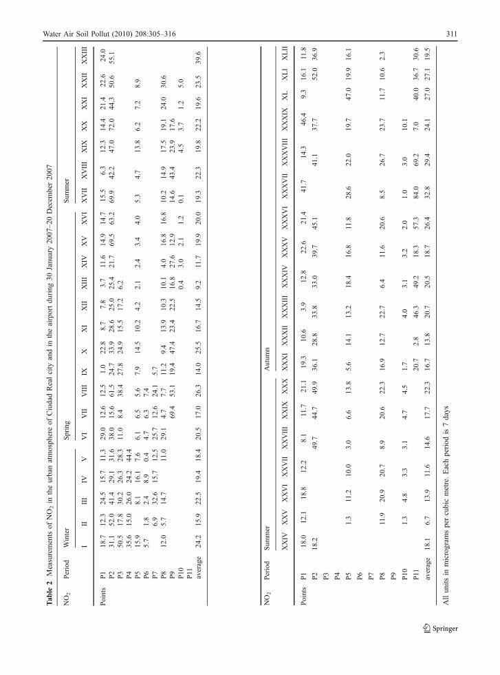
Tab

le2

Measurementsof

NO2in

theurbanatmosph

ereof

CiudadRealcity

andin

theairportdu

ring

30Janu

ary20

07–2

0Decem

ber20

07

NO2

Period

Winter

Spring

Sum

mer

III

III

IVV

VI

VII

VIII

IXX

XI

XII

XIII

XIV

XV

XVI

XVII

XVIII

XIX

XX

XXI

XXII

XXIII

Points

P1

18.7

12.3

24.5

15.7

11.3

29.0

12.6

12.5

1.0

22.8

8.7

7.8

3.7

11.6

14.9

14.7

15.5

6.3

12.3

14.4

21.4

22.6

24.0

P2

31.1

52.0

41.4

29.1

31.6

38.0

15.6

61.5

24.7

33.9

28.6

25.0

25.4

21.7

69.5

63.2

69.9

42.2

47.0

72.0

44.3

50.6

55.1

P3

50.5

17.8

30.2

26.3

28.3

11.0

8.4

38.4

27.8

24.9

15.5

17.2

6.2

P4

35.6

15.0

26.0

24.2

44.4

P5

15.9

8.1

16.1

7.6

6.1

6.5

5.6

7.9

14.5

10.2

4.2

2.1

2.4

3.4

4.0

5.3

4.7

13.8

6.2

7.2

8.9

P6

5.7

1.8

2.4

8.9

0.4

4.7

6.3

7.4

P7

6.9

32.6

15.7

12.5

25.7

12.6

24.1

5.7

P8

12.0

5.7

14.7

11.0

29.1

4.7

7.7

11.2

9.4

13.9

10.3

10.1

4.0

16.8

16.8

10.2

14.9

17.5

19.1

24.0

30.6

P9

69.4

53.1

19.4

47.4

23.4

22.5

16.8

27.6

12.9

14.6

43.4

23.9

17.6

P10

0.4

3.0

2.1

1.2

0.1

4.5

3.7

1.2

5.0

P11

average

24.2

15.9

22.5

19.4

18.4

20.5

17.0

26.3

14.0

25.5

16.7

14.5

9.2

11.7

19.9

20.0

19.3

22.3

19.8

22.2

19.6

23.5

39.6

NO2

Period

Sum

mer

Autum

n

XXIV

XXV

XXVI

XXVII

XXVIII

XXIX

XXX

XXXI

XXXII

XXXIII

XXXIV

XXXV

XXXVI

XXXVII

XXXVIII

XXXIX

XL

XLI

XLII

Points

P1

18.0

12.1

18.8

12.2

8.1

11.7

21.1

19.3

10.6

3.9

12.8

22.6

21.4

41.7

14.3

46.4

9.3

16.1

11.8

P2

18.2

49.7

44.7

49.9

36.1

28.8

33.8

33.0

39.7

45.1

41.1

37.7

52.0

36.9

P3

P4

P5

1.3

11.2

10.0

3.0

6.6

13.8

5.6

14.1

13.2

18.4

16.8

11.8

28.6

22.0

19.7

47.0

19.9

16.1

P6

P7

P8

11.9

20.9

20.7

8.9

20.6

22.3

16.9

12.7

22.7

6.4

11.6

20.6

8.5

26.7

23.7

11.7

10.6

2.3

P9

P10

1.3

4.8

3.3

3.1

4.7

4.5

1.7

4.0

3.1

3.2

2.0

1.0

3.0

10.1

P11

20.7

2.8

46.3

49.2

18.3

57.3

84.0

69.2

7.0

40.0

36.7

30.6

average

18.1

6.7

13.9

11.6

14.6

17.7

22.3

16.7

13.8

20.7

20.5

18.7

26.4

32.8

29.4

24.1

27.0

27.1

19.5

Allun

itsin

microgram

spercubicmetre.Eachperiod

is7days

Water Air Soil Pollut (2010) 208:305–316 311

presence of NOx, BVOCs act as precursors of ozoneand/or secondary organic aerosols in the troposphere.Globally, the BVOCs represent about 60% of the totalemissions of VOCs.

This fact could explain the ozone levels back-ground observed all year in rural or urban atmo-sphere. It can be concluded that the ozone formationin winter period is highly influenced by anthropogen-ic sources of their precursors, whereas in summerperiod, biogenic processes at local and regional levelwill be most favoured.

Respecting NOx, the main contribution is due toemissions from road traffic, bringing their valueskeep more or less constant throughout the year,slightly higher in the winter. Last fact can beattributed, as indicated above to the accumulationof ozone precursors during the winter as a result ofreduced solar radiation and lower temperature.Having less radiation, NOx are not photolysed andtrends to accumulate.

Finally, it is important to mention that duringholiday periods XXIII and XXIV, only samplingpoints P1 and P2 remained, and therefore, thesevalues are not average values of all sampling points.The empty points in Fig. 2 for periods XVIII and XIXcorrespond to lost samples.

3.2 Relationship with Climatologic Variables

Attempts were made to relate levels of ozone andNO2 obtained here with the variables pressure,temperature, humidity and wind. These variables(supplied by Spanish State Agency of Meteorology)

were averaged by each sampling periods and plottedin Fig. 2.

Ozone concentration (in micrograms per cubicmetre) showed a slight negative correlation withrelative humidity (RH in %) ([O3]=−0.62RH+88.66) and a positive correlation with temperature(T in degree Celsius; [O3]=0.37T +2.52). Periods withhigher temperatures and lower humidity usuallycorrespond to higher values of ozone. Thus, forperiods V and XIV, values of ozone were higher thanexpected and this fact could be due to the lowhumidity of those weeks (53% and 51%, respectively,compared with 61% of humidity in the spring period).Pressure and wind were very variable throughout theyear with an average value around of 94–95 kPa and

Fig. 2 Evolution of temper-ature, humidity and NO2

and O3 average concentra-tions of the 11 measuredpoints during the full period

Table 3 Mean values of NO2 and O3 for each sampling point(all period)

Point NO2 (μg/m3) O3 (μg/m

3)

P1 16.0±1.4 42.5±3.1

P2 41.1±2.4 26.3±2.5

P3 23.3±3.5 39.3±3.0

P4 29.0±5.0 37.5±10.1

P5 11.3±1.4 38.1±2.6

P6 4.7±1.0 47.4±6.3

P7 17.0±3.4 42.7±5.6

P8 14.7±1.1 43.1±3.1

P9 30.2±4.9 21.8±3.6

P10 3.1±0.4 45.5±3.2

P11 38.5±7.1 15.6±2.4

The error is typical error from statistic analysis of data

312 Water Air Soil Pollut (2010) 208:305–316

8 km/h, respectively. An insignificant variation withpressure has been observed. However, wind speedshows a positive correlation (WS in kilometres per hour;[O3]=6.54WS −15.15) since higher wind speed oftenleads to lower NO, and therefore, the loss of ozone isreduced. After analysing the wind rose for eachsampling period, it has not found any relation betweenthe levels of O3 and NO2 measured in each period withthe wind direction; therefore, we can conclude that thetransport from contaminated areas such as the petro-chemical complex of Puertollano is not important.

Similar variations of ozone concentration withmeteorological conditions have previously beenreported (Shan et al. 2009).

3.3 Average Sampling Values

Table 3 and Fig. 3 show the average values for eachpoint along the entire sampling period. As it is shownin Table 3, the higher levels of NO2 correspond to P2,

P3, P4, P9 and P11. These values of NO2 can beattributed to the intense flow of vehicles on thoseareas, to emphasise that point P11 is located on theentrance of an underground car parking, which alsojustifies that this point has a higher average level ofNO2. Points P1, P5, P6, P7 and P8 show lower valuesthan the other sampling points because they corre-spond to suburban areas. Also to mention that in P10,located in a zone where it was being constructed theCentral Airport of Ciudad Real, the lowest concen-trations of NO2 are recorded due to it is in a ruralarea, where road traffic is lower, and hence, NOx

emissions are very low. Respecting O3 levels, thehighest values are registered in the points that arelocated in suburban or rural areas except P3 and P4(although in these points, the period of sampling isvery different to the other points, see Table 1)

With the average values of points P1, P2, P3, P4,P5, P6, P8, P9 and P11, a spatial distribution map hasbeen developed for O3 and NO2 (Fig. 4) using SurGeProject Manager ver 1.4. As it can be seen, highervalues of O3 correspond to lower values of NO2 andvice versa. This behaviour is expected consideringthe inter-conversion of both species according tophotochemical cycle of tropospheric O3 production(Finlayson-Pitts and Pitts 2000).

3.4 Comparison of the Obtained Results with Limitand Threshold Environmental Levels Values

In the case of nitrogen oxides, limit values are set bythe RD 1073/2003, transposed the European Directive1999/30/EC, and are shown in Table 4.

Fig. 3 Plot of average levels of ozone and NO2 (microgramsper cubic metre) for each sampling point

Fig. 4 Maps of O3 andNO2 spatial distribution.Units in microgramsper cubic metre

Water Air Soil Pollut (2010) 208:305–316 313

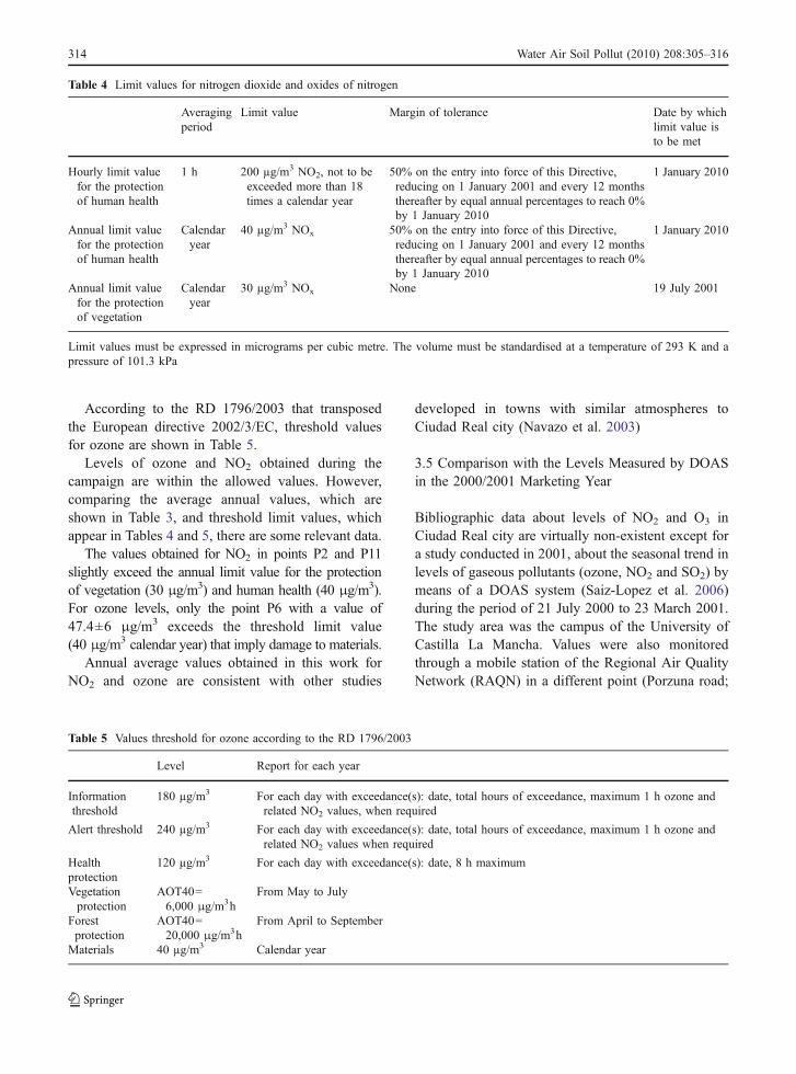
According to the RD 1796/2003 that transposedthe European directive 2002/3/EC, threshold valuesfor ozone are shown in Table 5.

Levels of ozone and NO2 obtained during thecampaign are within the allowed values. However,comparing the average annual values, which areshown in Table 3, and threshold limit values, whichappear in Tables 4 and 5, there are some relevant data.

The values obtained for NO2 in points P2 and P11slightly exceed the annual limit value for the protectionof vegetation (30 μg/m3) and human health (40 μg/m3).For ozone levels, only the point P6 with a value of47.4±6 μg/m3 exceeds the threshold limit value(40 μg/m3 calendar year) that imply damage to materials.

Annual average values obtained in this work forNO2 and ozone are consistent with other studies

developed in towns with similar atmospheres toCiudad Real city (Navazo et al. 2003)

3.5 Comparison with the Levels Measured by DOASin the 2000/2001 Marketing Year

Bibliographic data about levels of NO2 and O3 inCiudad Real city are virtually non-existent except fora study conducted in 2001, about the seasonal trend inlevels of gaseous pollutants (ozone, NO2 and SO2) bymeans of a DOAS system (Saiz-Lopez et al. 2006)during the period of 21 July 2000 to 23 March 2001.The study area was the campus of the University ofCastilla La Mancha. Values were also monitoredthrough a mobile station of the Regional Air QualityNetwork (RAQN) in a different point (Porzuna road;

Table 4 Limit values for nitrogen dioxide and oxides of nitrogen

Averagingperiod

Limit value Margin of tolerance Date by whichlimit value isto be met

Hourly limit valuefor the protectionof human health

1 h 200 µg/m3 NO2, not to beexceeded more than 18times a calendar year

50% on the entry into force of this Directive,reducing on 1 January 2001 and every 12 monthsthereafter by equal annual percentages to reach 0%by 1 January 2010

1 January 2010

Annual limit valuefor the protectionof human health

Calendaryear

40 µg/m3 NOx 50% on the entry into force of this Directive,reducing on 1 January 2001 and every 12 monthsthereafter by equal annual percentages to reach 0%by 1 January 2010

1 January 2010

Annual limit valuefor the protectionof vegetation

Calendaryear

30 µg/m3 NOx None 19 July 2001

Limit values must be expressed in micrograms per cubic metre. The volume must be standardised at a temperature of 293 K and apressure of 101.3 kPa

Table 5 Values threshold for ozone according to the RD 1796/2003

Level Report for each year

Informationthreshold

180 µg/m3 For each day with exceedance(s): date, total hours of exceedance, maximum 1 h ozone andrelated NO2 values, when required

Alert threshold 240 µg/m3 For each day with exceedance(s): date, total hours of exceedance, maximum 1 h ozone andrelated NO2 values when required

Healthprotection

120 µg/m3 For each day with exceedance(s): date, 8 h maximum

Vegetationprotection

AOT40=6,000 μg/m3h

From May to July

Forestprotection

AOT40=20,000 μg/m3h

From April to September

Materials 40 µg/m3 Calendar year

314 Water Air Soil Pollut (2010) 208:305–316

Saiz-López et al. 2006). These sampling points arecoincident with points P1 and P5, respectively, of ourcampaign. The average values of NO2 and O3 in thestudy of Saiz et al. (50 and 27 g/m3, respectively) aredifferent from those obtained by passive samplers andare shown in this study (16 and 42 μg/m3, respec-tively). But this difference may be partly attributableto the period of sampling, which in the case of Saiz etal. are not include the months of the main ozoneproduction, from May to July, whilst in this work areincluded. However, these results seem to agree thatthe highest values of NO2 are registered in thesampling points of the centre (DOAS and P1)compared with the points of the suburban areas,RAQN and P5.

4 Conclusions

& Ozone levels recorded in Ciudad Real area in2007 through the use of passive sensors, withaverage values of 38.5±3.5 μg/m3 for O3 and20.8±3.8 μg/m3 for NO2 are below the thresholdvalues. Then, it can be assumed that air quality inthe considered area is high.

& The seasonal distribution of ozone concentrationsseem to be related to levels of BVOCs, reachingmaximum values during periods in which plantshave a more intense activity (spring and earlysummer).

& The highest values of ozone are obtained insuburb areas, where the influence of road trafficis lower.

& The highest values for NO2 are obtained in thecentral areas of the city, where the influence ofvehicles is higher.

& There is an inverse relationship between levels ofozone and NO2.

& There have not been found a clear relationshipbetween meteorological variables and levels of O3

and NO2 obtained.& This is to emphasize that points P2 and P11 are

probably the most indicated points to installpermanent monitoring stations for NOx.

& Another important point is to control the airportarea (P6), with an annual level of ozone above thethreshold value. It is important to mention thatthese values will probably suffer variations whenthe airport is operating completely. Therefore, it

would be necessary to control this point in orderto see the influence of the airport in thecontaminants levels in the area.

Acknowledgments The authors gratefully thank to Foundationsof UCLM for supporting a part of this work.

References

Brown, R. H. (2000). Monitoring the ambient environment withdiffusive samplers: theory and practical considerations.Journal of Environmental Monitoring, 2(1), 1–9.

Cocheo, V., Boaretto, C., Cocheo, L., & Sacco, P. (1999).Radial path in diffusion: The idea to improve the passivesampler performances. In V. Cocheo, E. De Saeger, D.Kotzias (Eds.), International Conference Air Quality inEurope. Challenges for the 2000’s. Venice, Italy.

Finlayson-Pitts, B. J., & Pitts, J. N. (2000). Chemistry of theupper and lower atmosphere: Theory, experiments andapplications. San Diego: Academic.

Fondazione Salvatore Maugeri (2003). Instruction manual forRadiello sampler, version 1/2003. http://www.radiello.com.

Gorecki, T., & Namiesnik, J. (2002). Passive sampling. Trendsin Analytical Chemistry, 21(4), 276–291.

Hangartner, M., Kirchner, M., & Werner, H. (1996). Evaluationof passive methods for measuring ozone in the EuropeanAlps. Analyst, 121, 1269–1272.

Harper, M., & Purnell, C. J. (1987). Diffusive sampling—areview. American Industrial Hygiene Association Journal,48(3), 214–218.

Hauser, T. R., & Bradley, D. W. (1966). Specific spectropho-tometric determination of ozone in the atmosphere using 1,2 di(4-pyridyl) ethylene. Analytical Chemistry, 38, 1529–1532.

Kleinman, L. I. (1991). Seasonal dependence of boundary layerperoxide concentration: the low and high NOx regimes.Journal of Geophysical Research, 96, 20721–20733.

Krupa, S. V., & Legge, A. H. (2000). Passive sampling of ambient,gaseous air pollutants: an assessment from an ecologicalperspective. Environmental Pollution, 107, 31–45.

Lee, D. S., Holland, M. K., & Falla, N. (1996). The potentialimpact of ozone on materials in the UK. AtmosphericEnvironment, 30, 1053–1065.

Lieu, S. C., Trainer, M., Fehsenfeld, F. C., Parrish, D. D.,Williams, E. J., Fahey, D. W. (1987). Ozone production inthe rural troposphere and its implications for regional andglobal ozone distributions. Journal of Geophysical Re-search, 92, 4194–4207.

Mazzeo, N. A., & Venegas, L. E. (2002). Estimation ofcumulative frequency distribution for carbon monoxideconcentration from wind-speed data in Buenos Aires(Argentina). Water, Air and Soil Pollution: Focus, 2,419–432.

Mazzeo, N. A., & Venegas, L. E. (2004). Some aspects of airpollution in Buenos Aires City. International Journal ofEnvironment and Pollution, 22(4), 365–379.

Water Air Soil Pollut (2010) 208:305–316 315

Navazo, M., Durana, L, Alonso, J. A., García, J. L., Ilardia, M.C. y Gangoiti, G. (2003). Caracterización de compuestosorgánicos volátiles atmosféricos en áreas industriales,urbanas y rurales de la C.A.V 1995–2003.

Palmes, E. D., & Gunnison, A. F. (1973). Personal monitoringdevice for gaseous contaminants. American IndustrialHygiene Association Journal, 34, 78–81.

Penkett, S. A. (1986). The spring maximum of photo oxidantsin the Northern Hemisphere. Nature, 319, 655–657.

Posner, J. C., & Moore, G. A. (1985). Thermodynamictreatment of passive monitors. American Industrial Hy-giene Association Journal, 46(5), 277–285.

Puxbaum, H., Gabler, K., Smidt, S., & Glates, F. A. (1991).One-year record of ozone profiles in an Alpine Valley(Zillertal-Tyrol, Austria ,600–2000 m a.s.l). AtmosphericEnvironment, 25ª(9), 1759–1765.

R&P-Co. (2001). Radiello® Model 3310 passive samplingsystem. Passive gas sampling system for industrial indoor/outdoor and personal exposure assessment. East Green-bush: Rupprecht & Patashnick.

Saiz-López, A., Notario, A., Martínez, E., & Albadalejo, J.(2006). Seasonal evolution of levels of gaseous pollutants inan urban area (Ciudad Real) in central-southern Spain: ADOAS study. Water, Air and Soil Pollution, 171, 153–167.

Shan, W., Yin, Y., Zhang, J., Ji, X., & Deng, X. (2009). Surfaceozone and meteorological conditions in a single year at anurban site in central-eastern China. Environmental MonitoringAssessment, 151, 127–141.

Sillman, S., & Samson, P. J. (1995). Impact of temperature onoxidant photochemistry in urban, polluted rural and

remote environment. Journal of Geophysical Research,100, 11497–11508.

Tang, H., & Lau, T. (1999). A new all-season passive samplingsystem for monitoring NO2 in air. Field AnalyticalChemistry and Technology, 3(6), 338–345.

UNE-EN 14211 (2005). Ambient air quality. Standard methodfor the measurement of the concentration of nitrogendioxide and nitrogen monoxide by chemiluminescence.

UNE-EN 14625 (2005). Ambient air quality—standard methodfor the measurement of the concentration of ozone byultraviolet photometry.

Varshney, C. K., & Singh, A. P. (2003). Passive samplers forNOx monitoring: a critical review. The Environmentalist,23(2), 127–136.

Vogel, B., Fiedler, F., & Vogel, H. (1995). Influence oftopography and biogenic volatile organic compoundsemission in the state of Baden- Württemberg on ozoneconcentrations during episodes of high air temperatures.Journal of Geophysical Research, 100, 22907–22928.

WHO (2000). Chapter 7.2 Ozone and other photochemicaloxidants. Air Quality Guidelines-Second Edition.Copenhagen: WHO Regional Office for Europe.

Further Reading

www.jccm.es/medioambientewww.radiello.itwww.troposfera.org

316 Water Air Soil Pollut (2010) 208:305–316