Overview of Groundwater Conditions in Val Verde County ...
227
Overview of Groundwater Conditions in Val Verde County, Texas DECEMBER 2018 PREPARED BY: TEXAS WATER DEVELOPMENT BOARD WITH COOPERATION OF THE TEXAS COMMISSION ON ENVIRONMENTAL QUALITY AND THE TEXAS PARKS AND WILDLIFE DEPARTMENT
-
Upload
khangminh22 -
Category
Documents
-
view
1 -
download
0
Transcript of Overview of Groundwater Conditions in Val Verde County ...
Overview of Groundwater Conditions in
Val Verde County, Texas
December 2018
PrePareD by:Texas WaTer DeveloPmenT boarD
WiTh cooPeraTion of The Texas commission on environmenTal QualiTy anD The
Texas Parks anD WilDlife DeParTmenT
Geoscientist Seal
This report documents the work and supervision of work of the following licensed Texas Professional Geoscientists:
Andrew Weinberg, P.G.
Mr. Weinberg compiled data, evaluated available information and reports, and was the principal author of the report.
LawrenceN.French,P.G.
Mr. French supervised the preparation of the report, authored portions of the report, and reviewed the report.
Other Contributor
Jean Broce Perez
Mr. Perez was responsible for the GIS efforts associated with preparing illustrations and maps for the project.

This page is intentionally blank.

Table of Contents Executive Summary............................................................................................................................................................. E1
1.0 Introduction ....................................................................................................................................................................... 1
2.0 Geographic Setting and Natural Resources .......................................................................................................... 3
3.0 Geology ...............................................................................................................................................................................13
4.0 Hydrogeology...................................................................................................................................................................21
5.0 Groundwater Models....................................................................................................................................................66
6.0 Surface Water ..................................................................................................................................................................77
7.0 Water Supplies and Demands...................................................................................................................................88
8.0 Groundwater Management and Feasibility of Hydrologic Triggers .......................................................97
9.0 References......................................................................................................................................................................106
Appendix A ..............................................................................................................................................................................117
Appendix B ..............................................................................................................................................................................121
Appendix C ..............................................................................................................................................................................134
Appendix D..............................................................................................................................................................................146
List of Figures Figure 2-1. Map of Val Verde County, Texas ................................................................................................................. 5 Figure 2-2. Average monthly precipitation,evaporation,and temperature extremes at Amistad Dam........................................................................................................................................................................................................... 6 Figure 2-3. Soil map of Val Verde County ...................................................................................................................... 7 Figure 2-4. Generalized vegetation map of Val Verde County .............................................................................. 9 Figure 3-1. Surficial geology of Val Verde County . ...................................................................................................14Figure 3-2. Hydrostratigraphic chart of the central Edwards Plateau . ...........................................................15 Figure 3-3. Generalized cross-section (A-A’) of Cretaceous deposits in Val Verde County. ...................17 Figure 3-4. Generalized cross-section (B-B’) of Cretaceous deposits in Val Verde County ...................17 Figure 3-5. Generalized cross-section (C-C’) of Cretaceous deposits in Val Verde County .................. 18 Figure 3-6. Depositional environments in Central Texas during the Lower Cretaceous ........................19 Figure 3-7. Sinkholes, subsidence features, and faults in Val Verde County ................................................20 Figure 4-1. Karstic limestone at the contact between the Fort Terrett and Segovia Formations . ......23Figure 4-2. Elevation of the base of the Edwards section of the Edwards-Trinity (Plateau) Aquifer.24Figure 4-3. Thickness of the Edwards section of the Edwards-Trinity (Plateau) ......................................25 Figure 4-4.Thickness of the Trinity section of the Edwards-Trinity (Plateau) Aquifer ..........................26
i

Figure 4-5. Locations of observation wells in Val Verde County . ......................................................................29 Figure 4-6. 1994 water level contour map of the Dolan Springs drainage basin ..................................... 30 Figure 4-7. Water level contour map constructed from average winter water levels .............................31 Figure 4-8. Winter water level elevations ...................................................................................................................33 Figure 4-9. Estimated extent of the area influenced by the pressure head in Amistad Reservoir.......34Figure 4-10. Estimated specific capacity of wells in Val Verde County ..........................................................35 Figure 4-11. GAM model distribution of recharge across Val Verde County .............................................. 41 Figure 4-12. Locations of springs in Val Verde County ..........................................................................................46 Figure 4-13. Precipitation data for Brackettville used to guide Landsatimage analysis ...................... 47 Figure 4-14. Landsat 7 false-color near-infrared color composite image for September 22, 2007 ...48 Figure 4-15. Landsat 5 false color near-infrared image for April 6, 1995 .. ...................................................49Figure 4-16. Landsat 7 false-color near-infrared image for October 3, 2011 ..............................................50 Figure 4-17. National Wetlands Inventory, Sycamore Canyon Sheet ..............................................................51 Figure 4-18. Discharge from San Felipe Springs in Del Rio ..................................................................................52Figure 4-19. Location of Goodenough Springs relative to mapped faults and subsidence features.. .54Figure 4-20. Discharge from Goodenough Springs and the Devils River at Bakers Crossing ...............55 Figure 4-21. Monitoring points in the University of Texas Bureau of Economic Geology researchproject .........................................................................................................................................................................................57 Figure 4-22. Piper diagram of the water chemistry for Amistad Reservoir, the Rio Grande, the PecosRiver, the Devils River and Goodenough Springs .....................................................................................................59 Figure 4-23. Piper diagram for Well 7033501, southeast of Amistad Reservoir .......................................61 Figure 4-24. Piper diagram for Well 7033604, southeast of Amistad Reservoir .......................................61 Figure 4-25. Piper diagram for Well 7123502, north of Amistad Reservoir near Comstock ................62 Figure 4-26. Calcium distribution in Val Verde and neighboring counties ...................................................64 Figure 4-27. Piper diagram of fresh and brackish water samples from the Edwards aquifer unit ....65 Figure 5-1. Extent of the model domain for the Edwards-Trinity (Plateau) GAM .....................................67 Figure 5-2. Oblique view of the Devils River Watershed model ........................................................................69 Figure 5-3. Hydraulic conductivity distribution in the calibrated Val Verde County Model . ................73 Figure 5-4. Specific storage distribution in the calibrated Val Verde County Model . ...............................74 Figure 5-5. Simulation of spring locations based on various groundwater pumping scenarios .........76 Figure 6-1. Surface water features in Val Verde County .......................................................................................78 Figure 6-2.Totalannualflow of the Devils River,1960 to 2017, and Pecos River, 1968 to 2011.......79 Figure 6-3. Locations of stream gages in the Devils River and adjacentwatersheds ...............................81 Figure 6-4. Comparison of total streamflow and baseflow at the Devils River Pafford Crossing .......82 Figure 6-5 Comparison of Amistad Reservoir surface elevation and Devils River baseflow measured at Pafford Crossing .................................................................................................................................................................82Figure 6-6. Baseflow at the Bakers Crossing and Pafford Crossing gages on the Devils River............ 83 Figure 6-7. Summary of streamflow gain-loss studies of the Devils River ....................................................86 Figure 6-8. TCEQ streamflow measurements on the Devils River, September 2006 ...............................87 Figure 7-1. National Agricultural Imagery Program images of irrigated areas northeast of Del Rio,2008 to 2016 ............................................................................................................................................................................94 Figure 7-2. Water use per well for hydraulic fracturing operations in the U.S. ........................................ 95 Figure 7-3. Oil and gas drilling permits and estimated water use in Val Verde County ..........................95
ii
Figure 7-4. Estimated groundwater pumping in ValVerde County .................................................................96 Figure 8-1. Correlation between stream discharge at Bakers Crossing and groundwater levels atWell 5456403 ........................................................................................................................................................................101 Figure 8-2. Hydrographs of TWDB Recorder Wells in the Devils River Watershed ..............................102 Figure 8-3. Map of possible groundwater management areas for Val Verde County . ...........................105Figure B-1. Radiocarbon and tritium in groundwater samples from Val Verde and adjoiningcounties ....................................................................................................................................................................................123 Figure B-2. Monthly tritium concentrations in precipitation in west Texas quadrangle and at Wacomonitoring site and Devils River discharge at Comstock ..................................................................................125 Figure B-3. Tritium input function and decay curves for potential recharge events occurringbetween 1964 and 2007 ...................................................................................................................................................126 Figure B-4. Closeup of graph showing tritium decay curves relative to measured tritiumconcentrations in San Felipe and Goodenough Springs .....................................................................................126 Figure B-5. Geographic distribution of tritium in the groundwater in the Devils River basin. ..........127Figure B-6. Piper diagram comparing fresh Edwards Aquifer groundwater in Val Verde, Crockett,and Sutton counties with discharge from Goodenough and San Felipe springs ......................................128Figure B-7. Strontium isotope ratio and magnesium-calcium ratio for spring and groundwatersamples from Val Verde and neighboring counties ..............................................................................................130 Figure B-8. Deuterium and oxygen-18 isotope values for groundwater and spring samples from Val Verde and adjoining counties, with local meteoric water line based on Waco ........................................131 Figure B- 9. Geologic map of Coahuila, Mexico, southwest of Amistad Reservoir ................................. 132 Figure B-10. Drainage and fracture patterns around Tertiary volcanic intrusions southwest ofAmistad Reservoir in Coahuila, Mexico .....................................................................................................................133
List of Tables Table 2-1. Threatened and endangered aquatic species in Val Verde County .............................................10 Table 4-1. Summary of pump test results ....................................................................................................................37 Table 4-2. Comparison of recharge rate estimates from various publications ...........................................40 Table 4-3. Locations of mapped springs in Val Verde County ............................................................................44 Table 4-4. Average groundwater quality for fresh and brackish Edwards-Trinity (Plateau)................58Table 5-1. Aquifer properties in the different groundwater models of the Val Verde County .............70 Table 5-2. Modeled net flows in the Edwards-Trinity (Plateau) Aquifer in ValVerde County ............71 Table 6-1. Environmental flow standards for the Pecos River near Girvin, Texas ....................................84 Table 6-2. Environmental flow standards for the Devils River at Pafford Crossing near Comstock ..85Table 7-1. Val Verde County water user group demand projections, 2020 - 2070 ...................................89 Table 7-2. Val Verde County water surplus/needs, 2020 - 2070, in acre-feet per year ..........................89 Table 7-3. Water use estimates in various groundwater models, in acre-feet per year ..........................90Table 7-4. TWDB historical groundwater use estimates for Val Verde County,2000 - 2015 ...............92 Table 7-5. Revised groundwater pumping estimates for Val Verde County,acre-feet per year .........93 Table 8-1. City of Del Rio drought triggers and response actions ..................................................................100 Table 8-2. Possible hydrologic trigger criteria based on Devils River discharge measurements at
Pafford Crossing gaging station ..............................................................................................................103 Table C-1. Surface water analyses ................................................................................................................................135
iii

Table C-2. Groundwater analyses .................................................................................................................................136Table C-3. TWDB isotopic analyses – Val Verde County groundwater and spring discharge ............140 Table C-4. Isotope data for Crockett and Sutton County Edwards groundwater samples ..................144 Table C-5. Water quality data for Crockett and Sutton County Edwards groundwater samples ......145
iv

Executive Summary The Texas Water Development Board (TWDB) has completed an overview of the hydrogeology ofVal Verde County, similar to what would be required for a Priority Groundwater Management Area(PGMA) evaluation and assessed the feasibility of employing hydrologic triggers to manage theaquifer. PGMAs are identified and designated by the Texas Commission on Environmental Quality(TCEQ) as those areas of Texas not in any established groundwater conservation district (GCD) thatare experiencing or expected to experience criticalgroundwater problems,including shortages of surface water or groundwater. Priority Groundwater Management Areas and Groundwater Conservation Districts, Report to the 85th Texas Legislature, which was prepared jointly by the TCEQ and TWDB, included the following statement:“ValVerde County and the Devils River were discussed as potential areas of concern and may needfollow-up PGMA assessment as more data become available.”
Therefore, the scope of this study is tied closely to the purpose and scope of a PGMA study.Thescope of PGMA studies is defined in Texas Water Code § 35.007(d). According to the TCEQ:
A Priority Groundwater Management Area (PGMA) is an area designated and delineated by TCEQ that is experiencing, or is expected to experience, within 50 years, critical groundwater problems including shortages of surface water or groundwater, land subsidence resulting from groundwater withdrawal, or contamination of groundwater supplies.
Since the ultimate purpose of designating a PGMA is to ensure the management of groundwater in areas of the state with critical groundwater problems, a PGMA evaluation will consider the need for creating Groundwater Conservation Districts (GCDs, or "districts") and different options for doing so. Such districts are authorized to adopt policies, plans, and rules thatcan address criticalgroundwaterproblems.
Ifa study area is designated as a PGMA,TCEQ will make a specific recommendation on GCD creation. State law authorizes the citizens in the PGMA two years to establish a GCD. However, if local action is not taken in this time frame, TCEQ is required to establish a GCD that is consistent with the original recommendation. Under either scenario, the resultant GCD would be governed by a locally elected board of directors.
Among other requirements, a PGMA study must include an appraisal of the hydrogeology of thearea and other matters within the TWDB’s planning expertise relevant to the area and anevaluation of the potential effects of the designation of a PGMA on an area’s natural resources prepared by the Texas Parks and Wildlife Department (TPWD).Accordingly,this reportfocuses on the hydrogeology and naturalresources of Val Verde County, which is located in southwest Texas and borders the Rio Grande.
This report compiles and evaluates available information on groundwater conditions in Val VerdeCounty and discusses the feasibility of using hydrologic triggers to manage the aquifer. The TCEQ
E1

and TPWD participated in this study as agency stakeholders and technical contributors. In addition,a broad spectrum of stakeholders and citizens in Val Verde County participated in the review of thescope of work, submitted data and background information on water resources, and providedreview comments on the report. The House Committee on Natural Resources held a public hearingin Del Rio on September 13, 2018, in which testimony and comments were received concerninggroundwater and surface water issues in Val Verde County.
Groundwater Occurrence, Production, andUsage
The main source of groundwater in Val Verde County is the Edwards-Trinity (Plateau) Aquifer, amajor aquifer extending across much ofthe southwestern partofthe state.The water-bearing units are predominantly limestones and dolomites of the Edwards Group,with a few wells screened in the underlying Trinity Group limestone and sands.In the southern part of the county, small normalfaults and joints are common, resulting over time in the development of interconnected dissolutioncavities and conduits in the limestone rock that have been enlarged by percolating rainwater. Theoccurrence and movement of groundwater may be strongly influenced by these cavities andconduits.
Groundwater is found at depths ranging from a few feet below ground surface along majorwatercourses and near springs to several hundred feet below ground surface at higher elevationsand between drainage systems. Well yields vary from less than 1 gallon per minute to over 2,000gallons per minute. Groundwater quality is generally good, but is typically hard because of itsmineral contents, and there are local areas where some wells have encountered brackish groundwater. The TWDB is conducting additional work to define brackish groundwater resourcesin Val Verde County under the Brackish Resources Aquifer Characterization System (BRACS)program. A BRACS study of the Edwards-Trinity (Plateau) Aquifer is scheduled for completion inlate 2020.
Based on a comparison of historical groundwater pumping and the current value of modeledavailable groundwater, Val Verde County does not currently have a groundwater shortage.Groundwater pumping in Val Verde County has historically been less than 5,000 acre-feet per year,not including the amount of surface water originating from San Felipe Springs used for municipalsupply by Del Rio. In contrast, the modeled available groundwater totals 50,000 acre-feet per year,which is the amount of pumping that would achieve desired future conditions that are establishedfor the Edwards-Trinity (Plateau) Aquifer in the county.
Public supply wells serving Comstock, several small communities and commercial establishments near Amistad Reservoir,located on the Rio Grande,and state and national park facilities account formost of the groundwater volume used in Val Verde County.Irrigation,mostly along the upper Devils River and near Del Rio, is the second largest groundwater use in ValVerde County.Domesticand livestock use represents less than 10 percent of the total pumping but is the primary use formost of the wells in Val Verde County.Groundwater use by the oiland gas industry represents less than 5 percent of total groundwater use.
E2
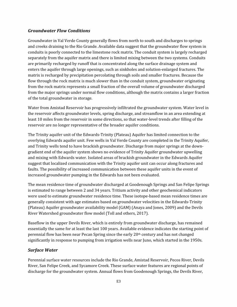
Groundwater Flow Conditions
Groundwater in Val Verde County generally flows from north to south and discharges to springsand creeks draining to the Rio Grande. Available data suggest that the groundwater flow system inconduits is poorly connected to the limestone rock matrix.The conduitsystem is largely recharged separately from the aquifer matrix and there is limited mixing between the two systems.Conduitsare primarily recharged by runoff that is concentrated along the surface drainage system andenters the aquifer through large openings, such as sinkholes and solution-enlarged fractures. Thematrix is recharged by precipitation percolating through soils and smaller fractures.Because the flow through the rock matrix is much slower than in the conduit system, groundwater originatingfrom the rock matrix represents a small fraction of the overall volume of groundwater dischargedfrom the major springs under normal flow conditions, although the matrix contains a larger fractionof the total groundwater in storage.
Water from Amistad Reservoir has progressively infiltrated the groundwater system.Water levelin the reservoir affects groundwater levels, spring discharge, and streamflow in an area extending atleast 10 miles from the reservoir in some directions, so that water-leveltrends after filling of the reservoir are no longer representative of the broader aquifer conditions.
The Trinity aquifer unit of the Edwards-Trinity (Plateau) Aquifer has limited connection to theoverlying Edwards aquifer unit. Few wells in Val Verde County are completed in the Trinity Aquifer,and Trinity wells tend to have brackish groundwater. Discharge from major springs at the down-gradient end of the aquifer system shows no evidence of Trinity Aquifer groundwater upwellingand mixing with Edwards water. Isolated areas of brackish groundwater in the Edwards Aquifersuggest that localized communication with the Trinity aquifer unit can occur along fractures andfaults. The possibility of increased communication between these aquifer units in the event ofincreased groundwater pumping in the Edwards has not been evaluated.
The mean residence time of groundwater discharged at Goodenough Springs and San Felipe Springsis estimated to range between 2 and 34 years. Tritium activity and other geochemical indicatorswere used to estimate groundwater residence time. These isotope-based mean residence times aregenerally consistent with age estimates based on groundwater velocities in the Edwards-Trinity(Plateau) Aquifer groundwater availability model (GAM) (Anaya and Jones, 2009) and the Devils River Watershed groundwater flow model (Toll and others, 2017).
Baseflow in the upper Devils River, which is entirely from groundwater discharge, has remainedessentially the same for at least the last 100 years. Available evidence indicates the starting point of perennial flow has been near Pecan Spring since the early 20th century and has not changed significantly in response to pumping from irrigation wells near Juno,which started in the 1950s.
Surface Water
Perennial surface water resources include the Rio Grande, Amistad Reservoir, Pecos River, Devils River, San Felipe Creek,and Sycamore Creek.These surface water features are regionalpoints of discharge for the groundwater system. Annual flows from Goodenough Springs, the Devils River,
E3
and San Felipe Springs are estimated to provide about 23 percent of the flow in the Rio Grandebelow Amistad Reservoir (Green, 2013). Permitted surface water rights and environmental flowstandards for new appropriations (if any) of surface water resources in Val Verde County may haveimplications for groundwater management.
The intimate connection between groundwater and surface water in Val Verde County hascomplicated measurements over time. Measured flow in the Devils River at Pafford Crossingincreased after Amistad Reservoir filled and may not be a good indicator of conditions in the upper,spring-fed reaches of the river. Also, flow measurements in the Devils River at the Bakers Crossinggage have been inconsistent over time, with measurements by both the U.S. Geological Survey and the International Boundary and Water Commission,complicating interpretation of any long-term trends.On the other hand,periodic low-flow gain-loss studies on the Devils River show nearlyidentical patterns of spring discharge to the river between 1928 and 2006.
Endangered Species Threatened or endangered aquatic species in Val Verde County include the Devils River minnow, Proserpine shiner, Rio Grande darter, the Conchos pupfish – Devils River subspecies, the Mexican blindcat, and the recently-listed Texas Hornshell mussel. Evaluation of threatened or endangeredspecies or habitats is an important consideration in the overall understanding of the hydrogeologicsystem and for groundwater management decisions. Streamflow requirements for these species arelinked to spring discharges and are therefore tied to groundwater conditions. Aquatic habitats for these species depend upon groundwater inflows to maintain sufficient,good quality river flows, particularly during droughts and summer low-flows when surface runoff is minimal and water quality begins to deteriorate. Water quality can be compromised during low flow events if water temperatures rise and dissolved oxygen decreases,further impacting these rare aquatic organisms.The TPWD has directly observed mass predation events on Texas Hornshell in the Devils Riverduring a prolonged low spring and streamflow period in 2015. Additionally, there are concerns about elevated water temperatures during periods of low flow that are potentially lethal to larval and adult mussels. The TPWD, The Nature Conservancy (TNC), University of Texas (UT), and TexasA&M University (TAMU) are currently conducting research to determine what these critical lethal temperatures are and under whatflows they mightoccur in Texas Hornshellhabitatin the Devils River. The threat of worsening drought, in concert with the potential for groundwater development,could exacerbate the loss of species habitat, thereby increasing the rate of species decline and leading to criticalgroundwater problems in the future.
The U.S. Fish and Wildlife Service, TPWD,and TNC have conducted extensive research on threatened and endangered species in Val Verde County and maintain active species managementprograms. Ongoing research by the UT Bureau of Economic Geology is examining the linkagesbetween habitat requirements and the groundwater system.
Groundwater Modeling
Several groundwater flow models have been developed that cover all or part of Val Verde County.The Edwards-Trinity (Plateau) Aquifer groundwater availability model (GAM) is a large regional
E4
model developed by the TWDB. Because it has a coarse model grid, annual time steps, and lack ofcalibration to spring discharges, the GAM is inappropriate for modeling critical flows at possiblehydrologic trigger locations. The Val Verde County (Eco-Kai and Hutchison, 2014) groundwatermodel, which is derived from a TWDB model of Kinney County and surrounding areas (Hutchison,Shi, and Jigmond, 2011), represents the best starting point for a Val Verde County groundwatermanagement model. The Val Verde County model employs a finer spatial grid than the TWDB GAM and has monthly time steps, includes calibration to several major springs, and specifiesconsiderable hydrogeological detail for both the U.S. and Mexican portions of the Edwards-Trinity(Plateau) Aquifer system. The Devils River Watershed Model, a combined surface water-groundwater model developed by Toll and others (2017), has daily time-steps and a much finergrid around critical areas, but covers only the Devils River watershed. In addition, the modelspecifies considerably more detailed aquifer properties than are supported by available data,making model calibration uncertain and complicating application to the remainder of the county,for which even less data are available.A coupled groundwater-surface water model remainsattractive because of the intimate connections between groundwater and surface water in thecounty but may not be practical at this time.
Improved groundwater flow models would help decision makers with groundwater managementissues in Val Verde County.Better models require more groundwater data with the appropriatespatial and temporal coverage. Water level measurements are the fundamental hydrological datasetand current monitoring networks do not provide adequate spatial or temporal coverage. Improvedaccuracy of groundwater use estimates in Val Verde County would also improve the usefulness of a model. Additional data – whether water levels or groundwater use estimates – requires time to develop and incorporate appropriately into any revisions or updates of groundwater flow models.
Effects of Groundwater Pumping
Groundwater pumping has the potential to affect streamflow and spring discharges in Val VerdeCounty.Due to the strong linkages between surface water and groundwater, reduction ingroundwater levels resulting from pumping may decrease surface flows. Pumping is unlikely toaffect groundwater recharge over most of Val Verde County.In mostareas,the groundwater levelis already well below the land surface and the base of the root zone. Lowering the water table furtherwill not induce greater recharge or reduce evapotranspiration. However, concentrated high-volumepumping near Amistad Reservoir or along perennial river reaches could induce capture,or flow, from surface water to groundwater.
Water Usage and Demand Projections
The 2017 State Water Plan indicates no near-term or long-term water supply shortages under current development scenarios, except for small unmet needs in the mining (oil and gas) sector.The total county water demand is expected to grow 26 percent over 50 years, from 16,777 acre-feetper year in 2020 to 21,127 acre-feet per year in 2070, while the modeled available groundwater is 50,000 acre-feet per year. Not including Del Rio’s use of surface water originating from San FelipeSprings, groundwater pumping for all uses in Val Verde County has averaged about 4,700 acre-feetper year since 2001. Total projected demand for groundwater remains less than projected supplies
E5

throughoutthe 50-year planning period. In recent years, several groundwater well fields have beenproposed to supply water outside the county. The modeled available groundwater value of 50,000acre-feet per year was estimated from groundwater flow modeling of three hypothetical well fields north of Del Rio.
Groundwater Management
Val Verde County does not have a groundwater conservation district but is included in groundwatermanagement planning as part of Groundwater Management Area 7 (GMA 7), which includes all orpart of 33 counties and 21 groundwater conservation districts in West-Central Texas. Groundwaterdistrict representatives voted to adopt new desired future conditions for the county in March 2018,specifying that total net drawdown through 2070 should maintain an average annual flow of 73 to75 million gallons per day (81,800 to 84,000 acre-feet per year) at San Felipe Springs. There is nocurrent mechanism in place to monitor groundwater conditions or enforce this management goalfor the Edwards-Trinity (Plateau) Aquifer.
The Texas Water Code (§36.108(d-1)) allows a groundwater conservation district to consider thespecific groundwater conditions in its area and establish separate desired future conditions forsubdivisions of aquifers or for different geographic areas of aquifers. Based on review of availablegroundwater data for the county, variations in the hydrogeological conditions in the county couldbe the basis for establishing four separate management zones to facilitate groundwatermanagement efforts.
Feasibility of Hydrologic Triggers
Index wells and hydrologic trigger levels are used as groundwater management strategies bygroundwater conservation districts in the Edwards Aquifer and elsewhere in Texas. Similarapproaches,as wellas use of spring flow measurements or streamflow measurements at specific locations,could also be applied to manage groundwater resources in Val Verde County.Index well selection and trigger level determination should be based on specific management objectives anddocumented correlations between the management objectives and aquifer conditions, such as indexwell water levels, or related surface water indicators, such as streamflow or spring flow.Demonstrating such correlations, however, is difficult with current data. Many of the wells where water levels have been measured historically are within the area of influence of Amistad Reservoirand may no longer be relevant for tracking aquifer conditions. Discharges at San Felipe Springs andother springs near Amistad Reservoir are likewise influenced by the lake level, and trigger levelsbased on discharge at these springs are of questionable value for groundwater managementpurposes. A well-calibrated and validated groundwater model will be essential for establishing defensible index well locations and trigger levels.
E6
1.0 Introduction Groundwater is the main source of water supply for municipal, domestic, and livestock uses in Val Verde County. Almost all water wells in Val Verde County are completed in the Edwards Group limestones,which form the upper-most portion of the Edwards-Trinity (Plateau) Aquifer,a majoraquifer in Texas extending throughout much of Central Texas. Val Verde County is situated at thesouthwestern edge of the Edwards Plateau, and is an area of regionalgroundwater discharge. Val Verde County has numerous springs, including several of the largest in Texas. These springs, such as San Felipe Springs, supply surface water for the City of Del Rio, sustain base flow in SanFelipe Creek and the Devils River, and contribute to flow in the Lower Rio Grande.
In recentyears, there have been a number of hydrogeologic investigations of limited scope coveringportions of Val Verde County.However,no comprehensive report on the groundwater resources ofthe county has been issued in over 45 years, since the U.S.GeologicalSurvey completed the study, Groundwater Resources of Val Verde County,Texas, for the Texas Water Development Board (TWDB)(Reeves and Small, 1973). This 2018 study presents an overview of groundwater data collectedsince that time through routine monitoring, localized investigations, well completions and testing,and groundwater flow modeling efforts.
Background
Groundwater development in Val Verde County has been limited to date; however, the possibility offuture groundwater development has raised questions regarding groundwater-surface waterrelationships, groundwater management, and possible impacts to streams supporting threatened orendangered species. Several numerical groundwater flow models have been developed on behalf ofdifferent groups, using a wide range of inputs and assumptions and reaching differing conclusionsas to the effects of potential groundwater development. There have been several unsuccessful efforts to establish a groundwater conservation district in the last decade.
This report compiles and evaluates the available information on groundwater resources inVal Verde County, identifies uncertainties and data gaps relevant to groundwater management, andassesses potential groundwater monitoring strategies and hydrological triggers that might be used.The TWDB has solicited input from other state agencies, the public, and other stakeholders in preparing this report. A public meeting was held in Del Rio on January 24, 2018, to kick off theprocess. We solicited groundwater data from the International Boundary and Water Commission,The Nature Conservancy, and from other interested groups and landowners in the county. TheHouse Committee on Natural Resources held a public hearing in Del Rio on September 13, 2018, inwhich testimony and comment were received concerning groundwater and surface water issues inVal Verde County.A draftversion of this reportwas provided to the public for review and comment, and this final report incorporates, where appropriate, those public comments.
Scope of Study
Priority Groundwater Management Areas (PGMAs) are identified and designated by the TexasCommission on Environmental Quality (TCEQ) as those areas of Texas not in any established
1
groundwater conservation district (GCD) thatare experiencing or expected to experience critical groundwater problems, including shortages of surface water or groundwater. Priority Groundwater Management Areas and Groundwater Conservation Districts, Report to the 85th Texas Legislature, which was prepared jointly by the TCEQ and TWDB, included the following statement: “Val Verde County and the Devils River were discussed as potential areas of concern and may need follow-upPGMA assessment as more data become available.”
Therefore, the scope of this study is tied closely to the purpose and scope of a PGMA study. Thescope of PGMA studies is defined in the Texas Water Code § 35.007(d). Among other requirements,a PGMA study must include an appraisal of the hydrogeology of the area and other matters withinthe TWDB’s planning expertise relevant to the area and an evaluation of the potential effects of thedesignation of a PGMA on an area’s natural resources prepared by the TPWD.Accordingly,thisreport focuses on the hydrogeology and natural resources of Val Verde County.
This report focuses on compiling and analyzing scientific and technical data on the groundwaterand related natural resources of Val Verde County. We also consider the feasibility of potentialhydrologic triggers as a groundwater management tool. Ideally, a trigger provides early warning ofgroundwater conditions that could cause an undesirable result. We examine existing data onpumping, water levels, and streamflow to determine if any currentmonitoring locations meet thesecriteria and to define the general types and locations of additional monitoring that might berequired to meet potential groundwater management objectives.
Previous studies of the Edwards-Trinity (Plateau) Aquifer have defined the environmental setting, geological framework, and regional groundwater movement (Barker and Ardis, 1996; Kunianskyand Ardis, 2004; Anaya and Jones, 2009). This report includes excerpts of those portions of the regional reports thatare relevant to the western Edwards Plateau. This study also has re-examined groundwater data maintained by the TWDB, the International Boundary and Water Commission,and the U.S.GeologicalSurvey, as well as reports commissioned by The Nature Conservancy, theCity of Del Rio, and other sources to reflect the most recent information on water levels, water quality, streamflow,and groundwater use in ValVerde and adjacentcounties.
This study also evaluated literature on historical spring flows and the effects of land-use changes ongroundwater recharge and stream baseflow. The evaluation included a review of well completionand water quality data in the TWDB Groundwater Database,U.S. Geological Survey streamflowrecords, National Oceanic and Atmospheric Administration (NOAA) weather data,and Landsat satellite imagery to assess the effectof historical landscape changes on the hydrology of Val Verde County.
Public Comments
The TWDB solicited and received public comments on the study and on the draft report following the public hearing conducted by the House Committee on National Resources on September 13,2018, in Del Rio. The draft report was revised as appropriate to incorporate the public comments.The comments are included in Appendix D.
2

2.0 GeographicSetting and NaturalResources Key findings
• Edwards Plateau geography is characterized by limestone outcrops and thin, loose soils. • On average, evaporation exceeds precipitation in all months. • Infrequent, extreme precipitation leads to rapid runoff and high flash flood potential. • Plant communities have changed over time in response to land use, but the effects of these
changes on the hydrological cycle are widely debated. • Several threatened and endangered aquatic species are present in Val Verde County. • Maintaining streamflow and water quality are important components of wildlife
management efforts led by the U.S. Fish and Wildlife Service, the Texas Parks and WildlifeDepartment, The Nature Conservancy, and cooperating landowners in Val Verde County.
• The prospects of worsening droughts, in concert with the potential for increasedgroundwater withdrawals, could exacerbate the loss of species habitat,thereby increasing the rate of species decline and leading to criticalgroundwater problems in the future.
Geography is a major factor in water availability and water use. Topography, climate, soils, vegetation, and land use affectrunoff and groundwater recharge,while habitatrequirements for sensitive wildlife populations can influence natural resource planning and management.
Val Verde County is in southwestern Texas (Figure 2-1).Itcovers an area of 3,145 square miles, or2,085,760 acres, and had a population of 48,879 at the time of the 2010 census.Approximately75 percent of the county’s population lives in the City of Del Rio, located in the southeastern cornerof the county. The county’s southern boundary is the Rio Grande.
Val Verde County is situated at the southwestern margin of the Edwards Plateau, “a resistant carbonate upland of nearly flat-lying limestone and dolostone,typically veneered with loose,thin soils. Caprock mesas, broad alluvial fans, and dry arroyos are the most prominent features”(Barker,Bush, and Baker 1994). The southwestern corner of the county, west of the Pecos River, is theeasternmost part of Trans-Pecos region, while the southeastern corner of the county is thenorthwestern-most part of the Gulf coastal plain.
Topography
The elevation of Val Verde County ranges from over 2,000 feet above sea level in the north andalong the divides between major drainages to about 850 feet along the Rio Grande below the Amistad Reservoir. The topography is relatively flat in the Rio Grande floodplain and along theridges but is characterized by narrow, steep-walled canyons cut into the carbonate terrain alongthe Pecos and Devils rivers and their tributaries as the drainages descend from the EdwardsPlateau toward the Rio Grande.
Climate
Val Verde County has a semiarid, subtropical climate characterized by dry winters and hotsummers. From 1965 to 2018, the daily high temperature averaged 81.3 degrees Fahrenheit and the daily low averaged 58 degrees FahrenheitatAmistad Dam. The extreme temperatures at
3

Amistad Dam during this period ranged from 114 degrees on July 29, 1995, to 5 degrees on February 3, 1992 (NationalCenters for EnvironmentalInformation,2018).
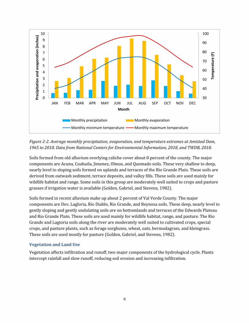
The average annual rainfall at Amistad Dam was 19.4 inches. Of this, 15.2 inches, or about 80percent, fell during the growing season, from April through October (Figure 2-2). May andSeptember are typically the wettestmonths,while December and January are the driest(National Centers for Environmental Information, 2018). On average, evaporation exceeds precipitation in every month.
Extreme storm events periodically cause severe flooding. From 1965 to 2018, the maximum monthly precipitation at Amistad Dam was 14.5 inches in July 1976. The maximum daily rainfallover this period was 7.1 inches on August 3, 2014. During the flood of 1954, when Hurricane Alicestalled over Crockett and Val Verde counties, as much as 24 inches of rain was reported for thestorm event at Pandale, with 16 inches in a 24-hour period (National Centers for EnvironmentalInformation, 2014). Unofficial “bucket surveys” reported as much as 34 inches of rain from thisstorm (Von Zuben, Hayes, and Anderson, 1957).
The Texas Department of Parks and Wildlife indicates that Val Verde County, included as part of theSouthern Great Plains, is projected to have an increased frequency of drought. If this happens, thearea will experience an increase of average temperatures and the frequency, duration, and intensityof extreme heat. These conditions would lead to enhanced evapotranspiration and depleted soilmoisture.
Soils
There are three broad soil groups in Val Verde County (Figure 2-3) mapped by the U.S.Departmentof Agriculture Natural Resources Conservation Service (Golden, Gabriel, and Stevens, 1982). Soilsderived from the Edwards Plateau limestones cover most of the county. Soils derived from olderalluvium deposits in the Rio Grande Plain occur along the river and near Del Rio. Finally, soils derived from recent alluvium, terraces, and valley fills are found along drainages throughoutthe county.
Soils formed from weathering of the Edwards Plateau limestone cover about 88 percent ofVal Verde County.The major components are Ector,Langtry,Lozier,Mariscal,Shumla,Tarrant,andZorra soils and rock outcrop. The Ector-rock outcrop association covers 48 percent of the county;the Langtry-rock outcrop-Zorra association covers 28 percent; and the Lozier-Mariscal-Shumla association covers 8 percent (Golden, Gabriel, and Stevens, 1982). The Edwards Plateau soils are very shallow, loamy, stony soil and exposed limestone bedrock on uplands. These soils drain easilyand typically developed under grass or savanna-type vegetation in sub-humid to semiarid climates. They typically form on the uplands of the Edwards Plateau. The soils are suitable mainly for wildlife habitat and range. Low rainfall, very low available water capacity, and restricted rooting depth limit the amountof range forage produced during mostyears (Golden,Gabriel,and Stevens,1982).
4

Baker’s Crossing
Pafford Crossing
Figure 2-1. Map of Val Verde County,Texas.
5
10 100 Pr
ecip
itatio
n an
d ev
apor
atio
n (in
ches
) 9
90 8
7 80
6 70 5
604
3 50 2
401
0 30 JAN FEB MAR APR MAY JUN JUL AUG SEP OCT NOV DEC
Month
Monthly precipitation Monthly evaporation
Monthly minimum temperature Monthly maximum temperature
Tem
pera
ture
(F)
Figure 2-2.Average monthly precipitation,evaporation, and temperature extremes at Amistad Dam, 1965 to 2018. Data from National Centers for Environmental Information, 2018, and TWDB, 2018.
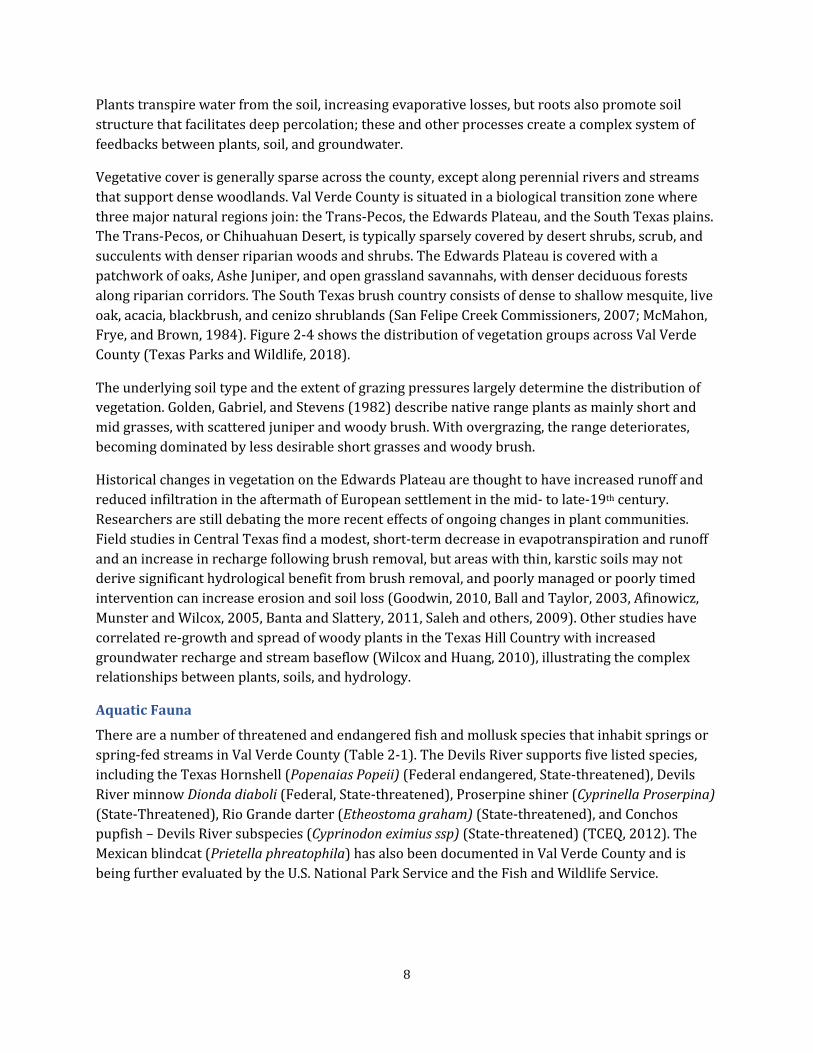
Soils formed from old alluvium overlying caliche cover about 8 percent of the county. The majorcomponents are Acuna, Coahuila, Jimenez, Olmos, and Quemado soils. These very shallow to deep,nearly level to sloping soils formed on uplands and terraces of the Rio Grande Plain. These soils arederived from outwash sediment, terrace deposits, and valley fills. These soils are used mainly forwildlife habitat and range. Some soils in this group are moderately well suited to crops and pasturegrasses if irrigation water is available (Golden, Gabriel, and Stevens, 1982).
Soils formed in recent alluvium make up about 2 percent of Val Verde County.The major components are Dev,Lagloria,Rio Diablo,Rio Grande,and Reynosa soils.These deep,nearly levelto gently sloping and gently undulating soils are on bottomlands and terraces of the Edwards Plateau and Rio Grande Plain. These soils are used mainly for wildlife habitat, range, and pasture. The RioGrande and Lagioria soils along the river are moderately well suited to cultivated crops, specialcrops, and pasture plants, such as forage sorghums, wheat, oats, bermudagrass, and kleingrass.These soils are used mostly for pasture (Golden, Gabriel, and Stevens, 1982).
Vegetation and Land Use
Vegetation affects infiltration and runoff, two major components of the hydrological cycle. Plants intercept rainfall and slow runoff, reducing soil erosion and increasing infiltration.
6

Figure 2-3.Soil map of Val Verde County.Data from Natural Resources Conservation Service,2018.
7
Plants transpire water from the soil,increasing evaporative losses,butroots also promote soil structure that facilitates deep percolation; these and other processes create a complex system offeedbacks between plants, soil, and groundwater.
Vegetative cover is generally sparse across the county,exceptalong perennialrivers and streams thatsupport dense woodlands. Val Verde County is situated in a biologicaltransition zone where three major naturalregions join: the Trans-Pecos, the Edwards Plateau,and the South Texas plains.The Trans-Pecos, or Chihuahuan Desert, is typically sparsely covered by desert shrubs, scrub, andsucculents with denser riparian woods and shrubs.The Edwards Plateau is covered with a patchwork of oaks,Ashe Juniper,and open grassland savannahs, with denser deciduous forestsalong riparian corridors.The South Texas brush country consists of dense to shallow mesquite, live oak, acacia, blackbrush, and cenizo shrublands (San Felipe Creek Commissioners, 2007; McMahon,Frye, and Brown, 1984). Figure 2-4 shows the distribution of vegetation groups across Val VerdeCounty (Texas Parks and Wildlife, 2018).
The underlying soil type and the extent of grazing pressures largely determine the distribution ofvegetation. Golden, Gabriel, and Stevens (1982) describe native range plants as mainly short andmid grasses, with scattered juniper and woody brush. With overgrazing, the range deteriorates,becoming dominated by less desirable short grasses and woody brush.
Historical changes in vegetation on the Edwards Plateau are thought to have increased runoff andreduced infiltration in the aftermath of European settlement in the mid- to late-19th century.Researchers are still debating the more recent effects of ongoing changes in plant communities.Field studies in Central Texas find a modest, short-term decrease in evapotranspiration and runoff and an increase in recharge following brush removal, but areas with thin, karstic soils may notderive significant hydrological benefit from brush removal, and poorly managed or poorly timedintervention can increase erosion and soil loss (Goodwin, 2010, Ball and Taylor, 2003, Afinowicz,Munster and Wilcox, 2005, Banta and Slattery, 2011, Saleh and others, 2009). Other studies havecorrelated re-growth and spread of woody plants in the Texas Hill Country with increasedgroundwater recharge and stream baseflow (Wilcox and Huang, 2010), illustrating the complexrelationships between plants, soils, and hydrology.
Aquatic Fauna
There are a number of threatened and endangered fish and mollusk species thatinhabitsprings or spring-fed streams in Val Verde County (Table 2-1). The Devils River supports five listed species, including the Texas Hornshell (Popenaias Popeii) (Federal endangered, State-threatened), Devils River minnow Dionda diaboli (Federal, State-threatened), Proserpine shiner (Cyprinella Proserpina) (State-Threatened), Rio Grande darter (Etheostoma graham) (State-threatened), and Conchos pupfish – Devils River subspecies (Cyprinodon eximius ssp) (State-threatened) (TCEQ, 2012). The Mexican blindcat (Prietella phreatophila) has also been documented in Val Verde County and isbeing further evaluated by the U.S. National Park Service and the Fish and Wildlife Service.
8
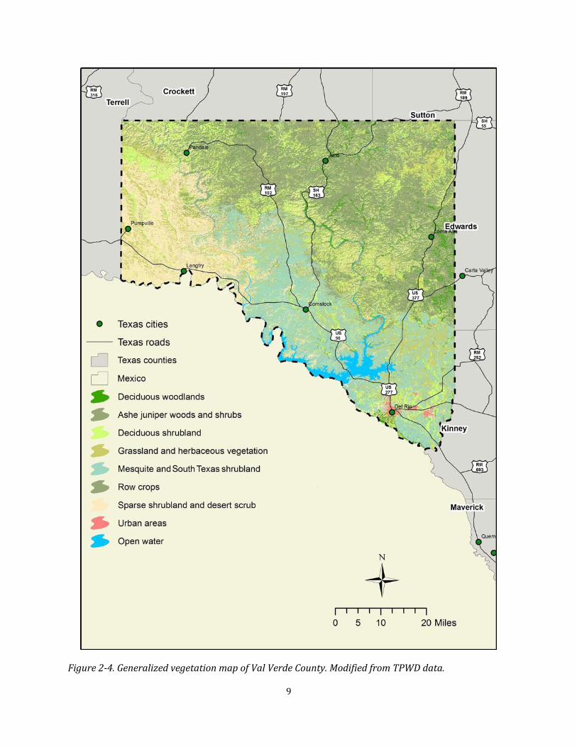
Figure 2-4.Generalized vegetation map of Val Verde County.Modified from TPWD data.
9
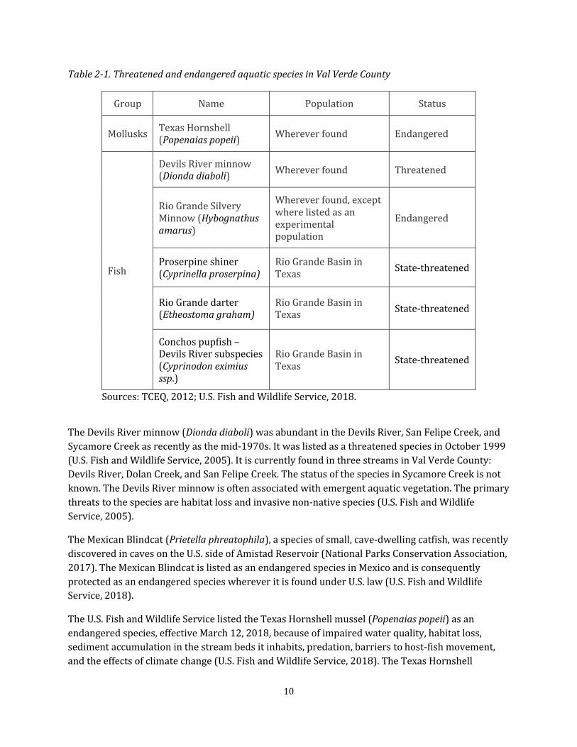
Table 2-1. Threatened and endangered aquatic species in Val Verde County
Group Name Population Status
Mollusks Texas Hornshell (Popenaias popeii) Wherever found Endangered
Devils River minnow (Dionda diaboli) Wherever found Threatened
Rio Grande SilveryMinnow (Hybognathus amarus)
Wherever found, exceptwhere listed as an experimentalpopulation
Endangered
Fish Proserpine shiner(Cyprinella proserpina)
Rio Grande Basin in Texas State-threatened
Rio Grande darter (Etheostoma graham)
Rio Grande Basin in Texas State-threatened
Conchos pupfish – Devils River subspecies(Cyprinodon eximius ssp.)
Rio Grande Basin in Texas State-threatened
Sources: TCEQ, 2012; U.S. Fish and Wildlife Service, 2018.
The Devils River minnow (Dionda diaboli) was abundant in the Devils River, San Felipe Creek, andSycamore Creek as recently as the mid-1970s. It was listed as a threatened species in October 1999(U.S. Fish and Wildlife Service, 2005). It is currently found in three streams in Val Verde County: Devils River,Dolan Creek, and San Felipe Creek. The status of the species in Sycamore Creek is notknown. The Devils River minnow is often associated with emergent aquatic vegetation. The primarythreats to the species are habitatloss and invasive non-native species (U.S. Fish and Wildlife Service, 2005).
The Mexican Blindcat(Prietella phreatophila), a species of small, cave-dwelling catfish, was recentlydiscovered in caves on the U.S. side of Amistad Reservoir (National Parks Conservation Association,2017). The Mexican Blindcatis listed as an endangered species in Mexico and is consequently protected as an endangered species wherever it is found under U.S. law (U.S. Fish and Wildlife Service, 2018).
The U.S. Fish and Wildlife Service listed the Texas Hornshell mussel (Popenaias popeii) as an endangered species, effective March 12, 2018,because of impaired water quality, habitat loss, sediment accumulation in the stream beds it inhabits, predation,barriers to host-fish movement, and the effects of climate change (U.S. Fish and Wildlife Service, 2018).The Texas Hornshell
10
historically ranged throughout the Rio Grande drainage in New Mexico, Texas, and Mexico.Currently, five known populations of Texas Hornshell remain in the United States, including in the Black River in Eddy County,New Mexico; in the Devils River and Pecos River in Val Verde County; in the lower canyons of the Rio Grande in Brewster and Terrell counties; and in the lower Rio Grande near Laredo.
The Texas Hornshell populations in Texas include a small remnant population in the Pecos River,multiple small, more dispersed populations in the Devils River,and moderate populations in the RioGrande. The Texas Hornshell were extirpated from the lower reaches of the Pecos River followinginundation by Amistad Reservoir, and salinity is frequently too high for mussel survival in the reachfrom the confluence with the Black River in New Mexico downstream to the confluence with Independence Creek (U.S. Fish and Wildlife Service, 2018). A small population survives in the PecosRiver downstream of the confluence with Independence Creek and upstream of Amistad Reservoirnear Pandale. Intensive surveys of the Devils River identified Texas Hornshell populations in thelower 29 miles of the river in the Dolan Falls Preserve and the Devils River State NaturalArea’s Big Satan Unit (U.S. Fish and Wildlife Service, 2018).
Streamflow requirements for these species are linked to spring discharges and therefore are tied to groundwater conditions. Aquatic habitats for these species depend upon groundwater inflows tomaintain sufficient, good quality river flows, particularly during droughts and summer low-flowswhen surface runoff is minimal and water quality begins to deteriorate. Water quality can becompromised during low flow events if water temperatures rise and dissolved oxygen decreases,further impacting these rare aquatic organisms. The Texas Park and Wildlife Department (TPWD)has directly observed mass predation events on Texas Hornshell in the Devils River during a prolonged low spring and streamflow period in 2015. Additionally, there are concerns about elevated water temperatures during periods of low flow that are potentially lethal to larval and adult mussels. The TPWD, The Nature Conservancy (TNC),University of Texas,and Texas A&M University are currently conducting research to determine what these critical lethal temperaturesare and under what flows they might occur in Texas Hornshell habitat in the Devils River. Thethreatof worsening droughtin concertwith the potentialfor groundwater development couldexacerbate the loss of species habitat, thereby increasing the rate of species decline and leading to critical groundwater problems in the future.
Conservation efforts for these species are being led by the TPWD and TNC.These organizationsmanage habitat areas in the Devils River State Natural Area and the Dolan Falls Preserve. TheTPWD owns and manages the Del Norte Unit and the Dan A.Hughes Unitof the Devils River State Natural Area. Together these units encompass approximately 37,000 acres. In addition, the TPWDcooperates with TNC, which owns or manages the 4,788-acre Dolan Falls Preserve as well as maintaining interest in nearly 130,000 acres in the Devils River basin through conservationeasements or fee title ownership. Recent and current research investigations have focused ongroundwater levels, spring discharge, river flows, and fish and wildlife habitat suitability. Variouscollaborative research and monitoring programs between the TPWD, TNC, and UT Bureau ofEconomic Geology were ongoing or in development as this reportwas in preparation.These programs and their estimated completion dates include:
11
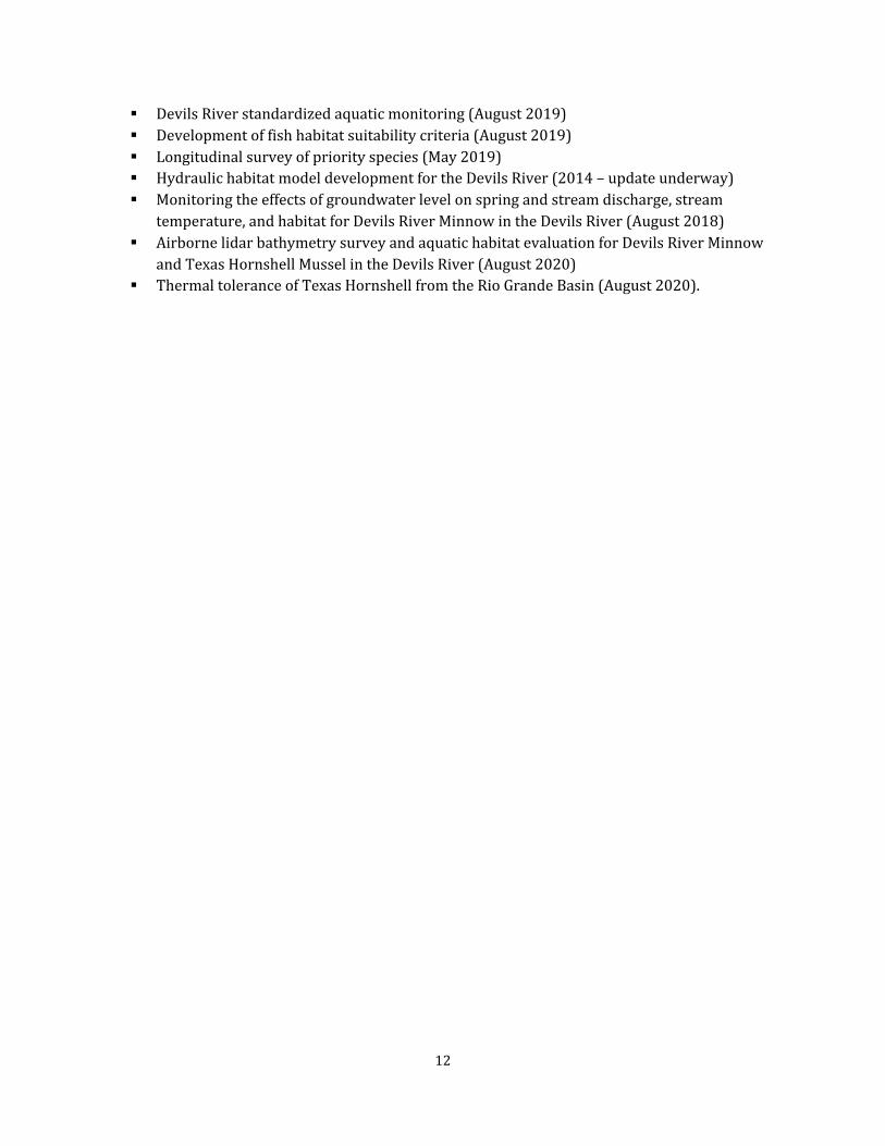
• Devils River standardized aquatic monitoring (August 2019) • Development of fish habitat suitability criteria (August 2019) • Longitudinal survey of priority species (May 2019) • Hydraulic habitat model development for the Devils River (2014 – update underway) • Monitoring the effects of groundwater level on spring and stream discharge, stream
temperature,and habitat for Devils River Minnow in the Devils River (August 2018) • Airborne lidar bathymetry survey and aquatic habitatevaluation for Devils River Minnow
and Texas Hornshell Mussel in the Devils River (August 2020) • Thermal tolerance of Texas Hornshell from the Rio Grande Basin (August 2020).
12
3.0 Geology Key findings
• Cretaceous limestone deposits dominate the surface and near surface geology of Val VerdeCounty.
• The geology varies from north to south, reflecting changes in the depositional environmentduring the Lower Cretaceous period.
• Weathering during periods of low sea levelin the Cretaceous period and in more recent times has dissolved channels in the limestone and associated evaporite minerals, creating akarst fabric.
• Areas of subsidence and sinkholes are common, especially in the outcrop of the Devils River Limestone in central Val Verde County.
The surficial geology of Val Verde County consists predominantly of Cretaceous-age carbonaterocks of the Edwards Plateau (Figure 3-1). The Edwards-Trinity (Plateau) Aquifer consists of rocksof the Edwards (Washita and Fredericksburg) Group and the Trinity Group (Figure 3-2). Rocksdeposited earlier than the Cretaceous period are nota source of water supply in Val Verde County.The Triassic Dockum Aquifer does not extend as far south as Val Verde County.
The Segovia Member of the Edwards Formation covers most of the northern half of the county, except for the area westof the Pecos River,where the Boquillas Flags and Austin Chalk formationsare present at the surface. The Devils River Formation crops out south of the Segovia Formation in aroughly east-west band approximately 8 miles wide. To the west of the Devils River, the DevilsRiver Formation is partially covered by outcrops of the Del Rio Clay, Buda Limestone, and AustinChalk formations on the higher elevations. The Salmon Peak Formation outcrops in broad areas south of the Devils River Formation.The Salmon Peak Formation is locally covered by the Upper Cretaceous Del Rio Clay, Buda Limestone, and Eagle Ford Group sediments, and Quaternarydeposits including the Uvalde Gravel Formation.
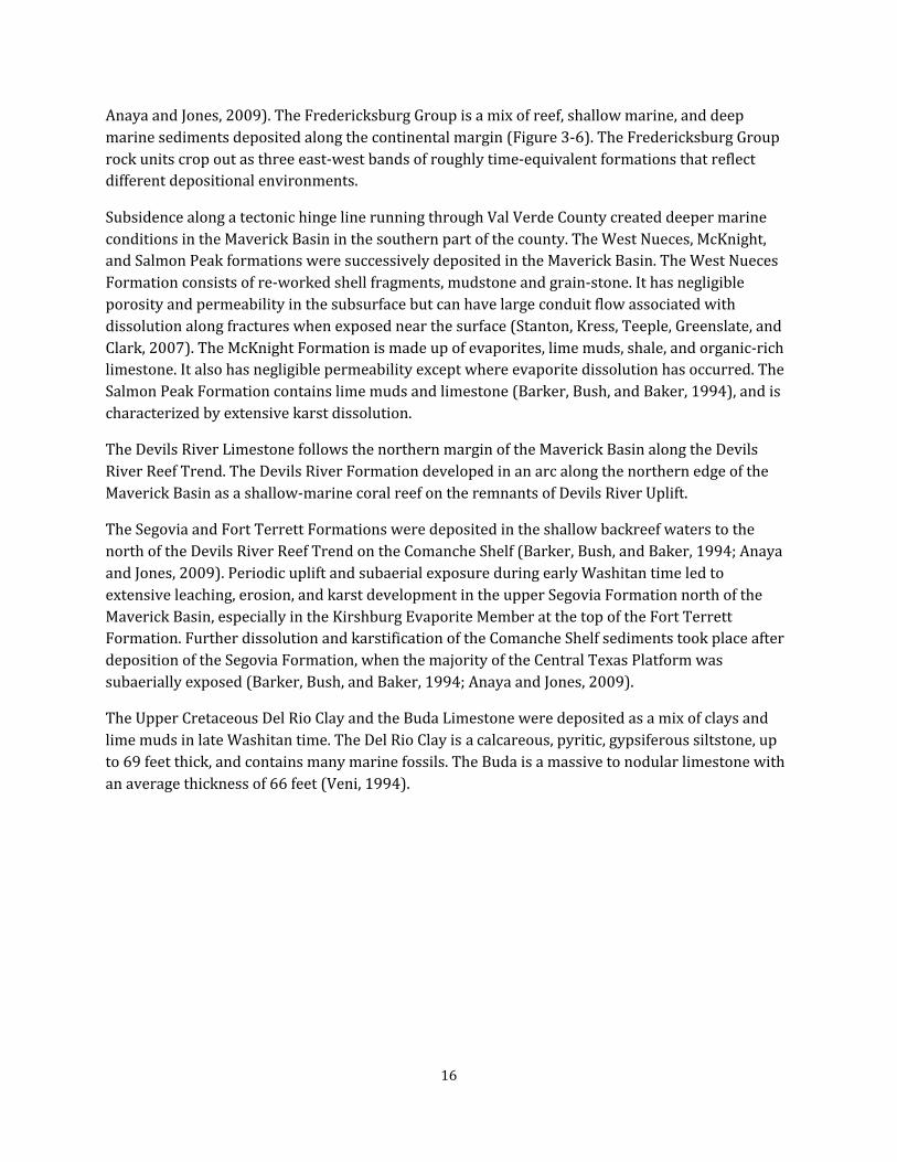
Figures 3-3 to 3-5 are generalized geologic cross-sections of Val Verde County.The geometry of the Trinity Group – identified in these sections as the Glen Rose Limestone – is not as well defined as the Edwards Group.Fewer wells are completed in the Trinity Group because adequate water is generally found at shallower depths in the Edwards Aquifer.As a result,wellcontrolto define the base of the Trinity Group is relatively sparse.
During the Cretaceous period (145 to 65 million years ago), carbonate sediments were depositedover an eroded surface and accumulated to form southward-dipping and thickening rock layers in Val Verde County (Figure 3-2).The base of the Cretaceous sediments extends from a current elevation of over 1,200 feet in the north to as much as 2,000 feet below sea level in the south near Del Rio (Barker, Bush, and Baker, 1994; Anaya and Jones, 2009).
13
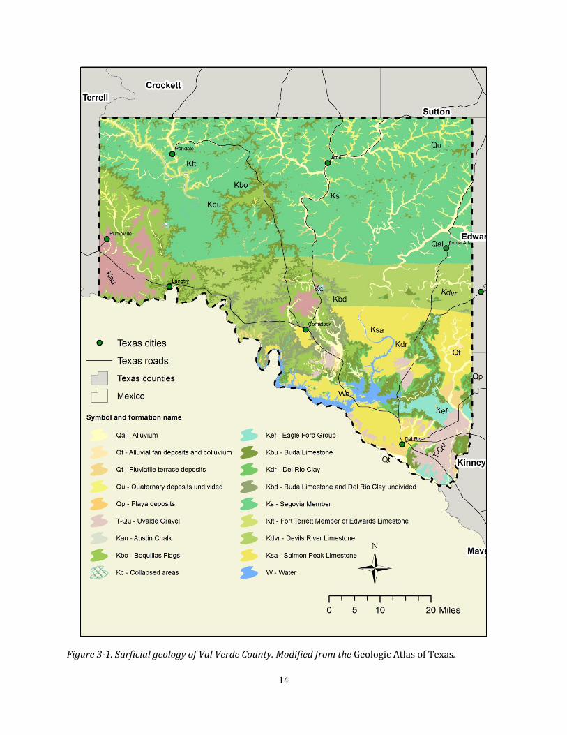
Figure 3-1.Surficial geology of Val Verde County. Modified from the Geologic Atlas of Texas.
14

Figure 3-2. Hydrostratigraphic chart of the central Edwards Plateau. Adapted from Anaya and Jones, 2009.
Lower Cretaceous (145 to 100 million years ago) rock units are composed of sandstones andmarine carbonates of the Trinity, Fredericksburg, and Washita groups. The basal Cretaceous Sand,an alluvial deposit formed by braided streams draining from the Devils River and Llano upliftssoutheast to the Gulf and of Mexico, is the oldest Trinity Group formation (“basement sands” onFigures 3-3 through 3-5). The Glen Rose Limestone was deposited on top of the basal sand in a shallow marine environment as the Gulf continued to subside (Barker, Bush, and Baker, 1994;
15
Anaya and Jones, 2009). The Fredericksburg Group is a mix of reef, shallow marine, and deepmarine sediments deposited along the continental margin (Figure 3-6). The Fredericksburg Grouprock units crop out as three east-west bands of roughly time-equivalent formations that reflectdifferent depositional environments.
Subsidence along a tectonic hinge line running through Val Verde County created deeper marineconditions in the Maverick Basin in the southern part of the county. The West Nueces, McKnight,and Salmon Peak formations were successively deposited in the Maverick Basin. The West NuecesFormation consists of re-worked shell fragments, mudstone and grain-stone. It has negligibleporosity and permeability in the subsurface but can have large conduit flow associated withdissolution along fractures when exposed near the surface (Stanton, Kress, Teeple, Greenslate, andClark, 2007). The McKnight Formation is made up of evaporites, lime muds, shale, and organic-richlimestone.Italso has negligible permeability exceptwhere evaporite dissolution has occurred.The Salmon Peak Formation contains lime muds and limestone (Barker, Bush, and Baker, 1994), and ischaracterized by extensive karst dissolution.
The Devils River Limestone follows the northern margin of the Maverick Basin along the DevilsRiver Reef Trend. The Devils River Formation developed in an arc along the northern edge of theMaverick Basin as a shallow-marine coral reef on the remnants of Devils River Uplift.
The Segovia and Fort Terrett Formations were deposited in the shallow backreef waters to the north of the Devils River Reef Trend on the Comanche Shelf (Barker, Bush, and Baker, 1994; Anayaand Jones, 2009). Periodic uplift and subaerial exposure during early Washitan time led toextensive leaching, erosion, and karst development in the upper Segovia Formation north of theMaverick Basin, especially in the Kirshburg Evaporite Member at the top of the FortTerrettFormation. Further dissolution and karstification of the Comanche Shelf sediments took place afterdeposition of the Segovia Formation, when the majority of the Central Texas Platform was subaerially exposed (Barker, Bush, and Baker, 1994; Anaya and Jones, 2009).
The Upper Cretaceous Del Rio Clay and the Buda Limestone were deposited as a mix of clays andlime muds in late Washitan time.The DelRio Clay is a calcareous,pyritic,gypsiferous siltstone,up to 69 feetthick,and contains many marine fossils. The Buda is a massive to nodular limestone withan average thickness of 66 feet (Veni, 1994).
16

Figure 3-3.Generalized cross-section (A-A’) of Cretaceous deposits in Val Verde County (Reeves and Small, 1973).
Figure 3-4. Generalized cross-section (B-B’) of Cretaceous deposits in Val Verde County (Reeves and Small, 1973).
17
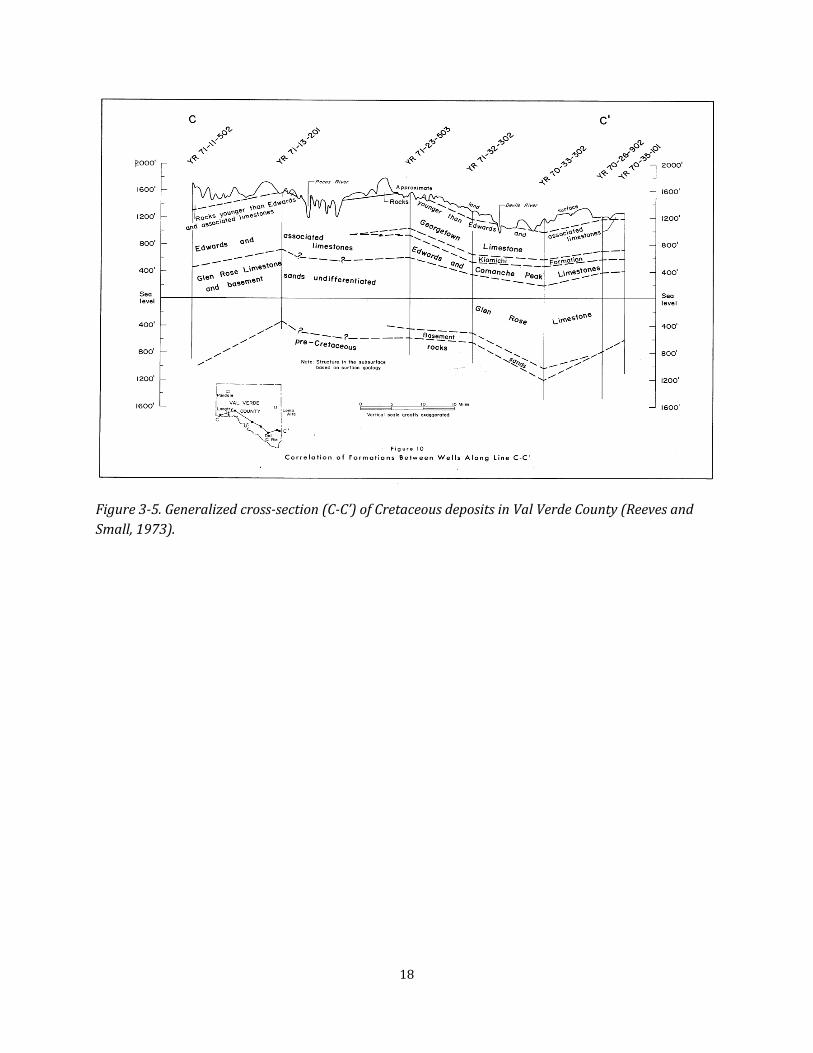
Figure 3-5.Generalized cross-section (C-C’) of Cretaceous deposits in Val Verde County (Reeves and Small, 1973).
18
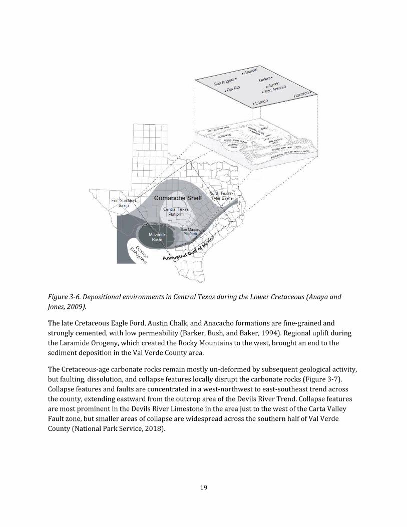
Figure 3-6. Depositional environments in Central Texas during the Lower Cretaceous (Anaya and Jones,2009).
The late Cretaceous Eagle Ford, Austin Chalk, and Anacacho formations are fine-grained and strongly cemented, with low permeability (Barker, Bush, and Baker, 1994). Regional uplift during the Laramide Orogeny, which created the Rocky Mountains to the west, brought an end to thesediment deposition in the Val Verde County area.
The Cretaceous-age carbonate rocks remain mostly un-deformed by subsequent geological activity,but faulting, dissolution, and collapse features locally disrupt the carbonate rocks (Figure 3-7).Collapse features and faults are concentrated in a west-northwest to east-southeast trend acrossthe county, extending eastward from the outcrop area of the Devils River Trend.Collapse features are most prominent in the Devils River Limestone in the area just to the west of the Carta ValleyFault zone, but smaller areas of collapse are widespread across the southern half of Val Verde County (National Park Service, 2018).
19

Carta Valleyfaultzone
Figure 3-7. Sinkholes, subsidence features, and faults in Val Verde County.Data from National Park Service, 2018.
20
4.0 Hydrogeology Key findings
• The Edwards-Trinity (Plateau) Aquifer is the principal aquifer in Val Verde County.Groundwater in the aquifer generally flows from north to south and discharges to springsand streams draining to the Rio Grande.
• Groundwater quality data suggest that most recharge supplying major springs occursthrough large fractures and sinkholes, and discharges through a system of conduits withminimal interaction with the aquifer matrix under normal flow conditions.
• Karst conduits associated with stream drainages are important elements of the Val Verdegroundwater system, although there remains ambiguity as to the nature of the conduits and their effects on groundwater movement and production at particular locations of interest.
• Widely varying recharge estimates introduce significantuncertainties in the groundwater budget.
• The mean residence time of groundwater discharged from the major springs may rangefrom 2 years to 34 years.
• Resolving the true sources of spring flows are necessary to properly calibrate models and to provide the most accurate estimates of aquifer properties and groundwater volumesavailable for use.
• Water levels in wells across much of the southern half of the county were affected asAmistad Reservoir filled. Spring flows also increased in this area.
• Water levels in parts of the county outside the area influenced by Amistad Reservoir arevery consistent over the period of record and do not exhibit any long-term decline in response to pumping or reduced recharge.
• Well yields are highly variable with the highest yields found along stream channels. • Available data suggest that the Devils River has had intermittent flow above Pecan Springs
over the last 100 years. • Localized areas of drawdown may be present near some larger capacity wells but cannot be
distinguished from background variability given the available network of observation wells. • Available water level records do not demonstrate any widespread, long-term effects on
recharge, streamflow, or groundwater-surface water interaction because of current levels ofpumping in Val Verde County.
• Groundwater pumping has the potential to affect the lateral movement of groundwater inVal Verde County.Pumping also has the potentialto reduce streamflows and spring discharge.
• More detailed monitoring is needed. The current groundwater monitoring network does not support detailed evaluation of changes in groundwater elevations or flow over time.
The extent and thickness of the different formations comprising the aquifers, and the geological structures developed in those formations,define the physicalframework of the groundwatersystem. Groundwater elevations within the aquifers indicate the directions in which groundwatergenerally flows. The hydraulic properties of the aquifer affect flow rates and the overall storagecapacity of the aquifer. Groundwater recharge and discharge, by pumping, spring flows, and
21
interaction with rivers and lakes, determine how the groundwater system evolves over time.Groundwater quality affects the usability of the resource and can serve as a useful tracer forgroundwater movement through the aquifer system.
Hydrostratigraphy
The primary source of groundwater in Val Verde County is the carbonate rocks of theFredericksburg Group and the lower part of the Washita Group,collectively known as the Edwards Aquifer (Figure 3-2).These include the Fort Terrett and Segovia formations,the Devils River Formation, and the West Nueces, McKnight, and Salmon Peak formations.
Regionally, the hydraulic relationship between the Edwards and the Trinity aquifers is variable and complex. Throughout much of the Edwards Plateau, the Edwards Aquifer is hydraulically connected to the underlying Trinity Aquifer and is mapped as the Edwards-Trinity (Plateau) Aquifer by theTWDB. However, in Val Verde County there appears to be limited communication between theEdwards and the Trinity aquifers,as illustrated by the GAM modeled water budget (Anaya and Jones, 2009),which estimates a netupward flux from the Trinity to the Edwards of about2,600 acre-feet per year. Veni (1996) considers the Glen Rose Formation as a locally impermeable lower boundary of the Edwards Aquifer in central Val Verde County.Kreitler,Beach,Symank,Uliana,Bassett, Ewing, and Kelly (2013) conclude that there is a small downward flux from the EdwardsAquifer to the Trinity Aquifer, except in a zone of regional discharge near the Rio Grande wherethere is up-flow of more saline water from the Trinity Aquifer.
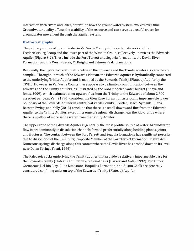
The upper zone of the Edwards Aquifer is generally the most prolific source of water.Groundwaterflow is predominantly in dissolution channels formed preferentially along bedding planes, joints,and fractures. The contact between the Fort Terrett and Segovia formations has significant porositydue to dissolution of the Kirshburg Evaporite Member of the Fort Terrett Formation (Figure 4-1).Numerous springs discharge along this contact where the Devils River has eroded down to its levelnear Dolan Springs (Veni, 1996).
The Paleozoic rocks underlying the Trinity aquifer unit provide a relatively impermeable base for the Edwards-Trinity (Plateau) Aquifer on a regional basis (Barker and Ardis, 1992). The UpperCretaceous Del Rio Clay, Buda Limestone, Boquillas Formation, and Austin Chalk are generallyconsidered confining units on top of the Edwards -Trinity (Plateau) Aquifer.
22
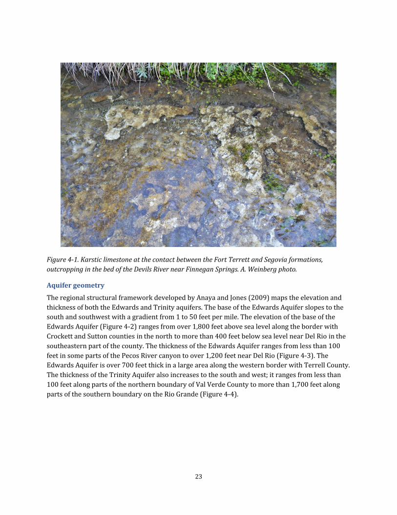
Figure 4-1.Karstic limestone at the contact between the Fort Terrett and Segovia formations, outcropping in the bed of the Devils River near Finnegan Springs. A. Weinberg photo.
Aquifer geometry
The regional structural framework developed by Anaya and Jones (2009) maps the elevation and thickness of both the Edwards and Trinity aquifers. The base of the Edwards Aquifer slopes to thesouth and southwest with a gradient from 1 to 50 feetper mile.The elevation of the base of the Edwards Aquifer (Figure 4-2) ranges from over 1,800 feet above sea level along the border withCrockett and Sutton counties in the north to more than 400 feetbelow sea levelnear DelRio in the southeastern part of the county. The thickness of the Edwards Aquifer ranges from less than 100feet in some parts of the Pecos River canyon to over 1,200 feet near Del Rio (Figure 4-3). TheEdwards Aquifer is over 700 feet thick in a large area along the western border with Terrell County.The thickness of the Trinity Aquifer also increases to the south and west; it ranges from less than100 feet along parts of the northern boundary of Val Verde County to more than 1,700 feetalong parts of the southern boundary on the Rio Grande (Figure 4-4).
23

Figure 4-2.Elevation ofthe base ofthe Edwards section ofthe Edwards-Trinity (Plateau) Aquifer in Val Verde County,in feet relative to mean sea level. Data from Anaya and Jones, 2009.
24

Figure 4-3.Thickness,in feet, of the Edwards section of the Edwards-Trinity (Plateau) Aquifer in Val Verde County.Data from Anaya and Jones,2009.
25

Figure 4-4.Thickness,in feet, of the Trinity section ofthe Edwards-Trinity (Plateau) Aquifer in Val Verde County.Data from Anaya and Jones, 2009.
26
Water Levels and Flow
Groundwater elevations in the Edwards-Trinity (Plateau) Aquifer range from over 1,800 feet abovesea level in northern parts of Val Verde County to about900 feetnear DelRio.Groundwater levels in wells near Amistad Reservoir show a strong correlation with the reservoir level.Groundwaterflow within the Edwards Aquifer generally follows surface topography and converges on the drainages of the Pecos and Devils rivers and Sycamore Creek.
The TWDB and the International Boundary and Water Commission (IBWC) maintain observationwell networks in Val Verde County. Two TWDB recorder wells measure water levels every hour and 20 current observation wells are measured manually by the TWDB once a year. These wells are mostly located along the Devils River and near Amistad Reservoir.In addition,the International Boundary and Water Commission measures water levels in 10 wells in the southern half of thecounty (Figure 4-5). Wells outside the area of influence of Amistad Reservoir have had generallystable water levels over the period of record. The water level variations of wells within the influence of the reservoir closely track the reservoir surface elevation.
The current groundwater monitoring networks are adequate for defining regional changes ingroundwater conditions, but do not provide sufficient spatial or temporal detail to define localgroundwater features, such as drainage areas around springs or areas of influence around pumping wells. Some locations (Figure 4-5) listed as TWDB observation wells are no longer accessible or cannot be measured. In addition, monitoring has been discontinued at about half of the IBWCobservation wells since 2011; therefore the TWDB has notreceived any of the IBWC monitoring data since 2011. There are no observation wells in the Pecos River drainage area; there is only one observation well in the Sycamore Creek drainage area; and there is sparse coverage along tributaries to the Devils River such as the Dry Devils River,Dolan Creek,and Johnson Draw.
Water level maps typically show synoptic conditions, reflecting measurements made over a shortperiod of time, and are used to evaluate groundwater flow direction and assess where changes ingroundwater level or flow may be occurring. Veni (1996) developed the most detailed map ofgroundwater levels for the Val Verde County area to date, reporting 172 water level measurementsduring 1994 and 1995 in the Dolan Springs drainage basin, covering portions of Val Verde, Crockett,Sutton, and Edwards counties. Veni’s groundwater elevation map (Figure 4-6) reflects a point-in-time view of the complex groundwater drainage patterns controlled by topography and karst structures but covers only a portion of Val Verde County.
Figure 4-7 shows contours of the interpolated groundwater elevation surface based on the averageof winter-time (non-pumping) water level measurements at each of the 261 wells in the TWDB groundwater database listed as completed in the Edwards Group or Edwards and associated limestones.The measurementdates span the intervalfrom 1937 to 2015.The water levelcontours thus representlong-term average groundwater conditions.To the extentthatgroundwater levels inVal Verde County have changed over time, these contours may not accurately represent currentconditions.
Groundwater elevations in most of Val Verde have been generally stable over the period of record,although there is significant variability because of naturalcycles of wetness and drought.
27
Hydrographs of water level measurements in 33 Edwards Aquifer wells with at least 10 years ofdata (Figure 4-8) mostly show no increasing or decreasing trends over time. The wells nearAmistad Reservoir,shown in the lower panelof Figure 4-8, are an exception. Water levels in these wells rose as much as 100 feet between 1968 and 1977 as the effect of Amistad Reservoir fillingpropagated through the hydrological system. Several wells in different parts of the county show adecreasing trend since about 2011,including wells 7033508 and 7033302 near Amistad Reservoir and wells 7001402 and 7001404 in the Devils River State NaturalArea.These trends could represent the effects of the drought that began in that year or the effects of local increases inpumping in response to the drought.
Figure 4-9 shows the arealextentarea affected by the hydraulic pressure of the reservoir based on the geographic distribution of wells where the potentiometric head increased as Amistad Reservoir filled. The pressure effect of the reservoir appears to extend at least 10 miles north of the reservoir,past wells 7123901 and 7114702.Itis difficultto distinguish the effects of the rising reservoir level from the effects of the flooding rains and groundwater recharge that caused the reservoir to rise.The groundwater elevation in Well 5456402 (located about two miles north of Juno) increasedfrom 1,692 feet in 1968 to 1,710 feet in 1972. This 18-foot increase in groundwater elevation iswithin the range of historical variability and is probably related to groundwater recharge from theseries of storms that filled the reservoir and not from any pressure effects created by the reservoiritself. Data collection at this well stopped in 1974, so no long-term correlation with reservoir levels can be established. Similar issues apply to interpreting water levelrecords for other wells near potential sources of recharge north of Amistad Reservoir, such as Well 7115501 near Deadman’s Canyon and Well 7001404 along Dolan Creek.
More detailed analysis of water level changes over time requires a denser and more stable networkof monitoring locations with regular measurements. We developed interpolated maps ofgroundwater elevation before and after the reservoir filled using the defaultkriging algorithms in ArcGIS to map the area of hydraulic influence by the reservoir in greater detail. We generated a mapof water level change by subtracting the pre-reservoir surface from the post-reservoir surface. Theresulting map, which is not included here, showed essentially random variations in groundwaterelevation generated by the interpolation process due to differences in the geographical distributionof the measurements.
28
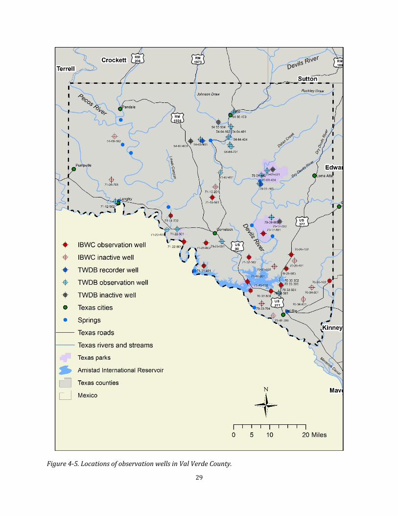
Figure 4-5. Locations of observation wells in Val Verde County.
29
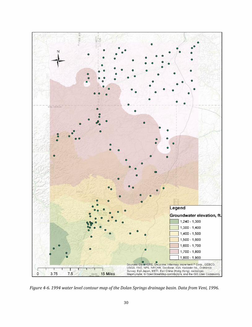
Figure 4-6. 1994 water level contour map of the Dolan Springs drainage basin. Data from Veni, 1996.
30
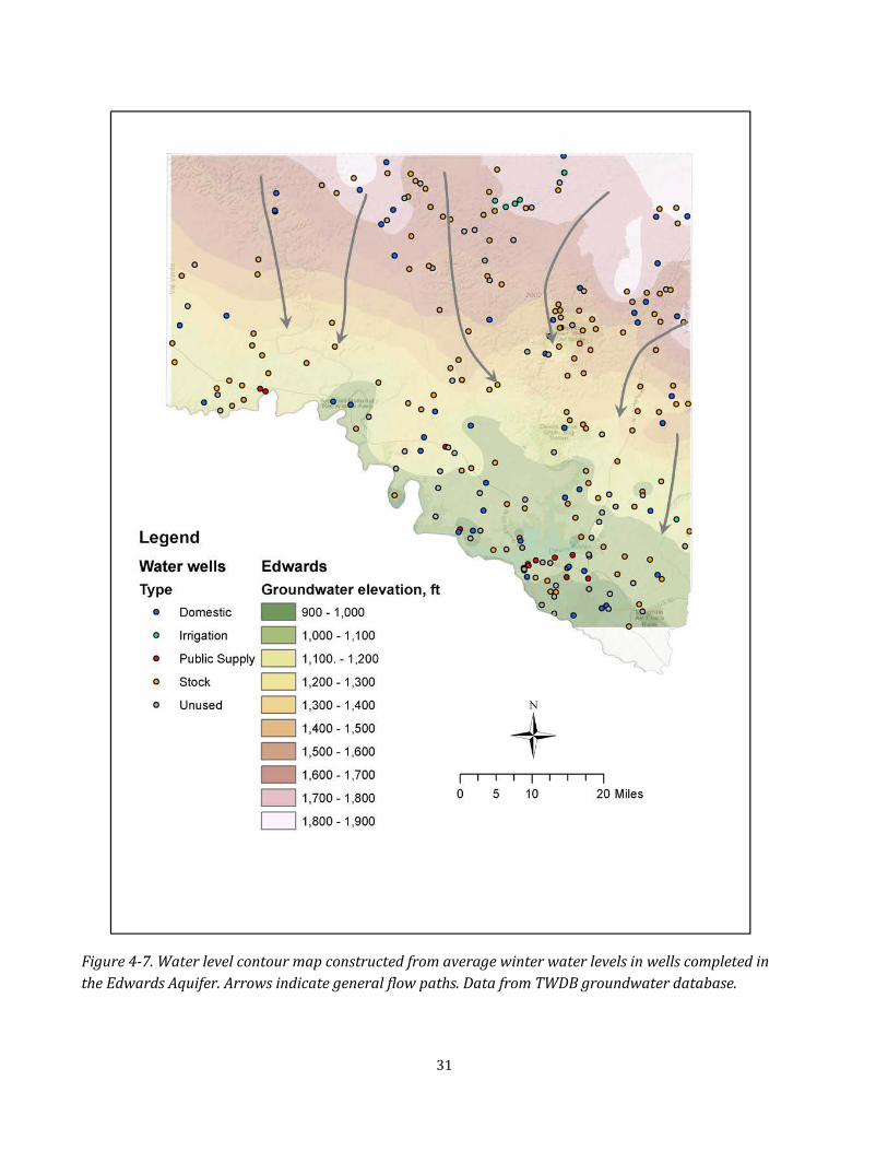
Figure 4-7.Water level contour map constructed from average winter water levels in wells completed in the Edwards Aquifer. Arrows indicate general flow paths. Data from TWDB groundwater database.
31

Water levels in parts of the county outside the area influenced by Amistad Reservoir are veryconsistent over the period of record and do not exhibit any long-term decline in response to pumping or reduced recharge. If landscape changes have had any effects on groundwater or springflows,such changes would have happened prior to the available water level records, the earliest of which are from 1937.
Regional Groundwater Flow Patterns
Groundwater flow patterns in karst aquifers are particularly challenging to determine on regionaland local scales. With the larger county-scale context, groundwater flows from generally north to south or southeast along the regional hydraulic gradient, buton smaller basin-levelscales groundwater flow directions can deviate significantly from those general patterns. Groundwaterflow velocities are often orders-of-magnitude higher in karst aquifers than in porous media aquiferssuch as the Ogallala Aquifer or the Carrizo-Wilcox Aquifer. Groundwater flow in karst aquifers typically is influenced by the occurrence and developmentof conduits or channels in limestone rock.
The degree to which preferential groundwater flow patterns are associated with existing riverchannels is a topic of interest. The Southwest Research Institute (SWRI) has conducted severalfocused studies to evaluate groundwater flow patterns in Val Verde County in general and in theDevils River basin in particular. The results of much of this work are summarized by Green and others (2014), in which a preferential groundwater flow environment is described in Val Verde County.Based on a review of groundwater wells,well capacities, and well locations, SWRIconcluded that there is a high correlation between high capacity wells and proximity to riverchannels that points to the occurrence of preferential groundwater flowpaths that coincide withriver channels. They further conclude that these preferential pathways are the primary means formovement of groundwater from the higher, upgradient portions of the basin to the lower,downgradient areas of the basin where groundwater exits via diffuse discharge in streams or asfocused discharge in major springs. This pattern is also incorporated in the Val Verde Countymodel, which assigns higher hydraulic conductivity values in stream channels. However, our reviewof available well capacity data indicates a possible, but not strong, correlation between wellcapacity and stream channels (Figure 4-10).
32
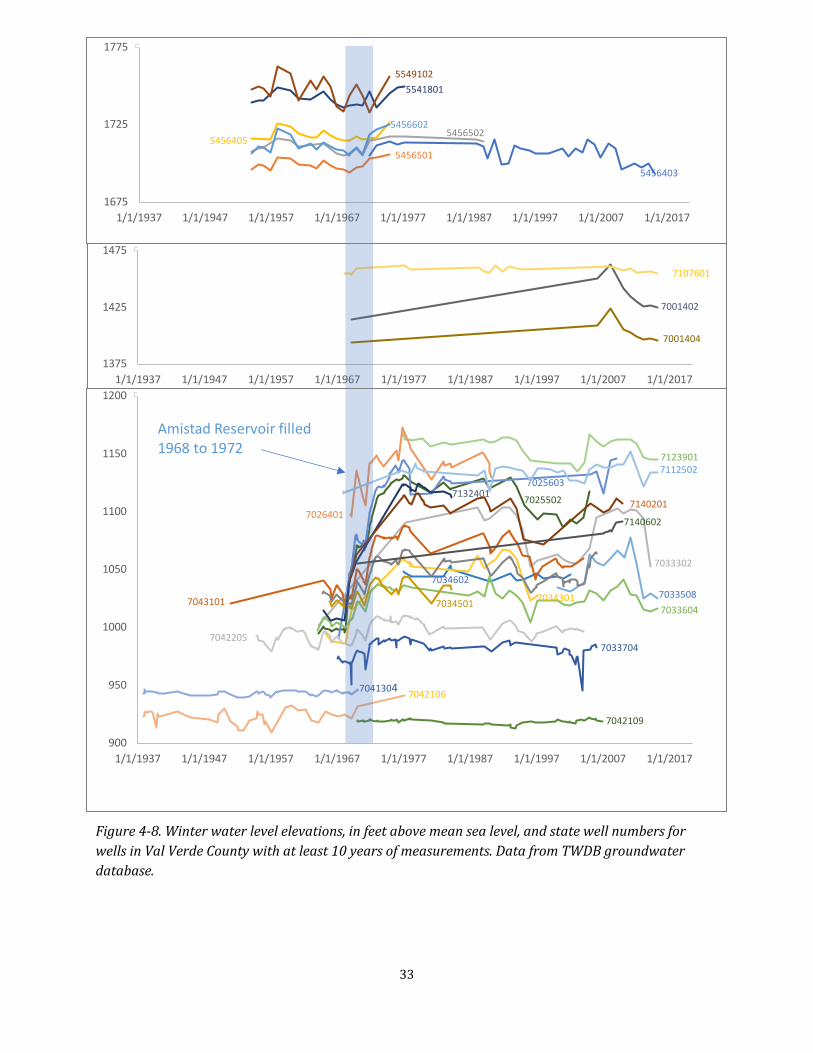
1775
5549102 5541801
1725 5456602 5456502
5456405 5456501
5456403
1675 1/1/1937 1/1/1947 1/1/1957 1/1/1977 1/1/1987 1/1/1997 1/1/2007 1/1/2017
1475
7107601
70014021425
7001404
1375 1/1/1937 1/1/1947 1/1/1957 1/1/1977 1/1/1987 1/1/1997 1/1/2007 1/1/2017
1200
1150 7123901 7112502
7025603
70255027132401
71402011100
7041304
1/1/1967
1/1/1967
Amistad Reservoir filled 1968 to 1972
7026401 7140602
70333021050 7034602
703350870343017043101 7034501 7033604
1000 7042205
7033704
950 7042106
7042109
900 1/1/1937 1/1/1947 1/1/1957 1/1/1967 1/1/1977 1/1/1987 1/1/1997 1/1/2007 1/1/2017
Figure 4-8. Winter water level elevations, in feet above mean sea level, and state well numbers for wells in Val Verde County with at least 10 years of measurements. Data from TWDB groundwater database.
33

Jun
5456402
Figure 4-9.Estimated extent ofthe area influenced by the pressure head in Amistad Reservoir,shaded in blue, with selected hydrographs for observation wells with data covering the period 1968 to 2000. No data for wells in Mexico are available. Data from TWDB groundwater database.
34
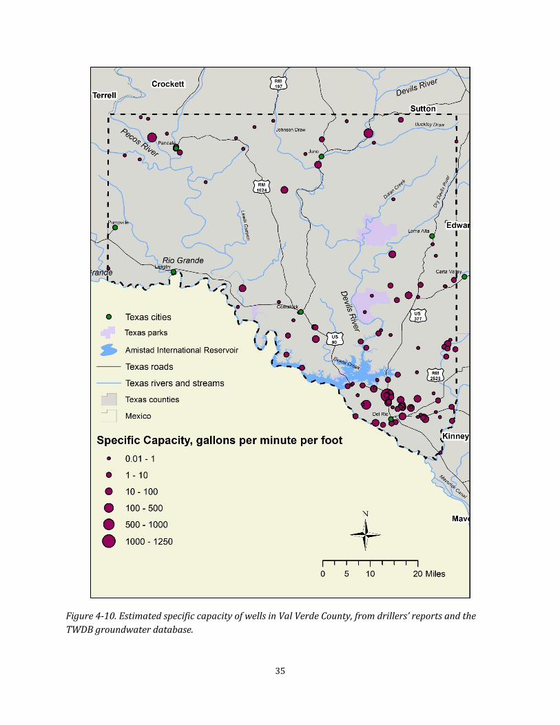
Figure 4-10. Estimated specific capacity of wells in Val Verde County,from drillers’ reports and the TWDB groundwater database.
35
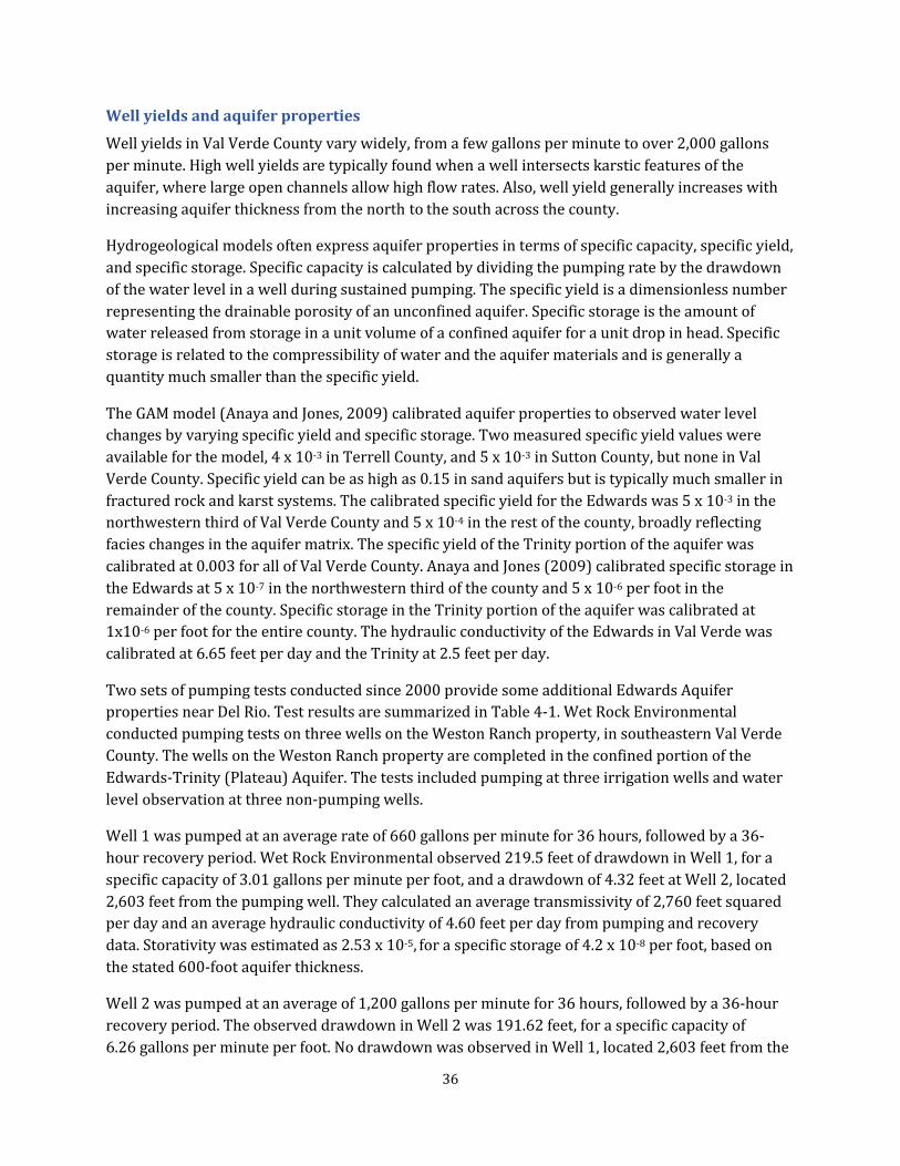
Well yields and aquifer properties
Well yields in Val Verde County vary widely, from a few gallons per minute to over 2,000 gallons per minute. High well yields are typically found when a well intersects karstic features of theaquifer, where large open channels allow high flow rates. Also, well yield generally increases with increasing aquifer thickness from the north to the south across the county.
Hydrogeological models often express aquifer properties in terms of specific capacity, specific yield,and specific storage. Specific capacity is calculated by dividing the pumping rate by the drawdownof the water level in a well during sustained pumping. The specific yield is a dimensionless numberrepresenting the drainable porosity of an unconfined aquifer. Specific storage is the amount ofwater released from storage in a unit volume of a confined aquifer for a unit drop in head. Specificstorage is related to the compressibility of water and the aquifer materials and is generally a quantity much smaller than the specific yield.
The GAM model (Anaya and Jones, 2009) calibrated aquifer properties to observed water level changes by varying specific yield and specific storage. Two measured specific yield values wereavailable for the model, 4 x 10⁻³ in Terrell County, and 5 x 10⁻³ in Sutton County,butnone in Val Verde County. Specific yield can be as high as 0.15 in sand aquifers but is typically much smaller infractured rock and karst systems. The calibrated specific yield for the Edwards was 5 x 10⁻³ in the northwestern third of Val Verde County and 5 x 10⁻⁴ in the rest of the county,broadly reflecting facies changes in the aquifer matrix.The specific yield of the Trinity portion of the aquifer wascalibrated at 0.003 for all of Val Verde County. Anaya and Jones (2009) calibrated specific storage inthe Edwards at5 x 10-7 in the northwestern third of the county and 5 x 10⁻⁶ per foot in theremainder of the county. Specific storage in the Trinity portion of the aquifer was calibrated at1x10-6 per foot for the entire county. The hydraulic conductivity of the Edwards in Val Verde was calibrated at 6.65 feet per day and the Trinity at 2.5 feet per day.
Two sets of pumping tests conducted since 2000 provide some additional Edwards Aquiferproperties near Del Rio. Test results are summarized in Table 4-1. Wet Rock Environmental conducted pumping tests on three wells on the Weston Ranch property, in southeastern Val VerdeCounty.The wells on the Weston Ranch property are completed in the confined portion of the Edwards-Trinity (Plateau) Aquifer. The tests included pumping at three irrigation wells and waterlevelobservation atthree non-pumping wells.
Well 1 was pumped at an average rate of 660 gallons per minute for 36 hours, followed by a 36-hour recovery period. Wet Rock Environmental observed 219.5 feet of drawdown in Well 1, for aspecific capacity of 3.01 gallons per minute per foot, and a drawdown of 4.32 feet at Well 2, located2,603 feet from the pumping well. They calculated an average transmissivity of 2,760 feet squaredper day and an average hydraulic conductivity of 4.60 feet per day from pumping and recoverydata. Storativity was estimated as 2.53 x 10⁻⁵, for a specific storage of 4.2 x 10⁻⁸ per foot, based on the stated 600-foot aquifer thickness.
Well 2 was pumped at an average of 1,200 gallons per minute for 36 hours, followed by a 36-hourrecovery period. The observed drawdown in Well 2 was 191.62 feet, for a specific capacity of6.26 gallons per minute per foot. No drawdown was observed in Well 1, located 2,603 feet from the
36

pumping well, or in Well A, located 5,221 feet from the pumping well. The calculated averagetransmissivity from pumping and recovery data was 4,170 feetsquared per day and the averagehydraulic conductivity was 6.96 feet per day. Storativity was estimated at 1.25 x 10⁻⁴, for a specific storage of 2.1 x 10⁻⁷ per foot, based on the stated 600-foot aquifer thickness.
Table 4-1. Summary of pump test results
Pumpingwell
Pumping rate, gpm
Pumpingduration, hours
Draw down, feet
Specificcapacity
Trans-missivity1, ft2/day
Hydraulicconductivity,feet/day
Specific storage,per foot 1
Well 1 660 36 219.5 3.01 2,760 4.60 4.2 x 10⁻⁸
Well 2 1200 36 191.6 6.26 4,170 6.96 2.1 x 10⁻⁷
Well 3 2700 168 73.11 36.7 22,300 37.1 1.0 x 10⁻⁸
Agarita 716 27.5 14.5 49 25,094 NA NA
Hackberry 286 24 230 1.3 1,936 NA NA
“Y”well, Salmon Peak
246 23.5 1.5 166 54,265* NA NA
“Y”well, West Nueces
35 1 3 11.5 3,080 NA NA
1: Transmissivity values based on stated aquifer thickness of 600 feet gpm= gallons per minute
Well 3 was pumped for seven days at an average rate of 2,700 gallons per minute, followed by aseven-day recovery period. The observed drawdown in Well 3 was 73.11 feet,for a specific capacityof 36.70 gallons per minute per foot. A maximum of 35.11 feet of drawdown was observed inWell B, located 1,811 feet from Well 1. The calculated average transmissivity for Well 3 was 22,300feet squared per day and the average hydraulic conductivity from pumping and recovery data was37.1 feet per day. The storativity is estimated at 6.05 x 10⁻⁶,giving a specific storage of 1.0 x 10⁻⁸ for the 600-foot aquifer thickness.
The pump test storage values are somewhat lower than the calibrated model values used in the GAM model (Anaya and Jones, 2009).
LBG-Guyton (2001) conducted pump tests on three wells but did not collect data from non-pumping wells and thus did not obtain hydraulic conductivity or storage estimates.LBG-Guyton didcollect geophysical and downhole video logs to define formation depths and identify productivezones. They classify the lower Edwards McKnight and West Nueces formations as confining beds
37

with little permeability. Pump test results for the upper part of the West Nueces showed atransmissivity of 3,080 feet squared per day, or more than one order of magnitude lower than theupper portion of the Edwards. LBG-Guyton (2001) also lists the Trinity Glen Rose Formation as a confining bed with low permeability and probably containing saline water, based on geophysical logs showing decreasing resistivity near the top of the Glen Rose.
The TWDB Record of Wells report for Val Verde County was used to evaluate the specific capacity of wells as a proxy for other, less direct measurements of aquifer properties such as specific yield andspecific storage.The county well report (TWDB, 2018a) lists 59 wells with reported well yield anddrawdown values. The median specific capacity for these wells was 2 gallons per minute per foot,with an average of 39.5 gallons per minute per foot, and a range of 0.01 to 1,256 gallons per minuteper foot. We derived specific capacity estimates for an additional 60 wells in Val Verde County fromthe TWDB Submitted Drillers Reports database (TWDB,2018b) and the Wet Rock pump tests.Specific capacity for these wells ranged from 0.01 gallons per minute per foot to 100 gallons perminute per foot,with an average of 5 and a median of 1.7 gallons per minute per foot.
The highest specific capacity wells are located near stream drainages (Figure 4-10),consistentwith the pattern in wellyields noted by Green and others (2014) and Toll and others (2017). Several high-capacity wells are located along the upper Devils River,above Juno,and along the Rio Grande in the Del Rio area. Several moderate-capacity wells are located near the Pecos River in the northwestern part of the county. The well yield data used by Green and others (2014), which includes more locations over a larger area, found a statistically significant correlation between wellyield and distance to third-order or higher stream segments. However, well yields alone can be apoor measure of aquifer properties because of widely varying test duration, drawdown, and aquiferthickness between locations.
Toll and others (2017) mention additional data collected to help define conduit locations, theirsizes,and orientation,including geophysics and geochemistry,butdo notinclude detailed analysis of these results in their model report. Geochemical data presented by Nunu, Bertetti and Green (2017) are discussed in Appendix B. In summary, Karst conduits associated with stream drainages are important elements of the Val Verde groundwater system, although there remains ambiguity as to the nature of the conduits and their effects on groundwater movement and production atparticular locations of interest.
38
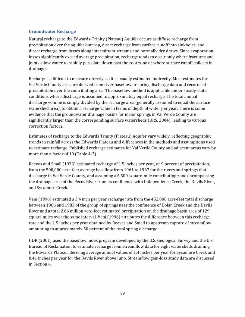
Groundwater Recharge
Natural recharge to the Edwards-Trinity (Plateau) Aquifer occurs as diffuse recharge fromprecipitation over the aquifer outcrop,directrecharge from surface runoff into sinkholes,and direct recharge from losses along intermittent streams and normally dry draws. Since evaporation losses significantly exceed average precipitation, recharge tends to occur only where fractures and joints allow water to rapidly percolate down pastthe rootzone or where surface runoffcollects in drainages.
Recharge is difficult to measure directly, so it is usually estimated indirectly. Most estimates forVal Verde County area are derived from river baseflow or spring discharge data and records ofprecipitation over the contributing area. The baseflow method is applicable under steady-stateconditions where discharge is assumed to approximately equal recharge. The total annualdischarge volume is simply divided by the recharge area (generally assumed to equal the surfacewatershed area),to obtain a recharge value in terms of depth of water per year. There is some evidence that the groundwater drainage basins for major springs in Val Verde County are significantly larger than the corresponding surface watersheds (URS, 2004),leading to various correction factors.
Estimates of recharge to the Edwards Trinity (Plateau) Aquifer vary widely, reflecting geographictrends in rainfallacross the Edwards Plateau and differences in the methods and assumptions used to estimate recharge. Published recharge estimates for Val Verde County and adjacent areas vary by more than a factor of 10 (Table 4-2).
Reeves and Small (1973) estimated recharge of 1.5 inches per year, or 9 percent of precipitation,from the 500,000 acre-feet average baseflow from 1961 to 1967 for the rivers and springs thatdischarge in Val Verde County,and assuming a 6,500-square-mile contributing zone encompassing the drainage area of the Pecos River from its confluence with Independence Creek, the Devils River, and Sycamore Creek.
Veni (1996) estimated a 3.4 inch per year recharge rate from the 452,000 acre-feet total dischargebetween 1966 and 1983 of the group of springs near the confluence of Dolan Creek and the DevilsRiver and a total 2.66 million acre-feet estimated precipitation on the drainage basin area of 129square miles over the same interval. Veni (1996) attributes the difference between this rechargerate and the 1.5 inches per year obtained by Reeves and Small to upstream capture of streamflowamounting to approximately 50 percent of the total spring discharge.
HDR (2001) used the baseflow index program developed by the U.S. Geological Survey and the U.S.Bureau of Reclamation to estimate recharge from streamflow data for eight watersheds drainingthe Edwards Plateau,deriving average annualvalues of 1.4 inches per year for Sycamore Creek and 0.41 inches per year for the Devils River above Juno. Streamflow gain-loss study data are discussed in Section 6.
39
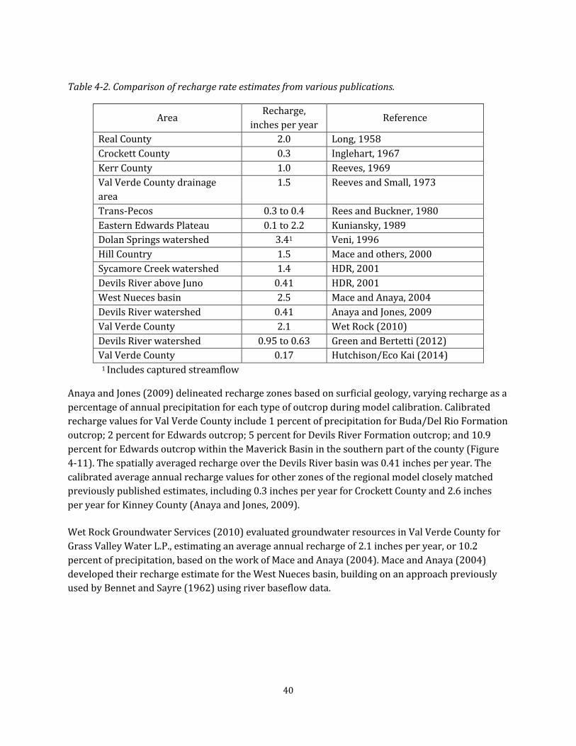
Table 4-2.Comparison ofrecharge rate estimates from various publications.
Area Recharge,
inches per year Reference
Real County 2.0 Long, 1958 Crockett County 0.3 Inglehart, 1967 Kerr County 1.0 Reeves, 1969 Val Verde County drainage area
1.5 Reeves and Small, 1973
Trans-Pecos 0.3 to 0.4 Rees and Buckner, 1980 Eastern Edwards Plateau 0.1 to 2.2 Kuniansky, 1989 Dolan Springs watershed 3.41 Veni, 1996 Hill Country 1.5 Mace and others, 2000 Sycamore Creek watershed 1.4 HDR, 2001 Devils River above Juno 0.41 HDR, 2001 West Nueces basin 2.5 Mace and Anaya, 2004 Devils River watershed 0.41 Anaya and Jones, 2009 Val Verde County 2.1 Wet Rock (2010) Devils River watershed 0.95 to 0.63 Green and Bertetti (2012) Val Verde County 0.17 Hutchison/Eco Kai (2014) 1 Includes captured streamflow
Anaya and Jones (2009) delineated recharge zones based on surficial geology, varying recharge as apercentage of annual precipitation for each type of outcrop during model calibration. Calibratedrecharge values for Val Verde County include 1 percent of precipitation for Buda/Del Rio Formationoutcrop; 2 percent for Edwards outcrop; 5 percent for Devils River Formation outcrop; and 10.9percent for Edwards outcrop within the Maverick Basin in the southern part of the county (Figure4-11).The spatially averaged recharge over the Devils River basin was 0.41 inches per year. Thecalibrated average annual recharge values for other zones of the regional model closely matchedpreviously published estimates,including 0.3 inches per year for Crockett County and 2.6 inches per year for Kinney County (Anaya and Jones, 2009).
Wet Rock Groundwater Services (2010) evaluated groundwater resources in Val Verde County forGrass Valley Water L.P., estimating an average annual recharge of 2.1 inches per year, or 10.2percent of precipitation, based on the work of Mace and Anaya (2004). Mace and Anaya (2004)developed their recharge estimate for the West Nueces basin, building on an approach previouslyused by Bennet and Sayre (1962) using river baseflow data.
40

Figure 4-11. GAM model distribution of recharge across Val Verde County (Anaya and Jones, 2009).
41
Mace and Anaya (2004) separate total recharge into two components, direct recharge wherestream courses intersect the faults and fractures of the Balcones Fault Zone, and diffuse recharge onthe Edwards Plateau.WetRock expresses the WestNueces diffuse recharge value as a percentageof total precipitation and, noting similarities in the surface geology between Kinney and Val Verdecounties, multiplies the average Val Verde precipitation by the West Nueces recharge percentage toderive a recharge value for Val Verde County.WetRock notes: “This is likely a conservative estimate of total inflow to the aquifer in Val Verde County as it does not account for direct recharge thatoccurs along stream channels in the county or underflow into Val Verde County from neighboring counties.”
Green and Bertetti (2012) also used average river baseflow to estimate recharge, deriving a value of0.95 inches per year for Val Verde County.They stated thatthis value seemed excessive and made a correction assuming the groundwater catchment area for the Devils River was 50 percent greaterthan the surface catchment, arriving at an average annual recharge rate of 0.63 inches per year, orabout 3 percent of precipitation, for the Devils River watershed and Val Verde County as a whole.Green and Bertetti (2012) also proposed calculating annual recharge as 15 percent of annualprecipitation over 16.5 inches per year, giving the following relationship between recharge (R) andprecipitation (P):
R =0.15(P -16.5) for P > 16.5, R = 0 for P ≤ 16.5
Hutchison and Eco Kai (2014) calculated monthly recharge rates as a function of precipitation andevaporation. They divided monthly rainfall by monthly evaporation, if the rainfall was above athreshold value,and then raised the resulting value by an assigned exponent. The time constant, threshold value, and the exponent were adjusted during calibration. They also adjusted recharge locally to accountfor focused recharge along drainages. The average model-calibrated recharge rate for Val Verde County was 0.17 inches per year, and annual values ranged from approximately zero to 0.55 inches per year. While estimated recharge for one year was near zero, in general the ValVerde County model (Hutchison and Eco-Kai, 2014) model produced some recharge even in dryyears, as the monthly time-step and focused recharge features account for local and short-termperiods where precipitation exceeds evaporation.
The amount of recharge entering the aquifer system plays a major role in long-term groundwateravailability. Anaya and Jones (2009) found that their regional groundwater availability model wasmore sensitive to recharge than any other parameter. They also found that recharge is the primarysource of inflow to the groundwater system, accounting for up to 85 percent of the Edwards aquiferunit water budget under steady state conditions, far outweighing lateralflows or inflows from other aquifers. Consequently, recharge has a major effect on predicted water levels, flow rates, and groundwater availability. Their sensitivity analysis suggested that a plus-or-minus 25 percentchange in recharge would resultin an average change in predicted water levelof about100 feet under steady-state conditions if other model inputs remained the same (Anaya and Jones, 2009).The wide range of recharge values used in recent models developed to assess the effects ofpotential pumping in Val Verde County imply that even larger differences in other modelparameters are needed to achieve calibration with respect to measured water levels.
42

Springs
Springs are natural outlets for groundwater discharge. Most springs in Val Verde County are located at points where streams have eroded down to intersect conduits in the saturated portion of theaquifer. A 2005 study prepared for the Plateau Regional Water Planning Group identified 45mapped springs in Val Verde County (Table 4-3 and Figure 4-12), while noting that numerousadditional wet weather springs likely exist (Ashworth and Stein, 2005).
Springs in Val Verde County represent regional points of discharge from the Edwards-Trinity(Plateau) Aquifer and an accurate representation of spring discharges is essential for groundwatermodels of the area. Goodenough Springs,now located under about150 feetof water in Amistad Reservoir, was historically the third largest in Texas, discharging an average flow of about 101,000acre-feet per year. In 2005 it was still discharging 52,000 acre-feet per year beneath the reservoir(Kamps, Tatum, Gault, and Groeger, 2009). San Felipe Springs, a collection of about 10 springs alongSan Felipe Creek, collectively represents the fourth largest spring flow in Texas, with an averagedischarge of about 80,000 acre-feet per year since Amistad Dam was completed in 1969 (Ashworthand Stein, 2005). Spring-fed baseflow in the Devils River totals approximately 197,000 acre-feet peryear between 1972 and 2017. Together these spring flows total almost 330,000 acre-feet per year,a rate that is substantially greater than discharge from pumping wells, which totals about 5,000 acre-feet per year.
While there is anecdotal evidence that spring flows along the Devils River have declinedsignificantly since the mid-19th century, other lines of evidence indicate that hydrological conditions in Val Verde County have been relatively stable since the early 20th century.Manysprings in Texas have ceased to flow because of groundwater development and landscapealterations since the late 19th century. Groundwater development can reduce the water level orpressure head in the aquifer around springs, which reduces spring flow or stops it entirely if the water level falls below the level of the spring orifice. Recorded water level measurements in ValVerde County generally do not document long-term declines in groundwater levels that would adversely affect spring flows since the early 20th century.Analysis of more recent data, from a variety of sources, suggest that observed variations in groundwater levels, spring flows, and streamflow are primarily a response to natural variability in rainfall and not an artifact ofgroundwater development. San Felipe Springs may be an exception to this pattern,reflecting more intensive groundwater use in the Del Rio area than in other parts of Val Verde County.
43
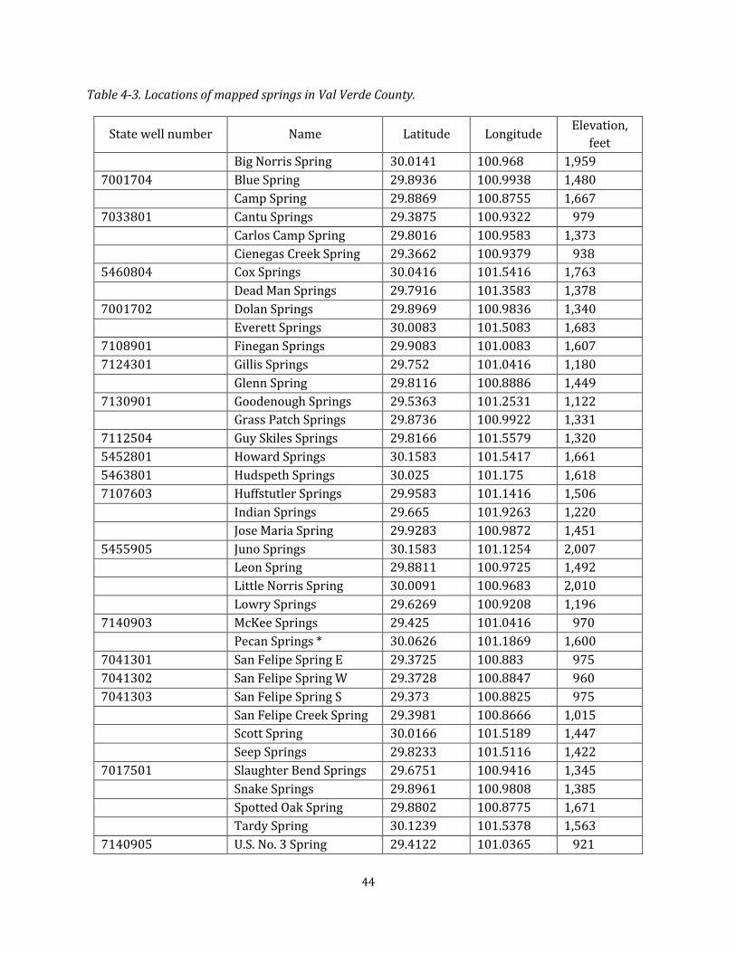
Table 4-3. Locations of mapped springs in Val Verde County.
State well number Name Latitude Longitude Elevation, feet
Big Norris Spring 30.0141 100.968 1,959 7001704 Blue Spring 29.8936 100.9938 1,480
Camp Spring 29.8869 100.8755 1,667 7033801 Cantu Springs 29.3875 100.9322 979
Carlos Camp Spring 29.8016 100.9583 1,373 Cienegas Creek Spring 29.3662 100.9379 938
5460804 Cox Springs 30.0416 101.5416 1,763 Dead Man Springs 29.7916 101.3583 1,378
7001702 Dolan Springs 29.8969 100.9836 1,340 Everett Springs 30.0083 101.5083 1,683
7108901 Finegan Springs 29.9083 101.0083 1,607 7124301 Gillis Springs 29.752 101.0416 1,180
Glenn Spring 29.8116 100.8886 1,449 7130901 Goodenough Springs 29.5363 101.2531 1,122
Grass Patch Springs 29.8736 100.9922 1,331 7112504 Guy Skiles Springs 29.8166 101.5579 1,320 5452801 Howard Springs 30.1583 101.5417 1,661 5463801 Hudspeth Springs 30.025 101.175 1,618 7107603 Huffstutler Springs 29.9583 101.1416 1,506
Indian Springs 29.665 101.9263 1,220 Jose Maria Spring 29.9283 100.9872 1,451
5455905 Juno Springs 30.1583 101.1254 2,007 Leon Spring 29.8811 100.9725 1,492 Little Norris Spring 30.0091 100.9683 2,010 Lowry Springs 29.6269 100.9208 1,196
7140903 McKee Springs 29.425 101.0416 970 Pecan Springs * 30.0626 101.1869 1,600
7041301 San Felipe Spring E 29.3725 100.883 975 7041302 San Felipe Spring W 29.3728 100.8847 960 7041303 San Felipe Spring S 29.373 100.8825 975
San Felipe Creek Spring 29.3981 100.8666 1,015 Scott Spring 30.0166 101.5189 1,447 Seep Springs 29.8233 101.5116 1,422
7017501 Slaughter Bend Springs 29.6751 100.9416 1,345 Snake Springs 29.8961 100.9808 1,385 Spotted Oak Spring 29.8802 100.8775 1,671 Tardy Spring 30.1239 101.5378 1,563
7140905 U.S. No. 3 Spring 29.4122 101.0365 921
44

7042601 Yoas Springs 29.3083 100.7751 980 7112501 Unnamed 29.8099 101.5732 1,260 5460301 Unnamed 30.1233 101.534 1,537 5460302 Unnamed 30.1235 101.5335 1,537 7108801 Unnamed 29.8952 101.0582 1,472 7001703 Unnamed 29.8913 100.9923 1,520 7001701 Unnamed 29.8955 100.9829 1,360
Source: Ashworth and Stein, 2005. Note: Locations may be approximate because of differing methods of location and map projections for historical data.
In general, spring flow measurements in Val Verde County are sparse. Brune (1975) describes JunoSprings as the headwaters of the Devils River. He states that:
“The Devil's River at this point was described in 1916 as a beautiful stream with large live oaks. The springs, Beaver Lake upstream, and the perennial flow of the Devil's River in this area have all disappeared. In May 1971, the first headwater springs were 15 miles downstream, at Pecan Springs.”
Toll and others (2017) have followed Brune’s description of the upper Devils River in modeling thepre-development steady-state condition of the Devils River Watershed Model.One of the major findings of their model is that a relatively modest volume of groundwater pumping is responsible for moving the starting pointof “live water” downstream from Juno Springs to Pecan Springs,suggesting a highly sensitive groundwater system. In contrast, our review of historical accounts andsatellite data suggests that Pecan Springs has been the start of perennial flow in the Devils River forat least the last 100 years. These two perspectives are not necessarily contradictory,buttogetherimply that any hydrological changes associated with development must have happened in the late 19th or early 20th century, before widespread groundwater pumping, suggesting an association withvegetation and land-use changes rather than groundwater abstraction.
Early descriptions of the Devils River suggest an intermittent flow in the upper reaches. In 1881,William Peery Hoover watered 200 head of cattle at Beaver Lake, just above the town of Juno.Weinger (1984) quotes James G. Bell, who in 1854 described the flow in the Devils River as “the water sinking and when up running over the dry beds,” suggesting low or intermittent flow. Bell reports that his group crossed the Devils River six times, with two dry crossings, before reachingCamp Hudson, just below Bakers Crossing and 19 miles by road south of Juno. Roberts and Nash(1918) provide the first recorded observations of the upper Devils River by professionalgeoscientists, noting that many springs discharge waters from the Edwards into the Devils River, and that “the most prominent of these springs are the Pecan Springs, which supply the main waterfor dry season flow of the Devils River.”
Byron Hodge (2018),whose family has owned the property surrounding Beaver Lake since about 1932, states that three major floods – in 1932, 1948, and 1954 – filled Beaver Lake with gravel, after which it ceased to hold water.
45
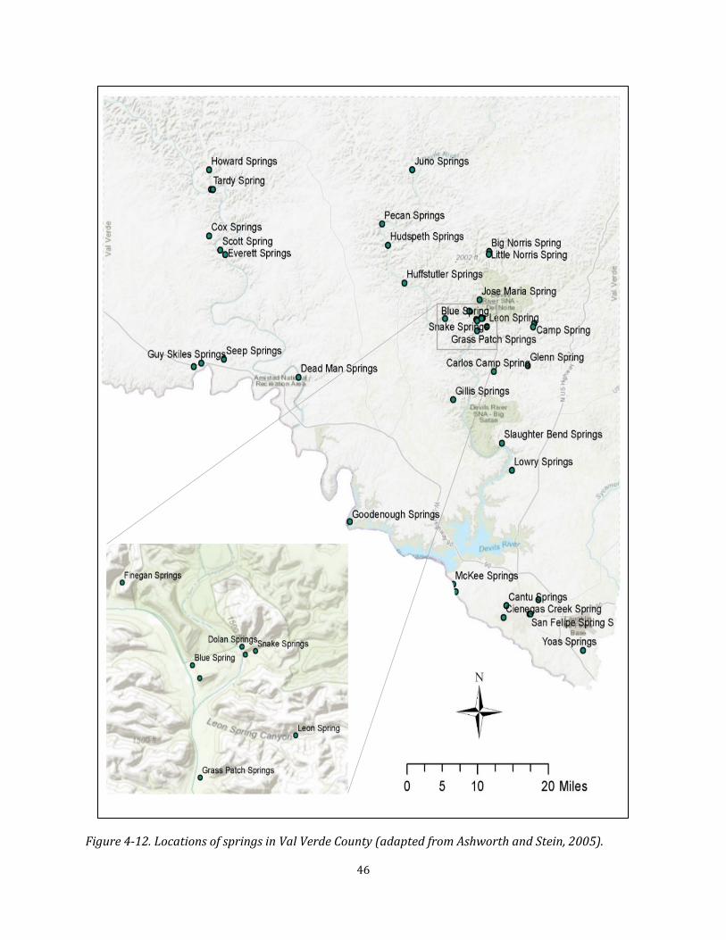
Figure 4-12.Locations ofsprings in Val Verde County (adapted from Ashworth and Stein, 2005).
46

Satellite imagery gives us a much clearer record of regular observations over the last 35 years. Landsat imagery from 1983 through 2018 shows continuous perennial flow in the Devils River downstream of Pecan Springs, while flow between Beaver Lake and Pecan Springs is discontinuousand restricted to periods following above-normal rainfall.
We used rainfall data for Brackettville and Ozona weather stations to selectimage dates following peaks in 365-day cumulative rainfall during the period of available Landsat coverage from 1983 to2017 (Figure 4-13). Images were selected for analysis based on peaks in accumulated rainfall overthe previous 90- and 365-day intervals (the Brackettville station was inactive from 2002 to 2006).Water is present in isolated pools between Juno and Pecan Springs in at least nine images. Only oneimage, from September 22, 2007 (Figure 4-14), shows nearly continuous flow between Juno andPecan Springs, following over 8 inches of rainfall in the upper watershed on August 18,2007.
Consistent flow downstream of Pecan Springs is observed in all images regardless of antecedent rainfall. Images acquired following localized heavy rainfall and runoff in the watershed above Juno(Figure 4-15) show evidence for stream bed infiltration instead of groundwater discharge in this reach. Images acquired under droughtconditions (Figure 4-16) show flow originating at PecanSprings and dry stream bed above that point. U.S. Fish and Wildlife Service wetlands mapping(Figure 4-17) also indicates that perennial flow in the Devils River begins at Pecan Springs.
While these records do not resolve the issue of how early European settlement changed theEdwards Plateau landscape in the mid-19th century, they do indicate that intermittent flow above Pecan Springs has been the norm for the last100 years and is not likely the resultof more recent irrigation development along the upper reaches of the Devils River.
60
50 9/4/1987, 43.66
10/3/1990, 42.25 7/23/1997, 35.34
7/12/1999, 35.55
9/13/2001, 32.46
9/4/2007, 48.36
9/2/2011, 5.41
6/14/2015, 36.43
5/11/2017, 41.03
40
30
20
10
0 1983 1988 1993 1998 2003 2008 2013 2018
365 day precipitation 90 day precipitation Period of record average
Cum
ulat
ive
rain
fall,
inch
es
Figure 4-13.Precipitation data for Brackettville used to guide Landsat image analysis. Data from National Centers for Environmental Information, 2018b.
47

Figure 4-14. Landsat 7 false-color near-infrared colorcomposite image for September 22, 2007, representing wet weather conditions.Rainfall in the upper Devils River watershed at the Ozona 22 SE weather station totaled 18 inches in the preceding 90 days and over 40 inches for the preceding year. Water (dark areas) is present between Juno and Pecan Springs, and actively growing vegetation (red) is widespread along the Devils River and tributary streams. Dark lines are an artifact of satellite scan line correction malfunction. Imagery from U.S.Geological Survey Earth Explorer.
48
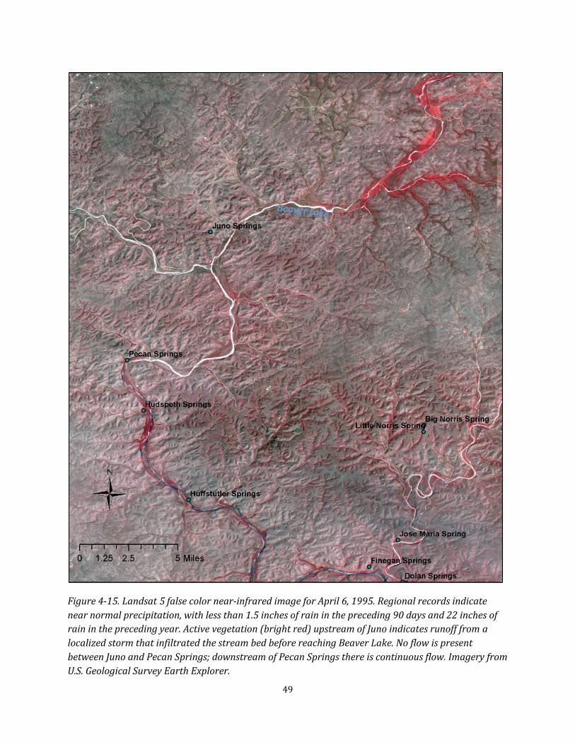
Beaver Lake
Figure 4-15.Landsat 5 false color near-infrared image for April 6, 1995. Regional records indicate near normal precipitation, with less than 1.5 inches of rain in the preceding 90 days and 22 inches of rain in the preceding year. Active vegetation (bright red) upstream of Juno indicates runoff from a localized storm that infiltrated the stream bed before reaching Beaver Lake. No flow is present between Juno and Pecan Springs; downstream of Pecan Springs there is continuous flow. Imagery from U.S. Geological Survey Earth Explorer.
49

Figure 4-16.Landsat 7 false-color near-infrared image for October 3, 2011, showing flow below Pecan Springs under drought conditions; rainfall in the preceding 90 days totaled 2.15 inches and 4.06 inches for the preceding year. Imagery from U.S.Geological Survey Earth Explorer.
50

yy
Palustrine, scrub shrub, deciduous, temporary flooding
Palustrine, forested, deciduous, temporary flooding
Riverine, intermittent streambed, intermittent flooding
Riverine, intermittent streambed, temporary flooding
Riverine, lower perennial, unconsolidated shore, temporary flooding
Riverine, lower perennial, unconsolidated bottom, permanently
fl d d Scale, miles
1 ½ 0
Area of detail Val Verde
Pecan Springs
Figure 4-17.National Wetlands Inventory,Sycamore Canyon Sheet,based on aerial photography dated February 1985, a period of slightly below normal rainfall. Perennial water is mapped only below Pecan Springs.
51
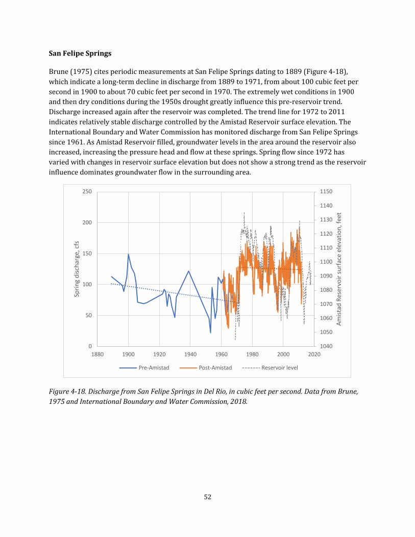
SanFelipeSprings
Brune (1975) cites periodic measurements atSan Felipe Springsdatingto 1889 (Figure 4-18),which indicate along-term decline in discharge from 1889 to 1971,fromabout100cubic feetpersecond in 1900 to about70 cubic feetper second in 1970.The extremelywetconditionsin1900andthen dry conditionsduringthe 1950s droughtgreatly influence thispre-reservoir trend.Dischargeincreasedagainafterthereservoirwascompleted.Thetrendline for 1972 to 2011indicatesrelativelystabledischargecontrolled by the Amistad Reservoir surface elevation.TheInternational BoundaryandWaterCommissionhas monitored discharge fromSan Felipe Springssince 1961.As Amistad Reservoir filled,groundwater levels in the area around the reservoir alsoincreased,increasing thepressureheadandflowat thesesprings.Spring flowsince 1972 hasvaried with changes in reservoir surface elevationbutdoes notshow astrongtrend as the reservoirinfluencedominatesgroundwaterflowinthesurroundingarea.
250 1150
1140
Sprin
g di
scha
rge,
cfs
200 1130
1120
150 1110
1100
100 1090
1080
1070
50 1060
1050
0 1880 1900 1920 1940 1960 1980 2000
1040 2020
Pre-Amistad Post-Amistad Reservoir level
Amis
tad
Rese
rvoi
r sur
face
ele
vatio
n, fe
et
Figure4-18.Discharge from San FelipeSpringsin DelRio,in cubic feetper second.DatafromBrune,1975 and International Boundary and WaterCommission,2018.
52
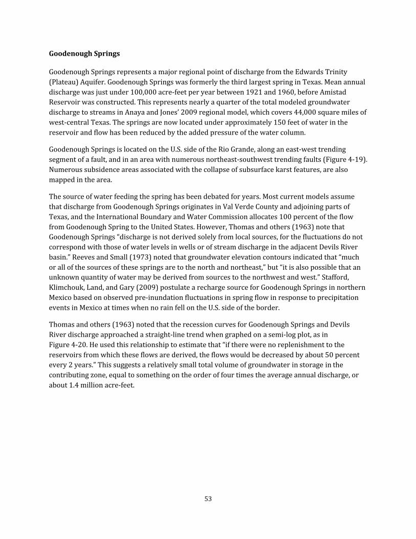
Goodenough Springs
Goodenough Springs represents a major regional point of discharge from the Edwards Trinity(Plateau) Aquifer. Goodenough Springs was formerly the third largest spring in Texas. Mean annualdischarge was just under 100,000 acre-feet per year between 1921 and 1960, before AmistadReservoir was constructed. This represents nearly a quarter of the total modeled groundwaterdischarge to streams in Anaya and Jones’ 2009 regional model, which covers 44,000 square miles ofwest-central Texas. The springs are now located under approximately 150 feet of water in thereservoir and flow has been reduced by the added pressure of the water column.
Goodenough Springs is located on the U.S. side of the Rio Grande, along an east-west trendingsegment of a fault, and in an area with numerous northeast-southwest trending faults (Figure 4-19).Numerous subsidence areas associated with the collapse of subsurface karst features, are alsomapped in the area.
The source of water feeding the spring has been debated for years. Most current models assumethatdischarge from Goodenough Springs originates in Val Verde County and adjoining parts ofTexas, and the International Boundary and Water Commission allocates 100 percent of the flowfrom Goodenough Spring to the United States. However, Thomas and others (1963) note thatGoodenough Springs “discharge is not derived solely from local sources, for the fluctuations do notcorrespond with those of water levels in wells or of stream discharge in the adjacent Devils River basin.” Reeves and Small (1973) noted that groundwater elevation contours indicated that “much or all of the sources of these springs are to the north and northeast,” but “it is also possible that anunknown quantity of water may be derived from sources to the northwest and west.” Stafford, Klimchouk, Land, and Gary (2009) postulate a recharge source for Goodenough Springs in northernMexico based on observed pre-inundation fluctuations in spring flow in response to precipitationevents in Mexico at times when no rain fell on the U.S. side of the border.
Thomas and others (1963) noted that the recession curves for Goodenough Springs and DevilsRiver discharge approached a straight-line trend when graphed on a semi-log plot,as in Figure 4-20. He used this relationship to estimate that “if there were no replenishment to thereservoirs from which these flows are derived, the flows would be decreased by about50 percent every 2 years.” This suggests a relatively small totalvolume of groundwater in storage in the contributing zone, equal to something on the order of four times the average annual discharge, orabout 1.4 million acre-feet.
53
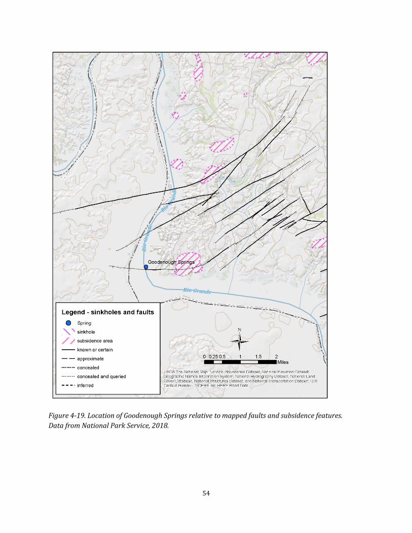
Figure 4-19.Location ofGoodenough Springs relative to mapped faults and subsidence features. Data from National Park Service, 2018.
54
500 D
isch
arge
, cub
ic fe
et p
er s
econ
d
50 6/1/1920 6/1/1925 6/1/1930 6/1/1935 6/1/1940 6/1/1945 6/1/1950
Goodenough Springs Devils River at Bakers Crossing .
Figure4-20.Discharge from Goodenough Springs and the Devils River at Bakers Crossing,1920 to1952.Discharge fromGoodenough Springsresponds toincreasedstreamflowinthe Devils River in1932 and 1935,butnotin 1942 or 1947,suggesting thatother areas outside the Devils River drainage alsocontributetoGoodenoughSprings. DatafromHeitmullerandReece, 2003andUSGS, 2018a.
Suchalow estimate of the groundwater volume contributing tospring flowcouldbe consistentwith totalestimated recoverable storage estimatesif groundwaterintheTrinityaquiferunit doesnotactively contribute to spring and streambaseflow. Anaya(2018)findsthattheEdwardsaquiferunitcontains only 20 percentof the totalvolume of groundwater in storageinValVerdeCounty,orapproximately 2million acre-feet.
A Mexican source for some ofGoodenough Springs discharge fits observations thatsome increasesinspring flowdonot correlatewithrunoff events in the U.S.,while the large cavern networkextendingdeepbelowAmistadReservoir(Kampsandothers,2009)providesaplausiblepathwayforflowtomovebeneaththe Rio Grandeandto discharge onthe U.S.side of the border.However, currentMexican estimatesof therechargetotheCerroColorado-LaPartidaaquifer,the EdwardsequivalentinCoahuila,totalonly5,270 acre-feetperyear(Secretaría deMedioAmbienteyRecursos Naturales,2015),whichrepresents only 5percentof the historicaldischarge fromGoodenough Springs.Ingeneral,hydrological dataforthisareaofMexicoissparse.
Resolvingthe source ofGoodenough Springs is importanttounderstandingandmanaginggroundwater in ValVerde County.Goodenough Springs representa large partof the water budgetforgroundwatermodelsof thearea.If a largepartof thewaterbudgetactuallyoriginatesoutside
55
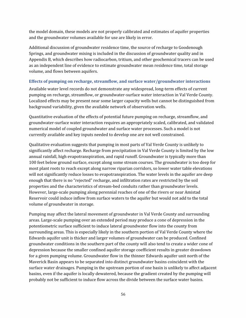
the modeldomain,these models are notproperly calibrated and estimates of aquifer propertiesand the groundwater volumes available for use are likely in error.
Additional discussion of groundwater residence time, the source of recharge to GoodenoughSprings,and groundwater mixing is included in the discussion of groundwater quality and in Appendix B,which describes how radiocarbon, tritium, and other geochemical tracers can be usedas an independent line of evidence to estimate groundwater mean residence time, total storage volume, and flows between aquifers.
Effects of pumping on recharge, streamflow, and surface water/groundwater interactions
Available water level records do not demonstrate any widespread, long-term effects of current pumping on recharge, streamflow, or groundwater-surface water interaction in Val Verde County. Localized effects may be present near some larger capacity wells but cannot be distinguished frombackground variability, given the available network of observation wells.
Quantitative evaluation of the effects of potential future pumping on recharge, streamflow, andgroundwater-surface water interaction requires an appropriately scaled, calibrated, and validatednumerical model of coupled groundwater and surface water processes. Such a model is notcurrently available and key inputs needed to develop one are not well constrained.
Qualitative evaluation suggests that pumping in most parts of Val Verde County is unlikely tosignificantly affect recharge. Recharge from precipitation in Val Verde County is limited by the lowannual rainfall, high evapotranspiration,and rapid runoff.Groundwater is typically more than 100 feet below ground surface, except along some stream courses. The groundwater is too deep formost plant roots to reach except along narrow riparian corridors,so lower water table elevations will not significantly reduce losses to evapotranspiration. The water levels in the aquifer are deepenough that there is no “rejected” recharge, and infiltration rates are restricted by the soilproperties and the characteristics of stream-bed conduits rather than groundwater levels. However, large-scale pumping along perennial reaches of one of the rivers or near AmistadReservoir could induce inflow from surface waters to the aquifer but would not add to the totalvolume of groundwater in storage.
Pumping may affect the lateral movement of groundwater in Val Verde County and surroundingareas. Large-scale pumping over an extended period may produce a cone of depression in thepotentiometric surface sufficient to induce lateral groundwater flow into the county fromsurrounding areas. This is especially likely in the southern portion of Val Verde County where theEdwards aquifer unit is thicker and larger volumes of groundwater can be produced. Confinedgroundwater conditions in the southern part of the county will also tend to create a wider cone of depression because the smaller confined aquifer storage coefficient results in greater drawdownfor a given pumping volume. Groundwater flow in the thinner Edwards aquifer unit north of theMaverick Basin appears to be separated into distinct groundwater basins coincident with thesurface water drainages. Pumping in the upstream portion of one basin is unlikely to affect adjacentbasins, even if the aquifer is locally dewatered, because the gradient created by the pumping willprobably not be sufficient to induce flow across the divide between the surface water basins.
56
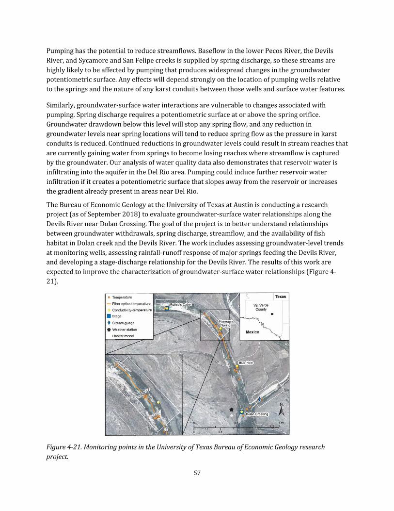
Pumping has the potential to reduce streamflows. Baseflow in the lower Pecos River, the DevilsRiver, and Sycamore and San Felipe creeks is supplied by spring discharge, so these streams are highly likely to be affected by pumping that produces widespread changes in the groundwaterpotentiometric surface. Any effects will depend strongly on the location of pumping wells relative to the springs and the nature of any karstconduits between those wells and surface water features.
Similarly, groundwater-surface water interactions are vulnerable to changes associated withpumping. Spring discharge requires a potentiometric surface at or above the spring orifice.Groundwater drawdown below this level will stop any spring flow, and any reduction ingroundwater levels near spring locations will tend to reduce spring flow as the pressure in karstconduits is reduced. Continued reductions in groundwater levels could result in stream reaches that are currently gaining water from springs to become losing reaches where streamflow is capturedby the groundwater. Our analysis of water quality data also demonstrates that reservoir water isinfiltrating into the aquifer in the DelRio area.Pumping could induce further reservoir water infiltration if it creates a potentiometric surface that slopes away from the reservoir or increasesthe gradientalready presentin areas near DelRio.
The Bureau of Economic Geology at the University of Texas at Austin is conducting a researchproject (as of September 2018) to evaluate groundwater-surface water relationships along theDevils River near Dolan Crossing. The goal of the project is to better understand relationshipsbetween groundwater withdrawals, spring discharge, streamflow, and the availability of fishhabitat in Dolan creek and the Devils River. The work includes assessing groundwater-leveltrendsat monitoring wells, assessing rainfall-runoff response of major springs feeding the Devils River, and developing a stage-discharge relationship for the Devils River. The results of this work areexpected to improve the characterization of groundwater-surface water relationships (Figure 4-21).
Figure 4-21. Monitoring points in the University of Texas Bureau of Economic Geology research project.
57
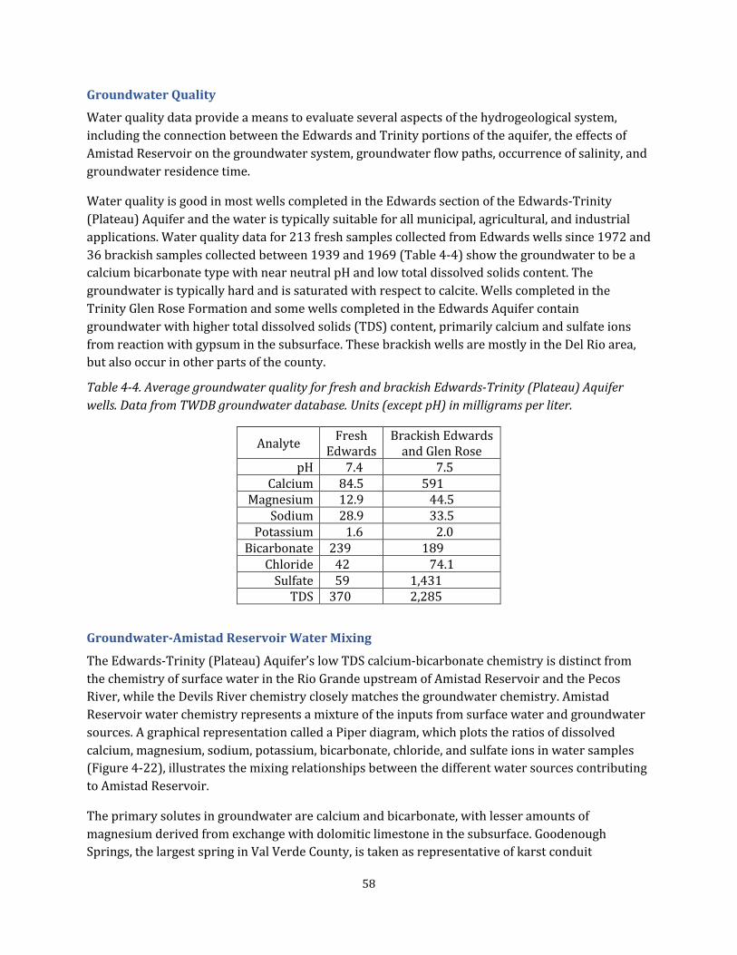
Groundwater Quality
Water quality data provide a means to evaluate several aspects of the hydrogeological system,including the connection between the Edwards and Trinity portions of the aquifer, the effects ofAmistad Reservoir on the groundwater system, groundwater flow paths, occurrence of salinity, andgroundwater residence time.
Water quality is good in most wells completed in the Edwards section of the Edwards-Trinity(Plateau) Aquifer and the water is typically suitable for all municipal, agricultural, and industrialapplications. Water quality data for 213 fresh samples collected from Edwards wells since 1972 and36 brackish samples collected between 1939 and 1969 (Table 4-4) show the groundwater to be acalcium bicarbonate type with near neutral pH and low total dissolved solids content. The groundwater is typically hard and is saturated with respect to calcite. Wells completed in theTrinity Glen Rose Formation and some wells completed in the Edwards Aquifer contain groundwater with higher totaldissolved solids (TDS) content,primarily calcium and sulfate ions from reaction with gypsum in the subsurface. These brackish wells are mostly in the Del Rio area, but also occur in other parts of the county.
Table 4-4. Average groundwater quality for fresh and brackish Edwards-Trinity (Plateau) Aquifer wells.Data from TWDB groundwater database. Units (except pH) in milligrams per liter.
Analyte Fresh
Edwards Brackish Edwards and Glen Rose
pH 7.4 7.5 Calcium 84.5 591
Magnesium 12.9 44.5 Sodium 28.9 33.5
Potassium 1.6 2.0 Bicarbonate 239 189
Chloride 42 74.1 Sulfate 59 1,431 TDS 370 2,285
Groundwater-Amistad Reservoir Water Mixing
The Edwards-Trinity (Plateau) Aquifer’s low TDS calcium-bicarbonate chemistry is distinct fromthe chemistry of surface water in the Rio Grande upstream of Amistad Reservoir and the PecosRiver, while the Devils River chemistry closely matches the groundwater chemistry. AmistadReservoir water chemistry represents a mixture of the inputs from surface water and groundwatersources. A graphical representation called a Piper diagram, which plots the ratios of dissolvedcalcium, magnesium, sodium, potassium, bicarbonate, chloride, and sulfate ions in water samples(Figure 4-22), illustrates the mixing relationships between the different water sources contributing to Amistad Reservoir.
The primary solutes in groundwater are calcium and bicarbonate, with lesser amounts of magnesium derived from exchange with dolomitic limestone in the subsurface. GoodenoughSprings, the largest spring in Val Verde County,is taken as representative of karstconduit
58

groundwater chemistry. Data points for the springs represent one 2005 sample collected from the spring orifice beneath the reservoir and the median ion concentrations in U.S. Geological Surveysamples collected in 1967 and 1968, before the reservoir filled (Kamps and others 2006). Medianvalues of chemical constituents in Devils River water from 104 samples collected at PaffordCrossing between 1978 and 1995 (Mast and Turk, 1999) plot close to the groundwater, as expected given the spring-dominated baseflow in the Devils River.
Ca
2+
CATIONS
Mg
2+
Na +
+K
+
CO
3
2- +
HC
O3
-
SO
4 2-
Cl
-
ANIONS
SO
4
2-
+C
l-
Ca 2+
+M
g 2+
EXPLANATION
Lake Amistad
Rio Grande above Amistad
Pecos River
Goodenough Spring
Devils River
263
5822.9
Figure 4-22.Piper diagram ofthe water chemistry for Amistad Reservoir, the Rio Grande, the Pecos River, the Devils River and Goodenough Springs. Symbols for each sample are scaled by the total dissolved solids content of the sample, which range from a minimum of 263 milligrams per liter in Goodenough Springs to a maximum of 5,823 milligrams per liter in the Pecos River. Data from TCEQ, 2018a, Mast and Turk, 1999, and Kamps and others, 2009.
The Pecos River water chemistry (TCEQ, 2018a) varies widely in terms of total salinity, but all the samples plotclose together on the Piper diagram, owing to their similar ratios of major ions. The Pecos River water is dominated by sodium and chloride, with lesser amounts of magnesium andsulfate. Water quality data for the Rio Grande upstream of Amistad Reservoir (USGS, 2007;TCEQ, 2018a) have a wider compositional range than groundwater or Pecos River inputs.
59

Rio Grande water is distinguished by its relatively high sulfate anion content and a mix of sodiumand calcium cations. Amistad Reservoir water chemistry represents a ternary mixture of theRio Grande, Pecos River, and groundwater components. The reservoir composition plots closer tothe Pecos River than to groundwater,despite the volumetrically larger contribution of combined flows from the Devils River and Goodenough springs, because most of the salt content is derivedfrom the high TDS Pecos River water.
The water chemistry of the Devils River at Pafford Crossing has slowly changed since AmistadReservoir filled. The average specific conductance of water samples analyzed by the TCEQ and USGSbetween 1967 and 2017 increased from 350 to 400 micro-siemens per centimeter over the 50-yearperiod. Water quality changes may be related to groundwater mixing with more saline reservoirwater driven by fluctuations in reservoir and groundwater elevations relative to each other.
Groundwater quality data also show how Amistad Reservoir water has mixed with and displacedgroundwater in downgradient areas. Piper diagrams for three wells at increasing distance from thereservoir (Figures 4-23 through 4-25) show varying amounts of reservoir influence. The groundwater chemistry in Well 7033501, located three-quarters of a mile south of the reservoir, changesrelatively rapidly. In June 1969, it already contained more sodium and chloride than typicalgroundwater. By 1976 the chloride and sulfate content of the well water was close to that of thereservoir and did not change appreciably over the next decade. The sodium content of the well water remains intermediate between the 1969 groundwater composition and the reservoircomposition, perhaps reflecting cation exchange reactions in the aquifer. Well 7033604, located 1.8 miles southeast of the reservoir near the intersection of U.S. Highways 90 and 377, shows agradual evolution from a groundwater signature to a reservoir water signature over the periodfrom 1968 to 2004. At these wells, the groundwater potentiometric surface is lower than the elevation of the reservoir surface and reservoir water has migrated into the aquifer.
In contrast, Well 7123502, located north of Amistad Reservoir near Comstock, is well within the area where the groundwater potentiometric surface was affected by the reservoir, but has not beenaffected by migration of solutes contained in the reservoir water and maintained a stable chemistryfrom 1968 through 2015 (Figure 4-25). Because the groundwater elevation in Well 7123502 ishigher than the elevation of the reservoir surface, the direction of groundwater flow at this locationremains toward the reservoir.
While the water pressure effects of reservoir elevation changes propagate both upgradient anddowngradientfrom the reservoir,solutes contained in the water have only migrated downgradient with the physical flow of the water. However, pumping within the area influenced by the pressureeffects of the reservoir could change the groundwater potentiometric surface and potentiallyinduce flow from the reservoir toward the pumping well. Under such conditions, changes ingroundwater chemistry could serve as a useful indicator that the pumping well was drawing insurface water from the reservoir and not just groundwater from the surrounding aquifer.
60

Well 7033501
EXPLANATION 1969 1976 1979 1985 Lake Amistad
-Cl
ANIONS Ca
2+
CATIONS
Mg
2+ Na ++
K + CO3
2- +H
CO3
-
SO4 2-
SO4
2- +Cl
- Ca 2++
Mg 2+
701350 1
Figure 4-23.Piper diagram for Well 7033501,0.75 miles southeast of Amistad Reservoir. Groundwater chemistry in this area is dominated by the reservoir influence by 1976. Data from TWDB and TCEQ, 2018a.
Well 7033604
Ca2+
CATIONS
Mg
2+ Na ++K + CO
32- + HCO
3-
SO4 2-
Cl -
ANIONS
SO4
2- + Cl- Ca 2+
+M
g 2+
EXPLANATION 1968 1976 1984 2004 Lake Amistad
703360 4
Figure 4-24. Piper diagram for Well 7033604, 1.8 miles southeast of Amistad Reservoir. Groundwater chemistry in this area has progressively moved toward reservoir composition during the period of 1968 to 2004. Data from TWDB and TCEQ.2018a.
61
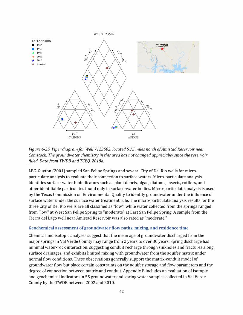
Well 7123502
Ca2+
CATIONS
Mg
2+ Na ++
K + CO3
2- +H
CO3
-
SO4 2-
Cl -
ANIONS
SO4
2- +Cl
- Ca 2++
Mg 2+
EXPLANATION 1965 1969 1993 2003 2015 Amistad
712350
Figure 4-25. Piper diagram for Well 7123502, located 5.75 miles north of Amistad Reservoir near Comstock. The groundwater chemistry in this area has not changed appreciably since the reservoir filled.Data from TWDB and TCEQ,2018a.
LBG-Guyton (2001) sampled San Felipe Springs and several City of Del Rio wells for micro-particulate analysis to evaluate their connection to surface waters. Micro-particulate analysisidentifies surface-water bioindicators such as plant debris, algae, diatoms, insects, rotifers, andother identifiable particulates found only in surface-water bodies. Micro-particulate analysis is usedby the Texas Commission on Environmental Quality to identify groundwater under the influence of surface water under the surface water treatment rule. The micro-particulate analysis results for thethree City of DelRio wells are allclassified as "low",while water collected from the springs ranged from "low" at West San Felipe Spring to "moderate" at East San Felipe Spring. A sample from the Tierra del Lago well near Amistad Reservoir was also rated as "moderate."
Geochemical assessment of groundwater flow paths, mixing, and residence time
Chemical and isotopic analyses suggest that the mean age of groundwater discharged from the major springs in Val Verde County may range from 2 years to over 30 years.Spring discharge has minimal water-rock interaction, suggesting conduit recharge through sinkholes and fractures alongsurface drainages, and exhibits limited mixing with groundwater from the aquifer matrix under normal flow conditions.These observations generally support the matrix-conduit model ofgroundwater flow but place certain constraints on the aquifer storage and flow parameters and thedegree of connection between matrix and conduit. Appendix B includes an evaluation of isotopicand geochemical indicators in 55 groundwater and spring water samples collected in Val VerdeCounty by the TWDB between 2002 and 2010.
62

Geochemical data for Val Verde, Crockett, and Sutton counties suggest that most of the flow from the major springs moves along flow-paths distinct from the groundwater found in the aquifermatrix, rather than integrating flow from the entire contributing area upgradientfrom the pointof discharge. This is possible in a karstic system where flow along major conduits is several orders of magnitude faster than groundwater flow in the aquifer matrix. Furthermore, it suggests that theconduit system does not simply aggregate diffuse flow from the matrix, but instead has a largelyseparate source of recharge. The obvious candidate for conduit recharge is captured surface waterrunoff that enters sinkholes or major fractures in the upper, intermittent reaches of the alluvialsystem. This conduit flow appears to largely remain distinct from groundwater that originates asdiffuse recharge under normal flow conditions, although under drought conditions matrixgroundwater is likely to be more important.
Nunu, Bertetti, and Green (2017) show that the distribution of groundwater calcium concentrationsgenerally follows the surface drainage network in the Devils River watershed (Figure 4-26), withhigher calcium concentrations in active recharge areas along the major surface drainage features and lower calcium concentrations away from the drainages. This distribution follows the patternoutlined by Nance (2010) where an increasing magnesium-to-calcium ratio is a measure of longergroundwater residence time, especially in areas capped by Buda Limestone.
Brackish Groundwater
Several wells in Val Verde County produce brackish groundwater, characterized by total dissolvedsolids content exceeding 1,000 milligrams per liter. Most brackish groundwater in the Del Rio area acquires salinity by dissolution of evaporite minerals in the McKnight Formation in the MaverickBasin, while brackish water in other parts of the county represents a mixture of Edwards aquiferunit groundwater and deeper, more saline groundwater associated with the Glen Rose LimestoneFormation in the Trinity Aquifer.
A Piper diagram of the major ion chemistry of groundwater from brackish wells grouped according to their geographic location (Figure 4-27) shows a broad dispersion in compositional spacerepresenting a three-component mixing of groundwater types. One mixing component is freshEdwards aquifer unit groundwater and spring water, which plots to the lower left in the calcium bicarbonate region of the plot. A second component is brackish groundwater in the Glen RoseLimestone, which plots in the lower right-hand corner of the cation graph and toward the center ofthe anion graph,representing a mix of sodium chloride and sodium sulfate type waters. The third component is brackish groundwater from wells in the Salt Creek drainage, near Del Rio, which plots in the extreme lower left of the cation graph and in the upper corner of the anion graph,representing a calcium sulfate type water. Brackish groundwater samples from wells in thenorthwest part of the county (NW trend) and along a line between Langtry and Comstock (Langtry)are similar to the Glen Rose groundwater, suggesting that these wells are influenced by Glen RoseLimestone waters migrating into the Edwards Aquifer along faults or fractures. Brackish wells inthe Zorro Creek area,near Laughlin Air Force Base,have compositions intermediate between the Glen Rose Limestone and Maverick Basin groundwater types.
63

Figure 4-26. Calcium distribution in Val Verde and neighboring counties.From Nunu,Bertetti and Green, 2017.
The limited number of brackish wells in Val Verde County,and their geographic specificity,suggests there is little interaction between groundwater in the Trinity Aquifer and the shallower EdwardsAquifer groundwater. While some regional discharge from the Trinity probably occurs along theRio Grande,we have no evidence thatitis volumetrically importantin the Val Verde area. Available data suggest that locally the Trinity Aquifer is relatively stagnant.
64

Additional research on brackish groundwater resources in Val Verde County is being conducted by the TWDB as partof the Brackish Resources Aquifer Characterization System (BRACS) study of theEdwards-Trinity (Plateau) Aquifer. The study is expected to be completed in late 2020.
Mg
2+ Na +
+K + C
O 3
2- +H
CO 3
-
SO4 2-
SO4
2-
+C
l-
Ca 2+
+M
g 2+
EXPLANATION
Edwards groundwater
Spring
Glen Rose
Langtry trend
NW trend
Salt Creek
McKee Creek
Zorro Creek
Ciengas Creek
210
2670
-2+ Ca Cl
CATIONS ANIONS
Figure 4-27.Piper diagram of fresh and brackish water samples from the Edwards aquifer unit. Glen Rose Limestone groundwater and spring water samples are also plotted for comparison. Symbol size is proportional to total dissolved solids content.
65

5.0 Groundwater Models Key findings
• Available groundwater models were developed for varying purposes,conceptualize the hydrogeological systems differently, and are calibrated to different parameter values, but all meet their calibration targets.
• The models can be used to evaluate measures such as total groundwater storage andresidence time for comparison with independently derived estimates.
• Models need to incorporate higher temporaland spatialresolution than the regionalEdwards-Trinity (Plateau) Aquifer GAM to assess compliance with desired futureconditions, but data to support more detailed models are generally lacking.
• Several lines of evidence suggest that a large part of the Val Verde water budget actually originates outside the model domain; if so, these models are notproperly calibrated and estimates of aquifer properties and the groundwater volumes available for use are likely in error.
• Targeted groundwater monitoring is needed to support refinements to groundwatermodels and groundwater management. Data gaps exist concerning key factors such asgroundwater-surface water interactions, aquifer storage, and recharge.
• The Val Verde County Model is potentially better suited for evaluating groundwatermanagement options than the regional Edwards-Trinity (Plateau) Aquifer GAM or thewatershed-based Devils River Watershed model.
Numerical groundwater models are computer tools used to represent and understand aquifer flowsystems. When properly calibrated, models may also be used to simulate groundwater conditionsfor a given set of assumptions. The level of complexity and usefulness of groundwater flow models are generally constrained by the availability of data and the range of conditions reflected in theavailable data. The relative scarcity of historical measurements for much of Val Verde County constitutes a challenge for modeling the Edwards-Trinity (Plateau) Aquifer groundwater flow system.
Several different groundwater flow models have been developed to evaluate groundwaterconditions in all or parts of Val Verde County (Wet Rock Groundwater Services, 2010; Eco-Kai andHutchison, 2014; Toll, Fratesi, Green, Bertetti, and Nunu, 2017). We examined modeldocumentation and the hydrogeological parameters used in each of these models to assess theirapplicability for groundwater management in Val Verde County.Since the TWDB does not haveaccess to the actual model files in some instances,we cannotformally review modeldesign or calibration; rather, we offer general insights on the conceptual framework and boundary conditionsas presented in the model reports. Additional data may be needed to resolve disparate modelpredictions. Therefore, we have limited our review to a brief overview of the models and their applicability for groundwater management in Val Verde County.
66
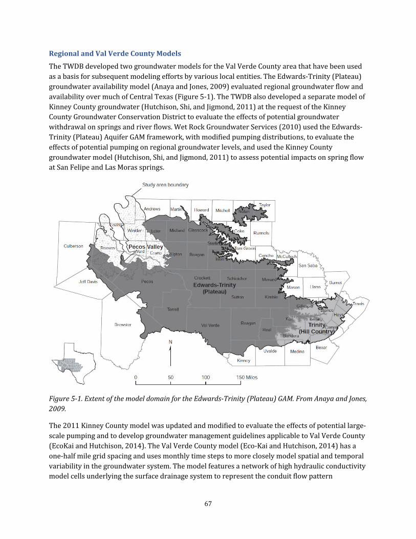
Regional and Val Verde County Models
The TWDB developed two groundwater models for the Val Verde County area thathave been used as a basis for subsequent modeling efforts by various local entities.The Edwards-Trinity (Plateau)groundwater availability model (Anaya and Jones, 2009) evaluated regional groundwater flow andavailability over much of Central Texas (Figure 5-1). The TWDB also developed a separate model ofKinney County groundwater (Hutchison, Shi, and Jigmond, 2011) at the request of the KinneyCounty Groundwater Conservation District to evaluate the effects of potential groundwaterwithdrawal on springs and river flows. Wet Rock Groundwater Services (2010) used the Edwards-Trinity (Plateau) Aquifer GAM framework,with modified pumping distributions, to evaluate the effects of potential pumping on regional groundwater levels,and used the Kinney Countygroundwater model (Hutchison, Shi, and Jigmond, 2011) to assess potential impacts on spring flowat San Felipe and Las Moras springs.
Figure 5-1.Extent ofthe model domain for the Edwards-Trinity (Plateau) GAM. From Anaya and Jones, 2009.
The 2011 Kinney County model was updated and modified to evaluate the effects of potential large-scale pumping and to develop groundwater management guidelines applicable to Val Verde County(EcoKai and Hutchison, 2014). The Val Verde County model (Eco-Kai and Hutchison,2014) has aone-half mile grid spacing and uses monthly time steps to more closely modelspatialand temporal variability in the groundwater system. The model features a network of high hydraulic conductivity model cells underlying the surface drainage system to represent the conduit flow pattern
67

associated with the karst aquifer. Monthly recharge is calculated from data on rainfalland evaporation, with a precipitation threshold level below which no recharge occurs and a variable lag term to simulate dependence on prior conditions. The Val Verde County model is calibrated toobserved groundwater levels and spring flow in Las Moras, McKee, and Cantu springs.
Devils River Watershed Model
Toll, Fratesi, Green, Bertetti, and Nunu (2017) used a different approach to model groundwater in the Devils River watershed in Val Verde,Crockett,and Sutton counties. Figure 5-2 illustrates thedomain of this groundwater model. They used a semi-distributed surface-water model, theHydrologic Modeling System (HEC-HMS), developed by the U.S. Army Corps of EngineersHydrologic Engineering Center to determine runoff and recharge components of the water budgetfrom gridded daily precipitation data. The surface water model is calibrated to gaged flows atPafford Crossing. The recharge component from the surface water model is used as input to agroundwater flow model. The groundwater model represents the upper 130 feet of the Edwardsaquifer unit as a network of highly conductive karst conduits underlying the river channels.Ituses the MODFLOW-USG program to create an unstructured grid with higher spatial resolution around the conduitfeatures and lower resolution for the aquifer matrix away from the streams.
Lower Pecos River Watershed Model
Green, Toll, Bertetti, and Hill (2016) developed a multi-county groundwater flow model of thelower Pecos River watershed that includes the portion of the watershed that contributes to thevolume of river flow that discharges to Amistad Reservoir. As such, this modelextends over much of the western portion of Val Verde County. The FEFLOW modeling package was used as themodeling code rather than the MODFLOW code.The modelconsists of two layers,one each for the Edwards and Trinity rock units. Unlike the Devils River watershed model, the lower Pecos River watershed model does not include a coupled surface water model that is coupled to the groundwater model.
Model Parameters
Table 5-1 summarizes critical aquifer properties in the available groundwater models for Val Verde County.The aquifer properties used in the Devils River Watershed Model (Toll and others, 2017)describe a groundwater system with more rapid flow along discrete channels and greater overallgroundwater storage than the GAM model. The Val Verde County Model has much higher hydraulicconductivities than the GAM model, while storage values are comparable.
Layer 1 of the GAM, representing the entirety of the Edwards aquifer unit, has a spatially averagedhydraulic conductivity of 6.65 feet per day, while Layer 2 of the GAM, representing the TrinityAquifer, has a hydraulic conductivity of 2.5 feet per day. The Devils River Watershed model has ahydraulic conductivity distribution of the aquifer matrix with values comparable to those used in the GAM,butwith hydraulic conductivity in the conduitchannels 100 to 1000 times higher than the matrix. The Devils River Watershed model also use specific storage and specific yield values for theaquifer matrix that are between 2 and 20 times higher than those used by the GAM.The high hydraulic conductivity channels represented in the Devils River Watershed Model was designed to simulate more rapid system response to short-term changes in externalconditions,such as storm
68

events, but the greater volume of groundwater in storage may damp model response to long-term stresses.
Figure 5-2. Oblique view of the Devils River Watershed model (Toll and others, 2017).
69
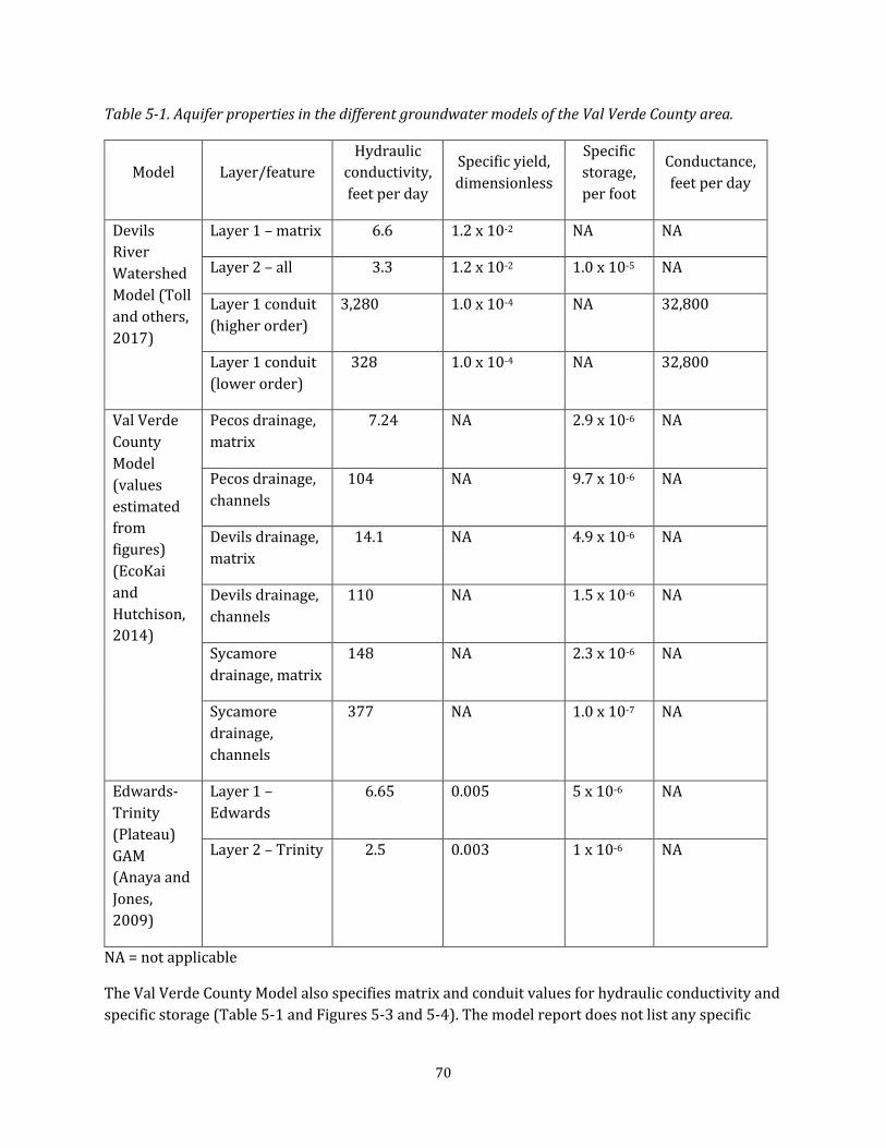
Table 5-1.Aquifer properties in the different groundwater models of the Val Verde County area.
Model Layer/feature Hydraulic
conductivity,feet per day
Specific yield,dimensionless
Specific storage,per foot
Conductance, feet per day
Devils River Watershed Model (Tolland others, 2017)
Layer 1 – matrix 6.6 1.2 x 10⁻² NA NA
Layer 2 – all 3.3 1.2 x 10⁻² 1.0 x 10⁻⁵ NA
Layer 1 conduit(higher order)
3,280 1.0 x 10⁻⁴ NA 32,800
Layer 1 conduit(lower order)
328 1.0 x 10⁻⁴ NA 32,800
Val Verde CountyModel (valuesestimated from figures)(EcoKaiand Hutchison, 2014)
Pecos drainage,matrix
7.24 NA 2.9 x 10⁻⁶ NA
Pecos drainage,channels
104 NA 9.7 x 10⁻⁶ NA
Devils drainage,matrix
14.1 NA 4.9 x 10⁻⁶ NA
Devils drainage,channels
110 NA 1.5 x 10⁻⁶ NA
Sycamoredrainage, matrix
148 NA 2.3 x 10⁻⁶ NA
Sycamoredrainage,channels
377 NA 1.0 x 10⁻⁷ NA
Edwards-Trinity(Plateau)GAM (Anaya andJones, 2009)
Layer 1 – Edwards
6.65 0.005 5 x 10⁻⁶ NA
Layer 2 – Trinity 2.5 0.003 1 x 10⁻⁶ NA
NA = not applicable
The Val Verde County Model also specifies matrix and conduit values for hydraulic conductivity andspecific storage (Table 5-1 and Figures 5-3 and 5-4). The model report does not list any specific
70
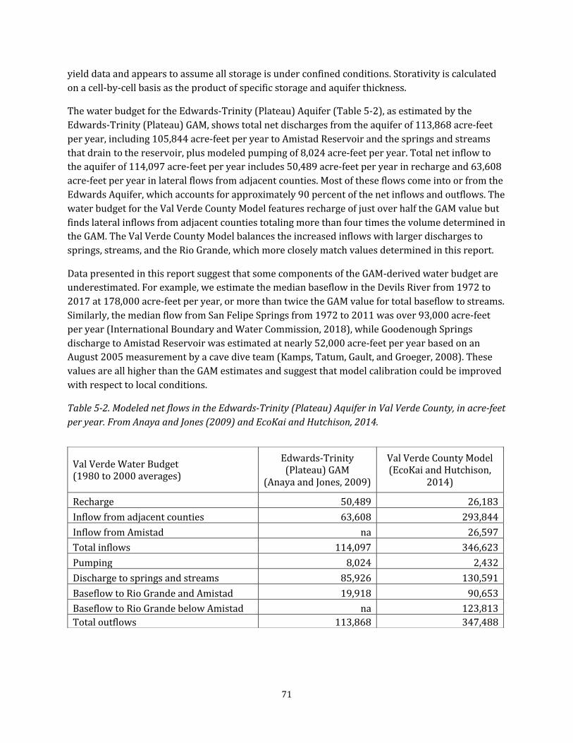
yield data and appears to assume all storage is under confined conditions. Storativity is calculatedon a cell-by-cell basis as the product of specific storage and aquifer thickness.
The water budget for the Edwards-Trinity (Plateau) Aquifer (Table 5-2), as estimated by theEdwards-Trinity (Plateau) GAM, shows total net discharges from the aquifer of 113,868 acre-feetper year, including 105,844 acre-feet per year to Amistad Reservoir and the springs and streamsthatdrain to the reservoir,plus modeled pumping of 8,024 acre-feet per year. Total net inflow to the aquifer of 114,097 acre-feet per year includes 50,489 acre-feet per year in recharge and 63,608 acre-feet per year in lateral flows from adjacent counties. Most of these flows come into or from theEdwards Aquifer,which accounts for approximately 90 percentof the netinflows and outflows.The water budget for the Val Verde County Model features recharge of just over half the GAM value butfinds lateral inflows from adjacent counties totaling more than four times the volume determined in the GAM.The Val Verde County Model balances the increased inflows with larger discharges tosprings, streams, and the Rio Grande, which more closely match values determined in this report.
Data presented in this report suggest that some components of the GAM-derived water budget areunderestimated. For example, we estimate the median baseflow in the Devils River from 1972 to2017 at 178,000 acre-feet per year, or more than twice the GAM value for totalbaseflow to streams. Similarly, the median flow from San Felipe Springs from 1972 to 2011 was over 93,000 acre-feetper year (International Boundary and Water Commission, 2018), while Goodenough Springsdischarge to Amistad Reservoir was estimated at nearly 52,000 acre-feet per year based on anAugust 2005 measurement by a cave dive team (Kamps, Tatum, Gault, and Groeger, 2008). Thesevalues are all higher than the GAM estimates and suggest that model calibration could be improvedwith respect to local conditions.
Table 5-2. Modeled net flows in the Edwards-Trinity (Plateau) Aquifer in Val Verde County,in acre-feet per year. From Anaya and Jones (2009) and EcoKai and Hutchison, 2014.
Val Verde Water Budget(1980 to 2000 averages)
Edwards-Trinity(Plateau) GAM
(Anaya and Jones, 2009)
Val Verde County Model(EcoKai and Hutchison,
2014)
Recharge 50,489 26,183
Inflow from adjacent counties 63,608 293,844
Inflow from Amistad na 26,597
Total inflows 114,097 346,623
Pumping 8,024 2,432
Discharge to springs and streams 85,926 130,591
Baseflow to Rio Grande and Amistad 19,918 90,653
Baseflow to Rio Grande below Amistad na 123,813 Total outflows 113,868 347,488
71

Applicability to Groundwater Management
The available groundwater flow models have varying applicability for groundwater managementand the appropriateness of one model or another depends on the management issue underconsideration. The Edwards-Trinity (Plateau) Aquifer GAM (Anaya and Jones, 2009) is regional in scale. With a one-mile grid cell spacing, annual stress periods, and broadly defined aquiferproperties, it is best suited to long-term evaluation of dispersed processes thatestablish the overall water budget for the region. Examples of applications that are suitable for GAMs include requiredtechnicalinputs such as groundwater budgets to groundwater managementplans.However,GAMsare not intended to represent local resource management decisions and are not appropriate formodeling groundwater behavior around a spring or single well.
72

Figure 5-3. Hydraulic conductivity distribution in the calibrated Val Verde County Model,from EcoKai and Hutchison, 2014.
73
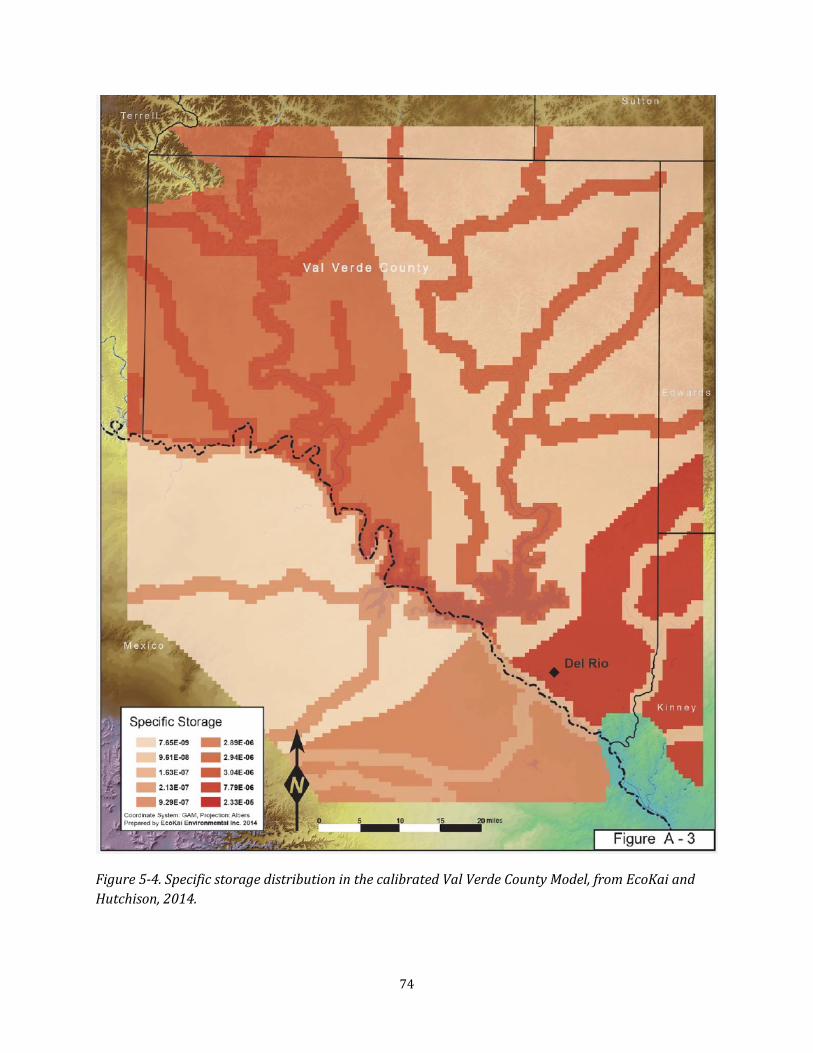
Figure 5-4. Specific storage distribution in the calibrated Val Verde County Model,from EcoKai and Hutchison, 2014.
74

The Wet Rock (2010b) model runs utilize existing GAM inputs and inherit the generalcharacteristics and limitations of the regional model. Wet Rocks’ water resource evaluation for the Weston Ranch (Wet Rock, 2010a) determines a groundwater recharge value more than four timeshigher than what was used by Anaya and Jones (2010), but their groundwater modeling report(Wet Rock 2010b) implies that the GAM Run 09-035, Scenario 10 (Hutchison, 2010) served as thebase case for evaluating the effects of potential pumping at Weston Ranch and makes no mention of revising the recharge values.
The Val Verde County Model is potentially better suited for evaluating groundwater managementoptions in Val Verde than the Edwards-Trinity (Plateau) Aquifer GAM. The refined grid size,monthly time step, more detailed representation of subsurface hydrogeology, inclusion of adjacent areas in Mexico, and model calibration to spring flows all represent improvements over theregional GAM,where adequately supported by new data. Continued refinement of the Val Verde County Model as more data become available probably represents the best path forward forsupporting groundwater management objectives in Val Verde County. In particular, the hydraulicconductivity distribution in the model needs more validation with field measurements,andboundary conditions should reflect the separation between watershed basins in the northern half ofVal Verde County.
The Devils River Watershed Model represents a very different approach that could be applied on a watershed basis. For example, Figure 5-5 illustrates the application of this model to simulating thebehavior of springs in the Devils River watershed to conditions ranging from no pumping to atheoreticalhigh volume (10,000 gallons per minute) well field near Juno. The figure compares a “no pumping” scenario in the left panel,groundwater pumping consistentwith thatin the Edwards-Trinity (Plateau) Aquifer GAM in upgradient counties in the middle, and the effects of thehypothetical well field on the right panel.This modelhas many intriguing features,including the explicit linkage between surface runoff processes and groundwater recharge, use of griddedprecipitation input, and the grid refinement around high conductance conduit channels. The modeldoes not encompass the whole area of Val Verde County and adds complexity beyond what issupported by the model documentation and the available data. Applying a coupled surface water-groundwater model with permeable conduits to the whole of Val Verde County would requirefurther extrapolation and conjecture given the relative scarcity of data outside the Devils Riverdrainage. While an integrated hydrological model of Val Verde County remains a worthwhile goal, itmay not be a practical alternative, pending additional monitoring, data collection, andhydrogeological study.
Data Gaps and Data Needs
Water level measurements are the fundamental record required to assess groundwater resources.The current network of observation wells does not provide adequate spatial or temporal detail overthe extentof Val Verde County.Establishing a representative network of atleast25 to 30 wells with known well completion and collecting regular water level measurements would give an appropriateand improved technical basis from which to support future groundwater management. Currentobservation wells should be logged and evaluated for installation of instrumentation to collect daily water level measurements at suitable wells with suitable completion. Additional observation wells
75
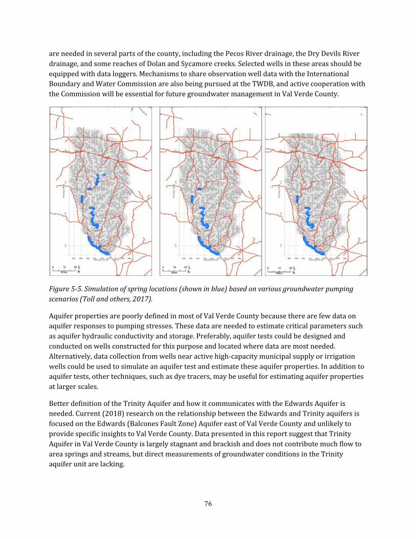
are needed in several parts of the county, including the Pecos River drainage, the Dry Devils Riverdrainage, and some reaches of Dolan and Sycamore creeks. Selected wells in these areas should be equipped with data loggers. Mechanisms to share observation well data with the InternationalBoundary and Water Commission are also being pursued at the TWDB, and active cooperation withthe Commission willbe essentialfor future groundwater managementin Val Verde County.
No pumping 10,000 gallon per minute wellfield
GAM pumping
Figure 5-5.Simulation of spring locations (shown in blue) based on various groundwater pumping scenarios (Toll and others, 2017).
Aquifer properties are poorly defined in most of Val Verde County because there are few data on aquifer responses to pumping stresses.These data are needed to estimate critical parameters suchas aquifer hydraulic conductivity and storage. Preferably, aquifer tests could be designed andconducted on wells constructed for this purpose and located where data are most needed. Alternatively, data collection from wells near active high-capacity municipal supply or irrigation wells could be used to simulate an aquifer testand estimate these aquifer properties.In addition to aquifer tests,other techniques,such as dye tracers,may be usefulfor estimating aquifer properties at larger scales.
Better definition of the Trinity Aquifer and how it communicates with the Edwards Aquifer isneeded. Current (2018) research on the relationship between the Edwards and Trinity aquifers isfocused on the Edwards (Balcones Fault Zone) Aquifer east of Val Verde County and unlikely toprovide specific insights to Val Verde County. Data presented in this report suggest that TrinityAquifer in Val Verde County is largely stagnant and brackish and does not contribute much flow toarea springs and streams, but direct measurements of groundwater conditions in the Trinityaquifer unit are lacking.
76
6.0 SurfaceWater Key findings
• Measured flow in the Devils River at Pafford Crossing is influenced by Amistad Reservoirwater level and is not a good measure of conditions in the upper, spring-fed reaches of theriver.
• Flow measurements at the Devils River Bakers Crossing gage have been inconsistent overtime,complicating interpretation of any long-term trends.
• Low-flow gain-loss studies on the Devils River show similar patterns of spring discharge to the river between 1928 and 2006 surveys for the reaches where comparable data are available.
Perennial surface water resources in Val Verde County include the Rio Grande, Amistad Reservoir,Pecos River, Devils River, and San Felipe Creek (Figure 6-1). These surface water features areregional points of discharge for the groundwater system. Annual flows from Goodenough Springs,the Devils River,and San Felipe Springs are estimated to accountfor approximately 23 percentof the flow in the Rio Grande below Amistad Reservoir (Green,2013).
Flow in the Rio Grande upstream of Val Verde County comes primarily from the Rio Conchos, which joins the Rio Grande near Presidio,Texas,about 350 river miles upstream. Storage in Amistad Reservoir is allocated to the United States and Mexico under a 1944 Treaty. Texas’ share of the U.S.storage is fully allocated. Amistad Reservoir typically operates in tandem with Falcon Reservoir, which is 340 river miles downstream. About 90 percent of the water released from AmistadReservoir flows through Falcon Reservoir for use in the lower Rio Grande Valley, with theremaining 10 percent going to municipal and agricultural water rights holders between Amistadand Falcon reservoirs (Purchase, Larsen, Flora, and Reber, 2001,TWDB,2017).
Because the U.S. share of flow in the lower Rio Grande is fully allocated under existing permits, any reduction in flow to the Rio Grande from tributaries in Val Verde County could affect downstreamusers. Val Verde groundwater is a major component of flow in the Lower Rio Grande. Currentgroundwater discharge in Val Verde County totals 330,000 acre-feet per year, as noted in theSection 4 discussion of springs, or about 30 percent of the 1.01 million acre-feet U.S. share of thefirm annual yield of the Amistad-Falcon reservoir system (U.S. Bureau of Reclamation, 2016).Regional water resources are already under stress. The 2017 State Water Plan (TWDB, 2017) projects annual water needs (projected shortages) of 708,000 to 797,000 acre-feet between 2020 and 2070. Any reduction in spring discharge will proportionately increase the projected shortages.
The Pecos River flows south from the Southern Rocky Mountains in New Mexico through WestTexas and into Amistad Reservoir, draining a watershed of 44,000 square miles. Pecos River water is allocated entirely to the United States. Several reservoirs impound water for irrigation along thePecos River; one is Red Bluff Reservoir at the Texas-New Mexico state line, completed in 1936.Total annual flow and baseflow at the mouth of the Pecos in Val Verde County generally declined between about 1970 and 2000 (Figure 6-2),which has been attributed to increasing upstream
77

Figure 6-1. Surface water features in Val Verde County.From Toll and others (2017).
78

1,200,000
Tota
l ann
ual f
low
, acr
e-fe
et
1,000,000
800,000
600,000
400,000
200,000
0 1960 1970 1980 1990 2000 2010 2020
Pecos River Devils River
Figure 6-2.Total annual flow of the Devils River, 1960 to 2017, and Pecos River, 1968 to 2011. Data from International Boundary and Water Commission (2018a).
surface and groundwater use (Purchase, Larsen, Flora, and Reber, 2001). For the 30-year period of1980 to 2010, InternationalBoundary and Water Commission data indicate no significant trend in totalflow (InternationalBoundary and Water Commission,2018).The salinity of the Pecos River water at the Red Bluff Dam, near the New Mexico border, can be as high as 6,000 milligrams perliter because of salts dissolved from deposits in the Delaware Basin (Hart,Jensen,Hatler,andMecke, 2007). The hydrology and chemistry of the lowermostsection of the Pecos River in Val Verde County is determined largely by the consistentfresh flows of Independence Creek,which enters the Pecos in Crockett County (Basnet, Hauck, and Pendergrass, 2013). Streamflow inIndependence Creek is maintained by springs draining the Edwards-Trinity (Plateau) Aquifer. ThePecos River contributes an estimated 26 percent of salt loading to Amistad Reservoir whilerepresenting only 9.5 percent of the reservoir’s total annual inflows (Texas Water ResourcesInstitute, 2010).
The Devils River drains an area of 4,305 square miles. There has been minimal development in thewatershed. There are no dams or other control structures on the river and land use in the watershed is primarily ranching, with low-density rural housing. Several stream gaging sites on theDevils River and contributing streams (Figure 6-3) are operated by the USGS and the InternationalBoundary and Water Commission.
Streamflow can increase quickly to peak values exceeding 100,000 cubic feet per second inresponse to large rainstorms. The estimated peak flow at Pafford Crossing during the June 1954flood was 393,000 cubic feet per second, eclipsing the previous record of 370,000 cubic feet persecond set during the flood of September 1932 (Breeding, 1954). Base flow,representing flow between storm events, from springs above Pafford Crossing averages from 100 to 500 cubic feet
79
per second. Streamflow in the Devils River typically decreases quickly following storm events,indicating minimal bed and bank storage (Figure 6-4).
Streamflow at the Pafford Crossing gage on the Devils River is influenced by Amistad Reservoir, andbase flow increased after the reservoir filled. When the dam was completed in 1969 and thereservoir filled over the next few years, groundwater levels rose in the area within about10 miles of the reservoir. The increased water levels resulted in increased spring flow, andconsequent increases in streamflow at locations near the reservoir. Because Amistad is a floodcontrol reservoir and does not maintain a near-constant surface elevation, reservoir level changessince 1970 continue to affect measured streamflow at the Pafford Crossing gage and complicate any trend analysis for this location.While streamflow measurements have a declining trend between 1972 and 2017 (Figure 6-5), this may have more to do with the extended periods of drawdown inAmistad Reservoir in the 1990s and 2010s than with changes in the groundwater system feedingthe Devils River.
We computed baseflow using the baseflow index method (Wahl and Wahl, 1985) using five-dayminimum flows to assess turning points in the hydrograph. In practice, the baseflow index methodassigns most flow in the Devils River to baseflow, with only brief periods of stormflow following precipitation events.We find thatthe baseflow index is a more accurate depiction of baseflow in the karst environment of Val Verde County than baseflow separation techniques using recursive digital filters, as proposed by Eckhardt (2004) or Nathan and McMahon (1990). These baseflow separationalgorithms assign a smaller fraction of total flow to baseflow when using commonly accepted inputvalues. The infrequent nature of storm events in West Texas and the limited bed and bank storageavailable along the Devils River imply that most flow in this river should be classified as baseflow.Baseflow separation using water quality data might help distinguish direct runoff, conduit, andmatrix flow components (Miller, Johnson, Susong, and Wolock, 2015), but such information is notcurrently available.
We evaluated trends in both average annual baseflow and total annual discharge between 1972 and2017 in daily gage data reported by the International Boundary and Water Commission (IBWC)(2018a) using the non-parametric Mann-Kendall trend test (Salmi, Maatta, Anttila, Ruoho-Airola,and Amnell, 2002). Both total discharge and average baseflow have a decreasing trend that issignificant at the 99 percent confidence level for the years from 1972 through 2016, the lastcomplete year of record available. The significance of the trends is largely based on high flowsrecorded at the beginning of the period in 1974 and low flows recorded at the end of the periodduring the 2011 to 2014 drought. The Mann-Kendall test indicated no significant trends in eithertotaldischarge or average baseflow for the period from 1975 to 2011.
80

Figure 6-3.Locations ofstream gages in the Devils River and adjacent watersheds (adapted from Toll and others, 2017)
81
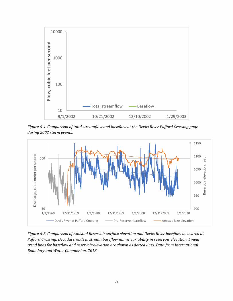
10000
Flow
, cub
ic fe
et p
er se
cond
1000
100
Total streamflow Baseflow 10 9/1/2002 10/21/2002 12/10/2002 1/29/2003
Figure 6-4. Comparison of totalstreamflow and baseflow at the Devils River Pafford Crossing gage during 2002 storm events.
1150
Dis
char
ge, c
ubic
met
er p
er s
econ
d 1100500
1050
1000
950
50 900
Devils River at Pafford Crossing Pre-Reservoir baseflow Amistad lake elevation
1/1/1960 12/31/1969 1/1/1980 12/31/1989 1/1/2000 12/31/2009 1/1/2020
Figure 6-5. Comparison of Amistad Reservoir surface elevation and Devils River baseflow measured at Pafford Crossing. Decadal trends in stream baseflow mimic variability in reservoirelevation. Linear trend lines for baseflow and reservoir elevation are shown as dotted lines. Data from International Boundary and Water Commission, 2018.
Rese
rvoi
r ele
vatio
n, fe
et
82
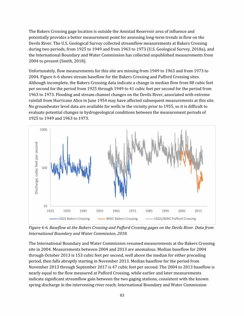
The Bakers Crossing gage location is outside the Amistad Reservoir area of influence andpotentially provides a better measurement point for assessing long-term trends in flow on the Devils River. The U.S. Geological Survey collected streamflow measurements at Bakers Crossingduring two periods, from 1925 to 1949 and from 1963 to 1973 (U.S. Geological Survey, 2018a), andthe International Boundary and Water Commission has collected unpublished measurements from2004 to present (Smith, 2018).
Unfortunately, flow measurements for this site are missing from 1949 to 1963 and from 1973 to2004. Figure 6-6 shows stream baseflow for the Bakers Crossing and Pafford Crossing sites.Although incomplete, the Bakers Crossing data indicate a change in median flow from 88 cubic feet per second for the period from 1925 through 1949 to 41 cubic feet per second for the period from1963 to 1973. Flooding and stream channel changes on the Devils River, associated with extremerainfall from Hurricane Alice in June 1954 may have affected subsequent measurements at this site.No groundwater level data are available for wells in the vicinity prior to 1955, so it is difficult toevaluate potential changes in hydrogeological conditions between the measurement periods of1925 to 1949 and 1963 to 1973.
100
1000
Dis
char
ge, c
ubic
feet
per
sec
ond
10 1925 1935 1945 1955 1965 1975 1985 1995 2005 2015
USGS Bakers Crossing IBWC Bakers Crossing USGS/IBWC Pafford Crossing
Figure 6-6. Baseflow at the Bakers Crossing and Pafford Crossing gages on the Devils River. Data from International Boundary and WaterCommission,2018.
The International Boundary and Water Commission resumed measurements at the Bakers Crossingsite in 2004. Measurements between 2004 and 2013 are anomalous. Median baseflow for 2004 through October 2013 is 153 cubic feet per second, well above the median for either preceding period, then falls abruptly starting in November 2013. Median baseflow for the period fromNovember 2013 through September 2017 is 47 cubic feet per second. The 2004 to 2013 baseflow isnearly equal to the flow measured at Pafford Crossing, while earlier and later measurementsindicate significant streamflow gain between the two gaging stations, consistent with the knownspring discharge in the intervening river reach. International Boundary and Water Commission
83
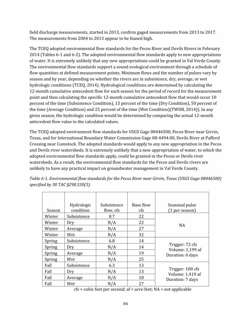
field discharge measurements, started in 2013, confirm gaged measurements from 2013 to 2017.The measurements from 2004 to 2013 appear to be biased high.
The TCEQ adopted environmental flow standards for the Pecos River and Devils Rivers in February 2014 (Tables 6-1 and 6-2). The adopted environmental flow standards apply to new appropriationsof water. Itis extremely unlikely thatany new appropriations could be granted in ValVerde County.The environmental flow standards support a sound ecological environment through a schedule offlow quantities at defined measurement points. Minimum flows and the number of pulses vary byseason and by year, depending on whether the rivers are in subsistence, dry, average, or wethydrologic conditions (TCEQ, 2014). Hydrological conditions are determined by calculating the12-month cumulative antecedent flow for each season for the period of record for the measurementpoint and then calculating the specific 12-month cumulative antecedent flow that would occur 10percent of the time (Subsistence Condition), 15 percent of the time (Dry Condition), 50 percent ofthe time (Average Condition) and 25 percent of the time (Wet Condition)(TWDB, 2014)). In anygiven season, the hydrologic condition would be determined by comparing the actual 12-monthantecedent flow value to the calculated values.
The TCEQ adopted environment flow standards for USGS Gage 08446500, Pecos River near Girvin,Texas, and for International Boundary Water Commission Gage 08-4494.00, Devils River at Pafford Crossing near Comstock. The adopted standards would apply to any new appropriation in the Pecosand Devils river watersheds. It is extremely unlikely that a new appropriation of water, to which theadopted environmental flow standards apply, could be granted in the Pecos or Devils riverwatersheds. As a result,the environmental flow standards for the Pecos and Devils rivers are unlikely to have any practical impact on groundwater management in Val Verde County.
Table 6-1. Environmental flow standards for the Pecos River near Girvin,Texas (USGS Gage 08446500) specified by 30 TAC §298.530(3).
licable
Season Hydrologiccondition
Subsistence flow, cfs
Base flow cfs
Seasonal pulse(1 per season)
Winter Subsistence 8.7 22
NAWinter Dry N/A 22 Winter Average N/A 27 Winter Wet N/A 32 Spring Subsistence 6.8 14
Trigger: 72 cfsVolume: 1,199 afDuration: 6 days
Spring Dry N/A 14 Spring Average N/A 19 Spring Wet N/A 25 Fall Subsistence 6.3 13
Trigger: 100 cfsVolume: 1,419 afDuration: 7 days
Fall Dry N/A 13 Fall Average N/A 18 Fall Wet N/A 27
cfs = cubic feet per second; af = acre-feet; NA = not app
84

Table 6-2. Environmental flow standards for the Devils River at Pafford Crossing near Comstock (International Boundary and Water Commission Gage 08-4494.00), as specified under specified under 30 TAC §298.530(4).
Season Hydrologiccondition Subsistence
Baseflow,cfs
Seasonal pulse(1 per season)
Annual pulse(1 per year)
Winter Subsistence 84 175
NA
Trigger: 3,673 cfsVolume: 34,752 afDuration: 13 days
Winter Dry NA 175 Winter Average NA 200 Winter Wet NA 243 Spring Subsistence 91 160
Trigger: 558 cfsVolume: 17,374 afDuration: 7 days
Spring Dry NA 160 Spring Average NA 207 Spring Wet NA 253 Fall Subsistence 87 166
Trigger: 1,872 cfsVolume: 27,781 afDuration: 9 days
Fall Dry NA 166 Fall Average NA 206 Fall Wet NA 238
cfs = cubic feet per second; af = acre-feet; NA = not applicable
Streamflow Gain-Loss Studies
The Texas Board of Water Engineers (1960) reported data from several low-flow streamflowstudies on the Devils River conducted in the 1920s. The TCEQ conducted another streamflow studyin 2006. Data from the 1921, 1925, 1928, and 2006 studies (Figure 6-7 and Appendix A) show verysimilar patterns of spring-flow contribution to the Devils River between Beaver Lake (mile zero)and Pafford Crossing (aka Rubboard Crossing, at mile 53.7). Amistad Reservoir now fills the Devils River stream channel starting just below Pafford Crossing so we cannot compare current conditionsin the lower portion of the river with measurements from before the reservoir was constructed.
The August 1925 study covered the entire length of the Devils River from Beaver Lake to the RioGrande. It found three major areas of groundwater discharge to the river: the reach between PecanSprings and Bakers Crossing; the 4-mile reach above Dolan Creek; and a 7-mile reach just belowPafford Crossing. It found 1.6 cubic feet per second flow in the Devils River just below Beaver Lake, but this water infiltrated the stream bed within 0.2 miles. There was no flow in the river for the next 13.8 miles down the stream bed, until just below Pecan Springs (Texas Board of WaterEngineers, 1960). Another gain-loss study conducted in February 1928 found somewhatlower flows overall, but found streamflow gains in the same river reaches, with minimal gain betweenthese areas of groundwater discharge.
85
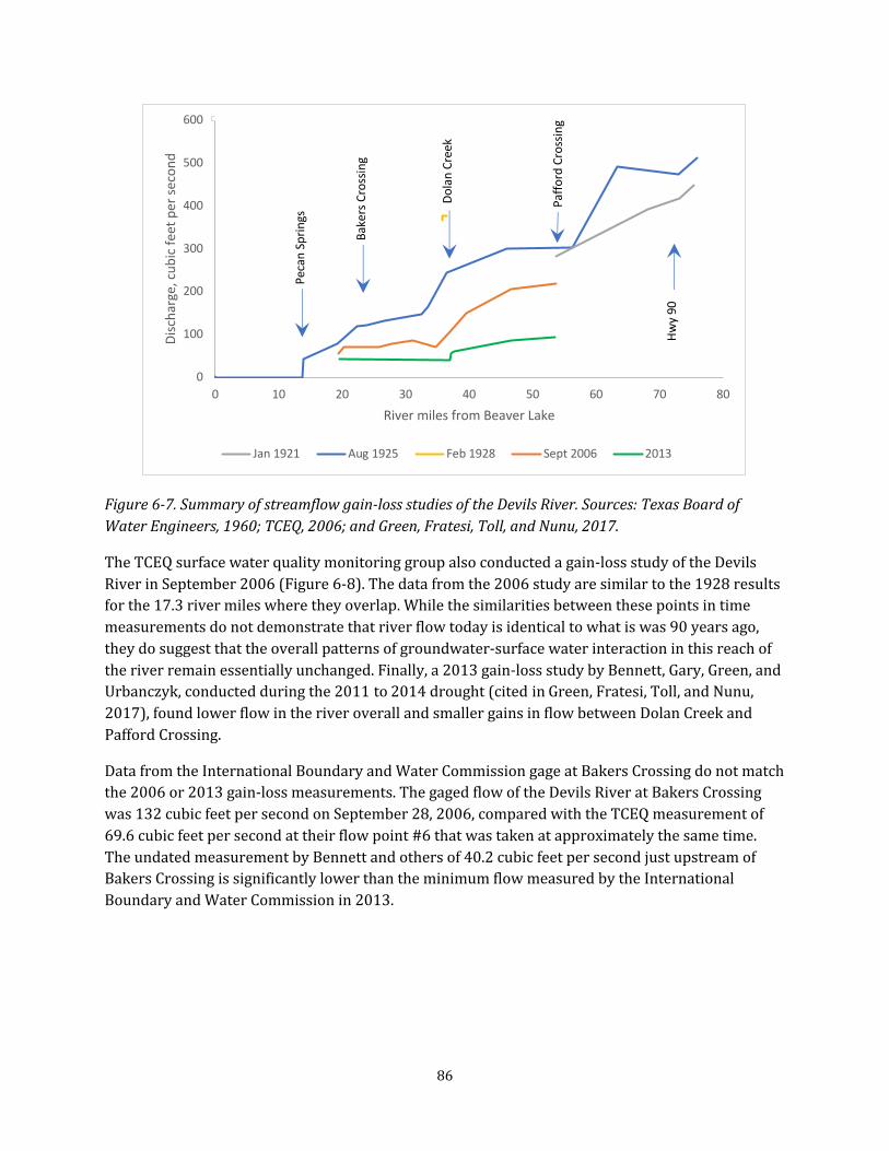
Dis
char
ge, c
ubic
feet
per
sec
ond
600
500
400
300
200
100
0
Peca
n Sp
rings
Bake
rs C
ross
ing
Dol
an C
reek
Paff
ord
Cros
sing
Hw
y 90
0 10 20 30 40 50 60 70 80
River miles from Beaver Lake
Jan 1921 Aug 1925 Feb 1928 Sept 2006 2013
Figure 6-7.Summary of streamflow gain-loss studies of the Devils River. Sources: Texas Board of Water Engineers, 1960; TCEQ, 2006; and Green, Fratesi, Toll, and Nunu, 2017.
The TCEQ surface water quality monitoring group also conducted a gain-loss study of the Devils River in September 2006 (Figure 6-8). The data from the 2006 study are similar to the 1928 results for the 17.3 river miles where they overlap. While the similarities between these points in timemeasurements do not demonstrate that river flow today is identical to what is was 90 years ago,they do suggestthatthe overallpatterns of groundwater-surface water interaction in this reach of the river remain essentially unchanged. Finally, a 2013 gain-loss study by Bennett,Gary,Green, and Urbanczyk, conducted during the 2011 to 2014 drought(cited in Green,Fratesi,Toll,and Nunu, 2017), found lower flow in the river overall and smaller gains in flow between Dolan Creek and Pafford Crossing.
Data from the International Boundary and Water Commission gage at Bakers Crossing do not matchthe 2006 or 2013 gain-loss measurements.The gaged flow of the Devils River atBakers Crossing was 132 cubic feet per second on September 28,2006,compared with the TCEQ measurement of 69.6 cubic feet per second at their flow point#6 thatwas taken atapproximately the same time. The undated measurement by Bennett and others of 40.2 cubic feet per second just upstream ofBakers Crossing is significantly lower than the minimum flow measured by the InternationalBoundary and Water Commission in 2013.
86

Figure 6-8. TCEQ streamflow measurements on the Devils River, September 2006.
87

7.0 Water Supplies and Demands Key findings
• Estimated existing groundwater supplies in Val Verde County exceed the projected demandthrough 2070,except for small projected needs associated with oil exploration andproduction.
• Past groundwater use and pumping data are inconsistent and incomplete. A betteraccounting system is needed if more active groundwater management is planned.
• We estimate that groundwater pumping for all uses in Val Verde County has averaged about4,700 acre-feet per year since 2001 and has increased from about 2,200 acre-feet per yearin the 1980s and 3,000 acre-feet per year in the 1990s.
Supply and Demands
The short- and long-term water supplies and water demands for Val Verde County are described inthe 2016 Plateau Region water plan (Ashworth, Herrera, and Brown, 2016). Val Verde County isexpected to grow from a projected 2020 population of 54,694 to 82,161 by 2070, an increase of 50percent over the 50-year planning period,leading to increased water demand.
The Plateau Region water plan (Ashworth, Herrera, and Brown, 2016) shows existing groundwatersupplies from the Edwards Trinity (Plateau) Aquifer remaining constant from 2020 through 2070 at 24,988 acre-feet per year and the total water supply, including surface water from the RioGrande, at 37,266 acre-feet per year throughout the planning period. Modeled availablegroundwater supplies based on the desired future conditions adopted in 2018 increase to 50,000acre-feet throughout the planning period.
Water demand in Val Verde County increases from 16,777 acre-feet per year in 2020 to 21,127acre-feet per year in 2070, an increase of 26 percent (Table 7-1). Demand growth is primarily fromthe City of DelRio,Laughlin Air Force Base,and County-other water user groups, while mining, livestock,and irrigation water uses are projected to be stable or decreasing from 2020 through2070 (Ashworth, Herrera, and Brown, 2016). While the total projected demand remains less than the projected groundwater supply throughoutthe 50-year planning period,the regionalplanninggroup identifies unmet water needs in the mining sector between 2020 and 2060, despite surplusesfor other water user groups (Table 7-2).
Water use and pumping
To date, groundwater development in Val Verde County and surrounding areas has been limited in scope and pumping volumes remain small. Most wells are used for ranch supply and livestock.Submitted Drillers Reports since about 2005 indicate that additional high-capacity irrigation wellshave been constructed recently but reported irrigation water usage has not increased.Aerialimagery suggests that most of the wells have not been used in the last 10 years.
88

Table 7-1. Val Verde County water user group demand projections, 2020 to 2070, in acre-feetper year.
2020 2030 2040 2050 2060 2070
Del Rio 10,645 11,144 11,649 12,229 12,837 13,435
Laughlin AFB 1,012 1,107 1,208 1,269 1,268 1,268
County-other* 1,937 2,267 2,596 2,959 3,331 3,694
Mining 190 249 259 223 192 171
Livestock 533 533 533 533 533 533
Irrigation 2,460 2,364 2,274 2,185 2,101 2,026
Total 16,777 17,664 18,519 19,398 20,262 21,127
*County-other refers to residential, commercial, and institutional water users in cities with less than 500 people or to utilities that provide less than 250,000 gallons of water per day.
Table 7-2. Val Verde County water surplus/needs, 2020 to 2070, in acre-feetper year.
2020 2030 2040 2050 2060 2070
Del Rio 16,255 15,756 15,251 14,671 14,063 13,465
Laughlin AFB 1,287 1,192 1,091 1,030 1,031 1,031
County-other* 2,576 2,246 1,917 1,554 1,182 819
Mining -4 -63 -73 -37 -6 15
Livestock 0 0 0 0 0 0
Irrigation 335 431 521 610 694 769
Total 22,469 21,592 20,747 19,878 19,024 18,169
*County-other refers to residential, commercial,and institutionalwater users in cities with less than 500 people or to utilities that provide less than 250,000 gallons of water per day.
89

Different investigators have come up with different historical use figures for Val Verde County. Differing estimates of historicaluse can impactmodelpredictions of the effects of future pumping.The fact that different models cover different areas of interest and use different calibration time periods makes it difficult to directly compare these effects. Given the small total volumes ofgroundwater involved, these differences are probably not very significant, but better processes forcollecting groundwater use data may be more important as groundwater use increases. Thepumping estimates from previous models and revised estimates calculated as described in thefollowing paragraphs are listed in Table 7-3.
Table 7-3.Water use estimates in various groundwater models,in acre-feetper year.
Model 1969-1980 1980s 1990s 2000s Val Verde County 1,167 2,445 2,419 5,754 Devils River Watershed 14,000 14,000 GAM, Val Verde County 4,728 8,401 7,326 This report 2,195 3,046 4,683
Total groundwater volumes used in Val Verde County from 2000 through 2014, as listed in the TWDB historical water use estimates, are shown in Table 7-4. As noted by Eco-Kai and Hutchison(2014), data for 2007 through 2009 municipal use appear to have been switched from groundwater to surface water; in Table 7-4,municipaluse is labeled as groundwater for allyears. Municipal use remains anomalously low for 2007 through 2009.
The Val Verde County model (Eco-Kai and Hutchison, 2014) also notes that Del Rio’s water supplyfrom San Felipe Springs does not represent any additional pumping stress on the aquifer beyondthe naturaldischarge from the springs, which is separately accounted for in the groundwater model water balance. The city has two water supply wells that may be used to supplement spring flow forfuture water supplies, but these are not currently in use (City of Del Rio, 2016). We estimatedmunicipal pumping by subtracting Del Rio water production data from TWDB municipal water use estimates. For the years in which Del Rio production data were not available, we estimated it basedon the average ratio of Del Rio production to totalmunicipal use from 2000 to 2013, excepting theyears 2000 and 2007 to 2009, which had suspect statistics. We estimated municipal groundwaterpumping for these years as 25 percent of the countywide reported municipal use, to reflect theapproximate volume of groundwater pumped by municipal users other than the City of Del Rio.Updated values for municipal pumping and other categories of water use are listed in Table 7-5.
Irrigation use ofgroundwater in Val Verde County is reported inconsistently and does not appear toreflect recent increases in irrigated acreage in the upper Devils River area and along the SycamoreCreek drainage north of Del Rio. Despite recent growth,groundwater use for irrigation remains restricted to limited areas in Val Verde County,covering a total of about 1,110 acres.
90
Historical imagery from Google Earth shows that the irrigated area along the Devils River upstreamfrom Juno doubled from 150 to 300 acres sometime between October 2008 and November 2009, while the reported irrigation usage of groundwater was zero for 2009. Google Earth historicalimagery also shows that a total of seven center-pivot systems were installed on the Weston Ranch,11 miles northeast of Del Rio, between 2004 and 2005, covering an area of almost 800 acres. GoogleEarth imagery shows active irrigation in 2005, 2006, and 2008, while reported groundwater use forirrigation in Val Verde County was 18 acre-feet in 2008.
Images acquired by the National Agricultural Imagery Program in 2008, 2010, 2012, 2014, 2015,and 2016 indicate some degree of irrigation under the Weston Ranch center-pivots each year(Figure 7-1), although the National Agricultural Statistics Service Crop Scape cropland data layerdoes not consistently identify crop type or irrigated area for these fields,mostlikely because of the poor condition of the vegetation under the pivots. Crop production in Val Verde County requires atleastone acre-foot of irrigation water per acre of land over the growing season. Based on theestimated center-pivot areas, annual groundwater use for irrigation probably increased to around900 acre-feet per year for 2005 through 2010,butsubsequently declined to approximately750 acre-feet per year from 2011 to 2016.
91

Table 7-4.TWDB historical groundwater use estimates for Val Verde County,2000 through 2015, acre-feetper year.
Year Municipal Mining Irrigation Livestock Total non-municipal Total
2000 14,455 0 270 614 884 15,339
2001 14,457 0 316 618 934 15,391
2002 14,471 0 322 550 872 15,343
2003 15,015 0 230 472 702 15,717
2004 15,049 0 107 426 533 15,582
2005 15,130 0 146 490 636 15,766
2006 11,365 0 150 472 622 11,987
2007 7,312 0 34 415 449 7,761
2008 8,867 9 18 506 533 9,400
2009 9,144 23 0 496 519 9,663
2010 11,537 37 276 466 779 12,316
2011 13,280 9 143 467 619 13,899
2012 12,933 0 67 414 481 13,414
2013 11,663 0 4 334 338 12,001
2014 10,850 0 21 268 289 11,139
2015 9,202 0 59 270 329 9,531
The mining and manufacturing sector, which includes oil and gas production, uses a relatively smallvolume of groundwater in Val Verde County,although italso appears to under-report water use formost years. Toll and others (2017) states that the average annual extraction of groundwater in theDevils River watershed is not well constrained due to un-metered wells and un-reported waterpumping by the oil and gas industry. We estimated groundwater use by the oil and gas industryusing data from Wood Mackenzie (2016) on the average water use per well during the firstdecade of the hydraulic fracturing boom between 2005 and 2015 (Figure 7-2), and the annual number of drilling permits issued in Val Verde County (Figure 7-3) by the Texas Railroad Commission (2018).The volume of water used per well for directional drilling and hydraulic fracturing has increasedsharply as the technology has evolved. Water use per well in the Midland Basin increased from afew hundred thousand gallons per well in 2006 (~1 acre-foot per well) to nearly 12 million gallons per well (36 acre-feet per well) in 2015 (Wood Mackenzie, 2016). Water use per hydraulicfracturing well decreased after around 2013, as producers seek to recycle more of the producedwater (Driver and Wade, 2013; Scanlon, Reedy, and Nicot, 2014).
92

Table 7-5. Revised groundwater pumping estimates for Val Verde County,acre-feetper year. Adapted from multiple sources,as described in text.
Year Municipal Mining,oil, and gas
Irrigation Domestic and
Livestock Total
2000 3,764 38 270 614 4,686
2001 2,291 54 316 618 3,279
2002 3,907 21 322 550 4,800
2003 5,600 39 230 472 6,341
2004 6,589 48 107 426 7,179
2005 5,522 92 896 490 7,000
2006 1,092 19 900 472 2,483
2007 1,904 27 814 415 4,622
2008 2,308 48 948 506 4,868
2009 2,381 42 930 496 4,750
2010 2,787 7 1,206 466 4,466
2011 2,317 15 750 467 3,549
2012 3,484 25 750 414 4,673
2013 2,538 43 750 334 3,665
2014 2,825 46 750 268 3,889
2015 3,764 36 750 270 4,802
Estimated oil and gas use of water averaged 16 acre-feet per year from 1990 to 2000 and 49 acre-feet per year for 2000 to 2015,peaking at170 acre-feet in 2016 (Figure 7-3). We estimated the oiland gas water use for the broader area of the Devils River watershed in Val Verde, Crockett, andSutton counties based on reported active oil lease areas within the Devils River watershed in each county. The Devils River watershed includes an estimated 66 percent of oilfield wells in Val Verde County,50 percentof wells in CrockettCounty, and 90 percent of wells in Sutton County. While these are rough estimates,they provide some realconstrainton the timing and magnitude of oil industry groundwater abstraction in northern Val Verde County and adjacent areas of the Devils River watershed. Estimated oil and gas use in the Devils River watershed area averaged 334 acre-feet per year for 1990 to 2000, and 1,585 acre-feet per year for 2000 to 2015. Oil and gasgroundwater use in the watershed area is estimated to have peaked in 2013, at about 4,250 acre-feet.
Overall, groundwater pumping for all uses in Val Verde County has averaged about 4,700 acre-feetper year since 2001 and has increased from about 2,200 acre-feet per year in the 1980s and3,000 acre-feet per year in the 1990s (Figure 7-4).
93
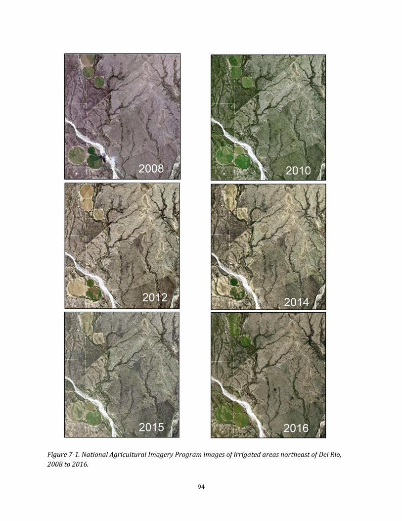
Figure 7-1.National Agricultural Imagery Program images ofirrigated areas northeast ofDel Rio, 2008 to 2016.
94
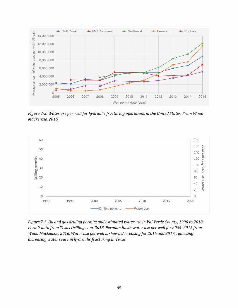
Figure 7-2.Water use per well for hydraulic fracturing operations in the United States.From Wood Mackenzie, 2016.
60 180
Dril
ling
perm
its
50 160
140
40 120
30 100
80
20 60
10 40
20
0 1990 1995 2000 2005 2010 2015
0 2020
Drilling permits Water use
Figure 7-3.Oil and gas drilling permits and estimated water use in Val Verde County,1990 to 2018. Permit data from Texas Drilling.com, 2018. Permian Basin water use per well for 2005–2015 from Wood Mackenzie, 2016. Water use per well is shown decreasing for 2016 and 2017, reflecting increasingwaterreuse in hydraulic fracturingin Texas.
Wat
er u
se, a
cre-
feet
per
yea
r
95
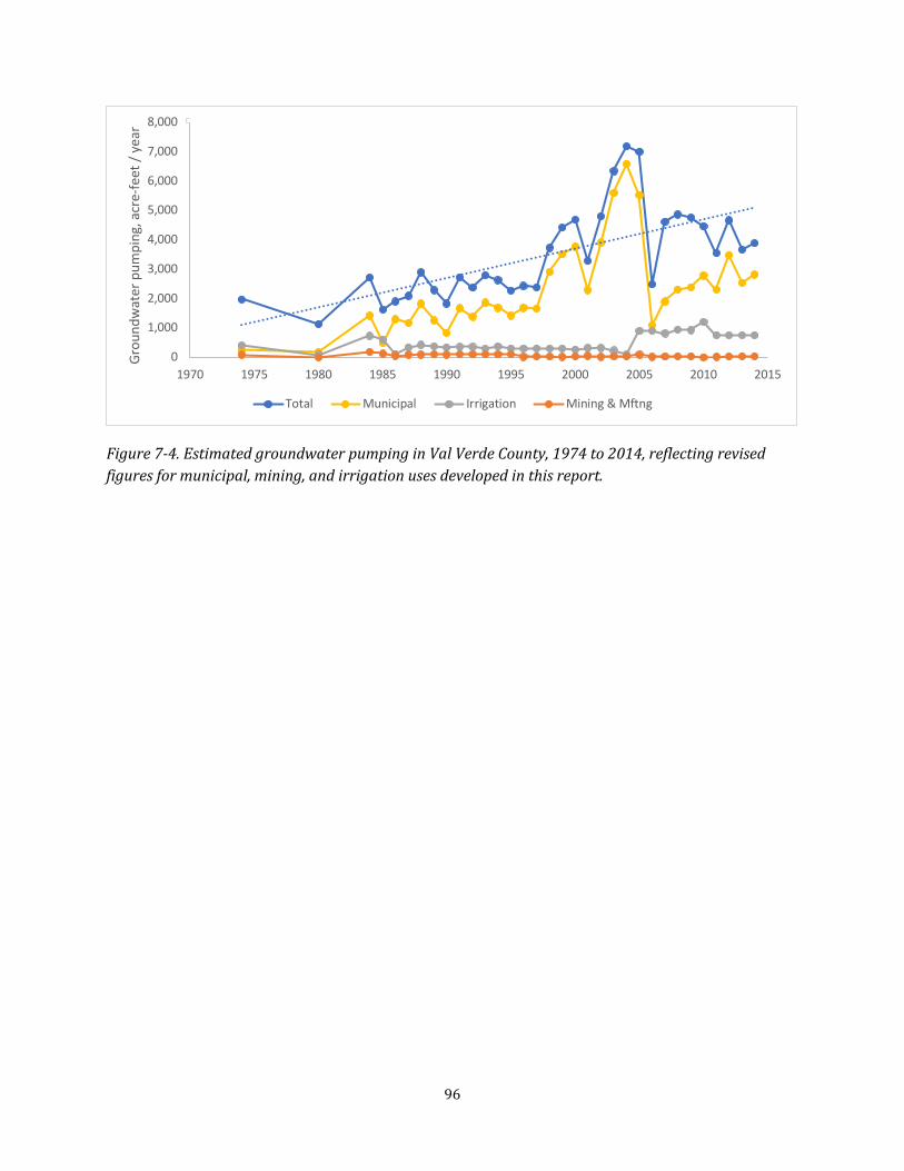
8,000
7,000
6,000
5,000
4,000
3,000
2,000
1,000
0
Total Municipal Irrigation Mining & Mftng
Figure 7-4.Estimated groundwater pumping in Val Verde County, 1974 to 2014, reflecting revised figures for municipal,mining, and irrigation uses developed in this report.
Gro
undw
ater
pum
ping
, acr
e-fe
et /
yea
r
1970 1975 1980 1985 1990 1995 2000 2005 2010 2015
96

8.0 Groundwater Management and Feasibilityof Hydrologic Triggers Key findings
• The currently adopted desired future condition for the Edwards-Trinity (Plateau) Aquifermay not adequately address all potential groundwater management concerns in Val VerdeCounty. Because there is no mechanism to enforce compliance with the desired futureconditions, rule of capture serves as the current groundwater management approach.
• Index wells and hydrological triggers would be feasible strategies for groundwatermanagement in Val Verde County. There is no current management entity to formally defineor implement hydrologic triggers in the county.
• Both additional field data and improved groundwater flow modeling would assist thedevelopment of groundwater management strategies.
• TWDB recorder wells, combined with existing water well data from long-term monitoring,can provide a reasonable basis for developing hydrologic triggers for portions of the county.
• Additional technical and stakeholder input is needed to develop management objectivesbefore specific trigger values based on groundwater levels can be determined.
• Four groundwater management zones generally based on watershed areas may beappropriate options for Val Verde County.
• The groundwater observation well network should be expanded to support groundwater management strategies and objectives.
Val Verde County participates in water planning activities as partof the Region J (Plateau) Planning Group and Groundwater Management Area 7 but is not currently part of any groundwaterconservation district. Managing groundwater in the Edwards-Trinity (Plateau) Aquifer wouldinvolve consideration of historical groundwater usage, consideration of private property interests,complex groundwater-surface water interactions, and ecologicaland species habitat concerns. There are several areas in Texas where the Edwards (Balcones Fault Zone) Aquifer discharges through major springs, and the process through which groundwater management has developed inthose areas may inform the path forward for Val Verde County.
Approaches to county-levelgroundwater managementshould be viewed in lightof regional groundwater management strategies,such as those in Groundwater ManagementArea 7.Some springs in Val Verde County represent the discharge points for a regional groundwater flow system thatextends welloutside the area of the county.The surface water drainage systems thatrechargegroundwater in Val Verde County extend into neighboring counties, New Mexico, and Coahuila,Mexico. Groundwater management may require cooperation across political boundaries. Within Texas, regional groundwater management objectives are addressed through a public process byestablishing desired future conditions identified by groundwater conservation districtrepresentatives through the regional groundwater management areas.
97
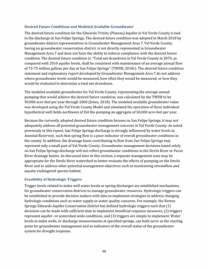
Desired Future Conditions and Modeled Available Groundwater
The desired future condition for the Edwards-Trinity (Plateau) Aquifer in Val Verde County is tied to the discharge at San Felipe Springs. The desired future condition was adopted in March 2018 bygroundwater district representatives in Groundwater Management Area 7. Val Verde County,having no groundwater conservation district, is not directly represented in GroundwaterManagement Area 7 and does not have the ability to enforce compliance with the desired futurecondition.The desired future condition is: “Totalnetdrawdown in Val Verde County in 2070, as compared with 2010 aquifer levels, shall be consistent with maintenance of an average annual flow of 73-75 million gallons per day at San Felipe Springs” (TWDB, 2018c). The desired future conditionstatement and explanatory report developed by Groundwater Management Area 7 do not addresswhere groundwater levels would be measured, how often they would be measured, or how theywould be evaluated to determine a total net drawdown.
The modeled available groundwater for Val Verde County, representing the average annualpumping that would achieve the desired future condition, was calculated by the TWDB to be 50,000 acre-feet per year through 2060 (Jones, 2018). The modeled available groundwater valuewas developed using the Val Verde County Model and simulated the operation of three individualhypothetical wellfields northwestof DelRio pumping an aggregate of 50,000 acre-feet per year.
Because the currently adopted desired future condition focuses on San Felipe Springs, it may notadequately address all potential groundwater management concerns in Val Verde County. As noted previously in this report,San Felipe Springs discharge is strongly influenced by water levels in Amistad Reservoir,such thatspring flow is a poor indicator of overallgroundwater conditions in the county.In addition,the drainage basin contributing to flow from San Felipe Springs may represent only a small part of Val Verde County.Groundwater managementdecisions based solely on San Felipe Springs discharge will not reflect groundwater conditions in the Devils River or Pecos River drainage basins. As discussed later in this section,a separate management zone may beappropriate for the Devils River watershed to better evaluate the effects of pumping on the DevilsRiver and to address other potential management objectives such as maintaining streamflow andaquatic endangered species habitat.
Feasibility of Hydrologic Triggers
Trigger levels related to index well water levels or spring discharges are established mechanismsfor groundwater conservation districts to manage groundwater resources. Hydrologic triggers canbe established to provide decision makers with data to implement strategies to address changinghydrologic conditions such as water supply or water quality concerns. For example, the BartonSprings Edwards Aquifer Conservation District has defined hydrologic triggers such that(1)decisions can be made with sufficient time to implement beneficial response measures, (2) triggersrepresent aquifer- or watershed-wide conditions, and (3) triggers are simple to implement. Water levels in index wells,or discharge measurements at specified springs, can both serve as the startingpoint for groundwater management and as indicators of the overall status of the groundwatersystem for drought response.
98
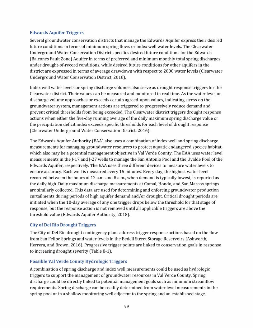
Edwards Aquifer Triggers
Several groundwater conservation districts thatmanage the Edwards Aquifer express their desired future conditions in terms of minimum spring flows or index well water levels. The ClearwaterUnderground Water Conservation District specifies desired future conditions for the Edwards(Balcones Fault Zone) Aquifer in terms of preferred and minimum monthly total spring dischargesunder drought-of-record conditions, while desired future conditions for other aquifers in thedistrict are expressed in terms of average drawdown with respect to 2000 water levels (Clearwater Underground Water Conservation District, 2018).
Index well water levels or spring discharge volumes also serve as drought response triggers for theClearwater district. Their values can be measured and monitored in real time. As the water level or discharge volume approaches or exceeds certain agreed-upon values, indicating stress on thegroundwater system, management actions are triggered to progressively reduce demand andprevent critical thresholds from being exceeded. The Clearwater district triggers drought responseactions when either the five-day running average of the daily maximum spring discharge value or the precipitation deficitindex exceeds specific thresholds for each levelof droughtresponse (Clearwater Underground Water Conservation District, 2016).
The Edwards Aquifer Authority (EAA) also uses a combination of index well and spring dischargemeasurements for managing groundwater resources to protectaquatic endangered species habitat, which also may be a potential management objective in Val Verde County.The EAA uses water level measurements in the J-17 and J-27 wells to manage the San Antonio Pool and the Uvalde Pool of theEdwards Aquifer, respectively. The EAA uses three different devices to measure water levels to ensure accuracy. Each well is measured every 15 minutes. Every day, the highest water level recorded between the hours of 12 a.m. and 8 a.m., when demand is typically lowest, is reported asthe daily high.Daily maximum discharge measurements atComal,Hondo,and San Marcos springsare similarly collected. This data are used for determining and enforcing groundwater productioncurtailments during periods of high aquifer demand and/or drought. Critical drought periods areinitiated when the 10-day average of any one trigger drops below the threshold for that stage ofresponse, but the response action is not removed until all applicable triggers are above thethreshold value (Edwards Aquifer Authority,2018).
City of Del Rio Drought Triggers
The City of Del Rio drought contingency plans address trigger response actions based on the flow from San Felipe Springs and water levels in the Bedell Street Storage Reservoirs (Ashworth,Herrera, and Brown, 2016). Progressive trigger points are linked to conservation goals in response to increasing droughtseverity (Table 8-1).
Possible Val Verde County Hydrologic Triggers
A combination of spring discharge and index well measurements could be used as hydrologic triggers to supportthe managementof groundwater resources in Val Verde County.Springdischarge could be directly linked to potential management goals such as minimum streamflow requirements. Spring discharge can be readily determined from water level measurements in the spring pool or in a shallow monitoring well adjacent to the spring and an established stage-
99

discharge relationship. Index well water levels in the aquifer should have a demonstratedcorrelation with groundwater management goals, such as maintaining streamflow or endangeredspecies habitat. Ideally, index well trigger levels should also have a predictive capability so thatmanagement options can be implemented proactively, before problems develop. Therefore, indexwells may be located upgradient of critical springs or reaches of streams depending on the natureof the hydrologic feature to be protected.
Table 8-1.City ofDel Rio drought triggers and response actions.From Ashworth,Herrera,and Brown, 2016.
Stage anddescription
1-Mild 2-Moderate 3-Severe 4-Extreme 5-Emergency
Trigger Water levels < 100% full; San FelipeSpring flow<40 mgd.
Water levels < 30 feet; San Felipe Springflow <25 mgd.
Water levels < 25 feet; San Felipe Springflow <20 mgd.
Water levels < 20 feet; San Felipe Springflow <15 mgd.
Water levels < 15 feet; San Felipe Springflow <10 mgd.
Conservation goal (percentreduction in pumping)
Reduce water demand to 95% of the 30-dayaverage prior to initiation
Reduce water demand to 90% of the 30-dayaverage prior to initiation
Reduce water demand to 80% of the 30-dayaverage priorto initiation
Reduce water demand to 70% of the 30-dayaverage prior to initiation
Notify TCEQ
mgd = million gallons per day
As an example of this approach, Well 5456403, northeast of Juno, is one candidate for an index wellin the Devils River watershed. Well5456403 is located on the north side of the Devils River about a mile northeast of Juno and 21 river miles upstream from Bakers Crossing. Water levels inWell 5456403 are moderately correlated with the streamflow at Bakers Crossing. Groundwaterelevation measurements are available for the period 1955 to 2015. Water levels in the well aremost highly correlated with stream baseflow measured one month after the groundwater level,indicating that groundwater levels have some limited predictive capacity for subsequentstreamflow (Figure 8-1).
Additional technical and stakeholder input is needed to develop management objectives before specific trigger values based on groundwater levels can be determined.
100
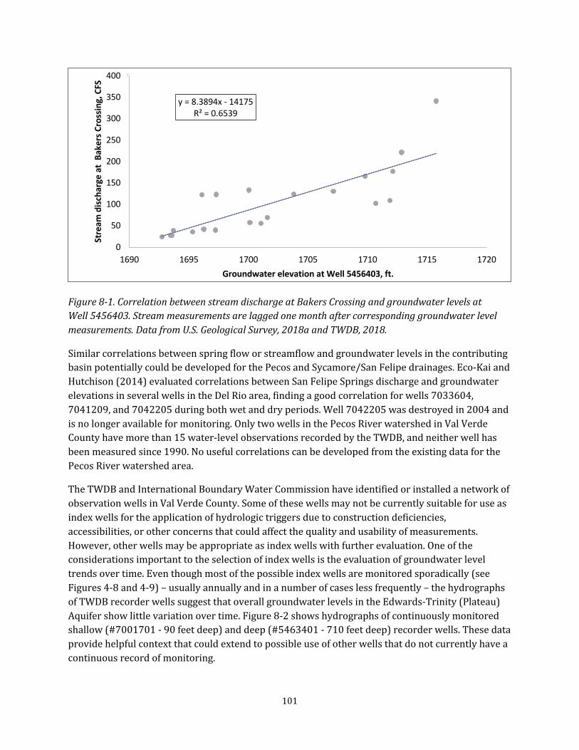
Stre
am d
isch
arge
at
Bake
rs C
ross
ing,
CFS
400
350 y = 8.3894x - 14175 R² = 0.6539 300
250
200
150
100
50
0 1690 1695 1700 1705 1710 1715 1720
Groundwater elevation at Well 5456403, ft.
Figure 8-1.Correlation between stream discharge at Bakers Crossing and groundwater levels at Well 5456403.Stream measurements are lagged one month after corresponding groundwater level measurements. Data from U.S. Geological Survey, 2018a and TWDB, 2018.
Similar correlations between spring flow or streamflow and groundwater levels in the contributingbasin potentially could be developed for the Pecos and Sycamore/San Felipe drainages. Eco-Kai andHutchison (2014) evaluated correlations between San Felipe Springs discharge and groundwaterelevations in several wells in the Del Rio area, finding a good correlation for wells 7033604,7041209, and 7042205 during both wet and dry periods. Well 7042205 was destroyed in 2004 andis no longer available for monitoring. Only two wells in the Pecos River watershed in Val VerdeCounty have more than 15 water-levelobservations recorded by the TWDB,and neither wellhas been measured since 1990. No useful correlations can be developed from the existing data for thePecos River watershed area.
The TWDB and International Boundary Water Commission have identified or installed a network ofobservation wells in Val Verde County. Some of these wells may not be currently suitable for use as index wells for the application of hydrologic triggers due to construction deficiencies,accessibilities, or other concerns that could affect the quality and usability of measurements.However, other wells may be appropriate as index wells with further evaluation. One of theconsiderations important to the selection of index wells is the evaluation of groundwater level trends over time.Even though mostof the possible index wells are monitored sporadically (see Figures 4-8 and 4-9) – usually annually and in a number of cases less frequently – the hydrographsof TWDB recorder wells suggest that overall groundwater levels in the Edwards-Trinity (Plateau)Aquifer show little variation over time. Figure 8-2 shows hydrographs of continuously monitored shallow (#7001701 - 90 feet deep) and deep (#5463401 - 710 feet deep) recorder wells.These data provide helpful context that could extend to possible use of other wells that do not currently have acontinuous record of monitoring.
101

Figure 8-2. Hydrographs of TWDB Recorder Wells in the Devils River watershed show little overall variation in water levels over a 10-year period. Data from TWDB, 2018.
In addition to considering county-specific data, the selection of possible index wells and hydrologictriggers may be influenced by conditions outside Val Verde County. For example, the main springs feeding the lower Pecos River are along Independence Creek in Terrell County, while the SycamoreCreek watershed extends into Kinney and Edwards counties. As previously discussed, AmistadReservoir water levels, which reflect conditions in a large, bi-national watershed, strongly influence flow from San Felipe Springs.
Southwest Research Institute (Green, 2016) identified and evaluated possible hydrologic triggersapplicable to groundwater in Val Verde County. Rather than measurement of groundwater levels inthe aquifer, this approach would rely on stream discharge measurements, with “triggers” set at pre-determined flow criteria.The approach features individual streamflow triggers for three separatewatersheds: the Pecos River, Devils River, and San Felipe Springs. When considered together, thethree watersheds cover nearly all of Val Verde County.The approach was structured similar to that used by the Edwards Aquifer Authority for the J-17 Index Well in the Edwards Aquifer. Water levelsin the J-17 well are used as the basis for implementing various stages of a water conservationprogram designed to reduce groundwater usage in times of drought and to protect levels of springflow that are important to maintaining critical habitats for endangered species. In the approach identified by Southwest Research Institute,multiple stage responses would be tied to dischargerates measured at the Pecos River (Langtry Gaging Station), the Devils River (Pafford CrossingGaging Station), and San Felipe Springs. Table 8-2 illustrates this approach as applied to the Devils River,which is based on over 55 years of stream gage measurements.
102
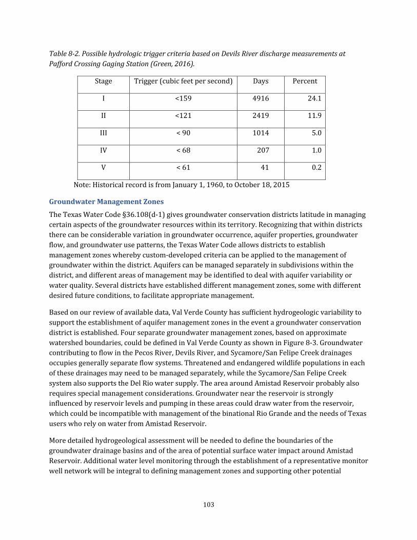
Table 8-2. Possible hydrologic trigger criteria based on Devils River discharge measurements at Pafford Crossing Gaging Station (Green, 2016).
Stage Trigger (cubic feet per second) Days Percent
I <159 4916 24.1
II <121 2419 11.9
III < 90 1014 5.0
IV < 68 207 1.0
V < 61 41 0.2
Note: Historical record is from January 1, 1960, to October 18,2015
Groundwater Management Zones
The Texas Water Code §36.108(d-1) gives groundwater conservation districts latitude in managingcertain aspects of the groundwater resources within its territory. Recognizing that within districtsthere can be considerable variation in groundwater occurrence,aquifer properties, groundwaterflow, and groundwater use patterns, the Texas Water Code allows districts to establish management zones whereby custom-developed criteria can be applied to the management ofgroundwater within the district.Aquifers can be managed separately in subdivisions within thedistrict, and different areas of management may be identified to deal with aquifer variability orwater quality. Several districts have established different management zones, some with differentdesired future conditions, to facilitate appropriate management.
Based on our review of available data, Val Verde County has sufficient hydrogeologic variability tosupport the establishment of aquifer management zones in the event a groundwater conservationdistrict is established. Four separate groundwater management zones,based on approximatewatershed boundaries, could be defined in Val Verde County as shown in Figure 8-3. Groundwatercontributing to flow in the Pecos River, Devils River, and Sycamore/San Felipe Creek drainagesoccupies generally separate flow systems. Threatened and endangered wildlife populations in eachof these drainages may need to be managed separately, while the Sycamore/San Felipe Creeksystem also supports the Del Rio water supply. The area around Amistad Reservoir probably alsorequires special management considerations. Groundwater near the reservoir is stronglyinfluenced by reservoir levels and pumping in these areas could draw water from the reservoir,which could be incompatible with management of the binational Rio Grande and the needs of Texasusers who rely on water from Amistad Reservoir.
More detailed hydrogeological assessment will be needed to define the boundaries of thegroundwater drainage basins and of the area of potential surface water impact around AmistadReservoir. Additional water level monitoring through the establishment of a representative monitorwell network will be integral to defining management zones and supporting other potential
103

groundwater management objectives. Additionally, groundwater geochemistry and micro-particulate analysis may all play a role in refining the boundaries of possible management zones.
Amistad Groundwater Zone
The Amistad Groundwater Zone would cover the area where groundwater levels and flow in theEdwards-Trinity (Plateau) Aquifer are believed to be affected directly by reservoir levels. Selected groundwater observation wells could serve as monitoring points to evaluate changing groundwaterconditions, particularly as they could affect withdrawal points and spring flow hydraulicallydowngradient of the reservoir.
San Felipe Springs Groundwater Zone
The San Felipe Springs Groundwater Zone would cover the watershed area that contributes to theSan Felipe Springs complex. However, groundwater outside this zone (in the vicinity of AmistadReservoir) exerts influence on the flow characteristics of the springs, where groundwater levels andflow in the Edwards-Trinity (Plateau) Aquifer are believed to be affected directly by reservoir levels.Selected groundwater observation wells could serve as monitoring points to evaluatechanging groundwater conditions, particularly as they could affect withdrawal points and springflow hydraulically downgradient of the reservoir. Connections between the San Felipe drainagebasin and the Sycamore Creek drainage basin need to be evaluated further; a separate managementzone may be justified for Sycamore Creek.
Pecos River Groundwater Zone
The Pecos River Groundwater Zone extends over the western portion of the county. This area currently has few suitable observation wells that could serve as hydrologic triggers, but the PecosRiver flow has been well characterized and would be a probable component of any groundwatermanagement approach.
Devils River Groundwater Zone
The Devils River Groundwater Zone would cover the Devils River watershed area. This zone has a number of possible suitable observation wells, springs, and gaging stations that could be used forhydrologic trigger locations. The two TWDB recorder wells (Figure 8-2) have yielded nearlycontinuous water level measurements since the mid-2000s and would provide a useful baselinefrom which to measure possible future changes in groundwater levels.
104
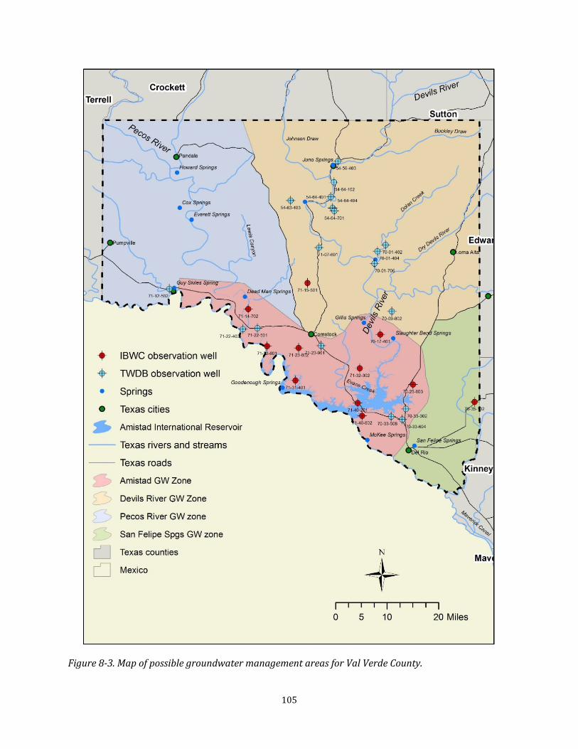
Figure 8-3. Map of possible groundwater management areas for Val Verde County.
105
9.0 References Afinowicz, J. D., Munster, C. L., and Wilcox, B. P., 2005, Modeling effects of brush management on therangeland water budget: Edwards Plateau, Texas, Journal of the American Water ResourcesAssociation vol. 41,no. 1, pp. 81-93.
Anaya and Jones, 2009,Groundwater Availability Modelfor the Edwards-Trinity (Plateau) andPecos Valley Aquifers of Texas: Texas Water Development Board Report 373, April 2009.
Ashworth, Herrera, and Brown, 2016, Plateau Region Water Plan, athttps://www.twdb.texas.gov/waterplanning/rwp/plans/2016/J/Region_J_2016_RWP.pdf accessed May 25,2018.
Ashworth, J.B., and Stein, W.G., 2005, Springs of Kinney and Val Verde counties; report prepared for the Plateau RegionalWater Planning Group,athttp://www.ugra.org/pdfs/SpringsKinneyValVerde2005.pdf accessed January 8, 2018.
Ball, L. and Taylor, M, 2003, Brush management: myth and facts, athttp://texaslivingwaters.org/wp-content/uploads/2013/04/tlw-brush_management-03.pdf,accessed Feb. 15, 2018.
Banta, J.R. and Slattery, R.N., 2011, Effects of brush management on the hydrologic budget andwater quality in and adjacent to Honey Creek State NaturalArea,ComalCounty,Texas,2001–10: U.S. Geological Survey Scientific Investigations Report 2011–5226, 48 p.
Basnet, N., Hauck, L.M., and Pendergrass, D., 2013, Pecos River water quality data analysis and dissolved oxygen modeling: Texas Institute for Applied EnvironmentalResearch,Tarleton State University report prepared for Texas State Soil and Water Conservation Board, athttp://pecosbasin.tamu.edu/media /441220/pecos_do_model_final_02jan2014.pdf, accessed April 2, 2018.
Baxter, D. 2009, Selah, Bamberger Ranch Preserve — Leopold/Lone Star Land Steward Award: Texas Wildlife magazine, September 2009, pp. 18-20; at http://brp-journal.blogspot.com/2009/09/selah-bamberger-ranch-preserve.html,accessed Feb 15,2018.
Breeding, S.D., 1954, Floods in the Devils and Pecos river basins of Texas, June 27, 28, 1954, miscellaneous data: U.S. Geological Survey open-file report 54-27, 9 pp.
Brune, G., 1975, Major and historical springs of Texas: TWDB report 189.
Clearwater Underground Water Conservation District, 2016, District management plan, January 2016 revision, at http://staging.cuwcd.org/pdf/CUWCD-District%20Management%20Plan.pdf, accessed May 16, 2018.
City of Del Rio, 2008: City of Del Rio water conservation and drought contingency study, at http://www.cityofdelrio.com/DocumentCenter/View/376/Del-Rio-Water-Conservation-Study-rev,accessed May 17, 2018.
106
City of Del Rio, 2016: Water quality report for 2016, athttp://www.cityofdelrio.com/DocumentCenter/ View/3386, accessed March 26, 2018.
Cross, B.L., 1989, Groundwater investigation and contamination potential of a portion of southeast Val Verde County,Texas: Texas Water Commission report 89-02, at http://www.twdb.texas.gov/publications/reports/other _reports/doc/miscreport89-02.pdf, accessed March 7, 2018.
Driver, A. and Wade, T., 2013, Fracking without fresh water: Scientific American, November 2013, at https://www.scientificamerican.com/article/fracking-without-freshwater-at-a-texas-oilfield/, accessed February 9, 2018.
Dumble, E. T., 1888: Texas Geological and Mineralogical Survey: first report of progress, Texas Department of Agriculture, Insurance, Statistics and History, Austin, Texas,athttps://books.google.com/books.
Dumble, E. T., 1891: Geological Survey of Texas: second report of progress, Texas Department of Agriculture, Insurance, Statistics and History, Austin, Texas,athttps://books.google.com/books.
Eco-Kai Environmental Inc. and Hutchison, W. R.,2014, Hydrogeological study for Val Verde County and City of Del Rio, Texas, report prepared for Val Verde County and City of Del Rio, 152 pp, at www.edwardsaquifer.net/pdf/Val_Verde_May_2014.pdf,accessed October 6,2017.
Eckhardt, K., 2004, How to construct recursive digital filters for baseflow separation: HydrologicalProcesses, vol. 19, no. 2, pp. 507-515.
Edwards Aquifer Authority, 2018, Critical period management tools, athttps://www.edwardsaquifer.org/groundwater-users/critical-period-management-tools,accessed May 16, 2018.
Freeman, V.L. 1964, Geology of the Comstock-Indian Wells area, Val Verde, Terrell, and BrewsterCounties, Texas: U.S. Geological Survey Professional Paper 594-K.
George, W.O., 1940, Record of Wells, Val Verde County, Texas: Texas Water Development Boardreport M285, reprinted March 1950.
Golden, M.L., Gabriel,W.J.,and Stevens,J.W.,1982,Soilsurvey of Val Verde County,Texas, at https://www.nrcs.usda.gov/Internet/FSE_MANUSCRIPTS/texas/TX465/0/Val%20Verde.pdf,accessed February 12, 2018.
Green, R. T. and Bertetti, F.P., 2012, Investigating the Water Resources of the Western Edwards-Trinity Aquifer: final report for Sutton County Groundwater Conservation District, at https://static.squarespace.com/static/535a88f6e4b0fbad919ef959/t/53864143e4b040c8980a70 73/1401307459476/WesternEdwardsTrinityFinalRev1.pdf, accessed October 28, 2016.
Green, R. T., Bertetti, F.P., and Toll, N., 2015,Pecos/Devils River watershed projects, Part II; presentation to Texas Water Conservation Association, 71st Annual Convention, Irrigation Panel. Accessed at https://www.slideshare.net/texasnetwork/3-green-twca-2015,March 2018.
107
Green, R. T., Bertetti, F.P., and Miller, M.S. 2014, Focused groundwater flow in a carbonate aquifer ina semi-arid environment, Journal of Hydrology, vol. 517 (2014), pp. 284—297.
Green, R. T., Toll, N., Bertetti, F.P., and Hill, N., 2016, Modeling groundwater flow to understand the water resources of the lower Pecos River watershed, final report, 49 p.
Green, R. T., 2016, Val Verde County Drought/Pumping Triggers, presentation to Devils Riverstakeholder group, October 27, 2016.
Green, R. T., Fratesi, B., Toll, N., and Nunu, R., 2017, Coupled surface water /groundwater evaluationin the Edwards Plateau, presentation to Groundwater Management Area 17 meeting, October 19, 2017.
Goodwin, W., 2010, Texas rancher an unlikely environmentalist, National Public Radio, February 2, 2010, at https://www.npr.org/templates/story/story.php?storyId=123068681,accessed Feb 27, 2018.
Hart, C., Jensen, R., Hatler, W., and Mecke, M., 2007, Water issues facing the Pecos Basin of Texas, Texas Water Resource Institute, at http://pecosbasin.tamu.edu/media/1885/pecos3.6.07.pdf, accessed March 15, 2018.
HDR Engineering, Inc., 2001, Investigation of a proposed well field in Val Verde County,Texas: report prepared for San Antonio Water System, 64 pp.
Heitmuller, F.T., and Reece, B.D., 2003, Database of historically documented springs and spring flowmeasurements in Texas: U.S. Geological Survey Open-File Report 03- 315, 4 p., at https://pubs.usgs.gov/of/2003/ofr03-315/, accessed April 13, 2018.
Hill, R.T., and Vaughn, T.W., 1898, Geology of the Edwards Plateau and Rio Grande Plain adjacent to Austin and San Antonio, Texas, with reference to the occurrence of underground waters: Eighteenthannual report of the U.S. Geological Survey, Part II – Papers chiefly of a theoretic nature,at https://pubs.er.usgs.gov/publication/ar18, accessed February 2, 2018.
Hodge, B. 2018, Letter to Ronald T. Green, “Re: Beaver Lake, ValVerde County,”dated June 6,2018.
Hutchison, W.R., 2010, Draft GAM run 09-035 (version 2), athttps://www.twdb.texas.gov/groundwater/ docs/GAMruns/GR09-35draft_v2.pdf,accessed May 17, 2018.
Hutchison, W. R., Shi, J., and Jigmond, M., 2011, Groundwater flow model of the Kinney County area: Texas Water Development Board alternative model report, athttps://www.twdb.texas.gov/groundwater/models/alt/knny/Kinney_County_Model_Report.pdf.
International Atomic Energy Agency, 2018,Globalnetwork of isotopes in precipitation - water isotope system for data visualization, analysis and electronic retrieval, athttps://nucleus.iaea.org/wiser,accessed April18,2018.
108

International Boundary and Water Commission, 2005, Flow of the Rio Grande and related data, at https://www.ibwc.gov/Water_Data/water_bulletins.html, accessed March 29, 2018.
International Boundary and Water Commission, 2018, Rio Grande historical mean daily dischargedata, at https://www.ibwc.gov/Water_Data/histflo1.htm,accessed February 8,2018.
International Boundary and Water Commission, 2018a, Daily discharge data, Devils River at Pafford Crossing, 1960 to 2011,at https://www.ibwc.gov/wad/DDQDEVIL.htm,accessed February 8,2018.
Jones, I.C., Bradley, R., Boghici, R.. Kohlrenken, W., and Shi, J., 2013, GAM task 13-030, Total estimated recoverable storage for aquifers in Groundwater Management Area 7, athttp://www.twdb.texas.gov/groundwater/docs/GAMruns/Task13-030.pdf,accessed April16,2018.
Jurgens, B.C., 2018, Data for Tritium deposition in precipitation in the United States, 1953-2012: U.S. Geological Survey data release, https://doi.org/10.5066/P92CEFXN,accessed October 21, 2018.
Kamps, R.H., Tatum, G.S., Gault, M., and Groeger, A.W., 2009, Goodenough Springs,Texas,USA, Discharge and water chemistry of a large spring deeply submerged under the binational Amistad Reservoir: Hydrogeology Journal, vol. 17, pp. 891–899.
Kendall, C., Snyder, D., and Caldwell, E., Resources on Isotopes, U.S. Geological Survey Menlo Park, at https://wwwrcamnl.wr.usgs.gov/isoig/period/h_iig.html, accessed April 18, 2018.
Kreitler, C.W., Beach, J.A., Symank, L., Uliana, M., Bassett, R.,Ewing,J.E.,and Kelley,V.A.,2013; Evaluation of hydrochemical and isotopic data in Groundwater Management Areas 3 and 7, contracted report prepared for the Texas Water Development Board, athttp://www.twdb.texas.gov/publications/ reports/contracted_reports/doc/1148301235.pdf,accessed April 16, 2018.
LBG-Guyton, 2001, Ground-Water Resources of the Edwards Aquifer in the Del Rio Area, Texas,athttp://www.ugra.org/pdfs/DelRioEdwards2001.pdf, accessed September 19,2017.
Lucas, L.L. and Unterweger, M.P., 2000, Comprehensive Review and Critical Evaluation of the Half-Life of Tritium: Journal of Research of the National Institute of Standards and Technology, vol. 105, no. 4, pp. 541-549.
Mace, R.E., and Anaya, R., 2004, Estimate of Recharge to the Edwards (Balcones Fault Zone) andEdwards-Trinity (Plateau) aquifers in Kinney County, Texas, Chapter 18, in Aquifers of the Edwards Plateau: Texas Water Development Board Report 360, 22 p.
Male, F., and Walsh, M., 2017, Water issues related to transitioning from conventional to unconventional oil production in the Permian Basin: Environ. Sci. Technol., 2017, vol. 51, no. 18,pp. 10903–10912.
109
Mast, M.A., and Turk, J.T., 1999, Environmental characteristics and water quality of Hydrologic Benchmark Network stations in the West-Central United States, 1963–95: U.S. Geological SurveyCircular 1173–B, 130 p. Data for Devils River at Pafford Crossing athttps://pubs.usgs.gov/circ/circ1173/circ1173b/ pdf-b/chapter12b.pdf,accessed April2,2018.
McMahan, C.A., Frye, R.G., and Brown, K.L., 1984, The vegetation types of Texas, Texas Parks and Wildlife Department, Wildlife Division,at https://tpwd.texas.gov/publications/pwdpubs/pwd_bn_w7000_0120/ accessed February 28, 2018.
Mecke, M. B., 1996, Historical vegetation changes on the Edwards Plateau of Texas and the effects upon watersheds: Proceedings’ 96 - moving ahead together, Technical Conference and Exposition, U. S. Environmental Protection Agency.
Michel, R.L., Jurgens, B.C., and Young, M.B., 2018, Tritium Deposition in Precipitation in the United States, 1953-2012: U.S. Geological Survey Scientific Investigations Report 2018–5086,athttps://pubs.usgs.gov/sir/2018/5086/sir20185086.pdf, accessed October 21, 2018.
Miller, M.P., Johnson, H.M., Susong, D.D., and Wolock, D.M.,2015,A new approach for continuous estimation of baseflow using discrete water quality data, Method description and comparison withbaseflow estimates from two existing approaches: Journal of Hydrology 522, pp. 203–210.
Morgenstern, U., Stewart, M.K., and Stenger, R., 2010, Dating of streamwater using tritium in a post nuclear bomb pulse world, continuous variation of mean transit time with streamflow: Hydrology and. Earth System Sciences, vol. 14, pp. 2289–2301,athttps://meetingorganizer.copernicus.org/EGU2011/ EGU2011-1538.pdf,accessed April19,2018.
Musgrove, M., and Banner, J.L.,2004,Controls on the spatialand temporalvariability of vadose dripwater geochemistry: Edwards Aquifer, central Texas; Geochimica et Cosmochimica Acta, vol. 68, no. 5, pp. 1007–1020, at http://www.geo.utexas.edu/faculty/banner/Publications/GCA-musgrove_banner.pdf,accessed April18,2018.
Nance,H.S.,2010,Controls on and uses of hydrochemicaland isotopic heterogeneity in the Plateau aquifer system, contiguous aquifers, and associated surface water, Edwards Plateau region, Texas; Ph.D. dissertation presented to faculty of the Graduate School of The University of Texas at Austin, at https://repositories.lib.utexas.edu/bitstream/handle/2152/ETD-UT-2010-05-803/NANCE-DISSERTATION.pdf,accessed January 11,2018.
Nathan, R. J., and McMahon, T. A., 1990, Evaluation of automated techniques for base flow and recession analyses: Water Resource Research, vol. 26, no. 7, pp. 1465–1473.
National Agricultural Statistics Service, 2018; CropScape - cropland data layer, at https://nassgeodata.gmu.edu/CropScape/, accessed March 28, 2018.
National Centers for Environmental Information, 2014, This month in climate history: Hurricane Alice, June 1954, at https://www.ncdc.noaa.gov/news/month-climate-history-hurricane-alice-june-1954,accessed February 7,2018.
110

National Centers for Environmental Information, 2018, daily weather observations for Amistad Dam, TX, U.S.,01/01/1965 to 1/31/2018,at https://www.ncdc.noaa.gov/cdo-web/datasets/GHCND/stations/ GHCND:USC00410225/detail,accessed February 5,2018.
National Centers for Environmental Information, 2018b,daily weather observations for Brackettville,TX, U.S.,01/01/1897 to 1/31/2018, at https://www.ncdc.noaa.gov/cdo-web/datasets/GHCND/ stations/GHCND:USC00411007/detail, accessed February 14, 2018.
National Parks Conservation Association, 2017, “Seeing the light,”accessed February 21,2018, at https://www.npca.org/articles/1415-seeing-the-light#sm.0000vmdlufkc7dmbzwt2m0t46pwvg.
NationalPark Service,2018,Geologicalresources inventory publications – Amistad National Recreation Area, at https://nature.nps.gov/geology/inventory_embed/gre_publications.cfm,accessed April 9, 2018.
Nelle, S., 1996, Holistic perspective on juniper, athttps://texnat.tamu.edu/library/symposia/juniper-ecology-and-management/holistic-perspective-on-juniper/, accessed February 24, 2018.
Nevarez, P., 2017; letter to Bech Bruun, Chairman, Texas Water Development Board, dated February 27, 2017, 2 pp.
Nunu, R.E., Bertetti, F.P., and Green, R.T., Characterization of hydrochemistry of the Edwards-Trinity (Plateau) Aquifer in Sutton County, Texas, presentation to the Geological Society of America, South-Central Section - 51st Annual Meeting – 2017.
Pearson, F.J, and Rettman, P.L., 1976, Geochemical and isotopic analyses of waters associated withthe Edwards Limestone Aquifer,CentralTexas: U.S. Geological Survey report to the EdwardsUnderground Water District, at https://pubs.er.usgs.gov/publication/70176053,accessed April16,2018.
Purchase, C.E., Larson, D., Flora, M/D., and Reber, J., Amistad national recreation area, Texas, waterresources scoping report: U.S. Department of the Interior, National Park Service Technical Report NPS/NRWRD/NRTR-2001/295.
Riskind, D.H., and Diamond, D.D., 1988, An introduction to environments and vegetation in Amos, B.B. and Gehlbach, F.R., eds., Edwards Plateau vegetation: plat ecological studies in central Texas, Baylor University Press, atwww.eahcp.org/documents/1988_RiskindDiamond_EnvironmentsVegetation.pdf,accessed February 28, 2018.
Saleh, A., Wu, H., Brown, C.S., Teagarden, F.M., McWilliams, S.M., Hauck, L.M.,and Millican,J.S.,2009, Effect of brush control on evapotranspiration in the North Concho River watershed using the eddy covariance technique: Journal of Soil and Water Conservation September/October 2009, vol. 64, no. 5, pp. 336-349.
111
Salmi, T., Maatta, A., Antitila, P., Ruoho-Airola, T., and Amnell, T.,2002,Detecting trends of annual values of atmospheric pollutants by the Mann-Kendall test and Sen’s slope estimates -The Excel template application Makesens; Finnish MeteorologicalInstitute, at http://en.ilmatieteenlaitos.fi/documents/30106/335634754/MAKESENS-Manual_2002.pdf/25bbe115-7f7e-4de3-97d8-5a96ac88499f, accessed April 12, 2018.
San Felipe Creek Commissioners, 2007, San Felipe Creek master plan, atwww.edwardsaquifer.net/pdf/san_felipe_master_plan.pdf,accessed February 14,2018.
Scanlon, B. R., Dutton, A. R., and Sophocleous, M., 2003, Groundwater recharge in Texas, TheUniversity of Texas at Austin, Bureau of Economic Geology: Contract report submitted to TexasWater Development Board, 62 p + attachments.
Scanlon, B.R., Reedy, R.C., and Nicot, J.P., 2014, Comparison of water use for hydraulic fracturing forunconventional oil and gas versus conventional oil: Environmental Science and Technology, 2014,vol. 48, no. 20, pp. 12386–12393.
Secretaría de Medio Ambiente y Recursos Naturales, Estados Unidos Mexicanos, 2015; Acuerdo porel que se da a conocer el resultado de los estudios técnicos de aguas nacionales subterráneas delAcuífero Cerro Colorado-La Partida, clave 0503, en el Estado de Coahuila de Zaragoza, RegiónHidrológico-Administrativa Río Bravo, athttp://dof.gob.mx/nota_detalle.php?codigo=5419411&fecha=09/12/2015,accessed April22, 2018.
Silvey, V., Lesikjar, B., and Persyn, R., Priority groundwater management areas: overview andfrequently asked questions: Texas Agrilife Extension Report B-6191, 2008, athttp://twon.tamu.edu/media/432474/ b619 priority-groundwater-management-areas.pdf, accessed March 5, 2018
Slade, R.M., Bentley, J.T., and Michaud, D., 2002, Results of streamflow gain-loss studies in Texas, with emphasis on gains from and losses to major and minor aquifers: U.S. Geological Survey open-file report 02-068, 136 pp.
Smeins, F., Fuhlendorf, S., and Taylor, C., 1997, Environmental and land use changes: a long-term perspective; in Taylor, C. ed., 1997 Juniper Symposium Proceedings, Texas A&M Agrilife Extension, Texas Natural Resources Server, at https://texnat.tamu.edu/library/ symposia/juniper-ecology-and-management/environmental-and-land-use-changes-a-long-term-perspective/, accessed February 28, 2018.
Smith, R. 2018, Daily streamflow in Devils River at Bakers Crossing, personal communication of IBWC data,March 22,2018.
Stafford, K. W.; Klimchouk, A.; Land, L.; and Gary, M. O., 2009, The Pecos River hypogenespeleogenetic province: a basin-scale karst paradigm for eastern New Mexico and West Texas, USA:Stephen F. Austin State University Faculty Publications, Paper 11,athttp://scholarworks.sfasu.edu/geology/11,accessed Feb.21,2018.
112

Schwinning, S., The ecohydrology of roots and rocks: Ecohydrology, vol. 3, pp. 238–245.
Stanton, G.P., Kress, W.H., Teeple, A.P., Greenslate, M.L., and Clark,A.K.,2007,GeophysicalAnalysisof the Salmon Peak Formation Near Amistad Reservoir Dam, Val Verde County,Texas,and Coahuila,Mexico, March 2006, to Aid in Piezometer Placement: U.S. Geological Survey ScientificInvestigations Report 2007–5143.
Taylor,C.A., and F.E. Smeins, 1994, A history of land use of the Edwards Plateau and its effect on thenative vegetation, pp 1-8. In. Juniper symposium: TAMU Research Station technical report 94-2,80p.
Texas Board of Water Engineers, 1960, Channel gain and loss investigations, Texas streams, 1918–1958: Texas Board of Water Engineers Bulletin 5807–D, 270 p.
Texas Commission on Environmental Quality, 2006, Devils River Flow Study,unpublished dataobtained from Ryan Smith of The Nature Conservancy, TCEQ Region 13 Surface Water QualityMonitoring team.
Texas Commission on Environmental Quality, 2014, Chapter 298 - Environmental flow standards for surface water, Subchapter H: Rio Grande, Rio Grande estuary, and lower Laguna Madre, athttps://www.tceq.texas.gov/assets/public/legal/rules/rules/pdflib/298h.pdf,accessed March 29,2018.
Texas Commission on Environmental Quality, 2017, Priority groundwater management areas andgroundwater conservation districts: Report to the 85th Texas Legislature; TCEQ ReportSFR-053/10, at https://www.tceq.texas.gov/assets/public/comm_exec/pubs/sfr/053-10.pdf,accessed March 5, 2018.
Texas Commission on Environmental Quality, 2018, Priority groundwater management areas, athttps://www.tceq.texas.gov/groundwater/pgma.html, accessed March 5, 2018.
Texas Commission on Environmental Quality, 2018a, Surface water quality web reporting tool, at https://www80.tceq.texas.gov/SwqmisPublic/public/default.htm, accessed April 2, 2018.
Texas Drilling.com, 2018, Oil Wells and Production in Val Verde County,TX,at http://www.texas-drilling.com/Val-verde-county,accessed February 12,2018.
Texas Parks and Wildlife, 2018, GIS data on vegetation by ecoregion, athttps://tpwd.texas.gov/gis/programs/landscape-ecology/by-ecoregion-vector,accessed February 27, 2018.
Texas Railroad Commission, 2018, Online wellbore query result for Val Verde County, athttp://webapps2.rrc.state.tx.us/EWA/wellboreQueryAction.do, accessed February 12, 2018.
Texas Water Resources Institute, 2010, A watershed protection plan for the Pecos River in Texas:an overview, at http://pecosbasin.tamu.edu/media/52381/pecos-river-overview.pdf, accessed April 2, 2018.
113
Texas Water Development Board, 2018, Groundwater database, well report by county, at(https://www3.twdb.texas.gov/Reports17/report/GWDB/RecordOfWellsByCounty), accessed March 12, 2018.
Texas Water Development Board, 2018a, Submitted Drillers Reports database, well report by county, athttps://www3.twdb.texas.gov/Reports17/report/SDR/WellRpts_County_Use,accessed March 22, 2018.
Texas Water Development Board, 2018c, Groundwater Management Area 7 – adopted desired future conditions, at https://www.twdb.texas.gov/groundwater/dfc/docs/summary/GMA7_DFC_2016.pdf,accessed May 16, 2018.
Texas Water Development Board, 2017; 2017 State Water Plan, Planning Region M, accessed at https://2017.TexasStateWaterPlan.org/region/M, September 4, 2018.
Tennesen, M., 2008, When juniper and woody plants invade, water may retreat: Science, v. 332, p. 1,630–1,631.
Thomas, H. E., and others, 1963, Drought in the Southwest 1942 – 56, Effects of drought in the RioGrande Basin: U.S. Geological Survey Professional Paper 372-D, 68 pp. athttps://pubs.usgs.gov/pp/0372d/report.pdf,accessed April13, 2018.
Thurow, T.L., and Hester, J.W., 1997, How an increase or reduction in juniper cover alters rangeland hydrology, 1997 Juniper Symposium Proceedings, Texas Agrilife Extension, at https://texnat.tamu.edu/library/symposia/juniper-ecology-and-management/, accessed February 28, 2018.
Toll, N., Fratesi, S.B., Green, R.T., Bertetti, F.P., and Nunu, R., 2017, Water resource management of the Devils River watershed,finalreport: Southwest Research Institute report under contract to theDevils River Conservancy, at http://www.devilsriverconservancy.org/research/, accessed October2017.
U.S. Bureau of Reclamation, 2016, Managing Water in the West: SECURE Water Act Section 9503©-Reclamation, Climate change and Water 2016, Chapter 7: Rio Grande Basin,accessed Sept. 4, 2018, at https://www.usbr.gov/climate/secure/docs/2016secure/2016SECUREReport-chapter7.pdf
U.S. Fish and Wildlife Service, 2005, Devils River Minnow (Dionda diaboli) Recovery Plan, U.S. Fishand Wildlife Service, Albuquerque, New Mexico, at https://www.fws.gov/southwest/es/Documents/R2ES/Devils_River_Minnow_FINAL_Recovery_Plan.pdf,accessed June 9, 2017.
U.S. Fish and Wildlife Service, 2018, Endangered and Threatened Wildlife and Plants; EndangeredSpecies Status for Texas Hornshell, at https://www.federalregister.gov/d/2018-02672/p-4, accessed February 14, 2018.
114
U.S. Fish and Wildlife Service, 2018, Environmental Conservation Online Service, at https://ecos.fws.gov/ecp0/profile/speciesProfile?sId=7657,accessed Feb 21,2018.
U.S. Fish and Wildlife Service, National Wetlands Inventory maps for Sycamore Canyon, Deaton Draw,Juno, and Bee Canyon quadrangles, at https://tnris.org/data-download, accessed Feb. 18, 2018.
U.S. Geological Survey, 2007, Water-Data Report TX-2007 08377200 Rio Grande at Foster Ranchnear Langtry, TX, at https://wdr.water.usgs.gov/wy2005/pdfs/08377200.2005.pdf, accessed April 29, 2018.
U.S. Geological Survey, 2018, Water-Data Report TX-2005 08450900 USGS Rio Grande belowAmistad Dam near Del Rio, TX, at https://wdr.water.usgs.gov/wy2005/pdfs/08450900.2005.pdf,accessed March 29, 2018.
U.S. Geological Survey, 2018a, Mean daily discharge, USGS 0844900 Devils River near Juno, TX, at https://waterdata.usgs.gov/tx/nwis/dv?referred_module=sw&site_no=08449000,accessed February 8, 2018.
Veni, G. 1994, Hydrogeology and evolution of caves and karst in the southwestern Edwards Plateau,Texas,pp. 13–30, in The Caves and Karst of Texas (W. R. Elliott and G. Veni, eds.). National Speleological Society, Huntsville, Alabama. 252 pp. athttps://www.texasspeleologicalsurvey.org/PDF/ Geologychapter.pdf,accessed April11,2018.
Veni, G., 1996, Drainage basin delineation and preliminary hydrogeological assessment of the Dolan Springs, Val Verde County,Texas: report prepared for The Nature Conservancy,San Antonio,Texas, 60 pp.
Von Zuben, F. J. Jr., Hayes, G. R., Jr., and Anderson, E. C., 1957; Public Health Disaster Aid in the RioGrande Flood of 1954: Public Health Reports (1896-1970), vol. 72, no. 11 (Nov 1957), pp. 1009-1017, at https://www.jstor.org/stable/4589967, accessed March 15, 2018.
Wahl, K.L., Wahl, T.L., 1988, Effects of regional ground water declines on streamflows in theOklahoma Panhandle. In: Proceedings of Symposium on Water-Use Data for Water ResourceManagement. Tucson, Arizona, Am. Water Resour. As., pp. 239–249.
Weniger, D., 1984, Explorers' Texas: the lands and waters: Eakin Publications, 1984, Austin, TX,pp. 224; the Dolph Briscoe Center for American History, The University of Texas at Austin.
Wet Rock Groundwater Services, L.L.C, 2010a, Water Resources Evaluation of the Edwards-Trinity(Plateau) Aquifer, Weston Ranch - Val Verde County,Texas: report of findings for Western Water Division, Grass Valley Water L.P.,107 pp.
Wet Rock Groundwater Services, L.L.C, 2010b, Groundwater Modeling of the Grass Valley Water Project: Weston Ranch - Val Verde County,Texas: report of findings for Western Water Division, Grass Valley Water L.P.,36 pp.
115

Wilcox, B. P., and Huang, Y., 2010, Woody plant encroachment paradox, Rivers rebound as degradedgrasslands convert to woodlands: Geophysical Research Letters, vol. 37, L07402.
Wilcox, B.P, Sorice, M.G., Angerer, J., and Wright, C.L., 2012, Historical changes in stocking densitieson Texas rangelands: Rangeland Ecology & Management, vol. 65, no. 3, pp.313-317, athttp://www.bioone.org/doi/full/10.2111/REM-D-11-00119.1,accessed February 23, 2018.
Wood Mackenzie, 2016, Global energy risk: tapping into the water opportunity, athttps://maplecroft.com/portfolio/new-analysis/2016/09/02/global-energy-risk-tapping-water-opportunity/, accessed February 7, 2018.
Zhang, I., Dawes, W.R., and Walker, G.R., 2001, Response of mean annual evapotranspiration tovegetation changes at the catchment scale, Water Resources Research, vol. 37, pp. 701-708.
116
Appendix A
Low-flow gain loss studies ofthe Devils River,1921-1928
117
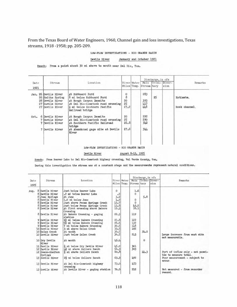
From the Texas Board of Water Engineers, 1960, Channel gain and loss investigations, Texasstreams, 1918 -1958; pp. 205-209.
118

119
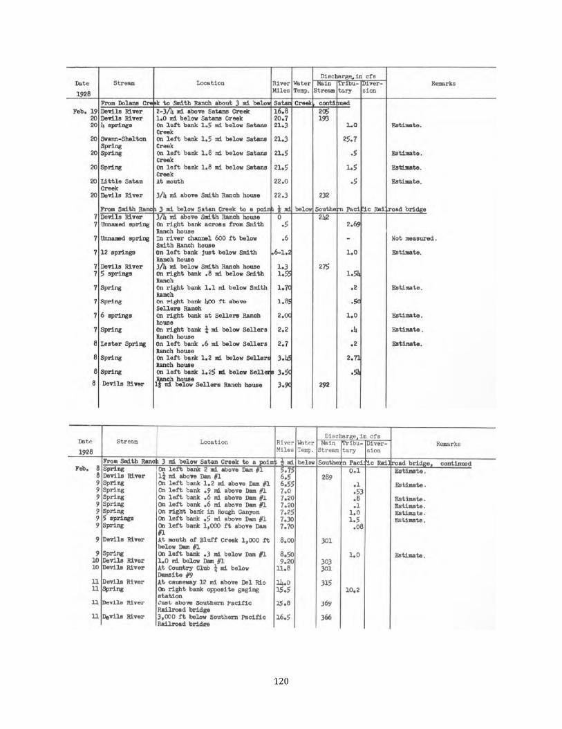
120
Appendix B
Geochemical assessment of groundwater flow paths, mixing, and residence time
121

Geochemical assessment of groundwater flow paths, mixing, and residence time
Chemical and isotopic analyses suggest that groundwater discharged from the major springs inVal Verde County may range from 2 years to over 30 years old. Spring discharge has minimal water-rock interaction, suggesting that recharge occurs primarily through sinkholes and fractures alongsurface drainages, and exhibits limited mixing with groundwater from adjacent countieshydraulically upgradient of Val Verde County.These observations generally supportthe matrix-conduitmodelof groundwater flow and place certain constraints on the aquifer storage and flowparameters and the degree of connection between matrix and conduit. We present an evaluation ofisotopic and geochemical indicators in 55 groundwater and spring water samples collected inVal Verde County by the TWDB between 2002 and 2010 (Appendix C). Together with TWDBanalyses reported by Nance (2010) for Crockett and Sutton counties, we obtain a coherent regionalmodel of groundwater recharge, storage, and flow.
Chemical and isotopic analyses have been used by many authors to assess groundwater flow andresidence time in aquifers, but there has not been a comprehensive geochemical assessment ofVal Verde groundwater to date. Groundwater residence time can provide a useful estimate of theaquifer storage volume independent of typical estimates based on aquifer geometry and hydraulicproperties. Nance (2010) and Kreitler and others (2013) used water quality data to evaluateconceptual models of groundwater flow in portions of the Edwards -Trinity (Plateau) Aquifer, but neither evaluated data for Val Verde County.Musgrove and Banner (2004) examined the effects of soil-water reactions during recharge on Edwards Aquifer groundwater geochemistry, focusing onseveral caverns in the Balcones Fault Zone. Pearson and Retmann (1976) collected geochemical and isotopic data for Edwards aquifer unit wells representative of recharge, fresh water, transitional,and saline conditions, but included only a limited suite of samples from Val Verde County.
Radiocarbon and tritium contents in Edwards groundwater from ValVerde and neighboringcounties (Figure B-1) exhibit a relatively tight linear trend that on casual inspection suggests aprogressive age distribution from ‘young’ waters with around two tritium units (TU) and up to85 percent modern carbon all the way to ‘old’ waters with no detectable tritium and around 10 percentmodern carbon. But the discordant apparent ages suggested by the radiocarbon and tritium data show thatthe system is more complex.Apparentradiocarbon ages range from approximately 1,000 to 20,000 years, while tritium results suggest much more recent ages in the range of years or decades rather than millennia.
Mixing and reaction models can be developed to explain these age disparities but can also raiseadditional problems. Groundwater mixing schemes tend to produce non-unique age estimates.Mixing is a linear process in terms of water volume, but non-linear in terms of radio-isotope activity, which decays exponentially. As a result, a 50:50 mix of ‘old’ and ‘young’ water doesn’t give an age corresponding to the average of the old and young end-members,and even a smallfraction of recent water can greatly change the apparent activity of a mostly old sample. Radiocarbonconcentrations in groundwater are also greatly influenced by reaction with non-radiogenic ‘dead’ carbon in the carbonate aquifer matrix. Much of this reaction can happen in the soil zone, with additional reaction along the flow path between recharge and discharge areas. Each process creates
122
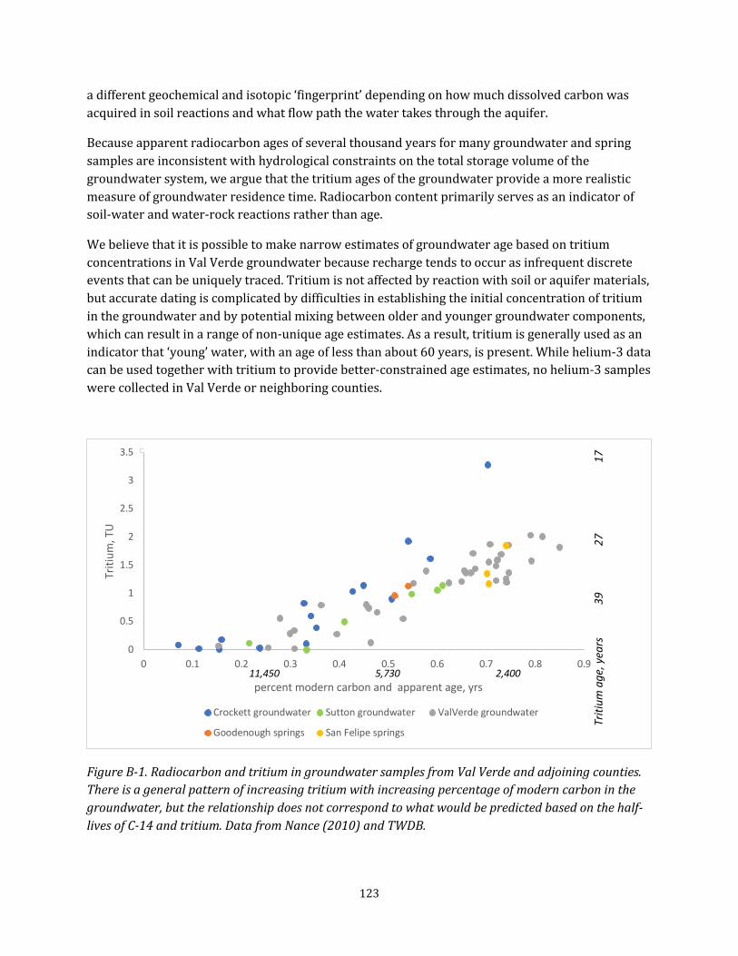
a different geochemical and isotopic ‘fingerprint’ depending on how much dissolved carbon wasacquired in soil reactions and what flow path the water takes through the aquifer.
Because apparent radiocarbon ages of several thousand years for many groundwater and springsamples are inconsistent with hydrological constraints on the total storage volume of thegroundwater system, we argue that the tritium ages of the groundwater provide a more realisticmeasure of groundwater residence time. Radiocarbon content primarily serves as an indicator ofsoil-water and water-rock reactions rather than age.
We believe that it is possible to make narrow estimates of groundwater age based on tritiumconcentrations in Val Verde groundwater because recharge tends to occur as infrequentdiscreteevents that can be uniquely traced. Tritium is not affected by reaction with soil or aquifer materials,but accurate dating is complicated by difficulties in establishing the initial concentration of tritiumin the groundwater and by potential mixing between older and younger groundwater components,which can result in a range of non-unique age estimates. As a result, tritium is generally used as an indicator that ‘young’ water, with an age of less than about 60 years, is present. While helium-3 datacan be used together with tritium to provide better-constrained age estimates, no helium-3 sampleswere collected in Val Verde or neighboring counties.
3.5
3
2.5
2
1.5
1 Tr
itium
age
, yea
rs
39
27
17
Triti
um, T
U
0.5
0 0 0.1 0.2 0.3 0.4 0.5 0.6 0.7 0.8 0.9
11,450 5,730 2,400 percent modern carbon and apparent age, yrs
Crockett groundwater Sutton groundwater ValVerde groundwater
Goodenough springs San Felipe springs
Figure B-1.Radiocarbon and tritium in groundwater samples from Val Verde and adjoining counties. There is a general pattern of increasing tritium with increasing percentage of modern carbon in the groundwater, but the relationship does not correspond to what would be predicted based on the half-lives of C-14 and tritium. Data from Nance (2010) and TWDB.
123
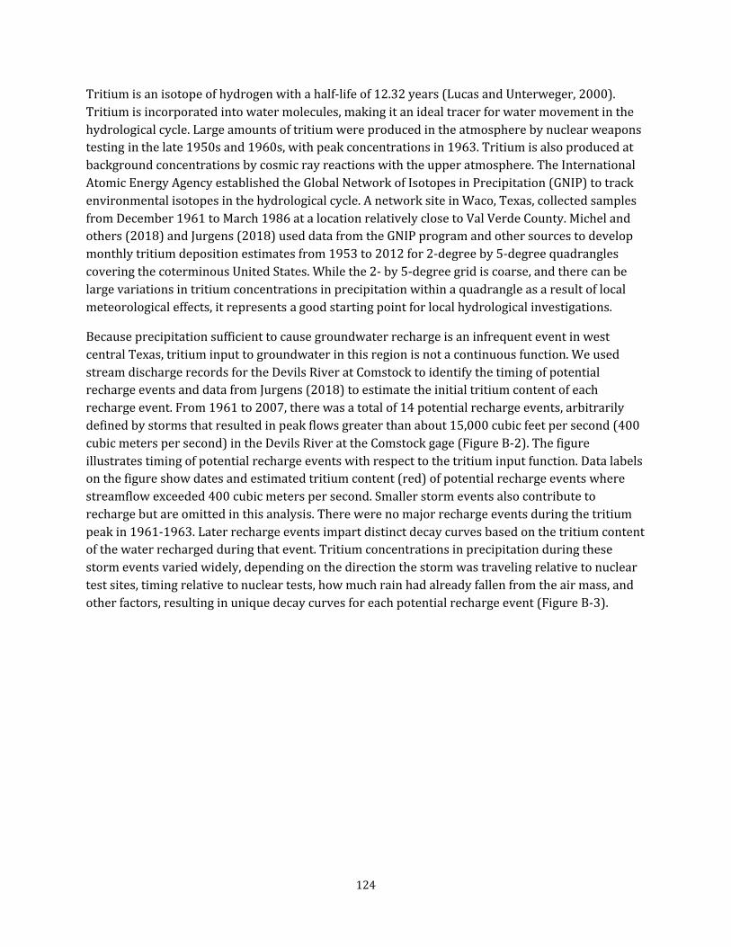
Tritium is an isotope of hydrogen with a half-life of 12.32 years (Lucas and Unterweger, 2000).Tritium is incorporated into water molecules, making it an ideal tracer for water movement in thehydrological cycle. Large amounts of tritium were produced in the atmosphere by nuclear weapons testing in the late 1950s and 1960s,with peak concentrations in 1963. Tritium is also produced atbackground concentrations by cosmic ray reactions with the upper atmosphere. The InternationalAtomic Energy Agency established the Global Network of Isotopes in Precipitation (GNIP) to trackenvironmental isotopes in the hydrological cycle. A network site in Waco, Texas, collected samples from December 1961 to March 1986 at a location relatively close to Val Verde County. Michel and others (2018) and Jurgens (2018) used data from the GNIP program and other sources to developmonthly tritium deposition estimates from 1953 to 2012 for 2-degree by 5-degree quadranglescovering the coterminous United States. While the 2- by 5-degree grid is coarse, and there can belarge variations in tritium concentrations in precipitation within a quadrangle as a result of localmeteorological effects,itrepresents a good starting pointfor localhydrological investigations.
Because precipitation sufficient to cause groundwater recharge is an infrequent event in westcentral Texas, tritium input to groundwater in this region is not a continuous function. We usedstream discharge records for the Devils River at Comstock to identify the timing of potentialrecharge events and data from Jurgens (2018) to estimate the initialtritium content of each recharge event. From 1961 to 2007, there was a total of 14 potential recharge events, arbitrarilydefined by storms that resulted in peak flows greater than about 15,000 cubic feet per second (400cubic meters per second) in the Devils River at the Comstock gage (Figure B-2). The figureillustrates timing of potential recharge events with respect to the tritium input function. Data labelson the figure show dates and estimated tritium content (red) of potential recharge events wherestreamflow exceeded 400 cubic meters per second. Smaller storm events also contribute torecharge but are omitted in this analysis. There were no major recharge events during the tritiumpeak in 1961-1963. Later recharge events impart distinct decay curves based on the tritium contentof the water recharged during that event. Tritium concentrations in precipitation during thesestorm events varied widely, depending on the direction the storm was traveling relative to nucleartestsites,timing relative to nuclear tests, how much rain had already fallen from the air mass, andother factors, resulting in unique decay curves for each potential recharge event (Figure B-3).
124

4000 1000
9/21/1964 300
8/15/1971 75 8/12/1972
25
9/18/1974 15
7/17/1976 15
9/25/1980 11
10/11/1981 6
10/20/1983 10
10/6/1986 7.0
9/23/1990 6.0
8/24/1998 5.4
11/4/2000 3.3
11/17/2004 4.0
6/10/2007 3.5
0
500
1000
1500
2000
2500
3000
3500
Stre
am d
isch
arge
, cub
ic m
eter
s pe
r se
cond
Triti
um, T
U
100
10
1 1/1/1961 1/1/1971 1/1/1981 1/1/1991 1/1/2001 1/1/2011
Tritium in precipitation, Waco Tritium (Jugens 2018) Devils River @ Comstock
Figure B-2. Monthly tritium concentrations in precipitation in westTexas quadrangle and at Waco monitoring site and Devils River discharge at Comstock. Data from Jurgens,2018, International Atomic Energy Agency, 2018, and International Boundary and WaterCommission,2018.
A close-up view of the decay curves covering the times when spring water samples were collected from San Felipe and Goodenough Springs (Figure B-4) shows that only the decay curve for 1981recharge matches the observed tritium activity. A set of decay curves for recharge ranging from 1976 to 2000 lies slightly above the observed spring values, while both earlier and more recent recharge contains higher tritium activities.These decay curves suggest a range of residence times from 2 to 34 years as recharge from different flood events and inlet locations mix along their flowpaths. The geographic distribution of tritium in groundwater (Figure B-5) shows higher activitiesnear stream drainages and lower activities in groundwater under plateau areas between drainages,consistent with the model of focused recharge from surface water sources in the more hydraulically conductive drainage areas.
125

Triti
um, T
U
50
45
40
35
30
25
20
15
10
5
0 6/11/68 6/11/78 6/11/88 6/11/98 6/11/08
Jurgens 2018 Waco 1964 1971 1972
1974 1976 1980 1981 1983
1986 1990 1998 2004 2007
Figure B-3.Tritium input function and decay curves for potential recharge events occurring between 1964 and 2007.
12
10 1971
8
2
4
6
Triti
um, T
U
1981 1986
1998
1990
1983 2004 1972
1976 2000
2007
Tritium in San Felipe and Goodenough springs, 2009-2010
Tritium in San Felipe spring, 2002
0 12/25/2001 5/9/2003 9/20/2004 2/2/2006 6/17/2007 10/29/2008 3/13/2010
1971 1972 1974 1976 1980
1981 1983 1986 1990 1998
2000 2004 2007 San Felipe Goodenough
Figure B-4.Closeup ofgraph above,showing tritium decay curves relative to measured tritium concentrations in San Felipe and Goodenough springs in 2002, 2009, and 2010.
126
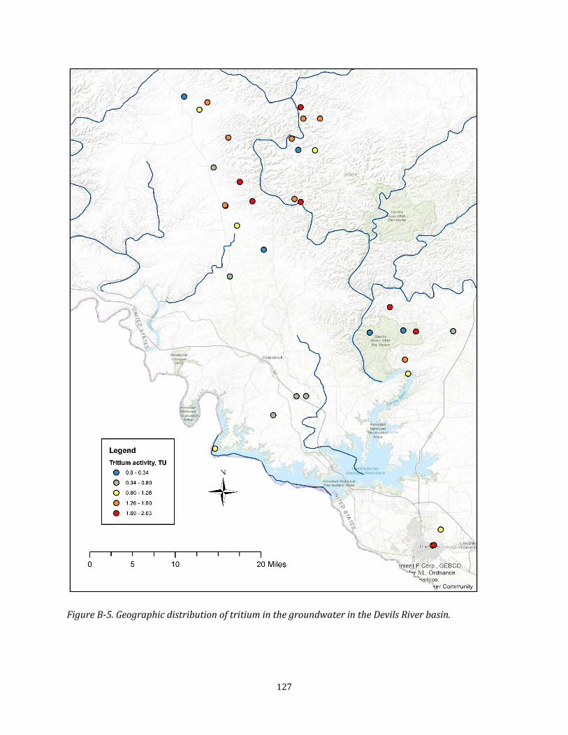
Figure B-5. Geographic distribution of tritium in the groundwater in the Devils River basin.
127
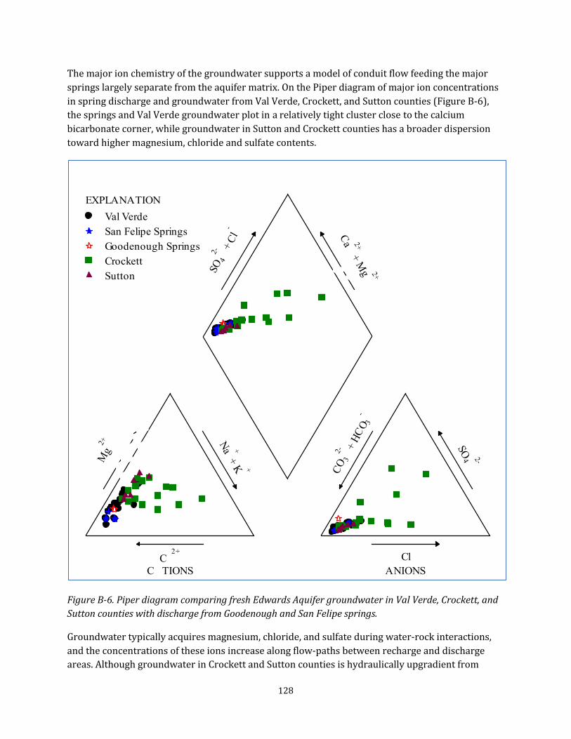
Ca 2+
CATIONS
Mg
2+ Na ++
K + CO3
2- +HC
O 3 -
SO4 2-
SO4
2- + Cl-
Ca 2++
Mg 2+
EXPLANA TION Val Verde San Felipe Springs Goodenough Springs Crockett Sutton
The major ion chemistry of the groundwater supports a model of conduit flow feeding the major springs largely separate from the aquifer matrix. On the Piper diagram of major ion concentrations in spring discharge and groundwater from Val Verde, Crockett, and Sutton counties (Figure B-6),the springs and ValVerde groundwater plotin a relatively tightcluster close to the calcium bicarbonate corner, while groundwater in Sutton and Crockett counties has a broader dispersiontoward higher magnesium, chloride and sulfate contents.
-Cl
ANIONS
Figure B-6.Piper diagram comparing fresh Edwards Aquifer groundwater in Val Verde, Crockett, and Sutton counties with discharge from Goodenough and San Felipe springs.
Groundwater typically acquires magnesium, chloride, and sulfate during water-rock interactions,and the concentrations of these ions increase along flow-paths between recharge and dischargeareas. Although groundwater in Crockett and Sutton counties is hydraulically upgradient from
128
Val Verde groundwater, the chemical data demonstrate that only a limited fraction of this upgradient groundwater can mix with Val Verde groundwater and still produce a compositionconsistent with the discharge from the major springs. Work by Nunu and others (2017) shows thatthese Crockettand Sutton county locations represent low recharge zones away from streamcourses, while calcium-bicarbonate type groundwater extends into Crockett and Sutton countiesalong major drainages as part of a larger, regional flow system.
Other isotope and chemical indicators suggest that Goodenough and San Felipe discharge representend-member compositions rather than integrating flow from the surrounding groundwater matrix.Nance (2010) uses the magnesium-to-calcium ratio (Mg/Ca) as a proxy for groundwater relativeage and as an indicator of relative recharge efficiency, based on the correlations between the Mg/Caratio and radiocarbon content in groundwater from Crockett, Sutton, and Schleicher counties wherethe Mg/Ca ratio increased with apparent radiocarbon age. Musgrove and Banner (2004) usegroundwater strontium isotope ratios (87Sr/86Sr) as an indicator of reaction with soil and aquifermaterials, with the typical strontium isotope composition of soil leachates ranging from 0.7084 to0.7094, while Edwards carbonate rocks cluster around values of 0.7076 to 0.7078. GoodenoughSprings discharge falls along the trend for groundwater reaction with calcite at a moderate water-rock ratio (Figure B-7), with a lower 87Sr/86Sr ratio than all groundwater samples and a lowerMg/Ca ratio than all but two samples. San Felipe Springs discharge has a strontium isotope ratiomidway between the Edwards carbonate sediments and soil leachates, suggesting it retains more ofthe signature of soils in its recharge area. Both springs lie along a calcite reaction path in contrast tomany of the groundwater samples, which have higher Mg/Ca ratios typical of reaction withdolomites.
These results suggest that much of the flow from these major springs moves along flow-paths distinctfrom the groundwater found in the aquifer matrix rather than integrating flow from theentire contributing area upgradient from the point of discharge. This is possible in a karstic systemwhere flow along major conduits is several orders of magnitude faster than groundwater flow in the aquifer matrix. Furthermore, it suggests that the conduit system does not simply aggregatediffuse flow from the matrix, but instead has a separate source of recharge. The obvious candidatefor conduit recharge is captured surface water runoff that enters sinkholes or major fractures in theupper, intermittent reaches of the alluvial system. This conduit flow moves through the aquiferrapidly and remains distinct from more slowly moving groundwater thatoriginates as diffuse recharge across the majority of the aquifer area. More work is needed to understand how conduitand matrix systems interact under varying aquifer conditions.
The deuterium and oxygen-18 isotope composition of groundwater and spring water providessome additional clues about recharge sources and processes.While the isotopic composition of San Felipe Springs is consistent with groundwater in its drainage basin, the isotopic composition ofGoodenough Springs differs from groundwater in Val Verde, Crockett, and Sutton counties,potentially indicating a significant contribution from recharge areas in Mexico.
Deuterium and oxygen-18 are stable isotopes of hydrogen and oxygen that are found in water. Theisotopic composition of precipitation varies regionally as a function of fractionation processes in the air masses that produce precipitation, with more negative values relative to standard mean
129

ocean water typically found with increasing distance from the coast and increasing altitude(Kendall, Snyder, and Caldwell, 2004). The isotopic composition of individual precipitation events varies widely but forms a trend known as the local meteoric water line. Groundwater samples typically plotas a cluster along the localmeteoric water line, reflecting the average properties of the more intense rain events responsible for most recharge.
1.6
0
0.2
0.4
0.6
0.8
1
1.2
1.4
Mg/
Ca (m
olar
)
calcite reaction path
dolomite reaction path
0.7075 0.708 0.7085 0.709 87Sr/86Sr Edwards carbonates Soil leachate
Crockett groundwater Sutton groundwater Val Verde groundwater
Goodenough springs San Felipe springs
Figure B-7.Strontium isotope ratio and magnesium - calcium ratio for spring and groundwater samples from Val Verde and neighboring counties. Blue boxes show the typical strontium isotope composition of Edwards carbonate rocks and of soil leachates from Musgrove and Banner (2004). Arrows show schematic compositional changes as soil leachates evolve through reactions with calcite and dolomite along groundwater flow-path. Goodenough Springs discharge retains minimal influence from soil leachates,while San Felipe Springs discharge has more of a soil signature.
Deuterium and oxygen-18 results for groundwater in Val Verde, Crockett, and Sutton counties andGoodenough and San Felipe springs water (Figure B-8) generally plot close to the local meteoric water line defined here by GNIP data for Waco, Texas, precipitation (IAEA, 2018), but exhibit somesignificant geographic differences. The isotopic composition of ValVerde and Sutton Countygroundwater is tightly clustered and is consistent with San Felipe Springs composition. CrockettCounty groundwater is more variable, with a large spread between the Pecos and Devils Riverdrainages. The isotopic composition of Goodenough Springs is distinct from Val Verde County
130

groundwater. While the isotopic composition of groundwater in the Pecos River drainage is similar to Goodenough Springs,the chemicalcomposition of the two differ.While Val Verde County groundwater plots along the local meteoric water line,data for Sutton and Crockettcounties plots progressively further below the line, reflecting changes in local rainfall patterns with distance from the dominantregionalsource of moisture in the Gulf of Mexico.San Felipe Springs discharge plotsbetween values for Val Verde and Sutton County groundwater, consistent with the geographiclocation of the drainage basins of San Felipe and Sycamore creeks,which includes portions of Val Verde and Edwards counties immediately south of Sutton County. In contrast, GoodenoughSprings discharge has significantly more negative deuterium and oxygen-18 values than any local groundwater samples, except for a few Crockett County wells in the Pecos River drainage. The major ion chemistry rules out the Pecos basin as a significant source for Goodenough Springs; thePecos area wells have very different chemical composition than Goodenough Springs discharge,with higher sodium, chloride, and sulfate contents.
20
10
0
-10
-20
-30
-40
-50
-60
local meteoric water line
groundwater in Pecos River drainage
groundwater in Devils River drainage
standard mean ocean water
-10 -8 -6 -4 -2 0 2 4
δD (‰
)
δ18O(‰)
Crockett groundwater Sutton groundwater Val Verde groundwater
Waco precipitation Goodenough springs San Felipe springs
Linear (Waco precipitation)
Figure B-8.Deuterium and oxygen-18 isotope values for groundwater and spring samples from Val Verde and adjoining counties, with local meteoric water line based on Waco, Texas, data from Global Network of Isotopes in Precipitation.
The geochemical evidence suggests that a significant component of recharge to GoodenoughSprings originates at a higher altitude than is found in Val Verde, Crockett, and Sutton counties. The d18O and dD values of precipitation typically decrease with increasing altitude, with a gradientranging from -0.45 to -1.5 ‰ per 1,000 feet for 18O, and -4.5 to -12 ‰ per 1,000 feet for deuterium(Kendall, Snyder, and Caldwell, 2004). This gradient implies that the average recharge elevation ofGoodenough Springs recharge is approximately 1,000 feet higher than the average recharge
131
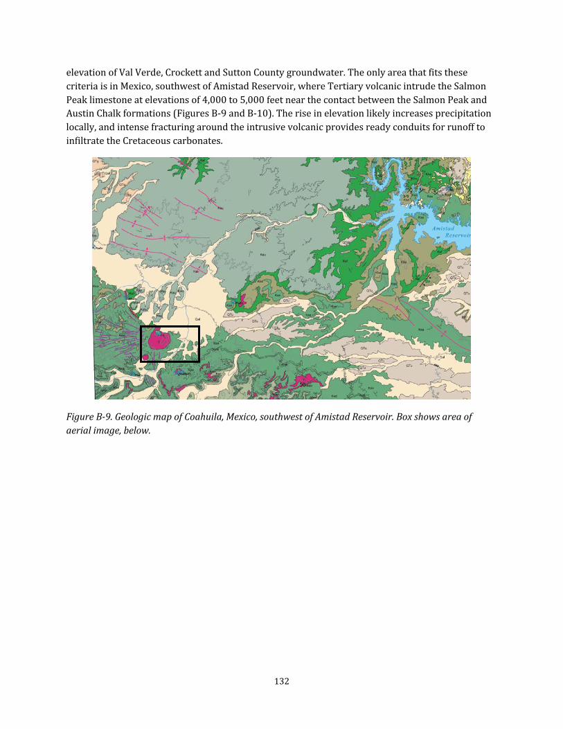
elevation of Val Verde, Crockett and Sutton County groundwater. The only area that fits thesecriteria is in Mexico, southwest of Amistad Reservoir, where Tertiary volcanic intrude the SalmonPeak limestone at elevations of 4,000 to 5,000 feet near the contact between the Salmon Peak and Austin Chalk formations (Figures B-9 and B-10). The rise in elevation likely increases precipitationlocally,and intense fracturing around the intrusive volcanic provides ready conduits for runoff toinfiltrate the Cretaceous carbonates.
Figure B-9. Geologic map of Coahuila, Mexico, southwest of Amistad Reservoir. Box shows area of aerial image, below.
132
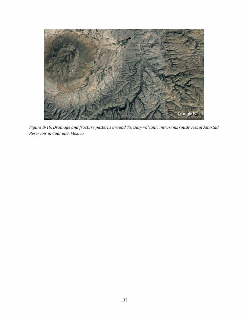
Figure B-10.Drainage and fracture patterns around Tertiary volcanic intrusions southwest ofAmistad Reservoir in Coahuila, Mexico.
133

Appendix C
Water quality data
134
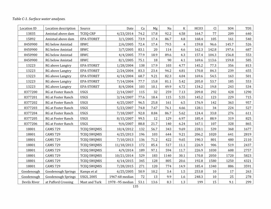
Table C-1. Surface water analyses.
Location ID Location description Source Date Ca Mg Na K HCO3 Cl SO4 TDS
13835 Amistad above dam TCEQ-CRP 4/23/2014 74.2 17.8 92.2 4.58 164.7 77 209 640
15892 Amistad above dam EPA-STORET 3/1/2005 73.9 17.4 86.7 4.8 168.4 105 161 540
8450900 RG below Amistad IBWC 2/6/2005 72.4 17.4 79.5 4 159.8 96.6 145.7 526
8450900 RG below Amistad IBWC 3/7/2005 83.1 20 114 4.6 162.3 142.8 197.6 687
8450900 RG below Amistad IBWC 4/4/2005 77.9 18.9 89.6 4.3 157.4 104.3 156.8 553
8450900 RG below Amistad IBWC 8/1/2005 75.1 18 90 4.1 169.6 113.6 159.8 585
13223 RG above Langtry EPA-STORET 1/28/2004 138 17.9 103 4.77 145.2 77.3 356 813
13223 RG above Langtry EPA-STORET 2/24/2004 83.3 23.4 94.2 4.81 170.8 84.3 239 655
13223 RG above Langtry EPA-STORET 4/14/2004 68.7 9.21 82.3 4.04 169.6 54.5 163 501
13223 RG above Langtry EPA-STORET 7/14/2004 77.7 15.8 81.1 5.42 205.0 53.7 185 553
13223 RG above Langtry EPA-STORET 8/4/2004 103 10.1 49.9 4.72 134.2 19.8 243 534
8377200 RG at Foster Ranch USGS 2/14/2007 115 32 259 7.13 209.8 292 428 1290
8377201 RG at Foster Ranch USGS 3/14/2007 77.6 18.4 115 5.55 145.2 123 229 715
8377202 RG at Foster Ranch USGS 4/25/2007 96.5 25.8 161 6.5 176.9 142 363 957
8377203 RG at Foster Ranch USGS 5/23/2007 74.8 7.67 76.1 4.66 128.1 34 224 527
8377204 RG at Foster Ranch USGS 7/18/2007 92.8 8.84 86.7 5.62 124.4 33.8 276 611
8377205 RG at Foster Ranch USGS 8/15/2007 99.5 12 129 6.97 185.4 88.9 319 825
8377206 RG at Foster Ranch USGS 9/6/2007 88.8 21.7 140 6.24 167.1 107 328 865
18801 CAMS 729 TCEQ SWQMIS 10/4/2012 132 56.7 343 9.69 228.1 539 368 1677
18801 CAMS 729 TCEQ SWQMIS 4/25/2013 196 103 644 9.21 206.2 1020 641 2819
18801 CAMS 729 TCEQ SWQMIS 7/10/2013 136 71.2 422 9.65 190.3 801 480 2110
18801 CAMS 729 TCEQ SWQMIS 11/18/2013 172 85.4 517 11.1 226.9 906 519 2437
18801 CAMS 729 TCEQ SWQMIS 4/9/2014 189 97.1 594 11.7 226.9 1030 608 2757
18801 CAMS 729 TCEQ SWQMIS 10/21/2014 529 183 1140 30.1 170.8 2050 1720 5823
18801 CAMS 729 TCEQ SWQMIS 4/14/2015 345 128 805 20.6 192.8 1580 1250 4321
18801 CAMS 729 TCEQ SWQMIS 7/28/2015 271 120 774 14.9 185.4 1340 886 3591
Goodenough Goodenough Springs Kamps et al 6/25/2005 50.9 10.2 3.4 1.5 253.8 10 17 263
Goodenough Goodenough Springs USGS,2005 1967-68 median 72 13 9.9 1.6 248.3 10 25 278
Devils River at Pafford Crossing Mast and Turk 1978 –95 median 53.1 13.6 8.3 1.3 199 15 9.1 299 135
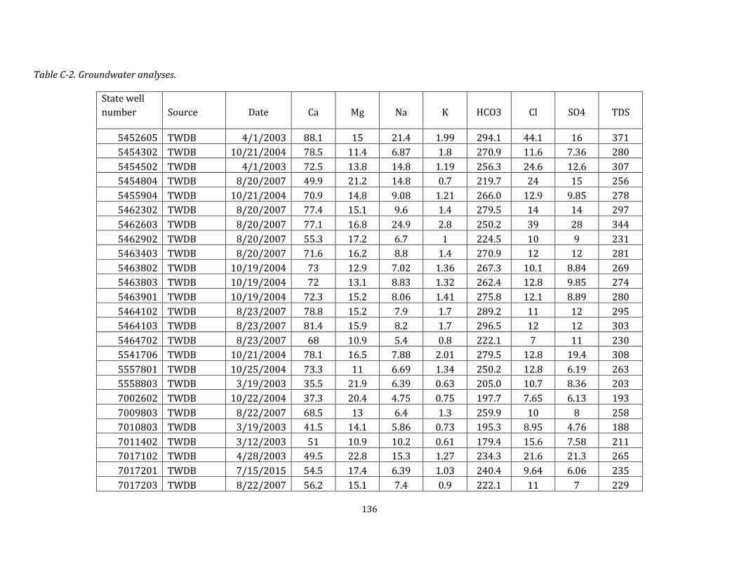
Table C-2. Groundwater analyses.
State well number Source Date Ca Mg Na K HCO3 Cl SO4 TDS
5452605 TWDB 4/1/2003 88.1 15 21.4 1.99 294.1 44.1 16 371 5454302 TWDB 10/21/2004 78.5 11.4 6.87 1.8 270.9 11.6 7.36 280
5454502 TWDB 4/1/2003 72.5 13.8 14.8 1.19 256.3 24.6 12.6 307 5454804 TWDB 8/20/2007 49.9 21.2 14.8 0.7 219.7 24 15 256
5455904 TWDB 10/21/2004 70.9 14.8 9.08 1.21 266.0 12.9 9.85 278 5462302 TWDB 8/20/2007 77.4 15.1 9.6 1.4 279.5 14 14 297
5462603 TWDB 8/20/2007 77.1 16.8 24.9 2.8 250.2 39 28 344
5462902 TWDB 8/20/2007 55.3 17.2 6.7 1 224.5 10 9 231 5463403 TWDB 8/20/2007 71.6 16.2 8.8 1.4 270.9 12 12 281
5463802 TWDB 10/19/2004 73 12.9 7.02 1.36 267.3 10.1 8.84 269 5463803 TWDB 10/19/2004 72 13.1 8.83 1.32 262.4 12.8 9.85 274
5463901 TWDB 10/19/2004 72.3 15.2 8.06 1.41 275.8 12.1 8.89 280
5464102 TWDB 8/23/2007 78.8 15.2 7.9 1.7 289.2 11 12 295 5464103 TWDB 8/23/2007 81.4 15.9 8.2 1.7 296.5 12 12 303
5464702 TWDB 8/23/2007 68 10.9 5.4 0.8 222.1 7 11 230 5541706 TWDB 10/21/2004 78.1 16.5 7.88 2.01 279.5 12.8 19.4 308
5557801 TWDB 10/25/2004 73.3 11 6.69 1.34 250.2 12.8 6.19 263 5558803 TWDB 3/19/2003 35.5 21.9 6.39 0.63 205.0 10.7 8.36 203
7002602 TWDB 10/22/2004 37.3 20.4 4.75 0.75 197.7 7.65 6.13 193
7009803 TWDB 8/22/2007 68.5 13 6.4 1.3 259.9 10 8 258 7010803 TWDB 3/19/2003 41.5 14.1 5.86 0.73 195.3 8.95 4.76 188
7011402 TWDB 3/12/2003 51 10.9 10.2 0.61 179.4 15.6 7.58 211 7017102 TWDB 4/28/2003 49.5 22.8 15.3 1.27 234.3 21.6 21.3 265
7017201 TWDB 7/15/2015 54.5 17.4 6.39 1.03 240.4 9.64 6.06 235
7017203 TWDB 8/22/2007 56.2 15.1 7.4 0.9 222.1 11 7 229
136
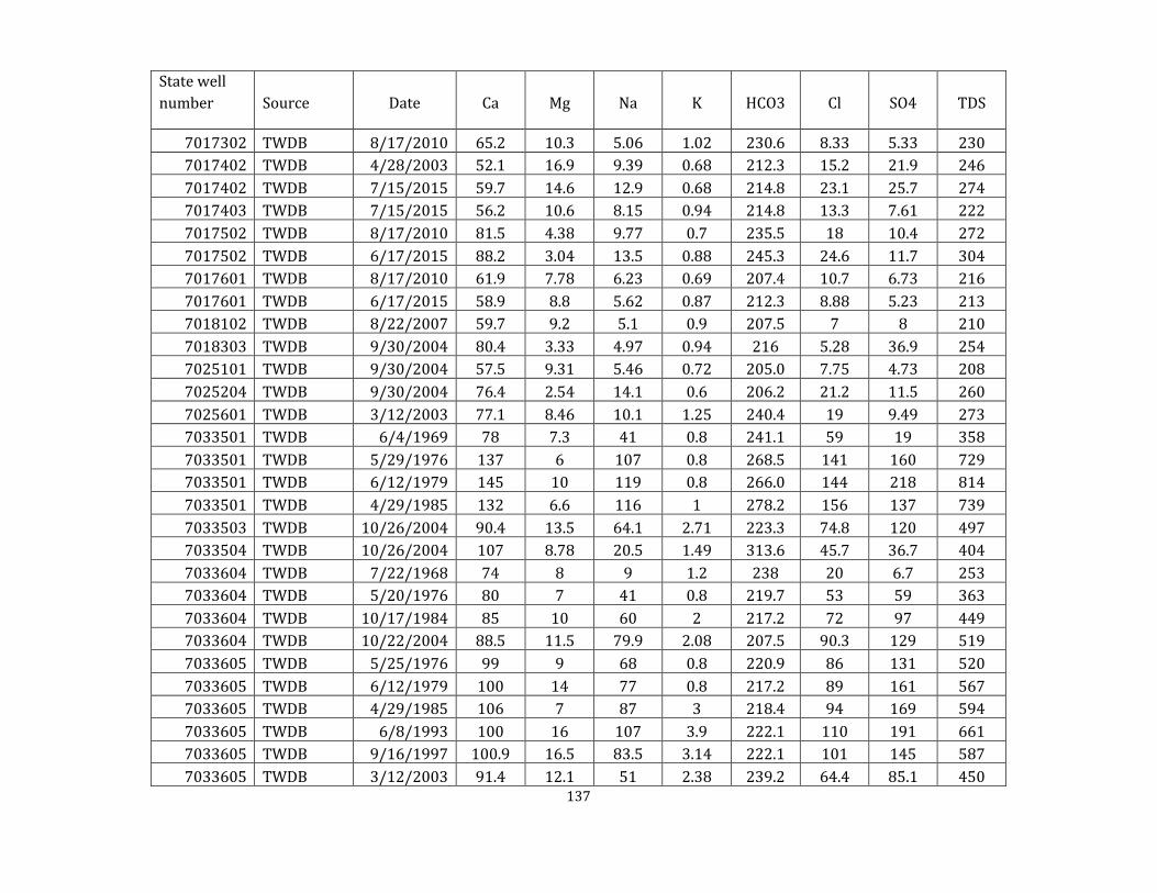
State well number Source Date Ca Mg Na K HCO3 Cl SO4 TDS
7017302 TWDB 8/17/2010 65.2 10.3 5.06 1.02 230.6 8.33 5.33 230 7017402 TWDB 4/28/2003 52.1 16.9 9.39 0.68 212.3 15.2 21.9 246
7017402 TWDB 7/15/2015 59.7 14.6 12.9 0.68 214.8 23.1 25.7 274 7017403 TWDB 7/15/2015 56.2 10.6 8.15 0.94 214.8 13.3 7.61 222
7017502 TWDB 8/17/2010 81.5 4.38 9.77 0.7 235.5 18 10.4 272
7017502 TWDB 6/17/2015 88.2 3.04 13.5 0.88 245.3 24.6 11.7 304 7017601 TWDB 8/17/2010 61.9 7.78 6.23 0.69 207.4 10.7 6.73 216
7017601 TWDB 6/17/2015 58.9 8.8 5.62 0.87 212.3 8.88 5.23 213 7018102 TWDB 8/22/2007 59.7 9.2 5.1 0.9 207.5 7 8 210
7018303 TWDB 9/30/2004 80.4 3.33 4.97 0.94 216 5.28 36.9 254 7025101 TWDB 9/30/2004 57.5 9.31 5.46 0.72 205.0 7.75 4.73 208
7025204 TWDB 9/30/2004 76.4 2.54 14.1 0.6 206.2 21.2 11.5 260
7025601 TWDB 3/12/2003 77.1 8.46 10.1 1.25 240.4 19 9.49 273 7033501 TWDB 6/4/1969 78 7.3 41 0.8 241.1 59 19 358
7033501 TWDB 5/29/1976 137 6 107 0.8 268.5 141 160 729 7033501 TWDB 6/12/1979 145 10 119 0.8 266.0 144 218 814
7033501 TWDB 4/29/1985 132 6.6 116 1 278.2 156 137 739
7033503 TWDB 10/26/2004 90.4 13.5 64.1 2.71 223.3 74.8 120 497 7033504 TWDB 10/26/2004 107 8.78 20.5 1.49 313.6 45.7 36.7 404
7033604 TWDB 7/22/1968 74 8 9 1.2 238 20 6.7 253 7033604 TWDB 5/20/1976 80 7 41 0.8 219.7 53 59 363
7033604 TWDB 10/17/1984 85 10 60 2 217.2 72 97 449 7033604 TWDB 10/22/2004 88.5 11.5 79.9 2.08 207.5 90.3 129 519
7033605 TWDB 5/25/1976 99 9 68 0.8 220.9 86 131 520
7033605 TWDB 6/12/1979 100 14 77 0.8 217.2 89 161 567 7033605 TWDB 4/29/1985 106 7 87 3 218.4 94 169 594
7033605 TWDB 6/8/1993 100 16 107 3.9 222.1 110 191 661 7033605 TWDB 9/16/1997 100.9 16.5 83.5 3.14 222.1 101 145 587
7033605 TWDB 3/12/2003 91.4 12.1 51 2.38 239.2 64.4 85.1 450 137

State well number Source Date Ca Mg Na K HCO3 Cl SO4 TDS
7033904 TWDB 3/10/2003 88.5 10.7 43.3 2.01 241.6 57.8 74.2 422 7034703 TWDB 3/12/2003 105 21.9 16.9 1.35 275.8 63 53.5 434
7034704 TWDB 8/18/2010 81.4 6.9 7.4 0.73 253.8 12.6 8.27 262 7041301 TWDB 2/4/1966 76 6.9 5.8 0.8 250 12 5.8 246
7041301 TWDB 5/25/1966 74 6.1 5.5 2.3 241.0 10 4.3 237
7041301 TWDB 9/21/1966 72 5.5 4.4 0.8 206.0 9.6 7.2 219 7041301 TWDB 10/11/1972 80 7.2 5.8 1.3 253 8.9 7 249
7041301 TWDB 2/20/1973 80 7.2 5.6 1 235 11 7.6 251 7041301 TWDB 10/31/1973 72 9.3 5.2 1 243 10 8.4 248
7041301 TWDB 7/9/1974 75 7.2 5.7 0.9 247 9.4 8.6 251 7041301 TWDB 1/16/1975 71 6.9 5.4 1.1 240.0 9.7 8.1 243
7041301 TWDB 1/16/1976 73 7.3 5.2 0.9 249 9.5 5.7 236
7041301 TWDB 6/12/1993 81 7.5 6.1 1.1 246.5 10 9 257 7041301 TWDB 4/1/1994 72 6.9 5.9 0.8 231.9 11 9.4 228
7041301 TWDB 9/15/1997 76.3 8.05 7.4 1.34 230.7 12.9 19.1 262 7041301 TWDB 3/11/1999 74.2 6.77 5.36 0.87 247.7 9.8 6.86 234
7041301 TWDB 3/13/2003 78.7 7.17 5.69 0.93 246.5 9.34 6.98 253
7041301 TWDB 3/13/2003 78.7 7.17 5.69 0.93 246.5 9.34 6.98 253 7041302 TWDB 6/16/2015 89.3 9.41 21.4 1.26 261.2 33.9 39.2 345
7103102 TWDB 3/20/2003 101 51 42.2 3.07 246.5 44.9 281 674 7104402 TWDB 10/23/2004 80.7 28.5 49.4 2.22 269.7 85.5 77.5 484
7104502 TWDB 3/20/2003 68.6 21.9 11.5 1.08 281.9 20.6 22.1 308 7107101 TWDB 8/21/2007 71.6 10.6 6.8 1.5 237.9 10 12 253
7107401 TWDB 10/20/2004 65.1 15.4 9.52 1.23 253.8 14.5 9.23 268
7107401 TWDB 8/21/2007 72 16.6 10.4 1.3 257.5 15 12 285 7107702 TWDB 8/21/2007 68.3 19.3 9.3 1.4 270.9 13 18 303
7108102 TWDB 8/23/2007 77.6 13.4 7.5 1.6 258.7 11 11 272 7108401 TWDB 8/23/2007 87.1 14.7 9.6 1.1 284.3 15 14 308
7112502 TWDB 3/11/2003 105 29.5 120 2.58 220.9 193 152 738 138
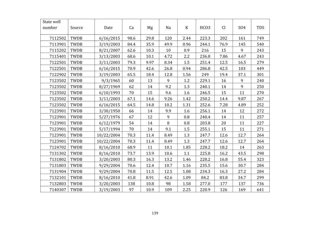
State well number Source Date Ca Mg Na K HCO3 Cl SO4 TDS
7112502 TWDB 6/16/2015 98.6 29.8 120 2.44 223.3 202 161 749 7113901 TWDB 3/19/2003 84.4 35.9 49.9 0.96 244.1 76.9 145 540
7115202 TWDB 8/21/2007 62.6 10.3 10 0.9 216 15 9 243 7115401 TWDB 3/13/2003 68.6 10.1 4.72 2.2 236.8 7.86 4.67 243
7122501 TWDB 3/11/2003 79.3 9.97 8.34 1.5 251.4 12.5 16.5 279
7122501 TWDB 6/16/2015 70.9 42.6 26.8 0.94 286.8 42.5 103 449 7122902 TWDB 3/19/2003 65.5 18.4 12.8 1.56 249 19.4 37.1 301
7123502 TWDB 9/3/1965 60 13 9 1.2 229.1 16 9 240 7123502 TWDB 8/27/1969 62 14 9.2 1.3 240.1 14 9 250
7123502 TWDB 6/10/1993 70 15 9.6 1.6 246.5 15 11 270 7123502 TWDB 3/11/2003 67.1 14.6 9.26 1.42 250.2 14.4 9.87 267
7123502 TWDB 6/16/2015 64.5 14.8 10.2 1.31 252.6 7.28 4.89 252
7123901 TWDB 3/30/1950 66 14 9.9 1.6 256.1 14 12 272 7123901 TWDB 5/27/1976 67 12 9 0.8 240.4 14 11 257
7123901 TWDB 6/12/1979 54 14 8 0.8 203.8 20 11 227 7123901 TWDB 5/17/1994 70 14 9.1 1.5 255.1 15 11 271
7123901 TWDB 10/22/2004 70.3 11.4 8.49 1.3 247.7 12.6 12.7 264
7123901 TWDB 10/22/2004 70.3 11.4 8.49 1.3 247.7 12.6 12.7 264 7124702 TWDB 8/16/2010 68.9 11 10.1 1.85 228.2 18.2 14 263
7131302 TWDB 8/16/2010 73.7 13.9 10.6 1.1 225.8 16.2 43.5 298 7131802 TWDB 3/20/2003 80.3 16.3 13.2 1.46 228.2 16.8 55.4 323
7131803 TWDB 9/29/2004 70.6 12.4 10.7 1.16 235.5 15.6 30.7 284 7131904 TWDB 9/29/2004 70.8 11.5 12.5 1.08 234.3 16.3 27.2 284
7132101 TWDB 8/16/2010 41.8 8.91 42.6 1.09 84.2 83.8 34.7 299
7132803 TWDB 3/20/2003 138 10.8 98 1.58 277.0 177 137 736 7140307 TWDB 3/19/2003 97 10.9 109 2.25 220.9 126 169 641
139

Table C-3. TWDB isotopic analyses – Val Verde County groundwater and spring discharge.
Well No.1 Latitude Longitude Sampledate
14C, pmc
δ13C,(‰)
δD (‰)
δ18O (‰)
δ18O SO4(‰)
87Sr/86Sr Sr,uG/L
δ34S SO4
(‰)
Tritium (TU)
5454804 30.131943 -
101.30528 8/1/2006 0.3079 -6.1 -
29.6 -5.8 2.7 0.708406 241.5 8.4 0.34
5454804 30.131943 -
101.30528 8/20/2007 0.3083 -6.8 -
32.4 -5.7 0.02
5455906 30.132221 -
101.15889 8/2/2006 0.701 -10.2 -
28.4 -5.5 0.708059 574.5 8.3
5462301 30.109722 -
101.27944 8/1/2006 0.6236 -12.3 -
29.4 -5.4 0.708255 291.7 8.5 1.19
5462302 30.122221 -
101.26583 8/1/2006 0.6579 -9.7 -
29.9 -5.6 3 0.708161 405.2 7.6 1.37
5462302 30.122221 -
101.26583 8/20/2007 0.7414 -8.6 -
30.7 -5.7
5462603 30.056111 -
101.26972 8/20/2007 0.5065 -6.4 -
27.5 -5.2
5462902 30.011944 -
101.25528 8/1/2006 0.5304 -8.5 -
30.7 -6.1 4.9 0.708129 279.6 7 0.55
5462902 30.011944 -
101.25528 8/20/2007 0.554 -7.8 -
32.6 -5.9
5463301 30.124166 -
101.14111 8/2/2006 0.6915 -9.9 -
28.1 -5.6 3.4 0.707936 1305 7.9
5463403 30.0625 -
101.23055 8/1/2006 0.6554 -9 -30 -5.5 2.8 0.708022 709.4 8.1 1.41
5463403 30.0625 -
101.23055 8/20/2007 0.7054 -8.7 -
30.2 -6 1.56
5464102 30.113888 -
101.10833 8/2/2006 -28 -5.9 0.707929 949.8 7.8 1.76
5464102 30.113888 -
101.10833 8/23/2007 0.815 -9.9 -
30.2 -5.3 2.01
5464103 30.094721 -
101.10361 8/2/2006 0.7223 -10.4 -
28.6 -5.8 0.707941 875.7 12.9 1.59
5464103 30.094721 -
101.10361 8/23/2007 0.7764 -9.6 -
31.5 -5.5
140

Well No.1 Latitude Longitude Sampledate
14C, pmc
δ13C,(‰)
δD (‰)
δ18O (‰)
δ18O SO4(‰)
87Sr/86Sr Sr,uG/L
δ34S SO4
(‰)
Tritium (TU)
5464205 30.094721 -
101.07555 8/2/2006 0.6778 -9.3 -
29.3 -5.9 2.9 0.707952 785.1 8.4 1.44
5464401 30.073054 -101.1175 8/2/2006 0.7341 -10.4 -
27.8 -5.8 0.7079455 866.5 9.5
5464402 30.060833 -
101.12333 8/2/2006 0.7232 -10.3 -
28.7 -6 0.7079535 713.8 8.7 1.6
5464404 30.041666 -101.1125 8/2/2006 0.2551 -9.4 -
29.1 -5.9 5.1 0.708166 136.3 4.1 0.04
5464702 30.04111 -
101.08417 8/3/2006 0.6498 -8.4 -28 -5.7 0.708257 182.6 16 1.21
5464702 30.04111 -
101.08417 8/23/2007 0.7979 -9.6 -
26.1 -5.2
7009803 29.775832 -100.9575 7/31/2006 0.7304 -10.3 -
29.3 -6 0.708124 247.1 9.1 1.69
7009803 29.775832 -100.9575 8/22/2007 0.7841 -4.5 -
33.3 -5.8
7017102 29.732777 -
100.99167 8/3/2006 0.1533 -7.5 -
25.8 -5.2 8.2 0.707925 589.6 7.1 0.07
7017102 29.732777 -
100.99167 4/28/2003
7017203 29.736388 -100.935 8/3/2006 0.4637 -8.8 -
28.9 -6.2 0.7081205 189.8 8.8 0.13
7017203 29.736388 -100.935 8/22/2007 0.5078 -7.4 -
31.3 -5.8
7017302 29.734444 -
100.91333 7/31/2006 0.7451 -10.1 -30 -6 2.3 0.70814 181.1 9.3 1.86
7017302 29.734444 -
100.91333 8/17/2010 0.7464 -11.7 -
31.6 -
5.23 3.7 0.708141 8.6 1.37
7017502 29.686944 -
100.93194 8/17/2010 0.7923 -13 -
26.8 -
3.89 2.6 0.708239 4.8 1.58
7017801 29.663333 -
100.92667 9/12/2009 0.7205 -11.5 -
33.6 -5.2 5.9 0.708129 9.2 1.23
7017801 29.663333 -
100.92667 3/5/2010 0.7408 -11.8 -
34.2 -
5.19 2.8 0.708124 8.2 1.26
141
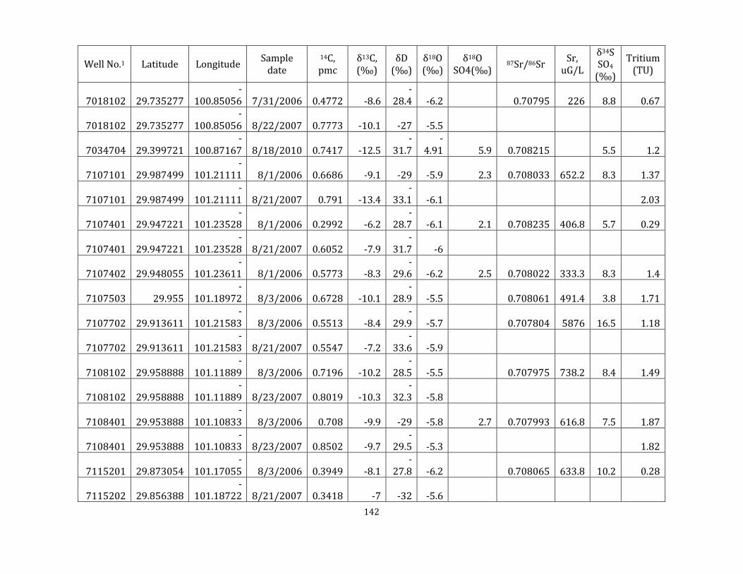
Well No.1 Latitude Longitude Sampledate
14C, pmc
δ13C,(‰)
δD (‰)
δ18O (‰)
δ18O SO4(‰)
87Sr/86Sr Sr,uG/L
δ34S SO4
(‰)
Tritium (TU)
7018102 29.735277 -
100.85056 7/31/2006 0.4772 -8.6 -
28.4 -6.2 0.70795 226 8.8 0.67
7018102 29.735277 -
100.85056 8/22/2007 0.7773 -10.1 -27 -5.5
7034704 29.399721 -
100.87167 8/18/2010 0.7417 -12.5 -
31.7 -
4.91 5.9 0.708215 5.5 1.2
7107101 29.987499 -
101.21111 8/1/2006 0.6686 -9.1 -29 -5.9 2.3 0.708033 652.2 8.3 1.37
7107101 29.987499 -
101.21111 8/21/2007 0.791 -13.4 -
33.1 -6.1 2.03
7107401 29.947221 -
101.23528 8/1/2006 0.2992 -6.2 -
28.7 -6.1 2.1 0.708235 406.8 5.7 0.29
7107401 29.947221 -
101.23528 8/21/2007 0.6052 -7.9 -
31.7 -6
7107402 29.948055 -
101.23611 8/1/2006 0.5773 -8.3 -
29.6 -6.2 2.5 0.708022 333.3 8.3 1.4
7107503 29.955 -
101.18972 8/3/2006 0.6728 -10.1 -
28.9 -5.5 0.708061 491.4 3.8 1.71
7107702 29.913611 -
101.21583 8/3/2006 0.5513 -8.4 -
29.9 -5.7 0.707804 5876 16.5 1.18
7107702 29.913611 -
101.21583 8/21/2007 0.5547 -7.2 -
33.6 -5.9
7108102 29.958888 -
101.11889 8/3/2006 0.7196 -10.2 -
28.5 -5.5 0.707975 738.2 8.4 1.49
7108102 29.958888 -
101.11889 8/23/2007 0.8019 -10.3 -
32.3 -5.8
7108401 29.953888 -
101.10833 8/3/2006 0.708 -9.9 -29 -5.8 2.7 0.707993 616.8 7.5 1.87
7108401 29.953888 -
101.10833 8/23/2007 0.8502 -9.7 -
29.5 -5.3 1.82
7115201 29.873054 -
101.17055 8/3/2006 0.3949 -8.1 -
27.8 -6.2 0.708065 633.8 10.2 0.28
7115202 29.856388 -
101.18722 8/21/2007 0.3418 -7 -32 -5.6
142
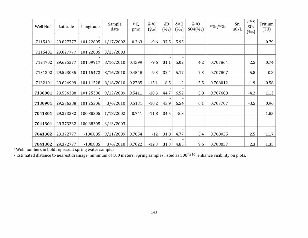
Well No.1 Latitude Longitude Sampledate
14C, pmc
δ13C,(‰)
δD (‰)
δ18O (‰)
δ18O SO4(‰)
87Sr/86Sr Sr,uG/L
δ34S SO4
(‰)
Tritium (TU)
7115401 29.827777 -
101.22805 1/17/2002 0.363 -9.6 -
37.5 -
5.95 0.79
7115401 29.827777 -
101.22805 3/13/2003
7124702 29.625277 -
101.09917 8/16/2010 0.4599 -9.6 -
31.1 -
5.02 4.2 0.707864 2.5 0.74
7131302 29.593055 -
101.15472 8/16/2010 0.4548 -9.3 -
32.4 -
5.17 7.3 0.707807 -5.8 0.8
7132101 29.624999 -
101.11528 8/16/2010 0.2785 -15.1 -
18.5 -2 5.5 0.708012 -1.9 0.56
7130901 29.536388 -
101.25306 9/12/2009 0.5411 -10.3 -
44.7 -
6.52 5.8 0.707688 -4.2 1.13
7130901 29.536388 -
101.25306 3/6/2010 0.5131 -10.2 -
43.9 -
6.54 6.1 0.707707 -3.5 0.96
7041301 29.373332 -
100.88305 1/18/2002 0.741 -11.8 -
34.5 -5.3 1.85
7041301 29.373332 -
100.88305 3/13/2003
7041302 29.372777 -100.885 9/11/2009 0.7054 -12 -
31.8 -
4.77 5.4 0.708025 2.5 1.17
7041302 29.372777 -100.885 3/6/2010 0.7022 -12.3 -
31.3 -
4.85 9.6 0.708037 2.3 1.35 1 Well numbers in bold represent spring water samples 2 Estimated distance to nearest drainage; minimum of 100 meters. Spring samples listed as 500 m to enhance visibility on plots.
143
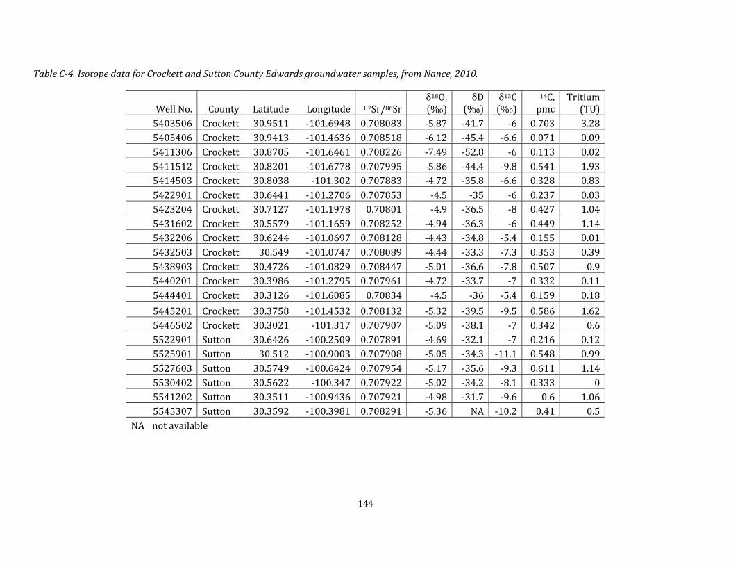
Table C-4.Isotope data for Crockett and Sutton County Edwards groundwater samples, from Nance, 2010.
Well No. County Latitude Longitude 87Sr/86Sr δ18O,(‰)
δD (‰)
δ13C (‰)
14C, pmc
Tritium (TU)
5403506 Crockett 30.9511 -101.6948 0.708083 -5.87 -41.7 -6 0.703 3.28 5405406 Crockett 30.9413 -101.4636 0.708518 -6.12 -45.4 -6.6 0.071 0.09
5411306 Crockett 30.8705 -101.6461 0.708226 -7.49 -52.8 -6 0.113 0.02
5411512 Crockett 30.8201 -101.6778 0.707995 -5.86 -44.4 -9.8 0.541 1.93 5414503 Crockett 30.8038 -101.302 0.707883 -4.72 -35.8 -6.6 0.328 0.83
5422901 Crockett 30.6441 -101.2706 0.707853 -4.5 -35 -6 0.237 0.03 5423204 Crockett 30.7127 -101.1978 0.70801 -4.9 -36.5 -8 0.427 1.04
5431602 Crockett 30.5579 -101.1659 0.708252 -4.94 -36.3 -6 0.449 1.14 5432206 Crockett 30.6244 -101.0697 0.708128 -4.43 -34.8 -5.4 0.155 0.01
5432503 Crockett 30.549 -101.0747 0.708089 -4.44 -33.3 -7.3 0.353 0.39
5438903 Crockett 30.4726 -101.0829 0.708447 -5.01 -36.6 -7.8 0.507 0.9 5440201 Crockett 30.3986 -101.2795 0.707961 -4.72 -33.7 -7 0.332 0.11
5444401 Crockett 30.3126 -101.6085 0.70834 -4.5 -36 -5.4 0.159 0.18
5445201 Crockett 30.3758 -101.4532 0.708132 -5.32 -39.5 -9.5 0.586 1.62 5446502 Crockett 30.3021 -101.317 0.707907 -5.09 -38.1 -7 0.342 0.6
5522901 Sutton 30.6426 -100.2509 0.707891 -4.69 -32.1 -7 0.216 0.12 5525901 Sutton 30.512 -100.9003 0.707908 -5.05 -34.3 -11.1 0.548 0.99
5527603 Sutton 30.5749 -100.6424 0.707954 -5.17 -35.6 -9.3 0.611 1.14
5530402 Sutton 30.5622 -100.347 0.707922 -5.02 -34.2 -8.1 0.333 0 5541202 Sutton 30.3511 -100.9436 0.707921 -4.98 -31.7 -9.6 0.6 1.06
5545307 Sutton 30.3592 -100.3981 0.708291 -5.36 NA -10.2 0.41 0.5 NA= notavailable
144
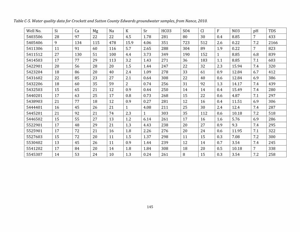
Table C-5.Water quality data for Crockett and Sutton County Edwards groundwater samples, from Nance, 2010.
Well No. Si Ca Mg Na K Sr HCO3 SO4 Cl F NO3 pH TDS
5403506 28 97 22 22 4.5 1.78 281 80 30 0.4 8.85 7 433
5405406 9 134 115 478 15.9 4.06 351 723 512 2.6 0.22 7.2 2166 5411306 11 91 60 116 5.7 2.65 288 304 89 1.9 0.22 7 823
5411512 27 130 51 100 4.4 3.73 349 190 152 1 8.85 6.8 839 5414503 17 77 29 113 3.2 1.43 271 36 183 1.1 8.85 7.1 603
5422901 20 56 28 20 1.5 1.44 247 22 32 2.3 15.94 7.4 320 5423204 18 86 20 40 2.4 1.09 278 33 61 0.9 12.84 6.7 412
5431602 22 85 23 27 2.1 0.64 308 22 40 0.6 12.84 6.9 386
5432206 18 60 35 59 2 0.74 256 31 92 1.3 14.17 7.4 439 5432503 15 65 21 12 0.9 0.44 250 14 14 0.4 15.49 7.4 280
5440201 17 63 25 17 0.8 0.73 268 15 22 0.6 4.87 7.1 297 5438903 21 77 18 12 0.9 0.27 281 12 16 0.4 11.51 6.9 306
5444401 16 45 26 21 1 4.08 211 25 30 2.4 12.4 7.4 287
5445201 21 92 21 74 2.3 1 303 35 112 0.6 10.18 7.2 518 5446502 15 55 27 13 1.2 6.14 261 17 16 1.6 5.76 6.9 286
5522901 17 48 29 21 1.3 4.43 238 20 27 0.9 9.3 7.4 295 5525901 17 72 21 16 1.8 2.26 276 20 24 0.6 11.95 7.1 322
5527603 15 72 20 11 1.5 1.37 298 11 15 0.3 7.08 7.2 300 5530402 13 45 26 11 0.9 1.44 239 12 14 0.7 3.54 7.4 245
5541202 17 84 20 14 1.8 1.84 308 18 20 0.5 10.18 7 338
5545307 14 53 24 10 1.3 0.24 261 8 15 0.3 3.54 7.2 258
145

Appendix D
Public comments
146
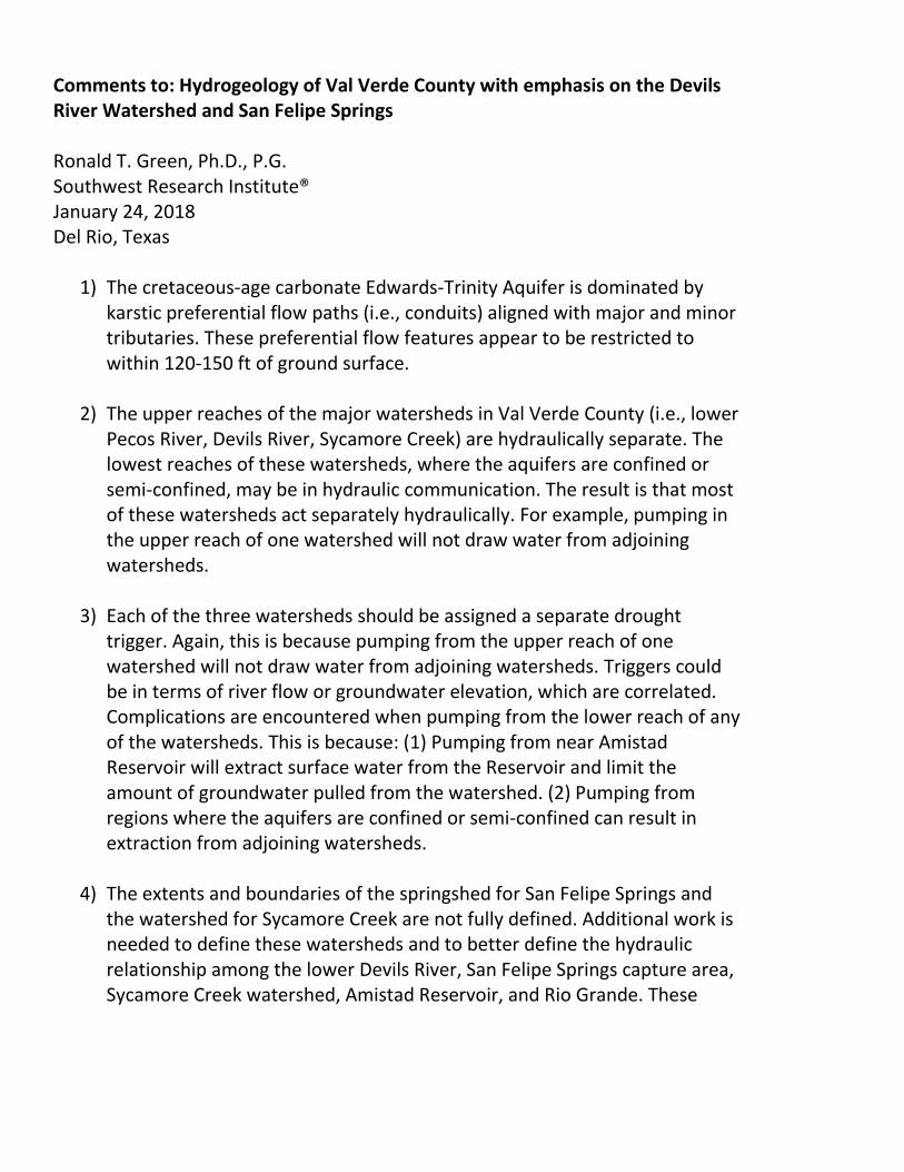
Comments to: Hydrogeology of Val Verde County with emphasis on the Devils River Watershed and San Felipe Springs
Ronald T. Green, Ph.D., P.G. Southwest Research Institute® January 24, 2018 Del Rio, Texas
1) The cretaceous-age carbonate Edwards-Trinity Aquifer is dominated by karstic preferential flow paths (i.e., conduits) aligned with major and minor tributaries. These preferential flow features appear to be restricted to within 120-150 ft of ground surface.
2) The upper reaches of the major watersheds in Val Verde County (i.e., lower Pecos River, Devils River, Sycamore Creek) are hydraulically separate. The lowest reaches of these watersheds, where the aquifers are confined or semi-confined, may be in hydraulic communication. The result is that most of these watersheds act separately hydraulically. For example, pumping in the upper reach of one watershed will not draw water from adjoining watersheds.
3) Each of the three watersheds should be assigned a separate drought trigger. Again, this is because pumping from the upper reach of one watershed will not draw water from adjoining watersheds. Triggers could be in terms of river flow or groundwater elevation, which are correlated. Complications are encountered when pumping from the lower reach of any of the watersheds. This is because: (1) Pumping from near Amistad Reservoir will extract surface water from the Reservoir and limit the amount of groundwater pulled from the watershed. (2) Pumping from regions where the aquifers are confined or semi-confined can result in extraction from adjoining watersheds.
4) The extents and boundaries of the springshed for San Felipe Springs and the watershed for Sycamore Creek are not fully defined. Additional work is needed to define these watersheds and to better define the hydraulic relationship among the lower Devils River, San Felipe Springs capture area, Sycamore Creek watershed, Amistad Reservoir, and Rio Grande. These

hydraulic relationships are complicated by the facts that the lower reaches of the aquifers may be confined or semi-confined and the close proximity of a surface-water boundary condition in Amistad Reservoir and the Rio Grande. One important limiting factor is that the discharge from either San Felipe Springs and in Sycamore Creek is limited due to the relatively modest sizes of their respective capture areas.
5) The upper reaches of all watershed aquifers, particularly the Devils River watershed, are relatively thin and unconfined. [Note the Edwards portion of the Edwards-Trinity Aquifer is treated hydraulically separately.] Detailed coupled surface-water/groundwater modeling has shown that relatively modest pumping in the upper reach of the Devils Rivers (i.e., 4,000-6,000 acre-ft/yr) has resulted in the cessation of live water between Pecan Springs and Beaver Lake, a distance of about 10 miles. It should be noted that the time during which this live water was lost (i.e., post 1960) corresponds with a period of increased spring and stream flow in the Edwards Plateau due to improved land management practices. The acute sensitivity of live flow to pumping is due to the fact that the permeable portion of the aquifer is relatively thin and that surface-water flow in the river and groundwater flow in the conduits are intricately linked with topography.
Woody plant encroachment paradox: Rivers rebound as degraded grasslands convert to woodlands
Wilcox, B. P., and Y. Huang (2010), Woody plant encroachment paradox: Rivers rebound as degraded grasslands convert to woodlands, Geophys. Res. Lett., 37, L07402.
Abstract The related phenomena of degradation and woody plant encroachment have transformed huge tracts of rangelands. Woody encroachment is assumed to reduce groundwater recharge and streamflow. We analyzed the long-term (85 years) trends of four major river basins in the Edwards Plateau region of Texas. This region, in which springs are abundant because of the karst geology, has undergone degradation and woody encroachment. We found that, contrary to widespread perceptions, streamflows have not been declining. The contribution of baseflow has doubled—even though woody cover has expanded and rainfall amounts have remained constant. We attribute this increase in springflow to a landscape recovery that has taken place concurrently with woody expansion—a recovery brought about by lower grazing pressure. Our results indicate that for drylands where the geology supports springs, it is degradation and not woody encroachment that leads to regional-scale declines in groundwater recharge and streamflows.

References:
Green, R.T., F.P. Bertetti, and M.S. Miller. 2014. Focused Groundwater Flow in a Carbonate Aquifer in a Semi-Arid Environment. Journal of Hydrology. 517:284–297. doi: 10.1016/j.jhydrol.2014.05.015
Green, R.T., N. Toll, and F.P. Bertetti. 2016. Develop a Groundwater Flow Model to Understand the Groundwater Resources of the Lower Pecos River Watershed. Contract Report for the City of Laredo. Final Report.
Toll, N., S.B. Fratesi, R.T. Green, F.P. Bertetti, and R. Nunu. 2017. Water-Resource Management of the Devils River Watershed Final Report. Contract Report for the Devils River Conservancy.

Comments on draft TWDB report:
“Overview of Groundwater Conditions in Val Verde County, Texas”
Thank you for the opportunity to provide comment.
The report provides a thorough review of available information related to the hydrologic system in Val VerdeCounty. The findings and discussion in Chapter 8.0, Groundwater Management and Feasibility of HydrologicTriggers, draw the technical information together in a coherentmanner and make reasonable recommendations.I especially agree with the groundwater zone concept and identification of the zones described in the report.
Other parts of the report have errors or other issues that should be addressed by the authors prior to final publication. Below, I have identified several items that I believe are problematic.
1. Factual error on page 37, 3rd paragraph (emphasis added)
“The currentevaluation considers spring discharges to streams and rivers separately from wells, while Green, Bertetti and Miller (2014) apparently grouped spring flow rates and well production rates together.The 22 springs in ValVerde County for which there are dischargeestimates included in the TWDB groundwater database have an aggregate total averagedischarge of nearly 7,000 gallons per minute and a median discharge of approximately 500gallons per minute; by definition, these large spring discharges are close to surface waterfeatures. While the presence of large springs is clear evidence of the karst nature of the aquifer,these spring flows are notdirectly comparable to wellyields or specific capacities under pumping conditions.”
The highlighted statement in Paragraph 3 above is factually incorrect. I’m not sure why it seems “apparent” that spring data were used, but that is an incorrect assumption and is made without merit. The analysis in Green et al. (2014) only included data from wells. These data were derived from the TWDB Groundwater Database, Submitted Driller’s Report Database, and independent well tests (some of which are included in this draft report). No springs were included at any time. Please correct the paragraph to remove the implication that springs were included, andas a result, biased the analyses of Green et al. (2014)
2. There appear to be some misconceptions regarding the findings of Green et al. (2104). Additionally, there seems to be some confusion regarding the reporting of correlation calculations produced by quantitative statistical analyses versus “eye-balling” limited data in a map figure.
Page 32, last paragraph (emphasis added)
“Based on a review of groundwater wells, well capacities, and well locations, SWRI concluded that there is a high correlation between high capacity wells and proximity to river channels thatpoints to the occurrence of preferentialgroundwater flowpaths thatcoincide with river channels.”…“This pattern is also incorporated in the Val Verde County model, which assignshigher hydraulic conductivity values in stream channels. However, our review of available well capacity data indicates a possible, but not strong correlation between well capacity and stream channels (Figure 4-10).”
Page 37, 2nd paragraph (emphasis added)
“The pattern ofincreased groundwater productivity near stream drainages noted by Toll and others (2017) is not apparent from the TWDB data.The distribution of wells with higherspecific capacity (Figure 4-10) shows several high-capacity wells along the upper Devils River,above Juno, and along the Rio Grande, especially in the Del Rio area. Several moderate-capacitywells are also located near the Pecos River in the northwestern part of the county. But lowcapacity wells are also found along drainages.”
The conclusions of Green et al. (2014) do not indicate there should be no low capacity wells found along drainages.The Edwards system in Val Verde County is a karst system and should be expected to have significant hydraulicvariability, especially where conduits are not present. Essentially, higher capacity wells are more likely to be foundnearer to drainages, but they shouldn’t be expected to be found exclusively near drainages.
Part of the analysis described in Green et al. (2014) was designed to quantitatively evaluate the conceptual modeloriginally proposed by Woodruff and Abbott (Abbott, 1975; Woodruff and Abbott, 1979, 1986) that conduitdevelopment might be preferentially co-located along drainage features.Although our initialvisualobservations of maps suggested a pattern or correlation of larger capacity wells with drainage channels, visual interpretation ofdata can often be skewed or biased by trivial things, such as use of certain colors or dark contrast to plot wells onthe map.Additionally, it was difficult to determine adequate criteria to identify a particular drainage or draw as afeature substantial enough to warrant inclusion in the analysis. We arbitrarily chose to include drainage featureswith stream order values of at least 3 (meaning that more than two drainages would have had to have merged toform the channel to be analyzed, see the figure below).
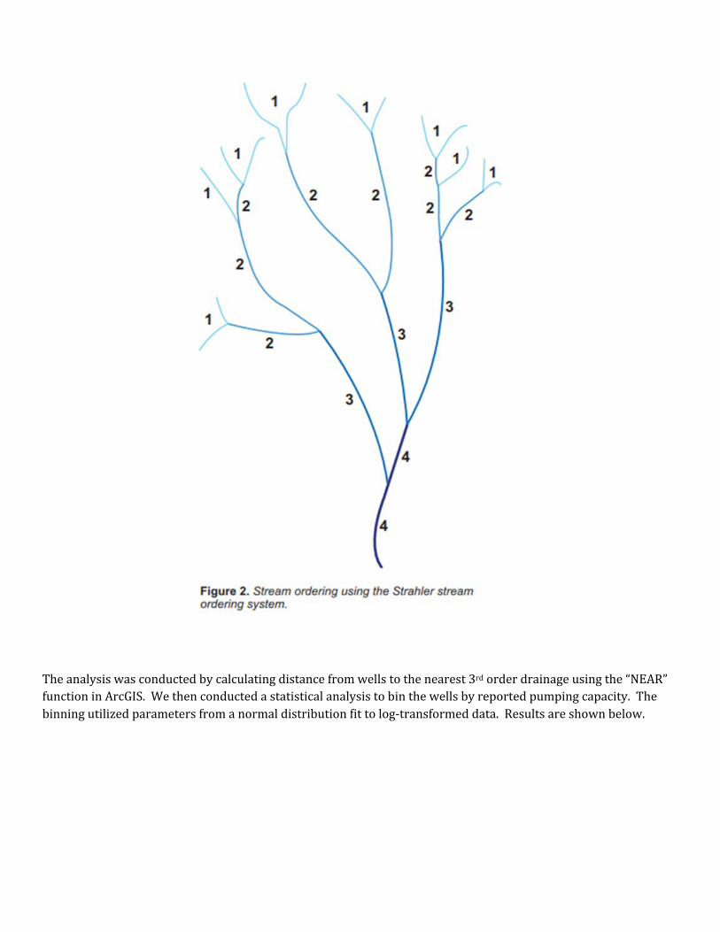
The analysis was conducted by calculating distance from wells to the nearest 3rd order drainage using the “NEAR” function in ArcGIS. We then conducted a statistical analysis to bin the wells by reported pumping capacity. Thebinning utilized parameters from a normal distribution fit to log-transformed data.Results are shown below.
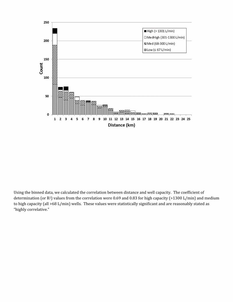
Using the binned data, we calculated the correlation between distance and well capacity. The coefficient ofdetermination (or R2) values from the correlation were 0.69 and 0.83 for high capacity (>1300 L/min) and medium to high capacity (all>68 L/min) wells.These values were statistically significant and are reasonably stated as “highly correlative.”
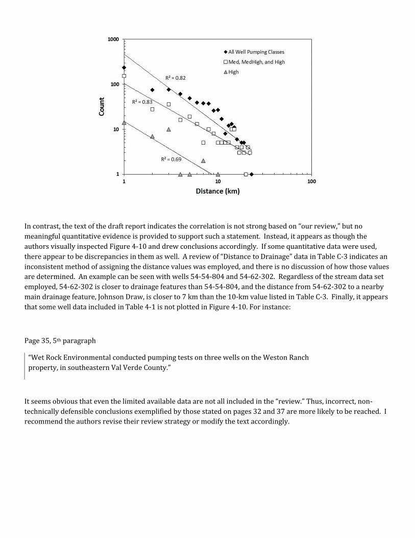
In contrast, the text of the draft report indicates the correlation is not strong based on “our review,” but no meaningful quantitative evidence is provided to support such a statement.Instead,itappears as though theauthors visually inspected Figure 4-10 and drew conclusions accordingly. If some quantitative data were used,there appear to be discrepancies in them as well.A review of “Distance to Drainage”data in Table C-3 indicates an inconsistent method of assigning the distance values was employed, and there is no discussion of how those valuesare determined. An example can be seen with wells 54-54-804 and 54-62-302. Regardless of the stream data setemployed, 54-62-302 is closer to drainage features than 54-54-804, and the distance from 54-62-302 to a nearbymain drainage feature, Johnson Draw, is closer to 7 km than the 10-km value listed in Table C-3. Finally, it appearsthatsome welldata included in Table 4-1 is not plotted in Figure 4-10. For instance:
Page 35, 5th paragraph
“WetRock Environmentalconducted pumping tests on three wells on the Weston Ranch property, in southeastern Val Verde County.”
It seems obvious that even the limited available data are not all included in the “review.” Thus,incorrect,non-technically defensible conclusions exemplified by those stated on pages 32 and 37 are more likely to be reached.I recommend the authors revise their review strategy or modify the text accordingly.
3. The analyses and conclusions in Appendix B – Geochemical assessment of groundwater flow paths, mixing, and residence time suffer from several inconsistent or inadequately defended arguments.
A. Discussion of tritium and GNIP data.
Page 121, 2nd paragraph
From 1961 to 2004 there were a total of 12 potential recharge events, defined by storms thatresulted in peak flows greater than about 15,000 cubic feet per second (425 cubic meters persecond) in the Devils River at the Comstock gage (Figure B-2).
What is the basis for establishing this flow value as a threshold for recharge in the Val Verde system? I amunaware of any data that correlate only high flow events to recharge. In fact, data from Table C-3, Well 54-62-302,show that over two successive sampling events in 2006 and 2007 the measured fraction of modern carbon (C-14)in the well increased from 0.66 to 0.74 (younger), indicating recharge of the system occurred. Not only does thisindicate recharge without a large flow event, but recharge along a smaller order drainage feature. Thus, the initial premise that some minimum value of flow in the Devils River is correlated with or required for recharge in thesystem is incorrect. As an aside, data such as this (recharge along drainages) are consistent with the inclusion of smallorder drainage features as recharge and flow paths in Tolletal.(2107).
Page 121, 2nd paragraph
GNIP data show that tritium concentrations in precipitation during these storm events variedwidely, depending on the direction the storm was traveling relative to nuclear test sites, timingrelative to nuclear tests, how much rain had already fallen from the air mass,and other factors, resulting in unique decay curves for each recharge event (Figure B-3).
The GNIP data are not corrected or calibrated for storm source or rainout. They may vary because of these factors but the data do not account for this. Thus, use of data recorded at Waco may be completely inconsistent withexpected tritium deposition in Val Verde County. Other calibrations have attempted to estimate tritium deposition on a sub-regional scale (e.g., Michel et al., 2018).
Page 122 (emphasis added)
These tritium decay curves indicate a mean residence times of 21 to 34 years for Goodenough and San Felipe Springs discharge.A close-up view of the decay curves covering the times when spring water samples were collected from San Felipe and Goodenough Springs(Figure 4-29) shows that only two of the decay curves, for 1976 and 1981 recharge, match theobserved tritium concentrations, with the 1980 decay curve slightly above observed values.

These decay curves match observed tritium concentrations,giving a mean residence time of 21 to 34 years.
The figure to which the paragraph refers is B-3 and not 4-29. Nonetheless, the conclusion that residence time canbe discerned from these plots is incorrect. One could argue that residence time is much longer or much shorter based on the data shown. As mentioned previously, there is no basis for the assumption that recharge hasoccurred only during the selected time periods (in fact, it is clearly shown that this is an incorrect assumption).First, potential mixing is not included the assessment. Obviously, water discharging from the springs should be a composite of many recharge events. If the mean residence time is reasonable, the discharge should be a compositeof many events including the 1971, 1972, 1974, and 1983 events in addition to the ones mentioned. The combination of each of these events indicates that, if anything, measured tritium at the springs should be much higher for the suggested residence time. The low values could just as well indicate that despite the predictedhigher tritium content, there is a longer residence time. Second, there is some suggestion in Appendix B that San Felipe and Good Enough Springs have very differentsource areas,yetFigure B-3 treats both as having similar source terms. Finally, and perhaps most importantly, the data included in the draft report aren’t consistent with this conceptualization.A rough map of the data in Table C-3 is shown below.

Despite predictions that recharge events should produce at least some samples with tritium concentrations greaterthan 2 TU (based on the information in Figure B-3), none are found. In fact, the data suggestthatallwater near the drainages in Val Verde county is approximately the same age, with older water found away from these drainages.This is consistent with recharge preferentially occurring in the more hydraulically conductive drainage areas andless so in the plateau regions away from drainages. Using this information and the measured values at the springs,it seems that residence time is reasonably less than 12 years.
B. Connection to Sutton and Crockett counties

Pages 124 and 125
Groundwater typically acquires magnesium, chloride and sulfate during water-rock interactions,and the concentrations of these ions increase along flow-paths between recharge and dischargeareas. Although groundwater in Crockett and Sutton counties is hydraulically upgradient fromVal Verde groundwater, the chemical data demonstrate that only a limited fraction of thisupgradient groundwater can mix with Val Verde groundwater and still produce a compositionconsistent with the discharge from the major springs. These results suggestthatmostdischargefrom Goodenough and San Felipe springs originates within or near Val Verde County and is notpart of a larger, regional flow system.
Water chemistry data for Sutton County in Figures B-5 and B-6 is biased by use of a limited data set and failure toaccommodate the spatial and hydraulic characteristics of the groundwater system.
San Felipe Springs may discharge water from a limited system in Val Verde County, but the data presented inFigure B-5 do not fully support that because there is no tie to the locations or characteristics of the wells whosedata are plotted. For example, most of the Val Verde well data appear to have compositions with a greatercontribution from Mg than samples from San Felipe Springs. This low Mg signal is typical of Edwards waters inKinney County (and wells east of San Felipe Springs). In short, the conclusion may be correct, but it does not follow from what is presented in the report.
The disconnect between Sutton County well data is a function of the limited number of samples considered in the report. Edwards waters in Sutton County are influenced by recharge in drainages and longer residence times inareas capped by Buda Limestone (as reported by Nance, 2010). A couple of figures below (from Nunu et al., 2017)clearly show the high concentrations of Ca associated with active recharge areas and zones of higher Mgconcentrations associated with greater residence times below the Buda capped regions. These figures weregenerated using data collected by Sutton County from 2013 to 2016 and known to be in the TWDB database. Other data (not shown) confirm some of the results of Nance (2010) and others and indicate higher Mg/Ca ratios areassociated with longer residence time.
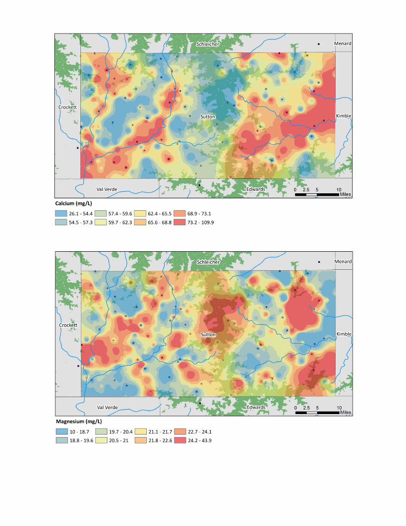

The trends Sutton County can be extended into ValVerde County to show the “active”flow and recharge areas associated with drainages (below). Thus, the chemical “disconnect” suggested in the report is really a function of the varying components of the hydrologic system and not really indicative of separation of the system from north to south (although Iagree thatCrockettCounty mostly affects the western (or Pecos) portion of ValVerde County.
In summary, I think the draft report is valuable and incorporates a great deal of work. I do believe it would bemuch improved if some attention was paid to addressing the items to which I refer in these comments. Should you have any questions or require additional information, please do not hesitate to contact me by emailor phone.
Thank you.
Paul Bertetti, P.G. Director -- Aquifer ScienceEdwards Aquifer Authority
References
Abbott, P.L., 1975. On the hydrology of the Edwards Limestone, south-central Texas.
J. Hydrol. 24, 251�269.
Green, R.T., Bertetti, F.P., and Miller,M.S.,2014,Focused groundwater flow in a carbonate aquifer in a semi-arid environment: Journal of Hydrology v. 517, p. 284-297.
Michel, R.L., B.C. Jurgens, and M.B Young. 2018. Tritium deposition in precipitation in the United States, 1953-2012,USGS Scientific Investigations Report 2018-5086.
Nance, H.S., 2010, Controls and uses of hydrochemical and isotopic heterogeneity in the plateau aquifer system,contiguous aquifers, and associated surface water, Edwards Plateau region, Texas, Ph.D. Dissertation, U.T. Austin.
Nunu, R.R., F.P. Bertetti, and R.T. Green. 2017. “Characterization of the Hydrochemistry of the Edwards-Trinity (Plateau) Aquifer in Sutton County, Texas,” Annual Meeting of the South-Central Section of the Geological Society ofAmerica, San Antonio, TX, March 13–14, 2017.
Toll, N., Fratesi, S.B., Green, R.T., Bertetti, F.P., and Nunu, R., 2017; Water resource management of the Devils Riverwatershed, final report. Southwest Research Institute report under contract to the Devils River Conservancy; athttp://www.devilsriverconservancy.org/research/
Woodruff Jr., C.M., Abbott, P.L., 1979. Drainage-basin evolution and aquifer development in a karstic limestoneterrain,South-Central Texas. USA Earth Surf. Process. 4, 319–334.
Woodruff Jr., C.M., Abbott, P.L., 1986. Stream piracy and evolution of the Edwards
Aquifer along the Balcones Escarpment, Central Texas. In: Abbott, P.L., Woodruff, C.M., Jr. (Eds.), The BalconesEscarpment. Geological Society of America, Central Texas, pp. 77�90.
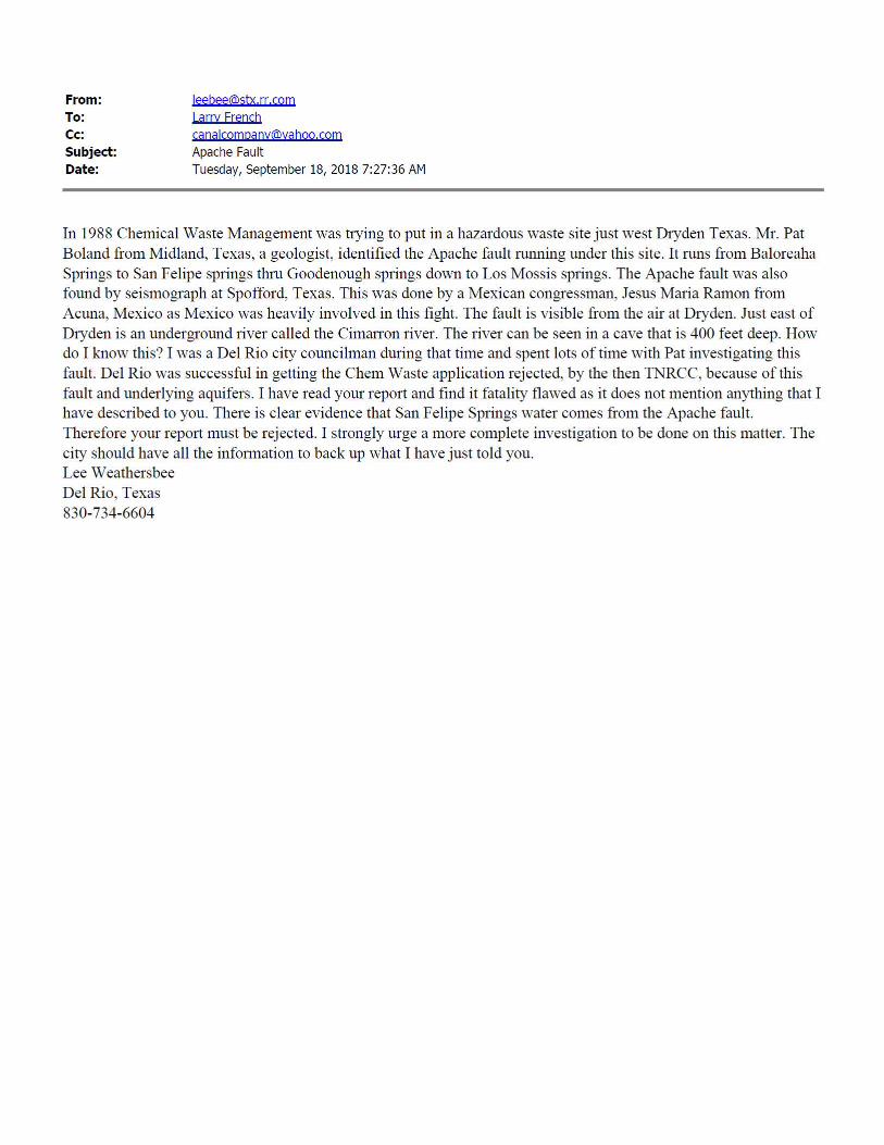
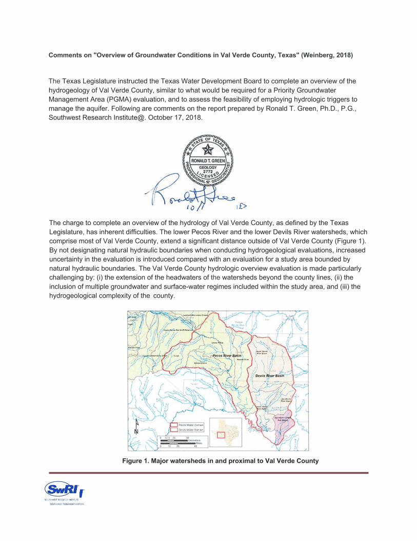
Comments on "Overview of Groundwater Conditions in Val Verde County, Texas" (Weinberg, 2018)
The Texas Legislature instructed the Texas Water Development Board to complete an overview of the hydrogeology of Val Verde County, similar to what would be required for a Priority Groundwater Management Area (PGMA) evaluation, and to assess the feasibility of employing hydrologic triggers to manage the aquifer. Following are comments on the report prepared by Ronald T. Green, Ph.D., P.G., Southwest Research Institute@. October 17, 2018.
I £>
The charge to complete an overview of the hydrology of Val Verde County, as defined by the Texas Legislature, has inherent difficulties. The lower Pecos River and the lower Devils River watersheds, which comprise most of Val Verde County, extend a significant distance outside of Val Verde County (Figure 1). By not designating natural hydraulic boundaries when conducting hydrogeological evaluations, increased uncertainty in the evaluation is introduced compared with an evaluation for a study area bounded by natural hydraulic boundaries. The Val Verde County hydrologic overview evaluation is made particularly challenging by: (i) the extension of the headwaters of the watersheds beyond the county lines, (ii) the inclusion of multiple groundwater and surface-water regimes included within the study area, and (iii) the hydrogeological complexity of the county.
Figure 1. Major watersheds in and proximal to Val Verde County
The water budget of Val Verde County is fairly well constrained in terms of discharge (i.e., the sum of pumping plus discharge via the Rio Grande). Calculating how much water is recharged to Val Verde County from each of the watersheds (e.g., Pecos River, Devils River, Sycamore Creek) is not well constrained even though the contributions from each of the major springs (e.g., Goodenough, San Felipe, Cienegas) is known.
Additional documentation is available to frame the following statement from Weinberg (2018) in the context of Val Verde County’s water resources. Weinberg (2018) stated the following:
Baseflow in the upper Devils River, which is entirely from groundwater discharge, has remained essentially the same for at least the last 100 years. Available evidence indicates that starting point of perennial flow has historically occurred near Pecan Spring and has not changed in response to pumping from irrigation wells near Juno.
Our research has resulted in evidence that partially contradicts this statement. The now-dry Beaver Lake, located adjacent to the Devils River near Juno, is a critical case exhibiting how ical status of the Devils River watershed. There is ample evidence that the springs to Beaver Lake were sufficient to sustain Beaver Lake as a persistent surface water body in a semi-arid environment even during periods of drought. It is unknown, although with limited observations, that spring flow at Beaver Lake was previously sufficient (i.e., prior to the early 20th century) to provide continuous outflow from Beaver Lake to Pecan Springs where current continuous surface flow (i.e., live water) is currently observed.
Absent in Wienberg (2018) are TWDB documents summarizing the history of water-well development in four of the counties that cover the Devils River watershed, namely Crockett County (Iglehart, 1967), Schleicher County (Muller and Crouch, 1971), Sutton County (Muller and Pool, 1972), and Val Verde County (George, 1950). These and other publications include documentation to substantiate the premise that Beaver Lake was a persistent surface-water pool prior to development and attendant increases in pumping in the upper half of the Devils River watershed. A number of historical accounts that describe Beaver Lake were assimilated into a 2011 publication by Patrick Dearen, Devils River: Treacherous Twin to the Pecos, 1535-1900 (Dearen, 2011). The historical accounts are mostly from records by the U.S. Cavalry, cattle drives, and wagon trains that ventured across south-central Texas in the mid to late 19th
century. The consensus of these observations is that prior to the 20th century, Beaver Lake was a persistent source of water prior to development for those who ventured across the upper Devils River watershed. Following are the salient comments from Dearen (2011) with relevance to the hydrology of Devils River and Beaver Lake.
Beaver lake features prominently in the report of the 1849 expedition led by Thomas B. Eastland through Texas to California:
Where the [Devils] river widened into a small, natural reservoir that would become known as Beaver Lake, twenty-two miles upstream from Second Crossing, Eastland and his companions camped July 27 [1849] and waited for the engineers to complete a trail out across the divide between the Devils and Pecos. The pool, fringed by line oaks, willows, and mesquites, was an exquisite site, even for a river of singular characteristics.
‘We are encamped in a beautiful Valley surrounded by an hundred Hills rich in fine Grass, enough for thousands of Animals’ described Eastland. ‘In the midst of the Valley
is a beautiful lake of pure water fed by many springs running out of the neighboring hills’. (Dearen 2011, p. 31-33)
Beaver Lake also appears in the account of Blake's 1854 geological mapping expedition from the Red River to the Rio Grande:
Although Blake’s [camp's] exact location is debatable, evidence points to the vicinity of Beaver Lake, a coveted oasis that long had nurtured passing military parties. Not only was the lake generally considered the river’s head, thus echoing the description in Camp Blake’s post return for April but on June 6 [1854] a traveler would delineate a ‘Devils River Station’ (presumably Blake) at the final watering point before the road struck out for Howard’s Spring—an accurate characterization of the Beaver Lake area. (Dearen 2011, p. 50)
Dearen (2011) pg 41. The drought that plagued the Devils in 1850 spread like a blight throughout West Texas and wreaked a toll.”
Brune (1975), in his survey Springs of Texas, stated that: “The Devil's River at this point {Juno, Headwater, or Stein Springs} was described in 1916 as a beautiful stream with large live oaks. The springs, Beaver Lake upstream, and the perennial flow of the Devil's River in this area have all disappeared.” Brune (1975) did not provide attribution for the observation made in 1916.
An additional recollection of Beaver Lake from prior to 1953 is provided in the Amarillo Sunday News Globe, December 13, 1953, edition, published in Amarillo, Texas, in a byline by Laura V. Hamner. In the article, Laura V. Hamner interviewed the wife of the owner of Beaver Lake Ranch at the time, whom she mistakenly identified as "Mrs. Earl Williams." In the following discussion, the interviewee will be referred to by her actual name, "Mrs. Byron Earl Wilson."
In the days of [Mr. Wilson's] youth, Beaver Lake was a deep pool of water. Mrs. [Wilson] recalls their early married life, when they had a motor boat on that lake which now is a dry depression.
Beaver Lake played a part in cattle history in those early days. In winter, cattle from the Concho country drifted southward and a general roundup on the Rio Grande was held annually. 'The cattlemen gathered up all the strays they could find and drove them north. Naturally, there would be local cattle caught in the herd. The men halted the cattle at Beaver Lake because it was the last water hole before they reached the Concho. Sometimes, 50,000 head would be held there for a day or two, sometimes four days, while cattle were being cut out. Then the cattle would be trailed northward, a string 15 miles long, and cattlemen would follow, cutting out their cattle as they located them. (Hamner, 1953)
Note that Mr. Byron Earl Wilson was born in 1882. His “early married life” was likely the late 1900s into the 1910s and possibly the 1920s. Based on the recollection of Mrs. Byron Earl Wilson, Beaver Lake was a “deep pool of water” into the 1910s and possibly later. The first Evinrude outboard motor was
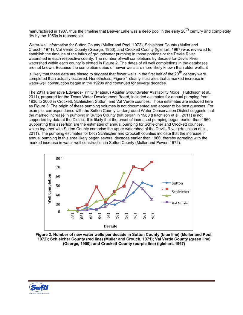
manufactured in 1907, thus the timeline that Beaver Lake was a deep pool in the early 20th century and completely dry by the 1950s is reasonable.
Water-well information for Sutton County (Muller and Pool, 1972), Schleicher County (Muller and Crouch, 1971), Val Verde County (George, 1950), and Crockett County (Iglehart, 1967) was reviewed to establish the timeline of the influx of groundwater pumping in those portions or the Devils River watershed in each respective county. The number of well completions by decade for Devils River watershed within each county is plotted in Figure 2. The dates of all well completions in the databases are not known. Because the completion dates of newer wells are more likely known than older wells, it is likely that these data are biased to suggest that fewer wells in the first half of the 20th century were completed than actually occurred. Nonetheless, Figure 1 clearly illustrates that a marked increase in water-well construction began in the 1920s and continued for several decades.
The 2011 alternative Edwards-Trinity (Plateau) Aquifer Groundwater Availability Model (Hutchison et al., 2011), prepared for the Texas Water Development Board, included estimates for annual pumping from 1930 to 2006 in Crockett, Schleicher, Sutton, and Val Verde counties. Those estimates are included here as Figure 3. The origin of these pumping volumes is not documented and appear to be best guesses. For example, correspondence with the Sutton County Underground Water Conservation District suggests that the marked increase in pumping in Sutton County that began in 1960 (Hutchison et al., 2011) is not supported by data at the District. It is likely that the onset of increased pumping began earlier than 1960. Supporting this assertion are the estimates of annual pumping for Schleicher and Crockett counties, which together with Sutton County comprise the upper watershed of the Devils River (Hutchison et al., 2011). The pumping estimates for both Schleicher and Crockett counties indicate that the increase in annual pumping in this area likely began several decades earlier than 1960, thereby agreeing with the marked increase in water-well construction in Sutton County (Muller and Power, 1972).
80
70
60
50
40
30
Sutton
Schleicher
Val Verde
0000000000
Well Com
p letion
196
195
194
193
192
191
190
189
198
197
Decade
Figure 2. Number of new water wells per decade in Sutton County (blue line) (Muller and Pool, 1972); Schleicher County (red line) (Muller and Crouch, 1971); Val Verde County (green line)
(George, 1950); and Crockett County (purple line) (Iglehart, 1967)
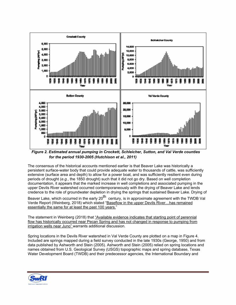
Figure 2. Estimated annual pumping in Crockett, Schleicher, Sutton, and Val Verde counties for the period 1930-2005 (Hutchison et al., 2011)
The consensus of the historical accounts mentioned earlier is that Beaver Lake was historically a persistent surface-water body that could provide adequate water to thousands of cattle, was sufficiently extensive (surface area and depth) to allow for a power boat, and was sufficiently resilient even during periods of drought (e.g., the 1850 drought) such that it did not go dry. Based on well completion documentation, it appears that the marked increase in well completions and associated pumping in the upper Devils River watershed occurred contemporaneously with the drying of Beaver Lake and lends credence to the role of groundwater depletion in drying the springs that sustained Beaver Lake. Drying of Beaver Lake, which occurred in the early 20th century, is in approximate agreement with the TWDB Val Verde Report (Weinberg, 2018) which stated “Baseflow in the upper Devils River…has remained essentially the same for at least the past 100 years.”
The statement in Weinberg (2018) that “Available evidence indicates that starting point of perennial flow has historically occurred near Pecan Spring and has not changed in response to pumping from irrigation wells near Juno” warrants additional discussion.
Spring locations in the Devils River watershed in Val Verde County are plotted on a map in Figure 4. Included are springs mapped during a field survey conducted in the late 1930s (George, 1950) and from data published by Ashworth and Stein (2005). Ashworth and Stein (2005) relied on spring locations and names obtained from U.S. Geological Survey (USGS) topographic maps and spring database, Texas Water Development Board (TWDB) and their predecessor agencies, the International Boundary and

Water Commission (IBWC), and in Springs of Texas by Brune (1975, 1981). Tables 1 and 2 list the springs from George (1950) and Ashworth and Stein (2005), respectively. Spring locations mapped in the late 1930s (denoted by green dots) are significantly more prevalent than locations from Ashworth and Stein (2005). This may be attributed to loss of springs due to pumping or simply that those additional springs mapped in the 1930s were not included in subsequent surveys.
Figure 4. Spring locations in the Devils River watershed in Val Verde County
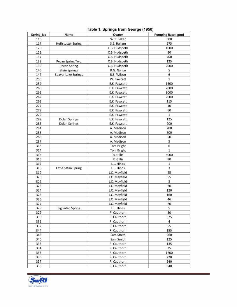
Table 1. Springs from George (1950) Spring_No Name Owner Pumping Rate (gpm)
116 W.T. Baker 500 117 Huffstutter Spring S.E. Hallam 275 120 C.B. Hudspeth 1000 121 C.B. Hudspeth 20 137 C.B. Hudspeth 700 138 Pecan Spring Two C.B. Hudspeth 125 139 Pecan Spring C.B. Hudspeth 2000 146 Stein Springs R.G. Nance 5 147 Beaver Lake Springs B.E. Wilson 6 255 W. Fawcett 1 259 E.K. Fawcett 1500 260 E.K. Fawcett 2000 261 E.K. Fawcett 8000 262 E.K. Fawcett 2000 263 E.K. Fawcett 115 277 E.K. Fawcett 10 278 E.K. Fawcett 60 279 E.K. Fawcett 1 282 Dolan Springs E.K. Fawcett 125 283 Dolan Springs E.K. Fawcett 200 284 A. Madison 200 285 A. Madison 500 286 A. Madison 50 287 A. Madison 5 313 Tom Bright 6 314 Tom Bright 1 315 R. Gillis 5000 316 R. Gillis 80 317 L.L. Hinds 1 318 Little Satan Spring L.L. Hinds 3 319 J.C. Mayfield 25 320 J.C. Mayfield 55 322 J.C. Mayfield 3 323 J.C. Mayfield 20 324 J.C. Mayfield 120 325 J.C. Mayfield 160 326 J.C. Mayfield 46 327 J.C. Mayfield 20 328 Big Satan Spring L.L. Hines 5 329 R. Cauthorn 80 330 R. Cauthorn 675 331 R. Cauthorn 4 332 R. Cauthorn 55 344 R. Cauthorn 155 345 Sam Smith 260 346 Sam Smith 125 333 R. Cauthorn 135 334 R. Cauthorn 35 335 R. Cauthorn 1700 336 R. Cauthorn 220 337 R. Cauthorn 540 338 R. Cauthorn 340

339 R. Cauthorn 70 340 R. Cauthorn 275 341 R. Cauthorn 490 342 R. Cauthorn 2500 343 R. Cauthorn 40 431 F. Cantu 105 433 San Felipe Spring City of Del Rio 55000 435 San Felipe Spring Jap Lowe 60
Table 2. Springs from Ashworth and Stein (2005)
ID_No State Well Number Name Latitude Longitude Elev_ft 1 Big Norris Spring 30.0141 -100.968 1959 2 7001704 Blue Spring 29.8936 -100.9938 1480 3 Camp Spring 29.8869 -100.8755 1667 4 7033801 Cantu Springs 29.3875 -100.9322 979 5 Carlos Camp Spring 29.8016 -100.9583 1373 6 Cienegas Creek Spring 29.3662 -100.9379 938 7 5460804 Cox Springs 30.0416 -101.5416 1763 8 Dead Man Springs 29.7916 -101.3583 1378 9 7001702 Dolan Springs 29.8969 -100.9836 1340
10 Everett Springs 30.0083 -101.5083 1683 11 7108901 Finegan Springs 29.9083 -101.0083 1607 12 7124301 Gillis Springs 29.752 -101.0416 1180 13 Glenn Spring 29.8116 -100.8886 1449 14 7130901 Goodenough Springs 29.5363 -101.2531 1122 15 Grass Patch Springs 29.8736 -100.9922 1331 16 7112504 Guy Skiles Springs 29.8166 -101.5579 1320 17 5452801 Howard Springs 30.1583 -101.5417 1661 18 5463801 Hudspeth Springs 30.025 -101.175 1618 19 7107603 Huffstutler Springs 29.9583 -101.1416 1506 20 Indian Springs 29.665 -101.9263 1220 21 Jose Maria Spring 29.9283 -100.9872 1451 22 5455905 Juno Springs 30.1583 -101.1254 2007 23 Leon Spring 29.8811 -100.9725 1492 24 Little Norris Spring 30.0091 -100.9683 2010 25 Lowry Springs 29.6269 -100.9208 1196 26 7140903 McKee Springs 29.425 -101.0416 970 27 Pecan Springs 30.0583 -101.1751 1844 28 7041301 San Felipe Spring E 29.3725 -100.883 975 29 7041302 San Felipe Spring W 29.3728 -100.8847 960 30 7041303 San Felipe Spring S 29.373 -100.8825 975 31 San Felipe Creek Spring 29.3981 -100.8666 1015 32 Scott Spring 30.0166 -101.5189 1447 33 Seep Springs 29.8233 -101.5116 1422 34 7017501 Slaughter Bend Springs 29.6751 -100.9416 1345 35 Snake Springs 29.8961 -100.9808 1385 36 Spotted Oak Spring 29.8802 -100.8775 1671 37 Tardy Spring 30.1239 -101.5378 1563 38 7140905 US No. 3 Spring 29.4122 -101.0365 921 39 7042601 Yoas Springs 29.3083 -100.7751 980 40 7112501 29.8099 -101.5732 1260 41 5460301 30.1233 -101.534 1537 42 5460302 30.1235 -101.5335 1537 43 7108801 29.8952 -101.0582 1472

44 7001703 29.8913 -100.9923 1520 45 7001701 29.8955 -100.9829 1360
Also included in Figure 3 are locations designated as potential springs based on the small-scale deviations of the stream bed from the overall stream gradient. Preferential flow paths often follow bedding plane partings that, when they intersect with a stream, often cause localized spots of increased stream incision. It is likely, therefore, that where the preferential flow paths intersect the stream valley, there exist small-scale depressions relative to the overall stream gradient. These depressions are more likely to intersect the water table and form springs than the stream reaches not located in one of these depressions.
To ascertain locations where the river bed cut down into the preferential flow paths, the basal elevation of the river channel was determined using a digital elevation map (DEM). Several orders of a polynomial were fit to these data. The thought behind this exercise is that pronounced deviations in the riverbed that are below the polynomial would indicate the likely locations of springs and pools of water that would form in the river bed where the elevation of groundwater is above ground level. Springs would form at these low points when the groundwater elevation was sufficiently high. Conversely, these same springs and pools would go dry when groundwater elevations went down. Deviations between actual river bed elevations and a 6th-order polynomial are plotted in Figure 5. Hypothetical spring/pool locations are noted in Figure 5 where the differences between measured and modeled elevations have the greatest negative values.
Noteworthy is that there are no springs or pools associated with the northern most dips in the river bed. This is reasonable. The water table at these locations is well below the river bed. Springs would only discharge at these locations if the water table were to significantly rise. This scenario is unlikely unless the watershed were to enter a pluvial period, something that would be expected during a glacial epoch. Also noteworthy is that location B in Figures 4 and 5 is aligned with Beaver Lake. The fact that Beaver Lake is a depression in the river bed is logical. The groundwater elevation at the springs Beaver Lake is interpreted to have been sufficiently high prior to the early 20th century that there was perennial discharge during those times. The lowering of the water table at Beaver Lake is interpreted to been modest, particularly since the aquifer is phreatic in this area, however this lowering has been sufficient that Beaver Lake springs no longer are perennial and rarely flow. Analyses and evaluations at SwRI support the premise that springs that sustained Beaver Lake have been depleted by pumping upgradient of Beaver Lake (Toll et al., 2017).

Figure 5. Difference between measured and modeled riverbed elevations
Limited documentation is available to ascertain whether there was consistent flow from Beaver Lake to Pecan Springs prior to the early 20th century. A gain-loss survey from August 1925 (Texas Board of Water Engineers, 1960) noted there was no flow in the Devils River at a point 0.2 miles below Beaver Lake. Significant flow in the Devils River was not observed upstream of Juno Springs. Beaver Lake was cited in the survey, but neither the status of the lake nor discharge at the springs that sustained Beaver Lake was noted in report.
In summary, Beaver Lake is viewed as a bell weather for the hydrogeological status of the Devils River watershed. There is ample evidence that the springs to Beaver Lake were sufficient to sustain Beaver Lake as a persistent surface water body in a semi-arid environment even during periods of drought. It is known, although with limited observations, that before the early 20th century spring flow at Beaver Lake was previously sufficient to provide continuous outflow from Beaver Lake to Pecan Springs where current continuous surface flow is currently observed.
Effects of pumping on recharge, streamflow, and surface water/groundwater interactions described in Weinberg (2018) are generally consistent with other recent similar discussions (Fratesi et al., 2014; presentations by R.T. Green to the Texas Legislature Natural Resources Committee, 2018). In summary, Weinberg (2018) notes :
Pumping may affect the lateral movement of groundwater in Val Verde County and surrounding areas. Large-scale pumping over an extended period may produce a cone of depression in the potentiometric surface sufficient to induce lateral groundwater flow into the county from surrounding areas. This is especially likely in the southern portion of Val Verde County where the Edwards aquifer unit is thicker and larger volumes of groundwater can be produced. Confined groundwater conditions in the southern part of the county will also tend to create a wider cone of depression because the smaller confined aquifer storage coefficient results in greater drawdown for a given pumping volume. Groundwater flow in the thinner Edwards aquifer unit north of the Maverick Basin appears to be separated into distinct groundwater basins coincident with the

surface water drainages. Pumping in the upstream portion of one basin is unlikely to affect adjacent basins, even if the aquifer is locally dewatered, because the gradient created by the pumping will probably not be sufficient to induce flow across the divide between the surface water basins. (Weinberg, 2018)
Weinberg (2018) provides Figure 6 with groundwater elevations measured at two wells, 5463401 and 7001707. The relatively flat response in measured groundwater is clearly indicative of a phreatic aquifer. Well 5463401 is located near Juno and well 7001707 is located near the confluence of Dolan Creek and Devils River. As discussed in the Numerical Model section of these comments, the Val Verde County Model does not honor this important tendency for the phreatic parts of adjoining watersheds in Val Verde County to act hydraulically separately.
Figure 6. Hydrographs of TWDB Recorder Wells in the Devils River Watershed showing little overall variation in water levels over a 10-year period. (Figure 8-2 in Weinberg, 2018)
Weinberg (2018) states that:
Available data suggest that the groundwater flow system in conduits is poorly connected to the limestone rock matrix. The conduit system is recharged separately from the aquifer matrix and there is limited mixing between the two systems. Conduits are primarily recharged by runoff that is concentrated along the surface drainage system and enters the aquifer through large openings, such as sinkholes and solution-enlarged fractures. The matrix is recharged by precipitation percolating through soils. Because the amount of recharge to the rock matrix is much smaller than that to the conduit system, groundwater originating from the rock matrix represents a small fraction of the overall volume of groundwater discharged from the major springs. (Weinberg, 2018)

Parts of this premise are problematic and are not aligned with current concepts on karst aquifers, which posit that the matrix and conduits (as well as fractures) are usually in direct communication with each other. Speleogenesis, the evolution of karst aquifers, is the technical basis of the integral hydraulic relationship between karst features and rock matrix. Seminal texts by Klimchouk et al. (2000) and Gabrošek (2002) provide clear explanations how karst aquifers form and how rock matrix can provide the principal source of conduit water. The conduits account for most of the permeability within the aquifer, and the matrix accounts for most of its storage capacity. Water is transmitted back and forth between the conduits and matrix during high- and low-flow events. It is true that preferential flow paths likely account for a large fraction of the discharge in the streambed, but these conduits are themselves fed by matrix flow in between storm events. The conceptualization that rock matrix and conduits are separate dual systems is not consistent with the karstic Edwards-Trinity Aquifer in the Devils River watershed (Green et al., 2014).
The amount of recharge experienced in Val Verde County and environs is discussed in some detail in Weinberg (2018). The range in recharge values by a number of researchers varies from a fraction on an inch/year to several inches/year. This uncertainty in recharge in the semi-arid karst landscape in Val Verde County adds to the uncertainty in calculating its water budget.
Weinberg (2018) asserted “The current evaluation considers spring discharges to streams and rivers separately from wells, while Green et al. (2014) apparently grouped spring flow rates and well production rates together.” Green et al. (2014) did not group spring flow rates and well production together. Figure 7 and 8 from Green et al. (2014) and associated evidence reflect only wells, not wells and springs as noted by Weinberg (2010).
Weinberg (2018) relies solely on specific capacity data for wells located in Val Verde County in arriving at the conclusion that “The pattern of increased groundwater productivity near stream drainages noted by Toll and others (2017) is not apparent from the TWDB data.” This position by Weinberg (2018) is a clear example of how Weinberg (2018) was limited by the restriction that the hydrologic overview was restricted to Val Verde County. Weinberg (2018) limited his assessment of whether conduits are aligned with river channels to 59 wells in Val Verde County with reported well yield and drawdown values to form his opinion that the pattern of increased groundwater productivity near stream drainages noted by Toll et al. (2017) is not apparent from the TWDB data. As noted in Green et al. (2014), specific capacity data in the Devils River watershed are sparse. It is for this reason that well capacity data were used as a surrogate for specific capacity data. Toll et al. (2017) relied on Green et al. (2014) in which the entire Devils River watershed, spanning parts of five counties, was used to support their conceptualization that pathways with high preferential flow (i.e., conduits) are aligned with river channels. Green et al. (2014) relied on the TWDB database of 2,200 wells of which 750 wells had pumping capacity data. Clearly, low capacity wells are not an indication that the aquifer is limited in terms of hydraulic conductivity. What is useful in this analysis is that: (i) high capacity wells are found only proximal to river channels and (ii) no high capacity wells are found distal from river channels.
The conceptual model of preferential flow paths aligned with river channels in the karstic Edwards-Trinity Aquifer was not proposed by Green et al. (2014). It was first proposed by Abbott (1975) and Woodruff and Abbott (1979, 1986). In fact, correlation between karst development and river channels has been observed elsewhere (Allen et al., 1997; MacDonald and Allen, 2001; Mocochain et al., 2009).

Green et al. (2014) corroborated the conceptualization of Abbott (1975) and Woodruff and Abbott (1979, 1986) that conduits align with river channels in the Edwards Plateau using well capacity data, chemical data, surface geophysical imaging, and well hydraulics.
To refute the conceptualization of Abbott (1975), Woodruff and Abbott (1979, 1986), Green et al. (2014) and Toll et al. (2017) is not difficult. All one needs is to identify high capacity wells located distal from river channels (i.e., the presence of wells with capacity greater than 100 gpm in the tablelands of the Devils River watershed). To date, no such wells have been identified.

Figure 7. Map of the Devils River watershed with well locations. Highest capacity wells [> 3,785 684 L/min (1,000 gpm)] are denoted by a red dot, higher capacity wells [between 1,890 L/min (500 685 gpm) and 3,784 L/min (999 gpm)] are denoted by a yellow dot, lower capacity wells [between 686 378 L/min (100 gpm) and 1,889 L/min (499 gpm)] are denoted with green dots, and wells with 687 capacity less than 100 gpm are denoted with a purple dot. As illustrated, the majority of wells 688 have capacities less than 378 L/min (100 gpm).
Figure 8. Graph of well capacity versus distance from closest river. The vertical red line indicates an approximate demarcation line that denotes the maximum probable distance that a well with capacity greater than 1,890 L/min (500 gpm) will be found from a river channel. One well with a capacity of 3,024 L/min (800 gpm) at a distance of 4.5 km from the closest river is the only known exception to this generalization.
Weinberg (2018) comments on the residence time of water discharged from Goodenough and San Felipe springs: “The mean residence time of groundwater discharged at Goodenough Springs and San Felipe Springs is estimated to be between 21 and 34 years.” This is predicated on an assumption that the Edwards-Trinity Aquifer in the Devils River watershed behaves as a porous medium. The Edwards-Trinity Aquifer in the Devils River watershed is a karstic carbonate aquifer.
The Devils River is recharged by groundwater issued from springs in the riverbed. Water samples collected from the Devils River are a mixture of matrix water and conduit water. In general, matrix water is older and conduit water is younger. The mix of matrix water and conduit water discharged to the river varies in time. The water mixture will tend to be younger if sampled during a period of active recharge (i.e., during a wet year) due the higher proportion of conduit water. Conversely, the water mixture will tend to be older if sampled during a period of limited recharge (i.e., during a drought) due to the higher proportion of matrix water. It is difficult to ascertain which portion of the water is derived from the rock matrix and which is derived from conduits.
If TWDB chooses to assert that the “age” of the water discharged from Goodenough Springs and San Felipe Springs is estimated to be between 21 and 34 years, it would be informative to have qualifying supporting discussion regarding what portion of the water is relatively young water representing conduit flow and what portion of the water is relatively old water representing matrix flow. If, as asserted elsewhere in the document, there is limited mixing between conduits and matrix, are the dates representative of conduit water? Groundwater flow in conduits is rapid, averaging a kilometer/day (0.6
miles/day) (Worthington, 2007). The draft document by Weinberg (2018) would benefit by a clarification of this discrepancy or ambiguity.
Weinberg (2018) states the following as an explanation of the impact of grazing and brush growth/control on recharge and surface runoff on the Edwards Plateau.
Historical changes in vegetation on the Edwards Plateau are thought to have increased runoff and reduced infiltration in the aftermath of European settlement in the mid to late-19th century. Researchers are still debating the recent effects of ongoing changes in plant communities. Field studies in Central Texas find a modest, short-term decrease in evapotranspiration and runoff and an increase in recharge following brush removal, but areas with thin, karstic soils may not derive significant hydrological benefit from brush removal and poorly managed or poorly timed intervention can increase erosion and soil loss (Goodwin, 2010, Ball and Taylor, 2003, Afinowicz, Munster and Wilcox, 2005, Banta and Slattery, 2011, Saleh and others, 2009).
Weinberg (2010) correctly notes that the technical community continues to debate whether the increase in brush growth in the Edwards Plateau has resulted in a decrease in recharge. The Texas Hill Country has undergone two phases of land-use change over the past 130 years. First, severe overgrazing and tree cutting from 1890 to 1960 resulted in a degraded open landscape. Starting in about 1960, the decline in overgrazing resulted in a more heavily wooded landscape than any time in the recent past (Wilcox and Huang, 2010). Also starting in about 1960, stream baseflow increased and is now about double compared with the baseflow of streams during times of overgrazing (Wilcox and Huang, 2010). Conventional thought was that the pervasive growth of woody plants leads to decreased recharge, spring discharge, and stream flow (see for example the widely cited Zhang et al., 2001). This belief came under scrutiny with the publication of a seminal paper by Wilcox and Huang (2010). Wilcox and Huang (2010) investigated the correlation of the encroachment of woody plants with stream baseflow in four watersheds in the Texas Hill Country, namely the Guadalupe, Frio, Nueces, and Llano river watersheds. In this work, they noted that recharge in the Texas Hill Country has doubled concurrent with the expansion of woody plants. Increased recharge is reflected in increased spring discharge and increased stream baseflow. Wilcox and Huang (2010) assert that increased recharge is due to improved land- management practices that reduced grazing pressure. Although this premise is not embraced by all, a number of subsequent studies and peer-reviewed publications targeting the Texas Hill Country have substantiated the claims by Wilcox and Huang (2010) (Bazan et al.,2012).
Similar to elsewhere in the Texas Hill County, land use in the Devils River watershed has experienced improved management practices and land use over the past half century. Much of the improved land management is due to decreased grazing pressures. Similar to other watersheds on the Edwards Plateau, this improvement in land management has resulted in increased woody growth in the Devils River watershed. Based on the work by Wilcox and Huang (2010), spring flow and stream flow in the Devils River should have increased over the same time frame as land-use improvement. The fact that Beaver Lake has experienced continued dewatering during a period during which spring discharge and stream baseflow should have increased suggests that another factor was at play. This other factor is identified as the increased quantity of water pumped from the upper Devils River watershed over this time frame.
Numerical Models.
Weinberg (2018) posits “The Val Verde County Model is potentially better suited for evaluating groundwater management options than the regional Edwards-Trinity (Plateau) Aquifer GAM or the watershed-based Devil River Watershed model.” A major limitation in the Val Verde County Model is that it is predicated on a porous media conceptualization that assumes a confined aquifer that does not honor separation of watershed basins. As a consequence, pumping from the phreatic portion of the model (the upland areas in the northern portion of the model, covering 70-80% of Val Verde County) in one
watershed will be hydraulically transmitted to adjoining watersheds. This tendency is clearly illustrated in Figures A-7 through A-27 in the Val Verde County Model report (EcoKai Environmental, Inc. and Hutchison, 2014). Figure A-21 from EcoKai Environmental, Inc. and Hutchison (2014) is included here as an example (Figure 9). The simulation by the Val Verde County Model in Figure 9 indicates that pumping from the Sycamore Creek watershed (e.g., at the Weston Ranch) will impact not only the Edwards-Trinity Aquifer in the Devils River watershed, but also the Edwards-Trinity Aquifer in the Pecos River watershed and also into Mexico. This simulation is in conflict with the hydraulic conceptualization stated by Weinberg (2018): “Pumping in the upstream portion of one basin is unlikely to affect adjacent basins, even if the aquifer is locally dewatered, because the gradient created by the pumping will probably not be sufficient to induce flow across the divide between the surface water basins”.
As a consequence, using the Val Verde County Model will predict that the hydraulic impact of pumping will be spread over a larger area than would actually occur if groundwater pumping were restricted to the watershed in which it is pumped. Also as a consequence, the predicted impact to the watershed in which the pumping is simulated will be less than what would otherwise be predicted if all pumped water were extracted only from the Edwards-Trinity Aquifer within that watershed.
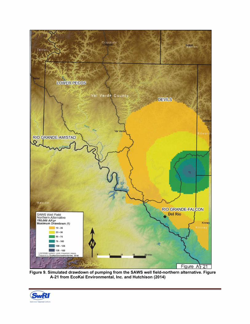
Figure 9. Simulated drawdown of pumping from the SAWS well field-northern alternative. Figure
A-21 from EcoKai Environmental, Inc. and Hutchison (2014)
Groundwater Management Zones
Weinberg (2018) notes the following:
“Based on our review of available data, Val Verde County has sufficient hydrogeologic variability to support the establishment of aquifer management zones in the event a groundwater conservation district is established. Four separate groundwater management zones, based on approximate watershed boundaries, could be defined in Val Verde County as shown in Figure 8-3. Groundwater contributing to flow in the Pecos River, Devils River, and Sycamore/San Felipe Creek drainages occupies generally separate flow systems.”
Figure 8-3 from Weinberg (2018) is reproduced here as Figure 10.
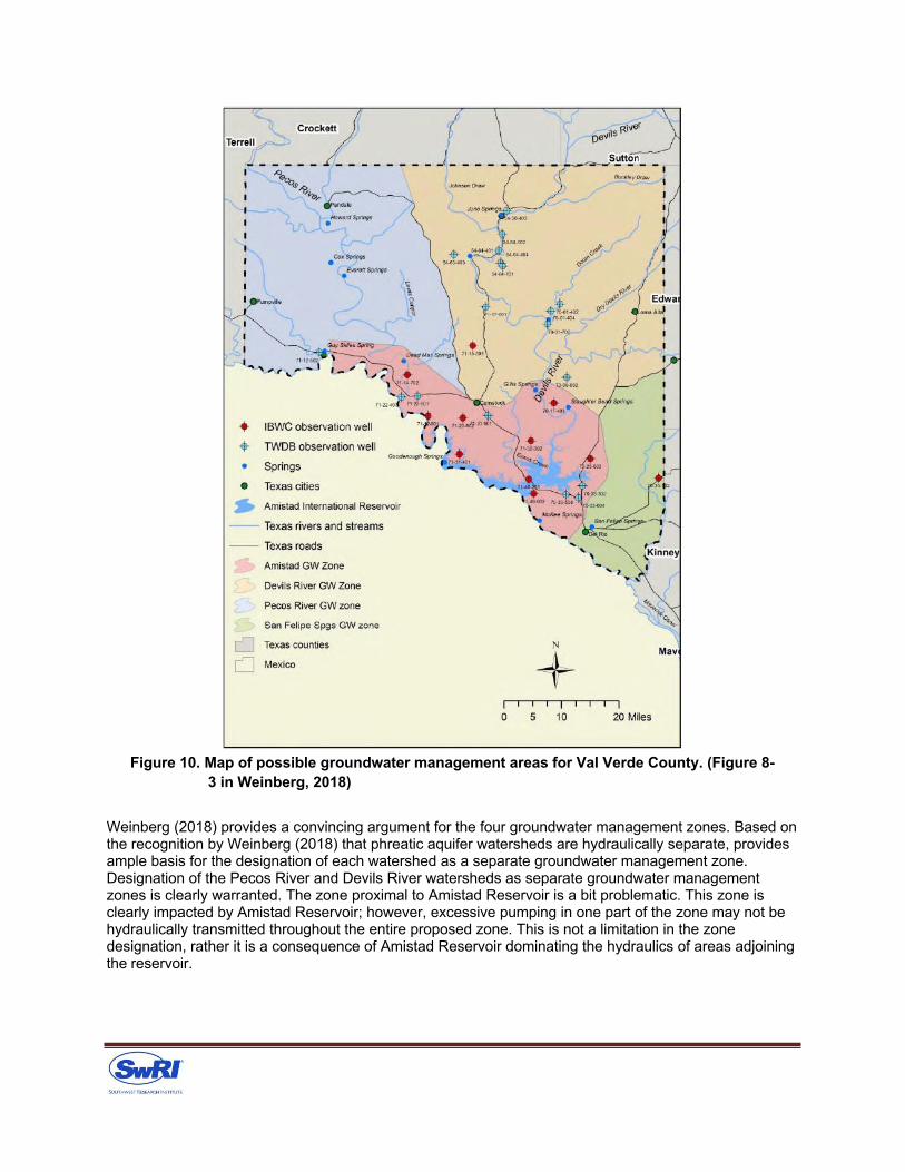
Figure 10. Map of possible groundwater management areas for Val Verde County. (Figure 8-3 in Weinberg, 2018)
Weinberg (2018) provides a convincing argument for the four groundwater management zones. Based on the recognition by Weinberg (2018) that phreatic aquifer watersheds are hydraulically separate, provides ample basis for the designation of each watershed as a separate groundwater management zone. Designation of the Pecos River and Devils River watersheds as separate groundwater management zones is clearly warranted. The zone proximal to Amistad Reservoir is a bit problematic. This zone is clearly impacted by Amistad Reservoir; however, excessive pumping in one part of the zone may not be hydraulically transmitted throughout the entire proposed zone. This is not a limitation in the zone designation, rather it is a consequence of Amistad Reservoir dominating the hydraulics of areas adjoining the reservoir.
The remaining zone to the southeast could be modified from what is proposed in Figure 10 (figure 8-3 in Weinberg, 2018). Analyses conducted by staff at SwRI suggest the designation of Sycamore Creek watershed as separate from the zone containing San Felipe Springs (Green et al., 2014; Toll et al., 2017). Sufficient evidence suggests parsing out Sycamore Creek watershed from San Felipe Springs.
One source of uncertainty in these zone designations is to identify the capture area that provides water for San Felipe Springs. The surface watershed that contains San Felipe Springs is only 53 mi2. Weinberg (2018) and others correctly note that discharge at San Felipe Springs increased subsequent to construction and filling of Amistad Reservoir. Given that San Felipe Springs is located downdip in the Edwards-Trinity Aquifer and is likely sourced from the confined portion of the Edwards-Trinity Aquifer, discharge at San Felipe Springs is likely sourced from a comingled source of confined aquifers that underlie an area that extends well beyond the extent of the surface watershed coincident with San Felipe Springs. Additional investigation could clarify the extent of this source area; however, this added detail is not deemed necessary to go forward in establishing groundwater management zones.
This perspective that the source area for San Felipe Springs is greater than the 53 mi2 watershed is supported by the observation that discharge at San Felipe Springs is augmented by Amistad Reservoir. Thus, if additional pumping were to occur in the capture zone of San Felipe Springs, some discharge to the springs would be offset by additional recharge from Amistad Reservoir. Understanding the intricacies of this hydraulic relationship is not critical to designating San Felipe Springs to be part of the Amistad Groundwater Zone and designating the area to the east to be part of the Sycamore Creek groundwater management zone.
Weinberg (2018) proposes the use of a combination of index wells and river gauges as hydrologic triggers. The designation of a river gauge would be appropriate for each of the three watershed management zones. San Felipe Springs discharge could be designated as the trigger for the Amistad groundwater management area, even though it is understood that the impact of pumping at the west end of this management zone would be muted or subdued in terms of its effect on discharge at San Felipe Springs.
Weinberg (2018) states that “Measured flow in the Devils River at Pafford Crossing is influenced by Amistad reservoir water levels and is not a good indicator of conditions in the upper, spring-fed reaches of the river.” This is predicated on the premise that the Pafford Crossing gauge is sufficiently close to Amistad Reservoir that the hydraulic gradient at Pafford Crossing has been altered.
Weinberg (2018) cites groundwater elevation data at well 7017401 as evidence that the river gauge at Pafford Crossing is hydraulically impacted by Amistad Reservoir. Well 7017401 is located approximately 1.6 miles east of Pafford Crossing. There are limited data for well 7017401 at the time Amistad Reservoir was completed (Table 4). There are no groundwater elevation data available for the period 1969-2006; thus, whether the impact of Amistad Reservoir reaches Pafford Crossing and how much of an impact Amistad Reservoir has had at this distance from the reservoir is uncertain. Given the data available (Table 3), the magnitude of the impact on river flow at Pafford Crossing does not appear significant.
This assessment is supported by flow measured at Pafford Crossing (Figure 11) compared with annual precipitation measured at Del Rio International Airport (Figure 12). As illustrated in Figure 11, baseflow at Pafford Crossing increased after Amistad Reservoir was constructed and filled in 1969. This increase in baseflow is consistent with a general increase in annual precipitation observed during the late 1960s

Figure 11. Discharge measured at Pafford Crossing gauge. (IBWC webpage accessed October 2018)
Di scharg e
(cubic
meter/secon
and into the 1970s. The fact that flow measured at Pafford Crossing demonstrated no significant change from the time prior to construction of Amistad Reservoir, suggests that the Pafford Crossing gauge could be a candidate trigger for the Devils River watershed.
Table 3. Data for well 70-17-401 accessed from TWDB on October 11, 2018
Date Depth to Water Groundwater Elevation (ft, msl) 11/9/1965 325.4 1135.6 7/1/1968 329.2 1131.8 7/1/1969 328.5 1132.5
11/20/1969 323 1138 1/9/2006 320.43 1140.57
7/17/2006 322.5 1138.5 10/27/2006 323.01 1137.99 1/22/2007 323.1 1137.9 4/2/2007 316.8 1144.2
7/16/2007 318.64 1142.36 10/15/2007 322.65 1138.35
1/7/2008 319.5 1141.5 4/21/2008 320.58 1140.42 7/7/2008 321.58 1139.42
3/16/2009 321.1 1139.9 9/20/2011 320 1141
The gauge at Pafford Crossing is recommended as a viable trigger gauge for Devils River watershed. Designation of this gauge as the trigger for the Devils River watershed can be reconsidered in the future by comparison with a new gauge located upstream for confirmation that the gauge is at a valid location. If justified, a new gauge location can be designated if appropriate. Nonetheless, the Pafford Crossing gauge is a viable gauge for this purpose.
1000 0
1000
100
196
0 196
2 196
4 196
6 196
8 197
0 197
2 197
4 197
6 197
8 198
0

Figure 12. Precipitation measured at Del Rio International Airport 1920-2000
Because the Val Verde County Model is a porous media model which characterizes the Edwards-Trinity Aquifer as confined, it does not honor the hydraulic separation of the major watersheds in Val Verde County (i.e., Pecos River, Devils River, and Sycamore Creek watersheds). The Val Verde County Model would not be an appropriate tool to simulate the designation of separate hydraulic triggers for each of the four proposed groundwater management zones.
The use of a model in which the hydraulic separation between adjoining watersheds is honored is recommended for use in water-resource management assessments. Watershed-scale models such as the Devils River watershed model by Toll et al. (2017) and the lower Pecos River watershed by Green et al. (2016) are possible candidates for this purpose; however, this is clearly the perspective of SwRI. If these models are not selected for future watershed-scale water-resource analyses, it is suggested that whatever model or models are used should honor the hydraulic separation between adjoining watersheds.
References
Abbott, P.L. 1975. On the hydrology of the Edwards Limestone, south-central Texas. J. Hydrology. 24. pp. 251-269.
Allen, D.J., L.J. Brewerton, L.M. Coleby, B.R. Gibbs, M.A. Lewis, S.J. Wagstaff, and A.T. Williams. 1997. The physical properties of major aquifers in England and Wales. British Geological Survey Technical Report WD/97/34. 312 p.
Bazan, R., B.P. Wilcox, C. Munster, M. Gary. 2012. Large-scale rainfall simulation over shallow caves– Part II: effect of shrub removal. Ecohydrology
Brune, G. 1975. Major and historical springs of Texas. Texas Water Development Board. Report 189.
Brune, G. 1981. Springs of Texas, volume 1: Fort Worth, Texas, Branch-Smith, Inc. Dearen, P. 2011. Devils River: Treacherous Twin to the Pecos, 1535-1900 TCU Press. Fort Worth, Texas.
Eco-Kai Environmental, Inc. and W.R. Hutchison. 2014. Hydrogeological study for Val Verde County and City of Del Rio, Texas, final draft report prepared for Val Verde County and the City of Del Rio, 152 pp; at www.edwardsaquifer.net/pdf/Val_Verde_May_2014.pdf, accessed October 6, 2017.
Fratesi, S.E., R.T. Green, F.P. Bertetti, R.N. McGinnis, N. Toll, H. Başağaoğlu, L. Gergen, J. Winterle, Y. Cabeza, and J. Carrera. 2015. Development of a finite-element method groundwater flow model of the Edwards Aquifer: Final Report. Southwest Research Institute. Conducted for the Edwards Aquifer Authority. 180 p.
Gabrošek, F. 2002. Evolution of Karst: From Prekarst to Cessation. Postojna-Ljubljana. ISBN 961-6358-63-4.
Green, R.T. and F.P. Bertetti. 2010. Investigating the Water Resources of the Western Edwards-Trinity Aquifer. Contract Report Prepared for the Sutton County Groundwater Conservation District. 79 p.
Green, R., F. Bertetti, and M. Hernandez. 2012. Recharge Variability In Semi-Arid climates. Nature Education Knowledge 3(10):34. http://www.nature.com/scitable/knowledge/library/recharge-variability-in-semi-arid-climates-26169682
Green, R.T., F.P. Bertetti, and M.S. Miller. 2014. Focused Groundwater Flow in a Carbonate Aquifer in a Semi-Arid Environment. Journal of Hydrology. 517:284–297. doi: 10.1016/j.jhydrol.2014.05.015
Green, R.T., N. Toll, and F.P. Bertetti. 2015. Sustainable Yield of a Carbonate Aquifer Dominated by Preferential Flow: Devils River Watershed, South Texas, USA. Final Report. Contract Report for the Nueces River Authority.
Green, R.T., N. Toll, and F.P. Bertetti. 2016. Develop a Groundwater Flow Model to Understand the Groundwater Resources of the Lower Pecos River Watershed. Contract Report for the City of Laredo. Final Report.
Hutchison, W.R., I.C. Jones, and R. Anaya. 2011. Update of the Groundwater Availability Model for the Edwards-Trinity (Plateau) and Pecos Valley Aquifers of Texas. Texas Water Development Board. 61 p.
Inglehart, H.H. 1967. Occurrence and quality of ground water in Crockett County, Texas. Report 47. Texas Water Development Board. 61 p.
Klimchouk, A.B., D.C. Ford, A.N. Palmer, and W. Dreybrodt (editors) with members of the Commission on Karst Hydrogeology and Speleogenesis. International Union of Speleology. January 2000 Edition. National Speleological Society, Huntsville, Alabama 527 p., ISBN 1-879961-09-1.
MacDonald, A.M., and D.J. Allen. 2001. Aquifer properties of the Chalk of England. Quarterly J. of Engineering Geology and Hydrogeology. 34. pp. 371-384.
Mocochain, L., P. Audra, G. Clauzon, O. Bellier, J.-Y. Bigot, O. Parize, and P. Monteil. 2009. The effect of river dynamics induced by the Messinian Salinity Crisis on karst landscape and caves: Example of the Lower Ardèche river (mid Rhône valley). Geomorphology. 106. pp. 46-61.
Muller, D.A. and H.E. Crouch. 1971. Water well and ground-water chemical analysis data, Schleicher County, Texas. Report 132. Texas Water Development Board.
Muller, D.A. and J.R. Pool. 1972. Water well and ground-water chemical analysis data, Sutton County, Texas. Report 147. Texas Water Development Board.
Scanlon, B. R., K. E. Keese, A. L. Flint, L. E. Flint, C. B. Gaye, M. Edmunds, and I. Simmers. 2006. Global synthesis of groundwater recharge in semiarid and arid regions. Hydrological Processes 20:3335-3370.
Stothoff, S.A. 1997. Sensitivity of long-term bare soil infiltration simulations to hydraulic properties in an arid environment. Wat. Res. Res. 33(4). 547-558.
Texas Board of Water Engineers. 1960. Channel gain and loss investigations, Texas streams, 1918– 1958: Texas Board of Water Engineers. Bulletin 5807–D, 270 p.
Toll, N., S.B. Fratesi, R.T. Green, F.P. Bertetti, and R. Nunu. 2017. Water-Resource Management of the Devils River Watershed Final Report. Contract Report for the Devils River Conservancy.
Weinberg, A. 2018. Overview of Groundwater Conditions in Val Verde County, Texas” Texas Water Development Board. 152 p.
Wilcox, B.P. and Y. Hang. 2010. Woody plant encroachment paradox: Rivers rebound as degraded lands convert to woodlands. Geophysical Research Letters. VOL. 37, L07402, doi:10.1029/2009GL041929.
Woodruff, C.M., Jr. and P.L. Abbott. 1979. Drainage-basin evolution and aquifer development in a karstic limestone terrain, South-Central Texas, USA. Earth Surface Processes. 4. pp. 319-334.

Woodruff, C. M., Jr. and P.L. Abbott. 1986. Stream piracy and evolution of the Edwards Aquifer along the Balcones Escarpment, Central Texas. In Abbott, P.L. and Woodruff, C.M. Jr. eds., The Balcones Escarpment, Central Texas: Geological Society of America. pp. 77-90.
Worthington, S.R.H. 2007. Ground-water residence times in unconfined carbonate aquifers. Journal of Cave and Karst Studies. 69(1). pp. 94–102.
Zhang, L., W. R. Dawes, and G. R. Walker 2001. Response of mean annual evapotranspiration to vegetation changes at catchment scale, Water Resour. Res., 37(3), 701–708, doi:10.1029/2000WR9003

1101 Satellite View | Suite 301 | Round Rock, Texas 78665 | (512) 962-7660 | www.lrewater.com
1101 Satellite View | Suite 301 | Round Rock, Texas 78665 | (512) 962-7660 | www.lrewater.com
T E C H N I C A L M E M O R A N D U M
TO: Mr. Ed McCarthy, Attorney for Val Verde County Landowner Interests
FROM: Michael R. Keester, P.G. and Jordan Furnans, Ph.D., P.E., P.G.
SUBJECT:
DATE:
Reviewof Water-Resource Management of the Devils River Watershed Report by Tolland others (2017)
September 10, 2018
On August 29, 2017, Southwest Research Institute (2017) published a press release indicating they completed a study that “provides detailed models linking groundwater in a Texas aquifer to the surface flows in one of the state’s most pristine rivers.” The press release stated that the study provides the first means for water managers to evaluate the relationship between pumping and spring flows. While not identified in the press release, the study that it refers to is the Water- Resource Management of the Devils River Watershed report (Toll and others, 2017) which was presented the following day at the Texas Alliance of Groundwater Districts Groundwater Summit (Green and others, 2017).
As requested, LRE Water, LLC conducted a preliminary review of the work documented in the report. As part of our review, we also considered previous hydrogeologic investigations conducted within the Devils River watershed, Val Verde County, and the Edwards-Trinity (Plateau) Aquifer along with our professional experience in surface water and groundwater modeling. Based on the information reviewed, we developed professional opinions regarding the modeling and results reported by Toll and others (2017). Importantly, as a preliminary review it was beyond the scope of our work to fully investigate all aspects of the reported modeling and we focused on those issues that appeared most significant to the applicability and credibility of the model.
Toll and others (2017) state that the “Devils River watershed basin is being threatened by proposed large-scale groundwater export projects.” To better understand the perceived threat, they conducted their study for the purpose of evaluating how pumping in the upper Devils River watershed would affect downstream discharge in the Devils River (Figure 1 is a location map for reference). To conduct the evaluation, the report authors developed what they called an integrated surface-water/groundwater model.
Conceptual Model
A conceptual model is simply a description the modeler’s understanding of the flow system. This understanding will then guide the collection of data to define the model structure, parameters, boundary conditions, and calibration. It is an important step in developing the subsequent numerical model and should be guided by the model’s purpose (Anderson and Woessner, 2002).
1101 Satellite View | Suite 301 | Round Rock, Texas 78665 | (512) 962-7660 | www.lrewater.com
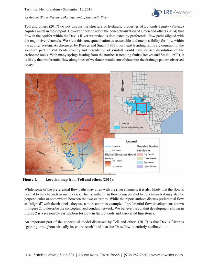
Technical Memorandum – September 10, 2018
ew of Water-Resource Management of the Devils River Revi
Toll and others (2017) do not discuss the structure or hydraulic properties of Edwards-Trinity (Plateau) Aquifer much in their report. However, they do adopt the conceptualization of Green and others (2014) that flow in the aquifer within the Devils River watershed is dominated by preferential flow paths aligned with the major river channels. We view this conceptualization as reasonable and one possibility for flow within the aquifer system. As discussed by Reeves and Small (1973), northeast trending faults are common in the southern part of Val Verde County and percolation of rainfall would have caused dissolution of the carbonate rocks. With many springs issuing from the northeast trending faults (Reeves and Small, 1973), it is likely that preferential flow along lines of weakness would consolidate into the drainage pattern observed today.
Figure 1. Location map from Toll and others (2017).
While some of the preferential flow paths may align with the river channels, it is also likely that the flow is normal to the channels in many cases. That is, rather than flow being parallel to the channels it may also be perpendicular or somewhere between the two extremes. While the report authors discuss preferential flow as “aligned” with the channels, they use a more complex example of preferential flow development, shown in Figure 2, to describe the conceptualized conduit network. We believe the conduit development shown in Figure 2 is a reasonable assumption for flow in the Edwards and associated limestones.
An important part of the conceptual model discussed by Toll and others (2017) is that Devils River is “gaining throughout virtually its entire reach” and that the “baseflow is entirely attributed to
1101 Satellite View | Suite 301 | Round Rock, Texas 78665 | (512) 962-7660 | www.lrewater.com
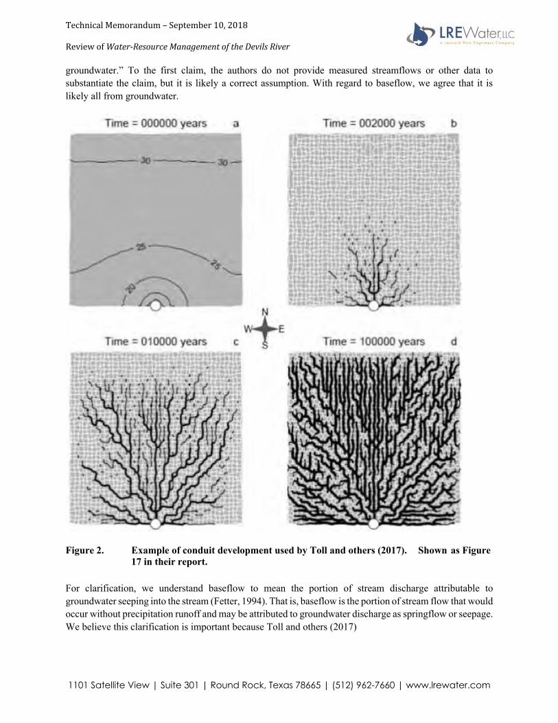
Technical Memorandum – September 10, 2018
ew of Water-Resource Management of the Devils River Revi
groundwater.” To the first claim, the authors do not provide measured streamflows or other data to substantiate the claim, but it is likely a correct assumption. With regard to baseflow, we agree that it is likely all from groundwater.
Figure 2. Example of conduit development used by Toll and others (2017). Shown as Figure 17 in their report.
For clarification, we understand baseflow to mean the portion of stream discharge attributable to groundwater seeping into the stream (Fetter, 1994). That is, baseflow is the portion of stream flow that would occur without precipitation runoff and may be attributed to groundwater discharge as springflow or seepage. We believe this clarification is important because Toll and others (2017)
1101 Satellite View | Suite 301 | Round Rock, Texas 78665 | (512) 962-7660 | www.lrewater.com
Technical Memorandum – September 10, 2018
ew of Water-Resource Management of the Devils River Revi
state that “[c]apturing the dynamic response of baseflow in the river is a prime objective” of their project. While we understand streamflows are dynamic, their statement suggests that they believe the groundwater discharge to the streams is as dynamic as streamflow changes are to runoff events. We feel this apparent view of groundwater discharge being highly dynamic is an incorrect conceptualization of the flow system and is contrary to accepted hydrogeological definition.
Regarding the flow features, Toll and others (2017) state that they are located within one mile of streams and rivers at depths less than 150 feet. The defined proximity to the streams is based on analysis of reported well yields compared to distance from the river (Green and others, 2014). Reeves and Small (1973) also stated that, based on available data, large capacity wells should be located near major rivers. Due to the likely development pattern of karst features, it is reasonable that there would be greater connectivity between conduits and one would be more likely to intersect a karst feature near the rivers. Regarding the depth, there is ample evidence that karst features can occur at greater depths. For example, a cursory review of the well data from 1973 shows many wells completed to depths greater than 150 feet (Reeves and Small, 1973), which would likely not occur if supplies were available from shallower depths.
As mentioned above, Toll and others (2017) do not discuss analysis of data to develop estimates of the hydraulic properties for the aquifers. For example, there is no discussion of using pumping test data to help constrain estimates of aquifer hydraulic conductivity, transmissivity, or storage coefficient. They reference the conceptual model of Green and others (2014) as the basis for their conceptual model, but the referenced article relates to well yields in relation to the major river channels and does not discuss distribution of aquifer hydraulic properties.
The lack of data analysis to determine a starting point and calibration constraint for the aquifer hydraulic characteristics is a significant concern. The apparent lack of analysis of aquifer properties may indicate that the modelers intended to set the properties in the model to meet their preconceived notion of how groundwater flows through the system rather than letting the data determine how the numerical model would be developed. Also, it prohibits potential users from being informed of the differences between modeled parameters and the measured values at specific locations. Perhaps most importantly, the lack of analysis does not provide constraint on aquifer hydraulic parameters during the model calibration process. The constraints during model calibration are very significant because they will inform the numerical model regarding the spatial distribution of the hydraulic parameters along with the aquifer heterogenity and anisotropy.
Other items that we believe are missing from the conceptual model discussion by Toll and others (2017), but are beyond the scope of this preliminary review, include:
• Aquifer structure such as formation contact elevations and faulting • Vertical flow within the Edwards and associated limestones
1101 Satellite View | Suite 301 | Round Rock, Texas 78665 | (512) 962-7660 | www.lrewater.com
Technical Memorandum – September 10, 2018
ew of Water-Resource Management of the Devils River Revi
• The effect of Lake Amistad on the groundwater conditions in the Devils River basin, including the rise in aquifer water levels documented after completion of Amistad Dam (HDR, 2001; Anaya and Jones, 2009; EcoKai, 2014)
• Aquifer water budget analyses, such as that of William F. Guyton and Associates (1964) or Reeves and Small (1973)
Overall, Toll and others (2017) focus their discussion on features and preferential groundwater flow in the aquifer aligned with rivers. While this conceptualization is partially valid, it does not capture the full complexity of flow within the aquifer. In addition, the focus is to the detriment of considering other important factors within the hydrogeologic system.
SurfaceWater Model
Toll and others (2017) state that they developed the surface-water model using HEC-HMS “to capture river-flow conditions and model land-surface processes, providing recharge to the groundwater model.” While they state that measured discharge was the target for calibration of the surface-water model, they also state that recharge to the groundwater model was “calibrated via the groundwater model” and was a more critical calibration target than measured discharge. However, the surface water model itself is not described very well and it is unclear as to how they calibrated to recharge. In addition, calibration results in the form of statistics that describe how well the model matches observed data were not reported.
To determine recharge to the groundwater system, the model authors used the initial losses and abstractions from the rainfall data used in the surface water model. Toll and others (2017) discuss these calculations in their report, but they do not document how much water the initial losses and abstractions contribute to the groundwater system nor do they document if the amounts are reasonable. To determine reasonability, the authors suggested that surface water discharges resulted from some storm events but not others, implying that the abstractions from the small storm events were accurate, thus providing reasonable assertions that the model accurately determines the portion of precipitation that becomes recharge. However, the report figures showing comparisons between the observed and modeled streamflow suggest uncertainity with regard to model validity. For example, the figures presented by Toll and others (2017), like their Figure15, focus on the comparison between the modeled and measured discharges after the larger storm events, which appear to be decent, but the figures do not really focus on the comparisonsbetween modeled and observed discharge after the minor storm events that have a greater effect on recharge.
The documentation of the surface water model is poor. Without documentation of how much water the initial losses and abstractions contribute to the groundwater system, it is not possible to evaluate the reasonability of the results. Based on their statement that recharge was a critical calibration target, it is not clear if the physical properties assigned in the model were based on measured or realistic values to determine potential recharge or if the property values were assigned to match a
1101 Satellite View | Suite 301 | Round Rock, Texas 78665 | (512) 962-7660 | www.lrewater.com
Technical Memorandum – September 10, 2018
ew of Water-Resource Management of the Devils River Revi
preconceived recharge amount regardless of whether they were realistic for the physical conditions.
GroundwaterModel
Toll and others (2017) used MODFLOW-USG (Panday and others, 2013) as the numerical code to simulate the aquifer system. Unlike the model grid in previous versions of MODFLOW, the selected code allows for grid refinement at specific areas where greater resolution in the model results is desired. We believe the code selected is appropriate for providing the additional detail along streams; however, it is important to remember that like the rest of the MODFLOW family, the code uses equations based on porous media flow, not fractures or conduits. While the use of MODFLOW to represent a karst system is common and accepted, extra care must be taken to ensure the aquifer if represent appropriately.
Model Grid and Boundary Conditions
Beyond describing the numerical model as having two layers with layer one representing the Edwards and associated limestones and layer two representing the Trinity, there is little discussion regarding the model grid. That is, grid dimensions are not provided nor is the level of refinement along the streams. Upon visual inspection of the figures provided in the report, we estimate the largest grid cells are 1,500 meters (4,921 feet) on each side (assuming map units are consistent with units used elsewhere in the report). There also appear to be two levels of refinement withthe cells proximal to the stream being 375 meters (1,230 feet) on each side and cells a short distance from the streams being 750 meters (2,461 feet) on each side.
The top of layer one appears to be defined by a digital elevation model to represent the ground surface which is standard for groundwater flow modeling. However, Toll and others (2017) defined the base of layer one as “40 meters below the bottom of the incised stream channels.” It appears that they selected this depth to correlate with their conceptual model that conduit formation only occurs within 100 to 150 feet of land surface. We believe it would have been more representative to define the base of the layer using existing maps of the formation structure such as those by Reeves and Small (1973). Additional vertical refinement using MODFLOW-USG could then have been added to represent and test the conceptualization.
To simulate the streams in the model, the authors used drain boundary conditions. A limitation of the drain boundary condition is that it does not allow for flow back into the aquifer. To more realistically model the Devils River and its tributaries, we believe it would be more appropriate to use the River or Streamflow Routing package in MODFLOW which would allow water movement both into and out of the aquifer and stream. Allowing water to move in and out of the stream would better serve the model’s purpose of evaluating the effects of pumping on streamflow by allowing the stream to contribute water to the aquifer if water levels are drawn down by a well field. Rather than setting up the model so that wells would only capture water that would otherwise discharge, a more robust simulation of the streams would better represent the physical processes by
1101 Satellite View | Suite 301 | Round Rock, Texas 78665 | (512) 962-7660 | www.lrewater.com

(16 cells perlevel 0)
Technical Memorandum – September 10, 2018
ew of Water-Resource Management of the Devils River Revi
potentially allowing streamflow to enter the aquifer if a well field causes water levels to decline near a stream. In addition, the Streamflow Routing package would allow the modelers to input runoff results from the surface water model to better simulate the portion of flow from runoff as well as baseflow.
Model Hydraulic Parameters
For the hydraulic characteristics of the model aquifers, Toll and others (2017) assigned hydraulic conductivity (“K”) and specific yield (“Sy”) as follows:
• For matrix cells in layer one o K = 2 m/d (6.6 ft/d) o Sy = 0.012
• For conduit cells in layer one (that is, cells within 200 m (656 ft) of a stream) o K = 100 m/d (328 ft/d) for low-order stream tributaries o K = 1,000 m/d (3,280 ft/d) for higher order streams o Sy = 0.0001
• For matrix of layer two o K =1 m/d (3.3 ft/d) o Sy = 0.012 o Specific Storage = 0.00001 m-1
While it is common for a karst system to have lower specific yield and specific storage values than a sand aquifer, the value of 0.0001 for the conduit portion of the system is questionable when compared to the value used for the matrix (that is, non-preferential flow) areas of the aquifer. To check what the values used could mean for layer one of the flow system, we used our estimate of the grid dimensions, the thickness of the aquifer as 40 meters, and the specific yield values to calculate the volume of drainable water in a grid cell. Table 1 summarizes the calculated values assuming a fully saturated thickness.
Table 1. Calculated drainable volume based on reported specific yield values used in theDevils River Watershed model.
Grid Cell Side Cell Volume, Specific Drainable Volume per Refinement Level Length, ft Acre-Feet Yield Level 0 Area, Acre-Feet
0 4,921 72,964 0.012 875.6
1 (4 cells per level 0) 2,461 18,241 0.0001 7.3
2 1,230 4,560 0.0001 7.3
1101 Satellite View | Suite 301 | Round Rock, Texas 78665 | (512) 962-7660 | www.lrewater.com
Technical Memorandum – September 10, 2018
ew of Water-Resource Management of the Devils River ReviTo ensure the calculations were comparable, the drainable volumes shown in Table 1 represent the same unit area. As the table illustrates, the drainable volume in the conduit cells is two orders of magnitude less than the non-conduit cells. The comparable low drainable volume in the conduit cells is highly questionable if it is to be consistent with the proposed preferential flow near the streams.
Unlike a porous media aquifer, water is stored and flows through fractures and conduits in the karst system. The calculated drainable volumes represent the minimum amount of open area within each grid block. While an over-simplification, if we assume fractures at regularly spaced intervals in the grid block, we can calculate the number of fractures and the average width of the fractures to achieve the minimum open area. For example, at 100 centimeter spacing there would 1,499 fractures in a grid refinement level 0 grid block and the average fracture width would be 1.2 centimeters (0.47 inch). Table 2 provides the calculated average fracture width at various fracture densities within a grid block.
Understanding how the specific yield values may translate into fracture width at various fracture densities, as shown in Table 2, is important when modeling a karst system using a porous media modeling code. The importance is related to the cubic law for fracture flow that defines the hydraulic conductivity of the rock matrix based on fracture width (Snow, 1968). The relation is defined using the following formula:
$%&'2! = 12*
where $% is the density of water, & is acceleration due to gravity, * is the viscosity of the water, and ' is the fracture width. Assuming constant fluid properties, the fracture width controls the hydraulic conductivity of the system and small changes in the width can change the hydraulic conductivity significantly. Using the average fracture widths shown in Table 2, we calculated the
1101 Satellite View | Suite 301 | Round Rock, Texas 78665 | (512) 962-7660 | www.lrewater.com
Technical Memorandum – September 10, 2018
ew of Water-Resource Management of the Devils River Revi
resulting hydraulic conductivity (in feet per day) assuming water at 20°C for comparison with the values used in the model (see Table 3).
Table 3. Calculated hydraulic conductivity for average fracture width at variousfracture densities within a grid block.
Calculated Hydraulic Conductivity (ft/d) Toll and others (2017) Hydraulic Conductivity
(ft/d) 6.6
Grid Average Distance between Fractures (cm) Refinement Level 1 10 100 1,000
0 3,311 331,200 33,200,000 3,360,000,000
1 0.23 23 2,300 236,000 (4 cells per level 0)
328 to 3,280
2 0.23 23 2,300 236,000 (16 cells per level 0)
328 to 3,280
Calculated hydraulic conductivity values based on the required open volume in the rocks to meet the assigned specific yield do not appear to correlate with the hydraulic conductivity values assigned by Toll and others (2017). For example, to achieve the hydraulic conductivity of the matrix cells (grid refinement level 0) would require an average fracture spacing of just over0.001 cm (10 micrometers or 0.0004 inches). This extremely small average spacing would result in an average fracture width of about 0.000012 cm (0.12 micrometers or 0.000005 inches) which is 500 times smaller than the width of normal human hair. The required average fracture width is essentially equivalent to the pore throat size of a tight sandstone (Nelson, 2009) with a resulting grain size of a fine silt (Fetter, 1994) neither of which are accurate descriptions of the rocks that make up the Edwards-Trinity (Plateau) Aquifer (Anaya and Jones, 2009). While the cubic law as shown above is known to overestimate hydraulic conductivity as it does not account for fracture roughness or tortuosity, it has been shown as valid in several studies [see discussion in Domenico and Schwartz (1998)]. Based on the information provided in the report, the aquifer parameters used in the model are not appropriate.
Model Calibration
Toll and others (2017) define the steady-state calibration of the model as the 16-year period from 2000 through 2015. Typically steady state refers to a simulation that represents the aquifer at a time prior to any significant stresses on the aquifer, such as pumping. It is possible that the authors incorrectly identified the period of time used for steady-state calibration as one of their figures contains the label “Observed Head 1960’s Data” [see Figure 23 in Toll and others (2017)]. If the authors did use the 16-year period for calibration, they would need to include current pumping in the model as part of the calibration. In addition, the fluctuations of Lake Amistad would need to be included due to the strong correlation of aquifer water levels and reservoir levels (HDR, 2001; Anaya and Jones, 2009; EcoKai, 2014). The most appropriate representation of steady state would
1101 Satellite View | Suite 301 | Round Rock, Texas 78665 | (512) 962-7660 | www.lrewater.com
Technical Memorandum – September 10, 2018
ew of Water-Resource Management of the Devils River Revi
be to follow the method used by HDR (2001) and simulate aquifer conditions prior to the construction of Amistad Dam.
Regarding the degree of calibration, the only information provided is a statement that simulated water levels were within 25 to 30 feet of measured water levels and a plot of the simulated versus measured water levels. Calibration statistics for the model, which would allow users to assess the model’s ability to match historical conditions, were not reported. These statistics are standard for any credible model and the lack of reporting suggests the model may be poorly calibrated to historical conditions. Visual review of the plot of simulated versus measured water levels for their steady-state period indicates some bias in the model; modeled water levels between 350 and 500 meters appear to be biased higher than measured levels and modeled water levels between 500 and 675 meters appear to be biased lower than measured levels (see Figure 3).
In assessing contributions to baseflow, the biases could have a significant impact. An overestimation bias results in water levels being higher than measured and potentially greater amounts of discharge to the surface water features if they are intersected by the groundwater level. Conversely, with an underestimation bias there may be areas where discharge should occur, but the modeled levels do not reach the elevation of the discharge location. We believe the apparent biases should be addressed and calibrations statistics reported.
For the transient calibration (that is, calibration of the model to historical measured conditions), the modelers refer to a 16-year period, but it is not clear how the period differs from their description of the steady-state calibration. Nonetheless, the available data allow for a much longer transient calibration period (HDR, 2001; EcoKai, 2014). To better understand the hydraulics of the aquifer system, Toll and others (2017) should have performed a transient calibration that began prior to the construction of Amistad Dam and used the changes in aquifer water levels as Lake Amistad filled to inform the model parameters.
No comparison of measured versus simulated water levels is provided or discussed by the modelers for their transient calibration. It is not possible to provide any meaningful assessment of the transient model calibration due to the absence of information in the model report. Based on the bias evident in the so-called steady-state calibration, it is likely that the model bias is also present in the transient model.
The modelers state that the “coupled surface-water and groundwater model produces a baseflow that responds much better with regards to the variation in magnitude of discharge” at Pafford Crossing. In support of their statement they present Figure 4 in which they identify the results as baseflow. However, the results shown on Figure 4 appear to be measurements of streamflow at the Pafford Crossing gaging station which would include contributions from runoff. As there is no discussion of how the baseflow component of flow is being calculated from the drain cell results, the statement that the model produces a better baseflow response is not supported by the reported results.
1101 Satellite View | Suite 301 | Round Rock, Texas 78665 | (512) 962-7660 | www.lrewater.com

Technical Memorandum – September 10, 2018
ew of Water-Resource Management of the Devils River Revi
Underestimation
Overestimation
Figure 3. Measured (that is, observed) versus modeled water levels (that is, head) reported by Toll and others (2017). Shown as Figure 23 in their report. Note that the figure indicatesthe observed water levels are from the 1960s, but the report text states they are from2000-2015.
1101 Satellite View | Suite 301 | Round Rock, Texas 78665 | (512) 962-7660 | www.lrewater.com
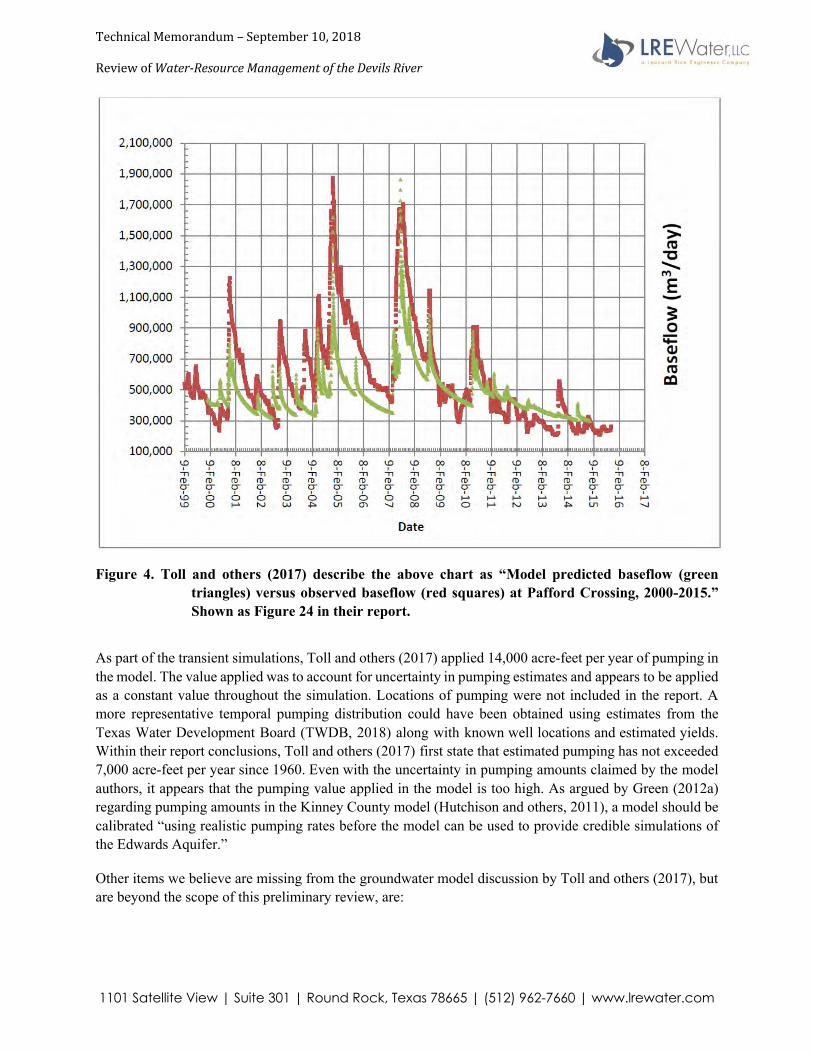
Technical Memorandum – September 10, 2018
ew of Water-Resource Management of the Devils River Revi
Figure 4. Toll and others (2017) describe the above chart as “Model predicted baseflow (green triangles) versus observed baseflow (red squares) at Pafford Crossing, 2000-2015.” Shown as Figure 24 in their report.
As part of the transient simulations, Toll and others (2017) applied 14,000 acre-feet per year of pumping in the model. The value applied was to account for uncertainty in pumping estimates and appears to be applied as a constant value throughout the simulation. Locations of pumping were not included in the report. A more representative temporal pumping distribution could have been obtained using estimates from the Texas Water Development Board (TWDB, 2018) along with known well locations and estimated yields. Within their report conclusions, Toll and others (2017) first state that estimated pumping has not exceeded 7,000 acre-feet per year since 1960. Even with the uncertainty in pumping amounts claimed by the model authors, it appears that the pumping value applied in the model is too high. As argued by Green (2012a) regarding pumping amounts in the Kinney County model (Hutchison and others, 2011), a model should be calibrated “using realistic pumping rates before the model can be used to provide credible simulations of the Edwards Aquifer.”
Other items we believe are missing from the groundwater model discussion by Toll and others (2017), but are beyond the scope of this preliminary review, are:
1101 Satellite View | Suite 301 | Round Rock, Texas 78665 | (512) 962-7660 | www.lrewater.com

Technical Memorandum – September 10, 2018
ew of Water-Resource Management of the Devils River Revi
• The water budget results from the model, which is standard for any credible model, to ascertain if the results are reasonable. Without the water budget results, it is impossible to determine if the model properly balances water inflow and outflow, resulting in zero-net creation or loss of water. Such a condition is a requirement for a realistic and properly developed groundwater model
• Sensitivity of model parameters to the calibration results which is standard for any credible model to inform user of how much a small change in a parameter may affect the model simulation results
• Connection between the formations of the Edwards-Trinity (Plateau) Aquifer
Though ample information exists to develop a numerical model of the Devils River watershed, the model reported by Toll and others (2017) does not appear to incorporate all the available information on the aquifer system. By focusing on a single component of the system, the resulting model, as reported, does not appear to be a realistic representation of the aquifer system and its interaction with the local surface water features.
Discussion The following provides a brief discussion of some of the issues identified in the model report.
Aquifer Hydraulic Properties and Pumping
In their observations, Toll and others (2017) state that “[g]roundwater flow and sustainability in the Devils River watershed appears to be controlled by the morphology of the area more than the bulk hydraulic properties of the rocks.” They claim that discharge to the Devils River was replicated only through the way they set up the “distribution, morphology, and alignment of conduits relative to the watershed topography.” However, the discharge they illustrate is of total streamflow which is not reflective of baseflow to the Devils River. Though Toll and others (2017) state that the model “replicates both flashy flow and low baseflow in the Devils River” as a coupled surface-water/groundwater model, they consistently address all flow in the river as baseflow (that is, the flow attributed to groundwater discharge). Based on the reported information, they setup the structure and hydraulics of the model to reproduce streamflow, but the hydraulic properties assigned to the aquifer are not consistent with their conceptualization nor are they shown to be realistic or comparable to aquifer test results. In particular, the low specific yield used along the streams is not consistent with the conduits they suggest exist and it would require lower hydraulic conductivity values for a karst aquifer.
One significant effect of using a low specific yield near the streams is that it increases the drawdown associated with pumping. For example, using the specific yield of 0.0001 that Toll and others (2017) assigned to the conduit cells along with hydraulic conductivity value from the model would result in more that five feet of drawdown one mile away from a well pumping 500 gallons per minute for three days. Using the same parameters, but increasing the specific yield to 0.001
1101 Satellite View | Suite 301 | Round Rock, Texas 78665 | (512) 962-7660 | www.lrewater.com

Technical Memorandum – September 10, 2018
ew of Water-Resource Management of the Devils River Revi
reduces the drawdown to essentially zero at one mile and increasing the value to 0.01 reduces the extent of drawdown to less than one-half mile. The parameterization of the model hydraulic parameters has a significant impact how pumping effects are simulated.
The simulated effects of pumping in the model is a critical issue for the model. With the opinion of Toll and others (2017) being that the “Devils River watershed basin is being threatened by proposed large-scale groundwater export projects” it is important that they accurately represent the effects of pumping in their model. However, as demonstrated previously, the specific yields assigned in their model are nonsensical when compared to the hydraulic conductivity for a karst system.
Toll and others (2017) may have been able to address some to the issues with the hydraulic properties with a robust calibration of the model. However, based on the information reported, the calibration appears to be poorly constrained by available data. In addition, the calibration does not consider the significant effect the completion of Amistad Dam had on water levels within the watershed (HDR, 2001; EcoKai, 2014). Also, the 14,000 acre-feet per year of pumping reportedly included for the transient calibration is double the maximum amount Toll and others (2017) state has occurred since 1960 which by itself, per the opinion of Green (2012a) regarding pumping amounts in the Kinney County model (Hutchison and others, 2011), makes the model not credible.
Beaver Lake
In their report, Toll and others (2017) point to the simulation results around Beaver Lake as an illustration of the impacts of pumping on the Devils River watershed. They claim that their “transient calibration of the groundwater flow model predicted that spring discharges occur further upstream in the Devils River basin then currently observed.” They imply that the simulated springflow is occurring at Beaver Lake and represents the accounts of continuous discharge that occurred there at sometimes between 1535 and 1900. They then claim that it is the pumping within the Devils River watershed that has caused this springflow to cease and move downstream.
There is no reason to doubt the historical accounts of flow at Beaver Lake. However, the reference cited by Toll and others (2017) focuses on a nearly 400 hundred year historical period where the flow may have occurred during periods of wetter conditions such as those used by Groundwater Management Area 9 to model groundwater availability (Hutchison, 2010). More recent accounts discussed by the current landowners indicate that there has not been significant groundwater discharge at Beaver Lake in over a century with flow only occurring intermittently following flooding on the Devils River (Hodge, 2018). Appendix 1 contains a copy of the local landowners account of recent conditions at Beaver Lake.
With regard to the simulated flow at Beaver Lake, it is important to recall the underestimation bias in the model for elevations above 500 meters mean sea level (1,640 feet mean sea level). The simulated flow to Beaver Lake occurs when the modelers remove all pumping from the model
1101 Satellite View | Suite 301 | Round Rock, Texas 78665 | (512) 962-7660 | www.lrewater.com
Technical Memorandum – September 10, 2018
ew of Water-Resource Management of the Devils River Revi
which allows simulated water levels rise, intersect land surface, and discharge to the river. However, the transient model calibration, which includes 14,000 acre-feet per year of pumping, is significantly biased to predict too low of a water level in the higher elevations such as Beaver Lake at approximately 1,710 feet mean sea level. Notwithstanding the other issues with the model, if an appropriate pumping amount were included in the model then water levels may be at or near discharging into Beaver Lake.
Toll and others (2017) only discuss their simulation results with regard to the impacts of pumping on flows at Beaver Lake. While not discussed in their modeled report it is important to note that a long history of measurements from an observation well near Beaver Lake does not correlate to the simulated results. The Texas Water Development Board’s Groundwater Database has water level measurements for State Well Number 54-56-403 dating back to 1955. The most recent measurement (collected in February 2018) showed a water level of 1,700 feet mean sea level. Looking back over more than 60 years of measurements, the water level has remained relatively stable between 1,690 and 1,710 feet mean sea level. That is, the effects of pumping on water levels in the aquifer as simulated by Toll and others (2017) do not appear to match observations.
Summary
There are many significant flaws in the model reported Toll and others (2017). The model report authors conclude that the “model is available to evaluate future water-resource management scenarios to be able to ascertain what impact groundwater extraction would have on downstream river flow.” However, due to numerous apparent flaws, the reported simulation results are not credible and should not be used for planning or assessing impacts of proposed production. To evaluate the potential effects of pumping on the aquifer and its interaction with the Devils River, the model should be reconceptualized to incorporate reasonable aquifer hydraulic parameters, aquifer structure, historical pumping, construction of Amistad Dam, and surface water interaction. The numerical model can then be developed to represent the conceptual model taking into account and reporting all available data and model results so that stakeholders may better understand simulation results, limitations, and uncertainty.
Conclusions
While there are some merits to the conceptual model of the Devils River watershed, development of the numerical model does not reasonably represent the overall aquifer characteristics or the interaction between surface water and groundwater. The following summarizes our conclusions for the conceptual, surface water, and groundwater models.
• The conceptual model does not capture the full complexity of flow within the aquifer. o Development of preferential flow along streams is reasonable for the groundwater flow
system, but it is not necessarily aligned with the channels. o It is unlikely that there is a “dynamic response of baseflow in the river” and it is more
likely that baseflow is a steady contributor to the measured discharge.
1101 Satellite View | Suite 301 | Round Rock, Texas 78665 | (512) 962-7660 | www.lrewater.com

Technical Memorandum – September 10, 2018
ew of Water-Resource Management of the Devils River Revi
o Karst feature development is likely to occur at depths greater than 150 feet below land surface which is contrary to the authors’ conceptual model.
o Aquifer hydraulic properties (transmissivity, hydraulic conductivity, and storage coefficients) as determined from well specific capacity data, pumping tests, or other means are not reported and should be incorporated into the conceptual model.
o As a major feature affecting the groundwater system, the conceptual model should include the effect of Lake Amistad on the groundwater conditions in the Devils River basin.
o Previous investigators, including William F. Guyton and Associates (1964) and Reeves and Small (1973), have reported a conceptual water budget for the system which, if not reevaluated by the model authors, should be incorporated.
• The surface-water model is not described very well. o Recharge was a critical calibration target of the surface-water model, but it is unclear as to
how the model was calibrated to recharge. o The model authors did not report calibration statistics for the model preventing any
quantitative assessment of the model’s ability to match measured data. o Toll and others (2017) focus on the comparison between the modeled and measured
discharges after the larger storm events rather than on the comparisons between modeled and observed discharge after minor storm events that have a greater effect on recharge.
o Due to the poor documentation, it is unknown if the physical properties in the model are realistic and provide a reasonable representation of potential recharge.
• The groundwater model does not appear to be a realistic representation of the aquifer system and its interaction with the local surface water features.
o MODFLOW-USG is an appropriate code for modeling the groundwater system. o Toll and others (2017) defined the base of layer one as 40 meters below the bottom of the
incised channels, but it would have been more representative to define the base of the model layers using available data on the formation structure.
o Rather than using drain cells, it would be more appropriate to use the River or Streamflow Routing package in MODFLOW to model the streams.
o Based on the information provided in the report, the aquifer parameters used inthe model are not appropriate for representing the groundwater flow system nor do they reasonably represent the model authors’ conceptual model.
o The steady-state model reportedly represents a 16-year period from 2000 through 2015 but should have been set up to represent conditions prior to the construction of Amistad Dam.
o The transient period also represents the 16-year period from 2000 through 2015 but includes pumping of 14,000 acre-feet per year which is approximately twice the reported historical pumping value for the area. The transient period should have included pumping as part of the model for calibration.
1101 Satellite View | Suite 301 | Round Rock, Texas 78665 | (512) 962-7660 | www.lrewater.com

Technical Memorandum – September 10, 2018
ew of Water-Resource Management of the Devils River Revi
o The transient calibration period should have started prior to the construction of AmistadDam and used the changes in aquifer water levels as Lake Amistad filled to inform themodel parameters.
o Calibration statistics are not provided for the model. These statistics should be reported toallow readers to understand how well the model matches historical conditions. Calibrationstatistics are standard for any credible model and the lack of reporting suggests the modelmay be poorly calibrated to historical conditions.
o Graphical information provided regarding how well the simulated water levels match themeasured water levels for the steady-state model shows a clear bias in model results.Comparison of modeled and measured water levels for the transient model were notprovided which raises questions regarding the ability of the model to match historicalaquifer conditions.
o Toll and others (2017) consistently equivocate measured surface water discharge at agaging station (flow from groundwater discharge and surface runoff) and baseflow (theportion of streamflow attributed to groundwater discharge only). As there is no discussionof how they calculated the baseflow component from the drain cell results, the claim thatthe model produces a better baseflow response is not supported by the reported results.
o The report should include a discussion of the water budget results from the model. Withoutsuch a discussion, it is unclear if the results are reasonable when compared to water budgetresults from previous investigations such as that of William F. Guyton and Associates(1964) or Reeves and Small (1973)
o Toll and others (2017) should document how sensitive their calibration is to changes inmodel parameters. Such a sensitivity analysis is standard for any credible model. Whilethey claim the model is “relatively insensitive to assignment of hydraulic properties” to theaquifer units, no data are provided to substantiate the claim. Since small changes in specificyield can significantly affect the drawdown associated with pumping, it is unlikely thattheir claim can be substantiated by a standard sensitivity analysis.
o There is no discussion of the hydraulic connection between the formations of the Edwardsand Trinity even though the Trinity is included as a layer in the model. The connectionbetween the modeled aquifers should be documented.
Many of the conclusions stated byToll and others (2017) maybe due to the model bias or boundary conditions. For example, their conclusions regarding springs drying due to pumping could simply be due to a bias in their steady-state calibration or the low specific yield applied near the drain cells, not to mention the artificially high modeled pumping compared to historical conditions. Toll and others (2017) conclusion that “[t]his model clearly demonstrates the strong linkage of groundwater extraction from the watershed on Devils River flow” stems from how the modelwas constructed. That is, the model was constructed to demonstrate a strong linkage between pumping
1101 Satellite View | Suite 301 | Round Rock, Texas 78665 | (512) 962-7660 | www.lrewater.com

Technical Memorandum – September 10, 2018
ew of Water-Resource Management of the Devils River Revi
and stream flow rather than allowing the model development, calibration, and testing process determine if there is a strong linkage, the strength of the linkage, and the uncertainty in the linkage.
This model should be revisited to incorporate reported geologic structure, more robust boundary conditions for surface water flow, realistic hydraulic parameters, pre-Amistad Dam steady-state conditions, a longer transient calibration period, robust calibration, model parameter sensitivity, and uncertainty in the simulation results. Based on the information in the model report, the model in its current state is not a defensible tool and does not credibly meet its purpose of evaluating how pumping in the upper Devils River watershed would affect downstream discharge in the Devils River. Contrary to the model authors claim that the “model is available to evaluate future water- resource management scenarios to be able to ascertain what impact groundwater extraction would have on downstream river flow,” due to numerous apparent flaws, the reported simulation results are not credible and should not be used for planning or assessing impacts of proposed production.
Recommendations Based on our review of the information reported, the model for the Devils River Watershed should be re-conceptualized, re-parameterized, and re-calibrated. To understand the potential effects of groundwater production on surface water flows, we recommend development of a well- documented model that realistically represents the aquifer system and the interaction between surface water and groundwater. As suggested above, a model for the area should incorporate the best available understanding of geologic structure and faulting, more robust boundary conditions for surface water flow, realistic hydraulic parameters, pre-Amistad Dam steady-state conditions, a transient calibration period that extends from pre-Amistad Dam through present time, a robust calibration, and a model parameter sensitivity and uncertainty analysis. To accomplish development of this model, we have included a proposed scope of work that outlines the tasks required which is included as Appendix 2.
We appreciate being able to provide you with this brief assessment. If you have any questions, please contact me at (512) 962-7660.
1101 Satellite View | Suite 301 | Round Rock, Texas 78665 | (512) 962-7660 | www.lrewater.com

Technical Memorandum – September 10, 2018
ew of Water-Resource Management of the Devils River Revi
Geoscientist andEngineerSeals
This report documents the work of the following licensed professional geoscientists and licensed professional engineers with LRE Water, LLC, a licensed professional geoscientist firm in the State of Texas (License No. 50516) and licensed professional engineering firm in the State of Texas (License No. 14368).
Dr. Furnans was responsible for review of the surface-water model.
Jordan Furnans, Ph.D., P.E. P.G. Vice President – Texas Operations
TX PE Firm: #14368 9/10/2018
1101 Satellite View | Suite 301 | Round Rock, Texas 78665 | (512) 962-7660 | www.lrewater.com

Technical Memorandum – September 10, 2018
ew of Water-Resource Management of the Devils River Revi
Bibliography
Anaya, R. and Jones, I., 2009, Groundwater Availability Model for the Edwards-Trinity(Plateau) and Pecos Valley Aquifers of Texas: Texas Water Development Board Report 373, 103 p.
Anderson, M.P. and Woessner, W.W., 2002, Applied Groundwater Modeling: Simulation of Flow and Advective Transport: San Diego, Academic Press,
Domenico, P.A. and Schwartz, F.W., 1998, Physical and Chemical Hydrogeology: (Second Edition) New York, John Wiley & Sons, Inc., 506 p.
EcoKai Environmental, Inc., 2014, Val Verde County / City of Del Rio Hydrogeological Study: Final Draft Report, 66 p.
Fetter, C.W., 1994, Applied Hydrogeology: (Third Edition) Upper Saddle River, New Jersey, Prentice Hall,
Green, R.T., 2012a, Re: Adopted Desired Future Conditions for Val Verde County: Letter dated January 18, 2012 to Ms. Suzanne West, City Attorney, City of Del Rio, 15 p.
Green, R.T., 2012b, Re: Adopted Desired Future Conditions for Val Verde County: Letter dated January 27, 2012 to Ms. Suzanne West, City Attorney, City of Del Rio, 3 p.
Green, R.T. and Bertetti, F.P., 2010a, Investigating the Water Resources of the Western Edwards- Trinity Aquifer: Prepared for Sutton County Groundwater Conservation District, 71 p.
Green, R. and Bertetti, P., 2010b, Edwards-Trinity Aquifer Water Budget Analysis: Status Report Presented to Groundwater Management Area 7, 31 p.
Green, R.T., Bertetti, F.P., and Miller, M.S., 2014, Focused groundwater flow in a carbonate aquifer in a semi-arid environment: Journal of Hydrogeology, v. 517, p. 284-297.
Green, R.T., Fratesi, B., and Toll, N., 2017, Use of Coupled Surface-Water/Groundwater Models in Managing Water Resources: Presentation at the Texas Alliance of Groundwater Districts Groundwater Summit, 59 p.
HDR, 2001, Investigation of a Proposed Well Field in Val Verde County, Texas: Prepared for San Antonio Water System, 64 p.
Hodge, B., 2018, Letter date June 6, 2018 Re: Beaver Lake, Val Verde County: Letter to Ronald T. Green, Ph.D., P.G., Southwest Research Institute, 4 p.
Hutchison, W.R., 2010, GAM Task 10-005: 13 p.
1101 Satellite View | Suite 301 | Round Rock, Texas 78665 | (512) 962-7660 | www.lrewater.com

Technical Memorandum – September 10, 2018
ew of Water-Resource Management of the Devils River Revi
Hutchison, W.R., Shi, J., and Jigmond, M., 2011, Groundwater Flow Model of the Kinney County Area: Texas Water Development Board Alternative Model Report, 219 p.
Nelson, P.H., 2009, Pore-throat sizes in sandstones, tight sandstones, and shales: AAPG Bulletin, v. 93, no. 3, p. 329-340.
Panday, S., Langevin, C.D., Niswonger, R.G., Ibaraki, M., and Hughes, J.D., 2013, MODFLOW- USG version 1: An unstructured grid version of MODFLOW for simulating groundwater flow and tightly coupled processes using a control volume finite-difference formulation: U.S. Geological Survey Techniques and Methods, book 6, chap. A45, 66 p.
Reeves, R.D. and Small, T.A., 1973, Ground-Water Resources of Val Verde County, Texas: Texas Water Development Board Report 172, 144 p.
Snow, D.T., 1968, Rock Fracture Spacings, Openings, and Porosities: Journal of the Soil Mechanics and Foundations Division, v. 94, no. 1, p. 73-92.
Southwest Research Institute, 2017, SwRI study links groundwater with surface water in Devils River,https://www.swri.org/press-release/swri-study-links-groundwater-surface-water-devils-river.
Texas Water Development Board, 2018, Historical Groundwater Pumpage -SumFinal_CountySumPumpage, http://www.twdb.texas.gov/waterplanning/waterusesurvey/historical-pumpage.asp, accessed April 2018.
Toll, N., Fratesi, S.B., Green, R.T., Bertetti, F.P., and Nunu, R., 2017, Water-Resource Management of the Devils River Watershed: Southwest Research Institute - Final Report, 53 p.
William F. Guyton and Associates, 1964, Report on Ground-Water Conditions in the Del Rio Area, Texas: Prepared for Del Rio Utilities Commission, 29 p.
(Note: Appendices 1 and 2 of this memorandum are not reproduced here but are available upon requestfrom the TexasWater Development Board)
1101 Satellite View | Suite 301 | Round Rock, Texas 78665 | (512) 962-7660 | www.lrewater.com