Out-Of-Core Algorithms for

Scientific Visualization and Computer Graphics

Claudio Silva∗ Yi-Jen Chiang† Wagner Correa‡ Jihad El-Sana§ Peter Lindstrom¶

Abstract

Recently, several external memory techniques have been developed for a wide variety of graphics

and visualization problems, including surface simplification, volume rendering, isosurface generation,

ray tracing, surface reconstruction, and so on. This work has had significant impact given that in re-

cent years there has been a rapid increase in the raw size of datasets. Several technological trends are

contributing to this, such as the development of high-resolution 3D scanners, and the need to visualize

ASCI-size (Accelerated Strategic Computing Initiative) datasets. Another important push for this kind of

technology is the growing speed gap between main memory and caches, which penalizes algorithms that

do not optimize for coherence of access. Because of these reasons, much research in computer graphics

focuses on developing out-of-core (and often cache-friendly) techniques.

This paper surveys fundamental issues, current problems, and unresolved questions, and aims to

provide graphics researchers and professionals with an effective knowledge of current techniques, as

well as the foundation to develop novel techniques on their own.

Keywords: Out-of-core algorithms, scientific visualization, computer graphics, interactive rendering, vol-

ume rendering, surface simplification.

1 INTRODUCTION

Input/Output (I/O) communication between fast internal memory and slower external memory is a major

bottleneck in many large-scale applications. Algorithms specifically designed to reduce the I/O bottleneck

are called external-memory algorithms.

This paper focuses on describing techniques for handling datasets larger than main memory in scientific

visualization and computer graphics. Recently, several external memory techniques have been developed for

a wide variety of graphics and visualization problems, including surface simplification, volume rendering,

∗OGI School of Science & Engineering at OHSU (Oregon Health & Science University)†Polytechnic University‡Princeton University§Ben-Gurion University¶Lawrence Livermore National Laboratory

isosurface generation, ray tracing, surface reconstruction, and so on. This work has had significant impact

given that in recent years there has been a rapid increase in the raw size of datasets. Several technological

trends are contributing to this, such as the development of high-resolution 3D scanners, and the need to

visualize ASCI-size (Accelerated Strategic Computing Initiative) datasets. Another important push for this

kind of technology is the growing speed gap between main memory and caches, which penalizes algorithms

that do not optimize for coherence of access. Because of these reasons, much research in computer graphics

focuses on developing out-of-core (and often cache-friendly) techniques.

The paper reviews fundamental issues, current problems, and unresolved solutions, and presents an

in-depth study of external memory algorithms developed in recent years. Its goal is to provide graphics

professionals with an effective knowledge of current techniques, as well as the foundation to develop novel

techniques on their own.

The paper starts with the basics of external memory algorithms in Section 2. Then, in the remaining

sections, it reviews the current literature in specific areas. Section 3 covers work in scientific visualization,

including isosurface computation, volume rendering, and streamline computation. Section 4 covers surface

simplification algorithms. Section 5 reviews rendering approaches for large datasets. Finally, Section 6

discusses methods for computing high-quality images using global illumination techniques.

2 EXTERNAL MEMORY ALGORITHMS

The field of external-memory algorithms started quite early in the computer algorithms community, es-

sentially by the paper of Aggarwal and Vitter [3] in 1988, which proposed the external-memory computa-

tional model (see below) that has been extensively used today. (External sorting algorithms were developed

even earlier—though not explicitly described and analyzed under the model of [3]; see the classic book of

Knuth [57] in 1973.) Early work on external-memory algorithms, including Aggarwal and Vitter [3] and

other follow-up results, concentrated largely on problems such as sorting, matrix multiplication, and FFT.

Later, Goodrich et al. [47] developed I/O-efficient algorithms for a collection of problems in computational

geometry, and Chiang et al. [17] gave I/O-efficient techniques for a wide range of computational graph prob-

lems. These papers also proposed some fundamental paradigms for external-memory geometric and graph

algorithms. Since then, developing external-memory algorithms has been an intensive focus of research, and

considerable results have been obtained in computational geometry, graph problems, text string processing,

and so on. We refer to Vitter [84] for an extensive and excellent survey on these results. Also, the volume [1]

is entirely devoted to external-memory algorithms and visualization.

Here, we review some fundamental and general external-memory techniques that have been demon-

strated to be very useful in scientific visualization and computer graphics. We begin with the computational

model of Aggarwal and Vitter [3], followed by two major computational paradigms:

(1) Batched computations, in which no preprocessing is done and the entire data items must be processed.

A common theme is to stream the data through main memory in one or more passes, while only

keeping a relatively small portion of the data related to the current computation in main memory at

any time.

(2) On-line computations, in which computation is performed for a series of query operations. A common

technique is to perform a preprocessing step in advance to organize the data into a data structure stored

in disk that is indexed to facilitate efficient searches, so that each query can be performed by searching

in the data structure that examines only a very small portion of the data. Typically an even smaller

portion of the data needs to be kept in main memory at any time during each query. This is in a similar

spirit of performing queries in database.

We remark that the preprocessing step mentioned in (2) is actually a batched computation. Other general

techniques such as caching and prefetching may be combined with the above computational paradigms to

obtain further speed-ups (e.g., by reducing the necessary I/O’s for blocks already in main memory and/or by

overlapping I/O operations with main-memory computations), again via exploiting the particular computa-

tional properties of each individual problem as part of the algorithm design.

In Sec. 2.1, we present the computational model of [3]. In Sec. 2.2, we review three techniques in

batched computations that are fundamental for out-of-core scientific visualization and graphics: external

merge sort [3], out-of-core pointer de-referencing [14,17,18], and the meta-cell technique [20]. In Sec. 2.3,

we review some important data structures for on-line computations, namely the B-tree [9,26] and B-tree-like

data structures, and show a general method of converting a main-memory, binary-tree structure into a B-tree-

like data structure. In particular, we review the BBIO tree [19, 20], which is an external-memory version of

the main-memory interval tree [33] and is essential for isosurface extraction, as a non-trivial example.

2.1 Computational Model

In contrast to random-access main memory, disks have extremely long access times. In order to amortize

this access time over a large amount of data, a typical disk reads or writes a large block of contiguous data

at once. To model the behavior of I/O systems, Aggarwal and Vitter [3] proposed the following parameters:

N = # of items in the problem instance

M = # of items that can fit into main memory

B = # of items per disk block

where M < N and 1 B ≤ M/21. Each I/O operation reads or writes one disk block, i.e., B items of

data. Since I/O operations are much slower (typically two to three orders of magnitude) than main-memory

accesses or CPU computations, the measure of performance for external-memory algorithms is the number

1An additional parameter, D, denoting the number of disks, was also introduced in [3] to model parallel disks. Here we considerthe standard single disk model, i.e., D = 1, and ignore the parameter D. It is common to do so in the literature of external-memoryalgorithms.

of I/O operations performed; this is the standard notion of I/O complexity [3]. For example, reading all of the

input data requires N/B I/O’s. Depending on the size of the data items, typical values for workstations and

file servers in production today are on the order of M = 106 to M = 108 and B = 102 to B = 103. Large-scale

problem instances can be in the range N = 1010 to N = 1012.

We remark that sequentially scanning through the entire data takes Θ( NB ) I/O’s, which is considered as

the linear bound, and external sorting takes Θ( NB log M

B

NB ) I/O’s [3] (see also Sec. 2.2.1), which is considered

as the sorting bound. It is very important to observe that randomly accessing the entire data, one item at a

time, takes Θ(N) I/O’s in the worst case and is much more inefficient than an external sorting in practice.

To see this, consider the sorting bound: since M/B is large, the term log MB

NB is much smaller than the term

B, and hence the sorting bound is much smaller than Θ(N) in practice. In Sec. 2.2.2, we review a technique

for a problem that greatly improves the I/O bound from Ω(N) to the sorting bound.

2.2 Batched Computations

2.2.1 External Merge Sort

Sorting is a fundamental procedure that is necessary for a wide range of computational tasks. Here we

review the external merge sort [3] under the computational model [3] presented in Sec. 2.1.

The external merge sort is a k-way merge sort, where k is chosen to be M/B, the maximum number of

disk blocks that can fit in main memory. It will be clear later for this choice. The input is a list of N items

stored in contiguous places in disk, and the output will be a sorted list of N items, again in contiguous places

in disk.

The algorithm is a recursive procedure as follows. In each recursion, if the current list L of items is

small enough to fit in main memory, then we read this entire list into main memory, sort it, and write it back

to disk in contiguous places. If the list L is too large to fit in main memory, then we split L into k sub-lists

of equal size, sort each sub-list recursively, and then merge all sorted sub-lists into a single sorted list. The

major portion of the algorithm is how to merge the k sorted sub-lists in an I/O-optimal way. Notice that

each sub-list may also be too large to fit in main memory. Rather than reading one item from each sub-list

for merging, we read one block of items from each sub-list into main memory each time. We use k blocks

of main memory, each as a 1-block buffer for a sub-list, to hold each block read from the sub-lists. Initially

the first block of each sub-list is read into its buffer. We then perform merging on items in the k buffers,

where each buffer is already sorted, and output sorted items, as results of merging, to disk, written in units

of blocks. When some buffer is exhausted, the next block of the corresponding sub-list is read into main

memory to fill up that buffer. This process continues until all k sub-lists are completely merged. It is easy to

see that merging k sub-lists of total size |L| takes O(|L|/B) I/O’s, which is optimal—the same I/O bound as

reading and writing all sub-lists once.

To analyze the overall I/O complexity, we note that the recursive procedure corresponds to a k-ary tree

(rather than a binary tree as in the two-way merge sort). In each level of recursion, the total size of list(s)

involved is N items, and hence the total number of I/O’s used per level is O(N/B). Moreover, there are

O(logkNB ) levels, since the initial list has N/B blocks and going down each level reduces the (sub-)list size

by a factor of 1/k. Therefore, the overall complexity is O( NB logk

NB ) I/O’s. We want to maximize k to

optimize the I/O bound, and the maximum number of 1-block buffers in main memory is M/B. By taking

k = M/B, we get the bound of O( NB log M

B

NB ) I/O’s, which is optimal2 [3].

Note the technique of using a 1-block buffer in main memory for each sub-list that is larger than

main memory in the above merging step. This has lead to the distribution sweep algorithm developed in

Goodrich et al. [47] and implemented and experimented in Chiang [15] for the 2D orthogonal segment in-

tersection problem, as well as the general scan and distribute paradigm developed by Chiang and Silva [18]

and Chiang et al. [20] to build the I/O interval tree [6] used in [18] and the binary-blocked I/O interval tree

(the BBIO tree for short) developed and used in [20], for out-of-core isosurface extraction. This scan and

distribute paradigm enables them to perform preprocessing to build these trees (as well as the metablock

tree [54]) in an I/O-optimal way; see Chiang and Silva [19] for a complete review of these data structures

and techniques.

2.2.2 Out-of-Core Pointer De-Referencing

Typical input datasets in scientific visualization and computer graphics are given in compact indexed forms.

For example, scalar-field irregular-grid volume datasets are usually represented as tetrahedra meshes. The

input has a list of vertices, where each vertex appears exactly once and each vertex entry contains its x-,

y-, z- and scalar values, and a list of tetrahedral cells, where each cell entry contains pointers/indices to its

vertices in the vertex list. We refer to this as the index cell set (ICS) format. Similarly, in an indexed triangle

mesh, the input has a list of vertices containing the vertex coordinates and a list of triangles containing

pointers/indices to the corresponding vertex entries in the vertex list.

The very basic operation in many tasks of processing the datasets is to be able to traverse all the tetra-

hedral or triangular cells and obtain the vertex information of each cell. While this is trivial if the entire

vertex list fits in main memory—we can just follow the vertex pointers and perform pointer de-referencing,

it is far from straightforward to carry out the task efficiently in the out-of-core setting where the vertex list

or both lists do not fit. Observe that following the pointers results in random accesses in disk, which is very

inefficient: since each I/O operation reads/writes an entire disk block, we have to read an entire disk block

of B items into main memory in order to just access a single item in that block, where B is usually in the

order of hundreds. Suppose the vertex and cell lists have N items in total, then this would require Ω(N)

I/O’s in the worst case, which is highly inefficient.

An I/O-efficient technique to perform pointer de-referencing is to replace (or augment) each vertex

pointer/index of each cell with the corresponding direct vertex information (coordinates, plus the scalar

value in case of volumetric data); this is the normalization process developed in Chiang and Silva [18],

carried out I/O-efficiently in [18] by applying the technique of Chiang [14, Chapter 4] and Chiang et al. [17]

as follows. In the first pass, we externally sort the cells in the cell list, using as the key for each cell the

2A matching lower bound is shown in [3].

index (pointer) to the first vertex of the cell, so that the cells whose first vertices are the same are grouped

together, with the first group having vertex 1 as the first vertex, the second group having vertex 2 as the first

vertex, and so on. Then by scanning through the vertex list (already in the order of vertex 1, vertex 2, etc.

from input) and the cell list simultaneously, we can easily fill in the direct information of the first vertex

of each cell in the cell list in a sequential manner. In the second pass, we sort the cell list by the indices

to the second vertices, and fill in the direct information of the second vertex of each cell in the same way.

By repeating the process for each vertex of the cells, we obtain the direct vertex information for all vertices

of each cell. Actually, each pass is a join operation (commonly used in database), using the vertex ID’s

(the vertex indices) as the key on both the cell list and the vertex list. In each pass, we use O( NB log M

B

NB )

I/O’s for sorting plus O(N/B) I/O’s for scanning and filling in the information, and we perform three or four

passes depending on the number of vertices per cell (a triangle or tetrahedron). The overall I/O complexity

is O(NB log M

B

NB ), which is far more efficient than Ω(N) I/O’s.

The above out-of-core pointer de-referencing has been used in [18, 20] in the context of out-of-core

isosurface extraction, as well as in [34,62] in the context of out-of-core simplification of polygonal models.

We believe that this is a very fundamental and powerful technique that will be essential for many other

problems in out-of-core scientific visualization and computer graphics.

2.2.3 The Meta-Cell Technique

While the above normalization process (replacing vertex indices with direct vertex information) enables us

to process indexed input format I/O-efficiently, it is most suitable for intermediate computations, and not

for a final database or final data representation stored in disk for on-line computations, since the disk space

overhead is large—the direct vertex information is duplicated many times, once per cell sharing the vertex.

Aiming at optimizing both disk-access cost and disk-space requirement, Chiang et al. [20] developed the

meta-cell technique, which is essentially an I/O-efficient partition scheme for irregular-grid volume datasets

(partitioning regular grids is a much simpler task, and can be easily carried out by a greatly simplified ver-

sion of the meta-cell technique). The resulting partition is similar to the one induced by a k-d-tree [10], but

there is no need to compute the multiple levels. The meta-cell technique has been used in Chiang et al. [20]

for out-of-core isosurface extraction, in Farias and Silva [40] for out-of-core volume rendering, and in Chi-

ang et al. [16] for a unified infrastructure for parallel out-of-core isosurface extraction and volume rendering

of unstructured grids.

Now we review the meta-cell technique. Assume the input dataset is a tetrahedral mesh given in the

index cell set (ICS) format consisting of a vertex list and a cell list as described in Sec. 2.2.2. We cluster

spatially neighboring cells together to form a meta-cell. Each meta-cell is roughly of the same storage size,

usually in a multiple of disk blocks and always able to fit in main memory. Each meta-cell has self-contained

information and is always read as a whole from disk to main memory. Therefore, we can use the compact

ICS representation for each meta-cell, namely a local vertex list and a local cell list which contains pointers

to the local vertex list. In this way, a vertex shared by many cells in the same meta-cell is stored just once

in that meta-cell. The only duplications of vertex information occur when a vertex belongs to two cells in

different meta-cells; in this case we let both meta-cells include that vertex in their vertex lists to make each

meta-cell self-contained.

The meta-cells are constructed as follows. First, we use an external sorting to sort all vertices by their

x-values, and partition them evenly into k chunks, where k is a parameter that can be adjusted. Then, for

each of the k chunks, we externally sort the vertices by the y-values and again partition them evenly into k

chunks. Finally, we repeat for the z-values. We now have k3 chunks, each having about the same number

of vertices. Each final chunk corresponds to a meta-cell, whose vertices are the vertices of the chunk (plus

some additional vertices duplicated from other chunks; see below). A cell with all vertices in the same meta-

cell is assigned to that meta-cell; if the vertices of a cell belong to different meta-cells, then a voting scheme

is used to assign the cell to a single meta-cell, and the missing vertices are duplicated into the meta-cell that

owns this cell. We then construct the local vertex list and the local cell list for each meta-cell. Recall that k

is a parameter and we have k3 meta-cells in the end. When k is larger, we have more meta-cell boundaries

and the number of duplicated vertices is larger (due to more cells crossing the meta-cell boundaries). On the

other hand, having a larger k means each meta-cell is more refined and contains less information, and thus

disk read of a meta-cell is faster (fewer number of disk blocks to read). Therefore, the meta-cell technique

usually leads to a trade-off between query time and disk space.

The out-of-core pointer de-referencing technique (or the join operation) described in Sec. 2.2.2 is essen-

tial in various steps of the meta-cell technique. For example, to perform the voting scheme to assign cells

to meta-cells, we need to know, for each cell, the destination meta-cells of its vertices. Recall that in the

input cell list, each cell only has the indices (vertex ID’s) to the vertex list. When we obtain k3 chunks of

vertices, we assign the vertices to these k3 meta-cells by generating a list of tuples (vid ,mid), meaning that

vertex vid is assigned to meta-cell mid . Then a join operation using vertex ID’s as the key on this list and the

cell list completes the task by replacing each vertex ID in each cell with the destination meta-cell ID of the

vertex. There are other steps involving the join operation; we refer to [20] for a complete description of the

meta-cell technique. Overall, meta-cells can be constructed by performing a few external sortings and a few

join operations, and hence the total I/O complexity is O( NB log M

B

NB ) I/O’s.

2.3 On-Line Computations: B-Trees and B-Tree-Like Data Structures

Tree-based data structures arise naturally in the on-line setting, since data items are stored sorted and queries

can typically be performed by efficient searches on the trees. The well-known balanced multiway B-tree [9,

26] (see also [27, Chapter 18]) is the most widely used data structure in external memory. Each tree node

corresponds to one disk block, capable of holding up to B items. The branching factor, Bf, defined as the

number of children of each internal node, is Θ(B) (except for the root); this guarantees that the height of a B-

tree storing N items is O(logB N) and hence searching an item takes optimal O(logB N) I/O’s. Other dynamic

dictionary operations, such as insertion and deletion of an item, can be performed in optimal O(logB N) I/O’s

each, and the space requirement is optimal O(N/B) disk blocks.

Typical trees in main memory have branching factor 2 (binary tree) or some small constant (e.g., 8 for

an octree), and each node stores a small constant number of data items. If we directly map such a tree to

external memory, then we get a sub-optimal disk layout for the tree: accessing each tree node takes one I/O,

in which we read an entire block of B items just to access a constant number of items of the node in the

block. Therefore, it is desirable to externalize the data structure, converting the tree into a B-tree-like data

structure, namely, to increase the branching factor from 2 (or a small constant) to Θ(B) so that the height of

a balanced tree is reduced from O(logN) to O(logB N), and also to increase the number of items stored in

each node from O(1) to Θ(B).

A simple and general method to externalize a tree of constant branching factor is as follows. We block

a subtree of Θ(log B) levels of the original tree into one node of the new tree (see Fig. 1 on page 10), so

that the branching factor is increased to Θ(B) and each new tree node stores Θ(B) items, where each new

tree node corresponds to one disk block. This is the basic idea of the BBIO tree of Chiang et al. [19, 20]

to externalize the interval tree [33] for out-of-core isosurface extraction, and of the meta-block tree of El-

Sana and Chiang [34] to externalize the view-dependence tree [37] for external memory view-dependent

simplification and rendering. We believe that this externalization method is general and powerful enough to

be applicable to a wide range of other problems in out-of-core scientific visualization and graphics.

We remark that the interval tree [33] is more difficult to externalize than the view-dependence tree [37].

When we visit a node of the view-dependence tree, we access all information stored in that node. In contrast,

each internal node in the interval tree has secondary lists as secondary search structures, and the optimal

query performance relies on the fact that searching on the secondary lists can be performed in an output-

sensitive way—the secondary lists should not be visited entirely if not all items are reported as answers to

the query. In the rest of this section, we review the BBIO tree as a non-trivial example of the externalization

method.

2.3.1 The Binary-Blocked I/O Interval Tree (BBIO Tree)

The binary-blocked I/O interval tree (BBIO tree) of Chiang et al. [19,20] is an external-memory extension of

the (main-memory) binary interval tree [33]. As will be seen in Sec. 3, the process of finding active cells in

isosurface extraction can be reduced to the following problem of interval stabbing queries [22]: given a set of

N intervals in 1D, build a data structure so that for a given query point q we can efficiently report all intervals

containing q. Such interval stabbing queries can be optimally solved in main memory using the interval

tree [33], with O(N) space, O(N log N) preprocessing time (the same bound as sorting) and O(logN + K)

query time, where K is the number of intervals reported; all bounds are optimal in terms of main-memory

computation. The BBIO tree achieves the optimal performance in external-memory computation: O(N/B)

blocks of disk space, O(logB N+ KB ) I/O’s for each query, and O( N

B log MB

NB ) I/O’s (the same bound as external

sorting) for preprocessing. In addition, insertion and deletion of intervals can be supported in O(logB N)

I/O’s each. All these bounds are I/O-optimal.

We remark that the I/O interval tree of Arge and Vitter [6] is the first external-memory version of

the main-memory interval tree [33] achieving the above optimal I/O-bounds, and is used in Chiang and

Silva [18] for the first work on out-of-core isosurface extraction. Comparing the BBIO tree with the I/O

interval tree, the BBIO tree has only two kinds of secondary lists (the same as the original interval tree [33])

rather than three kinds, and hence the disk space is reduced by a factor of 2/3 in practice. Also, the branching

factor is Θ(B) rather than Θ(√

B) and hence the tree height is halved. The tree structure is simpler; it is easier

to implement, also for handling degenerate cases.

Here we only review the data structure and the query algorithm of the BBIO tree; the preprocessing is

performed by the scan and distribute paradigm mentioned at the end of Sec. 2.2.1 and is described in [19,20].

The algorithms for insertions and deletions of intervals are detailed in [19].

2.3.1.1 Review: the Binary Interval Tree

We first review the main-memory binary interval tree [33]. Given a set of N intervals, such interval tree T

is defined recursively as follows. If there is only one interval, then the current node r is a leaf containing

that interval. Otherwise, r stores as a key the median value m that partitions the interval endpoints into two

slabs, each having the same number of endpoints that are smaller (resp. larger) than m. The intervals that

contain m are assigned to the node r. The intervals with both endpoints smaller than m are assigned to the

left slab; similarly, the intervals with both endpoints larger than m are assigned to the right slab. The left

and right subtrees of r are recursively defined as the interval trees on the intervals in the left and right slabs,

respectively. In addition, each internal node u of T has two secondary lists: the left list, which stores the

intervals assigned to u, sorted in increasing left endpoint values, and the right list, which stores the same set

of intervals, sorted in decreasing right endpoint values. It is easy to see that the tree height is O(log2 N).

Also, each interval is assigned to exactly one node, and is stored either twice (when assigned to an internal

node) or once (when assigned to a leaf), and thus the overall space is O(N).

To perform a query for a query point q, we apply the following recursive process starting from the root

of T . For the current node u, if q lies in the left slab of u, we check the left list of u, reporting the intervals

sequentially from the list until the first interval is reached whose left endpoint value is larger than q. At this

point we stop checking the left list since the remaining intervals are all to the right of q and cannot contain

q. We then visit the left child of u and perform the same process recursively. If q lies in the right slab of u

then we check the right list in a similar way and then visit the right child of u recursively. It is easy to see

that the query time is optimal O(log2 N +K), where K is the number of intervals reported.

2.3.1.2 Data Structure

Now we review the BBIO tree, denoted by T , and recall that the binary interval tree is denoted by T . Each

node in T is one disk block, capable of holding B items. We want to increase the branching factor Bf so

that the tree height is O(logB N). The intuition is very simple—we block a subtree of the binary interval

tree T into one node of T (see Fig. 1), as described in the general externalization method presented in the

beginning of Sec. 2.3. In the following, we refer to the nodes of T as small nodes. We take the branching

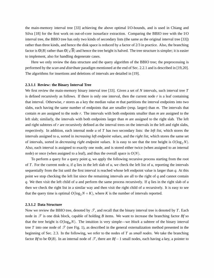
factor Bf to be Θ(B). In an internal node of T , there are Bf−1 small nodes, each having a key, a pointer to

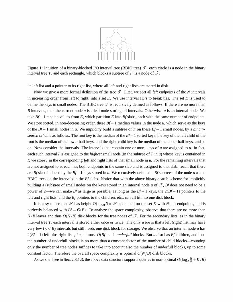
Figure 1: Intuition of a binary-blocked I/O interval tree (BBIO tree) T : each circle is a node in the binaryinterval tree T , and each rectangle, which blocks a subtree of T , is a node of T .

its left list and a pointer to its right list, where all left and right lists are stored in disk.

Now we give a more formal definition of the tree T . First, we sort all left endpoints of the N intervals

in increasing order from left to right, into a set E . We use interval ID’s to break ties. The set E is used to

define the keys in small nodes. The BBIO tree T is recursively defined as follows. If there are no more than

B intervals, then the current node u is a leaf node storing all intervals. Otherwise, u is an internal node. We

take Bf−1 median values from E , which partition E into Bf slabs, each with the same number of endpoints.

We store sorted, in non-decreasing order, these Bf−1 median values in the node u, which serve as the keys

of the Bf−1 small nodes in u. We implicitly build a subtree of T on these Bf−1 small nodes, by a binary-

search scheme as follows. The root key is the median of the Bf−1 sorted keys, the key of the left child of the

root is the median of the lower half keys, and the right-child key is the median of the upper half keys, and so

on. Now consider the intervals. The intervals that contain one or more keys of u are assigned to u. In fact,

each such interval I is assigned to the highest small node (in the subtree of T in u) whose key is contained in

I; we store I in the corresponding left and right lists of that small node in u. For the remaining intervals that

are not assigned to u, each has both endpoints in the same slab and is assigned to that slab; recall that there

are Bf slabs induced by the Bf−1 keys stored in u. We recursively define the Bf subtrees of the node u as the

BBIO trees on the intervals in the Bf slabs. Notice that with the above binary-search scheme for implicitly

building a (sub)tree of small nodes on the keys stored in an internal node u of T , Bf does not need to be a

power of 2—we can make Bf as large as possible, as long as the Bf− 1 keys, the 2(Bf− 1) pointers to the

left and right lists, and the Bf pointers to the children, etc., can all fit into one disk block.

It is easy to see that T has height O(logB N): T is defined on the set E with N left endpoints, and is

perfectly balanced with Bf = Θ(B). To analyze the space complexity, observe that there are no more than

N/B leaves and thus O(N/B) disk blocks for the tree nodes of T . For the secondary lists, as in the binary

interval tree T , each interval is stored either once or twice. The only issue is that a left (right) list may have

very few (<< B) intervals but still needs one disk block for storage. We observe that an internal node u has

2(Bf−1) left plus right lists, i.e., at most O(Bf) such underfull blocks. But u also has Bf children, and thus

the number of underfull blocks is no more than a constant factor of the number of child blocks—counting

only the number of tree nodes suffices to take into account also the number of underfull blocks, up to some

constant factor. Therefore the overall space complexity is optimal O(N/B) disk blocks.

As we shall see in Sec. 2.3.1.3, the above data structure supports queries in non-optimal O(log2NB +K/B)

I/O’s (where K is the number of intervals reported), and we can use the corner structures [54] to achieve

optimal O(logB N +K/B) I/O’s while keeping the space complexity optimal.

2.3.1.3 Query Algorithm

The query algorithm for the BBIO tree T is very simple and mimics the query algorithm for the binary

interval tree T . Given a query point q, we perform the following recursive process starting from the root of

T . For the current node u, we read u from disk. Now consider the subtree Tu implicitly built on the small

nodes in u by the binary-search scheme. Using the same binary-search scheme, we follow a root-to-leaf

path in Tu. Let r be the current small node of Tu being visited, with key value m. If q = m, then we report

all intervals in the left (or equivalently, right) list of r and stop. (We can stop here for the following reasons.

(1) Even some descendent of r has the same key value m, such descendent must have empty left and right

lists, since if there are intervals containing m, they must be assigned to r (or some small node higher than

r) before being assigned to that descendent. (2) For any non-empty descendent of r, the stored intervals

are either entirely to the left or entirely to the right of m = q, and thus cannot contain q.) If q < m, we

scan and report the intervals in the left list of r, until the first interval with the left endpoint larger than q is

encountered. Recall that the left lists are sorted by increasing left endpoint values. After that, we proceed

to the left child of r in Tu. Similarly, if q > m, we scan and report the intervals in the right list of r, until

the first interval with the right endpoint smaller than q is encountered. Then we proceed to the right child of

r in Tu. At the end, if q is not equal to any key in Tu, the binary search on the Bf− 1 keys locates q in one

of the Bf slabs. We then visit the child node of u in T which corresponds to that slab, and apply the same

process recursively. Finally, when we reach a leaf node of T , we check the O(B) intervals stored to report

those that contain q, and stop.

Since the height of the tree T is O(logB N), we only visit O(logB N) nodes of T . We also visit the

left and right lists for reporting intervals. Since we always report the intervals in an output-sensitive way,

this reporting cost is roughly O(K/B), where K is the number of intervals reported. However, it is possible

that we spend one I/O to read the first block of a left/right list but only very few (<< B) intervals are

reported. In the worst case, all left/right lists visited result in such underfull reported blocks and this I/O

cost is O(log2NB ), because we visit one left or right list per small node and the total number of small nodes

visited is O(log2NB ) (this is the height of the balanced binary interval tree T obtained by “concatenating”

the small-node subtrees Tu’s in all internal nodes u’s of T ). Therefore the overall worst-case I/O cost is

O(log2NB +K/B).

We can improve the worst-case I/O query bound. The idea is to check a left/right list of a small node from

disk only when it is guaranteed that at least one full block is reported from that list; the underfull reported

blocks of a node u of T are collectively taken care of by an additional corner structure [54] associated with

u. A corner structure can store t intervals in optimal space of O(t/B) disk blocks, where t is restricted to be

at most O(B2), so that an interval stabbing query can be answered in optimal O(k/B + 1) I/O’s, where k is

the number of intervals reported from the corner structure. Assuming all t intervals can fit in main memory

during preprocessing, a corner structure can be built in optimal O(t/B) I/O’s. We refer to [54] for a complete

description of the corner structure.

We incorporate the corner structure into the BBIO tree T as follows. For each internal node u of T , we

remove the first block from each left and right lists of each small node in u, and collect all these removed

intervals (with duplications eliminated) into a single corner structure associated with u; if a left/right list

has no more than B intervals then the list becomes empty. We also store in u a “guarding value” for each

left/right list of u. For a left list, this guarding value is the smallest left endpoint value among the remaining

intervals still kept in the left list (i.e., the (B+1)-st smallest left endpoint value in the original left list); for a

right list, this value is the largest right endpoint value among the remaining intervals kept (i.e., the (B+1)-st

largest right endpoint value in the original right list). Recall that each left list is sorted by increasing left

endpoint values and symmetrically for each right list. Observe that u has 2(Bf− 1) left and right lists and

Bf = Θ(B), so there are Θ(B) lists in total, each contributing at most a block of B intervals to the corner

structure of u. Therefore, the corner structure of u has O(B2) intervals, satisfying the restriction of the

corner structure. Also, the overall space needed is still optimal O(N/B) disk blocks.

The query algorithm is basically the same as before, with the following modification. If the current node

u of T is an internal node, then we first query the corner structure of u. A left list of u is checked from

disk only when the query value q is larger than or equal to the guarding value of that list; similarly for the

right list. In this way, although a left/right list might be checked using one I/O to report very few (<< B)

intervals, it is ensured that in this case the original first block of that list is also reported, from the corner

structure of u. Therefore we can charge this one underfull I/O cost to the one I/O cost needed to report

such first full block (i.e., reporting the first full block needs one I/O; we can multiply this one I/O cost by

2, so that the additional one I/O can be used to pay for the one I/O cost of the underfull block). This means

that the overall underfull I/O cost can be charged to the K/B term of the reporting cost (with some constant

factor), so that the overall query cost is optimal O(logB N +K/B) I/O’s.

3 SCIENTIFIC VISUALIZATION

Here, we review out-of-core work done in the area of scientific visualization. In particular, we cover recent

work in I/O-efficient volume rendering, isosurface computation, and streamline computation. Since 1997,

this area of research has advanced considerably, although it is still an active research area. The techniques

described below make it possible to perform basic visualization techniques on large datasets. Unfortunately,

some of the techniques have substantial disk and time overhead. Also, often the original format of the data is

not suited for visualization tasks, leading to expensive pre-processing steps, which often require some form

of data replication. Few of the techniques described below are suited for interactive use, and the development

of multi-resolution approaches that would allow for scalable visualization techniques is still an elusive goal.

Cox and Ellsworth [29] propose a framework for out-of-core scientific visualization systems based on

application-controlled demand paging. The paper builds on the fact that many important visualization tasks

(including computing streamlines, streaklines, particle traces, and cutting planes) only need touch a small

portion of large datasets at a time. Thus, the authors realize that it should be possible to page in the necessary

data on demand. Unfortunately, as the paper shows, the operating system paging sub-system is not effective

for such visualization tasks, and leads to inferior performance. Based on these premises and observations,

the authors propose a set of I/O optimizations that lead to substantial improvements in computation times.

The authors modified the I/O subsystem of the visualization applications to explicitly take into account the

read and caching operations. Cox and Ellsworth report on several effective optimizations. First, they show

that controlling the page size, in particular using page sizes smaller than those used by the operating system,

leads to improved performance since using larger page sizes leads to wasted space in main memory. The

second main optimization is to load data in alternative storage format (i.e., 3-dimensional data stored in sub-

cubes), which more naturally captures the natural shape of underlying scientific data. Furthermore, their

experiments show that the same techniques are effective for remote visualization, since less data needs to be

transmitted over the network and cached at the client machine.

Ueng et al. [82] present a related approach. In their work Ueng et al. focussed on computing streamlines

of large unstructured grids, and they use an approach somewhat similar to Cox and Ellsworth in that the

idea is to perform on-demand loading of the data necessary to compute a given streamline. Instead of

changing the way the operating system handles the I/O, these authors decide to modify the organization of

the actual data on disk, and to come up with optimized code for the task at hand. They use an octree partition

to restructure unstructured grids to optimize the computation of streamlines. Their approach involves a

preprocessing step, which builds an octree that is used to partition the unstructured cells in disk, and an

interactive step, which computes the streamlines by loading the octree cells on demand. In their work, they

propose a top-down out-of-core preprocessing algorithm for building the octree. Their algorithm is based

on propagating the cell (tetrahedra) insertions on the octree from the root to the leaves in phases. In each

phase (recursively), octree nodes that need to be subdivided create their children and distribute the cells

among them based on the fact that cells are contained inside the octree node. Each cell is replicated on the

octree nodes that it would potentially intersect. For the actual streamline computation, their system allows

for the concurrent computation of multiple streamlines at the same time based on user input. It uses a multi-

threaded architecture with a set of streamline objects, three scheduling queue (wait, ready, and finished),

free memory pool and a table of loaded octants.

Leutenegger and Ma [59] propose to use R-trees [48] to optimize searching operations on large unstruc-

tured datasets. They arge that octrees (such as those used by Ueng et al. [82]) are not suited for storing

unstructured data because of imbalance in the structure of such data making it hard to efficiently pack the

octree in disk. Furthermore, they also argue that the low fan-out of octrees leads to a large number of inter-

nal nodes, which force applications into many unnecessary I/O fetches. Leutenegger and Ma use an R-tree

for storing tetrahedral data, and present experimental results of their method on the implementation of a

multi-resolution splatting-based volume renderer.

Pascucci and Frank [67] describe a scheme for defining hierarchical indices over very large regular grids

that leads to efficient disk data layout. Their approach is based on the use of a space-filling curve for defining

the data layout and indexing. In particular, they propose an indexing scheme for the Lebesgue Curve which

can be simply and efficient computed by using bit masking, shifting, and addition. They show the usefulness

of their approach in a progressive (real-time) slicing application which exploits their indexing framework

for the multi-resolution computation of arbitrary slices of very large datasets (one example in the paper has

approximately one half tera nodes).

Bruckschen et al. [13] describes a technique for real-time particle traces of large time-varying datasets.

They argue that it is not possible to perform this computation in real-time on demand, and propose a solution

where the basic idea is to pre-compute the traces from fixed positions located on a regular grid, and to

save the results for efficient disk access in a way similar to Pascucci and Frank [67]. Their system has

two main components, a particle tracer and encoder, which runs as a preprocessing step, and a renderer,

which interactively reads the precomputed particle traces. Their particle tracer computes traces for a whole

sequence of time steps by considering the data in blocks. It works by injecting particles at grid locations and

computing their new positions until the particles have left the current block.

Chiang and Silva [18, 20] proposed algorithms for out-of-core isosurface generation of unstructured

grids. Isosurface generation can be seen as an interval stabbing problem [22] as follows: first, for each cell,

produce an interval I = [min,max] where min and max are the minimum and maximum among the scalar

values of the vertices of the cell. Then a cell is active if and only if its interval contains the isovalue q. This

reduces the active-cell searching problem to that of interval search: given a set of intervals in 1D, build

a data structure to efficiently report all intervals containing a query point q. Secondly, the interval search

problem is solved optimally by using the main-memory interval tree [33]. The first out-of-core isosurface

technique was given by Chiang and Silva [18]. They follow the ideas of Cignoni et al. [22], but use the I/O-

optimal interval tree [6] to solve the interval search problem. An interesting aspect of the work is that even

the preprocessing is assumed to be performed completely on a machine with limited main memory. With

this technique, datasets much larger than main memory can be visualized efficiently. Though this technique

is quite fast in terms of actually computing the isosurfaces, the associated disk and preprocessing overhead

is substantial. Later, Chiang et al. [20] further improved (i.e., reduced) the disk space overhead and the

preprocessing time of Chiang and Silva [18], at the cost of slightly increasing the isosurface query time, by

developing a two-level indexing scheme, the meta-cell technique, and the BBIO tree which is used to index

the meta-cells. A meta-cell is simply a collection of contiguous cells, which is saved together for fast disk

access.

Along the same lines, Sulatycke and Ghose [77] describe an extension of Cignoni et al. [22] for out-

of-core isosurface extraction. Their work does not propose an optimal extension, but instead proposes a

scheme that simply adapts the in-core data structure to an out-of-core setting. The authors also describe

a multi-threaded implementation that aims to hide the disk I/O overhead by overlapping computation with

I/O. Basically, the authors have an I/O thread that reads the active cells from disk, and several isosurface

computation threads. Experimental results on relatively small regular grids are given in the paper.

Bajaj et al. [8] also proposes a technique for out-of-core isosurface extraction. Their technique is an

extension of their seed-based technique for efficient isosurface extraction [7]. The seed-based approach

works by saving a small set of seed cells, which can be used as starting points for an arbitrary isosurface

by simple contour propagation. In the out-of-core adaptation, the basic idea is to separate the cells along

the functional value, storing ranges of contiguous ranges together in disk. In their paper, the authors also

describe how to parallelize their algorithm, and show the performance of their techniques using large regular

grids.

Sutton and Hansen [78] propose the T-BON (Temporal Branch-On-Need Octree) technique for fast

extraction of isosurfaces of time-varying datasets. The preprocessing phase of their technique builds a

branch-on-need octree [87] for each time step and stores it to disk in two parts. One part contains the

structure of the octree and does not depend at all on the specific time step. Time-step specific data is saved

separately (including the extreme values). During querying, the tree is recursively traversed, taking into

account the query timestep and isovalue, and brought into memory until all the information (including all

the cell data) has been read. Then, a second pass is performed to actually compute the isosurface. Their

technique also uses meta-cells (or data bricking) [20] to optimize the I/O transfers.

Shen et al. [75] proposes a different encoding for time-varying datasets. Their TSP (Time-Space Par-

tioning) tree encodes in a single data structure the changes from one time-step to another. Each node of the

octree has not only a spatial extend, but also a time interval. If the data changes in time, a node is refined

by its children, which refine the changes on the data, and is annotated with its valid time range. They use

the TSP tree to perform out-of-core volume rendering of large volumes. One of the nice properties is that

because of its encoding, it is possible to very efficiently page the data in from disk when rendering time

sequences.

Farias and Silva [40] presents a set of techniques for the direct volume rendering of arbitrarily large

unstructured grids on machines with limited memory. One of the techniques described in the paper is a

memory-insensitive approach which works by traversing each cell in the dataset, one at a time, sampling its

ray span (in general a ray would intersect a convex cell twice) and saving two fragment entries per cell and

pixel covered. The algorithm then performs an external sort using the pixel as the primary key, and the depth

of the fragment as the secondary key, which leads to the correct ray stabbing order that exactly captures the

information necessary to perform the rendering. The other technique described is more involved (but more

efficient) and involves extending the ZSWEEP algorithm [39] to an out-of-core setting.

The main idea of the (in-core) ZSWEEP algorithm is to sweep the data with a plane parallel to the

viewing plane in order of increasing z, projecting the faces of cells that are incident to vertices as they

are encountered by the sweep plane. ZSWEEP’s face projection consists of computing the intersection

of the ray emanating from each pixel, and store their z-value, and other auxiliary information, in sorted

order in a list of intersections for the given pixel. The actual lighting calculations are deferred to a later

phase. Compositing is performed as the “target Z” plane is reached. This algorithm exploits the implicit

(approximate) global ordering that the z-ordering of the vertices induces on the cells that are incident on

them, thus leading to only a very small number of ray intersection are done out of order; and the use of

early compositing which makes the memory footprint of the algorithm quite small. There are two sources

of main memory usage in ZSWEEP: the pixel intersection lists, and the actual dataset. The basic idea in

the out-of-core technique is to break the dataset into chunks of fixed size (using ideas of the meta-cell work

described in Chiang et al. [20]), which can be rendered independently without using more than a constant

amount of memory. To further limit the amount of memory necessary, their algorithm subdivides the screen

into tiles, and for each tile, which are rendered in chunks that project into it in a front-to-back order, thus

enabling the exact same optimizations which can be used with the in-core ZSWEEP algorithm.

Chiang et al. [16] propose a unified infrastructure for parallel out-of-core isosurface extraction and

volume rendering of unstructured grids which exploits a combination of the work of Chiang, Silva, and

Schroeder [20] and Farias and Silva [40]. Their work is based on building a unified data structure that

both algorithms can use, and then use a simple round-robin scheme for parallelization. Since the relevant

algorithms are output sensitive and only fetch the data they need to produce their output, this approach is

shown to be effective on a small cluster of PCs.

4 SURFACE SIMPLIFICATION

In this section we review recent work on out-of-core simplification. In particular, we will focus on methods

for simplifying large triangle meshes, as these are the most common surface representation for computer

graphics. As data sets have grown rapidly in recent years, out-of-core simplification has become an in-

creasingly important tool for dealing with large data. Indeed, many conventional in-core algorithms for

visualization, data analysis, geometric processing, etc., cannot operate on today’s massive data sets, and are

furthermore difficult to extend to work out of core. Thus, simplification is needed to reduce the (often over-

sampled) data set so that it fits in main memory. As we have already seen in previous sections, even though

some methods have been developed for out-of-core visualization and processing, handling billion-triangle

meshes, such as those produced by high resolution range scanning [60] and scientific simulations [66], is still

challenging. Therefore many methods benefit from having either a reduced (albeit still large and accurate)

version of a surface, or having a multiresolution representation produced using out-of-core simplification.

It is somewhat ironic that, whereas simplification has for a long time been relied upon for dealing with

complex meshes, for large enough data sets simplification itself becomes impractical, if not impossible. Typ-

ical in-core simplification techniques, which require storing the entire full-resolution mesh in main memory,

can handle meshes on the order of a few million triangles on current workstations; two to three orders of

magnitude smaller than many data sets available today. To address this problem, several techniques for out-

of-core simplification have been proposed recently, and we will here cover most of the methods published

to date.

One reason why few algorithms exist for out-of-core simplification is that the majority of previous meth-

ods for in-core simplification are ill-suited to work in the out-of-core setting. The prevailing approach to

in-core simplification is to iteratively perform a sequence of local mesh coarsening operations, e.g., edge

collapse, vertex removal, face clustering, etc., that locally simplify the mesh, e.g., by removing a single

vertex. The order of operations performed is typically determined by their impact on the quality of the

mesh, as measured using some error metric, and simplification then proceeds in a greedy fashion by always

performing the operation that incurs the lowest error. Typical error metrics are based on quantities such

as mesh-to-mesh distance, local curvature, triangle shape, valence, an so on. In order to evaluate (and re-

atomic vertex clustering

iterative vertex pair contraction

Figure 2: Vertex clustering on a 2D uniform grid as a single atomic operation (top) and as multiple pair con-tractions (bottom). The dashed lines represent the space-partitioning grid, while vertex pairs are indicatedusing dotted lines. Note that spatial clustering can lead to significant topological simplification.

evaluate) the metric and to keep track of which simplices (i.e., vertices, edges, and triangles) to eliminate in

each coarsening operation, virtually all in-core simplification methods rely on direct access to information

about the connectivity (i.e., adjacency information) and geometry in a neighborhood around each simplex.

As a result, these methods require explicit data structures for maintaining connectivity, as well as a priority

queue of coarsening operations, which amounts to O(n) in-core storage for a mesh of size n. Clearly this

limits the size of models that can be simplified in core. Simply offloading the mesh to disk and using virtual

memory techniques for transparent access is seldom a realistic option, as the poor locality of greedy simpli-

fication results in scattered accesses to the mesh and excessive thrashing. For out-of-core simplification to

be viable, such random accesses must be avoided at all costs. As a result, many out-of-core methods make

use of a triangle soup mesh representation, where each triangle is represented independently as a triplet of

vertex coordinates. In contrast, most in-core methods use some form of indexed mesh representation, where

triangles are specified as indices into a non-redundant list of vertices.

There are many different ways to simplify surfaces. Popular coarsening operations for triangle meshes

include vertex removal [73], edge collapse [53], half-edge collapse [58], triangle collapse [49], vertex pair

contraction [44], and vertex clustering [71]. While these operations vary in complexity and generality, they

all have one thing in common, in that they partition the set of vertices from the input mesh by grouping

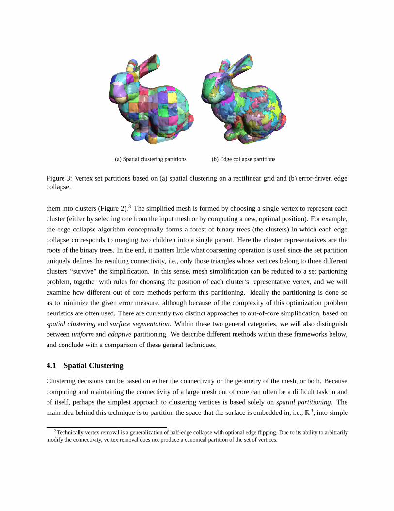
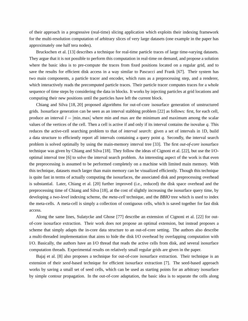
(a) Spatial clustering partitions (b) Edge collapse partitions

Figure 3: Vertex set partitions based on (a) spatial clustering on a rectilinear grid and (b) error-driven edgecollapse.

them into clusters (Figure 2).3 The simplified mesh is formed by choosing a single vertex to represent each

cluster (either by selecting one from the input mesh or by computing a new, optimal position). For example,

the edge collapse algorithm conceptually forms a forest of binary trees (the clusters) in which each edge

collapse corresponds to merging two children into a single parent. Here the cluster representatives are the

roots of the binary trees. In the end, it matters little what coarsening operation is used since the set partition

uniquely defines the resulting connectivity, i.e., only those triangles whose vertices belong to three different

clusters “survive” the simplification. In this sense, mesh simplification can be reduced to a set partioning

problem, together with rules for choosing the position of each cluster’s representative vertex, and we will

examine how different out-of-core methods perform this partitioning. Ideally the partitioning is done so

as to minimize the given error measure, although because of the complexity of this optimization problem

heuristics are often used. There are currently two distinct approaches to out-of-core simplification, based on

spatial clustering and surface segmentation. Within these two general categories, we will also distinguish

between uniform and adaptive partitioning. We describe different methods within these frameworks below,

and conclude with a comparison of these general techniques.

4.1 Spatial Clustering

Clustering decisions can be based on either the connectivity or the geometry of the mesh, or both. Because

computing and maintaining the connectivity of a large mesh out of core can often be a difficult task in and

of itself, perhaps the simplest approach to clustering vertices is based solely on spatial partitioning. The

main idea behind this technique is to partition the space that the surface is embedded in, i.e., R3, into simple

3Technically vertex removal is a generalization of half-edge collapse with optional edge flipping. Due to its ability to arbitrarilymodify the connectivity, vertex removal does not produce a canonical partition of the set of vertices.

convex 3D regions, and to merge the vertices of the input mesh that fall in the same region. Because the mesh

geometry is often specified in a Cartesian coordinate system, the most straightforward space partitioning is

given by a rectilinear grid (Figure 2). Rossignac and Borrel [71] used such a grid to cluster vertices in an

in-core algorithm. However, the metrics used in their algorithm rely on full connectivity information. In

addition, a ranking phase is needed in which the most “important” vertex in each cluster is identified, and

their method, as stated, is therefore not well suited for the out-of-core setting. Nevertheless, Rossignac and

Borrel’s original clustering algorithm is the basis for many of the out-of-core methods discussed below. We

note that their algorithm makes use of a uniform grid to partition space, and we will discuss out-of-core

methods for uniform clustering first.

4.1.1 Uniform Spatial Clustering

To extend the clustering algorithm in [71] to the out-of-core setting, Lindstrom [61] proposed using Garland

and Heckbert’s quadric error metric [44] to measure error. Lindstrom’s method, called OoCS, works by

scanning a triangle soup representation of the mesh, one triangle at a time, and computing a quadric matrix

Qt for each triangle t. Using an in-core sparse grid representation (e.g., a dynamic hash table), the three

vertices of a triangle are quickly mapped to their respective grid cells, and Qt is then distributed to these

cells. This depositing of quadric matrices is done for each of the triangle’s vertices whether they belong

to one, two, or three different clusters. However, as mentioned earlier, only those triangles that span three

different clusters survive the simplification, and the remaining degenerate ones are not output. After each

input triangle has been read, what remains is a list of simplified triangles (specified as vertex indices) and

a list of quadric matrices for the occupied grid cells. For each quadric matrix, an optimal vertex position is

computed that minimizes the quadric error [44], and the resulting indexed mesh is then output.

Lindstrom’s algorithm runs in linear time in the size of the input and expected linear time in the output.

As such, the method is efficient both in theory and practice, and is able to process on the order of a quarter

million triangles per second on a typical PC. While the algorithm can simplify arbitrarily large meshes, it

requires enough core memory to store the simplified mesh, which limits the accuracy of the output mesh.

To overcome this limitation, Lindstrom and Silva [62] proposed an extension of OoCS that performs all

computations on disk, and that requires only a constant, small amount of memory. Their approach is to

replace all in-core random accesses to grid cells (i.e., hash lookups and quadric matrix updates) with coher-

ent sequential disk accesses, by storing all information associated with a grid cell together on disk. This is

accomplished by first mapping vertices to grid cells (as before) and writing partial per-cluster quadric infor-

mation in the form of plane equations to disk. This step is followed by a fast external sort (Section 2.2.1)

on grid cell ID of the quadric information, after which the sorted file is traversed sequentially and quadric

matrices are accumulated and converted to optimal vertex coordinates. Finally, three sequential scan-and-

replace steps, each involving an external sort, are performed on the list of output triangles, in which cluster

IDs are replaced with indices into the list of vertices.

Because of the use of spatial partitioning and quadric errors, no explicit connectivity information is

(a) Uniform spatial clustering (b) Adaptive spatial clustering

Figure 4: Vertex set partitions and simplifications based on (a) uniform and (b) adaptive spatial clustering.Notice the long planar cuts made by the top-level BSP planes in (b).

needed in [61, 62]. In spite of this, the end result is identical to what Garland and Heckbert’s edge collapse

algorithm [44] would produce if the same vertex set partitioning were used. On the downside, however, is

that topological features such as surface boundaries and nonmanifold edges, as well as geometric features

such as sharp edges are not accounted for. To address this, Lindstrom and Silva [62] suggested computing

tangential errors in addition to errors normal to the surface. These tangential errors cancel out for man-

ifold edges in flat areas, but penalize deviation from sharp edges and boundaries. As a result, boundary,

nonmanifold, and sharp edges can be accounted for without requiring explicit connectivity information. An-

other potential drawback of connectivity oblivious simplification—and most non-iterative vertex clustering

algorithms in general—is that the topology of the surface is not necessarily preserved, and nonmanifold

simplices may even be introduced. On the other hand, for very large and complex surfaces, modest topol-

ogy simplification may be desirable or even necessary to remove noise and unimportant features that would

otherwise consume precious triangles.

4.1.2 Adaptive Spatial Clustering

The general spatial clustering algorithm discussed above does not require a rectilinear partitioning of space.

In fact, the 3D space-partitioning mesh does not even have to be conforming (i.e., without cracks or T-

junctions), nor do the cells themselves have to be convex or even connected (although that may be prefer-

able). Because the amount of detail often varies over a surface, it may be desirable to adapt the grid cells

to the surface shape, such that many small cells are used to partition detailed regions of the surface, while

relatively larger cells can be used to cluster vertices in flat regions.

The advantage of producing an adaptive partition was first demonstrated by Shaffer and Garland [74].

Their method makes two passes instead of one over the input mesh. The first pass is similar to the OoCS

algorithm [61], but in which a uniform grid is used to accumulate both primal (distance-to-face) and dual

(distance-to-vertex) quadric information. Based on this quadric information, a principal component analysis

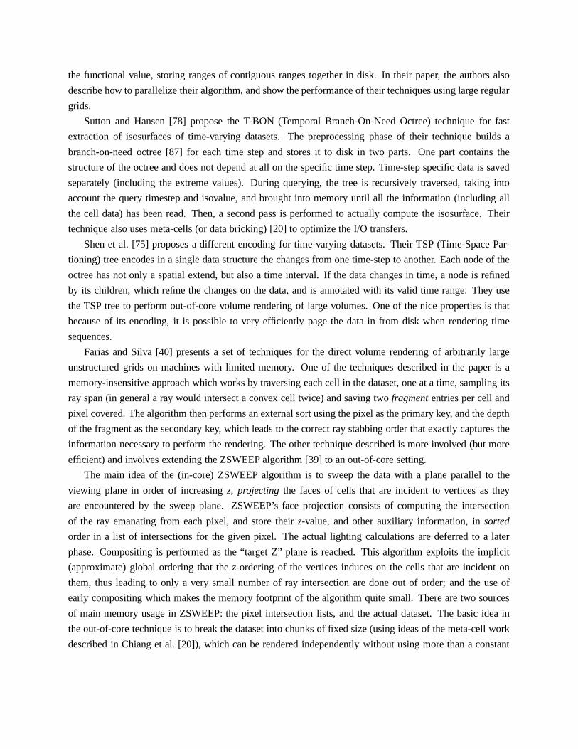
(a) Original (b) Edge collapse [63] (c) Uniform clustering [61]

Figure 5: Base of Happy Buddha model, simplified from 1.1 million to 16 thousand triangles. Notice thejagged edges and notches in (c) caused by aliasing from using a coarse uniform grid. Most of these artifactsare due to the geometry and connectivity “filtering” being decoupled, and can be remedied by flipping edges.

(PCA) is performed that introduces split planes that better partition the vertex clusters than the uniform grid.

These split planes, which are organized hierarchically in a binary space partitioning (BSP) tree, are then

used to cluster vertices in a second pass over the input data (see Figure 4). In addition to superior qualitative

results over [61], Shaffer and Garland report a 20% average reduction in error. These improvements come

at the expense of higher memory requirements and slower simplification speed.

In addition to storing the BSP-tree, a priority queue, and both primal and dual quadrics, Shaffer and Gar-

land’s method also requires a denser uniform grid (than [61]) in order to capture detailed enough information

to construct good split planes. This memory overhead can largely be avoided by refining the grid adaptively

via multiple passes over the input, as suggested by Fei et al. [41]. They propose uniform clustering as a first

step, after which the resulting quadric matrices are analyzed to determine the locations of sharp creases and

other surface details. This step is similar to the PCA step in [74]. In each cell where higher resolution is

needed, an additional split plane is inserted, and another pass over the input is made (processing only trian-

gles in refined cells). Finally, an edge collapse pass is made to further coarsen smooth regions by making use

of the already computed quadric matrices. A similar two-phase hybrid clustering and edge collapse method

has recently been proposed by Garland and Shaffer [45], who couple an initial spatial clustering phase with

a final in-core edge collapse phase. They show that, by passing per-vertex quadric matrices between the two

phases rather than recomputing them from the partially simplified mesh, the mesh quality is improved. This

approach allows trading off simplification speed and quality by varying the switch-over point between the

two phases, with the requirement that the first out-of-core phase has to coarsen the mesh sufficiently so that

it can be simplified in-core in the second phase.

The uniform grid partitioning scheme is somewhat sensitive to translation and rotation of the grid, and

for coarse grids aliasing artifacts are common (see Figure 5). Inspired by work in image and digital signal

processing, Fei et al. [42] propose using two interleaved grids, offset by half a grid cell in each direction,

to combat such aliasing. They point out that detailed surface regions are relatively more sensitive to grid

translation, and by clustering the input on both grids and measuring the local similarity of the two resulting

meshes (again using quadric errors) they estimate the amount of detail in each cell. Where there is a large

(a) Coarse spatial partitions (b) Refined error-driven partitions (c) Simplified mesh

Figure 6: Vertex set partitions and simplification based on (a) initial spatial and (b) ensuing error-drivenpartitioning. The surface patches in (a) are small enough to be simplified in core one by one.

amount of detail, simplified parts from both meshes are merged in a retriangulation step. Contrary to [41,

45, 74], this semi-adaptive technique requires only a single pass over the input.

4.2 Surface Segmentation

Spatial clustering fundamentally works by finely partitioning the space that the surface lies in. The method

of surface segmentation, on the other hand, partitions the surface itself into pieces small enough that they can

be further processed independently in core. Each surface patch can thus be simplified in core to a given level

of error using a high quality simplification technique, such as edge collapse, and the coarsened patches are

then “stitched” back together. From a vertex set partition standpoint, surface segmentation provides a coarse

division of the vertices into smaller sets, which are then further refined in core and ultimately collapsed

(Figure 6). As in spatial clustering, surface segmentation can be uniform, e.g., by partitioning the surface

over a uniform grid, or adaptive, e.g., by cutting the surface along feature lines. We begin by discussing

uniform segmentation techniques.

4.2.1 Uniform Surface Segmentation

Hoppe [52] described one of the first out-of-core simplification techniques based on surface segmentation

for the special case of height fields. His method performs a 2D spatial division of a regularly gridded terrain

into several rectangular blocks, which are simplified in core one at a time using edge collapse until a given

error tolerance is exceeded. By disallowing any modifications to block boundaries, adjacent blocks can then

be quickly stitched together in a hierarchical fashion to form larger blocks, which are then considered for fur-

ther simplification. This allows seams between sibling blocks to be coarsened higher up in in the hierarchy,

and by increasing the error tolerance on subsequent levels a progressively coarser approximation is obtained

partitionmesh

pre-simplifyblocks

simplify blocks& save ecol’s

stitch blocks intolarger blocks

simplifytop-level block

ecolA

ecolB

ecolS

apply bottom-up recursion

Figure 7: Height field simplification based on hierarchical, uniform surface segmentation and edge collapse(figure courtesy of Hugues Hoppe).

(see Figure 7). Hoppe’s method was later extended to general triangle meshes by Prince [69], who uses

a 3D uniform grid to partition space and segment the surface. Both of these methods have the advantage

of producing not a single static approximation but a multiresolution representation of the mesh—a pro-

gressive mesh [50]—which supports adaptive refinement, e.g., for view-dependent rendering. While being

significantly slower (by about two orders of magnitude) and requiring more (although possibly controllable)

memory than most spatial clustering techniques, the improvement in quality afforded by error-driven edge

collapse can be substantial.

Bernardini et al. [11] developed a strategy similar to [52,69]. Rather than constructing a multiresolution

hierarchy, however, a single level of detail is produced. Seams between patches are coarsened by shifting the

single-resolution grid (somewhat akin to the approach in [42]) after all patches in the current grid have been

simplified. In between the fine granularity provided by a progressive mesh [69] and the single-resolution

meshes created in [11], Erikson et al. [38] proposed using a static, discrete level of detail for each node in

the spatial hierarchy. As in [11, 52, 69], a rectilinear grid is used for segmentation in Erikson’s method.

One of the downsides of the surface segmentation techniques described above is the requirement that

patch boundaries be left intact, which necessitates additional passes to coarsen the patch seams. This re-

quirement can be avoided using the OEMM mesh data structure proposed by Cignoni et al. [23]. As in [69],

an octree subdivision of space is made. However, when processing the surface patch for a node in this

tree, adjacent nodes are loaded as well, allowing edges to be collapsed across node boundaries. Some extra

bookkeeping is done to determine which vertices are available for consideration of an edge collapse, as well

as which vertices can be modified or removed. This general data structure supports not only out-of-core

simplification but also editing, visualization, and other types of processing. Other improvements over [69]

include the ability to adapt the octree hierarchy, such that child nodes are collapsed only when the parent

cell contains a sufficiently small number of triangles.

Figure 8: Submesh for a set of spanning edges (shown as thick lines) used in El-Sana and Chiang’s simpli-fication method.

4.2.2 Adaptive Surface Segmentation

Some of the surface segmentation methods discussed so far already support adapting the vertex set partition

to the shape of the surface (recall that this partitioning is the goal of triangle mesh simplification). For

example, simplification within a patch is generally adaptive, and in [23] the octree space partition adapts

to the local complexity of the surface. Still, using the methods above, the surface is always segmented by

a small set of predefined cut planes, typically defined by an axis-aligned rectilinear grid. In contrast, the

out-of-core algorithm described by El-Sana and Chiang [34] segments the surface solely based on its shape.

Their technique is a true out-of-core implementation of the general error-driven edge collapse algorithm.

Like in other methods based on surface segmentation, edge collapses are done in batches by coarsening

patches, called sub-meshes, up to a specified error tolerance, while making sure patch boundaries are left

intact. In contrast to previous methods, however, the patch boundaries are not defined via spatial partitioning,

but by a set of edges whose collapse costs exceed a given error threshold. Thus patch boundaries are not

artificially constrained from being coarsened, but rather delineate important features in the mesh that are to

be preserved. Rather than finding such boundaries explicitly, El-Sana and Chiang sort all edges by error and

load as many of the lowest-cost edges, called spanning edges, and their incident triangles as can fit in main

memory. The highest-cost spanning edge then sets the error threshold for the current iteration of in-core

simplification. In this process, patches of triangles around spanning edges are loaded and merged whenever

possible, creating sub-meshes that can be simplified independently by collapsing all edges whose errors are

below the threshold. When the sub-meshes have been simplified, their edges are re-inserted into the priority

queue, and another iteration of sub-mesh construction and simplification is performed. As in [69], the final

output of the algorithm is a multiresolution mesh.

While El-Sana and Chiang use edge length as their error metric, their method can be adapted to work

with other metrics, with one caveat. Note that interior spanning edges connected to a sub-mesh boundary

may be collapsed only if the boundary geometry is not affected, i.e., by forcing the replacement vertex to lie

on the boundary. For error metrics that depend on the position of the collapsed-to vertex, such as the quadric

error metric [44], enforcing boundary constraints generally implies elevated edge costs and consequently

out-of-order edge collapses (as in the previous surface segmentation methods). Of course, disallowing such

edge collapses altogether also leads to an incorrect collapse order, and may in addition considerably limit

the set of possible coarsening operations, particularly when the sub-meshes are small and scattered, as is

often the case when the input mesh is much larger than available memory.

To support incidence queries and an on-disk priority queue, El-Sana and Chiang make use of efficient

search data structures such as B-trees (see also Section 2). Their method is surprisingly fast and works

well when sufficient memory is available to construct large sub-meshes and keep I/O traffic to a minimum,

and when enough disk space exists for storing connectivity information and an edge collapse queue for the

entire input mesh. Unfortunately their published results do not include examples of simplifying very large

surfaces (the largest example is just over one million triangles, simplified on a computer with 32 MB of free

RAM), and more studies are necessary to determine how the superlinear running time of the method affects

its scalability.

Iterative simplification of extremely large meshes can be a time consuming task, especially when the

desired approximation is very coarse. This is because the number of coarsening operations required is

roughly proportional to the size of the input. In such situations, it may be preferable to perform the inverse of

simplification, refinement, by starting from a coarse representation and adding only a modest amount detail,

in which case the number of refinement operations is determined by the size of the output. Choudhury and

Watson [21] describe an out-of-core version of the RSimp refinement method [12] that they call VMRSimp

(for Virtual Memory RSimp). Rather than using sophisticated out-of-core data structures, VMRSimp relies

on the virtual memory mechanism of the operating system to handle data paging. As in the original method,

VMRSimp works by incrementally refining a partition of the set of input triangles. These triangle sets are

connected and constitute an adaptive segmentation of the surface. The choice of which triangle patch to

refine is based on the amount of normal variation within it (essentially a measure of curvature defined over a

region of the surface). VMRSimp improves upon RSimp by storing the vertices and triangles in each patch

contiguously in virtual memory. When a patch is split in two, its constituent primitives are reorganized to

preserve this locality. As patches are refined and become smaller, the locality of reference is effectively

increased, which makes the virtual memory approach viable. Finally, when the desired level of complexity

is reached, a representative vertex is computed for each patch by minimizing a quadric error function. Even

though the simplification happens in “reverse,” this method, like all others discussed here, is yet another

instance of vertex set partitioning and collapse.

4.3 Summary of Simplification Techniques

In this section we have seen a variety of different out-of-core surface simplification techniques, and we

discussed how these methods partition and later collapse the set of mesh vertices. All of these methods have

shown to be effective for simplifying surfaces that are too large to fit in main memory. The methods do

have their own strengths and weaknesses, however, and we would like to conclude with some suggestions

category methodpeak mem. usage (MB) peak disk usage (GB) speedtheoretical example theoretical example (Ktri/s)

spatial clustering

[61] 144Vout 257 0 0 100–250a

[41] ' 200Vout ' 356 0 0 65–150[74] ≥ 464Vout ≥ 827 0 0 45–90[62] O(1) 8 120–370Vin 21–64 30–70

surface segmentation

[23] O(1) 80 ' 68Vin 12 6–13b

[34] O(1) 128 Ω(Vin) ? 5–7[21] O(1)c 1024 ≥ 86Vin ≥ 15 4–5[69] O(1) 512 Ω(Vin) ? 0.8–1

aSpeed of author’s current implementation on an 800 MHz Pentium III.bWhen the one-time OEMM construction step is included in the simplification time, the effective speed drops to 4–6 Ktri/s.cThis method is based on virtual memory. Thus all available memory is generally used during simplification.

Table 1: Simplification results for various methods. These results were obtained or estimated from theoriginal publications, and are only approximate. When estimating memory usage, here expressed in numberof input (Vin) and output (Vout) vertices, we assume that the meshes have twice as many triangles as vertices.The results in the “example” columns correspond to simplifying the St. Matthew data set [60], consistingof 186,810,938 vertices, to 1% of its original size. For methods with constant (O(1)) memory usage, welist the memory configuation from the original publication. The disk usage corresponds to the amountof temporary space used, and does not include the space needed for the input and output mesh. For theclustering techniques, the speed is measured as the size of the input over the simplification time. Becausethe surface segmentation methods work incrementally, the size of the output greatly affects the speed. Thus,for these methods the speed is measured in terms of the change in triangle count.

for when to a certain technique may be preferable over another.

Whereas spatial clustering is generally the fastest method for simplification, it often produces lower qual-

ity approximations than the methods based on surface segmentation. This is because surface segmentation

allows partitioning the vertex set based directly on error (except possibly along seams) using an iterative

selection of fine-grained coarsening operations. Spatial clustering, on the other hand, typically groups a

large number of vertices, based on little or no error information, in a single atomic operation. The incre-

mental nature of surface segmentation also allows constructing a multiresolution representation of the mesh

that supports fine-grained adaptive refinement, which is important for view-dependent rendering. Indeed,

several of the surface segmentation methods discussed above, including [23, 34, 38, 52, 69], were designed

explicitly for view-dependent rendering. Finally, because surface segmentation methods generally maintain

connectivity, they support topology-preserving simplification.

Based on the observations above, it may seem that surface segmentation is always to be favored over

spatial clustering. However, the price to pay for higher quality and flexibility is longer simplification times,

often higher resource requirements, and less straightforward implementations. To get a better idea of the

resource usage (RAM, disk, CPU) for the various methods, we have compiled a table (Table 1) based on

numerical data from the authors’ own published results. Note that the purpose of this table is not to allow

accurate quantitative comparisons between the methods; clearly factors such as quality of implementation,

hardware characteristics, amount of resource contention, assumptions made, data sets used, and, most im-

portant, what precisely is being measured have a large impact on the results. However, with this in mind, the

table gives at least a rough idea of how the methods compare. For example, Table 1 indicates that the spa-

tial clustering methods are on average one to two orders of magnitude faster than the surface segmentation

methods. Using the 372-million-triangle St. Matthew model from the Digital Michelangelo Project [60] as

a running example, the table suggests a difference between a simplification time of half an hour using [61]

and about a week using [69]. For semi-interactive tasks that require periodic user feedback, such as large-

isosurface visualization where on-demand surface extraction and simplification are needed, a week’s worth

of simplification time clearly is not practical.

In terms of resource usage, most surface segmentation methods make use of as much RAM as possible,

while requiring a large amount of disk space for storing the partially simplified mesh, possibly including

full connectivity information and a priority queue. For example, all surface segmentation methods discussed

above have input-sensitive disk requirements. Finally, certain types of data sets, such as isosurfaces from

scientific simulations [66] and medical data [2], can have a very complicated topological structure, resulting

either from noise or intrinsic fine-scale features in the data. In such cases, simplification of the topology is

not only desirable but is necessary in order to reduce the complexity of the data set to an acceptable level.

By their very nature, spatial clustering based methods are ideally suited for removing such small features

and joining spatially close pieces of a surface.

To conclude, we suggest using spatial clustering for very large surfaces when time and space are at a

premium. If quality is the prime concern, surface segmentation methods perform favorably, and should be

chosen if the goal is to produce a multiresolution or topology-equivalent mesh. For the best of both worlds,

we envision that hybrid techniques, such as [41, 45], that combine fast spatial clustering with high-quality

iterative simplification, will play an increasingly important role for practical out-of-core simplification.

5 INTERACTIVE RENDERING

The advances in the tools for 3D modeling, simulation, and shape acquisition have led to the generation of

very large 3D models. Rendering these models at interactive frame rates has applications in many areas,

including entertainment, computer-aided design (CAD), training, simulation, and urban planning.

In this section, we review the out-of-core techniques to render large models at interactive frame rates

using machines with small memory. The basic idea is to keep the model on disk, load on demand the parts

of the model that the user sees, an display each visible part at a level of detail proportional to its contribution

to the image being rendered. The following subsections describe the algorithms to efficiently implement

this idea.

5.1 General Issues

Building an Out-Of-Core Representation for a Model At preprocessing time, an out-of-core rendering

system builds a representation for the model on disk. The most common representations are bounding

volume hierarchies (such as bounding spheres [72]) and space partitioning hierarchies (such as k-D trees [43,

80], BSP trees [85], and octrees [4, 23, 28, 82, 83]).

Some approaches assume that this preprocessing step is performed on a machine with enough memory to

hold the entire model [43,83]. Others make sure that the preprocessing step can be performed on a machine

with small memory [23, 28, 85].

Precomputing Visibility Information One of the key computations at runtime is determining the visible

set — the parts of the model the user sees. Some systems precompute from-region visibility, i.e., they split

the model into cells, and for each cell they precompute what the user would see from any point within

the cell [4, 43, 80]. This approach allows the system to reuse the same visible set for several viewpoints,

but it requires long preprocessing times, and may cause bursts of disk activity when the user crosses cell

boundaries.

Other systems use from-point visibility, i.e., they determine on-the-fly what the user sees from the current

viewpoint [28, 83, 85]. Typically, the only preprocessing required by this approach is the construction of a

hierarchical spatial decomposition for the model. Although this approach needs to compute the visible set

for every frame, it requires very little preprocessing time, and reduces the risk of bursts of disk activity,

because the changes in visibility from viewpoint to viewpoint tend to be much smaller than the changes in

visibility from cell to cell.

View-Frustum Culling Since the user typically has a limited field of view, a very simple technique, that

perhaps all rendering systems use, is to cull away the parts of the model outside the user’s view frustum. If

a hierarchical spatial decomposition or a hierarchy of bounding volumes is available, view-frustum culling

can be optimized by recursively traversing the hierarchy from the root down to the leaves, and culling away

entire subtrees that are outside the user’s view frustum [24].

Occlusion Culling Another technique to minimize the geometry that needs to be loaded from disk and

sent to the graphics hardware is to cull away geometry that is occluded by other geometry. This is a hard

problem to solve exactly [56, 80, 85], but fast and accurate approximations exist [35, 55].

Level-of-Detail Management (or Contribution Culling) The amount of geometry that fits in main mem-

ory typically exceeds the interactive rendering capability of the graphics hardware. One approach to alleviate

this problem is to reduce the complexity of the geometry sent to the graphics hardware. The idea is to dis-

play a certain part of the model using a level of detail (LOD) that is proportional to the part’s contribution

to the image being rendered. Thus, LOD management is sometimes referred to as contribution culling.

Several level of detail approaches have been used in the various walkthrough systems. Some systems

use several static levels of detail, usually 3-10, which are constructed off-line using various simplification

techniques [25, 36, 44, 70, 81]. Then at real-time, an appropriate level of detail is selected based on various

criteria such as distance from the user’s viewpoint and screen space projection. Other systems use a multi-

resolution hierarchy, which encodes all the levels of detail, and is constructed off-line [31,37,50,51,64,89].

Then at real-time, the mesh adapts to the appropriate level of detail in a continuous, coherent manner.

Overlapping Concurrent Tasks Another technique to improve the frame rates at runtime is to perform

independent operations in parallel. Many systems use multi-processor machines to overlap visibility com-

putation, rendering, and disk operations [4, 43, 46, 83, 88]. Correa et al. [28] show that these operations can

also be performed in parallel on single-processor machines by using multiple threads.

Geometry Caching The viewing parameters tend to change smoothly from frame to frame, specially in

walkthrough applications. Thus, the changes in the visible set from frame to frame tend to be small. To

exploit this coherence, most systems keep in main memory a geometry cache, and update the cache as

the viewing parameters change [4, 28, 43, 83, 85]. Typically these systems use a least recently used (LRU)

replacement policy, keeping in memory the parts of the model most recently seen.

Speculative Prefetching Although changes in the visible set from frame to frame tend to be small, they

are occasionally large, because even small changes in the viewing parameters can cause large visibility

changes. Thus, although most frames require to perform few or no disk operations, a common behavior of

out-of-core rendering systems is that some frames require to perform more disk operations that can be done

during the time to render a frame. The technique to alleviate these bursts of disk activity is to predict (or

speculate) what parts of the model are likely to become visible in the next few frames and prefetch them

from disk ahead of time. Prefetching amortizes the cost of the bursts of disk operations over the frames that

require few or no disk operations, and produces much smoother frame rates [4, 28, 43, 83]. Traditionally,

prefetching strategies have relied on from-region visibility algorithms. Recently, Correa et al. [28] showed

that prefetching can be based on from-point visibility algorithms.

Replacing Geometry with Imagery Image-based rendering techniques such as texture-mapped impostors

can be used to accelerate the rendering process [5,30,65,76]. These texture-mapped impostors are generated

either in a preprocessing step or at runtime (but not every frame). These techniques are suitable for outdoor

models. Textured depth meshes [4, 30, 76] can also be used to replace far geometry. Textured depth meshes

are an improvement over texture-mapped impostors, because textured depth meshes provide perspective

correction.

5.2 Detailed Discussions

Funkhouser [43] has developed an interactive display system that allows interactive walkthrough large build-

ings. In an off-line stage a display database is constructed for the given architectural model. The display

database stores the building model as a set of objects which are represented at multiple level of detail. It

is include a space partition constructed by subdividing the space into cells along the major axis-aligned

polygons of the building model. The display database also stores visibility information for each cell. The

precomputed visibility determines the set of cells (cell-to-cell visibility) and objects (cell-to-object) which

are visible form any cell. The visibility computation is based on the algorithm of Teller and Sequin [80].

In real time the system relies on the precomputed display database to allow interactive walkthrough large

building models. For each change in the viewpoint or view direction system performs the following steps.

• It computes the set of potentially visible objects to render. Such set is always a proper subset of the

cell-to-object set.

• For each potentially visible object it selects the appropriate level-detail representation for rendering.

The screen space projection is used to select the LOD range, and then an optimization algorithm is

used to reduce the LOD range to maintain bounded frame rates.

• The potentially visible objects, each in its appropriate level of detail, are sent to the graphics hardware

for rendering.

To support the above rendering scheme for large building models, the system manages the display

database in an out-of-core manner. The system uses prediction to estimate the observer viewpoint to pre-

fetch objects which are likely to become visible in the upcoming future. The system uses the observer

viewpoint, movement, and rotation to determine the observer rang that includes the observer viewpoints

possible in the next n frames. The observer range is weighted based on the direction of travel and the solid

behavior of the walls.

The cell-to-cell and cell-to-object are used to predict a superset of the objects potentially visible from

the observer range. For each frame they computer the set of range cells that include the observer range by

performing shortest path search of the cell adjacency graph. Then they add the objects in the cell-to-object

visibly of each newly discovered cell to the lookahead set. After adding an object to the lookahead set the

system claims all its LODs. The rendering process select the appropriate static level of detail for each object

based on precomputed information and the observer position.

Aliaga et al. [4] have presented a system, which renders large complex model at interactive rates. As

preprocessing, the input models space is portioned into virtual cells that do not need to coincide with wall

or other large occluders. A cull box is placed around each virtual cell. The cull box partitions the space into

near (inside the box) and far (outside the box) geometry. Instead of rendering the far geometry, the system

generates textured depth mesh for the inside faces of the cell. Then the outside of the box as viewed from

the cell center-point. For the near geometry, they compute four level of detail for each object, and select

potential occluders in the preprocess stage. At run time, they cull to the view frustum, cull back facing, and

select the appropriate level of detail for the potentially visible objects. To balance the quality of the near and

far geometry they have used a pair of error metrics for each cell-a cull box size and the LOD error threshold.

The system stores the model in a scene graph hierarchy. They use the model’s grouping as the upper layer,

and below that they maintain an octree-like bounding volumes. They store the geometry in the leaf nodes

in a triangle strips form. Since large fraction of the model database is stored in an external media. The

prefetch performed based on the potentially visible near geometry for each cell, which is computed in the

preprocessing. At run time, the system maintains a list of cell the user may visit. The prediction algorithm

takes into account the user’s motion speed, velocity, and view direction.

Correa et al. [28] have developed the iWalk, which allows users to walkthrough large models at interac-

tive rates using typical PC. iWalk has presented a complete out-of-core process that include an out-of-core

preprocessing and out-of-core real-time multi-threaded rendering approach. The out-of-core preprocessing

algorithm creates a disk hierarchy representation of the input model. The algorithm first breaks the model

into sections that fit in main memory, and then incrementally builds the octree on disk. The preprocessing

algorithm also generates hierarchical structure file that include information concern the spatial relationship

of the nodes in the hierarchy. Hierarchical structure is a small footprint of the models and for that reason

they have assumed that it fits in local memory. At run time the algorithm utilizes the created hierarchy in

an out-of-core manner for multi-threaded rendering. It uses PLP [55] to determine the set of nodes which

are visible form user’s viewpoint. For each newly discovered node the system sends a fetch request, which

is processed by the fetch thread by loading the node from the disk into a memory cache. They system used

least recently used policy for node replacement. To minimize the I/O overhead, a look-ahead thread is used

to utilizes the user motion to predict the future user’s viewpoint, use the PLP [55] to determine the set of

potentially visible nodes, and send fetch request for these nodes.

Varadhan and Manocha [83] have developed an algorithm to render large geometric models at interactive

rates. Their algorithm organizes the model in the form of scene graph with precomputed hierarchical levels

of detail. At run time, the algorithm traverses the scene graph starting at the root node in each frame.

For each visited node, it performs culling tests to determine whether it needs to recursively traverse the

descendant nodes or not. These culling tests include view frustum culling and simplification culling. Upon

completion of the traversal, the algorithm computes a list of object representations that need to be rendered

for the current frame. They refer to the list of object representations as the front. As the user changes the

view position and view direction, the object representations in the front may change. These correspond to

level-of-detail switching events and visibility events.

The traversal of the scene graph in an out-of-core manner is achieved by maintaining a scene graph

skeleton that includes the nodes, connectivity information, bounding boxes, and error metrics. The resulting

skeleton size is typically a small fraction of the scene graph size. At runtime, they use two processes, one for

rendering and the other manages the disk I/O. These two processes operate in parallel. During the rendering

of one frame, the I/O process goes into three stages - continue prefetching for the previous frame, fetching,

and prefetching for the current frame. The goal of the prefetching is to increase the hit rate during the fetch

stage. The prefetching takes into account level-of-detail switching events and visibility events. In order to

scale to large front sizes, they assign priorities to object representations and perform prefetching based on

priorities. They use a variant of least recently used policy in order to remove object representations from the

cache.

6 GLOBAL ILLUMINATION

Teller et al. [79] describe a system for computing radiosity solutions of large environments. Their system

is based on partitioning the dataset into small pieces, and ordering the radiosity computation in such a way

as to minimize the amount of data that needs to be in memory at any given size. They exploit the fact that

when computing radiosity computation for a given patch only requires information about other parts of the

model that can be seen from that patch, which often is only a small subset of the whole dataset.

Pharr et al. [68] describe techniques for ray tracing very complex scenes. Their work is based on the

caching and reordering computations. Their approach uses three different types of caches: ray, geometry,

and texture caches. In order to optimize the use of the cache, they developed a specialized scheduler that

reorders the way the rendering computations are performed in order to minimize I/O operations by exploiting

computational decomposition, ray grouping, and voxel scheduling.

Wald et al. [85,86] present a real-time ray tracing system for very-large models. Their system is similar

in some respects to Pharr et al., and it is also based on the reordering of ray computations (ray grouping) and

voxel caching. By exploiting parallelism both at the microprocessor level (with MMX/SSE instructions)

and at the machine level (PC clusters), Wald et al. are able to compute high-quality renderings of complex

scenes in real time (although the images are relatively low resolution).

ACKNOWLEDGEMENTS

This work was performed under the auspices of the U.S. Department of Energy by the University of Califor-

nia, Lawrence Livermore National Laboratory under Contract No. W-7405-Eng-48. Yi-Jen Chiang has been

supported in part by NSF CAREER Grant CCR-0093373, NSF Grant ACI-0118915, and NSF ITR Grant

CCR-0081964. We would like to thank Gokul Varadhan for comments on parts of this article.

References

[1] J. Abello and J. Vitter. External Memory Algorithms and Visualization, vol. 50 of DIMACS Series.

American Mathematical Society, 1999.

[2] M. J. Ackerman. The Visible Human Project. Proceedings of the IEEE, 86(3):504–511, Mar. 1998.

URL http://www.nlm.nih.gov/research/visible.

[3] A. Aggarwal and J. S. Vitter. The Input/Output Complexity of Sorting and Related Problems. Com-

munications of the ACM, 31(9):1116–1127, 1988.

[4] D. Aliaga, J. Cohen, A. Wilson, E. Baker, H. Zhang, C. Erikson, K. H. III, T. Hudson, W. Sturzlinger,

R. Bastos, M. Whitton, F. B. Jr., and D. Manocha. MMR: an interactive massive model rendering

system using geometric and image-based acceleration. Symposium on Interactive 3D Graphics, 199–

206. 1999.

[5] D. G. Aliaga and A. A. Lastra. Architectural Walkthroughs Using Portal Textures. IEEE Visualization

’97, 355–362. 1997.

[6] L. Arge and J. S. Vitter. Optimal Interval Management in External Memory. Proc. 37th Annu. IEEE

Sympos. Found. Comput. Sci., 560–569. 1996.

[7] C. L. Bajaj, V. Pascucci, and D. R. Schikore. Fast Isocontouring for Improved Interactivity. 1996

Volume Visualization Symposium, 39–46. 1996.

[8] C. L. Bajaj, V. Pascucci, D. Thompson, and X. Y. Zhang. Parallel Accelerated Isocontouring for

Out-of-Core Visualization. Symposium on Parallel Visualization and Graphics, 97–104. 1999.

[9] R. Bayer and McCreight. Organization of large ordered indexes. Acta Inform., 1:173–189, 1972.

[10] J. L. Bentley. Multidimensional binary search trees used for associative search ing. Commun. ACM,

18(9):509–517, Sep. 1975.

[11] F. Bernardini, J. Mittleman, and H. Rushmeier. Case Study: Scanning Michelangelo’s Florentine Pieta.

SIGGRAPH 99 Course #8, Aug. 1999. URL http://www.research.ibm.com/pieta.

[12] D. Brodsky and B. Watson. Model Simplification Through Refinement. Graphics Interface 2000,

221–228. May 2000.

[13] R. Bruckschen, F. Kuester, B. Hamann, and K. I. Joy. Real-time out-of-core visualization of particle

traces. IEEE Parallel and Large-Data Visualization and Graphics Symposium 2001, 45–50. 2001.

[14] Y.-J. Chiang. Dynamic and I/O-efficient algorithms for computational geometry and graph problems:

theoretical and experimental results. Ph.D. Thesis, Technical Report CS-95-27, Dept. Computer Sci-

ence, Brown University, 1995. Also available at http://cis.poly.edu/chiang/thesis.html.

[15] Y.-J. Chiang. Experiments on the practical I/O efficiency of geometric algorithms: Distribution sweep

vs. plane sweep. Computational Geometry: Theory and Applications, 9(4):211–236, 1998.

[16] Y.-J. Chiang, R. Farias, C. Silva, and B. Wei. A Unified Infrastructure for Parallel Out-Of-Core Iso-

surface Extraction and Volume Rendering of Unstructured Grids’. Proc. IEEE Symposium on Parallel

and Large-Data Visualization and Graphics, 59–66. 2001.

[17] Y.-J. Chiang, M. T. Goodrich, E. F. Grove, R. Tamassia, D. E. Vengroff, and J. S. Vitter. External-

Memory Graph Algorithms. Proc. ACM-SIAM Symp. on Discrete Algorithms, 139–149. 1995.

[18] Y.-J. Chiang and C. T. Silva. I/O Optimal Isosurface Extraction. IEEE Visualization 97, 293–300, Nov.

1997.

[19] Y.-J. Chiang and C. T. Silva. External Memory Techniques for Isosurface Extraction in Scientific

Visualization. External Memory Algorithms and Visualization, DIMACS Series, 50:247–277, 1999.

[20] Y.-J. Chiang, C. T. Silva, and W. J. Schroeder. Interactive Out-Of-Core Isosurface Extraction. IEEE

Visualization 98, 167–174, Oct. 1998.

[21] P. Choudhury and B. Watson. Completely Adaptive Simplification of Massive Meshes. Tech. Rep.

CS-02-09, Northwestern University, Mar. 2002. URL http://www.cs.northwestern.edu/∼watsonb/

school/docs/vmrsimp.t%r.pdf.

[22] P. Cignoni, P. Marino, C. Montani, E. Puppo, and R. Scopigno. Speeding Up Isosurface Extraction

Using Interval Trees. IEEE Transactions on Visualization and Computer Graphics, 3(2):158–170,

April - June 1997.

[23] P. Cignoni, C. Rocchini, C. Montani, and R. Scopigno. External Memory Management and Simpli-

fication of Huge Meshes. IEEE Transactions on Visualization and Computer Graphics, 2002. To

appear.

[24] J. H. Clark. Hierarchical Geometric Models for Visible Surface Algorithms. Communications of the

ACM, 19(10):547–554, Oct. 1976.

[25] J. Cohen, A. Varshney, D. Manocha, G. Turk, H. Weber, P. Agarwal, F. P. Brooks, Jr., and W. V. Wright.

Simplification Envelopes. Proceedings of SIGGRAPH ’96 (New Orleans, LA, August 4–9, 1996), 119

– 128. August 1996.

[26] D. Comer. The ubiquitous B-tree. ACM Comput. Surv., 11:121–137, 1979.

[27] T. H. Cormen, C. E. Leiserson, R. L. Rivest, and C. Stein. Introduction to Algorithms, 2nd Ed.. MIT

Press, 2001.

[28] W. T. Correa, J. T. Klosowski, and C. T. Silva. iWalk: Interactive Out-Of-Core Rendering of Large

Models. Technical Report TR-653-02, Princeton University, 2002.

[29] M. B. Cox and D. Ellsworth. Application-Controlled Demand Paging for Out-of-Core Visualization.

IEEE Visualization 97, 235–244, Nov. 1997.

[30] L. Darsa, B. Costa, and A. Varshney. Navigating Static Environments Using Image-Space Simplifica-

tion and Morphing. Proceedings, 1997 Symposium on Interactive 3D Graphics, 28 – 30. 1997.

[31] L. De Floriani, P. Magillo, and E. Puppo. Efficient Implementation of Multi-Triangulation. Proceed-

ings Visualization ’98, 43–50. October 1998.

[32] D. Ebert, H. Hagen, and H. Rushmeier, eds. IEEE Visualization ’98. IEEE, Oct. 1998.

[33] H. Edelsbrunner. A new approach to rectangle intersections, Part I. Internat. J. Comput. Math.,

13:209–219, 1983.

[34] J. El-Sana and Y.-J. Chiang. External Memory View-Dependent Simplification. Computer Graphics

Forum, 19(3):139–150, Aug. 2000.

[35] J. El-Sana, N. Sokolovsky, and C. T. Silva. Integrating occlusion culling with view-dependent render-

ing. IEEE Visualization 2001, 371–378. Oct. 2001.

[36] J. El-Sana and A. Varshney. Topology Simplification for Polygonal Virtual Environments. IEEE

Transactions on Visualization and Computer Graphics, 4, No. 2:133–144, 1998.

[37] J. El-Sana and A. Varshney. Generalized View-Dependent Simplification. Computer Graphics Forum,

18(3):83–94, Aug. 1999.

[38] C. Erikson, D. Manocha, and W. V. Baxter III. HLODs for Faster Display of Large Static and Dynamic

Environments. 2001 ACM Symposium on Interactive 3D Graphics, 111–120. Mar. 2001.

[39] R. Farias, J. Mitchell, and C. Silva. ZSWEEP: An Efficient and Exact Projection Algorithm for Un-

structured Volume Rendering. Volume Visualization Symposium, 91–99. 2000.

[40] R. Farias and C. T. Silva. Out-Of-Core Rendering of Large, Unstructured Grids. IEEE Computer

Graphics & Applications, 21(4):42–51, July / August 2001.

[41] G. Fei, K. Cai, B. Guo, and E. Wu. An Adaptive Sampling Scheme for Out-of-Core Simplification.

Computer Graphics Forum, 21(2):111–119, Jun. 2002.

[42] G. Fei, N. Magnenat-Thalmann, K. Cai, and E. Wu. Detail Calibration for Out-of-Core Model Simpli-

fication through Interlaced Sampling. SIGGRAPH 2002 Conference Abstracts and Applications, 166.

Jul. 2002.

[43] T. A. Funkhouser. Database Management for Interactive Display of Large Architectural Models.

Graphics Interface ’96, 1–8. 1996.

[44] M. Garland and P. S. Heckbert. Surface Simplification Using Quadric Error Metrics. Proceedings of

SIGGRAPH 97, 209–216. Aug. 1997.

[45] M. Garland and E. Shaffer. A Multiphase Approach to Efficient Surface Simplification. IEEE Visual-

ization 2002. Oct. 2002. To appear.

[46] B. Garlick, D. R. Baum, and J. M. Winget. Interactive Viewing of Large Geometric Databases Us-

ing Multiprocessor Graphics Workstations. SIGGRAPH 90 Course Notes (Parallel Algorithms and

Architectures for 3D Image Generation), 239–245. ACM SIGGRAPH, 1990.

[47] M. T. Goodrich, J.-J. Tsay, D. E. Vengroff, and J. S. Vitter. External-Memory Computational Geometry.

IEEE Foundations of Comp. Sci., 714–723. 1993.

[48] A. Guttman. R-Trees: A Dynamic Index Structure for Spatial Searching. Proc. ACM SIGMOD Conf.

Principles Database Systems, 47–57. 1984.

[49] B. Hamann. A Data Reduction Scheme for Triangulated Surfaces. Computer Aided Geometric Design,

11(2):197–214, 1994.

[50] H. Hoppe. Progressive Meshes. Proceedings of SIGGRAPH 96, 99–108. Aug. 1996.

[51] H. Hoppe. View-Dependent Refinement of Progressive Meshes. Proceedings of SIGGRAPH ’97, 189

– 197. August 1997.

[52] H. Hoppe. Smooth View-Dependent Level-of-Detail Control and its Application to Terrain Rendering.

Ebert et al. [32], 35–42.

[53] H. Hoppe, T. DeRose, T. Duchamp, J. McDonald, and W. Stuetzle. Mesh Optimization. Proceedings

of SIGGRAPH 93, 19–26. Aug. 1993.

[54] P. C. Kanellakis, S. Ramaswamy, D. E. Vengroff, and J. S. Vitter. Indexing for Data Models with

Constraints and Classes. Journal of Computer and System Sciences, 52(3):589–612, 1996.

[55] J. T. Klosowski and C. T. Silva. The Prioritized-Layered Projection Algorithm for Visible Set Estima-

tion. IEEE Transactions on Visualization and Computer Graphics, 6(2):108–123, Apr. 2000.

[56] J. T. Klosowski and C. T. Silva. Efficient Conservative Visibility Culling Using the Prioritized-Layered

Projection Algorithm. IEEE Transactions on Visualization and Computer Graphics, 7(4):365–379,

Oct. 2001.

[57] D. Knuth. The Art of Computer Programming Vol. 3: Sorting and Searching. Addison-Wesley, 1973.

[58] L. Kobbelt, S. Campagna, and H.-P. Seidel. A General Framework for Mesh Decimation. Graphics

Interface ’98, 43–50. Jun. 1998.

[59] S. Leutenegger and K.-L. Ma. External Memory Algorithms and Visualization, vol. 50 of DIMACS

Book Series, chap. Fast Retrieval of Disk-Resident Unstructured Volume Data for Visualization. Amer-

ican Mathematical Society, 1999.

[60] M. Levoy, K. Pulli, B. Curless, S. Rusinkiewicz, D. Koller, L. Pereira, M. Ginzton, S. Anderson,

J. Davis, J. Ginsberg, J. Shade, and D. Fulk. The Digital Michelangelo Project: 3D Scanning of Large

Statues. Proceedings of SIGGRAPH 2000, 131–144. Jul. 2000. URL http://graphics.stanford.edu/

projects/mich.

[61] P. Lindstrom. Out-of-Core Simplification of Large Polygonal Models. Proceedings of SIGGRAPH

2000, 259–262. 2000.

[62] P. Lindstrom and C. T. Silva. A memory insensitive technique for large model simplification. IEEE

Visualization 2001, 121–126. Oct. 2001.

[63] P. Lindstrom and G. Turk. Fast and Memory Efficient Polygonal Simplification. Ebert et al. [32],

279–286.

[64] D. Luebke and C. Georges. Portals and Mirrors: Simple, Fast Evaluation of Potentially Visible Sets.

Proceedings, 1995 Symposium on Interactive 3D Graphics, 105 – 106. 1995.

[65] P. W. C. Maciel and P. Shirley. Visual Navigation of Large Environments Using Textured Clus-

ters. Symposium on Interactive 3D Graphics, 95–102, 211. 1995. URL citeseer.nj.nec.com/

cardosomaciel95visual.html.

[66] A. A. Mirin, R. H. Cohen, B. C. Curtis, W. P. Dannevik, A. M. Dimitis, M. A. Duchaineau, D. E.

Eliason, D. R. Schikore, S. E. Anderson, D. H. Porter, P. R. Woodward, L. J. Shieh, and S. W. White.

Very High Resolution Simulation of Compressible Turbulence on the IBM-SP System. Proceedings of

Supercomputing 99. Nov. 1999.

[67] V. Pascucci and R. Frank. Global Static Indexing for Real-time Exploration of Very Large Regular

Grids. Proc. SC 2001, High Performance Networking and Computing. 2001.

[68] M. Pharr, C. Kolb, R. Gershbein, and P. M. Hanrahan. Rendering Complex Scenes with Memory-

Coherent Ray Tracing. Proceedings of SIGGRAPH 97, 101–108. August 1997.

[69] C. Prince. Progressive Meshes for Large Models of Arbitrary Topology. Master’s thesis, University of

Washington, 2000.

[70] J. Rossignac and P. Borrel. Multi-Resolution 3D Approximations for Rendering. Modeling in Com-

puter Graphics, 455–465. June–July 1993.

[71] J. Rossignac and P. Borrel. Multi-Resolution 3D Approximations for Rendering Complex Scenes.

Modeling in Computer Graphics, 455–465. Springer-Verlag, 1993.

[72] S. Rusinkiewicz and M. Levoy. QSplat: A Multiresolution Point Rendering System for Large Meshes.

Proceedings of SIGGRAPH 2000, 343–352. 2000.

[73] W. J. Schroeder, J. A. Zarge, and W. E. Lorensen. Decimation of Triangle Meshes. Computer Graphics

(Proceedings of SIGGRAPH 92), vol. 26, 65–70. Jul. 1992.

[74] E. Shaffer and M. Garland. Efficient Adaptive Simplification of Massive Meshes. IEEE Visualization

2001, 127–134. Oct. 2001.

[75] H.-W. Shen, L.-J. Chiang, and K.-L. Ma. A Fast Volume Rendering Algorithm for Time-Varying Fields

Using a Time-Space Partitioning (TSP) Tree. IEEE Visualization 99, 371–378, Oct. 1999.

[76] F. Sillion, G. Drettakis, and B. Bodelet. Efficient Impostor Manipulation for Real-Time Visualization

of Urban Scenery. Computer Graphics Forum, 16(3):C207–C218, 1997.

[77] P. Sulatycke and K. Ghose. A fast multithreaded out-of-core visualization technique. Proc. 13th

International Parallel Processing Symposium, 569–575. 1999.

[78] P. M. Sutton and C. D. Hansen. Accelerated Isosurface Extraction in Time-Varying Fields. IEEE

Transactions on Visualization and Computer Graphics, 6(2):98–107, Apr. 2000.

[79] S. Teller, C. Fowler, T. Funkhouser, and P. Hanrahan. Partitioning and Ordering Large Radiosity

Computations. Proceedings of SIGGRAPH 94, 443–450. July 1994.

[80] S. Teller and C. Sequin. Visibility preprocessing for interactive walkthroughs. Computer Graphics,

25(4):61–68, 1991.

[81] G. Turk. Re-tiling polygonal surfaces. Computer Graphics: Proceedings SIGGRAPH ’92, vol. 26, No.

2, 55–64. 1992.

[82] S.-K. Ueng, C. Sikorski, and K.-L. Ma. Out-of-Core Streamline Visualization on Large Unstructured

Meshes. IEEE Transactions on Visualization and Computer Graphics, 3(4):370–380, Oct. 1997.

[83] G. Varadhan and D. Manocha. Out-of-Core Rendering of Massive Geometric Environments. IEEE

Visualization 2002. 2002. To appear.

[84] J. S. Vitter. External Memory Algorithms and Data Structures: Dealing with MASSIVE DATA. ACM

Computing Surveys, 33(2):209–271, 2001.

[85] I. Wald, P. Slusallek, and C. Benthin. Interactive Distributed Ray Tracing of Highly Complex Models.

Rendering Techniques 2001, 277–288, 2001.

[86] I. Wald, P. Slusallek, C. Benthin, and M. Wagner. Interactive Rendering with Coherent Ray Tracing.

Computer Graphics Forum, 20(3):153–164, 2001.

[87] J. Wilhelms and A. V. Gelder. Octrees for faster isosurface generation. ACM Transactions on Graphics,

11(3):201–227, July 1992.

[88] P. Wonka, M. Wimmer, and F. Sillion. Instant Visibility. Computer Graphics Forum, 20(3):411–421,

2001.

[89] J. Xia, J. El-Sana, and A. Varshney. Adaptive Real-Time Level-of-detail-based Rendering for Polygo-

nal Models. IEEE Transactions on Visualization and Computer Graphics, 171 – 183, June 1997.