High performance visualization through graphics hardware ...
243
UNIVERSITY OF A CORUÑA FACULTY OF INFORMATICS Department of Computer Science Ph.D. Thesis High performance visualization through graphics hardware and integration issues in an electric power grid Computer-Aided-Design application Author: Javier Novo Rodríguez Advisors: Elena Hernández Pereira Mariano Cabrero Canosa A Coruña, June, 2015
-
Upload
khangminh22 -
Category
Documents
-
view
1 -
download
0
Transcript of High performance visualization through graphics hardware ...

UNIVERSITY OF A CORUÑA
FACULTY OF INFORMATICS
Department of Computer Science
Ph.D. Thesis
High performance visualization throughgraphics hardware and integration issues
in an electric power gridComputer-Aided-Design application
Author: Javier Novo Rodríguez
Advisors: Elena Hernández Pereira
Mariano Cabrero Canosa
A Coruña, June, 2015


August 27, 2015UNIVERSITY OF A CORUÑA
FACULTY OF INFORMATICSCampus de Elviña s/n15071 - A Coruña (Spain)
Copyright notice:No part of this publication may be reproduced, stored in a re-trieval system, or transmitted in any form or by any means,electronic, mechanical, photocopying, recording and/or other-wise without the prior permission of the authors.


Acknowledgements
I would like to thank Gas Natural Fenosa, particularly Ignacio Manotas, for their long
term commitment to the University of A Coruna. This research is a result of their
funding during almost five years through which they carefully balanced business-driven
objectives with the freedom to pursue more academic goals.
I would also like to express my most profound gratitude to my thesis advisors, Elena
Hernandez and Mariano Cabrero. Elena has also done an incredible job being the lead
coordinator of this collaboration between Gas Natural Fenosa and the University of A
Coruna. I regard them as friends, just like my other colleagues at LIDIA, with whom
I have spent so many great moments. Thank you all for that.
Last but not least, I must also thank my family – to whom I owe everything – and
friends. I have been unbelievably lucky to meet so many awesome people in my life;
every single one of them is part of who I am and contributes to whatever I may achieve.
Javier Novo Rodrıguez
June, 2015
i

ii
Contents
1 Introduction 1
1.1 Power grids visualization . . . . . . . . . . . . . . . . . . . . . . . . . . . 1
1.2 What to expect from this thesis . . . . . . . . . . . . . . . . . . . . . . . 2
1.3 Thesis outline . . . . . . . . . . . . . . . . . . . . . . . . . . . . . . . . . 3
2 Electrical Distribution Power Grids 7
2.1 The electric utility system . . . . . . . . . . . . . . . . . . . . . . . . . . 7
2.2 Visualization in electrical engineering . . . . . . . . . . . . . . . . . . . . 10
2.3 Geographic and projected coordinate systems . . . . . . . . . . . . . . . 12
2.4 Datasets employed in this work . . . . . . . . . . . . . . . . . . . . . . . 14
3 Polyline Simplification Using Spatial Databases 17
3.1 Data visualization collisions . . . . . . . . . . . . . . . . . . . . . . . . . 18
3.2 Cartographic generalization techniques . . . . . . . . . . . . . . . . . . . 20
3.2.1 Conditions – when to generalize . . . . . . . . . . . . . . . . . . 21
3.2.2 Techniques – how to generalize . . . . . . . . . . . . . . . . . . . 21
3.2.2.1 Selection . . . . . . . . . . . . . . . . . . . . . . . . . . 22
3.2.2.2 Line simplification . . . . . . . . . . . . . . . . . . . . . 23
3.2.2.3 Merging . . . . . . . . . . . . . . . . . . . . . . . . . . . 23
3.3 Implementation . . . . . . . . . . . . . . . . . . . . . . . . . . . . . . . . 25
3.4 Experimentation results . . . . . . . . . . . . . . . . . . . . . . . . . . . 27
4 Graphics Cards Evolution 31
4.1 Origins . . . . . . . . . . . . . . . . . . . . . . . . . . . . . . . . . . . . . 31
4.2 2D acceleration . . . . . . . . . . . . . . . . . . . . . . . . . . . . . . . . 34
4.3 3D acceleration . . . . . . . . . . . . . . . . . . . . . . . . . . . . . . . . 36
4.4 Programmable GPUs . . . . . . . . . . . . . . . . . . . . . . . . . . . . . 39
4.5 General Purpose GPUs and High Performance Computing . . . . . . . . 44
4.6 Non-discrete graphics cards . . . . . . . . . . . . . . . . . . . . . . . . . 46
5 3D Graphics Fundamentals 47
5.1 Three-dimensional modeling . . . . . . . . . . . . . . . . . . . . . . . . . 48
5.1.1 Polygonal mesh models . . . . . . . . . . . . . . . . . . . . . . . 49
iii

5.1.2 Parametric surfaces . . . . . . . . . . . . . . . . . . . . . . . . . 50
5.2 Geometry processing . . . . . . . . . . . . . . . . . . . . . . . . . . . . . 52
5.3 Rasterization . . . . . . . . . . . . . . . . . . . . . . . . . . . . . . . . . 55
5.4 Shading . . . . . . . . . . . . . . . . . . . . . . . . . . . . . . . . . . . . 56
5.4.1 Texturing . . . . . . . . . . . . . . . . . . . . . . . . . . . . . . . 57
5.5 Frame buffer output . . . . . . . . . . . . . . . . . . . . . . . . . . . . . 59
5.6 Multi-pass rendering . . . . . . . . . . . . . . . . . . . . . . . . . . . . . 59
6 Direct3D 11 Pipelines 61
6.1 High Level Shading Language . . . . . . . . . . . . . . . . . . . . . . . . 62
6.1.1 Effects . . . . . . . . . . . . . . . . . . . . . . . . . . . . . . . . . 63
6.2 Graphics rendering pipeline . . . . . . . . . . . . . . . . . . . . . . . . . 63
6.2.1 Input Assembler . . . . . . . . . . . . . . . . . . . . . . . . . . . 65
6.2.1.1 Configuration . . . . . . . . . . . . . . . . . . . . . . . . 65
6.2.1.2 Data fetching . . . . . . . . . . . . . . . . . . . . . . . . 68
6.2.1.3 Primitive assembly . . . . . . . . . . . . . . . . . . . . . 71
6.2.1.4 System-generated values attaching . . . . . . . . . . . . 71
6.2.2 Vertex Shader . . . . . . . . . . . . . . . . . . . . . . . . . . . . . 72
6.2.3 Tessellation stages . . . . . . . . . . . . . . . . . . . . . . . . . . 74
6.2.3.1 Hull Shader . . . . . . . . . . . . . . . . . . . . . . . . . 76
6.2.3.2 Tessellator . . . . . . . . . . . . . . . . . . . . . . . . . 78
6.2.3.3 Domain Shader . . . . . . . . . . . . . . . . . . . . . . . 78
6.2.4 Geometry Shader . . . . . . . . . . . . . . . . . . . . . . . . . . . 80
6.2.5 Stream Output . . . . . . . . . . . . . . . . . . . . . . . . . . . . 81
6.2.6 Rasterizer . . . . . . . . . . . . . . . . . . . . . . . . . . . . . . . 83
6.2.6.1 Multi-Sample Anti-Aliasing . . . . . . . . . . . . . . . . 86
6.2.7 Pixel Shader . . . . . . . . . . . . . . . . . . . . . . . . . . . . . 88
6.2.8 Output Merger . . . . . . . . . . . . . . . . . . . . . . . . . . . . 89
6.3 Compute shader pipeline . . . . . . . . . . . . . . . . . . . . . . . . . . . 91
6.4 Memory resources . . . . . . . . . . . . . . . . . . . . . . . . . . . . . . 95
6.4.1 Buffers . . . . . . . . . . . . . . . . . . . . . . . . . . . . . . . . . 96
6.4.2 Textures . . . . . . . . . . . . . . . . . . . . . . . . . . . . . . . . 97
6.4.3 Accessing resources from shaders . . . . . . . . . . . . . . . . . . 98
6.4.3.1 Unordered access resources . . . . . . . . . . . . . . . . 99
6.4.4 Typeless resources and views . . . . . . . . . . . . . . . . . . . . 100
6.5 Configuration and execution examples . . . . . . . . . . . . . . . . . . . 101
6.5.1 Graphics pipeline example: drawing a triangle using lines . . . . 101
6.5.1.1 Managing pipeline state using Effects . . . . . . . . . . 107
iv
6.5.2 Compute pipeline example: matrix addition . . . . . . . . . . . . 107
7 Dynamic Polyline Simplification On The GPU 111
7.1 Quads generation . . . . . . . . . . . . . . . . . . . . . . . . . . . . . . . 111
7.1.1 Vertex shaders . . . . . . . . . . . . . . . . . . . . . . . . . . . . 113
7.1.2 Geometry shaders . . . . . . . . . . . . . . . . . . . . . . . . . . 115
7.2 Stream Output statistics support . . . . . . . . . . . . . . . . . . . . . . 116
7.3 D3DX Utility Library . . . . . . . . . . . . . . . . . . . . . . . . . . . . 119
7.3.1 Common GUI components . . . . . . . . . . . . . . . . . . . . . 120
7.4 GPU polyline simplification implementations . . . . . . . . . . . . . . . 121
7.4.1 Simplification algorithm . . . . . . . . . . . . . . . . . . . . . . . 122
7.4.2 Polyline simplification using the Compute pipeline . . . . . . . . 123
7.4.2.1 Simplification . . . . . . . . . . . . . . . . . . . . . . . . 123
7.4.2.2 Rendering . . . . . . . . . . . . . . . . . . . . . . . . . 127
7.4.2.3 Graphical user interface . . . . . . . . . . . . . . . . . . 129
7.4.3 Polyline simplification using the Geometry Shader stage . . . . . 130
7.4.3.1 Geometry shader instancing . . . . . . . . . . . . . . . 134
7.4.3.2 Graphical user interfaces . . . . . . . . . . . . . . . . . 135
7.4.4 Polyline simplification in the tessellation stages . . . . . . . . . . 138
7.4.4.1 Implementation . . . . . . . . . . . . . . . . . . . . . . 138
7.4.4.2 Hull Shader simplification . . . . . . . . . . . . . . . . . 142
7.4.4.3 Compiled tessellation shaders reutilization . . . . . . . 148
7.4.4.4 Graphical user interface . . . . . . . . . . . . . . . . . . 148
8 GPU Polyline Simplification Results 151
8.1 Rendering performance . . . . . . . . . . . . . . . . . . . . . . . . . . . . 151
8.1.1 Frame rate comparison . . . . . . . . . . . . . . . . . . . . . . . . 153
8.1.2 Optimum number of tessellation and geometry shaders . . . . . . 154
8.2 Memory consumption . . . . . . . . . . . . . . . . . . . . . . . . . . . . 158
8.2.1 Buffers . . . . . . . . . . . . . . . . . . . . . . . . . . . . . . . . . 159
8.2.2 Shaders . . . . . . . . . . . . . . . . . . . . . . . . . . . . . . . . 160
8.2.2.1 Compilation times . . . . . . . . . . . . . . . . . . . . . 164
8.3 Visual impact . . . . . . . . . . . . . . . . . . . . . . . . . . . . . . . . . 164
8.4 Conclusions . . . . . . . . . . . . . . . . . . . . . . . . . . . . . . . . . . 166
9 Conclusions 169
9.1 Work summary . . . . . . . . . . . . . . . . . . . . . . . . . . . . . . . . 169
9.2 Future work . . . . . . . . . . . . . . . . . . . . . . . . . . . . . . . . . . 171
9.2.1 Coordinate system translation on the GPU . . . . . . . . . . . . 171
v

9.2.2 Adoption of other visualization patterns . . . . . . . . . . . . . . 172
9.2.3 Introduction of more complex visualizations . . . . . . . . . . . . 172
9.2.4 Revision of the polyline simplification algorithm . . . . . . . . . 173
9.2.5 Migration to DirectX 12 . . . . . . . . . . . . . . . . . . . . . . . 173
9.3 Publications . . . . . . . . . . . . . . . . . . . . . . . . . . . . . . . . . . 175
I Patterns For Information Visualization 177
I.1 Reference model . . . . . . . . . . . . . . . . . . . . . . . . . . . . . . . 178
I.2 Renderer . . . . . . . . . . . . . . . . . . . . . . . . . . . . . . . . . . . . 178
I.3 Camera . . . . . . . . . . . . . . . . . . . . . . . . . . . . . . . . . . . . 180
I.4 Proxy tuple . . . . . . . . . . . . . . . . . . . . . . . . . . . . . . . . . . 180
I.5 Operator . . . . . . . . . . . . . . . . . . . . . . . . . . . . . . . . . . . 180
I.6 Dynamic query binding . . . . . . . . . . . . . . . . . . . . . . . . . . . 181
I.7 Scheduler . . . . . . . . . . . . . . . . . . . . . . . . . . . . . . . . . . . 181
I.8 Cascaded table . . . . . . . . . . . . . . . . . . . . . . . . . . . . . . . . 181
I.9 Other patterns . . . . . . . . . . . . . . . . . . . . . . . . . . . . . . . . 182
II DirectX Integration Into Windowed Applications 183
II.1 Introduction . . . . . . . . . . . . . . . . . . . . . . . . . . . . . . . . . . 183
II.2 Windows applications development . . . . . . . . . . . . . . . . . . . . . 184
II.3 Windows Vista graphics architecture . . . . . . . . . . . . . . . . . . . . 186
II.3.1 The Windows Display Driver Model . . . . . . . . . . . . . . . . 186
II.3.2 The Desktop Window Manager . . . . . . . . . . . . . . . . . . . 187
II.4 Direct3D integration with Windows Forms and WPF . . . . . . . . . . . 188
II.5 Direct3D integration in this work . . . . . . . . . . . . . . . . . . . . . . 190
IIIResumen en espanol 193
III.1 Contextualizacion . . . . . . . . . . . . . . . . . . . . . . . . . . . . . . . 193
III.2 Objetivos y actuaciones . . . . . . . . . . . . . . . . . . . . . . . . . . . 194
III.2.1 Generacion de lıneas con grosor mediante hardware . . . . . . . . 195
III.2.2 Simplificacion de las redes mediante bases de datos espaciales . . 195
III.2.3 Simplificacion de las redes en la GPU . . . . . . . . . . . . . . . 197
III.3 Estructura . . . . . . . . . . . . . . . . . . . . . . . . . . . . . . . . . . . 199
III.4 Conclusiones . . . . . . . . . . . . . . . . . . . . . . . . . . . . . . . . . 201
III.5 Trabajo futuro . . . . . . . . . . . . . . . . . . . . . . . . . . . . . . . . 202
III.6 Publicaciones . . . . . . . . . . . . . . . . . . . . . . . . . . . . . . . . . 203
IVResumo en galego 205
IV.1 Contextualizacion . . . . . . . . . . . . . . . . . . . . . . . . . . . . . . . 205
vi

IV.2 Obxectivos e actuacions . . . . . . . . . . . . . . . . . . . . . . . . . . . 206
IV.2.1 Xeracion de linas con grosor mediante hardware . . . . . . . . . 207
IV.2.2 Simplificacion das redes mediante bases de datos espaciais . . . . 207
IV.2.3 Simplificacion das redes na GPU . . . . . . . . . . . . . . . . . . 209
IV.3 Estructura . . . . . . . . . . . . . . . . . . . . . . . . . . . . . . . . . . . 211
IV.4 Conclusions . . . . . . . . . . . . . . . . . . . . . . . . . . . . . . . . . . 213
IV.5 Traballo futuro . . . . . . . . . . . . . . . . . . . . . . . . . . . . . . . . 213
IV.6 Publicacions . . . . . . . . . . . . . . . . . . . . . . . . . . . . . . . . . . 214
Bibliografıa 217
vii

viii

List of figures
2.1 The electric utility system. . . . . . . . . . . . . . . . . . . . . . . . . . 9
2.2 Unitary-width lines visualization of a distribution power grid. . . . . . . 11
2.3 Universal Transverse Mercator zones. . . . . . . . . . . . . . . . . . . . . 13
2.4 Rendered visualization for the different datasets. . . . . . . . . . . . . . 16
3.1 Visualization of the whole Galicia power grid. . . . . . . . . . . . . . . . 19
3.2 Comparison of generalized and non-generalized visualizations of a metropoli-
tan area. . . . . . . . . . . . . . . . . . . . . . . . . . . . . . . . . . . . . 30
4.1 Abstract rendering engine of the Voodoo Graphics [19]. . . . . . . . . . 37
4.2 Migration of different graphics pipeline parts from the CPU to the GPU. 39
4.3 Architecture of the Nvidia GeForce 6800 [39]. . . . . . . . . . . . . . . . 41
4.4 Architecture of the Nvidia GeForce 6800 vertex processing units [39]. . . 42
4.5 Architecture of the Nvidia GeForce 6800 pixel processing units [39]. . . 42
4.6 Unified shader architecture of the Nvidia GeForce 8800 [43]. . . . . . . . 43
5.1 A simple graphics pipeline. . . . . . . . . . . . . . . . . . . . . . . . . . 48
5.2 Generating a mesh from an object. . . . . . . . . . . . . . . . . . . . . . 49
5.3 Parametric surface defined by 16 control points. . . . . . . . . . . . . . . 51
5.4 Different levels of detail for a sphere. . . . . . . . . . . . . . . . . . . . . 51
5.5 View frustum. . . . . . . . . . . . . . . . . . . . . . . . . . . . . . . . . . 53
5.6 Line, curve, and polygon rasterization examples. . . . . . . . . . . . . . 55
6.1 Direct3D 11 graphics pipeline. . . . . . . . . . . . . . . . . . . . . . . . . 64
6.2 Primitive topologies [12]. . . . . . . . . . . . . . . . . . . . . . . . . . . . 68
6.3 Bezier curve tessellation into 9 lines using 4 control points. . . . . . . . 75
6.4 System-values semantics according to Dispatch and numthreads param-
eters [4]. . . . . . . . . . . . . . . . . . . . . . . . . . . . . . . . . . . . . 94
6.5 Texture2D array of 3 elements with 3 mipmap levels. . . . . . . . . . . . 98
7.1 Quad generation from a line and a width. . . . . . . . . . . . . . . . . . 112
7.2 Vertex displacement from the bisector line. . . . . . . . . . . . . . . . . 113
7.3 Capture of a windowed Direct3D application with a DXUT GUI. . . . . 119
7.4 Compute shader invocation. . . . . . . . . . . . . . . . . . . . . . . . . . 124
ix

7.5 Graphics pipeline configuration to render the results of the compute
pipeline. . . . . . . . . . . . . . . . . . . . . . . . . . . . . . . . . . . . . 127
7.6 Windowed Direct3D application implementing the compute shader sim-
plification. . . . . . . . . . . . . . . . . . . . . . . . . . . . . . . . . . . . 129
7.7 Strips and vertex buffers used by the geometry shader implementation. . 131
7.8 Windowed Direct3D application implementing the geometry shader sim-
plification with three possible shader configurations. . . . . . . . . . . . 136
7.9 Windowed Direct3D application implementing the variable geometry
shader simplification. . . . . . . . . . . . . . . . . . . . . . . . . . . . . . 137
7.10 Tessellation simplification process. . . . . . . . . . . . . . . . . . . . . . 147
7.11 Windowed Direct3D application implementing the tessellation and ge-
ometry shader simplification. . . . . . . . . . . . . . . . . . . . . . . . . 149
8.1 Performance comparison of all the implementations for the different
datasets. . . . . . . . . . . . . . . . . . . . . . . . . . . . . . . . . . . . . 153
8.2 Performance of both applications implementing geometry shader simpli-
fication. . . . . . . . . . . . . . . . . . . . . . . . . . . . . . . . . . . . . 156
8.3 Polyline lengths distributions. . . . . . . . . . . . . . . . . . . . . . . . . 157
8.4 Frames per second rendered for each dataset with different tessellation
configurations. . . . . . . . . . . . . . . . . . . . . . . . . . . . . . . . . 158
8.5 Video memory required to store buffer and shader resources by the im-
plementations for each dataset. . . . . . . . . . . . . . . . . . . . . . . . 163
8.6 Domain and hull shaders compilation times. . . . . . . . . . . . . . . . . 164
8.7 Polyline simplification for different threshold values. . . . . . . . . . . . 165
I.1 Software design patterns and their interactions. . . . . . . . . . . . . . . 177
II.1 Windows XP and Vista graphics subsystems. . . . . . . . . . . . . . . . 184
II.2 Areas of the same window rendered by different technologies [37]. . . . . 189
x

List of tables
2.1 Population density by region. . . . . . . . . . . . . . . . . . . . . . . . . 14
2.2 Distribution networks datasets. . . . . . . . . . . . . . . . . . . . . . . . 15
3.1 Points colliding in the same pixel of the visualization area. . . . . . . . . 19
3.2 Time consumed by the generalization process. . . . . . . . . . . . . . . . 27
3.3 Number of branches as a result of the generalization process with a
neighborhood factor of 3. . . . . . . . . . . . . . . . . . . . . . . . . . . 28
3.4 Number of branches as a result of the generalization process with a
neighborhood factor of 2. . . . . . . . . . . . . . . . . . . . . . . . . . . 29
3.5 Time required to render the different generalizations (in milliseconds). . 29
6.1 Input Assembler configuration API functions. . . . . . . . . . . . . . . . 72
6.2 Vertex Shader configuration API functions. . . . . . . . . . . . . . . . . 73
6.3 Format and semantics of tessellation factors varying with the domain. . 77
6.4 Hull Shader configuration API functions. . . . . . . . . . . . . . . . . . . 77
6.5 Domain Shader configuration API functions. . . . . . . . . . . . . . . . 80
6.6 Geometry Shader configuration API functions. . . . . . . . . . . . . . . 81
6.7 Stream Output configuration API functions. . . . . . . . . . . . . . . . . 82
6.8 Rasterizer configuration API functions. . . . . . . . . . . . . . . . . . . . 86
6.9 Pixel Shader configuration API functions. . . . . . . . . . . . . . . . . . 89
6.10 Output-Merger configuration API functions. . . . . . . . . . . . . . . . . 91
6.11 Compute Shader configuration API functions. . . . . . . . . . . . . . . . 95
6.12 Resource usages with their supported accesses and stage binding. . . . . 96
7.1 Range of points covered by each geometry shader for each possible con-
figuration. . . . . . . . . . . . . . . . . . . . . . . . . . . . . . . . . . . . 135
7.2 Variables used in the pseudo-code shown in Algorithm 17. . . . . . . . . 141
8.1 Number of triangle primitives outputted by the Geometry Shader stage
for each dataset. . . . . . . . . . . . . . . . . . . . . . . . . . . . . . . . 153
8.2 Range of points covered by each geometry shader for each possible con-
figuration. . . . . . . . . . . . . . . . . . . . . . . . . . . . . . . . . . . . 154
8.3 Buffer resources used by the different implementations. . . . . . . . . . . 159
8.4 Buffer sizes for each dataset (in megabytes). . . . . . . . . . . . . . . . . 160
xi

8.5 Video memory required to store buffers by the implementations for each
dataset (in megabytes). . . . . . . . . . . . . . . . . . . . . . . . . . . . 160
8.6 Video memory required to store shaders for each implementation (in
kilobytes, number of shaders in parenthesis). . . . . . . . . . . . . . . . 161
8.7 Total video memory required to store buffer and shader resources by the
implementations for each dataset (in megabytes). . . . . . . . . . . . . . 162
xii
List of algorithms
1 Multi-scale generation pseudo-code. . . . . . . . . . . . . . . . . . . . . . 26
2 Draw vertex fetching pseudo-code. . . . . . . . . . . . . . . . . . . . . . . 69
3 DrawIndexed vertex fetching pseudo-code. . . . . . . . . . . . . . . . . . . 69
4 DrawInstanced vertex fetching pseudo-code. . . . . . . . . . . . . . . . . . 70
5 Direct3D 11 device and resource creation pseudo-code. . . . . . . . . . . 102
6 Direct3D 11 graphics pipeline configuration and execution pseudo-code. . 105
7 Vertex and pixel shaders HLSL code. . . . . . . . . . . . . . . . . . . . . 106
8 HLSL code of an Effect managing the pipeline state. . . . . . . . . . . . . 108
9 Direct3D 11 compute shader example pseudo-code. . . . . . . . . . . . . 109
10 Compute shader HLSL code. . . . . . . . . . . . . . . . . . . . . . . . . . 110
11 Vertex shader quad generation HLSL code. . . . . . . . . . . . . . . . . . 114
12 Geometry shader quad generation HLSL code. . . . . . . . . . . . . . . . 117
13 Polyline simplification pseudo-code. . . . . . . . . . . . . . . . . . . . . . 122
14 Compute shader strip simplification pseudo-code. . . . . . . . . . . . . . 126
15 HLSL code for a geometry shader simplifying up to 32-vertices strips. . . 132
16 HLSL code for a geometry shader generating a quad for a single line. . . 133
17 Rendering pseudo-code using tessellation and geometry shader simplifica-
tion. . . . . . . . . . . . . . . . . . . . . . . . . . . . . . . . . . . . . . . . 140
18 Hull shader patch-constant function pseudo-code (first half). . . . . . . . 144
19 Hull shader patch-constant function pseudo-code (second half). . . . . . . 145
20 HLSL code of the domain shader returning the proper vertex. . . . . . . 146
xiii

xiv

CHAPTER1Introduction
This thesis presents the research carried along the development of a power grids Computer-
Aided-Design (CAD) application. Started on 2008, it spawned 4 years intertwined with
other research projects hired by an international power utility company. The central
line of work was the improvement of the power grids visualization performed by the
aforesaid application. A new rendering engine was developed and later increasingly
enhanced with the different versions of the graphic technologies available in Microsoft
Windows. As those graphic technologies evolved, new techniques were researched to
take advance of the new capabilities they offered.
The rendering engine started by taking advance of the graphics hardware to perform
the power grid visualization rendering. Later, efforts moved to simplifying the involved
data, first at the database where it was stored and then, upon its processing by the
graphics hardware. As new features were made available by the evolving hardware and
software, the work was revisited, analyzing if those new features could be exploited and
how.
1.1 Power grids visualization
A powerful technique, transversal to any field of engineering, is the visualization of
data. Power grids are no exception and when analyzing and designing them, it is useful
to be able to perform visualizations of the different entities and magnitudes involved
such as the power loads, the current flows, or the networks formed by power lines.
Although there are many visualizations that can be created for a given power grid,
the scope of this work is restricted to power grid networks: the representation of the
branches composing a power grid. Each branch corresponds to a polyline – a succession
of interconnected lines – defined using geographic coordinates. Thus, these polylines
1

Chapter 1. Introduction
correspond to the power lines physically laid over the ground. Those polylines are
exactly the primitives that this work focuses on in order to reduce the power grid
complexity upon visualization.
This work is concerned with improving the performance of any kind of visualization
and not with which particular visualization might be more suitable for a given context.
Therefore, the dominant visualization used in this work consists on representing the
power grid network using either unitary or fixed-width lines to represent each segment
of the branches. An example of another visualization could be parameterizing the power
lines width with some significant measurement – for instance, with the power load they
carry.
1.2 What to expect from this thesis
The main focus of this thesis is to present the techniques developed to improve the
rendering performance for distribution power grids visualization by means of reducing
the complexity of those grids. However, the following chapters have been written not
only aiming at that goal, but also with the intent on providing the reader some insight
into the following areas:
The use of spatial databases as an example of the traditional approach to reducing
data complexity: storing the data in a database and pre-processing it, so that no
further computations are required upon its consumption.
The evolution of graphics hardware from its inception, why it ended having the
architecture found in most modern graphics cards, and how close the graphics
APIs mimic that architecture.
The versatility of modern graphics hardware and how, even when employing
graphic-oriented features, they can be tamed to perform general-purpose compu-
tations.
How data pre-processing can be complemented or even replaced by dynamic pro-
cessing performed by graphics hardware, thanks to its vast processing power
available in most modern computers.
2

1.3 Thesis outline
1.3 Thesis outline
This thesis begins by contextualizing the work, presenting its aims and an initial so-
lution based on a classical approach. Then, graphics systems are introduced through
its history. Their architectures are then analyzed before presenting the developed tech-
niques that take advantage of them.
More in detail, the first two chapters introduce the context and motivation of this
work, and present the datasets employed in the rest of the chapters.
A non graphics-hardware-bound approach is presented in Chapter 3, where spatial
databases are employed to reduce the complexity of the datasets, using spatial operators
to operate over lines and the points composing them.
The rest of the work, is related with graphics. Chapter 4 presents a brief history
of graphics hardware, so that it is easier to understand the integration of hardware
and software in graphics. The main concepts involved in three-dimensional graphics
which concern this work are presented in Chapter 5. Those two chapters should give
the reader the foundations to understand modern graphics APIs, such as OpenGL and
DirectX. The latter is introduced in Chapter 6.
Chapter 7 presents the developed power grid simplification techniques, implemented
using the DirectX API, with Chapter 8 analyzing the experimentation results. The
techniques explore the different capabilities offered by the DirectX API. Such capa-
bilities depend on the software – the DirectX version, which in turn depends on the
Windows operative system version – as well as on the graphics hardware. Thus, each
technique might be more suitable than others for a given scenario, depending on the
specific combination of available software and hardware.
Appendixes I and II present common patterns used to implement visualization and
different options to integrate them into Windows applications, respectively. These
topics are transversal to the whole presented work.
On top of this introductory chapter, this thesis is structured in the following chap-
ters and appendices:
Chapter 2 introduces the research domain: electrical distribution power grid vi-
3
Chapter 1. Introduction
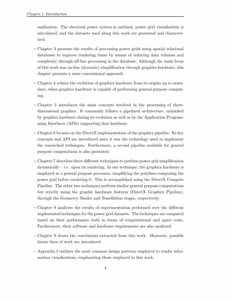
sualization. The electrical power system is outlined, power grid visualization is
introduced, and the datasets used along this work are presented and character-
ized.
Chapter 3 presents the results of processing power grids using spatial relational
databases to improve rendering times by means of reducing data volumes and
complexity through off-line processing in the database. Although the main focus
of this work was on-line (dynamic) simplification through graphics hardware, this
chapter presents a more conventional approach.
Chapter 4 relates the evolution of graphics hardware from its origins up to nowa-
days, when graphics hardware is capable of performing general-purpose comput-
ing.
Chapter 5 introduces the main concepts involved in the processing of three-
dimensional graphics. It commonly follows a pipelined architecture, mimicked
by graphics hardware during its evolution as well as by the Application Program-
ming Interfaces (APIs) supporting that hardware.
Chapter 6 focuses on the DirectX implementation of the graphics pipeline. Its key
concepts and API are introduced since it was the technology used to implement
the researched techniques. Furthermore, a second pipeline available for general
purpose computations is also presented.
Chapter 7 describes three different techniques to perform power grid simplification
dynamically – i.e. upon its rendering. In one technique, the graphics hardware is
employed as a general purpose processor, simplifying the polylines composing the
power grid before rendering it. This is accomplished using the DirectX Compute
Pipeline. The other two techniques perform similar general purpose computations
but strictly using the graphic hardware features (DirectX Graphics Pipeline),
through the Geometry Shader and Tessellation stages, respectively.
Chapter 8 analyzes the results of experimentation performed over the different
implemented techniques for the power grid datasets. The techniques are compared
based on their performance both in terms of computational and space costs.
Furthermore, their software and hardware requirements are also analyzed.
Chapter 9 draws the conclusions extracted from this work. Moreover, possible
future lines of work are introduced.
Appendix I outlines the most common design patterns employed to render infor-
mation visualizations, emphasizing those employed in this work.
4

1.3 Thesis outline
Appendix II exposes issues with the DirectX integration into windowed applica-
tions for the different versions of Microsoft Windows used in this work. As a
result of the supported integration, two different graphics rendering patterns had
to be employed during this work.
Appendix III reproduces a summary of this thesis in Spanish, in accordance with
the Regulations of the Ph.D. studies passed by the Governing Council of the
University of A Coruna at its meeting of July 17th 2012.
Appendix IV reproduces a summary of this thesis in Galician, in accordance with
the Regulations of the Ph.D. studies passed by the Governing Council of the
University of A Coruna at its meeting of July 17th 2012.
5

Chapter 1. Introduction
6

CHAPTER2Electrical Distribution Power Grids
This work is concerned with the efficient visualization of distribution power grids. More
specifically, the visualization of the network formed by power lines that form part of
the electricity distribution system. Power grid visualization has traditionally been
focused on transport networks [34, 48]. While these networks configure the backbone
of the power grid, distribution systems account for up to 90% of all customer reliability
problems [23]. Therefore, electric power utilities need their Computer-Aided-Design
(CAD) applications to be able to manage distribution networks as well. These concepts
are briefly introduced in the first section of this chapter.
Five datasets corresponding to distribution power grids from disparate areas were
used through this work. They are presented in this chapter, analyzing their character-
istics and the specifics of the power grid data subsets employed.
2.1 The electric utility system
Electric energy is a potential energy due to a difference in electric charges. Electric
power is the rate at which electric energy is transferred by an electric circuit and it
is the product of an electric current and an electric potential, also known as voltage.
Indeed, electric power – measured in watts – is the product of electric current and
voltage – measured in amperes and volts respectively.
Power management comprises disparate areas that conform a very complex system
known as the electric utility system. A power grid – or electrical grid – is a part
of the electric utility system: an interconnected network employed to deliver electricity
from suppliers to consumers. In order to categorize it, it is usually divided into three
stages: generation, transmission, and distribution. In complex systems, a fourth stage
called sub-transmission may be introduced [24]. However, since it usually overlaps with
7

Chapter 2. Electrical Distribution Power Grids
transmission and distribution stages, it is omitted from this characterization. Moreover,
the following depiction will focus on general classic power grids, not taking into account
smart grids or small renewable-energy power sources.
Most electricity has its origin in classical power generation systems, such as fos-
sil fuel or nuclear power plants, which transform kinetic energy into electric energy
through electromechanical generators, and yield voltages typically ranging between 11
and 30 kV. From these plants, the electricity must be transported and distributed to its
consumers. Energy losses during transmission are proportional to the current flowing
through the power lines. Therefore, in order to minimize the transmission losses, the
current is reduced by increasing the voltage.
Generation plants are connected to the transmission power lines through generation
substations, where a step-up transformer increases the voltage, generally up to well over
110 kV. Through that transformation, the electricity moves from the generation to the
transmission stage, in which it is transported over long distances – dozens or hundreds
of kilometers. During that journey, several transmission substations may be traversed,
where the voltages might be varied. These voltages usually stay over 30 kV, which is
considered a high-voltage and thus, the transmission stage portion of power grids are
usually called high-voltage networks. These networks are relatively simple since they
consist on long branches with few ramifications.
Once the electricity has been transported to the vicinities of its consumers, it must
be distributed to them, thus entering the distribution stage. In some countries such as
Spain, the transmission network is considered strategic and it is managed by a public or
at least partially state-controlled company. However, the distribution stage is normally
handled by competing private power utilities.
The distribution system can be split into primary and secondary distribution sys-
tems:
Primary distribution systems
Consists on feeders that deliver power from distribution substations to distribu-
tion transformers, joining the transmission stage with the secondary distribution
systems. Distribution power lines usually carry voltages ranging between 1 and
35 kV and thus, are also known as medium-voltage networks. Some large cus-
tomers such as factories may be directly connected to these networks, skipping
8

2.1 The electric utility system
Figure 2.1: The electric utility system.
the secondary distribution systems. Primary distribution systems have been the
focus of this research and will onwards be referred to as electrical distribution
power grids, or just power grids for short.
Secondary distribution systems
These systems retail the power from the distribution transformers to the con-
sumers. They contain power lines covering neighborhoods and arriving at con-
sumer homes. Since the carried voltages are usually between 220 and 240 V,
they are also named low-voltage networks. The complexity of these systems vary
greatly between regions. For instance, in the United States it is common to find
9

Chapter 2. Electrical Distribution Power Grids
less than ten consumers connected to each transformer, whereas in Europe the
number may go up to several hundreds.
Summing up, high-voltage networks carry power along many kilometers. Then it
traverses a medium-voltage network, covering distances between a few hundred meters
up to a few kilometers. Finally, the power is delivered to consumers through the low-
voltage network which typically cover distances shorter than a kilometer. The whole
process is resumed in Figure 2.1.
This research is focused on high-performance visualization of electrical distribution
power grids (medium-voltage networks, secondary distribution systems). The following
section introduces this area of visualization.
2.2 Visualization in electrical engineering
Traditionally, one-line diagram models – which provide schematic representations –
have been used as the main tool for mathematical analysis in electric networks design.
Their main tradeoff is the absence of any spatial attributes which also play an important
role in the networks design. Thanks to the progressive adoption of Geographic Infor-
mation Systems (GIS) by the utilities, CAD applications can now access very precise
data about the spatial relations within the networks and how they relate to external
elements in the real world. Several power grid visualization techniques that consume
this information have been developed over the years [47, 68, 32], the most common
being the Geographic Data Views (GDVs) which overlay technical power data such as
loads, flows, and contours over the geographic representation of the grid [49].
Depending on the intended usage, some forms of visualizations are more desirable
than others. The aforesaid one-line diagram models are useful for analysis and simula-
tion tools. Animated current flows are useful for real-time overseeing of power systems.
When studying physical coverage or terrain concerns, the physical layout of the network
is required.
This work is concerned with the efficient visualization of power distribution net-
works. This involves representing the power lines that conform a given network, main-
taining their topological and spatial relationships. As it will be seen in the following
10

2.3 Geographic and projected coordinate systems
section, the branches (power lines) forming the networks are defined using geographic
coordinates and thus, the visualization must try to properly display the network ac-
cording to its physical layout.
The aim was neither studying the existing power grid visualizations, nor introducing
new ones. Instead, the effort was put into improving the rendering of the most basic
visualization, so that more complex ones would also benefit from the performance
increase. Therefore, two visualizations are present through this work: representing
the network with lines having unitary-width or with all of them having the same fixed
width. Figure 2.2 shows the former: the visualization of the power distribution network
of the northeasternmost area of Spain, representing power lines as unitary-width lines.
Figure 2.2: Unitary-width lines visualization of a distribution power grid.
Many other visualizations are possible. For instance, power loads can be taken into
account to give varying widths to the rendered power lines. Furthermore, animations
showing the current flow could be introduced. Also, colors could be used to remark
problematic areas – such as those reaching maximum capabilities. Moreover, substa-
tions can also be represented in many ways – for instance, their size may be proportional
to their capacity.
11

Chapter 2. Electrical Distribution Power Grids
2.3 Geographic and projected coordinate systems
A coordinate system is a reference system used to represent some location by using one
or more numbers, called coordinates. This is a rather vague definition which applies to
many fields. One such field is the representation of physical locations on the surface of
the Earth. While many different coordinate systems can be defined for this, most fall
into one of the following two groups [2]:
Geographic coordinate systems are global or spherical coordinate systems,
such as latitude-longitude where angles are used to locate a point within an ellip-
soid modeling the shape of the Earth. Since the shape of the Earth is not uniform
and does not perfectly match an ellipsoid, depending on the requirements for the
geographic coordinate system, different ellipsoids will be used. For instance, the
Global Positioning System (GPS) uses an ellipsoid called GRS80 which is de-
signed to best-fit the whole Earth. The ellipsoid used for mapping in Britain is
the Airy 1830, which matches more closely the shape of the Earth in that specific
area, but is less exact than GRS80 for other parts of the Earth. Analogously,
when height must also be taken into account, the surface of the Earth must also
be modeled through what is called a geoid [45].
These parameters and others omitted here, define what is called the datum of
the geographic coordinate systems. The same geographic coordinate will most
likely yield different physical locations for different datums – the difference can
be up to hundreds of meters. However, it is possible to convert coordinates from
one geographic coordinate system to another, using well-defined mathematical
methods that take both datums into account.
Projected coordinate systems project Earth’s three-dimensional surface onto
a two-dimensional Cartesian coordinate plane. Because of this, they are also
known as map projections. A map projection cannot be a perfect representa-
tion, because it is not possible to show a curved surface on a flat map without
creating distortions and discontinuities. Therefore, different types of projections
exist, each one having its strengths and drawbacks; the chosen projection depends
on the requirements – whenever shapes, area or distances must be accurate. The
Universal Transverse Mercator (UTM) coordinate system is an example of a pro-
jected coordinate system.
12

2.4 Datasets employed in this work
All the coordinates present in the datasets used in this work, are UTM coordinates.
As can be glimpsed in Figure 2.3, this coordinate system splits the Earth between
80oS and 84oN into 60 zones covering 6 degrees of latitude each. Each zone is further
split into 20 latitude bands lettered from ”C” to ”X”. Each UTM coordinate has two
components, a northing and a easting, which are offsets in meters into a zone from the
lower left corner. UTM takes its name from the projection it uses, Transverse Mercator.
This projection preserves angles and approximates shapes, but distorts distances and
areas. Although the ellipsoid used in the UTM coordinate system varied over time,
nowadays the WGS84 ellipsoid is normally used to model the Earth.
Figure 2.3: Universal Transverse Mercator zones.
When integrating data using different coordinate systems, a common coordinate
system must be used. For instance, satellite imagery might be available, having the
area covered by each image indicated through the GPS coordinates of each corner of
the image. Even more, since images are bi-dimensional, a projection must be used. If
we were to visualize our datasets on top of the satellite images, coordinates would have
to be translated from one system to another. In order to do so, complex mathematical
operations are required, taking into account the datums of each geographic coordinate
systems and the projections applied for each one of them.
13

Chapter 2. Electrical Distribution Power Grids
2.4 Datasets employed in this work
Five different datasets have been used through this work. They are presented here,
explaining the physical areas they cover, the population densities in those areas, and
the available data for each one of them.
The data corresponds to the power grids of four countries and a significant region
within a fifth country:
Three different Central American countries: Guatemala, with a high population
density, and Nicaragua and Panama, with low population densities.
One Eastern European country, Moldova, which has a medium population density.
Galicia, the northwesternmost area of Spain, formed by 4 provinces with a scat-
tered, medium-density population.
Region Population Area (km2) Density
Nicaragua 5,677,771 130,373 43.55
Panama 3,394,528 75,517 44.95
Galicia 2,783,100 29,574 94.11
Moldova 3,633,369 33,846 107.35
Guatemala 13,675,714 108,890 125.59
Table 2.1: Population density by region.
Table 2.1 summarizes some population characteristics of the mentioned regions,
which have quite different populations and densities [69]. Population density provides
an indicator of the potential complexity of the distribution network, since the higher
the population the more likely that more power will be required.
For each region, we are interested in the available power grid data concerning the
networks – i.e. components of the network and their geographic and topological infor-
mation, not measurements such as power load or voltages. The available data for the
aforesaid regions in this regard can be divided into two categories:
Knots: points where three or more branches converge on. Typically, distribution
substations, transformers, and feeders are located at these points.
14

2.4 Datasets employed in this work
Branches: segments connecting knots and composed by two or more nodes linked
by power lines. Besides power lines interconnections, the nodes may also be
switchgear or medium-to-medium voltage transformers.
Table 2.2 shows the available data for each region, detailing the number of knots and
branches for each network. Furthermore, the number of lines and nodes that compose
the branches are also shown.
Region Knots Branches Nodes Lines
Moldova 59,726 43,769 160,717 116,948
Nicaragua 34,912 95,771 245,136 149,365
Panama 85,990 85,319 262,319 177,000
Guatemala 142,427 142,507 345,645 203,138
Galicia 23,812 91,959 301,118 209,159
Table 2.2: Distribution networks datasets.
As stated before, this work is focused on the visualization of power grid distribution
networks, more specifically the power lines composing them. Branches begin and end
in knots and thus, the position of their begin and end nodes coincide with those of the
knots they link. Thus, branches contain all the relevant information. Furthermore, the
type of node forming the branch – whenever it is a simple power post or a transformer
– is also irrelevant: only the position of the nodes forming the branch is required for
the visualization.
For each region, a dataset was created containing the power lines subset of the
branches. This information accounts for polylines whose points correspond to UTM
geographic coordinates. Thus, when represented preserving their spatial relationships,
they can be overlaid on a properly scaled map to be able to visualize its layout over
the terrain.
Figure 2.4 shows a visualization for each described dataset using one of the tech-
niques presented in this work. This visualization uses fixed-width lines for the power
lines and, as previously stated, is one of the two visualizations used through this work.
The other one consists on rendering the power lines with an unitary width. This was
earlier exhibited in Figure 2.2, where the Galicia dataset – same as in Figure 2.4e –
was visualized using an early implementation of the developed graphics engine.
15

Chapter 2. Electrical Distribution Power Grids
(a) Moldova. (b) Nicaragua.
(c) Guatemala. (d) Panama.
(e) Galicia.
Figure 2.4: Rendered visualization for the different datasets.
16

CHAPTER3Polyline Simplification Using Spatial Databases
This chapter presents the application of graphic cartography generalization techniques
to reduce the spatial resolution of power grids. This reduction decreases the data
volume involved in visualization which has two desirable consequences: it improves
optical legibility and yields faster rendering times.
The utter aim is to adjust the power grid resolution to the scale being used in the
visualization so that only the visually relevant data is processed and displayed. For
instance, a power grid may cover a whole state down to the city streets level; while
visualizing the whole power grid, there is no point in processing and displaying the
power lines covering streets since they will not be noticeable in the visualization.
Geographic Information Systems (GIS) support operations over data referenced
to a spatial coordinate system [27]. Commonly, they are implemented through spa-
tial databases which offer storage for primitives such as bi-dimensional and three-
dimensional points, lines, and polygons, as well as operations to efficiently manipulate
them. When employing spatial databases for GIS, a point will most likely correspond to
a geographic coordinate. Given the particularities of the shape of the earth, many dif-
ferent geographic coordinate systems are defined to support different needs. The proper
handling and translation of different coordinate systems is also a common feature of
spatial databases.
Since power grids are composed of branches whose nodes are defined using geo-
graphic coordinates, the graphic generalization is carried through a spatial database
where the data is stored and processed in order to generate the resolutions. The process-
ing is performed through stored procedures and each resolution is stored in a dedicated
table. It is an off-line process, that only requires being launched when the original
power grid data changes or whenever a new resolution is desired. The application per-
forming the power grid visualization simply queries the database to obtain the data
17

Chapter 3. Polyline Simplification Using Spatial Databases
from the table most closely matching the visualization resolution.
Due to historical data availability, in this chapter the Guatemala dataset is replaced
by a Central Spain dataset which comprises 9 provinces in the center of Spain, including
Madrid – the province with the highest population density in the country – and most
of the less densely-populated provinces of the country.
3.1 Data visualization collisions
No matter whenever a power grid is to be visualized on a screen or plotted on paper,
the physical space available is very limited. Thus, it imposes constraints on the rep-
resentation of the data that can be performed, yielding the need for the data to be
abstracted somehow to create a meaningful representation. That is what cartography
does through maps, as explained in the following section. Prior to that, this section
illustrates such need by analyzing the visualization of the datasets on a limited screen
area.
The Galicia dataset suffices to illustrate the resolution problems upon visualiza-
tion. Being the dataset covering the least area among the available ones, the following
considerations are aggravated when trying to visualize larger areas in the same visual-
ization resolution. This dataset contains branches ranging from a few meters up to 13
kilometers which are spread all over the northwestern-most region of Spain. The width
of the area covered by this region is 210 kilometers while the average power grid branch
length is 192 meters. Thus, an straight branch of average length represents only a 0.09%
of the total width of the Galicia area. When visualizing the whole region, there is no
point in processing all the data since most of the branches will not be visible and even
those which are visible may not be easily discerned if there are many branches in their
proximities. These two problems respectively correspond to the imperceptibility and
coalescence conditions of cartographic generalization.
In order to get an idea of how much redundancy is introduced by processing all
the available data to visualize a whole dataset, a matrix simulating the visualization
area was employed. The size of this matrix was the same as the screen visualization
area in Figure 3.1: 1,440 pixels of width and 820 pixels of height – thus having a total
of 1,180,800 positions. Each matrix entry holds the number of times that a point,
corresponding to the geographic coordinates of a node from the branches, has been
18

3.1 Data visualization collisions
Figure 3.1: Visualization of the whole Galicia power grid.
painted on the screen in the corresponding pixel. Note that only nodes are considered,
thus only pixels where the beginning and end points of individual lines are located are
considered, while pixels corresponding to the actual lines linking them are not.
Figure 3.1 exhibits a screenshot of a very simple visualization of the whole Galicia
dataset using unitary width-lines for the power lines. Coalescence is a condition spe-
cially found in cities, where there are hundreds of branches serving the streets which
can not be distinguished when using a small visualization scale. As a result, city areas
are too cluttered in the visualization.
Dataset Collisions Points % Collisions Max. Collisions
Galicia 258,285 301,118 86.15 % 331
Central Spain 468,750 493,121 95.06 % 2,991
Moldova 142,319 160,717 88.55 % 1,101
Nicaragua 217,637 245,135 88.78 % 295
Panama 232,122 262,319 88.49 % 309
Table 3.1: Points colliding in the same pixel of the visualization area.
Table 3.1 shows, for each dataset, how many times a pixel had more than a point
assigned (collisions), the total number of points that form the branches, the percentage
19

Chapter 3. Polyline Simplification Using Spatial Databases
of points that end up colliding with others in the same pixel, and the maximum number
of collisions for a single pixel. Between a 86.15% and a 95.06% of the points fall in
the same physical position of the visualization area. Even more, in the case of the
Central Spain dataset, there is one pixel of the screen which ended up being painted
2,991 which means that 2,990 node computations and coordinate translations could
have been afforded just for that pixel. By skipping the processing all of those nodes in
the first place, a big percentage of the computations required to visualize the data can
be avoided, resulting in a faster rendering of the visualization.
3.2 Cartographic generalization techniques
Cartography is in essence the discipline of making visual representations of a certain
area, using symbols to express spatial relationships between elements present in that
area. These representations are called maps and in most cases, are drawn to a scale:
the ratio of a distance on the map to the corresponding real distance on the ground.
For instance, a centimeter in a 1:25,000 scale map represents 250 meters on the ground.
Such a scale is considered a large scale, while a 1:1,000,000 – which is common for road
maps – is normally referred to as a small scale. The larger/smaller scale terminology
arises from the fact that it is common to write the scale as a fraction, which yields that
1/25,000 is larger than 1/1,000,000.
Obviously, maps can not capture all the detail existing in the area they repre-
sent. In cartography, generalization is the process of abstracting the representation
of geographic information to match the scale requirements of a map. By applying car-
tographic generalization, different maps carrying different levels of detail are generated
for different scales. This may result in different symbols being used to represent the
same information or the alteration of the existing ones. Following this consideration,
cartography generalization can be divided into two categories: conceptual and graphic
generalization. In the former – which is also known as information abstraction – either
the symbolization or the meaning of the symbols changes. On other hand, in graphic
cartography, which is focused on reducing spatial resolution, the type of symboliza-
tion used in the map is not changed but the symbols themselves may be transformed
– e.g. enhanced or exaggerated – to keep its optical legibility.
McMaster and Shea studied the generalization process by answering three questions:
why, when, and how to generalize [35] [36]. Why generalize is the most general question,
20

3.2 Cartographic generalization techniques
its answer being: to counteract the undesirable consequences of scale reduction on a
map. These consequences define the conditions on when to generalize the map, while
the concrete techniques employed to perform the generalization correspond to the how.
3.2.1 Conditions – when to generalize
The generalization conditions can be summarized in: congestion, coalescence, conflict,
complication, inconsistency and imperceptibility. Congestion and imperceptibility are
the more dominant forces in this work.
Congestion refers to the fact that upon scale reduction too many geographic fea-
tures need to be represented in a limited physical space on the map. This is the case
of geographic points colliding in the same physical pixel, seen in Section 3.1.
Imperceptibility occurs when some features of the map are not optically legible
for some reason – for instance when visualizing a large region, a branch which is only
a few meters long will fall below the minimal portrayal size of the map at that scale.
Another related condition is coalescence. In this case the features can be repre-
sented in the map but they are too close or in some kind of juxtaposition with other
features, making their area of the map too clogged. This would be the case of the cities
when the map is being visualized using a small scale.
3.2.2 Techniques – how to generalize
Generalization techniques help counteract the undesirable consequences of scale reduc-
tion and they can be grouped under six categories: reducing complexity, maintaining
spatial accuracy, maintaining attribute accuracy, maintaining aesthetic quality, main-
taining a logical hierarchy, and consistently applying generalization rules. While all of
these goals are desirable, this work is mainly focused on reducing the complexity while
maintaining spatial accuracy and improving the aesthetic quality.
McMaster and Shea classified generalization operators into spatial and attribute
transformations [36]. In this work, we are only concerted about the geographical and
topological perspective of the data and thus, attribute transformations do not apply.
21

Chapter 3. Polyline Simplification Using Spatial Databases
The authors identified ten spatial transformations: simplification, smoothing, collapse,
refinement, exaggeration, enhancement, displacement, aggregation, merging and amal-
gamation. The last three operations are essentially the same but operating on different
dimensions (points, lines or areas respectively). Spatial transformations over line fea-
tures are restricted to simplification, smoothing, displacement, merging and enhance-
ment.
In order to reduce the complexity of power grid topologies, simplification and merg-
ing operators were used, as described in the next sections after introducing the selection
process. Selection counteracts imperceptibility while merging reduces both congestion
and coalescence. While focused on reducing imperceptibility, line simplification may
also reduce congestion.
3.2.2.1 Selection
Before any technique can be applied, the involved data must be retrieved. This consti-
tutes the first chance to reduce the data volume by selecting only a relevant subset.
The most fundamental requirement is for the data to be optically visible in the final
visualization. Thus, any imperceptible feature found in the data upon retrieval, can be
dimmed as irrelevant and filtered out of the selection process. In order to apply this
filtering, a visibility measure must be introduced. The width and height of the area
covered by the power grid in meters, divided by the screen resolution of the visualization
area in pixels yield the meters per pixel (mpx) ratios. The most conservative – i.e.
the smallest ratio – of the two is used as the minimum length that a branch from the
power grid must have to be considered perceptible and thus selected.
In the case of branches composed by more than one line, the smallest bounding box
containing them is compared against the mpx ratios. The bounding box must be either
vertically or horizontally equal or larger than the corresponding mpx ratio.
Furthermore, in electrical power grids, the same physical line can be considered
as two different branches composed of the same points but with different directions.
However, when the power grid visualization is not concerned about the current flow
direction – as is the case of this work – those two branches are equivalent. Thus, the
first time that intersecting lines are found, a check is made to find whenever some of
22

3.2 Cartographic generalization techniques
them are equivalent. If they are, only one of them will be kept and all the equivalent
ones will be removed.
3.2.2.2 Line simplification
In the simplification context, the term line refers to the LineString OpenGIS standard
datatype, consisting of a set of interconnected line segments [44], referred to as a
polyline in the rest of this work. Line simplification produces a reduction in the
number of segments by removing inner points without modifying the coordinate position
of any point. In the case of power grid branches, this accounts for the removal of certain
nodes while leaving unchanged the geographic coordinates of the rest – i.e. those nodes
passing the line simplification filter.
Given its simplicity and efficient implementation in modern spatial databases, the
Ramer-Douglas-Pecker algorithm was used to perform the simplification [26]. It oper-
ates by recursively discarding those nodes that are not significant based on a certain
threshold, following the next steps:
1. Form a line connecting the beginning and end points.
2. For each other point, compute the orthogonal distance to that line.
3. Select the point with the largest orthogonal distance.
4. If the distance is larger than the threshold, repeat the process for the lines formed
by that point and the beginning and end points.
The algorithm ends whenever there are no points left, or none of them meet the
criteria. The threshold was set to the computed mpx ratio for a power grid area and a
visualization resolution.
3.2.2.3 Merging
The process of joining map symbols on the basis of their proximity is called aggre-
gation [46]. Its objective is generally a reduction of the spatial resolution, not only
23

Chapter 3. Polyline Simplification Using Spatial Databases
increasing the legibility of the symbols but also avoiding excessive accumulation of
symbols in a small area. Aggregation comprises a number of techniques among which
are amalgamation and merging. Amalgamation replaces two or more symbols of the
same or different type into a single symbol of a different type. Merging substitutes
symbols having the same type into a single symbol of that very same type. Two merge
operations were applied to power grid branches in this work:
1. Merge branches that share their beginning and end nodes.
Two branches, one having its end node as the beginning point of the other, can
be merged into a single branch. Merged branches can also share their beginning
and end nodes with other branches. This results in an iterative merging process
where several interconnected branches are merged into a single branch. Since the
resulting merged branches have more intermediate nodes, they become eligible
for line simplification. However, the beginning and end nodes of branches usually
correspond to significant power grid entities such as substations. Thus, applying
line simplification to merged branches may remove relevant nodes.
2. Merge branches located too close to each other to be individually distinguished.
Two close branches can be merged into a single branch formed by the equidistant
points to those of the branches. Since merged branches may be eligible for merging
with others, it is an iterative process just like the previous technique. However, the
original branches cease to exist since they do not form part of the merged branch
– as was the case with the previous technique. Furthermore, in the process, the
geographic coordinates of the nodes change, which impacts the aesthetics and
accuracy of the map. The process is controlled by a neighborhood parameter
determining the area surrounding a given branch to look into for other branches
for merging. The bigger this parameter is, the more branches that will be merged
and as a result, the more aesthetically noticeable in the visualization and the
higher the loss of accuracy.
Summing up, the first merge technique reduces the overall number of branches but
only removes redundant nodes, while the second technique replaces the two involved
branches by a new one, thus not only halving the number of branches but also the num-
ber of nodes. Moreover, the latter is visually noticeable as it removes the original nodes
and creates new ones on different locations, while the former is not. Both techniques
work at a higher level than line simplification since they operate over entire branches
instead of over the nodes within a given branch.
24

3.3 Implementation
3.3 Implementation
The described generalization techniques were implemented through stored procedures
in a spatial database. Specifically, the PostgreSQL relational database management
system [11] and its PostGIS spatial extensions [10] were employed, while using its
PL/pgSQL language to program the stored procedures. A spatial-enabled database was
created for each power grid dataset, containing different tables for the base data and the
different scales. This way, a multi-scale database architecture was implemented,
where multiple representations of the spatial data are stored using different resolutions
(scales) and a set of rules are applied to support the generalization decisions, selecting
the appropriate representations, governing updates, and maintaining database integrity
[31].
The stored procedures make intensive use of the spatial indexing system available
in PostGIS [29], notably the merging operator, which uses it to find the branches
intersecting with every branch and its neighbors, and the selection operator which
employs a bounding box to retrieve all the branches within the power grid subarea to
be visualized.
A set of 19 PostGIS functions were employed to implement the different techniques,
ranging from simple functions such as ST NPoints which enumerates the number of
points in a LineString to more complex functions like ST LineMerge or ST MakeLine.
Notably, the line simplification invokes ST SimplifyPreserveTopology which provides
an implementation of the Ramer-Douglas-Pecker algorithm.
The components of this implementation are the following:
Stored procedures library
Contains PL/pgSQL procedures implementing the different techniques, the gen-
eralization process using them, and a batch multi-scale generation in charge of
producing the tables with the different generalized scales.
Base and multi-scale tables
The original power grid data is stored in a base table and then each generalized
scale is stored in a dedicate table.
Trigger functions
25

Chapter 3. Polyline Simplification Using Spatial Databases
Triggers are used to keep the multi-scale tables synchronized with the base table
so that any change in the power grid data is reflected in all the generalized scales.
The generalization and multi-scale generation procedures require some parameters:
Generalization process
Requires the mpx and the merge neighborhood factor. The former is the meters
per pixel ratio representing the minimum desired segment length, while the latter
is used to define how far around a branch to look for its neighbors. The bigger
this parameter is, the more branches are merged and the more noticeable the
process becomes in the visualization. Based on the performed experimentation,
reasonable values are 2 and 3 times the mpx, which represents the maximum
number of pixels between branches to be considered neighbors.
Multi-scale generation
Requires the visualization and smallest desired scale resolutions, the number of in-
termediate scales to generate between them, and the generalization neighborhood
factor. Intermediate scales resolutions are calculated by interpolating the visu-
alization and smallest scale resolutions. Furthermore, for each one of them, the
corresponding mpx value is calculated by dividing the interpolated scale resolu-
tion by the visualization resolution. That value is passed along the neighborhood
parameter to the generalization process procedure during the batch generaliza-
tion. The pseudo-code for this procedure is shown in Algorithm 1.
Algorithm 1: Multi-scale generation pseudo-code.Data: LineStrings← LineString primitives composing the power grid
NumberOfScales← Number of desired scales to generateBaseScale← Original scale of the dataSmallestScale← Smallest desired scaleVisualizationScale ← Width and height of the target visualization area, in pixels
Result: GeneralizedTables← Tables containing the LineStrings generalizations
for i← 1 to NumberOfScales doscale← (BaseScale - SmallestScale) / impx← min(scale.Width / VisualizationScale.Width, scale.Height /VisualizationScale.Height)GeneralizedTables[i]← Generalize(LineStrings, mpx, NeighborhoodFactor)
end
26

3.4 Experimentation results
Once the different scales have been generated and stored in dedicated tables, they
can be consumed. In order to do so, a client application chooses the more suitable
table: the one holding the closest scale to the visualization resolution. That table is
queried using a two-dimensional bounding box with the same geographic coordinates as
the area being visualized. A box covering a larger area can be employed if pre-caching
of the surrounding regions is desired – for instance, to avoid delays or visual artifacts
when panning the power grid visualization.
3.4 Experimentation results
In order to analyze the developed implementation, some tests were conducted on a
PostgreSQL 8.4 with PostGIS 1.5.1 running on Windows XP SP3 in a Intel Core2 Q6600
2.4 GHz CPU machine with 2 GBs of memory. The experimentation objectives were
to measure the time required to perform the generalization, the data volume reduction,
and the resulting faster visualization rendering times. Also, the non-generalized and
generalized visualizations were optically compared.
The generalization was executed for the most intensive scenario: generalizing power
grid branches using their original scale resolution but restraining the visualization reso-
lution to an area with 1,440 pixels of width by 820 pixels of height. This corresponds to
the whole power grids being displayed in the visualization area, resulting in one of the
larger scales that may be required. As the user zooms into the visualization, a smaller
subarea of the power grid is displayed, thus requiring a smaller scale. Furthermore, the
generalization was performed for two neighborhood factors, corresponding to 2 and 3
times the mpx.
Dataset BranchesNeighborhood
2x mpx 3x mpx
Galicia 91,959 427s 430s
Central Spain 147,651 142s 158s
Moldova 45,769 294s 305s
Nicaragua 95,770 100s 101s
Panama 85,319 52s 55s
Table 3.2: Time consumed by the generalization process.
27

Chapter 3. Polyline Simplification Using Spatial Databases
Table 3.2 exhibits the time consumed by the generalization process for each dataset
using 2 and 3 times the mpx as the neighborhood factor. Using a neighborhood factor of
3 times thempx resulted in a 4.5% average time increase compared to a factor of 2 times
thempx. As the neighborhood factor is increased, so is the area around each branch into
which included or intersecting branches are searched. While this yields more merged
branches, it also increases the computational requirements, yielding higher execution
times.
The faster time resulted in almost a minute, making it obvious that the generaliza-
tion process can only be performed off-line. Therefore, the results must be stored so
they can be retrieved without incurring in delays.
Dataset Original Generalized 1st Merges 2nd Merges
Galicia 91,959 13,767 8,960 / 5 iters 2,120 / 5 iters
Central Spain 147,651 8,660 4,387 / 4 iters 3,035 / 7 iters
Moldova 43,769 9,012 6,049 / 4 iters 1,090 / 5 iters
Nicaragua 95,770 6,482 5,550 / 6 iters 900 / 4 iters
Panama 85,319 4,777 3,632 / 5 iters 831 / 6 iters
Table 3.3: Number of branches as a result of the generalization process with a neigh-borhood factor of 3.
Table 3.3 shows the results of generalizing the different datasets for a neighborhood
factor of 3. 1st Merges column refer to the merging of branches that share their ending
and beginning points, while the 2nd Merges are those creating a new branch averaging
a pair of branches. The generalized versions contain the 10.58% of the original data
on average. Since the merging is an iterative process stopping when there are no more
branches eligible for merging, the iterations required to complete each kind of merge
are also shown.
The same process with a neighborhood parameter of 2 times the mpx is shown
in Table 3.4. Compared to the previous result, it can be seen that using a factor
of 2 instead of 3, yields an average of 27.66% less 2nd Merges. The number of 1st
Merges do not change since they are not affected by the neighborhood parameter. The
generalized version contains in this case the 11.81% of the original data, slightly more
than the 10.58% yielded by the use of a neighborhood factor of 3.
28
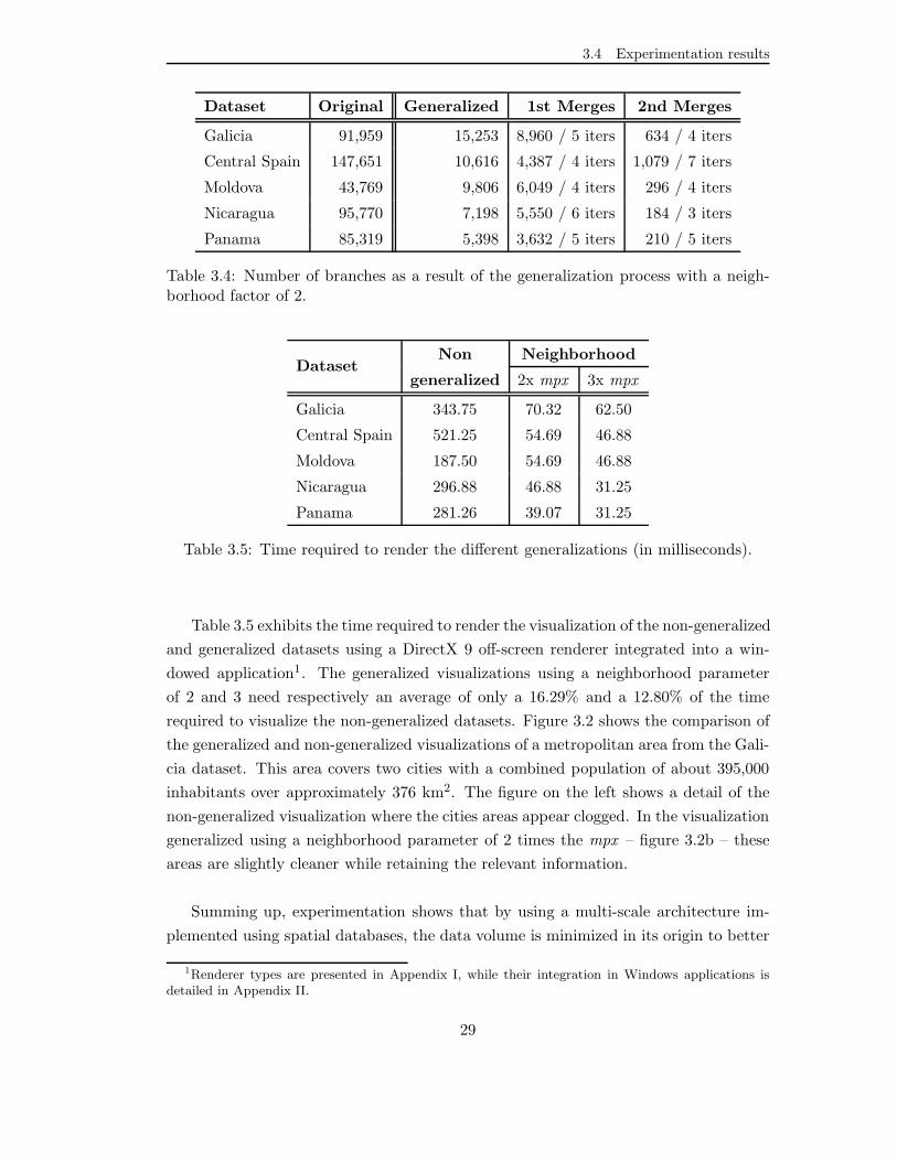
3.4 Experimentation results
Dataset Original Generalized 1st Merges 2nd Merges
Galicia 91,959 15,253 8,960 / 5 iters 634 / 4 iters
Central Spain 147,651 10,616 4,387 / 4 iters 1,079 / 7 iters
Moldova 43,769 9,806 6,049 / 4 iters 296 / 4 iters
Nicaragua 95,770 7,198 5,550 / 6 iters 184 / 3 iters
Panama 85,319 5,398 3,632 / 5 iters 210 / 5 iters
Table 3.4: Number of branches as a result of the generalization process with a neigh-borhood factor of 2.
DatasetNon Neighborhood
generalized 2x mpx 3x mpx
Galicia 343.75 70.32 62.50
Central Spain 521.25 54.69 46.88
Moldova 187.50 54.69 46.88
Nicaragua 296.88 46.88 31.25
Panama 281.26 39.07 31.25
Table 3.5: Time required to render the different generalizations (in milliseconds).
Table 3.5 exhibits the time required to render the visualization of the non-generalized
and generalized datasets using a DirectX 9 off-screen renderer integrated into a win-
dowed application1. The generalized visualizations using a neighborhood parameter
of 2 and 3 need respectively an average of only a 16.29% and a 12.80% of the time
required to visualize the non-generalized datasets. Figure 3.2 shows the comparison of
the generalized and non-generalized visualizations of a metropolitan area from the Gali-
cia dataset. This area covers two cities with a combined population of about 395,000
inhabitants over approximately 376 km2. The figure on the left shows a detail of the
non-generalized visualization where the cities areas appear clogged. In the visualization
generalized using a neighborhood parameter of 2 times the mpx – figure 3.2b – these
areas are slightly cleaner while retaining the relevant information.
Summing up, experimentation shows that by using a multi-scale architecture im-
plemented using spatial databases, the data volume is minimized in its origin to better
1Renderer types are presented in Appendix I, while their integration in Windows applications isdetailed in Appendix II.
29
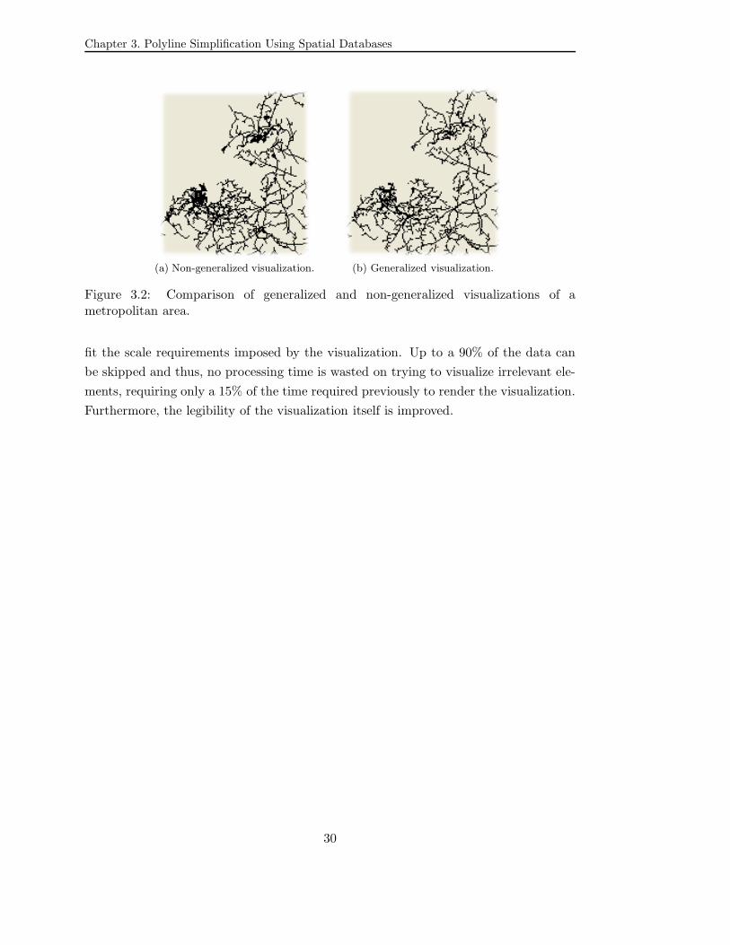
Chapter 3. Polyline Simplification Using Spatial Databases
(a) Non-generalized visualization. (b) Generalized visualization.
Figure 3.2: Comparison of generalized and non-generalized visualizations of ametropolitan area.
fit the scale requirements imposed by the visualization. Up to a 90% of the data can
be skipped and thus, no processing time is wasted on trying to visualize irrelevant ele-
ments, requiring only a 15% of the time required previously to render the visualization.
Furthermore, the legibility of the visualization itself is improved.
30

CHAPTER4Graphics Cards Evolution
Graphics cards have undergone a huge evolution since its origins in the eighties. Born
as mere adapters that allowed a computer to show characters on a screen, they quickly
evolved towards complex hardware equipped with powerful Graphical Processing Units
(GPUs) and dedicated high-performance memory. Graphics cards enabled the tran-
sition from command-line to graphical user interfaces. As video games became more
sophisticated, they started focusing on three-dimensional environments and consumer
graphics cards gradually adopted the pipelined architectures of high-end graphics work-
stations. More recently, as their hardware became more and more parallelized, general-
purpose computational applications beyond graphics rendering arose. Such is the com-
puting power of modern graphics cards that they are replacing many of the multi-core
CPU clusters typically used in supercomputers.
4.1 Origins
The history of consumer graphics cards – also known as video cards or graphics adapters
– can be said to have its origin in 1983 when IBM [6] launched its IBM 5150 Personal
Computer. It was shipped with the IBM Monochrome Display Adapter (MDA): a 8-bit
Industry Standard Architecture (ISA) expansion card with 4 KBs of memory allowing
to display single colored text in 80 columns by 25 lines. Consumers could opt to replace
it with the more advanced Color Graphics Adapter (CGA) which allowed not only text
modes but also graphics modes with a maximum resolution of 640 pixels of width by
200 pixels of height (640x200) and a 4-bit color depth, thus allowing the use of up to 16
colors – either 320x200 and 16 colors or 640x200 and 2 colors. The following year, the
first non-IBM vendor graphics card was released: the Hercules Graphics Card, offering
an increased resolution and compatibility with both MDA and CGA cards.
31
Chapter 4. Graphics Cards Evolution
Arguably, there were more advanced graphics systems around the time the IBM
Personal Computer (PC) was launched. For instance, the Commodore 64 and its
successor, the Amiga – released respectively in 1982 and 1985 – and the Apple II series
in the consumer field, or high-end SGI [15] workstations in the professional segment.
Nevertheless, it was the high level of customization – through ISA cards – offered by
the IBM PC architecture and its popularity among computer enthusiasts that fueled
the development of graphics cards by third-party vendors and the fierce competition
among them that led to modern graphics cards.
The successor of the IBM PC – the IBM PC/AT – was launched in 1984, offering
two new graphics cards: the Enhanced and the Professional Graphics Adapters (EGA
and PGA). On one hand, the former featured 64 KBs of video memory – expandable
to 256 KBs through a daughter-board – and increased resolution modes, while also
allowing the simultaneous use of 16 colors from a palette of 64. At the same time,
other vendors like ATI (now part of AMD [1]) and Paradise launched compatible cards.
Video modes offered by the EGA and compatible cards kept being supported by DOS
video-games until the early nineties. Notably, the EGA introduced an early form of
hardware acceleration by allowing mask registers and bitwise operations. On the other
hand, the PGA was not so successful. Targeted for users of Computer-Aided-Design
(CAD) applications, the PGA consisted of three cards in one. It was equipped with a
8088-2 microprocessor which could be depicted as the predecessor of dedicated graphics
processing units.
The launch of the IBM PS/2 in 1987 introduced the Video Graphics Array (VGA)
which conforms the basis of modern graphics systems. Its hardware was designed using
application-specific integrated circuits which led to the launch of the first motherboards
with integrated graphics systems. The VGA soon became a de facto standard and its
640x480 resolution stands nowadays as the lowest supported resolution to be expected
from any system without proper graphics drivers configured.
Up to this point, the graphics cards were mostly adapters connecting the video
output with the monitor. Hence, the adapter term employed to name most of the
graphics cards systems of the time. Vendors were focused on offering more resolution
and more colors than the competition – increasingly needing more video memory as a
result – while being able to connect to most monitors and keep compatibility with ex-
isting software. Circuitry present in these graphics cards consisted mostly of a graphics
controller chip, a BIOS ROM, a video memory, a Digital-to-Analog converter – to be
able to produce the analog output required by monitors – and some connectors. The
32
4.1 Origins
video memory is commonly known as the frame buffer since it would merely hold the
color value of each screen pixel to be displayed in the output monitor. The set of pixels
being displayed is called a frame, and the amount of frames a graphics system is able
to generate and display per second is known as the frame-rate. Because of memory
limitations, only a small set of colors could be offered. In order to allow more colors to
be available, palettes were used as indexing schemes. Given a big spectrum of colors
available, a subset of them is selected at each time to be displayed. These colors are the
entries of a palette and palette indices are stored in the frame buffer instead of color
values. Therefore, a palette is required in order for the graphics system to know which
color from the available spectrum correspond to each index found in the frame-buffer.
By changing the palette, different sets of colors can be used.
A video mode is the combination of a color depth and a given resolution. The
frame buffer size is a direct function of these values and thus, each video mode requires a
different amount of video memory in order to store the frame buffer. A given graphics
card would allow different video modes, some of them requiring less video memory
than others. For certain video modes, the frame buffer consumes half or less than the
available memory. In such cases, more than one frame can be stored simultaneously
in video memory. This led to the introduction of new techniques such as double
buffering, which reduces the visual flickering that would happen each time a new
frame is displayed. It works by using two frame buffers, one holding the output display
frame and other storing the next frame being rendered. Once the next frame is ready,
buffers are almost instantaneously swapped. As a result, there is no delay caused by
having to wait for its renderization since it is already in video memory. Following this
usage, the frame buffer can be seen as an image memory used to decouple the render
frame rate from the display frame rate.
The launch of many different graphics hardware along with different monitor config-
urations and working modes lacking standardization, created a chaos in the consumer
graphics industry that led to the foundation of the Video Electronics Standards Asso-
ciation (VESA) [17] in 1989. Its most significant standard is the VESA BIOS Exten-
sion specification which defines ”standard software access to graphics display controllers
which support resolutions, color depths, and frame buffer organizations beyond the VGA
hardware standard” [65].
In the same way that the graphics cards evolved, so did the bus used to communicate
them with the motherboard. As graphics cards became more powerful and enabled
larger resolutions, the amount of memory that could be transferred over the bus became
33
Chapter 4. Graphics Cards Evolution
the performance bottleneck. The Peripheral Component Interconnect (PCI) Local Bus
was launched in 1993 to replace the ISA and was itself replaced by PCI-X in 1998. These
were generic expansion cards buses, but graphics-oriented buses were also introduced
at the time: VESA created the VESA Local Bus to extend the existing ISA expansion
cards and Intel’s [5] Accelerated Graphics Port could also be found in motherboards
along PCI cards. Nowadays, all these buses have been replaced by the PCI Express
(PCIe) in its different versions.
4.2 2D acceleration
The IBM 8514/A graphics card was launched in 1987 – about the same time as the VGA
– and instead of being a mere controller, it was equipped with a coprocessor able to
execute graphics commands. It supported line drawing, area fills and video memory bit
block transfers (commonly known as BITBLTs), offloading the CPU from such work.
IBM released a programming interface called Adapter Interface which allowed to take
advantage of these features. For instance, instead of having to calculate the positions
of the pixels for a line and setting the proper color values in the frame-buffer, one could
paint a line simply by specifying the beginning and end points as well as its color. The
IBM 8514/A used a proprietary IBM bus and it was not backwards-compatible but it
was designed to be able to work along a standard VGA card for compatibility.
One year before, in 1986, Texas Instruments had released the TMS34010: the first
fully-programmable graphics card. Its hardwired graphics commands included those
of the 8514/A, plus pixel operations but it consisted on a full-fledged processor able
to execute complete programs. Since it was not compatible with the existing software,
the Texas Instruments Graphics Architecture was released for programming. It fea-
tured ”a CMOS 32-bit processor with hardware support for graphics operations such
as PixBlts [raster ops]2 and curve-drawing algorithms. Also included is a complete set
of general-purpose instructions with addressing tuned to support high-level languages.
(. . . ) TMS34010 graphics processing hardware supports pixel and pixel-array processing
capabilities for both monochrome and color systems that have a variety of pixel sizes.
The hardware incorporates two-operand raster operations with Boolean and arithmetic
operations, XY addressing, window clipping, window checking operations, 1 to n bits
per pixel transforms, transparency, and plane masking.” [63].
2The term raster operations refers to operations performed over the pixels that compose images.
34

4.3 3D acceleration
Microsoft [7] introduced graphical user interfaces (GUIs) to the PC market with the
launch of its Windows graphical environment. The popularity gained by its third re-
lease in 1990 resulted in a milestone in graphics cards evolution. As time passed, GUIs
started to become more common, gradually replacing DOS command line applications.
While applications requiring high-performance graphics, such as video games, contin-
ued being developed as DOS applications because of the direct access to the graphics
hardware it allowed, it soon became apparent that the future was in GUI applications
requiring graphics performance to be improved. Microsoft, working closely with graph-
ics hardware vendors, introduced the WinG library more oriented to animations than
its original Graphics Device Interface (GDI) library.
In 1991, S3 Graphics [14] released the S3 86C911 chip, which is commonly stated
to be the origin of main-stream 2D acceleration. This chip, designed for both moth-
erboards and graphics cards, was created with graphical user interfaces acceleration in
mind – in fact, S3 marketed it as a GUI accelerator. On top of the classic raster op-
erations, it included instructions to accelerate other GUI-specific areas such as mouse
cursors and hit-testing. These features were quickly adopted by other vendors.
With the launch of Windows 95, IBM PC Compatibles definitively moved from the
command line to graphical user interfaces. The Windows Games SDK was launched
to attract DOS video game developers to Windows. It was soon renamed as DirectX
and consisted on a set of libraries trying to cover all the aspects of game developments
from graphics or sound to control. The graphics library was called DirectDraw and
supported hardware overlays which allow each application to have a dedicated video
memory buffer for its visual representation. The graphics system automatically merges
all the individual buffers to the frame-buffer. As a result, there are no concurrency
issues because of different applications trying to write to the frame-buffer at the same
time.
ATI Mach series are an example of the evolution of 2D graphics acceleration cards
through this period of time. The first one – the Mach 8 released in 1991 – was a 8514/A
clone while its successor – the Mach 32, launched one year later – was regarded as a
GUI accelerator following the suit of the S3 86C911 chip. In 1994, the Mach 64 was
launched and one year later, the Mach 64 GT – later rebranded to 3D Rage – offered
basic 3D acceleration. Other common features of the time were video decoding and TV
tuning.
35
Chapter 4. Graphics Cards Evolution
4.3 3D acceleration
Main-stream 3D graphics systems have their origin at Silicon Graphics Incorporated
(SGI), which in 1984 launched the IRIS Workstation. Aimed at professionals requiring
high-end graphics performance, ”conceptually, the IRIS is divided into three pipelined
components: the CPU, the Geometry Engine (GE) subsystem, and the raster subsystem.
The system’s CPU, a Motorola 68000 or 68010, manages display lists, runs applica-
tion programs, and controls the Geometry Engine and raster subsystems. The geometry
subsystem provides 2-D and 3-D geometric processing with either 32-bit floating-point
or integer formats. All transformations, clipping, and scaling with perspective calcu-
lations are performed in the GEs. Geometric primitives for drawing lines, polygons,
characters, and parametric and rational cubic curves are supported by the geometry
subsystem. The raster subsystem controls up to 24 bit planes of image memory, which
can be used in either single- or double-buffered modes.” [40]. This architecture set the
foundation of upcoming graphics hardware which was following this concept of a geom-
etry transformation and rasterization pipeline. It evolved fast, firstly adding flat and
smooth shading as well as depth buffering. Reductions in memory costs and advances
in the development of application-specific integrated circuits (ASICs) led to huge im-
provements of the raster subsystem; chips equipped with multiple rendering processors
were introduced. At a following stage of evolution, anti-aliasing and texture mapping
features were introduced [20]. In 1992, and based on their previous graphics APIs,
SGI launched the OpenGL API and founded a board among other industry players to
oversee its evolution. Their aim was to provide a common graphics API that hardware
vendors would support through their software drivers.
Back in the consumer PC market, by 1995 2D hardware acceleration had become a
standard and graphics cards vendors starting shifting their innovations towards 3D ac-
celeration as a result of the increasing popularity of 3D video games of the time such as
Quake (which was the first blockbuster game offering full real-time 3D rendering). For
instance, Virge’s S3d Engine ”incorporates the key Windows accelerator functions of
BitBLT, line draw and polygon fill. 3D features include flat shading, Gouraud shading
and texture mapping support. Advanced texture mapping features include perspective
correction, bilinear and tri-linear filtering, MIP-Mapping, and Z-buffering. The S3d
Engine also includes direct support for utilizing video as a texture map. These fea-
tures provide the most realistic user experience for interactive 3D applications” [18].
Following the architecture engineered by SGI, the S3d Engine supported OpenGL.
36

4.3 3D acceleration
Vendors continued to launch new graphics cards offering slightly different architec-
tures such as unified frame-buffer and texture memory. Nevertheless, most of them
featured hardware triangle-based rasterization; some offered hardware triangle setup
and clipping support such as the ATI Rage Pro or the Rendition Verite 1000. It should
be noted that up to this point, 3D acceleration was really a evolution of the 2D raster
operations oriented towards speeding common 3D post-rasterization operations: blend-
ing pixels with alpha or fog values as well as textures, and executing operations based
on particular masks or Z values stored in special memory buffers. Most of the effort was
focused on maximizing the quality and performance of the texture mapping, while the
geometry processing such as vector-matrix multiplications were still being performed
entirely by the CPU.
Figure 4.1: Abstract rendering engine of the Voodoo Graphics [19].
Particularly successful were the Voodoo series by 3dfx which were add-in cards
providing 3D acceleration and which required a 2D card. Despite having launched
a couple of 2D/3D cards, their more successful ones were the exclusively 3D add-in
37

Chapter 4. Graphics Cards Evolution
cards. These cards offered a superior performance and its proprietary Glide API gained
wide acceptance among game developers. Since this API was specifically designed for
3dfx graphics cards, it was closer to the hardware than OpenGL implementations and
thus, offered a superior performance. Its first product – the Voodoo Graphics card
– consisted on two ASICs, one managing the frame buffer and another in charge of
textured rasterization with dedicated texture memory. Thus, it supported hardware
triangle-based rasterization and pixel operations, leaving geometry operations to the
CPU [19]. The architecture of the Voodoo Graphics card is presented Figure 4.1.
While the original card incorporated one texture unit (TREX), several cards could
work together, thus providing several texture units – 3 in the case of the figure.
All the graphics cards of the time supported OpenGL, which had became the domi-
nant graphics API in the video game market after its advantageous start position since
it dominated the high-end graphics workstations market. Microsoft launched its Di-
rectX API aiming at providing a whole set of libraries – not only graphics – to promote
video game development for Windows. Direct3D – launched with DirectX 2.0 – was the
response from Microsoft to OpenGL. Despite being difficult to program at the begin-
ning, Direct3D started to become more popular with each release of DirectX. At least
one new version of DirectX was launched every year from 1995 until 2006 – versions
2.0 and 3.0 were both launched in 1996 and version 4 was skipped. DirectX 10.1 was
released in 2008, followed by version 11 in 2009 and version 11.1 in 2012 – which was
launched along with the Windows 8 operating system. Current version is DirectX 11.2,
released in October 2013. DirectX 12 is expected to be launched in July 2015 along with
Windows 10 and follows the recent trend of graphics hardware of focusing on power
consumption efficiency. The fast release cycle enabled Microsoft to both influence and
adapt to the fast graphics hardware development, gradually gaining popularity among
video game and even CAD application developers who wanted to take advance of the
state of the art technologies. Direct3D eventually became the most relevant subsystem
of DirectX and nowadays, both names are used interchangeably most of the time.
Particularly relevant was the launch of DirectX 7, which introduced support for
transform and lighting hardware acceleration. The first DirectX 7-compliant graphics
card was the GeForce 256 – ”Ge” standing for Geometry and ”256” referencing the
four existing 64-bit rendering pipelines – released in October 1999. It was the first PC
consumer graphics card offering transform and lighting (T&L) hardware, thus offload-
ing geometry calculations from the CPU. These calculations account for matrix-vector
multiplications required to translate, scale and/or rotate the coordinates of vertices –
i.e. geometry transformation – and vector operations required for lighting. The per-
38

4.4 Programmable GPUs
formance gain was more than significant, even doubling the frame rate on some video
games.
Figure 4.2: Migration of different graphics pipeline parts from the CPU to the GPU.
Figure 4.2 provides a picture of the evolution of the graphics pipeline in terms of
how different parts of the graphics pipeline were gradually moved from the CPU to the
GPU in the late nineties [42].
4.4 Programmable GPUs
Three-dimensional applications – mainly video games – became more and more de-
manding with the graphics hardware. Not only did they require increased performance,
but also more flexibility. This led to the redesign of the graphics pipeline. Until this
point, the pipeline was composed of a sequence of fixed-function stages which could be
configured through the graphics card driver – and at a higher level using Direct3D or
OpenGL API calls.
DirectX 8, launched in 2000, introduced programmable vertex and pixel shaders,
which allowed to perform new operations on the hardware beyond the fixed vector cal-
culations and pixel blending. Through an assembly-level language, developers could
replace the per-vertex (transform and lighting) and per-pixel (raster operations) fixed-
function pipeline operations if supported by the hardware. DirectX 9 further enhanced
this functionality when it was released in 2002, introducing the High Level Shader Lan-
39

Chapter 4. Graphics Cards Evolution
guage (HLSL) which offered a higher-level C-like language for shading programming.
Shaders written in this language are compiled to a machine-independent intermediate
language which is translated to GPU-specific machine instructions at runtime using a
Just-In-Time compiler provided by the graphics card driver.
OpenGL 2.0, released in 2004, introduced a similar high-level shading language
called GLSL. Previously, vendors had to offer support for new features of their hardware
through a number of non-official extensions to the specification. This is a common trend
in the competition between DirectX and OpenGL: since several vendors must agree on
specification changes, OpenGL – which started with a significant advantage – lagged
behind DirectX when it came to supporting new features. Microsoft would not only
release new versions of its API quicker but also, given its dominant position in the PC
operative systems market, it was also able to influence the graphics cards manufacturers
and work closely with them to develop and support new graphics features.
DirectX 10 in 2006 and OpenGL 3.2 in 2009, introduced a new kind of shaders
operating over primitives as a whole, instead of single vertices: the geometry shaders.
DirectX 10 supposed a huge redesign of the Direct3D API, which had become quite
complex and cluttered. Unlike previous versions – based on the now deprecated fixed-
function pipeline – this new design was engineered with shaders in mind. Furthermore,
DirectX became part of the core of the operative system. It was released along a new
graphics architecture introduced by Microsoft in Windows Vista, called the DirectX
Graphics Infrastructure (DXGI) built upon a redesigned driver model named Windows
Driver Display Model (WDDM). This new architecture, moved DirectX to the core
of the graphics system and while legacy support for GDI was still offered, all the
graphics were channeled through the DirectX API. With DirectX 10, the default fixed-
function pipeline was abandoned and even the most basic transform operations have
to be explicitly defined by the developer3.
Up to this point, graphics cards mimicked the stages of the streamlined 3D-graphics
generation process in hardware. Cards supporting vertex and pixel shaders introduced
dedicated processors to execute them. In initial designs, the pixel processors would
outnumber the vertex processors since the number of pixels is normally much higher
than the number of vertices to process. For instance, ATI’s Radeon X800 – released
in 2004 and supporting DirecX 9.0b and OpenGL 2.0 – divided its 3D core into three
engines: the vertex processing engine featuring 6 programmable vertex processing units
3A more detailed depiction of this new architecture is provided in Appendix II.
40
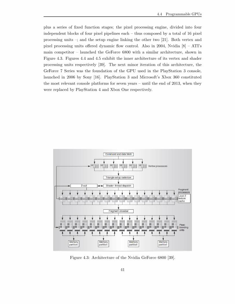
4.4 Programmable GPUs
plus a series of fixed function stages; the pixel processing engine, divided into four
independent blocks of four pixel pipelines each – thus composed by a total of 16 pixel
processing units –; and the setup engine linking the other two [21]. Both vertex and
pixel processing units offered dynamic flow control. Also in 2004, Nvidia [8] – ATI’s
main competitor – launched the GeForce 6800 with a similar architecture, shown in
Figure 4.3. Figures 4.4 and 4.5 exhibit the inner architecture of its vertex and shader
processing units respectively [39]. The next minor iteration of this architecture, the
GeForce 7 Series was the foundation of the GPU used in the PlayStation 3 console,
launched in 2006 by Sony [16]. PlayStation 3 and Microsoft’s Xbox 360 constituted
the most relevant console platforms for seven years – until the end of 2013, when they
were replaced by PlayStation 4 and Xbox One respectively.
Figure 4.3: Architecture of the Nvidia GeForce 6800 [39].
41

Chapter 4. Graphics Cards Evolution
Figure 4.4: Architecture of the Nvidia GeForce 6800 vertex processing units [39].
Figure 4.5: Architecture of the Nvidia GeForce 6800 pixel processing units [39].
After several generations of graphics cards, designers became aware of load balanc-
ing issues since there would be times when the pixel processors would be idle waiting
for early parts of the pipeline to finish. In other cases, the vertex processors would be
idle waiting for completion of following stages of the pipeline. As a result, graphics
cards engineers decided to create a unified shader architecture in which processors
42

4.4 Programmable GPUs
could be used to either process vertices or pixels and thus, being able to maximize the
utilization of the graphics processors. Microsoft Xbox 360 – launched by the end of
2005, a few months before the PlayStation 3 – equipped a custom GPU named Xenos
which is based on the Radeon R600 GPU, ATI’s first unified shader architecture. Until
this point, each shader type would use its own instruction set derived from the spe-
cific hardware implementation. DirectX 10 was launched approximately one year later
and, while not imposing a unified shader GPU implementation, it specified a unified
instruction set that compatible graphics cards must comply with. For this reason,
while not all the shaders offer the same capabilities, most of them – such as reading
from textures, data buffers, and arithmetic operations – are shared and based on the
same unified instruction set. It is important to note the decoupling between the real
hardware implementation – whether it uses unified shaders or not – and the instruction
set it supports. For instance, Xbox 360’s Xenos GPU is equipped with unified shaders
but it does not support the DirectX 10 unified shader instruction set. Those graphics
cards compatible with DirectX 10 must support the unified shader instruction set but
it is up to them whether they have different types of processors for each kind of shader
or they use unified shader processors.
Figure 4.6: Unified shader architecture of the Nvidia GeForce 8800 [43].
43

Chapter 4. Graphics Cards Evolution
About the same time DirectX 10 was released, Nvidia launched the GeForce 8800
which became the first unified shader GPU fully supporting it. Its architecture is
shown in Figure 4.6, shipped with 128 unified shader processors – called unified stream
processors (SPs) – grouped into 8 blocks. Each block has its own texture filter and
address units as well as a local cache shared by its 16 SPs. Texture and math operations
are decoupled, effectively reducing latency. Each SP output can be passed to any other
SP as input. The GPU dispatch and control logic dynamically assigns vertex, geometry
or pixel operations to available SPs. There are 6 raster operations partitions with 6
corresponding video memory partitions [43].
Nowadays, the dominance of mobile devices has driven the focus towards lowering
the power consumption. Nvidia moved along this line with its Kepler (2012) and
Maxwell (2014) GPU architectures, which evolved the foundation set by the Fermi
architecture – launched in 2010. Its main competitor – ATI, now part of AMD –
followed suit.
4.5 General Purpose GPUs and High Performance Com-
puting
The 3D graphics pipeline can be seen as a function that takes vertices and optionally
textures as inputs, and outputs pixels. These pixels normally consist of four component
numbers. Vertices can be customized; indeed, they are flexible data structures. Since
GPUs incorporate several parallel processing elements, they can be seen as stream
processors. Since GPUs started to offer hardware rasterization, efforts to employ them
for non-graphical applications – coined by the term GPGPU (General Purpose GPU)
– have been underway. Early experiments using graphics cards as stream processors
were based on adapting pixel processing to general parallel computation: each fragment
in the pipeline is a unit of data to be processed by a kernel (implemented as a pixel
shader). The pixels forming the render output in the frame-buffer actually correspond
not to an image but instead to the results of the computation – which can be thought
of as a result matrix.
As graphics cards evolved, shaders became increasingly capable of doing complex
computations, notably after the introduction of flow control instructions. Unified
shader architectures implementing versatile unified instruction sets, definitely enabled
44
4.6 Non-discrete graphics cards
GPUs to be used as powerful stream processors available in most consumer Personal
Computers. Since hardware is not designed for specific graphics pipeline stages it is
easier to use the GPU for non-graphic parallel computations. APIs such as Nvidia’s
CUDA [41] or OpenCL [9] were launched to allow developers to easily perform complex
parallel computations. Version 11 of DirectX introduced Compute Shaders which use
a new exclusive pipeline, different than the traditional graphics one. Even high-level
languages such as C# introduced parallel extensions which internally take advance of
these features.
Graphics cards continued to multiply their parallel performance over time by in-
corporating more processing elements, smaller as fabrication techniques evolved. On
the other hand, multi-core CPUs seem to have found a cost-imposed ceiling in their
development. This has led to the irruption of GPUs in the High Performance Com-
puting (HPC) market as well as the adoption of heterogenous computing in Personal
Computers. Heterogenous computing refers to systems using different types of com-
putational units – in this case CPUs and GPUs. Despite having been traditionally a
graphics cards manufacturer oriented to the PC gaming market, Nvidia experienced a
notable growth due to the popular usage of their graphics cards for GPGPU through
its CUDA API. Nvidia, aiming at this market – which they labeled as GPU Computing
–, launched the Tesla product line offering GPUs specifically designed for computing
instead of graphics renderization. It is based on the Fermi unified shader architec-
ture, usually incorporating more memory and more processing elements with improved
double-precision floating-point performance – more critical in scientific applications.
Nowadays, these GPUs form part of many supercomputers, progressively displacing
multi-core CPU clusters.
Processor architectures are evolving, taking on a long-term bet on using vector
processors to empower High Performance Computing. There seems to be little reward
in integrating more than four CISC cores in a single CPU and thus, the next step
in order to increase the processing power comes from the parallel architectures of the
GPUs and the adoption of heterogeneous computing. IBM’s Cell Broadband Engine
– present for instance in the PlayStation 3 – is an example. It consists on a general-
purpose processor optimized for complicated power control and eight computation-
intensive RISC processors interconnected to the main memory, graphics processor and
the rest of the system through a high-speed four rings bus [61]. Even Intel, who is the
arguably most interested defender of CISC multi-core systems has studied the viability
of a less-complex many-core approach [60].
45

Chapter 4. Graphics Cards Evolution
4.6 Non-discrete graphics cards
As their name implies, graphics cards were born as independent hardware pieces plugged
into the motherboard through expansion slots. These are known more specifically as
discrete graphics cards.
Systems not requiring a lot of graphics power and those with physical space limita-
tion – such as laptops – incorporated an Integrated Graphics Processor (IGP) into the
motherboard instead of a discrete card. Although there are some examples with dedi-
cated memory, IGPs would typically use the system RAM, accessing the same bus as
the CPU. As a result, they would have to compete against the CPU for the bus usage,
yielding a reduced performance. A notable example of these kind of GPUs present in
many early 2000s laptops is the Intel Graphics Media Accelerator family.
More recent are the Accelerated Processing Units (APUs) which consist on a CPU
equipped with a specialized processor on its same physical die, the most notable example
of such a processor being a GPU. By locating it on the same die as the CPU instead
of on the motherboard, latency is decreased and data transfers are hugely improved;
at the same time, power consumption is greatly reduced. This is specially important
in modern devices such as tablets or smart-phones where long-life battery is a greatly
desired characteristic. AMD’s [1] Fusion and Intel Core processors are examples of
APUs. Nvidia’s Tegra line targeted for tablets and smart-phones is a more complex
example. It is a system on a chip (SoC) containing the CPU, GPU, bridges and memory
controllers.
No matter whenever it is through a discrete graphics card plugged into an expan-
sion slot, through a stand-alone graphics processor integrated in the motherboard, or
integrated in the same die as the CPU, modern GPUs are very powerful parallel pro-
cessors featuring from dozens up to more than a thousand processing elements that
offer total programmability and which can be used not only to produce high frame-rate
very detailed graphics but also for advanced parallel computations.
46

CHAPTER53D Graphics Fundamentals
Three-dimensional computer graphics deal with the process of converting models of ob-
jects into a visualization. Such models are defined by either mathematical or geometric
descriptions in three-dimensional spaces, and after being processed they are visualized
in finite bi-dimensional spaces such as computer screens.
Many techniques have been developed over time in order to increase the realism of
the generated visualization. Arguably, the most relevant one is the use of bi-dimensional
images as textures applied to the three-dimensional models. These textures constitute
the look of a model and may simulate materials such as wood or bricks. The creation
and editing of textures is as important as the definition of the model of the object itself.
Techniques processing textures such as bump mapping were introduced to increase the
realism – in this case by altering the texture, replacing a smooth surface by a bumpy
one.
Another important group of techniques are those in charge of shading. Their func-
tion is to simulate lighting in a three-dimensional scene, giving a more realistic sense of
depth to the objects. Different types of light sources may be added to a scene, affecting
the coloring of objects.
Most of the algorithms are both computationally and data intensive and thus, a
great deal of effort has always been put in their optimization. The smaller the amount
of required resources, the more of them that can be used to further enhance the realism.
Rendering is a loose term used to refer to the aforesaid processes, or ”the collection
of operations necessary to project a view of an object or a scene onto a view surface”
[66]. Those operations are implemented by renderers which usually follow the pipeline
design pattern, regarded as graphics pipeline and composed of linear stages.
47

Chapter 5. 3D Graphics Fundamentals
Figure 5.1: A simple graphics pipeline.
Figure 5.1 illustrates the general rendering process and the data involved which
are briefly presented in this chapter. Modeling tools are employed to create three-
dimensional representations of objects or scenes, commonly through models and asso-
ciated textures. This data is fed to the graphics pipeline, which will process the model
as necessary, project it to the bi-dimensional domain (rasterization) and then modify
its appearance – normally according to lighting parameters. As a result of this process,
an image is usually generated to be displayed on the screen.
It must be noted that rendering is a very broad subject; different strategies exist
involving many different techniques. Even more, although most renderers are imple-
mented as graphics pipelines, their stages may follow different orders depending on the
specific techniques chosen. A basic graphics pipeline processing polygonal mesh mod-
els is presented in this chapter, introducing techniques such as back-face and occlusion
culling, clipping, Gourand and Phong shading, Z-buffering, and texturing.
5.1 Three-dimensional modeling
A three-dimensional scene is composed of different objects such as persons, cars, build-
ings, etc. Such objects can be defined in different number of ways. For instance, for
simple shapes – such as spheres or boxes – their mathematical formula can be used to
model them. Boolean operations can be performed over such simple objects to form
new ones using what is known as constructive solid geometry (CSG). Nevertheless,
there are two dominant modeling techniques: polygonal mesh models – which is by far
the most common one – and parametric surfaces.
48

5.1 Three-dimensional modeling
5.1.1 Polygonal mesh models
Modern graphics systems generally represent three-dimensional objects as polygonal
mesh models. Such a model is composed by planar polygons that in some cases, such
as cubes, are able to exactly represent the desired shape. In other cases, such as
curved figures like spheres or cylinders, the shape is approximated by using a number
of polygons to compose them; the more polygons used to approximate it, the bigger its
resemblance to the desired shape. Furthermore, any polygon can be split into triangles
and as a result, that is the main primitive that graphics systems work with.
Object Surfaces Polygons Edges/Vertices
Edge
Vertex
Figure 5.2: Generating a mesh from an object.
A mesh is defined by a set of vertices and information about how those vertices
form polygons. Figure 5.2 illustrates the process of defining a polygon mesh from an
object – in this case a cylinder. The object is split into elemental surfaces that are then
approximated by polygons. These polygons are defined by a list of vertices and edges
linking those vertices. Normally, these polygons will be split into triangles and meshes
will be processed as lists of vertices and edges forming triangles.
Complex polygonal meshes composed by up to millions of triangles can be created
using 3D modeling tools in order to be used in three-dimensional scenes. Each indi-
vidual mesh may probably have been created using its own local coordinate system.
Therefore, in order to integrate several meshes in a scene, a transformation is required
for them to use a common coordinate system – known as world or scene coordinates.
Even more, different copies of the same mesh can be used in a scene by slightly trans-
49

Chapter 5. 3D Graphics Fundamentals
forming it.
Mesh transformations usually comprise scaling, rotation, and translation. Scaling
and rotation are linear operations; therefore, they can be performed through vector-
matrix multiplication. Meshes are composed of vertices, located at three-dimensional
points, thus having three components (X, Y and Z) which constitute a vector. This
vector is multiplied by a 3x3 transform matrix whose components parameterize the
desired scaling and rotation. By increasing the dimensionality of the space, translation
also becomes a linear transformation. In order to do so, a fourth coordinate is added
to each point, and the other coordinates are divided by its value. These are called
homogenous coordinates and the value of the fourth coordinate is usually 1. The
transformation matrix is then extended up to a 4x4 matrix, and translation parameters
are also inserted into it. This matrix can be set up to perform several linear transfor-
mations in just one multiplication and also allows to perform different transformations
to different coordinates at once – for instance, a mesh can be scaled only in its vertical
axis, leaving the other two unchanged.
The input of a polygonal renderer is a list of polygons and the output is a color for
each pixel onto which each polygon projects on the screen. Polygons may be treated
as independent units, enabling very efficient parallel processing.
5.1.2 Parametric surfaces
Parametric surfaces are defined using mathematical equations governed by control
points. A well known example of a parametric geometry are Bezier curves, which
are parametric curves frequently used in vector graphics to model smooth curves [22].
By using a set of control points – normally three or four – the shape of the curve is
defined. This set of control points parameterizes the equation of the curve, and forms
what is called a patch. This concept can be extended for bi-cubic parametric surfaces
modeling quadrangles (or quads). Figure 5.3 shows a quad parametric surface and the
patch that defines it, in this case formed by 16 control points. Lifting one of the control
points would have the effect of pulling up the area of the surface below it.
50

5.2 Geometry processing
Figure 5.3: Parametric surface defined by 16 control points.
Although there are algorithms that render directly from a parametric description,
surfaces are more commonly approximated by polygon meshes. Modeling using para-
metric surfaces and then converting to polygonal meshes has two main advantages.
First, it allows for very detailed modeling bearing great resemblance with real objects.
Second, and more important, is that different levels of detail can be generated from
the parametric surfaces. By controlling the amount of subdivision to be performed on
each surface, modeling tools can export parametric surfaces as polygon meshes using
different amount of polygons. For instance, as shown in Figure 5.4, a sphere can be
converted using very few polygons which will yield a polygonal look or using thousands
of polygons which would be seen as an almost perfect sphere.
Figure 5.4: Different levels of detail for a sphere.
Modern graphics hardware implement tessellation units that allow to perform dy-
namic parametric subdivisions. Current graphics pipeline implementations accept not
only polygons but also patches as input that can be used to dynamically generate
parametric surfaces. Depending on how much detail is required in each moment, those
surfaces can be subdivided into a different number. The closer the location of an object
to the front of a scene, the more detail is given by subdividing its surfaces into more
polygons; when the object is located farther, less subdivision is performed and thus less
polygons are generated. While patches control the shape of the surfaces, tessellation
factors are defined to control the subdivision.
51

Chapter 5. 3D Graphics Fundamentals
5.2 Geometry processing
Different renderers have been created to process different types of models, but the most
commonly used ones are planar polygon renderers.
Polygonal meshes must undergone a series of transformations in order to be inte-
grated in a scene along with other meshes and then be projected to a screen. These
transformations account for a number of coordinate spaces translations that can be per-
formed using linear transformations through vector-matrix multiplication. The most
common coordinate spaces involved, presented in sequential order, are:
1. Local coordinate space
The local coordinate space is the one in which each mesh has been defined, nor-
mally having the origin at the mesh center. For instance, when using a 3D
modeling tool to create a mesh for a car, the origin of this local coordinate space
would probably be located inside the car.
2. World coordinate space
It is the common space of all the meshes composing a scene. Each mesh has to
be translated into it; as a result, relative spatial relationships between them are
implicitly established.
3. View coordinate space
Also known as camera or eye space. Objects are transformed according to a set
of viewing parameters representing a camera or the point from which a viewer
is looking at the scene. These parameters include a view point, a direction and a
viewing volume. This volume is also known as viewing frustum and is normally
defined as a rectangular pyramid delimited by near and far clipping planes which
are perpendicular to the view vector, as exhibited in Figure 5.5.
52

5.2 Geometry processing
Figure 5.5: View frustum.
Before coordinates have been translated to view space, relations between camera
and polygon directions are unknown. By taking advance of this newly available
information, new optimizations can be performed. Back face elimination is a
culling technique that checks whether polygons are not facing the camera or view
point and thus can be removed. The operation is pretty straight-forward since it
consists on computing the dot product of each polygon’s normal and the line of
sight vector. Only those polygons yielding a positive dot product are kept and
the rest are discarded. In an empty volumetric model such as that of a person,
this could account for approximately half of the polygons composing it – i.e. if
the person is facing the camera with its back pointing the opposite way, then the
polygons corresponding to its back can be discarded.
4. 3D screen space
This is the final space where the rendering operations take place. Objects in view
space are projected into a view or screen plane which is perpendicular to the
view vector. In order to introduce a sense of depth, a perspective projection is
normally applied but other projections such as parallel ones can be used. Once
projected, all the lines originating in the camera or view point become parallel
and perpendicular to the screen plane. In the process, vertex position coordinates
are also normalized with their values ranging between -1 and 1.
Transforming the view frustum to this space changes its shape from a rectangular
pyramid to a box. This makes it extremely easy to check whenever polygons fall
inside, outside, or intersect the boundaries. This is known as clipping and will
discard those polygons that fall outside the frustum and clip those intersecting the
boundaries. Clipping algorithms such as Sutherland-Hodgman – which performs
polygon edge clipping by performing dot products against clip boundaries recur-
sively – can be easily implemented on hardware [62]. More advanced clipping
techniques deal with bounding volumes such as boxes or spheres than enclose
53

Chapter 5. 3D Graphics Fundamentals
objects; clipping is performed over objects as a whole instead of its individual
polygons saving a lot of processing.
As its name implies, the projection plane corresponds to the screen. Thus, posi-
tions in the plane are directly related to those of the pixels in the bi-dimensional
rendering output. Transformation of the third coordinate (Z) – representing depth
or distance from the camera – may seem superfluous, but it is of great useful-
ness for hidden surface removal. As polygons are processed, their Z values can
be compared with those of the previous ones and they can be discarded if they
are hidden by any of them. Like clipping, higher order hidden surface removal
can be accomplished by comparing the Z values of objects instead of individual
polygons.
At this point, two clarifications about hidden surface removal must be made.
First, it may be performed at one stage of the graphics pipeline or another,
depending on whenever an object, a polygon, or a pixel is checked; normally it
follows rasterization. Second, although hidden surface removal is also a culling
technique, it is not to be confused with back-face elimination. More specialized
terms would be occlusion culling for hidden surface removal and back-face
culling for back-face elimination.
Back-face and occlusion culling, along with frustum clipping, are optimization
techniques that vastly reduce the number of polygons to be processed. For this
reason, they are implemented in the geometry processing stages of most graphics
pipelines implementing planar polygon renderers.
The bulk of geometry processing consists on coordinate space transformations, per-
formed using vector-matrix multiplications which can be efficiently implemented in
hardware. Furthermore, the usage of polygons allows for a great deal of parallel pro-
cessing given their independence from one another. Polygons and their vertices can be
processed in isolation with no side effects, even in the case of polygons forming a mesh.
Many vertices will form part of more than one polygon; in this case, the vertex will be
computed several times, potentially wasting some computing power. However, in most
occasions some of the output vertex data varies depending of the polygon they form
part of – normal vectors, for instance. Even when this is not the case, the increase
in performance derived from the attained degree of parallelism hugely overcomes this
waste.
A related issue is the fact that because of out-of-order polygon computations, many
of them may be rendered only to be occluded by other polygons closer to the viewer.
54

5.3 Rasterization
This has traditionally been an important field of research through the aforesaid hidden
surface removal techniques. For instance, in the same way that high-order clipping
techniques were developed, hidden surface removal techniques have been designed to
organize a three-dimensional scene as a graph ordered by proximity to the viewer; this
way, some nodes or whole branches of the graph can be early discarded if they are
occluded by others.
5.3 Rasterization
Rasterization – also historically named scan conversion – is the process of matching non-
discrete screen plane positions to discrete pixel positions. Many different algorithms
exist to perform this discretization but commonly, polygon edges are rasterized first and
then, based on their positions, the interior of the polygon is filled. Rasterization involves
a resolution reduction and detail loss is one of its consequences. The most noticeable
effects are usually located on the edges of the polygons which become jagged. This is
called aliasing and the development of anti-aliasing techniques is an important on-going
field of research.
Figure 5.6: Line, curve, and polygon rasterization examples.
Rasterization determines pixel positions covered by polygons, as illustrated in Fig-
ure 5.6. For each one of those positions, a pixel fragment – or fragment for short – is
generated. Fragments are the unit of information that will flow from the rasterizer to
the rest of the pipeline and eventually may turn into pixels in the output image. In the
same way that vertex position coordinates are interpolated to perform the rasterization,
55

Chapter 5. 3D Graphics Fundamentals
the rest of the vertex data is also interpolated and assigned to each fragment.
A very common optimization technique called Z-buffering is normally performed
after rasterization. It is a hidden surface removal technique that operates over fragments
and thus, does not require a specific model type [25]. In the case of polygonal mesh
models, each fragment has an associated Z value calculated from interpolating the
Z values of the vertices of its corresponding polygon. A Z-buffer having the same
dimensions as the output image is defined. For each pixel position, this buffer stores
the smallest Z value of a fragment generated for that position. If Z-buffer hidden surface
removal is active, for each fragment its Z value is checked against the one stored in
the corresponding Z-buffer position; if its larger, the fragment is discarded since it is
located farther from the camera than some other fragment and thus it is occluded by
it. Being its only disadvantage that it increases memory usage by requiring an extra
buffer, this technique is implemented by most of the renderers.
5.4 Shading
Shading calculates the appearance of each fragment. Normally, an output pixel color
will be generated based on the attributes defining that appearance. Most shading
techniques fall into two main categories: local reflection models and global shading
algorithms. Local models compute light at different points of a polygon by examining
its position relative to a light source. Since different objects may reflect light and thus
affect other objects, global algorithms take into account relations not only with light
sources but also between the objects in the scene. Obviously, global techniques are
much more expensive than local ones and most of the times are implemented in off-line
(non real-time) renderers.
Local reflection models base their computations on the angle between a polygon
surface and the light source shading it. This can be easily calculated using the normal
of the polygon surface, usually computed per vertex in the earlier geometry processing
stage. Based on distance, intensity and color of the light source, its angle with the
polygon surface, and reflection properties assigned to the surface, a shade value is
calculated for each point of the polygon.
Since normals are only calculated per vertex, interpolation must be performed in
order to shade the polygon surface. Vertices can be shaded individually and then
56

5.4 Shading
their values can be interpolated to obtain the corresponding value of each point on the
polygon surface. This is the basis of Gouraud shading which is computational cheap
[28]. More expensive but also more accurate is Phong shading, which interpolates
vertex normals across the polygon interior to obtain an interpolated normal, and then
performs the shading [50].
Up to this point, only lighting has been discussed. But in order for lighting to
impact the appearance of objects, they must have colors that can be affected by lighting.
This can be accomplished by using color attributes as part of vertex data that will be
interpolated after rasterization and passed to fragments. However, this interpolation
does not allow much control of the coloring. The most popular technique used to assign
colors to surfaces is texturing.
5.4.1 Texturing
Texturing refers to the process of simulating textures on object surfaces. Although
it is a very broad subject, texturing is normally accomplished through the use of bi-
dimensional color maps to modulate surface color or other properties of the shading
operation. A typical example consists on an image resembling a wooden surface being
mapped onto a polygon to give it a wooden look. Each generated fragment would access
the texture according to its position within the polygon in order to obtain its color.
This value would then be modified by lighting parameters in the shading process.
In order to know which position of the texture to access, UVW coordinates are
used. Their name comes from the alphabet letters preceding XYZ which are used for
vertex position coordinates. Normally, textures are bi-dimensional and so only two-
component coordinates – accordingly named UV – are used, ranging between 0 and 1.
These coordinates form part of the vertex data and are interpolated for each fragment,
effectively representing the position of the fragment within the polygon surface.
The same way 3D modeling tools are used to define complex meshes modeling ob-
jects, there are tools – in many cases integrated with those 3D modeling ones – to
generate textures that properly fit those meshes. This process, known as UV map-
ping, takes an input texture and generates a new one based on a projection algorithm
that fits the three-dimensional mesh. Upon rendering, the texture can be properly
mapped onto the mesh by using that projection.
57

Chapter 5. 3D Graphics Fundamentals
As previously stated, textures are usually bi-dimensional images with its pixels
having different meanings depending on the technique. These images are normally
rectangular, thus having both a different shape and resolution than the polygon they
are mapped onto. This generates a number of problems among which are aliasing
and anisotropy. Aliasing is a consequence of the resolution difference, analog to the
problem found in rasterization. Anisotropy refers to the visible blur and distortion
of shapes and angles that may occur as a consequence of the shape difference and
the required projection, specially when the polygon is on an almost oblique position
to the camera. Both problems are commonly attacked by sampling more than one
value from the texture for each fragment, normally from neighbor locations. By using
several samples to calculate the fragment’s value, edges can be smoothed and distortions
reduced.
Changes in the distance of the textured surfaces from the camera further aggravate
these problems since the resolution is varied. Mipmaps is a texture level-of-detail
technique used to store a texture in several resolutions [67]. An initial resolution – for
instance a 256x256 pixels texture – is reduced several times, to a quarter of its size
each time – thus yielding 128x128 pixels, 64x64 pixels, and so on. Commonly, all the
resolutions are stored in a single bigger texture which is accessed through offsetting to
the area of the texture where the desired resolution is located. Each resolution is called
a mipmap level. As a texture object moves away from the camera, smaller resolutions
can be used. This yields two advantages: faster processing times and higher resolutions
than required available for multi-sampling when smaller mipmap levels are used. Its
main disadvantage is that textures are bigger thus requiring more memory.
Although the most common usage of textures is simulating the look of different
materials, many other techniques also take advantage of them. Texture shadows for
instance, can be used to pre-compute fixed shadows of objects. Another technique uses
billboards: textured rectangles that are always perpendicular to the camera which
are commonly used to simulate clouds. Bump mapping stores height values as grey-
scale colors in a bi-dimensional image. This height is taken into account upon shading
to generate output pixel colors simulating non-flat polygon surfaces. Combining this
with a rock-looking material texture could produce a rock bumpy looking surface, for
example. A similar concept is used in displacement mapping which actually modifies
the geometry of the mesh based on the values stored in a texture. For example, a grey-
scale texture could be generated by computing the topographic map of a real terrain
area; this texture could then be used to dynamically modify the height of parts of a
grid mesh covering that area in a scene.
58

5.6 Multi-pass rendering
5.5 Frame buffer output
Once a color has been generated for each fragment, it can be written to the corre-
sponding pixel of the frame buffer. This buffer contains the final image that is
usually displayed on a screen. Post-processing effects can be applied on the moment of
writing each pixel to the buffer. For instance, by using transparency, several fragments
with different depths can contribute to the same pixel color value. This is common for
objects that lie behind glass materials in a scene or when simulating fog.
5.6 Multi-pass rendering
Graphics hardware evolved implementing most of the graphics pipeline stages and in-
creasing the available video memory, making it possible to store more data where
initially there was only room for the frame buffer. New techniques have kept arising
requiring more and more flexibility and in some cases, requiring several passes over the
graphics pipeline. Each pass would configure the pipeline in a specific way to produce
an intermediate result saved in video memory. The combination of all those results
would provide the desired outcome of the technique. This allowed the introduction of
advanced techniques such as a geometric shadows, where silhouettes of the meshes are
generated and stored in one pass, and then used for calculating shadowed volumes in
a subsequent pass.
59

Chapter 5. 3D Graphics Fundamentals
60

CHAPTER6Direct3D 11 Pipelines
Direct3D is the main API of DirectX, in charge of graphics. Like the rest of DirectX,
it is a C++ API using Component Object Model (COM) interfaces. It implements a
graphics rendering pipeline consisting on several stages, covering from the definition of
geometry composed by triangles and textures to apply after rasterization, up to the
generation of the final rendered image.
Graphics rendering pipelines – also known as the draw pipelines – have been the
traditional approach to programming graphics cards with 3D acceleration. In the be-
ginning, all the pipeline stages were fixed-function: both Direct3D and OpenGL APIs
functioned much like state-driven machines where developers would configure different
parameters of the pipeline before each renderization. With the increasing programma-
bility of graphics cards, several stages of the pipeline moved from fixed-function to
being fully programmable through small programs called shaders.
While each stage has its own specialized type of shaders, they quickly increased their
capabilities up to a point were shaders from different stages would share most of their
functionality. Following this trend, Microsoft introduced a unified shader instruction
set that graphics cards vendors were to support in order to be compatible with DirectX
10 and beyond. By that time, the usage of GPUs for non-graphics computations –
also known as General Purpose GPU (GPGPU) applications – was becoming more and
more popular and therefore, DirectX 11 introduced a new non-graphics pipeline: the
compute shader pipeline – also known as the dispatch pipeline. It consists on only one
programmable stage, the Compute Shader.
As graphics hardware evolved, each system would support a different set of features
making it hard for developers to handle all the possible scenarios. Direct3D 11 intro-
duced the concept of feature levels in order to be able to work with different hardware
supporting different features. A feature level is a well defined set of GPU functionality.
61

Chapter 6. Direct3D 11 Pipelines
This way, hardware supporting feature level 11 0 implements all the functionality of-
fered by Direct3D 11. Current hardware feature level support can be queried through
the API and a required feature level must be declared before any processing can be
done.
Both graphics and compute shader pipelines are just high-level abstractions offered
by Direct3D. They both use the same underlying hardware and resources even while
the latter only uses a subset of the available capabilities – e.g., it doesn’t use rasteri-
zation units. In this chapter, both pipelines are presented, discussing their individual
stages. The most relevant Direct3D 11 API calls and structures are introduced with-
out delving into details. Since shader stages are very flexible and can be programmed
in very different ways, more emphasis has been put into explaining the fixed-function
stages. The main source for this chapter is the Direct3D documentation found in the
Microsoft Developer Network, particularly the Programming Guide for Direct3D 11
and the Direct3D 11 Reference [3].
6.1 High Level Shading Language
Initially, shaders were programmed using an assembly-level language, directly mapping
to the hardware instructions. As their complexity grew, a C-like language called High
Level Shading Language (HLSL) was introduced. Using this language, shaders can
easily be defined using functions, control flow structures (if supported) and even objects.
HLSL shaders are compiled to a hardware neutral intermediate language that is then
mapped to specific hardware by the graphics driver. This compilation can either be done
off-line – thus compiled shaders are bundled as application resources – or be compiled
from source code at run-time. A particularly useful feature is the specification of pre-
processor constants upon compiling, which allows the parametrization of shaders for
specific execution environments.
Since its introduction along Direct3D 9, HLSL has evolved offering more features
to program shaders such as better control flow, more intrinsic functions, or new objects
for interaction with new pipeline stages. Nevertheless, in order to be able to use these
features, they must be supported by the underlying hardware. As stated before, in
Direct3D 11 hardware capabilities are organized through feature levels. Within feature
levels, shader support is further categorized by different shader models, with Direct3D
11 supporting up to Shader Model 5. Each shader model builds on the capabilities of
62

6.2 Graphics rendering pipeline
the previous model and supports one or more shader profiles which are set as targets
for shader compilation. Each type of shader has its own profile and can even have
several versions within a same shader model. For instance, Shader Model 4 includes
pixel shader profiles ps 4 0 and ps 4 1. Shaders compiled for a shader profile will be
able to use features available only to that and previous profiles and will only run on
hardware supporting that or posterior profiles.
6.1.1 Effects
A DirectX effect is a set of pipeline states organized into a single rendering function
called technique, written in HLSL. This includes not only shaders but also other pipeline
parameters such as rasterizer, blending, texture or sampler states. A technique is
composed by one or more passes, each pass corresponding to a execution of the pipeline
– either the graphics or the compute shader pipeline. Furthermore, techniques can be
grouped for better organization.
This Effects Framework allows for very advanced use of HLSL. Techniques can be
implemented altogether using HLSL, replacing most Direct3D API calls controlling the
pipeline state by a single call simply to set the appropriate technique in each moment.
This way, rendering logic can be separated from more general graphics hardware han-
dling logic. The application is left with the tasks of managing the Direct3D device and
its resources, choosing the required technique in every moment, and supplying data to
the pipeline.
6.2 Graphics rendering pipeline
The Direct3D graphics pipeline is a high-performance three-dimensional graphics ren-
derer. Its core is similar to the pipeline engineered by Silicon Graphics Incorporated
(SGI) [15] in the eighties, which is the foundation of OpenGL (the historical rival of
Direct3D in the field of graphics APIs). The general workflow of this pipeline is the
following. A polygonal geometry is defined by its vertices which need to be processed in
order to fit properly into the three-dimensional scene being rendered. Triangles formed
by these transformed vertices are rasterized into pixel fragments and given a color, ei-
ther interpolating vertex colors or using texture images. These pixel fragments can be
63

Chapter 6. Direct3D 11 Pipelines
further processed, be discarded if they fall behind fragments closer to the scene camera
(Z-buffering), merged with others (blending), etc. Once processed, the fragment’s color
may be written to its associated pixel within a render target – usually a bi-dimensional
image representing the frame buffer.
The Direct3D 11 graphics pipeline is the result of evolving the described core to
support the different graphics hardware generations and their increased capabilities.
Its stages are shown in Figure 6.1. There are two kinds of stages: fixed-function stages
and shader stages. While the former can be configured through a set of parameters,
its behavior is mostly fixed. On the other hand, shader stages are fully programmable
through shader programs written in HLSL. The first programmable stages were the
Vertex and Pixel Shader stages, introduced in Direct3D 8, allowing to customize the
operations to be performed over the vertices and over the pixel fragments, respectively.
Figure 6.1: Direct3D 11 graphics pipeline.
DirectX 10 supposed a huge redesign of both Direct3D API and its underlying
architecture. Available video memory resources, their capabilities and management
were also drastically improved. Two new pipeline stages – Geometry Shaders and
Stream Output – were also introduced. Version 11 was an incremental evolution of
64
6.2 Graphics rendering pipeline
Direct3D 10 which introduced significant new features among which are multi-threading
support, hardware feature levels, the compute shader pipeline, and tessellation support
– comprising the fixed-function Tessellator stage and the programmable Hull Shader
and Domain Shader stages. Following, the stages of the Direct3D 11 graphics rendering
pipeline are presented.
6.2.1 Input Assembler
The pipeline execution begins upon a Draw API call and its first stage is the Input
Assembler, in charge of supplying geometry data to the pipeline. The execution of
this stage can be split into three phases: fetch primitives data from user-filled buffers,
assembly them and attach system-generated values to them – i.e. information supplied
by the pipeline, such as an identification number for each vertex. In order to carry
these operations, the Input Assembler must be first properly set up.
6.2.1.1 Configuration
The Input Assembler consumes geometry data, consisting on different types of prim-
itives: points, lines and triangles. They are defined by one, two and three vertices
respectively. Vertices are stored in one or more video memory buffers called vertex
buffers, which can be bound to the pipeline through the Input Assembler by calling the
IASetVertexBuffers API call. In order to assembly each primitive, the Input Assembler
fetches the proper vertices from the corresponding vertex buffer.
The information required to set up the Input Assembler before a Draw call can be
invoked, is the following:
Input layout
It covers the description of the elements composing each vertex – which form
the different geometry primitives. In a common 3D application it could consist
of 3 elements: vertex position coordinates, requiring 3 floats, its normal vector
required for illumination (also 3 floats), and texture coordinates (2 floats). Each
element receives a semantic name, a format, and an input buffer slot from which
the data will be read. The semantic name will be used to map input data to
65

Chapter 6. Direct3D 11 Pipelines
variables in shader code. The input layout normally matches the input signature
of the vertex shader. This means that the vertex shader function receives the
elements of the vertex through its parameters. Which parameter receives which
element is defined by associating the semantic name of an element to the desired
parameter in the vertex shader function HLSL code.
Input vertex buffers
This information establishes the input buffers holding the vertices that compose
the primitives. Several input buffers can be defined, being 32 the maximum for
hardware supporting Direct3D 11. In order to fetch data from the proper input
buffer, the Input Assembler uses the input buffer slot number specified for each
element in the input layout.
Input index buffer
This information is required only when using an index buffer to store topology
information. Index buffers store indices pointing to positions of the vertex buffer.
Consecutive indices form a primitive and thus, the Input Assembler reads the
index buffer in order to know which vertices need to be fetched from the vertex
buffer in order to assembly each primitive. An index buffer can be bound through
the IASetIndexBuffer API call. In order for the Input Assembler to use it, the
pipeline must be executed by invoking DrawIndexed.
Primitive topology
This information indicates how to link vertices to form primitives. For instance, if
triangle list topology is set, the Input Assembler will retrieve vertices in groups of
3 and set up a triangle with them. There are 9 basic types of primitive topologies
– which come from different allocation modes of either points, lines, or triangles
– shown in Figure 6.2, found in the Microsoft Developer Network (MSDN) doc-
umentation [12]. Moreover, there are also 32 patch list topologies. Supported
primitive topologies are the following:
– Primitive lists: either point, line, or triangle lists. Primitives are to be set
up in groups of one, two, or three vertices. Suppose the set topology were
triangle lists and Draw(12, 0) was invoked to draw 12 vertices, starting
from the beginning of the vertex buffer – the second parameter indicates the
start vertex location within the input vertex buffer. In this case, the Input
Assembler would fetch the first 12 vertices from the vertex buffer, using the
first 3 vertices to form a triangle, the next 3 to form a second triangle and
66

6.2 Graphics rendering pipeline
so forth until setting up 4 triangles.
– Primitive strips: strips are series of connected primitives, and these primi-
tives may be either lines or triangles. For instance, having the topology set
to line strips, upon a Draw(12, 0) call, the Input Assembler would fetch 12
vertices and generate 11 consecutively connected lines. The first line would
link the first and second vertices, the second would be formed by the second
and third vertices, and so on. A separate Draw call is required for each
strip. In the case of triangles, previous two vertices are reused to form a
new triangle with the next fetched vertex. Obviously, there is no point strip
primitive since they only have one vertex.
– Primitive lists or strips, with adjacency: with the introduction of geometry
shaders in Direct3D 10, adjacency information became available. The prim-
itives supporting this new information, include extra vertices corresponding
to the adjacent primitives. For the triangle list with adjacency, a Draw(12,
0) call would cause the Input Assembler to fetch 12 vertices and issue 2
triangles. As illustrated in Figure 6.2, the first triangle would be formed by
vertices 0, 2 and 4, with vertex 1 conforming the adjacent triangle of the
side formed by vertices 0 and 2. Vertices 2, 3, 4 and 0, 4 and 5 would con-
form the other 2 adjacent triangles. The second triangle would be formed
by vertices 6, 8 and 10, while the adjacent triangles would be respectively
formed by vertices 6, 7 and 8, vertices 8, 9 and 10, and finally 6, 10 and
11. For the same call and the line strips with adjacency topology, 10 lines
would be issued, with vertices 0 and 11 conforming the adjacent lines along
with vertices 1 and 10 respectively. Adjacent vertices are only visible to
geometry shaders which receive the whole primitive topology – i.e. all the
vertices forming it, including the adjacent ones.
– Patch lists: patches are the input topologies used in tessellation. There are
32 different types, corresponding to the number of control points that can
form the input patch, from 1 up to 32.
67

Chapter 6. Direct3D 11 Pipelines
Figure 6.2: Primitive topologies [12].
6.2.1.2 Data fetching
Once the Input Assembler is configured, a Draw call can be invoked to start the pro-
cessing by the graphics pipeline. There are 5 different versions of the Draw call, which
affect how to Input Assembler fetches the data:
1. Draw(UINT VertexCount, UINT StartVertexLocation)
Draws non-indexed, non-instanced primitives. The first parameter indicates the
number of vertices to draw while the second is used as an offset in the vertex
68

6.2 Graphics rendering pipeline
buffer that points to where to start reading the vertices. Algorithm 2 exhibits
the pseudo-code for the vertex fetched associated with this call.
Algorithm 2: Draw vertex fetching pseudo-code.Data: VertexBuffer← Bound input vertices, VertexBuffer = {v1, . . . , vn}
VertexCount← Number of vertices to fetchStartVertexLocation← Initial position to start reading vertices from
/* Fetch the required vertices from the vertex buffer */
1 Vertex[] fetchedV ertices← new Vertex[VertexCount]2 for i← 0 to VertexCount do3 fetchedV ertices[i]← VertexBuffer[ StartVertexLocation + i ]
end
2. DrawIndexed(UINT IndexCount, UINT StartIndexLocation, INT BaseVertexLo-
cation)
Draws indexed, non-instanced primitives. This call requires an index buffer to
have been bound by calling IASetIndexBuffer. While vertex buffers contain the
data of the actual vertices, index buffers store indices pointing to positions inside
the vertex buffer. For instance, when using triangle list as primitive topology
the first 3 entries of the index buffer would contain the positions in the vertex
buffer of the corresponding vertices that form a triangle. By using index buffers,
the same vertex from the vertex buffer can be used in more than one primitive.
Therefore, index buffers can be used for optimization.
Algorithm 3: DrawIndexed vertex fetching pseudo-code.
Data: VertexBuffer← Bound input vertices, VertexBuffer = {v1, . . . , vn}IndexBuffer← Bound indices pointing to VertexBuffer positionsIndexCount← Number of indices to drawStartIndexLocation← Initial position into the index buffer to start reading indices fromBaseVertexLocation ← Initial position into the vertex buffer to start reading vertices from
/* Fetch the required vertices from the vertex buffer */
1 Vertex[] fetchedV ertices← new Vertex[IndexCount]2 for i← 0 to IndexCount do3 index← IndexBuffer[StartIndexLocation, i] + BaseVertexLocation4 fetchedV ertices[i]← VertexBuffer[ index ]
end
The third parameter specifies a value to be added to each index before reading
the vertex at that position in the vertex buffer. This is illustrated in Algorithm
3, exhibiting the pseudo-code for the vertex fetched performed when this call is
69

Chapter 6. Direct3D 11 Pipelines
invoked.
3. DrawInstanced(UINT VertexCountPerInstance, UINT InstanceCount, UINT StartVer-
texLocation, UINT StartInstanceLocation)
Draws non-indexed, instanced primitives. Primitive instancing allows to reuse
the same model geometry – i.e. vertex data – which may be partly modified.
An example could be the geometry of a soldier, which is instanced multiple times
varying only the relative position of arms and legs. An extra buffer called instance
buffer is required. This buffer holds the modification information for each instance
of the model geometry and it is set as an extra vertex buffer input with its
particular vertex input layout – i.e. vertex format. Algorithm 4 presents the
pseudo-code for the corresponding vertex fetching.
Algorithm 4: DrawInstanced vertex fetching pseudo-code.
Data: VertexBuffer← Bound input vertices, VertexBuffer = {v1, . . . , vn}PerInstanceData← Instance-specific data bufferVertexCountPerInstance← Number of vertices to fetchInstanceCount← Number of instances to drawStartVertexLocation← Initial position to start reading vertices fromStartInstanceLocation← Initial position to start reading instance-specific data from
/* Fetch the required vertices from the vertex buffer once */
1 Vertex[] fetchedV ertices← new Vertex[VertexCountPerInstance]2 for i← 0 to VertexCountPerInstance do3 fetchedV ertices[i]← VertexBuffer[ StartVertexLocation + i ]
end
/* Obtain per-instance vertices by updating the vertices with per-instance data
*/
4 Vertex[] perInstanceV ertices← new Vertex[VertexCountPerInstance]5 for i← 0 to InstanceCount do6 perInstanceV ertices← updateVertices(fetchedVertices, PerInstanceData[i +
StartInstanceLocation])
end
4. DrawIndexedInstanced(UINT IndexCountPerInstance, UINT InstanceCount, UINT
StartIndexLocation, INT BaseVertexLocation, UINT StartInstanceLocation)
Draws indexed, instanced primitives. Its a merge of both DrawIndexed and Draw-
Instanced.
5. DrawAuto()
70

6.2 Graphics rendering pipeline
Begins the pipeline execution for an unknown amount of vertices stored in a
read/write buffer. The content of that buffer must be the output of the Stream
Output stage. This stage, introduced in Direct3D 10, allows to save output
vertices from the Vertex and/or Geometry Shader stages to video memory. Its
combination with DrawAuto is very useful in scenarios where previous work per-
formed by the pipeline can be later reused, and it allows to do so without incurring
in a performance penalty due to requiring data interchange between the CPU and
the GPU. An internal counter keeps track of the size of the buffer and thus, there
is no need to query the GPU for it. However, the input layout – i.e. the format of
the vertices stored in the buffer – must be properly set before invoking DrawAuto.
6.2.1.3 Primitive assembly
After the vertices have been fetched from the vertex buffers, primitives can be assem-
bled. This is performed by linking vertices to form primitives, according to the con-
figured primitive topology. Primitive assembly is executed once the vertices have been
retrieved, right after the last lines of Algorithms 2 and 3, and within the per-instance
loop in the case of instanced draws – after line 6 in Algorithm 4.
6.2.1.4 System-generated values attaching
After vertex fetching and primitive assembly, the Input Assembler attaches system-
generated values both to the primitives and their composing vertices. In the same way
a semantic name for each element of a vertex input layout is defined, system-generated
values have predefined semantic names, used to indicate the pipeline to which shader
variables it must supply those values. More specifically, by examining semantic names
present in shader input and output signatures, the pipeline knows which data must be
carried from one shader to another, and into which shader variables it must be stored.
System-generated values are not generated unless they are included in some shader
signature. For instance, in order for SV PrimitiveID to be generated, it must be part
of the input signature of either a geometry or pixel shader bound to the pipeline.
Several system-generated values are issued by different pipeline stages. The values
that can be generated by the Input Assembler are:
71

Chapter 6. Direct3D 11 Pipelines
SV VertexID : visible to vertex shaders, it is unique among vertices issued within
the same Draw call and it gets reset between calls. In the case of indexed Draw
calls, it represents the index value.
SV InstanceID : visible to vertex shaders, it identifies the instance of the geometry
being processed.
SV PrimitiveID : visible to geometry and pixel shaders, it distinguishes assembled
primitives. In the case of primitives with adjacency, no value is generated for the
adjacent primitives, only for the interior ones. When using primitive instancing,
values are unique only for primitives within the same instance.
Once the Input Assembler has fetched the required vertices, assembled the proper
primitives and set up the system-generated values involved, vertices are passed as input
to the Vertex Shader stage.
Table 6.1 shows the API calls used to configure the Input Assembler stage. For
each call, there is a corresponding one retrieving the configured state.
Function name Description Remarks
IASetInputLayout Sets the layout of the ver-tices contained in vertexbuffers
IASetPrimitiveTopology Specifies the topology usedto link vertices
IASetVertexBuffers Binds buffers from wherevertex data will be read
Buffers must have been created with theD3D11 BIND VERTEX BUFFER flag
IASetIndexBuffer Binds an index buffer thatspecifies how to read vertices
The buffer must have been created withthe D3D11 BIND INDEX BUFFER flag.Requires invoking DrawIndexed*
Table 6.1: Input Assembler configuration API functions.
6.2.2 Vertex Shader
The Vertex Shader stage processes vertices received from the Input Assembler stage.
This stage is fully programmed and even if no transformation is to be performed over
vertices, a so called pass-through shader must be defined simply returning the input
vertex. A vertex shader can be bound to this stage by calling VSSetVertexShader.
If the Effects Framework is being used instead of the API, it will be bound through
72

6.2 Graphics rendering pipeline
the SetVertexShader HLSL function. The shader receives a single vertex as input and
outputs a single vertex as well. It is executed for all vertices, including the adjacent
ones in those primitives with adjacency. It is possible to query the number of times the
bound vertex shader has been executed through the VSInvocations pipeline statistic.
The Vertex Shader stage replaces the traditional fixed-function transform and light-
ing (T&L) stage. As a result, vertex shaders are usually in charge of transforming ver-
tex coordinates through vector-matrix multiplication and calculating vertex normals
for lighting.
All vertices forming a primitive must have been processed by the Vertex Shader
stage before they are fed to the next stage of the pipeline, no matter which stage is
next. Optionally, the output of this stage can be fed up to the Stream Output stage in
order to write the output vertices to a vertex buffer in memory.
Both the input and output vertex must include at least one scalar value and can
be comprised of up to 16 vectors, each formed by 4 components of 32-bits. The Input
Assembler can supply two system-generated values: SV VertexID and SV InstanceID.
No system-value semantics are compulsory for this stage but either the Vertex Shader
or the Geometry Shader stages must output a vector associated to the SV Position
semantic name, which is consumed by the Rasterizer stage.
Function name Description Remarks
VSSetShader Binds a vertex shader
VSSetShaderResources Binds shader resources to beaccessible from the shader
Receives Shader Resource Views which re-quire resources to be created with theD3D11 BIND SHADER RESOURCE flag
VSSetConstantBuffers Binds constant buffers Buffers must have been created with theD3D11 BIND CONSTANT BUFFER flag
VSSetSamplers Binds sampler states
Table 6.2: Vertex Shader configuration API functions.
Table 6.2 shows the API calls used to configure the Vertex Shader stage. For each
call, there is a corresponding one retrieving the current state.
73

Chapter 6. Direct3D 11 Pipelines
6.2.3 Tessellation stages
Tessellation is a process that essentially consists on subdividing a surface. Normally,
it is used to generate primitives from parametric surfaces. As explained in Section
5.1.2, these surfaces have a domain and are parameterized by a set of control points
forming a patch. In Direct3D 11, the domain can be either a quadrangle, a triangle
or an isoline and through tessellation they can be split into triangles, lines and points.
Control points may be used to determine the exact vertex positions of the generated
primitives. Three new stages were introduced in Direct3D 11 to support tessellation:
the Hull Shader, Tessellation and Domain Shader stages.
As stated in Section 6.2.1, in Direct3D 11 there are four types of primitives: points,
lines, triangles, and patches. For tessellation, the input primitives must be patches.
Patches are composed by a fixed number of control points ranging between 1 and 32.
Unlike triangles and lines, patches can only be defined using lists. Since they have a
fixed size, there is no strip support. Also, tessellation is not compatible with geometry
shaders receiving primitives with adjacency.
Cubic Bezier curves are a good example of tessellation. They can be defined us-
ing four control points, thus requiring patches composed by four points as primitive
topology. Four vertices are to be stored per curve – i.e. per patch – in the vertex
buffer. In essence each control point is a vertex. Indeed, control points are individually
processed by the Vertex Shader stage just like any vertex would. When tessellation is
active, the Vertex Shader stage operates over control points. While internally they are
actual vertices, their semantics change. Thus, when processing control points vertex
shaders usually perform different operations than when processing vertices. One exam-
ple is coarse mesh animation: controlling the animation through a few control points,
complex computations can be vastly optimized.
Once control points pass the Vertex Shader Stage, input patches are processed
by the Hull Shader stage. For each input patch, an output patch is generated and
tessellation factors are calculated. These factors are used by the Tessellator stage to
split a certain domain into smaller objects, generating point or topology lists. Following
the cubic Bezier curve example, a hull shader could just let the control points through
and set the tessellation factor to 64. As a result, the isoline domain input surface would
be split into 64 individual lines.
74

6.2 Graphics rendering pipeline
Finally, the Domain Shader stage is in charge of taking the split results – i.e. the
generated primitives – and calculating the corresponding vertex positions. For a cubic
Bezier curve, the 64 generated lines would be positioned consecutively, with their vertex
positions calculated using the four control points along with their relative position
within the generated curve. The Domain Shader stage is in charge of processing the
vertices generated by the Tessellator stage. Therefore, classic vertex shader operations
like world, view and projection matrix multiplication are performed in the domain
shader.
C0
C1
C2
C3
C0
C1
C2
C3
Figure 6.3: Bezier curve tessellation into 9 lines using 4 control points.
The process described is illustrated by Figure 6.3, although 9 lines are generated
instead of 64 for clarity. The input of the tessellation is a patch composed by 4 control
points and the result are 10 vertices composing 9 lines along the curve. The larger the
tessellation factor, the more lines will be generated and the better the approximation
of the curve will be. No patch processing is required by the hull shader beyond setting
the tessellator factors for the amount of lines to be generated – 9 in this case. Following
the value of the tessellation factor, the Tessellator stage simply generates 10 different
coordinates for the vertices. The domain shader, using these coordinates and the control
points, calculates each vertex position along the curve.
75

Chapter 6. Direct3D 11 Pipelines
The most common use for tessellation is the generation of levels of detail for para-
metric surfaces. Each surface is defined by a patch and thus, complex surfaces are
defined using a few control points. Since the surface division process is controlled dy-
namically through tessellation factors, different levels of detail – i.e. different amounts
of primitives – can be generated depending on the requirements of the rendered scene.
Although this is the more common scenario, the concrete meaning given to control
points and how to determine the location of generated primitives from them is up to
the developer.
6.2.3.1 Hull Shader
Being the first of the three tessellation stages, this programmable stage serves two main
purposes: transforming an input patch into an output patch and establishing tessellator
factors that control how finely the subsequent Tessellator stage must divide a domain.
In order to do this, a hull shader requires at least two functions: the main hull shader
function and a patch-constant function.
The main hull shader function is executed for each output control point. The
number of control points defining the output patch can be different from that of the
input patch and is specified by the HLSL attribute [outputcontrolpoints()]. The shader
has access to all the input control points in case it needs to perform some calculation
based on them. One example of a hull program could be basis transformation, taking
for instance 32 input control points and outputting 16 control points. Note that in
that example, the hull shader would be executed 16 times: it is executed once for each
output control point, not per input control point.
Patches are associated with a surface domain type which can either be ”quad”, ”tri”
(triangle) or ”isoline”. The domain must be specified by using the [domain()] attribute
with any of the previous values to annotate the main hull shader function. The following
stage (Tessellator) will take this domain and subdivide it into primitives. The type of
these primitives must also be declared in the hull shader using the [outputtopology()]
annotation which can take the values ”point”, ”line”, ”triangle cw” or ”triangle ccw”.
There are two possible values for triangles depending on whether the Tessellator stage
should define them using a clockwise or counter-clockwise winding. Output topologies
correspond to the available basic primitives and so, [outputtopology()] determines the
type of primitives result of the whole tessellation process.
76

6.2 Graphics rendering pipeline
The other function required by a hull shader is the patch-constant function. Unlike
the main hull shader function, it is executed only once per patch. It is in charge of calcu-
lating tessellation factors as well as any other desired per-patch data. This function has
read-only access to both input and output control points and must be specified in the
main hull shader function using the annotation [patchconstantfunc(”function name”)].
It receives an array containing the input patch control points and may use both the
SV PrimitiveID system-value identifying the input patch and SV OutputControlPointID
that identifies, within each output patch, the control point being processed. It returns
a structure that must contain at least the tessellation factors.
DomainSV TessFactor SV InsideTessFactor
Type Meaning Type Meaning
quad float[4] Sides of the quad float[2] Vertical and horizontal subdivi-sions of the quad center
triangle float[3] Sides of the triangle float Inner subdivisions
isoline float[2] Number of isolines (detail) andnumber of lines per isoline (den-sity) to generate
– –
Table 6.3: Format and semantics of tessellation factors varying with the domain.
Tessellation factors indicate the Tessellator stage how to split the domain into
smaller primitives. There are two types of tessellation factors: edge and inside fac-
tors. Each type of domain requires a different number of factors, as shown in Table
6.3. The maximum value for any tessellation factor is 64.
Once the Hull Shader stage is done processing the patches, it outputs the tessellation
factors to the Tessellator stage. Later, the output control points will be fed along with
the data outputted by the Tessellator stage to the Domain Shader stage.
Function name Description Remarks
HSSetShader Binds a hull shader
HSSetShaderResources Binds shader resources to beaccessible from the shader
Receives Shader Resource Views which re-quire resources to be created with theD3D11 BIND SHADER RESOURCE flag
HSSetConstantBuffers Binds constant buffers Buffers must have been created with theD3D11 BIND CONSTANT BUFFER flag
HSSetSamplers Binds sampler states
Table 6.4: Hull Shader configuration API functions.
Table 6.4 shows the API calls used to configure the Hull Shader stage. For each
call, there is a corresponding one retrieving the configured state. These functions are
77

Chapter 6. Direct3D 11 Pipelines
analogous to those used to configure the Vertex Shader stage.
6.2.3.2 Tessellator
This is a fixed-function stage in charge of the actual tessellation operation per se. It
subdivides a domain into smaller objects. The domain can be a quad, a triangle or
a line which may be split into triangles, lines or points. The amount of divisions to
be performed is controlled by the patch tessellation factors calculated in the previous
stage by the patch-constant function. This is the only data that is consumed by the
Tessellator stage; it does not use any of the control points or other per-patch data.
Several of the annotations in the main hull shader are used to configure the Tes-
sellator stage, namely [domain()] and [outputtopology()] – introduced in the previous
section. There is another required annotation that indicates the desired tessellation
scheme: [partitioning()]. These annotations are static definitions that can not be
changed after the shader is compiled. There is no API call used to configure any
state of the Tessellator stage, it is controlled through these annotations of the main
hull shader.
The tessellation actually generates either two or three dimensional coordinates that
represent sampling points over the surface domain. The coordinates of each sample
are fed to the Domain Shader stage to calculate its corresponding vertex position.
Furthermore, point or topology lists are issued – i.e. information about how samples
are connected to form primitives.
It is worth mentioning that the tessellator uses 16-bit fractions with fixed-point
arithmetic. This leads to some precision issues with an equivalent sampling precision
of 2 millimeters within a 64 meter wide patch.
6.2.3.3 Domain Shader
The Domain Shader stage could be pictured as a vertex shader running after the tes-
sellation, since a domain shader will be executed for each coordinate generated by the
Tessellator stage. However, domain shaders have access to the data of the tessellated
patch, thus allowing more complex operations than vertex shaders.
78

6.2 Graphics rendering pipeline
Recapitulating, between the Vertex Shader and this stage, two processes have taken
place. First, each input patch formed by control points was transformed into another
patch, and the fixed-function tessellator was configured. Second, a number of sam-
pling points were taken from a given domain surface, and a primitive list linking those
points was issued. In the Domain Shader stage, a shader is executed for each sampling
point, having access to the transformed patch. Its mission is to generate a vertex for
each point, using the coordinates of that point within the tessellated domain and the
transformed patch data.
The domain shader receives the SV PrimitiveID system-value identifying the tessel-
lated patch, its control points and per-patch data outputted by the Hull Shader stage,
along with the coordinates generated by the Tessellator stage through the SV Domain-
Location system-value. These coordinates have two components for quad and isoline
domains, and three components in the case of the tri domain. As in the hull shader,
the domain must be declared through the [domain()] attribute. The difference in the
number of coordinate components for different domains respond to different address-
ing methods. While both quad and isoline domains follow a grid coordinate system,
barycentric coordinates are used for the tri domain. In barycentric coordinates, each
component represents a weight, being 1 the sum of the three of them. For instance, a
value of 0.333 in the three components corresponds to the center of the triangle.
Using the available data, the domain shader generates the output vertex, forming
part of a newly generated primitive – whose topology was specified by the [outputtopol-
ogy()] attribute in the hull shader – which flows to the next stage in the pipeline.
A typical example of domain shader usage are parametric surfaces. For instance,
using a single four control points patch, a quad could be tessellated into 8192 triangles.
The domain shader would process the vertices of those triangles, calculating their posi-
tion using some parametric equation such as that of a sphere surface. After calculating
the position within the parametric surface, the domain shader would perform the cor-
responding world, view, and projection matrix multiplication, as well as the normal
vector calculation for lighting [64].
Table 6.5 shows the API calls used to configure the Domain Shader stage. For each
call, there is a corresponding one retrieving the configured state. These functions are
essentially the same used to configure the Vertex and Hull Shader stages.
79

Chapter 6. Direct3D 11 Pipelines
Function name Description Remarks
DSSetShader Binds a domain shader
DSSetShaderResources Binds shader resources to beaccessible from the shader
Receives Shader Resource Views which re-quire resources to be created with theD3D11 BIND SHADER RESOURCE flag
DSSetConstantBuffers Binds constant buffers Buffers must have been created with theD3D11 BIND CONSTANT BUFFER flag
DSSetSamplers Binds sampler states
Table 6.5: Domain Shader configuration API functions.
6.2.4 Geometry Shader
The Geometry Shader stage follows either the Vertex Shader or the Domain Shader
stages, depending on whenever tessellation is enabled or not. Unlike Vertex Shader, the
Geometry Shader stage is optional and is only executed if there is a bound geometry
shader.
Geometry shaders are invoked per-primitive and receive the whole primitive as in-
put. Specifically they receive an array containing all the vertices that conform the
primitive plus the adjacent vertices if a topology with adjacency is being used. They
output one of 3 different topologies: point lists, line strips and triangle strips. The
number of primitives outputted can vary between invocations, and the primitive may
be discarded by outputting nothing; the only restriction is that the maximum num-
ber of emitted components must be declared statically through the [maxvertexcount()]
geometry shader attribute. Despite its name, the value indicated in this attribute ac-
tually corresponds to the maximum number of components outputted, not the actual
maximum number of vertices – i.e. the product of the maximum number of vertices
multiplied by the number of components that form each vertex. This number has a
great impact on performance so it should always be set to the lowest possible value.
The maximum supported value in Direct3D 11 is 1024.
Primitives accepted by the geometry shader are not limited to either points, lines or
triangles with or without adjacency: they can also be patches. If no shaders are bound
to the Hull or Domain Shader stages then tessellation is inactive. As a result, given
a patch of any dimension set as primitive in the Input Assembler, its control points
will be processed by the Vertex Shader stage and they will be fed altogether to the
geometry shader input.
80

6.2 Graphics rendering pipeline
Primitives are outputted by the geometry shader by using either PointStream,
LineStream, or TriangleStream HLSL objects – depending on the chosen output topol-
ogy, which is declared statically in the geometry shader signature. These objects sup-
port the Append and RestartStrip operations to append a vertex to the current primitive
strip or start a new strip respectively. A new strip is automatically generated upon
each execution of a geometry shader. Outputs from executions of geometry shaders
running in parallel are independent from one another, even while ordering is respected.
Although the output HLSL objects work with strips, internally they are expanded to
primitive lists. These primitives can be the input of the Rasterizer and/or Stream
Output stages.
Geometry shader instancing was introduced in Direct3D 11 to allow the execu-
tion of a geometry shader several times for the same primitive. In order to activate it,
the geometry shader function must be annotated with the [instance()] attribute, spec-
ifying the number of desired geometry shader instances to be executed per primitive.
In Direct3D 11 the maximum instance count is 32. The SV GSInstanceID system-
generated value semantic may be attached to a geometry shader variable to track which
instance of the geometry shader is being executed.
Function name Description Remarks
GSSetShader Binds a geometry shader
GSSetShaderResources Binds shader resources to beaccessible from the shader
Receives Shader Resource Views which re-quire resources to be created with theD3D11 BIND SHADER RESOURCE flag
GSSetConstantBuffers Binds constant buffers Buffers must have been created with theD3D11 BIND CONSTANT BUFFER flag
GSSetSamplers Binds sampler states
Table 6.6: Geometry Shader configuration API functions.
Table 6.6 shows the API calls used to configure the Geometry Shader stage. For
each call, there is a corresponding one retrieving the configured state. These functions
are essentially the same used to configure the Vertex, Hull and Domain Shader stages.
6.2.5 Stream Output
This optional stage streams out input vertices, received from either the Vertex or Geom-
etry Shader stages, to memory. It can stream vertices to up to 4 buffers simultaneously.
If streaming to a single buffer, 64 scalar components per vertex or vertices with up to
81

Chapter 6. Direct3D 11 Pipelines
2048 bytes of stride can be outputted. When streaming to more than one buffer, only
one element having up to 4 components can be written to each buffer. In the same way
that vertex or index buffers must be created using specific bind flags, a buffer that is
to be bound to this stage requires the D3D11 BIND STREAM OUTPUT binding flag
upon creation.
In order for this stage to be active, a geometry shader created through the Cre-
ateGeometryShaderWithStreamOutput API call must be bound, and the destination
stream output buffers must have been set using SOSetTargets. Streaming the output
of the Vertex Shader stage instead of that of Geometry Shader stage is also possible. In
order to set it up, CreateGeometryShaderWithStreamOutput must also be called, but
instead of passing a pointer to the compiled geometry shader as first argument, either
a pointer to the compiled vertex shader or to its output signature must passed.
In the Stream Output stage, primitives are written as a whole – i.e. all their vertices
at the same time. Furthermore, strips are converted into lists before being streamed
out and adjacency data is discarded. The streamed-out vertex buffer can be used as
input for the Input Assembler stage, be bound to and read by shaders, or even be
copied to another buffer accessible by the CPU.
If needed, the number of streamed primitives can be queried. In order to do this,
a D3D11 QUERY SO STATISTICS query must be created to enclose the API calls
leading to the streaming. Once the pipeline has finished its execution, the GetData
method will fill a D3D11 QUERY DATA SO STATISTICS structure containing the
number of primitives written, and the number that would have been written in the case
of the buffers not having enough space. As querying imposes a performance penalty,
the DrawAuto call is available for those cases where a streamed-out vertex buffer is to
be used as input for the Input Assembler stage.
Function name Description Remarks
SOSetTargets Binds target output buffer Buffers must have been created with theD3D11 BIND STREAM OUTPUT flag
SOGetTargets Gets the target outputbuffers
Table 6.7: Stream Output configuration API functions.
Table 6.7 shows the API calls used to configure the Stream Output stage.
82
6.2 Graphics rendering pipeline
6.2.6 Rasterizer
This stage is in charge of taking vector information – i.e. primitives composed of vertices
– and generating raster images. This process, known as rasterization, was introduced in
Section 5.3. In this section, Direct3D implementation is explained, which also includes
some of the geometric processing optimizations presented in Section 5.2.
The output of the Rasterizer stage are pre-pixels commonly called pixel fragments.
They are the input of the Pixel Shader stage whose output are the actual pixels per
se. While both fragments and pixels have implicit coordinates into either a 2D or 3D
buffer, pixels contain only color information whereas fragments usually consist on more
complex attributes.
”The Rasterizer stage clips (including custom clip boundaries) primitives, performs
perspective divide on primitives, implements viewport and scissor selection, performs
render-target selection, and performs primitive setup”, according to the MSDN docu-
mentation [13]. These operations can be divided into three phases: pre-rasterization
operations executed over primitives, rasterization per se, and raster operations involv-
ing pixel fragments. The most relevant operations implemented by the Rasterizer stage
are, in order:
1. Culling
By default, a triangle is considered front-facing if its vertices are counter-clockwise
and back-facing if they are clockwise. Culling consists on discarding those trian-
gles that are either front- or back-facing. This is useful in complex models where
only the outer part of the model is to be seen and thus, rendering of the inner
side of the triangles can be skipped for optimization.
2. Clipping
Vertices arriving at the Rasterizer stage have been transformed normally using
world, view, and projection matrix multiplication. Now, the rasterizer must apply
a perspective transformation to them. Through this transformation, the viewing
frustum is converted into a new coordinate space and it becomes a cuboid. The
rasterizer takes this cuboid shape and discards primitives not contained by it.
Those with edges outside the cuboid are clipped. Therefore, only primitives
83

Chapter 6. Direct3D 11 Pipelines
within the viewing frustum will be rasterized.
3. Viewport mapping
A viewport is used to map vertex positions (in clip space) into render target
positions, projecting 3D positions into 2D space. Normally, a viewport will map
to the whole render target, but its size can actually be smaller; thus, the viewport
may map to a part of the render target.
4. Rasterization
This is the phase performing the actual rasterization – sometimes also called scan
conversion. It determines which pixels are affected by each primitive and gen-
erates fragments associated with them. Rasterization is divided in the following
operations:
(a) Pixel coverage
While primitives are defined in a non-discrete domain, the amount of avail-
able pixels is limited. No matter whenever they are to be stored in memory
or displayed on a screen, the available resolution is finite. Sampling is per-
formed by superposing the primitive on top of a squared grid. The inter-
sections of the grid correspond to pixel centers and those overlapped by the
primitive are said to be covered by it.
Optionally, spatial anti-aliasing techniques can be applied. Aliasing usually
appears as a result of the primitive edge mapping. Edges may appear jagged
because of the discrete resolution offered by the raster image in contrast
of the non-discrete vector data space. Anti-aliasing techniques use higher
intermediate resolutions to obtain more samples of the vector data – i.e.
a more finely grained grid. Then, a filter is applied to those samples to
determine how the available pixels are affected. Line anti-aliasing and multi-
sample anti-aliasing (MSAA) are offered by Direct3D, while other custom
techniques can be implemented.
(b) Fragment generation and attribute interpolation
Once it has been determined which pixels are covered, a fragment must be
created for each one of them. Vertex attributes are interpolated in order to
calculate the values of the attributes composing the fragments.
84

6.2 Graphics rendering pipeline
Pixels are ultimately positions filled by colors but fragments normally have
several attributes. Color may be one of those attributes whose value can be
determined by interpolating those of the vertices. More commonly, color is
assigned from a texture in the Pixel Shader stage.
The Rasterizer stage can be configured to only generate fragments for those
lines connecting the vertices, thus performing what is known as wire-frame
rendering. In that case, fragments are generated only for those pixels covered
by triangle edges; since no fragments are generated for pixels covered by the
interior of triangles, they are rendered unfilled.
(c) Pixel occlusion
Also known as early depth test, pixel occlusion is an implementation of
the classic Z-buffer algorithm. It checks whenever the affected pixels are
occluded by previously rendered pixels – i.e. they are located behind them.
If that is the case, they are discarded since they will not be visible.
Pixel occlusion requires a depth buffer where the depth of each pixel in
the render target is stored. The interpolated depth of each covered pixel is
checked against the corresponding entry in the depth buffer. If the covered
pixel is occluded – i.e. has more depth – it is discarded and won’t be further
processed. This way, occluded pixels are discarded as soon as possible instead
of being fed to the Pixel Shader stage.
However, there are times when this operation is postponed until pixel shad-
ing finalizes. This may happen for instance, when a pixel shader directly
modifies a fragment’s depth through the SV Depth system-value semantic.
5. Scissor test
This optional test allows the use a of a scissor rectangle to discard rasterized
fragments that fall outside the rectangle. It gives the opportunity to reduce the
number of pixels being sent to the Output-Merger stage. The scissor rectangle
has integer dimensions with maximum values being those of the render target size.
Note that while clipping and viewport mapping operate with vertices, scissor test
is performed over pixels.
Scissor test must be enabled through the ScissorEnable field of the structure used
to configure the rasterizer through the RSSetState API call. Several rectangles
can be set by calling RSSetScissorRects. The default rectangle is an empty rect,
which has the effect of discarding all the pixels if the scissor test is enabled.
85

Chapter 6. Direct3D 11 Pipelines
The Rasterizer stage functionality is configured through the RSSetState call. Fur-
thermore, several viewports and scissor rects can be set up passing them to RSSetView-
ports and RSSetScissorRects as arrays. Only one viewport and one scissor rect can be
applied at once. The SV ViewportArrayIndex semantic can be used at runtime to index
both arrays and thus, select a viewport and a rect. If this semantic is not set, the first
element of each array is used. There are a number of system-value semantics generated
by the Rasterizer stage which are passed to the Pixel Shader stage if required, such as
SV IsFrontFace.
The Rasterizer can be disabled by setting no pixel shader and disabling depth and
stencil testing in the Output-Merger stage.
Function name Description Remarks
RSSetState Sets the bulk of the raster-izer state
RSSetViewports Binds viewports Receives an array of D3D11 VIEWPORTstructs which are essentially volumes
RSSetScissorRects Binds scissor rectangles Receives an array of D3D11 RECT structsrepresenting rectangles
Table 6.8: Rasterizer configuration API functions.
Table 6.8 shows the API calls used to configure the Rasterizer stage. For each call,
there is a corresponding one retrieving the configured state.
6.2.6.1 Multi-Sample Anti-Aliasing
Single sampling pixel coverage makes a simple yes-or-no decision to determine whenever
a pixel is covered by a primitive. Thus, each pixel will only be covered by a single
primitive and the attributes affecting that pixel – i.e. forming the fragment – come
from the interpolation of that unique primitive, potentially producing jagged edges. As
previously mentioned, anti-aliasing can be used to smooth primitive edges.
When using anti-aliasing, the coverage decision is more complex. Several samples
are taken from different parts of a pixel. Work is done on a sub-pixel level – hence
a higher intermediate resolution is attained. This way, pixels can be considered to be
partly covered. Furthermore, by overlapping different samples of the same pixel, several
primitives may overlap a single pixel. As a result, in order to determine the attributes
of a fragment, the amount of coverage might need to be weighted and more than one
86
6.2 Graphics rendering pipeline
primitive may need to be considered. Not only does this result in more processing work,
but also more data must be shared between pipeline stages.
At a quick glance, multi-sample anti-aliasing (MSAA) uses a mask to determine
how a pixel is covered by a primitive. For instance, a 4xMSAA could use a 2x2 grid
mask to check four points – known as sub-samples – within each pixel. If these 4 sub-
samples are covered by the primitive then the whole pixel is. The amount of covered
sub-samples can be used to weight the pixel interpolated value. For instance, a pixel
inside a triangle composed by three red vertices would be colored in the very same red
while an edge pixel with only half of the sub-samples covered could get a dim red. As
a result, the color of pixels close to an edge vary on a gradient fashion depending on
how covered they are, effectively smoothing the appearance of the edge.
At some pixels, different primitives may cover some of the sub-samples. Using
4xMSAA – 4 sub-samples – up to four different triangles could fall into a single pixel,
one at each different sub-sample. Each one of those sub-samples would have different
values calculated from the interpolation of their respective vertices. If occlusion testing
is active, only one primitive can be assigned to each sub-sample.
In order to solve these scenarios, a render target big enough to hold pixel attributes
for all sub-samples is required. In a 8xMSAA it must store eight times as many pixels.
This is also true for the depth buffer since it is required to store the depth values for
the different sub-samples of each pixel. Each entry corresponds to a sub-sample and
holds the output of the pixel shader for the pixel that covers that sub-sample.
By default, vertex attributes are interpolated to a pixel center. If the center is
not covered by the primitive but a sub-sample is, attributes are extrapolated to the
corresponding pixel center. These attributes are passed to the Pixel Shader stage. The
pixel shader will be executed once per pixel and only for those pixels with at last one
covered sub-sample, but its output will be replicated in the MSAA Render Target in
all its corresponding covered sub-sample positions. For a pixel half covered by two
primitives in a 8xMSAA – each primitive covering four sub-samples – there will be two
pixel shader executions – one for each primitive covering that pixel. Each pixel shader
will write its output to all the entries in the MSAA Render Target assigned to the
covered sub-samples.
The MSAA Render Target is bigger than the output render target (the actual frame
buffer). Thus, it must be reduced to the output resolution. In order to perform this,
87

Chapter 6. Direct3D 11 Pipelines
MSAA Resolve is applied. The default resolve implementation averages all sub-samples
within given pixel. MSAA with the default resolve can be enabled simply by setting
MultisampleEnable rasterizer state to true. The number of samples is specified when
creating the render target, and support can be checked using the CheckMultisample-
QualityLevels method.
Custom anti-aliasing techniques can be implemented through pixel shaders by using
multiple render passes and custom MSAA Render Targets that can be accessed from
the shaders. The default resolve can be explicitly invoked using ResolveSubresource
which takes as arguments the source MSAA Render Target and the destination output
render target.
Besides custom anti-aliasing, vendors have launched hardware implementing more
advanced techniques. Since they are vendor-specific, the availability depends on hard-
ware support and they may not be accessible through Direct3D. For instance, Nvidia
offers Covered-Sample Anti-Aliasing (CSAA) in its GeForce 8 Series GPUs. If sup-
ported by the hardware, CSAA can be configured in Direct3D by setting certain values
of the DXGI SAMPLE DESC structure required to create render targets.
As a final note, it is worth mentioning that sampling is a broad term. Multi-
sampling anti-aliasing must not to be confused with texture sampling. The former refers
to techniques mainly used to smooth jagged edges caused by lowering the resolution
of primitives, while the latter regards the different ways in which texture data can be
read and processed in order to be applied onto triangles.
6.2.7 Pixel Shader
Although much more common than the Geometry Shader stage, the Pixel Shader stage
is also optional and will be skipped if no pixel shader is bound to the pipeline. If active,
it is executed for each pixel fragment generated by the Rasterizer stage.
The pixel shader maximum input size depends on whenever a geometry shader was
executed or not. If it was, the pixel shader can receive up to 32 inputs, each having
up to 4-component of 32-bits, otherwise it is limited to 16 inputs. Besides fragment
attributes, constant buffers and texture data are also commonly consumed by pixel
shaders.
88

6.2 Graphics rendering pipeline
A pixel shader can output from 0 up to 8 colors, each having up to 4 component of
32-bits. This could be used for instance to write a different RGBA (red, green, blue, and
alpha) color to 8 different render targets. Pixels outputted by the Pixel Shader stage
are said to be shaded and are passed to the Output Merger stage for final operations.
In order to do so, shader variables must be attached to the SV Target[n] system-value
semantic. The other system-value semantic that the pixel shader can modify is the
SV Depth which accesses the corresponding depth value of the pixel being processed in
the depth buffer.
Function name Description Remarks
PSSetShader Binds a pixel shader
PSSetShaderResources Binds shader resources to beaccessible from the shader
Receives Shader Resource Views which re-quire resources to be created with theD3D11 BIND SHADER RESOURCE flag
PSSetConstantBuffers Binds constant buffers Buffers must have been created with theD3D11 BIND CONSTANT BUFFER flag
PSSetSamplers Binds sampler states
Table 6.9: Pixel Shader configuration API functions.
Table 6.9 shows the API calls used to configure the Pixel Shader stage. For each
call, there is a corresponding one retrieving the configured state. These functions are
essentially the same used to configure the other shader stages of the pipeline – namely
the Vertex, Hull, Domain and Geometry Shader stages.
6.2.8 Output Merger
The Output Merger stage is in charge of generating the final rendered pixel color. It
is divided into two phases; first, it performs the last checks to determine if any pixels
shall be discarded and then, it blends the final pixel colors. While it is a fixed-function
stage, the operations are highly configurable and it can also be programmed through
shaders using multi-pass techniques.
There are two tests that can be used to filter pixels that should make it to the
final blending phase. These are the depth and stencil testing which can be individually
activated. They require a depth-stencil buffer. This buffer holds two components per
pixel, corresponding to depth and stencil values. When only depth testing is activated,
the depth-stencil buffer will contain only depth information.
89

Chapter 6. Direct3D 11 Pipelines
Depth testing is also known as depth- or Z-buffering. No matter whenever a pixel
comes from a pixel shader or straight from the Rasterizer stage, it has an associated
depth value. This value, is compared through a configurable function against the
corresponding value in the depth buffer. If the result of this comparison is negative
then the pixel is discarded. Otherwise, if stencil testing is also passed the depth buffer
will be updated. A depth write mask can be set in order to control how this update
is performed. Note that if both depth and stencil testing are active and a pixel passes
the depth test but fails the stencil one, it will not only be discarded but also its value
in the depth buffer will not be updated.
If stencil testing is activated, pixels passing the depth test – all pixels if depth
test is disabled – get their stencil value inside the depth-stencil buffer checked against
a reference value. This value can be specified by calling OMSetDepthStencilState. The
depth-stencil buffer value can be both read and written using a mask. Two actual tests
can be configured: one for pixels whose surface normal is facing towards the camera,
and other for those facing away from the camera. In each case, the stencil comparison
function as well as the fail and pass operations can be individually set. Unlike in the
depth test, when a stencil testing fails the stencil component of the depth-stencil buffer
can be updated if required. Stencil testing allows a lot of flexibility, enabling complex
techniques such as compositing or shadow mapping through silhouettes. The depth-
stencil buffer can be read by a shader as a texture when it is not active in the Output
Merger stage. Thus, one rendering pass could write to it and a second pass would
access it from a shader.
The final step performed by the Output Merger stage is blending, which creates the
final pixel color by combining one or more pixel values. The final color can be written
to up to eight render targets and blending can be individually configured for each one
of them. For each pixel, blending is split into two operations: color – i.e. red, green
and blue components – and alpha component blending. In each case, three operations
must be defined: what to do with the pixel shader output, what to do with the value
already in the render target and how to combine the results of both operations. If
MSAA is activated, blending is done at a sub-sample level for sub-samples that passed
the rasterization coverage test.
Normally, each color outputted by the Pixel Shader stage is blended with the color
already stored in the corresponding position in the render target. However, it is also
possible to use another pixel shader output instead. In this case, the resulting pixel
color written to the render target will be the result of blending two pixel shader outputs.
90

6.3 Compute shader pipeline
Like depth and stencil testing, blending can be disabled. If that is the case, the
pixel shader output is written to the render target using the render target write mask,
if set.
There is an additional feature that can be performed by the Output Merger stage:
Alpha-To-Coverage. It is a multi-sampling technique that uses the alpha component
of the pixel shader output as a n-step coverage mask. The Output Merger performs a
logical and operation of this mask with the proper coverage mask for the pixel. This
technique is very useful in situations with high density, low volume geometries.
Despite its flexibility, the Output Merger stages is easily configurable through a few
API calls. Both depth and stencil testing and blending are configured through the func-
tions OMSetDepthStencilState and OMSetBlendState. Furthermore, the render targets
and the depth-stencil buffer are bound to the pipeline by calling OMSetRenderTargets.
These API calls are resumed in Table 6.10. For each call, there is a corresponding one
retrieving the configured state.
Function name Description Remarks
OMSetBlendState Sets the blending state
OMSetDepthStencilState Sets the depth-stencil state
OMSetRenderTargets Binds render targetsand/or a depth-stenciltarget
Receives an array of Render TargetViews representing textures created withthe D3D11 BIND RENDER TARGETflag. A texture created with theD3D11 BIND DEPTH STENCIL canbe bound as depth-stencil target bypassing a corresponding Depth StencilView
OMSetRenderTargets-AndUnorderedAccess-Views
Binds render targets, adepth-stencil buffer andunordered access resources
Same as OMSetRenderTargets but also re-ceives an array of Unordered Access Viewsthat binds unordered access resources tothe Pixel Shader stage
Table 6.10: Output-Merger configuration API functions.
6.3 Compute shader pipeline
DirectX 11 introduced a new pipeline for general-purpose computations: the compute
shader pipeline. Although initially designed to be offered through a new API of the
DirectX family called DirectCompute, it is so tightly integrated with Direct3D that
it has become part of it. Despite being released with DirectX 11, a sub-set of its
91

Chapter 6. Direct3D 11 Pipelines
functionality can be run on some DirectX 10 hardware.
Most of the API calls used to set up the graphics pipeline are also required in order
to create a device and configure it to run compute shaders. However, the compute
shader pipeline execution starts by invoking a Dispatch call, in constrast to the Draw
calls that fire the graphics pipeline. For this reason, sometimes the compute shader
pipeline is also referred to as the dispatch pipeline. It consists of only one programmable
stage: the Compute Shader stage. Compute shaders allow to get out of the graphics
domain and see the GPU as a generic grid of parallel processors.
The Dispatch call takes three unsigned integer values whose product determines
how many thread groups to launch. A thread is an execution of the compute shader
and several threads are grouped in order to share memory and synchronization barriers.
The maximum value for each parameter of Dispatch is 65535. This does not mean that
the maximum number of groups that can be issued is 65535. Instead, it means that
each one of the three parameters can be up to 65535.
The compute shader function must be annotated with the HLSL [numthreads(X,Y,Z)]
attribute which specifies the number of threads to be executed in a single group. The
first two dimensions can take values up to 1024 while the third has a maximum value of
64. However, the product of the three dimensions can not be greater than 1024, which
is the maximum number of threads supported per group. These values are not to be
confused with those of the Dispatch call. The numthreads attribute specifies how many
threads are executed per group whereas Dispatch parameters determine how many
groups to launch.
There are four optional system-value semantics that can be consumed by compute
shaders. These semantics correspond to different ways of identifying the thread being
executed as well as its group. This information is commonly used to access a corre-
sponding subset of the input data for processing.
SV DispatchThreadID
It corresponds to the indices for the thread being executed by the compute
shader, within the total number of threads issued. This total number counts
all the threads from all groups. For instance, if a compute shader declared with
[numthreads(3,3,3)] is executed by calling Dispatch(2,2,2), SV DispatchThreadID
would range between 0 and 5 for each dimension.
92

6.3 Compute shader pipeline
SV GroupID
It holds the indices of the thread group to which the thread being executed
belongs. Values will range within those passed to Dispatch – i.e. the number of
groups launched in each dimension.
SV GroupThreadID
It contains the indices for the thread being executed within its thread group.
Possible values range within those specified in the [numthreads] compute shader
attribute.
SV GroupIndex
This is a scalar value corresponding to the flattened index of the thread within
its group – i.e. turns the three-dimensional SV GroupThreadID indices into a one-
dimensional value. Given [numthreads(numThreadsX,numThreadsY,numThreadsZ)],
its value ranges from 0 up to (numThreadsX * numThreadsY * numThreadsZ) –
1 and its formula is:
SV GroupIndex = SV GroupThreadID.z * numThreadsX * numThreadsY
+ SV GroupThreadID.y * numThreadsX
+ SV GroupThreadID.x
Figure 6.4, extracted from the MSDN documentation, shows the relation between
the different values for a Dispatch(5,3,2) call executing a compute shader declared with
[numthreads(10,8,3)] [4].
Memory sharing and thread synchronization are offered to allow more effective par-
allel programming. Variables can be declared to be shared within threads in the same
group by using the groupshared keyword. A number of HLSL intrinsic functions allow
for thread synchronization and memory barriers. For instance, GroupMemoryBarrier-
WithGroupSync, blocks execution of all threads in a group until all group shared access
have been completed and all threads in the group have reached the call (barrier).
93

Chapter 6. Direct3D 11 Pipelines
Figure 6.4: System-values semantics according to Dispatch and numthreads parameters[4].
As memory bandwidth is the main limitation in today applications using the GPU,
shared memory is actually the main reason for the existence of thread groups. Reads
and writes to shared memory are faster than buffer loads and stores.
Direct3D 11 supports double types in shader code but since it is not required by
any feature level it depends on hardware support. Check for its support by the cur-
rent graphics driver can be performed by querying CheckFeatureSupport for D3D11-
FEATURE DOUBLES.
Switching between the compute and graphics pipeline causes a hardware context
switch. Thus, pipeline switching should be minimized.
Table 6.11 shows the API calls used to configure the Compute Shader stage. For
each call, there is a corresponding one retrieving the configured state. With the excep-
94

6.4 Memory resources
Function name Description Remarks
CSSetShader Binds a compute shader
CSSetShaderResources Binds shader resources to beaccessible from the shader
Receives Shader Resource Views which re-quire resources to be created with theD3D11 BIND SHADER RESOURCE flag
CSSetUnorderedAccessViews Binds resources supportingunordered access
Receives Unordered Access Views whichrequire resources to be created with theD3D11 BIND UNORDERED ACCESSflag. It allows to specify the initial positioninto the buffer, if the views support suchfunctionality
CSSetConstantBuffers Binds constant buffers Buffers must have been created with theD3D11 BIND CONSTANT BUFFER flag
CSSetSamplers Binds sampler states
Table 6.11: Compute Shader configuration API functions.
tion of CSSetUnorderedAccessViews, these functions are essentially the same used to
configure the shader stages of the graphics pipeline.
6.4 Memory resources
Memory resources contain the data consumed or produced by the Direct3D pipelines.
At a high level, resources can be split into buffers and textures, created using the
CreateBuffer and CreateTexture API calls respectively. For each pipeline stage, up to
128 resources can be active.
Resources may be accessed from CPU, GPU, or both; each case may support read
access, write access, or both. Table 6.12 shows the different categories of resources
according to its intended usage. This usage is specified upon creation through the
D3D11 USAGE enumeration. CPU access is optional for those usages supporting it:
CPU write access can be given to dynamic and staging resources, as well as CPU
read access to staging resources. Resources should be created based on its exact usage
requirements in order to be optimized. For instance, immutable resources should be
used if their content will never get updated; a staging resource should not be given
CPU write access if it will only be used to copy data from the GPU to the CPU.
95

Chapter 6. Direct3D 11 Pipelines
Usage DescriptionGPU Access CPU Access
BindableRead Write Read Write
Default Most common resource usage ✓ ✓ Input,Output
Immutable Initialized upon creation and then onlyreadable by the GPU
✓ Input
Dynamic Read by the GPU and updated bythe CPU – typically once per frame –through the Map/Unmap API calls
✓ (✓) Input
Staging Used to transfer data from the GPU tothe CPU using CopyResource
Copy Copy (✓) (✓) No
Table 6.12: Resource usages with their supported accesses and stage binding.
6.4.1 Buffers
A buffer resource contains unstructured memory. Buffers may contain any kind of data,
managed by the CPU through the API or by the GPU through shaders. Direct3D is
not concerned about its format, types or semantics. The information required upon
creation comprises its total size in bytes, how it will be accessed by the GPU and
optionally the CPU, and how it will be bound to the pipeline.
Notwithstanding the general purpose and flexibility of buffers, there are three special
types employed for specific functions:
Vertex buffers
Contain the vertex data forming a geometry. Each vertex contains a number
of attributes defined through a layout, usually including position coordinates,
normal data for illumination algorithms and texture coordinates. They are read
by the Input Assembler stage to feed vertex data to the pipeline. In order to
do so, they must be bound by calling IASetVertexBuffers and the vertex layout
must also be specified through IASetInputLayout.
Index buffers
Constitute arrays of 16 or 32-bit integers. Each entry in an index buffer points
to the location of a vertex inside a vertex buffer. By using index buffers, vertices
can be reused and primitives can be rendered more efficiently. An index buffer
can be bound to the Input Assembler stage by calling IASetIndexBuffer.
Constant buffers
96
6.4 Memory resources
Contain 1-to-4 component elements that can be efficiently supplied as shader
constant data to the pipeline. Constant buffers must be bound to the shader
stage that requires them using the proper SetConstantBuffers API call. Up to
16 shader-constant buffers can be bound to a shader stage, each holding up to
4096 constants. Although constant buffers provide an efficient way of supplying
constant data to the shaders, they should be updated as few times as possible
in order to minimize pipeline state changes and data transfers between the CPU
and the GPU. In order to do so, data is usually grouped into constant buffers
according to update frequency.
Buffers can be simultaneously bound to multiple pipeline stages for reading. Also,
they can be bound to a single pipeline stage for writing, but the same buffer cannot be
bound simultaneously for reading and writing. Respecting this restriction, either vertex
or index buffers can be bound as targets to be written by the Stream Output stage by
calling SOSetTargets. Furthermore, if they are created as generic shader resources, they
can be bound to any stage using a Shader Resource View and calling the corresponding
SetShaderResources API function.
6.4.2 Textures
A texture is a structured resource with a known size storing texels. Each texel contains
1-to-4 components following one of the formats enumerated by the DXGI FORMAT
structure – provided by the DirectX Graphics Infrastructure, the underlying graphics
architecture. The format may be typeless or it may specify the data type of the com-
ponents. Furthermore, textures can be either 1D, 2D, or 3D; each of them created with
or without mipmap levels. Arrays of both 1D and 2D textures are also supported.
A mipmap level is a texture that is a power-of-two smaller than the level about it.
Mipmaps are used for level-of-detail (LOD) texturing as each level contains a different
level of the detail of the texture.
Figure 6.5 exhibits the composition of a 2D texture array with 3 mipmap levels.
Each element of the array is a 2D texture with 3 mipmap levels: the base level with
the complete grid of 5x3 texels, the second level with bottom rounded square root
dimensions (2x1) and the third with just one texel (its dimensions calculated the same
way). In HLSL shader code, texture objects have a mips method that can be used to
97

Chapter 6. Direct3D 11 Pipelines
access texels from a specific mipmap level.
Figure 6.5: Texture2D array of 3 elements with 3 mipmap levels.
Textures can be read directly but unlike buffers, they can also be filtered using up
to 16 samplers. Since they may be bound and read from different pipeline stages, the
*SetSamplers API methods are used to set samplers for each shader stage.
Unlike buffers, textures must always have an associated format specified through
the DXGI FORMAT enumeration. This format can include a type or not but at least
it will always specify the number of components and their size. If a texture is created
typeless, the type will be fully specified using a view adapter when the texture is bound
to the pipeline.
As stated in Section 5.4.1, while nowadays more sophisticated techniques have been
developed, traditionally textures have been used as images mapped onto polygons.
Related with this interpretation of textures as images, is their use as render targets
where the Output Merger stage stores the result of the rendering. The frame or front
buffer – storing what is shown in the screen as result of the rendering – is nothing more
than a bi-dimensional texture used as render target and internally associated with an
area of the screen.
6.4.3 Accessing resources from shaders
It has been explained that upon resource creation, its intended usage must be specified.
Using this information, Direct3D can perform optimizations. Another important issue
is how a resource is to be bound to the pipeline. For instance, a texture can be created
in order to be used as a render target for the Output Merger stage, an index buffer as
input for the Input Assembler stage, or a vertex buffer as an output buffer of the Stream
Output stage. By specifying the intended binding, Direct3D can further optimize the
resource allocation and usage. However, a resource can also be created indicating that it
98

6.4 Memory resources
is a generic shader resource and thus, it can be bound to any shader stage. Although this
has certain restrictions and is generally less efficient, generic shader resources provide
great flexibility.
Resources in Shader Model 4 are read only from shader code, and can only be read
through the HLSL Load method of either Buffer or Texture objects. Introduced with
Direct3D 11, Shader Model 5 extends the objects supporting the resources, not only
adding write access to existing objects – as is the case with RWTexture and RWBuffer
– but also introducing new objects with new access and structure capabilities:
RWTexture1D, RWTexture1DArray, RWTexture2D, RWTexture2DArray, RWTex-
ture3D : provide read and write access to textures as well as a mips method to
specify the mipmap level.
RWBuffer : provides read and write access to a buffer which can be indexed using
square brackets.
StructuredBuffer, RWStructuredBuffer : they provide read only, and read and
write access buffers containing elements of equal sizes. Its structure must be
declared through a struct type that is passed to its declaration and whose fields
can be used to access the individual elements of each position in the buffer.
ByteAddressBuffer, RWByteAddressBuffer : they provide read only, and read and
write access to raw buffers respectively through byte indexing – i.e. addressing
bytes instead of indexing the position of an element of the buffer. They can
be accessed through chunks of 1-to-4 32-bit typeless address values. These raw
buffers – also called byte address buffers – are not compatible with constant or
structured buffers.
A special type of structured buffers areAppendStructuredBuffer and ConsumeStruc-
turedBuffer which are stacked resources allowing unordered access from multiple
threads without memory conflicts.
6.4.3.1 Unordered access resources
Resources created with the D3D11 BIND UNORDERED ACCESS support temporary
unordered reads and writes from multiple threads and can be bound to either pixel or
compute shaders. For compute shaders, unordered access resources are set through the
99
Chapter 6. Direct3D 11 Pipelines
CSSetUnorderedAccessViews API call. In the case of pixel shaders, they are set through
the method OMSetRenderTargetsAndUnorderedAccessViews along with render targets
and the depth-stencil buffer if desired. Unordered access views used to bind these kind
of resources to the pipeline must be created with the DXGI FORMAT UNKNOWN
format.
Shader Model 5 objects AppendStructuredBuffer and ConsumeStructuredBuffer sup-
port unordered access. They behave like stack data structures, allowing respectively
to add and remove values from the end of a buffer through the Append and Consume
methods respectively. These objects are templated by a user-defined struct type that
specifies the format of each entry in the buffer.
While Direct3D 11 only supports unordered access resources in the Pixel and Com-
pute Shader stages, DirectX 11.1 enables their use from other shader stages.
6.4.4 Typeless resources and views
Resources can be typeless by specifying the number of components and bit count of its
elements, but not the type of the components. For instance, a resource may be formed
by elements of 4 components occupying 32 bits but it may not be specified whenever
the values of the components are integer, unsigned integer, floating point, etc. The
desired data type is established when the resource is bound to the pipeline through
a resource view – note that the number of components and bits per component must
match, only the type can vary. Views are data adapters indicating a pipeline stage
how to interpret resource data – this can be pictured as casting the resource data to a
particular context. Depending on the type of view, other capabilities are also exposed.
In Direct3D 11 there are 4 types of views:
ID3D11ShaderResourceView : used to bind generic resources to shader stages
through *SetShaderResources.
ID3D11UnorderedAccessView : used to bind unordered access resources to either a
pixel shader or a compute shader through OMSetRenderTargetsAndUnorderedAc-
cessViews and CSSetUnorderedAccessViews respectively.
ID3D11RenderTargetView : used to bind textures as render targets through OM-
SetRenderTargets* – i.e. as destination resources where the Output Merger stage
100
6.5 Configuration and execution examples
will write to.
ID3D11DepthStencilView : used to bind a texture as depth-stencil buffer through
OMSetRenderTargets*.
6.5 Configuration and execution examples
Two examples of applications using Direct3D 11 are illustrated in this section. The
first one, consists of a Windows application drawing an empty triangle by rendering
three lines using the graphics pipeline. The other one is a console application that uses
the compute pipeline to perform a matrix addition on the GPU and then print the
result.
Instead of C++, pseudo-code is used respecting API function names as well as
constant names, although stripped of their ”D3D11 ” prefix. Furthermore, parameters
are simplified, using individual elements instead of structures and focusing only on
those relevant for the example.
6.5.1 Graphics pipeline example: drawing a triangle using lines
In this section, a basic example of windowed application using Direct3D 11 is presented.
This example is intended to provide a quick but overall look of the Direct3D API and
how it is used to manage the graphics pipeline. Moreover, the concepts of swap chains
and contexts are introduced.
The pseudo-code in Algorithm 5 presents how to set up Direct3D 11. Algorithm
6 configures the pipeline and executes the rendering of three lines forming a triangle.
The code requires a window handle to a Windows window, and the width and height
of the render area within that window. Furthermore, two arrays are used: one holding
the vertices forming the lines and the other storing indices that define how to use the
vertices for drawing. Finally, a vertex and a pixel shader are used; their byte-code must
have been either loaded from a file or previously compiled at run-time from the HLSL
source.
The vertices array is composed of just 3 vertices that will be interconnected through
101

Chapter 6. Direct3D 11 Pipelines
Algorithm 5: Direct3D 11 device and resource creation pseudo-code.Data: windowHandle← Handle to the application window
width← Width of the render area within the window
height← Height of the render area within the window
vertices← Array with the vertex data
indices← Array with the indices pointing to vertex positions
vertexShaderBytecode← Pointer to the vertex shader byte-code
pixelShaderBytecode← Pointer to the pixel shader byte-code
/* Device and swap chain creation */
1 device, swapChain← D3D11CreateDeviceAndSwapChain(DRIVER TYPE HARDWARE,
FEATURE LEVEL 11 0, width, height, windowHandle,
USAGE RENDER TARGET OUTPUT, SWAP EFFECT DISCARD)
/* Buffer creation */
2 vertexBuffer← device.CreateBuffer(USAGE IMMUTABLE, BIND VERTEX BUFFER,
vertices)
3 indexBuffer ← device.CreateBuffer(USAGE IMMUTABLE, BIND INDEX BUFFER,
indices)
4 constantBuffer ← device.CreateBuffer(USAGE DYNAMIC, CPU ACCESS WRITE,
BIND CONSTANT BUFFER)
/* Render target view creation */
5 renderTargetT exture← swapChain.GetBuffer(0)
6 renterTargetV iew ← device.CreateRenderTargetView(renderTargetTexture)
/* Depth buffer, view required to bind it and associated state */
7 depthBuffer← device.CreateTexture2D(USAGE DEFAULT, BIND DEPTH STENCIL,
width, height)
8 depthV iew← device.CreateDepthStencilView(depthBuffer)
9 depthState← device.CreateDepthStencilState(COMPARISON LESS)
/* Input layout and more fixed-function state */
10 layout← device.CreateInputLayout(...)
11 blendState← device.CreateBlendState(ALPHA BLEND)
12 rasterizerState← device.CreateRasterizerState(FILL SOLID, CULL NONE)
/* Vertex and pixel shaders creation from previously compiled bytecode */
13 vertexShader← device.CreateVertexShader(vertexShaderBytecode)
14 pixelShader← device.CreatePixelShader(pixelShaderBytecode)
102

6.5 Configuration and execution examples
lines, thus drawing an empty triangle. This is achieved by using an indices array holding
the following six integers: { 0, 1, 1, 2, 2, 3 }. These numbers correspond to positions
of the vertices buffer and each successive pair forms a line connecting the corresponding
vertices. Both arrays are defined in main memory and need to be transferred to video
memory in order to be available for the Input Assembler stage. This is performed
through the creation of the vertex and index buffers at lines 2 and 3 of Algorithm 5.
Both buffers are created as immutable resources since they will not be updated, and
each one has a specific flag indicating its special purpose for the Input Assembler. A
constant buffer is also created in order to supply per-frame constant data to the vertex
shader from the CPU. In this example, this data consists on the transformation matrix
used to convert vertex positions.
Vertex detail is omitted from the code. In this example, they would be composed
by 7 floats: 3 for vertex position coordinates and 4 for red, green, blue, and alpha color
channels. This is specified through an input layout, created at line 10 of Algorithm 5,
and then passed to the Input Assembler at line 2 of Algorithm 6.
A swap chain is used to handle the presentation of the render results to the appli-
cation render area within the window. Swap chains are a generalization of the double
buffering technique. Double buffering uses two buffers: the back buffer, and the front
or frame buffer. The former is the working buffer, where the rendering result is being
written. The latter is the buffer corresponding to the graphics being shown on the
screen. When a new rendering pass has finished, the buffers are swapped: the back
buffer holding the result becomes the frame buffer and the next render is written to the
former frame buffer. This way, visual flickering resulting from intermediate rendering
results is avoided. Moreover, the swapping can be synchronized with the screen update
interval. As its name implies, swap chains extend the double buffering technique by
enabling the creation of chains composed of several back buffers.
Each buffer of a swap chain corresponds to a render target. Render targets are
resources where the pipeline can write its output to. More specifically, render targets
are bi-dimensional textures – i.e. images. Furthermore, render targets are usually as-
sociated to DXGI surfaces which are memory buffers associated to areas of the screen
handled by DXGI. In this example, this association is established upon swap chain cre-
ation by passing the application window handle to D3D11CreateDeviceAndSwapChain
at line 1 of Algorithm 5. Given the flexibility of render targets, a view adapter must be
103

Chapter 6. Direct3D 11 Pipelines
used in order to bind a resource as render target for the pipeline. This is accomplished
through the render target view created at line 6.
A bi-dimensional texture is created to be used as a depth buffer at line 7. In this
case, each pixel of the texture holds a depth value instead of a color. A view is also
created in order to instruct the pipeline to properly interpret it. Furthermore, it is
required to indicate which comparison the depth test must perform. A blending state
is created in order for the Output Merger to blend pixels based on their alpha color
component at line 11.
Algorithm 6 shows the pseudo-code in charge of configuring the pipeline and then
managing the rendering in the render loop. First, all the pipeline stages are configured:
resources are bound, states are set for fixed-function stages, and shaders are bound
to shader stages. Unless any of these change between render passes, there is no need
to configure the pipeline again. This is accomplished by the use of contexts. In the
example an immediate context is obtained from the device at line 11. While resources
are managed through the device interface, rendering is performed through contexts,
which can either be immediate or deferred. Immediate contexts are single-threaded
and are used to actually execute the render commands whereas deferred contexts can
be accessed from multiple threads recording differing render commands that will be
later executed by an immediate context. Contexts were introduced in Direct3D 11,
enabling a more efficient usage of the GPU through multi-threading.
The render loop is in charge of invoking the rendering. In this example, only
one pass (Draw invocation) is required per frame, but normally, several passes are
involved in order to generate a single frame. Furthermore, this example contemplates
the continuous rendering of frames while in some applications this is not the case and
rendering is performed upon request.
Line 14 updates the world-view-projection matrix in the constant buffer. In order
to do so, it must be mapped to main memory – hence the calls enclosing that line.
getUpdatedWorldViewProjMatrix call states an entry point for the transformation ma-
trix update logic, which normally takes into account a time variable for animation and
camera moves.
Both the render target and the depth buffer are reset, through their corresponding
104

6.5 Configuration and execution examples
Algorithm 6: Direct3D 11 graphics pipeline configuration and execution pseudo-
code.Data: device, resources, views, and states created in Algorithm 5
1 context← device.GetImmediateContext()
/* Configure the Input Assembler stage */
2 context.IASetInputLayout(layout)
3 context.IASetPrimitiveTopology(PRIMITIVE TOPOLOGY LINELIST)
4 context.IASetVertexBuffers(vertexBuffer)
5 context.IASetIndexBuffer(indexBuffer)
/* Configure shader stages */
6 context.VSSetShader(vertexShader)
7 context.PSSetShader(pixelShader)
/* Configure Rasterizer and Output-Merger stages */
8 context.RSSetState(rasterizerState)
9 context.OMSetBlendState(blendState)
10 context.OMSetDepthStencilState(depthState)
11 context.OMSetRenderTargets(1, renterTargetView, depthView)
/* Render loop */
12 for each render pass do
/* Update per-frame constant data */
13 context.Map(constantBuffer, MAP WRITE DISCARD)
14 constantBuffer.Matrix← getUpdatedWorldViewProjMatrix()
15 context.Unmap(constantBuffer)
16 context.VSSetConstantBuffer(constantBuffer)
/* Clear render target and depth-stencil buffers */
17 context.ClearRenderTargetView(renderTargetView, black)
18 context.ClearDepthStencilView(depthView, CLEAR DEPTH, 1)
/* Begin the pipeline execution */
19 context.DrawIndexed(6, 0, 0)
20 swapChain.Present()
end
105

Chapter 6. Direct3D 11 Pipelines
view adapters, prior to the draw call. The render target is cleared to a black color and
the depth buffer to 1 which corresponds to the farthest possible value since the default
viewport ranges between 0 and 1.
A DrawIndexed call is performed in order to launch the graphics pipeline execution.
Following the supplied parameters, the Input Assembler will read the first six indices
with neither vertex nor index offsets. Since the topology set corresponds to a line list,
each two indices are used to fetch the pointed vertices from the vertex buffer, assembly
a line primitive connecting them and feed it to the pipeline. Following, those vertices
are processed by the bound vertex shader, where the transform matrix stored in the
constant buffer is used to multiply the vertex position coordinates. After this operation,
primitives pass to the Rasterizer stage in charge of outputting pixel fragments to the
Pixel Shader stage. There, the pixel shader will output a color value for each fragment.
Finally, the Output Merger stage will take this color and perform alpha blending with
the color already stored in the same render target pixel, if any. Once the Output
Merger finishes processing all the colors outputted by the pixel shader, the render
target contains the final image, which can then be swapped to the frame buffer. This
is performed through the call to Present at line 20.
Algorithm 7: Vertex and pixel shaders HLSL code.
1 cbuffer cbPerFrame { // Constant Buffer2 matrix g mViewProjection;3 };
4 struct VS INOUT { // Vertex structure5 float4 Color : COLOR;6 float3 Position : SV Position;7 };
8 VS INOUT VS ( VS INOUT Input ) { // Vertex shader function9 VS INOUT output = Input; // Input is read-only, so a copy is used for modification
10 output.Position = mul( float4( Input.Position, 0.5), g mViewProjection) ;11 return output;12 }
13 float4 PS ( VS INOUT Input ) : SV Target { // Pixel shader function14 return Input.Color; // No-op: just pass through the color15 }
Algorithm 7 shows the HLSL code implementing both shaders. cbPerFrame declares
the constant buffer expected to be bound when the shaders are executed; it contains the
matrix used to transform vertex positions in the vertex shader at line 10. A structure
is defined in order to be used as both input and output of the vertex shader function
106

6.5 Configuration and execution examples
(VS ) as well as the input of the pixel shader function (PS ). In many cases the input
and output of the vertex shader differs, thus declaring two different data structures.
The pixel shader simply receives the output of the vertex shader and outputs the
color, which was previously interpolated by the rasterizer using the involved vertices
colors in each case. Two system-value semantics are used: SV Position and SV Target
system-value semantics, used to indicate the pipeline which data represents the vertex
position and the pixel output color, respectively. The other semantic name – (COLOR),
used in the VS INOUT struct – is user-defined, and matches the Color field with the
corresponding entry of the input layout set in the Input Assembler.
This example uses three lines to paint an empty triangle. This could have also been
accomplished by rendering directly an empty triangle using TOPOLOGY TRIANGLE-
LIST and FILL WIREFRAME at line 3 of Algorithm 6 and line 12 of Algorithm 5,
respectively. Furthermore, the draw call at line 19 would have to be replaced by Draw(3,
0), or by DrawIndexed(3, 0, 0) and the index buffer updated to { 0, 1, 2 }. However,
when the rasterizer is configured with wire-frame filling, no color interpolation is done
and thus, the lines would be painted in plain white unless the pixel shader takes care
of this.
6.5.1.1 Managing pipeline state using Effects
Using the Effects framework, all the graphics pipeline state can be managed using
HLSL code. Although in the example the Direct3D device and buffers creation, along
the Input Assembler configuration would still need to be created through the API, the
rest of the state and shader management could be disregarded. By managing it through
HLSL, the only concern for the application would be to load and compile the HLSL
file containing the effect and invoke it in the render loop. The HLSL code is shown in
Algorithm 8. Note that the vertex and pixel shaders from Algorithm 7 are also included
in this file at line 1. The HLSL structs defining the state correlate to those of the API.
6.5.2 Compute pipeline example: matrix addition
In this section, a simple sample of a compute shader performing the addition of two
8192-elements matrices is shown. Its pseudo-code is exhibited in Algorithm 9. The
107

Chapter 6. Direct3D 11 Pipelines
Algorithm 8: HLSL code of an Effect managing the pipeline state.
1 #include ”shaders.fx” // VS and PS shader functions
2 RasterizerState rs // Rasterizer stage state3 {4 FillMode = Solid;5 CullMode = NONE;6 };
7 DepthStencilState ds // Output-Merger depth-stencil state8 {9 DepthEnable = true;
10 DepthFunc = Less;11 };
12 BlendState bs // Output-Merger blending state13 {14 BlendEnable[0] = true;15 };
16 technique10 Render17 {18 pass P019 {20 SetVertexShader( CompileShader( vs 5 0, VS ) );21 SetPixelShader( CompileShader( ps 5 0, PS ) );22 SetRasterizerState(rs);23 SetDepthStencilState(ds);24 SetBlendState(bs);25 }26 }
result obtained is stored in a buffer in video memory and then mapped to the CPU in
order to print the data. The inputs for this operation are both matrices, their size and
the byte-code of the compiled compute shader.
A Direct3D 11 hardware device is created at line 1, followed by the creation of the
compute shader. Then, four buffers are created. The first two buffers, are initialized
with the data of the matrices, and are created as structured buffers, bindable as shader
resources. They are also immutable since their contents will not change. The third
buffer, also a structured one, will store the result of the matrix addition and is bindable
as unordered access view in order to support unordered writing from the different
threads performing the addition. These three buffers have the same byte size and
number of elements. The fourth buffer is a staging buffer, used to copy the data
contained in the result buffer and making it available to the CPU for reading through
108

6.5 Configuration and execution examples
Algorithm 9: Direct3D 11 compute shader example pseudo-code.Data: matrixSize← Number of floats composing the matrices: 8192
matrixA← Matrix A of size matrixSize
matrixB← Matrix A of size matrixSize
computeShaderBytecode← Pointer to the compute shader byte-code
/* Device and compute shader creation */
1 device← D3D11CreateDevice(DRIVER TYPE HARDWARE, FEATURE LEVEL 11 0)
2 computeShader← device.CreateComputeShader(computeShaderBytecode)
/* Buffer creation */
3 bufferSize← sizeof(float) * matrixSize
4 bufferA← device.CreateBuffer(USAGE IMMUTABLE, BIND SHADER RESOURCE,
RESOURCE MISC BUFFER STRUCTURED, bufferSize, matrixSize, matrixA)
5 bufferB ← device.CreateBuffer(USAGE IMMUTABLE, BIND SHADER RESOURCE,
RESOURCE MISC BUFFER STRUCTURED, bufferSize, matrixSize, matrixB)
6 resultBuffer ← device.CreateBuffer(USAGE DEFAULT, BIND UNORDERED ACCESS,
RESOURCE MISC BUFFER STRUCTURED, bufferSize, matrixSize)
7 copyBuffer ← device.CreateBuffer(USAGE STAGING, CPU ACCESS READ)
/* View creation */
8 shaderResourceV iewA← device.CreateUnorderedAccessView(bufferA,
SRV DIMENSION BUFFEREX, DXGI FORMAT UNKNOWN)
9 shaderResourceV iewB ← device.CreateUnorderedAccessView(bufferB,
SRV DIMENSION BUFFEREX, DXGI FORMAT UNKNOWN)
10 resultUnorderedAccessV iew← device.CreateUnorderedAccessView(resultBuffer,
UAV DIMENSION BUFFER, DXGI FORMAT UNKNOWN)
/* Configure the Compute Shader stage */
11 context← device.GetImmediateContext()
12 context.CSSetShader(pixelShader)
13 context.CSSetShaderResources(shaderResourceViewA, shaderResourceViewB)
14 context.CSSetUnorderedAccessViews(resultUnorderedAccessView)
/* Begin the execution: dispatch groups of threads */
15 context.Dispatch(matrixSize, 1, 1)
/* Copy the results to a CPU-readable buffer and map it for CPU access */
16 context.CopyResource(copyBuffer, resultBuffer)
17 mappedResource← context.Map(copyBuffer, MAP READ)
18 printResult(mappedResource.pData)
19 context.Unmap(copyBuffer)
109

Chapter 6. Direct3D 11 Pipelines
mapping.
Following, view adapters are created in order to bind the resources to the compute
shader. Two shader resource views are created for the input buffers storing the matrices
as well as an unordered access view for the result buffer. For structured buffers, the
DXGI FORMAT UNKNOWN is compulsory since buffer elements follow user-defined
structures instead of abiding a predefined DXGI format. If raw buffers were to be used
instead, DXGI FORMAT R32 TYPELESS would be required.
In order to prepare the compute pipeline for executing, its only stage must be
configured, in our example by binding the shader and the three views. Once this has
been done, the execution can begin. The call at line 15 dispatches 8192 groups of
threads. The number of threads forming each group is declared in the shader code, in
this example it would be just one, declared through the attribute [numthreads(1,1,1)]
annotating the main compute shader function.
After dispatching the thread groups, the result buffer is copied into the staging
buffer. Then, the staging buffer is mapped to the CPU for reading. The contents can
then be used, in this case being passed to a function in charge of printing the results
to a console, as illustrated at line 18.
Algorithm 10: Compute shader HLSL code.
1 StructuredBuffer<float> InputMatrixA : register(t0);2 StructuredBuffer <float> InputMatrixB : register(t1);3 RWStructuredBuffer<float> ResultMatrix : register(u0);
4 [numthreads(1,1,1)] // 1 thread per group5 void main ( uint gi : SV GroupIndex ) {6 ResultMatrix[gi] = InputMatrixA[gi] + InputMatrixB[gi];7 }
Algorithm 10 shows the HLSL code for the compute shader. It declares the required
structured buffers and simply performs the addition of the position corresponding to
the thread being executed within input matrices, storing it in the same position of the
result matrix.
110

CHAPTER7Dynamic Polyline Simplification On The GPU
Power grids are formed by power lines sprawled over the geography linking different
types of nodes such as substations, power plants, or consumers. Geometrically, they
are nothing more than polylines: sets of interconnected segments (or individual lines).
They are analogous to the Direct3D line strip primitive topology, defined by a set of
points where each point forms a line with its predecessor. This chapter presents three
different approaches to polyline simplification using the Direct3D 11 pipelines. They
all perform the simplification in the GPU and the results stay in its memory. Moreover,
each implementation performs the simplification on a different stage of the pipelines:
the Geometry and Hull Shader stages of the graphics pipeline, and the Compute stage
of the compute pipeline.
A windowed application has been implemented for each approach, with two vari-
ations in the case of geometry shader polyline simplification. Before presenting each
implementation in detail, the process of generating a quadrangle from a line primitive
is explained since it is extensively used by all of them. Furthermore, they all can be
compiled with support to output the number of rendered primitives, which is useful to
gather statistics of the simplification results. This is accomplished by taking advance
of the Stream Output stage features, as explained in this chapter along with the use of
the D3DX Utility Library (DXUT) to develop Graphical User Interfaces (GUI) for the
different applications.
7.1 Quads generation
Quadrangles – usually called quads for short – are planar polygons with four sides (or
edges) that can be formed using two adjacent triangles. Rectangles are a special case
111

Chapter 7. Dynamic Polyline Simplification On The GPU
of quads, having four edges of same lengths in pairs and thus, can be defined by two
lengths and an orientation. When that orientation is either vertical or horizontal, a
rectangle can be defined through a width and height. Figure 7.1 illustrates the process
of generating a quad from these two parameters: a width and a line corresponding to
its height. The width defines the length of the base of the rectangle while the line
defines its height. Once the dimensions of a rectangle are defined, the location of its
four vertices must be determined, yielding as result a positioned and oriented rectangle.
This can be done in several ways using the coordinates of the two points composing
the line that defines its length. For instance, the line itself could be used as the left
edge of the rectangle and the opposite edge calculated by adding the product of the
left normal vector to both vertices. Another approach consists on establishing the line
as the bisector line of the width: for each one of the points of the line, two vertices
are located in the perpendicular direction of the line at half the width distance from
it, one to the left and the other to the right. This is illustrated in the middle of Figure
7.1. By placing the line as the bisector, the rectangle widens uniformly to the left
and right of it, leaving the original line always in the center. This is useful when the
location is relevant as is the case of this work, where the position of the lines correspond
to geographic coordinates and maximum consistency is desired. Once the four vertex
positions have been calculated, two adjacent triangles can be created to form the quad.
Figure 7.1: Quad generation from a line and a width.
Other types of quadrilaterals besides rectangles can be formed by using two different
widths. Only a small modification of the algorithm would be required in order to use
the width of each point of the line instead of both points using the same width [33].
This width would be part of the vertex data for each point of the line and thus, would
be available for the vertex and geometry shaders just like its coordinates. However,
112
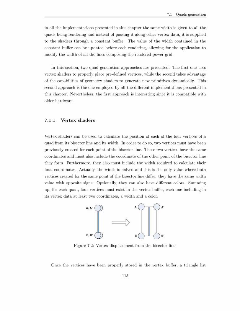
7.1 Quads generation
in all the implementations presented in this chapter the same width is given to all the
quads being rendering and instead of passing it along other vertex data, it is supplied
to the shaders through a constant buffer. The value of the width contained in the
constant buffer can be updated before each rendering, allowing for the application to
modify the width of all the lines composing the rendered power grid.
In this section, two quad generation approaches are presented. The first one uses
vertex shaders to properly place pre-defined vertices, while the second takes advantage
of the capabilities of geometry shaders to generate new primitives dynamically. This
second approach is the one employed by all the different implementations presented in
this chapter. Nevertheless, the first approach is interesting since it is compatible with
older hardware.
7.1.1 Vertex shaders
Vertex shaders can be used to calculate the position of each of the four vertices of a
quad from its bisector line and its width. In order to do so, two vertices must have been
previously created for each point of the bisector line. These two vertices have the same
coordinates and must also include the coordinate of the other point of the bisector line
they form. Furthermore, they also must include the width required to calculate their
final coordinates. Actually, the width is halved and this is the only value where both
vertices created for the same point of the bisector line differ: they have the same width
value with opposite signs. Optionally, they can also have different colors. Summing
up, for each quad, four vertices must exist in the vertex buffer, each one including in
its vertex data at least two coordinates, a width and a color.
Figure 7.2: Vertex displacement from the bisector line.
Once the vertices have been properly stored in the vertex buffer, a triangle list
113

Chapter 7. Dynamic Polyline Simplification On The GPU
topology may then be used along with an index buffer. For each quad, six entries are
stored in the index buffer pointing to the four vertices of the vertex buffer forming two
adjacent triangles.
Algorithm 11 shows the High-Level Shading Language (HLSL) code for the vertex
shader. The vertex shader function is called Widen and it receives all the enumer-
ated vertex data. It also has the transform matrix – required to transform vertex
coordinates to screen space – stored in a constant buffer, through the WorldViewProj
variable. The shader updates the vertex position according to the vector linking both
points of the bisector line and the width value. Then, multiplies the calculated po-
sition by the transform matrix, and returns the result along the received color. This
positioning is illustrated in Figure 7.2. The vertex shader is only concerned about cal-
culating the proper vertex positions. Based on the indices stored in the index buffer,
the corresponding vertices will be linked to form the triangles that will be received by
the Rasterizer stage.
Algorithm 11: Vertex shader quad generation HLSL code.
1 float4x4 WorldViewProj : WORLDVIEWPROJECTION;
2 struct VS OUTPUT {
3 float4 pos : POSITION;
4 float4 color : COLOR0;
5 };
6 VS OUTPUT Widen(float4 Pos : POSITION0, float4 Opp : POSITION1, float Width :
PSIZE0, float4 Color : COLOR) {
7 VS OUTPUT Out = (VS OUTPUT) 0;
8 float2 dir = Width * normalize(Pos.xy - Opp.xy);
9 Pos.x += dir.y;
10 Pos.y -= dir.x;
11 Out.pos = mul(Pos, WorldViewProj);
12 Out.color = Color;
13 return Out;
14 }
114

7.1 Quads generation
The HLSL code in Algorithm 11 only requires a vs 2 0 vertex shader profile and
thus, it may be used in older hardware. The main drawback of this approach is that
since each vertex requires to store not only the position corresponding to its point but
also the other point of the line, a lot of redundant information is required and thus,
storage requirements are increased. The next section shows how a geometry shader can
not only avoid this per-vertex data redundancy, but also halve the number of vertices
by only requiring two vertices per quad to be stored in the vertex buffer. As a result, by
using geometry shaders, the video memory required to store vertex positions is reduced
in a 75%. Nevertheless, as it was already stated, this vertex shader implementation can
be used in older hardware where geometry shaders will most likely not be supported.
7.1.2 Geometry shaders
Geometry shaders – introduced in Section 6.2.4 – are executed over the whole primitives
and allow to output a varying number of primitives. Furthermore, the type of the input
and output primitives can be different. These capabilities make geometry shaders ideal
for quad generation: a geometry shader can receive the bisector line as primitive and
output two adjacent triangles forming the quad. This allows to work with lines as
primitives, either using line lists or strips topologies. Neither duplicated vertices nor
vertex data besides the vertex position is required – although color and width may also
be included. This saves both memory and processing time.
The HLSL code of the geometry shader performing the quad generation is shown in
Algorithm 12. The calculation is analogous to that performed by the vertex shader in
the previous section, but in this case it is performed for all four vertices in one execution
of the geometry shader. Both vertices forming the line are received as input, following
the VS OUTPUT structure outputted by the vertex shader. The vertex shader code, in
charge of performing the vector-matrix multiplication, has been omitted for simplicity.
Note that since this matrix transformation is performed in the vertex shader, it is
carried only twice per line, whereas in the vertex shader quad generation it is performed
four times per line.
In the code shown, both the width and color are vertex data. Instead, they could be
provided as global variables supplied through constant buffers. The geometry shader
first calculates the quantities it must offset each of the line’s coordinates and then
115

Chapter 7. Dynamic Polyline Simplification On The GPU
appends four vertices to the output TriangleStream object corresponding to each quad
vertex. The HLSL TriangleStream object behaves like a strip and thus, by outputting
four vertices, two adjacent triangles are emitted. Since the geometry shader always
outputs four vertices, this is the maximum output vertex count. Accordingly, the
geometry shader function is annotated with [maxvertexcount(4)].
A comparison of vertex shader and geometry shader quad generation for power grid
visualization has been presented in [53]. In that work, two implementations of the
geometry shader quad generation were tested. The first one, performs the geometry
shader quad generation on every render – the same way it was presented in this section.
The second implementation performs the quad generation only when the width setting
is changed and then saves the results to a vertex buffer through the Stream Output
stage. That vertex buffer is then bound as input for rendering. Results show that the
latter is more expensive than the former both in terms of speed and memory. This
is due to the large amount of new vertices emitted by the geometry shader that are
stored in video memory and that must be processed by the vertex shader when reusing
its output in subsequent draws. When the quads are generated per-draw, only two
vertices per line must be processed by the vertex shader as opposed to the six vertices
of the two triangles generated by the geometry shader per line. Even the vertex shader
implementation requires less executions at the Vertex Shader stage, since it processes
four vertices per line. Even more, for power grids composed by more than one million
lines, when the geometry shader needs to write the generated quads to the Stream
Output buffer, it yields even slower rendering times than the implementation using
vertex shaders [53].
7.2 Stream Output statistics support
The different implementations presented in this chapter perform the simplification at
different stages of the graphics pipeline or using the compute pipeline, but all have
a common point at which the simplification has already been performed: after the
geometry shader. Primitives outputted by the Geometry Shader stage are those who
made it through the simplification process, no matter where it was performed. Know-
ing this, the Stream Output stage can be used to find out how many primitives are
being outputted by the geometry shader and thus, how many primitives yielded the
116

7.2 Stream Output statistics support
Algorithm 12: Geometry shader quad generation HLSL code.
1 struct VS OUTPUT {
2 float4 Position : POSITION;
3 float Width : WIDTH;
4 float4 Color : COLOR;
5 };
6 struct GS OUTPUT {
7 float4 Pos : SV Position;
8 float4 Color : COLOR;
9 };
10 [maxvertexcount(4)]
11 void GS( line VS OUTPUT input[2], inout TriangleStream<GS OUTPUT> Stream ) {
12 GS OUTPUT output = (GS OUTPUT) 0;
13 float2 dir = normalize(input[0].Position.xy - input[1].Position.xy);
14 float2 offset0 = input[0].Width / 2 * dir;
15 float2 offset1 = input[1].Width / 2 * dir;
16 output.Color = input[0].Color;
17 output.Pos = input[0].Position;
18 output.Pos.x -= offset0.y;
19 output.Pos.y += offset0.x;
20 Stream.Append(output);
21 output.Color = input[1].Color;
22 output.Pos = input[1].Position;
23 output.Pos.x -= offset1.y;
24 output.Pos.y += offset1.x;
25 Stream.Append(output);
26 output.Color = input[0].Color;
27 output.Pos = input[0].Position;
28 output.Pos.x += offset0.y;
29 output.Pos.y -= offset0.x;
30 Stream.Append(output);
31 output.Color = input[1].Color;
32 output.Pos = input[1].Position;
33 output.Pos.x += offset1.y;
34 output.Pos.y -= offset1.x;
35 Stream.Append(output);
36 }
117

Chapter 7. Dynamic Polyline Simplification On The GPU
simplification.
In order to be able to use the Stream Output stage, geometry shaders must be
compiled with Stream Output support. Normally this is done by calling CreateGeome-
tryShaderWithStreamOutput instead of the CreateGeometryShader API call. The only
difference is that the former requires a D3D11 SO DECLARATION ENTRY array
specifying the elements being outputted by the geometry shader to the Stream Output
stage. No buffers are created to hold those elements since the only interest for this
work is finding out their total count. To do so, a D3D11 QUERY SO STATISTICS
query must be created, and the Draw calls performing the rendering must be en-
closed between Begin and End calls received the query as parameter. After the End
has been called, a D3D11 QUERY DATA SO STATISTICS structure can be obtained
through the GetData call. This structure contains two fields: NumPrimitivesWritten
and PrimitivesStorageNeeded. The former indicates how many primitives have actually
been written to Stream Output buffers. In the event of buffers getting filled or if there
are no bound Stream Output buffers (as is the case presented here), the PrimitivesStor-
ageNeeded field hold the number of primitives that would have been written – on top
of those already written, if any.
It is worth mentioning that activating the Stream Output stage – by compiling
a shader with its support – imposes a small performance penalty, even if no data is
actually being written to Stream Output buffers. Because of this penalty, the Stream
Output support by the different implementations depends on a specific compiler flag.
When it is active, the GUI of the developed application has an extra button labeled
Peek SO primitives. When the user clicks this button, the number of primitives being
outputted by the geometry shader is queried in the next rendering and a message
is shown in the application console reporting the value. The rationale behind this
implementation is performing the query only after a request by the user – i.e. for the
subsequent draw – instead of continuously on every rendering, which would impact
performance.
118

7.3 D3DX Utility Library
7.3 D3DX Utility Library
The D3DX Utility Library (DXUT) is a support library providing helper functions for
Direct3D set up, texture handling, or graphical user interface (GUI) components among
others. Although its usage has been deprecated in Windows 8, it is nevertheless useful
for quick development and experimental applications. Evidencing the full integration of
DirectX with Windows, starting with Windows 8, the DirectX Software Development
Kit (SDK) has become part of the Windows SDK. The DXUT is no longer shipped
with it, but it can still be obtained from previous versions of the DirectX SDK. It is
distributed as C++ source code that has to be compiled prior to its use. Thus, it is
common to include it as a library project during development that is statically linked
to the application upon compilation.
Figure 7.3: Capture of a windowed Direct3D application with a DXUT GUI.
In this work, the DXUT has been used to initialize Direct3D, create a GUI and
manage the main loop of the application. DXUT handles the main loop by listening
for events and invoking the proper callbacks. These events include Direct3D events,
DXUT GUI interaction events, or Windows messages – such as the request to close the
119

Chapter 7. Dynamic Polyline Simplification On The GPU
main window.
A capture of a windowed Direct3D application using DXUT is displayed in Figure
7.3. This application corresponds to one of the implementations detailed later in this
chapter. Text drawing is not supported by Direct3D and thus, all the text displayed
is being drawn through DXUT. Furthermore, button, slider, and toggle button DXUT
GUI components are also used. When the user interacts with any of these components,
DXUT invokes a GUI event handler function which must have been set by the developer
during DXUT initialization.
7.3.1 Common GUI components
While several GUI components appear on Figure 7.3, the most relevant ones are the
Width and Threshold sliders. These sliders control the corresponding values passed
through constant buffers to the shaders. The width setting is used to control the quad
generation, as explained in the previous section. As it will be described in the following
sections, the threshold setting is in charge of controlling the polyline simplification
by establishing the minimum length that lines must have to survive the simplification
process. The third slider, labeled Tessellators, is specific for the implementation shown
in the figure and its purpose is explained in Section 7.4.4.4.
The first two sliders are common to all the implementations developed. Further-
more, the yellow text on the top left corner shows information about the current frame-
rate, dimension and format of the front and back buffers, as well as the current device
in use. Other controls that are common to the developed implementations are:
1. Toggle full screen: switches between windowed and full screen modes.
2. Toggle REF: switches the type of Direct3D device used for rendering, between a
hardware device and the reference software implementation. The latter provides a
software emulation device supporting all the Direct3D features but it is obviously
slower than hardware devices.
3. Change device: opens a detailed settings environment where advanced Direct3D
options can be changed.
120

7.4 GPU polyline simplification implementations
4. Save bitmap: writes the next rendered frame to a bitmap file on disk.
5. Peek SO primitives: available only when compiled with Stream Output support
(see Section 7.2). Once this button is clicked, the application prints to the console
the number of primitives outputted by the Geometry Shader stage.
6. Toggle HUD: shows or hides the user interface that is displayed on top of the
rendered power grid visualization.
7. Alpha blend: if checked, alpha blending is activated in the Output Merger stage.
8. Toggle wires: if checked, the rasterizer will only generate fragments for the poly-
gon edges – thus not filling the polygons.
Some of these controls have keyboard shortcuts, shown in parenthesis after their
names.
7.4 GPU polyline simplification implementations
Four different applications implementing three different GPU polyline simplification
approaches are presented in this section. They differ in the stage at which the sim-
plification is performed and the number of shaders involved. These stages correspond
to the Compute Shader stage of the compute pipeline, and the Geometry Shader and
Tessellation stages of the graphics pipeline. In order to test the Geometry Shader stage
approach more thoroughly, two applications have been developed instead of just one,
allowing for different configurations of geometry shaders to be tested.
All four applications present the render results in a window while also having a
console enabled to output log information such as average rendering performance, con-
figuration changes, number of primitives being processed on the GPU, or data statistics.
They all share the DXUT GUI previously introduced, they all can be compiled with
Stream Output statistics support to find out how many primitives survive the simpli-
fication, and they all perform quad generation through geometry shaders. They also
share the simplification algorithm, although the way it is implemented varies greatly.
Following, the simplification algorithm is presented before delving into the different
implementations.
121

Chapter 7. Dynamic Polyline Simplification On The GPU
7.4.1 Simplification algorithm
The main purpose of this work was to reduce the complexity of power grids through
polyline simplification in order to enhance the rendering performance and to make the
visualization appear less cluttered. More specifically, the intention was to engineer
different solutions taking advance of modern graphics cards. As a result, the main
focus was studying the different possible approaches, and less focus was put into the
specific algorithm performing the polyline simplification.
Algorithm 13: Polyline simplification pseudo-code.Data: inPolyline← Ordered list of points forming the input polyline
Threshold← Minimum length required for the segments of the polyline
Result: outPolyline← Ordered list of points forming the output polyline
1 outPolyline.Add(inPolyline.First)
2 previousPoint← inPolyline.First
3 for i← 1 to inPolyline.Size - 1 do
4 point← inPolyline.Get(i)
5 if distance(point, previousPoint) >= Threshold then
6 outPolyline.Add(point)
7 previousPoint← point
end
end
/* The last point has not been added */
8 if outPolyline.Last != inPolyline.Last then
outPolyline.Add(inPolyline.Last)
end
The pseudo-code of the polyline simplification algorithm implemented by the dif-
ferent solutions is shown in Algorithm 13. It is a simple algorithm, checking the length
of each segment forming the polyline. It does so in order, beginning by the segment
formed by the first and second points, then the next segment formed by the second
and third points and so forth, until the last point is reached. A segment must have a
length equal or greater than a certain threshold value in order to be kept. Otherwise,
its ending point is discarded and a new segment composed by the starting point and
the next point from the original polyline is formed. The length of this segment is then
checked against the threshold. This process goes on until either a new segment long
122

7.4 GPU polyline simplification implementations
enough is formed or the last point of the input polyline is reached. It may happen
that no segment including the last point was long enough. This scenario is handled
at line 8, where the last point of the input polyline is added to the output polyline if
it was not already there. The first point of the input polyline is always also the first
point of the output polyline, as can be seen at line 1. Keeping the same first and last
points is the only restriction of the algorithm. This is required in order to maintain the
topological connectivity between polylines. If the first and last points of polyline were
discarded, some polylines would cease to be connected with others. Thus, in the most
extreme case of simplification, the algorithm will return a polyline composed of just
one segment – i.e. a single line – linking the first and last points of the input polyline.
7.4.2 Polyline simplification using the Compute pipeline
In this implementation, a compute shader is used to perform the power grid simplifi-
cation. Branches of the power grid are stored as vertices composing consecutive line
strips in a vertex buffer, while another buffer holds strips information – namely, the po-
sition within the vertex buffer where each strip begins and how many vertices conform
it. The compute shader accesses these two buffers and processes the strips, removing
lines considered too short to be noticeable – criterion configurable through a threshold
value. As a result, the compute shader generates an index buffer that is used along the
original vertex buffer to render the power grid lines.
While rendering is performed continuously, the simplification is performed on-
demand. This means that the simplification is only performed when required: after the
application is initialized and prior to the first render, and every time the threshold is
changed. The user is allowed to modify the threshold through a slider of the GUI; when
that happens, the compute shader is executed previous to the next rendering. Since
the compute shader writes the simplification results to an index buffer stored in video
memory, it does not need to be executed again until the threshold parameter varies.
7.4.2.1 Simplification
The compute shader is invoked to operate over strips performing the simplification by
calling Dispatch; for each strip, a thread is dispatched, as illustrated in Figure 7.4. The
123
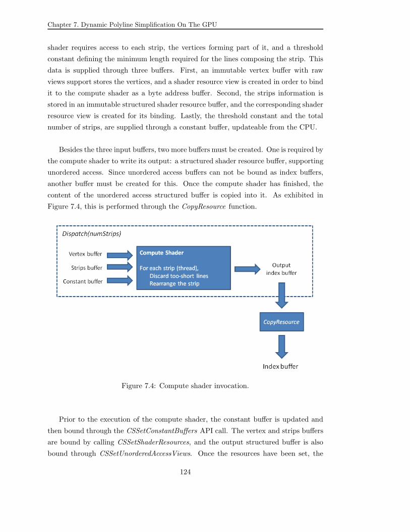
Chapter 7. Dynamic Polyline Simplification On The GPU
shader requires access to each strip, the vertices forming part of it, and a threshold
constant defining the minimum length required for the lines composing the strip. This
data is supplied through three buffers. First, an immutable vertex buffer with raw
views support stores the vertices, and a shader resource view is created in order to bind
it to the compute shader as a byte address buffer. Second, the strips information is
stored in an immutable structured shader resource buffer, and the corresponding shader
resource view is created for its binding. Lastly, the threshold constant and the total
number of strips, are supplied through a constant buffer, updateable from the CPU.
Besides the three input buffers, two more buffers must be created. One is required by
the compute shader to write its output: a structured shader resource buffer, supporting
unordered access. Since unordered access buffers can not be bound as index buffers,
another buffer must be created for this. Once the compute shader has finished, the
content of the unordered access structured buffer is copied into it. As exhibited in
Figure 7.4, this is performed through the CopyResource function.
Figure 7.4: Compute shader invocation.
Prior to the execution of the compute shader, the constant buffer is updated and
then bound through the CSSetConstantBuffers API call. The vertex and strips buffers
are bound by calling CSSetShaderResources, and the output structured buffer is also
bound through CSSetUnorderedAccessViews. Once the resources have been set, the
124

7.4 GPU polyline simplification implementations
compute shader can be invoked by dispatching as many threads as existing strips.
This is performed by calling Dispatch. Since memory sharing between threads is not
required, a group composed by a single thread is dispatched for each strip.
The compute shader uses its unique SV DispatchThreadID semantic value to access
the strips structured buffer. Each entry in that buffer contains two unsigned integers:
the first is an index pointing to the position of the initial vertex of the strip within the
vertex buffer, while the second holds the vertex count for that strip. Vertices forming
strips are stored consecutively in the vertex buffer. Thus, the compute shader loops
over the strip vertex count. On each iteration, the next vertex is loaded and the length
of the line formed by the retrieved vertex and the one loaded in the previous iteration
is checked against the threshold supplied through the constant buffer. If the length is
smaller than the threshold, the line is discarded and the previous vertex is marked as
pending of being connected. This vertex will then be used in the following iteration
as the starting vertex to form the next line, instead of the vertex which ended the line
discarded. If that line does not pass the test either, the process continues until another
does or the final vertex of the strip is reached. In the latter case, the pending vertex is
connected to the final one. Lines are outputted by the shader by writing the indices of
the two vertices composing each line to the output unordered access structured buffer.
The pseudo-code for the compute shader is shown in Algorithm 14. A simpler
version of this algorithm consists on merely discarding those lines not passing the
test, regardless of the topological connectivity. This yields a lighter algorithm and a
reduced number of outputted primitives. The drawback is that it has a great impact
on visualization since it removes the topological connectivity not only between strips
but also between the segments within strips.
As soon as the compute shader has processed all the strips, indices for the lines that
made through the simplification are stored in the output structured buffer. As stated
before, buffers created with index buffer bind flags can not be bound as unordered
resources and thus, the contents of the compute shader output buffer must be copied
onto an index buffer that will later be bound to the Input Assembler for rendering.
125
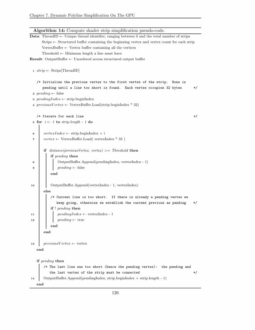
Chapter 7. Dynamic Polyline Simplification On The GPU
Algorithm 14: Compute shader strip simplification pseudo-code.Data: ThreadID← Unique thread identifier, ranging between 0 and the total number of strips
Strips← Structured buffer containing the beginning vertex and vertex count for each strip
VertexBuffer← Vertex buffer containing all the vertices
Threshold← Minimum length a line must have
Result: OutputBuffer← Unordered access structured output buffer
1 strip← Strips[ThreadID]
/* Initialize the previous vertex to the first vertex of the strip. None is
pending until a line too short is found. Each vertex occupies 32 bytes */
2 pending ← false
3 pendingIndex← strip.beginIndex
4 previousV ertex← VertexBuffer.Load(strip.beginIndex * 32)
/* Iterate for each line */
5 for i← 1 to strip.length - 1 do
6 vertexIndex← strip.beginIndex + i
7 vertex← VertexBuffer.Load( vertexIndex * 32 )
if distance(previousVertex, vertex) >= Threshold then
if pending then
8 OutputBuffer.Append(pendingIndex, vertexIndex - 1)
9 pending ← false
end
10 OutputBuffer.Append(vertexIndex - 1, vertexIndex)
else
/* Current line is too short. If there is already a pending vertex we
keep going, otherwise we establish the current previous as pending */
if ! pending then
11 pendingIndex← vertexIndex - 1
12 pending ← true
end
end
13 previousV ertex← vertex
end
if pending then
/* The last line was too short (hence the pending vertex): the pending and
the last vertex of the strip must be connected */
14 OutputBuffer.Append(pendingIndex, strip.beginIndex + strip.length - 1)
end
126

7.4 GPU polyline simplification implementations
7.4.2.2 Rendering
Once the strips have been simplified by the compute shader and the resulting output
structured buffer has been copied into the index buffer bindable to the Input Assembler
stage, the graphics pipeline execution in charge of rendering the lines can begin. As
it has been stated, it is not required for the compute shader to be executed prior to
each render, only when the threshold parameter controlling the minimum length for
the lines has changed.
Figure 7.5: Graphics pipeline configuration to render the results of the computepipeline.
127

Chapter 7. Dynamic Polyline Simplification On The GPU
Figure 7.5 exhibits all the active graphics pipeline stages with the most relevant
configured behavior. A DrawIndexed call is used to execute the pipeline and thus, not
only the vertex buffer but also an index buffer is required to be bound to the Input
Assembler. Furthermore, the consumed topology is line lists. After being fetched from
the vertex buffer, the required vertices are passed to the vertex shader where their
coordinates are transformed to screen space through vector-matrix multiplication. The
transformation matrix is used to control the viewpoint of the rendered scene and it is
passed from the application to the shader through a constant buffer that needs to be
explicitly bound to the vertex shader. This constant buffer is not the same as the one
used to pass the threshold to the compute shader, since neither the data nor the update
requirements are the same.
Lines with their vertices transformed by the vertex shader arrive at the geometry
shader which is in charge of generating a quad – i.e. two adjacent triangles forming a
rectangle – for each line. In order to do so, a width is required. In this implementation,
this information is obtained from the same constant buffer where the transformation
matrix is stored and thus, it must also be bound to the geometry shader. Note that
storing the width as vertex data would provide more flexibility, allowing each line its
own width and even different beginning and end widths. This would only impact
vertex storage requirements, not execution times, but would make updating widths
more costly. By passing a fixed width for all lines through the constant buffer, the
width can be easily updated between renderings.
The Rasterizer is configured to fill the triangles by interpolating the color values
of the vertices. Alternatively, wire-frame rendering can be activated through the GUI
in order to instruct the Rasterizer not to fill the generated triangles. Culling is not
required since the power grid topology has geographic coordinates without height and
thus, it is planar. Fragments generated by the Rasterizer arrive at the pixel shader
who simply outputs the interpolated color values. If alpha blending has been activated
through the GUI, these color values are then blended by the Output Merger with the
values already present in their corresponding render target pixels – if any – based on
the alpha component. When alpha blending is disabled, pixel colors present in the
render target are overwritten.
128

7.4 GPU polyline simplification implementations
7.4.2.3 Graphical user interface
A capture of the GUI of the implemented application is shown in Figure 7.6. All the
components are common to the other applications (described in Section 7.3.1) except
for the toggle button labeled Keep topology. When this toggle is checked (default)
Algorithm 14 is used, which maintains topological relationships. This means that
beginning and end points are always kept and that connectivity is always ensured
both between polylines and between segments within a polyline. When the toggle is
unchecked, these restrictions are ignored and polylines segments are discarded whenever
their length is smaller than the threshold. As a result, more primitives are discarded
at the expense of no longer maintaining the topology.
Figure 7.6: Windowed Direct3D application implementing the compute shader simpli-fication.
129

Chapter 7. Dynamic Polyline Simplification On The GPU
7.4.3 Polyline simplification using the Geometry Shader stage
In this implementation, the polyline simplification is performed at the Geometry Shader
stage. Three buffers are required: a constant buffer, an immutable byte access buffer
and an immutable vertex buffer. The constant buffer contains the vertex transformation
matrix, the threshold that controls the minimum length for the lines, and the width
desired for the generated quads. It may be updated a maximum of once per frame,
if either the view point, the width, or the threshold value are modified by the user
through the GUI. The immutable byte access buffer holds the vertices composing the
polylines, stored as strips. This means that vertices are laid out in the buffer following
their order in the strips and that vertices forming part of more than one strip will be
repeated. Furthermore, the strips have been sorted out by their length, in an ascending
fashion. Although vertices are stored in this buffer, it will not be bound as input of the
Input Assembler stage. Instead, the third buffer, holding information about the strips
will be bound as the input vertex buffer for the pipeline. Each entry of this vertex
buffer consists on two unsigned integers. The first one points to a position of the byte
access buffer where the initial vertex of a strip is located. The second integer, indicates
the length of that strip – i.e. the number of vertices composing it and thus, consecutive
positions on the byte access buffer containing the corresponding vertices. No primitive
is to be set up from this data and thus, the Input Assembler is configured with the
point list primitive topology. Since the byte access buffer is to be accessed from the
geometry shader, a shader resource view needs to be created in order to bind it. Figure
7.7 shows a strips buffer and its entries, pointing to the corresponding vertex buffer
locations; the layout of the data contained in each of those locations is also presented.
No vertex data is actually fed to the pipeline and thus, there is no work to do for the
vertex shader except just returning the received strip information. This information,
consisting on the strip initial vertex location and the strip length is then passed to the
Geometry Shader stage. There, a shader loads those vertices forming the strip from
the immutable byte access buffer. It does so iterating over the strip length, loading one
vertex on each iteration and checking whenever the line formed by the loaded vertex
and the previous one has a length equal or larger than the threshold parameter. The
geometry shader HLSL code is shown in Algorithm 15.
130

7.4 GPU polyline simplification implementations
Figure 7.7: Strips and vertex buffers used by the geometry shader implementation.
The HLSL code is the implementation of the Algorithm 14, adapted to the specifics
of the geometry shader and using the described buffers. The immutable byte access
buffer is accessed through the VertexBufferIn object. Using its Load2 method, two
floats corresponding to the first two coordinates of a vertex are retrieved from the
buffer on each iteration. A global color is used for all quads instead of using the value
from the vertex data. This value is stored in the UP TO 32 COLOR constant which
is specified at shader compile time. Also, the g fThreshold global variable holds the
threshold parameter passed through the bound constant buffer – whose declaration has
been omitted from the code for convenience.
The EmitQuad is an HLSL function created to factor code and omitted for sim-
plicity. Its code is basically the same shown in Algorithm 12, but receiving the two
vertices as two parameters instead of through a 2-element array, and also receiving the
output TriangleStream object as well as the desired color for the quad. Vector-matrix
multiplication is performed over the two input vertices to transform their positions to
screen space – subsuming the typical task of the vertex shader. Before returning, the
EmitQuad also calls the RestartStrip method of the TriangleStream, so that it is ready
to generate a new quad on a subsequent invocation.
The geometry shader is limited by its maximum output, restricted in Direct3D 11
131

Chapter 7. Dynamic Polyline Simplification On The GPU
Algorithm 15: HLSL code for a geometry shader simplifying up to 32-vertices
strips.
struct VS OUTPUT {
uint beginIndex : BASE INDEX;
uint length : VERTEX COUNT;
};
struct GS OUTPUT {
float4 Pos : SV Position;
float4 Color : COLOR;
};
ByteAddressBuffer VertexBufferIn : register(t0);
[maxvertexcount(128)]
void GS upto32( point VS OUTPUT strip[1], inout TriangleStream<GS OUTPUT> Stream )
{
bool isPending = false;
float2 vertex;
float2 prev = asfloat(VertexBufferIn.Load2( strip[0].beginIndex * 32));
float2 pendingVertex = prev;
float4 color = UP TO 32 COLOR;
for (uint i = 1; i < strip[0].length; i++) {
vertex = asfloat(VertexBufferIn.Load2( (strip[0].beginIndex + i) * 32 ));
if ( distance(prev, vertex) >= g fThreshold ) {
if (isPending) {
EmitQuad(pendingVertex , prev, Stream, color);
isPending = false;
}
EmitQuad( prev, vertex, Stream, color);
} else if (!isPending) {
pendingVertex = prev;
isPending = true;
}
prev = vertex;
}
if (isPending)
EmitQuad( pendingVertex, vertex, Stream, color);
}
132
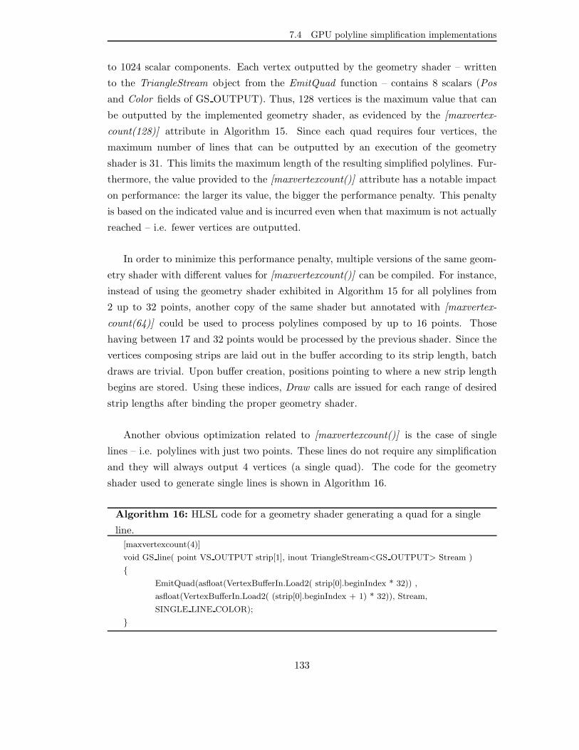
7.4 GPU polyline simplification implementations
to 1024 scalar components. Each vertex outputted by the geometry shader – written
to the TriangleStream object from the EmitQuad function – contains 8 scalars (Pos
and Color fields of GS OUTPUT). Thus, 128 vertices is the maximum value that can
be outputted by the implemented geometry shader, as evidenced by the [maxvertex-
count(128)] attribute in Algorithm 15. Since each quad requires four vertices, the
maximum number of lines that can be outputted by an execution of the geometry
shader is 31. This limits the maximum length of the resulting simplified polylines. Fur-
thermore, the value provided to the [maxvertexcount()] attribute has a notable impact
on performance: the larger its value, the bigger the performance penalty. This penalty
is based on the indicated value and is incurred even when that maximum is not actually
reached – i.e. fewer vertices are outputted.
In order to minimize this performance penalty, multiple versions of the same geom-
etry shader with different values for [maxvertexcount()] can be compiled. For instance,
instead of using the geometry shader exhibited in Algorithm 15 for all polylines from
2 up to 32 points, another copy of the same shader but annotated with [maxvertex-
count(64)] could be used to process polylines composed by up to 16 points. Those
having between 17 and 32 points would be processed by the previous shader. Since the
vertices composing strips are laid out in the buffer according to its strip length, batch
draws are trivial. Upon buffer creation, positions pointing to where a new strip length
begins are stored. Using these indices, Draw calls are issued for each range of desired
strip lengths after binding the proper geometry shader.
Another obvious optimization related to [maxvertexcount()] is the case of single
lines – i.e. polylines with just two points. These lines do not require any simplification
and they will always output 4 vertices (a single quad). The code for the geometry
shader used to generate single lines is shown in Algorithm 16.
Algorithm 16: HLSL code for a geometry shader generating a quad for a single
line.
[maxvertexcount(4)]
void GS line( point VS OUTPUT strip[1], inout TriangleStream<GS OUTPUT> Stream )
{
EmitQuad(asfloat(VertexBufferIn.Load2( strip[0].beginIndex * 32)) ,
asfloat(VertexBufferIn.Load2( (strip[0].beginIndex + 1) * 32)), Stream,
SINGLE LINE COLOR);
}
133

Chapter 7. Dynamic Polyline Simplification On The GPU
The Rasterizer and Output Merger stages are configured exactly as in the Compute
Shader implementation. The Rasterizer is configured either to fill the triangles by
interpolating the color values of vertices or to generate just wire-frames. Culling is not
required since the power grid topology has geographic coordinates without height and
thus, it is planar. Fragments generated by the rasterizer arrive at the pixel shader who
simply outputs the interpolated color values. If enabled through the GUI, these color
values are then blended by the Output Merger with the values already present in their
corresponding render target pixels – if any – based on the alpha component.
Two geometry shaders have been presented in this section: one simply generating
a quad for single lines, and other performing simplification over polylines but which
is able to only output up to 32 points. Although several versions of the latter have
been proposed in order to perform optimizations based on the lengths of the polylines,
the maximum output count of 32 points stands. In order to overcome this limitation,
geometry shader instancing was used.
7.4.3.1 Geometry shader instancing
Geometry shader instancing consists on executing the same geometry shader more than
once for the same primitive. It was introduced with Direct3D 11 and for that version,
the maximum instance count is 32 – i.e. a geometry shader may be executed up to 32
times for the same primitive. It is activated simply by annotating the geometry shader
function with [instance()], specifying the desired number of instances to be run for each
primitive.
When instancing is enabled, the SV GSInstanceID system-value semantic may be
assigned to a geometry shader parameter in order to check which instance is being
executed. Using instancing, the geometry shader presented in Algorithm 15, could be
used to output up to 1024 points for a single polyline. Note that the size of the input
polyline is theoretically unlimited since it is being directly accessed through the byte
access buffer instead of flowing from one pipeline stage onto another. In practice, it is
limited by the maximum loop iterations supported by Direct3D.
In order to support the simplification of polylines composed by more than 32 points
– more specifically, polylines that after having been simplified still have more than 32
134

7.4 GPU polyline simplification implementations
points – different versions of the geometry shader with [maxvertexcount(128)] (maxi-
mum 32 outputted points) were compiled, only differing in the [instance()] attribute.
The shader compiled with [instance(2)] can output up to 64 points, the one compiled
with [instance(3)] up to 96, and so on. By looking at the SV GSInstanceID value, each
shader instance focuses on a different subset of 32 points of the polyline. The downside
of this approach is that the segments where one instance ends and other begins are not
eligible for simplification. Furthermore, in this work, only the shader outputting up to
32 points has been instanced. Some performance gain could be attained by instancing
shaders with smaller [maxvertexcount()] at the expense of making more segments not
eligible for simplification – because the first and last points of each polyline must always
be kept.
7.4.3.2 Graphical user interfaces
Two applications using geometry shaders for polyline simplification have been devel-
oped. The first one allows the user to chose among 3 different polyline simplification
configurations, using either 4, 5, or 6 geometry shaders. These configurations are shown
in Table 7.1 and a capture of its GUI is shown in Figure 7.8. The Geometry shaders
slider has three different positions corresponding to each one of the mentioned config-
urations.
Configuration
1st 2nd 3rd
2 - 32
2 (single lines) 2 (single lines)
3 - 323 - 5
6 - 32
33 - 64 (2 instances)
65 - 96 (3 instances)
97 - 128 (4 instances)
Table 7.1: Range of points covered by each geometry shader for each possible configu-ration.
135

Chapter 7. Dynamic Polyline Simplification On The GPU
Figure 7.8: Windowed Direct3D application implementing the geometry shader simpli-fication with three possible shader configurations.
The second application allows the user to chose between 5 and 34 geometry shaders
through the slider labeled with # GS [3-32] – for the number of geometry shaders in
use – which ranges between 0 and 30. When set to 0, 5 geometry shaders are used: one
generating quads for single lines, other simplifying polylines having between 3 and 32
points inclusive, and 3 instanced versions of the latter, ranging between 33 and 64, 65
and 96, and 97 and 128 points inclusive. By increasing the value assigned to the slider,
other geometry shaders are introduced which adjust to specific polyline lengths. For
instance, when 1 is set, another geometry shader simplifying polylines composed of 3
points is used on top of the other 5. If the slider is set to 2, another one for polylines of
length 4 is added, for a total number of 7 geometry shaders being executed. This goes
on until the setting of 30, in which case, 34 geometry shaders are executed: one for
single lines, 30 for each length between 3 and 32 inclusive, and three instanced versions
of the 32-points length geometry shader for 2, 3, and 4 instance counts. A list of these
34 shaders can be seen on the left of the capture of this implementation, shown in
136

7.4 GPU polyline simplification implementations
Figure 7.9. Furthermore, the number of polylines having the corresponding length is
displayed in parenthesis for each shader.
Figure 7.9: Windowed Direct3D application implementing the variable geometry shadersimplification.
Note that all the 30 geometry shaders adjustable through the slider consist ex-
actly on the same HLSL code with their only difference being the value assigned to
the [maxvertexcount()] annotation. This value can be parameterized at compile time
through a constant passed to the shader compiler. This way, instead of repeating the
shader code, a simple loop compiling the same geometry shader code after updating
the corresponding value for each iteration can be used.
Like the compute shader implementation, both implementations feature an alter-
native simplification geometry shader that does not take into account topological con-
nectivity: its only regard is whenever each individual line has a length larger than the
threshold. The Keep topology toggle allows to switch to this geometry shader.
137

Chapter 7. Dynamic Polyline Simplification On The GPU
7.4.4 Polyline simplification in the tessellation stages
Tessellation employs a different set of topologies than the classic graphics pipeline:
the pipeline must be fed with patches instead of points, lines or triangles – either
as strips or lists, with or without adjacency information. Patches are composed by
between 1 and 32 control points. These control points can represent anything and
actually are handled as vertices by the pipeline, requiring an associated input layout
just like any other vertex. Therefore, polylines composed by up to 32 points can be
fed to the pipeline as patches. The potential benefit compared to the geometry shader
implementation presented in the previous section, is avoiding a considerable number of
direct memory accesses from the shader to retrieve the vertices for each strip. However,
the largest patch has 32 points, thus requiring other means to perform simplification
over larger polylines.
The implementation presented in this section, follows a mixed approach: for poly-
lines composed by up to 32 points, the simplification is performed in the patch-constant
function of the hull shader, while for lines with more than 32 points, it is carried by a
geometry shader with instancing. Actually, the length of the polylines to be simplified
through tessellation stages can be controlled by the user through a Tessellators param-
eter. The geometry shader will be in charge of simplifying those lengths not covered
by tessellation and, when the user sets the Tessellators parameter to 0, the implemen-
tation is equivalent to the geometry shader simplification from previous section. Thus,
this implementation can be seen as an extension of the geometry shader simplification,
introducing an alternative method for polylines having between 3 and 32 points.
7.4.4.1 Implementation
The same three buffers used by the geometry shader simplification are required for this
implementation: a constant buffer employed to pass the transformation matrix along
with the threshold and width parameters, an immutable byte access buffer storing the
vertices, and an immutable buffer holding the strips information bindable as input
vertex buffer. The only difference is that in this implementation, the byte access buffer
is also bindable as input vertex buffer – this is accomplished simply by enabling the
D3D11 BIND VERTEX BUFFER extra flag upon its creation. This buffer serves a
double purpose, depending on whether the simplification is being performed by the
138

7.4 GPU polyline simplification implementations
tessellation or the geometry shader. In the case of tessellation, it is bound as the input
vertex buffer and the patches control points are fetched from it. When simplification
is performed by the geometry shader, it is accessed directly from the geometry as
described in the previous section – a shader resource view is used to bind the resource
to the geometry shader. Two input layouts are required: one for the patches formed
by the vertices from the byte access buffer, and other for the strips.
The byte access buffer actually contains the vertices forming the strips, stored in a
increasing order by strip length, beginning by the single lines. Indices are kept for the
positions of the buffer where the length of stored strips change. These indices are used
to invoke batch draws for all the strips having the same length using the proper shaders,
as shown in Algorithm 17. Since there are many variables involved, their description
has been omitted from the pseudo-code, being shown instead in Table 7.2.
Rasterizer, Pixel Shader and Output Merger stages are independent of the simplifi-
cation method used and thus, are configured only once per rendered frame. The pixel
shader simply outputs the received fragment color. Like in the other implementations,
both the Rasterizer and Output Merger stages are configured according to what the
user has selected in the GUI. This allows the user to select whenever he wants alpha
blending to be active and/or wire-frame rendering – i.e. rendering only the edges of
the triangles.
First, polylines simplified using tessellators are rendered. In this work, the term tes-
sellator refers to a certain Tessellation stage state, including hull and domain shaders
for a given patch size. The byte access buffer holding the vertices is bound as input
vertex buffer and its layout is passed to the Input Assembler stage. The user selects
how many tessellators to use through a slider in the GUI. Possible values range from
0 (no tessellation simplification, only geometry shader simplification) up to 30 (corre-
sponding to polylines composed by 3 up to 32 points). A loop iterates over the selected
value, setting the proper hull and domain shaders and invoking the Draw upon the
polylines with the length corresponding to that iteration. The vertex and geometry
shaders are the same for all these draws, performing matrix multiplication and quad
generation, respectively.
Once the tessellation simplification has been performed, it is turn for the geometry
shader simplification, in charge of simplifying and rendering the rest of the polylines.
139

Chapter 7. Dynamic Polyline Simplification On The GPU
Algorithm 17: Rendering pseudo-code using tessellation and geometry shader
simplification.
/* Common pipeline state (Pixel Shader, Rasterizer and Output Merger stages) */
1 PSSetShader(PS)
if WireframeChecked thenRSSetState(Wireframe)
elseRSSetState(Fill)
end
if AlphaBlendChecked thenOMSetBlendState(AlphaBlend)
elseOMSetBlendState(NoBlend)
end
/* Render polylines using Tessellation simplification */
2 IASetInputLayout(VertexLayout)
3 IASetVertexBuffers(0, 1, VertexBuffer)
4 VSSetShader(VSmul) // Position transformation using the transformation Matrix
5 VSSetConstantBuffers(CB) // VS requires the transformation Matrix
6 GSSetShader(GSquadFromLine)
7 GSSetConstantBuffers(CB) // GS requires the desired Width
8 for i← 1 to TessellatorsCount do
9 IASetPrimitiveTopology()
10 HSSetShader(HullShaders[i-1])
11 DSSetShader(DomainShaders[i-1])
12 Draw(Indices[i+1] - Indices[i], Indices[i])
end
/* Render polylines using Geometry Shader simplification */
13 IASetInputLayout(StripLayout)
14 IASetVertexBuffers(0, 1, StripsBuffer)
15 IASetPrimitiveTopology(TOPOLOGY POINTLIST)
16 VSSetShader(VSpass) // No-op, just returns the strip (pass-through)
17 HSSetShader(NULL)
18 DSSetShader(NULL)
19 GSSetShaderResources(VertexBufferSRV)
20 GSSetConstantBuffers(CB) // GS requires the transformation Matrix and the desired Width
21 GSSetShader(GeometryShaders[0]) // No simplification: direct quad generation
22 Draw(Indices[1], 0)
23 for i← TessellatorsCount + 1 to size(Indices) do
24 GSSetShader(GeometryShaders[i])
25 Draw(Indices[i+1] - Indices[i], Indices[i])
end
140

7.4 GPU polyline simplification implementations
Block Variable Description
Common
PS Pixel shader returning the color fragment.
WireframeChecked Boolean stating whether or not the user has chosen to
render wireframe instead of filled triangles.
Fill Rasterizer state: fill triangles and no culling.
Wireframe Rasterizer state: do not fill triangles and no culling.
AlphaBlendChecked Boolean stating whether or not the user has activated the
alpha blending.
AlphaBlend Alpha blending state for the Output Merger.
NoBlend Output Merger state without blending.
CB Constant buffer holding the width and threshold param-
eters, and the transformation matrix.
Indices Array containing the positions of VertexBuffer where the
strip length varies.
TessellatorsCount Number of tessellators to be used (set by the user).
Tessellation
VertexBuffer Byte access vertex buffer storing the strip vertices.
VertexLayout Layout of each vertex in VertexBuffer.
VSmul Vertex shader transforming vertex position through
vector-matrix multiplication.
GSquadFromLine Geometry shader generating a quad from a single input
line.
TessellatorCount Number of tessellators to employ, set by the user through
the GUI (0-30).
HullShaders Array containing 30 hull shaders.
DomainShaders Array containing 30 domain shaders.
Geometry shaders
StripsBuffer Vertex buffer containing strip information.
StripLayout Layout of each entry of the StripsBuffer.
VSpass Vertex shader simply returning the input vertex (pass-
through).
VertexBufferSRV Shader resource view used to bind VertexBuffer to the
geometry shaders.
GeometryShaders Array containing 34 geometry shaders (2, 3 .. 32, 33-64,
65-96, 97-128).
Table 7.2: Variables used in the pseudo-code shown in Algorithm 17.
141

Chapter 7. Dynamic Polyline Simplification On The GPU
Furthermore, another geometry shader is also used to render single lines without per-
forming any simplification. For all these geometry shaders, the Input Assembler is
configured to bind the strips buffer as input vertex buffer, and its layout is set accord-
ingly. As a result, unlike the geometry shaders used after the tessellation simplification
which receive the resulting lines, these geometry shaders receive a strip as input. Thus,
they must access the byte access buffer and retrieve the vertices forming the lines.
The second entry of the Indices array points to the position of the byte access
buffer where the first vertex of the first polyline composed of 3 points is stored. Thus,
it accounts for the total number of vertices forming single lines – and the number of
single lines is that same number halved. The third entry of the Indices array points to
the position where the first vertex of the first polyline composed of 4 points is stored.
An so forth until 32 points is reached. From that point on, lengths vary in multiples
of 32 – i.e. up to 64, 96, 128, etc. As shown in Algorithm 17, this information is
used to invoke the Draw calls, specifying how many vertices to draw and where to
begin reading from the bound vertex buffer. Note the parallelism between the Indices
and the GeometryShaders array: for each strips length pointed in the Indices array, a
corresponding geometry shader exists in the GeometryShaders array.
The HullShaders and DomainShaders arrays contain the same shaders compiled
only varying a constant reflecting the number of points forming the polylines: 30 shaders
covering polylines having between 3 and 32 points. The same happens for elements
from 1 up to 30 of the GeometryShaders array. The first element (position 0) of the
GeometryShaders array contains the geometry shader for single lines and those beyond
position 30, geometry shaders with instancing, covering polylines with lengths multiple
of 32.
7.4.4.2 Hull Shader simplification
The geometry shader simplification in this implementation is the same developed in
Section 7.4.3. In this section, the simplification performed by the tessellation stages
is presented. More specifically, the simplification is performed by the patch-constant
function of the hull shader, executed once per patch. The main hull shader function is
a simple pass-through shader, returning each input control point untouched.
142

7.4 GPU polyline simplification implementations
The pseudo-code of the patch-constant function has been split into Algorithms 18
and 19 for convenience. It receives an input patch composed of the control points
representing the points composing the polyline, and outputs a structure composed of
two arrays. The first array is called ReorderIndices and represents the polyline after
its simplification. It actually holds the positions within the input patch array of those
points of the polyline that made it through the simplification. They are ordered so that
the corresponding strip can be generated. The second array is named Edges and it is
composed of two floats and has the system-value semantic SV TessFactor associated.
These two values will be consumed by the subsequent Tessellator stage in order to
generate line primitives.
Algorithm 18 corresponds to the first half of the hull shader patch-constant function.
First, the input patch is examined. Points having a negative width are marked as invalid
by setting their corresponding entries in the ReorderIndices array to -1. This can be
used to pass patches containing actually smaller polylines than their size by simply
setting the widths of the extra control points to negative values. Once finished, the
ReorderIndices array contains the positions of the strip points within the input patch.
Moreover, the lastValidPos variable indicates which is the last useful position of the
array. After this initialization, distances are calculated for all the lines composing the
strip – i.e. segments of the polyline. For those lines with a length smaller than the
Threshold, their corresponding ReorderIndices value is set to -1.
Algorithm 19 shows the second half the hull shader patch-constant function, contin-
uing where Algorithm 18 ends. The first step consists on reordering the ReorderIndices
array, moving invalid indices (those with a -1 value) to the end of the array. Then,
a check is made for those cases where all the segments of a polyline are too small.
In those cases, a single line must be generated connecting the start and end points.
Finally, the Edges array is set in order to instruct the Tessellator stage to generate one
line primitive for each segment of the polyline that passed the simplification.
Once the patches have been processed by the Hull Shader stage, the Tessellator
stage generates the required lines based on the SV TessFactor values received. In
order to do so, a bi-dimensional coordinate is generated for each vertex composing
those lines. These coordinates are called UV coordinates since they actually account
for a sampling performed over a planar rectangular mesh to obtain as many samples
as vertices required to form the lines. This sampling follows the pattern of laying lines
143

Chapter 7. Dynamic Polyline Simplification On The GPU
Algorithm 18: Hull shader patch-constant function pseudo-code (first half).
Data: InputPatch← Input patch control points
InputPatchSize← Number of control points in the input patch
Threshold← Minimum length for a line
Result: Output← Per-patch data: ReorderIndices array containing the indices of the control
points to keep, and the Edges array required by the Tessellator stage to generate the
lines
/* Initialization */
1 lastV alidPos← 0
2 for i← 0 to InputPatchSize - 1 do
3 if InputPatch[i].Width < 0 then
4 lastV alidPos← i
5 Output.ReorderIndices[i]← -1
6 for j ← i + 1 to InputPatchSize -1 do
7 Output.ReorderIndices[j]← - 1
end
8 break
else
9 Output.ReorderIndices[i]← i
end
end
10 if lastValidPos == 0 then
/* All indices were valid */
11 lastV alidPos← InputPatchSize - 1
end
/* Segment distances calculation */
12 for i← 0 to lastValidPos - 1 do
13 distances[i]← distance(InputPatch[i-1], InputPatch[i])
end
/* Mark points forming segments shorter than the threshold */
14 for i← 1 to lastValidPos - 1 do
15 if distances[i-1] < Threshold AND distances[i] < Threshold then
16 Output.ReorderIndices[i]← - 1
end
end
144

7.4 GPU polyline simplification implementations
Algorithm 19: Hull shader patch-constant function pseudo-code (second half).
Data: InputPatch← Input patch control points
InputPatchSize← Number of control points in the input patch
Threshold← Minimum length for a line
Result: Output← Per-patch data: ReorderIndices array containing the indices of the control
points to keep, and the Edges array required by the Tessellator stage to generate the
lines
/* Vertex reordering */
1 for i← 1 to lastValidPos - 1 do
2 if Output.ReorderIndices[i] == - 1 then
3 for j ← i + 1 to lastValidPos do
4 if Output.ReorderIndices[j] != -1 then
5 Output.ReorderIndices[i]← Output.ReorderIndices[j]
6 Output.ReorderIndices[j]← -1
7 break
end
end
end
end
/* Special case: if all segments were discarded, the start and end vertices
must be kept to maintain topological connectivity */
8 if Output.ReorderIndices[1] == -1 then
9 Output.ReorderIndices[0]← 0
10 Output.ReorderIndices[1]← lastValidPos - 1
end
/* Configure the Tessellator stage: set the number of lines it must generate
*/
11 lines← 1
12 for i← 2 to InputPatchSize - 1 do
13 if Output.ReorderIndices[i] != -1 then
14 lines← lines + 1
end
end
15 Output.Edges[0]← lines
16 Output.Edges[1]← 1
145

Chapter 7. Dynamic Polyline Simplification On The GPU
over the theoretical rectangle so that contiguous coordinates represent vertices forming
a line primitive.
Algorithm 20: HLSL code of the domain shader returning the proper vertex.
struct HS CONSTANT DATA OUTPUT {
float Edges[2] : SV TessFactor;
uint ReorderIndices[INPUT PATCH SIZE] : KEEPERS;
};
struct HS OUTPUT {
float4 Position : POSITION;
float Width : WIDTH;
float4 Color : COLOR;
};
struct DS OUTPUT {
float4 Position : SV POSITION;
float Width : WIDTH;
float4 Color : COLOR;
};
[domain(”isoline”)]
DS OUTPUT DS( HS CONSTANT DATA OUTPUT input, float2 UV : SV DomainLocation,
const OutputPatch<HS OUTPUT, OUTPUT PATCH SIZE> patch ) {
DS OUTPUT Output = (DS OUTPUT) 0;
int index = input.ReorderIndices[ round(UV.y * input.Edges[0] + UV.x) ];
Output.Position = patch[index].Position;
Output.Width = patch[index].Width;
Output.Color = patch[index].Color;
return Output;
}
The Domain Shader stage executes the domain shader function over each UV co-
ordinate generated by the tessellator. This function returns the proper output patch
control point, obtained by using the UV coordinates received from the Tessellator stage
to access the proper control point from the input patch, as shown in the HLSL code of
Algorithm 20. The INPUT PATCH SIZE and OUTPUT PATCH SIZE constants are
supplied by the compiler in order to automate the compilation of the domain shaders
146
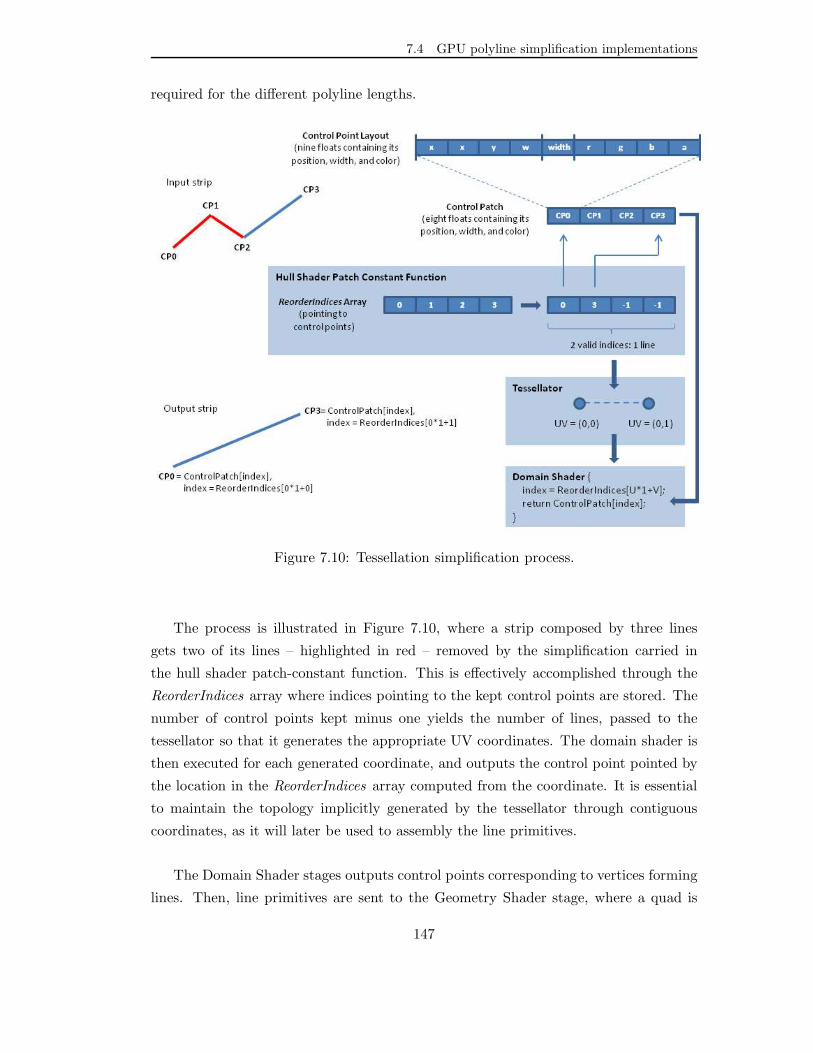
7.4 GPU polyline simplification implementations
required for the different polyline lengths.
Figure 7.10: Tessellation simplification process.
The process is illustrated in Figure 7.10, where a strip composed by three lines
gets two of its lines – highlighted in red – removed by the simplification carried in
the hull shader patch-constant function. This is effectively accomplished through the
ReorderIndices array where indices pointing to the kept control points are stored. The
number of control points kept minus one yields the number of lines, passed to the
tessellator so that it generates the appropriate UV coordinates. The domain shader is
then executed for each generated coordinate, and outputs the control point pointed by
the location in the ReorderIndices array computed from the coordinate. It is essential
to maintain the topology implicitly generated by the tessellator through contiguous
coordinates, as it will later be used to assembly the line primitives.
The Domain Shader stages outputs control points corresponding to vertices forming
lines. Then, line primitives are sent to the Geometry Shader stage, where a quad is
147

Chapter 7. Dynamic Polyline Simplification On The GPU
generated for each one of them. After that, the normal execution of the pipeline
continues: the Rasterizer stage generates fragments from the triangles which are fed to
the Pixel Shader stage; there, a pixel shader returns the color of each fragment, which
is subsequently merged into the frame buffer by the Output Merger stage. Just like in
the other implementations, alpha blending and wire-frame rendering can be configured
through the GUI.
7.4.4.3 Compiled tessellation shaders reutilization
The hull shader patch-constant function, whose pseudo-code is shown in Algorithms
18 and 19, exhibits a significant number of loops. When compiled, these loops are un-
rolled, converting the iteration into a sequence of repeated instructions. This increases
the number of total instructions and thus the length of the byte-code, but saves the
performance penalty imposed by flow control. However, as the number of iterations
grow along with the patch size, the loop unrolling yields prohibitive compilation times
that can reach up to several minutes for patches with more than 25 control points.
In order to overcome this issue, the implementation saves to disk each compiled
shader. Upon application start, it looks for the compiled shader file and, if present,
skips the compilation. The shader HLSL code is the same for all the tessellators ex-
cept for the patch sizes. This is parameterized through the INPUT PATCH SIZE and
OUTPUT PATCH SIZE constants supplied through the compiler. As a result, the
compilation process must be performed only once. Even more, since they are com-
piled to intermediate byte-code, the compiled shaders can be distributed along the the
application if desired.
7.4.4.4 Graphical user interface
The GUI of the implemented application is exhibited in Figure 7.11. It is very similar
to that of the other implementations presented in this chapter. The main difference
consists on the Tessellators slider, which allows the user to specify which polylines must
be simplified using tessellation. The slider ranges from 0 up to 30, corresponding to
polylines composed from 3 up to 32 points. The rest of the polylines will be simplified
using geometry shaders – with instancing for those having more than 32 points. Since
148

7.4 GPU polyline simplification implementations
single lines require no simplification, and they are always shown in order to keep topo-
logical connectivity, a geometry shader generating a quad for the input line is used to
render them.
The capture shown in Figure 7.11 shows a Tessellator slider setting of 17. As can
be seen on the list on the left, this means that polylines having between 3 and 19 points
inclusive are being rendered using simplification in the Tessellation stages. Polylines
having between 20 and 32 points inclusive are simplified using geometry shaders. Fur-
thermore, three instanced shaders are in charge of simplifying the rest of the polylines.
Single lines – 62537 in the capture – are being rendered using a geometry shader.
Figure 7.11: Windowed Direct3D application implementing the tessellation and geom-etry shader simplification.
149

Chapter 7. Dynamic Polyline Simplification On The GPU
150

CHAPTER8GPU Polyline Simplification Results
In this chapter, experimentation results are presented for the different implementations
performing polyline simplification on the GPU over five real power grids datasets. An
application rendering the whole datasets using indexed line primitives was also devel-
oped in order to provide reference values from an application performing the rendering
without any kind of simplification. This application is referred to as Bulk implementa-
tion through the chapter.
Tests were carried in order to analyze the different implementations from three
points of view: rendering performance, video memory consumption, and visual accuracy
of the rendered visualization.
8.1 Rendering performance
In order to measure the rendering performance, the frame rate or frames per second
(FPS) value was used. This value accounts for the number of complete render cycles
performed per second. A render cycle comprises the complete rendering process, from
the required pipeline configuration and invocation of draw calls up to the rendered
frame being presented to the screen – in this case, to the dedicated area of the window.
It does not include neither the device creation and set up, nor the resources creation;
this is performed upon application initialization, or whenever the device is lost for some
reason – e.g. the window is resized or the screen resolution is changed.
The FPS value usually fluctuates due to the same graphics hardware being used by
a significant number of applications simultaneously, including of course the operating
system. Thus, the average of 1024 consecutive FPS measurements has been calculated,
151

Chapter 8. GPU Polyline Simplification Results
also taking the maximum and minimum FPS obtained values in order to watch out for
possible outliers. The DXUT GUI was disabled during the process in order to avoid
the performance penalty of rendering it. The benchmark was carried on an Intel Core2
Quad Q6600 2.40 GHz CPU, equipped with 4 GBs of RAM and an NVIDIA GeForce
GTX 560 Ti graphics card, running on Windows 7 Professional 64-bit Service Pack 1
and NVIDIA graphics driver version 301.42.
The applications were compiled using default optimizations and disabling debug
support. Furthermore, the Stream Output support was disabled to avoid its perfor-
mance penalty, although small. As explained in Section 7.2, when supported, a GUI
button allows to output to the application console the number of primitives returned
by the Geometry Shader stage. Although disabled for the performance measurements,
versions compiled with Stream Output support were used to assess the number of prim-
itives returned for different threshold values as well as validating that the number is
consistent among all the implementations for the same threshold values – i.e. all the
implementations are performing the same simplification over the datasets.
The number of primitives outputted by the Geometry Shader stage for each dataset
is shown in Table 8.1. Although the datasets are composed of polylines and the input of
the Geometry Shader stage are individual lines, two adjacent triangles forming a quad
are outputted for each line that passed the simplification process – thus, the number
of individual lines is obtained by simply halving the values shown in the table. The
Original column shows the number of generated triangles when the threshold value is
0 and thus, no simplification is performed. The Simplified column exhibits the number
of primitives after simplification using the maximum threshold value available in the
applications. This value was chosen to account for a few kilometers for all the datasets,
so that the simplification results would be noticeable in the visualization. A value of
60 was empirically selected; when this maximum value is set, many polylines appear
straightened after getting most or all of their segments removed.
As expected, the percentage of simplified primitives is correlated with the lengths
distribution of the polylines forming a dataset: the higher the number of long polylines,
the more segments that are simplified. This can be noticed by contrasting the # of
different lengths – counting the number of different polyline lengths present in each
dataset – and the Simplified triangles columns of Table 8.1.
152
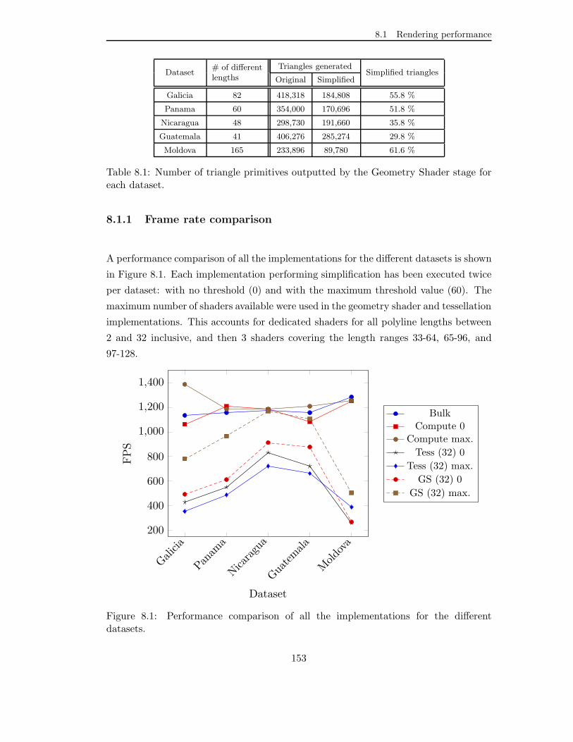
8.1 Rendering performance
Dataset# of differentlengths
Triangles generatedSimplified triangles
Original Simplified
Galicia 82 418,318 184,808 55.8 %
Panama 60 354,000 170,696 51.8 %
Nicaragua 48 298,730 191,660 35.8 %
Guatemala 41 406,276 285,274 29.8 %
Moldova 165 233,896 89,780 61.6 %
Table 8.1: Number of triangle primitives outputted by the Geometry Shader stage foreach dataset.
8.1.1 Frame rate comparison
A performance comparison of all the implementations for the different datasets is shown
in Figure 8.1. Each implementation performing simplification has been executed twice
per dataset: with no threshold (0) and with the maximum threshold value (60). The
maximum number of shaders available were used in the geometry shader and tessellation
implementations. This accounts for dedicated shaders for all polyline lengths between
2 and 32 inclusive, and then 3 shaders covering the length ranges 33-64, 65-96, and
97-128.
Galicia
Panama
Nicaragua
Guatemala
Moldova
200
400
600
800
1,000
1,200
1,400
Dataset
FPS
BulkCompute 0
Compute max.
Tess (32) 0
Tess (32) max.
GS (32) 0
GS (32) max.
Figure 8.1: Performance comparison of all the implementations for the differentdatasets.
153

Chapter 8. GPU Polyline Simplification Results
Results show that only the compute implementation gets a performance similar to
that of the bulk implementation, sometimes exceeding it. The geometry shader using
the maximum threshold value for simplification gets a similar performance for only two
of the five datasets. Tessellation with or without simplification, and geometry shader
without simplification attain approximately half the performance yielded by the bulk
and compute implementations.
Notice that the geometry shader and tessellation implementations perform notice-
ably better for the Nicaragua and Guatemala datasets, being the ones with a smaller
number of different polyline lengths. This suggests that the longer the polylines, the
worst is the performance, which can be attributed to the GPU having to perform longer
iterations, thus removing parallelism.
8.1.2 Optimum number of tessellation and geometry shaders
Geometry and tessellation implementations provide a high number of possible config-
urations based on the number of shaders of each type employed. In order to compare
the different configurations, the same kind of executions with minimum and maximum
threshold values presented in the previous section were carried.
Configuration
1st 2nd 3rd
2 - 32
2 (single lines) 2 (single lines)
3 - 323-5
6-32
33 - 64 (2 instances)
65 - 96 (3 instances)
97 - 128 (4 instances)
Table 8.2: Range of points covered by each geometry shader for each possible configu-ration.
Two applications were developed implementing the geometry shader simplification.
Their graphical user interfaces were presented in Section 7.4.3.2 and they differ in how
they organize the geometry shaders to perform the simplification. Table 8.2 – copied
from the aforesaid section – shows the 3 possible shader configurations for the first
application. These configurations respectively use 4, 5 and 6 geometry shaders to cover
different polyline length ranges. The second application allows the use of a geometry
154

8.2 Memory consumption
shader per polyline length between 3 and 32 inclusive. For single lines, and polyline
lengths greater than 32, the same shaders of the first applications are used.
The performance of the first application is shown in Figure 8.2a. It exhibits a
similar performance to that obtained in the global comparison. More interesting is the
experimentation for the second application, exhibited in Figure 8.2b. It shows that
initially, the performance increases with the number of geometry shaders employed.
Between 15 and 20, the performance curve stabilizes and, in most cases, after 25 it
degrades. Thus, the optimum number of geometry shaders is located between 15 and
25, depending on the dataset. Observation of the left side of the figure reflects that
using few shaders, with a single generic shader simplifying lines with up to 32 points
yields the worse performance. This is consistent with the fact that polyline lengths
distributions are biased towards the left for all the datasets – i.e. most of the polylines
have small lengths, as Figure 8.3a shows. On the other hand, the right side of the
figure exhibits how the performance slightly reduces when most of the possible shaders
are employed. The volume of polylines with more than 25 points is low compared
with those having less points, as exhibited in Figure 8.3b. As a result, the overhead
of introducing extra shaders which makes the rendering less batched, is not overcame
by the resulting simplification. Overall, the second application – adjusting more finely
to the polyline lengths – performs better than the first application using a few shaders
grouping ranges of polyline lengths.
The tessellation implementation was tested varying the number of tessellators used,
in a similar fashion of the second geometry shader implementation application. The
term tessellator refers to the combination of hull and domain shaders controlling the
tessellation stages of the pipeline. Each tessellator is in charge of processing an input
patch size, each size corresponding to the same polyline length. Results exhibited
in Figure 8.4 show that frame rate performance degrades with the number of hull
and domain shaders used. Geometry shaders are used to simplify all the polylines not
covered by tessellation shaders and thus, the results evidence than the geometry shader
is always superior.
155

Chapter 8. GPU Polyline Simplification Results
Galicia
Panama
Nicaragua
Guatemala
Moldova
200
400
600
800
Dataset
FPS
GS (4) 0
GS (5) 0
GS (6) 0
GS (4) max.
GS (5) max.
GS (6) max.
(a) Comparison of 3 predefined geometry shader groupings of the first application.
5 10 15 20 25 30
200
400
600
800
1,000
1,200
# geometry shaders
FPS
Galicia 0
Galicia max.Panama 0
Panama max.
Nicaragua 0
Nicaragua max.
Guatemala 0
Guatemala max.
Moldova 0
Moldova max.
(b) Possible shader configurations of the second application.
Figure 8.2: Performance of both applications implementing geometry shader simplifi-cation.
156

8.2 Memory consumption
0 5 10 15 20 25 30 35
0
1
2
3
·105
Frequency
#of
points Galicia
Panama
Nicaragua
Guatemala
Moldova
(a) Frequency distribution of polylines with lengths 3-32.
> 32 > 64 > 96 > 128
0
200
400
600
Frequency
#of
points
Galicia
Panama
Nicaragua
Guatemala
Moldova
(b) Cumulative distribution of polylines having more than 32points.
Figure 8.3: Polyline lengths distributions.
157

Chapter 8. GPU Polyline Simplification Results
0 5 10 15 20 25200
400
600
800
1,000
1,200
# tessellators
FPS
Galicia 0
Galicia max.Panama 0
Panama max.
Nicaragua 0Nicaragua max.
Guatemala 0
Guatemala max.
Moldova 0
Moldova max.
Figure 8.4: Frames per second rendered for each dataset with different tessellationconfigurations.
8.2 Memory consumption
There are essentially four types of resources consuming video memory in all the devel-
oped applications: state and shader objects, buffers, and a render target texture. A
bi-dimensional texture is used as render target, accounting for 1.88 MBs in the case of a
800x600 render area - i.e. four bytes per pixel corresponding to 32-bit red, green, blue,
and alpha components. State objects are used to configure the fixed-function parts of
the pipeline, saving a particular configuration so that it can be reused later in order to
minimize state changes since they impose performance penalties. These objects only
account for a few bytes of video memory.
The other two types of resources using significant amounts of video memory are
the buffers and shader objects. These can be quite demanding from the video memory
perspective, although their concrete requirements vary both with the implementation
used and the dataset processed, as presented in the following sections.
158

8.2 Memory consumption
8.2.1 Buffers
Buffer resources used by the different implementations are shown in Table 8.3. All the
implementations store the vertices using the same arrangement and thus, have identical
vertex buffers. The constant buffer used for rendering is also the same for all, storing
the transformation matrix, a width and a threshold value. All the implementations
performing simplification have a buffer storing the strips information, which is identical
for all of them. Although the bulk and compute implementations both use index buffers,
their contents differ. Finally, the compute implementation has two extra buffers used
for the execution of the compute pipeline: a constant buffer passing the threshold
value and the total number of strips, and a structured buffer where the results are
stored before being copied to the index buffer. Note that the structured and index
buffer contain the same information. It is duplicated because an structured buffer with
unordered access can not be bound as index buffer to the Input Assembler and thus,
its contents must be copied into a bindable buffer.
ImplementationConstant Buffers
Index Buffer1 Vertex Buffer Strips BufferStructuredBufferCompute Render
Bulk ✓ ✓ ✓
Compute ✓ ✓ ✓2 ✓ ✓ ✓2
Geometry ✓ ✓ ✓
Tessellation ✓ ✓ ✓
1 Unlike the other buffers, index buffers store different contents in Bulk and Compute.
2 Same content, copied from the structured buffer into the index buffer.
Table 8.3: Buffer resources used by the different implementations.
Some conclusions can be drawn by merely looking at the number of buffers involved
in each implementation. The compute implementation is the more demanding one,
since it requires the sum of all the buffers used by other implementations plus an extra
one; even more, the index buffer is actually larger than the one used by the bulk
implementation. The bulk differs from the geometry and tessellation implementations
in that it uses an index buffer instead of a strips buffer. This index buffer occupies
more space than the strips buffer, since 2 indices (pointing to the vertices forming the
line) must be stored for each individual line, whereas in the strips buffer 2 numbers
(an index to the starting vertex and the vertex count) are stored for each strip – and
there is no need to store any information regarding individual lines. Thus, both the
geometry and tessellation implementations must be the less memory intensive ones.
159

Chapter 8. GPU Polyline Simplification Results
DatasetIndex Buffer
Vertex Buffer Strips BufferStructuredBufferBulk Compute
Galicia 1.60 2.30 9.19 0.70 2.30
Panama 1.35 2.00 8.01 0.65 2.00
Nicaragua 1.14 1.87 7.48 0.73 1.87
Guatemala 1.55 2.64 10.55 1.09 2.64
Moldova 0.89 1.23 4.90 0.33 1.23
Table 8.4: Buffer sizes for each dataset (in megabytes).
Table 8.4 shows the memory occupied by the buffers for the different datasets. The
memory required to store the constant buffers has been omitted since it is negligible
as they account for 80 bytes, 16 bytes in the case of the constant buffer used in the
compute shader. As it has been stated, the structured buffer is used by the compute
shader to store its results and its contents are then copied to the index buffer; this is
the reason why the have they same size: they contain duplicated information.
ImplementationDataset
Galicia Panama Nicaragua Guatemala Moldova
Bulk 10.79 9.36 8.62 12.10 5.80
Compute 14.49 12.66 11.95 16.91 7.69
Geometry 9.89 8.66 8.21 11.64 5.24
Tessellation 9.89 8.66 8.21 11.64 5.24
Table 8.5: Video memory required to store buffers by the implementations for eachdataset (in megabytes).
The total amount of video memory required by each implementation to store buffer
resources for the different datasets is exhibited in Table 8.5. As expected, the compute
implementation is the most memory intensive. Geometry and tessellation implementa-
tions, which share the same vertex and strip buffers, are the less expensive ones.
8.2.2 Shaders
Shaders are compiled from the HLSL source code upon application initialization – or
they may be loaded from disk in the case of tessellation. The compiled bytecode is kept
in video memory through the proper Direct3D 11 COM objects. For small shaders these
objects may occupy few kilobytes. Geometry shaders performing polyline simplification
are compiled for all the polyline lengths between 3 and 32, inclusive. Each one of these
160

8.2 Memory consumption
shaders occupies 5 KBs. Geometry shaders simplifying up to 32 points and instanced 2,
3 and 4 times occupy 9, 12, and 16 KBs respectively. More complex shaders compiled
with unrolled loops may take up to hundreds of kilobytes. This is the case of the hull
shaders in the tessellation implementation, which implement for loops in the patch-
constant function. These loops iterate over the input patch and thus, their size grows
gradually from the 3 KBs used by the hull shader operating over a 3-point patch up to
the 160 KBs for 32-point patches. Having no loops, the domain shader grows just from
16 up to 29 KBs. The amount of video memory required to store the involved shader
objects for the different implementations is shown in Table 8.6. As it can be seen, the
geometry implementation requires over 183 KBs of video memory to store the shaders.
Even more, the tessellation includes those shaders plus the hull and domain shaders,
elevating the video memory requirements up to 1.69 MBs.
Loop unrolling improves speed performance at the expense of space and compilation
time by simply converting the loop into the succession of its iterations. This can only
be applied when the number of iterations is static – i.e. known at compile time. This
is the case of the hull shaders but does not apply to geometry shaders which use the
length stored in the strips buffer to iterate.
Implementation ComputeShaders
VertexShaders
GeometryShaders
DomainShaders
HullShaders
PixelShaders
Total
Bulk- 1.1 1.4 - - 1 3.5
(1) (1) (2) (3)
Compute3.9 1.1 1.4 - - 1 7.4
(2) (1) (1) (2) (4)
Geometry- 0.6 181.4 - - 1 183
(1) (35) (2) (38)
Tessellation- 1.8 182.8 1,497.6 43.4 1 1,726.6
(2) (35) (30) (30) (2) (99)
Table 8.6: Video memory required to store shaders for each implementation (in kilo-bytes, number of shaders in parenthesis).
All the implementations use two pixel shaders: one for normal solid fill rendering
and other for wireframe rendering. They are switched along with the Rasterizer stage
state when the user clicks the corresponding toggle button in the GUI.
The geometry shader implementation requires a total of 35 geometry shaders: one
to generate quads for single lines, 30 to cover the polyline lengths between 3 and 32
161
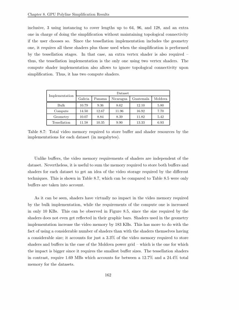
Chapter 8. GPU Polyline Simplification Results
inclusive, 3 using instancing to cover lengths up to 64, 96, and 128, and an extra
one in charge of doing the simplification without maintaining topological connectivity
if the user chooses so. Since the tessellation implementation includes the geometry
one, it requires all these shaders plus those used when the simplification is performed
by the tessellation stages. In that case, an extra vertex shader is also required –
thus, the tessellation implementation is the only one using two vertex shaders. The
compute shader implementation also allows to ignore topological connectivity upon
simplification. Thus, it has two compute shaders.
ImplementationDataset
Galicia Panama Nicaragua Guatemala Moldova
Bulk 10.79 9.36 8.62 12.10 5.80
Compute 14.50 12.67 11.96 16.92 7.70
Geometry 10.07 8.84 8.39 11.82 5.42
Tessellation 11.58 10.35 9.90 13.33 6.93
Table 8.7: Total video memory required to store buffer and shader resources by theimplementations for each dataset (in megabytes).
Unlike buffers, the video memory requirements of shaders are independent of the
dataset. Nevertheless, it is useful to sum the memory required to store both buffers and
shaders for each dataset to get an idea of the video storage required by the different
techniques. This is shown in Table 8.7, which can be compared to Table 8.5 were only
buffers are taken into account.
As it can be seen, shaders have virtually no impact in the video memory required
by the bulk implementation, while the requirements of the compute one is increased
in only 10 KBs. This can be observed in Figure 8.5, since the size required by the
shaders does not even get reflected in their graphic bars. Shaders used in the geometry
implementation increase the video memory by 183 KBs. This has more to do with the
fact of using a considerable number of shaders than with the shaders themselves having
a considerable size; it accounts for just a 3.3% of the video memory required to store
shaders and buffers in the case of the Moldova power grid – which is the one for which
the impact is bigger since it requires the smallest buffer sizes. The tessellation shaders
in contrast, require 1.69 MBs which accounts for between a 12.7% and a 24.4% total
memory for the datasets.
162

8.2 Memory consumption
Bulk
Compute
Geometry
Tessellation
10
11
12
13
14
Video
mem
ory
(MBs)
Galicia
BuffersShaders
(a)
Bulk
Compute
Geometry
Tessellation
9
10
11
12
13
Video
mem
ory
(MBs)
Panama
BuffersShaders
(b)
Bulk
Compute
Geometry
Tessellation
8
9
10
11
12
Video
mem
ory
(MBs)
Nicaragua
BuffersShaders
(c)
Bulk
Compute
Geometry
Tessellation
12
14
16
Video
mem
ory
(MBs)
Guatemala
BuffersShaders
(d)
Bulk
Compute
Geometry
Tessellation
5
5.5
6
6.5
7
7.5
Video
mem
ory
(MBs)
Moldova
BuffersShaders
(e)
Figure 8.5: Video memory required to store buffer and shader resources by the imple-mentations for each dataset.
163
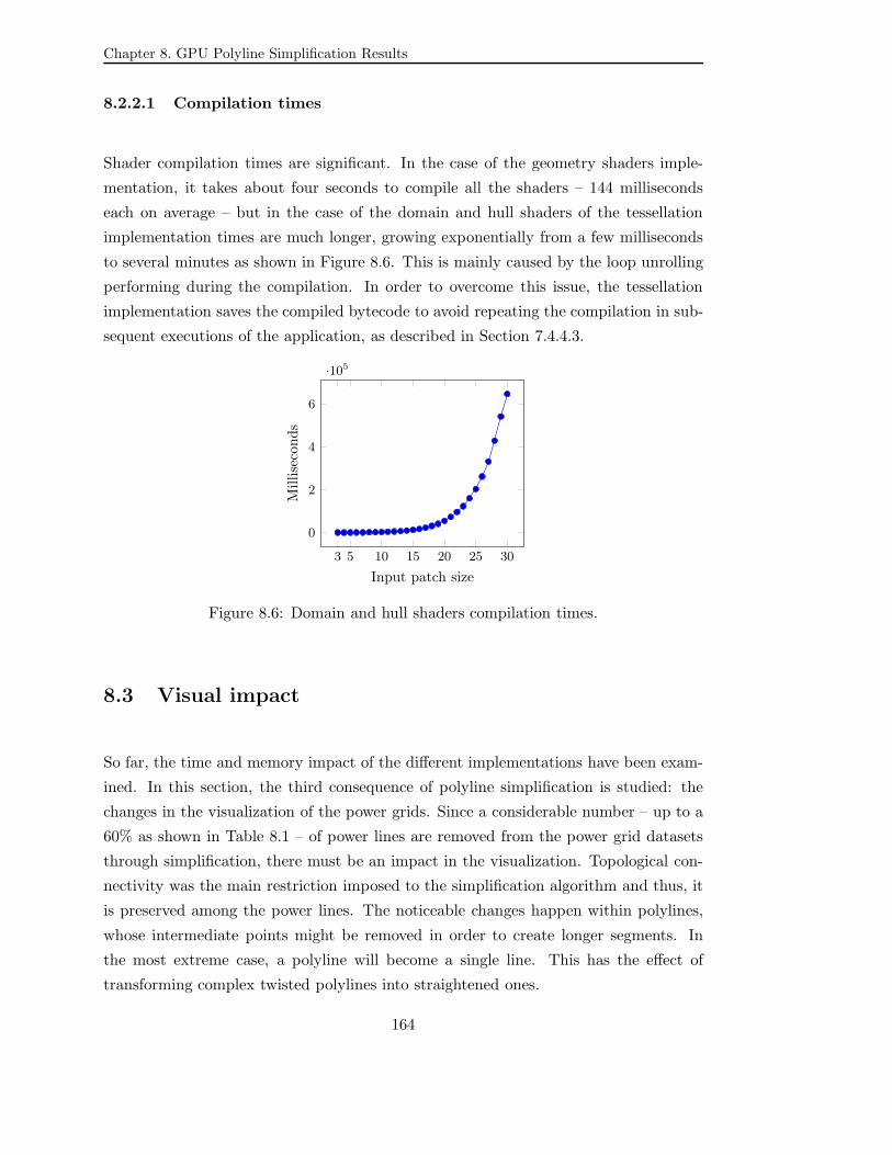
Chapter 8. GPU Polyline Simplification Results
8.2.2.1 Compilation times
Shader compilation times are significant. In the case of the geometry shaders imple-
mentation, it takes about four seconds to compile all the shaders – 144 milliseconds
each on average – but in the case of the domain and hull shaders of the tessellation
implementation times are much longer, growing exponentially from a few milliseconds
to several minutes as shown in Figure 8.6. This is mainly caused by the loop unrolling
performing during the compilation. In order to overcome this issue, the tessellation
implementation saves the compiled bytecode to avoid repeating the compilation in sub-
sequent executions of the application, as described in Section 7.4.4.3.
3 5 10 15 20 25 30
0
2
4
6
·105
Input patch size
Milliseconds
Figure 8.6: Domain and hull shaders compilation times.
8.3 Visual impact
So far, the time and memory impact of the different implementations have been exam-
ined. In this section, the third consequence of polyline simplification is studied: the
changes in the visualization of the power grids. Since a considerable number – up to a
60% as shown in Table 8.1 – of power lines are removed from the power grid datasets
through simplification, there must be an impact in the visualization. Topological con-
nectivity was the main restriction imposed to the simplification algorithm and thus, it
is preserved among the power lines. The noticeable changes happen within polylines,
whose intermediate points might be removed in order to create longer segments. In
the most extreme case, a polyline will become a single line. This has the effect of
transforming complex twisted polylines into straightened ones.
164

8.3 Visual impact
Although topological connectivity among polylines is preserved, the geographic ac-
curacy is lost within polylines. Once inner points of the polyline are removed, the
polyline no longer exactly represents the layout of the power grid over the terrain in
the real world. However, the begin and end points of the polyline are always left un-
touched and thus, their coordiantes are accurate. This is specially relevant as in many
cases, these points correspond to substations in the power grids.
(a) No simplification (threshold 0). (b) Threshold 0.8.
(c) Threshold 1.6. (d) Threshold 4.8.
Figure 8.7: Polyline simplification for different threshold values.
Figure 8.7 illustrates how the shape of a polyline changes as the threshold value is
increased. Close-up captures of wire-frame rendering are displayed, so that individual
segments formed by quads can be easily discerned. Figure 8.7a shows the original
165

Chapter 8. GPU Polyline Simplification Results
polyline with no simplification being applied. As the threshold value is increased,
more and more segments are gradually removed, and new longer segments are formed.
Eventually, the whole polyline becomes a single straight line.
This example is an extreme case since it shows a close-up of a polyline when using
threshold values for a whole power grid dataset. The threshold value must be adjusted
according to the scale being used. This way, most simplification results will not be no-
ticeable in the visualization. Since power grids cover kilometers, usually the threshold
is assigned based on a meters per pixel (mpx) value that represents how many meters
each pixel accounts for in the current scale. As the user zooms in or out the visual-
ization, the scale and thus the mpx change. As a result, the threshold value must be
changed accordingly. The great benefit of performing the simplification on the GPU is
that this nearly continuous adaptation is dynamic.
8.4 Conclusions
The number of primitives involved for the different datasets – less than half a million
triangles in the largest case – can be easily handled by modern graphics cards such as
the NVIDIA GeForce GTX 560 Ti used in these tests. Since the datasets do not push
the GPU to full utilization, there is no performance gain in reducing the number of
primitives through simplification. More load must be added to the GPU from other
applications running at the same time in order to take advance of the reduced number
of primitives produced by the simplification. This may also be the case when using
more advanced power grid visualizations – e.g., using varying widths as a function of
the power load carried by the line, flow animations, integration of satellite imaging,
etc.
More significantly, the simplification algorithm implementations reduce the paral-
lelism attained by the GPU when performed in the graphics pipeline. At some point
or another, the algorithm iterates over a polyline, thus stalling the pipeline. When
no simplification is performed, all the individual lines can flow independently through
the pipeline, regardless of the adjacent lines when they are part of a polyline. This is
the most favorable parallelism scenario. When simplification is introduced, the parallel
work units are polylines instead of lines, thus vastly reducing the granularity. Moreover,
166

8.4 Conclusions
while the line strip topology is analogous to a polyline and thus, the implementations
could perform the proper data adaptation, the closer primitive to polylines are patches
which are limited to a maximum of 32 points. This fact requires shaders to perform
actions that are natural enemies of parallelism: access memory buffers to retrieve the
vertices forming a polyline and then iterate over them. The shader stage at which this
happens, the memory access, and the looping involved, depend on the exact implemen-
tation and the concrete values of its parameters.
The implementation using the compute pipeline does not incur in this pitfall. Being
performed only when required – i.e. when the threshold value is changed – it can be seen
as a kind of off-line simplification. However, it happens entirely on the GPU and the
results stay in video memory, with no information needing to be transferred from the
GPU back to the CPU. Upon a threshold value change, the next render is preceded by
a compute shader execution performing the simplification, followed by a video memory
copy that transfers the results of the compute shader to an index buffer that can be
consumed by the subsequent renders. This introduces a small overhead for those cases,
which is comparable to the performance loss due to the reduction of parallelism from
the other implementations performing the simplification in every render on the graphics
pipeline. However, since the number of threshold value changes are marginal compared
to the number of renders performed (hundreds per second), the performance impact is
negligible.
Regarding video memory consumption, using strips instead of an index buffer at-
tains some reduction in the buffers size. The compute implementation, has elevated
requirements to store buffers since it requires the index buffer to be duplicated, taking
almost 17 MBs of video memory for one of the given datasets. The memory required to
store shader objects are negligible except for the tessellation implementation for which
they require 1.69 MBs. Furthermore, the tessellation implementation suffers another
penalty compared to the other implementations: domain and hull shaders compilation
takes up to several minutes, whereas the rest of the shaders only require a few millisec-
onds. This is partially overcome by storing the byte-code of the compiled shaders on
disk.
Overall, although the compute implementation has increased memory requirements,
it is the best option when simplification needs to be performed, given the poor perfor-
mance offered by the geometry shader and tessellation implementations due to the loss
167

Chapter 8. GPU Polyline Simplification Results
of parallelism they introduce into the rendering of every frame.
Finally, polyline simplification has an impact in power grid visualization. The more
aggressive the simplification, the more noticeable this impact is. Given the algorithm
employed in the different implementations, the result for those polyline composed of
small segments is a straightened polyline composed of less segments; the most extreme
case is a polyline becoming a single line. This is important not only because the change
might be evident to the user, but also because the positions of the polyline points
normally correspond to geographic coordinates. As a result, the visualization is not
completely accurate to the power grid layout over the terrain. However, by adapting the
performed simplification based on the level of detail required in each precise moment,
the visual impact can be minimized.
168

CHAPTER9Conclusions
9.1 Work summary
Chronologically, the work started by improving – i.e. decreasing – the rendering times
of power grid networks visualization by replacing an existing GDI+ renderer by a
new implementation using Managed DirectX – which is a .NET wrapper library for
DirectX version 9.0c. This resulted in a tenfold performance increase in the render-
ing times. However, due to application requirements regarding the hardware and the
operative system, the renderer had to be off-screen, which imposes a considerable per-
formance penalty. In order to overcome it, the data involved in the visualization was
pre-processed using spatial databases, reducing its volume by generating different scales.
The result led the visualization to be rendered in just a 15% of the time required be-
fore, enabling real-time rendering even while using an off-screen renderer. This was an
important milestone, as real-time rendering allows for animations. Thus, new visual-
izations such as animated power flows could be supported.
As some of the initial constraints on the available hardware and software were
lifted, the renderer was re-implemented using DirectX 10, this time directly through its
C++ API. New features present in DirectX 10 such as geometry shaders, allowed to
quickly improve the performance. Furthermore, such new capabilities opened the door
to moving the data volume reduction carried by spatial databases to the GPU, and even
perform it dynamically for every render; more so upon the release of DirectX 11 and its
tessellation stages. This was the main focus of this work: to study how to take advance
of the different features and programming capabilities of modern versions of DirectX to
reduce the data volume involved in power grid visualization – more specifically, power
branches simplification to speed up the visualization of power grid networks.
The following list summarizes the solutions presented in this thesis:
169

Chapter 9. Conclusions
Multi-scale architecture using spatial databases: the original data is pre-processed
generating different versions optimized for certain visualization scales. The pre-
processing includes not only polyline simplification, but also polyline merging and
filtering of imperceptible data.
Quad generation using vertex shaders: two adjacent triangles forming a quad are
created for each line of a given branch. Four predefined vertices are properly
positioned by the vertex shader by processing the corresponding two points and
either one or two width parameters.
Quad generation using geometry shaders: quads are generated dynamically from
two points and either one or two widths. No predefined vertices are required since
they are created by the geometry shader.
Polyline simplification using compute shaders: each power branch – formed by
several segments and stored in video memory – is processed every time a parame-
ter setting the minimum segment length changes. A general purpose computation
pipeline is employed instead of the typical graphical pipeline.
Polyline simplification using geometry shaders: the Geometry Shader stage of the
graphical pipeline is programmed to alter power branches stored in video memory
based on a threshold parameter. This processing is performed with every render.
Polyline simplification using tessellation: the Tessellation stages of the graphical
pipeline are configured to alter power branches stored in video memory based on
a threshold parameter. This processing is performed with every render.
Mixed polyline simplification using geometry shaders and tessellation: both poly-
line simplification implementations using tessellation and geometry shaders are
combined, each covering a range of power branch lengths. Just like in the indi-
vidual implementations, the processing is performed with every render.
170

9.2 Future work
9.2 Future work
9.2.1 Coordinate system translation on the GPU
During either bi-dimensional or three-dimensional rendering, all the primitives – no
matter whenever points, lines, or triangles – must be processed in several ways. They
might be transformed – e.g. translated, rotated, or scaled –, converted from one co-
ordinate system to another, projected from three-dimensional to bi-dimensional space,
etc.
This processing falls into what in three-dimensional pipelines is commonly known
as world-view-projection matrix multiplication, and on modern graphics hardware it is
usually performed by the vertex shader, as explained in Section 6.2.2. In its simplest
version, the vertex shader takes a vertex position defined in a local space, translates it
to a world – or scene – space, applies some kind of perspective – thus translating it to
view space –, and finally projects it to a bi-dimensional space. However, as it has been
seen all along this work, on modern graphics hardware – or even on emulating software
–, the vertex shader is a custom program which can do that and much more.
As seen in Chapter 2, power grids are composed by power lines which have a position
on the Earth’s surface. This position, can be expressed using many coordinate systems
in which coordinates take different values and, in some cases, even different number of
components. When integrating different sources of information, it is not uncommon to
find coordinates expressed in different systems.
One example is the visualization of a power grid network on top of satellite imaging.
The datasets used in this work contained coordinates defined in the Universal Trans-
verse Mercator coordinate system, which is a planar geographic coordinate system.
Google Maps images are defined using the WGS84 ellipsoid and then projected using a
Mercator projection. In order to properly render the power grid network on top of the
corresponding satellite images, there are two options: either transform the images or
translate the power grid network coordinates to the same system the images use, and
then perform the rendering. The former modifies the images, introducing distortions
and visual artifacts as a result. Thus, coordinate translation is more desirable.
171

Chapter 9. Conclusions
Since the vertex shader will transform the position of each vertex, the coordinate
translation can be added to that processing. Indeed, some parts of the operations
required to translate a coordinate from one system to another, are likely to be integrable
with the world-view-projection matrix multiplication. Note that depending on how the
graphics pipeline is configured, the job might be subsumed by some other stage, such
as a geometry shader.
Although not included in this thesis, as one of the several side projects that took
place during the development of the presented work, the unitary-width power grid net-
work visualization was successfully rendered on top of Google Maps imaging. However,
the proper coordinate translation was not performed by the vertex shader as described
here and it could constitute an interesting experimentation point.
9.2.2 Adoption of other visualization patterns
Commonly in engineering, time constraints forbid being as detailed in the design phase
as desirable. As this work is the result of the assignments of a power utility company,
some compromises had to be made in terms of design in order to comply with budget
and time requirements. One such example is the adoption of visualization patterns
which was kept to the ones providing more immediate results while sacrificing some
that would provide more long-term gains. The visualization patterns employed in this
work are outlined in Appendix I along with others that would be perfectly eligible for
their adoption, were the required time to become available.
9.2.3 Introduction of more complex visualizations
This work was concerned with improving the performance of any kind of visualization
and not with which particular visualization might be more suitable for a given context.
Therefore, the dominant visualization used in this work consists on representing the
power grid network using either unitary or fixed-width lines to represent each segment
of the branches.
However, as outlined in Section 2.2, there are many possible power grids visualiza-
tion techniques. For instance, power loads can be taken into account to give varying
172

9.2 Future work
widths to the rendered power lines. Also, colors could be used to remark problematic
areas – for instance, reaching maximum capabilities. Furthermore, given the perfor-
mance gains presented in this work, animations showing the current flow could be
introduced in the developed CAD application.
9.2.4 Revision of the polyline simplification algorithm
The multi-scale architecture using spatial databases presented in Chapter 3 employs
the Ramer-Douglas-Pecker line simplification algorithm [26]. This algorithm recursively
discards segments having an orthogonal distance to the line connecting the beginning
and end point shorter than a given threshold. However, dynamic polyline simplification
on the GPU implementations presented in Chapter 7 employs a simpler algorithm dis-
carding segments having lengths smaller than the threshold, as exhibited in Algorithm
13.
The rationale behind this difference lies in the fact that the focus was on explor-
ing the graphics hardware capabilities and not in the simplification algorithm itself.
An attempt could be made to implement the Ramer-Douglas-Pecker algorithm in the
shaders although complications might arise – for instance, due to limited recursion sup-
port. Furthermore, another simplification algorithm could be adopted, not only by the
GPU implementations but also by the multi-scale architecture approach.
9.2.5 Migration to DirectX 12
This work has presented the attempts to exploit the features offered by DirectX from
version 9.0c up to version 11. Although neither a new whole pipeline, nor new pipeline
stages were introduced with DirectX 12, a number of improvements focusing on effi-
ciency were introduced.
These changes are the consequence of the relatively high degree of standardization of
the graphics hardware in the last few years; earlier versions of DirectX had to cope with
a broader spectrum of hardware architectures and capabilities. A thick intermediate
layer was created between the hardware and the software in order to abstract hardware
variability. Nowadays, most graphics hardware is either architecturally similar, or able
173

Chapter 9. Conclusions
to offer the same capabilities – at least up to a great extent and although performance
may vary significantly. As a consequence, the middleware layer can now be thinner,
allowing the API to be closer to the hardware and thus, enabling more optimized code
to be developed.
The management of pipeline configurations, resources, and commands has been
redesigned aiming to provide more flexibility:
Pipeline state management
In prior versions, each pipeline stage is configured individually creating the need
to translate – from driver to GPU commands – and merge state changes each
time one stage is reconfigured. Although the pipeline state management had been
greatly improved with each DirectX version, there was still room to improvement
since during a single rendering, many individual stage changes may occur, creating
a small overhead each time that would add up to an important performance hit.
Pipeline state objects store the configuration of the whole pipeline at a certain
point, thus allowing to configure all the stages at once. This saves the overhead
of translating and merging each individual stage state change.
Resource management
More control is given to the developer over when and how certain resources must
be bound to the pipeline. The developer has an insight into the resource usage
that the system can not reach. Thus, by enabling him to explicitly specify it, the
resource management can be improved.
Furthermore, the view and slot resource binding system has been replaced through
a whole new set of entities – namely descriptors, heaps, and tables. This allows
to better organize resources into different tables – for instance, according to their
update frequency.
Memory buffers flexibility was also enhanced through dynamic heaps, which allow
to allocate a chunk of memory and use parts of it for different purposes. For
instance, in DirectX 12 is possible to sub-allocate a part of a buffer for usage as
vertex buffer while using another part of the very same buffer as an index buffer.
This flexibility results in a better data locality which in turn benefits parallelism.
Command management
174

9.3 Publications
Just like resources, GPU commands can also be grouped: command sequences
can be recorded to a bundle that can later be reused.
Multi-threading was also improved. Previously, there was an immediate context
which acted as a main thread and then deferred contexts taking much less GPU
time compared to the immediate context. In a DirectX 12 application, each
thread may create its own command list in parallel and then submit it to a
common command queue. Each list will be executed sequentially. Bundles can
be reused, even by different command lists.
Given that the pipeline stages remained unchanged, migrating the existing imple-
mentations to DirectX 12 should be a reasonable effort. Even if not special emphasis
were put on taking advance of these more finely-grained and lower level features, some
performance should be gained by upgrading to the new version of the library.
9.3 Publications
Part of the work presented in this thesis has been presented as the following papers in
several conferences, having been published in their corresponding proceedings:
Electrical Distribution Grid Visualization using Programmable GPUs
[51]
Abstract: Modern graphic cards enable applications to process big amounts of
graphical data faster than CPUs, allowing high-volume parallelizable data to be
visualized in real-time. In this paper, we present an approach to enable a power
grid planning Computer-Aided-Design application to use this processing power
to visualize electrical distribution grids in the fastest possible way. As a result,
the aforesaid application became able to offer highly responsive interactions with
them.
A revised version of this paper has also been published in a journal [52].
Digital Cartographic Generalization in Spatial Databases: application
issues in Power Grids CAD tools [54]
175

Chapter 9. Conclusions
Abstract: This work presents the results of applying several digital cartographic
generalization techniques to improve the performance of an Electrical Power Grids
Computer-Aided-Design application. The performance increase is attained by ad-
justing the level of detail of the grid topology being visualized in the CAD ap-
plication. This adjustment takes place at the database level using a multi-scale
architecture and the available spatial extensions of Geographic Information Sys-
tems databases. The data volume is minimized to fit the exact requirements of
the scale being used in the visualization so that no processing time is wasted on
representing irrelevant elements. Results show that up to a 90% of the data can
be skipped and thus, a 84% of the time required to render the visualization can be
saved on average.
Improving Electrical Power Grid Visualization using Geometry Shaders
[53]
Abstract: The graphics engine of a Power Grids Computer-Aided-Design appli-
cation was upgraded from Direct3D 9 to Direct3D 11, allowing the use of new
features such as the Geometry Shader and Stream Output stages of the graph-
ics pipeline to improve the performance of power grids visualization. Geometry
shaders have been used to generate two triangles forming a quadrangle (quad) for
each power line, giving it a width as a function of the power load carried by the
line. Two implementations were tested: one generating the quads in every draw
and other which only generates them once, saving the results to video memory
for subsequent draws. Both have been compared with the previous implementation
which used vertex shaders. The possibility of using the mentioned pipeline stages
to generate levels of detail for the power grids was also studied.
Furthermore, a brief version of this thesis is currently under review for publishing
in a journal.
176

APPENDIX IPatterns For Information Visualization
Many common software design patterns have been used both in this work and in the
developed power grid CAD application that employs the presented techniques. This
appendix outlines a subset of software design patterns for information visualization,
following the classification introduced in [30]. The original definition of each pattern is
quoted here before describing its usage in this work.
Figure I.1, extracted from [30], shows the different patterns for information visual-
ization along with other non-visualization patterns employed by them, as well as their
relationships.
Figure I.1: Software design patterns and their interactions.
The most relevant patterns for this work have been the reference model, renderer,
camera, proxy tuple, operator, and dynamic query binding – highlighted in Figure I.1.
177

Appendix I. Patterns For Information Visualization
The scheduler and cascaded tabled patterns have not been employed, but they could
be of use. A brief description of each one of them follows; each section begins with a
quote of the pattern description in the original work [30].
I.1 Reference model
Separate data and visual models to enable multiple visualizations of a data
source, separate visual models from displays to enable multiple views of a
visualization, and use modular controllers to handle user input in a flexible
and reusable fashion.
Arguably the most implemented version of this pattern is theModel-View-Controller
(MVC) in which a controller orchestrates the manipulation of a set of data represented
through a model and exposed to the user through a view. Each one of these three con-
cerns are isolated as much as possible, favoring cohesion and minimizing coupling among
them.
Although this thesis has focused on the actual researched techniques and not on the
CAD application taking advance of them, this pattern is specially relevant in the context
of the developed CAD application. It enables an easy transition from one rendering
engine to another without having to concern the rest of the CAD application with which
one is employed. More specifically the application uses a variation of the MVC pattern
which is commonly used in the Windows desktop applications development. Its name
is Model-View-ViewModel (MVVM) and it replaces the concept of the Controller
with that of the ViewModel which is an Adapter that eases the consumption of data
by the Windows graphical user interface APIs and their data bindings.
I.2 Renderer
Separate visual components from their rendering methods, allowing dynamic
determination of visual appearances.
Different concerns of the application should be as isolated from one another as much
178

I.2 Renderer
as possible. Thus, the renderer should be a module controlled through an interface,
whose details are hidden to other areas of the application. This way, once the data has
been abstracted into a reference model that can be consumed by visualizations, different
renderers in charge of generating that visualization can be employed and seamlessly
swapped.
This pattern has been employed in the developed power grid CAD application
to evolve the implementation of the visualization with new hardware and software
capabilities, as they became available, without affecting other areas.
Two different types of renderers have been used, which we label as online and off-
line renderers. The distinction lies on whenever they are constantly rendering (online)
or they only render a visualization upon request (off-line).
Online renderer: a loop constantly repeats the render process, performing any
required data or rendering parameters updates. This loop is usually referred to as
the main loop and may also be in charge of processing input – such as keyboard –
events. This kind of renderer is suited for animations or when navigation through
the visualization is required.
Off-line renderer: the render process is performed on demand instead of con-
stantly. This is usually employed on scenarios where the rendering takes a signif-
icant time or when neither animations nor navigation is required.
In both cases, the renderer can be outputting the visualization to a visible area of
the screen or to an off-screen area. The former is the most common case4, being faster
but requiring a good integration with the graphical user interface layer. Rendering to
an off-screen may be required when there are graphics integration problems – as can be
the case with Windows Presentation Foundation (WPF) applications and DirectX in
Microsoft Windows XP and Vista, further analyzed in Appendix II. The main drawback
of this approach is that there is a costly extra step: the off-screen area must be copied
onto the proper on-screen area.
Usually online renderers output directly to a on-screen area and the off-line renders
4Actually, in order to avoid visual artifacts such as flickering, two or more video buffers are normallyused, forming what is known as a swap chain. Although this has been simplified in this discussion, oneof the buffers of the chain still corresponds to the area visualized in the screen, as stated.
179

Appendix I. Patterns For Information Visualization
employ off-screen areas. Section 3.4 presented an application using an off-line off-
screen renderer since it was required to be integrated into an WPF application running
in Windows XP. On the other hand, the implementations introduced in Chapter 7 use
on-line on-screen renderers since they are ad-hoc Win32 applications using DXUT –
instead of WPF applications – created for experimentation purposes.
I.3 Camera
Provide a transformable camera view onto a visualization, supporting mul-
tiple views and spatial navigation of data displays.
Allows navigation through the visualization of the power grid to zoom, pan, etc.
This is implemented through the vector-matrix multiplication as explained in Section
5.2. The appropriate parameters of the matrix are set as a result of the interaction
from the user – through mouse or keyboard actions over the visualization.
I.4 Proxy tuple
Use an object-relational mapping for accessing table and network data sets,
improving usability and data interoperability.
The memory buffers described in this work constitute a very similar concept: the
data storage is re-shaped in order to accommodate it for its consumption by the graphics
hardware.
I.5 Operator
Decompose visual data processing into a series of composable operators, en-
abling flexible and reconfigurable visual mappings.
Parameterizable properties such as the width and the color of power lines can be
set through operators bound to user interface controls. The role of these operators
180
I.9 Other patterns
corresponds to the mapping of the values from the user interface to the corresponding
properties.
I.6 Dynamic query binding
Allow data selection and filtering criteria to be specified dynamically using
direct manipulation interface components.
User interface components such as sliders and toggle buttons have been employed
by the different implementations to allow the user to control different parameters of the
visualization. One central example is the use of a slider to set the threshold parameter
required by the simplification process, as described in Section 7.3.1.
I.7 Scheduler
Provide schedulable activities for implementing time-sensitive, potentially
recurring operations.
This pattern is useful to manage animations smoothly – for instance, animated
representations of the power transported along the power grid. Also in the off-line
renderer implementation it takes care of outdated rendering requests.
I.8 Cascaded table
Allow relational data tables to inherit data from parent tables, efficiently
supporting derived tables.
This pattern can be useful to provide default values such as those of the width and
color properties of the polylines present in this work.
181

Appendix I. Patterns For Information Visualization
I.9 Other patterns
Other patterns not considered for this work are:
Data column
Organize relational data into typed data columns, providing flexible data
representations and extensible data schemas.
Relational graph
Use relational data tables to represent network structures, facilitating
data reuse and efficient data processing.
Expression
Provide an expression language for data processing tasks such as spec-
ifying queries and computing derived values.
Production rule
Use a chain of if-then-else rules to dynamically determine visual prop-
erties using rule-based assignment or delegation.
182

APPENDIX IIDirectX Integration Into Windowed Applications
II.1 Introduction
Windows Vista was released in 2007 to replace Windows XP, which had a great re-
ception by the consumers since its release in 2001. Vista supposed a significant break-
through in the graphics field for the Windows series: the Windows graphics architec-
ture was redesigned in order to bring hardware acceleration as a first-class citizen to
the desktop.
This was accomplished by replacing GDI (Graphics Device Interface) in favor of
Direct3D as the main rendering technology for the desktop and the windows therein
contained, as exhibited in Figure II.1. A new graphics driver layer was engineered -
the Windows Display Driver Model (WDDM) - along with DXGI (DirectX Graphics
Infrastructure, a mapping layer between it and graphics API such as Direct3D). On top
of these, the Media Integration Library (MIL) was implemented to provide both a new
window manager called Desktop Window Manager (DWM) and Windows Presentation
Foundation (WPF), a managed graphical user interface framework taking full advance
of all the new Direct3D hardware acceleration capabilities for user interfaces [56].
Early parts of the work presented in this thesis were developed for Windows XP
while latter parts targeted Windows Vista. Thus, this work has been greatly affected
by the features available in each of those Windows versions. This appendix provides
insight into the graphics architecture redesign introduced by Windows Vista, how a
rendering engine using Direct3D can be fitted into windowed applications, and how the
targeted version of Windows affected this work.
183
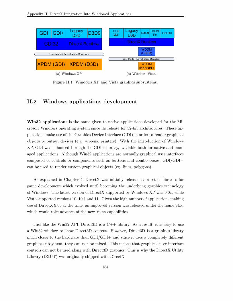
Appendix II. DirectX Integration Into Windowed Applications
(a) Windows XP. (b) Windows Vista.
Figure II.1: Windows XP and Vista graphics subsystems.
II.2 Windows applications development
Win32 applications is the name given to native applications developed for the Mi-
crosoft Windows operating system since its release for 32-bit architectures. These ap-
plications make use of the Graphics Device Interface (GDI) in order to render graphical
objects to output devices (e.g. screens, printers). With the introduction of Windows
XP, GDI was enhanced through the GDI+ library, available both for native and man-
aged applications. Although Win32 applications are normally graphical user interfaces
composed of controls or components such as buttons and combo boxes, GDI/GDI+
can be used to render custom graphical objects (eg. lines, polygons).
As explained in Chapter 4, DirectX was initially released as a set of libraries for
game development which evolved until becoming the underlying graphics technology
of Windows. The latest version of DirectX supported by Windows XP was 9.0c, while
Vista supported versions 10, 10.1 and 11. Given the high number of applications making
use of DirectX 9.0c at the time, an improved version was released under the name 9Ex,
which would take advance of the new Vista capabilities.
Just like the Win32 API, Direct3D is a C++ library. As a result, it is easy to use
a Win32 window to show Direct3D content. However, Direct3D is a graphics library
much closer to the hardware than GDI/GDI+ and since it uses a completely different
graphics subsystem, they can not be mixed. This means that graphical user interface
controls can not be used along with Direct3D graphics. This is why the DirectX Utility
Library (DXUT) was originally shipped with DirectX.
184

II.2 Windows applications development
A consequence of the different architectures underlying GDI and DirectX is how
the graphic commands are sent to the hardware for rendering. While GDI sends them
immediately as soon as they are issued, DirectX works in what is called retained mode:
commands can be organized in lists, allowing for optimizations not possible in the
immediate approach of GDI.
Native windows applications are developed in C++ through the Win32 API or
the Microsoft Foundation Class (MFC) library – which provides a higher level API.
However, both C++ and the Win32 API are quite complex to deal with and as a
result, Microsoft launched the .NET Framework along with several languages targeting
it - most notably C# - in order to ease Windows development. Applications developed
for the .NET Framework are dubbed as managed applications since resources such
as memory are automatically managed by an execution runtime called the Common
Language Runtime (CLR).
A managed version of DirectX 9.0c targeting .NET Frameworks 1.1 and 2.0 was
launched: Managed DirectX (MDX). However, just like the native version of Direct3D,
it does not mix well with graphical user interfaces. Furthermore, it was discontinued
in favor of the XNA Framework.
Two main managed graphical user interface libraries are available in Windows Vista:
Windows Forms: available since the first version of the .NET Framework, it
provides a high-level library based on the Win32 API - in the same way the MFC
library provides a Win32 API wrapper library for C++. Internally, Windows
Forms uses GDI+.
Windows Presentation Framework: introduced with .NET Framework 3.0, it
builds on the new graphics architecture developed for Windows Vista, thus ren-
dering the user interface through Direct3D instead of GDI/GDI+. Its implemen-
tation goes hand by hand with that of the Desktop Window Manager (DWM),
being part of the Media Integration Library.
Summing up, Win32 applications can be developed in C++ directly through its
API or through the MFC library; or using managed code through either Windows
Forms or WPF. Graphics can be rendered in Win32 applications in C++ using GDI,
185

Appendix II. DirectX Integration Into Windowed Applications
GDI+, or any version of Direct3D; or from managed code using GDI+, MDX, or using
higher-level graphics abstractions provided by WPF5.
The next sections present the architectural changes from Windows Vista compared
to its predecessor Windows XP and their effects on Windows applications development.
II.3 Windows Vista graphics architecture
As stated in the introduction of this appendix, Vista introduced a major redesign of
the graphics architecture of the Windows operative system, replacing the old GDI
by DirectX. Two key components of the new architecture are presented here: the
Windows Display Driver Model and the Desktop Window Manager that exploits its
new capabilities.
II.3.1 The Windows Display Driver Model
TheWindows Display Driver Model (WDDM) shipped with Windows Vista, introduced
three key new features [58]:
1. Video memory virtualization
It allows many applications to be running simultaneously without having to recre-
ate graphics resources. Previously, the developer would work directly against ei-
ther system or video memory, creating resources in both memories in some cases,
and moving data between them in others. A typical burden was the manage-
ment of lost surfaces that happened whenever a surface got kicked out from video
memory – normally because the space it occupied was required.
Video memory virtualization not only gets rid of this burden, it also improves the
performance by optimizing memory management. Resources such as surfaces, are
paged into and out of true video memory as required.
2. GPU interruptibility
5Please note that there are other technologies such as Direct2D or OpenGL, but have been omittedhere for simplicity.
186

II.3 Windows Vista graphics architecture
WDDM introduced GPU commands scheduling in order to avoid applications
preventing others from getting their share of the GPU.
3. Surface sharing
It enables redirection and composition which are key to the interoperability of dif-
ferent graphics technologies and the new window manager introduced in Windows
Vista.
The new window manager builds on these features as presented in the following
section.
II.3.2 The Desktop Window Manager
The Desktop Window Manager (DWM) introduced in Windows Vista is a DirectX
application responsible for the presentation of other DirectX applications. In fact, it
is built on top of a layer called the Media Integration Layer (MIL) which in turn uses
DirectX [55]. This layer is usually also known as milcore, and it is also an integral
part of the WPF implementation.
In prior versions of Windows, applications were asked to paint their visible region
and to do so directly to the video memory buffer displayed in the screen. In Vista,
each application has its own dedicated video memory buffer – called surface and also
referred to sometimes as bitmap or textures – and the DWM will compose them into
the buffer displayed in the screen [59].
A key design challenge was the support of other graphics technologies such as GDI.
API call interception and redirection were used to make them transparently write to
their assigned surfaces. Although most of the functionality could be maintained, this
approach introduced a number of restrictions derived from incompatibilities between
them. Some of these incompatibilities directly affect the integration of DirectX.
The contents of a window can be rendered using either GDI, DirectX or the com-
bination of both [57]:
GDI
187

Appendix II. DirectX Integration Into Windowed Applications
Applications using GDI or GDI+ (such as Windows Forms) receive a drawing con-
text and are asked to draw their contents through it. Traditionally, the drawing
operations performed by this drawing context would output to the video memory
buffer that stores what is shown in the screen. The DWM provides a new drawing
context that writes the output to a surface dedicated to each application. This is
transparent for the application, however, given the different natures of GDI and
DirectX, there is a number of integration issues to take into account.
DirectX
WDDM introduced surface sharing, allowing different applications to have access
to a surface located in video memory. When an application is initiated, it re-
ceives a surface created by the DWM for its contents. The DWM keeps track
of changes to this surface and schedules its composition along the surfaces from
other applications.
Both GDI and DirectX
Applications can have several windows and there is no problem when each window
is rendered using either GDI or DirectX. However, problems arise when a window
has contents from different graphics technologies. Due to their different natures,
there is no guarantee of the order in which the contents will be rendered. Even
more, if both technologies would write to the same area, there would be guarantee
of the final result. Therefore, areas of a window rendered by each technology can
not be overlapped. This is the main restriction when integrating both graphics
technologies in the same window and was named the airspace rule.
II.4 Direct3D integration with Windows Forms and WPF
The airspace rule previously introduced, forbids overlapping areas of a window from
being rendered by different rendering technologies. However, as illustrated in Figure
II.2, different areas of a window can be rendered using either GDI (Win32), WPF, or
DirectX – as long as their don’t overlap.
188
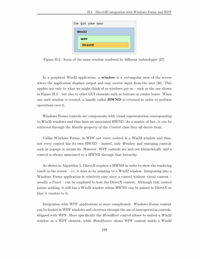
II.4 Direct3D integration with Windows Forms and WPF
Figure II.2: Areas of the same window rendered by different technologies [37].
In a graphical Win32 application, a window is a rectangular area of the screen
where the application displays output and may receive input from the user [38]. This
applies not only to what we might think of as windows per-se – such as the one shown
in Figure II.2 – but also to other GUI elements such as buttons or combo boxes. When
one such window is created, a handle called HWND is returned in order to perform
operations over it.
Windows Forms controls are components with visual representation corresponding
to Win32 windows and thus have an associated HWND. As a matter of fact, it can be
retrieved through the Handle property of the Control class they all derive from.
Unlike Windows Forms, in WPF not every control is a Win32 window and thus,
not every control has its own HWND – indeed, only Window and emerging controls
such as popups or menus do. However, WPF controls are laid out hierarchically and a
control is always associated to a HWND through that hierarchy.
As shown in Algorithm 5, DirectX requires a HWND in order to show the rendering
result in the screen – i.e. it does so by painting to a Win32 window. Integrating into a
Windows Forms application is relatively easy since a control without visual content –
usually a Panel – can be employed to host the DirectX content. Although that control
paints nothing, it still has a Win32 window whose HWND can be passed to DirectX so
that it renders to it.
Integration with WPF applications is more complicated. Windows Forms content
can be hosted in WPF windows and viceversa through the use of interoperation controls,
shipped with WPF. More specifically the HwndHost control allows to embed a Win32
window as a WPF element, while HwndSource shows WPF content inside a Win32
189

Appendix II. DirectX Integration Into Windowed Applications
window.
WindowsFormsHost is a WPF control deriving HwndSource which goes one step
further, allowing to embed a Windows Forms control inside WPF. Its aim is to support
the re-use of existing Windows Forms controls in newly-developed WPF applications.
The interoperation library also provides a WPF BitmapSource called D3DImage
which allows to present a surface rendered by DirectX. In order to do so, this class
provides a SetBackBuffer method receiving a pointer to the surface. In this case, no
HWND is explicitly involved: surfaces are managed instead of Win32 windows. Indeed,
the rendering is always performed to the off-screen surface which must then be passed to
SetBackBuffer – as opposed to rendering to a Win32 window shown on-screen, through
its HWND.
II.5 Direct3D integration in this work
Regarding Direct3D integration, the developments carried out during the work pre-
sented in this thesis can be summarized in chronological order as follows:
1. A new rendering engine implemented in Managed DirectX (which uses Direct3D
9.0c) was developed to replace an existing GDI+ rendering engine used in a Win-
dows Forms Computer-Aided-Design application for Windows XP. A Windows
Forms user control complying to the drawing interface used by the existing ap-
plication was implemented. Interoperability with GDI+ was required, since the
interface provides support for graphical layers that could be rendered by both
technologies.
A significant constraint was found in the integration of the MDX rendering engine
into Windows Forms applications: in order to merge the result of the rendering
with other layers shown in the graphical user interface, the video memory where
the output was stored had to by copied into the system memory, a bitmap had
to be created using that memory and passed to a Windows Forms control dis-
playing it as an image. As it could be expected, this imposed a very significant
performance penalty that yielded the rendering engine unsuitable for real-time
power grid visualizations such as those involving animations. Thus, the rendering
190
II.5 Direct3D integration in this work
engine was implemented as an off-screen, on-demand renderer6.
2. A custom Windows Forms application was developed to carry tests over that
rendering implementation in order to measure the improvement provided by using
spatial databases to reduce the data volume.
3. A new version of the Computer-Aided-Design application targeting Windows
Vista was developed using WPF, along with a new rendering engine developed
directly in C++ for Direct3D 10. Since WPF is only available in managed lan-
guages such as C#, a partially managed language called C++/CLI was used as
a bridge between the native libraries implementing the rendering engine and the
WPF application.
Being implemented in Direct3D, WPF offers a much better integration with a
rendering engine implemented in Direct3D. However, there are still a number of
limitations. The most significant is the incompatibility of WPF inputs (eg. key
presses, mouse events) over the DirectX portion of a WPF window. Because
of this, the rendering engine was once again implemented as an off-screen, on-
demand renderer.
4. Several custom native Win32 applications were developed to test new features
of Direct3D 11 and to elaborate performance and memory consumption compar-
isons. Instead of using a managed graphical user interface library, DXUT was
used to present controls such as buttons and sliders, as well as rendering text.
The first two developments, target Windows XP while the others target Windows
Vista and its new graphics features.
6See Section I.2 of Appendix I for a description of the renderer pattern and these concepts.
191

Appendix II. DirectX Integration Into Windowed Applications
192

APPENDIX IIIResumen en espanol
Esta tesis presenta los resultados de casi 5 anos de investigacion, desde el ano 2008
al 2013, en el contexto del desarrollo de una herramienta de planificacion de redes
electricas para la companıa Gas Natural Fenosa. Concretamente, el trabajo se centra en
mejorar el rendimiento de la visualizacion de las redes electricas en dicha herramienta.
Para conseguir dicha mejora, se comenzo por actualizar el motor de dibujo de la
herramienta, utilizando una tecnologıa grafica capaz de aprovechar la potencia del hard-
ware grafico disponible. Tras esto, el esfuerzo se centro en reducir el volumen de datos
involucrados en la visualizacion, primero mediante bases de datos espaciales y despues
utilizando un enfoque menos convencional, explorando las diferentes capacidades del
hardware grafico, no solo para realizar el dibujo de la red, sino tambien para llevar a
cabo la reduccion del volumen de datos.
Dada la naturaleza de la colaboracion con la companıa que financio este trabajo,
hubo que encontrar un equilibrio entre el trabajo de investigacion y el desarrollo de las
soluciones requeridas. A esto hay que anadir los requisitos derivados de las particulari-
dades de la companıa. Por ejemplo, la version del sistema operativo o las capacidades
del hardware grafico debıan de ajustarse a aquellos utilizados por la companıa. Esto
tuvo una influencia destacada en el proceso de investigacion.
III.1 Contextualizacion
Las redes electricas son complejos sistemas que llevan la electricidad desde su generacion
hasta sus consumidores. Tıpicamente se distinguen 3 fases: generacion, transporte, y
distribucion. La fase de transporte la forman redes electricas con lıneas de alta tension
193

Appendix III. Resumen en espanol
que cubren grandes distancias con una topologıa relativamente simple, conectando la
generacion con las redes de distribucion. Estas redes son mucho mas complejas y se
dividen en una primera fase de media tension y otra que lleva la electricidad a los
clientes finales mediante lıneas de baja tension. Es necesario destacar la simplificacion
de este resumen, puesto que los sistemas son mucho mas complejos: por ejemplo, hay
tanto productores como consumidores conectados a la red de media tension; ademas
con la aparicion de pequenos productores en los ultimos anos y las tecnologıas de Smart
Grids, este dibujo esta cambiando paulatinamente.
La herramienta de planificacion de redes electricas en torno a la que gira este tra-
bajo, permite realizar tareas de analisis, diseno, y simulaciones sobre redes electricas
de media tension. Estas redes abarcan areas geograficas que van desde comunidades
autonomas en el caso de Espana a pequenos paıses. La companıa electrica proporciono
datos de las redes correspondientes a la comunidad autonoma de Galicia y a los paıses
de Nicaragua, Panama, Moldavia, y Guatemala.
Los datos de interes de las redes son aquellos relativos a su estructura, no a medi-
ciones tales como el voltaje o la corriente en circulacion. La informacion relativa a
dicha estructura se divide en ramas – formadas principalmente por las lıneas electricas
– y nudos – donde convergen varias de esas ramas y donde se encuentran entidades
tales como subestaciones electricas. En todos los casos, se dispone de las coordenadas
geograficas UTM de su localizacion. Esto permite visualizar las redes sobre mapas o
imagenes satelite. Si bien como parte del trabajo encargado por la companıa se han
desarrollado ese tipo de visualizaciones, este trabajo se restringe a la visualizacion de
las redes electricas representando sus ramas como lıneas de un ancho fijo, utilizando
sus coordenadas geograficas para determinar las posiciones relativas de los nodos que
las componen.
III.2 Objetivos y actuaciones
El objetivo principal del trabajo presentado es la mejora del tiempo requerido para
la visualizacion de redes electricas de media tension realizada por una herramienta
de diseno asistido por ordenador para el analisis, diseno, planificacion y tareas de
simulacion de dicho tipo de redes.
194

III.2 Objetivos y actuaciones
La herramienta esta implementada utilizando la plataforma .NET de Microsoft
Windows. Para llevar a cabo la mencionada mejora, la primera actuacion consistio
en reemplazar el motor de dibujo existente, basado en GDI+, por una nueva imple-
mentacion utilizando la librerıa grafica DirectX en su version 9.0c. A pesar de que hubo
que adaptarse en parte a la forma de trabajar de GDI+ para poder integrar el nuevo
motor correctamente en la herramienta, la mejora de rendimiento fue mas que notable,
siendo del orden de diez veces mas rapido.
III.2.1 Generacion de lıneas con grosor mediante hardware
El hardware grafico moderno permite una gran flexibilidad al poder ser programado
mediante pequenos programas denominados shaders. La nueva version del motor de
dibujo hace uso de esta posibilidad para generar lıneas con grosor. A partir de dos
puntos y un parametro de grosor se realiza el calculo necesario para situar cuatro
vertices formando dos triangulos adyacentes que componen la lınea con grosor. Esto
se ha llevado a cabo mediante vertex shaders. Ademas, se presenta una evolucion
para la version DirectX 10 utilizando los nuevos geometry shaders que ofrece. Dado
que este tipo de shaders permiten generar nuevas primitivas geometricas de forma
dinamica, deja de ser necesario tener definidos cuatro vertices a priori: basta con los
dos puntos formando la lınea y el parametro de grosor para generar los dos triangulos
desde el geometry shader. Esto reduce la memoria de vıdeo necesaria para almacenar
los vertices en un 75%. Los triangulos generados por el shader pueden ser almacenados
en memoria de vıdeo para su posterior reutilizacion o se pueden volver a generar cada
vez. Aunque podrıa pensarse que almacenarlos y reutilizarlos resultarıa beneficioso, en
realidad aumenta tanto los requerimientos computacionales – por tener que procesar
los vertices generados – como los de memoria – por el espacio requerido para almacenar
dichos vertices.
III.2.2 Simplificacion de las redes mediante bases de datos espaciales
Una vez mejorado el rendimiento cumpliendo con los requisitos software, hardware, y
de integracion de la herramienta, se opto por reducir el volumen de datos para tratar
de disminuir aun mas los tiempos necesarios para llevar a cabo la visualizacion. Dada
la naturaleza de los datos, consistentes en coordenadas geograficas y la informacion
195

Appendix III. Resumen en espanol
topologica de las ramas, se estudio la viabilidad de emplear bases de datos espaciales
para dicha tarea.
Las bases de datos espaciales ofrecen tipos y operaciones especıficas para la gestion
de datos con relaciones espaciales. En este trabajo se utilizo la extension espacial Post-
GIS de PostgreSQL. Uno de los tipos soportados por dicha extension es el LineString,
que corresponde a una sucesion de lıneas conectadas. Este tipo es por tanto idoneo
para representar las ramas de las redes electricas. En este trabajo, se utiliza el termino
polilınea para referirse a una sucesion de lıneas conexas, equivalente tanto al tipo
LineString, como a las ramas electricas, u otros tipos de datos disponibles en DirectX.
Por otra parte, PostGIS ofrece multitud de funciones para el procesamiento de este tipo
de datos y su indexacion. Especialmente relevantes en este trabajo son las funciones
que permiten simplificar polilıneas u obtener todas las polilıneas dentro o intersecando
con una determinada area.
Teniendo en cuenta estas funcionalidades, se desarrollo una solucion para procesar
cada red electrica y generar varias resoluciones de los datos, almacenando cada una de
ellas en una tabla dedicada. Esto es lo que se denomina una arquitectura multi-escala.
Se desarrollo una librerıa formada por una serie de procedimientos almacenados en el
lenguaje PL/pgSQL de PostgreSQL y disparadores para mantener las tablas con las
diferentes escalas actualizadas respecto a los datos originales de las redes electricas.
Todo aquello que no sea relevante de cara a la visualizacion, bien porque no aporta
detalle o porque ni siquiera es visible, deberıa ser eliminado para disminuir la cantidad
de datos a procesar. La reduccion de los datos puede ir encaminada no solo a reducir los
requerimientos computacionales, sino tambien a mejorar la estetica de la visualizacion,
haciendola mas legible; por ejemplo, reduciendo la informacion mostrada en un area
donde hay tanta que no se puede discernir claramente – como puede suceder al mostrar
todas las ramas de una ciudad cuando la escala es pequena. Para analizar que polilıneas
pueden ser eliminadas y su potencial impacto en la visualizacion, se estudiaron las
condiciones y tecnicas de generalizacion cartografica.
Para generar las distintas escalas, se lleva a cabo un procesamiento de las ramas
consistente en la simplificacion de las polilıneas para eliminar segmentos indiscernibles y
se fusionan polilıneas adyacentes o muy proximas, ya que tampoco serıan distinguibles
en la visualizacion. Los resultados presentados muestran que gracias a la reduccion de
196

III.2 Objetivos y actuaciones
datos conseguida, se redujo el tiempo para representar la visualizacion hasta un 15%
del tiempo original.
III.2.3 Simplificacion de las redes en la GPU
Gracias a la disponibilidad de nuevo hardware grafico y nuevas versiones de DirectX,
se abrio la posibilidad de mover el proceso de simplificacion de las ramas de las redes
electricas a la GPU. Se presentan tres implementaciones que explotan diferentes partes
del pipeline grafico de DirectX, exponiendo un analisis comparativo de su rendimiento
en terminos de carga computacional y requisitos de memoria de vıdeo.
Uno de los objetivos a la hora de redactar esta tesis, fue tratar de dar al lector una
vision del proceso de evolucion sufrido por el hardware grafico en ordenadores persona-
les, desde sus inicios hasta la actualidad. Comenzaron siendo meros adaptadores para
poder mostrar caracteres alfanumericos, pasando a ser influenciados por la popularidad
de los videojuegos en entornos tridimensionales, para convertirse en procesadores con
gran capacidad para computacion paralela de proposito general.
Tambien se trato de dar una vision global aunque breve del API de DirectX 11, y
mas concretamente de Direct3D. Esta tecnologıa no es sino un reflejo de la arquitectura
dominante en el hardware grafico y consistente en una serie de etapas, algunas de ellas
programables mediante shaders, que conforman lo que se denomina el pipeline grafico.
De forma muy resumida, las etapas del pipeline grafico de DirectX 11 son las siguientes:
1. Input Assembler: obtiene los datos contenidos en buffers de memoria de vıdeo y
ensambla las primitivas de entrada al pipeline.
2. Vertex Shader: se invoca sobre cada vertice de las primitivas recibidas del Input
Assembler.
3. Hull Shader: requiere que las primitivas ensambladas por el Input Assembler
sean patches, siendo invocado para cada uno de ellos. Realiza las operaciones
requeridas sobre ellos y configura el Tesselator, definiendo cuantas primitivas
debe generar y de que tipo.
4. Tessellator: una vez que el Hull Shader ha procesado el patch correspondiente,
197

Appendix III. Resumen en espanol
genera tantas coordenadas como vertices sean necesarios para crear las primitivas
especificadas por el Hull Shader.
5. Domain Shader: procesa cada coordenada recibida del Tessellator, empleando
normalmente la informacion del patch procesado por el Hull Shader.
6. Geometry Shader: invocado para cada primitiva ensamblada por el Input Assem-
bler o generada por el Tessellator, puede alterar la geometrıa, tanto eliminando
como creando nuevas primitivas.
7. Stream Output: permite guardar las primitivas que salen del Vertex o Geometry
Shader a un buffer de memoria de vıdeo. Esto permite guardar los resultados del
procesamiento llevado a cabo para reutilizarlo mas adelante.
8. Rasterizer: es el encargado de generar fragments a partir de la informacion vec-
torial que representan las geometrıas. Los fragments pueden verse como pıxels
con informacion adicional.
9. Pixel Shader: procesa cada fragment generado por el Rasterizer, pudiendo generar
varios colores como resultado.
10. Output Merger: es el encargado de generar los pıxels que componen la imagen (o
imagenes) resultado.
Ademas, existe otro pipeline alternativo para computaciones de proposito general
que contiene una sola etapa programable: el Compute Shader.
Las implementaciones desarrolladas y presentadas en esta tesis son las siguientes:
Compute Shader: emplea el Compute Shader para pre-procesar las polilıneas,
simplificandolas en la GPU y guardando el resultado en memoria de vıdeo para
ser luego consumido por el pipeline grafico para generar la visualizacion. Este
pre-procesamiento solo es necesario llevarlo a cabo antes del primer renderizado
o cuando cambia el valor del parametro empleado en el proceso de simplificacion
para determinar la longitud mınima que tienen que tener los segmentos de las
polilıneas. Se desarrollo una aplicacion nativa en C++ que muestra la visuali-
zacion y permite configurar la tecnica presentada mediante una interfaz grafica
desarrollada con la librerıa de utilidad DXUT.
198

III.3 Estructura
Geometry Shader: el procesamiento llevado a cabo por el Compute Shader en la
implementacion anterior, se adapto a las particularidades del Geometry Shader.
Este impone mas restricciones, debido a las cuales solo se pueden generar 31 lıneas
por cada ejecucion del shader. No obstante, se presentan tecnicas para superar
esta limitacion realizado varias ejecuciones del shader para los mismos datos de
entrada. Se desarrollaron dos aplicaciones analogas a la desarrollada para el
Compute Shader para probar la implementacion: una con tres configuraciones
predefinidas y otra que permite configurar el numero de shaders a utilizar para
la simplificacion.
Tessellation: en este caso, se utilizan patches de 32 puntos para representar las
polilıneas, siendo generadas por el Tessellator tantas lıneas como las que hayan
pasado el proceso de simplificacion llevado a cabo en el Hull Shader. En caso de
polilıneas con menos puntos, simplemente se ignoran los puntos restantes. Esta
tecnica no es aplicable para polilıneas de mas de 32 puntos, ya que no hay op-
ciones similares a la instanciacion del Geometry Shader aprovechada por la imple-
mentacion anterior. Por ello, para esas polilıneas se utiliza dicha implementacion.
La aplicacion desarrollada para probar esta tecnica permite seleccionar el numero
maximo de puntos para las polilıneas simplificadas mediante Tessellation, uti-
lizando para el resto de las polilıneas la implementacion del Geometry Shader.
Los resultados de la experimentacion llevada a cabo para las tres implementaciones
descritas permiten concluir lo siguiente. Como se esperaba a priori, la mas adecuada
parece ser la implementacion del Compute Shader, ya que ademas de resultar mas
transparente, no introduce un impacto en el rendimiento cada vez que se genera la
visualizacion sino solo cuando cambia el criterio de simplificacion – esto suele corres-
ponder a una variacion del nivel de detalle requerido, por ejemplo a consecuencia de
un nivel distinto de zoom en la visualizacion. Por otra parte, dicha implementacion es
la que menos restricciones establece respecto a la longitud de las polilıneas.
III.3 Estructura
Esta tesis consta de los siguientes capıtulos:
199

Appendix III. Resumen en espanol
1. Capıtulo 1: presenta la introduccion, objetivos, y estructura del trabajo.
2. Capıtulo 2: introduce el dominio de la investigacion, es decir, la visualizacion de
redes electricas de media tension. Se presenta brevemente el sistema electrico y
se lleva a cabo un analisis de los conjuntos de datos empleados.
3. Capıtulo 3: describe una arquitectura multi-escala para reducir el volumen de
datos mediante bases de datos espaciales y los resultados experimentales. Ademas,
se introduce el campo de la generalizacion cartografica y como la reduccion del
volumen de datos no solo redunda en mejores tiempos de renderizado sino que
tambien puede mejorar la calidad de la visualizacion.
4. Capıtulo 4: presenta una perspectiva historica de la evolucion del hardware grafico
desde sus inicios hasta el disponible hoy en dıa.
5. Capıtulo 5: introduce los principales conceptos de la generacion de graficos tridi-
mensionales. Este capıtulo permite contrastar lo expuesto en el capıtulo anterior
sobre como el hardware replicaba las fases de este proceso de generacion y a la
vez, presenta conceptos fundamentales para comprender el API de Direct3D y
por extension las tecnicas implementadas con el.
6. Capıtulo 6: expone las partes mas relevantes del API de Direct3D en su version
11. Trata no solo de presentar las funcionalidades explotadas por las distintas
implementaciones llevadas a cabo en esta tesis, sino de dar una vision general de
Direct3D.
7. Capıtulo 7: describe las tres implementaciones de la simplificacion de polilıneas
en la GPU realizadas mediante DirectX 11.
8. Capıtulo 8: presenta los resultados experimentales de las implementaciones des-
critas en el capıtulo 7. Incluye una comparativa teniendo en cuenta los costes
computacionales y de memoria, ası como sus requisitos de hardware y software.
9. Capıtulo 9: expone las conclusiones de esta tesis y posibles lıneas de trabajo
futuro.
10. Apendice I: introduce algunos patrones software relevantes al campo de la visua-
lizacion, describiendo su aplicacion en este trabajo.
11. Apendice II: realiza un analisis de la integracion de las tecnologıas graficas em-
pleadas en este trabajo para las dos versiones de Microsoft Windows objetivo:
XP y Vista.
200

III.5 Trabajo futuro
12. Apendices III y IV: resumenes en espanol y gallego de la tesis, de acuerdo a la
normativa del programa de doctorado.
III.4 Conclusiones
Esta tesis presenta los resultados de trabajos de investigacion llevados a cabo para
mejorar la visualizacion de una herramienta de planificacion de redes electricas. La
primera actuacion consistio en actualizar su motor de dibujo para explotar el alto
rendimiento ofrecido por DirectX.
Una forma fundamental de mejorar el rendimiento de una visualizacion es la re-
duccion de los datos involucrados, puesto que cuanto menor sea su volumen, menor
sera el tiempo necesario para generar la visualizacion. Ademas, la reduccion de datos
puede mejorar la calidad estetica de la visualizacion, haciendola mas legible.
Se presentaron dos aproximaciones a la reduccion de datos: mediante bases de datos
espaciales y mediante hardware grafico. No son excluyentes, dado que la informacion
de las redes electricas normalmente proviene de una base de datos y, utilizando las
extensiones espaciales que proporcionan la mayorıa de sistemas de gestion de bases de
datos modernos, se puede procesar la informacion para adecuadarla a la visualizacion
a realizar.
El hardware grafico moderno esta equipado con potentes GPUs con gran capacidad
para la computacion paralela de alto rendimiento y proposito general. Se han presen-
tado tres tecnicas que no solo dibujan la visualizacion de las redes electricas, sino que
integran en el proceso la simplificacion de las redes electricas para tratar de generar la
visualizacion mas rapidamente.
Segun sigan evolucionando las capacidades del hardware grafico, nuevas tecnicas
podran ser implementadas y las existentes mejoraran su rendimiento de forma casi
transparente, lo que hace que este campo sea altamente dinamico y una fuente de
innovacion.
201
Appendix III. Resumen en espanol
III.5 Trabajo futuro
Como lıneas de continuacion de este trabajo se pueden destacar las siguientes:
Migracion a DirectX 12: este trabajo fue evolucionando segun lo permitio el
hardware y software disponible, de la version 9 de DirectX empleada inicialmente
hasta la 11. Aunque no presenta nuevas etapas del pipeline como sı paso en dichas
versiones, la version 12 se centra en mejorar la eficiencia lo que deberıa redundar
en una mejora del rendimiento, por lo que serıa interesante su adopcion.
Introduccion de visualizaciones mas complejas: la visualizacion utilizada en este
trabajo corresponde a la representacion de las ramas de las redes electricas como
lıneas de ancho fijo. Existen multitud de visualizaciones disponibles que podrıan
aprovechar las mejoras de rendimiento aquı presentadas. De hecho, este trabajo
ha abierto las puertas a la introduccion de animaciones en tiempo real en las
visualizaciones llevadas a cabo por la herramienta de planificacion.
Adopcion de otros patrones de visualizacion: en el Apendice I se mencionan
algunos patrones que no se adoptaron debido a restricciones de tiempo y que
podrıan resultar beneficiosos.
Conversion de coordenadas geograficas: en ocasiones se requiere algun tipo de
procesamiento especıfico sobre las coordenadas geograficas en que estan definidas
las ramas de las redes electricas. Un ejemplo es su visualizacion sobre mapas o
imagenes satelite. Normalmente los mapas o imagenes estaran definidos en otro
sistema de coordenadas y sera necesario convertir las coordenadas de las ramas.
Esta conversion se podrıa integrar en el procesamiento que realizan los vertex y
geometry shaders en la GPU.
Revision del algoritmo de simplificacion: al igual que en el caso de la visualizacion,
se opto por un algoritmo de simplificacion sencillo que podrıa ser revisado y
mejorado.
202

III.6 Publicaciones
III.6 Publicaciones
Parte del trabajo presentado en esta tesis ha sido presentado en las siguientes confe-
rencias y publicado en sus respectivas actas:
Electrical Distribution Grid Visualization using Programmable GPUs
Rodriguez J. N., Canosa M. C., y Hernandez Pereira E. Electrical distribution
grid visualization using programmable gpus. ”7th International Conference on
Electrical Engineering/Electronics Computer Telecommunications and Informa-
tion Technology (ECTI-CON 2010)”, paginas 1231-1235. ECTI (2010).
Digital Cartographic Generalization in Spatial Databases: application issues in
Power Grids CAD tools
Rodriguez J. N., Hernandez Pereira E., y Canosa M. C. Digital cartographic
generalization in spatial databases: application issues in power grids cad tools.
”Proceedings of the V Ibero-American Symposium in Computer Graphics (SIACG
2011)”, paginas 15-22. SIACG (2011).
Improving Electrical Power Grid Visualization using Geometry Shaders
Rodriguez J. N., Canosa M. C., y Hernandez Pereira E. Improving electrical
power grid visualization using geometry shaders. ”Computer Graphics, Imaging
and Visualization (CGIV), 2011 Eighth International Conference”, paginas 177-
182. IEEE (2011).
Actualmente se encuentra bajo revision un resumen de los trabajos presentados en
esta tesis. Ademas, una version ampliada de la primera publicacion se publico tambien
en la siguiente revista:
Rodriguez J. N., Canosa M. C., y Hernandez Pereira E. Electrical distribution
grid visualization using programmable gpus. ”ECTI Transactions on Computer
and Information Technology”, 5(1), paginas 30-37 (2011).
203

Appendix III. Resumen en espanol
204
APPENDIX IVResumo en galego
Esta tese presenta os resultados de case 5 anos de investigacion, dendo o ano 2008
ao 2013, no contexto do desenvolvemento dunha ferramenta de planificacion de redes
electricas para a companıa Gas Natural Fenosa. Concretamente, o traballo centrase en
mellora-lo rendemento da visualizacion das redes electricas na mencionada ferramenta.
Para acadar tal mellora, comezouse pola actualizacion do motor de debuxo da ferra-
menta, empregando unha tecnoloxıa grafica capaz de aproveita-la potencia do hardware
grafico disponible. Tras iso, o esforzo centrouse en reduci-lo volume de datos involucra-
dos na visualizacion, primeiro mediante bases de datos espaciais e logo empregando un
enfoque menos convencional, explorando as diferentes capacidades do hardware grafico,
non so para levar a cabo o debuxo da rede, senon tamen para levar a cabo a reduccion
do volume de datos.
Dada a natureza da colaboracion coa companıa que financiou este traballo, houbo
que atopar un equilibrio entre o traballo investigador e o desenvolvemento das solucions
requeridas. A isto hai que engadi-los requisitos derivados das particularidades da
companıa. Por exemplo, a version do sistema operativo ou as capacidades do hard-
ware grafico debıan de se axustar a aquelos empregados pola companıa. Isto tivo unha
influencia destacada no proceso investigador.
IV.1 Contextualizacion
As redes electricas son complexos sistemas que levan a electricidade dende sua xeracion
ata seus consumidores. Tıpicamente diferencianse 3 fases: xeracion, transporte, e dis-
tribucion. A frase de transporte esta formada por redes electrica con linas de alta
205

Appendix IV. Resumo en galego
tension que cubren grandes distancias cunha topoloxıa relativamente simple, conectando
a xeracion coas redes de distribucion. Estas redes son moito mais complexas e divıdense
nunha primeira fase de media tension e outra que leva a electricidade aos clientes finais
mediante linas de baixa tension. Compre destaca-la simplificacion deste resumo, posto
que os sistemas son moito mais complexos: por exemplo, hai tanto productores como
consumidores conectados a rede de media tension; ademais coa aparicion de pequenos
productores nos ultimos anos e das tecnoloxıas Smart Grids, este debuxo esta a cambiar
paulatinamente.
A ferramenta de planificacion de redes electricas en torno a que xira este traballo,
permite levar a cabo tarefas de analise, deseno, e simulacions sobre redes electricas
de media tension. Estas redes abarcan areas xeograficas que van dende comunidades
autonomas no caso de Espana ata pequenos paıses. A companıa electrica proporcionou
datos das redes correspondentes a comunidade autonoma de Galicia e aos paıses de
Nicaragua, Panama, Moldavia, e Guatemala.
Os datos de interese das redes son aquelos relativos a sua estructura, non a medicions
tales coma a voltaxe ou a corrente en circulacion. A informacion relativa a estructura
divıdese en polas – formadas principalmente polas linas electricas – e nos – onde con-
verxen varias desas polas e onde atopanse entidades tales como subestacions electricas.
En todolos casos, disponse das coordenadas xeograficas UTM da sua localizacion. Isto
permite visualiza-las redes sobre mapas ou imaxes satelite. Se ben como parte do tra-
ballo encargado pola companıa desenvolvıronse ese tipo de visualizacions, este traballo
so leva a cabo a visualizacion das redes electricas representando suas polas como linas
dun ancho fixo, empregando as coordenadas xeograficas para determina-las posicions
relativas dos nodos que as forman.
IV.2 Obxectivos e actuacions
O principal obxectivo do traballo presentado e a mellora do tempo requerido para
visualizar redes electricas de media tension por parte dunha ferramenta de deseno
asistido por ordenador para a analise, deseno, planificacion, e tarefas de simulacion do
mencionado tipo de redes.
206

IV.2 Obxectivos e actuacions
A ferramenta esta implementada empregando a plataforma .NET de Microsoft Win-
dows. Para levar a cabo a mencionada tarefa, a primeira actuacion consistiu en subs-
tituir o motor de debuxo existente, baseado en GDI+, por unha nova implementacion
empregando a librarıa grafica DirectX na sua version 9.0c. A pesar de que houbo que
adaptarse en parte a forma de traballar de GDI+ de cara a poder integra-lo novo motor
correctamente na ferramenta, a mellora de rendemento foi mais que notable, sendo da
orde de dez veces mais rapido.
IV.2.1 Xeracion de linas con grosor mediante hardware
O hardware grafico moderno permite unha gran flexibilidade ao poder ser programado
mediante pequenos programas denominados shaders. A nova version do motor de de-
buxo fai uso desta posibilidade para xerar linas con grosor. A partir de dous puntos
e un parametro de grosor levase a cabo o calculo necesario para situar catro vertices
formando dous triangulos adxacentes que componen a lina con grosor. Isto levouse
a cabo mediante vertex shaders. Ademais, presentase unha evolucion para a version
DirectX 10 empregando os novos geometry shaders que ofrece. Dado que este tipo de
shaders permiten xerar novas primitivas xeometricas de forma dinamica, deixa de ser
preciso ter definidos catro vertices a priori: basta cos dous puntos formando a lina
mais o parametro de grosor para xera-los dos triangulos dende o geometry shader. Isto
reduce a memoria de vıdeo precisa para almacena-los vertices nun 75%. Os triangulos
xerados polo shader poden ser almacenados en memoria de vıdeo para a sua poste-
rior reutilizacion ou poden volverse xerar cada vez. Aında que poderıa pensarse que
almacenalos e reutilizalos resultarıa beneficioso, en realidade aumenta tanto o custo
computacional – por ter que procesa-los vertices xerados – coma o de memoria – polo
espacio preciso para almacena-los vertices.
IV.2.2 Simplificacion das redes mediante bases de datos espaciais
Unha vez mellorado o rendemento cumplindo cos requisitos software, hardware, e de in-
tegracion da ferramenta, optouse por reduci-lo volume de datos para tratar de disminuir
mais aında os tempos requeridos para levar a cabo a visualizacion. Dada a natureza dos
datos, consistentes en coordenadas xeograficas e da informacion topoloxica das polas,
estudiouse a viabilidade de empregar bases de datos espaciais para esa tarefa.
207

Appendix IV. Resumo en galego
As bases de datos espaciais ofrecen tipos e operacions especıficas para a xestion de
datos con relacions espaciais. Neste traballo utilizouse a extension espacial PostGIS de
PostgreSQL. Un dos tipos soportados por esa extension e o LineString, que corresponde
a unha sucesion de linas conectadas. Este tipo e por tanto adecuado para representa-las
polas das redes electricas. Neste traballo, utilızase o termo polilina para referirse a unha
sucesion de linas conexas, equivalente tanto ao tipo LineString, como as polas electricas,
ou a outros tipos de datos disponibles en DirectX. Por outra banda, PostGIS ofrece
multitude de funcions para o procesamento deste tipo de datos e a sua indexacion.
Especialmente relevantes neste traballo son as funcions que permiten simplificar poli-
linas ou obter todalas polilinas dentro ou intersecando cunha determinada area.
Tendo en conta estas funcionalidades, desenvolvıuse unha solucion para procesar
cada rede electrica e xerar varias resolucion dos datos, almacenando cada unha delas
nunha taboa dedicada. Isto e o que se denomina unha arquitectura multi-escala. De-
senvolvıuse unha librerıa formada por unha serie de procedementos almacenados na
linguaxe PL/pgSQL de PostgreSQL e disparadores para mante-las taboas coas diferen-
tes escalas actualizadas respecto aos datos orixinales das redes electricas.
Todo aquelo que non sexa relevante de cara a visualizacion, ben porque non aporta
detalle ou porque nin tan sequera e visible, deberıa ser eliminado para disminuir a
cantidade de datos a procesar. A reduccion dos datos pode ir encaminada non so a
reduci-los requerimentos computacionais, senon tamen a mellora-la estetica da visuali-
zacion, facendoa mais lexible; por exemplo, reducindo a informacion mostrada nunha
area onde hai tanta que non se pode discenir claramente – como pode suceder cando
se mostran todalas polas dunha ciudade cando a escala e pequena. Para analizar que
polilinas poden ser eliminadas e o potencial impacto na visualizacion, estudiaronse as
condicions e tecnicas de xeneralizacion cartografica.
Para xera-las distintas escalas, levase a cabo un procesamento das ramas consistente
na simplificacion das polilinas para eliminar segmentos indiscernibles e fusionanse poli-
linas adxacentes ou moi proximas, xa que tampoco serıan distinguibles na visualiza-
cion. Os resultados presentados mostran que gracias a reduccion de datos conseguida,
reducıuse o tempo para representa-la visualizacion ata un 15% do tempo orixinal.
208

IV.2 Obxectivos e actuacions
IV.2.3 Simplificacion das redes na GPU
Gracias a disponibilidade de novo hardware grafico e novas versions de DirectX, abrıuse
a posibilidade de mover o proceso de simplificacion das polas das redes electricas a GPU.
Presentanse tres implementacions que explotan diferentes partes do pipeline grafico de
DirectX, exponendo unha analise comparativa do seu rendemento en termos de carga
computacional e requisitos de memoria de vıdeo.
Un dos obxectivos a hora de redactar esta tese, foi tratar de darlle ao lector unha
vision do proceso de evolucion sufrido polo hardware grafico en ordenadores personais,
dende seus inicios ata a actualidade. Comezaron sendo meros adaptadores para poder
mostrar caracteres alfanumericos, pasando a ser influenciados pola popularidade dos
videoxogos en entornos tridimensionais, para convertirse en procesadores con gran ca-
pacidade para computacion paralela de proposito xeral.
Tamen tratouse de dar unha vision global aında que breve do API de DirectX 11, e
mais concretamente de Direct3D. Esta tecnoloxıa non e senon un reflexo da arquiectura
dominante no hardware grafico e consistente nunha serie de etapas, algunhas delas
programables mediante shaders, que conforman o que denomınase o pipeline grafico.
De forma moi resumida, as etapas do pipeline grafico de DirectX 11 son as seguintes:
1. Input Assembler: obten os datos contidos en buffers de memoria de vıdeo e
ensambla as primitivas de entrada ao pipeline.
2. Vertex Shader: e invocado sobre cada vertice das primitivas recibidas do Input
Assembler.
3. Hull Shader: require cas primitivas ensambladas polo Input Assembler sexan
patches, sendo invocado para cada un deles. Realiza as operacions requeridas
sobre eles e configura o Tessellator, definindo cantas primitivas debe xerar e de
que tipo.
4. Tessellator: unha vez que o Hull Shader procesou o patch correspondente, xera
tantas coordenadas coma vertices sexan necesarios para crea-las primitivas es-
pecificadas polo Hull Shader.
5. Domain Shader: procesa cada coordenada recibida do Tessellator, empregando
normalmente a informacion do patch procesado polo Hull Shader.
209

Appendix IV. Resumo en galego
6. Geometry Shader: invocado para cada primitiva ensamblada polo Input Assem-
bler ou xerada polo Tessellator, pode altera-la xeometrıa, tanto eliminando como
creando novas primitivas.
7. Stream Output: permite garda-las primitivas que salen do Vertex ou Geometry
Shader a un buffer de memoria de vıdeo. Isto permite garda-los resultados do
procesamento levado a cabo para reutilizalo mais adiante.
8. Rasterizer: e o encargado de xerar fragments a partir da informacion vectorial que
representan as xeometrıas. Os fragments poden verse como pıxels con informacion
adicional.
9. Pixel Shader: procesa cada fragment xerado polo Rasterizer, pudindo xerar varias
cores como resultado.
10. Output Merger: e o encargado de xera-los pıxels que componen a image (ou
imaxes) resultado.
Ademais, existe outro pipeline alternativo para computacions de proposito xeral
que conten unha sola etapa programable: o Compute Shader.
As implementacion desenvolvidas e presentadas nesta tese son as seguintes:
Compute Shader: emprega o Compute Shader para pre-procesa-las polilinas, sim-
plificandoas na GPU e gardando o resultado en memoria de vıdeo para ser logo
consumido polo pipeline grafico para xera-la visualizacion. Este pre-procesamento
so e preciso levalo a cabo antes do primeiro renderizado ou cando cambia o valor
do parametro empregado no proceso de simplificacion para determina-la lonxitude
mınima que tenen que ter os segmentos das polilinas. Desenvolvıuse unha apli-
cacion nativa en C++ que mostra a visualizacion e permite configura-la tecnica
presentada mediante unha interfaz grafica desenvolvida coa librerıa de utilidade
DXUT.
Geometry Shader: o procesamento levado a cabo polo Compute Shader na im-
plementacion anterior, adaptouse as particularidades do Geometry Shader. Este
impon mais restriccions, debido as cales so se poden xerar 31 linas por cada exe-
cucion do shader. Presentanse tecnicas para superar esta limitacion realizando
varias execucions do shader para os mesmos datos de entrada. Desenvolvıronse
210

IV.3 Estructura
dous aplicacions analogas a desenvolvida para o Compute Shader para proba-la
implementacion: unha con tres configuracions predefinidas e outra que permite
configura-lo numero de shaders a empregar para a simplificacion.
Tessellation: neste caso, utilızanse patches de 32 puntos para representa-las poli-
linas, sendo xeradas polo Tessellator tantas linas como as que pasaran o proceso
de simplificacion levado a cabo no Hull Shader. No caso de polilinas con menos
puntos, simplemente ignoranse os puntos restantes. Esta tecnica non e aplicable
para polilinas de mais de 32 puntos, xa que non hai opcions similares a instan-
ciacion do Geometry Shader aproveitada pola implementacion anterior. Por iso,
para esas polilinas utilızase esa implementacion. A aplicacion desenvolvida para
probar esta tecnica permite selecciona-lo numero maximo de puntos para as poli-
linas simplificadas mediante Tessellation, utilizando para o resto das polilinas a
implementacion do Geometry Shader.
Os resultados da experimentacion levada a cabo para as tres implementacions descri-
tas permiten concluir o seguinte. Como esperabase a priori, a mais adecuada semella ser
a implementacion do Compute Shader, xa que ademais de resultar mais transparente,
non introduce un impacto no rendimiento cada vez que se xera a visualizacion senon
so cando cambia o criterio de simplifacion – isto corresponde normalmente a unha
variacion do nivel de detalle requerido, por exemplo a consecuencia dun nivel distinto
de zoom na visualizacion. Por outra parte, e a implementacion que menos restriccions
establece respecto a lonxitude das polilinas.
IV.3 Estructura
Esta tese consta dos seguintes capıtulos:
1. Capıtulo 1: presenta a introduccion, obxectivos, e estructura do traballo.
2. Capıtulo 2: introduce o dominio da investigacion, e dicir, a visualizacion de redes
electricas de media tension. Presentase brevemente o sistema electrico e levase a
cabo unha analise dos conxuntos de datos empregados.
211

Appendix IV. Resumo en galego
3. Capıtulo 3: describe unha arquitectura multi-escala para reduci-lo volume dos
datos mediante bases de datos espaciais e os resultados experimentais. Ademais,
introducese o campo da xeneralizacion cartografica e como a reduccion do volume
de datos non so redunda en mellores tempos de renderizado senon que tamen pode
mellora-la calidade da visualizacion.
4. Capıtulo 4: presenta unha perspectiva historica da evolucion do hardware grafico
dende os seus inicios ata o disponible hoxe en dıa.
5. Capıtulo 5: introduce os principais conceptos da xeracion de graficos tridimen-
sionais. Este capıtulo permite contrasta-lo exposto no capıtulo anterior sobre
como o hardware replicaba as fases deste proceso de xeracion e a vez, presenta
conceptos fundamentais para comprende-lo API de Direct3D e por extension as
tecnicas implementadas con el.
6. Capıtulo 6: expon as partes mais relevantes do API de Direct3D na sua version
11. Trata non so de presenta-las funcionalidades explotadas polas distintas imple-
mentacions levadas a cabo nesta tese, senon de dar unha vision xeral de Direct3D.
7. Capıtulo 7: describe as tres implementacions da simplificacion de polilinas na
GPU realizadas mediante DirectX 11.
8. Capıtulo 8: presenta os resultados experimentais das implementacions descritas
no capıtulo 7. Inclue unha comparativea tendo en conta os costes computacionais
e de memoria, ası como seus requisitos de hardware e software.
9. Capıtulo 9: expon as conclusions desta tese e posibles linas de traballo futuro.
10. Apendice I: introduce alguns patrons software relevantes ao campo da visualiza-
cion, describindo a sua aplicacion neste traballo.
11. Apendice II: realiza unha analise da integracion das tecnoloxıas graficas empre-
gadas neste traballo para as dos versions de Microsoft Windows obxectivo: XP e
Vista.
12. Apendices III e IV: resumenes en espanol e galego da tese, de acordo coa normativa
do programa de doutoramento.
212
IV.5 Traballo futuro
IV.4 Conclusions
Esta tese presenta os resultados de traballos de investigacion levados a cabo para
mellora-la visualizacion dunha ferramenta de planificacion de redes electricas. A primeira
actuacion consistiu en actualiza-lo seu motor de debuxo para explota-lo alto rendemento
ofrecido por DirectX.
Unha forma fundamental de mellora-lo rendemento dunha visualizacion e a re-
duccion dos datos involucrados, posto que canto menor sexa seu volume, menor sera
o tempo necesario para xera-la visualizacion. Ademais, a reduccion de datos pode
mellora-la calidade estetica da visualizacion, facendoa mais lexible.
Presentaronse dous aproximacions a reduccion de datos: mediante bases de datos
espaciais e mediante hardware grafico. Non son excluıntes, dado que a informacion das
redes electricas normalmente proven dunha base de datos e, empregando as extensions
espaciais que proporcionan a maiorıa dos sistemas de xestion de bases de datos moder-
nos, podese procesa-la informacion para adecuala a visualizacion a realizar.
O hardware grafico moderno esta equipado con potentes GPUs con gran capacidade
para a computacion paralela de alto rendemento e proposito xeral. Presentaronse tres
tecnicas que non so debuxan a visualizacion das redes electricas, senon que integran o
proceso a simplificacion das redes electricas para tratar de xera-la visualizacion mais
rapidamente.
Segun sigan a evoluciona-las capacidades do hardware grafico, novas tecnicas poderan
ser implementadas e as existentes melloraran o seu rendemento de forma casi transpa-
rente, o que fai que este campo sexa altamente dinamico e unha fonte de innovacion.
IV.5 Traballo futuro
Como linas de continuacion deste traballo podense destacar as seguintes:
Migracion a DirectX 12: este traballo foi evolucionando segun o permitiu o hard-
ware e software disponible, da version 9 de DirectX empregada inicialmente ata
213

Appendix IV. Resumo en galego
a 11. Aında que non presenta novas etapas do pipeline coma sı pasou nas men-
cionadas versions, a version 12 centrase en mellora-la eficiencia o que deberıa re-
dundar nunha mellora do rendemento, polo que serıa interesante a sua adopcion.
Introduccion de visualizacions mais complexas: a visualizacion empregada neste
traballo corresponde a representacion das ramas das redes electricas como linas
de ancho fixo. Existen multitude de visualizacions disponibles que poderıan
aproveita-las melloras de rendemento aquı presentadas. De feito, este traballo
abriu as portas a introduccion de animacions en tempo real nas visualizacions
levadas a cabo pola ferramenta de planifacion.
Adopcion doutros patrons de visualizacion: no Apendice I mencionanse alguns
patrons que non se adoptaron debido a restriccions de tempo e que poderıan
resultar beneficiosos.
Conversion de coordenadas xeograficas: en ocasions requırese algun tipo de proce-
samento especıfico sobre as coordenadas xeograficas na que estan definidas as
polas das redes electricas. Un exemplo e a sua visualizacion sobre mapas ou
imaxes satelite. Normalmente os mapas ou imaxes estaran definidos noutro sis-
tema de coordenadas e sera preciso convertir as coordenadas das polas. Esta
conversion poderıase integrar no procesamento que realizan os vertex e geometry
shaders na GPU.
Revision do algoritmo de simplificacion: igual que no caso da visualizacion,
optouse por un algoritmo de simplificacion sinxelo que poderıa ser revisado e
mellorado.
IV.6 Publicacions
Parte do traballo presentado nesta tese foi presentado nas seguintes conferencias e
publicado nas suas respectivas actas:
Electrical Distribution Grid Visualization using Programmable GPUs
Rodriguez J. N., Canosa M. C., e Hernandez Pereira E. Electrical distribution
grid visualization using programmable gpus. ”7th International Conference on
214

IV.6 Publicacions
Electrical Engineering/Electronics Computer Telecommunications and Informa-
tion Technology (ECTI-CON 2010)”, paxinas 1231-1235. ECTI (2010).
Digital Cartographic Generalization in Spatial Databases: application issues in
Power Grids CAD tools
Rodriguez J. N., Hernandez Pereira E., e Canosa M. C. Digital cartographic
generalization in spatial databases: application issues in power grids cad tools.
”Proceedings of the V Ibero-American Symposium in Computer Graphics (SIACG
2011)”, paxinas 15-22. SIACG (2011).
Improving Electrical Power Grid Visualization using Geometry Shaders
Rodriguez J. N., Canosa M. C., e Hernandez Pereira E. Improving electrical
power grid visualization using geometry shaders. ”Computer Graphics, Imaging
and Visualization (CGIV), 2011 Eighth International Conference”, paxinas 177-
182. IEEE (2011).
Actualmente atopase baixo revision un resumo dos traballos presentados nesta
tese. Ademais, unha version ampliada da primeria publicacion foi publicada tamen
na seguinte revista:
Rodriguez J. N., Canosa M. C., e Hernandez Pereira E. Electrical distribution
grid visualization using programmable gpus. ”ECTI Transactions on Computer
and Information Technology”, 5(1), paxinas 30-37 (2011).
215

Appendix IV. Resumo en galego
216

Bibliography
[1] Advanced Micro Devices, Inc. http://www.amd.com. Last access: 21-06-2015.
[2] ArcGIS Desktop 9.3 Help: About coordinate systems and map projec-
tions. http://webhelp.esri.com/arcgisdesktop/9.3/index.cfm?TopicName=
About_coordinate_systems_and_map_projections. Last access: 21-06-2015.
[3] Direct3D. http://msdn.microsoft.com/en-us/library/windows/desktop/
hh309466(v=vs.85).aspx. Last access: 21-06-2015.
[4] ID3D11 DeviceContext::Dispatch method. http://msdn.microsoft.com/en-us/
library/windows/desktop/ff476405(v=vs.85).aspx. Last access: 21-06-2015.
[5] Intel Corporation. http://www.intel.com. Last access: 21-06-2015.
[6] International Business Machines Corporation. http://www.ibm.com. Last access:
21-06-2015.
[7] Microsoft Corporation. http://www.microsoft.com. Last access: 21-06-2015.
[8] NVIDIA Corporation. http://www.nvidia.com. Last access: 21-06-2015.
[9] OpenCL - The open standard for parallel programming of heterogeneous systems.
http://www.khronos.org/opencl/. Last access: 21-06-2015.
[10] PostGIS: Spatial and geographic objects for PostgreSQL. http://www.postgis.
net. Last access: 21-06-2015.
[11] PostgreSQL: The world’s most advanced open source database. http://www.
postgresql.org. Last access: 21-06-2015.
[12] Primitive topologies. http://msdn.microsoft.com/es-es/library/windows/
desktop/bb205124(v=vs.85).aspx. Last access: 21-06-2015.
[13] Rendering pipeline. http://msdn.microsoft.com/es-es/library/windows/
hardware/ff569246(v=vs.85).aspx. Last access: 21-06-2015.
217

[14] S3 Graphics. http://www.s3graphics.com. Last access: 21-06-2015.
[15] Silicon Graphics International Corporation. http://www.sgi.com. Last access:
21-06-2015.
[16] Sony Corporation. http://www.sony.com. Last access: 21-06-2015.
[17] Video Electronics Standards Association. http://www.vesa.org. Last access:
21-06-2015.
[18] S3 ViRGE Integrated 3D Graphics/Video Accelerator. Product Overview (1996).
[19] SST-1 (a.k.a. Voodoo Graphics) High Performance Graphics Engine for 3D Game
Acceleration. 3dfx Interactive, Inc. (December 1999).
[20] Akeley K. Reality Engine Graphics. In “Proceedings of the 20th annual confer-
ence on Computer graphics and Interactive Techniques”, SIGGRAPH ’93, pages
109–116, New York, NY, USA (1993).
[21] ATI Technologies Inc. Radeon X800 3D Architecture White Paper. http:
//www.ati.com/products/radeonx800/RadeonX800ArchitectureWhitePaper.
pdf.
[22] Bohm W., Farin G., and Kahmann J. A survey of curve and surface methods
in cagd. Computer Aided Geometric Design 1(1), 1–60 (1984).
[23] Brown R. E. “Electric Power Distribution Reliability”, chapter Distribution
Systems, pages 1–38. (2008).
[24] Burke J. J. Power distribution engineering: Fundamentals and applications
[books and reports]. Power Engineering Review, IEEE 15(1), 1–27 (January 1995).
[25] Catmull E. E. “A Subdivision Algorithm for Computer Display of Curved Sur-
faces”. PhD thesis, Department of Computer Science. University of Utah (Decem-
ber, 1974).
[26] Douglas D. H. and Peucker T. K. Algorithms for the reduction of the number
of points required to represent a digitized line or its caricature. Cartographica:
The International Journal for Geographic Information and Geovisualization 10(2),
112–122 (1973).
[27] Foote K. E. and Lynch M. The geographer’s craft project. Geographic infor-
mation systems as an integrating technology: Context, concepts, and definitions.
218

http://www.colorado.edu/geography/gcraft/notes/intro/intro.html. Last
access: 21-06-2015.
[28] Gouraud H. “Computer display of curved surfaces”. PhD thesis, Department of
Computer Science. University of Utah (June, 1971).
[29] Guttman A. R-trees: A dynamic index structure for spatial searching. In “Pro-
ceedings of the 1984 ACM SIGMOD International Conference on Management of
Data”, SIGMOD ’84, pages 47–57, New York, NY, USA (1984).
[30] Heer J. and Agrawala M. Software design patterns for information visualiza-
tion. IEEE Transactions on Visualization and Computer Graphics 12(5), 853–860
(2006).
[31] Jones C. B. Database architecture for multi-scale GIS. In “Proceedings Auto-
Carto 10”, pages 1–14 (1991).
[32] Liu Y. and Qiu J. Visualization of power system static security assessment based
on GIS. In “1998 International Conference On Power System Technology, vol. II”,
pages 1266–1270 (1998).
[33] Lorach T. Fake volumetric lines. Technical Report, NVIDIA Corporation (Febru-
ary 2005).
[34] Mahadev P. M. and Christie R. D. Case study: Visualization of an electric
power transmission system. In “Proceedings of the Conference on Visualization
’94”, VIS ’94, pages 379–381, Los Alamitos, CA, USA (1994). IEEE Computer
Society Press.
[35] McMaster R. and Shea K. Cartographic generalization in a digital environ-
ment: a framework for implementation in a geographic information system. In
“GIS/LIS ’88. Proceedings 3rd International Conference, San Antonio, 1988. Vol.
1”, pages 240–249 (1988).
[36] McMaster R. B. and Shea K. S. Cartographic generalization in a digital
environment: When and how to generalize. In “Proceedings Auto-Carto 9”, pages
56–67 (1989).
[37] Microsoft. Technology regions overview. https://msdn.microsoft.com/
en-us/library/aa970688.aspx. Last access: 02-06-2015.
219

[38] Microsoft. Windows. https://msdn.microsoft.com/en-us/library/
windows/desktop/ms632595.aspx. Last access: 21-06-2015.
[39] Montrym J. and Moreton H. The GeForce 6800. Micro, IEEE 25(2), 41–51
(March 2005).
[40] Nickel R. The IRIS workstation. IEEE Computer Graphics and Applications
4(8), 30–34 (August 1984).
[41] NVIDIA Corporation. CUDA Parallel Computing Platform. http://www.
nvidia.com/object/cuda_home_new.html. Last access: 21-06-2015.
[42] NVIDIA Corporation. Technical brief: Transform and lighting.
[43] NVIDIA Corporation. Technical brief. NVIDIA GeForce 8800 GPU Archi-
tecture Overview. World’s First Unified DirectX 10 GPU Delivering Unparalleled
Performance and Image Quality (November 2006).
[44] Open GIS Consortium, Inc. OpenGIS simple features specification for SQL.
Revision 1.1 (1999).
[45] Ordnance Survey. A guide to coordinate systems in Great Britain. An introduc-
tion to mapping coordinate systems and the use of GPS datasets with Ordnance
Survey mapping. Version 2.2 (December 2013).
[46] Ormeling F. and Molenaar M. Aggregation objectives and related decision
functions. In “Netherlands Geodetic Commission, Publications on Geodesy New
Series 43”, pages 1–11 (1996).
[47] Overbye T. J. and Weber J. D. New methods for the visualization of electric
power system information. In “IEEE Symposium on Information Visualization,
2000”, pages 131–136 (October 2000).
[48] Overbye T. Wide-area power system visualization with geographic data views.
In “Power and Energy Society General Meeting - Conversion and Delivery of Elec-
trical Energy in the 21st Century, 2008 IEEE”, pages 1–3 (July 2008).
[49] Overbye T., Rantanen E., and Judd S. Electric power control center vi-
sualization using geographic data views. In “Bulk Power System Dynamics and
Control - VII. Revitalizing Operational Reliability, 2007 iREP Symposium”, pages
1–8 (August 2007).
220

[50] Phong B. T. Illumination for computer generated pictures. Communications of
the ACM 18(6), 311–317 (1975).
[51] Rodriguez J. N., Canosa M. C., and Hernandez Pereira E. Electrical
distribution grid visualization using programmable gpus. In “7th International
Conference on Electrical Engineering/Electronics Computer Telecommunications
and Information Technology (ECTI-CON 2010)”, pages 1231–1235. ECTI (2010).
[52] Rodriguez J. N., Canosa M. C., and Hernandez Pereira E. Electrical
distribution grid visualization using programmable gpus. ECTI Transactions on
Computer and Information Technology 5(1), 30–37 (2011).
[53] Rodriguez J. N., Canosa M. C., and Hernandez Pereira E. Improving
electrical power grid visualization using geometry shaders. In “Computer Graphics,
Imaging and Visualization (CGIV), 2011 Eighth International Conference”, pages
177–182. IEEE (2011).
[54] Rodriguez J. N., Hernandez Pereira E., and Canosa M. C. Digital carto-
graphic generalization in spatial databases: application issues in power grids cad
tools. In “Proceedings of the V Ibero-American Symposium in Computer Graphics
(SIACG 2011)”, pages 15–22. SIACG (2011).
[55] Schechter G. DWM’s use of DirectX, GPUs, and hardware accel-
eration. http://blogs.msdn.com/b/greg_schechter/archive/2006/03/19/
555087.aspx. Last access: 21-06-2015.
[56] Schechter G. How underlying WPF concepts and technology are being used in
the DWM. http://blogs.msdn.com/b/greg_schechter/archive/2006/06/09/
623566.aspx. Last access: 21-06-2015.
[57] Schechter G. Redirecting GDI, DirectX, and WPF applications. http://
blogs.msdn.com/b/greg_schechter/archive/2006/05/02/588934.aspx. Last
access: 21-06-2015.
[58] Schechter G. The role of the Windows Display Driver Model in
the DWM. http://blogs.msdn.com/b/greg_schechter/archive/2006/04/02/
566767.aspx. Last access: 21-06-2015.
[59] Schechter G. Under the Hood of the Desktop Window Manager. http://
blogs.msdn.com/b/greg_schechter/archive/2006/03/05/544314.aspx. Last
access: 21-06-2015.
221

[60] Seiler L., Carmean D., Sprangle E., Forsyth T., Abrash M., Dubey
P., Junkins S., Lake A., Sugerman J., Cavin R., Espasa R., Grochowski
E., Juan T., and Hanrahan P. Larrabee: A Many-core x86 Architecture for
Visual Computing. ACM Transactions on Graphics 27(3), 1–15 (August 2008).
[61] Sony Corporation. The Basics of Cell Computing Technology (2008).
[62] Sutherland I. E. and Hodgman G. W. Reentrant polygon clipping. Commu-
nications of the ACM 17(1), 32–42 (1974).
[63] Texas Instruments. TMS34010 Graphics System Processor. http://www.ti.
com/lit/gpn/tms34010 (June 1991). Last access: 21-06-2015.
[64] Valdetaro A., Nunes G., Raposo A., Feijo B., and De Toledo R. Un-
derstanding shader model 5.0 with directx11. In “IX Brazilian symposium on
computer games and digital entertainment” (2010).
[65] Video Electronics Standards Association. VESA BIOS Extensions (VBE)
Core Functions Standard, version 3.0 (1998).
[66] Watt A. H. “3D Computer Graphics”. Addison-Wesley Longman Publishing
Co., Inc., Boston, MA, USA, 2nd edition (1993).
[67] Williams L. Pyramidal parametrics. In “ACM Siggraph Computer Graphics”,
volume 17, pages 1–11. ACM (1983).
[68] Wong P. C., Schneider K., Mackey P., Foote H., Jr. G. C., Guttrom-
son R., and Thomas J. A novel visualization technique for electric power grid
analytics. IEEE Transactions on Visualization and Computer Graphics 15(3),
410–423 (2009).
[69] World Bank Group. World development indicators database (September 2009).
222

Index
aggregation, 23
airspace rule, 188
aliasing, 58, 84
alpha-to-coverage, 91
anisotropy, 58
APU, 46
ASIC, 36, 38
back-face elimination, 53
billboard, 58
BITBLT, 34
blending, 64
bump mapping, 47, 58
CAD, 32
camera, 52
cartography, 20
CGA, 31
clipping, 53, 83
CLR, 185
coalescence, 18, 21
color palette, 33
compute pipeline, 61, 92
congestion, 21
CSG, 48
CUDA, 45
culling, 53, 54, 83
datum, 12
depth testing, 90
Direct3D, 38
DirectX, 35
dispatch pipeline, 92
displacement mapping, 58
double buffering, 33, 103
DWM, 183
DXGI, 40, 97, 103, 110, 183
DXUT, 111, 119, 180, 184
EGA, 32
electric energy, 7
electric power, 7
electric utility system, 7
ellipsoid, 12, 171
feature level, 61
fixed-function pipeline, 61
FPS, 151
fragment, 55, 83
frame, 33, 151
frame buffer, 33, 59, 98, 103
frame rate, 33, 151
GDI, 35, 184
generalization, 20
geographic coordinate, 12
geoid, 12
geometry shader instancing, 81, 134
geometry shadow, 59
GIS, 17
GLSL, 40
Gouraud shading, 57
GPGPU, 44, 61
GPS, 12, 13
GPU, 31
graphic cartography, 20
223

graphics adapter, 31
graphics card, 31
graphics pipeline, 47, 61
GUI, 35, 111
HLSL, 40, 62, 114
HLSL effect, 63
homogenous coordinate, 50
HPC, 45
HWND, 189
IGP, 46
imperceptibility, 18, 21
index, 66
index buffer, 96
ISA, 31
line simplification, 23
LineString, 23
local space coordinate, 52
LOD, 58, 97
managed application, 185
map projection, 12
MDA, 31
MDX, 185
MFC, 185
mipmap, 58, 97
mpx, 22, 166
MSAA, 84
MSDN, 66, 83, 93
multi-sample anti-aliasing, 87
MVC, 178
MVVM, 178
occlusion culling, 54
off-line renderer, 179
off-screen renderer, 29, 179
online renderer, 179
OpenCL, 45
OpenGL, 36, 38
parametric surface, 50
patch, 50
PC, 31, 32
PCI, 34
PCIe, 34
PGA, 32
Phong shading, 57
pixel occlusion, 85
polygonal mesh, 49
polyline, 23
power grid, 7, 9
power grid branch, 11
primitive instancing, 70
projected coordinate, 12
quad, 50, 111
rasterization, 48, 55
rendering, 47
rendering context, 104
RGBA, 89
sampling, 88
scale, 20
SGI, 36, 63
shader, 61
shading, 47, 56
SoC, 46
stencil testing, 90
strip, 67
swap chain, 103
T&L, 38, 73
tessellation, 51, 67, 74
tessellation factor, 74
tessellator, 139, 155
224

texel, 97
texture, 47, 58
texture shadow, 58
texturing, 57
unified shader, 42
UTM coordinate, 12, 15, 171
UV mapping, 57
vertex, 66
vertex buffer, 96
VESA, 33
VGA, 32
video card, 31
video mode, 33
view space coordinate, 52
viewing frustum, 52
voltage, 7
WDDM, 40, 183
Win32, 184
Win32 window, 189
wire-frame rendering, 107, 128, 139, 165
world space coordinate, 52
WPF, 179, 183
XNA, 185
Z-buffering, 56, 64
225