www.orsea.net

1

UNIVERSITY OF NAIROBI

SCHOOL OF BUSINESS

ORSEA 2011 PROCEEDINGS

THE 7TH OPERATIONS RESEARCH OF EASTERN AFRICA CONFERENCE,

13TH AND 14TH OCTOBER 2011

K.I.C.C, NAIROBI, KENYA,

THEME

THE ROLE OF OPERATIONS RESEARCH

IN THE NATIONAL VISIONS WITHIN THE

EAST AFRICAN COMMUNITY AND REGIONAL

INTEGRATION.

www.orsea.net

2

ICT INNOVATIONS AND APPLICATIONS

CRITICAL LITERATURE REVIEW ON MOBILE BANKING REGULATORY

OVERLAP AND GAP IN KENYA

Research Paper Submitted To The Operation Research Society Of Eastern Africa

(ORSEA) Conference

BY

Kamoyo Elias Maore, Lecturer, Gretsa University, School of Business, Department of

Accounting & Finance & Management Science,

Thika – Kenya & PhD Student in UON: eliasmaore04@yahoo.com

Christopher Mutembei , Senior Lecturer, Kenya Methodist University, School of Business,

Department of Accounting & Finance,

Nairobi – Kenya & PhD Student in JKUAT: chrismutembei@yahoo.com

ABSTRACT

The field of m-payments and m-banking is not only new and fast evolving but also sits at the overlap of several

regulatory domains—those of banking, telecommunication and payment system supervisors, and anti-money

laundering agencies. The overlap substantially raises the risk of coordination failure, where legislation or

regulatory approaches are inconsistent or contradictory. In such environments, it is likely that m-banking may

simply be an added channel for already banked customers.

www.orsea.net

3

A comprehensive vision for market development between policy makers, regulators and industry players can

help to define obstacles and calibrate proportionate responses to risk at appropriate times.

1.0 INTRODUCTION

1.1 Background

Mobile banking offers the prospect of increasing efficiency of the payments system; and potentially, expanding

access to financial services. However, these objectives may be in tension with existing approaches which target

other objectives, such as financial integrity or consumer protection. While market enablement is often

understood as the process of simply identifying and removing regulatory and legal barriers to growth, in fact, it

requires the managing these complex trade-offs over time (Cray 2005).

In any new market, enablement requires a blend of legal & regulatory openness, which creates the opportunity

to startup and experiment, with sufficient legal & regulatory certainty that there will not be arbitrary or negative

changes to the regulatory framework, so that providers have the confidence to invest the resources necessary.

Countries with low levels of effective regulation may be very open but highly uncertain, since regulatory

discretion may lead to arbitrary action. Conversely, countries with greater certainty may be less open, in that the

types of entity and approach allowed to start up are restricted. Especially in a new market sector like mobile

banking, where business models are not yet stabilized, enablement in the policy and regulatory sector means a

move towards greater certainty and greater openness (Allen 2003).

The dynamic nature of Payment systems in Kenya has seen an increase in non-bank participants in payment

systems to the extent that the risks associated with their operations requires a sound legal basis to provide for

formal oversight and regulations in order to boost confidence among end users of payment systems. Attaining

such an enabling legal and regulatory framework (that would not stifle innovation or competition while

providing channels for non-bank participants to engage with the Bank and other stakeholders in a fair and

transparent way) is a milestone to be realized. The current regulatory regime not only focuses on banking

institutions but also carries insolvency provisions that may undermine finality and irrevocability of settlement.

Finality and irrevocability of settlement are attributes of a modern payment, clearing and settlement system.

The payment needs of the un-banked community is a goal national payment system seeks to fulfil through sound

programmes to increase the accessibility of the payment system by, inter alia, providing for new types of

participants and products, while maintaining the safety and efficiency of the payment systems by adhering to

sound internationally accepted payment system risk principles (Kenya ministry of finance, draft medium term

plan, 2008).

www.orsea.net

4

The increasing adoption of technological advancement in National Payment System (NPS) has seen the collapse

of national boundaries and the emergence of efficient cross-border payment systems in Kenya with attendant

legal regulatory questions. This phenomenon however promotes regional financial stability and regional

economic development. Oversight over these payment systems as tool for risk management necessitates the

development of oversight standards and common regional approach to payment systems oversight.

1.2 Conceptual Perspective

According to Porteous (2006), an enabling environment is a set of conditions which promote a sustainable

trajectory of market development in such a way as to promote socially desirable outcomes. These conditions are

forged by larger macro-political and economic forces, as well as sector specific policy and laws.

Mobile banking (m-banking) is a subset of e-banking in which customers access a range of banking products,

such variety of savings and credit instruments, via electronic channels. M-banking requires the customer to hold

a deposit account to and from which payments or transfers may be made.

An enabling environment is one which is sufficiently open and sufficiently certain; but in reality, there may well

be trade-offs between these two dimensions. It is often the case for new markets that one or other dimension is

neglected: for example, countries with few laws or regulations and with limited regulatory capacity may be very

open to new developments, but, if there is a high level of uncertainty, for example, as result of the possibility of

arbitrary action in vague areas of the law, there still may be little market development.

M-banking sits at the intersection of a number of important policy issues. Each issue is complex in its own right,

and is often associated with a different regulatory domain: as many as five regulators (bank supervisor, payment

regulator, telco regulator, competition regulator, anti-money laundering authority) may be involved in crafting

policy and regulations which affect this sector.

The complex overlap of issues creates the very real risk of coordination failure across regulators. This failure

may be one of the biggest impediments to the growth of m-banking, at least of the transformational sort.

However, even without the additional complexity introduced by m-banking, many of these issues require

coordinated attention anyway in order to expand access. It is possible, however, that m-banking may be useful

because the prospect of leapfrogging may help to galvanize the energy required among policy makers for the

necessary coordination to happen.

1.3 Problem Statement

Despite the appreciation of fast nature of m-banking, the regulatory regime have not kept phase with growth of

mobile banking. The field of m-payments and m-banking is not only new and fast evolving but also sits at the

overlap of several regulatory domains—those of banking, telecommunications and payment system supervisors,

and anti-money laundering agencies. The overlap substantially raises the risk of coordination failure, where

legislation or regulatory approaches are inconsistent or contradictory. In such environments, it is likely that m-

banking may simply be an added channel for already banked customers. A comprehensive vision for market

www.orsea.net

5

development between policy makers, regulators and industry players can help to define obstacles and calibrate

proportionate responses to risk at appropriate times.

Thus this study seeks to answer three main pertinent questions:

1) What are the regulatory overlap and gap of mobile banking?

2) What are the risk associated with mobile banking overlap and gap?

3) What measures are required to address mobile banking regulatory overlap and gaps?

4) What measures are required to manage the risk associated with mobile banking overlap and gaps?

1.4 Significance of the Study

This study will be useful to the following parties;

The policy makers

The findings would be important in the issue of prudential guideline on mobile banking that can be used in

policy formulation. Central Bank of Kenya could employ the findings of this study in formulating guidelines

that will enhance mobile banking in the banking sector, while protecting those who rely on deposit withdrawals

and bank credit.

Academic researchers

The findings will add to the existing body of knowledge in area of business finance and banking.

Commercial Banks

The study will enrich the field of the study in mobile banking especially bring out the factors that influence the

services accessibility of commercial banks. The bank will get to know of the factors that influence their

coverage and liquidity.

Development Agencies

The public value that mobile money creates in terms of financial inclusion and all its attendant benefits, opens

up the space for development agencies.

1.5 Organization of the Paper

The paper is structured as follows: In chapter one the paper looks at the background and the conceptual

perspectives of the enabling environment for mobile banking. The chapter two looks at general and theoretical

literature reviews and enabling environment for mobile banking. Chapter three discusses the empirical literature

www.orsea.net

6

review on forms of enabling environment for mobile banking is required and the impacts of enabling

environment for mobile banking. and finally chapter four gives the summary and conclusions of the findings.

2.0 GENERAL AND THEORETICAL LITERATURE REVIEW

2.1 Origins and Knowledge Developments on the enabling environment for mobile banking

Mobile Commerce is any transaction, involving the transfer of ownership or rights to use goods and services,

which is initiated and/or completed by using mobile access to computer-mediated networks with the help of an

electronic device.

Mobile commerce was born in 1997 when the first two mobile phone enabled Coca Cola vending machines

were installed in the Helsinki area in Finland. They used SMS text messages to send the payment to the vending

machines. In 1997 also the first mobile phone based banking service was launched by Merita bank of Finland

also using SMS.

In 1998, the first digital content sales were made possible as downloads to mobile phones when the first

commercial downloadable ringing tones were launched in Finland by Radionlinja (now part of Elisa)

In 1999, two major national commercial platforms for m-commerce were launched with the introduction of a

national m-payments system by Smart as Smart Money in the Philippines and the launch of the first mobile

internet platform by NTT DoCoMo in Japan, called i-Mode. i-Mode was revolutionary also in offering a

revenue-sharing deal where NTT DoCoMo only kept 9% of the content payment and returned 91% to the

content owner.

Mobile commerce related services spread rapidly in early 2000 from Norway launching mobile parking, Austria

offering mobile tickets to trains, and Japan offering mobile purchases of airline tickets.

The first conference dedicated to mobile commerce was held in London in July 2001 and the first book to cover

m-commerce was Tomi Ahonen's M-profits in 2002. The first university short course to discuss m-commerce

was held at the University of Oxford in 2003 with Tomi Ahonen and Steve Jones lecturing.

2.2 Theories/Models on enabling environment for mobile banking

2.2.1 Systemic Risk

The term Systemic Risk belongs to the standard rhetoric of economic policy discussions related to the banking

industry. Besides the goal of protecting small depositors, control of systemic risk is given as one of the main

arguments for banking regulation. Various recent financial crises have increasingly focused the regulatory

debate on issues of systemic risk and financial stability. There is, however, no generally accepted definition of

www.orsea.net

7

systemic risk and the effectiveness and the economic consequences of various instruments of banking regulation

that are intended to attenuate it are still only partially understood both theoretically and empirically.

2.2.2 The Economic-libertarian perspective - (sometimes known also as the private interest perspective).

This perspective tends to see the market as the best mechanism for maximizing social and economic welfare, to

treat with suspect the motives politicians and bureaucrats and to be skeptical as to their capabilities even in those

cases that politicians and bureaucrats really are pursing the public interest. The preferences for markets (even

imperfect one) are accompanied by a strong argument that regulation is unnecessary and/or useless in most

cases. Such economists as George Stigler have offered a theory to explain why, as a rule, "regulation is acquired

by the industry and is designed and operated primarily for its benefit" (Stigler, 1971). All firms seek to

maximize profits, and profits can be increased if competition is reduced or governmental subsidies are obtained.

Though firms will not refuse subsidies if they are offered, subsidies have the disadvantage of increasing

profitability without necessarily restricting entry into the industry. The prospect of these benefits will encourage

new companies to form, increase competition, and thus reduce each firms share of the subsidies.

2.2.3 The Normative-positive perspective

This perspective tends to see regulation as an outcome of sustained political effort to overcome market failures.

The normative theory of market-failure predicts that regulation will be instituted to improve economic

efficiency and protect social values by correction market imperfections. Six types of market-failures are

explained here: Natural monopoly, Externalities, Public Goods, Asymmetric information, Moral hazard,

Transaction cots. Anyone of these six failures legitimates regulation.

2.2.4 The Radical/Marxist anti-capitalist perspective

This perspective tends to see regulation as one of the systems of control that attest to the defects of markets (as

capitalism invention) and capitalist governments (which are highly depends on capitalists). To understand

Marxists perceptions of regulation, one should study their perceptions of the State. In principle three views of

the state can be found in the works of Marx and Engels. Regulation, according to the instrumentalist model

serves the interest of capitalist (paradoxically here Marxist are following the same logic of ultra-right or right

wing thinkers). The arbiter model is temporary one and holds best in crisis situation and therefore less useful for

understanding regulation. It is only through the functionalist approach that the Marxist can conceptualize

regulation as a common rather than private activity. It is only here that state policy follows the impersonal logic

which drives government in a capitalist society to develop the economic base and coercively maintain social

stability (Macmillan, 1987).

2.2.5 Pragmatic-administrative perspective

This perspective tends to see both markets and governments as the best of all possible options. Instead of

dealing with the normative and philosophical questions that are involved in regulation, the proponents of this

www.orsea.net

8

perspective are concentrating on the study of the empirical, day-to-day problems of regulation as a system of

governance.

One example of this approach may be demonstrated by Marver Bernstein's analysis of the Life Cycle of

Regulatory Commissions. I'll use Barry Mitnick's discussion in order to present this approach.

Marver H. Bernstein (1955) has argued that although there are "unique elements" in the experience of each

agency, "the history of commissions reveals a general pattern of evolution more or less characteristic of all" with

"roughly similar periods of growth, maturity, and decline". The length of periods may vary across commissions,

and periods may sometimes be skipped, but there is yet a "rhythm of regulation" that suggests a "natural life

style" (Bernstein 1955:74). Of note is Bernstein's argument that the cycle can repeat in the same agency. Four

periods are identified: gestation, youth, maturity, and old age.

2.3 Emergent Knowledge and Theoretical Perspectives

Since m-banking has progressed furthest among developing countries in the Philippines, how has the regulatory

regime there evolved? Much is not yet known about the overall approach there, but Lyman et al (2006) provide

useful insights.

Clearly, there was sufficient openness to enable the two major mobile operators to start their m-banking and m-

payment models, in 2000 and 2004 respectively. Specifically, there was no e-money regulation which prohibited

Globe from issuing G-Cash. However, there has apparently been close cooperation between the two major

providers and the financial regulators to address their key concerns, such as anti-money laundering. The bilateral

agreement between each telco and the Central Bank to limit the maximum size of wallet and transaction has

clearly helped: not only to limit the risk of money laundering to acceptable levels, but also to reduce possible

systemic risks. It is likely that the large size of the mobile operators, with the associated high brand visibility

and high solvency, also allayed fears that customers would not be adequately protected or that account balances

were at more risk in Globe than in a much smaller bank.

However, because of the significance of the Philippino models, closer examination of how the regulatory

approach has evolved, and its options for future evolution would be well worthwhile to guide other developing

countries.

In the domain of telecommunication regulation, there are precedents for achieving transformational enablement.

For example, in the OECD paper on ―Regulatory reform as a tool for bridging the digital divide‖ shows how the

timing of various enabling actions by the Indian telecommunication regulator has led to a sharp fall in the

effective mobile tariff since 1999, and a related large increase in Indian cellular subscribers since 2001. This

presents a picture of what may be achieved through a suitable enabling environment.

As Kumar et al (2006) show, Brazil provides a leading example of the possible effect of suitable enabling

regulations. India has recently followed suit with the publication in January 2006 of guidance which permits the

www.orsea.net

9

creation of agency relationships for small deposits, as part of an explicit move to increase access to financial

services. Note, however, that the passage of regulations may be necessary but not sufficient for growth in this

area: Kumar et al point out that other regulations, for example, setting high standards of branch security and

even labor laws, helped to make expansion through non-branch agencies more attractive than otherwise to

Brazilian banks.

3.0 EMPIRICAL LITERATURE REVIEW

3.1 Studies on forms of enabling environment for mobile banking

Porteous (2006) in his paper, ―enabling environment for mobile banking‖ collected information on

existing and intended legislation and regulations which impinge on mobile banking in Kenya and South

Africa. The study found that both countries are at an early, pioneering stage of market development,

with several models although none yet with critical mass. But in general, South Africa has a well

developed legislative and regulatory environment, which creates relatively high certainty. Areas such

as e-commerce, Ant Money Laundering / Combating the Financing of Terrorism(AML/CFT) and even

consumer protection are fully covered.

In Kenya, by contrast, much important legislation in areas like e-commerce, AML/CFT and payment

systems is still at the draft or bill stage. The state of legislative and regulatory uncertainty is therefore

relatively higher than South Africa, although uncertainty is reduced somewhat by the fact that there is

at least draft legislation and accepted policies in areas such as the national payment system. The lack of

specific legislation in various areas has left the Kenyan environment relatively more open. Kenya now

has the opportunity to coordinate and integrate its approach to the m-banking sector within and across

all the planned new laws before they are passed, thereby avoiding the confusion of any conflict or

ambiguity.

In both countries, high level strategy and policy documents have been developed and released for the

development of the National Payment Systems(NPS).

3.2 Studies on impacts of enabling environment for mobile banking

Many financial regulators in developed countries have formed specialist internal groups to monitor

developments, such as the Payment Studies Resource Centre at the Chicago Federal Reserve Bank or

the Emerging Payments Research Group at the Boston Federal Reserve Bank. These groups host

regular conferences which gather industry players with regulators and analysts to discuss latest trends.

The EU has adopted the approach that introducing legislation early can and should enable markets to

develop, whereas the US has avoided passing federal legislation in favor of an incremental state-based

approach which has evolved over time. However, the uncertainty over possible future regulation may

have been an impediment to innovation.

www.orsea.net

10

While the passage of e-money legislation in Europe did bring certainty, the recent review of the

directive found that it did not fully enable innovation, and has not led to take-off of issuance or usage.

In part, this was because legislation passed six years ago could not fully anticipate some of the

developments which have enabled new e-money forms today. The case of European e-money issuance

is not an argument against introducing or delaying legislation per se, however: rather, it is an argument

in favour of carefully assessing the need for certainty with the need for openness; and judging carefully

both the scope of any legislation and the timing of its introduction (Allen 2003).

3.4 Current Empirical Research Focus

The four direct providers who participated in Porteous (2006) study, completed a questionnaire which asked

them to identify barriers to the development of their business models. Three IT providers who provide m-

banking systems to providers in Africa were also polled.

The study found that biggest barriers reported by these providers are not primarily regulatory or legislative.

Rather they were customer adoption issues typical for a new product or service, such as:

• How to educate customers in the use of the mobile phone for transactions;

• How to build trust in and awareness of a new financial brand.

These are little different from the general obstacles to m-commerce becoming pervasive (‗u-commerce‘ or

ubiquitous commerce) identified by Schapp and Cornelius (2002):

Security (which generates user trust, essential in financial mechanisms)

Simplicity (or user friendliness).

They also include the need for common standards, which allow interoperability, and therefore greater utility to

clients and greater scale.

These barriers are also similar to those reported by respondents (mainly in developed countries) to the 2006

Mobile Payments study undertaken by consultancy Edgar Dunn: merchant adoption, customer adoption,

agreement on common mobile platforms and security and fraud issues tied as the most commonly reported

barriers.

4.0 ANTICIPATED OUTCOMES / FINDINGS

There should be sufficient legal certainty around the status of electronic contracting. This principle can

be fully effected only through the passage of suitable legislation which provides the necessary clarity.

In Africa, Egypt is the only country other than South Africa to have drafted electronic signature

legislation, while Kenya has not.

Customers should be adequately protected against fraud and abuse. Early self-regulation may help to

promote customer trust in m-banking. The principles may over time be amended to allow for market

evolution and eventually, become codified. While voluntary codes of practice may be sufficient in the

early stages of market development, they will not be sufficient to discipline or stop reckless operators

who do not subscribe. Less reputable providers may enter an industry which has benefited from

www.orsea.net

11

establishing an early trusted reputation and undermine it. Therefore, at some stage, probably during or

after the breakout phase when new providers are attracted to the market, legislation or regulations will

be necessary which compels adherence to a common standard.

Customers should at least be able to make deposits and withdraw cash through agents and remote

points outside of bank branches

Where banks are prohibited from appointing agent for deposit taking, this prohibition should be

revoked in favor of an enabling framework which regulates the bank-agent relationship appropriately.

Where there is no prohibition, banks could proceed to experiment with such relationships on a

commercial basis. However, they may be reluctant to do so without clarity from the regulators. In

addition, if agency relationships become as pervasive as in Brazil, regulators may require powers of

greater oversight of agents than existing law gives to them. Therefore, in either case, it is

recommended that specific regulations or guidance be promulgated to address the creation of bank

agency relationships for withdrawals and deposit at least.

If m-banking is to realize the potential of massively extending access to safe, convenient and affordable

financial services to those who today lack it, then enablement is likely to be required. In its absence, m-

banking may simply amount to adding another convenient channel for already banked customers. The

consequence will be a market trajectory with much lower ultimate levels of usage and access.

The regulatory and policy environment for m-banking is complex and often ill-defined since it cuts

across various regulatory domains. In some countries, the policy regime may not be sufficiently open to

allow a range of models to startup and develop; and in others, sufficiently certain to encourage the

investment necessary. Of the two countries reviewed, in which m-banking is still in the early or pioneer

stage, South Africa falls more into certain but less open and Kenya more open but less certain.

Enablement is not only about clearing regulatory space for the entry of new m-banking models. To be

sure, low income countries with limited financial legislation and regulatory capacity may not need

much space to be cleared—entry may be easy there and a successful model, likely telco driven, may

well emerge; but uncertainty will affect the development of the market, not least by limiting

competition over time. This will affect the pattern of future development. Rather, enablement is about

managing the delicate balance between sufficient openness and sufficient certainty, not least in the

mind of customers who must entrust money to the entity involved, whether bank, telco or other.

Applied at the early stages of market development, enablement means creating conditions favourable to

the emergence of sufficient appropriate models to be tried and to the successful ones being scaled up.

Applied at later stages, enablement means continuing to ensure openness, while increasing certainty for

stable growth.

www.orsea.net

12

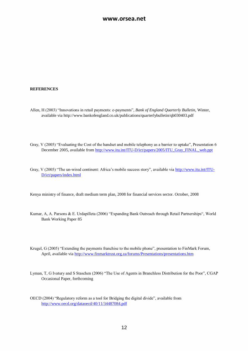
REFERENCES

Allen, H (2003) ―Innovations in retail payments: e-payments‖, Bank of England Quarterly Bulletin, Winter,

available via http://www.bankofengland.co.uk/publications/quarterlybulletin/qb030403.pdf

Gray, V (2005) ―Evaluating the Cost of the handset and mobile telephony as a barrier to uptake‖, Presentation 6

December 2005, available from http://www.itu.int/ITU-D/ict/papers/2005/ITU_Gray_FINAL_web.ppt

Gray, V (2005) ―The un-wired continent: Africa‘s mobile success story‖, available via http://www.itu.int/ITU-

D/ict/papers/index.html

Kenya ministry of finance, draft medium term plan, 2008 for financial services sector. October, 2008

Kumar, A, A. Parsons & E. Urdapilleta (2006) ―Expanding Bank Outreach through Retail Partnerships―, World

Bank Working Paper 85

Krugel, G (2005) ―Extending the payments franchise to the mobile phone‖, presentation to FinMark Forum,

April, available via http://www.finmarktrust.org.za/forums/Presentations/presentations.htm

Lyman, T, G Ivatury and S Staschen (2006) ―The Use of Agents in Branchless Distribution for the Poor‖, CGAP

Occasional Paper, forthcoming

OECD (2004) ―Regulatory reform as a tool for Bridging the digital divide‖, available from

http://www.oecd.org/dataoecd/40/11/34487084.pdf

www.orsea.net

13

Porteous, D (2006) Competition and interest rates in Microfinance, CGAP Focus Note No.33, available via

http://www.cgap.org/docs/FocusNote_33.pdf

Schapp, S & R Cornelius (2002) U-commerce: leading the new world of payments, VISA, available from

http://www.corporate.visa.com/md/dl/documents/downloads/u_whitepaper.pdf

Wright, Hughes, Richardson & Cracknell (2006) ―Mobile phone based banking: The Customer Value

Proposition‖, MicroSave Briefing Note 47, available via http://www.microsave.org/Briefing_notes.asp?ID=19

M-PESA UTILITY, OPERATION AND ENTREPRENEURIAL INNOVATIONS BY SMALL

ENTERPRISES IN KENYA

Erastus Thoronjo Muriuki,

PhD Entrepreneurship

Jomo Kenyatta University of Agriculture and Technology, Nairobi, Kenya

ethoronjo@gmail.com

Abstract

The introduction of the M-pesa in Kenya has been recognized as a key strategy for economic development and

poverty reduction particularly in developing countries. Since their independence, most economies have been

promoting the development of small enterprises as a means for economic growth. More recently, due to the

increase of unemployment and poverty, there has been a renewed focus on the promotion of small businesses not merely as an engine for growth, but more importantly as the key to job creation and poverty reduction. M-

pesa services and innovative transfer has transformed the push and pull technology greatly enhancing business

development in Kenya. Small enterprises have high failure rates which are enormous for most economies with

limited capital and other resources. The combined failure rates for businesses and barriers increases

unemployment rates and perpetuate poverty. In the light of the above, it seems necessary to call for a special

issue to address the problem surrounding small business development with the hope of encouraging more

innovativeness on M-pesa service by small entrepreneurs. This research study was therefore motivated to

determine whether the speed of service delivery, cost effectiveness, efficiency affect the demand for innovations

of the services of the small enterprises and how innovations on speed of service delivery, cost effectiveness and

efficiency affect the performance of the small enterprises.

A survey was conducted randomly within Nairobi town and the residential places in the other eight parts of Kenya. A questionnaire was provided to the selected samples of the micro enterprises in the selected places. In

the survey a total of 409 respondents completed the questionnaires out of the 2000 distributed originally. The

total number of those who returned well answered questionnaires and which were indeed used in this study was

381.

www.orsea.net

14

This study found that there exist a positive correlation between M-peas services and the level of their perceived

low costs, ease of their operations, efficiency and the speed of transaction. Further it is evident most of the

constructs and a major impact on the demand and the desire to use the M-peas services. This indicates that those

small enterprise owners who use the m-payment services also acknowledge the existence of all the perceived

variables used in this study and the positive attributes with the use of m-payment services in Kenya. However,

there exist a low degree of correlation between the perceived support from the government and the actual use of the M-payment services in Kenya. The study revealed that M-payment in Kenya is rapidly penetrating within

the country especially in the small enterprises and the micro business.

From the findings of this study, the government and the mobile service providers can promote the growth of the

small enterprises especially those which deal with M-payment by providing means of decongesting the lines,

increasing the maximum daily amount of money in the m-pesa accounts from the current amounts to facilitate

more transactions by the people and providing enough security to the services and creating awareness to the

public on how to keep their accounts secure and their PIN codes.

Key words: M-pesa; utility; entrepreneurial services; innovations; small enterprises

1 INTRODUCTION AND RESEARCH OBJECTIVES

Small enterprises have been known to play very crucial role in the development of economies and improvement

of the entrepreneurial skills of the people. The above contribute immensely towards creation of sustainable

development in the third world countries. However, these micro enterprises suffer the challenge of limited

technology and poor infrastructure which leads to loss in competitive advantage in the global scene.

Small enterprises mainly employ less than 50 workers. These, have been known to be the backbone of many

countries economic growth (Liedholm and Mead, 1999). Sustainable development implies the ability to meet current needs and seeking ways for the future generations to own their living also. In less developed countries

sustainable development aims at eradicating poverty through the associated benefits of industrial and economic

development to the less privileged in these cities.

African economies have been seeking ways of growing the small enterprise businesses through improving the

skills and technology in this very seemingly vital sector. The projected growth and upgrading of the small

enterprises into medium and large enterprises has not yet been achieved (Lukac, 2005). Such transition would

have been so important towards the growth of many African economies.

In Kenya, small enterprises have embarked on the use of m-payments in their transactions because they are

cheap and affordable to them. Many transactions are carried out by the use of mobiles such as payment of bills,

sending cash, withdrawals, payment of goods and services. Today, the services have been made cheaper by the

lowering of the value of calling cards to as low as twenty shillings. This has made many small enterprise owners to access the services (cck, 2008/2009). In 2007 a study by Arunga and Kahora found that sole proprietors and

small enterprise businesses reaped more benefits by using the mobile payments as they could make savings or

access many customers and do more services than before.

This research therefore seeks to find out the relationships that exist in the operations of the small enterprises

especially the entrepreneurial services and innovations. The survey is centered on one case of these innovations

by the small enterprises: M-pesa utility services in Kenya. The study seeks to establish the factors which

influence the small enterprises to come up with new innovations in their operations. These factors are assumed

to be related to the demand for innovations by the small enterprises.

www.orsea.net

15

Conceptual framework

Independent variable dependent variable

Figure 1: Hypothesized relationship between operations of small enterprises and innovativeness in

entrepreneurial services of the small enterprises.

The factors above are hypothesized to influence the level of innovations in the small enterprises in Kenya. This

is because they represent the general objects of most of these small enterprises which form the basis of the operations of their activities. The study will focus on how each affects the level of innovation in theses small

enterprises in their operations.

This study undertook an analysis on the two constructs of innovation and efficiency of the small enterprises

motivated by the following objectives:

1. To determine whether speed of service delivery, cost effectiveness, efficiency affect the demand for

innovations of the services of the small enterprises.

2. To establish how the innovations on speed of service delivery, cost effectiveness and efficiency affect

the performance of the small enterprises.

This study therefore seeks to establish those challenges affecting the operations of the small enterprises. The

paper also provides an analysis of how the need for speedy operations, cost effective, accessibility and ease of

operation leads to the highly innovated ideas of the small enterprises.

2 THEORETICAL BACKGROUNDS AND INFORMING LITERATURE

According to Schmitz, (1995) the desire to remain efficient is what has been the major drive for many small

enterprises in Kenya. Being efficient is brought by cluster of varied factors ranging from the emergence of suppliers, marketing agents, new service providers, specialized products, forming consortia, gathering of skilled

labour and associations which are specified by services and continued lobbying.

Accessibility

Speed of operation

Cost effectiveness

Ease of operation

Innovation by the small enterprises

enterprises

Money transfer

Technology

www.orsea.net

16

Infrastructural developments are very crucial in developing successful links within the clustered SMEs.

Planning for the infrastructure therefore starts when location choices are made and eventually spark spatial

distribution of industry compared to other aspects of the society. Planning for spatial distribution will ensure that

efficient utilization of the available land is achieved by balancing the competing factors in the scene of

sustainable development (Rozee, 2003). It is a continuing business of managing dynamics of nature by a range

of factors in the context of sustainable development (Tewdwr, 2004). This network based system in planning for the infrastructure combines mechanisms of competition and the rules of behavior. This eventually takes

advantage of differentiation and learning (Ombura, 1997). It concentrates on attracting infrastrucral facilities for

use in networking economies. Small enterprises on manufacturing sector reflect systems of high interactions

between technology and the advancement in infrastructure which determines the trends in the collective and

networking environment. The above underscores the importance of infrastructural planning to consider

promotion and development of requisite technologies.

In addition to creation of jobs small enterprise also are known to be avenues of innovation and entrepreneurial

growth. Indeed, in majority of the third world countries the micro enterprises have greatly contributed to

establishment of self-employment (Lukacs, 2005). In europe for example a study done by (Eurostat, 2008)

indicated that two thirds of employment came from the small enterprises while a similar study in Pakistan in

done by scholar Bashir(, 2008) indicated that 80 percent of the of non-agricultural employment came from the

small enterprises which contributed to nearly 40 percent of annual Gross domestic product(GDP). In the countries where majority of the people are low income earners a study done by Luckas (2005) indicated that

micro enterprises account for about 60 percent of the GDP and more than 70 percent of employment

opportunities. According to luckas most of theses micro enterprises faced the challenge of poor production

methods leading to low quality of products, low levels of production, local and narrow markets for their

products among other challenges. He highlighted the lack of technological advancement as the major block

towards the advancement of the small and large enterprises into medium or even large enterprises. Small

enterprises in less developed countries can be divided into two main categories: a) geographically segmented

enterprises which mostly concentrate on agricultural activities and are found in the rural areas and, b) clusters of

small enterprises mainly found in the urban and sub urban areas (Nadvi, 1999)

In Kenyan today, the manufacturing micro enterprises are mainly found in jua kali sheds. Jua kali is Swahili

word which means hot sun, since small enterprises mainly operate under the sun and in the open (Nadvi, 1999;

Schmitz, 1995). The advantage of theses clusters is that they enjoy the efficiency and flexibility which

individual producers may lack. Cluster model deals with growth processes of local firms. Hence, it is of great

importance to explore how these small and medium enterprises can be transformed into medium and large

enterprises in Kenya. This could be achieved better by assisting the clustered firms and not the individual ones

(Schimitz, 1995)

www.orsea.net

17

2.1: Technological Change

Information systems brought by the small enterprises was a big booster to the dissemination of information in

the market for the small enterprises in Kenya. This is because they are more efficient and thorough compared to

other methods. Today, many small and medium enterprises who invest in information system and information

technology focus on cost. According to Hagman and McCahon (1993) the adoption of IS by the small

enterprises as having brought competitive advantage. Recently Powell and Levy did a study on the small

enterprises operations‘ and reported that micro enterprises align their information systems in accordance to the

strategies so as to realize the cost advantages and value added benefits.

Advancement in technology has also created a very big challenge to small business on adoption basis since it is

sometimes costly and the small enterprises lack the know how of the technologies. According to Powell (2000),

even with the improvements in technology, little has been achieved as very few were able to use the new

upcoming technologies. He pointed out that some were unaware of new technologies and if they knew the

technology was either unavailable or unaffordable to them or away from their local settings. This meant that

foreigners still remained on the fore front in accessing technology and enjoyed the efficiency gains associated

with it, creating a gap in production between local and foreign small enterprises.

2.2 Small entrepreneurial services: A case of m-pesa services

Most small enterprises have embarked on the use of mobile methods of payments this is because it is cheap for

them in delivering cash to their creditors and business partners, could be used anywhere and any time (Anurang,

Tyagi and Raddi, 2009). By the year 2006 there were 183 banking and mobile services of making payments in

Kenya (Porteous, 2006). He even suggested that there could be more people with mobile handsets than those

who had bank accounts.

Mobile payment services have made the small enterprises to make direct transactions with their customers

without going to the banks and even going to their services premises (Anuradi, Tyagi and Raddi, 2009). They

suggested that the services were beneficial since it only required one to posses a phone and have the basics of

literacy in operating the phones. Similarly, the system did not require any physical infrastructure like the wires

and was accessible to very large portions of the population (Elder and Rashid, 2009); lastly the services could be

done in a speedy manner than before. The above features have made the operations of the small enterprises to be

so fast to operate with ease. The mobile payment agents are well distributed in the country such that the there is

ready accessibility of the payment services to the small enterprises and also they are able to access their

accounts any time.

2.2.1Transaction Costs

The costs associated with the sending of money using the mobile payment services is also very low as compared

to those from the commercial banks and other money transferring companies (Omwansa, 2009). This is true

since the cost of a transaction has a direct influence to the consumer if it is passed to them (Mallat, 2007).

Traction costs are supposed to be low if the transactions have to remain competitive. The cost of the mobile

payment services should be low than those of the banks and affordable to the micro enterprises. Recently there

are many mobile handsets which are easy to operate and have the same functions as those of the banks.

2.2.2 Speed and usability

According to the findings of a study done by Pagani (2004) most people described the current technology as

user friendly, he also suggested that it is the usability, usefulness, ease of service operation and speed that

people considered as bringing efficiency in the use of the mobile payment services. By the end of 2009, there

were more than 6.175 million known and registered m-pesa customers. The rate of registration per day stood at

11,580 (Annual report Safaricom, 20008/2009) the above figures indicates the wide use of the mobile payments

in Kenya and the satisfaction.

www.orsea.net

18

2.2.3 Easy accessibility

Accessibility is the ability to reach people. It is one of the main benefits of the mobile payment services (Pagan

(2004). Small and the medium enterprises form the biggest number of those most benefiting from the use of the

m-payment services. According to an Annual report from Safaricom (2008/2009) by march, 2009 there were

8,650 M-pesa agents through out Kenya. These services have made the micro enterprises to save more time and

go to the bank less often. The saved time is spending in their businesses. Similarly, the unbanked in Kenya now

can send and receive money (Omwansa, 2009). The use of the m-payment services is also attributable to the fact

that most of the Kenyans are familiar with the technology of the phones and require no formal training.

2.2.4 Actual Usage of the Mobile Payment and business performance

The high rate of use of the mobile phones and the transactions of the m-pesa in Kenya points to the fact that

there are more Kenyans with the m-pesa accounts than those with the bank accounts. This could to be due to the

low transaction costs of sending and receving money compared to the olden means and the banks. Secondly,

they are quicker than the rest of the methods. Person to person transactions had the value of Kshs. 120.61 billion

for the financial year 2008/2009 and the same had risen up to Kshs. 135.38 billion by the end of march 2010

(Annual report from Safaricom, 2009/2010). According to Vaughn (2009) this was reflecting how fast and deep

the services were reaching the unbanked in the society. The benefits accruing from the use of the services were

so huge that those who tried to frustrate the use of the services felt the guilty of it (Omwansa, 2009).

However, the degree of influence of the mobile payment to the operation performances of the small enterprises

largely depends on how conducive the environment is (Porteous, 2006). According to porteous an environment

is conducive if it has a set of conditions which enhanced a trajectory of developments in the market. This is

particularly on the environments where wide spread access could be rampant. M-pesa in Kenya is spread wide

but requires an enabling environment to improve the welfare of its consumers. In Kenya the small enterprise are

mostly clustered around the markets and the shopping centers providing the micro enterprises the ability to

register and transact with the other traders or their clients more effectively and efficiently as they are widely

distributed in Kenyan markets and places which receive huge gatherings.

www.orsea.net

19

Table 1 Trend of Mobile Payment Service M-Pesa

2008 march 2009 march Growth rate of the mobile

payment service

Number of registered

customers

2.075 million

6.175 million

198%

Number of retail outlets

2,262

8,650

282%

Number of person to

person transactions

14.74 billion

120.61 billion

718%

Average registrations per

day

9,965

11,580

19%

Source: Safaricom Annual Report, 2008/2009

3 RESEARCH QUESTIONS

i. Does the speed of service delivery, cost effectiveness, efficiency affect the demand for innovations of

the services of the small enterprises?

ii. How do the innovations on speed of service delivery, cost effectiveness and efficiency affect the

performance of the small enterprises?

4 RESEARCH DESIGN

A survey was conducted randomly within Nairobi town and the residential places in the other eight parts of Kenya. The reason for using the survey method was that it provides a quantitative data of the experiences, views

and even attitudes of the population chosen as the sample (Creswell, 2003; Viehland and Leong, 2007). A

questionnaire was provided to he selected samples of the micro enterprises in the selected places. The research

questionnaires included the factors from other previous studies (Davis, 1989; Venkatesh and Balla, 2008). The

respondents completed and provided the answers voluntarily. In the survey a total of 409 completed the

questionnaires out of the 2000 distributed originally. The total number of those who returned well answered

questionnaires and which were indeed used in this study was 381. This was after a rigorous process of checking

for completeness, plausibility and integrity for the purposes of ensuring quality of the study was high and

remained reflective.

In the study four independent variables were used after identifying their factors. They were subjected into a

measuring scale of likert using the five-point scale. The scale had anchors from the 5 (very great extent) to 1

www.orsea.net

20

(not at all). These were low cost, accessibility, ease of operation and efficiency. The respondents‘ data on their

demographics were collected using the single item structured questions. These were gender, years of business,

age of the agents and the period of use of the mobile payment services.

5 DATA ANALYSIS

From the original number of questionnaires distributed four hundred and nine questionnaires were returned. This

represented a response rate of ninety one percent. The questionnaires were thoroughly checked for plausibility and completeness leading to a remainder of three hundred and eighty one questionnaires.

Gender of the respondents

The researcher requested to know the gender of the respondents. Figure 1.0 below shows the results in a pie

chart.

From the findings of the study there were more male (54%) than female (46%) respondents.

Age group of the respondents

The researcher requested to know the age group of the respondents. The results are in figure 2.0 below.

From the findings of the study there were 107 aged between the ages of 18-24, 217 aged between 25-35 years

and 57 respondents had the age of 36 years and above. The results shows that there were more (57%) youths

(25-35 years), followed by the junior youths (18-25) with 28% percent and lastly the seniors (above 36 years)

youth (15%).

www.orsea.net

21

Duration of the respondents in the business

The researcher requested to know the number of years the respondents had spent in the business. The results are

given in figure 3.0 below.

From the findings, 41% percent of the respondents had worked in the business for less than a year, 40% percent

had worked in the business for a period between (2-3 years), and 11% had worked in the business for a period

ranging from (3-5 years) while 8% percent had worked in the business for more than five years. The findings

indicate that majority of the respondents had been in the business for a period below three years.

The bivariate relationship of the factors

Pearson‘s correlation coefficient was used to determine the bivariate correlation of the variables (factors being

studied). Pearson‘s correlation gives the degree to which two variables are correlated and the direction of the

correlation. Table 2 below presents the findings of the Bivariate Correlation analysis. It shows the extent of

correlation between the variables and also highlights the direction of the correlations. The variables showed

correlations ranging from 0.25 to 0.75. These are moderate correlations. The study revealed no negative

correlation of the variables.

www.orsea.net

22

Table 1: Factors which necessitate the use of M-pesa in Kenya

Not

at a

ll

Low

Exte

nt

Moder

ate

Exte

nt

Gre

at E

xte

nt

Ver

y G

reat

Exte

nt

Mea

n

Std

. D

ev.

Ease of operation 3 9 19 13 11 3.4 1.1

Lower cost (of doing

business) 1 5 23 18 8 3.5 0.9

Accessibility 3 8 22 13 9 3.4 1.1

Efficiency 2 10 19 13 11 3.4 1.1

Higher Profit 1 7 23 15 9 3.3 1.0

Table 3 shows the response on the usage of M-pesa service outcomes as a result of the benefits associated with.

A five-point Likert scale was used to interpret the respondent‘s extent. According to the scale those factors

which were not considered at all were awarded 1 while those which were considered to a very great extent were

awarded 5. Within the continuum are 2 for low extent, 3 for moderate extent and 4 for great extent. Mean and

standard deviation were used to analyze the data. According to the researcher those factors with a mean close to

3.5 were rated as to a very great extent while those with a mean close to 3.0 were rated to a low extent or even

not considered at all. On the same note the higher the standard deviation the higher the level of variations or

dispersion among the respondents.

6 DISCUSSIONS OF THE RESULTS

From the findings in table 2 above there exist a positive correlation between M-peas services and the the level of

their perceived low costs, ease of their operations, efficiency and the speed of transaction. Further it is evident most of the constructs and a major impact on the demand and the desire to use the M-peas services. This

indicates that those small enterprise owners who use the m-payment services also acknowledge the existence of

all the perceived variables used in this study and the positive attributes with the use of m-payment services in

Kenya.

However, there exist a low degree of correlation between the perceived support from the government and the

actual use of the M-payment services in Kenya at 0.170. This indicates that small enterprise users of the m-pesa

business look forward to getting support from the government and the service providers. This could be

informing of the decongestion of the lines or even regulation of the services by he government. The other factors

however, show that the use of the m-pesa services is beneficial to them with reference to cost of transaction,

ease of operation and efficiency.

From the research findings, the effect of M-pesa on lowering the cost of doing business was regarded to a very

great extent with a mean of 3.5 and a standard deviation of 0.9, the effect of M-pesa and the ease of operation

www.orsea.net

23

was regarded with a great extent mean of 3.4 and standard deviation of 1.1, accessibility was regarded with a

great extent with a mean of 3.4 and standard deviation of 1.1 .while efficiency in operations was regarded to a

great extent with a mean of 3.4 and standard deviations of 1.1 for the first two aspects and 1.0 for the last two.

The effect of M-pesa usage on profitability was regarded to a moderate extent with a mean of 3.3 and a standard

deviation of 1.1.

The research findings especially as interpreted by the standard deviation, clearly demonstrated the correlation

between the use of m-pesa in business and key strategic performance outcomes (building blocks to sustainable

competitive advantage) against which sustainable competitive advantage is achieved. As such, there is a linear

relationship between the invention of M-pesa services in Kenya and the performance outcomes.

7 RESEARCH LIMITATIONS

Although this study is highly useful, it suffers some notable limitations. Firstly, the study did not differentiate

between the informal and the formal small businesses hence a further study is recommended on this area.

Secondly, small enterprises operate in all forms of activities. This study did not differentiate the various

activities and the results should be treated with caution. This provides an avenue for further research.

Thirdly, no studies in the past have considered the success and growth factor in the micro business as a result of

using the mobile payment. Further research covering a wider scope of the small enterprises to refine these

results is needed.

Finally, the study did not look at gender in micro-business vis-à-vis the use of mobile payments. Further study

in this area remains an avenue to be explored in the future.

8 CONCLUSION AND IMPLICATIONS

The findings of this study compliments to the pool of the existing literature in various ways. The findings

indicate that perceived ease of operation, efficiency in the use, cost effectiveness and speed of operations were

all positively correlated. Some previous study highlighted the ease of operation as one of the major aspects that

motivated the use of m-pesa services in Kenya (pousttchi, 2003). These findings reflect the associated benefits

with the use of the m-pesa services in Kenya. Further most of those who returned the questionnaires were of the opinion that the services were easity accesssibile to most people than the banks

M-payment in Kenya is rapidly penetrating within the country especially in the small enterprises and the micro

business. The findings of this study confirm the earlier hypothesis of the study that the desire to operate easily,

less costly, speedily and with efficiency influences the rate of innovational adoption of the m-pesa services in

Kenya. The results of the study are useful to the Kenyan small enterprises M-pesa agents in particular they

provide greater support and enhance the customer‘s ease of operation to use the technology.

From the findings of this study, the government and the mobile service providers can promote the growth of the

small enterprises especially those which deal with M-payment by:

1) providing means of decongesting the lines

2) Increasing the maximum daily amount of money in the m-pesa accounts from the current amounts to

facilitate more transactions by the people.

3) Providing enough security to the services and creating awareness to the public on how to keep their accounts secure and their PIN codes.

These measures will go along way in motivating the mobile payment users and even enhance the growth of the

small enterprises in Kenya.

The study has identified very significant factors which influence the success of the small enterprises that is M-

pesa operators in Kenya. These factors which include: reduced cost of transactions, easily and widely accessible

services, easiness of operations of the m-payment services and the user friendliness (efficiency in the use) come

www.orsea.net

24

with the use of the M-pesa services. They represent the innovations which have been useful to the small

enterprises in Kenya.

References

Anurag, S, Tyagi, R, and Raddi S (2009). ―Mobile Payment 2.0: The Next-Generation Model,‖ in HSBC”s

Guide to cash, Supply Chain and Treasury Management in Asia Pacific.Ed.178-183.

Arunga J, Kahora B (2007). Cell phone Revolution in Kenya. International Policy Network.

Bashir, A. F. (2008). The Importance of SMEs in Economic Development. Banking, Finance and Accounting

Community. http://www.thefreelibrary.com/the importance of small and medium Enterprises I the

Economy.

Business Daily, April 18, 2009. ―Minister orders audit of Safaricom M-Pesa service‖. http://www.bdafrica.com

Accessed on 18th April, 2009

Creswell, J. W. (2003). Research Design: Qualitative, Quantitative, and Mixed method Approaches, 2nd ed.

Sage Publication, Thousand Oaks, California.

Eurostat (2003). Enterprise by Size Class-Overview of SMEs in the EU. Statistics in Focus 31/2008.

Liedholm, Can and D. Mead, (1999). Small Enterprises and Economic Development: The Dynamic Role of

Micro and Small Enterprises. London; Routledge.

Lukacs, E. (2005). The Economic role of SMEs in World Economy especially in Europe. Journal of European

Integration Studies, 4,1

Mallat, N. (2007). ―Exploring Consumer adoption of Mobile Payments- A Qualitative Study‖. The Journal of

Strategic Information Systems, 16 (4), 413-432.

Nadvi, K. (1999). Facing the Competition Business Associations in Developing Country Industrial Clusters.

Discussion Paper DP/103/1999, Geneva: International Institute of Labor Studies.

Pagani, M (2004). ―Determinants of Adoption of Third generation Mobile Multimedia services‖, Journal of

Interactive Marketing, 18 (2).

Porteous, D. (2006). The enabling environment for mobile banking in Africa. London: DFID.

Safaricom, (May, 2009), Financial Year 2008/2009; Annual Results Presentation and Investor update.

Schmitz, H. (1995). Collective Efficiency growth path for Small-Scale Industry. Small enterprises training and

technology project (MSETTP) draft report two 15- 5-1998. Ministry of Research and Technology.

Nairobi

Tewdwr, Mark-Jones. (2004). Spatial Planning: Principles and Culture. Journal of Planning and Environment

Law. May 2004.

www.orsea.net

25

APPENDIX 1

Table 2: Pearson correlation

paccess

pcost

pconvenience

psupport

actualusage

biu

paccess

1

pcost

.562(**)

1

pconvenience

.541(**)

.379(*

*)

1

psupport

.330(**)

.321(*

*)

.430(**)

1

actualusage

.265(**)

.240(*

*)

.322(**)

.170(**)

1

biu

.398(**)

.303(*

*)

.657(**)

.528(**)

.208(**)

1

** Correlation is significant at the 0.01 level (2-tailed).

* Correlation is significant at the 0.05 level (2-tailed).

www.orsea.net

26

CHALLENGES OF E-BANKING ADOPTION AMONG THE COMMERCIAL

BANKS IN KENYA

BY

Justus M Munyoki,PhD

and

Eva NdutaNgigi

Paper submitted for presentation at the 7th

ORSEA Conference to be held in Nairobi in

October 2011

www.orsea.net

27

ABSTRACT

The objective of this study was to investigate the factors influencing e-banking adoption among commercial

banks in Kenya, and the challenges faced by commercial banks in the adoption of E-banking. Descriptive

research design was adopted for the study. The study population comprised of all the 44 commercial banks in

existence at the time of study. The study was conducted by use of questionnaires which were distributed to all

commercial banks in Kenya

The results showed that banks had only partially adopted e-banking as a strategy. The issue of security was

found to be the most critical factor influencing e-banking adoption. Other major inhibitors were inadequate

regulatory support, lack of in-house it professionals and quality of infrastructure.

Key words: e-banking, adoption,

Justus M Munyoki teaches Marketing Management at the school of Business, University of Nairobi, and holds a

PhD in marketing. Eva NdutaNgigi has an MBA in marketing and is a Banker

Introduction

A strong banking industry is important in every country and can have a significant effect in supportingeconomic

development through efficient financial services. In Kenya the role of the banking industry needs to change to

keep up with the globalization movement, both at the procedural level and at theinformational level. This

change will include moving from traditional distribution channel banking toelectronic distribution channel

banking.Given the almost complete adoption of e-banking indeveloped countries, the reason for the lack of such

adoption in developing countries like Kenya is animportant research that will be addressed by this paper.

Environmental changes create pressure for change in the organization and this means that they have to respond

to relevant central change to ensure that they survive (Ansoff and Mc Donnell 1990). Technology which is a

constituent of the environment has facilitated electronic commerce, which has in turn relied heavily on the

presence of a stable and secure means of payment. The banking industry has taken advantage of the

opportunities presented by electronic commerce. Electronic Banking is a complimentary to, and a manifestation

of electronic commerce, for the simple reason that electronic commerce requires a payment system that is easily

and readily processed.

As the internet becomes more important for commerce, internet websites will take on a more central role in most

companies' strategic plans. The success of electronic banking is determined not only by banks or government

support, but also by customers' acceptance of it. Electronic banking acceptance has gained special attention in

academic studies during the past several years as banks move towards implementing electronic banking as part

of their overall strategy. The business benefit of the electronic banking is to generate additional revenue,

improve customer service, extend marketing, and increase cost saving.

www.orsea.net

28

Continuous technology development, particularly information technology revolution of the last two decades of

the 20th century has forced the banks to embrace e-banking as a strategy for their sustainable growth in an

expanded competitive environment. E-banking has made the financial transactions easier for the participants and

has introduced wide range of financial products and services.The internet has changed the operations of many

businesses, and has been becoming a powerful channel for business marketing and communication (American

Banker, 2000). The banking has followed this trend in recent years, and sometimes called E-Banking referring

to all banking transactions now completing through Internet applications (Fugazy 2000).

Electronic banking is defined by Barron‘s Dictionary (2006) as a form of banking where funds are transferred

through an exchange of electronic signals between financial institutions, rather than an exchange of cash,

checks, or other negotiable instruments.Electronic banking has changed the way the banking industry does

business by forcing the industry to consider non-traditional channels of delivering services to customers. No

doubt in the future, the banking environment will be more paperless and will overcome traditional barriers of

distance and geographic boundaries.

While e-banking has grown rapidly, there is not enough evidence of its acceptance amongst customers.

Robinson (2000) reported that half of the people that have tried online banking services will not become active

users.

The Kenyan banking industry has been expanding branch networking amid the introduction of branchless

banking system, which include the use of EFTs, ATM cards, SMS banking etc. The annual reports of CBK

clearly indicate that, branch network has been slowly expanding since 2002. By the end of December 2006,

Kenya had a total branch network of 575, as compared to 486 branches in the period ended December 2002.

Banks in Kenya have exponentially embraced the use of information and communication technologyboth in

their service provision and as a strategy to ensure their survival. They have invested huge amounts of money in

implementing the self and virtual banking services with the objective of improving the quality of customer

service. Some of the ICT-based products and services include the introduction of SMS banking, ATMs,

Anywhere banking software‘s, Core banking solution, Electronic clearing systems and direct debit among

others.

The banking industry has also over years continued to introduce a wide range of new products, prompted by

increased competition, embracing ICT and enhanced customer needs. As a marketing strategy, the new products

offered in this segment of market, continue to assume local development brand names to suit the domestic

environment and targeting the larger segment of local customer base. All the above clearly indicate that,

Kenya‘s banking Industry has great developments like any other banking market in the world.

www.orsea.net

29

Despite its importance in the economy, e-banking remains largely unexplored, with an exception of a few

studies. The objective of this study was to investigate the factors influencing e-banking adoption among

commercial banks in Kenya, and the challenges faced by commercial banks in the adoption of E-banking

The definition of e-banking varies amongst researchers partially because electronic banking refers to several

types of services through which a bank customer can request information and carry out most retail banking

services via computer, television or mobile phone (Daniel 1999; Sathye, 1999). Burr (1996) describes e-banking

as an electronic connection between the bank and customer in order to prepare, manage and control financial

transactions. On the other hand , Leow, Hock Bee (1999) state that the terms PC banking, online banking,

internet banking, telephone banking or mobile banking refer to a number of ways in which customer can access

their banks without having to be physically present at the bank branch.

E-Banking is therefore a generic term which can be separated into two categories; electronic money products

mainly in the form of stored value cards, and electronic delivery channel products. Electronic money products

are issued in exchange for cash or deposit or credit. Electronic delivery channel products are arrangements for

giving instructions for funds transfers, electronically.

Organizations will continue to invest in IT in the hope that it will improve their business process and increase

their productivity. However, for technologies to improve productivity, they must be accepted by intended users

(Venkatesh et al., 2003). Venkatesh et al., (2003) note that research in understanding user acceptance of new

technology has resulted in several theoretical models with roots in information systems, psychology and

sociology.

Theoretical Framework

Daniel (1999) in his study on provision of electronic banking in UK described electronic banking as the

provision of banking services to customers through Internet technology.

Other authors (Daniel, 1999; Karjaluoto, 2002a) found out that banks have the choice to offer their banking

services through various electronic distribution channels technologies

such as Internet technology, video banking technology, telephone banking technology, and WAP technology.

The study of Karjaluoto (2002a) further found that Internet technology is the main electronic distribution

channel in the banking industry.

Factors affecting customer acceptance and adoption of internet banking have been investigated in many parts of

the world( Williamson, 2006, Daniel 1999). On the other hand,not much has been done on this area concerning

electronic banking among commercial banks in Kenya.

www.orsea.net

30

Electronic banking acceptance has gained special attention in academic studies during the past five years as, for

instance, banking journals have devoted special issues on the topic (e.g. Karjaluoto et al., 2002) There are two

fundamental reasons underlying electronic banking development and diffusion. First, banks get notable cost

savings by offering electronic banking services. It has been proved that electronic banking channel is the

cheapest delivery channel for banking products once established (Sathye, 1999; Robinson, 2000). Second, banks

have reduced their branch networks and downsized the number of service staff, which has paved the way to self-

service channels as quite many customers felt that branch banking took too much time and effort (Karjaluoto et

al., 2003). Therefore, time and cost savings and freedom from place have been found the main reasons

underlying electronic banking acceptance

Several studies indicate that online bankers are the most profitable and wealthiest segment to banks (Robinson,

2000, Nyangosi, 2006). Electronic banking thus offers many benefits to banks as well as to customers. However,

in global terms the majority of private bankers are still not using electronic banking channel. There exist

multiple reasons for this. Foremost, customers need to have an access to the internet in order to utilize the

service. Furthermore, new online users need first to learn how to use the service .Secondly, nonusers often

complain that electronic banking has no social dimension, i.e. you are not served in the way you are in a face-to-

face situation at branch (Mattila et al., 2003). Finally, customers have been afraid of security issues (Sathye,

1999). However, this situation is changing as the electronic banking channel has proven to be safe to use and no

misuse has been reported by the media in Finland.

Many factors influence the adoption of electronic banking and it is important to take these factors into account

when studying consumer attitudes towards electronic banking. These include:

i. Effect of perceived ease of use on intention to adopt and use E-Banking. Consumers will seek out those

financial products and suppliers which offer the best value for money and they are educated about it. Hence,

for adoption of electronic banking, it is necessary that the banks offering this service make the consumers

aware about the availability of such a product and explain how it adds value relative to other products of its

own or that of the competitors. An important characteristic for any adoption of innovative service or

product is creating awareness among the consumers about the service/product (Sathye, 1999)

ii. Awareness Of services and its benefits. The amount of information a customer has about electronic banking

and its benefits may have a critical effect on its adoption. Moreover, Sathye (1999) notes that low

awareness of Internet Banking is a critical factor in causing customers not to adopt internet banking

iii. Perceived risk. Perceptions of risk are a powerful explanatory factor in consumer behavior as individuals

appear to be more motivated to avoid mistakes than to maximize purchasing benefits .The construct

Perceived Risk reflects an individual‘s subjective belief about the possible negative consequences of some

type of planned action or behavior due to inherent uncertainty.

www.orsea.net

31

iv. Quality of Infrastructure. Quality of the internet connection is seen to be an essential component of any

internet-based application. Sathye (1999) used internet access as one of the factors affecting the adoption of

Internet Banking. Without a proper internet connection the use of electronic banking is not possible.

v. Trust. Customer attitudes towards electronic banking are driven by trust, which plays an important role in

increasing usability within the electronic banking environment. The issue of trust is more important in

online as opposed to offline banking because transactions of this nature contain sensitive information and

parties involved in the financial transactions are concerned about access to critical files and information

transferred via the internet.

vi. Demographic Characteristics. Many studies have investigated the effects of customers‘ demographic

characteristics such as age gender, income and educational level on their attitude towards different banking

technologies and individual acceptance of new technology. Literature shows that there is a strong

relationship between age and the acceptance of new technologies. Older customers tend to have negative

attitude towards technology and innovations. On the other hand, younger adults are seen to be more

interested in using new technologies, like the internet to conduct activities such as looking for new products

and product information to compare and evaluate their options.

Another demographic factor of interest is income. Income has been shown to potentially exert a strong

effect on the adoption and diffusion of technology. Older individuals between 26 and 45 are over-

represented in categories of higher income, higher occupational positions, and higher educational

qualifications (Venkatesh and Morris, 2000). studies have found that there is a difference between the males

and females in using various types of technology (Burke, 2002; Li et al., 1999). Venkatesh and Morris

(2000) investigated gender differences in the context of individual adoption and sustained usage of

technology in the workplace, and found gender an important determinant of short-term usage, and can be

used to predict sustained usage behavior in individual adoption and continued usage of technology in work

places.

Education also plays a significant role with regards to attitude toward technology use. Higher educated

customers such as university graduates are more comfortable in using technology, like the internet or internet

banking. A reason for this is that education is often positively correlated with an individual‘s level of Internet

literacy (Burke, 2002).

www.orsea.net

32

Researchmethodology

This study adopted a descriptive survey design which. The study was cross-sectional in nature in that the

respondents were only interviewed once.The study population comprised of the 44 commercial banks in Kenya

in existence at the time of study. Since the population was relatively small and manageable, it was a census

study hence no sampling was done. Information was sought from the managers of the various commercial banks

in Kenya. Managers responsible for electronic banking per bank were selected for the data collection.

Data was analyzed using SPSS and presented using frequency tables and charts. The data analysis involved the

initial steps of coding, editing and tabulation as a basis for further analysis. The data was then analyzed by use

of descriptive statistics such as mean, variance and standard deviation.

DATA ANALYSIS AND PRESENTATION

A total of 300 questionnaires were distributed to the individuals working in the 44 commercial banks identified.

Of these 161 questionnaires were successfully completed and returned by respondents from 27 commercial

banks, giving a response rate of 54%.The respondents were asked to indicate the number of years their bank had

been operation. The results are shown in table 1.

Table 1: Years of Operation

No Of Years In

Operation

Frequency Percentage cumulative

percentage

0- 10 15 56% 56%

11-20 9 33% 89%

Above 20 3 11% 100%

Totals 27 100%

The results in table 1 show that 56.0% of the banks had been in operation forless than 10 years, while only 10%

have been in operation for 20 years and above. This indicates that majority of the banks have not operated more

a decade and their macroeconomic experience in the financial sector is in cycles of three years.

www.orsea.net

33

The respondents were asked to indicate the e-banking services that their banks offered. The available e-banking

services offered by the various commercial banks are listed in table 2

Table 2: E-Banking Services Offered

E-Banking Services Offered Frequency Percentage

SMS Banking/ Mobile

Banking

21 78%

Internet Banking 13 48%

Electronic Funds transfer 27 100%

The study found that all thebanks utilized EFT as one of the e-banking services to its customers. SMS banking

was adopted by 78% while internet banking was being adopted by 48% of the banks.

Respondents were asked to estimate, the proportion utility of e-banking services by their customers as presented

in Table 3

Table 3: Customer E-Service Utility

Customer E-Service Utility Frequency Percentage cumulative

percentage

Less than 20% 4 15% 15%

21%- 40% 13 48% 63%

41%- 60% 7 27% 90%

61%-80% 2 7% 97%

Over 80% 1 3% 100%

Totals 27 100%

As indicated in table 3, 48% of the respondents indicated an e-banking customer utility level of 21% to 40%,

while 27% of the respondents indicated an e-banking customer utility level of 41% to 60%. Only 10 % of the

www.orsea.net

34

respondents indicated an e-banking customer utility level of more than 60%.This means that customer utility

levels of e-banking services is just moderate.

Factors affecting the adoption of E-banking by commercial banks in Kenya

The respondents were asked to rate, on a five-point scale, the extent to which they agreed or disagreed with

statements describing why e-banking was not being adopted by their clients. The points ranged from 1 for

strongly disagree to 5 for strongly agree. The results are given in Table 4

Table 4: Factors affecting the adoption of E-banking by commercial banks in Kenya

Statement Theme Mean Std

Deviation

1 Security positively influences the perceived ease of use

of electronic banking.

Security 4.7431 0.25437

2 Quality of electronic connection and infrastructure has a

positive impact on customer‘s perceived ease of use.

Quality of ICT 4.6634 0.27986

3 Awareness of electronic banking services and its

benefits has a positive impact on customer‘s perceived

usefulness.

Awareness

programs

4.5673 0.25497

4 Electronic banking adoption has been slow since its

introduction in the bank.

Slow Adoption 4.5437 0.22239

5 Customer‘s attitude towards using electronic banking

has a significant impact on his/her intention to use it.

Customer

intention drivers

4.1875 0.26987

6 Customer‘s perceived usefulness has a positive impact

on his/her attitudes towards using electronic banking.

Customer attitude 4.1413 0.42333

7 Customer‘s perceived ease of use has a positive impact

on his/her attitude towards using electronic banking.

Ease of usage by

customer

4.1191 0.25569

8 Customer‘s perceived ease of use has a significant

impact on his/her perceived usefulness of electronic

banking.

Usefulness of e-

service to

customer

4.1095 0.25415

9 Customer‘s trust has a positive impact on his/her

attitude towards using electronic banking.

Customer Trust 4.0924 0.26392

10 Age has a significant impact on customer‘s attitude

towards electronic banking. Young customers are more

likely to adopt electronic banking.

Age of customer 4.0923 0.47821

www.orsea.net

35

11 Income has a significant impact on customer‘s attitude

towards using electronic banking.

Income levels 4.0404 0.48291

12 Education has a positive impact on customer‘s attitude

towards using electronic banking

Level of education 4.0238 0.28349

13 Gender has a significant impact on customer‘s attitude

towards electronic banking. Males are more likely to

adopt electronic banking.

Gender 4.0024 0.27396

The mean value of security was (4.7431) and a standard deviation of (0.25437). This indicates that the ICT

security is the highest factor affecting the adoption of E-banking by commercial banks in Kenya. Conversely,

gender is the lowest factor in consideration with mean of (4.0024). Quality of ICT (4.6634), Awareness

programs (4.5673) and slow adoption (4.5437) has high means that show a higher significant influence of the

adoption of E-banking in Kenya by commercial banks. Customer driven factors such as customer intention

drivers, customer attitude, ease of usage by customer, usefulness of e- service to customer and customer trust

respectively in the analysis were also rated highly. Age of customer, income levels and level of education had

lower means signifying lesser impact. Income levels, age and customer‘s perceived usefulness had a significant

standard deviation of 0.48291, 0.47821 and 0.42333 respectively indicating that the banks did not consider it as

a determining factor in e-banking adoption. The standard deviation for slow e-banking adoption was the lowest

indicating that the respondents agreed that e-banking adoption has been slow.

Challenges faced by banks in employing electronic banking as a strategy

The respondents were asked to rate, on a five-point scale, the extent to which they agreed or disagreed with

statements describing the challenges faced in implementing ICT related service in the banking main stream,

with respect to ICT industry readiness, inadequate regulatory support, Quality of ICT infrastructure and lack of

in-house IT professionals. The ratings ranged from 1 (strongly disagree) to 5 (strongly agree). Responses to

various statements were collapsed and a composite index (mean score) computed for each function. The results

are presented in Tables 5.

Table 5: The challenges faced by banks in employing electronic banking as a strategy

Theme Statement Mean Std Deviation

Inadequate regulatory support 4.13 0.80

Lack of in-house IT professional 3.99 0.96

Quality of ICT infrastructure 3.59 0.78

www.orsea.net

36

ICT industry Readiness 3.23 0.78

The results in Table 5 indicate that inadequate regulatory support was rated highest on average with a mean of

4.13 with responses deviating from this mean by a standard margin of 0.80. This is followed closely by lack of

in-house IT professional with the mean of 3.99, with standard deviation (STD DEV) of 0.96, Quality of ICT

infrastructure (mean = 3.59, STD DEV = 0.78) and ICT industry Readiness (mean = 3.23, STD DEV = 0.78) in

that order.

These findings indicate that inadequate regulatory support and lack of in-house IT professional are the greatest

challenges facing commercial banks towards the provision of e-banking services. ICT industry readiness was

lowest on the scale of effect, although it was still well above the average (mid-point), implying it is a factor

imprinting challenges to bank ICT strategy.

When asked what strategies had their banks put in place to respond to the challenges they had discussed, all the

respondents stated that they had outsourced IT support. 70% had resulted to advertising so as to create customer

awareness so as to change their perception.

60% of the banks had partnered with other players in the telecommunication industry so as to come up with

innovative e-banking products and services hence increase the number of e-banking users. One good example

given by the respondents is where banks had partnered with mobile operators to offer a money transfer service

to their customers.

www.orsea.net

37

Summaryand Discussion

The study revealed that e-banking is a relatively new banking distribution channel in Kenya

and it is at the early stages of growth and development. The study identified critical issues that stood out as

being inhibitors to e-banking adoption, among them being security, quality of ICT , awareness programs , slow

adoption , customer intention drivers , customer attitude, ease of usage by customer, usefulness of e- service to

customer, customer trust , Age of customer, level of education and gender. These findings were all in line with

previous studies that were earlier mentioned in this paper with authors like Sathye, (1999).

The study revealed that security was the most important attribute that could drive attitudes towards the adoption

of e-banking. Quality of infrastructure and awareness of electronic banking services were also a major inhibitor

on the adoption of e-banking.

There are also indicators that there are magnificent efforts on the part of the banks to create greater usage of the

e- banking, its benefits are also quite crucial for the success of the commercial banks competitive advantage.

This was observed on the demographic analysis. Responses indicated that there was a perceived risk element

and high cost in electronic banking investment besides other limiting factors identified in the study such as

inadequate regulatory support, Lack of in-house IT professional, Quality of ICT infrastructure and ICT industry

Readiness.

Recommendations

This study came up with several recommendations which have both policy as well as academic implications.

Foremost, it is evident that one major challenge of e-banking adoption is the issue of security. It is perceived

that these channels do not provide guaranteed security. It is therefore important that banks constantly improve

and upgrade their e-banking system‘s security. In order to change the perception, the bank will be required to

post security provisions on their websites so as to increase confidence and improve trustworthiness of the e-

banking systems. In Electronic transactions, which utilize the PIN, the PIN must be recognized by the Court as

being key and crucial to such transaction and there must be a method of upholding its validity in a transaction.

The issue of digital signatures must also be addressed.

Secondly, the study showed that awareness of electronic banking services and its benefits has a positive impact

on customer‘s perceived usefulness. Banks should therefore continually train their employees who will in turn

pass the knowledge to their customers hence the issue of perception is dealt with. Training will help improve

confidence as well as improve innovation. By training its employees they will realize the benefits of e-banking

services both to them and to their customers hence improve on the adoption of e-banking services.

www.orsea.net

38

Thirdly, banks need to carry out marketing research to identify the factors inhibiting e-banking adoption. Very

limited research has been carried out in this area. In this regard, banks need to regularly carry out customer

surveys so as to understand what their customer‘s needs are and as they develop their e-banking strategy then

they will formulate consumer driven strategies.

Fourthly, banks should seek to collaborate with internet service providers so as to gain high quality internet

infrastructure to enable the banks offer better quality services and at the same time enhance internet

accessibility.

Finally, this study was based on the challenges commercial banks in Kenya face during e-banking adoption. It is

therefore recommended that further study be conducted based on the customer‘s perspective.

REFERENCES

American Banker. (2000). Web Banks Beat Branches on Ratios but there‟s no competition (2000, February).

(http://web6.infotrac.galegroup.com)

Ansoff, H.I and McDonnell E. J. (1990), Implanting Strategic Management, Second Edition, Prentice Hall.

Burr, W. (1996), WieInformationtechnik die bankorganisationverandernKonnte, Bank und Markt, Vol. 11, pp.

28-31.

Burke, R.R. (2002). Technology and the customer interface: what customers want in the physical and virtual

store? Journal of the Academy and Marketing Science, Vol.30 (4), 411-32.

Daniel, E (1999). Provision of Electronic Banking in the UK and the republic of Ireland.International Journal of

Bank Marketing Vol.13 (3), 319-340.

Davis, F. D., Bagozzi, R. P. and Warshaw, P. R. (1989) User acceptance of computer technology: A comparison

of two theoretical models.Management Science, 35 (8), 982-1003.

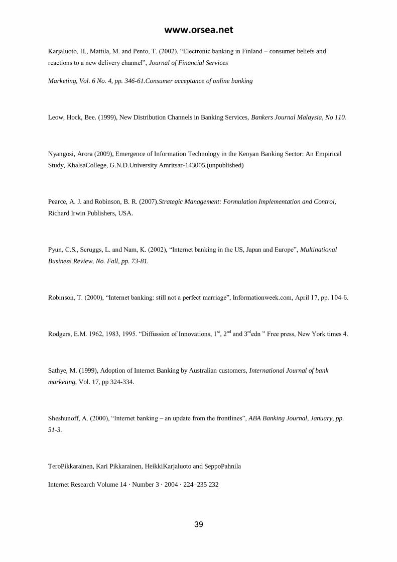
www.orsea.net

39

Karjaluoto, H., Mattila, M. and Pento, T. (2002), ―Electronic banking in Finland – consumer beliefs and

reactions to a new delivery channel‖, Journal of Financial Services

Marketing, Vol. 6 No. 4, pp. 346-61.Consumer acceptance of online banking

Leow, Hock, Bee. (1999), New Distribution Channels in Banking Services, Bankers Journal Malaysia, No 110.

Nyangosi, Arora (2009), Emergence of Information Technology in the Kenyan Banking Sector: An Empirical

Study, KhalsaCollege, G.N.D.University Amritsar-143005.(unpublished)

Pearce, A. J. and Robinson, B. R. (2007).Strategic Management: Formulation Implementation and Control,

Richard Irwin Publishers, USA.

Pyun, C.S., Scruggs, L. and Nam, K. (2002), ―Internet banking in the US, Japan and Europe‖, Multinational

Business Review, No. Fall, pp. 73-81.

Robinson, T. (2000), ―Internet banking: still not a perfect marriage‖, Informationweek.com, April 17, pp. 104-6.

Rodgers, E.M. 1962, 1983, 1995. ―Diffussion of Innovations, 1st, 2nd and 3rdedn ‖ Free press, New York times 4.

Sathye, M. (1999), Adoption of Internet Banking by Australian customers, International Journal of bank

marketing, Vol. 17, pp 324-334.

Sheshunoff, A. (2000), ―Internet banking – an update from the frontlines‖, ABA Banking Journal, January, pp.

51-3.

TeroPikkarainen, Kari Pikkarainen, HeikkiKarjaluoto and SeppoPahnila

Internet Research Volume 14 · Number 3 · 2004 · 224–235 232

www.orsea.net

40

Venkatesh, V. and F. D. Davis 2000. "A theoretical extension of the technology acceptance model: Four

longitudinal field studies." Management Science, vol. 46,

pp. 186-204.

Venkatesh, V., M. G. Morris, et al. 2003. "User acceptance of information technology:

towards a unified view." MIS Quarterly, vol. 27, no.2, pp. 425-478.

William, M. (2006) .Research methods Knowledge Base.New York: Atomic Dog Publishing.

www.orsea.net

41

An Analysis of E-learning Information System Adoption in Ugandan Universities; Case

of MUBS

By

Kituyi Mayoka & Robert Kyeyune

Department of Business Computing

Makerere University Business School

September, 2011

Abstract

This study examined e-learning failures and adoption problems in Ugandan universities based

on Rogers & Shoemaker‘s Diffusion of Technological Innovation Theory. Makerere

University Business School (MUBS) was used as a case study, where two systems i.e. KWEL

and eMUBS System were surveyed. A self-administered questionnaire was given to 200

respondents who comprised of MUBS academic staff, administrative staff and students. The

results were analyzed using SPSS and findings indicated that while the Assistant Lectures

and Lecturers have adapted to the technology, Professors were reluctant to adopt. On the

students‘ side, the results indicated that although students are aware of the technology, many

of them are not comfortable using it citing issues of accessibility and availability of the

required resources to use the technology. From the findings, a number of recommendations

have been made for faster adoption and use of e-learning at MUBS and other universities.

Key words: e-learning, adoption, sustainability, information systems

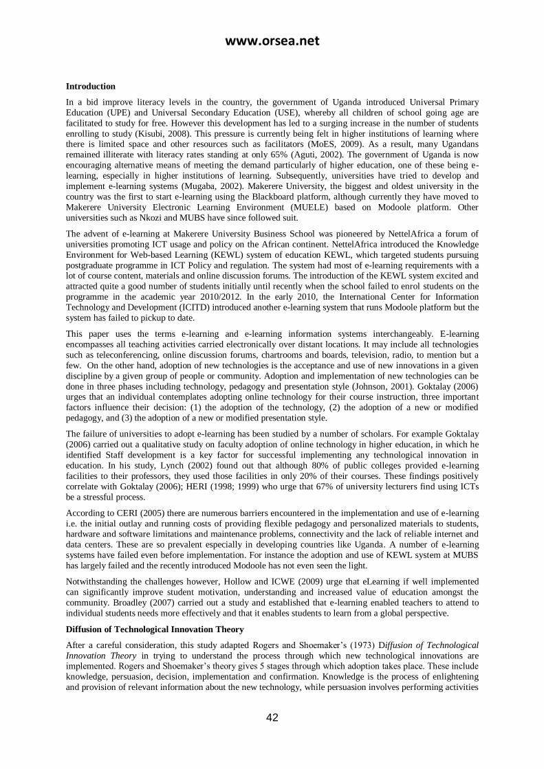
www.orsea.net

42

Introduction

In a bid improve literacy levels in the country, the government of Uganda introduced Universal Primary

Education (UPE) and Universal Secondary Education (USE), whereby all children of school going age are

facilitated to study for free. However this development has led to a surging increase in the number of students

enrolling to study (Kisubi, 2008). This pressure is currently being felt in higher institutions of learning where there is limited space and other resources such as facilitators (MoES, 2009). As a result, many Ugandans

remained illiterate with literacy rates standing at only 65% (Aguti, 2002). The government of Uganda is now

encouraging alternative means of meeting the demand particularly of higher education, one of these being e-

learning, especially in higher institutions of learning. Subsequently, universities have tried to develop and

implement e-learning systems (Mugaba, 2002). Makerere University, the biggest and oldest university in the

country was the first to start e-learning using the Blackboard platform, although currently they have moved to

Makerere University Electronic Learning Environment (MUELE) based on Modoole platform. Other

universities such as Nkozi and MUBS have since followed suit.

The advent of e-learning at Makerere University Business School was pioneered by NettelAfrica a forum of

universities promoting ICT usage and policy on the African continent. NettelAfrica introduced the Knowledge

Environment for Web-based Learning (KEWL) system of education KEWL, which targeted students pursuing

postgraduate programme in ICT Policy and regulation. The system had most of e-learning requirements with a lot of course content, materials and online discussion forums. The introduction of the KEWL system excited and

attracted quite a good number of students initially until recently when the school failed to enrol students on the

programme in the academic year 2010/2012. In the early 2010, the International Center for Information

Technology and Development (ICITD) introduced another e-learning system that runs Modoole platform but the

system has failed to pickup to date.

This paper uses the terms e-learning and e-learning information systems interchangeably. E-learning

encompasses all teaching activities carried electronically over distant locations. It may include all technologies

such as teleconferencing, online discussion forums, chartrooms and boards, television, radio, to mention but a

few. On the other hand, adoption of new technologies is the acceptance and use of new innovations in a given

discipline by a given group of people or community. Adoption and implementation of new technologies can be

done in three phases including technology, pedagogy and presentation style (Johnson, 2001). Goktalay (2006) urges that an individual contemplates adopting online technology for their course instruction, three important

factors influence their decision: (1) the adoption of the technology, (2) the adoption of a new or modified

pedagogy, and (3) the adoption of a new or modified presentation style.

The failure of universities to adopt e-learning has been studied by a number of scholars. For example Goktalay

(2006) carried out a qualitative study on faculty adoption of online technology in higher education, in which he

identified Staff development is a key factor for successful implementing any technological innovation in

education. In his study, Lynch (2002) found out that although 80% of public colleges provided e-learning

facilities to their professors, they used those facilities in only 20% of their courses. These findings positively

correlate with Goktalay (2006); HERI (1998; 1999) who urge that 67% of university lecturers find using ICTs

be a stressful process.

According to CERI (2005) there are numerous barriers encountered in the implementation and use of e-learning

i.e. the initial outlay and running costs of providing flexible pedagogy and personalized materials to students, hardware and software limitations and maintenance problems, connectivity and the lack of reliable internet and

data centers. These are so prevalent especially in developing countries like Uganda. A number of e-learning

systems have failed even before implementation. For instance the adoption and use of KEWL system at MUBS

has largely failed and the recently introduced Modoole has not even seen the light.

Notwithstanding the challenges however, Hollow and ICWE (2009) urge that eLearning if well implemented

can significantly improve student motivation, understanding and increased value of education amongst the

community. Broadley (2007) carried out a study and established that e-learning enabled teachers to attend to

individual students needs more effectively and that it enables students to learn from a global perspective.

Diffusion of Technological Innovation Theory

After a careful consideration, this study adapted Rogers and Shoemaker‘s (1973) Diffusion of Technological

Innovation Theory in trying to understand the process through which new technological innovations are implemented. Rogers and Shoemaker‘s theory gives 5 stages through which adoption takes place. These include

knowledge, persuasion, decision, implementation and confirmation. Knowledge is the process of enlightening

and provision of relevant information about the new technology, while persuasion involves performing activities

www.orsea.net

43

that convince the users to take-up the innovation. Decision stage is when the users chose to actually adopt or

reject the technology, thereby resulting into two opposing groups (adopters and rejecters). During the

implementation phase however, some adopters stop using the technology while the rejecters may change and

start using the technology. These are called late adopters. The last stage, confirmation presents 4 user groups at

the end of the process i.e. 1) continued adopters (those who have continued using the technology), 2) later

adopters (those who adopt late), 3) discontinuance (those early adopters who drop out), and 4) continued rejecters (those who maintain their rejections). The five phases of Rogers and Shoemaker (1973) Diffusion of

Technological Innovation Theory are in figure 1.

Figure 1: Diffusion of Technological Innovation Theory (Source: Rogers & Shoemaker, 1973)

Methodology

A survey research design was used, in which two e-learning systems at MUBS were surveyed. The study used

quantitative research methods to study e-learning systems at the business school. The study population covered

students, academic staff, administrative staff and IT personnel of Makerere University Business School. A target

sample of 200 respondents was used in line with Roscoe‘s (1970) rule of thumb that sample size between 30 and

500 is sufficient. Purposive sampling method was used to ensure multivariate respondents and diversity of

opinions from all the selected study groups i.e. students, academic staff, administrative staff and IT personnel of

Makerere University Business School. We collected data from two sources i.e. primary and secondary. Primary

sources included students and staff of MUBS while secondary data was gathered from published material both

within and outside Makerere University Business School. A self-administered questionnaire was given to the

selected respondents to fill-in. A total of 170 (85%) questionnaires were returned. However, we removed 66

questionnaires that were incomplete and inconsistent during data cleaning before we performed analysis on the 104 fully filled in questionnaires.

Content validity index was used to test for validity of the questionnaire (CVI > 0.50 for both experts) and

cronbach alpha coefficient was used to test for reliability (Cronbach alpha >0.60 for all variables). Using SPSS‘

descriptive statistics and means analysis methods we extracted the most important factors influencing the

success and/or failure of e-learning adoption in Ugandan universities. These factors were then fitted on Rogers

and Shoemakers Diffusion of Technological Innovation Theory, in order to help improve e-learning adoption in

Ugandan universities.

Findings

Challenges impeding e-learning IS adoption in Ugandan universities

A number of factors were put to the respondents suggesting the challenges to e-learning IS adoption in Ugandan universities. Using a likert scale of 1-5 (1= Strongly Disagree, 2=Disagree, 3=Neutral, 4=Agree and 5=Strongly

Agree). Out of the 14 factors suggested, on average, the respondents strongly agreed that Students have no

knowledge about e-learning (MEAN=4.44), Lack of top management support and leadership in e-learning

(MEAN=4.43), Resistance to change by members of staff (MEAN=4.36), Lack of resources for implementing e-

learning projects (MEAN=4.35) significantly explained why Ugandan universities have failed to adopt to e-

learning IS. However, some factors such as Students cannot afford using e-learning (MEAN=2.22), High cost of

www.orsea.net

44

telecommunication services (MEAN=3.17) were weak in explaining e-learning IS adoption failures in Ugandan

universities as seen in table 1:

Table 1: E-learning adoption challenges in Ugandan (Source: Primary data)

Minimum Maximum Mean Std.

Deviation

Resistance to change by members of staff 1 5 4.36 .637

Lack of staff training on e-learning 2 5 3.70 .725

Lack of computers and software for implementing e-learning 2 5 3.79 .997

Lack of e-learning skilled staff in universities 1 5 4.08 .915

Lack of policy and guidelines for using e-learning in universities 3 5 4.17 .663

Lack of government support for e-learning projects 1 5 3.26 1.343

Lack of private sector support for e-learning 1 5 3.33 1.465

High cost of telecommunication services 1 5 3.17 1.147

Lack of laws protecting e-learning practitioners in the country 1 5 4.25 .827

e-learning system are not secure enough to uphold academic integrity 1 5 3.23 .931

Students have no knowledge about e-learning 1 5 4.44 .709

Students cannot afford using e-learning 1 5 2.22 1.084

Lack of resources for implementing e-learning projects 2 5 4.35 .882

Lack of top management support and leadership in e-learning 3 5 4.43 .516

Valid N (list wise)

State of e-learning IS adoption at MUBS

A number of parameters were used to understand the current state of e-learning IS adoption at MUBS. These

included knowledge of e-learning, level of experience with e-learning IS and user characteristics. We applied

these parameters on both staff and students in isolation. The findings indicated that majority of MUBS staff

(62.5%) were knowledgeable about e-learning, while majority of MUBS students were not knowledgeable (40.5%). On the level of experience with e-learning usage, majority of MUBS staff (62.5%) indicated that they

used e-learning for a period of 2-5 years while majority of students (78.5%) had experienced e-learning usage

for period less than 2 years and only 18% had used e-learning for a period of 2-5 years. Thirdly, we looked at

user characteristics such as age, title and level of education in terms influencing e-learning adoption. Our

findings on the staff side show that Assistant Lecturers comprised majority users of e-learning scoring 35.6%

followed by Lectures with 24%. The Senior Lectures, Associate Professors and Professors score poorly in this

regard (12.5%, 12.5% and 2.9% respectively. While on the student‘s side, the results were centrally i.e. master‘s

students comprised of majority users of e-learning followed by PhD students with scores 52.5% and 22.8%

respectively. Results indicate that diploma and undergraduate students were the list users of e-learning with

scores 0.6% and 11.6% respectively as seen table 2.

Table 2: Staff knowledge of e-learning (Source: Primary data)

Percent

Not knowledgeable 5.0

Somewhat knowledgeable 12.5

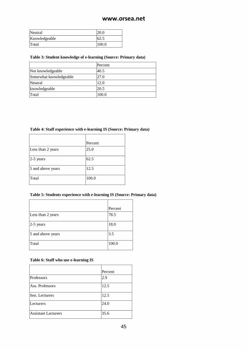
www.orsea.net

45

Neutral 20.0

Knowledgeable 62.5

Total 100.0

Table 3: Student knowledge of e-learning (Source: Primary data)

Percent

Not knowledgeable 40.5

Somewhat knowledgeable 27.0

Neutral 12.0

knowledgeable 20.5

Total 100.0

Table 4: Staff experience with e-learning IS (Source: Primary data)

Percent

Less than 2 years 25.0

2-5 years 62.5

5 and above years 12.5

Total 100.0

Table 5: Students experience with e-learning IS (Source: Primary data)

Percent

Less than 2 years 78.5

2-5 years 18.0

5 and above years 3.5

Total 100.0

Table 6: Staff who use e-learning IS

Percent

Professors 2.9

Ass. Professors 12.5

Sen. Lecturers 12.5

Lecturers 24.0

Assistant Lecturers 35.6

www.orsea.net

46

Total 87.5

System 12.5

Total 100.0

Table 7: Students who use e-learning IS

Percent

PhD students 22.8

Masters students 52.5

Undergraduate students 11.6

Diploma students 0.6

Total 87.5

System 12.5

Total 100.0

Factors influencing the use of e-learning

Guided by Rogers and Shoemakers‘ theory, we asked both students and staff to state their reasons for using e-

learning. Our findings indicate that 56.7% of staff used e-learning because of its relative advantage or need and

ease of use with that scored 21%. On the other hand, majority of students used e-learning out of curiosity

(4.2.6%) this was closely followed by relative advantage/need at 42% as seen in tables 8 and 9.

Table 8: Factors influencing staff use of e-learning (Source: Primary data)

Percent

Relative advantage/need 56.7

Compatibility 10.0

Ease of use 21.0

Curiosity 12.3

Total 100.0

Table 9: Factors influencing students use of e-learning (Source: Primary data)

Percent

Relative advantage/need 42.0

Compatibility 0.8

Ease of use 14.6

Curiosity 42.6

Total 100.0

Success factors for the adoption of e-learning in Ugandan universities

Based on Rogers and Shoemaker‘s theory of diffusion of technological innovation, and also based on the

suggested challenges impeding the adoption of e-learning, the respondents were asked to suggest that would influence successful adoption to e-learning IS by both staff and students in Ugandan universities. We used a

likert scale of 1-5 (1= Strongly Disagree, 2=Disagree, 3=Neutral, 4=Agree and 5=Strongly Agree). SPSS means

were analyzed and findings indicated that Availability of computer hardware and software (MEAN=4.53),

www.orsea.net

47

Sensitization of staff to embrace changes in technology (MEAN=4.5), Sensitization students about e-learning

benefits (MEAN=4.46) significantly influence the success of e-learning adoption in Ugandan universities.

Respondents were however in disagreement that Security and confidentiality of students and lectures data in e-

learning affected the successful adoption to e-learning as seen in table 9.

Table 9: Factors influencing successful adoption of e-learning IS (Source: Primary data)

Min Max Mean Std. Deviation

Sensitize staff to embrace changes in technology 3 5 4.50 .592

Staff training in ICTs and e-learning 2 5 4.31 .929

Availability of computer hardware and software 2 5 4.53 .826

Existence of e-learning policy and guidelines in universities 2 5 4.12 .973

Government support for e-learning projects in universities 2 5 4.35 .936

Private sector support for e-learning projects 2 5 4.23 1.050

Affordable telecom rates /prices 2 5 4.08 .926

Existence of laws governing the use of e-learning 2 5 4.23 .888

Security and confidentiality of students and lectures data in e-learning 1 5 3.77 1.173

Sensitize students about e-learning benefits 2 5 4.46 .764

Free e-learning equipments for students 1 5 4.06 1.008

Strong Top management support for e-learning 2 5 4.30 .906

Summary of findings in relation to Rogers and Shoemaker’s theory

Rogers and Shoemaker (1973) outlined the factors influencing adoption of new technologies as knowledgeable,

top mgt leadership, incentives through persuasion, relative advantage, implementation resources and perceived

ease of use. The findings in this study to a greater extent agree with Rogers and Shoemaker on these factors. For

example, majority of e-learning users and those who were willing to use e-learning were staff who were most

knowledgeable about the technology. The staff, PhD and masters students used e-learning because they had

been persuaded about the relative advantage of e-learning, while diploma and undergraduate students shunned it

because they did not know its benefits, instead they used the technology out of curiosity. The fact that resistance

to change is mainly manifested in older groups of community explains why only 2.9% of professors, the most

senior and elderly category used e-learning systems.

From the findings therefore, we identified lower level academic staff (Assistant Lecturers and Lecturers) as

early adopters to e-learning. On the other hand, findings indicate that medium level and senior academic staff including Senior Lecturers, Associate Professors and Professors were the rejecters/later adopters of the e-

learning technology. On the students‘ side postgraduate students i.e. Masters and PhD students are early

adopters of e-learning while diploma and undergraduates students were the rejecters/later adopters of e-learning.

Recommendations and Conclusion

The challenges to e-learning adoption were found to be both knowledge and Usability based. On the knowledge

based challenges, we recommend that universities should work towards improving knowledge and skills of

students and staff through training in order to increase chances of technology acceptability by users as had been

suggested by Rogers and Shoemaker. Training will also improve on perceived ease of use which directly

translates into early adoption. On Usability factors, we recommend that the government and university

management should address resistance to change through persuasion and sensitization programmes, lack of e-

learning laws through enactment of laws to guide e-learning usage and above all top management support through resource mobilization, monitoring and establishment of internal mechanisms that foster e-learning

usage.

Since lower level academic staff a postgraduate students have shown significant interest in the e-learning

technology, they should be supported and encouraged so that they do not drop out through a discontinuation

process of Rogers & Shoemakers model, while the senior academic staff and undergraduate students have been

www.orsea.net

48

identified to be rejecters/later adopters, management should sensitized on the benefits of e-learning technology

in order improve their acceptance. Management can setup a mechanism that provides incentives to these

categories directly aimed at persuading them into becoming later adopters through the process of late adoption

according to Roger and Shoemaker (1973).

References

Aguti Jessica Norah (2002). Facing up to the Challenge of Universal Primary

Education, (UPE) In Uganda through Distance Teacher Education Programmes, a Paper Presented at Pan

Commonwealth Forum on Open Learning: Open Learning: Transforming Education for Development

Broadley Tania (2007). Implementation of E-Learning: A Case Study of Three

Schools Curtin University of Technology (SiMERR WA), AARE

Goktalay Sehnaz Baltaci (2006). Faculty Adoption of Online Technology in

Higher Education, The Turkish Online Journal of Educational Technology – TOJET

HERI (1999). Faculty Survey 1998/1999. Retrieved from

http://www.gseis.ucla.edu/heri/fac_survey.html on May 13, 2011

Jonassen, D. (1994). Thinking technology. Educational Technology, 34 (4), 34-

37.

Kisubi Alfred T. (2008). Critique and Analysis of Universal Primary Education

(UPE) In Uganda in General and Suggestions for Improvement In Particular Local Areas, Presented At The Houston, Texas Busoga Twegaite Annual International Convention, May 22 – 26th, 2008

Lynch, D. (2002). Professors should embrace technology in courses. Chronicle

of Higher Education. p. B15.

Ministry of Education and Sports, (2001c), Policy Statement for 2000/2001,

MoES

Mugaba V., (20th Feb 2002). No School for 100,000; Minister Named in

Election Fraud, Enter Uganda

Rogers, E. M. (1995). Diffusion of innovation. The Free Press, New York (1995).

www.orsea.net

49

THE INFLUENCE OF ICT INFRASTRUCTURE ON READINESS TO ADOPT

E-LEARNING IN SECONDARY SCHOOLS IN KITUI DISTRICT, KENYA

BY

ANGELINE SABINA MULWA

LECTURER, UNIVERSITY OF NAIROBI

Department of Extra-Mural Studies

P.O. BOX 92, KIKUYU

E-mail: asmulwa2008@yahoo.com

Cell phone: 0724473490.

DOROTHY NDUNGE KYALO

SENIOR LECTURER, UNIVERSITY OF NAIROBI

Department of Extra-Mural Studies

P.O. BOX 92, KIKUYU

E-mail:ndunge.kyalo@yahoo.com.

Cell phone:0722821341

ABSTRACT

This article advocates for speedy provision of ICT infrastructure in all secondary schools to make it

possible for the teachers and learners to adopt e-learning to accelerate development and economic

growth of our Nation. The article explores the relationship between ICT infrastructure and readiness to

adopt e-learning in secondary schools It is based on literature review and field research by employing

cross–sectional survey research design to determine the extent to which Information Communication

Technology (ICT) infrastructure influences readiness to adopt e-learning in secondary schools in Kitui

district. A single questionnaire coupled with observation schedule were used to collect data from 15

provincial and 36 District schools selected through stratified random sampling .Null hypotheses were

tested by using two way ANOVA at 0.05 and regression analysis. The results established that institutional

factors such as infrastructure (connectivity, sources of energy and e-equipment) have a significant

influence on readiness to adopt e-learning. However, most schools in Kitui district did not have adequate

infrastructure to support the adoption of e-learning. It was recommended that the government should

seek to address the issue of e-learning infrastructure in secondary schools in Kitui district and indeed all

other districts before embarking on full scale implementation of e-learning in schools.

Key Words= Connectivity, Power/Energy, Equipment

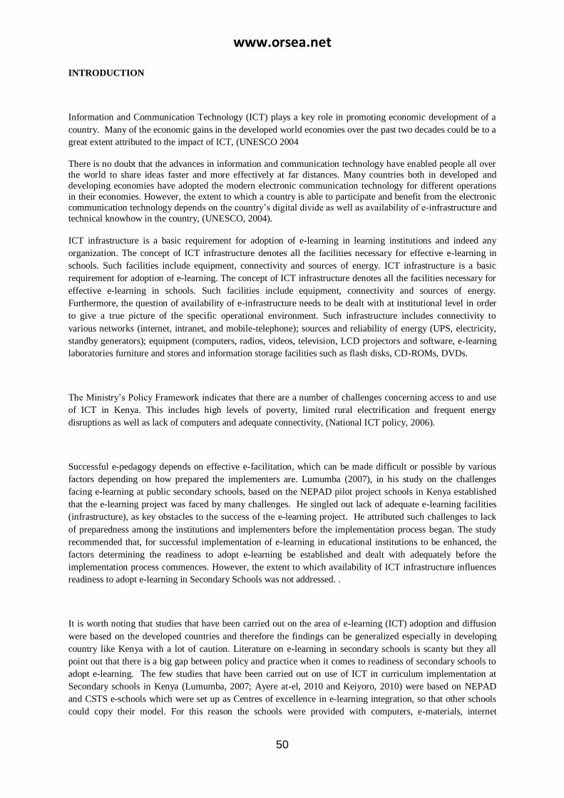
www.orsea.net

50

INTRODUCTION

Information and Communication Technology (ICT) plays a key role in promoting economic development of a

country. Many of the economic gains in the developed world economies over the past two decades could be to a

great extent attributed to the impact of ICT, (UNESCO 2004

There is no doubt that the advances in information and communication technology have enabled people all over

the world to share ideas faster and more effectively at far distances. Many countries both in developed and

developing economies have adopted the modern electronic communication technology for different operations

in their economies. However, the extent to which a country is able to participate and benefit from the electronic

communication technology depends on the country‘s digital divide as well as availability of e-infrastructure and

technical knowhow in the country, (UNESCO, 2004).

ICT infrastructure is a basic requirement for adoption of e-learning in learning institutions and indeed any

organization. The concept of ICT infrastructure denotes all the facilities necessary for effective e-learning in

schools. Such facilities include equipment, connectivity and sources of energy. ICT infrastructure is a basic

requirement for adoption of e-learning. The concept of ICT infrastructure denotes all the facilities necessary for

effective e-learning in schools. Such facilities include equipment, connectivity and sources of energy.

Furthermore, the question of availability of e-infrastructure needs to be dealt with at institutional level in order

to give a true picture of the specific operational environment. Such infrastructure includes connectivity to

various networks (internet, intranet, and mobile-telephone); sources and reliability of energy (UPS, electricity,

standby generators); equipment (computers, radios, videos, television, LCD projectors and software, e-learning

laboratories furniture and stores and information storage facilities such as flash disks, CD-ROMs, DVDs.

The Ministry‘s Policy Framework indicates that there are a number of challenges concerning access to and use

of ICT in Kenya. This includes high levels of poverty, limited rural electrification and frequent energy

disruptions as well as lack of computers and adequate connectivity, (National ICT policy, 2006).

Successful e-pedagogy depends on effective e-facilitation, which can be made difficult or possible by various

factors depending on how prepared the implementers are. Lumumba (2007), in his study on the challenges

facing e-learning at public secondary schools, based on the NEPAD pilot project schools in Kenya established

that the e-learning project was faced by many challenges. He singled out lack of adequate e-learning facilities

(infrastructure), as key obstacles to the success of the e-learning project. He attributed such challenges to lack

of preparedness among the institutions and implementers before the implementation process began. The study

recommended that, for successful implementation of e-learning in educational institutions to be enhanced, the

factors determining the readiness to adopt e-learning be established and dealt with adequately before the

implementation process commences. However, the extent to which availability of ICT infrastructure influences

readiness to adopt e-learning in Secondary Schools was not addressed. .

It is worth noting that studies that have been carried out on the area of e-learning (ICT) adoption and diffusion

were based on the developed countries and therefore the findings can be generalized especially in developing

country like Kenya with a lot of caution. Literature on e-learning in secondary schools is scanty but they all

point out that there is a big gap between policy and practice when it comes to readiness of secondary schools to

adopt e-learning. The few studies that have been carried out on use of ICT in curriculum implementation at

Secondary schools in Kenya (Lumumba, 2007; Ayere at-el, 2010 and Keiyoro, 2010) were based on NEPAD

and CSTS e-schools which were set up as Centres of excellence in e-learning integration, so that other schools

could copy their model. For this reason the schools were provided with computers, e-materials, internet

www.orsea.net

51

appliances and trained personnel. Such studies do not reflect the real situation of readiness to adopt e-learning in

normal Kenyan Secondary Schools This article examines the concept of e-learning, followed by a brief

discussion on the influence of ICT infrastructure on readiness to adopt e-learning. The rest of the article

describes the methodology used, data analysis, interpretation and discussion of findings and finally outlines the

recommendations to improve the speed to which the government and the secondary schools are moving towards

the installation of ICT infrastructure as the basic requirement for sustainable adoption of e- learning in

secondary schools.

THE CONCEPT OF E-READINESS

Mcconnel Intl, (2001) describes e-readiness as the measure of the extent to which nations are capable to

participate in the networked world. He clarifies that e-readiness measures the capacity of a nation to participate

in the digital economy by judging the relative advancement of the key important applications. E-readiness

originated with the attempt to provide a unified framework to evaluate the breadth and depth of the digital

divide between the less developed and the developed countries (Arce and Hopman, 2002). Today there is no

doubt that there is a wide gap between the developed and the developing world in terms of e-readiness. It is

therefore agreeable that e-readiness is a critical area that must be assessed and prudently addressed before

adoption of e-learning in Kenyan learning institutions and indeed all other developing countries.

Gakuu (2006) observes that information is now viewed as a basic raw material that is being consumed at an

enormous scale in the socio-economic processes and thus having competitive importance. Sadly, neither

competitive value accrues evenly across countries nor technological diffusion limits the difference in national,

political, economic, social and cultural structures. Thus Carlsson, (2004) claims that, it is very likely that

digitization of information will only benefit a few countries which have the capacity to harness the required

resources. It is also true to say that even within a country only some few well endowed regions will be able to

benefit from the digitization of information due to different levels of development.

Various international agencies have focused their attention on the phenomenon of the digital divide; The UN,

UNESCO, OECD, UNDP, the World Bank and many others. In particular, UNESCO was the first international

body who focused on the issue of digital divide which it considered as one of the most pressing ethical and

social challenges of our time. In a recent document named ―Towards the knowledge Society‖, (UNESCO World

Report (2005), it is claimed that bridging the digital divide is a priority of UNESCO mission.

Focus is placed on the need to develop a culture of knowledge enabling not only ―formal‖ but also ―effective‖

access for all to information and communication technologies (ICT). It is pointed out in the UNESCO (2005)

that new technologies cannot be implanted from the top in deprived and disadvantaged contexts. In order to be

effective; they need to come as specific local needs by means of a ―bottom- up‖ process. It is therefore

paramount to start from local practices and involve all the actors concerned (at institutional and non institutional

levels) in the specific contexts where such projects and policies are implemented. It is for this reason that the

current study focused on specific institutional and human factors that influence readiness to adopt e- learning in

secondary schools.

www.orsea.net

52

THE INFLUENCE OF ICT INFRASTRUCTURE ON READINESS TO ADOPT E-LEARNING

E-learning is new in many developing countries and is somewhat being practiced on a trial and error method. It

is actually at infancy stage. A number of African countries have just completed the pilot stage with the NEPAD

e-schools e-learning project. The experience of these schools in the pilot study indicate that successful

implementation of e-learning in secondary schools needs careful planning as there are many challenges that

need to be addressed.

The Kenya Internet Usage and Marketing Report (2006) indicate that only a few people in Kenya have a

computer at home. Radio and television access is much better while mobile phone are common place and the

number of internet users is increasing rapidly due to the number of internet cafes, shops and access centres that

are available, particularly in urban areas. However, it is feared that, due to wide use of English in Kenya usage

of internet may be congested since most sites on the internet are in English (Kenya Internet Usage and

Marketing Report, 2006). Table 2.1 below provides a statistical overview of the ICT infrastructure that is

available to the general population in Kenya.

Table 1: ICT Infrastructure in Kenya

Type of Infrastructure No. Of subscribers

Telephone lines(2005) 281,800 (2005)

Mobile telephones (2006) 4,612,000 (2006)

Internet users (3.1% of the population) 200,000 and 1,054,900

(2000 & 2006)

Internet hosts 13,274 (2006)

Television Broadcast stations 8 (2002)

Radio stations 24 AM; 18FM (2001)

Source: The world Fact Book, (2007)

As shown in Table 1, only a small percentage of the Kenyan population has access to ICT infrastructure (only

3.1% internet users). However, given the high rate at which the use of ICT is spreading especially the mobile

phones and the internet, there is hope that in few years time many Kenyans will have access to ICT.

Kenya data profile (2006) indicates that most secondary schools have some computer equipment. However, this

could consist of one computer in the office of the Head teacher. The profile also points out that very few

secondary schools have sufficient ICT tools for teachers and students. Further, it was observed that even in

www.orsea.net

53

schools that have computers, the student-computer ratio is 150:1 (Kenya data profile, 2006). Notably, given that

the conditions above are described as they were in 2006, it is likely that with the effort made by the government

toward preparation for introduction of e-learning in schools, things have improved and hence the need for a

study to establish the current situation at the grassroots.

The major problem pointed out by the Data and Statistics (2006) was that Kenya lacked adequate connectivity

and network infrastructure. It was pointed out that, although a small number of schools had direct access to high

speed connectivity through an internet service provider, generally there was limited penetration of the national

physical telecommunication infrastructure into rural and low-income areas. This fact raised a greater need for

investigating the role played by ICT infrastructure in determining readiness to adopt e-learning in secondary

schools against the ministry‘s plan to leverage the e-government initiative of networking public institutions

countrywide to facilitate the educational sector.

METHODOLOGY

The study adopted cross-sectional descriptive survey design. The design was chosen for this study due to its

ability to ensure minimization of bias and maximization of reliability of evidence collected. Furthermore

descriptive survey design raises concern for the economical completion of the research study. The method is

rigid and focuses on the objectives of the study. The study used ex-post-facto design, which is a systematic

empirical inquiry in which the researcher does not have direct control of independent variables because their

manifestation have already occurred or they are inherently not manipulable, (Emory,1985).

The study further adopted a combination of both qualitative and quantitative techniques which according to

Emory (1985) and Kothari (2004) supplement each other in that qualitative technique provides the in-depth

explanations while quantitative technique provides the hard data needed to meet the requirements of objectives

and to test hypotheses. The philosophical foundation of this study is positivism which stresses that the social

world exists externally, and that its properties should be measured through objective methods, rather than being

inferred subjectively through such approaches as intuition, sensation and reflection, (Easterby-Smith, Thorpe

and Lowe, 2002)

.

The population for this study included 51 out of 80 Public Secondary Schools in Kitui District. The sample was

selected through stratified random sampling. Data were collected by means of a questionnaire and observation

schedules. To ensure reliability of the research instrument self-administration approach was applied in data

collection and Cronbach‘s co-efficient Alpha was determined in order to measure internal consistency of the

research instruments.

Data analysis was done following the four phases normally used in many research projects, namely, data clean

up, data reduction, data differentiation and explanation. Factor analysis was done to identify the most important

infrastructure factors in influencing readiness to adopt e-learning by computing factor loadings for each factor.

These are the factors that were used in further analysis of the variables. In this study, parametric tests were used

since they are more powerful due to their ability to reduce chances of committing type II error, less likely to not

reject a null hypothesis which should be rejected. The main approaches used were the Analysis of Variance

ANOVA, Pearson‘s coefficient of correlation and Regression analysis.

www.orsea.net

54

Operationalization of the dependent and independent variables

Operational definition of the dependent and independent variables is provided here. In this study the dependent

variable for is readiness to adopt e-learning, while the independent variable is ICT infrastructure whose key

indicators include connectivity, sources of power and equipment.

Table 2: Summary of Variables and Indicators

VARIABLE INDICATORS MEASUREMENT

SCALE

Infrastructure Connectivity

Internet connectivity

mobile network coverage

Intranet connectivity

Ratio scale

Sources of power/energy

Electricity

Standing generators

Uninterruptible energy supply (UPS)

Equipment

Computers (hard software)

Radios

Televisions

Mobile phones

LCD projectors

Software

Computer laboratories

Furniture

Equipment stores

Flash disks

CD-ROMs

Diskettes

CDS

Readiness to adopt e-

learning

Reliable sources of energy.

Variety of network connections

Sufficient internet connectivity

Sufficient electronic learning equipment

Relevant skills in handling e-learning

Access to e-learning facilities in school

operationalize the e-learning machines

Teachers‘ and students‘ Interest in the use of e-

learning.

Readiness to devote extra time for- e-learning

Provision of the time e-learning in the time

table

Interval scale

www.orsea.net

55

FINDINGS AND DISCUSSION

The study set out to establish the significance of infrastructure in influencing readiness to adopt e-learning in

curriculum implementation. ICT infrastructure was studied under three indicators, namely; connectivity, source

of power/energy and equipment, from which three hypotheses were formulated to guide the study. Readiness

was measured using two key indicators, namely; availability of sufficient electronic-learning equipment and

availability of relevant skills in handling e-learning.

Principals’ Evaluation of the Schools’ Readiness to adopt e-learning based on

e- Infrastructure

The principals were requested to indicate the extent to which their schools were ready to adopt e-learning in

relation to availability of various facilities essential for e-learning which were listed in the questionnaire. They

were required to indicate in a 5 point Likert scale within the range described below.

Very great extent = 5

Great extent = 4

Minimal extent = 3

Very minimal extent = 2

No extent at all = 1

The results are summarized in Table 3.

Table 3: Principals opinion on the extent to which their schools’ are ready with e-infrastructure

Facilities Very

great

extent

Great

extent

No

extent

at all

Minimal

extent

Very

minimal

extent

CONNECTIVITY

Internet connectivity 15.7 33.3 27.5 7.8 15.7

Mobile network coverage 41.2 15.7 21.6 15.7 5.9

Intranet connectivity 25.5 23.5 41.2 2.0 7.8

EQUIPMENT

Computers 21.6 35.3 19.6 13.7 9.8

Mobile telephones 39.2 11.8 15.7 29.4 3.9

LCD Projectors 7.8 27.5 51.0 3.9 9.8

SOURCES OF POWER/ENERGY

www.orsea.net

56

Electricity supply 60.8 19.6 9.8 7.8 2.0

Uninterruptible Power Supply (UPS) 23.5 25.5 39.2 7.8 3.9

Standby generators 27.5 23.5 31.4 7.8 9.8

The findings shown in Table 3 indicate that over half of the schools enjoyed reliable mobile network coverage

as reported by 56.9% of the principals, though some 21.6% complained of total lack of network coverage in

their schools while another 21.6% suffered unreliable network coverage. This shows that, though mobile

network coverage was spread over many areas in the district some areas were still either not covered or the

network was not reliable. According to the findings, the schools were found to be at varied levels of readiness in

relation to internet connectivity. Schools that had very great access to internet constituted 15.7% while those

with great access were 33.3%. Twenty seven percent (27%) of the schools had no access to internet at all, while

the extent of access to internet of the remaining 7.8% and 15.7% of the schools had minimal to very minimal

extent of access to internet probably, because they could only access the internet from the cyber cafes in Kitui

town. With regard to intranet connectivity, only 49% of the schools were reportedly ready with this facility,

while 10% had minimal to very minimal intranet connectivity. The remaining 41% had no intranet connectivity

at all.

Most Principals felt that their schools were ready with electricity supply. For example 60.8% were ready to a

very great extent while 19.6%were ready to great extent. Those whose schools were ready to minimal and very

minimal extent constituted a combined percentage of 9.8% while those not ready at all were 9.8%. Electricity

seemed to have spread out to many schools thanks to government policy of Rural Electrification. The study

reveals that almost half of the schools had either Uninterruptible Power Supply (UPS) or standby generators.

Some 49% had UPS and 51% had standby generators while 51% and 49% respectively do not have. This

indicates that such sources of power/energy were not as widespread as electricity. The availability of electricity

could have been made through the implementation of rural electrification programme.

LCD Projectors were rare equipment in many of the schools. For example 51% of the schools were not ready

with LCD projectors, 3.9% and 9.8% were ready to a minimal and very minimal extent respectively. However,

27.5% were ready to a great extent and only7.8% of the schools was ready to very great extent. This could be

due to the high cost and skill requirement for the equipment. With regard to availability of computers in schools,

21.6%were ready to adopt e-learning to a very great extent while 35.3% ready to a great extent as they had

enough computers. However, 13.7% were ready to a minimal extent while 9.8% were ready to a very minimal

extent and only 19.6 were not ready at all. This is an indication that with some government subsidy on

computers, the schools could easily attain the required level of readiness to adopt e-learning. Furthermore, the

findings indicate that a combined percentage of 51% of the principals felt that their schools had enough mobile

phones which could facilitate e-learning, while 33.3% felt that their schools did not have adequate mobile

phones to support adoption of e-leaning while 15.7% were not ready at all. This implies that a lot of investment

needed to be committed to equipping the schools with e-facilities so as to improve on the school‘s readiness to

adopt e-learning as they were found to be very poorly equipped. The findings of the study were scientifically

validated through testing of the following three hypotheses.

Hypothesis H1 Information Communication Technology (ICT) connectivity has no significant influence on

readiness to adopt e-learning in Secondary Schools

www.orsea.net

57

ICT connectivity was measured in terms of internet connectivity, intranet connectivity and mobile telephone

network connectivity/coverage. A summary of the findings is provided in Table 4.

Table 4: The influence of Information Communication Technology Connectivity on Readiness to adopt e-

learning.

Schools’ readiness to adopt e-

learning subject to availability

of sufficient electronic learning

equipment

Schools’ readiness to adopt e-

learning subject to availability

of relevant skills in handling e-

learning

Internet

connectivity

Pearson

Correlation

.330(*)

.313(*)

Sig. (2-tailed) .018 .025

N

51 51

Intranet

connectivity

Pearson

Correlation

.233

.254

Sig. (2-tailed) .100 .072

N

51 51

Mobile

network

coverage

Pearson

Correlation

.245

.256

Sig. (2-tailed) .083 .070

N 51 51

** Correlation is significant at the 0.01 level (2-tailed).

* Correlation is significant at the 0.05 level (2-tailed).

The first finding on hypothesis H1 indicated that ICT connectivity has positive influence on readiness to adopt e-

learning. Internet connectivity had a significantly positive influence on readiness to adopt e-learning while

intranet and mobile telephone network connectivity/coverage had insignificantly positive influence on readiness

to adopt e-learning.

www.orsea.net

58

Table 5 Regression Prediction Model for Connectivity and Readiness to Adopt e-Learning subject to

Availability of Relevant Skills in Handling e-Learning

Model

summary

R R2

Adjusted

R2

Std. Error

of the

Estimate

Change Statistics

R Square

Change

F

Chang

e

df

1

df2 Sig. F

Change

.344(

a)

.118 .062 1.20961 .118 2.103 3 47 .113

Model ANOVA Sum of Squares df Mean

Squar

e

F Sig.

Regres

sion

9.231 3 3.077 2.103 .113(a)

Residu

al

68.769 47 1.463

Total 78.000 50

Model

Coefficients

Unstandardize

d Coefficients

Standardize

d

Coefficients

t Sig. 95% Confidence

Interval for B

B Std.

Error

Beta Lower

Bound

Upper

Bound

(Constant) 2.937 .463 6.348 .00

0

2.006 3.868

internet

connectivity

.198 .170 .202 1.163 .25

1

-.144 .540

Mobile

network

coverage

.109 .152 .115 .718 .47

7

-.197 .416

intranet .111 .181 .101 .612 .54 -.253 .474

www.orsea.net

59

connectivity 3

a Dependent Variable: Readiness to adopt e-learning subject to availability of relevant skills in handling

e-learning

Table 6: Regression model for Connectivity and Readiness to Adopt e-learning subject to availability of

Adequate Electronic Learning Equipment

Model Summary R R2

Adjusted R2

Std. Error of the

Estimate

1 .347(a) .120 .064 1.60110

Model ANOVA Sum of

Squares

df Mean

Square

F Sig.

Regression 16.495 3 5.498 2.145 .107(a)

Residual 120.485 47 2.564

Total 136.980 50

Model

Coefficients

Unstandardized

Coefficients

Standardize

d

Coefficients

T

Sig.

B Std. Error Beta

(Constant) 2.301 .612 3.757 .000

internet

connectivity

.322 .225 .249 1.431 .159

mobile

network

coverage

.122 .202 .097 .604 .549

intranet

connectivity

.091 .239 .062 .380 .705

a Dependent Variable: School’s readiness to adopt e-learning subject to availability of sufficient

electronic learning equipment

The findings of the regression prediction model for ICT connectivity and readiness to adopt e-learning based on

the two indicators of readiness (availability of relevant skill in handling e-learning and availability of sufficient

electronic learning equipment) indicated that ICT connectivity could be used to predict a schools‘ readiness to

adopt e-learning, with the connectivity accounting for up to 12% of the change in a school‘s level of readiness to

adopt e-learning.

www.orsea.net

60

It was further discovered that internet connectivity is the most important type of connectivity since it accounted

for almost half (1/2) of the ICT connectivity as it is evidenced by the beta values of the connectivity indicators.

The beta values for the three connectivity indicators (internet connectivity, intranet connectivity and mobile

telephone connectivity) were 0.202, 0.101, and 0.115 respectively, when readiness is measured in terms of the

availability of relevant skills in handling e-learning and 0.249, 0.062 and 0.097 respectively when readiness is

measured in terms of the availability of sufficient electronic learning equipment. This implies that without

sufficient and reliable internet connectivity in the schools successful adoption of e-learning in the

implementation of secondary school curriculum will be impossible. In fact unless the government plans and

ensures that schools especially in the rural areas are connected to internet the benefits associated with e-learning

may end up being enjoyed by only a few urban schools which are capable of acquiring internet connectivity on

their own. Based on these findings therefore, the null hypothesis which stated that the ICT connectivity has no

significant influence on readiness to adopt e-learning in secondary schools was rejected and it was concluded

that readiness to adopt e-learning in secondary school is significantly influenced by the level of ICT

connectivity in the schools.

Hypothesis H02 Sources of energy do not significantly influence Secondary Schools‘ readiness to adopt e-

learning.

The indicators for sources of energy/power included electricity supply, uninterruptible power

Supply (UPS) and stay-by generators. The findings indicated that the source energy/power has a

Positive influence on readiness to adopt e-learning which was tested as shown on Table 5.

Table 7: The Correlation between Sources of Energy/Power and Readiness to

adopt e-learning

Schools’ readiness to adopt e-

learning based on;

Electricity

supply

Uninterruptible

power supply

(UPS)

Standby

generators

Availability of relevant skills in

handling e-learning

Pearson

Correlation

.316(*)

.256

.255

Sig. (2-

tailed)

.024 .070 .071

N 51 51 51

Availability of sufficient electronic

learning equipment

Pearson

Correlation

.378(**) .374(**) .364(**)

Sig. (2-

tailed)

.006 .007 .009

www.orsea.net

61

N 51 51 51

** Correlation is significant at the 0.01 level (2-tailed).

* Correlation is significant at the 0.05 level (2-tailed).

It is evident in table 5 that electricity supply, uninterruptible power supply (UPS) and standby generators

(indicators of sources of energy) correlated significantly and positively with the availability of sufficient

electronic learning equipment (which was an indicator of readiness to adopt e-learning) with correlation

coefficient of r = 0.378, 0.374 and 0.364 respectively, while P= 0.01.

This implies that, availability of e-learning equipment will be a sufficient measure of schools‘ readiness to adopt

e-learning only if reliable sources of energy are available. It is also common sense that electronic equipment

cannot be practically useful unless there is reliable source of power/energy. For example equipping a school

with computers without providing the school with reliable sources of power will be of no use since the

computers cannot be utilized unless they are connected to power.

Hypothesis H03 (ICT) equipment does not have significant influence on Secondary Schools‘ readiness to adopt

e-learning.

The findings on this hypothesis indicated that information and communication technology (ICT) equipment had

significantly positive influence on readiness to adopt e-learning in secondary schools as shown in Table 6.

Table 8: The influence of ICT Equipment on Readiness to Adopt e-learning

Schools’ readiness to

adopt e-learning based

on;

LCD projectors

availability

Mobile

telephone

availability

Computers

availability

Availability of sufficient

electronic learning

equipment

Pearson

Correlation

.385(**) .347(*) .287(*)

Sig. (2-tailed) .005 .013 .041

N 51 51 51

Availability of relevant

skills in handling e-

learning

Pearson

Correlation

.256 .303(*) .243

Sig. (2-tailed) .070 .031 .086

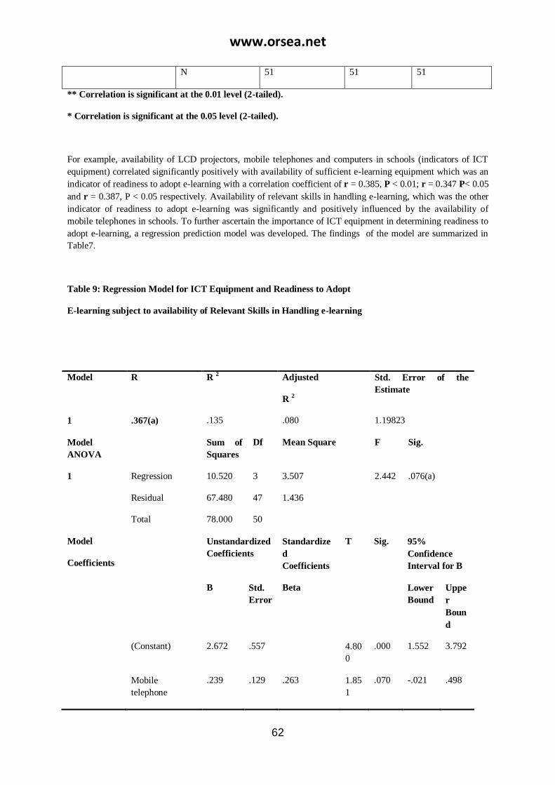
www.orsea.net

62

N 51 51 51

** Correlation is significant at the 0.01 level (2-tailed).

* Correlation is significant at the 0.05 level (2-tailed).

For example, availability of LCD projectors, mobile telephones and computers in schools (indicators of ICT

equipment) correlated significantly positively with availability of sufficient e-learning equipment which was an

indicator of readiness to adopt e-learning with a correlation coefficient of r = 0.385, P < 0.01; r = 0.347 P< 0.05

and r = 0.387, P < 0.05 respectively. Availability of relevant skills in handling e-learning, which was the other

indicator of readiness to adopt e-learning was significantly and positively influenced by the availability of

mobile telephones in schools. To further ascertain the importance of ICT equipment in determining readiness to

adopt e-learning, a regression prediction model was developed. The findings of the model are summarized in

Table7.

Table 9: Regression Model for ICT Equipment and Readiness to Adopt

E-learning subject to availability of Relevant Skills in Handling e-learning

Model R R 2 Adjusted

R 2

Std. Error of the

Estimate

1 .367(a) .135 .080 1.19823

Model

ANOVA

Sum of

Squares

Df Mean Square F Sig.

1 Regression 10.520 3 3.507 2.442 .076(a)

Residual 67.480 47 1.436

Total 78.000 50

Model

Coefficients

Unstandardized

Coefficients

Standardize

d

Coefficients

T Sig. 95%

Confidence

Interval for B

B Std.

Error

Beta Lower

Bound

Uppe

r

Boun

d

(Constant) 2.672 .557 4.80

0

.000 1.552 3.792

Mobile

telephone

.239 .129 .263 1.85

1

.070 -.021 .498

www.orsea.net

63

Computers .023 .208 .023 .110 .913 -.395 .440

LCD projectors .243 .253 .194 .960 .342 -.266 .752

a Dependent Variable: Schools’ readiness to adopt e-learning subject to availability of relevant skills in

handling e-learning

Regression analysis produced a prediction model which could be used to estimate a schools level of

readiness to adopt e-learning using ICT equipment. From the findings on the model, a schools readiness to

adopt e-learning in terms of availability of relevant skills in handling e-learning could be estimated well on

the basis of the extent to which the school has acquired ICT equipment. The model has an r2 value of 0.135,

meaning that 13.5% of change in a schools readiness with relevant skills in handling e-learning is accounted for

by availability of ICT equipment in the school.

When ICT equipment is used to predict a schools‘ readiness to adopt e-learning based on the availability

of sufficient e-learning equipment, the findings show that such a model is strong for estimating readiness

to adopt e-learning for a given level of ICT equipment could account for approximately 31% of the change

in a schools‘ readiness to adopt e-learning with a standard error of 1.2.

The findings therefore indicate that ICT equipment is crucial requirement for readiness to adopt e-learning in

curriculum delivery. For the schools to be able to utilize this modern technology meaningfully, they must

acquire the necessary ICT equipment. These would include computers, LCD projectors and mobile telephones

among others. However, lack of adequate ICT equipment was reported in almost half of the schools in Kitui

district, meaning that the schools were inadequately prepared to adopt e-learning hence an issue that the

government needs to address be implementation of e-learning commences.

As it is evident from the study, readiness to adopt e-learning was positively and significantly influenced by ICT

infrastructure. This means that successful adoption of e-learning is determined to a large extent by the extent to

which schools have acquired the necessary ICT infrastructure including adequate connectivity, reliable sources

of energy and ICT equipment. However, most schools in Kitui District were found to lack adequate ICT

infrastructure, hence not adequately ready to adopt e-learning.

Discussion of the study findings

The study established that all the three ICT connectivity indicators had some influence on readiness to adopt e-

learning in secondary schools. However, only internet connectivity had significant influence on readiness to

adopt e-learning. The findings of this study also revealed that sources of power/energy such as electricity

supply, uninterruptible power supply (UPS) and stand-by generators have significant influence on readiness to

adopt e-learning in secondary schools. The study further showed that, ICT equipment has significantly positive

influence on readiness to adopt e-learning. The study also revealed that ICT equipment was inadequate in almost

half of the schools in Kitui district.

www.orsea.net

64

The findings of this study are in agreement with the existing literature which indicates that ICT infrastructure

such as connectivity, sources of energy/power and equipment are positive influence on readiness to adopt e-

learning. However, this study is different in that, while such studies did not show the magnitude of the influence

of ICT equipment on readiness to adopt e-learning in secondary schools. neither the extent to which ICT

equipment were available in secondary schools in Kitui district- Kenya, this current study has addressed the

issue of the extent to which ICT infrastructure influences readiness to adopt e-learning in secondary schools and

the level of availability of ICT equipment in the secondary schools in Kitui district. Such studies include

Lumumba (2007) Shetty (2007) Nyaki, Oyelaran and Oyeyinka (2002) and Keiyoro (2010).

Conclusions of the Study

First, it was concluded that internet connectivity is very crucial in determining readiness to adopt e-learning. It

should also be noted that intranet connectivity and mobile network coverage will enhance a school‘s readiness

to adopt e-learning especially because internet services could be accessed via mobile phones, hence mobile

telephone network connectivity could suffice for internet connectivity particularly in the remotely located

schools. We therefore reject the null hypothesis which stated that there ICT connectivity has no significant

influence on readiness to adopt e-learning in secondary schools and conclude that readiness to adopt e-learning

in secondary school is significantly influenced by the level of ICT connectivity in the schools.

Second it was concluded that availability of e-learning equipment will be a sufficient measure of schools

readiness to adopt e-learning only if reliable sources of energy are available. Hence we reject the hypothesis and

conclude that sources of energy/power have significant influence on readiness to adopt e-learning.

Third, it could be concluded that ICT equipment are a crucial requirement for readiness to adopt e-learning in

curriculum delivery. For the schools to be able to utilize this modern technology meaningfully, they must

acquire the necessary ICT equipment, including computers, LCD projectors and mobile telephones among

others. Hence the null hypothesis and conclude that ICT equipment has significant influence on readiness to

adopt e-learning in secondary schools. However, lack of adequate ICT equipment was reported in almost half of

the schools in Kitui district, meaning that the schools were inadequately prepared to adopt e-learning hence an

issue that the government needs to address before implementation of e-learning commences.

As it is evident from the study findings, infrastructure positively and significantly influenced readiness to adopt

e-learning. This means that successful adoption of e-learning is determined to a large extent by the extent to

which schools have acquired the necessary ICT infrastructure including adequate connectivity, reliable sources

of energy and ICT equipment. However, most schools in Kitui District were found to lack adequate ICT

infrastructure, hence not adequately ready to adopt e-learning.

Recommendations of the Study

Based on the discussions and findings of this study, the researchers find it in order to make a few

recommendations which she considers important to guide other readers, researchers and policy makers. The

recommendations have been divided into those with policy implications and those meant for other researchers

for further reading.

Policy Implications

Based on the results of the study, the following recommendations are made:

The government should embark on equipping the schools with the necessary ICT infrastructure before the

process of full scale implementation of e-learning commences. Specifically the government should ensure that

all the schools are provided with electricity power supply, connected to internet services and equipped with

adequate and up-to-date computers and LCD Projectors.

www.orsea.net

65

BIBLIOGRAPHY

Allen, M. W. (2003). Guide to e-Learning: Building Interactive, Fun and Effective

Learning Program for any Company. New Jersey: John Wiley and Sons, Nairobi.

Arce, M.E. and Hopman, A. (2002). The Concept of e-Readiness and its application in Developing Countries.

Methodological Problems and Results for the e-Readiness of Nicaragua; Managua, September 2002.

Retrieved November 22, 2004 from the Ne two Startup Resource Centre (NSRC). Available from

<http://www.nsrc.org.>. [7th September, 2009].

ARC Fund (2002). Bungaria: ICT Infrastructure and e-Readiness assessment. Applied and Research

Communications Fund. Retrieved November 21st, 2004. Available from <

http://www.arc.online.bg.>. [7th June, 2009].

Ayere, A.M., Odera, F.Y. and Ayak, J.O. (2010). E-learning in Secondary Schools in Kenya: A Case of the

NEPAD e-Schools: Educational Research and Reviews Vol.5 (5), PP.218-223, May, 2010 Available

from<http://www.academic Journals.Org/ERR2 ISSN1990-3839>. [19th July, 2009].

Farrell, G. M. and Wachholz, C. (eds). (2003). ICT in Education: Meta-survey on the use of Technologies in

Asia and the Pacific. UNESCO.

Available from < www.unescobkk.org/index.php?id=1225>. [25th May, 2009].

Field, A.P. (2009). Discovering Statistics using SPSS: Sex and Drugs and rock ‗n‘ roll

(3rd edition). London: Sage.

Gakuu, C.M. and Kidombo H.J. (2008). Closing the Chasm: Are Secondary School Teachers in Kenya using

ICTs, effectively to deliver curriculum content? E-learning Africa, Book of Abstracts, ICWE, Berlin -2008

http//www/uonbi.ac.ke. Accessed on 7/7/09

Gakuu, C.M. (2006). Analysis of the Factors and Attitudes that influence lecturers‘ readiness to adopt Distance

Education and the use of ICT in Teaching: The case of the University of Nairobi. Unpublished PhD

Thesis University of Nairobi.

www.orsea.net

66

.

Hennessy, S. & Onguko, B. (eds.) (2010). Developing use of ICT to enhance teaching

and learning in East African schools: a review of the literature. Cambridge and

Dar es Salaam: Faculty of Education, University of Cambridge and Aga Khan

University, Institute for Educational Development - Eastern Africa.

Hardin, K. (1998). The old teacher in the new classroom: suggestions for: effective distance instruction (on-

line). Available from <http://www.cameron.edu/v/accessed in 2004 Karenh/disrlearn.html>. [ 20th

June, 2009].

ITU (2006). Cited in Lumumba P. (2007). A survey of challenges facing e-learning at Public Secondary

Schools: A case study of the NEPAD pilot project in Schools in Kenya. Unpublished M.ED project of

the Catholic University of East Africa

Kasomo, D. (2006). Research Methods in Humanities and Education. Eldoret: Zapf Chancery.

Keiyoro, P.N. (2010). Factors Influencing the Effective Use of ICT in Teaching and

Learning Science Curriculum in Kenyan Secondary Schools: The Case of Cyber and NEPAD e-

Schools. An Unpublished PhD Thesis of the University of Nairobi.

Kenya Data Profile. (2006). World Bank. Available from

<http://devdata.worldbank.org/external/CPProfile.asp?CCODE=KEN&PTYPE=CP>.

[29th August,2009].

Kenya Internet Usage and Marketing Report (2006). http://che.org.ke/news.html

Krecie and Morgan (1970), in Kasomo, D. (2006). Research Methods in Humanities and Education. Zapf

Chanery; Eldoret, Kenya.

Kothari. C.R. (2002). Research Methodology (2nd Edition): New Age International, New Delhi.

Kotler, P. and Armstrong, G. (2001). ―Principles of Marketing‖ (9th edition). Prentice Hall of India, New Delhi.

www.orsea.net

67

Levin, B. (1993) School response to a changing environment. Journal of Educational administration 31(2), 4-

20.

Lumumba P. (2007) A survey of challenges facing e-learning at Public Secondary Schools: A case study of the

NEPAD pilot project in Schools in Kenya. Unpublished M.ED project of the Catholic University of

East Africa.

Lundall,P. and Howell, C. (2000). Computers in Schools: A national survey of

Information and Communication Technology in South African Schools.

University of Western Cape. Education Policy Unit, University of Western Cape.

Mcconnel Intl (2001) in Gakuu C.M. (2006). Analysis of the Factors and Attitudes that influence lecturers‘

readiness to adopt Distance Education and the use of ICT in Teaching: The case of the University of

Nairobi. Unpublished PhD Thesis University of Nairobi.

Mitullah W and Waema, T.M, (2005). State of ICTs and local Governance in Kenya: Needed Analysis and

Research priorities.‘ Proceedings of worship of the local Governance and ICTs Research Network for

Africa (LOG-in Africa) held in Nairobi, 3-5the September 2005. Available from.

<http://unpan/:un.or/intradoc/public/documents/CAFRAD/UNPAN 021416.pdf>. [15th July, 2010].

O‘Kennedy, F.(1995). Accepting the new Technology. Info media, October: 8-9. Upetd.up.ac.za/submitted/etd-

09192005/06.pdf-

Omwenga I.E. (2002. Modeling and analyzing a computer – mediated learning

Infrastructure PhD thesis. University of Nairobi.

Omwenga E.I, Waema TM & Wagenda P.W (2004) A model for introducing and Implementing e-learning for

delivery of educational content within the African Context. African Journal of science & Tec (AJST)

science and Engineering Series Vol. 5 No. 1 Pg 3.

Pallant, J. (2005). SPSS Survival Manual. London: Open University Press.

www.orsea.net

68

Peterson, (1971). Theoretical aspects of correspondence instruction in Mackenzie O and Christensen, E.L (eds),

The changing world of correspondence study: University Park: Pennyslavia State University Press.

Polvin, D.J. (1976). An analysis of the urological approach to the didactics of distance education. In G.

Graholm (Ed), Programme in Kenya: A Case Study of Kisumu and Siaya Districts of Nyanza Province

Rattakul, R. and Morse, A.G (2005). ―An Assessment of e-learning Market Opportunities in the Government

Sector in Thailand,‖ Special Issue of IJCIM Proceedings of the Second International Confrerence on e-

learning for Knowledge Based Society. Bangokok, Thailand, 4-7 August 2005.

Republic of Kenya (2005). Sessional Paper No.1 of 2005, on ―A Policy Framework. For Education, Training

and Research: Meeting the Challenges of Education, Training and Research in Kenya in the 21st

Century. Nairobi: Government printer.

Republic of Kenya, (2003). Economic Recovery Strategy for Wealthy and Employment creation. Nairobi:

Government Printer.

Republic of Kenya, (2005). Ministry of Education Strategic Plan (2006 – 2011). Nairobi: Government Printer.

Samiullah, Y. and Rao, S. (2002) ―Roles of ICTs in urban and rural poverty Reduction. A Paper in the Cll-

MOEF UNEP Regional Workshop for Asia and Pacific on ICT and environment 2-3 May, 2002, New

Delhi.

Shetty (2007). Cited in Lumumba P. (2007) A survey of challenges facing e-learning at Public Secondary

Schools: A case study of the NEPAD pilot project in Schools in Kenya. Unpublished M.ED project of

the Catholic University of East Africa

www.orsea.net

69

ENVIRONMENT AND CLIMATE CHANGE

APPLICATION OF GOAL ALGORITHM IN QUANTIFYING THE EFFECT OF

TILLAGE AND EQUIPMENT ON SMALLHOLDER FARM PRODUCTIVITY

Name of author?

ABSTRACT

This study addressed the problem of inadequate utilization of farm equipment for conservation tillage

production in Kenya. It aimed at analyzing the effect of tested farm equipment on optimum maize production

subject to available labour, land, power and specified crop residue recycle. After selecting and testing available

tools and equipment it was found that land breaking, furrow making, timely planting and weeding are possible.

It was also found that innovative animal draft power (ADP) tillage equipment could significantly minimize

runoff. A single objective linear programming (LP) model was formulated to estimate optimum production with

input data drawn from technical test performance. The input parameters used were available farm labour, land,

schedule of maize production tillage operations and expected yield for various levels of timeliness of planting

and weeding. The output production was kilograms of maize grain dry matter available per farm. LP models

suffer serious limitations due to assumptions of linearity, certainty and use of single goal whereas reality is non-

linear, is risky and multiple goaled. Multiple goal models impose serious complexities in data collection,

analysis and interpretation. Goal programming was therefore recommended because of its simplicity. Goal

programming was carried out to determine optimum energy use subject to specified crop residue recycles. The

energy consumption for various timeliness combinations was substituted for yield as the coefficient of the

objective function to minimize energy use. Results show that farmers who own ADP do not require tractor

powered (TP) mechanization for seasonal operations unless more than 4 ha per farmer cultivated land is

available. For farmers who do not own ADP, it is more beneficial to switch to new ADP equipment than to

supplement their capacity with hired tractors. It is recommended that researchers consider long term quantifiable

productivity attributable to farm equipment for smallholders as one of the prerequisite for mechanization

selection.

1. INTRODUCTION

The optimum time period for farm operations depends on crop growth requirements on one hand, and on the

other, on the machine workable time limited by the weather and soil conditions, as well as crop conditions in

case of harvesting, Van Elderen (1977 & 1978); Portiek (1975); Tulu (1973); Cervinka & Chancellor (1972). If

the farmer wants to be 90% sure to get the job done, then the number of hours must be assumed likely at 90%

probability. This then becomes the basis for acquiring labour and machines with the relevant capacities to get

the operations done on time with that level of confidence.

Available farm operation scheduling models have been developed to select machines for specific timeliness

requirements. Except in certain harvesting and sometimes planting situations, Cervinka & Chancellor (1972);

Van Elderen (1977), few timeliness functions relating loss in yield or revenue to the time of a particular

operation have been developed. In other words, the actual physical effect on crop growth of the particular

delayed operation has not been explicitly stated. Consequently, the timeliness requirements have been unduly

rigid. For this reason, the machine selection and scheduling models have in many cases been designed to meet

these exact timeliness requirements at minimum cost. The fact that allowing some degree of delay may be

optimum has not received sufficient attention since neither power nor energy requirements were considered

www.orsea.net

70

limiting. The other possible reason for not considering less than timely alternatives is that, in developed

countries farming is already very profitable and generally timely. The problem is usually to select and schedule

farm machinery to guarantee timeliness at the time of very adverse weather. Models are therefore used to

optimize the selection minimizing investment on machinery and increasing profit.

The situation is different in the Less Developed Countries (LDCs) especially in semi arid small-holder

agriculture where operations are generally untimely and farming is generally unprofitable. The main reasons for

this are that soil conditions in these areas are too difficult for the available human and animal power and the

implements may be inappropriate, Muchiri (1984). Furthermore labour bottlenecks are experienced not only during land preparation and planting but also during the subsequent weeding and even harvesting. Thus early

land preparation of a relatively large area to take advantage of limited rainfall may create labour bottlenecks

during early weeding and may nullify the benefits of early planting, Muchiri (1976). Spread-out planting, i.e.,

allowing some late planting deliberately, may make it possible for the farmer to take care of early germinating

weeds while planting and delay the weeding operation to a time when there is no labour bottleneck, Nadar

(1984). In this way, better labour utilization may be achieved. The problem arises when early weeding

requirements coincide with late planting and the farmer cannot easily determine the optimum labour allocation,

Muchiri (1976). However due to weather uncertainties and inadequate soil moisture conservation, late planting

takes precedence over early weeding.

The other important point is that increased yield does not arise from one operation but a set of operations such

as land preparation, planting and weeding. The opportunity cost for carrying out a single operation is

meaningless in this case. What is required is an optimization model in which timeliness requirements are

included as constraints over the cropping season. This is the approach adopted for this study. The main objective

was therefore to develop a model for quantifying the effect of tillage and equipment on maize production and

energy consumption subject to available labour, land, power and specified crop residue recycle.

2. LITERATURE REVIEW

1.1 Various Small-holder Modelling Techniques

The need to incorporate several interacting factors that affect technological impact on small-holder farm

business has led many researchers to use various modelling techniques. Linear programming (LP) techniques

have been used to examine the effect of technological innovations, Low (1975); Heyer (1971); Hardaker (1979);

Kinsey (1980); Mutebwa (1979); Mc Carl and Nuthall (1982); Mc Rota (1997). Low (1975) for example used a

farm level LP model to test the effect of new technologies including tractor mechanisation, improved cropping

system, storage and credit on small Ghanaian farms. While observing that the farmers‘ resource allocation was

near optimum, Low (1975) conceded that there is a need for technological interventions. Neither tractor

mechanization which solves the labour problem during land preparation only to create another at weeding time

nor high yielding but drought evading, hence risky maize variety were appropriate. However, incorporating

storage facilities to guarantee subsistence in adverse years improved cost benefit ratio considerably.

Hadarker (1979) identified three general criticisms against linear programming applications to farm level

problems: assumption of certainty when the pervasiveness of risk is widely appreciated assumption of linearity

whereas reality is invariably non-linear, and use of single goal instead of multiple goal objective functions

which are closer to reality. Anderson et al. (1977) observed that the problems of non-linearity and programming

under risk are connected with the additional computational burden. The extra effort is therefore likely to be

ignored in project development. Anderson and Hadarker (1979) in their comprehensive review of economic

analysis in design of new technologies for small farmers have recognized the general complexity of small farm

www.orsea.net

71

enterprise and that any attempt to include all the possible activities and constraints would soon lead to

computational problems. It was suggested that a new technology could be classified into one of the following

three categories, i.e., notional technologies which are analyzed through models only, preliminary technologies

which are analyzed for certain target groups, and developed technologies which are well tested and require

communication to the target group for adoption.

A multi-criteria approach to the choice of technology for farmers in semi-arid smallholder agriculture proposed

an attempt to develop a simple farm equipment selection model that can integrate available information that

affects production. By using single criterion objective functions the models are unable to examine other equally

important objectives, which may be conflicting, or having different units of measurements. Alocilia and Ritchie

(1993) have observed that existence of multiple objectives in agriculture is a rule rather than an exception –

profitability being only a part of the overall concern for agricultural sustainability.

Van Latesteijn (1993) discussed A Methodological Framework to Explore Long Term Options for Land Use.

The framework showed how quantitative relations between a number of self-contained technical development

processes in agriculture, socio-economic and environmental policy objectives can be modelled. A dynamic crop

simulation model and a geographical information system that comprise soil characteristics, climatic conditions

and crop properties were used to calculate regional yield potentials for indicator crops. Next, a linear

programming model that contains several policy derived objective functions is applied to calculate optimal

regional allocation of land use. Different restrictions can be put to the objective functions. The model proposed

by Van Latesteijn (1993) is simply a mathematical instrument to explain the relationship between policy

objectives and technical performance at farm level. Thus, the model assists the policy makers to understand and

select strategies that can achieve policy objectives, subject to the potential limits fixed by socio-economic and

physical environment.

In this study consideration is given to technologies, which are well developed and require communication to

farmers. A linear programming (LP) model is used in conjunction with ‗Interactive Multiple Goal

Programming‘ (IMGP). An LP-Model is generally used to optimize a single objective function. The IMGP

procedure makes it possible to optimize a set of objective functions in an interactive process.

1.2 Goal Programming

Bhattacharya (2005) developed a goal programming model to predict the yield of sugarcane three months before

harvest. The biometric characteristics used were plant height, girth of the cane, number of canes per plot and

width of third leaf from the top. Goal programming was compared with the conventional multivariable

regression analysis. Although some of the characteristics are correlated, regression analysis is based on the

assumptions of normality, independence and homoscedasticity. After demonstrating that both have equal level of

accuracy, goal programming was recommended for predicting sugarcane yield three months before harvesting in

situations where the assumptions of conventional regression analysis are violated.

Sharma et al. (2007) developed ‗Fuzzy‘ goal programming for optimum allocation of land under cultivation and

proposes an annual plan for different crops. Goals such as crop production, net profit, and machine requirements

are modelled as fuzzy. The fuzzy goals are transformed to linear constraints by introducing tolerance variables.

He showed that the model allows tolerances in the allocation of resources in order to fit the prevailing

circumstance of the analysis.

www.orsea.net

72

Taha (1997) explained that there are situations where it is impossible to find a single solution that optimizes the

conflicting objectives. In such situations, a compromise solution based on the relative importance of each

objective is all that can be achieved. The principal idea in goal programming is to convert the original multiple

objectives into a single goal. The resulting model yields what is usually referred to as an efficient solution

because it may not be optimum with respect to all the conflicting objectives of the problem. This is the

mathematical modelling adopted for this study.

3. METHODOLOGY

3.1 Effect of Tested Conservation Tillage and Equipment on Farm Production

Linear and goal programming techniques are appropriate for quantifying the effect of technologies on small

farm production which focused on linear and goal programming, Taha (1997).

3.1.1 The Conceptual Model

The purpose of the model illustrated in Figure 3.1 below is to show how the analysis was carried out including

secondary sources of data. From Figure 3.1 it is clear that reliable yield data estimates are required. This will

combine with data on available land, available labour and equipment field test data on capacity (ha/hr) to

generate production at individual farm or a group of farmers. Linear programming model was used for

quantifying expected production of a single farm or a group of small farms in case innovative farm equipment is

successfully adopted.

Figure 3.1 illustrates input data and the expected outputs. The data required include (i) expected yield (ii)

available labour (iii) available land for cultivation (iv) field capacity of available equipment innovations and (v)

specified crop residue recycle. Figure 3.2 illustrates input data and the expected outputs. The data required

include (i) expected energy consumption per ha (ii) available labour (iii) available land for cultivation (iv)

equipment field capacity (v) optimum productivity (LP solution) and (vi) specified crop residue recycle. The

high lights of data sources are given below.

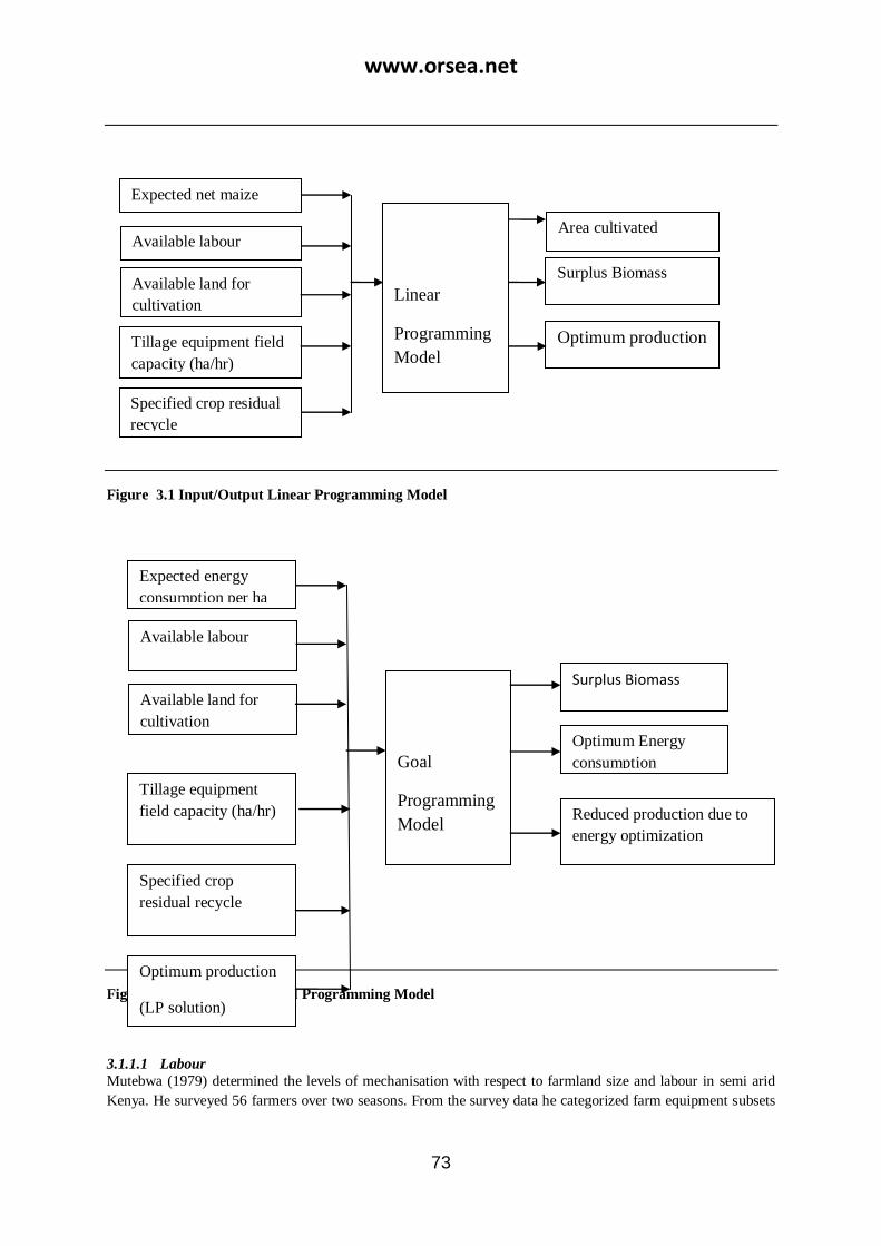
www.orsea.net

73

Figure13.1 Input/Output Linear Programming Model

Figure23.2 Input/Output Goal Programming Model

3.1.1.1 Labour

Mutebwa (1979) determined the levels of mechanisation with respect to farmland size and labour in semi arid

Kenya. He surveyed 56 farmers over two seasons. From the survey data he categorized farm equipment subsets

Specified crop residual

recycle

Linear

Programming

Model

Expected net maize

yield

Available labour

Available land for

cultivation

Surplus Biomass

Optimum production Tillage equipment field

capacity (ha/hr)

Area cultivated

Goal

Programming

Model

Expected energy

consumption per ha

Available labour

Available land for

cultivation

Surplus Biomass

Optimum Energy

consumption

Tillage equipment

field capacity (ha/hr)

Specified crop

residual recycle

Optimum production

(LP solution)

Reduced production due to

energy optimization

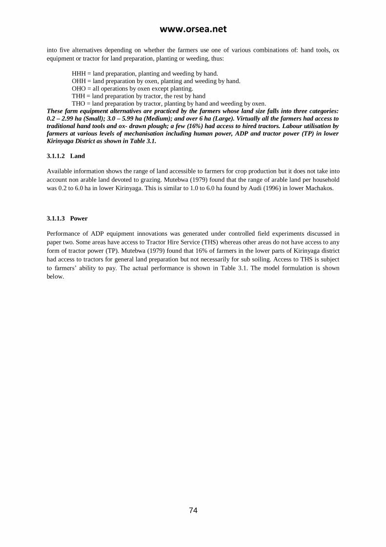
www.orsea.net

74

into five alternatives depending on whether the farmers use one of various combinations of: hand tools, ox

equipment or tractor for land preparation, planting or weeding, thus:

HHH = land preparation, planting and weeding by hand.

OHH = land preparation by oxen, planting and weeding by hand.

OHO = all operations by oxen except planting.

THH = land preparation by tractor, the rest by hand

THO = land preparation by tractor, planting by hand and weeding by oxen.

These farm equipment alternatives are practiced by the farmers whose land size falls into three categories:

0.2 – 2.99 ha (Small); 3.0 – 5.99 ha (Medium); and over 6 ha (Large). Virtually all the farmers had access to

traditional hand tools and ox- drawn plough; a few (16%) had access to hired tractors. Labour utilisation by

farmers at various levels of mechanisation including human power, ADP and tractor power (TP) in lower

Kirinyaga District as shown in Table 3.1.

3.1.1.2 Land

Available information shows the range of land accessible to farmers for crop production but it does not take into

account non arable land devoted to grazing. Mutebwa (1979) found that the range of arable land per household

was 0.2 to 6.0 ha in lower Kirinyaga. This is similar to 1.0 to 6.0 ha found by Audi (1996) in lower Machakos.

3.1.1.3 Power

Performance of ADP equipment innovations was generated under controlled field experiments discussed in

paper two. Some areas have access to Tractor Hire Service (THS) whereas other areas do not have access to any

form of tractor power (TP). Mutebwa (1979) found that 16% of farmers in the lower parts of Kirinyaga district

had access to tractors for general land preparation but not necessarily for sub soiling. Access to THS is subject

to farmers‘ ability to pay. The actual performance is shown in Table 3.1. The model formulation is shown

below.

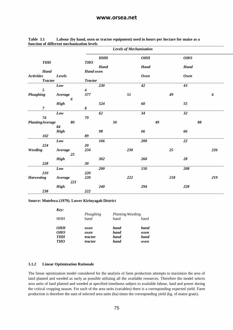
www.orsea.net

75

Table23.1 Labour (by hand, oxen or tractor equipment) used in hours per hectare for maize as a

function of different mechanization levels

Levels of Mechanisation

HHH OHH OHO

THH THO

Hand Hand Hand

Hand Hand oxen

Activities Levels Oxen Oxen

Tractor Tractor

Low 230 42 43

5 4

Ploughing Average 377 51 49 6

6

High 524 60 55

7 8

Low 62 34 32

74 79

Planting Average 80 50 49 88

84

High 98 66 66

102 89

Low 166 200 22

224 20

Weeding Average 234 230 25 226

25

High 302 260 28

228 30

Low 200 150 208

210 220

Harvesting Average 220 222 218 219

221

High 240 294 228

238 222

Source: Mutebwa (1979). Lower Kirinyagah District

Key:

Ploughing Planting Weeding

HHH hand hand hand

OHH oxen hand hand

OHO oxen hand oxen

THH tractor hand hand

THO tractor hand oxen

3.1.2 Linear Optimization Rationale

The linear optimization model considered for the analysis of farm production attempts to maximize the area of

land planted and weeded as early as possible utilizing all the available resources. Therefore the model selects

area units of land planted and weeded at specified timeliness subject to available labour, land and power during

the critical cropping season. For each of the area units (variables) there is a corresponding expected yield. Farm

production is therefore the sum of selected area units (ha) times the corresponding yield (kg. of maize grain).

www.orsea.net

76

For each variable there is a specified number of operations that must be carried out according to a given time

schedule in order to attract the corresponding yield. The tillage subsystem is defined by the nature of operations

that are specified. Each operation is carried out by a tillage equipment subset which consists of operation

schedule, equipment hardware, field capacity, and number of men.

Therefore for each variable the number of subsets in the subsystem defines the tillage that is applied. The

purpose of this model is not to optimize the allocation of resources in a particular farm unit but rather to

quantify the optimum production of typical farm size units for the purposes of corporate planning of a

mechanization scheme. Therefore actual labour or land resources in a particular farm setting are not necessary.

For these reasons, family specific socio-economic and cultural factors, which affect access to labour, land and

power, are not considered. The model considers a range of labour, land and power utilization and computes the

corresponding farm production. In addition to farm production, the model attempts to minimize energy

consumption. The model also recycles a specified amount of crop residue to contribute to building up of organic

matter content.

3.1.2.1 Single Objective Linear Programming

Farmer’s production is the sum of the product of the cultivated area units and associated expected yield of

each of the selected timeliness crop production schedules (variables).

The general Linear Program (LP) is;

Maximise

j

n

J

j xcz

1

3.1

Such that

j

n

J

ij xa1

3.2

And ,,2,1, ibx ij

njx j ,,2,1,0

Farmers‘ gross production is the sum of the product of the cultivated area units multiplied by the corresponding

crop yield to the selected timelines crop production schedules.

The variables are defined as

xnm= Area of the maize activity planted n weeks late and weeded m weeks late for n, m=0, 1, 2, 3.

ynm = the expected yield corresponding to the timeless schedule nm.

www.orsea.net

77

Therefore the objective function becomes

nm

n m

nm yxz

3

0

3

0

3.3

The problem has four constraints

1. The number of hours available from each power unit during the critical (week) period cannot be

exceeded. Given that is the number of hours available for ith crop operated by the power unit j

during working period t.

Given that H (i,j,k,t) = hours per ha required for ith crop in kth operation powered by jth power unit in the

week period t , then the constraint becomes

),,(

1

3

0

3

0

),,,( tji

k

kn m

nm btkjiHx

3.4

For i=1; j=1, 2, 3; t=1, 2… 10.

For animal draft power (ADP), j=1; tractor power (TP), j=2;

2. The number of man hours available during the critical (week) period cannot be exceeded. Where M(i,j,k,t)

is the man hours per ha required for ith crop in the kth operation by jth power unit during working period t.

So the second constraint becomes

),,(

1

3

0

3

0

),,,( tji

k

kn m

nm btkjiMx

3.5

3. The model recycles a predetermined quantity of crop residue regardless of the quantity produced. If

necessary the model draws from uncultivated land. The constraint equation to ensure residue recycle is

given by

0)(3

0

3

0

nmr

n m

nm YCBx 3.6

B is the specified crop residue recycle in kg per ha and Cr is crop residue / maize grain ratio.

The accessible land for cultivation ranges from 2 ha to 4 ha per farmer. So the fourth constraint

becomes

hxn m

nm

3

0

3

0

3.7

4. The non-negativity constraint where xnm cannot assume negative values.

xnm ≥ 0, n = 0, 1, 2, 3; m=0, 1, 2, 3.

www.orsea.net

78

Thus the whole LP becomes

Maximise equation 3.3 subject to equations 3.4-3.7

With xnm ≥ 0, n=0, 1, 2, 3; m = 0, 1, 2, 3.

For the purpose of maximizing net production the net crop yield can be substituted for the gross crop yield

where the net crop yield is given by

∆ynm = ynm – y‟nm

and y‟nm is the break even yield

The LP model formulated above was used to carry out estimates of net production per farm unit.

),,,(

),,,(

),,,(

),,,(

),,,(

)(

)(

)(10

tkjia

tkji

tkji

tkji

tkjiC

rnp

wev

rnpH

3.8

),,,(

),,,(

),,,(

),,,(

),,,(

)(

)(

)(10

tkjia

tkji

tkji

tkji

tkjiC

rnmnp

wev

rnmnpM

3.9

Where: np is the number of power units operating together, nm the number of men per power unit, r the number

of replications per operation, v the speed in km/h, e efficiency, w = width in meters and

10

wevCa

3.10

3.1.3 Goal Programming

The purpose for agricultural development is to achieve high but sustainable profit. Therefore the following

goals must be achieved concurrently namely:

Increased production

Optimum energy consumption

Residue bio-mass recycle

Goal formulation was as follows:

Maximize net production expressed in equation 3.3

www.orsea.net

79

Since high priority goal values of Z were determined by the single objective LP formulation discussed above,

energy goal was optimized as follows:

Minimize energy requirements

nm

n m

nm EIPXEIG )(3

0

3

0

3.11

Where (EIP)q is the energy requirement per hectare and EIG is the gross energy requirement.

Subject to

ZSSyx nm

n m

nm

11

3

0

3

0

(Production Goal) 3.12

0)( 11

3

0

3

0

SSYCBx nmr

n m

nm (Residue recycle goal) 3.13

Equations 3.4, 3.5 and 3.7

x1, x2,------------, xq , 1 1 S S, 2 2

S S, ≥ 3.14

The optimum solution was obtained by TORA, Taha (1997). The single objective LP model, equation 3.3 above,

defined optimum production subject to the constraints of the farming system also defined by equations 3.4-3.7

as shown above. In goal programming, the optimum production (already determined above) was set as the

priority goal, which is achievable. The corresponding objective function was then formulated as a constraint

equation 3.12 to ensure that the production goal already achieved is not violated when energy consumption is

being optimized. If the system produced less than the previous optimum, this was considered a violation of

production goal and the model estimated the degree to which this goal was violated. Biomass for recycling was

set as an achievable goal. A corresponding constraint equation 3.13 was formulated with a restriction that a

certain amount of the biomass must be recycled as shown above. The model quantified any surplus biomass

after recycling specified amount. In short the same objective function for single goal was maintained for

optimization of energy use. The coefficients now became the energy consumption instead of maize yield

equivalent; other constraints remaining the same.

3.2 Energy Use for Crop Production Activities

3.2.1 Tractor power

www.orsea.net

80

According to Panesar (1993), total energy (EI) consumption for a soil-working tool is given by:

tctctc

TPLPTRP

s

evKMRP

s

TevMRPDEI

)1(

)1(

)1(

)( 1 3.15

Where

D = draft; k1 = constant;

v = speed; MRP = rolling resistance;

T = total time; e = field efficiency;

t = traction efficiency; s = wheel slip;

RP = rotary power requirement at P.T.O; c = engine efficiency;

PLP = power requirement for accessories;

In a heavy non-rotary tillage operation RP=0 and PLP is negligible. The second of the two remaining

components is the energy consumption during non-working period. The fuel consumption during time T is given

by:

)1(

)1(

)1(

)(

s

eTvMRP

s

eTvMRPDEIFC

tctc

3.16

Where = fuel calorific value

For simplicity it can be assumed that the energy requirement during non-working period is the same as that

during working period considering the following factors: stops and starts, turns out and back in the field, and

engine speed increases as soon as load is reduced and lowers as the load is applied. Under these circumstances

the field efficiency, e, can be assumed to be equal to unity. Thus both the energy used when the implement is in

the soil and that used when it is out of the soil (turning etc.) is accounted for equally. Accordingly it is assumed

that fuel used and traction efficiencies stay the same and that energy used per unit time is the same during total

time T. The above equation can therefore be reduced to the form:

)1(

)(

s

TvMRPDFC

tc

3.17

Therefore the rate of fuel consumption is given by

)1(

)(

s

TvMRPD

T

FCRFC

tc

3.18

www.orsea.net

81

Alternatively the rate of fuel consumption is given by

factorLoadingewv

AreaBPSFCRFC

3.19

Where RFC is the rate of fuel consumption, SFC is specific fuel consumption and BP is brake power.

The alternative method of calculating the F.C. is convenient because SFC and BP for common tractors are

published periodically. The relevant loading factors are also published periodically. The calorific value of the

diesel fuel was taken from Liljedahl et al. (1989). Diesel number 2-D with density of 0.847kg/l has high heating

value of 39020 kJ per litre. A 60 Hp or 45 kW tractor was assumed.

3.2.2 Animate Energy Consumption

Energy consumption from human beings and animals depends on several factors including: body weight,

physical condition, type of work, motivation and experience. It is normally estimated by oxygen consumption

and pause rate. Binning, Pathak and Panesar (1984) published Energy Audit of Crop Production Systems

in which they have standardised methods of analysis using data from various researchers in India. They

found that energy for labour varied from 0.18 to 2.04 MJ/man-hour. For the purpose of this study an average

figure of 1.96 MJ/man-hour undertaking heavy agricultural tasks such as tillage is assumed. In a similar

manner, they analysed data on energy output from draft animals. They found that the range for oxen varies

from 2.68 to 31.40 MJ per bullock hour. For the purpose of this study an average of 10.1MJ per bullock hour

has been used as recommended by Binning et al (1984) referred to above.

3.3 Machinery Performance

When a group of farmers have adopted a form of farm power and equipment, the degree of adoption is measured

for example in the form of how many hectares are being ploughed per season. The gross benefits associated with

the selected schedule of planting and weeding are estimated from the list of alternative production schedules.

The seasonal cost of ploughing per ha is estimated in terms of owning costs and variable costs. Custom hire

service rates are good indicators of the cost of mechanization of the relevant operations.

In order to estimate the cost of machine hours or man-hours, accurate measurements of machine hours and/ or

labour inputs per season for each of the operations were carried out. Alternatively available secondary data on

machine utilization were used in estimating the relevant field capacity, field efficiency, labour requirement, and

associated costs. Definitions used here are based on ASAE standards namely: S495 on uniform terminology,

EP496 on machinery management and D497 on machinery management data, Srivastava, Goering and

Rohrbach, Engineering Principles of Agricultural Machines and Efficiency ASAE (1995).

3.3.1 Field Capacity

On an area basis field capacity is given by:

CaVWe

10

3.20

Where, Ca is the field capacity, V is the actual travel speed (km/h), W is the machine working width (m) and e is the field efficiency (decimal). The term theoretical field capacity is used to describe ideal conditions when full working width is used and when no interruptions in the form of turns or idle time take place. Under such circumstances the field efficiency is deemed to be equal to 1.

www.orsea.net

82

3.3.2 Field Efficiency

Theoretically, time required to perform a given operation varies inversely with the theoretical field capacity and

can be calculated with equation 3.21, where Tt is the time theoretically required to perform an operation (h), Cat

is the theoretical field capacity (ha/h) and A is the area to be processed (ha).

tat

TA

C

3.21

The actual time required to perform the operation will be increased due to overlap, time required for turning on

the ends of the field, time required for loading or unloading materials etc. Such time losses lower the field

efficiency below 100%. Equation 3.22 can be used to calculate the field efficiency. In this equation, Te = Tt / Kw

is effective operating time (h), Kw is fraction of implement width actually used, Ta is time losses that are

proportional to area (h) and Th equals time losses that are not proportional to area.

t

e h a

T

T T T

3.22

3.3.3 Machinery Costs

Machinery cost consists of ownership and operations including penalties for lack of timeliness.

Ownership Costs

The total annual ownership costs can be expressed in the following equation:

os

oa

uv

r tis

CC

PS

I rI

rI

KL

L

( )

( )

( )1

1

1 1 100

3.23

Where, Cos is specific annual ownership costs (1/yr), Coa is total annual ownership costs (Kshs/yr), Pu is

purchase price machine (Kshs), l is economic life of the machine, Sv is salvage value as fraction of purchase

price, Ir is real annual interest rate (decimal) and Ktis is annual cost of taxes, insurance and shelter as percentage

of purchase price.

The real interest rate, as defined by Bartholomew (1981) is given by equation 3.24, where Ip is the prevailing

annual interest rate and Ig is the general inflation rate.

r

p g

g

II I

I

1

3.24

Operating Costs

Operating costs are associated with use of machine, and they include the costs of labour, fuel and oil, repair and

maintenance.

www.orsea.net

83

3.4 Workable Time

Kijne (1980) showed that the basic infiltration rate for Katumani Alfisols is 20 mm rainfall per hr. Therefore 40

mm would take over 2 hrs. It was therefore considered prudent to allow unworkable time as follows: one day

was considered unworkable if 20-40 mm rainfall was received within 24 hours and two days were considered

unworkable if more than 40mm rainfall was received within 24 hours.

The linear programming model was run for each of the 19 years using actually available workable days per

week assuming a maximum of 5 working days per week. For instance, for 2 AME whose weekly labour input is

50 man-hours, only 40 hours were taken if one working day was lost.

From these runs, it was determined that the difference between the average output of the 19 year runs the output

of one run using the average workable time for each week over the season was negligible. Therefore, all

subsequent runs were done using 19-year averages of workable time during the season.

4. RESULTS AND DISCUSSION

4.1 Effect of Tillage and Equipment on Production

4.1.1 Maize Grain Production

It is apparent from Table 3.1 that at 2 adult labour equivalent (AME) the traditional hired ADP for land

preparation does not increase production when more land is made available unless labour is increased at the

same time. When labour constraints are addressed by hiring traditional ADP for weeding, production is

increased 26% (9.4 to 11.9) at all the three levels (2, 3 and 4ha) of access to land for cultivation. If one AME

was available instead, production would have increased by 46% (9.4 to 13.7). When THS is made available for

land preparation to replace ADP, production is increased 33% 11.9 to 15.8) at all the three levels (2, 3 and 4ha)

of access to land for cultivation; less than 51% (11.9 to 18.0) had labour access been increased from 2 to 3 AME

instead of THS replacing ADP for land preparation. The obvious reason is that labour and not land is a

constraint at these levels of mechanization. Moreover access to additional labour has a hire marginal return than

either ADP weeding or THS.

However when labour constraints are addressed by introducing hired traditional ADP for weeding combined

with additional labour, farmers realize a 31% (13.7-18.0) increase in production at all the three levels (2, 3 and

4ha) of access to land for cultivation. This figure is doubled from 18.0 to 35.5 quintals (qu) when hired tractor is

made available for timely land preparation to replace hired ADP. If the farmer hires innovative equipment for

land preparation and weed control (NCOHO) there is a substantial increase of 107% (18.0 to 37.4 qu) in

production. Therefore tractor hire service (THS) is slightly less profitable than hired innovative ADP equipment.

The impact of THS on farmers, who own ADP equipment (OHO), is negligible at 3.5% (43 to 44.5qu). However

if both land and labour are increased at the same time the THS impact is significant at 24% (43.0 to 53.4). This

impact would be doubled at 47% (43.0 to 63.3) if the farmers adopted equipment innovations instead of THS for

www.orsea.net

84

land preparation. This again underscores the superiority of innovative ADP equipment compared to THS. The

following conclusions can be made:

i. For a farmer with 3ha cultivated land and 3 AME but does not own ADP, it makes little difference

whether he uses THS or hired innovative ADP equipment for land preparation and weeding. However

if the farmer who owns ADP equipment replaced them with innovative ADP equipment he would have

extra capacity to increase cultivated land of his own or offer custom hire service to his neighbour who

does not own ADP. An increase of up 47% can be realized at 4ha cultivated land. ii. For the purpose of policy prescription it is apparent that adoption of innovative ADP equipment can

cater for both ADP owners and non owners. The need for tractors can therefore be restricted to

reclamation of badly compacted soils through sub soiling.

Adoption of innovative ADP equipment and THS for sub soiling has implications for investments in the relevant

agricultural sector. It means improved rural access roads, development of agro-service centres with repair

workshops and distribution centres for fuel and other inputs. It also means better harvesting and post- harvest

processing, preservation and storage facilities as well as marketing.

4.2 Access to Land

Table 3.2 gives production increases in quintals of maize grain per farm unit as access to land increases from 2

to 3 ha and 3 to 4 ha with access to labour remaining the same at 3 AME. On the one hand for farmer who do

not own traditional animal draft power (OHO) there is little to be gained from more land above 2 ha until they

adopt tractors (COHOTHO) or equipment innovations (NCOHO) to improve timeliness of planting. Hiring of

traditional equipment alone will not improve the situation because it has low rate of work and farmers get it late.

This implies that labour is the main constraint. On the other hand farmers who own traditional animal draft

power can increase production by 27.6% by adding one more ha to reach ha but not beyond that. Benefits of

additional land are associated with increased rate of work implied in NCOHO, NCOHOTHO and NOHO

reaching 25%, 39% and 44% respectively. The new animal draft power equipment has high rate of work for

land preparation, planting and weed control (see chapters three, four and five). The benefits diminish as access

to lard increase beyond 3 ha even if more labour is available. The tractor hire service which is available for one

full day (8 hrs) per season is unlikely to make an impact.

Table33.1 Model Results: Farm Unit Net Production in Quintals (100kg D.M) of Maize

Labour ,AME Land , Ha

2 3 4

COHH 2 9.4 9.4 9.4

3 13.7 13.7 13.7

4 17.8 17.8 17.8

COHO 2 11.9 11.9 11.9

3 18.0 18.0 18.0

4 20.5 20.5 20.5

www.orsea.net

85

COHHTHH 2 15.8 15.8 15.8

3 22.8 22.8 22.8

4 27.0 28.4 28.4

COHOTHO 2 28.0 28.0 28.0

3 29.1 35.5 35.5

4 29.6 38.4 38.4

OHO 2 30.2 33.9 33.9

3 33.7 43.0 43.0

4 33.7

44.7 46.4

OHOTHO 2 33.2 33.9 33.9

3 33.7 44.5 47.5

4 35.0 48.0 53.4

NCOHO 2 24.8 27.6 27.6

3 26.5 37.4 41.8

4 28.3 39.2 50.1

NCOHOTHO 2 30.5 41.4 48.7

3 31.1 43.1 54.0

4 31.1 44.9 55.8

NOHO 2 31.6 42.6 48.8

3 33.0 47.5 59.3

4 33.2 48.8 63.3

Note: AME = Adult Men Equivalent Price in 1990: KShs. 3/- per kg

www.orsea.net

86

Table43.1(a) Model results: Farm Unit Net Income in Ksh. worth Maize Grain

Labour ,AME Land , Ha

2 3 4

COHH 2 2820 2820 2820

3 4110 4110 4110

4 5340 5340 5340

COHO 2 3570 3570 3570

3 5400 5400 5400

4 6150 6150 6150

COHHTHH 2 4740 4740 4740

3 6840 6840 6840

4 8100 8520 8520

COHOTHO 2 8400 8400 8400

3 8730 1065 10650

4 8880 11520 11520

OHO 2 9060 10170 10170

3 10110 12900 12900

4 8880 11520 11520

OHOTHO 2 9960 10170 10170

3 10110 13350 14250

4 10500 14400 16020

NCOHO 2 7440 8280 8280

3 7950 11220 12540

4 8490 11760 15030

NCOHOTHO 2 9150 12420 14610

3 9330 12930 16200

4 9330 13470 16740

NOHO 2 9480 12780 14640

3 9900 14250 17790

www.orsea.net

87

4 9960 14640 18990

Note: AME = Adult Men Equivalent price in 1990: Ksh. 3/- per kg.

Table53.2 Increases in Net Maize Production in Quintals per Farm Unit as access to Land Increases

Farm Equipment Changes in cultivated lands for AME=3 Adult labour

2-3 ha % 3-4 ha %

COHO 0 0

OHO 9.3 28 0

COHOTHO 6.4 22 0

OHOTHO 10.8 32 3.0 7

NCONHO 10.9 41 4.4 12

NCOHOTHO 12.0 37 10.9 25

NOHO 14.5 44 11.8 25

4.3 Is It Animal Draft Power (ADP) or Tractor Power (TP)?

From Tables 3.1 and 3.2, it is evident that access to animal draft power at COHO and OHO makes a big

difference for the latter. When the two farmers moved to new ADP equipment namely: from COHO to

NCOHO and from OHO to NOHO, the corresponding increases were 108% and 12% respectively. However,

when tractor power is added to both the increase in production at 3×3 (3 AME and 3 ha) farm unit for both

COHOTHO and OHOTHO are 56% and 5% respectively. When access to combined new animal draft

power equipment and tractor hire services were allowed for farmers who do not own oxen namely: COHO to

NCOHOTHO production increased by a total of 139% (18.0 to 43.1 qu/3 ha farm). Clearly it is the farmers

who do not own oxen who stand to benefit more by access to animal draft power equipment innovations and

tractor power albeit by custom hire services. This has implications for common infrastructure not only to

facilitate easy movement of farm power and equipment from farm to farm, but to carry out R & D, local

manufacture and support services as well.

On long-term economic grounds a choice has to be made between moving from OHO to OHOTHO or OHO

to NOHO. The latter requires an investment of sh. 50,000 to cater for two households. The former requires

an infrastructure to cater for tractor hire services among several farmers. Due to the fact that more than half

of the farmers do not own oxen, NCOHO and NCOHOTHO are good propositions. In other words changes

can take place as follows:

COHO to NCOHO 108% increase

(18.0 to 37.4)

NCOHO to NCOHOTHO 15.0% increase

(37.4 to 43.1)

The combined increase from COHO to NCOHOTHO (18.0 to 43.1) is 139%. A case can be made for support

infrastructure of R & D training and local manufacture of animal draft power innovations. Given the

massive infrastructure for access and support services for tractor hire service 15% increase in production

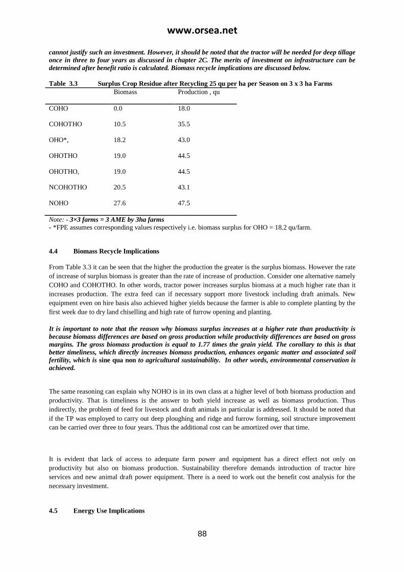
www.orsea.net

88

cannot justify such an investment. However, it should be noted that the tractor will be needed for deep tillage

once in three to four years as discussed in chapter 2C. The merits of investment on infrastructure can be

determined after benefit ratio is calculated. Biomass recycle implications are discussed below.

Table63.3 Surplus Crop Residue after Recycling 25 qu per ha per Season on 3 x 3 ha Farms

Biomass Production , qu

COHO 0.0 18.0

COHOTHO 10.5 35.5

OHO*, 18.2 43.0

OHOTHO 19.0 44.5

OHOTHO, 19.0 44.5

NCOHOTHO 20.5 43.1

NOHO 27.6 47.5

Note: - 3×3 farms = 3 AME by 3ha farms

- *FPE assumes corresponding values respectively i.e. biomass surplus for OHO = 18.2 qu/farm.

4.4 Biomass Recycle Implications

From Table 3.3 it can be seen that the higher the production the greater is the surplus biomass. However the rate

of increase of surplus biomass is greater than the rate of increase of production. Consider one alternative namely

COHO and COHOTHO. In other words, tractor power increases surplus biomass at a much higher rate than it

increases production. The extra feed can if necessary support more livestock including draft animals. New

equipment even on hire basis also achieved higher yields because the farmer is able to complete planting by the

first week due to dry land chiselling and high rate of furrow opening and planting.

It is important to note that the reason why biomass surplus increases at a higher rate than productivity is

because biomass differences are based on gross production while productivity differences are based on gross

margins. The gross biomass production is equal to 1.77 times the grain yield. The corollary to this is that

better timeliness, which directly increases biomass production, enhances organic matter and associated soil

fertility, which is sine qua non to agricultural sustainability. In other words, environmental conservation is

achieved.

The same reasoning can explain why NOHO is in its own class at a higher level of both biomass production and

productivity. That is timeliness is the answer to both yield increase as well as biomass production. Thus

indirectly, the problem of feed for livestock and draft animals in particular is addressed. It should be noted that

if the TP was employed to carry out deep ploughing and ridge and furrow forming, soil structure improvement

can be carried over three to four years. Thus the additional cost can be amortized over that time.

It is evident that lack of access to adequate farm power and equipment has a direct effect not only on

productivity but also on biomass production. Sustainability therefore demands introduction of tractor hire

services and new animal draft power equipment. There is a need to work out the benefit cost analysis for the

necessary investment.

4.5 Energy Use Implications

www.orsea.net

89

Basing energy analysis on economic and biomass recycle implications two farm power and equipment subsets

deserve to be analyzed namely OHOTHO and NCOHOTHO. Energy optimization was the basis for tractor

power and animal draft power selections. It also indicated the optimum combination of tractor and animal draft

power in terms of cultivated land in hectares.

From Table 3.4 it is evident that farmers need to apply both animal draft power and tractor power in order to

realize the production potential. The main constraints are labour available during land preparation and weeding

in the 6th and 7th week. The former occurs when there is competition for labour between late planting and early

weeding while the latter occurs when demands for weeding are excessive. Important observation was that the

farmer can achieve both optimum productivity as well as energy use with negligible violation of the former.

This is a small price to pay to remain close to optimum energy consumption.

90

Table73.4 Goal programming with energy objective function and productivity and biomass recycle as constraints

OBJ. Variables in ha Constraints Biom

ass

Productivity Productivity

qu

MJ. 1 5 9 12 13 1,2,3,17 Land qu Set level qu Surplus Actual

NCOHOTHOe1 2*2 1.106 0.038 0.83 1.13 3.2 25 7.78

NCOHOTHOe1 2*2 3.99 0.56 0.82 0.61 9.9 28 3.4

NCOHOTHOe1 2*2 5.91 0.91 0.83 0.25 14.4 30 0.68

NCOHOTHOe1 2*3 1.172 0.061 0.83 1.19 0.37 0.59 0 28 7.87

NCOHOTHOe1 2*3 2.13 0.16 0.83 1.19 0.59 0.23 0 32 6.7

NCOHOTHOe1 2*3 5.96 0.87 0.83 1.19 0.13 0 40 1.25

NCOHOTHOe1 2*3 6.56 0.95 0.83 1.19 0.028 13.4 41

NCOHOTHOe1 2*4 6.96 0.94 0.83 1.19 0.9401 0.1 5.13 48 0.46

NCOHOTHOe2 3*3 4.77 0.62 1.32 1.06 12.5 41 3

NCOHOTHOe2 3*3 5.73 0.7997 1.32 0.88 14.8 42 1.6

NCOHOTHOe2 3*3 6.69 0.97 1.32 0.71 43

NCOHOTHOe3 4*3 5.967 0.84 1.8 0.35 18.4 44 1.26

NCOHOTHOe3 4*4 1.589 1.8 1.73 0.46 6.95 45 8

NCOHOTHOe3 4*4 5.55 0.68 1.8 1.51 15.1 54 2.5

NCOHOTHOe3 4*4 6.51 0.86 1.8 1.34 17.4 55 1.1

NCOHOTHOe3 4*2 6.11 0.95 1.05 16.3 31 0.38

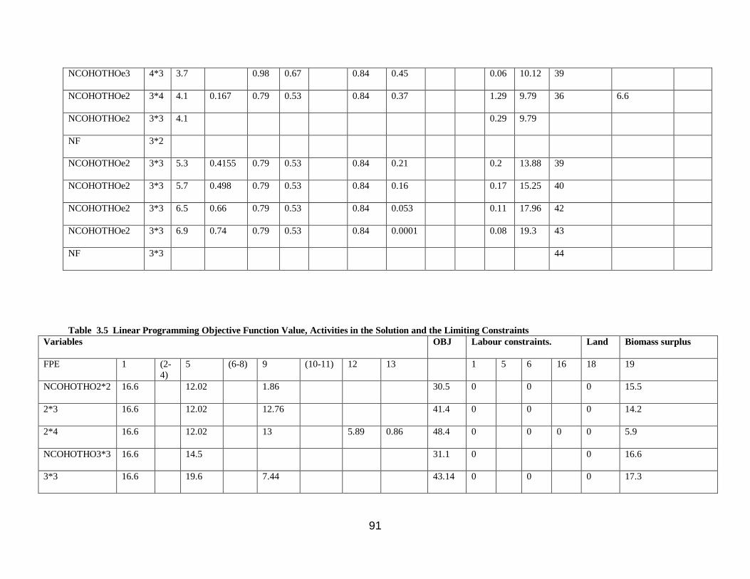
91

NCOHOTHOe3 4*3 3.7 0.98 0.67 0.84 0.45 0.06 10.12 39

NCOHOTHOe2 3*4 4.1 0.167 0.79 0.53 0.84 0.37 1.29 9.79 36 6.6

NCOHOTHOe2 3*3 4.1 0.29 9.79

NF 3*2

NCOHOTHOe2 3*3 5.3 0.4155 0.79 0.53 0.84 0.21 0.2 13.88 39

NCOHOTHOe2 3*3 5.7 0.498 0.79 0.53 0.84 0.16 0.17 15.25 40

NCOHOTHOe2 3*3 6.5 0.66 0.79 0.53 0.84 0.053 0.11 17.96 42

NCOHOTHOe2 3*3 6.9 0.74 0.79 0.53 0.84 0.0001 0.08 19.3 43

NF 3*3 44

Table83.5 Linear Programming Objective Function Value, Activities in the Solution and the Limiting Constraints

Variables OBJ Labour constraints. Land Biomass surplus

FPE 1 (2-

4)

5 (6-8) 9 (10-11) 12 13 1 5 6 16 18 19

NCOHOTHO2*2 16.6 12.02 1.86 30.5 0 0 0 15.5

2*3 16.6 12.02 12.76 41.4 0 0 0 14.2

2*4 16.6 12.02 13 5.89 0.86 48.4 0 0 0 0 5.9

NCOHOTHO3*3 16.6 14.5 31.1 0 0 16.6

3*3 16.6 19.6 7.44 43.14 0 0 0 17.3

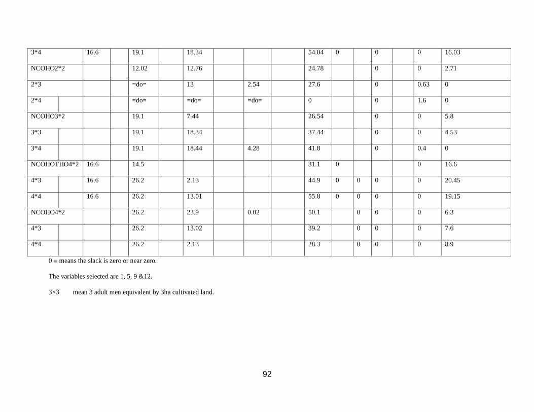
92

3*4 16.6 19.1 18.34 54.04 0 0 0 16.03

NCOHO2*2 12.02 12.76 24.78 0 0 2.71

2*3 =do= 13 2.54 27.6 0 0.63 0

2*4 =do= =do= =do= 0 0 1.6 0

NCOHO3*2 19.1 7.44 26.54 0 0 5.8

3*3 19.1 18.34 37.44 0 0 4.53

3*4 19.1 18.44 4.28 41.8 0 0.4 0

NCOHOTHO4*2 16.6 14.5 31.1 0 0 16.6

4*3 16.6 26.2 2.13 44.9 0 0 0 0 20.45

4*4 16.6 26.2 13.01 55.8 0 0 0 0 19.15

NCOHO4*2 26.2 23.9 0.02 50.1 0 0 0 6.3

4*3 26.2 13.02 39.2 0 0 0 7.6

4*4 26.2 2.13 28.3 0 0 0 8.9

0 means the slack is zero or near zero.

The variables selected are 1, 5, 9 &12.

3×3 mean 3 adult men equivalent by 3ha cultivated land.

93

Table93.6 L.P Model Output showing the Variables in the Solution and the Limiting Constraints

File Obj

valu

e

Variables Labour constraints Lan

d

Biomas

s

1 2 4 5 7 8 10 11 13 1 2 3 4 5 6 7 8 9 10 11 12 13 14 15 16 17 18 19

OHO22 30.2 19.2 4.9 6.2 2.6 0.0 13.3

OHO23 33.9 14.9 4.9 6.3 0.6 11.8

OHO24 33.9 14.9 4.9 6.3 1.6 11.8

OHOTHO2

2

30.2 19.2 4.9 6.2 0.0 13.3

OHOTHO2

3

33.9 0.02 14.8 8.0 4.9 6.3 0.6 11.8

OHOTHO2

4

33.9 0.02 14.8 8.0 4.9 6.3 1.6 11.8

OHO32 33.7 26.2 7.5 0.0 19.6

OHO33 43.0 26.2 7.6 8.92 0.30 0.1 18.2

OHO34 43.0 26.2 7.6 8.9 0.31 1.1 18.2

OHOTHO3

2

33.9 1.13 26.2 6.6 0.0 20.0

OHOTHO3

3

44.5 2.5 23.7 1.7 7.6 0.0 19.0

OHOTHO3

4

47.3 8.7 12.8 9.4 7.6 0.6 17.6

94

OHO42 33.7 26.2 7.5 0.0 19.6

OHO43 44.7 26.2 9.5 8.9 0.14 0.0 19.1

OHO44 46.4 26.2 9.5 8.9 1.8 0.76 17.2

OHOTHO4

2

35.0 8.8 26.2 0.0 23.0

OHOTHO4

3

48.0 8.8 26.2 9.5 3.5 0.0 26.0

OHOTHO4

4

53.4 8.8 26.2 9.5 8.9 0.49 25.3

NCOHOT4*

4

50.1 26.2 23.9 0.02 0.0 6.3

NCOHOT4*

3

39.2 26.2 13.0 0.0 7.65

NCOHOT4*

2

28.3 26.2 2.10 0.0 8.95

NCOHOT3*

4

55.8 16.6 26.2 13.02 0.0 19.15

NCOHOT3*

3

44.9 16.6 26.2 2.1 0.0 20.45

NCOHOT3*

2

31.1 16.6 14.5 0.0 16.6

NCOHOT2*

4

48.7 16.6 12.0 13.0 7.0 0.1 0.0 6.54

95

NCOHOT2*

3

41.4 16.6 12.0 12.8 0.0 14.2

NCOHOT2*

2

30.5 16.6 12.0 1.86 0.0 15.5

96

5. CONCLUSION AND RECOMMENDATIONS

The study was prompted by the need to inform policy on the development of tillage and equipment for

semi-arid smallholder agriculture. The purpose of the study was to develop a specific methodology for

predicting the effect of tillage and equipment on farm production.

5.1 Conclusion

i. Access to 3 ha cultivated land and 3 adult labour equivalent can be implemented and sustain

conservation tillage with hired new ADP at an estimated increase in income which can be paid for by

the increased production in one season.

ii. However, the innovative ADP equipment has no capacity for land reclamation involving sub-soiling

20-30 cm deep and associated land development.

5.2 Recommendations

i. It is recommended that further controlled tests be carried out in other semi-arid areas in order to identify location specific requirements for ADP equipment.

ii. It is recommended that estimates of the cost benefit ratio and associated rate of return on investment be

made in order to inform policy for investment on infrastructure.

iii. It is also recommended that researchers consider long-term quantifiable productivity attributable to

farm equipment for samllholders as one of the prerequisite for mechanization selection (as is the case

with irrigation technology).

______

This is an academically inspired scientific paper, it ought to have selected bibliography or references;

the author has cited some works in this study and this ought to be reflected in the references.

97

SOCIO-LEGAL, CULTURAL AND POLITICAL DIMENSIONS

Microfinance and Enterprises Performance in Tanzania: Does Gender Matter?

Authors

Dr. Sylvia Temu and Dr. Severine Kessy, University of Dar es Salaam, P. O. Box 35046,

Dar es Salaam, Tanzania

Abstract

The purpose of this paper was to examine whether there is a difference in performance among the

female owned enterprises and male owned enterprises. The analysis centred on the clients of microfinance institutions with premises that Microfinance institutions enable enterprises owner to

develop their micro and small enterprises, which enhance their income earning capacity, and

hence enjoy an improved living standard. The comparison between these two groups was important in identifying the motivational and individual characteristics that exist between females

and males. Following the discussion in this paper, the female owned enterprises demonstrated a

slightly lower level of growth compared to enterprises owned by male. In fact the results of t-test

revealed that male owned enterprises have higher level of assets, sales revenue and number of employees compared to female owned enterprises.

Key words: Gender, Microfinance, and Enterprises Performance Introduction

In developing countries, there are a big number of individuals who are financially underserved. In

response to the widespread financial exclusion, microfinance programmes and institutions have been

established globally as a prospective component of strategies of development organisations,

governments, and societies to promote enterprises in developing countries (Hulme, 2000).

They are organisations with a goal to serve the needs of underserved markets as a means of meeting

development objectives (Ledgerwood, 1998). It is postulated that owners of micro and small enterprises

(MSEs) can through the services of micro finance institutions in particular credit accumulate wealth

and attain firms’ growth after some time. Specifically, microfinance institutions provide a broad range

of services including deposits, loans, payment services, money transfer and insurance to the poor/low

income households and their enterprises (Chijoriga, 2000; Conford, 2001 and Pilipinas, 2002). In

addition, some of microfinance institutions provide non-financial services such as training, business

advice, market assistance and business counselling to their clients (Hishigsuren, 2004 and CIDA, 1999).

Microfinance institutions are thus seen as a critical element in enhancing the lives of the poor and low

income earners in developing economies because their services target the clients who have been

excluded from conventional formal institutions.

Microfinance institutions enable MSE‘s owners to develop their enterprises, which enhance their income

earning capacity, and hence enable them enjoy an improved living standard (Mosley, 2001; ADB, 2000).

98

For instance, over the last twenty years, microfinance providers in developing economies have shown

impressive results as tools for delivery of financial services to the poor and their enterprises (Bastelaer,

2000). Access to micro finance services give the clients an opportunity to improve working capital in MSEs

thus expand economic activities as well as their meet household financial management and consumption

needs (URT, 2000). Along this line of thinking micro-credit has proved to be an important liberating force

in societies where disadvantaged groups, women in particular have to struggle against repressive social and

economic conditions. This is achieved because microfinance enables these disadvantaged groups to

accumulate capital for their enterprises. These enterprises are expected to grow and generate income to

these groups which will have positive effect to the social and economic conditions.

The principal providers of microfinance services to the low income households and MSEs in Tanzania

consist of licensed commercial banks, regional and rural community banks, savings and credit

cooperative societies (SACCOS), and non-governmental organizations (NGOs) (Randhawa and

Gallardo, 2003. Micro finance service delivery operations of the financial NGOs in Tanzania are mainly

funded and supported with technical assistance of international donors (Randhawa and Gallardo, 2003).

Although these institutions charge interest rates which are relatively the same as the market rates, they

provide loans with affordable collaterals and most of the time without collaterals. Microfinance

institutions mainly focus on low income earners and MSEs as most of them have small size liquidity and

capital needs, contrary to the needs of most of the high-income earners in developing countries, whose

capital needs are higher and for larger projects (Mosley and Hulme, 1998).

Impact assessment studies in microfinance have since 1990s become increasingly popular worldwide. The focus has been on measuring MFI programs‘ success by considering the changes brought about by their

interventions on clients (borrower) and their enterprises. (Woller and Parsons, 2002, Mosley, 2001), have

become increasingly popular worldwide. Most of the impact assessment studies revealed that microfinance

interventions specifically microcredit have had beneficial economic and social impacts (e.g. Mosley, 2001).

While the results of these studies suggest positive impacts, little has been done about the impact on female

owned enterprises compared to male owned enterprises. The objective of this paper is therefore to compare

the performance of female owned enterprises against male owned enterprises that have received micro

finance services. The comparison between these two groups is inevitable because it enables the researchers

to identify the motivational and individual characteristics that exist between females and males recipients

of microfinance services. The research question that guided the study was: ―Does the performance of

enterprises owned by microfinance clients differ gender-wise?‖

Gender Differences and Theories of Growth

Female entrepreneurs are behind a substantial proportion of micro-enterprises (World Bank 2004). Studies

carried out on comparison on gender differences in enterprises have revealed that enterprises owned by

women, experience the same constraints as those owned by men. At the same time, it is often argued that

female entrepreneurs face certain gender-specific challenges, and may be affected differently by policies to

promote private sector development

(Buvinic 1993; Ellis 2003) such as micro finance interventions. Liedholm and Mead (1999) find, however,

that the principal problems facing female and male entrepreneurs are fairly similar.

Others argue that certain characteristics are typical for female owned enterprises when compared to male

owned enterprises. These characteristics include small sized firms, limited prospects for profitability and

failure to provide collateral for obtaining loans (Coleman, 2002 and Fielden et al, 2003). Female owners are

somewhat more constrained by market size than male owners, and men more often cite regulations and

taxes as a problem, but the differences are small. In Tanzania specifically, women are constrained by

education/training, business experience, discrimination, socialization/networking capacity and lower

99

propensity to risk taking (Nchimbi, 2002; Coleman, 2002 and Fielden et al, 2003). Also the overall

negative attitudes towards the business owned by women (particularly by men) and inadequate and

affordable business premises also limit the overall performance of female owned enterprises.

It is further agreed that there is a significant variation between male and female especially when

considering sources of funds for start up and running their businesses. For example, Katwalo (2007)

established that female entrepreneurs relied more on family funds than male entrepreneurs. In this case it is

difficult for female owned enterprises to take advantage of external finance opportunities. This is against

the internal finance theory of growth (see for example Carpenter and Petersen, 2002; Binks and Ennew,

1996 and Reid, 1996), which argues that firms whose financial needs exceed their internal resources may

be constrained to pursue potential opportunities for growth (Demirgüç-Kunt and Maksimovic, 1998).

The insufficient internally generated liquidity is frequently cited one of the factors which causes business

failure in MSEs in developing countries (Chijoriga and Cassimon, 1999). It is from this perspective, the

micro credits are considered to be an appropriate solution because the amount of money needed to start a

micro or small business is generally quite minimal (Sonfield and Barbato, 1999). Access to credit enables

the MSEs‘ owners to acquire working tools and equipment expands their business activities or renovates

working premises and buildings (ILO/UNDP, 2000). Credit also assists the small business owners with

working capital to cover cash flow shortage, to purchase inventories, to invest in new technology,

expanding the market and being able to take advantages of suppliers‘ discount. Without sufficient capital

therefore, micro and small firms are unable to develop new products and services or grow to meet demand

of their customers (Coleman, 2000).

Despite the importance of funds to finance start up and existing business enterprises, there are other factors

that can explain differences between male and female owned enterprises. These other factors can be

explained by human motivation view of growth. The human motivation view of growth holds that the

social and psychological motives can significantly influence growth seeking behaviour and therefore

growth itself (Shane et al, 2003; Olomi, 2001 and Nchimbi, 2002). The view sees growth as resulting from

personal needs of the owner-managers and these needs are socially generated, socially sustained and

socially changed (Shane et al, 2003). The theories under this view of growth can be categorised into two

types. The explanatory models which relate growth to motivations and antecedents, and the second is the

theories which attempt to categorise owner managers into unique typologies on the basis of the meaning

they attach to business activity, which in turn imply different levels of growth motivation (Olomi, 2001). In

developing countries, gender differences are very high, Tanzania not exclusive. The way men are groomed

is quite different compared to women. The level of labour division in different social and economic

activities is very high, and therefore the extent of adopting and doing things differ gender wise.

There are different characteristic features between women and men resulting from division of labour some

of which may explain the differences in business performance. It is for instance argued under human

motivation view that the characteristic features of firm owners are motivators that can trigger MSEs

Owners to start and run business for growth motives. The argument here is based on the assumption that

growth would be realized when completing a job, solving problems, seeing the results of one‘s efforts,

being recognized for a job well done and performing interesting work (Apospori et al, 2005 and Shane et

al, 2003). Other prerequisites include successful completion of a (difficult, demanding or challenging) task,

100

having control over one's own job, upward movement of enterprises activities, creating more opportunities

for enterprises, learning new skills by working in challenging environments and sometimes poverty

reduction motive (Davidsson and Wiklund, 1999; Shane et al, 2003; Olomi, 2001 and Apospori et al,

2005). It is from these beliefs, the realization of these features create the possibility of MSEs to grow. As

mentioned above, different features can be built from previous experiences and sometimes by using role

models, in such a case the labour division in developing countries dictate different characteristic features

between women and men. It is therefore expected that performance differentials would be observed when

comparing the business performance for enterprises owned by women and men.

Another theory that has been used by researchers who subscribe on human motivation view is

McClelland‘s (1961) achievement motivation theory (for example: Davidsson and Wiklund, 1999; Olomi,

2001 and Nchimbi, 2002). The underlying logic in this theory is that someone‘s choice of work-tasks and

the time and energy devoted to these work-tasks, is dependent on the individual‘s motivation to perform

different tasks. The theory argues that running a business requires people to take moderate risks, assume

personal responsibility for their own performance, pay close attention to feedback in terms of costs and

profits, and find new or innovative ways to make a new product (Davidsson and Wiklund, 1999). This

view purports that most of the growing MSEs are managed and operated by the owners with a need to

achieve growth of their enterprises. In this respect, the theory predicts that people with a high need for

achievement, value particular work-task situations and perform well in these, while their counterparts will

perform poorly. Consequently the high need for achievement should make people particularly interested in,

and able to perform well as entrepreneurs. In developing countries women are considered to be risk averse

compared to their men (Coleman, 2002 and Fielden et al, 2003). In this regard their businesses are not

expected to perform better compared to men owned enterprises because it is postulated that higher risk

businesses are associated with higher returns than less risky businesses (Mosley, 2001). From this

discussion it can be hypothesised that men owned enterprises have higher growth potentials than women

owned enterprises.

Materials and Methods

In addition to the foregoing theoretical explanations an empirical study was carried out to test whether

differences on business performance between women owned enterprises against men owned enterprises

exist. To achieve the test, a survey was conducted in August to October 2007 to different MSEs supported

by MFIs in Tanzania. Specifically the survey covered a total of 225 respondents from four different

regions; Dar es Salaam (92), Mwanza (52), Arusha (47) and Mbeya (34). These were selected as being

major urban centres in the country and with the highest concentration of micro finance services (Bank of

Tanzania, 2004). A total of 225 MSE owner/managers were involved in the survey. The profile of the

respondents shows that the composition of sample size was 53.8 percent and 46.2 percent for women and

men respectively.

In assessing the performance of MSEs, three different measures i.e. sales revenue, number of employees

and asset levels were used for comparison. In this regard, independent t-test was used to perform the

analysis. Before testing, we applied natural logarithm to all data in order to maintain linearity because some

of observations were highly skewed either to the right or left .

Findings

101

The profile of the respondents shows that the composition of sample size was 53.8 percent and 46.2 percent

for women and men respectively. Independent samples t-test was used and the output produced presented

in tables 1 and 3. The table of group statistics revealed that all averages (mean) of men owned enterprises

were higher than those of women owned enterprises in all indicators of growth. That is the men owned

enterprises had higher assets, average revenue and more number of employees than their counterparts.

Despite these results, this sounds as a tentative conclusion that cannot be statistically accepted without the

interpretation of independent samples table.

Table 1: Group Statistics

Indicators SEX N Mean Std. Deviation

Std. Error

Mean

Number of

Employees

Male 104 1.5702 .69323 .06798

Female

121 1.2799 .53667 .04879

Average Revenue

Male 104 12.3084 6.35368 .62303

Female 121 11.7709 1.36825 .12439

Asset

Male 104 15.1648 3.20824 .31459

Female 121 13.3028 4.28054 .38914

In interpreting the independent samples table, we referred to one important assumption of independent

samples t-test. This assumption states that the two groups that are compared by independent samples t-test

should have approximately equal variance on the dependent variable. In order to use the results in table 1

for a meaningful statistical conclusion, the Levene‘s test (O'Neill and Mathews, 2002) was used to evaluate

the homogeneity of variance assumption. The null hypothesis for this test is that the variances are

homogeneous. Therefore, if the Levene‘s test is significant (i.e. less than 0.05), then the variances of the

two groups are significantly different. However if the value is not significant then the null hypothesis is

rejected and conclusion that they are not different (i.e. they are homogeneous). The output of our t-statistic

revealed that the Levene‘s test for equality of variance for all indicators of growth were greater than 0.05

(table 2). It is therefore concluded that the variances of these two groups were approximately equal.

102

Table 2: Levene's Test for Equality of Variance

Indicator F Sig.

Asset 2.576 .110

Average Revenue 1.399 .238

No of Employees 2.185 .141

Because the Levene‘s test provides an assurance of homogeneity variances, the next step was to use the

values of t-statistics in the rows of ―equal variances assumed‖ to test and make conclusion on whether there

is a significant difference among the growth indicators of micro finance beneficiary MSEs owned by

women against those owned by men.

By using the column of sig. (2-tailed), the values of assets accumulated and number of employees were

significant at 0.05 level of significance (table 3). These results led to the conclusion that there were

significant differences among these two growth indicators (number of employees and assets) of enterprises

owned by men against the enterprises owned by women. The fact that the averages of these two growth

indicators of enterprises owned by men were greater than the averages of women owned MSEs after micro

finance interventions, we can conclude that the men owned enterprises had demonstrated higher growth

performance than the women owned enterprises in the two performance indicators; namely employment

creation and growth in assets value. When considering average revenue among these two groups, the values

were not statistically different. This conclusion was made following the results obtained from the column

of sig. (2-tailed) in table 3, which is 0.366. At the level of 0.05 of significance; the value obtained is

insignificant. Although the average sales revenue of men owned enterprises is higher than that of women

owned enterprises, there is no statistical evidence of making such conclusion.

Table 3: Independent Samples Test

Ind

icato

rs

Levene's Test for

Equality of Var. t-test for Equality of Means

F Sig. T df

Sig.

(2-

tailed)

Mea

n

Dif.

Std.

Error

Diff.

95% C.I. of the

Difference

Lower Upper

No. of Equal variances 6.301 .063 3.536 223 .000 .290 .0821 .12849 .4520

103

Emp. assumed 6

Equal variances

not assumed 3.469 192.58 .001 .290 .0836 .12524

.4553

1

Av.

Rev.

Equal variances

assumed 112.60 .071 .907 223 .366 .537 .5927

-

.63073

1.705

6

Equal variances

not assumed .846 111.22 .399 .537 .6353

-

.72145

1.796

3

Asset

Equal variances

assumed 1.991 .160 3.643 223 .000 1.86 .5111 .85465

2.869

3

Equal variances

not assumed 3.721 219.08 .000 1.86 .5004 .87579

2.848

2

Following the fact t-test results did not support all three indicators of measuring

performance/growth that have been used for comparison, further analysis was done on some

motivational factors that influenced the owners of these enterprises to engage in their business.

Different factors like motives of starting the businesses, prospects of the businesses and future plan

were assessed by comparing the groups. In this analysis, the findings revealed that most of the

women owning MSEs started their business to meet the basic needs whereas the male entrepreneur’s

counterpart perceived that particular objective as of no importance. Furthermore, while men MSEs

owners (80%) admitted that they do business because they do not like to work under others’ control,

women entrepreneurs only slightly value this objective of starting business as of no importance. On

assessing the motive of owning a growing and big business enterprise in the two groups, it was highly

agreed (96%) among the male MSEs owners that they opened their business with intention of having

very big organisation while females owners were not willing to own very big enterprise because they

believe that management of big organisations is tedious and consume a lot of time that can be used to

care their families. Furthermore, most (about 65%) of the women entrepreneurs who were involved

in the survey expressed preference to opening multiple small businesses rather than dealing with only

one and big organisation. Other motives among the MSEs respondents included supplementing the

businesses owners’ normal income, security to the family, and exploiting business opportunities and

these were rated similar by the two groups of respondents. These factors seem to be common for both

women and men engage in MSEs and who have benefited from micro finance services.

Conclusion and Implication of the Findings The findings of this study revealed that women and men owned MSEs that have received services from

micro finance institutions have experienced differences in performance of their enterprises. The results

show that despite the similar level of external support from MFI, female MSEs have experienced slower

growth compared to male owned enterprises. Although the results did not provide evidence statistical

differences on average sales revenue between male owned enterprises and female owned enterprises, the

average assets value and number of employees after the micro finance interventions were different among

these two groups. Different motives of owning and running businesses were also observed among the

groups. Consistent to prior studies women entrepreneurs were observed to be more risk averse compared to

men. Due to risk evasiveness, it is clear that the returns of female owned enterprises were also expected to

be low. The low level of growth of women owned enterprises also recounts to our theoretical base which

104

sees females in developing countries as a disadvantaged group which are not groomed for opening and

running business. Here we concur with theoretical explanation that the growth which resulting from

personal needs of the owner managers are socially generated, socially sustained and socially changed. In

this regard, the social relationship explains growth motives of the business owners. This point further

underscores that the social environment where the women both young and elderly are groomed up in

developing countries partly explains the differences in performance/growth of their enterprises. Despite the fact that both female owned enterprises and male owned enterprises experienced microfinance

interventions; males owned enterprises demonstrated higher level of growth than female owned enterprises.

The above results call for special action and attention that can address the limited motivations that

surrounding women in business and those who wish to venture into it. In particular the women who have

benefited from microfinance services need to undergo special training that will build their capacity in doing

business with growth prospects. Through training the women entrepreneurs are expected to change their

perceptions about future prospects of their business and acquire additional skills that will enable them grow

their business in paricture creation of additional assets and also contribute more significantly to

employment creation.. Additionally, they will be endowed with motivational characteristics discussed

under human motivation view, training helps small business owners, managers and potential entrepreneurs

to meet the challenges of today‘s business environment, manage the ever-changing world and plan for

future of their business. This would be achievable because it is argued that in order to effectively pursue

growth strategies an entrepreneur requires business management skills to to manage enterprise growth

effectively and attain market efficiencies (Fisher, 1998). Furthermore, skills obtained from training become

an embeded asset in the entrepreneurs which can help to tap into unfolding opportunities and overcome

uncertainties in the ever changing business environment. It is from this argument that different other have

found that training has significant impact on participant characteristics and final participant outcomes

(Edgcomb, 2002; Bratton and Gold, 2003 and Grizzell, 2003).

References

ADB, (2000). Finance for the Poor: Microfinance Development Strategy, Asian Development

BankRetrieved 3rd November 2004 from

http://www.adb.org/Documents/Policies/Microfinance/financepolicy.pdf.

Apospori, E.; N. Papalexandris and E. Galanaki (2005). Entrepreneurial and professional CEOs Differences

in motive and responsibility profile, Leadership & Organization Development Journal, 26 (2), 141 –

162

Bank of Tanzania and Ministry of Cooperatives and marketing (2004): Improving operational performance

of SACCOS in Tanzania Final Report, United Republic of Tanzania

Bastelaer, T. (2000). Reform of Legal and Regulatory Framework for Microfinance, IRIS Center

Binks, M. R. and C. T. Ennew (1996). Growing Firm and Credit Constraint, Journal of Small Business

Economics, 8 (1), 17 – 25.

Bratton, J. and J. Gold (2003). Human Resources Management: Theories and Practices, 3rd Ed., NY,

Palgrave Macmillan

Carpenter, R. E. and B. C. Petersen (2002). Is the Growth of Small Firms Constrained by Internal Finance?,

The Review of Economics and Statistics, 84 (2), 298 – 309

Chijoriga M. M. (2000). The performance and sustainability of micro finance institution in Tanzania,

Unpublished manuscript

105

Chijoriga, M. and D. Cassimon (1999). Micro Enterprise Financing: Is there a Best Model?: in Rutashobya

L. K. and Olomi, D. R.(eds), African Entrepreneurship and Small Business Development, Dar es

Salaam, DUP (1996) Ltd

CIDA (1999). Report on CIDA's Programming in Microfinance & Microenterprise Development (1998-

1999), Canadian International Development Agency, Gatineau, Quebec, Also found in

http://www.acdi-cida.gc.ca/INET/IMAGES.NSF/vLUImages/development/$file/micro-rept.pdf,

Coleman, S. (2000). Access to Capital and Terms of Credit: A comparison of Men-and Women-Owned

Small Business, Journal of Small Business Management, 38(3), 37 – 52

Coleman, S. (2002). Constraints Faced by Women Small Business Owners: Evidence from the Data,

Journal of Development Entrepreneurship, 7(2), 151 – 174

Cornford, R. (2001). ‗Microcredit,‘ ‗microfinance‘ or ‗access to financial services‘ What do Pacific people

need?, Retrieved 7th June 2004 from http://www.devnet.org.nz/conf/Papers/cornford.pdf

Davidsson, P. and J. Wiklund (1999). Theoretical and Methodological issues in the study of firm growth,

Retrieved 10th November 2004 from http://www.ihh.hj.se/eng/research/publications/wp/1999-

6%20Davidsson,%20Wiklund.pdf

Demirgüç-Kunt, A. and V. Maksimovic (1998). Law, Finance, and Firm Growth, The Journal of Finance,

53(6), 2107 – 2137.

Edgcom, E. L. (2002). What makes for Effective Microenterprise Training?, Journal of Microfinance, 4

(1), 99 – 114

Fielden, S. L., M. F. Davidson, A. F. Dawe and P. F. Makin (2003). Factors inhibiting the economic growth

of female owned small business in North West England, Journal of Small Business and

Entrepreneurship Development, 10(2), 152 – 166

Fisher, M. J. (1998). MSE Growth: The Importance of Market Analysis and Technology Development,

Retrieved 24th June 2003 from www.nbs.ntu.ac.uk/cgb/CONFER/1998-03-a/Fisher.doc

Grizzell, J. (2003). Behavior Change Theories and Models, Retrieved 19th September, 2006 from

http://www.csupomona.edu/~jvgrizzell/best_practices/bctheory.html

Hishigsuren, G. (2004). Scaling up and mission drift: can microfinance institutions maintain a poverty

alleviation mission while scaling up?, Retrieved 7th July 2007 from

http://marriottschool.byu.edu/conferences/selfreliance/presentations/BYU%20paper_Scaling%20up.

doc

Hulme, D. (2000). Impact Assessment Methodologies for Microfinance: Theory, Experience and Better

Practice, World Development, 28 (1), 79 – 98.

ILO/UNDP (2000). Micro and Small enterprises Development & Poverty Alleviation in Thailand,

International Best Practice in Micro and Small Enterprises Development Working Paper No. 2,

Edited by Gerry Finnegan.

Katwalo A. M. (2007). Differences Between Men and Women Entrepreneurs in the Informal Business

Sector of Uganda: A Cultural Perspective, 2007 IAABD Proceedings, pp 54 - 59

Ledgerwood, J. (1998). Microfinance Handbook, An Institutional and Financial Perspective, Washington,

D.C., The World Bank

Mosley, P. (2001). Microfinance and Poverty in Bolivia, Journal of Development Studies, 37 (4), 101-132.

Mosley, P. and D. Hulme (1998). Microenterprise Financing: Is there a conflicting Between Growth and

Poverty Alleviation?, World development 26 (5), 783 – 790.

106

Nchimbi, M. I. (2002). Gender and Entrepreneurship in Tanzania: A Comparative Analysis of Male-

Female‟s Start-up Motivation, Individual Characteristics and Perceptions of Business Success, PhD

Thesis, University of Dar es Salaam.

Nchimbi, M. I. (2002). Gender and Entrepreneurship in Tanzania: A Comparative Analysis of Male-

Female‟s Start-up Motivation, Individual Characteristics and Perceptions of Business Success, PhD

Thesis, University of Dar es Salaam.

Olomi, D. R. (2001). Entrepreneurial Motivation in a Developing Country Context-Incidence-Antecedents,

and consequences of Growth-seeking Behaviour Among Tanzanian Owner-manager, PhD. Thesis,

University of Dar es Salaam.

O'Neill, M. E. and Mathews K. L. (2002). Levene Tests of Homogeneity of Variance for General Block and

Treatment Designs, Biometrics, 58 (1): 216-224, Available from:

http://www.jstor.org/stable/pdfplus/3068309.pdf [Accessed 26 November 2009]

Pilipinas, B. S. (2002). Notes on Microfinance, Retrieved 3rd November, 2004 from

http://www.bsp.gov.ph/archive/Regulations_2002/Circulars/notes.htm

Randhawa, B. and Gallardo, J. (2003). Microfinance Regulation in Tanzania: Implications for Development

and Performance of the Industry, Retrieved on 17th October, 2004 from

http://www.worldbank.org/afr/wps/wp51.pdf

Reid, G. C. (1996). Mature Micro – Firms and their Experience of Funding Shortages, Journal of Small

Business Economics, 8 (1), 27 – 37.

Shane, S., E. A. Locke and C. J. Collins (2003). Entrepreneurial Motivation, Human Resource Management

Review, 13, 257 – 279

Sonfield, M.C., and R. J. Barbato (1999). Credit and equity support as components of self-employment

development programs, Retrieved 11th November 2004 from

http://www.gdrc.org/icm/micro/sonfield-barbato.html

URT, (2000). National Micro Finance Policy, Ministry of Finance, Dar es Salaam

Woller, G. and R. Parsons (2002). Assessing the Community Economic Impact of Microfinance

Institutions, Journal of Development Entrepreneurship, 7 (2), 133 – 148.

107

FACTORS PREDISPOSING BOYS RISKY BEHAVIOURS IN BOYS’ DAY

SECONDARY SCHOOLS IN KISUMU MUNCIPALITY

By

Joy Akoyi Nyende and G.P. Pokhariyal

School of Continuing and Distance Education and School of Mathematics

University of Nairobi

P.O.Box 30197-00100, Nairobi, Kenya

ABSTRACT

This study sought to explore the extent to which the factors are dominant in urban

secondary schools with focus clearly on boys‘ day secondary schools in Kisumu

municipality. The research targeted male day school students between 14-21 years of age.

From a sample of 192 day students in two boys‘ day secondary schools in Kisumu

municipality, the study endeavoured to ascertain the parameters of their school life and

how such factors affect their lives. The study involved the analysis of secondary

information and primary data collected in the study area with the help of questionnaires.

The study established that unprotected sex was the main risky behaviour students

involved in mostly during school holidays, and that peer influence alongside access to

pornographic material had great influence on their behaviour. The availability of money

through adult female friends and also their peers, and watching television late in the night

influenced the students to engaging in risky behaviours.

The study recommended that learning institutions ought to participate in enlightening

students on the consequences of risky behaviours such as engaging in unprotected sex in

order to mitigate spread of sexually transmitted diseases Human Immunodeficiency

Virus. Further, the study also suggested parental guidance to ensure their children desist

from engaging in risky behaviours.

Keywords: Predispose, Risky Behaviour, Adolescence, Day Schools

108

INTRODUCTION As boys grow, parents always prescribe to them a particular way of life. This determines their cognitive

abilities and the general development in early childhood and may even extend to early adolescence.

Nonetheless, the impact is usually perceived as authoritarian and limiting their freedom. It is this perception

that provokes the boys to develop some sort of rebellion, Kathleen (2003).When the idea to explore other

ways of life and purported freedom sets in, boys will more often than not seek the opinion, approval and company of their peers to test the variability of self-identity as observed by Prinstein & Dodge (2008).

Reasons for flourishing of risky behaviors include poor parenting, curiosity, enabling environment,

carelessness by teenagers, peer pressure, modern technology, and legal regulations such as the famous

Children‘s Act Cap 586, 2001, Valsiner (2007).

Globally, a handful of studies have been conducted on the factors influencing the youth to engage in risky

behaviours.Cunningham and Bagby (2010) sought to determine factors that predispose youth to risky

behaviours and found that relationships with parents and institutions, household behaviours and social

exclusion influences adolescents‘ to risky behaviour. Danjin and Onajole (2010) conducted a cross sectional survey of HIV/AIDS risky behavioural tendencies among secondary school students in Nigeria.

They found that the students had multiple sex partners, low rate of condom use, sex in exchange for money

or favours and some had been diagnosed with Sexually Transmitted Infections (STI).

In Kenya, few studies have been done on the same leaving a knowledge gap as the factors predisposing

students to risky behavior is not a one situation describe all. The adolescent boy needs to be helped to

become more responsible in matters affecting his sexuality and self-identity development. In almost all

countries, the majority of men 20-24 report having had sexual intercourse before their 20th birthday. Similarly, 35% of males aged 16-24 first had sex before their 15th birthday. In sub-Saharan Africa, less

than half of the sexually active men between 15-24 years use protective contraceptives or rely on their

partner‘s method, compared with 63-93% in industrialized countries and parts of Latin America and the

Caribbean, World Health Organization, (2005).

Notwithstanding, there was little literature on interventions targeting male adolescents. More emphasis was

placed on girls who were considered to be at risk. Lodiaga, et al. (2007) observed that the most

fundamental issue of main concern thereto revolves around the biological makeup of girls and the fact that

they are the victims of teenage pregnancy. The question is: what about other risks that have nothing to do with biological makeup? When it comes to the risk of HIV/AIDS infection, drug abuse, casual sex, school

dropout, peer influence – the issue of biology does not really hold. The effects cut across all sexes

regardless of the gender relations.

Survey data in Kenya over the last 5 years indicate that 14% HIV/AIDS prevalence is highest among the

youth in the range of 10-25 years. This include 0.71 million students in the 3,080 secondary schools as

observed by Lodiaga et al. (2007), thereby revealing the danger secondary school students are faced with.

The urban setting also avails the accessibility to drugs, and other unhealthy socio-economic factors that

affect day school students. While such factors are greatly controlled in boarding schools by a well structured school program, day scholars are left with more room and freedom for exploration.

Peer pressure was deemed as the most profound factor that influences the modalities of young people,

Prinstein & Dodge (2008). Several other factors interplay alongside peer pressure to determine the

character and behaviour of adolescents such as the advent of new technology, parenting and school life,

adolescents seek to develop their own identity, opinions, and values, Mwiti (2005).Given the freedom to

experiment, this stage also entails taking some risks.

Day school refers to a system of education where students attend classes from their homes every day. As

the population continues to grow the cost of living escalates each day. The government therefore

introduced a kitty for secondary school developments stimulus advanced to reduce the burden of

unaffordable fees. This initiative enhanced cheaper mode of secondary education especially for day

schooling program (CIA, Factbook, 2010). Consequently, it became a little bit affordable for middle

income earners to access day schools for their children.

109

Life in day schools for boys is very dynamic and prone to several challenges. This includes the influence of

peers, and need to afford average lifestyle of a city dweller even though their family resources do not allow.

They start to explore other opportunities to bridge the financial gap thereof and experiment the fascinating

phenomenon of observed adult lifestyle, Miller (1994).

On the other hand, technology has played a big role in promoting moral deviation among adolescents. As

day scholars leave school at around 4.30 p.m. daily, they have ample time to access the internet in the urban

settings. They are exposed to pornographic sites which have great negative impacts like addiction and

casual sex. Besides this, day scholars are relatively susceptible to drugs and substance abuse especially

when such consumables are easily available in the vicinity. When a person is under the influence of

intoxicating substances, he loses control of his cognitive ability. Drugs are associated with crime and in

most cases, dealers utilize the loyalty of children and level headed teenagers who cannot be easily

suspected. The participation in selling and/or distributing the drugs is risky in its own capacity.

These students have access to various television programs some of which are not suitable for persons under

the age of 18 years. As a result, the teenagers gather a lot of information that manipulates their psychology.

This easily leads to high chances of the teenager engaging in risky bahaviour.

This study sought to address the challenges in day secondary schools that predispose boys to risky

behaviours within Kisumu municipality with the aim of developing relevant information gathering systems

from which health players and the school management can institute appropriate intervention programs for the boy child.

RESEARCH DESIGN

The study used descriptive survey design approach since it was relevant in finding out the factors

predisposing adolescents to risky behaviours in boys‘ day secondary schools. The study‘s target population

was 2100 students who were male students at Kisumu Boys‘ High School and Kisumu Day High School in

Kisumu municipality. Stratified random sampling technique was used such that 24 streams were selected

and 4 students from each stream were picked. This resulted to 96 students from each school and 24 for each

form making an aggregate sample size of 192.The data was collected by use of semi-structured

questionnaires and the analysis was by both descriptive and inferential techniques.

Correlation analysis was used to describe the association between the variables in this study in terms of

magnitude and eventually their direction. Multiple regression analysis was also used in the prediction of the

variables:

Y = β0+ β1X1 + β2X2 + β3X3 + ε

Whereby:

Y = Indulgence in Risky Behaviour

β0 = Model‘s Constant/Y-Intercept

β1 – β3= Beta coefficients of the regression model

X1= Internet

X2= Peer Pressure

X3= Access to Drugs

ε = error term

The study also used narrative analysis where the findings were presented in a detailed description of the

observations.

RESULTS

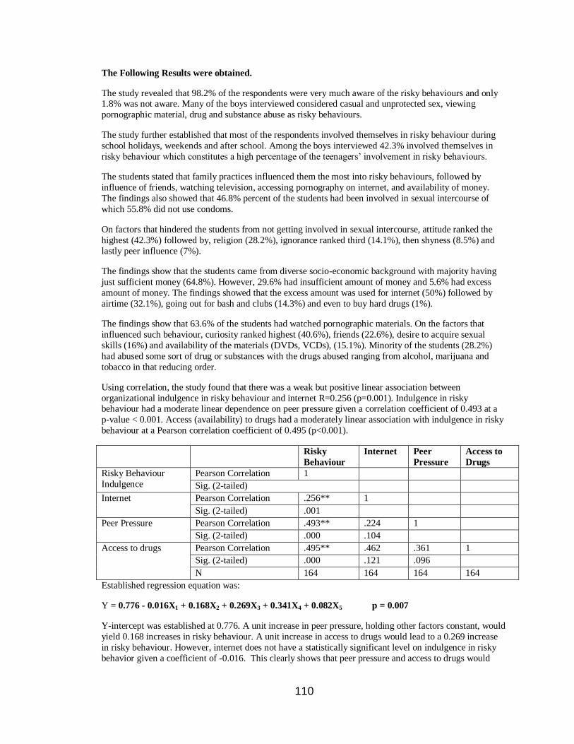
110

The Following Results were obtained.

The study revealed that 98.2% of the respondents were very much aware of the risky behaviours and only 1.8% was not aware. Many of the boys interviewed considered casual and unprotected sex, viewing

pornographic material, drug and substance abuse as risky behaviours.

The study further established that most of the respondents involved themselves in risky behaviour during

school holidays, weekends and after school. Among the boys interviewed 42.3% involved themselves in

risky behaviour which constitutes a high percentage of the teenagers‘ involvement in risky behaviours.

The students stated that family practices influenced them the most into risky behaviours, followed by

influence of friends, watching television, accessing pornography on internet, and availability of money.

The findings also showed that 46.8% percent of the students had been involved in sexual intercourse of

which 55.8% did not use condoms.

On factors that hindered the students from not getting involved in sexual intercourse, attitude ranked the

highest (42.3%) followed by, religion (28.2%), ignorance ranked third (14.1%), then shyness (8.5%) and

lastly peer influence (7%).

The findings show that the students came from diverse socio-economic background with majority having

just sufficient money (64.8%). However, 29.6% had insufficient amount of money and 5.6% had excess

amount of money. The findings showed that the excess amount was used for internet (50%) followed by

airtime (32.1%), going out for bash and clubs (14.3%) and even to buy hard drugs (1%).

The findings show that 63.6% of the students had watched pornographic materials. On the factors that

influenced such behaviour, curiosity ranked highest (40.6%), friends (22.6%), desire to acquire sexual

skills (16%) and availability of the materials (DVDs, VCDs), (15.1%). Minority of the students (28.2%)

had abused some sort of drug or substances with the drugs abused ranging from alcohol, marijuana and

tobacco in that reducing order.

Using correlation, the study found that there was a weak but positive linear association between

organizational indulgence in risky behaviour and internet R=0.256 (p=0.001). Indulgence in risky behaviour had a moderate linear dependence on peer pressure given a correlation coefficient of 0.493 at a

p-value < 0.001. Access (availability) to drugs had a moderately linear association with indulgence in risky

behaviour at a Pearson correlation coefficient of 0.495 (p<0.001).

Risky

Behaviour

Internet Peer

Pressure

Access to

Drugs

Risky Behaviour

Indulgence

Pearson Correlation 1

Sig. (2-tailed)

Internet Pearson Correlation .256** 1

Sig. (2-tailed) .001

Peer Pressure Pearson Correlation .493** .224 1

Sig. (2-tailed) .000 .104

Access to drugs Pearson Correlation .495** .462 .361 1

Sig. (2-tailed) .000 .121 .096

N 164 164 164 164

Established regression equation was:

Y = 0.776 - 0.016X1 + 0.168X2 + 0.269X3 + 0.341X4 + 0.082X5 p = 0.007

Y-intercept was established at 0.776. A unit increase in peer pressure, holding other factors constant, would

yield 0.168 increases in risky behaviour. A unit increase in access to drugs would lead to a 0.269 increase

in risky behaviour. However, internet does not have a statistically significant level on indulgence in risky

behavior given a coefficient of -0.016. This clearly shows that peer pressure and access to drugs would

111

lead to rise in risky behaviour indulgency among students. However, internet had the lowest effect on risky

behaviour.

DISCUSSION

From the findings, the study concluded that unprotected sex was the main risky behaviour most of the

respondents had involved in mostly during school holidays where those who did not involve in those

behaviours did so with reference to their conscience.

The study also concluded that friends had a great influence on respondents‘ behaviour since friends and

adult female friends provided them with money. Access to social information on internet such as

pornographic materials influenced respondents by arousing their curiousity, and television greatly

influenced students behaviour in engaging in risky behaviour.

The study, in line with the objectives, recommended that learning institutions ought to participate in

enlightening students on the consequences of risky behaviour. Further the study recommended that parents

and guardians advised their children during the holidays to dissuade them from risky behaviour.

The study also recommended that access to internet and pornographic material to students should be

limited. It was recommended that school administration should ensure there is thorough inspection to

ensure students do not carry with them illegal and harmful substances such as drugs.

REFERENCES

Alemu, H., Mariam, D. H., Belay, K.A., & Davey, G. (2007). Factors Predisposing Out-of-School Youths

to HIV/AIDS-related Risky Sexual Behaviour in Northwest Ethiopia. J Health Popul Nutr. 25(3): 344–350.

Brundrett, M., & Terrell, I. (2003). Learning to Lead in the Secondary School: Becoming an Effective Head

of Department. London: Routledge Publishers.

CIA Factbook, (2010). Demographic Data: Kenya. Retrieved from: http://www.ciafactbook.org/kenya_html/

Cunningham, W., & Bagby, E. (2010). Factors that Predispose Youth to Risk in Mexico and Chile. Policy

Research Working Paper. WPS5333

Danjin, M., & Onajole, A.T. (2010). HIV/AIDS Risk Behavioural Tendencies Among Secondary School

Students In Gombe (Nigeria). The Internet Journal of Health, 11(1).

Fletcher, J. F. (1997). Situation Ethics: The New Morality. Westminster: John Knox Press.

International Narcotics Control Board, INCB (2006). Report of the International Narcotics Control Board for 2005 Geneva: United Nations Publications.

Kathleen, B. S. (2003). The Developing Person through Childhood and Adolescence, (3rd Edition). Worth

Publishers.

Kenya AIDS Indicators Survey, (2010). National AIDS Report, 2010. Nairobi: Ministry of Public Health & Sanitation.

Lodiaga, M., Wanjama, & Kimani, J. (2007). HIV and AIDS: The Pandemic. Nairobi: Jomo Kenyatta

Foundation.

Miller, G. N. (1994). Challenging in Schools. London: Route ledge.

112

Ministry of Education, MOE. (2008). All Trends in Kenyan Secondary Schools. Nairobi: Government

Press.

Mugenda, O., & Mugenda, A. G. (2003). Quantitative and Qualitative Approaches. Nairobi: Africa Centre

for Technical Studies (ACTS).

Mwiti G. (2005). Moving on Towards Maturity. Evangel Publishing House.

NACADA. (2010). Drug and Substance Abuse among Youth in Kenya: Preliminary Survey 2009. Nairobi: Ministry of Health.

Orodho, M., & Kombo, D. (2002). Research Methods. Nairobi: Kenyatta University Press.

Peter, J. & Valkenburg, P.M. (2009). Adolescents‘ Exposure to Sexually Explicit Internet Material and

Sexual Satisfaction: A longitudinal Study. Journal of Human Communication Research. 35: 171–194.

Prinstein, M. J., & Dodge K. A. (2008). Understanding Peer Influence in Children and Adolescents.

Guilford Press.

Sahoo, F. M. (2002). Dynamics of Human Helplessness. Concept Publishing Company.

Siegel, L. J., & Welsh, B. C. (2008). Juvenile Delinquency: Theory, Practice, and Law. London: Cengage

Learning.

Thorpe, P. (2003). Moving from Primary to Secondary School. National Autistic Society.

United Nations, (2010). World Drug Report 2010. Geneva: United Nations Publications.

Valsiner, J. (2007). Personal Culture and Conduct of Value. Journal of Social, Evolutionary & Cultural

Psychology. 1 (2): 59–65.

World Health Organization, WHO. (2005) Alcohol Use and Sexual Risk: a Cross-Cultural Study in Eight

Countries. World Health Organization

Zins, J. E., & Elias M. J. (1993). Promoting Student Success through Group Interventions. Routledge.

113

ATTITUDE TOWARDS GOING PUBLIC AMONG UGANDAN FIRMS

BY

ELIZABETH KATEME

elikates@yahoo.com

KYAMBOGO UNIVERSITY- UGANDA

BACKGROUND TO THE STUDY Going public is the process of offering securities, generally shares and bonds of a privately owned

company for sale to the general public (Cohn and Zake, 1999; PricewaterhouseCoopers, 2001). The first

time the securities are offered is referred to as an “Initial Public Offering‖, (IPO).

Companies and their shareholders benefit a lot from a public flotation. A share issue for instance,

allows companies to increase the equity base of the company and raise more capital without bearing the

burden of interest payments associated with borrowed funds from financial institutions. In addition, the

public profile of the company is improved, attracting greater business opportunities. Also, full disclosure

requirements of a listing on the exchange encourage companies to observe good business and management

practices and ensure better corporate governance. An investor also gains from investing in securities.

He/she can gain returns in terms of dividends; the securities certificate can be used as collateral to secure

loans and interest income can be earned on fixed income securities. Also investors are given an

opportunity to buy and sell shares in the companies of their choice (London Stock Exchange, 2003).

The setting up and licensing of the Stock Exchange in Uganda (USE) in 1997 has been one of the

most significant developments in building a capital markets industry in Uganda. Capital markets refer to all facilities and the institutional arrangements for the borrowing and loaning of long-term funds (Cohn &

Zake, 1999). A typical capital market comprises of several institutions, namely: banks, insurance

companies, mortgage firms, finance companies and stock markets. Capital markets are an essential part of

the financial sectors of modern economies (Wagacha, 2001). Providing alternative savings tools to savers

and non-bank sources of financing for enterprises, the markets promote economic growth through

improved efficiency in savings mobilization (Schmidt-Hebbal.K, L.Serven and A. Solimano, 1996; USE-

Guide 1999).

Much as the benefits of capital markets are generally acknowledged, the Uganda Securities

Exchange (USE) market is still very slow in that is has failed to attract a significant number of industries

for listing. This is evidenced by the fact that on the USE, only five companies are listed: Uganda Clays Ltd, British American Tobacco Ltd (BATU), East African Breweries, Bank of Baroda and Kenya Airways.

Interestingly, Uganda Clays is the only indigenous listed company on USE. Thus there is no doubt that

more stimuli is needed to induce more private firms in Uganda to go public and thus list on the stock

exchange.

STATEMENT OF THE PROBLEM

Despite the many benefits that a firm gets by going public, the private sector in Uganda

particularly is reluctant to make full use of this facility. The primary market is there but is dominated by

institutional investors and individuals who typically buy and hold on to their securities (Cohn & Zake,

1999). This makes the securities on the USE quite illiquid as indicated by the outstanding offers and bids

and low volume of trading during floor trading. The problem therefore is ―why are potential private firms in Uganda reluctant to go public?‖

114

The strength of securities markets that make them focal points of modern finance is their ability to

mobilize long-term savings for financing long-term ventures, to improve efficiency of resource allocation

through competitive pricing mechanisms, to providing risk capital (equity to entrepreneurs), and to

encourage broader ownership of firms (Wagacha, 2001). These functions are jeopardized if there are few

listings by eligible firms. As already argued above, this is the current scenario in Uganda.

Some seemingly plausible postulations are worth noting. It is argued that for unlisted companies,

the question is not so much lack of knowledge but a concern that the risks associated with additional

disclosure are not adequately compensated by additional returns. In addition, banks in their dual role of

being investment advisors as well as lenders may tend to indirectly discourage the stock exchange as a

means of raising capital. For the stock exchange, there is both inadequate marketing of itself as well as

lack of a sufficient number of products to attract the investing public.

The study examines why companies qualified to go public and list, desist from doing so. A sample

of 140 unlisted companies was identified and surveys carried out, using a questionnaire. Another sample of

the 5 listed companies on the USE was surveyed as a control measure. Also another sample of 6 brokerage

firms and regulatory bodies was also surveyed.

PURPOSE OF THE STUDY

The study sought to identify factors that affect a firm‘s intention to go public by examining and

analyzing the relationship between perceived stock liquidity, perceived tax implications, rules regulations

as well as capital market awareness & know - how and a firm‘s attitude towards going public.

OBJECTIVES OF THE STUDY

The following specific research objectives were adopted: To establish a firm‘s owners/manager

attitude towards going public in Uganda; To establish a firm‘s perception of stock liquidity, tax, rules and

regulations as well as their awareness and know-how of capital markets in Uganda, and, to establish the

relationship between perceived stock liquidity, tax, rules and regulations, capital market awareness and

know-how on one hand and a firm‘s attitude towards going public on the other hand.

RESEARCH QUESTIONS

The study focused on the following research questions for guidance:

o What is the firm‘s owners/managers attitude towards going public?

o How does a firm‘s perception of stock liquidity, tax, rules and regulations, capital market

awareness and know-how, affect a firm‘s attitude towards going public?

o What is the relationship between perceived stock liquidity, tax implications, rules and regulations

as well as capital market awareness & know- how and a firm‘s attitude towards going public?

SIGNIFICANCE OF THE STUDY

It is hoped that the findings of this study should be of use to the following:

115

Regulatory bodies like CMA and Bank of Uganda in formulating effective rules, regulations and guidelines

for proper and effective conduct of the USE activities, the USE will benefit by learning about the

impediments to going public and listing and how to overcome them. The study will also benefit other

researchers should find the research useful in further research of related areas.

SCOPE OF THE STUDY

The study was confined to measures of stock liquidity (market size, demand& and supply of

securities, volume of trading and bid-ask spread); tax, rules and regulations (costs, listing rules, disclosure

effect and loss of autonomy; a firm‘s capital market awareness & know-how (public campaigns and

media publications) and a firm‘s attitude towards going public (market size, market liquidity, stringent

rules and costs of going public and stock market awareness).

THE CONCEPTUAL FRAMEWORK

This is an outline of the different variables used in the study. These were: attitude towards going

public as the dependent variable; perceived stock liquidity, tax, rules and regulatory framework and firms‘

capital market awareness and know-how as the independent variables. Firm‘s attitude towards going

public is said to be affected by the way it perceives stock liquidity, tax, rules and regulations as well as

capital market awareness and its operations. However, macro-economic factors like inflation and interest

rates also impact on a firm‘s attitude towards going public and listing. This is shown as figure 1.8 below:

Figure 1: Conceptual Framework

Source: Self Developed model.

LITERATURE REVIEW

―Going Public‖ simply means that a private company relinquishes parts of its ownership to the

general public by sale of part of or all its shares to the public (USE Guide, 2000; Cohen & Zake 1999;

Perceived stock liquidity

Market size

Number of shares

Bid – Ask Spread Perceived Tax, rules, and

regulations

Cost

Disclosure

Autonomy Capital Market

Awareness & know

how

Public campaigns & media

Attitude towards going

public

Market size

Liquidity of market

Rules & regulations

Market awareness

Macro

economic

factors

inflation

interest rates

116

Pandian, 2001; PricewaterhouseCoopers, 2000). Usually, a company begins to think of going public when

the funding required to meet the demands of the business expansion is not enough (PWHC, 2000). Other

objectives of a capital issue or going public may be to promote a new company, to diversity the production

or to meet the regular working capital requirements of the company, (ibid).

Going public is one of the ways through which companies may raise funds to finance their

projects. Other methods may be through borrowing from financial institutions, promoters bringing in their

own money or using retained profits (Pandian, 2000).

In the current scenario, investing in stock markets is a major challenge even for seasoned

professionals (Pandian, 2001). Investing in various types of assets is an activity that attracts people from

all walks of life irrespective of their occupation, economic status, education and family background.

What matters is that when a person has more money than he requires for current consumption, he should

be taken as a potential investor. The investor who is having extra cash could invest it in securities.

The Initial Public Offer (IPO) is the first sale of stock/shares by a company that has gone public

(Cohn & Zake 1999; USE Guide, 1999). A company can raise money by issuing either debt (bonds) or

equity (Halstead, 2001; Oliveira, 2004). According to Lott, (2002) an IPO is the process by which a private

company transforms itself into a public company. The company offers, for the first time, shares of its

equity (ownership) to the investing public. These shares subsequently trade on a public stock exchange like

the Uganda Securities Exchange (USE).

Nunes (2004) has noted that the most common method of going public is through an IPO. IPO is

done on the primary market which is a situation where a company floats its shares for the first time to

members of the general public (Pandian, 2001; USE, 1991; Cohn & Zake, 1999). The issuer may be of a

new or an existing company. The issues may be of new type or the security issued in the past. Thus, the

first question one may ask is why a company would want to go public, yet many private companies succeed

remarkably well as privately owned enterprises.

For many entrepreneurs, taking their company public is the ultimate measure of success (Dawn,

2002). PricewaterhouseCoopers (2002) noted that it‘s one of the major decisions that a private firm has to

make. Cohn & Zake (1999) concurs with this in that a lot is involved in terms of time, money and

disclosure. Nevertheless, a private company, which has gone public, obtains the benefits of public trading

of its securities namely:

Nearly all companies go public because they need money. Lott (2002) concurs with this in that

the primary reason for going through the rigors of an IPO is to raise cash to fund the growth of a company.

According to Halstead (2001), going public raises cash and also opens up many financial doors for a

company. An IPO offers access to additional capital both through the IPO itself and through ―secondary”

offerings of securities, that is, a public company has direct access to the capital markets and can raise more

117

capital by issuing additional stock in a secondary offering. Public companies can also more easily raise

funds privately (Dawn 2002).

The value of a public company is often substantially higher than a private company with the same

structure in the same industry. The more money a company can attract, the higher its valuation. The

higher its valuation, the more a personal net worth is as a large shareholder of the company

(PricewaterhouseCoopers, 2002; Cohn & Zake 1999; Dawn 2002). Lott (2002) noted that the owners will

sell shares in the IPO in order to diversity their net worth. Also, because of increased scrutiny, public

companies can usually get better rates when they issue debts

Going public enhances the liquidity of a company‘s stock and it is one of the most common

techniques for achieving liquidity for shares. Because the stock of a public company has market value, it

can easily be traded, providing investors with a degree of liquidity (Dawn 2002; Lott, 2002;

PricewaterhouseCoopers, 2002).

Going public leads to good business and management practices and ensures better corporate

governance. Transparency is very relevant for listed companies as far as good governance is

considered essential to the well being of the stock market (Levite, 1999).

While there are predictable benefits and drawbacks of becoming a public company, there are also

many unknowns (Dawn 2002). The securities markets for instance are extremely volatile and focus on

short-term performance, three years performance (Macey & O‘Hara 2001). Hence it has been noted that

the price of a company‘s stock is largely dependent on how the company performs against the expectations

of financial analysts, not necessarily against its own past performance. Thus, if you conclude that the

disadvantages of an IPO outweigh the advantages, and your company requires extra funding, then consider

other alternatives.

It has been observed that there is a very strong relationship between the two markets vs the

primary market and the secondary market. The new issue market (IPO) cannot function without the

secondary market. The secondary market (stock exchange market) provides liquidity for the issued

securities (Pandian, 2001; Watkins, 2004). The issued securities are traded in the secondary market

offering liquidity to the stocks at a fair price. In addition, the stock exchanges through their listing

requirements, exercise control over the primary market in that any company seeking for listing on the

respective stock exchange has to comply with all the rules and regulations required by the stock exchange.

Furthermore, the primary market provides a direct link between the prospective investors and the

company. I.e. by providing liquidity and safety, the stock markets encourage the public to subscribe to the

new issues (Pandian 2001; Cohn & Zake 1999). Thus, the health of the primary market depends on the

secondary market and vice versa, concludes Levitte (1999).

CAPITAL MARKET AUTHORITY OF UGANDA AND THE USE

The CMA in Uganda was set up by enactment of the Capital Market Authority statute by the

parliament of Uganda in 1996(Cohen & Zaake 1999). As the regulatory authority, CMA was charged with

the responsibility of promoting and developing an orderly, fair and efficient capital market (Bohnstedt, et al

118

(2000). Under the statute, rules on licensing, prospectus requirements, establishment of stock exchanges,

conduct of business by licensees, accounting and financial requirements were developed (IMF, 1999).

CMA does not only regulate the USE, but also stock brokers/dealers or any other persons dealing in

securities within the national territory. In addition, on all policy matters concerning capital market

development, the CMA has an advisory and consultative role.

It has been observed that the key factors of the capital markets industry in Uganda is that it has a

fully liberalized capital account, there are no restrictions to foreign investors, has a well regulated financial

market and has access to regional markets. CMA signed a memorandum between the securities regulators

in Kenya, Uganda and Tanzania. The objective is to harmonize the development of capital markets in the

East African region (New Vision, 9th October, 2004; pp 27). Bohnstedt 2000, in their research, adds that the

respective statute governing the Ugandan securities market, largely conforms to the disclosure and

reporting standards applicable in Tanzania and Kenya. Both the CMA as well as the USE are members of

East African member states Securities Regulatory Authority (EASRA). The objective of this is to

harmonize securities laws and standards with a view towards integrating the individual markets, building

up a regional exchange, and establishing cross-border investments and listings (IMF, 1999).

Tax, Regulatory and Legal framework and going public

Most countries worldwide rely on taxes as a means of raising revenue for the government.

Various taxes are paid by companies such that a firm may find itself paying at least two or three different

types of taxes to the government. Such taxes particularly, encroach on the operations of any business

organization, thus affecting profits that would have been earned, (Pownall & Schipper, 2004). Such taxes

among others include income tax, VAT, Excise duties and custom duties, Sales Tax and corporation tax

(Katto, 2003). Dividends for instance distributed to shareholders are subject to a final withholding tax. To

this issue, Onegi, (Chairman of the USE), 2004, argued that withholding tax is discouraging investment on

the bourse/exchange. To this effect, during the DFCU Ltd listing on the USE, he recommended that taxes

on dividends (withholding tax) should be scrapped.

Also, dividends not distributed (retained profits) out of after tax profits are subject to

compensating tax at the company rate of tax (Pownall & Schipper, 2004; Katto, 2003). Capital gains tax is

also another tax to be paid by public companies. Capital gains refer to the increase in value of shares of a

company. Share prices move up and down. When the price of the shares you hold goes up then your

investment appreciates in value. Such increment in value of shares is capital gain to the business and

therefore is taxed. VAT is compulsory to any manufacturing company within the country and taxable

services provided. The standard VAT rate has been 15% in East Africa. Excise duty is yet another tax on

all goods manufactured within a country. In this case, the rates vary for different products; (wines, Spirits,

Tobacco products, mineral water, biscuits, match boxes, etc). Customs duties are paid by all importing and

exporting companies for goods imported to or exported out of a country. Such and many more other taxes

impede the firm‘s operations.

Thus, tax incentives provided should improve the post tax returns for the companies, thereby

encouraging them to invest more in the companies and therefore improve on their performance. In the long

run the economy should benefit by having more competitive firms eligible to list. Conclusively tax regime

119

is considered problematic by many firms. This tax plus exchange rate fluctuations particularly, influence

the manufacturing sectors, commerce and trade, (Bohnstedt et al, 2000). This influences their attitude

towards listing as taxes are taken to be extra burden.

The Legal & Regulatory Framework

There is a plethora/excess of rules and regulations governing the public offering of securities

(NewWest, 2004). In this context, the legal framework generally refers to the laws that govern trade in

securities in an economy. It‘s made up of the Companies Act, which governs the general operation of

businesses (company law) and specific laws enacted for the purpose of trade in securities. The Regulatory

framework is therefore that set of specific rules and regulations governing the respective bodies involved in

the operations of the market (USE, 1991; CMA, 2000; Wagacha 2001; Chege, 2003). The legal and

regulations framework guide operators in the market (Alile, 1992). They provide rules and regulations and

principles and procedures that guide the conduct of all participants in the market.

A great deal of empirical evidence suggests that a strong equity market requires strong investor

protection laws measured by legal rules in play and quality of law enforcement, (Lelenx and Muzyk 1999).

To Frost, et al, 2002, the major objectives of prudent regulations in an equity market are investor protection

and market equity. To them, investor protection means that investors are provided with material

information and are protected through monitoring and enforcement. High quality markets are fair, orderly,

efficient and free from abuse and misconduct. In their research analysis, it was found out that higher levels

of investor protection are associated with higher quality markets leading to higher liquidity resulting in

increased returns and thus impacting on investor‘s decisions. Lelenx and Muzyk observed that French civil

laws appear to have the weakest investor protections and consequently the least developed capital markets.

Thus, they add that changing this state of things will require more than a few costmetic changes to market

regulations.

The major objectives of prudential regulations are to ensure: public confidence in the activities of

financial markets, operational stability of the market, and operating efficiency of equity markets (Ibid).

This view is shared by the Eastern Caribbean Central Bank (ECCB, 2004). To then, one of the primary

concerns of investors is the security of their investments. They need positive assurance that their

investments are protected and are safe. Therefore in acknowledgement of this, every effort has to be made

to ensure that the market operates under secure conditions. They noted that a sound regulatory structure

has to be put in place to ensure that all market activities are conducted with international standards of

fairness, transparency, professionalism and integrity.

Chege (2003) emphasizes this point in that lack of vibrant financial sector regulations erodes

confidence in the market and is a disincentive to investment in capital markets. She adds that regulators in

this industry must literally exercise their functions as watch dogs and protect investors.

In Uganda, the two major players in the markets concerning rules and regulations are the CMA

and the USE. The CMA of Uganda, as the regulator is a creative of statute, (CMA Act, Cap. 84), which

provides the establishment of the CMA, charged with the dual duty of promoting and regulating the

120

development of the capital market. In some countries, it‘s known as the ―Securities Commission‖, (SEC),

(Chege 2003; CMA Digest, 1998; Cohn & Zake 1999). I.e. it‘s a body that regulates the capital markets

industry. This is done through regulation, enforcement, monitoring, compliance, setting standards and

licensing market players such as investment advisors and brokers, dealers, fund managers, collective

investment schemes and approving prospectuses of issuers of securities. It‘s the overseer of all capital

markets and stock market operations in the country. It also formulates rules and guidelines with regard to

companies wishing to go public.

The USE is the actual market on which securities are traded. It is approved by the CMA. Its main

function is to ensure orderly transactions in securities. It‘s self- regulatory and has its own rules that issuers

of securities are expected to abide by such as the USE listing rules. There are three market segments on

which securities may be traded on the securities exchange i.e. the main investments market segment

(MIMS), the alternative investment market segment (AIMS) and the fixed income securities market

segment (FIMS). These segments have different requirements, (See appendix).

Public disclosure is perhaps the most difficult matter for private companies to come to grips with,

(Dawn, 2002). By law is must disclose the intimate details of their business operations, including financial

information. Thus, listed companies are governed not only by company law but also by stock exchange

regulations (ACCA). By law, all public companies must disclose all materials and relevant information

about their performance, activities, operations and accounts (CMA, 1999). However, this reduces the

firm‘s autonomy especially the family business. This disclosure requirement is put in place to ensure

investor protection and to promote investor confidence in the market (ECCB, 2004; Cohn & Zake, 1999;

USE, Quarterly Bulletin 2002).

Public companies benefit from increased opportunities for financing and growth by obtaining long

term finance. For founders and management shareholders, going public provide enhanced liquidity for

their stock ownership at a market based valuation. The costs of going public however, includes among

others the burdens of complying with the ongoing disclosure requirements of the CMA (SME) and the

Stock Exchange and increased potential liability management will also bear the burden of increased

scrutiny of corporate conduct compared to owning and operating a privately held concern. In addition, an

extensive publicity campaign is necessary so as to inform and educate the public about the capital markets

and its role in order to change their attitude toward going public.

Research Design

The study was conducted as cross-sectional study i.e. different categories of subjects were studied

at one point in time based on the results from self test questionnaires and interviews. It was cross sectional

because of the need to overcome time and financial constraints.

Study Population

The targeted population for the study was 1434 organizations comprising of the following strata: -

16 – Commercial banks; 17 – Insurance companies; 1386 other private businesses; the 5 listed companies

by then and 10 stakeholders (CMA, USE, BOU plus brokerage firms).

121

Unlike Bohenstedt (2001) whose respondents included only private firms, this study preferred to

include listed companies as well as stakeholders‘ views about the USE market.

Sample size

The targeted sample size was 151 organizations obtained from a population of 1434 using Krejcie

& Morgan (1970 table). The 151 respondents were selected from the 151 organizations. The 151

organizations is big enough as confirmed by Bailey K.D. (1994). He regards 100 cases as the minimum.

The selected respondents included Chief Executive Officers (CEO), Chief financial managers/

Accountants, company secretaries and owners/ managers. The purpose of choosing these elements was to

gather information data from persons who are in decision making positions.

Out of the 151 questionnaires administered, 131 were returned making a percentage of 86.7%

which is more than half the sample size and therefore representative enough. The 10- Commercial banks in

Kampala comprised the sampling frame of the respondents from the commercial banks. Source of the

population got from Bank of Uganda Supervisory department as per December 2002. The 10 -Insurance

companies in Kampala made the sampling frame of the respondents from the insurance industry. Source of

population was got from Bank of Uganda supervisory Department as per December 2002.

The 120- private businesses formed the sampling frame of the respondents from other private

businesses. Source of population was drawn from the Uganda Manufacturer‘s Directory 2003/2004.

All the 5 listed companies on the USE comprised the sample frame as well as the population of

respondents for this category. This is because they are few thus it would not be fair to leave out any of

them. Source population got from the USE investor‘s Guide and CMA website. The 10- other stake

holders formed the sampling frame for this category. Source population got from USE investor‘s Guide and

CMA Journal.

Sampling Design and Procedure

The population chosen for the study was first stratified into groups (strata): Commercial Banks,

Insurance companies, other private businesses, listed companies and the stakeholders. Unproportionate

stratified sampling was used to obtain the sample of 151 companies. Then simple random sampling was

applied to the selected organizations from each stratum. This method was preferred because it gave each business organization an equal chance of being selected without bias. However, for other private

businesses, purposive sampling was used because the aim was to choose the businesses with the highest

potential of going public.

Perceived Stock Liquidity

Using the 4-point Likert Scale, Perceived stock liquidity variables measured included: market size

measured in terms of capitalization and number of companies listed on the exchange; volume/number of

shares traded on the exchange annually and the bid-ask spread.

Perceived Tax regime, rules and Regulations

Using the four point Likert scale, tax regime was measured in terms of the different taxes paid by companies and businesses generally. Still using the same scale, rules and regulations were measured using

the cost variable, the disclosure effect and loss of autonomy by owners of the businesses. Statements

regarding this variable were adopted and modified from various researchers such as Bohenstedt (2000), and

Wagacha (2001)‘s surveys.

122

Perceived Capital Market Awareness and know-how

Still using the four point Likert scale this variable was measured in terms of public awareness,

technical know-how and willingness to learn about capital markets. Some of the statements regarding this

variable were drawn from Wagacha (2001) and Ngoma (1995).

Attitude towards Going Public

This variable was measured in terms of the personal feelings of the owners/managers of the

businesses about going public, the size of the stock market, and volume of shares traded on the market,

costs involved, and the disclosure effects. Most statements were self developed and similar scores were

used as above.

Sources of Data

Data for the study was collected from both primary and secondary sources but with

more emphasis being placed on the primary data since the study was about perception. The

primary data was mainly derived from various respondents as specified in the sample to the questions in the

questionnaires and interviews posed directly to them. In this case, the questionnaires formed the key data

collection instrument. Secondary data was collected mainly from: company reports and prospectuses,

company journals, research papers by various researchers down loaded from the internet and other publications. The purpose here was to compare the secondary data with the responses from primary data

gathered from the field so as to derive a meaningful interpretation.

Data Processing and Analysis

Raw data collected through questionnaires was analyzed. First, qualitative data was summarized,

categorized and then analyzed using percentages in tables and charts. In order to establish whether the

relationships exist between stock liquidity, tax, rules and regulations, capital market knowledge and a

firm‘s attitude towards going public, data was analyzed quantitatively using the correlation options of

statistical package for social sciences (SPSS) computer programs with the aim of answering the questions.

This package was considered because it is more user-friendly, quite available and powerful in data analysis.

Entering the data involved defining the variables in the variable view and inputting the data in the

data view. Data was then analyzed to generate both descriptive and inferential statistics. Under descriptive

statstics, information on demographic characteristics was generated, while under inferential statistics,

correlations were done.

FINDINGS

The study found that stock liquidity has a significant positive relationship with attitude towards

going public (r = 0.414, p-value < 0.01). This implies that stock market liquidity significantly influences

firms‘ attitudes towards going public. These findings are consistent with the findings of Wagacha (2001),

PWHC (2001) Cohen and Zaake (1999) and Bohenstedt (2000).

Tax, rules and regulations had significant negative relationship with firm‘s attitude towards going

public (r = - 0.375, p = value < 0.01) implying that taxes, rules and regulations negatively affect firms from

going public. This confirms Wagacha‘s, Emily‘s and Bohenstedt‘s findings that taxes are taken by many as

a burden and that the stingy rules chases away eligible firms.

123

The study also found that market awareness had a significant positive relationship with attitude

towards going public, (r = 0.579, p value< 0.01). The implication here is that market awareness improves

firms‘ attitude toward going public.

CONCLUSION

The findings revealed that quite a substantial number of private firms (58%) have a positive

attitude towards going public. The results also indicated that firms attitude towards going public will be

changed positively if the USE market becomes more liquid. Liquidity of a stock market is very important

to firms going public and therefore should be addressed by the USE. It was also found that a large

percentage of the unlisted firms (77.1%) revealed that if incentives such as tax holidays are given to firms

going public, then many more firms would change their attitude towards going public as their costs would

be reduced.

The study further found that if the costs for an IPO and listing were reduced, then the firm‘s

attitude towards going public would be changed immediately. This is an eye opener that IPO costs should

be reduced. Also, they reveled that if the disclosure requirements were made less stringent then their

attitude towards going public could be changed immediately. Thus strict rules deter firms from going public. Respondents also indicated that public awareness is an important factor to firms going public.

Recommendations

Based on the survey of both listed companies and unlisted companies in Uganda and the findings

above it is evident that the USE and the CMA need to address specific factors inimical to the growth of the

stock market in Uganda. The market needs to pay attention to various aspects including the following:

Enhancement of stock liquidity, increase in returns, international integration, and relaxing the stringent

rules and regulations of listing.

.

It is can be concluded that if the Stock Exchange Market in Uganda is to be enhanced as a vehicle

for mobilizing capital for development, then all players in the market must change their approaches. The USE must play an increasingly educational role; the CMA as the regulatory agency must alter its approach

from the sometimes heavy-handed type of control to a more proactive, creative and supportive role in order

to assist in the creation of a more vibrant and formal working capital environment. It can do this by seeing

itself as a catalyst in development rather than as a traditional regulator of what is a very small market.

124

REFERENCES

Adam c, Cavendish W & Mistry P. (1992): Adjusting Privatization: Case studies from Developing

countries, James Currey; London.

Advantages & Disadvantages of Going Public (2004): htt://www.stanfordcapitalinc.com/goingpublic.htm.

Alile, H. I. (1992): Promoting Capital Markets in Africa. ―Establishing a Stock market: Nigerian

Experience: Presented at the international conference, Abuja, Nigeria, 11 – 13th November 1992.

Anderson, M. Anne & Dyl Edward (2002): Market Structure and Trading Volume:

http://www.nyse.com/marketinfor/1020656068407.html

Bilki Jaggi (1997): Accuracy of Forecast Information Disclosed in the IPO Prospectuses of Hong Kong

companies, The International Journal of Accounting, Vol. 32, No. 3, pp – 301 – 302; JAI press Inc:

Greenwich, London, England.

Bohnstedt Andrea, Hanning Alfred and Ondendall, P. Ralph (2000): Capital Market Development in

Uganda – Private Sector Opinions on Listing: Bank of Uganda (B.O.U) – German Technical Co-operation

(GTZ), Kampala, Uganda.

Bortolotti Bernardo, Giovann Nicodiaes & Ibolya Schundel (2003): Privatization & Stock Market

Liquidity – Finance Group – World Bank, Amsterdam, Netherlands.

CMA Digest (2000): The Rationale for Capital Markets in Uganda.Vol.2, July 2000, CMA. Kampala,

Uganda.

CMA (1999): General Information and Guidelines for issue of Securities. Austrian Development

Cooperation, Kampala, Uganda.

Cohn, S.R. & Zake, F. (1999): Capital Market Development in Uganda. International Law Institute (ILI) –

Uganda Legal Centre of Excellence, Kampala – Washington.

125

Davis Philliph E, (2004): Russia/ LTCM & Market Liquidity Risk; Bank of England, London.

Dawn Call, (2002): The Advantages and Disadvantages (and alternatives of IPO‘s).

Direct Public offerings (2004): Weigh the pros & cons of Going Public. Nevwest Securities Corporation

Las Vegas, NV.

Eastern Caribbean Central Bank –ECCB (2004): Investment Insights. Author

Fe‘ Ernesto, A., Mauro Leos, Mindlin Marcelom, Molan Walter T. & Ugeux Georges (2000): An Outlook

on Capital Markets: Presented to Mercosur Economic Summit. World Economic Forum 2003.

Fleming Michael J. (2003): Measuring Market Liquidity. Federal Reserve Bank of New York (FRB) The

FRB Journal: Economic Policy Review: Volume one, Year 2003, issue month – Sept: pgs 83 – 108).

Frost A. Carol (Suffolk University), Gordon A Elizabeth (Rutgers University) and Hayes F. Andrew (Ohio

State University), (2002): Stock Exchange Disclosure and Market Liquidity: An analysis of 50

International Exchanges.

Gindici Giancarlo & Parteari Stefano (2003): Online Journal (www.blackwellpublishing.com): Should

Firms Going Public enjoy Tax benefits? An analysis of the Italian Experience in the 1990‘s. Black well

Synergy Publishing. Inc.

Gluck, T. & Verfsasser (2002, April): The Vienna Stock Exchange‘s Solution to the Problems Arousing in

a Changing Environment for Stock Exchange. Journal of Liquidity and investor Attitude - Internet).

Halder (2002): Going Public: A Source of Fresh Capital for medium sized businesses.

http://www.halder.nl/E-5-0-Going-Public.htm.

Halstead, T. (2001): Traders Edge: ―Why the ―Bid – Ask‖ Spread is so Important. (Working paper on Bid

– Ask Spread).

Hasbrouck & R.A Schwartz (1998): ―Liquidity and Execution costs in Equity markets.‖ The Journal of

Port folio Management.

126

International Finance Corporation (IFC), (1993): Emerging Stock Markets Fact book, 1993. Washington,

DC: IFC.

International Finance Corporation (IFC), (1994): Annual Report – Washington, DC: IFC.

Jefferis, K. (1995): The Botswana Share market and its role in Financial and Economic Development.

World Development Journal, vol.23,No.4.

Jefferis, K. (1996): Department of Economics, University of Botswana. The Development of Stock

Markets in Sub-Saharan Africa. Makerere Business Journal, Vol. 1. No. 11, 1996.

Katto, J. (2003): A Plausible source of Long-Term Finance. Capital Markets Journal for the Capital

Markets Industry in Uganda. Vol. 6, 2nd

Quarter 2003, pp 28-32. CMA, Kampala-Uganda.

Lelenx Benoit F, (Babson College), Wellesley Muzyka Daniel .F. (1999): Counting the European Growth

firms: A survey of Attitudes Toward listing Alternatives. INSEAD.

Lelenx, F.B., & Muzyka, F.D. (1999): Courting the European Growth firms. Babson College, Wellesley.

Levine R. (1996): ―Financial Development & Economic Growth: Views and Agenda‖. Policy working

Paper No.1678. The World Bank, Washington D.C.

Levine .R & Zerros (1996): ―Stock Market Development and Long run Growth‖. Policy working Paper

No. 1582. The World Bank, Washington D.C.

Levitt, A. (1999): Evidence on the Reaction Corporate Governance Characteristics and the quality of

Financial Reporting. (Working Paper Internet).

London Stock Exchange (2003): Going Public. A survey of recently floated companies. Eversheds-London.

Macey, R. Jonathan & O‘Hara Mauren (2002): The Economics of Listing Fees and Listing Requirements.

Johnson Graduate School of Management Cornell University, New York, USA.

127

Macrae, H. & Caincross, F. (1985): Capital City, London as a financial Centre. Methenem London Ltd.

London.

Meier, R.T (1998): Benchmarking Analysis of Stock Exchange Trading: International Federation of stock

Exchanges, Paris/Zurich.

Nunes d‘Agrella Peter (2003): Going Public (IPO): http://planmagic.com/toolkit/tools/go-public.IPO.html.

Ngoma, T. (1995): The Viability of Stock Exchange in Uganda. Unpublished

Master‘s Dissertation, Makerere University, Kampala Uganda.

Oliveira Alvaro (2004): Suitable Stocks For Day Trading: Going Public.com

http://daytrading.about.com/cs/educationtraining /a/suitable_stocks.htm.

Ole Nkeri Simon Peter (2003): Investor Education, Awareness and sensitization programmes: A Paper

presented during the CMA, Uganda, end of year seminar, 2003.

Onegi-Obel Geoffrey (2004): Tax Burden. The New Vision – November 4th, 2004, Pg. 20. The New

Vision Printing and Publishing Co. Kampala, Uganda.

Pagano (1993): The floatation of companies and the stock market: European Economic Review.

Pandian, P. (2001): Security Analysis and Portfolio Management. Vikas Publishing House. PVT Ltd. New

Delhi.

Panzarasal Pietro, Jennings Nicholas R, Norman J. Timothy (2004): Going Public and the sale of shares

with Heterogeneous Investors; University of Southampton, UK.

Peter Kaujju (2004): Business Communication hails Vision Sale. New vision, Sept 24th 2004, Vol. 19, No.

230, Pg 49.The New Vision Printing and Publishing Co. Kampala, Uganda.

128

PricewaterhouseCoopers (2001): The Going Public Decision. Author

Postel, E. (2004): Emerging Capital Markets in Africa: Challenges and Opportunities

hppt://www/un.org/Depts/ecaldivis/espd/5.hml.

Pownall Grace & Schipper Katherine (1999): The SEC‘s Decision Criteria & Academic Accounting

Research; Accounting Horizons Journal Vol. 13, No. 3, Sept. 1999; Accounting Association, Florida.

Reicin v. Cheryl, Cifrino A. David, Colbran L. Philips & Robinson .K. John (2002): An Insiders Guide to

Going Public; Reuters Inc.

Reilly, K.F. (1985): Investment Analysis Portfolio Management (2nd Ed.). CBS College Publishing. The

Dryden Press.

Rutega, S. (2003): USE Commentary on USE Activities. Uganda’s Journal of The Capital Markets

Industry. Vol. 6, No. 2, 2nd

Quarter 2003. Pp7.CMA, Kampala, Uganda.

Schmidt-Hebbal, K., L.Serven & A.Solimano (1996):‖Saving Investment: Paradigms, Puzzles & Policies‖.

The World Bank Research Observer, Vol.1, No. 1, Feb.

Tacis INVAS Centre (2003): The Capital Markets Investment Advisory Services Project: EU Workshops,

Round tables, Press Conferences and presentations to domestic private investors; MICEX Publishers,

Moscow, Russia.

Tarinyebwa, W. & Chege, M. (2003): ―The Legal & Practical Aspects of Capital Markets‖. A presentation

made to BAR course students at LDC, Kampala. CMA –

Kampala, Uganda.

Times of Oman Newspaper, Monday, 22nd March (2004): Sulaimi calls for Augmenting Savings

Entrepreneurship. www.timesoforman.com.

USE (1999): Investors Guide to buying and selling shares on the USE. USE, Kampala, Uganda.

USE (1997): Listing on the USE. ―Who, Why and How?‖ USE. Kampala, Uganda.

129

USE, Quarterly Bulletins. Author. Kampala, Uganda.

Wagacha Mbui (2001, July): Kenya‘s Capital Market: To list or not to list. Discussion Paper No.28. IPAR.

Watkins, T. (2004): ―The Determinants of Demand for financial Assets – San Jose‘ State University.

World Bank (1993): Global Economic Prospects and the Developing Countries; World Bank, Washington

D.C.

130

ADMISSION REQUIREMENTS AND CLASS SIZE INFLUENCE ON

STUDENTS’ PERFORMANCE

BY

MOYA MUSA

BYARUGABA PONTIOUS

NASSUNA AGNES

BACKGROUND TO THE STUDY

Over time, the number of students admitted to public universities in Uganda has been increasing. This has

had tremendous effects on the general performance of these universities and it has affected the ultimate

product of these universities, which is the performance of the students. In addition to this, many new

courses have been introduced in public universities, which have seen various changes in the admission and

entry requirements. Various arguments have been advanced by a multiplicity of scholars on the effect of

entry requirements on the ultimate performance of university students. (Geiger and Dangerfield 1996,

Lawrence and Pharr, 2003, Ineson and Kempa ,2007).

Traditionally, specific key areas like Mathematics and Economics were essential requirements for pursuing

Business courses, however, this has been relaxed such that currently at some universities, any two principal

passes in any subjects, done at advanced certificate level can enable someone pursue a business related

course. It has been noted that there are many students who though have not pursued, the essential courses,

eventually excel at the university in terms of their overall cumulative grade points.

In a study done by Pharr (2006), it was established that while admission standards were effective for all

students under the traditional business core curriculum for areas like accounting and statistics, it was not

equally appropriate for the integrated business core curriculum in general areas like Business law, Business

ethics and Economics. He highlights that a one size fit approach to business schools admission

requirements may not be an appropriate policy given significant curricular redesigns.

Admission requirements are commonly employed as a means of matching the quality of an academic

program and the student pool. As a result, they play an important role in ensuring the overall quality of the

program and present a critical quality control design that allows the admitting of students with a high probability of succeeding in the specific program, while preventing those students who would likely

perform poorly from enrolling.

Generally, smaller class sizes tend to be associated with better teaching and therefore better student‘s

performance (Hooper and Page, 1986; Cohen, 1983; Aleamoni, 1989; Raval, 1991; Koh and Tan, 1997),

although non-linear relationships have also been reported in the literature (Holtfreter, 1991).

In some research studies, students in smaller classes have realized achievement goals superior to those in

larger classes (McConnell and Sosin, 1984; Liaw and Goh, 2003). Some research suggests that large

classes are simply not as effective as small classes for retention of knowledge, critical thinking, and attitude

change (McKeachie, 1978, p. 207; Siegfried and Fels, 1997, pp. 938-9; Glass et al., 1981; Toby, 1993;

Cranton and Smith, 1986; Koh and Tan. 1997).

However, some studies found a negative relationship between teaching and class size (Marquardt et al., 1975), while other studies found a weak or insignificant relationship (Stumpf and Freedman, 1979; Marsh,

131

1984; Langbein, 1994). it is on this basis therefore, that an investigation has been carried out to assess the

relationship between entry requirements, class size and university students performance.

STATEMENT OF THE PROBLEM

Over time students‘ performance has declined with a big number of students failing to complete their study

program in the scheduled time characterized by failure of quantitative subjects like accounting, statistics,

and quantitative methods (Faculty board reports, 2007-2009). This may be attributed to various factors

including, the admission criteria and class sizes, which in turn influence the study environment thence

affecting students‘ performance associated with lower CGPA and number of students graduating at

particular year. This situation jeopardizes the overall mission of the university that aims at producing well-

trained graduates with adequate skills to enable them perform efficiently out there in the job market.

PURPOSE OF THE STUDY

The purpose of the study therefore is to analyze the admission criteria and the changes in class sizes and to

what extent these factors influence the overall performance of the students in terms of the Cumulative

Grade Point Average (CGPA).

OBJECTIVES OF THE STUDY

To find out the relationship between admission criteria and the study environment.

To investigate the relationship between class size and the study environment.

To examine the relationship between admission criteria, class size and students‘ performance.

RESEARCH QUESTIONS

What is the relationship between the admission criteria and study environment?

What is the relationship between the class size and study environment?

What is the relationship between admission criteria, class size and student‘s performance?

SCOPE OF THE STUDY

The research focused on admission requirements and the class size as the independent variables and review

students‘ level of performance as the dependent variable.

It was limited to MUBS as the case study and reviewed programs of BBA, BCOM, BBC and BOIM and

considered a period of 13 years from 1997 to 2009.

132

CONCEPTUAL FRAME WORK

Source: Literature review

It is assumed that the admission criteria in terms of the score of points and the essential subjects taken,

together with the number of students admitted in relation to the room capacity and number of faculties

present to deliver curriculum affect the output of the learning process at the university in terms of performance levels at the university. This study focuses on students admitted on direct entry. We are

assuming that the study environment in terms of student book ratio, library capacity and total time in

terms of credit units is constant and we limiting students‘ performance to the cumulative grade point

attained by a student and the number of students who graduate compared to those admitted in 1st year.

Admission

Requirements:

Total Weights

Maths & Econ.

grades

Study environment:

Student book ratio

Library capacity

Total credit units

per programme

Students’

Performance

CGPA

Number of

graduates

Class Size:

Students room

ratio

Student lecturer

ratio

133

LITERATURE REVIEW

Review of existing work on university performance, student‘s performance, study environment, admission requirements, class size and the relationships that exist between them in order to gain a deeper

understudying of the study variables and appreciate the gaps that exist.

UNIVERSITY PERFORMANCE

Universities assist in the development of a country through developing innovative capacity and students transformation, (Chessman et al, 2006), therefore there is need to focus on improving its operations through

research. Masmiliano, Abigali, Robin and Jeremy (2008), assert that demonstrating success and a high level

of performance, helps any university to attract and retain resources, recruit quality faculty and students and

maintain partnerships with other stakeholders like government and research facilities.

It should be appreciated that the university performance is highly indicated by the extent they are able to

educate students who on learning are transformed into individuals capable of making a positive difference

at regional, national and global levels, though sometimes it is not always the case. Identifying and

analyzing student‘s performance is of great importance to educators, psychologists and the student‘s community at large.

According to Maria de Conceicao (2004), universities are centers of creativity, transmission, and

propagation of culture, science and technology who through teaching and research enhance the life of

society. In order to appreciate the performance of university students, let us first review the factors that

influence the overall university performance.

Various factors determine the performance of universities. According to Srikanthan (2003), the essential

drivers of university performance are the assertions of autonomy and accountability and this are embedded

into the educational policy of the country. He explains that autonomy gives freedom to the academicians to

develop curricula and conduct research. Therefore, university academic staff should not be treated like

employees of corporate enterprises rather they should be treated like independent thinkers of future visions.

Autonomy not withstanding universities should be accountable to their funding authorities to ensure that

the affairs of the institutions are being governed and managed properly. (Cannon, 1994)

Taking a big picture, overall university performance is a result of a diversity of factors as highlighted by

Bratti, Mcknight, Naylor and Smith (2003). In their research on higher education outcomes, graduate

employment and university performers indicators they identified factors like Matriculate academic

preparation, ranking in top continental universities, diversity of students, number of international students,

retention of students, transfer of students, graduation numbers, post baccalaureate enrollment, average class

size, doctoral attainment of full time teaching faculty, financial strength and giving back to society.

Building on this the university of Lancaster report (2006) noted that university performance can be

analyzed basing on factors like quality of teaching and graduates produced in terms of degree awarded,

student satisfaction, retention of students and graduate track employment. Other factors that were

highlighted by the report included quality of research, financial viability, staff quality, estates quality, IT

quality and availability of transformational projects. It should be appreciated that this report is line with earlier findings.

Maria de Conceicao (2004), on the other hand, looks at university performance in terms of customer

orientation, level of competitiveness and accountability of the leaders. She argues that in order to assess

their performance , universities should review internal performance indicators which are based on the

internal information produced by the university such as the pass rate, graduate rate, number of dissertations

produced, average duration of course, assessment of professors by students and indicators of operational

performance which refer to activities of departments such as student/professor ratio, student/staff ratio, unit cost of programs, class size, ratio of employees and student computer ratio. Maria goes ahead to identify

external performance indicators such as employability of graduates, reputation of the university in the work

place and research performance indicators which aim at assessing the research activities at the university

which may include number of publications, research contracts, dissertations accepted, consultations

provided, inventions and patents, invitation to relevant scientific conferences and organization of such,

134

awards and distinctions. This paper helps and to understand university performance is because of a

diversity of factors.

Having appreciated the big picture, the sections that follow review specifically students‘ performance, as it

is the focus of this research paper.

STUDENTS PERFORMANCE AT THE UNIVERSITY

Student‘s performance at a particular university is a key predicator of the overall university performance. It can be looked at in terms of the course grades or grade point averages attained by individual students,

skills attained and the level of employability (Nuttali, 1992). The higher the grades, and level of

employability and the more the skills attained the higher the performance. For purposes of reliability, this

paper is going to be limited to the grades in terms of cumulative grade point averages as measures of the

students‘ performance.

Normally performance of university students if influenced by various factors including student‘s

demographic profile, admission qualifications, subject taken by students in pre university level, gender,

attendance, linguistic capacity, ethnicity, culture, age among others. (Ervina, 2005).

Recent research shows that an increase in students performance is associated with improvement in teaching

that is linked with technology and the internet and the entrance examination scores especially in

mathematics, science and research, gender differences and availability of appropriate supplemental

instruction or technical assistance .(Waples & Daraysah, 2005, Cheesman, Simpson and Wint 2006 Sicat

& Broncs, 2009). Analysis of these papers shows that large class size and heavy teaching load for the

instruction may also affect the performance of the students.

According to Alfan, 2006, performance of the university student should be looked at in terms of the overall

quality of the student as the final product of the institution released to the labor market. He goes on to

explain that the overall performance of the university‘s products should have minimized drop outs at that

level, as students who drop out would not only find it difficult to search for jobs, they could also hinder the

development of the labor market.

Carpenter et al (1993) found out that student‘s performance could depend on his or her expectations and

also on their race. In addition Bordes (1998), advances factors like gender, age, academic origin, grade

point average, extra curriculum activities and employment influence as determinants of the grades obtained

by a student.

Another key determinant of performance at the university is the performance at level prior to admission at

the university. Ardila (2001) in his paper on predictors of university performance in Columbia discovered

that scores at examinations that determine entry at the university , much as they are used as a major

criterion for university admission, performance in such exams , has low correlation with the students GPAs and vary widely from one academic program to another.

In another research by Durr (2000), several factors were identified to affect students‘ performance at the

university and these included students original attitude towards some courses, personality of the instructor,

and performance in entrance exams, motivation and effort of the students, gender differences and student‘s

age, in this study it was found that men performed better than ladies, students would perform better if they

had similar learning styles with their professors or if they tried to model them, high scores in standardized

entrance exams did not guarantee high students performance and that the determination to graduate also

motivated to work hard and therefore score better grades.

According to Pharm (2008), key factors that affect students‘ performance include-

Academic Competence – this is the proficiency of students with respect to the content taught during the

course and their ability to understand the course materials.

135

Test Competence- this reflects how students cope with the amount of study materials for examinations and

tests. It refers to the difficulties associated with managing the amount of study materials for an examination

and in preparing for them.

Strategic Studying- this is the knowledge and application of effective study skills or techniques by

students. Key strategic studying techniques include - K-W-L (Know- Want- Learn), SQ3Rs (Survey-

Question- Read- Recite –Review), summarizing and note taking, graphics usage, and self-questioning.

Exclusive course loads at university level requires the use of such techniques for academic success.

Time Management Skills- This is the ability of students to balance leisure and study time to prepare for

examinations. Such techniques include activities like planning, prioritizing work, test preparation and

following schedules. It can be noted that that time management requires behavior skills that are important in organization of ones‘ study.

Test Anxiety- This affects the performance of students negatively. It refers to a set of responses like worry,

depression, nervousness, and task relevance, cognitions from an individual‘s experience of assessing or

testing. it therefore accompanies an individual students‘ reaction to stimuli that are associated with an

individual‘s experience of testing and evaluating situations.

From Pham‘s research it should be observed that the above factors are within the control of students and

they are related to students‘ performance during the course of study at the university.

Another key determinant of student‘s performance is the student‘s attitude and the lecturers‘ teaching

methods according to Onn (1999). In another study done by Ho (2000), it was established that the academic

achievement of students is related to the attitude of the students‘ towards the course, time, and perception

of parental support, teacher‘s influence and socio economic status.

In another study by Manan and Mohammed (2003), it was still emphasized that a student‘s performance

especially in quantitative courses depends highly on their performance in Mathematics and Economics at

their high school. Recent literature shows that student‘s performance in universities is also affected by

factors like contact hours allocated to a particular unit, passing of prerequisite courses, enrolment status,

lecturer‘s abilities, on versus off campus residence, and availability of financial assistance (Cheesman,

Simpson and Wint, 2006, Tho 2004).

In a study by Lambelet & Mihailov (2003), it was established that personal and family background, work

and study discipline and the type of degree were significant determinants of student‘s. In another study by

Betts & Morell (1998), it was found out that factors like gender, ethnicity, family income as well as socio

economic environment of the campus have an important role in explaining why students obtain different

Grade point average (CPA)

Vandamme and Superby (2002), assert that performance of a student in the university is determined by various factors, which can be grouped in three categories i.e. those factors that relate to the personal history

of the student. i.e his identity, his socio-family past and his academic past. They then discusses the factors

that are a result of the student‘s involvement in his studies at the university i.e. participation on class

activities, interaction with the professors, asking of questions, ability to seek feedback on performance.

lastly they highlight those factors relate to the students participation towards the program he or she is

undertaking .i.e. students confidence in his or her abilities and level of persistence, belief in how easy or

difficult the course is, how good or bad the course is according to the student and students preference to

group work or individual work.

Based on the review of literature above, where divergence of factors in influencing student‘s performance

were advanced, this study is undertaken to examine the extent to which admission requirements and class

size influence the students‘ performance, following therefore is a closer look at these two factors..

Admission Requirements and students performance

136

Admission requirements are commonly employed as a means of matching the quality of an academic

program‘s student pool and as a result the program itself (Lawrence and Pharr, 2003). They therefore play

an important role in ensuring the overall quality of the program and represent a critical quality control

design that allows the admitting of students with a high probability of succeeding in the specific program,

while preventing those students who would likely perform poorly from enrolling. They further argue that

the admission standard used should be used as a predictor of students; future performance and thus help to enroll only those likely to succeed.

Geiger and Dangerfield (1996), explain that admission requirements are important because they help to

ration the many applicants to fit limited capacities of the admitting college or school and also to screen out

students with a low probability of success on the other hand.

Ineson and Kempa (2007) show that the selection of students on a course should focus on the competences

that are required to succeed in the chosen career and not on succeeding in the course. On the other hand in

an earlier study by Cheesman et al (2006), it was observed that performance in the earlier levels before

coming to the university is an indicator of the students ability to cope with the matching studies at a higher

level and the quality of secondary education obtained, and should therefore be given due consideration, this

view is supported by another study by Sabot and Wakemann-Linn (1991), where it was noted that a student

grade in studies prior to university is a measure of previous achievement and therefore a proxy measure of

ability to pursue university education. it is also an indicator of the quality of students to be admitted and

therefore it is expected to have a positive impact on the student‘s performance.

From the above analysis of literature, it can be seen that admission requirement is a key predictor of the

performance of students, however there are cases where, students who qualify for specific cases at the

university depending on the assumed relevant admission criteria end up performing below expectation. it is

on this basis that it has been selected by the researchers as one of the key predictor variable to be analyzed

in studying the students performance at Makerere University.

Class Size and Performance of University Students.

Class size simply refers to the number of students for whom a lecturer is responsible for during a specific

semester (Lewit & Baker, 1997). Generally, smaller class sizes tend to be associated with better teaching

and therefore better student‘s performance (Hooper and Page, 1986; Cohen, 1983; Aleamoni, 1989, Raval,

1991; Koh and Tan, 1997), although non-linear relationships have been reported in the literature

(Holtfreter, 1991).

In various research works, it has been urged that the class sizes have no direct relationship with

performance of students. (Hanushek, 1999), He argues that, the enormous research aimed at reducing class

size to improve students‘ performance has failed to achieve results.

Various findings on the general ineffectiveness of reducing class size tend to be controversial. Some argue

that there is little gain in reducing class size for example in the University of Rochester Report (1998), it is

explained that the achievement for a typical student was unaffected by the size of the class.

In an earlier research by Nuttali (1992), it is argued that class size is a poor approximation of students‘

performance and that it is widely used because a number can easily be attached to it. Findings in this paper

indicated that there is little or no relationship between course grades, standardized achievement scores,

student‘s satisfaction and learning and that it is more important to look at what actually goes on in the

classroom than focus on the size of the class.

However Baker and Lewi (2008) argue that with class size reductions, it‘s possible to teach more

effectively because the class is more cohesive and dynamic, there is room for students to spread out and

complete assignments without being distracted and it‘s possible to have a one to one interaction with the

student, which ensures that learning actually takes place.

Conclusion to literature review

137

There are differing and contradicting views on the extent to which admission or entry requirements and

class size, influence the overall student‘s performance, as seen from the analysis of literature. The purpose

of this paper therefore is to establish the extent to which admission requirements and class size influences

student‘s performance in a Ugandan setting.

METHODS AND MATERIALS

RESEARCH DESIGN

Longitudinal, descriptive, exploratory and analytical research designs were used to examine the admission

requirements, class size and students performance.

STUDY POPULATION

A population comprised of all undergraduate degree graduates for 13 years ranging from years 1997 to 2009 were used. This was selected basing on commencement of MUBS to date. The unit of analysis was

student.

138

SAMPLE SIZE

Sample size of 4173 graduates from the programmes of Bachelor of Business Administration, Bachelor of Commerce, Bachelor of Business Computing and Bachelor of Office and Information Management were

used, because of the availability of student‘s records and need to broaden the program scope to include old

and new programs of MUBS.

MEASUREMENT OF VARIABLES

Admission requirements were measured in terms of number of points scored at high school, number of

principal passes, mathematics or economics taken at A-level (as dummy variable, 1 for math or Economics

done at A-level and 0 otherwise).

Class size was measured in terms of number of students allocated / attended particular program vis a viz

lecture room capacity (student lecture room ratio) and lecturer student ratio. The average number of

students, average capacity, average number of lecturers for the 3 years of study per program, BCOM, BBA,

BBC and BOIM.

Student‘s performance as dependent variable was measured in terms of student CGPA at end of third year

number of graduates per year.

SOURCES OF DATA

Secondary source of data was used to extract secondary data from published examination results,

graduation lists, admission records and lecture room/ size allocation records from school registrars‘ office.

METHODS OF DATA COLLECTION

Abstraction method was used to obtain data from published records.

QUALITY CONTROL

Academic Boards records dully and approved by Chairpersons and secretaries were used.

DATA ANALYSIS

Ms excel, E-views, SPSS were used to examine the admission requirements, Class size and students‘

performance by use of descriptive statistics.

Performance model was tested and fitted using ordinary least squares regression methods, this enabled

determination of the various relationships between study variables.

LIMITATIONS OF THE STUDY

Only four programs two old and two new programs were considered.

The study considered only data on students who have completed and graduated.

Student‘s performance was at end of third year, cumulative.

Obtaining soft copies of each student record was not easy.

Literature on study variables and their relationship may not be sufficient as few studies have

previously been conducted on the same.

FINDINGS

DESCRIPTIVE ANALYSIS

139

Table 1: Number of Graduates

Source: Primary data

Results in table 1 indicate that 532 students graduated every year with a BBA on average, 59 with

BIOM, 85 with BBC and 126 with a B.COM degree. The average number of students admitted every

year for BBA is over 1000, BBC, B.COM and BIOM over 200.

DIAGNOSTICS

Normality test using Jackiebera statistic was used as its good for time series data and all study

variables were fairly normally distributed after natural log transformation (Sig>0.05).

Multicollinearity was tested using VIF and condition index, all VIFs were relatively small less than 3

and condition index were less than 20 an indication that there was no severe multicollinearity among

study variables. Linearity test was performed using scatter plots and tested with F statistic (Sig<0.05),

implied that the variables were linearly related. There was no serial correlation as indicated by Durbin

Watson statistic (DW= 2.4521> R2=0.414). Homogeneity test using Levens test Sig F >0.05 for all the

study variables indicating equal variances and from same population. The parametric tests were

therefore chosen for this study.

INFERENTIAL ANALYSIS

Parametric tests were used namely Pearson correlation and Ordinary least square regression analyses

were used to determine the relationships between the study variables as shown in tables 2 and 3 below.

Table 2: Correlation Matrix

Student room ratio

Student

lecturer ratio

Total credit Units

Total

weights Dummy(Math or Econ) CGPA

Student room ratio 1.000

Student lecturer

ratio

.420** 1.000

Total credit Units -.342** -.392** 1.000

Total weights .312** .273** .453** 1.000

Dummy(Math or

Econ)

.260** .279** .313** .097 1.000

CGPA -.349** -.369** .262* .377** .251* 1.000

Source: Primary data

Admission requirements, study environment and performance

There was a significant positive relationship between total weights of a student attained at High school with

total credit units (r=.453, p-value<0.01). This implies that total weights for a student had a positive effect

on the total credit earned by a student. There was a significant positive relationship between math/economics and total credit scores (r=.313, p-

value<0.01). This implies that economics and mathematics plays enhanced students total credit units.

Admission requirements in terms of total weights and math or economics taken at high school had a

significant positive relationship with students CGPA (r=.377, .251, p-value< .01, .05) respectively. This

implies that admission requirements for B.COM, BBA, BBC and BIOM students to have done math or

economics and high total weights attained at high school enabled the student to perform well at University.

Class size, study environment and performance

There was a significant negative relationship between student room ratio and total credit units (r=-0.342, p-

value<0.01). This implies that increase in student room ratio reduced on the total credit units of a student.

140

There was a significant negative relationship between student lecturer ratio and total credit units (r=-0.392,

p-value<0.01). This implies that increase in student lecturer ratio reduced on the total credits earned by

each student.

Class size in terms of student lecturer ratio, student class ratio had significant negative relationship with

CGPA (r=-.349, -.369, p-value<0.01). This implies that increase in class size in terms more students and

reduced lecture space and staff reduces the CGPA of a student.

Multiple regression analysis

Table 3: Regression Model

Model

Unstandardized Coefficients

Standardized

Coefficients

T Sig. B Std. Error Beta

(Constant) .997 1.251 .797 .042

Total weights .238 .002 .312 3.215 .000

Student lecturer ratio -.182 .008 -.217 -2.644 .008

Student room ratio -.098 .018 -.203 -2.456 .022

Total credit Units .087 .010 .187 1.652 .029

Dummy(Math or Econ) .079 .046 .119 1.429 .042

R-Square=0.414, Adj R-Square=0.386, F=3.281, Sig=.000

Durbin Watson statistic = 2.4521

Source: Primary data

Model; P=0.997+238TW-182SLR-.098SRR+.087TCU+.079D.

Admission requirements and class size significantly predicted 38.6% students performance (F=3.281,

Sig=.000). Total weights attained at High school, total credit units, mathematics and economics subjects at

high school significantly and positively predicted student‘s performance.

Student lecturer and room ratios significantly and negatively predicted students‘ performance.

DISCUSSION OF FINDINGS

Admission criteria and the study environment.

Admission criteria in terms of total weights of a student attained at High school positively affected study

environment in terms of total credit units. This implies that students with good total weights earned better

total credits. Good total weights at high school are a perquisite to good total credits.

Admission criteria in terms math/economics positively affected total credit scores. This implies that

economics and mathematics plays enhanced role on students total credit units.

Class size and the study environment.

Class size in terms of student lecturer ratio and student room ratio negatively affected the study

environment. Increasing number of students not matched with appropriate lecture room size and number of

lecturers impact negatively on the students‘ scores of total credit units.

Admission criteria, class size and students’ performance.

Admission criteria positively affected the students‘ performance as Mathematics and or Economics

subjects at high school prepare a student to effectively study business and management courses of

BBA, B.COM, BBC, BIOM programs.

Above findings are in conformity with literature, Normally performance of university students if

influenced by various factors including student‘s demographic profile, admission qualifications,

subject taken by students in pre university level, gender, attendance, linguistic capacity, ethnicity,

culture, age among others. (Ervina, 2005).

Recent research shows that an increase in students performance is associated with improvement in teaching

that is linked with technology and the internet and the entrance examination scores especially in

mathematics, science and research, gender differences and availability of appropriate supplemental

141

instruction or technical assistance .(Waples & Daraysah, 2005, Cheesman, Simpson and Wint 2006 Sicat

& Broncs, 2009).

Maria de Conceicao (2004), on the other hand, looks at university performance in terms of customer

orientation, level of competitiveness and accountability of the leaders. She argues that in order to assess

their performance , universities should review internal performance indicators which are based on the

internal information produced by the university such as the pass rate, graduate rate, number of dissertations

produced, average duration of course, assessment of professors by students and indicators of operational

performance which refer to activities of departments such as student/professor ratio, student/staff ratio, unit

cost of programs, class size, ratio of employees and student computer ratio. Maria goes ahead to identify

external performance indicators such as employability of graduates, reputation of the university in the work

place and research performance indicators which aim at assessing the research activities at the university

which may include number of publications, research contracts, dissertations accepted, consultations

provided, inventions and patents, invitation to relevant scientific conferences and organization of such,

awards and distinctions.

Big numbers of students and few academic staff have reduced on the performance of students on BBA,

BCOM, BBC and BIOM programs at MUBS. This is supported by literature that , smaller class sizes

tend to be associated with better teaching and therefore better student‘s performance (Hooper and

Page, 1986; Cohen, 1983; Aleamoni, 1989, Raval, 1991; Koh and Tan, 1997), although non-linear

relationships have been reported in the literature (Holtfreter, 1991).

In various research works, it has been urged that the class sizes have no direct relationship with

performance of students. (Hanushek, 1999), He argues that, the enormous research aimed at reducing class

size to improve students‘ performance has failed to achieve results.

Some findings on the general ineffectiveness of reducing class size tend to be controversial. Some argue

that there is little gain in reducing class size for example in the University of Rochester Report (1998), it is

explained that the achievement for a typical student was unaffected by the size of the class.

Nuttali, (1992) indicates that Students performance at a particular university is a key predictor of the

overall university performance. It can be looked at in terms of the course grades or grade point averages

attained by individual students, skills attained and the level of employability.

CONCLUSION

Taking Economics or mathematics and Good principle passes of A, B and C attained by students at high

school resulting in good total weights are a perquisite for good performance of students doing BBA,

BCOM, BBC and BIOM programmes at MUBS.

Class size and lecturers matching the student numbers enable students to study well and perform well with good CGPA.

RECOMMENDATIONS

Students with high total aggregate weights at high school should be the ones for selection of BBA, BCOM,

BBC, and BIOM programs for better results. Mathematics or Economics should also be emphasized as one of the admission criteria.

MUBS should provide lecture rooms large enough to accommodate students undertaking these programs

for enhanced performance. Admitted student numbers should match the existing lecture room

infrastructure.

Academic staff numbers proportionately matching student numbers should be recruited to further improve

on the performance of students.

AREAS OF FUTURE RESEARCH

142

Academic staffs work load, competence, teaching aids and related infrastructure with student

performance.

REFERENCES

Alfan Ervina, et al ―undergraduate students‘ performance: the case of the university of Malaya‖Quality

Assurance in Education, volume 13, No.4, 2005, pp 329-343(15), Emerald Group Publishing

Limited; as at 29th, 04 2008.

Ardila .A. (2001), ―Predictors of University Academic Performance in Columbia‖. International Journal

Of Education Research Vol 35. Pp 411-417

Baker and Lewi (2008) ―Policy choices and class size reduction‖ CSR report.

Betts.J.R & Morell.D. (1998), ― The Determinants of undergraduate Grade point average. The relative

importance of family background, high school resources and peer group effects‖, The Journal of

human resources 34, pp 268- 293.

Cannon R.A. (1994), Quality and Traditional University Values; Policy Developments through

Consultations, the Australia Universities Review Pp. 26- 30\

Cheesman J, Simpson .N. & Wint A (2006),‖ Determinants of student‘s performance at university:

Reflections from the Caribbean‖.

Durr Carol Jo (2000), ―Factors Affecting Students Performance in Principles of Macro Economics‖

South West Missouri State University.

Hanushek Eric a, 1998 ―the evidence on class size‖ Harvard university. Conference paper, Meritocracy and

Inequality, Harvard University.

John Lawrence and Steven Pharr (2003), ―Evolution of admission requirements in response to

curriculum integration. Quality Assurance in Education, volume 11, No.4 pp 222-22‖

Kempa F. Richard (1997), ―Selecting Students: is there an education mismatch?‖ international journal of

contemporary Hospitality Management.

Lambelet J & Mihailov A (2003), ―Determinants of Academic Performance of HEC-Lausanne Graduates‖,

Universite de Lausanne.

Lawrence John and Steven Pharr (2003), ―Evolution of Admission standards in response to curriculum

integration‖ Quality Assurance in Education, volume 11, No.4, 2003, pp 223- 233(15), Emerald Group

Publishing Limited; as at 29th, 04, 2008.

Manna S.K and Mohammad (2003), managing class sizes in Pakistan, social and managerial research

journal, vo. 1, No. 1. Pp 141-155.

Masmiliano.B. , Abigali.M., Robin.N.&Jeremy.S.(2008), ―Benchmarking, Ranking and Evaluating

University Performance of Toronto.

Nuttali Desmond (1992), the functions and limitations of international education indicators, OECD

international, Paris.

143

Onn A (1999) ―A study of factors affecting student‘s performance in accounting‖ research paper, Faculty

of Business and Accounting, University of Malaya.

Pharm J.A.M (2009), ―Students‘ satisfaction and academic performance‖

Quality Assurance in Education, volume 13, no. 4, 2005, pp 329-343 (15), Emerald Group

Publishing Limited; as at 29th , 04, 2008.

Sabot R and College .W.(1991), ― Determinants of performance in introductory courses in Economics and Seven other Disciplines‖ International Food Policy Research Institute.

Scott L. Thomas (1998) ―student characteristics, pre departure qualifications and performanceabroad‖

international journal of education management, volume 12, no.2. pp. 57-64

Sicat Gerardo and bronco J.Y ,Kristine (2009), ― Determinants of students performance in introductory economics at university.

Srikanthan .G. (2003), ―A Comparative Study of Factors Determining Education Quality in the Universities

in Developed Nations‖, Rmit University Australia

Steven Pharr (2007), ―Admission Requirements for transfer and non-transfer students: should one size fit all‖ Quality Assurance in Education, volume 25, No.4, 2007, pp 167-177, Emerald Group

Publishing Limited.

Vandamme J.P & Superby J.F. (2002), ―Determinants of Factors Influencing the Achievement of the First

Year University Students Using Data Mining Methods

Waples e and Daraysah .M. (2005), ― Determinants of students performance in intermediate accounting‖,

Journal of College, Teaching and Learning.

144

An Analysis of Accountants’ Perceptions of the Effectiveness of Continued Professional

Education (CPE) for Accountants in Tanzania

By Dr Muhsin Salim Masoud E mail masoud@udbs.udsm.ac.tz

University of Dar es Salaam Business School

and

Mr Amani A. Sokko E mail asokko@ealawsociety.org

Finance and Administrative Manager

East Africa Law Society, Arusha, Tanzania

ABSTRACT

In July 2001 the Governing Board of the National Board of Accountants and Auditors Tanzania (NBAA) introduced mandatory CPE scheme. The objective of the CPE scheme is to encourage

all the Board‘s members to update and expand their knowledge and practical skills in order to

maintain high standards of accounting in Tanzania. The underlying emphasis is that the members must receive value from the training and the training has some effect in changing the practice or

way of working of the members.

The objectives of this research were to measure CPE effectiveness, identify deterrents to effective continued professional education experienced by Tanzania Chartered Public Accountants (CPAs)

and the relationship between the identified deterrents and the perceptions of the CPAs on the CPE

effectiveness. Using self-perceptions of the members as the reasonable procedure for measuring

the value receivable from CPE participation, this study adopted the questionnaire developed and used in USA. The questionnaires were distributed to CPAs working in various public and private

organizations located in Dar es Salaam. Dar es Salaam was picked because it absorbs nearly 77

per cent of all CPAs in Tanzania. About 200 questionnaires were distributed and 116 questionnaires were collected achieving a response rate of 58 per cent.

The result of the analysis showed that in general the CPAs are in agreement that the CPE Scheme

is effective in transmitting the knowledge gained into real working place. It is also observed that the deterrents to CPE effectiveness are also experienced by Tanzanian CPAs in varying degrees.

As regards the relationship between CPE effectiveness and the identified deterrents the study

showed that there is significant negative relationship between CPE effectiveness and the

dispositional deterrent. The situational and informational deterrents showed weak negative relationship with CPE effectiveness. Institutional deterrent showed significant positive

relationship with CPE effectiveness. These results show little support to the study similar to this

conducted in USA.

145

Introduction

In Tanzania the responsibility of regulating the Accounting profession is vested in the National Board of

Accountants and Auditors (NBAA) which is under the Ministry of Finance. This body was established

under the Auditors and Accountants (Registration) Act.No.33 of 1972, as amended by Act No. 2, of 1995.

NBAA is a regulatory accountancy body committed to the continuous transformation of the accounting

profession in Tanzania through development, promotion and good conduct. This is accomplished through

setting high quality standards for the profession, regulating registration of members and students,

monitoring accountancy training and conducting professional examinations, regulating the conduct of

members and students and providing continued professional development programs to enhance members‘

professional knowledge and skills.

The NBAA Governing Board in its 112th meeting approved the establishment of a Quality Review Scheme

and introduction of Mandatory CPE Scheme which became operational with effect from 1st July, 2001. The

objective of CPE is to positively encourage all the Board‘s members to update and expand their knowledge

in the face of changes and growth in the body of knowledge and skills required to maintain high standards

demanded of a modern professional accountant. (NBAA web: www.nbaa-tz.org/cpepolicy.htm

29/08/2009).

Effective July 2001 NBAA made Continued Professional Education for accountants mandatory. It has been

implementing the CPE program through organizing seminars, workshops and symposiums in different

venues. Sometimes it conducts joint CPE program with other institutions such as the Bank of Tanzania

using local and international facilitators. An effective CPE program should help the CPAs maintain

competency, update their knowledge, improve professional practice and provide professional growth.

There is some reason to believe that the CPE program may not be as effective as it could be. For example,

most current mandatory continuing professional education laws require CPAs to participate in CPE

courses, but the regulations refer mainly to attendance. Evidence that CPE courses are not always effective

is captured by comments made by many CPAs who view CPE as ―hours I get to keep my license‖

(Wessels, 2005). Clyde (1998) states that CPAs are often ―confronted with the necessity to meet regulatory

measurements (how many hours?), classification (was it technical or nontechnical?), and appropriateness

(what counts?)‖. The result may be that those taking CPE courses end up focusing on compliance rather

than on real competence. If the hours and resources devoted to CPE courses are not being well utilized to

enhance competency, then a key issue is why not?

Due to the need to conduct research which will highlight the effectiveness of CPEs in Tanzania and the

availability of similar study conducted in USA. This study applied philosophical underpinning advocated

by Manwa and Manwa (2007) where they applied models and theories developed in the west developed

countries in Zambabwe a developing country. They studied the applicability of Western mentoring in

Zimbabwe. Contrary to possible expectations, Western concepts were not applicable. Similarly Masoud and

Tim (2011) tested the model developed by Mitchell, Agle, and Wood (1997) and tested in USA by Agle,

Mitchell, and Sonnenfeld, (1999) in Tanzania. Masoud and Tim (2011) results were in some cases similar

to those of Agle et al (1999) and in some other cases they were different. In this research following similar

philosophical underpinning Concepts used by Wessels (2005) in USA are applied in Tanzania to

investigate the effectiveness of CPE for Accountants in Tanzania.

Problem Statement and Literature Review

146

It is also important to understand the reasons professionals do not participate in learning activities. The

causes of non-participation are called deterrents to participation and are a key element of most theoretical

models of participation (Cross, 1981; Darkenwald and Merriam, 1982). A deterrent is a reason or related

group of reasons contributing to an individual‘s decision not to engage in organized learning activities

(Wessels, 2005). Prior research on deterrents to participation in various types of adult education identified

several categories of deterrents which include situational deterrents, dispositional deterrents institutional deterrents and informational deterrents.

Situational deterrents are constraints which inhibit participation and are external to the individual‘s control

(Johnstone and Rivera, 1965). Scanlan and Darkenwald (1984) identified three distinct variables relating to

situational deterrents: cost, work constraints, and family constraints. Work constraints, as identified by

several researchers (Dao, 1975; Johnstone and Rivera, 1965; and Scanlan and Darkenwald, 1984), include

conflicts between course offerings and work responsibilities and the difficulty of taking time off from work

in order to participate. Family constraints involve the problems caused by child care issues and other family

commitments and have been identified in several research studies (Cross, 1981; Darkenwald and Valentine

1985; Scanlan and Darkenwald, 1984).

Dispositional deterrents are factors that hinder participation and represent internal barriers based on

personal attitudes toward continuing professional education (Johnstone and Rivera, 1965). One type of

dispositional deterrent is the individual‘s perception about the lack of benefit from engaging in further learning activities (Darkenwald and Valentine, 1985; Scanlan and Darkenwald, 1984). Another type of

dispositional deterrent is the individual‘s disengagement or apathy toward further education (Darkenwald

and Valentine, 1985; Scanlan and Darkenwald, 1984).

Institutional deterrents are practices and procedures of the CPE provider that inhibit participation in

continuing education (Cross, 1981). Some of the institutional deterrents identified in the literature include

the quality of course offerings, location, scheduling, relevance, and ease of registration (Cross, 1981;

Darkenwald and Merriam, 1982; Scanlan and Darkenwald, 1984).

Informational deterrents are barriers to participation relating to a lack of information about the available

courses or a lack of information from which to judge the appropriateness of a CPE course (Darkenwald and

Merriam, 1982).

Wessels, (2005) made a study similar to this in North Carolina where she identified deterrents to CPE programs and their relationship to perceptions of the effectiveness of the overall program. In her survey of

North Carolina CPAs it was shown that deterrents identified in earlier participation studies are negatively

and significantly related to the effectiveness of mandatory continuing professional education for the

accounting profession. The study found that there was strong negative correlation between the institutional

deterrent score and the CPE effectiveness score implying that institutional deterrents were the major

predictor of CPE effectiveness (the more the institutional deterrents the lesser the CPE effectiveness).

Remember institutional deterrents are those emanating from the CPE provider. The situational deterrents

emerged as the second predictor of CPE effectiveness. Dispositional deterrents were the third predictor of

CPE effectiveness while informational deterrents were the last predictor of CPE effectiveness as they

showed weak negative relationship with CPE effectiveness.

Table 1: Wessels (2005) Correlation between Deterrent Scores and CPE Effectiveness (N = 1850)

Institutional

deterrent score

Situational

deterrent score

Dispositional

deterrent score

Informational

deterrent score

CPE effectiveness score

Pearson Correlation

Sig (2-tailed)

-.509**

<.0005

-.347**

<.0005

-.114**

<.0005

-.054*

.020

** Correlation is significant at the .01 level (2-tailed) * Correlation is significant at the .05 level (2-tailed)

147

No specific research has been done in Tanzania to examine effectiveness of mandatory continuing

education for the accountants in Tanzania. The objective of this research were; first to identify the

perception of the CPA in Tanzania on the effectiveness of continuing professional education. Secondly to

identify the level of deterrents to effective continued professional education experienced by Tanzania CPAs

and the relationship between the identified deterrents and the perceptions of the CPAs on the CPE

effectiveness.

The conceptual framework of this research (developed by the researchers) was built on the assumption that

there is inverse relationship between CPE effectiveness and Deterrents meaning that as the Deterrents‘

Score increases the CPE effectiveness Score decreases and vice versa as depicted in the figure below:

148

Figure 1: Relationship between Deterrent and CPE Effectiveness Scores

Deterrent’s Score

High

Low

Low High

CPE Effectiveness Score

Developed by the Researchers

Methods

This research used a questionnaire method. The items used in the survey instruments were developed based

on review of the study conducted by Wessels, (2005). This questionnaire was adopted after being tested.

The questionnaire was designed in two parts. Part I of the questionnaire was designed to collect

demographic information on gender, years of experience, current position, type of the organization and size

of the organization (based on number of employees). Part II contained 25 items where the respondents were

required to answer using a five-point Likert-type response scale with response descriptors ranging from

―strongly disagree‖ (value =1), ―disagree‖ (Value = 2), ―neutral‖ (Value = 3), ―agree‖ (Value = 4) and

―strongly agree‖ (value=5).

The analysis basically involved looking for means and standard deviations. The CPE effectiveness score

involved the finding of the mean response on question 1. A mean score close to 5 (strongly agree) indicated

that the respondent perceived the CPE program to be highly effective and a mean score close to 1 (strongly

disagree) indicated that the respondent perceived the CPE program to be highly ineffective. The question

on deterrents involved finding the mean response on question 2 (institutional deterrents), question 3

(situational deterrents), question 4 (dispositional deterrents) and question 5 (informational deterrents). The

149

mean score close to 5 indicated that institutional, situational, dispositional and informational deterrents

were major predictors of CPE ineffectiveness.

Standard deviation was used to measure variation from the mean. In probability theory and statistics, the

standard deviation of a statistical population, a data set, or a probability distribution is the square root of its

variance. It is a widely used measure of the variability or dispersion. It shows how much variation there is

from the ―average‖ (mean or expected/budgeted value). A low standard deviation indicates that the data

points tend to be very close to the mean, whereas high standard deviation indicates that the data is spread

over a large range of values (Hair, Black, Babin, Anderson, and Tatham, 2006)

The question on relationship between deterrents and CPE effectiveness involved finding the correlation

between all four deterrents and CPE effectiveness by using two-tailed Pearson‘s Product Moment

Correlation Coefficient (PMCC). A correlation coefficient enabled us to quantify the strength of

relationships between two ranked or quantifiable data (Hair et al, 2006). This coefficient (represented by

the letter r) can take any value between -1 and +1. A value of +1 represents a perfect positive correlation.

This means that the two variables are precisely related and that, as values of one variable increase, values

of the other variable will increase. By contrast a value of -1 represents a perfect negative correlation. In this

case, as the values of one variable increase those of the other decrease. Correlation coefficients between +1

and -1 represent weaker positive and negative correlations (Hair et al 2006).

Sampling Frame

The latest issue of the Directory of Members and Firms including the Board‘s By-Laws as at 1st January,

2009 Tanzania was used as the sampling frame. The issue had 1,179 Certified Public Accountants

distributed as follows;

Table 2: Distribution of CPAs in Tanzania.

Category Dar es Salaam Other Regions. Total

Certified Public Accountants in Public

Practice (Auditors).

285 83 368

Certified Public Accountants 625 186 811

Total 910 269 1,179

Percentage (%) 77 23 100

Source: Directory of Members and Firms including the NBAA By-Laws as at 1st January, 2009 Tanzania

Hair et al (2006) indicates that a population size of 1,000 attracts a sample size of 278 at 5% margin of

error (or 95% level of certainty). Since this sampling frame contains 1,179 members the adjusted sample

size is 328 Certified Public Accountants.

Pilot Study

A pilot test was conducted to detect weaknesses in design and instrumentation and provide proxy data for

selection of a probability sample (Hair et al 2006).The purpose of the pilot test was to refine the

questionnaire so that respondents would have no problems in answering the questions and in recording the

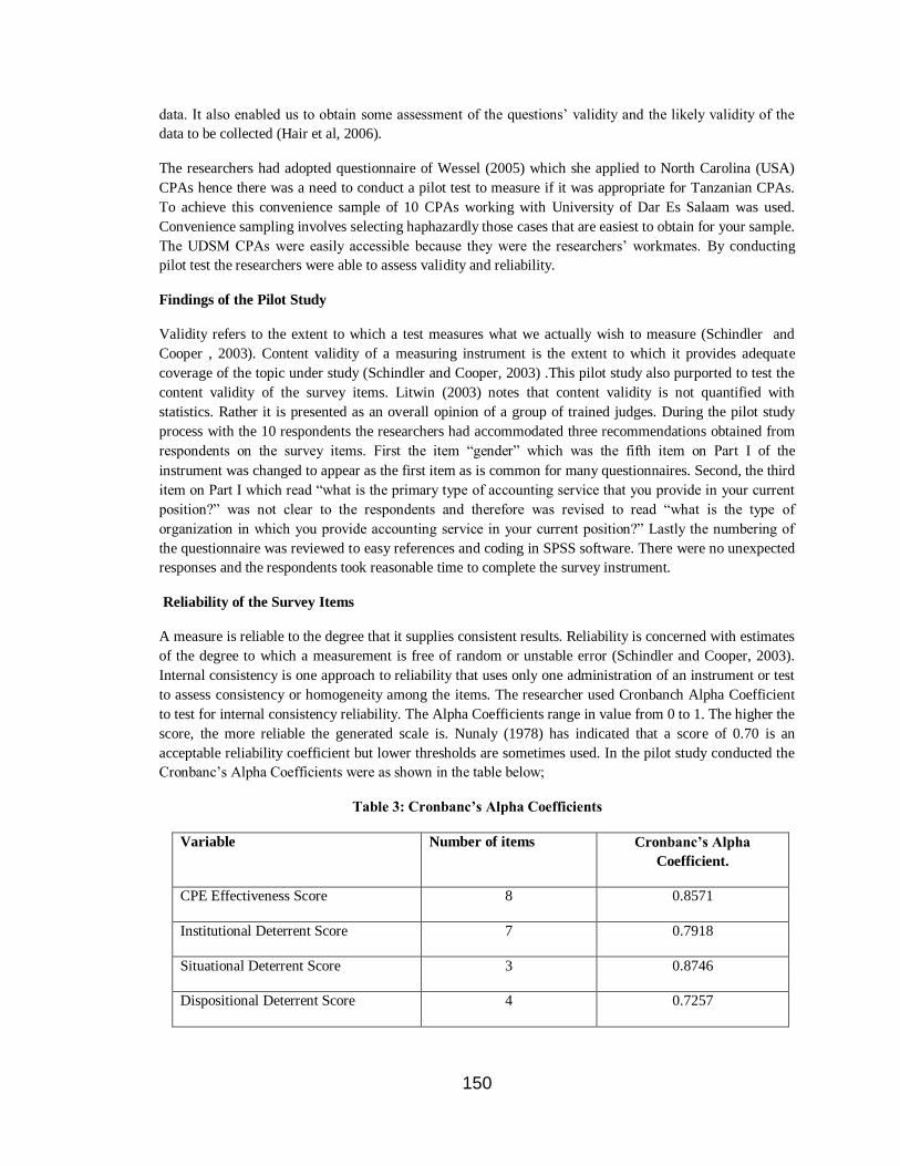
150

data. It also enabled us to obtain some assessment of the questions‘ validity and the likely validity of the

data to be collected (Hair et al, 2006).

The researchers had adopted questionnaire of Wessel (2005) which she applied to North Carolina (USA)

CPAs hence there was a need to conduct a pilot test to measure if it was appropriate for Tanzanian CPAs.

To achieve this convenience sample of 10 CPAs working with University of Dar Es Salaam was used.

Convenience sampling involves selecting haphazardly those cases that are easiest to obtain for your sample.

The UDSM CPAs were easily accessible because they were the researchers‘ workmates. By conducting

pilot test the researchers were able to assess validity and reliability.

Findings of the Pilot Study

Validity refers to the extent to which a test measures what we actually wish to measure (Schindler and

Cooper , 2003). Content validity of a measuring instrument is the extent to which it provides adequate

coverage of the topic under study (Schindler and Cooper, 2003) .This pilot study also purported to test the

content validity of the survey items. Litwin (2003) notes that content validity is not quantified with

statistics. Rather it is presented as an overall opinion of a group of trained judges. During the pilot study

process with the 10 respondents the researchers had accommodated three recommendations obtained from

respondents on the survey items. First the item ―gender‖ which was the fifth item on Part I of the

instrument was changed to appear as the first item as is common for many questionnaires. Second, the third

item on Part I which read ―what is the primary type of accounting service that you provide in your current

position?‖ was not clear to the respondents and therefore was revised to read ―what is the type of

organization in which you provide accounting service in your current position?‖ Lastly the numbering of

the questionnaire was reviewed to easy references and coding in SPSS software. There were no unexpected

responses and the respondents took reasonable time to complete the survey instrument.

Reliability of the Survey Items

A measure is reliable to the degree that it supplies consistent results. Reliability is concerned with estimates

of the degree to which a measurement is free of random or unstable error (Schindler and Cooper, 2003).

Internal consistency is one approach to reliability that uses only one administration of an instrument or test

to assess consistency or homogeneity among the items. The researcher used Cronbanch Alpha Coefficient

to test for internal consistency reliability. The Alpha Coefficients range in value from 0 to 1. The higher the

score, the more reliable the generated scale is. Nunaly (1978) has indicated that a score of 0.70 is an

acceptable reliability coefficient but lower thresholds are sometimes used. In the pilot study conducted the

Cronbanc‘s Alpha Coefficients were as shown in the table below;

Table 3: Cronbanc’s Alpha Coefficients

Variable Number of items Cronbanc’s Alpha

Coefficient.

CPE Effectiveness Score 8 0.8571

Institutional Deterrent Score 7 0.7918

Situational Deterrent Score 3 0.8746

Dispositional Deterrent Score 4 0.7257

151

Informational Deterrent Score 2 0.6708

Source: Field Data

From the results we can conclude according to Nunnaly (1978) that the survey instrument is reliable

(supplies internally consistent results).

Area of the study

This research was conducted in Dar es Salaam since 77 per cent of the Certified Public Accountants were

in Dar es Salaam according to the Directory of Members and Firms including By-Laws as at 1st January

2009. Dar es Salaam is a city in the eastern part of Tanzania having more than 3 million people. It is also

the biggest commercial and industrial area in Tanzania. Dar es Salaam also happened to be the most easily

accessible place because the researchers work and had permanent residence in the city. The researchers

selected 18 organizations of various orientations. The approach was mostly to target all organizations

having a reasonable number of accountants. This is the reason why the sample contained most government

institutions which due to their size are having more certified public accountants. The distribution and

collection of the questionnaires are as shown on the table below;

Table 4: Distribution and collection of questionnaires.

Organization Questionnaires

Distributed

Questionnaires

Collected

Ministry of Finance 30 21

PKF 8 5

Bank of Tanzania 20 9

PriceWaterhouse Coopers 12 7

Tanesco 16 11

BEST 3 0

TTCL 8 3

Zanzibar Telecom Company (Zantel) 18 15

University of Dar es Salaam 16 12

NBAA 5 3

International Commercial Bank 2 2

Tanzania Employment Agency 2 2

Tanzania Communication Regulatory Authority 4 3

152

Imara Consultants 7 5

Tanzania Postal Bank 5 3

Higher Education Students Loan Board 25 5

Tanzania Institute of Accountancy 3 2

Tanzania Revenue Authority 16 8

200 116

Source: Field Data

Data Analysis

Data analysis involved steps such as coding the responses, cleaning, screening the data and selecting the

appropriate data analysis strategy. Data in the questionnaire was coded and entered into the statistical

analysis software package, SPSS ready for analysis. To meet the purposes of this study, the researcher used

both descriptive and inferential analysis.

Results and Discussion

Discussion of the Results of Part I of the Questionnaire

Part I of the questionnaire was designed to collect demographic information of the respondents under five

variables gender, years of experience, current position, type of organization and size of the organization.

The following tables show the results followed by a brief discussion on each variable.

On gender the results show that 71 per cent of the respondents were male. The results further show that 66

per cent of the respondents had experience of less than 10 years. This explains the fact that most

accountants of the old generation in Tanzania had no CPA qualifications and were therefore excluded in

this study. As regarding current position the results show that 88 per cent of the respondents were

employed while only 8 per cent were at the managerial level and only 1 per cent is self employed. The

results further show that most respondents were working in Government (73 per cent). This is because, as

explained above, the sample included most government institutions which usually employ a large number

of accountants. The results also show that 50 per cent of the respondents were working in organization having over more than 500 employees. This is because, as explained above, the sample included most

government institutions which usually employ a large number of employees.

Discussion of Results on the First Objective (CPE Effectiveness)

To determine how the CPAs perceive the effectiveness of CPE program for accountants was the first

specific objective of this study. As previously explained transfer of knowledge gained through CPE

participation into real working place was the major concern of this study. The findings of this objective are

obtained by observing the means and standard deviations results of question one which contained 8

variables. The table below shows the result:

Table 5: Means and standard deviation for CPE effectiveness variables

Question Description of variable Mean Std

Deviation

1 (i) a Enhancement of knowledge base 4.23 0.637

1 (i) b Enhancement of employability 3.46 1.025

1 (i) c Enhancement of income 2.77 1.167

153

1 (ii) a Provision of networking opportunities with peers 4.05 0.708

1 (ii) b Provision of valuable experts in the field 3.93 0.821

1 (iii) a Helping in improving the profession 4.23 0.664

1 (iii) b Helping in protecting the public from incompetent

professionals

3.78 0.885

1 (iii) c Making it more likely that CPAs are competent 3.63 0.840

Overall mean 3.76 0.843

Source: Field Data

The overall mean score is 3.76 which imply that in general the CPAs agree that the CPE scheme is

effective in transfusing the knowledge gained into real working place. The respondents are particularly in

agreement with three variables enhancement of knowledge base, provision of networking opportunities

with peers and helping in improving the accountancy profession. The results further show that most CPAs

perceive that CPE scheme does not enhance their income with mean score of 2.77. This implies that

employers do not consider CPE participation as a basis for increasing the earnings of the CPAs. This poses

challenge to NBAA to educate employers that CPAs who participate in CPE program are more competent and knowledgeable. On the other hand the employers who usually provide financial and time support to the

CPAs to participate in CPE program should receive value for the investment they are making. They should

therefore demand training report. The employers have also the challenge of providing necessary support to

the CPAs in order for them to practice the new skills and knowledge. Without the employers support the

whole CPE program becomes futile. Another variable with small score is enhancement of employability

3.46. This is because participation in CPE scheme has not been regarded as one of the employment criteria

by employers.

Using Schindler and Cooper, (2003) proposal to determine whether the reported standard deviations for

CPE effectiveness variables are small or large it is found that all variables give the ratio of range to

standard deviation between 2 and 6. The overall standard deviation also gives the ratio 4.74 (4/0.843)

which falls between 2 and 6. These results imply that most respondents had homogeneous perceptions as to

the agreement or disagreement with the CPE effectiveness variables.

Discussion of Results on the Second Objective (CPE deterrents)

To identify deterrents to CPE effectiveness and how they affect the CPAs in Tanzania was the second

specific objective of this study. Literature identifies four types of deterrents for participation namely

institutional, situational, dispositional and informational deterrents. These deterrents have the same effect

whether participation is voluntary or mandatory (Wessels, 2005). The findings of this study for each

deterrent are as follows;

Institutional Deterrents

Institutional deterrents were defined as the practices and procedures of the CPE providers that inhibit

participation in continuing education (Cross, 1981). The table 6 below shows the results of the seven

institutional deterrent variables;

Table 6: Means and Standard Deviations for Institutional Deterrent Variables

Question Description of variable Mean Std Deviation

2 (a) A good value in relation to cost 3.30 0.971

2 (b) Time of the year 3.28 0.900

2 (c) Quality 3.66 0.770

154

2 (d) Right level 3.73 0.715

2 (e) Relevance 3.84 0.871

2 (f) Time length 3.32 0.891

2 (g) Publicity 3.57 0.815

Overall 3.53 0.848

Source: Field Data

The general observation is that most respondents are between neutral and agree regarding the institutional

deterrents. Speaking it differently NBAA which is responsible for the implementation of CPE scheme is

generally not doing fine to eliminate the identified institutional deterrents. The more good mean result

should have been between 4 and 5. It is also revealed from the table that among the seven variables NBAA

does relatively good in terms of relevance, right level and publicity with the mean score of 3.84, 3.73 and

3.66 respectively. The results show response approaching neutral on item b time of the year. This implies

that on average the CPAs are no neutral with the time schedule of the CPE scheme. NBAA has therefore the

challenge of eliminating all institutional deterrents so that CPE program if effective.

Using Schindler and Cooper, (2003) proposal to determine whether the reported standard deviations for

institutional deterrent variables are small or large it is found that all variables give the ratio of range to

standard deviation between 2 and 6. The overall standard deviation also gives the ratio 4.72 (4/0.848) which falls between 2 and 6. These results imply that most respondents had homogeneous perceptions as to

the agreement or disagreement with the institutional deterrent variables.

Situational Deterrents

Johnston and Rivera, (1965) defined situational deterrents as constraints which inhibit participation and are

external to the individual control. Situational deterrents include costs, work and family constraints. The

study shows the result below;

Table 7: Means and Standard Deviations for Situational Deterrent Variables

Question Description of variable Mean Std Deviation

3(a) Cost 3.34 0.952

3(b) Job demand leave little time for CPE

courses

3.37 1.043

3(c) Long distance travel 3.22 1.193

Overall 3.31 0.810

Source: Field Data

Question 3 was designed to extract the responses on how situational deterrents affect the CPE effectiveness.

The overall mean score is 3.31 implying that respondents were almost neutral as to whether situational

deterrents affect CPE effectiveness. This is explained by the fact that participation costs are covered by

employers and therefore are not directly born by the participants. With the improved transport infrastructure

long travel is not a significant problem and usually NBAA selects convenient locations which are easily

accessible by all participants.

Among the three situational deterrent variables the item on job demand seems to have more impact with the

mean score of 3.37. This can have effect as follows: if the job leaves little time for CPE courses the

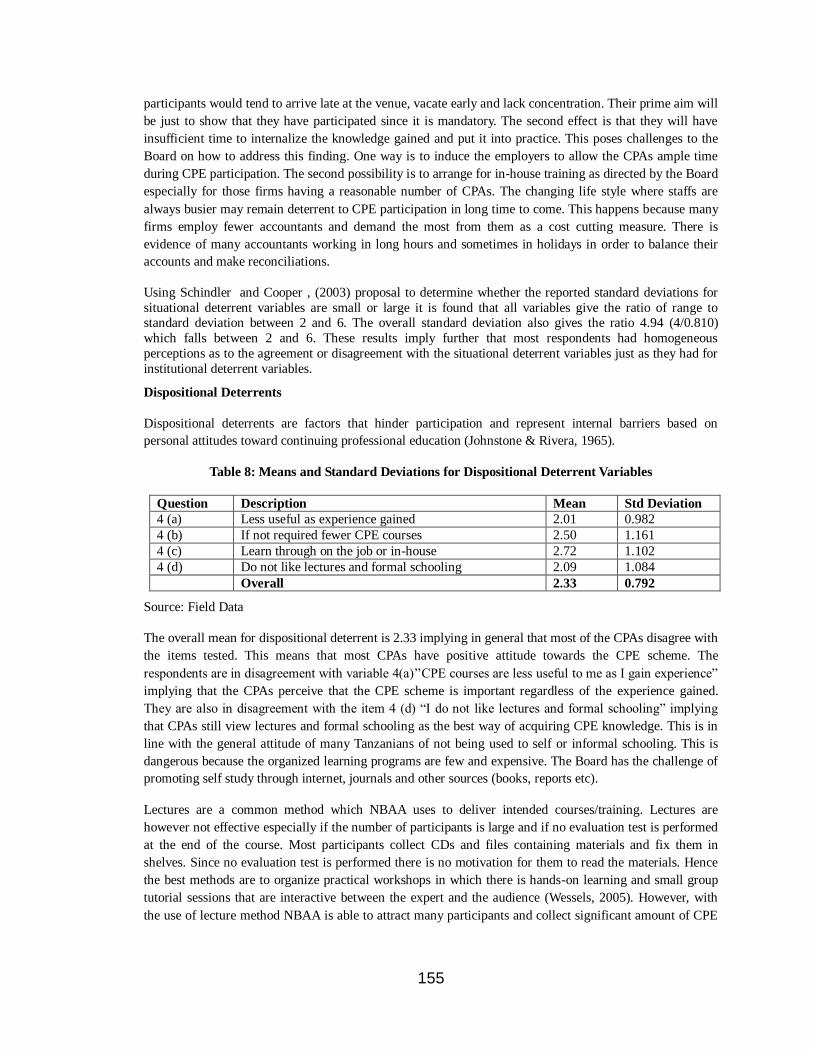
155

participants would tend to arrive late at the venue, vacate early and lack concentration. Their prime aim will

be just to show that they have participated since it is mandatory. The second effect is that they will have

insufficient time to internalize the knowledge gained and put it into practice. This poses challenges to the

Board on how to address this finding. One way is to induce the employers to allow the CPAs ample time

during CPE participation. The second possibility is to arrange for in-house training as directed by the Board

especially for those firms having a reasonable number of CPAs. The changing life style where staffs are

always busier may remain deterrent to CPE participation in long time to come. This happens because many

firms employ fewer accountants and demand the most from them as a cost cutting measure. There is

evidence of many accountants working in long hours and sometimes in holidays in order to balance their

accounts and make reconciliations.

Using Schindler and Cooper , (2003) proposal to determine whether the reported standard deviations for

situational deterrent variables are small or large it is found that all variables give the ratio of range to standard deviation between 2 and 6. The overall standard deviation also gives the ratio 4.94 (4/0.810)

which falls between 2 and 6. These results imply further that most respondents had homogeneous

perceptions as to the agreement or disagreement with the situational deterrent variables just as they had for

institutional deterrent variables.

Dispositional Deterrents

Dispositional deterrents are factors that hinder participation and represent internal barriers based on

personal attitudes toward continuing professional education (Johnstone & Rivera, 1965).

Table 8: Means and Standard Deviations for Dispositional Deterrent Variables

Question Description Mean Std Deviation

4 (a) Less useful as experience gained 2.01 0.982

4 (b) If not required fewer CPE courses 2.50 1.161

4 (c) Learn through on the job or in-house 2.72 1.102

4 (d) Do not like lectures and formal schooling 2.09 1.084

Overall 2.33 0.792

Source: Field Data

The overall mean for dispositional deterrent is 2.33 implying in general that most of the CPAs disagree with

the items tested. This means that most CPAs have positive attitude towards the CPE scheme. The

respondents are in disagreement with variable 4(a)‘‘CPE courses are less useful to me as I gain experience‖

implying that the CPAs perceive that the CPE scheme is important regardless of the experience gained.

They are also in disagreement with the item 4 (d) ―I do not like lectures and formal schooling‖ implying

that CPAs still view lectures and formal schooling as the best way of acquiring CPE knowledge. This is in

line with the general attitude of many Tanzanians of not being used to self or informal schooling. This is

dangerous because the organized learning programs are few and expensive. The Board has the challenge of

promoting self study through internet, journals and other sources (books, reports etc).

Lectures are a common method which NBAA uses to deliver intended courses/training. Lectures are

however not effective especially if the number of participants is large and if no evaluation test is performed

at the end of the course. Most participants collect CDs and files containing materials and fix them in

shelves. Since no evaluation test is performed there is no motivation for them to read the materials. Hence

the best methods are to organize practical workshops in which there is hands-on learning and small group

tutorial sessions that are interactive between the expert and the audience (Wessels, 2005). However, with

the use of lecture method NBAA is able to attract many participants and collect significant amount of CPE

156

participation fees. The resulting challenge is to compromise between financial gains (participation fees) on

one hand and the quality of delivery (effectiveness) on the other hand.

Again using Schindler and Cooper, (2003) proposal to determine whether the reported standard deviations

for dispositional deterrent variables are small or large it is found that all variables give the ratio of range to

standard deviation between 2 and 6. The overall standard deviation also gives the ratio 5.1 (4/0.792) which

falls between 2 and 6. These results imply again that most respondents had homogeneous perceptions as to

the agreement or disagreement with the dispositional deterrent variables just as they had for situational and institutional deterrent variables.

Informational Deterrents

Informational deterrents are barriers to participation (Darkenwald and Merriam, 1982) relating to a lack of

information about the available courses or a lack of information from which to judge the appropriateness of

a CPE course

Table 9: Means and Standard Deviations for Informational Deterrent Variables

Question Description Mean Std Deviation

5 (a) Previous ratings 3.41 1.087

5 (b) Suitability of upcoming course 2.89 1.163

Overall 3.15 0.909

Source: Field Data

As for informational deterrent the mean score is 3.15 implying that most CPAs were almost neutral on

informational deterrents. This proposes that the dissemination of the information by NBAA as CPE

organizer is not effective. The CPAs should be given specific information. On individual basis the CPAs are

neutral on easiness for them to determine in advance if a course is right for them or if it would benefit them

professionally. The decision as to the rightness or benefit is confronted with the challenge that even if the

course is not right for the CPA there is no option because the CPA has to clock the annual hours required

whether the course is right or not. This observation is crucial and should not be left out by NBAA. NBAA

takes general approach in designing courses while the CPAs work in different nature. For example a CPA

who works in a University will find a course on financial assets not so relevant as compared to the CPA

working in a banking industry. It is difficult to structure a course which would be equally beneficial to all

CPAs. The Board should therefore segment the CPAs and offer courses that specifically benefit a special

segment instead of designing courses that are targeted to all CPAs.

Again using Schindler and Cooper , (2003) proposal to determine whether the reported standard deviations for informational deterrent variables are small or large it is found that all variables give the ratio

of range to standard deviation between 2 and 6. The overall standard deviation also gives the ratio 4.4

(4/0.909) which falls between 2 and 6. These results imply again that most respondents had homogeneous

perceptions as to the agreement or disagreement with the informational deterrent variables just as they had

for dispositional, situational and institutional deterrent variables.

Discussion of Results on the Third Objective (CPE Effectiveness and Deterrents Relationship)

The third objective of this study was, to determine the relationship between each of the four categories of

deterrents and perceived CPE effectiveness. Using two-tailed Pearson product-moment correlation, it was

found that two deterrent scores were significantly correlated with the CPE effectiveness score as shown in

the Table 10 below and the subsequent discussion.

Table 10: Correlation between Deterrent Scores and CPE Effectiveness (N = 116)

Institutional

deterrent score

Situational

deterrent score

Dispositional

deterrent score

Informational

deterrent score

CPE effectiveness score

157

Pearson Correlation

Sig (2-tailed)

.456**

.000

-.003

.974

-.207*

.026

-.064

.493

** Correlation is significant at the .01 level (2-tailed) * Correlation is significant at the .05 level (2-tailed)

Source: Field Data

Cohen (1988) suggests the following guidelines in evaluating the strength of correlations: (r = +/- .10 to +/-

.29) is classified as small; (r = +/- .30 to +/- .49) is classified as medium; and (r = +/- .50 to +/- 1.00) is

classified as large. Using this classification, the institutional deterrent score correlation would be classified

as a medium correlation, the dispositional deterrent score as a small correlation, the situational deterrent

score and the informational deterrent score are classified as less than small correlations. Institutional

deterrent score was significantly positively correlated with the CPE effectiveness score. This is a strange

situation and is contrary to the conceptual framework of this study. Dispositional deterrent score was

significantly negatively correlated with the CPE effectiveness score. This position is in agreement with the

conceptual framework of this study and consistent with the study of Wessels, (2005) as shown in table 1.

The dispositional deterrent items represent attitudes that the respondents have toward continuing professional education including perceptions relating to a lack of benefit (―one can learn on-the-job or

through in-house training‖) and attitudes of disengagement (―dislike formal schooling and lectures‖).

NBAA as the CPE provider may be able to address these attitudes by offering unique programs that are

unlikely to be offered at the work site. For example, NBAA may want to consider offering CPE courses

that lead to a specific credential such as Certified Financial Planner. While the survey showed a high

degree (76 percent agreement) of overall satisfaction with CPE (Item 6 part II ―Overall I am very satisfied

with my CPE experience.‖), it is troubling that 58 percent would take fewer courses if not required. This

suggests that while most courses are useful, the marginal ones are not. The timing, level, and variety of

courses may need to be examined so that all of the required credit hours are well spent.

Situational and informational deterrent scores showed weak negative relationship with CPE effectiveness

score. Participation may be ―reduced‖ by enrolling in inappropriate courses in convenient locations rather than selecting courses that actually enhance their professional competencies. Many of the deterrent items

had low scores (less than 3 on a scale in which 5 is a high deterrent). This position is not in agreement with

the study of Wessels (2005) where in her study she found that there was significant negative relationship

between each deterrent score and the CPE effectiveness score and therefore all deterrents were statistically

significant predictors of CPE effectiveness. In her study the institutional deterrent score was the most

predictive of the CPE effectiveness with the correlation of -0.509.

The informational deterrent score was the second weak predictor of effectiveness. One of the survey items

that comprised this score had the highest mean (―Before selecting a CPE course, it would be useful to know

the course satisfaction ratings given by previous participants‖) with nearly 75 percent of respondents

agreeing or strongly agreeing with the statement. The high mean indicates that most respondents view the

lack of this kind of information to be a deterrent. CPE providers might want to consider whether this information might be made available in brochures and materials about CPE courses.

The situational deterrent score was the last weak predictor of effectiveness. Previous studies (Scanlan and

Darkenwald, 1984) had identified three distinct types of situational factors; i.e., cost, family constraints,

and work constraints. In the present study, when the means for these items were ranked, all were ranked in

the top 35th percentile. This indicates that the respondents as a whole view the indirect costs, job demands,

and travel burdens as important. However, these deterrents were less likely to be negatively related to

perceptions of effectiveness compared with the institutional or dispositional deterrents.

Conclusions and Implications

Main Findings

158

As regards demographic information which had five variables the study showed that 71 per cent of the

respondents were male, 66 per cent had working experience of less than 10 years and 88 per cent were

employed. It was further shown that 23 per cent of the respondents were working in Government

institutions while 50 per cent were working in organizations having more than 500 employees.

The study further showed that the CPAs are in agreement that the CPE scheme is effective in transfusing

the knowledge gained into real working place. It has also been observed that the Tanzania CPAs experience

the same institutional, situational, dispositional and informational deterrents in varying degrees. It has also

been observed that most CPAs have homogeneous perceptions on how the deterrents affect the CPE

effectiveness.

The study showed that there is relationship between the deterrents and the CPE effectiveness though the

relationship is not as strong as that revealed by Wessels (2005) in her study of North Calorina CPAs. We

have seen significant negative relationship between dispositional deterrent and CPE effectiveness. The

situational and the informational deterrent showed weak negative relationship with CPE effectiveness.

Institutional deterrents showed significantly positive relationship with CPE effectiveness. This position is

totally contradicting with the study of Wessels (2005) in which institutional deterrent had strong negative

relationship with the CPE effectiveness and therefore emerged as the major predictor of CPE effectiveness.

Whatever the case, NBAA should work hard to address those deterrents to CPE effectiveness identified in

this study. The deterrents have varying degrees of impact and influence on CPE effectiveness. It is worth

noting that the CPE scheme of Tanzania is just young which become mandatory only in 2001. In U.S.A the

CPE scheme become mandatory in the late 60‘s. Therefore NBAA has to learn from the CPE schemes

implemented in other countries in order to improve the CPE effectiveness and meet the public expectation

of having improved accounting profession.

The first specific objective of this research was to determine how the certified public accountants in

Tanzania perceive the effectiveness of continuing professional education for accountants. The research has

shown that the Tanzania CPAs are in agreement that the CPE scheme conducted by NBAA is effective in

transfusing the knowledge gained into real working place though a number of improvements have to be

made at the institutional level.

The second specific objective was to identify the deterrents to effective continued professional education

for certified public accountants in Tanzania. The research has shown that the Tanzania CPAs experience

the same institutional, situational, dispositional and informational deterrents in varying degrees. It has also

been observed that most CPAs have homogeneous perceptions on how the deterrents affect the CPE

effectiveness.

The third specific objective was to determine the relationship between the identified deterrents and the

perceived CPE effectiveness. The research has shown that there is relationship between the deterrents and

the CPE effectiveness. There is significant negative relationship between dispositional deterrent and CPE

effectiveness. The situational and the informational deterrent showed weak negative relationship with CPE

effectiveness. Institutional deterrents showed significantly positive relationship with CPE effectiveness.

Recommendations

Recommendations to NBAA

There is a compelling public interest to require that CPAs maintain and improve their competency through

continuing professional education. To ensure the best outcome, NBAA needs to address those factors that

might be reducing the effectiveness of mandatory CPE.

159

To address institutional deterrent NBAA should examine the feasibility of publicizing course evaluations.

Findings show that most CPAs would find it useful to know the course satisfaction rating given by previous

participants. To the extent that CPAs select the ―wrong‖ course because of a lack of information, CPE

effectiveness will be impaired. All CPE courses currently conduct a brief course evaluation by the

participants. NBAA needs also to better understand the needs of the learners and the things that limit the

effectiveness of those programs. NBAA should also think of segmenting the courses so that direct link is

created between what the CPA does and the CPE course he is attending. The current practice of designing

generic courses does not promote CPE effectiveness.

NBAA should also apply course delivery methods which are effective. The research has shown that lecture

method which is commonly used by the Board does not sufficiently promote CPE effectiveness. The

researcher recommends practical workshops in which there is hands-on learning and small interactive

tutorial sessions. NBAA should also start issuing certificates as a way of compelling participation and

implementing other by-laws. The Board should also foster improved relationship with employers both

public and private so that the public receives the best service from the accountants.

To address dispositional deterrents which reflect internal barriers based on personal attitudes toward

continuing professional education NBAA may be able to allay concerns that job demands leave little time

for CPE by offering on-site courses at firms that employ large numbers of accountants. To assure that all credit hours are well-utilized, NBAA should review whether the timing, level, and variety of course

offerings are relevant to all types of CPAs including those in industry.

Barriers relating to situational deterrents such as long travel distances could be alleviated if NBAA would

offer more internet or self-study options to ease travel burdens. Courses offered at resort locations would

permit CPAs to combine additional education with a family vacation thereby easing the difficulty of being

away from the family while completing CPE.

The informational deterrents reported by some respondents may be remedied if NBAA would investigate

ways for CPAs to find out course satisfaction ratings given by previous participants. Perhaps these ratings

could be posted on the website of the NBAA. In addition, NBAA needs to clearly describe the subject

matter and level of course in informational literature to help practitioners more accurately determine if a

course is right for them.

Recommendations for Future Research

This study was designed to seek responses from CPAs only. However the NBAA CPE scheme is also

mandatory for other cadres of the accounting profession including the Accounting Technicians. Another

study ought to be done which will incorporate all members of the Board to whom CPE scheme is

mandatory.

The researcher is also recommending another study which will broaden the sample size. The sample size

should not only be relatively large but should include all cadres of the accountants required to attend CPE

program. Another study needs to be done to examine the effectiveness of the Board itself as the principal

CPE provider for accountants.

There is also a need to find out the reasons which inhibit women to acquire CPA qualification as the current

study showed that 71 per cent of the respondents were male. This is material gender imbalance for the

accounting profession.

In order to know the reasons for the differences in results between this research and the one conducted by

Wessels (2005) in USA there is a need to conduct a qualitative inquiry. The inquiry will investigate in

detail through in depth interviews and discover the probable causes of the differences.

LIMITATIONS OF THE STUDY

160

This study suffered from several limitations. The first limitation was that a self-administered questionnaire

was used to collect the responses. Any questions that were unclear or ambiguous to the respondents may

have resulted in unusable or incorrect information. In a self-administered questionnaire there is no face to

face interaction between the respondent and the researcher. Non presence of the researcher denies the

respondent the chance to get clarification or explanations in areas not clear to the respondent while filling

the questionnaire. However this method avoids the interviewer‘s bias.

The second limitation was that respondents were being asked to recall their CPE experiences over the past

year. Consequently, the individuals‘ perceptions of CPE effectiveness or deterrents may be limited by

faulty memory. It can be argued that the memory loss was minimized because the CPAs have been

attending these courses frequently and they have been practicing the accounting profession.

The third limitation was that the questionnaire used structured questions only. Open ended questions would

enable respondents to express their perceptions more freely. The structured question method was chosen

because this study replicates the Wessels (2005) study.

REFERENCES

Agle, B. R., Mitchell, R. K., & Sonnenfeld, J. A. (1999). ―Who matters to CEOs? An investigation of stakeholder

attributes and salience, corporate performance, and CEO values‖ Academy of Management Journal, 42 (5),

507–525.

Cohen, J. W. (1988). Statistical power analysis for the behavior sciences (2nd edition). Hillsdale, NJ Lawrence

Erlbaum Associates.

Cross, K. P. (1981). Adults as learners. San Francisco, CA: Jossey-Bass.

Clyde, N. J. (1998). ―CPE is broke; let‘s fix it‖. Journal of Accountancy 186 (6), 77-83.

Dao, M. N. S. (1975). ―The orientations toward nonparticipation in adult education‖. (Doctoral dissertation,

University of Chicago, 1975).

Dhanidina, L., and Griffith, W. S. (1975). ―Costs and benefits of delayed high school completion‖. Adult Education

25 (4), 217-230.

Darkenwald, G. G. and Merriam, S. B. (1982). Adult education: foundations of practice. New York: Harper & Row.

Darkenwald, G. G. and Valentine, T. (1985). ―Factor structure of deterrents to public participation in adult

education‖. Adult Education Quarterly, 35 (4), 177-193.

Hair, J. F., Jr., Black, W. C., Babin, B. J., Anderson, R. E., & Tatham, R. L. (2006).

Multivariate data analysis (6th ed.). Upper Saddle River, NJ: Prentice Hall.

Icek, Ajzen, Driver B.L, (1992), ―Application of the Theory of Planned Behaviour to Leisure Choice‖ Journal of

Leisure Research, Vol. 24, No. 3, pp. 207-224

Johnstone, J. W. C. and Rivera, R. J. (1965). Volunteers for learning. Chicago: Aldine.

Litwin, M. S. (2003) How to assess and interpret survey psychometrics (second edition). Newbury Park, CA: Sage

Publications.

Manwa, H., & Manwa, F. (2007). ―Applicability of the Western concept of mentoring to African organizations: A

case study of Zimbabwean organizations‖ Journal of African Business, 8 (1), 31–44.

Masoud, M. S. and Wilson T. L. (2011). ―Stakeholder Salience in Public and Private Firms: Results from Tanzania‖

Journal of African Business, 12:252–267,

Mitchell, R. K., Agle, B. R., & Wood, D. J. (1997). Toward a theory of stakeholder

161

identification and salience: Defining the principle of who and what really counts. Academy of Management Review,

22 (4), 853–886.

Nunnaly, J. (1978). Psychometric theory. New York: McGraw-Hill.

Scanlan, C. L. (1986). ―Deterrents to participation: An adult education dilemma‖. Columbus, OH: ERIC

Clearinghouse on Adult, Career, and Vocational Education, The Ohio State University.

Scanlan, C. L., and Darkenwald, G. G. (1984). ―Identifying deterrents to participation in continuing education‖. Adult Education Quarterly 34 (3), 155-166.

Schindler, P. S. and Cooper, D. R. (2003), Business Research Methods (8th Ed.), New York, McGraw Hill

Young, W. H. (1998). ―Systematic efforts in continuing professional education focusing on mandatory continuing

professional education‖. In W. H. Young (Ed.), Continuing Professional Education in Transition (p. 129-

140). Malabar, FL: Krieger Publishing Company.

Wessels, S. B. (2005) ―The Deterrents to CPE Effectiveness in the Accounting

Profession: A Factor Analytic Study,‖ Journal of Business & Economics

Research 3 (6).

REWARD SYSTEM AND ORGANIZATIONAL CITIZENSHIP BEHAVIOUR IN

UGANDA COLLEGES OF COMMERCE.

BY HOJOPS ODOCH J.P

B.A (SS), MUK; PGDE, UCU; MBA, MUK.

LECTURER, BUSINESS ADMINISTRATION DEPT., MUBS

ABSTRACT

The researcher was inspired to carry out the research because stakeholders often question why performance

in Uganda Colleges of Commerce (UCCs) is low. The main aim of the research was to explain the

relationship between reward system and organizational citizenship behavior (OCB) in UCCs.

The respondents of the study included lecturing staff and administrative staff of UCCs. The structured

questionnaires were used to gather information on the relationships between variables under study. The

library search was done through reading textbooks, dissertations, newspapers, policy instruments and

internet and was used for compiling introduction of the study and literature review. The processed data was

analyzed quantitatively through statistical package for social scientists (SPSS).

The Pearson correlation matrix indicates a positive and significant relationship reward system and

organizational citizenship behavior in Uganda colleges of commerce.

The regression analysis results provide an adjusted R2 of 0.535. This means that reward system explains

53.3% of the variance in Organizational Citizenship behavior in UCCs. Thus the remaining 46.5% is

explained by other variables outside this study.

Reward system should be improved by making all staff access the government payroll. This would reduce

relying on the meager colleges‘ collections and irregular Government grants. UCCs should streamline its

162

promotion practices so that staff could be promoted across the ladders regularly according to Government

standing orders, as this will adjust salary scales accordingly. Organizational citizenship behavior should be

inculcated in UCCs by encouraging team spirit so that members could be willing to go beyond what they

are expected to do. A culture should be developed to make staff realize that mistakes/omissions by few

people affect the survival of the entire organization. This will make staff to see assignments of their

colleagues as theirs; and would come in to help when needs arise.

CHAPTER ONE

1.1 BACKGROUND TO THE STUDY

Organizations need employees with competence that directly or indirectly affect job performance,

Woodruffe (1998). Reward system, (promotion, pay raises and other rewards), is equally

important for most employees (Baron and Byrne, 1999). This leads to job satisfaction, which will

be higher when individuals believe that rewards are fairly and impartially distributed than when

they believe they are distributed unfairly. This enhances employees‘ willingness to maintain

membership with the organization, that is, organizational commitment. Organ (1998) observed

that when employees perceive that equity has obtained in the distribution of resources, they are

more likely to be satisfied with their jobs and behave with a sense of citizenship.

The government of Uganda established Uganda College of Commerce (UCC) Nakawa to offer

business – related courses. The increased demand for this kind of education led to the

establishment of five (5) more colleges of commerce (UCCs) in 1982, whose curriculum was to be

coordinated from UCC Nakawa, which later became National College of Business Studies, Apono

(2002). The general problems associated with coordination of tertiary education include: lack of

systematic planning in institutions of higher education resulting in their haphazard development,

the poor state of physical facilities, the deteriorating quality of higher education, and the need to

streamline development and management of tertiary education. There is poor and unattractive

terms and conditions of service for the teaching professional in the country since the colonial

times (Education Policy Review Report, 1992).

NCBS merged with Faculty of Commerce, Makerere University in 1997 to form Makerere

University Business School (MUBS) which continued to coordinate UCCs. MUBS realized in

February 2002 that over 60% of UCCs students failed their semester examinations and, so special

examinations were set for them in August 2003. MUBS has restrained all UCCs Lecturers without

degree qualifications and above from handling MUBS programs except Uganda National

Examinations Board (UNEB) certificate courses until they upgrade to degree level. MUBS then

came up with staff Development Program for UCCs where each college has to send two (2) staff

members, one for undergraduate and one for Postgraduate course each year (Appendix E).

Currently, only 50% are appointed and about 20% promoted out of those who have been in the

service for the last ten years.

Promotion of teachers is no longer automatic even after upgrading due to the limited resources,

Lubega W. Badru (2004), (Appendix D). Thus if one had joined with a diploma, s (he) would

continue to earn the same salary even if one upgrades to a master‘s degree.

163

Survey of the staff list of UCCs indicates that about 20% have not accessed the payroll. They are

paid from college collections, which are small, and Government grants which are irregular

(Appendices F, G, H, & I). UCCs are characterized by high incidence of absenteeism, late-coming,

inability to stand in for absent colleagues and numerous complaints.

1.2 STATEMENT OF THE PROBLEM

Performance in UCCs is low, as is reflected in poor academic results (MUBS academic board

minutes, 2001-2). There is high incidence of absenteeism, late coming, inability to stand in for a

colleague when absent (Minutes of Governing council, 2003), plus numerous complaints due to

poor reward system administration which usually results into refusal to work until the dispute is

resolved (UCC Aduku strike by lecturers in March 2003).

1.3 PURPOSE OF THE STUDY

The study seeks to explain the relationship between Reward system and organizational citizenship

behavior in Uganda colleges of commerce.

1.4 OBJECTIVES OF THE STUDY

1. To explain the relationship between reward system and organizational citizenship behavior.

2. To explain the effect of reward system on organizational citizenship behavior.

1.5 RESEARCH QUESTIONS

1. What is the relationship between reward system and organizational citizenship behavior?

2. What is the effect of reward system on organizational citizenship behavior (OCB)?

1.6 SIGNIFICANCE OF THE STUDY

The study will create knowledge about reward system and organizational citizenship behavior in

UCCs and other organizations will use the findings to enhance their performance. The study will

also add to the existing literature on reward system and organizational citizenship behavior.

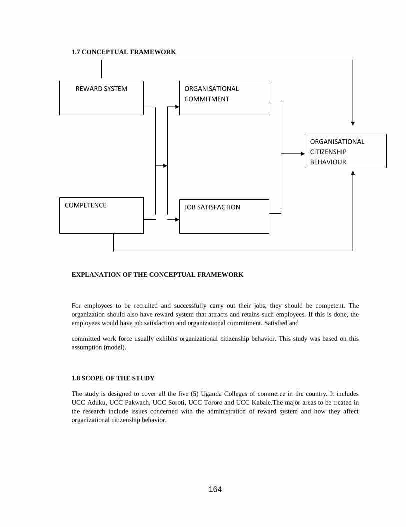
164

1.7 CONCEPTUAL FRAMEWORK

EXPLANATION OF THE CONCEPTUAL FRAMEWORK

For employees to be recruited and successfully carry out their jobs, they should be competent. The

organization should also have reward system that attracts and retains such employees. If this is done, the

employees would have job satisfaction and organizational commitment. Satisfied and

committed work force usually exhibits organizational citizenship behavior. This study was based on this

assumption (model).

1.8 SCOPE OF THE STUDY

The study is designed to cover all the five (5) Uganda Colleges of commerce in the country. It includes

UCC Aduku, UCC Pakwach, UCC Soroti, UCC Tororo and UCC Kabale.The major areas to be treated in

the research include issues concerned with the administration of reward system and how they affect

organizational citizenship behavior.

REWARD SYSTEM ORGANISATIONAL

COMMITMENT

COMPETENCE JOB SATISFACTION

ORGANISATIONAL

CITIZENSHIP

BEHAVIOUR

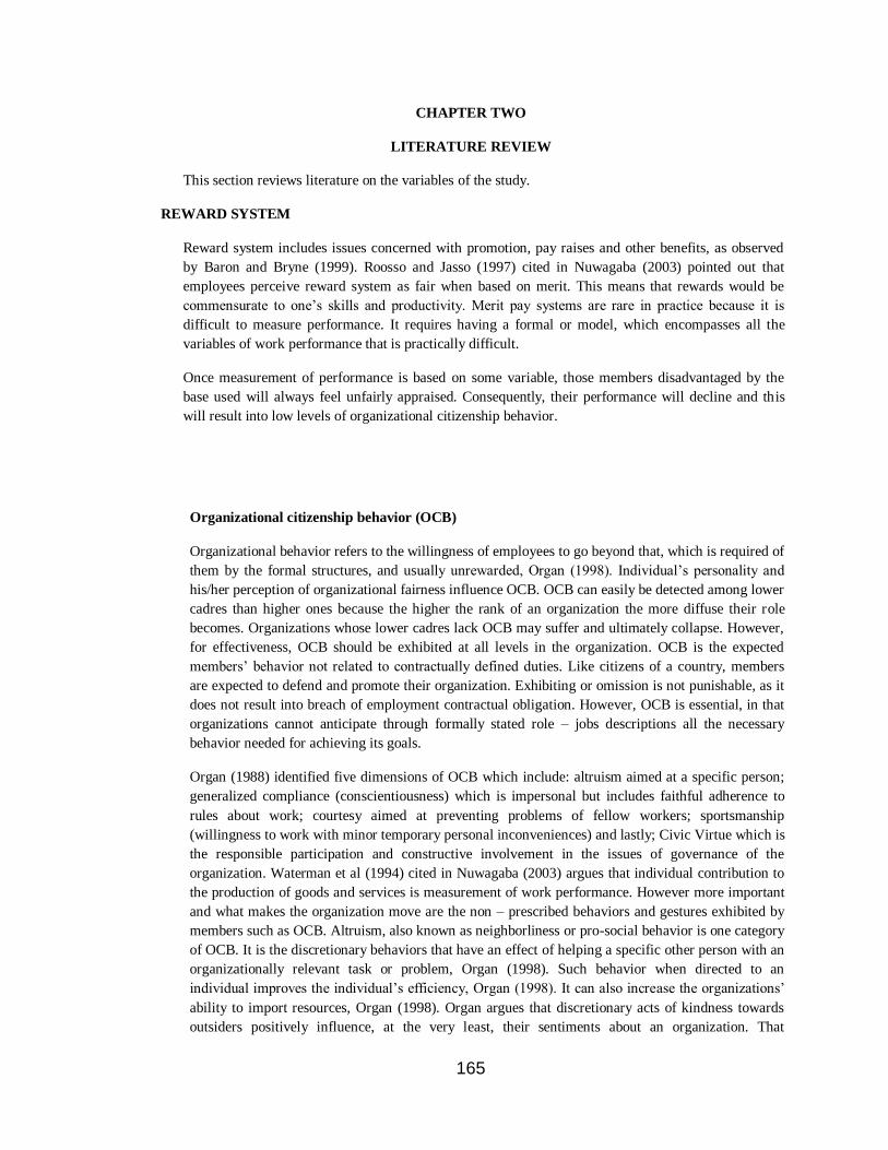
165

CHAPTER TWO

LITERATURE REVIEW

This section reviews literature on the variables of the study.

REWARD SYSTEM

Reward system includes issues concerned with promotion, pay raises and other benefits, as observed

by Baron and Bryne (1999). Roosso and Jasso (1997) cited in Nuwagaba (2003) pointed out that

employees perceive reward system as fair when based on merit. This means that rewards would be

commensurate to one‘s skills and productivity. Merit pay systems are rare in practice because it is

difficult to measure performance. It requires having a formal or model, which encompasses all the

variables of work performance that is practically difficult.

Once measurement of performance is based on some variable, those members disadvantaged by the

base used will always feel unfairly appraised. Consequently, their performance will decline and this

will result into low levels of organizational citizenship behavior.

Organizational citizenship behavior (OCB)

Organizational behavior refers to the willingness of employees to go beyond that, which is required of

them by the formal structures, and usually unrewarded, Organ (1998). Individual‘s personality and

his/her perception of organizational fairness influence OCB. OCB can easily be detected among lower

cadres than higher ones because the higher the rank of an organization the more diffuse their role

becomes. Organizations whose lower cadres lack OCB may suffer and ultimately collapse. However,

for effectiveness, OCB should be exhibited at all levels in the organization. OCB is the expected

members‘ behavior not related to contractually defined duties. Like citizens of a country, members

are expected to defend and promote their organization. Exhibiting or omission is not punishable, as it

does not result into breach of employment contractual obligation. However, OCB is essential, in that

organizations cannot anticipate through formally stated role – jobs descriptions all the necessary

behavior needed for achieving its goals.

Organ (1988) identified five dimensions of OCB which include: altruism aimed at a specific person;

generalized compliance (conscientiousness) which is impersonal but includes faithful adherence to

rules about work; courtesy aimed at preventing problems of fellow workers; sportsmanship

(willingness to work with minor temporary personal inconveniences) and lastly; Civic Virtue which is

the responsible participation and constructive involvement in the issues of governance of the

organization. Waterman et al (1994) cited in Nuwagaba (2003) argues that individual contribution to

the production of goods and services is measurement of work performance. However more important

and what makes the organization move are the non – prescribed behaviors and gestures exhibited by

members such as OCB. Altruism, also known as neighborliness or pro-social behavior is one category

of OCB. It is the discretionary behaviors that have an effect of helping a specific other person with an

organizationally relevant task or problem, Organ (1998). Such behavior when directed to an

individual improves the individual‘s efficiency, Organ (1998). It can also increase the organizations‘

ability to import resources, Organ (1998). Organ argues that discretionary acts of kindness towards

outsiders positively influence, at the very least, their sentiments about an organization. That

166

potentially, such sentiments in turn affect customer loyalty, community goodwill, the commitment of

vendors and suppliers, and the interest of prospective employees.

Conscientiousness is another OCB category, Organ (1998). It captures the various instances in which

organizational members carry out certain behaviors well beyond the minimum required levels.

Conscientiousness permits the use of scarce resources and thus improves the efficiency and

effectiveness of the organization, Organ (1998).

CHAPTER THREE

3.1 RESEARCH DESIGN

The research followed both qualitative and quantitative approach. This approach was chosen because it

involves the measures of respondents‘ attitudes and opinion /feelings, and due to the large number of

respondents involved in the study. The qualitative survey design was used because it involved the

development of competency profile, which was primarily done through interview with the respondents.

The quantitative survey design involved the administration of structured questionnaires developed in

order to capture the behaviors and attitudes of the respondents.

3.2 Description of the Geographical Area

The study covered all the five (5) Uganda colleges of commerce of Pakwach, Aduku, Soroti, Tororo

and Kabale.

3.3 Description of the Population

The study population composed of all the lecturing and Administrative staff in the five UCCs in the

Country. It consists of thirty (30) from UCC Packwach, thirty (30) from UCC Soroti , thirty five (35)

from UCC Aduku, forty (40) from UCC Tororo and thirty five (35) from UCC Kabale making a

population of 170 (One hundred seventy).

3.4 Sampling Procedures

This was purposive in that despite the fact that Uganda has five UCCs, four representative colleges

were selected to represent all the regions namely Pakwach, Aduku, Soroti and Kabale.

The study sample comprised of 25 lecturing and five (5) administrative staff from each of the four

colleges. It totaled up to a study sample of 120 out of a total study population of 170 in the five UCCs,

giving 70% of representation (Appendix K). The colleges selected are controlled by the same

government policies.

3.5 Data Collection Methods

Questionnaires and structured interviews were used to elicit primary data. Secondary data were got

from Library search, internet surfing and related research.

3.6 Measurements

Reward System

These were measured using the attitude statements of a 5- point likert type ranging from strongly

disagree (1) to strongly agree (5) of Munene ( 2000) local measure.

167

Organizational citizenship behaviour

The study used Kagga‘s (2000) measure of 21 items.

3.7 Validity /Reliability

For validity and reliability of instruments, the structured Questionnaires were presented. A cross

section of UCCs staff was selected to fill the Questionnaires so as to discover loopholes and refine the

final Questionnaires. This was done by performing Crocbach‘s Alpha tests. The final Alpha values are

shown in the table below:

Table 1. Crocbach’s Alpha Measures of Variables.

Variable Reward system OCB

Alpha values 0.8326 0.8554

From the above table, the different section showed satisfactory Alpha values indicating that the

instrument was good. Questions were carefully arranged according to the respective variables tested.

3.8 Data Analysis

Raw data was collected from respondents and edited. They were organized to enable quantitative

analysis like regression, correlation and factor analysis tests be done using computer software called

Statistical Package for Social Scientists (SPSS).

3.9 Limitations of the Study

Since my sponsorship did not include fund for research financial constraints affected the completion of

the research on schedule.

Many respondents were of the view that they would not obtain any direct benefit from the research,

which were only of value to the researcher. This implied that the time and effort involved in responding

to the questionnaires have been correspondingly affected.

Unwillingness of the respondents to fill the long quantitative questionnaires. The researcher had to give

the respondents a time frame within which to fill the questionnaires.

168

CHAPTER FOUR

DATA PRESENTATION AND INTERPRETATION OF RESULTS

4.0 INTRODUCTION

This Chapter comprises a presentation of results and their interpretation. The presentation and

interpretation in this chapter show the results as tested according to the objectives of the study. Factor

analysis, Pearson correlation and multiple regression analysis tests were used.

4.1 FACTOR ANALYSIS

Factor analysis was used to show the indices for the variables used in the study. The variables for which a

factor analysis was computed are competence, reward system and commitment. The principle component

analysis method was used. Only factors having eigen value greater than 1.0 were considered essential and retained.

Rotated Component Matrix for Reward System

1. The organization‘s vision is well communicated to employees

2. Employees are often trained/prepared to perform well

3. Development of skills and knowledge in employees is viewed as an investment

in this organization

4. Skills and knowledge development happens as an ongoing process in this

organization

5. In this organization employees are properly trained to perform their roles

6. Employees are rewarded for giving priority to work 7. Employees who provide excellent service are rewarded for their effort.

8. The reward system in this organization encourages employees to work together

9. Employee‘s salary is transferred to the new station if one is transferred

10. Reward system matches with the level of performance f staff of this organization

11. Employees who provide service are rewarded for their effort

0.843

0.826

0.824

0.810

0.736

0.630

0.717

0.690 0.672

0.669

0.616

Eigen value

% Variance

Cumulative %

4.455

40.502

4.502

1.99

18.089

58.580

Two indices identified from the measure of reward system are pay reward and unidentified reward. Pay

reward has the higher eigen value (4.455) accounting for 40.5 percent variance in reward system and

unidentified factor, a lower eigen of (1.990) accounting for 18.09% of the variance in reward system.

Overall the indices make up 58.5% of reward system.

4.2 PEARSON CORRELATION MATRIX

This test was used to show the relationship between the variables of reward system and OCB.

169

Pearson Correlation Matrix

Rewards OCB

Rewards

OCB 0.421**

*Correlation is significant at the 0.05 level (1-tailed)

**Correlation is significant at the 0.01 level (1-tiled)

The table above indicates that there is a significant relationship between reward system and OCB with

reward (r=0.421, (p<0.01)p<0.01).

4.3 MULTIPLE REGRESSION ANALYSIS

Multiple regression tests were used to show the effect of the independent and intervening variables on the

dependent variable.

Multiple Regression Analysis

Un standardized coefficient

Standardized coefficient

Model B Standard

error

BETA T Sig R2 Adjusted

R2 F P

(Constant) 2.122 0.363 5.846 0.000

Reward system 2.149E-02

0.091

0.031

0.237

0.814

0.693

0.535

10.00

0.000

Dependent variable: OCB

Results from the table above show that reward system has significant impact on OCB. The adjusted R2

indicates that the independent variable positively predict 53.5% of the variance in OCB.

CHAPTER FIVE

DISCUSSION, CONCLUSION AND RECOMMENDATIONS

5.0 INTRODUCTION

This chapter presents a discussion and conclusion of the results presented in the previous chapter, followed

by the recommendations arising out of findings from the study. The presentation of the discussion follows

the order in which the objectives of the study were stated (see chapter one). The first part discusses the

relationship between reward system and organizational citizenship behavior .The second part discusses the

effect of reward system on Organizational Citizenship Behavior. The chapter ends with a conclusion,

recommendations and areas for further studies.

5.1 Discussion of the Findings.

5.1.1 The Relationship between Reward System and Organizational Citizenship Behaviour The Pearson correlation matrix indicates a positive and significant relationship reward system and

organizational citizenship behavior in Uganda colleges of commerce. This is in agreement with

Organ‘s(1998)assertion that when employees perceive that equity has been obtained in the distribution of

resources they are more likely to be satisfied with their jobs and behave with a sense of citizenship. Since

OCB is unrewarded, for one to exhibit it, he/she should have been properly rewarded otherwise he/she will

concentrate on the rewarded assignments only.

This is confirmed by Greene et al. (1994) that without an encouraging reward system, employee‘s

commitment is bound to fail. When employees are rewarded, it will lead to employee‘s satisfaction.

5.1.2 The Effect of Reward System on Organizational Citizenship Behavior.

170

The regression analysis results provide an adjusted R2 of 0.535. This means that reward system explains

53.3% of the variance in Organizational Citizenship behavior in UCCs. Thus the remaining 46.5% is

explained by other variables outside this study.

5.2 Conclusion

The study was about reward system and organizational citizenship behavior in Uganda Colleges of Commerce. The various tests employed indicate positive and significant relationships between the variables

under study. The study indicated that UCCs has to improve on the rewards of its staff. Reward system

should be revisited to ensure that all staff access the Government payroll. Periodic promotion would satisfy

staff and make them more committed to their work and exhibit organizational citizenship behavior.

5.3 RECOMMENDATIONS

Reward system should be improved by making all staff access the government payroll. This would reduce

relying on the meager colleges‘ collections and irregular Government grants. UCCs should streamline its

promotion practices so that staff could be promoted across the ladders regularly according to Government

standing orders, as this will adjust salary scales accordingly. Organizational citizenship behavior should be

inculcated in UCCs by encouraging team spirit so that members could be willing to go beyond what they

are expected to do. A culture should be developed to make staff realize that mistakes/omissions by few

people affect the survival of the entire organization. This will make staff to see assignments of their

colleagues as theirs; and would come in to help when needs arise.

5 .4 Areas for Further Research

The study should widen its scope to include more tertiary institutions especially National Teachers‘

colleges, Uganda Technical colleges. And Universities These have staff with similar qualifications and pay;

and admit students with similar qualifications and are trained to get similar awards. This would increase the

sample size to make it statistically more significant.

REFERENCES

Allen N. and Meyer. J., (1990, 1994, 1999). The Measurement and Antecedents of Effective Continuance

and Normative Commitment to the Organization:

Journal of Occupation Technology (33, 178).

Apono S.Z., (2002). An Assessment of Factors Contributing to Recruitment and Selection of the

Inadequately Qualified Lecturers in Uganda Colleges of Commerce, Masters Dissertation submitted to

UMI, Kampala.

171

Baron, R.A., and Byrne, D., (1999). Social Psychology (8th ed.), Prentice – Hall of India.

Bewley, T., (2002). Fairness, Reprocity and Wage Rigidity. Cowles Foundation Discussion No. 1383, Yale

University.

Boshoff, C. and Allen, J., (2000). The Influence of Selected Antecedents on Frontline Staff‘s Perceptions of

Service Recover Performance. International Journal of Service Industry Management, 11,1,63 – 90.

Cohen, A, Vigoda, E., (2000). Do Good Citizens Make Good Organizational Citizenship Behaviour?

Administration and Society, 32, 596-624.

Eby, L.T., Freeman, D.M., Rush, M.C., and Lance, C.E., (1999). Motivational Bases of Affective

Organizational Commitment: a Partial Test of an Integrative Theoretical Model.

Journal of Occupational Organization Psychology, 72, 463-483.

Government of Uganda. Sixth Education Sector Review Workshop

22-26(2001), presented by National and International Education Stakeholders.

MOES.http://www.Education.go.ug.Sixth.edu Sector review.

Government of Uganda: Universities and other Tertiary Institutions

Act (2001). Printed by UPPC, Entebbe.

Government Standing Orders (1991) Hr – guide com (2000) http://www.hrguide.com

Data ug.

Government of Uganda, (2001). Report of the Stakeholders forum on Pay Reform Strategy, Ministry of

Public Service, Kampala.

Greenberg, J., and Baron, R.A., (1997). Behaviour in Organizations, 6th ed., Prentice-Hall, Eaglewood

Cliffs, NJ.

Hefferman, M.M., & Flood, P.C., (2000). An Exploration of the Relationship between the adoption of

Managerial Competencies, Organizational Characteristics, Human Resource Sophistication and

Performance in Irish Organizations. Journal of European Industrial Training 24, 35-59.

Lubega, W.B., (March, 2, 2004). The New Vision Printing and Publishing Corporation, Kampala.

Markin, J.P., and McDonald, J.D., (2000). The Psychological Contract, Organizational Commitment and

Job Satisfaction of Temporary Staff Leadership and Organizational Development Journal, vol21, Issue 2.

Miner, (1992). Industrial Organizational Psychology. McGraw-Hill, Inc.

Minutes of the Governing Councils of Uganda Colleges of Commerce (2003-2004)

Munene J.C. (1995). Not in Seat: An Investigation of some Correlation of OCB in Nigeria.

Applied Psychology International Review.

172

O‘Reilly, and Chartman, C.A., (1986, 1990). Building Organizational Commitment: A Multi-firm Study

Journal of Occupational Psychology, 63:245-261.

Organ, D.W., (1998). Organizational Citizenship Behaviour, the Good Soldier Syndrome, D.C. Health and

Company, Lexington and Toronto.

Organ, D.W., (1998). Organizational Citizenship Behaviour, its Nature and Antecedents.

Journal of Applied Psychology.

Simpson, S (1999). Competencies – the Core of Human Resource Management. Internet publication.

Suliman, A., and Lles, P., (2000). is continuance commitment beneficial to organizations?

Commitment-performance relationship: a New Lool.

Journal of Management Psychology,15,5,407-26.

Unzicker, D., Clow, K.E., and Babacus, E., (2000). The Role of Organizational Communications on

Employee Perceptions of a Firm. Journal of Professional Services Marketing, 21, 2, 87-103.

Wagner, S., Rush, M., (2000). Altruistic Organizational Citizenship Behaviour: Context, Disposition Age.

The Journal of Social Psychology, 140,379-91.

Woodruffe, C., (1998). Getting Ready for the Centre: Pre-selection, Briefing, Documents and Timetables,

Assessment Centre: Identifying and Developing Competence. IPD House, pp134-141.

Zeithami, V.A., and Bitner, M.J., (2000). Services Marketing : Integrating Customer Focus across the Firm

(2nd ed)McGraw-Hill, NY.

173

FACTORS THAT INFLUENCE CONSUMER PREFERENCE OF TELEVISION

STATIONS BY PUBLIC PRIMARY SCHOOL TEACHERS IN LANGATA

DIVISION, NAIROBI

BY

Justus M Munyoki

jmmunyoki@uonbi.ac.ke

And

Wachira, Rose Kirigo

Paper submitted for presentation at the 7th

ORSEA Conference to be held in

Nairobi in October 2011

174

ABSTRACT

The urban viewer especially in Nairobi has an abundance of channel choice because of the number of new

television stations and proliferation of alternative entertainment sources (such as the internet, video

rentals, digital radio and the mobile phone).The viewer decision making process is influenced by both

internal and external factors that can be measured by the viewer‟s choice of channels, programs and the

number of repeat visits orthe level of awareness. By measuring the factors that influence viewer‟s

preferences, television stations can develop marketing strategies that are responsive to customer‟s needs

and wants thus gaining a competitive advantage.

The purpose of the study was to determine thepreferred television stations, and factors that influence

consumer preference of television stations by public primary school teachers in Langata Division. This

study was a cross sectional survey undertaken among the public primary school teachers in Langata

Division. A sample size of 56 public primary school teachers was surveyed. A questionnaireswas used to

collect the data. Data was analyzed using descriptive statistics such as the frequencies, mean and the

standard deviations.

The study found out that Citizen TV was preferred bymajority of the teachers. The study further found that

news coverage, the type of programs aired, TV station presenters, and clear reception of the TV station

signals as the major factors that influence preference of Television stations by public primary school

teachers in Langata Division.The study recommends that the government should encourage and reinforce

production and airing of local programs by television stations and also reinforce and encourage media

houses in News coverage. It further recommends that more vetting should be done for programs before

airing them to determine the audience and to ensure their relevance in meeting the viewers‟ needs.

Key words: television stations, Public primary school, teacher, attitude

175

176

INTRODUCTION

The liberalization of airwaves in Kenya in the 1990s by the communication commission of Kenya has led to the

emerging of many television stations that are competing for viewership. Consequently, the viewers (especially in

Nairobi)are exposed to different stations ranging from free-to-air stations e.g. state owned Kenya Broadcasting

Corporation(KBC) to Pay TV stations (e.g. DSTV) in addition to alternative sources of information and entertainment

such as the internet.

The existence of alternatives demands preference and choice of television stations based on the viewers unique and

diverse needs. Like all consumers of other products, the viewer decision making process is influenced by both internal

and external factors that can be measured by the viewer‘s choice of channels, programs and the number of repeat visits

orthe level of awareness. By measuring the factors that influence viewer‘s preferences, television stations can develop

marketing strategies that are responsive to customer‘s needs and wants thus gaining a competitive advantage.

Companies are interested in knowing about consumers attitudes toward their products because attitudes influence

consumers‘ purchase and consumption intentions. Although a consumer may have a favorable attitude toward a product,

it does not necessarily translate into purchase behavior. This is because liking one product does not preclude the

possibility that another product is liked even more. For this reason attitudes are sometimes measured in form of

preferences.Preferences represent attitude toward one object in relation to another. (Blackwell et al, 2006). The term

―preferences‖ can be used in a variety ways. One could interpret the term ―preference‖ to mean evaluative judgment in

the sense of liking or disliking an object.When a person likes one of the alternativesmore than the other, he has

developed preference for the oneliked and is more likely to choose it. Preference is also used primarily to mean an option

that has the greatest value among a number of options (Blackwell, 2006). This refers to achoicebetween alternatives and

the possibility of rank ordering of these alternatives, based on the degree of happiness, satisfaction, gratification,

enjoyment, or utility they provide.

Kenya has diverse and lively mass media sector characterized by television, radio, print and a thriving new media such

as internet and mobile telephonesThe types of media can be classified broadly as private/independent media; the public

state broadcaster; the private local language radio; community radio; the independent religious stations; the alternative

press; international media and new media (Mshindi et al, 2008). They serve various and diverse information, education,

religious, advertising and entertainment needs of various segments of the audiences. The television industry in Kenya has

for a long time had a single organization in existence. According to the Kenya communication Act 2, 1998, Section 88,

part 1 the dominance and the monopoly of Kenya Broadcasting Corporation (KBC) ended with the coming of airwaves

liberalization (Mwaba, 2008).

The growth of Television industry has led to emergence of several private and public television stations, growing from a

mere 2 Television Stations in 1990 to the current 54.

Past research can be questioned regarding their ability to determine those factors. For instance, Mwaba, (2008) sought to

establish media consumer market segmentation practices used by television stations in Kenya butthe study did

notestablish the factors that influence viewers‘ decision making in preference of a Television station. On the other hand,

Mwabu (2009) surveyed viewers‘ perceived quality of Television stations in Kenya but apart from perceived quality

there are other factors that influence preference of one television station to another. Surveys of factors that determine

preference of products and services in other areas have been done; for example Muriuki, (2003) surveyed the factors that

determine architects preference for roofing material in Nairobi but the researcher is not aware of any study that has been

carried out to establish the factors that influence preference of television stations by public primary school teachers in

Nairobi. This study therefore sought to determine the factors that influence consumer preference of television stations by

public primary school teachers in Langata Division, Nairobi. The objectives of the study were:

i. To determine thepreferred television stations bypublic primary school teachers in Langata Division, Nairobi.

177

ii. To determine the factors that influence consumer preference of television stations by public primary school

teachers in Langata Division, Nairobi.

Theoretical Framework

Marketing theory suggests that understanding consumer behaviour is the first step in identifying those stimuli that affect

the decision-making process. Solomon et al (2010), defines consumer behaviour as the study of the processes involved

when individuals or groups select, purchase, use or dispose of products services ideas or experiences to satisfy needs and

desires. It is therefore concerned with how individuals make their decisions to spend their available resources like time,

money and effort on consumption related items. It includes of what they want to buy why they want to buy it, when they

buy it, where they buy it and how often they buy. Consumer behavior provides a conceptual framework for carrying out

consumer segmentation (Schiffman and Kanuk, 2009). By analyzing consumers‘ characteristics and decision processes,

marketers develop strategies to influence the choices consumers make and thus gaining a competitive advantage in the

market place.

The decision involved inthe development of preference for and choice of an object willvary depending on the complexity

of the needs and thealternative means of satisfying them. When the decision process is especially detailed and rigorous,

extended problem solving then occurs. For instance when the consumer is faced with the problem of whether to buy a

new colour television set or to send the old black and white set out for repair - regardless of the particular situation - the

conflict may be considerable. Consumers are open to information from various sources and are motivated to undertake

the effort required in making ―the right choice‖. The process of analysis and reflection however does not cease after

purchase and use (Blackwell, 2009).

On the other hand limited problem solving occurs when the decision is more straightforward and simple. In this case the

consumer is not nearly as motivated to search for information or to evaluate each alternative rigorously. Instead the

consumer uses simple decision rules to choose among alternatives (Solomon et al 2010). In most situations consumers

have neither the time, the resources, nor the motivation to engage in extensive problem solving. For example, the

decision to watch either Citizen Television or Nation-TV is a limited conflict situation. This is because the viewer is not

under any obligation to watch any particular channel or any particular programme. He is on his own and, therefore,

decides whether to watch channel 'A' or Channel "B" depending on his perceived instrumentality. This implies that any

TV station that offers clear pictures and interesting programmes, other things being equal, is more likely to have more

viewers. The above mentioned problem solving modes involve some degree of information search and deliberation. On

the other hand habitual decision making choices are made with little or no conscious effort. (Solomon et al 2010). At this

level consumers have experience with the product category and a well established set of criteria with which to evaluate

brands they are considering. In some situation they may search for a small amount of additional information; in others

they simply review what they already know (Schiffman and Kanuk 2009).

Human choice behavior is a complex and dynamic process. A consumer buying behavior is influenced by many factors.

These may include cultural, social, personal and psychological ones (Kotler ,2003). Cultural factors include culture,

subculture, and social class. Culture is the most determinant factor of a person‘s wants and behavior. Preferences, values,

perceptions and behavior are acquired through a person‘s family and other key institutions. Each culture consists of

smaller subcultures that provide more specific identification and socialization for their members. Subcultures include

nationalities, religions racial groups and geographic regions.Social classes are divisions within the society that are

composed of individuals sharing similar values, interests and behavior. Social economic status differences may lead to

differing forms of consumer behavior.

In addition to cultural factors a consumer‘s behavior is influenced by such social factors as reference groups, family and

social roles and statuses. A person‘s reference group consists of all groups that have a direct or indirect influence on the

person‘s attitudes or behavior (Kotler, 2003). As consumers our behavior is often affected by those with whom we

closely associate. This is referred to as personal influence. Consumers often respond to perceived pressure to conform to

the norms and the expectations provided by others – seeking and taking their counsel on buying choices, observing what

178

others are doing, as information about consumption choices and comparing their decisions to those of others (Blackwell

2006). Another important social factor is the family. Its members constitute the most influential primary reference

group. It is the primary decision making unit with a complex and varying pattern of roles and functions (Kotler 2003).

The third social factors are an individual‘s positionin each group can be defined in terms of roles and statuses. People

choose products that communicate roles and statuses in society.

A buyer‘s decisions are also influenced by personal characteristics. They include the buyer‘s age and stage in life cycle.

Tastes and preference for products including Television programmes is age related. Consumption is shaped by family

life cycle. Different lifecycles have different financial situations and different product and services interests. Occupation

and economic circumstances is another category of personal factors that influences a person‘s consumption (Kotler,

2003). Product choice is greatly affected by economic circumstances: spendable income (level, stability and time pattern)

savings and assets debts, borrowing power and attitude towards borrowing and saving. Lifestyle is also another personal

characteristic that influences a buyer‘s decision. People from the same subculture, social class and occupation may lead

quite different lifestyle. A lifestyle is a person‘s pattern of living in the world as expressed in activities interests and

opinions. Lifestyles portray the ―whole person‖ interacting with his or her environment. (Kotler, 2003). In addition to the

above mentioned factors, personality and self-concept also influences decision making. Each person has a distinct

personality that influences his decision making. Strong correlation exists between certain personality types and products

and or brand choices. Self concept, others self concept or ideal concept also influences decision making.

People‘s choices are also influenced by four major psychological factors - motivationperception, learning and beliefs and

attitudes. Kanuk (2009) defines motivation as the driving force within individuals that that impels them to action. This

driving force is produced by state of tension which exists as a result of unfulfilled need. Every individual has needs.

Some are innate and others are acquired. The satisfiers of these needs will make a major difference as to which brands or

services a consumer chooses or prefers. A motivated person is ready to act. How the motivated person actually acts is

influenced by his or her perception of the situation. People have different perceptions of the same object and which also

influences the choices and preferences that they make for products and services. The third psychological factor is

learning. When people act they learn. Learning involves changes in an individual behavior arising from experience. Most

human behavior including choice and preferences of products and services is learned. Through doing and learning,

people acquire beliefs and attitudes. These are the fourth psychological factors that influence buying behavior. These

beliefs make up product and brand images and people act on their images. Just as important as beliefs are attitudes.

Attitudes lead people to behave in a fairly consistent way toward similar objects. Depending on the attitudes towards

each of the brand, the consumer forms preferences. This may then lead to making a brand, vendor, quantity, timing and

payment method decisions (Kotler, 2003).

Consumer decision making is also influenced by situational influences such as social and physical surroundings,

temporal effect such as time of the day and the amount of time available and antecedent states which includes

consumer‘s mood when a decision is being made. Marketing communication programs such as advertising, promotion,

public relations publicity and direct marketing are used by marketers to reinforce choice and preference decisions of a

consumer.

Gutman‘s (1978) mode of media exposure, presumes that persons select specific types of programmes to meet different

specific needs. Entertainment may be associated with emotional and diversionary needs while public affairs programmes

may be identified with information and activism needs however most programs overlap. A programme classified as

information may at the same time be both educational and entertaining. Researchers in the past had dichotomized TV

programmes into information and entertainment (Barwise, et al 1981). The information provided by television is

obtained first and foremost through news programmes. All of the viewer categories in almost all of the Member States

watch the television news. Indeed for some individuals, who do not read the press and do not listen to radio news,

television is the only source of regular information on current affairs. In another study by Barwise et al (1981),

information programmes had smaller audience but higher appreciation scores than entertainment programmes. They

179

interpreted this to mean that the more demanding a programme is the more interesting and/or enjoyable it has to be

before people will watch it.

Research into program choice falls into two schools of thought: program choice is related to content, or program choice

is related to program scheduling (Webster and Wakshlag, 1983).‗Models of choice‘ hold implicit assumption that

program choice is a function of individual preferences as TV is a ‗free-good‘ and is an ‗active‘ decision by viewers.

Other views suggest that,Channel choice is influenced by audience duplication: if two programs are of the same general

type, people who like to watch a program genre are likely to watch both programs. Audience duplication is the theory

that people who watch Program A will watch Program B regardless of channel or time (Webster, 1985). This

presupposes that viewers who like a programme of a particular type must like all other programmes of the same type.

This is not necessarily the case as shown by the studies of Webster (1985). The studies established that programme

choice is affected by programme scheduling characteristics in terms of timing and duration.

Inheritance effects are important variables in programme scheduling. Also known as lead-in effects or simply audience

flowthey describe the tendency of people who watch one program on a given network to stay tuned to the next." If the

lead-in program has a big rating, it confers an advantage on the following program. Conversely, if the first show has a

small audience, it handicaps its successor (Eastman & Ferguson, 2006; Webster 1985). Webster (1985) further argued

that the general phenomenon of adjacent program audience duplication was, in the first instance, the result of audience

availability. That is, programs scheduled back-to-back were likely to enjoy high levels of duplication simply because the

same people tended to be available (i.e., watching TV) in adjacent time periods. Thus programming and scheduling are

important variables for predicting choice and behaviour.

Preference for programs is also based on the language of programming. Media environments in non-English speaking

societies mix both local and foreign productions and channels. Foreign programs require local viewers to negotiate the

cultural differences between the texts produced abroad (predominantly in the U.S.) and their own lives.Local programs

are also more likely to cater to local taste and touch on issues and themes more relevant to viewers' lives(Liebes and

Katz,1990). Thus, there is reason to believe that in a multicultural society like Kenya, language may play a pivotal role in

the choices of television programs.Mwanzia (2009), notes that a lot of foreign content on Television (which is primarily

English) is slowly losing relevance with the audiences in East Africa. Mwanzia (2009) further notes that local

productions are having a positive impact on their audience level and stations that air local programs (drama, comedies,

and reality shows) before and after prime time news have high viewership.

Channel loyalty is another factor that influences television station‘s choice. Goodhardt et al., (1987) defines channel

loyalty as the extent to which viewers tend to view programs from one channel rather than distributing their viewing time

equally among different channels.Investigations of overall television viewing patterns have found that viewers tend to be

loyal to specific channels and programs (e.g., Webster &Washklag, 1983; Zubayr, 1999), and have come up with mixed

results on the importance of content to viewers' choices. It has generally been assumed that viewers' loyalty to any single

channel decreases with the availability of more channels and the availability of remote control devices (RCDs), which

make channel switching easier. However,despite the large number of channels, viewers tend to limit their choices to a

rather small number of channels ((Neuendorf, Jefferes, &Atkin, 1999).If channels succeed in appealing to the tastes of

specific groups, this implies that a viewer watching a show on a given channel is more likely to view other programs on

the same channel.

Weaver (1991) notes that there is a considerable correspondencebetween personality characteristics (extraversion,

neuroticism, and psychoticism) and media preferences (prime-time television programs, contemporary movies, and

popular music) in a study carried out on personality and individual differences. For example, respondents scoring high

on neuroticism expressed a strong preference for information/news television programs and ―downbeat‖ music while

tending to avoid more lighthearted comedy and action/adventure fare. Those scoring high on psychoticism, on the other

hand, evidenced significantly less interest in comedy offerings but displayed a strong preference for graphically violent

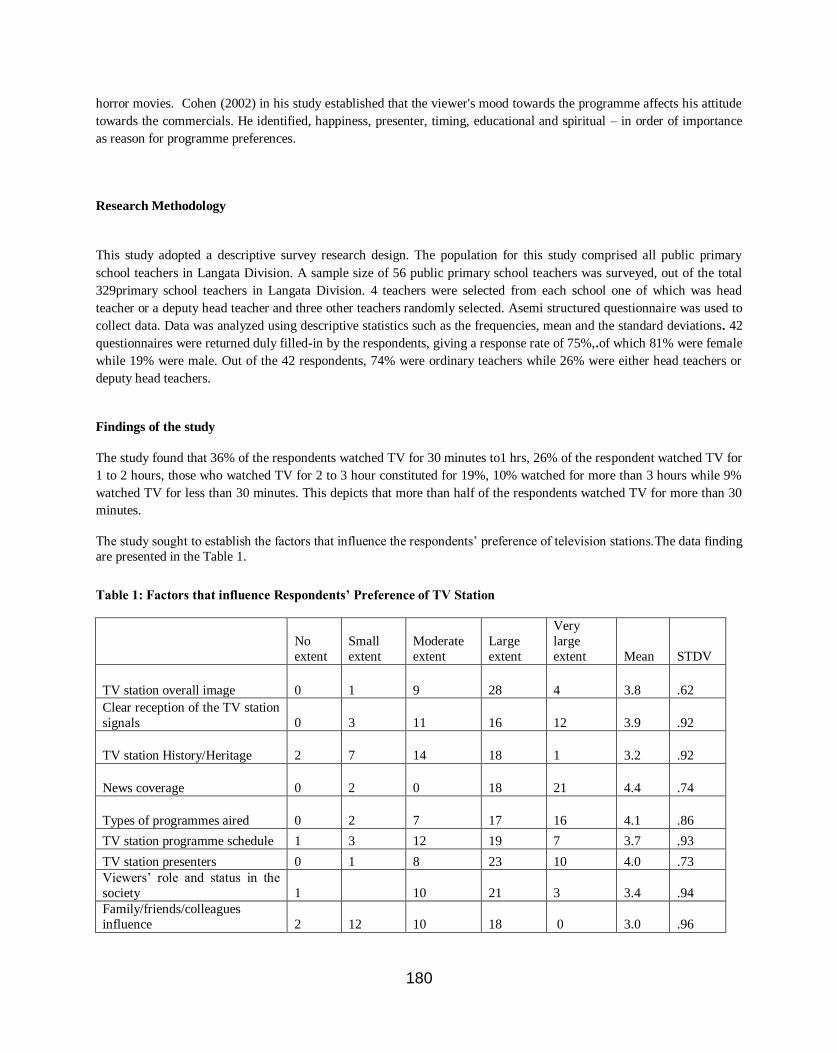
180

horror movies. Cohen (2002) in his study established that the viewer's mood towards the programme affects his attitude

towards the commercials. He identified, happiness, presenter, timing, educational and spiritual – in order of importance

as reason for programme preferences.

Research Methodology

This study adopted a descriptive survey research design. The population for this study comprised all public primary

school teachers in Langata Division. A sample size of 56 public primary school teachers was surveyed, out of the total

329primary school teachers in Langata Division. 4 teachers were selected from each school one of which was head

teacher or a deputy head teacher and three other teachers randomly selected. Asemi structured questionnaire was used to

collect data. Data was analyzed using descriptive statistics such as the frequencies, mean and the standard deviations. 42

questionnaires were returned duly filled-in by the respondents, giving a response rate of 75%,.of which 81% were female

while 19% were male. Out of the 42 respondents, 74% were ordinary teachers while 26% were either head teachers or

deputy head teachers.

Findings of the study

The study found that 36% of the respondents watched TV for 30 minutes to1 hrs, 26% of the respondent watched TV for

1 to 2 hours, those who watched TV for 2 to 3 hour constituted for 19%, 10% watched for more than 3 hours while 9%

watched TV for less than 30 minutes. This depicts that more than half of the respondents watched TV for more than 30

minutes.

The study sought to establish the factors that influence the respondents‘ preference of television stations.The data finding

are presented in the Table 1.

Table 1: Factors that influence Respondents’ Preference of TV Station

No

extent

Small

extent

Moderate

extent

Large

extent

Very

large

extent Mean STDV

TV station overall image 0 1 9 28 4 3.8 .62

Clear reception of the TV station

signals 0 3 11 16 12 3.9 .92

TV station History/Heritage 2 7 14 18 1 3.2 .92

News coverage 0 2 0 18 21 4.4 .74

Types of programmes aired 0 2 7 17 16 4.1 .86

TV station programme schedule 1 3 12 19 7 3.7 .93

TV station presenters 0 1 8 23 10 4.0 .73

Viewers‘ role and status in the

society 1

10 21 3 3.4 .94

Family/friends/colleagues

influence 2 12 10 18 0 3.0 .96

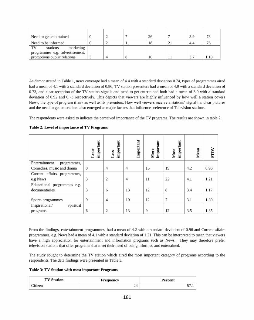
181

Need to get entertained 0 2 7 26 7 3.9 .73

Need to be informed 0 2 1 18 21 4.4 .76

TV stations marketing

programmes e.g. advertisement,

promotions public relations 3 4 8 16 11 3.7 1.18

As demonstrated in Table 1, news coverage had a mean of 4.4 with a standard deviation 0.74, types of programmes aired

had a mean of 4.1 with a standard deviation of 0.86, TV station presenters had a mean of 4.0 with a standard deviation of

0.73, and clear reception of the TV station signals and need to get entertained both had a mean of 3.9 with a standard

deviation of 0.92 and 0.73 respectively. This depicts that viewers are highly influenced by how well a station covers

News, the type of program it airs as well as its presenters. How well viewers receive a stations‘ signal i.e. clear pictures

and the need to get entertained also emerged as major factors that influence preference of Television stations.

The respondents were asked to indicate the perceived importance of the TV programs. The results are shown in table 2.

Table 2: Level of importance of TV Programs

Lea

st

imp

orta

nt

Less

imp

orta

nt

Imp

orta

nt

Mo

re

imp

orta

nt

Mo

st

imp

orta

nt

Mea

n

ST

DV

Entertainment programmes,

Comedies, music and drama 0 4 4 15 19 4.2 0.96

Current affairs programmes,

e.g News 3 2 4 11 22 4.1 1.21

Educational programmes e.g.

documentaries 3 6 13 12 8 3.4 1.17

Sports programmes 9 4 10 12 7 3.1 1.39

Inspirational/ Spiritual

programs 6 2 13 9 12 3.5 1.35

From the findings, entertainment programmes, had a mean of 4.2 with a standard deviation of 0.96 and Current affairs

programmes, e.g. News had a mean of 4.1 with a standard deviation of 1.21. This can be interpreted to mean that viewers

have a high appreciation for entertainment and information programs such as News. They may therefore prefer

television stations that offer programs that meet their need of being informed and entertained.

The study sought to determine the TV station which aired the most important category of programs according to the

respondents. The data findings were presented in Table 3.

Table 3: TV Station with most important Programs

TV Station Frequency Percent

Citizen 24 57.1

182

NTV 11 26.2

KTN 6 14.3

No response 1 2.4

Total 42 100.0

Basing on the factors in Table 3, we find that 57.1% of the respondents stated that Citizen TV aired their most important

programs, 26.2% gave NTV, and 6% gave KTN as the station airing the most important category of programs while

2.4% of the respondents did not respond. This depicts that Citizen TV airs entertainment and current affairs programs

which were identified as the most important types of programs to the viewers.

The study also sought to determine the factors that influence respondents‘ preferences of programs aired on TV Stations.

Respondents were asked to state the extent to which selected factors influenced their preference of programs aired on the

television stations on study. Likert-type scale was used in data collection and analysis on a scale of 1 to 5. Point 1 was

assigned to No at all, indicating very low or no influence while 5 was assigned to very great extent, to indicate high level

of influence by the factors on the choice of a TV Programs.The results are given in Table 4.

Table 4: Factor Influencing Choice of Aired Programs

Not at

all

Small

Extent

Moderate

Extent

Great

extent

Very Great

Extent Means STDV

Awareness of the

programs 0 3 13 17 9 3.8 0.88

Language of the

programs 0 1 5 26 10 4.1 0.68

Viewers interactivity

with the channel during

the program 3 4 13 15 7 3.5 1.11

Timing of the program 2 0 18 15 7 3.6 0.94

Duration of the program 0 7 10 21 4 3.5 0.89

Number of the

commercial breaks in

the program 8 13 7 10 4 3.9 0.91

presenter of the

program 1 2 4 22 12 4.0 0.91

Content of the program 1 1 4 16 20 4.3 0.91

Quality of the program 1 0 5 17 19 4.3 0.86

Preference of the

family/groups 2 5 8 22 5 3.5 1.02

According to the data findings in table 4, content of the program and quality of the program both had a mean of 4.3 with

standard deviations of 0.91 and 0.86 respectively, language of the programs had a mean of 4.1 with a standard deviation

of 0.68, and presenter of the program had a mean of 4.0 with a standard deviation of 0.91. This may be interpreted to

mean that viewers‘ preference and choice of programs is highly influenced by the following factors: the content, quality,

language and the presenter of the program in that order of reducing importance.

183

In this study the respondents were required to give their rating to the TV Stations based on various factors. The rating

was as follows : least preferred (never likes) was given range of 1 – 1.75, slightly preferred (slightly likes) was given

1.76 – 2.5, preferred (likes) was assigned 2.51 – 3.25 while highly preferred (highly likes) was given range of 3.26 – 4.0.

The results are given in Table 5.

Table 5: Rating of the TV Stations by the respondents

Citizen KTN KBC NTV

TV station overall image 2.9 (1) 2.7 (3) 1.4 (4) 2.9 (1)

Clear picture (reception of the TV station signals) 2.8 (2) 3.0 (1) 1.9 (4) 2.8 (2)

TV station presenters 3.1 (1) 3.0 (2) 1.7 (4) 3.0 (2)

News coverage and presentation 3.1 (1) 2.9 (3) 1.7 (4) 3.0 (2)

Viewers interactivity with the channel during the program 3.0 (1) 2.6 (3) 1.7 (4) 2.9 (2)

Program Schedule e.g. timing of the programs, programs line up 3.2 (1) 2.5 (3) 2.0 (4) 2.9 (2)

Variety of the programs 3.1 (1) 2.4 (3) 1.9 (4) 3.1 (1)

Local programs 3.4 (1) 2.1 (4) 2.4 (2) 2.2 (3)

Current affairs programs 3.0 (1) 2.5 (3) 2.1 (4) 3.0 (1)

Entertainment programs 3.2 (1) 2.1 (3) 1.9 (4) 2.7 (2)

Educational programs 3.1 (1) 2.3 (3) 2.2 (4) 2.6 (2)

Sports programs 2.6 (3) 2.7 (2) 2.3 (4) 2.8 (1)

Quality of the program 4.0 (1) 2.5 (3) 2.1 (4) 2.8 (2)

Corporate social responsibility (how the station gives back to the

community)

2.9 (1) 2.5 (3) 2.1 (4) 2.9 (1)

Overall mean 3.1(1) 2.6 (3) 2.0 (4) 2.8 (2)

From the results in Table 5, Citizen TV was ranked as the overall preferred Televisionstation with a mean of 3.1 as well

as on factors such as, it‘s presenters, it‘s News coverage, program schedule and in airing quality and Local Programs

with a mean of 3.1,3.1, 3.2,4.0 and 3.4 respectively . NTV was ranked second overall preferred station with a mean of

2.8 but was rated first in sports programs which had a mean of 2.8. It shared the first position with Citizen TV on its

overall image ,current affairs programs, variety of programs that it airs as well as in Corporate social responsibility with

a mean of 2.9,3.0 3.1 and 2.9 respectively. KTN was ranked third overall preferred station and had a mean of 2.6 but

was rated first in clear pictures with a mean of 3.0

The respondent were required to state why they preferred the channel they had chosen as favorite. They gave clear

reception, clear and competent newscaster, bringing up to date news and having comprehensive news coverage, many

local programs and having programs that are suitable for the whole family watching as reasons why these station are

favorite to them. In addition, good color background, encouraging public views on some matters in their news, and

educative and entertaining programs were also cited as their catching bait.

Discussion

This study has been able to establish very important aspects about TV viewing, some of the findings are discussed here

below. It has shown that majority of the respondent watched TV for more than 30 minutes. It also shows that majority of

the teachers who were respondents to these questions owned a TV set. This study also shows that majority of the

184

teachers preferred Citizen TV to other stations. For majority of teachers, the study has illustrated that their preferred

stations had remained favorite to them for more than 3 years, indicating that the respondent were well conversant with

their favorite stations and the factors that influenced their preferences had remained constant for a period of at least three

years.

Some of the factors that this study has identified as being important in influencing teachers‘ preference of television

stations include; News coverage, the types of programs that the station airs, the television station presenters as well as

the needs of the viewers. The depth, width and presentation of news highly influence viewers‘ preference of television

stations. The viewers identified current affairs programs which include news as their most important type of program as

it meets the viewers‘ most important need of being informed. Citizen TV which was ranked first in news coverage also

emerged as the most preferred station. This leads to a conclusion that news coverage by a station drive preference and

choice of viewers.

The study also established that the programs that a station airs highly influence the choice and preference of television

stations by public primary school teachers. This study established that program choice is related to content as opposed to

programs scheduling. Majority of viewers watched programs of the same general type regardless of the station that they

aired. The respondents preferred local Programs to foreign programs based on the language of programs, tastes and

issues that are relevant to the viewers‘ lives. Quality and variety of programs were also established as important factors

in choice of programs and stations to watch. Citizen TV was rated highly on the above mentioned factors in

programming and it also emerged as the most preferred television station and thus a conclusion can be drawn that the

type, content, quality and language of the programs aired on television are important factors that influence choice and

preference of television stations.

Further, the study established that TV stations presenters also influence preference of viewers. Presenters‘ maturity,

image, and competence also carry the image of a television station. This emerged as an important factor to public

primary teachers in Langata division - majority of who are in the age category of between 40 – 50 years. The station that

had presenters who were rated highly was also ranked as the most preferred station. Other factors that emerged as

important in influencing preference television stations include; clear reception of TV station signal, television stations

overall image, corporate social responsibilities of television stations as well as the viewers need to get entertained and

informed

Conclusion

The study sought to establish the preferred television station by the public primary school teachers in Langata division,

Nairobi. To this objective the study found out that Citizen TV was preferred bymajority of the teachers.The study also

aimed at determining factors that influence consumer preference of TV stations by the public primary school teachers in

Langata division, Nairobi. In line with this the study determined that news coverage, types of programs aired, TV

station presenters, and clear reception of the TV station signalsinfluence preference of TV station. Also, the viewer‘s

need to get entertained, TV station overall image, TV station programs schedule, and TV stations marketing programs

are other factors that influence the same. The study also found out that role and status of the respondent in the society,

TV station History/Heritage and family/friends/colleaguesinfluences the choice of TV stations as well.

Recommendations with Policy Implications

From the finding and basing on the objectives, the study recommends the following; the government should encourage

and reinforce production and airing of local programs by television stations in Kenya. For example policies need to be

formulated on the ratio of local and foreign programs that should aired by television stations in a given period of time.

The study further recommends that more vetting should be done for programs before airing them to determine the

audience andto ensure their relevance in meeting the viewers‘ needs. The study also recommends that the Government

reinforces and encourage media houses in News coverage as this has been identified as one of the most important need of

the viewers. Television stations are also recommended to improve in their news coverage as this contributes to stations

185

gaining competitive advantage. They are further recommended to have TV presenters who communicate the TV station‘s

image since choice and preference of Television stations is highly driven by TV stations presenters.

Suggestion for Further Studies

The research dealt with investigating the factors that influence preference of TV station by public primary school

teachers in Langata division, Nairobi. The research recommends that a similar study be carried out to investigate whether

the same factors would influence preference of TV Stations among other category of people e.g. the students, or people

in other professions. On the same note, since the study was conducted on an urban population the study recommends that

a similar study should be carried out on a rural population to establish whether the same factors would influence

preference of TV channel in a rural setting.

References

Blackwell , R. D, Miniard, P. W & Engel. J. F (2006) Consumer Behaviour 10thedition , Thomson South- Western

Barwise T. P., Ehrenberg A. S &Goodhardt G. J, "Audience Appreciation and Audience size, In Psychological Abstracts, Vol. 69,

1981, p.939

Cohen, J., (2002) Television viewing preferences: Programs, schedules, and the structure of viewing choices made by Israeli

adults.Journal of Broadcasting & Electronic Media June, p.204-221.

Eastman, S. T., & Ferguson, D. A. (2006), Media programming: Strategies and practices.7th editionBelmont, CA: Wadsworth.

Goodhart, G. J., Ehrenberg, A. S. C., & Collins, M. A. (1987).The television audience: Patterns of viewing2nd edition West mead, U.K.: Gower.

Gutman, J.(1978); Viewer Types: A Q-Analysis, Journal of Broadcasting, Vol. 22, pp.505-515

Kotler, P (2003) Marketing Management, 11th edition, Prentice Hall, of India Ltd

Kotler, P., Brown, L., Adam, S., Armstrong, G., (2004).Marketing 6th edition.Pearson EducationAustralia, Frenchs Forest.

Liebes, T., & Katz, E. (1990).The export of meaning: Cross-cultural readings of "Dallas."New York: Oxford University Press.

Mbeke, P. O. &Mshindi, T. (2008) Kenya Media Sector Analysis Report. A report prepared for Canadian International Development Agency Kenya (CIDA – Kenya)

Muriuki, J. W (2003) A Survey of Factors that Determine Architects Preference for Roofing Materials in Nairobi,Unpublished

MBA Project, University of Nairobi.

Mwabu , A M. (2009) A Survey of Viewers Perceived Service Quality of Television Stations in Nairobi, Unpublished MBA

Project, University of Nairobi.

Mwaba, J. N. (2008) A survey of Media Consumer Market Segmentation Practices Used by Television Stations in Kenya,

Unpublished MBA Project, University of Nairobi.

Mwanzia, W. (2009) Unmasking the African Consumer- Media Consumption Habits: a case study of Kenya, Uganda and Tanzania, A report prepared for Steadman- Synnovate, Kenya

Neuendorf, K., Jefferes, L. W., &Atkin, D. (1999, May).The television of abundance arrives: Cable choices and interest

maximization. Paper presented at the annual conference of the International Communication Association, San Francisco

Schiffman , L.G &Kanuk, L.L. (2009) Consumer Behavior,9th edition Pearson Education, Inc., Upper Saddle River, New Jersey

186

Solomon, R.M., Bamossy G., Askegaard,S. and Hogg, M.K. (2010) Consumer Behaviour:a European perspective4th edition

Prentice Hall, Harlow, England

Weaver, IIJames BPersonality and Individual Differences, Volume 12, Issue 12, 1991, Pages 1293-1299

Webster, J. G. (1985). Program audience duplication: A study of television inheritance effects.Journal of Broadcasting & Electronic Media, 29, 121-133.

Webster, J. G., &Washklag, J. J. (1983).A theory of television program choice.Communication Research, 10, 430-446.

Zubayr, C. (1999). The loyal viewer?Patterns of repeat viewing in Germany.Journal of Broadcasting & Electronic Media,43,

346-363.

187

Naïve Reinforcement Learning As a Guide for Path Discovery

Elisha T. O. Opiyo, SCI, University of Nairobi, Nairobi, Kenya, opiyo@uonbi.ac.ke

Eric Ayienga, SCI, University of Nairobi, Nairobi, Kenya, ayienga@uonbi.ac.ke

William Okello-Odongo, SCI, University of Nairobi, Nairobi, Kenya, opiyo@uonbi.ac.ke

Bernard Manderick, COMO, VUB, Brussels, Belgium, bmanderi@vub.ac.be

Ann Nowé, COMO, VUB, Brussels, Belgium, ann.nowe@vub.ac.be

Abstract

Usually, a problem arises given that one is at a point – call it A, and needs to reach a destination, let‘s say point G

through several other intermediate points in a large space. In the absence of a viable tool to use in getting to the

destination, it becomes very hard to get to it especially if the search space is large. Sometimes one may resort to trial and

error and this method is normally very inefficient in a large space. The exhaustive search is also inefficient in a large

space, especially where the resources are limited. Reinforcement learning can play the role that provides the necessary

guide for the search process to successfully discover the destination. We demonstrate, using a concrete example of a map

representation, that by only indicating that the action taken is 'right' (1) or 'wrong'(-1) the search process proceeds

successfully to the destination. The 'right' and 'wrong' indications come from the environment. This is naïve

reinforcement learning since it neither takes into account the cumulative reinforcement values nor insists on discovering

a policy. The contribution of this technique is that there are little overheads and resource inputs, while the search

problem is successfully solved. The challenge with this method is the need to model the environment.

Keywords: Naïve Reinforcement Learning, Machine Learning, Learning Agent

Introduction

In this paper we consider the problem that arises when a path from a given point A to a goal point G is to be found.

Limited knowledge is assumed in which the environment can only supply a limited guide. The environment can only tell

whether the direction taken is right or wrong. Such a problem can be solved using search techniques in which the search

space is examined, Russel & Novig (2003). The difficulty is that when the search space is large it is hard to apply the

usual search methods such as systematic exhaustive search. The required time may, also, be too long and impractical to

get. It is, further, more challenging when there is limited knowledge of the space such that it is not easy to enumerate the

search space elements. In case of the path finding the search space would consist of a set of all possible paths. The issue

is that the path finder has no idea about the future intermediate points, nor where to proceed. The path seeker knows the

destination, G but not how to get to it.

The reinforcement learning approach is adopted in solving the problem of finding a path when the available information

is limited. Reinforcement learning is a machine learning technique in which the learner has a goal with no knowledge of

how to attain it but takes some actions and gets some reward from the environment. The learner interprets this reward

and seeks the actions that will maximize the cumulative reward, as observed by Sutton & Barto (1998); Kaelbling &

Littman (1996).

188

The naïve reinforcement learning is a process in which the learner has a goal without any knowledge of how to get to it

but gets the reward from the environment. The learner interprets the reward and avoids some actions and prefers others.

The learner remembers the incremental progress made and actions taken at local points or states. The naïve

reinforcement learning is demonstrated using a learner that is situated at a geographical point A, and seeks to reach

another geographical point G. The learner, at some local point, chooses a direction and gets to a destination. The

environment indicates to the learner that she is 'right' (1) or 'wrong'(-1). The search process then proceeds successfully to

the destination provided the learner is given enough chances to choose directions. This naïve reinforcement learning does

not take into account the cumulative reinforcement values nor insist on discovering a policy. A policy is guide at every

state that tells the learner how to act. The advantage of this technique is that there are fewer overheads and the required

resource inputs, while at the same time the search problem is successfully solved.

The rest of this paper considers the reinforcement learning model, the naïve reinforcement learning model, the

experiments, results, the discussion and the conclusion.

The Reinforcement Learning Model and the Related Work

Learning in human beings is the process that results in the changes of attitudes and behaviors. These changes occur due

to the acquisition of knowledge, skills and values. Learning in machines, is handled under machine learning that is a

subfield of artificial intelligence, Mitchel (2005). In machine learning the algorithms are developed to model the

learning processes. The learning processes in machines are categorized in some of the groups that include the supervised,

unsupervised, semi-supervised and reinforcement learning processes. In supervised learning the learner is required to

learn input-output pairs that are used as examples to enable the learner to subsequently perform the matching. In

unsupervised learning the learner has only a set of inputs; the learner must discover how to match the inputs to the

outputs. In semi-supervised learning, the learner has some examples with complete input-output pairs and some

examples without the pairs. In reinforcement learning the learner has a goal with no knowledge of how to attain it but

takes some actions and gets some reward from the environment. The learner needs to discover a policy that guides

actions in given states of the environment. Reinforcement learning is a machine learning technique in which the learner

has a goal with no knowledge of how to attain it but takes some actions and gets some reward from the environment. The

learner interprets this reward and seeks the actions that will maximize the cumulative reward, Sutton & Barto (1998).

Consider the learner as an agent that is in some environment. The agent interacts with her environment so that a goal is

achieved. According to Russel & Novig (2003), agents are objects in the environment that perceive and react to states in

the environment. Examples of agents include anything for which an environment can be specified, and that acts and

reacts such as humans, animals, ants, some Internet software or computational processes in operating systems context.

A model for reinforcement learning consists of the agent that is taken to be the learner. The agent interacts with the

environment. The agent selects an action and the environment responds to the action by moving to a different state and

gives a reward to the agent. The interactions of the agent and the environment occur in a sequence of discrete time steps,

Sutton & Barto (1998); Kaelbling & Littman (1996). In the model there is a set of environment states, a set of actions

that the agent can take, a set of rules of changing between the states, a set of rules that determine the reward of the

transitions, and a set of rules that describe what the agent perceives.

Reinforcement learning has many applications. It has been used to solve problems in many areas including robot control,

elevator scheduling, telecommunications, backgammon, chess, jobshop scheduling, project scheduling, robotic soccer,

resource allocation, Sutton & Barto (1998); Wei and Dietterich (1995); Arai et al. (2000); Wauters et al. (2010);

Kaelbling & Littman (1996); Maes et al. (2007); Maes (2003), Galstyan, et al. (2005).

The Naïve Reinforcement Learning Model

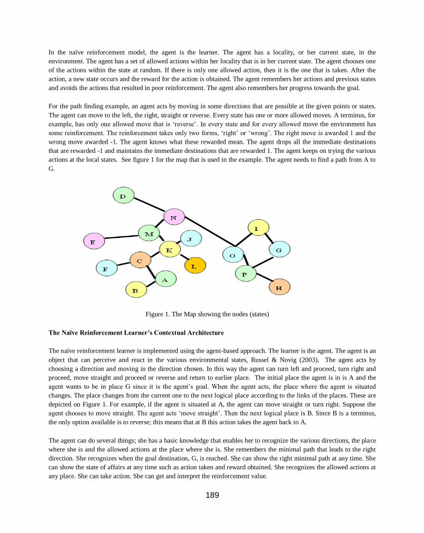
189

In the naïve reinforcement model, the agent is the learner. The agent has a locality, or her current state, in the

environment. The agent has a set of allowed actions within her locality that is in her current state. The agent chooses one

of the actions within the state at random. If there is only one allowed action, then it is the one that is taken. After the

action, a new state occurs and the reward for the action is obtained. The agent remembers her actions and previous states

and avoids the actions that resulted in poor reinforcement. The agent also remembers her progress towards the goal.

For the path finding example, an agent acts by moving in some directions that are possible at the given points or states.

The agent can move to the left, the right, straight or reverse. Every state has one or more allowed moves. A terminus, for

example, has only one allowed move that is ‗reverse‘. In every state and for every allowed move the environment has

some reinforcement. The reinforcement takes only two forms, ‗right‘ or ‗wrong‘. The right move is awarded 1 and the

wrong move awarded -1. The agent knows what these rewarded mean. The agent drops all the immediate destinations

that are rewarded -1 and maintains the immediate destinations that are rewarded 1. The agent keeps on trying the various

actions at the local states. See figure 1 for the map that is used in the example. The agent needs to find a path from A to

G.

Figure 1. The Map showing the nodes (states)

The Naïve Reinforcement Learner’s Contextual Architecture

The naïve reinforcement learner is implemented using the agent-based approach. The learner is the agent. The agent is an

object that can perceive and react in the various environmental states, Russel & Novig (2003). The agent acts by

choosing a direction and moving in the direction chosen. In this way the agent can turn left and proceed, turn right and

proceed, move straight and proceed or reverse and return to earlier place. The initial place the agent is in is A and the

agent wants to be in place G since it is the agent‘s goal. When the agent acts, the place where the agent is situated

changes. The place changes from the current one to the next logical place according to the links of the places. These are

depicted on Figure 1. For example, if the agent is situated at A, the agent can move straight or turn right. Suppose the

agent chooses to move straight. The agent acts ‗move straight‘. Then the next logical place is B. Since B is a terminus,

the only option available is to reverse; this means that at B this action takes the agent back to A.

The agent can do several things; she has a basic knowledge that enables her to recognize the various directions, the place

where she is and the allowed actions at the place where she is. She remembers the minimal path that leads to the right

direction. She recognizes when the goal destination, G, is reached. She can show the right minimal path at any time. She

can show the state of affairs at any time such as action taken and reward obtained. She recognizes the allowed actions at

any place. She can take action. She can get and interpret the reinforcement value.

190

The environment is modeled using the basic elements that are related to each local place or decision point. For each local

place such as K, see figure 1 for the places labeled A .. O, one or more tuples, is maintained. A basic tuple is:- <place,

direction, destination, reinforcement score>. In this case the place is any one of A .. O, the direction is any one of left,

right, straight, or reverse. Destination is any one of A .. O, and reinforcement score is right (-1) and wrong (1). Enough

tuples are kept for each place according to the possible allowed actions at that place. At any one point when the agent

takes an action at one place, the reinforcement score can be given using the appropriate tuple. The contextual architecture

is as shown in Figure 2.

The overall agent control loop consists only of the agent taking an action each time. This activity of the agent is only

constrained by the allowed number of chances or the discovery of the path.

Figure 2. Basic Contextual Architecture

The Experiment, Results and Discussion

The naïve reinforcement learner was implemented using an agent approach. The learner was implemented as an agent

through an object oriented development environment. A base agent with the functionalities was implemented and then

instantiated. The functionalities are the capabilities of the agent such as the ability to recognize where she is, the

available options and take action. Out of possible actions at any place, the agent selects options at random and relies on

the reinforcement for subsequent actions. The main objective of the experiment is to find out the empirical efficiency of

the naïve reinforcement learning process. The learner is given a number of chances to try to find a path from A to G. The

learner or the agent may find the path or not. Out of the number of chances that are given it was noted at which trial stage

the learner discovered the path. The learner operated in a context with 16 places or nodes as shown on figure 1. Every

time the learner starts at node or place A and gets a number of chances to find a path to G. The chances given were 10,

15, 20, 25, 30, 35, 40, 45, 50, 55, 60 and 100. For every number of chances, say for example 15 chances, the experiment

was repeated five (5) times and in each replication the following were noted: time taken in seconds, if the path was found

and the number of trials before the path was found. In every case the mean value was computed and rounded. Efficiency

of the search effort was computed to give an indication of the chances that were given and the number of chances used

before the correct path is found.

The results that ware obtained are shown on Figures 3, 4 and 5.

191

Figure 3. Getting the right path versus the chances given

Figure 4. The search effort

Figure 5. The time it takes for the run

We now discuss the results. In Figure 3, the results for getting the right path versus the chances that are given are shown.

For all the replications when the chances were 5 and 10, no correct path was found. This can be explained by the fact that

there were 16 places or nodes and the learner guesses most of the time. The chance of getting directions correctly and

successively is low. For chances 15 to 30 the correct path is found most of the time with a probability ranging from 0.6

to 0.8. For the chances ranging from 35 and above, the correct path was found, every time. From figure 3 it is strongly

indicated that beyond some number of chances, the correct path is certainly found. In this example the number is 35

changes. This works out to approximately 2 trials for every node or place. It may also be noted that under the same

example, the possibility space is 20736 for exhaustive search. At 35 trials for a guaranteed correct path, the saving on the

192

search effort seems significant. Figure 4 shows the search effort. This is a measure of the number of trials taken against

the total number of changes that are given. In all cases the after 15 chances and beyond, the learner did not exhaust the

number of chances given. The learner took fewer numbers of trials to find the correct path compared to the total number

of chances given. The implication of this is that the naïve reinforcement learning process can also be effective. Figure 5

shows the time it takes to end the run. A run is the time it takes to exhaust the chances or find the correct path. Either

way the search process stops, when the chances are exhausted or the correct path is found. The run time is generally the

same, varying from 0.03 seconds to 0.28 seconds. The most notable observation is that the number of chances does not

affect the length of the run. This is explained by the fact that the run stops when the correct path is found. These results,

though very limited in variation, indicate that the naïve reinforcement learning process can be useful. A typical use may

be in the embedded control for robots, where a robot may have a range of actions and some environmental indicators that

show him that the actions are right or wrong. There are some notable limitations of the naïve reinforcement learner. First,

like reinforcement learning, it needs the environmental feedback without which it cannot work. Secondly, the local

environmental elements or tuples may be too many if the learner has to cope with varying start places and goal places.

The naïve reinforcement learner however, both explores and exploits in the sense of Sutton & Barto (1998). She explores

since the actions are selected at random and exploits since the reinforcement is useful information that forms the basis

for avoiding some places.

The Conclusion

This paper has considered the problem of finding a path from one place to another using the naïve reinforcement learning

method. The naïve reinforcement model, unlike the usual reinforcement model, only considers providing the learner with

a right and wrong indicators on their actions from the environment. This alone has been found to be sufficient to guide

the learner in discovering the correct path. The empirical results with a single context show that out of a total of 20736

possible trials needed for the exhaustive search only 35 trials are needed to guarantee finding the correct path. Whereas

this is not indicative of the actual savings ratio in other contexts that may be different, substantial savings on the search

effort is expected where the naïve reinforcement method is used to guide in path finding where local knowledge and

information is very limited. The most important strength of the method is the little overhead that it has, and the ease of

implementation. The usual reinforcement model has been extensively relaxed yet the learner still manages to find a

correct path. Its drawback is the need for environment and the many knowledge elements that may be needed for a

generalized application.

Acknowledgment

We are grateful to the University of Nairobi and Free University of Brussels for the various types of support that we have

received for our research work.

References

Arai, S., K. Sycara ,T. R. Payne (2000). Multi-agent Reinforcement learning for Planning and Scheduling Multiple

Goals. Proceedings of The International Conference on Multi-Agent Systems (ICMAS2000), pp. 359-360.

Galstyan, Aram, Karl Czajkowski, Kristina Lerman (2005). Resource Allocation in the Grid with Learning Agents.

Journal of Grid Computing, vol. 3, pp 91–100.

Kaelbling, Leslie Pack & Michael L. Littman (1996). Reinforcement Learning: A Survey. In Journal of Artificial

Intelligence Research, Vol. 4, pp 237-285.

Maes Sam, Karl Tuyls, Bernard Manderick (2007). Reinforcement Learning in Large state spaces: simulated robotic

soccer as testbed. Retrieved from http://citeseerx.ist.psu.edu/viewdoc/ summary? doi=?doi=10.1.1.4.1998 ; Quelle

http://como.vub.ac.be/Members/karl/rl-robo02.ps, last visited July, 2011.

193

Maes, S. (2003). Reinforcement Learning in Large State Spaces-simulated Robotic Soccer as Testbed. Robocup 2002

Robot Soccer World Cup VI, 2752, p 319-326.

Mitchel ,Tom (2005). Machine Learning. McGraw Hill Publishers.

Russell, Stuart J., Peter Norvig (2003). Artificial Intelligence: A Modern Approach, (2nd ed.), Upper Saddle River, New

Jersey: Prentice Hall.

Sutton, Richard S. and Andrew G. Barto (1998). Reinforcement Learning: An Introduction. MIT Press, Cambridge,

MA.

Wauters T., K. Verbeeck, G. Vanden Berghe, P. De Causmaecker (2010). Learning Agents for the Multi-mode Project

Scheduling Problem. Journal of the Operational Research Society, Vol. 62, pp 281–290, 2010.

Wei Zhang and Thomas G. Dietterich (1995). A Reinforcement Learning Approach to Job-shop Scheduling.

Proceedings of the Fourteenth International Joint Conference on Artificial Intelligence (IJCAI 1995), Vol.2, Morgan

Kauffman Publishers.

194

UNIVERSITY OF DAR ES SALAAM

UNIVERSITY OF DAR ES SALAAM BUSINESS SCHOOL (UDBS)

Name of candidate: Latifa Mbelwa

Name of Supervisors:

1. Prof Sylvia S. Temu University of Dar es Salaam

2. Dr. Musa J.Assad University of Dar es Salaam

3. Dr. Karl Bonnedahl Umeå School of Business

4. Prof. Hakan Bohman Umeå School of Business

Institute Department of Accounting

Proposed Degree: PhD in Business Administration

Title: The Determinants of Accounting Information Use by Political and

Administrative Actors in Public Sector Decision making (The case of Local Government

Authorities in Tanzania)

195

INTRODUCTION

Public Sector Decision Making and Use of Accounting Information

The public sector plays a crucial role for social and economic development of any state. Development of infrastructure

and provision of basic services such as health, primary and secondary education and other public services and goods to

the people lie in the public domain. The public sector is broadly synonymous with government sector (Schacter, 2000).

The government sector operation includes Central Government and Local Government Authorities activities (LGAs)

(Mohammed et al, 2008). Globally, since 1980‘s, public sector has been undergoing reforms which represent the aspects

of New Public Management (NPM) (World Bank, 2008).The main motive of NPM is to achieve efficiency in operations

and financial management processes of public sector entities (Watkins et al, 2004: Groot et al, 2008). Guthrie at al

(2005) argue that NPM involves development of performance measurement systems and change of financial reporting

systems including adoption of accrual basis accounting across government departments and sectors and reliance on

professionally accounting body which set accounting standards.

Accrual basis accounting has been adopted and is being implemented by governments of developed and developing

countries such as UK, New Zealand, Italia, Australia Norway, Sweden, India, Srilanka, Pakistan ,Tanzania and others

(Groot and Budding, 2008: Newberry and Pallot, 2004: Caccia and Steccolini, 2006: Barton, 2009: SAARC, 2006: URT,

2010). The accrual basis accounting is based on the argument that it enhances the quality of accounting information by

recognizing all cost of transactions or events regardless of the cash received or paid (Monsen, 2006). The accrual basis

accounting provides more useful information than cash basis accounting which leads to poor quality information thus not

useful to the users (Ouda, 2003). Essentially, this reform shows the importance of accounting information in public

sector decision making and its role of facilitating the decision making process (Chalu, 2007). However, the facilitation

role depends mainly on the use of accounting information in decision making (Assad, 2001).

Use of information is defined by Philemon (2008) as taking the research finding into account (Weiss and Bucuvalass,

1977), the conversion of data into ultimate actions (Barabba, 1983) or the extent to which interpreted data influence the

user‘s decision making (Moorman et al, 1992). Chua (1998) point out that accounting information can be used in two

main ways, which are for symbolical use and instrumental use. Symbolical use is characterized by interactions of actors

on social constructed norms, values, identification and meaning about reality as presented by accounting numbers (Chua,

1988). Melia et al (2003), comment that, symbolic use is where accounting information is used for legitimating purposes.

On other hand instrumental use is characterized for analysis, evaluation search for data and test for solution (Chua,

1988). It assumes a rational decision making process: decision makers have clear goals, seek direct attainment of these

goals and have access to relevant information (Walle and Bovaird, 2007). Melia et al (2008) add conceptual use as a use

of accounting information for general enlightenment.

The increased use of accounting information as social and institutional practice is among the proposed elements to

improve efficiency of public sector decision making (Miller, 1994) which justifies the symbolic use of accounting

information. The existence of different of professions in LGAs might make accounting information to be deployed in

budgeting decision by shaping the conflicts between the professionals as legitimating device (Melia et at, 2008). The

accounting information can be used to elaborate budget of next period based on the results of the previous period and of

the real financial situation (Alijarde, 2002). Accounting information in LGAs‘ is communicating about source of fund,

utilization of generated fund, and justification for their utilization (Chalu, 2007). The accounting information enables

decision makers to determine the adequacy of tax policy and allows the assessment of future source and revenue needs.

Thus, LGAs forecast the revenues for the next period and in consequence the expenditures that they might have to incur.

196

In fact LGAs‘ budgeting is revenue driven, in that the revenue constrain generally dominates decision making (Gianakis

and McCUE, 1999).

Additionally, the accounting information can be used in cost and benefits analysis of contracting out decision. As a

result, accounting information can be used by public sector actors to legitimize contracting out decisions at most

efficiency manner (Scuill, 2008). Definitely, the uses of accounting information contribute to efficiency in decision

making by insuring scarce resources are best used in provision of public services through clear determination of input

and output basing on real financial situational (Assad, 2001;Alijarde, 2002).

Despite the role of accounting information in public sector decision making, factors influencing its use still remain

unclear in government decision making irrespective of the adoption of accrual basis accounting system. The government

decision making can be seen as a bureaucratic and political process involving multiple actors with inconsistent

preferences, interest and motives that are discovered by acting rather than by being delivered upon in advance (Lawton et

al., 2000: Pilcher, 2005). According to institutional theories, the best way to understand political behavior (seemingly

both individual and collective) is through a ―logic of appropriateness‖ that individuals acquire through their membership

in institutions (Peter, 2000). Peter (2000) argues that people functioning within institutions behave as they do because of

normative standards and institutions arranged as rules and incentives, and the members of the institutions behave in

response to those basic components of institutional structure. In the democratic countries, the institutional set up of

government decision making process involves the elected political actors who have legitimized power to make decision

on behalf of the voters. Additionally, government decision making process includes permanent public officials as

administrative actors who have the responsibilities of preparing and implementing decisions which are made by political

actors.

The decision structure of LGAs is headed by full councils who make important financial and non financial decisions

(Gomes, 2003). In these councils, political actors (councilors) and administrative actors meet, but councilors remain

decision makers basing on their power to vote for all decisions which need their consent. The technical preparation for

decision making is done by administrative actors and finally some of decisions such as budgeting approval are made by

the political actors (Jalonen, 2006). Gerboth, (1997) pointed out that, when a decision-making process depends for its

success on public confidence, the critical issues are not technical but they are political, which is inclined towards

satisfying the constituents' interests. Utmost, the public sector decisions are resulted from compromising, bargaining and

politics (Rainey, 2003). The complexities of the structure of public sector decision making do not ruin out the importance

of using accounting information in decision making especially in African developing countries including Tanzania which

are characterized with high needs of government services and limited resources (World Bank, 2006). LGAs of these

countries are characterized with implementation of decentralization policy which gives mandate to LGAs‘ actors to make

decision through transferring of functions and resources including financial resources from central government to local

level (World Bank, 2006). In fact, in terms of expenditure responsibilities, Tanzania has achieved a significant amount of

decentralization; approximately, 19% of the budget on recurrent government spending is done at the local level with

central government transfers (Boex et al., 2003). Thus, more accounting information is expected to be produced in LGAs

to inform actors for decision making.

Therefore, the enhancement of quality of accounting information as one of input in decision making by adoption of

accrual accounting in public sector explains the importance of information in this sector. However the nature of decision

197

making process of public sector, calls for a study to investigate the factors that influence accounting information use by

decision makers (political and administrative actors) in decision making.

6.2 Statement of the Problem

The pressure of public sector accounting not only changes to achieve efficiency but also to expands its sphere of

influence in public sector decision making process which is characterized by compromise, bargaining and politics in

order the dream of efficiency to be realized (Hopwood 1984). However, despite of the importance of accounting

information in decision making and nature of public sector decision making process, little is known about the factors

which influence accounting information use by political and administrative actors in public sector decision making. The

studies which analysed the factors influencing accounting information use in decision making has been done in private

sector (Heidhues and Patel, 2008). Moynihan et al (2004); Askim (2007); Proeller et al (2010) analysed the factors

influencing performance information with limited focus on accounting information. Additionally, the studies were based

on a single actor, political or administrative, in developed country contexts. The main argument of these studies

however, is that there are several factors influencing the use of information in public sector which are associated with

organization‘s institutional environment.

Factors identified in these studies cannot be generalized to this study because of gaps inherited in those studies. The

studies lacked a clear research model for understanding the determinants of accounting information use by multiple

actors involved in public sector decision making. Yet, there are models which have been developed by Luder (1992); Xu

(2003); Chalu, (2007) concerning the government accounting. At most, these models provide understanding of the

factors which determine the Accounting Information Systems (AISs), innovation or effectiveness in public sector but not

the use of accounting information in decision making.

Miller (1994) argues that accounting practice as particular economic form of calculation, should be similar located as a

social and institutional practice and its practice analysis should address the dispersed organization matrix within which it

operates. The institutional theory has long been established as important perspective in accounting especially in public

sector because it provides insight to institutional dynamics. The institutional theory considers social, regulative and

cultural aspects on shaping the attitude of organization and its actors towards organization form and process such as

decision making process (DiMaggio and Powell 1983). Assad (2001) argues that accounting information can be used by

actors, if the accounting becomes part of the socio-cultural and regulative context; where external environmental cultural

norms have implications on how organizational actors understood and interpreted accounting functions, processes and

information. The contingency model of government innovation by Luder (1992) suggests that for understanding attitude

of government actors‘ towards accounting practice, the factors which are associated with institutional environment of

organization should be taken into consideration.

Accounting information as technical calculation in institutionalized environment still it should have the standards and

characteristics to be useful as an instrumental and symbolic representation of accounting number in decision making in

order to create efficient in decision making (Potter, 2005). Staubus, (1960) argues that the use of accounting information

depend on accounting information itself. The accounting information should have relevance quality in order to be useful

in decision making. Ultimately, the users (actors) are assumed to be able to interpret the information and use in decision

making (IPSAS, 2010). Therefore, individual actors‘ characteristics as suggested by contingency model of government

innovation by Luder, (1992) that Social and Economic Status (SES) such as education background and experience of

using information shape attitude of actors in using information. Luder (1992) argues that individuals‘ actors do not have

identical demands for information, as they are not identical in the socio-economic attributes relevant for predicting their

198

demand for government accounting information. Utara (2011) observed that public decision makers (actors) consist of

various levels of knowledge, expertise, and experience. They are varied from experts to laymen. Other scholars such as

Askim (2007) argues that demographic characteristics such as age of the individual actors have role in the shaping the

actors to use information in public sector decision making.

Following the above discussion, the main problem to be addressed by this study is lack of knowledge on determinants of

accounting information use by administrative and political as the key actors in public sector decision making process.

Consequently the main question of the study is ‘What are factors which determine accounting information use by

political and administrative actors in public sector decision making process? Therefore the study investigates on the

factors relate to organization institutional environment, factors related to individual actors‘ SES and demographic

characteristics and factors related to accounting information quality. The study will focus on budgeting and contracting

out decisions making. For the facts, that the budgeting decision process is required to deploy accounting information in

order to achieve efficiency and it is emphasizing on future service delivery rather than the past; and it is associated with

political, institutional systems and structures at large in LGAs (Goddard, 2005). On other hand, contracting out decision

making has the potential not only to change the way government services are delivered and the ultimate structure of

government itself, but also to affect the nature, extent and importance of accounting information for informed decision-

making (Scuill, 2004).

Therefore, the study will develop a model by using institutional theory which is supported by Contingency model for

government accounting innovation by Luder (1992) and decision usefulness concept and empirical studies. The model

will be refined or affirmed by doing the explorative case study in LGAs of developing countries, in the case of Tanzania.

Thereafter, the model will be tested by using survey methods, to establish the extent the factors identified determining

the use of accounting information in decision making by political and administrative actors.

6.3 Research Objective

6.3.1 General objective

The main objective of this study is to investigate the determinants of accounting information use by political and

administrative actors with the aim of contributing to the efficiency in decision making. The study will be done in Local

Government Authorities (LGAs) of developing countries context in general and Tanzania in particular.

6.3.2 Specific Objectives

The study has the following specific research objectives:

1. To develop the model of determinant of accounting information use in decision making by political and

administrative actors

2. To explore how accounting information is used by political and administrative actors in decision making such as

budgeting and contracting out decisions

3. To identify factors associated with organization institutional environment

4. To identify factors associated with Social and Economic Status (SES) and demographic characteristics of individual

actors

5. To identify factors associated with accounting information quality 6. To establish the extent identified factors determine the use of accounting information in decision making by political

and administrative actors.

199

6.4 Significance of the study

The contribution of this research can be seen in different ways. The first is theoretical contribution. This study is

expected to contribute more on Institutional theory; Institutional theory has been used by researchers in public sector to

explain the changes made, through public sector accounting reforms such as adoption of accrual base financial reporting.

This study is using the institutional theory to explain the influence of the organization internal institutions and external

environmental pressures in the use of accounting information by actors in LGAs decision making process. Secondly, is

empirical contribution whereby, the study findings are expected to establish empirical model which will show

determinants of accounting information use by actors in LGAs decision making. The model will provide answer to the

current question, and guide future research on understanding the determinants of accounting information use in public

sector decision making. Thirdly, is practical contribution, the findings will help the reformers to select appropriate

measures and actions to make sure accounting information produced in LGAs is used by political and administrative

actors in decision making. This will lead to realize the promise of reforms and ensures that it contributes to greater

efficiency in the performance of LGAs.

6.5 Literature Review

6.5.1 Definition of Key Terms

6.5.1.1 Decision making

Decision making can be regarded as the mental processes (cognitive process) resulting in the selection of a course of

action among several alternative scenarios. Every decision making process produces a final choice. The output can be an

action or an opinion of choice. The decision making process can viewed in different perspectives. Cognitive perspective

views decision making process as continuous process integrated in the interaction with the environment, while normative

perspective views decision making as the analysis of individual decisions concerned with the rationality and logic of

decision making process, where specialists apply their knowledge in a given area to making informed decisions. Rainey

(2003) identifies the decision making four approaches from public management literature. (1) The rational decision-

making approach view of decision making suggests that decision-makers follow a specific process where goals are

decided upon, alternatives are developed in accordance with such goals, and then the most efficient alternative is

implemented. (2) The contingency perspective decision-making approach as where the decision maker use judgment and

intuition, undertake in bargaining and political maneuvering in their decision-making process because rational decision-

making cannot occur under unstable, unclear or complicated conditions. (3) Incremental decision making approach, this

is where decision-makers choose to make less controversial (the requirement for political consensus and compromise),

intermediary decisions to ensure some degree of success of achieving vague goals presented instead of choosing an

alternative that a rational decision-making process would predict. (4) The garbage decision making approach comes from

the observation that decisions are made in organizations when particular decision-making opportunities or requirements

arise and it is often unclear who has the authority to decide what and for whom. The developers of information

(accounting information in this case) hope that their work will be utilized in some form of rational decision-making

processes or that at the very least, their tools and information are used to help inform incremental decision-making

processes (Rainey, 2003). For the matter of this study the decision making process is defined as continues process

integrated in the interaction with the environment with combination incremental and rational decision approaches as

explained by Rainey, (2003).

6.5.1.2 Accounting Information

Collier (2006) defines accounting as the process of identifying, measuring and communicating economic information to

permit informed judgments and decisions by users of the information. Therefore, accounting information is defined as a

means by which we measure and communicate economic events (Collier 2006). There are two type of accounting

information; financial and management accounting information. Financial accounting information is information from

financial statements such as statements of financial position, statement of financial performance, cash flow statement,

statement of change in equity or net assets and accounting policies and notes to the financial statements. These

200

statements contain information about assets, liability, net assets/equity, revenue, expenses and cash inflows (IPSAS 1,

2006). Therefore, the financial statements describes information about sources, allocation and uses of the financial

resources; ability of entity to finance activities and to meet its liabilities and how the entity financed its activities and met

its cash requirements (IPSAS 1, 2006). The financial information is information designed primarily to assist external

users in deciding where to place their scarce resources (collier, 2006).

Managerial accounting information on the other hand is the one specifically intended to aid management in the running

of the organization (Drury, 1996). The information in the previous budgets shows that LGAs have been efficiency in

raising as well as using financial resources for citizens‘ wellbeing (Chalu, 2007). Managers such as political actors

(councilors) and administrative actors (public officials) can use the accounting information in setting up the organization

overall goals, performance evaluation and in making all types of managerial decisions. For the purpose of this study,

both types of accounting information are considered in the discussion.

6.5.1.3 The use of accounting information in decision making

Accounting Information is not an end by itself, but it is a means to an end (Collier, 2006). The end is a better-informed

decision than would not have been the case without the information. Thus, accounting information use can be defined as

taking accounting data and information into account; the conversion of accounting data into ultimate actions or the extent

to which interpreted accounting data influence the user‘s decision making. Chua (1988) point out that, there is symbolic

and instrumental use of accounting information in decision making. Chua (1988) further posits that symbolic use of

accounting information refers to the use of information basis on symbolic meaning constructed from social action as the

product of the actor‘s compliance with stable, shared norms or meaning and personal knowledge and experience.

Symbolic use of information is seen in individual actor construction rather than organization perspective (Vyas and

Souchon, 2003). Philemon (2008) point out that instrumental use refers as to the use of information to undertake a

specific decision or action that can be clearly designated. The instrumental accounting information use involves official

order of documents and basically hierarchical in nature with well defined areas of responsibility and accountability

(Chua, 1988). Both uses are part of constructed reality that has been attributed particular levels of significant in decision

making (Chua, 1998). Another way of using accounting information is conceptual use. Philemon (2008) argues that

conceptual use refers as to thinking of an issue without putting information to any specific documentable use. Conceptual

use is based on ‗a gradual accumulation and synthesis of information‘ and a gradual incorporation ‗into the user‘s overall

frame of reference‘ (Walle and Bovaird, 2007).

The various decisions which LGA can make using accounting information are budget decision which include resources

allocation decision and distribution decision for economic development (Richard and Schwartz, 2004), and borrowing

decisions. Budgeting in function perspective is a very strategic perspective because it refers directly to the output of the

entity and it plays important role in the goal of public sector of financial management and resources allocation

(Bergmann, 2009). Thus decision may include increase or decreases in the provision of that output, the quality of the

output, introduction or increase of fees, investing in improved facilities and others. Therefore, the prepared and approved

budget in government sector form a law which guides all transactions on services delivered to the people. Goddard

(2005) posits that enhancement of efficiency on budgeting practice in government sector might improve transparence

and accountability and overall good governance.

The accounting information can also be used by decisions makers in the contracting out decision making process in

public sector (Sciulli, 2004). The accounting information use in contracting out decision is used to identify the service to

outsource, evaluate competing bidders thus justify the final awarding decisions (Sciulli, 2004). For the purpose of this

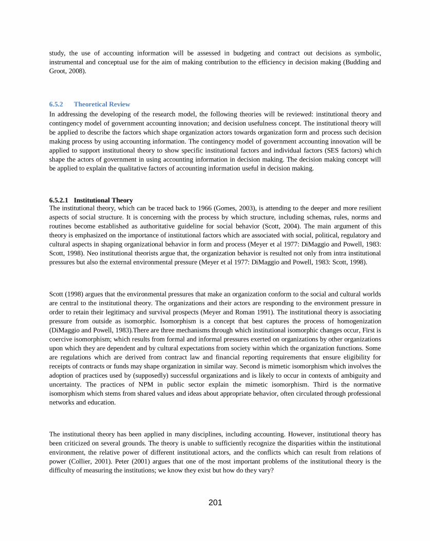
201

study, the use of accounting information will be assessed in budgeting and contract out decisions as symbolic,

instrumental and conceptual use for the aim of making contribution to the efficiency in decision making (Budding and

Groot, 2008).

6.5.2 Theoretical Review

In addressing the developing of the research model, the following theories will be reviewed: institutional theory and

contingency model of government accounting innovation; and decision usefulness concept. The institutional theory will

be applied to describe the factors which shape organization actors towards organization form and process such decision

making process by using accounting information. The contingency model of government accounting innovation will be

applied to support institutional theory to show specific institutional factors and individual factors (SES factors) which

shape the actors of government in using accounting information in decision making. The decision making concept will

be applied to explain the qualitative factors of accounting information useful in decision making.

6.5.2.1 Institutional Theory

The institutional theory, which can be traced back to 1966 (Gomes, 2003), is attending to the deeper and more resilient

aspects of social structure. It is concerning with the process by which structure, including schemas, rules, norms and

routines become established as authoritative guideline for social behavior (Scott, 2004). The main argument of this

theory is emphasized on the importance of institutional factors which are associated with social, political, regulatory and

cultural aspects in shaping organizational behavior in form and process (Meyer et al 1977: DiMaggio and Powell, 1983:

Scott, 1998). Neo institutional theorists argue that, the organization behavior is resulted not only from intra institutional

pressures but also the external environmental pressure (Meyer et al 1977: DiMaggio and Powell, 1983: Scott, 1998).

Scott (1998) argues that the environmental pressures that make an organization conform to the social and cultural worlds

are central to the institutional theory. The organizations and their actors are responding to the environment pressure in

order to retain their legitimacy and survival prospects (Meyer and Roman 1991). The institutional theory is associating

pressure from outside as isomorphic. Isomorphism is a concept that best captures the process of homogenization

(DiMaggio and Powell, 1983).There are three mechanisms through which institutional isomorphic changes occur, First is

coercive isomorphism; which results from formal and informal pressures exerted on organizations by other organizations

upon which they are dependent and by cultural expectations from society within which the organization functions. Some

are regulations which are derived from contract law and financial reporting requirements that ensure eligibility for

receipts of contracts or funds may shape organization in similar way. Second is mimetic isomorphism which involves the

adoption of practices used by (supposedly) successful organizations and is likely to occur in contexts of ambiguity and

uncertainty. The practices of NPM in public sector explain the mimetic isomorphism. Third is the normative

isomorphism which stems from shared values and ideas about appropriate behavior, often circulated through professional

networks and education.

The institutional theory has been applied in many disciplines, including accounting. However, institutional theory has

been criticized on several grounds. The theory is unable to sufficiently recognize the disparities within the institutional

environment, the relative power of different institutional actors, and the conflicts which can result from relations of

power (Collier, 2001). Peter (2001) argues that one of the most important problems of the institutional theory is the

difficulty of measuring the institutions; we know they exist but how do they vary?

202

Irrespective of its criticism, the institutional theory has been used in accounting discipline to explain the organization

change, such as in public sectors accounting reforms see in (Frumkin et al, 2004, BOGT, 2008). Basing on the argument

that institutions shape behavior of actors (organization and individuals) through socialization process without actors even

to realize that their behavior is in fact partly controlled by an institution. This study applies institutional theory to

identify the factors which might influence organization actors to use accounting information in decision making.

Hopwood and Miller (2004) point out that accounting could not and should not be studied as an organization practices in

isolation from the wider social and institutional context in which it operates. To support institutional theory in

determining the institutional factors which influence the use of accounting information by political and administrative

actors, the study use contingency model of government accounting innovation by Luder (1992); and decision making

concept for explanation of the technical features of accounting information to be useful in decision making.

6.5.2.2 The Contingency Model of Governmental Accounting Innovation

A contingency model of governmental accounting was developed by Lüder (1992) to specify the social-political

administrative environment and its impact on governmental accounting innovations. The model provides four contextual

variables associated with organization institutions which influence the government accounting innovation. The variables

are stimuli, users of accounting information, producers of accounting information and implementation barriers. Luder

(1992) argues that the situation of financial problems, financial scandal, capital markets, external standard setting and

professional interest are factors associated with stimuli of innovation.

The factors associated with users of information are social structural variables such as Social Economic Status (SES) and

political culture as political behavior which influence the basic attitude of the users thus the expectation change to the

citizens, Member of Parliament and others. The factors which are associated by producers of accounting information are

structure variable of the political-administrative system as such staff training and recruitment, administrative culture and

political system. These factors influence the basic attitude of the user of information to politicians, managers and

accountants. The last variable is the implementation barriers which are obstacles to innovation including organization

system, legal systems, and qualification of accountants and size of jurisdiction (Ludea, 1992).

The model has been widely applied and tested through several studies such Luder (1992), Ludea (1993), Godfrey et al.

(1996), El-Batanoni and Jones (1996), Monsen and Nasi (1998), Christensen (2001), Mark (2002), Carmen et al (2009).

Through, testing of the model, the favorability and un-favorability of variables towards government innovation imaged

in different environment.

This study applies the contingency model of government accounting to identify the institutional and individual actors‘

factors which can influence the attitudinal behavior of actors (users of accounting information) to use accounting

information in decision making. Luder (1992) argues that, political actors are the users and producers of accounting

information while the administrative actors such as accountants and managers are producers of accounting information

only. This study argues that both actors are the users of accounting information, by regarding administrative actors as

technical users of accounting information in preparation and implementation of decisions which are made by political

actors (Jalonen, 2006).

6.5.2.3 Decision usefulness concept

203

„The objective of accounting is to provide financial information regarding an enterprise/organization for use in making

decision making‟. By George Staubus (1960)

This is focal point of decision making theory. The decision making theory was founded by George Staubus in mid of

twentieth century, when he was doing the PhD study for examination of revenue concept with the objective of defining

revenue. Further was followed with question, for what purpose? Eventually comes up with the objective of accounting.

Through analysis of the users of accounting output and the uses the made of those outputs, the study concluded that all

users sought information for decisions (Staubus, 1960). Decision usefulness is the main characteristic of accounting

information quality as it captures value of accounting information for interested parties in making their decisions

(Staubus, 1960: Shipper & Vincent 2003). Thus, for the accounting information to be useful in decision making, it

should have relevance quality (IPSASB, 2010). Relevance and faithful representation are the primary qualities of

accounting information for useful decision making. If either is missing completely from a piece of information, the

information will not be useful (Obaidat, 2007). IPSASB, (2010) points out that, for accounting information to be useful

and applied in decision making, it must be understandable by users. The understandability increase when information is

classified characterized and presented clearly and concisely (Beest, Braam and Boelens, 2009). Generally, the technical

characteristic of information (accounting information in this case) quality includes, accuracy, accessibility, timeliness,

completeness, reliability, consistency, accuracy, relevance objective and understandability (Mbamba, 2003; Seddon,

1997; Chalu, 2007; XU, 2003).

However, some scholars, such as Philemon, (2008) view the quality of information on the way users perceive the

information. The perceived usefulness is measured in terms of importance and usableness (Lacker and Lessig, 1980).

Perceived ease of use which refers to the degree to which a person believes that using particular system will be free from

effort or free of difficulties (Davis, 1989). Perceived accessibility by users refers to the ease of access, availability and

convenience of information (Jeong and Lambert, 2001). The perception on the information creates attitude of users

towards information. Chalu, (2007) explains the quality of information as the product of the effectiveness of Accounting

Information System (AIS) which satisfy users need and demand. The quality information is also defined in terms of the

extent information successfully serves the purpose of the users, thus the extent information fits the users‘ needs (Kahn, et

al, 2002; Walle and Bovaird, 2007). Houghton, (1998) views quality of information, as the way the producers and users

communicate to make more informative meaning and enhance knowledge to the users, and hence users will be able to

interpret information and use in decision making. In concluding, for accounting information to be useful and influence

users (actors) to use it in decision making it should have the relevant quality.

6.5.3 Empirical Studies on the accounting information use in decision making

Since 1980, research on the public sector accounting has been dedicated either on the accounting reforms and

accountability (see Cochrane, 1993:Goddan and Powell, 1994: Guthrie, 1998: Assad, 2001: Goddan, 2004: Newberry

and Pallot, 2004: Goddan, 2005: Carnegie and West, 2005: Bidding at al, 2008: Steccolini, 2009: Hyndman and

Connolly, 2011). Some of these studies utilized institutional theory with the view that accounting is a social and

institutional practice, instead of merely a technical practice (Potter, 2005).

Some few studies have been made contribution empirical on the use of accounting information in decision making by

actors such as Heidhues and Patel (2008). Heidhues and Patel (2008) provides evidence that contextual factors

associated by political, social, cultural and regulatory setting together with manager‘s preferences strongly influence the

utilization and interpretation of accounting information in decision-making strategies and processes. The case study of

German Dairy Cooperative which applied the institutional theory cannot be generalized by the current study. However,

the German Dairy Cooperative is operating as business oriented organization and its nature of decision making process is

not similar with the public sector decision making.

204

The studies in information use no specifically to accounting information in public sector (Dull 2008, Moynihan and

Ingraham 2004, Moynihan et al. 2009, Proeller et al 2010), identified the factors influencing actors to use information in

public sector decisions, are external pressure, the individual characteristics of public managers (administrative actors)

and the capacity of support units possess to help processing information. Furthermore, Askim (2007), observed that in

the LGAs in Norway, the factors influence the use of information are existence of NPM practice, political climate,

education level of councilors, and infrastructures which allow expenditure tracking by the central government and

availability of AIS. Lastly, is the force from demand side of the voters such as citizens as they are being well educated.

Moynihan et al (2009) further observed that, demographic characteristics (such as age and gender) shape actors to using

performance information in public sectors. They (op cit) argue that more aged councilors are using performance

information in LGAs dialogue than younger councilors.

The studies carried to investigate factors influencing accounting information and other information use by public sector

actors in decision making, have shown that there are multiple factors influencing information use in decision making

process. It is considered that the factors can be grouped into two; first is factors affecting attitude of actors in using

information and second is information factors. However, the previous studies focused more on institutional and

behavioral factors affecting attitude of single actors rather multiple actors (politician actors and administrative actors)

and less or no consideration on information factors. General issues which remain unsolved by previous studies in relation

to the research problem are specific model for determinants of accounting information use by political and administrative

actors in public sector (LGA) decision making. In relation to the study objectives the study will the following questions:

How accounting information is used by political and administrative actors in public sector decision making?

Which are factors associated with institutional environment (external environmental pressures) influence attitude of political and administrative actors of using accounting information in public sector decision making?

Which are factors associated with institutional environment (internal institutions conditions) affect attitude of

political and administrative actors‘ of using accounting information, which are similar to both?

What are individual characteristics influence behavior and attitude of multiple actors of using accounting

information in decision making?

Which are factors associated with quality of accounting information influence accounting information use in

decision making in public sectors?

To what extent identified factors determine the accounting information use in decision making?

6.5.4 Conceptualization of the Proposed Research Model

By using the theoretical and empirical frameworks, the study argues that institutional factors, individual actors‘ and

information factors associated with the quality of accounting information can be the determinants of the use of

accounting information by actors in decision making for the aim of increasing efficiency.

6.5.4.1 Factors Which are Associated with Institutional Environment (Institutional factors)

By applying institutional theory (Meyer and Roman et al 1977: DiMaggio and Powell, 1983: Scott, 1998 : Potter, 2005,

Frumkin et al, 2004), the institutional factors are defined as institutional conditions which affect the attitude and behavior

of actors in using accounting information in decision making. The institutional conditions are classified into two,

environmental pressure (isomorphic) and organization internal institutions.

Environmental pressures are described by this study as stimulus form external environment which are associated by

regulative, social and cultural aspects which initiates and create a force to the organization and actors to use accounting

information for decision making. The pressures are expected to be associated with regulations from contracts, financial

205

reporting, professional interest, and socialization of professional education networking, financial distress and the practice

of NPM (DiMaggio and Powell, 1983). The pressure are expected to influence actors attitude indirectly (formal

influence) through internal organization institutions and directly influence (informal influence) to actors.

Organization Internal Institutions: Basis to (Meyer and Roman et al 1977: DiMaggio and Powell, 1983: Scott, 1998,

Luder, 1992, Askim, 2007, Moynihan and Ingraham 2004, Moynihan et al. 2009), the study argues that internal

institutions are regulative, social, and political and culture rules which shape structure of organization and attitude of

actors which affect organization form and process. These internal institutions are expected to affect attitude of political

and or administrative actors of using accounting information in decision making. The study categorizes these institutions

into two; (1) Social political institution such which affect attitude of political actors (2) Social administrative institutions

which affect attitude of administrative actors (Luder, 1992; Saleh, 2007).

6.5.4.2 Individual actor’s factors

The individual actor‘s characteristics have been seen as important factors which shape attitude and behavior of actors of

using information (Dull 2008, Moynihan and Ingraham 2004, Moynihan et al. 2009). The study argues that, individual

characteristics differ across the political and administrative actors and across individuals (Luder, 1992). Therefore, the

study groups the individual factors into two: personal political actors‘ factors and personal administrative actors‘ factors.

Luder (1992) argues that individuals do not have identical demands for information because they are not identical in the

socioeconomic (SES) attributes such education background and experience of using of accounting information relevant

for predicting their demand of information. The study also considers individual actor‘s demographic characteristics such

as age and gender as part of individual characteristics which will be assessed if they have contribution on shaping

attitude of individual actors in using accounting information in decision making.

6.5.4.3 Information Factors

The information factors are defined as the factors which describe the quality of information as factor to influence the use

of accounting information in decision making. The study classifies the information factors into four categories: (i)

Quality derived from technical characteristics (Mbamba, 2003; Seddon, 1997; Chalu, 2007:XU, 2003): (ii) Quality of

information derived from services of AIS to meet users information needs as suggested by Chalu, (2007):(iii) Quality of

information derived from service of producers of information to the users as argued by Houghton, (1998) and Luder

(1992) (iv) Quality of information derived from perception of the users as suggested by Philemon, (2008).

6.5.4.4 The use of Accounting Information by Actors in Decision making

The study defines the use of accounting information as dependent variables related to the institutional factors, individual

actors‘ factors and information factors. The use of accounting information is explained by the accounting information is

taken into account, in the conversion of accounting data into ultimate decision and the extent to which accounting data

interpreted influence the actors in decision making (Philemon, 2008). The accounting information can be used in a

symbolical, instrumental and conceptual manner (Chua, 1988; Philemon, 2008). The study assumes that if the actors use

accounting information symbolic, it can lead to instrumental use hence conceptual use. Finally, the accounting

information use will contribute to the efficiency in decision making (Alijarde, 2002).

6.5.4.5 Increase of Efficiency in Decision making

206

Efficiency in government is about the change in the relationship of inputs to outputs at current prices in specific areas of

public service (Commonwealth of Australia, 2011). The increasing of efficiency in decision making means the best use

of the resources available for the provision of public services to achieve: reduced numbers of inputs (e.g. people or

assets) whilst maintaining the same level of service provision; lower prices for the resources needed to provide public

services; creating additional outputs, such as enhanced quality or quantity of service, for the same level of inputs;

improved ratios of output per unit cost of input; and changing the balance between different outputs aimed at delivering a

similar. The accounting information as an input in financial decisions such as budgeting and contracting decisions plays

important role of increasing efficiency in decision making process by reducing uncertainty in such process (Alijarde,

2002; Sciulli, 2004). Therefore, the study posits that the use of accounting information by political and administrative

actors can be resulted to increase efficiency in public sector decision making.

Figure: Proposed model for Determinants of accounting Information Use by Actors in Public Sector

Decision making

Source: Developed by this study from theoretical framework and empirical studies

RESEARCH METHODOLOGY

7.1 Research Paradigms

For any research work, there is a need of determining with justification appropriate research paradigm of study (XU,

2003). Research paradigm is defined by Assad (2001) as a set of beliefs and feelings which represent a worldview

concerned with studying and understanding the world. The positivism and interpretive are the main research paradigms.

207

The study believes in both paradigms (Masoud, 2004), in order to get understanding of the factors influencing the

accounting information use by actors in public sector decision making. The exploration of reality through interactive way

of experiencing natural phenomenon will offer greater understanding of current practises of accounting information use

in LGAs‘ decision making by political and administrative actors. Through interactive way, the study will be able to

identify the institutional, individual actors‘ and information factors which influence accounting information use in

LGAs‘ decision making. After a clear understanding of reality from natural phenomenon, the study needs to go beyond

by testing the research model which will have been developed through interpretive way. The model will be tested in

order to establish the extent to which identified factors determine the accounting information use by political and

administrative actors in public sector decision making. Both interpretive and positivism paradigms will be adapted to

gain understanding of phenomenon from reality and by assuming that reality can be objectively described and used for

theory (model) testing (Xu, 2003) by using qualitative and quantitative techniques respectively.

7.2 Research strategies

The choice of research strategy depends on the nature of the research problem, questions and availability of researcher

intellectual capacity (Assad, 2001: Yin, 2003). The main research question of this study is ‘What are factors which

determine accounting information use by political and administrative actors in public sector decision making

process? To answer the research question, this study uses two research strategies. The study will use exploratory case

study and analytical survey strategies.

7.2.1 Case study Strategy

The case study, as defined by Yin (1992), is empirical inquiry which investigates contemporary phenomenon within its

real context when the boundaries between phenomenon and context are not clear evident and in which multiple sources

of evidence are used. Descriptive, explorative and explanatory are the most types of case studies (Yin, 1994). The

multiple explorative cases will be used to enhance validity (XU, 2003) on gaining deeper understanding of how

accounting information is used by political and administrative actors in decision making and identification of the

influencing factors. Eventually, six cases will be used to refine and modify a study model (Lee et al, 2003) through

theoretical logical replication (Yin 1994: XU, 2003).

7.2.1.1 Case selection

The selection of six cases will based on the following factors, first is the nature of study unit of analysis. The unit of

analysis of the study is LGAs. Local Government Authority (LGA) is defined as part of government of a country

operating in a local level, function through a representative organ known as Council, established by law to exercise

specific power within defined area of jurisdiction (Warioba 1999: 2008). LGAs in Tanzania are categories in rural

district authorities and urban authorities which were established by Local Government Act 1982, (Warioba, 2008). Rural

district authorities include district councils, township councils and village councils which further are divided into wards

each comprising a village. On other hand, urban authorities include town councils, municipal councils and city councils,

which are further divided into wards each of which comprise several streets. The nature of LGAs in Tanzania creates

differences between the LGAs. Urban authorities might differ with rural authority in terms of quality of infrastructures

such as electricity, transport, communication facilities and modernized way of living which attract the educated people

(Chalu, 2007). Thus, the study will have three rural district authorities (district, township and village councils) and three

urban authorities (municipal and city and town councils) and by also considering the trends of local revenue collection;

budget surplus and deficit; types of audited reports; political climate; age of the LGA; and the location of LGAs.

General factors are possibility of entry, presence of rich mixed of participant, interactions and credibility of assurance as

suggested by Assad, (2001). The study expects difference and similarities of LGAs to portray different results about the

accounting information use in decision making by political and administrative actors as well as the factors influencing

the use. The data will be collected from the political actors (mayor, and councilors) and administrative actors (Director of

208

LGAs, Head of departments, accountants, planners, and economist and other employees) as key actors in Local

Government decision making process.

7.2.1.2 Data Collection Methods

The data collection instruments of the study for case study will be semi structured interviews, observation which will be

non-participatory observation. The researcher will attend some full council and council‘s committee meetings to observe

how accounting information is used when decisions are made. The focus group will be used to confirm what will be

collected in semi structured interviews and observation in order to reduce the biasness of researcher and respondents in

data collection. The study will review documents such as audited financial statements, budget guidelines, budget

documents, plan and strategies, contracts, minutes of full councils and councils‘ committees to assess kind of questions

and arguments raised in relation with accounting information use and any documents concerning accounting matters.

Therefore, the study is using triangulation method in order to reduce threats to validity (Modell, 2005, Yin 1994). To

insure data are well captured, the researcher will use tape recorder, video camera, files, notebooks and flash disc on

interviews, observation, focus group discussion and documenting (XU, 2003) .

7.2.1.3 Data Analysis

The first phase of data analysis is basing of data collection from the cases study. According to Melyoki (2005) data

analysis of case study is concerned with case write-ups and reflection on descriptions for each case. Rowley (2002)

argues that analysis of case study evidence is not easy because case study database will include a multitude of different

evidence from different sources. The study, will analyses data by using systematical analytical protocols based on

multiple of evidence in order to reduce interpretative bias and enhances confidence in the impartiality of qualitative

analysis (Smith, 2003). The data will be coded by putting together all groups‘ of words, phrase, or events that appear

similar. The data will base on the five categories of questions: (1) Current use of accounting information by political and

administrative actors in budgeting and contracting out decision making (2) Institutional factors associated with

environmental pressure (Stimulus)(3)The institutional factors associated with internal institutions conditions such as

social, culture, regulative and political (4) Individual factors associated with Social and Economic Status of actors (5)

Information factors associated with quality of accounting information. The analysis will be done in individual case

followed by cross cases analysis bases on individual LGA as unit of analysis when comparing differences between cases

and individual participants as the unit of analysis when comparing the views of different participants.

7.3 Survey Strategy

The phase two of study is all about model testing. The survey strategy will be used. Gomes, (2006) point out that survey

is feasible strategy when researcher want cover large amount of opinions from different people about the same issues.

Survey is more suitable to collect data that uses measurements such as quantity, value and magnitude (Yin, 1994). The

survey can be analytical or descriptive surveys. The Analytical or explanatory survey attempts to test a theory by taking

the logic out of laboratory and into the field (Masoud, 2004). The analytical survey aims to establish causal relationship

between variables. Therefore, the study will use single analytical cross section survey to test the research model in order

to establish determinants of accounting information use by actors in decision making. The data will be collected by using

questionnaires to the political and administrative actors to establish the determinants of accounting information use in

decision making.

7.3.1 Sampling and sample size

The population of survey research is a target group which will be investigated through which the sample is selected

(Chalu, 2010). The population of this study is public sector (government sector) organizations. Local Government

Authority has been selected as basis of data collection due to following reasons. According to ongoing reforms for

209

objective of achieving efficiency, such as the implementation of the Decentralization by Devolution Policy (D by D) this

involved the transfer of functions and financial resources from central to local government levels. Thus the more power

has been given to the local authorities‘ political and administrative actors to make decisions about allocation of the

resources without central government interference. Other reforms, such as adoption of accrual based accounting which

aim to increase the quality of accounting information produced for decision making. Therefore more financial decisions

are expected to be made by political and administrative actors by using financial reports (accounting information) which

most likely to be produced with relevant quality as result of reforms for achieving efficiency in scarce resources

allocation.

The study uses cluster sampling techniques to determine LGAs which will be surveyed by divided the Tanzania into four

zones then selected one region from each zone by using judgmental sampling techniques. Therefore the survey will be

done in the all LGAs of Dar es Salaam, Dodoma, Kilimanjaro and Mbeya regions which make 21 LGAs. Dar es Salaam

was selected because it represents the coastal zone regions, and also all of its‘ LGAs is in urban area. Dodoma is

representing central zone regions and also is headquarter of Tanzania. Kilimanjaro is representing northern zone regions

and. Mbeya is representing southern zone regions. The data will be collected from 10 political actors (councilors) and 20

administrative actors. The total sample size of councilors of 210 and administrative actors of 420, make the total sample

size of 630 of total population. The administrative actors will compose the heads of all departments, directors of councils

and the staff of each department.

7.3.2 Data Measurement

The independent variables are identified factors and dependent variables are the extent accounting information is used in

budgeting and contracting decision making. The main measures in data collection both for independent and dependent

variables will be is Likert Scale seven points from strongly agree to strongly disagree. The hypotheses to be tested will

be developed on the basis of what will be found in the case study.

7.3.3 Data Analysis

In analyzing data three main phases will involved namely data preparation, presentation, descriptive analysis and

hypothesis testing. This will include organizing and summarizing the data collected through statistical package for social

scientists (SPSS) which will convey a good overall picture and facilitates the computations of some percentages and

actual analysis on the answering the research questions as well testing the hypotheses by using multiple regression model

to test the correlation between the variables.

REFERENCE

Alijarde, M, (2002), ‗The Usefulness of Financial Reporting in Spanish Local Governments‘ Financial Accountability

and Management vol 13, no 1.

210

Askim, J (2007). How do politicians use performance information? An analysis of the Norwegian local government

experience. International Review of Administrative Sciences Vol. 73.

Askim, J. (2007). ‗How do politicians use performance information? An analysis of the Norwegian local government

experience.‘ SAGE Publications, Vol 73(3):

Assad, M. J. (2001). Accounting in Non-Government organizations: Towards a theory of navigating legitimacy,

Unpublished Doctor of Philosophy, University of Southampton.

Barabba, V.P., and Zaltman G. (1991). Hearing the voice of the market: competitive advantage through creative use of

market information, Harvard Business School Press, USA.

Barton, A. (2009). ‗The Use and Abuse of Accounting in the Public Sector Financial Management Reform Program in

Australia‘ ABACUS, Vol. 45, No. 2, doi: 10.1111/j.1467-6281.2009.00283.x

Barton. A. (2009). ‗The Use and Abuse of Accounting in the Public Sector Financial The Use and Abuse of Accounting

in the Public Sector Financial Management Reform Program in Australia Management Reform Program in

Australia‘ ABACUS, Vol. 45, No. 2.

Beest, F and Braam G. (2006) ―Convergence through divergence, An analysis of relationships between qualitative

characteristics of the conceptual frameworks of the FASB and IASB‖ Nijmegen Center for Economics (NiCE)

Institute for Management Research Radboud University Nijmegen

Boex. J. (2003) ―The Incidence of Local Government Allocations in Tanzania‖ John Wiley & Sons, Ltd.

Bogt .H. J. T (2008) Management accounting change and new public management in local government: a reassessment

of ambitions and results – an institutionalist approach to accounting change in the Dutch public sector

Caccia. L and Steccolini I. (2006). ‗Accounting change in Italian local governments: What‘s beyond managerial

fashion?‟ Critical Perspectives on Accounting vo.17, pp 154–174

Chalu, H. (2007). ‗A Model Determine of Accounting Information System Effectiveness in Tanzania LGA‘ BA-

publication: Umea School of Business Sweden.

Christensen, M. 820019. Public sector accrual accounting: Who made the emperior‟s clothes. Third Asian Pacific

Interdisciplinary Research in Accounting, Adelaide, South Australia.

Chua, W (1988) Interpretative Sociology and Management Accounting - A Critical Review, Accounting, Auditing &

Accountability Journal, Vol. 1, No. 2, pp. 59-79.

Collier, P (2006) Accounting for Managers, Interpreting Accounting Information for Decision Making, John Wiley and

Sons, 2nd Edition

Collier. P. M. (2001) ―The power of accounting: a field study of local financial management in a police force‖

Management Accounting Research, Academic Press

Common Wealth (2011). ‘Review of Measures of Agency Efficiency‘. Department of Finance and Deregulation, King

Edward Terrace.

Commonwealth of Australia (2011). ‗Report of the Review of the Measures of Agency Efficiency‘ Department of

Finance and Deregulation.

211

Controller and Auditor General (CAG), URT (2010), ‗Annual General Report of the Controller Auditor General‘ on

Financial Statements of Local Government Authorities for the financial year ended 30th June, 2009. General Report

on LGAs for 2008/2009

DiMaggio, P. J., and W. W. Powell. (1983), ‗The Iron Cage Revisited: Institutional Isomorphism‘, and Collective

rationality in Organization Field‘ America Sociological Review vo. 48, issie 2 pg 147-160.

Drury, C. (1996). Management and cost accounting 4th ed. Berkishirie House, London, UK: International Thomson

Business Press

El-Batanoni, K. & Jones, R. H (1996). Governmental accounting in the Sudan. Research in Governmental and Nonprofit

Accounting, vol 9, pp 209-217

Gerboth, D.L.(1973) ―Research, Institution, and Politics in Accounting Inquiry‖ The Accounting Review ,vol, 48, issue 3,

pp. 475-482.

Gianakis, G and McCue C (1999). ‗Local Government Budgeting‘ A Managerial Approach. Praeger Publishers, USA

Gianakis, G.A and McCUE, C. P (1999). ‗Local Government Budget: A Managerial Approach‘,(1st ed) Westport. USA

Praeger Publisher

Goddard, A. (2005) ‗Accounting and NPM in UK Local Government Contributions towards Governance and

Accountability‘ Financial Accountability & Management, vol 21 issues 2

Goddard, A.R. (2004). Budgeting practices and accountability habitus - A grounded theory. Accounting Auditing &

Accountability Journal, Vol 17 (4), 543 - 577.

Godfrey, A. D. et al (1999). A diffusion-contingency model for government accounting innovation. 7th Comparative

International Governmental Accounting

Gomes, R. C. (2003), ‗Does stakeholder orientation matters? Empirical Evidence about Power and influence in local

government decision making Unpublished Doctor of Philosophy, University of Aston.

Gomes, R.C, ‗Does stakeholder Orientation Matter? Empirical Evidence about power and Influnce in Local Government

Decision-Making‘, Unpublished PhD Dissertation, University of Aston

Groot T and Budding.T. (2008). Public Sector Management, Current issues and future Prospects‘ Financial

Accountability and Management vo. 24, issue 1

Guthrie, J. at al (1999) ―Debating developments in New Public Financial Management: The limit of global theorizing

and some new ways forward. Financial Accountability & Management Journal, 15 (3) & (4)

Guthrie, J., C. Humphrey, L. Jones and O. Olson (eds.) (2005), Debating Public Sector Financial Management Reforms:

An International Study (USA: Information Age Press).

Heidhues, E and Patel C. (2008) ―The Role of Accounting Information in Decision-Making Processes in a German Dairy

Cooperative‖, International Conference on Accounting and Business, Shanghai, China.

Houghton, K.H (1998) Measuring Meaning In Accounting: Sharing Connotations of underpinning Concepts. The Annual

Conference of the British Accounting Association

Jalonen. H. (2006). ‗The Role of Complexity in Preparing for Municipal Decision-Making‘ Institute of Information

Business Management, Tampere University of Technology

212

Jeong, M. and Lambert, C.U. (2001). Adaptation of an information quality framework to measure customer‘s behavioral

intention to use lodging website. Hospitality Management vol 20, pp 129 -146.

Kahn, B. K et al (2002). Information quality benchmarks: Product and service performance. Communications of the

ACM, 41 (4ve), 185

Lacker, D.F,and Lessig, V.P. (1980). Perceived usefulness of information: A psychometric examination. Decision Sci.

vol 11, issues 1, pp 121-134

Larbi, G. A. (1999). The new public management approach and crisis states, United Nations Research Institute for Social

Studies

Luder, K. G 1992. ‗A contingency model of governmental accounting innovations in the political administrative

environment‘ In Research in Governmental and Nonprofit Accounting, Vol. 7, 99-127. Greenwich, CT: JAI Press.

Masoud, M.S (2007). ‗Effects of Stakeholder Attributes and Managers‘ Value on Stakeholder Salience‘ BA-publication:

Umea School of Business Sweden.

Melia K, Lapsley, I and Kurunmaki, L. (2003). Accountingization v. legitimation: a comparative study of the use of

accounting information in intensive care. Management Accounting Research vol, 14, pp 112–139

Mellemvik, F., Monsen, N. and Olsen, O. (1988), ―Functions of Accounting - A Discussion‖, Scandinavian Journal of

Management, Vol. 4, No 3/4, 101-119.

Melyoki, L. L (2005). ‗Determinants of effective corporate governance in Tanzania‘. Doctor of Philosophy, University

of Twente

Meyer, J., and B. Rowan, ‗Institutionalized Organizations: Formal Structure as Myth and Ceremony‘, American Journal

of Sociology, Vol. 83, No. 2, 1977.

Miller, P (1994), ‗Accounting as Social and Institutional Practice: An Introduction‘, in A. G. Hopwood and P. Miller

(eds), Accounting as a Social and Institutional Practice, Cambridge University Press.

Mniwasa, E and Shauri V. (2001) Review of the Decentralization Process and Its Impact on Environment and Natural

Resources Management in Tanzania. Dar es Salaam, Publishers, LEAT (Lawyers Environmental Action Team)

Mohamed, J. and Farooq. S. (2008) ‗The role of Public Sector in Economic Development of Balochistan‘ Dialogue vol

III, No. 4

Monsen, N. (2006). ‗Historical Development of Local Governmental Accounting in Norway‘ Financial Accountability &

Management, Vol 22 Issue 4

Monsen, N., Näsi, S. (1998), ―The Contingency Model of Governmental Accounting Innovations: a discussion.‖, The

European Accounting Review, 7, pp. 275-288

Moorman, C, et al (1992). Relationships between Providers and Users of market research: The Dynamic of trust within

and Between Organizations, Journal of Marketing Research, volume

Moynihan, D. and Ingraham, P. (2004): Integrative Leadership in the Public Sector: A Model of Performance-

Information Use. Administration & Society, 36(4), pp. 427-453.

Newberry S and Pallot J. (2004). ‗Freedom or Coercion? NPM incentive in New Zealand central Government

Department‘ Management Accounting Research vo 15 pp 246-266

213

Ng‘ethe, N. (1998). The politics of decentralization in Kenya. Policy and Practice with emphases on district focus for

rural development. Occasional Paper No. 45 Iowa, University of Iowa

Ouda, H.A (2003). ‗Public Sector Accounting and Budget Reforms: The main Issues involved‘ Faculty of Economics,

Department of Accounting and Accountancy, Tilburg University, Tilburg – Holland

Pallot, J (1991), ―The Legitimate Concern with Fairness: a Comment‖ Accounting, Organizations and Society, Vol. 17

No.3 pp 165-80

Peters, B.G (2000) Institutional Theory: Problems and Prospects. Political Science Series

Philemon, J.R.M (2008), Export Information Use and SMEs Performance in Tanzania-Development of a Conceptual

Framework. Unpublished Licentiate Thesis, Umea School of Business.

Pilcher, R (2005). ‗Local government financial key performance indicators – not so relevant, reliable and accountable‘

Productivity and Performance Management Vol. 54 No. 5/6, pp. 451-467

Potter, B.N (2005) Accounting as a Social and Institutional Practice: Perspectives to Enrich our Understanding of

Accounting Change, ABACUS, Vol. 41, No. 3,

Proeller, I. (2010). Explaining the Use of Performance Information by Public Managers: The Impact of External

Pressure, Capacity, and Control. 14th Annual Conference of the International Research Society for Public

Management. Berne, Switzerland

Rainey, H. (2003). Understanding and Managing Public Organizations. San Francisco: Jossey-Bass.

Rowley, J. (2002). ‗Using Case Studies in Research‘. Management Research News, Vol. 25, No. 1

Schacter. M. (2000). ‗Public Sector Reform in Developing Countries, issues lessons and Future Directions. Institute on

Governance. Ottawa, Canada.

Sciulli, N (2004). ‗The Use of Management, Accounting of Information to Support Contracting out Decision Making in

the Public Sector‘ QURAM, vol , issue No. 2

Shipper, K. & Vincent, L. (2003). Earnings quality. Accounting Horizons, Suppl., 97-110.

Staubus G. J. (1960) ‗The decision Usefulness theory of Accounting‘ Garland Publshing Inc. New York.

Saleh. Z (2007). ‗Malaysian Governmental Accounting: National Context and User Orientation‘ International Review of

Business Research Papers Vol.3 No.2, Pp.376 - 384

United Republic of Tanzania (URT) (1982). The local government finances act, Dar es Salaam Tanzania: Government

Printer

Utara. J (2011). Enhancing Participation Process in Public Decision Making with MCDA and Trust Modeling.

International Journal of Computer Science Issues, Vol. 8, Issue 2

Waltikins, L.A. (2007). Accounting, New Public Managements and American Politics: Theoretical into National

Performance Review‘. Critical Perspective on Accounting vo. 18 pp 33-58

Weiss, C.H. (1981), ―Measuring the use of evaluation‖, in Ciarlo, J. (Ed.), Utilizing Evaluation: Concepts and

Measurement Techniques, Sage Publications Inc., Beverly Hills, CA

214

Weiss, C.H. and Bucuvalas, M.J. (1977), ―The challenge of social research to decision making‖, in Weiss, C.H. (Ed.),

Using Social Research in Public Policy Making, Lexington Books, Lexington, MA.

World Bank (2006). ‗Public Sector Governance and Accountability Series: Local Governance in Developing Countries‘

World Bank DC, ISBN-10: 0-8213-6565-7

World Bank (2008). ‗Public Sector Reform, What works and Why: An IEG Evaluation of World Bank Support. World

Bank InfoShop: ISBN-13: 978-0-8213-7589-1

Vyas, R. and Souchon, L.A (2003). Symbolic use of export information: A multidisciplinary approach to conceptual

development and key consequences. International Marketing Review Vol. 20 No. 1, 2003 pp. 67-94

Xu, H. (2003). Critical success factors for accounting Information Systems data quality. Unpublished Doctor of

Philosophy, University of Southern Queensland

Yin, R.K. (1992). The Case Study Methods as tool for doing evaluation, Sage Publications, Newbury Park.

Yin, R.K. (1994). Case Study Research-Design and Methods, Sage Publications, Newbury Park.

Yin, R.K. (2003). Case study research: Design and methods (3rd ed.). Thousand Oaks, Calfornia: SAGE Publication

215

ENTREPRENEURSHIP AND BUSINESS MANAGEMENT

STRUCTURAL CHANGES IN THE SUPPLY MARKET AS A CHALLENGE IN THE APPLICATION OF

COMPETITIVE TENDERING: LESSONS FROM THE NORWEGIAN FERRY SECTOR

Deodat E. Mwesiumo,

University of Dar es Salaam Business School, P.O. Box 35046 Dar es Salaam, Tanzania.

Email address: mwesiumod@yahoo.com.

Abstract

Competitive tendering is highly advocated as a means for enhancing efficiency and effectiveness in public procurement. Studies report that competitive tendering is capable of reducing cost for about 20% to 30%, as shown in Hensher and

Wallis (2005), Preston (2005), Domberger and Rimmer (1994). Because of its promising benefits, in 1980‘s and 1990‘s

most governments worldwide started to apply competitive tendering in public procurement, Rimmer (1994). However,

despite its celebrated benefits, the application of competitive tendering faces some challenges and limitations. In the

current paper, we present structural changes in the supply market as a challenge that may threaten efficiency and quality

prospects promised by competitive tendering. Real world lessons are drawn from the Norwegian ferry sector in which

competitive tendering has been applied for fifteen years. Through mergers and acquisitions of ferry operating companies, the structure of the Norwegian ferry sector has changed from about 15 operating companies to 4 giant operators with

strong bargaining power. An exploratory design has been employed to establish evidence from both, the case in point

and scientific literature. Based on the analysis, we conclude that: by reducing competition among potential suppliers,

market structural changes pose a serious challenge in applying competitive tendering.

Keywords: Competitive tendering; Market structural changes.

Introduction

The use of competitive tendering as a method for procurement of goods, civil works and services is highly applied in

public procurement practice. Rimmer (1994) reports that, during the 1980‘s and early 1990‘s, all the governments surveyed had increased their use of competitive tendering. Literally, competitive tendering simply refers to the

mechanism of purchasing goods or services by inviting bids and choosing the supplier with the best terms from among

the bids received. The process is actually nothing but an auction in which the bidders (suppliers) compete for the

exclusive right to sell their products or services, Krishna (2002). When applied by the government, competitive tendering

is in effect an auction whereby a public authority awards monopoly franchise to the company that offers to supply the

product on best terms, Hervik and Sunde (2000). The applause accorded to competitive tendering is due to the promising

prospects of enhancing efficiency and effectiveness in acquisition of goods and services. It has been reported in several

studies that competitive tendering is capable of reducing cost for an average of about 20% to 30%, Hensher and Wallis

(2005), Preston (2005), Domberger and Rimmer (1994), Domberger and Farago (1994). In addition, competitive

tendering is said to improve quality of the tendered services, Domberger and Jensen (1997). Further, Tadelis and Bajari

(2006) reckon that open competitive tendering is known for transparency and providing equal opportunity among

potential suppliers. It is also suggested that competitive tendering has the potential to improve accountability in service delivery (Australian Industry Commission 1996).

216

However, despite the potential benefits of the tendering practice, there are several challenges that need to be considered

in order for the procuring entity to attain the desired results. These are the aspects that arise either from within or from

the external environment of the procurement system. These aspects are very important as it has been widely argued that

unless competitive tendering is properly designed and implemented, its potential benefits cannot be realized, Domberger

and Jensen (1997), OECD (2008).

The major challenges of implementing competitive tendering are:

i. Making the right choice and adequate specifications of the goods, services or works to be procured. The procuring

entity has the obligation to provide adequate specifications and tell explicitly what is expected from the potential

suppliers. It is a challenge to the procuring agency to gather adequate information about what and how the supplier

should deliver. Failure to providing adequate information may mislead suppliers and eventually cause them to deliver

wrong output.

ii. Challenge in designing appropriate contractual obligations and methods of remuneration. The design of contractual

obligations and methods of compensation have an influence on the results of the tendering practice. Different forms

of contractual terms have different impact on influencing the willingness of potential bidders. For example, White

and Tough (1995) conducted an empirical survey on public transport tendering and they concluded that, due to the

difference in risk levels that the suppliers are required to bear, gross-cost contracts encourage more bids than net-

subsidy contracts. iii. Challenge in ensuring sufficient competition among bidders. Existence of sufficient competition among potential

suppliers is a key to achieving desired results in competitive tendering, Cambini and Filippini (2003). However, as

Keisler and Buehring (2009) noted, often the government is the only buyer for certain products or services; therefore,

in such cases the biggest challenge is to create an atmosphere that will steer enough competition among suppliers.

Having pointed out the challenges of implementing competitive tendering, the focus of this paper is to discuss the

structural changes in the supply market as a challenge in the application of competitive tendering. Basically, structural

changes affect the level of competition in a given industry/sector from which a good or service is procured and in turn it has an impact on competitive tendering. This is because, as mentioned earlier, competition among suppliers is the key to

competitive tendering Cambini and Filippini (2003). The paper draws practical lessons from the Norwegian ferry sector

that apparently has implemented competitive tendering for about 15 years since its introduction in 1996. An intensive

exploratory study was undertaken to address the following key question: How is competitive tendering affected by

structural changes the in the Norwegian ferry sector?

Competitive Tendering in the Norwegian Ferry Sector

Ferry services play a vital role in the Norwegian transport system as fjord crossings form an important part of the Norwegian trunk road network. The country has about 136 ferry links connecting between islands as well as the

mainland. Owing to that fact, improvement in efficiency of such services is significant for social and economic

prosperity of the country. Several measures have always been taken as part of improvement initiatives, these include

deployment of new ferries, increasing capacity, increasing frequencies and extending opening hours. Of all the measures

that have been taken, the most remarkable is the amendment of the transport act in 1991, which among other things,

legalized the use competitive tendering in the Norwegian ferry sector to a limited extent from 1994 onwards. Following

accomplishment of the relevant policy procedures, competitive tendering was implemented in the Norwegian ferry sector

in 1996. Generally, the Norwegian government introduced competitive tendering in the ferry sector for two main

reasons; first was to promote efficiency, and second was to improve the quality of ferry services.

The history of competitive tendering implementation in this sector can be divided into three phases. The phases are categorized based on the structural changes that have taken place in this sector; this is done mostly as reflection of the

central focus of this paper. The first phase was the experimental implementation that begun in 1996 when tendering was

introduced for the first time. Six (6) ferry links were subjected to tendering for the trial purpose. During this phase, there

were about 15 major operating companies in the sector. Out of the 6 contracts, 5 contracts were won by incumbent

companies and only one was won by a ―new operator‖. The tender participation was very promising, the number of

217

bidders ranged between 6 and 9 for a given contract. An evaluation study to measure the efficiency consequences of the

experimental phase reported that the results were very promising, Hervik and Sunde (2000). Since the results of the

experimental phase were so promising, in 2003, the Norwegian Parliament ordered that tendering should be applied to all

domestic ferry services, within 7 to 10 year period, Bråthen et al. (2004).

The second phase lasted between 2001 and 2005. In this phase, significant structural changes started to take place in the

sector. Operating companies began to pursue mergers and acquisitions and thus reducing the number of ferry companies

in the sector. Out of the 7 contracts that were tendered out, only two contracts were won by incumbents while the

remaining 5 contracts were won by ―new operators‖. On average, the number of bidders ranged between 3 and 6 for a

given contract. Odeck and Bråthen (2009) undertook efficiency measurement of the Norwegian ferry sector for the data

covering 2003 to 2005, their results indicated that there was a large potential for efficiency improvements in the sector as

whole. The last phase began 2006 to date. In this phase the effect of structural changes became vivid. Mergers and

acquisitions continued to prevail in this phase as well. As a result most of the contracts tendered during this period have

suffered small number of bidders due to structural changes. Once again as in the beginning, more of the contracts have

been won by incumbent companies.

In this paper we make an argument that the introduction of competitive tendering stimulated mergers and acquisitions in

the Norwegian ferry sector and as a result, the number of operating companies in the sector has declined. The decline in

the number of operators implies the reduction of competition which obviously jeopardizes the application of competitive

tendering. The figure below portrays the scenario surrounding the implementation of competitive tendering in the

Norwegian ferry sector.

Figure 1: A model portraying the scenario surrounding the implementation competitive tendering in the Norwegian ferry

sector (Own construction).

Theoretical Perspectives

The Auction Theory

Competitive Tendering as an Auction

Competitive tendering applied in procurement is a typical example of an auction. Hervik and Sunde (2000) note that,

competitive tendering is in effect an auction where a public agency awards a monopoly franchise to the company that

offers to supply the product on best terms. Price has been often emphasized as the main selection criterion, that is, the

company which can produce a pre-specified output at the lowest possible cost is in most cases appointed as the winner of

the tender. It is this kind of competitive tendering that has been implemented in the Norwegian ferry sector. According to

Demsetz (1968) the selection of the lowest price bidder should induce both internal and allocative efficiency;

nevertheless, Hervik and Sunde (2000) argue that in practice, tender competitions have usually been limited to induce

218

internal efficiency only. Along all these scientific contentions, it is widely accepted that competitive bidding is a method

which can best achieve efficiency, quality improvement, equal treatment and transparency, Soudry (2004).

Since auctions promise some benefits (efficiency, effectiveness, etc.), it makes a lot of sense to undertake evaluations

and assess their performance. There are two main grounds commonly used to evaluate auctions; these are the revenue

basis and the efficiency basis, Krishna (2002). Under the revenue basis, the auctioneer is more concerned about the

auction format that will yield the possible maximum revenue for the object, whereas, under the efficiency basis, an auction is successful if the bidder that ex-post values the item most, actually gets it. In the case of procurement of

services, efficiency means that the contract is won by the lowest possible price bidder and the service is delivered at a

high level. It is the efficiency criterion that has been the unit of analysis in several studies undertaken on the competitive

tendering in the Norwegian ferry sector, see Hervik and Sunde (2000), Bråthen et al. (2004), Odeck and Bråthen (2009).

Auctions and the Number of Bidders

The general proposition presented in the auction theory is that, the larger the number of bidders, the higher the

competition and therefore, the more it benefits the buyer, Gomez-Lobo and Szymanski (2001). That is to say, there will

be lower selling winning bids (or higher buying winning bids) as the number of bidders increases and vice-versa, as

noted by Brannman et al. (1987). Mathisen and Solvoll (2008) note that, when competitive tendering is applied, a profit-

increasing strategy for a company is to reduce the number of actual competitors in order to capture market power

(example, through cross-ownership or mergers) so that bids can be raised and increase producer surplus. In the case of

3G auctions in Europe, it happened that after the first successful auction in 2000 by the UK government, the next auction

was held in Netherlands, due to formation of alliances between the incumbents and the potential new entrants,

competition was poor and the Dutch government collected only €2.7 billion far less than £22.5 billion that was collected by UK government, Douma and Schreuder (2005). In their study, Gomez-Lobo and Szymanski (2001), have established

that a higher number of bids is associated with the lower cost of service. Therefore, the auction theory proclaims that the

benefits from an auction, among other things, depend on the number of participating bidders. Specifically it is argued

that, the higher the number of bidders in an auction, the more likelihood that the buyer will receive lower quoted prices

(bids), Waterson (1988), Hensher and Stanley (2008).

Market Structure, Conduct and Performance (SCP) Paradigm

It is argued that the analysis of a given market‘s structure is a vital point of departure for making predictions about firms‘

conduct, Waldman and Jensen (2006). Such analysis can be done with the help of the conventional Industrial economics

tool, Structural-Conduct-Performance (SCP) paradigm. The SCP framework suggests that, market structure has an

influence on the conduct of firms; and the conduct determines performance of those firms. More specifically, the

paradigm propounds that the degree of market concentration is inversely related to the degree of competition among

firms; and there is a positive correlation between market concentration and profitability, Edwards et al. (2006). Figure

3.1 portrays the SCP paradigm; it is illustrated that market structure determines conduct; and conduct determines

performance and there are the feedback effects of conduct on structure; performance on conduct; and of performance on

structure. Moreover, it is shown that government policies have a direct influence on all three variables; structure, conduct and performance.

With respect to the subject addressed in this paper, as introduced earlier, the Norwegian ferry sector is a typical example

of the impact of conduct on structure; whereby the mergers and acquisitions that have taken place in the past ten years,

have reduced the number of ferry operating companies and thus altering the structure of the sector. That is to say, the

conduct in the Norwegian ferry sector in terms of mergers and acquisitions), has resulted into structural changes (reduced

number of firms).

219

Figure 2: The structure-Conduct-Performance (SCP) Paradigm (Own construction)

Structural changes in the Norwegian ferry sector

As illustrated in Figure 1 above, four aspects structural changes in the Norwegian ferry sector will be addressed in

reflection to the objective of this paper. The aspects to be discussed herein below are: Number of operating companies,

Ownership structure, Market dominance and Entry barriers.

Changes in the Number of Operating Companies

The number of operating companies in the Norwegian ferry sector has tremendously declined. When competitive

tendering was introduced in 1996, the sector had about 15 operators, Hervik (2010); today the ferry sector in Norway is dominated by only 4 companies1. The decline in number of operators occurred through mergers and acquisitions of the

companies. As a result, most of the contracts that have been tendered recently have involved only 1, 2 or 3, and at

maximum 4 bidders whereas in the beginning, according to Hervik and Sunde (2000), the number of bidders ranged on

average between 6 and 9 for a given contract.

Motives behind Mergers and Acquisitions in the Norwegian Ferry Sector

With intent of adopting a broader perspective to the problem, we make an attempt to present arguments for the

occurrence of mergers and acquisitions in the Norwegian ferry sector. These arguments are based on the statements

captured from the annual reports of the respective ferry companies especially for the years in which mergers or acquisitions took place. Usually the management would use an annual report as a forum to describe and justify major

events that happen to a company within a given financial year. As expected, the various annual reports of the companies

that were reviewed stated explicitly the motives behind either merging with or acquisition of another company or its

subsidiary. The motives that were captured from the operating companies‘ annual reports are summarized as follows:

1 These are the companies that currently operate a total of over 95% of the ferry routes in the sector.

220

Economies of Scale: Some companies argued that merging with or acquiring another company would reduce production

and marketing costs and hence achieve economies of scale. That is to say, the merging firms were motivated by the

promised efficiencies resulting from the consolidation of their production activities.

Improving Financial Performance: Some companies argued that due to increased competition in the sector their

financial performance had continued to decline; and therefore, merging was one of the options that would help

strengthen their market power and improve financial performance.

Business Expansion. Some companies justified a merger or acquisition as means for attaining business expansion. As

pointed out earlier, procurement of ferry services in Norway is organized in five regions and thus sufficient capacity is a

necessary condition for a company to make appearances in several tender competitions. Therefore, the companies argued

that merging with or acquiring another company would help them to increase their capacity and compete more

effectively.

Creation of Financial Synergy. With this motive, the companies argued that the merging with or acquiring another

company would have both, short run and long run impacts. In the short run, it would result in increased earnings per

share and improved liquidity; and in the long-run, it would lead to increased debt capacity, improved capital

redeployment, reduction in debt and bankruptcy cost, and stabilizing earnings. In addition, increased firm size would

give them an access to cheaper capital.

Risk Diversification. It has been argued by some companies that merging with or acquiring another company can help

to spread risks by providing a company with several alternative business lines or several market segments. This is so because by increasing the size of the firm and at the same time reducing the number of competitors, a company is able to

spread its presence across the market. That being the case, such a company can compensate losses in one business

line/market segment by gains obtained other business lines/market segments.

In quest for the validity of these arguments asserted by operating companies in the Norwegian ferry sector, literature

search was conducted to compare them with the evidence presented in other scholarly works. Apparently the arguments

coincide with the evidence collected from other scientific studies as summarized in Table 1 below.

Table 1: Motives behind Mergers and Acquisitions as cited in the Literature

221

Source: Own compilation

The Impact of Structural Changes on Competition Level in the Ferry Sector

Literature on auction theory suggest that the amount of bid placed by a bidder in an auction is partly determined by the

level of competition in that particular auction, see in: Waterson (1988), Gomez-Lobo & Szymanski (2001), Hensher and

222

Stanley (2008). That being the case, the vice versa could be true, i.e., the amounts of bids placed by bidders can tell us

something about the level of competition. According to Saunders et al. (1998), one of the ways to measure competition

among bidders is to look at measures of bid spreads; they report that as the number of bidders increase, the second

highest bidder tends to use the lowest possible valuation (where bidding is done for selling a service/good) or the highest

possible valuation (where bidding is done for buying a service/good). Put it in other words, the higher the number of

bids, the smaller the difference between the best and the second best bids.

Data from 17 tender rounds conducted in two regions, Møre and Romsdal (6 rounds) and the Western Region (11

rounds) have been analyzed in order to assess the level of competition among bidders. These are the tender rounds that

took place in the third phase of the competitive tendering in the ferry sector (2006 to date). The selection of these two

regions owes to their extensive experience acquired since the introduction of competitive tendering and also the fact that

they comprise over 60% of the ferry links in the country. Due to limited competition the procuring entities in the two

regions allowed companies to submit multiple bids for each tendered contract. The Norwegian directives for

procurement transport services require that price be the main selection criterion and given that all basic prerequisites are

fulfilled, other criteria will be considered only if the difference between the best and the second best bid is 5%.

Findings: Møre and Romsdal

For all the reviewed tender rounds in this region, the price difference between the best and second best bidder was above

5% except in one incident where there was only one bidder who submitted two bids with price difference of 1.1%.

Tender rounds that involve more than one bidder had the minimum difference of 9% and the maximum of 56% (See

figure 3).

One notable observation is that, in some tender rounds, bidders submitted two or more bids; obviously this aimed at

increasing their chance of being selected. In such cases, it appears that the bidders submitted multiple bids with small price differences such that if they happen to be the only bidders for a particular contract, they can still secure a good deal.

The tender round that had 9% difference (which was the smallest difference among tender rounds with more than one

bidder), is the tender round that also had the largest number of bids (7 bids, out of which 5 were submitted by the same

bidder). This observation is partly consistent with the theory [the higher the number of bids, the smaller the difference

between the best and the second best bids].

Another interesting observation is the incident where the difference between the best and second best bids was 1.1%. The

contracting authorities‘ rule of thumb is to consider other evaluation criteria only if the price difference is within 5%; this

rule is irrelevant in such a case where there is only one bidder. Submission of multiple bids with small differences helps the bidder to secure a good deal when price is the main selection criterion. However, if there is a threat of high

competition, even if a bidder submits multiple bids, the smallest of his bids would not be very high above his private

valuation so as to avoid the risk of losing the contest. However, if such a bidder were informed in advance he would be

the only bidder, the likelihood is that the smallest of his bids could be very high above his actual private valuation.

223

Figure 3: Difference between the best and the second best bids: Møre and Romsdal

Findings: Western Region

Eleven tender rounds were assessed in this region. Five tender rounds had price difference of below 5% between the best

and the second best bidder. But of those five tender rounds, four of them had interesting pattern; the pattern was either

only one bidder was involved, or the best and the second best bids were placed by the same bidder. In such cases the

issue of considering other criteria becomes less important. The submission of multiple bids was intended for and

definitely increased the chance of winning the contracts.

The remaining six contracts had the minimum difference of 10% and the maximum of 438% (see figure 4). As the case in Møre and Romsdal, the round with 10% difference is the one that had the largest number of bids (5 bids, out of which

3 were submitted by the same bidder). This is partly consistent with the theory. The 438% difference occurred in a tender

round that involved only two bids, again this is in line with the prediction of the theory; the less the competition, the

greater the difference between the best and the second best bid.

Figure 4: Difference in between the best and the second best bids: Western region

The data for both regions can be combined together and run a simple regression analysis to test the relationship between

the number of bids as an independent variable and, the difference between the best and the second best bids as the dependent variable. The results can be summarized by the graph given in Figure 4.3. The linear regression equation

suggest that for every additional bid, the difference between the best and the second best bids declines by approximately

9.9% but the relationship seems insignificant as the value of R2 is very small. One explanation to the small value of the

R2 is the fact that in the studied tender rounds suppliers could submit multiple bids while the theory we employed

explains the situation each bidder is allowed to submit only one bid.

224

Figure 5: Simple regression analysis to check the relationship between number of bids and the difference in between the

best and the second best bids.

Changes in the Ownership Structure of the Operating Companies

It is worth noting that the ownership structure of the companies in the Norwegian ferry sector has changed over time. This is exhibited in the comparison of two periods; the base year 1996 when competitive tendering was introduced in the

Norwegian ferry sector, and 2011 the year in which this study occured. The ownership structure has changed with

respect to public/private2 ownership as well as foreign/local ownership3. The sector has witnessed many public

companies disappearing after the introduction of competitive tendering and interestingly, one foreign company entered

the sector. Figure 4.2 summarizes the changes in the ownership structure in the Norwegian ferry sector.

2 A company is defined as privately owned if majority (more than 50%) of its shares is controlled by individuals or private companies;

otherwise the company is defined as publicly owned (Adopted from Terje and Solvoll, 2008). 3 A company is defined as foreign owned if majority (more than 50%) of its shares is controlled by individuals or companies from another country; otherwise the company is defined as locally owned (Adopted from Terje and Solvoll, 2008).

225

Figure 6: Changes in the Ownership Structure of the Ferry Companies

Arguments for Disappearance of Public Companies from the Ferry Sector

Reporting on the disappearance of public companies might be irrelevant unless an attempt is made to establish the

ground for such disappearance. In this paper, an attempt is made to explain why public companies would disappear after

the introduction of competitive tendering. This question can be addressed by first considering the essence of the objectives for introducing competitive tendering. As stated earlier, two main objectives are usually asserted to justify the

application tendering processes – these are; improvement of efficiency and quality of services. Of significance is the fact

that there is overwhelming evidence from existing literature that suggest private companies are generally more efficient

than public companies (see Table 2).

Now, when tendering is applied the buying entities expect to achieve cost efficiency and high quality of

products/services by stimulating competition among potential suppliers. From the case studies of Møre and Romsdal

and the Western region, we could see that the main criterion for selection of a ferry company is price. This implies that in

order to survive in such a market, a firm must develop a competitive edge based on price differentiation and cost efficiency. Obviously, that would require a lot of flexibility, innovation, and agility on the part of suppliers who are

competing for the contracts. The question follows, are public companies sufficiently flexible, innovative and agile to

survive competition?

Existing literature hold, as noted in OECD (2003), Hansmann and Kraakman (2000), Qian and Roland (1998), Frydman

et al. (2000) that the main reasons for inefficiency of public entities are among others excessive regulations, formalities,

guaranteed back-up support from the government and difficulty in mobilizing equity capital. Public firms dedicate much

of their effort in meeting compliance requirements, and at the same time have less incentive to promote cost efficiency since they have that assured financial back-up from the government. These conditions discourage firm‘s innovativeness

and kill the spirit of competitiveness.

With regard to the disappearance of public companies from the Norwegian ferry sector, we argue that the introduction of

competitive tendering most likely made it more difficult for public entities to survive in the sector due to the practical

factors stated herein above. It became vivid to public entities that in order to survive in this game, which apparently had

become highly competitive, they had to have a single and clear focus – efficiency. However, we are aware that the

owners of such companies – the government, have multiple objectives and sticking to efficiency alone might contradict

other objectives. Therefore, the rules of the game force them out of the industry and leave it in the hands of privately owned firms. This argument is in line with the views of Sheilefer (1998) in his paper “State versus Private Ownership”

226

in which his argument leads to the conclusion that ―…private ownership should generally be preferred to public

ownership when the incentives to innovate and to contain costs must be strong‖.

Table 2: Empirical Evidence on the Efficiency of Public versus Private Ownership

Source: Own Compilation

227

Barriers to Entry in the Norwegian Ferry Sector While the number of ferry companies is declining, history shows that entry of new companies into the Norwegian ferry

sector is very difficult. This paper seeks to establish major aspects that may impede entrance into this sector. The

revelation of these aspects may help the relevant authorities take measures so as to facilitate entry into the ferry sector

and thus promote competition which in turn will make competitive more meaningful. Based on interviews with relevant

authorities and review of academic and practitioners‘ reports pertaining to the Norwegian ferry sector, we argue that this sector is characterized by the following barriers to entry:

Asset Specificity

Williamson (1975) observes that specific assets are those assets that are deployed to support a particular transaction and

they have a higher value to that transaction than they would have if they were redeployed for any other purpose. NCHRP

(2008) gives examples of specific assets in transportation system; they include highway assets, ferries, tunnels, and

bridges. Usually such assets are built to suit the purpose for which they were intended or suit particular locations or

routes. In case of ferries, the operator may be required to make several specific investments in order to meet the needs of

a particular route. Such investments could relate to specific features like size of the ferry, communication technology, special facilities such as those needed for handicapped passengers, size of parking spaces, and specific engine features

such as gas powered engines needed for environmental friendliness.

In the case of ferry contracts in the Norwegian ferry sector, the issue of asset specificity is vivid. For instance, ferry

companies are required to deploy vessels that are compatible with the existing ferry terminal infrastructure or else

modify the infrastructure to suit their vessels. Both options involve huge investments since modification of one ferry

terminal may cost up 10 million NOK (About $ 2 mil.). In some cases, due to environmental concerns, operators are

required to introduce gas powered ferries which may compel a company to build a new ferry specifically for that contract

(This is evident in several contracts that were issued recently).

Klein et al. (1978) argue that, investments in specific assets may represent a sunk cost since their value cannot easily be

recovered elsewhere. For that reason, the requirement of specific assets may discourage new firms from entering a given industry. Therefore, we argue that the presence of specific investments in the Norwegian ferry sector could be one of the

factors that discourage new ferry companies from entering this sector.

High Capital Requirement and Difficulties in Securing Finances

From the study conducted by Baird (2009) regarding investments in the European ferry industry, it is clear that the

amount of capital required to establish a ferry company, is significantly high. This implies that for such industry, it is less

likely that one entrepreneur can finance entry out of his savings. A potential entrant in the ferry industry may therefore

be required to turn to lending organizations for funds. However, lending institutions such as investment banks are usually

very skeptical on start-ups and small scale operators.

One of the factors that make soliciting finances for ferry operations even more complicated than for other shipping

segments is the presence of specific investments. In an interview, vice president of Shipping, Offshore & Logistics for

DnB NOR, which is Norway‘s leading ship industry financing bank, was quoted saying that:

―What differentiates ferry financing to more traditional shipping segments is the lack of a transparent

second hand market for ferries. Unlike most other segments with more standard tonnage, many ferries are

purpose-built in one way or another. It is difficult to establish what value such a ferry would have for

another operator on another route‖

[Source: Det Norske Veritas (DNV) 2010]

According Waldman and Jensen (2006), usually financiers are very much concerned about risk of bankruptcy and

default; and for that reason, in industries that have high uncertainties they would prefer large and well established firms

rather than new firms. Therefore, we formally argue that, high capital requirement and difficulties involved in securing

finances is one of the factors that may preclude new firms from entering Norwegian ferry sector.

The Effect of Tendering Ferry Links in Packages/Bundles

The procurement of ferry services is done in such a way that ferry links are tendered in bundles/packages. This means

that, a set of two or more ferry links are tendered jointly. The problem of bundling as a barrier to entry is widely

discussed in anti-trust literature; however, it is covered mostly from the suppliers‘ point of view, as noted by Nalebuff

(2004), Adams et al. (1976), Bakos and Brynjolfsson (1999). In the Norwegian ferry sector, this problem can be looked

228

at from the buyer‘s point of view; that is, the practice of the contracting authorities to package several ferry links for

competitive tendering.

When ferry links are tendered in packages, the issue of capacity immediately turns out to be vital to the potential bidders.

It is a big challenge for small companies to compete in such a situation where a relatively larger fleet is required in order

to meet the conditions of the tendered contracts. Now, as evidence shows that entrants tend to be small relative to all

firms in an industry Waldman and Jensen (2006), it is tempting to argue that the practice of tendering the ferry links in bundles will perpetuate the dominance of the existing large firms and discourage small firms from entering this sector.

Market Dominance: Regional Dimension

Through the review of tendering reports and the websites of operating companies, it was clear that market dominance in

the Norwegian ferry sector has taken a regional dimension. Each of the operating companies has strong influence and

dominance in a given zone that is it has won majority of the contracts in that particular region. However, two of the

companies appear to be more powerful as they capture about 65% of the market share combined together. This tendency

of regional dominance has started showing some implications that are unhealthy to the practice of competitive tendering.

The companies have gradually started building monopolies in their respective regions of influence. This monopoly is mostly facilitated by substantial specific investments that are required in ferry operations. As reported in the previous

section, currently there are tender rounds in which only one bidder shows up and thus making the aspect competition

non-existing. Worse enough, because of the presence of specific investments, in most cases a company can easily predict

that it is going to be the only bidder for a given contract. This may encourage a tendency of companies to place higher

bids than their actual private valuation as they know that there is no competitor to challenge them.

Discussion

The analysis of the major structural aspects of the Norwegian ferry sector may give rise to some useful questions that

require answers with scientific arguments. This section is devoted to discussing some of these questions. We could

begin by questioning whether competitive tendering stimulated mergers and acquisitions in the Norwegian ferry sector.

Based on the evidence collected and our synthesis, it is obvious that the answer to this question is not straight forward

but rather is inferable. The motives behind mergers and acquisitions in the Norwegian ferry sector have been revealed, these include; economies of scale, business expansion, synergy creation, market power, financial performance and risk

diversification. Competitive tendering is not mentioned directly, but if the scenario is examined carefully, it is clear that

those factors would not be that much important in the absence of competition. Prior to introduction of competitive

tendering, the large majority of the operators in the ferry sector were public companies that received back-up support

from the local authorities, and thus were not much concerned about efficiency issues. The introduction of competitive

tendering awakened and demanded them to be more strategic and produce more efficiently without compromising

quality. Therefore, it can be argued that the strategic moves that have been taken by ferry companies, especially mergers

and acquisitions, can be directly linked to the introduction of competitive tendering in this sector. The motives for

mergers and acquisitions in a way are the factors that would allow them to overcome the challenges of competitive

tendering.

Second, we may also wish to inquire the motives behind mergers and acquisitions in the Norwegian ferry sector. The

answer to this, we want to believe, is pretty much straight forward. The aim for posing this question was to trigger an exploration into the underlying motives behind mergers and acquisitions in the ferry sector. From the beginning, it was

clear that such a question is sensitive and the companies would not be willing to have an interview on such a subject. We

therefore resorted to explore past annual reports of the ferry companies especially in the years when those companies

either merged or acquired other companies. Out of this effort, we were able to capture statements from management

reports that justify mergers or acquisitions. The reported justifications for mergers and acquisitions were economies of

scale, business expansion, synergy creation, and financial performance.

Third, it is vital to investigate whether it is the case that competitive tendering leads to disappearance of public

companies from the ferry sector. Based on the synthesis which was done by corroborating evidence from existing

literature and that from the ferry sector, it is clear that public companies face more challenges in operating within

competitive environment than private companies. Basically there are no sufficient technical reasons to justify public

company‘s participation in such competitive environment. That being the case, it can be concluded that the disappearance of public companies from the Norwegian ferry is due to competitive forces that apparently are too tough

for a public company to handle.

229

Lessons Drawn from the Norwegian Ferry Sector

Lessons to the Practitioners in Procuring Entities

This paper provides insights that might be useful to the practitioners responsible for undertaking procurement especially

in the public sector. The paper discusses on one hand, how competitive tendering may trigger structural changes in the

industry; and on the other hand, how those changes may pose challenges of implementing competitive tendering. It is

clear that in the situation where the number of bidders is limited, the competition level becomes low and thus the selection process becomes more challenging. As argued in the introduction section, efficiency and quality can be attained

in competitive tendering because of the stimulated competition among potential suppliers; this means that, when

competition declines, the benefits of competitive tendering might be jeopardized. Based on extensive literature review,

the following is recommended to the practitioners:

No One Size Fits All

According to Klemperer (2002), different procurement situations may require different mechanisms. This implies that

the use of competitive tendering is not expected to be effective in all situations. OECD (2008) reckons that, not all

bidding models are equal from the competition point of view. Where the number of firms in the market is enough to

sustain reasonable competition, efficient procurement outcomes may be achieved through a simple auction or tender

process, but when the number is not sufficient to sustain reasonable competition, more sophisticated arrangements may

be necessary to achieve an efficient outcome. Tadelis and Bajari (2006) also argue that competitive tendering may perform poorly when there are few available bidders. The most important lesson here is that there is a need for procuring

authorities to assess their position with respect to market the structure in order to decide on the best alternative

procurement procedures. Such procedures may include direct negotiations or combination of both, tendering and

negotiations.

Help to Reduce the Costs of Participating in Competitive Tendering

In order to encourage tender participation, the procuring entity should consider helping potential bidders by reducing the

some participation costs. Milgrom (2004) argue that, since the driving force behind the success of procurement is

competition between bidders, the more bidders enter the contest, the more likely the end result is satisfactory for the

buyer; and thus, it makes sense for the buyer to keep the entry costs as low as possible. Companies‘ participation in the

tendering processes involve some costs such as gathering information on operational requirements, prepare a bidding strategy and submit bids. The contracting authority may be capable of affecting each of these, for example by providing

detailed information on the operational requirements to all potential bidders. Also, there may be a need to consider

exploring ways to reduce other barriers to entry such as economies of scale, bundling effect and access to capital to new

and small and medium size entrants. For example in the case of Norwegian ferry sector the practice of tendering ferry

links in packages could be reviewed to determine the optimal size of bundles that can promote efficiency without causing

significant entry deterrence.

Understand Cost Structures of the Potential Suppliers

In the world of strategy the smartest move a player makes is learning the strategy of his opponent and using it against him. That said, the knowledge about cost structures of the potential suppliers is very important to the procuring entity as

this will help them benchmark the various quotations made by bidders. Strong knowledge base of cost structures for the

goods or services procured will allow the contracting authorities to compare the bids not only against each other but also

in real terms. More important, in case negotiation procedure is being adopted, the knowledge of cost structures becomes

very useful for the purpose of comparison and carrying out dialogues with suppliers. Procurement practitioners can

acquire knowledge about cost structures by cooperating with experts in the user departments or through research.

Lessons to the Competition Authorities The subject addressed in this paper emphasizes an aspect that is practically useful to the Competition Authorities. The

main function of a competition authority in any country is to promote healthy competition in the economy for the benefit

of consumers, businesses and industries. It is on that account that the issues discussed in this paper are relevant and

should receive attention of the anti-trust authorities. It is obvious that the market structure such as that of the Norwegian

ferry sector is likely to jeopardize competition due to increased market concentration. The following lessons are

important in view of the Norwegian experience:

Permission of Mergers and Acquisitions should base on Industry Characteristics.

230

This paper argues that the application of competitive tendering stimulated mergers and acquisitions in the Norwegian

ferry sector. However, the competition authority should have foreseen this in advance considering the characteristics of

the ferry industry and thus tough conditions could have been imposed to restrict mergers and acquisitions. This lesson

can be been learnt by any other competition authority since mergers and acquisitions are now a common phenomenon

worldwide.

Watch Concentrated Industries for Possible Anti-practices.

OECD (2008) note that, a market structure in which only a few firms exist in a particular sector is one of the industry

characteristics that have been found to help collusions in a procurement market. Such collusions may be organized to the

disadvantage of the consumers. Therefore, competition authorities should carefully watch in view of the possibility for

anti-competitive practices.

Limitation of the Study

This paper is based on an exploratory study conducted on the Norwegian ferry sector. Despite the fact that exploratory

research approach provides huge flexibility and versatility in terms of data collection, methods and analysis, it does not

permit to undertake rigorous quantitative tests. The evidence presented is largely qualitative and this mainly because of

limited data availability as stakeholders in this sector are highly sensitive to confidentiality concerns especially now

when competition is a critical issue. Future studies can assess quantitatively the impact of mergers and acquisitions on

the efficiency of Norwegian ferry sector.

Conclusion

This paper is devoted to assess the impact of market structural changes on the application of competitive tendering by

drawing lessons from the Norwegian ferry sector. The relevance of the study is justified by the need for the public

procuring authorities to achieve efficiency and effectiveness through competitive tendering. Theoretical frameworks

have been used extensively in describing the phenomenon. Four major structural aspects of the Norwegian ferry sector

have been discussed and appropriate lessons drawn from it.

The key question posed in the beginning was: How is competitive tendering affected by structural changes the in the

Norwegian ferry sector? The paper has attempted to draw an answer to this question by showing how mergers and

acquisitions resulted into declining number of potential suppliers and thus affecting competition which apparently is vital

for success of competitive tendering. It has been shown that due to structural changes in Norwegian ferry sector the,

today there are occasions where only bidder shows up for a tender; this is unhealthy and kills the essence of competitive tendering.

In addition, the paper discusses some other interesting observations such the systematic disappearance of public

companies from the Norwegian ferry sector. The question of whether to privatize or not has been widely discussed in

literature and other forums, however, from the experience of the Norwegian ferry sector it can be concluded that: in the

face of competitive environment, private entities are dominant over public entities. Nevertheless, one should not jump

into generalizing this conclusion since it essentially based from an experience of a transport sector thus cannot be quickly

inferred to other industries such as those involves high value natural resources where an issue of trust and royalty are

important.

References

Adams, W. and Yellen, J. (1976). Commodity Bundling and the Burden of Monopoly. Quarterly Journal of Economics.

90 (3), 475-498.

Australian Industry Commission. (1996). Reform and the Distribution of Income, Industry Commission Staff Research

Paper. Industry Commission, Canberra.

Baird, A.J. (2009). Private Equity Fund Investment in the European Ferry Industry. European Transport. 42:47-66.

231

Bakos, Y. and Brynjolfsson, E. (1999). Bundling Information Goods: Pricing, Profits and Efficiency. Management

Science. 45(12): 1613-1630.

Berkovitch, E. and Narayanan, M.P. (1993). Motives for Take-overs: An Empirical Investigation. Journal of Financial

and Quantitative Analysis. 28: 347-62.

Black, B.S. (1989). Bidder Overpayment in Takeovers. Stanford Law Review. 41: 597-653.

Boardman, A., Laurin, C. and Vining, A.R. (2000). Privatization in Canada: Operating, Financial, and Stock Price Performance with International Comparisons. Working Paper. University of British Columbia.

Boubakri, N.; Cosset, J.C. (1998). The Financial and Operating Performance of Newly Privatized Firms in Developing

Countries. Journal of Finance. 58: 1081-1110.

Brannman, L.; Klein, D. and Weiss, L. (1987). The Price Effects of Increased Competition in Auction Markets. Review

of Economics and Statistics. 69, 24–32.

Bråthen, S.; Hervik, A., Odeck, J. and Sunde, Ö. (2004). Competitive Tendering versus Subsidy Schemes in Public

Transport Services: Comparing Efficiency in the Provision of Ferry Services. Association for European Transport.

Cambini, C. and Filippini M. (2003). Competitive Tendering and Optimal Size in the Regional Bus Transportation

Industry, Annals of Public and Cooperative Economics. 74(1), 163-182.

Capron L. (1999). The Long-term Performance of Horizontal Acquisitions. Strategic Management Journal. 20(11): 987-

1018.

Chaaban J.; Réquillart, V.; Trévisiol, A. (2005). The Role of Technical Efficiency in Takeovers: Evidence from the French Cheese Industry, 1985-2000. Agribusiness. 21(4): 1-20.

D‘Souza, J.; Megginson, W. L. (2000). Sources of Performance Improvement in Privatized Firms: A Clinical Study of

the Global Telecommunications Industry. Working Paper, University of Oklahoma: Norman.

Demsetz, H. (1968). Why Regulate Utilities? Journal of Law and Economics, 11:55-65.

Det Norske Veritas – DNV. (2010). Ferry-Financing Criteria are Different to Those for Other Shipping. Maritime

publications, available at:

http://www.dnv.com/industry/maritime/publicationsanddownloads/publications/ferry_update/2010/01_2010/Ferryfi

nancingcriteriaaredifferenttothoseforothershipping.asp

Dewenter, K.L. and Malatesta, P.H. (2001). State-Owned and Privately Owned Firms: An Empirical Analysis of

Profitability, Leverage, and Labor Intensity. American Economic Review. 91: 320-334.

Domberger, S. and Farago, S. (1994). Competitive tendering and the performance of Government Trading Enterprises in NSW. Economic Papers. 13: 40-52.

Domberger, S. and Jensen, P. (1997). Contracting out by the public sector: theory, evidence, prospects. Oxford Review of

Economic Policy. 13: 67-78.

Domberger, S. and Rimmer, S. (1994). Competitive tendering and contracting in the public sector: A Survey.

International Journal of the Economics of Business. 1:439-453.

Douma, S., and Schreuder, H. (2005). Economic Approaches to Organizations. 3rd ed. Harlow, England: Prentice Hall.

Dwards, S., Allen, A., and Shaik, S. (2006). Market Structure Conduct Performance (SCP) Hypothesis Revisited Using

Stochastic Frontier Efficiency Analysis. Selected Paper prepared for presentation at the American Agricultural

Economics Association Annual Meeting. Long Beach, California.

Frydman, R., et al. (2000). The Limits of Discipline: Ownership and Hard Budget Constraints in the Transition

Economies. Economics of Transition. 8(3): 577-601.

Ghosh, A. (2004). Increasing Market Share as a Rationale for Corporate Acquisitions. Journal of Business Finance & Accounting. 31(1-2): 209-247.

Goldberg W.H. (1983). Mergers: Motives, Modes, Methods. Hampshire: Gower Publishing Company Limited.

Gomez-lobo, A., and Szymanski, S. (2001). A Law of Large Numbers: Bidding and Compulsory Competitive Tendering

for Refuse Collection Contracts. Review of Industrial Organization. 18:105-113.

Hansmann, H. and Kraakman, R.H. (2000). Organizational Law as Asset Partitioning. European Economic

Review, 44: 807-817.

Hensher, D. A. and Wallis, I. P. (2005). Competitive Tendering as a Contracting Mechanism for Subsidising Transport:

The Bus Experience. Journal of Transport Economics and Policy. 39(3): 295-322.

Hensher, D.A. and Stanley, J.K. (2008). Transacting Under a Performance-based Contract: the Role of Negotiation and

Competitive Tendering. Transportation Research. A Special Issue on Public Transport Reform (Thredbo 10),

42A(10): 1295-1301. Hervik, A. (2010). Eierstruktur – Konsekvenser for Anbudskonkurransen, Fergekonferanse available at:

http://www.vegvesen.no/_attachment/184775/binary/357963

Hervik, A. and Sunde, Ö. (2000). An Evaluation of Competitive Tendering in the Ferry Sector in Norway. Research

report, Molde Research Institute, Norway.

232

Hurtigruten, A. S. A. (2006). Annual report available at: http://www.hurtigruten.com/Utils/About-

Hurtigruten/Investor/Financial-reports/

Hurtigruten, A.S.A. (2008). Annual report available at: http://www.hurtigruten.com/Utils/About-

Hurtigruten/Investor/Financial-reports/

Jensen, M.C. (1986). Agency costs of free cash flow, corporate finance, and takeovers. American Economic Review.

76:323–9. Keisler, J.M. and Buehring, W.A. (2009). How Many Vendors Does It Take to Screw Down a Price? A Primer on

Competition in Procurement. International Handbook of Public Procurement. 211-228.

Kim, E. H. and Singal, V. (1993). Mergers and Market Power: Evidence from the Airline Industry. American Economic

Review. 83(3): 549–69.

Klein, B., Crawford, R.G. and Alchian, A. A. (1978). Vertical Integration, Appropriable Rents and the Competitive

Contracting Process. Journal of Law and Economics. 21 (2): 297–226.

Klemperer, P. (2002). What Really Matters in Auction Design? Journal of Economic Perspectives. 16. 169–190.

Krishna, V. (2002). Auction Theory. San Diego, USA: Academic Press.

Krishnan R.A. and Krishnan, H. (2003). Effects of Hospital Mergers and Acquisitions on Prices. Journal of Business

Research. 56:647–56.

Lehto, E and Lehtoranta, O. (2004). Becoming an Acquirer and Becoming Acquired. Technological Forecasting and

Social Change. 51:635–650. Malmendier, U. and Tate G. (2008). Who Makes Acquisitions? CEO Overconfidence and the Market‘s Reaction.

Journal of Financial Economics. 89:20–43.

Mathisen, T.A. and Solvoll, G. (2008). Competitive Tendering and Structural Changes: An Example from the Bus

Industry. Transport Policy. 15:1–11.

Megginson, W. L., Nash, R. and Randenborgh, M.V. (1994). The Financial and Operating Performance of Newly

Privatized Firms: An International Empirical Analysis. Journal of Finance. 49: 403-452.

Milgrom, P. (2004). Putting Auction Theory to Work. Cambridge: Cambridge University Press.

Nalebuff, B. (2004). Bundling as an Entry Barrier. The Quarterly Journal of Economics. MIT Press, 119(1): 159-187.

NCHRP (2008). Costing Asset Protection: An All Hazards Guide for Transportation Agencies. Surface Transportation

Security. Vol. 15. Online publications, available from:

http://onlinepubs.trb.org/Onlinepubs/nchrp/nchrp_rpt_525v15.pdf Odeck, J. and Bråthen, S. (2009). The Efficiency of Norwegian Ferries in Providing Public Transport Services.

International Journal of Transport Economics. 36. 1, 121-139.

OECD (2003). Privatising State-Owned Enterprises: An Overview of Policies and Practices in OECD Countries,

available at: http://www.apec.org.au/docs/10_TP_PFI%204/Privatising%20SOEs.pdf

OECD (2008). South-East European Conference, RAI: OECD Recommendation on Enhancing Integrity in Public

Procurement. Available at: http://www.rai-

see.org/doc/OECD_Recommendation_on_Enhancing_Integrity_in_Public_Procurement-Ms_Elodie_Beth.pdf

Porter, M. E. (1987). From Competitive Advantage to Corporate Strategy. Harvard Business Review. May/June: 43-59.

Preston, J. (2005). Tendering of Services. In: Button, K., Hensher, D.A. (Eds.), Handbook of Transport Strategy, Policy

and Institutions. Vol. 6. Elsevier, Amsterdam, pp. 65–81.

Qian, Y. and Roland, G. (1998). Federalism and Soft Budget Constraint. American Economic Review. 88(5):1143-1162.

Rimmer, S.J. (1994). Competitive Tendering and Contracting: Theory and Research. The Australian Economic Review. 27(3): 79 – 85.

Roll, R. (1986). The Hubris Hypothesis of Corporate Takeovers. The Journal of Business, 59:197–216.

Saunders, A., Srinivasan, A., and Walter, I. (2002). Price Formation in the OTC Corporate Bond Markets: a Field Study

of the Inter-dealer Market. Journal of Economics and Business. 54(1): 95-113.

Shleifer, A. (1998). State versus Private Ownership. Journal of Economic Perspectives. 12(4): 133-150.

Soudry, O. (2004). Promoting Economy: Electronic Reverse Auctions under the EC Directives on Public Procurement.

Journal of Public Procurement. 4(3):340-374.

Tadelis, S. and Bajari, P. (2006). Incentives and Award Procedures: Competitive Tendering vs. Negotiations in

Procurement. Handbook of Procurement. (Chpt 5). Cambridge University Press. New York, USA.

Waldman, D.E.; Jensen, E.J. (2006). Industrial Organization: Theory and Practice, 3rd Ed. New York: Pearson

Education. Walter, G. and Barney J. (1990). Research Notes and Communications: Management Objectives in Mergers and

Acquisitions. Strategic Management Journal. 11(1): 79–86.

Waterson, M. (1988). Regulation of the Firm and Natural Monopoly. Oxford:

233

Blackwell.

White, P. and Tough, S. (1995). Alternative Tendering Systems and Deregulation in Britain. Journal of Transport

Economics and Policy. 23(3):275-289.

Factors that Influence Growth in Small Enterprises: A Study on Petroleum Retail Outlets in

Kenya

P. KARANJA NGUGI

Jomo Kenyatta University of Agriculture and Technology

Thika, Kenya

Ngugipk1@gmail.com

Mob: +254-720-746-991

WARIO GUYO

Jomo Kenyatta University of Agriculture & Technology

Nairobi, Kenya

warioguyo@yahoo.com

Mob: +254-722-593-525

R. W. GAKURE

Jomo Kenyatta University of Agriculture & Technology

rwgakure@gmail.com

+254-722-711-295

234

ABSTRACT

Small Enterprises sector is an important sector in any economy as it forms a base for economic growth. Petroleum Retail

Outlets fall under this sector. The liberalization of the industry in Kenya in 1994 gave rise to many outlets being

established in urban centers and on major highways. More often than not, one finds billboards reading ―Station Coming

up soon,‖ ―Station under new management,‖ implying that new outlets are being established and others are changing

hands often. There also seems to be stagnation in growth in a number of stations. There was need therefore, to

investigate factors that contribute to this trend. The purpose of this study was to explore the factors that influence the

growth of these small enterprises.

The ultimate objective of this study was to explore the factors that influence growth of petroleum retail outlets in Kenya.

The study objectives were: effect of business location, influence of management skills of the entrepreneur/manager,

effect of quality customer service, the influence of credit management and the effect of product mix on the performance

of petroleum retail outlets.

The population of the study comprised Petroleum Retail Outlets in Thika town and its environs. The target population

represented urban, rural and major highway outlets. A census of the whole population of 25 operational outlets in Thika

town and its environs within 15 kilometers radius was conducted. A survey method of research was used and the

instruments of survey were questionnaires, interviews and where possible, examination of records. The data collected

was both qualitative and quantitative in nature and was analyzed in terms of: business location, management skills of the

entrepreneur/ manager, quality customer service, credit management policy and product mix. The data were analyzed

both qualitatively and quantitatively. Statistical Package for Social Scientists (SPSS) version 17 was used as the tool for

analysis.

The findings were that business location; management skills of the entrepreneur/manager; quality customer service;

credit management policy; and product mix are the factors that influence the performance and growth of the small

enterprises sector in Kenya.

The recommendations were that security, convenience and ease accessibility of the outlets should be given priority in

choosing the location of the outlets; entrepreneurs and their managers should acquire good management skills; high

quality customer service should be offered to all customers; credit management policy should be put in place for

entrepreneurs willing to extend credit facilities to their customers and entrepreneurs should offer products and services

convenient to the customers simultaneously with the main products (one stop shop).

235

KEY WORDS: Customer Service, Economic Growth, Entrepreneur, Franchise, Management Skills, Petroleum Retail

Outlets, Product Mix

INTRODUCTION

In the 20th Century, entrepreneurs radically transformed the world economy by 95% growth rate from 5%, by value

addition of consumer goods. Entrepreneurs from all over the world are responsible for the creation and growth of Micro

and Small Enterprises (MSE). In Kenya, in 2008, MSE helped create 374,000 new jobs out of the total 467,300 jobs

created. In the same year, the total employment was 8,281,700, out of which 7,478,600 were created through the MSE

(RoK, 2009). In the year 2009, out of 469,000 new jobs created, 418,000 were from this sector (RoK, 2010).

The MSE sector is, therefore, important to any economy. Sessional Paper No. 1 of 1986, The Development Plan of 1989-

1993 and The Rural Enterprise Fund of 1989 (to finance Jua Kali Enterprises) were remarkable policies that recognized

the MSE sector in Kenya, as observed by McCormick et al. (1996). Subsequent Sessional Papers, namely, No. 2 of 1992

and No. 2 of 2005, developed policy frameworks to strengthen this sector. The Kenya government in the Finance Bill,

2007, abolished 225 licenses out of the existing over 1300 licenses for trading in the country (Finance Bill, 2007). This

was a remarkable step towards the promotion of the MSE sector as the licensing system had been a great impediment

towards the growth of the sector. The study looks forward to the day of a single business permit.

The Sessional Paper No. 2 of 1992 clustered the sector according to the number of employees.

Micro enterprises - 1-10 Employees

Small enterprises- 11-50 Employees

Medium - 51-100 Employees

Out of the total employments in Kenya, only about 1% falls in the medium enterprises (GoK, 2006).

Sessional Paper No. 2 of 2005 stated that ―[…] according to empirical research, only a few MSE grow to medium

enterprises. The MSE are established in great numbers, but the mortality rate is high such that most of them do not

survive beyond their third anniversaries.‖ This phenomenon affects the government policy of creating 500,000 jobs

every year and also the base for sustaining economic development.

The Petroleum Retail Outlets

The Economic Surveys of Kenya, 2009 and 2010, classified the petroleum industry at 20% of the Gross National

Expenditure (GNE). All the sectors of the economy are affected by this industry because of transportation – which in

most cases is fueled through the retail outlets. The Petroleum Retail Outlets sector is, therefore, an important sector,

whose performance directly or indirectly affects every economy.

236

Most Petroleum Retail Outlets (Petroleum Service Stations) fall under the cluster of small enterprises and are the subject

of this study. The Petroleum Act, Cap 116 of the laws of Kenya established the petroleum industries. The Act mandates

the Minister of Energy to enforce the regulation to cover importation, storage, transportation, safety, quality, licensing

and retailing (RoK, 1948).

The industry was liberalized in October 1994 by the Kenya Government following recommendation by the Bretton

Woods Institutions. This gave rise to two main categories: independents and franchises. Independent Petroleum Retail

Outlets are where the entrepreneurs build their own outlets and buy their products for resale from any marketer.

Franchise is where a franchisor grants a license to an individual, partnership or a company which grants the franchisee

the right to trade under the franchisor‘s brand name. The franchisee is commonly referred to as the ―dealer.‖ The

arrangement is formalized by a dealership contract. The franchisor provides to the franchisee training programmes and a

detailed operation manual so that each franchise operates within the franchisor‘s corporate image, offering customers

products and services that are consistent.

The liberalization of the industry scaled down barriers of entry into the business. These included the removal of price

controls, shifting the burden of ―dead stock‖ (unutilized stock in the pipeline transportation system) to the major oil

companies, allowing retailers to buy refined oil products rather than imported murban or crude oil and pay for the cost of

refinery, Apungu (2003). The liberalization of the petroleum industry in 1994 spurred the growth of the industry itself

from about 300 stations countrywide to over 800 stations in 2006, Mobil (2007). However, even with liberalization,

some petroleum dealers do well while others do not. What are the factors that influence the performance of these

dealers?

The deregulation of the sector gave rise to proliferation of petroleum service stations on major highways and urban

centers by both the multinationals and independent petroleum entrepreneurs.

At the beginning of 2007, Mobil Oil was sold to Turmoil, a Libyan government corporation and is trading in Kenya as

―Oilybia.‖ In March 2007, Shell Company was allowed to acquire the assets of its partner in Kenya, British Petroleum,

with the condition to offload 13 stations to National Oil Corporation of Kenya (NOCK), a government corporation, as

observed in the Sunday Nation (April 8, 2007: pp 21-22). In 2009, Caltex exited the Kenyan market and sold off its

interest to Total Oil and offloading 22 of their stations to NOCK.

Statement of the Problem

Petroleum Product Retail Outlets, commonly known as Petrol Stations or Gas Stations, fall under the cluster of small

enterprises (most of them) in Kenya. These outlets have high revenue turnover and handle a lot of cash daily, yet most of

them do not grow vertically to become medium enterprises. McCormick et al. (1996) describes two patterns of growth in

a sector as:

(i). Vertical Growth – where an enterprise increases its workers, expands its markets and improves its technology and

revenue collection.

237

(ii). Horizontal Growth – where an entrepreneur chooses not to invest in a single enterprise but invests in other

enterprises.

Performance of Petroleum Retail Outlets is varied. It could be good or poor. Good performance leads to good profits and

if wisely re-invested into the business, leads to the growth of the business. Poor performance, on the other hand, leads to

losses and subsequent closure of the business.

More often than not, it is common to see bill boards reading ―station under new management‖ and others ―new station

opening soon.‖ There also seems to be stagnation in growth in quite a number of petrol stations. For example, some

stations have retained the same number of employees for long periods. Others have no observable improvement in the

infrastructure or equipment. These observations imply that there is no remarkable growth in this sector and thus there is

need to investigate the factors that contribute to this trend.

General Objective

The general objective of this study was to investigate the factors that influence the growth of Petroleum Retail Outlets in

Kenya.

Specific Objectives

1. To investigate the effect of business location on the growth of Petroleum Retail Outlets.

2. To identify the influence of management skills of the entrepreneur/manager on the growth of the Petroleum Retail

Outlets.

3. To establish the effect of quality customer service on the growth of Petroleum Retail Outlets.

4. To examine the influence of credit management policy on the growth of the Petroleum Retail Outlets.

5. To find out the effect of the product mix on the growth of Petroleum Retail Outlets.

LITERATURE REVIEW

The study was exploratory in nature. Both empirical and secondary literature was reviewed to investigate the factors that

influence growth of petroleum retail outlets. The variables investigated included: business location, management skills of

the entrepreneur/manager, quality customer service, credit management policy and the product mix. The gaps identified

gave rise to the conceptual framework.

238

Conceptual Framework

Independent Variables Dependent Variable

Figure 2.1: Conceptual Framework

Business Location

Choosing a business location is a onetime decision normally made at the establishment of a new business. However,

entrepreneurs occasionally consider relocation, for reasons ranging from reducing operation costs to getting closer to

customers and other advantages. Relocation could also be necessitated by expansion. Bothma et al. (2003) observe that

if the choice of site is poor, the business may never be able to get off the ground, even with adequate financing and

superior managerial ability. Established businesses spend a lot of money investigating sites before establishing new

branches. In franchising, the franchisors assist entrepreneurs in site selection, which is an advantage to the franchisee.

Management Skills of the Entrepreneur

Smit and Cronje (2002) define management as the process of planning, organizing, leading and controlling a firm‘s

resources to achieve the stated firm‘s goals as optimally as possible. A skill is ―a special ability in a task.‖ Daft (1994)

identifies three main skills prerequisite for sound management: conceptual skills – these refer to the mental ability to

view the operation of the organization and its parts holistically. Conceptual skills involve the manager‘s ability to plan

and think strategically; interpersonal skills – these refer to the ability to work with people, to communicate and

understand their behaviors, to resolve conflicts and to motivate groups and individuals; technical skills – this is the

ability to use the knowledge or techniques of a specific discipline to attain goals. An entrepreneur in the petrol station

business requires the above management skills to manage their resources effectively for good performance. Financial and

Business Location

Management Skills of

Entrepreneur

Credit Management Policy

Quality Customer Service Growth of Petroleum Retail

Outlets

Product Mix

239

credit management are important for healthy cash flows. Management conceptual skills in such an enterprise lead to

achievement of a competitive advantage as a result of strategic planning – the right ideas, good marketing strategies,

good business planning, innovativeness, the ability to set and achieve goals, the ability to recognize and exploit

opportunities, flexibility to customer needs and customer relationship marketing.

Interpersonal skills help the entrepreneur in communicating with the employees, customers and all stakeholders. The

skills also help in conflict management in helping the customer recover from a bad experience, good staff retention and

motivation. Technical skills help the entrepreneur in sound financial and credit management, knowledge of industry and

good management of people.

Customer Service

Customer service is the manner in which a product or service is conveyed to the buyer. Good customer care and service

strategies involve choosing strategically to serve only a specific type of customers or serving all types of customers,

Murage (2001). Longenecker et al. (2003) further observe that, customer satisfaction results from a customer‘s

interaction with the firm. Better understanding of the customers, therefore, should lead to higher levels of customer

satisfaction. It is therefore important for the staff in customer service to understand the consumer (customer) decision

making process.

Credit Management Policy

A seller in a credit sale conveys goods or services to the buyer in return for the buyer‘s promise to pay later. The major

reason for giving goods on credit is to increase sales volumes. Credit influences decisions to buy, by providing an

incentive for customers to buy now and pay later.

Gitman (2002) defines credit policy as the determination of credit selection, credit standards and credit terms. He further

defines credit selection as the decision whether to extend credit to a customer and how much credit to extend.

Product Mix

Strydom et al. (2002) define the term product as a tangible good, a service, an idea (or a combination of both) that,

through the exchange process satisfies consumer or business customer needs. Brink and Berndt (2004) give the

objectives of relationship marketing as to identify and establish, maintain and enhance relationships with customers at a

profit so that the objectives of the enterprise are achieved. The objectives of the relationship are achieved by mutual

exchange and fulfillment of promises and they involve collaboration between the supplier and the customers for mutual

value creation. Brink and Berndt (2004) further give the concept of one-to-one marketing as seeking to sell one specific

customer as many products as possible over a period of time and across different lines. This is to say the focus is not on

240

the number of customers that the firm seeks to reach with the product, but on the number of each of the products that

each individual customer buys counts.

RESEARCH METHODOLOGY

The following chapter covers the methods used to collect data in this study. It comprises of the following sections:

research design, population, sampling design instruments, pilot testing and data analysis.

Research Design

This study is descriptive survey and exploratory in nature. This study used an exploratory survey as it attempted to

provide an exploration into the factors that influence performance and growth of Petroleum Retail Outlets in Kenya. The

study attempted to explore how far the independent variables influence the dependent variables as shown in the

Conceptual Framework.

Population

The population of interest was all the 25 operational petrol service stations in Thika and its environs within a 15km

radius. All the service stations had been in operation for more than three years at the time of the research (May, 2007).

The list of the Petroleum Retail Outlets was obtained from the Thika District Commissioner‘s (DC) office, licensing

section, which is responsible for the licensing of storage of petroleum products.

Sampling Design

In order to collect enough data and information, the study carried out a census of all the 25 Petroleum Retail Outlets in

the area of interest. This was a complete enumeration of all the items in the population and hence it was a census inquiry.

The service stations were clustered according to location. They were in three locations: those along Thika dual carriage

way; those in Thika town centre; and those located along Garissa Road. This categorization was based on similarity

within their location, in regard to competitive environmental dynamics, and the social-economic status and business

environment of the customers.

Data Collection Instruments

241

A survey questionnaire incorporating the variables identified in line with the objectives of this study was prepared to

collect primary data. The questionnaire covered the background information of both the enterprise and the owner, and

the factors considered in the evaluation of the business performance and growth. In this case, the number of employees,

sales volumes, annual profits, number of customers and average daily consumption of each customer served, and the

capital base at the time of this study. Part of the questionnaire was semi structured and had the advantage of enumerators

being able to interpret questions for any semi-literate respondents. It also had the advantage of increasing the response

rate as it motivated the respondents to express their feelings.

Pilot Testing

The questionnaire was pilot tested in five outlets randomly selected from the population. The pilot test was used to

validate the data for any adjustments, additions or omissions and to detect any weaknesses so as to conform to the

research objectives and questions.

Data Analysis

Emerging themes from qualitative data were used for content analysis. The analysis examined which patterns were

embedded in the data. The themes were arranged in categories based on the study variables. Descriptive data collected

was coded, classified and subjected to Statistical Package of Social Scientists (SPSS) version 17. The data was analyzed

in terms of: business location; management skills of the entrepreneurs/managers; quality customer service; credit

management policies; and product mix. The numeric analyses were interpreted and presented in prose form.

DATA ANALYSIS AND FINDINGS

Outlet Demographics

The demographic characteristics of respondents were discussed in terms of location, number of years in business and

business growth.

Outlet Location

Most of the petroleum retail outlets were located along Thika Dual Carriageway (45%), 33% were from Thika Town

centre while 22% were located along Thika-Garissa Road. The findings imply that a high number of petroleum retail

outlets are established in highways and urban centres where large numbers of customers frequent.

242

Length of Service

Most of the respondents (33%) had been in business between 4-6 years while 28% had been in business for over 13 years and a further 22% between 1-3 years. The findings show that most respondents were in business for a period exceeding

business incubation period and chances of failure were low.

Business Growth

Revenue

Revenue is discussed in terms of initial investment and current investment. Majority of the respondents (67%) started

their business with a capital of between Kshs.1M to Kshs. 5M, while 17% had a capital of Kshs.10M among others.

However, 6% did not respond to this question. The study further found that 29% of the respondents had capital

investment above Kshs.10M. Twenty four percent said their current investment was between Kshs.1M to Kshs.5M.

Eighteen percent had investments of between Kshs.6M to Kshs.10M. However, 33% did not respond implying that some

entrepreneurs were sensitive to matters relating to their investments. The findings show that there was remarkable

growth in revenue.

Increase in number of Employees

Most of the respondents (39%) had 6-10 employees when they started operating. Thirty three percent had less than 5

employees while 22% had above 11 employees. Only 5% had no employee. Currently, the number of employees had

risen with 56% outlets having above 20-25 employees while 22% had between 10-19 employees and 22% had above 25

employees. These findings show growth of the enterprises in terms of the number of employees.

Increase in Number of Outlets

Eighty three percent or 15 entrepreneur/managers did not have branches, while 17% or 3 entrepreneur/managers had

branches elsewhere. These findings show that most entrepreneurs do not prefer this form of growth.

Factors that Influence Growth

The data indicates that the factors that influence growth include business location, management skills, quality customer

service, credit management policy and product mix. These factors are analyzed and presented in this section.

Business Location

Customers patronizing the service stations were interviewed on the factors that influenced their choice of the outlet and

they noted the following: 89% customers chose most convenient outlet, 85% chose the most accessible, 83% chose the

best in security, 60% chose the cleanest and 40% considered the price of the products. The findings indicate that

243

motorists give a lot of priority to convenience, security and accessibility more than the price of the products. They also

give some priority to the general cleanliness of the station.

Management Skills

i) Experience on Management

Majority of the entrepreneurs and managers (56%) had over ten years of experience in management. Thirty three percent

of them had between five and ten years of experience. Seventy eight percent of them had formal training in business

management. The findings show that management skills of the entrepreneur/manager influence the growth of the

enterprise.

ii) Credit Management Policy

Half of the respondents (50%) indicated that they did not offer credit facility to their customers, 30% offered credit, and

10% used credit cards only while 10% used both credit cards and offered credit to their customers. The findings indicate

that the majority of the respondents did not offer credit and sold cash. Among those who offered credit, a majority of

them had credit policy in place. This shows the importance of effectively managing credit facilities through credit

management policy. This then, influences the growth of the PRO as most of them bought their products cash.

Product Mix

i) Services Offered

Most of the respondents (83%) offer carwash services. Seventy two percent (72%) have convenience stores and garage

facilities. However, carwash topped the list as the service being offered by the majority of the respondents (73%).

Twenty seven percent of the respondents felt that they will offer convenience stores, barbershop/saloon and other

facilities in future.

ii) Other Products in the Mix

The respondents gave other products and services they offer to attract more customers. Sixty two per cent (62%) gave

priority to professionalism and good service, 45% attracted more customers with discounts and gifts, 22% ensured they

sell quality products, 11% extended their business 24 hours a day, 11% used personal marketing, 6% ensured their prices

were lower than the competitors, 6% offered tyre repair and carwash services while 6% opened a mini market in their

stations. This implies that product mix is important to the growth of the PROs.

Quality Customer Service

Fifty percent of the respondents felt that staff training helped them offer quality customer service, 44% used customer

feedback, 33% used personalized customer service, while 11% used customer database. The findings show that the

majority of the entrepreneurs valued quality customer service which influences the growth of the outlets.

244

Strategies Used to Develop “Critical Few” Action Plans

Action Plan Strategies

Good action plan strategies were used to measure the extent of perception on the issues outlined on a scale of 1-5 where

1 is ―not used at all‖ and 5 is ―used to a great extent‖. A descriptive study of the mean and standard deviation was used.

A mean above 4.5 was used to indicate that the particular issue was used to a great extent. A mean of 3.5 but less than

4.5 indicated that the issue was used to some extent. A mean of 2.5 but less than 3.5 indicated the issue was moderately

used. A mean score of 1.5 but less than 2.5 indicated that the particular issue was not used. Finally, a mean of 1 but less

than 1.5 indicated that the issue was not used at all. A standard deviation of 1 or higher indicated that the respondents

varied in their opinion regarding the particular issue. A standard deviation less than 1 indicated that the respondents were

all in agreement regarding the particular issue.

Business Location

The vast majority of the respondents agreed to a great extent that security measures should be in place e.g. proper

lighting (100%), The outlet should be convenient and easily accessible (84%), general cleanliness of the outlet

environment (89%) and special considerations in outlet layout and design were used to a great extent by 72% of the

respondents. The findings show that security, customer convenience, and general cleanliness of outlet environment

scored highly. They all influence the choice of a location.

Management Skills

Acquisition of management skills and financial management were ranked highly implying that they were used to a great

extent (61% and 67% respectively). Setting goals for self and the firm was used to some extent by 61% of the

respondents. Thirty nine percent of the respondents agreed that implementation of goals and plans are used to some

extent compared to 33% who said it was used to a great extent. Further, 39% of the respondents agreed that short and

long term plans for the firm were used to a great extent. However, 44% were not sure to what extent staff motivation and

retention schemes were used.

Respondents agreed on ―setting goals for self and the firm‖ and ―short and long term plans for the firm.‖ As shown in the

table below standard deviations less than 1 implied that they were all in agreement in regard to the statements. The

findings reveal that management skills for the entrepreneurs/managers are important to the growth of the outlet.

Credit Management Policy

Overall, almost half of the respondents (44%) agreed that putting credit policy in place was used to a great extent. Thirty

nine percent were of the opinion that offering discounts was also used to a great extent. A further 33% tend to agree that

assessing customers for credit worthiness before extending credit facilities was also used to a great extent. It was also

worth noting that, offering credit facilities to customer was found to be used to some extent by 39% of the respondents.

Although 44% were not sure about the issue of taking deposits from credit customers, payment by credit card was split

between those who said it was not used at all (33%) and those who said it was not used often (33%). This implies that

245

two thirds of the respondents disagreed with the statement. The high standard deviation shown from the table indicates

that respondents gave varied responses. The findings imply that putting credit management policy in place is important

to the success of the enterprise.

Product Mix

Overall, the statement was ranked highly implying that most respondents agreed that offering high quality products and

services was used to a great extent. Nearly half of the respondents (50%) said offering products and a service not

provided by competitors was used to a great extent. Likewise, 56% were of the opinion that providing other services that

offer convenience to the customers simultaneously with the main products/services was used to a great extent. One

eighth of the respondents agreed that offering services/products that complement each other was used to some extent.

The findings indicate that providing products and services that offer convenience simultaneously with the main

products/services influences the growth of a Petroleum Retail outlet.

Quality Customer Service

Most of the respondents (78%) agreed that serving all customers with high quality customer service was used to a great

extent. Forty four percent further agreed that having a good system for getting feedback from customers is used to a great

extent. Striving to know and understand one‘s customers was used to a great extent by 50% of the respondents. However,

33% were of the opinion that having data banks for the customers was not used often while 50% agreed that serving

specific type of customers only, was not used at all. The findings indicate that the majority of respondents agreed that

offering high quality customer service to all customer feedback and personalized service influences the growth of the

outlets.

Overview

Customers patronizing the outlets were interviewed impromptu and they gave the following reasons for patronizing the

outlets:

Product Appeal

Some of the reasons mentioned by consumers for using products included good customer service (89%), strategic

location of outlet (83%), good facilities (78%), competent staff (72%) and lower prices (50%). However, 6% were not

aware. The findings of the product appeal confirm that quality customer service and business location influence the

growth of Petroleum Retail Outlets.

Challenges Encountered

The respondents were asked to give the challenges they experience: Competition from other businesses was found to be

the biggest challenge encountered by 35% of the respondents. Other difficulties mentioned included shortage of facilities

(30%), price fluctuations (24%), and rude customers (18%) among others.

246

Majority of the respondents (78%) indicated that finances are a hindrance to financial and physical facilities. Other

challenges mentioned include poor profit margin, legal requirements and erratic world oil prices (11% respectively) and

6% of the respondents did not respond. The findings indicate that management skills of the leadership of an enterprise

influence the growth of that enterprise. Most challenges given above can be overcome with good management skills.

RECOMMENDATIONS

The following were the recommendations that could enhance the growth of small enterprises particularly petroleum retail

outlets:

Business Location

It is recommended that, security, convenience and easy accessibility of the outlets should be given priority in choosing

the location of a small enterprise particularly Petroleum Retail Outlets as these contribute to the growth of the same.

Management Skills

It is recommended that entrepreneurs and their managers should be well educated and also acquire good management

skills to improve the performance and growth of their enterprises.

Quality Customer Service

The study recommends that Petroleum Retail Outlets‘ dealers and other entrepreneurs should offer quality customer

service, and if possible offer personalized service, maintaining customer database will also improve the performance of

Small Enterprises including Petroleum Retail Outlets.

Credit Management Policy

The study recommends that credit management policy should be put in place by the entrepreneurs willing to extend

credit to their customers as it influences performance and growth of these enterprises.

Product Mix

The study recommends that the Petroleum Retail Outlet dealers should offer products and services convenient to their

customers simultaneously with the main products to improve the performance and growth of their enterprises.

Recommendations for Further Research

There are also many independent variables that can influence the performance of a Petroleum Retail Outlet; these

include, accessibility to working capital, cost of capital, quality of products, timely quality deliveries, low profit margins

and stringent business terms by supply companies.

Due to the limitations and the independent variables discussed above which could not be covered, the following areas are

recommended for further research:

a. What is the influence of working capital accessibility to the performance of PRO? b. How does the cost of capital influence the performance of PRO?

247

c. How do the business terms set by the petroleum supply companies influence the performance of PRO?

REFERENCES

Apungu, C. G., (2003). Factors that Influence Customer‟s Choice of Petrol

Stations in Nairobi, University of Nairobi, Thesis.

Bothma, N et al, (2003), Integrated Marketing Communication, New Africa Books Ltd,

Garfield, South Africa.

Brink, A., and Berndt, A., (2004). Customer Relationship Management & Customer

Service, Juta Academic Publishers, Lansdowne, South Africa.

Collins, W., (2003). English Dictionary Complete and Unabridged, Harper Collins

Publishers, Glasgow, Great Britain.

Daily Nation, 31st October, 2007, Nation Centre, Nairobi.

RoK, (1948). The Petroleum Cap 116, Government Printers, Nairobi, Kenya.

RoK, (1992). Sessional Paper No. 2 of 1992, Government Printers, Nairobi, Kenya.

RoK, (1999). National Micro & Small Enterprises Baseline Survey 1999, Survey Results

Central Bureau of Statistics, International Centre for Economic Growth, K-Rep

Holdings Ltd, Government Printers, Nairobi, Kenya.

RoK, (2005). Sessional Paper No. 2 of 2005, Government Printers, Nairobi, Kenya.

RoK, (2009). Economic Survey 2009, Government Printers, Nairobi, Kenya.

RoK, (2010). Economic Survey 2010, Government Printers, Nairobi, Kenya.

RoK, (2007). Finance Bill 2007, Government Printers, Nairobi, Kenya.

Gregory, E. and Myers, R., (2002). Help Clients Take Free Measure, Journal of

Accountancy 193(6), pp 53-58.

Kothari, C. R., (2004). Research Methodology; Methods & Techniques, New Age

International Publishers, New Delhi, India.

Longenecker, J. G. et al. (2003). Small Business Management: An Entrepreneurial

Emphasis (12th Ed) Thomson, South Western USA.

248

McCormick, D., et al. (1996). Entrepreneurship as a Strategy at Development, Longhorn,

Nairobi, Kenya.

Mobil Oil, (2007). Competitor Survey, Mobil Plaza, Muthaiga, Nairobi.

Mugenda, O. M., and Mugenda, A. G., (2003). Research Methods; Quantitative and

Qualitative Approaches, Acts Press, Nairobi, Kenya.

Murage, S. N., (2001). Competitive Strategies Adopted by Independent Petroleum

Dealers in Kenya. Unpublished Thesis, Nairobi University, Nairobi.

Smit, P. J., and Cronje, G. J., (2002). Management Principles: A Contemporary Edition for

Africa. Juta and Co. Lansdowne, Cape Town.

Strydom, J. W., et al (2002). Marketing Management (4th Ed) Juta and Co. Ltd, Cape

Town South Africa.

Sunday Nation, April 8, 2007, Nation Centre Nairobi.

The Standard, 23rd October, 2007, I&M Bank Tower, Nairobi.

Thika Municipal Council, (2007). Thika Town Profile for 2006, Town Hall, Thika.

Timmons, J. A. and Stephen S., (2003). New Venture Creation, Entrepreneurship for the 21st Century (6th Ed)

McGraw-Hill, New York.

249

EFFECTS OF A SHARED SERVICES STRATEGY ON COST REDUCTION A CASE STUDY OF

EAST AFRICAN BREWERIES LIMITED

Authors: Mbugua Michael M. And Mary W. Kinoti , Lecturer Department of Business

Administration, School Of Business, University Of Nairobi.

Email mkinoti@yahoo.co.uk/m.kinoti@uonbi.ac.ke

ABSTRACT

Moving to a shared service method of operation entails a huge culture change for an organization. The entire business

context must be changed. It takes time, effort and vast amounts of management energy to move from a mindset of purely

decentralized management of support activities within each business unit or centralized management of support activities

at the corporate level to a mindset of partnership between business units and the consolidated, shared service

organization. Together with this, shared service units, despite their importance, receive much less senior executive

attention than business units in most companies. The logic for this is that business divisions generate profits, and that is

where top management often focuses its time. There is therefore a risk that an organization can lose its focus on shared

services if the method is not shown to result in tangible benefits.

The objectives of the study were to establish whether there has been a reduction of transactional costs at EABL as a

result of moving to a shared service environment; determine the extent to which the shared service strategy resulted in

reduction in employee headcount and overheads; find out how shared service strategy led to improvement in inventory

management and establish how shared service strategy at East African Breweries Ltd has impacted on procurement

costs.

The study employed the case study design, targeting all the departmental heads working at EABL‘s shared services

centre. Purposive sampling was used to select 10 respondents, among them nine departmental heads from Information

Technology (IT), finance, procurement, Human Resource, EABL Kenya Demand, EABL Kenya Supply, CGI, East

Africa Malt Ltd, and UDV; and one top management representative. Data was collected from the participants using a

semi-structured questionnaire and an interview schedule. Qualitative and quantitative techniques were employed in data

analysis. Qualitative techniques involved giving a detailed account of the impact of moving to a shared services strategy

on EABL‘s cost reduction efforts. Quantitative data was analyzed using descriptive statistics including percentages and

frequency counts.

The study established that moving to a shared services environment has led to significant cost reduction efforts of East

African Breweries Limited. Shared services led to reduction in procurement costs, reduction in employee headcount and

overheads, improvement in inventory management, and reduction of transactional costs. As such, companies running

their different functions as disparate competing entities should be encouraged to adopt shared services strategy to cut

costs and operate more efficiently.

INTRODUCTION AND BACKGROUND

As competition in the world of business increases, and demand for quality products and services from a more informed

clientele rises, businesses are moving at a frantic pace to develop and capitalize on the competitive advantage that sets

them apart from the competition. Additionally, companies have stepped up their globalization efforts to take advantage

of opportunities in emerging markets throughout the world. As a result, we have seen a rush of mergers, acquisitions, and

divestitures, as well as downsizing, rightsizing, and restructuring, all in an effort to position businesses to leverage their

competitive advantage and build greater shareholder value (Forst, 2001).

250

Strategic positioning in a competitive environment is of paramount importance. In order to maintain a competitive

advantage while embracing growth and expansion, organizations need to contain costs while maintaining best

practice and world-class standards and processes. When championing penetration into geographically dispersed new

markets, the need to ensure that best practice processes and standards are in place and continually improved becomes

a basic survival tool for rapidly growing organizations (Porter, 1985).

One of the ways companies are looking for competitive advantage in this frenetic environment is through the

reengineering or redesign of their core business processes, the end-to-end processes that touch customers and

through which a company can make strategic changes. Another way is through the use of a tactical technique called

shared services. In a shared service environment, a company pulls activities that support core business processes out

of each business unit and consolidates them into a separate operating unit that runs these supporting processes as its

core business process (Schulman et al., 1999).

Organizations and industries all over the world are under pressure to make business processes more efficient, eliminate

unnecessary administrative support activity cost, and to banish duplication of effort and resources (Van Denburg &

Cagna, 2000). Porter (1985) also identified support service as an area in the organizational structure where a competitive

advantage may be gained by stating that the ability to share activities is a potent basis for corporate strategy because

sharing enhances comprehensive advantages by lowering differentiation costs.

Statement of the Problem

Moving to a shared service method of operation entails a huge culture change for an organization. The entire business

context must be changed. It takes time, effort and vast amounts of management energy to move from a mindset of purely

decentralized management of support activities within each business unit or centralized management of support activities

at the corporate level to a mindset of partnership between business units and the consolidated, shared service

organization. Together with this, shared service units, despite their importance, receive much less senior executive

attention than business units in most companies. The logic for this is that business divisions generate profits, and that is

where top management often focuses its time. There is therefore a risk that an organization can lose its focus on shared

services if the method is not shown to result in tangible benefits. EABL moved to a shared services environment in 2001

but no studies have been conducted to show whether this has in any way contributed to the growth of the organization.

Kirui (2001) conducted a study on competitive advantage through outsourcing of Non –core logistics activities within

the supply chain of British American Tobacco Kenya. No study had, to the best knowledge of the researcher, been

undertaken on the extent to which sharing of noncore services impacts on cost control efforts of corporate entities, this

study will address itself to this problem.

Main objective of the Study

The purpose of the study was to establish the extent to which shared services strategy affect Cost reduction efforts of

East African Breweries Limited.

251

Specific Objectives

The specific objectives of the study were:

i. Establish whether there been a reduction of transactional costs at EABL as a result of moving to a shared

service environment.

ii. Determine the extent to which the shared service strategy resulted in reduction in employee headcount and

overheads.

iii. Find out whether shared service strategy improved inventory management.

iv. Establish how shared service strategy at EABL has impacted on procurement costs.

LITERATURE REVIEW

The concept of shared Services

Shared services is a collaborative strategy whereby the staff functions of a firm are concentrated in a semi-autonomous

organization and managed like a business unit competing in the open market to promote greater efficiency, value

generation and improved service for internal customers. This strategy facilitates organizational flexibility and horizontal

integration with good vertical control. Cost reduction, better service, best practices in delivering internal services to users

are some positive outcomes of this application, as internal services now need to be delivered with a service-oriented

approach to all users within the firm (Rao, 2006).

For most firms, switching to a shared services model inadvertently involves layoffs and major workforce restructuring.

Further, new levels and kinds of cooperation are needed. All members of the new shared services unit are expected to

interact and be interactive. This naturally requires new skills and demands from employees (Victor and Stephens, 1994).

Having common business processes and common IT applications are important to justify the migration to a shared

services model.

Schulman et al. (1999) suggest that three important levels of change are needed for this migration: defining

responsibilities, that is, governance, accountability and measures to create accountability; focusing on efficiency, that is,

processes, systems and economies of scale; and focusing on effectiveness, that is, skills, delivery system and

organization. To develop the shared services organization in a phased manner, firms should gradually shift from being

the service provider to being customer driven, and finally to being the business partner leveraging on the success

achieved at each phase. The primary focus of shared services has been the concentration of transaction- orientated

services that are repetitive and are much the same for each business unit. Generally, the types of services included in a

shared services model include financial services including accounts payable and accounts receivable; procurement;

human resources including payroll; property and facilities management; and information technology operations.

Theoretical models of shared service strategy

According to Schulman et al. (1999) the decision to create a shared services business environment is a strategic decision

and should be undertaken as a part of an organization‘s overall strategic vision. A shared service per se is ―tactical‖

(Schulman et al., 1999), and in this way the operations of a shared services provides a key factor in the organization

ability to reach its strategic goals. Quinn, et al. (2000) identified four models that can be used to explain where an

organization is in the journey towards shared services. These are, the basic model, the market place model, the advanced

marketplace model, and the independent business model. According to the basic model the move to shared services

involves the consolidation of transactional processing and administrative work. At this point the predominant drivers are

cost reduction through economies of scale, standardization of processes, and a focus on customer service. The basic

transactional model is also a mandatory service as all business units and companies must use this service within an

organization, and are not allowed to go outside and source that particular service. Moving to a basic model creates value

252

at two levels. First, operating costs are lower with a positive effect on the bottom line. Secondly, corporate functions and

business units reduce human resources at transactional level, which can be re-positioned at tactical and strategic level

(Quinn et al., 2000).

The marketplace model is the next step in the shared services journey. The difference between the marketplace model

and the basic model is the inclusion of professional and advisory services, as well as the separation of governance related

activities. The professional and advisory services operate on a principle of an internal consulting service. According to

Quinn et al. (2000) the separation of governance activities from the delivery of services is ―the move to a real internal

marketplace‖. The advanced marketplace model takes the total service approach further by bundling functional

competencies (human resources, finance, information technology) with cross-functional synergies (people, knowledge,

systems) to create a total service solution. This total service solution also implies that the shared services business unit is

not protected and the internal customer can purchase the service from outside. In the advanced marketplace model

pricing is based on market prices. The shared services business unit must compete for the internal customers business,

not only on pricing but also on offering, efficiency and effectiveness. In the basic and marketplace models, the shared

services business unit is protected from outside competitors as business units are prohibited from using outside service

providers for a period of up to two years. This is to give the business unit time to establish itself. During this period

senior management can see if the shared services business unit supports the overall business strategy, or if it should be

outsourced (Van denburgh & Cagna, 2000).

In the advanced marketplace model the shared services product offering can respond to changing market and customer

needs quickly and efficiently, due to flexibility. In the advanced marketplace model the shared services move into the

realm of supporting the organization‘s vision by being supplier of choice, and by supporting cross functional strategies.

Performance measures should focus on achieving the organization‘s vision, market based pricing and possible external

sales of the function and related activities. The Independent Business Model occurs when shared services operate as a

separate business entity and becomes a profit center serving both internal customers as clients, and external customers.

Few shared service business units are in this stage of independent business units. According to Gunn et Al. (1993), only

17% of today‘s shared services are separate legal entities. They are also of the opinion that ―commercializing‖ the shared

services business unit will lead to a higher performance of the shared services business unit (Gunn Partners, 2001).

Figure 2.1 presents a summary of the four models of shared services.

Figure 2.1: The four shared services models

253

Benefits Attributed to a Shared Services Model

Organizations that have implemented shared services are constantly reaping benefits that go beyond cost cutting and

head count. These benefits are both tangible and intangible in nature. Tangible benefits includes; Cost savings through

shared service centres can be in the order of 30%, sometimes more (Lester, 2001). According to Van der Linde (2002)

cost savings is the major reason for implementing shared services. However, cost savings must go together with an

increase in performance, effectiveness and efficiency (Quinn et al., 2000).Working capital improvement gained from

standardizing, concentrating and netting treasury activities, operating receivables, payables, and inventory management

in a centre of excellence. This creates economies of scale, improves control and decreases expenses. Increased

productivity which is achieved through (Forst, 2001).Enhanced professional services, shared services business units

liberate governance functions from transactional functions, as well as professional staff from transactional processes to

offering professional service (Quinn et al., 2000).

Through process re-engineering, benchmarking and the use of best practices, cost savings are achieved that add value to

the organization. According to Schulman et al. (1999) economies of scale are achieved through the standardization of

processes that are experienced by customers. Quinn et al. (2000) are of the opinion that because shared services rely on a

team principle and the empowerment of employees to take decisions, it creates motivated teams that provide a consistent

reliable cost effective service. Technology as well as qualified and multilingual staff enables a shared services business

unit to conduct relationships with local, regional and global entities such as banks, governments and suppliers (Shah,

1998). According to Schulman et al (1999), shared services create one company approach where members of one

organization view the organization as a single entity. According to Uhlrich (1995) employees still have a boundary

mindset about functions and functionality; shared services remove these boundaries by creating a common goal from

doing a ―job‖ to ―add value‖. Members in a shared services team share expertise (knowledge management), solve

problems and add value through process re-engineering. This enhances team knowledge and according to Uhlrich (1995)

it creates a new set of competencies and roles within the organization.

Conceptual Framework

The figure 2.2 below presents the conceptual framework of the study.

254

Figure 2.2: Conceptual framework

Source: Researcher (2008)

The study will find out whether shared services strategy, and existence of supportive infrastructure for success and

growth of the shared services centre (the independent variables), have had an impact on cost reduction efforts of East

African Breweries in terms of reduction of transactional costs, reduction in targeted headcounts and overheads,

improvement in inventory management, and reduction in procurement costs (the dependent variable

RESEARCH METHODOLOGY

Research Design

The study was a case study of the effects of the extent to which a shared services strategy has affected the cost reduction

efforts of East African Breweries Limited. According to Gay (1992), a case study is a research approach in which one or

a few instances of a phenomenon are studied in depth. The main advantage of a case study is that it enables researchers

to study a given case in depth. Since the interest of this study was to understand the benefits of shared services on one

organization, case study was considered the best approach.

The Population of the study and data collection methods

The target population of study was all the functional heads of departments working at EABL‘s Shared Service Centre

and the MDs of the Kenyan based companies; viz KBL(2), UDV,CGI EAML. The organization has a total of 798

employees. Being a case study, the study involved functional heads of the following departments, which are represented

in the Shared Services Centre: procurement, IT, finance, HR and MDs of the Kenyan based companies. As such, nine

respondents will be selected. The study used both primary and secondary data. Primary data was collected from the

respondents using a semi-structured questionnaire designed by the researcher. This was a questionnaire consisting of

both open-ended and closed questions. It provides greater depth than is possible with a totally structured questionnaire.

Secondary data sources included reports such as the financial reports and cost report from EABL. An interview guide

was used to collect in-depth information from the top management on the impact of Shared services on cost reduction..

To ensure reliability and validity before the actual data collection, piloting or testing of questionnaires was conducted

among five employees of EABL’s shared services centre, who were not selected to participate in the actual study. The

pilot study helped to improve face validity of the instruments. According to Chaves (1996), content validity of an

instrument is improved through expert judgment.

Shared services

strategy

Supportive infrastructure

Top management support and leadership

People management issues

Effective governance arrangement

Business process redesign

Building a new culture

Overall

organizational

cost reduction

Reduction of transactional costs

Reduction in targeted headcounts and overheads

improvement in inventory management

reduction in procurement costs

Independent variables Dependent variables

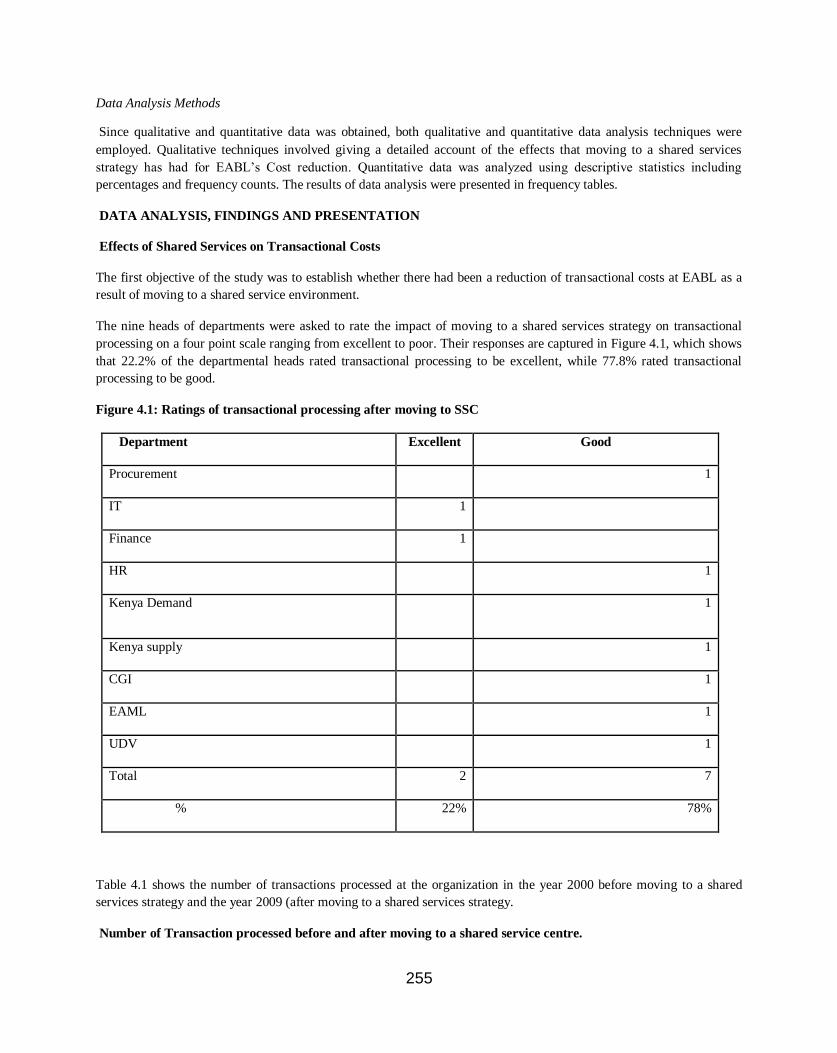
255

Data Analysis Methods

Since qualitative and quantitative data was obtained, both qualitative and quantitative data analysis techniques were

employed. Qualitative techniques involved giving a detailed account of the effects that moving to a shared services

strategy has had for EABL‘s Cost reduction. Quantitative data was analyzed using descriptive statistics including

percentages and frequency counts. The results of data analysis were presented in frequency tables.

DATA ANALYSIS, FINDINGS AND PRESENTATION

Effects of Shared Services on Transactional Costs

The first objective of the study was to establish whether there had been a reduction of transactional costs at EABL as a

result of moving to a shared service environment.

The nine heads of departments were asked to rate the impact of moving to a shared services strategy on transactional

processing on a four point scale ranging from excellent to poor. Their responses are captured in Figure 4.1, which shows

that 22.2% of the departmental heads rated transactional processing to be excellent, while 77.8% rated transactional

processing to be good.

Figure 4.1: Ratings of transactional processing after moving to SSC

Department Excellent Good

Procurement 1

IT 1

Finance 1

HR 1

Kenya Demand 1

Kenya supply 1

CGI 1

EAML 1

UDV 1

Total 2 7

% 22% 78%

Table 4.1 shows the number of transactions processed at the organization in the year 2000 before moving to a shared

services strategy and the year 2009 (after moving to a shared services strategy.

Number of Transaction processed before and after moving to a shared service centre.

256

In the year 2000 (before SSC), the average number of manual journal vouchers raised in a month organization reduced

by about 70%. The average number of invoices processed reduced by 44%.The average number of days taken to produce

monthly accounts reduced by 57%. The average number of days taken to fully process and pay an invoice reduced by

33%.All this has come through as a result of process re-engineering and knowledge sharing see table 4.2 below.

Table 4.2: Transaction processing for the period before and after moving to a shared services environment

Impact of the Shared Services Centre on Employee Headcount and Overheads

The second study objective was to determine the extent to which the shared service strategy resulted in reduction in

employee headcount and overheads. Table 4.3 shows the number of employees working in each of the nine departments

for the year 2000 before moving to a shared services strategy and the year 2009 after moving to a shared services

strategy. In all the nine departments, year 2000 had more employees than year 2009. This is an indication that moving to

a shared services strategy led to overall reduction of 21% in number of employees. Based on the fact that reports from

EABL show that the organization has recorded growth in performance over the last four years, it can be concluded that

reduction in the number of employees resulted to efficiency.

Table 4.3: Number of employees per department before and after moving to a shared services environment

Item Year 2000 (before

moving to shared

services)

Year 2009 (After

moving to shared

services)

%

Change

Average number of manual journal

vouchers raised in a month

200 60 70%

Average number of invoices

processed?

1600 900 44%

Average number of days taken to

produce monthly accounts

7 2 57%

Average number of days taken

before an invoice is finally paid.

90 60 33%

Department Number of employees in 2000

(Before SSC)

Number of employees in

2009 (After SSC)

% Change

Procurement 25 12 52%

IT 20 13 35%

Finance 55 35 36%

HR 20 5 75%

Kenya Demand 185 165 11%

Kenya supply 260 238 8%

CGI 175 148 15%

257

Annual overheads on salaries and wages before and after moving to shared services

As shown in Table 4.4, annual overheads for salaries and wages in all departments were lower in year 2009 than in 2000

by about 8% despite the general annual inflation and cost of living adjustments on the salaries. It therefore emerges that

moving to a shared services environment availed a better control on the salaries and wages costs.

Table 4.4: Annual overheads on salaries and wages per department

Function

Salaries & Wages (Millions)

Year 2000 Year 2009 % change

Procurement 19 10 47%

IT 21 15 29%

Finance 58 40 31%

HR 9 3 66%

Kenya Demand 288 282 2%

Kenya Supply 394 393 0%

CGI 192 178 7%

EAML 144 140 2%

UDV 67 33 51%

Total 1,191 1,094 8%

Costs incurred on overtime for the years 2000 and 2009.

Figure 4.1 shows that for all the departments, the costs incurred on overtime were higher in year 2000 (before SSC) than

in year 2009 (after SSC). In total, overhead cost for year 2000 was KShs 184 million, as compared to KShs 156 million

in 2009, a decrease of 15%.

Figure 4.1: Costs incurred on overtime

EAML 138 122 12%

UDV 135 60 56%

Total 1,013 798 21%

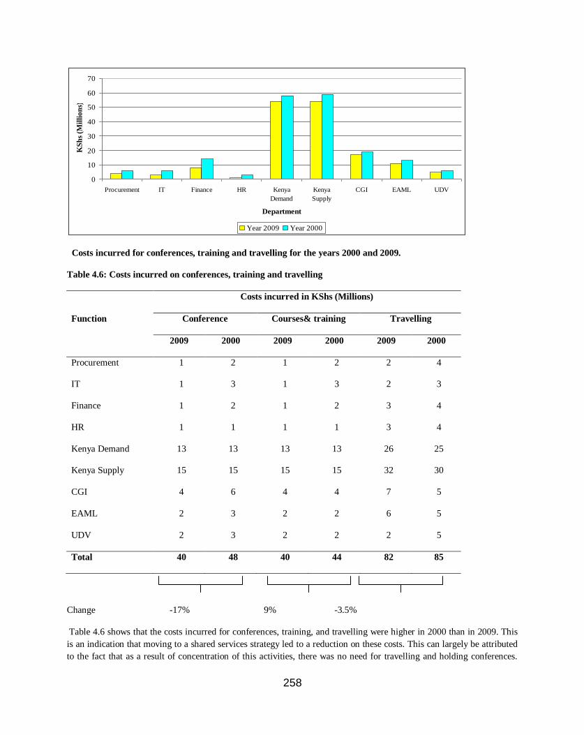
258

0

10

20

30

40

50

60

70

Procurement IT Finance HR Kenya

Demand

Kenya

Supply

CGI EAML UDV

Department

KS

hs

(Mil

lio

ns)

Year 2009 Year 2000

Costs incurred for conferences, training and travelling for the years 2000 and 2009.

Table 4.6: Costs incurred on conferences, training and travelling

Function

Costs incurred in KShs (Millions)

Conference Courses& training Travelling

2009 2000 2009 2000 2009 2000

Procurement 1 2 1 2 2 4

IT 1 3 1 3 2 3

Finance 1 2 1 2 3 4

HR 1 1 1 1 3 4

Kenya Demand 13 13 13 13 26 25

Kenya Supply 15 15 15 15 32 30

CGI 4 6 4 4 7 5

EAML 2 3 2 2 6 5

UDV 2 3 2 2 2 5

Total 40 48 40 44 82 85

Change -17% 9% -3.5%

Table 4.6 shows that the costs incurred for conferences, training, and travelling were higher in 2000 than in 2009. This

is an indication that moving to a shared services strategy led to a reduction on these costs. This can largely be attributed

to the fact that as a result of concentration of this activities, there was no need for travelling and holding conferences.

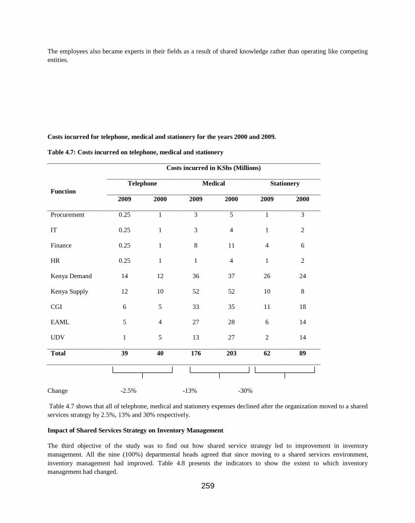
259

The employees also became experts in their fields as a result of shared knowledge rather than operating like competing

entities.

Costs incurred for telephone, medical and stationery for the years 2000 and 2009.

Table 4.7: Costs incurred on telephone, medical and stationery

Costs incurred in KShs (Millions)

Function

Telephone Medical Stationery

2009 2000 2009 2000 2009 2000

Procurement 0.25 1 3 5 1 3

IT 0.25 1 3 4 1 2

Finance 0.25 1 8 11 4 6

HR 0.25 1 1 4 1 2

Kenya Demand 14 12 36 37 26 24

Kenya Supply 12 10 52 52 10 8

CGI 6 5 33 35 11 18

EAML 5 4 27 28 6 14

UDV 1 5 13 27 2 14

Total 39 40 176 203 62 89

Change -2.5% -13% -30%

Table 4.7 shows that all of telephone, medical and stationery expenses declined after the organization moved to a shared

services strategy by 2.5%, 13% and 30% respectively.

Impact of Shared Services Strategy on Inventory Management

The third objective of the study was to find out how shared service strategy led to improvement in inventory

management. All the nine (100%) departmental heads agreed that since moving to a shared services environment,

inventory management had improved. Table 4.8 presents the indicators to show the extent to which inventory

management had changed.

260

Table 4.8: Inventory management indicators

Item Year 2009 Year 2000 Variance

Stockholding Level (Billions) 2.6 2.4 +8%

Stocktaking costs (Millions) 3 4.5 -33%

Stock loss due to pilferage

(Millions)

4 14.5 -69%

Stock loss due to stock obsolescence

(Millions)

72 154 -53%

Insurance costs for stocks (Millions) 10 15 -33%

Table 4.8 shows that stockholding level was at KShs 2.4 billion in year 2000 and this rose to KShs 2.6 billion in year

2009, meaning that moving to a shared services strategy led to rise in stockholding level by 8% despite the impressive

growth in turnover and production level. After moving to a shared services strategy, stocktaking costs reduced from

KShs 4.5 million in 2000 to 3 million in 2009 reflecting a 33% improvement in stockholding costs. Stock loss due to

pilferage reduced by a massive 69%, loss due to stock obsolescence reduced by 53%, while insurance costs reduced by

33% between year 2000 (before SSC) and 2009 (after SSC).

Impact of Shared Services Strategy on Procurement Costs

The fourth research objective was to establish how shared service strategy at EABL has impacted on procurement costs.

The nine heads of departments were asked to rate the impact of moving to a shared services strategy on procurement

costs on a four point scale ranging from excellent to poor. Their responses are presented in Figure 4.2 below.

Figure 4.2: Ratings of procurement costs after moving to SSC

2 (22.2%)

4 (44.4%)

3 (33.3%)

0 5 10 15 20 25 30 35 40 45 50

Excellent

Good

Fair

Ra

tin

gs

Percentage

Figure 4.2

shows that 44.4% of the departmental heads rated procurement costs as good, 33.3% rated them fair, while 22.2% of the

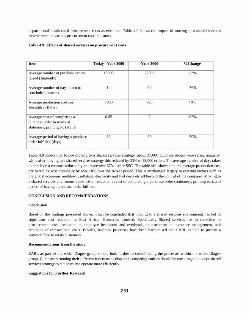
261

departmental heads rated procurement costs as excellent. Table 4.9 shows the impact of moving to a shared services

environment on various procurement cost indicators.

Table 4.9: Effects of shared services on procurement costs

Item Today –Year 2009 Year 2000 %Change

Average number of purchase orders

raised (Annually)

18000 27000 -33%

Average number of days taken to

conclude a contract

14 60 -76%

Average production cost per

Hectolitre (KShs)

1000 925 +8%

Average cost of completing a

purchase order in terms of

stationary, printing etc (KShs)

0.85 2 -63%

Average period of having a purchase

order fulfilled (days)

30 60 -50%

Table 4.9 shows that before moving to a shared services strategy, about 27,000 purchase orders were raised annually,

while after moving to a shared services strategy this reduced by 33% to 18,000 orders. The average number of days taken

to conclude a contract reduced by an impressive 67% after SSC. The table also shows that the average production cost

per hectolitre rose nominally by about 8% over the 8-year period. This is attributable largely to external factors such as

the global economic meltdown, inflation, electricity and fuel costs etc all beyond the control of the company. Moving to

a shared services environment also led to reduction in cost of completing a purchase order (stationery, printing etc), and

period of having a purchase order fulfilled.

CONCLUSION AND RECOMMENDATIONS

Conclusion

Based on the findings presented above, it can be concluded that moving to a shared services environment has led to

significant cost reduction at East African Breweries Limited. Specifically Shared services led to reduction in

procurement costs, reduction in employee headcount and overheads, improvement in inventory management, and

reduction of transactional costs. Besides, business processes have been harmonised and EABL is able to present a

common face to all its customers

Recommendations from the study

EABL as part of the wider Diageo group should look further to consolidating the processes within the wider Diageo

group. Companies running their different functions as disparate competing entities should be encouraged to adopt shared

services strategy to cut costs and operate more efficiently.

Suggestions for Further Research

262

Since this study was conducted in only one organization, findings may not be generalized to other organizations. It is

therefore important to study other organizations employing the shared services strategy to find out the impact the

strategy has had in those organizations. A study on the challenges experienced by organizations in the process of moving

to a shared services environment and the strategies employed to counter such challenges could also be useful.

REFERENCES

Aguirre, D., Couto, V., Disher, C., & Neilson, G. (1998). Shared Services: Management Fad or Real Value. Chicago:

Booz-Allen & Hamilton Inc.

Bell, J. (1993). Doing your Research Project, Open University Press, Maidenhead, Philadelphia.

Benassi, F.E. (2002). Shared services: running IT as a business, Energy IT, Vol. 7 No. 1, pp. 24-9.

Borg, W. R. and Gall, M. D. (1983). Education Research: An Introduction. 4th

Edition. Longman, New York.

Cecil, B. (2000). Shared services: Moving beyond success. Strategic Finance, 81(10), 64-68.

Chaves, F. (1996). Research Methods in Social Sciences. 5th Edition, St. Martins Press, London

Connell, R. (1996). Learning to share, Journal of Business Strategy, Vol. 17 No. 2, pp. 55-8.

Cozby, P.C., (1993). Methods in Behaviour Research (3rd

Ed.). California: Mayfield Publishing Company.

Forst, L. I. (2001). Shared Services Grows Up. Journal of Business Strategy, 22(4), 13-15.

Gay, L. R. (1992): Educational Research, Competences for Analysis and Application. Ohio: Charles E. Merrill

Publishing Co.

Gunn, R. W., Carberry, D. P., Frigo, R., & Behrens, S. (1993). Shared services. Management Accounting, 75(5), 22-

29.

Kakabadse, A. and Kakabadse, N. (2000). Sourcing: new face to economies of scale and the emergence of new

organizational forms, Knowledge and Process Management, Vol. 7 No. 2, pp. 107-18.

Lester, T. (2001). How to pool resources via the web, Financial Times, May 11, p. 17.

Osterloh, M., Frost, J. and Frey, B.S. (2002) The dynamics of motivation in new organizational forms, International

Journal of the Economics of Business, Vol. 9 No. 1, pp. 61-77.

Porter, M. (1985). Competitive Advantage, Free Press, New York.

Quinn, B., Cooke, R. and Kris, A. (2000), Shared Services: Mining for Corporate Gold, Pearson Education,

London.

Rao, M.P. (2006). A performance measurement system using a profit-linked multi-factor measurement model,

Industrial Management & Data Systems, Vol. 106 No. 3, pp. 362-79.

Schulman, D.S., Harmer, M.J., Dunleavy, J.R. and Lusk, J.S. (1999). Shared Services: Adding Value to the Business

Units, Wiley, New York, NY.

Shah, B. (1998). Shared services. Industrial Management, 40(5), 4-8.

263

Theaker, M. (2001)“HR’s New Breed” HR Magazine

Triplett, A., & Scheumann, J. (2000). Managing shared services with ABM. Strategic Finance, 81(8), 40-45.

Ulrich, D. (1995). Shared services: From vogue to value. HR. Human Resource Planning, 18(3), 12-24.

Vandermerwe, S. and Gilbert, D. (1999). Making internal services market driven, Business Horizons, Vol. 32 No. 6,

pp. 83-9.

Walsh, P., McGregor, L., and, Cameron, N. (2006). Shared Services: Lessons from the Public and Private Sectors for

the Nonprofit Sector, CPNS Working Paper No 34. Brisbane: QLD.

The Need for Operations Research in Ensuring Franchiseable Brand Presence in Uganda

Abbey Mutumba +256 712 683334

abbeymutumba@yahoo.co.uk / amutumba@mubs.ac.ug

Lecturer/Department of Leisure and Hospitality Management

Makerere University Business School

P.O Box 1337, Kampala, Uganda.

Assoc. Prof. Bakunda Geoffrey

gbakunda@yahoo.com / gbakunda@mubs.ac.ug

Senior Lecturer and Dean/Faculty of Marketing and Hospitality Management

Makerere University Business School

P.O Box 1337, Kampala, Uganda

ABSTRACT

Introduction

Studies show that franchiseable brand presence is one of the main determinants of the successful use of franchising for competitive business expansion, job creation and wealth creation which are part of Uganda‘s national visions in the East African integration. The current and/or potential franchiser should ensure

franchiseable brand presence for mutual success in the franchiser-franchisee partnership. This calls for

competitive operations research to establish proven/time-tested, standard but adaptable/flexible operating systems, procedures, manuals, and other key features of franchiseable brands.

264

Purpose

To examine which constructs/areas show a greater need for operations research in ensuring franchiseable brand presence

for Uganda‘s regional competitiveness.

Design/methodology/approach

This paper uses a mixture of quantitative and qualitative methodology. A survey of 346 service-related business chains is

used alongside a selection of key informants within and around Kampala who are interviewed to further examine those

areas where operations research is more needed in ensuring franchiseable brand presence.

Findings

The study revealed that although there is a generally high level of franchiseable brand presence among the studied

business chains, there was low ease to manage (for example, its combined mean was 2.88, and factor analysis revealed

variance change of only 11.9%). Key informants analysis of the interviewees‘ responses confirmed that there is need for

operations research to establish teachable business systems that can be easily duplicated and managed by the franchisees.

Practical implications

This paper provides practical information to owners and managers of business chains that are likely to become

franchisers through franchisee-owned outlets that are easier to be managed. Operations researchers now know where,

why, and when to use which mathematical models in ensuring franchiseable brand presence for Uganda‘s regional

competitiveness in job and wealth creation.

Key Words: Operations Research, Franchiseable brand, Ease to manage, Uganda

Introduction

Uganda as a country is seeking for strategies that can lead to competitive economic growth focusing on the promotion of

business expansion, job and wealth creation, (Uganda‘s Budget Speech for the Financial Year 2011/2012). Franchising is one of Africa‘s proven and adaptable strategies that can and will enable the country‘s aspirations especially in terms of

competitive economic growth and development across the nation and region, (Hoffman & Preble, 2004; Saunders, 2002).

Franchising is the selling of rights by the franchiser to the franchisee through a franchise contract allowing the franchisee

to use the brand name, patents, trade mark, and proven/time-tested operating system of the franchiser in line with the set

standards of the entire franchise system, (Kotler, Makens, & Bowen, 2007). Studies show that franchiseable brand

presence is one of the main determinants of the successful use of franchising for competitive business expansion, job

creation and wealth creation which are part of Uganda‘s national visions in the East African integration, (Uganda‘s

Budget Speech for the Financial Year 2011/2012; Doherty, 2007; Hoffman & Preble, 2004; Mutumba, 2010; Sen, 1998).

Exemplar countries like South Africa, Egypt, and Kenya whose leading business chains have been enabled to ensure

their franchiseable brand presence are competitively expanding their respective brands while creating jobs and wealth for

their people and communities across the East African region, (Hoffman & Preble, 2004; Kotler, et al., 2007; Mutumba,

2010). Although Uganda is experiencing an increasing number of franchisers and franchisees especially in the service-

related businesses, most of the current franchisers are foreign brands while the respective Ugandan business partners are

the franchisees, (Mutumba, 2010; Mutyabule, 2006). Such a trend indicates one of the main reasons why South African

and Kenyan business chains have more branches/brands in Uganda and vice-versa especially in the private service

sector. Those service-related business chains that try to expand using their own resources instead of choosing franchising

265

as their business expansion strategy end up collapsing especially after 6-10 years in Uganda, (Mutumba, 2010; Oketch,

2008; Zake, 2007). Their collapse may also be attributed to Uganda‘s business expansion environment which the

country‘s local business community generally blames to favor the foreign investors at the expense of Ugandan business

chain, but, without empirical data to back up this allegation. Whichever the cause, whenever Uganda‘s business chains

collapse, employees lose their jobs while the investors and entrepreneurs lose their wealth instead of expanding their

business chains, (Oketch, 2008; Zake, 2007). Franchising researchers like Doherty, (2007) and Sen., (1998) stress that there is a need to ensure franchiseable brand presence for the survival and competitiveness of any service-related

business chain that intends to growth and expand using franchising partnerships.

In a study conducted by Mutumba & Tuzinde in 2009 on how to create franchiseable club football brands in Uganda, it

was recommended that operations researchers should find and use the right tools that enable the respective potential franchisers to make use of operations research in this challenge. Other scholars like Altinay, (2007), Illtetschok, (1999),

Mutumba, (2010), Reeb & Leavengood, (2002), Saunders, (2002), and Sen., (1998), generally support the use of

operations research in ensuring franchiseable brand presence for mutual success in most franchiser-franchisee

partnership in a country like Uganda. However there is little empirical evidence to specifically show where and why

franchiseable brand presence should be ensured and how to continuously improve on this key success factor for

sustainable and competitive business expansion, job and wealth creation in Uganda, (Mutumba, 2010; Mutyabule, 2006).

This calls for competitive operations research from the universities and other research institutions to enable the potential

franchisers to establish proven/time-tested, standard but adaptable/flexible operating systems, procedures, manuals, and

other key features of franchiseable brands, (Gappa, 2007; Huang, Hsu, and Cheng, 2006; Mutumba & Tuzinde, 2009;

Mutumba, 2010; Reeb & Leavengood, 2002). That is why the purpose of this study is to examine which constructs/areas

show a greater need for operations research in ensuring franchiseable brand presence for Uganda‘s regional competitiveness. The researchers go further to examine the specific areas/issues under the identified construct(s) where

operations research is needed, why it is needed, and which mathematical tools are to be used to ensure franchiseable

brand presence in Uganda.

This paper begins with the above introduction which gives the background to the research challenge and the purpose which reflects the respective research objectives. This introduction is followed by the literature review on what other

scholars and/or researchers say about the need for operations research in ensuring franchiseable brand presence in a

country like Uganda. The reviewed literature leads into the research methodology which describes where and how the

data was collected, processed, analyzed, discussed, presented, and how the resultant conclusions were drawn for the right

recommendations/policy implications. Other parts like the limitations to the study and acknowledgements are also

presented at the end of this paper.

Literature review

All over the world, the franchising concept continues to grow in popularity as a business expansion, job creation, and wealth creation strategy, (Hoffman & Preble, 2004; Mutumba, 2010). Business chains like McDonalds‘ attribute their

faster business expansion to selling their proven franchise systems to well-selected franchisees compared to their rival

non-franchise chains, (Duckett, 2008; Wolfe, 1995). Franchising is a strategic choice which is usually taken by the

potential franchisers. A franchising choice is the decision to become a franchiser usually to expand the business chain in

mutually beneficial ways, (Ducket, 2008; Sen, 1998). For the franchiser to be successful at expanding the business chain

elsewhere using franchising there is need for franchiseable brand presence in a favorable business expansion

environment like that in South Africa, (Doherty, 2007; Hoffman & Preble, 2004; Mutumba, 2010; Saunders, 2002).

Franchiseable Brand Presence

Doherty, (2007) stresses that presence of a franchiseable brand is mainly determined by the business/brand‘s ability to be

duplicated elsewhere (duplicability) and its ease to be managed by other people especially the franchisees. Proven

business success, and the customers‘ brand recognition are the other determinants of whether a brand can be franchised

or not, (Bandura, 1977; Siebert, 2006; Walker, 1996; Wolfe, 1995). Research findings by Stanworth et al., (2004) and

Kotler et al., (2001) show that small expansion/growth-oriented owners and/or managers whose businesses are perceived

to be franchiseable are likely to exploit the existing business expansion environment by selling franchises to well

selected franchisees. When they become aware of their ability to use franchising as their collaborative business

266

expansion strategy, such owners and managers (potential franchisers) are encouraged to the choice of ensuring

franchiseable brand presence across their business network/partnership. This is an indication of the relationship between

franchiseable brand presence and the franchising choice especially among owners and managers of service-related

business chains, (Doherty, 2007).

Franchiseable Brand Presence and the Franchising Choice

Appreciating that the business chain has a franchiseable brand increases its key managers‘ likelihood of making a

franchising choice for business expansion, (Campbell & Srikant, 2008; Doherty, 2007; Wolfe, 1998). The likely

franchiser ought to be willing to make some strategic changes in the way that the entire business will be managed

throughout its mix of both company-owned and franchise outlets for mutual benefits on a sustainable basis, (Altinay,

2007; Doherty & Alexander, 2006; and Sen., 1998). Such changes come through franchise system development

initiatives like attending franchising awareness events, and seeking franchising and operations research consultancy

among other initiatives, (Carter, 2002; Gappa, 2007; Saunders, 2002; Wolfe, 1998). Willingness to change and/or

restructure the business chain‘s management control systems in order to match the next role of working like a ‗parent‘ or

‗champion‘ of the entire franchise system, is another important determinant of the likelihood of a franchising choice, (Campbell & Srikant, 2008; DiPietro, Welsh, Raven, & Severt, 2007; Doherty, 2007; Doherty & Alexander, 2004;

Doherty & Alexander, 2006; Sen, 1998). For sustainable business expansion, the likely franchiser has to be willing to

create a new structure through which the franchisees will be supported in terms of; intensive support for the initial outlet

opening, on-going visits from franchisers to franchisees and vice versa, operating manuals that are easy to use in

mutually beneficial ways, supporting the continuous customer-centered innovations by the individual franchisees,

training of franchisee‘s staff, and the monitoring of sales and other financial data (Doherty & Alexander, 2006; Walker,

1996). Since establishing a really franchiseable brand with the right operating guidelines and support for the potential

franchiser‘s future franchisees is based on research and experience from the daily operations, there seems to be a need

for operations research for a competitive franchising choice, (Gappa, 2007; Mutumba, 2010; Mutumba & Tuzinde, 2009;

Saunders, 2002).

The Need for Operations Research

Operations research is concerned with scientifically deciding how to best design and operate people-machine systems

under conditions requiring allocation of scarce resources, (Reeb & Leavengood, 2002). Franchiseable brands are said to

have mastered the science and art of allocating and managing scarce resources at their respective company-owned and

franchisee- outlets, (Kotler, Makens, & Bowen, 2007; Roh & Yoon, 2009; Sen, 1998). Operations research has been

found to play a vital role in ensuring franchiseable brand presence because franchiseable brands usually establish their

attractiveness for their current and future franchisees through time-testing, proving, and properly documenting their

competitive know-how/intellectual property from their daily operational experience, (Doherty, 2007; Huang, Hsu, and

Cheng, 2006; Mutumba & Tuzinde, 2009; Reeb & Leavengood, 2002). When daily operations data from the experienced owners and/or managers of the respective business chains is collected, analyzed, documented into time-tested operating

guidelines, it becomes easier to manage the chain‘s operations as the duplication of the brand to other locations in

partnership with franchisees goes on, (Doherty, 2007; Wolfe, 1998). The way such operational data is used to establish

the optimum sales and inventory levels is well demonstrated using OR tools like Economic Order Quantity-EOQ to

create frameworks like the Material Requirement Planning-MRP1 in Van Weele‘s 2006 book on purchasing and supply

chain management. In so doing, one is making use of operations research as a means of ensuring franchiseable brand

presence, besides Van Weele argues that MRP1 can even have a software version since most franchise chains are

becoming software/ICT-driven in their daily operations. Scholars like Carter, (2002) and Kotler et al., (2002), warn that

using operations research (OR) in service-related businesses is challenging because service delivery is usually difficult to

standardize across the various locations of the business/franchise chain. In spite of such an application challenge,

franchise managers and other practitioners in today‘s retail, healthcare, and other related businesses are showing a need for operations research solutions, (Carter, 2002; Konts, Jacks, & Aartjes, 2008). Such managers believe that their

practical operational problems in areas like transportation, outlet location, queuing, staff scheduling, sales maximization,

cost minimization, and establishing the fees to be charged especially by service-related franchisers can be solved using

operations research, (Carter, 2002; Doherty, 2007; Huang, Hsu, and Cheng, 2006; Kotler et al., 2002; Reeb & Leaven

good, 2002). For example, Huang, et al., (2006) indicate that the franchiser usually delivers the stock to the respective

franchisee location which calls for an operation research solutions in transportation and distribution management to

267

make it easier for the franchisees to minimize such costs and maximize the respective profits. OR-driven software will

deliver faster and more economical results, (Konts, et al., 2008).

The applicable need for operation research has also been demonstrated in a study conducted by Reeb & Leavengood,

(2002) on USA‘s wood industry. It revealed how the transportation model of operations research is used in combination

with an decision support software like LINDO can make it easier for the managers to plan the trucks/vehicles‘ routes

between outlets. This way of adapting operations research in service-related business chains makes it easier to ensure

franchiseable brand presence in African countries like Uganda, (Konts, Jacks, & Aartjes, 2008; Mutumba, 2010; Reeb &

Leavengood, 2002). Researchers like Konts, Jacks, & Aartjes, (2008) have revealed that operations research increases

franchiseable brand presence especially in terms of making it easier to manage the distribution problem in mutually

beneficial ways. Carter, (2002) highlights those mathematical tools such as linear programming may not be applicable enough in some operations areas of some service business chains. Such challenging calls for successful application of

operations research in ensuring franchiseable brand presence raises the following research questions that are answered by

this paper;

1. Which general and specific areas/issues in ensuring franchiseable brand presence are showing a greater need for operations research?

2. Why do the respective owners and/or managers believe that operations research ensures franchiseable brand

presence in the above area(s), and how?

3. Which mathematical tools are to be used in ensuring franchiseable brand presence among Uganda‘s service-

related business chains?

Research Methodology/approach

This paper used a mixture of a quantitative and qualitative research methodology in collecting, analyzing, drawing

conclusions from the data in line with the above purpose and research questions, (Creswell, 2002; Hofman & Preble,

2004; Roh & Yoon, 2009). A sample of 346 businesses chains from a population of 3,757 of service-related businesses which were registered and located within and around Kampala was initially used, (Uganda Business Register,

2007/2008). This sample includes service-related business chains in retail trade, restaurants and hotels, and car (fuel)

sales, repair and maintenance. The researchers selected these industry categories out of the other service-related

businesses because the franchising choice is most popularly made by the owners and managers of such chains compared

to other service-related chains (Hoffman & Preble, 2004; Perigot, 2006; Sen, 1998; Stanworth et al., 2004). The business

chains were the unit of analysis while the respective owners, managers, and 3 lecturers were the respondents in this

study, (Doherty, 2007; Mutumba, 2010; Stanworth et al., 2004; Watson & Kirby, 2004).The research was limited to

Kampala because 45% of the registered businesses in Uganda including the above service-related chain businesses are in

Kampala, (Uganda Business Register (2007/ 2008). Qualitative data was collected from a selection of 10

key informants using a semi-

structured interview guide to further examine those areas that show a greater need for operations research is more needed

to ensure franchiseable brand presence for the respective business chains, (Doherty, 2007). The above key informants included 7 managers from the above sample-4 retail/supermarket managers,2 hotel and restaurant managers, and 1 car

(fuel) sales, repair, andmaintenance according to their categories‘ respectiveresponse rates above, and 3 lecturers of oper

ations research related course units at MUBS, (Roh & Yoon, 2009; Watson & Kirby, 2004). The 7 managers responded

to questions one and two in the interview guide while the 3 lecturers answered question three from all the 7 managers‘

documented interview guides/sheets in order to establish which mathematical (operations research) tool to use where,

why, and when.

The survey data used was from 281 questionnaires out of the 332 which were returned and the data collection took around 6 weeks. The interviews with the 10 key informants which were conducted after analyzing the

quantitative/questionnaire data took 1 week (5 working days) with 10-20 minutes per interviewee during the data

collection. The quantitative data was analyzed using SPSS Version 12 while the qualitative data was analyzed using Key

Informant Analysis in order to establish trend/links an comparisons with the figures analyzed from the survey. The

268

respective conclusions and recommendations were drawn from such a quantitative and

qualitative data analysis in line with the above purpose of the study. Below are the data and a discussion of the study resu

lts.

The Data

A response rate of 81% (281/346 X 100) is reported for the study. In describing the data characteristics, the researchers

present and briefly describe the industry categories and number of branches of the service-related business chains where

the respondents came from, using the frequency tables below.

Table 1 Showing the Industry Category of the Respondents

Frequency Percent Valid Percent Cumulative Percent

Restaurant & hotel 55 19.6 19.6 19.6

Retail/supermarket 203 72.2 72.2 91.8

Car (fuel) sale, repair & Maintenance 23 8.2 8.2 100.0

Total 281 100.0 100.0

Source: Primary.

The majority of the respondents came from the retail/supermarket category of service-related businesses with a frequency of 203 respondents and making a percentage of 72.2% of the total number of respondents. 91.8% of the

respondents came from the Restaurant & Hotel and the Retail/supermarket categories while only 8.2% (23 respondents)

came from the car (fuel) sale, repair & maintenance category. This confirms the Doherty, (2007) and Sen., (1998) view

that retail and restaurant/hotel business chains are usually more interested in establishing whether they can take on

franchising choice using their franchiseable brands presence.

Table 2 Showing the Number of Branches for the Respondents’ Business Chains

Frequency Percent Valid Percent Cumulative

Percent

2-5 Branches 139 49.5 49.5 49.5

6-10 branches 104 37.0 37.0 86.5

Above 10 branches 38 13.5 13.5 100.0

Total 281 100.0 100.0

Source: Primary.

Table 2 above shows that 49.5% of the respondents‘ business chains were consisting of 2-5 branches. This implies that

most of the sampled business chains in the above 3 categories were still small in terms of number of branches.

The following findings are mainly based on data from service-related business chains with the above characteristics.

269

Discussion of Findings

The study revealed that although there is a generally high level of franchiseable brand presence among the studied

business chains, there was low ease to manage according to the following tables.

According to Sarandakos, (2005), the mean which is the most common measure of central tendency is the average of all

observations and is obtained by adding up all scores and dividing the sum by the number of scores. The data collected on the 2 variables was ordinal in nature and the distributions were showing some central tendency which makes mean

analysis more appropriate to establish the average level of responses. Mean analysis was conducted in order to

empirically establish the perceived level of appreciation for the variables and respective contracts under this study since

the statement of the problem highlighted low franchising choice might be due to limited franchiseable brand presence in

Uganda, among other factors.

Areas/Constructs Showing a Greater Need for Operations Research

The respective responses were analyzed to establish the perception levels of the 2 variables as reflected by the means of

the constructs/areas under franchiseable brand presence and franchising choice respectively, as presented in Table 3

below.

Table 3: Means and Standard Deviations

Franchiseable Brand Presence

N

Minimum

Maximum

Mean

Std.

Deviation

Duplicability 281 2 5 3.97 .53

Proven Business Success 281 2 5 3.98 .57

Brand Recognition 281 3 5 3.90 .52

Ease to Manage 281 2 4 2.88 .46

Franchising Choice

N

Minimum

Maximum

Mean

Std.

Deviation

Awareness of Franchising Benefits 280 2 5 3.44 .58

Willingness to Change 281 2 5 3.12 .71

Franchise System Development Initiatives 281 1 5 3.28 .74

Motivation of Key Managers 281 1 5 3.24 .79

Source: Primary.

270

A 5-Point Anchor ranging from 1-5 (where 1=Strongly Disagree, 2=Disagree, 3=Not Sure, 4=Agree, and 5=Strongly

Agree) was used in the semi-structured questionnaire. Where a mean was close to 4 or 5 such as 3.97, it indicated that

the respondents were generally in agreement with that construct‘s combination of items/issues raised in the questionnaire

hence there was a high perception level of the construct in question. Means close to 3 (not above or below 3) indicated

that the respondents were Not Sure about the construct relating to the variable hence had average appreciation of the

construct. While means close to 2 indicated that the respondents generally disagreed with the construct under study

meaning there was low perception of the construct.

Mean results from Table 3 above show that the respondents generally agreed that their chains were enjoying high

franchiseable brand presence. High/positive perception or presence was reported on the 3 constructs while low

franchiseable brand presence was reported on the construct of ease to manage (mean=2.88). The mean for duplicability was 3.97, the mean for proven business success was 3.98, and the mean for brand recognition was 3.90. This implies that

the respondents perceived that their chains had high presence of franchiseable brands but with limited ease to manage the

branches. The low perceived ease to manage the branches and/or future franchisee-outlets is line with Doherty, (2007)

who argues that when a chain still has a smaller number of branches, the owners and managers may be less interested in

developing the chain into an easy to manage system for business format franchising. Table 1 above shows that most

(49.5%) of the sampled business chains had small number (2-5) of branches which is a reflection of low duplicability

that affects the ease to manage the branches/future franchisee-outlets and affects the likelihood of a franchising choice.

Why Operations Research in Ensuring Ease to Manage (Using Quantitative Data)

To explain why the sampled owners and managers might believe that proper use of operations research in ensuring ease

to manage is important to any business chain that is likely to make a franchising choice, correlation analysis is one of the

analyses which were conducted. Correlation analysis measures the direction and the strength (and significance) of the

relationship between the independent/explanatory variable(s) and the dependent/explained variable, (Sarantakos, 2005).

The researchers had to conduct the correlation analysis because the research objectives reflected some relationships.

Spearman‘s rank correlation (r) was used to establish the direction and significance of the association/relationship

between the 2 variables and the 8 constructs because the findings are in terms of ranked data (Sarantakos, 2005). A

simple correlation analysis of relationships between the 8 constructs under study is presented in Table 4 below.

Table 4 Spearman Correlation Coefficients between the 8 Constructs under Study

1

2

3

4

5

6

7

8

Duplicability (1) 1.000

Proven Business Success (2) .153* 1.000

Brand Recognition and Loyalty (3) .370*

*

.179*

*

1.000

Ease to Manage (4) .392*

*

.242*

*

.270*

*

1.000

Appreciation of Franchising Benefits (5) .107 .174*

*

-.004 .101 1.000

Willingness to Change(6) .082 .163*

*

-.062 .050 .491*

*

1.00

0

Franchise System Development

Initiatives (7)

.217*

*

.017 .089 .222*

*

.199*

*

.138

*

1.000

Motivation of Key Managers(8) .134* .125* .115 .281*

*

.123* -.024 .387*

*

1.000

Source: Primary

It was further revealed that there is a positive and significant relationship between duplicability and perceived ease to

manage the branches (r = .392**, p ‹ .01), which means that the more duplicable a chain is the more the respondents

perceived it to be easy to be managed. This is likely attract to attract entrepreneurs/franchisees hence increasing the

likelihood to make a franchising choice for the business chain as reflected by relationships between ease to manage and

constructs 5 to 8 under the variable of franchising choice. This is in line with Doherty, (2007), Sen, (1998), and Wolfe,

271

(1998) who stress that potential franchisees are attracted to business chain that they perceive to be easy to manage. That

is why there is a positive and significant relationship between ease to manage the branch (es) and motivation of key

managers towards making a franchising choice (r = .281**, p ‹ .01), which means that the more the branches become

easier to manage the more the respective key managers pick interest in making a franchising choice as their business

expansion strategy. The positive and strong relationship between ease to manage and franchise system development

initiatives is in line with Carter (2002), Gappa (2007), and Saunders (2002) who argues that the motivated key managers need to make some strategic changes. The respective changes come through franchise system development initiatives

like attending franchising awareness events, and seeking franchising and operations research (OR) consultancy among

other initiatives in order to find ways of improving and competitively standardizing their daily operations to ensure their

respective business chains‘ franchiseable brand presence in a country like Uganda.

The perceived low ease to manage the potential franchiser‘s respective branches and future franchisee outlets calls for

operations research because according to researchers like Mutumba, (2009) and Richielieu & Pons, (2006), the right

operations research tools enable current and/or potential franchisers to create franchiseable brands that have well

developed systems which are easy to be managed by the respective franchisees and their staff. Operations research being

more concerned with finding specific management solutions to daily operational problems, according to Reeb & Leaven

good, (2002), there was a need to further identify the specific problem areas where operations research was need.

Where and when is Operations Research Specifically Needed for Ease to Manage?

The researchers used the main questionnaire items on the construct of ease to manage from the factor analysis below to

specifically establish the main challenges that complicate this revealed franchiseable brand presence issue.

Factor analysis is a multivariate technique which allows for a big number of original variables/constructs and respective

questionnaire items to be reduced to a small number of observable abstract variables, called factors (Murakumi & Cruz, 2004). The researchers also needed to conduct a factor analysis in order to establish the relative significance of the best-

value contributing factors (BVCFs) to the variable under this study. Using a factor loading of .400, factor analysis was

conducted in order to identify, reduce, distribute, rank, and form a factor (construct) structure out of those items in the

questionnaire that best describe the specific factors/issues under the low scoring construct of ease to manage as

presented and discussed below ;

Table 4 Factor Analysis for Franchiseable Brand Presence

Rotated Component Matrix

Component

Duplica

bility

Proven

Business

Success

Brand

Recognit

ion

Ease to

Manage

Our branch meets the uniform standards like our sister branches .741

Our chain's proven success attracts individual investors out there .648

Our uniformity across our business chain is appreciated by our customers .574

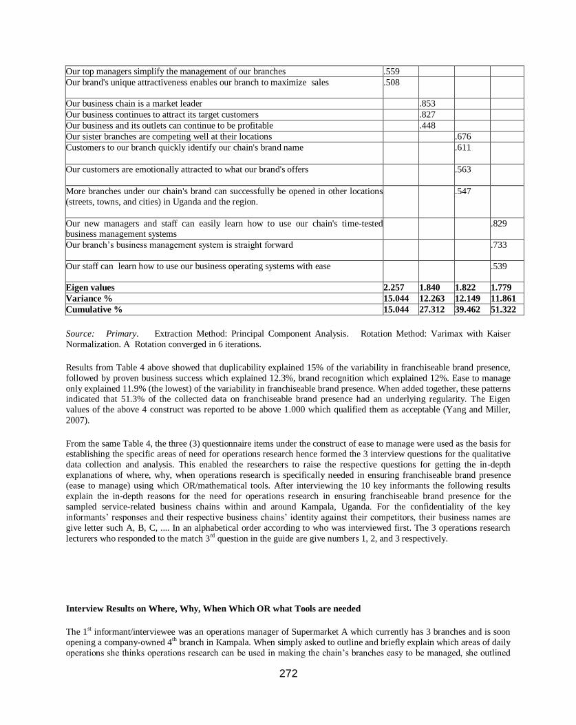
272

Our top managers simplify the management of our branches .559

Our brand's unique attractiveness enables our branch to maximize sales .508

Our business chain is a market leader .853

Our business continues to attract its target customers .827

Our business and its outlets can continue to be profitable .448

Our sister branches are competing well at their locations .676

Customers to our branch quickly identify our chain's brand name .611

Our customers are emotionally attracted to what our brand's offers .563

More branches under our chain's brand can successfully be opened in other locations

(streets, towns, and cities) in Uganda and the region.

.547

Our new managers and staff can easily learn how to use our chain's time-tested business management systems

.829

Our branch‘s business management system is straight forward .733

Our staff can learn how to use our business operating systems with ease .539

Eigen values 2.257 1.840 1.822 1.779

Variance % 15.044 12.263 12.149 11.861

Cumulative % 15.044 27.312 39.462 51.322

Source: Primary. Extraction Method: Principal Component Analysis. Rotation Method: Varimax with Kaiser

Normalization. A Rotation converged in 6 iterations.

Results from Table 4 above showed that duplicability explained 15% of the variability in franchiseable brand presence,

followed by proven business success which explained 12.3%, brand recognition which explained 12%. Ease to manage

only explained 11.9% (the lowest) of the variability in franchiseable brand presence. When added together, these patterns indicated that 51.3% of the collected data on franchiseable brand presence had an underlying regularity. The Eigen

values of the above 4 construct was reported to be above 1.000 which qualified them as acceptable (Yang and Miller,

2007).

From the same Table 4, the three (3) questionnaire items under the construct of ease to manage were used as the basis for establishing the specific areas of need for operations research hence formed the 3 interview questions for the qualitative

data collection and analysis. This enabled the researchers to raise the respective questions for getting the in-depth

explanations of where, why, when operations research is specifically needed in ensuring franchiseable brand presence

(ease to manage) using which OR/mathematical tools. After interviewing the 10 key informants the following results

explain the in-depth reasons for the need for operations research in ensuring franchiseable brand presence for the

sampled service-related business chains within and around Kampala, Uganda. For the confidentiality of the key

informants‘ responses and their respective business chains‘ identity against their competitors, their business names are

give letter such A, B, C, .... In an alphabetical order according to who was interviewed first. The 3 operations research

lecturers who responded to the match 3rd question in the guide are give numbers 1, 2, and 3 respectively.

Interview Results on Where, Why, When Which OR what Tools are needed

The 1st informant/interviewee was an operations manager of Supermarket A which currently has 3 branches and is soon

opening a company-owned 4th branch in Kampala. When simply asked to outline and briefly explain which areas of daily

operations she thinks operations research can be used in making the chain‘s branches easy to be managed, she outlined

273

areas like.... staff scheduling especially for the till cashiers, queuing standards to reduce the time that customers have to

wait in order to clear their bills, the layout decisions of where to install/place which stand for displaying which category

of retail products and services to the satisfaction of the supermarket‘s customers. The researcher asked her why she

believes OR can solve the identified areas of need to improve the ease to be managed by their branch managers and

future franchisees, her responses includes answers like............................

‗Operations research can enable us to establish the standard number of cashiers for each branch depending on the size and seasonal demand‘, we are currently using 7 cashiers per shift but this key issue is yet to be standardized because we

lack a well studied operational standards to make it easy for our supervisor to learn the formula for.....................across

our branches. This response links well with the high correlation (r = .829) for the questionnaire item of ‗Our new

managers and staff can easily learn how to use our chain's time-tested business management systems‘ in Table 5 above.

She said that their management needs to set product quality and quantity specifications/standards for supermarket‘s.........

according to seasons like back-to-school and Xmas shopping at our branches and/or future franchisee-outlets‘. The 2nd

informant who was OR-related Lecturer 1 who was advising on which OR tools to use ,recommended linear

programming (LP) to the best mathematical tool for standardizing the staff scheduling and product mix-location

problem. However he stressed the need for not over- relying on the manual LP calculations in a very busy supermarket,

he recommended a OR-oriented software which name he could not mention, he tried to say ORSE...... but he failed. The

researchers agree with the lecturer‘s recommendation of turning the manual LP algorithms into software language

because it is line with Reeb & Leaven good, (2002) who support the use of more economical approaches like the transportation model and software(s) like LINDO.

The 3rd informant/interviewee belonged to business chain B which was a Car Garage that also dealt in selling spare parts.

This supervisor‘s response to the question of where their 2nd or 3rd or next branch needed OR as a means of ensuring ease

to manage the vehicle repairs and maintenance plus the sale of spare parts, his areas of need included solving issues

like… ‗Deciding which mechanic of which training background and experience to allocate/deploy to which section of

the garage‘ this he said is to be key because they have built a reputation for quality service delivery which they are not

ready to lose at any branch, ‗we rather lose the money, BUT, not our reputation, we have a book that guides us on the

process of repairing the different parts of any vehicle……..‘ Besides deciding on the mechanics, we also need to use

research to set the customer waiting time, are you willing to assist us in doing this…….you university guys think that we

cannot understand and use research in our garage work‘. Let me see … I think, your operations research idea is good for us as we open-up more branches and sell those franchise rights you mentioned, besides, we also have a

training/internship department just like Spear Motors. This interviewee could not give more areas of need because his

branch manager seemed to be in need of his help in solving a wiring problem for a certain Japanese vehicle. This garage

supervisor believed that in OR tools enabling them to standardize their daily operating procedures, they will be able to

opening more garages in various in Kampala, Jinja, Mbarara, and other big towns in Uganda with ease and at low

business risk. On asking the 4th informant who was the 2nd OR-related lecturer (Lecturer 2) to identify and match which

mathematical tool can help such a garage, he matched ‗the decision on the deployment of mechanics with the

transportation model‘, and matched ‗the waiting time standardization problem with Local Search Algorithm which

seemed to be too complicated for simple minds and also suggested the Queuing Method as the other matching OR tool

for this assignment problem‘. He added……What I have to tell you is that although the transportation model is not the

same as the Queuing Method of……………..it can also be used to solve both problems. When we go into the details,

you might not………..or you may even think of OR tools as being too academic moreover they are used in solving daily management problems like sequencing the traffic lights. ‗It is better to just understand the simple OR tools and then use

them to easily learn and use the appropriate software instead of the manual simplex, LP, and other time-consuming

approaches like…………Unfortunately MUBS is yet to provide us -the management science/OR lecturers with the

teaching software to demonstrate how OR and software can be used together in solving such transportation, distribution,

scheduling problems. The garage supervisor and Lecturer 2‘s appreciation of OR making it easy to set the right

management standards for the respective business chain‘s outlets is in line with researchers like Konts, Jacks, & Aartjes,

(2008) whose study on the Coca-Cola Enterprises (CCE) revealed that operations research increases franchiseable brand

presence. This is true when ensuring that it easy to manage the distribution problem in standardized and mutually

beneficial ways especially when you use related software like SHORTREC. With the use of mathematical tools in

connection with OR software solutions makes it more straight forward for the branch managers, supervisors, and

respective franchisees to use the business and/or potential franchise chain‘s management systems which is in line with importance give to this issue in the Factor Analysis Table 5 above.

The 5th informant was another supervisor from supermarket chain C whose specific areas of need for operations research

were reflected in his responses such as;

274

… ‗as you defined it, we need operations research to set the sales targets per section of our supermarket per day, per

week, per month, etc… according to the changes in the branch territory/location‘s demand and other factors like

availability of what to sell,……. , ……. , and other factors that determine what we sell here‘. He also identified the area

of establishing who should work overtime, when, and at what cost? This problem has been disturbing us especially when

there is a sudden change in customer traffic at 2 or 3 of branches. Let me ask you, ‗can operations research also help us

to solve our delivery service vans problem more efficiently and with less customer delays?‘ Lucky enough by then, the researcher was near Lecturer 3 who interjected with the matching answer that operations research tools like linear

programming can solve the overtime and delivery issues especially where there is a profit maximization target (objective

function) set by the management. The same 5th informant also asked for ways of implementing such standards in ways

that deliver competitive advantages for the different branches and/or franchisee-outlets because their chain was

considering the idea of becoming a franchise network of branches in a few years to come. Apart from recommending a

step-by-step software solution, the other answers from Lecturer 3 (6th informant) were not enough. However the step-by-

step approach to implementing any OR-related solution was in line with both Konts, et al., (2008) and Reeb & Leaven

good, (2002) whose studies demonstrated the efficient applicability of this implementation approach towards making the

franchise outlets/branches easy to be managed by the respective managers of the franchiseable brand.

The 7th informant was some owner of a 3-branch chain of restaurants who had ever been introduced to the need for OR

in ensuring franchiseable brand presence, but in general terms. She was eager to be helped in identifying those specific areas of need because she already had 2 potential independent operators who were interested in becoming franchisees to

her 4-branch chain of restaurants. After a 5 minute interactive discussion of what makes a franchiseable brand ensure

ease to manage, she mentioned areas of need for OR with phrases like, ‗mmhh‘, we need to test and standardize the

distance between both our company-owned and franchisee-owned outlets in order to ensure harmonious sales according

the respective agreement which the researcher interpreted as operations research-based territorial agreements. Her other

areas of need for operations research were establishing the optimum levels of food and other restaurant inventory to be

purchased on a weekly basis under normal business condition, also to establish how much franchise fees and on-going

fees to charge the franchisees when the time comes. She asked, ‗am I right? What do you think?‘ The researcher‘s

answer was that, ‗ you are right BUT on deciding the fees to the respective franchisees, you need to also first pilot at

least 3 branches in different locations for at least 14 months for Uganda and at least 1 year when trying to expand into

regional markets like Kenya, Rwanda, and Tanzania‘. When the researcher asked the 6th informant for the right OR tools for the restaurant owner‘s 3 areas of need, this female lecturer recommended the optimization algorithms like the

construct algorithm for the outlet location (territorial) distance problem between the different outlets at the respective

sub-regional, national, and levels. The OR-related lecturer‘s match was in agreement with Konts, et al., (2008) whose

study on CCE‘s distribution trucks approach revealed the use of such mathematical tools. On the operations area of

establishing the standard optimum restaurant inventory he suggested tools that establish standards like EOQ. These

suggestions are in line with Van Weele, (2006), who demonstrated how the EOQ is used in the MRP1 hence making it

easy to predict sales demand and the needed inventory to meet the demand across the brand‘s branches and franchisee

outlets according the changing business levels.

The 8th informant was from a nearby restaurant branch which was located about 300 meters away from the above

restaurant. This manager‘s area of need for operations research which he claimed to already using since he claimed to

have been good at statistics was in terms of establishing the optimum sales levels for the different outlets at the different locations. I believe this will enable us to tell our future franchise partners how much they should expect to sell since I

think our percentage is likely to come from sales made, isn‘t so? This was related to the 7th informant above who also

needed to find OR solutions to establishing sales standards and calculating the franchisee fees which are both issues

raised by writers like Kotler, et al., (2007) who argue that franchise fees should be established the set and/or actual sales

made. He also raised the operations research need in establishing how many supervisors, chefs, waiters and waitresses,

cashiers, and cleaners should particular suppliers in specific territories should be hired and at what labor costs per staff.

These identified 2 areas of need are accompanied with the expected operational/business advantages of enabling the easy

to be managed, duplicability, brand loyalty, and mutual benefits were in agreement with the above correlations in Table

4 above. The respective interpretations of those correlations were in line with researchers like Doherty, (2007), Sen,

(1998), Stanworth et al., (2004); and Wolfe, (1998) who stress that franchisees are attracted to brands that are easy to

manage. Lecturer 1 matched such OR needs with Linear Programming-LP and other tools that use the objective function and optimization models in ensuring the achievement of such business objectives for the respective branches and

franchisee-outlets.

275

The 9th and 10th informants were a relationship manager and a section manager respectively from the same supermarket

which is located near MUBS and is an arch rival to the like of Uchumi and Shoprite especially in terms of customer turn-

over. The relationship manager‘s OR need was in the area of establishing the flexible-but-standard waiting times at the

different inquiry desks and establishing the standard operating procedures in handling cross-cutting customer complaints

and enquiries especially during peak seasons. This she expected the respective operations research answers will help in

reducing the average handling time while increasing the affected customer satisfaction and loyalty (as a quality standard) which matches with the fact that there exists a positive and strong correlation between ease to manage and brand

(customer-based) recognition and loyalty as presented in Correlation Table 3 above. The 10th informant‘s areas of OR

need were reflected in his interview responses like, if indeed operations research is concerned with finding tested

mathematical formulae for solving our daily management challenges in a section like mine which mainly sells fruits and

vegetables in this branch of our supermarket chain, then I think we need operations research in establishing weekly and

monthly sales target for his section 7 staff members. Such formulae may also help us in setting standards for ensuring

that we have the needed fruits and vegetable in their freshness especially towards the weekends when families are

shopping as we try out, fine-tune such sales and inventory formulae we might be able to establish flexible, adaptable, and

profitable standards for other vegetable sections at our other 2 branches around Kampala. The respective lecturer

recommended the use of the software instead of manual approaches. However when the supermarket buys the generic

version, it needs to involve an operations consultant to ensure that the specific waiting, staff scheduling, sales

optimization, and profitability problems are properly addressed more economically using OR-related software. This suggestion is in line with the software recommendation from Lecturer 1 above and researchers like Konts, et al., (2008).

Conclusions

From the above discussion of the findings, there is need for operations research in ensuring franchiseable brand presence

among Uganda‘s service-related business chains in the industry categories of hotel and restaurants, retail

trade/supermarkets, and the car repair and maintenance/garages within and around Kampala. Making the respective

branches/outlets easy to be managed is the main construct/area where operations research is greatly needed. Key

informants analysis of the interviewees‘ responses confirmed that there is need for operations research to establish teachable business systems that can be easily duplicated and managed by the potential franchisees. The specific business

areas where operations research is needed to ensure ease to manage have been established to be in the challenges of

using formulae for establishing standards for staff scheduling, waiting and queuing durations, sales targets, optimum

inventory levels, territorial distances between outlets among others, especially for the retail/supermarket chains. This

implies that operations researchers and consultants under the ORSEA now know where to focus their mathematical tools

for these chains. The restaurant chains' specific areas where they need operations research solutions are in setting

uniform standards for deciding on the optimum inventory per outlet, sales targets, number of chefs and waiter/waitress to

deploy for the outlets, and establishing standard formulae for establishing and charging the respective franchise fees.

This last area of need is also needed for industry categories above. The garages mainly needed OR tools in deciding

which mechanics to work on which cars in which sections, and deciding on how to pay the staff among others.

The main reason why the survey respondents needed OR solutions were to increase the motivation of the key managers

towards making a franchising choice as their brands become duplicable and easy to be managed by the respective branch

managers and franchisees. The other main reason for their OR need in making the branches easy to be managed include

being able to use their franchise system development initiatives in increasing the success of their franchising choices as

they expand across Uganda and East Africa. The key informants revealed that the specific reasons why they needed

operations research were to establish standard operation procedures to be documented in their franchise

manuals/documents as they choice franchising to be their expansion strategy, to set flexible-but-standard sales targets to

be based on in charging the respective franchise fees, to ensure duplicability/opening more branches while maintaining

the quality standards across the chain in profitable and mutually beneficial ways. Inspite of these expected business benefits of using operations research that the key informants hope for, most of the interviewed managers are informally

demanding the universities' operations researchers to work with them in ensuring the above benefits in the above areas of

need.

The main OR/mathematical tools that were recommended by the above 3 lecturers were linear programming, the

transportation model, optimization algorithms like the construction algorithms, and the economic order quantity for the

above areas of need and to achieve the above franchising benefits that the interviewed managers hope for in their

respective franchising choices. However they strongly recommend that OR-based software like LINDO or SHORTREC

is more practical for busier business chains because it delivers faster and more economical results for the chains

276

involved. Unfortunately, leading ORSEA members like MUBS are not facilitating their management science lecturers

with the teaching versions of such software moreover the respective students are expected to use them especially when

they get employed or start their own businesses that might expand using the franchising strategy.

Policy Implications

This paper provides practical information to owners and managers of business chains that are likely to become franchisers with franchisee-owned outlets that are easier to be managed. Operations researchers now know where, why,

and when to use which mathematical models in ensuring franchiseable brand presence for Uganda‘s regional

competitiveness in job and wealth creation.

Managers of service-related chains that are beginning to appreciate the need and benefits of OR tools and software

should be encourage to put in place a policy of involving the surrounding university/institutional operations researchers

in standardizing their business operations and ensuring their franchiseable brand presence especially in terms of ensuring

the wanting area of ease to manage. Operations research dissemination strategies like this 7th ORSEA Conference by the

respective universities need a policy on how to attract more of such potential franchisers and franchisees. This twin-

suggested policy which focuses on both the respective managers and operations researchers can be productively

implemented through the formation of collaborations between the respective universities and such potential franchise

chains.

Since ease to manage was reported to be low, the researcher recommends that the owners and managers of the business

chains should be facilitated in developing the right management systems and manuals that can be taught and easily learnt

by the potential franchisees in order to increase the level of franchiseable brand presence and franchising choice in

Kampala and Uganda at large. Establishment of business incubators at the respective universities with support from the respective ORSEA Chapters and governments especially the Ugandan government will enable the operations researchers

to test and pilot standard operating systems , manuals, and the jointly design OR-based software intended increase access

to better solutions locally. Huaug, et al., (2006) have demonstrated how the how universities in developing markets have

become the main providers of OR-based software solutions to the respective franchise chains through the flagship

approach that encourages the current and potential franchisers to integrate operations research incubation in their

budgeting. This is a win-win approach for us.

Study Limitations

This study was only carried out within and around Kampala, and it did not consider the contribution of the moderating

variables on franchising choice. Similar studies that include the moderating variables of university contribution to OR

solutions, use of software‘s in OR solutions, franchising laws/regulatory framework, and the business culture of need to

be conducted at various levels. Related multi-disciplinary studies that connect OR, franchising, and disciplines line

marketing and organizational development need to conducted.

Acknowledgements

We are grateful to the entire management of Makerere University Business School (MUBS) for sponsoring at least 60%

of this study and the conference registrations, travel, and other related expenses. The entire ORSEA community is

appreciated for providing us with this opportunity to be part of this field of study which is key in franchising as

illustrated in this study and other related studies.

References;

Altinay, L. (2007).The Internationalization of Hospitality Firms: Factors Influencing a franchise Decision Making

Process. Journal of Services Marketing. Vol. 21. No. 6.

277

Bandura, A. (1997). Self-efficacy; Guide for Constructing Self-efficacy Scales. Psychological Review. Vol. 84.

Campbell, D. & Srikant, D. (2008). Managers‘ Motivation towards Franchising and expansion into Complex Markets. Harvard Business School Working knowledge. http/:Hbs.hbswk.edu

Carter, M. (2002). Health Care Management: Real World Operations Research. OR/MS Today. April 2002.

Connell, J. (1999). Diversity in Large Firm International Franchise Strategy. Journal of Consumer Marketing. Vol. 16.

No 1. Pg 86-95.

Creswell, J.W. (2002). Research Design: Qualitative, Quantitative, and Mixed Methods approaches. Sage Publications,

Inc. Sage Publications Website.

Doherty, A. M. (2007). The Internationalizing of Retailing: Factors Influencing the choice of Franchising as a Market

Entry Strategy. International Journal of Service Industry Management. Vol 18 . No 2

Doherty, A. M. & Alexander, N. (2006). Power and Control in International Retail Franchising. European Journal of

Marketing. Vol 40 .No 11/12.

Ducket, B. (2008).Business Format Franchising: A Strategic Option –at Home and Abroad. Journal of Strategic

Direction. Vol 24. No 2

Gappa, R. (2007). Creating an Effective Operations Manual: A ‗How-To‘ Guide. Franchising World March 2007.

Retrieved on 22/08/11

Hoffman ,R .C. & Preble, J. F. (2004).Global Franchising: Current Status and Future Challenges. Journal of Services

Marketing.Vol 18. No 2.

Huang, H., Hsu, Y., and Cheng, J. (2006). The Internationalization of Franchise System in Developing Market: 7

Eleven‘s Flagship View. First University of Science and Technology. Retrieved 06/07/11.

Illtetschok, K. (1999). Becoming a Franchiser. Franchise Association of Southern Africa (FASA). NAMAC Trust.

Jackson, P. & Sparks, L. (2005). Retailing Internationalization: Marks and Spencer in Hong Kong. International Journal

of Retail and Distribution Management. Vol 33. No 10.

Kaberuka, W. (2003). Statistical Techniques: A Basic Course for Social Scientists. 2nd Edition.

Krejcic , R.V & Morgan , D. W.(1970). Determining Sample Size for Research Activities. Education and Psychological

Measurement. Vol.30. Pg 607-610.

Konts, C., Jacks, M., & Aartjes, C. (2008). Coca-Cola Enterprises Optimizes Vehicle Routes for Efficient Product

Delivery. Interfaces. Vol. 38(1). Pg 40–50. INFORMS

Kotler P, Makens J, & Bowen J (2002). Marketing for Hospitality and Tourism Management. 2nd Edition. Pearson

Education Asia.

Kotler ,P. Makens, J., & Bowen, J. (2007). Marketing for Hospitality and Tourism Management. 2nd Edition. Pearson

Education Asia.

Murakumi, M.D. & Cruz, D.C (2004).Proposal for Methodologies for Environmental Stratification and Analysis of

Genotype Adaptability. Crop Breeding and Applied Biotechnology. 4:7-11

Mutumba, A. (2010). Franchiseable Brand Presence, Business Expansion Environment, and Franchising Choice in

Uganda. MBA Thesis. Makerere University/MUBS

Mutumba, A., (2010). Time to Put a Franchise on your Brand. The Daily Monitor. www.monitor.co.ug

Mutumba, A. & Tuzinde, M. (2009). Club Football Branding, Management System Development, and Creation of

Franchiseable Club Football Brands in Uganda. 6th ORSEA Conference Proceedings. Held in Dar es Salam.

278

Mutyabule, R. I. (2006). Status of Franchising Development in Uganda. Seminar on Franchising. Rabat, Morocco.

November 13-17, 2006.

Nunnally J. C (1978). Psychometric Theory. 2nd Edition. New York: McGraw-Hill.

Oketch, L.M (2008). Banks to Help SMEs on Loan Repayment. Business Power. Monitor Online.February 26, 2008.

Preble, J. F. & Hoffman, R. C. (1998). Competitive Advantage through Specialty. Franchising. Journal of Consumer

Marketing. Vol 15. No 1.

Reeb, J. & Leavengood, S. (2002). Transportation Problem: A Special Case for Linear Programming Problems.

Performance Excellence in the Woods Products Industry. Operations Research Society of America. E8779 Oregon State

University.

Repede, J.F., & Bernardo, J.J. (1994). Developing and Validating a Decision Support System for Locating Emergency Medical Vehicles in Louisville, Kentucky. European Journal of Operational Research. Vol. 75, pp. 567-581.

Richielieu A, & Pons, F (2006). Toronto Maple Leafs vs. Football Club Barcelona: How two Legendary Sports Teams

built their Brand Equity. (CASE STUDY: Peer reviewed).International Journal of Sports Marketing & Sponsorship.

Roh, E. Y. & Yoon, J. (2009). Franchisor‘s On-going Support and Franchisee‘s Satisfaction: A Case of Ice Cream

Franchising in Korea. International Journal of Contemporary Hospitality Management. Vol 21. No1.

Sarantakos, S. (2005). Social Research. 3rd Edition. Palgrave MacMillan. New York.

Saunders, J. (2002). Franchising Opportunities: Unlocking Africa‘s Potential. FASA. Retrieved on 07/03/10

Sen K.C, (1998). The Use of Franchising as a Growth Strategy for US Restaurants Franchisors. Journal of Consumer Marketing. Vol.15. No.4.

Stanworth, J. Stanworth, C., Watson ,A., & Healeas, S. (2004). Franchising as a Small Business Growth Strategy: A

Resource- Based View of Organizational Development. International Small Business Journal. Vol 22 (6). No 10.

Steven, C. (2009). Statistics Tutorial Overview: ANOVA. Statistically Significant Consulting LLC.Retrieved 25/08/09

Tripathi P. C (2002). A Textbook of Research Methodology in Social Sciences. 1st Edition. Chand & Son. New Delhi-

India

Uganda Business Register (2007/ 2008). Uganda Bureau of Statistics Annual Reports.

Utts, J. M. & Heckard, R. F. (2006). Statistical Ideas and Methods. Thomson Higher Education. books.google.co.ug.

Van Weele A.J. (2006). Purchasing & Supply Chain Management: Analysis, Strategy, Planning, and Practice. 4th

Edition. Thomson Learning: Australia.

Walker, J. (1996). The Introduction to Hospitality. 4th Edition. Prentice-Hall. United Kingdom.

Watson ,A. & Kirby, D. A. (2004). Public Perceptions of Franchising in Britain: Releasing Potential. Journal of Small

Business and Enterprise Development. Vol 11. No.1

Wolfe, J. (1998). Case Study: Pepsico and the Fast Food Industry. Cases in Strategic Management .

Zake, F. (2007). The Other Side of Investing in Uganda. Fredzake@infocom.co.ug

279

A PAPER PRESENTED FOR THE ANNUAL CONFERENCE AT KICC

KENYATTA UNIVERSITY OF AGRICULTURE AND TECHNOLOGYKENYATTA UNIVERSITY OF

AGRICULTURE AND TECHNOLOGY

THEME: ROLE OF OPERATIONS RESEARCH IN THE NATIONAL VISIONS WITHIN THE

EAST AFRICAN COMMUNITY & NATIONAL AND REGIONAL INTEGRATION

SUB- THEME; ENTREPRENEUERSHIP AND BUSINESS MANAGEMENT

TITLE; HINDRANCES TO THE GROWTH OF YOUTH LED MICRO AND SMALL AGRI-

BUSINESSES IN KENYA

BY; DR. R. W. GAKURE, JOMO KENYATTA UNIVERSITY OF AGRICULTURE AND TECHNOLOGY, DR.

KABARE KARANJA, JOMO KENYATTA UNIVERSITY OF AGRICULTURE AND TECHNOLOGY, AND

PETER PAUL KITHAE, KENYA INSTITUTE OF MANAGENT (CORRESPONDING AUTHOR) Cell phone;

0721493984, email pkithae2001@yahoo.com

APRIL, 2011

HINDRANCES TO THE GROWTH OF YOUTH LED MICRO AND SMALL AGRI-BUSINESSES IN KENYA

ABSTRACT

Micro and Small Enterprises have been identified as the engine for economic growth and technological innovations in

developing countries. Consequently, he Kenyan government has put in place interventions geared towards improving the

business environment through appropriate policy frameworks. However, the MSE sector continues to be dodged with

myriad of constraints which include; lack of appropriate technology, access to market information, credit, business

management skills, rigid legal and regulatory framework, among others.

The study focused on the following

a. Determining forms of investment in technology prevalent amongst youth led micro and small agri-businesses

b. Investigating effect of investment in technology to youth led micro and small agri-businesses‘ performance.

c. Discovering challenges faced by micro and small agri-businesses in applying emerging technologies to get

competitive advantage and sustained productivity

280

The study focused on youth led micro and small agri-businesses in Makueni District of Kenya in November 2010. A

descriptive research design was used to carry out the study. Stratified random sampling technique was employed to select

the sample. An interview guide was the main instrument for collecting data. Data was analyzed using the SPSS software.

From the study, three main discoveries came to the limelight. First, our youths have no problem working in agri-

businesses if that‘s where they see their future prospects contrary to our common belief that youths are lazy and would

only opt for white collar jobs. Secondly, people including our educated youths fear technology. Finally, adults do not

take youth requests seriously even when youths are paying for land and premises rent; a situation which leaves our

youths frustrated and therefore not knowing whom to turn to for the services.

Among key recommendations from the study are that youth led micro and small agri-businesses need to be provided with

adequate finances, relevant tools and equipment and frequent refresher courses to upgrade their business skills.

Key words

Youth, micro and small enterprises (mses), technology, agri-businesses

1. INTRODUCTION AND RESEARCH OBJECTIVES

The foregoing is a research project conducted in Makueni district and whose aim was to find out whether the

Kenyan youth are making use of their acquired technology to improve quality of their products and thus enhance

their agri- business competitiveness. Technology has been identified as an enabler of economic growth as well as

a means through which SMEs can gain competitiveness through creativity and innovativeness.

Statement of the problem

Youths are innovative, enthusiastic, vibrant and optimistic. If given a chance, they are capable of transferring their

acquired technologies into business enterprises and drive Kenya towards achieving its vision 2030. However things are

different. Youths are not employed. They are not starting own enterprises to create jobs for themselves and for others.

Even the already started MSES are closing up within their first two years after start up (Nelson, 1986).

Study objectives

The study focused on the following

a. Determining forms of investment in technology prevalent amongst youth led micro and small agri-businesses

b. Investigating effect of investment in technology to youth led micro and small agri-businesses‘ performance.

c. Discovering challenges faced by micro and small agri-businesses in applying emerging technologies to get

competitive advantage and sustained productivity

Definition of terms

This section deals with operational definitions whose role is to indicate the specific manner in which a term or concept is

to be applied. Their use may be different in another perspective. This study used the following concepts.

281

Micro and small enterprises (MSEs) A micro or small enterprise is an undertaking, which employs between 1 and 20

employees, with capital investment of not more than kshs 30 million. Operational and administrative management lies in

the hands of one to three persons who usually make major decisions.

Technology According to Van Dijk (2001), Technology may be seen as a resource that can be useful if adapted by

firms to improve their efficiency and factor productivity. This study used the same definition.

Appropriate technology Is defined as the technology that is suitable to the needs of an MSE operating in the labour

intensive, low-skill spheres and using local materials and resources

2. THEORETICAL BACKGROUND AND INFORMING LITERATURE REVIEW

The Kenyan youth

A Kenyan Youth has been defined as one aged between 15 – 30 years. The youth in Kenya, who number about 9.1

million, account for about 32% of the population. They form 60% of the total labour force but many of them have

not been absorbed in the job market owing to the country's high unemployment level (GOK, 2006). Youths are

innovative, enthusiastic, vibrant and optimistic. If given a chance, they are capable of transferring their acquired

technologies into business enterprises and drive Kenya towards achieving its vision 2030.

Micro and small enterprises (MSES)

The economic recovery strategy for wealth and employment creation recognizes the great role that MSE sector

play in wealth generation, employment creation and poverty reduction (GOK, 2003). The strategy paper goes on

to state that the sector contributes about 18% GDP and plays a critical role in easing foreign exchange constraint,

in penetrating new markets and in stimulating growth and development particularly in the rural areas. The sector

also acts as the seed bed for entrepreneurial pursuits and complements the process of adjustment in large

enterprises by bringing backward and forward linkages for products and services previously not available in the

market.

In Kenya, much of existing technology is insufficient and cannot produce goods of a quality or type that enables

them to break into new, expanding or more demanding markets. This is because choosing a technology requires

specific skills and knowledge that MSEs just do not have (Buainain, 2004). The Kenyan‘s sessional papers No. 2

of 1992 and 2005 clearly summarize the problem of technology in Kenya as follows.

―MSEs have restricted levels of technology, in appropriate technology and inadequate institutional capacity to

support adaptation and absorption of modern technological skills. Such enterprises suffer from lack of information

on existing technologies and are exposed to a weak environment that hampers coordination and transfer of

technology. They have no way of gauging appropriateness of technology. In addition, there is a wide gap between

the suppliers of technology and the end users of technology products.‖(GOK, 2003). Effective transfer of

technology is therefore not taking place in the country because decisions relating to cost aspects rest with

multinational corporations‖ (GOK, 1982).

282

Technology

The purpose of technology is to improve productivity of enterprises, and enhance the quality of goods produced by

enterprises to help them with-stand local and international competition (ILO/UNDP, 2000). Technology transfer can be

defined as the process that allows techniques, knowledge as well as products and management practices to flow from one

entity to another (Moyi and Njiraini, 2005). Formal means of technology transfer include acquisition of capital

equipments and machinery through trade, licensing and/ or franchising agreements. Informal technology transfer mainly

occurs via technology-spillovers such as demonstration, imitation effects, competition, printed information, observations

during visits to foreign plants and so on. Successful business operation depends on the ability to complete; the ability to

compete depends largely on the quality of the product (Lyman & Grubellini, 1975). This will therefore require that an

entrepreneurial organization works towards product/service improvement on a continuous basis. This will, in turn, call

for managerial talent that is capable of harnessing organizational resources – human, material, physical and

informational resources- efficiently and effectively toward meeting the organizations objectives and goals. Most

organizations objectives are to make profit; which is partly realized through the provision of competitive and quality

products/services.

3. RESEARCH METHODOLOGY

Research design

The study used both qualitative and quantitative research designs which were descriptive in nature; Qualitative

data was manually analyzed using the researcher‘s insight and research skills to bring out the main themes..

Data Analysis

Graphical analysis as well as descriptive statistics of the variables was used in the study and which conforms to

Gall and Borg (1989) observations that ―descriptive studies by nature emphasis interpretation‖. Data was collected

using a predominantly 5 point likert type scale. The choices were coded and so also were the questions to facilitate

analysis.

4. RESEARCH FINDINGS AND DISCUSSIONS.

Introduction

This chapter examined the research objectives formulated in relation to the findings obtained.

Conclusions and recommendations were subsequently given being based on information generated from the analysis of

the questionnaire.

Summary of the findings.

Family Background

283

From the findings, majority of entrepreneurs were aged 21 to 25 years (38.8%), single (52.4%) and with zero to

one child (71.8%). They had trade test professional qualification (45.6%) and 3 to 4 years of working experience

(39%). These findings agree very well with our expectations that youths are either single or have just gone into

family life. They have therefore very little or no resources; an assertion shared by the Ministry of youth affairs and

sports in their draft strategic plan (GOK, 2006).

Major investment in technology

The study revealed that 54% of all businesses had training as their major investment in technology, 28% in

equipment, 16% in franchise and 2% on others. These findings tend to strengthen Ikiara‘s and UNIDO‘s assertion

that education and on job training are drivers of adoption, survival and growth amongst enterprises and economies

(Ikiara et al, 2005; UNIDO, 2004). Likewise, the results also compare fairly well with Biggs et al (1995) and

Gichira (1999) that firms in Africa have not invested much since they are young and small and that most of their

investment in technology is in training.

This means that these businesses are not able to reap much from emerging technologies as they have invested in

only one form, training.

Figures1 below shows entrepreneurs‘ major investment in

technology

training equipment franchise others

Major Investment in Technology

0

10

20

30

40

50

60

Per

cent

Major Investment in Technology

.Fig1 Major Investment in Technology and their frequencies

Effect of Technology Adoption on Business Performance

Record Keeping

284

The study revealed that 48% of respondents were of the opinion that technology helps them very much in

calculating their profits as well as keeping their business records. Forty-three per cent (43%) responded that

technology assists them fairly well, 6% said it has not been of much help while only 3% said it does not at all

assist them.

These results confirm Gichira (2002) findings that technology helps MSES achieve effectiveness of financial

assistance, strengthens communication channels and helps in marketing. They also concur with Buainainn (2002)

assertion that appropriate technology helps SMES to operate in low-skill spheres with local materials and

resources. Equally, Biggs et al (1995) states that high technology firms which have invested in research and

development, foreign technical licenses and technical assistance contracts have higher productivity than lower

technology firms. He also contends that investment in technology adds about 25% to value added (Biggs, 1995).

These findings show that technology is of paramount importance in enhancing MSEs technical documentation and

business record keeping.

Marketing

When asked the extent to which technology is addressing problems of lack of market, most respondents (38%)

indicated fairly well, 29% of respondents said technology was of much help in addressing their marketing

problems, 27% said it was not of much help while 6% were of the opinion that technology was either not of help

or were non committal. This information is represented in fig. 4.4 and seemed to concur very well with a number

of scholars as follows; Albu (1997) and Maskell (1999) indicated that one way of achieving and maintaining

competitiveness in a market oriented environment is to be able to create, distribute and exploit knowledge faster

than competitors. In turn, this depends on cost advantages, innovations and continuous improvement of products

and services; they claimed (Albu, 1997; Maskell and Malmberg, 1999). Biggs et al (1995) suggested that

investment in technology and worker training should be incorporated at firm level policies as they are major

determinants of firms‘ ability to get connected to foreign markets‘ through exporting‘. Gichira (2002) defines

technology capabilities as information and skills that allow productive enterprises to utilize equipment and

technology efficiently.

As a result of efficiently utilization of technology, MSES become innovative and achieve improved product

consistency and reliability; better packaging technology for bulk markets; increased output to open up bulk

markets and thus increased marketing independence.

These results mean that technology is very crucial in improving MSES product marketability and growth. It

improves product design, quality control and ensures increased product markets. Figure 4.4 below represents

respondents‘ views on how technology helps them solve problems of lack of market.

Business competitiveness

285

For effects of appropriate technology on business competitiveness, 32% of respondents said it helps them increase

their sales, 28% stated it improves quality, 19% talked of increasing efficiency while 16.5% said it improves their

customer royalty.

These results bring out two most important outcomes that technological assistance to MSES can achieve, also

mentioned by Gichira (2002) Biggs (1995), Oakland (1993) and Government of Kenya (G O K, 2005).

These two achievements from use of appropriate technology are improvement of quality of products and increase

in sales volume of an enterprise. This is reflected in table 1 and figure 2 below and shows that most entrepreneurs

perceived use of appropriate technology is helping them to increase their sales volume and improve quality of

their products to enhance their competitiveness.

Table.1 Information on Appropriate Technology

A. Effect of Technology on Business Competitiveness

Options Percent

Quality products 28.2

Increased sales volume 32.0

Reduced waste 3.9

Fast/ efficient production 19.4

Customer loyalty/repeat buying 16.5

Total 100.0

286

Fig. 2 Effect of Technology on Business Competitiveness

When plotted on a normal regression graph, effect of technology as perceived by entrepreneurs and business

competitiveness produces a perfect positive regression line.

This implies that there is a one-on-one relationship between the two variables (effect of technology as perceived

by entrepreneurs and business competitiveness). This is similar to ILO/UNDP (2000) expectations that the

purpose of technology is to improve productivity of enterprises and help them withstand local and international

competitions. According to Gichira (1999), technology has proved to be the engine of economic growth when

applied to micro and small enterprises amongst ‗Asian Tigers‘. Lucas (1993) observes that accumulations of

human capital in form of technological capabilities far outweigh all other factors of production and that it is a

cause of sustained development success. Lastly, Moyi and Njiraini (2005) say that technology is a key source of

growth and competitiveness. They conclude that ability to use technology is best measured by the production and

investment capabilities. These results therefore imply that Technology is very effective in enhancing

entrepreneurs‘ business competitiveness. Figure 3 below represents the relationship between Effect of Technology

and Business Competitiveness.

0.00 1.00 2.00 3.00 4.00 5.00 6.00 Effect of Techno on business

Competitiveness

0

10

20

30

40

Frequency

Mean = 2.6408 Std. Dev. = 1.48095 N = 103

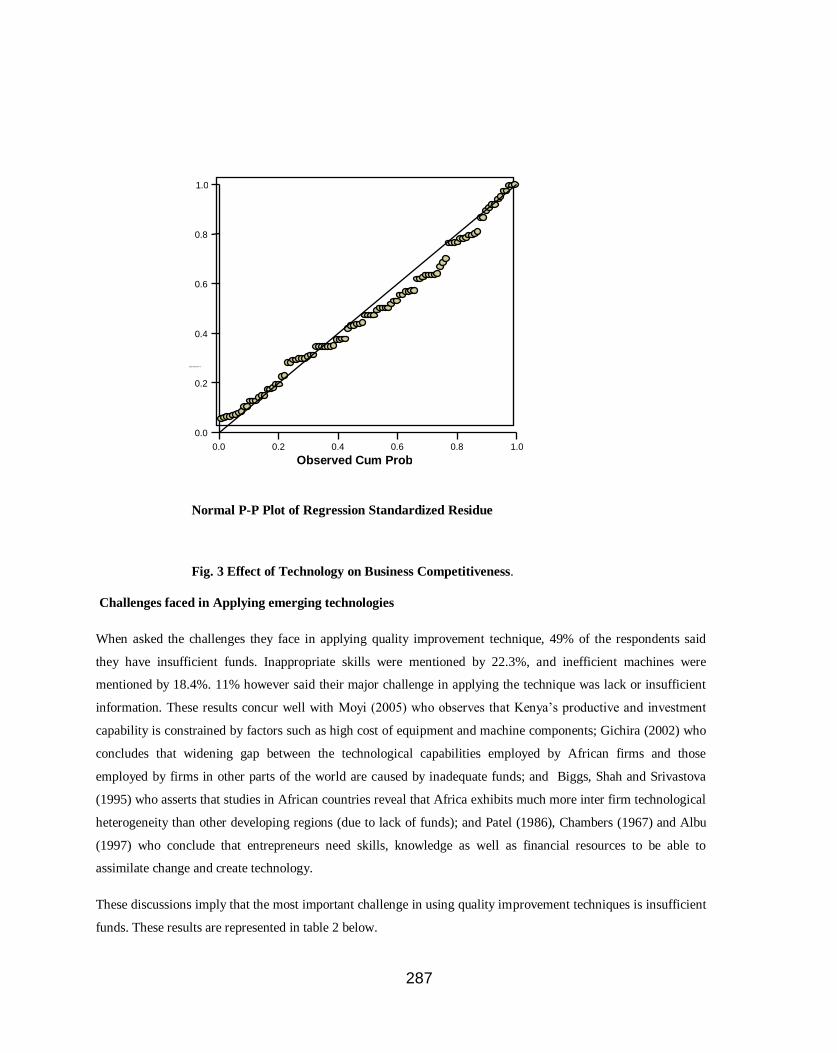
287

Normal P-P Plot of Regression Standardized Residue

Fig. 3 Effect of Technology on Business Competitiveness.

Challenges faced in Applying emerging technologies

When asked the challenges they face in applying quality improvement technique, 49% of the respondents said

they have insufficient funds. Inappropriate skills were mentioned by 22.3%, and inefficient machines were

mentioned by 18.4%. 11% however said their major challenge in applying the technique was lack or insufficient

information. These results concur well with Moyi (2005) who observes that Kenya‘s productive and investment

capability is constrained by factors such as high cost of equipment and machine components; Gichira (2002) who

concludes that widening gap between the technological capabilities employed by African firms and those

employed by firms in other parts of the world are caused by inadequate funds; and Biggs, Shah and Srivastova

(1995) who asserts that studies in African countries reveal that Africa exhibits much more inter firm technological

heterogeneity than other developing regions (due to lack of funds); and Patel (1986), Chambers (1967) and Albu

(1997) who conclude that entrepreneurs need skills, knowledge as well as financial resources to be able to

assimilate change and create technology.

These discussions imply that the most important challenge in using quality improvement techniques is insufficient

funds. These results are represented in table 2 below.

0.0 0.2 0.4 0.6 0.8 1.0 Observed Cum Prob

0.0

0.2

0.4

0.6

0.8

1.0

Expec te d Cum Prob

288

Table 2; Challenge Faced In Applying Quality Improvement Techniques

Qualit

ative

Questi

ons

These

were

mainly

from

part

three

of the questionnaire. The questions in part three were aimed at checking and confirming the outcomes of the quantitative

questions as they also bring out other main themes. The section had varied responses. However the responses which

could be grouped were analyzed in numerical terms using the SPSS. They are as follows.

Comment on Any Other Technology Issue

When asked to comment on any other technology issue, 62.1% had no comment. 1.9% said they do not know what to

say. 15.5% said technology is complicated while 2.04% talked of other issues. These results imply that entrepreneurs

fear technology as it is complicated. This observation is also shared by the Government of Kenya that ―MSEs have

restricted levels of technology, in-appropriate technology and inadequate institutional capacity to support adaptation and

absorption of modern technological skills. In addition, there is a wide gap between the suppliers of technology and the

end users of technology products.‖(GOK, 2003). Fig.4 below shows respondents‘ comments on other technological

issues not captured in the main questionnaire.

Options Percent

No/ little money 48.5

No/inappropriate skills 22.3

No efficient machines 18.4

No/little information 10.7

Total 100.0

289

Fig.4: Comments on Other Technology Issues

Comment on Any Other Technology Issue of Importance to Youth Led Business

For comments on any other technology issue of importance to youth businesses, a shocking revelation came out that

many landlords do not take requests on repairs and maintenance of business premises from youth tenants seriously. This

view is very well supported by the Ministry of Youth Affairs and Sports strategic objectives of empowering youth to

participate in decision making at all levels (GOK, 2006).

Recommendations.

1. To enable MSEs cope with challenges of financial resources, it is recommended that the government of Kenya

provide them with accessible, cheap and adequate loans.

2. The government should capacity build young entrepreneur‘s human resource base with relevant skills to be able to

benefit from emerging technologies

3. The government should promote all sectors of the economy including agriculture for young entrepreneurs to invest

in

4. Finally, it is highly recommended that youth entrepreneurs be given a forum where they can air their views

concerning issues affecting their businesses, a situation which would build their confidence in entrepreneurship and

business management skills.

REFERENCES

Not applicable i don’t know Technology is Complicated

Others

Other comments on Techno issue

0

10

20

30

40

50

60

70

Frequency

290

Ablu M (1997).‖Technological learning and innovating in industrial clusters in the south” science policy unit,

electronic working paper No. 7 Brighton: university of sussex.

Argris c. (1985).Strategy, change and routines, New York, Pitman

Aw; B. and Tan, H. (1995).―Training Technology and Firm-Level Productivity in Taiwan (China).” Conference on

Enterprise and Training Strategies and Productivity. World Bank, June 1995

Awasthi D.N. Murali BP, (1990).Entrepreneurship Development and New Enterprise creation,

Experience of the entrepreneurship Development Institute of India. ILO Geneva

Biggs, T., Shah, m.and Srivastava, P. (1995).Technological capabilities and learning in African

enterprises, technical paper no. 288, Washington DC, World Bank.

Deakins D. (2003).Entrepreneurship and Small Firms 3rd ed. MC. Graw Hill, New York.

Drucker(1986)Innovation and entrepreneurship Heinemann publishers,London

Embu (2001). Embu District Development Plan (2002-2008) on Effective Management for

sustainable growth and Poverty reduction, Embu County Council, Embu

Engelman R: (1993).Jua Kali Development Project, Management Training KIM, Nairobi

Enos, J.(1992). The creation of technological capabilities in Developing Countries,

London: pinter.

Fulop C. (1970).Retailing and the consumer printed by Longman Group LTD London

Gall and Borg (1989). Educational Research, an introduction (5thEd) New York and London,

Longman.

Gibb A.A. (1991).Defining success in Entrepreneurship Approach, ILO Geneva.

Gichira R. (2002).Policies, Strategies and Programmes for Enhancing the Participation of

Small and Medium Enterprises in E-Trade. Paper Prepared for Ntfecom‘s Strategic Workshop Held at Safari

Park Hotel, 20th April, 2002

Gichira R, Amondi R, Njoroge,J And Kabugua,M (2002).E-Trade bridge programme for Kenya,

A draft for discussion ,International Trade Centre.

291

Government of Kenya (1986).Sessional Paper No.2 of 1986 on Economic Management for

renewed Growth. Government Printers, Nairobi.

Government of Kenya (1989).Strategy for small enterprise development in Kenya towards the year 2000

Government Printers, Nairobi.

Government of Kenya (1996).Sessional paper No. 2 of 1996 on Industrial Transformation to the

year 2020.Government Printers, Nairobi

Government of Kenya (1997). 8th National Development Plan (1997-2000). Government Printers, Nairobi

Government of Kenya (2004). (22nd Jan. 2004) Draft Sessional Paper on Development of Micro and small

enterprises for wealth and employment creation for poverty reduction.

Government Printers, Nairobi

Government of Kenya (2004).Central bureau of statistics, Government Printers, Nairobi

Government of Kenya (2005).Economic recovery strategy for wealth and employment creation:

2003 – 2007, Nairobi

Government of Kenya (2006). Ministry of state for youth affairs, Draft strategic plan

2006-2011, March 2006. Government Printers, Nairobi

Government of Kenya (2007).The National youth Policy, Government Printers, Nairobi

Green law and Biggs (1979).Modern personnel management printed by W.B Sounders Co. USA

Guthrie, C. (1983) Selection and training for entrepreneurship Development ILO Geneva.

Hammer, M and Champy, J. (1983). Re-engineering the corporation – A manifesto for

Business revolution, Nicholas Brealey, London

Harper, M. (1993).Selection and training for Entrepreneurship Development ILO Geneva.

Healey, M. J. (199).Obtaining information from business. Harlow, Longman)

Hernes T. (1988).A guide for trainers and training managers, ILO Geneva

Ikiara M.and Okatch (2005).services trade related development strategies in tourism,

ILO (1986).The promotion of small and medium sized enterprises ILO, Geneva.

292

Kasina,C.K (1991).―Directorate of industrial training‖ News letter

Kelly C, et al. (1969).How to organize and Operate a small business Printed by prentice-Hall ,Inc Toronto Canada

Liedholm, C and Mead, C. (1991).Dynamics of Micro-enterprises Research issues and

approaches, Michigan State University.

MC Comic, D. (1988).Small enterprise in Nairobi; A golden opportunity or dead end? PhD

Dissertation, University of Nairobi.

Morrison, A, (1998).Entrepreneurship – an International Perspective Butter worth Heinemann

Moyi E and Njiraini p (2005). Towards Technology models for MSES in Kenya: common principles and best

practices Kippra Discussion paper NO. 51. Bulletin.

Mugenda and mugenda(1999).Research methods, quantitative approaches. Act press, Nairobi

Kenya

Neuman, W. I. (2000). Social research methods, 2nd ed. London, Allyn and Bacon

Ngahu, C. (1995) choice of technology in small-scale enterprise: International Development

Research Center (IDRC)

Nzomo, N.D. (1986). Entrepreneurship development policy in National Development Planning

The Kenya – Case Article Eastern Africa Economic Review

Oakland, J.S. (1993). Total quality management –The route to improving performance, 2nd

edition, Butterworth – Heinemann oxford .

Oakland, J. S. (1995).Total quality management – Text with cases, Butterwoth – Heinemann,

Oxford

Oakland, J. S. (1999).Total organizational excellence –Achieving word class performance,

Butterworth –Heinemann in oxford.

Powell, V. (1987).Improving public enterprise performance ILO Geneva

Sifuna, D. (1986).Unemployment and non-formal training in the informal sector in Kenya.

293

Presented to a staff graduate seminar, held in Kenyatta University. Nairobi.

Stevenson L. and Onge A. (2005).Support for Growth Oriented Women Entrepreneurs in Kenya,

African Development Bank, Tunis

UNIDO (2002).Industrial development report: competing through innovation and learning venna: united Nation

industrial development organization

UNIDO (2004).Integrated institutional capacity building services and programmer for technology centers and parks

venna: United Nations industrial development organization

Van Dijki (2001).Innovation and micro and small enterprise development in developing countries: linking knowledge as

skills to produce employment: University of Erasmus Netherlands.

Willimack D. K. (2002).Understanding unit and item non response in business surveys, Wiley

Inter Science,New York,

World Bank (1978).Appraisal of small-scale industrial project Kenya Washington, DC

Yambo, M. (1986).Technical Training and Work Experience in Kenya – unpublished

294

RELATIONSHIP MARKETING AND FIRM PERFORMANCE:

A CRITICAL LITERATURE REVIEW

Presented by

DR. MARGARET A. OLOKO

Jomo Kenyatta University of Agriculture and Technology,

Department of Commerce and Economic Studies

e-mail – olokoma@ihrd.jkuat.ac.ke

olokomargaret@yahoo.com

August, 2011

Abstract

Despite the existence of a large and growing body of literature on relationship marketing, there is still some

misunderstanding surrounding the practice and how it influences performance. Today, marketing is taking on a new

paradigm that aims at engaging the customer interactively in creating value which is shared between the service provider

and the customer. The concern is how an organization can establish and maintain long-term relationship with its

customers. This paper explores the theoretical foundations of relationship marketing practice and performance in

organizations. It attempts to provide insights into the understanding of relationship marketing and how the practice

contributes to favourable performance. Existing literature proposes that there is a positive relationship between

relationship marketing and organizational performance. It involves a two-way communication that creates value to the

stakeholders. The conclusion is that organizations should put more emphasis on establishing long-term customer lasting

relationships within their operations through interactive marketing, customer value creation in terms of loyalty, customer

satisfaction and retention and strategic partnerships.

Key Words: Relationship Marketing, Interactive Marketing, Customer Value Creation, Strategic Partnership.

295

1.0 Introduction

Today, relationship marketing has caught attention of most scholars in many parts of the world, including North

America, Europe, Australia and Asia. Its scope covers the entire spectrum of marketing disciplines, including marketing

channels, business-to-business marketing, services marketing, marketing research, customer behavior, marketing

communication, marketing strategy, international marketing and direct marketing. Sewell (1990) refers to this process as

―customers for Life.‖ That is, an organization must become a life-time partner with the customer, anticipating needs and

developing a level of trust that commits the customer to staying in the relationship. To Webster (1992), the ability to

create a long-lasting relationship with the customer has been singled out as the most important business asset for an

organization. According to Peppers and Rogers (1995) the success of an organization depends on relationship marketing

and further adds that it can cost between six to nine times more to acquire new customers than to retain current ones. To

Morgan and Hunt (1994) relationship marketing refers to all marketing activities directed toward establishing,

developing and maintaining successful relational exchanges.

Previously known as customer relationship management, relationship marketing today has emerged as the favorite

catchword in business world at the turn of the millennium (Storbacka & Lehtinen, 2000). Today, the concept has been

proliferated with many definitions and many programs (Parvatiyar and Sheth, 2000). It includes affinity marketing,

loyalty marketing, cross selling, up-selling, co-branding, co-marketing and customer-supplier partnering among others.

In professional services, it includes personalized one-to-one relationship with individual clients and dedication of

organization‘s resources to the individual relationships. Edelstein (2000) further reported that relationship marketing

should help organizations improve the profitability of their interactions with current and potential customers while at the

same time making those interactions appear friendly through individualization and personalization of processes.

Relationship marketing can be defined as the process of attracting, maintaining and enhancing relationships with key

people or customers (Young, 1988, Kotler and Armstrong, 2002). Researchers like (Kotler and Armstrong, 2002);

Zikmund et al., 2003; Jobber and Fahy, 2006) concurred with this and further stated that, it is a process of creating,

maintaining and enhancing strong value-laden relationships with customers and other stakeholders.

The present day business environment is characterized by increasingly saturated markets, caused by changes in the

nature of competition and an ever-changing environment making it difficult for organizations to achieve a

comprehensive appreciation of customer needs. Thus, matching the growing complexity of the business environment has

led to an ever-more diversified and demanding customer base (Barnes et al., 2004). However, relationship marketing

emphasizes that relationships are partnerships and mainly focuses on social bonding, co-operation, and joint problem

solving, sharing resources and activities, and basing relationship on a common goal. It emphasizes that long-term

relationships are mutually beneficial. Despite all these attempts, customers are smarter; more informed and have an

access to many channels and choices.

Bhardwaj (2007) asserted that today, customers easily defect to competitors that promise them better offerings at lower

prices. The researcher further reported that the challenge facing the marketers today is in finding ways of increasing

customer loyalty and retention and transforming indifferent customers into loyal ones and, thus establishing a long term

relationship with them is a critical issue. For success of organizations, there is need to increasingly strive to establish

long-term relationship with the target customers. This can be achieved by offering a product or service, which satisfies

customers‘ needs that is delivered in a friendly, caring, responsive, convenient and flexible way. Hence, the key success

296

factor for organizational survival in mature markets relies on sustaining long-term relationships with customers (De

Madariaga and Valor, 2007).

2.0 The Theoretical Background

Literature on relationship marketing evolved in the 1980s from the transactional marketing of the 1960s and 1970s and

also migrated from organizational behavior and industrial marketing where interdependence between firms was the

foundation of successful business operations. Notwithstanding the existence of a large and growing body of literature on

the subject, there continues to be ambiguity about the nature of marketing relationships in enhancing business

performance. According to Berry (1983) relationship marketing is attracting, maintaining and enhancing customer

relationships. It aims at increasing organizational profitability while providing better services for customers. The focus of

relationship marketing is frequently considered to be customer retention because current literature suggests that retention

is less costly than acquisition and small increases in retention rates can have a dramatic effect on the profits of a

company (Reichheld and Sasser, 1990; Reichheld, 1996).

Several studies have empirically demonstrated a positive association between relationship marketing strategies and

business performance (Naidu et al. 1999). However, most scholars have argued that relationship marketing will not

automatically lead to stronger customer relationships but rather, customers will exhibit different levels of relationship

closeness and strength with the organization (Berry, 1995 and Liljander and Strandvik, 1995). Thus, in order to be able

to attract and maintain customers, organizations must put in place strategies that enhance customers‘ perceived benefits

of engaging in a relationship. One of the basic tenets of relationship marketing is customer orientation which is based on

the premise that this orientation increases customers‘ long-term satisfaction. In the past, selling oriented sales people

were considered to prioritise the achievement of an immediate sale at the expense of customer needs. Today, subsequent

research has shown that the degree of customer orientation indeed has an effect on a firm‘s relationships with its

customers (Liljander and Strandvik, 1995).

Theory and practice of marketing has now taken a paradigm shift from traditional or transactional marketing to

relationship marketing (Gronroos, 2000 and Parvatiyar and Sheth, 2000). Thus today, managers realize that their most

valuable resource is the relationship with their customers and acknowledge the increased emphasis on customer centric

strategies. The researchers further asserted that if organizations are able to manage the relationships better than their

competitors, they will not only succeed in business but will retain and attract new customers too.

3.0 Interactive Marketing

Interactive marketing refers to buyer- seller communications in which the consumer controls the amount and type of

information received from the marketer. In today‘s highly volatile world of dynamic change, organizations have to adopt

interactive techniques like interactive advertising, (point-of-sales brochures, displays and coupon dispensers have to be

put in place) for continued survival of firms. Interactive marketing frees communication between marketers and their

297

customers. That is, today customers come to companies for information thus, creating opportunities for one-to-one

marketing.

According to Boone and Kurtz (2007) interactive marketing involves a two-way communication which results in the

creation and development of one-to-one marketing. It further depends on the development of close ties between the

buyer, whether an individual or company and the seller. This underlying relationship is based on promises from

organizations that go beyond obvious assurance that potential customers expect. It represents an asset of promises, which

could either be outside or within the organization and between buyers and sellers that determine whether a marketing

encounter will be positive or negative. To this extent, an organization that makes unrealistic promises can disappoint

customers who may not buy the good or service again. That is, every customer interaction with a business reaches the

moment of truth when a good or service is provided to the customer that meets their level of expectation. Therefore,

buyer-seller relationship defines the point at which a company keeps its promises, hence emphasizes on cooperation

rather than competition.

The conclusion here is that, every marketing transaction involves a relationship between the buyer and seller in a

transaction-based situation where the relationship may be quite short in duration and narrow in scope. The customer-

seller bonds develop in a relationship marketing situation and are likely to last longer and cover a much broader scope

than those developed in transaction marketing. In this case, customer contacts are more frequent when a company

emphasizes on customer service thus, contributing to consumer satisfaction (Armstrong and Kotler, 2008).

3.1 Buyer-Seller Relationship

Relationship marketing depends on the development of close ties between the buyer and the seller. This tie considers the

core elements of the buyer-seller relationship incorporating the promises that form the basis of relationship marketing

(Gronroos, 1994 and Boone & Kurtz, 2007).

Today, most firms make promises to potential customers through external marketing that communicates what a customer

expects from the firm's goods and services. The promises must be both realistic and consistent. According to Zeithmal et

al. (2006) and Boone and Kurtz (2007), a firm that makes unrealistic promises will disappoint customers who may not

buy the product again. Therefore, organizations must keep these promises and follow up carefully through external

marketing to ensure customer satisfaction and retention. Thus, all relationships depend on the development of emotional

links between the parties including dimensions like bonding, empathy, reciprocity, trust and tangibility (Chris and

Graham, 2007).

3.2 Customer Value Creation

Researchers like Engel and Blackwell (1982) reported that value is constantly used to mean benefits to the consumers.

This means that customer value is considered an important constituent of relationship marketing and the ability of a

company to provide superior value to its customers is regarded as one of the most successful competitive strategies in

business performance. The researchers further emphasized on the importance of value creation by organizations and

suggested that organizations must be able to identify what customers are trying to satisfy by offering the best at a

particular time and place. Thus, any company attempting to provide competitive value to its customers must gain a

298

thorough understanding of the customers‘ needs and wants which constitutes the customer‘s value chain. This ability has

become a means of differentiation and a key to the riddle of how to find a sustainable competitive advantage (McKenna,

1991, Treacy and Wiersema, 1993, Gronroos, 1994 and Heskett et al. 1994).

According to Peterson (1995) marketing has progressed from a simplistic focus on giving the customer what he or she

wants to an orientation in which the specific capabilities of the business are focused around creating and delivering

customer value much better than competition. This constitutes an opportunity for the company to improve the customer-

perceived value and thereby establish and maintain a long-term relationship (Monroe, 1991). Therefore, creating superior

customer value is key to a company‘s long-term survival and success (Slater, 1997). Today, customer value is the

cornerstone of the marketing management process and it is the perceived sacrifice customers undertake (Anderson and

Narus, 2004). To Zeithaml et al. (2006), the key role of marketing in this new paradigm is to determine what value

proposition to create and deliver to the target customer or market.

3.3 Customer-Perceived Value

The concept of perceived value has been defined severally by the different researchers. According to Porter (1985), the

buyer‘s value chain is the starting point for understanding what is valuable to the customer who represents the sequence

of activities performed by an individual buyer or a household with various members in which the product or service is

appropriate. Zeithaml (1988) reported that customer-perceived value should be viewed in terms of the consumer‘s

overall assessment of the utility of a product based on a perception of what is received and what is given and stated that

quality can be viewed as an overall judgment of the superiority or excellence of a product. The researcher further

pointed out that perceived value is subjective and individual, and therefore will vary among consumers. For example, a

person may evaluate the same product differently on different occasions and in many instances, the price may be the

most important criterion at the time of purchase while, a clear and easily comprehensible manual may be of importance

at installation and assembly. But, Zeithaml has not given a reason as to why consumers may have different perceptions

of the value attached to an offering.

On the other hand, Monroe (1991) reported that perceived value can be defined as the ratio of perceived benefits relative

to the perceived sacrifice which include all the costs the buyer faces when making a purchase decision in terms of the

purchase price, acquisition costs, transportation, installation, order handling, repairs and maintenance and risk of failure

or poor performance.

4.0 Customer Loyalty and Retention

According to Oliver (1980) customer loyalty explains that the loyal customers of today might not be so loyal in the

future. In a study by Dwyer, Schurr, and Oh (1987) customer loyalty is reported to contribute to increased revenues

along the relationship life cycle because of cross-selling activities and increased customer penetration rates. However,

Dick and Basu (1994) argued that brand loyalty should not be regarded as mere repurchase behavior, but rather as a

combination of purchase behavior and attitudes. According to the researchers like, Reichheld and Sasser (1990) and

Oliver (1999), the connection between loyalty and retention and performance has been the focus of both theoretical and

empirical studies. According a study by Berry (1995) this body of research has found customer loyalty and retention to

positively influence organizational performance through increased revenues per customer. Basically, customer loyalty

refers to the tendency of customers to select one company or product over another so as to satisfy a particular need. It

299

also describes the behavior of repeat customers hence loyalty is observed through the actions of the customers. However,

Dick and Basu (1994) argue that brand loyalty should not be regarded as a mere repurchase behavior, but rather as a

combination of purchase behavior and attitudes.

Customer loyalty is defined as a deeply held commitment to rebuy or repatronize a preferred product/service

consistently in the future, thereby causing repetitive same-brand or same brand-set purchasing, despite situational

influences and marketing efforts having the potential to cause switching behaviour (Oliver, 1999). It is assumed that

customers who are behaviourally loyal to a firm display more favourable attitudes towards the firm in comparison to

competitors. However, in some cases behavioural loyalty does not necessarily reflect attitudinal loyalty, since there might exist other factors that prevent customers from defecting to other competitors (Reinartz and Kumar, 2002).

According to Breshnahan (1998) many organizations have begun to implement one-to-one marketing and loyalty-

programs with their end user customers. However, Novo (2008) reported that organizations are today focusing on

customer retention and customer commitment in order to outdo their competitors in the market. The scholar further noted

that a loyal customer is more than a customer who frequently purchases from a company but one that is also emotionally

bonded with the organization. To the researcher, true brand loyalty requires repeat purchase behavior in addition to a

significant psychological attachment to the chosen brand. Eisingerich & Bell (2007) concurs with this and finds

empirical support that customer loyalty emerges as the dominant, significant, direct determinant of repurchase intention.

Numerous studies have shown positive links between loyalty and firm profitability and that, not all loyal customers are

profitable (Hallowell, 1996 and Reichheld, 1996). Nonetheless, (Storbacka, 1997). In addition, customer relationship

and profitability arises through the acquisition and retention of high quality customers with low maintenance costs and

high revenue (Anderson and Mittal, 2000). Over the past years the interest in retaining customers has increased

considerably with marketing attention shifting gradually but definitely from mutually independent transactions to

loyalty-based repeat purchases and cross-selling opportunities (Berry, 1995; Peterson, 1995; Blattberg and Dayton,

1996 and Winer, 2001). Today, it is argued that the primary goal of value creation can sometimes even be equated to

relationship marketing concept itself (Sheth, 1996). The connection between loyalty and performance has been the focus

of both theoretical and empirical studies (Reichheld and Sasser, 1990). Customer loyalty is also reported to contribute to

increased revenues due to cross-selling activities and increased customer penetration rates (Dwyer, Schurr, and Oh,

1987).

Another researcher (Businesstown, 2008) reported that customer loyalty can be built through effective communication,

customer service, employee loyalty, employee training, customer incentives, product awareness, reliable service

provision, flexibility in solving customer problems or complaints, customer service, and knowledge of names of regular

customers. Thus, relationship marketers need to note that a key to winning customer loyalty in competitive industries is

to view interactions with customers not as one time transactions but as a means to establish a long-term relationship and

also being customer centric.

3.0 Customer Satisfaction

According to Heskett et al. (1994) customer satisfaction is one of the most important criteria for achieving customer

loyalty. A study by Liljander and Strandvik (1995) on customer relationships in service sector revealed that overall

customer satisfaction is a better predictor of intentions to rebuy. Thus, a satisfied customer is supposed not to defect but

to stay loyal to the company for a long period of time and to buy more and more often than others, not so loyal,

customers do. Furthermore, new customers may be attracted and the market shares increased, but any long-lasting bonds

will hardly be tied. In addition, Bennett and Rundle-Thiele (2004) reported that customer satisfaction has a good

feedback to the firms and that it is central to the development of business relationships.

300

Customer retention can be defined as a commitment to continue to do business or exchange with a particular company on

an ongoing basis. In today‘s highly competitive markets, companies strive to build professional customer retention

management systems alongside common strategies like process re-engineering and employee redundancy exercises.

Retention strategy also builds barriers to customer switching. This can be done by product bundling (combining several

products or services into one package and offering them at a single price), cross selling (selling related products to

current customers), cross promotions (given discounts or other promotional incentives to purchasers of related products),

loyalty program (giving incentives for frequent purchases) and increasing switching costs (adding termination costs, such

as mortgage termination fees) and integrating computer systems of multiple organizations particularly in industrial

marketing.

4.0 Strategic Partnership Alliances

Business or partnership alliances can be defined broadly as collaborative efforts between two or more firms that pool

their resources in an effort to achieve mutually compatible goals that they could not achieve easily alone (Das and Teng,

2000 and Day, 1995). These alliances have been identified as a core competence of an organization (Gulati, 1995).

Therefore organizational performance can be explained in terms of partner satisfaction with the relationships (Cannon

and Perreault 1999). That is, relationship marketing fosters external partnerships that cater for the mega-marketing needs

of a business through external networks as well as alliances. These sets of external relations bring together market

elements synergistically. The deep personal and social contacts fostered under the umbrella of relation building helps

solve the external decisions to a firm-customer relationship. Therefore most companies today are partnering with other

members of the supply chain to improve the performance of the customer value-delivery network.

5.0 Relationship Marketing and Performance

A study by World Bank shows the presence many firms operating in Kenya, both domestic and internationally.

Literature shows that a majority of them have not embraced relationship marketing in their operations. Business

partnerships and alliances are being increasingly used to achieve a sustainable competitive advantage. Whilst

partnerships might be popular, they are often risky, unstable and vulnerable to failure with less than 50% of alliances

performing satisfactorily (Das and Teng, 2000).

Christopher et al. (2002) emphasized that the key feature of organization performance is the development of mutually

beneficial relationships. The assumption is that, a satisfied customer equates to a loyal customer and that a loyal

customer implies a long-term relationship thus, leading to improved performance (Thurau, et al. 2002).

6.0 Suggested Conceptual Framework for Research

Fig. 1 depicts the relationship marketing in terms of interactive marketing, customer value creation and partnership

alliance influences organizational performance. It is assumed that through the proper use of the indicated dimensions,

organization performance is bound to be higher.

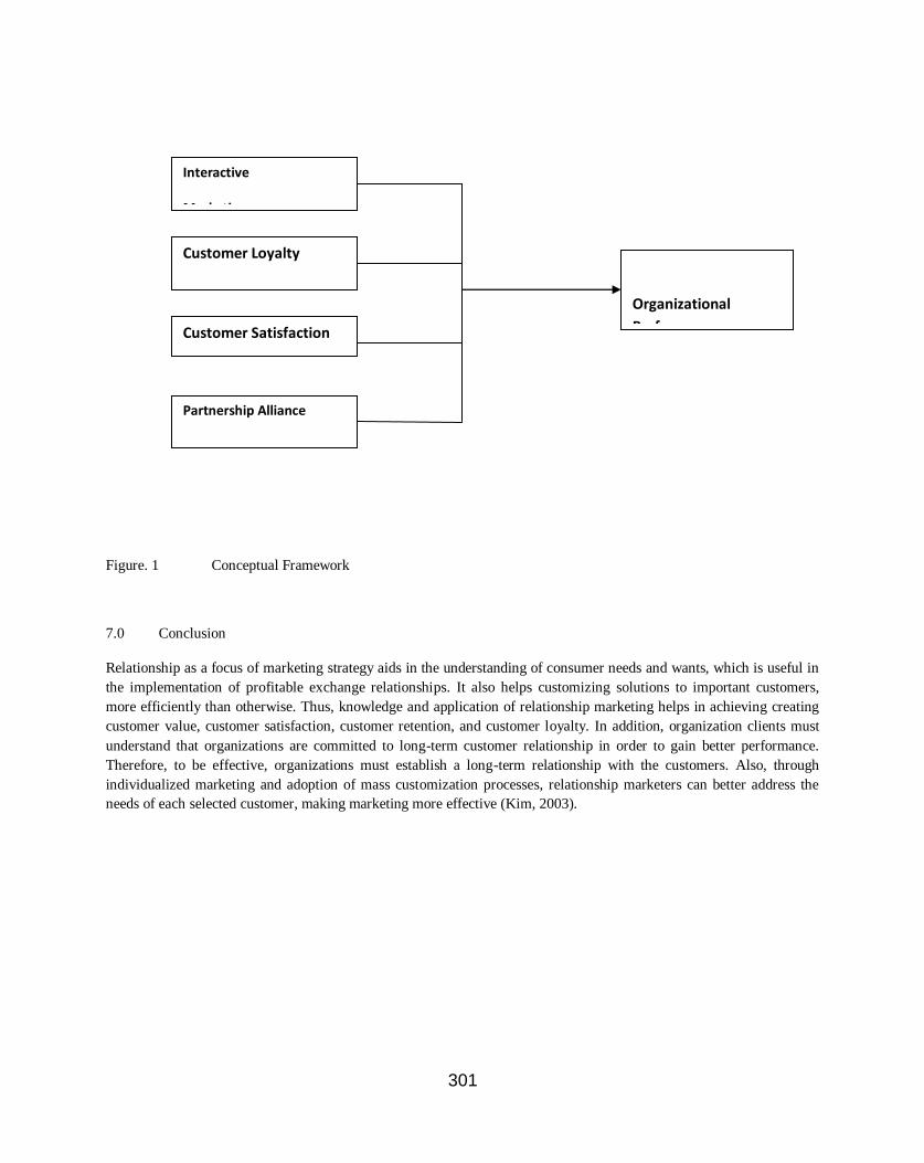
301

Figure. 1 Conceptual Framework

7.0 Conclusion

Relationship as a focus of marketing strategy aids in the understanding of consumer needs and wants, which is useful in

the implementation of profitable exchange relationships. It also helps customizing solutions to important customers,

more efficiently than otherwise. Thus, knowledge and application of relationship marketing helps in achieving creating

customer value, customer satisfaction, customer retention, and customer loyalty. In addition, organization clients must

understand that organizations are committed to long-term customer relationship in order to gain better performance.

Therefore, to be effective, organizations must establish a long-term relationship with the customers. Also, through

individualized marketing and adoption of mass customization processes, relationship marketers can better address the

needs of each selected customer, making marketing more effective (Kim, 2003).

Interactive

Marketing

Customer Loyalty

and Retention

Customer Satisfaction

Partnership Alliance

Organizational

Performance

302

REFERENCES

Anderson, J.C. and Narus, J.A. (2004). Business Market Management: Understanding, Creating, and Delivering Value,

Prentice Hall, 2nd Ed., Upper Saddle River.

Barnes, Bredley R., Fox, Martin T., & Morris, D.S. (2004). ―Exploring the Linkage between Internal Marketing,

Relationship Marketing and Service Quality: A Case Study of a Consulting Organization,‖ Total Quality

Management, Vol. 15, No. 5

Bennett, R. and Rundle-Thiele, S. (2004). ―Customer Satisfaction should not be the only Goal,‖ Journal of Services

Marketing, Vol. 18 No. 7.

Berry, L.L. (1983). ―Relationship Marketing‖, in Berry, L.L., Shostack, G.L. and Upah, G.D. (Eds), Emerging

Perspectives of Services Marketing, American Marketing Association, Chicago.

Berry, L. L. (1995). On Great Service, New York: The Free Press.

Bhardwaj, D. (2007). ―Relationship Marketing in Context to the IT Industry,‖ The Journal of Business Perspective, Vol.

11, No. 2.

Boone, L. E. and Kurtz, D. L. (2007). Contemporary Marketing, Harcourt College Publishers, Philadelphia.

Breshnahan, J. (1998). ―Improving the Odds,‖ CIO Enterprise Magazine, November.

Businesstown, H. (2008). ―Marketing – Basic Marketing Customer Loyalty‖. Journal of Marketing, January.

Cannon, J.P. and Perreault, W.D. (1999). ―Buyer-Seller Relationships in Business Markets,‖ Journal of Marketing

Research, Vol. 36, No. 4.

Christopher, M., Payne, A. and Ballantyne, D. (2002). Relationship Marketing: Creating Stakeholder Value,

Butterworth, Heine, Oxford.

Chris, F. and Graham H. (2007). ―Relationship and Marketing Communication,‖ Journal of

Relationship Marketing, Published by Financial Time.

Day, G.S. (1995). ―Advantageous Alliances,‖ Journal of the Academy of Marketing Science, Vol. 23, No. 4.

Das, T.K. and Teng, B.S. (2000). ―Instabilities of Strategic Alliances: An Internal Tensions‘ Perspective,‖ Organization

Science, Vol. 1, No. 1.

De Madariaga J. G. and Valor, C. (2007). ―Stakeholders Management Systems: Empirical Insights from Relationship

Marketing and Market Orientation Perspectives,‖ Journal of Business Ethics, Vol. 71.

Dick, A.S. and Basu, K. (1994). ―Customer Loyalty: Toward an Integrated Conceptual Framework,‖ Journal of the

Academy of Marketing Science, Vol. 22, No. 2

Dwyer, R. F., Schurr, P. H. and Oh, S. (1987). ―Developing Buyer-Seller Relationships,‖ Journal of Marketing, Vol. 55,

January.

Eisingerich, A. B. and Bell, S. J. (2007). ―Maintaining Customer Relationships in High Credence Services,‖ Journal of

Services Marketing, Vol. 21, No. 4.

303

Edelstein, H. (2000). How CRM differs from OLAP: What you Need to Understand When Implementing Mining

Techniques for Analytic CRM..

Engel, J.F. and Blackwell, R.D. (1982). Consumer Behavior, 4th Ed., Dryden Press, Chicago, IL.

Gronoos, C. (1994). ―From Marketing Mix to Relationship Marketing: Towards a Paradigm Shift in Marketing,‖

Marketing Management Journal, Vol. 32, No. 2.

Gronroos, C. (2000). Service Management And Marketing – A Customer Relationship Management Approach,

Chichester: Wiley & Sons

Gulati, R. (1995). ―Does Familiarity Breed Trust? The implications of Repeated Ties for Contractual Choice in

Alliances,‖ Academy of Management Journal, Vol. 38, No. 1.

Heskett, J. L., Jones, T. O., Loveman, G. W., Sasser, W. E. and Schlesinger, L. A. (1994). ―Putting the Service-Profit

Chain to Work,‖ Harvard Business Review, Vol. 72, No. 2.

Hunt, D., Lambe, C.J. and Wittmann, C.M. (2002). ―A Theory and Model of Business Alliance Success,‖ Journal of

Relationship Marketin, Vol.1, No. 1

Kim, Y. (2003). "How will Market Orientation and Environment and Firm's character influence Performance," Cross

Cultural Management, Vol. 10, No. 4.

Kotler, P. and Armstrong, G. (2002). Principles of Marketing An Introduction, Pearson, Prentice-Hall. Upper Saddle

River, 9th, Ed, New Jersey

Kotler, P. and Armstrong, G. (2008). Marketing Principle, Pearson Education, New Jersey.

Lambe, C.J., Hunt, D. and Wittmann, C.M. (2002). ―'A theory and Model of Business Alliance Success,‖ Journal of

Relationship Marketing, Vol. 1, No. 1.

Lambe, C.J., Spekman, R.E., Hunt, S.D. (2002). ―Alliance Competence, Resources, and Alliance Success:

Conceptualization, Measurement, and Initial Test,‖ Journal of the Academy of Marketing Science, Vol. 30, No.

2.

Liljander, V. and Strandvik, T. (1995). ―The Nature of Customer Relationships in Services,‖ In

Swartz, T.A., Bowen, D.E. and Brown, S.T. (Eds), Advances in Services Marketing and

Management, Vol. 4, JAI Press.

McKenna, R. (1991), Relationship Marketing – Successful Strategies for the Age of the Customer, Addison-Wesley,

Reading.

Monroe, K.B. (1991). Pricing – Making Profitable Decisions, McGraw-Hill, New York.

Morgan, R.M. and hunt, S. D. (1994). ―The Commitment Thrust-Theory of Relationship Marketing.‖ Journal of

Marketing, Vol. 58, January.

Naidu, G.M. Parvatiyar, A. Sheth J.N. and Westgate, L. (1999). ―Does Relationship Marketing Pay? An Empirical

investigation of Relationship Marketing Practices in Hospitals,‖ Journal of Business Research, Vol. 46, No.3.

304

Novo, J. (2008). ―Customer Loyalty‖, Drilling Down: Turning Customer Data into Profits, Journal of Marketing

Management,‖ Vol. 10, No. 3.

Oliver, R. L. (1980). ―A Cognitive Model of the Antecedents and Consequences of Satisfaction Decisions,‖ Journal of

Marketing Research, Vol. 17, November.

Oliver R L. (1999). Whence Consumer Loyalty? Journal of Marketing, Vol. 63.

Payne, A. and Frow, P. (2005). ―A Strategic Framework for Customer Rlationship Management,‖ Journal of Marketing,

Vol. 69, No. 4.

Peppers, D. and Rogers, M. (1995). ―A New Marketing Paradigm,” Planning Review, Vol. 23, No. 2.

Peterson, R.A. (1995). ―Relationship Marketing and the Consumer,‖ Journal of the Academy of Marketing Science, Fall,

Vol. 23.

Reicheld, F.F. and Sasser, W.E. Jr, (1990). ―Zero Defections: Quality comes to Services,‖ Harvard Business Review,

September-October.

Sewell, C. (1990). Customers for Life. New York: Pocket Book.

Sheth, J. N. (1996). ―Relationship Marketing: Frameworks and Concepts,‖ Paper presented at the 1996 International

Conference on Relationship Marketing,‖ Development, Management and Governance of Relationships, March

Sheth, J. N. and Parvatiyar, A. (2000). Handbook of Relationship Marketing, Thousand Oaks, Sage Publications

Slater, S. R. (1997). "Developing a Customer Value-Based Theory of the Firm," Journal of The Academy of Marketing

Science, Vol. 25, No. 2.

Storbacka, K., & Lehtinen, J. (2000). Customer Relationship Management, Singapore: McGraw Hill.

Thurau T. H., Gwiner, K. P. and Gremler, D. D. (2002). ―Understanding Relationship Marketing Outcomes: An

Integration of Relational Benefits and Relationship Quality,‖ Journal of Service Research, Volume 4, No. 3.

Treacy, M. and Wiersema, F. (1993). ―Customer Intimacy and other Value Disciplines,‖ Harvard Business Review,

January-February.

Webster, Jr, F.E. (1992). ―The Re-discovery of the Marketing Concept,‖ Business Horizons, Vol. 31, May-June.

Young, B.D. (1988). What‘s Relationship Marketing? Journal of Extension, Vol, 26. No. 3.

Zeithaml, V.A. (1988). ―Consumer Perceptions of Price, Quality and Value: A Means-End Model and Synthesis of

Evidence,‖ Journal of Marketing, Vol. 52.

Zeithaml, V. et al. (2006). Service Marketing: Integrating Customer Focus across the Firm, McGraw-Hill/Irwin, 4th Ed.

New York.

The Impact of Informal Sector Training on Economic Development

(Perspectives from Kisii County, Kenya)

Erick Nyakundi Onsongo erickonsongo@yahoo.com

305

Abstract This paper is about the impact of informal Sector Training on economic development, astudy of Kisii County.

Theobjectives of the study were to find out whether there is a relationship between informal sector training and economic

development and evaluate the factors that influenced informal sector training. To achieve this, a sample of 300

respondents in all the districts in Kisii County was selected. 20 training centers and working places were picked using

simple random sampling from 50 informal sector training centers and work place identified. Questionnaires were administered to the respondents.Assistants presented copies of the questionnaires to workers tocomplete and

supplementary information was obtained from management staff of the training centers. Data collected was analyzed

using descriptive and inferential statistics. Chi-square test was used to establish the relationship between informal sector

training and economic development. The Chi-square value that was obtained at 95% confidence level revealed that there

were more than the principle factors that influenced informal sector training. The informal sector or informal economy is

the part of an economy that is not taxed, monitored by any form of government, or included in any gross national product

(GNP), unlike the formal economy. The informal sector in developing countries plays significant roles: the provision of

employment, incomes and supplying ignored markets. However, the working and employment conditions in the sector

are still poor. Thus, its expansion and changing structures have drawn the attention of scholars and international policy

makers on factors hindering its formalization. The Ways to improve the informal sector include formalizing informal

jobs through regulation by the state. Informal sector training plays a vital role in empowering the people who work in the

informal sector with the necessary skills and knowledge to be able to work better.Another possible improvement would be to provide better protections and benefits in the informal sector.It might also be possible to create other methods of

generating income through microloans.

KEY WORDS: GNP- Gross Domestic Product, IS- informal sector, ILO- international Labor Organization, GDP- Gross

Domestic Product.

Introduction

There is a growing acceptance of the need to base training offerings on identified market needs and opportunities,

together with an increasing institutionalization of instruments and processes (e.g. development of training curricula and

modules. Good experiences are gained with participatory approaches in which the informal sector operators are involved

at an early stage in the design of training programs, as well as in implementation. There is fresh evidence that, with an

appropriate framework, skills upgrading of the technical and pedagogical skills has a positive effect on their training and

production activities.(Lynch& Black 1998)

Training projects in informal sector often combine technical skills training with functional literacy training, though no

solid data on the advantages and disadvantages of this combination were identified, informal sector actors are also more

and more involved in efforts to improve training delivery for the informal sector. In the field they participate, through

their members, in training project committees (to assist in trainee selection, curriculum development, organization of

trade testing) and, at national level, in boards of Employment and Training Funds (levy administration, guidance for

selection of training providers and financing of Skills training).(Addison, 2005)

The informal sector refers to the part of the economy that does not fall under the purview of organized economic

activities. The concept has a very interesting and cheered history. As the concern of the world community increased over

the lack of economic growth and perpetuation of poverty in the developing countries, policy makers began looking for a

solution to ease the situation. A planned promotion of growth in selected leading sectors of the economy would then lead to the overall growth of the economy. Thus, the primary problems were perceived to be the identification of the

target sectors with maximum linkages to the rest of the economy and the mobilization of enough finance to enhance the

growth rate of the target sectors. (Adeke, 2003)

The growth that was visualized by those early development economists was essentially the growth of organized

economic activities through rapid industrialization via capital formation and the expansion of domestic and export

demand. The reality that a large section of the population was earning a daily living by participating in activities that fell

outside the orbit of the organized sector was summarily ignored as it was considered to be a temporary phenomenon. It

was expected that those activities would disappear with the growth of the economy. In other words, the idea was that

once the take-off in economic growth was accomplished, with the growth of the organized economy the demand for, and

returns to labor would increase. (Bangazer, 2000)

306

The informal economy contributes significantly toproduction, consumption, employment and incomegeneration in

developing countries. It is a source oflivelihood to a majority of the poor, unskilled, sociallymarginalized and female

population and is an importantmeans of survival for people in countries lacking propersocial safety nets and

unemployment insurance especiallythose lacking skills for formal sector jobs.Apart from being a major source of

employment, the informaleconomy also contributes significantly to the output ofdeveloping countries. According to the

World Bankestimates, the informal economy accounts for 40 percent ofGross National Product (GNP) of low-income countries, to illustrate, the ‗unorganized sector‘ in Kenya accounts for62 percent of Gross Domestic Product (GDP), 50

percent ofgross national savings and 40 percent of national exports. In addition, the informal workforce is estimated to

make upabout 93 percent of total workforce and 83 percent of non-agricultural employment in Kenya.Such figures

across countries, however, are arrived at usinga varied range of measures of the informal economy.(ILO, 2002 (a))

The importance of the informal sector in supporting livelihoods and contributing toproduction and consumption activities of developing countries is widely evident. However,lack of consensus across countries in regard to a clear and

uniform definition of theinformal sector has hampered its identification and measurement for proper comparison.In

addition, relationship between informality and economic growth is not straightforwardand there is no concrete evidence

that this sector enhances economic growth. (Meyer, 1993)

Training refers to the acquisition of knowledge, skills, and competencies as a result of the teaching of vocational or

practical skills and knowledge that relate to specific useful competencies. It forms the core of apprenticeships and

provides the backbone of content at institutes of technology (also known as technical colleges or polytechnics). In

addition to the basic training required for a trade, occupation or profession, observers of the labor-marketrecognize as of

2008 the need to continue training beyond initial qualifications: to maintain, upgrade and update skills throughout

working life. People within many professions and occupations may refer to this sort of training as professional

development(Lynch& Black 1998)

On-the-job training takes place in a normal working situation, using the actual tools, equipment, documents or materials

that trainees will use when fully trained. On-the-job training has general reputations most effective for vocational work.

Off the job training is training from normal work situations — implying that the employee does not count as a directly

productive worker while such training takes place. Off-the-job training has the advantage that it allows people to get

away from work and concentrate more thoroughly on the training itself. This type of training has proven more effectivein

inculcating concepts and ideas.

Informalsector training in KisiiCounty, Kenya

There have been attempts to re-focus some public and non- governmental Organization training providers to become

more ‗business-like‘ and ‗market responsive‘, for instance by involving them in complementary training. Such efforts

have enjoyed Mixed success as it is necessary to re-equip them, adjust the technical skills of the Instructors, and adapt

their teaching methodologies in recent years there has been a rapid expansion of private-for-profit training institutions,

But so far their relevance for the Informal sector appears limited as they largely focus on office (e.g. computer) and

business skills rather than technical skills, in part because of the high demands of training colleges that offer technical

training aimed Mainly at modern wage employment.(Lynch& Black 1998)

There have emerged a number of private small one-trade training Centers, for instance in hairdressing and dressmaking,

which are directly relevant forinformal sector operators (e.g. suitable level of technology, practical training, and short

duration) there are interesting embryonic examples of public-private sector partnerships,Such as private training

providers that issue training certificates or diplomas.Useful training Mechanism by which formal sector businesses

interact with informal sector firms to help them to upgrade their skills, products and markets (and by so doing. create

interesting, value-adding sub-niches) through training, technology transfer and sometimes

Longer term partnerships; whereas apprenticeship training used to be of particular importance for the training of

members of the family, such training is now much more open (i.e. non-clanor family based), especially in ‗modern‘

trades (e.g. welding and hairdressing).(Lynch& Black, 1998)

Training in the informal sector has the means to increase the skills and qualification levels of employees and micro-entrepreneurs, and make a positive contribution to their working conditions and the profitability of their activities.The

formal methods of training and acquiring qualifications, there is a whole range of ways and means of developing skills

307

that are either not known to those responsible for existing formal training systems or under-valued in terms of the

knowledge and know-how generated, and are consequently neither recognized nor validated: skills acquisition in the

family, on-the-job training, through observation and imitation, and by means of traditional apprenticeship in the

countries where this is well developed. These alternative routes taken by the sector‘s workers account for the training of

up to 90% of a country‘s workforce. In terms of the results achieved, they often amount to being the countries‘ real

training systems. The time has come for developing countries to acknowledge the true role played by the informal sector in training young people and adults and helping them enter the labor market. It is also time to recognize the content and

levels of knowledge and skills thus acquired and to incorporate the best skills development schemes and practices into a

comprehensive reform of existing systems.(Jack, 2004)

Impact of informal sector training on the economy

The informal economy is, at many times, referred to asthe non-observed economy. It should be noted that theinformal

economy is only a component of the non-observedeconomy and needs to be distinguished from undergroundand illegal

production activities, although these may notalways be mutually exclusive.‗Underground production‘ activities are

legally notforbidden but are intentionally hidden from publicauthorities with the objective of evading tax and

socialsecurity payments as well as to avoid bureaucraticprocedures and regulatory compliance. ‗Illegal production‘

activities are those that are ‗forbiddenby law‘ or become illegal when undertaken by unauthorized individuals. For

example, drugs and narcotic production and trafficking, production of certain explosives, productionand distribution of counterfeit goods, and services such asunlicensed medical practice. (Becker, 2004)

Underground production isillegal as it involves non-compliance with administrativerules, while ‗illegal production‘ is

associated with criminalbehavior.In many instances, different terms such as the informal, shadow, parallel or black

economy among others, are usedinterchangeably wherein informal sector operations are notdistinguished from illegal

and underground productionactivities. Informal sector operations pertain to activitieswhere a legal counterpart exists and

are not alwaysperformed with the deliberate intention of evading taxesand infringing labor and other regulations, hence

departingfrom the concepts of illegal and underground production.Therefore, most informal sector activities in

developingcountries are not underground and not illegal as these areundertaken as measures for survival.Some scholars

have even objected to conceptualizing informality through a dualistic economy, i.e. a distinctbifurcation between the

formal and informal which identifies informal employment. (Brown, 2007)

In describing this sector, one should bear in mind that the informal economy is not a deviation of the formal economy, if

only because all economic activities started informal and formed the basis from which the formal economy sprang, with

firms and annual accounts, taxes, chambers of commerce, etc. Although the informal economy is often associated with

developing countries, where up to 60% of the labor force (with as much 40% of GDP) work, all economic systems

contain an informal economy in some proportion. (Blanch, 2001)

Governments have tried to regulate (formalize) aspects of their economies for as long as surplus wealth has existed

which is at least, yet no such regulation has ever been wholly enforceable. Archaeological and anthropological evidence

strongly suggests that people of all societies regularly adjust their activity within economic systems in attempt to evade regulations. Therefore, if informal economic activity is that which goes unregulated in an otherwise regulated system

then informal economies are as old as their formal counterparts, if not older. The term itself, however, is much more

recent. The optimism of the modernization theory school of development had led most people in the 1950s and 1960s to

believe that traditional forms of work and production would disappear as a result of economic progress in developing

countries. As this optimism proved to be unfounded, scholars turned to study more closely what was then called the

traditional sector. They found that the sector had not only persisted, but in fact expanded to encompass new

developments. (Carr, 2001)

308

Case problem

The increase in unemployment in Kenya as a direct result of the economic crisis, Loss of employment in the affected

sectors, as businesses closed down and GDP contracted, was considered to be the most important social consequence of

the crisis. But the unemployment figures told just one part of the story. The bulk of the job losses were concentrated in

modern sectors that depended on institutionalfinances, the lack of which resulted in the closures. As a result, many skilled workers were pushed into taking relatively inferior jobs in the informal sector. Flexible labor markets in many of

the affected countries allowed the affected employees to be reallocated from the formal sector to the informal sector, thus

moderating the impact of the recession.

The informal sector was originally treated as a residualemanating from the insufficient absorptive capacity ofthe formal

economy. It has been emphasizedthat productivity growth in the formal sector acts as a ‗pull‘factor in drawing informal

sector workers and enterprisestowards it. Paradoxically, informal sectors of mostdeveloping countries have actually

increased over time.Informality has been characterized as a response to hightransaction costs caused by cumbersome

bureaucraticprocedures for business start-ups, and irksome compliancewith unclear and prohibitive rules and

regulations.Rise in informality is associated with economic restructuringand economic crisis. For example, the structural

adjustmentprograms (SAPs) of the 1980s and 1990s is said to haveincreased the informal economy due to retrenchment

of thepublic sector and associated liberalization policies. The relationship between informality and growth is not onlyinconclusive but it can go in both directions: Economicgrowth can have expansionary effects onthe informal

economyand the informal economy canhave a positive or negative impact on economic growth.Sustained economic

growth that is pro-poor is believed toreduce informality. Developing countries with no growth, capital intensive growth

(jobless growth), or high-tech growth (rise in demand for skilled service sector jobsrather than unskilled manufacturing

jobs) could experiencean expansion in their informal sectors

The contribution of the informal sector or informalenterprises to non-agricultural GDP is substantial, Street vending

units usually referred to as ‗informal traders ‗make up a large proportion of informal sector enterprises.Their contribution

to total trade value added (GDP fromtrade) ranges from 50 to 90 percent Informal sector‘s share.Despite substantial

contribution from the informal sectorto the GDPs of many developing countries, there isinadequate evidence of informal

sector enterprises contributing to economic growth.

The study sought to determine the impact of informal sector training since its operations provide a wayout of the

draconian reigns confronting the formal sector.Low entry barriers and low operation costs in certain sectors(e.g. food,

repair, trade and transport) imply dominance ofinformal firms. The large number of small producers andsellers

producing almost identical products, for example inthe fruit and vegetable markets, also facilitates a high degreeof competition. As a result, consumers, mostly from the lowand middle income brackets, can avail of relatively low

prices.This leads to a rise in household savings, which canpotentially translate into economic growth.

3.0 Research strategy

This study was about the impact of informal training on economic development. The research partly involved a complete

survey of all informal sector training centers and work place and a sample of workers and customers who accessed the

informal sector services within the study setting. Information regarding the factors that influenced the need for informal

sector training was obtained via administering questionnaires to the respondents at the various training centers.

Assistants were engaged in presenting the questionnaires to the respondents. Data collected was analyzed using

descriptive and inferential statistics.Supplementary information was obtained from management staff of the informal

sector training centers. Primary data collection involved the use of self- administered questionnaires for literate

respondents and researcher administered questionnaires to cater for those who would not easily interpret the questions

due to their low literacy levels.

The research was based in Kisii County,which is a rural county with a relatively adult population of 470,531 residents

(Central Bureau Of Statistics Census Report, 1999). The county is central to the neighboring districts of Homabay,

Migori, Nyamira and Rachuonyo. The population of the proposed study was drawn from Kisii County consisting of Kisii

Central District, Gucha District, Nyamache District, Sameta District, Kenyenya District, South Kisii District and Masaba

309

North District. The study targeted 300 respondents from all informal sector training centers and work placesand the

customers who accessed the informal sector services in Kisii Countyduring the period of research.

Informal training centers and workplace were selected because the target population was big. The respondents to

participate in the research were selected using the random sampling procedure. Customers were picked randomly from

the work place were 50 and 100 respondents from the management staff (caretakers and executive staff to represent the informal sector trainers). Respondents from the stakeholders in the informal sector selected were 150.This consequently

ended up with 300 respondents selected.

A questionnaire was used to collect data. The questionnaires were administered to respondents at the work place and

informal sector training centers. The questionnaires were filled as the researcher waited to reduce non-response rates.

They presented copies of the questionnaires to customers as they left after the service has been renderedtheresearcher

presented the questionnaire to the management staff to fill.

The study incorporated data analysis tools, which included descriptive and inferential statistics to analyze the data

collected. Likert scale was used to identify the degree of importance of each factor. Chi- square test was used to establish

the relationship between informal sector training and the impact on human resource development.

4.0 Data Analysis, Findings and Discussions

4.1. General characteristics of the respondents

4.1.1. Gender, marital status and age of the respondents

Table 1 presents the general characteristics of the respondents. Males (72%) worked in the informal sector. It is apparent

that compared to males, women were less attached to the labor market and tended to accumulate less specific human

capital. Informal sector services have traditionally been directed to the needs of male members. Women were,

therefore,likely to be offered informal sector training. Many shied away due to cultural beliefs that women are not

supposed to be involved in strenuous activities.The findings concur with those of Tadić, (2005). Studies on gender and

career development have also shown that women were more committed to their careers than their male counterparts

(Jack, 2004). Conversely, no significant relationship between gender and career development of the respondents have

been found to exist (Akinyemi, 2001; Popoola and Oluwole, 2007).

Those married (89%) were the majority of the informal sector players followed by the singles (7.3%) and least were the

widowed (1.2%). The married members were responsible not only for themselves but also for their families, a situation

that would increase the propensity to work, especially when one had children or when one is the only bread earner for the family. The findings concur with those of Popoola and Oluwole (2007) that majority of the personnel in the informal

sector in Osun State in Nigeria were married. Besides, married workers had a lower mean career commitment than the

unmarried ones, implying that the married workers are more committed to their family matters and career.

The age category of 46-55 years was the majority (50%) followed by the age bracket 36-45 (29.3%) then 56-65 (15.9%).

It was, therefore, apparent that the majority of the people who work in the informal sector were relatively old. The reason

why the old are the majority may be because many organizations have reduced investment in younger employees.

Previous studies have found that, younger employees are more willing and eager to learn, develop themselves and have

more opportunities for career development than old employees (Meyer et al., 1993). Other studies have indicated that, in

any organization, old workers were more likely to be committed to their careers than young employees (e.g., Adeleke,

2003; Robert 2005; Popoola and Oluwole, 2007).

Table 10: Biographical characteristics of the Respondents

Variable Aspect Frequency %

310

Gender Male 216 72

Female 84 28

Total 300 100

Marital status of respondent Single 24 8

Married 267 89

Widowed 3 1

No response 6 2

Total 300 100

Age of respondent (years) Below 30 12 4

31-35 15 5

36-45 87 29

46-55 150 50

56-65 36 12

Total 300 100

Length of service < 1 6 2

1-3 39 13

4-6 78 26

> 6 168 56

No response 9 3

Total 300 100

Table 2 show standard errors and standard deviations of mean for the general characteristics of the Respondents. The standard errors of the means are less than the standard deviation, implying the information provided by the respondents

was reliable.

Table 11:Means and standard deviations for the Respondent’s biographical characteristics

Variable N Mean SE SD

Age of respondent 300 3.77 0.09 0.78

Academic qualification 300 3.12 0.11 1.02

Length of service 300 3.74 0.06 0.56

SE = standard error of the mean; SD = standard deviation.

311

4.3. The contribution of the informal sector training to employee career development and performance

Table 3 presents the contribution of the informal sector training to employee career development and performance.

Majority of the respondents (54%) had artisan certificates in electrical engineering, beauty therapy, computer packages,

mechanical engineering and welding. Diploma (44%), Higher National Diploma and first Degree holders were few (1%

each). Consequently, the informal sector respondents who had artisan Certificates were the majority and corresponded

to the level of knowledge an individual worker has can be apprised in terms of performance, which signify the level of

success that has been attained (Colarelli and Bishop, 1990; Brown et al., 2007). However, the findings of Popoola and

Oluwole (2007) are at variance that low educational qualifications may force workers to have strong commitment to their

job

Table 3:The contribution of informal Sector Training on employee career development and performance

Variable Level Frequency %

Academic qualification First Degree 3 1

Higher National Diploma 3 1

Diploma 132 44

Artisan Certificate 162 54

Total 300 100

Frequency of employee training High 48 16

Moderate 192 64

Low 51 17

very low 3 1

Not sure 6 2

Total 300 100

Extent to which investment in human

capital contributes to development

None 12 4

Small 84 28

Moderate 144 48

Large extent 39 13

Very large 15 5

Not negotiated 3 1

No response 3 1

Total 300 100

312

The perception of the respondents on the frequency of employee training was moderately high. Respectively 16% and 64% of the respondents agreed that employee training had highly and moderately improved. Correspondingly, 17% and

1%, perceived it as low and very low (Table 3)Motivation is the key to performance improvement, and ability to perform

depends on experience and training. It has been observed that the probability of receiving on-the job training and the

amount of work-related training received are higher (e.g., Lynch 1992; Harley et al., 1995).

On the extent to which the investment in human capital contributed to career development, respectively, 4% and 28% of

the respondents believed that there was no contribution or it was small. Correspondingly, 48% and 13% believed the

contribution was moderate or large (Table 3). These findings concur with those of Lynch (1992) and Harley et al. (1995)

who found development to be significantly and positively correlated with employee training and career advancement.

However, Duncan and Stafford (1980) observed a significant and negative correlation between performance and employee training while Lynch and Black (1998) established no significant relationship between performance and

employee training.

Table 4 depicts the mean contribution of training on employee career advancement and employee performance. The

standard deviations of the means were greater than the respective standard errors, indicating that the information provided by the respondents was reliable. The mean response when rounded-off was 3 (moderately agree), showing that

the respondents agreed that the training moderately improved their career advancement.

Table 4:Means and standard deviations for the aspects explaining employee training,career advancement and

performance

Parameter Academic qualification Employee training Employee performance

N valid 300 300 300

Mean 3.12 3.11 2.96

SE 0.11 0.09 0.11

SD 1.02 0.77 1.04

SE = standard error of the mean; SD = standard deviation.

The variables explaining employee training career development and performance had a mean response of between 3.21 and 3.80, indicating that training moderately improved employee career development (Table 4). Informal sector training

had a similar (Friedman test: 2= 5.59, df= 3, P= 0.35) impact on the employee career development (Table 5) relevance

of training, investment in human capital, academic qualification, and frequency of employee training.

Table 5:Means and ranks for the aspects explaining employee career development and performance as

contributed by training

Aspect Mean

Relevance of employee training and economic development 3.47

Extent to which investment in human capital 3.21

Academic qualification 3.45

Frequency of employee training 3.43

313

Table 6: Friedman test for the aspects explaining employee career advancement and performance as contributed

by training

N 300

Chi-Square 5.59

Df 5

Asymp. Sig. 0.35

Level of significance used– 5%

The impact of the informal sector training on economic development

Table 7 depicts the mean responses for wage rates, employee morale, organization performance and working practices,

employee commitment to the job, satisfaction with job performance, employee‘s individual output, and employee

training and development assessed in the current study. The mean responses for all the factors were greater than their

respective standard deviations, indicating the information provided by the respondents was reliable.

The extent to which investment in human capital positively affected the effective mix of wages and employee living

standards (r=0.32, p<0.01), employee morale, motivation and cooperation towards productivity (r=0.34, p<0.01), and

organizational performance or improved working practices (r=0.25, p<0.05). Ensuring investment in human capital

positively and significantly affected effective mix of wages and employee living standards (r=0.44, p<0.01), employee morale, motivation and cooperation towards productivity (r=0.37, p<0.01), organizational performance or working

practices (r=0.51, p<0.01), and employee commitment to achieving organizational goals

314

There was strong agreement regarding employee morale, with a mean response of 4.86 (Table 7).

This showed that economic development increased due to the training offered to the respondents. This is supported by the fact that among the respondents 85.7% and 14.3% strongly agreed and

agreed, respectively, that the economic status of the respondents improved. No respondent disagreed

or was neutral to the issue. The increased economic standard could be attributed to the increased

wage rates of the respondents as the respondents improved living standards by having high saving

and investment. Olatunji (2004) noted that an attractive salary package and participative management

besides regular promotion influenced workers to exhibit high career commitment in any organization.

Conversely, low salarygrowth was responsible for low career commitment and productivity (Okorie,

1995).

Improved organizational performance and working practices had a mean response of 4.29 (agreed),

the observation was supported by, correspondingly, 14.3% and 71.4% of the respondents who agreed

and strongly agreed. Only 14.3% of the respondents strongly disagreed (Table 7). The improved

workers morale and increased output may be attributed to the improved working conditions and

living standards due to a good wage that lead the employee to make a saving and investment provided

for by training. The findings concur with those of Olatunji (2004) who found that a good working

environment significantly and positively influenced commitment and performance of employees.

Freeman and Medoff (1984) also observed that training could have a positive impact on the employee who works on the informal sector competitiveness by encouraging management to introduce more

productive work practices.

Studies have shown that the informal sector training leads to lower probabilities of quitting, longer

job tenure and a lower lay-off rate, which in turn reduces the costs of recruitment, and increases productivity this lead to the increase in the GDP of the country. (Freeman and Medoff, 1984; Delery

et al., 2000.

Table 9. The impact of informal sector training on economic development

Variable Response N Valid %

Better organizational performance

Strongly disagree 42 14

Agree 42 14

Strongly agree 216 72

Total 300 100.0

Improved employee morale Agree 42 14

Strongly agree 258 86

Total 300 100.0

Improved wage rates Strongly disagree 42 14

Strongly agree 258 86

Total 300 100.0

Improved living standards of the employee Agree 42 14

Strongly agree 258 86

Total 300 100.0

315

Improved employee commitment Agree 171 57

Strongly agree 129 43

Total 300 100.0

Improved individual output Agree 42 14

Strongly agree 258 86

Total 300 100.0

Improved economic growth Neutral 42 14

Agree 42 14

Strongly agree 216 72

Total 300 100.0

It was apparent that employee training contributed to better living standards, the respondents agreed (57 %) and strongly agreed (42 %) that the services improved commitment of the respondents to their

jobs (Table 7). There is evidence that employee training makes an important contribution to

workplace performance by reducing exit behavior, including quits, absenteeism, malingering and

quiet sabotage, (Addison, 2005; Ramirez et al., 2007).

It was apparent in the present study that the output per individual member increased due to informal

sector training (agreed 14 %, strongly agreed 86 %) and training of members enhanced them to be

economically endowed, the responders indicated that through training they were able to make

informed choices, be able to perform better, get promotions, work effectively and efficiently hence

employees were satisfied and had some investment which increased the saving and investment hence

increasing the GDP of the country. The living standards of the respondents were better than before

training (neutral 14 %, agreed 14 %, strongly agreed 72 %) had improved. This increased output may

be attributed to the increased morale and commitment as a consequence of increased wage rate, training, improved working practices and employment terms and conditions. The findings concurred

with those of Okorie (1995) who observed that performance among Nigerian employees working in

the informal sector was positively related to continued commitment in their jobs.

5.0 Conclusion and Recommendation

The study concluded that informal sector training has an impact in the general economic growth of a

nation in this period when there is a rapid increasein unemployment, high inflation rates,

technological and globalization. Informal sector training provided the employees with better skills to

be able to perform get promotions, increase efficiency and effectiveness in the workplace, and get

better pay which increases their savings and investment hence the country GDP increases.

The study recommended on Ways to improve the informal sector training that includes formalizing

informal jobs through regulation by the state. The issue with this policy is that so many different

types of informality exist. It would be extremely difficult to create solutions to meet so many diverse

circumstances. Another possible improvement would be to provide better protections and benefits in

the informal sector, but creating protection programs could lead to a disconnect between the labor market and protections, which may not actually improve informal employment.

It might also be possible to create other methods of generating income through microloans or land

rights when access to the formal sector is limited. This is not a satisfactory solution to effectively

combat the issues underlying the informal sector though, efforts towardsconceptualizing, defining

and measuring the informal sector training have evolved and progressed over time both at the

316

nationaland international levels. However, our knowledge of thesector, its impact and inter-linkages

with various economicand social spheres is still rudimentary. This calls for moreresearch and study to

comprehend the heterogeneity andreach of the informal sector for targeted policy making.

References

Addison, J. (2005). The determinants of firm performance: unions, works councils, and employee involvement/high-performance work practices. Scottish Journal ofPolitical Economy

52(3): 406-450.

Adeleke, B.A. (2003). Comparative study of career commitment of journalists in print and electronic

media organizations in Nigeria. Journal of Personnel Management 15(2): 50-68.

Akinyemi, M.T. (2001). Patterns of Career Commitment Among Nurses in Osun State, Nigeria. Med

Dissertation, University of Ibadan, Ibadan, 89 pp.

Bangasser, P E (2000), ―ILO and the Informal Sector: An Institutional History‖ ILO, 2000

Becker, K F (2004) ―The Informal Economy‖ Fact Finding Study, SIDA

Blanch, N Canagarajah, S and Raju, D (2001), ―The Informal Sector Revisited: A Synthesis across

Space and Time‖ Social Protection Discussion Paper Series, World Bank

Brown, A.W., Adams, J.D., Amjad, A.A. (2007). The relationship between human capital and time performance in project management: A path analysis. International Journal of Project Management

1: 77-89.

Carr, Marilyn and Martha A. Chen. 2001. ―Globalization and the Informal Economy: How Global

Trade and Investment Impact on the Working Poor‖. Background paper commissioned by the ILO

Task Force on the Informal Economy. Geneva, Switzerland: International Labour Office.

Colarelli, S., Bishop, R.C. (1990). Career commitment: Functions, correlates, and management.

Group and Organizational Studies 15(2): 76-158.

Delery, J., Gupta, N., Shaw, J., Jenkins, J., Ganster, M. (2000). Unionization,Compensation, and

Voice Effects on Quits and Retention. Industrial Relations39(4): 625-645.

Duncan, G., Stafford, F. (1980). Do union members receive compensating differentials?‖ American

Economic Review 70: 355-371.

Freeman, R., Medoff, J. (1984). What Do Unions Do? Basic Books Ltd., New York, USA, Accessed

on 25th October, 2010 from http://www.press.uillinois.edu/ journals/irra/

proceedings2004/12c_singh.html.

ILO (2002a). Unorganized sector includes ―units run by cooperative societies, trusts, private and

public limited companies not Included in Annual Survey of Industries (ASI) in manufacturing

inaddition to unincorporated proprietary and partnership Enterprises‖ (see Page 7) in ILO and Delhi

Group (2007c)

317

Harley, F.J., Herz, D.E., Horrigan, M.W. (1995). Employer-provided training: Results from a new

survey. Monthly Labour Review 118: 3-17.

Jack, R.M. (2004). Gender and career commitment across some professions in selected developed

countries. Industrial Psychological Bulletin 38: 124-38.

Lynch, L.M., Black, E. (1998). Beyond the incidence of employer provided-training. Industrial and

Labour Relations Review 52: 64-81.

Meyer, J.P., Allen, N.J., Smith, C. (1993). Commitment to organizations and occupations: extension

and test of a three-component model. Journal of Applied Psychology 78: 538-51.

Okorie, I.A. (1995). Employees' commitment and performance in Nigerian business and service

organizations. Ife Psychological: An International Journal 3(1): 32-42.

Olatunji, A.A. (2004). Analysis of career commitment of health workers in Nigeria. Human Resource

Management Review 12(1): 40-52.

Popoola, S.O., Oluwole, D.A. (2007). Career commitment among records management personnel in a

State Civil Service in Nigeria. Records Management Journal17(2): 107-116.

Ramirez, M., Guy, F., Beale, D. (2007). Contested resources: unions, employers, andthe adoption of

new work practices in US and UK Telecommunications. BritishJournal of Industrial

Relations 45(3): 495-517.

Robert, D.M. (2005). Relationship between salary, work experience, age and career commitment of

industrial workers in Ghana. Journal of Personnel Management 17(1): 10-22.

Tadić, I. (2005). Career Development of Graduates in Economics and Business Administration in

Croatia. Masters Thesis, Faculty of Economics, University of Ljubljana, Croatia.

318

FOOD SECURITY

Performance of National Agricultural Advisory Services Projects in

Uganda; does Stakeholder Commitment Matter?

Hassan Bashir

bhassan@mubs.ac.ug

Joseph M. Ntayi

jntayi@mubs.ac.ug

Mohammed Ngoma

mngoma@mubs.ac.ug

Makerere University Business School: Kampala (Uganda)

Abstract

The increased poor performance of National Agricultural Advisory Services (NAADS) projects

in Uganda has become a concern of many stakeholders. This paper presents findings of a study

carried out to examine the performance of NAADS projects which were set up by the

government in 2001 to eradicate poverty in Uganda. The data showed low performance levels of

these projects and raised pertinent questions on the influence of NAADS stakeholders‘

commitment to the performance of the projects. Data was sought from farmers and coordinators

of the projects. Mukono district was used as a case study and a sample of 323 NAADS projects

was used, covering a wide range of agricultural activities. Cross sectional and quantitative survey

designs were also used. The paper therefore calls for urgent review of NAADS policy and

practices to ensure that project managers and coordinators discuss with famers the personal

benefits of carrying out activities of NAADS such that farmers fill a great deal of personal

meaning of the project to their lives.

Key words: NAADS, project performance, stakeholder, commitment

319

INTRODUCTION

The increasing turbulence in the modern business environment has made it necessary for many

organizations both private and public to adopt project approach as the means to achieving

organizational goals. Each project however, strives for excellence and success yet is by definition

a unique task normally subjected to severe restrictions on budget and time (Andersen, 2006). A

project has therefore to perform well in terms of the planned budget, time, and the quality of the

project processes and outputs, Munns & Bjeirmi (1996) so as to fulfill the intended objectives of

satisfying the stakeholder‘s needs, Baccarini (1999); Shenhar et al. ( 2001). Failure to achieve

this, the project will be branded unsuccessful and failed.

In Uganda the government has started many projects in order to eradicate poverty. A case in

point is the District Development Project (DDP), Entandikwa scheme and Bonna Bagaggawale.

These projects aimed at giving low income earners financial support in form of capital to start

small businesses. According to DDP pilot report of 2000, these projects were mismanaged and

failed to achieve the set objectives. The government also established the Northern Uganda Social

Action Fund (NUSAF) projects as a transitory tool and funding mechanism to assist Northern

Uganda to catch up with the rest of the country in matters of development. However, according

to NUSAF report of 2008, this project did not live to the expectations of the government. In 2001

the government established the National Agricultural Advisory Services (NAADS) projects to

eradicate poverty through enhancement of agriculture. However according to the NAADS

secretariat report of 2007/08, NAADS projects had registered 60% failure rate with some

projects in districts like Kotido registering 100% failure rate while projects in more than 10

districts registering a failure rate of above 90%.

As a result of this high failure rate of poverty eradication projects in Uganda, the poverty level

has remained high with more than 31% of Ugandan population living below a dollar a day.

According to Steers (1977), the weak performance of projects can be attributed to the low

commitment of the key stakeholders to the projects. The NAADS secretariat report of 2003/04

points out that in districts like Kotido farmers who are the principle beneficiaries of the projects

were not involved in the projects activities thus registering 100% failure rate. The Auditor

General‘s report of 2008 also indicates that NAADS coordinators spent most of the money on

workshops which were never attended by farmers.

It is therefore probable there is a link between stakeholder commitment to the project and performance of poverty eradication projects, Crawford (2005); Koh & Boo (2001). The

challenge for project champions is to ensure commitment of key stakeholders in project activities

so as to improve performance of poverty eradication projects in Uganda.

LITRETURE REVIEW & CONCEPTUAL ANALYSIS

Past studies have defined commitment in many different ways. Mowday et al. (1979) and Porter

et al. (1974) defined organization commitment as the relative strength of an individual‘s

identification with, and involvement in, a particular organization. According to Moorman et al.

(1992) commitment is an enduring desire to maintain a valued relationship. Dwyer, Schurr and

Sejo (1987) described commitment as the existence of an implicit or explicit pledge of relational

continuity of exchange partners. Morgan and Hunt (1994) described commitment as exchange

partner believing that an ongoing relationship with another is so important as to warrant

320

maximum efforts at maintaining it. Porter et al. (1974) characterized commitment by three

factors. These factors are a strong belief in and acceptance of the organization‘s goals and values,

a willingness to exert considerable effort on behalf of the organization, and a strong desire to

maintain membership in the organization. Allen and Meyer (1990b) conceptualized three

components of organizational commitment: affective (i.e., employee‘s emotional attachment to,

identification with, and involvement in the organization); continuance (i.e., commitment based

on the costs that the employee associates with leaving the organization); and normative (i.e.,

employee‘s feeling of an obligation to stay with the organization). However, Kanter (1968) with

her argument that different types of commitment result from the different behavioral

requirements imposed on employees by the organization, suggests three different forms of

commitment: Continuance commitment (member‘s dedication to the survival of the organization.

This is caused by requiring members to make personal sacrifices to join or remain with an

organization); Cohesion commitment (attachment to social relationships in an organization

brought on by such techniques as public renunciation of previous social ties or by engaging in

ceremonies that enhance group cohesion); and Control commitment (member‘s attachment to the

organization‘s norms that shape behavior in desired directions. It exists when employees believe

their organization‘s norms and values serve as a model for suitable behavior).

A project is a temporary endeavor undertaken to create a unique product, service, or results

(PMBOK, 2004). It‘s an undertaking with defined scope, time and budget to create a unique

output. Project performance can be viewed narrowly as achievement of intended outcomes in

terms of project specification, completing the activities on time, completing the project on the

agreed budget, only carrying out activities within the Scope and with requisite performance

(technical requirements), Atkinson (1999); Pinto & Slevin (1988); Wateridge (1998). According

to PMI Standards Committee (2004) and Bryde (2005), this is the golden or the iron triangle

measurement of project performance i.e. if the project is completed on time, within budget,

according to agreed specification, it will have performed well. This is the operational mindset,

which is influenced by the ―get the job done‖ approach as observed by Dvir et al. (2006). Several

studies support the inclusion of customer satisfaction as a fourth dimension of project

performance, Lipovetsky et al. (1997); Lim & Mohamed (1999); Zwikael & Globerson (2006);

Kerzner (2006); Voetsch (2004); Bryde (2005). This study therefore adopts the measurement of

project performance in terms of Schedule, project quality, Customer satisfaction, time

management and achieving project objectives.

Various scholars have established that commitment has a positive influence to organizational

performance, Lum et al. (1998); Sims & Kroeck (1994). Commitment to the project affects its

performance, Benkhoff (1997); Brett et al. (1995). Stakeholders with strong affective

commitment remain with the project because they want to, and they attach strong belief in and

acceptance of the project‘s goals and values. According to Tansky et al. (1997), affective

organizational commitment connects a worker to the organization‘s goals and values because of

the strong cognitive desire to belong to the organization (Steers, 1977). A worker therefore

bonds with organization because he or she chooses to do so, McElroy et al. (1999), thus

improving performance. Stakeholders with strong continuance commitment remain attached to

the project because they need to, and they are willing to exert a considerable effort on behalf of

the organization. According to Becker‘s (1960) side-bet theory, employees form sunken costs,

such as monetary, social, physical, psychological, lost opportunities, and so forth and the greater

321

the sunken costs a person develops with an organization, the less likely he or she is willing to

leave employment with the organization. This means that the sacrifice of leaving becomes so

great that the employee becomes bonded to the organization, Jaros et al. (1993). Therefore,

commitment to the organization occurs under continuance commitment because the investments

made with an organization tie the person to that organization, McElroy et al. (1999). It reflects a

sense of being locked in place because of the high costs of leaving. According to Hrebiniak and

Alutto (1972), this type of commitment is a structural phenomenon which occurs as a result of

individual– organizational transactions and alterations in investments over time. According to

Lambert, Barton, & Hogan, (1999), Continuance commitment is also referred to as calculative

commitment where an employee calculates in some manner the costs and benefits of working for

a given organization and it is these calculations that determine the level of commitment to the

organization. Stakeholders with strong normative commitment remain in the project because they

feel they ought to, due to their strong loyalty to the project, Schappe & Doran (1997). This is so

because according to Jaros et al. (1993) normative commitment involves acceptance of the norms

of the organization and the need to be loyal to employers. It therefore makes the employee fill a

sense of duty or obligation to be committed to the organization because it has employed him/her,

Jaros et al. (1993). It is this that pressurizes the employee to act in a way that meets the

organizational goals and interests, Allen & Meyer (1990). According to Weiner (1982), the

stronger the normative commitment, the stronger is the person‘s predisposition to be guided in

his actions by such internalized standards rather than by a consideration of the consequences of

these actions. Thus, committed individuals may exhibit certain behaviors not because they have

figured that doing so is to their personal benefit, but because they believe that it is the ―right‖ and

moral thing to do, Weiner & Vardi (1980).

In their study of antecedents (causes) and consequences (results) to organizational commitment,

Steers (1977) and Aven (1988) conclude that highly committed employees are more likely to

have higher levels of participation, remain with the organization for longer periods and make

more contributions for achieving organizational objectives, higher levels of involvement in their

jobs and exert considerably more effort on behalf of the organization. According to Etzioni‘s

(1961) commitment model focusing on employee compliance with organizational objectives, any

actual or perceived authority or power organizations have over individuals is rooted in the nature

of employee commitment in the organization. This means that organizations have substantially

less authority or power over employees who have lower levels of commitment. Etzioni (1961)

concludes that when employees have higher levels of commitment to organizational objectives,

the organization will have more authority and power over these employees.

Hypothesis

The purpose of this study is to establish whether commitment of stakeholders influences the

performance of National Agricultural Advisory Services Projects in Uganda. To achieve this

goal, the following hypotheses are formed for examination in this study. Hypothesis 1 (H1):

there is no affective, continuance, normative and cohesion commitment among the stakeholders

of NAADS projects. Hypothesis 2 (H2): Affective, Continuance, normative and cohesion

commitment positively affects performance of projects.

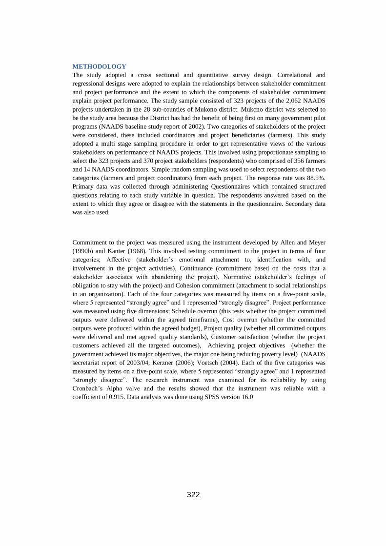
322

METHODOLOGY

The study adopted a cross sectional and quantitative survey design. Correlational and

regressional designs were adopted to explain the relationships between stakeholder commitment

and project performance and the extent to which the components of stakeholder commitment

explain project performance. The study sample consisted of 323 projects of the 2,062 NAADS

projects undertaken in the 28 sub-counties of Mukono district. Mukono district was selected to

be the study area because the District has had the benefit of being first on many government pilot

programs (NAADS baseline study report of 2002). Two categories of stakeholders of the project

were considered, these included coordinators and project beneficiaries (farmers). This study

adopted a multi stage sampling procedure in order to get representative views of the various

stakeholders on performance of NAADS projects. This involved using proportionate sampling to

select the 323 projects and 370 project stakeholders (respondents) who comprised of 356 farmers

and 14 NAADS coordinators. Simple random sampling was used to select respondents of the two

categories (farmers and project coordinators) from each project. The response rate was 88.5%.

Primary data was collected through administering Questionnaires which contained structured

questions relating to each study variable in question. The respondents answered based on the

extent to which they agree or disagree with the statements in the questionnaire. Secondary data

was also used.

Commitment to the project was measured using the instrument developed by Allen and Meyer

(1990b) and Kanter (1968). This involved testing commitment to the project in terms of four

categories; Affective (stakeholder‘s emotional attachment to, identification with, and

involvement in the project activities), Continuance (commitment based on the costs that a

stakeholder associates with abandoning the project), Normative (stakeholder‘s feelings of

obligation to stay with the project) and Cohesion commitment (attachment to social relationships

in an organization). Each of the four categories was measured by items on a five-point scale,

where 5 represented ―strongly agree‖ and 1 represented ―strongly disagree‖. Project performance

was measured using five dimensions; Schedule overrun (this tests whether the project committed

outputs were delivered within the agreed timeframe), Cost overrun (whether the committed

outputs were produced within the agreed budget), Project quality (whether all committed outputs

were delivered and met agreed quality standards), Customer satisfaction (whether the project

customers achieved all the targeted outcomes), Achieving project objectives (whether the

government achieved its major objectives, the major one being reducing poverty level) (NAADS

secretariat report of 2003/04; Kerzner (2006); Voetsch (2004). Each of the five categories was

measured by items on a five-point scale, where 5 represented ―strongly agree‖ and 1 represented

―strongly disagree‖. The research instrument was examined for its reliability by using

Cronbach‘s Alpha valve and the results showed that the instrument was reliable with a

coefficient of 0.915. Data analysis was done using SPSS version 16.0

323

RESULTS AND DISCUSSION

The study used Factor analysis with principal Component Analysis to extract variables from the

questionnaire and to analyze them. The Kaiser-Meyer-Olkin value was 0.908 and Bartlett‘s test

was significant at [x2(231) = 3769.7, P<0.001] thus implying that factor analysis was a suitable

model for analysis in this study. The communalities for each of the variables were within the

range of 0.287 to 0.786. Variables with a communality of 0.55 were considered to have a strong

variance and variables with a communality of less than 0.55 were considered to have a week

variance. This is shown in Table 1

Table1; Extracted Communalities for Variables of Commitment

Initial Extraction

1) I would be very happy to spend the rest of my career with this project 1.000 .562

2) I enjoy discussing my project with people outside it 1.000 .748

3) I really feel as if this project's problems are my own 1.000 .735

4) I think that I could easily become as attached to another project as I am to this one 1.000 .777

5) I feel like part of the family when with project team members 1.000 .287

6) I feel emotionally attached to this project 1.000 .466

7) This project has a great deal of personal meaning for me 1.000 .686

8) I feel a strong sense of belonging to my project 1.000 .714

9) I feel I have an obligation to remain part of this project 1.000 .786

10) Even if it were to my advantage, I do not feel it would be right to leave my project

now

1.000 .670

11) I would feel guilty if I left my project now 1.000 .623

12) This project deserves my loyalty 1.000 .682

13) I have a sense of obligation to the people in this project 1.000 .631

14) I owe a great deal to this project 1.000 .419

15) I am afraid of what might happen if I quit this project without having another one

lined up

1.000 .472

16) It would be very hard for me to leave this project right now, even if I wanted to 1.000 .661

17) Too much in my life would be disrupted if I decided to leave this project now 1.000 .707

324

18) It would be too costly for me to leave this project right now 1.000 .752

19) Right now remaining part of this project is a matter of necessity as much as desire 1.000 .759

20) I feel that I have too few options to consider leaving this project 1.000 .777

21) One of the few serious consequences of leaving this project would be the scarcity

of available alternatives

1.000 .647

22) One of the major reasons I continue working with this project is that leaving would

require considerable personal sacrifice - another project may not match the overall

benefits that I have here

1.000 .643

Extraction Method: Principal Component Analysis.

Variables 1-8 represented affective commitment, with variables 2 (I enjoy discussing my project

with people outside it), 3 (I really feel as if this project's problems are my own), 4 (I think that I

could easily become as attached to another project as I am to this one) and 8 (I feel a strong sense

of belonging to my project) having the strongest variances of 0.748, 0.735, 0.777 and 0.714

respectively. Variables 9-14 represented normative commitment, with variable 9 (I feel I have an

obligation to remain part of this project) having the strongest variance of 0.786. Variables 15-22

represented continuance commitment with variables 17 (Too much in my life would be disrupted

if I decided to leave this project now), 18 (It would be too costly for me to leave this project right

now), 19 (Right now remaining part of this project is a matter of necessity as much as desire) and

20 (I feel that I have too few options to consider leaving this project) having the strongest

variance.

A factor analysis with principal component method using varimax rotation was also applied to all

the variables to determine any underlying components for each variable and validate whether the

respondents perceived the four components of commitment to be distinct. The components of

commitment included commitment; affective, continuance, normative and coherent commitment.

Table2: Rotated Component Matrixa

Component

1

Affective

2

Continuanc

e

3

Cohesion

4

Normative

I enjoy discussing my project with people outside it .839

I really feel as if this project's problems are my own .826

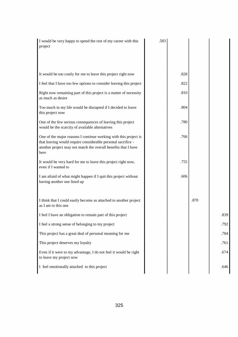
325

I would be very happy to spend the rest of my career with this

project

.583

It would be too costly for me to leave this project right now .828

I feel that I have too few options to consider leaving this project .822

Right now remaining part of this project is a matter of necessity

as much as desire

.810

Too much in my life would be disrupted if I decided to leave

this project now

.804

One of the few serious consequences of leaving this project

would be the scarcity of available alternatives

.780

One of the major reasons I continue working with this project is

that leaving would require considerable personal sacrifice -

another project may not match the overall benefits that I have

here

.766

It would be very hard for me to leave this project right now,

even if I wanted to

.755

I am afraid of what might happen if I quit this project without

having another one lined up

.606

I think that I could easily become as attached to another project

as I am to this one

.870

I feel I have an obligation to remain part of this project .839

I feel a strong sense of belonging to my project .792

This project has a great deal of personal meaning for me .784

This project deserves my loyalty .761

Even if it were to my advantage, I do not feel it would be right

to leave my project now

.674

I feel emotionally attached to this project .646

326

The results as indicated in Table 2, showed a four factor loadings with eigenvalues greater than

1.0 for all the components of commitment. The total variance explained was 64.57%. A closer

examination revealed that for factor 1 (Affective), the total variance explained was 7%. For

factor 2 (continuance), the total variance explained was 41.96%, for factor 3 (cohesion), the total

variance explained was 4.84% and for factor 4 (normative) the total variance explained was

10.767%. This implied that continuance commitment has the highest variance explained

followed by normative commitment, followed by affective commitment and cohesion

commitment having the least variance.

I would feel guilty if I left my project now

I have a sense of obligation to the people in this project

I owe a great deal to this project

.642

.640

.505

Eigenvalues 1.541 9.231 1.065 2.369

Percentage of variance explained 7.004 41.959 4.839 10.767

Cumulative Percentage of variance explained 7.004 48.963 53.802 64.569

Extraction Method: Principal Component Analysis.

Rotation Method: Varimax with Kaiser Normalization.

a. Rotation converged in 6 iterations.

327

Zero-order Pearson correlations among study variables were used and is presented in table 3

Table3: Zero- Order Pearson Correlations

Mean S.D 1 2 3 4 5 6

Affective (1)

4.0962 .79167 1.00

Continuance (2) 3.8633

.99206 .304** 1.00

Cohesion (3)

3.2238 1.45298 .051 -.131* 1.00

Normative (4) 3.9151

.84981 .438** .619** .007 1.00

Commitment to the projects (5) 3.7712 .62970 .619** .628** .548** .725**

1.00

Performance of NAADS Projects

(6)

3.6718 .46686 .318** .315** -.059 .363**

.303** 1.00

**. Correlation is significant at the 0.01 level (2-tailed).

*. Correlation is significant at the 0.05 level (2-tailed).

Affective commitment (mean= 4.0962, s.d=0.79167), continuance commitment (mean= 3.8633,

s.d= 0.99206), cohesion commitment (mean= 3.2238, s.d=1.45298) and normative commitment

(mean= 3.9151, s.d=0.84981), exists among stakeholders of NAADS projects which leads to

performance of NAADS projects (mean=3.6718, s.d= 0.46686). This finding partially rejects

H1; (there is no affective, continuance, normative and cohesion commitment among the

stakeholders of NAADS projects). The finding shows that there is relatively high affective

commitment with low continuance, normative and cohesion commitment.

Results from Table 3 also revealed a strong positive relationship between commitment and

performance of NAADS projects (r = .303**, p<.01). Results also showed that Affective,

Normative and Continuance are positively related to performance of NAADS projects with the

parameters (r = .318**, p<.01), (r = .363**, p<.01) and (r = .315**, p<.01) respectively. These

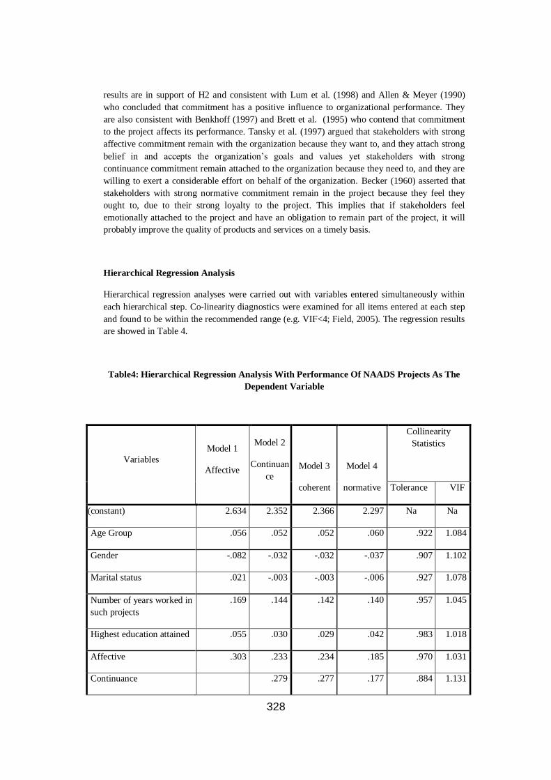
328

results are in support of H2 and consistent with Lum et al. (1998) and Allen & Meyer (1990)

who concluded that commitment has a positive influence to organizational performance. They

are also consistent with Benkhoff (1997) and Brett et al. (1995) who contend that commitment

to the project affects its performance. Tansky et al. (1997) argued that stakeholders with strong

affective commitment remain with the organization because they want to, and they attach strong

belief in and accepts the organization‘s goals and values yet stakeholders with strong

continuance commitment remain attached to the organization because they need to, and they are

willing to exert a considerable effort on behalf of the organization. Becker (1960) asserted that

stakeholders with strong normative commitment remain in the project because they feel they

ought to, due to their strong loyalty to the project. This implies that if stakeholders feel

emotionally attached to the project and have an obligation to remain part of the project, it will

probably improve the quality of products and services on a timely basis.

Hierarchical Regression Analysis

Hierarchical regression analyses were carried out with variables entered simultaneously within

each hierarchical step. Co-linearity diagnostics were examined for all items entered at each step

and found to be within the recommended range (e.g. VIF<4; Field, 2005). The regression results

are showed in Table 4.

Table4: Hierarchical Regression Analysis With Performance Of NAADS Projects As The

Dependent Variable

Variables

Model 1

Affective

Model 2

Continuan

ce Model 3

coherent

Model 4

normative

Collinearity

Statistics

Tolerance VIF

(constant) 2.634 2.352 2.366 2.297 Na Na

Age Group .056 .052 .052 .060 .922 1.084

Gender -.082 -.032 -.032 -.037 .907 1.102

Marital status .021 -.003 -.003 -.006 .927 1.078

Number of years worked in

such projects

.169 .144 .142 .140 .957 1.045

Highest education attained .055 .030 .029 .042 .983 1.018

Affective .303 .233 .234 .185 .970 1.031

Continuance .279 .277 .177 .884 1.131

329

Cohesion -.009 -.018 .914 1.094

Normative .173 .507 1.974

R .385b .466c .466d .482e Na Na

R square .148 .217 .217 .232 Na Na

Adjusted R square .126 .193 .190 .202 Na Na

F- statistics Na Na

Sig .000 .000 .879 .034 Na Na

R square change .089 .069 .000 .015 Na Na

F change-statistics 24.299 20.298 .023 4.524 Na Na

Sig F Change .000 .000 .879 .034 Na Na

Affective commitment was entered in model 1 and predicted 14.8% of the variance in

performance of NAADS projects. (R2 = .148, P<0.01). The R2 change was 8.9% and the F change

statistics was significant (F – statistics = 24.299, β= .385, F change of 0.00), supporting H2.

When a second model was run entering continuance commitment, both affective commitment

and continuance commitment were significant predictors of performance of NAADS projects

with a predictive potential of 21.7%, the R2 change was 6.9% and the F change statistics was

significant (F – statistics = 20.298, β= .466, F change of 0.00). This implied that continuance

commitment predicted 6.9% of the variance in performance of NAADS projects thus supporting

H2. A third model was run entering cohesion commitment, the results revealed that the

predictive potential of the three variables remained 21.7%, the R2 change dropped to 0.00% and

the F change statistics was insignificant (F – statistics = 0.23, β= .466, F change of 0.879). This

meant that cohesion commitment did not influence and predict performance of NAADS projects,

thus partially rejecting H2. In model 4 normative commitment was entered in the regression

model and results showed that the predictive potential of the four variables (affective,

continuance, cohesion and normative) increased to 23.2%, the R2 change increased to 0.15% and

the F change statistics was insignificant (F – statistics = 4.524, β= .482, F change of 0.034). This

implied that normative commitment predicted 1.5% of the variance in performance of NAADS

projects, thus partially supporting H2.

330

POLICY AND MANAGERIAL IMPLICATIONS

At the policy level, there is need to increase commitment of key stakeholders of NAADS

projects. This can be done by ensuring that project coordinators discuss with farmers the personal

benefits of carrying out activities of the projects such that farmers fill a great deal of personal

meaning of the project to their lives. The procedures and guidelines should be clearly

communicated to all stakeholders such that they are willing to be part of the project. This will

make farmer fill like spending the rest of their career carrying out project activities.

CONCLUSION

From the discussion above, it can be concluded that stakeholders of NAADS projects have low

commitment to the projects‘ activities. However this commitment can be increased in order to

improve performance of the projects. The correlation and regression models show that

commitment to the project strongly correlates positively and predicts performance of NAADS

projects. Implying that in order to improve performance of NAADS projects, commitment of

stakeholders to the projects activities has to be increased.

LIMITATION OF THE STUDY

The major limitation of this study was that it focused on stakeholders of NAADS projects in

Mukono districts. This may limit the generalization of the findings to all NAADS projects in

Uganda due to different factors affecting stakeholders in the different localities. The other

limitation is that most of the farmers were illiterate which posed a problem of language barrier.

Though the researcher spent time with respondents trying to interpret the questionnaire for them

in Luganda, the local language, this might have caused some bias and common understanding of

the questionnaire.

References

Allen, N.J., and Meyer, J.P. (1990b). The Measurement and Antecedents of Affective,

Continuance, and Normative Commitment to the Organization. Journal of Occupational

Psychology, 63, 1-18.

Auditor General Report. (2008). Report on National Agricultural Advisory Services Program

(NAADS). Kampala, Uganda: Ministry Of Agriculture, Animal Industry and Fisheries (MAAIF)

Baccarini, D. (1999). The Logical Framework Method for Defining Project Success. Project

Management Journal, 30(4), 25-32.

Benkhoff, B. (1997). Ignoring Commitment is costly: New Approaches Establish the Missing

Link between Commitment and Performance. Human Relations, 50,701-26.

Bryde, J.D. (2003). Project Management Concepts, Methods and Application. International

331

Journal of Operations & Production Management, 23(7), 775-93.

Crawford, L.H., Hobbs, J.B. and Turner, J.R. (2005). Project Categorization Systems: Aligning

Capability with Strategy for better Results, Project Management Institute, Upper Darby, PA.

Dwyer, F., Schurr, R. P. and Sejo, O. (1987). Developing Buyer-Seller Relationships. Journal of

marketing, 51, 11-27.

Kerzner, H. (2006). Project Management: A Systems Approach to Planning, Scheduling and

Controlling, (9th ed). Wiley, New York, NY.

Koh, H.C. and Boo, E.H. (2001). The Link between Organizational Ethics and Job Satisfaction:

A Study of Managers in Singapore. Journal of Business Ethics, 29, 309-24.

Lim, C.S. and Mohamed, M. (1999). Criteria of Project Success: an Exploratory Re-examination.

International Journal of Project Management, 17(4), 243-8.

Lum, L., Kervin, J., Clark, K., Reid, F. and Sirola, W. (1998). Explaining Nursing Turnover

Intent: Job Satisfaction, Pay Satisfaction, or Organizational Commitment? Journal of

Organizational behaviour, 19, 305-20.

McElroy, B. and Mills, C. (2000). Managing Stakeholders. Gower Handbook of Project

Management, Gower, Aldershot.

Morgan, R. M. & Hunt, S.D (1994). The Commitment-Trust Theory of Relationship Marketing.

Journal of marketing, 58, 20-38.

Mowday, R.T., Steers, R.M. and Porter, L.W. (1979).The Measurement of Organizational

Commitment. Journal of Vocational Behavior, 14(2), 224-47.

Munns, A.K. and Bjeirmi, B.F. (1996). The Role of Project Management in Achieving Success.

International Journal of Project Management, 14(2), 81-7.

NAADS secretariat report. (2003/04). Report on Performance of National Agricultural Advisory

Services Program. Kampala, Uganda: Ministry Of Agriculture, Animal Industry and Fisheries

(MAAIF)

Porter, L., Steers, R., Mowday, R. and Boulian, P. (1974). Organizational Commitment,

Job Satisfaction and Turnover among Psychiatric Technicians. Journal of Applied Psychology,

59, 603-9.

332

Schappe, S. and Doran, A.C. (1997). How does Fair Treatment Affect Employee

Commitment to an Organization? A field study of financial holding company employees. The

Mid-Atlantic Journal of Business, 33, 191-201.

Shenhar, A.J., Dvir, D., Levi, O. and Maltz, A. (2001). Project Success: a Multidimensional

Strategic Concept. Long-Range Planning, 34, 699-725.

Sims, R.L. and Kroeck, K.G. (1994). The Influence of Ethical fit on Employee Satisfaction,

Commitment and Turnover. Journal of Business Ethics, 13, 939-48.

Tansky, J.W., Gallagher, D.G. and Wetzel, K.W. (1997). The Effect of Demographics, Work

Status, and Relative Equity on Organizational Commitment: looking among part-time workers.

Canadian Journal of Administrative Sciences, 14, 315-26.

Voetsch, R.J. (2004). The Current State of Project Risk Management Practices among Risk

Sensitive Project Management Professionals. PhD thesis, The George Washington University,

559 pages, AAT 3112236.

Zwikael, O., and Globerson, S. (2006). From Critical Success Factors to Critical Success

Processes. International Journal of Production Research, 44(17), 3433-49.

333

AN APPLICATION OF OPTICAL ACTIVITY AND FARADAY EFFECT TO

PROMOTE FOOD SECURITY: A CASE STUDY OF VEGETABLE OILS

ERIC R. R. MUCUNGUZI-RUGWEBE

KYAMBOGO UNIVERSITY

E-mail: ericmucunguzi@yahoo.com

&

J. P. WEFAFA

KYAMBOGO UNIVERSITY

E-mail: wefafapeter@yahoo.com

&

N. W. NZALA

KYAMBOGO UNIVERSITY

E-mail: nzalanicholas@yahoo.ca

Sub-Theme: Food Security

ABSTRACT

The purpose of the study was to examine the relationship between the angle of rotation of the

Vibration Plane and Calorific Value of Transparent Oils.

Fourteen different types of vegetable oils and three mineral oils samples were studied.

For vegetable oils contaminated with impurities or expired, the cut-off angle was found to satisfy

the relationship

VHLAvimpVegi

(1)

Where Av is the impurity concentration in the sample, V is the Verdict constant, H is the

magnetization and L is the length traversed by the light in the sample.

334

For vegetable oils without impurities and unexpired therefore suitable for human consumption, the

cut-off angle obeyed the equation.

VHL (2)

For transparent mineral oils the cut-off angle gave the relationship

VHLAeral minmin (3)

Where minA is the constant that causes intrinsic circular briefings responsible for optical activity in

mineral oils?

The calorific values of both mineral and vegetable oils were determined by using the equation

WVVIVInWWK /12/21 (4)

Where W1 is the weight of water in grams, W2 is water value of the apparatus in grams and W is

weight of oil sample. VI is the rate of temperature fall in degrees per minute at the end of the test and

V is the rate of temperature rise in degrees per minute at the beginning of the test, n is the number of

minutes between the ignition and attainment of the maximum temperature.

The graph of angle of rotation per unit current against calorific value of oils was plotted.

A straight line graph of the relationship 25.25781.8 xy was obtained.

This technique is a potential method for designing an instrument that can be used to determine

calorific values of transparent oils by using Faraday Effect.

Key words: angle of rotation, verdet constant, briefringes and Calorific value.

INTRODUCTION

Food security is the assurance of food availability in terms of both quality and quantity. This involves

the following (Kyaruzi, 1980), (a) Land, (b) Labour, (c) Production, (d) Processing, (e) Storage, (f)

Quality control, (g) Preservation, (h) Marketing and (i) Distribution.

In many parts of East Africa farmers produce food in large quantities for subsistence and for sale.

Cash crops are sold cheaply because farmers lack:

(i) Technology for processing their produce, (ii) Mechanisms for ensuring quality control for

processed products, (iii) Facilities for storage, (iv)Transportation to the market (Kyaruzi, 1980).

In addition there is no policy to cater for prices of agricultural products all over East Africa. Farmers

lack awareness about foods which have high Calorific value (Kyaruzi, 1980).

335

This has resulted in cases of malnutrition in East Africa each year, for example children suffer from

kwashiorkor, and others lack calcium in their bodies. In some cases when vegetable oil of poor

quality particularly that one with high level of fats is consumed, high blood pressure may result from

accumulation of cholesterol and other associated complications.

Despite the health hazards associated with poor quality of vegetable oil, the rate of using oil as one of

the ingredients in cooking has drastically gone up. There is need to improve on the quality of

vegetable oils in order to suppress health hazards.

Oil industries in East Africa produce vegetable oils that do not meet international standards and so

cannot compete on the world market with similar products from other regions. Because of poor

methods of production, farmers get low returns from the sale of their produce (raw materials). This

could also be attributed to the inferior technology used in vegetable oil quality control.

In the vegetable oil industry, it is difficult to get pure oils from the methods of processing such as

Solvent Extraction (SE) and Single Refinery (SR) Mucungizi-Rugwebe (2000). In the SE which is

superior to SR the raw material is crushed and then mixed with petroleum product as an oil solvent.

The mixture is distilled, and then purified oil is obtained as a distillate. SR is the classical approach

technique in which Caustic Soda (NaOH) is used for preservation, bleaching and isolating oil from

impurities. In this process the semi refined oil is obtained as a filtrate. Afterwards, semi refined oil is

mixed with charcoal and the mixture is heated, and then filtered out to get pure oil.

Vegetable oils may contain impurities like: (i) Variety of particles, (ii) Drops of foreign liquids, (iii)

Soap, (iv) Sand, (v) Wax , etc. the product often has either oil fats, oil-moisture or oil-fats-mixture.

In the Uganda National Bureau of Standards the most used quality indices are chemical indices.

Optical Activity is an intrinsic property of molecular structure and is one of the best methods of

obtaining structural information of a sample. Whenever the d.c. magnetic field is applied through a

material (without birefringence) in the direction parallel to that of propagation of light, it will exhibit

a phenomenon known as induced circular birefringence.

Mucunguzi-Rugwebe (2000) reports that, Hecht, emphasizes that Faraday Effect can be used to

analyse mixtures of hydrocarbons like vegetable oils, since each constituent has a characteristic

magnetic rotation.

In experiments where Optical Activity and Faraday Effect is highly utilized it is clear that there exists

a connection between the angle of rotation of the vibration plane and Calorific value of the oil tested

336

Mucunguzi-Rugwebe (2000). If this connection can be established, then the principle presents a novel

method for determining the calorific values of the different oil products in the oil industry.

The purpose of this work is to utilize Optical Activity and Faraday Effect technique to study the

dependence of rotation angle on Calorific value of some mineral and vegetable oils. This relationship

will be used as a tool to analyse oil quality in terms of its calorific value.

Farmers, oil consumers and the oil industry will be the beneficiaries as this project is geared towards

protecting customer needs.

METHODOLOGY

Fourteen different samples of vegetable oils and three types of mineral oils were analyzed to

determine the relationship between the rotation angles of the vibration plane per unit current with

their calorific values.

The calorific values of oils were determined by using bomb calorimeter as described in the Parr bomb

calorimeter system arrangement in Figure 1.

Recommended steps necessary for safety precautions and ensuring complete combustion of the

sample were followed with due care using the guidelines given in the manual ―instructions for the

1341 Plain Oxygen Bomb Calorimeter, Parr Instrument Co. (Moline 1960).

Experimental lay out for determining calorific values of oils

Apparatus

Parr bomb calorimeter system including a bomb, pail, jacket, cover, stirring motor and Beckmann

thermometer. Support stands for the calorimeter cover and the bomb head. Ignition unit for the

calorimeter, oxygen filling system, sample holder and fuse wire, 2000 ml volumetric flask and timer

and an oxygen cylinder.

337

thermometer

O2

samplewaterstirrer

ignition

unit

bomb

dewar

Figure 1: Schematic diagram of the bomb calorimeter system.

Recommended steps necessary for safety precautions and ensuring complete combustion of the

sample were followed with due care.

The bomb calorimeter was checked to ensure that it was clean and dry with no bits of iron wire in

the terminals.

A fuse wire free from kinks or sharp bends of 10 cm length was accurately measured and

weighed with the help of a half metre rule and an analytical balance respectively.

A sample of about 0.7g of oil was determined using an analytical balance and then placed in the

pan.

Care was taken to ensure that the fuse wire only came into contact with the two electrode

terminals and the sample, not the pan or the walls of the bomb.

The temperature range of the thermometer was first checked.

A 200ml volumetric flask near the lower end of the thermometer was filled with deionized water

up to about three - quarters of its volume.

The bomb lifting handle was attached to the two holes in the side of the screw cap on the bomb

The bomb was carefully lowered into water in order to avoid the sample and the fuse wire from

being disturbed.

The gas leakage was checked by looking for gas bubbles around the screw cap

The stirrer was first turned using the hand to be sure that it rotated freely, and after that, it was

rotated by a motor.

Then the ―10cm fuse‖ terminals on the ignition unit were connected to the leads on the

calorimeter jacket.

The temperature change per minute was recorded as water temperature slowly increased.

After the water temperature had become fairly constant for about four or five minutes, the bomb

was ignited.

To ignite the bomb, the button on the ignition unit was pressed to fire the charge.

The passage of current through the fuse wire ignited the sample.

The temperature began rising after a short time delay.

Values of temperature change per minute were recorded until the run was over.

338

After a few minutes, the water temperature reached its maximum value.

After this maximum value, the water temperature dropped at a slow, steady rate.

Recording of temperature change per minute continued for about 5 minuets.

After the last temperature observation, the stirrer motor was stopped.

All the recommended steps to open the calorimeter were followed with due care.

UN burnt fuse wire was removed and weighed.

The weight of the UN burnt fuse wire was subtracted from the initial wire weight to obtain the

net weight of the wire UN burnt.

The graph of temperature in 0C versus time in minutes was plotted for each sample of oil used.

The equation for radiation correction used was

2VVI

nVIt

(1)

Where t is the temperature correction, n is the number of minutes between the ignition and the

attainment of maximum temperature, VI is the rate of temperature fall in degrees per minute at the

end of the test and V is the rate of temperature rise in degrees per minute at the beginning of the test.

Then, corrected rise in temperature

2VVI

nVItT

(2)

Where t is the temperature rise during test.

Hence the calorific value of mineral or vegetable oils is given by

3

2 21

W

VVInVItWW

Where W1 is the weight of water in grams, W2 is water value of the apparatus in grams and W is

weight of oil sample.

Equation (3) was used to calculate the calorific value of the sample.

EXPERIMENTAL SET UP TO MEASURE ANGLE OF ROTATION

The light source is the laser beam. It‘s used for the advantage that it produces monochromatic light

and the light it produces is polarized.

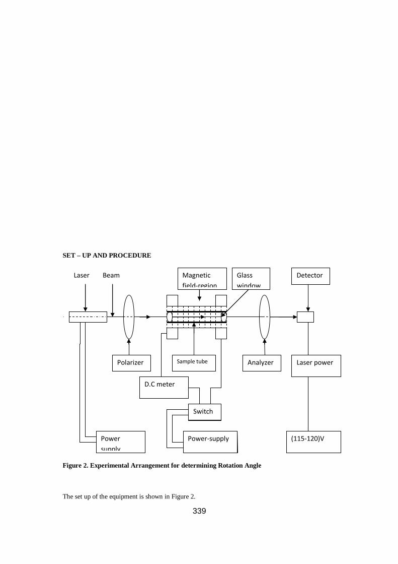
339

SET – UP AND PROCEDURE

Figure 2. Experimental Arrangement for determining Rotation Angle

The set up of the equipment is shown in Figure 2.

Polarizer Sample tube Analyzer

Laser Beam

Power-supply Power

supply

D.C meter

Volt/Ampere

Switch

Magnetic

field-region

Glass

window

(115-120)V

Power-supply

Laser power

Meter

Detector

340

The analyzer, polarizer, sample holder, laser and the head sensor of the laser power meter were fixed

on the optical bench using clamps (which were strongly fixed to avoid any change of position during

the experiment). The laser beam was directed to pass through the centres of the polarizer, sample and

analyzer thus all these were at the same height.

The head sensor was adjusted from time to time to be in line with the beam transmitted through the

sample because the beam kept on being rotated. The sample container was thoroughly cleaned with

liquid soap to remove any stain along its walls and then properly dried with blotting paper.

One end of the container was closed with a lid leaving the other end open purposely for the container to be inserted in the hole through the hub of the coil framework.

After inserting the sample container in the hub, the coil and container were positioned on a table

in such a way that the open end of the container faced directly vertically upwards while the

closed end rested on the table.

The sample was poured in the container and the open end was closed.

The coil into which the sample holder was inserted (as shown in the diagram) was symmetrically

and centrally fixed in its support which was firmly fixed on the optical bench.

Without d.c. magnetic field, the beam was directed through the sample and the angle at which minimum irradiance Imin occurred was determined for each vegetable sample.

It was found that oils suitable for human consumption there cut–off angle c was equal to cut-off

angle for water w.

However, if oil is contaminated or expired the cut-off angle is different from w. Then, the rotation caused by impurity concentration in the sample is given by

A = - w

The solenoid current was varied to change the magnetic field which consequently changed the

angle of rotation for oil suitable for human consumption to.

The angle of rotation due to application of d.c. magnetic field is obtained as the

Difference between two angles i.e. = – c

For each sample a graph of angle against current I was plotted and the angle the angle of

rotation per unit current i.e. I

for each oil sample was obtained.

RESULTS

In this section results are presented starting with graphs (temperature versus time) used to determine

calorific values, the angle of rotation versus current and lastly a graph of angle of rotation per unit

current versus calorific values of the oils.

341

Figure 3: Graphs of Temperature against Time for Vegetable Oils from Mukwano

Group of Companies

Table 1: Showing Calorific values of vegetable oils from Mukwano Group of Industries

Type of vegetable oil Calorific value in (kJ/kg)

Corn Oil 39,555

Sunflower Seed Oil 43,011

Fully refined Palm Olein + Sunflower

Seed Oil

45,161

Fully refined Palm Olein 46,276

The results show that Fully refined Palm Olein is superior to the three types, followed by Fully

refined Palm Olein + Sunflower Seed Oil, then Sunflower Seed Oil and the lowest calorific value is

found in Corn Oil.

0

1

2

3

4

5

6

0 2 4 6 8 10 12 14 16 18 20

Time (min)

Tem

p (

deg

C)

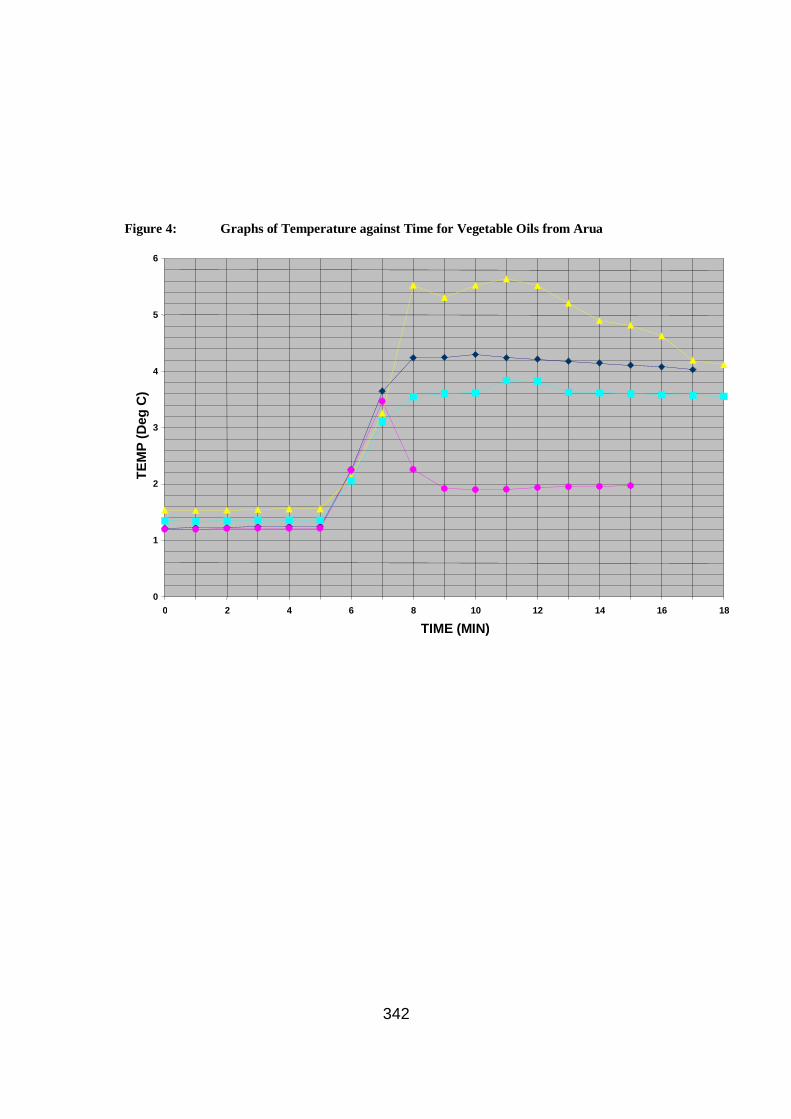
342

Figure 4: Graphs of Temperature against Time for Vegetable Oils from Arua

0

1

2

3

4

5

6

0 2 4 6 8 10 12 14 16 18

TIME (MIN)

TE

MP

(D

eg

C)

343

Figure 5: Graphs of Temperature against Time for Vegetable Oils from Tororo

0

0.5

1

1.5

2

2.5

3

3.5

4

0 2 4 6 8 10 12 14 16 18

TIME (MIN)

TE

MP

(D

eg

C)

344

Figure 6: Graphs of temperature against time for Vegetable Oils from

Bidco

The calorific values of three samples of mineral oils were also determined for the sake of comparison,

that is, to see the difference between calorific values of mineral oils and vegetable oils

0

0.5

1

1.5

2

2.5

3

0 2 4 6 8 10 12 14 16 18 20

Time (min)

Tem

p (

deg

C)

345

Figure7: Graphs of temperature against time for diesel from Jinja, and for Petrol and

Kerosene from Kampala.

Table 2: Calorific values of mineral oils

Type of mineral oil Calorific value (kJ/kg)

Petrol 46,239

Diesel 45,624

Kerosene 34,998

Figure 8: Graphs of angle of rotation against current for vegetable oils from Mukwano

Group of Companies

0

0.5

1

1.5

2

2.5

3

3.5

4

4.5

0 2 4 6 8 10 12 14 16

TIME (MIN)

TE

MP

(D

eg

C)

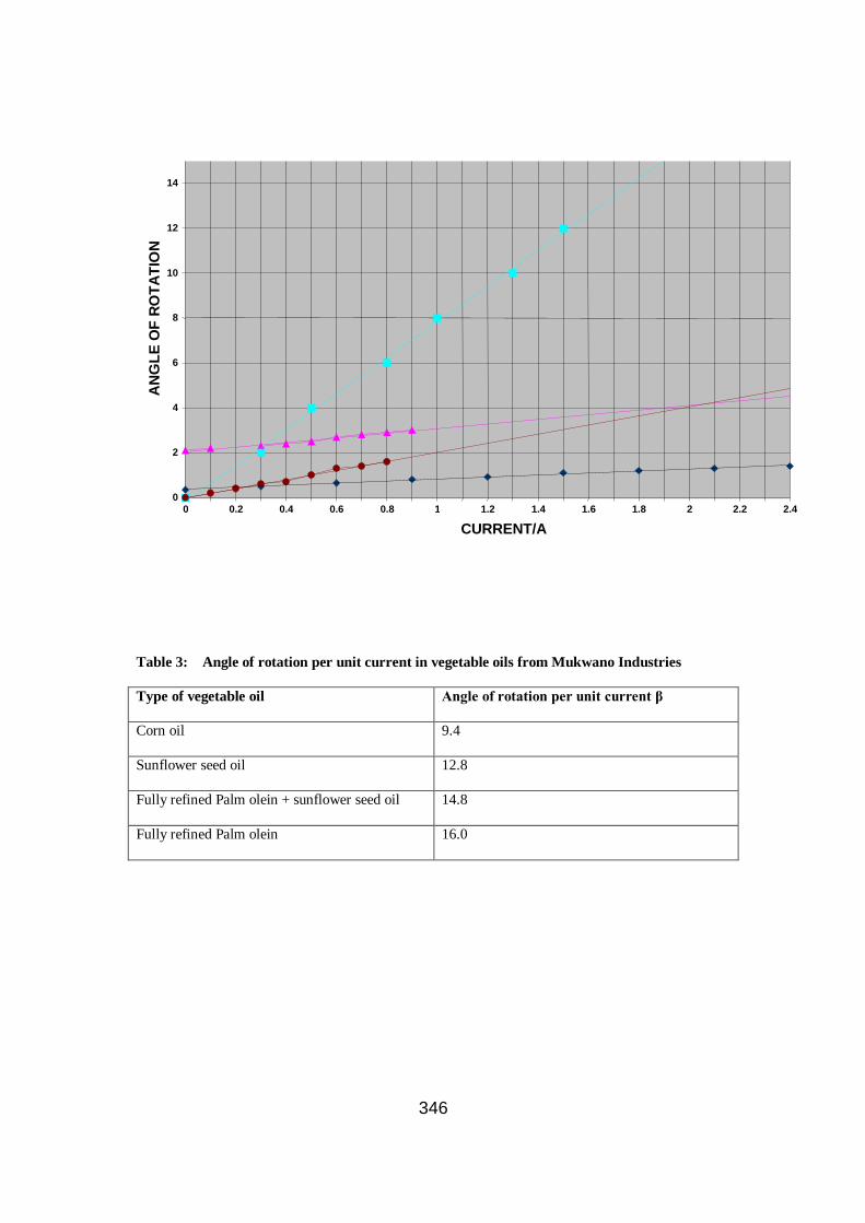
346

Table 3: Angle of rotation per unit current in vegetable oils from Mukwano Industries

Type of vegetable oil Angle of rotation per unit current β

Corn oil 9.4

Sunflower seed oil 12.8

Fully refined Palm olein + sunflower seed oil 14.8

Fully refined Palm olein 16.0

0

2

4

6

8

10

12

14

0 0.2 0.4 0.6 0.8 1 1.2 1.4 1.6 1.8 2 2.2 2.4

CURRENT/A

AN

GL

E O

F R

OT

AT

ION

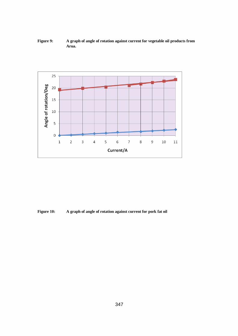
347

Figure 9: A graph of angle of rotation against current for vegetable oil products from

Arua.

Figure 10: A graph of angle of rotation against current for pork fat oil

348

Fig 11: A graph of angle of rotation against current for cooking oil from Bidco.

349

Figure 12: A graph of Angle of Rotation against Current for Expired Palm Seed Oil

Sample

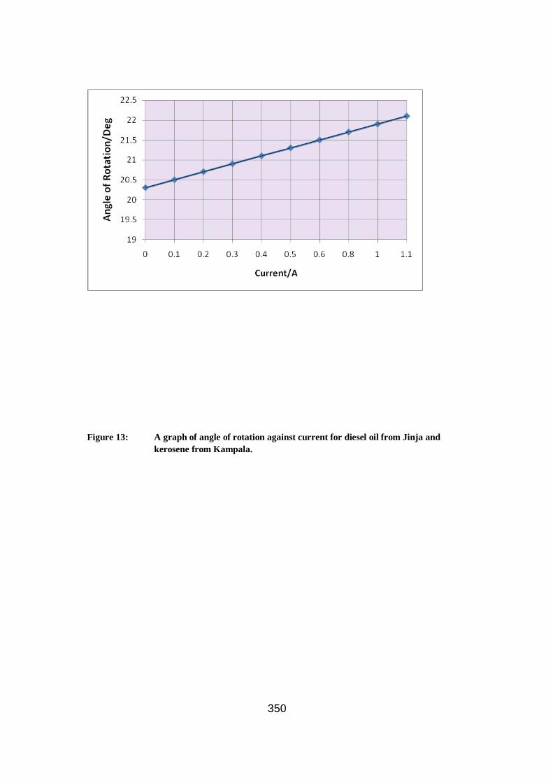
350

Figure 13: A graph of angle of rotation against current for diesel oil from Jinja and

kerosene from Kampala.

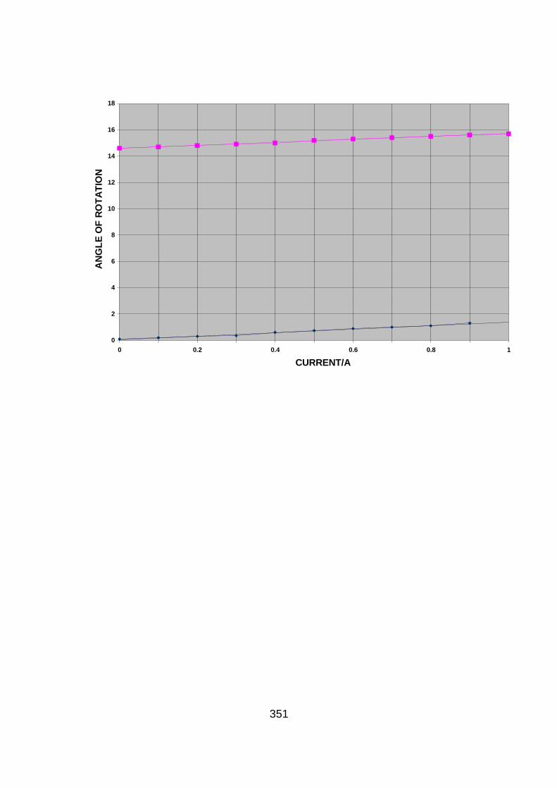
351

0

2

4

6

8

10

12

14

16

18

0 0.2 0.4 0.6 0.8 1

CURRENT/A

AN

GL

E O

F R

OT

AT

ION

352

Figure 10: Rotation β per unit current Vs Calorific values in x 108 J/kg

DISCUSSION OF RESULTS

It was observed that the calorific values of both vegetable and mineral oils lie in the range of 35.0 to

48.2 MJ/kg. It was noted also that kamura oil from Arua has the highest vegetable calorific value of

47.2 MJ/kg followed by groundnut oil from the same area with 46.9 MJ/kg. Groundnut oil from

Tororo had a calorific value of 45.7 MJ/kg.

The results also show that kamura oil from Arua has the highest rotation per unit current β

Of 16.30 followed by groundnuts oil from Arua with 15.70. A plot of rotation angle per unit current β

against calorific value gave a straight line graph given by the equation

353

5.25781.8 xy

CONCLUSION

The results show a good linear relation between calorific value and the angle of rotation per unit

current. This technique is a potential method for designing an instrument that can be used to

determine calorific values of transparent oils using Faraday Effect.

ACKNOWLEDGEMENT

The group is highly indebted to Research Grants and Publications Committee of Kyambogo

University that sponsored this project. The team is very grateful to the Manager of Mukwano

Industries, the Cottage Industries of Tororo and Arua for providing them with samples for analysis.

We express heartfelt thanks to the team of experts of Chemistry Department of Makerere University

whose cooperation made it possible to obtain the measurement of calorific values.

We are also grateful to the Physics Department Makerere University for assisting us with their optical

bench and other components that enabled the team to obtain measurements of the angle of rotation β

per unit current.

Last but not least, we thank very much the\Department of Physics Kyambogo University for their

cooperation and encouragement while undertaking this study.

354

REFERENCES

Cussons G. Instruction Manual for Bomb Calorimeter P6310 Cussons Ltd U.K.

Dra S.S. 1991 A text book on Experiments and Calculations Engineering Chemistry S. Ghana &

Co. Ltd, Ram Nagar Delhi – 110055.

Konnen G. P. and Berling G. A. 1985 Polarized Light in Nature Cambridge University Press.

Kyaruzi V. K. 1980. Nutrition in East Africa. A Manual for Teachers and Others . Longman

KenyLtdNairobi, Kenya

Longhurst R. S. 1973 Geometrical and Physical Optics 3rd Ed. Longman Group Ltd. NewYork,

USA.

Moline IL 1960 Instruction for the 1341 Plain oxygen Bomb Calorimeter Parr Instrument Ltd. U.K.

Mucunguzi-Rugwebe E. R. R. 2000 Optical Activity and Faraday Effect in some Mineral and

Vegetable Oils. Ph.D Dissertation Makerere University Kampala – Uganda.Mugalu S 2009. Private

Communicaction, Biological Science Department, Kyambogo University P. o. Box 1, Kyambogo

Kampala – Uganda Pye D. 1992 Polarised Light in Science and Nature 3rd Ed. Institute of Physics

Publishing London UK.

Sears F. W. 1990 University Physics 6th Ed. Addison Wesley Publishing Company USA

Shoemaker D.P., Garland C.W. and Nibler J. W. 1996. Experiments in Physical Chemistry 6th Ed. Pp

152-158 McGraw-Hill New York.

Sime R. J. 1990 Physical Chemistry; Methods, Techniques and Experiments pp

420-431 Saunders, Philadelphia, PA.

355

FINANCIAL SERVICES

DEBT FINANCING AND RETURN ON EQUITY

A CASE OF LARGE CORPORATE TAXPAYERS IN UGANDA

BY

ROBINAH AKODO

Assistant Director

Makerere University Business School

arobinah@yahoo.com

ABSTRACT

This study examined the relationship between debt equity ratio and return on equity for large

corporate taxpayers in Uganda. It addresses the question of whether debt financing magnifies return

on equity. The research also established the capital structure of large taxpayer companies and

confirms that the theories on the advantages of debt financing are true in a developing economy like

Uganda. It was established that all sectors under study employed debt in their capital structure during

the study period and they had a positive correlation (r = 0.322, p-value <0.05) between debt equity

ratio and return on equity. Sector by sector analysis showed that the Manufacturing sector had the

strongest relationship between debt equity ratio and return on equity (r = 0.835, p-value <0.05) and

the Construction sector had the weakest correlation between debt and equity (r = 0.128, p > 0.05)

Construction sector had a high probability of leverage chance (r = 0.76). Empirical evidence shows

that debt financing improves return on equity. The findings for all the sectors were in line with the

theory that debt financing magnifies shareholders‘ return.

356

Keywords: Debt financing, Return on Equity, Uganda

357

Background to the Study

Many firms use debt as a major source of financing. A research by Booth et al., (2000), on 5,281 firms in Europe,

Asia and USA revealed that the debt to equity ratio ranged from a low of 30.3% in Brazil to a high of 73.4% in South

Korea.

In theory, the primary motive of a company using financial leverage was to magnify the shareholders‘ return Pandy,

(1997). According to Paranque (1992), the capitalization of a given firm closely connected to its return on equity and

that highly profitable slow-growing firms should generate cash and can finance their operations by internally

generated funds whereas less profitable fast-growing firms need significant external financing. Paranque and Pandy‘s

theories did not show the extent to which financial leverage could magnify shareholders‘ return; an aspect this

research sought to establish.

Divya et al (2011), in their study on Inside Debt and the Design of Corporate Debt Contracts found out that a higher

CEO relative leverage, defined as the ratio of the CEO's inside leverage (debt-to equity compensation) to corporate

leverage, was associated with lower cost of debt financing and fewer restrictive covenants. Additional analysis on a

sample of new public bond issues also showed a negative relation between CEO relative leverage and bond yield

spread. The evidence supports the notion that debt holders recognize the incentive effects of executive debt-like

compensation and adjust the terms of corporate debt contracts accordingly.

Hull (2011), in his non empirical study of Debt-equity decision-making with and without growth attempted to instill

knowledge and skills to students when making debt-equity and plowback-payout choices.

According to Nadeem (2011), empirical study of firms in manufacturing industry of Pakistan, suggested that

profitability, liquidity, earnings volatility, and tangibility (asset structure) are related negatively to the debt ratio,

whereas firm size was positively linked to the debt ratio. Non-debt tax shields and growth opportunities do not appear

to be significantly related to the debt ratio. The findings of this study are consistent with the predictions of the trade-

off theory, pecking order theory, and agency theory which showed that capital structure models derived from

Western settings does provide some help in understanding the financing behavior of firms in Pakistan.

Govindasamy (2010), Leverage‖ – An Analysis and its Impact on Profitability with Reference to Selected Cement

Companies in India, established that the leverage, profitability and growth are related and the leverage has impact on

the profitability of the firm.

Abimbola (2004), a test of the endogenous relationship between financial leverage and bank debt‘s use in the UK

indicated that industry classification has a significant effect on reliance on bank debt. Although firms that used bank

debt seemed to have higher agency cost potential than firms that did not use debt, long term leverage does not have a

significant relationship with long term bank debt‘s use in the evidence. But total leverage has a significant positive

relationship with total bank debt‘s use. It appears that banks give only more short term debt, but not more long term

debt, to their borrowers than other lenders. It also appears that the firms observed used long term and short term bank

debt for different purposes.

Molina (2005), in the study are firms underleveraged found out that the leverage's effect on ratings was three times

stronger if the endogeneity of leverage was ignored. This stronger effect results in a higher impact of leverage on the

ex ante costs of financial distress, which can offset the current estimates of the tax benefits of debt.

358

Elliott et al. (2007), "Target debt ratios: The impact of equity mis-pricing‖ reported that portion of variance was

caused by two factors. First, firms faced a ‗hard‘ boundary when over levered. This was due to the present value of

bankruptcy costs increasing at an increasing rate. These firms will adjust towards a target debt ratio more rapidly than

under leveraged firms which face a ‗soft‘ boundary. Second, if a firm‘s equity was mis-priced, the cost of issuing

equity may be reduced /increased.

Elliott at el. (2008), ―Target Debt ratios: differential rates of adjustment and market timing‖. The findings were

robust to various means of measuring leverage and mis-pricing.

Nishat (2000), ―The Systematic Risk and Leverage Effect in the Corporate Sector of Pakistan,‖ indicated that the

debt-equity ratios across industries are higher throughout the study period, except for a few industries like tobacco

and vanaspati and allied. The returns and risk relationship with the hypothesis that leverage causes a change in the

volatility of stock returns.

Jiming et al. (2010). The Impact of Debt Financing on Firm Investment Behavior: Evidence from China‖ established

that there was a negative relation between debt financing and investment behavior in both firms with low-growth

opportunities and high-growth opportunities and a negative effect was more significantly stronger for firms with low-

growth opportunities than those with high-growth opportunities.

Secondly, there was a positive relation between debt financing and investment behavior in firms with mid growth

opportunities and operating performance.

Thirdly, for the state-owned holding companies, there was a positive relation between the scale of investment and

debt financing; while a negative relation between investment and debt financing exists in non-state-owned holding

companies.

Chava. S., & Micheal R. R. (2008). ―How Does Financing Impact Investment? The Role of Debt Covenants.‖ Found

out that Capital expenditures declined by approximately 1% of capital per quarter in response to covenant violations

with a 13% decline relative to the pre-violation level of investment. Additionally, this decline concentrated among

firms in which agency and information problems were relatively more severe. Thus, the results highlighted how the

state-contingent allocation of control rights mitigated investment distortions arising from financing frictions.

Cîrciumaru, et al., (2010), study on the return on equity for the Romanian industrial companies found out that there

were positive relationships between study variables; Operating margin, Total assets turnover (Efficiency of Assets)

and leverage as independent variables positively affected ROE.

Adamia et al, (2010), The Leverage Effect on Stock Returns, Indicated that returns were decreasing in firm leverage.

Their study tested the relationship empirically with other risk factors and found that the results remained robust.

Further their results showed that leverage was a firm characteristic that loads on a risk factor. This suggested that

leverage should be priced as a risk factor and required adequate incorporation into common asset pricing models.

The leverage effect on monthly returns for all three models was negative and significant although very small. Thus it

remained negative and significant when other risk factors such as tax-rate and industry concentration were added.

When their study used leverage as sole explanatory variable and estimate returns with the CAPM the results still

indicated a negative and significant relation between leverage and returns.

In trading, when a firm employs debt in its capital structure, it has to pay fixed charges on the debt regardless of the

firm‘s income generating capacity. There was a risk of making low profits or even losses and faced liquidation when

the expected return on investment fell short of the cost of borrowed funds. However, management of business

enterprises usually enter into loan covenants using financial projections that assume favorable or optimistic economic

conditions and hope that the fixed charge on debt remain lower than the firms‘ expected rate of return on capital

employed and as such project higher returns on equity.

In a developing economy like Uganda, there was no guarantee for the prevalence of favorable economic conditions.

The liberalization of the economy and subsequent economic reforms in Uganda since 1986 exposed the economy to

359

both local and foreign competitions. For example Celtel, a mobile telephone company pioneered the introduction of

mobile phone services in Uganda. Shortly after MTN joined the market and discounted call charges, monthly

subscriptions and sold handsets at tremendously reduced price compared to that of the competitor. Uganda telecom

and other networks joined the market and also offered substantial discounts for the use of their networks. In addition,

Uganda eased its tariff barriers; however, non-tariff barriers remained non-transparent and inconsistent. For example

bureaucracy was non transparent, inconsistent and subject to corruption. Corruption has remained pervasive and the

most serious impediment to advancing Uganda‘s overall economic freedom. Load shading of power, poor feeder

road network, political interference, poverty and other factors were the major encumbrance to productivity and

profitability of various sectors of the Ugandan economy.

Statement of the Problem

Capital structure theories depict debt financing as a double-edged sword. That is, it is the cheapest source of capital

when a firm has income generating capacity to meet the debt obligations but when the return on capital slips below

the cost of debt, business will make losses and may gradually be liquidated on failure to meet the debt obligations.

The theories on debt financing were developed premised on developed country case scenarios. It is not clear whether

debt-financing effects are relevant and true in a developing economy like that of Uganda. This study set out to

establish the relationship between debt equity ratio and return on equity for the targeted sectors of the study.

Purpose of the Study

The study set out to establish the relationship between debt equity ratio and shareholders‘ return for various business

sectors in the Ugandan economy.

Objectives of the Study

The following were the major objectives of the study:

a) To establish the capital structure of the two large tax paying business entities in Uganda.

b) To establish the effect of leverage chance and leverage risk on return on equity of the two sectors of large

taxpayers.

c) To examine the relationship between capital structure and return on equity.

Research Questions

The study focused on answering the following questions:

a) What is the capital structure of the two large corporate taxpaying entities in Uganda?

b) What is the effect of leverage chance and leverage risk on return on equity of the study population?

c) To what extent does debt financing magnify shareholders‘ return on equity in Uganda?

The conceptual framework

The researcher has discussed research findings in the subsequent chapters based on the conceptual framework as

follows:

Fig.1 Conceptual Framework (adapted from Du Pont Model)

360

Leverage Effect

The common and direct ratio for calculating a firm‘s return on equity is the ratio of retained earnings to owner‘s

equity.

However, the Du Pont‘s model (http://www.uic.educ) decomposes the ratio as a function of three factors; the firm‘s

profitability, assets turn over and leverage summarized as:

Profit Margin X Asset Turnover X Leverage = Return on Equity

Profit Margin = Net income/Net Sales

Asset Turnover = Net Sales / Average Total Assets

Leverage = Average Total Assets/Average Owner‘s Equity

Profit margin shows the percentage of each shilling in sales that result in net income, asset turn over measures how

efficiently assets are used to generate sales and the leverage indicates how the assets used in generating sales are

financed. Leverage shows that the firm is entirely equity financed and higher ratio indicates a higher leverage. The

Du Pont model return on Equity decomposition formed a basis for the choice of the independent variables in this

study.

Significance of the Study

The findings will benefit the following:

Shareholders

The study will enable shareholders to appreciate the contribution of debt financing to the return on their funds.

It will enable them examine those sectors that give a higher return on equity for a given combination of debt and

equity.

Managers of business enterprises

The study will enable managers to ascertain proportion of debt that has a high contribution to the shareholders‘ funds.

Debt/Equity

Ratio

Return on

Equity

Leverage Chance

Leverage risk

Interest cost

Return on capital Employed

361

It will provide information on the various costs associated with debt financing and also provide a guide for the choice

of capital structure for certain business sectors.

The study will provide management with information about which sector is best suitable for equity financing, debt

financing or a mixture of debt and equity and in what proportions.

Tax Administrators

The study will provide a basis for assessing the earning capacity of equity holders in the various

business sectors.

Scope of Study

The scope of the study was in terms of geographical scope, subject matter and time.

Geographical Scope

The study covered a sample of 43 large taxpaying companies in construction and manufacturing in Uganda that

submit financial statements to Uganda Revenue Authority at Crested Towers Kampala.

The major reasons for choosing Large tax paying companies was that their business operations were centrally

monitored by the Large Tax payer Unit of the Uganda Revenue Authority and their financial statements were

prepared by reputable audit and accounting firms like Price Water House Coopers, Ernest and Young, KPMG; and

the large taxpayers were frequently audited or monitored by Uganda Revenue Authority.

Subject Matter

The study aimed at finding out:

(a) The composition of capital structure of the selected companies

(b) The relationship between return on equity and the various combinations of debt and equity for the

selected companies.

Time

The study covered a period of 11years (2000-2010).

Literature review

Relevant materials drawn from various sources for the researcher believes that any literature related to debt financing

and return on equity regardless of the time or place may still be substantial to provide a good basis upon which the

findings of the study may be based. It was reviewed along the major theme of the topic: debt financing and return of

equity under which sub themes like leverage chance and leverage risk were discussed.

Debt and Equity

Theories on proportions of debt and equity in the capital structure of business enterprises were developed and the

relevancy of some of the theories was studied.

Modigliani and Miller (1958) theorized that the capital structure of a firm does not affect its value. They illustrated

and justified their theory by holding the weighted average cost of capital constant and assumed perfect capital

markets, absence of corporate taxes, easy classification of firms into equivalent returns and that the expected values

of the probability distributions of operating earnings for all future periods are the same as present operating earnings.

The Modigliani and Miller (MM) theory was based on ideal assumptions that do not exist in many countries. For

example in Uganda corporation tax (30% for resident and 25-45% for mining companies) is existent and compulsory.

Average cost of capital cannot remain constant because most financial institutions practice price discrimination by

362

categorizing their clients into corporate clients and non-corporate clients and charge different rates of interest on

borrowed funds

The MM theory did not put into perspective the reaction of lenders as capital shifts from equity to debt, a factor

Smith and Watts (1992) examined and established that when capital structure shifts from equity to debt, lenders

restrict borrowers in the usage of working capital, capital expenditure for fixed assets and equity re-evolvements. By

focusing on the value of a firm, which is market value of stock outstanding plus market value of debt outstanding

Van Horne (2002) Modigliani and Miller mainly concerned themselves with one entity, the firm. The firm as an

entity has a number of stakeholders who share in its value namely, shareholders, the public, the government,

employees among others. It is not clear whether the shareholders‘ value increases proportionately and whether the

theory is relevant in Uganda.

This study focused more on what happens to the value of shareholders as the proportions of debt and equity in the

capital structure vary.

Other theories or models reviewed are the capital asset pricing model (CAPM), According to

Investopedia (2011), CAPM describes the relationship between risk and expected return and used in

the pricing of risky securities.

―Fama-French three factor model and the Fama-French plus Carhart four factor model from other

studies on; Stock returns for each company calculated monthly, using the percentage change in

consecutive closing prices adjusted for dividends, splits and rights issues (Fama et al. 1969), then

estimates of abnormal returns in excess of the risk free rate using Sharpe (1964)‘s Capital Asset

Pricing Model, Fama-French (1993) model and Carhart (1997) model‖.

Divya et al (2011), in their study on Inside Debt and the Design of Corporate Debt Contracts found out that a higher

CEO relative leverage, defined as the ratio of the CEO's inside leverage (debt-to equity compensation) to corporate

leverage, is associated with lower cost of debt financing and fewer restrictive covenants. Additional analysis on a

sample of new public bond issues also shows a negative relation between CEO relative leverage and bond yield

spread. The evidence supports the notion that debt holders recognize the incentive effects of executive debt-like

compensation and adjust the terms of corporate debt contracts accordingly.

Hull (2011), in his non empirical study of Debt-equity decision-making with and without growth attempted to instill

knowledge and skills to students when making debt-equity and plowback-payout choices.

According to Nadeem (2011), empirical study of firms in manufacturing industry of Pakistan, suggested that

profitability, liquidity, earnings volatility, and tangibility (asset structure) are related negatively to the debt ratio,

363

whereas firm size was positively linked to the debt ratio. Non-debt tax shields and growth opportunities do not appear

to be significantly related to the debt ratio. The findings of this study are consistent with the predictions of the trade-

off theory, pecking order theory, and agency theory which showed that capital structure models derived from

Western settings does provide some help in understanding the financing behavior of firms in Pakistan.

Govindasamy (2010), Leverage‖ – An Analysis and its Impact on Profitability with Reference to Selected Cement

Companies in India, established that the leverage, profitability and growth are related and the leverage has impact on

the profitability of the firm.

Hasanhodzic J.&Lo. A. W., (2010). In their study of sample of all-equity financed companies from

January 1972 to December 2008, found out that the leverage effect were just as strong if not stronger,

implying that the inverse relationship between price and volatility was not based on leverage, but was

more likely driven by time-varying risk premia or cognitive mechanisms of risk perception.

Riddiough (2004), in a study of optimal capital structure articulated the economics underlying the market for outside

finance in commercial real estates and established that mortgage debt is typically the optimal form of finance as it

economizes on transaction costs and provides proper incentives for the property owners. An inside equity-outside

mortgage financing maximizes comparative advantage. He concluded that for commercial real estate, debt financing

was cheaper than equity.

However, his study did not involve numerical figures to show the contribution of debt financing to shareholders. His

focus was mainly on how to determine the optimal capital structure for one form of business: commercial real estate

business.

The current study considered two sectors, establish their capital structure, and then analyze its relationship with

return on equity.

Brounen and Eichholtz (2001), examined the stock price reaction on announcements of additional equity and debt

on European property companies‘ capital offerings. They established a positive reaction on employing more debt

than equity as a result of perceived tax shield benefit from debt financing. The study justified the use of more debt

than equity in an environment were capital markets are perfect.

However, it‘s not known whether the same results are true for unlisted companies operating in an environment of

developing imperfect capital markets as in the case of Uganda.

Theory on debt financing

The advantage of debt financing in taxation of business enterprises is that interest payments are tax deductible.

They elude taxation at the corporate level, whereas dividends or retained earnings associated with stock are not

deductible for corporation tax purposes. Debt financing improves the total amount of payments available for

stockholders Van Horne (2002)).

Pandy (1997), states that the role of debt financing is to magnify the shareholders‘ return. The assumption that the

fixed charge funds are obtained at a cost lower than the firm‘s rate of return on the assets was the basis for the

magnifying impact of debt financing.

Julius Kakuru (2000), observed that whereas debt could be beneficial especially in times of economic boom,

excessive debt financing will mean that business enterprises have high interest obligations and the burden of

repayment of principle amounts periodically.

364

Firms enter into agreements to borrow funds with a view of boosting their capital base, asset turnover and to enable

the company expand its operations.

Debt financing was desirable when cost was lower than the expected rate of return on investment.

Elliott, B., W., Koëter-Kant, J., & Warr. R., S. (2008) found out that the average book debt ratio for

all firms was about 23%, compared to a market debt ratio of approximately 28%. On average, sample

firms had earnings 6.7% of assets, before interest and taxes.

Omole D. A.,and Falokun. G. O., (1999), indicated that there was a link between interest rates and the

corporate financing strategies and the profitability of firms. It also revealed that interest rate

liberalization had a link with the growth of the equity markets. On sectorial analysis, their study

indicated that the interest rate liberalization does not seem to have similar effects on all the

investigated quoted companies

Leverage Chance and Leverage risk

Pandy (1997), states that debt financing provides a potential of increasing shareholders‘ earnings only when the

interest rate charged on borrowed funds was less than the rate of return on assets financed by debt. When the rate of

return falls below the cost of borrowed funds, the firm stands a risk of making a loss. Risk adverse managers, under

such circumstance, opt for increased equity financing.

Pandy (1997) gave numeric illustrations of how debt financing increases shareholders‘ return for constant earnings

before interest and tax (EBIT) and for a varying EBIT. However, the values used were not for specific firm or

industry.

The study used data from financial statements of business enterprises for specific sectors in Uganda, examined the changes

in return on equity, and established that sector that had the highest or lowest potential of maximizing shareholders‘ return

from assets financed by debt.

Volatility risk alone predicted 50% of credit default swap CDS spread variation, while jump risk

alone forecast was 19%. After controlling for credit ratings, macroeconomic conditions, and firms‘

balance sheet information, explained 77% of the total variation. Moreover, the marginal impacts of

volatility and jump measures increased dramatically from investment grade to high-yield entities. The

estimated nonlinear effects of volatility and jumps were in line with the model implying that there

was a relationship between equity returns and credit spreads (Benjamin Yibin Zhang, Hao Zhou,

Haibin Zhu 2005).

The corporate level taxes decreased the effect of leverage on the cost of equity and personal tax

disadvantage of debt did not have a significant effect. Firms‘ capital structure choices related with

corporate and investor level taxes in a predicted manner. Dhaliwal D, Heitzman. S. & Li.O. Z. 2005.

Bandi. F. M., Bandi & Ren`o. Roberto (2009), Kernel estimate of leverage effects had asymptotic

sampling distributions which crucially depended on the features of objects that are fundamentally

hard to pin down, namely the probability and size distribution of the individual and joint

discontinuities in the return and volatility sample paths. Their study focused on the nature of

365

dependence and its implications, while providing tools for feasible identification of (potentially time-

varying) leverage effects under mild parametric structures and weak recurrence assumptions. It

empirically showed that, for stock index futures, stronger leverage effects are associated with higher

volatility regimes that economically important time-variation in leverage with more negative values

associated with higher volatility levels.

According to The Journal of Finance (2000), a study on Boeing, Intel, Pacific gas and Electric, RJR Nabisco and Safe

Way for the period (1983-1993) indicated that large liquid and profitable collateralized firms with low expected costs

of distress and small research expenses had the largest tax benefits arising from debt financing. Firms below average

growth opportunities had larger benefits than growth firms.

Taylor (2001) analyzed the impact of debt financing on return on equity where he used an example of an

entrepreneur investing in a machine worth $250,000 to generate an expected profit of $75,000. In his analysis, if the

investment were financed 100% equity, the return on investment would be 30%. In addition, if the entrepreneur used

50% debt at an interest of 12%, the rate of return on investment remained 30% but the rate of return on equity

increases to 48%. He considered an increase in the interest rate while holding expected profits constant and

established a negative rate of return on equity.

Taylor‘s analysis assumed absence of corporation tax and did not take into account capital allowances the firm would

enjoy.

In Uganda firms that bring into use eligible property for the first time during the year of income, enjoy initial capital

allowance at the rate of 50%, 70% or 20% of the cost base (Section 29 of Income Tax Act 1997 and Sixth Schedule)

depending on the location of the investment. In chapter four, the study considered earnings after corporation tax. The

study did not investigate whether the tax shield advantage was applicable in Uganda.

Capital structure and Return on Equity

Cohen (2004) in his illustration of the effect of Modigliani and Miller theorem on capital structure used simplified

financial statements and arrived at a generic conclusion that as the ratio of debt to equity in the capital structure of the

firm increases, return on equity also increases. He assumed constant earnings before interest and tax (EBIT), and a

constant cost of capital for all periods. In practice, EBIT cannot be constant within a firm or industry. Different firms

apply different accounting policies for example in the computation of depreciation of fixed assets. The rates and

method of calculation vary from firm to firm. Operational expenses and sales volume may vary in response to

changes in economic factors of a given country.

In this study, empirical data from financial statements of business enterprises in Uganda was used to establish

whether the same relationship as in Cohen‘s conclusion exists.

McDonald (2004) examined a number of factors that drive return on equity. He examined in detail profit margins of

Corporate America in relation to the lowest long term interest rates, inflation rate and return on equity, Just in Time

inventory management and turnover, restructuring and accounting charges (using Dow Jones Industrials) and return

on equity.

However, on the part of the effect of leverage on return on equity he did not illustrate but stated the factors that can

deplete equity and attract a high leverage.

366

The study provided details establishing the extent to which leverage drives return on equity.

At http://partners.financenter.com, retrieved on 16/9/2005), financial leverage was analyzed considering an example

of varying debt-equity ratio and constant net sales. It was established that leverage magnifies return on equity.

However, in practice net sales differ over time for a given firm or within the industry as a result of changes in the

environment of business. This was put into consideration in this study.

METHODS AND MATERIALS

Research Design

The purpose of this study was to establish the relationship between debt financing and return on equity. A

longitudinal research design was used to analyze secondary data based on financial statements for the selected

corporate taxpayers in Uganda. The descriptive survey research design is a method of investigation in which self

report data collection from various samples of interest can be generated. Given the nature of the study, the researcher

needed to adequately describe the different combinations of debt and equity and the resultant return on equity.

Area and Survey Population

The survey population for the study was 99 large corporate taxpayers in Construction and manufacturing classified

by Uganda Revenue Authority and distributed as:

Table 1: DISTRIBUTION OF LARGE TAXPAYERS BY SECTOR

SECTOR CONSTRUCTI

ON

MANUFACTURI

NG

TOTAL

NO. OF TAXPAYERS (x) 18 81 99

Source: URA Large Taxpayer Register2010

Each sector represented a stratum and from each stratum sampling units proportionate to stratum size were selected

randomly.

Sample size and selection

Sample size determination

The researcher set confidence level at 95% and error term of ±1 such that from table1 and using the Z-distribution

tables, the sample size was determined using the formula

n = NZ2S

2 adopted from Krieger, (1999)

NE2 + Z

2S

2

367

Where

N = Total number of companies

Z = 1.96 (for 95% confidence interval)

E = 1

S2 = population variance

= Σ (xi-µ) 2

= 322 +31

2 + = 20

N 99

µ = 99 =50

2

n = 99*1.96 * 1.96 * 20 = 7606.368/175.832=43

99 *1 + 1.96 * 1.96 *20

Sample selection

Sample size of 43 was obtained using Simple random sampling.

The response rate was as shown in table 2 below;

Table2. NUMBER OF SAMPLE UNITS PER STRATUM

SECTOR CONS MAN TOT

Sample units) 5 20 25

Source: URA large tax payers register

Data collection

Research Instruments

The study used Uganda Revenue Authority Large Taxpayer registry document analysis, observation and taxpayer

profile schedules that served as questionnaires.

The URA staff working in the registry served as local agents through whom the information was collected.

Each staff was given taxpayer profile schedules detailing the specific fields of data records.

Source of Data

368

The study involved the use of secondary data from financial statements of the selected companies and

documents, textbooks and journals with data related to debt financing and return on equity.

Measurement of variable

Capital structure

The study used the ratio of total debt in the balance sheet to the total of ordinary share capital, retained earnings and

other equity instruments to determine debt/equity fraction for all sectors of study.

Imputed interest rates

This was obtained by dividing total finance costs excluding foreign exchange movements with total short term and

long term borrowed funds extracted from the balance sheets.

Return on equity

This was computed by dividing retained earnings for the year with ordinary share equity.

Leverage risk/ chance

Leverage risk and leverage chance were measured by comparing return on capital employed with imputed interest

rate. Leverage chance was measured by the excess of return on capital employed over imputed interest rate and

leverage risk was measured by the excess of imputed interest rate over return on capital employed.

Quality Control

Quality was ensured by collecting data from the two sectors of the population legible for the study using data

schedules and cross checked for completeness and accuracy of the data collected with that in the audited and

published financial statements specifically for those taxpayers such as Stanbic Bank, DFCU Bank, Uganda Clays,

BAT that were listed on the stock exchange.

Data schedules had a provision of coding each sample unit for purposes of editing the extracted data in the event of

incorrect data capture by the local agents.

Model specification and estimation

Expanding on Modigliani and Miller‘s (1958) Proposition II, abnormal returns are estimated using

the asset pricing models of Sharpe and Lintner (the traditional Capital, Asset Pricing Model, CAPM),

of Fama and French and of Carhart.

The estimated model ROE = a+b1 DER+b2LE

Where,

a = represents other factors other than Debt Equity Ratio and Leverage effect

b1= the regression coefficient of DER

b2 = the regression coefficient of Leverage effect.

DER = Debt equity ratio

369

LE= leverage effect

Data Analysis

The study used a combination of Microsoft Excel and SPSS for analysis. Microsoft Excel was used to capture the

financial statements and compute the Debt equity leverage and return on equity ratios. Figures or graphs showing

ratio trends were generated from the Microsoft Excel. Correlation and regression analysis were generated from SPSS

to determine the magnitude of the relationship between study variables and to fit the Debt financing model.

RESULTS/FINDINGS

Basis of categorization of firms in the sample

A total of 43 out of 99 large corporate tax payers in construction, manufacturing, oil industry, general trade, financial

services and those in other services other than financial services were selected for the study. For each company data

was extracted from financial statements for the period (2000 – 2010).

Uganda Revenue Authority defined the sectors adopted for the study in the year 1998 when Uganda Revenue

Authority set up the Large Tax Payer Department (LTD). Following the general restructuring of URA in (2005), the

Large Taxpayer Department was restructured to Large Tax payer Unit (LTU).

The study used the list of the Large taxpayer Department that was in use since the year 2000 with a distribution of the

large taxpayer companies distributed as follows:

Table 3 Distribution of Large Taxpayers

SECTOR

NUMBER OF

COMPANIES

SAMPLE SIZE

PER SECTOR

Construction 18 5

Manufacturing 81 20

TOTAL 99 25

Source: Large Tax Department tax payer List 2000-2010.

The Commissioner Domestic taxes, in-charge of the Large Corporate Taxpayers Unit, confirmed that the choice of

the selection of taxpayers into the LTD/LTU was based on annual tax contribution to URA over a period of at least

370

four years time. In light of the Commissioner‘s clarification on the criteria for selection of taxpayers into the large

taxpayer department, the sector distribution of large taxpayers in table 3 shows that few oil companies followed by

construction companies contributed large taxes to the central treasury.

Descriptive Analysis of findings

To answer the research questions and to achieve the objectives of this study, return on equity ratios, debt equity

ratios, return on capital employed, leverage chance/risk and imputed interest costs were calculated for Construction

and Manufacturing. The average ratios for the sectors understudy were used to generate line graphs to depict trends

of behavior of the study variables as in tables 4 to 5 and in figures 1 to 2 discussed in the subsequent sections of this

report.

It was established that firms in the two sectors of study employed debt financing in their capital structure as depicted

by the following bar graph.

The graph shows that the manufacturing sector had the highest debt proportion in its capital structure followed by the

construction sector.

The study also performed analysis of variance (ANOVA) to determine whether there were significant

differences among the various sample means for purposes of identifying those sectors that

experienced high or low variations in the study variable and subsequently provide a guide to the users

of this research to assess the two sectors in Uganda that were suitable for debt financing.

Table 4: MEAN FOR THE STUDY VARIABLES

Minimum Maximum Mean Std. Deviation

DEBT EQUITY .1211 .8900 .4324 .3014

LEVERAGE CHANCE RISK -.1430 .2030 .0272 .1081

IMPUTED INTEREST RATE .1166 .3052 .1902 .0451

ROCE -.0268 .3615 .2174 .1023

ROE -.1858 .3069 .1328 .1151

Source: URA-financial statements for selected large taxpayer companies 2000-2010

From table 4 and 5 the results were significant at 5% (α = 0.05). The computed values of F, in the F

column in table 5 and the critical values Fc in the footnote to table 5 revealed that the computed F for

ROCE, Imputed interest rates, debt equity ratio and leverage chance and leverage risk was greater

than the critical value of F. This implied that there was a significant difference between the means of

the study variables for each sector. However, the F test also showed that there were no significant

differences between ROE of the two sectors of the study (the computed F = 1.750 < Fc = 2.49)

371

Table 5: ANOVA FOR THE STUDY VARIABLES

SUM OF

SQUARES

MEAN

SQUARES

F-COMPUTED

SIG

ROCE

Between

groups

Within groups

Total

.381

.618

.999

0.07621

0.00172

4.436 0.003

ROE

Between

groups

Within groups

Total ROE

.010

.409

.509

0.00199

0.00114

1.750 0.148

IMP.

INT

RATE

Between

groups

Within groups

Total

.205

.008

.282

0.00410

0.00021

19.296 .000

DEBT/

EQUITY

Between

groups

Within groups

Total

297.676

19.267

316.943

59.535

.535

111.238 .000

Leverage

chance/leverage

risk

Between

groups

Within groups

Total

.536

.628

1.164

6.145 .000

Source: URA-financial statements for selected large taxpayer companies 2000-2010

Based on the analysis of variances (ANOVA) in table 5 the sector by sector analysis of the relationships between the

study variables and then performed overall analysis for all sectors.

Table 6 shows sample means for each study variable per sector. The highest variations were realized in the debt-

equity means with computed F = 111.238, p-value <0.05, compared to the critical F=2.49. Comparing the sector

means with the population means in table 4, the manufacturing sector controlled its debt equity ratio at an average of

0.0001 far below the industrial mean of 0.1773. Imputed interest rate, leverage chance and leverage risk and ROCE

with computed F-values of 19.296, 6.145 and 4.436 respectively registered significant variations in their means.

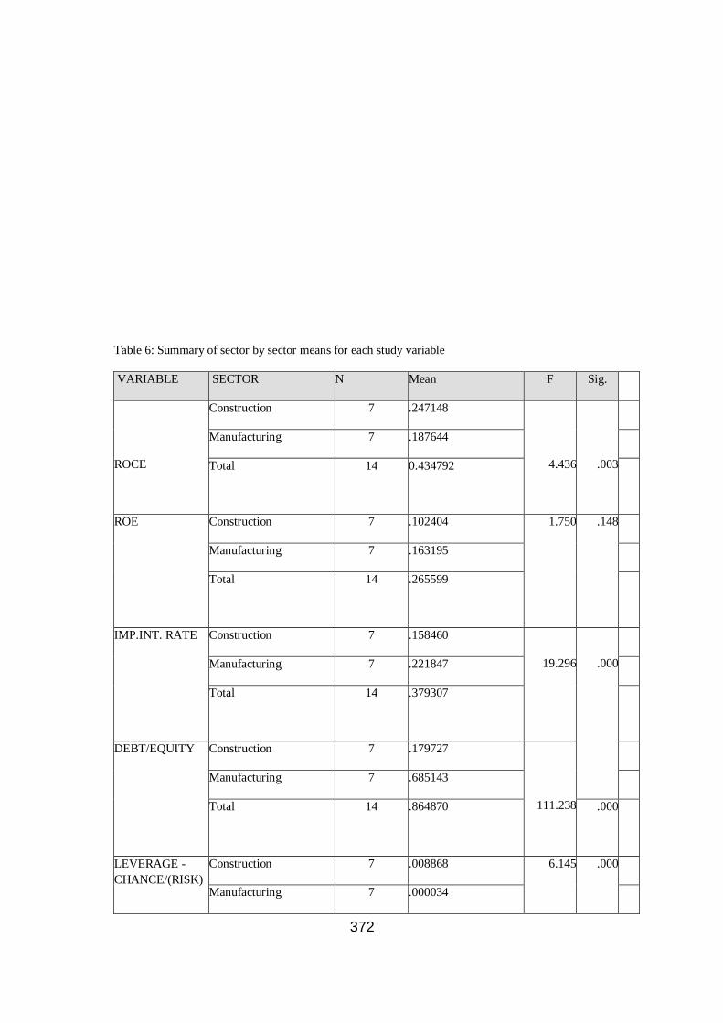
372

Table 6: Summary of sector by sector means for each study variable

VARIABLE SECTOR N Mean F Sig.

ROCE

Construction 7 .247148

4.436

.003

Manufacturing 7 .187644

Total 14 0.434792

ROE

Construction 7 .102404 1.750

.148

Manufacturing 7 .163195

Total 14 .265599

IMP.INT. RATE

Construction 7 .158460

19.296

.000

Manufacturing 7 .221847

Total 14 .379307

DEBT/EQUITY

Construction 7 .179727

111.238

Manufacturing 7 .685143

Total 14 .864870 .000

LEVERAGE -

CHANCE/(RISK)

Construction 7 .008868 6.145 .000

Manufacturing 7 .000034

373

Total 14 .008902

Source: URA-financial statements for selected Large taxpayer companies 2000-2010

Construction sector analysis

Average financial ratios for five construction companies for the years 2000 to 2010 were computed and summarized

as in table 7.

Source: URA -Construction company financial statements 2000-2010.

Capital structure of construction sector

Table 7 shows that debt to equity ratio was highest in 2002 at a rate of 24% and lowest in 2000 at 12%. Implying that

over 76% of the capital structure of large corporate taxpayers in the construction sector in Uganda in the period of

study was equity.

Capital structure and return on equity for construction sector

From table 7, return on equity was highest at 31% in 2001 in the construction sector when debt-equity ratio was at

20%. The return on equity was lowest at 14% in 2003 when debt equity ratio reduced to 15% respectively. This trend

is depicted by the line graphs in figure 4.1 that showed a general decline in return on equity as debt on equity

declined over the years (2000 -2010).

A correlation analysis revealed a positive relationship between debt equity ratio and return on equity (R = 0.125, p-

value > 0.05). This implied that as debt equity ratio increased in the construction sector during the period of study,

return on equity increased respectively.

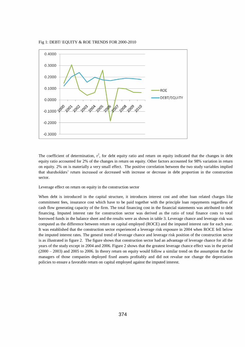
374

Fig 1: DEBT/ EQUITY & ROE TRENDS FOR 2000-2010

The coefficient of determination, r2, for debt equity ratio and return on equity indicated that the changes in debt

equity ratio accounted for 2% of the changes in return on equity. Other factors accounted for 98% variation in return

on equity. 2% on is materially a very small effect. The positive correlation between the two study variables implied

that shareholders‘ return increased or decreased with increase or decrease in debt proportion in the construction

sector.

Leverage effect on return on equity in the construction sector

When debt is introduced in the capital structure, it introduces interest cost and other loan related charges like

commitment fees, insurance cost which have to be paid together with the principle loan repayments regardless of

cash flow generating capacity of the firm. The total financing cost in the financial statements was attributed to debt

financing. Imputed interest rate for construction sector was derived as the ratio of total finance costs to total

borrowed funds in the balance sheet and the results were as shown in table 3. Leverage chance and leverage risk was

computed as the difference between return on capital employed (ROCE) and the imputed interest rate for each year.

It was established that the construction sector experienced a leverage risk exposure in 2004 when ROCE fell below

the imputed interest rates. The general trend of leverage chance and leverage risk position of the construction sector

is as illustrated in figure 2. The figure shows that construction sector had an advantage of leverage chance for all the

years of the study except in 2004 and 2006. Figure 2 shows that the greatest leverage chance effect was in the period

(2000 – 2003) and 2005 to 2006. In theory return on equity would follow a similar trend on the assumption that the

managers of those companies deployed fixed assets profitably and did not revalue nor change the depreciation

policies to ensure a favorable return on capital employed against the imputed interest.

375

Fig.2 LEVERAGE CHANCE AND LEVERAGE RISK TRENDS FOR

CONSTRUCTION SECTOR FOR THE PERIOD 2000-2010

A further analysis of leverage effect on return on equity using the ratios in table 7 revealed that at lowest imputed

interest rate of 12% in the year 2006, return on equity was 19% and at the highest imputed interest rate of 20% in

2003, ROE was 3%. This was a prima-facie demonstration that the higher the imputed interest the lower the ROE.

However, the study extended the analysis to cover other years in table 3. A correlation analysis of the study variables

revealed a positive relationship between leverage chance and leverage risk and return on equity (r = 0.76, p-value

<0.05). The coefficient of determination showed that the leverage effected accounted for 58% of the variations in

return on equity while other factors accounted for 42%. This analysis confirmed the double-edged sword theory of

debt financing. That is, shareholders would benefit from debt financing as long as the return on capital employed

remained higher than the imputed interest rate and vice versa.

The extent to which debt financing magnifies return on equity (ROE)

To assess the extent to which changes in debt /equity proportion affects the shareholders return, the researcher

performed a correlation analysis of debt equity ratio and return on equity and established that there was a positive

correlation between the two variables (r = 0.125, p-values > 0.05). However, the relationship was weak. That is, the

coefficient of determination, r2, demonstrated that changes in debt financing accounted for 2% of the changes in ROE.

This implied that 98% of the variations in return on equity for the construction company were accounted for by other

factors other than changes in debt to equity ratio during the period 2000 to 2010. Considering these results above, this

can be deduced that the mix of debt and equity in the capital structure in Uganda during the study period did not have

376

a significant magnifying effect on return on equity instead the rate at which the funds were borrowed and other factors

had a significant effect. These findings matched the Modigliani and Miller theory stated earlier in the literature review.

Manufacturing sector analysis

Financial statements for 20 out of 81 manufacturing companies in the large taxpayers unit of the Uganda Revenue

Authority were examined in accordance with the research objectives and questions. Average financial ratios

summarized in table 8 were computed.

Table 8 Manufacturing sector computed Ratios

S0URCE: URA-financial statements for manufacturing companies 2000-2010

Capital structure of manufacturing sector

The computed debt to equity ratio for the manufacturing sector in table 8 shows that for the period 2000 to 2010, the

ratio of debt to equity was highest in 2001 at 89% and lowest in 2005 at 25%. Apart from 2005, the debt equity ratios

in this sector were above 60% indicating that the capital structure of manufacturing large corporate taxpayers in

Uganda, for the period under study, was mainly debt.

Capital structure and return on equity for manufacturing sector

The line graph for debt equity ratio and return on equity in figure 3 shows that debt equity ratio ranged between a low

of 26% in 2005 and a high of 89% in 2001 and ROE was 13% and 16% respectively. Figure 3 further shows that

fluctuations in debt equity ratio were not proportionate to those in the ROE.

Fig 3: Manufacturing Company Trends

377

A correlation analysis of debt equity ratio and return on equity established that there was a positive correlation

between debt equity ratio and return on equity (r = 0.84, p-value < 0.05). The coefficient of determination showed

that 71% of the changes in return on equity in the manufacturing sector of large tax payers were attributable to

changes in debt equity ratio. Implying that for a 100% increase in return on equity, 71% was brought about by

increase in debt equity ratio.

Leverage effect on return on equity in the manufacturing sector

In assessing the leverage effect on return on equity in this sector, the researcher compared ROCE and imputed

interest rate.

It was established that the manufacturing sector was exposed to a leverage risk throughout the study period with

exception of the year 2004 when ROCE was greater than the Imputed interest rate. Figure 4 shows the general trend

of ROCE and imputed interest rates during the period of study.

FIG 4 LEVERAGE CHANCE AND LEVERAGE RISK TRENDS FOR

MANUFACTURING SECTOR FOR THE PERIOD 2000 -2010

378

Figure 4 demonstrated that, apart from the year 2004, return on capital employed was above the imputed interest rate.

The changes in imputed interest rates were in tandem with charges in ROCE. Imputed interest rate ranged higher

than the ROCE for the period 2001 to 2010.

This implied that firms that employed debt financing in this sector were exposed to a high risk of low return on

equity for the period 2001 and 2010. The fluctuations in ROCE were an indication of fluctuations in cash flows in

this sector. The risk associated with uncertain cash flows is failure to meet the loan repayment deadlines.

The magnitude of imputed interest rate impact on return on equity was assessed using correlation coefficient analysis.

The results of the analysis revealed that there was a negative correlation between return on equity and imputed

interest in the manufacturing sector (r = -0.36, r2 = 13%, p-value >0.05). This implied that imputed interest

accounted for 13% of the changes in return on equity. Other factors accounted for 87% of the variations in the return

on equity in the period of study.

Debt equity ratio and return on equity in the manufacturing sector.

A correlation between debt equity and return on equity was computed. It was established that there was a positive

correlation between the two variables (r = 0.84, p-value <0.05). The coefficient of determination for debt equity ratio

and ROE showed that changes in debt equity ratio accounted for 71% of the changes in ROE. Other factors account

for only 29% of the changes in return on equity. This shows that debt equity ratio has a significant effect on return on

equity in the manufacturing sector.

INFERENTIALANALYSIS

Sector suitable for debt financing

379

The study adopted the criteria of comparing debt equity ratio and the return on equity as a basis for establishing that

sector suitable for more debt financing.

Table 9 A COMPARATIVE VIEW OF THE RELATIONSHIP BETWEEN RETURN

ON EQUITY AND THE INDEPENDENT VARIABLES

SECTOR

VARIABLES

CORRELATION

COEFFICIENT r

COEFFICIENT OF

DETERMINATION

r2

Manufacturing Debt equity Vs ROE 0.835 0.697

Imputed Interest Vs ROE -0.362 0.131

Leverage Vs ROE 0.150 0.023

Construction Debt equity Vs ROE 0.125 0.016

Imputed Interest Vs ROE 0.319 0.102

Leverage Vs ROE 0.763 0.582

Source: URA – Financial statements for all sectors understudy for 2000 to 2010.

The results in table 9 show that all sectors had a positive correlation between debt and equity. Manufacturing sector

had the strongest positive correlation (r = 0.84) between debt equity ratio and return on equity and therefore more

suitable for debt financing. This was followed by the construction sector as listed in a descending order. This implies

that as increase in debt equity ratio for those sectors would result into an increase ROE. However, the coefficient of

determination in table 9 indicates that the extent to which debt equity ratio increases return on equity is not

proportionate within the sector and across the sectors.

Correlation matrix for all the study variables

Table 10 Pearson Correlation matrix summarizing the relationships between ROE

And other independent study variables

STUDY VARIABLES

ROE

ROCE

IMPUTED

INTEREST

RATE

DEBT/

EQUITY

LEVREGE

CHANCE/RISK

ROE 1.000

380

ROCE .258

1.000

IMPUTED INTEREST RATE -.060

.111

1.000

DEBT/EQUITY .322*

-.527**

-.343*

1.000

LEVEREGE CHANCE/RISK .268

.872**

-.390*

-.320*

1.000

*. Correlation is significant at the 0.05 level (2-tailed)

**. Correlation is significant at the 0.01 level (2-tailed)

Results in table 10 indicate a significant positive relationship between Debt to Equity Ratio and Return on Equity (r=

0.322, p-value<0.05). This implies that high Debt to Equity ratio had a positive contribution to return on equity for all

sectors and on average, changes in the proportion of debt equity in the capital structure accounted for 10% of changes

in return. There was a negative weak relationship between imputed Interest rate with Return on Equity (r = -0.060, p-

value>0.05). This implies that high Imputed Interest rate reduced Return on Equity.

There was a positive relationship between ROCE and ROE (r = .258, p-value>0.05). This revealed that ROCE

positively enhanced ROE for the various sectors under study.

Multiple Regressions

There was a linear relationship between Debt to Equity Ratio, Imputed Interest Cost, ROCE and ROE (F = 7.340,

0.001). This was derived from analysis of variance as summarized in the ANOVA table 11.

Table 11 ANOVAb

MODEL

SUM OF

SQUARES

MEAN

SQUARE

F

Sig.

Regression

Residual

Total

.187

.322

.509

0.00622

0.00084

7.340 .001a

a. Predictors: (Constant), Leverage chance/risk, Debt/Equity, Imp. Int rate

b. Dependant variable: ROE c. Fc= 2.49

The results in table 11 revealed a high correlation between ROCE and leverage chance/ risk.

381

To eliminate the problem of multi-co linearity arising from the two study variables, enter method of

regression analysis was used to select the variable used in the multiple regression analysis for all the

sectors as shown in the table below.

The multiple regression analysis of the selected study variables was as summarized in the table 12.

The regression analysis indicated that debt Equity Ratio, Imputed Interest Cost and Leverage chance explain 31.7%

of the total variance of ROE for the whole population.

Debt Equity Ratio explains more of the changes in ROE (Beta =.676) followed by Leverage Chance (Beta = 0.650)

and Imputed Interest rate (Beta = .425). That is, the Beta coefficient shows that Debt to equity ratio had a significant

effect of 68% on the changes in return on equity. All sectors had a positive relationship between return on equity and

debt equity ratio. The results imply that return on equity for all sectors would increase by shs.68 as debt proportion

increased by shs.100. Imputed interest rate and leverage chance also had a significant impact on return on equity of

43% and 65% respectively. However, imputed interest had a weak negative 6% relationship with return on equity.

CONCLUSIONS

Capital structure of large taxpayers in Uganda

The study showed that all large corporate tax paying companies in Uganda used debt financing in their capital

structure during the period of study. The manufacturing sector registered 0.89:1 in the year 2001.This showed that

companies in Uganda combined debt financing with equity financing just like firms in Europe, Asia and USA as

established by Booth et al., (2000). The debt equity ratio in Uganda was found to be higher (9.83:1) than that in

Europe Asia and USA (0.734:1) as reported by Booth et al., (2000).

Table 12 MULTIPLE REGRESSION ANALYSIS

0.0019 .043 .433 .667

.571 .223 .425 2.563 .014

0.0027 .006 .676 4.190 .000

.430 .109 .650 3.952 .000

(Constant)

IMP.INT. RATE

DEBT/EQUITY

LEVERAGE -

CHANCE/

(RISK)

Model

B Std. Error

Unstandardized

Coefficients

Beta

Standardi

zed

Coefficien

ts

t Sig.

Dependent var. =ROE; R = 0.606; R2 = 0.367; Adjusted R2= .317

382

Relationship between debt financing and return on equity

There was a positive correlation between debt equity ratio and ROE for all sectors. The manufacturing sector had the

highest debt equity ratio and highest return on equity followed by the construction sector. These results conformed to

Pandy‗s (1997) statement that debt financing magnifies shareholders‘ return. They also agreed with Brounen and

Eichholtz (2001) conclusion that employment of more debt in the capital structure results in higher return to the

equity holders.

The leverage effect on return on equity

A correlation between imputed interest and return on equity indicated a positive correlation between the two

variables for all sectors and the coefficient of determination for leverage chance and return on equity ranged from

0.64% to 58% for the six sectors. Construction sector had the highest coefficient of determination of 58% for

leverage chance and return on equity. The results agreed with Van Horne (2002) statement that equity shareholder

get a higher return on their funds when more debt is employed in the capital structure.

The magnifying effect of Debt financing to return on equity

The findings in this study revealed that debt financing significantly magnified return on equity for all sectors.

However, the magnifying effect was greatest in the manufacturing sector followed by the construction sector. This

signified that the Manufacturing sector was more suitable for debt financing compared to the construction sector.

Shareholders in those sectors would realize significant growth in the return on equity when debt financing is

employed.

RECOMMENDATIONS

The research finding showed that for desirable growth in shareholder value, business entities should mix debt

financing with equity financing provided the cost of the borrowed funds does not exceed the actual return from assets

financed by debt.

Sectors that had a positive correlation between debt ratio and return on equity with a coefficient of

determination of 30% or more could blend equity financing with debt financing for a better return to

the shareholders.

However, management of business enterprises in Uganda should cautiously consider other factors

that accounted for 90% in changes in ROE, when choosing the mix of debt financing equity financing

that would maximize equity holders‘ value. Over reliance on ROE as a major factor may result into

loss of investment in some sectors such as construction sector that require a lot of initial capital for

investments and generate better returns in the long run.

383

REFERENCES

An Analytical Process for Generating the WACC Curve and Locating the Optimal CapitalmStructure.

Retrieved from http://rdcohen.50negs.com/ocsabstract.htm in December 2005.

Blazenko, George. Corporate Leverage and Distribution of Equity Returns. Journal of Business and

Accounting (October 1996) pp 1097-1120.

Booth, Aivazian, Demirguc and Maksimovic (2000). Capital Structure in Developing Countries.

Research Paper of 10th M ay 2000.

Buccino, Gerald P. and Kraig S. McKinley. The Importance of Operating Leverage in a Turnaround.

Secured Lender (Sept/Oct. 1997) pp.1097-1120.

Brounen D and Eichholz P. M.A (2001). Capital Structure Theory Evidence from European

Companies‘ Capital Offerings. Research paper 21(4) 2001

Capital structure Decisions. Retrieved from http://wwwharcourtcollege.com/finance/theory10e in

December 2005.

Capital and Locating the Optimal Capital Structure. Research paper Retrieved in December 2005

from http://rdcohen.50megs.com Chandan and Khanna, Business Statistic (2nd Edition). Vikas

Publishing House PVT Ltd

Fernando Diz. Commodity Trading Advisors‘ Leverage and Reported Margin to Equity.

Research Paper Retrieved in Sept 2005 from http://dizleveragefinal.pdf Foulkslynch (2002). Financial

Management and Control. Foulkslynch Publishers.

Frank Wood (1996). Business Accounting (7th Ed). Pitman Publishing.Financial Leverage. Retrieved

from http://partnersfinancenter.com/hancoct/learn/guides/smbizfinancing in December 2005.

Graham (2000).How big are the tax benefit of Debt. The Journal of Finance, Vol.55 No.5 October

2000.

384

Huffman, Stephen P. The Impact of the degrees of Operating and Financial Leverage on the

Systematic Risk of Common Stock: Another look. Quarterly Journal of Business and Economics

(Winter 1989), pp.83-100 Keep your eye on the ROE. Retrieved from

http://wwwinvestopedia.com/articles/fundamental/03/100103.as in December 2005.

Kiregyera (1999). Sample Surveys with special Reference to Africa. Hookkab Printers.

Kakuru J (2000). Financial Management (1st Ed), Kampala: Publishing Press Corporation McDonald.

What is Driving Return on Equity. Research paper Retrieved in Sept 2005 from

http://www.uic.edu.Pandy (1997). Financial Management ( 6th Ed). Publishers.

Return on Equity. Retrieved from http://www.onlinewbc.gov/docs/finance/lever.htm in December

2005.

Return on Equity. Retrieved from http://www.fool.com in December 2005.

Riddiough T.J. Optimal Capital Structure and The Market for outside Finance in ―Commercial Real

Estate. Research Paper of August 2004.

Teresa A. John and Kose John. Top Management Compensation and Capital Structure.

Journal of Finance, Vol. 48, No. 3(July 1993)

The Income Tax Act 1997. The Uganda gazette No.81 Vol. XC 1997.Van Horne C. J. (2002).

Financial Management and Policy (2nd Ed). Pearson Education (Singapore) Pte Ltd.

Divya Anantharaman, Vivian W. Fang, Guojin Gong (2011) Inside Debt and the Design of Corporate

Debt Contracts *www.utah wac.org/2011/Papers/anantharaman_UWAC

Robert M. Hull (2011), Debt-equity decision-making with and without growth. Managerial Finance

Vol. 37 No. 8, pp. 765-787 Emerald Group Publishing Limitedwww.emeraldinsight.com/0307-

4358.htm

Nadeem Ahmed Sheikh, (2011), an empirical study of firms in manufacturing industry of Pakistan,

Managerial Finance Vol. 37 No. 2, pp. 117-133 Emerald Group Publishing Limited

385

Govindasamy P. (2010), Leverage‖ – An Analysis and its Impact on Profitability with Reference to

Selected Cement Companies in India European Journal of Economics, Finance and Administrative

Sciences ISSN 1450-2275 Issue 27 (2010) © EuroJournals, Inc. http://www.eurojournals.com

Abimbola Adedeji (2004), a test of the endogenous relationship between financial leverage and bank

debt‘s use in the UK the Eleventh Annual Conference of the Multinational Finance Society Istanbul,

Turkey.

Carlos A. Molina (2005), Are Firms Underleveraged? Blackwell Publishing and American Finance

Association, The journal of finance Vol. LX, NO. 3 http://www.jstor.org

Elliott, W.B., J. Koëter-Kant, and R.S. Warr (2007): "Target debt ratios: The impact of equity mis-

pricing‖, Working Paper.

http://feweb.vu.nl/fb/oldweb/output.pl?since=&year=&order_by=alph&ID=102&name= August 01,

2011

William B. Elliott,

Johanna Koëter-Kant, and Richard S. Warr (2008), ―Target Debt ratios:

differential rates of adjustment and market timing‖ Working Paper

www.poole.ncsu.edu/documents/warr_equitymispricing.pdf, August 01, 2011

Nishat M, (2000). ―The Systematic Risk and Leverage Effect in the Corporate Sector of Pakistan,‖

The Pakistan Development Review 39: 4 Part II, pp. 951–962

Jiming. L., Chengqin. S, ZhaoHua W., (2010). ―The Impact of Debt Financing on Firm Investment

Behavior: Evidence from China‖ International Journal of Digital Content Technology and its

Applications Vol. 4, No. 9

Chav. S, & Micheal R. R., (2008). ―How Does Financing Impact Investment? The Role of Debt

Covenants.‖ The Journal of Finance Vol. LXIII, No. 5

Daniel Cîrciumaru, Marian Siminica, Nicu Marc (2010), study on the return on equity for the

Romanian industrial companies, Annals of University of Craiova - Economic Sciences Series, 2010,

vol. 2, issue 38, pages 8.

Roberta Adamia, Orla Goughb, Gulnur Muradogluc, Sheeja Sivaprasadd, (2010), The Leverage

Effect On Stock Returns, www.scribd.com/doc/..

386

Elliott, B., W., Koëter-Kant, J., & Warr. R.S (2008). Target Debt Ratios: The Impact of Equity Mis-

Pricing

Benjamin Yibin Zhang, Hao Zhou, Haibin Zhu, (2005). Explaining Credit Default Swap Spreads

With Equity Volatility and Jump Risks of Individual Firms

Omole D. A. and Falokun. G. O., (1999). The impact of interest rate liberalization on the corporate

financing strategies of quoted companies in Nigeria, The African Economic Research Consortium.

Dhaliwal. D., Heitzman. S., & Li. O. Z., (2005). Taxes, Leverage, and the Cost of Equity Capital

Bandi. F. M., Bandi & Ren`o. Roberto., (2009). Non-parametric Leverage Effects

Hasanhodzic. J., & Lo. A. W., (2010). Black's Leverage Effect Is Not Due To Leverage.

http://www.investopedia.com/terms/c/capm.asp#ixzz1XNQ9avrj

387

CODE OF CONDUCT AND ETHICS ON PERCEIVED FINANCIAL PERFORMANCE IN

UGANDA PUBLIC SERVICE:

A CASE OF MINISTRY OF EDUCATION AND SPORTS IN UGANDA

BY

MUSUMBA IRENE

MUSA MOYA

AMIR LUBANGA

Abstract

The study examined the code of conduct and ethics and financial performance of the Ministry of

Education and Sports in Uganda. There was deteriorating situation in financial performance as per

audits of the Ministry despite having code of conduct and ethics in place. Across sectional design

followed by descriptive and correlation methods were used to examine and determine the relationship

between the code of conduct and ethics with financial performance. Code of Conduct and ethics in

terms of transparency and trust, positively explained 53.4% of the financial performance.

There is ongoing need to focus on trust and transparency for improved financial performance of the

Ministry. Keywords: Code of conduct and ethics, financial performance, Uganda.

388

Background to the Study

The code of conduct and ethics for Uganda Public Service sets out standards of behaviour for public

officers in the Public Service. It is designed to ensure the impartiality, objectivity, transparency,

integrity and effectiveness of public officers when performing their duties, Lwamafa (2004). It is

intended to guide public officers in their behaviour and how they relate to each other and the public.

There are various forms of violation of the code of conduct and ethics by the public officers directly

charged with accounting and financial management in the Ministry of Education and Sports (MoES).

These include bribery, illegal use of pubic assets for private gain, payment of salaries to non-existent

workers (ghost workers), payment for goods and services not supplied, fraud and embezzlement, ten

percent commissions, misappropriation of public assets, removing documents from case files or even

carrying off the whole file, Bertucci (2006). Due to widespread concern about the quality of SFG, the

8th Education Sector Review in October 2002 recommended that an independent auditor undertakes a

value for money audit of the programme; a report was submitted in October 2003. The report raised

the concern that the government and the donors are not getting value for money. It is stated in an

overall evaluation of the procurement process in SFG that delays in the programme implementation

were caused by failure in administering guidelines.

Based on the enrolment of 2.5 million students (Ministry of Finance and Planning, 2002), the overall capitation grant should have been approximately UShs.8 billion. In 2002, schools received 21.9% of

their entitlement but around UShs.6 billion was diverted. In Financial Year (FY) 2000/2001 the

government released UGX 38.9 billion for Universal Primary Education (UPE) Capitation Grant

according to the Ministry of Education and Sports (2007). At this time schools then received 81.8%

of their entitlement. This means that about 7 billion Ushs (18.2%) was diverted in 2001. The

Permanent Secretary Ministry of Education admitted that Gulu had problems accounting for its

School Facilities Grant (SFG) fund. The district is yet to account. This case involved some MoES

officers who were responsible for diversion of funds before they reached the final destination.

Concerning accountability, the code of conduct and ethics stipulates that a public officer shall hold

office in public trust and shall be accountable to the public, has been violated. This is evident in the

SFG project under the MoES. Due to wide spread concern about the quality of SFG, the 8th Education Sector Review in October 2002 recommended that an independent auditor undertakes a value for

money audit programme. A submitted in October 2003 raised the concern that the government and

the donors are not getting value for money. Loss in value is estimated between Ushs.75 Ushs 125 bn

out of a total expenditure of Ushs 240 bn in 2003. Based on expenditure and personnel audits and

evaluations, the estimated leakages of recurrent expenditures between the Ministry of Finance,

Planning and Economic Development and the schools is UGX16 billion, or 6 percent of total

budgeted recurrent primary education expenditures (Annual Budget Performance Report, 2005/06).

The single largest source of government to school leakage is the UPE grant. The leakage is 16

percent of total UPE grants, or Ug Shs 5 billion (USAID, 2006).

Statement of the Problem The existence of a Code of Conduct and Ethics for public officers to enhance performance and reflect

a good image of the public service and promote good governance has not mitigated against the

financial malpractices in the Ministry of Education and Sports, Lwamafa (2004). Public officers are

accountable for the financial dealings they are engaged in, they however rarely account for all

resources under them. In the execution of official government business, the public officers directly

charged with accounting and financial management have put themselves in a position where their

personal interests conflict with their duties and responsibilities as public officers. They directly or

indirectly enter into any contracts with Government. This is unethical since it affects the impartiality

of a Public Officer and mars his or her reasonable judgement which may affect the financial performance. This research therefore focuses on effect of these violations of the Code of Conduct and

ethics on the financial performance in the Ministry of Education and Sports.

Purpose of the Study

The study seeks to establish the effect of the code of conduct and ethics on the financial performance

in the Ministry of Education and Sports in Uganda.

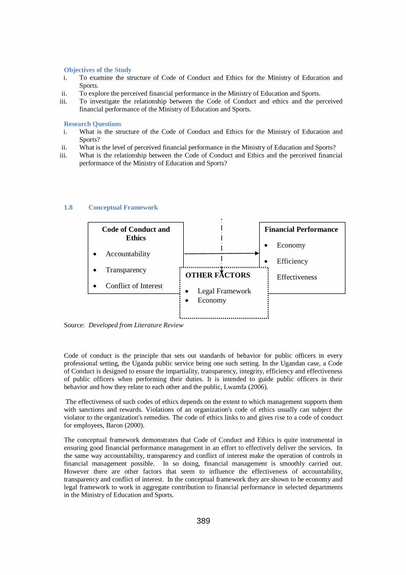
389

Objectives of the Study

i. To examine the structure of Code of Conduct and Ethics for the Ministry of Education and

Sports.

ii. To explore the perceived financial performance in the Ministry of Education and Sports.

iii. To investigate the relationship between the Code of Conduct and ethics and the perceived

financial performance of the Ministry of Education and Sports.

Research Questions

i. What is the structure of the Code of Conduct and Ethics for the Ministry of Education and

Sports?

ii. What is the level of perceived financial performance in the Ministry of Education and Sports?

iii. What is the relationship between the Code of Conduct and Ethics and the perceived financial

performance of the Ministry of Education and Sports?

1.8 Conceptual Framework

Source: Developed from Literature Review

Code of conduct is the principle that sets out standards of behavior for public officers in every professional setting, the Uganda public service being one such setting. In the Ugandan case, a Code

of Conduct is designed to ensure the impartiality, transparency, integrity, efficiency and effectiveness

of public officers when performing their duties. It is intended to guide public officers in their

behavior and how they relate to each other and the public, Lwamfa (2006).

The effectiveness of such codes of ethics depends on the extent to which management supports them

with sanctions and rewards. Violations of an organization's code of ethics usually can subject the

violator to the organization's remedies. The code of ethics links to and gives rise to a code of conduct

for employees, Baron (2000).

The conceptual framework demonstrates that Code of Conduct and Ethics is quite instrumental in

ensuring good financial performance management in an effort to effectively deliver the services. In

the same way accountability, transparency and conflict of interest make the operation of controls in

financial management possible. In so doing, financial management is smoothly carried out.

However there are other factors that seem to influence the effectiveness of accountability,

transparency and conflict of interest. In the conceptual framework they are shown to be economy and

legal framework to work in aggregate contribution to financial performance in selected departments in the Ministry of Education and Sports.

Code of Conduct and

Ethics

Accountability

Transparency

Conflict of Interest

Financial Performance

Economy

Efficiency

Effectiveness

OTHER FACTORS

Legal Framework Economy

390

LITERATURE REVIEW

Code of Conduct and Ethics According to Baron (2000), ethical standards in major corporations are coming under scrutiny, and

financial institutions have been challenged about conflicts of interest and their investment advice.

Considering that ethical scandals have been exposed even in the very large corporations, e.g. Enron,

WorldCom etc., managers are becoming more conscious of how they are perceived by the public, and

want to be seen as ‗ethical‘.

Corporate codes of business ethics studies generated evidence of a positive relationship between

ethics/ CSP and financial performance (Orlitzky, Schmidt and Rynes, 2003).

Although quite a number of previous researchers have revealed that there is a positive relationship

between ethics and financial performance, a few others have found that this said link could neither be

proved nor disproved. Barnett and Salomon (2003) supported the inconclusiveness of these previous studies when they said that despite the intensity of study directed at it, the relationship between Code

of ethics and financial performance remains in dispute.

Also, the review of previous literature shows that many of these studies are quite dissimilar in their

findings. However, these inconsistencies could be due to the fact the different methods used for

researching and reviewing the link between Code of ethics and financial performance were not

sophisticated enough to find correlations that were obscured by methodological errors such as

sampling or measurement errors13. To address this issue, this paper will review those studies that

have applied meta-analysis in reviewing the subject (Report by Social Investment Forum Foundation,

2004).

Orlitzky, Schmidt and Rynes (2003) describes business ethics can be simply seen as the application

of moral philosophies to issues in business and its goal is to describe morally good behaviour for

managers and corporations as a whole. It can also be defined as the study of business situations,

activities and decisions where issues of right and wrong are addressed and it deals with those issues

not explicitly covered by law. In some cases, ethical and /or socially responsible behavior can be

considered an investment in transparency and trust, and consequently, help reduce transaction costs

within and across an organisation.

Ethical Investment Research Services (EIRIS) (2005) defines business ethics as how a company

conducts its business and the behaviour of its employees. Therefore, in present times, it is expected

that most, if not all companies should have a code of ethics and also an ethical identity.

Constructs of Code of Ethics

The values of integrity, transparency and accountability in public administrations have enjoyed

resurgence within the past three decades or so. Sound public administration involves public trust.

Citizens expect public servants to serve public interests with fairness and to manage public resources

properly on a daily basis. Fair and reliable public services and predictable decision-making inspire

public trust and create a level playing field for businesses, thus contributing to well-functioning

markets and economic growth, Elia (2005).

Accountability

According to Elia (2005) accountability refers to the obligation on the part of public officials to report

on the usage of public resources and answerability for failing to meet stated performance objectives. In leadership roles, accountability is the acknowledgment and assumption of responsibility for

actions, products, decisions, and policies including the administration, governance, and

implementation within the scope of the role or employment position and encompassing the obligation

to report, explain and be answerable for resulting consequences.

Recently, accountability has become an important topic in the discussion about the legitimacy of

international institutions. Because there is no global democracy to which organizations must account,

global administrative bodies are often criticized as having large accountability gaps. One

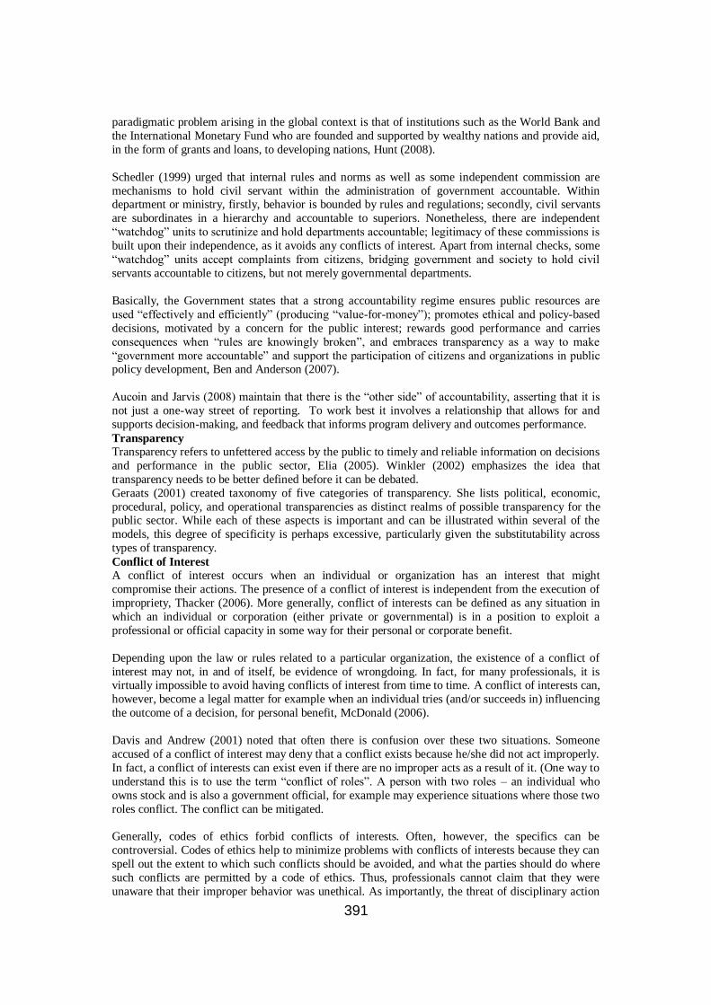
391

paradigmatic problem arising in the global context is that of institutions such as the World Bank and

the International Monetary Fund who are founded and supported by wealthy nations and provide aid,

in the form of grants and loans, to developing nations, Hunt (2008).

Schedler (1999) urged that internal rules and norms as well as some independent commission are

mechanisms to hold civil servant within the administration of government accountable. Within department or ministry, firstly, behavior is bounded by rules and regulations; secondly, civil servants

are subordinates in a hierarchy and accountable to superiors. Nonetheless, there are independent

―watchdog‖ units to scrutinize and hold departments accountable; legitimacy of these commissions is

built upon their independence, as it avoids any conflicts of interest. Apart from internal checks, some

―watchdog‖ units accept complaints from citizens, bridging government and society to hold civil

servants accountable to citizens, but not merely governmental departments.

Basically, the Government states that a strong accountability regime ensures public resources are

used ―effectively and efficiently‖ (producing ―value-for-money‖); promotes ethical and policy-based

decisions, motivated by a concern for the public interest; rewards good performance and carries

consequences when ―rules are knowingly broken‖, and embraces transparency as a way to make

―government more accountable‖ and support the participation of citizens and organizations in public policy development, Ben and Anderson (2007).

Aucoin and Jarvis (2008) maintain that there is the ―other side‖ of accountability, asserting that it is

not just a one-way street of reporting. To work best it involves a relationship that allows for and

supports decision-making, and feedback that informs program delivery and outcomes performance.

Transparency

Transparency refers to unfettered access by the public to timely and reliable information on decisions

and performance in the public sector, Elia (2005). Winkler (2002) emphasizes the idea that

transparency needs to be better defined before it can be debated.

Geraats (2001) created taxonomy of five categories of transparency. She lists political, economic,

procedural, policy, and operational transparencies as distinct realms of possible transparency for the public sector. While each of these aspects is important and can be illustrated within several of the

models, this degree of specificity is perhaps excessive, particularly given the substitutability across

types of transparency.

Conflict of Interest

A conflict of interest occurs when an individual or organization has an interest that might

compromise their actions. The presence of a conflict of interest is independent from the execution of

impropriety, Thacker (2006). More generally, conflict of interests can be defined as any situation in

which an individual or corporation (either private or governmental) is in a position to exploit a

professional or official capacity in some way for their personal or corporate benefit.

Depending upon the law or rules related to a particular organization, the existence of a conflict of

interest may not, in and of itself, be evidence of wrongdoing. In fact, for many professionals, it is virtually impossible to avoid having conflicts of interest from time to time. A conflict of interests can,

however, become a legal matter for example when an individual tries (and/or succeeds in) influencing

the outcome of a decision, for personal benefit, McDonald (2006).

Davis and Andrew (2001) noted that often there is confusion over these two situations. Someone

accused of a conflict of interest may deny that a conflict exists because he/she did not act improperly.

In fact, a conflict of interests can exist even if there are no improper acts as a result of it. (One way to

understand this is to use the term ―conflict of roles‖. A person with two roles – an individual who

owns stock and is also a government official, for example may experience situations where those two

roles conflict. The conflict can be mitigated.

Generally, codes of ethics forbid conflicts of interests. Often, however, the specifics can be

controversial. Codes of ethics help to minimize problems with conflicts of interests because they can

spell out the extent to which such conflicts should be avoided, and what the parties should do where

such conflicts are permitted by a code of ethics. Thus, professionals cannot claim that they were

unaware that their improper behavior was unethical. As importantly, the threat of disciplinary action

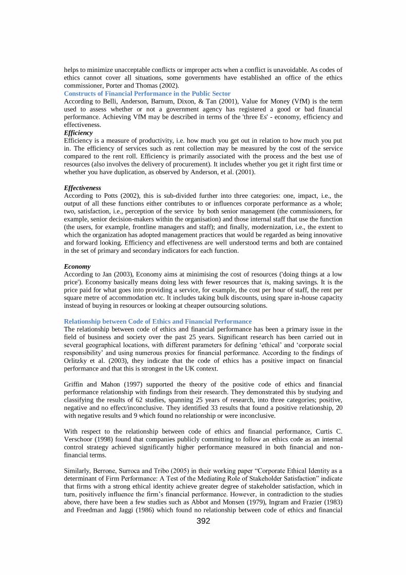
392

helps to minimize unacceptable conflicts or improper acts when a conflict is unavoidable. As codes of

ethics cannot cover all situations, some governments have established an office of the ethics

commissioner, Porter and Thomas (2002).

Constructs of Financial Performance in the Public Sector

According to Belli, Anderson, Barnum, Dixon, & Tan (2001), Value for Money (VfM) is the term

used to assess whether or not a government agency has registered a good or bad financial performance. Achieving VfM may be described in terms of the 'three Es' - economy, efficiency and

effectiveness.

Efficiency

Efficiency is a measure of productivity, i.e. how much you get out in relation to how much you put

in. The efficiency of services such as rent collection may be measured by the cost of the service

compared to the rent roll. Efficiency is primarily associated with the process and the best use of

resources (also involves the delivery of procurement). It includes whether you get it right first time or

whether you have duplication, as observed by Anderson, et al. (2001).

Effectiveness

According to Potts (2002), this is sub-divided further into three categories: one, impact, i.e., the

output of all these functions either contributes to or influences corporate performance as a whole; two, satisfaction, i.e., perception of the service by both senior management (the commissioners, for

example, senior decision-makers within the organisation) and those internal staff that use the function

(the users, for example, frontline managers and staff); and finally, modernization, i.e., the extent to

which the organization has adopted management practices that would be regarded as being innovative

and forward looking. Efficiency and effectiveness are well understood terms and both are contained

in the set of primary and secondary indicators for each function.

Economy

According to Jan (2003), Economy aims at minimising the cost of resources ('doing things at a low

price'). Economy basically means doing less with fewer resources that is, making savings. It is the

price paid for what goes into providing a service, for example, the cost per hour of staff, the rent per square metre of accommodation etc. It includes taking bulk discounts, using spare in-house capacity

instead of buying in resources or looking at cheaper outsourcing solutions.

Relationship between Code of Ethics and Financial Performance

The relationship between code of ethics and financial performance has been a primary issue in the

field of business and society over the past 25 years. Significant research has been carried out in

several geographical locations, with different parameters for defining ‗ethical‘ and ‗corporate social

responsibility‘ and using numerous proxies for financial performance. According to the findings of

Orlitzky et al. (2003), they indicate that the code of ethics has a positive impact on financial

performance and that this is strongest in the UK context.

Griffin and Mahon (1997) supported the theory of the positive code of ethics and financial performance relationship with findings from their research. They demonstrated this by studying and

classifying the results of 62 studies, spanning 25 years of research, into three categories; positive,

negative and no effect/inconclusive. They identified 33 results that found a positive relationship, 20

with negative results and 9 which found no relationship or were inconclusive.

With respect to the relationship between code of ethics and financial performance, Curtis C.

Verschoor (1998) found that companies publicly committing to follow an ethics code as an internal

control strategy achieved significantly higher performance measured in both financial and non-

financial terms.

Similarly, Berrone, Surroca and Tribo (2005) in their working paper ―Corporate Ethical Identity as a determinant of Firm Performance: A Test of the Mediating Role of Stakeholder Satisfaction‖ indicate

that firms with a strong ethical identity achieve greater degree of stakeholder satisfaction, which in

turn, positively influence the firm‘s financial performance. However, in contradiction to the studies

above, there have been a few studies such as Abbot and Monsen (1979), Ingram and Frazier (1983)

and Freedman and Jaggi (1986) which found no relationship between code of ethics and financial

393

performance, and furthermore, others such as Vance (1975), Shane and Spicer (1983) and Hill,

Kelley and Agle (1990) which have shown that a negative code of ethics and financial performance

relationship exists.

Conclusion

Following the above literature review, it is evident that the above authors and writers do not close the

gap between the code of ethics and the financial performance of the public sector. Further, most of the literature about the study variables is for the public sector but in the developed world.

Therefore, this study provides findings that tend to close the gap on code of ethics and financial

performance.

METHODOLOGY

Research Design

A cross sectional research design was used and selected because it ably facilitated the collection of

data from the different strata of respondents namely accounting officer, accountants, auditors,

accounts assistants and department heads.

Study Population

The study population comprised employees from middle to top level managers in departments of

Accounts, Audit, Procument, Finance and Administration at the Ministry‘s headquarters in Kampala

who are 140 permanent staff in total.

Sample Size

As Ministry of Education and Sports maintains a total of 140 staff at the top and middle level as

managers, the sample size for this study will be 60 respondents. This has been determined in line

with Roscoe‘s (1970) rule of thumb that states sample size between 30 and500 as sufficient. This

number is considered to be large enough to yield reliable data and to guard against non-responses.

Sampling Design and Procedure

Simple random sampling and purposive sampling designs were used to select the 60 respondents and

managers respectively. Sampling frame was a payroll since it contained the names of all serving

employees.

Measurement of Variables

The independent variable had three major constructs that included accountability, transparency and

conflict of interest, while the dependent variable had constructs which mainly summarized the Value

for Money concept (Effectiveness, Efficiency, and Economy).

a) Accountability

This was measured by identifying its attributes such as rules, procedures and regulations. These were

measured in terms of the degree of divergence between the accepted standards and the actual

prevailing practices. Therefore, to test perceived accountability a set of statements were used and

applied to a five-point likert scale ranging from strongly agree (5), Agree (4), Not sure (3), Disagree

(2) to strongly disagree (1).

b) Transparency This construct was measured by examining the degree of regression of the current practices on the

required practices. The attributes used in measurement included adherence to transparency

regulations, policies, procedures and rules and these were measured on a five-point likert scale

ranging from strongly agree (5), Agree (4), Not sure (3), Disagree (2) to strongly disagree (1).

c) Conflict of Interest

This was measured by looking at the extent to which individuals have interest that might

compromise their actions by using a five-point likert scale that range from strongly agree (5), Agree

(4), Not sure (3), Disagree (2) to strongly disagree (1).

d) Financial Performance This was measured using the three indicators of Value for Money (VFM) a good measure for

financial performance in the public sector. That is, economy, efficiency, and effectiveness. Therefore,

to test financial performance the research will we devise for each measure a set of statements to test

the perceptions of the respondents, using a five-point scale from strongly agree to strongly disagree.

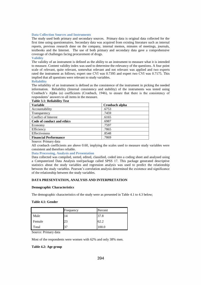
394

Data Collection Sources and Instruments

The study used both primary and secondary sources. Primary data is original data collected for the

first time using questionnaires. Secondary data was acquired from existing literature such as internal

reports, previous research done on the company, internal memos, minutes of meetings, journals,

textbooks and the Internet. The use of both primary and secondary data gave a comprehensive

coverage of challenges facing procurement of drugs.

Validity

The validity of an instrument is defined as the ability to an instrument to measure what it is intended

to measure. Content validity index was used to determine the relevancy of the questions. A four point

scale of relevant, quite relevant, somewhat relevant and not relevant was applied and two experts

rated the instrument as follows; expert one CVI was 0.7395 and expert two CVI was 0.7175. This

implied that all questions were relevant to study variables.

Reliability

The reliability of an instrument is defined as the consistence of the instrument in picking the needed

information. Reliability (Internal consistency and stability) of the instruments was tested using

Cronbach‘s Alpha (α) coefficients (Cronbach, 1946), to ensure that there is the consistency of

respondents‘ answers to all items in the measure.

Table 3.1: Reliability Test

Variable Cronbach alpha

Accountability .6753

Transparency .7459

Conflict of Interest .6165

Code of conduct and ethics .6987

Economy .7597

Efficiency .7865

Effectiveness .8548

Financial Performance .7869

Source: Primary data

All cronbach coefficients are above 0.60, implying the scales used to measure study variables were

consistent and therefore reliable.

Data Processing, Analysis and Presentation

Data collected was compiled, sorted, edited, classified, coded into a coding sheet and analysed using

a Computerized Data Analysis tool/package called SPSS 17. This package generated descriptive

statistics about the study variables and regression analysis was used to predict the relationship

between the study variables. Pearson‘s correlation analysis determined the existence and significance

of the relationship between the study variables.

DATA PRESENTATION, ANALYSIS AND INTERPRETATION

Demographic Characteristics

The demographic characteristics of the study were as presented in Table 4.1 to 4.3 below;

Table 4.1: Gender

Frequency Percent

Male 14 37.8

Female 23 62.2

Total 37 100.0

Source: Primary data

Most of the respondents were women with 62% and only 38% men.

Table 4.2: Age group

395

Frequency Percent

18 - 29 2 5.4

30 - 39 9 24.3

40 - 49 21 56.8

> 49 5 13.5

Total 37 100.0

Source: Primary Data

Majority of the respondents were in the age group 40-49 with 57% followed by 30-39 with 24%, >49

with 14% and lastly 18-29 with 5%.

396

Table 4.3: Highest level of Education

Frequency Valid Percent

O'level & Below 2 5.6

"A" level 1 2.8

Diploma 7 19.4

Degree 14 38.9

Postgraduate 12 33.3

Total 36 100.0

Source: Primary data

Most of the respondents were graduates with at least first degree 72% followed by 19% Diploma, 3%

A-Level and 6% O-Level and below.

Data Analysis

Data was analyzed by using descriptive statistics, factor analysis, and correlation and regression

analyses as shown in tables 4.3 to 4.9.

Examine the Structure of Code of Conduct and Ethics (Objective One)

Table 4.4: Descriptive Statistics

Mean Std. Deviation

The MOES Officials have an obligation to report on the usage of public resources

and answerability for failing to meet the stated performance objectives

4.3810 .97346

The MOES Officials are answerable for failing to meet the stated performance

objectives

4.3952 .87458

The MOES Officials acknowledge and assume responsibility for actions within the

scope of their employment under the reporting obligations.

4.0952 .94365

The MOES Officials acknowledge and assume responsibility for decisions within

the scope of their employment under the reporting obligations.

3.9048 1.13599

The MOES Officials acknowledge and assume responsibility for their policies

within the scope of their employment.

4.0476 .86465

In the MOES there are internal rules and norms that hold Civil Servants

accountable.

4.5238 .67964

In the MOES there are independent commissions that hold Civil Servants

accountable.

3.5714 1.07571

There is a special Department in the MOES which accepts complaints from

citizens, bridging government and society to hold Civil Servants accountable to citizens.

3.2381 .94365

The government of Uganda has a strong accountability regime that ensures that

public resources are used "effectively and efficiently".

3.9524 1.07127

he government of Uganda (GoU) promotes ethical and policy-based decisions,

motivated by a concern for the public interest.

3.8095 .98077

The GoU has a mechanism that rewards good performance. 2.4286 1.02817

The GoU has a mechanism that carries consequences when "rules are knowingly

broken".

3.8571 1.06234

The GoU has a mechanism that embraces accountability. 4.0952 1.04426

397

The MOES supports the participation of citizens and organizations in public policy

development issues.

4.0000 .83666

The MOES has created a relationship that allows for and supports decision making. 3.7143 .90238

The MOES has created a relationship that allows for and supports feedback that

informs program/project delivery and outcomes performance.

3.6667 .91287

Iam personally accountable for all the resources under the office I hold. 4.0000 1.30384

I can confirm that there is free access by the public to timely information on

decisions and performance in the MOES.

3.8095 .74960

I can confirm that there is free access by the public to reliable information on decisions and performance in the MOES.

3.9048 .83095

There is effective communication, not simply announcements in MOES. 3.8571 .79282

In the MOES there is potential transparency as a distinct realm of possible

transparency for the public sector.

3.5714 .74642

In the MOES there is economic transparency as a distinct realm of possible

transparency for the public sector.

3.8095 .67964

In the MOES there is procedural transparency as a distinct realm of possible

transparency for the public sector.

3.9048 .62488

In the MOES there is operational transparency as a distinct realm of possible

transparency for the public sector.

5.8095 8.77279

All MOES staff are fully informed of relevant matters and there are never any

surprises.

3.5714 1.02817

There is full and accurate reporting on MOES affairs to the stakeholders and beneficiaries.

4.0000 .77460

There is openness in order to enhance public confidence in the Ministry. 3.9048 .83095

Ministry staff is consulted whenever introducing ideas affecting the Ministry. 3.4762 .92839

Ministry meetings are always conducted in a manner that encourages open

communication.

4.0476 .92066

The various MOES projects requirements are communicated to project staff on a

regular basis.

3.7143 .84515

MOES Financial information is easily accessible by stakeholders and other users. 3.3810 1.07127

MOES Technical information is easily accessible by stakeholders and other users. 3.9048 .62488

The Ministry Administration publishes financial details in the press to allow a

balanced judgment of overall Ministry performance.

2.9524 1.07127

The Ministry Administration publishes technical details in the press to allow a

balanced judgment of overall Ministry performance.

3.6667 1.11056

All staff of MOES are as open as possible about the decisions and actions they take.

3.3333 1.06458

All staff of MOES are always prepared when called upon to give reasons for the

decisions and actions they have taken.

3.5714 .74642

A conflict of interest occurs when an individual or organization has an interest that

might compromise their actions.

4.1905 .92839

Most Officers in the MOES are in a position to exploit a professional or official

capacity in some way for their personal or corporate benefit.

2.9524 1.11697

According to our Code of ethics, the existence of a conflict of interest may not, in

and of itself, be evidence of wrongdoing.

3.1905 1.20909

For many officials, it is virtually impossible to avoid having conflicts of interest from time to time.

2.9524 1.11697

398

We have had cases of in which conflict of interests became a legal matter

especially when individual tried (and/or succeeded in) influencing the outcome of a

decision, for personal benefits.

3.2381 .94365

In our code of conduct someone accused of a conflict of interest may deny that

conflict exists because he/she did not act improperly.

3.2857 1.14642

Generally, our code of ethics forbids conflicts of interests. 3.9048 .99523

Codes of ethics help to minimize problems with conflicts of interests because they can spell out the extent to which such conflicts should be avoided.

4.0000 .94868

Codes of ethics spell out what the parties should do in case there are conflicts that

are permitted by a code of ethics.

3.7143 .95618

The threat of disciplinary action helps to minimize unacceptable conflicts or

improper acts when a conflict is unavoidable.

4.0000 1.18322

The codes of ethics used by MOES covers all situations. 3.3333 1.23828

The MOES has established an office in charge of ethics and integrity. 2.4286 .81064

Whenever i realize that there is a conflict of interest in any of my duties, i inform

my supervisor of the nature and extent of my interest.

3.1429 1.19523

Every Civil servant/staff in the MOES holds his/her office in public trust and is

personally responsible for his/her actions.

3.8571 1.27615

I always hold my office in public trust and iam accountable to the public at all

times.

3.8571 1.31475

My ethical behavior is considered an investment in the public trust. 3.9048 1.04426

My social behavior is considered an investment in the public trust. 3.8571 1.06234

Everything, i do it for the public benefit which increases the public trust. 3.8095 1.07792

I act responsibly in my office which increases public trust for the ministry services 4.0000 1.09545

There are high standards of accountability set for my supervisors which increases

public trust.

3.9524 1.11697

Source: Primary Data

Most of the item means are approximately 4 and above which is the score for agree and strongly

agree, implying that Code of conduct and ethics largely exists in the MOES.

MOES Officials have an obligation to report on the usage of public resources and answerability for

failing to meet the stated performance objectives 4.3810, are answerable for failing to meet the stated

performance objectives 4.3952, acknowledge and assume responsibility for actions within the scope

of their employment under the reporting obligations 4.0952, acknowledge and assume responsibility

for decisions within the scope of their employment under the reporting obligations 3.9048,

acknowledge and assume responsibility for their policies within the scope of their employment

4.0476, there are internal rules and norms that hold Civil Servants accountable 4.5238 and there are

independent commissions that hold Civil Servants accountable 3.5714.

The government of Uganda has a strong accountability regime that ensures that public resources are

used ―effectively and efficiently‖ 3.9524, promotes ethical and policy-based decisions, motivated by

a concern for the public interest 3.8095, has a mechanism that carries consequences when ―rules are

knowingly broken‖ 3.8571and has a mechanism that embraces accountability 4.0952.

The MOES supports the participation of citizens and organizations in public policy development issues 4.0000, created a relationship that allows for and supports decision making 3.7143, created a

relationship that allows for and supports feedback that informs program/project delivery and

outcomes performance 3.666.

Staff are personally accountable for all the resources under their offices 4.0000, can confirm

that there is free access by the public to timely information on decisions and performance in the

399

MOES 3.8095 and also can confirm that there is free access by the public to reliable information on

decisions and performance in the MOES 3.9048.

There is effective communication, not simply announcements in MOES 3.8571, there is potential

transparency as a distinct realm of possible transparency for the public sector 3.5714, there is

economic transparency as a distinct realm of possible transparency for the public sector 3.8095, there

is procedural transparency as a distinct realm of possible transparency for the public sector 3.9048,

there is operational transparency as a distinct realm of possible transparency for the public sector

5.8095 and staff are fully informed of relevant matters and there are never any surprises 3.5714.

There is full and accurate reporting on MOES affairs to the stakeholders and beneficiaries 4.0000,

openness in order to enhance public confidence in the Ministry3.9048, Ministry staff are consulted whenever introducing ideas affecting the Ministry 3.4762, meetings are always conducted in a

manner that encourages open communication 4.0476, and various MOES projects requirements are

communicated to project staff on a regular basis 3.7143.

MOES Financial information is easily accessible by stakeholders and other users 3.3810, technical

information is easily accessible by stakeholders and other users 3.9048, Administration publishes

technical details in the press to allow a balanced judgment of overall Ministry performance

3.6667and all staff of MOES are always prepared when called upon to give reasons for the decisions

and actions they have taken 3.5714.

A conflict of interest occurs when an individual or organization has an interest that might

compromise their actions 4.1905, Generally, our code of ethics forbids conflicts of interests 3.9048,

Codes of ethics help to minimize problems with conflicts of interests because they can spell out the

extent to which such conflicts should be avoided 4.0000 and Codes of ethics spell out what the parties

should do in case there are conflicts that are permitted by a code of ethics 3.7143.

The threat of disciplinary action helps to minimize unacceptable conflicts or improper acts when a

conflict is unavoidable 4.0000, Every Civil servant/staff in the MOES holds his/her office in public

trust and is personally responsible for his/her actions 3.8571, staff hold offices in public trust and

accountable to the public at all times 3.8571, staff ethical behavior is considered an investment in the

public trust 3.9048, social behavior is considered an investment in the public trust 3.8571,

Everything staff do, do it for the public benefit which increases the public trust 3.8095, act

responsibly in office which increases public trust for the ministry services 4.0000 and there are high

standards of accountability set for my supervisors which increases public trust 3.9524.

However , there is a disagreement and not being aware of the code of conduct issues below; GoU has

no mechanism that rewards good performance 2.4286, not aware of special Department in the MOES

which accepts complaints from citizens, bridging government and society to hold Civil Servants

accountable to citizens 3.2381, not aware of Ministry Administration publishing financial details in

the press to allow a balanced judgment of overall Ministry performance 2.9524, Officers being in

position to exploit a professional or official capacity in some way for their personal or corporate

benefit 2.9524, According to Code of ethics, the existence of a conflict of interest may not, in and of

itself, be evidence of wrongdoing 3.1905.

For many officials, it is virtually impossible to avoid having conflicts of interest from time to time

2.9524, had cases of in which conflict of interests became a legal matter especially when individual

tried (and/or succeeded in) influencing the outcome of a decision, for personal benefits 3.2381, In

our code of conduct someone accused of a conflict of interest may deny that conflict exists because

he/she did not act improperly 3.2857, The codes of ethics used by MOES covers all situations 3.3333,

The MOES has established an office in charge of ethics and integrity 2.4286, Whenever staff realize

that there is a conflict of interest in any of my duties, i inform my supervisor of the nature and extent

of my interest 3.1429 and all staff of MOES are as open as possible about the decisions and actions

they take 3.3333.

Table 4.5: Rotated Component Matrix

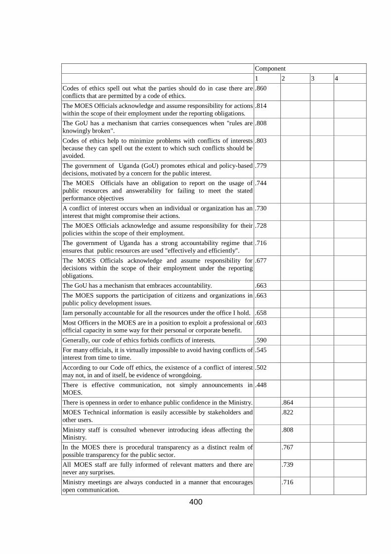
400

Component

1 2 3 4

Codes of ethics spell out what the parties should do in case there are

conflicts that are permitted by a code of ethics.

.860

The MOES Officials acknowledge and assume responsibility for actions

within the scope of their employment under the reporting obligations.

.814

The GoU has a mechanism that carries consequences when "rules are

knowingly broken".

.808

Codes of ethics help to minimize problems with conflicts of interests because they can spell out the extent to which such conflicts should be

avoided.

.803

The government of Uganda (GoU) promotes ethical and policy-based

decisions, motivated by a concern for the public interest.

.779

The MOES Officials have an obligation to report on the usage of

public resources and answerability for failing to meet the stated

performance objectives

.744

A conflict of interest occurs when an individual or organization has an

interest that might compromise their actions.

.730

The MOES Officials acknowledge and assume responsibility for their

policies within the scope of their employment.

.728

The government of Uganda has a strong accountability regime that

ensures that public resources are used "effectively and efficiently".

.716

The MOES Officials acknowledge and assume responsibility for

decisions within the scope of their employment under the reporting

obligations.

.677

The GoU has a mechanism that embraces accountability. .663

The MOES supports the participation of citizens and organizations in

public policy development issues.

.663

Iam personally accountable for all the resources under the office I hold. .658

Most Officers in the MOES are in a position to exploit a professional or official capacity in some way for their personal or corporate benefit.

.603

Generally, our code of ethics forbids conflicts of interests. .590

For many officials, it is virtually impossible to avoid having conflicts of

interest from time to time.

.545

According to our Code off ethics, the existence of a conflict of interest

may not, in and of itself, be evidence of wrongdoing.

.502

There is effective communication, not simply announcements in

MOES.

.448

There is openness in order to enhance public confidence in the Ministry. .864

MOES Technical information is easily accessible by stakeholders and

other users.

.822

Ministry staff is consulted whenever introducing ideas affecting the

Ministry.

.808

In the MOES there is procedural transparency as a distinct realm of

possible transparency for the public sector.

.767

All MOES staff are fully informed of relevant matters and there are

never any surprises.

.739

Ministry meetings are always conducted in a manner that encourages

open communication.

.716

401

The MOES has created a relationship that allows for and supports

decision making.

.703

The various MOES projects requirements are communicated to project

staff on a regular basis.

.692

There is full and accurate reporting on MOES affairs to the stakeholders

and beneficiaries.

.674

I can confirm that there is free access by the public to timely information on decisions and performance in the MOES.

.662

All staff of MOES are always prepared when called upon to give

reasons for the decisions and actions they have taken.

.655

I can confirm that there is free access by the public to reliable

information on decisions and performance in the MOES.

.602

In the MOES there is economic transparency as a distinct realm of

possible transparency for the public sector.

.568

The MOES has created a relationship that allows for and supports

feedback that informs program/project delivery and outcomes

performance.

.549 .

All staff of MOES are as open as possible about the decisions and actions they take.

.505

MOES Financial information is easily accessible by stakeholders and

other users.

.505

There is a special Department in the MOES which accepts complaints

from citizens, bridging government and society to hold Civil Servants

accountable to citizens.

.444

My ethical behavior is considered an investment in the public trust. .866

Everything i do, i do it for the public benefit which increases the public

trust.

.845

There are high standards of accountability set for my supervisors which increases public trust.

.826

I act responsibly in my office which increases public trust for the

ministry services

.821

My social behavior is considered an investment in the public trust. .820

The threat of disciplinary action helps to minimize unacceptable

conflicts or improper acts when a conflict is unavoidable.

.797

Every Civil servant/staff in the MOES holds his/her office in public

trust and is personally responsible for his/her actions.

.762

I always hold my office in public trust and iam accountable to the

public at all times.

.752

The codes of ethics used by MOES covers all situations. .739

Whenever i realize that there is a conflict of interest in any of my

duties, i inform my supervisor of the nature and extent of my interest.

.617

In our code of conduct someone accused of a conflict of interest may

deny that conflict exists because he/she did not act improperly.

.525

The Ministry Administration publishes technical details in the press to

allow a balanced judgment of overall Ministry performance.

.787

The Ministry Administration publishes financial details in the press to

allow a balanced judgment of overall Ministry performance.

.747

In the MOES there is potential transparency as a distinct realm of

possible transparency for the public sector.

.549

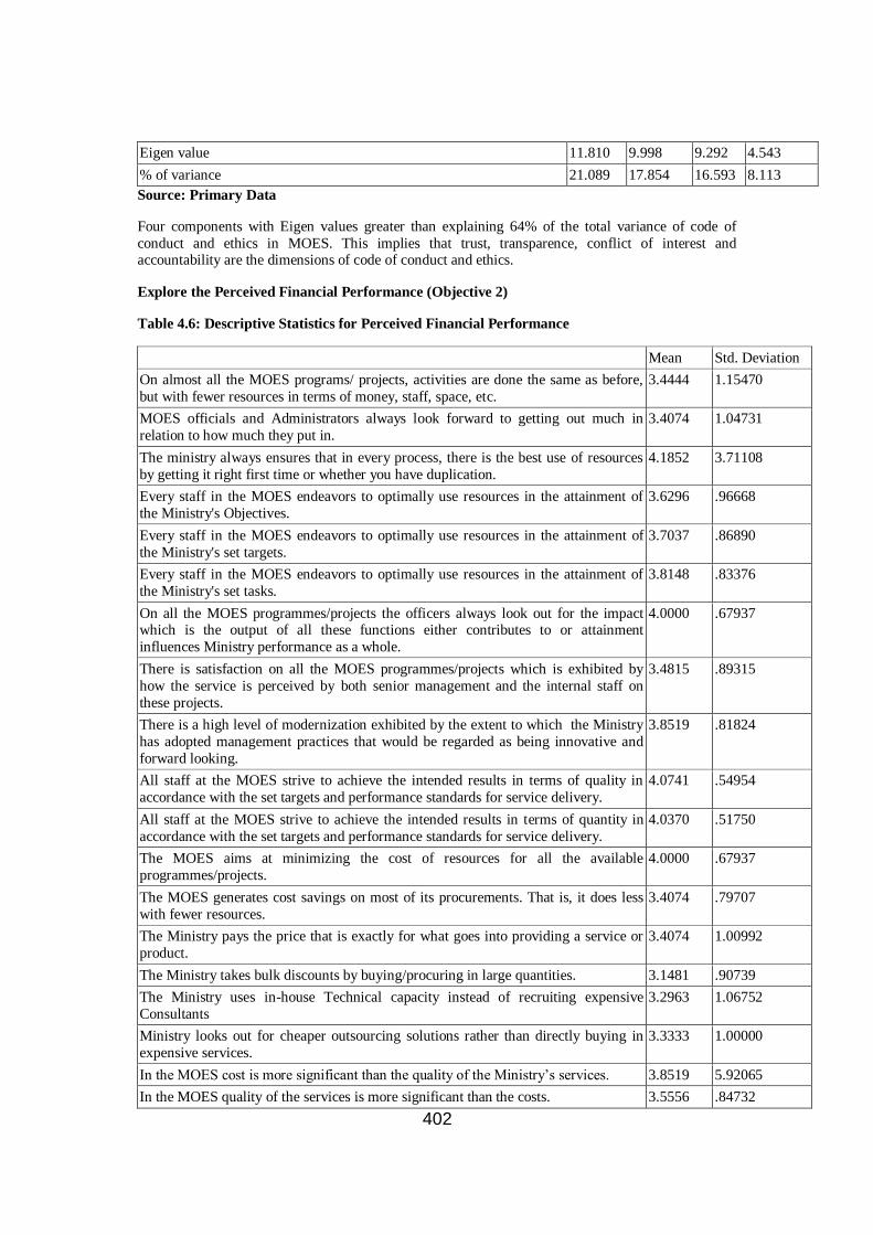
402

Eigen value 11.810 9.998 9.292 4.543

% of variance 21.089 17.854 16.593 8.113

Source: Primary Data

Four components with Eigen values greater than explaining 64% of the total variance of code of

conduct and ethics in MOES. This implies that trust, transparence, conflict of interest and accountability are the dimensions of code of conduct and ethics.

Explore the Perceived Financial Performance (Objective 2)

Table 4.6: Descriptive Statistics for Perceived Financial Performance

Mean Std. Deviation

On almost all the MOES programs/ projects, activities are done the same as before,

but with fewer resources in terms of money, staff, space, etc.

3.4444 1.15470

MOES officials and Administrators always look forward to getting out much in

relation to how much they put in.

3.4074 1.04731

The ministry always ensures that in every process, there is the best use of resources

by getting it right first time or whether you have duplication.

4.1852 3.71108

Every staff in the MOES endeavors to optimally use resources in the attainment of

the Ministry's Objectives.

3.6296 .96668

Every staff in the MOES endeavors to optimally use resources in the attainment of

the Ministry's set targets.

3.7037 .86890

Every staff in the MOES endeavors to optimally use resources in the attainment of

the Ministry's set tasks.

3.8148 .83376

On all the MOES programmes/projects the officers always look out for the impact which is the output of all these functions either contributes to or attainment

influences Ministry performance as a whole.

4.0000 .67937

There is satisfaction on all the MOES programmes/projects which is exhibited by

how the service is perceived by both senior management and the internal staff on

these projects.

3.4815 .89315

There is a high level of modernization exhibited by the extent to which the Ministry

has adopted management practices that would be regarded as being innovative and

forward looking.

3.8519 .81824

All staff at the MOES strive to achieve the intended results in terms of quality in

accordance with the set targets and performance standards for service delivery.

4.0741 .54954

All staff at the MOES strive to achieve the intended results in terms of quantity in

accordance with the set targets and performance standards for service delivery.

4.0370 .51750

The MOES aims at minimizing the cost of resources for all the available

programmes/projects.

4.0000 .67937

The MOES generates cost savings on most of its procurements. That is, it does less

with fewer resources.

3.4074 .79707

The Ministry pays the price that is exactly for what goes into providing a service or

product.

3.4074 1.00992

The Ministry takes bulk discounts by buying/procuring in large quantities. 3.1481 .90739

The Ministry uses in-house Technical capacity instead of recruiting expensive

Consultants

3.2963 1.06752

Ministry looks out for cheaper outsourcing solutions rather than directly buying in

expensive services.

3.3333 1.00000

In the MOES cost is more significant than the quality of the Ministry‘s services. 3.8519 5.92065

In the MOES quality of the services is more significant than the costs. 3.5556 .84732

403

I always ensure that there is proper and economical utilization of public funds. 3.9259 .61556

I always safeguard the public property/assets entrusted to me to ensure that there is

no damage.

4.3333 .55470

The procurement staff of the MOES always ensures that there is no loss or

misappropriations in the process of procurement, storage, utilization, and disposal.

3.4444 .93370

Source: Primary Data

Most of the items have means above 3.5 indicating the score of 4 with agree category of agree which

implies that there is minimum performance by MOES.

The ministry always ensures that in every process, there is the best use of resources by getting it right

first time or whether you have duplication 4.1852, Every staff in the MOES endeavors to optimally

use resources in the attainment of the Ministry's Objectives 3.6296, Every staff in the MOES

endeavors to optimally use resources in the attainment of the Ministry's set targets 3.7037

Every staff in the MOES endeavors to optimally use resources in the attainment of the Ministry's set

tasks 3.8148, On all the MOES programmes/projects the officers always look out for the impact

which‘s is the output of all these functions either contributes to or attainment influences Ministry

performance as a whole 4.0000, there is satisfaction on all the MOES programmes/projects which is exhibited by how the service is perceived by both senior management and the internal staff on these

projects 3.4815, there is a high level of modernization exhibited by the extent to which the Ministry

has adopted management practices that would be regarded as being innovative and forward looking

3.8519, All staff at the MOES strive to achieve the intended results in terms of quality in accordance

with the set targets and performance standards for service delivery 4.0741, All staff at the MOES

strive to achieve the intended results in terms of quantity in accordance with the set targets and

performance standards for service delivery 4.0370, The MOES aims at minimizing the cost of

resources for all the available programmes/projects 4.0000, In the MOES cost is more significant than

the quality of the Ministry‘s services 3.8519, In the MOES quality of the services is more significant

than the costs 3.5556, I always ensure that there is proper and economical utilization of public funds

3.9259, and always safeguard the public property/assets entrusted to me to ensure that there is no damage 4.3333. However there is a disagreement, and lack of awareness of the following:

The procurement staff of the MOES always ensures that there is no loss or misappropriations in the

process of procurement, storage, utilization, and disposal 3.4444, and MOES generates cost savings

on most of its procurements that is, it does less with fewer resources 3.4074. Further, the Ministry

pays the price that is exactly for what goes into providing a service or product 3.4074, it also takes

bulk discounts by buying/procuring in large quantities 3.1481 and uses in-house Technical capacity

instead of recruiting expensive Consultants 3.2963. The Ministry also looks out for cheaper

outsourcing solutions rather than directly buying in expensive services 3.3333.

Table 4.7: Rotated Component Matrix for Perceived Financial Performance

Component

1 2 3

Every staff in the MOES endeavors to optimally use resources in the

attainment of the Ministry's set targets.

.869

Every staff in the MOES endeavors to optimally use resources in the

attainment of the Ministry's set tasks.

.847

Every staff in the MOES endeavors to optimally use resources in the

attainment of the Ministry's Objectives.

.775

All staff at the MOES strive to achieve the intended results in terms of

quality in accordance with the set targets and performance standards for

service delivery.

.715

404

All staff at the MOES strive to achieve the intended results in terms of

quantity in accordance with the set targets and performance standards for

service delivery.

.664

There is satisfaction on all the MOES programmes/projects which is

exhibited by how the service is perceived by both senior management and the internal staff on these projects.

.586

I always safeguard the public property/assets entrusted to me to ensure

that there is no damage.

.584

There is a high level of modernization exhibited by the extent to which

the Ministry has adopted management practices that would be regarded

as being innovative and forward looking.

.583

On all the MOES programmes/projects the officers always look out for

the impact which is the output of all these functions either contributes to

or attainment influences Ministry performance as a whole

.574

The Ministry pays the price that is exactly for what goes into providing a

service or product.

.775

he Ministry looks out for cheaper outsourcing solutions rather than

directly buying in expensive services.

.743

The Ministry uses in-house Technical capacity instead of recruiting

expensive Consultants

.742

The MOES generates cost savings on most of its procurements. That is,

it does less with fewer resources.

.697

The MOES aims at minimizing the cost of resources for all the available

programmes/projects.

.656

The Ministry takes bulk discounts by buying/procuring in large

quantities.

.650

The ministry always ensures that in every process, there is the best use of

resources by getting it right first time or whether you have duplication.

.557

In the MOES quality of the services is more significant than the costs. .538

I always ensure that there is proper and economical utilization of public

funds.

.767

The procurement staff of the MOES always ensures that there is no loss

or misappropriations in the process of procurement, storage, utilization,

and disposal.

.669

MOES officials and Administrators always look forward to getting out

much in relation to how much they put in.

.449

Eigen value 5.284 4.196 2.756

% of variance 24.020 19.074 12.528

Source: Primary Data

Three factors explaining 54% of the total variation of perceived performance were extracted. This

implies that three Es are the dimensions of perceived performance.

Investigate the Relationship between Code of Conduct and Ethics and Perceived Financial

Performance (Objective 3).

Table 4.8: Zero Order Correlation Matrix

405

Acc

ounta

bil

ity

Tra

nsp

aren

cy

Confl

ict

of

inte

rest

Tru

st

Code

of

conduct

and e

thic

s

Eff

icie

ncy

Eff

ecti

ven

ess

Eco

nom

y

Fin

anci

al

per

form

ance

Accountability 1

Transparence .583** 1

Conflict of interest .467** .173 1

Trust .264 -.048 .530** 1

Code of conduct and ethics .813** .623** .726** .646** 1

Efficiency .449** .592** .285 .260 .578** 1

Effectiveness .379* .451** .382* .419** .593** .539** 1

Economy .498** .510** .402* .284 .604** .462** .569** 1

Financial performance .536** .633** .426** .383* .715** .835** .837** .804** 1 1

**. Correlation significant at 0.01 levels

*. Correlation significant at 0.05 levels

Source: Primary data

There is a significant positive relationships between code of conduct and ethics and perceived

performance (r=.715, p-value<0.01). This implies that code of conduct and ethics enhances on the

performance of MOES in terms of efficiency, effectiveness and economy.

There are significant positive relationships between accountability and financial performance

(efficiency, effectiveness and economy), (r=.536,.449,.379,.498, p-values<0.01, 0.05) respectively.

This implies that accountability improves on the financial performance in terms of efficiency,

effectiveness and economy of MOES.

There are significant positive relationships between transparency and financial performance

(efficiency, effectiveness and economy), (r=.633,.592,.451,.510, p-values<0.01). This implies that

transparency improves on the financial performance of MOES.

Conflict of interest had significant positive relationship with financial performance (effectiveness and

economy), r=.426,.382,.402, p-values<0.01, 0.05), This implies that conflict of interest improved on

the financial performance of MOES. However no significant relationship with efficiency (r=.285, p-

value>0.05).

Trust had significant positive relationship with financial performance in terms of effectiveness only

(r=.383, .419, p-value<0.05, 0.01). This implies that trust enhances on the financial performance of

MOES.

406

Table 4.9 : Regression Model

Model

Unstandardized

Coefficients

Standardized

Coefficients

t Sig.

Collinearity Statistics

B Std. Error Beta Tolerance VIF

(Constant) -.165 .615 -.268 .791

Accountability .035 .168 .034 .211 .834 .510 1.960

Transparency .547 .131 .607 4.186 .000 .615 1.625

Conflict of

interest

.170 .196 .127 .867 .392 .604 1.655

Trust .279 .114 .336 2.443 .020 .684 1.463

R-Square =0.585, Adj R-Square=0.534, F=11.299,

Sig=0.000, Durbin–Watson=1.706.

Source: Primary data

Transparency and trust significantly predicted 53% financial performance of MOES (F=11.299,

Sig=0.000). Transparency predicts more (beta=0.607) to financial performance than trust

(beta=0.336). Improvement in transparency led to 0.607 increase in financial performance and

change in trust led to 0.336 enhancement in financial performance. Accountability and conflict of

interest were no significant predictors of perceived financial performance.

Results above are in line with the findings of Orlitzky et al. (2003), they indicate that the code of

ethics has a positive impact on financial performance and that this is strongest in the UK context.

Griffin and Mahon (1997) supported the theory of the positive code of ethics and financial

performance relationship with findings from their research. They demonstrated this by studying and

classifying the results of 62 studies, spanning 25 years of research, into three categories; positive,

negative and no effect/inconclusive. They identified 33 results that found a positive relationship, 20

with negative results and 9 which found no relationship or were inconclusive.

With respect to the relationship between code of ethics and financial performance, Verschoor (1998)

found that companies publicly committing to follow an ethics code as an internal control strategy achieved significantly higher performance measured in both financial and non-financial terms.

Conclusion and Recommendation

Code of conduct and ethics is a determinant of the financial performance of the Ministry of Education

and sports in Uganda. Transparency and trust are paramount in the code of conduct and ethics in the

Ministry of Education and Sports in Uganda. There is need for the employees to uphold to be more

transparent and trust one another for the betterment of the Ministry financial performance.

407

REFERENCES

Ablo, E. & Reinika, R. (1998). Do Budgets Really Matter? Evident from Public Spending on Education and Health in Uganda. World Bank Policy Research Working Paper No. 1926

Aucoin and Jarvis (2008). Modernising Government: The Way Forward – an analysis Haque

International Review of Administrative Sciences. 72: 319-325

Belli, P., Anderson, J. R., Barnum, H.N., Dixon, J. A., & Tan, J-P, (2001). Economic Analysis, of

Investment Operations. Analytical Tools and Practical Applications. WBI, World Bank,

Washington D.C.

Berrone, Surroca and Tribo (2005). Corporate Ethical Identity as a Determinant of Firm Performance:

A Test of the Mediating Role of Stakeholder Satisfaction. Universidad Carlos III De

Madrid, Departmento de Economia de la Empressa, Working Papers 05-31, Business

Economics Series 08.

Bevan D.L. (2001). The Budget and Medium Term Expenditure Framework in Uganda. Africa

Region Working Paper Series No.24, Washington DC: World Bank. Birdstall, L.I. (2005). Toward Universal Primary Education: Investments, Incentives and Institutions.

UN Millennium Project, Task Force on Education and Gender Equality, 2005. Downloaded

on 20/08/09 from http://www.unmillenniumproject.org/documents/Education-complete.pdf

Brandeis, L. (1914). Other People‟s Money and How Bankers Use it. New York: Friedrich, A

Strokes.

Cronbach, L.J. (1946). Response Sets and Tests Validating. Journal for Educational & Psychological

Measurement. Vol. 6, 475 -494.

Collier, P. (2007). The Bottom Billion: Why Poorest Countries are failing and what can be done About It. London. Oxford University Press.

Commonwealth Human Rights Initiative (2006). Information Disclosure Policy: A Toolkit for Pacific

Governments. Retrieved from http://www.pacmcf.com/PMCFinfo/full_report.pdf

Davis, M. & Andrew, S. (2001). Conflict of Interest in the Professions. Oxford: Oxford University

Press. ISBN 0-19-512863-X.

Elia, A. (2005). Integrity, Transparency and Accountability in Public Administration: Recent Trends,

Regional and International Developments and Emerging Issues. Economic & Social Affairs.

August 2005, United Nations Publication

Geraats, P. (2001). Why Adopt Transparency? The Publication of Central Bank Forecasts. European

Central Bank Working Paper No. 41, January.

Griffin, J.J. & Mahon, J.F. (1997). The Corporate Social Performance and Corporate Financial Performance Debate: Twenty-Five Years of Incomparable Research. Business and Society.

Vol. 36, No. 1. 5-31.

Guild, M., Wolf, D. & Wandira (1995). Support for Ugandan Primary Education Reform: A

Formative Evaluation August 1995.

Hallak, J. & Poisson, M. (2007). Corrupt Schools, Corrupt Universities: What can be done?

UNESCO/International Institute for Education Planning. Retrieved from

http://unpan1.un.org/intradoc/groups/public/documents/unesco/unpan025403.pdf and

http://www.education.go.ug/UPEFormula.html

http://www.worldbank.org/external/default/WDSContentServer/WDSP/IB/2004/01/2/0/000/0001600

16_20040120110828/Rendered/PDF/275380UG.pdf

Hunt, G. (2008). Whistleblowing in the Social Services: Public Accountability & Professional Practice.

Jan, R. (2003). The Cost-Effectiveness Analysis – a Superior Alternative to the Cost-Benefit Analysis

of Environmental Infrastructure Investments. Working paper presented at the Fifth

European Conference on Evaluation of the Structural Funds. Budapest

McDonald, M. (2006). Ethics and Conflict of Interest. W. Maurice Young Centre for Applied Ethics.

Ministry of Education and Sports (1999). The Ugandan Experience of Universal Primary Education

(UPE) Kampala.

Ministry of Education and Sports (2001). Sixth Education Sector Review Final Aide Memoire.

Retrieved from

http://www.usaid.or.ug/SO8Annexes/Aide%20Memoire%20Education%20Sector%20%-

202001.doc

408

Ministry of Education and Sports. (2007). UPE Allocation Formulae since Inception.

Ministry of Planning and Economic Development. (1991). Background to the Budget, Kampala.

Ministry of Planning and Economic Development (1992). Background to the Budget. Kampala.

Orlitzky, M., Schmidt, F. and Rynes, S. (2003). Corporate Social and Financial Performance: A

Meta-analysis. Organizational Studies. 24 (3). 403-441, Sage Publications, London.

Porter, R.J. & Thomas E.M. (2002). Biomedical Research: Collaboration and Conflict of Interest. Baltimore: Johns Hopkins University Press. ISBN 0-8018-4400-2.

Potts, D. (2002). Project Planning and Analysis for Development. Lyann Rienner Publishers.

Schedler, Andreas (1999). Conceptualizing Accountability. London: Lynne Rienner Publishers. 13–

28.

Thacker, P.D. (2006). Environmental Journals Feel Pressure to Adopt Disclosure Rules.

Environmental Science & Technology 40: 6873–6875.

Verschoor, C. C. (1998). A Study of the Link between a Corporation‘s Financial Performance and its

Commitment to Ethics. Journal of Business Ethics. Vol. 17. 1509 – 1516.

Ward, P. (2006). Education Reform in Uganda – 1997 to 2004. Reflections on Policy, Partnership,

Strategy and Implementation. Department for International Development, Researching the

Issues 2006:60.

Winkler, B. (2002). Which Kind of Transparency? On the Need for Effective Communication in Monetary Policy Making. Ifo Studies vol. 48, issue 3, pp. 401-27.

World Bank. (1993). Uganda: Social Sectors. Washington DC.

World Bank. (1998). Development Credit Agreement (Education Sector Adjustment Operation)

between The Republic of Uganda and International Development Association, April,

http://web.worldbank.org/external/projects/main?pagePK=64283627&piPK=73230

&theSitePK=40941&menuPK=22842&Projectid=P002972

World Bank (2004a). Project Performance Assessment Report Uganda, Primary Education and

Teacher Development Project (Credit 2493) and Education Sector Adjustment Credit

(Credit 3049). Washington DC January 8, 2004.

World Bank (2004b). Uganda-Primary Education and Teacher Development and Education Sector

Adjustment Credit Project. World Bank (2004c). Achieving EFA in Uganda: the Big Bang Approach. Washington DC,

http://www.worldbank.org/education/pdf/efa.case_uganda.pdf

409

CREDIT RISK MANAGEMENT AND PROFITABILITY OF COMMERCIAL BANKS IN

KENYA

BY

ANGELA M. KITHINJI

AND

NGUGI WILSON

SCHOOL OF BUSINESS

UNIVERSITY OF NAIROBI

NAIROBI – KENYA.

akithinji@yahoo.com or akithinji@uonbi.ac.ke

A Paper Presented at the ORSEA Conference at the Kenyatta International Conference

Centre, NAIROBI- KENYA

October, 2011

410

1.0 INTRODUCTION

1.1 Background

The risk focused examination process has been adopted to direct the inspection process to the more

risk areas of both operations and business. Skills in risk-focused supervision are continually being

developed by exposing bank examiners to relevant training. By adopting this approach, the banking

industry, are forced to embrace formal and documented risk management frameworks, De Juan

(1991). Notably, the more complex a risk type is, the more specialized, concentrated and controlled

its management is expected to be, Seppala (2000), Matz and Neu, (1998) Ramos (2000). Risk

management is defined as the process that a bank puts in place to control its financial exposures.

According to Bikker and Metzmakers (2005), and Buttimer (2001), the process of risk management

comprises the fundamental steps of risk identification, risk analysis and assessment, risk audit

monitoring, and risk treatment or control (Whereas a risk in simple terms can be measured using

standard deviation, some risks may be difficult to measure requiring more complex methods of risk

measurement. Good risk management is not only a defensive mechanism, but also an offensive

weapon for commercial banks and this is heavily dependent on the quality of leadership and

governance. Jorion (2009) observes that a recognized risk is less ―risky‖ than the unidentified risk.

Risk is highly multifaceted, complex and often interlinked making it necessary to manage, rather than

fear. While not avoidable, risk is manageable – as a matter of fact most banks live reasonably well by

incurring risks, Payle (1997) and Greuning and Bratanovic (1999).

Financial institutions are exposed to a variety of risks among them; interest rate risk, foreign

exchange risk, political risk, market risk, liquidity risk, operational risk and credit risk, Yusuf (2003),

Cooperman, Gardener and Mills (2000). In some instances, commercial banks and other financial

institutions have approved decisions that are not vetted; there have been cases of loan defaults and

non-performing loans, massive extension of credit and directed lending. Policies to minimize on the

negative effects have focused on mergers in banks and NBFIs, better banking practices but stringent

lending, review of laws to be in line with the global standards, well capitalized banks which are

expected to be profitable, liquid banks that are able to meet the demands of their depositors, and

maintenance of required cash levels with the central bank which means less cash is available for

lending (Central Bank Annual Report, 2004). This has led to reduced interest income for the

commercial banks and other financial institutions and by extension reduction in profits, De Young

and Roland (2001), Dziobek (1998), Uyemura and Van Deventer (1992).

Credit risk is the possibility that the actual return on an investment or loan extended will deviate from

that, which was expected, Conford (2000). Coyle (2000) defines credit risk as losses from the refusal

or inability of credit customers to pay what is owed in full and on time. The main sources of credit

risk include, limited institutional capacity, inappropriate credit policies, volatile interest rates, poor

management, inappropriate laws, low capital and liquidity levels, directed lending, massive licensing

of banks, poor loan underwriting, reckless lending, poor credit assessment., no non-executive

directors, poor loan underwriting, laxity in credit assessment, poor lending practices, government

interference and inadequate supervision by the central bank. To minimize these risks, it is necessary

for the financial system to have; well-capitalized banks, service to a wide range of customers, sharing

of information about borrowers, stabilization of interest rates, reduction in non-performing loans,

411

increased bank deposits and increased credit extended to borrowers. Loan defaults and non-

performing loans need to be reduced, Bank Supervision Annual Report (2006), Laker (2007),

Sandstorm (2009).

The key principles in credit risk management are; firstly, establishment of a clear structure, allocation

of responsibility and accountability, processes have to be prioritized and disciplined, responsibilities

should be clearly communicated and accountability assigned thereto Lindergren (1987). According to

the Demirguc-kunt and Huzinga (1999), the overwhelming concern on bank credit risk management

is two-fold. First, the Newtonian reaction against bank losses regards the realization that the losses

are unbearable after they have occurred. Second, recent developments in the field of financing

commercial paper, securitization, and other non-bank competition have pushed banks to find viable

loan borrowers. This has seen large and stable companies shifting to open market sources of finance

like bond market. Organizing and managing the lending function in a highly professional manner and

doing so pro-actively can minimize the degree of risk assumed losses. Banks can tap increasingly

sophisticated measuring techniques in approaching risk management issues, Gill (1989).

Technological developments, particularly the increasing availability of low cost computing power

and communications, have played an important role in facilitating the adoption of more rigorous

credit risk; however, implementation of some of these new approaches still has a long way to go for

many of the banks. The likely acceleration of change in credit risk management in banks is viewed as

an inevitable response to an environment where competition in the provision of financial services is

increasing and, thus, need for banks and financial institutions to identify new and profitable business

opportunities and properly measure the associated risks, is growing Lardy (1998), Roels et al. (1990).

Inevitably, as banks improve their ability to assess risk and return associated with their various

activities, the nature and relative sizes of the implicit internal subsidies will become more transparent.

Brown and Manassee (2004) observe that credit risk arose before financing of business ventures. The

Bible is hostile to credit by stating that one should not let the sun go down on an unpaid wage. Banks

and other intermediaries can transfer the payment delays and the credit risk among producers, or

between producers and outside investors, Demirguc-kunt and Huzinga (2000).

While the commercial banks have faced difficulties over the years for a multitude of reasons, the

major cause of serious financial problems continues to be directly related to credit standards for

borrowers, poor portfolio risk management or lack of attention to changes in the economic

circumstances and competitive climate, Central Bank Annual Supervision Report (2000). The author

observes that the credit decision should be based on a thorough evaluation of the risk conditions of

the lending and the characteristics of the borrower.

Numerous approaches have been developed for incorporating risk into decision-making process by

lending organizations. They range from relatively simple methods, such as the use of subjective or

informal approaches, to fairly complex ones such as the use of computerized simulation models,

Montes-Negret (1998), CBK Annual Supervision Report (2000). According to Saunders (1996),

banks need to gather adequate information about potential customers to be able to calibrate the credit

risk exposure. The information gathered will guide the bank in assessing the probability of borrower

default and price the loan accordingly. Much of this information is gathered during loan

documentation. The bank should however go beyond information provided by the borrower and seek

412

additional information from third parties like credit rating agencies and credit reference bureaus,

Simson and Hempel (1999).

Credit extended to borrowers could be at the risk of default since as banks extend credit on the

understanding that borrowers would repay their loans, some borrowers usually default and as a result

banks income decrease due to the need to provision for the loans. Where commercial banks do not

have an indication of what proportion of their borrowers will default, earnings will vary thus

exposing the banks to an additional risk of variability of their profits. Every financial institution bears

a degree of risk when the institution lends to business and consumers and hence experiences some

loan losses when certain borrowers fail to repay their loans as agreed. Principally, the credit risk of a

bank is the possibility of loss arising from non-repayment of interest and the principle, or both, or

non-realization of securities on the loans.

Risks exposed to commercial banks threaten a crisis not only in the banks but to the financial market

as a whole and credit risk is one of the threats to soundness of commercial banks. To minimize credit

risk, banks are encouraged to use the ―know your customer‖ principle as expounded by the Basel

Committee on Banking Supervision as noted by Kunt-Demirguc and Detragiache, (1997), Parry

(1999), Kane and Rice (1998). Subjective decision-making by the management of banks may lead to

extending credit to business enterprises they own or with which they are affiliated. A solution to this

may be the use of tested lending techniques and especially quantitative ones, which filter out

subjectivity, Griffith and Persuad (2002).

Credit provision by foreign owned banks tend to be less sensitive to exogenously determined changes

in interest rate margins than credit supply by domestically owned banks. In being more stable, credit

supply by foreign owned banks may limit the magnitude and frequency of lending booms. Since this

also reduces the rate of loan default, the operation of foreign owned banks is expected to stabilize the

performance of the domestic banking system, Sailesh et al. (2005). Gizycki (2001) observe that the

effect of real credit growth on bank‘s credit risk is in line with the view that difficulties in monitoring

bank performance can weaken their credit standards in times of rapid expansion of aggregate credit,

Chirwa and Montfort (2004).

In the years before the Basle Accord, large banks in all but a few major countries seemed to hold

insufficient capital relative to the risks they were taking, especially in light of the aggressive

competition for market share in the international arena. The intention of the original Accord was

clearly to arrest a slide in international capital ratios and to harmonize different levels of approaches

to capital among the G-10 countries. The Basle II recognizes the common shareholders‘ equity as the

key element of capital; however ensuring maintenance of integrity of capital public disclosure is key

since each component of capital need to be disclosed. The Accord applies to international states that

ownership structures should not be allowed to weaken capital positions of banks, Federal Reserve

Release (2002), The Basle Accord (2001), Conford (2000).

413

Several theories have been put forward which have implications on credit risk management. Interest

rates theories recognize that interest rates have an effect on credit risk because the higher the interest

rate the higher the risk that the loan might not be repaid and thus the higher the credit risk. The term

structure of interest rate theories contends that the long term interest rates are more risky than short

term interest rates, thus investors expect a higher return if they have to be motivated to hold

instruments that are long term interest bearing instrument. Theories of financial crises contend that

crises in the financial sector affect the ability of commercial banks to extend credit as well as the

ability of the borrowers to service their loans. Portfolio theory in the banking sector is applied in

constitution of loan portfolios of banks where there are guidelines on loans that banks should extend

to their clients, such as limit in terms of credit that should be extended to third parties. The agency

theory contends that many banks are managed by the managers and not by the owners. Banks that are

managed by professional managers are expected to better analyze and monitor credit awarded to their

clients. Commercial banks should be properly managed and management should be ―fit and proper‖

to be able to make decisions on credit risk management and that which should steer banks to high

levels of profitability.

Regulatory constraints may directly limit banks‘ risk-taking as regulations may limit banks‘ portfolio

composition or may force banks to expand into areas that they previously would not have entered.

Regulations may lower the credit standards applied by banks while enhancing rapid expansion of

credit, Coyle (2000). Evolution of credit risk management in banking in the last decade from the

point of view of the regulator was that of protecting the interests of depositors by promoting prudent

business behaviour and risk management on the part of individual banking institutions though not to

eliminate failure but to keep their incidences low. The pace of evolution can be linked to the

realization that the techniques are developed for the measurement of credit risk, Laker (2007),

McDonough (1998), Couhy (2005), Brown (2004). Adopting different credit risk management

practices is meant to differentiate different banks in terms of credit evaluation.

Gizycki (2001) examined the overall variability of Australian banks‘ credit risk taking in the 1990s

and found out that the impaired asset ratios of smaller banks tend to be more variable than for the

larger banks. Foreign banks with small assets bases within Australia experienced particularly high

levels of impaired assets and low but variable profits between 1990 and 1992. The variance of the full

panel data was decomposed to distinguish variation across banks and variation through time.

Berger(1995) argue that more capitalized banks are able to attract higher earnings because of lower

expected bankruptcy costs, which enabled them to pay lower interest on unsecured debt. Hortlund

(2005) argue that successful banks could tend to be both more capitalized and more profitable in the

short run, which could obscure the fundamental positive relationship between leverage and returns.

Hortlund (2005) uses data for Sweden in the year 1870-2001 and finds out that there is a strong

positive long-term relationship between leverage and profitability in banking, where long-term is

defined as a century.

Commercial banks are the foundation of the payment system in many economies by playing an

intermediary role between savers and borrowers. They further enhance the financial system by

414

ensuring that financial institutions are stable and are able to effectively facilitate financial

transactions. The main challenge to commercial banks in their operations is the disbursement of loans

and advances. There is need for commercial banks to adopt appropriate credit appraisal techniques to

minimize the possibility of loan defaults since defaults on loan repayments lead to adverse effects

such as the depositors losing their money, lose of confidence in the banking system, and financial

instability, Central Bank of Kenya (1997).

In Kenya, commercial banks play an important role in mobilizing financial resources for investment

by extending credit to various businesses and investors. Lending represents the heart of the banking

industry and loans are the dominant assets as they generate the largest share of operating income.

Loans however expose the banks to the greatest level of risk. There are 44 licensed commercial banks

in Kenya, one mortgage finance company and one credit reference bureau. Of the 45 financial

institutions, 32 are locally owned and 13 are foreign owned. The credit reference bureau, Credit

Reference Bureau Africa was the first of its kind to be registered in Kenya by the Central bank of

Kenya aimed at enabling commercial banks to share information about borrowers to facilitate

effectiveness in credit scoring.

1.2 Statement of the Problem

Weaknesses in the Kenya banking system became apparent in the late 1980s and were manifest in the

relatively controlled and fragmented financial system. Differences in regulations governing banking

and non-bank financial intermediaries, lack of autonomy and weak supervisory capacities to carry out

the Central Bank‘s surveillance role and enforce banking regulations, inappropriate government

policies which contributed to an accumulation of non-performing loans, and non-compliance by

financial institutions to regulatory requirements among others posed a challenge to the Kenya

banking system. Many banks that collapsed in the late 1990‘s were as a result of the poor

management of credit risks which was portrayed in the high levels of non-performing loans, Central Bank Supervision Report (2005).

The liberalization of the Kenya banking industry in 1992 marked the beginning of intense

competition among the commercial banks, which saw banks extend huge amounts of credit with the

main objective of increasing profits. The low quality loans led to high levels of non-performing loans

and subsequently eroded profits of banks through loan provisioning.

Management of credit by commercial banks is influenced by; ownership of the banks (privately

owned, foreign owned, government influenced and locally owned), credit policies of banks, credit

scoring systems, banks regulatory environment and the caliber of management of the banks. Looking

at the emphasis that is laid on credit risk management by commercial banks the level of contribution

by this factor to profits is essential. Rajan (1994) notes that expanding lending in the short-term

boosts earnings, thus the banks have an incentive to ease their credit standards in times of rapid credit

growth, and likewise to tighten standards when credit growth is slowing.

Using the amount of credit and the level of non-performing loans as proxies of credit risk, this paper

analyses the relationship between the level of profits, amount of credit and the level of non-

performing loans. A relationship is further established between the amount of credit and the level of

non-performing loans.

415

1.3 Objective of the Study

This study seeks to establish the relationship between the amount of credit, level of non-performing

loans and profitability of commercial banks in Kenya.

2.0 DATA ANALYSIS APPROACH

Data on the amount of credit, level of non-performing loans and profits were collected for the period

2004 to 2008 from the banking surveys. Amount of credit was measured by loan and advances to

customers divided by total assets, non-performing loans was measured using non-performing loans/ total loans, and profits were measured using ROTA (Return on Total assets). The trend of level of

credit, non-performing loans and profits were established during the period 2004 to 2008. A

regression model was used to establish the relationship between amount of credit, non-performing

loans and profits during the period of study. R2 and t-test at 95% confidence level were estimated. A

second regression model was fitted to establish whether there was a relationship between the

independent variables and r2 was estimated to establish the strength of the relationship between the

independent variables.

3.0 FINDINGS AND DISCUSSION OF THE RESULTS

3.1 Amount of Credit and Level of Non-performing Loans

Credit risk management which refers to identification, analysis and assessment, monitoring and

control of credit has direct implications on the amount of loans and advances extended to customers

as well as on the level of non-performing loans. Amount of credit as measured by loan and advances

extended to customers and non-performing loans are used as proxies for credit risk. Amount of credit

was expressed as a proportion of total assets to control for the size of the banks. Non-performing

loans was expressed as a proportion of the total loans extended by the commercial banks. Analysis

focused on the banking sector as well as banks categorized in their groups. Commercial banks in

Kenya are categorized in three tier groups on the basis of the value of bank assets. Tier group one are

banks with an asset base of more than Ksh40 billion, tier group two are commercial banks with asset

base between Ksh40 billion and Ksh10 billion while tier group three are banks with asset base of less

than Ksh10 billion. According to the 2009 Banking Survey, there are eleven commercial banks in tier

group one, eleven commercial banks in tier group two and twenty one commercial banks in tier group

three comprising of a total of forty three commercial banks.

Table 1: Tier Groups of Commercial Banks

Tier Group Total Assets (billions) Percentage of Total Assets

One 948.814 78%

Two 172.616 14%

416

One 93 8%

Total Assets 1214.43 100%

Source: Research Data

In terms of total assets in the banking sector, commercial banks in tier group one constitutes 78% of

total assets of commercial banks, tier group two constitutes 14% of the total banking sector asset

value while tier three commercial banks constitutes 8% of the total asset value of the banking

institutions.

Table 2: Average Assets by Tier Groups for 2008

Source: Research Data

The average value of assets in tier one category averaged Ksh86.25582 billion, tier group two

averaged Ksh15.69236 billion while banks in tier group three averaged Ksh4.411667 billion in 2008

(Also see Appendix I). The average assets for all commercial banks was Ksh49.37933 billion in

2008, Ksh22.22574 billion in 2007, Ksh16.95755 billion in 2006, Ksh15.19133 billion in 2005 and

Ksh13.5056 billion in 2004.

Credit extended by commercial banks averaged Ksh16.2087 billion in 2008, Ksh15.44379 billion in

2007, Ksh14.76513 billion in 2006, Ksh12.93275 billion in 2005 and Ksh10.5044 billion in 2004.

Total loans and advances to total assets, which is a measure of level of credit averaged 64% for all

commercial banks, 67.4% in 2007, 144.2% in 2006, 129.7% in 2005 and 115% in 2004. The

observation is that the level of credit was high in the early years of the implementation of Basle II but

decreased significantly in 2007 and 2008, probably when the Basle II was implemented by

commercial banks. Notably Basle II came into being in 2004 but the impact of this Accord was not

immediate explaining why there was a time lag in reduction of the amount of credit. When the

amount of credit exceeds the level a bank assets as in the case of 2004, 2005 and 2006, banks are

exposed to more risk of the credit ending up being non-performing.

The non-performing loans as a proportion of total loans which is another proxy for credit risk

averaged 5.08% in 2008, 13.5% in 2007, stood at 14.3% in 2006, and further averaged 16.07% in

2005 and 19.64% in 2004. Notably, the level of non-performing loans given by non-performing loans

to total loans decreased during the period 2004 to 2008. The requirement by the Basle II might have

enabled commercial banks to control their level of non-performing loans thus reducing banks credit

risk.

Tier Group Average Assets

(Billions)

One 86.25582

Two 15.69236

Three 4.411667

Average For All Banks 49.37933

417

3.2 Profitability of the Banks

Profitability of the 43 commercial banks that were in operation in 2008 averaged Ksh1027.628

billion, while of the 42 banks in 2007 averaged Ksh818.19 billion as the First Community Bank

started its operations in 2008. The operations of the 40 commercial banks that were in operation in

2006, 2005 and 2004 resulted to average profits of Ksh644.3 billion, Ksh465.75 billion and

Ksh351.15 billion respectively. Net profits as a proportion of total assets for the banks averaged

0.0225 (2.25%) in 2008, 0.02434 (2.434%) in 2007, 0.02444 (2.444%) in 2006, 0.0182 (1.82%) in

2005 and 0.0132 (1.32%) in 2004. Thus on average the profits of the banking industry increased

during the period 2004 to 2008 from 1.32% to 2.4%. Notably Gulf Africa Bank started its operations

in 2007 while Family Bank converted to a commercial bank in 2007. The average figures for each

year take into account the number of institutions that were in operation in each of the years.

3.3 Profitability, Level of Credit and Non-performing Loans

Table 3: Average Assets, Average Amount of Credit, Average Non-performing Loans and Average

Profits for the Banks

Average for All

Banks

2008 2007 2006 2005 2004

Amount of

Credit/Total

Assets

0.64 0.674 1.442 1.297 1.15

Non-performing

loans/Total

Loans

0.0508 0.135 0.143 0.1607 0.1964

Profits/Total

Assets

0.0225 0.02434 0.02444 0.0182 0.0132

Source: Research Data

From the table above, the level of credit extended decreased during the period and so did the level of

non-performing loans. However profitability of the commercial banks fluctuated during the period

but on average increased during the period 2004 to 2008.

418

3.4 The Relationship between Profits, Amount of Credit and Non-performing Loans

Profits, Credit and Nonperforming Loans

0

20

40

60

80

100

120

140

160

1 2 3 4 5

Period in Years

Pro

fit,

Cre

dit

, N

PL

Ns

Profits

Credit

NPLNs

Source: Research Data

The figure above indicates that profits of the banks were generally low during the period 2004 to

2008 while the level of non-performing loans decreased. The amount of credit extended to customers

was relatively high but assumed a downward trend during the period. Whereas the level of credit and

profits were relatively low and stable, the amount of credit was high and relatively volatile.

3.5 The Regression Model

3.5.1 Profits, Credit and Non-performing Loans

The regression equation was of the form Y = a + b1X1 + b2X2

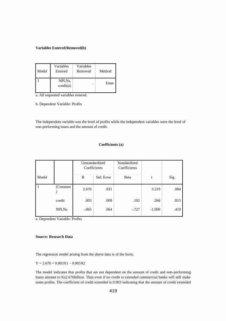
419

Variables Entered/Removed(b)

Model

Variables

Entered

Variables

Removed Method

1 NPLNs,

credit(a) . Enter

a. All requested variables entered.

b. Dependent Variable: Profits

The independent variable was the level of profits while the independent variables were the level of

non-performing loans and the amount of credit.

Coefficients (a)

Model

Unstandardized

Coefficients

Standardized

Coefficients

t Sig. B Std. Error Beta

1 (Constant

) 2.676 .831 3.219 .084

credit .003 .009 .192 .266 .815

NPLNs -.065 .064 -.727 -1.009 .419

a. Dependent Variable: Profits

Source: Research Data

The regression model arising from the above data is of the form;

Y = 2.676 + 0.003X1 – 0.065X2

The model indicates that profits that are not dependent on the amount of credit and non-performing

loans amount to Ks2.676billion. Thus even if no credit is extended commercial banks will still make

some profits. The coefficient of credit extended is 0.003 indicating that the amount of credit extended

420

contributes positively to profits but marginally. Additionally, as the level of non-performing loans

increase, profits decrease. There is therefore a positive relationship between the amount of credit

extended and the amount of profits while there is a negative relationship between the level of non-

performing loans and profits. The t-test indicates that the profits that do not depend on credit and non-

performing loans are significant. The test of significance indicates that the coefficient of 0.003 in the

case of credit and the coefficient of -0.65 in the case of non-performing loans are not significant or

are due to chance. This means that there is no association between profits, amount of credit and the

level of non-performing loans. Ordinarily, commercial banks should focus on other factors other than

the non-performing loans if their objectives are to predict profits.

Model Summary

Model R R Square

Adjusted R

Square

Std. Error of

the Estimate

1 .622(a) .387 -.226 .53078

a. Predictors: (Constant), NPLNs, credit

Source: Research Data

The R-Square indicates that only 38.7% of the profits are explained by amount of credit and the level

of non-performing loans. The adjusted R-Square of -0.226 however indicates that amount of credit

and non-performing loans do not explain the level of profits made by commercial banks. This means

that there is no relationship between the amount of credit, non-performing loans and the amount of

profits.

ANOVA(b)

Model

Sum of

Squares df Mean Square F Sig.

1 Regressio

n .356 2 .178 .631 .613(a)

Residual .563 2 .282

421

Total .919 4

a. Predictors: (Constant), NPLNs, credit

b. Dependent Variable: profits

Source: Research Data

ANOVA F2,2 statistic of 0.631 is significant with a P-value > 0.05. The model does not establish a

relationship between profits, amount of credit and the level of non-performing loans.

3.5.2 Amount of Credit and Non-Performing Loans

A regression was run to establish whether there was any relationship between amount of credit and

the level of non-performing loans of commercial banks.

Variables Entered/Removed(b)

Model

Variables

Entered

Variables

Removed Method

1 CR(a) . Enter

a. All requested variables entered.

b. Dependent Variable: NPLS

The dependent variable was the level of non-performing loans while the amount of credit was the

independent variable.

Coefficients (a)

Model

Unstandardized

Coefficients

Standardized

Coefficients t Sig.

422

B Std. Error Beta

1 (Constant

) .039 .071 .550 .620

CR .094 .065 .640 1.442 .245

a Dependent Variable: NPLS

The regression model established was of the form;

Y= 0.039 + 0.094X

This reveals that even when no credit is extended by, the level of non-performing loans would be

Ksh0.039 billion, an indication that commercial banks in Kenya incur other credit other than on non-

performing loans. The coefficient of 0.094 indicates that an increase in the amount of credit leads to

an increase in the level of non-performing loans. Therefore there is a positive relationship between

the amount of credit extended by commercial banks and the level of non-performing loans.

Model Summary

Model R R Square

Adjusted R

Square

Std. Error of

the Estimate

1 .640(a) .409 .212 .04771

a. Predictors: (Constant), CR

The r2 value of 40.9% indicates that there is a weak relationship between the amount of credit and the

level of non-performing loans.

ANOVA (b)

Model

Sum of

Squares df Mean Square F Sig.

1 Regressio

n .005 1 .005 2.078 .245(a)

Residual .007 3 .002

Total .012 4

a. Predictors: (Constant), CR

423

b. Dependent Variable: NPLS

The ANOVAF1,3 statistic of 2.078 is significant with a P-value > 0.05. The model reveals that there

is no relationship between the amount of credit and the level of non-performing loans of commercial

banks in Kenya.

4.0 SUMMARY OF FINDINGS AND CONCLUSIONS

The findings reveal that the level of credit was high in the early years of the implementation of Basle

II but decreased significantly in 2007 and 2008, probably when the Basle II was implemented by

commercial banks.

Notably, the level of non-performing loans given by non-performing loans to total loans decreased

during the period 2004 to 2008. The requirement by the Basle II might have enabled commercial

banks to control their level of non-performing loans thus reducing banks credit risk.

Thus on average the profits of the banking industry increased during the period 2004 to 2008.

However, profitability of the commercial banks fluctuated during the period; conversely on average

increased marginally during the period 2004 to 2008. The profits were generally low during the

period of study. The amount of credit extended to customers was relatively high but assumed a

downward trend during the period. Whereas the level of credit and profits were relatively low and

stable, the amount of credit was high and relatively volatile.

The regression results indicate that there is no relationship between profits, amount of credit and the

level of non-performing loans.

The R-Square indicates that only 38.7% of the profits are explained by amount of credit and the level

of non-performing loans. The adjusted R-Square of -0.226 however indicates that amount of credit

and non-performing loans do not explain the level of profits made by commercial banks. This means

that there is no relationship between the amount of credit, non-performing loans and the amount of

profits. ANOVA F2,2 statistic of 0.631 is significant with a P-value > 0.05. The model does not

establish a relationship between profits, amount of credit and the level of non-performing loans.

Further analysis undertaken to establish whether there was any relationship between the amount of

credit and the level of non-performing loans established that even when no credit was extended by

commercial banks, the level of non-performing loans would be at the level of Ksh0.039 billion, an

indication that commercial banks in Kenya incur other credit other than on non-performing loans.

The coefficient of 0.094 indicates that an increase in the amount of credit leads to an increase in the

level of non-performing loans. Therefore there is a positive relationship between the amount of credit

extended by commercial banks and the level of non-performing loans. The r2 value of 40.9%

indicates that there is a weak relationship between the amount of credit and the level of non-

performing loans. The ANOVAF1,3 statistic of 2.078 is significant revealing that there is no

relationship between the amount of credit and the level of non-performing loans of commercial banks

in Kenya.

424

The findings reveal that the bulk of the profits of commercial banks is not influenced by the amount

of credit and non-performing loans suggesting that other variables other than credit and non-

performing loans impact on profits. Commercial banks that are keen on making high profits should

concentrate on other factors, other than focusing more on amount of credit and non-performing loans.

The implication is that an institution specializing in the collection of non-performing loans which

could save the banking institutions the cost of collecting non-performing loans

REFERENCES

Akerlof, G.A. (1970). The Market for ―Lemons‖: Quality Uncertainty and the Market Mechanism.

The Quaterly Journal of Economics. 84(3)

Alien, L. and Jagliani, J. (2000). The Impact of New Bank Powers (Security and Insurance

Activities) on Bank Holding Companies Risk. Journal of Economics and Business

Allen and Cale (2000). Financial Stability Analysis Using Aggregated Data. Bis.org

Altman, E. I. (1968). Financial Ratio Discriminant Analysis and the Prediction of Corporative

Bankruptcy. Journal of Finance. Vol.23

Apps, R. and Goacher, S. (1993). Business and Investing: Monetary and Financial System.

Amazon.fr.

Aristobulo, J. (1991). From Good Bankers to Bad Bankers: Ineffective Supervision and

Management Deterioration as Major Elements in Banking Crisis. EDI Working Paper

Washington, D.C.: Economic Development Institute of the World Bank. Auronen, L. (2003). Asymmetric Information: Theory and Applications. Helsinki University of

Technology, Department of Industrial Engineering and Management, Lauri.Auronen@hut.fi

Banking Survey (2001). A Comprehensive Analysis and Ranking of 46 Kenyan Banks. Market

Intelligence. The Business and Finance Journal.

Banking Survey (2000). The Unending Saga of Bank Failures in Kenya: Market Intelligence. The

Business and Finance Journal.

Barajas, A. R.S., and Salazar, N. (1996). Interest Spread in Banking: Costs, Financial Taxation,

Market Power and Loan Quality in the Columbian Case, 1974-1988. IMF Working Paper,

No.110, Washington D.C.

Basle Committee on Bank Supervision (1988). International Convergence of Capital

Measurement and Capital Standards. The Basle Committee, July. Basle Committee on Bank Supervision (1996a). Amendment to the Capital Accord to Incorporate

Market Risks. The Basle Committee, July.

Basle Committee on Bank Supervision (1996b). Supervisory Framework for the Use of

“Backtesting” in Conjunction with the Internal Models Approach to the Market Risk Capital

Requirements. The Basle Committee, January.

Basle Committee on Banking Supervision (2001a). The New Basel Accord, The Basle Committee,

January.

Basle Committee on Banking Supervision (2001b). The Standard Approach to Credit Risk. The

Basle Committee, January.

Basle Committee on Bank Supervision (2001c). The Internal Ratings-Based Approach. The Basle

Committee, January.

Basle Committee (1998). Framework for the Internal Controls Systems in Banking Organizations. BIS BASEL, September.

Basle Committee (2000). Other Risks. Risk Management, Discussion Paper, BIS BASEL. April.

Barclays, M. and Holderness, C. (1998). Private Benefits from Control of Public Corporations.

Journal of Financial Economics. Vol. 3.

Beaver, W. H., (1996). Financial Ratios as a Predictor of Failure. Empirical Research in

Accounting. Selected Studies.71-111.

425

Bergen, A. (1998). Managing Systemic Banking Crisis in Practice. The Swedish Bank Support

Process, World Bank, Washington D.C.

Berger, Allen N. (1995). The Relationship between Capital and Earnings in Banking. Journal of

Money, Credit and Banking. Vol. 27, No.2, pp.432-456.

Berger, et al. (1995). The Role of Capital in Financial Institutions. Journal of Banking and

Finance. Vol.19, No.3-4, pp.393-430. Berle, A. and Means, G. (1932). The Modern Corporation and Private Property. Wikipedia,

Encyclopedia.

Berle, A. (JR) and Means, G. (1930). Corporations and the Public Investor. The American

Economic Review. 20(1)

Bery, S.K. and Garcia, V.F. (1996). Preventing Banking Sector Distress and Crises in Latin

America. Proceedings of a Conference Held in Washington D.C. April.

Bett, K. A. K, (1992). Financial Performance in Banking Sector. The Case for Kenya Banks and

Financial Institutions (1986-1990); Unpublished MBA Research Project of the University of

Nairobi.

Bikker, J.A. and Metzemakers, P.A.J. (2005). Bank Provisioning Behaviour and Procyclicality.

Journal of International Financial Markets, Institutions and Money, Elsevier. Vol. 15(2), Pages

141-157, April (Downloadable) Black, F. and Scholes, M. (1973). On the Pricing of Options and Corporate Liabilities. Journal of

Political Economy. 81

Bonin, J. and Huang, Y.P. (2001). Dealing With the Bad Loans of the Chinese Banks. Journal of

Asian Economies. Summer.

Bonish, M. et al. (1995). Enterprise and Bank Restructuring: Recent Losses from Transition

Countries. World Bank Discussion Paper, 229, January.

Bonish, M. and Montes-Negret, (1998). Restructuring Distressed Banks in Transition Economies.

Lessons from Central Europe and Ukraine, The World Bank, Washington D.C.

Brealey, R.A. and Myers, S.C. (1996). Principles of Corporate Finance 5th Edition, McGraw-Hill

Companies.

Brewer, M. B. and Barry, E. C. (1981). Scientific Inquiry and the Social Sciences. San Francisco. Jossey-Bass Publishers

Brinberg, D., and Joseph, M. (1985). Validity and the Research Process. Newbury Park, Calif.

Sage Publications.

Brown, F., and Manassee, P. (2002). The Information Content of the Term Structure of Interest

Rates: Theory and Evidence. Monetary and Fiscal Policy Division

Brownbridge, (1999). Banking Sector Reform and Financial Regulation. http:competition-

regulation.or.uk

Buttimer, R. (2008). Risk, Return and Risk Management. The Journal of Real Estate Finance and

Economics. Sterling Valuation Group Inc.

Callier, P. (1991). Financial Systems and Development in Africa. Economic Development

Institute of the World Bank. Seminar Series, Washington D.C.

Campanero, J.P. and Leone, A.M. (1991). Liberalisation and Financial Crisis in Uruguay, 1974-1987. IMF Publications, Washington D.C.

Campell, D. T. and Thomas, D. C. (1979). Quasi-Experimentation. Shokie, Rand McNally.

Capie, F. and Billings, M. (2001a). Profitability in English Banking in the Twentieth Century.

European Review of Economic History. Vol. 5, No.3, pp. 367-401.

Capie, F. and Billings, M. (2001b). Accounting Issues and the Management of Profits English

Banks 1920-1968. Accounting, Business and Financial History. Vol.11, No.2, pp. 225-251.

Caprio (jr) G., et al. (1998). Preventing Bank Crisis: Lessons from Recent Global Bank

Failures. EDI Development Studies, The World Bank, Washington D.C

Caprio (jr) G. and Klingebiel D. (1996). Bank Insolvencies: Cross Country Experience.

Finance and Private Sector Development Division Policy Research Department. The World

Bank, Washington D.C.

426

Cassel, C., and Symon, G. (1994). Qualitative Methods in Organizational Research. Thousand

Oaks, C.A Sage

CBK (1976). Central Bank of Kenya Annual Report

CBK (1985 to 1990). The Central Bank of Kenya Annual Reports

CBK (1995-2001). Bank Supervision Annual Reports. The Central Bank of Kenya.

Credit Suisse Group (2003).Operational Risks in Financial Services. April Report

Chakravarty, S., et al. (1998). Information Asymmetry, Market Segmentation and the Pricing of

Cross Listed Shares: Theory and Evidence from Chinese A and B Shares.

Chava, F. N., and David, N. (1996). Research Methods in the Social Sciences. St Martin‘s Press, Fifth

Edition

Checkley, K. and Dickinson, K. (2001). Business Lending. Selwood Printing, Burgess

Hill. The Chartered Institute of Bankers.

Chiang, A. C. (1980). Fundamental Methods of Mathematical Economics. Third Edition. McGraw-

Hill International Book Company

Chirwa W.E and Montfort M (2004). Financial Reforms and Interest Rate Spreads in the

Commercial Banking System in Malawi. IMF Staff Papers, International Monetary Fund,

Vol. 51(1).

Claessens, S. (1998). Systemic Bank and Corporate Restructuring. The World

Bank, Washington D.C.

Claessens, S., Djankov S., and Klingebiel, D. (1999). Financial Restructuring in East Asia: Halfway

There? Financial Sector Discussion Paper. 3. The World Bank, September.

Claeys, S. and R. Vander Vennet. (2003). Determinants of Bank Interest Margins in Central and

Eastern Europe. Convergence to the West? Working Papers of Faculty of Economics and

Business Administration, Ghent University, Faculty of Economics and Business

Administration.

Conford, A. (2000). The Basel Committee‟s Proposals for Revised Capital Standards: Rationale,

Design and Possible Incidence, G-24 Discussion Paper Series. United Nations, No.3.

Constantinides, G. and Malliaris, A.G. (1995). Portfolio Theory. Handbooks in Operations Research and Management Science. Volume 9. Elsevier Science Publishers

Cooper, D.R. and Schindler, P.S. (2003). Business Research Methods. 8th Edition, McGraw Hill, New

York.

Cooperman E., Mills D., and Gardner J., (2000). Managing Financial Institutions: An

Asset/Liability Approach. The Dryden Press, Harcout College Publishers, Orlando.

Coyle, B. (2000). Framework for Credit Risk Management. Chartered Institute of Bankers, United

Kingdom.

Creswell, J.W. (1994). Research Design: Qualitative and Quantitative Approaches. Thousand Oaks,

C.A. Sage.

Crouhy, M. (2005). The Essentials of Risk Management. McGraw-Hill Companies.

Davis, J. A. (1985). The Logic of Causal Order. Newbury Park, Calif, Sage Publications

De Has, R., and Van Lelyveld, I. (2004). The Mix of International Banks Foreign Claims: Deteminants and Implications. World Bank.

427

De Has, R., and Van Lelyveld I. (2006). The Impact of Foreign Banks Entry on Domestic Banks

Profitability. The World Bank.

De Juan, A. (1991). From Good Bankers to Bad Bankers: Ineffective Supervision and Management

Determination as Major Elements in Banking Crisis. EDI Working Paper, Economic

Development Institute of the World.

De Juan, A. (1990). Does Bank Insolvency Matter? And What to Do About It? The International Bank for Reconstruction and Development/the World Bank, Washington D.C.

De-Luna-Martinez, J. (2000). Management and Resolution of Banking Crises. Lessons from the

Republic of Korea and Mexico. The World Bank, Washington D.C.

Demirguc-Kunt, (1989). Banking Crises and Bank Concentration. The World Bank

Demirguc, A., and Huzinga, H. (1999). Determinants of Commercial Banks Interest Margins and

Probability: Some International Evidence. World Bank Economic Review 13

Demirguc-Kunt A., and Huzinga, H. (2000). Financial Structure and Bank Profitability. World Bank,

Research Paper, Washington D.C.

Demirguc-kunt, A. and Huzinga, H. (1999). Determinants of Commercial Bank Interest Margins and

Profitability: Some International Evidence. The World Bank Economic Review. Vol.13, No.2, pp.

379-408.

Demsetz, H. and Leln (1985). Management Ownership and Firm‘s Value: An Empirical analysis Using Panel Data. Retrieved from www.iser.osaka-u.ac.jp/library/dp/2003

Demsetz, H. and Villalonga (2001). Ownership Structure and Performance in Large Spanish

Companies: Empirical Evidence in the Context of an Endogenous Relation. University of

Valladolid, Department of Financial Economics and Accounting. VALLADOLID

De Young, and Roland, K. (2001). Product Mix and Earnings Volatility: Evidence from the Degree

of Total Leverage Model. Research Paper. Retrieved from http://paperspssrn.com/so13/papers.cfm

Diamond, D. and Dybvig, P. (1983). Bank Runs, Deposit Insurance and Liquidity. Journal of

Political Economy

Duffie, D. (2003). Dynamic Asset Pricing Theory. 3rd Edition, Princeton U. Press.

Dziobek, C. and Pazarbsioglu, C. (1998). Lessons from Systemic Bank Restructuring: A Survey of 24

Countries. Economic Issues No. 14, IMF. May. Retrieved from: http://www.imf.org/external

/pubs/ft/issues 14/ and µhttp://www.imf.org/external /pubs/ft/issues 14/§

Dziobek, C. (1998). Market-Based Policy Instruments for Systemic Bank Restructuring. IMF

Working Paper, 98/113, International Monetary Fund, Washington, D.C. Early, J.S. (1966). Problems in the Measurement of the Quality of Credit. Proceedings of the

Business and Economic Statistics Section of the American Association, 202-217.

Early W., Rodriguez C.A. and Schmidt, H.K. (1994). Public Sector Deficits and Macro

Economic Performance. A World Bank Publication, Oxford University Press, New York.

EL-Nil, Y.S.H. (1990). The Prerequisites for a Successful Financial Reform. The World Bank, EAI

Seminar Series, Washington D.C.

Fama, E. and Jensen, M. (1983). Separation of Ownership and Control. Journal of Law and

Economics. Vol. 26.

Fama, E.F. and M.C. Jesen (1985). Agency Problems and Residual Calims. Journal of Law and

Economics.

Fama, E., and French, K. R. (1996). The CAPM is Wanted, Dead or Alive. Journal of Finance. 51, No.5.

Federal Reserve Release (2002); ―Basle II: A False Sense of Security?‖ New York, USA, August.

Fischer, S. (1983). A Framework for Monetary and Banking Analysis. Economic Journal 93.

Fisher, S. (1997). Banking Soundness and the Role of the Fund. Paper Presented at the 7th Seminar on

Central Banking, Washington DC, IMF Publications Services.

Flannerry, M. J., and Rangan, K.P. (2002). Market Forces at Work in the Banking Industry: Evidence

from the Capital Build-up of the 1990s.” AFA 2003 Washington, DC Meetings; EFA 2002 Berlin

Meetings Presented Paper: http://ssrn.com/abstract=302138

Fleming, A., et al. (1996). The Baltics – Banking Crises Observed. The World Bank: Enterprise and

Financial Sector Development Division, September.

Friedman, M. (1968). The Role of Monetary Policy. American Economic Review. Vol. 63

428

Gallagher, C.A. and Watson, H. J. (1984). Quantitative Methods for Business Decisions. McGraw-

Hill International Book Company.

Gamba, A. et al. (2007). Investment and Credit Risk: A Structural Approach. Department of

Economics, University of Verona, Italy.

Gargill, T. (1991). Market Discipline by Depositors: Evidence from Reduced Form Equations.

Federal Reserve Bank. Giammarino, R., (1989). The Resolution of Financial Distress. Review of Financial Studies, Vol. 2.

No. 1.

Gill, P. (1989). Change in Product Liability Reform. AuconstrlawNlr48, Australian Construction

Law.

Gilson, Stuart C., Kose J., and Larry H.P.L., (1990). Trouble Debt Restructurings: An Empirical

study of Private Reorganization of Firms in Default. Journal of Financial Economics. 27. 315-

353.

Gizycki, M. (2001). The Effect of Macroeconomic Conditions on Banks‟ Risk and profitability. RBA

Research Discussion Papers rdp2001-06, Reserve Bank of Australia.

Goldberg, L.G. and Rai, A. (1996). The Structure –Performance Relationship for European Banking.

Journal of Banking and Finance. Elsevier, Vol. 20(4). 745-771, May.

Goldstein, R. et al. (2001). An EBIT-Based Model of Dynamic Capital Structure. Journal of Business. 74, 483-512.

Gonzalez-Hermssillo, Pazarbasioglu and Billings (1997). Macroeconomic and Financial Soundness

Indicators. International Monetary Fund, May.

Greuning, H. and Bratanivic, S.B. (1999). Analyzing Banking Risk. The World Bank.

Griffith-Jones, S. and Persaud, A. (2002). The Political Economy of Basle II and Implications for

Emerging Economies. A Paper Presented to the Economic Commission of Latin America,

April.

Grinblatt, M., and Titman, S. (2002). Financial Markets and Corporate Strategy. Second Edition,

Mcgraw Hill Inc.

Hammersley, M. (1995). Theory and Evidence in Qualitative Research: Quality and Quantity, 29 (1),

55-66. Hawkins, J. and Turner, P., (1999). Bank Restructuring in Practice – An Overview. in BIS, Bank

Restructuring in Practice. BIS Policy Paper No.6. Bank International Settlements, Basel,

Switzerland.

Hayne, E.L. (1979). Quacks, Lemons, and Licensing: A Theory of Minimum Quality Standards. The

Journal of Political Economy. 87 (6).

Hellwig, M. (1991). Banking, Financial Intermediation and Corporate Finance: A. Giovannini and

C. Mayer (eds), European Financial Integration, Cambridge: Cambridge university Press.

Hinds, M. (1988). Economic Effects of Financial Crises. PPR Working Paper WS 104. The World

Bank, Washington D.C.

Holderness, K. et al. (1999). Ownership-Control Discrepancy and Firm Value: Evidence from

France. Universite‘ Paris XII, Val de Marne, France.

Hortlund, Per. (2005). The Long-Term Relationship Between Capital and Earnings in Banking.

Working Paper Series in Economics and Finance. 611, Stockholm School of Economics.

Revised 17 Nov 2005.

Huzinga, Harry And Demirguc-Kunt, Asili (2000); “Financial Structure and Bank Profitability”,

Policy Research Working Paper Series 2430, the World Bank.

Hsiu-Kwang, W. (1969). Bank Examiner Criticisms, Bank Loan Defaults, and Bank Loan Quality.

The Journal of Finance. Vol. 24, September, 697-705.

International Monetary Fund (1997). Banking Soundness and Monetary

Policy in a World of Global Capital Flows. Proceedings of the Seventh Central Banking

Seminar. Jan. 27-31 Washington D.C.

Jacob, A. B., and Metzemakers, A.J. (2003). Bank Provisioning Behaviour and Procyclicality. DNB

Staff Reports, 111, Netherlands Central Bank (Downloadable)

429

Jankov, L. (2000). Banking Sector Problem: Causes, Resolutions and Consequences.

Occassional Paper No.10

Jankov, L. and Kraft, E. (2000). Lending Booms, Foreign Entry and Competition: The Croatian

National Bank. www:hnb.hr/dub-konf/9

Jensen, M.C. and Meckling, W.H. (1976). Theory of the Firm: Managerial Behaviour, Agency Costs

and Ownership Structure. Journal of Financial Economics.

Jensen, M.C. and Smith, C. (2000). the Theory of Corporate Finance: A Historical Overview, New

York. McGraw-Hill Incl.

Jorion, P. (2009). Risk Management Lessons from the Credit Crisis. Pacific Alternative Asset

Management Co. (PAAMCO), September.

Jovanovic, B. (1982). Favourable Selection with Asymmetric Information. The Quarterly Journal of

Economics. 97 (3).

Julie, C. and Strauss, A. (1996). Basics of Qualitative Research, Techniques and Procedures for

Developing Grounded Theory. Sage Publications, International Educational and Professional

Publisher, Second Edition.

Kamara, et al. (1997). The Impact of Institutional Investors on the Monday Seasonal. Journal of

Business. University of Chicago.

Kane, E.J. and T. Rice. (1998). Bank Runs and Banking – Lessons for African Policy

Makers. Journal of Money, Credit and Banking. Vol. 26, No.I February.

Karacadag, C. and Taylor, M.W. (2000). Toward a New Global Banking Standard: The

Basel Committee‟s Proposals. Finance and Development. Vol. 37 No. 4. Dec.

―http://www.imf.org/external/pubs/ft/fandd/2000/12/karacada.htm‖

µhttp://www.imf.org/external /pubs/ft/fandd/2000/12/karacada.htm§.

Kenya Commercial Bank (1992-2001). Published Annual Accounts.

Keynes, J. M. (1936). The General Theory of Employment, Interest and Money, Mcmillan

Cambridge University Press.

Khun, (1962). Where Is Psychology Going? Structural Fault Lines Revealed by Psychologists.

Harvard University.

Kiptui, M. and Kipyegon, L. (2008). External Shocks and Real Exchange Rate Movements in Kenya.

Central Bank of Kenya.

Kirk, J. and Miller, M. (1986). Reliability, Validity and Qualitative Research; Beverly Hills, C.A.

Sage Publications.

Kiyai, T. K., (2003), Bad Debts Restructuring Techniques and Non- performing

Loans of Commercial Banks in Kenya, MBA Unpublished Research Project of the

University of Nairobi.

430

Klingebiel, D. (2000). Financial Restructuring in East Asia. The World Bank,

Washington D.C., July.

Klingebiel, D. (1996). The Use of Asset Management Companies in the Resolution of Banking Crisis:

Cross-Country Experience. IMF Working Paper.

Kunt-Demirguc and Detragiache (1997). The Determinants of Banking Crises: Evidence from

Developing and Developed Countries. International Monetary Fund. Working Paper, WP/97/106.

Laker, A. (2007). Go to Every Laker Home Game for College Credit. The Los Angeles Lakers

Community Relations Department, Los Angeles.

La Porta, et. al. (1999). Investor Protection and Corporate Ownership. Harvard University and New

York University.

Lando, D. (2009). Credit Risk Modelling. Copenhagen Business School, department of Finance,

Solberg Plads 3, denmark, DK-2000, Frederiksberg

Lardy, N.R. (1998). China‟s Unfinished Economic Revolution. The Brookings

Institution. Washington, D.C.

Larrian and Montes-Negret. (1996). Bank Restructuring in Spain 1977-1985. World

Bank Pubications.

Lindgren H. (1987), Bank, Investment Company, Banking Firm. Stockholms Enskilda

Bank [1924-1945]. Stockholm: Institute for Research in Economic History at the Stockholm

School of Economics.

Lintner, J. (1965). Security Prices, Risk, and Maximal Gains from Diversification.

Journal of Finance. 20.

Madura, A. and Wiant, K. (1995). Banking System, Real Estate Markets and Non-performing Loans.

nccuir.lib.nccu.edu.tw/bitstream

Madura and Wiant (1995). Insider Trading and the Predictability of Stock Returns. efmaefm.org

Markowitz H. (1959); Portfolio Selection: Efficient Diversification of Investments.

New York. John Wesley

Martinez, P., et al. (2010). Does Foreign Bank Penetration Reduce Access to Credit in Developing

Countries? Evidence from Asking Borrowers. Policy Research Working Paper. Series, 2716,

The World Bank. (Downloadable)

Matz, L.M. and Neu, P. (1998). Liquidity Risk Measurement and Management. John Wiley and Sons

Publishers.

McDonough, W. J. (1998). Issues for the Basle Accord: Basle Committee on Bank

431

Supervision. Conference on Credit Risk Modelling and Regulatory Implications. Barbican

Centre, London, England, September.

Merton, M. (1972). Dynamic Downside Risk Measure and Optimal Investment Behaviours.

fma.org/Prague/pdf

Merton R.C. (1974). The Pricing of Corporate Debt: The Risk Structure of Interest Rates. Journal of

Finance. 29.

Merton, R.C. (1995b). Financial Innovation and the Management and regulation of Financial

Institutions. Journal of Banking and Finance. 19.

Merton, R.C. and Bodie Z. (1993); “Deposit Insurance Reform: a Functional Approach”, Carnegie-

Rochester Conference Series on Public Policy 38

Miles. M. and Hubberman, A. (1994). Qualitative Data Analysis: Thousand Oaks, C.A Sage

Publications.

Miller, G.P. (1996). Is Deposit Insurance Inevitable? Lessons from Argentina.

International Review of Law and Economics. 16.

Miller, S. H. (1989). Experimental Design and Statistics. 2nd Ed. New York, Methuen.

Mishkin, A.K. (1998); “The Economics of Money, Banking and Financial Markets”

Addition – Wesley 5th Edition.

Montes-Negret, F. (1989). An Overview of Colombia‟s Banking Crisis.

World Development Report Background Paper, Washington D.C.; the World Bank,

December.

Moore, G.H. (1956). The Quality of Credit in Booms and Depressions. Journal of

Finance. Vol. 11. May.

Moore, G.H. and Klein, P.A. (1967). The Quality of Consumer Installment Credit, New

York.

Mork, R. S.A., and Vishy, R. (1988). Management Ownership and Market

Valuation: An Empirical Analysis. Journal of Financial Economics. Vol. 20.

Ngugi, R.W. (2001). An Empirical Analysis of Interest Rate Spread in Kenya.

Research Paper No. 106, Africa Economic Research Consortium.

Ngugi, R.W. and Kabubo, J.W. Financial Sector Reforms and Interest Rate

Liberalization: The Kenya Experience. Africa Economic Research Consortium.

Njuguna, S.N. (2000). The Exchange Rate and Interest Rate Differential in Kenya:

432

A Monetary and Fiscal Policy Dilemma. KIPPRA Discussion Paper No.10 NAIROBI

KIIPRA.

Omutunde, J.O. (2002). Financial Risks, Stability and Globalization. Papers Presented at

the Eighth Seminar on Central Banking Washington, D.C. June 5-8, 2000.

International Monetary Fund (IMF)

Olena, H. and Emilia, J. (2006). Profitability of Foreign and Domestic Banks in Central and Eastern

Europe: Does the Mode of Entry Matter? LICOS Discussion Papers 16606, LICOS – Centre

for Transition Economics, K.U. Leuven.

Pandey, I. M. (2009). Financial Management, Indian Institute of Management. Ahmedabad, Ninth

Edition; Vikas Publishing House PVT Ltd.

Parry, C. (1999). Lending and Securities: A Practical Guide to the Principles of Good Lending.

Kenwood Books Ltd.

Payle, D. (1997). Bank Risk Management. Working Paper No.272, University of

California.

Pyle, D.H. (1971). On the Theory of Financial Intermediation. Journal of Finance. 26.

Pazaarbasioglu, C. (1998). Leading Indicators of Banking Crisis: Was Asia Different? IMF Working

Paper.

Peek, J. and Rosengreen, S. (2000). Crowding Out, Interest and Exchange Rate Shocks and Bank

Lending. World Bank

Petersen, M.A. and Rajan, R.G. (1997). Trade Credit: Theories and Evidence. National Bureau of

Economic Research, International Monetary Fund

Polizatto, V. (1990). Prudential Regulation and Banking Supervision: Building an

Institutional Framework for Banks. Economic Development Institute of the World Bank.

The World Bank Washington D.C. Popiel, P.A. (1990). Developing Financial Markets in Sub-Saharan Africa. The

World Bank, EAI Seminar Series, Washington D.C.

Quinn, J. B. et al. (1988). The Strategy Process: Concepts, Contexts and Cases. Prentice-Hall

International Editions.

Rajan, R. G. (1994). The Entry of Commercial Banks into the Securities Business: A Selective

Survey of Theories and Evidence. Graduate School of Business, University of Chicago.

Rajan, R.G. and Petersen, M.A. (1994). Relationship Lending: Is It Incentives or Hidden

Information? http://www.econ.puc-rio.br/pdf/td519.pdf

Rajan, R. (1995). The Effect of Credit Market Competition on Lending Relationships. The Quarterly

Journal of Economics.

Reilly, F.K. and Brown, C.K. (1997). Investment Analysis and Portfolio Management. Dryden Press, Harcout Brace.

Ramos, S.J. (2000). Financial Risk Management. Inter-American Development Bank.

Reisen, H. (2001). Will Basel II Contribute to Convergence in international Capital

Flows? Oesterreichische Nationalbank, 29, Tagung.

Reynolds, Ratanakomut and Gander (2000). Banking System, Real Estate Markets and Non-

Performing Loans. International Real Estate Review. Vol.6.

Ritter, S., Siller, W. and Udell, G. (1997). Principles of Money, Banking and Financial

Markets. Addison - Wesley Longman, Inc New York.

Roels, et.al. (1990). Financial Systems and Development in Africa. EDI Policy

Seminar held in Nairobi, Kenya.

433

Rose, P.S. (1994). The Rescue of Troubled Banks; Consequences for Corporate Strategies to Deal

with Financial and Operating Stress. Journal of Financial and Strategic Decisions. Vol 7,No.2

Summer.

Rose, P.S. (1997). Money and Capital Markets, Financial Institutions and Instruments in a Global

Market Place. Sixth Edition Irwin.

Rothschild, M. and Stiglitz, J. (1976). Equilibrium in Competitive Insurance Markets: An Essay on

the Economics of Imperfect Information. The Quartely Journal of Economics. 90 (4)

Roulier, R.P. (1995). Bank Governance Contracts, Establishing Goals and Accountability in Bank

Restructuring. World Bank Discussion Paper. The World Bank, Washington D.C.

Rouse, C. N. (1989). Bankers‘ Lending Techniques. Chartered Institute of Bankers Publication.

Samuelson, W. (1984). Bargaining Under Asymmetric Information. Econometrica, 52(4)

Sandstorm, A. (2009). Political Risk in Credit Evaluation. World Bank Group.

Sasaki Y.N. (2006). Japanese Banks‟ Credit Allocation under the Requirement of

Basle Capital Standards and the Burden of Non-Performing Loans. Department of

Economics, Meiji Gakuin University.

Saunders, A. and Wilson, B. (1999). The Impact of Consolidation and Safety-Net Support

on Canadian, US and UK Banks. Journal of Banking and Finance. Vol. 23, No. 2-4, pp.

537-571.

Sailesh Tanna and Kyriaki Kosmidou and Fotios Pasiouras (2005). Determinants of

Profitability of Domestic U.K. Commercial Banks: Panel Evidence from the Period 1995-2002.

Money Macro and Finance (MMF) (2005) Research Group Conference. A Money Macro and Finance

Research Group.

Segalla, T. A. et.al (2001). The Determinants of Bank Interest Spread in Brazil. Anais do XXiX Encontro Nacional de Economia (Proceedings of the 29th Brazilian Economics Meeting) 051,

ANPEC – Brazilian Association of Graduate Programs in Economics.

Senbet, W.L. (1998). Global Financial Crisis: Implications for Africa. University of

Maryland, The Robert H. Smith school of Business, College Park.

Seppala, J. (2000). The Term Structure of Real Interest Rates: Theory and Evidence from U.K. Index-

Linked Bonds. Department of Economics. University of Illinois at Urbana, Champaign,

September.

Sharpe, W. (1970). Portfolio Theory and Capital Markets. Qfinance.com

Sheng, A. (1996). Bank Restructuring in Spain: Lessons from the 1980s.

Washington D.C. World Bank.

Sheng, A. (1990). Bank Supervision: Principles and Practices. EAI Seminar Series.

The World Bank, Washington D.C.

434

Shleifer, A. and Vishy, R. (1986). Large Shareholders and Corporate Control. Journal of

Political Economy. Vol. 94.

Short, H. (1994). Ownership, Control, Financial Structure and Performance of Firms.

Journal of Economic Survey. Vol. 8 (3).

Silverman, D. (1993). Interpreting Qualitative Data. Newbury Park, C.A Sage Publications.

Simson, D.N. and Hempel, G.H. (1999). Bank Management, Text and Cases, 5th Ed, John Wesley and Sons Inc., New York.

Sinkey, J. F. (1975). A Multivariate Statistical Analysis of the Characteristics of Problem

Banks. Journal of Finance. Vol. 30. Number 1 March.

Sinkey, J. (1992). Commercial Bank Financial Management. McMillan Publishing

Company, New York.

Sobert, J.R. et al. (2000). Moody‟s Public Risk Firm Risk Model: A Hybrid Approach to Modelling

Short Term Default Risk. Moody‘s Investor Service, Global Credit Research, Rating

Methodology.

Stiglitz, J.E. (1975). The Theory of ‗Screening‘, Education, and the Distribution of Income. The

American Economic Review. 65 (3).

Stiglitz, J.E. and Weiss, A. (1981). Credit Rationing in Markets with Imperfect Information. The

American Economic Review. 71(3). Spence, M. (1973). Job Market signalling. The Quarterly Journal of Economics. 87(3).

Sundarajan, V. (1988). Banking Crisis and Adjustment: Recent Experience. IMF

Central Banking Seminar Papers; Washington D.C. IMF, December.

Sundarajan, V. and Molho, L. (1988). Financial Reform and Monetary Control in

Indonesia. IMF Working Paper 88/4. Washington D.C. IMF, January.

Thompson, G., (2006). Banking Crises in Kenya. Kenya Banking and Securities,

Thompson Corporation.

Thygerson, J. and Kenneth (1995). Management of Financial Institutions, Harper

Collins, College Publishers, New York.

Tudela, M. and Young, G. (2003). A Merton Model Approach to Assessing the Default Risk of UK

Public Companies. Bank of England, Mimeo.

Uyemura, D.G. and Van Deventer, D.R. (1992). Financial Risk Management in Banking. The Theory

and Application of Asset and Liability Management, McGraw-Hill.

World Bank (1997). Bank Restructuring in Sub-Saharan Africa: Lessons Learned

Findings. Africa Region, No. 89, June.

Yan, W., and Bayrakktar, N. (2004). Foreign Bank Entry, Performance of Domestic Banks, and

Sequence of Financial Liberalization. Policy Research Working Paper Series 3416. The World Bank

Yeager, F.C. (1999). Financial Institutions Management. Eaglewood Cliffs, N.J.

Xu, X., and Yan, W. (1997). Ownership Structure, Corporate Governance and Firms‘

Performance. The Case of Chinese Stock Companies; Amherst College, China.

435

CHARARCTERISTICS OF SAVERS AND SAVING TYPE ON RURAL HOUSEHOLD

SAVING BEHAVIOUR

BY

Susan Watundu

susanwatundu@yahoo.com

Moya Musa

Fred Mukyasi

MAKERERE UNIVERSITY BUSINESS SCHOOL

ABSTRACT

Savings can be referred to as part of disposable income that people can put aside after meeting their

basic living expenses. The savings rate in Uganda of 4.8% of Gross Domestic Product is one of the

lowest in the world compared to the African average of 17%. Most households‘ savings in Uganda

are in kind and according to World Bank guidance estimates Uganda‘s non-monetised economy is

about 30%. This study carried out an in-depth analysis of the saving behaviour of such households

in relation to their saver‘s characteristics and type.

The study examined the significant characteristics of savers and saving type of rural households, and

their effect on the saving behaviour of rural households. Findings indicate that the significant

characteristics of saving type are liquidity, proximity, and safety as they showed moderate presence

within rural households. Characteristics of savers are income level, education level, intergenerational

links, and religious beliefs as they showed a positive moderate presence within rural households.

Characteristics of saving type and savers are determinants of saving behaviour among the rural

households.

There is need to channel savings into the formal financial sector through provision of safe financial

facilities within the rural communities.

436

Key words: Saving behaviour, Characteristics of Saving type and Savers, Rural

Households, Uganda

437

Background to the study

Savings can be referred to as whatever people can put aside after meeting their basic living expenses.

The importance of savings as a catalyst in economic development of less developed countries is

widely recognised by development economists e.g. McKinnon 1973, Shaw 1973. It‘s increasingly

important to put greater emphasis on domestic savings and or resource mobilisation if a desired level

of economic development is to be achieved (Miracle & Cohen, 1980). Savings as an alternative to

consumption consists of a voluntary aspect subject to the economic actor‘s decision and an

involuntary aspect subject to external factors. Although attention has been focused on income as a

determinant of savings behaviour, it is believed that the low-income households do actually possess

adequate savings potential. The focus on income alone has not provided much information on how to

channel consumers‘ savings capacity (Dadzie, et al, 2003).

In Uganda, despite macroeconomic stabilisation efforts, the domestic savings ratio is still negligible.

As a consequence of the low domestic savings effort, Uganda has had to rely to a great extent on

foreign savings to help finance domestic investment and growth. The level of private savings in an

economy depends on the saving behaviour of individuals, which in turn depends on factors that are

explained by the long established theories on savings and demand for money. The theory for savings

regards supply side factors as being most important in determining the level of savings (Ddumba,

1998). The theory establishes the ability and capacity of individuals to save, and includes the level of

income both absolute and relative, the amount of wealth of an individual and the age of the saver.

Whereas the theory for demand for money on the other hand regards demand side factors as being

most important in influencing the savings behaviour of individuals. The theory identifies the issues

that attract or entice individuals to save in an institution. These include availability and nearness of

Savings Service Delivery Point (SDP), Rate of return and liquidity of the savings products. The

World Bank guidance estimates Uganda‘s non-monetised economy to about 30 % of GDP yet

Uganda is predominantly an agricultural country with up to 80% of her population living in rural

areas with 95% of all rural households‘ incomes accruing largely from surpluses of their harvest.

Statement of the problem

According to the minister of Finance, Planning & Economic Development, the people of Uganda

have known from time in memorial the importance of dividing their resources so as to provide not

only for today but also for tomorrow…(Daily Monitor 18/6/2005.p14).

The savings rate in Uganda of 4.8% of Gross Domestic Product (GDP), (Bank of Uganda, 2002), is

one of the lowest in the world compared to the African average of 17%. According to Ddumba,

(1998), the level of private savings in an economy depends on the saving behaviour of individuals.

This saving behaviour could be attributed to different factors including the characteristics of savers

and saving type perceived by such households.

Therefore, this study carried out an in-depth analysis of the saving behaviour of such households in

relation to their saver‘s characteristics and type by establishing whether saver‘s characteristics and

type have a significant effect on the savings behaviour of rural households.

Objectives of the study

The study sought to achieve the following objectives;

1. To examine the significant characteristics of savers of rural households

438

2. To examine the significant characteristics of saving type of rural households.

3. To establish the effect of the characteristics of savers and saving type on the saving

behaviour of rural households.

Research hypotheses

1. There are no significant characteristics of rural households‘ savers 2. There are no significant characteristics of saving type rural households

3. The characteristics of savers and saving type have no significant effect on the behaviour of

rural households.

Scope of the study

The study covered 376 households as per UBOS, 2002 National Census results within Bungokho

County in Mbale District which has a population of 16340 households. Snapshots data from 376

households was collected in 2005. The study examined the characteristics of savers, characteristics of

saving type and their effect on the saving behaviour of households.

Significance of the study

The study would create knowledge about the different ways in which rural households in Uganda

carry out their savings activities. It also exposes government to potential resources that can be

mobilised domestically for development rather than over depending on external financing.

Literature Review

Conceptual framework

Savings can be referred to as whatever people can put aside after meeting their basic living expenses.

Abstaining/deferring consumption is one way of saving. The saving behaviour of households largely

depends on the characteristics of saving type and the characteristics of savers. It‘s a theoretical

concept that when these factors are varied the saving behaviour will be varied as well. This

conceptual framework was developed basing on the works of Ddumba, (1998), Dadzie (2003),

Mashigo (2004) and Dauner, (2004:4)

439

Figure 1: Conceptual framework

Independent variables Dependent variable

House hold saving behaviour

Characteristics of saving type

Liquidity

Proximity

Safety

Characteristics of savers

Income level.

Consumer behaviour. Education level.

Intergenerational links.

Religious beliefs

440

Savings decisions among low-income rural households

An important characteristic of the environment of the poor is risk and uncertainty to cover and protect

themselves against calamities, illness, drought, loss of income etc; they take protection in insurance

mechanisms that help them spread their financial risk (Bouman, 1994). Available evidence shows

that the saving behaviour among the poor varies from country to country and even from culture to

culture. But certain aspects of this behaviour are universal. They have the desire to turn small savings

into large amounts and they will hence use whatever service available to them to achieve this

objective (Aryeetey et al., 1991, Rutherford, 1998).

Rural households will save in a financial form if appropriate institutions and savings products are

available (Robinson, 1994). When there is no financial institution available nearby, poor households

tend to save in non financial forms such as a livestock but if they were given assurance that their

savings would be securely held, maintain value and remain fairly liquid in a convenient location, they

would prefer to save in a financial form as some of the most successful programs have shown (Rhyne

& Otere, 1994).

The safety of savings is of paramount importance because of daily temptations of attractive

consumption alternatives; the ever present possibility of theft, fire or other calamities and above all

the potential demands from relatives who may discover that wealth has been accumulating at an

individual‘s home.

Robinson and Vogel (2000) suggest three features about savings products which respond to specific

needs of rural households and which are likely to influence their savings behaviour. These include

convenience of location, positive real return, and liquidity.

Similar studies carried out in Bangladesh and Tanzania suggest that rural households do desire to

save and what they need is a reasonable mechanism to enable them save and the assurance that they

can access those savings when need arises (Wright, 2000).The Tanzanian study observes that most

households are dissatisfied with modes of saving that are outside formal institutions. The study

concludes that given an option most rural households would save in formal institutions but

emphasises that such institutions would have to be accessible, and offer their clients a good

combination of liquidity, convenience, safety and a fair rate of return (Musinga et al., 1997).

According to a study by Obwana and Ssentamu (1998), three factors were found to be determinants

of the saving behaviour of households in Uganda these are, household disposable income and

expenditure, socio-cultural and economic factors like the family obligation to educate children, the

opportunity to save and returns on savings. This contradicts Rural SPEED (2000) and other studies

pointed out earlier that access and security are the most important priorities for rural savers.

Theories of households saving behaviour

According to Mauri (1983), governments in many African countries neglected personal savings in the

1960s.In the wake of the ―vicious circle‖ model (Nurske, 1953), aid programs were considered the

only tool for fighting underdevelopment for more than three decades (Adams, Graham and Von

Pischke, 1984)

441

The awareness that poor people are potential saver, resulting from studies of micro finance activities,

is a leading paradigm in development issues (Adams, Vogel, 1997)

The role of financial markets in mobilising savings and in channelling funds into productive

investments is central to a successful strategy for economic and human development (Musinguzi,

2000). However, it is noted that, LDCs a standstill in structural changes and easy access to

development aid tend to discourage private savings mobilisation.

In the studies of saving, formal financial institutions frequently ask the question of how poor

households save since they are the potential deposit receivers (Dauner, 2004:4). Poor households save

in various forms, for reasons and purposes specific to their needs and entrust their monetary savings

to different persons or places (neighbours, financial institutions, under mattresses).

Wright (2001:2) mentions that many emergencies or opportunities necessitate instant access to cash,

and these explain why almost all low-income and poor families keep some amount of emergency

savings in the home.

The theories discussed in this section attempt to explain how individuals save from their income.

Commentary on the relevance of Keynesian‘s view for the present discussion is also provided at the

beginning of this section. According to the literature, there are two major theoretical hypotheses

explaining household saving behaviour, namely the permanent income and the life-cycle hypotheses.

Keynes explained that income was the most systematic determinant of individual (household) saving

behaviour. Individuals with low income cannot save. That is why the Keynesian savings function in

its most common form is linear with a constant marginal propensity to save (MPS).

Therefore: S = α0 + α1YP………………………………………………………………. (1)

Where:

S = gross domestic saving

YP = gross national product and

α 1 = Constant marginal propensity to save.

It is assumed that α0 < 0, and 0 < α1<1, so that as the level of income rises, the average propensity to

save will also increase (Mikesell and Zinser; 2001:3).

Permanent-income Hypothesis

Following on this innovative work by Keynes, Friedman (1957) postulated the Permanent –Income

Hypothesis (PIH). This theory differentiates between permanent and transitory components of income

as determinants of households saving behaviour.

The permanent –Income Hypothesis provided the first major breakthrough in the literature on

household saving behaviour and received empirical support. According to Kelley and Williamson

(1968), the marginal and average propensity to save tends to rise with a positive interaction between

442

wealth and income .Gupta (1970) found that marginal propensity to save is an increasing function of

income at lower levels of development.

Based on Friedman‘s version Campbell (1987) redefines disposable income as the total of earnings

and asset income, and shows that saving is the difference between the disposable income and

consumption. For Carroll and summers (1991:300) ―if income growth is anticipated, saving should be

negative, so that the PIH is consistent with household savings (eg.Thailand, Japan, Korea, Hong

Kong and Taiwan) only if the residents of those countries continue to be surprised by the growth of

their incomes.

In its most simple form the linear equation is:

St = α0 + α1 YPt + α2YTt……………………………………………………… (2)

Where:

St = gross domestic saving in year t

α1 = Constant marginal propensity to save

YPt = Permanent income and

YTt = transitory income in year t.

Equation (2) is the simplest specification of permanent income hypothesis. Friedman explained that at

α1, the individual consumes nearly transitory income where marginal propensity to save on this

transitory income will be unity (MPSt = 1). The size of marginal propensities to save out of the

permanent and transitory income as well as the effect of initial wealth on savings is relevant for

empirical testing of the PIH. Nevertheless, changes

in transitory income cannot generally be anticipated because it‘s a result of occurrences such as an

inheritance (Rousseas, 1972:173)

According to Modigliani (1986:299), a major limitation was that systematic variation in income and

needs (i.e. maturing and retirement and or changes in family size), which occurred over the life-cycle

of a household, was not specified.

Life-cycle Hypothesis

The life-cycle theory of savings behaviour was first formalised by Franco Modigliani and Richard

Brumberg (1954) and Albert Ando and Modigliani in (1963). In its original formulation, the Life-

cycle Hypothesis (LCH) presented a theory of saving behaviour focussing on the individual. The

.LCH analysed the saving behaviour of individuals who spread their lifetime consumption over their

lives by accumulating savings during earning years and maintaining consumption levels during

retirement .this theory assumes.

That there are opportunities, in which income is constant until retirement and zero with zero

interest rates, rates thereafter, with zero interest rates.

Tastes and preferences to be constant over life, with no bequests(no children)

443

Later on Modigliani expanded the perspective of the hypothesis in a number of articles. As said

previously this model has the basic assumption that most individuals are not prejudiced but rather

take their expected lifetimes into account when deciding how much out of current income to save and

how much to spend (Modigliani, 1986:303). According to him, most evidence on age –saving and or

age –wealth profiles is based on the concept of disposable income that does not take into account the

role of compulsory savings through pension schemes,

The life-cycle predicts that, in any given population, young people will save too little (because

individuals initially earn relatively little and borrow to fulfil their high consumption needs) Middle

aged people with high earnings tend to save the most .The elderly tend to have low or even negative

savings rate (because once an individual reaches the retirement age, income drops to the level below

consumption and dissaving occurs).In other cases, the individual must dissave in order to maintain

his consumption close to his needs, until death (Modigliani 1986).

CHARACTERISTICS OF SAVING TYPE

Whether savings are made in real assets or in monetary form depends primarily on the degree of

monetisation in the economy. The monetary form of holding wealth or capital formation, which a

household chooses, depends on the return, risk, convenience and flexibility or liquidity of the

alternative investment.Dumba, 1998, argues that poor households prefer physical assets to monetary

savings. The savings mode people opt for and the savings behaviour that they display in particular are

influenced by a number of factors among which the following:

Proximity

The nearness of a service delivery point (SDP) is one of the most important factors that affect the

savings decisions of the rural savers.Ddumba, (1998) concurs that saving for instance in a financial

institution is a function of ability, willingness and opportunity to save. Even where the ability and

willingness to save are present, opportunity in the form of the nearness of an SDP may be absent and

this remains the challenge of rural financial institutions (Temu, 1994).

The impact of nearness of SDPs on the saving behaviour of rural households was confirmed by a

study in Ghana, which showed that almost 93% of the total deposits in the rural banks studied were

made by individuals within easy walking distance of those banks (Aryeetey, 1991). Like other

studies, this study observed that in rural areas the direct and indirect costs of travel have a higher

impact on behaviour than they do in an urban setting.

The BRI Unit System in Indonesia is a good demonstration of the effect of the nearness of an SDP on

the saving behaviour of rural households. The system offers a network of branch banks and service

posts reaching villages throughout Indonesia. It uses village service posts, comprising two person

teams, to extend services to villages that do not have sufficient transactions to justify the opening of a

fully-fledged bank branch. A post collects savings deposits and loan repayments, and receives loan

applications but does not make loans. At its peak, the Unit Desa system covered about one third of all

the villages in Indonesia (Boomgard and Angell, 1994).

The experience of the BRI Unit Desa System confirms the popular view that the nearer an SDP is to

rural savers the higher will be the number of rural savers making use of the savings service. However,

it is not possible to tell from the analysis by Boomgard et al., to what extent variations in the level of

444

nearness can affect the usage of an SDP.In the Ugandan context therefore, the question remains as to

whether a village (LC 1) network of SDPs can be more effective than a parish level (LC 11) in

mobilising rural savings.

A study carried out in Ghana about the impact of nearness of SDPs on the saving behaviour of rural

savers found out that almost 93% of the total deposits in the rural banks studied were made by

individuals living within easy walking distance of those banks (Aryeetey, 1991).this study like many

others, observed that in rural areas the direct and indirect costs of travel have a bigger impact on

saving behaviour than they do in an urban setting. A similar study by Aryeetey et al., 1994, in Ghana,

found out that rural savers were willing to pay a fee to save with deposit collectors, simply because

this fee was much less than the transaction costs of saving directly in formal financial institutions. In

Kenya, a K-Rep study found that most Kenyan savers prefer to save in an SDP located within a

radius of one kilometre from their premises (K-Rep,1996:10).The Tanzanian study, came to the

conclusion that availability of a savings facility close by would be the most significant reason for

rural households to change from their current mode of saving ( cash and other non-bank forms of

saving) to saving in financial institutions ( Musinga et al., 1997 ).It found out that 96 % of rural

households save part of their income, and that 83 % of their savings are placed in cash and other non-

bank forms.

A study about the use and impact of savings services in Kenya, found that although Financial

Services Associations (FSAs) had penetrated to some remote locations in rural areas, their services

were not attracting the rural poor (Mugwanga, 1999).This finding contradicts the expectation that the

nearer the SDP, the more would be the number of rural savers seeking to use its services. The failure

by FSAs to attract rural savers in their neighbourhood thus throws this long accepted theory into

question. A similar study in Uganda ,found that there is no demand among rural households for

savings services in formal banks because their SDPs are located too far away (Mutesasira et

al.,1999).However the study never established what would be optimal distance. Another study in

Moyo and Adjumani came up with similar findings. Almost all respondents covered indicated that

they did not save in the bank because its too far away (ACDI/VOCA, 1999) unfortunately, this study

also failed to quantify the issue of distance and consequently the question of ―how near is near

enough?‖ remains unanswered.

Liquidity

The measured incidence of liquidity constraints was found to be substantially greater in developing

countries (Rossi: 1988).Households in these countries often have a limited access to credit markets

and credit is mostly rationed.

The amount of savings in the hands of rural households in Uganda is substantial, and the rural people

do desire to save within the formal sector. One of the most important factors which affect the saving

actions of such households is the type of saving products available to them. One of such important

factor is the liquidity of the product i.e. how often can the savings be accessed after the account is

opened and money deposited. Wright, 2000, observes from experiments with open access and

compulsory locked in savings systems by Bangladesh micro finance institutions that most rural savers

prefer open access (highly liquid) savings products to the illiquid locked in savings products. Open

access products do not limit the number of times a saver carries out transactions on their accounts in a

period. The experience of ASA a leading MFI in Bangladesh confirms this view that there was a clear

preference for voluntary open access savings products among rural households (Christen et al, 2000).

445

Studies from East Africa paint a different picture. Contrary to the view held by Robinson and other

authors that the liquid type of savings products is the most demanded by rural households‘ savers, the

East African studies showed that there are equally many rural savers who demand illiquid savings

products. One study by Wright (1999) observed that due to the varying nature of their needs, rural

savers in East Africa demand different savings products simultaneously and prefer to target each need

with a specific product.

However, according to another study by Mutesasira et al., 1999, most rural Ugandan households‘

savers seem to dislike the illiquid savings products and instead prefer highly liquid ones but also

found evidence of growing demand for more illiquid products. Neither of these studies quantified the

preferences for different products and it‘s therefore not possible to draw a clear ‗map‘‘ of rural

savers‘ demand for savings products nor to draw specific conclusions about their preferences among

different types of savings products.

Safety

The safety of savings is of paramount importance because of daily temptations of attractive

consumption alternatives; the ever present possibility of theft, fire or other calamities, and above all

the potential demands from prying relatives who may discover that wealth has been accumulating at

an individual‘s home.

CHARACTERISTICS OF SAVERS

Savings as an alternative to consumption consists of a voluntary aspect subject to the economic

actor‘s decision and an involuntary aspect subject to external factors. Most low-income rural

households are suspicious about the government‘s motives and interference in their lives and there

has to be strategies and methods in place to change attitudes and beliefs towards savings

Income level

Empirical research recently underlines the fact that saving ratios are low where income is low or near

to subsistence levels. In developing countries however, saving ratios differ partly because of the per

capita income level. The magnitude of this effect is likely to decline as per capita income increases

(Carroll and Weil, 1994).Therefore, the very low per capita incomes render it almost impossible for

households in developing economies to save.Kraay (2000) finds that the savings ratios and levels of

income per capita exhibit a modest positive correlation .He claims that average saving ratios rise as

household income increases beyond the base minimum required for survival. For Chakravarthy and

Patnaik (1970) consumption, savings and investment patterns may be related to income in at least two

ways; firstly through the level of income and secondly through the trends of income change.

Deaton (1989) explains that household income in developing countries is uncertain and cyclical,

making longer-term estimation difficult. He also suggests that saving behaviour of individuals may be

directed by rules of thumb, and emphasized that short term increases and or decreases in income are

the primarily causes of saving/dissaving.For Caballero (1990) the uncertainty of expected income

would enhance the precautionary motive for saving in a stable macroeconomic environment.

446

Although attention has been focused on income as a main determinant of savings behaviour, its

believed that the low-income households do infact possess adequate savings potential. The focus on

income alone has not provided much information on how to channel consumers‘ savings capacity.

The effect of income on savings will be moderated by an individual‘s attachment to social beliefs.

Individuals who belief that financial institutions are incompatible with their savings norms are less

likely to save with them.Dadzie et al.,(2003) refers to such savings beliefs as prevailing savings

norms, practices and attitudes as they pertain to rural consumers‘ traditional means of meeting their

savings and investment needs.

Heikkila et al. (2009) found that individual-level social capital, which included a trust component,

was found to have a positive and more pronounced effect in access to credit from financial

institutions for poorer people.

Intergenerational links

Intergenerational links were found to be a significant determinant of saving behaviour in developing

countries, where these links are particularly strong due to the large size of families.Gersovitz (1988)

found that extended family links might lengthen the effective planning horizon over which

households make saving decisions. Deaton (1989) agreed that households in developing economies

are larger than in industrialised economies and more likely to consist of several generations. As a

result there is less to save for retirement or for intergenerational transfers. Furthermore, Oberta

(2006), in analysing the role of children and family size on household saving, stresses the negative

and regressive effects that additional children have on both the saving ratios and levels of households

saving.

In addition, in rural societies, the number of dependent children is also a good indicator of

households‘ savings because a large number of children is a rational adaption to the lack of social

security for the elderly and high infant mortality. Thus households with a large number of children

will have less to save because of high households expenses associated with children

Education level

The level of formal education attained by households‘ heads in rural areas is another variable that is

likely to have an impact on the savings behaviour displayed by such households. The majority of

them are illiterate and often intimated by reading and writing skills required to interact with banks. In

contrast the use of savings associations and keeping cash at home does not entail such risks.

The concentration of banks is biased in favour of urban areas. Among the reasons for this, is the fact

that the established banks erroneously underrate the volume of savings seeking to be mobilised and

channelled into productive investment in the informal or rural areas. It‘s often argued that since the

rural economy operates a near subsistence level, there is very little that can be squeezed out of their

income and consumption. Because of this perception, it has not been realised that large volumes of

idle funds, though in small units per household exist in rural areas.

These instances of market failure and information asymmetry often distort the decision of individuals

to save (Black et al.., 2005:21)

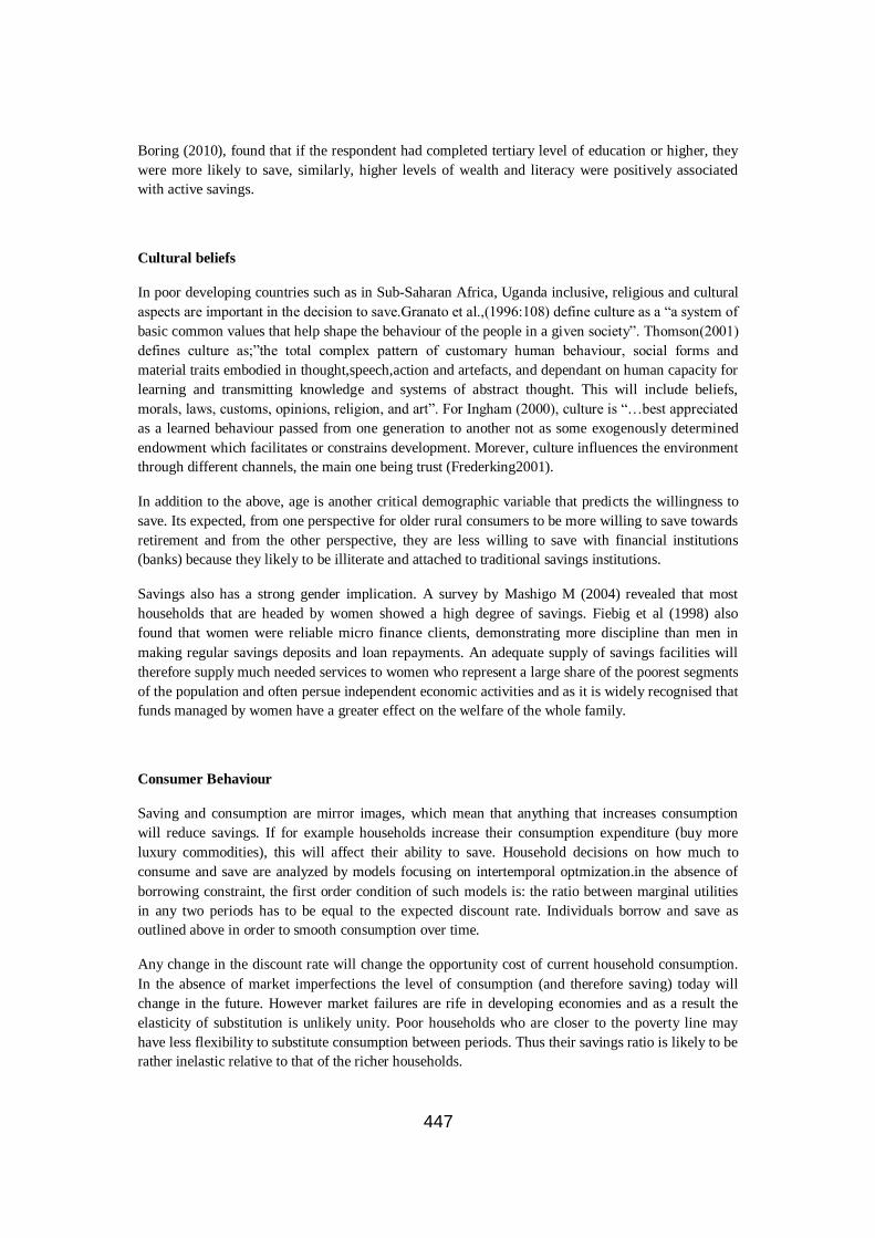
447

Boring (2010), found that if the respondent had completed tertiary level of education or higher, they

were more likely to save, similarly, higher levels of wealth and literacy were positively associated

with active savings.

Cultural beliefs

In poor developing countries such as in Sub-Saharan Africa, Uganda inclusive, religious and cultural

aspects are important in the decision to save.Granato et al.,(1996:108) define culture as a ―a system of

basic common values that help shape the behaviour of the people in a given society‖. Thomson(2001)

defines culture as;‖the total complex pattern of customary human behaviour, social forms and

material traits embodied in thought,speech,action and artefacts, and dependant on human capacity for

learning and transmitting knowledge and systems of abstract thought. This will include beliefs,

morals, laws, customs, opinions, religion, and art‖. For Ingham (2000), culture is ―…best appreciated

as a learned behaviour passed from one generation to another not as some exogenously determined

endowment which facilitates or constrains development. Morever, culture influences the environment

through different channels, the main one being trust (Frederking2001).

In addition to the above, age is another critical demographic variable that predicts the willingness to

save. Its expected, from one perspective for older rural consumers to be more willing to save towards

retirement and from the other perspective, they are less willing to save with financial institutions

(banks) because they likely to be illiterate and attached to traditional savings institutions.

Savings also has a strong gender implication. A survey by Mashigo M (2004) revealed that most

households that are headed by women showed a high degree of savings. Fiebig et al (1998) also

found that women were reliable micro finance clients, demonstrating more discipline than men in

making regular savings deposits and loan repayments. An adequate supply of savings facilities will

therefore supply much needed services to women who represent a large share of the poorest segments

of the population and often persue independent economic activities and as it is widely recognised that

funds managed by women have a greater effect on the welfare of the whole family.

Consumer Behaviour

Saving and consumption are mirror images, which mean that anything that increases consumption

will reduce savings. If for example households increase their consumption expenditure (buy more

luxury commodities), this will affect their ability to save. Household decisions on how much to

consume and save are analyzed by models focusing on intertemporal optmization.in the absence of

borrowing constraint, the first order condition of such models is: the ratio between marginal utilities

in any two periods has to be equal to the expected discount rate. Individuals borrow and save as

outlined above in order to smooth consumption over time.

Any change in the discount rate will change the opportunity cost of current household consumption.

In the absence of market imperfections the level of consumption (and therefore saving) today will

change in the future. However market failures are rife in developing economies and as a result the

elasticity of substitution is unlikely unity. Poor households who are closer to the poverty line may

have less flexibility to substitute consumption between periods. Thus their savings ratio is likely to be

rather inelastic relative to that of the richer households.

448

Methods and Materials

Research design

A cross sectional survey and correlational design were used to establish the effect of characteristics of

savers and saving type on saving behaviour of the rural household. Both primary and secondary data

was used.

Study population

The study was carried out in Bungokho County in Mbale District with a population of 16340

households. The study was carried out in 3 sub-counties of Busiu, Busoba and Bukiende.

Sample Size and Sampling Procedure

A sample of 376 households was used, determined scientifically by Krejcie and Morgan (1970) table

of findings. Proportionate stratified sampling and simple random sampling were used to obtain 376

households from the three sub-counties of Busiu, Busoba and Bukiende.

Table1.The sample size.

Sub-County Population (Households) Sample (Households)

Busiu 5,612 129

Bukiende 5,101 117

Busoba 5,627 130

Total 16,340 376

Source: Uganda Population and Housing Census Results (2002)

Measurement of study variables

Dependent variable

The dependent variable is saving behaviour which was measured using the existing literature relating

to the study variable.

Independent variable

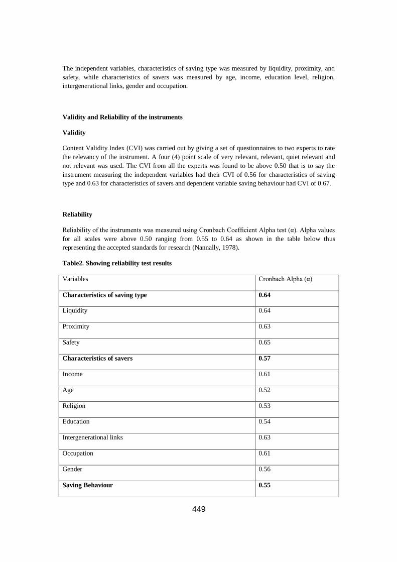
449

The independent variables, characteristics of saving type was measured by liquidity, proximity, and

safety, while characteristics of savers was measured by age, income, education level, religion,

intergenerational links, gender and occupation.

Validity and Reliability of the instruments

Validity

Content Validity Index (CVI) was carried out by giving a set of questionnaires to two experts to rate

the relevancy of the instrument. A four (4) point scale of very relevant, relevant, quiet relevant and

not relevant was used. The CVI from all the experts was found to be above 0.50 that is to say the

instrument measuring the independent variables had their CVI of 0.56 for characteristics of saving

type and 0.63 for characteristics of savers and dependent variable saving behaviour had CVI of 0.67.

Reliability

Reliability of the instruments was measured using Cronbach Coefficient Alpha test (α). Alpha values

for all scales were above 0.50 ranging from 0.55 to 0.64 as shown in the table below thus

representing the accepted standards for research (Nannally, 1978).

Table2. Showing reliability test results

Variables Cronbach Alpha (α)

Characteristics of saving type 0.64

Liquidity 0.64

Proximity 0.63

Safety 0.65

Characteristics of savers 0.57

Income 0.61

Age 0.52

Religion 0.53

Education 0.54

Intergenerational links 0.63

Occupation 0.61

Gender 0.56

Saving Behaviour 0.55

450

Source: Primary data

Methods of data analysis

The data was analysed using descriptive and inferential statistics options provided by Statistical

Package for Social Scientists (SPSS). Spearman Correlation Coefficient analysis was used to

determine the strength and direction of the relationship between independent variables

(characteristics of savers and saving type) and the dependent variable (saving behaviour). Binary

Logistic regression was used to predict saving behaviour.

Presentation and interpretation of the findings

Forms of saving

The most predominant saving form is MFI (32%) followed by reciprocal lending (17%), deposit

collectors (11%), cash at home (11%) and least being Bank Account (1%) as shown in table 3 below.

Table 3: Showing the different saving forms of the households

Form of saving Frequency Percent

Bank account (current a/c) 2 0.7

Bank account (savings a/c) 23 8.0

Micro Finance institution 93 32.4

Cash at home e.g. in tins, cupboard mattress etc, 31 10.8

Deposit collectors 32 11.1

Physical assets e.g. cattle,land,jewelry etc 24 8.4

Reciprocal lending 48 16.7

Money guards 26 9.1

No savings 8 2.8

Total 287 100

Source: Primary data

451

Findings on characteristics of saving type of rural households

The characteristics of saving type were liquidity, proximity, and safety as shown in table 4.2 below.

452

Table 4: Descriptive statistics of Characteristics of saving type

N Mean Std. Deviation Skewness Kurtosis

Statistic Statistic Statistic Std. Error Statistic Std. Error

Liquidity 287 3.5865 1.11335 -.794 .144 -.314 .287

Proximity 287 3.3837 1.03608 -.624 .144 -.396 .287

Safety 287 2.7855 1.13486 .334 .144 -1.013 .287

Valid N (listwise) 287

Source: Primary data

Liquidity, proximity, and Safety are fairly normally distributed with skewness and kurtosis statistics

lying between -1 and +1 except for kurtosis statistic for Safety which is between -2 and +2. The

liquidity mean value is 3.5865 which is above the scale of 3 implying that the rural household are

liquid. The proximity mean of 3.3837 which is adequate for the rural households, the service delivery

is within the proximity.

Level of liquidity of savings products preferred by rural households

The study established that the majority of rural household savers (85.50%) prefer a relatively illiquid

savings product that permits withdrawals at a frequency of once a month or less, with 47.90 %

preferring the highly illiquid type, and 37.60 % preferring illiquid type i.e. one that allows for

monthly withdrawals. Only 14.50 % of rural savers interviewed expressed preference for savings

products accessible for withdrawals at daily or weekly intervals, referred in here as highly liquid and

liquid respectively, as shown in the table 4.3 below.

Table 5: Level of Liquidity preferred by rural households savers

Research category Total

Highly liquid 4.10

Liquid 10.40

Illiquid 37.60

Highly illiquid 47.90

453

Total 100.0

Source: Primary data.

These findings concur with observations made by other studies on East Africa, which showed that

rural household savers demand relatively illiquid savings product (Wright 1999, Mugwanga, 1999).

The strength of the relationship between the liquidity of savings products and the number of rural

households‘ savers demanding the products was found to be statistically significant at the 0.05 level

of confidence. This implies that the number of savers demanding savings services increases with

increasing level of illiquidity of the savings products on offer with the highest preference (37.0 %)

desiring products accessible for withdrawals on a monthly basis. Regression analysis revealed that

25% of the variation in rural households‘ savers‘ preference for savings products can be explained by

the liquidity of the products on offer.

Reasons for the choice of preferred level of liquidity

Table 6: Showing reasons for preferred level of liquidity.

(Chi-square= 13.236, DF=3, Sig=0.000).

The researcher found out that the majority of the research population (73.9 %) were influenced by

lifecycle and emergency needs in choosing the type of savings service in which to save (table 4.5

above).It was also discovered that 21.6 % are influenced by expected future opportunities and 4.5 %

were influenced by other factors.

Lifecycle needs are those needs that arise from human life cycle events such as

birth,marriage,death,home making,widowhood,old age and the desire to leave behind something

behind for one‘s heirs. Emergency needs arise from the possibility of calamities and misfortunes such

as landslides, fires,accident,illness,floods,etc.Anticipated future opportunities also require large sums

of money, like starting a business, acquiring productive assets, building a permanent house and

acquiring life enhancing consumer durables ( Rutherford et al.,1999). Rutherford observed that the

poor require large sums of money to deal with these needs and opportunities and argues that finding

these large sums of money is their main money management problem. Building large sums of money

Reasons Frequency Percent

Lifecycle needs 119 41.5

Emergency needs 93 32.4

Opportunities 62 21.6

Others 13 4.5

Total 287 100

454

out of small savings takes a long time and this explains why the preference for more illiquid savings

products among rural savers is quiet high.

Table 7: Analysis of Liquidity preference by reason for the choice

Product type Analysis

Criterion

Reasons for liquidity preference

Total

Lifecycle

needs

Emergency

needs

Opportunities Others

Highly liquid

(Daily)

Count

2

4

5

1

12

% within

Product

18.7 %

31.3 %

37.5 %

12.5 %

100 %

% within

Reason

1.7 %

4.3 %

8.1 %

7.7 %

4.2 %

Liquid

(Weekly)

Count

7

13

8

2

30

% within

Product

24.4 %

43.9 %

26.8 %

4.9 %

100 %

% Within

Reason

5.9 %

14 %

13 %

15.4 %

10.5 %

Illiquid

(Monthly)

Count

42

43

22

1

108

% within

Product

38.9 %

40.3 %

19.5 %

1.3 %

100 %

% Within

Reason

35.3 %

46.2 %

35.5 %

7.7 %

37.6 %

455

Highly illiquid

(Quarterly&

longer)

Count

67

33

29

8

137

% Within

Product

48.9 %

24.2 %

21.1 %

5.8 %

100 %

% Within

Reason

56.3 %

35.5 %

46.8 %

61.5 %

47.7 %

Total Count 119 93 62 13 287

% Within

Product

41.5 %

32.4 %

21.6 %

4.5 %

100 %

% Within

Reason

99.2 %

100 %

103.4 %

92.7 %

100 %

(0.8) (3.4) (7.3)

(Chi-Square= 44.345, Sig=0.000)

Source: Primary data

The study established that of the rural households whose savings decisions are influenced by lifecycle

needs, 91.6 % prefer illiquid products, with 56.3 % preferring the highly illiquid type and 35.3 %

preferring the illiquid type of monthly withdrawals. The study also found that among the savers

whose decisions were driven by emergency needs, the overwhelming majority (81.7 %) also

preferred illiquid products with 46.2 % preferring the illiquid type and 35.5 % preferring the highly

illiquid type. It was established that majority (82.3 %) of rural savers whose decisions were driven by

future opportunities preferred illiquid products with 46.8 % preferring highly illiquid type and 35.5 %

preferring the illiquid type.However,despite the driving force, the majority of the rural savers

preferred illiquid savings products.

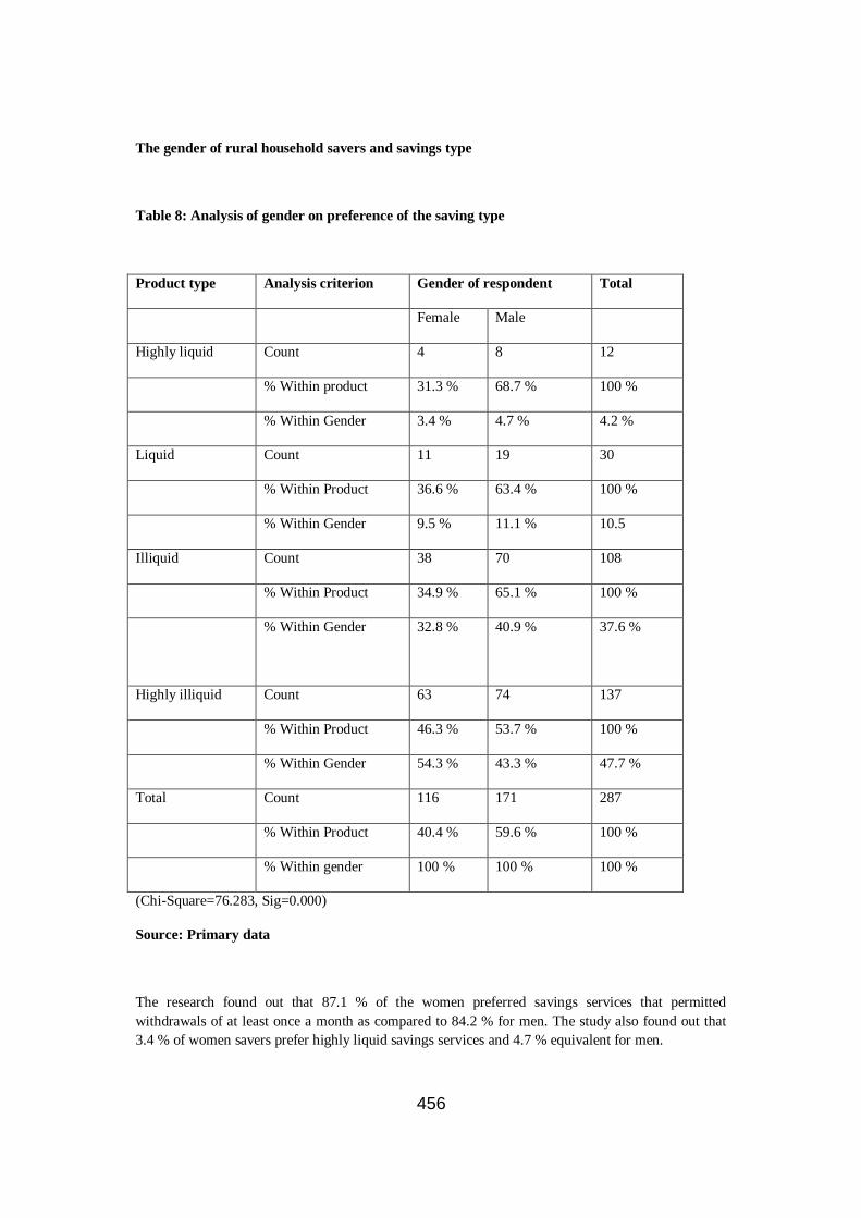
456

The gender of rural household savers and savings type

Table 8: Analysis of gender on preference of the saving type

Product type Analysis criterion Gender of respondent Total

Female Male

Highly liquid Count 4 8 12

% Within product 31.3 % 68.7 % 100 %

% Within Gender 3.4 % 4.7 % 4.2 %

Liquid Count 11 19 30

% Within Product 36.6 % 63.4 % 100 %

% Within Gender 9.5 % 11.1 % 10.5

Illiquid Count 38 70 108

% Within Product 34.9 % 65.1 % 100 %

% Within Gender 32.8 % 40.9 % 37.6 %

Highly illiquid Count 63 74 137

% Within Product 46.3 % 53.7 % 100 %

% Within Gender 54.3 % 43.3 % 47.7 %

Total Count 116 171 287

% Within Product 40.4 % 59.6 % 100 %

% Within gender 100 % 100 % 100 %

(Chi-Square=76.283, Sig=0.000)

Source: Primary data

The research found out that 87.1 % of the women preferred savings services that permitted

withdrawals of at least once a month as compared to 84.2 % for men. The study also found out that

3.4 % of women savers prefer highly liquid savings services and 4.7 % equivalent for men.

457

The influence of age of rural savers on liquidity preferred.

The study established that preference for savings products which permit withdrawals of once a month

or less frequently was 82.7 % and 84.3 % among the age groups of 31 – 40 and 41 – 49 respectively

(table 8).Rural savers falling in these age categories accounted for 28.2 % and 37.6 % respectively of

all the households surveyed. Preference for the same product among other age group is all above 82

%.This finding suggests that age has no significant influence on the demand for the level of liquidity

of a savings product among rural savers.

Table 9: Age of savers and liquidity preference

Liquidity level Analysis criterion Age of rural saver Total

< 30 31- 40 41 – 50 >50

Highly liquid Count 1 4 5 2 12

% Within product 12.5 % 31.3 % 37.4 % 18.8 % 100 %

Liquid Count 2 10 12 6 30

% Within product 4.9 % 33.3 % 41.5 % 20.3 % 100 %

Illiquid Count 10 26 49 23 108

% Within Product 9.4 % 24.2 % 45 % 21.4% 100 %

Highly illiquid Count 5 41 42 49 137

% Within product 3.6 % 29.9 % 30.7 % 35.8 % 100 %

Total Count 18 81 108 80 287

% Within product 6.3 % 28.2 % 37.6 % 27.9 % 100 %

(Chi-square=65.237, Sig=0.000)

Source: primary data

Income of rural savers and liquidity preference

Table 10: Analysis of Influence of income of rural savers on liquidity choice

Product liquidity Analysis criterion

Income

Total

Very low Low Medium Upper

Highly

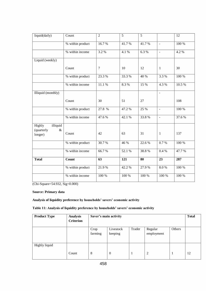
458

liquid(daily) Count 2 5 5 12

% within product 16.7 % 41.7 % 41.7 % - 100 %

% within income 3.2 % 4.1 % 6.3 % - 4.2 %

Liquid (weekly)

Count

7

10

12

1

30

% within product 23.3 % 33.3 % 40 % 3.3 % 100 %

% within income 11.1 % 8.3 % 15 % 4.3 % 10.5 %

Illiquid (monthly)

Count

30

51

27

-

108

% within product 27.8 % 47.2 % 25 % - 100 %

% within income 47.6 % 42.1 % 33.8 % - 37.6 %

Highly illiquid

(quarterly &

longer)

Count

42

63

31

1

137

% within product 30.7 % 46 % 22.6 % 0.7 % 100 %

% within income 66.7 % 52.1 % 38.8 % 0.4 % 47.7 %

Total Count 63 121 80 23 287

% within product 21.9 % 42.2 % 27.9 % 8.0 % 100 %

% within income 100 % 100 % 100 % 100 % 100 %

(Chi-Square=54.932, Sig=0.000)

Source: Primary data

Analysis of liquidity preference by households’ savers’ economic activity

Table 11: Analysis of liquidity preference by households’ savers’ economic activity

Product Type Analysis

Criterion

Saver’s main activity Total

Crop

farming

Livestock

keeping

Trader Regular

employment

Others

Highly liquid

Count

8

0

1

2

1

12

459

%Within

Product

62.5 %

0

6.3 %

25.0 %

6.3 %

100 %

Liquid Count 18 1 6 3 2 30

% Within

Product

61.0 %

2.4 %

19.5 %

9.8 %

7.3 %

100 %

Illiquid Count 77 2 11 9 9 108

% Within

Product

71.8 %

2.0 %

10.0 %

8.1 %

8.1 %

100 %

Highly illiquid Count

101

2

14

11

9

137

% Within

Product

73.7 %

1.6 %

10.0 %

7.9 %

6.8 %

100 %

Total Count 204 5 31 25 21 287

% Within

product

71.2 %

1.8 %

10.9 %

8.8 %

7.3 %

100 %

% within

activity

99.9 %

100 %

103.3 %

100 %

100.1 %

100 %

(Chi-Square=65.23, Sig=0.000)

Source: Primary data

The study established that majority (87.2 %) of the rural households engaged in crop farming

preferred savings products that allow withdrawals of a frequency of once a month or less, of these,

49.5 % preferred highly illiquid ones and 37.7 % preferring illiquid products as summarised in table 7

below. However, the researcher did not find any evidence that showed any relationship between

economic activity and savings products required by these households as shown in the table above.

Characteristics of rural household savers

The characteristics of savers of rural households are income levels, consumer behaviour, education

level, intergenerational links and religious beliefs as shown in table below.

460

Table 12: Descriptive statistics of Characteristics of rural household Savers

N Mean Std. Deviation Skewness Kurtosis

Variable

Statistic Statistic Statistic Std. Error Statistic

Std.

Error

Income level 287 3.1612 1.13265 -.282 .144 -1.166 .287

Consumer

behaviour

287 3.3527 1.17209 -.643 .144 -.666 .287

Education level 287 3.6089 1.17154 -.725 .144 -.452 .287

Intergenerational

Links

287 3.5055 1.17185 -.473 .144 -.957 .287

Religious

beliefs

287 3.0218 1.23168 .014 .144 -1.039 .287

Valid N (list

wise)

287

Source: Primary Data

The income levels, consumer behaviour, education level, intergenerational links and religious beliefs

are fairly normally distributed with skewness and kurtosis statistics between -1 and +1, except

kurtosis for income level and religious beliefs.

The mean value of income level is 3.1612 which is moderate, consumer behaviour mean of 3.3527

which is moderate, education level mean of 3.6089 which is above average, intergenerational links

mean of 3.5055, average and religious beliefs mean of 3.0218 being moderate.

Findings of rural household saving behaviour

The Overall saving behaviour is moderate for rural households as shown in table below.

461

Table 13: Descriptive statistics of saving behaviour

N Mean

Std.

Deviation Skewness Kurtosis

Variable

Statistic Statistic Statistic Std. Error Statistic

Std.

Error

Saving Behaviour 287 2.7791 .76317 .359 .144 .134 .287

Source: Primary data

The saving behaviour is normally distributed with skew ness statistic and kurtosis between -1 and +1.

462

The economic activity of households’ savers and choice of savings.

The study established that only 8.7 % of the rural savers made their savings in the bank with 8.0 %

having savings accounts and 0.7 % maintaining current accounts. Among these, 52 % of the

households reported regular employment as main source of their income as compared to the

equivalent 8 % for crop farming.

Also 32.4 % of the households kept their savings with micro finance institutions and out of these,

households whose main source of income was crop farming were 74.2 %,1.1 %, 3.2 %,14% and 7.5

% for livestock keeping,trader,regular employment and others respectively.

Majority of the rural households surveyed (58.9%) reported keeping their savings either as cash at

home, in physical assets, reciprocal lending, deposit collectors, or with money guards. The highest

number of these households (78.7 %) was mainly engaged in crop farming compared to 1.2 % who

reported their main source of income to be livestock keeping as shown in the table below.

Table 14: Analysis of saving form preference by households’ savers’ economic activity

Form of saving Analysis

criterion

savers‘ main economic activity Total

Crop

farming

Livestock

keeping

Trader Regular

employme

nt

Other

Bank account (current

a/c)

Count

0

0

0

2

0

2

% within form 0 % 0 % 0 % 100 % 0 % 100 %

Bank account (savings

a/c)

Count

2

1

5

11

4

23

% within form 8.7 % 4.3 % 21.7 % 47.8 % 17.4 % 100 %

M F I Count 69 1 3 13 7 93

% within form 74.2 % 1.1 % 3.2 % 13.9 % 7.5 % 100 %

Cash at home in tins,

mattresses etc

Count

15

0

4

9

3

31

% within form 48.4 % 0 % 12.9 % 29 % 9.7 % 100 %

463

Deposit collectors Count 30 0 1 0 1 32

% within form 93.8 % 0 % 3.1 0 % 3.1 % 100 %

Physical assets e.g.

cattle,land,jewelry etc

Count

13

2

3 4 2 24

% within form 54.2 % 8.3 % 12.5 % 16.7 % 8.3 % 100 %

Reciprocal lending Count 41 0 2 4 1 48

% within form 85.4 % 0 % 4.2 % 8.3 % 2.1 % 100 %

Money guards Count 26 0 0 0 0 26

% within form 100 % 0 % 0 % 0 % 0 % 100 %

Others Count 8 0 0 0 0 8

% within form 100 % 0 % 0 % 0 % 0 % 100 %

Total 204 4 18 43 18 287

% within form 71.1 % 1.4 % 6.3 % 15 % 6.3 % 100 %

(Chi-Square=45.432, Sig=0.000)

Source: Primary data

Proximity of service delivery points to rural savers.

Generally, the study established that 95.8 % of the rural households savers surveyed would make use

of an SDP if it were located nearer to their home. These findings confirm the observations made by many

scholars like Musinga et al,that availability of a saving facility in a near enough location is the biggest factor

that would make most rural households change from their current mode of saving (cash and other non-

bank forms of saving),to saving in formal financial institutions.

Table 15: Would saver use SDP if it were located nearer to his home?

RespoResponse Frequ Frequency Perc percent

Yes 275 95.8

No 12 4.2

Total 287 100

(Chi-Square=3.145, df=1, Sig=0.000)

Source: Primary data

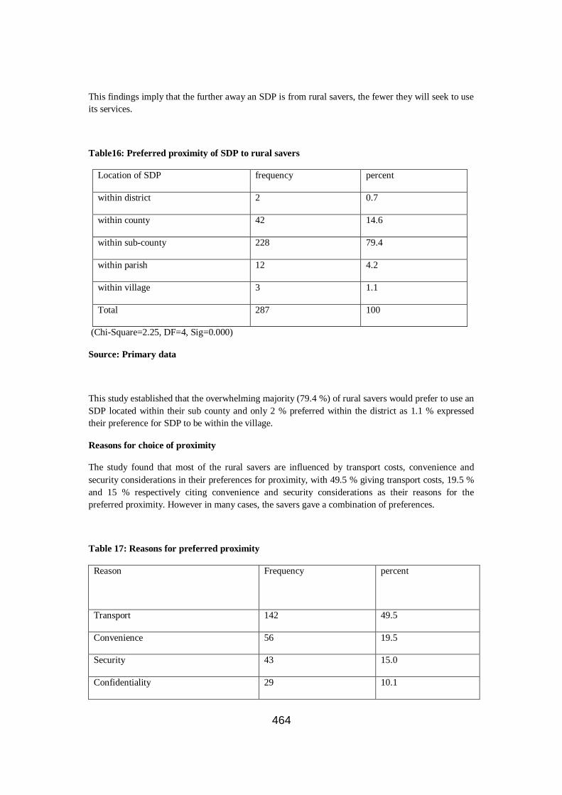
464

This findings imply that the further away an SDP is from rural savers, the fewer they will seek to use

its services.

Table16: Preferred proximity of SDP to rural savers

Location of SDP frequency percent

within district 2 0.7

within county 42 14.6

within sub-county 228 79.4

within parish 12 4.2

within village 3 1.1

Total 287 100

(Chi-Square=2.25, DF=4, Sig=0.000)

Source: Primary data

This study established that the overwhelming majority (79.4 %) of rural savers would prefer to use an

SDP located within their sub county and only 2 % preferred within the district as 1.1 % expressed

their preference for SDP to be within the village.

Reasons for choice of proximity

The study found that most of the rural savers are influenced by transport costs, convenience and

security considerations in their preferences for proximity, with 49.5 % giving transport costs, 19.5 %

and 15 % respectively citing convenience and security considerations as their reasons for the

preferred proximity. However in many cases, the savers gave a combination of preferences.

Table 17: Reasons for preferred proximity

Reason

Frequency percent

Transport 142 49.5

Convenience 56 19.5

Security 43 15.0

Confidentiality 29 10.1

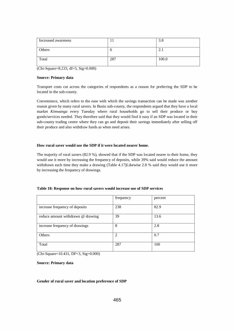
465

Increased awareness 11 3.8

Others 6 2.1

Total 287 100.0

(Chi-Square=8.233, df=5, Sig=0.000)

Source: Primary data

Transport costs cut across the categories of respondents as a reason for preferring the SDP to be

located in the sub-county.

Convenience, which refers to the ease with which the savings transaction can be made was another

reason given by many rural savers. In Busiu sub-county, the respondents argued that they have a local

market Kimwanga every Tuesday where rural households go to sell their produce or buy

goods/services needed. They therefore said that they would find it easy if an SDP was located in their

sub-county trading centre where they can go and deposit their savings immediately after selling off

their produce and also withdraw funds as when need arises.

How rural saver would use the SDP if it were located nearer home.

The majority of rural savers (82.9 %), showed that if the SDP was located nearer to their home, they

would use it more by increasing the frequency of deposits, while 39% said would reduce the amount

withdrawn each time they make a drawing (Table 4.17)Likewise 2.8 % said they would use it more

by increasing the frequency of drawings.

Table 18: Response on how rural savers would increase use of SDP services

frequency percent

increase frequency of deposits 238 82.9

reduce amount withdrawn @ drawing 39 13.6

increase frequency of drawings 8 2.8

Others 2 0.7

Total 287 100

(Chi-Square=10.431, DF=3, Sig=0.000)

Source: Primary data

Gender of rural saver and location preference of SDP

466

The study established that 95.9 % of rural female savers would use an SDP to their satisfaction if it

were located within the sub-county or county, with the former corresponding to 79.5 % and the latter

16.4 % (Table 17 below).

The men showed that 93.4 % would use SDP to their satisfaction if it were located either within the

sub-county or county, with corresponding percentages of 79.4 % and 14 % respectively. Therefore,

the study did not find any significant influence of gender on the preferred location of SDPs by rural

savers.

Table 19: gender of rural saver and location preference of SDP

Gender

of saver

Analysis criterion location of

SDP

Total

District County Sub-county parish village

Female Count - 12 58 1 2 73

% within Gender - 16.4 % 79.5 % 1.4 % 2.7 % 100

% within location - 28.6 % 25.4 % 8.3 % 66.7 % 25.4%

Male Count 2 30 170 11 1 214

% within gender 0.9 % 14 % 79.4 % 5.1 % 0.5 % 100 %

% within location 100 % 71.4 % 74.6 % 91.7 % 33.3 % 74.6 %

Total Count 2 42 228 12 3 287

% within gender 0.7 % 14.6 % 79.4 % 4.2 % 1 % 100 %

% within location 100 % 100 % 100 % 100 % 100 % 100 %

(Chi-Square=6.431, Sig=0.000)

Source: Primary data

Economic activity of rural saver and nearness of SDP preferred.

The study established that majority of the rural savers engaged in crop farming 85.8 % and 25 %

engaged in livestock farming would use an SDP to their satisfaction if it were located within the sub-

county.

The study also found that irrespective of the economic activity, the majority of rural savers would use

an SDP to their satisfaction if it were located within the sub-county. This is reflected by 58.1 % of

rural savers in regular employment, 72.2 % engaged in trading and 77.8 % engaged in other activities

that would use an SDP to their satisfaction if it were located within sub-county.

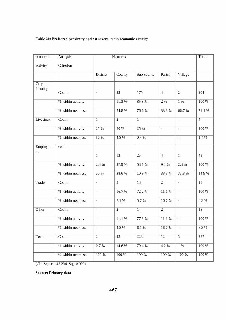
467

Table 20: Preferred proximity against savers’ main economic activity

economic

activity

Analysis

Criterion

Nearness

Total

District County Sub-county Parish Village

Crop

farming

Count

-

23

175

4

2

204

% within activity - 11.3 % 85.8 % 2 % 1 % 100 %

% within nearness - 54.8 % 76.6 % 33.3 % 66.7 % 71.1 %

Livestock Count 1 2 1 - - 4

% within activity 25 % 50 % 25 % - - 100 %

% within nearness 50 % 4.8 % 0.4 % - - 1.4 %

Employme

nt

count

1

12

25

4

1

43

% within activity 2.3 % 27.9 % 58.1 % 9.3 % 2.3 % 100 %

% within nearness 50 % 28.6 % 10.9 % 33.3 % 33.3 % 14.9 %

Trader Count - 3 13 2 - 18

% within activity - 16.7 % 72.2 % 11.1 % - 100 %

% within nearness - 7.1 % 5.7 % 16.7 % - 6.3 %

Other Count - 2 14 2 18

% within activity - 11.1 % 77.8 % 11.1 % - 100 %

% within nearness - 4.8 % 6.1 % 16.7 % - 6.3 %

Total Count 2 42 228 12 3 287

% within activity 0.7 % 14.6 % 79.4 % 4.2 % 1 % 100 %

% within nearness 100 % 100 % 100 % 100 % 100 % 100 %

(Chi-Square=45.234, Sig=0.000)

Source: Primary data

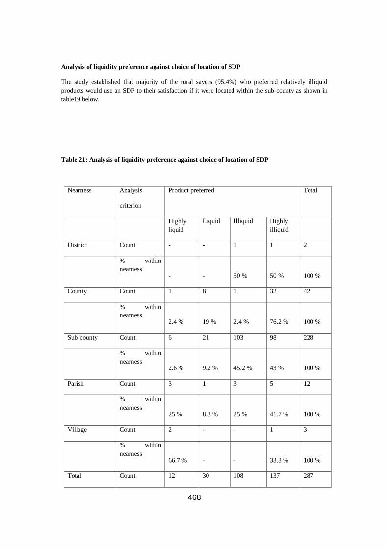
468

Analysis of liquidity preference against choice of location of SDP

The study established that majority of the rural savers (95.4%) who preferred relatively illiquid

products would use an SDP to their satisfaction if it were located within the sub-county as shown in

table19.below.

Table 21: Analysis of liquidity preference against choice of location of SDP

Nearness Analysis

criterion

Product preferred Total

Highly

liquid

Liquid Illiquid Highly

illiquid

District Count - - 1 1 2

% within

nearness

-

-

50 %

50 %

100 %

County Count 1 8 1 32 42

% within

nearness

2.4 %

19 %

2.4 %

76.2 %

100 %

Sub-county Count 6 21 103 98 228

% within

nearness

2.6 %

9.2 %

45.2 %

43 %

100 %

Parish Count 3 1 3 5 12

% within

nearness

25 %

8.3 %

25 %

41.7 %

100 %

Village Count 2 - - 1 3

% within

nearness

66.7 %

-

-

33.3 %

100 %

Total Count 12 30 108 137 287

469

% within

nearness

4.2 %

10.5 %

37.6 %

47.7 %

100 %

(Chi-Square=56.432, Sig=0.000)

Source: Primary data

The study further established that irrespective of the type of product preferred, the majority of rural

savers would use an SDP to their satisfaction if it were within the sub-county with 50 % of those who

preferred highly liquid products and 70 % for less liquid products.

Form of savings kept and proximity preference.

The study established that 90.3 % of savers who keep their savings at home would use an SDP

instead if it were located within the sub-county as per table 20.below.

The study further found that irrespective of the form of savings kept, majority of rural savers would

shift to depositing in an SDP if it were located within the sub-county,88.6 % of rural savers who

maintain their savings in kind ,would consider monetising them and depositing them with an SDP if it

were located within their sub-county. The equivalent ratios for savers who maintain their savings in

the bank (savings & current accounts), MFIs, deposit collectors, reciprocal lending, money guards

and others were, 62%, 66.6%, 81 %, 85.4%, 88.5 % and 87.5 % respectively.

Table 22: form of savings kept and proximity preference

Form of saving Analysis criterion

Nearness

Total

District county sub-county parish village

Bank current

a/c

Count

1

-

1

-

-

2

% within nearness 50 % - 0.4 % - - 0.7 %

% within form 50 % - 50 % - - 100 %

Bank savings

a/c

Count

1

5

17

-

-

23

% within nearness 50 % 11.9% 7.5 % - - 8 %

% within form 4.3 % 21.7% 73.9 % - - 100 %

470

MFI Count - 28 62 2 1 93

% within nearness - 66.7% 27.2 % 16.7% 33.3% 32.4%

% within form - 30.1% 66.6 % 2.2 % 1.1 % 1.1%

Cash(home) Count - 1 28 1 1 31

% within nearness - 2.4 % 12.3 % 8.3 % 33.3% 10.8%

% within form - 3.2 % 90.3 % 3.2 % 3.2 % 100%

Deposit

collectors

Count

-

1

17

2

1

21

% within nearness - 2.4 % 7.5 % 16.7% 33.3% 7.3%

% within form - 4.8 % 81 % 9.5 % 4.8 % 100%

physical assets

Count

-

2

31

1

-

35

% within nearness - 4.8 % 13.6 % 8.3 % - 12.2%

% within form - 5.7 % 88.6 % 2.9 % -

reciprocal

lending

Count

-

2

41

5

-

48

% within nearness - 4.8 % 18 % 41.7% - 16.7%

% within form - 4.2 % 85.4 % 10.4% - 100 %

money guards

Count

2

23

1

-

26

% within nearness - 4.8 % 10.1 % 8.3 % - 9.1 %

% within form - 7.7 % 88.5 % 3.8 % - 100 %

Others Count 1 7 - - 8

% within nearness - 2.4 % 3.1 % - - 2.8 %

% within form - 12.5% 87.5 % - - 100 %

Total Count 2 42 228 12 3 287

% within nearness 100 % 100 % 100 % 100 % 100 % 100 %

471

% within form 0.7 % 14.6% 79.4 % 4.2 % 1 % 100 %

(Chi-Square=65.523, Sig=0.000)

Source: Primary data

Income of savers and preferred proximity of SDP

The study established that 96.8 % of the very low income group rural savers could satisfactorily use

an SDP if it were located within their sub-county. The equivalent percentages for rural savers at low,

middle and upper income levels were 87.6 %, 73.8 % and 8.7 % respectively. Hence with the

exception of the upper level income group, the majority of rural savers within other categories would

prefer to use an SDP if it were located within the sub-county. It was also found that majority of rural

savers in upper level category (82.6 %) preferred an SDP to be within the county.

Table 23: The income of savers and preferred proximity of SDP

Nearness

Within

Analysis

Criterion

Income category of rural savers Total

very low Low Medium Upper

District Count - - - 2 2

% within nearness - - - 100 % 100 %

% within income - - - 8.7 % 0.7 %

County Count - 5 18 19 42

% within nearness - 11.9 % 42.9 % 45.2 % 100 %

% within income - 4.1 % 22.5 % 82.6 % 14.6 %

Sub-county Count 61 106 59 2 228

% within nearness 26.7 % 46.5 % 25.9 % 0.9 % 100 %

% within income 96.8 % 87.6 % 73.8 % 8.7 % 79.4 %

Parish Count 1 9 2 - 12

% within nearness 8.3 % 75 % 16.7 % - 100 %

% within income 1.6 % 7.4 % 2.5 % - 4.2 %

Village Count 1 1 1 - 3

472

% within nearness 33.3 % 33.3 % 33.3 % - 100 %

% within income 1.6 % 0.8 % 1.3 % - 1 %

Total Count 63 121 80 23 287

% within nearness 100 % 100 % 100 % 100 % 100 %

% within income 22 % 42.1 % 27.9 % 8 % 100 %

(Chi-Square= 45.737, sig=0.000)

Source: primary data

Relationship between characteristics of saving type and saving behaviour

Characteristics of saving type were correlated with the saving behaviour as shown in the table below.

Table 24: Spearman rank Correlation matrix

1 2 3 4

Liquidity 1.000

Proximity .350** 1.000

Safety .254** .036 1.000

Saving Behaviour .313** .152** .230** 1.000

**. Correlation significant at 0.01 level (2 tailed)

*. Correlation significant at 0.05 level (2 tailed)

Source: primary data

Results from table above indicate significant positive relationship between liquidity and saving

behaviour (r=0.313, p<0.01). This implies that when liquidity increases, the saving behaviour

improves.

There was a significant positive relationship between proximity and saving behaviour (r=0.152,

p<0.01). This implies that when proximity improves, then saving behaviour improves.

There was a significant positive relationship between safety and saving behaviour (r=0.388, p<0.01).

This implies that safety enhances on the saving behaviour of rural households.

473

Characteristics of savers and saving behaviour

The relationship between characteristics of savers and saving behaviour is shown in the correlation

matrix table below.

Table 25: Spearman rank correlation matrix for characteristics of savers and saving behaviour

1 2 3 4 5 6

Income level 1.000

Consumer behaviour .465** 1.000

Education level .306** .477** 1.000

Intergenerational Links .205** .468** .676** 1.000

Religious beliefs -.099 .176** .431** .388** 1.000

Saving Behaviour .266** .073 .468** .345** .284** 1.000

**. Correlation significant at 0.01 level (2 tailed)

*. Correlation significant at 0.05 level (2 tailed)

Source: Primary data

Results in the table above indicate significant positive relationship between characteristics of savers

and saving behaviour except for consumer behaviour which is very weak with saving behaviour (r=

0.266, 0.468, 0.345,0.284, p<0.01 and r=0.07, p>0.05) respectively for income level, education level

intergenerational links, religious beliefs and consumer behaviour. When the income levels, education

level, intergenerational links, religious beliefs are high then saving behaviour also improves.

Binary Logistic regressions Analysis

The characteristics of saving type and savers significantly and linearly relates to the saving behaviour

of the rural households Hosmer and Lemeshow Test (Chi-Square= 9.881, DF= 6, Sig=.436), this

implied that the data fitted the model well.

The educational level, safety, consumer behaviour, liquidity, intergenerational links, income level of

households that save significantly predicted saving behaviour by 36.5%. Proximity and religious

beliefs did not significantly predict saving behaviour (sig>0.05).

474

Model Summary (-2Log likelihood =432.034; Cox & Snell R Square= .254; Nagelkerke R Square=

.365).Higher education levels, safety, good consumer behaviour, liquidity, intergenerational links and

income level of households improved the saving behaviour of rural households.

Table 26 : Binary Logistic Model

B Wald Sig Exp(B)

Liquidity .189 2.048 .001 3.314

Proximity .035 .040 .056 1.919

Safety .198 2.034 .000 5.307

Income level .143 1.039 .037 2.096

Consumer behaviour .154 2.037 .000 4.515

Education level .203 1.045 .000 6.589

Intergenerational Links .132 1.056 .031 2.169

Religious .010 1.036 .095 1.677

Constant .463 2.180 .001 3.427

Source: Primary data

Discussion of the findings

Findings in section 4.7 and 4.8 above are supported by literature below.

An important characteristic of the environment of the poor is risk and uncertainty to cover and protect

themselves against calamities, illness, drought, loss of income etc; they take protection in insurance

mechanisms that help them spread their financial risk (Bouman, 1994).

Available evidence shows that the saving behaviour among the poor varies from country to country

and even from culture to culture. But certain aspects of this behaviour are universal. They have the

desire to turn small savings into large amounts and they will hence use whatever service available to

them to achieve this objective (Aryeetey et al., 1991, Rutherford, 1998).

Rural households will save in a financial form if appropriate institutions and savings products are

available (Robinson, 1994).When there is no financial institution available nearby, poor households

tend to save in non financial forms such as a livestock but if they were given assurance that their

savings would be securely held, maintain value and remain fairly liquid in a convenient location, they

would prefer to save in a financial form as some of the most successful programs have shown (Rhyne

& Otere,1994).

475

Similar studies carried out in Bangladesh and Tanzania suggest that rural households do desire to

save and what they need is a reasonable mechanism to enable them save and the assurance that they

can access those savings when need arises (Wright, 2000).

Wright (2001) further mentioned that many emergencies or opportunities necessitate instant access to

cash and this explains why almost all low-income and poor families keep some amount of emergency

savings in the home.

In the studies of saving, formal financial institutions frequently ask the question of how poor

households save since they are the potential deposit receivers (Dauner,2004:4).poor households save

in various forms, for reasons and purposes specific to their needs and entrust their monetary savings

to different persons or places(neighbours, financial institutions, under mattresses.).

Wright (2001:2) mentions that many emergencies or opportunities necessitate instant access to cash,

and these explain why almost all low-income and poor families keep some amount of emergency

savings in the home.

The life-cycle theory of savings behaviour was first formalised by Franco Modigliani and Richard

Brumberg (1954) and Albert Ando and Modigliani in (1963).

In its original formulation, the Life-cycle Hypothesis (LCH) presented a theory of saving behaviour

focussing on the individual. The .LCH analysed the saving behaviour of individuals who spread their

lifetime consumption over their lives by accumulating savings during earning years and maintaining

consumption levels during retirement

Dumba, 1998, argues that poor households prefer physical assets to monetary savings. The savings

mode people opt for and the savings behaviour that they display in particular are influenced by a

number of factors.

The magnitude of this effect is likely to decline as per capita income increases (Carroll and Weil,

1994).Therefore, the very low per capita incomes render it almost impossible for households in

developing economies to save.Kraay (2000) finds that the savings ratios and levels of income per

capita exhibit a modest positive correlation .He claims that average saving ratios rise as household

income increases beyond the base minimum required for survival. For Chakravarthy and Patnaik

(1970) consumption, savings and investment patterns may be related to income in at least two ways;

firstly through the level of income and secondly through the trends of income change.

Deaton (1989) explains that household income in developing countries is uncertain and cyclical,

making longer-term estimation difficult. He also suggests that saving behaviour of individuals may be

directed by rules of thumb, and emphasized that short term increases and or decreases in income are

the primarily causes of saving/dissaving. For Caballero (1990) the uncertainty of expected income

would enhance the precautionary motive for saving in a stable macroeconomic environment.

476

Intergenerational links were found to be a significant determinant of saving behaviour in developing

countries, where these links are particularly strong due to the large size of families.Gersovitz (1988)

found that extended family links might lengthen the effective planning horizon over which

households make saving decisions. Deaton (1989) agreed that households in developing economies

are larger than in industrialised economies and more likely to consist of several generations. As a

result there is less to save for retirement or for intergenerational transfers. Furthermore, Oberta

(2006), in analysing the role of children and family size on household saving, stresses the negative

and regressive effects that additional children have on both the saving ratios and levels of households

saving.

The concentration of banks is biased in favour of urban areas. Among the reasons for this, is the fact

that the established banks erroneously underrate the volume of savings seeking to be mobilised and

channelled into productive investment in the informal or rural areas. It‘s often argued that since the

rural economy operates a near subsistence level, there is very little that can be squeezed out of their

income and consumption. Because of this perception, it has not been realised that large volumes of

idle funds, though in small units per household exist in rural areas.

These instances of market failure and information asymmetry often distort the decision of individuals

to save (Black et al.., 2005:21)

In poor developing countries such as in Sub-Saharan Africa, Uganda inclusive, religious and cultural

aspects are important in the decision to save.Granato et al.,(1996:108) define culture as a ―a system of

basic common values that help shape the behaviour of the people in a given society‖. Thomson(2001)

defines culture as;‖the total complex pattern of customary human behaviour, social forms and

material traits embodied in thought,speech,action and artefacts, and dependant on human capacity for

learning and transmitting knowledge and systems of abstract thought. This will include beliefs,

morals, laws, customs, opinions, religion, and art‖. For Ingham (2000), culture is ―…best appreciated

as a learned behaviour passed from one generation to another not as some exogenously determined

endowment which facilitates or constrains development. Morever, culture influences the environment

through different channels, the main one being trust (Frederking2001).

Savings also has a strong gender implication. A survey by Mashigo M (2004) revealed that most

households that are headed by women showed a high degree of savings. Fiebig et al (1998) also

found that women were reliable micro finance clients, demonstrating more discipline than men in

making regular savings deposits and loan repayments. An adequate supply of savings facilities will

therefore supply much needed services to women who represent a large share of the poorest segments

of the population and often persue independent economic activities and as it is widely recognised that

funds managed by women have a greater effect on the welfare of the whole family.

Conclusion

In the build up to this research, it was clear that the traditional theories of household saving behaviour

do not really explain the saving behaviour of low-income households in developing countries. It is

477

also clear that the majority of rural households have the potential to save but do not have access to

formal financial institutions due to the conditions governing the financial services offered.

Characteristics of saving type are liquidity, proximity, and safety as they showed moderate presence

within rural households.

Characteristics of savers are income level, education level, intergenerational links, religious beliefs as

they showed a positive moderate presence within rural households.

Characteristics of saving type and savers are determinants of saving behaviour among the rural

households.

It was established during the research that 85.4% of the rural savers interviewed would prefer savings

that permits withdrawals of once a month or less frequently. According to the statistical analysis, the

number of savers demanding savings services increases with increasing illiquidity of the services

from daily to monthly withdrawal rights ,and then off tangent as illiquidity inceases.At a correlation

coefficient of 0.0901,the relationship between these variables has been found to be significant at the

0.05 level of confidence.

The savings behaviour of most rural households are influenced by lifecycle and emergency needs,

and of the rural savers whose savings decisions are driven by lifecycle needs, the overwhelming

majority ( 85%) prefer the relatively illiquid savings. This implies that rural savers could be a

dependable source of stable savings for term financing in formal financial institutions

No significant difference was found between men and women in their preference of the level of

illiquidity. And likewise no evidence was established to show that the nature of the economic activity

of rural savers changes the pattern.

Whereas the number of savers demanding savings services increases as proximity increases from the

district level to the sub-county level, notably the reverse was found to be the case as proximity

increases from sub-county to village level. However majority of the rural savers would use an SDP

located within their sub-county by increasing the frequency of their depoits.

It was mentioned that most empirical evidence emphasized that income is the main determinant of

saving which seems unlikely in the context of a developing Sub-Saharan African economy like

Uganda. Empirical investigations also show that the dominance of other factors than income,

informal institutions coupled with their motives and a social financial exclusion, contribute to the low

saving ratios of rural households

Some countries (Singapore, Malaysia and China) have successfully created a culture of saving

amongst poor households and continue to enjoy the benefits associated with a high saving ratio by the

households through the use of combined policy approaches.

478

An important question that emerges from these findings is why informal savings continue to be

ignored by the formal financial institutions. This possible complementary relationship between

informal and formal saving is suggested as a topic for future research.

Recommendations

In light of the set study objectives, findings and conclusions thereof, it was established that the

volume of savings in rural areas is substantial but remains outside the formal sector. Most rural

households prefer keeping their savings in the informal sector and This was attributed to lack of

formal sound financial institutions to mobilise such savings in the rural areas. There is need of

channelling such savings into the formal financial sector to create capital accumulation.

Individuals require different types of savings products because they have different needs. Much as

there is literature on about factors affecting savings behaviour of individuals, literature about the

preferences for specific product is still lacking.

The saving behaviour of most of these households is influenced by lifecycle and emergency needs.

This requires them to have easy access to such savings as and when the need arises.

AREA OF FUTURE RESEARCH

This study was carried out in Bungokho county Mbale District. The findings of the study therefore

may not apply to other areas of the country; similar studies should be carried out so as to come up

with a more representative national outlook.

Further to complete the picture as articulated in the opening quote from Fiebig et al….,an additional

study to establish how institutions should be structured in order to adequately meet the needs of rural

savers on a sustainable basis may also be necessary.

Further a study can be carried out to establish the relationship between the characteristics of saving

type and characteristics of rural household savers.

479

An Empirical Analysis of Risk and Size Factors in Momentum Profitability at

the Nairobi Stock Exchange

By

Lisiolo Lishenga

Lecturer, School of Business, University of Nairobi

jlishenga@uonbi.ac.ke.

Cell phone: 0722638664

A paper submitted for presentation at the Operation Research Society of East

Africa (ORSEA) Conference, University of Nairobi, 2011.

Abstract

A generation ago, the intellectual dominance of the efficient markets hypothesis as the accepted

asset pricing paradigm was unchallenged. By the start of the twenty-first century, however, the

acceptance of the efficient market hypothesis had become far less universal. Many financial

economists and statisticians began to believe that stock prices are at least partially predictable.

The profitability of the momentum strategy - the strategy of buying recent winning stocks and

shorting recent losing stocks- as first documented in Jegadeesh and Titman (1993) remains one of

the anomalies that continue to confound the efficient markets theory. This study sought, first, to

establish whether the NSE experienced price momentum in the period covered. Next we tested

whether momentum profitability could be explained by, and was compensation for, risk. Finally,

we investigated any relationship between price momentum and the well documented size

anomaly. We found out that the NSE experienced significant degree of price momentum in the

480

period covered. And that this momentum profitability could not be explained by the three factor

risk factors of Fama-French, and that there was no size effect to momentum.

Terms: price momentum, size effect, risk, winners losers.

1. Introduction

The profitability of the momentum strategy- the strategy of buying recent winning stocks and

shorting recent losing stocks- as first documented in Jegadeesh and Titman (1993) remains one of the

anomalies that cannot be explained by the otherwise very successful Fama-French three factors

model, and is thus very puzzling (Fama and French (1996). Jegadeesh and Titman (2001) show that

momentum profits remain large even subsequent to the period of their 1993 study. Rouwenhorst

(1998), and Griffin, Ji, and Martin (2003), report economically significant and statistically reliable

momentum profits in areas outside the US. These studies suggest that the momentum phenomenon is

not a product of data mining or snooping bias, and neither is it market specific.

Although the momentum phenomenon has been well accepted, the source of the profits and the

interpretation of the evidence are widely debated. Two possible explanations for momentum are size

and market wide risk.

Ever since the publication of Banz (1981) findings, size of stock has been recognised as one of the

anomalous determinants of stock returns. In recent years, size together with book–to–market price

and dividend–to–price has been used to distinguished value from glamour stocks. Fama and French

(1992) find that size and book-to-market predict future returns. Fama and French (1993), Daniel and

Titman (1997), and Davis et al (2000) provide evidence that sorting stocks according to market

capitalisation and book-to-market explains a big proportion of stock returns. Hong, Lim, and Stein

(2000) find that the momentum effect in the U.S. securities is strongest in small firms and declines

sharply as market capitalisation increases. Hong, Lim, and Stein argue that, since price momentum

results from gradual information flow, there should be relatively stronger profits in those stocks for

which information gets out slowly, that is, the small stocks. Lakonishok, Shleifer and Vishny (1992)

find evidence of pension fund managers either buying or selling in herds with evidence that they herd

around small stocks. To the contrary, Hameed and Kusnadi (2002) find no size influence in

momentum profits in five of the six Asian markets they studied.

481

Other studies have suggested that the profitability of momentum strategies may simply be

compensation for risk. Conrad and Kaul (1998) argue that the momentum profit is attributed to the

cross-sectional dispersion in (unconditional) expected returns. Lewellen (2002) finds that the

negative cross – serial correlation among stocks, not underreaction, is the main source of momentum

profits4. Using the frequency domain component method to decompose stock returns, Yao (2003)

provides strong evidence that momentum is a systematic phenomenon.

Models have been developed that are based on momentum on economic risk factors affecting

investment life cycles and growth rates. Berk, Green and Naik (1999) illustrate that momentum

profits arose because of persistent systematic risk in a firm‘s project portfolios. Johnson (2002)

posits that momentum comes from a positive relation between expected returns and firm growth

rates. Chordia and Shivakumar (2002) report that the profits to momentum strategies are completely

explained by predicative returns using the lagged common macroeconomic variables (e.g. dividend

yield, term spread, default spread, and short term rate). The momentum profits are related to the

business cycles and mainly reflect the persistence in the time varying expected returns.

Momentum strategies are part of the bigger universe of technical trading rules that posit

predictability of stock returns using past trends in prices and trading volumes. Studies using the

NSE data base are just beginning to trickle in. Lishenga et al. (2011) report the existence of

significant price momentum at the NSE that could be the basis of profitable trading strategies. Atiti

(2003) also documents evidence of price momentum in the short to medium term, while Ndungu

(2005) finds the existence of a size effect at the NSE.

A scrutiny of the NSE-20 index shows trends that attest to both reversal and continuation in returns

that can be predictable. Over the past decade, the Nairobi Stock Exchange-20 Index has swung like

a pendulum from a peak of 3784 in 1996, then to a low of 1384 in 2003 followed by a tremendous

rally that reached an all time high of 5679 in 2007. What is remarkable is that, between the peaks

and lows, there is a sustained momentum in a given direction of change of the index. Whenever a

downward spiral sets in (as happened in 1996) it continues until it bottoms up 4 to 5 years later.

This is followed by an upward recovery that is also unbroken until the high of 5679 of 2007 is

reached. This is clear in the Figure 2 below.

4 Both Conrad and Kaul (1998), and Lewellen (2002), employ Lo and MacKinlay‘s (1990) statistical

framework to decompose the profits of an investments strategy.

482

Figure 2:Shows the free fall generated by negative momentum

in the years 1997-2002 which then reverses and turns into

sustained price rally creating a positive momentum 2003-2007

-1.5

-1

-0.5

0

0.5

1

1 10 19 28 37 46 55 64 73 82 91 100 109 118 127

Months from January 1997-December 2007

Cu

m.r

et.

t

NSE-20 cum ret

The current study builds on Lishenga (2011) and investigates the influence of two firm-level

characteristics on the propensity of a stock to exhibit price momentum. We will investigate

whether the market wide risk and size stories can explain the phenomenon.

The rest of the paper is arranged as follows; Section 2 reviews related literature on the momentum

anomaly. Section 3 describes the data and the methodology used to test existence of momentum and

how momentum is influenced by risk and size factors. Section 4 presents and discusses the results

and Section 5 concludes.

2. Review of Related Literature

Momentum in prices has been recognized as the most robust market efficiency anomaly. It has been

documented in stock exchanges the world over and has persisted even after wide publication. Fama

(1998), indeed, recognizes the momentum phenomenon as constituting the chief embarrassment to

EMH.

The first and most impressive examples of return momentum (continuation in price movement)

came from cross-sectional returns of individual stocks seminal study of Jegadeesh and Titman‘s

(1993) whose findings are the first in the copious body of momentum literature. Using a U.S.

sample of NYSE/AMEX stocks over the period from 1965 to 1989, they find that a strategy that

buys six-months winners and shorts past six-month losers earns approximately one per cent per

month over the subsequent six months. Chan, Jegadeesh, and Lakonishok (1996) show that

483

momentum strategies yield spreads in returns of extreme deciles of 8.8% over the subsequent six

months suggesting a price momentum effect, which is due to underreaction. Hong, Lim and Stein

(1999) attribute the underreaction of stock prices to analysts‘ coverage, which is more pronounced

in the case of bad news.

Rouwenhorst (1998) obtains similar numbers as those of Jegadeesh and Titman in a sample of 12

European countries over the period 1980 to 1995. Strong and Xu (1999) document profitable price

momentum strategies in the U.K. market that are consistent with market underreaction to industry-

or-firm specific news. Ryan and Overmeyer (2004) adduce evidence from Germany showing that

relative strength (momentum) strategies based on the constituents of the DAX 100 index are

―extremely profitable. Haugen and Baker (1996) and Daniel (1996) show that, although there is

evidence of strong book-to-market effect in Japan, there is little or no evidence of a momentum

effect.

In the event study area, it has been observed that, stocks tend to experience post-event drift in the

same direction as the initial event impact. The most studied events in this genre include earnings

announcements (Bernard and Thomas (1989, 1990)), stock issues (Loughran and Ritter (1995) and

Spiess and Affleck-Graves (1995)); repurchases (Ikenberry, Lakonishok, and Vermaelen (1995)),

dividend initiation and omissions (Michaely, Thaler, and Womack (1995)), and analyst

recommendations (Womack (1996)).

Bernard (1992) and Chan et al. (1996) find that stocks with higher earnings surprises also earn

higher returns in the period after portfolio formation. Chan et al. (1996) found spreads of 4.2% in

returns of extreme deciles formed on the basis of standardized unexpected earnings (SUE). The

findings support the hypothesis of drift to earnings announcements.

Ikenberry et al. (1995) find that stock prices rise on the announcement of share repurchases but then

continue to drift in the same direction over the next few years. Michaely et al. (1995) documents

drift evidence following dividend initiation and omission. Ikenbery (1990) finds evidence of drift

following stock splits while Loughran and Ritter, and Spiess and Affeck-Graves (1995) find

evidence of drift following seasoned equity offerings.

484

Analysis of aggregate stock market indices has also produced evidence of underreaction. Cuttler et

al. (1991) examine auto-correlation in excess returns on various indexes and generally find positive

auto-correlation in excess returns of around 0.1 for stocks, and in bonds of 0.2. This auto-

correlation is statistically significant and consistent with the underreaction hypothesis. Chan,

Hameed, and Tong (2000) implement momentum strategies on stock markets of 23 countries and

find that a great proportion of momentum profits come from price continuation in stock indices, and

very little from movements in exchange rates.

A common belief noted by Chan et al. (2000) is that, ‗it takes volume to move prices.‘ Conrad et al.

(1994) find that high volume securities experience more price continuation, Gervais et al. (1998)

show that individual stocks whose volumes are unusually large (small) tend to experience large

(small) subsequent returns and Lee and Swaminathan (1998) illustrate that past trading volume

predicts both the magnitude and persistence of future price momentum..

Chan et al. (2000) found that when momentum strategies were implemented on markets that

experienced increases in volume in the previous period, the profits were higher than average. Hong

et al. (1999) find hat the underreaction of stock prices depends on the analyst coverage of the stock:

less coverage means underreaction is severe and the opportunities for profitable trading are

enhanced.

While momentum is associated to a large extent with underreacting markets, overreaction could

also generate momentum. One of the first and influential papers in the overreaction category is

DeBondt and Thaler (1985) who find that stock returns are negatively correlated at the long horizon

of 3 to 5 years. Chopra, Lakonishok, and Ritter (1992) support DeBondt and Thaler. Other

contributions have been made by Fama and French (1996), Poterba and Summers (1998), Richards

(1997) and Carmel and Young (1997) among many others.

Emerging market5 evidence on price momentum is now trickling in. Rouwenhorst (1999)

documents evidence to the effect that stocks returns in emerging markets exhibit momentum.

Bekaert et al. (1997) find momentum strategies implemented in emerging markets are consistently

profitable, though they perform better when only the investable indexes are examined. More

5 The data for these studies were drawn from the Emerging Markets Data Base (EMDB) of the IFC

and included Argentina, Brazil, Chile, Colombia, Greece, Indonesia, India, Jordan, Korea, Malaysia,

Mexico, Nigeria, Pakistan, Philippines, Portugal, Taiwan, Thailand, Turkey, Venezuela and

Zimbabwe.

485

recently, contradictory evidence has been documented by Hameed and Kusnadi (2002) who

investigated the profitability of momentum investment strategy in six Asian markets. Hameed and

Kusnadi find that unrestricted momentum strategies do not yield significant profits and conclude

that factors that contribute to the momentum phenomenon in the United States are not prevalent in

the Asian markets.

3. Data Analysis

3.1 Measuring the Returns to Momentum Strategies

This research used the causal comparative design (a.k.a. ex-post-facto design.).We analyzed the

returns of the portfolio strategies for the period 2000 to 2007 on data from the NSE. To test the

significance of momentum profitability, we first formed the relative strength portfolios as described

in Jegadeesh and Titman (1993). At the end of each month t, all stocks are ranked in descending order

on the basis of their past J months‘ returns (J = 3, 6, 9, or 12). Based on these rankings, the stocks are

assigned to one of five quintile portfolios. The top quintile portfolio is called the ―Winner‖, while the

bottom quintile called the ―Loser‖. These portfolios are equally weighted at formation, and held for K

subsequent months (K=3, 6, 9, and 12).

To minimize small-sample biases and to increase the power of the test, we implement trading

strategies for overlapping holding periods on a monthly frequency. Therefore, in any given month t,

the strategies hold a series of portfolios that are selected in the current month as well as in the

previous K-1 months. This is equivalent to a composite portfolio in which 1/K of the holding is

replaced each month. To avoid the potential ―survival biases‖, we do not require all securities

included in a particular strategy in the formation period to survive up to the end of the holding period.

If a security survives for less than J periods, we use a (J-j) period in calculating returns, where j is the

period of delisting. If a security does not survive the formation period, it is dropped from the

particular strategy.

Having analyzed the momentum effect for all the sixteen strategies and arrived at general

conclusions, the investigation of the risk and size effects were pursued by employing the standard

J=-6month, K=6month strategy. This is consistent with JT (1993), Rouwenhorst (1997), and

Hameed and Kusnadi (2002) who focus only on this one representative strategy. This is the strategy

formed on the basis of the preceding 6 month ranked returns, formed immediately at the end of the

ranking period, and held for next 6 months.

486

3.2 Size and Momentum Profits

Ever since the publication of Banz (1981) findings, size of stock has been recognised as one of the

anomalous determinants of stock returns. In recent years, size together with book–to–market price

and dividend–to–price has been used to distinguished value from glamour stocks. Fama and French

(1992) find that size and book-to-market predict future returns. Fama and French (1993) provide

evidence that sorting stocks according to market capitalisation and book-to-market explains a big

proportion of stock returns. Daniel and Titman (1997), Davis et al (2000) corroborate Fama and

French studies. Hong, Lim, and Stein (2000) find that the momentum effect in the U.S. securities is

strongest in small firms and declines sharply as market capitalisation increases. Hong, Lim, and Stein

argue that, since price momentum results from gradual information flow, there should be relatively

stronger profits in those stocks for which information gets out slowly, that is, the small stocks.

Hameed and Kusnadi (2002) find no size influence in momentum profits in five of the six Asian

markets they studied. Ndung‘u (2004) reports that the size effect is present at the NSE.

To examine whether the small firm price momentum holds at the NSE, we considered a size-neutral

strategy, comprising of 15 portfolios of 3 size sorted, and 5 momentum based. Firm size is

measured by the market capitalization of equity at the beginning of each year under consideration

while momentum is measured by a stock‘s past six-month‘s performance. Consequently size

portfolios were categorized into ―Big‖ stocks which made up of 30% of the largest capitalization

stocks; The ―medium‖ which made up the 40% medium capitalization stocks, while the remaining

30% made up the ―Small‖ stocks.

The momentum sorted stocks were made up of Loser (P5) portfolio which consisted of twenty

percent of stocks with the lowest past six-month performance from each size group, while the

Winner (P1) portfolio consisted of twenty percent of stocks with the highest past six-month

performance from each size group. The P2, P3, and P4 will be similarly constituted. . Both the

Winner and Loser, and the three intermediate portfolios therefore contained the same number of

stocks for the three size classifications, and were in that sense size-neutral. The summary statistics

of returns for each classification were established. Any evidence observed of significant differences

in the winner and loser portfolios would confirm that continuation effect was not a mere reflection

of the effect of firm size.

3.3 Risk-Adjusted Momentum Returns

To date, there is no risk-based explanation that completely accounts for momentum returns. Although

a number of authors have found that long term reversals are not robust to risk adjustment (Fama and

487

French (1996), Lee and Swaminathan (2000), and Grinblatt and Moskowitz (2003), the intermediate

return continuation has been a more resilient anomaly. Fama and French (1998) cannot explain the

phenomenon using a three factor pricing model. Grundy and Martin (2001), studying the risk of

momentum strategies, conclude that factor models cannot explain mean returns. Indeed the

unexplained persistence of intermediate term momentum returns is viewed as one of the most serious

challenges to asset pricing literature (Korajczyk and Sadka (2004). Nevertheless, despite the

burgeoning to the contrary, proponents of risk-based explanation still harbour hopes of finding a risk-

based explanation for momentum profitability (Conrad and Kaul (1998) and Moskowitz and Grinblatt

(1998)).

This subsection explored the relationship between the returns of momentum portfolios and risk

factors. First we employed a market version of the CAPM, and secondly the broader Fama-French

three factor model.

The testable version of the CAPM can be rendered in the form,

)(,,,, rfRrfR ttMmttRSS

Where,

R TRSS , =Average return of momentum strategy for the month t.

rft, The risk free rate of return observed at the beginning of the month, t.

R tM , Average monthly return on the overall market factor

The intercept in the regression equation

We posited that excess momentum profits can be fully explained by their co variation with the returns

from the market as whole (The market is proxied by the NSE-20 Index returns).

Subsequently, the relationship between the returns of momentum portfolios and Fama-French risk

factors, namely, the overall market factor (the value-weighted NSE20 index minus the risk-free rate),

the size factor (SMB, small stocks minus big stocks), and the book-to-market factor (HML, high

488

minus low book-to-market stocks) was explored. We regressed the monthly returns of the momentum

strategy in excess of the risk-free interest rate, on the excess return of the NSE-20 index over the risk-

free interest rate, and the Fama-French SMB and HML factors over the sample periods. The

regression took the form below:

tthmltsmbttMmttRSS HMLSMBrfRrfR )(,,,,

(3.1)

Where

R TRSS , =Average return of the relative strength strategy for the month t.

rft, =The risk free rate of return observed at the beginning of the month, t.

R tM , =Average monthly return on the overall market factor

SMBt =The monthly difference between the returns of a portfolio of small stocks and the

portfolio of big stocks

HMLt The monthly difference between the returns of a portfolio of high BE/ME stocks

and the portfolio of low BE/ME stocks

The intercept in the regression equation

SMB

The sensitivity of the size factor to relative strength strategy (RSS) profits

M

The sensitivity of RSS profits to the overall market factor

HML

The sensitivity of RSS profits to the B-M factor

t The error term of the regression

From the regression of the three factor model, the coefficients (the betas) were analyzed and tested to

ascertain the explanatory powers of the factors for momentum profits. The alphas and the R-squared

were determined and interpreted in light of the evidence from the coefficients.

489

4. Results and Discussions

4.1 Profitability of Momentum Strategies

Table 1 shows the average monthly buy-and-hold returns on the composite portfolio strategies

implemented during different periods at the NSE. For each strategy, the table lists the returns of the

―Winner‖ and the ―Loser‖, as well as the excess returns (and t-stat) from buying ―Winner‖ and selling

―Loser‖. For instance, during the period, buying ―Winner‖ from a 3-month/3-month strategy earns an

average return of 2.68 percent per month, 1.59 percent higher than buying ―Loser‖ in the same

strategy, which returns 1.09 percent. The excess return is significant at the 1 percent level, with a t-

statistic of 2.36.

Table 2 (a): Average Monthly Returns to Momentum Strategies for the Period 2000 to

2007

Formation

Period (J)-

months

Portfolio 2000-2007 Holding period (K)- months

3 6 9 12

3

Winner(W) .0268 .0272 .0262 .0258

Loser(L) .0109 .021 .0234 .0283

W-L .0159 .0062 .0028 -.0025

(t-stat) 2.36** 1.11* 0..54* -0.46*

6

Winner(W) .0435 .0293 .0290 .0293

Loser(L) .0221 .0149 .0244 .0269

W-L .0214 .0144 .0046 .0025

(t-stat) 2.44** 2.58** 0.78* 0.4*

9

Winner(W) .0252 .0426 .0313 .0326

Loser(L) .0221 .0230 .0081 .0240

W-L .0031 .01196 .0232 .0086

(t-stat) 0.41 2.31* 4.2** 1.42**

Winner(W) .0227 .0411 .0201 .0326

Loser(L) .0209 .0218 .0177 .0221

490

12 W-L .0018 .0193 .0024 .0103

(t-stat) 0.24 2.26* 0.35 1.88**

Key: J =Formation Period , K= Holding Period

The table shows average monthly profits to relative strength (or momentum) strategies (RSS)

mounted at the NSE from 2000 to 2007. At the end of each month t, all stocks at the stock market are

ranked in descending order on the basis of their J-months‘ past returns. Based on these rankings, the

stocks are assigned to each of the equally weighted 5 (quintile) portfolios. The top quintile portfolio

is called the ―Winner‖, while the bottom quintile portfolio is called the ―Loser‖. These equally

weighted portfolios are held for K subsequent months. T-statistic is the average return divided by its

standard error.

* represents significance at the 5% level and ** significance at 1% level.

Significantly positive excess returns are observed at the 5 percent level for seven strategies, and at 1

percent level for six, of the sixteen strategies implemented. In all 13 out of the 16 strategies

implemented are significantly profitable at or below the 5 per cent level. Specifically, the excess

monthly returns of buying ―Winner‖ over buying ―Loser‖ range from -0.25 per cent for the 3-by-12

strategy to 2.32 percent for the 9-by-9 strategy (indeed the only negative return is the -0.25 percent of

the 3 by 12 strategy). The 6-by-6 strategy that is standard for most studies registers a mean return of

1.44 percent per month which is statistically and economically significant at the 1 percent level. The

average Winner-Loser return for the entire sample was 0.91 percent with a standard deviation of 0.78

percent.

491

Figure 13: Average monthly momentum returns 2000-

2007

-0.005

0

0.005

0.01

0.015

0.02

0.025

3 6 9 12

Holding period (months)

Avera

ge r

etu

rns

3 month formation period

6 month formation period

9 month formation period

12 month formation period

Figure 13 is a chart constructed from Table 1. During the sub-period analyzed, momentum was

evidently widespread. Twelve of the sixteen strategies exhibit significant momentum (6 at the 1%

level and the remaining 6 at 5 % level of significance). Average monthly returns were as high as

2.32% for the 9 by 9 strategy, with the only negative return at – 0.25% (significant at 5% level) being

registered in the 3 by 12 strategy.

Table 2: Momentum Returns Reported in the Literature

Momentum T-Value Sample Weight Percentage

Jegadeesh and Titman (1993) 0.95 3.07 1965-1989 EW 10

Conrad and Kaul (1998) 0.36 4.55 1962-1989 WRSS N/A

Moskowitz and Grinblatt (1999) 0.43 4.65 1973-1995 VW 30

Lee and Swaminathan (2001) 1.05 4.28 1965-1995 EW 10

Jegadeesh and Titman (2001) 1.23 6.46 1965-1998 EW 10

Chordia and Shivakumar (2002) 1.51 6.52 1963-1994 EW 10

In the first column of the table, the references are listed and the second and third columns report the excess

returns on winner minus loser strategies with corresponding t values. The last three columns indicate the

sample period, the weighting scheme (EW= equally weighted, VW=value weighted, and WRS=weighted

492

relative strength) and the percentage of the sample stocks in the portfolio

.Considering the results for all the 16 strategies implemented, there is concrete evidence of

momentum in individual stocks at the NSE. Comparing the findings of the current study with those of

studies from the US (See Table 2) most of which report the existence of momentum, it is clear the

NSE is in the same league. The conclusion that appears inevitable from our test findings is that a

significant degree of momentum is present in stock prices at the NSE.

4.2 Size and Momentum Profits

The first column in Table 4 confirms that there is significant momentum, in the full sample. A

strategy that goes long in the best performing quintile and short in the worst performing quintile

generates 1.44 percent per month. The next columns break the momentum effect down by size: the

―Big‖ stocks, the ―medium‖ stocks, and the ―Small‖ stocks, as defined in the preceding paragraph.

Figures 14(a) and 14(b) illustrate the results, plotting the relationship between size and the

magnitude of the winner, loser and momentum effects. Figure 14(a) shows that in size extremes there

is reversal in returns. Losers outperform winners in the small and the big capitalization categories;

only for the medium category do continuation in returns manifest. From Figure 14(b), it is apparent

that momentum profits follow a hump shape (an Inverted U-shape) with respect to size. Considering

the small sub-sample with a mean capitalization of Sh.486 million, momentum effect is virtually

absent: in fact it is marginally negative. The momentum effect reaches a peak of 1.55 percent per

month among the medium cap stocks, whose mean capitalization is Sh. 2,404 million. The

momentum return of the medium sub-sample is more than 3 times the return for the whole sample.

The momentum effect then dissipates when one moves to the big capitalization sub-sample,

registering an average return of 1.14 percent per month. Overall, however, momentum profits

reported for all three size portfolios are not significant at conventional levels.

Table 3: Returns to size-based momentum portfolios

MOMENTUM

PORTFOLIOS

SIZE CLASS

All stocks Big Medium Small Small minus

Big

)(1

winnersP 0.0293 0.0352 0.0264 0.0183 -0.0169

493

(3.31) (2.57) (1.90) (1.35)

P2 0.0380

(3.33)_

0.0182

(1.51)

0.0459

(2.24)

0.0479

(2.05)

0.0297

P3 0.0246

(2.39)

0.0201

(1.65

0.0268

(1.16)

0.0250

(1.59)

0.0049

P4 0.0192

(2.84)

0.0172

(1.30)

0.0065

(0.83)

0.0292

(2.55)

0.0119

)(5

losersP 0.0149

(2.25)

0.0238

(1.58)

0.0111

(1.21)

0.0192

(1.06)

-0.0046

PP 51 0.0144

(0.38)

0.0114

(0.63)

0.0155

(1.27)

-0.0008

(-0.05)

-0.01228

PPPP

51

53

-0.3247

1.0151

-6.9754

Mean size (Sh.

millions)

16791 2404 486

Median (Sh.

millions)

6938 1617 289

In this table, equally weighted quintile momentum portfolios were formed on the basis of 6 months lagged

returns and held for 6 months. The winner –portfolios comprised the top performing quintile P1, while the

loser portfolio comprised worst performing quintile, P5. The stocks were next ranked independently on the

basis of size (market capitalization at the beginning of the year). ―Big‖ comprised 30% of the large cap

stocks, ―Medium‖, 40% of medium stocks, and ―Small‖, 30% of the small cap stocks. Average monthly

returns of the resultant sub-samples are reported here. The sample period is January 2000 to December

2007.

.

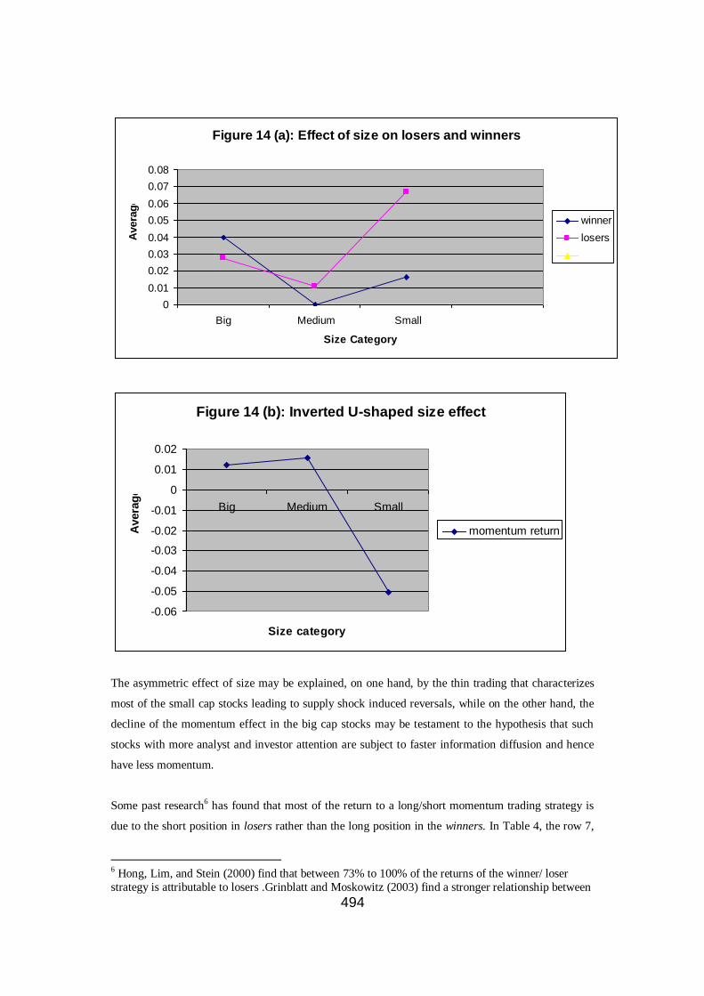
494

Figure 14 (a): Effect of size on losers and winners

0

0.01

0.02

0.03

0.04

0.05

0.06

0.07

0.08

Big Medium Small

Size Category

Avera

ge

winner

losers

Figure 14 (b): Inverted U-shaped size effect

-0.06

-0.05

-0.04

-0.03

-0.02

-0.01

0

0.01

0.02

Big Medium Small

Size category

Avera

ge

momentum return

The asymmetric effect of size may be explained, on one hand, by the thin trading that characterizes

most of the small cap stocks leading to supply shock induced reversals, while on the other hand, the

decline of the momentum effect in the big cap stocks may be testament to the hypothesis that such

stocks with more analyst and investor attention are subject to faster information diffusion and hence

have less momentum.

Some past research6 has found that most of the return to a long/short momentum trading strategy is

due to the short position in losers rather than the long position in the winners. In Table 4, the row 7,

6 Hong, Lim, and Stein (2000) find that between 73% to 100% of the returns of the winner/ loser

strategy is attributable to losers .Grinblatt and Moskowitz (2003) find a stronger relationship between

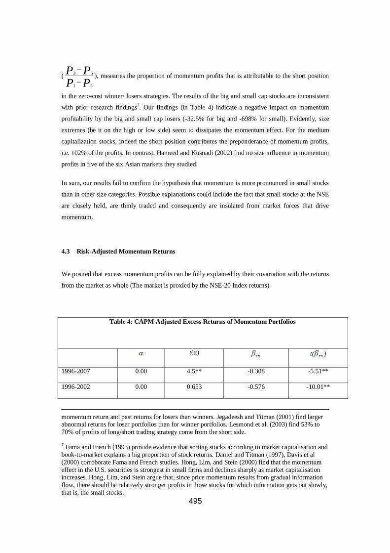
495

(

PPPP

51

53

), measures the proportion of momentum profits that is attributable to the short position

in the zero-cost winner/ losers strategies. The results of the big and small cap stocks are inconsistent

with prior research findings7. Our findings (in Table 4) indicate a negative impact on momentum

profitability by the big and small cap losers (-32.5% for big and -698% for small). Evidently, size

extremes (be it on the high or low side) seem to dissipates the momentum effect. For the medium

capitalization stocks, indeed the short position contributes the preponderance of momentum profits,

i.e. 102% of the profits. In contrast, Hameed and Kusnadi (2002) find no size influence in momentum

profits in five of the six Asian markets they studied.

In sum, our results fail to confirm the hypothesis that momentum is more pronounced in small stocks

than in other size categories. Possible explanations could include the fact that small stocks at the NSE

are closely held, are thinly traded and consequently are insulated from market forces that drive

momentum.

4.3 Risk-Adjusted Momentum Returns

We posited that excess momentum profits can be fully explained by their covariation with the returns

from the market as whole (The market is proxied by the NSE-20 Index returns).

Table 4: CAPM Adjusted Excess Returns of Momentum Portfolios

t(α)

t( )

1996-2007 0.00 4.5** -0.308 -5.51**

1996-2002 0.00 0.653 -0.576 -10.01**

momentum return and past returns for losers than winners. Jegadeesh and Titman (2001) find larger abnormal returns for loser portfolios than for winner portfolios. Lesmond et al. (2003) find 53% to

70% of profits of long/short trading strategy come from the short side.

7 Fama and French (1993) provide evidence that sorting stocks according to market capitalisation and

book-to-market explains a big proportion of stock returns. Daniel and Titman (1997), Davis et al

(2000) corroborate Fama and French studies. Hong, Lim, and Stein (2000) find that the momentum

effect in the U.S. securities is strongest in small firms and declines sharply as market capitalisation

increases. Hong, Lim, and Stein argue that, since price momentum results from gradual information

flow, there should be relatively stronger profits in those stocks for which information gets out slowly,

that is, the small stocks.

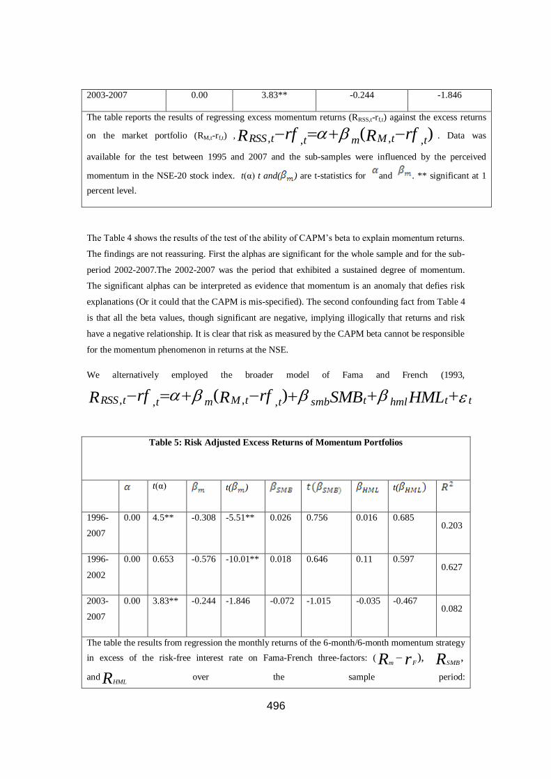
496

2003-2007 0.00 3.83** -0.244 -1.846

The table reports the results of regressing excess momentum returns (RRSS,t-rf,t) against the excess returns

on the market portfolio (RM,t-rf,t) , )(,,,, rfRrfR ttMmttRSS . Data was

available for the test between 1995 and 2007 and the sub-samples were influenced by the perceived

momentum in the NSE-20 stock index. t(α) t and( ) are t-statistics for and . ** significant at 1

percent level.

The Table 4 shows the results of the test of the ability of CAPM‘s beta to explain momentum returns.

The findings are not reassuring. First the alphas are significant for the whole sample and for the sub-

period 2002-2007.The 2002-2007 was the period that exhibited a sustained degree of momentum.

The significant alphas can be interpreted as evidence that momentum is an anomaly that defies risk

explanations (Or it could that the CAPM is mis-specified). The second confounding fact from Table 4

is that all the beta values, though significant are negative, implying illogically that returns and risk

have a negative relationship. It is clear that risk as measured by the CAPM beta cannot be responsible

for the momentum phenomenon in returns at the NSE.

We alternatively employed the broader model of Fama and French (1993,

tthmltsmbttMmttRSS HMLSMBrfRrfR )(,,,,

Table 5: Risk Adjusted Excess Returns of Momentum Portfolios

t(α)

t( )

t(

1996-

2007

0.00 4.5** -0.308 -5.51** 0.026 0.756 0.016 0.685 0.203

1996-

2002

0.00 0.653 -0.576 -10.01** 0.018 0.646 0.11 0.597 0.627

2003-

2007

0.00 3.83** -0.244 -1.846 -0.072 -1.015 -0.035 -0.467 0.082

The table the results from regression the monthly returns of the 6-month/6-month momentum strategy

in excess of the risk-free interest rate on Fama-French three-factors: ( ),rR Fm ,RSMB

and RHML over the sample period:

497

ttHMLhmltSMBsmbtftMmtftRSS RRrRrR ,,,,,,

)(

R2

is the coefficient of determination adjusted for degrees of freedom; t is the related

coefficient divided by its standard error. T-statistics are in parenthesis. **significant at 1%: *

significant at 5%.

Table 5 reports the results of the regression for the whole period and the two sub-periods. As is

shown in column 4, all the market factor coefficients ( m) are negative, indicating that market

wide risk factors far from explaining excess returns instead confound them. It is also reflects that

losers are somewhat more sensitive to the market risk factor than the winners. A closer look at

column 5 shows that coefficients for the whole sample and 1996-2002 sub-period are significantly

different from zero, meaning that market betas for winners and losers differ significantly.

Columns 6-9 reveal the effect of the size factor coefficients (SMB

) and book-to-market factor

coefficients (HML

). The signs are positive for the entire sampled period, and the period 1996-2002;

but negative for the sample sub-period 2003-2007. Tests of significance reveal that the coefficients

are not significantly different from zero. This leads to the inference that size and the value factor have

some, but marginal explanatory power for momentum profits

Columns 2 and 3 of Table 5 report the alpha (α) of the various momentum portfolios as estimated by

regressing the monthly excess momentum returns on the Fama-French factors. The alphas for these

risk-adjusted portfolios are positive and significantly different from zero. This means that the three

factor model is not adequate to explain the sources of momentum profits. This begs the question

whether or not there may be other variables with more correlation with momentum profits not

specified in the three factor model.

The last column of the table presents the R-square of each regression, ranging from 0.082 to 0.0627.

This means the Fama-French factors can only explain 6% to 8% of the momentum profits. We are let

to conclude that momentum profits cannot be explained by the risk factors contained in the Fama-

498

French three-factor model. We therefore, fail to confirm the hypothesis that momentum profitability

is a compensation for additional risk inherent in the momentum strategies.

5. Conclusions

The striking finding from our test is that one can earn abnormal returns by implementing momentum-

based trading strategies at the NSE. This momentum is caused by investors underreacting, trading in

herds, or the limitations of the arbitrage process. Investor education, institutional, legislative,

regulatory strengthening and improvement in operational efficiency could reduce the misevaluation

in stocks at the bourse.

We did not find a size effect in the momentum profitability. This contrasts findings in prior studies.

The discrepancies in the findings on NSE data may be the result of the differences in what

constitutes small or big stocks in the different markets. For instance the typical small capitalization

in NSE will be the stocks that are excluded from samples using NYSE data as being outliers that

could distort results. A future study should exclude the typical small and infrequently traded stocks

in the alternative segment, and concentrate only on the main segment. A size investigation confined

to the main segment would reduce the operation of omitted variables and allow the size effect to

stand out.

As regards the explanatory power of risk, the analysis revealed that the market wide co-variation,

the book-to-market and the size factors cannot explain the out-performance of momentum stock

selection strategies at the Nairobi Stock Exchange. Consistent with the findings of a majority of

extant studies, our tests failed to explain momentum profits within the framework of two risk

motivated models. Thus we are led to conclude that investors and markets do not react only to risk

in pricing assets. We are led to conclude that, perhaps, behavioural factors and psychological biases

are a major influence on the demand and supply forces at the NSE. Additionally, the restrictions on

short selling and the limitations in the operation of arbitrage forces can lead to the persistence of

profitable arbitrage opportunities unexploited.

REFERENCES

Atiti, R., 2003. A study of price momentum at NSE. Unpublished MBA research project,

University of Nairobi

Banz, R., 1981. The relationship between return and the market value of common stocks.

Journal of Financial and Quantitative Analysis 14, 421-441.

499

Berk, J., Green, R., and Naik, V., 1999. Optimal investment, growth options, and security n

returns. Journal of Finance 54, 1553-1608.

Bekaert, G. Erb, C. Harvey, C. and Viskanta, T., 1997. What matters in emerging markets

investment? Emerging Markets Quarterly 1, 1-30.

Bernard, V., 1992. Stock price reactions to earnings announcements: In Thaler, R. (eds.) Advances in

Behavioural Finance. Russel Sage Foundation, New York pp. 303-340.

Bernard, V.L., Thomas, J.K., 1989. Post-earnings-announcement drift: delayed price response or risk

premium? Journal of Accounting Research 27 (Supplement), 1-48.

Bernard, V.L., Thomas, J.K., 1990. Evidence that stock prices do not fully reflect the implications of

current earnings for future earnings. Journal of Accounting and Economics 13, 305-340.

Chan, K., Hameed, A., Tong, W., 2000. Profitability of momentum strategies in the international equity

markets. Journal of Financial and Quantitative Analysis 35, 153-172.

Chan, K., Jegadeesh, N., Lakonishok, J., 1996. Momentum strategies. Journal of Finance 51, 1681-

1714.

Chopra, N., Lakonishok, J., Ritter, J.R., 1992. Measuring abnormal performance: do stocks

overreact? Journal of Financial Economics 31, 235-268

Chordia, T., and Shivakumar, L., 2002. Momentum, business cycle, and time-varying expected

returns. Journal of Finance 57, 985-1019.

Conrad, J., and Kaul, G., 1998. An anatomy of trading strategies. Review of Financial Studies 11,

489-519.

Cuttler, D.M., Poterba, J.M., Summers, L.H., 1989. What moves stock prices? Journal of Portfolio

Management 15, 4 12.

Cuttler, D.M., Poterba, J.M., Summers, L.H., 1990. Speculative dynamics. Review of Economic

Studies 58, 529-546.

Daniel, K.D., Titman, S., 1997. Evidence on the characteristics of cross-sectional variation in

common stock returns. Journal of Finance 52, 1-33.

Davis, J., Fama, E., and French, K., 2000. Characteristics, covariances and average stock returns.

Journal of Finance 55,389-406.

De Bondt, W., and Thaler, R., 1985. Does the stock market overreact? Journal of Finance 40, 793 –

807.

Fama, E., 1998. Market efficiency, long-term returns and behavioural finance. Journal of

Financial Economics 49, 283-306.

Fama, E., and French, K., 1992. The cross-section of expected stock returns. Journal of Finance 47,

427-465.

500

Fama, E., and French, K., 1996. Multifactor explanations of asset pricing anomalies. Journal of Finance

51, 55-84.

Griffin, J., Ji, S., and Martin, J., 2002. Momentum investing and business cycle risk: Evidence from

pole to pole. Journal of Finance Forthcoming.

Grinblatt, M., Titman, S., and Wermers, R., 1995. Momentum investment strategies, portfolio

performance, and herding: a study of mutual fund behaviour. American Economic Review 85,

1088-1105

Grundy, B., and Martin, J., 2001. Understanding the nature of the risks and the sources of the rewards

to momentum investing. Review of Financial Studies 14, 29-78.

Hameed, A., and Kusnadi, Y., 2002. Momentum strategies: evidence from Pacific Basin stock

markets. Journal of Financial Research 25, 383-397.

Hastie, R., and Dawes, R., 2001. Rational choice in an uncertain world: the psychology of judgment

and decision making. Thousand Oaks: Sage Publications.

Haugen, R.A., Baker, N.L., 1996. Commonality in the determinants of expected stock returns. Journal

of Financial Economics 41, 401-439.

Hong, H., Lim, T., and Stein, J., 2000. Bad news travels slowly: size, analyst coverage and the

profitability of momentum strategies. Journal of Finance 55, 265-295.

Ikenberry, D., Lakonishok, J., and Vermaelen, T., 1995. Market underreaction to open market share

repurchases, Journal of Financial Economics 39, 181-208.

Jegadeesh, N., Titman, S., 1993, Returns to buying winners and selling losers: Implications for

stock market efficiency. Journal of Finance 48, 65-91.

Jegadeesh, N., Titman, S., 2001. Profitability of momentum strategies: an evaluation of

alternative explanations. Journal of Finance 56, 699-720.

Johnson, T., 2002. Rational momentum effects. Journal of Finance 567, 585-6076.

Korajczyk, R. A., and Sadka, S., (2004) ‗Are Momentum Profits Robust to Trading Costs?‘ Journal

of Finance 59, 1039-1082.

Lakonishok, J., Shleifer, A., and Vishny, R., 1992. The impact of institutional trading on stock prices.

Journal of Financial Economics 32, 23—43.

Lee, C., and Swaminathan, B., 2000. Price momentum and trading volume. Journal of Finance

501

Lewellen, J., 2002. Momentum and autocorrelation in stock returns .Review of Financial Studies 15,

533-563.

Liu, W., Strong, N., and Xu, X., 1999. The profitability of momentum investing. Journal of Business,

Finance and Accounting 9/10, 1043-1091.

Lo, A., and MacKinlay, A., 1990. When are contrarian profits due to stock market overreaction? Review

of Financial Studies 3, 175-205.

Loughran, T., Ritter, J., 1995. The new issues puzzle. The Journal of Finance 50, 23-52.

Michaely, R., Thaler, R., and Womack, K., 1995, Price reactions to dividend initiations and

omissions, Journal of Finance, 50, 573-608. ,

Richards, A.J., 1997. Winner-loser reversals in national stock market indices: can they be explained?

Journal of Finance 52, 2129-2144.

Rouwenhorst, K.G., 1998. International momentum strategies. Journal of Finance 53, 267-284.

Ryan, P., and Overmeyer, I., 2004. Profitability of price momentum strategies: The DAX 100

evidence. Journal of Investing Summer 2004, 55-62...

Shleifer, A., and Vishny, R., 1997. The limits to arbitrage. Journal of Finance 52, 35-55.

Spiess, D.K., Affleck-Graves, J... 1999. The long-run performance of stock returns following debt

offers. Journal of Financial Economics 54, 45-73

Womack, K.L., 1996. Do brokerage analysts' recommendations have investment value? Journal of

Finance 51, 137-168

Wong, K., and Ho, H.., 1980. The weekend effect on stock returns in Singapore. Hong Kong Journal of

Business Management 4, 31-50.

Yao, T., 2003. Systematic Momentum. Working Paper, University Of Arizona.

502

DEBT FINANCING AND RETURN ON EQUITY

A CASE OF LARGE CORPORATE TAXPAYERS IN UGANDA

BY: ROBINAH AKODO

Assistant Director

Makerere University Business School

arobinah@yahoo.com

ABSTRACT

This study examined the relationship between debt equity ratio and return on equity for large

corporate taxpayers in Uganda. It addressed the question of whether debt financing magnifies return

on equity. The research also established the capital structure of large taxpayer companies and

confirmed that the theories on the advantages of debt financing are valid for a developing economy

like Uganda‘s.

The study established that all sectors under study employed debt in their capital structure

during the study period and had an overall positive correlation (r = 0.322, p-value < 0.05) between

debt equity ratio and return on equity. Sector by sector analysis showed that the manufacturing sector

had the strongest relationship between debt equity ratio and return on equity (r = 0.835, p-value <

0.05) and the construction sector had the weakest correlation between debt and equity (r = 0.128, p >

0.05). The construction sector had a high probability of leverage chance (r = 0.76). Empirical

evidence shows that debt financing improves return on equity. The findings for all the sectors were in

line with the theory that debt financing magnifies shareholders‘ return.

Keywords: Debt financing, Return on Equity, Uganda

502

Background to the Study

Many firms use debt as a major source of financing. A research by Booth et al., (2000) of

5,281 firms in Europe, Asia and USA revealed that the debt to equity ratio ranged from a low of

30.3% in Brazil to a high of 73.4% in South Korea. In theory, the primary motive of a company

using financial leverage was to magnify the shareholders‘ return (Pandy, 1997). According to

Paranque (1992), the capitalization of a given firm is closely connected to its return on equity and

highly profitable but slow-growing firms should generate cash and finance their operations by

internally generated funds. On the other hand, less profitable but fast-growing firms need significant

external financing. Paranque and Pandy‘s theories did not show the extent to which financial leverage

could magnify shareholders‘ return; an aspect this research sought to establish.

Divya et al (2011), in their study on Inside Debt and the Design of Corporate Debt Contracts

found that a higher CEO relative leverage, defined as the ratio of the CEO's inside leverage (debt-to-

equity compensation) to corporate leverage, was associated with lower cost of debt financing and

fewer restrictive covenants. Additional analysis on a sample of new public bond issues also showed a

negative relation between CEO relative leverage and bond yield spread. The evidence supports the

notion that debt holders recognize the incentive effects of executive debt-like compensation and adjust

the terms of corporate debt contracts accordingly.

Hull (2011), in his non-empirical study of Debt-equity decision-making with and without

growth attempted to instill knowledge and skills to students when making debt-equity and plowback-

payout choices.

According to Nadeem (2011), an empirical study of firms in the manufacturing industry in Pakistan

suggested that profitability, liquidity, earnings volatility, and tangibility (asset structure) are related

negatively to the debt ratio whereas firm size was positively linked to the debt ratio. Non-debt tax

shields and growth opportunities do not appear to be significantly related to the debt ratio. The

findings of this study are consistent with the predictions of the trade-off theory, pecking order theory,

and agency theory which showed that capital structure models derived from Western settings do

provide some help in understanding the financing behavior of firms in Pakistan.

Abimbola (2004) tested the endogenous relationship between financial leverage and bank

debt‘s use in the UK. The study‘s findings indicated that industry classification has a significant

effect on reliance on bank debt. Although firms that used bank debt seemed to have higher agency

cost potential than firms that did not use debt, long term leverage did not have a significant

relationship with long term bank debt‘s use in the evidence.

Elliott et al. (2007) did a study on the impact of equity mispricing on target debt ratios. The

study found that the reported portion of variance was caused by two factors. First, firms faced a

‗hard‘ boundary when over levered. This was due to the present value of bankruptcy costs increasing

at an increasing rate. These firms will adjust towards a target debt ratio more rapidly than under

leveraged firms which face a ‗soft‘ boundary. Second, if a firm‘s equity was mispriced, the cost of

issuing equity could be reduced or increased.

A study by Nishat (2000) entitled ―The Systematic Risk and Leverage Effect in the

Corporate Sector of Pakistan,‖ indicated that the debt-equity ratios across industries are higher

throughout the study period, except for a few industries like tobacco and vanaspati and allied.

Jiming et al. (2010) studied the impact of debt financing on firm investment behavior in

China. The study established that there was a negative relation between debt financing and

503

investment behavior in firms with both low-growth opportunities and high-growth opportunities and a

negative effect was more significantly stronger for firms with low-growth opportunities than those

with high-growth opportunities.

Chava. S., and Micheal R. R. (2008) studied the role of debt covenants and how these impact

financing investment. Their study found that capital expenditures declined by approximately 1% of

capital per quarter in response to covenant violations with a 13% decline relative to the pre-violation

level of investment. Additionally, this decline was concentrated among firms in which agency and

information problems were relatively more severe. Thus, the results highlighted how the state-

contingent allocation of control rights mitigated investment distortions arising from financing

frictions.

A study by Adamia et al (2010) on the effect of leverage on stock returns indicated that

returns decreased with firm leverage. The study tested the relationship empirically with other risk

factors and found that the results remained robust. Further, it was found that leverage was a firm

characteristic that loaded on a risk factor. This suggested that leverage should be priced as a risk

factor and required adequate incorporation into common asset pricing models.

In trading, when a firm employs debt in its capital structure, it has to pay fixed charges on

the debt regardless of the firm‘s income generating capacity. There was a risk of making low profits

or even losses and the risk of liquidation when the expected return on investment fell short of the cost

of borrowed funds. However, management of business enterprises usually enter into loan covenants

using financial projections that assume favorable or optimistic economic conditions and hope that the

fixed charge on debt would remain lower than the firms‘ expected rate of return on capital employed.

Statement of the Problem

Capital structure theories depict debt financing as a double-edged sword. That is, it is the

cheapest source of capital when a firm has income generating capacity to meet the debt obligations but

when the return on capital slips below the cost of debt, businesses will make losses and may gradually

be liquidated on failure to meet the debt obligations.

The theories on debt financing were developed premised on developed country case

scenarios. It is not clear whether debt-financing effects are relevant and true in a developing economy

like Uganda‘s. This study set out to establish the relationship between debt equity ratio and return on

equity for the targeted sectors of the study.

Purpose of the Study

The study set out to establish the relationship between debt equity ratio and shareholders‘

return for various business sectors in the Ugandan economy.

Objectives of the Study

The study had the following objectives:

d) To establish the capital structure of the two large tax paying business entities in Uganda.

e) To establish the effect of leverage chance and leverage risk on return on equity of the two

sectors of large taxpayers.

f) To examine the relationship between capital structure and return on equity.

504

Research Questions

The study focused on answering the following questions:

d) What is the capital structure of the two large corporate taxpaying entities in Uganda?

e) What is the effect of leverage chance and leverage risk on return on equity of the study

population?

f) To what extent does debt financing magnify shareholders‘ return on equity in Uganda?

The conceptual framework

The researcher discusses research findings in the subsequent chapters based on the conceptual

framework as follows:

Fig.1 Conceptual Framework (adapted from Du Pont Model)

Leverage Effect

The common and direct ratio for calculating a firm‘s return on equity is the ratio of retained

earnings to owner‘s equity. However, the Du Pont‘s model (http://www.uic.educ) decomposes the

ratio as a function of three factors; the firm‘s profitability, assets turn over and leverage summarized

as:

Profit Margin X Asset Turnover X Leverage = Return on Equity

Profit Margin = Net income/Net Sales

Asset Turnover = Net Sales / Average Total Assets

Leverage = Average Total Assets/Average Owner‘s Equity

Debt/Equity

Ratio

Return on

Equity

Leverage Chance

Leverage risk

Interest cost

Return on capital Employed

505

Profit margin shows the percentage of each shilling in sales that results in net income, asset turn over

measures how efficiently assets are used to generate sales and the leverage indicates how the assets

used in generating sales are financed. The Du Pont model return on equity decomposition formed the

basis for the choice of the independent variables in this study.

Significance of the Study

The findings will benefit the following:

Shareholders

The study will enable shareholders appreciate the contribution of debt financing to the return

on their funds. It will also enable them examine those sectors that give a higher return on equity for a

given combination of debt and equity.

Managers of business enterprises

The study will enable managers ascertain the proportion of debt that has a high contribution

to the shareholders‘ funds. It will also provide information on the various costs associated with debt

financing and provide a guide for the choice of capital structure for certain business sectors.

Tax Administrators

The study will provide a basis for assessing the earning capacity of equity holders

in the various business sectors.

Scope of Study

The scope of the study was in terms of geographical scope, subject matter, and time.

Geographical Scope

The study covered a sample of 43 large taxpaying companies in construction and

manufacturing in Uganda that submit financial statements to Uganda Revenue Authority at Crested

Towers Kampala.

The major reasons for choosing large tax paying companies was that their business

operations were centrally monitored by the Large Tax Payer Unit of the Uganda Revenue Authority

and their financial statements were prepared by reputable audit and accounting firms like

PriceWaterhouseCoopers, Ernest and Young, and KPMG. The large taxpayers were frequently

audited or monitored by Uganda Revenue Authority.

Subject Matter

The study aimed at finding out:

(b) The composition of capital structure of the selected companies

(b) The relationship between return on equity and the various combinations of debt and

equity for the selected companies.

506

Time

The study covered a period of 11years (2000-2010).

Literature review

Relevant materials were drawn from various literature sources related to debt financing and

return on equity regardless of the time or place. Materials were reviewed along the major theme of

debt financing and return of equity and under the sub-themes of leverage chance and leverage risk.

Debt and Equity

Theories on proportions of debt and equity in the capital structure of business enterprises

were developed and the relevance of some of the theories was studied. Modigliani and Miller (1958)

theorized that the capital structure of a firm does not affect its value. The Modigliani and Miller

(MM) theory was based on ideal assumptions that do not exist in many countries. The MM theory

did not put into perspective the reaction of lenders as capital shifts from equity to debt, a factor

Smith and Watts (1992) examined and established that when capital structure shifts from equity to

debt, lenders restrict borrowers in the usage of working capital, capital expenditure for fixed assets

and equity re-evolvements.

This study focused on what happens to the value of shareholders as the proportions of debt

and equity in the capital structure vary. Other theories or models reviewed are the Capital Asset

Pricing Model (CAPM), the Fama-French three factor model, and the Fama-French plus Carhart

four factor model.

Govindasamy (2010) analysed the impact of leverage on profitability in cement companies

in India. This study established that leverage, profitability and growth are related and leverage has an

impact on the profitability of the firm. Hasanhodzic. J. & Lo. A. W., (2010), in their study of a

sample of all-equity financed companies found that the leverage effects were just as strong, if not

stronger, implying that the inverse relationship between price and volatility was not based on

leverage, but was more likely driven by time-varying risk premiums or cognitive mechanisms of risk

perception.

Riddiough (2004), in a study of optimal capital structure articulated the economics

underlying the market for outside finance in commercial real estates and established that mortgage

debt is typically the optimal form of finance as it economizes on transaction costs and provides

proper incentives for the property owners. An inside equity-outside mortgage financing maximizes

comparative advantage. He concluded that for commercial real estate, debt financing was cheaper

than equity. His study, however, did not involve numerical figures to show the contribution of debt

financing to shareholders.

Brounen and Eichholtz (2001) examined the stock price reaction on announcements of

additional equity and debt on European property companies‘ capital offerings. They established a

positive reaction on employing more debt than equity as a result of perceived tax shield benefit from

debt financing. The study justified the use of more debt than equity in an environment where capital

markets are perfect. It is, however, not known whether the same results are true for unlisted

507

companies operating in an environment of developing imperfect capital markets as in the case of

Uganda.

Theory on debt financing

The advantage of debt financing in taxation of business enterprises is that interest payments

are tax deductible. They elude taxation at the corporate level, whereas dividends or retained earnings

associated with stock are not deductible for corporation tax purposes. Debt financing improves the

total amount of payments available for stockholders, Van Horne (2002).

Pandy (1997), states that the role of debt financing is to magnify the shareholders‘ return.

The assumption that the fixed charge funds are obtained at a cost lower than the firm‘s rate of return

on the assets was the basis for the magnifying impact of debt financing. Kakuru (2000), observed that

whereas debt could be beneficial especially in times of economic boom, excessive debt financing will

mean that business enterprises have high interest obligations and the burden of repayment of principal

amounts periodically. Firms enter into agreements to borrow funds with a view to boosting their

capital base, asset turnover and to enable them expand their operations. Debt financing was desirable

when cost was lower than the expected rate of return on investment.

Elliott, B., W., Koëter-Kant, J., & Warr. R., S. (2008) found that the average book debt ratio

for all firms was about 23%, compared to a market debt ratio of approximately 28%. On average,

sample firms had earnings 6.7% of assets, before interest and taxes.

Omole. D. A., and Falokun. G. O., (1999) found a link between interest rates, corporate

financing strategies, and the profitability of firms. Their study also revealed that interest rate

liberalization had a link with the growth of the equity markets. On sectoral analysis, their study

indicated that the interest rate liberalization does not seem to have similar effects on all the

investigated quoted companies

Leverage Chance and Leverage risk

Pandy (1997), states that debt financing provides a potential of increasing shareholders‘

earnings only when the interest rate charged on borrowed funds is than the rate of return on assets

financed by debt. When the rate of return falls below the cost of borrowed funds, the firm stands a risk

of making a loss. Risk averse managers, under such circumstance, opt for increased equity financing.

This study used data from financial statements of business enterprises for specific sectors in

Uganda, examined the changes in return on equity, and established that sectors that had the highest or

lowest potential of maximizing shareholders‘ return from assets were financed by debt. This study

found that volatility risk alone predicted 50% of credit default swap (CDS) spread variation, while

jump risk alone forecast was 19%. After controlling for credit ratings, macroeconomic conditions,

and firms‘ balance sheet information, it explained 77% of the total variation. Moreover, the marginal

impacts of volatility and jump measures increased dramatically from investment grade to high-yield

entities. The estimated nonlinear effects of volatility and jumps were in line with the model implying

508

that there was a relationship between equity returns and credit spreads (Benjamin Yibin Zhang, Hao

Zhou, Haibin Zhu 2005).

In Uganda, firms that bring into use eligible property for the first time during the year of income

enjoy initial capital allowance at the rate of 50%, 70% or 20% of the cost base (Section 29 of Income

Tax Act 1997 and Sixth Schedule) depending on the location of the investment.

Capital structure and Return on Equity

Cohen (2004), in his illustration of the effect of Modigliani and Miller theorem on capital

structure, used simplified financial statements and arrived at a generic conclusion that as the ratio of

debt to equity in the capital structure of the firm increases, return on equity also increases. He assumed

constant earnings before interest and tax (EBIT), and a constant cost of capital for all periods. In

practice, EBIT cannot be constant within a firm or industry. Different firms apply different accounting

policies (for example in the computation of depreciation of fixed assets). The rates and method of

calculation vary from firm to firm. Operational expenses and sales volume may vary in response to

changes in economic factors of a given country. In this study, empirical data from financial statements

of business enterprises in Uganda was used to establish whether the same relationship as in Cohen‘s

conclusion exists.

McDonald (2004) examined a number of factors that drive return on equity. He examined in

detail profit margins of Corporate America in relation to the lowest long term interest rates, inflation

rate and return on equity, Just in Time inventory management and turnover, restructuring and

accounting charges (using Dow Jones Industrials) and return on equity. His study provided details

establishing the extent to which leverage drives return on equity.

METHODS AND MATERIALS

Research Design

The purpose of this study was to establish the relationship between debt financing and return on

equity. A longitudinal research design was used to analyze secondary data based on financial

statements for the selected corporate taxpayers in Uganda. A descriptive survey research design

method of investigation was used given the nature of the study which called for adequate description

of the different combinations of debt and equity and the resultant return on equity.

Area and Survey Population

The survey population for the study was 99 large corporate taxpayers in construction and

manufacturing classified by Uganda Revenue Authority and distributed as:

Table 1: Distribution of Large Taxpayers by Sector

SECTOR CONSTRUCTI MANUFACTURI TOTAL

509

ON NG

NO. OF TAXPAYERS (n) 18 81 99

Source: URA Large Taxpayer Register, 2010

Each sector represented a stratum and from each stratum sampling units proportionate to stratum size

were selected randomly.

Sample size and selection

Sample size determination

The researcher set confidence level at 95% and error term of ±1 such that from table 1 and using the Z-

distribution tables, the sample size was determined using the formula

n = NZ2S

2

NE2 + Z

2S

2

(Adapted from Kiregyera, 1999)

Where

N = Total number of companies

Z = 1.96 (for 95% confidence interval)

E = 1

S2 = population variance

= Σ (xi-µ)2 = 32

2 +31

2 = 20

N 99

µ = 99 =50

2

n = 99*1.96 * 1.96 * 20 = 7606.368/175.832=43

99 *1 + 1.96 * 1.96 *20

Sample selection

Sample size of 43 was obtained using Simple random sampling.

510

The response rate was as shown in table 2 below;

Table 2: Number of sample units per stratum

Sector Construction Manufacturing Total

Sample units 5 20 25

Source: URA large tax payers register, 2011

Data collection

Research Instruments

The study used Uganda Revenue Authority Large Taxpayer registry document analysis, observation

and taxpayer profile schedules that served as questionnaires. The URA staff working in the registry

served as local agents through whom the information was collected. Each staff was given taxpayer

profile schedules detailing the specific fields of data records.

Source of Data

The study involved the use of secondary data from financial statements of the selected companies and

documents, textbooks and journals with data related to debt financing and return on equity.

Measurement of variable

Capital structure

The study used the ratio of total debt in the balance sheet to the total of ordinary share capital,

retained earnings and other equity instruments to determine debt/equity fraction for all sectors of

study.

Imputed interest rates

This was obtained by dividing total finance costs excluding foreign exchange movements with total

short term and long term borrowed funds extracted from the balance sheets.

Return on equity

This was computed by dividing retained earnings for the year with ordinary share equity.

Leverage risk/ chance

511

Leverage risk and leverage chance were measured by comparing return on capital employed with

imputed interest rate. Leverage chance was measured by the excess of return on capital employed

over imputed interest rate and leverage risk was measured by the excess of imputed interest rate over

return on capital employed.

Quality Control

Quality control was done by ensuring that data was obtained from the two sectors of the population

eligible for the study. Data was cross checked for completeness and accuracy by the help of audited

and published financial statements. Data schedules had a provision of coding each sample unit for

purposes of editing the extracted data in the event of incorrect data capture by the local agents.

Model specification and estimation

Expanding on Modigliani and Miller‘s (1958) Proposition II, abnormal returns are estimated

using the asset pricing models of Sharpe and Lintner (the traditional Capital Asset Pricing Model,

Fama and French and of Carhart).

The estimated model is given by: ROE = a+b1 DER+b2LE

Where:

a = represents factors other than Debt Equity Ratio and Leverage effect

b1= the regression coefficient of DER

b2 = the regression coefficient of Leverage effect.

DER= Debt equity ratio

LE= leverage effect

Data Analysis

The study used a combination of Microsoft Excel and SPSS for analysis. Microsoft Excel was used to

capture the financial statements and compute the debt equity leverage and return on equity ratios.

Figures or graphs showing ratio trends were generated from the Microsoft Excel. Correlation and

regression analysis were generated from SPSS to determine the magnitude of the relationship

between study variables and to fit the debt financing model.

RESULTS/FINDINGS

Basis of categorization of firms in the sample

512

A total of 43 out of 99 large corporate tax payers in construction, manufacturing, oil

industry, general trade, financial services and those in other services other than financial services

were selected for the study. For each company data was extracted from financial statements for the

period (2000 – 2010). The study used the list of the Large taxpayer Department that has been in use

since the year 2000 with a distribution of the large taxpayer companies distributed as follows:

Table 3: Distribution of Large Taxpayers

Sector

Number of

companies

Sample size

per sector

Construction

Manufacturing

18

81

5

20

Total 99 25

Source: Large Tax Department tax payer List 2000-2010

Descriptive Analysis of findings

To answer the research questions and to achieve the objectives of this study, return on equity

ratios, debt equity ratios, return on capital employed, leverage chance/risk and imputed interest costs

were calculated for the construction and manufacturing sectors. The average ratios for the sectors

under study were used to generate line graphs to depict trends of behavior of the study variables as

shown in tables 4 and 5 and in figures 1 to 2 discussed in the subsequent sections of this report.

It was established that firms in these two sectors employed debt financing in their capital structure.

The manufacturing sector had a higher debt proportion in its capital structure compared to

construction. The study also performed analysis of variance (ANOVA) to determine whether there

were significant differences among the various sample means for purposes of identifying those

sectors that experienced high or low variations in the study variable. The results are summarized

below:

Table 4: Mean and standard deviation scores for the study variables

Minimum Maximum Mean Std. Deviation

DEBT EQUITY .1211 .8900 .4324 .3014

LEVERAGE CHANCE RISK -.1430 .2030 .0272 .1081

513

IMPUTED INTEREST RATE .1166 .3052 .1902 .0451

ROCE -.0268 .3615 .2174 .1023

ROE -.1858 .3069 .1328 .1151

Source: URA financial statements for selected large taxpayer companies 2000-2010

From table 4 and 5 the results were significant at 5% significance level (α = 0.05). The computed

values of F, in the F column in table 5 and the critical values Fc in the footnote to table 5 revealed that

the computed F for ROCE, imputed interest rates, debt equity ratio and leverage chance and leverage

risk was greater than the critical value of F. The F test for ROE showed that there were no significant

differences between ROE of the two sectors of the study (the computed F = 1.750 < Fc = 2.49)

Table 5: ANOVA for study variables

SUM OF

SQUARES

MEAN

SQUARES

F-COMPUTED

SIG

ROCE

Between

groups

Within groups

Total

.381

.618

.999

0.07621

0.00172

4.436 0.003

ROE

Between

groups

Within groups

Total ROE

.010

.409

.509

0.00199

0.00114

1.750 0.148

IMP.

INT

RATE

Between

groups

Within groups

Total

.205

.008

.282

0.00410

0.00021

19.296 .000

DEBT/

EQUITY

Between

groups

Within groups

297.676

19.267

59.535

.535

111.238 .000

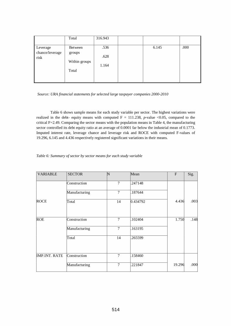
514

Total 316.943

Leverage

chance/leverage

risk

Between

groups

Within groups

Total

.536

.628

1.164

6.145 .000

Source: URA financial statements for selected large taxpayer companies 2000-2010

Table 6 shows sample means for each study variable per sector. The highest variations were

realized in the debt- equity means with computed F = 111.238, p-value <0.05, compared to the

critical F=2.49. Comparing the sector means with the population means in Table 4, the manufacturing

sector controlled its debt equity ratio at an average of 0.0001 far below the industrial mean of 0.1773.

Imputed interest rate, leverage chance and leverage risk and ROCE with computed F-values of

19.296, 6.145 and 4.436 respectively registered significant variations in their means.

Table 6: Summary of sector by sector means for each study variable

VARIABLE SECTOR N Mean F Sig.

ROCE

Construction 7 .247148

4.436

.003

Manufacturing 7 .187644

Total 14 0.434792

ROE

Construction 7 .102404 1.750

.148

Manufacturing 7 .163195

Total 14 .265599

IMP.INT. RATE

Construction 7 .158460

19.296

.000 Manufacturing 7 .221847

515

Total 14 .379307

DEBT/EQUITY

Construction 7 .179727

111.238

Manufacturing 7 .685143

Total 14 .864870 .000

LEVERAGE -

CHANCE/(RISK)

Construction 7 .008868 6.145 .000

Manufacturing 7 .000034

Total 14 .008902

Source: URA-financial statements for selected Large Taxpayer companies 2000-2010

Construction sector analysis

Average financial ratios for five construction companies for the years 2000 to 2010 were computed

and summarized as in table 7.

Table 7: Financial Ratios for Construction Companies, 2000-2010

Source: URA -Construction company financial statements 2000-2010.

Capital structure of construction sector

Table 7 shows that debt to equity ratio was highest in 2002 at a rate of 24% and lowest in

2000 at 12%. This implies that over 76% of the capital structure of large corporate taxpayers in the

construction sector in Uganda in the period of study was equity. Return on equity was highest at 31%

in 2001 in the construction sector when debt-equity ratio was at 20%. The return on equity was

lowest at 14% in 2003 when debt equity ratio reduced to 15% respectively. This trend is depicted by

the line graphs in figure 4.1 that showed a general decline in return on equity as debt on equity

declined over the years (2000 -2010).

516

A correlation analysis revealed a positive relationship between debt equity ratio and return

on equity (r = 0.125, p- value > 0.05). This implied that as debt equity ratio increased in the

construction sector during the period of study, return on equity increased respectively.

517

Fig 1: Debt/ equity and ROE trends for 2000-2010

The coefficient of determination, r2, for debt equity ratio and return on equity indicated that the

changes in debt equity ratio accounted for 2% of the changes in return on equity. Other factors

accounted for 98% variation in return on equity. The positive correlation between the two study

variables implied that shareholders‘ return increased or decreased with increase or decrease in debt

proportion in the construction sector.

Leverage effect on return on equity in the construction sector

When debt is introduced in the capital structure, it introduces interest cost and other loan-

related charges like commitment fees and insurance costs which have to be paid together with the

principal loan repayments regardless of cash flow generating capacity of the firm. The total financing

cost in the financial statements was attributed to debt financing. Imputed interest rate for construction

sector was derived as the ratio of total finance costs to total borrowed funds in the balance sheet and

the results were as shown in Table 3. Leverage chance and leverage risk was computed as the

difference between return on capital employed (ROCE) and the imputed interest rate for each year. It

was established that the construction sector experienced a leverage risk exposure in 2004 when ROCE

fell below the imputed interest rates.

The general trend of leverage chance and leverage risk position of the construction sector is

as illustrated in figure 2. The figure shows that construction sector had an advantage of leverage

chance for all the years of the study except in 2004 and 2006. The figure shows that the greatest

leverage chance effect was achieved in the period (2000 – 2003) and 2005 to 2006. In theory return on

equity would follow a similar trend on the assumption that the managers of those companies deployed

fixed assets profitably and did not revalue or change the depreciation policies to ensure a favorable

return on capital employed against the imputed interest.

518

Fig.2: Leverage Chance and Leverage Risk trends for Construction sector for the period 2000-2010

A further analysis of leverage effect on return on equity using the ratios in table 7 revealed

that at lowest imputed interest rate of 12% in the year 2006, return on equity was 19% and at the

highest imputed interest rate of 20% in 2003, ROE was 3%. This was a prima-facie demonstration that

the higher the imputed interest the lower the ROE. However, the study extended the analysis to cover

other years in table 3. A correlation analysis of the study variables revealed a positive relationship

between leverage chance and leverage risk and return on equity (r = 0.76, p-value <0.05).

The coefficient of determination showed that the leverage effected accounted for 58% of the

variations in return on equity while other factors accounted for 42%. This analysis confirmed the

double-edged sword theory of debt financing. That is, shareholders would benefit from debt financing

as long as the return on capital employed remained higher than the imputed interest rate and vice

versa.

The extent to which debt financing magnifies return on equity (ROE)

To assess the extent to which changes in debt /equity proportion affects the shareholders

return, the researcher performed a correlation analysis of debt/equity ratio and return on equity and

519

established that there was a positive correlation between the two variables (r = 0.125, p-values > 0.05).

However, the relationship was weak. That is, the coefficient of determination, r2, demonstrated that

changes in debt financing accounted for 2% of the changes in ROE.

This implied that 98% of the variations in return on equity for the construction company were

accounted for by other factors other than changes in debt to equity ratio during the period 2000 to

2010.

Considering these results above, this can be deduced that the mix of debt and equity in the

capital structure in Uganda during the study period did not have a significant magnifying effect on

return on equity instead the rate at which the funds were borrowed and other factors had a significant

effect. These findings matched the Modigliani and Miller theory stated earlier in the literature review.

Manufacturing sector analysis

Financial statements for 20 out of 81 manufacturing companies in the large taxpayers unit of

the Uganda Revenue Authority were examined in accordance with the research objectives and

questions. Average financial ratios were computed and are summarized in table 8.

Table 8: Manufacturing Sector Computed ratios

Source: URA-financial statements for manufacturing companies 2000-2010

Capital structure of manufacturing sector

The computed debt to equity ratio for the manufacturing sector in table 8 shows that for

the period 2000 to 2010, the ratio was highest in 2001 at 89% and lowest in 2005 at 25%. Apart from

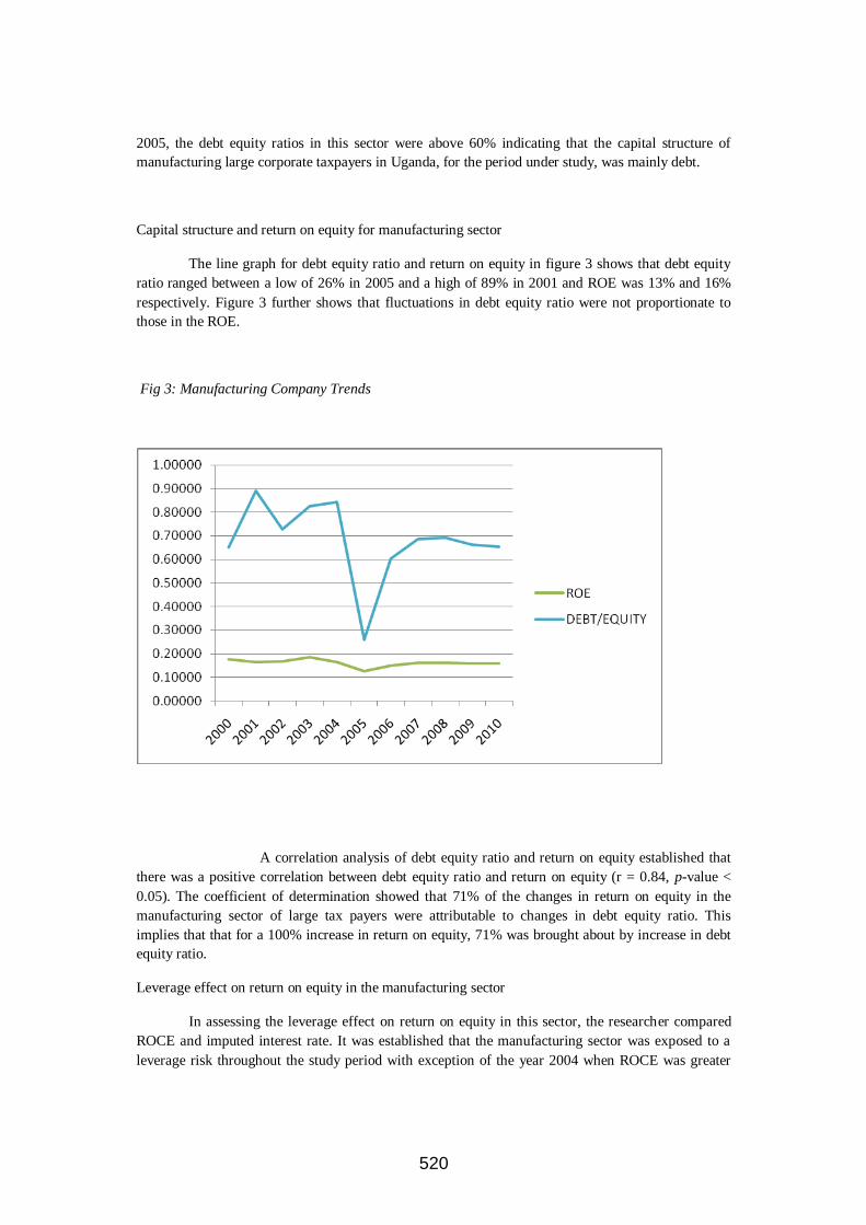
520

2005, the debt equity ratios in this sector were above 60% indicating that the capital structure of

manufacturing large corporate taxpayers in Uganda, for the period under study, was mainly debt.

Capital structure and return on equity for manufacturing sector

The line graph for debt equity ratio and return on equity in figure 3 shows that debt equity

ratio ranged between a low of 26% in 2005 and a high of 89% in 2001 and ROE was 13% and 16%

respectively. Figure 3 further shows that fluctuations in debt equity ratio were not proportionate to

those in the ROE.

Fig 3: Manufacturing Company Trends

A correlation analysis of debt equity ratio and return on equity established that

there was a positive correlation between debt equity ratio and return on equity (r = 0.84, p-value <

0.05). The coefficient of determination showed that 71% of the changes in return on equity in the

manufacturing sector of large tax payers were attributable to changes in debt equity ratio. This

implies that that for a 100% increase in return on equity, 71% was brought about by increase in debt

equity ratio.

Leverage effect on return on equity in the manufacturing sector

In assessing the leverage effect on return on equity in this sector, the researcher compared

ROCE and imputed interest rate. It was established that the manufacturing sector was exposed to a

leverage risk throughout the study period with exception of the year 2004 when ROCE was greater

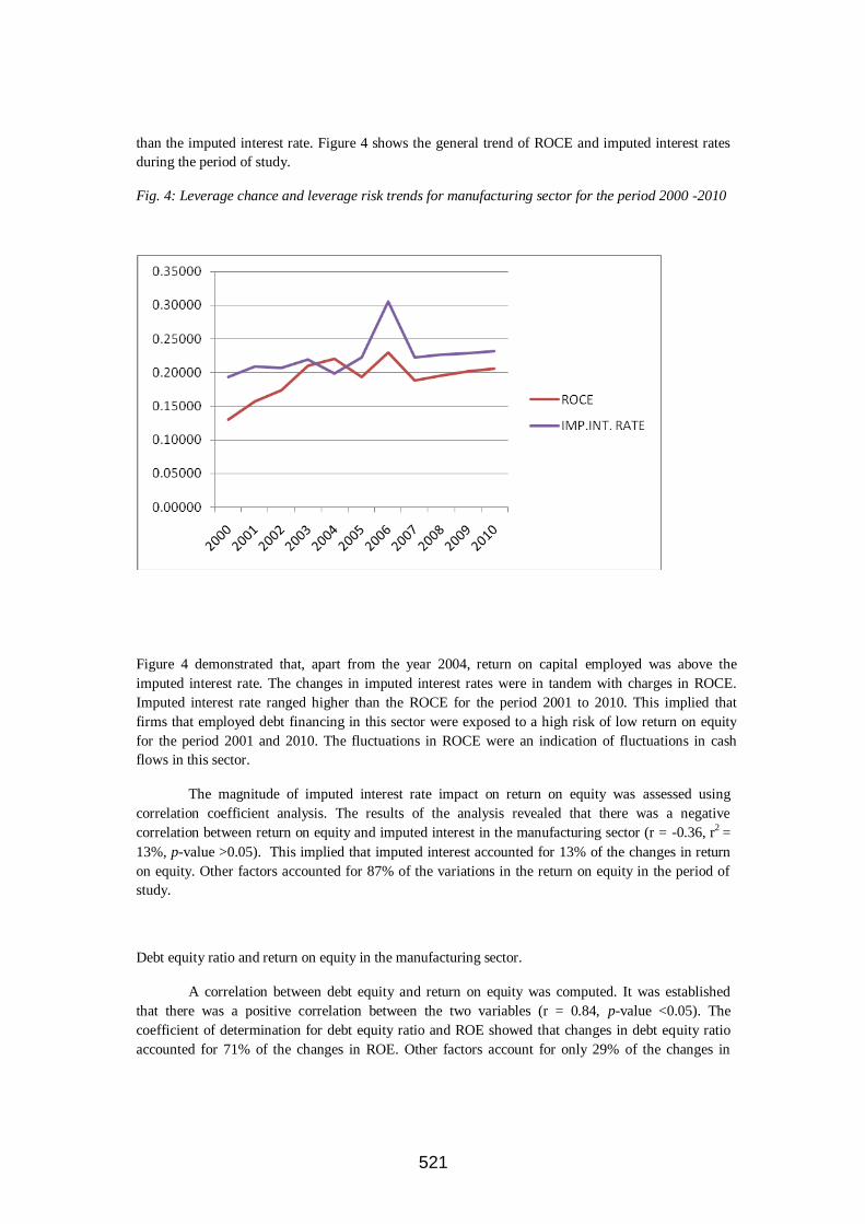
521

than the imputed interest rate. Figure 4 shows the general trend of ROCE and imputed interest rates

during the period of study.

Fig. 4: Leverage chance and leverage risk trends for manufacturing sector for the period 2000 -2010

Figure 4 demonstrated that, apart from the year 2004, return on capital employed was above the

imputed interest rate. The changes in imputed interest rates were in tandem with charges in ROCE.

Imputed interest rate ranged higher than the ROCE for the period 2001 to 2010. This implied that

firms that employed debt financing in this sector were exposed to a high risk of low return on equity

for the period 2001 and 2010. The fluctuations in ROCE were an indication of fluctuations in cash

flows in this sector.

The magnitude of imputed interest rate impact on return on equity was assessed using

correlation coefficient analysis. The results of the analysis revealed that there was a negative

correlation between return on equity and imputed interest in the manufacturing sector (r = -0.36, r2 =

13%, p-value >0.05). This implied that imputed interest accounted for 13% of the changes in return

on equity. Other factors accounted for 87% of the variations in the return on equity in the period of

study.

Debt equity ratio and return on equity in the manufacturing sector.

A correlation between debt equity and return on equity was computed. It was established

that there was a positive correlation between the two variables (r = 0.84, p-value <0.05). The

coefficient of determination for debt equity ratio and ROE showed that changes in debt equity ratio

accounted for 71% of the changes in ROE. Other factors account for only 29% of the changes in

522

return on equity. This shows that debt equity ratio has a significant effect on return on equity in the

manufacturing sector.

INFERENTIALANALYSIS

Sector suitable for debt financing

The study adopted the criteria of comparing debt equity ratio and the return on equity as a basis for

establishing that sector suitable for more debt financing.

Table 9: A comparative view of the relationship between return on equity and the independent

variables

Sector

Variables

Correlation

coefficient

r

Coefficient of

determination

r2

Manufacturing Debt equity Vs ROE 0.835 0.697

Imputed Interest Vs ROE -0.362 0.131

Leverage Vs ROE 0.150 0.023

Construction Debt equity Vs ROE 0.125 0.016

Imputed Interest Vs ROE 0.319 0.102

Leverage Vs ROE 0.763 0.582

Source: URA Financial statements for all sectors under study for 2000 to 2010.

523

The results in table 9 show that all sectors had a positive correlation between debt and equity.

Manufacturing sector had the strongest positive correlation (r = 0.84) between debt equity ratio and return on equity

and therefore more suitable for debt financing. This was followed by the construction sector as listed in a descending

order.

Correlation matrix for all the study variables

Table 10: Pearson Correlation matrix for relationships between ROE and other

independent study variables

Variables

ROE

ROCE

Imputed interest

rate

Debt/

Equity

Leverage

chance/risk

ROE 1.000

ROCE .258

1.000

IMPUTED

INTEREST RATE

-.060

.111

1.000

DEBT/EQUITY .322*

-.527**

-.343*

1.000

524

LEVEREGE

CHANCE/RISK

.268

.872**

-.390*

-.320*

1.000

*. Correlation is significant at the 0.05 level (2-tailed)

**. Correlation is significant at the 0.01 level (2-tailed)

Results in table 10 indicate a significant positive relationship between Debt to Equity Ratio

and Return on Equity (r= 0.322, p-value<0.05). This implies that high Debt to Equity ratio had a

positive contribution to return on equity for all sectors and on average, changes in the proportion of

debt equity in the capital structure accounted for 10% of changes in return. There was a negative weak

relationship between imputed Interest rate with Return on Equity (r = -0.060, p-value>0.05). This

implies that high Imputed Interest rate reduced Return on Equity.

There was a positive relationship between ROCE and ROE (r = .258, p-value>0.05). This revealed that

ROCE positively enhanced ROE for the sectors under study.

Multiple Regressions

There was a linear relationship between Debt to Equity Ratio, Imputed Interest Cost, ROCE

and ROE (F = 7.340, 0.001). This was derived from analysis of variance as summarized in the

ANOVA table 11.

Table 11: ANOVAb

MODEL

SUM OF

SQUARES

MEAN

SQUARE

F

Sig.

Regression

Residual

Total

.187

.322

.509

0.00622

0.00084

7.340 .001a

a. Predictors: (Constant), Leverage chance/risk, Debt/Equity, Imp. Int rate

b. Dependent variable: ROE c. Fc= 2.49

The results in table 11 revealed a high correlation between ROCE and leverage chance/ risk.

The multiple regression analysis of the selected study variables was as summarized in the table 12.

525

The regression analysis indicated that debt Equity Ratio, Imputed Interest Cost and Leverage chance

explain 31.7% of the total variance of ROE for the whole population. Debt Equity Ratio explains

more of the changes in ROE (Beta =.676) followed by Leverage Chance (Beta = 0.650) and Imputed

Interest rate (Beta = .425). That is, the Beta coefficient shows that Debt to equity ratio had a

significant effect of 68% on the changes in return on equity. All sectors had a positive relationship

between return on equity and debt equity ratio.

The results imply that return on equity for all sectors would increase by shs.68 as debt

proportion increased by shs.100. Imputed interest rate and leverage chance also had a significant

impact on return on equity of 43% and 65% respectively. However, imputed interest had a weak

negative 6% relationship with return on equity.

CONCLUSIONS

The study showed that all large corporate tax paying companies in Uganda used debt

financing in their capital structure during the period of study. The manufacturing sector registered

0.89:1 in the year 2001.This showed that companies in Uganda combined debt financing with equity

financing just like firms in Europe, Asia and USA as established by Booth et al., (2000). The debt

equity ratio in Uganda was found to be higher (9.83:1) than that in Europe Asia and USA (0.734:1) as

reported by Booth et al., (2000).

There was a positive correlation between debt equity ratio and ROE for all sectors. The

manufacturing sector had the highest debt equity ratio and highest return on equity followed by the

construction sector. These results conformed to Pandy‗s (1997) statement that debt financing

magnifies shareholders‘ return. They also agreed with Brounen and Eichholtz (2001) conclusion that

employment of more debt in the capital structure results in higher return to the equity holders.

Table 12: Multiple Regression Analysis

0.0019 .043 .433 .667

.571 .223 .425 2.563 .014

0.0027 .006 .676 4.190 .000

.430 .109 .650 3.952 .000

(Constant)

IMP.INT. RATE

DEBT/EQUITY

LEVERAGE -

CHANCE/(RISK)

Model

B Std. Error

Unstandardized

Coefficients

Beta

Standardi

zed

Coefficien

ts

t Sig.

Dependent var.=ROE; R = 0.606; R2 = 0.367; Adjusted R2= .317

526

The correlation between imputed interest and return on equity indicated a positive

correlation between these two variables for all sectors. The results agreed with Van Horne (2002)

statement that equity shareholder get a higher return on their funds when more debt is employed in

the capital structure.

The findings in this study revealed that debt financing significantly magnified return on

equity for all sectors. However, the magnifying effect was greatest in the manufacturing sector

followed by the construction sector. This signified that the Manufacturing sector was more suitable

for debt financing compared to the construction sector. Shareholders in those sectors would realize

significant growth in the return on equity when debt financing is employed.

RECOMMENDATIONS

The research finding showed that for desirable growth in shareholder value, business entities

should mix debt financing with equity financing provided the cost of the borrowed funds does not

exceed the actual return from assets financed by debt. Sectors that had a positive correlation between

debt ratio and return on equity with a coefficient of determination of 30% or more could blend equity

financing with debt financing for a better return to the shareholders.

However, management of business enterprises in Uganda should cautiously consider other

factors that accounted for 90% in changes in ROE, when choosing the mix of debt financing equity

financing that would maximize equity holders‘ value. Over reliance on ROE may result into loss of

investment in sectors (such as construction sector) that require a lot of initial capital for investments.

REFERENCES

An Analytical Process for Generating the WACC Curve and Locating the Optimal Capital

Structure. Retrieved from http://rdcohen.50negs.com/ocsabstract.htm in December 2005.

Blazenko, George. Corporate Leverage and Distribution of Equity Returns. Journal of

Business and Accounting (October 1996) pp 1097-1120.

Booth, Aivazian, Demirguc and Maksimovic (2000). Capital Structure in

Developing Countries. Research Paper of 10th M ay 2000.

527

Buccino, Gerald P. and Kraig S. McKinley. The Importance of Operating Leverage in a

Turnaround. Secured Lender (Sept/Oct. 1997) pp.1097-1120.

Brounen D and Eichholz P. M.A (2001). Capital Structure Theory Evidence from European

Companies‘ Capital Offerings. Research paper 21(4) 2001

Capital structure Decisions. Retrieved from

http://wwwharcourtcollege.com/finance/theory10e in December 2005.

Capital and Locating the Optimal Capital Structure. Research paper Retrieved in December

2005 from http://rdcohen.50megs.com Chandan and Khanna, Business Statistic( 2nd

Edition). Vikas Publishing House PVT Ltd

Fernando Diz. Commodity Trading Advisors‘ Leverage and Reported Margin to Equity.

Research Paper Retrieved in Sept 2005 from http://dizleveragefinal.pdf

Foulkslynch (2002). Financial Management and Control. Foulkslynch Publishers.

Frank Wood (1996). Business Accounting (7th Ed). Pitman Publishing.

Financial Leverage. Retrieved from

http://partnersfinancenter.com/hancoct/learn/guides/smbizfinancing in December 2005.

Graham (2000).How big are the tax benefit of Debt. The Journal of Finance, Vol.55 No.5

October 2000.

Huffman, Stephen P. The Impact of the degrees of Operating and Financial Leverage on the

Systematic Risk of Common Stock: Another look. Quarterly Journal of Business and

Economics (Winter 1989), pp.83-100

Keep your eye on the ROE. Retrieved from

http://wwwinvestopedia.com/articles/fundamental/03/100103.as in December 2005.

528

Kiregyera (1999). Sample Surveys with special Reference to Africa. Hookkab Printers.

Kakuru J (2000). Financial Management (1st Ed), Kampala: Publishing Press Corporation

McDonald. What is Driving Return on Equity. Research paper Retrieved in Sept 2005

from http://www.uic.edu.

Pandy (1997). Financial Management ( 6th Ed). Publishers.

Return on Equity. Retrieved from http://www.onlinewbc.gov/docs/finance/lever.htm in

December 2005.

Return on Equity. Retrieved from http://www.fool.com in December 2005.

Riddiough T.J. Optimal Capital Structure and The Market for outside Finance in

―Commercial Real Estate. Research Paper of August 2004.

Teresa A. John and Kose John. Top Management Compensation and Capital Structure.

Journal of Finance, Vol. 48, No. 3(July 1993)

The Income Tax Act 1997. The Uganda gazette No.81 Vol. XC 1997.

Van Horne C. J. (2002). Financial Management and Policy (2nd Ed). Pearson Education

(Singapore) Pte Ltd.

Nadeem Ahmed Sheikh, (2011), An empirical study of firms in

manufacturing industry of Pakistan, Managerial Finance Vol. 37 No. 2, pp. 117-133

Emerald Group Publishing Limited

Abimbola Adedeji (2004), A test of the endogenous relationship between

financial leverage and bank debt‘s use in the UK The Eleventh Annual Conference of the

Multinational Finance Society Istanbul, Turkey.

529

Carlos A. Molina (2005), Are Firms Underleveraged? Blackwell Publishing

and American Finance Association, The journal of finance Vol. LX, NO. 3

http://www.jstor.org

Elliott, W.B., J. Koëter-Kant, and R.S. Warr (2007): "Target debt ratios: The

impact of equity mis-pricing‖, Working Paper.

http://feweb.vu.nl/fb/oldweb/output.pl?since=&year=&order_by=alph&ID=102&name=

August 01, 2011

William B. Elliott,

Johanna Koëter-Kant, and Richard S. Warr (2008), ―Target

Debt ratios: differential rates of adjustment and market timing‖ Working Paper

www.poole.ncsu.edu/documents/warr_equitymispricing.pdf, August 01, 2011

Nishat. M., (2000). ―The Systematic Risk and Leverage Effect in the Corporate

Sector of Pakistan,‖ The Pakistan Development Review 39: 4 Part II, pp. 951–962

Jiming. L., Chengqin. S., ZhaoHua W., (2010). ―The Impact of Debt Financing

on Firm Investment Behavior: Evidence from China‖ International Journal of Digital

Content Technology and its Applications Vol. 4, No. 9

Chava. S., & Micheal R. R., (2008). ―How Does Financing Impact Investment?

The Role of Debt Covenants.‖ The Journal of Finance Vol. LXIII, No. 5

Roberta Adamia, Orla Goughb, Gulnur Muradogluc, Sheeja Sivaprasadd,

(2010), The Leverage Effect On Stock Returns, www.scribd.com/doc/..

Benjamin Yibin Zhang, Hao Zhou, Haibin Zhu, (2005). Explaining Credit

Default Swap Spreads With Equity Volatility And Jump Risks Of Individual Firms

Omole. D. A., and Falokun. G. O., (1999). The impact of interest rate

liberalization on the corporate financing strategies of quoted companies in Nigeria, The

African Economic Research Consortium.

530

Bandi. F. M., Bandi & Ren`o. Roberto., (2009). Non-parametric Leverage

Effects

Hasanhodzic. J., & Lo. A. W., (2010). Black's Leverage Effect Is Not Due To

Leverage.

http://www.investopedia.com/terms/c/capm.asp#ixzz1XNQ9avrj

531

CODE OF CONDUCT AND ETHICS ON PERCEIVED FINANCIAL PERFORMANCE IN

UGANDA PUBLIC SERVICE: A CASE OF MINISTRY OF EDUCATION AND SPORTS IN

UGANDA

BY:

MUSUMBA IRENE

MUSA MOYA

AMIR LUBANGA

Abstract

The study examined the code of conduct and ethics and financial performance of the

Ministry of Education and Sports in Uganda. There was deteriorating situation in financial

performance as per audits of the Ministry despite having a code of conduct and ethics in place. A

cross-sectional design followed by descriptive and correlation methods were used to examine and

determine the relationship between the code of conduct and ethics with financial performance. The

study found that the code of conduct and ethics positively explained 53.4% of the financial

performance. There is ongoing need to focus on trust and transparency for improved financial

performance of the Ministry.

Keywords: Code of conduct and ethics, financial performance, Uganda.

532

Background to the Study

The code of conduct and ethics for Uganda Public Service sets out standards of behaviour

for public officers in the Public Service. It is designed to ensure the impartiality, objectivity,

transparency, integrity and effectiveness of public officers when performing their duties (Lwamafa,

2004). It is intended to guide public officers in their behaviour and how they relate to each other and

the public.

There are various forms of violation of the code of conduct and ethics by the public officers

directly charged with accounting and financial management in the Ministry of Education and Sports

(MoES). These include bribery, illegal use of public assets for private gain, payment of salaries to

non-existent workers (ghost workers), payment for goods and services not supplied, fraud and

embezzlement, ten percent commissions, misappropriation of public assets, removing documents

from case files or even carrying off the whole file (Bertucci, 2006).

Statement of the Problem

The existence of a Code of Conduct and Ethics for public officers to enhance performance

and reflect a good image of the public service and promote good governance has not stopped

occurrence of financial malpractices in the Ministry of Education and Sports (Lwamafa, 2004).

Although public officers are supposed to be accountable to the public for their financial dealings,

they, however, rarely account for all resources under them. In the execution of official government

business, the public officers directly charged with accounting and financial management have put

themselves in a position where their personal interests conflict with their duties and responsibilities as

public officers. They directly or indirectly enter into contracts with Government. This is unethical

since it affects their impartiality. This research focuses on the effect of violations of the code of

conduct and ethics on the financial performance in the Ministry of Education and Sports.

Purpose of the Study

The study seeks to establish the effect of the code of conduct and ethics on the financial

performance in the Ministry of Education and Sports in Uganda.

533

Objectives of the Study

iv. To examine the structure of Code of Conduct and Ethics for the Ministry of Education and

Sports.

v. To examine the perceived financial performance in the Ministry of Education and Sports.

vi. To examine the relationship between the Code of Conduct and Ethics and the perceived

financial performance of the Ministry of Education and Sports.

Research Questions

iv. What is the structure of the Code of Conduct and Ethics for the Ministry of Education and

Sports?

v. What is the level of perceived financial performance in the Ministry of Education and Sports?

vi. What is the relationship between the Code of Conduct and ethics and the perceived financial

performance of the Ministry of Education and Sports?

Conceptual Framework

Source: Authors

A code of conduct is a principle that sets out standards of behavior for public officers. It is

designed to ensure the impartiality, transparency, integrity, efficiency and effectiveness of public

officers when performing their duties. It is intended to guide public officers in their behavior and how

they relate to each other and the public, (Lwamfa, 2006).

Code of Conduct and

Ethics

Accountability

Transparency

Conflict of Interest

Financial Performance

Economy

Efficiency

Effectiveness

OTHER FACTORS

Legal Framework Economy

534

The conceptual framework demonstrates that the Code of Conduct and Ethics is instrumental

in ensuring good financial performance management. In the same way accountability, transparency

and conflict of interest make the operation of controls in financial management possible. In so doing,

financial management is smoothly carried out. However there are other factors that seem to influence

the effectiveness of accountability, transparency and conflict of interest. In the conceptual

framework, they are shown to be the economy and the legal framework.

LITERATURE REVIEW

Code of Conduct and Ethics

According to Baron (2000), ethical standards in major corporations are coming under

scrutiny, and financial institutions have been challenged about conflicts of interest and their

investment advice. Considering that ethical scandals have been exposed even in the very large

corporations, e.g. Enron, WorldCom etc., managers are becoming more conscious of how they are

perceived by the public, and want to be seen as ‗ethical‘. Corporate codes of business ethics studies

generated evidence of a positive relationship between ethics/ CSP and financial performance

(Orlitzky, Schmidt and Rynes, 2003).

Although quite a number of researchers have revealed that there is a positive relationship

between ethics and financial performance, a few others have found that this said link could neither be

proved nor disproved. Barnett and Salomon (2003) supported the inconclusiveness of these previous

studies when they said that despite the intensity of study directed at it, the relationship between Code

of ethics and financial performance remains in dispute.

Orlitzky, Schmidt and Rynes (2003) describe business ethics as the application of moral

philosophies to issues in business. Its goal is to describe morally good behaviour for managers and

corporations as a whole. It can also be defined as the study of business situations, activities and

decisions where issues of right and wrong are addressed and it deals with those issues not explicitly

covered by law. In some cases, ethical and /or socially responsible behavior can be considered an

investment in transparency and trust, and consequently, help reduce transaction costs within and

535

across an organisation. Ethical Investment Research Services (EIRIS) (2005) defines business ethics

as how a company conducts its business and the behaviour of its employees.

Constructs of Code of ethics

The values of integrity, transparency and accountability in public administrations have

enjoyed resurgence within the past three decades or so. Sound public administration involves public

trust. Citizens expect public servants to serve the public interest with fairness and to manage public

resources properly on a daily basis. Fair and reliable public services and predictable decision-making

inspire public trust and create a level playing field for businesses, thus contributing to well-

functioning markets and economic growth (Elia, 2005).

Accountability

According to Elia (2005), accountability refers to the obligation on the part of public

officials to report on the usage of public resources and answerability for failing to meet stated

performance objectives. In leadership roles, accountability is the acknowledgment and assumption of

responsibility for actions, products, decisions, and policies including the administration, governance,

and implementation within the scope of the role or employment position and encompassing the

obligation to report, explain and be answerable for resulting consequences.

Recently, accountability has become an important topic in the discussion about the

legitimacy of international institutions. Because there is no global democracy to which organizations

must account, global administrative bodies are often criticized as having large accountability gaps.

One paradigmatic problem arising in the global context is that of institutions such as the World Bank

and the International Monetary Fund who are founded and supported by wealthy nations and provide

aid, in the form of grants and loans, to developing nations (Hunt, 2008).

Schedler (1999) urged that internal rules and norms as well as some independent

commission are mechanisms to hold civil servant within the administration of government

536

accountable. A strong accountability regime ensures public resources are used effectively and

efficiently, promotes ethical and policy-based decisions, rewards good performance and carries

consequences when rules are knowingly broken (Ben and Anderson, 2007). Aucoin and Jarvis (2008)

maintain that there is another side of accountability which should allow for and support decision-

making, and provide feedback to inform program delivery and outcomes performance.

Transparency

Transparency refers to unfettered access by the public to timely and reliable information on

decisions and performance in the public sector (Elia, 2005). Winkler (2002) emphasizes the idea that

transparency needs to be better defined before it can be debated.

Geraats (2001) created taxonomy of five categories of transparency in the public service, namely:

political, economic, procedural, policy, and operational.

Conflict of interest

A conflict of interest occurs when an individual or organization has an interest that might

compromise their actions. The presence of a conflict of interest is independent from the execution of

impropriety (Thacker, 2006). More generally, conflict of interests can be defined as any situation in

which an individual or corporation (either private or governmental) is in a position to exploit a

professional or official capacity in some way for their personal or corporate benefit.

Depending on the law or rules related to a particular organization, the existence of a conflict

of interest may not, in and of itself, be evidence of wrongdoing. A conflict of interests can, however,

become a legal matter for example, when an individual tries (and/or succeeds in) influencing the

outcome of a decision, for personal benefit (McDonald, 2006). Davis and Andrew (2001) noted that

there often is confusion over these two situations. Someone accused of a conflict of interest may deny

that a conflict exists because he/she did not act improperly. As codes of ethics cannot cover all

situations, some governments have established an office of the ethics commissioner (Porter and

Thomas, 2002).

537

Constructs of Financial Performance in the Public Sector

According to Belli, Anderson, Barnum, Dixon, & Tan (2001), Value for Money (VfM) is the

term used to assess whether or not a government agency has registered a good or bad financial

performance.. Achieving VfM may be described in terms of the 'three Es' - economy, efficiency and

effectiveness.

Relationship between Code of Ethics and Financial Performance

The relationship between code of ethics and financial performance has been a primary issue

in the field of business and society over the past 25 years. Significant research has been carried out in

several geographical locations, with different parameters for defining ‗ethical‘ and ‗corporate social

responsibility‘ and using numerous proxies for financial performance. According to the findings of

Orlitzky et al (2003), the code of ethics has a positive impact on financial performance and is

strongest in the UK context.

Griffin and Mahon (1997) supported the theory of the positive code of ethics and financial

performance relationship. They demonstrated this by studying and classifying the results of 62

studies, spanning 25 years of research, into three categories; positive, negative and no

effect/inconclusive. They identified 33 results that found a positive relationship, 20 with negative

results and 9 which found no relationship or were inconclusive. With respect to the relationship

between code of ethics and financial performance, Verschoor (1998) found that companies publicly

committing to follow an ethics code as an internal control strategy achieved significantly higher

performance measured in both financial and non-financial terms. Similarly, Berrone, Surroca

and Tribo (2005) found that firms with a strong ethical identity achieve greater degree of stakeholder

satisfaction, which in turn, positively influence the firm‘s financial performance.

However, in contradiction to the studies above, there have been a few studies such as Abbot

and Monsen (1979), Ingram and Frazier (1983) and Freedman and Jaggi (1986) which found no

538

relationship between code of ethics and financial performance, and furthermore, others such as Vance

(1975), Shane and Spicer (1983) and Hill, Kelley and Agle (1990) have shown that a negative code of

ethics and financial performance relationship exists.

METHODOLOGY

Research Design

A cross sectional research design was used and selected because it ably facilitated the

collection of data from the different strata of respondents namely accounting officer, accountants,

auditors, accounts assistants and department heads.

Study Population

The study population was employees from middle to top level managers in departments of

Accounts, Audit, Procument, Finance and Administration at the Ministry‘s headquarters in Kampala

who are 140 permanent staff in total.

Sample Size

As Ministry of Education and Sports maintains a total of 140 staff at the top and middle

level as managers, the sample size for this study will be 60 respondents. This has been determined in

line with Roscoe‘s (1970) rule of thumb that states sample size between 30 and 500 as sufficient.

This number is considered to be large enough to yield reliable data and to guard against non-

responses.

Sampling Design and Procedure

Simple random sampling and purposive sampling designs were used to select the 60

respondents and managers respectively.

Measurement of Variables

The independent variable had three major constructs that included accountability,

transparency and conflict of interest, while the dependent variable had constructs which mainly

summarised the Value for Money concept (Effectiveness, Efficiency, and Economy).

539

e) Accountability

This was measured by identifying its attributes such as rules, procedures and regulations.

These were measured in terms of the degree of divergence between the accepted standards and the

actual prevailing practices. Therefore, to test perceived accountability, a set of statements were used

and applied to a five-point Likert scale ranging from strongly agree (5), Agree (4), Not sure (3),

Disagree (2) to strongly disagree (1).

f) Transparency

This construct was measured by examining the degree of regression of the current practices

on the required practices. The attributes to be used in measurement included adherence to

transparency regulations, policies, procedures and rules. These were measured on a five-point likert

scale ranging from strongly agree (5), Agree (4), Not sure (3), Disagree (2) to strongly disagree (1).

g) Conflict of Interest

This was measured by looking at the extent to which individuals have interest that might

compromise their actions by using a five-point Likert scale that range from strongly agree (5), Agree

(4), Not sure (3), Disagree (2) to strongly disagree (1).

h) Financial Performance

This was measured using the three indicators of Value For Money (VFM) for financial

performance in the public sector, namely: economy, efficiency, and effectiveness.

Data Collection Sources and Instruments

The study used both primary and secondary sources. Secondary data was acquired from

existing literature such as internal reports, previous research done on the company, internal memos,

minutes of meetings, journals, textbooks and the Internet

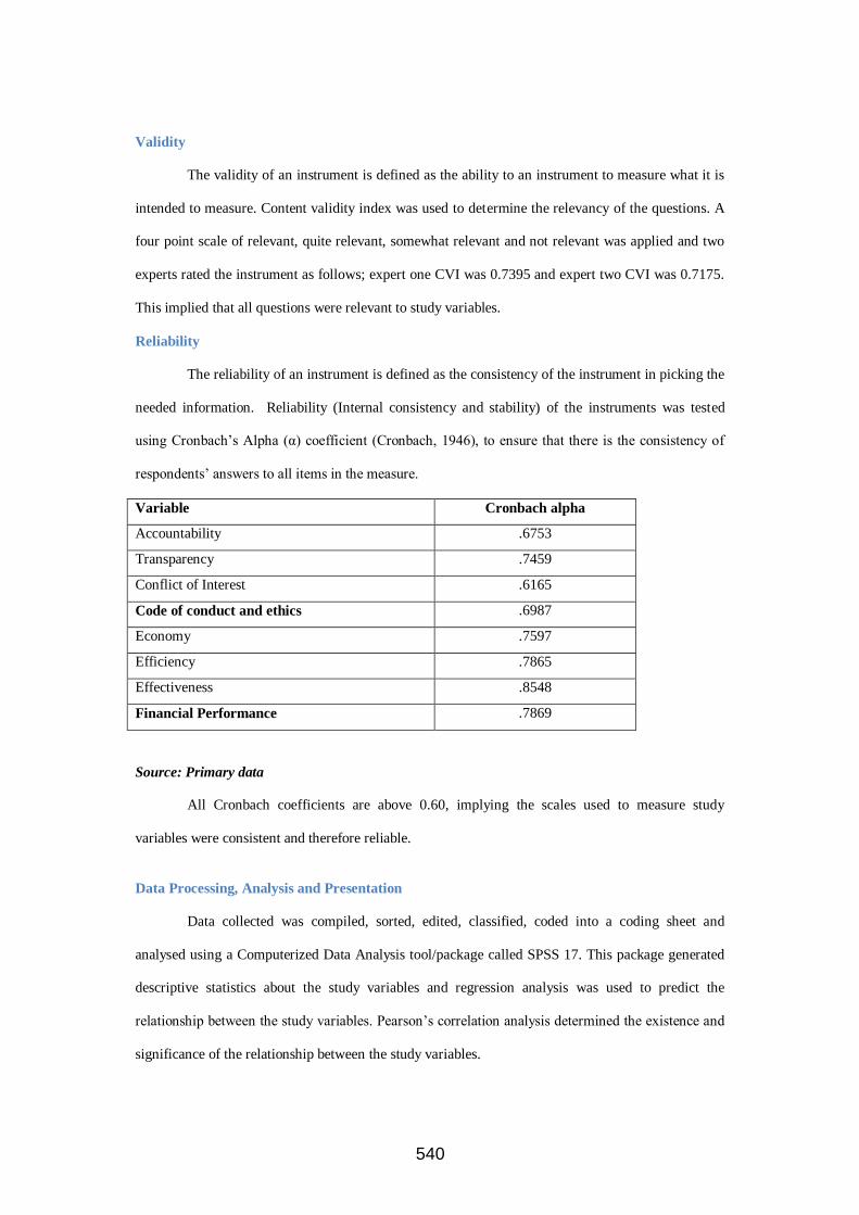
540

Validity

The validity of an instrument is defined as the ability to an instrument to measure what it is

intended to measure. Content validity index was used to determine the relevancy of the questions. A

four point scale of relevant, quite relevant, somewhat relevant and not relevant was applied and two

experts rated the instrument as follows; expert one CVI was 0.7395 and expert two CVI was 0.7175.

This implied that all questions were relevant to study variables.

Reliability

The reliability of an instrument is defined as the consistency of the instrument in picking the

needed information. Reliability (Internal consistency and stability) of the instruments was tested

using Cronbach‘s Alpha (α) coefficient (Cronbach, 1946), to ensure that there is the consistency of

respondents‘ answers to all items in the measure.

Variable Cronbach alpha

Accountability .6753

Transparency .7459

Conflict of Interest .6165

Code of conduct and ethics .6987

Economy .7597

Efficiency .7865

Effectiveness .8548

Financial Performance .7869

Source: Primary data

All Cronbach coefficients are above 0.60, implying the scales used to measure study

variables were consistent and therefore reliable.

Data Processing, Analysis and Presentation

Data collected was compiled, sorted, edited, classified, coded into a coding sheet and

analysed using a Computerized Data Analysis tool/package called SPSS 17. This package generated

descriptive statistics about the study variables and regression analysis was used to predict the

relationship between the study variables. Pearson‘s correlation analysis determined the existence and

significance of the relationship between the study variables.

541

DATA PRESENTATION, ANALYSIS AND INTERPRETATION

Data analysis

Data was analyzed by using descriptive statistics, factor analysis, and correlation and

regression analysis.

Examining the structure of code of conduct and ethics

Most of the items means were approximately 4 and above which is the score for agree and

strongly agree, implying that the code of conduct and ethics largely exists in the MOES. The

Ministry officials have an obligation to report on the usage of public resources and answerability for

failing to meet the stated performance objectives (mean score 4.3810), are answerable for failing to

meet the stated performance objectives (mean score = 4.3952), acknowledge and assume

responsibility for actions within the scope of their employment under the reporting obligations (mean

score = 4.0952) and acknowledge and assume responsibility for decisions within the scope of their

employment under the reporting obligations (mean score = 3.9048).

The study also found that MOES officials acknowledge and assume responsibility for their

policies within the scope of their employment (mean score = 4.0476), there are internal rules and

norms that hold Civil Servants accountable (mean score = 4.5238) and there are independent

commissions that hold Civil Servants accountable (mean score = 3.5714).

The government of Uganda has a strong accountability regime that ensures that public

resources are used "effectively and efficiently"(mean score = 3.9524), promotes ethical and policy-

based decisions, motivated by a concern for the public interest (mean score = 3.8095) and has a

mechanism that carries consequences when rules are knowingly broken (mean score = 3.8571) and

also has a mechanism that embraces accountability (mean score = 4.0952).

The study found that the MOES supports the participation of citizens and organizations in

public policy development issues (mean score =4.0000), created a relationship that allows for and

542

supports decision making (mean score = 3.7143), and created a relationship that allows for and

supports feedback that informs delivery and outcomes performance (mean score =3.666).

Examining the relationship between code of conduct and perceived financial performance

Most of the items under this public service objective have means above 3.5 indicating that

respondents that MOES officials meet the minimum performance targets set out in their performance

contracts.

The ministry always ensures that in every process, there is the best use of resources by

getting it right first time (mean score = 4.1852), and every staff in the MOES endeavors to optimally

use resources in the attainment of the ministry's objectives (mean score = 3.6296).

Examining the relationship between code of conduct and ethics and perceived financial

performance

The study found a significant positive relationships between code of conduct and perceived

performance (r=.715, p-value<0.01). This implies that code of conduct and ethics enhances the

performance of MOES in terms of efficiency, effectiveness and economy.

Further, the study found significant positive relationships between accountability and

financial performance which implies that accountability improves financial performance. There are

also significant positive relationships between transparency and financial performance implying that

transparency improves the ministry‘s financial performance. Analysis of the relationship between

conflict of interest and financial performance showed no significant relationship with efficiency

(r=.285, p-value>0.05). Trust had a significant positive relationship with financial performance

(r=.383, p-value<0.05,).

The study found that transparency and trust significantly predicted 53% financial

performance of MOES (F=11.299, Sig=0.000). However, accountability and conflict of interest did

not have a significant predictive relationship with respect to financial performance. The results

543

obtained and described above are in line with the findings of Orlitzky et al (2003), which indicate

that the code of ethics has a positive impact on financial performance.

Conclusion and recommendation

The study concludes that the code of conduct and ethics is a determinant of the financial

performance of the Ministry of Education and Sports in Uganda. Transparency and trust are the most

important aspects of the code of conduct in the Ministry. It is, therefore, concluded that there is need

for public servants in Uganda in general, and those of the Ministry of Education and Sports in

general, to uphold transparency and trust in the performance of their duties. This has a positive

impact on the government‘s financial performance.

544

REFERENCES

Ablo, E. & Reinika, R. (1998). Do Budgets Really Matter? Evident from Public Spending on

Education and Health in Uganda. World Bank Policy Research Working Paper No. 1926

Aucoin and Jarvis (2008). Modernising Government: The Way Forward—an analysis Haque

International Review of Administrative Sciences.2006; 72: 319-325

Belli, P., Anderson, J. R., Barnum, H.N., Dixon, J. A., & Tan, J-P, (2001). Economic Analysis, of

Investment Operations. Analytical Tools and Practical Applications, WBI, World Bank,

Washington D.C.

Berrone, Surroca and Tribo (2005) ―Corporate Ethical Identity as a determinant of Firm Performance:

A Test of the Mediating Role of Stakeholder Satisfaction‖. Universidad Carlos III De

Madrid, Departmento de Economia de la Empressa, Working Papers 05-31, Business

Economics Series 08.

Bevan D.L. (2001). The Budget and Medium Term Expenditure Framework in Uganda. Africa

Region Working Paper Series No.24, Washington DC: World Bank.

Birdstall, L.I. (2005). Toward Universal Primary Education: Investments, Incentives and Institutions.

UN Millennium Project, Task Force on Education and Gender Equality, 2005. Downloaded

on 20/08/09 from http://www.unmillenniumproject.org/documents/Education-

complete.pdf).

Brandeis, L. (1914). Other People‟s Money and How Bankers Use it. New York: Friedrich, A

Strokes.

Cronbach, L.J. (1946). Response sets and tests validating. Journal for Educational & Psychological

Measurement. Vol. 6, 475 -494.

Collier, P. (2007). The Bottom Billion: Why Poorest Countries are failing and What Can be Done

About It. London. Oxford University Press.

Commonwealth Human Rights Initiative (2006). Information Disclosure Policy: A Toolkit for Pacific

Governments, 2006, http://www.pacmcf.com/PMCFinfo/full_report.pdf.

Davis, M. & Andrew, S. (2001). Conflict of interest in the professions. Oxford: Oxford University

Press. ISBN 0-19-512863-X.

Elia, A. (2005). Integrity, Transparency and Accountability in Public Administration: Recent Trends,

Regional and International Developments and Emerging Issues. Economic & Social Affairs.

August 2005, United Nations Publication

545

Geraats, P. (2001). Why Adopt Transparency? The Publication of Central Bank Forecasts. European

Central Bank Working Paper No. 41, January.

Griffin, J.J. & Mahon, J.F. (1997). The Corporate Social Performance and Corporate Financial

Performance Debate: Twenty-Five Years of Incomparable Research. Business and Society,

Vol. 36, No. 1, pp. 5-31.

Guild, M., Wolf, D. & Wandira (1995). Support for Ugandan Primary Education Reform: A

Formative Evaluation August 1995.

Hallak, J. & Poisson, M. (2007). Corrupt Schools, Corrupt Universities: What can be done?‖

UNESCO/International Institute for Education Planning, 2007 . Downloaded on 18/07/09

from http://unpan1.un.org/intradoc/groups/public/documents/unesco/unpan025403.pdf

http://www.education.go.ug/UPEFormula.htm (last accessed 8 August 2007).

http://www.worldbank.org/external/default/WDSContentServer/WDSP/IB/2004/01/2/0/000/0001600

16_20040120110828/Rendered/PDF/275380UG.pdf

Hunt, G. (2008). Whistleblowing in the Social Services: Public Accountability & Professional

Practice, Arnold (Hodder), 1998.

Jan, R. (2003). The cost-effectiveness analysis – a superior alternative to the cost-benefit analysis of

environmental infrastructure investments. Working paper presented at the Fifth European

Conference on Evaluation of the Structural Funds. Budapest 26/27 June 2003

McDonald, M. (2006) Ethics and Conflict of Interest. W. Maurice Young Centre for Applied Ethics.

Ministry of Education and Sports (1999), The Ugandan Experience of Universal Primary Education

(UPE) Kampala.

Ministry of Education and Sports (2001), Sixth Education Sector Review Final Aide Memoire,

Downloaded on 30/08/09 from

http://www.usaid.or.ug/SO8Annexes/Aide%20Memoire%20Education%20Sector%20%-

202001.doc.

Ministry of Education and Sports (2007), UPE Allocation Formulae since inception.

Ministry of Planning and Economic Development (1991), Background to the Budget 1991-1992,

Kampala.

Ministry of Planning and Economic Development (1992), Background to the Budget 1991-1992,

Kampala.

Orlitzky, M., Schmidt F. and Rynes, S (2003). Corporate Social and Financial Performance; A Meta-

analysis. Organisational Studies 24 (3); 403-441, Sage Publications, London.

546

Porter, R.J. & Thomas E.M. (2002). Biomedical research: collaboration and conflict of interest.

Baltimore: Johns Hopkins University Press. ISBN 0-8018-4400-2.

Potts, D. (2002). Project Planning and Analysis for Development. Lyann Rienner Publishers.

Schedler, Andreas (1999). Conceptualizing Accountability. London: Lynne Rienner Publishers.

pp. 13–28. ISBN 1-55587-773-7.

Thacker, P.D. (2006). Environmental journals feel pressure to adopt disclosure rules. Environmental

Science & Technology 40: 6873–6875.

Verschoor, C. C. (1998). A study of the link between a corporation‘s financial performance and its

commitment to ethics‘. Journal of Business Ethics, Vol 17, pp 1509 – 1516.

Ward, P. (2006). Education Reform in Uganda -1997 to 2004. Reflections on Policy, Partnership,

Strategy and Implementation, Department for International Development, Researching the

Issues 2006:60.

Winkler, B. (2002). Which kind of transparency? On the Need for Effective Communication in

Monetary Policy Making. Ifo Studies vol. 48, issue 3, pp. 401-27.

World Bank (1993), Uganda: Social Sectors, Washington DC.

World Bank (1998), Development Credit Agreement (Education Sector Adjustment Operation)

between The Republic of Uganda and International Development Association,

April,http://web.worldbank.org/external/projects/main?pagePK=64283627&piPK=73230&t

heSitePK=40941&menuPK=22842&Projectid=P002972

World Bank (2004a), Project Performance Assessment Report Uganda, Primary Education and

Teacher Development Project (Credit 2493) and Education Sector Adjustment Credit

(Credit 3049), Washington DC January 8, 2004.

World Bank (2004b), Uganda-Primary Education and Teacher Development and Education Sector

Adjustment Credit Project, 2004/01/08,

World Bank (2004c), Achieving EFA in Uganda: the Big Bang approach, Washington DC,

http://www.worldbank.org/education/pdf/efa.case_uganda.pdf

547

AGENT BASED REALTIME CONTINUOUS AUDITING

By

Tirus Mutoru, Elisha Opiyo and William Okello-Odongo

Abstract

Within the industry there is a lack of some monitoring decision support systems that enable the

implementation of continuous auditing. This leads to the lack of a reliable process to ensure that the

real time transactions also benefits from real time monitoring so that financial losses are prevented.

The distinctive character of continuous auditing is the short time lapse between the facts to be audited

and the correction of evidence and audit reporting. Software packages exist which offer batch

processing of extracted data and they can perform powerful examination of transactions. These

Computer Assisted Audit Tools (CAATS) are routines that are common among auditors around the world, but they only exist in the batch mode and depend upon the creativities of the operators

utilizing them. They also to some extent depend on the speed, integrity and willingness of

Information Technology department to extract and provide data from the databases. A solution to

this problem is suggested through an audit approach that guarantees a better monitoring of controls

within an organization. It is based on a distributed problem solving multi-agent systems (MAS)

technique. A system, multi-agent system for continuous auditing (MASCA) is presented. The system

is characterized by group of individual agents cooperating to identify audit exceptions and report in a

timely manner. Automated processes which are usually monitored and reviewed by human auditors

are automatically monitored real-time and reported by the group of agents within the system. We

report a successful implementation of a multi-agent system for continuous auditing. The professional

users who evaluated the system, found it useful and acceptable. The system performs the continuous monitoring and reporting to a level that is acceptable to the audit professionals.

1 Introduction

Within the industry there is a lack of some monitoring decision support systems that enable the

implementation of continuous auditing. This leads to the lack of a reliable process to ensure that the

real time transactions also benefits from real time monitoring so that financial losses are prevented.

548

The distinctive character of continuous auditing is the short time lapse between the facts to be audited

and the correction of evidence and audit reporting. Software packages exist which offer batch

processing of extracted data and they can perform powerful examination of transactions. These

Computer Assisted Audit Tools (CAATS) are routines that are common among auditors around the

world, but they only exist in the batch mode and depend upon the creativities of the operators

utilizing them. They also to some extent depend on the speed, integrity and willingness of Information Technology department to extract and provide data from the databases. A solution to

this problem is suggested through an audit approach that guarantees a better monitoring of controls

within an organization. It is based on a distributed problem solving multi-agent systems (MAS)

technique. A system, multi-agent system for continuous auditing (MASCA) is presented. The system

is characterized by group of individual agents cooperating to identify audit exceptions and report in a

timely manner. Automated processes which are usually monitored and reviewed by human auditors

are automatically monitored real-time and reported by the group of agents within the system. We

report a successful implementation of a multi-agent system for continuous auditing. The professional

users who evaluated the system, found it useful and acceptable. The system performs the continuous

monitoring and reporting to a level that is acceptable to the audit professionals.

Depending on the risk levels and impact of findings, the Board authorizes senior management to

oversee implementation of corrective action which could be; strengthening/addition of controls, insuring the risk, or ignoring the risk. The audit reports are tabled in the Board audit committee.

According to Institute of Internal Auditors' Global Technology Audit guide 3 (Coderre 2007),

continuous auditing is defined as the automatic method used to perform control and risk assessments

on a more frequent basis. As the guide states, technology plays a key role in continuous audit

activities by helping to automate the identification of exceptions or anomalies, analyze patterns

within the digits of key numeric fields, review trends, and test controls, among other activities.

Audit work is guided by an organization‘s policies and the regulatory requirements. The Audit charter forms the contract between the Audit function and the Board of Directors to which auditor‘s

report to.

Audit work involves review of computer system controls, financial controls and process/transaction

controls. The frequency of the review in a continuous auditing (CA) environment differentiates

continuous auditing from periodic traditional auditing. In continuous auditing the controls,

transactions and financial reports are reviewed as soon as the data/evidence becomes available. The

―continuous‖ aspect of continuous auditing and reporting refers to the near real-time capability for

financial information to be checked and shared.

The interval management choices for evaluation depend on the frequency of updates within the

accounting information systems. Analysis of the data may be performed hourly, daily, weekly,

monthly, etc. depending on the application. The controls and process are owned by specific

individuals within an organization. The responsible individuals (Auditees) are answerable to the audit

findings that may be raised within their operational environment.

The need for continuous auditing thus arises.

2 Need for Continuous Auditing

2. 1 Why Employ multi-agent systems in Continuous Auditing?

Auditing domain lacks a monitoring decision support system enabling implementation of continuous

auditing was the main driver. Thus there is need for a reliable process to ensure real time transactions

also benefits from real time monitoring and thus prevents financial losses. The distinctive character of continuous auditing is the short time lapse between the facts to be audited and the correction of

evidence and audit reporting.

Ways are sought to provide an audit approach guaranteeing a better monitoring of controls within a

company.

2.2 Issues in Continuous Auditing

The following are the key domain issues.

549

First there is need to have an efficient continuous controls monitoring approach. Secondly there are

different people with different (some possibly conflicting) goals. Auditees want zero reporting;

auditors have to report while the board requires the position as is. Thirdly, having multiple agents

could speed up a system's operation by providing a method for parallel computation. Since multi-

agent systems are inherently modular, it should be easier to add new agents to a multi-agent system

than it is to add new capabilities to a monolithic system. Finally elucidation of intelligence can be done to study intelligent patterns in continuous auditing. As Weiß (1996) put it: Intelligence is deeply

and inevitably coupled with interaction‘‘. Intelligence patterns in continuous auditing can be studied.

2.3 Sample Scenario

A bank‘s branch has a cash holding limit (say Kshs. 20 million) which is defined for each branch in

accordance to Central Bank of Kenya guidelines. At close of business at 4:30pm the branch tellers

collate their cash which is summed together with the cash in the vault to determine current branch cash holding limits. If the cash exceeds 20 million Insurance companies cannot pay for any losses

recorded, Central Bank may impose a fine as well. To prevent this kind of a scenario periodic reviews

are done by the branch manager during the day. These cash position reviews are time consuming and

prone to errors. The branches are often caught unawares with excess cash and penalties are paid to

Central Bank.

3 System’s Architecture

Multi-agent based technologies were used in developing the system for decision support in

continuous auditing.

Continuous auditing is a distributed problem and it‘s dynamic. A distributed problem solving multi-

agent based system was designed for this problem domain. The system was characterized by group of

individual agents cooperating to identify audit exceptions and report in a timely manner. Automated

processes which are monitored and reviewed by human auditors was monitored and reported by the

group of agents within the multi-agent system. Essentially multi-agent system for continuous auditing

removes the need to have a huge number of auditors within an organization.

Below is the architecture of the multi-agent system for continuous auditing.

550

Databases (DB)

Interface

Agent

Coordinator Agent (CoA)

Collector-Analyzer

Agents

Reporting Agent

Policy and

Standards

Database

(PSDB)

Audit History

Database

(AHDB)

Information Sources-System configuration

parameters

-Systems audit trails

-Daily processing reports

-Process Alerts

Communication control

-Language

-Protocol

-Error Handling

-Send/receive priority

Data

Acquisition

Monitoring

engine

Decision logic

Communicati

on module

Communicati

on module

Domain

Database

Agent Coordination

>Schedule permits

>Conflict resolution

>Intelligent controls

Control flags

>Updating

>Query processes

Information

Security Auditor

(ISA)

User

Database

Administrator

(DBA)

System Security

Administrator

(SSA)

Figure 1: Architecture for the multi-agent system for continuous auditing

The agent design was generally based on the following:

Agent reviews the policy database to determine violation criteria for its tasks, then reviews the target (text file, database entries, and system setting) for task identifiers and finally if there are exceptions

the exceptions is reported into the audit history database.

4 Experimentation

The PC running the application system was setup in the banking environment as a system demo. This

PC together with other PCs and check/audit variables within the banking environment were used as

the test environment and were presented to prospective users who included: IS auditors, Internal

Auditor and IT Systems Administrators. Each Agent‘s tasks were tested over a period of 5 days (15th to 19th November 2010).

Below is a summary of the multi-agent system for continuous auditing review by auditors from

various banks within Kenya.

551

Figure 2: Test results by audit professionals

5 Related Works

Software packages exists which offer batch processing of extracted data and they can perform

powerful examination of transactions. These Computer Assisted Audit Tools (CAATS) routines are

common among auditors around the world, but they only exist in batch and depend upon the whims

of operators utilizing them. They also to an extent depend on the speed, integrity and willingness of

IT department to extract and provide data from the databases. The alerts sent (emails and text to mobile phones) may be triggered by fairly primitive events and are certainly not rule based.

6 Conclusions

A multi agent approach in continuous auditing support was successfully implemented and

demonstrated. User acceptance test feedback ascertained the following:

Multi-agent system for continuous auditing was able to identify exceptions faster than in traditional

auditing. I.e. agents recognized an exception close to the time of its occurrence by analyzing large data files far much faster than human based analysis. The system of agents reported audit findings as

soon as they were identified.

Information System Auditors output would be increased since there was no time-consuming reviews

of large files.

With the multi-agent system for continuous auditing implementation there is increased value in audit

reports since, the findings are recent and thus relevant to management.

Multi-agent system for continuous auditing implementation enabled the distinctive character of

continuous auditing; short time lapse between an audit-incidence occurrence and identification of the

incidence to be attained. An enterprise can thus accrue the benefits of continuous auditing by

deploying the multi-agent systems based system. Since multi-agent systems are inherently modular, it

was easier to add new agents to the multi-agent architecture to address future needs. The research

project demonstrated that through a multi-agent based system for continuous audit support, leveraging on technology offers continuous audit considerable advantages over traditional auditing.

References

1. Balch, T 1997, Learning roles: Behavioral diversity in robot teams, College of Computing Technical

Report GIT-CC-97-12, Georgia Institute of Technology, Atlanta, Georgia.

552

2. Balch, T & Arkin, RC 1995, Motor schema-based formation control for multi-agent robot teams, In

Proceedings of the First International Conference on Multi-Agent Systems (ICMAS-95), Menlo Park,

California, AAAI Press.

3. Bordini, RH, Dastani, M & Winikoff, M 2006, Current Issues in Multi-Agent Systems Development, In the proceedings at European Workshop on Aspects in Software (ESAW

2006), Enschede, The Netherlands.

4. Bordini, RH, Fisher, M, Wooldridge, M & Visser, W 2009, Property-based Slicing for Agent

Verification, Journal of Logic and Computation, Oxford Journal, Oxford University Press.

5. Coderre, D 2007, Continuous Auditing: Implications for Assurance, Monitoring, and Risk

Assessment, [Online] GTAG Guide 3, Available from

http://www.theiia.org/guidance/technology/gtag3

[Accessed 21/07/2009].

6. Iglesias, CA, Garijo, M, Gonzalez, CJ &Velasco, RJ 2005, A methodological proposal for multiagent systems development extending CommonKADS, [Online], Available from

http://www.ksi.cpsc.ucalgary.ca/iglesias.html

[Accessed 20/07/2009].

7. Weiß, G & Sen, S, 1996, Adaptation and Learning in Multi-agent Systems, Springer Verlag, Berlin.

8. Wooldridge, M 2009, An Introduction To Multi-Agent Systems, 2nd edn, John Wiley &

Sons.

9. Continuous auditing demand, http://www.isaca.org

[Accessed 21/07/2009].

10. Continuous auditing definition http://www.wikipedia.org

[Accessed 21/07/2009].

Analysis of Price Fluctuations Using a Markov Chain Model: A Case Study of Dar es

Salaam Stock Exchange (DSE).

Said A. Sima: University of the Witwatersrand, Johannesburg, South Africa.

simasaid@yahoo.co.uk

Abstract

Price movements are normal phenomena in the market. However, if the nature or trends of fluctuations

are known, they will help to measure the efficiency of the market for the decision making in the future

development of the firm concerned. In this study price fluctuation at the DSE in Tanzania is analysed.

Three levels or states of price movements are identified as ―Unchanged price‖, ―Gain in price‖ or ―Loss

in price‖ with reference to the immediate price. Six years secondary data collected from DSE records are

analysed and found to satisfy the randomness test, a requirement for Markov chain modelling. The

matrix approach of the Markov chain model is used such that the transition probability matrix and steady

state vectors of different periods are obtained using Maple software. Findings of the study reveal that

using the steady state vectors, (0.5177, 0.2820, and 0.2003); about 52% of the time, the price remained

unchanged, 28% of the time the price increased and 20% of the time the price decreased. The results of

this work should be taken into consideration by all partners as suggested in the conclusion section so as

to improve the future performance of their firms.

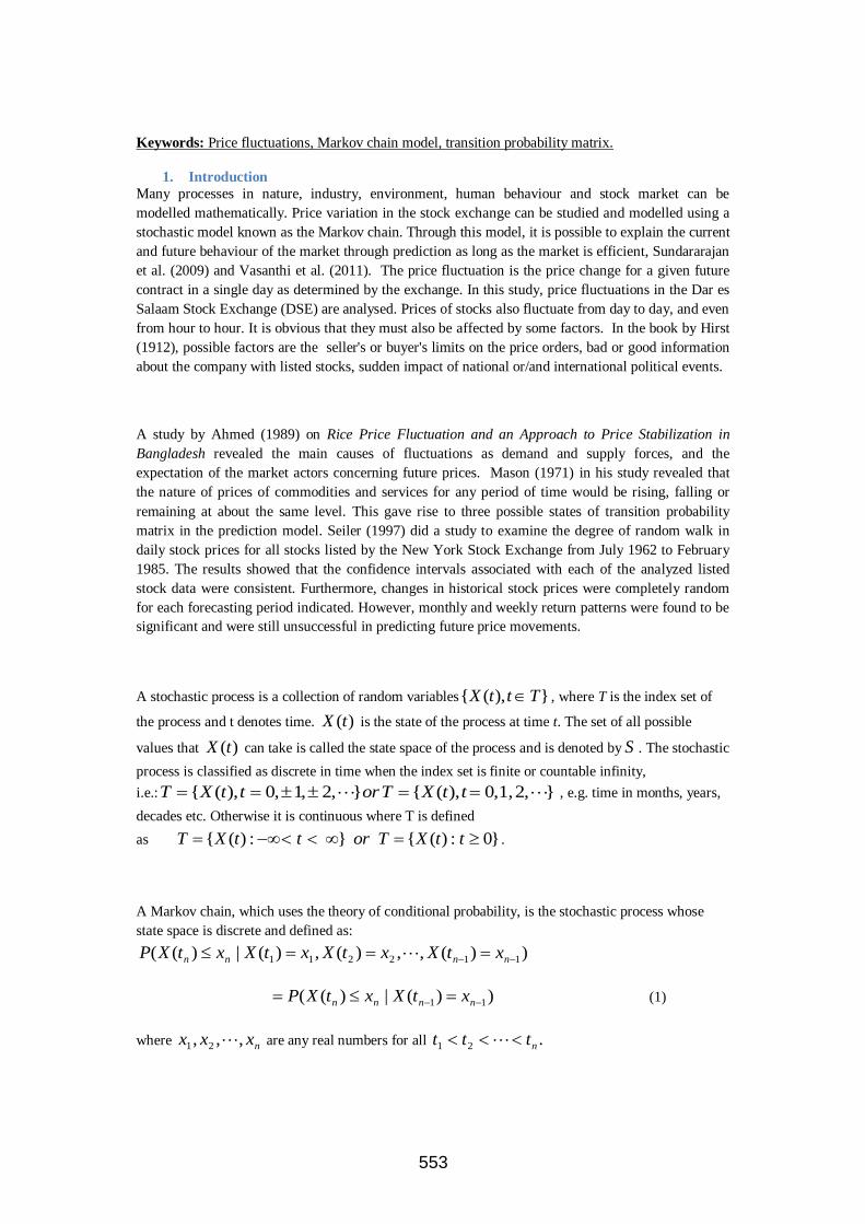
553

Keywords: Price fluctuations, Markov chain model, transition probability matrix.

1. Introduction

Many processes in nature, industry, environment, human behaviour and stock market can be

modelled mathematically. Price variation in the stock exchange can be studied and modelled using a

stochastic model known as the Markov chain. Through this model, it is possible to explain the current

and future behaviour of the market through prediction as long as the market is efficient, Sundararajan

et al. (2009) and Vasanthi et al. (2011). The price fluctuation is the price change for a given future

contract in a single day as determined by the exchange. In this study, price fluctuations in the Dar es

Salaam Stock Exchange (DSE) are analysed. Prices of stocks also fluctuate from day to day, and even

from hour to hour. It is obvious that they must also be affected by some factors. In the book by Hirst

(1912), possible factors are the seller's or buyer's limits on the price orders, bad or good information

about the company with listed stocks, sudden impact of national or/and international political events.

A study by Ahmed (1989) on Rice Price Fluctuation and an Approach to Price Stabilization in

Bangladesh revealed the main causes of fluctuations as demand and supply forces, and the

expectation of the market actors concerning future prices. Mason (1971) in his study revealed that

the nature of prices of commodities and services for any period of time would be rising, falling or

remaining at about the same level. This gave rise to three possible states of transition probability

matrix in the prediction model. Seiler (1997) did a study to examine the degree of random walk in

daily stock prices for all stocks listed by the New York Stock Exchange from July 1962 to February

1985. The results showed that the confidence intervals associated with each of the analyzed listed

stock data were consistent. Furthermore, changes in historical stock prices were completely random

for each forecasting period indicated. However, monthly and weekly return patterns were found to be

significant and were still unsuccessful in predicting future price movements.

A stochastic process is a collection of random variables }),({ TttX , where T is the index set of

the process and t denotes time. )(tX is the state of the process at time t. The set of all possible

values that )(tX can take is called the state space of the process and is denoted by S . The stochastic

process is classified as discrete in time when the index set is finite or countable infinity,

i.e.: },2,1,0),({},2,1,0),({ ttXTorttXT , e.g. time in months, years,

decades etc. Otherwise it is continuous where T is defined

as }0:)({}:)({ ttXTorttXT .

A Markov chain, which uses the theory of conditional probability, is the stochastic process whose

state space is discrete and defined as:

))(,,)(,)(|)(( 112211 nnnn xtXxtXxtXxtXP

))(|)(( 11 nnnn xtXxtXP (1)

where nxxx ,,, 21 are any real numbers for all .21 nttt

554

This implies that, in order to compute the probability of an event in the future given the knowledge of

the past and present, one needs to be concerned about the present and not the history. A Markov

chain can be expressed by the use of the matrix called transition probability matrix. It can be assumed

that for all i and j and all t ixjxP tt |( 1) is independent of t , then we can write

ijtt pixjxP )|( 1 . (2)

Any Markov chain that satisfies (2) is called a stationary Markov chain, Stone (1972). It is also

known as a stationary first order Markov chain (Sundararajan et al. (2009) and Vasanthi et al.

(2011)). So ijp is the probability that the state value undergoes a transition from i to j in one trial.

In the trading mechanism, the prices are expected to remain unchanged, increase or to decrease by

chance depending on the sellers‘ and buyers' order as supervised by the broker. Stock prices can be

considered to reflect Markovian model in their variations. Three identified states are:

State i to state i (no change in price from the previous time).

State i to state 1i (decrease in price from the previous time)

State i to state 1i (increase in price from the previous time)

In other words the transition is from i to j , where }1,1,{ iiij .

In the trading process, sometimes there occurs some bad news about a company with listed stocks

that would make the stocks worth substantially less, Pike (1983). In this situation the broker will let

the stock fall to its own level. If the situation prevails for a long time, it is possible for the company to

drop out of business. Such cases can be considered in state classifications as the absorbing state in

Markov model. Therefore, by considering the DSE as the stock market in Tanzania, the business

process is similar as discussed above. Price variations in the DSE have never been modelled as a

Markov chain before. In this case study, price variations are observed and mathematical modelling of

these prices is constructed to fit the Markov model. Hence, efficient estimation functions of the

Markov chain transition probability matrix are derived for the DSE from which stationary states of

DSE price variations probabilities are established.

The main objective of the study is to investigate the nature of price variations in the DSE and to

examine the possibility of predicting price variations using the Markov chain transition probabilities.

Assuming that the market is efficient, the specific objectives are: -

(i) To determine the probabilities of price variations in the future years using current year's

prices.

(ii) To establish the cause of the price variations.

(iii) To determine the accuracy of the Markov chain model developed with the

DSE known data.

555

The rest of the sections are organized as follows: In the next section we present the mathematical

model. Section 3 presents methodology and data analysis and last section presents conclusion and

recommendations.

2. Mathematical Model

The mathematical model developed is used to show the nature of price movements at the DSE in the

given duration. Through the observed price variations by transition probability matrices, it is possible

to establish the cause of the movements under specified periods of time. The initial transition

probability matrix offers a convenient way of predicting the price variations due to the fact that

matrix multiplication provides the Markovian system at some period beyond a given reference time.

It is assumed that the Markov chain is stationary and the market is efficient.

In the model formulation, the first day‘s price of trading is considered as the reference price ―R‖ at

that particular time in formulating the matrix. By referring to the first day, the second day price can

be interpreted into three possible results that form three states (variables). These are:

1. Price remains the same-―Unchanged‖ denoted by ‗U ‘

2. Price increases-―Gain‖- denoted by ‗ G ‘ or

3. Price decreases-―Loss‖- denoted by ‗ L ‘.

So the state space },,{ LGUS (finite set).

The 33 matrix of transitions will have the following combinations:

LLandLGLUGLGGGUULUGUU ,,,,,,, where UU is the transition from state U to

another stateU , UG is the transition from state U to state G and so on.

The pictorial model representation is shown in Figure 3.1 below.

Figure 2.1: The model for the possible states of price movements in the DSE.

U

LL UU

G

L

LG / GL UG / GU

UL / LU

GG

556

The analysis of the three states is in a discrete time of 3 months interval (quarterly), semi-annually (6

months), annually or any duration as far as the Markovian model possibilities. Thus the matrix

formed is of the order 33 .

The first matrix to be formed is one with entries whose elements are called states, obtained from

tallying 3 states in a given duration ( ijNN ).

333231

232221

131211

NNN

NNN

NNN

N

The ijN in the above matrix is the number of transitions from state i to j for a specified time and

.,,, LGUji E.g. 11N = Number of transitions made from state U to state U in a given interval

time. The rows and columns are both of Unchanged, Gains and Losses. The second matrix is a

stochastic matrix with entries called transition probabilities obtained from the first matrix

ijP =

i

ij

N

N. (4)

Where iN =

3

1

3,2,1,j

ij iforN and ijP 0 ,

3

1

1j

ijP for .3,2,1i

The probabilities sPij ' are displayed in a transition probability matrix P as shown in the next

section.

2.1 Transition Probability Matrix (TPM)

In this case a transition matrix P of the order 33 with entries sPij ' represents the probabilities of

moving from state i of price change at t to another price state j at 1t where t is the first day of

trade after the reference day price. The three states are Unchanged, Gain and Loss. Given that the

state at time t is i , the process must be somewhere at time 1t . This means that for each i ,

1|1

1

Sj

j

tt iXjXP

and 0|1 iXjXP tt

where s is a state space.

The structure of transition probability matrix P is as follows:-

557

.

333231

232221

131211

PPP

PPP

PPP

P

It is possible for values 0ijN and hence 0ijP if no transition occurred over that period and

again we can have 1ijP . All the two cases can be explained in business terms. By determining the

unknown parameters of sPij ' , the behaviour of the transitions (dominance, rare) can be identified

and the interpretations in business terms can be stated. For example, the value 12P in the matrix

represents the probability that a price in the ―Unchanged state, U‖ at time t will move to the ―Gain

state, G‖ at time 1t . Again the value 33P represents the probability that a price in the ―Loss state,

L‖ at time t will remain in the same state at time 1t . The transition probability matrix 1PorP

will be used to find the other next matrices such as nPPP ..., 32

by matrix multiplication where

...,3,2,1n and n is a discrete value that can represent the number of days, weeks, months or

years. This can be explained by the concept of n-step transition probability matrix.

2.2 n-Step Transition Probability Matrix

A Markov Chain will be constructed under the assumption that it is stationary.

The n-step probability of transition from state i to state j is given by

n

ijonmnm PiXjXPiXjXP )|()|( (5)

The probability is independent of m as we are dealing with the stationary Markov chain. Using the

definition of P , equation (5) can be written as

.0

1jandiPPP

nk

k

n

kjik

n

ij

(6)

where

ijif

ijifPij

0

10

Equation (6) gives the probability of transition from state i to state j in one time period n

where 1n .

2.3 Steady-State Probabilities

If it happens that the transition probability matrix P obtained is regular (with only positive elements),

then after a long time period n the matrix nP will have identical rows. Each of these rows gives the

steady-state probabilities and is given by a vector ][ 321 . These can also be obtained by

solving the system

558

P

(7)

But the system in (7) has infinitely many solutions. To get a unique solution, we impose the

constraint.

1321 (8)

Then the steady-state probabilities are obtained using these probabilities, and thus the prediction (in

the long run) of the number of possible transitions before the matrix settled can be identified.

3. Methodology and Data Analysis

3.1 Source of Data

The secondary data are collected from DSE management in a softcopy form. These are daily

securities prices (high and low) from April 1998 to November 2004. DSE is stock market in Tanzania

located in Dar es Salaam city.

The listed companies by 2004 whose stocks were traded in the DSE with listing date in brackets are

Tanzania Oxygen Limited - TOL (April 1998), Tanzania Breweries Limited - TBL (September

1998), Tanzania Tea Packers Limited - TATEPA (December 1999), Tanzania Cigarette Company

Limited - TCC (November 2000), Tanga Cement Company Limited - SIMBA (September 2002) and

Swissport Tanzania limited- SWISSPORT (June 2003). Other listed companies by 2011 are Tanzania

Portland Cement Company Limited (TWIGA), National Investment Company Limited (NICOL), Dar

Es Salaam Community Bank (DCB), National Microfinance Bank Plc (NMB), Kenya Airways

Limited (KA), East African Breweries Limited (EABL), Jubilee Holdings Limited (JHL), Kenya

Commercial Bank Limited (KCB), CRDB Bank Public Limited Company (CRDB) and Nation Media

Group Limited (NMG). These make a total of 16 companies.

3.2 Data Analysis and Presentation

The data obtained are analyzed to fit a mathematical model known as Markov chain. The data are as

presented in Table 3.1.

559

Table 3.1: DSE 2004 - listed companies and their respective number of days traded per month.

Compa

ny

Year

Liste

d

Jan Feb Mar Ap

r.

Ma

y

Jun

e

July Au

g.

Sep

t

Oct No

v

Dec

TOL 1998 3 4 4 4 4 1 1 2 4

1999 2 2 6 1 4 3 2 4 7 1 2 0

2000 1 1 1 1 2 2 2 2 1 8 1 2

2001 2 5 7 4 3 0 2 1 6 2 3 3

2002 12 5 8 7 4 4 8 7 3 4 5 5

2003 5 5 5 9 11 4 9 6 5 6 0 1

2004 6 8 12 9 8 7 9 10 9 1 1 -

TBL

TBL

1998 4 5 3 6

1999 7 8 10 9 8 9 9 9 9 8 9 6

2000 11 12 14 14 11 14 13 12 13 12 13 10 7

2001 13 12 13 11 13 12 13 13 12 13 13 7

2002 14 12 12 12 13 11 12 12 12 14 12 7

2003 12 11 12 14 11 11 15 12 10 12 13 10

2004 13 15 16 16 15 16 16 17 17 16 7 -

TATEP

A

1999 4

2000 5 4 2 5 6 8 4 7 7 7 5 0

2001 5 2 12 6 4 1 2 2 1 3 2 3

2002 3 6 7 5 5 7 7 2 4 4 4 0

2003 2 1 4 0 0 4 1 2 5 3 5 3

2004 9 9 5 2 4 5 1 1 3 3 1 -

TCC 2000 7 7

2001 8 10 11 9 13 11 10 9 9 10 12 6

560

2002 13 12 10 12 12 10 13 10 12 13 11 8

2003 9 8 11 12 11 11 14 11 10 7 8 9

2004 16 15 14 12 15 15 15 10 16 14 6 -

SIMBA 2002 1 14 12 9

2003 12 11 7 13 11 12 13 13 11 13 11 11

2004 15 15 15 15 13 18 14 17 16 14 4 -

SWISS

PORT

2003 12 15 12 11 13 13 11

2004 16 16 18 17 16 18 17 17 15 15 4 -

Source: DSE (Overall Daily Trading Time Series‘ Data)

The most reliable data collected from the DSE is from TBL as shown clearly in Table 3.1. The TBL

data covered a period of 6 years from October 1998 to September 2004, the period which is long

enough (more trading days in a month) for modelling by Markov chain compared with other

companies. For this reason data from TBL was used for modeling. The daily mean prices which are

the average of highest and lowest daily prices are computed. Using the Maple tool (Matrix -

numerical computations), the steady state vectors are obtained.

3.3 The Study of Annual Prices Behaviour

From the first day of trading of TBL‘s shares, there were remarkable price changes for each month in

a given year. The general trend of price changes in each year was summarized in the Tables 3.2 in

which average annual prices, variances and standard deviations are displayed. The variance 2 of the

prices was computed using equation (9),

2

22

2

n

xxn ii (9)

where index ni ,...,3,2,1 and 12n . The standard deviation is .

Table 3.2: The variance and standard deviations of the annual prices

Year Average Annual Price Variance Standard

Deviation

1998/99 595 1142.6 33.8

1999/00 564 247.9 15.7

2000/01 590 3997.2 63.2

561

2001/02 1288 65261.0 255.5

2002/03 1583 2643.0 51.4

2003/04 1410 5006.9 70.8

Tables 4.3 (1998/99) show the sample of monthly prices for different years. The other entries were

obtained as follows: row three (mean price) is the annual average price computed as the average of all

monthly prices within a year. Row four was obtained by summing the mean monthly price and three

times the standard deviation ( 3 ) while row five was obtained by subtracting three times the

standard deviation ( 3 ) from the mean monthly prices. Other monthly prices for the rest years are

obtained in a similar way.

Moreover, the values in Tables 3.3 and others are used to draw the graphs depicted in Figures 3.1 to

3.6 in order to display the nature of the prices. The graphs drawn have several parameters that can be

used in the interpretation of the price behaviour. The mean price line in the graphs helps to study the

movements of the prices by observing the values which are below and above it. Lines for the mean

price 3 are used to test whether values are within accepted ranges from the mean (process not to

be out of control). The linearity trend line helps in studying overall price changes as increasing,

decreasing or remaining the same. Generally, all the graphs are also helpful in investigating the

randomness of the data.

Table 3.3: Monthly Prices for Year 1998/99

MONTH Oct Nov Dec Jan Feb Mar Apr May June July Aug. Sept.

PRICE

(Tshs)

665 643 615 598 609 595 566 566 566 611 557 554

MEAN

PRICE

595 595 595 595 595 595 595 595 595 595 595 595

MEAN

PRICE+3

696 696 696 696 696 696 696 696 696 696 696 696

MEAN

PRICE-3

494 494 494 494 494 494 494 494 494 494 494 494

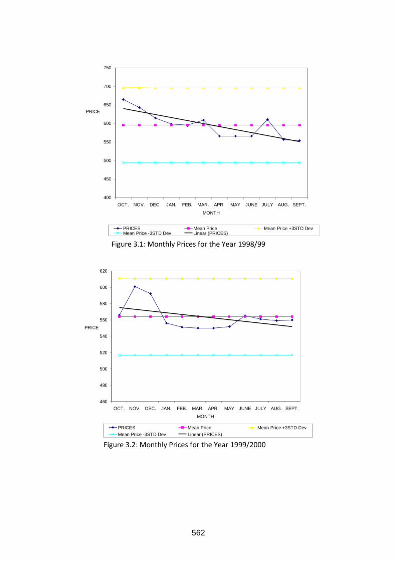
562

Figure 3.2: Monthly Prices for the Year 1999/2000

460

480

500

520

540

560

580

600

620

OCT. NOV. DEC. JAN. FEB. MAR. APR. MAY JUNE JULY AUG. SEPT. MONTH

PRICE

PRICES Mean Price Mean Price +3STD Dev Mean Price -3STD Dev Linear (PRICES)

Figure 3.1: Monthly Prices for the Year 1998/99

400

450

500

550

600

650

700

750

OCT. NOV. DEC. JAN. FEB. MAR. APR. MAY JUNE JULY AUG. SEPT. MONTH

PRICE

PRICES Mean Price Mean Price +3STD Dev Mean Price -3STD Dev Linear (PRICES)

563

Figure 3.4: Monthly Prices for the Year 2001/2002

400

600

800

1000

1200

1400

1600

1800

2000

2200

OCT. NOV. DEC. JAN. FEB. MAR. APR. MAY JUNE JULY AUG. SEPT.

MONTH

PRICE

PRICES Mean Price Mean Price +3STD Dev Mean Price -3STD Dev Linear (PRICES)

Figure 3.3: Monthly Prices for the Year 2000/2001

350

400

450

500

550

600

650

700

750

800

850

OCT. NOV. DEC. JAN. FEB. MAR. APR. MAY JUNE JULY AUG. SEPT.

MONTH

PRICE

PRICES Mean Price Mean Price +3STD Dev Mean Price -3STD Dev Linear (PRICES)

564

Figure 3.6: Monthly Prices for the Year 2003/04

1000

1100

1200

1300

1400

1500

1600

1700

OCT. NOV. DEC. JAN. FEB. MAR. APR. MAY JUNE JULY AUG. SEPT.

MONTH

PRICE

PRICES Mean Price Mean Price +3STD Dev Mean Price -3STD Dev Linear (PRICES)

Figure 3.5: Monthly Prices for the Year 2002/03

1400

1450

1500

1550

1600

1650

1700

1750

1800

OCT. NOV. DEC. JAN. FEB. MAR. APR. MAY JUNE JULY AUG. SEPT.

MONTH

PRICE

PRICES- 2002/03 Mean Price Mean Price +3STD Dev Mean Price -3STD Dev Linear (PRICES- 2002/03)

565

3.4 Interpretation of the Graphs

Graphs from the Figures 3.1 to 3.6 are the monthly prices in their respective years. The natures of the graphs have

their interpretations depending on the time and event that happened over that time. However, all graphs are within

―mean price 3 Standard deviation‖ (Control Chart). This shows that the fluctuations are within the acceptable

ranges and hence the process is in control as stated in Chandan (1998). The randomness of the data is also displayed

in Figures 3.1, 3.5, 3.4 and 3.6 with respect to mean value and linear trend lines.

From the stock market point of view, if the market is efficient then the price movements always obey the stochastic

process and hence the Markov chain model (randomness property). The Figures 3.1 and 3.5 have shown randomness

since the values above and below the mean price line are equal, i.e. five values in each. Also within the linearity the

randomness exists although it decreases instead of increasing. Particularly the graph in Figure 4.5 is typical of the

stock prices model except that it decreases.

The general picture that can be drawn from the graphs in Figures 3.1 – 3.6 is that the monthly prices are decreasing

with time except those in Figures 3.3 and 3.4 which are clearly increasing with time. The reason for the increase in

the monthly average prices for the periods 2000/01 and 2001/02 is not known for sure but it may be attributed to

some historical events and, in this particular case, the increase could have been due to the 2000 National elections

(Presidential, Parliamentary and Council). The September 11, 2001 bomb blast in New York, USA could also have

contributed to the increase in the monthly prices in 2001/02 through the appreciation of the dollar, thereby pushing

up the price in Tanzanian shillings.

However, monthly price‘s randomness was tested by Run‘s test and the results, p-values in the brackets show that:

1998/1999 (0.0346), 1999/2000 (0.0537) and 2002/2003 (0.0346) are moderate random and 2000/2001 (0.0014),

2001/2002 (0.0013) and 2003/2004 (0.0013) are not random. From these results the randomness of the data set is

expected. Further analysis of the data for Markov chain model can be done by using TPM behaviours.

Generally all the graphs are of unique trend or shape showing that the price changes were random and therefore that

any errors in prices changes are due to chance. For Run‘s test also suggest the presence of randomness as explained

to some years. So the use of the stochastic model is therefore justified.

3.5 Determination of the Unknown Parameters

The collected raw data are further analysed to obtain the other valuable information from the study. In the analysis,

data was grouped in various time intervals: quarterly, semi-annual, annual up to six years duration. Using the

assigned states ―U‖, ―G‖, and ―L‖, the TPM are obtained from respective state matrices and other parameters in the

given time frame. The state matrices and TPM were formed at different durations.

Further analysis of the TPM using the Maple software was carried out. The monthly TPM were not obtained since

some TPM did not meet the requirements that the row elements should add to unit. This was due to the fact that

some of the transitions had not taken place as per data we have.

Note that from the results, probability values in the TPM and steady state vectors were rounded to 2 or 4 decimal

places respectively while meeting the condition that row sums must be unity (equation 4 and 8 respectively). Tables

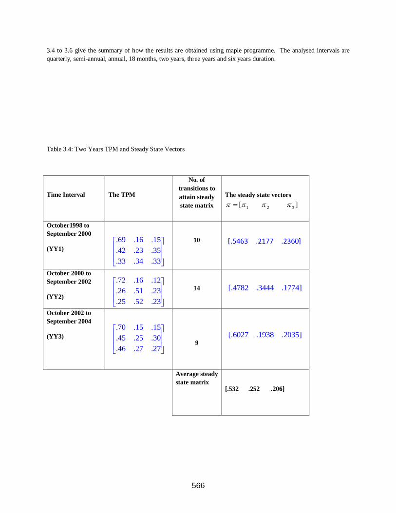
566

3.4 to 3.6 give the summary of how the results are obtained using maple programme. The analysed intervals are

quarterly, semi-annual, annual, 18 months, two years, three years and six years duration.

Table 3.4: Two Years TPM and Steady State Vectors

Time Interval

The TPM

No. of

transitions to

attain steady

state matrix

The steady state vectors

][ 321

October1998 to

September 2000

(YY1)

.69 .16 .15

.42 .23 .35

.33 .34 .33

10

October 2000 to

September 2002

(YY2)

.72 .16 .12

.26 .51 .23

.25 .52 .23

14

[ ].4782 .3444 .1774

October 2002 to

September 2004

(YY3)

.70 .15 .15

.45 .25 .30

.46 .27 .27

9

[ ].6027 .1938 .2035

Average steady

state matrix

[.532 .252 .206]

[ ] .5463 .2177 .2360

567

Table 3.5: Three Years TPM and Steady State Vectors

Time Interval

The TPM

No. of

transitions to

attain steady

state matrix

The steady state vectors

][ 321

October 1998 to

September 2001

(THY1)

.74 .14 .12

.39 .31 .30

.33 .42 .25

14

[ ].5828 .2314 .1858

October 2001 to

September 2004

(THY2)

10

[ ].4697 .3185 .2118

Average steady

state matrix

[.526 .275 .199]

Table 3.6: Six Years TPM and Steady State Vectors

Time Interval

The TPM

No. of

transitions to

attain steady

state matrix

The steady state vectors

][ 321

.61 .24 .15

.33 .41 .26

.37 .35 .28

568

October 1998 to

September 2004

(SX)

12

[ ].5177 .2820 .2003

In order for the TPM in Tables 3.4 - 3.6 to comply with the properties of Markov chain model, the corresponding

elements of the steady state vectors in consecutive intervals must be close to each other. In this situation the n-step

transition probability matrices can be used for prediction purposes and other Markovian computations. The closer

the values of the steady state vectors in consecutive intervals, the more the data agrees with the stationary Markov

chain model.

Using the steady state values ][ 321 in the results, the highest differences in each interval were

computed (highest value – lowest value). The differences were converted into percentages. These computations are

as tabulated in Table 3.7. For example consider the (Annual TPM and Steady State Vectors) the largest and smallest

values of , are 0.6553 and 0.3080 respectively. Their difference is 0.3473 or 34.73%. This value is then recorded

in Table 3.7 in the row labeled ―Annual‖. The rest of the entries in Table 3.7 were computed similarly.

Table 3.7: The summary of the steady state differences in percentage within the classified group.

Group

Interval

Duration

Highest %

difference for

1

Highest %

difference for

2

Highest %

difference for

3

Average %

difference

Quarterly 73.9 54.9 34.9 54.6

Semi-annual 69.4 52.9 38.7 53.7

Annual 34.7 27.4 22.5 28.2

18 Months 29.6 21.6 16.7 22.6

2 Years 12.5 15.1 5.9 11.2

3 Years 11.3 8.7 2.6 7.5

It is noted from the results in Table 3.7 that the average percentage differences diminish with increasing time

intervals/more data (Column 5). This indicates that the larger the interval, the smaller the average percentage

difference and therefore the closer the steady state vectors to the Markov chain model. In other words, the last two

(2 to 3 years) intervals are best as they give the smallest average percentage differences of 11.2 and 7.5 percent,

respectively. Therefore for prediction purposes, the 3 years interval steady state vectors will be used as the expected

probability of future price changes. The corresponding TPM will be used for predicting future n-step transition

probabilities.

.67 20. .13

.35 .37 .28

.36 .37 .27

569

Using the average steady state vectors at the bottom of each interval, the overall average steady state vector

computed was found to be 0.5294, 0.2656, and 0.2050. These averages can be used to get another interpretation of

the price changes for the six years of business for DSE, particularly TBL‘s shares. That is there are 52.94% chance

that prices remained unchanged, 26.56% of the time prices increased, and 20.50% of the time the prices decreased.

From these figures it can therefore be concluded that most of the time the prices remained unchanged.

The TPM obtained from six years combination is

with a steady state vector of [0.5177 0.2820 0.2003]. This result shows the general performance of the Stock

Market (DSE) for six years as follows-: About 52% of the price changes remained the same indicating that there was

no very serious competition in the market. The price increased 28% of the time over six years of business and it

decreased by 20% of the time. Values are very close to the general average obtained above. The situation shows that

the Stock Market is not performing well in business because the competition of investors is very low. As a result of

limited number of customers who are involved in the business, the DSE gets very low returns.

4. Conclusion and Recommendations

4.1 Conclusion

4.1.1 Results and Discussion

In this study, Markov chain model for the analysis of the price dynamics was developed and used. From the first part

of testing, the data were found to be appropriate for stochastic model as shown in graphs (Figures 4.1 to 4.6). The

graphs were drawn using the Excel package. The observed trends of the prices were decreasing since about 67% (4

out of 6) of the graphs had linear decreasing trend. The general randomness of the graphs also supports the use of

stochastic modelling. However, from the known nature of the efficient stock market general graphs model, it can be

deduced that the market has not performed according to the required model and thus more efforts are needed to

enhance the market.

For prediction purposes, by using Markov chain model (using Maple package), the steady state matrices established

in different durations gave the proper direction to this. The 3 years combination TPM has been analysed and

observed to be more Markovian as its first steady state vector is closely correlated with the second in regards to all

the three states. This can be used to predict the general market performance in the price changes for the next three

years.

4.1.2 The Utility of the Model

The developed model in this study is of great importance to DSE management as it can be used for planning,

decision making and implementation. The management or practitioners can use the results of the model to review

their activities according to the nature of their customers. The results will also help the management to improve their

strategies on public education towards DSE activities awareness.

.67 .20 .13

.35 .37 .28

.36 .37 .27

570

Customers on the other hand are interested in knowing at what time they can buy or sell their shares using the

model. Although the model agrees well with 3 years interval data, but still, it is possible to reformulate the model

using monthly or weekly data.

4.2 Recommendations

4.2.1 General Recommendations

The results from this work are very useful to DSE and the related financial sectors. This is particularly in the use of

idle resources (surplus money) for sure investment that can boost the socio-economic status of the people. Thus

apart from banking system, investors may use this as it caters for the exchange rate of our money in the world

network of finance. Therefore it can be recommended that:-

i. DSE should take into consideration the results of this work and review their business strategies so as to use

it as one of the guiding factor in decision making.

ii. DSE should identify the geographical and general background of their customers so as to add other

customers who have never been in the market since opening of the centre.

iii. DSE should provide public education about their activities by conducting seminars or workshops at

different centres such as higher learning institutions.

iv. DSE should use performance of other Stock Markets in East Africa, Africa and world wide as a challenge

to them.

v. DSE should set up a research department to carry out different analysis of the market performance and

hence use it in decision making. This is based on the fact that DSE is a financial firm that needs to expand its activities to other parts of the country. Its expansion is a function of its performance.

4.2.2 Further Studies Recommendations

1. Research on the other listed companies can be done so as to compare and may be to come up with true

colour of the market.

2. Analysis by using other models like deterministic models also can be conducted.

3. Studies that use all the prices obtained in the day is highly recommended so as to establish monthly, even

weekly TPM.

571

References

Ahmed R. and Bernard A. (1989). Research report on Rice Price Fluctuation

and an Approach to Price Stabilization in Bangladesh. International

Food Policy Research Institute, Washington. pp 22 - 34.

Chandan, J.S. (1998). Statistics for Business and Economics, 1st ed. Vikas Publishing House PVT Ltd. Pg 551-588.

Hirst, F.W. (1912). The Stock Exchange. Henry Holt and Co., New York. pp187 - 211.

http://www.dse.co.tz/main/index.php?rec=main&page=5. Retrieved on 30/07/2011.

Mason, P. (1971). Price Level Changes and Financial Statements: Basic Concepts and Methods.

American Accounting Association. pp 1 - 12.

Pike,W. H. (1983). Why Stocks Go Up (and Down). A guide to Sound Investing.

Dow Jones - Irwin-Homewood, Illinois. pp 157 - 165.

Seiler, M. J. and Walter R. (1997). A Historical Analysis of Market Efficiency: Do

Historical Returns Follow a Random Walk? Retrieved from

http://www.studyfinance.com/jfsd/pdffiles/v10n2/seiler.pdf

Stone, C.J., et al. (1972): Introduction to Stochastic Processes, Waveland Press, Inc. Illinois U.S.A. p. 1 - 36, 47 -

67.

Sundararajan, R., et al. (2009). Stock market trend prediction Using Markov Models.

Vasanthi, S., et al. (2011). An Empirical Study On Stock Index Trend Prediction Using Markov Chain Analysis.

572

TRANSPORTATION AND LOGISTICS MANAGEMENT

The capacitated plant location problem with customer and supplier matching and interval demands

uncertainties

M. Salahi and K. Mehdi

Faculty of Mathematical Sciences, University of Guilan, Rasht, Iran

salahim@guilan.ac.ir

Abstract

The capacitated plant location problem with customer and supplier matching can be modeled as a mixed integer

linear program, where the product distribution from plants to customers and the material supply from suppliers to

plants are considered together. In order to save allocation cost, distribution trip and a supply trip is merged into one

triangular trip. Moreover, vehicles from plants visit a customer and a supplier for each trip. In this paper, we assume

interval uncertainties in the demands of costumers. We show that the robust counterpart of the original model with

interval uncertainty is equivalent to a larger mixed integer linear program. Finally, the original and robust models

are compared on several randomly generated examples for different level of uncertainties.

Keywords: Capacitated plant location, Matching, Mixed integer linear program, Interval uncertainty.

1. Introduction

The capacitated plant location problem (CPL) consists of locating a set of potential plants with capacities, and

assigning a set of customers to these plants. The goal is to minimize the total fixed and shipping costs such that the

demand of all customers is satisfied without violating the capacity of plants. The CPL is modeled as a mixed integer

linear programming problems, where several heuristic algorithms are designed to solve it [2-6, 8].

A slightly different problem is CLP with customer and supplier matching. In this problem, customers, suppliers and

a set of potential plants are mixed in a same network and each open plant holds its fleet of homogenous vehicles. It

is assumed that the vehicles serve customers from a plant, the same vehicles visit suppliers from customers, and then

the vehicles transport material/parts from suppliers back to the plant [9]. In this paper, first we describe CLP with

customer and supplier matching and then present its robust counterpart when interval uncertainties are assumed for

demands [1]. It is shown that the robust counterpart of CLP is a larger mixed integer linear program. Finally, on

several randomly generated examples, original and robust problems are compared using Lingo 11 [7].

2. CLP with Customer and Supplier Matching

Let us consider a graph G= (N, A), where N denotes the nodes and A denotes the set of directed arcs between

nodes [9]. Nodes are divided to three categories: a set of potential plants H, a set of customers , and a set of potential suppliers J such that

573

Each potential plant has a limitted capacity and fixed cost . The limited capacity of suppliers is denoted

by . The demand of each cotumer is , where for all and for all The trigonal

distance is equal to

Which means the distance from the plant h visiting customer i, from customer i to supplier j, from supplier j back to

plant h [9]. The optimizer‘s goal is to design a model which minimizes the total opening costs of plants and

allocation costs subject to the following constraints: Each customer should be served by one plant and matched with

one supplier, each open plant does not supply more than its capacity, suppliers capacity cannot exceeded. Moreover,

is equal to 1 if and only if customer and supplier are assigned to plant otherwise it is equal to 0. If plant

is open, then , otherwise it is equal to 0. Thus the problem can be formulated as the following binary integer

linear program [1]:

min

1

(1)

0,1 , ,

0,1 .

h h i hij hijPh h i j

hij

h j

i hij h h

i j

i hij j

h i

hij

h

f y c v d x

x i I

v x b y h H

v x w j J

x i I j J h H

y h H

Z

However, it is known that most of real world problems are having certain uncertainties in problem data. In such a

case, the solution of the previous model might not lead to the solution which we expect. In the next section, we

consider uncertainty on the demand of customers and show the robust counterpart of (1) is a larger mixed integer

linear program under interval uncertainties.

2. Robust Model

In this section, we consider uncertainties on parameter Each uncertain coefficient is known to belong to an

interval centered at its nominal value and of half-length We define the scaled deviation of parameter from its

nominal value as , which belongs to the interval . We always have where .

Now let us consider the third set of constraints in (1):

.

Its robust counterpart is given by

ˆ ˆ .i i i hij i hij i i hij j

h i h i h i

v v z x v x v z x w j J

This should hold in the worst case. Thus it is sufficient to solve the following problem for

j J :

574

ˆmax

2

0 1

0,1 .

i i hij

h i

i

i

i

hij

v z x

z

z

x

The dual of (2) is given by

min

ˆ

, 0, 0,1 .

j i

i

j i i hij

h

j i hij

q r

q r v x i I

q r x

Thus the third set of constraints in the robust case is equivalent to

ˆ

, 0, 0,1 .

i hij j i j

h i i

j i i hij

h

j i hij

v x q r w j J

q r v x

q r x

The robust counterpart of the second set of constraints can be worked out in the same manner. Therefore, the robust

counterpart of (1) is

min

1

ˆ ( ) ,

ˆ ( ) ,

ˆ ( ) ,

, , ,

h h

h

hij

h j

i hij h i h h

i j i

h i i hij

j

i hij j i j

h i i

j i i hij

h

i hij hij t i

h i j i

t i i hij hij

h j

h j t i

f y ct

x i I

v x q r b y h H

q r v x h H i I

v x q r w j J

q r v x i I j J

v d x q r t

q r v d x i I t

q q q r

0 , 0,1hij hand x y

As we see, the robust counterpart of (1) is a mixed integer linear program but it is much larger.

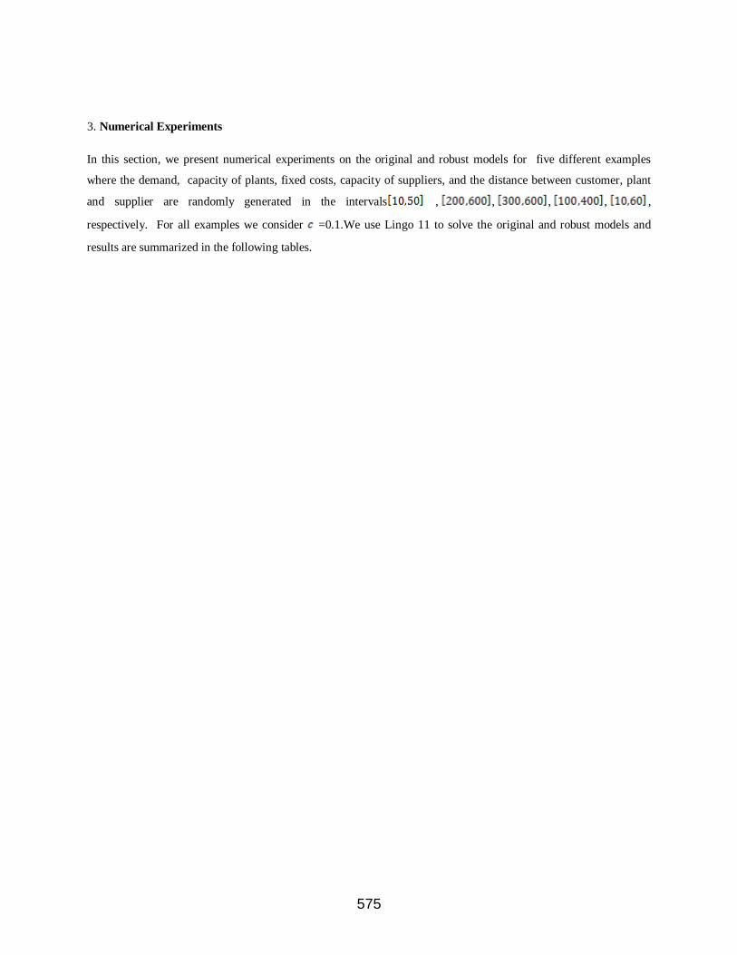
575

3. Numerical Experiments

In this section, we present numerical experiments on the original and robust models for five different examples

where the demand, capacity of plants, fixed costs, capacity of suppliers, and the distance between customer, plant

and supplier are randomly generated in the intervals , , , , ,

respectively. For all examples we consider =0.1.We use Lingo 11 to solve the original and robust models and

results are summarized in the following tables.

576

Table 1: Comparison of Original and Robust model for 5 different examples

i 20 20 30 40 50

j 5 10 10 10 20

h 5 5 5 5 15

Original

Objective 1956.119 1811.909 2455.055 3493.492 3152.593

Time (sec) 1 2 21 19 2.36

ˆ 0.1iv 1960.179 1814.911 2458.179 3500.35 3160.972

Time (sec) 19 6 1.04 1.39 9.21

ˆ 0.2iv 1964.239 1817.914 2462.111 3506.683 3168.469

Time (sec) 5 10 1.40 1.5 4.29

ˆ 0.3iv 1968.299 1820.916 2467.098 3512.493 3243.501

Time (sec) 7 17 1.19 1.28 127.2

ˆ 0.4iv 1998.341 1823.918 2471.052 3518.285 3249.946

Time (sec) 19 7 1.52 1.11 6.44

577

ˆ 0.5iv 2007.015 1826.920 2474.176 3524.605 3257.908

Time (sec) 24 4 1.15 1.55 3.04

ˆ 0.6iv 2021.707 1829.923 2480.046 3530.459 3264.707

Time (sec) 20 5 1.14 1.3 2.25

ˆ 0.7iv 2025.883 1832.925 2483.170 3536.251 3272.567

Time (sec) 24 5 1.21 12 3.0

ˆ 0.8iv 2030.06 1835.927 2486.295 3542.043 3279.039

Time (sec) 16 4 1.20 11 2.54

ˆ 0.9iv 2058.976 1838.929 2493.091 3547.835 3292.888

Time (sec) 27 5 1.07 11 2.59

ˆ 1iv 2083.711 1841.931 2499.4 3553.627 3301.474

Time (sec) 36 4 1.12 39 3.22

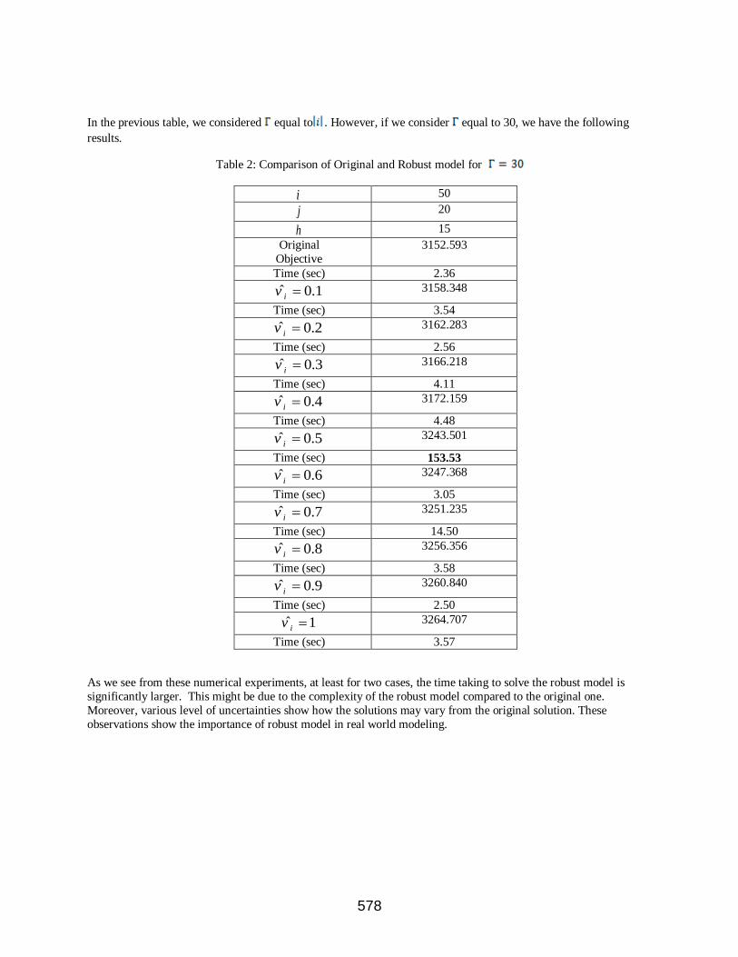
578

In the previous table, we considered equal to . However, if we consider equal to 30, we have the following

results.

Table 2: Comparison of Original and Robust model for

50 i 20 j

15 h

3152.593 Original

Objective

2.36 Time (sec)

3158.348 ˆ 0.1iv

3.54 Time (sec)

3162.283 ˆ 0.2iv

2.56 Time (sec)

3166.218 ˆ 0.3iv

4.11 Time (sec)

3172.159 ˆ 0.4iv

4.48 Time (sec)

3243.501 ˆ 0.5iv

153.53 Time (sec)

3247.368 ˆ 0.6iv

3.05 Time (sec)

3251.235 ˆ 0.7iv

14.50 Time (sec)

3256.356 ˆ 0.8iv

3.58 Time (sec)

3260.840 ˆ 0.9iv

2.50 Time (sec)

3264.707 ˆ 1iv

3.57 Time (sec)

As we see from these numerical experiments, at least for two cases, the time taking to solve the robust model is

significantly larger. This might be due to the complexity of the robust model compared to the original one.

Moreover, various level of uncertainties show how the solutions may vary from the original solution. These

observations show the importance of robust model in real world modeling.

579

4. References

[1] D. Bertsimas, Aurélie Thiele. A robust optimization approach to inventory theory, Operations Research, 54(1),

2006, pp. 150--168.

[2] H. Delmaire, J.A. Di´az and E. Ferna´ndez. Reactive GRASP and tabu search based heuristics for the single

source capacitated plant location problem, INFOR, Canadian Journal of Operational Research and Information

Processing, 37, 1999, pp. 194–225.

[3] W. Domschke and A. Drexl. ADD-heuristics‘ starting procedures for capacitated plant location models,

European journal of operational research 21 (1), 1985 , pp. 47–53.

[4] E. Feldman, F.A. Lehrer and T.L. Ray. Warehouse location under continuous economies of scale, Management

Science 12, 1966, pp. 670–684.

[5] S.K. Jacobsen. Heuristics for the capacitated plant location model, European journal of operational research 12 (3), 1983, pp. 253–261.

[6] J. Kratica, D. Tosic, V. Filipovic and I. Ljubic. Solving the simple plant location problem by genetic algorithm,

RAIRO Operations Research 35, 2001, pp. 127–142.

[7] Lingo 11, http://www.lindo.com.

[8] G. Sa. Branch and bound and approximate solutions to the capacitated plant location problem, Operations

Research 17 (6),1969, pp. 1005–1016.

[9] Z. Zhu, F. Chu, Linyan Sun. The capacitated plant location problem with customers and suppliers matching,

Transportation Research Part E, 46( 3), 2010, pp.469--480.