ORIGINAL PAPER A numerical study of the interactions of urban breeze circulation with mountain slope...

ORIGINAL PAPER

A numerical study of the interactions of urban breeze circulationwith mountain slope winds

Gantuya Ganbat & Jong-Jin Baik & Young-Hee Ryu

Received: 11 December 2013 /Accepted: 14 April 2014 /Published online: 2 May 2014# Springer-Verlag Wien 2014

Abstract The two-dimensional interactions of urban breezecirculation with mountain slope winds are investigated usingthe Weather Research and Forecasting (WRF) model coupledwith the Seoul National University Urban Canopy Model(SNUUCM). A city is located near an isolated mountain,and there is no basic-state wind. Circulation over the urbanarea is asymmetric and characterized by the weakenedmountain-side urban wind due to the opposing upslope windand the strengthened plain-side urban wind in the daytime.The transition from upslope wind to downslope wind on theurban-side mountain slope occurs earlier than that on themountain slope in a simulation that includes only an isolatedmountain. A hydraulic jump occurs in the late afternoon,when the strong downslope wind merges with weakermountain-side urban wind and stagnates until late evening.The sensitivities of the interactions of urban breeze circulationwith mountain slope winds and urban heat island intensity tomountain height and urban fraction are also examined. Asmountain height decreases and urban fraction increases, thetransition from urban-side upslope wind to downslope windoccurs earlier and the urban-side downslope wind persistslonger. This change in transition time from urban-side upslopewind to downslope wind affects the interactions betweenurban breeze circulation and mountain slope winds. Urbanheat island intensity is more sensitive to urban fraction than tomountain height. Each urban fraction increase of 0.1 results inan average increase of 0.17 °C (1.27 °C) in the daytime(nighttime) urban heat island intensity. A simulation in

which a city is located in a basin shows that theurban-side downslope wind develops earlier, persistslonger, and is stronger than in the simulation that in-cludes a city and an isolated mountain.

1 Introduction

Many interesting thermally induced wind systems occurlocally, including sea/land breezes, mountain/valley winds(or downslope/upslope winds), lake breezes, and urbanbreezes. Of these local wind systems, sea/land breezes,mountain/valley winds, and lake breezes have been investi-gated extensively through observational, theoretical, and nu-merical modeling studies (Simpson 1994; Pielke 2002). How-ever, urban breezes have been less investigated despite theimportant roles urban breezes play in local weather and airquality (Ryu et al. 2013a).

Urban breeze circulation (also known as urban heat islandcirculation) is induced by the difference in near-surface airtemperature between the urban area and its surrounding ruralarea, that is, the urban heat island. Urban breeze circulationhas been observed in many cities (Wong and Dirks 1978;Hidalgo et al. 2008b) and has been simulated numerically(Lemonsu and Masson 2002; Hidalgo et al. 2008a; Ryu andBaik 2013). These previous studies indicate that urban breezecirculation is characterized by inward flow toward the citycenter in the lower boundary layer, upward motion near thecity center, outward flow toward the surrounding rural area inthe upper boundary layer, andweak downwardmotion outsideand that urban breeze circulation is stronger in the daytimethan in the nighttime. For example, the boundary layer simu-lated over the Paris area in France was deeper in the daytimethan in the nighttime, with converging (diverging) flow of 5–7 m s−1 at lower (upper) levels and upward vertical velocitiesof ~1 m s−1 (Lemonsu and Masson 2002).

G. Ganbat : J.<J. Baik (*) :Y.<H. RyuSchool of Earth and Environmental Sciences,Seoul National University, Seoul 151-742, South Koreae-mail: [email protected]

Y.<H. RyuDepartment of Civil and Environmental Engineering,Princeton University, Princeton, NJ 08544, USA

Theor Appl Climatol (2015) 120:123–135DOI 10.1007/s00704-014-1162-7

When a city is located near mountains, both the urbanbreeze and upslope/downslope winds are thermally inducedand interact with each other. Previous numerical modelingstudies have investigated wind modifications in the presenceof urban areas and topography or interactions between theurban breeze and upslope/downslope winds. Savijarvi andLiya (2001) examined local winds around a valley citythrough idealized two-dimensional simulations. They foundthe daytime urban breeze circulation to oppose the weakdaytime upslope circulation of a narrow valley, resulting inrelatively weak daytime winds. Conversely, the nighttimedownslope wind wipes out the weak nighttime urban breezecirculation, resulting in purely katabatic winds in the night-time and morning. Ohashi and Kida (2002) examined theeffects of mountains and urban areas on daytime local circu-lations in the Osaka and Kyoto regions in Japan. Their resultsdemonstrated that valley circulation weakens the urban breezecirculation and causes surface air temperatures to increasethrough adiabatic warming by subsidence. Lee and Kim(2010) performed idealized two-dimensional simulations andshowed that the urban sensible heat flux acts to acceleratenocturnal drainage flow, which tends to increase the returnflow above. Ryu and Baik (2013) simulated local circulationsin the Seoul metropolitan area in South Korea and demon-strated that the upslope wind turns to downslope wind and thedownslope wind strengthens with gradual strengthening of theurban breeze circulation in the daytime. These modeling stud-ies provide valuable insights into interactions between urbanbreeze circulation and upslope/downslope winds.

Many factors, including urban fraction and urban surfaceroughness, affect the intensity of urban breeze circulation, andmountain shape and height influence upslope/downslopewind speeds. Thus, the degree of interactions between urbanbreeze circulation and upslope/downslope winds depends onsuch factors. The present study investigates the interactions ofurban breeze circulation with upslope/downslope winds andthe dependences of these interactions and urban heat islandintensity on mountain height and urban fraction using a me-soscale model coupled with an advanced urban canopymodel.Idealized two-dimensional simulations are conducted to clear-ly understand these interactions and these dependences withina simple framework.

In Section 2, the numerical model used and the experimen-tal design are described. The simulation results are presentedand discussed in Section 3. Summary and conclusions areprovided in Section 4.

2 Model description and experimental design

The numerical model adopted in the present study is theWeather Research and Forecasting (WRF) model version 3.2(Skamarock et al. 2008) coupled with the Seoul National

University Urban Canopy Model (SNUUCM) (Ryu et al.2011). The model physics options are as follows: the YonseiUniversity (YSU) planetary boundary layer scheme (Honget al. 2006), the Rapid Radiative Transfer Model (RRTM)longwave radiation scheme (Mlawer et al. 1997), the Dudhiashortwave radiation scheme (Dudhia 1989), and the PurdueLin cloud microphysics scheme (Chen and Sun 2002). TheSNUUCM parameterizes important physical processes thatoccur in urban canopies, including absorption and reflectionof shortwave and longwave radiation, turbulent energy andwater exchanges between surfaces (road, two facing walls,and roof) and adjacent air, and conductive heat transferthrough substrates (Ryu et al. 2011). The SNUUCM iscoupled with the Noah Land Surface Model (Chen andDudhia 2001) in a tile approach. The WRF modelcoupled with the SNUUCM has been applied previouslyto investigate local circulations and urban impacts on airquality in the Seoul metropolitan area (Ryu et al.2013b; Ryu and Baik 2013).

A city and an isolated mountain are considered to examinetwo-dimensional interactions between urban breeze circulationandmountain slope winds. The city has a size of 20 km, and theurban area consists of built-up (80 %) and natural (20 %) areas.All natural areas consist of cropland–woodland mosaic (60 %)and loamy soil sand (40 %). Some important urban parametersin the SNUUCM are specified as follows: the roof level heightis 15 m, the canyon aspect ratio is 1, and the emissivity andalbedo of all artificial surfaces (road, wall, and roof) are 0.95and 0.2, respectively. The mountain is Gaussian-shaped with asize of 20 km,which is given by h xð Þ ¼ hme

− x−ckð Þ2 , where hm is

the maximum mountain height, c is the horizontal location ofthe mountain peak, and k is the slope parameter (k=5,000 m).

The domain size is 200 km in the horizontal and 8 km in thevertical. The horizontal grid interval is 500 m. The verticalgrid interval is stretched with height, with the lowest modellevel being z=48 m, and the number of vertical layers is 82.The Rayleigh damping layer is set to z=6–8 km to avoid thereflection of waves at the top of the physical domain(z=6 km). The lateral boundary condition is periodic. Themountain height is set to zero at mountain-edge grid points.The initial potential temperature at the surface is 298 K, andthe lapse rate of the initial potential temperature is 5 K km−1.No basic-state wind is considered to ensure that focus isplaced on thermally induced circulation/flow. The initial rela-tive humidity is uniform throughout z=0–4 km (30 %), de-creases linearly with height up to z=6 km (where it is 10 %),and remains constant above this height. Since this study isconcerned with thermally induced local circulations, the initialrelative humidity is set to be low so that clouds and precipi-tation do not occur. The effect of Earth’s rotation is neglected,and the latitude is set to 30° N. The model is integrated for27 h starting from 0500 LST on June 23, and the 24-hsimulation data starting from 0800 LST are used for analysis.

124 G. Ganbat et al.

3 Results and discussion

3.1 Urban breeze circulation and mountain slope winds

In this section, the simulated general features of urban breezecirculation and mountain slope winds are presented in brief.Figure 1 shows the horizontal velocity, vertical velocity, andvelocity vector fields and the potential temperature anomalyfield at 0900, 1300, 1900, and 2300 LST in a simulation thatincludes only a city (hereafter, the URBAN simulation). Thepotential temperature anomaly is calculated as the differencebetween total and horizontally averaged values at each height.

The city spans x=100–120 km. The urban breeze circulationis induced by the horizontal temperature difference betweenthe urban area and the surrounding rural area.

At 0900 LST, a weak horizontal potential temperaturedifference is present and an urban breeze circulation is aboutto form. As the horizontal temperature difference increaseswith time, the urban breeze circulation becomes wellestablished. The urban breeze circulation is symmetric aboutthe urban center (x=110 km) because there is no basic-statewind. At 1300 LST, urban breeze fronts are located at x=105and 115 km and the horizontal wind behind the urban breezefronts is strong. The two urban breeze fronts move toward the

Fig. 1 Horizontal velocity(shading), vertical velocity(contour), and velocity vectorfields at a 0900, b 1300, c 1900,and d 2300 LST andcorresponding potentialtemperature anomaly field(shading) at e 0900, f 1300, g1900, and h 2300 LST in theURBAN simulation. The graybox on the x-axis indicates theurban area. The contour levels ofvertical velocity are 0.5, 1, and2 m s−1

Interaction of urban breeze circulation with mountain slope winds 125

urban center, colliding with each other around 1455 LST andsubsequently merging to produce strong upward motion. At1900 LST, a strong updraft cell centered at the urban centerappears, with a maximum updraft intensity of 2.0 m s−1

at z=1,150 m. Note that 1900 LST is very close to the sunsettime on June 23 (~1858 LST). The urban breeze circulation isstronger in the late afternoon/early evening than in the earlyafternoon (Fig. 1b, c). This is consistent with the result ofSavijarvi and Liya (2001). The simulated urban breeze circu-lation is characterized by converging flow in the lower layerand diverging flow in the upper layer (Fig. 1b, c). At 1300 and1900 LST, deeper urban boundary layer results in the negative(cold) potential temperature anomaly in the upper layer owingto higher potential temperature in the rural area than in theurban area at the same upper level because of strong stratifi-cation above the top of rural boundary layer (Fig. 1f, g). Thehorizontal size of the urban breeze circulation at 1300 (1900)LST is 2.0 (3.9) times as large as the urban size. This is similarto the results of Hidalgo et al. (2008a) and Ryu et al. (2013a).The vertical size of the urban breeze circulation is ~1.8 km at1300 LST and ~2.2 km at 1900 LST. It is notable that thehorizontal and vertical sizes of the urban breeze circulationvary considerably with time. In the nighttime, although thenear-surface potential temperature difference between the ur-ban area and the surrounding rural area is relatively large(i.e., larger nighttime urban heat island), the urban breezecirculation is weak owing to nighttime stable stratification thatsuppresses vertical motion (Fig. 1d).

A simulation with Earth’s rotation was performed with flatterrain and a city being considered, and simulation resultswere compared with the results of the simulation withoutEarth’s rotation (that is, the URBAN simulation). In both thesimulations, daytime urban breeze circulations are similar toeach other. When the Earth’s rotation is included, in the lateevening, winds start to turn away from the city above thesurface, exhibiting an anti-urban heat island circulation-likefeature (Savijarvi and Liya 2001). The transverse wind(v velocity) arises in the simulation with Earth’s rotation dueto the Coriolis force, but in the daytime its magnitude issmaller than that of u velocity.

Figure 2 shows the horizontal velocity, vertical velocity,and velocity vector fields and the potential temperature anom-aly field at 0900, 1300, 1900, and 2300 LST in a simulationthat includes only a mountain (hereafter, the MOUNT simu-lation). In this simulation, the mountain peak is located atx=90 km, and the maximum mountain height (hm) is 500 m.As expected, the upslope (downslope) wind appears at 0900and 1300 (1900 and 2300) LST. Note that the downslope windat 1900 LST occurs near the mountain slope surface. At 1300LST, a strong updraft cell is produced over the mountain topand flow in the upper layer diverges away from the mountain,forming an apparent mountain circulation. Above the moun-tain top, a weak warm region and a relatively strong cold

region are observed. The upslope wind attains a maximumintensity of 2.2 m s−1 around 1340 LST. The transition fromupslope wind to downslope wind at a midslope location(x=95 km) occurs around 1845 LST. During the 24-h period,the occurrence frequency of the 10-m upslope wind at themidslope location (47 %) is similar to that of the downslopewind (53 %).

3.2 Interactions of urban breeze circulation with mountainslope winds

To examine interactions between urban breeze circulation andmountain slope winds, a numerical experiment in which botha city and a mountain exist is performed. This simulation isreferred to as the URBAN-MOUNT simulation. The horizon-tal size of the city (20 km) is the same as that of the mountain,and the horizontal location of the mountain peak (urban cen-ter) is x=90 (110) km. Themaximummountain height is set to500 m. Several terms are utilized in the present study toindicate areas or locations within the domain. The mountainslope on the rural (urban) side is referred to as the rural-side(urban-side) mountain slope and spans x=80–90 (90–100) km(Fig. 3). The urban area whose edge borders the mountain(plain) area is referred to as the mountain-side (plain-side)urban area and spans x=100–110 (110–120) km. The urbanperiphery that borders the mountain (rural) area is referred toas the mountain–urban (urban–rural) edge [x=100 (120) km].In the URBAN-MOUNT simulation, the mountain–urbanedge is located at the center of the domain.

Figure 3 shows the horizontal velocity, vertical velocity,and velocity vector fields and the potential temperature anom-aly field at five different times (1300, 1500, 1600, 1900, and2300 LST) in the URBAN-MOUNT simulation. At 1300LST, the upslope wind on the mountain slope and an updraftcell over the mountain top are produced. The upslope wind isstronger on the rural-side mountain slope than on the urban-side mountain slope because the mountain upslope wind onthe urban-side mountain slope is opposed by the urban breeze.The circulation over the urban area is not symmetric about theurban center owing to the influence of the mountain circula-tion. At 1500 LST, the upslope wind exists on the rural-sidemountain slope, whereas the downslope wind exists in thelower region of the urban-side mountain slope. Two updraftcells over the urban area are apparent and are associated withurban breeze fronts. The updraft cell centered at x=105.5 kmis influenced more by the mountain circulation than thatcentered at x=109.5 km. A deep warm region centered atx=105.5 km is formed (Fig. 3g). The two updraft cells movetoward each other, colliding around 1540 LST and subse-quently merging to produce a strong updraft cell. At 1600LST, the downslope wind on the urban-side mountain slope isproduced and the two updraft cells are merged into a strongupdraft cell centered at x=106.5 km. The plain-side urban


wind pushes the urban breeze convergence zone toward themountain. At 1900 LST, the downslope wind on the urban-side mountain slope is enhanced. At 2300 LST, the downslopewind is present on both sides of the mountain, the urban windweakens, and a shallow warm region is observed over theurban area. In this study, night–morning transitions and circu-lations are not focused, but they deserve an investigation witha longer time simulation.

Fernando (2010) noted that downslope flow approaching aslope break may undergo hydraulic adjustment and thenmerge with the urban nocturnal atmospheric boundary layer.

In the URBAN-MOUNT simulation, a clear hydraulic jumpappears at 1900 LST (Fig. 3d). The urban-side mountaindownslope wind accelerates while descending through a thinlayer (Fig. 3d). Around 1800 LST, a hydraulic jump starts tooccur near the mountain–urban edge when the strong and thindownslope wind merges with the urban wind. Additionally,the larger roughness length in the urban area contributes partlyto the development of this hydraulic jump. The upward mo-tion in association with the hydraulic jump has a maximumintensity of 1 m s−1 at 2000 LST, and afterward the hydraulicjump begins to weaken and eventually disappears.

Fig. 2 Same as in Fig. 1 but forthe MOUNT simulation. Thecontour levels of vertical velocityare 0.5 and 1 m s−1


A simulation was performed with the hydrostatic mode ofthe WRF model. It was revealed that a hydraulic jump also

occurs in the hydrostatic mode but with later onset, weakerintensity, and shorter presence period. Since the hydraulic

Fig. 3 Horizontal velocity(shading), vertical velocity(contour), and velocity vectorfields at a 1300, b 1500, c 1600, d1900, and e 2300 LST andcorresponding potentialtemperature anomaly field(shading) at f 1300, g 1500, h1600, i 1900, and j 2300 LST inthe URBAN-MOUNTsimulation. The gray box on the x-axis indicates the urban area. Thecontour levels of vertical velocityare −0.5 (dashed line, d), 0.5, 1,and 2 m s−1


jump is an interesting phenomenon, we plan to study deep intoits occurrence conditions and occurrence mechanisms throughextensive numerical simulations and analyses.

Savijarvi and Liya (2001) demonstrated that urban breezecirculation opposes the weak daytime upslope circulation of anarrow valley. Similarly, Ohashi and Kida (2002) showed thatin the daytime the weakening of winds toward urban andmountain areas is caused by their opposing wind direc-tions. In essence, the results of the present study areconsistent with those of both Savijarvi and Liya (2001)and Ohashi and Kida (2002).

The combined effects of the city and mountain on thelocal wind system produce some interesting features,including an earlier transition from upslope wind todownslope wind on the urban-side mountain slope anda stronger downslope wind. At the midslope location ofthe urban-side mountain slope, the transition from up-slope wind to downslope wind occurs around 1430 LST,which is approximately 4 h earlier than the transition inthe MOUNT simulation. The rural-side upslope windpasses over the mountain top, and the urban-side down-slope wind is enhanced (Fig. 3c, d). The combinedeffects of the city and mountain also produce an ex-tended period of urban-side downslope wind. The oc-currence frequency of downslope wind at the urban-sidemidslope location constitutes 68 % of total wind duringthe 24-h period.

Figure 4 shows the distance–time section of 10-m horizon-tal wind in the URBAN, MOUNT, and URBAN-MOUNTsimulations. Note that the mountain and city spanx=80–100 km and x=100–120 km, respectively. The urbanbreeze is weaker, and its horizontal extent is smaller in thenighttime than in the daytime (Fig. 4a). Around 1635 LST, theurban breeze reaches its maximum intensity of 2.9 m s−1 atx=103 and 117 km. The horizontal extension and intensityof downslope wind are smaller and weaker, respectively,than those of upslope wind (Fig. 4b). Around 1840LST, the transition from upslope wind to downslopewind begins near the mountain top. The downslopewind reaches its maximum intensity of 1.5 m s−1

around 1925 LST, and the upslope wind starts againaround 0650 LST.

In the URBAN-MOUNT simulation, asymmetric windsover the urban area appear owing to the combined effects ofthe city and mountain (Fig. 4c). The onset of the mountain-side urban breeze is delayed by about 2 h with respect to thatof the plain-side urban breeze. The transition from upslopewind to downslope wind on the urban-side mountain slopeoccurs earlier than that on the rural-side mountain slope. Themaximum downslope wind speed at the urban-side midslopelocation (4.2 m s−1) is roughly twice the maximum downslopewind at the rural-side midslope location (1.9 m s−1). More-over, the plain-side urban wind in the URBAN-MOUNT

simulation is slightly stronger than that in the URBAN simu-lation. In the nighttime, the urban wind is slightly stron-ger in the URBAN-MOUNT simulation than in theURBAN simulation and the downslope wind is slightlystronger in the URBAN-MOUNT simulation than in theMOUNT simulation.

The vertical profiles of potential temperature atx=110 km in the URBAN, MOUNT, and URBAN-MOUNT simulations are presented in Fig. 5 for 1600LST. A well-mixed boundary layer is produced. Theboundary layer height in the URBAN (~2,430 m) andURBAN-MOUNT (~2,340 m) simulations is higher thanthat in the MOUNT simulation (~1,730 m) owing tostronger surface sensible heat flux in the presence of thecity. The potential temperature near z=2 km is higher inthe URBAN-MOUNT simulation than in the URBANsimulation, although the potential temperature profilesfor these simulations are generally very similar.

Fig. 4 Distance–time section of horizontal wind at 10 m above thesurface in the a URBAN, b MOUNT, and c URBAN-MOUNT simula-tions. The gray box on the x-axis indicates the urban area. Themountain islocated in the region from x=80 to 100 km in b and c. The contourintervals are 0.5 m s−1


3.3 Sensitivity to mountain height and urban fraction

The effects of mountain height and urban fraction on interac-tions between urban breeze circulation and mountain slopewinds and urban heat island intensity are examined here,based upon sensitivity experiments conducted for variousmaximum mountain heights and urban fractions in the pres-ence of both a city and a mountain.

Figure 6 shows the horizontal velocity, vertical velocity,and velocity vector fields at 1500 LST in simulations withmaximummountain heights of 300, 500, 700, and 900 m. Themean slope angles of mountains are 1.7°, 2.8°, 3.9°, and 5.1°,respectively, for maximummountain heights of 300, 500, 700,and 900 m. The 500-m case is the URBAN-MOUNT simula-tion case (Section 3.2). The experimental setup and parametervalues in the other three cases are the same as those in theURBAN-MOUNT simulation but for maximum mountainheight (hm). As mountain height increases, the rural-sideupslope wind weakens slightly but exists longer. In the simula-tion with hm=300 m, the downslope wind is evident on theurban-side mountain slope (Fig. 6a). The urban-side downslopewind in the simulation with hm=300 m is much stronger thanthat in the simulation with hm=500 m (Fig. 6a, b). In thesimulations with hm=700 and 900 m, the upslope wind anddownslope wind coexist on the urban-sidemountain slope, withstronger upslope wind in the upper slope region and weakerdownslope wind in the lower slope region in the hm=900 msimulation than in the hm=700 m simulation (Fig. 6c, d). Thesefeatures likely occur because the urban effect becomes moreimportant than the mountain effect at 1500 LST as mountainheight decreases. Lee and Kimura (2001) demonstrated thatanabatic winds strengthen asmountain height increases and thatmountain height is one of the major factors affecting the tem-poral evolution of predominant mesoscale circulation overinhomogeneous land surfaces and non-uniform terrain. In the

present study, the plain-side urban wind intensifies slightly asmountain height increases (Fig. 6). In the simulation withhm=900 m, the updraft cell lies immediately over the mountaintop. Two updraft cells over the urban area, which are associatedwith the two urban breeze fronts, are located further toward themountain as mountain height increases. This is likely related tothe stronger plain-side urbanwind that occurs in the simulationswith greater mountain heights.

Fig. 5 Vertical profiles of potential temperature at x=110 km and t=1600LST in the URBAN (dashed), MOUNT (dotted), and URBAN-MOUNT(solid) simulations

Fig. 6 Horizontal velocity (shading), vertical velocity (contour), andvelocity vector fields at 1500 LST in the simulations with maximummountain heights of a 300, b 500, c 700, and d 900 m. The contour levelsof vertical velocity are 0.5 and 1 m s−1


The horizontal velocity, vertical velocity, and velocity vec-tor fields at 1500 LST in simulations with urban fractions of0.2, 0.4, 0.6, and 0.8 are presented in Fig. 7. The 0.8 case is theURBAN-MOUNT simulation case (Section 3.2). The exper-imental setup and parameter values in the other three cases arethe same as those in the URBAN-MOUNT simulation but forurban fraction (fu). As urban fraction increases, the urbanbreeze circulation intensifies owing to stronger sensible heatflux. This is consistent with the results of Zhang et al. (2014).

In the simulation with fu=0.8, the urban wind is stronger thanthat in the simulation with fu=0.6. In the simulations withfu=0.6 and 0.8, the upslope wind and downslope wind coexiston the urban-side mountain slope, with stronger downslopewind in the lower region and weaker upslope wind in theupper region in the simulation with fu=0.8 than in the simu-lation with fu=0.6. These features likely occur because themountain effect becomes more important than the urban effectat 1500 LST as urban fraction decreases. The rural-side up-slope wind tends to accelerate slightly in the upper sloperegion with increasing urban fraction (Fig. 7). In the simula-tions with fu=0.6 and 0.8, the updraft cells with verticalvelocity greater than 0.5 m s−1 are evident over the urban area(Fig. 7c, d). The updraft cell over the mountain top weakensand moves slightly toward the urban-side slope as urbanfraction increases.

Extensive numerical experiments are conducted to exam-ine the dependencies of urban wind and slope winds onmountain height and urban fraction. To achieve this, maxi-mum mountain height is varied from 100 to 1,000 m atintervals of 100 m and urban fraction is varied from 0.2 to0.9 at intervals of 0.1; this results in 80 simulations. Figure 8shows the transition time from upslope wind to downslopewind and the percentage of occurrence frequency of down-slope wind at the urban-side midslope location (x=95 km) andthe horizontal winds at the mountain–urban edge (x=100 km)and the urban–rural edge (x=120 km) as a function of maxi-mum mountain height and urban fraction. The horizontalwinds at the mountain–urban and urban–rural edges are aver-aged over the period 0800–2000 LST, and the percentage ofthe occurrence frequency of downslope wind at x=95 km isover a 1-day period spanning 0800–0800 LST.

The transition from upslope wind to downslope wind startsearlier as mountain height decreases and urban fraction in-creases (Fig. 8a). The transition time exhibits a greater depen-dency on mountain height when urban fraction is larger. Thesimulation with the highest mountain (hm=1,000 m) andsmallest urban fraction (fu=0.2) exhibits the latest transitionfrom upslope wind to downslope wind, which occurs at 1835LST. Conversely, the simulation with the lowest mountain(hm=100 m) and largest urban fraction (fu=0.9) shows theearliest transition, which occurs at 1125 LST. This change intransition time influences interactions between urban breezecirculation and mountain slope winds.

The occurrence frequency (%) of downslope wind at theurban-side midslope location during the 1-day period in-creases as mountain height decreases and urban fraction in-creases (Fig. 8b). The occurrence frequency of downslopewind is more sensitive to urban fraction whenmountain heightis lower. When urban fraction is smaller, the occurrencefrequency of downslope wind has a smaller sensitivity tomountain height. The occurrence frequency of upslope windis similar to that of downslope wind when urban fraction is

Fig. 7 Same as in Fig. 6 but for the simulations with urban fractions of a0.2, b 0.4, c 0.6, and d 0.8


very small. In the simulation with the lowest mountain andlargest urban fraction, the downslope wind consists of 85% oftotal wind according to its occurrence frequency.

The averaged 10-m horizontal wind at the mountain–urbanedge is toward the urban or mountain area depending onmountain height and urban fraction (Fig. 8c). The strongestwind toward the mountain area (0.8 m s−1) occurs in the

simulation with the highest mountain and smallest urbanfraction, whereas the strongest wind toward the urban area(1.8 m s−1) occurs in the simulation with the lowest mountainand largest urban fraction. Each urban fraction increase of 0.1results in an average increase of 0.3 m s−1 in the speed of windtoward the urban area. Each maximum mountain height in-crease of 100 m results in an average increase of 0.1 m s−1 inthe speed of wind traveling toward the mountain area.

The averaged 10-m horizontal wind at the urban–rural edgestrengthens as mountain height increases and urban fractionincreases (Fig. 8d). The dependency of the horizontal wind onmountain height is small for a given urban fraction, whereasthe dependency of the horizontal wind on urban fraction for agiven mountain height is relatively large. The horizontal windis strongest (2.1 m s−1) in the simulation with the highestmountain and largest urban fraction and weakest (0.4 m s−1)in the simulation with the lowest mountain and smallest urbanfraction. Here, each urban fraction increase of 0.1 results in anaverage increase of 0.2 m s−1 in the plain-side urban wind.

Figure 9 shows the daytime- and nighttime-averaged urbanheat island intensities as a function of maximum mountainheight and urban fraction. Here, the urban heat island intensityis calculated as the difference in 2-m air temperature averagedover x=100–120 km between any case with given maximummountain height and urban fraction and the case with homo-geneous surface and uniform terrain (no city and no moun-tain). The daytime and nighttime averages are taken from1200 to 1700 LST and from 0000 to 0500 LST, respectively.As expected, the urban heat island is stronger in the nighttime

Fig. 8 a Transition time from upslope wind to downslope wind (at 10 mabove the slope) at the urban-side midslope location (x=95 km), bpercentage of the occurrence frequency of downslope wind (at 10 mabove the slope) at the urban-side midslope location, and 10-m horizontalwind at c the mountain–urban edge (x=100 km) and d the urban–ruraledge (x=120 km) as a function of maximum mountain height and urbanfraction. c and d are averaged over the period 0800–2000 LST, and b isfor the 1-day period 0800–0800 LST. The contour intervals in a, b, c, andd are 1 h, 2.5 %, 0.2 and 0.2 m s−1, respectively

Fig. 9 a Daytime (1200–1700 LST) and b nighttime (0000–0500 LST)averaged urban heat island intensities as a function of maximum moun-tain height and urban fraction


than in the daytime. In both the daytime and nighttime, thesensitivity of urban heat island intensity to urban fraction ismore significant than that to maximum mountain height. Thedaytime urban heat island intensity increases as mountainheight increases and urban fraction increases. In the nighttime,the dependency of urban heat island intensity on urban frac-tion is considerably large for a given maximum mountainheight. The nighttime urban heat island intensity for a givenurban fraction varies very little with mountain height whenmaximum mountain height is greater than about 500 m. Eachurban fraction increase of 0.1 results in average increases of0.17 and 1.27 °C in the daytime and nighttime urban heatisland intensities, respectively.

3.4 A city in a basin

This section presents the results of a simulation in which a cityis located in a basin between two isolated mountains (theBASIN simulation). In this case, the urban center coincideswith the domain and basin centers, two identical mountainshavemaximum heights of 500m, and the urban fraction is 0.8.

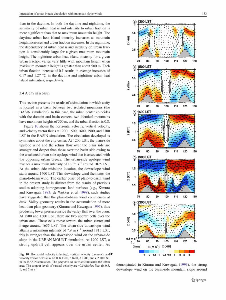
Figure 10 shows the horizontal velocity, vertical velocity,and velocity vector fields at 1200, 1500, 1600, 1900, and 2300LST in the BASIN simulation. The circulation developed issymmetric about the city center. At 1200 LST, the plain-sideupslope wind and the return flow over the plain side arestronger and deeper than those over the basin side owing tothe weakened urban-side upslope wind that is associated withthe opposing urban breeze. The urban-side upslope windreaches a maximum intensity of 1.9 m s−1 around 1025 LST.At the urban-side midslope location, the downslope windstarts around 1400 LST. This downslope wind facilitates theplain-to-basin wind. The earlier onset of plain-to-basin windin the present study is distinct from the results of previousstudies adopting homogeneous land surfaces (e.g., Kimuraand Kuwagata 1993; de Wekker et al. 1998); such studieshave suggested that the plain-to-basin wind commences atdusk. Valley geometry results in the accumulation of moreheat than plain geometry (Kimura and Kuwagata 1995), thusproducing lower pressure inside the valley than over the plain.At 1500 and 1600 LST, there are two updraft cells over theurban area. These cells move toward the urban center andmerge around 1635 LST. The urban-side downslope windattains a maximum intensity of 7.9 m s−1 around 1815 LST;this is stronger than the downslope wind on the urban-sideslope in the URBAN-MOUNT simulation. At 1900 LST, astrong updraft cell appears over the urban center. As

demonstrated in Kimura and Kuwagata (1993), the strongdownslope wind on the basin-side mountain slope around

�Fig. 10 Horizontal velocity (shading), vertical velocity (contour), andvelocity vector fields at a 1200, b 1500, c 1600, d 1900, and e 2300 LSTin the BASIN simulation. The gray box on the x-axis indicates the urbanarea. The contour levels of vertical velocity are −0.5 (dashed line, d), 0.5,1, and 2 m s−1


sunset or after dusk is owing to the plain-to-basin wind as wellas the downslope wind. The transition time from upslope windto downslope wind at the rural-side midslope location in theBASIN simulation is almost the same as that in the URBAN-MOUNTsimulation. The urban-side downslope wind persistslonger than the rural-side downslope wind. Around 1745 LST,hydraulic jumps occur near the mountain–urban edges. Theypersist until 2145 LST. The potential temperature anomalyover the urban area is smaller in the BASIN simulation than inthe URBAN-MOUNT simulation (not shown). This is likelyassociated with stronger plain-to-basin wind from the plainareas in the BASIN simulation, which contributes to coolingof the basin air.

4 Summary and conclusions

The present study examined interactions between urbanbreeze circulation and mountain slope winds in two dimen-sions using the WRF model coupled with an advanced urbancanopymodel. Circulation over the urban area is characterizedby the weakened mountain-side urban wind owing to theopposing upslope wind and the strengthened plain-side urbanwind in the daytime. The transition from upslope wind todownslope wind on the urban-side slope starts earlier thanthat in a simulation that includes only an isolated mountain. Ahydraulic jump is observed in the late afternoon and stagnatesuntil late evening. Extensive numerical experiments wereperformed to examine the sensitivities of the interactionsof urban breeze circulation with mountain slope windsand urban heat island intensity to mountain height andurban fraction. It was found that the transition fromurban-side upslope wind to downslope wind starts ear-lier and that the urban-side downslope wind persistslonger with decreasing mountain height and increasingurban fraction. The change in transition time from up-slope wind to downslope wind affects interactions be-tween urban breeze circulation and mountain slopewinds. Urban heat island intensity was found to bemore sensitive to urban fraction than to mountainheight. Finally, a case in which a city is located in abasin between two identical mountains was examined.Here, the urban-side downslope wind develops earlierand persists longer than the rural-side downslope windand the plain-to-basin wind is stronger than in thesimulation that includes a city and an isolated mountain.

This study investigated the interactions of urban breezecirculation with mountain slope winds in two dimensions. Inthree dimensions, various shapes of urban heat island andmountain can be considered and more complex but morerealistic interactions can be simulated. Thus, extension of thepresent study to three dimensions will be required to further

improve understanding of the interactions between urbanbreeze circulation and mountain slope winds.

Acknowledgments The authors are grateful to two anonymous re-viewers and Jaemyeong Mango Seo for providing valuable commentson this work. This work was funded by the National Research Foundationof Korea (NRF) grant funded by the Korea Ministry of Education,Science and Technology (MEST) (No. 2012-0005674).

References

Chen F, Dudhia J (2001) Coupling an advanced land surface–hydrologymodel with the Penn State–NCAR MM5 modeling system. Part I:model implementation and sensitivity. Mon Weather Rev 129:569–585

Chen SH, Sun WY (2002) A one-dimensional time dependent cloudmodel. J Meteorol Soc Jpn 80:99–118

de Wekker SFJ, Zhong S, Fast JD, Whiteman CD (1998) Anumerical study of the thermally driven plain-to-basin windover idealized basin topographies. J Appl Meteorol 37:606–622

Dudhia J (1989) Numerical study of convection observed during thewinter monsoon experiment using a mesoscale two-dimensionalmodel. J Atmos Sci 46:3077–3107

Fernando HJS (2010) Fluid dynamics of urban atmospheres in complexterrain. Annu Rev Fluid Mech 42:365–389

Hidalgo J, Masson V, Pigeon G (2008a) Urban-breeze circulation duringthe CAPITOUL experiment: numerical simulations. MeteorolAtmos Phys 102:243–262

Hidalgo J, Pigeon G, Masson V (2008b) Urban-breeze circulation duringthe CAPITOUL experiment: observational data analysis approach.Meteorol Atmos Phys 102:223–241

Hong SY, Noh Y, Dudhia J (2006) A new vertical diffusion package withan explicit treatment of entrainment processes. Mon Weather Rev134:2318–2341

Kimura F, Kuwagata T (1993) Thermally induced wind passing fromplain to basin over a mountain range. J Appl Meteorol 32:1538–1547

Kimura F, Kuwagata T (1995) Horizontal heat fluxes over complexterrain computed using a simple mixed-layer model and a numericalmodel. J Appl Meteorol 34:549–558

Lee SH, Kim HD (2010) Modification of nocturnal drainage flow due tourban surface heat flux. Asia-Pac J Atmos Sci 46:453–465

Lee SH, Kimura F (2001) Comparative studies in the local circulationsinduced by land-use and by topography. Bound-Layer Meteorol101:157–182

Lemonsu A,MassonV (2002) Simulation of a summer urban-breeze overParis. Bound-Layer Meteorol 104:463–490

Mlawer EJ, Taubman SJ, Brown PD, Iacono MJ, Clough SA (1997)Radiative transfer for inhomogeneous atmospheres: RRTM, a vali-dated correlated-k model for the longwave. J Geophys Res 102:16663–16682

Ohashi Y, Kida H (2002) Effects of mountains and urban areas ondaytime local-circulations in the Osaka and Kyoto regions. JMeteorol Soc Jpn 80:539–560

Pielke RA (2002) Mesoscale meteorological modeling, 2nd edn.Academic Press, San Diego

Ryu YH, Baik JJ (2013) Daytime local circulations and their interactionsin the Seoul metropolitan area. J Appl Meteorol Climatol 52:784–801


Ryu YH, Baik JJ, Lee SH (2011) A new single-layer urban canopy modelfor use in mesoscale atmospheric models. J Appl Meteorol Climatol50:1773–1794

Ryu YH, Baik JJ, Han JY (2013a) Daytime urban breeze circulation and itsinteraction with convective cells. Q J R Meteorol Soc 139:401–413

Ryu YH, Baik JJ, Kwak KH, Kim S, Moon N (2013b) Impacts of urbanland-surface forcing on ozone air quality in the Seoul metropolitanarea. Atmos Chem Phys 13:2177–2194

Savijarvi H, Liya J (2001) Local winds in a valley city. Bound-LayerMeteorol 100:301–319

Simpson JE (1994) Sea breeze and local winds. Cambridge UniversityPress, New York

Skamarock WC, Klemp JB, Dudhia J, Gill DO, Barker DM, Duda MG,Huang XY, Wang W, Powers JG (2008) A description of theadvanced research WRF version 3. NCAR, Boulder

Wong KK, Dirks RA (1978) Mesoscale perturbations on airflow in theurban mixing layer. J Appl Meteorol 17:677–688

Zhang N, Wang X, Peng Z (2014) Large-eddy simulation of mesoscalecirculations forced in inhomogeneous urban heat island. Bound-Layer Meteorol 151:179–194


ORIGINAL PAPER A numerical study of the interactions of urban breeze circulation with mountain slope...

Documents

Transcript of ORIGINAL PAPER A numerical study of the interactions of urban breeze circulation with mountain slope...