The role of galactic winds in galaxy evolution and formation ...

HAL Id: tel-01772821https://tel.archives-ouvertes.fr/tel-01772821

Submitted on 20 Apr 2018

HAL is a multi-disciplinary open accessarchive for the deposit and dissemination of sci-entific research documents, whether they are pub-lished or not. The documents may come fromteaching and research institutions in France orabroad, or from public or private research centers.

L’archive ouverte pluridisciplinaire HAL, estdestinée au dépôt et à la diffusion de documentsscientifiques de niveau recherche, publiés ou non,émanant des établissements d’enseignement et derecherche français ou étrangers, des laboratoirespublics ou privés.

The role of galactic winds in galaxy evolution andformation using 3D spectroscopy

Ilane Schroetter

To cite this version:Ilane Schroetter. The role of galactic winds in galaxy evolution and formation using 3D spec-troscopy. Astrophysics [astro-ph]. Université Paul Sabatier - Toulouse III, 2017. English. NNT :2017TOU30012. tel-01772821

https://tel.archives-ouvertes.fr/tel-01772821

https://hal.archives-ouvertes.fr

THESETHESEEn vue de l’obtention du

DOCTORAT DE L’UNIVERSITE DE TOULOUSE

Delivre par : l’Universite Toulouse 3 Paul Sabatier (UT3 Paul Sabatier)

Presentee et soutenue le 05/01/2017 par :Ilane SCHROETTER

La formation et l’evolution des galaxies grace a la spectroscopie 3D : lerole des vents

JURYRoser PELLO Astronome Presidente du JuryFrederic BOURNAUD Ingenieur chercheur RapporteurDaniel SCHAERER Professeur adjoint RapporteurPhilippe AMRAM Professeur ExaminateurNicolas BOUCHE Charge de recherche Directeur de theseThierry CONTINI Directeur de recherche Co-directeur de these

Ecole doctorale et specialite :SDU2E : Astrophysique, Sciences de l’Espace, Planetologie

Unite de Recherche :Institut de Recherche en Astrophysique et Planetologie (UMR 5277)

Directeur(s) de These :Nicolas BOUCHE et Thierry CONTINI

Rapporteurs :Frederic BOURNAUD et Daniel SCHAERER

Acknowledgments

i

Abstract

0.1 French version

Le modele cosmolgique standard Λ-CDM est celui qui connaıt le plus grand succesdans la cosmologie moderne. Pourtant, malgre sa capacite a expliquer la domina-tion de la matiere noire sur la structuration de l’univers a grande echelle, il echoue,parfois dramatiquement, lorsque la physique complexe de la matiere baryoniqueentre en jeu. En particulier, l’une des plus grandes questions restant encore sansreponse concerne la difference importante entre la quantite de matiere baryoniquepredite et celle reellement observee dans les halos de galaxies de faible et de grandemasse (e.g. Behroozi et al., 2013b). Les modeles theoriques predisent beaucouptrop de masse compare a ce qui est veritablement observe, ce qui mene a la con-clusion qu’il existe des mecanismes permettant d’ejecter une partie du reservoir dematiere baryonique des galaxies, ce qui affectera donc leur evolution. En d’autrestermes, si nous voulons comprendre l’evolution des galaxies, il est essentiel decomprendre de maniere precise comment ces galaxies perdent une partie de leurmatiere baryonique.

Pour les galaxies de faibles masses, un ingredient cle est contenu dans les ventsproduits par les explosions de supernovae (Dekel & Silk, 1986). Non seulement cesvents peuvent etre efficaces pour ejecter le gaz et les metaux du disque galactique,pour enrichir le milieu inter-galactique en elements lourds (Oppenheimer et al.,2010), mais ils sont aussi observes dans presque toutes les galaxies a formationd’etoiles (Veilleux et al., 2005a), ce qui donne a ces vents un role important con-cernant le cycle de la matiere dans les galaxies. Notre connaissance incompleteconcernant les relations entre la galaxie et les proprietes du gaz qu’elle ejecte,comme le lien entre le taux de formation stellaire (SFR) et la quantite de masseejectee Mout, limite notre capacite a produire des simulations numeriques precisessur l’evolution des galaxies.

L’objectif de cette these est de quantifier les proprietes des vents galactiquesen utilisant des quasars en arriere plan et la spectroscopie 3D. Afin d’y parvenir,nous utiliserons une quantite importante de donnees provenant de plusieurs in-struments (SDSS, LRIS au Keck, SINFONI, UVES et MUSE au VLT). Grace acette nouvelle strategie d’observation et l’utilisation d’instruments de pointe, nous

iii

avons pu augmenter l’echantillon d’un ordre de grandeur et ainsi obtenir de bienmeilleures contraintes sur les proprietes du gaz qui s’echappe des galaxies de faiblemasse.

0.2 English version

The Λ-CDM model is one of the most resounding triumphs of modern cosmol-ogy. Yet, even though it is immensely successful at explaining the dark matterdominated large scale structures, it fails, sometimes dramatically, when the com-plex physics of baryonic matter comes into play. In particular, one of the majorremaining discrepancies is between the observed and predicted baryonic densitiesof the dark matter halos of galaxies both in the high mass and low mass regimes(e.g. Behroozi et al., 2013b). Theoretical models predict much more mass thanis actually observed, leading to the conclusion that there are mechanisms at playejecting part of the baryonic matter reservoir from galaxies and therefore affectingtheir evolution. In other words, if we want to understand the evolution of galaxies,it is essential to understand precisely how galaxies lose a fraction of their baryonicmatter.

For low mass galaxies, a key part of the solution lies on supernovae-drivenoutflows (Dekel & Silk, 1986). Not only can such outflows efficiently expel gasand metals from galactic disks, enriching the inter-galactic medium (Oppenheimeret al., 2010), they are also observed in almost every star-forming galaxy (Veilleuxet al., 2005a), making them an important part of the matter cycle of galaxiesin general. Our incomplete knowledge of scaling relations between galaxies andthe properties of their outflowing material, such as between the star formationrate (SFR) and the ejected mass rate Mout, limits our ability to produce accuratenumerical simulations of galaxy evolution.

The objective of this thesis is to quantify galactic wind properties using back-ground quasars and 3D spectroscopy. In order to achieve our goal, we use largedata sets from several instruments (SDSS, LRIS at Keck, SINFONI, UVES andMUSE on VLT).

After developing observational strategies in order to have the largest data setpossible with this technique, we increased the number of observations by 1 orderof magnitude which resulted in better constraints on the outflowing materials forthe low mass galaxies.

iv

Contents

Acknowledgments i

Abstract iii0.1 French version . . . . . . . . . . . . . . . . . . . . . . . . . . . . . . iii0.2 English version . . . . . . . . . . . . . . . . . . . . . . . . . . . . . iv

Introduction xxiii0.3 French version . . . . . . . . . . . . . . . . . . . . . . . . . . . . . . xxiii0.4 English version . . . . . . . . . . . . . . . . . . . . . . . . . . . . . xxvi

1 General context 11.1 Galaxy formation and evolution . . . . . . . . . . . . . . . . . . . . 2

1.1.1 What is a galaxy? . . . . . . . . . . . . . . . . . . . . . . . . 21.1.2 Galaxy spectrum . . . . . . . . . . . . . . . . . . . . . . . . 21.1.3 Star formation in galaxies . . . . . . . . . . . . . . . . . . . 4

1.2 Galaxy and cosmology fundamentals . . . . . . . . . . . . . . . . . 81.2.1 Cosmology fundamentals . . . . . . . . . . . . . . . . . . . . 81.2.2 Galaxy fundamentals . . . . . . . . . . . . . . . . . . . . . . 101.2.3 The Tully-Fisher relation and other mass estimator . . . . . 141.2.4 The galaxy “main sequence” . . . . . . . . . . . . . . . . . . 151.2.5 What is a quasar? . . . . . . . . . . . . . . . . . . . . . . . 161.2.6 The low efficiency of galaxy formation . . . . . . . . . . . . 16

1.3 Galactic winds “state of the art” . . . . . . . . . . . . . . . . . . . . 181.3.1 Galactic winds are multi-phased and collimated . . . . . . . 191.3.2 Wind properties in emission . . . . . . . . . . . . . . . . . . 221.3.3 Wind properties in absorption . . . . . . . . . . . . . . . . . 231.3.4 Wind properties using background sources . . . . . . . . . . 251.3.5 Perspective from numerical simulations . . . . . . . . . . . . 25

2 Observational strategy and sample selection 292.1 The background quasar methodology . . . . . . . . . . . . . . . . . 30

2.1.1 Observational strategies . . . . . . . . . . . . . . . . . . . . 30

v

2.1.2 Why do we need integral field spectroscopy? . . . . . . . . . 312.1.3 Critical parameters derived from IFUs . . . . . . . . . . . . 322.1.4 A 3D fitting tool: GalPaK3D . . . . . . . . . . . . . . . . . . 33

2.2 The SINFONI Mg ii Program for Line Emitters (SIMPLE) sample . 332.2.1 Selection criteria . . . . . . . . . . . . . . . . . . . . . . . . 332.2.2 Sample description . . . . . . . . . . . . . . . . . . . . . . . 34

2.3 The MUSE GAs Flow and Wind (MEGAFLOW) survey . . . . . . 352.3.1 Selection criterion . . . . . . . . . . . . . . . . . . . . . . . . 352.3.2 Sample description . . . . . . . . . . . . . . . . . . . . . . . 35

3 Data acquisition and reduction 393.1 SIMPLE observations and data reduction . . . . . . . . . . . . . . . 403.2 MUSE observations and data reduction . . . . . . . . . . . . . . . . 41

3.2.1 GTO observations . . . . . . . . . . . . . . . . . . . . . . . 413.2.2 Pre-processing data reduction . . . . . . . . . . . . . . . . . 413.2.3 Science reduction . . . . . . . . . . . . . . . . . . . . . . . . 433.2.4 Post-processing reduction . . . . . . . . . . . . . . . . . . . 443.2.5 Exposures combination . . . . . . . . . . . . . . . . . . . . . 463.2.6 Sky emission lines removal . . . . . . . . . . . . . . . . . . . 46

4 Data analysis 474.1 Methodology . . . . . . . . . . . . . . . . . . . . . . . . . . . . . . 48

4.1.1 Estimate of Star Formation Rate (SFR) . . . . . . . . . . . 484.1.2 A simple cone model for galactic winds . . . . . . . . . . . . 49

4.2 SIMPLE sample . . . . . . . . . . . . . . . . . . . . . . . . . . . . . 534.2.1 Morpho-kinematics from GalPaK3D . . . . . . . . . . . . . . 534.2.2 Galaxy-quasar pairs classification . . . . . . . . . . . . . . . 544.2.3 Outflow properties . . . . . . . . . . . . . . . . . . . . . . . 54

4.3 MEGAFLOW survey . . . . . . . . . . . . . . . . . . . . . . . . . . 604.3.1 Survey status . . . . . . . . . . . . . . . . . . . . . . . . . . 604.3.2 Morpho-kinematics from GalPaK3D . . . . . . . . . . . . . . 604.3.3 Galaxy-quasar pairs classification . . . . . . . . . . . . . . . 664.3.4 Outflow properties . . . . . . . . . . . . . . . . . . . . . . . 67

5 Combining both samples: galactic wind properties as a functionof galaxy properties 775.1 Basic properties of the sampled galaxies . . . . . . . . . . . . . . . 78

5.1.1 Galaxy redshift distribution . . . . . . . . . . . . . . . . . . 785.1.2 Galaxy stellar mass measurement . . . . . . . . . . . . . . . 79

5.2 How far do winds go? . . . . . . . . . . . . . . . . . . . . . . . . . . 825.3 Do winds escape? . . . . . . . . . . . . . . . . . . . . . . . . . . . . 845.4 Wind scaling relations . . . . . . . . . . . . . . . . . . . . . . . . . 86

vi

5.4.1 Previous studies on galactic winds . . . . . . . . . . . . . . . 865.4.2 Scaling relations involving Vout . . . . . . . . . . . . . . . . . 905.4.3 Scaling relations involving Mout . . . . . . . . . . . . . . . . 925.4.4 Scaling relations on loading factor η . . . . . . . . . . . . . . 92

5.5 What mechanisms drive galactic winds? . . . . . . . . . . . . . . . 95

6 Conclusions and perspectives 996.1 French version . . . . . . . . . . . . . . . . . . . . . . . . . . . . . . 100

6.1.1 Conclusions de these . . . . . . . . . . . . . . . . . . . . . . 1006.1.2 Perspectives . . . . . . . . . . . . . . . . . . . . . . . . . . . 102

6.2 English version . . . . . . . . . . . . . . . . . . . . . . . . . . . . . 1036.2.1 Thesis conclusions . . . . . . . . . . . . . . . . . . . . . . . 1036.2.2 Perspectives . . . . . . . . . . . . . . . . . . . . . . . . . . . 104

A Schroetter et al. 2015: The SINFONI Mg ii Program for LineEmitters (SIMPLE) II: background quasar probing z∼1 galacticwinds 113

B Schroetter et al. 2016: MusE GAs FLOw and Wind (MEGAFLOW):first MUSE results on background quasars 133

vii

List of Tables

4.1 Kinematic and morphological parameters for the 10 SIMPLE galaxy-quasar pairs. . . . . . . . . . . . . . . . . . . . . . . . . . . . . . . 54

4.2 Results for galaxies J0448+0950, J2357-2736, J0839+1112. . . . . . 574.3 MEGAFLOW survey status. . . . . . . . . . . . . . . . . . . . . . . 624.4 GalPaK3D results on 26 MEGAFLOW galaxies with reliable morpho-

kinematic parameters. . . . . . . . . . . . . . . . . . . . . . . . . . 654.5 Results on outflow properties for MEGAFLOW galaxies. . . . . . . 75

5.1 Summary of other wind studies . . . . . . . . . . . . . . . . . . . . 87

ix

List of Figures

1 Scheme of the fraction of baryons versus galaxy halo mass. Thepredicted amount is represented by the dashed black curve whereasthe observations are represented by the green one. We can see thetwo major problems : the global shift between observations andtheory as well as the two cutoffs at low and high mass regimes. Thetwo phenomena invoked to explain these cutoffs are Active GalacticNuclei (AGN in blue) for the high mass regime and galactic winds(in red) for low mass galaxies. . . . . . . . . . . . . . . . . . . . . xxv

1.1 Scheme of electron excitation. A coming photon (on left) will: (1)give energy to the electron (represented in dark gray). The electronwill go to the next atomic level (2) in an excited state (top right). Itwill then unleash the excess energy as an emitted photon (bottomright) and come back to its initial atomic level. . . . . . . . . . . . 3

1.2 Representation of three types of galaxy spectra with the principleemission lines: the red spectrum at the bottom represents an early-type galaxy spectrum with no emission lines, as this type of galaxydoes not form stars anymore. We can see the Lyman break (at ∼1200 A) as well as the Balmer break (∼4000 A). The middle spec-trum (in blue) represents a late-type galaxy: this type of galaxy isstill forming stars and has a bright blue continuum as well as emis-sion lines. The top spectrum represents a low-mass galaxy spectra,it does not have a continuum but we clearly see the main emis-sion lines tracing star formation: Lyα(λ1216), C iii](λ1909), [O ii](λλ3727, 3729), Hδ (λ4102), Hβ (λ4862), [O iii] (λλ4960, 5008), [N ii](λλ6549, 6585), Hα (λ6564) and [S ii] (λ6718). . . . . . . . . . . . . 5

xi

1.3 Scheme of the Doppler effect: The observer is represented by tele-scopes on the left. The top row represents a galaxy emitting at awavelength in green. This galaxy is not moving so the observedwavelength is the same as the emitted wavelength. The middle rowshows a galaxy moving towards the observer and thus the observedwavelength is compressed as compared to the emitted one, we callthat shift a blue-shift. The bottom row represent a galaxy mov-ing away from us and thus the observed wavelength is diluted ascompared to the emitted one, the wavelength is thus red-shifted. . 6

1.4 The star formation rate density (SFRD) as a function of redshift.We can see that the SFRD increases from high redshift to peak atredshift z ∼ 2 − 3 and then drops to redshift z = 0. This figure isfrom Madau & Dickinson (2014). . . . . . . . . . . . . . . . . . . . 8

1.5 The anisotropies of the Cosmic microwave background (CMB) asobserved by Planck. The CMB is a snapshot of the oldest light in ourUniverse, imprinted on the sky when the Universe was just 380 000years old. It shows tiny temperature fluctuations that correspondto regions of slightly different densities, representing the seeds of allfuture structure: the stars and galaxies of today. Copyright: ESAand the Planck Collaboration. . . . . . . . . . . . . . . . . . . . . 9

1.6 Scheme of Hubble classification for galaxy morphologies. . . . . . . 11

1.7 Scheme of a galaxy in rotation. The galaxy is in black and is rep-resented on the sky plane x, y (y representing the celestial north).This galaxy has a position angle PA which is the angle between thecelestial north and the major axis of the galaxy. At the bottom,we can see 3 Gaussians on a wavelength axis (λ) corresponding toemission lines in 3 different regions of the galaxy. The left part ofthe galaxy is moving towards us, so its emission line is blue-shifted,its middle do not move with respect to its systemic velocity and theright part is moving away from us, so its emission line is red-shifted. 13

1.8 SDSS transmission curves for the different filters. . . . . . . . . . . 14

1.9 Scheme of the galaxy “main sequence” in blue as well as outliers:starbursts above this main sequence (purple) and red or dead (notforming stars anymore) galaxies (red). Space between the mainsequence and red galaxies is called the green valley. . . . . . . . . . 15

1.10 Scheme of a typical quasar spectrum. . . . . . . . . . . . . . . . . . 17

xii

1.11 Figure from Papastergis et al. (2012). The ratio of galactic stellarmass to halo mass as a function of host halo mass (M∗/Mh −Mh

relation). The thick yellow line shows Papastergis et al. (2012)main result, obtained from abundance matching the stellar massfunction of optically-selected sample with the halo mass functionincluding subhaloes. The dotted-dashed horizontal line shows thecosmic baryon fraction fb ≈ 0.16. . . . . . . . . . . . . . . . . . . . 18

1.12 The galaxy M82 in visible wavelength, taken with HST. We can seethat this galaxy is almost edge-on, in white we see the stars andgas contributions and the dust is shown in dark filaments along thegalaxy. . . . . . . . . . . . . . . . . . . . . . . . . . . . . . . . . . 19

1.13 On left panel, the galaxy M82 in B,V (blue and visible) combinedwith Hα, taken with the Subaru telescope. Like Figure 1.12, we seethe disk of the galaxy (B and V filters) in white. In addition, theHα is represented in red. We see the presence of this ionized gasperpendicular to the galactic disk. Hence, these outflows appear tobe collimated in a cone. This gas is a direct imaging of galacticwinds. On right panel, the galaxy M82 in X-ray, taken with theChandra telescope. Unlike Figure 1.12 and left panel of this figure,we do not see the disk of the galaxy. We can, however, see the hotgas at almost the same location where we see the Hα gas on leftpanel. Again, we can see the conical structure of these outflows. . . 20

1.14 Other examples of galactic outflows seen in emission in local galaxiesNGC 253, NGC 1482 and NGC 3079. On each of these galaxieswe have a zoom of their center which clearly show the presence ofoutflows. Like M82, these outflows are ejected perpendicular to thegalactic disk. Hence, we clearly see (especially for NGC 1482 and3079) that galactic winds are likely collimated in a cone. . . . . . . 21

1.15 Scheme of the blue-shifted component for Hα and [N ii] produced bygalactic outflows. The green Gaussian correspond to the systemic(narrow) component and the broad component is shown in blue.The velocity difference (corresponding to the outflow velocity) be-tween the two components is shown by the label ∆V . . . . . . . . 22

1.16 Outflow absorption lines seen in a galaxy spectrum from Heckmanet al. (2015). This absorption is blue-shifted with respect to thegalaxy systemic velocity. We can also see that the different absorp-tion lines have the same absorption behavior like their asymmetry. 24

1.17 Loading factor as a function of galaxy rotational velocity (bottom xaxis) and halo mass (top x axis) assumed by theoretical/empiricalmodels. . . . . . . . . . . . . . . . . . . . . . . . . . . . . . . . . . 26

xiii

2.1 Scheme of an 3D IFU cube: the foreground image represents awhite-light image of the cube and the extracted image representsa slide of the cube at a given wavelength. On this extracted im-age one can see only one galaxy which is emitting at the extractedwavelength. . . . . . . . . . . . . . . . . . . . . . . . . . . . . . . . 31

2.2 Scheme geometry configuration: the quasar LOS, represented bythe yellow star, is crossing galactic outflows represented by the redcrosses getting out of the galaxies. The Azimuthal angle is repre-sented by the blue cross going from the galaxy major axis to thequasar LOS. b represents the impact parameter for the galaxy−quasarpair, represented by the light green cross showing the distance be-tween the galaxy center and the quasar LOS. . . . . . . . . . . . . . 32

2.3 W λ2796r as a function of impact parameter b for galaxy-quasar pairs

classified as wind-pairs. The red colored area shows the selectioncriterion of the SIMPLE sample (W λ2796

r > 2.0A). . . . . . . . . . 34

2.4 Scheme of our target strategy: the quasar LOS, represented by theyellow arrow heading toward the telescope, is crossing two galacticoutflows represented by the red arrows getting out of the galaxies.These galactic outflows are absorbing a portion of the quasar spec-tra which gives the two Mg ii absorption systems at two differentredshifts. b represents the impact parameter for one galaxy−quasarpair. . . . . . . . . . . . . . . . . . . . . . . . . . . . . . . . . . . . 36

2.5 W λ2796r as a function of impact parameter b for galaxy-quasar pairs

classified as wind-pairs. Horizontal dashed black lines shows theW λ2796r > 0.5A and W λ2796

r > 0.8A selection criteria. . . . . . . . . 37

2.6 Redshift distribution of MEGAFLOW galaxies. . . . . . . . . . . . 38

3.1 Association map for the basic science data reduction. This diagramshows the part of the pipeline that operates on the basis of a singleIFU. . . . . . . . . . . . . . . . . . . . . . . . . . . . . . . . . . . . 42

3.2 Association map for the second part of the science data reduction.This part of the pipeline deals with data of all 24 IFUs simultane-ously. . . . . . . . . . . . . . . . . . . . . . . . . . . . . . . . . . . 45

xiv

4.1 Representation of a galaxy position angle (PA) and inclination (i).Top left: sky plane (x, y) representation of the PA of a galaxy.This angle is defined to be the angle between the “y” axis (pointingthe North) and the galaxy major axis. The galaxy PA is usuallygiven positive towards the East. Bottom right: side view (y, z) ofa galaxy inclined with the i angle. The inclination of a galaxy isdefined to be the angle between the disk plane (y, z) and the skyplane (y, x). The telescope on the left is to better illustrate the sideview: the black arrow pointing to the telescope represents the lineof sight, the z axis represents the depth. . . . . . . . . . . . . . . . 50

4.2 Wind model principle description. On the left side one can see ageometric representation of a galaxy-quasar system. The observeris on the left, the background quasar is represented by the yellowstar labeled “QSO”. The quasar LOS is crossing galactic outflows(red). We fill particles inside the cone with a constant radial velocityVout (blue arrows). We project the velocities on the quasar LOS toend up with a simulated profile (absorption profile on the top rightside). We compare this profile with the data (bottom absorptionprofile, UVES data), and we fit the data by changing Vout or thecone opening angle (θmax). For this case, Vout = 115 ± 10 km s−1

and θmax= 40± 5. . . . . . . . . . . . . . . . . . . . . . . . . . . . 51

4.3 Examples of simulated absorption profiles with different galaxy in-clinations (i), opening angle (θ) and wind velocities (Vout): whileeach of the simulated profiles has the same number of particles, theapparent depth decreases as each parameter increases due to largervelocity projections for i and θ, and larger range of velocities forVout. Top row: absorption profiles for galaxies inclined at 30, 60and 90 degrees with Vout= 100 km s−1and θ= 30. The noise effectis due to the Monte Carlo distribution of particles. Middle row: ab-sorption profiles for wind cones with opening angles of 30, 40 and 45degrees with Vout= 100 km s−1and i=45. Bottom row: absorptionprofiles with wind velocities of 50, 100 and 150 km s−1with i= 45degrees and θ= 30. Each simulated profile has the same amountof particles but show a larger velocity range due to the increasinggas speed, hence the varying apparent depths. . . . . . . . . . . . . 52

4.4 Zoom of QSO-subtracted Hα maps of the 10 SIMPLE galaxies:quasar LOS is represented by the white contours if present or pointedout with a white arrow. The 4 wind-pairs are framed with a blackrectangle. . . . . . . . . . . . . . . . . . . . . . . . . . . . . . . . . 55

xv

4.5 Galaxy inclinations for the SIMPLE sample as a function of theazimuthal angle α. Note there are three types of galaxies in thissample: the wind-pairs which have an azimuthal angle larger than60±10, the inflow-pairs with α lower than 60±10 and pairs thatare ambiguous due to uncertainty on α. It is difficult to derivethe azimuthal angle for a nearly face-on galaxy. The wind-pair andinflow-pair classes describe the fact of having the quasar absorptionstracing outflows and inflows, respectively. . . . . . . . . . . . . . . 56

4.6 Left column: from top to bottom: simulated absorption profileswith r0=1,5,10 kpc. Notice that the asymmetry changes as r0 in-creases, it goes from outward to inward asymmetry. Right column:The velocity profile corresponding to the associated simulated pro-file to the left where the turn over radius of the velocity profile(r0) varies, from top to bottom: r0=1,5,10 kpc. The red dashedline represents the distance between the galaxy and the quasar LOS(b/sin(α)/sin(i)), corrected for the inclination i. . . . . . . . . . . . 58

4.7 Wind models for the three wind-pairs. The bottom row correspondsto UVES quasar Mg i λ2852 absorption lines for the three fields:J0448+0950, J0839+1112 and J2357−2736 from left to right. Theupper row shows the resulting simulated profiles for each case. Onecan see that we reproduce the equivalent widths and the profileasymmetries for each galaxy. Note that we do not reproduce thedepth as the simulated profile is normalized ’by hand’. On eachsimulated profile, the red lines correspond to the wind contributiononly whereas the black part corresponds to the galaxy component. 59

4.8 Comparison of predicted mass loading factors from theoretical/empiricalmodels (curves) with values derived from observations (dots and tri-angles) as a function of the maximum rotational velocity. The re-sults from the SIMPLE sample are represented by the cyan circles(Schroetter et al., 2015). The red circle shows the mass loading fac-tor for a z ∼ 0.2 galaxy (Kacprzak et al., 2014). The triangles showthe results for z ∼ 0.2 galaxies from Bouche et al. (2012). The graytriangles show the galaxies with quasars located at >60kpc wherethe mass loading factor is less reliable due to the large travel timeneeded for the outflow to cross the quasar LOS (several 100 Myr)compared to the short time scale of the Hα derived SFR (∼ 10Myr).The upper halo mass axis is scaled on Vmax at redshift 0.8 from Mo& White (2002). . . . . . . . . . . . . . . . . . . . . . . . . . . . . 61

xvi

4.9 Results for 10 MEGAFLOW galaxies: Each set of result for a galaxyis composed of 3 maps: left: zoom of QSO-subtracted [O ii] maps.On each of these maps, on top of them is indicated the redshift ofthe galaxy and at the bottom the quasar field name. Middle: zoomof QSO-subtracted Camel velocity map. Right: Zoom of QSO-subtracted GalPaK3D PSF-deconvolved velocity map. Wind-pairsare framed with a red rectangles for Camel and GalPaK3D velocitymaps. . . . . . . . . . . . . . . . . . . . . . . . . . . . . . . . . . . 63

4.10 Same as Figure 4.9 for the 10 next galaxies. . . . . . . . . . . . . . 644.11 Same as Figure 4.9 for the last 6 galaxies. . . . . . . . . . . . . . . 644.12 Galaxy inclination as a function of azimuthal angle α for 26 galaxies

with reliable morpho-kinematic parameters detected in the MUSEfields. The dashed areas correspond to azimuthal angle ranges forwhich we classify pairs as inflow-pairs (blue and narrow dashes) orwind-pairs (green and wider dashes). These areas stop for face-ongalaxies as uncertainty on position angles are too large. It is thusdifficult to determine α and to classify galaxy-quasar pairs in thisarea. We note that 11 galaxies are classified as wind-pairs. . . . . . 66

4.13 Azimuthal angle α distribution for 26 galaxies with reliable morpho-kinematic parameters detected in the MUSE fields. We note that11 galaxies are classified as wind-pairs and that there is a bimodaldistribution of α. There are more galaxy-quasar pairs in a config-uration favorable for wind study.. This is probably due to the factthat we select only strong Mg ii REW in the quasar spectra and thelargest Wλ2796

r tend to be associated with outflows (e.g. Kacprzaket al., 2011; Lan et al., 2014a). . . . . . . . . . . . . . . . . . . . . 67

4.14 Representation of simulated profile and quasar spectrum associatedwith the J0014−0028 galaxy. Simulated wind profile (top) repro-ducing the Mg i absorption profile (centered at z = 0.8343) fromUVES (bottom). This outflow has a Vout of 210± 10 km s−1 and anopening angle θmax of 25± 5. . . . . . . . . . . . . . . . . . . . . 69

4.15 Same as Figure 4.14 but for the J0937+0656 galaxy at redshift z ≈0.9340. This outflow has a Vout of 150± 10 km s−1 and an openingangle θmax of 30± 5 for the galaxy at redshift z = 0.9340. . . . . . 70

4.16 Same as Figure 4.14 but for the J1039+0714 galaxy at redshift z ≈0.9495. This outflow has a Vout of 65 ± 10 km s−1 and an openingangle θmax of 30± 5 for this galaxy. . . . . . . . . . . . . . . . . . 70


xvii


4.19 Same as Figure 4.14 but for the J0131+1303 galaxies at redshiftz ≈ 1.0106. For this case, because two galaxies were detected at theabsorber redshift, we needed to run wind models for both of them(at redshift 1.0106 and 1.0108) in order to reproduce the absorptionlines in red. The outflow in green has a Vout of 205 ± 10 km s−1

and an opening angle θmax of 35 ± 5 for the galaxy at redshiftz = 1.0108. The outflow in black has a Vout of 80 ± 10 km s−1 andan opening angle θmax of 35 ± 5 and θin of 8±2 for the galaxy atredshift z = 1.0106. . . . . . . . . . . . . . . . . . . . . . . . . . . 72

4.20 Same as Figure 4.19 but for the J0937+0656 galaxies at redshift z ≈0.7024. The outflow in green (the positive absorption component)has a Vout of 100±10 km s−1 and an opening angle θmax of 30±5 forthe galaxy at redshift z = 0.7022 (this pair has an azimuthal angle αof 55). The outflow in black (the negative absorption components)has a Vout of 120± 10 km s−1 and an opening angle θmax of 35± 5and θin of 8±2 for the galaxy at redshift z = 0.7024 (his pair hasan azimuthal angle α of 84). Results on these two pairs are shownin Tables 4.4 and 4.5. . . . . . . . . . . . . . . . . . . . . . . . . . 73

4.21 Same as Figure 4.14 but for the J1107+1757 galaxy at redshift z ≈1.1620. This outflow has a Vout of 150± 10 km s−1 and an openingangle θmax of 30± 5 and θin of 20±2 for this galaxy. . . . . . . . 73

4.22 Same as Figure 4.14 but for the J1314+0657 galaxy at redshift z ≈0.9085. This outflow has a Vout of 210± 10 km s−1 and an openingangle θmax of 30± 5 and θin of 7±2 for this galaxy. . . . . . . . . 74

4.23 Same as Figure 4.14 but for the J2152+0625 galaxy at redshift z ≈1.3185. This outflow has a Vout of 150± 10 km s−1 and an openingangle θmax of 20± 5 and θin of 7±2 for this galaxy. . . . . . . . . 74

5.1 Redshift distribution of the 36 galaxies from SIMPLE and MEGAFLOW.78

5.2 V/σ distribution of all the galaxies from both surveys. Orange col-ored bar represents dispersion-dominated galaxies (V/σ < 1). . . . 80

5.3 Galaxy stellar mass as a function of the S0.5 parameter for HDFS,SINS and MASSIV data. The dashed red line represent a fit withcoefficients shown in the legend. . . . . . . . . . . . . . . . . . . . 81

xviii

5.4 Star formation rate as a function of galaxy stellar mass (bottomx-axis) and S0.5 (top x-axis) for our surveys. MUSE-HDFS observa-tion from Contini et al. (2016) has been added in order to place oursurvey in a more general context. Galaxies with 1.0 < z < 1.5 arerepresented in red for our surveys. The two dashed lines representthe empirical relations between SFR and stellar mass for differentredshifts between 0.5 < z < 1.5 from Whitaker et al. (2014). . . . . 82

5.5 Azimuthal angle distribution of all the galaxies from SIMPLE andMEGAFLOW. We note the bimodal distribution of the whole survey. 83

5.6 Mg ii (λ2796) rest equivalent width as a function of impact param-eter b for galaxy-quasar pairs classified as wind-pairs. Horizontaldashed black lines shows the W λ2796

r > 0.5A and W λ2796r > 0.8A

selection criteria. The thick black dashed line represent a fit to thedata. Fitting coefficients are shown in the legend. Errors on W λ2796

r

are typically ∼ 10−3 A and ∼ 0.5 kpc for b. . . . . . . . . . . . . . 84

5.7 Left: Mg ii (λ2796) rest equivalent width as a function of impactparameter b for galaxy-quasar pairs classified as inflow-pairs. Right:same as left panel with the W λ2796

r normalized by the disk pathlength X = X0/ cos(i) where i is the galaxy inclination and X0is a normalization factor, taken as X0 = cos(60). The thick blackdashed line represent a fit to the data. Fitting coefficients are shownin the legend. Errors on W λ2796

r are typically ∼ 10−3 A and ∼ 0.5kpc for b. . . . . . . . . . . . . . . . . . . . . . . . . . . . . . . . . 85

5.8 Vout/Vesc as a function of S0.5 (bottom x-axis) and M? (top x-axis).Yellow triangles are from Bouche et al. (2012), cyan and red circlesare from Schroetter et al. (2015) and Schroetter et al. (2016) respec-tively. The horizontal line corresponds to Vout = Vesc. The dashedblack line corresponds to a fit with coefficients shown in the legend. 86

xix

5.9 Scheme of the two main technique to study outflowing materials inabsorption. On the right part of this scheme, we can see a star-forming galaxy (in black) ejecting gas in a cone (represented by thetwo red arrows). The horizontal dark blue arrow represents the LOSas used in Heckman et al. (2015). In this LOS type observation,the galaxy is face-on and the outflowing gas creates blue-shiftedabsorption lines in the galaxy spectrum. This absorption profile isrepresented on top of the telescope on the left in dark blue. Wecan see that this absorption profile is asymmetric, only blue-shifted(on the left of the systemic velocity, represented by the 0 verticaldashed line) and with an outflow velocity corresponding to wherethe absorption crosses the galaxy continuum. On the right partof this figure, the light blue vertical arrow represent a quasar (theyellow star labeled “QSO”) LOS crossing the outflowing materialof the same galaxy. This configuration represent our backgroundquasar technique and the galaxy is seen as edge-on. The projectedvelocities onto this LOS creates an absorption profile representedin light blue at the bottom of the figure. This absorption profile issymmetric and centered on the galaxy systemic velocity. . . . . . . 89

5.10 Vout as a function of SFR for both surveys (MEGAFLOW andSIMPLE) as well as observations from Bouche et al. (2012) andHeckman et al. (2015). The dashed black line show a fit (log V =(0.35± 0.06) log(SFR) + (1.56± 0.13)) from Martin (2005). Errorson Heckman et al. (2015) observations are 0.2 dex for SFR and 0.05dex for Vout. . . . . . . . . . . . . . . . . . . . . . . . . . . . . . . 91

5.11 Ejected mass rate as a function of star formation rate (left) andstar formation rate by surface area (ΣSFR, right) for both surveys(MEGAFLOW and SIMPLE) as well as observations from Boucheet al. (2012). On left panel, the dashed red line shows a predictionMout ∝ SFR0.7 from Hopkins et al. (2012) model. On left panel,the black line shows Mout ∝ SFR1.11 from Arribas et al. (2014). theblue dotted line correspond to a loading factor (Mout/SFR) equals2. Errors for Heckman et al. (2015) are 0.25 dex for Mout and 0.2dex for SFR and ΣSFR. . . . . . . . . . . . . . . . . . . . . . . . . 93

xx

5.12 η as a function of SFR (left) and ΣSFR (right) for both surveys(MEGAFLOW and SIMPLE) as well as observations from Boucheet al. (2012) and Heckman et al. (2015). On left panel, the dashedred line shows a fit η ∝ SFR−0.3 from Hopkins et al. (2012) and theblack line shows a fit η ∝ SFR0.11 from Arribas et al. (2014). Onright panel, the dashed red line shows a fit η ∝ Σ−1/2

SFR from Hopkinset al. (2012) and the black line shows a fit η ∝ Σ0.17

SFR from Arribaset al. (2014). Again, errors for Heckman et al. (2015) are 0.2 dexfor SFR (and ΣSFR) and 0.45 dex for η. . . . . . . . . . . . . . . . 94

5.13 η as a function of S0.5 for both surveys (MEGAFLOW and SIMPLE)as well as observations from Bouche et al. (2012) and Heckman et al.(2015). The dashed red line shows a fit η ∝ S−1.2

0.5 from Hopkins et al.(2012). The black line shows η ∝ V −2. Errors on Heckman et al.(2015) are 0.45 dex for η and 0.1 dex for Vmax. . . . . . . . . . . . 96

5.14 Comparison of mass loading factors assumed by theoretical/empiricalmodels (curves) with values derived from background quasar obser-vations (dots and triangles) as a function of the maximum rotationalvelocity. MEGAFLOW results are represented by the blue squares.The result from Schroetter et al. (2016) is represented by the redcircle. Arrows represent the loading factors of the galaxies withthe subtracted mass from the inner cone models. The cyan circlesshow the results for galaxies at z ≈ 0.8 from Schroetter et al. (2015).The green square shows the mass loading factor for a z ≈ 0.2 galaxy(Kacprzak et al., 2014). The triangles show the results for z ≈ 0.2galaxies from Bouche et al. (2012). The gray triangles and squaresshow the galaxies with quasars located at >60kpc where the massloading factor is less reliable due to the large travel time needed forthe outflow to cross the quasar LOS (several 100 Myr) compared tothe short time scale of the Hα derived SFR (∼ 10Myr). The upperhalo mass axis is scaled on Vmax at redshift 0.8 from Mo & White(2002). . . . . . . . . . . . . . . . . . . . . . . . . . . . . . . . . . 97

xxi

Introduction

0.3 French version

Certains evoquent que nous serions des manifestations de l’univers essayant de secomprendre.

Ainsi, depuis la nuit des temps, l’Homme porte un regard fascine vers le ciel,contemplant ces objets brillants que sont les etoiles, galaxies, planetes et autreselements cosmiques.

Cette contemplation activera rapidement la curiosite et l’envie, voire meme lebesoin, de comprendre comment tout cela fonctionne. Afin d’y repondre, l’Hommefera preuve de genie et inventera des instruments de plus en plus complexes etperformants. Des instruments qui nous permettent d’observer le ciel en detail etmeme de remonter le temps, de plus en plus loin, en quete de l’origine de l’univers.

La majorite des informations que nous avons sur l’Univers vient de la lumierequi nous permet d’acceder a la connaissance de proprietes telles que la distancea laquelle se situe un objet astrophysique, sa vitesse de rotation, sa taille et bienplus encore.

Toutefois aujourd’hui, malgre les grandes avancees dans la comprehension denotre univers, force est de constater notre manque de connaissances concernantla “machine” galaxie. Les galaxies, appelees autrefois nebuleuses, se forment etevoluent suite a de nombreux mecanismes physiques, comme la formation desetoiles, les fusions, l’accretion de matieres ou son ejection... pour n’en citer quequelques-uns.

Pour comprendre et contraindre ces mecanismes, deux voies principales sontutilises : les observations et les simulations.

Les observateurs vont regarder directement le ciel comme nous pouvons le faireavec nos yeux mais via de grands telescopes ayant une surface collectrice de lumierebeaucoup plus importante. Ces telescopes sont situes sur Terre comme au Chili(Very Large Telescope, VLT) ou bien dans l’espace comme le Hubble Space Tele-scope (HST).

Les simulations, quant a elles, vont tenter de re-creer notre univers, c’est adire qu’elles vont essayer de reproduire les observations en se basant sur desmodeles cosmologiques, simulant de la matiere en la faisant interagir en utilisant

xxiii

des mecanismes physiques complexes. Actuellement, les simulations utilisant lemodele cosmologique standard marchent plutot bien car elles reussissent a repro-duire l’univers que nous observons a tel point qu’on ne peut plus faire la differenceentre une simulation et une observation si l’on regarde a grande echelle. Cessimulations arrivent meme a reproduire les morphologies des galaxies que nousobservons si les bons parametres initiaux sont utilises.

Le modele cosmologique standard se base sur l’hypothese d’un univers com-pose de matiere collisionnelle (que l’on appele matiere baryonique, celle que nousvoyons, qui nous constitue et constitue les objets qui nous entourent) et d’unematiere non collisionnelle : la matiere noire, que nous ne voyons pas, mais quiagit gravitationnelement. Ces deux matieres (baryonique et noire) sont supposeesen proportions constantes, la quantite de matiere noire etant beaucoup plus im-portante que la quantite de matiere baryonique (environ six fois plus abondante).Malgre les succes de ce modele cosmologique standard, un probleme importantreste a eclaircir : beaucoup trop peu de baryons se retrouvent dans les galax-ies compare a la theorie. Trop peu voulant dire que l’on observe au maximum20% de ces baryons dans les galaxies de masse intermediaire (masse intermediairecorrespondant a la masse de notre galaxie).

La faible quantite de baryons observee par rapport aux predictions des simula-tions est une chose, mais ce qui est le plus perturbant est le fait que cette quantitediminue pour les galaxies de haute et de faible masse. La question qui se pose iciest de savoir ou sont passes les baryons. La Figure 1 represente ce probleme.

Afin de repondre a cette question, deux hypotheses de mecanismes permettantd’ejecter les baryons en dehors de la galaxie ont ete proposees, une pour les galaxiesde faible masse, une pour les galaxies de grande masse. Concernant ces dernieres,le principal mecanisme serait que le noyau actif de la galaxie ejecte de manierefortement collimate de la matiere s’accretant autour du trou noir central. De plus,ces jets peuvent s’averer efficace pour entraıner et pousser la matiere hors de lagalaxie (en plus de la matiere passant par le disque d’accretion du trou noir).

Le principal mecanisme invoque pour ejecter les baryons des galaxies de faiblemasse est ce que l’on appelle les vents galactiques. Ces vents sont principalementproduits par accumulation d’ejection de supernovae. Ce phenomene est maintenantbien connu par la communaute astrophysique car on l’observe dans presque toutesles galaxies de faible masse a forte formation d’etoiles. Le principal probleme estque ce mecanisme est peu contraint par les observations. En effet, le gaz ejectepar les vents n’est pas assez dense pour qu’on puisse l’observer en emission mais ilpeut absorber tout de meme une partie de la lumiere emise par une source brillanteen arriere plan. Les vents galactiques sont donc contraints par la lumiere qu’ilsabsorbent.

La source de cette lumiere peut etre la galaxie hote de ces vents mais l’absorptiondepend de l’orientation de la galaxie et est souvent tres faible. C’est pourquoi unemethode consiste a additionner des spectres de galaxies, ayant les memes pro-

xxiv

Figure 1: Scheme of the fraction of baryons versus galaxy halo mass. The predictedamount is represented by the dashed black curve whereas the observations are repre-sented by the green one. We can see the two major problems : the global shift betweenobservations and theory as well as the two cutoffs at low and high mass regimes. Thetwo phenomena invoked to explain these cutoffs are Active Galactic Nuclei (AGN inblue) for the high mass regime and galactic winds (in red) for low mass galaxies.

prietes, afin de contraster cette absorption. En essayant de reproduire cette ab-sorption par des modeles de vents, les proprietes telles que la vitesse d’ejection oula quantite de masse ejectee peuvent etre caracterisees. Cependant, en utilisantcette technique, nous ne connaissons pas la distance a laquelle se situe le gaz ejecte,ce qui engendre des erreurs de plusieurs ordres de grandeur.

Une autre methode est d’utiliser un quasar en arriere plan afin de contraindreces vents galactiques. Le quasar est une galaxie a noyau actif extremement brillant.La lumiere emise par le quasar en arriere plan traverse donc le gaz ejecte parla galaxie. Comme mentionne precedemment, ce gaz va absorber une partie dela lumiere du quasar et ainsi creer ce qu’on appelle des raies d’absorption. Ensimulant ces raies d’absorption, tout comme la methode precedente, les proprietesdes vents peuvent etre estimees avec comme avantage principal de connaıtre laposition du gaz que nous detectons. L’inconvenient de cette methode est qu’ellenecessite d’avoir un quasar dont la ligne de visee traverse l’environnement d’unegalaxie en avant plan, et cette configuration est rare.

L’objectif principal de cette these est de placer des contraintes fortes sur lesproprietes des vents galactiques, et plus particulierement en utilisant la methode

xxv

des quasars en arriere plan. Comme enonce precedemment, la configuration requiseetant rare, contraindre les proprietes des vents galactiques necessite une strategied’observation specifique afin d’optimiser le nombre de paires galaxie-quasar.

Tout au long de ma these, nous avons utilise des observations venant d’instrumentslocalises sur le plus grand telescope du monde (le VLT au Chili), principalementUVES, SINFONI et MUSE. Grace a ces instruments, nous avons pu construire desstrategies d’observation, les tester et ainsi amener a une meilleure contrainte desproprietes des vents galactiques.

0.4 English version

Some evoke that we would be the Universe made manifest, trying to understanditself. Thus, since dawn of time, mankind looks, fascinated, skyward contemplatingthese shiny objects that are stars, galaxies, planets and other cosmic objects.

This contemplation quickly activates curiosity and desire, even the need tounderstand how it all works. To answer this, man will demonstrate engineeringand invent instruments of increasing complexity and performance. Instrumentsthat allow us to observe the sky and even look back in time, further and furtherin quest of the origin of the Universe.

The majority of information we have about the universe comes from light thatallows us to access to knowledge of properties such as the distance of an astrophys-ical object, its speed, size and many more. However today, despite major advancein the understanding of our universe, it is important to note our lack of knowledgeabout the galaxy ”machinery”. Galaxies, formerly called nebulae form and evolvethrough many physical mechanisms such as star formation, mergers, accretion ofmaterials or ejection...to name a few. To understand these mechanisms and force,two main paths are available: observations and simulations.

Observations will directly look to the sky like we do with our eyes but via largetelescopes having huge light-collectible surface. These telescopes are located onEarth like in Chile (Very Large Telescope, VLT) or in space like the Hubble SpaceTelescope (HST).

Simulations, meanwhile, will try to re-create our universe, that is, they will tryto reproduce the observations based on cosmological models , matter simulationand interaction of the latter using complex physical mechanisms. Currently, sim-ulations using the standard cosmological model have great success because theymanage to reproduce the universe we observe such that we can not make thedifference between simulation and observation if one looks at large scale. Thesesimulations even manage to reproduce galaxy morphologies that we see if good ini-tial parameters are used. The standard cosmological model hypothesis is based ona universe composed of collisional matter (which is called baryonic matter, whichwe see, which constitutes us and objects around us) and a non collisional matter:black matter that we do not see but which interacts gravitationally. Both matters

xxvi

(baryonic and dark) are assumed to be in constant proportions, the amount ofdark matter being much higher than the amount of baryonic one (about six timesmore abundant). Despite the success of this standard cosmological model, an im-portant problem remains: far too few baryons are found in galaxies compared totheory. Too few meaning that we observe only 20% at maximum of these baryonsin intermediate galaxies (intermediate corresponding to the mass of our galaxy).

The low amount of baryons observed compared to simulation predictions is onething, but what is most disturbing is the fact that this amount decreases for highand low-mass galaxies. The question that arises here is: where are the baryons?Figure 1 represents this problem.

To answer this question, two main mechanisms to eject baryons outside thegalaxy have been proposed, one for low-mass galaxies and one for the high-massgalaxies. Regarding the latter, the main mechanism should be that the active coreof the galaxy ejects, highly-collimated, the material accreting around the centralblack hole. Furthermore, these jets can be effective in driving and pushing off thematter out of the galaxy (in addition to the material through the accretion diskof the black hole).

The main mechanism invoked to eject baryons for low-mass galaxies is what wecall galactic winds. These winds are mainly produced by accumulation of super-novae explosions. This phenomenon is now well known by the astrophysics com-munity as it is observed in almost all low-mass galaxies with high star formation.The main problem is that mechanism is somewhat constrained by observations.Indeed, the gas ejected by winds is not dense enough to be observed in emissionbut can absorb a part of the light emitted from a bright source in the background.The galactic wind properties are thus constrained by the light they absorb.

The source of this light can be the host galaxy of the winds but the absorp-tion depends on the orientation of the galaxy and this absorption is often veryweak. This is why one method consists in stacking galaxy spectra having the sameproperties to contrast this absorption. Trying to reproduce the absorption windpatterns, properties such as the outflow velocity or the amount of ejected mass maybe constrained. However, using this technique, we do not know the distance wherewe probe the ejected gas, which generates errors by several orders of magnitude.

Another method is to use a background quasar in order to constrain thesegalactic winds. The quasar is an active galaxy nucleus and is extremely bright.The light emitted by the background quasar crosses the eject gas by the galaxy.As mentioned previously, this gas will absorb a part of the light of the quasar andthus create what is called absorption lines. By simulating these absorption lines,like the previous method, the wind properties can be constraints with the mainadvantage of knowing the position of the gas we detect. The drawback of thismethod is that it requires having a quasar whose line of sight is passing throughthe environment of a foreground galaxy, and this configuration is rare.

The main objective of this thesis is to put strong constraints on galactic wind

xxvii

properties, especially using the method of background quasars. As stated previ-ously, the required configuration is rare, thus constraining outflow properties re-quires a specific observational strategy to maximize the number of galaxy-quasarpairs. Throughout my thesis , we used observations from instruments located onthe largest telescope in the world (the VLT in Chile), mainly UVES , SINFONIand MUSE. With these instruments, we were able to build observing strategies,test them and thus lead to a better constraints on galactic wind properties.

xxviii

Chapter 1

General context

Contents1.1 Galaxy formation and evolution . . . . . . . . . . . . . . . . . . 2

1.1.1 What is a galaxy? . . . . . . . . . . . . . . . . . . . . . . . . . 21.1.2 Galaxy spectrum . . . . . . . . . . . . . . . . . . . . . . . . . . 21.1.3 Star formation in galaxies . . . . . . . . . . . . . . . . . . . . . 4

1.2 Galaxy and cosmology fundamentals . . . . . . . . . . . . . . . 81.2.1 Cosmology fundamentals . . . . . . . . . . . . . . . . . . . . . 81.2.2 Galaxy fundamentals . . . . . . . . . . . . . . . . . . . . . . . . 101.2.3 The Tully-Fisher relation and other mass estimator . . . . . . . 141.2.4 The galaxy “main sequence” . . . . . . . . . . . . . . . . . . . 151.2.5 What is a quasar? . . . . . . . . . . . . . . . . . . . . . . . . . 161.2.6 The low efficiency of galaxy formation . . . . . . . . . . . . . . 16

1.3 Galactic winds “state of the art” . . . . . . . . . . . . . . . . . 181.3.1 Galactic winds are multi-phased and collimated . . . . . . . . . 191.3.2 Wind properties in emission . . . . . . . . . . . . . . . . . . . . 221.3.3 Wind properties in absorption . . . . . . . . . . . . . . . . . . 231.3.4 Wind properties using background sources . . . . . . . . . . . . 251.3.5 Perspective from numerical simulations . . . . . . . . . . . . . 25

1

In this chapter, we describe our knowledge on galaxy formation and evolution,unresolved mechanisms as well as proposed solutions.

1.1 Galaxy formation and evolution

The ultimate aim of extragalactic astrophysics is to understand how galaxies formand evolve from the quantum initial conditions to the Universe we observe today.Two approaches to achieve that goal are via observations and simulations. Bothapproaches are directly connected as they both need each other to make progressin our understanding of the Universe.

1.1.1 What is a galaxy?

Before jumping into complex mechanisms and problems we face in astrophysics, itis important to begin with some definitions. As mentioned in this thesis title, wewill talk about galaxies. What is a galaxy? By definition, a galaxy is assumed tobe composed of stars, dust of the interstellar medium (ISM), gas (mostly hydrogen)and dark matter (non collisional matter). Each of these components will contributeto the galaxy luminosity (apart for the dark matter which is non collisional andthus does not emit light), each with different intensities, stars being the mainlight source of a galaxy. These light contributions will form what we call a galaxyspectrum.

1.1.2 Galaxy spectrum

As mentioned just before, stars are the main light component of a galaxy. Hotstars are mainly emitting in ultra-violet (UV) whereas “cold” stars will emit ininfra-red (IR). Adding all different populations of stars contributions in a galaxy,it will lead to the stellar component of a galaxy spectrum. In addition, stars,beaming photons, will ionize and excite their surrounding ISM gas. But whatdoes it mean to ionize and excite a gas?

To ionize a gas is mainly to give enough energy to free an electron from anatom or a molecule. The gas around stars will stay in an ionized state mainly dueto stars heating it. In order to clearly understand the excitation process, let us goback to elementary physics.

Gas excitation process

A gas is composed with molecules and/or atoms. Each atom has a specific numberof electrons rotating around them. These electrons are not orbiting freely aroundthe atom, indeed, they are forced to move following specific orbitals. These orbitalsare quantified, which means that only some orbitals are allowed for electrons to

2

rotate on. These allowed orbitals are called atomic levels (these orbitals or atomiclevels are represented by the dashed gray circles on left part of Figure 1.1). Givinga specific amount of energy to an electron is, by definition, exciting it. With thisenergy, this electron will move to an upper atomic level. This electron is then inan excited state. It means that the electron is not stable because it has too muchenergy and needs to unload this excess energy. This excess energy is unleashed bythe electron as a photon, the electron is then going back to its initial atomic level.All these processes are represented in Figure 1.1.

Figure 1.1: Scheme of electron excitation. A coming photon (on left) will: (1) give energyto the electron (represented in dark gray). The electron will go to the next atomic level(2) in an excited state (top right). It will then unleash the excess energy as an emittedphoton (bottom right) and come back to its initial atomic level.

Coming back inside a galaxy, the stars will ionize and excite the surroundingISM, and by unleashing the excess energy, the ionized gas will emit radiationswhich will be detected as narrow emission lines in a galaxy spectrum. In addition,dust in the ISM will be “heated” by short-wavelength stellar photons (mostly UVphotons) and then emit at larger wavelength, typically in the IR. This dust hasa tendency to absorb UV and we talk of spectrum reddening. This reddeningdepends on the amount of dust grains in the ISM. In some cases, a galaxy is notdetected in visible wavelength domain but is detected in IR.

A galaxy is something which is alive. Indeed, it evolves, feed on gas to grow,forms stars and also accretes and ejects matter.

3

1.1.3 Star formation in galaxies

As just mentioned, a galaxy is alive and forms stars. A galaxy which forms starsis called a star-forming galaxy (SFG). SFGs are characterized by the amount ofstars they form per year. The amount of stars a galaxy forms per year is calledthe star formation rate (SFR), given in solar mass per year (M yr−1).

Star formation rate

To estimate the amount of stars a galaxy forms, we relate mainly on specificemission lines and photometry. There are several ways of deriving galaxy SFRsdepending on the type of galaxy we study, the available emission lines observed,etc...

We detect the signatures of star formation by looking at ionized gas in thegalaxy. Indeed, young massive stars produce strong UV radiations that ionize thesurrounding gas. This ionized gas recombines, emitting photons with the energycorresponding to the atomic level transition. Lyα (λ1216) and Hα (λ6564) are,for instance, atomic transitions tracing this radiation. If one assumes a massdistribution of the stars in the galaxy (called a mass function), we can convert thisUV radiation into a global SFR. Figure 1.2 represents different types of galaxyspectra and shows the main bright emission lines used to trace the SFRs. Correctestimates of SFRs are made from hydrogen emission lines (mainly Hα and Hβ).Other “collision” lines (like [O ii]) are less reliable as their intensities depend alsoon gas physical properties (i.e. degree of ionization, metallicity, etc...).

Another method to estimate SFRs is to reproduce the observed galaxy contin-uum using a Spectral Energy Distribution (SED) fitting algorithm. The SED fit-ting method generates a galaxy spectrum using template spectra from well knowngalaxies and, depending on a large number of parameters, like a specific InitialMass Function (IMF), dust content of the galaxy, its age, a constant SFR... onecan derive the star formation history of a galaxy. This method is more complexthan the emission line calibration and can give SFRs on a different time scale.To measure the SFR over longer periods of time, the ultraviolet is the tracer ofchoice as it is sensitive to stars living up to a few 100 Myrs. Unfortunately, simplerecipes to measure the SFR from the UV can be severely affected by degeneracies(e.g., is a galaxy red because it is star–forming but dusty, or is it rather because ithas stopped forming stars?) and contamination by long–lived stars (e.g. Boquienet al., 2016). New models making use of data from the far–ultraviolet (FUV) tothe far–infrared (FIR), such as CIGALE (Noll et al. (2009a), Boquien et al. inprep.) now allow to have more reliable measurements of the SFR over timescalesof 100 Myr. This coverage is not always available, as far-UV and far-IR obser-vations cannot be obtained with ground-based telescopes due to the atmosphericabsorption.

Another useful parameter is called the star formation density (see further in the

4

Figure 1.2: Representation of three types of galaxy spectra with the principle emissionlines: the red spectrum at the bottom represents an early-type galaxy spectrum with noemission lines, as this type of galaxy does not form stars anymore. We can see the Lymanbreak (at ∼ 1200 A) as well as the Balmer break (∼4000 A). The middle spectrum (inblue) represents a late-type galaxy: this type of galaxy is still forming stars and has abright blue continuum as well as emission lines. The top spectrum represents a low-massgalaxy spectra, it does not have a continuum but we clearly see the main emission linestracing star formation: Lyα(λ1216), C iii](λ1909), [O ii] (λλ3727, 3729), Hδ (λ4102), Hβ(λ4862), [O iii] (λλ4960, 5008), [N ii] (λλ6549, 6585), Hα (λ6564) and [S ii] (λ6718).

text), and more importantly, its evolution with the redshift. In order to describethis parameter, we first need to define what we call the redshift.

Redshift

Other galaxies than our Milky-way are located far away from us. This distance isusually characterized by what we call the redshift. We all know that the Universeis in expansion. This was observed for the first time by G. Lemaitre in 1927(and after by E. Hubble in 1929) who calculated distances of galaxies and foundthat they were moving away from each other, like in an expanding box. If one

5

observes an astrophysical source, the observed wavelength of this object is shiftedfrom its emitted wavelength. This shift in observed versus emitted wavelength is aconsequence of motion (this is the Doppler effect): blueshift when moving towardsthe observer and redshift when moving away from the observer (see Figure 1.3).In an expanding universe, objects like galaxies, at rest, are redshifted due to theexpansion of space. The redshift also corresponds to a distance.

The redshift z of an object is defined by the following equation:

1 + z = λoλe

(1.1)

where λo is the observed wavelength and λe is the emitted wavelength.

Figure 1.3: Scheme of the Doppler effect: The observer is represented by telescopeson the left. The top row represents a galaxy emitting at a wavelength in green. Thisgalaxy is not moving so the observed wavelength is the same as the emitted wavelength.The middle row shows a galaxy moving towards the observer and thus the observedwavelength is compressed as compared to the emitted one, we call that shift a blue-shift. The bottom row represent a galaxy moving away from us and thus the observedwavelength is diluted as compared to the emitted one, the wavelength is thus red-shifted.

There are two ways to measure redshifts: from photometric data and fromspectroscopic data. The photometric redshift (photo-z) is mainly derived fromSED fitting. The principle of SED fitting, as described above, is to reproduce

6

the object photometry from the different broad band filters magnitudes. Thisfitting correlates against a set of templates (typical galaxy spectra with variousproperties). SED fitting can also provide the stellar mass of a galaxy, its SFR,age, etc... using the same process. Photometric redshifts can be accurate (typically∼ 3− 5%, dz ∼ 0.05(1 + z)) if one have enough wavelength coverage on an object.However, it can also lead to catastrophic redshift errors if the number of availablemagnitudes for an object is not enough.

The spectroscopic redshift, on the other hand, is very accurate (dz ∼ 0.001).Indeed, the principle is to identify observed spectral features to rest-frame knownfeatures such as emission/absorption lines (if the spectral resolution of the instru-ment is high enough and the observation is deep enough).

Spectroscopy with a resolution of 3000 can identify spectral features with anaccuracy of 10−4, hence, a redshift accuracy of 10−4. Multi-band photometrywith typical resolution of 50 to maybe 500 (when there are many filters) onlyhave accuracy of a few percents.

These two methods of redshift determination are complementary but differs intheir accuracy.

Star formation rate density

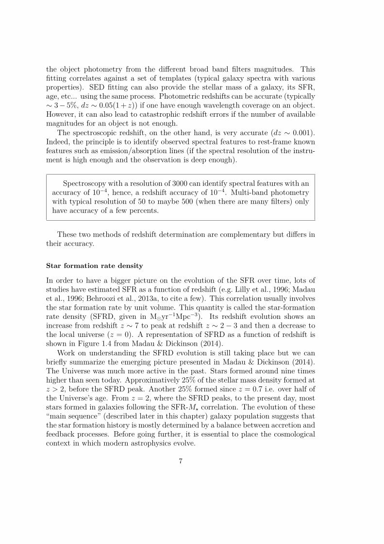
In order to have a bigger picture on the evolution of the SFR over time, lots ofstudies have estimated SFR as a function of redshift (e.g. Lilly et al., 1996; Madauet al., 1996; Behroozi et al., 2013a, to cite a few). This correlation usually involvesthe star formation rate by unit volume. This quantity is called the star-formationrate density (SFRD, given in Myr−1Mpc−3). Its redshift evolution shows anincrease from redshift z ∼ 7 to peak at redshift z ∼ 2− 3 and then a decrease tothe local universe (z = 0). A representation of SFRD as a function of redshift isshown in Figure 1.4 from Madau & Dickinson (2014).

Work on understanding the SFRD evolution is still taking place but we canbriefly summarize the emerging picture presented in Madau & Dickinson (2014).The Universe was much more active in the past. Stars formed around nine timeshigher than seen today. Approximatively 25% of the stellar mass density formed atz > 2, before the SFRD peak. Another 25% formed since z = 0.7 i.e. over half ofthe Universe’s age. From z = 2, where the SFRD peaks, to the present day, moststars formed in galaxies following the SFR-M? correlation. The evolution of these“main sequence” (described later in this chapter) galaxy population suggests thatthe star formation history is mostly determined by a balance between accretion andfeedback processes. Before going further, it is essential to place the cosmologicalcontext in which modern astrophysics evolve.

7

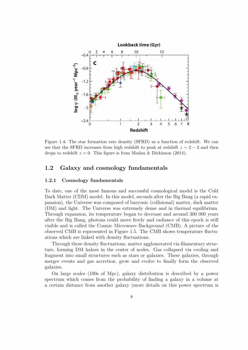
Figure 1.4: The star formation rate density (SFRD) as a function of redshift. We cansee that the SFRD increases from high redshift to peak at redshift z ∼ 2 − 3 and thendrops to redshift z = 0. This figure is from Madau & Dickinson (2014).

1.2 Galaxy and cosmology fundamentals

1.2.1 Cosmology fundamentals

To date, one of the most famous and successful cosmological model is the ColdDark Matter (CDM) model. In this model, seconds after the Big Bang (a rapid ex-pansion), the Universe was composed of baryonic (collisional) matter, dark matter(DM) and light. The Universe was extremely dense and in thermal equilibrium.Through expansion, its temperature began to decrease and around 300 000 yearsafter the Big Bang, photons could move freely and radiance of this epoch is stillvisible and is called the Cosmic Microwave Background (CMB). A picture of theobserved CMB is represented in Figure 1.5. The CMB shows temperature fluctu-ations which are linked with density fluctuations.

Through these density fluctuations, matter agglomerated via filamentary struc-ture, forming DM haloes in the center of nodes. Gas collapsed via cooling andfragment into small structures such as stars or galaxies. These galaxies, throughmerger events and gas accretion, grow and evolve to finally form the observedgalaxies.

On large scales (100s of Mpc), galaxy distribution is described by a powerspectrum which comes from the probability of finding a galaxy in a volume ata certain distance from another galaxy (more details on this power spectrum is

8

given in the next framed text on simulations). This power spectrum is usually thestarting point of cosmological simulations.

Figure 1.5: The anisotropies of the Cosmic microwave background (CMB) as observed byPlanck. The CMB is a snapshot of the oldest light in our Universe, imprinted on the skywhen the Universe was just 380 000 years old. It shows tiny temperature fluctuationsthat correspond to regions of slightly different densities, representing the seeds of allfuture structure: the stars and galaxies of today. Copyright: ESA and the PlanckCollaboration.

In simulations, we need a power spectrum to begin with. This power spec-trum is found from a two point correlation function which will quantify theclustering of galaxies later in the simulation. This correlation function is theprobability to find an object (i.e. a galaxy) at a distance r from another object.This function is defined as follows:

ξ(r) = 1 + 〈N(r + dr)〉NPoisson(r + dr) (1.2)

This function is defined as a measure of the excess probability dP of findinga galaxy in a volume element dV at a separation r from another galaxy:

dP = n[1 + ξ(r)]dV (1.3)

Where n is the mean number of the galaxy sample (Peebles, 1980). The Fouriertransform of ξ(r) gives the power spectrum which is used to describe densityfluctuations observed in the Cosmic Microwave Background (CMB) (see Fig-ure 1.5).

In most simulations, we need sub-grid physics in order to make the universeevolve and this usually ask for huge computational resources.

9

Look-back time

From this standard model, lots of cosmological parameters help us deriving astro-physical objects properties. In particular, it is important to define what we callthe look back time. We define the look-back time as the time it takes for the lightto come to us from an object at redshift z. The look-back time of an object is thedifference between the age of the Universe now (at observation) and the age of theUniverse when the photons of the object were emitted.

Cosmological simulations try to reproduce the observed universe. They startfrom a certain amount of matter, initial conditions and make them evolve and formstructures with time to afterwards compare with what we observe. Simulationsare based on several ingredients and physical mechanisms:

- Initial conditions which mainly comes from observations from WMAP orPlanck, providing a starting environment for the Universe to evolve from,

- Physics of collisionless fluid for Dark Matter (DM) and star particles,- Physics of collisional fluid for gas heated and cooled radiatively (atomic and

molecular),- “Galaxy physics” for star formation and feedback on the surrounding gas

(supernovae, turbulence, black hole growth, jets, chemistry of heavy elements,dust...).

1.2.2 Galaxy fundamentals

At galaxy scale (scale of kpc), several properties can be derived from observationof galaxies such as apparent magnitude and the galaxy morphology. From thesedirect measurements, several indirect ones can be made such as relative velocities,velocity fields, physical sizes, absolute luminosities, stellar masses, star formationrate, age, metallicity, dust...

Apparent magnitude, flux and galaxy morphology

Once objects are identified, we get the total observed flux on an image to derivethe apparent magnitude (Eq. 1.4) using calibrated reference sources.

m = −2.5 log(Flux) + C (1.4)

where m is the apparent magnitude and C is a normalized constant derived fromthe reference source.

The Hubble sequence

From the apparent shape of a galaxy, one can classify them following the Hubblesequence. This sequence classifies galaxies by their morphology (see Figure 1.6).

10

Figure 1.6: Scheme of Hubble classification for galaxy morphologies.

In order to classify galaxies, one can fit their morphology using models to representthe galaxy in 2 dimensions. We usually use a Sersic (Sersic, 1963) profile to fit theflux distribution of a galaxy as a function of its radius:

I(r) = I0 exp(−kr1/n) (1.5)

and thus:ln I(r) = ln I0 − kr1/n (1.6)

Where I(r) is the intensity at radius r, n being the Sersic index.A typical flux profile for spiral galaxies is an exponential flux distribution (Sersic

index n = 1), whereas an elliptical galaxy is best fitted by a de Vaucouleurs profile(n = 4).

This method offers a basis to automated classification of galaxy morphology.However, it becomes complicated for galaxies at z > 1 mainly due to the fact thatthey become mostly irregular. Hence, these “high redshift” galaxies are usuallynot resolved and it is thus difficult to classify them on the Hubble sequence.

11

It is important to define “red early-type” and “blue star-forming” galaxies.A red early-type galaxy is usually an elliptical galaxy. These galaxies starvedof star-forming gas at high redshift and thus do not form stars anymore (ortheir SFR is very low). They appear yellow-red because of old star populationthey are composed of, as compared to the blue star-forming galaxies which areusually spirals and appear blue due to the young and hot stars in their spiralarms. The blue star-forming galaxies are also called late-type galaxies as theyare still forming stars.

Relative velocities

In galaxies, one can derive their rotational velocities and their redshifts. For deriv-ing the velocity field of a galaxy, i.e to determine which part of a galaxy is movingtoward us and which part away from us, we basically need to look at this galaxyspectrum. Emission lines from this galaxy will blue/red shift from its systemicvelocity (usually located at the center of this galaxy). We can see a representationof this effect on Figure 1.7. On this figure, the right part of the galaxy arm willhave an emission red-shifted compared to its center, whereas the left end arm willhave its emission blue-shifted. Mapping all the galaxy will lead to building thevelocity field of this galaxy.

Physical sizes

The aim is to transform the observed angular size to physical dimension of thesource. In order to do this, we use a cosmological model (the ΛCDM is the mostpopular to date). We use Equation 1.7 to derive the angular diameter distance fora source at redshift z.

da = Sk(r)1 + z

(1.7)

where Sk(r) is the FLRW (Friedmann-Lemaıtre-Robertson-Walker) coordinate de-fined as:

Sk(r) =

sin(

√−ΩkH0r)/(H0

√|Ωk|), if Ωk < 0

r, if Ωk = 0

sinh(√

ΩkH0r)/(H0

√|Ωk|), if Ωk > 0

(1.8)

where da is the angular diameter distance, Ωk the curvature density z is the red-shift of the object, r the comoving distance and H0 is the Hubble constant.

12

Figure 1.7: Scheme of a galaxy in rotation. The galaxy is in black and is represented onthe sky plane x, y (y representing the celestial north). This galaxy has a position anglePA which is the angle between the celestial north and the major axis of the galaxy. Atthe bottom, we can see 3 Gaussians on a wavelength axis (λ) corresponding to emissionlines in 3 different regions of the galaxy. The left part of the galaxy is moving towardsus, so its emission line is blue-shifted, its middle do not move with respect to its systemicvelocity and the right part is moving away from us, so its emission line is red-shifted.

Absolute luminosities

From apparent magnitude, we can derive the absolute magnitude using Equa-tion 1.9.

M = m− 5 log10( DL

10pc)−K (1.9)

where M is the absolute magnitude, m is the apparent magnitude, DL is the lu-minosity distance of the object and K is a correction factor for the redshift effecton object outside our galaxy. This K correction depends on filter used to makethe observation and the shape of the object spectrum. If one have access to all thelight in all wavelength of an object or if the light is measured in an emission line,the K correction is not needed. However, if one has access only to a filter (onlysee a fraction of the object spectrum) and want to compare measurements withdifferent objects at different redshifts in this filter, estimation of this K correctionis needed. An example of filters for the Sload Digital Sky Survey (SDSS) is shownin Figure 1.8.

13

Figure 1.8: SDSS transmission curves for the different filters.

Stellar masse, star formation rate, age, dust...

These quantities are usually derived from SED fitting method. The stellar popu-lation add up to produce a galaxy luminosity and colors. The stellar populationsynthesis models aim at reproducing the observed stellar light from galaxies, thesemodels include changes with age, metallicity and extinction law from dust. It isdifficult to be confident in results from these models as lots of degeneracies occur(i.e. age and metallicity, IMF and SFR laws...).

1.2.3 The Tully-Fisher relation and other mass estimator

A very popular relation is the Tully-Fisher relation (TFR, Tully & Fisher, 1977;Miller et al., 2011, 2014; Vergani et al., 2012; Simons et al., 2015, to cite a few).This empirical relation is linking the galaxy rotational velocity with the intrinsic lu-minosity of the galaxy and thus its stellar mass. Indeed, the stellar mass of a galaxyis directly proportional to the amount of stars within, and the amount of stars isdirectly linked to the galaxy luminosity. The TFR applies for rotation-dominatedgalaxies, where the dispersion velocity of the galaxy is negligible compared to therotational velocity.

Another mass estimator which include a combination of the galaxy dispersionvelocity σ and the rotational velocity Vmax can be used. Weiner et al. (2006); Kassinet al. (2007) and Price et al. (2016) argued that the quantity S2

K = K×V 2max +σ2,

14

where K is a constant, can be used as a dynamical mass estimator as it combinesdynamical support from ordered motion (Vmax) and disordered motions (σ). Thismass estimator will be used in § 5.1.2. In order to clearly understand on whichtype of galaxies these mass estimators work with, it is important to define thegalaxy “main sequence” as well as some type of galaxies we will later encounter.

1.2.4 The galaxy “main sequence”

Like stars, there is what we call a galaxy “main sequence”. If one investigates therelation between galaxy SFR and stellar mass, one can see that most of galaxieslie along a scattered line. This line is called the galaxy “main sequence”. However,even if most galaxies lie on this line, some galaxies are outliers. These outliersare above (starbursts) or under (red) the main sequence. Figure 1.9 shows arepresentation of this main sequence as well as outliers categories. We will quicklydescribe galaxies located above the main sequence: starburst galaxies.

Figure 1.9: Scheme of the galaxy “main sequence” in blue as well as outliers: starburstsabove this main sequence (purple) and red or dead (not forming stars anymore) galaxies(red). Space between the main sequence and red galaxies is called the green valley.

Star-burst galaxies

It is important for us to define this type of galaxies. Indeed, further in thismanuscript, we will encounter such type of galaxies used in other studies to com-pare with ours. The galaxy M82 for instance (presented in § 1.3), is the starburstarchetype. This galaxy has high SFR and therefore lots of supernovae which leadsto galactic winds.

15

As mentioned earlier, starburst galaxies have higher SFR (above the mainsequence) compared to other galaxies for the same stellar mass. The rate of starformation is so large in starbursts that they will consume almost all their gasreservoir used to form stars in a shorter timescale compared to “main sequence”galaxies. There are different types of starburst galaxies, and within these types, apopular one is the Ultra Luminus Infra Red Galaxy (ULIRG).

U/LIRGs

ULIRGs are generally extremely dusty objects. As their name tells us, thesegalaxies are emitting in IR. Indeed, as mentioned before, the dust is absorbing UVphotons produced mainly by star formation and re-emit them in larger wavelength,typically in IR. This could explain the red color associated with ULIRGs.

In addition, these galaxies are extreme cases of starbursts. They are oftengalaxies in major interactions or even in advanced merging process. ULIRGs canform a huge amount of stars (SFR∼100 to 1000 M yr−1). However, due to theirextreme properties, these galaxies are rare.

1.2.5 What is a quasar?

Another type of astrophysical objects we will largely encounter and use during thisthesis are quasars. A quasar is among the most energetic and luminous type ofobject in the universe. They belong to the class of object called Active GalacticNuclei (AGN) and are the most luminous and distant objects of this class. AnAGN is a compact region in the center of galaxies. Quasars are thus powered bya super massive black hole and are active galaxies. A typical quasar spectrum isrepresented in Figure 1.10.

1.2.6 The low efficiency of galaxy formation

It is important to remind the reader that galaxies are not only isolated astro-physical objects living their life without interacting. Indeed, they have gas flows,inflowing and outflowing gas which play an important role in galaxy evolution.

In order to introduce the main question we want to address in this thesis, wefirst need to present the baryonic mass function. The baryonic mass function isbuilt from the sum of the stellar mass function and the gas mass function, i.e.it represents the baryon budget locked into galaxies. The stellar mass function isderived from the conversion of the luminosity function and requires a mass-to-lightratio for the stellar populations. This ratio usually depends on galaxy type, ageand metallicity.

Concerning the gas mass function, the principle is to estimate the total coldmass density. It corresponds to the sum of atomic (H i) and molecular (H2) hy-drogen gas content of galaxies. Large samples of atomic hydrogen H i gas (e.g. the

16

Figure 1.10: Scheme of a typical quasar spectrum.

Australian HIPASS survey Koribalski et al. (2004)) allowed to derive a gas massfunction (e.g. Zwaan et al., 2003) for galaxies in the local universe. The molecularhydrogen reservoir, however, is difficult to constrain due to the lack of electricdipole moment in the H2 molecule, which is the main component in molecularclouds. In order to derive the molecular gas content of a galaxy, one needs a tracerwhich is robust and directly linked to the molecular hydrogen density. Keres et al.(2003) derived a molecular gas mass function of galaxies using CO as a proxy forH2 because CO is abundant and easily excited by collision with H2.

Summing the stellar mass and gas mass functions, one can obtain the baryonicmass function of galaxies. Papastergis et al. (2012) derived this baryonic massfunction and compared it with the predicted amount from the CDM model (seeFigure 1.11).

The main results from this baryonic mass function are that in low and highmass haloes (log(Mh/M) < 12 and log(Mh/M) > 12 respectively), there arehuge differences between observations (yellow thick curve) and the cosmic value ofbaryon fraction fb ≈ 0.16 (black dotted-dashed horizontal line). Indeed, we onlyobserve a few percents of the baryonic matter and there are even less matter inlow and high mass regimes (see yellow curve as compare to the horizontal dottedline in Figure 1.11). These differences lead to the conclusion that there must bemechanisms responsible for this lack of observed matter. Feedback is thereforeneeded in order to expel baryons out of galaxies for low and high mass galaxies.

In the high-mass galaxy regime, feedback from Active Galactic Nuclei is in-voked as an efficient mechanism to expel baryons out of the galaxy halo, but wewill not detail this mechanism here. From now on, we will focus on low mass

17

Figure 1.11: Figure from Papastergis et al. (2012). The ratio of galactic stellar mass tohalo mass as a function of host halo mass (M∗/Mh −Mh relation). The thick yellowline shows Papastergis et al. (2012) main result, obtained from abundance matching thestellar mass function of optically-selected sample with the halo mass function includingsubhaloes. The dotted-dashed horizontal line shows the cosmic baryon fraction fb ≈0.16.

galaxies since this thesis is focused on these objects. Low-mass galaxies need feed-back mechanisms such as baryons blown out by supernova explosions and thesemechanisms must be very efficient in pushing away gas out of the galaxy. Thismechanism is called galactic winds and our scientific goal is to constrain propertiesof this phenomenon such as the ejected mass rate, the outflowing velocity or theability for the gas to leave the galaxy halo.

1.3 Galactic winds “state of the art”

As described in the previous section, and in spite of successes of the ΛCDM cosmo-logical model, a major discrepancy remains between the predicted baryonic den-sity of dark matter haloes and the observed ones in the low-mass galaxy regime(L < L∗) (Behroozi et al., 2013b). This fundamental problem is usually explainedby supernovae(SN)-driven outflows (Dekel & Silk 1986) which expel baryons outof the galactic disk. Indeed, these galactic outflows are observed in almost every

18

star-forming galaxy (SFG) (Veilleux et al., 2005a) and are a viable mechanism toenrich the inter-galactic medium (Oppenheimer et al., 2010).

Various observational techniques are used to study galactic outflows. In orderto better understand the main geometrical properties of galactic winds, one canobserve SFGs in the local universe at z = 0.

1.3.1 Galactic winds are multi-phased and collimated

Messier 82 (or M82) is a famous local galaxy. This galaxy can be observed in thenight sky using a personal telescope. However, in order to see the details of thisgalaxy, one needs a large telescope and a wide wavelength coverage. This galaxyhas been observed in lots of different wavelengths with several instruments.

Galactic winds geometry

Figure 1.12 shows the galaxy M82 taken with the Hubble Space Telescope (HST),in visible. On this figure, we can see the disk of the galaxy as well as the dustin dark filaments. This galaxy has the advantage of being almost edge-on, whichmeans that we have a side view of the galaxy. If we look closer at this image,we can see the presence of gas perpendicular to the galactic disk, but this is notobvious in these wavelengths. If we observe this same galaxy with a differentwavelength filter, we will see that this galaxy does not only have a disk.

Figure 1.12: The galaxy M82 in visible wavelength, taken with HST. We can see thatthis galaxy is almost edge-on, in white we see the stars and gas contributions and thedust is shown in dark filaments along the galaxy.

Left panel of Figure 1.13 shows a combined picture of this galaxy from differentfilters: B (blue, in blue), V (visible, in white) and Hα (in red). We can clearly seethe presence of a gas perpendicular to the galactic plane. The Hα filter detectsthe presence of ionized gas. This ionized gas is ejected from the galaxy with a

19

direction perpendicular to its plane. This ejected gas is a direct observation ofgalactic winds in emission.

Figure 1.13: On left panel, the galaxy M82 in B,V (blue and visible) combined with Hα,taken with the Subaru telescope. Like Figure 1.12, we see the disk of the galaxy (B andV filters) in white. In addition, the Hα is represented in red. We see the presence ofthis ionized gas perpendicular to the galactic disk. Hence, these outflows appear to becollimated in a cone. This gas is a direct imaging of galactic winds. On right panel,the galaxy M82 in X-ray, taken with the Chandra telescope. Unlike Figure 1.12 and leftpanel of this figure, we do not see the disk of the galaxy. We can, however, see the hotgas at almost the same location where we see the Hα gas on left panel. Again, we cansee the conical structure of these outflows.

Again, looking at a different wavelength, and in X-ray to be precise, one cantrace the hot gas of this galaxy. Right panel of Figure 1.13 shows the same galaxyobserved in X-rays by the space telescope called Chandra. We do not see thegalactic disk anymore but only the hot gas ejected from the galaxy. This hot gasis located at the same place as the red ionized gas seen in Figure 1.13. Here, weare tracing the hot phase of galactic winds.

Through a simple example, we already seen major properties about galacticwinds. Indeed, we saw that they are located perpendicular to the galactic planeand are multi-phased. The hot phase of the gas, directly connected to supernovaeexplosions, is pushing the cold gas out of the galaxy. The hot gas is supposed tohold most of the outflow energy with low mass and flux whereas the cold gas isbelieved to hold most of the outflowing flux and mass.

20

Bi-conical outflows

In addition to these properties, we can also see that galactic winds appear to becollimated in a cone. We talk of bi-conical outflows as they are ejected in bothdirections perpendicular to the galaxy. These properties are confirmed if we lookat other local star-forming galaxies like in Figure 1.14.

However, even if we can directly see these geometrical properties for local galax-ies, direct imaging of galactic winds is not yet possible for z > 0 galaxies. Indeed,the outflowing gas has a very low surface brightness compared to its host galaxyand other observational techniques are needed in order to derive outflow geomet-rical properties.

Figure 1.14: Other examples of galactic outflows seen in emission in local galaxies NGC253, NGC 1482 and NGC 3079. On each of these galaxies we have a zoom of theircenter which clearly show the presence of outflows. Like M82, these outflows are ejectedperpendicular to the galactic disk. Hence, we clearly see (especially for NGC 1482 and3079) that galactic winds are likely collimated in a cone.

The outflowing gas is thus not visible in emission for z > 0 galaxies, but thecircum-galactic gas can be observed in absorption. Several studies have shown thatgalactic outflows are collimated using stacked background galaxy spectra (Bordoloiet al., 2011, 2014; Rubin et al., 2014) and using background quasars passing nearstar-forming galaxies (Bouche et al., 2012; Lan et al., 2014b). These studies showed

21

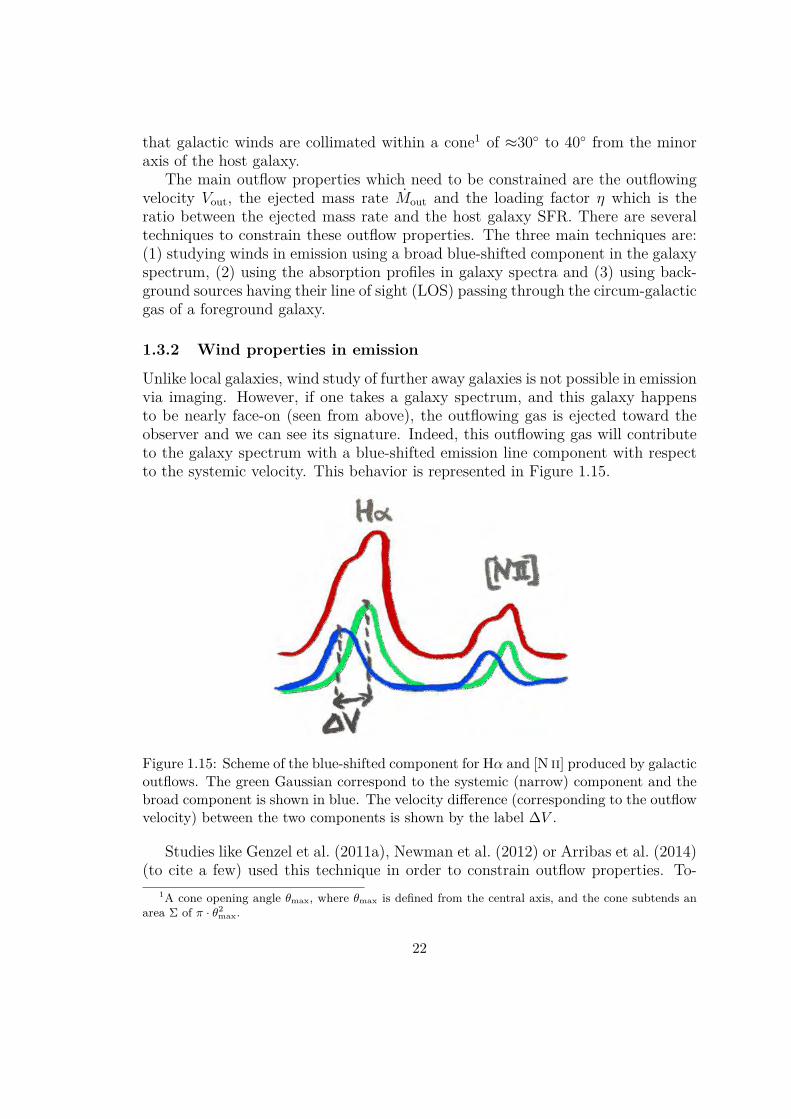
that galactic winds are collimated within a cone1 of ≈30 to 40 from the minoraxis of the host galaxy.

The main outflow properties which need to be constrained are the outflowingvelocity Vout, the ejected mass rate Mout and the loading factor η which is theratio between the ejected mass rate and the host galaxy SFR. There are severaltechniques to constrain these outflow properties. The three main techniques are:(1) studying winds in emission using a broad blue-shifted component in the galaxyspectrum, (2) using the absorption profiles in galaxy spectra and (3) using back-ground sources having their line of sight (LOS) passing through the circum-galacticgas of a foreground galaxy.

1.3.2 Wind properties in emission

Unlike local galaxies, wind study of further away galaxies is not possible in emissionvia imaging. However, if one takes a galaxy spectrum, and this galaxy happensto be nearly face-on (seen from above), the outflowing gas is ejected toward theobserver and we can see its signature. Indeed, this outflowing gas will contributeto the galaxy spectrum with a blue-shifted emission line component with respectto the systemic velocity. This behavior is represented in Figure 1.15.

Figure 1.15: Scheme of the blue-shifted component for Hα and [N ii] produced by galacticoutflows. The green Gaussian correspond to the systemic (narrow) component and thebroad component is shown in blue. The velocity difference (corresponding to the outflowvelocity) between the two components is shown by the label ∆V .

Studies like Genzel et al. (2011a), Newman et al. (2012) or Arribas et al. (2014)(to cite a few) used this technique in order to constrain outflow properties. To-

1A cone opening angle θmax, where θmax is defined from the central axis, and the cone subtends anarea Σ of π · θ2

max.

22

gether with theoretical prediction (e.g. Hopkins et al., 2012), Newman et al. (2012)found that:

• the loading factor η correlates with galaxy size and inclination.

• Argue for strong dependence of the loading factor with SFR per unit area(ΣSFR).

• That galaxies should have a SFR per unit area larger than 1Myr−1kpc−2 inorder to be able to show the presence of galactic winds.

• And it is harder for a massive galaxy to launch winds.

These results are based on SINFONI2 data of z ∼ 2 star-forming galaxies from theSINS and zC-SINF surveys (e.g. Forster Schreiber et al., 2004). They used thebroad emission lines component (without stacking) as in Shapiro et al. (2009) andGenzel et al. (2011b) in order to put outflowing gas constraints.

Work of Arribas et al. (2014) study 58 local (low-z) (Ultra) Luminous Infra-Red Galaxies (U/LIRG) using the Visible Multi Object Spectrograph (VIMOS, LeFevre et al., 2003) and INTEGRAL (Arribas et al., 1998) instruments. In theirwork, they also use the blue-shifted broad component of several emission lines likeHα and [N ii] in order to derive the outflow velocity. This velocity is derived byfitting a Gaussian profile to this blue-shifted broad component (see Figure 1.15).In their paper, they assume impact parameters3 b of 0.7 kpc and find that:

• the outflow velocity is proportional to the SFR (Vout ∝ SFR0.24),

• that high-z galaxies also require SFR per unit area larger than 1 (ΣSFR > 1)for launching strong outflows (as in Newman et al., 2012).

• The mass loading factor is correlated with SFR per unit area (η ∝ Σ0.17SFR).

1.3.3 Wind properties in absorption

The second technique is to use the absorption lines produced by the outflowinggas in the galaxy spectrum (see Figure 1.16 for an example).

Because galaxies with redshifts larger than 0.5 are usually fainter, it can bedifficult to see the absorption lines produces by outflowing gas in the spectrumof these galaxies. Therefore, a number of investigations on intermediate redshift(0.5 < z < 1.5) SFGs (e.g. Weiner, 2009; Martin et al., 2012; Bordoloi et al., 2014;Rubin et al., 2014) used stacked galaxy spectra. This method consists in stack-ing strong absorption lines like the Mg ii λ2796 doublet of galaxies with similar

2SINFONI is an Integral Field Unit (IFU, described in § 2.1.2) instrument on the Very Large Telescope(VLT) in Chile.

3The impact parameter corresponds to the distance where the outflowing gas is probed from the hostgalaxy.

23

properties and constrain outflows for a specific type of galaxy. The recent studyof Heckman et al. (2015) uses the absorption technique but does not use stackedgalaxy spectra as they have enough signal to noise ratio (SNR) to characterize theoutflows in individual galaxies.

Figure 1.16: Outflow absorption lines seen in a galaxy spectrum from Heckman et al.(2015). This absorption is blue-shifted with respect to the galaxy systemic velocity. Wecan also see that the different absorption lines have the same absorption behavior liketheir asymmetry.

In the paper of Heckman et al. (2015), they assume impact parameters of 5kpc for a sample of 39 low-z galaxies. They study two samples of low-z starburstgalaxies. The first sample is composed of 19 galaxies observed by Far UltravioletSpectroscopic Explorer (FUSE) (previously analysed by Grimes et al. (2009) andHeckman et al. (2001)). The second sample they use is composed of 21 Lymanbreak analogs (LBAs) observed with Cosmic Origin Spectrograph (COS) on HSTand previously analysed by Alexandroff et al. (2015). These galaxies are starburstgalaxies, which means that they have high SFRs and thus are likely to have galac-tic winds. In order to derive outflow velocities, they used the absorption linesproduces by the outflowing gas but without stacking different galaxy spectra asthey have enough SNR to analyze almost each galaxy individually. To estimateVout, they used the value corresponding to 80% of the absorption profile in order toavoid instrumental noise seen in the galaxy continuum. Using these blue-shiftedabsorption lines, they found that:

• the outflow velocity correlates weakly with the galaxy stellar mass and itsmaximum rotational velocity.

• That there is strong correlation between the outflow velocity and SFR (andalso with SFR per unit area (ΣSFR)).

24

• And the mass loading factor is not correlated with the outflow velocity (com-pared to Hopkins et al. (2012)).

In summary they claim that the outflowing gas should be accelerated by the com-bined force due to gravity and momentum flux from starburst.

This technique has the advantage of having lots of observations since it mainlyneeds a face-on SFG. However, estimates of ejected mass rates and thus loadingfactors are uncertain by order of magnitude and are therefore mostly indicative.The major cause of these uncertainties is the lack of knowledge on the outflowinggas location. Indeed, as they look at face-on galaxies, the outflowing gas is directedtowards the observer and the probed outflowing gas can be at 1 parsec (pc), 10 pcor even 10 kiloparsecs (kpc) away from the host galaxy. To bypass this problem,another technique is the use of background sources to probe the surrounding gasof a galaxy.

1.3.4 Wind properties using background sources

Two kinds of background sources can be used in order to probe the outflowinggas and therefore knowing the gas location. These background sources can beeither a galaxy or a quasar. Background quasars studies showed galactic windsare indeed collimated in a bi-conical shape (i.e. Bouche et al., 2012; Lan et al.,2014b). To date, star-forming galaxies having a background quasar LOS passingnear is rare and building large samples is therefore difficult. Thus, it requiresspecific observational strategies. Increasing the number of galaxy-quasar pairs isone of this thesis objective.

From results of various techniques we just presented, the correlation betweenthe loading factor and the galaxy SFR must be taken with caution as plotting y/xvs. x can lead to non physical correlations (and it is the same with ΣSFR). Asthere is a peak in star-formation density at redshift 2-3 (Lilly et al., 1996; Madauet al., 1996; Behroozi et al., 2013a), if η correlates with SFR, one can expect acorrelation between η and redshift. The result from Heckman et al. (2015) on thenon correlation between η and Vout makes sense as there is no specific reason for agalaxy to eject more gas if this gas velocity changes.

Other constraints on galactic winds are thus needed in order to find whatdrives winds out of the galaxy and this is exactly what we intended to during thisthesis. With the background quasar methodology (described in § 2.1), we intendto estimate galactic wind properties with higher accuracy (as we know where weare probing the outflowing gas).

1.3.5 Perspective from numerical simulations

As mentioned earlier, concerning numerical simulations, the incomplete knowledgeon scaling relations between a galaxy and its outflowing material properties, such

25

as between the ejected mass rate Mout and the star formation rate (SFR), limitsour ability to produce accurate numerical models. In simulations, outflows areusually implemented with sub-grid prescriptions (e.g. Schaye et al., 2010; Oppen-heimer et al., 2010; Vogelsberger et al., 2014). A popular sub-grid recipe is toset the loading factor η be a function of galaxy circular velocity Vc (Oppenheimeret al., 2010) (and thus the galaxy (halo) mass). These relations are usually set toη ∝ V −1

c for momentum-driven winds and η ∝ V −2c for energy-driven winds. An al-

ternative way to implement the collective effect of SN explosions is the (stochastic)implementation of thermal feedback. Using this method, galactic winds developwithout imposing any input outflow velocity nor mass loading factor. This methodis used by popular simulations such as the EAGLE simulations (e.g. Schaye et al.,2015), the FIRE simulations (Hopkins et al., 2014; Muratov et al., 2015), and themulti-phase scheme of Barai et al. (2015).

Figure 1.17: Loading factor as a function of galaxy rotational velocity (bottom x axis)and halo mass (top x axis) assumed by theoretical/empirical models.

Figure 1.17 shows assumed loading factors (η = Mout/SFR) as a function of

26

the galaxy rotational velocity (and halo mass) by theoritical/empirical models. Weclearly see on this figure that there is absolutely no consensus about the loadingfactor behavior on the galaxy halo mass. Thus, we definitely need observationalconstrains on outflow properties.

27

Chapter 2

Observational strategy andsample selection

Contents2.1 The background quasar methodology . . . . . . . . . . . . . . 30

2.1.1 Observational strategies . . . . . . . . . . . . . . . . . . . . . . 302.1.2 Why do we need integral field spectroscopy? . . . . . . . . . . . 312.1.3 Critical parameters derived from IFUs . . . . . . . . . . . . . . 322.1.4 A 3D fitting tool: GalPaK3D . . . . . . . . . . . . . . . . . . . 33

2.2 The SINFONI Mg ii Program for Line Emitters (SIMPLE)sample . . . . . . . . . . . . . . . . . . . . . . . . . . . . . . . . . 33

2.2.1 Selection criteria . . . . . . . . . . . . . . . . . . . . . . . . . . 332.2.2 Sample description . . . . . . . . . . . . . . . . . . . . . . . . . 34

2.3 The MUSE GAs Flow and Wind (MEGAFLOW) survey . . 352.3.1 Selection criterion . . . . . . . . . . . . . . . . . . . . . . . . . 352.3.2 Sample description . . . . . . . . . . . . . . . . . . . . . . . . . 35

29

In this chapter, we present the methodology we use to constrain galactic outflowproperties as well as observational strategies aiming to build a statistical sample.

2.1 The background quasar methodology

Contrary to the stacked spectra technique, background quasars have 3 main ad-vantages. (1) We know the location of the outflowing gas we are tracing with theimpact parameter b, which is the distance between the quasar LOS and the galaxycenter. (2) We know the galaxy redshift without knowing its position at first bylooking at the absorber redshift in the quasar spectrum. (3) The quasar gives adirect information of the Point Spread Function (PSF).

The only drawback of this technique is the number of galaxy-quasar pairs.Indeed, this technique needs a galaxy-quasar pair in the right geometrical config-uration allowing to study the outflowing materials. In order to have a maximumnumber of galaxy-quasar pairs and thus have a statistical sample, we need to buildobservational strategies.

2.1.1 Observational strategies

We use a background quasar as a probe for constraining properties of the surround-ing gas of galaxies, also known as circum-galactic medium (CGM). This CGM willabsorb a part of the background quasar light which will create absorption lines inthe quasar spectrum. Our observational strategy will be first to identify and selectthese absorption lines, in particular the Mg ii (λλ2796, 2802) doublet. This Mg iidoublet has the advantages of being strong and being a doublet, which facilitatesits identification.

A first strategy to gather galaxy-quasar pairs was to select blue z ∼ 0.1 SFGsnear higher redshift quasars from the SDSS database. Together with observationsfrom the blue sensitive spectrograph (Keck Low Resolution Imaging Spectrometer(LRIS Oke et al., 1995) and the double imaging spectrograph (DIS) at the ApachePoint Observatory (APO)), one can identify the Mg ii low-ionization lines at lowredshift z ∼ 0.1− 0.3. The slit of LRIS was placed to get both the quasar and thegalaxy spectra. The slit of DIS was placed on the galaxy major axis to get its Hα(λ6564) flux. We then looked for Mg ii absorptions in the quasar spectrum as wellas in the galaxy one. The detection rate was around 30% and one galaxy-quasarpair is presented in Kacprzak et al. (2014).

In order to have a large sample composed of galaxy-quasar pairs suitable forwind study, we need to look at already observed quasars spectra to search forabsorption lines. One of the largest quasar surveys is the SDSS-III Baryon Oscil-lation Spectroscopic Survey (BOSS) (Alam et al., 2015). Catalogs such as Menard& Chelouche (2009) directly gives detected absorption lines and their properties

30

(i.e. absorber redshift, Rest Equivalent Width (REW)) for a large number ofquasar spectra.

Looking at the Mg ii REW in the quasar spectrum, the host galaxy can belocated far away from the quasar LOS. Depending on the available instrument,we need to select strong Mg ii absorbers, strong being Wλ2796

r > 0.3 − 0.5 A asin Nestor et al. (2005). This selection criteria is indeed dependent of the IntegralField Unit (IFU) instrument we want to use and can differ. Using this method,we thus need powerful instrument in order to detect galaxies responsible for theabsorptions seen in quasar spectra.

2.1.2 Why do we need integral field spectroscopy?

We select strong Mg ii absorbers in background quasar spectra. By doing that, weknow the host galaxy redshift without knowing its position. We therefore need anIFU in order to detect and identify the host galaxy.

An IFU has the particularity to have a FOV in which every pixel has a spectrum(see an example in Figure 2.1). This avoids the pre-selection of SFGs as we cansearch for host galaxies all around the quasar LOS.

After observing a quasar field with an IFU, we then search for galaxies respon-sible for the Mg ii absorption lines at a specific redshift around the quasar LOS.When the host galaxy is detected, we need its morpho-kinematic properties andgeometrical configuration with respect to the background quasar.

Figure 2.1: Scheme of an 3D IFU cube: the foreground image represents a white-lightimage of the cube and the extracted image represents a slide of the cube at a givenwavelength. On this extracted image one can see only one galaxy which is emitting atthe extracted wavelength.

31

2.1.3 Critical parameters derived from IFUs

In order to constrain galactic outflows, we first need to classify the galaxy-quasarpairs depending on their geometrical configurations. Indeed, one drawback ofgalaxy-quasar pairs is that the quasar LOS can go through gas associated withseveral mechanisms depending on the inclination of the galaxy with respect tothe LOS. If the quasar is aligned with the galaxy major axis, it is likely probinginflowing or galactic disk material. If the quasar LOS is aligned with the galaxyminor axis, then it is likely probing the outflowing material from the galaxy. Hence,in order to study outflows, we need to untangle these geometrical effects.

We can sort out the geometry ambiguity by classifying pairs in two classes(“wind-pair” and “inflow-pair”) using the azimuthal angle α, defined as the anglebetween the galaxy major axis and the quasar LOS. If 60 < α < 90, then thegalaxy quasar pair is classified as a “wind-pair”, as it is likely to probe galacticoutflows. However, if 0 < α < 30, then we classify this galaxy-quasar pair asan “inflow-pair”, as the quasar LOS is likely probing inflowing material or galacticdisk component. Figure 2.2 shows the geometrical configuration of a galaxy-quasarsystem.

Figure 2.2: Scheme geometry configuration: the quasar LOS, represented by the yellowstar, is crossing galactic outflows represented by the red crosses getting out of the galax-ies. The Azimuthal angle is represented by the blue cross going from the galaxy majoraxis to the quasar LOS. b represents the impact parameter for the galaxy−quasar pair,represented by the light green cross showing the distance between the galaxy center andthe quasar LOS.

In order to determine α, we need to measure/determine the galaxy major-axis.

32

The galaxy major axis can be determined by directly looking at the morphol-ogy of the galaxy or better by looking at the kinematics and morphology. Thegalaxy morpho-kinematical properties are derived with the 3D fitting tool calledGalPaK3D (Bouche et al., 2015).

2.1.4 A 3D fitting tool: GalPaK3D

From IFU data, it is customary to extract moment maps (e.g. flux, velocity anddispersion maps) from the emission line(s) spectra. This is usually done on apixel by pixel basis, as most algorithms treat the spaxels to be independent (e.g.Law et al., 2007, 2009; Forster Schreiber et al., 2004; Cresci et al., 2009; Epinatet al., 2009), a condition that requires high quality data with a high signal-to-noise ratio (SNR) in each spaxel1, in order to constrain the width and centroid ofthe emission lines. Here, we avoid shortcomings of the traditional techniques bycomparing the three-dimensional data cubes directly to a three-dimensional galaxydisk model using the GalPaK3D tool. GalPaK3D uses a disk parametric modelwith 10 free parameters and a MCMC algorithm with non-traditional samplinglaws in order to efficiently probe the parameter space. The algorithm also usesa 3-dimensional kernel to convolve the model with the instrument PSF and linespread function (LSF), and thus returns the intrinsic (free of the PSF) galaxyproperties (such as half-light radius, inclination, and maximum rotation velocity).Other parameters include the major-axis position angle, the galaxy flux, position,redshift and intrinsic velocity dispersion. Extensive tests presented in Bouche et al.(2015) show that the algorithm requires data with a SNRmax > 3 in the brightestpixel. For high SNR, all parameters can be well recovered, but in low SNR data,degeneracies can appear: for instance between turn-over radius and Vmax.

Once galaxy parameters are derived, we can classify them into the previouslydefined categories : wind-pairs or inflow-pairs depending on their azimuthal angle.We will now describe galaxy-quasar samples we obtained.

2.2 The SINFONI Mg ii Program for Line Emitters (SIM-PLE) sample

The SINFONI Mg ii Program for Line Emitters (SIMPLE) sample (Bouche et al.,2007) is built by a combination of VLT/SINFONI and VLT/UVES (Dekker et al.,2000) data.

2.2.1 Selection criteria

As mentioned before, we select quasar fields based on Mg ii absorption lines inthe quasar spectrum. SINFONI is a near infra-red (IR, 1.1 − 2.45µm) IFU and

1A spaxel being a pixel on the sky containing a whole spectrum.

33

Figure 2.3: W λ2796r as a function of impact parameter b for galaxy-quasar pairs classified

as wind-pairs. The red colored area shows the selection criterion of the SIMPLE sample(W λ2796

r > 2.0A).

to detect a SFG, this galaxy must have emission lines falling into this wavelengthrange. We thus select Mg ii absorption lines having a redshift between 0.8 and 1.0in order to detect the galaxy Hα (λ6564) emission line in SINFONI J band. Giventhe SINFONI field of view (∼ 8′′×8′′), it is important to ensure that the galaxy willfall inside the field of view. For this purpose, we used the anti-correlation betweenb and equivalent width (e.g. Lanzetta & Bowen, 1990; Steidel, 1995; Bouche et al.,2006; Menard & Chelouche, 2009; Chen, 2012) (see Figure 2.3) and select absorberswith Wλ2796

r > 2 A.For this sample, the Mg ii REW (W λ2796

r ) has to be at least 2 A.

2.2.2 Sample description

This sample was observed in two major steps:First, 21 quasar fields were observed using SINFONI GTO time in which 14

host galaxies were detected (Bouche et al., 2007)2. These observations were shallowwith exposure times ≤ 40 min and seeing conditions ≥ 0.8′′. Then, in order tocompare the host galaxy kinematics with the kinematics of the absorbing materials,10 fields were re-observed both with SINFONI and UVES in open time.

2under program IDs 077.A-0576, 078.A-0600, 078.A-0718 and 079.A-0600.

34

These 10 re-observed pairs were aquired under SINFONI GO time3. This sub-sample was selected to have the highest initial Hα host galaxy fluxes and wasre-observed with longer integration times (2-3 hr) and in better seeing conditions(≤ 0.8′′). Details on these observations are given in Schroetter et al. (2015).

2.3 The MUSE GAs Flow and Wind (MEGAFLOW) sur-vey

We seek to increase the sample size by almost an order of magnitude in order toallow for statistical analysis between the absorption properties with the galaxyproperties. Thanks to the large wavelength range of MUSE, having a sampleof 80–100 pairs is now within reach in only 20–25 quasar fields with multiplemetal absorption lines. The MUSE GAs Flow and Wind (MEGAFLOW) surveyis composed of VLT/MUSE (Bacon et al., 2006) and UVES data.

2.3.1 Selection criterion

The selection principle is similar to the SIMPLE sample : we select quasar fieldswith Mg ii λ2796 absorption lines. To select quasar fields, we search for multiple(three, four or five) Mg ii absorbers (see Figure 2.4) in the quasar catalog fromthe Sloan Digital Sky Survey (SDSS) data release (DR12, Ross et al., 2012; Alamet al., 2015). These Mg ii absorption lines should have redshifts between 0.4 and1.4 such that the [O ii] (λλ3727, 3729) galaxy emission lines fall into the MUSEwavelength range (4800A to 9300A). We used the Zhu and Menard catalog4 (Zhu& Menard, 2013). MUSE having a larger FOV compared to SINFONI (1′ × 1′compared to 8′′ × 8′′), we thus lower the REW (W λ2796

r ) criterion from 2 A to0.8 A. This limit corresponds to b ∼ 100 kpc.

2.3.2 Sample description

Our MEGAFLOW survey is composed (at the time of writing) of 22 quasar fields.19 of these 22 fields have been observed with MUSE and 15 of them have UVESfollowed up data. Out of these 19 quasar fieds, two (J2137+0012 and J2152+0625)are published in Schroetter et al. (2016, submitted to ApJ). Figures 2.5 and 2.6show the W λ2796

r as a function of impact parameter (for galaxies with their asso-ciated quasar roughly aligned with their minor axis) and the redshift distributionof host galaxies respectively.

3Under program 080.A-0364(A) 080.A-0364(B) and 079.A-0600(B).4This catalog can be found at http://www.pha.jhu.edu/∼gz323/Site/Download Absorber Catalog.html

35

Figure 2.4: Scheme of our target strategy: the quasar LOS, represented by the yellowarrow heading toward the telescope, is crossing two galactic outflows represented by thered arrows getting out of the galaxies. These galactic outflows are absorbing a portionof the quasar spectra which gives the two Mg ii absorption systems at two differentredshifts. b represents the impact parameter for one galaxy−quasar pair.

36

Figure 2.5: W λ2796r as a function of impact parameter b for galaxy-quasar pairs classified

as wind-pairs. Horizontal dashed black lines shows the W λ2796r > 0.5A and W λ2796

r >0.8A selection criteria.

37

Figure 2.6: Redshift distribution of MEGAFLOW galaxies.

38

Chapter 3

Data acquisition and reduction

Contents3.1 SIMPLE observations and data reduction . . . . . . . . . . . . 403.2 MUSE observations and data reduction . . . . . . . . . . . . . 41

3.2.1 GTO observations . . . . . . . . . . . . . . . . . . . . . . . . . 413.2.2 Pre-processing data reduction . . . . . . . . . . . . . . . . . . . 413.2.3 Science reduction . . . . . . . . . . . . . . . . . . . . . . . . . . 433.2.4 Post-processing reduction . . . . . . . . . . . . . . . . . . . . . 443.2.5 Exposures combination . . . . . . . . . . . . . . . . . . . . . . 463.2.6 Sky emission lines removal . . . . . . . . . . . . . . . . . . . . . 46

39

In this chapter, we describe how the data were observed and focus on datareduction.

3.1 SIMPLE observations and data reduction

SINFONI observations, obtained in service mode, were optimized by adopting a‘on source’ dithering strategy designed to ensure a continuous integration at thehost location.

SINFONI data reduction was performed as in Bouche et al. (2007); ForsterSchreiber et al. (2009); Bouche et al. (2012), using the SINFONI pipeline (SPRED,Schreiber et al., 2004; Abuter et al., 2006) complemented with custom routines suchas the OH sky line removal scheme of Davies (2007) and the Laplacian edge cosmicray removal technique of van Dokkum (2001).

Regarding the wavelength calibration, we emphasize that we applied the helio-centric correction to the sky-subtracted frames. Each frame was associated witha single reference frame by cross-correlating each of the science frames spectrallyagainst the reference frame (the first science exposure). For each observing block,we use the quasar continuum to spatially register the various sets of observations.Finally, we created a co-added cube from all the individual sky-subtracted 600sexposures using a median clipping at 2.5σ.

Flux calibration was performed on a night-by-night basis using the broadbandmagnitudes of the standards from 2MASS. The flux calibration is accurate to∼ 15%. Finally, the atmospheric transmission was calibrated out by dividing thescience cubes by the integrated spectrum of the telluric standard.

UVES data were taken in both visitor mode and service mode. These datawere reduced using version 3.4.5 of the UVES pipeline in MIDAS. Master biasand flat images were constructed using calibration frames taken closest in time tothe science frames. The science frames were extracted with the optimal option.The blue portion of the spectra was checked order by order to verify that all wereproperly extracted. The spectra were then corrected to the vacuum heliocentricreference frame. The resulting spectra were combined, weighting each spectrumwith its signal-to-noise ratio. To perform absorption line analysis, the spectra werenormalized using cubic spline functions of the orders of 1–5 as the local continuum.Note that UVES and SINFONI data have their wavelength calibrations made invacuum.

40

3.2 MUSE observations and data reduction

3.2.1 GTO observations

Our MUSE data were taken from September 2014 in visitor mode during Guar-anteed Time Observations (GTO) runs1. We first point the telescope towards aquasar and then offset the first exposure by ≈ 4−5′′ in Right Ascension (RA) andDeclination (DEC). Observing Blocks (OBs) were composed of four exposures of900 seconds (or 2× 1500s) with a rotation of 90 between each exposure. EachOB has 1 hour exposure time and each field is observed for 2 hours (so 8 or 4exposures). This observation strategy is used to minimize the slice pattern whichappears during image reconstruction. Some observations were composed of twoexposures of 1500 seconds with the same 90 rotation between the two exposures.The two-exposure OBs were used to reduce the overheads produced mainly byCCD readout and rotations between exposures. Prolonging the exposure time ofone exposure leads to better chance of seeing fluctuation and thus lower guidingaccuracy. We used this strategy when the quasar field happens to have at leastone star falling in the Slow Guiding System (SGS) of MUSE so the guiding is moreaccurate and thus allows for longer exposure time.

3.2.2 Pre-processing data reduction

These first steps of the data reduction build up all the needed files for the sciencereduction. The calibration recipes are executed on the basis of single CCDs onan IFU per IFU basis. Figure 3.1 shows a basic science MUSE data reductiondiagram.

We combine the raw bias frames into one master–bias which will be used for thereductions. These raw bias frames are separate images that contains pixels valuesof the raw bias exposures. The recipe trims the raw data and record the overscanstatistics used to correct the data levels and combine the exposures using theinput method parameters such as the type of image combination (sigma clipping,median, average...) or the way of rejecting values for instance. The read-out noiseis computed for each quadrant of the raw images and stored as Quality Control(QC) parameter, so we can control the quality of combined data. Every outputframe has a variance extension which is filled with initial values according to theread-out noise before image combination. Additionally, bad columns are searchedfor and marked in the data quality extension. One has to take into account theweather temperature (which is found in the header of each raw frame) of eachexposure and reject the ones with large temperature difference compared to theother frames. A double check the mean bias value of each IFU is also needed inorder to continue the reduction.

1program IDs 096.A-0164, 096.A-0609, 095.A-0365, 094.A-0211

41

Figure 3.1: Association map for the basic science data reduction. This diagram showsthe part of the pipeline that operates on the basis of a single IFU.

The second step should be to combine raw dark frames. Since modern CCDshave a very small dark current, master dark frames are not used further in thedata reduction. This recipe trims the raw data and, like the bias recipe, recordsthe overscan statistics, subtracts the bias, scales the pixel count according to theirexposure time and combines them using input parameters (we used the sigma-clipping method, which is the default parameter).

The next step is to combine separate flat-field images into one master flat-field,trace the location of the slices on the CCD and locate dark pixels. To trace theposition of the slices on the CCD, their edges are located using a threshold method.At given interval, the edge detection is repeated tracing the central position andwidth of each slit vertically across the CCD. A polynomial fitting is then appliedto all positions measured for one slice and saved in an output trace table.

Once we obtained master files for bias, flat-field (dark is optional) and the

42

trace table, we can run the wavelength calibration recipe (“muse wavecal” recipein Figure 3.1). This recipe will reduce the arc frames to detect arc emission linesand also to determine a wavelength solution for each file. To ensure a wavelengthsolution across the entire range, three lamps are combined. For a complete wave-length coverage, one should aim for at least one arc frame per lamp or a frame withall lamps on. This recipe can, in addition to the other recipes described before,optionally subtract the dark and the lamp frame can be divided by the flat-field.This option is, however, not recommended. At first, the data is combined usinginput parameters into separate images for each lamp. These separate lamp expo-sures are then summed (by sigma clipping) to create a single combined master arc.As for the wavelength solution, arc lines are detected at the center of each sliceand subsequently assigned wavelengths. This is done using pattern matching toidentify lines from the input line catalog given by the pipeline package. Each lineis traced to the edge of the slice using a Gaussian centering in each CCD column.In each arc line, a polynomial fit is done to detect deviant fits and reject them.The two-dimensional fit uses all lamps positions, their wavelengths and the givenpolynomial orders to compute the final wavelength solution for each slice.

3.2.3 Science reduction

In addition to the flat-field, observations usually include twilight sky flat-fields.The next step is to combine these twilight sky flat-fields into a three-dimensionalillumination correction (“muse twilight” recipe in Figure 3.1). This processinghandles each raw input image separately. It trims the raw data, records the over-scan statistics, subtract bias, dark, divides by the flat-field and combines all theexposures using input parameters. The geometry table, trace table and wavelengthcalibration table are used to assign 3D coordinates to each CCD-based pixel. Itcreates a pixel-table from the master sky-flat. Pixel-tables are then cut in wave-length using the input parameters. Integrated flux in each IFU is saved in thepixel table header to be used later as estimate for the relative throughput of eachIFU. An additional correction can be applied if an ILLUM file is given as an inputto correct relative illumination between all slices of one IFU. This ILLUM file isan additional illumination exposure taken between each OB or when the weathertemperature changes more than 1.5. The data in each slice within the pixel-tableof each IFU is multiplied by the normalized median flux of that slice in the ILLUMexposure. Pixel-tables of all 24 IFUs are then merged, using the integrated fluxas inverse scaling factors, leading to a reconstructed skyflat cube. A white-lightimage is also created from this cube and the skyflat cube is then saved to diskwith the white-light image as an extension.

The last step in the basic reduction phase is the removal of the instrumental sig-nature from the data of each CCD and convert them into pixel-table (“muse scibasic”recipe in Figure 3.1). This processing handles each raw input image separately,

43

as above, trims the raw data and record the overscan statistics, subtracts bias,can detect cosmic rays (if the input setting is set), subtract dark, divides by theflat-field and optionally propagates the integrated flux value from the twilight-skycube. The input calibrations (geometry table, trace table and wavelength calibra-tion table) are used to assign 3D coordinates to each CCD-based pixel, creating apixel table for each exposure. If an ILLUM exposure is given as input, it is usedto correct the relative illumination between all slices of one IFU. Since ILLUM ex-posures are taken every hour and every time the temperature changes more than1.5C, it is best to use this additional exposure for every set of data we reduce.The last step of this recipe is to divide the data by the normalized twilight cubeusing the 3D coordinates of each pixel in the pixel table to interpolate the twilightcorrection onto the data. For each exposure, the pre-reduced pixel-table is savedto disk.

3.2.4 Post-processing reduction

Figure 3.2, like Figure 3.1, shows a diagram of the post-processing steps of thedata reduction.

The first post-processing step is to create a flux response curve from a standardstar exposure (“muse standard” recipe in Figure 3.2). This processing merges thepixel tables of standard star from all IFUs and corrects for atmospheric refraction.To derive the flux response curve, this recipe integrates the flux of all objectsdetected within the FOV using the given profile. It then select one object asthe standard star (either the brightest or the nearest object, depending on inputparameter) and compare its measured fluxes to tabulated fluxes to derive thesensitivity over wavelength. The final response curve is then linearly extrapolatedto the largest possible MUSE wavelength range and smoothed depending on inputparameter.

One of the last step before combining exposures is to prepare reduced andcombined science products (“muse scipost” recipe in Figure 3.2). The processingmerges the pixel tables from all IFUs of each exposure. If a previously processedresponse curved is given, then the flux calibration is carried out. One can use asky subtraction method at this point but the results show that it does not seemto work properly with the version we used at the time of our data reduction.We therefore do not use this method to remove sky emission lines. Afterwardsthe data is corrected for the radial velocity of the observer before the input (ora default) astrometric solution is applied. Finally (if the “save” parameter ofthe recipe contains “cube”), the data is resampled into a datacube. The extentand orientation of the cube is computed from the data itself and as a last step,the computed cube is integrated over all filter function given in the input “filter”parameter.

Once pixel-tables are reduced by exposure, we need to combine them.

44

Figure 3.2: Association map for the second part of the science data reduction. This partof the pipeline deals with data of all 24 IFUs simultaneously.

45

3.2.5 Exposures combination

In order to combine all exposures into one final data cube, we first need to computethe offsets between them. To do so, one can either compute them by hand, orusing a recipe. The recipe computes the coordinate offset for each input FOVimage with respect to a reference. When this offset table is created, we combinethe different exposures giving the pixel table locations we want to combine withthe corresponding offsets. This creates a final combined data cube.

One last step we need to finally exploit the science data is the sky emissionlines removal that we skipped before.

3.2.6 Sky emission lines removal

On the combined data cube, we perform the sky subtraction with ZAP (ZurichAtmosphere Purge), an algorithm developed by Soto et al. (2016). ZAP first oper-ates by subtracting baseline sky level, found by calculating the median per spectralplane and then uses principal component analysis. This principal component anal-ysis determines the minimal number of eigenspectra.

46

Chapter 4

Data analysis

Contents4.1 Methodology . . . . . . . . . . . . . . . . . . . . . . . . . . . . . 48

4.1.1 Estimate of Star Formation Rate (SFR) . . . . . . . . . . . . . 484.1.2 A simple cone model for galactic winds . . . . . . . . . . . . . 49

4.2 SIMPLE sample . . . . . . . . . . . . . . . . . . . . . . . . . . . 534.2.1 Morpho-kinematics from GalPaK3D . . . . . . . . . . . . . . . 534.2.2 Galaxy-quasar pairs classification . . . . . . . . . . . . . . . . . 544.2.3 Outflow properties . . . . . . . . . . . . . . . . . . . . . . . . . 54

4.3 MEGAFLOW survey . . . . . . . . . . . . . . . . . . . . . . . . 604.3.1 Survey status . . . . . . . . . . . . . . . . . . . . . . . . . . . . 604.3.2 Morpho-kinematics from GalPaK3D . . . . . . . . . . . . . . . 604.3.3 Galaxy-quasar pairs classification . . . . . . . . . . . . . . . . . 664.3.4 Outflow properties . . . . . . . . . . . . . . . . . . . . . . . . . 67

47

In this chapter, we describe and detail the analysis of all the data acquired tostudy gas flows with galaxy-quasar pairs.

4.1 Methodology

With the aim of constraining galactic outflow properties, the methodology we useis made of the following steps. We first need to detect the host galaxy(ies) in theIFU FOV responsible for the Mg ii absorption lines. Once detected, we run theGalPaK3D algorithm to constrain their morpho-kinematics.

Each galaxy-quasar pair is then classified as wind-pair or inflow-pair basedon azimuthal angles α (defined in § 2.1.3). We focus on wind-pairs in order toconstrain their loading factors. This loading factor is defined to be the ratiobetween the ejected mass rate Mout and the star formation rate (SFR) of the hostgalaxy (described in § 4.1.1).

The ejected mass rate is derived by simulating an absorption profile using acone model to reproduce the absorption lines in the UVES quasar spectrum. Thiscone model and the formulas used to derive this ejected mass rate are describedlater in § 4.1.2.

4.1.1 Estimate of Star Formation Rate (SFR)

A very popular calibration to convert Hα flux into SFR is the Kennicutt (1998)relation (Equation 4.1) which assumes a Salpeter (1955) Initial Mass Function(IMF) because the hydrogen Balmer line Hα is currently the most reliable line touse for deriving SFRs as its luminosity scales directly with the total ionizing fluxof the stars.

SFR(M yr−1) = 7.9× 10−42 LHα (4.1)Where LHα is the intrinsic dust-corrected Hα luminosity.

Since this line is not always observable in the visible for ’high’ redshift (z >∼0.4) galaxies, other calibrations, like the one based on [O ii] (λλ3727, 3729) doubletline fluxes, can be used. Line-based fluxes other than hydrogen for SFR calibra-tion usually depend on other properties like dust reddening or abundance. Toderive SFRs based on [O ii] fluxes, Kennicutt (1998) also provides a calibration(Equation 4.2) which also assumes a Salpeter (1955) IMF:

SFR(M yr−1) = (1.4± 0.4)× 10−41 LO ii(erg s−1) (4.2)

Where LO ii is the luminosity of the [O ii](λλ3727, 3729) doublet. Using a Chabrier(2003) IMF and assuming a mean flux attenuation of AV = 1, which is typical forz = 1 galaxies (e.g. Charlot et al., 2002), gives the same results (within 10%) asEquation 4.2.

48

Equation 4 in Kewley et al. (2004, hereafter K04) uses also a Salpeter IMFbut makes no assumption of reddening. The [O ii] doublet is closely linked tothe electron temperature and abundance. In K04 paper, they show that usingthe “average” attenuation correction of 0.3 mag leads to underestimate the highSFR[O ii] (> 1M yr−1) and overestimate the low SFRs. They provide a way ofderiving the E(B-V) (Eq.16 and 18 of K04) color excess which leads to a moreaccurate mean attenuation, assuming that AV = 3.1 × E(B − V ). We use thefollowing equations (Eq 4.3 and 4.4 from K04) to derive SFRs from [O ii] fluxes.

SFR(M yr−1) = (6.58± 1.65)× 10−42 L([O ii])i(erg s−1) (4.3)

L([O ii])i = 3.11× 10−20 L([O ii])1.495o (4.4)

Where L([O ii])o is the observed luminosity of the source, L([O ii])i being theintrinsic extinction-corrected luminosity. For our z ∼ 1 SFGs, we cannot use theSED fitting method (described in § 1.1.3 with MUSE as its wavelength range doesnot cover FIR and FUV.

After deriving the SFRs for all the wind-pairs classified galaxies, we can move onto the outflowing gas properties. In order to put constraints on galactic outflows,we build a simple cone model to reproduce the absorption lines in the quasarspectrum.

4.1.2 A simple cone model for galactic winds

The cone model is based on the assumption that galactic outflows are collimatedinside a bi-conical geometry (e.g. Bordoloi et al., 2011; Bouche et al., 2012; Rubinet al., 2014; Bordoloi et al., 2014; Lan et al., 2014b; Kacprzak et al., 2015, see§ 1.3).

To model our cone, we use the geometric parameters (inclination, azimuthalangle α) derived from our IFU data (see § 2.1.4). We create a cone perpendicularto the galaxy disk and fill it with particles, created randomly with a uniformdistribution, and assume that the mass flux is conserved. Each particle representsa cold gas cloud being pushed away by a hot medium or radiation pressure. Forsimplicity, we assign the clouds a constant radial velocity, Vout, i.e. we assumethat the LOS intercepts the clouds far from the acceleration region1. In addition,a single LOS probes a rather small range of distances from the host galaxy suchthat a gradient in the outflow velocity would have no significant impact on ourresults. The only free parameters are Vout and the cone opening angle θmax.

The cone is first built along the x, y, z axes where x and y represent the skyplane and z corresponds to the cone height (see representation in Figure 4.1). We

1So far, only in one LOS with an impact parameter less than 10 kpc in Schroetter et al. (2015), werequired an accelerated wind profile.

49

then rotate the cone along the y-axis to match the galaxy’s inclination derivedfrom the data and create a simulated absorption profile from the distribution ofcloud velocities projected along the quasar LOS (z axis). Particles are grouped bybins of LOS-projected velocities. We typically use ∼ 106 particles inside the cone.

Figure 4.1: Representation of a galaxy position angle (PA) and inclination (i). Top left:sky plane (x, y) representation of the PA of a galaxy. This angle is defined to be theangle between the “y” axis (pointing the North) and the galaxy major axis. The galaxyPA is usually given positive towards the East. Bottom right: side view (y, z) of a galaxyinclined with the i angle. The inclination of a galaxy is defined to be the angle betweenthe disk plane (y, z) and the sky plane (y, x). The telescope on the left is to betterillustrate the side view: the black arrow pointing to the telescope represents the line ofsight, the z axis represents the depth.

The quasar LOS is set by the impact parameter (b, the distance between thegalaxy center and the quasar LOS) and the azimuthal angle derived from the data.The distribution of the projected velocities gives us a simulated “optical depth τv”,which we turn into an absorption profile ∝ exp(−τv). The asymmetry of the profiledepends of the system geometry. Examples on how the wind model behaves as wechange the different parameters can be seen in Figure 4.3. This simulated absorp-tion profile will be compared to the quasar absorption lines, aiming to reproducethe equivalent width and the shape (asymmetry) of the observed absorption lines.To have enough accuracy in the outflow properties, we use high resolution quasarspectra obtained with the UVES instrument.

Due to the Monte Carlo generation of particles, stochastic effects create noise inthe simulated profiles. This noise does not impact the resulting equivalent widths

50

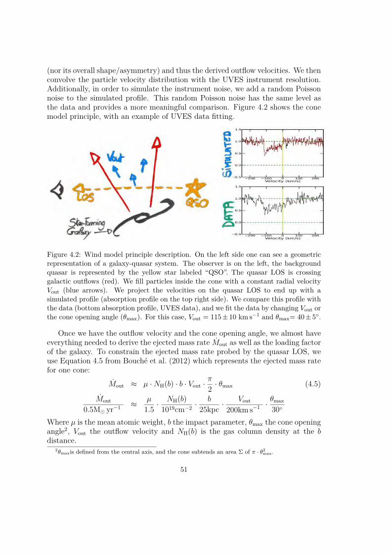
(nor its overall shape/asymmetry) and thus the derived outflow velocities. We thenconvolve the particle velocity distribution with the UVES instrument resolution.Additionally, in order to simulate the instrument noise, we add a random Poissonnoise to the simulated profile. This random Poisson noise has the same level asthe data and provides a more meaningful comparison. Figure 4.2 shows the conemodel principle, with an example of UVES data fitting.

Figure 4.2: Wind model principle description. On the left side one can see a geometricrepresentation of a galaxy-quasar system. The observer is on the left, the backgroundquasar is represented by the yellow star labeled “QSO”. The quasar LOS is crossinggalactic outflows (red). We fill particles inside the cone with a constant radial velocityVout (blue arrows). We project the velocities on the quasar LOS to end up with asimulated profile (absorption profile on the top right side). We compare this profile withthe data (bottom absorption profile, UVES data), and we fit the data by changing Vout orthe cone opening angle (θmax). For this case, Vout = 115± 10 km s−1 and θmax= 40± 5.

Once we have the outflow velocity and the cone opening angle, we almost haveeverything needed to derive the ejected mass rate Mout as well as the loading factorof the galaxy. To constrain the ejected mass rate probed by the quasar LOS, weuse Equation 4.5 from Bouche et al. (2012) which represents the ejected mass ratefor one cone:

Mout ≈ µ ·NH(b) · b · Vout ·π

2 · θmax (4.5)

Mout

0.5M yr−1 ≈ µ

1.5 ·NH(b)

1019cm−2 ·b

25kpc ·Vout

200km s−1 ·θmax

30

Where µ is the mean atomic weight, b the impact parameter, θmax the cone openingangle2, Vout the outflow velocity and NH(b) is the gas column density at the bdistance.

2θmaxis defined from the central axis, and the cone subtends an area Σ of π · θ2max.

51

Figure 4.3: Examples of simulated absorption profiles with different galaxy inclinations(i), opening angle (θ) and wind velocities (Vout): while each of the simulated profiles hasthe same number of particles, the apparent depth decreases as each parameter increasesdue to larger velocity projections for i and θ, and larger range of velocities for Vout. Toprow: absorption profiles for galaxies inclined at 30, 60 and 90 degrees with Vout= 100km s−1and θ= 30. The noise effect is due to the Monte Carlo distribution of particles.Middle row: absorption profiles for wind cones with opening angles of 30, 40 and 45degrees with Vout= 100 km s−1and i=45. Bottom row: absorption profiles with windvelocities of 50, 100 and 150 km s−1with i= 45 degrees and θ= 30. Each simulatedprofile has the same amount of particles but show a larger velocity range due to theincreasing gas speed, hence the varying apparent depths.

52

The only parameter which is yet to be constrained is the gas column densityNH(b). To do so, we use the empirical relation 4.6 from Menard & Chelouche(2009) between the neutral gas column density and the Mg ii λ2796 REW W λ2796

r :

NHI = (3.06± 0.55)× 1019 × (W λ2796r )1.7±0.26. (4.6)

This relation, together with the tight correlation between Mg ii equivalentwidth and dust content (as determined statistically from quasar extinction) fromMenard & Chelouche (2009), leads to a gas-to-dust ratio slightly smaller than thatof the Milky Way H i column densities of log(NH i) =19.5 and above. Further-more, the redshift evolution of the dust content of Mg ii absorbers, extrapolatedto z = 0, shows that Mg ii–selected absorbers extend the local relation betweenvisual extinction AV and the total hydrogen column NH of Bohlin et al. (1978).This in turn indicates that the ionized gas contribution is negligible in regions withH i columns above log(NH i) =19.5, as also argued by Jenkins (2009), and thatone can use the correlation between Mg ii equivalent width and NH i as a proxyfor the NH gas column density.

Now that we described the methodology we use in order to constrain galacticoutflows, we will now focus on the data analysis from our IFU surveys.

4.2 SIMPLE sample

As mentioned in § 2.2.2, this sample is composed of 10 galaxy-quasar pairs. Foreach galaxy, we first derive their morpho-kinematic parameters.

4.2.1 Morpho-kinematics from GalPaK3D

Using the GalPaK3D tool, we fit the kinematics and flux distribution (chosen tobe exponential or Gaussian in our cases) directly to the data-cubes. Table 4.1summarizes the morpho-kinematics parameters for each galaxy. We emphasizethat the surface-brightness profile breaks the common inclination-Vmax degeneracyfrom the axis ratio b/a in kinematic analysis compared to traditional methodsfitting the kinematics on velocity field. For every galaxy, we checked that theMCMC chain converged for each of the parameters and estimated the uncertaintiesfrom the last 60 percents of the iterations. For J1422−0001, some of the kinematicparameters remain unconstrained, because the rotation curve appears shallow suchthat the turn-over radius rt and the circular velocity Vmax are degenerate Theparameters relevant for wind study for defining the kinematic major axis (positionangle (PA)) are well constrained, however.

Once morpho-kinematics of all galaxies are constrained, we need to selectgalaxy-quasar pairs suitable for wind studies.

53

Table 4.1: Kinematic and morphological parameters for the 10 SIMPLE galaxy-quasarpairs.Galaxy inclination (˚) PA (˚) flux Vmax redshift r 1

2(1) (2) (3) (4) (5) (6) (7)J0147+1258 24.4±3.3 −69±3 1.63 · 10−16 241±38 1.0389 7.11 ± 0.20J0226-2857 47.9±1.0 91±1 2.01 · 10−16 50±12 1.0223 2.69 ± 0.04J0302-3216 30.4±1.5 −37±3 2.70 · 10−16 180±15 0.8223 8.99 ± 0.31J0448+0950 52.0±1.2 31±1 5.03 · 10−16 253±10 0.8391 7.85 ± 0.07J0822+2243 17.9±0.7 168±1 5.04 · 10−16 328±14 0.8102 4.14 ± 0.06J0839+1112 72±5† 139±4 1.53 · 10−16 113±20 0.7866 5.65 ± 0.29J0943+1034 43±5†† 140±1 3.81 · 10−16 327±10 0.9956 8.73 ± 0.21J1422-0001 55±5 81±3 8.93 · 10−17 130±20††† 0.9096 4.30 ± 0.16J1441+0443†† · · · 87±4 6.62 · 10−17 · · · 1.0384 2.99 ± 0.18J2357-2736 51.6±2.2 109±2 1.29 · 10−16 187±15 0.8149 5.53 ± 0.14(1) Quasar name; (2) Galaxy inclination (degrees); (3) Position Angle (degrees); (4)

Integrated Hα flux of the galaxy (erg s−1 cm−2); (5) Maximum rotation velocity(km s−1); (6) Hα-based redshift; (7) Half-light radius (kpc); † the inclination is

determined from the HST data. †† galaxy parameters are derived from 2D fitting(galfit2D). ††† turn-over radius is fixed to rt/r1/2 = 0.25.

4.2.2 Galaxy-quasar pairs classification

Based on azimuthal angles, we classify galaxy-quasar pairs into wind or inflow pairs(see § 2.1.3). For this sample, we classified 4 pairs suitable for wind studies (galax-ies framed with black rectangles in Figure 4.4), 4 suitable for accretion studies and2 are ambiguous cases mainly due to their low-inclination. The low-inclinationof a galaxy increase the uncertainty on its position angle (it is difficult for anedge-on galaxy to differentiate the major axis to its minor one) and thus on theazimuthal angle. For our study, we focus on wind-pairs (J0448+0950, J0839+1112,J1441+0443 and J2357-2736). Figure 4.4 shows the 10 galaxies of the SIMPLEsample. Figure 4.5 shows that four galaxies are favorable to study galactic windsproperties: J0448+0950, J2357-2739, J0839+1112 and J1441+0443, and are clas-sified as wind-−pairs. J1441+0443 is excluded from subsequent analysis becauseour SINFONI data does not meet the requirement of SNR∼ 3 imposed by ourintensive tests of the GalPaK3D algorithm.

4.2.3 Outflow properties

For each of the four galaxy-quasar pairs suitable for wind study, we run our windmodel (described in § 4.1.2) with the geometrical parameters derived by GalPaK3D.In UVES quasar spectra, the Mg ii λ2796 absorption lines are saturated. We thususe the Mg i λ2852 absorption line which is not saturated. Out of these 4 galax-

54

Figure 4.4: Zoom of QSO-subtracted Hα maps of the 10 SIMPLE galaxies: quasar LOSis represented by the white contours if present or pointed out with a white arrow. The4 wind-pairs are framed with a black rectangle.

ies, only 3 have well constrained morpho-kinematical parameters (J0448+0950,J0839+1112 and J2357-2736). The J1441+0443 associated galaxy has too lowSNR for GalPaK3D to converge.

Since this galaxy-quasar sample consists of pairs with small impact parameters(b < 20 kpc) and with moderately-inclined galaxies (from ∼ 18 to ∼ 55), weimprove our wind model by adding galaxy’s interstellar medium (ISM) contributionfor the galaxy-quasar pairs with the lowest impact parameters such as J2357-2736and J0448+0950. The procedure is nearly the same as the cone model: we generateparticles in a disk with a random exponential distribution from the center witha FWHM corresponding to the galaxy radius previously derived with GalPaK3D.We take the galaxy half light radius derived with GalPaK3D to estimate a realisticcontribution from the disk. The thickness of the disk is set to be 0.15 times itsradius. We assign the particles a constant circular velocity corresponding to themaximum velocity of the galaxy. We assume that particles have only the maximumrotational velocity of the galaxy since this model simulates the galaxy contributionat the impact parameter, which is far away from the galaxy center and thereforeat this distance, the rotational velocity of the galaxy is considered as constant.The velocity absorption distribution of the disk is naturally strongly dependent onthe azimuthal angle with a maximum offset at α = 0 and a distribution centeredaround 0 km s−1 at α = 90.

One “wind” pair has a low impact parameter b = 6.7 kpc (J2357−2736). Forthis galaxy, our assumption of a constant outflow velocity may break down. Indeed,

55

Figure 4.5: Galaxy inclinations for the SIMPLE sample as a function of the azimuthalangle α. Note there are three types of galaxies in this sample: the wind-pairs which havean azimuthal angle larger than 60±10, the inflow-pairs with α lower than 60±10 andpairs that are ambiguous due to uncertainty on α. It is difficult to derive the azimuthalangle for a nearly face-on galaxy. The wind-pair and inflow-pair classes describe the factof having the quasar absorptions tracing outflows and inflows, respectively.

56

the low-ionization material in momentum-driven winds and energy-driven winds isthought to be accelerated (e.g. Murray et al., 2005; Steidel et al., 2010) by the hotgas, by the radiation pressure, or both. Therefore, instead of using a constant windspeed, we used a generic velocity profile such as V (r) = Vout 2/π arctan(r/r0)(e.g. Puech et al., 2008) where r is the distance from the galaxy and r0 is thecharacteristic turn-over radius. Behavior of this model can be seen in Figure 4.6.The major impact of the simulated profile using this accelerated wind model isthat it affects the asymmetry of the profile when changing r0.

The accelerated wind model that best describes the data for the J2357−2736system is using a characteristic turn-over radius r0 of 10 kpc. In addition, we alsoincluded a contribution from the galaxy which appears to account for the bluestcomponents (see left column of Figure 4.7). Figure 4.7 shows the results for thethree wind-pairs of the SIMPLE sample. The bottom row shows the UVES dataand the upper row the simulated absorption profiles. We can see that we reproducethe equivalent widths of each galaxy-quasar pair as well as the asymmetry in eachprofile.

If we assume that galactic winds are symmetric with respect to the galacticplane (Figure 2.2), the total ejected mass rate for a galaxy must be increased bya factor of 2. Table 4.2 shows the results for the three wind-pairs.

Table 4.2: Results for galaxies J0448+0950, J2357-2736, J0839+1112.Galaxy b (kpc) log(NH(b)) Vout θmax SFR Mout

VoutVesc

η

(1) (2) (3) (4) (5) (6) (7) (8) (9)J0448+0950 13.7 20.30±0.3 115± 10 40 ± 5.0 13.6±0.3 4.6 +4.9

−3.2 0.16 0.70J0839+1112 26.8 20.10±0.3 105± 10 30 ± 5.0 3.4±0.2 3.6 +3.4

−2.2 0.43 2.11J2357−2736 6.7 19.92±0.2 130± 10 45 ± 5.0 3.3±0.2 1.2 +1.1

−0.7 0.24 0.75(1) Galaxy name; (2) Impact parameter (kpc); (3) Gas column density at the impactparameter (cm−2); (4) Wind velocity (km s−1); (5) Cone opening angle (degrees) (6)Star Formation Rate (M yr−1); (7) Ejected mass rate for one cone (M yr−1); (8)

Ejection velocity divided by escape velocity; (9) Mass loading factor: ejected mass ratedivided by star formation rate (for both cones);

In each case, the derived loading factors are around unity and the outflowvelocity do not reach the escape velocity so that the outflowing gas is likely to fallback onto the galaxy. The resulting loading factors for these 3 wind-pairs are shownin Figure 4.8. In this Figure, the different lines represent theoretical (Okamotoet al., 2010; Dave et al., 2011; Hopkins et al., 2012; Puchwein & Springel, 2013;Vogelsberger et al., 2014; Muratov et al., 2015; Barai et al., 2015) and empiricalmodels (Zahid et al., 2014; Peeples & Shankar, 2011). The parameters of thesemodels are listed in Table 1 of Zahid et al. (2014). It is important to note that thecurve from Barai et al. (2015) only includes gas particles with velocities greaterthan the escape velocity. In addition to this sample, observational constraint

57

Figure 4.6: Left column: from top to bottom: simulated absorption profiles withr0=1,5,10 kpc. Notice that the asymmetry changes as r0 increases, it goes from outwardto inward asymmetry. Right column: The velocity profile corresponding to the associatedsimulated profile to the left where the turn over radius of the velocity profile (r0) varies,from top to bottom: r0=1,5,10 kpc. The red dashed line represents the distance betweenthe galaxy and the quasar LOS (b/sin(α)/sin(i)), corrected for the inclination i.

include the redshift z ∼ 0.1 (Bouche et al., 2012, triangles), and Kacprzak et al.(2014) result (square), although very few measurements on individual galaxies

58

J0448+0950 J0839+1112 J2357-2736

Figure 4.7: Wind models for the three wind-pairs. The bottom row corresponds to UVESquasar Mg i λ2852 absorption lines for the three fields: J0448+0950, J0839+1112 andJ2357−2736 from left to right. The upper row shows the resulting simulated profilesfor each case. One can see that we reproduce the equivalent widths and the profileasymmetries for each galaxy. Note that we do not reproduce the depth as the simulatedprofile is normalized ’by hand’. On each simulated profile, the red lines correspond to thewind contribution only whereas the black part corresponds to the galaxy component.

exist so far. We raise here the problem of large impact parameters. The loadingfactor η is, by definition, the ratio between the ejected mass rate Mout and theSFR. If the impact parameter is large (typically if b > 60 kpc), these two quantities(Mout and SFR) are on different time scales. Indeed, we derive the ejected massrate at the quasar LOS, whereas the SFR is derived from emission lines of the hostgalaxy. For large b, the travel time b/Vout is orders of magnitude larger than thetime scale of SFR derived from emission lines. SED fitting is a method allowingus to derive SFR on the same time scale than the travel time of the gas to getfrom the galaxy to the quasar LOS. We took the SED-derived SFRs from theBouche et al. (2012) sample, given their longer travel times (b/Vout) to the impactparameters, using UV-to-IR photometry from the Galex+SDSS+Wise surveys andthe Code Investigating GALaxy Emission (CIGALE) software (Noll et al., 2009b).The pairs with the largest impact parameters are shown in grey as these mass

59

loading factors can suffer strong biases due to the significant travel time.

4.3 MEGAFLOW survey

As mentionned in § 2.3, the aim of this survey is to increase the number of wind-pairs by 1 order of magnitude in order to allow for statistical analysis.

4.3.1 Survey status

Aiming for 80+ pairs in 20-25 quasar fields, the MEGAFLOW survey is ongoingat the time of writing. As mentioned in § 2.3.2, 19 (out of 25) quasar fields havebeen observed (as of July 30th 2016) with MUSE as part of GTO time and 17out of the 25 quasar fields have UVES high resolution quasar spectra follow-up.We do have 15 complete quasar fields with both MUSE and UVES observations.So far, 56 host galaxies have been detected in MUSE data out of 66 candidates(84% detection). Table 4.3 shows MEGAFLOW survey status. The number ofdetection corresponds to the number of galaxies assumed to be responsible forMg ii absorption lines. In some cases, the number of detected galaxies is largerthan the number of absorbers. This means that for one Mg ii absorber, more thanone galaxy are detected at one absorber redshift and assumed to be the hosts.

4.3.2 Morpho-kinematics from GalPaK3D

As in § 4.2.1, for each detected galaxy we run GalPaK3D in order to derive theirmorpho-kinematics properties. Every 56 galaxies were GalPaK3D-processed, usingdefault parameters with no assumption. These 56 galaxies were also processedwith the 2D fitting tool called Camel3 in order to cross check the results.

Out of these 56 galaxies, 26 have converged parameters, based on MCMC chainsand comparison with the input data and Camel results. The 30 other galaxies didnot converged for several reasons. These reasons are either a low SNR, mergers orthe galaxy was too small (r1/2 < seeing FWHM).

For mergers, a reason for GalPaK3D not to converge is that the “simple” modelof a rotating disk represented with a smooth symmetric light profile is not adaptedto complex kinematic of some galaxies, and these galaxies are usually gravitation-ally interacting or in advance merging process.

For “non-converged” galaxies, some parameters like PA or Vmax are still acces-sible with Camel or GalPaK3D but because lack of time needed to study each ofthese galaxies forced us to only focus on converged galaxies.

Middle and right columns of each case in Figures 4.9, 4.10 and 4.11 showvelocity maps of each galaxy corresponding to the ones presented on left panels.What is important to look at between these two columns is to compare the position

3The source code can be found at https://bitbucket.org/bepinat/camel.git

60

Figure 4.8: Comparison of predicted mass loading factors from theoretical/empiricalmodels (curves) with values derived from observations (dots and triangles) as a functionof the maximum rotational velocity. The results from the SIMPLE sample are repre-sented by the cyan circles (Schroetter et al., 2015). The red circle shows the mass loadingfactor for a z ∼ 0.2 galaxy (Kacprzak et al., 2014). The triangles show the results forz ∼ 0.2 galaxies from Bouche et al. (2012). The gray triangles show the galaxies withquasars located at >60kpc where the mass loading factor is less reliable due to the largetravel time needed for the outflow to cross the quasar LOS (several 100 Myr) comparedto the short time scale of the Hα derived SFR (∼ 10Myr). The upper halo mass axis isscaled on Vmax at redshift 0.8 from Mo & White (2002).

61

Table 4.3: MEGAFLOW survey status.Target name / QSO Texp additional Comments zqso UVES(1) (2) (3) (4) (5)SDSSJ001453.19+091217 3.0h / 3.0h detection 1/3 2.308 1/3OB P96 P97SDSSJ001453.36−002827 2.0h / 2.0h detection 3/3 1.924 3/3OB P96SDSSJ001535.17−075103 2.0h / 2.0h detection 3/3 0.874 Pending P98SDSSJ005855.75+011128 1.0h / 2.0h detection 1/3 1.222 Pending P98SDSSJ010332.30+133233 2.0h / 2.0h detection 2/3 1.663 Pending P98SDSSJ013136.44+130331 2.0h / 2.0h detection 4/4 1.589 2/2OB P96SDSSJ013405.70+005109 2.0h / 2.0h detection 2/4 1.519 Pending P98SDSSJ014513.10+105626 1.0h / 2.0h detection 3/3 0.938 1/3OB P96SDSSJ080004.54+184935 2.0h / 2.0h detection 3/4 1.292 2/2OB P96SDSSJ083852.05+025703 2.0h / 2.0h detection 3/4 1.768 1/1OB P96SDSSJ093749.58+065656 2.0h / 2.0h detection 4/4 1.814 3/3OB P96SDSSJ103936.66+071427 2.0h / 2.0h detection 3/3 1.532 3/3OB P97SDSSJ110735.26+175731 2.0h / 2.0h detection 2/2 2.133 3/3OB P96SDSSJ110742.70+102126 2.0h / 2.0h detection 3/5 1.922 2/2OB P96SDSSJ123624.40+072551 2.0h / 2.0h detection 2/4 1.605 1/1OB P96SDSSJ131405.60+065721 2.0h / 2.0h detection 9/4 1.879 1/1OB P97SDSSJ135217.67+061433 0.0h / 2.0h detection ?/3 1.798 1/1OB P97SDSSJ135809.49+114557 2.0h / 2.0h detection 3/3 1.716 2/2OB P97SDSSJ142538.05+120919 1.0h / 2.0h detection ?/4 1.618 2/2OB P97SDSSJ150900.12+150634 1.0h / 2.0h detection ?/4 2.237 2/2OB P97SDSSJ213748.44+001220 3.0h really out of spec 1.668 —SDSSJ213748.44+001220 1.0h detection 3/4 1.668 P94SDSSJ215200.03+062516 2.0h / 2.0h detection 3/4 2.409 P94(1) Quasar field name; (2) Total exposure time of the field; (3) Number of detectedgalaxy corresponding to Mg ii absorber; (4) Quasar redshift; (5) UVES follow-up

observation period.

angles of each galaxy as well as the velocity fields (check if the positive and negativevelocities areas correspond to each other). We can see that for almost every galaxy,these parameters are in good agreements. Some galaxy like the one at redshift1.0108 in the J0131+1303 quasar field show a position angle difference of ∼ 60.

Table 4.4 show the GalPaK3D results for the 26 galaxies. Figures 4.9, 4.10 and4.11 show the 26 galaxies of the MEGAFLOW survey as well as wind-pairs whichare framed with a red rectangle.

62

Figure 4.9: Results for 10 MEGAFLOW galaxies: Each set of result for a galaxy iscomposed of 3 maps: left: zoom of QSO-subtracted [O ii] maps. On each of these maps,on top of them is indicated the redshift of the galaxy and at the bottom the quasarfield name. Middle: zoom of QSO-subtracted Camel velocity map. Right: Zoom ofQSO-subtracted GalPaK3D PSF-deconvolved velocity map. Wind-pairs are framed witha red rectangles for Camel and GalPaK3D velocity maps.

63

Figure 4.10: Same as Figure 4.9 for the 10 next galaxies.

Figure 4.11: Same as Figure 4.9 for the last 6 galaxies.

64

Table 4.4: GalPaK3D results on 26 MEGAFLOW galaxies with reliable morpho-kinematic parameters.

field name redshift α b W λ2796r PA incl Vmax Vdisp Flux

(1) (2) (3) (4) (5) (6) (7) (8) (9) (10)J0014p0912 0.6679 26± 2 63.5 . . . -160 ± 2 61 ± 2 158 ± 15 38 ± 5 2.9×10−17

J0014m0028 0.8343 79± 10 10.8 2.232 78 ± 68 65 ± 5 16 ± 16 40 ± 2 3.2×10−17

J0131p1303 G1 1.0106 76± 1 26.8 1.165 -32 ± 1 50 ± 1 151 ± 17 30 ± 2 3.0×10−17

J0131p1303 G2 1.0108 53± 1 125.8 1.165 16 ± 1 65 ± 2 189 ± 14 27 ± 6 2.1×10−17

J0131p1303 G3 1.1052 60± 2 72.8 1.168 -74 ± 2 78 ± 5 107 ± 26 58 ± 4 2.3×10−17

J0800p1849 G1 0.6085 22± 1 62.3 0.915 112 ± 1 65 ± 1 102 ± 3 40 ± 0.7 6.9×10−17

J0800p1849 G2 0.9937 72± 1 76.8 0.934 -146 ± 1 66 ± 1 174 ± 19 50 ± 1 4.4×10−17

J0937p0656 G1 0.7024 84± 1 37.5 1.767 -56 ± 1 47 ± 1 215 ± 13 64 ± 2 1.4×10−16

J0937p0656 G2 0.7022 55± 1 67.8 1.767 76 ± 1 44 ± 1 203 ± 21 33 ± 2 9.5×10−17

J0937p0656 G3 0.9340 72± 1 38.1 1.519 -71 ± 1 66 ± 1 131 ± 29 47 ± 2 6.9×10−17

J1107p1757 1.1620 72± 3 47.6 1.97 -114 ± 3 61 ± 4 66 ± 5 38 ± 3 6.4×10−17

J1039p0714 G1 0.9493 4± 1 48.7 1.22 152 ± 1 53 ± 1 152 ± 7 54 ± 2 8.5×10−17

J1039p0714 G2 0.9494 66± 4 72.7 1.22 -129 ± 4 69 ± 7 191 ± 65 83 ± 6 2.6×10−17

J1107p1021 1.0479 23± 2 40.9 0.499 151 ± 2 70 ± 4 294 ± 38 33 ± 14 3.5×10−17

J1314p0657 G1 0.9080 35± 1 66.3 0.889 37 ± 1 67 ± 1 135 ± 2 78 ± 1 1.9×10−16

J1314p0657 G2 0.9084 85± 3 96.2 0.889 -168 ± 3 44 ± 2 225 ± 22 11 ± 11 1.4×10−17

J1314p0657 G3 0.9867 89± 4 37.9 0.977 24 ± 4 36 ± 3 330 ± 24 50 ± 2 6.4×10−17

J1314p0657 G4 0.9871 7± 3 104.1 0.977 -30 ± 3 30 ± 15 118 ± 117 39 ± 9 1.4×10−17

J1236p0725 G1 0.6341 77± 2 66.3 1.412 177 ± 2 65 ± 12 168 ± 12 71 ± 5 1.0×10−16

J1236p0725 G2 0.9137 2± 2 18.2 2.24 85 ± 2 47 ± 2 232 ± 12 6 ± 4 6.7×10−17

J2137p0012 G1 0.8069 25± 2 88.1 0.724 74 ± 2 54 ± 2 132 ± 5 39 ± 2 8.3×10−17

J2137p0012 G2 1.1892 71± 10 63.7 0.308 -134 ± 68 52 ± 2 12 ± 12 102 ± 1 1.4×10−16

J2137p0012 G3 1.2139 47± 4 87.2 1.122 -83 ± 4 32 ± 6 203 ± 39 11 ± 7 4.0×10−17

J2152p0625 G1 1.0533 4± 1 45.4 0.522 -128 ± 1 75 ± 1 173 ± 2 2 ± 2 8.7×10−17

J2152p0625 G2 1.3184 88± 10 34 1.347 -87 ± 10 75 ± 9 139 ± 52 29 ± 12 1.3×10−17

J2152p0625 G3 1.4303 72± 3 62.5 1.152 -162 ± 3 28 ± 1 299 ± 25 22 ± 12 3.1×10−17

(1) Quasar field name; (2) Galaxy redshift; (3) Azimuthal angle (α) in degrees; (4) Impact parameter (kpc); (5) Mg ii REW(A); (6) Galaxy position angle (degrees); (7) Galaxy inclination (degrees); (8) Maximum rotational velocity (km s−1); (9)

Velocity dispersion (km s−1); (10) [O ii] flux (erg s−1 cm−2);

65

In the next sections, we only focus on the 26 converged galaxies.

4.3.3 Galaxy-quasar pairs classification

To put constraints on galactic outflows, we first need to select galaxy-quasar pairssuitable for wind studies (wind pairs). To do so, we measure the angle betweenthe galaxy major axis and the apparent quasar location, which is referred to as theazimuthal angle α (see Figure 2.2 and § 2.1.3). Figure 4.12 shows galaxy inclinationas a function of quasar azimuthal angle. We can see that 3 pairs are classified asambiguous whereas 9 are likely to be inflow-pairs and 11 likely to be wind-pairs.Figure 4.13 shows the distribution of azimuthal angles. We note that there is abimodal distribution of azimuthal angle and there are more galaxy-quasar pairs ina configuration favorable for wind study. This is probably due to the fact that weselect only strong Mg ii REW in the quasar spectra and the largest Wλ2796

r tendto be associated with outflows (e.g. Kacprzak et al., 2011; Lan et al., 2014a).

Now that we classified our galaxy-quasar pairs, we can focus on wind-pairs inorder to constrain galactic outflow properties.

Figure 4.12: Galaxy inclination as a function of azimuthal angle α for 26 galaxies withreliable morpho-kinematic parameters detected in the MUSE fields. The dashed areascorrespond to azimuthal angle ranges for which we classify pairs as inflow-pairs (blueand narrow dashes) or wind-pairs (green and wider dashes). These areas stop for face-ongalaxies as uncertainty on position angles are too large. It is thus difficult to determineα and to classify galaxy-quasar pairs in this area. We note that 11 galaxies are classifiedas wind-pairs.

66

Figure 4.13: Azimuthal angle α distribution for 26 galaxies with reliable morpho-kinematic parameters detected in the MUSE fields. We note that 11 galaxies are classifiedas wind-pairs and that there is a bimodal distribution of α. There are more galaxy-quasarpairs in a configuration favorable for wind study.. This is probably due to the fact thatwe select only strong Mg ii REW in the quasar spectra and the largest Wλ2796

r tend tobe associated with outflows (e.g. Kacprzak et al., 2011; Lan et al., 2014a).

4.3.4 Outflow properties

With the 11 wind-pairs we have, we proceed as in § 4.2.3. For each wind-pair,we build our cone model in order to reproduce the absorption lines in the UVESquasar spectra. In some absorption lines (Fe ii in Figures 4.19, 4.20 and 4.23, Mg iin Figure 4.21, Mg ii in Figure 4.22), we can see a lack of absorption in roughlythe middle of a line, and this happens when the quasar LOS is aligned with thegalaxy minor axis (α > 80). This lack of absorbing particles at these velocitiesshows that the outflowing cone must have a low density region inside it. We thusdeveloped a partially empty cone model in order to reproduce absorption profilesfor the cases where α > 80.

The principle is the same as described in § 4.1.2 except that we only fill thecone with particles from a certain opening angle θin to θmax. The inner cone istherefore empty. As mentioned in Schroetter et al. (2016), this empty inner conecould be the signature of a highly ionized gas filled in the inner cone while thelow-ionized gas that we are tracing is entrained in the outskirts of the outflowingcone in a manner similar to Fox et al. (2015) for the MilkyWay and to Veilleux &Rupke (2002) for NGC1482. This scenario is also motivated by references cited inVeilleux et al. (2003) or Bland-Hawthorn et al. (2007).

In addition to this empty cone model, in some cases (for J0131+1303 and

67

J0937+0656 quasar fields), multiple galaxy candidate for the same absorptionare assumed to be responsible for the absorption in the quasar spectrum. If thedetected galaxies happen to have a geometrical configuration suitable to be wind-pairs, then we need to generate multiple wind models for the same absorption lines(see Figures 4.19 and 4.20). We can differentiate three main models: “classic” windmodels, “empty cone” wind models and “multiple contribution” wind models.

“Classic” wind models are processed to wind-pairs for which there is only onegalaxy detected around the Mg ii absorption redshift in a quasar field and thatthe corresponding absorption lines in UVES data do not show a lack of absorptionin the middle of the profile. These wind-pairs correspond to pairs with Mg iiabsorptions in the associated quasars at redshifts z =0.8343 for the J0014−0028quasar field, z = 0.9340 for J0937+0656, z = 0.9495 for J1039+0714, z = 0.9867for J1314+0657 and z = 0.6342 for J1236+0725. These wind-pairs have impactparameters b of 10.8, 38.1, 72.7, 37.9 and 66.3 kpc, azimuthal angles α of 79, 72,66, 89 and 77 respectively. The outflowing velocities and cone opening angles areVout= 210± 10 km s−1 with θmax= 25± 5 for J0014−0028, Vout= 150± 10 km s−1

with θmax= 30 ± 5 for J0937+0656, Vout= 65 ± 10 km s−1 with θmax= 30 ± 5for J1039+0714, Vout= 95 ± 10 km s−1 with θmax= 20 ± 5 for J1314+0657 andVout= 65± 10 km s−1 with θmax= 30± 5 for J1236+0725.

“Empty cone” wind models are processed to wind-pairs like the “classic” pairsexcept that absorption lines in UVES data show a lack of absorption in the roughlymiddle of the absorption profile. These wind-pairs correspond to pairs with Mg iiabsorptions in the associated quasars at redshifts z = 1.1620 for the J1107+1757quasar field, z = 0.9085 for J1314+0657 and z = 1.3185 for J2152+0625. Thesewind-pairs have impact parameters b of 47.6, 96.2 and 34.0 kpc, azimuthal anglesα of 72, 85 and 88 respectively. The outflowing velocities and cone opening anglesare Vout= 150± 10 km s−1 with θmax= 30± 5 and θin = 20± 2 for J1107+1757,Vout= 210 ± 10 km s−1 with θmax= 30 ± 5 and θin = 7 ± 2 for J1314+0657 andVout= 150± 10 km s−1 with θmax= 20± 5 and θin = 7± 2 for J2152+0625.

The remaining wind-pairs are then in the “multiple contribution” wind modelscategory. These are the two cases where we do find two galaxies at very closeredshifts that are considered responsible for the Mg ii absorption lines in the quasarspectra.

The first two galaxies detected to be responsible for the Mg ii absorption linesare from the J0131+1303 quasar field. These galaxies have redshifts z = 1.0108and z = 1.0106, impact parameters b of 125.8 kpc and 26.8 kpc, azimuthal anglesα of 53 and 76 respectively. Resulting simulated profiles are shown on top panelof Figure 4.19. The outflow in green has a Vout of 205± 10 km s−1 and an openingangle θmax of 35 ± 5 for the galaxy at redshift z = 1.0108. The outflow in blackhas a Vout of 80± 10 km s−1 and an opening angle θmax of 35± 5 and θin of 8±2for the galaxy at redshift z = 1.0106.

The last two galaxies detected to be responsible for the Mg ii absorption lines

68

are from the J0937+0656 quasar field. These galaxies have redshifts z = 0.7022and z = 0.7024, impact parameters b of 67.8 kpc and 37.5 kpc, azimuthal anglesα of 84 and 55 respectively. Resulting simulated profiles are shown on top panelof Figure 4.20. The outflow in green has a Vout of 100± 10 km s−1 and an openingangle θmax of 30 ± 5 for the galaxy at redshift z = 0.7022. The outflow in blackhas a Vout of 120± 10 km s−1 and an opening angle θmax of 35± 5 and θin of 8±2for the galaxy at redshift z = 0.7024.

Figures 4.14, 4.19, 4.20, 4.15, 4.16, 4.21, 4.18, 4.22, 4.15 and 4.23 (Figures 4.19and 4.20 shows results for two wind-pairs each) show the UVES absorption linescentered at the galaxy redshift for every wind-pair as well as corresponding sim-ulated profiles on top. As in § 4.2.3, we derive outflow velocities as well as coneopening angles for each wind-pair. For simplicity, results on outflows are listed inTable 4.5.

Vout = 210 km/s

Figure 4.14: Representation of simulated profile and quasar spectrum associated withthe J0014−0028 galaxy. Simulated wind profile (top) reproducing the Mg i absorptionprofile (centered at z = 0.8343) from UVES (bottom). This outflow has a Vout of 210±10km s−1 and an opening angle θmax of 25± 5.

In summary of this chapter, we managed to put further constraints on galacticoutflows thanks to the background quasar technique. Before showing our resultson loading factors as a function of the galaxy halo mass, further investigations onrelations between galactic winds and galaxy properties are needed.

69

Vout = 150 km/s

Figure 4.15: Same as Figure 4.14 but for the J0937+0656 galaxy at redshift z ≈ 0.9340.This outflow has a Vout of 150± 10 km s−1 and an opening angle θmax of 30± 5 for thegalaxy at redshift z = 0.9340.

Vout = 65 km/s

Figure 4.16: Same as Figure 4.14 but for the J1039+0714 galaxy at redshift z ≈ 0.9495.This outflow has a Vout of 65± 10 km s−1 and an opening angle θmax of 30± 5 for thisgalaxy.

70

Vout = 95 km/s


Vout = 60 km/s


71

Vout = 80 km/sVout = 205 km/s

Figure 4.19: Same as Figure 4.14 but for the J0131+1303 galaxies at redshift z ≈ 1.0106.For this case, because two galaxies were detected at the absorber redshift, we needed torun wind models for both of them (at redshift 1.0106 and 1.0108) in order to reproducethe absorption lines in red. The outflow in green has a Vout of 205 ± 10 km s−1 and anopening angle θmax of 35±5 for the galaxy at redshift z = 1.0108. The outflow in blackhas a Vout of 80 ± 10 km s−1 and an opening angle θmax of 35 ± 5 and θin of 8±2 forthe galaxy at redshift z = 1.0106.

72

Vout = 120 km/sVout = 100 km/s

Figure 4.20: Same as Figure 4.19 but for the J0937+0656 galaxies at redshift z ≈ 0.7024.The outflow in green (the positive absorption component) has a Vout of 100± 10 km s−1

and an opening angle θmax of 30± 5 for the galaxy at redshift z = 0.7022 (this pair hasan azimuthal angle α of 55). The outflow in black (the negative absorption components)has a Vout of 120± 10 km s−1 and an opening angle θmax of 35± 5 and θin of 8±2 forthe galaxy at redshift z = 0.7024 (his pair has an azimuthal angle α of 84). Results onthese two pairs are shown in Tables 4.4 and 4.5.

Vout = 150 km/s

Figure 4.21: Same as Figure 4.14 but for the J1107+1757 galaxy at redshift z ≈ 1.1620.This outflow has a Vout of 150± 10 km s−1 and an opening angle θmax of 30± 5 and θinof 20±2 for this galaxy.

73

Vout = 210 km/s


Vout = 150 km/s


74

Table 4.5: Results on outflow properties for MEGAFLOW galaxies.Galaxy zgal b (kpc) log(NH(b)) Vout θmax SFR Mout

VoutVesc

η

(1) (2) (3) (4) (5) (6) (7) (8) (9) (10)J0014m0028 0.8343 10.8 20.08±0.13 210 ± 10 25 ± 5 2.0±0.1 2.3 +2.3

−1.2 8.20 2.21J0131p1303 1.0106 26.8 19.60±0.05 80 ± 10 35 ± 5 3.4±0.3 1.0 +0.6

−0.4 0.24 0.58J0131p1303 1.0108 125.8 19.60±0.05 205 ± 10 35 ± 5 2.2±0.1 11.9 +4.5

−3.6 0.70 10.93J0937p0656 0.7024 37.5 19.90±0.10 120 ± 10 35 ± 5 7.6±0.9 4.2 +2.7

−1.8 0.24 1.11J0937p0656 0.7022 67.8 19.90±0.10 100 ± 10 30 ± 5 4.6±0.4 5.4 +3.7

−2.3 0.24 2.38J0937p0656 0.9340 38.1 19.79±0.08 150 ± 10 30 ± 5 7.5±0.9 3.6 +2.1

−1.4 0.56 0.95J1107p1757 1.1620 47.6 19.98±0.11 150 ± 10 30 ± 5 13.4±2.0 6.9 +4.7

−3.0 1.59 1.03J1039p0714 0.9495 72.7 19.63±0.06 65 ± 10 30 ± 5 2.4±0.2 2.0 +1.2

−0.8 0.18 1.71J1314p0657 0.9085 96.2 19.40±0.04 210 ± 10 30 ± 5 0.9±0.0 5.1 +1.9

−1.5 0.51 11.09J1314p0657 0.9867 37.9 19.47±0.04 95 ± 10 20 ± 5 8.0±1.0 0.7 +0.4

−0.3 0.12 0.18J1236p0725 0.6342 66.3 19.74±0.08 60 ± 10 35 ± 5 3.8±0.3 2.5 +1.6

−1.1 0.18 1.34J2152p0625 1.3184 34.0 19.70±0.07 150 ± 10 20 ± 5 4.6±0.4 1.7 +1.1

−0.8 0.54 0.74(1) Galaxy name; (2) Galaxy redshift; (3) Impact parameter (kpc); (4) Gas column

density at the impact parameter (cm−2); (5) Wind velocity (km s−1); (6) Cone openingangle (degrees) (7) Star Formation Rate (M yr−1); (8) Ejected mass rate for one cone(M yr−1); (9) Ejection velocity divided by escape velocity; (10) Mass loading factor:

ejected mass rate divided by star formation rate (for both cones);

75

Chapter 5

Combining both samples: galacticwind properties as a function ofgalaxy properties

Contents5.1 Basic properties of the sampled galaxies . . . . . . . . . . . . 78

5.1.1 Galaxy redshift distribution . . . . . . . . . . . . . . . . . . . . 785.1.2 Galaxy stellar mass measurement . . . . . . . . . . . . . . . . . 79

5.2 How far do winds go? . . . . . . . . . . . . . . . . . . . . . . . . 825.3 Do winds escape? . . . . . . . . . . . . . . . . . . . . . . . . . . 845.4 Wind scaling relations . . . . . . . . . . . . . . . . . . . . . . . 86

5.4.1 Previous studies on galactic winds . . . . . . . . . . . . . . . . 865.4.2 Scaling relations involving Vout . . . . . . . . . . . . . . . . . . 905.4.3 Scaling relations involving Mout . . . . . . . . . . . . . . . . . . 925.4.4 Scaling relations on loading factor η . . . . . . . . . . . . . . . 92

5.5 What mechanisms drive galactic winds? . . . . . . . . . . . . . 95

77

In this chapter, we combine our two samples (SIMPLE and MEGAFLOW) tocharacterize galactic winds as a function of galaxy properties. In section 5.1, wepresent the main properties of all the galaxies in the two samples and comparethem to the general underlying galaxy population. In section 5.2, we investigatethe spatial extent of galactic winds. In section 5.3, we investigate whether galacticwind material (traced by low-ionization lines) escape the gravitational potentialwells of the host. In section 5.4, we investigate relations, if any, between galacticwinds and galaxy properties. Finally, in section 5.5, we conclude on mechanismsthat drive galactic outflows.

5.1 Basic properties of the sampled galaxies

In this section, we present some basic properties of our sample galaxies to becompared with the general galaxy population. Star-forming galaxies are knownto follow fundamental scaling relations such as the SFR-M? main-sequence (e.g.Tacconi et al., 2013) and the M?-Vmax or Tully-Fisher (TF) relation (Tully &Fisher, 1977; Miller et al., 2011, 2014; Vergani et al., 2012; Simons et al., 2015, tocite a few). Rotational velocity, dispersion velocity, stellar mass, SFR and redshiftare fundamental galaxy properties.

5.1.1 Galaxy redshift distribution

We first need to see where our galaxies are located in look-back-time, i.e. inredshift space. Figure 5.1 shows the redshift distribution of both surveys.

Figure 5.1: Redshift distribution of the 36 galaxies from SIMPLE and MEGAFLOW.

This distribution clearly peaks around z ∼ 1 with a tail toward lower redshiftsbut with a few galaxies only extending up to z ∼ 1.4, reflecting our selection of

78

Mg ii absorbers. This figure shows that our sample is representative of galaxiesforming stars at around the peak of the cosmic star-formation density, which occursat z ≈ 1.5 (Lilly et al., 1996; Madau et al., 1996; Behroozi et al., 2013a).

5.1.2 Galaxy stellar mass measurement

In order to place our sample onto the SFR−M? diagram, the two fundamentalproperties for star-forming galaxies are their SFRs and stellar masses. Indeed,whether our galaxies (selected from the gaseous halo properties via our Mg ii cri-teria) lie on, above or below, the main sequence will shed light on the connectionbetween the circum-galactic medium properties and the star-formation activity.For instance, are galaxies producing winds starbursting, i.e. with a high SFR bysurface area ΣSFR and above the main-sequence?

In order to address these questions, we thus need SFR and stellar mass mea-surements. Contrary to the SFR, which can be derived directly from our datausing the Hα or [O ii] luminosities (see discussion in section § 4.1.1.), the stel-lar masses cannot be measured directly as our IFU observations are typically tooshallow to detect the stellar continuum. Hence, we need an indirect indicator ofgalaxy (stellar) mass and the kinematics properties (such as the rotational max-imum velocity) of our galaxies (see § 2.1.4 for more details) can be used to thispurpose.

Indeed, the kinematics properties of galaxies tightly correlate with their stellarmass as demonstrated by the existence of the TF scaling relation (e.g. Milleret al., 2011, 2014; Simons et al., 2015; Contini et al., 2016). The TF relation,traditionally between M? and Vmax is, however, valid only for galaxies that arerotation-dominated (V/σ > 1). The galaxies in our samples are mostly rotation-dominated, but Figure 5.2 shows that about 10 % are dispersion-dominated.

As described in § 1.2.3, the SK factor should be a better mass estimator forour galaxies as it includes the dispersion velocity (disordered motion) contribu-tion. Looking at the V/σ distribution of our galaxies we see that about 50% haveV/σ < 5. This motivates us to include disordered motions in estimating our galaxydynamical masses. For disk galaxies (V/σ > 1) with exponential M? profiles, anapproximation of K = 1/2 or K = 1/3 is adopted by Kassin et al. (2007). More-over, as argued by Weiner et al. (2006), real galaxies at, or beyond, the peak ofbaryonic contribution to the rotation curve have α = 2 − 3 (if we assume thatσ = V/α) for a spheric mass distribution, and thus adopting K = 1/3 − 1/2 isreasonable.

Because, most of the literature on SK (as in Kassin et al. (2007)) use kinematicsmeasurements from long-slit spectroscopy, where the slit could be mis-aligned withthe galaxy kinematic major-axis, we choose to calibrate the SK-M? relation on asample observed with an IFU instrument. To date, the deepest MUSE field withthe most exquisite kinematic data-set is the Hubble-Deep-Field South (HDFS;

79

Figure 5.2: V/σ distribution of all the galaxies from both surveys. Orange colored barrepresents dispersion-dominated galaxies (V/σ < 1).

Bacon et al., 2015). Contini et al. (2016) presented the kinematic analysis of thatsample, extending the TF relation to the low mass regime M? = 108-109, and wechoose to use this sample as reference. In addition, we used the galaxies fromSINS (Cresci et al., 2009) and MASSIV (Epinat et al., 2009; Contini et al., 2012)surveys to sample the high-mass regime as well. Figure 5.3 shows the correlationbetween M? and S0.5 for these samples. A fit of these data yields the relation:

M? ∝ Sb0.5 (5.1)

where b = 4.75 ± 0.39. The fitted coefficients are estimated from the orthogonaldistance regression (ODR) module of scipy taking into account the errors in S0.5and M? and are shown in Figure 5.3. This dynamical estimator S0.5 together withEquation 5.1 yield estimate of stellar masses of our galaxies.

For a rotation-dominated galaxy, the dynamical mass of the galaxy, insidea radius r, Mdyn(r) is proportional to V 2 × r:

Mdyn(r) = V 2 × rG

∝ V 2 × r (5.2)

where V is the rotational velocity of the galaxy and G is the gravitationalconstant. As mentioned before, our galaxies have non-negligible dispersionvelocities and we therefore use the S0.5 parameter. The dynamical mass of ourgalaxies becomes:

Mdyn(r) ∝ S20.5 × r (5.3)

The surface density is defined by:

ΣMdyn(r) = Mdyn(r)π × r2 (5.4)

80

thus:ΣMdyn(r) ∝ S2

0.5 × rπ × r2 ∝

S20.5 × rr2 (5.5)

Figure 5.3: Galaxy stellar mass as a function of the S0.5 parameter for HDFS, SINS andMASSIV data. The dashed red line represent a fit with coefficients shown in the legend.

Figure 5.4 shows SFR as a function of the galaxy stellar mass M? (bottomx-axis) and S0.5 (top x-axis) from Eq. 5.1. We added galaxies from Hubble DeepField South (HDFS) (Contini et al., 2016) to better see where our galaxies areplaced in a larger mass/SFR range. We can see on this figure that most of ourgalaxies have a stellar mass larger than 109M. This is not surprising as all ourfields only have one or two hours exposure time (compared to 27 hours for HDFS)and thus only bright/luminous galaxies (and thus massive) are detected.

We note also that above a stellar mass of ∼ 1010M, our galaxies do not followthe “main-sequence” relations calibrated at different redshifts (dashed curves fromWhitaker et al. (2014)). Our galaxies mostly have a lower SFR or/and a largerstellar mass. These differences may come from two major points. We estimatethe SFR from the galaxy emission lines (Hα or [O ii]) compared to most of otherstudies which estimate their SFRs from SED fitting. This may lead to biases in ourSFR estimates. The other point concerns the stellar mass estimations. To computethe galaxy stellar mass, we use the S0.5 which is a combination of rotational anddispersion velocities whereas, as for SFR, M? is usually estimated from SED fitting.

81

Figure 5.4: Star formation rate as a function of galaxy stellar mass (bottom x-axis) andS0.5 (top x-axis) for our surveys. MUSE-HDFS observation from Contini et al. (2016)has been added in order to place our survey in a more general context. Galaxies with1.0 < z < 1.5 are represented in red for our surveys. The two dashed lines representthe empirical relations between SFR and stellar mass for different redshifts between0.5 < z < 1.5 from Whitaker et al. (2014).

Because we are using assumptions which include large uncertainties, we should notethat derived stellar masses for our galaxies are mostly indicative. However, we canargue that, except for two cases, our galaxies are not starbursts as they seem toland below the galaxy “main sequence”. Our galaxies have, on average, low SFRscompared to galaxies with similar stellar masses.

We showed that our galaxies are not starburst and that they are estimated tohave stellar masses between 108.5 and 1011.5. This thesis aims to answer severalquestions about galactic winds. Based on detection, azimuthal angles and impactparameters, we can now answer the first question which is: how far do winds go?

5.2 How far do winds go?

In order to address this question, we need to select only galaxy-quasar pairswith suitable geometrical configuration for wind study (see § 2.1.3 for more de-tails). Figure 5.5 shows the distribution of azimuthal angles for both SIMPLEand MEGAFLOW surveys. We can clearly see the bimodal distribution between

82

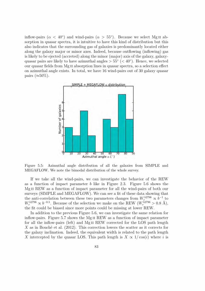
inflow-pairs (α < 40) and wind-pairs (α > 55). Because we select Mg ii ab-sorption in quasar spectra, it is intuitive to have this kind of distribution but thisalso indicates that the surrounding gas of galaxies is predominantly located eitheralong the galaxy major or minor axes. Indeed, because outflowing (inflowing) gasis likely to be ejected (accreted) along the minor (major) axis of the galaxy, galaxy-quasar pairs are likely to have azimuthal angles > 55 (< 40). Hence, we selectedour quasar fields from Mg ii absorption lines in quasar spectra, so a selection effecton azimuthal angle exists. In total, we have 16 wind-pairs out of 30 galaxy quasarpairs (≈50%).

Figure 5.5: Azimuthal angle distribution of all the galaxies from SIMPLE andMEGAFLOW. We note the bimodal distribution of the whole survey.

If we take all the wind-pairs, we can investigate the behavior of the REWas a function of impact parameter b like in Figure 2.3. Figure 5.6 shows theMg ii REW as a function of impact parameter for all the wind-pairs of both oursurveys (SIMPLE and MEGAFLOW). We can see a fit of these data showing thatthe anti-correlation between these two parameters changes from W λ2796

r ∝ b−1 toW λ2796r ∝ b−0.5. Because of the selection we make on the REW (W λ2796

r > 0.8 A),the fit could be biased since more points could be missing at lower REW.

In addition to the previous Figure 5.6, we can investigate the same relation forinflow-pairs. Figure 5.7 shows the Mg ii REW as a function of impact parameterfor all the inflow-pairs (left) and Mg ii REW corrected for the LOS path lengthX as in Bouche et al. (2012). This correction lowers the scatter as it corrects forthe galaxy inclination. Indeed, the equivalent width is related to the path lengthX intercepted by the quasar LOS. This path length is X ∝ 1/ cos(i) where i is

83

Figure 5.6: Mg ii (λ2796) rest equivalent width as a function of impact parameter bfor galaxy-quasar pairs classified as wind-pairs. Horizontal dashed black lines showsthe W λ2796

r > 0.5A and W λ2796r > 0.8A selection criteria. The thick black dashed line

represent a fit to the data. Fitting coefficients are shown in the legend. Errors on W λ2796r

are typically ∼ 10−3 A and ∼ 0.5 kpc for b.

the galaxy inclination. The normalization of this correction is taken to be 0.5 (seethe appendix in Law et al. (2009)). Again, this figure shows an anti-correlationbetween these two parameters for inflow-pairs. The fit indicates that W λ2796

r ∝ b−1

for inflow pairs. The difference between the anti-correlations W λ2796r ∝ b−0.5 for

wind-pairs and W λ2796r ∝ b−1 for inflow-pairs could lead to the conclusion that the

outflowing gas has larger REW than the inflowing gas at the same distance (i.e.the slope is flatter for wind-pairs). This could support the idea that largest REWare likely to come from outflowing materials.

So far, we can argue that galactic outflows can travel at least up to 80−100 kpcaway from their host galaxy leading to the following question: are galactic windsable to escape the gravitational well of their host galaxy?

5.3 Do winds escape?

To estimate the escape velocity of our galaxies, we used the escape velocity relationfor an isothermal sphere given by the following Eq. 5.6 (Veilleux et al., 2005b):

Vesc = Vmax ×√

2[1 + ln

(Rvir

r

)](5.6)

84

Figure 5.7: Left: Mg ii (λ2796) rest equivalent width as a function of impact parameterb for galaxy-quasar pairs classified as inflow-pairs. Right: same as left panel with theW λ2796r normalized by the disk path length X = X0/ cos(i) where i is the galaxy inclina-

tion and X0 is a normalization factor, taken as X0 = cos(60). The thick black dashedline represent a fit to the data. Fitting coefficients are shown in the legend. Errors onW λ2796r are typically ∼ 10−3 A and ∼ 0.5 kpc for b.

where Vmax is the maximum rotation velocity of the galaxy and Rvir is the virialradius. The virial radius is approximately Rvir ≈ Vmax/10H(z) where H(z) is theHubble constant at redshift z.

Figure 5.8 shows the ratio between the outflow velocity and the escape velocity(Vout/Vesc) as a function of S0.5

1 (and thus the galaxy stellar mass on top x-axis).Different samples using the background quasar technique are shown in this

figure. Yellow triangles are from Bouche et al. (2012) (survey from a combina-tion of LRIS and SDSS data), cyan and red circles are from Schroetter et al.(2015) (SIMPLE) and Schroetter et al. (2016) (the only wind-pair within 2 fieldsof MEGAFLOW) respectively. Again, blue squares are from MEGAFLOW (notpublished at the time of writing) survey. We can see that in two cases only, thegas is able to reach the escape velocity of the galaxy. These two points are forthe lowest mass galaxies. The ability of the gas to leave the gravitational well ofthe galaxy is, as one can expect, proportional to S0.5 (see the fit coefficients in thefigure). It is thus easier for an outflow from a low-mass galaxy (M? ≤ 109 M atredshift z = 1) to escape the gravitational well of the host, whereas outflows fromhigh-mass galaxies have difficulties leaving their host as the well is too deep.

One of the most important question about galactic winds is what drives theseoutflows out of the galactic disk. To answer this question, one need to first lookfor scaling relations between outflow and galaxy properties.

1this parameter is described in § 5.1

85

Figure 5.8: Vout/Vesc as a function of S0.5 (bottom x-axis) and M? (top x-axis). Yellowtriangles are from Bouche et al. (2012), cyan and red circles are from Schroetter et al.(2015) and Schroetter et al. (2016) respectively. The horizontal line corresponds toVout = Vesc. The dashed black line corresponds to a fit with coefficients shown in thelegend.

5.4 Wind scaling relations

This section is an attempt to look for scaling relations between properties of galac-tic winds and host galaxies. Because galaxy properties like SFR and mass appearto be directly linked with properties of galactic winds, we will investigate the rela-tion, if any, between outflow properties like their velocity Vout, their ejected massrate Mout and their loading factors η with these main galaxy properties. We needto keep in mind that our sample is limited in term of wind case number. However,this unique sample has a real interest as it probes a large range of galaxy stellarmasses (from ∼ 108.5M to ∼ 1011.5M). Before going further in investigatingwind relations, we first need to describe previous studies on galactic winds thatwe will use for comparison.

5.4.1 Previous studies on galactic winds

As in § 1.3, we will briefly describe two previous galactic outflow studies fromArribas et al. (2014) and Heckman et al. (2015). We choose to compare our resultswith these two studies for several reasons. As we can see in Table 5.1, (1) these two

86

studies focus on low-redshift galaxies (z < 0.2) and are thus complementary to our0.6 < z < 1.4 sample. (2) The stellar mass range probed by these studies is similarto ours and (3) their galaxies are mostly starbursts, and thus complementary to ourmore “normal” star-forming galaxies. In addition, these two papers are using twodifferent methods to derive outflow properties: from absorption and emission lines(as described in § 1.3). We however choose to include the results from Heckmanet al. (2015) only. Indeed, their method to derive outflow properties is similar toours as they use the absorptions produced by outflows. Finally, Heckman et al.(2015) sample includes both SFGs and starbursts, which allow for a comparisonwith our “normal” SFGs.

Because Arribas et al. (2014) use the emission line method to derive outflowproperties, we decided to exclude their sample of the comparison. Indeed, becausetheir method is completely different from ours, systematic biases can exist.

Table 5.1: Summary of other wind studiesPaper Ngal zgal SFRs Galaxy type Vout log(M?)(1) (2) (3) (4) (5) (6) (7)A14 58 0.01 < z < 0.2 Hα U/LIRGs Emission 9.5− 11.8H15 40 z < 0.2 SED SFGs and Starbursts Absorption 7− 11Our sample 16 0.6 < z < 1.4 Hα and [O ii] SFGs Absorption 8.5− 11.5

(1) Study, A14 for Arribas et al. (2014) and H15 for Heckman et al. (2015); (2) Samplesize. (3) Redshift range; (4) Method to estimate galaxy SFR; (5) Type of galaxies; (6)

Method to estimate Vout, “emission” stands for broad blue-shifted emission lines,“absorption” stands for absorption lines in the galaxy spectrum; (7) Galaxies stellar

mass range.

Even if we do not include galaxies from Arribas et al. (2014), we will stillconsider the relations they found to see if there are significant differences betweenSFGs and U/LIRGs outflow properties. We briefly described the results of Arribaset al. (2014) in § 1.3 but give here a more detailed description.

Work of Arribas et al. (2014) summary

Arribas et al. (2014) focus on 58 local (low-z) (U/LIRGs) using the Visible MultiObject Spectrograph (VIMOS, Le Fevre et al., 2003) and INTEGRAL (Arribaset al., 1998) instruments. Their galaxies have redshifts between z ≈ 0.01 andz ≈ 0.2, and dynamical masses between 109.5M and 1011.8M. They derivedSFRs from Hα fluxes using Kennicutt (1998) calibration adapted for Chabrier(2003) IMF. In their work, they do not use absorption lines in galaxy spectra butrather study outflows using the blue-shifted broad component of several emissionlines like Hα and [N ii]. Outflow velocities are derived by fitting a Gaussian profileto this blue-shifted broad component (see Figure 1.15). They define the outflow

87

velocity as follows:Vout = |∆V − FWHM/2| (5.7)

where ∆V is the shift in velocities of the broad component with respect to thesystemic velocity and FWHM is the full width half maximum of this blue-shiftedbroad component.

As mentioned in § 1.3.2, their main result is that the outflow velocity correlateswith the galaxy SFR (Vout ∝ SFR0.24). They also find that the ejected mass rateMout correlates with SFR. For non-AGN-LIRGs, they derive Mout ∝ SFR1.11.

Work of Heckman et al. (2015) summary

In the study of Heckman et al. (2015), they combined two samples of low-z star-burst galaxies: 19 from FUSE and 21 from COS. Their galaxies have redshiftsz < 0.2 and stellar masses between 107M and 1011M. Their stellar masses wereestimated by SED fitting using near-IR or multiband optical photometry. SFRswere derived using a combination of GALEX FUV, IRAS and Herschel far-IR,and WISE and Spitzer mid-IR photometry. In all their cases, a Kroupa/Chabrier(Kroupa, 2000; Chabrier, 2003) IMF was adopted to estimate masses and SFRs.As mentioned previously, these galaxies are starburst galaxies, which means thatthey have high SFRs. In order to derive outflow velocities, they used the absorp-tion lines produced by the outflowing gas but without stacking different galaxyspectra as they have enough SNR to analyze almost each galaxy individually. Arepresentation of the two techniques (wind absorption in galaxy spectrum andabsorption using background quasar) is represented in Figure 5.9. In this fig-ure, we mainly show the difference between absorption profiles depending on usedLOS. Because of their technique, they have a selection effect on galaxy inclination.Indeed, in order to detect absorption, the outflowing gas must be between thegalaxy and the observer. Because the galaxy is ejecting the gas perpendicular toits plane, galaxies must be roughly face-on and therefore have low inclinations. Asa reminder of § 1.3.3, to estimate Vout, they used the value corresponding to 80%of the absorption profile in order to avoid instrumental noise seen in the galaxycontinuum.

Concerning the estimate of Vout, we tried building a wind model with theconfiguration of a galaxy with 0 inclination and a LOS crossing this galaxy(impact parameter b = 0 kpc). With a constant outflow velocity, the simulatedabsorption profile has an inverse asymmetry compared to what we observe.However, since the LOS is crossing all the outflowing gas from the galaxy, theaccelerated phase of the gas is also probed. We thus simulated an absorptionprofile using an accelerated wind model like in Schroetter et al. (2015). Thissimulated profile reproduces the right asymmetry. Hence, the input outflow

88

Figure 5.9: Scheme of the two main technique to study outflowing materials in absorp-tion. On the right part of this scheme, we can see a star-forming galaxy (in black)ejecting gas in a cone (represented by the two red arrows). The horizontal dark bluearrow represents the LOS as used in Heckman et al. (2015). In this LOS type observa-tion, the galaxy is face-on and the outflowing gas creates blue-shifted absorption linesin the galaxy spectrum. This absorption profile is represented on top of the telescopeon the left in dark blue. We can see that this absorption profile is asymmetric, onlyblue-shifted (on the left of the systemic velocity, represented by the 0 vertical dashedline) and with an outflow velocity corresponding to where the absorption crosses thegalaxy continuum. On the right part of this figure, the light blue vertical arrow repre-sent a quasar (the yellow star labeled “QSO”) LOS crossing the outflowing material ofthe same galaxy. This configuration represent our background quasar technique and thegalaxy is seen as edge-on. The projected velocities onto this LOS creates an absorptionprofile represented in light blue at the bottom of the figure. This absorption profile issymmetric and centered on the galaxy systemic velocity.

velocity is indeed found to be where the absorption crosses the continuum. Forthis reason, we find it relevant to use results from Heckman et al. (2015) astheir outflow velocities seem not to be over or under-estimated.

From their outflow velocities estimates, they derive the ejected mass rate usingthe following equation:

Mout = Ω×Nout× < m > ×Vout × rout (5.8)

where Ω is the solid angle occupied by the outflow Ω = 4π, Nout is the total column

89

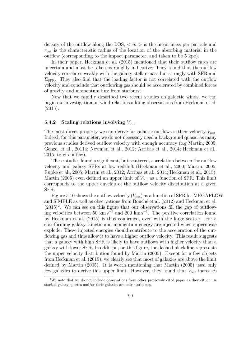
density of the outflow along the LOS, < m > is the mean mass per particle androut is the characteristic radius of the location of the absorbing material in theoutflow (corresponding to the impact parameter, and taken to be 5 kpc).

In their paper, Heckman et al. (2015) mentioned that their outflow rates areuncertain and must be taken as roughly indicative. They found that the outflowvelocity correlates weakly with the galaxy stellar mass but strongly with SFR andΣSFR. They also find that the loading factor is not correlated with the outflowvelocity and conclude that outflowing gas should be accelerated by combined forcesof gravity and momentum flux from starburst.

Now that we rapidly described two recent studies on galactic winds, we canbegin our investigation on wind relations adding observations from Heckman et al.(2015).

5.4.2 Scaling relations involving Vout

The most direct property we can derive for galactic outflows is their velocity Vout.Indeed, for this parameter, we do not necessary need a background quasar as manyprevious studies derived outflow velocity with enough accuracy (e.g Martin, 2005;Genzel et al., 2011a; Newman et al., 2012; Arribas et al., 2014; Heckman et al.,2015, to cite a few).

These studies found a significant, but scattered, correlation between the outflowvelocity and galaxy SFRs at low redshift (Heckman et al., 2000; Martin, 2005;Rupke et al., 2005; Martin et al., 2012; Arribas et al., 2014; Heckman et al., 2015).Martin (2005) even defined an upper limit of Vout as a function of SFR. This limitcorresponds to the upper envelop of the outflow velocity distribution at a givenSFR.

Figure 5.10 shows the outflow velocity (Vout) as a function of SFR for MEGAFLOWand SIMPLE as well as observations from Bouche et al. (2012) and Heckman et al.(2015)2. We can see on this figure that our observations fill the gap of outflow-ing velocities between 50 km s−1 and 200 km s−1. The positive correlation foundby Heckman et al. (2015) is thus confirmed, even with the large scatter. For astar-forming galaxy, kinetic and momentum energy are injected when supernovaeexplode. These injected energies should contribute to the acceleration of the out-flowing gas and thus allow it to have a higher outflow velocity. This result suggeststhat a galaxy with high SFR is likely to have outflows with higher velocity than agalaxy with lower SFR. In addition, on this figure, the dashed black line representsthe upper velocity distribution found by Martin (2005). Except for a few objectsfrom Heckman et al. (2015), we clearly see that most of galaxies are above the limitdefined by Martin (2005). It is worth mentioning that Martin (2005) used onlyfew galaxies to derive this upper limit. However, they found that Vout increases

2We note that we do not include observations from other previously cited paper as they either usestacked galaxy spectra and/or their galaxies are only starbursts.

90

with SFR and their upper limit seems to be in agreement with low-SFR galaxiesbut is clearly under-estimating Vout for SFRs≥ 4− 5 M yr−1. From SFR≥ 4− 5M yr−1, it appears that their is an increase of the slope between Vout and SFR.

Figure 5.10: Vout as a function of SFR for both surveys (MEGAFLOW and SIMPLE) aswell as observations from Bouche et al. (2012) and Heckman et al. (2015). The dashedblack line show a fit (log V = (0.35±0.06) log(SFR)+(1.56±0.13)) from Martin (2005).Errors on Heckman et al. (2015) observations are 0.2 dex for SFR and 0.05 dex for Vout.

Concerning the correlation between Vout and the SFR by surface area (ΣSFR),there has been disagreements about its existence (e.g. Chen et al., 2010; Rubinet al., 2014) but galaxies from these studies only have small range of SFRs. Asmentioned before, Heckman et al. (2015) found a strong correlation between theoutflow velocity and ΣSFR. Adding our observations to their sample we do not findsuch a correlation.

The next obvious step is to investigate whether the outflow velocity dependson the host galaxy mass. Following the SFR-M? relation and the tendency of Voutto increase with the host galaxy star formation rate, we could naively expect thatthe outflow velocity correlates also with the host galaxy mass. However, a moremassive galaxy has a deeper gravitational well, and thus it is more difficult for agas to accelerate. We investigated the relation between Vout and S0.5 (Mdyn(r) andΣMdyn(r)) but found no correlation between these properties.

To summarize, we confirm that Vout correlates with the SFR but not with ΣSFR.

91

5.4.3 Scaling relations involving Mout

Other wind properties are derived from outflow velocities, namely the outflow rateand the loading factor. The ejected mass rate usually has lots of uncertainties asone need to make assumption on the location of the probed outflowing gas.

From the previous result on the relation between the outflow velocity and SFR,Mout being directly derived from Vout, it is interesting to investigate whether theejected mass rate correlates with the galaxy SFR as well. Hopkins et al. (2012)predicted a dependency of the ejected mass rate Mout ∝ SFR0.7 whereas Arribaset al. (2014) derived a stepper index Mout ∝ SFR1.11. Even if the uncertaintyon the ejected mass rate is larger without knowing exactly where we trace theoutflowing gas, we choose to continue adding observations from Heckman et al.(2015). We recall here that they used Equation 5.8 to estimate the ejected massrate assuming an impact parameter of 5 kpc for their galaxies.

Figure 5.11 represents the ejected mass rate (Mout) as a function of SFR (leftpanel), and ΣSFR (right panel). Not surprisingly, we see a strong correlation be-tween the outflow mass rate and the SFR, hence, this correlation has a scattermuch lower than the one between the outflow velocity and SFR. Because the SFRis directly linked with the amount of ejected mass by supernova explosions, it isthen intuitive that SFR correlates with Mout. Like in Heckman et al. (2015), weadded a line corresponding to a constant loading factor η = 2 (dotted blue line)showing that a constant loading factor is consistent with the results. Because re-sults from Heckman et al. (2015) are only indicative, we did not try to fit all thegalaxies together. Both relations from Hopkins et al. (2012) and Arribas et al.(2014) are represented on left panel of this figure. We will see in § 5.4.4 that theprediction from Hopkins et al. (2012) is in better agreement with the observationsthan Arribas et al. (2014) for SFGs.

The previous attempt to see a correlation between Vout and ΣSFR failed. But,because SFR and Mout are correlated, it is interesting to investigate whether theejected mass rate depends on SFR by surface area. On right panel of Figure 5.11,we can see a weak correlation between the ejected mass rate and ΣSFR. We notethat our galaxies allow to probe for low ΣSFR and thus can confirm the (scat-tered) correlation between the two quantities. From this result, we can argue thatmechanisms impacting the amount of ejected mass are acting more on local (SFR,ΣSFR) than global galaxy scales like their masses. Indeed, comparison between theejected mass rate and the S0.5 factor (and thus its stellar mass) show no obviouscorrelation. This would mean that a massive galaxy does not necessary eject moremass than a less massive one.

5.4.4 Scaling relations on loading factor η

The last but maybe the most important parameter concerning galactic outflowsis the loading factor η. This loading factor is the ratio between the ejected mass

92

Figure 5.11: Ejected mass rate as a function of star formation rate (left) and star forma-tion rate by surface area (ΣSFR, right) for both surveys (MEGAFLOW and SIMPLE) aswell as observations from Bouche et al. (2012). On left panel, the dashed red line showsa prediction Mout ∝ SFR0.7 from Hopkins et al. (2012) model. On left panel, the blackline shows Mout ∝ SFR1.11 from Arribas et al. (2014). the blue dotted line correspondto a loading factor (Mout/SFR) equals 2. Errors for Heckman et al. (2015) are 0.25 dexfor Mout and 0.2 dex for SFR and ΣSFR.

rate Mout and the SFR of the galaxy. This parameter is popular as it representswhat fraction of gas, used in the formation of stars, is actually ejected out of thegalactic disk.

We previously found that the ejected mass rate correlates with the galaxy SFR.If :

Mout ∝ SFRα (5.9)

thenη = Mout

SFR ∝ SFRα−1 (5.10)

Depending on the value of α in Equations 5.9 and 5.10, correlation betweenthe mass loading factor and SFR can be positive (α > 1), negative (α < 1) or ηcan be constant (α = 1). These three possibilities are represented by the curvesin Figure 5.11 with α = 0.7 (Hopkins et al., 2012), α = 1.11 (Arribas et al., 2014)and α = 1 (a constant loading factor η = 2).

Left panel of Figure 5.12 shows the mass loading factor as a function of SFR.We can see a scattered anti-correlation between these two properties. This meansthat η ∝ SFRα−1 with α < 1. As on Figure 5.11, we added curves from Hopkins

93

et al. (2012) and Arribas et al. (2014) (red dashed line and black line respectively).Because we found a negative correlation (α < 1) between η and SFR, we can saythat our observations are in good agreement with predictions from Hopkins et al.(2012). Hence, we can argue that there is an upper limit of α < 1 for star-forminggalaxies and thus η ∝ SFRβ with −1 < β < 0. A direct consequence is thatthe correlation found by Arribas et al. (2014) does not apply for “normal” star-forming galaxies like ours but rather apply to extreme starbursts galaxies suchas (U)LIRGs. Indeed, as mentioned in § 5.1.2, our galaxies tend to lie bellowthe galaxy “main sequence”. This result leads to the conclusion that galacticwinds launched from “normal” star-forming galaxies have different properties thanoutflows from starbursts.

Figure 5.12: η as a function of SFR (left) and ΣSFR (right) for both surveys(MEGAFLOW and SIMPLE) as well as observations from Bouche et al. (2012) andHeckman et al. (2015). On left panel, the dashed red line shows a fit η ∝ SFR−0.3 fromHopkins et al. (2012) and the black line shows a fit η ∝ SFR0.11 from Arribas et al.(2014). On right panel, the dashed red line shows a fit η ∝ Σ−1/2

SFR from Hopkins et al.(2012) and the black line shows a fit η ∝ Σ0.17

SFR from Arribas et al. (2014). Again, errorsfor Heckman et al. (2015) are 0.2 dex for SFR (and ΣSFR) and 0.45 dex for η.

Because, like other wind properties, we want to know whether the mass load-ing factor depends on global or local galaxy properties, we investigate relationsbetween the mass loading factor and SFR by surface area. Other wind studies likeGenzel et al. (2011b), Newman et al. (2012) and Heckman et al. (2015) found thatthe loading factor is strongly correlated with ΣSFR. On right panel of Figure 5.12,we show the mass loading factor as a function of ΣSFR. Prediction and observationsfrom Hopkins et al. (2012) and Arribas et al. (2014) are represented by red-dashed

94

and black lines respectively. Restricting to loading factors from Heckman et al.(2015) only, there is a clear correlation with ΣSFR. However, our results clearlyquestion this correlation. Thus, we can argue that, including ”normal” SFGs tothe extreme starbursts sample of Arribas et al. (2014), the mass loading factordoes not correlate with ΣSFR.

It is also important to remind the reader that as mentioned in § 1.3, Arribaset al. (2014) and Newman et al. (2012) found that galaxies (low-z galaxies fromArribas et al. (2014) and high-z galaxies from Newman et al. (2012)) require aΣSFR larger than 1 (ΣSFR > 1) for launching strong outflows. This statement isnot supported by our galaxies since all of them have winds and a ΣSFR below 1.

Another aspect about the loading factor is its redshift dependency. Indeed,as mentioned in § 1.3, as there is a peak in star-formation density at redshift 2-3(Lilly et al., 1996; Madau et al., 1996; Behroozi et al., 2013a), if η correlates withSFR (which appears to be the case), one can expect a correlation between η andredshift. We thus investigated on this relation but the loading factor does notappear to be redshift dependent (compared to Muratov et al. (2015)).

As a last investigation, we looked for a relation between η and the outflowvelocity. We mentioned in § 1.3 that their is no reason for a galaxy to eject moregas if the outflow velocity is larger and their is indeed no correlation between themass loading factor and the outflow velocity. This is in agreement with resultsfrom Heckman et al. (2015) who find no correlation between η and Vout.

5.5 What mechanisms drive galactic winds?

We will now try to answer the last and most important question of what mech-anisms drive galactic winds out of the galaxy. There are two major mechanismswhich could be responsible for driving materials out of the galaxy: energy-drivenand momentum-driven.

The momentum-driven wind scenario considers that the two primary sourcesof momentum deposition in driving galactic winds are supernovae and radiationpressure from the central starburst (i.e. Murray et al., 2005). This model assumesthat the wind speed scales as the galaxy velocity dispersion (e.g. Martin, 2005;Oppenheimer & Dave, 2006; Dave et al., 2011). This implies that the mass loadingfactor must be inversely proportional to the outflow velocity (Oppenheimer &Dave, 2008). In summary, momentum conservation implies η ∝ V −1

max.Energy-driven wind model assumes that when stars evolve, they put energy into

the ISM. The amount of gas blown out of the disk is assumed to be proportionalto the total energy given by supernovae and inversely proportional to the escapevelocity squared. In energy-driven scenario, energy conservation implies η ∝ V −2

max(e.g. van den Bosch, 2001).

One of the most popular relation is the loading factor as a function of galaxystellar mass. It is indeed crucial to look for dependences between these two proper-

95

ties if we want to step forward in understanding the role of galactic winds concern-ing the lack of observed baryons (see § 1.2.6). Figure 5.13 shows the mass loadingfactor as a function of galaxy maximum rotational velocity (bottom x-axis) andgalaxy stellar mass (top x-axis). This figure is almost the same as Figure 5.14but with added observations from Heckman et al. (2015) and without simulationpredictions (apart from Hopkins et al. (2012)).

Figure 5.13: η as a function of S0.5 for both surveys (MEGAFLOW and SIMPLE) aswell as observations from Bouche et al. (2012) and Heckman et al. (2015). The dashedred line shows a fit η ∝ S−1.2

0.5 from Hopkins et al. (2012). The black line shows η ∝ V −2.Errors on Heckman et al. (2015) are 0.45 dex for η and 0.1 dex for Vmax.

We find a weak correlation between η and S0.5. This correlation is in goodagreement with the prediction of Hopkins et al. (2012) where η ∝ S−1.2±0.2

0.5 . How-ever, we also show η ∝ V −2 (the black line) in order to see if we could disentanglebetween the two mechanisms which could explain what drives outflows (see above).We can see that due to the large scatter of our sample, it is not possible to concludeon which curve best fits the data.

As a final result, we need to compare our results with simulations like we did inSchroetter et al. (2015, 2016). We can now show the loading factor η as a functionof galaxy halo mass. The results are shown in Figure 5.14.

On this Figure, the first thing to note is the number of gray squares, whichcorrespond to galaxy-quasar pairs having an impact parameter larger than 60 kpc.But, since all these gray squares have large loading factors, this indicates that theejected mass rate is larger than the SFR of the galaxy. This can mean that theoutflowing gas probably quenched the SFR of the host galaxy. Indeed, we derivethe SFR from the galaxy [O ii] emission lines at the time we observe (∼ 10Myrs).Because the distance b is large, the ejected gas needed a long time (several 100Myrs) to get to the quasar LOS at an outflow velocity of ∼ 200 km s−1. The SFR

96

Figure 5.14: Comparison of mass loading factors assumed by theoretical/empirical mod-els (curves) with values derived from background quasar observations (dots and triangles)as a function of the maximum rotational velocity. MEGAFLOW results are representedby the blue squares. The result from Schroetter et al. (2016) is represented by the redcircle. Arrows represent the loading factors of the galaxies with the subtracted massfrom the inner cone models. The cyan circles show the results for galaxies at z ≈ 0.8from Schroetter et al. (2015). The green square shows the mass loading factor for az ≈ 0.2 galaxy (Kacprzak et al., 2014). The triangles show the results for z ≈ 0.2 galax-ies from Bouche et al. (2012). The gray triangles and squares show the galaxies withquasars located at >60kpc where the mass loading factor is less reliable due to the largetravel time needed for the outflow to cross the quasar LOS (several 100 Myr) comparedto the short time scale of the Hα derived SFR (∼ 10Myr). The upper halo mass axis isscaled on Vmax at redshift 0.8 from Mo & White (2002).

of the host galaxy was different at the time when the gas was ejected and if agalaxy eject gas, that means ejecting a part of the gas reservoir that could formstars and thus lower or even quench the SFR.

97

We can, however, focus on the blue squares which are close to unity. Loadingfactors of these wind pairs have their component on almost same time scales andare thus more comparative with simulations.

Among simulations represented on this figure, three of them clearly do not fitthe data for low mass galaxies. Hence, they are roughly one order of magnitudeabove the observations. These three simulations are the ones from Okamoto et al.(2010); Puchwein & Springel (2013) and Vogelsberger et al. (2014). These curvescorrespond to loading factors applied in theoretical models and not empirical.In these simulations, they assume a similar wind modeling and try to fit theobserved stellar mass function for low mass galaxies. They only assume energy-driven feedback and do not explore momentum-driven winds. In order to reproducethe baryonic mass distribution of galaxies, they need massive outflows. Consideringobservational constraints, these needed massive outflows are unrealistically large.These theoretical wind models are therefore over-estimated for low-mass galaxies.

The other wind models (theoretical and empirical), however, are in agreementwith the observational constraints. Even if the theoretical models from Daveet al. (2011); Hopkins et al. (2012); Muratov et al. (2015) and Barai et al. (2014)also try to fit the stellar mass function, they do not appear to over-estimate themass loading. These models assume momentum-driven outflows but as seen inFigure 5.13, we cannot favor one of the two proposed mechanisms to drive galacticwinds (energy-driven or momentum-driven).

At the sight of the previous section, we investigated if any relation exist be-tween different galaxy and winds properties. This investigation was motivatedby previous works on observations and theoretical predictions. Some correlationswere confirmed (i.e. Vout vs SFR, Mout vs SFR or η vs SFR, S0.5) and some wererefuted (i.e. Vout vs M? or η vs redshift).

The most important figures that allows to conclude on what mechanism driveswinds are Figure 5.13 and 5.14 showing the loading factor as a function of thegalaxy stellar and halo mass respectively. These figures tell us that we can notdisentangle between momentum and energy-driven winds due to the large scatter.However, this is also showing that a combination of the two mechanisms could bethe best assumption for driving outflows out of the galactic disk.

98

Chapter 6

Conclusions and perspectives

Contents6.1 French version . . . . . . . . . . . . . . . . . . . . . . . . . . . . 100

6.1.1 Conclusions de these . . . . . . . . . . . . . . . . . . . . . . . . 1006.1.2 Perspectives . . . . . . . . . . . . . . . . . . . . . . . . . . . . . 102

6.2 English version . . . . . . . . . . . . . . . . . . . . . . . . . . . . 1036.2.1 Thesis conclusions . . . . . . . . . . . . . . . . . . . . . . . . . 1036.2.2 Perspectives . . . . . . . . . . . . . . . . . . . . . . . . . . . . . 104

99

6.1 French version

6.1.1 Conclusions de these

Dans le contexte de la formation et de l’evolution des galaxies, et plus par-ticulierement celui des flots de matiere autour des galaxies de faibles masses,d’importantes questions se posaient. Des questions comme “quelle quantite dematiere est ejectee par les vents galactiques? A quelle vitesse?”, ou encore “est-ce que le gaz est capable de quitter le halo gravitationnel de la galaxie et ainsienrichir le milieu inter-galactique ou aurait-il tendance a retomber sur celle-ci etapporter du combustible permettant la formation de futures etoiles?” Nous noussommes efforces de repondre a ces questions du mieux possible. Il est importantde rappeler que l’observation du gaz ejecte en emission est tres difficile car ce gaza une brillance de surface tres faible par rapport a celle de la galaxie hote. Cegaz ejecte est donc detecte principalement en absorption. C’est a dire qu’il vaabsorber une partie de la lumiere emise par l’objet en arriere plan (dans notre casle quasar) et pour pouvoir quantifier les proprietes de ce gaz, il va falloir essayerde reproduire cette absorption. La technique que nous utilisons fait appel a desquasars en arriere plan.

Au debut de cette these, nous avions deja acces a de nombreuses donnees ac-quises avec SINFONI et UVES necessitant d’etre analysees. Le premier echantillonde donnees (SIMPLE) fut analyse et publie dans Schroetter et al. (2015) (voir Ap-pendice A). Nous avons obtenu les caracteristiques de vents galactiques pour 3paires galaxie-quasar. Pour une de ces trois paires, nous avons complexifie lemodele de vent afin de reproduire les donnees. Cette complexification corresponda l’implementation d’une composante d’acceleration pour les paires ayant un faibleparametre d’impact afin de reproduire l’assymetrie du profil d’absorption (voir lesdetails au § 4.2.3 et dans Schroetter et al. (2015)). Combinant notre analyse aceux de la litterature (voir Figure 4.8), nous avons vu que le facteur de chargeavait tendance a etre de l’ordre de l’unite, ce qui correspond a une quantite dematiere ejectee equivalente au taux de formation stellaire de la galaxie. Mais il yavait trop peu d’observations pour pouvoir conclure sur des proprietes generalesdes vents galactiques. Nous avions donc besoin d’observations supplementaires.

Pendant ce temps, la construction de l’instrument MUSE etait en chemin etnous avions deja commence a etablir notre strategie d’observation afin d’augmenterle nombre de paires galaxie-quasar d’un ordre de grandeur. Pour atteindre cetobjectif, nous avons utilise la strategie decrite en detail dans la section § 2.3.1.Cette strategie consiste a chercher plusieurs absorbants Mg ii (au moins 3) dans lespectre de quasars contenus dans la base de donnee SDSS. Ces absorbants devaientavoir une largeur equivalente au repos (W λ2796

r ) supperieure a 0.8 A (compare a 2 Apour SIMPLE), ainsi qu’un redshift compris entre 0.4 et 1.4 afin de pouvoir detecterl’emission [O ii] des galaxies potentiellement responsables de ces absorptions.

Lorsque cet instrument a ouvert ses yeux vers le ciel pour la premiere fois le 5

100

Mars 2014, MUSE fut un veritable succes et commenca a collecter de nombreusesobservations. Nous avons aussi obtenu des donnees complementaires de nos champsde quasar avec le spectrographe a haute resolution UVES afin d’avoir la resolutionspectrale necessaire dans les profils d’absorptions detectes dans les spectres desquasars. Contrairement au temps MUSE, le temps d’observation avec l’instrumentUVES ne nous etait pas garanti.

Etant les premiers a avoir des observations MUSE, un travail intensif sur lareduction des donnees brutes etait necessaire afin de pouvoir travailler avec lesmeilleurs donnees possibles pour atteindre nos objectifs scientifiques (voir § 3.2).Suite a ce travail de reduction, nous avons reussi a detecter 85% des galaxies quenous qualifions etre a l’origine des absorptions Mg ii dans les spectres des quasars.Ceci nous a amene a multiplie par 2-3 l’echantillon que nous avions ainsi que lescontraintes sur les proprietes physiques des vents galactiques (dont une paire estdecrite dans Schroetter et al. (2016), accessible a l’Apendice B). Ces contraintessont presentees sur la Figure 5.14.

Nous en avons conclu que si nous voulions mesurer un facteur de charge qui aitune signification, il fallait que la quantite de masse ejectee et le taux de formationd’etoiles de la galaxie soient estimes sur des echelles de temps similaires afin depouvoir etre compare avec les simulations. Ceci donna lieu a une discussion sur lapertinence de ce parametre. D’autres parametres etaient donc necessaires si nousvoulions en deduire des proprietes entre les vents galactiques et les parametres desgalaxies hotes (voir § 5.4).

Un resume des resultats obtenus durant cette these est la suivante:

• Les facteurs de charge ont tendance a etrent proches de l’unite (η ∼ 1), cequi veut dire que le taux de matiere ejecte est de l’ordre du taux de formationstellaire de la galaxie.

• Le gaz faiblement ionise que nous detectons semble retomber sur la galaxie apartir du moment ou la galaxie possede une masse stellaire d’environ 109M(voir § 5.3).

• Nous avons montre que les vents ont une phase d’acceleration jusqu’a environ10 kpc de la galaxie.

• Nous avons aussi developpe un modele de cone creux afin de pouvoir re-produire le profil d’absorption cree par les vents et nous avons trouve cetteconfiguration dans 5 cas de l’echantillon MEGAFLOW.

• En combinant nos observation avec d’autres travaux sur les vents, nous avonsconfirme certaines correlations entre differentes proprietes des vents et deleurs galaxies hotes comme la vitesse d’ejection des vents et le SFR de lagalaxie, le taux de masse ejectee et le SFR ou bien le facteur de charge et lamasse de la galaxie.

101

• Certaines correlations comme la dependance entre la vitesse d’ejection desvents et la masse de la galaxie ou bien celle entre le facteur de charge et leredshift furent, quand a elles, infirmees.

• Les vents galactiques semblent etre entraınes par une combinaison des mecanismesde transfert de moment cinetique et d’energie cinetique (voir dernier chapitre).

6.1.2 Perspectives

Les observations MEGAFLOW sont extremement riches. Si elles nous permettentd’explorer des galaxies ayant des vents galactiques, chaque champ contient aussi denombreuses autres galaxies dont les vents n’ont pas ete detectes dans le spectre duquasar. Par exemple, nous avons detecte environ 40 galaxies en emission ayant unredshift entre 0.4 et 1.4 (voir Figure 5 dans Schroetter et al. (2016)). Celles-ci sontseulement les galaxies ayant une forte raie d’emission (principalement le doubletde [O ii]) et d’autres galaxies detectees par leur continuum n’ont pas ete prises encompte. Il serait interessant de regarder le spectre de ces galaxies (ayant un redshiftsupperieur a 0.8) afin de chercher la signature de vents ou non (forte absorptionMg ii λ2796) et de caracteriser les vents detectes. Cette analyse pourrait permettrede rechercher les proprietes des galaxies pouvant etre responsables de la presenceou non de vents galactiques.

Afin de pouvoir mettre de meilleurs contraintes sur les phenomenes de retro-action des galaxies, il est necessaire d’avoir des mesures de Mout et SFR sur desechelles de temps similaires. Pour calculer le SFR sur une plus longue periodede temps, l’ultraviolet est le traceur de choix, etant sensible aux etoiles vivantjusqu’a quelques 100 millions d’annees. Malheureusement, les methodes simplistespermettant de mesurer le SFR peuvent etre affectees par des degenerescences (e.g.est-ce que la galaxie est rouge parce qu’elle forme des etoiles et contient de lapoussiere ou parce qu’elle a cesse de former des etoiles?) et peut etre contamineepar des etoiles vivant tres longtemps (e.g. Boquien et al., 2014). De nouveauxmodeles utilisant des donnees de l’ultraviolet lointain (FUV) a l’infrarouge lointain(FIR), tel que CIGALE (Noll et al. (2009a), Boquien et al. in prep.) permettentdesormais d’acceder a de meilleures estimations du SFR sur des echelles de tempsde 100 Myrs. Ceci impliquerait donc l’observation de suivi de galaxies selectionneesavec d’autres instruments afin d’avoir une couverture de longueurs d’ondes treslarge (du FUV au FIR).

De plus, des donnees de l’observatoire du Keck ont ete analysees et des modelesde vents lances sur une paire galaxie-quasar (Kacprzak et al., 2014) ainsi que sur5 autres paires. Ces dernieres necessitent du travail supplementaire afin d’obtenirleur facteur de charge et autres proprietes qui nous permettront d’augmenter lenombre de contraintes sur le gaz autour des galaxies (Bouche, Schroetter et al, inprep.).

102

6.2 English version

6.2.1 Thesis conclusions

In the context of galaxy formation and evolution, and in particular about thegas flows around low-mass galaxies, important questions remained. Questionslike “what is the amount of ejected mass by galactic winds? how fast are thesewinds?” or even “is the gas able to escape the gravitational well of the hostgalaxy to enrich the interstellar medium or is it likely to fall back onto the galaxyand fuel future star formation?” During this thesis, we tried to answer thesequestions as best as we could. It is important to remind that it is difficult todirectly observe the outflowing gas in emission as the surface brightness of thisgas is negligible compared to the host galaxy’s. This outflowing gas is thereforedetected in absorption. It will absorb a part of the background object light (in ourcase the quasar) and to quantify this gas properties, one needs to reproduce thisabsorption. The technique we are using implies background quasars.

When starting this thesis, we already had a lot of available data from UVESand SINFONI that needed to be analyzed. The first sample (SIMPLE) was an-alyzed and published in Schroetter et al. (2015) (see Appendix A). We obtainedgalactic wind properties for 3 galaxy-quasar pairs. For one of these three pairs,our wind model has been modified in order to reproduce the data. This modifi-cation corresponds to an implementation of an acceleration component for pairswith low impact parameter in order to fit the absorption profile asymmetry (seedetails in § 4.2.3 and in Schroetter et al. (2015)). Combining our analysis withother works in the literature (see Figure 4.8), we first saw that the loading factorhad a tendency to be around unity (which corresponds to an ejected mass rateequivalent to the star formation rate of the galaxy) but had too few observationsin order to derive general outflow properties. We thus needed lots of additionalobservational constraints.

In the mean time, MUSE was building up and we already began to establishour observational strategies in order to increase the number of galaxy-quasar pairsby one order of magnitude. To do so, we proceeded as described in § 2.3.1. Thisstrategy consists in searching for multiple Mg ii absorptions (3 at least) in quasarspectra from SDSS database. These absorbers needed to have a rest equivalentwidth (W λ2796

r ) larger than 0.8 A (compared to 2 A for the SIMPLE sample) andredshift between 0.4 and 1.4 in order to detect the [O ii] emission lines of thegalaxies assumed to be responsible for these absorptions.

When the instrument had its first light in March 5th 2014, MUSE was successfulin all aspects so we began gathering lots of observations. We also acquired followup observations of our quasar fields with the high resolution spectrograph UVES inorder to have the necessary spectral resolution of absorption lines seen in the quasarspectra. Contrary to MUSE, observing time with UVES was not guaranteed.

Being the first to have MUSE observations, we needed to work on data re-

103

duction in order to have the best data reduced to achieve our science goals (see§ 3.2). After intensive data reductions, we analyzed our quasar fields to look forwind-pairs. Our observational strategy was successful as we detected 85% of thegalaxies we assumed responsible for the Mg ii absorption lines in quasar spectra.This, in turn, led to multiply by 2-3 our sample as well as physical constraints ongalactic outflows (one is described in Schroetter et al. (2016), added in AppendixB). These constraints are shown in Figure 5.14.

We then concluded that if we wanted to estimate meaningful loading factors,the ejected mass rate and the star formation rate of the galaxy needed to beestimated on similar time scales in order to be comparable with simulation results.This opened a discussion on the pertinence of our loading factors. New parametersneeded to be used in order to put real constraints on galactic winds as a functionof galaxy properties (see § 5.4).

A summary of our results is as follow:

• Loading factors tend to be η ∼ 1, which means that the ejected mass rate isof the same order as the galaxy SFR.

• The low-ionization gas we are tracing is likely to fall back onto the galaxyfor galaxies with stellar mass larger than 109M (see § 5.3).

• We found that galactic winds should be accelerated until 10 kpc away fromthe host galaxy.

• We also needed to develop an empty inner cone model to fit the data andthis configuration is found for 5 cases in the MEGAFLOW sample.

• Combining our observations with previous works, we confirmed some correla-tions between outflow and galaxy properties such as the outflowing velocityand the SFR of the galaxy, the ejected mass rate and the galaxy SFR orbetween the loading factor and the galaxy stellar mass.

• Some correlations like the one between the outflow velocity and the galaxystellar mass or between the loading factor and the galaxy redshift were, how-ever, refuted.

• Galactic winds seem to have a tendency to be driven by a combination ofmomentum and kinetic energy mechanisms (see the last chapter).

6.2.2 Perspectives

MEGAFLOW observations are exquisitely rich. If they allow us to explore galax-ies with outflows, each field also contains many more galaxies without detectedoutflows. For instance, we detected around 40 galaxies in emission with redshiftsbetween 0.4 and 1.4 (see Figure 5 from Schroetter et al. (2016)). These are just

104

the galaxies with strong emission lines (mainly the [O ii] 3727,3729 doublet), othergalaxies detected from their continuum were not taken into account. It would beof interest to look at these galaxy spectra (with redshift larger than 0.8) in orderto search for galactic winds signature or not (strong Mg ii λ2796 absorption) andcharacterize the detected outflow properties. This analysis could allow to look forgalaxy properties responsible for the presence or absence of galactic winds.

In order to put better constraints on galaxy feedback, one needs to have mea-sures of Mout and SFR on roughly similar timescales. To measure the SFR overlonger periods of time, the ultraviolet is the tracer of choice as it is sensitive tostars living up to a few 100 Myrs. Unfortunately, simple recipes to measure theSFR from the UV can be severely affected by degeneracies (e.g., is a galaxy redbecause it is star-forming but dusty, or is it rather because it has stopped formingstars?) and contamination by long-lived stars (e.g. Boquien et al., 2014). Newmodels using data from the far-ultraviolet (FUV) to the far-infrared (FIR), suchas CIGALE (Noll et al. (2009a), Boquien et al. in prep.) now allow us to havemore reliable measurements of the SFR over timescales of 100 Myr. This shouldimplies follow up from other instruments to have a very large wavelength coverage(from FUV to FIR) of selected galaxies.

Hence, data from Keck observatory had to be processed and wind modelslunched on one galaxy-quasar pair (Kacprzak et al., 2014) and 5 additional windpairs have results from wind models. These latter data still need additional work inorder to derive loading factors and other outflow properties to increase the numberof constraints on gas around galaxies (Bouche, Schroetter et al, in prep.).

105

Bibliography

Abuter, R., Schreiber, J., Eisenhauer, F., et al. 2006, New Astronomy Review, 50,398

Alam, S., Albareti, F. D., Allende Prieto, C., et al. 2015, ArXiv e-prints,arXiv:1501.00963

Alexandroff, R. M., Heckman, T. M., Borthakur, S., Overzier, R., & Leitherer, C.2015, ApJ, 810, 104

Arribas, S., Colina, L., Bellocchi, E., Maiolino, R., & Villar-Martın, M. 2014,A&A, 568, A14

Arribas, S., del Burgo, C., Carter, D., et al. 1998, in Astronomical Society of thePacific Conference Series, Vol. 152, Fiber Optics in Astronomy III, ed. S. Arribas,E. Mediavilla, & F. Watson, 149

Bacon, R., Bauer, S., Boehm, P., et al. 2006, in Society of Photo-Optical In-strumentation Engineers (SPIE) Conference Series, Vol. 6269, Society of Photo-Optical Instrumentation Engineers (SPIE) Conference Series, 0

Bacon, R., Brinchmann, J., Richard, J., et al. 2015, A&A, 575, A75

Barai, P., Monaco, P., Murante, G., Ragagnin, A., & Viel, M. 2014, ArXiv e-prints,arXiv:1411.1409

—. 2015, MNRAS, 447, 266

Behroozi, P. S., Wechsler, R. H., & Conroy, C. 2013a, ApJ, 762, L31

—. 2013b, ApJ, 770, 57

Bland-Hawthorn, J., Veilleux, S., & Cecil, G. 2007, Ap&SS, 311, 87

Bohlin, R. C., Savage, B. D., & Drake, J. F. 1978, ApJ, 224, 132

Boquien, M., Buat, V., & Perret, V. 2014, A&A, 571, A72

Boquien, M., Kennicutt, R., Calzetti, D., et al. 2016, A&A, 591, A6

107

Bordoloi, R., Lilly, S. J., Knobel, C., et al. 2011, ApJ, 743, 10

Bordoloi, R., Lilly, S. J., Hardmeier, E., et al. 2014, ApJ, 794, 130

Bouche, N., Carfantan, H., Schroetter, I., Michel-Dansac, L., & Contini, T. 2015,GalPaK 3D: Galaxy parameters and kinematics extraction from 3D data, As-trophysics Source Code Library, ascl:1501.014

Bouche, N., Hohensee, W., Vargas, R., et al. 2012, MNRAS, 426, 801

Bouche, N., Murphy, M. T., Peroux, C., Csabai, I., & Wild, V. 2006, MNRAS,371, 495

Bouche, N., Murphy, M. T., Peroux, C., et al. 2007, ApJ, 669, L5

Chabrier, G. 2003, PASP, 115, 763

Charlot, S., Kauffmann, G., Longhetti, M., et al. 2002, MNRAS, 330, 876

Chen, H.-W. 2012, MNRAS, 427, 1238

Chen, H.-W., Wild, V., Tinker, J. L., et al. 2010, ApJ, 724, L176

Contini, T., Garilli, B., Le Fevre, O., et al. 2012, A&A, 539, A91

Contini, T., Epinat, B., Bouche, N., et al. 2016, A&A, 591, A49

Cresci, G., Hicks, E. K. S., Genzel, R., et al. 2009, ApJ, 697, 115

Dave, R., Oppenheimer, B. D., & Finlator, K. 2011, MNRAS, 415, 11

Davies, R. 2007, MNRAS, 375, 1099

Dekel, A., & Silk, J. 1986, ApJ, 303, 39

Dekker, H., D’Odorico, S., Kaufer, A., Delabre, B., & Kotzlowski, H. 2000, inSociety of Photo-Optical Instrumentation Engineers (SPIE) Conference Series,Vol. 4008, Optical and IR Telescope Instrumentation and Detectors, ed. M. Iye& A. F. Moorwood, 534–545

Epinat, B., Contini, T., Le Fevre, O., et al. 2009, A&A, 504, 789

Forster Schreiber, N. M., van Dokkum, P. G., Franx, M., et al. 2004, ApJ, 616, 40

Forster Schreiber, N. M., Genzel, R., Bouche, N., et al. 2009, ApJ, 706, 1364

Fox, A. J., Bordoloi, R., Savage, B. D., et al. 2015, ApJ, 799, L7

Genzel, R., Newman, S., Jones, T., et al. 2011a, ApJ, 733, 101

108

—. 2011b, ApJ, 733, 101

Grimes, J. P., Heckman, T., Aloisi, A., et al. 2009, ApJS, 181, 272

Heckman, T. M., Alexandroff, R. M., Borthakur, S., Overzier, R., & Leitherer, C.2015, ApJ, 809, 147

Heckman, T. M., Lehnert, M. D., Strickland, D. K., & Armus, L. 2000, ApJS, 129,493

Heckman, T. M., Sembach, K. R., Meurer, G. R., et al. 2001, ApJ, 554, 1021

Hopkins, P. F., Keres, D., Onorbe, J., et al. 2014, MNRAS, 445, 581

Hopkins, P. F., Quataert, E., & Murray, N. 2012, MNRAS, 421, 3522

Jenkins, E. B. 2009, ApJ, 700, 1299

Kacprzak, G. G., Churchill, C. W., Evans, J. L., Murphy, M. T., & Steidel, C. C.2011, MNRAS, 416, 3118

Kacprzak, G. G., Muzahid, S., Churchill, C. W., Nielsen, N. M., & Charlton, J. C.2015, ApJ, 815, 22

Kacprzak, G. G., Martin, C. L., Bouche, N., et al. 2014, ApJ, 792, L12

Kassin, S. A., Weiner, B. J., Faber, S. M., et al. 2007, ApJ, 660, L35

Kennicutt, Jr., R. C. 1998, ApJ, 498, 541

Keres, D., Yun, M. S., & Young, J. S. 2003, ApJ, 582, 659

Kewley, L. J., Geller, M. J., & Jansen, R. A. 2004, AJ, 127, 2002

Koribalski, B. S., Staveley-Smith, L., Kilborn, V. A., et al. 2004, AJ, 128, 16

Kroupa, P. 2000, in Astronomische Gesellschaft Meeting Abstracts, Vol. 16, As-tronomische Gesellschaft Meeting Abstracts, ed. R. E. Schielicke

Lan, T.-W., Menard, B., & Zhu, G. 2014a, ApJ, 795, 31

—. 2014b, ApJ, 795, 31

Lanzetta, K. M., & Bowen, D. 1990, ApJ, 357, 321

Law, D. R., Steidel, C. C., Erb, D. K., et al. 2007, ApJ, 669, 929

—. 2009, ApJ, 697, 2057

109

Le Fevre, O., Saisse, M., Mancini, D., et al. 2003, in Proc. SPIE, Vol. 4841, Instru-ment Design and Performance for Optical/Infrared Ground-based Telescopes,ed. M. Iye & A. F. M. Moorwood, 1670–1681

Lilly, S. J., Le Fevre, O., Hammer, F., & Crampton, D. 1996, ApJ, 460, L1

Madau, P., & Dickinson, M. 2014, ARA&A, 52, 415

Madau, P., Ferguson, H. C., Dickinson, M. E., et al. 1996, MNRAS, 283, 1388

Martin, C. L. 2005, ApJ, 621, 227

Martin, C. L., Shapley, A. E., Coil, A. L., et al. 2012, ApJ, 760, 127

Menard, B., & Chelouche, D. 2009, MNRAS, 393, 808

Miller, S. H., Bundy, K., Sullivan, M., Ellis, R. S., & Treu, T. 2011, ApJ, 741, 115

Miller, S. H., Ellis, R. S., Newman, A. B., & Benson, A. 2014, ApJ, 782, 115

Mo, H. J., & White, S. D. M. 2002, MNRAS, 336, 112

Muratov, A. L., Keres, D., Faucher-Giguere, C.-A., et al. 2015, ArXiv e-prints,arXiv:1501.03155

Murray, N., Quataert, E., & Thompson, T. A. 2005, ApJ, 618, 569

Nestor, D. B., Turnshek, D. A., & Rao, S. M. 2005, ApJ, 628, 637

Newman, S. F., Genzel, R., Forster-Schreiber, N. M., et al. 2012, ApJ, 761, 43

Noll, S., Burgarella, D., Giovannoli, E., et al. 2009a, A&A, 507, 1793

—. 2009b, A&A, 507, 1793

Okamoto, T., Frenk, C. S., Jenkins, A., & Theuns, T. 2010, MNRAS, 406, 208

Oke, J. B., Cohen, J. G., Carr, M., et al. 1995, PASP, 107, 375

Oppenheimer, B. D., & Dave, R. 2006, MNRAS, 373, 1265

—. 2008, MNRAS, 387, 577

Oppenheimer, B. D., Dave, R., Keres, D., et al. 2010, MNRAS, 406, 2325

Papastergis, E., Cattaneo, A., Huang, S., Giovanelli, R., & Haynes, M. P. 2012,ApJ, 759, 138

Peebles, P. J. E. 1980, The large-scale structure of the universe

Peeples, M. S., & Shankar, F. 2011, MNRAS, 417, 2962

110

Price, S. H., Kriek, M., Shapley, A. E., et al. 2016, ApJ, 819, 80

Puchwein, E., & Springel, V. 2013, MNRAS, 428, 2966

Puech, M., Flores, H., Hammer, F., et al. 2008, A&A, 484, 173

Ross, N. P., Myers, A. D., Sheldon, E. S., et al. 2012, ApJS, 199, 3

Rubin, K. H. R., Prochaska, J. X., Koo, D. C., et al. 2014, ApJ, 794, 156

Rupke, D. S., Veilleux, S., & Sanders, D. B. 2005, ApJS, 160, 115

Salpeter, E. E. 1955, ApJ, 121, 161

Schaye, J., Dalla Vecchia, C., Booth, C. M., et al. 2010, MNRAS, 402, 1536

Schaye, J., Crain, R. A., Bower, R. G., et al. 2015, MNRAS, 446, 521

Schreiber, J., Thatte, N., Eisenhauer, F., et al. 2004, in ASP Conf. Ser. 314: Astro-nomical Data Analysis Software and Systems (ADASS) XIII, ed. F. Ochsenbein,M. G. Allen, & D. Egret, p.380

Schroetter, I., Bouche, N., Peroux, C., et al. 2015, ApJ, 804, 83

Schroetter, I., Bouche, N., Wendt, M., et al. 2016, ApJ, 833, 39

Sersic, J. L. 1963, Boletin de la Asociacion Argentina de Astronomia La PlataArgentina, 6, 41

Shapiro, K. L., Genzel, R., Quataert, E., et al. 2009, ApJ, 701, 955

Simons, R. C., Kassin, S., Trump, J., et al. 2015, IAU General Assembly, 22,2257477

Soto, K. T., Lilly, S. J., Bacon, R., Richard, J., & Conseil, S. 2016, ZAP: ZurichAtmosphere Purge, Astrophysics Source Code Library, ascl:1602.003

Steidel, C. C. 1995, in QSO Absorption Lines, ed. G. Meylan, 139

Steidel, C. C., Erb, D. K., Shapley, A. E., et al. 2010, ApJ, 717, 289

Tacconi, L. J., Neri, R., Genzel, R., et al. 2013, ApJ, 768, 74

Tully, R. B., & Fisher, J. R. 1977, A&A, 54, 661

van den Bosch, F. C. 2001, MNRAS, 327, 1334

van Dokkum, P. G. 2001, PASP, 113, 1420

Veilleux, S., Cecil, G., & Bland-Hawthorn, J. 2005a, ARA&A, 43, 769

111

—. 2005b, ARA&A, 43, 769

Veilleux, S., & Rupke, D. 2002, Anglo-Australian Observatory Epping Newsletter,99, 6

Veilleux, S., Shopbell, P. L., Rupke, D. S., Bland-Hawthorn, J., & Cecil, G. 2003,AJ, 126, 2185

Vergani, D., Epinat, B., Contini, T., et al. 2012, A&A, 546, A118

Vogelsberger, M., Genel, S., Sijacki, D., et al. 2014, MNRAS, 438, 3607

Weiner, B. J. 2009, in American Institute of Physics Conference Series, Vol. 1201,American Institute of Physics Conference Series, ed. S. Heinz & E. Wilcots,142–145

Weiner, B. J., Willmer, C. N. A., Faber, S. M., et al. 2006, ApJ, 653, 1027

Whitaker, K. E., Franx, M., Leja, J., et al. 2014, ApJ, 795, 104

Zahid, H. J., Torrey, P., Vogelsberger, M., et al. 2014, Ap&SS, 349, 873

Zhu, G., & Menard, B. 2013, ApJ, 770, 130

Zwaan, M. A., Staveley-Smith, L., Koribalski, B. S., et al. 2003, AJ, 125, 2842

112

Appendix A

Schroetter et al. 2015: TheSINFONI Mg ii Program for LineEmitters (SIMPLE) II:background quasar probing z∼1galactic winds

113

THE VLT SINFONI Mg II PROGRAM FOR LINE EMITTERS (SIMPLE). II. BACKGROUND QUASARSPROBING ~Z 1 GALACTIC WINDS*

Ilane Schroetter1,2, Nicolas Bouché1,2, Céline Péroux3, Michael T. Murphy4, Thierry Contini1,2, andHayley Finley1,2

1 CNRS/IRAP, 14 Avenue E. Belin, F-31400 Toulouse, France2 University Paul Sabatier of Toulouse/ UPS-OMP/ IRAP, F-31400 Toulouse, France

3 Aix Marseille Université, CNRS, LAM (Laboratoire d’Astrophysique de Marseille) UMR 7326, F-13388, Marseille, France4 Centre for Astrophysics and Supercomputing, Swinburne University of Technology, Hawthorn, Victoria 3122, Australia

Received 2014 November 18; accepted 2015 February 26; published 2015 May 5

ABSTRACT

The physical properties of galactic winds are of paramount importance for our understanding of galaxy formation.Fortunately, they can be constrained using background quasars passing near star-forming galaxies (SFGs). Fromthe 14 quasar–galaxy pairs in our Very Large Telescope (VLT)/SINFONI Mg II Program for Line Emitters sample,we reobserved the 10 brightest galaxies in Hαwith the VLT/SINFONI with 0″. 7 seeing and the correspondingquasar with the VLT/UVES spectrograph. Applying geometrical arguments to these 10 pairs, we find that four arelikely probing galactic outflows, three are likely probing extended gaseous disks, and the remaining three are notclassifiable because they are viewed face-on. In this paper we present a detailed comparison between the line-of-sight kinematics and the host galaxy emission kinematics for the pairs suitable for wind studies. We find that thekinematic profile shapes (asymmetries) can be well reproduced by a purely geometrical wind model with aconstant wind speed, except for one pair (toward J2357−2736) that has the smallest impact parameter b = 6 kpcand requires an accelerated wind flow. Globally, the outflow speeds are ∼100 km s−1 and the mass ejection rates(or Mout) in the gas traced by the low-ionization species are similar to the star formation rate (SFR), meaning thatthe mass loading factor, h = Mout SFR, is ≈1.0. The outflow speeds are also smaller than the local escape velocity,which implies that the outflows do not escape the galaxy halo and are likely to fall back into the interstellarmedium.

Key words: galaxies: evolution – galaxies: formation – galaxies: kinematics and dynamics – intergalactic medium– quasars: absorption lines

1. INTRODUCTION

Currently, under the cold dark matter scenario, galaxies formvia the growth of initial density fluctuations. This scenario isvery successful because the observed large-scale structure iswell matched by the clustering of halos in N-body simulations(e.g., Springel et al. 2006). With the help of state-of-the-arthydrodynamical simulations (Genel et al. 2014; Muratovet al. 2015; Schaye et al. 2015), this scenario has recentlysuccessfully reproduced more complex observables such as thegalaxy morphologies (Genel et al. 2014; Vogelsbergeret al. 2014).

A major success of these recent hydro-simulations is abetter understanding of disk formation at high redshifts>z 1. Indeed, these simulations (Genel et al. 2012, 2014) are

in good agreement with the morphologies and kinematicsobserved for Lyman break galaxies, which appear to bedominated by gas-rich rotating disks, based on data fromdeep Hubble Space Telescope (HST) observations (Elme-green et al. 2007; Wuyts et al. 2011) and large Integral FieldUnits (IFU) surveys like SINS (Förster Schreiber et al. 2006,2009; Genzel et al. 2008) and MASSIV (Contini et al. 2012;Epinat et al. 2012).

One major problem remains, however, namely, that theluminosity function for low-mass galaxies ( <L L*) is difficultto reproduce. For instance, the Illustris simulations (Genelet al. 2014) overpredict the number of z = 0 low-mass galaxies

despite implementing strong galactic outflows (but see Schayeet al. 2015). This tension can be recast in terms of the “galaxyformation efficiency” (Behroozi et al. 2010; Moster et al. 2010;Leauthaud et al. 2011, 2012; Papastergis et al. 2012), which ismaximal for ~L* galaxies and steeply decreases in the low-mass regime ( <L L*). In the low-mass regime, galactic winds,created by accumulated supernova explosions, are commonlyinvoked to expel baryons back into the intergalactic medium(Dekel & Silk 1986; White & Frenk 1991) since baryons inthese galaxy halos are expected to cool rapidly (White &Rees 1978; White & Frenk 1991; Kereš et al. 2005; Dekelet al. 2009).Although galactic winds seem to occur in every star-forming

galaxy, their properties remain poorly constrained despite manyattempts at characterizing them (Lehnert & Heckman 1996;Martin 1998, 1999; Heckman et al. 2000; Rupke et al. 2005;Rubin et al. 2010; Martin et al. 2012). This lack of knowledgeprevents us from correctly modeling galaxies in numericalsimulations, which often require ad hoc recipes (Oppenheimerand Davé 2006; Dubois & Teyssier 2008; Oppenheimer et al.2010; Shen et al. 2012, 2013; Rosdahl et al. 2013; Dekelet al. 2013; Roškar et al. 2014). In particular, the best estimatesfor the ejected mass rate (Mout) using standard galaxyabsorption lines are uncertain by orders of magnitude (e.g.,Heckman et al. 1990, 2000; Martin et al. 2002, 2012, 2013;Pettini et al. 2002; Martin 2005).The main reason for the large uncertainties is that

traditional spectroscopy does not give information of thematerial physical location because the gas could be at a

The Astrophysical Journal, 804:83 (18pp), 2015 May 10 doi:10.1088/0004-637X/804/2/83© 2015. The American Astronomical Society. All rights reserved.

* Based on observations made at the ESO telescopes under program 080.A-0364(A) 080.A-0364(B) and 079.A-0600(B).

1

distance of 100 pc, 1 kpc, or 10 kpc from the galaxy. Indeed,the standard method usually uses the galaxy spectrum and insome cases stacked galaxy spectra, to obtain the absorptionlines corresponding to the outflowing materials. However,background quasars have been recently used to constrain theproperties of winds (Bouché et al. 2012; Kacprzaket al. 2014) using low-ionization absorption lines, like Mg II

ll2796, 2803. Indeed, when the quasar apparent location isclose to the galaxy minor axis, the line of sight (LOS) isexpected to intercept the wind. Thus, background quasarsgive us the three main ingredients necessary for determiningaccurate ejected mass rates: the gas localization (impactparameter), the gas column density, and the wind radial (de-projected) velocity, provided that the galaxy inclination isknown.

The background quasar technique also provides the ability tobetter constrain the ejected mass outflow rate and its relation tothe galaxy star formation rate (SFR) via the so-called massloading factor h º Mout SFR, which is a critical ingredient fornumerical simulations (Oppenheimer and Davé 2006; Oppen-heimer et al. 2010; Dekel et al. 2013). As opposed to relyingonly on the galaxy spectra to study outflows, the backgroundquasar method has several advantages: it gives us a moreprecise location of the absorbing gas relative to the galaxy and,because the quasar is seen as a point source, it also provides uswith a good characterization of the point-spread function(PSF), an important ingredient for deriving the intrinsic galaxyproperties from IFU data.

Recently, there has been progress in this field with low-redshift ~z 0.1 star-forming galaxies (SFGs) (Bouchéet al. 2012; Kacprzak et al. 2014) applying this technique. Inthis paper, we use the sample of 14 intermediate-redshift ~z 1galaxy–quasar pairs from the SINFONI Mg II Program for LineEmitters (SIMPLE, Bouché et al. 2007, hereafter Paper I) toconstrain the outflow properties (e.g., mass ejection rate,outflow velocity) of SFGs when the quasar is suitably locatedrelative to the foreground galaxy.

The outline of this paper is as follows: Section 2 describesthe sample and the new Very Large Telescope (VLT)SINFONI/UVES data acquired. In Section 3, we present theanalysis of the SINFONI and UVES data together with theselection of pairs suitable for wind studies (wind-pairs). InSection 4, we describe our wind model and the derived outflow

rates for the wind-pairs. We end with our conclusions anddiscussions in Section 5. In this study we used the followingcosmological parameters: H0 = 70 km s−1, LΩ = 0.7, and ΩM= 0.3.

2. THE SIMPLE SAMPLE

Because the probability of finding galaxy–quasar pairs isvery low, one must employ targeted strategies for gathering asuitable sample of galaxy–quasar pairs to study the propertiesof circumgalactic gas (Péroux et al. 2013; Tumlinson et al.2013; Werk et al. 2014) around galaxies, which can lead toconstraints on outflows (Bouché et al. 2012; Kacprzaket al. 2014) or inflows (Bouché et al. 2013). We thus designedthe SIMPLE survey to build a sample of intermediate-redshift~z 1 quasar–galaxy pairs (Paper I).The SIMPLE sample (Bouché et al. 2007) was selected with

the following criterion: the rest-frame equivalent width ofintervening Mg II ( lWr

2796) absorptions detected in backgroundquasar spectra had to be at least 2 Å. This criterion ensures thatthe associated galaxies will be at small impact parameters( <b 3″), given the Wr-impact parameter anti-correlation (e.g.,Steidel 1995; Bouché et al. 2006; Ménard and Chelouche 2009;Chen 2012), and thus that they will be located within the fieldof view (FOV) of the IFU SINFONI (8″ each side). Moreover,the absorber’s redshift must be < <z0.8 1.0 so that theHα emission line falls inside the SINFONI J band. Thesecriteria led to the detection of 14 galaxies out of 21(70% success rate) (Bouché et al. 2007).The SINFONI data presented in Bouché et al. (2007) were

shallow with exposure times ⩽40minutes and seeing condi-tions> 0 . 8. Since we aim to precisely compare the host galaxykinematics (derived from the Hα emission line) with thekinematics of the absorbing material measured in the quasarLOS, we acquired new VLT/SINFONI and VLT/UVES data.From the sample of 14 galaxies in Bouché et al. (2007), we re-observed a sub-sample of 10 galaxies (Table 1), those with thehighest initial Hα fluxes, with longer integration times(2–3 hr), and in better seeing conditions (< 0 . 8 ).The SINFONI observations, done in service mode, were

optimized by adopting an “on-source” dithering strategydesigned to ensure a continuous integration at the host location.

Table 1Summary of SINFONI 080.A-0364(B) Observations

Field zqso lWr2796(Å) PSF(″) Texp(s) Date

(1) (2) (3) (4) (5) (6)

J0147+1258 1.503 4.025 0.6 9600 2007 Oct 12 2008 Jan 03, 04, 09J0226–2857 2.171 4.515 0.6 9600 2007 Oct 06 2008 Jan 03, 05J0302–3216 0.898 2.27 0.7 7200 2007 Oct 02J0448+0950 2.115 3.169 0.8 4800 2007 Dec 04, 16J0822+2243 1.620 2.749 0.8 4800 2007 Dec 18 2008 Jan 03J0839+1112 2.696 2.316 0.8 4800 2007 Dec 14, 15, 23 2008 Jan 01J0943+1034 1.239 3.525 0.6 7200 2007 Dec 22 2008 Jan 06J1422–0001 1.083 3.185 0.7 9600 2008 Feb 15, 25 2008 Mar 14J1441+0443 1.112 2.223 0.6 12000 2008 Mar-14, 15, 25J2357–2736 1.732 1.940 0.6 7200 2007 Oct 02

Notes:(1) Quasar name; (2) quasar emission redshift; (3) Mg II rest equivalent width; (4) FWHM of the seeing PSF; (5) exposure time; (6) dates of observations.

2

The Astrophysical Journal, 804:83 (18pp), 2015 May 10 Schroetter et al.

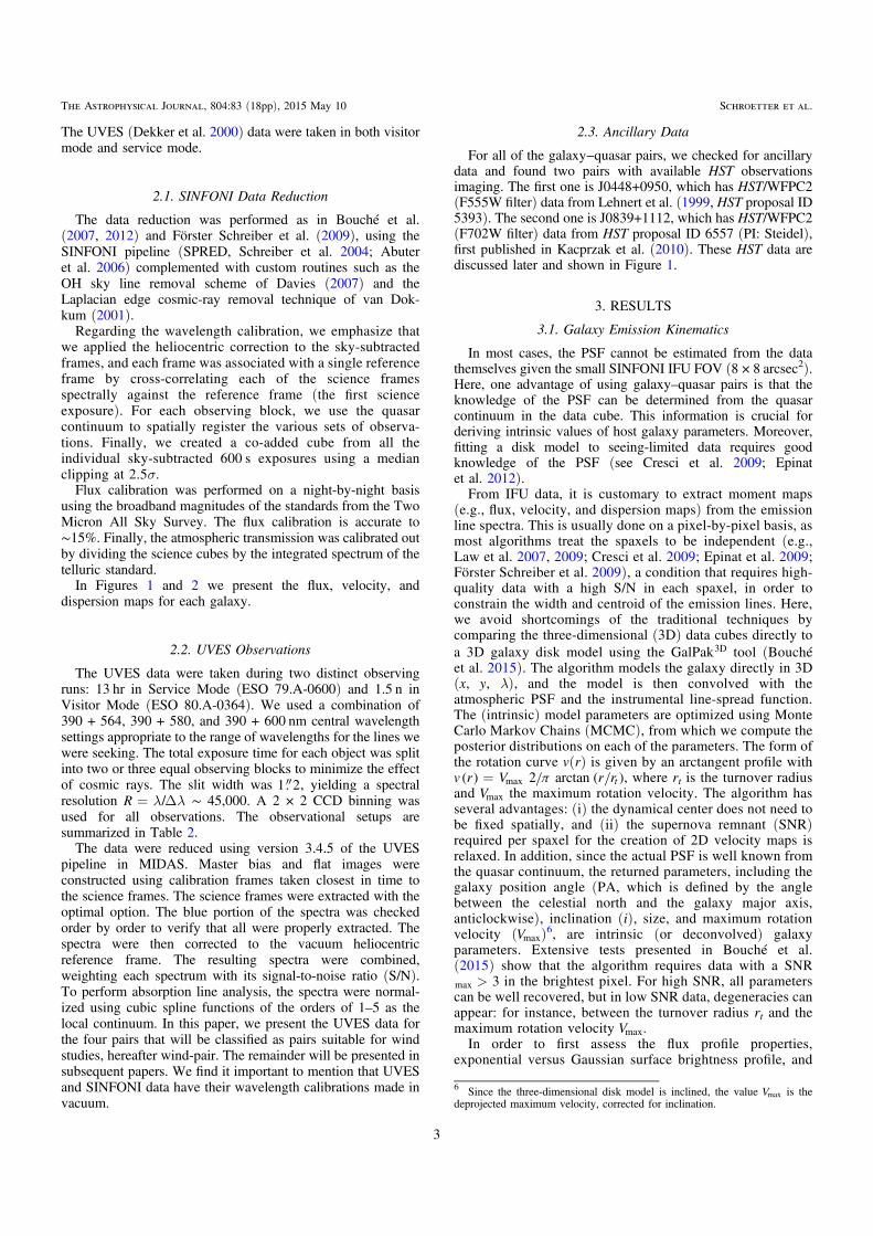
The UVES (Dekker et al. 2000) data were taken in both visitormode and service mode.

2.1. SINFONI Data Reduction

The data reduction was performed as in Bouché et al.(2007, 2012) and Förster Schreiber et al. (2009), using theSINFONI pipeline (SPRED, Schreiber et al. 2004; Abuteret al. 2006) complemented with custom routines such as theOH sky line removal scheme of Davies (2007) and theLaplacian edge cosmic-ray removal technique of van Dok-kum (2001).

Regarding the wavelength calibration, we emphasize thatwe applied the heliocentric correction to the sky-subtractedframes, and each frame was associated with a single referenceframe by cross-correlating each of the science framesspectrally against the reference frame (the first scienceexposure). For each observing block, we use the quasarcontinuum to spatially register the various sets of observa-tions. Finally, we created a co-added cube from all theindividual sky-subtracted 600 s exposures using a medianclipping at 2.5σ.

Flux calibration was performed on a night-by-night basisusing the broadband magnitudes of the standards from the TwoMicron All Sky Survey. The flux calibration is accurate to∼15%. Finally, the atmospheric transmission was calibrated outby dividing the science cubes by the integrated spectrum of thetelluric standard.

In Figures 1 and 2 we present the flux, velocity, anddispersion maps for each galaxy.

2.2. UVES Observations

The UVES data were taken during two distinct observingruns: 13 hr in Service Mode (ESO 79.A-0600) and 1.5 n inVisitor Mode (ESO 80.A-0364). We used a combination of390 + 564, 390 + 580, and 390 + 600 nm central wavelengthsettings appropriate to the range of wavelengths for the lines wewere seeking. The total exposure time for each object was splitinto two or three equal observing blocks to minimize the effectof cosmic rays. The slit width was 1. 2, yielding a spectralresolution l=R / lD ∼ 45,000. A 2 × 2 CCD binning wasused for all observations. The observational setups aresummarized in Table 2.

The data were reduced using version 3.4.5 of the UVESpipeline in MIDAS. Master bias and flat images wereconstructed using calibration frames taken closest in time tothe science frames. The science frames were extracted with theoptimal option. The blue portion of the spectra was checkedorder by order to verify that all were properly extracted. Thespectra were then corrected to the vacuum heliocentricreference frame. The resulting spectra were combined,weighting each spectrum with its signal-to-noise ratio (S/N).To perform absorption line analysis, the spectra were normal-ized using cubic spline functions of the orders of 1–5 as thelocal continuum. In this paper, we present the UVES data forthe four pairs that will be classified as pairs suitable for windstudies, hereafter wind-pair. The remainder will be presented insubsequent papers. We find it important to mention that UVESand SINFONI data have their wavelength calibrations made invacuum.

2.3. Ancillary Data

For all of the galaxy−quasar pairs, we checked for ancillarydata and found two pairs with available HST observationsimaging. The first one is J0448+0950, which has HST/WFPC2(F555W filter) data from Lehnert et al. (1999, HST proposal ID5393). The second one is J0839+1112, which has HST/WFPC2(F702W filter) data from HST proposal ID 6557 (PI: Steidel),first published in Kacprzak et al. (2010). These HST data arediscussed later and shown in Figure 1.

3. RESULTS

3.1. Galaxy Emission Kinematics

In most cases, the PSF cannot be estimated from the datathemselves given the small SINFONI IFU FOV (8 × 8 arcsec2).Here, one advantage of using galaxy–quasar pairs is that theknowledge of the PSF can be determined from the quasarcontinuum in the data cube. This information is crucial forderiving intrinsic values of host galaxy parameters. Moreover,fitting a disk model to seeing-limited data requires goodknowledge of the PSF (see Cresci et al. 2009; Epinatet al. 2012).From IFU data, it is customary to extract moment maps

(e.g., flux, velocity, and dispersion maps) from the emissionline spectra. This is usually done on a pixel-by-pixel basis, asmost algorithms treat the spaxels to be independent (e.g.,Law et al. 2007, 2009; Cresci et al. 2009; Epinat et al. 2009;Förster Schreiber et al. 2009), a condition that requires high-quality data with a high S/N in each spaxel, in order toconstrain the width and centroid of the emission lines. Here,we avoid shortcomings of the traditional techniques bycomparing the three-dimensional (3D) data cubes directly toa 3D galaxy disk model using the GalPak3D tool (Bouchéet al. 2015). The algorithm models the galaxy directly in 3D(x, y, λ), and the model is then convolved with theatmospheric PSF and the instrumental line-spread function.The (intrinsic) model parameters are optimized using MonteCarlo Markov Chains (MCMC), from which we compute theposterior distributions on each of the parameters. The form ofthe rotation curve v(r) is given by an arctangent profile with

=v r V π r r( ) 2 arctan ( )tmax , where rt is the turnover radiusand Vmax the maximum rotation velocity. The algorithm hasseveral advantages: (i) the dynamical center does not need tobe fixed spatially, and (ii) the supernova remnant (SNR)required per spaxel for the creation of 2D velocity maps isrelaxed. In addition, since the actual PSF is well known fromthe quasar continuum, the returned parameters, including thegalaxy position angle (PA, which is defined by the anglebetween the celestial north and the galaxy major axis,anticlockwise), inclination (i), size, and maximum rotationvelocity (Vmax)

6, are intrinsic (or deconvolved) galaxyparameters. Extensive tests presented in Bouché et al.(2015) show that the algorithm requires data with a SNR

> 3max in the brightest pixel. For high SNR, all parameterscan be well recovered, but in low SNR data, degeneracies canappear: for instance, between the turnover radius rt and themaximum rotation velocity Vmax.In order to first assess the flux profile properties,

exponential versus Gaussian surface brightness profile, and

6 Since the three-dimensional disk model is inclined, the value Vmax is thedeprojected maximum velocity, corrected for inclination.

3


Figure 1. From left to right: top: the HST/WFPC2 image (when available), the Hα J-band SINFONI flux (erg s−1 cm−2), the velocity map (in -km s 1) derived fromthe SINFONI data, and the dispersion map (in -km s 1). Bottom: the residuals cube represented in 2D (in σ), the intrinsic reconstructed galaxy with GalPaK3D

(deconvolved from the PSF given by the quasar), its velocity map, and the dispersion map. The quasar position is represented by the white contours on the observedflux maps when present in the map. In each panel, north is up and east is to the left.

4


Figure 1. (Continued.)

5


Figure 1. (Continued.)

6


axis ratios, we analyzed the collapsed cubes (i.e., lineintegrated, continuum-subtracted) with the galfit2D tool. Thistool is our custom 2D version of GalPak3D, an equivalent toGalfit (Peng et al. 2010), which fits isophotes to the images(with the PSF convolution) and then uses these isophotes to

compute the radial surface brightness profile. With the resultsfrom the 2D algorithm, we obtain an initial indication of thegalaxy inclination from the axis ratio and the profile shape(exponential versus Gaussian), before analyzing the kine-matics in the 3D data. We find that seven galaxy surface

Figure 2. Same as Figure 1 but for the J1441+0443 galaxy. This galaxy has the lowest SNR, below the threshold where we can trust the GalPaK3D results. Even if thisgalaxy is classified as wind-pair from its apparent PA, the low SNR does not allow us to build a wind model.

Table 2Summary of UVES Observations

Target Setting lc (nm) Texp (s) Run IDa Date

J0147+1258 390+580 4440 SM/079.A-0600(B) 2007 Jul 23 2007 Aug 14J0226–2857 390+580 9000 SM/079.A-0600(B) 2007 Jul 24, 27 2007 Sep 04J0302–3216 390+564 5430 SM/079.A-0600(B) 2007 Aug 02J0448+0950 390+564 13200 VM/080.A-0364(A) 2008 Jan 28, 29J0822+2243 390+564 7200 VM/080.A-0364(A) 2008 Jan 29J0839+1112 390+564 13200 VM/080.A-0364(A) 2008 Jan 28J0943+1034 390+580 9000 SM/079.A-0600(B) 2007 Apr 18, 22J1422–0001 390+564 9000 SM/079.A-0600(B) 2007 Apr 12, 14J1441+0443 390+600 8100 VM/080.A-0364(A) 2008 Jan 28, 29J2357–2736 390+564 4440 SM/079.A-0600(B) 2007 May 15

Note:a SM stands for Service Mode and VM for Visitor Mode.

Table 3Kinematic and Morphological Parameters

Galaxy b(kpc) α ( ) Inclination ( ) PA ( ) Flux Vmax Redshift r 12

Profile Class(1) (2) (3) (4) (5) (6) (7) (8) (9) (10) (11)

J0147+1258 17.9 ± 1.02 30 ± 30 24.4 ± 3.3 −69 ± 3 -1.63 · 10 16 241 ± 38 1.0389 7.11 ± 0.20 EXP Face-onJ0226–2857 ⩽2.0 ± 1.01 56 ± 3.0 47.9 ± 1.0 91 ± 1 -2.01 · 10 16 50 ± 12 1.0223 2.69 ± 0.04 EXP Ambig.J0302–3216 19.7 ± 0.95 16 ± 15 30.4 ± 1.5 −37 ± 3 -2.70 · 10 16 180 ± 15 0.8223 8.99 ± 0.31 EXP Face-onJ0448+0950 13.7 ± 0.96 79 ± 3.0 52.0 ± 1.2 31 ± 1 -5.03 · 10 16 253 ± 10 0.8391 7.85 ± 0.07 EXP Wind-pairJ0822+2243 21.8 ± 0.95 32 ± 30 17.9 ± 0.7 168 ± 1 -5.04 · 10 16 328 ± 14 0.8102 4.14 ± 0.06 EXP Face-onJ0839+1112 26.8 ± 0.94 59 ± 6.0 72 ± 5a 139 ± 4 -1.53 · 10 16 113 ± 20 0.7866 5.65 ± 0.29 EXP Wind-pairJ0943+1034 24.3 ± 1.01 32 ± 3.0 43 ± 5b 140 ± 1 -3.81 · 10 16 327 ± 10 0.9956 8.73 ± 0.21 EXP Inflow-pairJ1422–0001 12.7 ± 0.98 17 ± 5.0 55 ± 5 81 ± 3 -8.93 · 10 17 130 ± 20c 0.9096 4.30 ± 0.16 GAU Inflow-pairJ1441+0443b 10.1 ± 1.02 90 ± 6.0 L 87 ± 4 -6.62 · 10 17 L 1.0384 2.99 ± 0.18 GAU Wind-pairJ2357–2736 6.7 ± 0.95 68 ± 4.0 51.6 ± 2.2 109 ± 2 -1.29 · 10 16 187 ± 15 0.8149 5.53 ± 0.14 GAU Wind-pair

Notes:(1) Quasar name; (2) impact parameter; (3) azimuthal angle α (Section 3.3); (4) galaxy inclination (degrees); (5) position angle (degrees); (6) integrated Hα flux ofthe galaxy (erg s−1 cm−2); (7) maximum rotation velocity ( -km s 1); (8) Ha redshift (see Section 3.2); (9) half-light radius (kpc); (10) assumed flux profile (Exp. orGau.); (11) class (inflow-pair/wind-pair) based on α selection.a The inclination is determined from the HST data.b Galaxy parameters are derived from 2D fitting (galfit2D).c Turn-over radius is fixed to =r r 0.25t 1 2 .

7


brightness profiles can be described by exponential profiles,while three are best described by a Gaussian profile (e.g.,J1422–0001).

Using the GalPaK3D tool, we fit the kinematics directly tothe data cubes. The results are shown in Table 3. We emphasizethat the surface brightness profile breaks the commoninclination-Vmax degeneracy in kinematic analysis. For everygalaxy, we ran the algorithm for 10,000 iterations and checkedthat the MCMC converged for each of the parameters andestimated the uncertainties from the last 60% of the iterations.For J1422−0001, some of the kinematic parameters remainunconstrained, because the rotation curve appears shallow suchthat the turnover radius rt and the circular velocity Vmax aredegenerate. The parameters relevant for this study for definingthe kinematic major axis (PA) are well constrained, however.

As we will see in Section 4 (also illustrated in Figure A1),galaxy inclination is a critical parameter for the wind model.We cross-check the inclination measured using variousmethods (mainly galfit2D and GalPaK3D) and from theSINFONI and HST data sets when present. In particular, forJ0943+1034, the galaxy’s inclination is set to the valueobtained from the 2D profile fitting since GalPaK3D did notconverge for the turnover radius parameter. For J0839+1112,the galaxy’s inclination is set to the value obtained from thearchival HST image. For J0448+0950, the galaxy’s inclinationobtained from the SINFONI and HST data is consistent.

In Figure 1 we present the data, i.e., the observed flux andkinematics maps, and the fitted model. For each galaxy, theSINFONI data are shown in the first row, along with the HSTimage when available. In the second row, we present the resultsfrom the 3D kinematic fitting with the GalPaK3D algorithm,where we show the dispersion, velocity, flux, and residualmaps, from right to left. The residuals maps are generated fromthe residual cubes, which are just the difference between thedata and the model normalized by the pixel noise. The 2D maps

show the mean of the residuals in each spaxel normalized by itsstandard error. All the panels have north up and east to the left.

3.2. Redshifts

An accurate systemic redshift is crucial to characterize theoutflow velocity and ultimately the outflow mass loadingfactor. The GalPaK3D algorithm outputs the wavelength of theHα emission line from the axisymmetric disk model. Since thegalaxy distribution may be somewhat asymmetric, this some-times lead to a redshift bias.Therefore, we use two different methods. First, we

determine the redshift from the mean of the wavelength ofthe reddest and the bluest (Gaussian) Hα emission linesalong the kinematic major axis. As a second check, we createa pseudo-longslit along the kinematic major axis anddetermine zsys from the sharp transition in the p–v diagram.We find that both methods yield consistent results. Theseredshifts are listed in Table 3.The resulting intrinsic galaxy parameters will now allow us

to build a cone model in order to reproduce the data for galacticoutflows.

3.3. Azimuthal Dependence

In order to begin the wind modeling, we must first selectgalaxy–quasar pairs for which the quasar LOS intercepts thegalactic winds. This can be achieved using the quasarazimuthal angle α between the galaxy major axis and thequasar (Figure 3), because the presence of strong Mg II

absorbers is a strong function of α as demonstrated bynumerous recent studies (Bohlin et al. 2011; Bouchéet al. 2012; Bordoloi et al. 2014; Lan et al. 2014). Hence,we use the quasar position relative to the associated galaxymajor axis, using the inclination and major-axis determinedfrom the SINFONI data (Figure 1), to classify the differentgalaxy–quasar pairs in two main categories: pairs suitable forwind studies (wind-pair) for likely outflows and pairssuitable for accretion studies (inflow-pair) for likely inflows.

Figure 3. Scheme showing the alpha angle, corresponding to the angle betweenthe galaxy major axis and the quasar position.

Figure 4. Galaxy inclinations for the SIMPLE sample as a function of theazimuthal angle α. Note there are three types of galaxies in this sample: thewind-pairs, which have an azimuthal angle larger than 60° ± 10°; the inflow-pairs, with α lower than 60° ± 10°; and pairs that are ambiguous due touncertainty on α. It is difficult to derive the azimuthal angle for a nearly face-ongalaxy. The wind-pair and inflow-pair classes describe the fact of having thequasar absorptions tracing outflows and inflows, respectively.

8


Figure 4 shows the azimuthal angles α versus the galaxy’sinclinations for our SIMPLE sample of 10 galaxy–quasar pairs.Pairs with a ⩽ ⩽60 90 are selected to be wind-pairs. Pairswith a ⩽ ⩽0 30 correspond to the cases where the quasarLOS does not probe outflows but rather probes the extendedparts of gaseous disks, where the gas can potentially (or islikely) to be inflowing (inflow-pair) as in Bouché et al. (2013).

Naturally, the azimuthal angle for galaxies with lowinclinations, corresponding to face-on cases, is very difficultto constrain. These are then indexed as “face-on” cases. Pairswith a ~ 45 correspond to ambiguous cases where it isdifficult to argue for outflows or inflows. For instance,J0226–2857 falls into that category with the additionaldifficulty that this galaxy has a very low impact parameter(b = 0. 3 or <2.0 kpc), i.e., the LOS is likely dominated byabsorption from the galaxy interstellar medium.

Figure 4 shows that four galaxies are favorable to studygalactic wind properties: J0448+0950, J2357–2739, J0839+1112, and J1441+0443 these are classified as wind-pairs inTable 3. J1441+0443 is excluded from subsequent analysisbecause our SINFONI data do not meet the requirement ofSNR∼ 3 imposed by our intensive tests of the GalPaK3D

algorithm.

4. WIND PROPERTY ANALYSIS

4.1. Wind Sub-sample Analysis

For each galaxy–quasar pair, we have the quasar spectrumfor all the SIMPLE galaxies taken with the VLT/UVESinstrument. In these spectra, we identified three main absorp-tion features: the Mg II (ll2796, 2803) doublet and the Mg I

l2852 absorption line. Because of our selection in lWr2796 of

2 Å (to ensure that the host was within the SINFONI FOV), theMg II doublet is saturated. Hence, we use the Mg I absorptionline, which is not saturated and in most cases shows anasymmetric profile. This asymmetry can sometimes be seen inthe Mg II doublet, but less clearly. We center the spectrum onevery absorption line using the derived redshifts. For eachabsorption line, we transform wavelength to velocity, using thereference wavelengths in the vaccum. From the absorptionsystem kinematics and geometrical properties of the galaxy, wecan now build the wind model for the three galaxies.

4.1.1. Cone Wind Modeling

We follow Bouché et al. (2012) and Kacprzak et al. (2014)in modeling the wind as a bi-conical outflow using thegeometric parameters (inclination, α) set by the SINFONIdata. The principle is to create a cone perpendicular to thegalactic plane, fill it with uniformly distributed particles, andassume that the mass flux is conserved. The particlesrepresent cold gas clouds entrained in the wind, since theequivalent width of the absorption lines is the sum/combination of several individual components (Ménard andChelouche 2009), each of which corresponds to a “cold” gascloud (10 K4 ) entrained by supernova-heated hot winds( >T 10 K6 ). Since the galaxy inclination, PA, and azimuthalangle are previously determined from observations usingGalPaK3D and other methods, the only free parameters areVout and the cone opening angle qmax. For simplicity, weassign the clouds a constant radial velocity Vout, i.e., weassume that the LOS intercepts the clouds far from theacceleration region.

The cone is built along the x-, y-, and z-axes: x and yrepresent the sky plane, and z corresponds to the cone height.For a galaxy with 0° inclination, the cone direction will bealong the LOS. We then rotate the cone along the y-axis tomatch the galaxy’s inclination derived from our SINFONIdata and create a simulated absorption profile from thedistribution of cloud velocities projected along the quasarLOS (z-axis).We generate ∼106 particles in a cone, which are grouped by

bins of projected velocities. The quasar LOS is set by theimpact parameter (b) and α, both of which are derived from theSINFONI data cubes. Due to the Monte Carlo generation ofparticles, stochastic effects create fluctuations in the simulatedprofiles. This noise does not impact the resulting equivalentwidths and thus the derived outflow velocities.We then convolve the particle velocity distribution with

the UVES instrument resolution. Additionally, in order tosimulate the instrument noise, we add Poisson noise to thesimulated profile. This random Poisson noise has the same S/N as the data and provides for a more meaningfulcomparison. In order to give an intuitive feel for thisgeometric model, we show in the Appendix examples ofsimulated profiles using different galaxy inclinations, outflowvelocities, and opening angles.

4.1.2. Galaxy Contribution Model

Since our sample consists of pairs with small impactparameters ( <b 20 kpc) and with inclined galaxies (from~ 18 to ~ 55 ), we improve our model by adding the galaxycontribution for the quasar–galaxy pairs with the lowestimpact parameters ( ⩽b 10 kpc) such as J2357–2736(Section 4.2.3). The procedure is nearly the same as thecone model: we generate particles in a disk with anexponential distribution from the center to the edge. Wetake the galaxy half-light radius derived with GalPaK3D toestimate a realistic contribution from the disk. The thicknessof the disk is set to be 0.15 times this radius. We assign theparticles a constant circular velocity corresponding to themaximum velocity of the galaxy. The velocity distribution ofthe disk is naturally strongly dependent on the azimuthalangle with a maximum offset at a = 0 and a distributioncentered around 0 -km s 1 at a = 90 .

4.2. Comments on Individual Wind-pairs

4.2.1. J0448+0950

The galaxy near the quasar J0448+0950 has an impactparameter =b 13.7 kpc and an Hα flux of ´ -5.03 10 16

erg s−1 cm−2. Its azimuthal angle α of ∼79° and inclination i of∼52°make it a wind-pair (Figure 4). This galaxy has an SFR of∼13 M yr−1 (see Section 4) and a redshift of 0.8390.In addition to our SINFONI data, we retrieved ancillary

data from HST/WFPC2 (F555W filter). These HST dataallow us to compare the morphology of the galaxy (seeFigure 1) with the SINFONI one. In both data sets, one seesthat the galaxy has an asymmetric flux distribution (Figure 1)with a brighter area somewhat offset with respect tothe kinematic center. Comparing the HST image andSINFONI flux map (the quasar was subtracted in SINFONIHα flux), the PA and inclination of the galaxy are in goodagreement.

9


After determining the geometrical parameters for this galaxy,we can build a cone model as described in Section 4.1.1. InFigure 5, we compare the simulated profile for Mg I l2852 7 tothe observed absorption in the UVES data (right column of thefigure). To generate this simulated profile,8 we adjusted theoutflow speed Vout and the cone opening angle θ, while keepingthe geometrical parameters fixed. The best values are anoutflow speed Vout of 115± 10 -km s 1 and a cone openingangle qmax of 40° ± 5°. The errors represent the maximumallowed range values for Vout and qmax.

We note that our simulated profile reproduces the asymmetryand equivalent width of the observed profile. Note, our modeldoes not attempt to reproduce the depth of the profile since it isarbitrarily normalized. The fluctuations in the simulated profile

are due to stochastic effects from the Monte Carlo particledistribution.Outflow rates and mass loading factors for each galaxy

identified as wind-pairs are detailed in Section 4.3.

4.2.2. J0839+1112

In our sample, the galaxy toward J0839+1112 has the largestimpact parameter b 26.8 kpc. With an Hα flux of ´ -1.53 10 16

erg s−1 cm−2, an inclination i of ∼72°, and an azimuthal angleα of ∼59°, this galaxy also belongs to the wind-pair subsampledefined in Section 3.3. Its SFR is ∼3.4 M yr−1, and it has aredshift of =z 0.7866.In Figure 1 we compare archival HST/WFPC2 (F702W

filter) images to our SINFONI Hα data. Both data sets show aslight asymmetry in the galaxy flux distribution and a similarPA. For the galaxy inclination, we used galfit2D on the HST

Figure 5. Representation of the cone model and quasar spectrum associated with the J0448+0950 galaxy. Left: the cone model seen in the sky plane where the y-axiscorresponds to the galaxy major axis and x to its minor one. The gray circle represents the inclined galaxy disk, and the black circles illustrate the gas outflow cone.Bottom left: a side view of the cone where the z-axis corresponds to the quasar LOS direction with the observer to the left. Right: normalized flux for the Mg I l2852absorption line observed with UVES (bottom) where we can see an outward asymmetry, and the reconstructed profile (top). The red dashed line gives the simulatedprofile without taking into account the galaxy contribution. The black line does take into account this contribution. Note that this model does not reproduce the depthof the absorption line.

7 We use Mg I l2852 since Mg II l2796 is saturated.8 The galaxy contribution is also considered in the simulated profile (theredshifted contribution in upper right of Figure 5).

10


image to cross-check the results from the 3D fitting and foundgood agreement (within 15 ) between the two methods.

As for J0448+1112, we generated a simulated profile fromthe wind cone model using the geometrical parameters from theSINFONI+HST data and adjusted the outflow speed Vout andthe cone opening angle θ, while keeping the geometricalparameters fixed. Figure 6 shows the simulated profile and theMg I absorption from the UVES data (right column of thefigure). We constrained an outflow speed Vout of 105± 10

-km s 1 and a cone opening angle of qmax of 30° ± 5°. Theimpact parameter b is too high to consider any contributionfrom the galaxy.

4.2.3. J2357−2736

The last individual case from our wind subsample is thegalaxy along the J2357−2736 LOS. The host galaxy has thesmallest impact parameter b to the quasar LOS with b of6.7 kpc. This galaxy has an Hα flux of ´ -1.29 10 16 erg s−1

cm−2 and an SFR of ∼3.3 M yr−1. Its inclination i is ∼52, andit is classified as wind-pair because of its azimuthal angle α

of ∼68°.

As in the previous two cases, we generated a simulatedUVES profile using the wind model described in Section 4.1.Figure 7 (bottom) shows the UVES Mg I l2852 absorptionprofile, whose asymmetry is reversed compared to the twoother cases with a maximum optical depth at ~V 0 -km s 1.However, any constant wind speed model will have an outwardasymmetry (Figure A1), and the data clearly show theopposite, an inward asymmetry. For a profile with inwardasymmetry, the strongest part of the absorption profile islocated closer to the systemic velocity (e.g., bottom left ofFigure 7). An outward asymmetry profile has the oppositebehavior (e.g., Figure 5). This inward asymmetry is seen in theother non-saturated transitions (Zn IIl2026, Mg I l2026, Mn II

(ll2576, 2594, 2606)) present in the UVES data (Figure 8).Contrary to the other two cases, this galaxy has a very low

impact parameter ( ~b 6.7 kpc), where the assumption ofconstant wind speed might break down. Indeed, the low-ionization material in momentum-driven winds and energy-driven winds is thought to be accelerated (e.g., Murrayet al. 2005; Steidel et al. 2010) by the hot gas, by the radiationpressure, or both.Therefore, instead of using a constant wind speed, we added

a generic velocity profile such as =V r V π r r( ) 2 arctan ( ),out 0

Figure 6. Same as Figure 5 for the J0839+1112 galaxy where no galaxy contribution can be seen.

11


Figure 7. Left column: Mg I absorption from the J2357−2736 galaxy indicating that the model must include accelerating winds, from top to bottom: simulatedabsorption profiles with r0 = 1, 5, 10 kpc, and the UVES data centered on Mg I l2852. Notice that the asymmetry changes as r0 increases; it goes from outward toinward asymmetry. Right column: the velocity profile corresponding to the associated simulated profile to the left where the turnover radius of the velocity profile (r0)varies, from top to bottom: r0 = 1, 5, 10 kpc. The red dashed line represents the distance between the galaxy and the quasar LOS (b/sin(α)/sin(i)), corrected for theinclination i. The final simulated profile is the one directly above the data, with r0 = 10 kpc.

12


where r is the distance from the galaxy and r0 is thecharacteristic turnover radius. Figure 7 shows the behavior ofthis model (dashed line) on the profile asymmetry for differentvalues of r0, illustrating that the asymmetry reverses as r0increases. The accelerated wind model that best describes thedata is the one with =r 100 kpc shown above the UVESspectrum in Figure 7. Similar to J0448+0950, we also includeda contribution from the galaxy that appears to account for thebluest components.

For this case, we found an outflow speed Vout of 130± 10-km s 1 using a cone opening angle qmax of 45° ± 5°. Note that

there is no degeneracy between Vout and r0 as the varioussimulated profiles shown in Figure 7 are for the same outflowvelocity. In other words, Vout is set by the reddest part of theprofile, whereas r0 is constrained by the profile shape.

Having determined outflow velocities for the three wind-pairs, we now focus on deriving the ejected outflow rates Mouttogether with the mass loading factors η.

4.3. Outflow Rate

As discussed in Section 4.2.3, the equivalent width of theMg I l2852 absorption lines depends only on qmax and Voutfrom the cumulated distribution of projected velocities of gascloud intercepted along the LOS, while the profile asymmetry

depends on the system geometry, the particle density, and theoutflow velocity (Vout). From these constraints, we canconstrain the total mass flux of this material traced by thelow-ionization lines following Bouché et al. (2012) using thefollowing equation:

q»

»

´ q

- -

-

M μ N b b Vπ˙ · ( ) · · ·2

· ,

· ·

· , (1)

M

M

μ N b b

V

out H out max

˙

0.5 yr 1.5

( )

10 cm 25 kpc

200 km s 30

out

1

H

19 2

out

1

max

where μ is the mean atomic weight, b the impact parameter,qmax the cone opening angle,9 and N b( )H the gas columndensity of hydrogen at the b distance.The only parameter that remains to be constrained is the

column density N b( )H . In order to determine the gas columndensity NH, we use the empirical relation of Ménard andChelouche (2009) between neutral gas column density andMg II equivalent width lWr

2796:

=é

ëêê

´ ´ù

ûúú

l ( )N Wlog (3.06 0.55) 10 . (2)rH19 2796 1.7 0.26

I

This relation, together with the tight correlation between Mg II

equivalent width and dust content (as determined statisticallyfrom quasar extinction) from Ménard and Chelouche (2009),leads to a gas-to-dust ratio slightly smaller than that of theMilky Way H I column densities of =Nlog ( ) 19.5HI andabove. Furthermore, the redshift evolution of the dust contentof Mg II absorbers extrapolated to z = 0 shows that Mg II–

selected aborbers extend the local relation between visualextinction AV and the total hydrogen column NH of Bohlin et al.(1978). This in turn indicates that the ionized gas contributionis negligible in regions with H I columns above

=Nlog ( ) 19.5HI , as also argued by Jenkins (2009), and thatone can use the correlation between Mg II equivalent width andNHI as a proxy for the NH gas column density.Given our selection criteria of >lW 2r

2796 Å, we are verylikely in a regime where the gas is mostly neutral. For our threewind-pair sight lines, the H I column densities are

»Nlog ( ) 20.3HI for J0448+0950, »Nlog ( ) 20.1HI for J0839+1112, and »Nlog ( ) 19.9HI for J2357−2736. The restequivalent widths lWr

2796 determined from the UVES dataand the corresponding NH column densities for the wind-pairgalaxies are listed in Table 4. In future work, we will be able tomeasure NHI directly from UV spectroscopy with HST/CosmicOrigins Spectrograph (COS).Figure 9 shows the Mg II rest equivalent width lWr

2796 as afunction of impact parameter b for quasar–galaxy pairs wherethe quasar is aligned with the minor axis (wind-pairs) fromvarious literature samples (Kacprzak et al. 2011a, 2011b) andthis paper. This figure shows that the tight anti-correlationbetween impact parameter b and Wr (Bouché et al. 2012) isconfirmed at <b 30 kpc. The solid line traces the fiducial b1relation for mass-conserved bi-conical outflows (see Bouchéet al. 2012).

Figure 8. Absorption lines observed with UVES for J2357–2736. The solidlines are a Gaussian smoothing of the data (with a sigma of 1 pixel) to aid theeye. The gray shaded area in the Zn II (l2026) panel is the absorption expectedfrom the Mg I l2026 line (derived by scaling the observed optical depth of theMg I l2852 line, ignoring potential saturation effects).

9 qmax is defined from the central axis, and the cone subtends an area Σ ofqπ · max2 .

13


Table 4 lists our estimated outflow rates determined usingEquation (1). In order to determine the error bars for Mout, wetake the maximum error of every parameter used to derive it.We thereby objectively determine the maximum uncertainty onthe ejected mass rate. We also note that the errors on Mout aredominated by the errors on NHI.

From the outflow rates, we compute the mass loading factorη by comparing it to the SFR. We derived the SFR fromHα using the Kennicutt (1998) calibration, which assumes aSalpeter (1955) initial mass function (IMF):

= ´ a- -

( )M LSFR yr 7.9 10 , (3)1 42H

where aLH is the Hα luminosity in erg s−1 cm−2. We note thatthe SFRs for the Salpeter IMF with no extinction correction areidentical to using a dust correction of 1 mag (Zahid et al. 2013)with the Chabrier (2003) IMF, as the two IMFs are offset by−0.25 dex (see Table 2 in Bernardi et al. 2010).The results for the three galaxies are shown in Table 4. If we

assume that galactic winds are symmetric with respect to thegalactic plane (Figure 3), the total ejected mass rate for a

galaxy must be increased by a factor of 2, which gives»M 9out M yr−1 for J0448+0950, »M 2out M yr−1 for

J2357–2736, and »M 7out M yr−1 for J0839+1112.Considering the ejection velocity of the winds (115, 105,

and 130 -km s 1 for J0448+0950, J0839+1112, and J2357−2736, respectively), it is interesting to test whether thisvelocity is large enough for the gas to leave the galaxy halo orif it will end up falling back onto the galaxy. The escapevelocity Vesc for an isothermal sphere is given by the followingequation (Veilleux et al. 2005):

=é

ëêê

+æèççç

öø÷÷÷ù

ûúú

V VR

r· 2 1 ln , (4)esc max

vir

where Vmax is the maximum rotation velocity of the galaxy andRvir is the virial radius. Given that our galaxies’ halos have amass close to 1012 M , their virial radius is approximately

»R V H z10 ( )vir max , where H(z) is the Hubble constant atredshift z. For the wind-pairs, their virial radii are 225 kpc forJ0448+0950, 103 kpc for J0839+1112, and 168 kpc for J2357−2736. We give these results in Table 4, along with the resultson mass loading factors h = Mout/SFR.The ratio <V V 1out esc shows that the ejected gas does not

escape from the galaxy halo and should therefore fall back intothe galaxy. This gas contributes to the regulation of starformation in the galaxies.

5. CONCLUSIONS AND DISCUSSIONS

In this paper, we studied gas flows around SFGs using theSIMPLE sample of galaxy−quasar pairs (Paper I). Thegalaxies in this sample are located within ⩽3″ (⩽20 kpc) ofthe background quasar sightlines due to the selection ofabsorption with rest equivalent width ⩾2Å. Thanks to theSINFONI IFU on the VLT and the new algorithm GalPaK3D,we were able to recover the intrinsic morphological andkinematic properties of the galaxies from their Hα emission(Figure 1). The galaxies in our sample can be classifiedas wind-pairs or inflow-pairs according to the apparent

Table 4Results for Galaxies J0448+0950, J2357–2736, J0839+1112 together with Literature Results

Galaxy b (kpc) log(N b( )H ) Vmax Vout ( -km s 1) qmax SFR Mout

V

Vout

esc η Reference(1) (2) (3) (4) (5) (6) (7) (8) (9) (10) (11)

J0448+0950 13.7 20.30 ± 0.3 253 ± 10 115 ± 10 40 ± 5.0 13.6 ± 0.3 4.6 -+3.24.9 0.16 0.70 This work

J0839+1112 26.8 20.10 ± 0.3 115 ± 8 105 ± 10 30 ± 5.0 3.4 ± 0.2 3.6 -+2.23.4 0.43 2.11 This work

J2357−2736 6.7 19.92 ± 0.2 186 ± 15 130 ± 10 45 ± 5.0 3.3 ± 0.2 1.2 -+0.71.1 0.24 0.75 This work

J081420G1 51.1 19.07 ± 0.2 131 ± 10 175 ± 25 30 ± 5.0 5.0a 1.0 -+0.71.4 0.63 0.42 B2012

J091119G1 71.2 19.34 ± 0.2 231 ± 10 500 ± 100 30 ± 5.0 1.2a 7.8 -+4.512.2 0.97 12.9 B2012

J102847G1 89.8 18.60 ± 0.2 162 ± 10 300 ± 25 30 ± 5.0 9.0a 1.1 -+0.71.5 0.95 0.23 B2012

J111850G1 25.1 19.97 ± 0.2 116 ± 10 175 ± 80 30 ± 5.0 7.0a 4.1 -+1.110.0 0.63 1.17 B2012

J225036G1 53.9 19.54 ± 0.2 240 ± 10 225 ± 50 30 ± 5.0 8.0a 4.2 -+2.27.3 0.40 1.06 B2012

J1659+3735 58.0 18.89 ± 0.15 140 ± 10 40–80 40 ± 5.0 4.6–15 1.6–4.2 0.12–0.27 0.1–0.9 K2014

Notes:(1) Galaxy name; (2) impact parameter (kpc); (3) gas column density at the impact parameter (cm−2); (4) maximum rotational velocity of the galaxy ( -km s 1); (5)wind velocity ( -km s 1); (6) cone opening angle (degrees); (7) star formation rate ( M yr−1); (8) ejected mass rate for one cone ( M yr−1); (9) ejection velocitydivided by escape velocity; (10) mass loading factor: ejected mass rate divided by star formation rate (for both cones); (11) references: B2012: Bouché et al. (2012),K2014: Kacprzak et al. (2014).a SED-derived SFRs.

Figure 9. lWr2796 as a function of impact parameter b for galaxy–quasar pairs

classified as wind-pairs.

14


location of the quasar with respect to the galaxy major axis(Figure 4).

With this classification, we focused the analysis on theproperties of galactic winds for the sub-sample of foursuitable wind-pairs, although one galaxy has an SNR too lowfor a robust morphological (inclination) measurement.The wind properties are constrained from the high-resolutionUVES spectra of the minor-axis quasars. We show thatan simple cone model for galactic winds (Section 4.1.1)can reproduce the morphology of the UVES Mg I

absorption profiles. The wind properties can be summarizedas follows:

1. Like other recent works (e.g., Chisholm et al. 2014;Rubin et al. 2014), outflow velocities are smaller than theescape velocities, so the gas traced by low-ionizationlines does not escape the galaxy halo.

2. At the lowest impact parameter ( ~b 6 kpc), onequasar–galaxy pair (J2357−2736) has an absorptionprofile consistent with an accelerated wind (Sec-tion 4.2.3).

3. Loading factors η vary between ∼0.65 for the twomassive galaxies and ∼2 for the galaxy with the lowestmass (Figure 10). Our results indicate that the massloading factors tend to be higher for smaller galaxies, inagreement with theoretical expectations (e.g., Murrayet al. 2011; Hopkins et al. 2012).

Figure 10 also includes observational constraints on themass loading factor from the ~z 0.1 survey of Bouché et al.

(2012) (triangles) and ~z 0.2 pair of Kacprzak et al. (2014)(square). For the Bouché et al. (2012) sample, we usedspectral energy distribution (SED) derived SFRs (Table 4)given their larger impact parameters and longer travel times( >b Vout 100 s of Myr) compared to the timescale for Hα-derived SFRs (few Myr). The SED-derived SFRs arecomputed from the UV-to-IR photometry (using Galex+SDSS+Wise surveys) with the Code Investigating GALaxyEmission software (Noll et al. 2009). The pairs with thelargest impact parameters (>60 kpc) are shown in gray, sincethese mass loading factors can suffer strong biases due toeven larger travel times (∼300 Myr). Other measurements athigher redshift from stacked spectra of SFGs (Weiner et al.2009; Newman et al. 2012) indicate an average mass loadingfactor of ∼2 (Newman et al. 2012).The different lines in Figure 10 represent various

theoretical (Okamoto et al. 2010; Davé et al. 2011; Hopkinset al. 2012; Puchwein & Springel 2013; Vogelsbergeret al. 2014; Barai et al. 2015; Muratov et al. 2015) andempirical models (Peeples & Shankar 2011; Zahid et al.2014).10 In comparing observations and models, it isimportant to bear in mind that some are fiducial scalingrelations put in the sub-grid physics (e.g., Davé et al. 2011;Puchwein & Springel 2013; Vogelsberger et al. 2014), whileothers are from more complex numerical approaches (e.g.,Hopkins et al. 2012, 2013; Barai et al. 2015; Muratov et al.2015)11 and thus are more directly comparable withobservations.Currently our data do not allow us to discriminate between

energy- and momentum-driven winds, but thanks to ongoingwork at redshift ~z 0.2 with Keck/LRIS (N. Bouché et al.2015, in preparation; C. L. Martin et al. 2015, in preparation)and to the new-generation IFU Multi Unit SpectroscopicExplorer (MUSE) on the VLT (Bacon et al. 2010, 2015),we will be able to significantly increase the sample sizeand put tight constraints on the wind scaling relations.

We would like to thank the referee for his/her thoroughread of the manuscript and for the useful suggestions andcomments. This work is based on observations taken at ESO/VLT in Paranal and partially from the data archive of theNASA/ESA HST, which is operated by the Association ofUniversities for Research in Astronomy, Inc. We would liketo thank the ESO staff. N.B. acknowledges support from aCarreer Integration Grant (CIG) (PCIG11-GA-2012-321702)within the 7th European Community Framework Program.M.T.M. thanks the Australian Research Council for Dis-covery Project grant DP130100568 which supported thiswork. C.P. thanks the Agence Nationale de la Recherche forsupport (contract ANR-08-BLAN-0316-01). This researchmade use of Astropy, a community-developed core PYTHONpackage for astronomy (Astropy Collaboration et al. 2013),NumPy and SciPy (Oliphant 2007), Matplotlib (Hunter2007), IPython (Perez& Granger 2007), and of NASA’sAstrophysics Data System Bibliographic Services.

Figure 10. Comparison of predicted mass loading factors from theoretical/empirical models (curves) with values derived from observations (dots andtriangles) as a function of the maximum rotational velocity. The results fromthis work are represented by the cyan circles. The red square shows the massloading factor for a ~z 0.2 galaxy (Kacprzak et al. 2014). The triangles showthe results for ~z 0.2 galaxies from Bouché et al. (2012). The gray trianglesshow the galaxies with quasars located at >60 kpc where the mass loadingfactor is less reliable due to the large travel time needed for the outflow to crossthe quasar LOS (several 100 Myr) compared to the short timescale of theHα-derived SFR (∼10 Myr). The upper halo mass axis is scaled on Vmax atredshift 0.8 from Mo & White (2002).

10 The parameters of some of these models are listed in Table 1 of Zahid et al.(2014). We also took the values of the corrected version of Vogelsbergeret al. (2014).11 Note that the outflow rate from Barai et al. (2015) only includes gasparticles with velocities greater than the escape velocity.

15


APPENDIXUNDERSTANDING THE GEOMETRIC WIND MODEL

In this appendix we demonstrate how varying differentparameters within the cone model impacts the simulatedabsorption profile. For the cone model (Section 4.1.1), wechange three parameters in order to investigate the behavior ofthe simulated profile: for different galaxy inclinations (i), coneopening angles (θ), and wind outflow velocities (Vout)

(Figure A1). The general trends are as follows. The differentinclinations and cone opening angles change the left portion ofthe simulated absorption profile, while the wind velocityextends the right portion. Note that, except for the case of 90°galaxy inclination, all the simulated absorption profiles inFigure A1 present an outward asymmetry.We also present in Figure A2 the UVES Mg I l2852

absorption lines of our SIMPLE sample galaxies.

Figure A1. Examples of simulated absorption profiles with different galaxy inclinations (i), opening angle (θ), and wind velocities (Vout): while each of the simulatedprofiles has the same number of particles, the apparent depth decreases as each parameter increases due to larger velocity projections for i and θ and larger range ofvelocities for Vout. Top row: absorption profiles for galaxies inclined at 30°, 60°, and 90°with Vout = 100 -km s 1and θ = 30°. The noise effect is due to the MonteCarlo distribution of particles. Middle row: absorption profiles for wind cones with opening angles of 30°, 40°, and 45° with Vout = 100 -km s 1and i = 45°. Bottomrow: absorption profiles with wind velocities of 50, 100, and 150 -km s 1with i = 45° and θ = 30°. Each simulated profile has the same amount of particles but shows alarger velocity range due to the increasing gas speed, hence the varying apparent depths.

16


REFERENCES

Abuter, R., Schreiber, J., Eisenhauer, F., et al. 2006, NewAR, 50, 398Bacon, R., Accardo, M., Adjali, L., et al. 2010, Proc. SPIE, 7735, 8Bacon, R., Brinchmann, J., Richard, J., et al. 2015, A&A, 575, A75Barai, P., Monaco, P., Murante, G., Ragagnin, A., & Viel, M. 2015, MNRAS,

447, 266Behroozi, P. S., Conroy, C., & Wechsler, R. H. 2010, ApJ, 717, 379Bernardi, M., Shankar, F., Hyde, J. B., et al. 2010, MNRAS, 404, 2087Bordoloi, R., Lilly, S. J., Hardmeier, E., et al. 2014, ApJ, 794, 130Bohlin, R. C., Savage, B. D., & Drake, J. F. 1978, ApJ, 224, 132Bohlin, R. C., Savage, B. D., & Drake, J. F. 2011, ApJ, 743, 10Bouché, N., Carfantan, H., Schroetter, I., Michel-Dansac, L., & Contini, T.

2015, arXiv:1501.06586Bouché, N., Hohensee, W., Vargas, R., et al. 2012, MNRAS, 426, 801Bouché, N., Murphy, M. T., Kacprzak, G. G., et al. 2013, Sci, 341, 50Bouché, N., Murphy, M. T., Péroux, C., Csabai, I., & Wild, V. 2006, MNRAS,

371, 495Bouché, N., Murphy, M. T., Péroux, C., et al. 2007, ApJL, 669, L5Chabrier, G. 2003, PASP, 115, 763Chen, H.-W. 2012, MNRAS, 427, 1238Chisholm, J., Tremonti, C. A., Leitherer, C., et al. 2014, arXiv:1412.2139Contini, T., Garilli, B., le Fèvre, O., et al. 2012, A&A, 539, A91Cresci, G., Hicks, E. K. S., Genzel, R., et al. 2009, ApJ, 697, 115Davé, R., Oppenheimer, B. D., & Finlator, K. 2011, MNRAS, 415, 11Davies, R. 2007, MNRAS, 375, 1099Dekel, A., & Silk, J. 1986, ApJ, 303, 39Dekel, A., Sari, R., & Ceverino, D. 2009, ApJ, 703, 785Dekel, A., Zolotov, A., Tweed, D., et al. 2013, MNRAS, 435, 999Dekker, H., D’Odorico, S., Kaufer, A., Delabre, B., & Kotzlowski, H. 2000,

Proc. SPIE, 4008, 534Dubois, Y., & Teyssier, R. 2008, A&A, 477, 79

Elmegreen, D. M., Elmegreen, B. G., Ravindranath, S., & Coe, D. A. 2007,ApJ, 658, 763

Epinat, B., Contini, T., Le Fèvre, O., et al. 2009, A&A, 504, 789Epinat, B., Tasca, L., Amram, P., et al. 2012, A&A, 539, A92Förster Schreiber, N. M., Genzel, R., Bounché., et al. 2009, ApJ, 706, 1364Förster Schreiber, N. M., Genzel, R., Eisenhauer, F., et al. 2006, Msngr, 125, 11Genel, S., Naab, T., Genzel, R., et al. 2012, ApJ, 745, 11Genel, S., Vogelsberger, M., Springel, V., et al. 2014, MNRAS, 445, 175Genzel, R., Burkert, A., Bouché, N., et al. 2008, ApJ, 687, 59Heckman, T. M., Armus, L., & Miley, G. K. 1990, ApJS, 74, 833Heckman, T. M., Lehnert, M. D., Strickland, D. K., & Armus, L. 2000, ApJS,

129, 493Hopkins, P. F., Kereš, D., Murray, N., et al. 2013, MNRAS, 433, 78Hopkins, P. F., Quataert, E., & Murray, N. 2012, MNRAS, 421, 3522Jenkins, E. B. 2009, ApJ, 700, 1299Kacprzak, G. G., Churchill, C. W., Barton, E. J., & Cooke, J. 2011a, ApJ,

733, 105Kacprzak, G. G., Churchill, C. W., Ceverino, D., et al. 2010, ApJ, 711, 533Kacprzak, G. G., Churchill, C. W., Evans, J. L., Murphy, M. T., &

Steidel, C. C. 2011b, MNRAS, 416, 3118Kacprzak, G. G., Martin, C. L., Bouché, N., et al. 2014, ApJL, 792, LL12Kennicutt, R. C., Jr. 1998, ApJ, 498, 541Kereš, D., Katz, N., Weinberg, D. H., & Davé, R. 2005, MNRAS, 363, 2Lan, T.-W., Ménard, B., & Zhu, G. 2014, ApJ, 795, 31Law, D. R., Steidel, C. C., Erb, D. K., et al. 2007, ApJ, 669, 929Law, D. R., Steidel, C. C., Erb, D. K., et al. 2009, ApJ, 697, 2057Leauthaud, A., George, M. R., Behroozi, P. S., et al. 2012, ApJ, 746, 95Leauthaud, A., Tinker, J., Behroozi, P. S., Busha, M. T., & Wechsler, R. H.

2011, ApJ, 738, 45Lehnert, M. D., & Heckman, T. M. 1996, ApJ, 472, 546Lehnert, M. D., van Breugel, W. J. M., Heckman, T. M., & Miley, G. K 1999,

ApJS, 124, 11

Figure A2. Here we present the UVES Mg I l2852 absorption lines for 8 out of 10 galaxies. We do not have these absorption lines for J0147+1258 and J0226−2857as they fall in the gap of UVES data. The top row corresponds to UVES Mg I centered data of the four wind-pairs. The bottom row presents the UVES Mg I centereddata of the two inflow-pairs and the two ambiguous cases from left to right.

17


Martin, C. L. 1998, ApJ, 506, 222Martin, C. L. 1999, ApJ, 513, 156Martin, C. L. 2005, ApJ, 621, 227Martin, C. L., Kobulnicky, H. A., & Heckman, T. M. 2002, ApJ, 574, 663Martin, C. L., Shapley, A. E., Coil, A. L., et al. 2012, ApJ, 760, 127Martin, C. L., Shapley, A. E., Coil, A. L., et al. 2013, ApJ, 770, 41Ménard, B., & Chelouche, D. 2009, MNRAS, 393, 808Mo, H. J., & White, S. D. M. 2002, MNRAS, 336, 112Moster, B. P., Somerville, R. S., Maulbetsch, C., et al. 2010, ApJ, 710, 903Muratov, A. L., Keres, D., Faucher-Giguere, C.-A., et al. 2015,

arXiv:1501.03155Murray, N., Ménard, B., & Thompson, T. A. 2011, ApJ, 735, 66Murray, N., Quataert, E., & Thompson, T. A. 2005, ApJ, 618, 569Newman, S. F., Genzel, R., Förster-Schreiber, N. M., et al. 2012, ApJ, 761, 43Noll, S., Burgarella, D., Giovannoli, E., et al. 2009, A&A, 507, 1793Okamoto, T., Frenk, C. S., Jenkins, A., & Theuns, T. 2010, MNRAS,

406, 208Oppenheimer, B. D., & Davé, R. 2006, MNRAS, 373, 1265Oppenheimer, B. D., Davé, R., Kereš, D., et al. 2010, MNRAS, 406, 2325Papastergis, E., Cattaneo, A., Huang, S., Giovanelli, R., & Haynes, M. P. 2012,

ApJ, 759, 138Peeples, M. S., & Shankar, F. 2011, MNRAS, 417, 2962Peng, C. Y., Ho, L. C., Impey, C. D., & Rix, H.-W. 2010, AJ, 139, 2097Péroux, C., Bouché, N., Kulkarni, V. P., & York, D. G. 2013, MNRAS,

436, 2650Pettini, M., Rix, S. A., Steidel, C. C., et al. 2002, ApJ, 569, 742Puchwein, E., & Springel, V. 2013, MNRAS, 428, 2966Rosdahl, J., Blaizot, J., Aubert, D., Stranex, T., & Teyssier, R. 2013, MNRAS,

436, 2188

Roškar, R., Teyssier, R., Agertz, O., Wetzstein, M., & Moore, B. 2014,MNRAS, 444, 2837

Rubin, K. H. R., Prochaska, J. X., Koo, D. C., et al. 2014, ApJ, 794, 156Rubin, K. H. R., Weiner, B. J., Koo, D. C., et al. 2010, ApJ, 719, 1503Rupke, D. S., Veilleux, S., & Sanders, D. B. 2005, ApJS, 160, 115Salpeter, E. E. 1955, ApJ, 121, 161Schaye, J., Crain, R. A., Bower, R. G., et al. 2015, MNRAS, 446, 521Schreiber, J., Thatte, N., Eisenhauer, F., et al. 2004, in ASP Conf. Ser. 314:

Astronomical Data Analysis Software and Systems (ADASS) XIII, ed.F. Ochsenbein, M. G. Allen, & D. Egret (San Francisco, CA: ASP), 380

Shen, S., Madau, P., Aguirre, A., et al. 2012, ApJ, 760, 50Shen, S., Madau, P., Guedes, J., et al. 2013, ApJ, 765, 89Springel, V., Frenk, C. S., & White, S. D. M. 2006, Natur, 440, 1137Steidel, C. C. 1995, in QSO Absorption Lines, ed. G. Meylan (Berlin:

Springer), 139Steidel, C. C., Erb, D. K., Shapley, A. E., et al. 2010, ApJ, 717, 289Tumlinson, J., Thom, C., Werk, J. K, et al. 2013, ApJ, 777, 59van Dokkum, P. G. 2001, PASP, 113, 1420Veilleux, S., Cecil, G., & Bland-Hawthorn, J. 2005, ARA&A, 43, 769Vogelsberger, M., Genel, S., Sijacki, D., et al. 2014a, MNRAS, 438, 3607Vogelsberger, M., Genel, S., Springel, V., et al. 2014b, Natur, 509, 177Weiner, B. J., Coil, A. L., Prochaska, J. X., et al. 2009, ApJ, 692, 187Werk, J. K., Prochaska, J. X., Tumlinson, J., et al. 2014, ApJ, 792, 8White, S. D. M., & Frenk, C. S. 1991, ApJ, 379, 52White, S. D. M., & Rees, M. J. 1978, MNRAS, 183, 341Wuyts, S., Förster Schreiber, N. M., van der Wel, A., et al. 2011, ApJ,

742, 96Zahid, H. J., Torrey, P., Vogelsberger, M., et al. 2014, Ap&SS, 349, 873Zahid, H. J., Yates, R. M., Kewley, L. J., & Kudritzki, R. P. 2013, ApJ, 763, 92

18


Appendix B

Schroetter et al. 2016: MusEGAs FLOw and Wind(MEGAFLOW): first MUSEresults on background quasars

133

Draft version August 7, 2016Preprint typeset using LATEX style emulateapj v. 12/16/11

MUSE GAS FLOW AND WIND (MEGAFLOW) I: FIRST MUSE RESULTS ON BACKGROUND QUASARS 1

I. Schroetter2,4, N. Bouche3, M. Wendt5,6, T. Contini2,4, H. Finley2,4, R. Pello2,4, R. Bacon7, S. Cantalupo9,R. A. Marino9, J. Richard7, S. J. Lilly9, J. Schaye8, K. Soto9, M. Steinmetz5, L. A. Straka8, L. Wisotzki5

Draft version August 7, 2016

Abstract

The physical properties of galactic winds are one of the keys to understand galaxy formation andevolution. These properties can be constrained thanks to background quasar lines of sight (LOS)passing near star-forming galaxies (SFGs). We present the first results of the MusE GAs FLOw andWind (MEGAFLOW) survey obtained of 2 quasar fields which have 8 Mg ii absorbers of which 3 haverest-equivalent width greater than 0.8 A. With the new Multi Unit Spectroscopic Explorer (MUSE)spectrograph on the Very Large Telescope (VLT), we detect 6 (75%) Mg ii host galaxy candidateswithing a radius of 30′′ from the quasar LOS. Out of these 6 galaxy–quasar pairs, from geometricalarguments, one is likely probing galactic outflows, two are classified as “ambiguous”, two are likelyprobing extended gaseous disks and one pair seems to be a merger. We focus on the wind−pairand constrain the outflow using a high resolution quasar spectra from Ultraviolet and Visual EchelleSpectrograph (UVES). Assuming the metal absorption to be due to gas flowing out of the detectedgalaxy through a cone along the minor axis, we find outflow velocities of the order of ≈ 150 km s−1

(i.e. smaller than the escape velocity) with a loading factor, η = Mout/SFR, of ≈ 0.7. We see evidencefor an open conical flow, with a low-density inner core. In the future, MUSE will provide us withabout 80 multiple galaxy−quasar pairs in two dozen fields.Subject headings: galaxies: evolution — galaxies: formation — galaxies: intergalactic medium —

quasars: individual: SDSSJ213748+001220, SDSSJ215200+062516

1. INTRODUCTION

In spite of the successes of the ΛCDM cosmologicalmodel (i.e. Springel et al. 2005), a major discrepancyremains between the predicted number density of darkmatter halos and the observed number density of galax-ies in the low-mass regime (L < L∗) (i.e. Guo et al.2010; Papastergis et al. 2012; Moster et al. 2010, 2013;Behroozi et al. 2013). This behavior is usually explainedby supernova(SN)-driven outflows (Dekel & Silk 1986)which expel baryons from the galactic disk. Indeed,these galactic outflows are observed in almost every star-forming galaxy (SFG) (Veilleux et al. 2005, for a review)and are likely to enrich the inter-galactic medium (e.g.Dekel & Silk 1986; Aguirre et al. 2001; Oppenheimer &Dave 2006).

1 Based on observations made at the ESO telescopes underprograms 094.A-0211(B) and 293.A-5038(A).

2 IRAP, Institut de Recherche en Astrophysique etPlanetologie, CNRS, 14, avenue Edouard Belin, F-31400Toulouse, France

3 IRAP/CNRS, 9, avenue Colonel Roche, F-31400 Toulouse,France

4 University Paul Sabatier of Toulouse/ UPS-OMP/ IRAP,F-31400 Toulouse, France

5 AIP, Leibniz-Institut fur Astrophysik Potsdam, An derSternwarte 16, D-14482 Potsdam, Germany

6 Institut fur Physik und Astronomie, Universitat Potsdam,D-14476 Golm, Germany

7 Univ Lyon, Univ Lyon1, Ens de Lyon, CNRS, Centrede Recherche Astrophysique de Lyon UMR5574, F-69230,Saint-Genis-Laval, France

8 Leiden Observatory, Leiden University, PO Box 9513, 2300RA Leiden, The Netherlands

9 ETH Zurich, Institute of Astronomy, Wolfgang-Pauli-Str.27, 8093 Zurich, Switzerland

10 AIG, Institut fur Astrophysik, Universitat Gottingen,Friedrich-Hund-Platz 1, D-37077 Gottingen, Germany

The physical mechanisms for driving galactic winds arecomplex and the cold gas could be accelerated by ther-mal energy injection (Springel & Hernquist 2003), by mo-mentum injection from radiation pressure (e.g. Murrayet al. 2005), by cosmic ray pressure (e.g. Booth et al.2013; Salem & Bryan 2014) or by a combination of thesemechanisms (e.g. Hopkins 2015) The wide range physi-cal scales that describe SN explosions from AstronomicalUnit (AU) to tens of kiloparsecs (kpc), are beyond thecapabilities of cosmological simulations.

Hence, in most of these simulations, outflows are usu-ally implemented with sub-grid prescriptions (e.g. Schayeet al. 2010; Oppenheimer et al. 2010; Vogelsberger et al.2014). A popular sub-grid recipe is to let the loading fac-

tor η, i.e. the ratio between the outflow rate Mout andthe star-formation rate (SFR), be a function of galaxy(halo) mass or circular velocity Vc (Oppenheimer et al.2010) such as η ∝ V −1

c for momentum-driven winds andη ∝ V −2

c for energy-driven winds. An alternative wayto implement the collective effect of SN explosions is the(stochastic) implementation of thermal feedback, wheregalactic winds develop without imposing any input out-flow velocity nor mass loading factor such as in the EA-GLE simulations (e.g. Schaye et al. 2015), the FIRE sim-ulations (Hopkins et al. 2014; Muratov et al. 2015), andthe multi-phase scheme of Barai et al. (2015).

Given the high impact of SN feedback on galaxy for-mation and the wide range of mass loading factors usedin numerical simulations (see the compilations in Zahidet al. 2014; Torrey et al. 2014; Schroetter et al. 2015),observational constraints are of paramount importance.Unfortunately, our knowledge on the loading factor orthe mass outflow rate Mout is incomplete despite of the

2

many efforts made in the past decades (i.e. Lehnert &Heckman 1996; Heckman et al. 2000; Martin 1998, 1999;Rupke et al. 2005; Rubin et al. 2010; Martin et al. 2012).

Indeed, estimates of the ejected mass flux Mout usingstandard galaxy absorption lines (e.g. Heckman et al.1990, 2000; Pettini et al. 2002; Martin et al. 2002; Martin2005; Martin et al. 2012, 2013) are uncertain by ordersof magnitude mainly due to the difficulty in constrainingthe location of the probed outflowing gas 1. Indeed, thegas responsible for the blue shifted absorption lines ingalaxies could be 0.1, 1 or 10 kpc away from the host.Some recent studies have made serious attempts at de-termining the scaling of outflow rates with galaxy prop-erties by setting the absorbing gas at a fixed distance(Heckman et al. 2015; Chisholm et al. 2015; Wood et al.2015).

Background quasars can give us the minimum distanceof the gas from the impact parameter b and thereby po-tentially yield more accurate outflow rates (Bouche et al.2012; Kacprzak et al. 2014; Schroetter et al. 2015; Muza-hid et al. 2015). One difficulty is that it is rare forthe LOS to a background quasar to pass near a star-forming galaxy. Hence, one needs to devise strategiesto build large samples of galaxy-quasar pairs. Anotherdifficulty is that background quasars can probe not onlythe circum-galactic medium but also the outer regions ofgaseous disks and the gas near other, undetected galax-ies.

In order to obtain large samples of galaxy-quasar pairs,one can select quasars around galaxies or galaxies aroundquasars with absorption systems. The former requiresquasar follow-up observations, while the latter requiresone to detect the associated galaxies. In the era of largequasar catalogs from Sloan Digital Sky Survey (SDSS),we favor the absorption selection technique combinedwith integral field unit (IFU) observations. Indeed, fromMg ii absorption−selected quasar spectra, because weknow the host galaxy redshift without knowing its po-sition, IFUs can detect galaxies at previously unknownimpact parameters. This kind of instrument also al-lows us to determine geometrical and kinematic prop-erties of galaxies in the same observation. So far, IFUssuch as SINFONI allowed us to probe galaxies within20 kpc from the quasar line of sight (at redshift around1). With the new VLT/MUSE instrument (Bacon et al.2006, 2009), one can now detect galaxies further away(∼250 kpc away at z = 1) thanks to its field of view of1 × 1 arcmin (compared to 8′′ × 8′′ for SINFONI). Thelarge wavelength coverage of MUSE (4800A to 9300A)allows us to target quasar fields with multiple Mg ii(λλ2796, 2802) absorption lines having redshifts from 0.4to 1.4 for [O ii](λλ3727, 3729) identification. We comple-ment the VLT/MUSE IFU observations (which have aresolution R ∼ 2000 or 150 km s−1) with VLT/UVESfollow-up high-resolution spectra of the quasars in or-der to study the line-of-sight kinematics with the res-olution (< 10 km s−1) necessary for obtaining accurateconstraints on outflow properties.

In this paper, we present the first results on galac-

1 Furthermore, outflow rates from these low-ionization metallines also require uncertain ionization corrections (e.g. Chisholmet al. 2016).

tic outflows from our MUSE survey. In § 2 we presentthe survey, the MUSE+UVES data and the data reduc-tion. § 3 describes the sample results while § 4 presentsour wind model as well as individual galaxy properties.Conclusions are then discussed in § 5.

We use the ΛCDM standard cosmological parameters:H0=70 km s−1, ΩΛ=0.7 and ΩM=0.3.

2. THE MEGAFLOW SURVEY

2.1. Target selection strategy

Current samples of galaxy−quasar pairs for strongMg ii absorbers, as in Bouche et al. (2012); Schroetteret al. (2015); Muzahid et al. (2015) and Bouche et al.(2016), are made of a dozen pairs. Here, we seek to in-crease the sample size by almost an order of magnitudein order to allow for statistical analysis of the relationbetween the absorption properties (and ultimately windproperties such as outflow rates and loading factors) andthe galaxy properties. Thanks to the multiplexing capa-bilities of MUSE, having a sample 80—100 pairs is nowwithin reach using 20–25 quasar fields.

As in our previous surveys, we first select backgroundquasar spectra with Mg ii λ2796 absorption lines. Forour MusE GAs FLOw and Wind (MEGAFLOW) sur-vey, our strategy consists in selecting multiple Mg ii ab-sorbers (three, four or five) in quasar spectra from theZhu and Menard catalog2 (Zhu & Menard 2013) basedon the SDSS survey (Ross et al. 2012; Alam et al. 2015).These Mg ii absorptions should have redshifts between0.4 and 1.4 such that the [O ii] λλ3727, 3729 galaxy emis-sion lines fall into the MUSE wavelength range (4800Ato 9300A).

To restrict the impact parameter range, we constrainthe rest equivalent width (REW) of these absorptions

Wλ2796r to Wλ2796

r >0.5 A because of the well-known

anti-correlation between impact parameter and Wλ2796r

(Lanzetta & Bowen 1990; Steidel 1995; Chen et al. 2010;Kacprzak et al. 2011b; Bordoloi et al. 2011; Werk et al.

2013; Nielsen et al. 2013). Also the largest Wλ2796r

tend to be associated with outflows (e.g. Kacprzak et al.2011b; Lan et al. 2014). We define a strong absorber an

absorber with Wλ2796r > 0.3− 0.5 A as in Nestor et al.

(2005). This limit of 0.5 A corresponds to b .100 kpc.We also need to pay attention to where the galaxy emis-sion lines will appear in the spectrum and try to avoidbright sky emission lines as much as possible.

The MEGAFLOW survey will consist of 20–25 quasarfields and the MUSE observations started in Septem-ber 2014. In October 2014, we obtained UVES ob-servations on the first two fields (Table 1)3. In thispaper, we present the first results on these two fieldstowards SDSSJ213748+0012 and SDSSJ215200+0625,which have 4 Mg ii absorption systems each.

2.2. Observations and data reduction

2.2.1. MUSE observations

MUSE data were taken in September 2014 in visitormode during the first Guaranteed Time Observations

2 This catalog can be found athttp://www.pha.jhu.edu/ gz323/Site/Download Absorber Catalog.html

3 as Director Discretionary Time (DDT) program 293.A-5038(A)

3

(GTO) run (program ID 0.94A-0211). We first point thetelescope towards a quasar and then we offset the firstexposure by ≈ 4−5′′ in Right Ascension (RA) and Decli-nation (Dec). This first offset is made to avoid the quasarflux to fall in the same pixels than the first pointing.Each observation was composed of four exposures of 900seconds with a rotation of 90 between every exposure aswell as small dithering (< 1′′). This observation strat-egy is used in order to minimize systematics. From eachMUSE observation, we obtain a combined cube of 317× 316 spatial pixels (spaxels). Each spaxel has ∼ 3680spectral pixels ranging from 4750 A to 9350 A. With aspectral sampling of 1.25 A/pixel, the average spectralresolution of the data is ∼ 2.4 AFWHM. The spatial res-olution for the two quasar fields is ∼ 0.8′′ FWHM withspatial sampling of 0.2′′/pixel at 7000 A. The seeing con-straint (< 0.9′′) is necessary if we want to derive galaxyparameters and detect them. Indeed, galaxies at red-shift ∼ 1 can be small in size (< 1.2′′) and we need theseeing to be smaller than the galaxy to better derive itsparameters.

2.2.2. MUSE data reduction

The data are reduced using version 1.0 of the MUSEdata reduction software (DRS) pipeline4. We processbias, flat field calibrations and arc lamp exposures takenduring the night of the observations. Following calibra-tion processing, raw science frames are bias subtractedand flat-fielded using master bias and master flat fieldsrespectively. The flat-fielding is renormalized in eachslice to account for slight changes due to temperaturevariations using a single flat field exposure taken hourlybefore the science observation or when the instrumenttemperature changes by more than 0.5 C. An additionalflat-field correction was performed using the twilight skyexposures taken at the beginning of each night to cor-rect for slight optical path differences between sky andcalibration unit. Geometrical calibration and astromet-ric solution are then applied. The wavelength solution isobtained from the arc lamps and calibrated in air. Wave-lengths are also corrected for the heliocentric velocity.The flux calibration is obtained from a spectrophotomet-ric star observed for each night.

On each individual exposure, we use the default con-figuration of the DRS recipe and with the sky removalmethod turned off. This produces, for the 4 individ-ual exposures, a large table called the “pixel-table”. Foreach individual exposure, star positions were registeredin order to have accurate relative astrometry as shiftscan occur between exposures due to the derotator wob-ble (< 0.3′′). The “pixel-tables” were then combinedinto a single data cube using the previously calculatedoffsets. The sky-subtraction was performed on this com-bined data cube with ZAP (Zurich Atmosphere Purge),an algorithm developed by Soto et al. (2016a,b). ZAPoperates by first subtracting a baseline sky level, foundby calculating the median per spectral plane and thenuses principal component analysis and determines theminimal number of eigenspectra that can reconstruct theresidual emission features in the data cube. Absolute as-

4 A short description of the pipeline is given in Weilbacher et al.(2014).

trometry is obtained by matching the positions of pointsources in the data cube against the SDSS astrometry.

Finally, we cross−checked the flux calibration of thesepoint sources against the SDSS magnitudes in the r and ifilter bands (the central wavelengths are λr = 6165A andλi = 7481A for r and i filters respectively) whose band-pass are within the MUSE wavelength coverage. Usingthe r and i images obtained from the MUSE data cubeconvolved with the SDSS filters, we fitted a Moffat profileon each of the stars to calculate their total flux in eachfilter and then compare them with the SDSS ones. SDSSfilters are design to be in AB magnitudes, but there arestill corrections needed for some filters. Given that forthe r and i filters, the AB to SDSS magnitudes correctionis negligible, we can correct fluxes into AB magnitudesdirectly using the following relation:

AB = −2.5 log10(f)− 5 log10(< λ >)− 2.406 (1)

where f is the flux in erg s−1 cm−2 A−1 and < λ > thefilter central wavelength in A.

The comparison between MUSE and SDSS magnitudesis shown in Table 2. For both fields (J2137+0012 andJ2152+0625), the agreement is around 1/10th of a mag-nitude. In addition, another data reduction was per-formed using CubeFix and CubeSharp (Cantalupo, inprep) in order to show cleaner images of the fields in theAppendix (Fig A.1 and A.2).

2.2.3. UVES observation and reduction

The high resolution spectra for J213748+0012 andJ215200+0625 were taken with UVES mounted on the8.2m VLT at Paranal, Chile (Dekker et al. 2000). Thesetwo fields were observed in DDT time under the pro-gram 293.A-5038(A). UVES is a cross-dispersed echellespectrograph with two arms that are functionally iden-tical: one covers the wavelengths in the range 3000-5000 A(Blue) and the other covers the range 4200-11000A(Red). The details of the observational campaigns arepresented in Table 3. The slit width of 1.2 arcsec and aCCD readout with 2x2 binning used for all the observa-tions resulted in a spectral resolution power R ≈ 38000dispersed on pixels of ∼1.3 km s−1. The settings werechosen in order to have a maximum of absorptions fromhost galaxies (from Fe ii λ2586 to Mg i λ2852). The Com-mon Pipeline Language (CPL version 6.3) of the UVESpipeline was used to bias correct and flat field the expo-sures and then to extract the wavelength and flux cali-brated spectra. After the standard reduction, the customsoftware UVES popler5 (version 0.66) was used to com-bine the extracted echelle orders into single 1D spectra.The continuum was fitted with low-order polynomials.

3. MEGAFLOW SAMPLE FIRST RESULTS

3.1. Galaxy detections

As we mentioned, the two fields (SDSSJ213748+0012and SDSSJ215200+0625) were selected to each have atleast 3 absorbing systems with Wr > 0.5 A (see Table 4).

In each MUSE field, we search for [O ii] λλ3727, 3729emission lines corresponding to the Mg ii absorption red-shifts seen in the quasar spectrum. However, the MUSE

5 http: //astronomy.swin.edu.au/ ∼mmurphy/UVES popler/

4

TABLE 1Summary of MUSE 094.A-0211(B) observations.

Field zqso PSF(′′) Texp(s) Date(1) (2) (3) (4) (5)

J213748+0012 1.668 0.8 3600 2014-09-23J215200+0625 2.409 0.7 7200 2014-09-24

(1) Quasar name; (2) Quasar emission redshift; (3) FWHM of the seeing PSF (at ≈7000 A); (4) Exposure time; (5) Date of observations.

TABLE 2Magnitude differences between MUSE and SDSS for J213748+0012 and J215200+0625 fields.

Field object Instrument RA DEC magr magi Difference(1) (2) (3) (4) (5) (6) (7) (8)

J213748+0012 QSO MUSE 21:37:48.41 +00:12:20.49 18.33 18.19 −0.13SDSS 21:37:48.44 +00:12:20.00 18.20 18.05

Star MUSE 21:37:47.65 +00:12:21.29 19.71 19.55 −0.09SDSS 21:37:47.65 +00:12:20.89 19.61 19.46

J215200+0625 QSO MUSE 21:52:00.05 +06:25:17.26 19.42 19.44 −0.07SDSS 21:52:00.03 +06:25:16.36 19.42 19.30

Star MUSE 21:51:59.84 +06:25:05.48 16.71 16.47 −0.17SDSS 21:51:59.83 +06:25:04.72 16.53 16.29

(1) Field; (2) Object type; (3) Instrument (MUSE or SDSS); (4) Right Ascension (RA); (5) Declination (DEC); (6) Magnitude in r filter(central wavelength λr = 6165A); (7) Magnitude in i filter (central wavelength λi = 7481A); (8) Average difference SDSS−MUSE (mag).

TABLE 3Summary of UVES 293.A-5038(A) observations.

Target setting λc (nm) Texp (s) Date

J213748+0012 390+580 5970 2014-10-19J215200+0625 390+580 9015 2014-10-21,24 2014-11-18

field of view of 1′ × 1′ allows us to search for other com-panions in the fields, giving insight into the environmentrelated to the host. We allow the potential host galax-ies to have a redshift difference within a velocity intervalof ≈ 1000 km s−1 with respect to the absorber redshift(zgal = zabs ± 0.01 for a z ≈ 1 galaxy). This velocityinterval is set to prevent selection effects on surroundinggas velocities and thus not rejecting gas able to escapethe gravitational well of the host galaxy in case of out-flowing gas (more details on escape velocity in § 4.2). Inthe case where there are multiple galaxy candidates fora single Mg ii line, we select the galaxy with the smallestimpact parameter from the quasar LOS. Table 4 showsthe detection rates for each field. For one of the un-detected galaxies the expected emission line falls near asky emission line at 7618 A (the z ≈ 1.0437 absorber inSDSSJ213748+0012) and the other line is too faint to bedetected. For the reader interested in all of the galaxiesdetected in these MUSE data, we provide in the appendixa catalog with all the galaxies for which a redshift couldbe determined.

We detect galaxies at redshifts of three of the fourMg ii absorbers for the SDSSJ213748+0012 quasar field(see Table 4). For the Mg ii absorber at z = 0.8063,we find one [O ii] emission-line galaxy at a distance b of88 kpc. For the z = 1.1890 Mg ii absorber, we also findone galaxy at an impact parameter of 63 kpc. For the lastz = 1.2144 Mg ii absorber, we find three [O ii] emitters,at impact parameters of 87, 212 and 246 kpc. Giventhe large impact parameters of the latter two galaxiescompared to the typical galaxy halo at these redshifts,and given the large Mg ii REW of 1 A, we assume the

TABLE 4Summary of MUSE galaxy detection.

Field name zabsorber Wλ2796r Ndet b

(1) (2) (3) (4) (5)

J213748+0012 0.8063 0.724±0.09 1 881.0437 0.767±0.08 0a · · ·1.1890 0.308±0.06 1 631.2144 1.144±0.06 3 87, 212, 246

J215200+0625 1.0534 0.522±0.14 2 45, 1891.1761 0.526±0.15 0 · · ·1.3190 1.347±0.12 1 341.4309 1.152±0.11 4 62, 78, 184, 211

(1) Quasar field name; (2) Mg ii absorption lines redshift; (3)Mg ii (λ2796) REW (A); (4) Number of detected galaxies near

absorber redshift; (5) Impact parameter(s) of the detectedgalaxy(ies) (kpc);

aAffected by OH emission line at 7618A.

galaxy with the smallest impact parameter to be the hostgalaxy.

For the SDSSJ215200+0625 field, we also detect galax-ies at the redshifts of three out of the four Mg ii absorbers(see Table 4). Two galaxies are identified for the firstMg ii absorber at z = 1.0534, at impact parameters of45 and 189 kpc. The host of the second absorber atz = 1.1761 is not detected in spite of the wavelengthfor the expected [O ii] line being clear of OH lines. Thethird Mg ii absorption has a redshift of 1.3190 and hasonly one galaxy corresponding to that redshift at an im-pact parameter of 34 kpc. The last Mg ii absorption isat z = 1.4309 and we found 4 [O ii] emitters at that red-shift, which have impact parameters of 62, 78, 184 and211 kpc (see Figure 7). This might be indicative of agroup environment. Among, two have impact parame-

5

ters very close to each other (62 and 78 kpc). We chooseto assume that the closest galaxy (at 62 kpc) should beresponsible for the Mg ii absorption because it is the mostmassive and the brightest (Vmax = 298 km s−1and 200km s−1, [O ii] fluxes being 5.05× 10−17erg s−1 cm−2 and1.38× 10−17erg s−1 cm−2, respectively).

Using the propagated noise in the MUSE datacube,we can estimate flux (and surface brightness) limits onthe expected [O ii] emission line for the non-detected hostgalaxies. For the SDSSJ213748+0012 quasar field, at thefirst expected [O ii] wavelength (∼ 6730A), with a noiseof 2.3× 10−20 erg s−1 cm−2 A−1 (1σ), we estimate a sur-face brightness limit of 1.43×10−18 erg s−1 cm−2 arcsec−2

(1σ) for emission line objects (assuming a FWHM = 2.48A). This corresponds to a flux limit of 1.04 × 10−18

erg s−1 cm−2 (1σ) for an unresolved emitter at 0.82′′ see-

ing. The flux limit is√

2 times for the [O ii] doublet (as-suming a resolved doublet), or 1.47×10−18 erg s−1 cm−2

(1σ), which corresponds to a SFR of 0.13 M yr−1 atz = 1, typical of our sample. Surface brightness and fluxlimits are shown in Table 5.

3.2. SFR determination

We use the LO ii (λλ3727, 3729) luminosity to esti-mate the SFR as follows. We use the Kennicutt (1998)calibration, which assumes a Salpeter (1955) Initial MassFunction (IMF):

SFR(M yr−1) = (1.4± 0.4)× 10−41 L([O ii])o(erg s−1)(2)

Where L([O ii])o is the [O ii] observed luminosity. Usinga Chabrier (2003) IMF and assuming a mean flux atten-uation of AV = 1, which is typical for z = 1 galaxies (e.g.Charlot et al. 2002), gives the same results (within 10%)as Equation 2.

Equation 4 in Kewley et al. (2004, hereafter K04) usesalso a Salpeter IMF but makes no assumption of red-dening. In their paper, they show that using the “aver-age” attenuation correction of 0.3 mag leads to under-estimate the high SFR[O ii] (> 1M yr−1) and overes-timate the low SFRs. They provide a way of derivingthe E(B-V) (Eq.16 and 18 of K04) color excess whichleads to a more accurate mean attenuation, assumingthat AV = 3.1 × E(B − V ). We choose to use the fol-lowing equations (Eq 3 and 4 from K04) to derive ourSFRs.

SFR(M yr−1) = (6.58±1.65)×10−42 L([O ii])i(erg s−1)(3)

L([O ii])i = 3.11× 10−20 L([O ii])1.495o (4)

3.3. Galaxy morpho-kinematic properties

Before classifying the galaxy−quasar pairs as favorablefor gas outflows or inflows based on the azimuthal angleα of the apparent quasar location with respect to thegalaxy major axis, we need to determine the galaxy’smajor axis position angle (PA)6.

6 The position angle (PA) of a galaxy is the angle between thegalaxy major axis and the celestial north.

Fig. 1.— Scheme representing the azimuthal angle: The galaxyis represented at the center in black, the red arrows represent theoutflowing gas expelled from both side of the galaxy minor axis.The azimuthal angle α is represented by the blue angle betweenthe galaxy major axis and the quasar LOS (in yellow).

We determine the PAs from the morpho-kinematicproperties of each galaxy using two approaches. First,we used the 2D fitting tool Camel7 on the [O ii] emis-sion lines to extract velocity and dispersion maps as inEpinat et al. (2012) in order to establish whether thegalaxy has a regular velocity field compatible with adisk. Second, we use the GalPaK3D algorithm (Boucheet al. 2015) to derive simultaneously the morphologi-cal and kinematic properties of these galaxies using thecontinuum subtracted sub-cubes extracted around the[O ii] emission lines. GalPaK3D uses a disk paramet-ric model with 10 free parameters and a Monte-CarloMarkov Chain (MCMC) algorithm with non-traditionalsampling laws in order to efficiently probe the parameterspace. Because the algorithm uses a 3-dimensional ker-nel to convolve the model with the spatial point-spreadfunction (PSF or seeing) and the instrument line spreadfunction (LSF), it returns the intrinsic (free of the PSF)galaxy properties (such as half-light radius, inclination,and maximum velocity). Other parameters include themajor-axis position angle, the galaxy flux, position, red-shift and intrinsic velocity dispersion. Results on thegeometrical and kinematic properties of each galaxy arepresented in Table 6.

Figures 2−7 show GalPaK3D reconstructed models aswell as Camel velocity maps for the 6 galaxies in the twofields. In Figure 2 (SDSSJ213748+0012 field), the otheremission sources are the quasar and a star’s residual con-tinuum. In these figures, the left panel corresponds toa narrow band image of 30 pixels (37.5 A) around thegalaxy’s [O ii] emission lines. The background contin-uum has been subtracted so that we can only see thegalaxy in emission. In each of these Figures, we seethe galaxy (inside the white rectangles) within 15′′ ofthe quasar LOS (represented by a white cross). In thetwo right columns of these Figures, [O ii] integrated fluxand velocity maps are shown. The top row correspondsto a 2×2 (2 pixels FWHM) spatial Gaussian-smoothedflux map (left) and the Camel velocity map (right). Thebottom row shows the GalPaK3D model flux (left) andthe PSF-deconvolved velocity (right) maps. We can see

7 The source code can be found athttps://bitbucket.org/bepinat/camel.git

6

TABLE 5Surface brightness and flux limits.

Quasar field zabsorber LSF Noise PSF Surface brightness limit [O ii] flux limit(1) (2) (3) (4) (5) (6) (7)

J213748+0012G1 0.8063 2.48 2.3× 10−20 0.82 1.43× 10−18 1.47× 10−18

J213748+0012 1.0437 2.37 3.7× 10−20 0.78 2.19× 10−18 2.14× 10−18

J213748+0012G2 1.1890 2.57 2.4× 10−20 0.75 1.54× 10−18 1.45× 10−18

J213748+0012G3 1.2144 2.43 2.4× 10−20 0.76 1.45× 10−18 1.39× 10−18

J215200+0625G1 1.0534 2.28 2.1× 10−20 0.67 1.19× 10−18 1.01× 10−18

J215200+0625 1.1761 2.60 1.7× 10−20 0.66 1.10× 10−18 9.14× 10−19

J215200+0625G2 1.3190 2.41 3.6× 10−20 0.66 2.17× 10−18 1.79× 10−18

J215200+0625G3 1.4309 2.60 2.1× 10−20 0.66 1.36× 10−18 1.13× 10−18

(1) Quasar field name; (2) Mg ii absorption line redshift; (3) Line Spread Function FWHM (LSF) of the MUSE data (A); (4) Data cubenoise at the expected [O ii] wavelength (erg s−1 cm−2 A−1) given at 1 σ; (5) PSF of the data (′′); (6) Surface brightness limit

(erg s−1 cm−2 arcsec−2) given at 1 σ; (7) [O ii] flux limit (erg s−1 cm−2) given at 1 σ.

that in all cases, except in Figure 3 for the dispersion-dominated SDSSJ213748+0012G2 galaxy, the model fluxmaps from GalPaK3D is in a good agreement with theobserved flux, and that GalPaK3D and Camel velocitymaps are consistent. Table 6 lists the resulting parame-ters for each galaxy.

GalPaK3D results are reliable if the central galaxypixel has, at minimum, a Signal to Noise Ratio(SNR) pixel−1 of 3 (Bouche et al. 2015). For eachgalaxy, we have SNR pixel−1 of 11.0, 11.0, 4.5,9.3, 4.2, 10.5 for SDSSJ213748+0012G1, G2, G3 andSDSSJ215200+0625G1, G2, G3 respectively. We checkedthat the parameters have converged for each galaxy aswell as cross checked on raw data.

3.4. Classification and notes on the individual cases

To put constraints on galactic outflows, we first needto select galaxy−quasar pairs suitable for wind studies(wind pairs). To do so, we measure the angle betweenthe galaxy major axis and the apparent quasar location,which is referred to as the azimuthal angle α (see Fig-ure 1). Depending on this angle, the quasar LOS islikely to probe different phenomena around the galaxy.If 55 ≤ α ≤ 90, the quasar’s position on the skyis roughly along the galaxy minor axis and is likely tocross the outflowing material of the galaxy8 (e.g. Bor-doloi et al. 2011, 2014; Kacprzak et al. 2012, 2014). Ifa pair has such an azimuthal angle, it will be classifiedas a wind-pair. On the other hand, if the quasar is po-sitioned along the galaxy major axis (0 ≤ α ≤ 30),the quasar LOS is likely to probe inflowing or circum-galactic gas. With such configuration, we classify thepair as suitable for accretion studies (inflow pair). In be-tween, (35 ≤ α ≤ 55), we cannot distinguish betweenthese two extreme cases.

In addition to the azimuthal angle, if a galaxy has a lowinclination, classification can be ambiguous given thatthe uncertainty on the position angle will be large. Fig-ure 8 shows galaxy inclination as a function of quasarazimuthal angle. From the 5 detected galaxies in thetwo quasar fields that are non-mergers, 2 are classifiedas inflow−pairs, one is an ambiguous case as its az-imuthal angle is 47, one is a face-on galaxy and only1 (J215200+0625G2) can be robustly classified as awind-pair.

8 the Bordoloi papers have the definition of azimuthal angle re-versed, i.e. their minor axis correspond to an α angle < 45.

3.4.1. SDSSJ213748+0012G1 galaxy

The first detected galaxy (‘G1’) in theSDSSJ213748+0012 quasar field (Figure 2) has animpact parameter b ≈ 88 kpc and corresponds to thezabs ≈ 0.8063 Mg ii absorption lines with a REWWλ2796r of 0.789 A. This J213748+0012G1 galaxy is

inclined by i ≈ 49 ± 1.4 and its derived maximumrotation velocity is Vmax ≈ 127 ± 5 km s−1. With an[O ii] integrated flux of 8.7× 10−17erg s−1 cm−2, its SFRis ≈ 6.3± 0.7 M yr−1. In Figure 2, we can see that themorphology and the position angle is well reproducedby GalPaK3D. The azimuthal angle α with the quasarLOS is α = 25 deg, i.e. the LOS is aligned with themajor-axis.

3.4.2. SDSSJ213748+0012G2 galaxy

The galaxy J213748+0012G2 (Figure 3) correspondingto the zabs ≈ 1.1890 Mg ii absorption lines with a REWWλ2796r of 0.308 A in the J213748+0012 quasar spectrum,

has an impact parameter of b ≈ 64 kpc and a total [O ii]doublet flux of 1.47×10−16 erg s−1 cm−2. From the [O ii]integrated flux we derive a SFR of ≈ 41 ± 8.0 M yr−1.This galaxy has a large velocity dispersion σ ≈ 114 ±2.3 km s−1, i.e. it is a dispersion dominated system withV/σ ∼ 0.2. Furthermore, the velocity field derived fromthe line fitting algorithm Camel does not agree with itsmorphology, i.e. its morphological and kinematic mainaxes are strongly misaligned, by ≈ 80 (Figure 3). Thisis a strong indication for a merger, and therefore thisgalaxy will not be considered as a wind case since theposition angle of this galaxy is ambiguous.

3.4.3. SDSSJ213748+0012G3 galaxy

The other galaxy (J213748+0012G3, Figure 4) fromthe J213748+0012 field corresponding to the Mg ii ab-sorption lines at redshift zabs ≈ 1.2144 and a REWWλ2796r of 1.144A has an impact parameter b of ≈ 87 kpc.

This galaxy has an inclination i ≈ 40 ± 5, a maxi-mum rotational velocity Vmax≈ 166 ± 18 km s−1and an[O ii] flux of 4.17 × 10−17 erg s−1 cm−2. From this fluxwe derive a SFR of ≈ 8.9 ± 1.1 M yr−1. Contrary toJ213748+0012G2, the kinematic and morphological PAsagree well (Figure 4), hence the 3D GalPaK3D model ac-counts for the 3D emission of this galaxy. In this case,the quasar LOS is at ≈ 45 from the major axis of thisgalaxy, this pair is thus classified as ambiguous.

7

3.4.4. SDSSJ215200+0625G1 galaxy

The first detected galaxy from the SDSSJ215200+0625quasar field corresponds to the Mg ii absorption lines atredshift zabs ∼ 1.0534 with a REW Wλ2796

r of 0.545 A.This galaxy (J215200+0625G1) has an impact parameterb ≈ 45 kpc, a maximum rotational velocity Vmax ≈ 161±2 km s−1 and an inclination i ≈ 69 ± 0.7. With an[O ii] integrated flux of 1.09× 10−16 we derive a SFR of≈ 19.0± 3.1 M yr−1. For this galaxy, Figure 5 shows agood agreement between GalPaK3D and Camel flux andvelocity maps. We can clearly see that the quasar LOSis aligned with the major axis of this galaxy with α = 4deg and is thus classified as an inflow-pair.

3.4.5. SDSSJ215200+0625G2 galaxy9 The galaxy (J215200+0625G2) corresponding to

the redshift zabs ≈ 1.3190 Mg ii absorption lines with arest equivalent width Wλ2796

r of 1.424 A has an impactparameter b ≈ 34 kpc. The derived galaxy redshift is1.31845 with an inclination of i ≈ 59 ± 11 and a maxi-mum rotational velocity Vmax ≈ 130± 29 km s−1. Withan [O ii] flux of ≈ 1.99× 10−17 erg s−1 cm−2, we derive aSFR of ≈ 4.6± 0.4 M yr−1. Even if this galaxy is faint,as seen in Figure 6, its GalPaK3D-derived morphologyand position angle are in good agreement with Camelmaps. The quasar LOS is aligned with the minor axis ofthis galaxy with α = 88± 5 deg.

3.4.6. SDSSJ215200+0625G3 galaxy

The last galaxy (J215200+0625G3) in theJ215200+0625 quasar field has an impact parame-ter b ≈ 63 kpc and corresponds to the Mg ii absorptionlines at redshift zabs ≈ 1.4309 with Wλ2796

r = 1.152 A.The galaxy has an inclination of i ≈ 13±4, a maximumrotational velocity Vmax ≈ 298 ± 40 km s−1 and an[O ii] integrated flux of ≈ 5.05 × 10−17 erg s−1 cm−2.With this flux we derive a SFR of ≈ 19 ± 3.0 M yr−1.Figure 7 shows that the morphology is in agreementwith Camel but the position angle derived for thisgalaxy is more uncertain due to the low inclination ofthis galaxy. With an azimuthal angle of α = 72± 20 degand its low inclination, we cannot determine whetherthe quasar LOS is aligned with the minor or major axisof the galaxy.

3.5. Radial dependence of CGM

For each quasar spectrum, we measure the REW forthe Mg ii absorption lines (Wλ2796

r ) in the UVES dataand compare them with the SDSS values Wλ2796

r (seeTable 7). We find that the results are consistent witheach other. We also calculate REWs of the Mg ii λ2803,Mg i λ2852, Fe ii λ2586 and Fe ii λ2600 in UVES quasarspectra. Results are shown in Table 7. Figures 9 and 10show the UVES MgI λ2852, Mg ii λλ2796, 2802 and Fe iiλλ2586, 2600 absorption profiles and label the measuredREW of each profile for both quasar fields.

One of the first deductions we can make from Figures 9and 10 is that there is no clear difference (like differentasymmetry behavior for instance) between what seems to

9 In all the paper (text, Tables and Figures), the only wind-pairwill appear in bold font to help the reader

be outflowing material and circum-galactic or inflowinggas concerning the different absorption lines.

Figure 11 shows the distribution of REW Wλ2796r for

pairs with an azimuthal angle α > 45 as a function ofimpact parameter b for this work as well as Kacprzaket al. (2011b,a) and Schroetter et al. (2015). This Figureshows that for wind pairs, as mentioned in Bouche et al.(2012), we clearly see a tight correlation between Wλ2796

r

and b. This Wλ2796r − b correlation goes approximatively

as b−1. This figure shows that the anti-correlation be-tween impact parameter b and Wr is again confirmed atb < 100 kpc. The scatter around the relation in Figure 11is ≈ 0.3 dex (delineated with the dotted lines). The solidline traces the fiducial 1/b relation for mass-conservedbi-conical outflows (see Bouche et al. 2012).

4. WIND MODEL

In this section, we describe the wind modeling. Wecreate a cone having an opening angle corresponding toθmax

10 and fill it randomly with particles representingcold gas clouds being pushed away by a hot medium orradiation pressure. These particles are distributed suchthat their number goes like 1/r2, where r is the distanceto the galaxy center. The particle density is normalizedarbitrarily to reproduce the optical depth of the absorp-tion profiles.

Such entrained clouds are accelerated to their termi-nal velocity quickly in a few kpc or < 10 kpc sincethe pressure from the hot medium or the radiation fieldscales as 1/r2. The range of impact parameters for thegalaxy−quasar pair in our sample is always larger than30 kpc. Hence, we assume, for simplicity, that the parti-cles have a constant radial velocity corresponding to Vout.In addition, a single LOS probes a rather small range ofdistances from the host galaxy such that a gradient inthe outflow velocity would have no significant impact onour results. So far, only in one LOS with an impact pa-rameter less than 10 kpc in Schroetter et al. (2015), werequired an accelerated wind profile.

We then orient the cone following the galaxy incli-nation and simulate the quasar LOS such that thegalaxy−quasar pair matches the geometrical configura-tion of the MUSE data.

The particle velocities are then projected along thesimulated quasar LOS and the distribution of the pro-jected velocities gives us a simulated optical depth τv,which we turn into an absorption profile ∝ exp(−τv).In order to facilitate comparison with the data, Poissonnoise is added to the simulated absorption profile to sim-ulate the instrumental noise. This noise is chosen to havethe same level as the data.

The model has two main free parameters, the windspeed Vout and θmax the wind opening angle. These twoparameters are independent for a given galaxy inclina-tion as one can see from the following arguments (seealso Schroetter et al. (2015) for more details). The outeredges of the absorption profile (reddest for a cone point-ing away from the observer, bluest for a cone pointingtowards the observer) depends directly on the wind ve-locity (Figure A-1 in Schroetter et al. (2015)). The inneredge (towards Vsys) of the absorption profile depends

10 θmaxis defined from the central axis, and the cone subtendsan area Σ of π · θ2max.

8

Fig. 2.— GalPaK and Camel results on galaxy J213748+0012G1. Left: Narrow band image (30 pixels corresponding to 37.5 A) for [O ii]λ3727, 3729 at redshift z = 0.8069. The quasar LOS is represented by the white cross and the galaxy is inside the white rectangle. Theother spot on the right corresponds to continuum residuals from a star. Right: from left to right: [O ii] doublet integrated flux and velocitymaps. The top row corresponds to a 2×2 Gaussian smoothed flux map (the left panel) and Camel velocity map (top right). The bottomrow represents the GalPaK3D model flux (left) and PSF-deconvolved velocity maps (right). Color bars on the right show the velocities ofthe corresponding Velocity maps, in km s−1. This galaxy has a maximum SNR/pixel of ≈11.

Fig. 3.— Same as Figure 2 but for J213748+0012G2 at redshift z = 1.1893. This galaxy has a maximum SNR/pixel of ≈11. For thisgalaxy, we can see that the velocity maps do not agree with each other. Because one part of the galaxy is not reproduced by our modeland clearly has a flux component (top middle panel), this galaxy seems to be a merger and therefore the azimuthal angle of this pair is notreliable.

9

Fig. 4.— Same as Figure 2 but for J213748+0012G3 at redshift z = 1.2140. This galaxy has a maximum SNR/pixel of 4.5. The spotslocated bottom right in the narrow band image corresponds to other galaxies. These galaxy have very low probability to be the host of theMg ii absorption line in the quasar spectrum as they are located further away from the quasar LOS (212 kpc and 246 kpc).

Fig. 5.— Same as Figure 2 but for J215200+0625G1 at redshift z = 1.0534. This galaxy has a maximum SNR/pixel of 9.3. The spotlocated top middle-right in the narrow band image corresponds to another galaxy. Like the one in Figure 4, this galaxy is less likely to bethe host of the Mg ii absorption line in the quasar spectrum as it is located further away from the quasar LOS (189 kpc).

10

Fig. 6.— Same as Figure 2 but for J215200+0625G2 at redshift z = 1.3184. This galaxy has a maximum SNR/pixel of 4.2 and is thusdifficult to see in the left image but can be seen in the smoothed [OII] flux image.

Fig. 7.— Same as Figure 2 but for J215200+0625G3 at redshift z = 1.4303. Note that the emissions around the galaxy in the observed[O ii] flux panel is noise and not tidal tails. This galaxy has a maximum SNR/pixel of 10.5. Again, as in Figures 4 and 5, residual spots aregalaxies further away from the quasar LOS and are thus less likely to be the host of the absorbing materials (78, 184 and 211 kpc). The78 kpc away galaxy is close enough to be considered as an host galaxy but we choose to ignore it based on impact parameter argument.

11

TABLE 6Morpho-kinematics results on host galaxies.

Galaxy zabs zgal b SNR Size i Vmax Flux α Class(1) (2) (3) (4) (5) (6) (7) (8) (9) (10) (11)

J213748+0012G1 0.8063 0.80690±0.00001 88.1±0.2 11 2.43±0.06 49.6±1.4 126.2±5 8.67× 10−17 25±1 InflowJ213748+0012G2 1.1890 1.18925±0.00001 63.7±0.2 11 3.15±0.08 55.6±0.8 15.9±8 1.47× 10−16 · · · MergerJ213748+0012G3 1.2144 1.21397±0.00003 87.2±0.2 4.5 5.38±0.33 40.4±5.0 166.5±18 4.18× 10−17 47±2 Ambig.J215200+0625G1 1.0534 1.05335±0.00001 45.4±0.2 9.3 5.52±0.09 69.4±0.7 161.4±2 1.09× 10−16 4±1 InflowJ215200+0625G2 1.3190 1.31843±0.00005 34.0±0.2 4.2 3.06±0.51 58.9±10.8 130.6±29 1.99× 10−17 88±5 WindJ215200+0625G3 1.4309 1.43033±0.00004 62.5±0.2 10.5 1.51±0.12 13.3±3.4 298.5±39 5.05× 10−17 72±20 Wind/Ambig.

(1) Quasar name; (2) Mg ii absorption redshift; (3) Galaxy redshift; (4) Impact parameter (kpc); (5) SNR per pixel; (6) Galaxy half-lightradius (kpc); (7) Galaxy inclination (degrees); (8) Galaxy maximum velocity (km s−1); (9) Integrated [O ii] flux of the galaxy

(erg s−1 cm−2); (10) Azimuthal angle (degrees); (11) Class (inflow-pair/wind-pair) based on α selection.

TABLE 7UVES rest equivalent widths.

Galaxy Wλ2796r (SDSS) Wλ2796

r Wλ2802r Wλ2852

r Wλ2586r Wλ2600

r log(NH i) Class(1) (2) (3) (4) (5) (6) (7) (8) (9)

J213748+0012G1 0.724±0.09 0.789±0.02 0.572±0.02 0.145±0.02 0.135±0.02 0.309±0.02 19.24 InflowJ213748+0012G2 0.308±0.06 0.294±0.02 0.155±0.02 0.039±0.02 · · · 0.058±0.02 18.61 MergerJ213748+0012G3 1.122±0.06 1.132±0.02 1.040±0.02 0.223±0.02 0.707±0.02 0.947±0.02 19.58 Ambig.J215200+0625G1 0.522±0.14 0.545±0.02 0.460±0.02 0.116±0.02 0.175±0.02 0.271±0.02 19.01 InflowJ215200+0625G2 1.347±0.12 1.424±0.02 1.065±0.02 0.158±0.02 0.322±0.02 0.709±0.02 19.71 WindJ215200+0625G3 1.152±0.11 1.157±0.02 · · · · · · 0.122±0.02 0.242±0.02 19.59 Wind/Ambig.

(1) Quasar name; (2) SDSS Mg ii λ2796 rest equivalent width (A); (3) UVES Mg ii λ2796 rest equivalent width (A); (4) UVES Mg iiλ2803 rest equivalent width (A); (5) UVES Mg i λ2852 rest equivalent width (A); (6) UVES Fe ii λ2586 rest equivalent width (A); (7)

UVES Fe ii λ2600 rest equivalent width (A); (8) Gas column density at the impact parameter (cm−2); (9) Class (inflow-pair/wind-pair)based on α selection.

12

Fig. 8.— Galaxy inclinations as a function of azimuthal an-gle α for the 5 non-merger galaxies detected in the two fieldsJ213748+0012 and J215200+0625. We note that only one galaxy isclassified as a wind-pair. The dashed areas correspond to azimuthalangle ranges for which we classify pairs as inflow-pairs (blue andnarrow dashes) or wind-pairs (green and wider dashes). These ar-eas stop for face-on galaxies as uncertainty on position angles aretoo large and thus difficult to classify pairs.

directly on the wind opening angle θmax (Figure A-1 inSchroetter et al. (2015)). Note that the galaxy inclina-tion impacts the absorption profiles similarly to the θmax

parameter but since the inclination is determined by our3D fit with GalPaK3D, there are no degeneracies.

In order to choose which model best reproduces thedata, we generate tens of simulated profiles for every setof parameters. The best-fit model is found “by eye” anderrors on these parameters are given by the range of val-ues allowed by the data11. We proceed as follow: Wefirst generate models changing only one parameter to fitone part of the absorption profile (outer part for Vout orinner part for θmax). Then, we change only the otherparameter (θmax or Vout) generating other models to fitthe other part of the absorption. We generate modelswith range of values of 10 to 500 km s−1 (with steps of10 km s−1) for Vout and 20 to 50 (with steps of 5) forθmax. As mentioned before, these two parameters beingindependent, there is no degeneracy between generatedmodels.

Examples on how the wind model behaves as we changethe different parameters can be seen in the appendix ofSchroetter et al. (2015).

4.1. The wind−pair case of J215200+0625G2

Figure 10, middle column (b), shows the UVES Mg iλ2852, Mg ii λλ2796, 2802 and Fe ii λλ2586, 2600 absorp-tion lines for this galaxy-quasar pair. From this Figure,we can see that the Mg ii λλ2796, 2802 absorption linesare saturated and thus the need to simulate the absorp-tion from Fe ii λ2586 which is the only non-saturatedabsorption lines in the presented transitions.

The bottom right panel of Figure 12 shows theUVES Fe ii λ2586 absorption lines corresponding to theJ215200+0625G2 galaxy redshift of z = 1.3184. Thisabsorption is the one we intend to fit in order to constrain

11 Thus, errors on Vout and θmax correspond to ≈3σ.

outflow properties since other absorption lines like Mg iiare saturated (see panel (b) of Figure 10). In this profile,we can see a suppression of absorption around 80 km s−1.We first tried to fit this absorption with our wind modeldescribed in § 4 but failed to reproduce this gap, evenwith stochastic effects. This lack of absorbing particlesat these velocities shows that the outflowing cone musthave a low density region inside it.

Given that the geometry of this galaxy-quasar system(with a galaxy inclination i of 59) and that the quasarline of sight is crossing the outflowing cone near its mid-dle (α = 88), we thus developed a partially empty conemodel in order to reproduce the absorption profile.

The principle is the same as the wind model describedin § 4 except that we only fill the cone with particlesfrom a certain opening angle θin to θmax. The innercone is thus empty. This model should only work if theazimuthal angle α of a galaxy−quasar system is above∼ 80, so the quasar LOS is crossing this empty regionand thus creating a gap of velocities in the simulatedprofile.

This empty inner cone could be the signature of a hot-ter gas filling the inner cone while the ionized gas tracedby our low-ionization lines would correspond to the wallsof the outflowing cone in a manner similar to Fox et al.(2015) for the MilkyWay and to Veilleux & Rupke (2002)for NGC1482.

Figure 12 illustrates the resulting wind modeling forthis galaxy. The first left column corresponds to the windmodel representation. The top left panel shows a [O ii]integrated flux, continuum subtracted, image with theorange cross showing the quasar LOS position. The in-clined circles represent the outflowing cone. The bottomleft panel represents a side view of the cone, the quasarLOS being represented by the dashed red line, the ob-server being on the left. This representation allows us tosee if the outflowing material is ejected toward or awayfrom us, assuming our cone model is representative. Thered part of the cone represents the empty inner part.

On the middle column are represented the simulatedprofiles (top) and UVES spectrum around the absorp-tion line Fe ii λ2586 (bottom). The red part of the sim-ulated profile is the profile without instrumental noiseand the apparent noise is due to stochastic effects fromthe Monte Carlo particle distribution. The red simulatedabsorption profile does not change much for the UVESdata as compare to the noise-added one. We also presentin Figure 12, top right panel, a similar simulated profile(with the same parameters) but without the empty innercone model. We clearly see on this Figure that we cannotreproduce the gap shown in the data without an emptyregion.

The bottom middle panel corresponds to UVES data.It corresponds to the QSO spectrum absorption lines cen-tered at the galaxy systemic velocity. The element Fe iiλ2586 corresponding to the absorption lines is shown inthe bottom middle column panel.

To reproduce the shape of this absorption profile andgenerate the simulated profile shown in the top middlepanel of Figure 12, we adjust the outflow speed Vout andthe cone opening angle θmax while keeping the geometri-cal parameters of the galaxy fixed as described in § 4.

The best values for reproducing the UVES Fe ii λ2586

13

(a) (b) (c)

Fig. 9.— UVES Mg i λ2852, Mg ii λλ2796, 2802 and Fe ii λλ2586, 2600 absorption lines centered at host galaxy systemic velocity for theSDSSJ213748+0012 quasar spectrum. The left panel corresponds to absorption lines from the SDSSJ213748+0012G1 host galaxy (a). Themiddle panel to the SDSSJ213748+0012G2 host galaxy (b), and right panel to SDSSJ213748+0012G3 (c). Note that in the right column,the Fe ii λ2586 REW is calculated without the ≈200 km s−1 absorption component.

Fig. 10.— UVES Mg i λ2852, Mg ii λλ2796, 2802 and Fe ii λλ2586, 2600 absorption lines centered at host galaxy systemic velocity forthe SDSSJ215200+0625 quasar spectrum. The left panel corresponds to absorption lines from the SDSSJ215200+0625G1 host galaxy (a).The middle panel to the SDSSJ215200+0625G2 host galaxy (b), and right panel to SDSSJ215200+0625G3 (c).

14

Fig. 11.—Wλ2796r as a function of impact parameter b for galaxy-

quasar pairs classified as wind-pairs. The dashed blue lines showthe 0.3 dex scatter. The horizontal dotted black lines represent theWλ2796r =0.8 A and Wλ2796

r =0.5 A selection limits.

absorption profile are an outflow velocity Vout of 150 ±10 km s−1 and a cone opening angle θmax of 20± 5. Forthis specific case, we derive an inner opening angle of thecone of θin ≈ 7.

4.2. Outflow rates

Having constrained the outflow velocity and cone open-ing angle for the wind-pair, we can now derive the ejectedmass rate Mout as well as the loading factor.

For our wind-pair, the equivalent width of the absorp-tion lines only depends on θmax and Vout (see § 4). Aftertesting several opening angles and outflow velocities, wefitted the width of the absorption profile created by gasoutflowing from the galaxy. The asymmetry of the pro-file depends on the system geometry. To constrain theejected mass rate probed by the quasar LOS, we use re-lation 5 from Bouche et al. (2012) and Schroetter et al.(2015):

Mout≈µ ·NH(b) · b · Vout ·π

2· θmax (5)

Mout

0.5M yr−1 ≈µ

1.5· NH(b)

1019cm−2· b

25kpc· Vout

200km s−1 ·θmax

30

µ being the mean atomic weight, b the impact parameter,θmax the cone opening angle12, Vout the outflow velocityand NH(b) is the gas column density at the b distance.

The only parameter which is yet to be constrained isthe gas column densityNH(b). To do that, we use the em-pirical relation 6 between the neutral gas column densityand the Mg ii λ2796 REW Wλ2796

r (Menard & Chelouche2009):

log(NHI)(cm−2) = log[(3.06±0.55)×1019×(Wλ2796r )1.7±0.26].

(6)To compute the errors, we assume a gaussian error

distribution. As described in Schroetter et al. (2015), forregions with H i column density above log(NHI) = 19.5,the ionized gas contribution is negligible. Also arguedby Jenkins (2009), if this column density is above this

12 We remind the reader that θmaxis defined from the centralaxis, and the cone subtends an area Σ of π · θ2max.

limit, one can use the correlation between Mg ii equiv-alent width and NHI as a proxy for the NH gas columndensity. For the wind-pair J215200+0625G2, we havea gas column density of log(NHI) ≈ 19.7± 0.07.

Another aspect of outflow properties is whether theoutflowing gas is able to escape from the galaxy gravi-tational well. To determine this, we derive the escapevelocity Vesc for the J215200+0625G2 galaxy. The es-cape velocity for an isothermal sphere is defined by Eq. 7(Veilleux et al. 2005).

Vesc = Vmax ·√

2

[1 + ln

(Rvir

r

)](7)

Vmax being the maximum rotation velocity of the galaxyand Rvir its virial radius. The virial radius of the galaxiescan be define as Rvir ≈ Vmax/10H(z) where H(z) is theHubble parameter at redshift z. In Table 8, we comparethe outflow velocity with the escape velocity for the wind-pair. This ratio Vout/Vesc of 0.52 shows that the outflow-ing material is not able to reach the escape velocity andwill thus likely to fall back onto the galaxy, assuming weare tracing the gas going out of the galaxy. One can askwhether we are already tracing the gas falling back ontothe galaxy. If this is the case, we should see another op-posite component (with respect to the systemic velocity)in the absorption profile corresponding to the outflowinggas.

Table 8 also lists the estimated outflow rate. The errorson the ejected mass rate Mout are dominated by the oneson the gas column density NHI and the SFR.

From the outflow rate, we compute the mass loadingfactor η by comparing it to the SFR (η = Mout/SFR).For our SDSSJ215200+0625G2 pair, we used theempty cone model to reproduce the absorption profilewith an inner cone opening angle θin of 7. To be consis-tent with the other cases, we give two solutions for thisgalaxy−quasar pair: one with the filled cone and onewith the inner cone subtracted.

Figure 13 shows the loading factor η as a function ofhalo mass and maximum rotational velocity Vmax for thiswork and previous similar studies (Bouche et al. 2012;Kacprzak et al. 2014; Schroetter et al. 2015). The derivedloading factor for galaxy SDSSJ215200+0625G2 fol-lows the same trend as the others. The green arrow showsthe loading factor for the subtracted mass from the low-density inner cone.

MUSE allows us to probe galaxies with an impact pa-rameter larger than before with an IFU. But, in Fig-ure 13, we caution the reader that loading factor forgalaxies with impact parameters larger than 60 kpc areless reliable because of the time needed for the gas totravel from the galaxy to the quasar LOS (∼ 400 Myrat Vout ≈ 150km s−1 with b = 60 kpc). A major lim-itation for the comparison between data and models inFigure 13, is that η in simulations are usually measuredon a scale of a few kpc away from the galaxy, which is oneorder of magnitude lower than most of the observations(tens of kpc).

5. DISCUSSION AND CONCLUSIONS

We present results on 2 GTO VLT/MUSE fields inwhich we searched for galaxy-quasar pairs. These fields

15

No empty cone

Fig. 12.— Representation of the cone model and quasar spectrum associated with the J215200+0625G2 galaxy (z = 1.31845). Topleft: the cone model seen in the sky plane (xy). This is a narrow band image centered around the galaxy [O ii] emission lines with thecontinuum subtracted. The dashed circle represents the inclined galaxy disk and the black and white inclined circles illustrate the gasoutflow cone. The orange cross represents the position of the quasar LOS. Bottom left: a side view of the cone where the z-axis correspondsto the quasar LOS direction with the observer to the left. The red part of the cone represents the empty inner cone. Middle: Normalizedflux for the Fe ii (λ2586) absorption line observed with UVES (bottom) and the reconstructed profile (top). Note that this model does notreproduce the depth of the absorption line. In UVES simulated absorption profile, the red line corresponds to the simulated profile withoutany instrumental noise. This wind model uses a very low-density inner cone as described in § 4.1. Right: same as the top middle panel butwith no empty inner cone model. This simulated profile has the same parameters as the empty inner cone one. We can clearly see that wecannot reproduce the gap in absorptions seen in the UVES absorption profile without the empty cone model. This outflow has a Vout of150±10 km s−1, a cone opening angle θmax of 20±5 and an inner opening angle θin of 7±2.

TABLE 8Results for the galaxy J215200+0625G2.

Galaxy b (kpc) log(NH(b)) Vmax Vout θmax SFR MoutVoutVesc

η

(1) (2) (3) (4) (5) (6) (7) (8) (9) (10)

J215200+0625G2 34.0 19.7±0.07 140.8± 51 150± 10 20 ± 5.0 4.6±0.4 1.7 +1.1−0.8 0.52 0.75

1.1 +0.9−0.6 0.49

(1) Galaxy name; (2) Impact parameter (kpc); (3) Gas column density at the impact parameter (cm−2); (4) Maximum rotational velocityof the galaxy (km s−1); (5) Wind velocity (km s−1); (6) Cone opening angle (degrees) (7) Star Formation Rate (M yr−1); (8) Ejected

mass rate for one cone (M yr−1); (9) Ejection velocity divided by escape velocity; (10) Mass loading factor: ejected mass rate divided bystar formation rate (for both cones). We note that values in row 2 correspond to the empty inner cone model.

16

Fig. 13.— Comparison of mass loading factors assumed by theoretical/empirical models (curves) with values derived from backgroundquasar observations (dots and triangles) as a function of the maximum rotational velocity. The result from this work is represented bythe red circle. The red arrow represents the loading factor of the SDSSJ215200+0625G2 galaxy with the subtracted mass from theinner cone model. The cyan circles show the results for galaxies at z ≈ 0.8 from Schroetter et al. (2015). The green square shows the massloading factor for a z ≈ 0.2 galaxy (Kacprzak et al. 2014). The triangles show the results for z ≈ 0.2 galaxies from Bouche et al. (2012).The gray triangles show the galaxies with quasars located at >60kpc where the mass loading factor is less reliable due to the large traveltime needed for the outflow to cross the quasar LOS (several 100 Myr) compared to the short time scale of the Hα derived SFR (∼ 10Myr).The upper halo mass axis is scaled on Vmax at redshift 0.8 from Mo & White (2002).

were selected from the SDSS database where we searchedfor multiple Mg ii absorbers, with z ≈ 0.8 − 1.4 andWλ2796r > 0.5A, in the quasar spectra. Out of 8 Mg ii

absorptions in the quasar spectra of these two fields, wedetect 6 redshift-corresponding SFGs. For these 2 fields(J213748+1112 and J215200+0625) we also have highresolution spectra of the quasars from the VLT/UVESinstrument. In each of these two fields, we detected morethan 40 emitters in the 1′ × 1′ MUSE field of view (seethe Appendix). We focused on galaxies at MgII absorp-tions redshifts in the quasar spectra and for which theassociated quasar LOS is aligned with their minor axis(α > 55) and is thus likely to probe outflowing materials(wind−pairs). Among the 6 detected SFGs, one is likelyto be a wind-pair due to its orientation with respect toits relative quasar.

In summary, thanks to our new GTO VLT/MUSE andVLT/UVES data, MUSE allows us to detect galaxies faraway from their associated quasar (∼ 100 kpc) as com-pare to previous similar works (i.e. Bouche et al. 2012;

Kacprzak et al. 2014; Schroetter et al. 2015). For thewind-pair SDSSJ215200+0625G2, we found that theoutflow velocity Vout is ≈ 150 km s−1. The outflowinggas is likely to stay inside the gravitational well of thegalaxy and the loading factor is η ≈ 0.7. We showed agap in velocities in the absorption profile which led to alow-density inner cone modeling. At this point, we haveoutflowing constraints for one galaxy but we showed thatMUSE is able to provide very good data and will play afundamental role in this field.

MUSE allowed us to probe multiple galactic wind casesat the same time and enhance the number of cases withonly two quasar fields. We also have a case of low-densityinner cone which opens discussions on geometrical prop-erties of outflowing materials. The MEGAFLOW sampleis currently growing and successful in detecting galaxiesin each quasar field (≈84% detection). Future work willbe done with a lot more observation with MUSE+UVES,and in a short time, the MEGAFLOW sample shouldbe large enough to produce statistical results on outflow

17

properties.

Acknowledgments. We would like to thank the refereefor his/her thorough read of the manuscript and for theuseful suggestions and comments. NB acknowledges sup-port from a Career Integration Grant (CIG) (PCIG11-GA-2012-321702) within the 7th European CommunityFramework Program. This work has been carried outthanks to the support of the ANR FOGHAR (ANR-13-BS05-0010-02), the OCEVU Labex (ANR-11-LABX-0060) and the A*MIDEX project (ANR-11-IDEX-0001-02) funded by the “Investissements d’Avenir” Frenchgovernment program managed by the ANR. This workreceived financial support from the European ResearchCouncil under the European Union’s Seventh FrameworkProgramme (FP7/2007-2013) / ERC Grant agreement278594-GasAroundGalaxies.

18

REFERENCES

Aguirre, A., Hernquist, L., Schaye, J., et al. 2001, ApJ, 561, 521Alam, S., Albareti, F. D., Allende Prieto, C., et al. 2015, ArXiv

e-prints, arXiv:1501.00963Bacon, R., Bauer, S., Boehm, P., et al. 2006, in Society of

Photo-Optical Instrumentation Engineers (SPIE) ConferenceSeries, Vol. 6269, Society of Photo-Optical InstrumentationEngineers (SPIE) Conference Series, 0

Bacon, R., Bauer, S., Brau-Nogue, S., et al. 2009, Astrophysicsand Space Science Proceedings, 9, 331

Barai, P., Monaco, P., Murante, G., Ragagnin, A., & Viel, M.2015, MNRAS, 447, 266

Behroozi, P. S., Wechsler, R. H., & Conroy, C. 2013, ApJ, 770, 57Booth, C. M., Agertz, O., Kravtsov, A. V., & Gnedin, N. Y. 2013,

ApJ, 777, L16Bordoloi, R., Lilly, S. J., Kacprzak, G. G., & Churchill, C. W.

2014, ApJ, 784, 108Bordoloi, R., Lilly, S. J., Knobel, C., et al. 2011, ApJ, 743, 10Bouche, N., Carfantan, H., Schroetter, I., Michel-Dansac, L., &

Contini, T. 2015, GalPaK 3D: Galaxy parameters andkinematics extraction from 3D data, Astrophysics Source CodeLibrary, ascl:1501.014

Bouche, N., Hohensee, W., Vargas, R., et al. 2012, MNRAS, 426,801

Bouche, N., Finley, H., Schroetter, I., et al. 2016, ApJ, 820, 121Chabrier, G. 2003, PASP, 115, 763Charlot, S., Kauffmann, G., Longhetti, M., et al. 2002, MNRAS,

330, 876Chen, H.-W., Wild, V., Tinker, J. L., et al. 2010, ApJ, 724, L176Chisholm, J., Tremonti, C. A., Leitherer, C., Chen, Y., &

Wofford, A. 2016, ArXiv e-prints, arXiv:1601.05090Chisholm, J., Tremonti, C. A., Leitherer, C., et al. 2015, ApJ,

811, 149Dekel, A., & Silk, J. 1986, ApJ, 303, 39Dekker, H., D’Odorico, S., Kaufer, A., Delabre, B., & Kotzlowski,

H. 2000, in Society of Photo-Optical Instrumentation Engineers(SPIE) Conference Series, Vol. 4008, Optical and IR TelescopeInstrumentation and Detectors, ed. M. Iye & A. F. Moorwood,534–545

Epinat, B., Tasca, L., Amram, P., et al. 2012, A&A, 539, A92Fox, A., Jenkins, E. B., Hernandez, S., et al. 2015, in American

Astronomical Society Meeting Abstracts, Vol. 225, AmericanAstronomical Society Meeting Abstracts, 203.02

Guo, Q., White, S., Li, C., & Boylan-Kolchin, M. 2010, MNRAS,404, 1111

Heckman, T. M., Alexandroff, R. M., Borthakur, S., Overzier, R.,& Leitherer, C. 2015, ApJ, 809, 147

Heckman, T. M., Armus, L., & Miley, G. K. 1990, ApJS, 74, 833Heckman, T. M., Lehnert, M. D., Strickland, D. K., & Armus, L.

2000, ApJS, 129, 493Hopkins, P. F. 2015, MNRAS, 450, 53Hopkins, P. F., Keres, D., Onorbe, J., et al. 2014, MNRAS, 445,

581Jenkins, E. B. 2009, ApJ, 700, 1299Kacprzak, G. G., Churchill, C. W., Barton, E. J., & Cooke, J.

2011a, ApJ, 733, 105Kacprzak, G. G., Churchill, C. W., Evans, J. L., Murphy, M. T.,

& Steidel, C. C. 2011b, MNRAS, 416, 3118Kacprzak, G. G., Churchill, C. W., & Nielsen, N. M. 2012, ApJ,

760, L7Kacprzak, G. G., Martin, C. L., Bouche, N., et al. 2014, ApJ,

792, L12Kennicutt, Jr., R. C. 1998, ApJ, 498, 541Kewley, L. J., Geller, M. J., & Jansen, R. A. 2004, AJ, 127, 2002Lan, T.-W., Menard, B., & Zhu, G. 2014, ApJ, 795, 31Lanzetta, K. M., & Bowen, D. 1990, ApJ, 357, 321Lehnert, M. D., & Heckman, T. M. 1996, ApJ, 472, 546Martin, C. L. 1998, ApJ, 506, 222

—. 1999, ApJ, 513, 156—. 2005, ApJ, 621, 227Martin, C. L., Kobulnicky, H. A., & Heckman, T. M. 2002, ApJ,

574, 663Martin, C. L., Shapley, A. E., Coil, A. L., et al. 2012, ApJ, 760,

127—. 2013, ApJ, 770, 41Menard, B., & Chelouche, D. 2009, MNRAS, 393, 808

Mo, H. J., & White, S. D. M. 2002, MNRAS, 336, 112Moster, B. P., Naab, T., & White, S. D. M. 2013, MNRAS, 428,

3121Moster, B. P., Somerville, R. S., Maulbetsch, C., et al. 2010, ApJ,

710, 903Muratov, A. L., Keres, D., Faucher-Giguere, C.-A., et al. 2015,

ArXiv e-prints, arXiv:1501.03155Murray, N., Quataert, E., & Thompson, T. A. 2005, ApJ, 618,

569Muzahid, S., Kacprzak, G. G., Churchill, C. W., et al. 2015, ApJ,

811, 132Nestor, D. B., Turnshek, D. A., & Rao, S. M. 2005, ApJ, 628, 637Nielsen, N. M., Churchill, C. W., & Kacprzak, G. G. 2013, ApJ,

776, 115Oppenheimer, B. D., & Dave, R. 2006, MNRAS, 373, 1265Oppenheimer, B. D., Dave, R., Keres, D., et al. 2010, MNRAS,

406, 2325Papastergis, E., Cattaneo, A., Huang, S., Giovanelli, R., &

Haynes, M. P. 2012, ApJ, 759, 138Pettini, M., Rix, S. A., Steidel, C. C., et al. 2002, ApJ, 569, 742Ross, N. P., Myers, A. D., Sheldon, E. S., et al. 2012, ApJS, 199, 3Rubin, K. H. R., Weiner, B. J., Koo, D. C., et al. 2010, ApJ, 719,

1503Rupke, D. S., Veilleux, S., & Sanders, D. B. 2005, ApJS, 160, 115Salem, M., & Bryan, G. L. 2014, MNRAS, 437, 3312Salpeter, E. E. 1955, ApJ, 121, 161Schaye, J., Dalla Vecchia, C., Booth, C. M., et al. 2010, MNRAS,

402, 1536Schaye, J., Crain, R. A., Bower, R. G., et al. 2015, MNRAS, 446,

521Schroetter, I., Bouche, N., Peroux, C., et al. 2015, ApJ, 804, 83Soto, K. T., Lilly, S. J., Bacon, R., Richard, J., & Conseil, S.

2016a, MNRAS, submitted (astro-ph/1602.08037),arXiv:1602.08037

—. 2016b, ZAP: Zurich Atmosphere Purge, Astrophysics SourceCode Library, ascl:1602.003

Springel, V., & Hernquist, L. 2003, MNRAS, 339, 289Springel, V., White, S. D. M., Jenkins, A., et al. 2005, Nature,

435, 629Steidel, C. C. 1995, in QSO Absorption Lines, ed. G. Meylan, 139Torrey, P., Vogelsberger, M., Genel, S., et al. 2014, MNRAS, 438,

1985Veilleux, S., Cecil, G., & Bland-Hawthorn, J. 2005, ARA&A, 43,

769Veilleux, S., & Rupke, D. 2002, Anglo-Australian Observatory

Epping Newsletter, 99, 6Vogelsberger, M., Genel, S., Springel, V., et al. 2014, Nature, 509,

177Weilbacher, P. M., Streicher, O., Urrutia, T., et al. 2014, in

Astronomical Society of the Pacific Conference Series, Vol. 485,Astronomical Data Analysis Software and Systems XXIII, ed.N. Manset & P. Forshay, 451

Werk, J. K., Prochaska, J. X., Thom, C., et al. 2013, ApJS, 204,17

Wood, C. M., Tremonti, C. A., Calzetti, D., et al. 2015, MNRAS,452, 2712

Zahid, H. J., Torrey, P., Vogelsberger, M., et al. 2014, Ap&SS,349, 873

Zhu, G., & Menard, B. 2013, ApJ, 770, 130

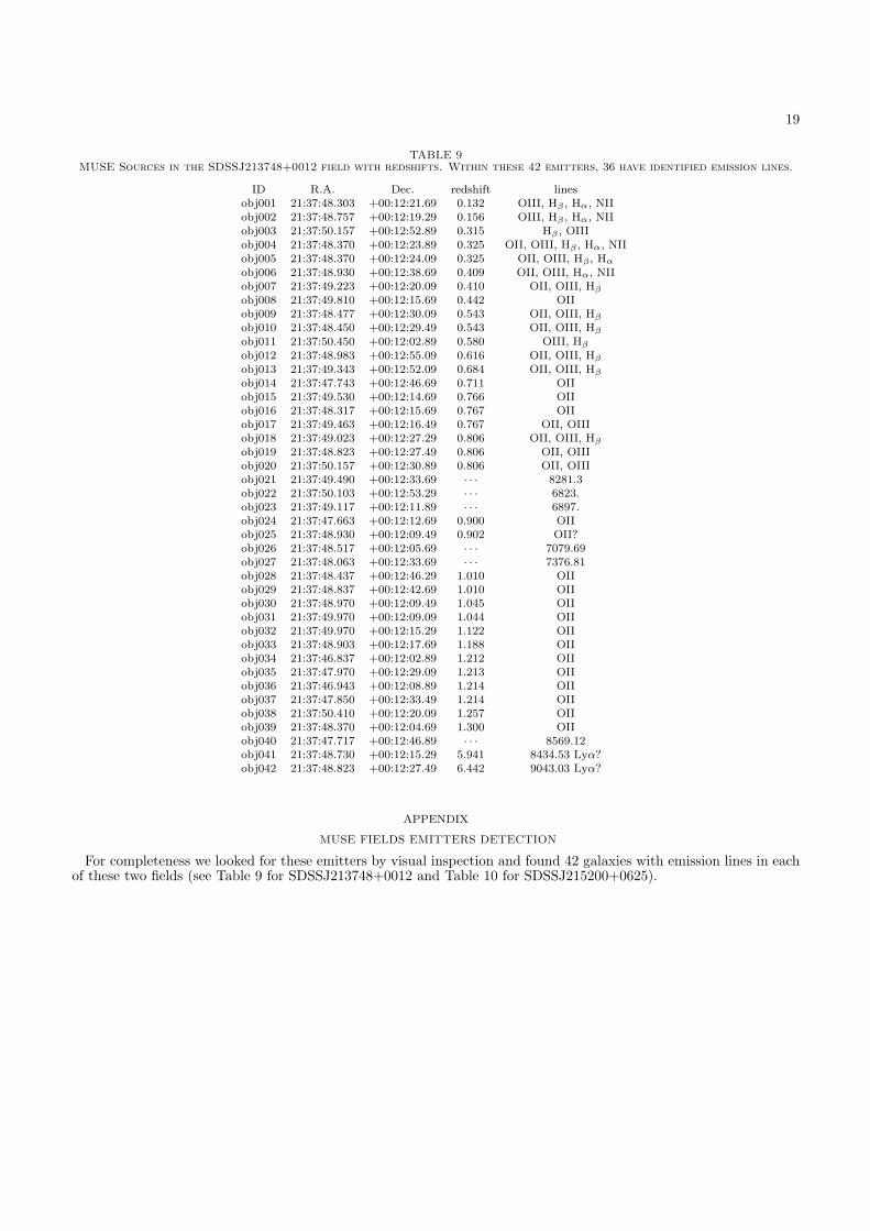
19

TABLE 9MUSE Sources in the SDSSJ213748+0012 field with redshifts. Within these 42 emitters, 36 have identified emission lines.

ID R.A. Dec. redshift linesobj001 21:37:48.303 +00:12:21.69 0.132 OIII, Hβ , Hα, NIIobj002 21:37:48.757 +00:12:19.29 0.156 OIII, Hβ , Hα, NIIobj003 21:37:50.157 +00:12:52.89 0.315 Hβ , OIIIobj004 21:37:48.370 +00:12:23.89 0.325 OII, OIII, Hβ , Hα, NIIobj005 21:37:48.370 +00:12:24.09 0.325 OII, OIII, Hβ , Hαobj006 21:37:48.930 +00:12:38.69 0.409 OII, OIII, Hα, NIIobj007 21:37:49.223 +00:12:20.09 0.410 OII, OIII, Hβobj008 21:37:49.810 +00:12:15.69 0.442 OIIobj009 21:37:48.477 +00:12:30.09 0.543 OII, OIII, Hβobj010 21:37:48.450 +00:12:29.49 0.543 OII, OIII, Hβobj011 21:37:50.450 +00:12:02.89 0.580 OIII, Hβobj012 21:37:48.983 +00:12:55.09 0.616 OII, OIII, Hβobj013 21:37:49.343 +00:12:52.09 0.684 OII, OIII, Hβobj014 21:37:47.743 +00:12:46.69 0.711 OIIobj015 21:37:49.530 +00:12:14.69 0.766 OIIobj016 21:37:48.317 +00:12:15.69 0.767 OIIobj017 21:37:49.463 +00:12:16.49 0.767 OII, OIIIobj018 21:37:49.023 +00:12:27.29 0.806 OII, OIII, Hβobj019 21:37:48.823 +00:12:27.49 0.806 OII, OIIIobj020 21:37:50.157 +00:12:30.89 0.806 OII, OIIIobj021 21:37:49.490 +00:12:33.69 · · · 8281.3obj022 21:37:50.103 +00:12:53.29 · · · 6823.obj023 21:37:49.117 +00:12:11.89 · · · 6897.obj024 21:37:47.663 +00:12:12.69 0.900 OIIobj025 21:37:48.930 +00:12:09.49 0.902 OII?obj026 21:37:48.517 +00:12:05.69 · · · 7079.69obj027 21:37:48.063 +00:12:33.69 · · · 7376.81obj028 21:37:48.437 +00:12:46.29 1.010 OIIobj029 21:37:48.837 +00:12:42.69 1.010 OIIobj030 21:37:48.970 +00:12:09.49 1.045 OIIobj031 21:37:49.970 +00:12:09.09 1.044 OIIobj032 21:37:49.970 +00:12:15.29 1.122 OIIobj033 21:37:48.903 +00:12:17.69 1.188 OIIobj034 21:37:46.837 +00:12:02.89 1.212 OIIobj035 21:37:47.970 +00:12:29.09 1.213 OIIobj036 21:37:46.943 +00:12:08.89 1.214 OIIobj037 21:37:47.850 +00:12:33.49 1.214 OIIobj038 21:37:50.410 +00:12:20.09 1.257 OIIobj039 21:37:48.370 +00:12:04.69 1.300 OIIobj040 21:37:47.717 +00:12:46.89 · · · 8569.12obj041 21:37:48.730 +00:12:15.29 5.941 8434.53 Lyα?obj042 21:37:48.823 +00:12:27.49 6.442 9043.03 Lyα?

APPENDIX

MUSE FIELDS EMITTERS DETECTION

For completeness we looked for these emitters by visual inspection and found 42 galaxies with emission lines in eachof these two fields (see Table 9 for SDSSJ213748+0012 and Table 10 for SDSSJ215200+0625).

20

Fig. A.1.— RGB image of the J213748+0012 field with identifications of emission detected galaxies. The white cross points the quasarlocation. Circles represent emission detected galaxies corresponding to Table 9. Not all the galaxy-like spots are circled on the image.These spots are either stars or galaxies with a continuum but without obvious emission line.

Fig. A.2.— Same as Figure A.1 but for the J215200+0625 quasar field. Again, the white cross shows the quasar location and galaxieswith emission lines are circled and listed in Table 10.

21

TABLE 10MUSE Sources in the SDSSJ215200+0625 field with redshifts. We found 40 galaxies out of 41 having identified emission

lines

ID R.A. Dec. redshift linesobj001 21:52:02.018 +06:25:47.66 0.433 OII, OIII, Hβobj002 21:52:02.246 +06:25:25.06 0.439 OIIobj003 21:51:58.905 +06:25:20.26 0.452 OII, OIII, Hβobj004 21:52:02.085 +06:25:13.26 0.489 OII, OIII, Hβobj005 21:51:58.409 +06:24:54.86 0.517 OIIobj006 21:51:59.429 +06:25:43.06 0.554 OII, OIIIobj007 21:52:02.273 +06:24:56.06 0.597 OII, OIII, Hβobj008 21:52:00.770 +06:25:17.26 3.931? 5992.37 Lyα?obj009 21:51:59.200 +06:24:54.86 4.196? 6314.05 Lyα?obj010 21:51:58.878 +06:25:01.46 0.742 OII, OIII, Hβobj011 21:51:59.912 +06:25:15.66 0.748 OII, Hβobj012 21:52:02.139 +06:25:31.26 0.770 OII, OIII, Hβobj013 21:51:59.375 +06:25:40.26 0.786 OIIobj014 21:52:00.341 +06:25:22.46 0.332 OII, OIII, Hαobj015 21:52:01.092 +06:25:16.26 0.824 OII, OIIIobj016 21:52:00.636 +06:25:37.66 0.289 Hα, NIIobj017 21:51:58.597 +06:25:11.86 0.847 OII?obj018 21:51:59.818 +06:25:29.66 0.873 OIIobj019 21:52:00.126 +06:25:13.06 0.879 OII, OIIIobj020 21:52:00.234 +06:24:50.86 0.438 OII, OIII, Hβobj021 21:51:59.630 +06:25:40.46 0.943 OIIobj022 21:52:00.287 +06:25:06.46 0.989 OIIobj023 21:52:02.058 +06:25:40.46 1.013 OIIobj024 21:51:58.436 +06:25:04.46 1.013 OIIobj025 21:52:00.381 +06:25:20.46 1.052 OIIobj026 21:51:59.549 +06:25:39.06 1.053 OIIobj027 21:52:02.380 +06:24:58.06 0.185 OIII, Hβ , Hα, NIIobj028 21:51:58.583 +06:25:34.26 · · · 8413.87obj029 21:52:00.904 +06:24:50.26 1.302 OIIobj030 21:52:00.019 +06:25:13.26 1.318 OIIobj031 21:51:59.952 +06:25:15.46 1.318 OIIobj032 21:51:58.355 +06:25:03.06 1.349 OIIobj033 21:51:58.489 +06:24:59.06 · · · 8757.32obj034 21:52:02.354 +06:25:15.46 1.362 OIIobj035 21:51:58.355 +06:25:23.66 1.403 OIIobj036 21:52:00.435 +06:25:13.46 1.430 OIIobj037 21:52:00.623 +06:25:15.86 1.430 OIIobj038 21:52:01.629 +06:25:24.06 1.431 OIIobj039 21:52:00.972 +06:25:33.06 1.433 OIIobj040 21:52:00.703 +06:25:43.06 1.435 OIIobj041 21:52:00.180 +06:25:41.26 1.432 OII

Auteur : Ilane Schroetter

Titre :La formation et l’evolution des galaxies grace a la spectroscopie 3D : le role des vents

Directeur et co-directeur de these : Nicolas Bouche et Thierry Contini

Date et lieu de soutenance : Le jeudi 5 Janvier 2017 en salle Coriolis de l’ObservatoireMidi-Pyrenees

Resume :Le modele cosmolgique standard Λ-CDM est celui qui connaıt le plus grand succes dansla cosmologie moderne. Pourtant, malgre sa capacite a expliquer la domination de lamatiere noire sur la structuration de l’univers a grande echelle, il echoue, parfois dra-matiquement, lorsque la physique complexe de la matiere baryonique entre en jeu. Enparticulier, l’une des plus grandes questions restant encore sans reponse concerne ladifference importante entre la quantite de matiere baryonique predite et celle reellementobservee dans les halos de galaxies de faible et de grande masse. Les modeles theoriquespredisent beaucoup trop de masse compare a ce qui est veritablement observe, ce quimene a la conclusion qu’il existe des mecanismes permettant d’ejecter une partie dureservoir de matiere baryonique des galaxies, ce qui affectera donc leur evolution. End’autres termes, si nous voulons comprendre l’evolution des galaxies, il est essentiel decomprendre de maniere precise comment ces galaxies perdent une partie de leur matierebaryonique.Pour les galaxies de faibles masses, un ingredient cle est contenu dans les vents produitspar les explosions de supernovae. Non seulement ces vents peuvent etre efficaces pourejecter le gaz et les metaux du disque galactique, pour enrichir le milieu inter-galactiqueen elements lourds, mais ils sont aussi observes dans presque toutes les galaxies a for-mation d’etoiles, ce qui donne a ces vents un role important concernant le cycle de lamatiere dans les galaxies. Notre connaissance incomplete concernant les relations entrela galaxie et les proprietes du gaz qu’elle ejecte, comme le lien entre le taux de formationstellaire (SFR) et la quantite de masse ejectee Mout, limite notre capacite a produire dessimulations numeriques precises sur l’evolution des galaxies.L’objectif de cette these est de quantifier les proprietes des vents galactiques en utilisantdes quasars en arriere plan et la spectroscopie 3D. Afin d’y parvenir, nous utiliseronsune quantite importante de donnees provenant de plusieurs instruments (SDSS, LRIS auKeck, SINFONI, UVES et MUSE au VLT). Grace a cette nouvelle strategie d’observationet l’utilisation d’instruments de pointe, nous avons pu augmenter l’echantillon d’un ordrede grandeur et ainsi obtenir de bien meilleures contraintes sur les proprietes du gaz quis’echappe des galaxies de faible masse.

Mots-cles : Galaxie : evolution; Galaxie : formation; Spectroscopie 3D; Vents galac-tiques; Quasar en arriere plan

Discipline administrative : Astrophysique

Laboratoire d’accueil : IRAP

2

The role of galactic winds in galaxy evolution and formation ...

Documents

Transcript of The role of galactic winds in galaxy evolution and formation ...