Order-Restricted Covariate Effects and Hazard Regression ...

www.manaraa.com

ORDER-RESTRICTED COVARIATE EFFECTS AND

HAZARD REGRESSION MODELS

Ph.D. Thesis

ARNAB BHATTACHARJEE

INDIAN STATISTICAL INSTITUTE

APPLIED STATISTICS UNIT

KOLKATA, INDIA.

February 2008

www.manaraa.com

ORDER-RESTRICTED COVARIATE EFFECTS AND

HAZARD REGRESSION MODELS

Arnab Bhattacharjee

B.Stat. (Hons.), Indian Statistical Institute, 1991

M.Stat., Indian Statistical Institute, 1993

PhD in Economics, University of Mumbai, 2002

Thesis submitted to the Indian Statistical Institute

in partial fulfillment of the requirement

for

the award of

DOCTOR OF PHILOSOPHY

Supervisor: Professor Debasis Sengupta

INDIAN STATISTICAL INSTITUTE

APPLIED STATISTICS UNITKOLKATA, INDIA.

February 2008

www.manaraa.com

1

List of papers by the author included in this thesis

References in the thesisTitle, Co-author(s), Publication

Discussed in Referred in

1. Testing for the proportionality of hazards in two samples against the

increasing cumulative hazard ratio alternative. (Co-authors: D.

Sengupta, B. Rajeev). Publication: Scandinavian Journal of Statistics

25(4), 1998, 637–647.

Chapter 2 Chapters 1, 3,

4, 5, 6 and 8.

2. Estimation in hazard regression models under ordered departures from

proportionality. (Co-authors: None). Publication: Computational Statistics

and Data Analysis 47(3), 2004, 517–536.


6, 7 and 8.

3. Macroeconomic conditions and business exit: determinants of failures

and acquisitions of UK firms. (Co-authors: C. Higson, S. Holly, P.

Kattuman). Publication: Economica, forthcoming.


4, 5, 6 and 8.

4. Macroeconomic instability and corporate failure. (Co-authors: C. Higson,

S. Holly, P. Kattuman). Publication: Review of Law and Economics,

forthcoming.


5, 6 and 8.

5. Monotone departures from proportional hazards with respect to

continuous covariates: inference procedures and applications. (Co-

authors: None). Publication: Mimeo, 2003. Proceedings of 54th Binennial

Session of the International Statistical Institute.


7 and 8.

6. Testing the Proportional Hazards Model with Continuous Covariates in

Duration Models against Monotone Ordering. (Co-authors: None).

Publication: Mimeo, Current version: 2007. Working Paper, University of

Cambridge, UK.


5, 6, 7 and 8.

7. A simple test for the absence of covariate dependence in hazard

regression models. (Co-authors: None). Publication: Mimeo, Current

version: 2007. Working Paper, University of St Andrews, UK.


6, 7 and 8.

8. Bayesian analysis of hazard regression models under order restrictions

on covariate effects and ageing. (Co-authors: M. Bhattacharjee).

Publication: Mimeo, Current version: 2007. Working Paper, University of

St Andrews, UK.


5, 6 and 8.

9. Models of firm dynamics and the hazard rate of exits: is unobserved

heterogeneity really that important? (Co-authors: None). Publication:

Mimeo, Current version: 2007. Working Paper, University of St Andrews,

UK.


5 and 8.

www.manaraa.com

2

ACKNOWLEDGEMENTThis thesis represents a rather long and personal journey. It has taken me through widely differentenvironments and experiences, and encompassing considerable expanses of space and time. I started myresearch work in statistics, as a research student at the Indian Statistical Institute, way back in 1993.In 1994, I moved into the professional field, joining the Reserve Bank of India, and subsequentlymoved to a different academic discipline – economics. Therefore, the work here represents a line ofresearch I have followed, as a leisure activity, over a long period of time.

Many people – friends, family, colleagues and senior professionals have encouraged me to continuewith my research work in statistics. I particularly express my deep sense of appreciation for myresearch supervisor, Prof. Debasis Sengupta for his guidance and persuation at each stage of this thesiswork. I am also deeply indebted to Elja Arjas, R.B. Barman, Sushama Bendre, Arup Bose, SanjoyBose, Madhuchhanda Bhattacharjee, Snigdhansu Chatterjee, Prabal Chaudhuri, Samarjit Das, JayantDeshpande, Anup Dewanji, Chris Higson, Sean Holly, (Late) Chris Jensen-Butler, Peter Jupp, AjitKarnik, Paul Kattuman, Roderick McCrorie, Mukul Majumdar, Sumit Majumdar, Rahul Mukerji,Charles Nolan, Abhay Pethe, Gavin Reid, P.G. Sankaran and David Ulph for providing manysuggestions and help in academic matters. Sincere thanks are also due to my dear friends, particularlySubhomoy Bhattacharyya, Jean Bonnet, Bram Boskamp, Jagjit Chadha, Subhasis Chakraborty,Eduardo Anselmo de Castro, Jim Jin, Caroline Moore, Debdulal Roy, Christoph Thoenissen, CarmeVila and Andrew Vivian, who provided the support that was necessary to sustain my passion for thislong period of time, often over tumultuous periods. Without their active help and understanding overall these years, this work would never have materialised.

I am thankful to many people at the Indian Statistical Institute for their help and support over theyears. In addition to seniors and colleagues mentioned above, particular thanks are due Prof. PradiptaBanerjee, Prof. Alok Goswami, Prof. Bimal Roy, Dr. Rudrapada Sarkar and Prof. Ashis Sengupta,and Aparesh-da, Ashok-da and Sangal-da.

Over the years, Madhuchhanda, and of late, little Ausija have borne much of the adverse shocksrelated to my research. Without their sincere support and love, and immense patience, this work wouldnever have been complete. Special thanks are due to my friend Sabarna, but particularly Nandini andSudur, for being fantastic company and providing the support that was required during the stressfulfinal stages of this journey.

I gratefully acknowledge financial support from the Leverhulme Trust and KPMG UK for fundingpart of the work included in this thesis (particularly Chapters 4 and 7). Last but not the least, sincerethanks and gratitude are due to Luc Bauwens, John Beath, David Dunson, Peter Hart, ErricosKontoghiorges, Manfredi La Manna, Geoff Meeks, Oliver Linton, Hashem Pesaran, ElvezioRonchetti, Ananda Sen, Gerard van den Berg and Melvyn Weeks, in addition to fellow academicsmentioned above, for helpful comments and suggestions on various parts of this research.

Arnab BhattacharjeeKolkata, February 2008

www.manaraa.com

Contents

1 Introduction 8

1.1 Motivation for the research . . . . . . . . . . . . . . . . . . . . . . . . . . . . . . 9

1.1.1 Two sample setup . . . . . . . . . . . . . . . . . . . . . . . . . . . . . . . 10

1.1.2 Continuous covariates . . . . . . . . . . . . . . . . . . . . . . . . . . . . . 11

1.1.3 Modeling nonproportional hazards . . . . . . . . . . . . . . . . . . . . . . 12

1.2 Order restrictions in hazard regression models . . . . . . . . . . . . . . . . . . . . 14

1.2.1 The Cox regression model . . . . . . . . . . . . . . . . . . . . . . . . . . . 14

1.2.2 E¤ect of misspeci�cation . . . . . . . . . . . . . . . . . . . . . . . . . . . . 17

1.2.3 Goodness-of-�t tests of the PH assumption . . . . . . . . . . . . . . . . . 21

1.2.4 Order restrictions on covariate dependence . . . . . . . . . . . . . . . . . 24

1.2.5 Order restrictions on ageing . . . . . . . . . . . . . . . . . . . . . . . . . . 29

1.2.6 Individual level frailty . . . . . . . . . . . . . . . . . . . . . . . . . . . . . 33

1.2.7 Other hazard regression models . . . . . . . . . . . . . . . . . . . . . . . . 38

1.2.8 Bayesian semiparametric inference . . . . . . . . . . . . . . . . . . . . . . 45

1.3 Outline of the thesis . . . . . . . . . . . . . . . . . . . . . . . . . . . . . . . . . . 50

1.3.1 Testing proportionality with respect to a binary covariate . . . . . . . . . 50

1.3.2 Testing proportionality with respect to continuous covariates . . . . . . . 51

1.3.3 Estimation under order restrictions on covariate dependence . . . . . . . . 51

1.3.4 Testing proportionality with unrestricted frailty . . . . . . . . . . . . . . . 51

1.3.5 Order restrictions on both covariate dependence and ageing . . . . . . . . 52

1.3.6 Applications to �rm dynamics . . . . . . . . . . . . . . . . . . . . . . . . 52

1.3.7 Real data and applications . . . . . . . . . . . . . . . . . . . . . . . . . . 53

3

www.manaraa.com

2 Testing for the Proportionality of Hazards in Two Samples Against Ordered

Alternatives 59

2.1 Chapter summary . . . . . . . . . . . . . . . . . . . . . . . . . . . . . . . . . . . 59

2.2 Introduction . . . . . . . . . . . . . . . . . . . . . . . . . . . . . . . . . . . . . . . 60

2.3 Development of the test statistic . . . . . . . . . . . . . . . . . . . . . . . . . . . 62

2.4 Consistency and asymptotic normality . . . . . . . . . . . . . . . . . . . . . . . . 64

2.5 Graphical methods . . . . . . . . . . . . . . . . . . . . . . . . . . . . . . . . . . . 68

2.6 Data Analysis . . . . . . . . . . . . . . . . . . . . . . . . . . . . . . . . . . . . . . 69

2.7 Choice of weight functions . . . . . . . . . . . . . . . . . . . . . . . . . . . . . . . 69

2.8 Testing Proportionality of Hazards due to Competing Risks . . . . . . . . . . . . 72

2.8.1 A graphical method . . . . . . . . . . . . . . . . . . . . . . . . . . . . . . 73

2.8.2 A family of analytical tests . . . . . . . . . . . . . . . . . . . . . . . . . . 76

2.8.3 Choice of the weight functions . . . . . . . . . . . . . . . . . . . . . . . . 77

2.8.4 Monte Carlo study . . . . . . . . . . . . . . . . . . . . . . . . . . . . . . . 79

2.8.5 Data analysis . . . . . . . . . . . . . . . . . . . . . . . . . . . . . . . . . . 82

2.8.6 Testing against the monotone cumulative hazard ratio alternative . . . . . 83

2.9 Concluding remarks . . . . . . . . . . . . . . . . . . . . . . . . . . . . . . . . . . 83

3 Testing for Proportional Hazards against Ordered Alternatives with respect

to Continuous Covariates 87

3.1 Chapter summary . . . . . . . . . . . . . . . . . . . . . . . . . . . . . . . . . . . 87

3.2 Introduction . . . . . . . . . . . . . . . . . . . . . . . . . . . . . . . . . . . . . . . 88

3.3 Partial orders with respect to a continuous covariate . . . . . . . . . . . . . . . . 89

3.4 Test statistics . . . . . . . . . . . . . . . . . . . . . . . . . . . . . . . . . . . . . . 93

3.4.1 Monotone hazard ratio . . . . . . . . . . . . . . . . . . . . . . . . . . . . . 94

3.4.2 Monotone cumulative hazard ratio . . . . . . . . . . . . . . . . . . . . . . 96

3.4.3 Large sample results . . . . . . . . . . . . . . . . . . . . . . . . . . . . . . 97

3.5 Implementation and extensions . . . . . . . . . . . . . . . . . . . . . . . . . . . . 101

3.5.1 Small sample correction . . . . . . . . . . . . . . . . . . . . . . . . . . . . 101

3.5.2 Choice of r and covariate pairs . . . . . . . . . . . . . . . . . . . . . . . . 102

3.5.3 Comparison with other tests . . . . . . . . . . . . . . . . . . . . . . . . . 103

4

www.manaraa.com

3.5.4 Choice between the proposed tests . . . . . . . . . . . . . . . . . . . . . . 103

3.5.5 Extensions . . . . . . . . . . . . . . . . . . . . . . . . . . . . . . . . . . . 104

3.6 Monte Carlo study . . . . . . . . . . . . . . . . . . . . . . . . . . . . . . . . . . . 106

3.7 Empirical applications . . . . . . . . . . . . . . . . . . . . . . . . . . . . . . . . . 109

3.7.1 Data on Strike Durations . . . . . . . . . . . . . . . . . . . . . . . . . . . 109

3.7.2 A related graphical test . . . . . . . . . . . . . . . . . . . . . . . . . . . . 112

3.7.3 Survival with Malignant Melanoma . . . . . . . . . . . . . . . . . . . . . . 114

3.7.4 Child mortality in India . . . . . . . . . . . . . . . . . . . . . . . . . . . . 115

3.8 Conclusion . . . . . . . . . . . . . . . . . . . . . . . . . . . . . . . . . . . . . . . 117

4 Estimation in nonproportional hazard regression models with monotone co-

variate e¤ect 125

4.1 Chapter summary . . . . . . . . . . . . . . . . . . . . . . . . . . . . . . . . . . . 125

4.2 Introduction . . . . . . . . . . . . . . . . . . . . . . . . . . . . . . . . . . . . . . . 126

4.3 A hazard regression model admitting order restrictions in covariate e¤ects . . . . 128

4.4 Estimation under order restrictions . . . . . . . . . . . . . . . . . . . . . . . . . . 131

4.4.1 Isotonic regression approach . . . . . . . . . . . . . . . . . . . . . . . . . . 131

4.4.2 Estimation based on projections . . . . . . . . . . . . . . . . . . . . . . . 132

4.4.3 Taut string method . . . . . . . . . . . . . . . . . . . . . . . . . . . . . . 132

4.4.4 Density regression approach . . . . . . . . . . . . . . . . . . . . . . . . . . 133

4.4.5 Biased bootstrap methods . . . . . . . . . . . . . . . . . . . . . . . . . . . 133

4.4.6 Choice of estimation methods . . . . . . . . . . . . . . . . . . . . . . . . . 134

4.5 Estimation procedures based on biased bootstrap techniques . . . . . . . . . . . . 136

4.5.1 Data tilting . . . . . . . . . . . . . . . . . . . . . . . . . . . . . . . . . . . 136

4.5.2 Local adaptive bandwidth . . . . . . . . . . . . . . . . . . . . . . . . . . . 140

4.6 Applications and simulations . . . . . . . . . . . . . . . . . . . . . . . . . . . . . 144

4.6.1 Simulation study . . . . . . . . . . . . . . . . . . . . . . . . . . . . . . . . 144

4.6.2 Example: Malignant melanoma data . . . . . . . . . . . . . . . . . . . . . 147

4.6.3 Example: Macroeconomic instability and business failure . . . . . . . . . 148

4.7 Concluding remarks . . . . . . . . . . . . . . . . . . . . . . . . . . . . . . . . . . 151

5

www.manaraa.com

5 Testing for Proportional Hazards with Unrestricted Univariate Frailty 153

5.1 Chapter summary . . . . . . . . . . . . . . . . . . . . . . . . . . . . . . . . . . . 153

5.2 Introduction . . . . . . . . . . . . . . . . . . . . . . . . . . . . . . . . . . . . . . . 154

5.3 Formulation of the testing problems . . . . . . . . . . . . . . . . . . . . . . . . . 155

5.3.1 Testing proportional hazards . . . . . . . . . . . . . . . . . . . . . . . . . 155

5.3.2 Testing absence of covariate dependence . . . . . . . . . . . . . . . . . . . 158

5.3.3 Estimation of baseline hazard functions . . . . . . . . . . . . . . . . . . . 159

5.4 Proposed tests . . . . . . . . . . . . . . . . . . . . . . . . . . . . . . . . . . . . . 161

5.4.1 Alternative hypotheses . . . . . . . . . . . . . . . . . . . . . . . . . . . . . 161

5.4.2 Testing absence of covariate dependence . . . . . . . . . . . . . . . . . . . 165

5.4.3 Testing the proportional hazards assumption . . . . . . . . . . . . . . . . 172

5.4.4 Choice of weight functions . . . . . . . . . . . . . . . . . . . . . . . . . . . 182

5.5 Simulation study . . . . . . . . . . . . . . . . . . . . . . . . . . . . . . . . . . . . 183

5.6 An application . . . . . . . . . . . . . . . . . . . . . . . . . . . . . . . . . . . . . 188

5.7 Conclusion . . . . . . . . . . . . . . . . . . . . . . . . . . . . . . . . . . . . . . . 191

6 Bayesian Analysis of Hazard Regression Models under Order Restrictions on

Covariate E¤ects and Ageing 201

6.1 Chapter summary . . . . . . . . . . . . . . . . . . . . . . . . . . . . . . . . . . . 201

6.2 Introduction . . . . . . . . . . . . . . . . . . . . . . . . . . . . . . . . . . . . . . . 202

6.3 Background . . . . . . . . . . . . . . . . . . . . . . . . . . . . . . . . . . . . . . . 204

6.3.1 Bayesian semiparametric inference . . . . . . . . . . . . . . . . . . . . . . 205

6.3.2 Order restricted frequentist inference . . . . . . . . . . . . . . . . . . . . . 206

6.4 Our Bayesian model . . . . . . . . . . . . . . . . . . . . . . . . . . . . . . . . . . 208

6.4.1 Order restricted covariate dependence . . . . . . . . . . . . . . . . . . . . 209

6.4.2 Frailty . . . . . . . . . . . . . . . . . . . . . . . . . . . . . . . . . . . . . . 210

6.4.3 Order restrictions on ageing . . . . . . . . . . . . . . . . . . . . . . . . . . 211

6.4.4 Prior speci�cation . . . . . . . . . . . . . . . . . . . . . . . . . . . . . . . 211

6.4.5 Model Implementation . . . . . . . . . . . . . . . . . . . . . . . . . . . . . 213

6.5 Results and discussion . . . . . . . . . . . . . . . . . . . . . . . . . . . . . . . . . 213

6.5.1 Model using retrospective data . . . . . . . . . . . . . . . . . . . . . . . . 214

6

www.manaraa.com

6.5.2 Model using data with staggered entries . . . . . . . . . . . . . . . . . . . 218

6.6 Conclusion . . . . . . . . . . . . . . . . . . . . . . . . . . . . . . . . . . . . . . . 222

7 Applications to Firm Dynamics 225

7.1 Firm dynamics and the hazard rate of �rm exits . . . . . . . . . . . . . . . . . . 227

7.1.1 Active and Passive Learning . . . . . . . . . . . . . . . . . . . . . . . . . . 227

7.1.2 Impact of macroeconomic shocks . . . . . . . . . . . . . . . . . . . . . . . 230

7.1.3 Unobserved heterogeneity . . . . . . . . . . . . . . . . . . . . . . . . . . . 234

7.2 Macroeconomic conditions and business exit: determinants of failures and acqui-

sitions of UK �rms . . . . . . . . . . . . . . . . . . . . . . . . . . . . . . . . . . . 235

7.2.1 Data . . . . . . . . . . . . . . . . . . . . . . . . . . . . . . . . . . . . . . . 236

7.2.2 Econometric Methodology . . . . . . . . . . . . . . . . . . . . . . . . . . . 240

7.2.3 Results . . . . . . . . . . . . . . . . . . . . . . . . . . . . . . . . . . . . . 247

7.2.4 Conclusions . . . . . . . . . . . . . . . . . . . . . . . . . . . . . . . . . . . 251

7.3 Business failure in UK and US quoted �rms: impact of macroeconomic instability

and the role of legal institutions . . . . . . . . . . . . . . . . . . . . . . . . . . . . 253

7.3.1 Econometric methodology . . . . . . . . . . . . . . . . . . . . . . . . . . . 253

7.3.2 The e¤ect of bankruptcy code . . . . . . . . . . . . . . . . . . . . . . . . . 255

7.3.3 Data and construction of variables . . . . . . . . . . . . . . . . . . . . . . 256

7.3.4 Results . . . . . . . . . . . . . . . . . . . . . . . . . . . . . . . . . . . . . 261

7.3.5 Conclusions . . . . . . . . . . . . . . . . . . . . . . . . . . . . . . . . . . . 271

7.4 Empirics of �rm dynamics: modeling the role of frailty . . . . . . . . . . . . . . . 272

7.4.1 New French �rms . . . . . . . . . . . . . . . . . . . . . . . . . . . . . . . . 273

7.4.2 Quoted UK �rms . . . . . . . . . . . . . . . . . . . . . . . . . . . . . . . . 279

7.4.3 Conclusions . . . . . . . . . . . . . . . . . . . . . . . . . . . . . . . . . . . 280

8 Conclusion 281

8.1 Contributions of the thesis . . . . . . . . . . . . . . . . . . . . . . . . . . . . . . . 281

8.2 Limitations and future work . . . . . . . . . . . . . . . . . . . . . . . . . . . . . . 283

7

www.manaraa.com

Chapter 1

Introduction

The proportional hazards (PH) model, but more speci�cally its special case the Cox regression

model (Cox, 1972), plays an important role in the theory and practice of lifetime and dura-

tion data analysis. This is because the PH model (and the Cox regression model) provides

a convenient way to evaluate the in�uence of one or several covariates on the probability of

conclusion of lifetime or duration spells. However, the PH speci�cation substantially restricts

interdependence between the explanatory variables and the lifetime in determining the hazard.

In particular, the Cox regression model model restricts the coe¢ cients of the regressors in the

logarithm of the hazard function to be constant over the lifetime. This restriction may not hold

in many situations, or may even be unreasonable from the point of view of relevant theory.

Further, this and other kinds of misspeci�cation often lead to misleading inferences about the

e¤ects of explanatory variables and the shape of the baseline hazard.

Testing the Cox PH model, particularly against the omnibus alternative, has therefore been

an area of active research. However, the omnibus tests do not o¤er much clarity regarding

the nature of departure from underlying assumptions. As a result, these tests do not provide

useful inference for further modeling covariate e¤ects when the Cox regression model does not

hold. For example, it is often of interest to explore whether the hazard rate for one level of the

covariate increases in lifetime relative to another level (i.e., the hazard ratio increases/decreases

with lifetime). Ordered departures from proportionality of this and related types are useful

in the two-sample (or binary covariate) setup for studying commonly observed features like

crossing hazards. Similar situations also occur quite frequently in the k-sample setup and

8

www.manaraa.com

when the covariate is continuous. Throughout this thesis, we call such ordered departures

generically as "order restrictions on covariate dependence", as distinct from "order restrictions

on ageing" which refers to restrictions on the shape of the baseline hazard function (or, on

duration dependence).

The work included in this thesis develops analytical and graphical inference on covariate

e¤ects in situations when the Cox regression model, or more generally the PH model, may not

hold. In particular, we develop methods to study covariate e¤ects in the presence of potentially

order restricted departures from proportionality. The thesis places emphasis on both theory

and applications, and extends the literature along both these dimensions in several ways. In

this sense, the work is �rmly set within the tradition of research in applied statistics and

econometrics.

In the following section (Section 1.1), we motivate our research on order restrictions on

covariate dependence using a few real life examples, focusing on some useful ways in which order

restrictions can be characterised and hazard regression models accommodating order restricted

covariate e¤ects. Next, in Section 1.2, we review recent research on hazard regression models,

which are useful for modeling and estimation of covariate dependence under order restrictions,

particularly when the covariate is continuous. The review is selective, focusing largely on order

restrictions in these models and aimed at identifying gaps in the literature. As we proceed, we

place the main contributions made in the thesis within the context of the literature. Finally,

we outline the new research and describe the chapter scheme for the rest of the thesis (Section

1.3).

1.1 Motivation for the research

The main focus of our research is on the way covariate e¤ects deviate from the proportional

hazards assumption. We �rst discuss the two sample setup, where the covariate under consider-

ation is binary. Following this, we discuss continuous covariates and �nally, a regression model

for nonproportional hazards. In each of these main themes, we motivate our research using real

life applications.

9

www.manaraa.com

1.1.1 Two sample setup

In the two sample setup, Gill and Schumacher (1987) and Deshpande and Sengupta (1995) con-

sider departures where the ratio of hazard rates in the two samples is monotonically increasing

or decreasing with the lifetime1. They develop tests of the null hypothesis of proportionality

against the increasing (decreasing) hazard ratio alternative. Sengupta and Deshpande (1994)

show that this kind of departure is equivalent to convex-ordering of the lifetime distributions

in the two samples (Kalashnikov and Rachev, 1986). Denoting by �F and �G (correspondingly,

�F and �G) the hazard functions (cumulative hazard functions) in the two samples,

�F (t)

�G(t)" t on [0;1)() F �

cG; (1.1)

where convex ordering of the lifetime distributions is de�ned as the condition that �F � ��1Gis a convex function on [0;1). Similarly, Deshpande and Sengupta (1994) also show that

star-ordering of the lifetime distributions is equivalent to monotone ratio of cumulative hazard

functions�F (t)

�G(t)" t on (0;1)() F �

�G; (1.2)

where star-ordering of the lifetime distributions is de�ned by �F � ��1G being a star-shaped

function from [0;1) to [0;1)2.

One important starting point for our work is the analysis, in Gill and Schumacher (1987),

of the Veterans�Administration data (Detre et al., 1977) on a controlled clinical trial in chronic

stable angina. The main purpose of the analysis is to compare survival times of patients

receiving coronary artery bypass graft surgery and of patients receiving a conservative medical

treatment. The tests proposed by Gill and Schumacher (1987) fail to reject the null hypothesis

of proportionality against the alternative of decreasing hazard ratio for surgery versus medical

treatment. However, a plot of the empirical trend function (Lee and Pirie, 1981) with log rank

weight function (Gill and Schumacher (1987), shown in Figure 1-1 with axes interchanged)

1The word "increasing" would mean "non-decreasing" throughout this thesis; similarly "decreasing" will mean"non-increasing".

2A non-negative valued function is star-shaped function if any straight line through the origin intersects it atmost once and from above; a negative star-shaped function has the opposite property. Note that star-shapednessis a weaker property than convexity; similarly negative star-shapedness is weaker than concavity.

10

www.manaraa.com

Figure 1-1: Lee-Pirie plot for Veterans�Administration data (Figure 5, Gill and Schumacher(1987), with axes interchanged)

demonstrate clear evidence of ordered departure from proportionality. In fact, the star-shaped

pattern (Kalashnikov and Rachev, 1986) suggests that a monotone cumulative hazard ratio

alternative, which is weaker than concave ordering, may characterise the nature of depature

from proportionality more accurately.

This example motivated us to develop tests for proportionality against the weaker monotone

cumulative hazard ratio alternative. Further, the success of alternatives such as convex and star

ordering in describing ordered departures from proportional hazards in the two-sample setup

also motivate our work on extending the tests to a competing risk framework.

1.1.2 Continuous covariates

While the above characterisation of covariate dependence in nonproportional hazards situation

is useful in studying commonly observed phenomena like crossing hazards, the two sample

setup itself is rather restrictive in its application. At the same time, similar evidence of ordered

departures from proportionality with respect to continuous covariates are quite common in

applications.

For survival with malignant melanoma, for example, Andersen et al. (1993) observe that,

while �hazard seems to increase with tumor thickness� (pp. 389), the plot of estimated cu-

11

www.manaraa.com

mulative baseline hazards for patients with �2 mm � tumor thickness < 5 mm�and �tumor

thickness � 5 mm�against that of patients with �tumor thickness < 2 mm�reveal �concave

looking curves indicating that the hazard ratios decrease with time�(pp. 544�545). Similarly,

Jayet and Moreau (1991), using data on French employment durations, �nd that the ratio of

hazard function for individuals in the age groups 24 � 28 years to that for 37 � 40 years is

increasing upto a duration of approximately 120 days.

Motivated by applications like the above, we extend the notions of order restricted covariate

dependence to the case of continuous covariates. For example, we de�ne the lifetime random

variable T to have increasing hazard ratio for continuous covariate (IHRCC) with respect to

a continuous covariate X if,

whenever x1 > x2; (T jX = x1) �c(T jX = x2): (1.3)

Within this very general framework, we develop tests of the proportional hazards assumption

against ordered alternatives. These tests are powerful and can detect departures not only in the

direction of alternatives like IHRCC, but also violations of the proportional hazards hypothesis

where the covariate e¤ects change at an unknown changepoint.

1.1.3 Modeling nonproportional hazards

For further inference and modeling of covariate e¤ects in the presence of such non-proportionality

of conditional hazard functions, it is useful to consider appropriate alternative hazard regres-

sion models. We argue the use of a multiplicative hazard regression model with time-varying

coe¢ cients

� (tjx) = �0(t): exp (�(t):x)

for modeling the nature of nonproportionality. Under this model, monotonicity of the coe¢ -

cients as a function of lifetime is equivalent to ordered departures of the IHRCC type (1.3):

�(t) " t on [0;1)() (T jX = x1) �c(T jX = x2) whenever x1 > x2;

12

www.manaraa.com

while changepoint departures like in the unemployment duration data (Jayet and Moreau, 1991)

correspond to the time-varying coe¢ cients increasing over one range of lifetimes and decreasing

over another.

To demonstrate the �exibility and usefulness of this approach, we consider an application to

exits due to bankruptcy among listed �rms in the UK (Bhattacharjee et al., 2008a, 2008b). The

main purpose of our focus is to study the e¤ect of macroeconomic instability on business failure.

Based on economic theory and prior evidence, we expect instability to have an adverse e¤ect on

�rm survival, and therefore a positive covariate e¤ect on bankruptcy hazard. Further, the e¤ect

of instability is expected to reduce with the age of the �rm, implying time varying coe¢ cients

that decrease to zero. Inference on the strength of the e¤ect of instability and its variation with

age have important relevance for economic and legislative policy implications. In fact, using

exchange rate volatility as a measure of instability, the null hypothesis of proportional hazards

is rejected against a decreasing hazard ratio for continuous covariate (DHRCC) alternative.

Our research demonstrates that biased bootstrap methods, such as data tilting and par-

ticularly local adaptive bandwidths provide useful order restricted estimates of such hazard

regression models. The plot of adaptive bandwidth estimates (Figure 1-2a) demonstrate the

variation in and strength of covariate e¤ects over the lifetime of the �rm, and provide useful

and policy relevant inference. Figure 1-2b reports bayesian order restricted inference on the

covariate e¤ect of instability on discrete failure time data in the presence of arbitrary frailty.

These estimates provide similar inference, though accounting for frailty somewhat reduces the

inferred strength of the e¤ect of instability.

The above applications motivate the main research ideas developed in this thesis. We

develop analytical and graphical inference tools to examine evidence of nonproportional hazards

in two sample and continuous covariate setups, and to infer on the nature of nonproportionality.

Further, we develop frquentist and bayesian inference in regression models admitting a variety of

nonproportional hazard situations. Finally, we make contributions towards developing economic

theory and applications for understanding macroeconomic e¤ects on the survival of �rms.

13

www.manaraa.com

2a: Order restricted adaptive bandwidth estimatesand 95% confidence interval

0.1

0.0

0.1

0.2

3 9 15 21 27 33Age (in years post listing)

Adaptive bandw idth point estimates 95% low er CI 95% upper CI

2b: Posterior mean and 95% posterior interval

0.4

0.2

0.0

0.2

0.4

1 6 11 16 21 26 31 36Age (in years post listing)

Posterior mean Posterior distbn. 2.5 percentile Posterior distbn. 97.5 percentile

Figure 1-2: E¤ect of exchange rate volatility on bankruptcy exit hazard

1.2 Order restrictions in hazard regression models

The Cox regression model (Cox, 1972) has been the workhorse of hazard regression models and

played an important role in the theory and practice of lifetime and duration data analysis over

the past few decades. This is because this model (and more generally the PH model) provides

a convenient way to evaluate the in�uence of one or several covariates on the probability of

termination of lifetime or duration spells. Limitations and extensions of this model provide the

context of the present review of recent research.

1.2.1 The Cox regression model

The model3 speci�es that the hazard function of the failure time conditional on a set of possibly

time varying covariates is the product of an arbitrary baseline hazard function and a regres-

sion function of the covariates. For a failure time variable T associated with an experimental

unit with vector of possibly time-dependent covariates X(t), this model postulates that the

conditional hazard rate function of T at time t, given X(t), is

� (tjX(t)) = �0(t): exp��T :X(t)

�; (1.4)

3The discussion of the Cox regression model here is largely based on Andersen et al. (1993).

14

www.manaraa.com

where �0(:) is some baseline hazard function, � is a vector of regression coe¢ cients, and su-

perscript T (T ) denotes vector/matrix transpose4. An alternative, and often more convenient,

way of representing the Cox regression model is in the form of a linear transformation model,

in terms of the baseline cumulative hazard function �0(t) =R t0 �0(s)ds:

ln�0(t) = ��T :X(t) + ";

where ln�0(t) is a positive-valued but arbitrary increasing function and " has the usual extreme

value distribution5.

The Cox regression model allows the baseline hazard function to assume a completely un-

restricted shape. The multiplicative separation of the e¤ect of lifetime from that of the other

covariates has a very important implication. The hazard functions conditional on two di¤erent

values of the covariate vector is independent of the lifetime

� (tjXi(t))

��tjXj(t)

� = exp ��T : �Xi(t)�Xj(t)��:

In other words, the conditional hazard functions are proportional to each other. The propor-

tionality also holds under the more general PH model

� (tjX(t)) = �0(t):��T :X(t)

�; (1.5)

where �(:) is an arbitrary (smooth) monotone function. An alternative interpretation of this

result is that the impact of the covariate vector on the conditional hazard is the same multiplica-

tive factor exp��T :X(:)

�at any lifetime; this interpretation will be important in subsequent

developments in this thesis.

Cox (1972, 1975) introduced the ingenious partial likelihood principle to eliminate the in-

�nite dimensional baseline hazard function from the estimation of regression parameters with

censored data and potentially time varying covariates. For untied failure time data with time-

4Please note that throughout this thesis, the failure time variable will be denoted by T while superscript T(T ) will denote the tanspose of a matrix or vector.

5When " has a standard logistic distribution, we get the proportional odds model.

15

www.manaraa.com

varying covariates, the Cox partial likelihood has the form

PL��=

nYi=1

Yt�0

(Yi(t): exp

��T :Xi(t)

�Pj Yj(t): exp

��T :Xi(t)

�)dNi(t) ; (1.6)

where Yi(t) is the at-risk indicator taking value 1 if individual i is under observation and at risk

at time t (zero otherwise), andNi(t) denotes the number of observed failures for individual i over

the interval [0; t]; dNi(t) takes the value 1 if the individual has failed at time t (zero otherwise).

The beauty of the above formulation is in that the in�nite dimensional baseline hazard function

is not included in the partial likelihood function at all. Having obtained the maximum partial

likelihood estimator, b�, by maximising the partial likelihood (1.6), the baseline cumulativehazard function is estimated using the Aalen-Breslow estimator (Breslow, 1975; Aalen, 1993)

c�0 �t; b�� =

tZ0

dN(s)PYi(s): exp

hb�T :Xi(s)i ; (1.7)

dN(s) =

nXi=1

dNi(s):

If there are no covariates, this estimator reduces to the familiar Nelson-Aalen estimator (Nelson,

1969, 1972; Aalen, 1975, 1978)

c�0 (t) = tZ0

dN(s)

Y (s); dN(s) =

nXi=1

dNi(s); Y (s) =nXi=1

Yi(s): (1.8)

for the cumulative hazard function of a lifetime or duration variable.

In a seminal paper, Andersen and Gill (1982) extended the Cox regression model to general

counting processes and established the asymptotic properties of the maximum partial likelihood

estimator and the associated Breslow (1974) estimator of the cumulative baseline hazard func-

tion via the elegant counting process martingale theory. This follows from the representation

of the log partial likelihood as

l��=

nXi=1

1Z0

hYi(t):�

T :Xi(t)� ln�X

jYj(t): exp

��T :Xi(t)

��idNi(t); (1.9)

16

www.manaraa.com

and the Doob-Meyer decomposition of the counting process Ni(t)

dMi(t) = dNi(t) + Yi(t):�0(t): exp��T :Xi(t)

�:dt (1.10)

where Mi(t) is a standard counting process martingale (for details, see Andersen et al., 1993).

The partial likelihood argument follows through in the case of staggered entry (sometimes

also called delayed entry) where some individuals are not observed from time zero. This kind

of situation is present in some of the empirical applications included later in the thesis. Large

sample theory for this case has been developed in Tsiatis (1981) and Sellke and Siegmund

(1983).

These contributions render the Cox regression model very convenient for empirical analysis

while at the same time retaining the �exibility of a fully nonparametric baseline hazard function.

This �exibility comes at a cost �the partial likelihood estimates of the covariate e¤ects as well

as the shape of the baseline hazard function are known to be highly sensitive to violation of the

model�s various assumptions. This issue has been discussed in the literature, for example, in the

work of Johnson et al. (1982), Lagakos and Schoenfeld (1984), Solomon (1984), Struthers and

Kalb�eisch (1986) and Lagakos (1988). A large simulation study reported in Li et al. (1996)

highlight these issues quite strongly.

1.2.2 E¤ect of misspeci�cation

There are several basic and important features of the Cox regression model,.tests for the under-

lying assumptions for many of which are critical for the model�s use in empirical studies. These

various aspects of the model as well as the corresponding assumptions also suggest directions

for extending the model (Therneau and Grambsch, 2000)6. The �rst of these, and perhaps

most crucial, is the assumption that the hazard functions conditional on di¤erent values of the

covariate vector are proportional to each other. This PH speci�cation substantially restricts

interdependence between the explanatory variables and the lifetime in determining the hazard

(Gill and Schumacher, 1987; Kiefer, 1988; Neumann, 1997).

Proportionality of hazards is not consistent with the crossing hazards or converging/ diverg-

6This Section borrows heavily from Therneau and Grambsch (2000), and also Andersen et al. (1993).

17

www.manaraa.com

ing hazards phenomena frequently observed in empirical studies; see Stablein et al. (1981), Han

and Hausman (1990), Manton et al. (1991), Caplehorn and Bell (1991) and Liu et al. (2007)

for some examples from biomedicine, economics and demography. Further, the assumption may

even be unreasonable from the point of view of relevant theory. In many applications in the

medical �eld, one expects the prognostic relevance of some covariates to decay, or even disap-

pear, in the long run (Gill and Schumacher, 1987; Therneau and Grambsch, 2000); evidence

of such decay can be found, for example, in Pocock et al. (1982), Champlin et al. (1983) and

Begg et al. (1984). Predictions of non-proportional hazards can also be found in economic

theory. For example, Mortensen (1977) and Burdett (1979) developed theoretical models where

unemployment bene�ts have di¤erent e¤ects on the hazard from unemployment as the spell

lengthens; using British data, Atkinson et al. (1984) and Narendranathan and Stewart (1993)

�nd evidence of such non-proportional hazards in unemployment duration. Similarly, in this

thesis, we develop a model of �rm exits through competing routes of bankruptcy and acquisition

(Bhattacharjee et al., 2008a, 2008b), where adverse macroeconomic e¤ects decay with the age

of the �rm.

Since violation of the PH assumption leads to inaccurate inference on covariate e¤ects and

the baseline hazard (Breslow et al., 1984; Stablein and Koutrouvelis, 1985; Schemper, 1992;

Tubert-Bitter et al., 1994; Hsieh, 1996), testing the PH model has been an area of active

research. The main focus of this thesis is in developing methods to detect departures from

the proportional hazards assumption, as well as modeling and estimation when proportionality

does not hold.

The second main assumption, that of no frailty, is violated when there are omitted covariates.

With scalar multiplicative frailty7, u, representing the combined e¤ect of unobserved covariates

independent of included regressors, we have the standard frailty model

� (tjXi(t)) = �0(t): exp��T :Xi(t)

�:ui; ui� (0;1)

iid� FU :

7Frailty is alternatively called unobserved heterogeneity, particularly in the econometrics literature. We �ndthis de�nition slightly ambiguous; while unobserved heterogeneity can be both in the nature of random and �xede¤ects, frailty usually refers to multiplicative random e¤ects unobserved heterogeneity in the Cox regressionmodel. We use the term frailty throughout this thesis.

18

www.manaraa.com

The model8 was �rst used in the econometrics literature by Lancaster (1979) and Nickell (1979),

and Vaupel et al. (1979) introduced it in demography. With unrestricted individual level frailty,

the above model can be expressed as a linear transformation model

ln�0(t) = ��T :X(t)� U + "; U � FU : (1.11)

where ln�0(t) is a positive-valued but arbitrary increasing function, " has the usual extreme

value distribution and the log-frailty U = ln(u) has an arbitrary distribution.

The presence of multiplicative frailty invalidates partial likelihood inference, both on the co-

variate e¤ects and the baseline hazard function (Lancaster; 1985, 1990; Struthers and Kalb�eisch,

1986; Henderson and Oman, 1999); see Hougaard (2000) and van den Berg (2001) for discussion.

Research, based on both simulations (Bretagnolle and Huber-Carol, 1988; Baker and Melino,

2000) and empirical applications (Heckman and Singer, 1984b; Trussell and Richards, 1985;

Hougaard et al., 1994; Keiding et al., 1997), also suggests that inference is usually sensitive to

the choice of the frailty distribution. Therefore, Kiefer (1988) argues that it may be preferable

to model frailty using the nonparametric approach of Heckman and Singer (1984a, 1984b),

where a sequence of discrete multinomial distributions with a progressively increasing number

of support points is used to approximate the unknown frailty distribution.

Further, like the proportionality assumption, the assumption that frailty is absent is also

frequently violated in applications, and is often even unjusti�able from theoretical considera-

tions. The shared frailty model, where individuals are clustered a priori based on the value of

their shared but unobserved frailty, is commonly used in biomedical applications (Lin, 1994;

Andersen et al., 1999; Hougaard, 2000). However, many economic applications have strong rea-

sons, both theoretical and empirical, to anticipate unobserved heterogeneity at the individual

level. The work in this thesis incorporates such univariate frailty, either with a known frailty

distribution or with a completely nonparametric treatment of unobserved heterogeneity.

The Cox regression model incorporates two further important features: (a) multiplicative

separability of the e¤ect of the baseline hazard and of each individual covariate, and (b) the

exponential link function. By representing violation of proportionality through interaction

8Also known as the Mixed Proportional Hazards (MPH) model.

19

www.manaraa.com

between the lifetime and the covariate e¤ects, the work in this thesis develops a richer model of

covariate dependence as compared with multiplicative separability. This line of inference follows

the work of Mau (1986), who demonstrated the use of the additive hazard model (Aalen, 1980) in

detecting possible time dependent e¤ect of a covariate. Further, Pettitt and Bin Daud (1990)

show that, when covariate e¤ects are not very large, the hazard regression model with time

varying coe¢ cients provides a �rst order Taylor approximation to other popular alternatives

� the additive hazard and the accelerated failure time models; see Therneau and Grambsch

(2000) for further discussion.

The issue of �nding adequate covariates with loglinear e¤ects is highly speci�c to any ap-

plication, and is therefore a matter of empirical modeling. Further, we do not directly discuss

the problem of inferring on an appropriate functional form or transformation through which

a covariate�s e¤ect is expressed in the regression model. We, however, take on board several

contributions to this line of research, including Lagakos (1988), Lin et al. (1993), Grambsch et

al. (1995) and Holländer and Schumacher (2006).

The above literature highlights the importance of the special features of the Cox regression

model, particularly the proportionality and the no frailty assumptions, for obtaining useful

inference on covariate e¤ects. The presence of censoring exacerbates the e¤ect of model mis-

speci�cation, particularly when there are omitted covariates (Andersen et al., 1996). Perhaps

most importantly, the literature suggests extensions that would make the Cox regression model

more useful for studying the prognostic relevance of various regressors.

As regards estimation of the baseline hazard function, the e¤ects of misspeci�cation are

even more severe. First, under the partial likelihood approach, estimation of the baseline

hazard function depends on the estimates of the covariate e¤ects (1.7). Hence, any violation of

assumptions that are crucial for covariate e¤ects are also important for inference on the baseline

hazard function. Second, and perhaps more importantly, several studies of real-life single-spell

failure time data �nd that estimates of both the covariate e¤ects and the shape of the baseline

hazard function depends crucially on appropriate modeling of frailty; see, for example, Heckman

and Singer (1984a, 1984b), Hougaard et al. (1994) and Keiding et al. (1997). This is true even

when the overall �t of the model does not change with inclusion of frailty in any substantial

way. The crucial nature of the no frailty assumption can also be easily seen within a model

20

www.manaraa.com

without covariates, which satis�es the PH assumption by de�nition, even though the observed

hazard rates will not be proportional across the di¤erent levels of frailty. In fact, identi�cation

of the unknown frailty distribution in the proportional hazards frailty model (1.11) comes from

this nonproportionality of the observed conditional hazard functions (see Hougaard, 1991; van

den Berg, 1992; and Keiding, 1998).

Unfortunately, the presence of frailty can often be confused with interaction between the

failure time and the explanatory variables (Elbers and Ridder, 1982; Aalen, 1994). Andersen

et al. (1993, pp. 550�551) present similar evidence, in that a model omitting an important

covariate appears to exhibit evidence of non-proportional hazards. In a similar vein, Abbring

and van den Berg (2007) show how tests for proportional hazards can be adjusted to test for

the no frailty hypothesis when the PH assumption holds. This observation of the close rela-

tionship between non-proportionality and unobserved covariates is a major motivation behind

our treatment of frailty in this thesis. Speci�cally, we will consider hazard regression models

for single-spell failure time data with potentially non-proportional hazards and frailty having

an unknown distribution.

1.2.3 Goodness-of-�t tests of the PH assumption

Given the crucial nature of the proportionality assumption, an important focus of research

has been in the development of analytical and graphical tests for the proportional hazards

hypothesis. Most of these tests are based on goodness-of-�t, testing for proportional hazards

either against an omnibus alternative or an alternative within which the Cox regression model

is nested9.

Many of the available tests, both graphical and analytical, set the Cox regression model as

the null hypothesis and use an omnibus alternative. For example, Kay (1977), Crowley and Hu

(1977) and Crowley and Storer (1983) used cross-plots of the estimated martingale residuals

cMi(t) = Ni(t)�Z t

0Yi(s): exp

hb�T :Xi(s)i:dc�0(s);

either against a covariate value or against a set of order statistics from the unit exponential

9The review here is largely based on Therneau and Grambsch (2000) and Andersen et al. (1993).

21

www.manaraa.com

distribution. Lagakos (1981) proposed a method based on permuted rank statistics of such

residuals. Andersen (1982) developed graphical methods similar to Kay (1977) and a goodness-

of-�t test that involves the estimation of a piecewise constant baseline hazard. Cox (1979)

suggested a graphical method using total cumulative baseline hazard between k successive

order statistics; if the Cox model is correct, this statistic has a Gamma distribution with shape

parameter k and unit scale parameter. Schoenfeld (1982) suggested plotting the di¤erences

between the actual value of the covariate for the individual who fails at time tj and the expected

value over all individuals at risk at that time. Consider the score process for the i-th individual

Ui (�; t) =

Z t

0

�Xi(s)� x

��; s��:dMi(s);

where Mi(t) is the counting process martingale

Mi(t) = Ni(t)�Z t

0Yi(s): exp

��T :Xi(s)

�:d�0(s)

and

x��; s�=

PYi(s): exp

��T :Xi(s)

�:Xi(s)P

Yi(s): exp��T :Xi(s)

� :

Then the Schoenfeld residual at the k-th failure time is given by

sk =

Z tk

tk�1

Xi

hXi(s)� x

�b�; s�i :dcMi(s)

=

Z tk

tk�1

Xi

hXi(s)� x

�b�; s�i :dNi(s):This is a useful way to detect departures from the proportional hazards model. Other useful

graphical tools for assesing the PH assumption under the Cox regression model have been

developed in Arjas (1988) and O�Quigley (2003).

There are many analytical tests of the Cox regression model against the omnibus alternative,

often based on the graphical tools for model validation. Schoenfeld (1980) proposed a goodness-

of-�t statistic for the Cox proportional hazards model by partitioning the subjects into mutually

exclusive regions based on their covariate values. The goodness-of-�t statistic is then calculated

as a sum of squared di¤erences between the observed and predicted number of failures in

22

www.manaraa.com

these regions. Other goodness-of-�t statistics are proposed by Kalb�eisch and Prentice (1980),

Andersen (1982), Lancaster (1983), Gray and Pierce (1985), Lancaster and Chesher (1985),

Arjas (1988), Barlow and Prentice (1988), Hjort (1990), Lin and Wei (1991), McKeague and

Utikal (1991), Chen and Wang (1991), Henderson and Milner (1991), Andersen et al. (1993, pp.

545-550), Li and Doss (1993), and Grambsch and Therneau (1994); the testing procedures di¤er

mainly in the notions of goodness-of-�t (usual �2, Kolmogorov-Smirnov or Cramér-von Mises)

and the de�nition of residuals (martingale or generalised residuals, Schoenfeld residuals, Arjas

(1988) type residuals, etc.). Nagelkerke et al. (1984) propose a goodness-of-�t test based on the

autocovariance of successive contributions to the log likelihood. Similar tests were proposed

by Therneau et al. (1990), Horowitz and Neumann (1992) and Lin et al. (1993) based on

cumulative sums of martingale-based residuals or on maximum deviation of the score process

from the zero line. A di¤erent approach to the omnibus alternative is to assume a more general

model within which the Cox regression model can be nested. Such nested tests have been

considered by Aranda-Ordaz (1983), O�Quigley and Moreau (1984, 1986), Moreau et al. (1985,

1986). Excellent summaries of some of these procedures have been given by Andersen et al.

(1993) and Fleming and Harrington (1991).

There are two main aspects where the above tests of the proportionality assumption can

be improved. First, the available choices are often too extreme; the omnibus tests have very

low power against many alternatives of interest, while the nested tests are very limited in the

dimensions along which departures from the PH model is allowed. Therefore, there is need to

develop a trade-o¤ between the two approaches. Second, and more importantly, these tests

provide little assistance in understanding the nature of the regression relationship when the

null hypothesis of proportional hazards is rejected. Graphical tools may be useful in these

situatuions to identify suitable alternatives (see, for example, Sengupta 1996). We address

these two issues in this thesis. We develop new methods, both analytical and graphical, that

allow for modeling the nature of nonproportionality in the two-sample (binary covariate) setup,

as well as when the covariates are continuous and time-varying.

23

www.manaraa.com

1.2.4 Order restrictions on covariate dependence

As opposed to broad alternatives like the omnibus alternative or alternatives considered in the

general nested tests discussed above, it is often of interest to understand the nature of depar-

tures from the proportionality assumption. As discussed earlier, the PH assumption essentially

implies that hazard functions conditional on di¤erent covariate values are proportional to each

other. It is therefore of interest to identify which of the explanatory factors have nonpropor-

tional e¤ects and to examine the nature of the covariate e¤ect.

A useful approach is based on checking proportional hazards within the context of a hazard

regression model

� (tjX(t)) = �0(t): exp��(t)T :X(t)

�; (1.12)

where proportionality corresponds to the condition that the time varying regression coe¢ cient

process, �(t), is constant over time: �(t) � �. Estimators for �(t) have been developed using

the histogram sieve (Murphy and Sen, 1991; Gore et al., 1984), spline models (Hess, 1994;

Abrahamowicz et al., 1996), local partial likelihood (Valsecchi et al., 1996), penalized partial

likelihood (Zucker and Karr, 1990; Gray, 1992; Hastie and Tibshirani, 1993; Verweij and van

Houwelingen, 1995), kernel-weighted partial likelihood (Tian et al., 2005), local linear estima-

tion (Cai and Sun, 2003) and recursive estimation using Schoenfeld residuals (Winnett and

Sasieni, 2003). Starting from any initial consistent estimator for the time-varying coe¢ cients,

Martinussen and Scheike (2002) and Martinussen et al. (2002) propose a one-step estimation

procedure for the cumulative coe¢ cient B(t) =R t0 �(s)ds.

In an important contribution, Grambsch and Therneau (1994) show that a plot of the

Schoenfeld residuals for covariate l, properly scaled, gives a �rst order approximation to �l(t); l =

1; : : : ; p. Expressing �l(t) as a regression on some function gl(t) (either a known �xed function

of time or a speci�ed predictable process)

�l(t) = �l + �l:gl(t);

they derive a test for proportionality where �l = 0 constitutes the null hypothesis of proportional

hazards. Andersen et al. (1993, pp. 539-545) describe an alternative strategy where strati�ed

Cox regression models are �tted based on a pre-speci�ed partition of the covariate space, and

24

www.manaraa.com

proportionality is checked by a test that the baseline hazard for all the strata are equal. Marzec

and Marzec (1997) follow the histogram sieve approach of Murphy and Sen (1991) in de�ning

an increasingly �ne partition of the time scale and using the Arjas (1988) methodology to

develop a test that the covariate e¤ect is constant across time. Kvaløy and Neef (2004) and

Kraus (2007) develop similar tests based on cumulative sums of Schoenfeld residuals that test

for the constancy of the covariate e¤ect. Scheike and Martinussen (2004) base their test of the

PH assumption on the fact that under the null hypothesis, the time-integrated covariate e¤ect

process estimated using the methodology developed in Martinussen et al. (2002), should be a

straight line through the origin.

The above tests help in understanding of the nature of covariate e¤ects in situations when

the PH assumption does not hold. Further, by assuming the time-varying coe¢ cient model,

these tests also obtain higher power than the earlier tests for proportionality. However, many

empirical applications involve speci�c order restrictions on the covariate e¤ect which is not

explicitly incorporated in these tests. For example, it is often of interest to explore whether

the hazard rate for one level of the covariate increases in lifetime, relative to another level (i.e.,

the hazard ratio increases/ decreases with lifetime), particularly when the covariate is discrete

(two-sample or k-sample setup).

As opposed to omnibus alternatives, it is therefore often of interest to consider more speci�c

situations where the covariate e¤ect is order-restricted. In the two-sample setup, Wei (1984),

Gill and Schumacher (1987) and Deshpande and Sengupta (1995) have constructed analytical

tests of the PH hypothesis against the alternative of �increasing hazard ratio�; Lin (1993) extends

the Gill and Schumacher (1987) test to the Cox regression model The alternative hypothesis

accomodates the commonly observed phenomenon of �crossing hazards�, and is a useful ordered

alternative to the proportional hazards model in the two-sample setup. Empirical evidence

of such ordering is abundant in the literature on empirical survival analysis, demography and

economic duration models. Besides, this framework permits more explicit modeling of the

covariate e¤ect in the two sample setup, when the covariate e¤ect is time-varying and ordered.

The test developed in Gill and Schumacher (1987) is particularly interesting, and motivates

much of the work in this thesis. For censored data in a two-sample setup, they develop a test

25

www.manaraa.com

for the hypotheses

H0 : �2(t)=�1(t) = � for some positive �

versus H1 : �2(t)=�1(t) 6= � for any positive �;

where �1(:) and �2(:) are the hazard functions in the two samples. Gill and Schumacher (1987)

construct their test statistic based on the intuition that under H0, the contrast between two

di¤erent estimators of the hazard ratio, �, should be close to zero. They choose the two esti-

mators as generalised rank estimators (Begun and Reid, 1983; Andersen, 1983) using di¤erent

predictable weight functions. The test is particularly useful in detecting ordered departures

from the PH assumption (i.e., when the hazard ratio is monotone), for which it is unbiased

when the ratio of the weight functions is monotone.

The Gill and Schumacher (1987) test is also motivated through a graphical tool developed

by Lee and Pirie (1981), the so-called trend function (u)

(u) = �2��11 (u)

�; u� (0;�1 (�)) ;

where �1(:) and �2(:) are the cumulative hazard functions in the two samples, and ��11 (:) is

the functional inverse of the cumulative hazard function in sample 1. Gill and Schumacher

(1987) show that their test statistic is a weighted measure of the area between the straight line

through the origin and the empirical trend function.

The Lee-Pirie plot is a powerful tool to graphically detect proportionality of hazards as well

as di¤erent kinds of partial orders in failure time distributions10. It is a straight line through

the origin under proportionality �H0 in this case. Whenever the hazard ratio is monotonically

increasing11 (in other words, the failure time distribution in sample 2 is convex ordered with

respect to sample 1, denoted T2 �cT1), the Lee-Pirie plot is convex. The converse is also

true �the plot is concave whenever �2(t)=�1(t) is monotonically decreasing (concave ordering,

10Convex ordering and star ordering (and their duals � concave and negative star ordering respectively) aretwo important partial orders in this context. See Kalashnikov and Rachev (1986) and Sengupta and Deshpande(1994) for de�nition and further discussion of their properties.11Throughout this thesis, the word �increasing�would mean �non-decreasing�, and �decreasing�would mean

�non-increasing�.

26

www.manaraa.com

denoted T1 �cT2). The property of convexity of a function from [0;1) to [0;1) is a special

case of a weaker property called star-shapedness. If the trend function is star-shaped, then the

survival distribution of sample 2 is star-ordered with respect to that of sample 1. This happens

if and only �2(t)=�1(t) is increasing (Sengupta and Deshpande, 1994). The above two concepts

of partial ordering of failure time distributions are very useful in applications, and represent

meaningful ordered alternatives to proportionality.

The Gill and Schumacher (1987) test provides a logical starting point for the work in this

thesis for two important reasons. First, unlike the goodness-of-�t tests discussed earlier, this

test has demonstrated unbiasedness against ordered alternatives where the hazard ratio is either

increasing or decreasing (convex/ concave ordering). Further, examination of the Lee-Pirie plot

in combination with rejection of the null hypothesis of PH provides additional information on

the nature of covariate dependence. This additional information can be used to model the

ordered nature of covariate dependence more precisely. Second, as discussed in Section 1.1.1,

Gill and Schumacher (1987) present an application of their methodology to data comparing

surgery and medical treatment for patients with chronic stable angina (Detre et al., 1977).

While their tests fail to reject the null hypothesis of proportionality, the Lee and Pirie (1981)

empirical trend plot (Figure 5 in Gill and Schumacher, 1987) show evidence that the hazard

functions are not proportional. The plot is not convex but apears to be star-shaped. This

suggests monotone cumulative hazard ratio, which is a weaker order than the monotone hazard

ratio.

We extend the Gill and Schumacher (1987) work on testing the PH model with respect to a

binary covariate in two ways. First, motivated by the above example, we develop censored data

tests of proportional hazards in two samples against the alternative hypothesis of �increasing

ratio of cumulative hazards�(star ordering of the two samples). Second, we extend the Gill and

Schumacher (1987) test and the Lee and Pirie (1981) plot to the case of two competing risks;

the test against monotone ratio of cumulative hazards can also be extended in a similar way

to the competing risks situation. These developments are useful in many applications. The

alternative hypothesis of �increasing ratio of cumulative hazards�provide an explanation for

the phenomenon of �crossing hazards�often observed in applications. In fact, in the empirical

literature on survival analysis, convex-ordering/star-ordering of one sample with respect to

27

www.manaraa.com

another in the two-sample setup, or one cause of failure to another in the competing risks

setup, as well as their duals (the concave-ordering/ negative-star-ordering hypotheses), can be

useful for modeling the ordered nature of covariate e¤ects. Empirical evidence of such ordering

are abundant in the literature on survival analysis, demography and economic duration models.

The above tests and graphical tools are potentially useful in analysing lifetime/ duration

data because, not only do they detect departures from proportionality, they also provide further

clues about the nature of covariate dependence. However, their practical usefulness is limited

by the fact that many of the important covariates in biomedical/ economic applications are

continuous in nature (Horowitz and Neumann, 1992). Similar ordered departures are also

common and potentially meaningful alternatives to the PH model in the case of continuous

covariates. If, for example, the time-varying coe¢ cient corresponding to a covariate X is

increasing in age, the distribution of the lifetime T conditional on a higher value of the covariate

(x2) would be convex ordered with respect to the lifetime distribution conditional on a smaller

covariate value (x1). Notationally expressed as

(T jX = x1) �c(T jX = x2);

this provides a useful notion of ageing order with respect to a continuous covariate. The higher

the covariate, the faster the ageing of the individual �a situation which is empirically not an

uncommon experience.

In biomedical applications, such monotonically time-dependant covariate e¤ects have been

noted in the literature, both under additive hazard models (Aalen, 1980; Mau, 1986) and mul-

tiplicative hazard models (Anderson and Senthilselvan, 1982; Andersen et al., 1993). In Section

1.1.2, we have discussed evidence of ageing order in data on survival with malignant melanoma

(Andersen et al., 1993) and unemployment durations (Jayet and Moreau, 1991). Decay or even

disappearence of covariate e¤ects with time (age) has been observed in several other medical

applications. For example, Sather et al. (1981), in studying survival from childhood acute

lymphoblastic leukemia, observe that the strong prognostic e¤ect of lymphocyte count at di-

agnosis disappears with time. Gore et al. (1984), in a study of breast cancer, provide another

demonstration of decay in covariate e¤ect. Similarly, O�Quigley and Natarajan (2004) observe

28

www.manaraa.com

that the e¤ect of histology grade, one of the main factors a¤ecting survival and recurrence rates

of breast cancer, have its in�uence signi�cantly dimisnished with time. While the literature

addresses time-varying coe¢ cients in various ways, order restrictions on covariate e¤ects for

continuous covariates has not been discussed.

This thesiscontributes in this area in several ways. First, we develop a suggestion in Fleming

and Harrington (1991) and suggest several notions of ordered departure from proportionality

with respect to continuous covariates. We use these notions to propose tests for the PH hy-

pothesis against such ordered departures. As in the two sample case, these tests are based on

comparing estimates of the cumulative baseline hazard functions conditional on di¤erent co-

variate values. Second, we propose the time-varying coe¢ cients model as an alternative hazard

regression model under which such departures can be studied. The model�s usefulness in study-

ing order restricted covariate e¤ects is highlighted, with special focus on continuous covariates.

Third, we consider estimation of hazard regression models with continuous covariates under

ordered departures from the PH relation. Here, we propose biased bootstrap methods such as

data tilting (Hall and Presnell, 1999; Hall and Huang, 2001) and local adaptive bandwidths

(Brockmann et al., 1993; Schucany, 1995; Hermann, 1997) for order restricted inference; lo-

cal adaptive bandwidths are also closely related to SiZer maps (Chaudhuri and Marron, 1999,

2000).

1.2.5 Order restrictions on ageing

In the literature, the Cox regression model has been used mostly to study the prognostic

e¤ect of the covariate(s) on the hazard rate, leaving the baseline hazard function �0(t) (1.4)

completely unspeci�ed. In fact, an important feature of the partial likelihood approach (1.6)

is that inferences on the covariate e¤ects can be drawn, while the baseline hazard is treated

as an in�nite-dimensional nuisance parameter. Indeed, the �exibility to leave �0(t) completely

unrestricted is a major advantage of the Cox regression model over parametric hazard regression

models, in that it provides robustness against violations of any maintained assumptions on the

baseline hazard.

Therefore, the Cox regression model o¤ers the possibility of inference on the shape of the

baseline hazard function, though this line of enquiry is largely unexplored in empirical stud-

29

www.manaraa.com

ies. Estimates of �0(t) are typically used either to test for the proportionality assumption by

strati�cation over the range of covariate values (as in Andersen et al., 1993, pp. 539�545), or

to predict survival probabilities. While in many applications, the baseline hazard function is

expected to be constant (exponential regression), systematic departures from this pattern is

often observed in practice (see, for example, Andersen et al., 1993, pp. 533�535; Baltazar-Aban

and Peña, 1995). Such departures may be due to omitted covariates or other kinds of model

misspeci�cations, or may re�ect genuine underlying patterns of ageing in the conditional base-

line hazard functions. In many applications, it is therefore of interest to understand ageing

properties structural or inherent in the baseline hazard, after accommodating covariate e¤ects

in an appropriate way. For example, in the popular passive learning economic model of �rm

dynamics (Jovanovic, 1982; Lippman and Rumelt, 1982), hazard rates of �rm exits are often

non-increasing with age conditional on the main covariate, size (for further discussion, see Pakes

and Ericson, 1998).

Ageing properties like the above may be conveniently studied using the notions of positive

and negative ageing in reliability theory. The most commonly used classes describing notions

of positive ageing are increasing failure rate (IFR), increasing failure rate in average (IFRA),

new better than used (NBU); these are de�ned as follows. Let T be a non-negative (failure

time) random variable with survival function F (t) = P [T > t] and hazard rate �(t) and assume,

for simplicity, that F (0) = 1. Then T is IFR if

�(t) " t () F (s+ t)

F (t)# t ..for all s � 0;

T is IFRA if

1

t

tZ0

�(s)ds " t () F (�t) � F�(t) ..for all t � 0; 0 < � < 1;

and T is NBU if

F (s+ t) � F (s):F (t) ..for all s; t � 0:

The corresponding negative ageing classes (decreasing failure rate (DFR), decreasing failure

rate in average (DFRA) and new worse than used (NWU)) are similarly de�ned. There are

30

www.manaraa.com

also weaker notions of ageing like new better than used in expectation (NBUE), harmonic

new better than used in expectation (HNBUE), L-class and decreasing mean residual life

(DMRL), as well as their duals.

The above ageing notions have been very useful in reliability theory; see Barlow and

Proschan (1975) for detailed discussion of their properties. There are several reasons why these

classes of distributions are useful for characterising ageing in the context of hazard regression

models. First, these ageing classes all include the exponential distribution on the boundary,

and further most of them form a nice sequence of nested classes for positive ageing

Exponential � IFR � IFRA � NBU � NBUE � HNBUE � L-class

as well as for negative ageing

Exponential � DFR � DFRA � NWU � NWUE � HNWUE � L-class:

This structure makes tests for the Exponential distribution against these ageing classes useful

for inference on the nature of ageing present in the data. A large literature has, therefore,

evolved on such tests; see Klefsjö (1983) and Doksum and Yandell (1984) for good reviews of

the literature and Ahmad (2001) a recent contribution. These tests can be adapted to the

hazard regression context, as in Chang and Chung (1998).

Second, the above notions of ageing suggest partial orders of failure time distributions.

For example, the IFR and IFRA classes have important connections with convex and star

ordering respectively and their duals (Sengupta and Deshpande, 1994); similar connections

exist between DFR and concave ordering and DFRA and negative star ordering. For two

failure time distributions F and G,

F �cG () F �G�1 is IFR; F �

cG () F �G�1 is DFR

F ��G () F �G�1 is IFRA; F �

�G () F �G�1 is DFRA:

As we have discussed, it is useful to test the nature of partial order of lifetime distributions

using notions of positive and negative ageing. Therefore, the above ageing classes provide a

31

www.manaraa.com

uni�ed framework where order restrictions on both covariate dependence and ageing can be

characterised and empirically studied.

Finally, this framework provides a convenient way to integrate study of ageing properties

of hazard functions conditional on any covariate values with the shape of the baseline hazard

function. This follows from the observation that, if the baseline distribution is IFR/ DFR/

IFRA/DFRA/NBU/NWU , then the failure time distribution at other values of the covariate

also has the same ageing property, provided the covariate e¤ect is not time-varying12. This

is because these properties correspond to various geometric shapes of the cumulative hazard

function �(t) = � ln�F (t)

�, which continue to hold after multiplication of the function by a

scalar. Thus, looking into the ageing property of the baseline hazard amounts to looking into

that of an entire class of distributions over all covariate values. The PH assumption in the

above argument is not very restrictive; if nonproportionality is present, the relevant covariates

can be interacted with histogram sieves (Murphy and Sen, 1991) appropriately constructed to

re�ect the time-varying nature of coe¢ cients.

Because of the above reasons, the proposed framework is convenient and useful for inference

on order restrictions on ageing, once covariate dependence has been appropriately modeled.

Though not in the context of order restrictions on covariate e¤ects, inference on ageing in hazard

regression models has been studied in a couple of previous contributions to the literature. Peña

(1998) develops inference on the baseline hazard function, by considering the goodness-of-�t

problem of testing whether �0(:) is equal to some speci�ed hazard rate function. He uses this

methodology to test for exponentiality in the baseline hazard function against the omnibus

alternative. In research more closely related to our work, Chang and Chung (1998) develop

an estimator for monotone baseline hazard function under the Cox regression model. However,

ageing properties in the baseline hazard function in the presence of potential nonproportionality

in the hazards remains largely unexplored in the literature.

In this thesis, we advance research in this area in two ways. First, we use tests for the expo-

nential distribution to identify departures along the dimension of speci�c ageing classes. These

tests are applied to baseline cumulative hazard functions estimated after taking into account

12Note that the covariate can be time-varying, but all covariates should have proportional hazard e¤ects.

32

www.manaraa.com

order restrictions on the nature of covariate dependence. Second, in addition to order restric-

tions related to nonproportionality, it is of interest to build in order restrictions on ageing in the

estimation of hazard regression models. However, inference under multiple order restrictions

using biased bootstrap methods turns out to be computationally very challenging. We develop

a Bayesian modeling framework to understand these ageing properties, in the presence of order

restrictions on covariate dependence and unrestricted multiplicative frailty.

1.2.6 Individual level frailty

In many applications of hazard regression models, there is reason to suspect the in�uence of

unobserved random variables or frailty. Since Lancaster (1979) and Vaupel et al. (1979),

there has been general recognition of the need to account for frailty in models for lifetime

and duration data. Failure to consider unobserved random covariates causes the estimated

hazard rate to decrease more with the duration than the hazard rate of a randomly selected

member of the population. Moreover, the estimated proportional e¤ect of explanatory variables

on the population hazard rate is smaller in absolute value than that on the hazard rate of the

average population member and decreases with the duration; see van den Berg (2001) for further

discussion.

In the PH model, a scalar frailty variable uncorrelated with the included covariates is usually

assumed to have multiplicative e¤ect on the hazard rate. Inference in this mixed proportional

hazards (MPH) model,

� (tjXi(t)) = �0(t): exp��T :Xi(t)

�:ui; ui� (0;1)

iid� FU ; (1.13)

is complicated by the fact that the popular counting process methodology does not apply here

(Petersen et al., 1996). Recent research, for example in Spiekerman and Lin (1998) and Kosorok

et al. (2004), has developed an approach based on empirical process theory for the asymptotic

analysis of frailty models.

In many applications, particularly in biomedicine or when there are repeated failure time

data, it is reasonable to assume a classi�cation of the data based on the magnitude of the

unobserved frailty variable; these are called shared frailty models. However, in other applica-

33

www.manaraa.com

tions, particularly in economic duration data, the frailty variable is unique to each individual.

Given the nature of most of the important applications considered in this thesis, we focus pri-

marily on univariate (or individual level) frailty, and do not discuss shared frailty models in

detail. We note, however, that Spiekerman and Lin (1998) have proposed estimation, based on

�quasi-partial likelihood�estimating equations, of the Cox PH model in a multivariate duration

model setting with shared frailty. A special case of this setup is a competing risk model with

unrestricted frailty at the individual level, but the frailty random e¤ect is shared between the

two competing risks; see also Wei et al. (1989). In this thesis, we use this approach for infer-

ence on business failure in UK and US �rms through competing exit routes of bankruptcy and

acquisition (Bhattacharjee et al., 2008a, 2008b).

In this thesis, our primary interest lies in inference on order restrictions on covariate depen-

dence and ageing in the presence of individual level frailty. Inference under both these types of

order restrictions rest crucially on good estimates of the baseline cumulative hazard function.

Below we review research on identi�ability and estimation under univariate frailty, focusing

mainly on the cumulative baseline hazard function13. Within the class of individual-level frailty

models, we distinguish between estimation under a known (parametric) frailty distribution and

nonparametric treatment of frailty.

Known distribution of individual frailty

Several parametric continuous distributions for individual-level frailty have been considered in

the literature: the gamma frailty (Lancaster, 1979; Vaupel et al., 1979); the inverse Gaussian

frailty (Hougaard, 1984), the positive stable frailty (Hougaard, 1986), the log-normal frailty

(McGilchrist and Aisbett, 1991), the power variance frailty (Aalen, 1988), the uniform frailty

(Lee and Klein, 1988) and the threshold frailty (Lindley and Singpurwalla, 1986). While theory

provides little insight about the appropriate frailty distribution, the choice of gamma frailty in

most empirical studies is driven by analytical and computational ease14.

Nielsen et al., (1992) showed that the partial likelihood estimator of Cox (1972) can be gen-

eralized to the frailty model with Gamma distributed frailty. Their estimator is semiparametric

13The review is partly based on van den Berg (2001).14Abbring and van den Berg (2007) provide partial justi�cation for this choice, showing that the frailty distrib-

ution of survivors asymptotically converges to the gamma distribution. This insight is, however, not particularlyuseful in our applications, where inference on survival at lower durations is important.

34

www.manaraa.com

in that it uses parametric speci�cations of the regression function and the frailty distribution,

but an unrestricted baseline hazard. Han and Hausman (1990) and Meyer (1990) proposed esti-

mators assuming a piecewise-constant baseline hazard and frailty having a gamma distribution.

In an important recent contribution, Kosorok et al. (2004) provide a rigorous foundation for

inference within a wide class of parametric frailty models, and propose robust estimates of the

cumulative baseline hazard function, the regression parameters and the parameter describing

the frailty distribution. They extend their results to one-jump frailty intensity models with

time dependent covariates, including the gamma, the lognormal and the generalized inverse

Gaussian frailty intensity models.

However, both simulations (Bretagnolle and Huber-Carol, 1988; Baker and Melino, 2000)

and empirical studies (Heckman and Singer, 1984b; Trussell and Richards, 1985; Hougaard et

al., 1994; Keiding et al., 1997; Hausman and Woutersen, 2005) with these models reveal that

the estimates are rather sensitive to the assumed frailty distribution. Hence, we take the view

that, in the absence of a strong justi�cation for an assumed parametric form, nonparametric

speci�cation of the distribution of unobserved heterogeneity is preferable.

Arbitrary distribution of individual-level frailty

Before discussing estimation and inference in models with unrestricted frailty distribution, it is

important to consider identi�ability of such models. Infact, constructive identi�cation can also

point to useful methods of inference in these models. Elbers and Ridder (1982) showed that the

standard frailty model (1.13) is semiparametrically identi�ed if there is minimal variation in

the regression function. A single indicator variable in the regression function su¢ ces to recover

the regression function, the baseline hazard, and the distribution of the frailty, provided that

frailty is independent of the included covariates. Semi-parametric identi�cation means that

semiparametric estimation is feasible; however, their proof of identi�ability is not constructive,

and therefore does not suggest an estimation method.

Heckman and Singer (1984a) derived the non-parametric maximum likelihood estimator of

the MPH model with a parametric baseline hazard and regression function. Based on prior

work by Laird (1978) and Lindsay (1983a, 1983b), they approximate the frailty distribution

by a discrete mixture of degenerate distributions. Starting with the no frailty case (single

mass point degenerate distribution), the number of support points is sequentially increased

35

www.manaraa.com

until the in-sample �t cannot be improved any further. This method is very useful in that it

approximates the nonparametric frailty distribution using an increasing sequence of parametric

distributions. However, the rate of convergence and the asymptotic distribution of the Heckman

and Singer (1984a) estimator are not known. Another estimator that does not require the

speci�cation of the unobserved heterogeneity distribution was suggested by Honoré (1990). This

estimator assumes a Weibull baseline hazard and only uses very short durations to estimate the

Weibull parameter. The main limitation of both these estimators lies in the strong parametric

assumptions imposed on the baseline hazard function (ageing).

Under an arbitrary heterogeneity distribution, Melino and Sueyoshi (1990) provide a con-

structive proof of identi�ability in the MPH model for the continuous regressor case. Their

proof relies heavily on the observed duration density at t = 0, and therefore cannot be used to

devise an attractive estimation strategy. Kortram et al. (1995) provided a constructive proof

for the two-sample (binary regressor) case (i.e., where �x can take only two distinct values),

and Lenstra and Van Rooij (1998) used this to construct a consistent nonparametric model

estimator for the two-sample case. This idea is potentially useful; however, the asymptotic

distribution of their estimator of the baseline cumulative hazard function is unknown.

Horowitz (1996, 1999) consider the representation of the MPH model in a linear transfor-

mation model form (1.11),

ln�0(t) = ��T :X(t)� U + "; U � FU ;

where ln�0(t) is an increasing function, log-frailty U has an arbitrary distribution that is

independent of the covariates, and " has the usual extreme value distribution; see Cheng et al.

(1995) for related work. Since U has an arbitrary distribution, so does �U + ", and hence this

is a standard transformation model. Under some additional smoothness assumptions, Horowitz

(1999) proposes a nonparametric kernel-based estimator for the regression coe¢ cients �, the

baseline cumulative hazard function �0(t) =Z t

0�0(s):ds and the distribution function of the

scalar frailty FU , and derives asymptotic distributions. It is important to note that this model

is identi�ed only upto a location and scale transformation (see Horowitz, 1999), and therefore

has to be normalised before estimation. The location normalisation sets ln�0(t) to zero at a

36

www.manaraa.com

given duration t:

ln�0(t) � 0) �0(t) � 1:

The model also requires a scale transformation, which requires setting the absolute value of the

regression coe¢ cient for a given covariate to a given �xed positive number. Unfortunately, the

Horowitz (1999) estimates are sensitive to the choice of bandwidths, rendering this methodology

di¢ cult to employ in practice. In an alternative approach, Hausman and Woutersen (2005)

consider discrete failure time data and treat the frailty distribution as nuisance parameters.

They propose estimators for the other parameters of the MPH model under an unspeci�ed

frailty distribution, based on the maximum rank correlation methodology of Han (1987) and

Sherman (1993).

McCall (1996) establish identi�ability of the standard frailty model with time-varying coef-

�cients

� (tjXi(t)) = �0(t): exp��(t)T :Xi(t)

�:ui; ui� (0;1)

iid� FU ; (1.14)

under the condition that at least one of the included regressors has unbounded support. The

result is not constructive, but McCall (1996) suggests using the histogram sieve estimator

(Murphy and Sen, 1991) to estimate the time-varying coe¢ cients, in combination with the

Heckman and Singer (1984a) methodology for nonparametric estimation of the unknown frailty

distribution.

The existing literature on frailty models reviewed above does not consider order restrictions

on covariate dependence or ageing. However, there is some empirical work to suggest that

the issue of time-varying coe¢ cients may be confounded with omitted random variables. For

example, Andersen et al. (1993, Examples 7.3.1 and 7.3.4) achieve a good �t to a decaying

treatment e¤ect by introducing a frailty parameter. This thesis augments the existing literature

in two ways. First, we develop tests for the proportional hazards assumption against order

restricted covariate e¤ects in the presence of frailty. We consider individual-level frailty with

completely arbitrary distribution, and also the simpler case of.shared frailty. Second, we develop

Bayesian inference where there are order restrictions on covariate dependence and ageing, as

well as individual level frailty modeled using a degenerate mixture distribution.

37

www.manaraa.com

1.2.7 Other hazard regression models

As we have discussed, a major issue with the use of the Cox regression model in empirical

studies is that inferences are highly sensitive to the model�s various assumptions, particularly

proportional hazards and no frailty. This has encouraged development of many alternative

hazard regression models; the main competitors are brie�y discussed below15. It has, however,

come to be generally acknowledged that an important advantage of the Cox regression model

lies in that it o¤ers simple semiparametric analysis of covariate e¤ects. The main aim of

our discussion will be to motivate extensions to the Cox regression model that would allow

incorporation of di¤erent aspects of the association between covariates and failure time.

Additive hazards model

In contrast to the PH model, the additive hazards (AH) model (Aalen, 1978, 1980; Lin and

Ying, 1994),

� (tjXi(t)) = �0(t) + �T :Xi(t); (1.15)

speci�es that covariates have additive rather than multiplicative e¤ect on the hazard function. If

the additive hazards model holds then the di¤erence of hazards rates under constant covariates

does not depend on the failure time.

As compared with the PH model, the main di¤erence in inference arises from the property

that the additive hazards model is not rank invariant; therefore, partial likelihood inference is

no longer applicable. Using the counting process martingale approach, Lin and Ying (1994)

obtain closed form estimators for the covariate e¤ects, �, and the baseline hazard, �0(t).

Like the PH model, the additive hazards model also has the so-called �absence of memory

property�(Bagdonaviµcius and Nikulin, 2004), in that the hazard rate at the given time does

not depend on the past values of time varying covariates. However, this is not a major issue �

if such dependence were postulated, appropriate covariates that incorporate such e¤ects can be

constructed.

The choice between the proportional and additive hazards models is often empirical, but

may also be guided by relevant theory. Nevertheless, in many applications, the additive versus

15Part of our discussion borrows from Fleming and Lin (2000) and Bagdonaviµcius and Nikulin (2004).

38

www.manaraa.com

multiplicative model choice is not very clear. Lin and Ying (1996) and Sasieni (1996) have

proposed models that provide a synthesis between the two.

Such amalgam models are similar in spirit to hazard rgression models with time varying

coe¢ cients. In fact, one of the ways the additive hazards model has been motivated is through

its use in detecting nonproportional hazards (Mau, 1986). However, a wide range of nonpropor-

tional hazards situations can be accomodated within the multiplicative hazard framework by

considering time varying coe¢ cients. Further, the additive hazards model is well-approximated

by the time varying coe¢ cients model if covariate e¤ects are not very large (Pettitt and Bin

Daud, 1990).

Accelerated failure time (AFT) models

The accelerated failure time (AFT) model was �rst considered in Bagdonaviµcius (1978) and was

motivated by the idea that conditional hazard rates may incorporate the e¤ect of past covariate

values:

FX(:)(t) = F 0

�Z t

0r [X(u)] du

�;

where r(:) is a known decreasing function and the baseline survival function F 0(:) does not

depend on the covariate values, X(:). With constant covariates and the usual choice

r(x) = exp��T :x

�;

we obtain the standard AFT model

FX(t) = F 0�exp

��T :x

�:t�:

The above representation suggests the interpretation that the e¤ect of the covariates is to

transform the time scale: t ! exp��T :x

�:t �hence the name accelerated failure time model

(Cox and Oakes, 1984). For any given function r(:), the model can be represented as a linear

transformation model

h(t) = �T :Xi + "i; (1.16)

where h(:) is a known monotone function and the errors "i are IID with known or unknown

39

www.manaraa.com

distribution; for the standard AFT model, h(t) = ln(t). Note that, if instead h(:) were arbitrary

and the errors followed an extreme value distribution, this would give the Cox regression model.

The transformation model representation above (1.16) highlights an important advantage of the

AFT model, in that frailty due to independent unobserved covariates can be easily accomodated

by considering a completely unrestricted error distribution. On the other hand, the model can

be rather restrictive because the function h(:) (equivalently, r(:)) has to be completely speci�ed

a priori.

With censored data, several approaches have been proposed for the estimation and in-

ference on the AFT model. Rank-based methods were developed, among others, in Tsiatis

(1990), Wei et al. (1990), Lai and Ying (1991), Ying (1993) and Fygenson and Ritov (1994);

Koul et al. (1981), Ritov (1990) and Lai and Ying (1991) have considered least squares

based and M-estimation methods. Robins and Tsiatis (1992) make an useful extension to

the AFT model, where time-varying covariates are included through the modi�ed mapping

t!�Rexp

��T :x

�du�:t. However, since the estimating functions are typically neither di¤er-

entiable nor monotone, the methods are numerically complicated and di¢ cult to implement,

particularly when the number of covariates is large. Further, the covariance matrices of the

estimators are rather di¢ cult to obtain because they involve nonparametric estimation of the

underlying unknown error distribution. Recently proposed counting process (Lin et al., 1998)

and rank-based (Jin et al., 2003) methods address some of these issues.

In biostatistics, lack of robustness of the Cox regression model combined with methodological

developments has led to a renewed interest in the AFT models for the analysis of single-spell

failure time data. While the AFT model provides a convenient framework for dealing with

unobserved heterogeneity, restrictive assumptions on h(:) (closely related to the shape of the

baseline hazard) is a serious mitigating factor; Bagdonaviµcius and Nikulin (2004) argue that

the AFT model may be a good choice when the researcher has a good idea about the nature

of ageing. Even when unobserved covariates are expected to be important, many practitioners

may prefer the frailty model to the AFT model. This is particularly true if they are interested

in either disentangling genuine ageing from the e¤ect of frailty, or in quantifying the e¤ect of

covariates on the individual hazard as opposed to the observed hazard, with univariate failure

time data. Finally, like the additive hazards model, the AFT model is similar to the model

40

www.manaraa.com

with age varying coe¢ cients when covariate e¤ects are not very large (Pettitt and Bin Daud,

1990).

Generalized proportional hazards model

Generalized Proportional Hazards (GPH) models (Bagdonaviµcius and Nikulin, 1999, 2004) are

powerful alternatives to the PH and AFT models, and are also a potentially useful alternative

to the time varying coe¢ cients model. With constant covariates, the GPH models allow ratios

of the hazard rates to be not only constant but also increasing or decreasing. They include

AFT and PH models as particular cases. The models are de�ned by postulating that the hazard

rate at any failure time is proportional not only to a function of the covariate at this moment

and to a baseline rate, but also to a function of the probability of survival until that time (or,

equivalently, to the cumulative hazard function):

FX(:)(t) = G

�Z t

0r [X(s)] d�0(s)

�;

�0(t) =

Z t

0�0(s)ds; G = H�1; H(u) =

Z � ln(u)

0

d�

q(�);

where r(:) is a known function and H�1 denotes the inverse function of H(:). The models

obtained by completely specifying q(:) are rather narrow in their applicability; more useful

models are obtained by either by parametrizing q(:) or by leaving it completely unspeci�ed

(Bagdonaviµcius and Nikulin, 2004).

The most useful property of these models is that they can accommodate a wide range of

hazard ragression models considered in the literature. Particular cases are the PH model (q(u) �

1) and the AFT model (�0(u) � �0), with r(x) = exp��T :x

�in either case. Further, assuming

constant covariates and r(x) = exp��T :x

�, various families of models with monotone hazard

ratios are obtained by specifying q(u) = (1 + u)� +1 (�rst GPH model), q(u) = (1 + u)�1

(second GPH model) or q(u) = exp (� u) (third GPH model); see Bagdonaviµcius and Nikulin

(1999, 2004) for further discussion.

Bagdonaviµcius and Nikulin (2004) discuss the connection of these models with frailty mod-

els, models with time varying coe¢ cients and additive multiplicative hazard models, as well

as heteroscedastic hazard regression models (Hseih, 2001) and models with crossing survival

41

www.manaraa.com

functions. Bagdonaviµcius and Nikulin (1999, 2004) also discuss semi-parametric inference un-

der the GPH models. The main limitations are, however, the lack of �exibility in dealing with

time-varying covariates and unrestricted frailty distributions.

Time varying coe¢ cients model

In this thesis, we mainly focus on the hazard regression model (1.14)

��tjXi(t)

�= �0(t): exp

��(t)T :Xi(t)

�:ui; ui� (0;1)

iid� FU ;

with time varying coe¢ cients and individual level frailty. The covariates, Xi(t), if time varying,

have a clear interpretation as the values of prognostic factors measured over time, so that �(t)

is precisely identi�ed as the regression e¤ect of Xi(t) on the log hazard at failure time t. As

discussed earlier, this model provides a simple framework that accommodates order restrictions

on both covariate e¤ects and ageing, and permits inference on the nature of these order re-

strictions. Besides, the model is identi�ed under the assumption that one of the covariates has

unbounded support (McCall, 1996).

The time varying coe¢ cients model, without frailty, has been widely used in the biomedical

literature for modeling covariate dependence under nonproportional hazards; for a representa-

tive selection, see Moreau et al. (1985), Zucker and Karr (1990), Liang et al. (1990), Murphy

and Sen (1991), O�Quigley and Pessione (1991), Gray (1992), Hastie and Tibshirani (1993), Ver-

weij and van Houwelingen (1995), Lausen and Schumacher (1996), Marzec and Marzec (1997),

Martinussen et al. (2002) and Schieke and Martinussen (2004). Inference under the model is

more complicated than the Cox regression model because the additional in�nite dimensional

parameter �(t) does not admit to a simple partial likelihood treatment. As discussed earlier,

many di¤erent estimation methodologies have been proposed, of which the most convenient and

attractive one is based on histogram sieves (Murphy and Sen, 1991). Sieve methods are typi-

cally used to estimate an in�nite dimensional parameter (Grenander, 1981). The essence of the

method is that a sequence of increasing subspaces (sieves) is used to estimate a large parameter

space such that, asymptotically, the closure of the limiting subspace contains the original para-

meter space. The histogram sieve implementation (Murphy and Sen, 1991) assumes that �(t)

is a time-varying function that is constant over consecutive intervals L1; L2; : : : ; Lk spanning

42

www.manaraa.com

the sample space of the failure time variable T :

�(t) = �1:I ft 2 L1g+ �2:I ft 2 L2g+ : : :+ �k:I ft 2 Lkg ;

where I f:g denotes the indicator function. The asymptotic setup is one where the partition

L1(n) ; L2(n) ; : : : ; Lk(n) becomes �ner and �ner as more data become available. Given a partition

and in the absence of frailty, the time varying coe¢ cients can be estimated by maximising the

Cox partial likelihood (1.6) with modi�ed time varying covariates

Xi(t):I ft 2 L1g ; Xi(t):I ft 2 L2g ; : : : ; Xi(t):I ft 2 Lkg ;

and the baseline hazard function can then be estimated in the usual way (1.7). In the presence of

frailty with unrestricted distribution, we can combine the histogram sieve approach with either

the Horowitz (1999) kernel based estimator, or with the discrete multinomial mixing distribution

proposed in Heckman and Singer (1984a). In the second approach, the distinct mass-points

m1 � 1;m2; : : : ;mJ as well as the corresponding probabilities �1; �2; : : : ; 1 �XJ�1

j=1�j (0 <

�j < 1; j = 1; 2; : : : ; J) are estimated from the data.

One of the main challenges in inference on age-varying coe¢ cients is that the estimates can

be quite volatile and unsmooth, particularly when there are limited data in some time intervals.

This issue prompted Martinussen and Scheike (2002) and Martinussen et al. (2002) to propose

inference on the cumulative coe¢ cients B(t) =R t0 �(s)ds. An alternative approach, proposed

by Gamerman (1991), postulates a dynamic model for the time variation through a Markov

structure; see Sargent (1997) for a re�nement.

Overall, the time varying coe¢ cients model is an useful framework combining many of the

strengths of the Cox regression model with the possibility of nonproportional hazards. the

main advantages of the approach lie in the complete �exibility in the patterns of duration

dependence and ageing, as well as in allowing the presence of frailty. In this thesis, we will

explore the usefulness of the model in studying order restrictions, both on covariate e¤ects and

in the shape of the baseline hazard function.

43

www.manaraa.com

Discrete duration data regression models

Many real life applications, including some of the data analysed in this thesis, have reported

failure times grouped into time intervals �days, months, years, etc. This motivates the use of

discrete time hazard regression models, since models for continuous failure times are rendered

inadequate because of the large number of ties. Discrete failure time models have a long history

in biostatistics, and several models have been proposed in the literature. The two most popular

models are:

(a) the grouped time version of the Cox PH model, also called the complementary log-log

model or discrete PH model (Cox, 1972; Kalb�eisch and Prentice, 1973; Prentice and

Gloeckler, 1978; Cox and Oakes, 1984)

ln [� ln f1� hj (X)g] = �T :X + j ; (1.17)

where the time intervals are indexed by j = 1; 2; : : :and hj denotes the discrete hazard

rate in interval j (assumed constant over the interval); and

(b) the proportional odds, or the logistic hazard, model (Cox, 1972, 1975; Arjas and Haara,

1987; McCullagh and Nelder, 1989)

ln

�hj (X)

1� hj (X)

�= logit [hj (X)] = �T :X + �j : (1.18)

While the discrete PH model (1.17) assumes that latent continuous failure times have a

proportional hazards speci�cation but are grouped into intervals, the proportional odds model

(1.18) o¤ers a speci�c interpretation with regard to the relative odds of failure in period j con-

ditional on survival upto the previous period. There are some important connections between

the two models. Sueyoshi (1995) shows that, like the discrete PH model, the proportional

odds model can also be consistent with an underlying continuous time PH model. In practice,

the two models share similar ageing properties in the baseline hazard function and yield sim-

ilar estimates of covariate e¤ects, so long as the hazard rate is relatively small. On the other

hand, Chen and Manatunga (2007) point out important di¤erences between the two models

and caution against use of the proportional odds model when the PH assumption holds.

44

www.manaraa.com

Sengupta and Jammalamadaka (1993) develop a counting process formulation of the pro-

portional odds and discrete PH models without any assumptions on the origin of the discrete

data. While this approach is potentially useful, asymptotic results can only be derived undera

strict iid assumption. This is not reasonable in some of our applications. Following Jenkins

(1995), the e¤ect of a scalar unobserved covariate can be incorporated by estimating a model

where the frailty distribution is chracterised by the nonparametric approach of Heckman and

Singer (1984a).

The above literature has considered several alternatives to the Cox PH model; many of

these models are aimed at characterising the nature of nonproportionality in the data. How-

ever,.the literature is not very informative when there are potential order restrictions or omitted

covariates. We advance the literature on regression models for failure time data by proposing

the use of the model with time varying coe¢ cients (1.14) in these situations. Speci�cally, we

argue that this model is useful for studying both covariate dependence and ageing under order

restrictions and in the presence of unrestricted frailty. We also demonstrate the usefulness of

the model by considering several real life applications. In the case of discrete failure time data,

we take a similar view, advocating the use of the discrete PH model with a nonparametric

multinomial frailty distribution, allowing the number of mass points to increase sequentially.

Finally, we demonstrate how this model can be used to address the question as to what explains

nonproportionality better �time varying coe¢ cients or frailty?

1.2.8 Bayesian semiparametric inference

Bayesian semiparametric modeling and inference in the context of hazard regression models,

with order restrictions on covariate dependence and ageing and in the presence of frailty, of-

fers several important advantages over frequentist inference (Sinha and Dey, 1997; Sinha et al.,

1999). First, Bayesian methods enable exact small-sample inference from moderately sized data

sets on parameters of interest which are themselves either high-dimensional or in the presence of

in�nite dimensional nuisance parameters. This is important in this thesis, where parametric as-

sumptions are not imposed on either time variation in the covariate e¤ects or the baseline hazard

function. Second, powerful computational tools enable remarkably complex Bayesian models to

be �tted with relative ease, and facilitate the choice of suitably parsimonious models. This is

45

www.manaraa.com

particularly true of semiparametric hazard regression models where nonparametric frequentist

estimation of the frailty distribution presents severe computational challenges, especially in a

model with a �exible baseline hazard function (Campolieti, 2001). The computational issues

are compounded even further when we attempt joint inference on order restrictions in covariate

e¤ects and ageing in the presence of unobserved covariates. Third, prior beliefs about order

restrictions on parameters can often be expressed in a way that places no support on part of

the parameter space. In this case, the posterior also exhibits the same property; we exploit this

useful property of Bayesian inference for studying order restrictions on covariate dependence

and ageing.

While there is little prior work on order restricted Bayesian modeling and inference in hazard

regression models, there has been some research on several related areas. We survey related

literature brie�y with a view towards placing our work within the context of the literature

and highlighting the distinctive nature of our approach. The survey is partly based on several

review papers: Sinha and Dey (1997), Ibrahim et al. (2001) and Damien (2005).

Bayesian inference in the Cox PH model

Semiparametric approaches to Bayesian inference in hazard regression models usually assume

the Cox proportional hazards model (1.4)

� (tjX(t)) = �0(t): exp��T :X(t)

�;

where �0(:) is some baseline hazard function, X(t) is a vector of (possibly time varying) covari-

ates, and � is a vector of corresponding regression coe¢ cients. Various Bayesian formulations

of the model di¤er mainly in the nonparametric speci�cation of �0(t).

A model based on an independent increments gamma process was proposed by Kalb�eisch

(1978) who studied its properties and estimation. In the context of multiple event time data,

Sinha (1993) considered an extension of Kalb�eisch�s (1978) model for �0(t). The proposal

assumes the events are generated by a counting process with intensity given by a multiplicative

expression similar to (1.4), but including an indicator of the censoring process, and individual

frailties to accommodate the multiple events occurring per subject.

46

www.manaraa.com

Several other modeling approaches based on the Cox PH model have been studied in the

literature. Laud et al. (1998) consider a Beta process prior for �0(t) and propose an MCMC

implementation for full posterior inference. Nieto-Barajas and Walker (2002a) propose their

�exible Lévy driven Markov process to model �0(t), and allowing for time dependent covariates.

Full posterior inference is achieved via substitution sampling.

Other Bayesian survival data models

While Bayesian formulation of the Cox proportional hazards model has been rather narrow in

the speci�cation of the baseline hazard function, several other models have been used more

generally in Bayesian survival analysis. These models can be used in the context of hazard

regression models to specify the baseline hazard or baseline cumulative hazard functions.

Many stochastic process priors that have been proposed as nonparametric prior distributions

for survival data analysis belong to the class of neutral to the right (NTTR) processes. A random

probability measure F (t) is an NTTR process on the real line, if it can be expressed as F (t) =

1� exp(�Y (t)), where Y (t) is a stochastic process with independent increments, almost surely

right-continuous and non-decreasing with PfY (0) = 0g = 1 and Pflimt�!1 Y (t) = 1g = 1

(Doksum 1974). The posterior for a NTTR prior and i.i.d. sampling is again a NTTR process.

Ferguson and Phadia (1979) showed that for right censored data the class of NTTR process

priors remains closed, i.e., the posterior is still a NTTR process.

NTTR processes are used in many approaches that construct probability models for the haz-

ard function �(t) or the cumulative hazard function �(t). Dykstra and Laud (1981) de�ne the

extended gamma process as a model for �(t), generalizing the independent gamma increments

process studied in Ferguson (1973). Dykstra and Laud (1981) show that the resulting function

�(t) is monotone, making it useful for modeling ageing in the nature of monotone hazard rates.

An alternative Beta process prior on �(t) was proposed by Hjort (1990), where the baseline

hazard comprises piecewise constant independent beta distributed increments. This model is

closed under prior to posterior updating as the posterior process is again of the same type. Full

Bayesian inference for a model with a Beta process prior for the cumulative hazard function

using Gibbs sampling can be found in Damien et al. (1996). Walker and Mallick (1997) specify

a similar structure for the prior, but use independently distributed gamma hazards.

47

www.manaraa.com

While the above models for �(t) are based on independent hazard increments f�jg, con-

sidering dependence provides a di¤erent modeling perspective. A convenient way to intro-

duce dependence is a Markovian process prior on f�jg. In a model with time-varying co-

e¢ cients, Gamerman (1991) proposes the following characterization for the baseline hazard

function: ln (�j) = ln (�j�1) + "j for j � 2, where f"jg are independent with E ("j) = 0 and

V ar ("j) = �2 <1. Later, Gray (1994) used a similar prior process but directly on the hazards

f�jg, without the log transformation. A further generalization involving a martingale process

was proposed in Arjas and Gasbarra (1994). More recently, Nieto-Barajas and Walker (2002b)

proposed a model based on a latent process fujg such that f�jg is included as

�1 �! u1 �! �2 �! u2 �! : : :

and the pairs (u; �) are generated from conditional densities f (uj�) and f (�ju) implied by a

speci�ed joint density f (u; �). The main idea is to ensure linearity in the conditional expecta-

tion: E (�j+1j�j) = aj + bj�j . Both the gamma process of Walker and Mallick (1997) and the

discrete Beta process of Hjort (1990) are obtained as special cases of the above construction.

Frailty

Accounting for unobserved covariates is important in the analysis of hazard regression models.

With single survival data and individual-level frailty, estimation of the frailties is not possible

but their distribution can be inferred on. Clayton (1991) and Walker and Mallick (1997)

both consider Bayesian inference in the Cox proportional hazards model with gamma frailty

distribution, but with di¤erent priors on the baseline hazard function. Sinha (1993) also assumes

gamma distributed frailties, but in multiple event survival data. Extensions of this model to

the case of positive stable frailty distributions and a correlated prior process with piecewise

exponential hazards can be found in Qiou et al. (1999).

In its ability to deal with potentially large number of latent variables, the Bayesian frame-

work is convenient for nonparametric modeling of individual level frailty. Based on repeated

failures data, Bhattacharjee et al. (2003) and Arjas and Bhattacharjee (2003) have proposed

a hierarchical Bayesian model based on a latent variable structure for modeling unobserved

heterogeneity; the model is very powerful and shown to be useful in applications.

48

www.manaraa.com

Order restricted inference

The literature on order restricted Bayesian inference, with restrictions either on the shape of the

baseline hazard function or on the nature of covariate depence, is indeed very sparse. Notable

contributions to the literature in this area are Arjas and Gasbarra (1996), Sinha et al. (1999),

Gelfand and Kottas (2001) and Dunson and Herring (2003).

Arjas and Gasbarra (1996) develop models of the hazard rate processes in two samples

under the restriction of stochastic ordering. They de�ne their prior on the space of pairs

of hazard rate functions; the unconstrained prior in this space consists of piecewise constant

gamma distributed hazards which incorporate path dependence. The constrained prior is then

constructed by restricting to a subspace on which the maintained order restriction holds. In

their work, Arjas and Gasbarra (1996) propose a coupled and constrained Metropolis-Hastings

algorithm for posterior elicitation based on the order restriction and also for Bayesian evaluation

of the stochastic ordering assumed in the analysis. For the same problem, Gelfand and Kottas

(2001) developed an alternative prior speci�cation and computational algorithm. The Bayesian

model in Arjas and Gasbarra (1996), in combination with the general treatment of Bayesian

order restricted inference (for example, in Gelfand et al., 1992), is related to the current chapter.

Sinha et al. (1999) develop Bayesian analysis and model selection tools using interval

censored data where covariate dependence is possibly nonproportional. They model the baseline

hazard function using an independent Gamma prior and time varying coe¢ cients are endowed

with a Markov type property �k+1j�1; : : : ; �k � N (�k; 1) :While Sinha et al. (1999) do not

explicitly consider order restrictions either on covariate dependence or on ageing, they provide

Bayesian inference procedures to infer on the validity of the proportional hazards assumption.

In research closely related to this thesis, Dunson and Herring (2003) consider an order re-

striction on covariate dependence in hazard regression models. They develop Bayesian methods

for inferring on the restriction that the e¤ect of an ordinal covariate is higher for higher levels of

the covariate; in other words, they conduct inference on trend in conditional hazard functions.

We work with restrictions on covariate dependence which are di¤erent in two respects. First,

the covariate is continuous in our case and not categorical. Second, our order restriction is

related to convex/ concave partial ordering of conditional hazard functions rather than trend.

Consequently, we express our constraints in terms of monotonic time varying coe¢ cients, and

49

www.manaraa.com

propose a di¤erent methodology for Bayesian inference.

Our work extends the literature on Bayesian modeling and inference in hazard regression

models by considering order restrictions in covariate dependence and ageing as well as individ-

ual level frailty. We propose Bayesian models in which order restrictions on both the covariate

e¤ects and the shape of the baseline hazard can be studied. Since our applications are based

on single failure per subject data, we use a latent variable structure for inferring on the frailty

distribution rather than the latent variables themselves. We model frailty in two di¤erent ways.

First, we divide the subjects into groups and incorporate �xed e¤ects unobserved heterogeneity

across these di¤erent groups. Second, we model individual level frailty in a more nonparametric

tradition (Heckman and Singer, 1984a) by introducing a sequence of multinomial frailty distri-

butions with increasing number of support points; for a related Bayesian implementation, see

Campolieti (2001).

1.3 Outline of the thesis

As discussed above, this thesis makes several contributions to order restricted inference and

modeling in hazard regression models. In addition to order restrictions on covariate depen-

dence, we consider order restrictions on ageing and individual level frailty with unrestricted

distributions.

1.3.1 Testing proportionality with respect to a binary covariate

In Chapter 2, we develop new tests for the proportional hazards assumption in the two-sample

setup where existing tests are either too general (like the omnibus tests) or the alternative

hypothesis is too strong (like monotone hazard ratio). Speci�cally, our method test for propor-

tionality against the monotone cumulative hazard ratio alternative, which is a weaker partial

order (Sengupta et al., 1998). Asymptotic distribution of the test is derived and small sample

properties studied. The new tests as well as existing inference procedures for the two-sample

case are also extended to the competing risks framework (Sengupta and Bhattacharjee, 1994).

Several examples are considered.

50

www.manaraa.com

1.3.2 Testing proportionality with respect to continuous covariates

In Chapter 3, we extend partial orders in two samples, like convex/ concave ordering or star/

negative star ordering, to the continuous covariate case. Tests for proportionality against such

ordered alternatives are developed, combining evidence from two-sample tests based on failure

times conditional on di¤erent pairs of covariate values (Bhattacharjee, 2007a)16. Asymptotic

distributions are derived and �nite sample performance of the tesst are explored. Usefulness of

the tests is demonstrated using real life applications.

1.3.3 Estimation under order restrictions on covariate dependence

The context of Chapter 4 is estimation and modeling of order restricted covariate e¤ects using

hazard regression models. Following Bhattacharjee (2003), we argue that the time varying

coe¢ cients model is useful for the study of order restricted covariate e¤ects. Under this model,

we propose estimation of hazard regression models with continuous covariates under ordered

departures using various biased bootstrap techniques (Bhattacharjee, 2004a). We �nd that

kernel estimation with locally adaptive bandwidths is particularly useful for such order restricted

inference and modeling. An application to data on �rm exits shows decay with age in the

adverse e¤ect of macroeconomic instability on �rm survival. We also discuss the potential

usefulness of the time varying coe¢ cients model for studying order restrictions on ageing as

well as incorporating the e¤ect of unobserved covariates.

1.3.4 Testing proportionality with unrestricted frailty

Chapter 5 extends our testing problem to a model with unrestricted frailty. The tests developed

earlier can be extended to frailty with known distribution and to shared frailty models. In

this chapter, we develop tests for proportional hazards against ordered alternatives, where the

distribution of frailty is completely unrestricted (Bhattacharjee, 2007b)17. As an extension, we

also develop tests for the related hypothesis of no covariate e¤ect with respect to continuous

covariates. The asymptotic properties of the tests are studied and their use is demonstrated

using real applications.

16A previous version was circulated as Bhattacharjee and Das (2001).17A previous version was circulated as Bhattacharjee (2004b).

51

www.manaraa.com

1.3.5 Order restrictions on both covariate dependence and ageing

In Chapter 6, we develop Bayesian inference in hazard regression models under potential order

restrictions on both covariate dependence and ageing, and there is multiplicative frailty with

arbitrary distribution (Bhattacharjee and Bhattacharjee, 2007). We �nd strong evidence of

decay in the e¤ect of macroeconomic instability on �rm exits with age. However, evidence on

any ageing pattern in the baseline hazard is very weak. While the data demonstrates �xed e¤ects

heterogeneity at the industry level, evidence of frailty is not found. The inference highlights

the strengths of the proposed modeling framework.

1.3.6 Applications to �rm dynamics

Three applications of the methods developed in the thesis to study of �rm exits is presented

in Chapter 7. In this chapter, we use our methodology and framework to make important

contributions to the theory and application surrounding an important research problem in

applied economics �the study of �rm dynamics.

First, following Bhattacharjee et al. (2008a), we develop a theoretical framework for study-

ing macroeconomic in�uences on �rm exits through dependent competing routes �bankruptcy

and acquisitions. Our empirical work shows the importance of macroeconomic stability, as well

as evidence of ordering in both covariate dependence and ageing among listed �rms in the UK.

In addition to order restrictions on covariate dependence, we �nd evidence of negative ageing

of the new worse than used type in the shape of the baseline hazard, and relative ageing in the

nature of convex ordering between two baseline hazards of two competing risks.

Second, in Bhattacharjee et al. (2008b), we take a similar approach to data on US �rms

and �nd that macroeconomic in�uences have been less important since the introduction of a

new bankruptcy code (called Chapter 11) in 1979. The work has important policy implications

with regard to the design and conduct of legislative procedures related to bankruptcy codes.

Additional issues addressed in the work relate to unobserved heterogeneity and to robustness

from truncation potentially dependent on the exit process.

Finally, in Bhattacharjee (2007c)18, we consider a model developed in Bhattacharjee et al.

18A previous version of the paper was circulated as Bhattacharjee (2005).

52

www.manaraa.com

(2006) where individuals in the labour market make an endogenous decision to become entre-

preneurs and the survival of their �rms is conditioned on their, potentially partly unobserved,

human capital. The model indicates potential unobserved covariates as well as order restricted

covariate e¤ects. Applied work incorporating such completely arbitrary frailty is usually very

demanding on the data and on computing facilities, and such inference is therefore often not

very useful � discrete life history data o¤ers considerable simpli�cation. Data on new �rms

incorporated by French entrepreneurs demonstrate the importance of segregating these two

issues, both theoretically and empirically.

1.3.7 Real data and applications

Throughout the thesis, we retain a strong applied focus and develop various applications, par-

ticularly from biomedicine and economic duration data. Further, as discussed above, the thesis

makes particularly important contributions to developing one particular area of applications

��rm exits. We add to the literature on �rm dynamics by developing an economic models

for the competing risks of bankruptcy and acquisitions, and emphasize the distinction between

unobserved heterogeneity and order restrictions on covariate dependence. Order restrictions

on both covariate dependence and ageing are important in our estimated models. The various

data sets and applications used in the thesis are summarised below.

Ovarian cancer data (Fleming et al., 1980)

The two-sample censored data, drawn from a study at Mayo Clinic, on patients having limited

low-grade (Stage II, 15 patients) or high-grade (Stage IIIA, 20 patients) ovarian carcinoma

are reported and analysed in Fleming et al. (1980); further analysis are reported in Gill and

Schumacher (1987) and Deshpande and Sengupta (1995). The purpose of the analyses are to

study the dependence of time to progression of disease on the grade.

Our analysis in Chapter 2, based on analytic and graphical procedures, suggests that the

cumulative hazard ratio of high-grade to low-grade tumour has an increasing trend. This

supports earlier �ndings that the hazard ratio is increasing.

53

www.manaraa.com

Veteran�s administration data (Detre et al., 1977)

Gill and Schumacher (1987) analyse these two-sample data, on survival times of patients re-

ceiving coronary artery bypass graft surgery and of patients receiving a conservative medical

treatment, based on a controlled clinical trial in chronic stable angina. They fail to reject the

hypothesis of proportional hazards against a monotone hazard ratio alternative.

We do not include any new analyses of the data. However, based on graphical evidence,

we argue (Chapter 2; see also discussion in Chapter 1, Section 1.1.1) that the departure from

oproportionality may be weaker. We use this example to motivate our tests of proportionality

against the monotone ratio of cumulative hazards alternative.

Unemployment duration data (Han and Hausman, 1990)

These are US data on a sample of 1051 heads of households between the ages of 20 and 65,

from waves 14 and 15 (1980 and 1981) of the Panel Study of Income Dynamics (PSID), on

duration of unemployment in weeks and whether the reason for the end of the spell is a new

job, recall, or censoring; see Han and Hausman (1990) for detailed discussion of the sampling

scheme including potential sample selection biases. 58 per cent of the spells end in recall, 23

per cent in a new job, while the remaining 19 per cent are censored. An important feature

observed in previous work is signi�cantly high exits from unemployment at 26 and 39 weeks,

which correspond to exhaustion points of unemployment insurance bene�ts.

We analyse competing risks of recall to old job and new job, and �nd evidence of nonpro-

portional hazards in the nature of concave ordering (Chapter 2).

Mice cancer data (Hoel, 1972)

The competing risks data pertain to 99 male mice examined after exposure to 300 rads of

radiation. There are 60 deaths due to cancer and 39 deaths attributed to other causes; there is

no censoring in the data. Previous analyses of the data are reported in Hoel (1972) and Bagai

et al. (1989a).

Our analysis of the data in Chapter 2 uncover evidence that the risk due to cancer increases

in the long run relative to the other competing causes. The nature of departure from propor-

tionality is in the nature of monotone hazard ratio. This evidence adds additional dimension

54

www.manaraa.com

to previous �ndings that the hazard due to cancer is smaller than the other hazards combined.

Survival with malignant melanoma (Drzewiecki and Andersen, 1982)

These data pertain to 205 patients (148 of these are censored) with malignant melanoma (cancer

of the skin) on whom a radical operation was performed at the Department of Plastic Surgery,

University Hospital of Odense, Denmark in the period 1962-77. Andersen et al. (1993) include

detailed analyses of the data, and identify tumour thickness as one of the main prognostic

factors for survival.

One of the main motivations of our work on continuous covariates (particularly Chapters 3

and 4) is the observation, in Andersen et al. (1993), of order restrictions in the covariate e¤ect

of tumour thickness; see also Chapter 1, Section 1.1.2. We analyse these data in Chapter 3

and �nd evidence of order restrictions in that the covariate e¤ect of tumour thickness decreases

with time since surgery. There is also limited evidence that the above evidence is strongly

supported only for large tumours. In Chapter 4, we also �nd strong support for the above order

restrictions and obtain biased bootstrap estimates of time varying coe¢ cients.

Data on Strike Durations (Kennan, 1985)

The data pertain to durations of 566 contract strikes in the U.S., each involving 1000 workers

or more, beginning during the period January 1968 to December 1976. Several authors have

analysed these data, including Kennan (1985), Kiefer (1988), Horowitz and Neumann (1992),

and Neumann (1997), a major focus of the analysis being on thee¤ect of the business cycle

(measured by production index) on strike duration. Given that, strike durations are also known

to exhibit some seasonal e¤ects (Neumann, 1997), we use only the data on 292 strikes beginning

in the �rst half of each year (none of these failure times are censored).

Our analysis of these data in Chapter 3, both graphical and analytical, show evidence of

order restrictions on the e¤ect of production index on the hazard rate of strike termination.

Child mortality in rural India (Bhalotra and Bhattacharjee, 2001)

The data are extracted from the National Family Health Survey 1992-93 for the study of

mortality outcomes of children in rural India. In particular, we are interested in understanding

55

www.manaraa.com

the relationship between mortality hazards and mother�s age at child birth, which is one of the

most important (physiological) determinants of child mortality.

Our analysis of the data, reported in Chapter 3, provides evidence of order restrictions in

the nature of covaraite dependence for mother�s age. Mortality decreases with mother�s age

upto about 24 years and declines thereafter; the magnitude of the prognostic e¤ect, however,

declines with age of the child. The data are reanalysed in Chapter 5, this time with emphasis

on changepoint trend in the covariate e¤ect of mother�s age.

Listed UK �rms

The dataset pertains to �rms quoted in the UK, constructed by combining the Cambridge-

DTI, DATASTREAM and EXSTAT databases of �rm accounts. The relevant failure time

variable is age since listing, where listing dates are compiled by merging these data with the

London Share Price Database. The main objective of our analyses are to evaluate the impact

of macroeconomic �uctuations on business exits due to competing risks of bankruptcy and

acquisition, which requires data running over several business cycles. The combined �rm level

accounting data provides an unbalanced panel of about 4,100 UK listed companies over the

period 1965 to 2002. Data on macroeconomic conditions, macroeconomic stability and �rm

speci�c accounting information are used in the analyses. There were 206 instances of bankruptcy

and 1858 acquisitions among 48,046 �rm years over the 38 year period.19 In terms of life history

analysis, the data are right-censored and left-truncated20.

The data are used at several places in the thesis. In Chapters 4 and 6, order restricted

covariate e¤ects of macroeconomic instability on bankruptcy hazard is studied (see also Chapter

1, Section 1.1.2), and Chapter 5 includes studies on whether aggregate Q has any impact on

bankruptcies, and on testing for proportional hazards against monotone alternatives. Chapter

19A �rm that has irretrievably entered the path to bankruptcy may, in a precursor phase of distress, stoppublishing accounts one or two years prior to actually being declared bankrupt. From the point of view ofeconometrically modelling bankruptcy it is sensible to reassign the date of �real�bankruptcy to the year of lastpublished accounts when the �rm has been declared legally bankrupt within a 2 year period. Our assignmentof a bankruptcy to a particular point in time captures the date of economic bankruptcy rather than declarationof bankruptcy. We assign accounting data for each company �scal year to the calendar year that covers themajority of the accounting year corresponding to the �scal year.20The data used pertain to years, since 1965, during which each company is listed in the London Stock

Exchange. Hence, for each company, the available data are left-truncated, and do not pertain to the entireperiod that it is listed.

56

www.manaraa.com

7 includes integrated study of several issues including comparison with US �rms. The above

analyses draw on methods developed in Chapters 2, 3 and 4, as well as frequentist inference on

estimated baseline hazard functions using notions of ageing and ageing orders.

Listed US �rms

These data are constructed by matching the Compustat accounting database with the CRSP

database to identify all listed �rms21 and to extract listing dates. This gives an unbalanced

panel of about 13,700 US industrial and commercial �rms over the period 1969 to 2000. There

were 566 exits due to bankruptcy and 2,529 acquisitions in around 133,000 �rm years over

the 32 year period. Failure time data, measuring the postlisting lifetime of each �rm, are

augmented by annual indicators of macroeconomic conditions, as well as �rm and industry-

speci�c factors. These variables constitute the time-varying covariates used to explain exit-

probabilities or hazard rates. The lifetime data are left-truncated, randomly right censored by

potentially dependent competing risks, and the covariates explaining the nature of the cause-

speci�c hazards are time-varying.

These data are analysed in Chapter 7 to understand the impact of macroeconomic instability

on competing risks of exit due to bankruptcy and acquisitions, using methods developed in

Chapters 2, 3 and 4. Further, comparison with exits of UK �rms is conducted and the e¤ect

of Chapter 11 introduction is studied. The analysis also includes empirical investigation of

potentially dependent left truncation and unrestricted frailty shared between competing risks.

French new �rms

The data are extracted from the SINE 9422 survey, which was conducted by the French Na-

tional Institute of Statistical and Economic Studies 23 in 1994. It provides qualitative data

on entrepreneurship and, more speci�cally, variables pertaining to the entrepreneur and the

circumstances in which entrepreneurship occurred. A second survey carried out in 1997 (SINE

97) gives information about the situation of the same �rms (closed down or still running; when

21Listed on the NYSE/AMEX, NASDAQ, Over-the-Counter or any of the regional exchanges (Boston, Midwest,Montreal, Paci�c or Philadelphia).22�Système d�informations sur les nouvelles entreprises�(Information system on new �rms)23 Insee (Institut National des Statistiques et des Etudes Economiques).

57

www.manaraa.com

closed down, the date of the discontinuation). The surveyed units belong to the private pro-

ductive sector in the �eld of industry, building, commerce and services. These data are merged

with an individual-level survey database on French entepreneurs, to extract information on the

entrepreneur�s education level, previous situation in the labor market, �nancial endowments

etc.

The data are analysed in Chapter 7 to evaluate the relative importance of time varying

coe¢ cients and frailty due to unobserved human capital on the survival of �rms. We take the

framework developed in Chapters 3, 4 and 5, particularly in the context of discrete failure time

data.

58

www.manaraa.com

Chapter 2

Testing for the Proportionality of

Hazards in Two Samples Against

Ordered Alternatives

2.1 Chapter summary

A number of tests of the proportional hazards hypothesis have been proposed in the past.

Previous researchers have proposed tests geared specially for the alternative hypothesis of �in-

creasing hazard ratio�, keeping in mind the case of crossing hazards (see Gill and Schumacher,

1987; Deshpande and Sengupta, 1995; and Lin, 1991). This alternative may be too restrictive

in many situations. In this chapter, based on Sengupta et al. (1998), we develop a test of the

proportional hazards model for the weaker �increasing cumulative hazard ratio� alternative.

The work is motivated by a data analytic example given by Gill and Schumacher (1987) where

their test fails to reject the null hypothesis of proportional hazards even though the faster age-

ing of one group is quite apparent from a plot. The normalised test statistic proposed here has

an asymptotically normal distribution under either hypothesis. We also present two graphical

methods related to our analytical test. We also adapt these methods, as well as those of Gill and

Schumacher (1987), to the competing risks setup, where one cause-speci�c hazard is sometimes

oberved to overtake another.

59

www.manaraa.com

2.2 Introduction

The proportional hazards (PH) model has played an instrumental part in data analysis in

such areas as survival analysis, reliability, economics, demography and environmental studies.

The validity of the PH assumption in a two-sample problem may be checked through one

of the traditional graphical methods proposed, among others, by Cox (1972), Kay (1977),

Andersen (1982) or Arjas (1988) (see Sengupta (1995) for a review). Several analytical tests

are also available; see, for example, Schoenfeld (1980), Andersen et al. (1982), Wei (1984),

Nagelkerke et al. (1984), Breslow et al. (1984) and Ciampi and Etezadi-Amoli (1985). Gill

and Schumacher (1987) and Deshpande and Sengupta (1995) proposed analytical tests of the

PH hypothesis against the alternative of "increasing hazard ratio", which may account for the

"crossing hazards" phenomenon (Lin, 1991).

If F1 and F2 are two life distributions on the positive real line with hazard rates �1 and �2

and cumulative hazard functions �1 and �2, respectively, then the condition �1=�2 increasing is

equivalent to the composition �1 ��12 being convex on [0;1). Using this equivalence, Lee and

Pirie (1981) suggested plotting an estimator of �1 (e.g. the Nelson-Aalen estimator) against

that of �2. It is expected that the graph would be approximately convex when the hazard ratio

is increasing, and a straight line through the origin when the ratio is constant.

The "increasing hazard ratio" alternative may be too strong in some cases. Consider the

situation where the hazard rate �2 has jump discontinuities. The ratio �1=�2 cannot be

increasing unless �1 also has a jump of adequate size at every point of discontinuity of �2.

On the other hand, the consistency of an "omnibus" test is not guaranteed. It would be nice

to have a test which is consistent for a weaker alternative hypothesis.

We consider a weaker form of relative ageing represented by the condition "�1 ��12 is star-

shaped", that is, �1 � ��12 intersects any straight line passing through the origin at most once

and from below. Convexity is a special case of star-shapedness. Sengupta and Deshpande (1994)

showed that the above condition holds if and only if the cumulative hazard ratio (CHR) �1=�2

is an increasing function. Thus, the plot of �1 against �2 is star-shaped if and only if �1=�2

is increasing. The empirical plot of Lee and Pirie (1981) should also be approximately star-

shaped when the CHR for the two groups is increasing. Such a phenomenon is indeed observed

in the case of the Veterans�Administration data (Detre et al., 1977). The plot given by Gill

60

www.manaraa.com

Figure 2-1: Lee-Pirie plot for Veterans�Administration data (Figure 5, Gill and Schumacher(1987), with axes interchanged)

and Schumacher (1987) (with the coordinates interchanged) is star-shaped, but not convex (for

discussion on star-shaped and convex function, see Kalashnikov and Rachev, 1986); see Figure

2-1. Hence, it is not surprising that the analytical tests proposed by Gill and Schumacher

(1987) failed to reject the PH hypothesis in favour of the increasing hazard ratio alternative.

Perhaps a test designed for the increasing CHR alternative would have been able to reject the

PH hypothesis.

In this chapter we propose a family of tests for the null and alternative hypotheses

H0 : �1(t)=�2(t) = a for all t > 0; for some a > 0

H1 : �1(t)=�2(t) is a non-constant increasing function of t over [0;1):

The family of statistics presented here are consistent for testing H0 vs H1. The asymptotic

distribution of a suitably normalized form of the test statistic is standard normal both under

H0 and H1. While the results are obtained in the general context of comparing two counting

processes, the case of censored survival data is given special consideration. We also present two

graphical methods related to our analytical test. Finally, we adapt these methods, as well as

those developed by Gill and Schumacher (1987) to the competing risks setup.

61

www.manaraa.com

The chapter is organised as follows. In Section 2.2, we develop the test statistics, followed

by consideration of consistency and asymptotic distributions in Section 2.3. In Section 2.4, we

explore related graphical methods and develop real applications in Section 2.5, while in Section

2.6 we discuss the choice of weight functions in the proposed tests. Sections 2.1 through 2.6 are

based on Sengupta et al. (1998). In Section 2.7, based on Sengupta and Bhattacharjee (1994),

we extend these methods to the competing risks setup. Finally, we provide some concluding

remarks in Section 2.8.

2.3 Development of the test statistic

Let Nj(t) for j = 1; 2 and t�[0;1) represent two components of a bivariate counting process.

Let the Doob-Meier decomposition of the processes be of the form

dMj(t) = dNj(t)� Yj(t)d�j(t); j = 1; 2

where �j(:); j = 1; 2 are deterministic functions on [0;1) and Yj(:); i = 1; 2 are non-negative

processes which are predictable with respect to the �ltration on which the martingales on the

left hand side are de�ned. The above coincides with the "multiplicative intensity" model of the

compensator process (see Aalen, 1978). When Nj(t) corresponds to the number of failures or

deaths up to time t in the j-th group consisting of individuals with i.i.d. life distributions, �j(t)

is the cumulative hazard rate corresponding to this distribution. In general, Nj(t) may be the

number of type j transitions in a Markov chain, Yj(t) the number at risk for type j transition

and �j(t) the integrated transition rate.

Under H1, it is expected that �1(y):�2(x)��1(x):�2(y) would be non-negative for all x < y

and positive for some x < y. If the ratio �1=�2 is a fast increasing function, the above di¤erence

would be generally large. This fact may be used to de�ne a measure of non-proportionality of

the cumulative hazard functions,

q(w) =

Z Z0<x<y<�

w(x; y): [�1(y)�2(x)� �1(x)�2(y)] :dx:dy; (2.1)

where w(x; y) is a positive weight function and � is a large positive number such that �j(�) <1

62

www.manaraa.com

for j = 1; 2. The idea is similar to that of Deshpande and Sengupta (1995), who considered

a measure of non-proportionality of the hazard rates. The double integral may be reduced to

products of single integrals by choosing the weight function w(x; y) = k1(y)k2(x)� k1(x)k2(y),

k1(:) and k2(:) being positive weight functions with an increasing ratio. With this choice, the

above measure simpli�es to

q(k1; k2) = t11t22 � t12t21; (2.2)

where

tij =

Z �

0ki(s)�j(s)ds; i = 1; 2; j = 1; 2:

Clearly, q(k1; k2) is positive under H1 and zero under H0. Therefore a consistent estimator of

this di¤erence can serve as a test statistic for the problem at hand. Suppose for j = 1; 2, b�j(t)be the Nelson-Aalen estimator of �j(t) given by

R t0 dNj(s)=Yj(s) where the reciprocal of Yj(s)

is de�ned to be 0 whenever Yj(s) is 0. Let Ki(:), i = 1; 2 be right-continuous functions with left

limits (rcll) converging in probability to ki(:); i = 1; 2, respectively. We de�ne the test statistic

as

QK1K2 = T11T22 � T12T21;

where Tij =R �0 Ki(s)b�j(s)ds; i = 1; 2; j = 1; 2. It is shown in the appendix that a consistent

estimator of the variance of the test statistic under the null hypothesis is

dVar(QK1K2) = T21T22V11 � T21T12V12 � T11T22V12 + T11T12V22; (2.3)

where

Vij =

Z �

0

Z �

0Ki(t)Kj(s)V (s ^ t)dsdt i = 1; 2; j = 1; 2;

and

V (t) =

Z t

0

dN1(s) + dN2(s)

Y1(s)Y2(s):

Note that the form of QK1K2 is similar to the statistic proposed by Gill and Schumacher

(1987). In fact, if the cumulative hazard functions are replaced by the corresponding hazard

63

www.manaraa.com

rates, q(k1; k2) becomes a measure of non-proportionality of the hazard rates. The family of

statistics given by Gill and Schumacher (1987) may be motivated by this measure, although

they did not mention it. An important di¤erence between these two families is that the tests

proposed here are not functions of the ranks alone; the actual lengths of time between successive

jumps are made use of.

The weight functions K1(t) and K2(t) may be chosen so that K1(t)=K2(t) is an increasing

function, in order to make sure that k1(t)=k2(t) is increasing. Gill and Schumacher (1987) have

indicated several choices of weight functions for their family of statistics. Some of the choices

are suitably normalized versions of

Ka(t) = Y1(t)Y2(t)

Kb(t) = Y1(t)Y2(t) [Y1(t) + Y2(t)]�1

Kc(t) = Y1(t)Y2(t) [Y1(t) + Y2(t)]�1 bS(t)

Kd(t) = Y1(t)Y2(t) [Y1(t) + Y2(t)]�1hbS(t)i1=2

where bS(t) is the Kaplan-Meier estimator computed from the combined sample. One may

choose any pair of weight functions from the above that have an increasing ratio. All these

weight functions are predictable, and hence satisfy the conditions of Gill and Schumacher (1987).

Being rcll, these may also be used in the test statistic proposed here. In fact, the usable class

of weight functions is larger here, because predictability is not required. For instance, one

may replace the Kaplan-Meier estimator in the expression of Kc(t) or Kd(t) by a smoothed

estimator.

2.4 Consistency and asymptotic normality

The form of the test statistic QK1K2 is similar to that of Gill and Schumacher (1987). However,

here Tij is not a stochastic integral but rather an ordinary Stieljes integral of a stochastic

process. Therefore we take the following route to obtain the convergence results: (a) we show

the convergence of the integral Tij from that of the corresponding integrand (obtained from

standard martingale convergence results); (b) subsequently we obtain the convergence of the

64

www.manaraa.com

test statistic by arguing that it is a constant function of the Tij�s.

The �rst step comes from the following theorem.

Theorem 2.3.1

Let Kn and Xn be vector stochastic processes with sample paths in D[0;1)p and D[0;1)q,

such that KnP�! k and Xn

D�!X, where k is a deterministic function in C[0;1)p and X is

a stochastic process with sample paths in D[0;1)q. Then for every positive constant � ,

Z �

0Kn(t)Xn(t)dt

D�!Z �

0k(t)X(t)dt: (2.4)

(In the above, "" indicates the Kronecker product.)

Proof. See the appendix to this chapter.

In order to study the convergence of Tij ; i = 1; 2; j = 1; 2, we replaceKn(t) andXn(t) in the

above theorem by [K1(t) : K2(t)]T and a suitably normalized version of

hb�1(t)� �1(t) : b�2(t)� �2(t)iT ,respectively. The latter process can be written as

�b�1(t)� �1(t)b�2(t)� �2(t)�=

�R t0 Y

�11 (s)dM1(s)R t

0 Y�12 (s)dM2(s)

�:

We denote this vector martingale byM(t). Further, let

K(:) =

�K1(:)

K2(:)

�;k(:) =

�k1(:)

k2(:)

�;�(:) =

��1(:)

�2(:)

�; b�(:) = �b�1(:)b�2(:)

�

where Ki(:); ki(:);�i(:) and b�i(:) for i = 1; 2 are as de�ned in the Section 2.2. Finally, let

T = (T11T12T21T22)T and t = (t11t12t21t22)

T . Note that the dependence of each of these

quantities on n is suppressed here for notational simplicity. The convergence of the integral

takes place as indicated below.

Corollary 2.3.2

Suppose there is a positive sequence fang, approaching in�nity as n goes to 1, such that the

65

www.manaraa.com

following three conditions hold for j = 1; 2:

an

Z s

0

d�j(u)

Yj(u)

P�!Z s

0

d�j(u)

yj(u)8s 2 [0; � ] ; (2.5)

an

Z �

0Y �1j (u):I

�� anYj(u)

�� > �

�d�j(u)

P�! 0 8� > 0; (2.6)

pan

Z �

0I (Yj(u) = 0) d�j(u)

P�! 0; (2.7)

where y�11 and y�12 are bounded on [0; � ]. Then

T =

Z �

0K(t)�(t)dt P�! t; (2.8)

T =

Z �

0K(t) b�(t)dt P�! t; (2.9)

pan�T � T

�=

pan

Z �

0K(t)M(t)dt

D�!Z �

0K(t)W (t)dt; (2.10)

whereW (:) is a vector of two independent Gaussian processesW1(:) andW2(:) with zero mean,

independent increments and variance functionR �0 y

�1j (s)d�j(s); j = 1; 2, respectively.

Proof. The de�nition of M(:) implies that its components are orthogonal martingales with

variation processesR �0 Y

�1j (s)d�j(s); j = 1; 2. Therefore the conditions (2.5)�(2.7) ensure, by a

version of Rebolledo�s martingale central limit theorem (see th. IV1.2 of Andersen et al., 1993),

thatpanM(t)dt

D�!W (t):

The results (2.8), (2.9) and (2.10) follow from theorem by replacing Xn(t) with �(t), b�(t) andpanM(t), respectively.

Remark. The stronger condition

sup0�t��

��Yj(t)an� yj(t)

�� P�! 0 as n �!1; j = 1; 2 (2.11)

implies the conditions (2.5)�(2.7).

The second step in the asymptotic argument is similar to that of Gill and Schumacher

(1987). The results (2.9) and (2.10), coupled with the version of the delta-method given by Gill

66

www.manaraa.com

and Schumacher (1985) imply that

QK1K2

P�! q (k1; k2) ;

pan (QK1K2 � q (k1; k2))

D�!Z �

0[c(t)W1(t)� d(t)W2(t)] dt;

where

c(t) = t22k1(t)� t12k2(t);

d(t) = t21k1(t)� t22k2(t):

The limiting distribution is therefore Gaussian with zero mean, while the variance is given by

Z �

0

Z �

0[c(t)c(s)V1 (s ^ t) + d(t)d(s)V2 (s ^ t)] dsdt;

where

Vj(t) =

Z t

0

d�j(s)

yj(s); j = 1; 2:

Under the null hypothesis, the ratio �2(:)=�1(:) is a constant �, which can also be called the

hazard ratio. Further, c(:)=d(:) is also equal to � under H0. Thus an alternative expression for

the asymptotic null variance is

var (panQK1K2) =

Z �

0

Z �

0c(t)d(s)

��V1 (s ^ t) + ��1V2 (s ^ t)

�dsdt

=

Z �

0

Z �

0c(t)d(s)

Z s^t

0

�d�2(u)

y1(u)+d�1(u)

y2(u)

�dsdt

= t21t22v11 � t21t12v12 � t11t22v12 + t11t12v22;

where

vij =

Z �

0

Z �

0ki(t)kj(s)

Z s^t

0

�d�2(u)

y1(u)+d�1(u)

y2(u)

�dsdt; i = 1; 2; j = 1; 2:

This variance is estimated consistently by an times the expression given in (2.3), as shown in

the appendix to this chapter, provided Yj(t)an

P�! yj(t) pointwise on [0; � ]. Since q(K1;K2) is

zero under H0 and positive under H1, the normalized statistic can be used for a one-sided test.

67

www.manaraa.com

2.5 Graphical methods

The following three graphical procedures are of special interest here:

(a) the plot of b�1(t) vs b�2(t), proposed by Lee and Pirie (1981),(b) the plot of

�b�1(t)� b�2(t)� vs t, due to Dabrowska et al. (1989) and(c) the plot of the log cumulative hazard di¤erence ln

�b�1(t)� b�2(t)� against t, suggestedby Dabrowska et al. (1992).

A monotone trend in any of the last two plots suggests a monotone CHR of the two samples,

while no trend corresponds to the PH model. Plot (a) is expected to be close to a straight line

in the PH case and star-shaped when the CHR is (monotone) increasing. Thus, all the three

plots are expected to bring out monotone CHR-type departures from the PH model, although

they have so far been used to look for monotone hazard ratio.

The above plots can be quite unstable. Plots (b) and (c) can have wild �uctuations for

small values of t (see Dabrowska et al., 1989), while plot (a) may lack precision for large values

of t. Gill and Schumacher (1987) suggested a modi�cation of plot (a), replacing b�j(t) withb�Kj (t) = R t0 K(s)db�j(s); j = 1; 2, where K(:) is a predictable weight function (see Section 2.2).This modi�cation can also be used in plots (b) and (c). The modi�ed plots have the same

characteristic features when the hazard ratio is constant or monotone, but such a feature no

longer exists for monotone CHR.

To overcome this problem, we propose two graphical tests based on the estimated func-

tions TKj (t) =R t0 K(s)d

b�j(s); j = 1; 2, where K(:) is now a rcll weight function. The plot of

TK1 (t)=TK2 (t) against t is expected to be like a horizontal straight line when the PH model

holds. On the other hand, a monotone ratio of the cumulative hazards of the two populations

is expected to produce a monotone trend in the plot, irrespective of the choice of the weight

function. Since b�K = TK1 (�)=TK2 (�) is a consistent estimator of the hazard ratio in the PH

case, the horizontal straight line passing through the right end-point of the graph serves as a

reference corresponding to the PH hypothesis.

The other suggested plot is that of TK1 (:) against TK2 (:). This graph is expected to be

close to a straight line when the PH model holds and approximately convex or concave when

68

www.manaraa.com

the CHR is monotone. The straight line joining the origin with the end-point of the graph�TK2 (�); T

K1 (�)

�, may serve as a reference for the PH hypothesis. The two suggested plots are

expected to be smoother and more stable than their unweighted counterparts.

2.6 Data Analysis

The analytic and graphical procedures proposed in Sections 2.2 and 2.4 were used to analyse

the ovarian cancer data set reported by Fleming et al. (1980), which describes the number of

days from treatment to progression of disease. Here, groups 1 and 2 consist of 20 patients with

high-grade tumor (stage IIA) and 15 patients with low-grade tumor (stage II), respectively. The

statistic QKbKa (after normalization) is 2:258. The corresponding two-sided p-value is 0:024,

suggesting an increasing trend of the ratio �1(t)=�2(t). This supports the �ndings of Gill and

Schumacher (1987) and Deshpande and Sengupta (1995) that the hazard ratio is increasing.

The plot of b�1(t)=b�2(t) vs. t, shown in Figure 2-2 has by and large an increasing trend, butthe �uctuations are substantial. Figure 2-3 shows the plot of TKb

1 (t)=TKb2 (t) against t which was

suggested in Section 2.4. This graph is smoother and more clearly suggestive of an increasing

trend of the CHR.

The plot of b�Kb1 (t) vs. b�Kb

2 (t) shown in Figure 2-4 is approximately convex, indicating an

increasing hazard ratio. However, the plot of TKb1 (t) against TKb

2 (t) shown in Figure 2-5 is

smoother and clearly convex, suggesting an increasing CHR.

2.7 Choice of weight functions

The role of the weight functions in the family of tests proposed here is crucial. An interesting

question that can be posed in this connection is: "Can the weight functions be chosen �optimally�

according to some chosen criterion?" We have no clear answer to this question as yet. If a

sequence of alternative hypotheses converging to H0 at a suitable rate is considered, it can be

shown that the asymptotic relative e¢ ciency is of the form

�R �0 l(t)g(t)dt

�2R �0

R �0 l(s)W (t; s)dsdt

;

69

www.manaraa.com

Figure 2-2: Plot of b�1(t)=b�2(t) vs t for the ovarian cancer data.

Figure 2-3: Plot of TKb1 (t)=TKb

2 (t) vs t for the ovarian cancer data.

70

www.manaraa.com

Figure 2-4: Plot of b�Kb1 (t) vs b�Kb

2 (t) for the ovarian cancer data.

Figure 2-5: Plot of TKb1 (t) vs TKb

2 (t) for the ovarian cancer data.

71

www.manaraa.com

where l(t) is the probability limit of the ratio of the weight functions, g(t) is a function de-

termined by �1(t) and �2(t), and W (t; s) is a positive de�nite function of two variables, also

determined by �1(t) and �2(t). A function l(t) that maximizes this expression would lead to a

suitable weight function. Unfortunately a closed form solution to this problem is not available.

This is in contrast to the similar problem addressed by Gill and Schumacher (1987), where the

"optimal" solution could be obtained in closed form through the Cauchy-Schwartz inequality.

This is not a major issue since the role of optimal weight functions is rather limited in ap-

plications where a precise idea of departures from H0 is rarely available a priori ; for further

discussion, see Section 2.7.3.

Here, we explore the role of the weight functions in the two-sample testing problem by

performing a small-scale simulation study. The two samples were generated from an exponential

distribution and a piecewise exponential distribution, respectively. Several combinations of

weight functions were tried out. Out of these, the combination Y1(t)Y2(t)exp[�t=TTT ] and

Y1(t)Y2(t), where TTT is the total time on test statistic for the combined sample, yielded the

highest power. The former weight function could not have been used for the family of tests

proposed by Gill and Schumacher (1987), since it is not predictable. This underscores the wide

scope of the class of rcll weight functions considered here.

2.8 Testing Proportionality of Hazards due to Competing Risks

Consider a system or unit which is exposed to several risks that can induce failure. The system

can be an individual su¤ering from more than one disease, as found commonly in survival data.

In Reliability, a series system �ts well into the competing risk framework. Di¤erent types of

employment of an unemployed individual can serve as a third example of this model.

The nonparametric analysis of competing risks data is often made tractable by means of

simplifying assumptions such as the independence of risks. Comparing one risk with another

is an important problem in this context. Bagai et al. (1989a) studied a test for equality of

two risks against the alternative of one hazard dominating the other. In another paper (Bagai

et al., 1989b) they considered the alternative of stochastic dominance. In these works the

independence of risks is a key assumption and the presence of a third risk is ruled out.

72

www.manaraa.com

Deshpande and Sengupta (1995) proposed a test, based on U-statistics, for the hypothesis

that the hazards due to two risks are proportional to each other, against the alternative that

the hazard ratio is monotonically increasing. As discussed earlier in the thesis, this problem is

important because of two reasons. The proportional hazards assumption is commonly used in

applied work in survival analysis and reliability models, as well as duration models in economet-

rics (see Kalb�eisch and Prentice, 1980 and Kiefer, 1988). Secondly, the alternative provides a

reasonable description for the �crossing hazards�situation often observed in empirical studies.

Crossing hazards represent the situation where the importance of one risk as compared to an-

other becomes noticeable only in the long run. An interesting additional aspect of their work

is that the presence of a third risk is also taken into account. This is a crucial generalisation

because all the risks which are di¤erent from the risks being compared can be pooled to form

the third group of risks.

In this Section, we propose an alternative methodology, by adapting the family of tests

proposed by Gill and Schumacher (1987) and in Section 2.2, originally proposed for two-sample

data, to the competing risks situation. The asymptotic properties of the tests follow from

the counting process theory, which hold even when the risks are not independent. A related

graphical technique is also discussed.

2.8.1 A graphical method

Consider Gill and Schumacher�s (1987) modi�cation of the plot of Lee and Pirie (1981), where

the Nelson-Aalen estimators of the cumulative hazards of two samples be plotted against one

another. A convex or concave trend would indicate a monotone hazard ratio. In a competing

risks situation, the Nelson-Aalen estimators of the integral of each cause-speci�c hazard rate

can be easily computed. Let the estimators be b�j(:), where j is 1 for risk 1 and 2 for risk 2.Therefore a convex or concave trend in the plot of b�1 vs b�2 would indicate that �1(t)=�2(t)is a monotonic function of t, where �j(:) is the j-th cause-speci�c hazard. When the risks are

independent, each cause-speci�c hazard reduces to a simple hazard rate due to a given risk. On

the other hand, the proportional hazards model would correspond to approximately a straight

line passing through origin on the above graph. These properties continue to hold if, in order

to ensure stability of the plot in the tail region, one uses the generalised plot (see Gill and

73

www.manaraa.com

Schumacher, 1987) of b�K2 (:) vs. b�K1 (:), whereb�Kj (t) = Z t

0K(s)

dNj(s)

Y (s); j = 1; 2;

and K(s) is a predictable weight function. As usual, Y (s) is the number at risk at time s

and Nj(s) is the number of type j absorptions up to time s. A simple weight function such as

K(s) = Y (s) would put greater weight on the more reliable part of the estimate, thus producing

a smoother plot.

The graph can be quite revealing when the sample size is large. Take for example the unem-

ployment duration data due to Han and Hausman (1990). The data consists of the duration of

unemployment of 1051 individuals, 603 of whom are recalled to the old job, 245 eventually get

a new job, while the remaining 203 are censored at various points of the study. If absorption

into a new job_ and recall to the old job are taken as risks 1 and 2, respectively, then the

plot of b�K2 (t) vs. b�K1 (t) (with K(t) = Y (t)) is as shown in Figure 2-6. The concave trend of

the plot is quite clear. It shows that the rate of recall has a decreasing ratio with the rate of

getting a new job. The latter becomes more signi�cant in the long run. It is surprising that

Han and Hausman used the proportional hazards model for this data. Although they did this in

the presence of a binary covariate (unemployment insurance coverage), their basic assumption

seems to be wrong.

A second example considered here is that of the male mice cancer data due to Hoel (1972).

The group of 99 mice are examined after exposure to 300 rads of radiation. The 60 deaths due

to cancer are attributed to risk 1. The other 39 deaths are gut together as deaths due to risk 2.

There is no censoring in the data. The plot b�K2 (t) vs. b�K1 (t) shown in Figure 2-7 is somewhatconvex. indicating that the risk due to cancer increases in the long run.

While the indication from Figure 2-5 is quite clear, the conclusions to be drawn from Figure

2-7 are not as obvious. The latter is a situation where analytical tests, discussed in the next

section (Section 2.7.2), can play a particularly decisive role.

74

www.manaraa.com

Figure 2-6: Weighted cumulative hazards due to recall and new job for the unemployment data.

Figure 2-7: Weighted cumulative hazards due to cancer and other deaths for the mice data.

75

www.manaraa.com

2.8.2 A family of analytical tests

Suppose �1(t) and �2(t) are the cause-speci�c hazard rates due to risk 1 and risk 2, respectively.

We focus on the following testing problem:



Gill and Schumacher (1987) suggested a test for H0 vs. H1 when �1(t) and �2(t) are hazard

rates of two isolated samples. The idea is that when H0 is true, di¤erent estimators of the

hazards ratio should be close to each other. This leads to the statistic

RK1K2 =bK11

bK22 � bK21bK12;

where bKij =R �0 Ki(t)db�j(t); i = 1; 2; j = 1; 2, K1(t) and K2(t) are two di¤erent predictable

weight functions, and � is a stopping point. The statistic is directly applicable to the competing

risks framework where b�j(t) for j = 1; 2 are the Nelson-Aalen estimator of the cause-speci�c

cumulative hazard functions. Speci�cally, b�j(t) = R t0 [Y (s)]�1 dNj(s), where Nj(s) and Y (s)have their usual interpretations. In this competing risks setup, the following weight functions

may be used:

Ke(t) = Y (t);

Kf (t) = Y (t)S(t);

Kg(t) = Y 2(t);

Kh(t) = Y (t)S1=2(t);

where S(t) is the Kaplan-Meier estimator for the entire sample, treating the absorptions due to

the third risk as censored observations. In the two-sample case, the above four weight functions

correspond to the logrank test, the Prentice-Wilcoxon test, the Gehan test and the Harrington-

Fleming test (see Gill and Schumacher, 1985). In the competing risks situation these weight

functions do not have any such interpretations, but they are easy to use anyway.

76

www.manaraa.com

The estimated variance of the test statistic is given by

dVar (RK1K2) =bK21

bK22bV11 � bK21

bK12bV12 � bK11

bK22bV21 + bK11

bK12bV22;

where bVij = Z �

0Ki(t)Kj(t)

d (N1(t) +N2(t))

Y 2(t); i; j = 1; 2:

Let us assume that as the sample size goes to in�nity, the censoring proportion and the

proportion of each type of absorption stabilises. The asymptotic normality of the statistic

TK1K2 =RK1K2pVar(RK1K2)

under the null hypothesis follow from the counting process theory; see Gill and Schumacher

(1987). The arguments given by Gill and Schumacher (1985) for consistency also go through in

the competing risks case. A su¢ cient condition for consistency is that the ratio of the weight

functions K1(t)=K2(t) should be increasing in the limiting sense, as the number of subjects go

to in�nity. Several pairs of weight functions from the above list satisfy this criterion.

Note that when the risks are assumed to be independent, the statistic TK1K2 becomes a

competitor of the statistic V0 of Deshpande and Sengupta (1995). In fact, the class of statistics

discussed here have a wider range of application because the assumption of independence is not

needed.

2.8.3 Choice of the weight functions

Suppose K1(t) and K2(t) converge in probability, as n �! 1, to k1(t) and k2(t), respectively.

Further, let k(t) = k2(t) and l(t) = k1(t)=k2(t). Gill and Schumacher (1987) considered the

issue of asymptotic relative e¢ ciency (ARE) by taking a sequence of alternatives approaching

H0 in a speci�c way. Speci�cally, they assumed that: as sample size n �!1, the hazard rates

indexed on sample size, �(n)j (t), approaches �j(t), j = 1; 2, in such a way that

limn�!1

pn

�(n)2 (t)

�(n)1 (t)

� �!= m(t); where � =

�2(t)

�1(t):

77

www.manaraa.com

Under these assumptions, they showed that the normalized test statistic in the two-sample case

converges to a normal distribution with unit variance and mean given by

��1=2Rlk (m�m) d�1q�l � l

�2k2d�1=y

;

where

l =

Rlkd�1Rkd�1

and m =

Rmkd�1Rkd�1

:

Here

y =y1y2

(y1 + �y2);

where yj(t) is the probability limit of Yj(t)=n; j = 1; 2, where Y1(t) and Y2(t) correspond to the

numbers at risk in the two samples at time t. From this result they concluded, through the

use of Cauchy-Schwartz inequality, that the Pitman e¢ cacy is maximised (within the family of

tests considered here) by choosing k(l � l) / y(m �m): However, this argument is somewhat

misleading, since the optimization should have been carried out explicitly under the constraintRk(l � l)d�1 = 0. This constraint introduces a correction term, suggesting that the optimal

choice would be

k(l � l) / y

�m�

Rmyd�1Ryd�1

�:

If k is chosen as y, the right hand side becomes y(m�m), leading to the choice l = m. Happily

this pair of solutions coincides with the suggestion of Gill and Schumacher (1985, 1987).

The same argument also holds in the competing risks situation with y(t) as the probability

limit of Y (t)=n. The highest ARE is achieved by choosing

K2(t) =Y (t)

n; K1(t) = n�1Y (t)m(t):

Naturally the latter function can only be computed with a particular alternative in mind.

Nevertheless, the �optimal�pair of weight functions may serve as a benchmark for comparing

the performance of other tests within the family. Its role is similar to that of the locally most

powerful rank test in examining the performance of rank tests.

We illustrate the above result by computing the �optimal�weight function in the case of

78

www.manaraa.com

three parametric families, assuming the risks to be independent.

Example 2.7.3.1 (Weibull): Let F j(t) = exp��jt�j

for j = 1; 2. Then �2(t)=�1(t) is an

increasing function of t if and only if �1 � �2, irrespective of �1 and �2 which are positive.

Holding �1, �2 and �1 �xed, let �(n)2 = �1

�1 + n�1=2

�. Then the above conditions are satis�ed,

with m(t) = �2�1(1 + �1 ln t).

Example 2.7.3.2 (Linear Failure Rate or LFR): Let F j(t) = exp��j

�t+ 1

2�jt2�for

j = 1; 2. In this case, �2(t)=�1(t) is an increasing function of t if and only if �1 � �2, irrespective

of �1 and �2 which are positive. In this case the same con�guration of the parameters as above

produces m(t) = �2�1

�1 + 1

�1t

��1.

Example 2.7.3.3 (Pareto): Let F j(t) = (1 + t=�j)��j for j = 1; 2. In this case, �2(t)=�1(t)

is an increasing function of t if and only if �1 � �2, irrespective of �1 and �2 which are positive.

Once again let �1, �2 and �1 be �xed, let �(n)2 = �1

�1 + n�1=2

�. The resulting m(t) is ��2

�1�1�1+t

.

We emphasize that the above choice is optimal within a given family only in the context

of ARE. Choosing the appropriate weight function does not ensure highest power for a �xed

sample size and an alternative well separated from H0.

2.8.4 Monte Carlo study

We examine the following test statistics:

1. T1: the statistic with weight functions Ke and Kf ;

2. T2: the statistic with weight functions Ke and Kg;

3. T3: the statistic with weight functions Ke and Kh;

4. T4: the statistic with weight functions Kh and Kf ;

5. T5: the statistic with weight functions Ke and Ko, where the latter is optimal for a given

family of distributions, as described in Section 2.7.3;

6. V0: the U-statistic proposed by Deshpande and Sengupta (1995) normalized by the as-

ymptotic variance 4 bE2=n, where bE2 is the U-statistic estimator of E2 (Deshpande andSengupta, 1995, p. 257).

79

www.manaraa.com

Figure 2-8: Empirical power curves when risks have Weibull distribution.

Figure 2-9: Empirical power curves when risks have LFR distribution.

80

www.manaraa.com

Figure 2-10: Empirical power curves when risks have Pareto distribution.

The null distributions of these statistics are checked �rst. The empirical distributions of

the six statistics from 1000 monte carlo simulations were compared to the standard normal cdf.

The sample size for each experiment was 40. Each risk corresponded to a Weibull distribution

of the notional lifetime. The parameters of the distributions were: �1 = 1, �2 = 0:5 and

�1 = �2 = 2. The censoring distribution was chosen to be exponential with mean 10. All the

empirical cdf�s showed reasonable closeness to the theoretical curve. For the sake of brevity we

are not reproducing these plots. Instead, the Shapiro-Francia (1972) test of normality (from

100 monte carlo runs) is carried out. The Shapiro-Francia statistics for the six tests mentioned

above turn out to be 0:9893, 0:9875, 0:9923, 0:9851, 0:9857 and 0:9884, respectively. These

may be compared to the percentage points 0:980(p = 0:1), 0:984(p = 0:2), 0:989(p = 0:5) and

0:993(p = 0:8). The results are quite satisfactory. The reason for using only 100 runs for the

analytical tests is that the percentage points are not readily available for higher sample sizes.

The same experiments were also carried out for the LFR and Pareto distributions of notional

lifetimes. The parameters in the LFR case were: �1 = 1, �2 = 0:1 and �1 = �2 = 1, while the

sample size was 50. The parameters in the Pareto case were: �1 = 0:5, �2 = 1 and �1 = �2 = 1,

81

www.manaraa.com

while the sample size was 40. The same censoring distribution (exponential with mean 10) was

used. The empirical distribution of all the six test statistics from 1000 monte carlo runs showed

closeness to the standard normal cdf. The Shapiro-Francia statistics from 100 runs in the LFR

case were 0:9856, 0:9848, 0:9842, 0:9796, 0:9889 and 0:9834, respectively. In the Pareto case

the statistics were 0:9856, 0:9849, 0:9811, 0:9823, 0:9834 and 0:9911, respectively. The results

assure us that the cut-o¤ points from the asymptotic null distribution may be used for further

study.

Empirical power computations from monte carlo experiments were also made. Figures 2-8

to 2-10 show the empirical power curves from 500 experiments for the three families of distri-

butions. In each case the parameter �2 was gradually increased, holding the other parameters

�xed at their respective values in the previous experiment. The plots generally reveal the su-

periority of the family of tests considered here over the U-statistic. The �optimal� choice of

weight functions from ARE considerations does not always lead to the best power, as expected.

Compared to this benchmark, the performance of T2 appears to be good in all the cases. The

performances of T1 and T4 are also quite good.

2.8.5 Data analysis

The statistics T1 to T4, when evaluated for the unemployment duration data of Han and Haus-

man (1990), turn out to be 11:83, 11:93, 11:96 and 11:48, respectively. The U-statistic V0 in

this case is 10:63. All these strongly indicate that the rates of absorption into new and old

jobs are not proportional to each other. This is in accordance with the indications from the

plot of Section 2.7.1 (Figure 2-6), and contradicts the basic assumption of Han and Hausman.

Consequently a fresh analysis of the data may be in order.

The mice cancer data due to Hoel (1972) has no censored observations. Hence T1 and T2

are identical, while the computation of the null variance of the U-statistic is simpli�ed (see

Deshpande and Sengupta, 1995). The statistics are T1 = T2 = 1:895, T3 = 1:823, T4 = V0 =

1:87. The corresponding one-sided p-values are 0:029, 0:032 and 0:031, respectively. Once again

all the test statistics tell the same story �that the hazard due to cancer increases with time

when compared to the hazard due to other causes. This adds a signi�cant dimension to the

analysis of the same data by Bagai et al. (1989a) who found the hazard due to cancer to be

82

www.manaraa.com

smaller than the other hazards combined.

2.8.6 Testing against the monotone cumulative hazard ratio alternative

As in the two sample case, the monotone CHR alternative may be more appealing and appro-

priate than increasing/ decreasing hazard ratio in many competing risks applications. Let �1(t)

and �2(t) denote the cause-speci�c hazard rates due to risks 1 and 2, with the corresponding

cumulative cause-speci�c hazard rates denoted by �j(t) =R t0 �j(s)ds; j = 1; 2. Therefore, our

testing problem is:



The analytical test proposed in Section 2.2 can easily be adapted to this competing risks

situation. The test statistic QK1K2 will now be based on two distinct rcll weight functions

K1 and K2 appropriate for the competing risks setup. An important advantage of this test is

that an independence assumption on the risks is not necessary. Further, the presence of other

risks can be accommodated in a way similar to that discussed in Section 2.7.2. Consistency

and asymptotic distributions, as well as variance estimation, follows exactly in the same way

as in the two sample case (see Section 2.3), and the graphical tests proposed in Section 2.4

also work perfectly well. Dauxois and Kirmani (2004) have developed a closely related test for

proportionality of cumulative incidence functions.

2.9 Concluding remarks

In this chapter, we proposed tests of the proportional hazards assumption in two samples

against the monotone cumulative hazard ratio alternative. This partial order is weaker than

the monotone hazard ratio hypothesis considered in the literature. The use of the proposed

graphical and analytical tests are illustrated with several applications. Further, we extend tests

for both the above kinds of partial orders to a competing risks setup. This extension has the

important advantages of relaxing the common assumption of independence of competing risks

and in allowing the presence of other risks. In the competing risks context, we also clarify the

83

www.manaraa.com

nature of optimal tests in the sense of e¢ cacy.

The tests proposed here can be generalised in three ways. First, an useful and interesting

research problem is to extend the partial orders describing nonproportional hazards situations

and the corresponding tests to the case of continuous covariates. This line of research will be

developed in the following chapters of the thesis. Second, the e¤ect of covariates can be taken

into consideration in a manner similar to Breslow (1974) and Dabrowska et al. (1992). The null

hypothesis would then be equivalent to checking the proportionality of the e¤ect of a binary

covariate (such as a group indicator or a discretised covariate), assuming the other covariate

e¤ects to be proportional. However, an extension to the Cox regression model with continuous

covariates along the lines of Lin (1991) may not be possible. Instead, as indicated above,

we extend the framework to continuous covariates by de�ning new notions of partial order in

this case. The third generalisation may involve the cumulative -rate functions considered by

Dabrowska et al. (1989), which includes as a special case the cumulative hazard function and

the odds ratio function.

A nice feature of the graphical methods suggested here is that they produce smooth plots,

even for small sample sizes. Thus the user need not be wary of reading too much from the shape

of the plot. Further, as demonstrated by the examples, these graphical tools are quite powerful

in detecting departures from the PH assumption in the direction of ordered alternatives.

Other researchers have used the work in this chapter to advance the literature in di¤erent

ways. The measure of non-proportionality of hazards developed here (2.1) and the main result

on weak convergence and asymptotic distribution of ordinary Stieljes integral of a stochastic

process (Theorem 2.3.1; Theorem 3.1 of Sengupta et al., 1998) have been particularly useful in

this context. Speci�cally, tests for the proportional odds model (Dauxois and Kirmani, 2003),

relative risk (Kirmani and Dauxois, 2003), of the Koziol-Green model (Koziol and Green, 1976)

against monotone conditional odds for censoring (Kirmani and Dauxois, 2004), proportionality

of cumulative incidence functions of competing risks (Dauxois and Kirmani, 2004), of equality

of survival functions against monotone ratio (Dauxois and Kirmani, 2005), and of proportional

odds with interval-censored data (Sun et al., 2007) have made good use of the above ideas.

The work has also been discussed in Alvarez-Andrade et al. (2007a) and in a review article on

hazard ratios (Andersen, 1998).

84

www.manaraa.com

Appendix to Chapter 2

Proof of Theorem 2.3.1

Consider the function h : D[0;1)p�D[0;1)q �! D[0;1)pq de�ned by h (k;x) (t) = k(t)x(t).

It is easy to show that h is continuous at all points (k;x) such that k is rcll and x is continuous.

The probability that (k;X) does not belong to the continuity set of h is the same as the

probability that X does not belong to D[0;1)q � C[0;1)p. The assumptions of the theorem

ensures that this probability is zero. Therefore Kn(:)Xn(:)D�! k(:)X(:) by virtue of the

continuous mapping theorem.

Now consider the function f : D[0;1)pq �! Rpq de�ned by f(x) =R �0 x(t)dt. To show that

f is continuous, let xn �! x in D[0;1)pq and notice that every component of f(xn) converges

to the corresponding component of f(x) by the dominated convergence theorem. Since the

domain and range of f are spaces equipped with product topologies, this implies that f(xn)

converges to f(x). Therefore f is continuous and the result of the theorem follows from the

continuous mapping theorem.

Consistency of the variance estimator (2.3)

Assuming that Yj(t)=anP�! yj(t) for j = 1; 2 pointwise on [0; � ], we have anV (t)

P�! v(t)

in D[0;1) under the usual Rebolledo conditions, where

v(t) =

Z t

0

�d�2(u)

y1(u)+d�1(u)

y2(u)

�:

Let us also assume that KiP�! ki for i = 1; 2, and that each of the functions v, k1 and k2 is

continuous. In view of (2.9), we only have to show that anVijP�! vij , i = 1; 2; j = 1; 2. We

write vij as (kij ; � (kj ; �)), where and � are functions from D[0;1) � D[0;1) to R and

D[0;1), respectively, de�ned as

(k; l) =

Z �

0k(s)l(s)ds;

� (k; l) (t) =

Z �

0k(s)l(s ^ t)ds:

In such a case anVij = (Ki; � (Kj ; anV )). The convergence of anVij to vij in distribution is

85

www.manaraa.com

proved by showing that � (Kj ; anV )D�! � (kj ; �). Since the limit of convergence in either step

is deterministic, we can invoke the continuous mapping theorem and show that the functions

� and are continuous at the limit points. To show the continuity of �, let (kjn; �n) be a

sequence in D[0;1)�D[0;1) converging to (kj ; �). Thus kjn �! kj and vn �! v in D[0;1).

Since kj and v are assumed to be continuous, prop. 1.17(b) of Jacod and Shiryayev (1980, p.

292) ensures that for each t, sups�t

jkjn(s)� kj(s)j �! 0 and sups�t

jvn(s)� v(s)j �! 0. Note that

� (k; v) 2 C[0;1). It follows that for s 2 [0; � ],

j� (kjn; �n) (s)� � (kj ; v)j =

��Z �

0[kjn(t) (vn(s ^ t)� v(s ^ t)) + v(s ^ t) (kjn(t)� kj(t))] dt

�� sup

s2[0;� ]jvn(s)� v(s)j :

Z �

0jkjn(t)j dt+ � : sup

s2[0;� ]jv(s)j : sup

s2[0;� ]jkjn(s)� kj(s)j :

Thus � (kjn; �n) converges to � (kj ; �) locally uniformly. Therefore � (kjn; �n) converges to

� (kj ; �) in D[0;1), and � is continuous at (kj ; �). The continuity of at (ki; � (kj ; �)) is

proved in a similar manner.

86

www.manaraa.com

Chapter 3

Testing for Proportional Hazards

against Ordered Alternatives with

respect to Continuous Covariates

3.1 Chapter summary

Several two-sample tests of the proportional hazards assumption against ordered alternatives

have been proposed; see Chapter 1 for discussion. Gill and Schumacher (1987) and Deshpande

and Sengupta (1995) considered the monotone hazard ratio alternative, while we (Sengupta

et al. (1998), our Chapter 2) developed a test against the weaker alternative of monotone

ratio of cumulative hazards. In this chapter, based on Bhattacharjee (2007a), we propose a

natural extension of these partial orders to the case of continuous covariates. We develop tests

for the proportional hazards assumption against ordered alternatives and a graphical method

to identify the nature of departures from proportionality. The proposed tests do not make

restrictive assumptions on the underlying regression model, and are applicable in the presence

of multiple covariates and frailty. Small sample performance and applications to real data

highlight the usefulness of the framework and methodology.

87

www.manaraa.com

3.2 Introduction

As discussed in Chapter 1, testing the proportional hazards assumption is important for em-

pirical studies and has been an active area of research. Most of the analytical tests are either

omnibus tests or tests in which the PH model is embedded in a larger class of semiparametric

models. However, many of these tests are not satisfactory. The omnibus tests usually have low

power, while the semiparametric alternatives typically make unveri�able assumptions about

the shape of the regression function. Further, when the PH assumption does not hold, ap-

plied researchers require additional information regarding the nature of the covariate e¤ects.

In this context, it is often useful to explore whether the hazard rate for one level of the co-

variate increases in lifetime relative to another level, particularly when the covariate is discrete

(two-sample or k-sample setup); for further discussion, see Section 1.2.4.

In the two-sample setup, Gill and Schumacher (1987) and Deshpande and Sengupta (1995)

developed analytical tests of the PH hypothesis against the alternative of �increasing hazard

ratio�, which is equivalent to convex partial order of the lifetime distribution in the two samples.

In Chapter 2 (Sengupta et al., 1998), we proposed a two-sample test of the PH model against the

weaker alternative hypothesis of �increasing ratio of cumulative hazards�(star ordering of the two

samples). As discussed earlier (Section 1.2.4 and Chapter 2), the above alternative hypotheses

(�increasing hazard ratio�and �increasing ratio of cumulative hazards�) provide explanations for

the phenomenon of �crossing hazards�often found in applications. These two-sample tests are

useful for analysing survival data because, not only are they powerful in detecting departures

from proportionality, they also provide further clues about the nature of covariate dependence.

However, their applicability is limited because many important covariates in biomedical or

economic applications are continuous in nature (Horowitz and Neumann, 1992).

In this chapter, we extend partial orders in the above two-sample problems to the case of

continuous covariates. This extension is particularly motivated by applications in biomedicine

and economics where covariate e¤ects typically change monotonically over lifetime.1 Based on

examples from the applied literature as well as new applications, we argue that the proposed

partial orders provide meaningful alternatives to the PH model in the continuous covariate case.

1Often the prognostic e¤ects decay over time, but sometimes they also increase for certain range of covariatevalues.

88

www.manaraa.com

We propose tests of the PH model against such ordered departures and study their asymptotic

properties. Our framework does not assume any speci�c underlying regression model, and the

tests are applicable in the presence of additional covariates �observed or unobserved. Monte

Carlo studies and applications to real data highlight the advantages of the proposed methods.

The current chapter, based on Bhattacharjee (2007a), is organised as follows. In Section 3.2,

we develop notions of ordered alternatives to the PH model in the case of continuous covariates.

Tests of the PH assumption against such partial orders are constructed and their asymptotic

properties studied in Section 3.3, and issues regarding implementation and extensions are dis-

cussed in Section 3.4. Small sample properties are studied in Section 3.5, while two real life

applications are presented in Section 3.6. We also discuss modeling non-proportional covariate

e¤ects and develop a related graphical test. Section 3.7 concludes.

3.3 Partial orders with respect to a continuous covariate

Partial orders of lifetime distributions are commonly used in theory and applications. The two

most popular notions of partial ordering, namely convex ordering and star ordering (Kalash-

nikov and Rachev, 1986; Sengupta and Deshpande, 1994), o¤er useful interpretations in terms

of monotonicity of ratios of hazard and cumulative hazard functions respectively over time; for

further discussion, see Section 1.1.1. Therefore, they describe useful and intuitively appealing

ways to characterise departures from the PH model in two samples and in the competing risks

framework. Gill and Schumacher (1987), Deshpande and Sengupta (1995) and Sengupta et al.

(1998) (our Chapter 2) consider several empirical applications where the departure from the PH

model in two samples is evident from the fact that the ratio of the hazard rates is not constant

over the lifetime; see also Andersen (1998).

For the two-sample setup, Gill and Schumacher (1987) and Deshpande and Sengupta (1995)

developed tests of the PH model against the �increasing hazard ratio� alternative, which is

equivalent to convex ordering of the life-time distribution in one sample with respect to the

other. In Chapter 2 (based on Sengupta et al., 1998), we constructed a test against the weaker

alternative hypothesis of �increasing ratio of cumulative hazards� (star ordering of the two

samples). Sengupta and Bhattacharjee (1994) (Section 2.7), Deshpande and Sengupta (1995)

89

www.manaraa.com

and Dauxois and Kirmani (2004) extend these tests to the competing risks problem.

The following de�nitions describe natural extensions of the above partial orders to the

continuous covariate case. Let T be a lifetime variable, X a continuous covariate and let �(tjx)

denote the hazard rate of T , given X = x, at T = t.2

De�nition 3.2.1. The lifetime random variable T is de�ned to be increasing hazard ratio

for continuous covariate ( IHRCC) with respect to the covariate X if, whenever x1 > x2,

�(tjx1)=�(tjx2) " t. In other words, the lifetime distribution conditional on the lower covariate

value is convex ordered with respect to that conditional on the higher value:

(T jX = x1) �c(T jX = x2)::

The dual decreasing hazard ratio for continuous covariate (DHRCC) is correspondingly de-

�ned.

De�nition 3.2.2. The lifetime random variable T is de�ned to be increasing cumulative hazard

ratio for continuous covariate ( ICHRCC) with respect to X if, whenever x1 > x2,

�(T jx1)=�(tjx2) " t ( � (T jX = x1) �� (T jX = x2);

where ��denotes star ordering of the conditional lifetime distributions. The dual decreasing

cumulative hazard ratio for continuous covariate (DCHRCC) is correspondingly de�ned.

De�nition 3.2.3. The lifetime random variable T is de�ned to be increasing then decreasing

hazard ratio for continuous covariate ( IDHRCC) with respect to the covariate X if, there

exists a point x within the range of X such that, T is IHRCC on the interval (�1; x) and

DHRCC on the interval (x;1). Similarly, we can de�ne decreasing then increasing hazard

ratio for continuous covariate (DIHRCC).

De�nitions 3.2.1 and 3.2.2 describe notions of positive ageing with respect to a continuous

covariate. The higher the covariate, the faster the ageing of the individual �a situation which is

2See Fleming and Harrington (1991) for related discussion.

90

www.manaraa.com

common in empirical studies. In biomedical applications, such monotonically time-dependant

covariate e¤ects have been discussed both under additive hazard models (Aalen, 1980; Mau,

1986) and multiplicative models (Anderson and Senthilselvan, 1982; Andersen et al., 1993).

Examples of such partial orders are common in applications. In Section 1.1.2, we have

discussed an application to survival with malignant melanoma. Analysing these data, Andersen

et al. (1993) observe that, while �hazard seems to increase with tumor thickness� (pp. 389),

the plot of estimated cumulative baseline hazards for patients with �2 mm � tumor thickness

< 5 mm�and �tumor thickness � 5 mm�against that of patients with �tumor thickness < 2

mm�reveal �concave looking curves indicating that the hazard ratios decrease with time�(pp.

544�545). In fact, it is commonly observed in medical settings that treatment e¤ects of an

active drug decays with time (Therneau and Grambsch, 2000; Scheike and Martinussen, 2004).

Similar evidence has also been noted in the applied econometrics literature. Using French data

on unemplyment durations, Jayet and Moreau (1991) observe that the ratio of hazard function

for individuals in the age groups 24�28 years to that for 37�40 years increases with duration of

unemployment upto approximately 120 days.

De�nition 3.2.3 describes a notion of non-monotonic departure from the PH model, with

respect to the e¤ect of a continuous covariate. An application considered later in the chapter

demonstrate evidence of such non-monotonic departures. The following examples illustrate

some simple data generation processes (DGPs) that generate monotone and non-monotonic

departures from the PH assumption with respect to a continuous covariate.

Example 3.2.1. Consider the hazard regression model with time varying coe¢ cients (Murphy

and Sen, 1991; Martinussen et al., 2002) discussed in Sections 1.2.4 and 1.2.7.4. Assume the

hazard function �(tjx) = �0(t): exp(�(t):x), where x is a continuous covariate and �(:) is an

increasing function of lifetime t (1.12). This model is appropriate when the prognostic value of

the covariate is expected to be higher at higher lifetimes. Then, if x1 > x2, �(tjx1)=�(tjx2) =

exp(�(t):(x1�x2)) is increasing in t. In other words, the lifetime random variable T is IHRCC

with respect to the covariate X. Conversely, if �(:) is a decreasing function of the lifetime,

T would be DHRCC with respect to X, a feature commonly observed in empirical studies.

Put di¤erently, the hazard regression model with time varying coe¢ cients exhibits IHRCC

(DHRCC) partial order if and only if the integrated (or cumulative) regression e¤ect B(t) =

91

www.manaraa.com

R t0 �(s)ds is a convex (concave) function over the lifetime.

Example 3.2.2. Consider a changepoint survival model given by the cumulative hazard func-

tion �(tjx) = �0(t): exp(I (t > t�) :�x), where x is the covariate, I(:) the indicator function,

and t� is a lifetime in the interior of the sample space. This is a model where initially the

covariate has no e¤ect on the lifetime. The e¤ect of the covariate begins as soon as the life-

time crosses a certain threshold t�, and it lifts the distribution function upto a level where it

would have been, if the e¤ect of the covariate would have persisted over the entire past life

of the lifetime variable. If � > 0, this model is ICHRCC, but not IHRCC.3 This kind

of model may be useful in analysing the e¤ect of active labour market programmes on un-

employment duration, where the e¤ect may become signi�cant only around the time when

unemployment bene�ts are terminated; see, for example, Narendranathan and Stewart (1993).

More generally, the hazard regression model with time varying coe¢ cients has ICHRCC partial

order if and only if the integrated (or cumulative) regression e¤ect is star-shaped; the converse

holds for DCHRCC partial order.

Example 3.2.3. Consider the hazard function �(tjx) = �0(t): exp(�(t): jx� aj), where x is

the covariate, a is a point on the covariate space, and �(:) is an increasing function of lifetime

t. This model is neither IHRCC nor DHRCC, but it is DIHRCC; it is IHRCC on one

region of the covariate space (x > a), and DHRCC on another region (x < a). An application

where such a feature is observed is the e¤ect on mother�s age on infant mortality. Because of

physiological reasons, mortality is lowest around an optimal childbearing age; however, keeping

mother�s age �xed, the e¤ect itself declines with age of the child (Bhalotra and Bhattacharjee,

2001). Another application is considered later in the chapter (Section 3.6).

As the above examples illustrate, the notions of ordering introduced in De�nitions 3.2.1,

3.2.2 and 3.2.3 encompass a wide range of non-PH situations, and are potentially useful in many

empirical applications. There may be a number of di¤erent explanations for changes in the

covariate e¤ects over lifetime. In fact, in many applications, monotone departures from the PH

model may be more reasonable even from a theoretical point of view. Examples include medical

3The distribution function here has a jump discontinuity, but one can construct examples where ICHRCCholds, and the distribution function is absolutely continuous.

92

www.manaraa.com

applications where one expects the prognostic relevance of some covariates to decay, or even

disappear, in the long run (Pocock et al., 1982; Therneau and Grambsch, 2000). Similar decline

in covariate e¤ects are observed in economic studies on the e¤ect of bene�ts on unemployment

duration (Narendranathan and Stewart, 1993) and on the e¤ect of macroeconomic conditions

on �rm exits (Bhattacharjee et al., 2008a). Construction of tests of the PH model against

monotone alternatives with respect to continuous covariates is therefore important.

The above examples also demonstrate typical patterns of time varying coe¢ cients when

proportionality does not hold. These are useful for modeling ordered departures (IHRCC or

DHRCC) as well as non-monotonic violations (IDHRCC orDIHRCC) of the PH assumption.

Using the empirical applications (Section 3.6), we will demonstrate how such time varying

covariate e¤ects can be used, in combination with the proposed tests, to draw useful inferences

in non-PH situations.

3.4 Test statistics

Several two-sample tests of the PH model against monotone alternatives exist in the literature.

For a continuous covariate, a natural approach for testing the PH assumption against ordered

alternatives IHRCC and ICHRCC (and their duals) would be repeated applications of the

corresponding tests in the two-sample setup. In this chapter, we consider the two-sample test

statistics proposed in Gill and Schumacher (1987) (TGS) and Section 2.2 (also Sengupta et al.,

1998) (TSBR).

Taking this approach, we propose a simple construction of our tests as follows. First, we �x

a positive integer r > 1, and randomly select r pairs of distinct points on the covariate space.

Next, for each pair, we construct the two-sample standardised test statistics (TGS and TSBR)

based on counting processes conditional on the two distinct covariate values. Finally, our test

statistics are constructed by taking maxima, minima or average of these basic test statistics

over the r pairs.

93

www.manaraa.com

3.4.1 Monotone hazard ratio

For the alternative of �increasing hazard ratio�(convex partial order) in two samples, Gill and

Schumacher (1987) proposed the test statistic

TGS;std =TGSqdVar [TGS ] ; (3.1)

where

TGS = T11T22 � T12T21; (3.2)

dVar [TGS ] = T21T22V11 � T21T12V12 � T11T22V21 + T11T12V22; (3.3)

Tij =

Z �

0Li(t)db�j(t); (i; j = 1; 2);

Vij =

Z �

0Li(t)Lj(t)fY1(t)Y2(t)g�1d (N1 +N2) (t); (i; j = 1; 2);

� is a random stopping time,4 L1(t) and L2(t) are two predictable processes, and for the j-th

sample (j = 1; 2), �j(t) is the cumulative hazard function and b�j(t) its Nelson-Aalen estimator,Yj(t) denotes the number of individuals on test at time t, and Nj(t) the counting process for

the number of failures in the sample at time t.

Gill and Schumacher (1987) show that the unstandardised test statistic (TGS) has mean zero

under the null hypothesis (PH) and positive (negative) mean if the hazard ratio �1(t)=�2(t) is

monotonically increasing (decreasing) in t on [0;1) and L1(:) and L2(:) are so chosen that

L1(t)=L2(t) is monotonically decreasing, and that its standard error falls to zero as sample size

increases to 1 under both the null and alternative hypotheses. Hence, while the standardized

test statistic TGS;std is asymptotically standard normal under the null hypothesis, the mean

increases (decreases) to 1 (�1) under the alternative hypotheses of monotonically increasing

(decreasing) hazard ratio. In many applications, L1 and L2 are chosen corresponding to the

Gehan-Wilkoxon and log rank tests, where L1 = Y1Y2 and L2 = Y1Y2(Y1 + Y2)�1, so that

L1(t)=L2(t) is monotonically decreasing in t.

For testing H0 : PH vs. H1 : IHRCC, we propose the following procedure. We �x r > 1,

4For example, � may be taken as the time at the �nal observation in the combined sample.

94

www.manaraa.com

and select 2r distinct points fx11; x21; : : : ; xr1; x12; x22; : : : ; xr2g on the covariate space X , such

that xl2 > xl1; l = 1; : : : ; r. We then construct our test statistics T(max)GS ; T

(min)GS and TGS based

on the r statistics TGS;std(xl1; xl2); l = 1; : : : ; r (each testing convexity with respect to the pair

of counting processes N (t; xl1) and N (t; xl2)), where

TGS;std(xl1; xl2) =TGS(xl1; xl2)qdVar [TGS(xl1; xl2)] ;

TGS(xl1; xl2) = Tl11Tl22 � Tl12Tl21;dVar [TGS(xl1; xl2)] = Tl21Tl22Vl11 � Tl21Tl12Vl12 � Tl11Tl22Vl21 + Tl11Tl12Vl22;

Tlij =

Z �

0Li(xl1; xl2)(t)db�(t; xlj);

and

Vlij =

Z �

0Li(xl1; xl2)(t)Lj(xl1; xl2)(t)

d [N(t; xl1) +N(t; xl2)]

Y (t; xl1)Y (t; xl2)

for i; j = 1; 2.

Therefore, our test statistics are:

T(max)GS = max fTGS;std(x11; x12); TGS;std(x21; x22); : : : ; TGS;std(xr1; xr2)g ; (3.4)

T(min)GS = min fTGS;std(x11; x12); TGS;std(x21; x22); : : : ; TGS;std(xr1; xr2)g ; (3.5)

and

TGS =1

r

rXl=1

TGS;std(xl1; xl2): (3.6)

For the choice of L1 and L2 mentioned above, these statistics are close to zero under the

null hypothesis. Under the alternative hypothesis IHRCC, TGS and T(max)GS increases to 1

as sample size increases, while under DHRCC, TGS and T(min)GS decreases to �1. Under

IDHRCC or DIHRCC, T (max)GS and T (min)GS will both diverge, to 1 and �1 respectively, as

sample size increases to 1.

95

www.manaraa.com

3.4.2 Monotone cumulative hazard ratio

The form of the test statistic proposed in Section 2.2 (also Sengupta et al., 1998), for testing

the proportional hazards model against the �increasing cumulative hazard ratio�(star partial

order) alternative, is similar to TGS;std. The standardised statistic5 is given by

TSBR;std =TSBRqdVar [TSBR] ; (3.7)

where

TSBR = S11S22 � S12S21; (3.8)

dVar [TSBR] = S21S22W11 � S21S12W12 � S11S22W21 + S11S12W22; (3.9)

Sij =

Z ��

0Ki(t):b�j(t):dt; (i; j = 1; 2);

Wij =

Z ��

0

Z ��

0Ki(t):Kj(s):Kj(s):W (min(s; t)) dsdt; (i; j = 1; 2);

W (t) =

Z t

0(Y1(s)Y2(s))

�1:d (N1 +N2) (s);

�� is a large lifetime with �j(��) < 1; j = 1; 2;6 and Kj(t)(j = 1; 2) are right continuous

functions with left limits (rcll functions) that need not be predictable processes.

As shown in Section 2.3, this standardised test statistic is also asymptotically standard

normal under the null hypothesis of proportional hazards. Under the monotone cumulative

hazard ratio alternative, it is asymptotically normal with mean diversing to1 (�1) accordingly

as the cumulative hazard ratio �1(t)=�2(t) is monotonically increasing (decreasing) in t on

[0;1) and K1 and K2 are so chosen that K1(t)=K2(t) is a decreasing process.

As before, we construct our test statistics T (max)SBR ; T(min)SBR and TSBR based on the r statistics

TSBR;std(xl1; xl2); l = 1; : : : ; r (each testing star-ordering with respect to the pair of counting

5The notation for the test statistic in Chapter 2 is QK1K2 , which emphasizes the important role for the weightfunctions. Since our focus here is on values of the test statistic conditional on di¤erent covariate pairs, we choosethe simpler notation TSBR and suppress the dependence on weight functions.

6Note that, unlike � in the Gill-Schumacher statistic TGS , �� need not be a stopping time.

96

www.manaraa.com

processes N (t; xl1) and N (t; xl2)). Thus, we have:

T(max)SBR = max fTSBR;std(x11; x12); TSBR;std(x21; x22); : : : ; TSBR;std(xr1; xr2)g ; (3.10)

T(min)SBR = min fTSBR;std(x11; x12); TSBR;std(x21; x22); : : : ; TSBR;std(xr1; xr2)g ; (3.11)

and

TSBR =1

r

rXl=1

TSBR;std(xl1; xl2): (3.12)

3.4.3 Large sample results

We now derive the large sample results for the proposed test statistics, using the counting

process methods (Gill and Schumacher, 1987; Andersen et al., 1993) and a result on convergence

of ordinary Stieljes integral of a stochastic process proved earlier (Theorem 2.3.1 in the thesis

and Theorem 3.1 in Sengupta et al., 1998). It is also indicated how these results can be used, in

combination with extreme value theory, to obtain p-values of T (max)GS , T (min)GS , T (max)SBR and T (min)SBR .

Consider a counting processes fN(t; x) : t�[0; � ]; x�Xg, indexed on a continuous covariate

x, with intensity processes fY (t; x):�(t; x)g such that �(t; x) = �x�(t) for all t (under the null

hypothesis of proportional hazards). As before, L1 and L2 denote two predictable processes,

each indexed on a pair of distinct values of the continuous covariate x (i.e., indexed on (x1; x2),

x1 6= x2, x1; x2�X ), and let � be a stopping time. Similarly, let K1 and K2 be right continuous

functions with left limits, which are each indexed on f(x1; x2); x1 6= x2; x1; x2�Xg, and �� is

a large positive time such that �(��; xi) < 1, i = 1; 2. Now, let r be a �xed positive integer

(r > 1) and fx11; x21; : : : ; xr1; x12; x22; : : : ; xr2g are 2r points on the covariate space X , such

that xl2 > xl1; l = 1; : : : ; r.

Assumption 3.3.1 For each l; l = 1; 2; : : : ; r, let L1(xl1; xl2)(t) and L2(xl1; xl2)(t) be pre-

dictable processes indexed on the pair of �xed covariate values (xl1; xl2).

Assumption 3.3.2 Let � be a random stopping time. In particular, � may be taken as the

time at the �nal observation of the counting process �rl=1�2j=1N(t; xlj). In principle, one could

also have di¤erent stopping times � (xl1; xl2) ; l = 1; : : : ; r for each of the r basic test statistics

TGS;std(xl1; xl2); l = 1; : : : ; r.

97

www.manaraa.com

Assumption 3.3.3 The sample paths of Li(xl1; xl2) and Y (t; xli)�1 are almost surely bounded

with respect to t, for i = 1; 2 and l = 1; : : : ; r. Further, for each l = 1; : : : ; r, L1(xl1; xl2) and

L2(xl1; xl2) are both zero whenever Y (t; xl1) or Y (t; xl2) are.

Assumption 3.3.4 There exists a sequence a(n), a(n) �!1 as n �!1, and �xed functions

y(t; x), l1(xl1; xl2)(t) and l2(xl1; xl2)(t), l = 1; : : : ; r such that

supt�[0;� ]

��Y (t; x)=a(n) � y(t; x)�� P�! 0 as n!1, 8x�X

supt�[0;� ]

jLi(xl1; xl2)(t)� li(xl1; xl2)(t)jP

�! 0 as n!1; i = 1; 2; l = 1; : : : ; r

where jli(xl1; xl2)(:)j are bounded on [0; � ] for each i = 1; 2 and l = 1; : : : ; r, and y�1(:; x) is

bounded on [0; � ], for each x�X.7

Let the test statistics T (max)GS ; T(min)GS and TGS be as de�ned earlier (3.4 �3.6).

Theorem 3.3.1. Let Assumptions 3.3.1 through 3.3.4 hold. Then, under H0 : PH, as n!1,

(a) PhT(max)GS � z

i! [�(z)]r,

(b) PhT(min)GS � �z

i! [�(z)]r, and

(c)pr:TGS

D�! N(0; 1),

where �(z) is the distribution function of a standard normal variate.

(Proof in Appendix.)

Corollary 3.3.1.

Phar

nT(max)GS � br

o� zi! exp [� exp(�z)] as r !1

and

Phar

nT(min)GS + br

o� zi! exp [� exp(z)] as r !1;

where ar = (2 ln r)1=2 and br = (2 ln r)

1=2 � 12 (2 ln r)

�1=2 (ln ln r + ln 4�) :

(Proof in Appendix).

7The condition on probability limit of Y (t; x) can be replaced by a set of weaker conditions. See, for example,Sengupta et al. (1998).

98

www.manaraa.com

Corollary 3.3.2. Given a vector w = (w1; w2; : : : ; wr) of r weights, each possibly dependent

on xlj ( l = 1; 2; : : : ; r; j = 1; 2) but not on the counting processes N (t; xlj), let us de�ne the

test statistics

T(max)GS;w = max

l=1;:::;rfwl:TGS;std(xl1; xl2)g ;

T(min)GS;w = min

l=1;:::;rfwl:TGS;std(xl1; xl2)g ;

and

TGS;w =

Prl=1wl:TGS;std(xl1; xl2)Pr

l=1wl:

Let Assumptions 3.3.1 through 3.3.4 hold. Then, under H0 : PH, as n!1,

(a) PhT(max)GS;w � z

i!Qrl=1 [�(z=wl)],

(b) PhT(min)GS;w � �z

i!Qrl=1 [�(z=wl)], and

(c)Prl=1 wlpPrl=1 w

2l

:TGS;wD�! N(0; 1),



Theorem 3.3.1, along with Corollaries 3.3.1 and 3.3.2, establish the asymptotic results for

testing proportionality against monotone hazard ratio alternatives (IHRCC and DHRCC) as

well as non-monotonic violations (IDHRCC or DIHRCC) of the PH assumption.

Next, we derive similar results for partial orders based on cumulative hazard ratios.

Assumption 3.3.5 For each l; l = 1; 2; : : : ; r, let K1(xl1; xl2)(t) and K2(xl1; xl2)(t) be stochas-

tic processes with sample paths in D[0;1) (i.e., are right continuous and have left limits).

Assumption 3.3.6 Let �� be a positive lifetime such that � (��; xlj) < 1; l = 1; 2; : : : ; r; j =

1; 2.

Assumption 3.3.7 There exists a sequence a(n), a(n) ! 1 as n ! 1, and deterministic

functions y(t; x), k1(xl1; xl2)(t) and k2(xl1; xl2)(t), l = 1; : : : ; r such that

supt�[0;��]

��Y (t; x)=a(n) � y(t; x)�� P�! 0 as n!1, 8x�X

supt�[0;��]

jKi(xl1; xl2)(t)� ki(xl1; xl2)(t)jP�! 0 as n!1, i = 1; 2; l = 1; : : : ; r

99

www.manaraa.com

where k1(xl1; xl2)(t) and k2(xl1; xl2)(t), l = 1; : : : ; r are continuous functions with respect to t,

and y�1(:; x) is bounded on [0; � ], for each x�X .

Let the test statistics T (max)SBR ; T(min)SBR and TSBR be as de�ned earlier (3.10 �3.12).

Theorem 3.3.2. Let Assumptions 3.3.5 through 3.3.7 hold. Then, under H0 : PH, as n!1,

(a) PhT(max)SBR � z

i! [�(z)]r,

(b) PhT(min)SBR � �z

i! [�(z)]r, and

(c)prTSBR

D�! N(0; 1),



Corollary 3.3.3.

Phar

nT(max)SBR � br

o� zi! exp [� exp(�z)] as r !1 and

Phar

nT(min)SBR + br

o� zi! exp [� exp(z)] as r !1;

where ar = (2 ln r)1=2 ;

and br = (2 ln r)1=2 � 12(2 ln r)�1=2 (ln ln r + ln 4�) :




test statistics

T(max)SBR;w = max

l=1;:::;rfwl:TSBR;std(xl1; xl2)g ;

T(min)SBR;w = min

l=1;:::;rfwl:TSBR;std(xl1; xl2)g ;

and TSBR;w =

Prl=1wl:TSBR;std(xl1; xl2)Pr

l=1wl:

Let Assumptions 3.3.5 through 3.3.7 hold. Then, under H0 : PH, as n!1,

(a) PhT(max)SBR;w � z

i!Qrl=1 [�(z=wl)],

(b) PhT(min)SBR;w � �z

i!Qrl=1 [�(z=wl)], and

100

www.manaraa.com

(c)Prl=1 wlpPrl=1 w

2l

TSBR;wD�! N(0; 1),



Remark 3.3.1. Restricting the statistics T (max)GS , T (min)GS , T (max)SBR and T (min)SBR to depend on a �xed

number (r) of distinct pairs of points is crucial for the asymptotic results. This is because, the

processes TGS;std(x1; x2) and TSBR;std(x1; x2) on the space f(x1; x2) : x2 > x1; x1; x2�Xg are

pointwise standard normal and independent, and therefore the maxima (minima) diverges to

+1(�1) without having well-de�ned asymptotic distributions.

Remark 3.3.2. Corollaries 3.3.1 and 3.3.3 provide simple ways to calculate the p-values for

the extremal test statistics T (max)GS and TminGS (and similarly, T (max)SBR and T (min)SBR ) provided r is

reasonably large. Note that since r is held �xed it cannot increase to 1, but with a value large

enough (say, 20 or higher) the approximation is quite accurate.

Remark 3.3.3. Corollaries 3.3.2 and 3.3.4 can be used to weight the underlying test statistics

by some measure of the distance between xl1 and xl2. In other words, one can give higher

weights to a covariate pair where the covariates are further apart. In practice, this is expected

improve the empirical performance of the tests. We have, however, not used these weights in

the empirical work in Sections 3.5 and 3.6.

3.5 Implementation and extensions

In this Section, we discuss some issues regarding implementation of the proposed tests, partic-

ularly in small samples, and extensions to other cases.

3.5.1 Small sample correction

Since the covariate under consideration is continuous, it is not feasible to construct the basic

tests (TGS and TSBR) based solely on two distinct �xed points on the covariate space. In our

implementation, we consider "small" intervals around the (randomly) chosen points, assuming

the hazard function within these intervals to be approximately constant over covariate values.

While the asymptotic distributions in Section 3.3 are based on speci�ed points in the covariate

101

www.manaraa.com

space, the tests will be valid for small intervals around these points, provided the hazard function

(for T (max)GS , T (min)GS and TGS) or the cumulative hazard function (for T(max)SBR , T (min)SBR and TSBR)

is continuous at these points.

However, in small samples, these intervals often overlap, causing independence of the basic

test statistics to be violated. Our Monte Carlo studies suggest that the average test statistics

are susceptible to this problem, resulting in a sample variance larger than 1=r. We suggest

making a small sample correction in such cases, by normalizing the average statistic using a

jacknife or bootstrap (subsample) estimate of the standard error. In this chapter, we have used

the Quenouille-Tukey jacknife variance estimator for this purpose. This adjustment improves

the performance of the tests in small samples, and does not a¤ect our asymptotic results. We

denote these adjusted test statistics as TGS;Adj and TSBR;Adj respectively.

3.5.2 Choice of r and covariate pairs

The proposed tests take r, the number of covariate pairs, as �xed a priori. If the chosen value is

su¢ ciently high (say, 20 or more), Corollaries 3.3.1 and 3.3.3 can be used to compute p-values

very easily; the choice of r is not very critical otherwise. For the Monte Carlo study reported

in Section 3.5, we choose r = 45.

However, the choice of covariate pairs can be quite critical for the performance of the tests.

Typically, the choice will have to take account of the design density in an appropriate way.

This is to ensure that the underlying two sample tests (TGS and TSBR) are based on reasonable

sample sizes and on representative samples of the covariate values.

We considered three methods to choose covariate pairs. In the �rst aproach, we resample

from the realised covariate distribution using a simple bootstrap. Once covariate values are se-

lected, we computed TGS and TSBR based on small samples of 20 nearest neighbour observations

corresponding to each chosen value. Our second approach was the nonparametric bootstrap

using a kernel estimate of the design density. This should work better particularly in regions

where covariate values are sparse. The samples were constructed as in the previous approach.

Third, we divided the sample observations into deciles based on the covariate values, and then

chose the�102

�= 45 combinations given by the partition.

102

www.manaraa.com

All the three approaches gave comparable results in our Monte Carlo experiments. We,

however, prefer the third approach because of its simplicity and its advantages of generating

non-overlapping intervals and adequately covering the covariate space.

3.5.3 Comparison with other tests

As discussed earlier, a convenient way to interpret the ordered alternatives considered here is

through time varying coe¢ cients in a multiplicative hazard regression model. In this sense,

our tests are somewhat related to other analytical tests of time-dependant covariate e¤ects

proposed in the literature.

However, our approach embodies several important points of departure. First, our tests

are based on the partial orders de�ned in Section 3.2 and not on any restrictive regression

model. Second, some of the available analytical tests are based on partitioning the sample space

of the lifetime variable into intervals (Anderson and Senthilselvan, 1982; Murphy, 1993) and

consequently do not make use of the full information that the data o¤ers. Our tests do not have

this shortcoming. Third, unlike some other tests (Grambsch and Therneau, 1994; Scheike and

Martinussen, 2004), our methods enable us to identify useful non-monotonic departures from

the PH model, like IDHRCC and DIHRCC. Fourth, while the previous tests merely identify

violation of the constancy of covariate e¤ects over the lifetime, our tests are based on explicit

partial orders and provide additional insight into the nature of the regression relationship. This

is useful for further inference and modeling. Finally, along with the test proposed by Scheike

and Martunussen (2004), our tests have the advantage that tests of proportionality can be

conducted sequentially for di¤erent covariates. This is often very useful in applications.

Notwithstanding these iportant di¤erences, we compare the performance of the proposed

tests against the popular test for time constant e¤ects (PH model) due to Grambsch and

Therneau (1994), using a simulation study (Section 3.5).

3.5.4 Choice between the proposed tests

The choice between the maxima, minima and average test statistics can be important in prac-

tice. The maxima and minima tests detect more complicated departures from the PH model

(IDHRCC, DIHRCC, and their counterparts based on the cumulative hazard functions),

103

www.manaraa.com

and thereby facilitate detailed investigation of ordered covariate e¤ects. On the other hand,

as we shall see in the Monte Carlo simulations (Section 3.5), the adjusted average statistics

outperform the maxima and minima tests in terms of power.

3.5.5 Extensions

The proposed ethodology o¤ers several straightforward extensions.

k-sample problem

The proposed tests can be used to study monotone departures in k-sample (discrete covariate)

problems. In this case, an a priori ordering of the k samples can be obtained using estimators

of hazard ratio proposed in Gill and Schumacher (1987) or Chapter 2 (Sengupta et al., 1998),

or using the tree-structured modeling approach (Ahn and Loh, 1994). One can then easily

apply the test for the PH model proposed here. The tests can also be similarly extended to the

competing risks problem with more than 2 competing risks.

Di¤erent censoring and sampling plans

While our proposed methods are developed under the standard random censorship model (Flem-

ing and Harrington, 1991; Andersen et al., 1993), these can be easily extended to other censoring

and sampling plans. For example, Bordes (2004) and Alvarez-Andrade et al. (2007) extend the

counting process approach to estimation of the cumulative hazard function and proportional

hazards regression based on progressive type-II censoring. Their results can be easily used to

extend our results to this setup. Similarly, Sellke and Siegmund (1983) extend partial likelihood

inference under the Cox regression model to the case of staggered (delayed) entry. Here, the

counting process approach does not work. However, large sample results for our tests can still

be derived using Theorem 2.3.1 in combination with Theorem 3.3.2.

Frailty

Like in the case of staggered entry, the counting process approach is not applicable in the

presence of frailty. Under the shared frailty model, where individuals are clustered a priori

based on the value of their shared but unobserved frailty, "quasi partial likelihood" inference

104

www.manaraa.com

was developed in Spiekerman and Lin (1998) based on empirical process theory. Similar theory

for the univariate frailty model with a known one-parameter frailty distribution is developed

in Kosorok et al. (2004). In either case, combining Theorem 2.3.1 with Theorem 3.3.2 gives us

asymptotic results for the test statistics.

Presence of other covariates

While the proposed method is presented in the context of a single covariate, it can be extended

to a multiple covariate setup in several ways. First, we may assume that the other covariates

have proportional e¤ects on the hazard function, as in the Cox regression model. In this case,

the usual Aalen-Breslow estimator of the cumulative baseline hazard function, conditional on

di¤erent values of the index covariate, can be used to construct the tests. Large sample results

follow in the same way as before.

Second, if it is suspected that some of the other covariates may have nonproportional e¤ects,

these can be accommodated by incorporating time varying coe¢ cients for these covariates. In

this case, the tests can be constructed using estimates of the cumulative baseline hazard function

based on estimated cumulative baseline hazard function using the histogram sieve estimator

proposed by Murphy and Sen (1991). The asymptotic arguments described above still follow.

In fact, in general, we recommend starting with a model where all the covariates are allowed to

have time varying e¤ects, and then reduce the model by sequentially testing for proportionality

of each covariate. This is similar to the approach in Scheike and Martinussen (2004).

Third, the proposed method can be used to nonparametrically study covariate e¤ects in

the context of more general regression models, without the assumption of time varying coe¢ -

cients. For example, one could de�ne the lifetime T to be IHRCC with respect to continuous

covariates X and Z if, whenever x1 > x2 and z1 > z2, �(tjx1; z1)=�(tjx2; z2) " t. More gener-

ally, one may de�ne T to be IHRCC with respect to X and Z if, given some function h(:; :),

�(tjx1; z1)=�(tjx2; z2) " t whenever h(x1; z1) > h(x2; z2). Further, the appropriate speci�cation

of the function h(:; :), which will be typically application-speci�c, can be made from the values

of the underlying two sample test statistics. A proposed graphical method, discussed later,

may be particularly useful in this situation. This demonstrates the versatility of the proposed

framework and methodology for studying covariate e¤ects.

105

www.manaraa.com

It is clear from the above discussion that, though the testing procedure is applied sequentially

to individual covariates or a small number of covariates, its applicability is almost universal.

This outlines the usefulness of the proposed methods.

3.6 Monte Carlo study

Now, we explore the �nite sample performance of the tests for di¤erent speci�cations of the

baseline hazard function and covariate dependence. The selected data generation processes

are similar to those used in Horowitz (1999) and Martinussen et al. (2002). In particular, we

consider models of the form

�(t; x) = �0(t): exp [�(t; x)] ; (3.13)

where �0(t) and �(t; x) are chosen to assume a variety of functional forms. Note that, un-

der model (3.13), the PH assumption holds if and only if �(t; x) depends only on x. If, for

�xed x, �(t; x) increases (decreases) in t, we have the IHRCC and ICHRCC (DHRCC and

DCHRCC) alternatives. If, on the other hand, �(t; x) increases in t over some range of the

covariate space, and decreases over another (as in Example 3), the alternatives IDHRCC or

DIHRCC may hold. While the proposed average tests are consistent for ordered alternatives

to the null hypothesis of proportional hazards, our maxima and minima tests are consistent in

both monotonic and non-monotonic cases.

In addition to the proposed tests, we included in our study the popular test for proportion-

ality proposed by Grambsch and Therneau (1994) (GT ). While the GT test is designed for

testing speci�c parametric departures in the single covariate case, it is known to be very power-

ful in detecting departures from the PH model. A simulation study in Scheike and Martinussen

(2004) suggests that a particular implementation of the GT test has higher power than the test

proposed in their chapter. Hence, the GT test is a good benchmark for comparison.

Our Monte Carlo simulations are based on independent right-censored data from eight data

generating processes (DGPs), de�ned by combinations of four speci�cations of the regression

106

www.manaraa.com

function

�(t; x) =

8>>>>>><>>>>>>:

0

x

ln (t) :x

ln (t) : jxj

and two speci�cations of the baseline hazard function �0(t) (= 2; 12t); see Table 3.5.1 for

de�nitions and notations for the DGPs. Randomly right-censored data are generated using

the Gauss 386 random number generator, where the covariate X is i.i.d. U(�1; 1), and the

censoring time C is i.i.d. U(0:2; 2:2). Of the eight, four DGPs belong to the null hypothesis

of PH, and two have IHRCC (also ICHRCC speci�cations). The two remaining models,

with �(t; x) = ln (t) : jxj, have DIHRCC speci�cations, being IHRCC and ICHRCC over the

range x�[0; 1] and DHRCC and DCHRCC over the range x�[�1; 0].

TABLE 3.5.1: Data Generating ProcessesModel �0(t) �(t; x) Median cens. % cens. Expected signi�cance

DGP11 2 0 0.36 16.4 None

DGP12 2 x 0.30 19.2 None

DGP13 2 ln(t):x 0.25 15.8 T(max)GS ; TGS;Adj ; T

(max)SBR ; TSBR;Adj ; GT

DGP14 2 ln(t): jxj 0.52 26.9 T(max)GS ; T

(min)GS ; T

(max)SBR ; T

(min)SBR ; GT?

DGP21 12t 0 0.32 8.9 None

DGP22 12t x 0.32 9.6 None

DGP23 12t ln(t):x 0.30 8.9 T(max)GS ; TGS;Adj ; T

(max)SBR ; TSBR;Adj ; GT

DGP24 12t ln(t): jxj 0.42 13.8 T(max)GS ; T

(min)GS ; T

(max)SBR ; T

(min)SBR ; GT?

Table 3.5.2 reports, for each of the above eight data generation processes, the observed

rejection rates (in percentage) of each of the test statistics, at 5 per cent con�dence level, for

di¤erent sample sizes. The reported percentages of rejection are based on 1000 Monte Carlo

simulations in each case, and asymptotic distributions are used to compute the cut-o¤s. The

covariate values considered are midpoints of each decile of the empirical distribution of realised

covariate samples. Our test statistics are computed based on 45 random pairs of points on the

covariate space (r = 45) in each case, given by each distinct combination of the above covariate

values. Conditional on each covariate value, a sample of 20 nearest neighbour data points are

used to construct the underlying two-sample test statistics TGS and TSBR.

107

www.manaraa.com

TABLE 3.5.2: Rejection Rates (%) at the 5% Asymptotic Confidence Level

Model Test Sample size Model Test Sample size

100 200 500 1000 100 200 500 1000

DGP11 T(max)GS 18.8 7.7 5.5 4.9 DGP21 T

(max)GS 13.1 7.3 5.7 5.2

T(min)GS 23.0 7.5 5.4 5.0 T

(min)GS 21.4 8.0 4.5 5.1

TGS;Adj 4.1 4.4 4.7 5.2 TGS;Adj 5.5 5.5 5.4 4.8

T(max)SBR 13.2 7.8 6.0 4.7 T

(max)SBR 11.8 7.0 5.6 4.8

T(min)SBR 12.9 7.1 5.6 4.9 T

(min)SBR 12.9 7.3 5.7 5.2

TSBR;Adj 5.5 5.1 5.0 5.1 TSBR;Adj 15.2 6.0 4.9 5.0

GT 4.5 4.1 4.7 5.8 GT 3.7 3.7 5.3 4.1

DGP12 T(max)GS 19.6 9.4 6.3 5.4 DGP22 T

(max)GS 28.8 8.9 5.6 5.1

T(min)GS 18.2 7.9 5.7 4.8 T

(min)GS 16.4 8.8 6.4 4.6

TGS;Adj 12.3 6.3 5.2 5.3 TGS;Adj 5.7 5.2 5.0 4.8

T(max)SBR 13.2 6.9 5.4 4.9 T

(max)SBR 12.5 7.7 5.5 5.1

T(min)SBR 16.9 8.1 5.8 5.2 T

(min)SBR 12.1 7.0 5.7 4.7

TSBR;Adj 5.6 5.5 5.6 4.6 TSBR;Adj 3.1 3.9 4.4 5.3

GT 1.6 1.5 2.6 2.3 GT 0.8 1.9 1.7 1.9

DGP13 T(max)GS 52.3 83.8 100.0 100.0 DGP23 T

(max)GS 33.1 49.6 100.0 100.0

T(min)GS 11.9 6.1 0.5 0.0 T

(min)GS 13.1 5.4 1.9 2.0

TGS;Adj 37.8 100.0 100.0 100.0 TGS;Adj 75.8 92.3 100.0 100.0

T(max)SBR 85.2 100.0 100.0 100.0 T

(max)SBR 14.8 26.6 98.3 100.0

T(min)SBR 4.4 0.1 0.0 0.4 T

(min)SBR 3.3 1.9 0.0 0.2

TSBR;Adj 42.2 100.0 100.0 100.0 TSBR;Adj 86.1 98.2 100.0 100.0

GT 99.1 100.0 100.0 100.0 GT 69.0 95.4 100.0 100.0

DGP14 T(max)GS 31.7 33.2 57.9 91.2 DGP24 T

(max)GS 24.6 32.1 40.8 46.3

T(min)GS 29.4 42.1 70.6 94.8 T

(min)GS 22.0 29.1 49.5 53.2

TGS;Adj 15.4 12.1 7.7 10.1 TGS;Adj 11.0 10.3 5.5 2.8

T(max)SBR 10.2 22.4 39.5 87.3 T

(max)SBR 11.2 19.8 35.9 45.4

T(min)SBR 21.1 33.9 75.2 97.8 T

(min)SBR 14.4 18.1 27.9 56.3

TSBR;Adj 9.2 13.5 9.1 8.3 TSBR;Adj 13.9 10.2 4.1 4.6

GT 2.7 2.4 2.4 2.7 GT 1.8 2.1 3.7 3.1

108

www.manaraa.com

For the maxima and minima tests, the one-sided cut-o¤ for the relevant extreme value

approximation is used, while the average test statistics have the two sided normal cut-o¤s.

As discussed earlier, the average test statistics are standardized using the Quenouille-Tukey

jacknife estimator of variance, to account for small sample distortions.

The results show that the proposed tests have good power in small samples, except for

DGP24. This is not surprising since DGP24 is DIHRCC, possessing IHRCC features over

one-half of the covariate space, and DHRCC over the other. Hence, when a pair of points

are drawn at random from the covariate space, only a quarter of them may be expected to

re�ect the IHRCC nature of the underlying data generating process, and another quarter

would re�ect the DHRCC nature. When we increased the sample size to 1500, the rejection

rates for T (max)GS , T (min)GS , T (max)SBR and T (min)SBR rose to 77, 68, 61 and 83 per cent respectively. The

GT test (Grambsch and Therneau, 1994) performed very poorly for both the non-monotonic

DGPs (DGP14 and DGP24).

Overall, our tests are powerful and maintain their nominal sizes in �nite samples. By

comparison, the GT test has serious de�ciencies in not being able to maintain its nominal size

under PH DGPs. However, its power is higher for the monotone alternatives. The results

also re�ect the strength of the maxima and minima test statistics in their ability to detect

non-monotonic departures from the PH model (DGP14 and DGP24).

3.7 Empirical applications

Now, we illustrate the use of the tests with three applications: to (a) durations of contract strikes

in the US (Kennan, 1985), (b) survival with malignant melanoma (Drzewiecki and Andersen,

1982; Andersen et al., 1993), and (c) infant mortality in India (Bhalotra and Bhattacharjee,

2001).

3.7.1 Data on Strike Durations

The data, reported in Kennan (1985), pertain to durations of 566 contract strikes in the U.S.,

each involving 1000 workers or more, beginning during the period January 1968 to Decem-

ber 1976. Several authors have analysed these data, including Kennan (1985), Kiefer (1988),

109

www.manaraa.com

0

1

2

3

4

5

0.0 0.5 1.0 1.5 2.0

Lambda(t|x=0.048)

Lam

bda(

t|x=0

.037

)

Figure 3-1: Lee-Pirie Plot of b�(tjx = 0:037) versus b�(tjx = �0:048).Horowitz and Neumann (1992), and Neumann (1997). A important question of research inter-

est, and of previous analyses, is the e¤ect of business cycles (measured by production index) on

strike duration. This production index represents the continuous covariate in our application.

Since strike durations are also known to exhibit seasonal e¤ects (Neumann, 1997), we use only

the data on 292 strikes beginning in the �rst half of each year.

Empirical investigations of Kennan�s strike data by previous authors suggest that the level of

production index signi�cantly a¤ects strike duration (Kennan, 1985; Neumann, 1997). Higher

values of the production index were associated with higher conditional probability of ending

the strike, implying signi�cant counter cyclical pattern of strike duration. However, the PH

model speci�es much more than merely the sign of the covariate e¤ect. In order to graphically

explore whether the data exhibit monotone departures from the PH model, we use Lee-Pirie

plots (Lee and Pirie, 1981) of cumulative hazard functions conditional on various randomly

chosen pairs of covariate values. Many of these plots indicate an increasing ratio of the hazards,

as evident from the convexity (in some cases, star-shapedness) of the plot lending credence to

a priori suspicion of monotone ordering of the IHRCC type; as an illustration, see Figure 3-1,

the Lee-Pirie plot conditional on covariate values �0:048 and 0:037).

110

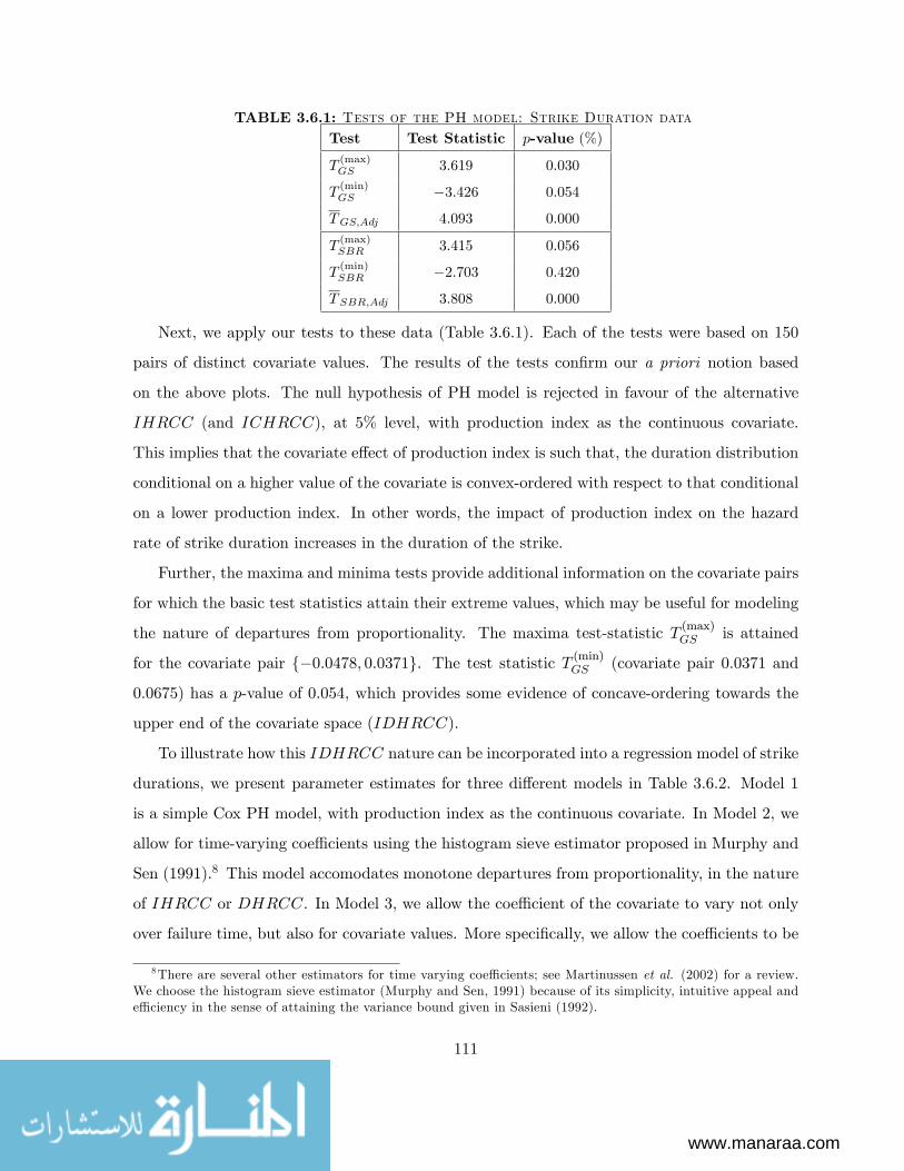
www.manaraa.com

TABLE 3.6.1: Tests of the PH model: Strike Duration dataTest Test Statistic p-value (%)

T(max)GS 3:619 0:030

T(min)GS �3:426 0:054

TGS;Adj 4:093 0:000

T(max)SBR 3:415 0:056

T(min)SBR �2:703 0:420

TSBR;Adj 3:808 0:000

Next, we apply our tests to these data (Table 3.6.1). Each of the tests were based on 150

pairs of distinct covariate values. The results of the tests con�rm our a priori notion based

on the above plots. The null hypothesis of PH model is rejected in favour of the alternative

IHRCC (and ICHRCC), at 5% level, with production index as the continuous covariate.

This implies that the covariate e¤ect of production index is such that, the duration distribution

conditional on a higher value of the covariate is convex-ordered with respect to that conditional

on a lower production index. In other words, the impact of production index on the hazard

rate of strike duration increases in the duration of the strike.

Further, the maxima and minima tests provide additional information on the covariate pairs

for which the basic test statistics attain their extreme values, which may be useful for modeling

the nature of departures from proportionality. The maxima test-statistic T (max)GS is attained

for the covariate pair f�0:0478; 0:0371g. The test statistic T (min)GS (covariate pair 0:0371 and

0:0675) has a p-value of 0:054, which provides some evidence of concave-ordering towards the

upper end of the covariate space (IDHRCC).

To illustrate how this IDHRCC nature can be incorporated into a regression model of strike

durations, we present parameter estimates for three di¤erent models in Table 3.6.2. Model 1

is a simple Cox PH model, with production index as the continuous covariate. In Model 2, we

allow for time-varying coe¢ cients using the histogram sieve estimator proposed in Murphy and

Sen (1991).8 This model accomodates monotone departures from proportionality, in the nature

of IHRCC or DHRCC. In Model 3, we allow the coe¢ cient of the covariate to vary not only

over failure time, but also for covariate values. More speci�cally, we allow the coe¢ cients to be

8There are several other estimators for time varying coe¢ cients; see Martinussen et al. (2002) for a review.We choose the histogram sieve estimator (Murphy and Sen, 1991) because of its simplicity, intuitive appeal ande¢ ciency in the sense of attaining the variance bound given in Sasieni (1992).

111

www.manaraa.com

di¤erent for covariate values below and above 0:0371, enabling us to model departures of the

IDHRCC or DIHRCC type. Here again, we use the estimators given by Murphy and Sen

(1991) for inference.

Model 1 indicates a signi�cant impact of production index on the hazard rate of strike

durations. However, this evidence is misleading. Model 3 estimates show that the true nature

of covariate dependence is strikingly di¤erent. These time- and covariate-varying nature of the

parameter estimates closely relate to the results of our analytical tests on the nature of covariate

dependence. For lower values of the covariate, the coe¢ cient increases with duration, while the

opposite holds for higher covariate values. These results point to new evidence on asymmetric

business cycle e¤ects on strike duration which has important policy implications.

TABLE 3.6.2: Model Estimates: Strike Duration dataModel/ Parameter Coe¢ cient z-stat.

Model 1

Production Index, x 3:529 3:17

Model 2

x:I [t�[0; 75)] 5:179 3:90

x:I [t�[75; 150)] 0:360 0:27

x:I [t�[150;1)] 9:416 1:19

Model 3

x:I [x�(�1; 0:037)] :I [t�[0; 75)] �1:178 �0:75

x:I [x�(�1; 0:037)] :I [t�[75; 150)] 9:362 4:32

x:I [x�(�1; 0:037)] :I [t�[150;1)] 45:266 3:43

x:I [x�[0:037;1)] :I [t�[0; 75)] 10:173 4:96

x:I [x�[0:037;1)] :I [t�[75; 150)] �14:910 �5:96

x:I [x�[0:037;1)] :I [t�[150;1)] �27:619 �5:90

3.7.2 A related graphical test

Plotting the contours of the underlying standardised test statistics on a covariate � covariate

two-dimensional plane provides an useful graphical tool for inference on monotonic and non-

monotonic departures considered in this chapter. Figure 3-2 shows a contour diagram of the

standardized test statistic TGS;std (smoothed using the Epanechnikov kernel) for the strike

duration data. The signi�cant height of the peaks and troughs indicate nonproportionality, and

112

www.manaraa.com

the shift in the slopes about the covariate value of approximately 0:04 indicate non-monotonic

departures from proportionality about this point. The use of the plot here con�rms the inference

drawn from our analytical tests, and in particular helps in choosing the changepoint for the

IDHRCC pattern.

0.06 0.04 0.02 0 0.02 0.04 0.06 0.080.06

0.04

0.02

0

0.02

0.04

0.06

0.08

Covariate

Cov

aria

teContour Plot of TGS,std

3

3

1

111

2

2

In applications with multiple covariates, similar graphical analysis can also provide valuable

insights into the interaction between di¤erent covariates. With two continuous covariates x

and z, one can obtain similar plots for di¤erent candidate functions h(x; z) (see Section 3.4.5)

to examine which of these provides the sharpest slopes in the contour plot. The candidate

functions can sometimes be implied by the relevant application. For example, in survival of

a series system with covariates measuring proneness to failure of the two components, the

relevant function may be max(x; z). In other situations where there is no a priori knowledge

about h(:; :), one can either hypothesize linear functions of the form x+ z, or �nd the function

using regression methods. The identity of the covariate pairs with high (low) values for the

maxima (minima) test statistics can be very helpful in such analyses.

113

www.manaraa.com

3.7.3 Survival with Malignant Melanoma

The data pertain to 205 patients (148 of these are censored) with malignant melanoma (cancer


University Hospital of Odense, Denmark. The analysis of these data in Andersen et al. (1993)

identi�es tumor thickness as one of the most important prognostic factors. Further, Andersen

et al. (1993) show that the Lee-Pirie plots of Nelson-Aalen estimates of the cumulative hazard

functions for patients with �2 mm � tumor thickness < 5 mm�and �tumor thickness � 5 mm�

against that of patients with �tumor thickness < 2 mm�are �concave looking curves�, indicating

possible violation of the PH model in favour of DHRCC. Similarly, the plot of the cumulative

regression functions for log-thickness (Martinussen et al., 2002) also indicate a distinct concave

shape. However, surprisingly, the constant coe¢ cient estimate lies almost entirely within the

95 percent con�dence band of their estimates of the cumulative regression functionR t0 �(s)ds.

Our analytical tests (Table 3.6.3) based on 100 pairs of distinct covariate values show that

T(min)GS and T (min)SBR are signi�cant at 1 percent level and T (max)GS is signi�cant at 5 percent level, but

TGS;Adj and TSBR;Adj are not signi�cant. Further, T(min)GS and T (max)GS are attained for covariate

pairs f1:9; 7:7g and f1:0; 1:8g respectively. This provides partial support for the observation in

Andersen et al. (1993), in that the null of PH is rejected in favour of the alternatives DHRCC

and DCHRCC over the upper range of the covariate space. However, in patients with small

tumors, there is some evidence of an IHRCC pattern (probably the reason why TGS;Adj and

TSBR;Adj are not signi�cant). The inference from the Murphy-Sen histogram sieve estimators

(Table 3.6.4) is similar.

TABLE 3.6.3: Tests of the PH model: Malignant Melanoma DataTest Test Statistic p-Value (%)

T(max)GS 3:462 0:035

T(min)GS �4:985 0:000

TGS;Adj �1:080 0:188

T(max)SBR 2:559 0:420

T(min)SBR �8:255 0:000

TSBR;Adj �1:235 0:249

114

www.manaraa.com

TABLE 3.6.4: Model Estimates: Malignant Melanoma DataModel/ Parameter Coe¢ cient z-stat.

Model 1

Log Tumor Thickness, ln(x) 0:823 5:49

Model 2

ln(x):I [t�[0; 1062)] 1:123 5:09

ln(x):I [t�[1062;1)] 0:518 2:89

Model 3

ln(x):I [x�(0; 1:9)] :I [t�[0; 1062)] 0:097 0:15

ln(x):I [x�(0; 1:9)] :I [t�[1062;1)] 1:177 2:39

ln(x):I [x�[1:9;1)] :I [t�[0; 1062)] 1:184 5:90

ln(x):I [x�[1:9;1)] :I [t�[1062;1)] 0:444 1:99

This demonstrates the usefulness of the proposed methods for detecting non-proportional

covariate e¤ects which previous tests fail to identify.

3.7.4 Child mortality in India

The third application is adapted from a study (Bhalotra and Bhattacharjee, 2001) of child

mortality across the three Indian states of Kerala, West Bengal and Uttar Pradesh. As argued

by Sen (1998), infant and child mortality are important indicators of quality of life, in that

they vary widely across space and time, they contain substantial information about and social

inequalities (including gender bias), and are quite strongly in�uenceable by economic policy.

The literature highlights a host of determinants that a¤ect child mortality �economic, socio-

cultural and physiological, and identi�es the importance of provision and access to welfare

measures and community infrastructure.

There is substantial spatial variation in infant and child mortality within India. Here we

consider data for the state of Kerala which has demographic features more typical of a middle-

income country than of a poor developing country. A large number of covariates are included,

covering economic, socio-cultural and physiological determinants of child mortality. The data

are from the National Family Health Survey of 1992-93 and we use retrospective data for ten

years for each ever-married women who had at least one live-birth during the ten years preceding

the date of survey.

115

www.manaraa.com

Our main focus is on the mother�s age at childbirth, which has been identi�ed in previous

research as an important covariate (Martin et. al., 1983; Trussell and Hammerslough, 1983;

Pebley and Stupp, 1987; Guo and Rodríguez, 1992). However, the e¤ect of maternal age on

mortality outcomes depends critically on the age of the child. Children born to very young

(teenage) mothers are expected to be disadvantaged, both at birth (because of physiological

reasons) and during early childhood because very young mothers may not be able to provide

adequate childcare. Similarly, the e¤ect of a higher maternal age on child survival may be

mixed; while children born to older mothers may be physiologically disadvantaged at birth, such

mothers may be more experienced and better able to provide adequate childcare. Therefore,

a priori, we expect the covariate e¤ect to be negative and falling to zero at lower ranges of

maternal age (IHRCC). The e¤ect may be non-monotonic (IDHRCC) if the age bene�ts of

better childcare provision at higher maternal ages are not strong.

As expected for a state with good socio-economic conditions (including maternal education

and post-natal childcare provision), T (max)GS and TGS;Adj are signi�cant at 1% level, while T (min)GS

is not (r = 150; T(max)GS = 6:72 �covariate pair 23, 29 years; T (min)GS = �2:52; TGS;Adj = 0:30).

The Grambsch and Therneau (1994) test fails to reject the PH assumption, though the p-value

is fairly small at 0:079.

We use a sequential testing procedure to identify all covariates with non-PH e¤ects. Two

other covariates, preceding and succeeding birth intervals, also demonstrated monotone covari-

ate e¤ects. Interestingly, our tests fail to reject the null hypothesis for one covariate, distance

to nearest town, which was identi�ed by the Grambsch and Therneau (1994) test to have time

varying coe¢ cients. However, the histogram sieve estimates of age-varying coe¢ cients strongly

support the inferences drawn using our tests for all the covariates.

The three applications considered here demonstrate the value of studying departures from

the PH model with respect to continuous covariates in terms of monotonicity of the covariate

e¤ects. These examples also illustrate the use of our test statistics in identifying monotonic

and non-monotonic structures in the data. Similar inference has been used in Bhattacharjee et

al. (2008a, 2008b) in applications to business failures in the UK and the US, which we discuss

in Chapter 7 (Sections 7.2 �7.4).

116

www.manaraa.com

3.8 Conclusion

In this chapter, we develop notions of partial ordering of lifetime distributions with respect to

continuous covariates and propose tests of the PH model against such monotone or ordered

departures. Departures of these kinds are common in applications. Therefore, both empirical

and theoretical work in lifetime models need to have a framework �exible enough to accomodate

these kinds of covariate dependence. Unlike other tests available in the literature, the proposed

methodology works in very general situations and does not require any assumptions on the

underlying regression models. Further, the methods o¤er a great deal of �exibility in terms of

accommodating the e¤ects of other covariates, both observed and unobserved.

An important advantage of the tests is that they provide valuable insights into the pattern

of covariate dependence where the PH assumption does not hold. Unlike other competing tests,

this is true for both monotonic and non-monotonic covariate e¤ects. The methods are therefore

useful for regression modeling in non-PH cases. Further, since the proposed partial orders can

be interpreted in terms of time varying coe¢ cients, existing inference methods can be easily

used. Monte Carlo evidence and real life examples demonstrate the strength and usefulness of

the proposed framework based on partial orders as well as the tests developed here.

Several promising areas of future research emerge from the research in this chapter. First, in

the derivation of asymptotic results, we show that the basic underlying two-sample test statistics

for distinct covariate pairs are independent of each other. This fact can be exploited to extend

many familiar two-sample inference techniques to the case of continuous covariates. In Chapter

5, we will take this approach in developing tests for the absence of covariate dependence. Second,

research can be directed towards extension of the proposed tests to models with unrestricted

univariate frailty. The notions of partial ordering introduced in this chapter will be valid in

this case, and we can in principle construct similar tests using estimators of the cumulative

hazard function under such models. However, this inference problem is quite distinct from the

one addressed here, because of identi�ability restrictions and the di¤erent nature of estimators

proposed in the literature (see, for example, Horowitz, 1999). In Chapter 5, we show that this

problem is related to testing for the absence of covariate dependence, and develop tests for the

PH model in the univariate frailty case. Third, estimation of semiparametric regression models

under order restrictions motivated by the current work is an area of considerable research

117

www.manaraa.com

potential. In Chapter 4 (also Bhattacharjee, 2004a), we develop biased bootstrap methods

for such order restricted inference on covariate e¤ects, while Bayesian inference under oder

restrictions on both covariate e¤ects and ageing, and in the presence of frailty, is developed in

Chapter 6.

Fourth, it will be useful to develop further inference on the changepoint in non-monotonic

models using covariate pairs corresponding to the maxima and minima tests. Fifth, a somewhat

related problem is inference on the unknown h(:; :) function in the multiple covariate case. These

problems will be retained for future work.


Proof of Theorem 3.3.1: It follows from Gill and Schumacher (1987) that, under PH, as n �!

1,

�a(n)

�1=2TGS (xl1; xl2)

D�! N�0; �2GS;l

�; and

a(n)dVar [TGS (xl1; xl2)] P�! �2GS;l;

where

�2GS;l =

Z �

0

�l2 (xl1; xl2) l1 (xl1; xl2) (t)� l1 (xl1; xl2) l2 (xl1; xl2) (t)

�2�xl1�xl2

�d�(t; xl1)

y(t; xl2)+d�(t; xl2)

y(t; xl1)

�;

and li (xl1; xl2) =

Z �

0li (xl1; xl2) (t)d�(t; xli); i = 1; 2:

so that,

TGS;std (xl1; xl2) =TGS (xl1; xl2)qdVar [TGS (xl1; xl2)]

D�! N(0; 1); l = 1; : : : ; r:

The proof of the Theorem would follow, if it further holds that TGS;std (xl1; xl2) ; l = 1; : : : ; r

118

www.manaraa.com

are asymptotically independent. In other words,

26666664TGS;std (x11; x12)

TGS;std (x21; x22)...

TGS;std (xr1; xr2)

37777775D�! N (0; Ir) ;

where Ir is the identity matrix of order r.

Following Gill and Schumacher (1987), let

Z(n)lij =

Z �

0Li(xl1; xl2)(t)d

nb�(t; xlj)� �(t; xlj)o ; (i; j = 1; 2; l = 1; : : : ; r):

Then

�a(n)

�1=2Z(n)lij =

�a(n)

�1=2 Z �

0Li(xl1; xl2)(t)

dN(t; xlj)� Y (t; xlj)d�(t; xlj)Y (t; xlj)

D�!Z �

0li(xl1; xl2)(t)dM(t; xlj);

where M(t; xlj); l = 1; : : : ; r; j = 1; 2 are independent Gaussian processes with zero means,

independent increments and variance functions

V ar [M(t; xlj)] =

Z �

0

d� (s; xlj)

y(s; xlj):

This follows from a version of Rebolledo�s central limit theorem (see Andersen et al., 1993),

which states that the innovation martingales corresponding to components of a vector count-

ing process are orthogonal, and the vector of these martingales asymptotically converge to a

Gaussian martingale.

It follows, by a version of the �-method proved in Gill and Schumacher (1987), that

�a(n)

�1=226666664TGS;std (x11; x12)

TGS;std (x21; x22)...

TGS;std (xr1; xr2)

37777775D�!

26666664

P2i;j=1 l

1ij R �0li(x11; x12)(t)dM(t; x1j)P2

i;j=1 l2ij R �

0li(x21; x22)(t)dM(t; x2j)

...P2i;j=1 l

rij R �0li(xr1; xr2)(t)dM(t; xrj)

37777775

119

www.manaraa.com

where

llij

= (�1)i+jll;3�i;3�j

and llij =

Z �

0li(xl1; xl2)(t)d�(t; xlj); l = 1; : : : ; r; i; j = 1; 2:

Now, under H0 : PH; llij = �xlj li (xl1; xl2), so that

2Xi;j=1

llijZ �

0li(xl1; xl2)(t)dM(t; xlj) =

Z �

0

�ll22l1(xl1; xl2)(t)� ll12l2(xl1; xl2)(t)

�dM(t; xl1)

+

Z �

0

��ll21l1(xl1; xl2)(t) + ll11l2(xl1; xl2)(t)

�dM(t; xl2):

It follows that 26666664TGS (x11; x12)

TGS (x21; x22)...

TGS (xr1; xr2)

37777775D�! N

�0;X�

;

whereP= diag

�(�2GS;l)

�; l = 1; : : : ; r, with

�2GS;l =

Z �

0

�ll22l1(xl1; xl2)(t)� ll12l2(xl1; xl2)(t)

�2 d�(t; xl1)y(t; xl1)

+

Z �

0

��ll21l1(xl1; xl2)(t) + ll11l2(xl1; xl2)(t)

�2 d�(t; xl2)y(t; xl2)

:

Further, following Gill and Schumacher (1987), it can be shown that �2GS;l can be consistently

estimated by dV ar [TGS (xl1; xl2)]. Hence, it follows that26666664TGS;std (x11; x12)

TGS;std (x21; x22)...

TGS;std (xr1; xr2)

37777775D�! N (0; Ir) ;


Proofs of (a), (b) and (c) follow.

�

120

www.manaraa.com

Proof of Corollary 3.3.1: Proof follows from the well known result in extreme value theory

regarding the asymptotic distribution of the maximum of a sample of iid N(0; 1) variates (see,

for example, Berman, 1992), and invoking the �-method by noting that maxima and minima

are continuous functions.

�

Proof of Corollary 3.3.2: From Theorem 3.3.1, we have:

26666664TGS;std (x11; x12)

TGS;std (x21; x22)...

TGS;std (xr1; xr2)

37777775D�! N (0; Ir) ;


The proof follows immediately.

�

Proof of Theorem 3.3.2: It follows from Section 2.3 that, under H0, as n �!1,

�a(n)

�1=2TSBR (xl1; xl2)

D�! N�0; �2SBR;l

�; and

a(n)dVar [TSBR (xl1; xl2)] P�! �2SBR;l;

where

�2SBR;l =

Z �

0

Z �

0[c(t)c(s)V (min(s; t); xl1) + d(t)d(s)V (min(s; t); xl2)] dsdt;

V (t; xlj) =

Z �

0

d� (s; xlj)

y(s; xlj); j = 1; 2;

c(t) = s2 (xl2) k1 (xl1; xl2) (t)� s1 (xl2) k2 (xl1; xl2) (t);

d(t) = s2 (xl1) k1 (xl1; xl2) (t)� s1 (xl1) k2 (xl1; xl2) (t);

and si (xlj) =

Z �

0ki (xl1; xl2) (s):�(s; xlj)ds; i = 1; 2; j = 1; 2:

121

www.manaraa.com

so that,

TSBR;std (xl1; xl2) =TSBR (xl1; xl2)qdV ar [TSBR (xl1; xl2)]

D�! N(0; 1); l = 1; : : : ; r:

Like Theorem 3.3.1, the proof will follow, if it further holds that

26666664TSBR;std (x11; x12)

TSBR;std (x21; x22)...

TSBR;std (xr1; xr2)

37777775D�! N (0; Ir) ;


The essential di¤erence in the arguments required to establish asymptotic distributions

here, from those in Theorem 3.3.1, lie in the fact that the integrals considered in Theorem 3.3.1

are transformations of stochastic integrals, while here, they are functions of ordinary Steiljes

integrals of stochastic processes.

Let us de�ne

Z�(n)lij =

Z �

0Ki(xl1; xl2)(t)

nb�(t; xlj)� �(t; xlj)o dt; (i; j = 1; 2; l = 1; : : : ; r):

Then, by Rebolledo�s central limit theorem and Theorem 2.3.1 (Theorem 3.1 in Sengupta et

al., 1998), we have, as n!1,

�a(n)

�1=2Z�(n)lij

D�!Z �

0ki(xl1; xl2)(t)M(t; xlj)dt;

where M(t; xlj); l = 1; : : : ; r; j = 1; 2 are independent Gaussian processes with zero means,

independent increments and variance functions

V ar [M(t; xlj)] =

Z �

0

d� (s; xlj)

y(s; xlj):

122

www.manaraa.com

Now, as in Theorem 3.3.1, invoking the �-method of Gill and Schumacher (1987), it follows that

�a(n)

�1=226666664TSBR;std (x11; x12)


TSBR;std (xr1; xr2)

37777775D�!

26666664

P2i;j=1 k

1ij R �0ki(x11; x12)(t)M(t; x1j)dtP2

i;j=1 k2ij R �

0ki(x21; x22)(t)M(t; x2j)dt

...P2i;j=1 k

rij R �0ki(xr1; xr2)(t)M(t; xrj)dt

37777775where

klij

= (�1)i+jkl;3�i;3�j

and klij =

Z �

0ki(xl1; xl2)(t)�(t; xlj)dt; l = 1; : : : ; r; i; j = 1; 2;

and under H0,

2Xi;j=1

klijZ �

0ki(xl1; xl2)(t)M(t; xlj)dt =

Z �

0

�kl22k1(xl1; xl2)(t)� kl12k2(xl1; xl2)(t)

�M(t; xl1)dt

+

Z �

0

��kl21k1(xl1; xl2)(t) + kl11k2(xl1; xl2)(t)

�M(t; xl2)dt:

It follows that 26666664TSBR (x11; x12)

TSBR (x21; x22)...

TSBR (xr1; xr2)

37777775D�! N

�0;X�

;

whereP

= diag�(�2SBR;l)

�; l = 1; : : : ; r, and following similar arguments as Appendix to

Chapter 2, it can be shown that �2SBR;l can be consistently estimated by dVar [TSBR (xl1; xl2)].Hence, it follows that 26666664

TSBR;std (x11; x12)


TSBR;std (xr1; xr2)

37777775D�! N (0; Ir) ;



�

123

www.manaraa.com

Proof of Corollary 3.3.3: Proof follows from extreme value theory and the �-method, as in

Corollary 3.3.1.

�

Proof of Corollary 3.3.4: From Theorem 3.3.2, we have:

26666664TSBR;std (x11; x12)


TSBR;std (xr1; xr2)

37777775D�! N (0; Ir) ;


The proof follows immediately.

�

124

www.manaraa.com

Chapter 4

Estimation in nonproportional

hazard regression models with

monotone covariate e¤ect

4.1 Chapter summary

In this chapter, based on Bhattacharjee (2003, 2004a), we build on the notion of ordered

departures from proportionality introduced in Chapter 3, and propose estimation methods for

hazard regression models under such order restrictions. In our proposed test of the proportional

hazards assumption (Bhattacharjee, 2007a �our Chapter 3), the ordered alternative of special

interest was that the lifetime distribution conditional on a higher covariate value was convex

(concave) ordered with respect to that conditional on a lower value. Here we argue that hazard

regression models with time varying coe¢ cients provide an appropriate framework for studying

such order restrictions. Building on a natural interpretation of these alternatives in terms

of monotonicity of time varying coe¢ cients, we use biased bootstrap methods to estimate

the covariate e¤ects when such monotone departures are known to hold. In particular, it is

shown how order restricted estimation can be performed using biased bootstrap techniques

such as adaptive bandwidth kernel estimators (Brockmann et al., 1993) or data tilting (Hall

and Presnell, 1999). The performance of the estimators is compared using simulated data, and

125

www.manaraa.com

their use is illustrated with applications from biomedicine and economic duration data. The

methods are relatively simple to implement, and provide useful inference in nonproportional

hazard situations.

4.2 Introduction

As discussed earlier in the thesis (Chapters 1 through 3), the proportional hazards assump-

tion is often violated in applications, or may even be unreasonable from the point of view of

relevant theory. Further, such violation leads to misleading inferences based on the Cox PH

model. Johnson et al. (1982), Lagakos and Schoenfeld (1984), Solomon (1984), Struthers and

Kalb�eisch (1986) and Lagakos (1988) discuss the e¤ect of misspeci�cation on inferences about

the e¤ects of explanatory variables, and Li et al. (1996) reports results of a large simulation

study. Similarly, inaccurate inferences on the shape of the baseline hazard function has been

discussed by Breslow et al. (1984), Stablein and Koutrouvelis (1985), Schemper (1992), Tubert-

Bitter et al. (1994) and Hsieh (1996). Testing the PH model, particularly against the omnibus

alternative, has therefore been an area of active research.

Recently, speci�c attention has focussed on testing the PH assumption against ordered

alternatives. As discussed earlier, it is often of interest to explore whether the hazard rate

for one level of the covariate increases in lifetime, relative to another level (i.e., the hazard

ratio increases/ decreases with lifetime). Such tests have the important advantage of providing

inferences useful for regression modeling when the proportionality assumption does not hold.

In the two-sample setup, Gill and Schumacher (1987) and Deshpande and Sengupta (1995)

have constructed analytical tests of the PH hypothesis against the alternative of �increasing

hazard ratio�, while Sengupta et al. (1998) (our Chapter 2) have proposed a test of the PH

model against the weaker alternative hypothesis of �increasing ratio of cumulative hazards�. In

Chapter 3 (Bhattacharjee, 2007a), we developed a natural extension of such monotone ordering

to the case of continuous covariates, and constructed tests for the proportional hazards model

against these alternatives.

It is observed that monotone departures are common in economic and biomedical applica-

tions (Bhattacharjee, 2007a; Scheike, 2004), and provide useful information about the nature

126

www.manaraa.com

of covariate dependence. Besides, they may also be suggested by theory. Estimation of hazard

regression models under such order restrictions is therefore important. These methods are ap-

propriate when either analytical tests or relevant theory suggests order restrictions rather than

proportionality.

A popular approach in the literature is to interpret violations of the PH model in terms of

time varying coe¢ cients (for a review, see Scheike, 2004). Several authors have suggested vali-

dation of the PH assumption by testing for time varying coe¢ cients (see, for example, Grambsch

and Therneau, 1994; Scheike and Martinussen, 2004), and several methods for estimation of

these time varying coe¢ cients have been proposed (see, for example, Zucker and Karr, 1990;

Murphy and Sen, 1991; Martinussen et al., 2002). However, none of these estimators consider

the case when the covariate e¤ects are order restricted. As discussed in Chapter 3, Bhattachar-

jee (2007a) considers testing the proportionality assumption against the alternative of order

restricted covariate e¤ects in a more general framework. This framework includes the hazard

regression model with time varying coe¢ cients as a special case.

In this chapter, we build on the notion of ordered departures from proportionality introduced

in Bhattacharjee (2007a) and propose estimation methods for hazard regression models under

such order restrictions. We argue that a natural framework for hazard regression models in

such situations is the one that allows time varying coe¢ cients. Further, building on a natural

interpretation of these alternatives in terms of monotonicity of time varying coe¢ cients (see

Example 3.2.1), we use biased bootstrap methods to estimate the covariate e¤ects when such

monotone departures from proportional hazards hold. Small sample properties of the estimators

are explored using simulated data. Algorithms are developed for using these methods, and the

nature of inference derived is demonstrated using a couple of applications.

The chapter is organised as follows. In Section 4.2, we motivate modeling ordered depertures

from PH by a hazard regression model with monotonically time-varying coe¢ cients, while

Section 4.3 brie�y reviews some alternative methods for order restricted inference that can be

potentially used in the current context. Sections 4.2 and 4.3 are based on Bhattacharjee (2003).

Next, following Bhattacharjee (2004a), we discuss estimation of hazard regression models with

order restricted covariate e¤ects. The proposed estimation methodologies based on biased

bootstrap methods are developed in Section 4.4. In Section 4.5, we illustrate the use of the

127

www.manaraa.com

estimators using simulations and two real life applications. Section 4.6 collects the concluding

remarks.

4.3 A hazard regression model admitting order restrictions in

covariate e¤ects

As discussed in Chapter 3, Bhattacharjee (2007a) extended to the continuous covariate setup

the notion of monotone hazard ratio in two samples developed in Gill and Schumacher (1987),

Sengupta and Deshpande (1994) and Deshpande and Sengupta (1995). Let T be a lifetime

variable, X a continuous covariate and let � (tjx) denote the hazard rate of T , given X = x, at

T = t. Then, T is de�ned to be increasing (decreasing) hazard ratio for continuous covariate

( IHRCC (DHRCC)) with respect to X if, whenever x1 > x2, the ratio � (tjx1) =� (tjx2) is

increasing (decreasing) in t (De�nition 3.2.1).

Further, Bhattacharjee (2007a) showed that, within the context of the hazard regression

model with time varying coe¢ cients (Murphy and Sen, 1991; Martinussen et al., 2002)

�(tjx) = �0(t): exp(�(t):x);

the lifetime random variable T is IHRCC with respect to the covariate X if and only if the

time varying covariate e¤ect �(:) is an increasing function of lifetime t (Example 3.2.1); this is

also true in the presence of additional covariates or frailty. The converse holds for the partial

order DHRCC.

The above result suggests that the time varying coe¢ cients model (1.12) may be useful

for regression modeling in situations where covariate e¤ects are non-proportional. However, it

is also clear that the partial orders IHRCC and DHRCC are de�ned in more general set-

tings than the time varying coe¢ cients model. Therefore, before considering estimation under

order restrictions, we characterise the additional assumptions embodied in the time varying

coe¢ cients hazard regression model.

First, we consider the single covariate case. For simplicity, we assume that the the lifetime

variable T is discrete and takes values 0; 1; : : :, and that the covariate X takes three possible

128

www.manaraa.com

values: l = 0 (low), m = 1 (medium) and h > m (high). Here, the most general hazard

regression model is given by

�(tjx) = �0(t): exp [ (t; x)] ; (t; 0) � 0: (4.1)

Without loss of generality, the exponential function can be substituted by any other monotonic

positive valued function. We treat the hazard rate corresponding to the lowest covariate value,

�(tjX = 0), as the baseline hazard rate �0(t). Then, the time varying covariate e¤ects, �(t),

implied by the general model (4.1) for various combinations of T and X are as follows:

Covariate Lifetime, T = 0 Lifetime, T = 1 : : : Lifetime, T = k : : :

X = l(= 0) �(0) unrestricted �(1) unrestricted �(k) unrestricted

X = m(= 1) �(0) = (0; 1) �(1) = (1; 1) �(k) = (k; 1)

X = h(> 1) �(0) = (0; h) =h �(1) = (1; h) =h �(k) = (k; h) =h

When the covariate is zero, the conditional hazard rate is the same as the baseline hazard,

and � (:) is completely unrestricted. Clearly, when the covariate is binary,1 the time vary-

ing coe¢ cients model coincides with the most general model, and an exact correspondence

�(t) = (t; 1) holds. However, when the covariate is not binary (takes more than two possible

values), the time varying e¤ect model holds only when two conditions are satis�ed. First, the

following scaling condition holds: (t; x1)

x1= (t; x2)

x2;

where x1 and x2 are any two non-zero values of the covariate X. Second, the logarithm of

conditional hazard rates for di¤erent covariate values have to be proportional to each other.2

The �rst condition can be addressed by suitable transformations of the covariate X. The

second assumption is more critical. However, if it fails to hold, we can use a histogram sieve

(Grenander, 1981) to divide the covariate space into disjoint intervals within which the shape

of � (:) is approximately similar.3 Thus, we can still construct an appropriate time varying

1 In this case, without loss of generality, X can be assumed to take values 0 and 1.2Note that proportionality of hazards implies the much stronger condition that logarithm of conditional hazard

rates are constant over lifetime.3See, for example, the applications reported in Sections 3.6.1 and 3.6.3, particularly Model 3 estimates in

Tables 3.6.2 and 3.6.4

129

www.manaraa.com

coe¢ cients model and estimate the model using methods similar to those proposed in Murphy

and Sen (1991); see discussion in Section 1.2.7. In fact, the above assumption can also be tested

using methods similar to those developed by Murphy (1993) in the context of testing the PH

model.

The above arguments can be simply extended to the continuous failure time case, as well

as the continuous covariate case.

Next, let us consider the case when there are multiple covariates. From the above argument,

it is clear that, even in the simplest case with 2 binary covariates the time varying coe¢ cients

model (1.12) may fail to hold. This is because of potential interaction between the covariates.

However, in this case, the time varying coe¢ cients model

�(tjx; z) = �0(t): exp [�X(t):x+ �Z(t):z + �XZ(t):x:z]

is exactly equivalent to the most general case.

Carrying this intuition to the case of several continuous covariates, it can be seen that the

time varying coe¢ cients model is valid under the additional assumption of additive covariate

e¤ects on the logarithm of conditional hazard rates. The assumption too can be tested. For

example, one can use a Hausman-type test (Hausman, 1978), based on the di¤erence between

a consistent unrestricted nonparametric estimate and an e¢ cient estimate under the additivity

assumption. Under additivity, both the Murphy and Sen (1991) histogram sieve estimator and

the Martinussen et al. (2002) estimator of the cumulative coe¢ cients are e¢ cient in that they

attain the bounds based on e¢ cient in�uence functions given by Sasieni (1992).4 Further, as

before, even when additivity is rejected, a valid time varying coe¢ cients model can be built by

placing histogram sieves on the product space of the covariates.

Thus, the time varying coe¢ cients model incorporates two important assumptions relating

to variation in the shape of the time varying coe¢ cients over covariate values and to additivity

of covariate e¤ects. At the same time, even when these conditions are invalid, one can work with

a modi�ed model where the time varying coe¢ cients are allowed to also vary with covariate

4Gozalo and Linton (2001) developed a similar test for additivity in nonparametric regression which can bemodi�ed to the current framework.

130

www.manaraa.com

values and may include interaction between covariates. Further, it is easy to estimate these

models, either by using histogram sieves along the lines of Murphy and Sen (1991) or using

kernel based methods. All the above arguments also hold in the presence of frailty and time

varying covariates.

In summary, the time varying coe¢ cients model is potentially a very useful hazard regression

model for order restricted inferences of the kind developed in this chapter and thesis.

4.4 Estimation under order restrictions

Curve estimation under shape constraints is of considerable interest in many applications. In

the context of nonparametric regression, typical examples include the study of dose response

experiments in medicine and the study of indirect utility, cost and production functions in

economics, and pricing of options in �nance, among others. In the context of hazard regres-

sion models, monotonicity of time varying coe¢ cients provides a useful way to express order

restrictions on covariate e¤ects; see also discussion in Chapter 3 and Section 4.2.

Starting from the classic works of Hildreth (1954) and Brunk (1955), there exists a large

literature on the problem of estimating monotone, concave or convex regression functions; for

further discussion, see Barlow et al. (1972) and Robertson et al. (1988). More recently,

attention has focussed on simple, smooth and e¢ cient estimation of shape restricted regression

functions. In the following subsections, we provide a very brief overview of some of these

methods, focussing mainly on monotonicity (or isotonic regressions) and methods that are

particularly attractive for hazard regression modeling. We also discuss our choice of estimation

methodologies.

4.4.1 Isotonic regression approach

The isotonic regression approach (Barlow et al., 1972; Hanson et al., 1973) represents the

most traditional method for estimating a nonparametric regression function under monotonicity

constraints. The method obtains a least squares solution under the monotonicity restriction by

the pool adjacent violators (PAV) algorithm. Whenever monotonicity is violated at a particular

data point, the algorithm averages over neighbouring data, expanding the neighbourhood until

131

www.manaraa.com

monotonicity is restored. Newer generations of isotonic regression methods and their properties

have been studied by Mukerjee (1988), Mammen (1991a, 1991b), Qian (1994), and others. In

the sense that pooling is similar to expanding the bandwidth in the kernel regression framework,

this method is similar to local adaptive bandwidths. The idea is also related to taut strings.

4.4.2 Estimation based on projections

Mammen et al. (2001) developed a general framework where the constrained smoothing problem

can be interpreted as a projection of the unconstrained estimator in an appropriate Hilbert

space. Special cases include smoothing spline and local polynomial methods; see also Ramsay

(1988), Tantiyaswasdikul and Woodroofe (1994), Mammen and Thomas-Agnan (1999) and

Mammen et al. (1999). In fact, Mammen et al. (2001) also show how the usual Nadaraya

Watson nonparametric kernel regression estimator can also be interpreted as a projection.

4.4.3 Taut string method

The taut string method has its origins in isotonic regression, and speci�cally the familiar result

that the greatest convex minorant of the data is a taut string and its derivative is the isotonic

estimator (Barlow et al., 1972; Leurgans, 1982). The taut string method is also related to the

notion of excess mass which motivated the development of scale space view of kernel smoothing

(SiZer maps) by Chaudhuri and Marron (1999, 2000).

Mammen and van de Geer (1997) developed the method further and extended its use to

locally adaptive nonparametric regression. In recent times, the method has attracted substantial

attention because of two main reasons. First, the work of Dümbgen (1998) and Davies and

Kovac (2001) established a connection between taut string and the number and location of

local extremes. This has important implications for testing qualitative order restrictions as well

as nonparametric smoothing under order restrictions. Second, the method has been found to

o¤er good control over the number of local extreme values. In other words, it does very well in

detecting even low peaks without picking up arti�cial peaks.

132

www.manaraa.com

4.4.4 Density regression approach

The density regression method proposed by Dette et al. (2006) is implemented in two steps.

In the �rst step, the unconstrained Nadaraya Watson nonparametric regression estimator is

obtained. In the second step, an isotonic estimator of the inverse regression function is obtained,

using a di¤erent kernel from the �rst step. The resulting estimator has the desirable property

that it is of the same order of smoothness as the unconstrained estimator.

The above four approaches are all based on intuitive and attractive ideas. However, we �nd

the biased bootstrap methods discussed below more intuitively appealing, particularly because

they are easy to implement and provide smooth estimates that agree with the corresponding

unconstrained (kernel or sieve) estimators most of the time. Besides, there are issues relating to

computational intensity and the lack of a simple way to visualise departures from hypothesized

order restrictions.

4.4.5 Biased bootstrap methods

"Biased bootstrap" is usually taken to mean a weighted bootstrap procedure where the weights

are chosen to satisfy the constraints imposed by the statistical model. Following Hall and

Turlach (1999), we adopt a slightly di¤erent interpretation, where the notion is enlarged to also

include reweighting data in a neighbourhood of the covariate space.

Data tilting

The data tilting method (Hall and Presnell, 1999; Hall and Huang, 2001) starts with an uncon-

strained estimator, and then reduces the relative weights on observations in�uential for violation

of the maintained order restrictions. In this way, the method preserves the smoothness of the

unconstrained estimator in large samples.

This idea is very attractive in the current context. It is closely related to in�uence func-

tions and identi�cation of in�uential observations, and can provide valuable information about

the strength of the maintained order restriction. We also �nd it quite convenient to use in

combination with the histogram sieve estimator (Murphy and Sen, 1991).

133

www.manaraa.com

Local adaptive bandwidths

Local adaptive bandwidths (Brockmann et al., 1993; Schucany, 1995) are based on a similar

idea of leaving the unrestricted nonparametric kernel estimator unchanged at most places, and

only reweighting in regions where the monotonicity property is violated. The reweighting is

implemented by adjusting the bandwidth locally.

Like data tilting, the degree to which local adjustments are required can provide insights

into the validity of the hypothesized order restriction. In this sense, the idea of local adaptive

bandwidths is similar to SiZer maps (Chaudhuri and Marron, 1999, 2000. A closely related

idea is adaptive weights smoothing, introduced by Polzehl and Spokoiny (2003) in the context

of image denoising.

Data sharpening

In data sharpening (Choi and Hall, 1999), the idea is to modify the data just that little bit so

that the estimates maintain the hypothesized order restrictions. Since such data modi�cation

works a bit like changing the bandwidth, the method is related to local adaptive bandwidths.

Potentially, the approach is useful in our context. Extensions to hazard rate estimation with

censored data were developed by Claeskens and Hall (2002). In a nonparametric regression

context, data sharpening has been often used to adapt to sparse design density in certain regions

(Choi et al., 2000), and can be similarly used for estimating monotone regression curves. This

is usually implemented by adjusting both the explanatory and the response variables prior to

substitution into a local linear estimator. However, since most of our applications include time

varying covariates, it is di¢ cult to implement data sharpening methods directly. Speci�cally,

if the response variable (lifetime) is raised, it will generate missing values in the time varying

covariates.

4.4.6 Choice of estimation methods

There are several reasons guiding our choice of biased bootstrap methods, particularly data

tilting and local adaptive bandwidths, for estimating hazard regression models with ordered

covariate e¤ects. First, as we will demonstrate in the later sections, they are simple to im-

plement with the kernel and histogram sieve estimators. They also o¤er intuitively appealing

134

www.manaraa.com

interpretation in terms of local bandwidths and sampling weights.

Second, since they modify the underlying unrestricted estimator only in regions where they

are non-monotone (Hall and Turlach, 1999), the biased bootstrap methods preserve the degree of

smoothness in the original estimator.5 Smoothness is an attractive property which is not shared

by some other estimation methods, such as those based on projections (Hall and Huang, 2001).

E¤ectively, the adaptive bandwidth estimator smoothes away �spurious wiggles�by increasing

the local bandwidth at the middle of the wiggles, and reducing the bandwidth towards the

boundaries. Data tilting estimators achieve a similar objective by reducing the sampling weight

on observations that are atypical, and help create an illusion of non-monotonic covariate e¤ects.

While in large samples, the monotone nature of the data would dominate, and biased bootstrap

estimators may not be necessary, these methods usually produce more visually appealing curve

estimates in small samples (Farmen and Marron, 1999).

Thirdly, the biased bootstrap methods facilitate inferences relating to in�uence functions

(in�uential observations) or local violations of maintained order restrictions. In case the main-

tained order restrictions do not hold, this helps in understanding why this might be so. Further,

since both these methods are based on modifying unconstrained estimators only in �small�re-

gions where they are non-monotone, they also provide means for testing the strength of the

maintained monotone relationship. With respect to adaptive bandwidth estimation, this testing

philosophy is very similar to SiZer maps (Chaudhuri and Marron, 1999, 2000; see also Bowman

et al., 1998 and Fisher et al., 1994). Similarly, in the case of data tilting, the power measure of

divergence (Cressie and Reid, 1984) can be used to construct a measure of the strength of the

monotonic relationship.

Last, but not the least, the two biased bootstrap methods are quite popular in the literature

on nonparametric and semiparametric curve estimation under order restrictions. This is not

only because of their convenient application and easier interpretation, but also because recent

research is facilitating better appreciation of their attractive theoretical properties; see, for

example, Hall and Huang (2001) and Prewitt (2003). For these compelling reasons we choose

to focus on these two biased bootstrap techniques.

5The density-regression method is based on a di¤erent approach, but it also achieves good smoothnessproperties.

135

www.manaraa.com

In the following section (Section 4.4), we describe how biased bootstrap methods can be

applied to unconstrained kernel and histogram sieve estimators to restore monotonicity in the

estimated time varying coe¢ cients.

4.5 Estimation procedures based on biased bootstrap techniques

We consider a age-varying covariate e¤ect regression model � (tjx) = �0(t): exp (�(t):x), where

�(t) is known to increase or decrease in t. The basis for this monotonicity assumption can either

be tests of proportionality against monotone alternatives (Bhattacharjee, 2007a, our Chapter 3),

or theoretical considerations, or prior knowledge. As discussed in Section 4.2, with adequately

de�ned covariates, this model can be very general. Nonmonotonic covariate e¤ects, discussed

in Chapter 3, can also often be expressed in this form, in terms of auxilliary covariates. For

example, if �(t) increases in t over one range of the covariate space, say x � x0, and decreases

in t otherwise, we can write the regression model as

� (tjx) = �0(t): exp (�1(t):x1 + �2(t):x2) ;

x1 = x:I (x � x0) ; x2 = �x:I (x > x0) ;

where �1(t) and �2(t) both increase in t.

In this section, we discuss estimation of �(t) under such models. We consider two biased

bootstrap methods by which usual kernel regression or sieve estimators can be monotonised to

obtain the required order-restricted estimators. In Section 4.3, we have discussed several other

ways by which order restricted estimates of hazard regression models can be obtained �namely

isotonic regression, projection on to constrained subspaces, taut strings and density regression

approach. However, we choose biased bootstrap methods because of their ease of interpretation

and implementation, as well as their attractive smoothness properties.

4.5.1 Data tilting

We begin with a suitable estimator of time varying coe¢ cients at r distinct ordered lifetimes

t(1) < t(2) < : : : < t(r). Denote this estimator �̂,

136

www.manaraa.com

�̂r�1 =

26666664�̂�t(1); tn�1; xn�1; Yn�k; �n�1; pn�1

��̂�t(2); tn�1; xn�1; Yn�k; �n�1; pn�1

�...

�̂�t(r); tn�1; xn�1; Yn�k; �n�1; pn�1

�

37777775 ;

where the observed (possibly censored) data are of the form�ti; xi; yi(1�k); �i

�, i = 1; 2; : : : ; n,

and pn�1 (pi � 0;Ppi = 1) represents the weights assigned to the n data points. Here, xn�1

represents the covariate for which the age-varying e¤ects are under study, Yn�k denotes other

covariates (whose e¤ects are assumed to be age-constant, for simplicity), and �̂ may be taken

as one of the usual estimators of time varying coe¢ cients, like the ones proposed by Zucker and

Karr (1990), Murphy and Sen (1991) or Martinussen et al. (2002).

Following Hall and Huang (2001), and taking p = punif = (1=n; 1=n; : : : ; 1=n)0 as the base

case, the objective of the data tilting methodology is to �nd p = p� that minimises a power

measure of divergence (Cressie and Read, 1984) from punif among all p�s for which the constraint

is satis�ed, i.e., for which

�̂�t(1); t; x; Y; �; p

�� ̂

�t(2); t; x; Y; �; p

�� : : : � �̂

�t(r); t; x; Y; �; p

�:

The usual measure of divergence used is

D�(p) =

(n�

nXi=1

(npi)�

)= f�(1� �)g ; � 6= 0; 1;

D0(p) = �nXi=1

log(npi)

and D1(p) = �nXi=1

pi log(npi):

Then, the estimator is given by

137

www.manaraa.com

�̂DT

r�1 =

26666664�̂�t(1); tn�1; xn�1; Yn�k; �n�1; p

�n�1�

�̂�t(2); tn�1; xn�1; Yn�k; �n�1; p

�n�1�

...

�̂�t(r); tn�1; xn�1; Yn�k; �n�1; p

�n�1�

37777775 :

It is reasonably straightforward to abstract to an estimator over a continuous range on the

lifetime axis, instead of the discrete set of points t(1); t(2); : : : ; t(r). In this case, one can have

the constraint as

L (p; t; x; Y; �) =

Z T

0�̂T(s; t; x; Y; �; p) :I

��̂T(s; t; x; Y; �; p) < 0

�ds = 0;

where I(:) is the indicator function.

Hall and Huang (2001) have discussed estimation of order restricted regression functions

using data tilting when the regression function is monotonically increasing or decreasing. The

extension of the procedure to the case of hazard regression models is conceptually similar.

However, while this is theoretically an appealing estimation procedure, there are some issues

regarding its implementation in the general form.

First, the likelihood function is complicated, and the in�uence function (measuring the

in�uence of each observation on L(p)) is not available in closed form.6 However, estimates of

the in�uence of each observation can be estimated, either by row-deletion (jacknife) of each

observation by turn, or by computing partial likelihood estimators for di¤erent weighting of the

observations using the method proposed recently in Cai and Sun (2003).

Second, following estimation of the in�uence of each observation, a typical application of the

data tilting procedure would involve convex optimisation (with linear constraints) in very high

dimensions. This dimension increases with sample size, making the procedure computationally

very demanding.

In order to proceed, we restrict attention to the class of estimators for which pj = ij=n

where ij � 0 are integers. This reduces the problem to a discrete optimization problem, though

6For notational convenience, here and in the following, we denote L (a function of �ve parameters) as afunction only of p. The other parameters of L are held constant throughout the estimation process.

138

www.manaraa.com

the number of candidate p�s, 2n � 1, is still very large. We now propose an algorithm, in two

simpler steps, to obtain data tilting estimates within this class of weighting vectors.

In the �rst step, we �x n0 � 1, initialize the weighting vector ~p(0) = punif and adopt

the following iterative procedure. At iteration r, the procedure modi�es the weighting vector

from ~p(r�1) to ~p(r) by increasing the weight of the n0 observations with the highest in�uence

on L(~p(r�1)) by 1=n each, and correspondingly reduce the weight of the n0 lowest in�uence

observations. This iterative procedure is continued till we achieve L(p) = 0. Let the weighting

vector at this stage be denoted p�; the corresponding divergence is D�(p�). This gives us one

potential estimate.

In the second step, we enumerate L(p) for all p�s (within the class pj = ij=n; ij � 0) for

which D�(p) � D�(p�) . We then estimate the �nal solution p�� as the one in this class for

which L(p) = 0 and D�(p) is the minimum:

p�� = argminpfD�(p) : D�(p) � D�(p

�); L(p) = 0g :

The search involved in this step is considerably less computation-intensive than what would

be necessary if we were to optimise over all p�s (instead of only over p�s for whichD�(p) � D�(p�),

even after taking into account the computations in the �rst step of the algorithm. Thus, the

division of the algorithm into these two steps reduces the computational complexity of the

estimation procedure substantially. This procedure does not necessarily produce an unique

solution; however, in our simulations, the e¤ect of this on the �nal estimates was negligible.

The steps of this procedure are summarized in Algorithm 4.4.1.

It must be mentioned here that this algorithm does not strictly give data tilting estimators,

since we restrict to the set of p�s for which pj = ij=n; ij � 0. For a reasonable sample size,

however, this is not likely to be an issue. An attractive feature of this algorithm is that the

most computation-intensive sub-steps of the procedure (Step 2a and Step 3a) are amenable to

parallel computation. The computation-intensity of the whole algorithm depends to a large

extent on how large the search procedure in Step 3a is, which in turn depends critically on

the choice of n0. If n0 is too large, the algorithm can rapidly reduce e¤ective sample size, by

reducing a sizeable number of the pj�s to nil, in which case the set P will also be very large.

On the other hand, if n0 is too small, a large number of iterations will be required in Step2 to

139

www.manaraa.com

get a feasible solution. In fact, the algorithm is particularly useful if sample size reduction is

matched with fast convergence towards monotonicity. The choice of n0 and the e¤ectiveness

of the algorithm in applications are important empirical issues which will be addressed in the

next Section.

Algorithm 4.4.1

Computation of data tilting estimates

Step 1. Initialize: Fix ~p(0) = punif and n0 (the number of pj�s reduced

at each iteration). Compute age-varying coe¢ cients and L(~p(0)).

Step 2. Loop: Do while L(~p(r)) < 0

a) Computation of in�uence functions (for each observation

for which ~p(r�1)j > 0): This can be done by actual row-deletion

(jacknife) followed by estimation of age-varying regression

coe¢ cients.

b) Compute ~p(r): Increase pj by 1=n for the n0 data points with

highest in�uence on L(~p(r�1)), and correspondingly reduce pj for

the n0 data points with lowest in�uence.

c) Compute L(~p(r)) and age-varying coe¢ cients.

Endo: End of loop. Return p� and D� = D�(p�).

Step 3. Find p��.

a) Construct the set P = fp : D�(p) � D�; L(p) = 0g.

b) Find p�P for which D�(p) is minimum. Set p�� = p.

c) Return �nal p�� and age-varyng regression coe¢ cients.

4.5.2 Local adaptive bandwidth

Adaptive bandwidth selection has a long and established tradition in nonparametric regression;

some recent contributions to this literature are Brockmann et al. (1993), Schucany (1995),

Hermann et al. (1995) and Hermann (1997). In addition to the ability to adapt to the density

of design points, and to the presence of heteroscedasticity, adaptive bandwidth regression esti-

mators also have the advantage that they can adapt readily to the structure of the regression

function, smoothing more in �at parts of the curve and less in peaky parts (Brockmann et al.,

140

www.manaraa.com

1993). This feature suggests the use of adaptive bandwidth estimators for order restricted in-

ference in regression models, including hazard regressions. If one were to smooth more in peaky

parts rather than the �at ones, adaptive bandwidth would be useful in estimating regression

functions under order restrictions in the nature of monotonicity of shape or slope parameters.

This method involves reweighting of the original data in a particular way, and in this sense,

it falls within the general class of biased bootstrap methods (Hall and Turlach, 1999). The

estimation procedure may be considered richer than the data tilting method in the sense that it

o¤ers the possibility of choosing di¤erent bandwidths at di¤erent age levels, instead of choosing

a general overall reweighting of the whole data.

Adaptive bandwidth estimation is also similar in spirit to the way in which the location

and scale view (SiZer maps) has been proposed as an attractive way for exploring structures in

curves (scale is interpreted here as the �level of resolution�or �bandwidth�) (Chaudhuri and

Marron, 1999, 2000). However, while Chaudhuri and Marron (1999, 2000) focus on identifying

features of a nonparametric curve that are relatively more robust to changes in bandwidth (in

a sense, their focus is on testing), we propose to use adaptive bandwidths to perform kernel

regression estimation subject to some maintained monotone structure.

In order to implement an adaptive bandwidth estimation algorithm, we require, for each

lifetime t and local bandwidth h(t), an estimator for the local kernel regression age-varying

covariate e¤ect �̂ (t; h(t)) in the neighbourhood of t. This can be appropriately estimated by

putting the weights from the kernel function on the corresponding term in the partial likelihood

function, and then obtain partial likelihood estimates of the time varying coe¢ cients (Cai and

Sun, 2003).

The estimation procedure begins with choosing a global bandwidth h(0) (which provides

an initial kernel estimator that is reasonably smooth), and several candidate bandwidths h1 <

: : : < h(0) < : : : < hr, both above and below h(0). The choice and range of these bandwidths

depend on the particular context and application, and the degree of smoothness desired. For

each of these candidate bandwidths, we estimate the kernel regression time varying coe¢ cients

�̂ (t; hi) ; i = 1; : : : ; r and �̂�t; h(0)

�using the methodology proposed in Cai and Sun (2003).

The objective of estimation is to achieve monotonicity with minimum deviation from the

baseline bandwidth h(0). Hence, our adaptive bandwidth kernel estimator will be given by

141

www.manaraa.com

�̂ (t; h�(t)), where h�(:) minimisesR T0 jjh(t)� h(0)jj:dt within the class of h(t)�s satisfying

M (h(:); t; x; Y; �) =

Z T

0�̂T(s; h(:)) :I

��̂T(s; h(:)) < 0

�ds = 0:

Note that, the adaptive bandwidth h�(t) varies with age t, and, at each t, is equal to one

of the r + 1 candidate bandwidths h(0); h1; : : : ; hr. If none of the candidate bandwidths gives

M (h(:)) = 0, the choice of bandwidths has to be extended. This extension would usually be

more towards the higher side.7 A lower bandwidth will typically compromise the desirable

smoothness properties of the estimator and, besides, monotonicity will always be achieved if

the bandwidth is increased su¢ ciently.8

On the other hand, even when a feasible h(:) has been identi�ed, one may decide to extend

candidate bandwidths over �ner grids for one of the two following reasons. Either, if one �nds

multiple h(:)�s havingM (h(:)) = 0 and the same divergence measureR T0 jjh(t)�h(0)jj:dt, so that

�netuning the bandwidths around the potential candidate adaptive bandwidths is necessitated.

Or, if one wishes to �netune the grids further to ensure that the estimated adaptive bandwidth

does indeed minimise the divergence from h(0) within the class of adaptive bandwidths for

which M (h(:)) = 0. The process of selecting candidate bandwidths and estimating the kernel

regression time varying coe¢ cients for these bandwidths is continued until a suitable adaptive

bandwidth h�� is found. The steps of this proposed estimation procedure are outlined in

Algorithm 4.4.2.

The algorithm is quite easy to implement and involves only moderate computational inten-

sity. The choice of candidate bandwidths is a critical issue. Choice of h(0) will depend on the

smoothness desired in any particular application, and the choice may be made using available

methods for choosing an optimal bandwidth.9 The other bandwidths may initially be chosen

on the basis that they do not compromise the smoothness of the estimates too much (on the

lower side), and include some bandwidths that give reasonably �at estimates (on the higher

side), so that the initial admissible h� can be identi�ed quickly. In the re�nement stage of the

7For notational convenience, we denote M as a function only of h, and supress the other four parameters. Allparameters in M , other than h, are held constant throughout the estimation procedure.

8This is because a very large bandwidth will e¤ectively reduce the age-varying kernel estimates to the usual(age-constant) partial likelihood estimate of the covariate e¤ect, which is monotone by default.

9See Delaigle and Gijbels (2003) for an excellent practitioner-oriented review of the techniques in the contextof density estimation with contaminated data; similar methods apply to kernel regression applications.

142

www.manaraa.com

procedure, the aim of the choice of further bandwidths is to minimise the divergence from h(0),

so the additional bandwidths chosen would typically be closer to h(0) than those in the current

h� at that stage.

Algorithm 4.4.2

Computation of local adaptive bandwidth estimates

Step 1. Fix h(0); h1; : : : ; hr: Choose a bandwidth h(0) that gives

age-varying coe¢ cient estimates that are as smooth as desired,

and several other candidate bandwidths h1; : : : ; hr that also give

reasonably smooth estimates. Set h�(:) = h(0).

Step 2. Loop: Do while M (h�(:)) < 0

a) Search for admissible adaptive bandwidth estimators:

Enumerate the set H of h(:)�s as

H =�h(:) : h(t)�

�h(0); h1; : : : ; hr

;M (h(:)) = 0

.

b) Select h�:

If H is not empty, set h�(:) = argminh�HR T0 jjh(t)� h(0)jj:dt.

c) Expand choice of candidate bandwidths: If H is empty,

select a larger set of candidate bandwidths, particularly

including higher bandwidths that would �atten out the

kernel estimates of age-varying coe¢ cients.

Endo: End of loop. Return h� and �̂ (t; h�(t)).

Step 3. Re�ne estimates: If h� given in Step 2 is unique, consider other

candidate bandwidths close to this and re�ne estimates. If there

are multiple candidate h��s, choose other candidate bandwidths

close to these, and resolve the tie. Return �nal h�� and

age-varying regression coe¢ cients.

The search for admissible adaptive bandwidths (Step 2a) is the most computation intensive

step in the algorithm, and it is useful to keep the number of candidate bandwidths within

bounds. The ways by which this can be achieved depend largely on the particular context of

the application at hand. In our experience, it is often apparent that some of the bandwidths are

not useful in achieving monotonicity, and these may then be omitted in favour of more useful

143

www.manaraa.com

bandwidths at that stage.

Since this method allows the choice of widely di¤erent bandwidths at di¤erent points on

the duration scale, it can be less parsimonious than data tilting. Consequently, the method

o¤ers more choice and makes it easier to attain the desired monotonicity. Further, the adaptive

bandwidth method is easier to implement, being less computation intensive than data tilting.

Further, we �nd adaptive bandwidth estimators easier to interpret than data tilting. Since a

higher bandwidth �attens out the kernel estimates, the adaptive bandwidth method is expected

to give higher bandwidths to points on the lifetime scale that are either peaky in terms of the

time varying coe¢ cients, or where the data are sparse. As mentioned earlier, this feature of

the estimation procedure has the potential of being interpreted as a strength of the maintained

monotone relationship, much in the same way as SiZer maps (Chaudhuri and Marron, 1999,

2000).

Also, standard con�dence intervals are easier to construct, and provide useful inference

about the strength of the maintained order restriction at di¤erent ages. These con�dence

intervals are, however, not proper con�dence intervals of the adaptive bandwidth estimator

since they are not adjusted for pretesting. Pretesting-adjusted con�dence intervals can be

constructed by resampling (bootstrap or jacknife) from the original sample �such computations

are, however, quite intensive.

4.6 Applications and simulations

In this section, we explore empirical performance of the two proposed biased bootstrap esti-

mation methods, based on a small simulation study and two real applications �one each from

biomedicine and economic duration data. We also provide some practical guidance as to the

choice of parameters during implementation of the algorithms.

4.6.1 Simulation study

In the simulation study, we use the histogram sieve estimator (Murphy and Sen, 1991) to

benchmark the performance of the proposed estimators. It is worth noting that, while the

application of biased bootstrap methods to order-restricted inference in the hazard regression

144

www.manaraa.com

context is new, several other papers have reported simulation studies in the linear regression

context. Hall and Huang (2001) have examined the performance of data tilting estimators under

monotonicity constraints, the performance of spline-based nonparametric regression estimators

has been empirically evaluated in Lee (2003), and Lee and Solo (1999) have compared the

empirical performance of bandwidth selection methods for local linear regression.

Randomly right censored data are generated from the following age-varying coe¢ cient haz-

ard regression model:

� (tjX = x) = 2: exp (tx) ;

whereX are generated from Uniform[1; 2], and the censoring random variable C has distribution

function F (c) = (c�0:005)3; c�[0:005; 1:005]. 100 random samples of 500 observations each were

generated from this data generating process and Murphy-Sen histogram sieve estimation and

the two biased bootstrap techniques described in Sections 4.3 and 4.4 were applied to each.

The estimates of age-varying coe¢ cients based on the three estimators were evaluated at 10

equidistant lifetimes 0.06 through 0.60 with increments of 0.06.

For the implementation of Algorithm 4.4.1 (data tilting), we set n0 to 10 and � to unity. The

choice of � has been discussed by previous authors (Hall and Presnell, 1999; Hall and Huang,

2001), and we do not have anything new to add to the discussion in the present context. As

discussed in Section 4.4, an e¤ective choice of n0 is necessary to strike a good balance between

sample size reduction (and therefore enlargement of the set P ) and fast convergence towards

monotonicity. We experimented with several values of n0 and decided on 10 based on our

experience (for a sample size of 100, the choice of n0 = 5 appeared to work well). With

n0 = 10, it took an average of 21 iterations to achieve monotonicity. The e¤ective sample size

reduced to 432 on average; on average, 378 observations had frequency 1, 41 had frequency 2

and 10 had frequency 3. Hence, construction of the set P was quite computation intensive;

however, optimising for the lowest divergence D�(p) (Step 3b) did not change the age-varying

coe¢ cients substantially. For many empirical applications, therefore, we feel that one may

terminate the algorithm at Step 2.

For our implementation of Algorithm 4.4.2, we used an Epanechnikov kernel, and the Cai

and Sun (2003) method was used to estimate the time varying coe¢ cients. Our choice of initial

145

www.manaraa.com

bandwidths were h(0) = 0:11, and 0:07, 0:09, 0:13, 0:15, 0:19 and 0:25. This, in our opinion,

constituted a good mix of candidate bandwidths that gave smooth coe¢ cient estimates over

lifetime, and made the time-variation quite �at at the upper end.

The performance of the data tilting method was the worst of the three methods under

study. As mentioned earlier, the e¤ective sample size was reduced to about 430 on average,

over the 100 samples. The �nal estimates were poor, particularly towards the boundaries of

the sample space. For t = 0:06, t = 0:30 and t = 0:60, for example, the average estimates

were �0:675 (quartiles �1:08, �0:65 and �0:21), 0:253 (quartiles 0:11, 0:22 and 0:32) and 4:283

(quartiles 2:89, 4:22 and 5:55) respectively, as compared to parameter values of �(0:06) = 0:06,

�(0:30) = 0:30 and �(0:60) = 0:60 respectively under the model. The problem with this

implementation of the data tilting method appeared to be that the algorithm systematically

reduced the weights on observations having high in�uence towards the boundaries, with the

result that estimates in these neighbourhoods were pushed too far out of sync.

The adaptive bandwidth estimator performed the best of the three, the average estimates for

t = 0:06, t = 0:30 and t = 0:60 being �0:021 (quartiles �0:11, 0:04 and 0:16), 0:292 (quartiles

0:18, 0:30 and 0:39) and 0:631 (quartiles 0:41, 0:62 and 0:83) respectively. The Murphy-Sen

estimator by contrast had average estimates for t = 0:06, t = 0:30 and t = 0:60 of 0:057

(quartiles �0:16, 0:05 and 0:32), 0:195 (quartiles �0:17, 0:20 and 0:55) and 0:675 (quartiles

0:22, 0:65 and 1:31) respectively.

On the basis of the simulations, the adaptive bandwidth estimator was the most e¢ cient of

the three estimators considered, with the estimates for the di¤erent samples tightly clustered

together, as seen from the box plots in Figure 4-1 (adaptive bandwidth) and Figure 4-2 (Murphy-

Sen histogram sieve estimator). The average absolute deviation of the estimates from actual

values for these 10 points was, on average over the 100 samples, 0:150 for adaptive bandwidth

and 0:468 for Murphy-Sen, while this measure was as high as 0:805 for our implementation of

the the data tilting estimator.

Therefore, on the basis of our simulation study, the adaptive bandwidth estimator appears

to work better in terms of empirical performance, and we concentrate on this estimator in the

following two applications.

146

www.manaraa.com

Figure 4-1: Box plot of adaptive bandwidth estimates (duration 0:06; 0:12; : : : ; 0:60; 100 sam-ples; sample size 500).

4.6.2 Example: Malignant melanoma data

These data pertain to 205 patients (148 of these are censored) with malignant melanoma (cancer


University Hospital of Odense, Denmark. Andersen et al. (1992) have reproduced the data

and elaborately analysed it, and have discussed the �ndings of several other researchers who

have worked on these data. One of the strongest prognostic factors in malignant melanoma

identi�ed in the literature is tumor thickness. As discussed in Chapters 1 and 3 (Sections 1.1.2

and 3.6.3 respectively), Andersen et al. (1992) �nd possible violation of the PH model in these

data, particularly in favour of alternatives like DHRCC. Further, the plot of the cumulative

regression functions for log-thickness (Martinussen et al., 2002) also indicate a distinct con-

cave shape, though the constant coe¢ cient estimate lies almost entirely within the 95 percent

con�dence band of the cumulative regression function.

Bhattacharjee (2007a, our Chapter 3) showed that the null hypothesis of proportional hazard

was rejected in these data, in favour of the alternative DHRCC over the upper range of the

covariate space, while for patients with small tumors, there was some evidence of an IHRCC

147

www.manaraa.com

Figure 4-2: Box plot of Murphy-Sen estimates (duration 0:06; 0:12; : : : ; 0:60; 100 samples; sam-ple size 500).

pattern (this was also con�rmed by the Murphy-Sen histogram sieve estimators). Figures 4-

3 and 4-4 show kernel estimators of the time varying coe¢ cients for various bandwidths, for

patients with tumor thickness less than, and greater than 1.8 mm respectively. One can see

that the monotonicity evident from the tests emerge prominently in these plots, and that

constrained estimation using adaptive bandwidth selection can be used to obtain estimates of

order-restricted covariate e¤ects for tumor thickness.

4.6.3 Example: Macroeconomic instability and business failure

We analyse data from Bhattacharjee et al. (2008a) on �rm exits in the UK over the period 1965

to 1998; see Sections 1.1.3 and 1.3.7.1 for previous discussions of the data and the application.

A major focus of the analysis is on the e¤ect of macroeconomic instability on business failure.

Two measures of macoeconomic instability are considered: turnaround in business cycle (a

measure of the curvature of the Hodrick-Prescott �lter of output per capita) and volatility in

exchange rates (maximum monthly change in exchange rates over a year). Theory suggests that

the e¤ect of the �rst measure on bankruptcy may be negative, and the second one positive.

148

www.manaraa.com

Figure 4-3: Age varying covariate e¤ects: ln (Thickness)� 1 (Thickness � 1:8).

Figure 4-4: Age varying covariate e¤ects: ln (Thickness)� 1 (Thickness > 1:8).

149

www.manaraa.com

Figure 4-5: Age varying covariate e¤ects: turnaround in business cycle.

Because of learning e¤ects, the adverse impact of instability is expected to decline in the age

of the �rm, post-listing.

The tests of proportional hazards against monotone departures proposed in Bhattacharjee

(2007a) indicate monotone departures in both cases, and this is also con�rmed by the Murphy-

Sen estimates (see Chapter 7), after conditioning on industry dummies and �rm level factors

like size, pro�tability and cash �ow.

The kernel estimates of time varying coe¢ cients for several candidate bandwidths con�rm

that the detrimental e¤ect of uncertainty diminishes with the age of the �rm, post-listing.

The adaptive bandwidth estimators along with 90 per cent con�dence bands (not adjusted for

pre-testing) con�rm these �ndings (Figures 4-5 and 4-6), and provide useable and meaningful

estimates of the prognostic impact of instability on corporate failure. The con�dence bands also

provide useful inference about the strength of the monotonicity relationship, in that they depend

closely on the magnitude of the bandwidth given by the estimator, which in turn depends on

the peakedness feature of the kernel estimates at di¤erent durations and on the density of data

150

www.manaraa.com

Figure 4-6: Age varying covariate e¤ects: volatility in exchange rate.

around these durations.

In summary, the adaptive bandwidth estimators appear to be a convenient way to estimate

hazard regression models under monotone departures from proportionality. Their empirical

performance is good, and they provide useful inference in applications. By contrast, data

tilting methods are comparatively more di¢ cult to implement, and their performance in the

simulation study was poor.

4.7 Concluding remarks

In this chapter, we discussed estimation in hazard regression models under order restrictions,

where the time varying coe¢ cients are known to be monotonically increasing or decreasing.

Such situations occur frequently in applications, and encompass a wide range of data generating

processes. We consider estimation using two biased bootstrap methods, one based on data

tilting and the other on local adaptive bandwidths.

The adaptive bandwidth estimator performed much better than the histogram sieve estima-

151

www.manaraa.com

tor and the data tilting estimator in simulations, and was useful in applications. In combination

with research reported earlier in Chapter 3 (Bhattacharjee, 2007a), on testing proportionality

against monotone alternatives in hazard regression models, these inference techniques provide

a new and useful way to analyse covariate dependence in hazard regression models when the

PH assumption does not hold.

Several lines of potential further research emerge from our work. First, while our focus here

was on biased bootstrap methods, estimation under constraints using other methods (particu-

larly taut string and density regression approach) may be useful. Second, while we point out the

usefulness of the proposed methods in detecting departures from monotonicity, more work needs

to be done on formal testing for order restrictions using these approaches. Third, many appli-

cations imply order restrictions on ageing in addition to those on covariate e¤ects. In Chapter

6 (Bhattacharjee and Bhattacharjee, 2007), we develop Bayesian methods for analysis in these

situations; frequentist inference may be developed in future work. Fourth, our discussion of

the time varying coe¢ cients model highlighted additional assumptions relating to additivity

and proportional variation in time varying coe¢ cients. Development of formal tests for the

time varying coe¢ cients model in these respects will be an useful research direction. Finally,

it is well acknowledged that monotone covariate e¤ects may often be confounded with frailty.

Inference on frailty models to address this issue will be reported in Chapter 5 (Bhattacharjee,

2007b), Chapter 6 (Bhattacharjee and Bhattacharjee, 2007) and Section 7.4 (Bhattacharjee,

2007c).

152

www.manaraa.com

Chapter 5

Testing for Proportional Hazards

with Unrestricted Univariate Frailty

5.1 Chapter summary

Based on Bhattacharjee (2007b), here we develop tests of the proportional hazards assumption,

with respect to a continuous covariate, in the presence of individual level frailty with unknown

distribution. Unlike the case where the frailty distribution is known upto �nite dimensional

parameters (Chapter 3, Bhattacharjee, 2007a), the null hypothesis for the current problem

is similar to a test for absence of covariate dependence. However, the two testing problems

di¤er in the nature of relevant alternative hypotheses. We �rst develop tests for absence of

covariate dependence, particularly against trending alternatives, by extending two-sample tests

for equality of hazard rates. Next, we adapt the above methods to testing for proportional

hazards by making suitable choice of weight functions. The proposed tests are particularly useful

for detecting trend in the underlying conditional hazard rates, and for testing proportionality

against ordered alternatives, respectively. Asymptotic distribution of the test statistics are

established, followed by a Monte Carlo study. An application to the e¤ect of aggregate Q on

corporate failure in the UK shows evidence of trend in the covariate e¤ect, and violation of

proportional hazards assumption, whereas a traditional score test under the Cox regression

model failed to detect evidence of any covariate e¤ect.

153

www.manaraa.com

5.2 Introduction

In Chapter 3 (Bhattacharjee, 2007a), we extended the notion of monotone hazard ratio in two

samples to the continuous covariate case, and proposed tests for proportionality against or-

dered alternatives. These tests are useful when there is random e¤ects heterogeneity in the

nature of shared frailties, or when the distribution of individual level frailties belongs to a

known �nite dimensional family. However, the above inferential approach is not applicable

when there is individual level frailty with arbitrary distribution. Our contribution here is to de-

velop tests for proportional hazards in the presence of individual level unobserved heterogeneity

with completely unrestricted and unknown frailty distribution. Allowing for an arbitrary frailty

distribution is particularly important in the hazard regression context, since the frailty distrib-

ution assumptions are very important. Both simulations (Bretagnolle and Huber-Carol, 1988;

Baker and Melino, 2000) and empirical applications (Heckman and Singer, 1984b; Trussell and

Richards, 1985; Hougaard et al., 1994; Keiding et al., 1997) show that inference is sensitive to

the choice of the frailty distribution.

The chapter is organised as follows. In Section 5.2, we formulate the proposed test for

proportional hazards under the mixed proportional hazards (MPH) model incorporating un-

restricted univariate frailty. Identifying conditions of the MPH model imply that testing for

the PH assumption is the same testing as testing for equality of conditional hazard functions.

Therefore, we extend tests for equality of hazard rates in two samples to testing for absence of

covariate dependence with respect to continuous covariates, and then adapt these tests to our

main testing problem. In Section 5.3, we develop the tests, outlining the relevant alternative

hypotheses, assumptions and asymptotic properties, and discuss choice of weight functions. We

present results of a Monte Carlo study in Section 5.4, followed by a real life application in

Section 5.5. Finally, Section 5.6 concludes.

154

www.manaraa.com

5.3 Formulation of the testing problems

5.3.1 Testing proportional hazards

We �rst consider the standard mixed proportional hazards (MPH) model (introduced in Section

1.2.2 and discussed elaborately in Section 1.2.6)

� (tjX = x;Z = z; U = u) = �0 (t) exp��X :x+ �

TZ :z + u

�() ln�0(T ) = �

��X :x+ �

TZ :z + U + "

�; (5.1)

where �0(t) =R t0 �0(s):ds is an increasing function of arbitary shape (the cumulative baseline

hazard function), X is the covariate under test and Z the vector of other covariates, log-frailty

U has an arbitrary distribution that is independent of the covariates X and Z, and " has

an extreme value distribution; see, for example, Horowitz (1999). Since U has an arbitrary

distribution, so does U + ", and hence this is a special case of the monotonic transformation

model considered, for example, by Han (1987), Härdle and Stoker (1989), Sherman (1993),

Cheng et al. (1995) and Horowitz (1996).

Since our interest here is in testing whether the hazard functions conditional on di¤erent

values of the covariate X are proportional, we now consider a more general MPH model with

time varying coe¢ cients

� (tjX = x;Z = z; U = u) = �0 (t) exp��X (t) :x+ �Z(t)

T :z + u�; (5.2)

with covariates X and Z, which are both allowed to have potentially time varying e¤ects

(�X (t) and �Z(t)).1 Under this model, the null hypothesis of proportional hazards corresponds

to covariate e¤ects constant over lifetime

H0;PH : �X(t) � b; (5.3)

1While we assume �xed covariates for the sake of simplicity, time varying covariates can be considered bya simple extension. Speci�cally, we can place a histogram sieve (Grenander, 1981) on the covariate over thelifetime scale, and restrict the time varying coe¢ cient corresponding to every time interval to be zero except onthe speci�c interval considered.

155

www.manaraa.com

and the ordered alternative of monotone covariate e¤ects

� (tjX = x2; Z = z; U = u)

� (tjX = x1; Z = z; U = u)" t whenever x2 > x1; for all z; u; (5.4)

corresponds to increasing time varying coe¢ cients

H1;PH : �X(t) " t: (5.5)

While, we assume the above MPH model with time varying coe¢ cients (5.2) for expositional

simplicity, the methods developed here are valid within the context of the model

� (tjX = x;Z = z; U = u) = �0 (t) exp [�X (x; t) + �Z (z; t) + u] ;

where the covariate e¤ects are completely unrestricted. This is about the most general frailty

model that can be considered in this problem.2

As shown by McCall (1996), su¢ cient conditions for identi�ability of the MPH model with

individual level frailty and time varying coe¢ cients (5.2) is the inclusion of a covariate with

proportional hazards that has support over the whole real line. We feel this condition may be

justi�able in empirical applications. McCall (1996) suggests estimation of the model using the

histogram sieve estimator (Murphy and Sen, 1991) for time varying coe¢ cients, in combination

with unrestricted frailty distribution modeled as a sequence of discrete multinomial mixtures

with increasing number of support points (Heckman and Singer, 1984a).

The alternative hypothesis (5.4, 5.5) is the IHRCC condition introduced in De�nition 3.2.1

and developed in Chapters 3 and 4. This suggests that tests similar to those developed in

Chapter 3 may be useful here. However, the formulation of our testing problem has to be mod-

i�ed to re�ect the identifying restrictions of the transformation model (5.1, 5.2).3 Speci�cally,

since the MPH model still continues to hold if a constant is added to both sides, a location

2The main assumption underlying this model is that of multiplicative separability of the e¤ect of X, Z andU on the conditional hazard rate; see also discussion in Section 4.2.

3Strictly speaking, the MPH model with time varying coe¢ cients (5.2) is not a linear transformation model.However, it can be cast as a transformation model, if one makes the (histogram sieve) assumption that the timevarying coe¢ cients are piecewise constant, changing values across known or hypothesized intervals. The widthof these intervals will be allowed to decrease to zero with sample size.

156

www.manaraa.com

normalisation is required for identi�cation. This can be achieved by setting

�0(t0) � 1

for some �xed and �nite t0 > 0.4 In fact, our tests of the PH assumption will be based on the

shape of the estimated baseline hazard function conditional on di¤erent values of the covariate

X. Accordingly, the above normalisation here takes the form

�0(t0jX = x) =

Z t

0�0(s): exp [�X (s) :x] :ds � 1; (5.6)

conditional on every covariate value X = x

Because of the above scale normalisation, the baseline cumulative hazard function in (5.6)

is only identi�ed upto a factor of proportionality, restricting it to take the value unity at

a �xed failure time t0. As a result, if the covariate X has proportional hazards e¤ect, the

constrained baseline cumulative hazard function conditional on di¤erent covariate values will

be the same. Correspondingly, nonproportional covariate e¤ects imply that cumulative baseline

hazard functions conditional on di¤erent covariate values, while constrained to be equal at

t0, will be di¤erent at other failure times. Therefore, nonproportionality implies violation of

equality of the cumulative baseline hazard functions condtional on di¤erent covariate values.

In other words, the above normalisation renders testing for proportionality equivalent to

testing the equality of hazard functions conditional on di¤erent values of the chosen covariate,

X. Based on the above argument, our modi�ed null hypothesis is

H0;PH : �0(tjX = x) = �0(t) for all x

() �0(tjX = x1) = �0(tjX = x2) for all x1 6= x2; (5.7)

where �0(tjX = x) = �0(t): exp [� (�X (t) :x)]. The proposed test will extend two sample tests

4Note that, the MPH model has an important distinction from the standard transformation model, in that theusual scale normalisation is not necessary here. In other words, �X and �Z are exactly identi�ed by the fact that" has the extreme value distribution. Since the scale of " is �xed, a scale transformation is not required in thiscase. However, the scale parameter is di¢ cult to estimate, which has implications for the rate of convergence ofmodel estimates. The fastest achievable rate of convergence for the cumulative baseline hazard function estimatesis only n�2=5 (Ishwaran, 1996), which is slower than the usual convergence rate of n�1=2; see Horowitz (1999)for further discussion.

157

www.manaraa.com

for equality of hazard functions to the continuous covariate setup. The relevant alternative

hypothesis, discussed in Section 5.3, will determine the appropriate choice of the underlying

two-sample test statistics.

5.3.2 Testing absence of covariate dependence

We now turn to a related testing problem suggested by the modi�ed null hypothesis (5.7).

Since, in the formulation above, the null hypothesis of proportional hazards is that of equality

of baseline hazard rates conditional on di¤erent values of the index covariate X, the above

testing problem is closely related to testing for the absence of covariate dependence. This itelf

is an important inference problem, particularly since understanding the nature of covariate

dependence is one of the main objectives of regression analysis of failure time data.

We consider the general hazard regression model

� (tjX = x;Z = z) = �0 (t) exp [�X (x; t) + �Z (z; t)] ;

where, as before, X and Z are covariates with completely unrestricted covariate e¤ects. Our

interest is to test whether the covariate X has any e¤ect on the hazard rate. As discussed in

Section 4.2, by suitable transformations and use of the histogram sieve, the e¤ect of the other

covariates Z can be approximated by time varying e¤ects:

�Z (z; t) = �Z(t)T :z;

which is a convenient form for regression modeling.

Within the context of the above model, the strength of covariate dependence can be assessed

by conducting a test of the hypothesis

H0;Eq : �0(tjX = x) = c(t) for all x

() �0(tjX = x1) = �0(tjX = x2) for all x1 6= x2 (5.8)

against relevant alternatives. The similarity between the above null hypothesis (5.8) and that

for testing proportional hazards (5.7) suggests that similar tests can be developed for either

158

www.manaraa.com

case.

The choice of the alternative hypothesis usually depends on the expected nature of covariate

dependence. We propose tests for the null hypothesis of absence of covariate dependence where

the covariate is continuous and the alternative hypothesis is either omnibus

H1;Eq : not H0;Eq; (5.9)

or trended (when the covariate has positive or negative e¤ect), or changepoint trended (when

the sign of the covariate e¤ect, positive or negative, varies over di¤erent regions of the sample

space). We will focus mainly on trended and changepoint trended alternatives since these are

more useful in regression modeling; we discuss relevant alternative hypotheses in Section 5.3.

Finally, note that we have not considered unrestricted frailty in our regression model spec-

i�cation for the test for absence of covariate dependence. In fact, an important implication of

the location normalisation (5.6) inherent in the corresponding MPH model with unrestricted

frailty distribution is that, absense of covariate dependence cannot be tested in this model.

This is because equality of the conditional hazard rates is also outcome of proportional haz-

ards. However, models with either shared frailty or with �nite dimensional frailty distributions

are accommodated easily within our framework. Further, the case of unrestricted frailty distri-

bution can be addressed under the time varying coe¢ cients model, by developing tests for the

condition �X(t) = 0 for all t; we do not discuss this case here.

5.3.3 Estimation of baseline hazard functions

Our proposed inference procedures for the above two testing problems will be based on esti-

mates of the conditional baseline cumulative hazard and hazard functions. For this purpose,

we consider estimators for the cumulative baseline hazard b�0 (tjx1) ; b�0 (tjx2) ; : : :, conditionalon di¤erent covariate values X = x1; x2; : : :, in models including additional covariates, Z, and

possibly unrestricted univariate frailty. Various candidate estimators are avaiable in the litera-

ture.

For the hazard regression model with time varying coe¢ cients but without frailty, the

histogram sieve estimator (Murphy and Sen, 1991) can be used. While several alternative

159

www.manaraa.com

estimators have been proposed in the literature, including the ones proposed by Zucker and

Karr (1990) and Martinussen et al. (2002), we use the histogram sieve estimator in our tests

for absence of covariate dependence. The choice is based on simplicity for use and interpretation.

For lifetime data with shared frailties, one can either use the marginal modeling approach

with unrestricted frailty distribution (Spiekerman and Lin, 1998), or assume gamma frailties

and use the e¢ cient estimator proposed by Parner (1998). Kosorok et al. (2004) have proposed

another estimator, which can be used when the distribution of individual level frailty can be

assumed to belong to a given one-parameter family of continuous distributions.

For the tests of proportional hazards, we focus lies in the unrestricted univariate frailty case.

Contributions in this area, reviewed earlier in Section 1.2.6, are rather limited. Of particular

interest are the kernel-based estimators of the baseline cumulative hazard function proposed

in Horowitz (1999) and Gørgens and Horowitz (1999), in the presence of scalar unobserved

heterogeneity with completely unrestricted distribution. The proposed estimators for the base-

line hazard function and baseline cumulative hazard function, based on previous work on the

transformation model (Breiman and Friedman, 1985; Horowitz, 1996), can be made to converge

at a rate arbitrarily close to the optimal n�2=5 by suitable choice of bandwidths. However, the

choice of bandwidths and other tuning parameters is itself a di¢ cult problem in implementa-

tion. Further, the methods do not allow for time varying covariates. While an extension to this

case is certainly possible, the properties of such estimators is yet to be studied.

With discrete lifetime data (discussed earlier in Section 1.2.7) over a �nite dimensional

sample space, estimation of the baseline hazard function reduces to a simpler problem. Further,

if one approximates the unknown frailty distribution by a sequence of discrete mixtures of

degenerate distributions (Heckman and Singer, 1984a), estimation of the frailty distribution

also becomes a parametric problem. The approach, proposed by Jenkins (1995), of considering

the grouped time proportional hazards model (Prentice and Gloeckler, 1978) in combination

with discrete mixture frailty is therefore an attractive strategy.

An alternative approach based on maximum rank correlations (Han, 1987), proposed by

Hausman and Woutersen (2005), may also be useful. This method treats the unknown frailty

distribution as nuisance parameters.

160

www.manaraa.com

In summary, a variety of estimators of the conditional baseline hazard function are avail-

able. Most of these estimators, suitably normalised, converge weakly to a Gaussian processes

under appropriate assumptions. For the construction of our proposed tests, we assume that an

appropriate estimator has been chosen. In practise, an appropriate choice will have to be made

based on both the assumed underlying model and properties of the estimator itself.

5.4 Proposed tests

In this Section, we discuss test procedures for the two testing problems. We �rst describe the

alternative hypotheses, followed by the test for absence of covariate e¤ect, and then the test for

proportionality. Like the two sample tests on which they are based, a class of tests are proposed

in either case, where the user can specify a relevant weight function; see also Chapters 2 and 3.

We establish the statistical properties of the tests, and discuss the choice of weight functions.

5.4.1 Alternative hypotheses

As discussed in the previous Section, the null hypothesis for both the tests posit that the

hazard functions conditional on di¤erent covariate values are the same. However, our alternative

hypotheses in these two cases are di¤erent, and re�ect the expected nature of departures from

the null.

Consider �rst the problem of testing whether the covariateX has proportional hazard e¤ects

against ordered alternatives of the kind considered in Chapters 3 and 4. Speci�cally, we con-

sider alternatives de�ned by nonproportional partial orders, speci�cally IHRCC or DHRCC

(De�nition 3.2.1):

IHRCC : whenever x1 > x2; �(tjx1)=�(tjx2) " th� (T jX = x1) �

c(T jX = x2)

i;(5.10)

DHRCC : whenever x1 > x2; �(tjx2)=�(tjx1) " th� (T jX = x2) �

c(T jX = x1)

i;(5.11)

where we supress dependence of other covariates Z and frailty U for notational convenience.

Let us initially consider two distinct covariate values, x1 and x2. As in Chapter 3, our

strategy will be to �rst test for proportional hazards against the partial order conditional on

these two values, and then extend the test by considering multiple covariate pairs. Without

161

www.manaraa.com

loss of generality, the two distinct values of the covariate X, x1 > x2, can be set to x1 = 1 and

x2 = 0. In this binary covariate case, the most general model (see discussion in Section 4.2) is

the time varying covariate e¤ects model

� (tjx; z; u) � �0;x2(t): exph�(x1>x2)(t):x

i: exp [�Z (z(t); t) + u] ;

under the assumption of multiplicative separability in the e¤ects of X, Z and U . This implies

that the above null hypothesis can be restated as

H0;PH;(x1>x2) : �(x1>x2)(t) = 0; for all t;

where we add (x1 > x2) to the index set to emphasize that the statement of the null is speci�c

to this covariate pair.

As discussed in Chapter 4 (Section 4.2) and Section 4 above, under the time varying coe¢ -

cients model, the ordered alternative IHRCC

H1;PH;(x1>x2) : �(tjx1)=�(tjx2) " t

holds if and only if �(x1>x2)(t) " t. Since identi�ability restrictions under the model require

that � (t0jx) � 1, the following conditions must therefore holdZ t0

0�0;x2(s)ds = 1 and

Z t0

0�0;x2(s) exp

h�(x1>x2)(s)

ids = 1:

In other words, under the alternative hypothesis �(x1>x2)(t) starts from a negative value at

t = 0, rises to a positive value at t = t0 such that the above relationship holds, and continues

to rise thereafter.

Thus, under this model with individual level frailty, the PH assumption is represented by a

null hypothesis of equal conditional hazards, and the alternative posits monotone covariate e¤ect

with crossing hazards character. Following the approach in Chapter 3 (Bhattacharjee, 2007a),

we will consider tests of the above hypotheses by extending two sample tests for equality of

hazard functions. Several tests of this hypothesis will be conducted, corresponding to di¤erent

pairs of covariate values. Our tests for proportionality of hazards will be based on a combination

162

www.manaraa.com

of several two sample tests.

The underlying two sample tests are rank tests of the form

T2s =

Z �

0L(t)db�1(t)� Z �

0L(t)db�2(t); (5.12)

where L(:) is some appropriate weight function and � is a large failure time, either �xed or

random. Most of the standard censored data two sample tests for equality of hazard functions

belong to this general class with di¤erent choices of the weight function. The Mantel-Haenszel

or logrank test (Mantel, 1966; Peto and Peto, 1972), one of the most popular tests in this

class, has optimal power if the two compared groups have proportional hazard functions under

the alternative (Peto and Peto, 1972). The Gehan-Breslow (Gehan, 1965; Breslow, 1970) and

Prentice (1978) tests generalise the Wilcoxon and Kruskal-Wallis tests to right censored data.

Tarone and Ware (1977) and Harrington and Fleming (1982) have proposed weighted log-rank

tests. The theoretical properties of these tests and their use in applications has been discussed

elsewhere (Fleming and Harrington, 1991; Andersen et al., 1993). Later in the chapter, we will

discuss how these tests can be adapted to our speci�c testing problem, and the related issue of

choice of weight functions.

When the covariate is binary or categorical, the above tests are often used to test the

null hypothesis of absence of covariate dependence (5.8) against the omnibus alternative (5.9).

However, the omnibus alternative in the above tests is often too broad and does not convey

su¢ cient information about the nature of covariate dependence. In many empirical applications,

it is important to infer not only whether there is signi�cant covariate dependence, but also about

the direction of the covariate e¤ect, i.e., whether an increase in covariate value is expected to

increase or decrease the lifetime, according to some notion of relative ageing. In the k-sample

setup, several trend tests have been proposed; these procedures test for equality of hazards

against the alternatives H1 : �1 � �2 � : : : � �k or H1 : S1 � S2 � : : : � Sk (one or more of the

inequalities being strict), where �j and Sj are the hazard and survival functions respectively in

the j-th sample.

Modi�ed score tests against trend in hazard functions have been proposed by Tarone (1975)

and Tarone and Ware (1977), while Liu et al. (1993) and Liu and Tsai (1999) have proposed

163

www.manaraa.com

ordered weighted logrank tests to detect similar trend in survival functions. Mau (1988) pro-

posed trend tests for censored failure time data by applying isotonic regression to scores from

existing k-sample tests. These two-sample and k-sample tests are, however, of limited use in

applications. The usual method of extending these inference procedures to the case of contin-

uous covariates involves strati�cation with respect to the covariate, followed by application of

existing inference procedures for k samples. The outcomes of these inference procedures are

highly sensitive to the choice of such intervals, and relevant procedures for optimally choosing

these intervals are not available in general (Horowitz and Neumann, 1992; Neumann, 1997).

In our continuous covariate setting, the trended alternative that the covariate has a positive

or negative e¤ect on the hazard function can be represented by the hypothesis

H(t)1;Eq : �(tjx1; z) � �(tjx2; z) for all z and t whenever x1 > x2 (or its dual), (5.13)

the strict inequality holding for at least one covariate pair (x1; x2). The changepoint trended

alternative posits that the covariate has a positive e¤ect on the hazard rate over one region of

the sample space and negative e¤ect over another. A typical example is:

H(c)1;Eq : there exists x� such that �(tjx) " x for all z and t

whenever x < x�; and �(tjx) # x whenever x > x� (or its dual): (5.14)

Some trend tests in the literature are speci�c to continuous covariates and consider (5.13) as

the alternative hypothesis. If an underlying hazard hazard regression model is assumed (like the

Cox proportional hazards (PH) model or the accelerated failure time model), then one can use

score tests for the signi�cance of the regression coe¢ cient (Cox, 1972; Prentice, 1978). Other

tests assume a known covariate label function. Brown et al. (1974) developed a permutation

test based on ranking of both the covariate values and the observed lifetimes, and O�Brien

(1978) proposed inverse normal and logit rank tests using the respective transformations of

the ranked covariates. Jones and Crowley (1989, 1990) consider a more general class of test

statistics which nests most of the other trend tests as well as their robust versions. All the above

tests are rather restrictive since, they assume either validity of a speci�ed regression model, or

a known covariate label function. Therefore, they fail to retain the attractive nonparametric

164

www.manaraa.com

�avour of the corresponding two-sample or k-sample tests.

Further, these tests are not useful when covariate dependence is in the nature of a change-

point trend (5.14). Jespersen (1986) has proposed inference procedures in the context of a single

changepoint regression model; however, the assumptions of a speci�ed regression model and a

single changepoint are quite restrictive. Thus, appropriate tests for absence of covariate depen-

dence for continuous covariates are not available in the literature, in applications where neither

the form of the regression relationship nor an appropriate covariate label function are known

a priori. In many applications, insigni�cance of the estimated parameter in a Cox regression

model is interpreted as a test for covariate dependence. Such an implication is inappropriate,

since lack of signi�cance can be due to other reasons, like violation of proportionality or model

misspeci�cation5.

5.4.2 Testing absence of covariate dependence

First, we consider the single covariate case. Let T be a lifetime variable, X a continuous

covariate and let �(tjx) denote the hazard rate of T at T = t, given X = x. We intend to

test the hypothesis (5.8) against the alternative H1;Eq : �(tjx1) 6= �(tjx2) for some x1 6= x2. In

particular, we are interested in test statistics that would be useful in detecting trend departures

from H0;Eq of the form H(t)1;Eq (5.13), and changepoint trend departures like H(c)1;Eq (5.14).

As mentioned earlier, several two-sample tests of the equality of hazards hypothesis exist in

the literature. Many of these tests are of the form:

T2s;std =T2sqdVar [T2s] ; (5.15)

where

T2s =

Z �

0L(t)db�1(t)� Z �

0L(t)db�2(t);

dVar [T2s] =

Z �

0L2(t)fY1(t)Y2(t)g�1d (N1 +N2) (t);

L(t) = K(t)Y1(t)Y2(t)fY1(t) + Y2(t)g�1;

5A large simulation study by Li et al. (1996) highlights the serious consequences of these issues in the contextof the Cox PH model.

165

www.manaraa.com

� is a random stopping time (in particular, � may be taken as the time at the �nal observation in

the combined sample), K(t) is a predictable process depending on Y1+Y2; but not individually

on Y1 or Y2; b�j(t) is the Nelson-Aalen estimator of the cumulative hazard function in the j-thsample (j = 1; 2), Yj(t) (for j = 1; 2) denote the number of individuals on test in sample j at

time t; and N1; N2 are counting processes counting the number of failures in either sample.

In particular, for the logrank test,

K(t) = I [Y1(t) + Y2(t) > 0] ; (5.16)

and for the Gehan-Breslow modi�cation of the Wilcoxon test,

K(t) = I [Y1(t) + Y2(t) > 0] :fY1(t) + Y2(t)g: (5.17)

These standardised two sample test statistics have zero mean under the null hypothesis of

equal hazards and positive (negative) mean accordingly as the hazard functions are trended

upwards (downwards). Further, they are asymptotically normally distributed under the null

hypothesis.

Based on the above test statistics, we propose a simple construction of our tests as follows.

We �rst select a �xed number, r, of pairs of distinct points on the covariate space, and construct

the standard two-sample test statistics (T2s;std) for each pair, based on counting processes

conditional on two distinct covariate values. We then construct our test statistics, by taking

maximum, minimum or average of these basic test statistics over the �xed number of pairs.

Thus, we �x r > 1, and select 2r distinct points

fx11; x21; : : : ; xr1; x12; x22; : : : ; xr2g

on the covariate space X , such that xl2 > xl1; l = 1; : : : ; r. We then construct our test statistics

T(max)2s , T (min)2s and T 2s based on the r statistics T2s;std(xl1; xl2), l = 1; : : : ; r (each testing

166

www.manaraa.com

equality of hazard rates for the pair of counting processes N (t; xl1) and N (t; xl2)), where

T2s;std(xl1; xl2) =T2s(xl1; xl2)qdVar [T2s(xl1; xl2)] ;

T2s(xl1; xl2) =

Z �

0L(xl1; xl2)(t)db�(t; xl1)� Z �

0L(xl1; xl2)(t)db�(t; xl2); (5.18)

dVar [T2s(xl1; xl2)] =

Z �

0L2(xl1; xl2)(t)fY (t; xl1)Y (t; xl2)g�1:d (N(t; xl1) +N(t; xl2) ;

where L(xl1; xl2)(t) is a random (predictable) process indexed on the pair of covariate values xl1

and xl2, and b�(t; xl1) and b�(t; xl2) are the Nelson-Aalen estimators of the cumulative hazardfunctions for the respective counting processes.

Then, our test statistics are:

T(max)2s = max fT2s;std(x11; x12); T2s;std(x21; x22); : : : ; T2s;std(xr1; xr2)g ; (5.19)

T(min)2s = min fT2s;std(x11; x12); T2s;std(x21; x22); : : : ; T2s;std(xr1; xr2)g ; (5.20)

and T 2s =1

r

rXl=1

T2s;std(xl1; xl2): (5.21)

We now derive the asymptotic distributions of these test statistics.

Consider a counting processes fN(t; x) : t�[0; � ]; x�Xg, indexed on a continuous covariate

x, with intensity processes [Y (t; x):�(tjx)] such that �(tjx) = �(t) for all t and x (under the

null hypothesis of equal hazards). Let, as before, L(x1; x2)(:) be a process indexed on a pair of

distinct values of the continuous covariate x (i.e., indexed on (x1; x2); x1 6= x2; x1; x2�X ). Now,

let fx11; x21; : : : ; xr1; x12; x22; : : : ; xr2g be 2r (r is a �xed positive integer, r > 1) distinct points

on the covariate space X , such that xl2 > xl1; l = 1; : : : ; r.

Assumption 5.3.1 For each l; l = 1; 2; : : : ; r, let L(xl1; xl2)(t) be a predictable processes

indexed on the pair of �xed covariate values (xl1; xl2).

Assumption 5.3.2 Let � be a random stopping time. In particular, � may be taken as the

time at the �nal observation of the counting process �rl=1�2j=1N(t; xlj). In principle, one could

also have di¤erent stopping times � (xl1; xl2) ; l = 1; : : : ; r for each of the r basic test statistics

T2s;std(xl1; xl2); l = 1; : : : ; r.

Assumption 5.3.3 The sample paths of L(xl1; xl2) and Y (t; xli)�1 are almost surely bounded

167

www.manaraa.com

with respect to t, for i = 1; 2 and l = 1; : : : ; r. Further, for each l = 1; : : : ; r, L(xl1; xl2)(t) is

zero whenever Y (t; xl1) or Y (t; xl2) are.

Assumption 5.3.4 There exists a sequence a(n), a(n) �!1 as n �!1, and �xed functions

y(t; x), l1(xl1; xl2)(t) and l2(xl1; xl2)(t), l = 1; : : : ; r such that

supt�[0;� ]

��Y (t; x)=a(n) � y(t; x)�� P�! 0 as n!1, 8x�X

supt�[0;� ]

jL(xl1; xl2)(t)� l(xl1; xl2)(t)jP

�! 0 as n!1; l = 1; : : : ; r

where jl(xl1; xl2)(:)j is bounded on [0; � ] for each l = 1; : : : ; r, and y�1(:; x) is bounded on [0; � ],

for each x�X.

Assumptions 5.3.1 through 5.3.4 constitute a simple extension, to the continuous covariate

framework, of the standard set of assumptions for the counting process formulation of lifetime

data (see, for example, Andersen et al., 1993). As discussed in Chapter 2 (Sengupta et al.,

1998), the condition on probability limit of Y (t; x) in Assumption 5.3.4 can be replaced by a set

of weaker conditions. All the assumptions are satis�ed in the random censorship model with

continuous failure times, for any choice from the predictable weight functions discussed earlier.

Let the test statistics T (max)2s ; T(min)2s and T 2s be as de�ned earlier (5.19 �5.21).

Theorem 5.3.1. Let Assumptions 5.3.1 through 5.3.4 hold. Then, under H0;Eq : �0(tjX =

x) = c(t) for all x, as n!1,

(a) PhT(max)2s � z�

i! [�(z�)]r,

(b) PhT(min)2s � �z�

i! [�(z�)]r, and

(c)pr:T 2s

D�! N(0; 1),

where �(z�) is the distribution function of a standard normal variate.


Corollary 5.3.1.

Phar

nT(max)2s � br

o� z�

i! exp [� exp(�z�)] as r !1

and Phar

nT(min)2s + br

o� z�

i! exp [� exp(z�)] as r !1;

168

www.manaraa.com


1=2 � 12 (2 ln r)

�1=2 (ln ln r + ln 4�) :




test statistics

T(max)2s;w = max

l=1;:::;rfwl:T2s;std(xl1; xl2)g ;

T(min)2s;w = min

l=1;:::;rfwl:T2s;std(xl1; xl2)g ;

and T 2s;w =

Prl=1wl:T2s;std(xl1; xl2)Pr

l=1wl:

Let Assumptions 5.3.1 through 5.3.4 hold. Then, under H0;Eq, as n!1,

(a) PhT(max)2s;w � z�

i!Qrl=1 [�(z

�=wl)],

(b) PhT(min)2s;w � �z�

i!Qrl=1 [�(z

�=wl)], and

(c)Prl=1 wlpPrl=1 w

2l

:T 2s;wD�! N(0; 1).


The above results establish the asymptotic properties of the proposed tests. Some other

features of the testing procedure (similar to Chapter 3) merit further discussion. First, the

number of covariate pairs, r, on which the statistics (T (max)2s , T (min)2s and T 2s) are based is �xed

a priori. This is crucial, since the process T2s;std(x1; x2) on the space

f(x1; x2) : x2 > x1; x1; x2�Xg ;

is pointwise standard normal and independent, but do not have a well-de�ned limiting process.

Therefore, if r is allowed to grow, the maximum (minimum) diverges to +1 (�1). Second,

Corollary 5.3.1 provides a simple way to compute p-values for the test statistics when r is

reasonably large.6 Third, Corollary 5.3.2 shows that one can weight the underlying test statistics

by some measure of the distance between xl1 and xl2. For example, one can give higher weight

6Note that r is �xed and �nite; however, if it assumes a large enough value (say, 20 or higher), the approxi-mation can be useful.

169

www.manaraa.com

to a covariate pair where the covariates are further apart. In practice, this is expected to

improve the empirical performance of the tests.

Fourth, since the covariate under consideration is continuous, it may not be feasible to

construct the basic tests T2s;std based exactly on two distinct �xed points on the covariate

space. In our empirical implementation, we consider "small" intervals around these chosen

points, such that the hazard function within these intervals is approximately constant (across

covariate values). The average test statistics constructed in this way, however, sometimes fail to

maintain their nominal sizes under the null hypothesis because of correlation between statistics

based on overlapping intervals (see also Chapter 3, Bhattacharjee, 2007a). This issue can be

resolved by using a jacknife estimator for the variance of the average estimator.

Fifth, following arguments in Gill and Schumacher (1987) as well as Chapters 2 and 3

(Sengupta et al., 1998; Bhattacharjee, 2007a), the tests are consistent against the trended

alternative (5.13). The average test statistic T 2s has asymptotically gaussian distributions

under both the null and alternative hypothesis, with mean zero under the null and positive mean

under the alternative. Under the null hypothesis of absence of covariate e¤ect, the maxima test

statistic T (max)2s has the extreme value distribution given in Theorem 5.3.1, whereas under the

trended alternative (5.13), it diverges to +1; therefore, the test is consistent. Similarly, the

average and minima test statistics are consistent when departures are trended in the opposite

direction: �(tjx1) � �(tjx2) whenever x1 > x2. Further, both the maxima and the minima

test statistics are consistent when there is a changepoint trend in the covariate e¤ect (5.14).

The ability to detect both trended and changepoint trended covariate e¤ects highlights an

important advantage of the proposed tests. The power of the tests depend on the choice of

weight functions, which we discuss in Section 5.3.4.

Finally, the choice of the r pairs of covariate values may be important in applications. The

issues regarding this choice are similar to those relating to strati�cation in goodness-of-�t tests.

Quantiles of the cross-sectional distribution of the covariate can be used to select these covariate

pairs and to construct the "small" intervals around the covariate values �this, in a simple way,

ensures that variations in the density of design points are adjusted for (none of the intervals

are too sparse) and that the intervals corresponding to each pair of covariate values do not

overlap. In our simulation studies (Section 5.4), we divided the sample into deciles by the

170

www.manaraa.com

magnitude of the covariate, and based our tests on the�102

�= 45 covariate pairs generated by

this construction, while for the empirical application (Section 5.5), we used 20 covariate pairs

obtained by random sampling.

Extension of the tests to the case when other covariates, Z, are also present is straightfor-

ward. Here, we build an appropriate Cox model, possibly with time varying coe¢ cients on Z,

and estimate the model by the histogram sieve method (Murphy and Sen, 1991). The regression

coe¢ cients are estimated by partial likelihood estimators, b�Z , and the baseline cumulative haz-ard function by the standard Breslow estimator (Breslow, 1974), b�(t; xlj ; b�Z). This estimatorof the baseline cumulative hazard function is plugged into the two sample test statistic (5.12)

in place of the Nelson-Aalen estimator of the cumulative baseline hazard function, giving

T(Z)2s (xl1; xl2) =

Z �

0L(xl1; xl2)(t)db�(t; xl1; b�Z)� Z �

0L(xl1; xl2)(t)db�(t; xl2; b�Z):

The asymptotic properties follow in a similar way as above, by noting that, in place of the

usual counting process martingale, we now have

cM(t; xlj) = N(t; xlj)�Z t

0Y (s; xlj) : exp

hb�Z(s)T :z(s)i :db�(t; xlj ; b�Z)which is a local martingale (Andersen et al., 1993).

When there is shared frailty or parametric frailty, the tests are constructed as above, using

an appropriate estimator for the baseline cumulative hazard function. Though martingale based

arguments are not valid any more, the asymptotic arguments still hold, with some minor mod-

i�cations. For the shared frailty model, results from Spiekerman and Lin (1998) demonstrate

this; see Theorems 1 and 2 in Spiekerman and Lin (1998). For the parametric individual level

frailty model, a procedure similar to continuously distributed unrestricted frailty can be used.

This is discussed below (Section 5.3.3) in the context of the Horowitz (1999) estimator.

Finally, in applications with multiple covariates, the tests developed here can be used to

sequentially evaluate the absence of covariate dependence for the covariates. This provides an

intuitive and convenient way to build an appropriate hazard regression model in such cases; see

also Scheike and Martinussen (2004).

171

www.manaraa.com

5.4.3 Testing the proportional hazards assumption

Our proposed tests for proportional hazards are similar to those for the previous testing problem.

Here, too, we estimate the baseline cumulative hazard function under maintained assumptions

on the model and nature of frailty, and plug these estimators into the two sample test statistic

(5.12) in place of the Nelson-Aalen estimator. The asymptotic properties are similar to those

given by Theorem 5.3.1 and Corollaries 5.3.1 and 5.3.2. However, the assumptions underlying

the tests re�ect the di¤erences in the models and methods, and similarly there are important

di¤erences in the asymptotic arguments. Below, we discuss continuous failure time data with

arbitrary continuous frailty, followed by discrete failure time data combined with a discrete

mixture frailty distribution.

We �rst consider the kernel-based estimation procedure proposed by Horowitz (1999) under

the continuous failure time MPH model with unrestricted continuously distributed frailty. The

estimator for the baseline hazard function extends an estimator for the transformation model

(Horowitz, 1996), accounting for censoring and the fact that the scale of the MPH model

with time varying coe¢ cients (5.2) is �xed by the extreme value distribution for ". Horowitz

(1999) proposed estimating the scale separately and plugging this into the transformation model

estimator for the baseline cumulative hazard function.

We assume that the e¤ect of the other covariates Z has been modeled a priori and a well-

speci�ed MPH model with time varying coe¢ cients (5.2),

� (tjX = x; z; u) = �0 (t; x) exp��Z(t)

T :z(t) + u�;

has been found. The model is then estimated, conditional on various covariate values. We

denote by b�0;H (t; x) the corresponding estimator of the baseline hazard function, incorporatingunrestricted frailty and conditional on X = x.

The testing procedure will be similar to Section 5.3.2, starting with the choice of r > 1 and

selection of 2r (r is a �xed positive integer, r > 1) distinct points, fx11; x21; : : : ; xr1; x12; x22; : : : ; xr2g ;

172

www.manaraa.com

xl2 > xl1; l = 1; : : : ; r on the covariate space X . Next, we construct the basic statistics as

TH;std(xl1; xl2) =TH(xl1; xl2)qdVar [TH(xl1; xl2)] ; (5.22)

TH(xl1; xl2) =

Z ��

0L(xl1; xl2)(t):b�0;H (t; xl1) :dt� Z ��

0L(xl1; xl2)(t):b�0;H (t; xl2) :dt;

dVar [TH(xl1; xl2)] =

Z ��

0

Z ��

0bc(t):bc(s):b�2L(xl1; xl2)(s ^ t):ds:dt;

where L(xl1; xl2)(t) is a random process indexed on the pair of covariate values xl1 and xl2,b�2L(xl1; xl2)(t) is the sample variance (pointwise) of L(xl1; xl2)(t), andbc(t) = hb�0;H (t; xl1)� b�0;H (t; xl2)i :

As in (5.19 �5.21), these basic statistics are combined to construct our maxima, minima and

average test statistics (denoted T (max)H ; T(min)H and TH , respectively).

We now state the assumptions required for our asymptotic results. The �rst two assumptions

pertain to our testing procedure, while the following three relate to the estimator for baseline

hazard function under unrestricted frailty. For the sake of brevity, we give only a brief �avour

of the kind of assumptions required for estimation, and refer to Horowitz (1999) for technical

details.

The failure time data (Ti; �i; Xi; Zi (t) ; Ui) are independently and identically sampled from

the MPH model with time varying coe¢ cients (5.2), for i = 1; : : : ; n. Here, Ti denotes the

observed lifetime, �i is the censoring indicator, Xi and Zi (t) are covariates, and Ui is the

unobserved frailty. The following additional assumptions apply.

Assumption 5.3.5 The cut-o¤ failure time, �� > t0 > 0, is a (large) positive lifetime such that

�0 (��; xlj) <1; l = 1; 2; : : : ; r; j = 1; 2. The intermediate lifetime t0 is speci�ed in Assumption

5.3.7 (b) below.

Assumption 5.3.6 For each l; l = 1; 2; : : : ; r, let L(xl1; xl2)(t) be a monotonic stochastic

process with sample paths in D[0;1) (i.e., right continuous with left limits), and with pointwise

�nite �rst and second moments over the interval [0; ��].

Assumption 5.3.7 (Identi�ability conditions)

173

www.manaraa.com

(a) Frailty U is independent of covariates Z and censoring, and there is a tail restriction on

the frailty distribution.7

(b) For every covariate value X = x, �0 (t; x) is strictly increasing on [0;1) and is zero at

a �xed t0 (location normalisation).

(c) The covariate e¤ect of at least one of the covariates, say Z1, is signi�cant and spans the

whole of the real line. The distribution of Z1 is absolutely continuous with respect to all

the others. There is no perfect multicollinearity amongst the covariates Z.

(d) Censoring is random, and possibly dependent on Z, but only through the single index

�Z(t)T :z(t). In particular,censoring can be dependent on X, the covariate under test.

Assumption 5.3.8 (Smoothness conditions and kernel properties)

(a) Smoothness conditions involving several bounded derivatives for the unknown frailty distri-

bution, the baseline cumulative hazard function, the regression single index, �Z(t)T :z(t),

and the distribution of the leading covariate Z1.

(b) Several technical restrictions on admissible kernel functions and bandwidths.

Assumption 5.3.9 (Conditions on regression estimator) The underlying regression estimator

for the transformation model converges at n�1=2 rate and has bounded second moments.

Some qualifying comments are necessary. First, dependence between frailty and X is not

ruled out. However, we view testing for ptoportional hazards as a step towards appropriate

speci�cation of a regression model. The additional assumption of independence may be required

for further modeling. Second, unlike the standard literature (see, for example, Andersen et al.,

1993), the setup in Horowitz (1999) allows censoring to depend on the covariates through the

single index. This, in our view represents a strength of the methodology, particularly allowing

censoring to depend on the covariate under test. Third, the methodology does not directly

allow for time varying covariates. However, if the regression coe¢ cient is �xed, a time varying

7The tail condition is stronger than Heckman and Singer (1984a), but facilitates achieving a faster convergencerate (Horowitz, 1999).

174

www.manaraa.com

covariate can be naturally accomodated by replacing the time varying covariate by its average

value over the observed lifetime. A similar approach can also be easily applied if the covariate

has time varying coe¢ cients modeled using a histogram sieve (i.e., the coe¢ cient is constant over

time intervals).8 Fourth, standard regression estimators for the transformation model satisfy

the covergence rate and �nite second moments conditions. Fifth, the smoothness and kernel

conditions are satis�ed by the Horowitz (1999) estimator. Further, it turns out that appropriate

choice of bandwidths and other tuning parameters is very important for good performance of

the estimator. Finally, the Assumptions 5.3.7 through 5.3.9 ensure pointwise consistency of the

baseline hazard estimator, which is required for our tests.9

Additional conditions required for the test are given in Assumptions 5.3.5 and 5.3.6. These

comprise a deterministic cut-o¤ at a failure time where the cumulative hazard function is �nite,

and existence of second moments and monotonicity of the stochastic weight function. Another

required assumption, that of continuity of the baseline hazard rate, is already assumed in the

estimation procedure.

We are now ready to state the asymptotic results.

Theorem 5.3.2. Let Assumptions 5.3.5 through 5.3.9 hold. Then, under H0;PH : �0(tjX =

x) = c(t) for all x, as n!1,

(a) PhT(max)H � z�

i! [�(z�)]r,

(b) PhT(min)H � �z�

i! [�(z�)]r, and

(c)pr:TH

D�! N(0; 1).


Corollary 5.3.3.

Phar

nT(max)H � br

o� z�


and Phar

nT(min)H + br

o� z�


8A standard assumption in the literature, that of bounded total variation in the time varying coe¢ cients, isnot required in the current setup.

9Horowitz (1999) actually shows that the estimator is uniformly consistent and pointwise asymptoticallygaussian.

175

www.manaraa.com


1=2 � 12 (2 ln r)

�1=2 (ln ln r + ln 4�) :


A result similar to Corollary 5.3.2 on covariate dependent weighted tests is also available.

Details are very similar to Section 5.2, and are omitted. A �nal point worth noting is that,

while the form of the above test is similar to the test for absence of covariate e¤ects (Section

5.2), as well as the test in Chapter 3 (Bhattacharjee, 2007a), there is a major point of di¤erence.

The asymptotics here is derived by interpreting the test statistic as an integral of the baseline

hazard function with respect to the weight function, which is exactly the opposite from our

earlier approach. This is because, in this case, the weight functions are independent while

the baseline hazard estimates are dependent across the sample points. Di¤erent asymptotic

arguments are therefore required.

For the alternative estimator, proposed by Gørgens and Horowitz (1999), which we consider

next, the above approach is not directly applicable, since an estimator is available only for the

baseline cumulative hazard function.10 On the other hand, this estimator has the advantage

of convergence to a Gaussian process with continuous sample paths. Despite this, it seems

inevitable that either a mixing or a m-dependence kind of assumption would be necessary for

the asymptotics in this case. This appears to be too strong a condition. Hence, we attempted

an alternative strategy, which is intuitive and potentially promising. Though this approach is

not entirely satisfactory, we report this below for the sake of completeness.

The estimator proposed by Gørgens and Horowitz (1999) is an extension of Horowitz (1996)

to include censoring. It is valid for the more general transformation model and imposes the scale

normalisation restricting one of the regression coe¢ cients to be unity (positive or negative). Like

the estimator in Horowitz (1999), this estimator too cannot directly accomodate time varying

covariates. However, an attractive feature of this approach is that the estimator for the baseline

cumulative hazard function converges to a Gaussian process with a consistent estimator for the

covariance function.

For our purpose, we adjust the Gørgens and Horowitz (1999) estimator in the following way.

First, we assume that the e¤ect of the other covariates Z has been modeled a priori and an

10However, as in Chapter 3 (Bhattacharjee, 2007a), a related test based on the cumulative hazard functioncan be developed. The natural alternative hypothesis here will be based on star (or negative) star ordering.

176

www.manaraa.com

appropriate MPH model with time varying coe¢ cients (5.2) has been found. Next, we adjust

the model in a way suitable for our test. Speci�cally, what we require are estimators of the

processes Z �

0L(xl1; xl2)(t):�0(t; xlj):dt; j = 1; 2;

where L(xl1; xl2)(t) is the random weight function corresponding to the covariate pair (xl1; xl2).

Now,R �0 L(xl1; xl2)(t):�0(t; xlj) is the cumulative baseline hazard function in the modi�ed model

�� (tjX = xlj ; z; u) = [L(xl1; xl2)(t):�0(t; xlj)] : exp�� lnL(xl1; xl2)(t) + �Z(t)T :z(t) + u

�;

where lnL(xl1; xl2)(t) is an additional time varying covariate.

This model can now be estimated using the Gørgens and Horowitz (1999) estimator. An

attractive feature of this procedure is that the scale normalisation is automatically satis�ed,

since the new covariate lnL(xl1; xl2)(t) has a regression coe¢ cient �1. Note that the estimation

method does not directly allow for time varying covariates. This is because the MPH model with

time varying covariates is not a transformation model. But, in the case that the corresponding

coe¢ cient is �xed, this can be addressed by substituting the covariate value by an average over

the lifetime of the time varying covariate. This procedure can be followed for the additional

covariate above, by substituting for it the average valueR �0 �

�1 lnL(xl1; xl2)(t):dt. Since time

varying coe¢ cients are incorporated in the model using histogram sieves, a similar procedure

can also be followed for all other time varying covariates.

We denote the resulting estimator for the baseline cumulative hazard function, conditional

on a given value for the index covariate, X = x, by b�GH;L(xl1;xl2) �t; xlj ; b�Z�. Similar assump-tions are required here as the above method using the Horowitz (1999) estimator, with the

following modi�cations:

Assumption 5.3.7a (Identi�ability conditions)

(a) In addition to covariates and censoring, frailty U is independent of the weight function

L(xl1; xl2)(t).

(b) The e¤ect of one of the covariates, in our case L(xl1; xl2)(t), is scaled to �1 (scale nor-

malisation).

177

www.manaraa.com

(d) Censoring is independent of Z, and possibly depends on X, but only through the weight

function L(xl1; xl2)(t).

Some qualifying comments are required for our implementation of the Gørgens and Horowitz

(1999) estimator. First, dependence between frailty and the weight function is a strong assump-

tion in our case. We take the view that the relevant component of frailty here is its projection

onto the orthogonal space of the covariates and the weight function. This is in line with inter-

pretation of frailty as the e¤ect of omitted covariates. Second, Gørgens and Horowitz (1999)

allow censoring to depend on the covariates through the single index, which in our case is

� lnL(xl1; xl2)(t) + �Z(t)T :z(t). We assume independent censoring. However, since the weight

function itself may depend on the censoring pattern, we allow censoring to depend on X, but

only through the weight function. Third, as discussed above, the scale normalisation has a

natural interpretation in our case, since the weight function has a regression coe¢ cient of �1.

Fourth, like the Horowitz (1999) procedure, appropriate choice of bandwidths and tuning para-

meters is di¢ cult, and a potential limitation of this approach. Finally, while the test statistic

is obtained quite easily using the above procedure, variance estimation is a bit more critical.

For this purpose, we suggest the weighted and nonparametric bootstrap procedures developed

in Kosorok et al. (2004). These methods are valid under a wide class of continuous frailty

distributions, but under some additional assumptions; see Kosorok et al. (2004) for details.

In summary, for arbitrary continuous frailties, the tests based on the estimator proposed

by Horowitz (1999) is implementable. We have proposed an alternative procedure based on

the Gørgens and Horowitz (1999) which, though potentially attractive, requires some further

development before it can be implemented in real data situations.

We now turn to an alternative nonparametric procedure to accomodate unrestricted frailty.

This is based on the Heckman and Singer (1984a, 1984b) idea of chracterising the unknown

frailty distribution by discrete mixtures of degenerate distributions in a sequence with increasing

178

www.manaraa.com

number (s = 2; 3; : : :) of components:

ui 2 fm1 = 0;m2; : : : ;msg =

8>>>>>><>>>>>>:

m1 with prob. �1

m2 with prob. �2...

ms with prob. �s

; s = 2; 3; : : :

The sequential procedure is terminated when subsequent steps lead to degeneracy or no im-

provement in the maximised likelihood. This methodology for approximating any arbitrary

frailty distribution is very useful in that it approximates the nonparametric frailty distribu-

tion by an increasing sequence of parametric distributions, and it produces robust estimates of

regression parameters and the baseline hazard function.11

In our implementation, we follow Jenkins (1995) in combining the above frailty distrib-

ution with a discrete grouped failure time version of the proportional hazards model (1.17),

or the complementary log-log model (Cox, 1972; Kalb�eisch and Prentice, 1973; Prentice and

Gloeckler, 1978; Cox and Oakes, 1984), discussed previously in Section 1.2.7.5

ln [� ln f1� ht (X = xlj ; Z = z; U = u)g] = t;xlj + �TZ;t:zt + u;

where the time intervals are indexed by t (= 1; 2; : : :), ht denotes the discrete hazard rate in

interval t conditional on X = xlj , Z = z and U = u, and t;xlj denotes the baseline hazard rate

conditional on X = xlj . The model can be estimated using parametric maximum likelihood, for

each chosen covariate valueX = xlj , to obtain the estimates b t;xlj , b�Z;t, bs, fm1 = 0; bm2; : : : ; bmsg

and fb�1; b�2; : : : ; �s = 1� b�1 � b�2 � : : :� b�s�1g. The covariate pairs are chosen as before.The assumptions underlying the testing procedure, and a brief description of assumptions

for estimation are as follows.

The discrete failure time data (Ti; �i; Xi; Zi (t) ; Ui) are independently and identically sam-

pled from the above complementary log-log model with discrete mixture frailties, for i =

11However, the method often suggests frailty distributions with only 2 or 3 support points even when theoriginal is known to be a well dispersed continuous distribution. This could be because estimation of the frailtydistribution is a very di¢ cult problem, with well documented convergence problems (Horowitz, 1999) .

179

www.manaraa.com

1; : : : ; n. The following additional assumptions hold.

Assumption 5.3.10 The cut-o¤ failure time 0 < T <1 is large but �nite, and subject to the

condition that, for each x = xlj ; j = 1; : : : ; r; j = 1; 2, and for each t; t = 1; 2; : : : ; T , we have a

positive baseline hazard rate: t;x > 0.

Assumption 5.3.11 For each l; l = 1; 2; : : : ; r, let Lt(xl1; xl2) be a monotonic discrete time

stochastic process with �nite �rst and second moments for each t = 1; : : : ; T .

Assumption 5.3.12 (Identi�ability conditions)

(a) Frailty U is independent of covariates Z and censoring. A tail restriction is required on

the frailty distribution, for both discrete and continuous failure times. For the test, we

also assume independence between frailty and the index covariate X.

(b) There is minimal variation in covariate e¤ect for each covariate in Z. There is at least one

covariate e¤ect that spans the whole of the real line. There is no perfect multicollinearity

amongst the covariates.

(c) Censoring is random, and independent of Z and X.

Assumption 5.3.13 (Identi�cation of �nite mixture frailty distribution) The conditions, orig-

inally given by Lindsay (1983a, 1983b), state that the density of the data at each mass point of

the frailty distribution is a bounded function of the regression parameters.

Assumption 5.3.14 Boundedness and right continuity of the baseline hazard function and the

regression parameters.

The above assumptions are fairly standard. They are also less restrictive than the previous

case, since estimation here is a �nite dimensional parametric problem, for each candidate value

of s � 1. However, like most other problems with mixture distributions, convergence is slow,

whether one uses gradient based methods or the EM (Expectations-Maximisation) algorithm.

Having obtained estimates under an appropriate model with time varying coe¢ cients, the test

180

www.manaraa.com

statistics are constructed as before. The basic statistics as

THS;std(xl1; xl2) =THS(xl1; xl2)qdVar [THS(xl1; xl2)] ;

THS(xl1; xl2) =

TXt=1

Lt(xl1; xl2):�b t;xl1 � b t;xl2� ; (5.23)

dVar [THS(xl1; xl2)] =

TXt=1

TXs=1

�b t;xl1 � b t;xl2� : �b s;xl1 � b s;xl2� :b�2s^t(xl1; xl2);where b�2s^t(xl1; xl2) is the (pointwise) sample variance of the weight process Lt(xl1; xl2). As in(5.19 �5.21), these basic statistics are combined to construct our maxima, minima and average

test statistics (denoted T (max)HS ; T(min)HS and THS , respectively).

Then, we have the following asymptotic results.

Theorem 5.3.3. Let Assumptions 5.3.10 through 5.3.14 hold. Then, under H0;PH : t;x = ct

for all x, as n!1,

(a) PhT(max)HS � z�

i! [�(z�)]r,

(b) PhT(min)HS � �z�

i! [�(z�)]r, and

(c)pr:THS

D�! N(0; 1).


Corollary 5.3.4.

Phar

nT(max)HS � br

o� z�


and Phar

nT(min)HS + br

o� z�



1=2 � 12 (2 ln r)

�1=2 (ln ln r + ln 4�) :


As in the continuous frailty case, covariate dependent weighted tests can also be employed.

Details are omitted here.

This completes our description of the proposed tests. A �nal point to note is that, the

discrete mixture frailty can also be used to model the frailty distribution in the continuous

181

www.manaraa.com

time MPH model. This approach may have some advantages both in ease of implementation

and computational e¤ort. Similarly, the method based on maximum rank correlations, recently

proposed by Hausman and Woutersen (2005), may be useful in the discrete failure time setting,

particularly if we are not as such interested in estimating the frailty distribution. We have not

pursued either of these approaches here.

5.4.4 Choice of weight functions

As emphasized earlier, the form of the null hypothesis in the two testing problems considered

here are remarkably similar, and so are the test statistics proposed in Sections 5.3.2 and 5.3.3.

However, the nature of departures from the null hypothesis that we are interested in is di¤erent

for the two problems. Further, the choice of weight functions for the tests is left unspeci�ed,

and will depend on the type of violations expected in either case.

In our tests for absence of covariate dependence, the relevant null hypothesis is (5.8) and

the alternatives of special interest are either trended (5.13) or changepoint trended (5.14). For

the corresponding two sample tests, the logrank weight function (Mantel, 1966; Cox, 1972; Peto

and Peto, 1972), given by L(t) = Y1(t):Y2(t), is optimal for proportional hazards alternatives;

see, for example, Gill and Schumacher (1987) and Andersen et al. (1993). The proportional

hazards model describes in a natural and intuitive way the notion of trend, as represented in

the alternative hypothesis (5.13). However, a one-sided score test for �X = 0 under the null

hypothesis may be too restrictive, as demonstrated in an application considered later. Further,

the log rank weight function is also useful for a changepoint trend alternative of the kind

(5.14), because both positive and negative trends are evident on di¤erent regions of the sample

space. In other words, the log rank weight function may be quite appropriate for the proposed

test for absence of covariate dependence, particularly if the suspected alternative is of a PH

nature. The Gehan-Breslow weight function (Gehan, 1965; Breslow, 1970), given by L(t) =

Y1(t):Y2(t): [Y1(t) + Y2(t)], may also be useful, particularly if censoring is high. Compared to

the logrank test, this weight function places higher weight on di¤erences in the hazard function

at shorter failure times (Andersen et al., 1993).

By contrast, the two sample Peto-Prentice generalisation of the Wilcoxon test (Peto and

Peto, 1972; Prentice, 1978) is optimal for a time-transformed logistic location family (An-

182

www.manaraa.com

dersen et al., 1993), and has higher power against alternatives with hazard ratio ordering

(convex or concave ordering). This property of the Prentice weight function is discussed in

Prentice (1978) and Gill and Schumacher (1987), and demonstrated in simulation studies

(Krogen and Magel, 2000; Jung and Jeong, 2003). The above weight function is given by

L(t) = Y1(t):Y2(t) [Y1(t) + Y2(t)]�1 bS(t), where bS(t) is a predictable analogue for the Kaplan

Meier estimator. Our interest here is in tests for proportional hazards against order restricted

covariate dependence, where the two sample representation of order restrictions IHRCC and

DHRCC is described by convex or concave ordering of the two failure time distributions. Hence,

the Prentice weight function will be appropriate for testing proportionality against these ordered

alternatives.12

5.5 Simulation study

The asymptotic distributions of the proposed test statistics were derived in Section 5.3. Here,

we report results of a two simulation studies exploring the performance of the proposed tests for

absence of covariate e¤ect and proportional hazards respectively, with respect to a continuous

covariate.

For absence of covariate dependence, we consider models of the form

�(t; x) = �0(t): exp [�(t; x)] ;

where �0(t) and �(t; x) are chosen to represent di¤erent shapes of the baseline hazard function

and patterns of covariate dependence. In all cases, the null hypothesis of absence of covariate

dependence, H0;Eq (5.8), holds if and only if �(t; x) = 0. If, for �xed x, �(t; x) increases (or

decreases) in x, we have trended alternatives of the type H(t)1;Eq (5.13). If, on the other hand,

�(t; x) increases in x over some range of the covariate space, and decreases over another, we

have changepoint trend departures of the type H(c)1;Eq (5.14). The tests discussed in Section 5.3.2

are consistent against the global alternative H1;Eq (5.9), but are also expected to be powerful

12Note that, because of frailty, a martingale based framework is not available here and the predictabilityproperty is therefore not useful. However, the cadlag nature of bS(t) makes the weight function itself cadlag,which is required for our tests.

183

www.manaraa.com

against the above kinds of speci�c alternatives to the null hypothesis. Speci�cally, we consider

2 di¤erent speci�cations of the baseline hazard function in combination with 3 patterns of

covariate dependence. The Monte Carlo simulations are based on independent right-censored

data from the following 6 data generating processes described in Table 5.4.1.

TABLE 5.4.1: Data Generating Processes

(Test for absence of covariate dependence)

Model �0(t) �(t; x) Median cens.dur. % cens. Expected signi�cance

DGP11 2 0 0.32 7.7 None

DGP12 2 x 0.30 9.2 T(max)2s ; T 2s

DGP13 2 jxj 0.20 6.6 T(max)2s ; T

(min)2s

DGP21 20t 0 0.17 9.4 None

DGP22 20t x 0.16 10.4 T(max)2s ; T 2s

DGP23 20t jxj 0.14 7.4 T(max)2s ; T

(min)2s

The covariate X is distributed as Uniform(�1; 1). The independent censoring variable C

is distributed as Exp(6) for DGP11, DGP12 and DGP13 and Exp(2) for DGP21, DGP22 and

DGP23. The data generating processes DGP11 and DGP21 belong to the null hypothesis (5.8),

DGP12 and DGP22 are trended, and DGP13 and DGP23 are changepoint trended alternatives.

We use the logrank test to construct the basic test statistics, and 100 distinct pairs of covariate

values are used to construct the maxima, minima and average test statistics (T (max)2s ; T(min)2s and

T 2s, respectively). Table 5.4.1 presents simulation results for 1; 000 simulations from the above

data generating processes with sample sizes of 100 and 200.

The nominal sizes are approximately maintained in the random samples, and the tests have

good power, with the exception of DGP13 and DGP23. This is not surprising, since these two

data generation processes are changepoint trended, so that when a pair of points are drawn at

random from the covariate space, only a quarter of them will re�ect the increasing nature of

covariate dependence, and another quarter re�ect the decreasing trend. The results also re�ect

the strength of the maxima and minima test statistics (T (max)2s and T (min)2s respectively) in their

ability to detect non-monotonic departures (DGP13 and DGP23) from the null hypothesis of

absence of covariate dependence.

184

www.manaraa.com

TABLE 5.4.2: Test for absence of covariate dependence

(Rejection Rates (%) at 5 % and 1 % Asymptotic Confidence Levels)

Model Test Sample size, Con�dence level

statistic 100, 5% 200, 5% 100, 1% 200, 1%

DGP11 T(max)2s 3.76 5.59 0.67 1.08

T(min)2s 7.23 5.66 1.18 0.88

T 2s 5.46 5.35 1.19 0.99

DGP12 T(max)2s 95.46 100.00 82.98 100.00

T(min)2s 2.43 1.91 0.41 0.80

T 2s 96.82 100.00 87.95 100.00

DGP13 T(max)2s 26.06 63.30 5.67 29.41

T(min)2s 38.19 70.62 12.29 40.40

T 2s 5.67 4.83 1.23 0.94

DGP21 T(max)2s 3.90 5.51 0.53 1.61

T(min)2s 7.24 6.12 1.45 0.79

T 2s 5.62 5.68 0.92 1.35

DGP22 T(max)2s 97.18 100.00 86.03 99.87

T(min)2s 2.69 1.85 0.41 0.82

T 2s 97.71 100.00 92.02 100.00

DGP23 T(max)2s 21.26 54.50 4.39 23.04

T(min)2s 36.44 69.35 11.64 37.73

T 2s 7.18 6.96 1.56 2.06

Though the tests proposed here are not directly comparable with other trend tests, we have

examined how these two categories of tests compare in terms of power. For the purpose of

applying the trend tests in the current context, we had to stratify the samples with respect to

the value of the covariate. This comparison shows our tests to perform favourably in comparison

with the Tarone (1975) and Liu and Tsai (1999) tests. For the models DGP22 and DGP23, and

sample size 200, the Tarone (1975) test had rejection rates at the 5% con�dence level, of 73

and 7 per cent respectively. The corresponding �gures for the test proposed by Liu and Tsai

(1999) were 81 and 9 per cent respectively.

Next, we examine the performance of the tests for the proportional hazards assumption in

the presence of frailty (5.3) against ordered alternatives of the IHRCC type (5.4, 5.5). The

185

www.manaraa.com

design of the data generating process is a combination of Horowitz (1999) and our Chapter 3

(Bhattacharjee, 2007a), and samples are generated from the model

� (tjx; z; u) = �0(t): exp [� (�X(t):x+ �Z :z + u)] ;

with two scalar covariates X and Z, and independent frailty U . The covariate Z has pro-

portional hazards e¤ect, �Z = 1, while X has potentially time varying coe¢ cients. In the

experiments, Z � N(0; 1) while X has a right censored normal distribution with mean zero,

variance 0:25 and censoring point 1:9.13 We consider a single speci�cation of the baseline hazard

function as

�0(t) = 0:087t;

and 2 di¤erent patterns of covariate dependence

�X(t) =

8<: 1

ln(t);

in combination with 2 frailty distributions. One frailty distribution is continuous and de�ned

by the distribution function

F (u) = exp [� exp (�u)] ;

so that exp (�U) has the unit exponential distribution, while the other is a discrete mixture with

masspoints at 0:48 and 0:64, and corresponding probabilities 0:6 and 0:4. The simulated lifetime

data are right censored by independent censoring times distributed as Uniform (0:5; 25:5).

Therefore, these Monte Carlo simulations are based on independent right-censored data

from 4 data generating processes (DGPs), de�ned by combinations of 2 speci�cations of the

regression function and 2 speci�cations of the frailty distribution. The description of the DGPs

and expected results are summarised in Table 5.4.3. The two DGPs with �X(t) = 1 belong to

the null hypothesis of proportional hazards, while the other two, with �X(t) = ln(t), are of the

IHRCC type. There is substantial censoring, around 25 per cent, in each of the four models.

13The censoring addressed a discontinuity in the inverse of the distribution function at x = 2, and makessimulations easier; this adjustment should not a¤ect our results.

186

www.manaraa.com

TABLE 5.4.3: Data Generating Processes

(Test for proportional hazards, with frailty)

Model �0(t) �X(t) Frailty Median cens.dur. % cens. Expected signi�cance

DGP31 0:087t 1 Continuous 5.23 23.4 None

DGP32 0:087t ln(t) Continuous 5.37 25.8 T(max)HS ; THS

DGP41 0:087t 1 Mixture 5.16 23.6 None

DGP42 0:087t ln(t) Mixture 5.37 25.4 T(max)HS ; THS

For constructing the test statistics, we divide the sample into deciles by the value of the

covariate X. The 45 pairwise combinations of these 10 deciles are used to construct the maxima,

minima and average tests.

However, implementing the test procedures for continuous unrestricted frailty using the

Horowitz (1999) estimator turned out to be very challenging. The main problem was �nding

appropriate bandwidths and tuning parameters in a consistent manner to make the Monte Carlo

useful.14 Horowitz (1999) suggests the use of cross-validation or bootstrap for this purpose.

Using cross-validation, we could implement the method fairly well for individual samples, but

not consistently over repeated runs of the Monte Carlo experiment. How far the bootstrap

procedures suggested in Kosorok et al. (2004) are useful remains a research question. On the

positive side, our study shows that, using cross-validation, the method can be implemented in

individual applications fairly well.

Implementing the Heckman and Singer (1984a) method was relatively more straightforward.

For this purpose, we transformed our data into grouped data form by censoring over unit

intervals. As noted in the literature (see, for example, Jenkins, 1995), the maximum likelihood

procedure had convergence problems. Making use of multiple starting values, di¤erent candidate

maximisation algorithms, and by adjusting tolerance levels on the Hessian, we were able to

implement the procedure with sample sizes upwards of 1000.15 The results presented in Table

5.4.4 are based on a larger sample size of 10; 000, which was convenient for working with repeated

Monte Carlo samples. Our exercise also suggests that it may be useful to use the entire data

to estimate the frailty distribution, while using data for each decile to estimate the baseline

14The critical issue is that estimation of the scale parameter is a di¢ cult problem. Further, attempts toestimate this parameter well compromises the baseline hazard estimate, which is the main input for our tests.15With a sample size of 1000, each decile has only 100 data points, which makes estimation of the frailty

distribution quite challenging.

187

www.manaraa.com

hazard function; we have not investigated this approach further.

TABLE 5.4.4: Test for Proportional Hazards, with Frailty

(Rejection Rates (%) at 5 % and 1 % Asymptotic Confidence Levels)

Model Test Sample size, Con�dence level

statistic 10000, 5% 10000, 1%

DGP31 T(max)HS 8.5 0.5

T(min)HS 3.0 1.0

THS 3.5 2.0

DGP32 T(max)HS 91.0 61.5

T(min)HS 1.5 0.0

THS 100.0 100.0

DGP41 T(max)HS 7.5 0.5

T(min)HS 3.5 1.5

THS 5.5 1.5

DGP42 T(max)HS 96.5 69.0

T(min)HS 2.0 0.0

THS 100.0 99.5

Considering the challenges noted above, and slow convergence of the maximum likelihood

procedure, we report results based on a modest 200 Monte Carlo replications for each of the four

DGPs. The performance of the tests is encouraging, in that nominal sizes are approximately

maintained, and power is very good.

Overall, our Monte Carlo study con�rms the usefulness of the proposed tests for both the

testing problems considered. In the next Section, we put our methods to test on real life data.

5.6 An application

Here, we illustrate the use of the tests proposed in this chapter using an application based

on real life data. The objective is to study the e¤ect of aggregate Q on the hazard rate of

corporate failure in the UK. The data are on �rm exits through bankruptcy over the period

1980 to 1998 and pertain to 2789 listed manufacturing companies, covering 24,034 company

years and includes 95 bankruptcies. The data are right censored (by the competing risks of

188

www.manaraa.com

acquisitions, delisting etc.), left truncated in 1980, and contain staggered entries. Here the focus

of our analysis is on the impact of aggregate Q on corporate failure. Following usual practice,

we consider the reciprocal of Q as the continuous covariate in our regression model.16

A priori, we expect periods with higher values of the covariate to correspond to lower

incidence of bankruptcy. However, estimates of the Cox proportional hazards model on these

data reports a hazard ratio (exponential of the regression coe¢ cient) of 0.92, with p-value 0:156

per cent. Taking this evidence on face value, one might therefore be inclined to believe that

covariate dependence is absent. However, such lack of evidence for the covariate e¤ect could

also result from model misspeci�cation. This possibility suggests that we could take a more

nonparametric approach that does not assume a priori the structure of the regression model.

TABLE 5.5.1: Tests for absence of covariate dependence

(UK Corporate Bankruptcy Data)

Test Test Statistic p-value

T(max)2s - Logrank 0:592 1:0000

T(min)2s - Logrank �3:732 0:0188

T(max)2s - Gehan-Breslow 0:500 1:0000

T(min)2s - Gehan-Breslow �3:046 0:0370

Descriptive graphical tests based on counting processes conditional on several pairs of co-

variate values indicate signi�cant trend in the hazard functions. Since our tests of absence of

covariate dependence are powerful against trended alternatives, we apply the tests to these data

(Table 5.5.1). Each of the tests were based on 20 pairs of distinct covariate values, drawn at

random from the marginal distribution of the covariate. The results of the tests support our a

priori belief; the null hypothesis is rejected at 5 per cent level of signi�cance in favour of the al-

ternative of negative trend, H�1 : �(tjx1) � �(tjx2) for all x1 > x2 (with strict inequality holding

for some x1 > x2). This implies that, contrary to estimates of a standard Cox regression model,

higher aggregate Q signi�cantly depresses the hazard of business exit due to bankruptcy.

Further, the maxima and minima test statistics provide additional information on the co-

variate pairs for which the basic test statistics assume their extreme values, which may be

16The dataset constitutes the empirical context behind much of the work in this thesis. It has been discussedearlier in Chapters 3 and 4, and will be used in Chapter 6 too. More detailed analysis of these data, based onBhattacharjee et al. (2008a, 2008b) will be discussed in Chapter 7.

189

www.manaraa.com

useful for investigating the nature of departures from proportionality.17 For example, the sig-

ni�cant test-statistics T (min)2s are attained for the covariate pairs f�0:058; 0:116g (7th and 63rd

percentile) for the logrank weight function (and f�0:017; 0:098g (10th and 50th percentile) for

the Gehan-Breslow weight function). This provides further evidence of trend.

TABLE 5.5.2: Time Varying Coefficients Model

(Estimates based on UK Corporate Bankruptcy Data)

Model/ Parameter Hazard Ratio z-stat.

Q:I [t�[0; 9)] 0:947 �0:54

Q:I [t�[9; 17)] 0:773 �1:30

Q:I [t�[17; 26)] 0:147 �2:06

Q:I [t�[26;1)] 0:193 �2:96

To explore whether this apparent trend in conditional hazard functions was masked in the

Cox regression model (and the score test) by lack of proportionality, we present in Table 5.5.2 a

time varying coe¢ cient model for the same data estimated using the histogram sieve estimators

(Murphy and Sen, 1991).

The results con�rm the presence of trend, particularly at higher ages. Similarly, tests for

proportional hazards against order restricted covariate e¤ects in the absence of frailty, discussed

in Chapter 3 (Bhattacharjee, 2007a), reject the null hypothesis of proportionality against a

DHRCC (5.11) alternative.18

However, the above inference could also be misleading because of model misspeci�cation,

particularly in the form of omitted covariates. In fact, the estimated empirical model, with a

single covariate, is rather simplistic and it is quite likely that frailty is present in these data.

Therefore, we include �rm size (measured by logarithm, of �xed assets divided by 10 and

incremented by one), as an additional covariate and apply the proposed tests for proportional

hazards allowing for unrestricted frailty. The measure of size considered assumes both positive

and negative values, and is expected to be an important �rm level covariate. We allow size to

have age varying coe¢ cients, model frailty using the Heckman and Singer (1984a) procedure,

and estimate grouped failure time proportional hazards models conditional on various values

17This is in line with the way we approximately located changepoints in Chapter 3 (Bhattacharjee, 2007a).18Speci�cally, the test statistics T (min)GS and TGS are both signi�cant at the 1 per cent level of signi�cance.

190

www.manaraa.com

of the covariate under test, Q. As expected, there is signi�cant frailty in the data. However,

the tests for proportional hazards, based on 20 randomly chosen covariate pairs, produce the

same inference as before. The null hypothesis of proportionbal hazards is rejected in favour of

a DHRCC alternative. Both T (min)GS and TGS are signi�cant, at the 5 per cent and 1 per cent

levels of signi�cance respectively.

The above application demonstrates the use of the proposed test statistics. The �rst set of

tests are useful not only for detecting presence of covariate dependence for continuous covariates,

but also for detecting trend and changepoint trend in the e¤ect of a covariate. Further, these

tests can provide clues about the approximate location of such changepoints, when present.

Similarly, the proposed tests for proportional hazards are powerful against ordered covariate

e¤ects, in the presence of arbitrary frailty. These tests are useful not only for detecting violation

of the proportional hazards assumption, but also for understanding the nature of departures

from proportionality and for subsequent modeling.

5.7 Conclusion

In summary, the tests described in this chapter add important tools to the armoury of a lifetime

or duration data analyst. Our work extends an important class of two sample tests for equality

of hazards to a continuous covariate framework, both for discrete and continuous failure time

data, and with and without the presence of frailty. The work extends the horizon of inference

procedures beyond martingale based continuous failure time methods described in Fleming and

Harrington (1991) and Andersen et al. (1993), extensions to discrete life history data (Hjort,

1985; Sengupta and Jammalamadaka, 1993), shared frailty models (Spiekerman and Lin, 1998;

Andersen et al., 1999) and recurrent failure time data (Lin et al., 2000; Lin and Ying, 2001).

The proposed tests for absence of covariate e¤ect are powerful against trended and change-

point trended alternatives. Hence, they allow more precise inferences on the direction of co-

variate e¤ects. Perhaps most importantly, the methods do not make any strong assumptions

regarding the underlying regression model, and thereby provide robust inference. Using simu-

lated data and a real life application, the strength of the tests is demonstrated and more speci�c

inferences are derived regarding the nature of covariate dependence.

191

www.manaraa.com

Further, our main contribution here is in extending tests for proportionality with respect

to a continuous covariate against ordered alternatives in the presence of individual level frailty

with unrestricted distribution. Here, counting process arguments do not hold, but we use

empirical process theory to extend standard two sample tests to this setup. In conjunction

with Chapter 3 (Bhattacharjee, 2007a), this work therefore extends many of the two sample

tests to the continuous covariate setup, and thereby makes these tests more readily usable in

real life applications.

The basic statistics encountered in our tests for proportional hazards are of the form

nXi=1

ZKi(t):H(t):dt; (5.24)

where Ki(:) (i = 1; : : : ; n) are iid copies of stochastic processes, and H(:) involves data from all

the n observations. By contrast, for testing absence of covariate dependence, we used statistics

likenXi=1

ZKi(t):dMi(t); (5.25)

which are standard in the analysis of failure time data based on counting processes. For (5.25),

asymptotic results typically follow from martingale theory, under the conditions that Mi(:) are

martingales and Ki(:) are predictable processes. Using empirical process arguments, Lin et al.

(2000) and Lin and Ying (2001) have extended inference methods for (5.25) to statistics where

the Ki(:) are replaced by a process H(:) involving data from all the observations. We show how

modern empirical process theory in combination with Theorem 2.3.1 (Sengupta et al., 1998)

can be used to derive asymptotic theory for the statistics like (5.24).

Several areas of further research emerge from our work. First, the development of asymptotic

arguments for statistics like (5.24) is useful in contexts well beyond the current application. In

fact, the tests proposed here do not fully use the strengths of this methodology. While the

fact that Ki(:) are monotonic simpli�es arguments in our case, the condition required is that

the process has a �nite pseudodimension, as de�ned by Pollard (1990). Similarly, the main

condition required of H(t) is that it has a continuous probability limit. For example, in the

context of frailty models, one can think of alternate statistics constructed by plugging-in the

192

www.manaraa.com

estimated frailty distribution in the counting process martingale. Exploration of these and

other applications is beyond our current scope.

Second, the tests for absence of covariate dependence extend a well-known family of two-

sample tests to the continuous covariate setup. Together with related tests for proportional

hazards developed in Chapter 2, these methods raise important new research questions, par-

ticularly relating to inference on the changepoint in hazard regression models, and on e¤ective

and e¢ cient ways to conduct joint inference on several continuous covariates. These problems

will be retained for future work.

Third, development of new tests for the proportional hazards assumption using either the

Gørgens and Horowitz (1999) estimator, or by pooled estimation of the frailty distribution using

the Heckman and Singer (1984a) approach, will be useful extensions of the current work.

Fourth, the proposed tests for proportional hazards in the presence of frailty, together with

the application considered here, further emphasize the importance of considering frailty together

with monotonic covariate e¤ects in empirical studies. In Section 7.4 (Bhattacharjee, 2007c),

we return to this issue and consider joint modeling of nonproportional covariate e¤ects and

unrestricted frailty.

Fifth, our work here demonstrates that appropriate speci�cation of the frailty distribution

is important not only for inference on the nature of and order restrictions on the covariate

e¤ects, but also on the shape of the baseline hazard function. In Chapter 6 (Bhattacharjee and

Bhattacharjee, 2007), we develop Bayesian methods to address the issue of joint inference on

potentially nonproportional covariate e¤ects and order restrictions on ageing, in the presence

of unrestricted frailty.

Finally, and perhaps most importantly, our simulation study as well as the application con-

sidered point to the need to make important progress in the estimation of hazard regression

models under unrestricted frailty. This is statistically a di¢ cult problem. As we have dis-

cussed, currently available methods are not satisfactory, either due to convergence issues or

the degree of speci�c tuning required for their implementation. We have discussed some al-

ternative approaches earlier. In particular, developing an appropriate bootstrap procedure for

the Horowitz (1999) estimator and the maximum rank correlation approach of Hausman and

193

www.manaraa.com

Woutersen (2005) may both be useful.19 This is currently an active research area, and further

developments will emerge in coming years.



It follows from standard counting process arguments (see, for example, Andersen et. al, 1993)

that, under H0;Eq (5.8), for l = 1; : : : ; r,

T2s (xl1; xl2) =

2Xj=1

Z �

0K(xl1; xl2)(t):

h�1j � Y (t; xl1) fY (t; xl1) + Y (t; xl2)g�1

i:dM(t; xlj);

where � is the Kronecker delta function, and M(t; xlj); l = 1; : : : ; r; j = 1; 2 are the innovation

martingales corresponding to the counting processes N(t; xlj); l = 1; : : : ; r; j = 1; 2.

Therefore, M(t; xlj); l = 1; : : : ; r; j = 1; 2 are independent Gaussian processes with zero

means, independent increments and variance functions

V ar [M(t; xlj)] =

Z �

0

d� (s; xlj)

y(s; xlj):

Since dVar [T2s (xl1; xl2)] is a consistent estimator for the variance of T2s (xl1; xl2), we have asn �!1,

T2s;std (xl1; xl2) =T2s (xl1; xl2)qdVar [T2s (xl1; xl2)]

D�! N(0; 1); l = 1; : : : ; r:

The proof of the Theorem would follow, if it further holds that T2s;std (xl1; xl2) ; l = 1; : : : ; r

are asymptotically independent.

This follows from a version of Rebolledo�s central limit theorem (see Andersen et al.,

1993), noting that the innovation martingales corresponding to components of a vector count-

19Another recent approach developed in Zeng and Lin (2007) makes it possible to computationally addressfrailty issues in much more challenging models; the statistical content of their work uses empirical processmethods. However, their development appears to be heavily speci�c to the assumption of the lognormal frailtydistribution, which appears to be quite restrictive (Bickel, 2007; Horowitz, 2007).

194

www.manaraa.com

ing process are orthogonal, and the vector of these martingales asymptotically converge to a

Gaussian martingale. A similar argument in the context of testing for proporional hazards is

given in Chapter 3 (Bhattacharjee, 2007a).

It follows that 26666664T2s;std (x11; x12)

T2s;std (x21; x22)...

T2s;std (xr1; xr2)

37777775D�! N (0; Ir) ;



�

Proof of Corollary 5.3.1

Proof follows from the well known result in extreme value theory regarding the asymptotic

distribution of the maximum of a sample of iid N(0; 1) variates (see, for example, Berman,

1992), and invoking the �-method by noting that maxima and minima are continuous functions.

�


From Theorem 5.3.1, we have:

26666664T2s;std (x11; x12)

T2s;std (x21; x22)...

T2s;std (xr1; xr2)

37777775D�! N (0; Ir) ;


The proof follows straightaway.

�

195

www.manaraa.com


Recall that our basic statistics, conditional on the covariate pair (xl1; xl2), are

TH(xl1; xl2) =

Z ��

0L(xl1; xl2)(t):b�0;H (t; xl1) :dt� Z ��

0L(xl1; xl2)(t):b�0;H (t; xl2) :dt:

We �rst show that the above statistic converges weakly to a mean zero normal distribution

under the null hypothesis, then show that the variance estimator is consistent, so that the

standardised statistic is asymptotically standard normal, and �nally that the statistics are

aysmptotically independent for di¤erent pairs of covariate values. The proof then follows from

Theorem 5.3.1 above.

For proving weak convergence of the basic statistic, we make use of Theorem 2.3.1 (Sengupta

et al., 1998). In order to study the convergence of Ti; i = 1; 2, we replace Kn(t) and Xn(t) in

the above theorem byhb�0;H (t; xl1) : b�0;H (t; xl2)iT and [L(xl1; xl2)(t)], respectively.

It follows from Horowitz (1999) (Corollary 1.1) that

�b�0;H (t; xl1)b�0;H (t; xl2)�

P�!��0;H (t; xl1)

�0;H (t; xl2)

�;

for t 2 [0; ��], and by our assumptions, �0;H (t; xlj) are continuous functions on [0; ��].

Now, by our assumption, the weight function L(xl1; xl2)(t) is monotone. Since monotone

functions have pseudodimension 1, the process L(xl1; xl2)(t) is manageable (Pollard, 1990; Bilias

et al., 1997). It then follows from the functional central limit theorem (Pollard, 1990) that

L(xl1; xl2)(t) converges weakly to a Gaussian process. Example 2.11.16 in van der Vaart and

Wellner (1996) can also be slightly modi�ed to show that a monotonic process with �nite �rst

and second moments on an interval converges weakly to a Gaussian process. However, we

prefer the �rst approach because it can be used in other applications where the process is not

necessarily monotonic.

Now, by applying Theoren 2.3.1, we have

�R ��0 n�1=2 [L(xl1; xl2)(t)� l(xl1; xl2)(t)] :b�0;H (t; xl1) :dtR ��0 n�1=2 [L(xl1; xl2)(t)� l(xl1; xl2)(t)] :b�0;H (t; xl2) :dt

�D�!�R ��

0 �0;H (t; xl1) :W (xl1; xl2)(t):dtR ��0 �0;H (t; xl2) :W (xl1; xl2)(t):dt

�;

196

www.manaraa.com

where l(xl1; xl2)(t) is the asymptotic mean process corresponding to L(xl1; xl2)(t), andW (xl1; xl2)(t)

is a Gaussian process. It follows that

Z ��

0n�1=2 [L(xl1; xl2)(t)� l(xl1; xl2)(t)] :

hb�0;H (t; xl1)� b�0;H (t; xl2)i :dtD�!Z ��

0[�0;H (t; xl1)� �0;H (t; xl2)] :W (xl1; xl2)(t):dt:

This completes the �rst part of the proof.

The above limiting distribution is Gaussian with mean zero, and variance

Z ��

0

Z ��

0c(t):c(s):V (s ^ t) :dsdt;

where

c(t) = [�0;H (t; xl1)� �0;H (t; xl2)]

and V (:) is the variance process of the limiting distribution of n�1=2 [L(xl1; xl2)(t)� l(xl1; xl2)(t)].

Since, conditional on the covariate pair (xl1; xl2), c(t) is consistently estimated byhb�0;H (t; xl1)� b�0;H (t; xl2)i, and V (t) is estimated consistently (pointwise) by the sample vari-ance of L(xl1; xl2)(t),dVar [TH(xl1; xl2)] is a consistent estimator of the variance of TH(xl1; xl2).

SincedVar [TH (xl1; xl2)] is a consistent estimator for the variance of TH (xl1; xl2), we have asn �!1,

TH;std (xl1; xl2) =TH (xl1; xl2)qdVar [TH (xl1; xl2)]

D�! N(0; 1); l = 1; : : : ; r:

The proof of the Theorem will now follow, if it further holds that TH;std (xl1; xl2) ; l = 1; : : : ; r

are asymptotically independent. This follows because sampling is independent for the counting

processes N (t; xlj) conditional on di¤erent covariate values xlj (l = 1; : : : ; r; j = 1; 2).

197

www.manaraa.com

It follows that 26666664TH;std (x11; x12)

TH;std (x21; x22)...

TH;std (xr1; xr2)

37777775D�! N (0; Ir) ;



�


Proof follows exactly in the same way as Corollary 5.3.1.

�


With discrete data, the problem here is �nite dimensional, and therefore the proofs are simpler.

Our basic statistics, conditional on the covariate pair (xl1; xl2), are

THS(xl1; xl2) =TXt=1

Lt(xl1; xl2):�b t;xl1 � b t;xl2�

We follow a similar approach to the proof of Theorem 5.3.1, �rst showing that the above statistic

converges weakly to a mean zero normal distribution under the null hypothesis, then showing

that the variance estimator is consistent, so that the standardised statistic is asymptotically

standard normal, and �nally that the statistics are aysmptotically independent for di¤erent

pairs of covariate values. The proof then follows from Theorem 5.3.1.

Since THS(xl1; xl2) is a �nite linear combination of statistics like Lt(xl1; xl2):b t;xlj (t =1; : : : ; T ; l = 1; : : : ; r; j = 1; 2), weak convergence of the basic statistic follows from weak con-

vergence of a vector comprising all the above statistics to the multivariate normal distribution.

Arguing as in Theorem 5.3.2, monotonicity of the weight function Lt(xl1; xl2) implies it has

pseudodimension 1, and therefore the process Lt(xl1; xl2) is manageable (Pollard, 1990; Bilias

et al., 1997). It then follows from the functional central limit theorem (Pollard, 1990) that

Lt(xl1; xl2) converges weakly to a Gaussian process.

198

www.manaraa.com

Further, b t;xlj are consistent estimators of the corresponding parameters t;xlj , implyingthat b t;xlj P�! t;xlj .

Weak convergence of THS(xl1; xl2) to a mean zero Gaussian distribution now follows by

routine application of Slutsky�s theorem, continuous mapping theorem and the multivariate

central limit theorem.

As in proof of Theorem 5.3.2, the variance of the limiting distribution is given by

TXt=1

TXs=1

� t;xl1 � t;xl2

�:� s;xl1 � s;xl2

�:�2s^t(xl1; xl2);

where �2t (xl1; xl2) is the variance process of the limiting distribution of Lt(xl1; xl2). Since, condi-

tional on the covariate pair (xl1; xl2),� t;xl1 � t;xl2

�is consistently estimated by

�b t;xl1 � b t;xl2�,and �2t (xl1; xl2) is estimated consistently by the sample variance of Lt(xl1; xl2),dVar [THS(xl1; xl2)]is a consistent estimator of the variance of THS(xl1; xl2).

Further, sincedVar [THS (xl1; xl2)] is a consistent estimator for the variance of THS (xl1; xl2),we have as n �!1,

THS;std (xl1; xl2) =THS (xl1; xl2)qdVar [THS (xl1; xl2)]

D�! N(0; 1); l = 1; : : : ; r:

The proof of the Theorem would follow, if it further holds that THS;std (xl1; xl2) ; l = 1; : : : ; r

are asymptotically independent. This follows because sampling is independent for the counting

processes N (t; xlj) conditional on di¤erent covariate values xlj (l = 1; : : : ; r; j = 1; 2).

It follows that 26666664THS;std (x11; x12)

THS;std (x21; x22)...

THS;std (xr1; xr2)

37777775D�! N (0; Ir) ;



�

199

www.manaraa.com


Proof follows exactly in the same way as the proof of Corollary 5.3.1.

�

200

www.manaraa.com

Chapter 6

Bayesian Analysis of Hazard

Regression Models under Order

Restrictions on Covariate E¤ects

and Ageing

6.1 Chapter summary

In this chapter, based on Bhattacharjee and Bhattacharjee (2007), we propose Bayesian infer-

ence in hazard regression models where the baseline hazard is unknown, covariate e¤ects are

possibly non-proportional, and there is multiplicative frailty with unknown distribution. The

covariate e¤ects, which are potentially ordered rather than proportional, are estimated and eval-

uated using time varying coe¢ cients. In addition, we consider restrictions on ageing, speci�cally

in the nature of a decreasing baseline hazard function. Thus, the proposed framework enables

evaluation of order restrictions in the nature of both covariate and duration dependence (age-

ing), and in the presence of unrestricted frailty. The usefulness of the proposed Bayesian model

and inference methods are illustrated with an application to corporate bankruptcies in the UK.

201

www.manaraa.com

6.2 Introduction

Understanding the nature of covariate dependence and ageing are the main objectives of regres-

sion analysis of lifetime data. In many applications, relevant underlying theory or preliminary

analysis may suggest that there are important order restrictions on either covariate dependence,

or the shape of the baseline hazard, or both. Parametric inference in such situations can be

conducted by making functional form or distributional assumptions that impose the above order

restrictions. However, such assumptions can be very restrictive and may lead to weak inference.

Instead, one may aim to conduct order restricted nonparametric analysis under the constraints

implied by theory or past experience. In fact, such inference can also be used to judge the

validity of the order restrictions themselves.

In this chapter, we propose Bayesian models to conduct order restricted nonparametric in-

ference in applications with single spell lifetime data. Speci�cally, our framework for inference

in hazard regression models incorporates three important features. First, we do not assume

proportional hazards with respect to all covariates included in the analysis. As discussed ear-

lier in Chapters 2, 3, 4 and 5 (Sengupta et al., 1998; Bhattacharjee, 2004a, 2007a, 2007b),

the proportionality assumption underlying the Cox regression hazards model does not hold in

many applications. At the same time, credible inference under the model depends crucially

on the validity of the proportionality assumption. Further, the e¤ect of a covariate is often

monotone, in the sense that the lifetime (or duration) conditional on a higher value of the co-

variate ages faster or slower than that conditional on a lower value (Chapter 3, Bhattacharjee,

2007a). In particular, we consider relative ageing in the nature of convex or concave ordering

(Kalashnikov and Rachev, 1986) of lifetime distributions conditional on di¤erent values of the

covariate in question. Ordered departures of this kind are common in applications, and the

models provide useful and intuitively appealing descriptions of covariate dependence in non-

proportional situations. Further, as discussed in Chapter 4, ordered departures of the above

kind can be convenienty studied in a Cox type regression model with time varying coe¢ cients

(Bhattacharjee, 2003, 2004a), where positive ageing for higher covariate values implies that the

time varying e¤ect of the covariate is a nondecreasing function of lifetime. In other words,

our hypothesized covariate efects are of the IHRCC or DHRCC type (De�nition 3.2.1), with

monotone time varying coe¢ cients for some selected covariates, in cases when the proportional

202

www.manaraa.com

hazards assumption fails to hold.

Second, in addition to order restricted covariate dependence, we allow for constraints on the

shape of the baseline hazard function. These order restrictions will typically be in the nature of

monotone increasing or decreasing baseline hazard rates. They could also be characterised by

weaker notions of ageing, such as "new better than used". As discussed above, these kinds of

ordering are important in many applications, and re�ect the inherent structural nature of the

ageing process, irrespective of di¤erences in observed or unobserved covariates.

The third feature of our work is in the treatment of frailty. In our approach, unobserved

covariates induce hazard rates to vary across individuals in two di¤erent ways. Unobserved

covariates that act at the group level (and are therefore identi�ed by group membership) are

incorporated in our model as �xed e¤ects heterogeneity. In addition, as in Chapter 5 (Bhat-

tacharjee, 2007b), we allow a scalar unobserved covariate independent of the included regressors

which has a completely unspeci�ed distribution. Our approach is in contrast of much of the lit-

erature that speci�es a parametric frailty distribution. Our chosen nonparametric approach to

modeling frailty (Heckman and Singer, 1984a) operates through a sequence of discrete multino-

mial distributions. Each of these distributions comprises a set of mass points along with the

probabilities of a subject being located at each mass point. By progressively increasing the

number of mass points, we are able to approximate any arbitrary frailty distribution; see also

Section 1.2.6 and Chapter 5 (Bhattacharjee, 2007b) for previous discussion of the Heckman and

Singer (1984a) approach.

The Bayesian approach adopted in the current work o¤ers three main advantages. First,

as discussed above, we develop Bayesian inference incorporating order restrictions jointly on

covariate and duration dependence, in the presence of unrestricted univariate frailty. As dis-

cussed in Chapter 5 (Bhattacharjee, 2007b), frequentist inference on nonproportional covariate

e¤ects with an unrestricted frailty distribution is itself a challenging problem. As one may

imagine, the computational challenges would be further enhanced in the presence of additional

order restrictions on ageing. In this regard, the Bayesian framework, with its associated e¢ -

cient MCMC implementations, o¤ers an attractive and implementable approach. Second, the

framework enables prior beliefs to be explicitly incorporated in the model, particularly beliefs

regarding the assumed order restrictions. Therefore, this constitutes a natural and particularly

203

www.manaraa.com

attractive approach for inference under order restrictions. Further, if these prior beliefs can be

represented by models that place zero mass on speci�c regions of the parameter space, the pos-

terior distributions too would have the same property. This feature of the Bayesian approach

makes it an useful framework for studying order restrictions. Third, the Bayesian framework

o¤er the important advantage of accommodating, in a natural way, parameter uncertainty in-

volved in the inference process. As discussed in Chapter 4 (Bhattacharjee, 2004a), it is di¢ cult

in the frequentist approach to adjust estimation procedures for such uncertainty, and obtain

standard errors accounting for pretesting. This issue is addressed in a very natural way in the

Bayesian approach adopted in this chapter.

The chapter is organised as follows. Section 6.2 presents a selective review of the literature.

We describe our model in Section 6.3 and our application is presented and discussed in Section

6.4. Finally, Section 6.5 concludes.

6.3 Background

Here, our context is order restricted Bayesian semiparametric inference for hazard regression

models. Speci�cally, we consider the MPH model with time varying coe¢ cients (1.14, 5.2)

� (tjXi(t)) = �0(t): exp��(t)T :Xi(t)

�:ui; ui� (0;1)

iid� FU ;

where order restrictions on covariate dependence posit monotone time varying coe¢ cients for

some of the covariates, and order restricitions on ageing imply shape constraints on �0(t).

Further, the distribution of individual level frailty is completely unrestricted.

The work here is quite unique in that there is very little prior literature in this speci�c

area. However, there is literature in several related areas, both in a Bayesian paradigm as

well as frequentist inference. Earlier, in Section 1.2.8, we have surveyed the related literature

on Bayesian semiparametric inference in the hazard regression models. Similarly, the relevant

literature in the frequentist framework has been discussed in Chapters 1, 2 and 3.

Here, we brie�y survey the literature on order restricted Bayesian and frequentist inference

with a view to place our current work within the context of the literature and to highlight the

distinctive nature of our approach.

204

www.manaraa.com

6.3.1 Bayesian semiparametric inference

Semiparametric approaches to Bayesian inference in hazard regression models usually assume

the standard Cox proportional hazards model with (time varying) covariates. The covariate

e¤ects are held constant over the lifetime, but the baseline hazard function is unrestricted.

Various Bayesian formulations of the model di¤er mainly in the nonparametric speci�cation of

�0(t); see Section 1.2.8 for further discussion. A notable departure is the work of Gamerman

(1991), where time varying coe¢ cients are modeled using a Markov process, and a subsequent

re�nement proposed by Sargent (1997).

As discussed in Section 1.2.8.3, Bayesian approaches have genrally addressed the presence

of frailty using various parametric distributions. At the same time, in its ability to deal with

potentially large number of latent variables, the Bayesian framework o¤ers the possibility of

a more nonparametric approach to modeling individual level frailty. Based on repeated fail-

ures data, Bhattacharjee et al. (2003) and Arjas and Bhattacharjee (2003) have proposed

a hierarchical Bayesian model based on a latent variable structure for modeling unobserved

heterogeneity; the model is very powerful and shown to be useful in applications. Since our

application here is based on single failure per subject data, we use a latent variable structure

but with the objective of inferring on the frailty distribution rather than the latent variables

themselves. We model frailty in two di¤erent ways. First, we divide the subjects into groups

and incorporate �xed e¤ects unobserved heterogeneity across these di¤erent groups. Second,

as in Chapter 5 (Bhattacherjee, 2007b), we model individual level frailty in a more nonpara-

metric tradition (Heckman and Singer, 1984a) by introducing a sequence of multinomial frailty

distributions with increasing number of support points; for a related Bayesian implementation,

see Campolieti (2001).

However, our main focus in this chapter is on order restricted inference in hazard regression

models. The literature on order restricted Bayesian inference, with restrictions either on the

shape of the baseline hazard function or on the nature of covariate depence, is rather limited.

Contributions in this area relevant to our current work include Arjas and Gasbarra (1996),

Sinha et al. (1999), Gelfand and Kottas (2001) and Dunson and Herring (2003).

Arjas and Gasbarra (1996) developed models of the hazard rate processes in two samples

205

www.manaraa.com

under the restriction of stochastic ordering. They de�ned their prior on the space of pairs

of hazard rate functions; the unconstrained prior in this space consists of piecewise constant

gamma distributed hazards which incorporate path dependence. The constrained prior is then

constructed by restricting to a subspace on which the maintained order restriction holds. In

their work, Arjas and Gasbarra (1996) propose a coupled and constrained Metropolis-Hastings

algorithm for posterior elicitation based on the order restriction and also for Bayesian evaluation

of the stochastic ordering assumed in the analysis. For the same problem, Gelfand and Kottas

(2001) developed an alternative prior speci�cation and computational algorithm. The Bayesian

model in Arjas and Gasbarra (1996), in combination with the general treatment of Bayesian

order restricted inference (for example, in Gelfand et al., 1992), is related to the current work.

Sinha et al. (1999) proposed Bayesian analysis with interval censored data where covariate

dependence is possibly nonproportional. They modeled the baseline hazard function using an

independent Gamma prior and the time varying coe¢ cients were endowed with a Markov type

property �k+1j�1; : : : ; �k � N (�k; 1) :While Sinha et al. (1999) did not explicitly consider

order restrictions either on covariate dependence or on ageing, they provide Bayesian inference

procedures to infer on the validity of the proportional hazards assumption.

In another important contribution related to our work, Dunson and Herring (2003) consid-

ered order restriction on covariate dependence, and developed Bayesian methods for inferring on

the restriction that the e¤ect of an ordinal covariate is higher for higher levels of the covariate.

In other words, similar to our tests on absence of covariate e¤ects (Chapter 5, Bhattacharjee,

2007b), they conducted inference on trend in conditional hazard functions. By contrast, our

current work with restrictions on covariate dependence is di¤erent in two respects. First, in

our case the covariate is continuous and not categorical. Second, our order restriction is re-

lated to convex or concave partial ordering of conditional hazard functions rather than trend.

Consequently, we express our constraints in terms of monotonic time varying coe¢ cients, and

propose a di¤erent methodology for Bayesian inference.

6.3.2 Order restricted frequentist inference

Order restrictions relating both to the shape of the baseline hazard function (ageing) as well as

the e¤ect of covariates (covariate dependence) are important in the study of hazard regression

206

www.manaraa.com

models. However, as discussed in Sections 1.2.4 and 1.2.5, the literature on frequentist order

restricted inference in hazard regression models mainly addresses covariate dependence. In the

two sample (binary covariate) setup, testing for proportionality of hazards against di¤erent

notions of relative ageing has been an active area of research. The monotone hazard ratio

alternative was considered by Gill and Schumacher (1987) and Deshpande and Sengupta (1995),

while in Chapter 2 (Sengupta et al., 1998), we develop tests for proportionality against the

weaker alternative hypothesis positing a monotone ratio of cumulative hazards. Order restricted

estimation in two samples under the corresponding partial orderings (convex ordering and star

ordering) has not been explicitly considered in the literature, though methods developed in

Chapter 3 (Bhattacharjee, 2004a) can be adapted to this problem. Further, estimation in two

samples with right-censored survival data under the stronger constraint of stochastic ordering

has been considered in Dykstra (1982), and extended to uniform conditional stochastic ordering

in the k-sample setup by Dykstra et al. (1991). These inference procedures are, however, not

very useful in the hazard regression context, where covariates are typically continuous in nature.

In Chapter 3 (Bhattacharjee, 2007a), we extended the notion of monotone hazard ratio in

two samples to the situation when the covariate is continuous, and proposed tests for propor-

tional hazards against ordered alternatives. Speci�cally, the alternative hypothesis here states

that, lifetime conditional on a higher value of the covariate is convex (or concave) ordered with

respect to that conditional on a lower covariate value:

IHRCC : whenever x1 > x2; �(tjx1)=�(tjx2) " t(� (T jX = x1)�c(T jX = x2);

DHRCC : whenever x1 > x2; �(tjx2)=�(tjx1) " t(� (T jX = x2)�c(T jX = x1); (6.1)

where x1 and x2 are two distinct values of the covariate under study, �cdenotes convex or-

dering, and IHRCC (DHRCC) are acronyms for "Increasing (Decreasing) Hazard Ratio for

Continuous Covariates" (De�nition 2.3.1). In Section 4.2 (Bhattacharjee, 2003), we showed

that monotone covariate dependence of this type can be naturally represented by monotonic

207

www.manaraa.com

time varying coe¢ cients, so that

IHRCC : �(tjxi) = �0(t): exp [�(t):xi] ; �(t) " t; (6.2)

DHRCC : �(tjxi) = �0(t): exp [�(t):xi] ; �(t) # t:

Thus, the above partial orders (6.1) can be studied using time varying coe¢ cients. In Chapter

4 (Bhattacharjee, 2004a), we used this representation to propose biased bootstrap methods

(like data tilting and local adaptive bandwidths) to estimate hazard regression models under

these order restrictions. Finally, in Chapter 5 (Bhattacharjee, 2007b), we extended the test

for proportionality to a regression model with individual level unobserved heterogeneity with

unrestricted frailty distribution.

In this chapter, we consider order restrictions on the shape of the baseline hazard function

in addition to constraints on covariate dependence. This kind of ordering is relevant in many

applications. For example, relevant theory may suggest that the the e¤ect of a covariate is

positive but decreases to zero with age. In addition, the baseline hazard function may be

expected to decrease with age.

6.4 Our Bayesian model

As discussed above (Section 6.1), the Bayesian framework o¤ers several advantages, including

computational convenience, opportunity to incorporate beliefs into prior distributions, account-

ing for parameter uncertainty. The major challanges, on the other hand, are (a) appropriate

representation of prior beliefs in the model, and (b) ensuring numerical tractability of poste-

rior simulations. Here, we describe how our model speci�cation takes account of the speci�c

empirical features of our application, and addresses the challenges mentioned above.

As discussed earlier, our proposed inference procedures are illustrated by an application to

�rm exits due to bankruptcy in the UK. In this context, the major objective of our empirical

analysis is to understand the e¤ect of macroeconomic conditions on business failure. Age of the

�rms is measured in years post-listing. The lifetime data are right censored, left truncated and

contain staggered entries. Most of the covariates included in the regression model (�rm-speci�c

208

www.manaraa.com

and macroeconomic) are time-varying. In addition, our data includes industry dummies which

are �xed over age.

Initially, we consider the Cox proportional hazards model with time varying covariates, �xed

regression coe¢ cients and completely unrestricted baseline hazard function (1.4)

� (tjXi(t)) = �0(t): exp��T :Xi(t)

�; (6.3)

where Xi(t) are a set of (potentially time varying) covariates with proportional covariate e¤ects.

We will incorporate into the model additional features of our analysis: (a) order restricted

covariate dependence �time varying (and possibly monotonic) covariate e¤ects, (b) unobserved

heterogeneity ��xed e¤ects heterogeneity and frailty, and (c) order restrictions on ageing.

To facilitate analysis and presentation, we partition the time axis [0;1) into a �nite number

of disjoint intervals (in our case, in years), say I1; I2; : : : ; Ig+1, where Ij = [aj�1; aj) for j =

1; 2; : : : ; g + 1 with a0 = 0 and ag+1 = 1. We assume the baseline hazard function to be

constant within each of these intervals (taking values �1; �2; : : : ; �g+1), and the time varying

coe¢ cients are also similarly piecewise constant.

6.4.1 Order restricted covariate dependence

Like other applied disciplines, economic theory does not usually imply functional forms or exact

distributions, but rather order restrictions such as monotonicity, convexity, homotheticity etc.

In the context of failure time hazard regression models, there are many applications where there

is evidence of order restrictions of the kind described by (6.1) or (6.2) on the nature of covariate

dependence.

For example, Metcalf et al. (1992) and Card and Olson (1992) observed that the impact

of real wage changes varied with duration of strikes, and the variation was in the nature of

ordered departures. In particular, Card and Olson (1992) found that, while longer duration

strikes (lasting more than 4 weeks) were most common for strikes with wage changes of less than

15 per cent, shorter duration strikes (1 to 3 days) were most frequent for wage changes above 15

per cent. Similarly, Narendranathan and Stewart (1993) found that the e¤ect of unemployment

bene�ts on unemployment durations decreases the closer one gets to the termination of bene�ts.

209

www.manaraa.com

Using the current data on �rm exits, Bhattacharjee et al. (2008a, 2008b) found that the

impact of macroeconomic instability on business exit decreases with age of the �rm post-listing;

these results are presented in further detail in Chapter 7. Further, as discussed in Chapters 1,

3 and 4, such evidence of monotonic covariate e¤ects are not con�ned to economic applications.

For survival with malignant melanoma, for example, Andersen et al. (1993) observed that, while

conditional hazard rates increase with tumor thickness, the hazard ratios decrease decrease with

lifetime.

Based on the above discussion, we allow some covariates in our analysis to have �xed coe¢ -

cients and some others with time varying coe¢ cients. For some covariates with nonproportional

hazards, the time varying coe¢ cients could monotonically increase or decrease with time, ac-

cordingly as the covariate e¤ects are IHRCC or DHRCC.

6.4.2 Frailty

We account for unobserved covariate e¤ects in two distinct ways. First, there are unobserved

covariates at the industry level which create variation in exit rates across industries (other

factors remaining constant). Since industry membership is observed for all �rms, these factors

can be incorporated by including �xed e¤ects heterogeneity. In essence, we include a dummy

variable for each industry in our regression model. The estimates for these �xed e¤ects will

then be interpreted as the e¤ect of all unobserved regressors at the industry level.

Second, we include scalar multiplicative frailty that is independent of all other covariates.

Unlike previous Bayesian studies, the frailty distribution is fully nonparametric in our case.

We implement this feature using a method suggested by Heckman and Singer (1984a), where

the unknown distribution is approximated by a sequence of multinomial distributions based on

progressively increasing number of mass points; see also Chapter 5 (Bhattacharjee, 2007b). For

example, with two mass points, log-frailty is assumed to have a two point distribution (say, with

mass at m1 = 0 and m2, and corresponding probabilities �1 and �2 = 1� �1); one of the mass

points is set to zero because of scaling. The number of mass points is increased sequentially

until no substantial improvement in the model is observed. At that point, the multinomial

distribution approximates the unknown frailty distribution reasonably well.1

1Modeling frailty distribution in this way o¤ers good opportunities for inference and interpretation. For

210

www.manaraa.com

6.4.3 Order restrictions on ageing

In addition to covariate dependence, it is often reasonable to expect order restrictions on the

shape of the baseline hazard function. For example, in an application based on the current data

discussed in Chapter 7 (Bhattacharjee et al., 2008a), we �nd that the baseline hazard function

exhibits some negative ageing. However, this evidence is not in the nature of a decreasing

hazard rate, but perhaps a weaker form of partial order, indicating thereby a weak form of

learning not related to other observed covariates. This suggests an additional order restriction,

perhaps in the nature of a "new worse than used" lifetime distribution. We incorporate such

order restrictions in our application to evaluate any evidence on ageing.

Incorporating the above three features in the Cox PH model (6.3), we have the following

hazard regression model:

��tjJ (d)i; z(f)i(t); z(v)i(t); �i

�= �0(t): exp

h�(d)

T:J (d)i + �

(f)T :z(f)i(t) + �(v)(t)T :z(v)i(t)

i:�i;

(6.4)

where �0(t) is the unknown baseline hazard function which could potentially incorporate order

restrictions on ageing, J (d)i is a vector of dummy variables indicating membership in the var-

ious industry groups, z(f)i(t) are covariates with proportional e¤ects on the hazard function,

z(v)i(t) are covariates with nonproportional e¤ects potentially represented by order restrictions

on covariate dependence, and �i is a multiplicative frailty variable with arbitrary distribution.

6.4.4 Prior speci�cation

We explore several models with di¤erent speci�cations for the prior distributions. These prior

distributions are related to models considered in the literature, for example in Sinha et al.

(1999). However, our models are unique in that they explicitly consider order restrictions in

covariate dependence and ageing, in the presence of individual level multiplicative frailty. Below

we describe speci�cation of priors for the three main categories of parameters for our model:

covariate e¤ects, baseline hazard and frailty.

example, a two support point distribution with �1 = 0:25 would indicate that, with respect to the unobservedcovariate, there are two types of subjects. 25% of these subjects draw a lower value from the population andconsequently have a lower hazard rate.

211

www.manaraa.com

Covariate e¤ects

We use three alternative prior distributions for modeling the covariate e¤ects:

1. Truncated normal, with truncation re�ecting whether the covariate e¤ect is expected to

be positive or negative. For the industry �xed e¤ects, there is no truncation, and the

distribution is centered at zero.

2. Truncated normal, with variance proportional to the number at risk (for time varying

coe¢ cients).

3. Exponential prior. Like the truncated normal prior above, the shape parameter is pro-

portional to the number at risk (for time varying coe¢ cients).

For the covariates with potentially time varying coe¢ cients, we model order restrictions in

three di¤erent ways:

1. Initially, no order restriction is imposed, leaving the e¤ects free to assume any value (posi-

tive or negative). However, a �rst order smoothing condition is assumed: E [� (tk) j� (tk�1)] =

� (tk�1) : Further, variance is set at 10 for � (tk)�s up to age 35, and at 1 thereafter. This

adjustment is a measure to control for the cumulative uncertainty e¤ect due to the Markov

smoothing assumption.

2. Order restrictions in the posterior mean.

3. Stochastic ordering: For example, for decreasing covariate e¤ects, mean is set at a reason-

able level initially, decreasing by a step each year. Steps have exponential distributions,

with parameter proportional to number at risk.

We make use of the well known consistency property of Bayesian updating procedures that

if the prior is supported completely by a subset of the parameter space, then so is the posterior.

Baseline hazard

Four di¤erent speci�cations for the baseline hazard prior are explored.

1. Gamma independent increments.

212

www.manaraa.com

2. Truncated normal independent increments.

3. Neutral to the right gamma process.

4. Gamma independent increments till age 10, stochastically decreasing thereafter (this re-

�ects a weak form of negative ageing).

Frailty

Our empirical work is based on a two-point support frailty distribution. Since we do not

�nd substantial evidence of individual level frailty, we did not extend the analysis to frailty

distributions with higher number of support points.

6.4.5 Model Implementation

We formulate the model in the Bugs language and performed parameter estimation using Win-

BUGS 1.4 (Spiegelhalter et al., 1999).

6.5 Results and discussion

The data on �rm exits due to bankruptcy in the UK, used for our analysis here, pertain to

around 4300 listed manufacturing companies over the period 1965 to 2000.2 The data are right

censored (by the competing risks of acquisitions, delisting etc.), left truncated in 1965, and

contain staggered entries. Age is measured in years post-listig, and all time varying covariatesare

measured at an annual frequency. An important focus of the current analysis is the e¤ect of

macroeconomic conditions and instability on business failure. Industry dummies are included

in the analysis �these are �xed covariates.

To address the issue of staggered entries, we take two distinct approaches, leading to separate

analyses. In the �rst approach, we include covariate information retrospectively for �rms that

were not covered in the sample for the �rst few years of their lifetime. Such retrospective data

2See Chapters 3, 4 and 5 for previous analyses of these data in the thesis. Further analysis will be reportedin Chapter 7, Sections 7.2, 7.3 and 7.4.

213

www.manaraa.com

on the macroeconomic environment can be collected in this way, but not for the �rm level

covariate �size, or for industry dummies.3

In the second approach, our inference is based solely on the partial likelihood based on

an appropriate de�nition of risk sets, ignoring the past history for the staggered entry �rms.

This limited information strategy is valid in a wide range of situations with staggered entries

(Andersen et al., 1993; Sellke and Siegmund, 1983), even though some standard properties of

counting processes do not hold here.

Four measures of macroeconomic conditions and instability are considered: (a) US business

cycle (Hodrick-Prescott �lter of US output per capita), (b) instability in foreign currency mar-

kets (maximum monthly change, year on year for each month, in exchange rates over a year),

(c) instability in prices (similar to exchange rates, but measured in terms of RPI in�ation), and

(d) a measure of business cycle turnaround (measured by the curvature, or second order di¤er-

ence, of the annual Hodrick-Prescott �ltered series of UK output per capita). Theory suggests

that the e¤ect of the �rst and the fourth measure on bankruptcy may be negative, and the

second and third ones positive. Because of learning e¤ects, the adverse impact of instability is

expected to decline in the age of the �rm, post-listing. Similarly, the e¤ect of the US business

cycle, negative initially, may also rise with age.

A �rm level variable �size, measured as logarithm of gross �xed assets in real terms �is also

included as a covariate. Industry dummies are used as �xed e¤ects to control for unobserved

factors at the industry level.

Next, we report results of the two models under di¤erent treatments for staggered entry, as

well as di¤erent speci�cations of the prior distribution and order restrictions.

6.5.1 Model using retrospective data

First, we describe our model using retrospective data on a limited set of covariates. For the i-th

subject (in this case company), let the corresponding counting process be denoted by Ni(t).

We model the process as having increments dNi(t) in the time interval [t; t+ dt) distributed as

independent Poisson random variables with means �i(t)dt.

3An alternative approach might be treating the unobserved �rm level information as missing at random(MAR) (Little and Rubin, 1987). Adjusting for such missing data is quite convenient in WinBUGS. However,the MAR assumption itself may be rather strong in teh current context.

214

www.manaraa.com

For computational simplicity we use the conjugacy property of Poisson-Gamma distributions

in this context and model the baseline hazard function as a Gamma distributed random variable

for each distinct age (measured in years). In our implementation, we model the baseline hazard

�0(t) using a Gamma process prior with unit mean.

Two time varying macroeconomic indicators are included as covariates, namely instability

in exchange rates and business cycle turnaround. Note that these indicators are calender time

speci�c, while their e¤ect on a company could potentially depend on the age of the company.

Therefore, these two covariates are assumed to have time varying coe¢ cients; we denote the

covariates by Zve (t) and Zvt (t) respectively.

Because we use retrospective data to account for staggered entry, information on company

size and industry dummies cannot be used in this preliminary model. Also, no order restriction

on ageing is included in the model.

Annual unbalanced panel data on 4320 listed companies over the period 1965 to 2000 are

used for the analysis, accumulating to a total of 45546 company years. The maximum age

observed in this data was 50 years. As mentioned above, calender year speci�c data on exchange

rates and US business cycle were included in the analysis.

A total of 166 exits due to bankruptcy (involuntary liquidation) were observed for these

4320 companies. Age at exit ranges form 1 year to 48 years. However, very few exits were

observed after the age of 35 years. The lack of failure data on the age range between 35-48

years requires a slightly stronger modeling assumption in order to obtain usable inference.

The distributional assumptions for the likelihood and priors for this model are as follows:

dNi(t) � Poisson [�i(t)dt] ;

�i(t)dt = d�0(t)� exp [�ve(t)� Zve (t) + �vt (t)� Zvt (t)] ; (6.5)

d�0(t) � Gamma(1; 1); for t = 1; : : : ; 50;

where d�0(t) = �0(t)dt is the increment in the integrated baseline hazard function during the

time interval [t; t+ dt), with Z�s and ��s being the corresponding (time varying) covariates and

(possibly time varying) regression coe¢ cients.

215

www.manaraa.com

Economic intuition, and prior empirical evidence, indicates that the e¤ect of the business

cycle on bankruptcy hazard is negative while te covariate e¤ect of exchange rate instability is

positive. Further, these e¤ects are strong for a newly listed �rm but gradually wane o¤ with

age; this issue will be discussed in further detail in Chapter 7 (Bhattacharjee et al., 2008a). As

mentioned above we will not assume any order restrictions on the covariate e¤ects explicitly,

however we would like to infer on the direction of e¤ect and variation of covariate e¤ects with

age. This structure is incorporated in the prior distributions as follows:

a) �ve(1) � Normal(25; 0:1) and �vt (1) � Normal(�25; 0:1). Note that the second parameter

of normal indicates precision (i.e. inverse variance) and not variance.

b) �vk(t) � Normal(�vk(t� 1); 0:1) where k = e; t and t = 1; : : : ; 35.

c) �vk(t) � Normal(�vk(t� 1); 1) where k = e; t and t = 36; : : : ; 50. Note that, data for later

ages do not contain as much information as earlier ones. The precision is accordingly set at

a higher value to adjust for the lack of data and to control the compounding propagation

of uncertainty through the �rst order model.

The posterior distributions for the time varying coe¢ cients and the baseline hazard function

o¤er useful and intuitively appealing interpretation. The baseline hazard estimates do not show

any apparent trend. In other words, no substantial ageing is evident in the data, after accounting

for covariate e¤ects of exchange rate instability and business cycle turnaround.

However noticeable trend over time is evidenced in the regression coe¢ cients. The posterior

estimates strongly re�ect time variation on the e¤ect of exchange rate instability (Figure 6-1).

There is a strong positive e¤ect on exits when the �rm is newly listed, but the e¤ect decreases

with age and dies out at about the age of 13 years post-listing.

Similarly, the time varying coe¢ cient of business cycle turnaround is negative initially and

rises to zero with age (Figure 6-2).

It is worth noting that these observed trends in the posterior is actually a contribution

from the data and not from the prior. In fact, other than setting positive or negative direction

for only the initial starting values for regression coe¢ cients of the two covariates no further

structural assumptions were made.

216

www.manaraa.com

1a

0

10

20

30

40

50

1 6 11 16 21 26 31 36 41 46 51

Age

1b

10505

10152025

1 6 11 16 21 26 31 36 41 46 51

Age

Figure 6-1: Time varying coe¢ cients for exchange rate volatility:(a) Prior (b) Posterior

2a

50

40

30

20

10

0

1 6 11 16 21 26 31 36 41 46 51

Age

2b

30

2520

1510

50

5

1 6 11 16 21 26 31 36 41 46 51

Age

Figure 6-2: Time varying coe¢ cients for business cycle turnaround:(a) Prior (b) Posterior

217

www.manaraa.com

Therefore the results con�rm the economic intuition and prior evidence on order restrictions

in covariate dependence. In summary, the model which is rather simplistic nevertheless seems

to yield meaningful and useful results.

6.5.2 Model using data with staggered entries

Having experimented with a rather simplistic hazard regression model in the preceding subsec-

tion, we now enhance the model in several important ways. First, in addition to macroeconomic

factors, we include covariate e¤ect in an important �rm level covariate �size (measured by the

log of gross �xed assets). Second, we drop business cycle turnaround and include instability in

price and the US business cycle as covariates. Third, we include several industry dummies to

account for unobserved �xed e¤ects heterogeneity at the industry level. Fourth, and in addition

to the above, we include a multiplicative frailty term representing unobserved heterogeneity or-

thogonal to observed covariates. The frailty distribution is modeled as a two support point

multinomial distribution. Fifth, we now measure age in years since inception, rather than years

post-listing. This change is motivated partly by the lack of evidence on negative ageing in the

baseline hazard function, with age measured in years post listing. The current de�nition of age

is more in line with prior research in empirical industrial organisation, where negative ageing

is interpreted as evidence of learning.

Because our model now includes individual level frailty, our dataset needs to be modi�ed

to ensure that all included �rms contain data for at least two years. We also include two

additional years of data on UK listed �rms; our data now covers the period 1965 to 2002.

Further, as discussed above, we now measure age in years since inception. The data includes

4117 companies with 48176 company years. The maximum age of any company covered in

these data is 186 years and maximum exit age is 113 years. The data includes 208 exits due to

bankruptcy, of which 203 exits occur by the age of 50 years post listing.

As before we continue to exploit the conjugacy property of Poisson-Gamma distributions

and the baseline hazard function is modeled as a Gamma distributed random variable in each

year. However the prior distribution for the baseline hazard is adjusted to re�ect the availability

of information at di¤erent ages. This is achieved by allowing the variance to depend on the

number at risk at the speci�ed age.

218

www.manaraa.com

We model the base line hazard �0(t) using a Gamma process prior, with the parameter

depending on the number at risk at each age. The prior distribution is de�ned as follows:

a) d�0(1) � Gamma(1; 1),

b) d�0(t) � Gamma [�1(t); �2(t)], for t = 2; : : : ; 50 where �1(t) and �2(t) such that the

mean is d�0(t� 1) and variance Y (t)=100 (Y (t) being the number at risk at age t), and

c) d�0(t) = d�0(t� 1) for t > 50.

We implement the hazard regression model with �xed and time varying coe¢ cients, with

�xed e¤ects heterogeneity, and with individual level frailty (6.4) as follows:

�i(t)dt = d�0(t)� exp

24 XJ

j=1�(d)j :J

(d)ji + �

(f)s :z

(f)si (t) + �

(f)y :z

(f)yi (t)

+�(v)e (t):z

(v)ei (t) + �

(v)� (t):z

(v)�i (t) + �i

35 (6.6)

The following covariates are included in the model:

1. Industry dummies, J (d)ji (J distinct industries, j = 1; : : : ; J), are included in the analysis

as �xed covariates.with corresponding age constant �xed e¤ects coe¢ cients �(d)j ,

2. Covariates with proportional hazards (with coe¢ cients constant over time): z(f)si (t) is size

of the �rm and z(f)yi (t) is a measure of the US business cycle (Hodrick-Prescott �lter of

output per capita), with corresponding coe¢ cients �(f)s and �(f)y ,

3. Covariates with time varying coe¢ cients: z(v)ei (t) and z(v)�i (t) denote exchange rate and

price instability, with corresponding nonproportional covariate e¤ects �(v)e (t) and �(v)� (t)

respectively (the covariate e¤ects are expected to be positive initially and decreasing with

age), and

4. �i = exp(�i) is an individual level multiplicative frailty term with a two point support

distribution.

The prior distribution for log-frailty (�i) is modeled as having two support points m1 = 0

and m2, with corresponding probabilities p1 and p2 = 1 � p1; m1 is �xed at zero because

of scaling. We assume a standard normal distribution for the prior of m2. The population

219

www.manaraa.com

assignment of a company is then given by a latent variable, here assumed to have a multinomial

distribution with a Dirichlet prior for the probability p1. Our implementation, which is similar

to Campolieti (2001), has two major advantages. First, it exploits the Multinomial-Dirichlet

conjugacy property which helps in computations. Second, the model is easily extendible to a

larger number of support points for the frailty distribution.

Standard normal priors were considered for the industry �xed e¤ects. For the time constant

coe¢ cients, nearly half normal distributions were considered as priors, with a slight shift from

zero:

�(f)s ; �(f)y � Normal(�0:01; 10) truncated on (�1; 0):

For the time varying coe¢ cients decreasing with age, Gamma distributed increments were

taken away from the coe¢ cient at the previous age to maintain monotonicity in the prior

distributions:

a) �(v)k (1) � Normal(0:25; 1); k = e; �;

b) For t�(2; 50), �(v)k (t) = �(v)k (t�1)�

hb0k(t� 1)�

Y (t)c

i, where b0k(t�1) � Gamma(0:01; 1),

Y (t) is the number at risk at age t, and c is the maximum number at risk at any age in

the data.

c) For t > 50 �(v)k (t) = �(v)k (t� 1)

The posterior estimates for the baseline hazard function (Figure 6-3a) do not show any

obvious evidence of ageing. This is a bit surprising since earlier work has found evidence of

negative ageing. This observation, however, does not seem to be feature of the current data.

In fact, estimates of the baseline hazard function based on the partial likelihood estimates also

show a very similar time varying pattern to the posterior mean (Figure 6-3a).

The time varying coe¢ cients for exchange rate and price instability (Figures 6-4 and 6-5

respectively) indicate strong evidence of non-proportionality. The coe¢ cients are positive when

the �rm is newly listed, but decline to zero as the �rm gets older.

The usefulness of our model of unobserved heterogeneity, in terms of �xed e¤ects hetero-

geneity at the industry level combined with individual level frailty with distribution on a �nite

220

www.manaraa.com

3a

0.000

0.005

0.010

0.015

1 6 11 16 21 26 31 36 41 46Age

0.02.04.06.08.010.012.014.0

Partial likelihood estimate Posterior mean

3b

1.00

0.50

0.00

0.50

1.00

Food

Met

als

Engg

.

Elec

t.

Text

iles

Pape

r

Con

str.

Med

ia

ICT

Che

m.

Oth

ers

Figure 6-3: Posterior Estimates: (3a) Baseline hazard, (3b) Industry �xed e¤ects (with 95%posterior intervals)

4a

0.30.20.10.00.10.20.3

1 6 11 16 21 26 31 36 41 46

AgePrior Posterior

4b

3.02.01.00.01.02.03.0

1 6 11 16 21 26 31 36 41 46

Age

4c

0.60.40.20.00.20.40.6

1 6 11 16 21 26 31 36 41 46

Age

Figure 6-4: Time varying coe¢ cients for exchange rate volatility:(a) Prior and posterior mean (b) prior mean and 95% interval (c) posterior mean and 95%interval

5a

0.6

0.4

0.2

0.0

0.2

0.4

1 6 11 16 21 26 31 36 41 46

AgePrior Posterior

5c

0.80.60.40.20.00.20.40.60.8

1 6 11 16 21 26 31 36 41 46

Age

5b

3.0

2.01.0

0.0

1.02.0

3.0

1 6 11 16 21 26 31 36 41 46

Age

Figure 6-5: Time varying coe¢ cients for price instability:(a) Prior and posterior mean (b) prior mean and 95% interval (c) posterior mean and 95%interval

221

www.manaraa.com

number of support points, is emphasized by the empirical results. The posterior distributions

of the industry level �xed e¤ects demonstrate evidence of substantial unobserved heterogeneity

(Figure 6-3b). Other factors being equal, high technology industries such as "ICT" and "Elec-

tronics and Electricals" have a lower hazard rate of exit due to bankruptcy, while the "Textiles"

industry attracts a substantially higher hazard. This is in reasonable agreement with economic

intuition and prior empirical evidence.

At the same time, we do not �nd evidence of multiplicative frailty at the level of the

individual �rm. In fact, the posterior distribution of frailty converges to a single mass point.

From an economic point of view, this evidence is not surprising, because unobserved human

capital may be rather homogeneous in a sample of successful listed �rms.

In summary, we �nd strong support for the order restrictions on covariate dependence,

but not much evidence of expected shape in the baseline hazard function. We also �nd that

the models and priors developed here are useful for inference on order restricted covariate

dependence and ageing, as well as on the e¤ect of unobserved heterogeneity.

6.6 Conclusion

Research on order restricted Bayesian inference in the context of hazard regression models has

been rather limited. In this chapter, we make contributions to this literature by proposing a

Bayesian framework for order restricted inference in hazard regression models in the presence

of unrestricted univariate frailty. We consider constraints on covariate dependence; these con-

straints are in the nature of convex (concave) ordering of lifetime distributions conditional on

distinct covariate values. Our proposed methods are very useful in understanding covariate

dependence in situations where the proportional hazards assumption does not hold.

In addition to covariate dependence, we also discuss order restrictions on the shape of the

baseline hazard function. These order restrictions inform about ageing properties of the lifetime

distributions, holding observed covariates and frailty constant.

Our methodology pays special attention to the modeling of frailty. In addition to �xed

e¤ects unobserved heterogeneity, we model individual level frailty nonparametrically using a

sequence of discrete mixture of multinomial distributions with increasing number of mass points

222

www.manaraa.com

(Heckman and Singer, 1984a). This is in sharp contrast to much of the existing literature where

frailties are assumed to have parametric distributions that do not o¤er additional insights.

The analysis of corporate failure data using our methodology o¤ers interesting new evidence

on the nature of covariate dependence. In particular, we �nd that the macroeconomic environ-

ment has a strong e¤ect on the hazard rate of �rm exits due to bankruptcy. Further, the e¤ect

of adverse economic conditions which is quite drastic on young �rms decreases to zero as the

�rm gains in experience. However, in our application, we do not �nd much evidence on ageing

characteristics in the baseline hazard function. Further, while we observe substantial �xed ef-

fects unobserved heterogeneity at the industry level, evidence points to absence of signi�cant

multiplicative frailty at the level of the individual �rm.

In the context of the thesis, the current work extends research reported in Chapters 4 and 5

in several ways. In Chapter 4 (Bhattacharjee, 2004a), we proposed estimation of hazard regres-

sion models under monotone time varying covariate e¤ects, while tests proposed in Chapter 5

(Bhattacharjee, 2007b) extended tests for proportional hazards against order restrictions on co-

variate e¤ects (Chapter 3, Bhattacharjee, 2007a) to the case when there is arbitrary univariate

frailty. Here, we extend the above work by developing Bayesian inference on order restricted

covariate e¤ects in the presence of unrestricted frailty, but also potentially order restricted age-

ing patterns. The methods developed here are simple to use, and o¤er inferences on both the

strength of order restrictions, and estimates under such assumed shape constraints. Impor-

tantly, we consider order restrictions on both covariate dependence and duration dependence

(ageing), in the presence of unrestricted frailty.

The work reported in this chapter raise several important research questions. It has been

noted in the literature that the presence of frailty can often be confused with nonproportional

covariate e¤ects (Elbers and Ridder, 1982; Andersen et al., 1993; Aalen, 1994). This issue

is further emphasized by the application considered here, in that, when the macroeconomic

variables are allowed to have order restricted covariate e¤ects, no evidence for frailty is found.

This observation has two important implications for further research. First, estimation of the

unknown frailty distribution has to be carefully conditioned on the possibility that nonpropor-

tional covariate e¤ects may be present. This is an approach that we explore further in Section

7.4 (Bhattacharjee, 2007c). Second, it implies that the approach proposed in Abbring and van

223

www.manaraa.com

den Berg (2007), of using hazard ratios to test for the signi�cance of frailty, is invalidated in the

presence of nonproportional covariate e¤ects. Developing appropriate inference procedures in

this situation will be an useful direction of research. Third, there is substantial current research

on order restricted Bayesian inference that aims to place the approaches under an appropriate

theoretical setting. In particular, recent research in the area, both in the context of stochastic

ordering (Dunson and Peddada, 2007; Wang and Dunson, 2007) and trend ordering in hazard

rates (Gunn and Dunson, 2007), are developing methods of Bayesian inference for testing of

partial ordering across groups, and estimation under partial orders. Extending the methods

developed here, in terms of convex ordering and order restrictions on ageing, to the above

framework will be a challenging and useful direction of future research.

224

www.manaraa.com

Chapter 7

Applications to Firm Dynamics

In this Chapter, we use the concepts and methods developed in the thesis to understand the

dynamic nature of a �rm�s survival rate. The empirical framework draws on the theoretical

economic literature on �rm dynamics, and places it within the context of hazard regression

models under order restrictions.

While the theory of survival analysis provides a multitude of analytical tools, their appli-

cation to the analysis of economic duration data is somewhat limited. The main reason is that

most economic theoretical models do not make veri�able predictions about the distributions of

duration variables (van den Berg, 2001). Notable exceptions are economic models of unemploy-

ment and strike durations. Several theoretical models of search for jobs by individual agents

in the labour market have been developed in the labour economics literature; see van den Berg

(2001) for further discussion. These job search models have been very popular as explana-

tory theoretical frameworks for reduced-form econometric duration analyses of unemployment

spells (Devine and Kiefer, 1991; van den Berg, 2001). Similarly, Kennan and Wilson (1989)

describe bargaining models for strike durations. While the hazard regression models implied by

the above economic theories do not postulate nonproportional e¤ects of the covariates, there

are shape restrictions on the baseline hazard function1 and omitted covariate represented by

univariate frailties.

Another promising area of application is the theory of �rm dynamics, which gives rise

1The above models for unemployment durations imply a constant baseline hazard rate, while the baselinehazard for strike durations can be U-shaped.

225

www.manaraa.com

to several testable predictions about the age at which di¤erent �rms exit, through failure or

censoring, from a cohort of new �rms that entered the population at the same time. The

primary object of our empirical analysis in this chapter is to understand how the hazard rate of

�rm exits depends on the level of e¢ ciency of the �rm and on exogenous macroeconomic shocks,

as well as appropriate modeling of frailty in such applications. Theoretical research facilitating

the empirical study of such hazard regression models has been advanced in work on learning

models; see, for example, Jovanovic (1982), Lambson (1991), Hopenhayn (1992), Ericson and

Pakes (1995), Pakes and Ericson (1998), and Bergin and Bernhardt (2004). However, a major

challenge in this line of research is that, unlike job search mdels, theoretical models of �rm

dynamics do not predict proportional hazard functions for di¤erent values of the covariates.

This chapter presents new empirical evidence on exits of �rms, through competing exit routes

of bankruptcies (liquidations) and acquisitions. The theoretical framework is based on models

of �rm dynamics that typically imply nonproportional hazards of �rm exits and an important

role for frailty, and empirical inference is obtained using statistical methods developed in this

thesis.

The chapter is organised as follows. We brie�y review existing and new theoretical economic

models in Section 7.1, focusing mainly on the e¤ect of macroeconomic conditions on business

exit (Bhattacharjee et al., 2008a) and on the role of unobserved human capital of entrepreneurs

(Bhattacharjee et al., 2006). This is followed by analysis of �rm exits in the UK through

competing routes of liquidation (bankruptcies) and acquisitions (Section 7.2, Bhattacharjee et

al., 2008a) and on comparative analysis for US �rms (Section 7.3, Bhattacharjee et al., 2008b).

The work highlights the important impact of macroeconomic instability on business failures in

the UK, while di¤erences in covariate e¤ects in the US can be partly attributed to legislative

reforms in the late 1970s. The empirical work in Sections 7.2 and 7.3 incorporate shared

(proportional) frailties between the competing risks. In Section 7.4, we consider the UK data

on �rm exits in combination with French data on new �rms to ask the question as to how far

the issues of frailty and nonproportional covariate e¤ects are related. While the analyses point

to important frailty e¤ects on the UK data in addition to order restrictions in covariate e¤ects,

the French data are better explained by a model incorporating nonproportional hazards only.

Thus, the three applications points to several important aspects of modeling order restricted

226

www.manaraa.com

covariate e¤ects using nonproportional hazard regression models proposed in the thesis, as well

as the importance of modeling frailty appropriately. Notably, economic inferences drawn form

our analyses have important policy implications.

7.1 Firm dynamics and the hazard rate of �rm exits

7.1.1 Active and Passive Learning

The literature on industrial organisation proposes several theoretical models of the dynamics

of �rm behaviour that incorporate heterogeneity among �rms, di¤erent sources of uncertainty

(either �rm-speci�c or idiosyncratic) and exit/ entry outcomes2. Two of these models are

popular: the "passive learning" model (Jovanovic, 1982; Lippman and Rumelt, 1982) and the

"active learning" (also known as active exploration) model (Ericson and Pakes, 1995; Pakes and

Ericson, 1998). Consistent with evidence that �rms make their entry investments unsure of their

success, both these models assume that new �rms that make their entries are uncertain of their

quality and use "noisy" cost and pro�t signals to learn about their true e¢ ciency or productivity

levels. However, while the passive learning model assumes that the state variable (e¢ ciency)

remains constant over the lifetime of the �rm, the active learning model allows �rms to change

the level of their stochastic state variable through potentially quality-enhancing investments.

There are many other theoretical contributions to this literature, including models proposed

by Lambson (1991), Hopenhayn (1992), Cooley and Quadrini (2001) and Asplund and Nocke

(2003). The empirical implications of these models are similar to each other in some respects,

and di¤erent in others. Studying these empirical implications is important for understanding

the nature of �rm survival in di¤erent industries, as well as their market structure, attrition,

and response to possible changes in policy or other environmental conditions.

The starting point of the current literature on stochastic dynamic industry equilibria with

heterogenous �rms is the seminal paper by Jovanovic (1982). In this model of "passive learning"

(see also Lippman and Rumelt, 1982; Hopenhayn, 1992; and Cabral, 1993), the potential

entrant into a perfectly competitive industry with heterogeneous but time-invariant e¢ ciency

2Caves (1998) provides an extensive survey of the theoretical and empirical literature on turnover and mobilityof �rms.

227

www.manaraa.com

levels is assumed to know the distribution of the state variable across all �rms, but not its own

realisation. Upon paying a (nonrecoverable) entry fee, it starts to receive noisy information

on its true e¢ ciency. Firms which learn that they are e¢ cient grow and survive, while �rms

that obtain consistently negative signals decline and eventually leave the market. The model

produces a rich array of empirical predictions on the relationship between �rm growth and

survival on the one hand and �rm age and size on the other. However, under passive learning

all �rms eventually learn their e¢ ciency level, and so there is no �rm turnover in the long run.

By contrast, in "active learning" models such as Ericson and Pakes (1995) (see also Pakes

and Ericson, 1998), entrants invest in uncertain but expectedly pro�table innovations or cost

reductions. Here, �rms entering an industry have e¢ ciency varying over time due to stochastic

market changes, their own investment decisions and those of other market participants. The

�rm grows if successful, shrinks or exits if unsuccessful. Thus, the passive learning model by

Jovanovic (1982) di¤ers from the active learning model in that the stochastic process generating

the size of a �rm is non-ergodic. Pakes and Ericson (1998) use this di¤erence to develop empirical

tests to distinguish between the two models.

Hopenhayn (1992) considers a perfectly competitive industry. The main prediction of his

model is that �rm turnover is negatively related to entry costs. Due to the absence of the price

competition e¤ect, however, market size has no e¤ect on entry and exit rates. An extension of

the model to an imperfectly competitive market with monopolistic competition is considered in

Asplund and Nocke (2003); the model generates implications of sunk costs and market size on

�rm exits and the size distribution of surviving �rms. Bergin and Bernhardt (2006) consider

business cycle e¤ects in a similar model of perfect competition.

Lambson (1991) considers a model with atomistic price takers, where there are no idiosyn-

cratic shocks but instead common shocks to input price (and demand). In equilibrium, �rms

may choose di¤erent technologies and hence be a¤ected di¤erently by the common shocks. The

model predicts that the variability of �rm values is negatively related to the level of sunk costs.

The large literature on empirical industrial organisation has collected several regularities

regarding �rm e¢ ciency, size, growth and exit rates. Following Pakes and Ericson (1998), we

outline some of the most important stylised relationships (R1, R2, R3a, R3b, R4a and R4b)

and relate these to theoretical models of �rm dynamics.

228

www.manaraa.com

R1 Conditional on age, the hazard rate is decreasing in current size.

R2 The size distribution of the �rms that survive from a cohort of

�rms increases, in a stochastic dominance sense, with age.

R3 Hazard rate (unconditional, and conditional on size):

(a) The hazard rate is decreasing in age conditional on size

(current size and/or initial size). Sometimes, the hazard rate

increases with age initially, but decreases at older ages.

(b) The unconditional hazard rate may also decrease with age,

at least at older ages.

R4 E¤ect of initial size:

(a) The initial value of the state variable may also matter;

hazard rate may decrease in initial size (proxy for e¢ ciency).

(b) The e¤ect of initial size may persist even at an older age.Pakes and Ericson (1998) show that the �rst two relationships (R1 and R2) hold both for

the passive and the active learning models.

The third relationship (R3a and R3b) implies that younger �rms experience higher hazard

rates, and that the hazard rate declines with age. Empirical studies have shown consistent

evidence of declining hazard rates at higher ages, though the hazard rate for entrants some-

times increases with age. This is true for both unconditional hazard rates and hazard rates

conditioned on initial size. Dunne et al. (1989) and related studies have advanced the view that

a monotonically decreasing hazard function provides evidence in favour of the passive learning

model. However, Pakes and Ericson (1998) show that the passive learning model does not nec-

essarily predict hazard rates falling from the outset. They could rise at �rst, if ill-fated �rms

need some experience to be sure of their low e¢ ciency. Thus, a monotonically decreasing hazard

rate, and hazard rate that increases upto a certain age and then decreases, may be consistent

with both active and passive learning models.

The fourth relationship (R4a and R4b) is the most useful for distinguishing between the

active and passive learning models. Both R4a and R4b hold for the passive learning model, since

this model does not allow the �rm an opportunity to change its e¢ ciency through investment.

However, R4b does not hold for the active learning model; the e¢ ciency of a �rm depends

229

www.manaraa.com

on investment and evolves over time, with the result that the relationship between the hazard

rate of exit and initial size diminishes with age, and �nally dies out. Pakes and Ericson (1998)

use this di¤erence to construct empirical tests to distinguish between the active and passive

learning models.

Other models of �rm dynamics are also consistent with some of these stylised relationships

(Pakes and Ericson, 1998). The model of Hopenhayn (1992) satis�es R1 but not R4, while

Lambson�s (1991) model satis�es the R4, and not R1. This, in a sense, reinforces the view of

Caves (1998) that tests of persistence of the impact of initial size do not necessarily validate

speci�c theoretical models, such as the passive or the active learning model.

In the context of the hazard regression model with time varying coe¢ cients, the above ob-

servation implies that the covariate e¤ect of initial size is negative in both the passive and active

learning models. While in the active learning model, this e¤ect drops to zero with age of the

�rm, the e¤ect remains persistent in the passive learning model. Further, the above economic

models imply negative ageing in the shape of the baseline hazard function. As discussed above,

this negative ageing may not always be in the nature of a decreasing hazard rate (Pakes and

Ericson, 1998), but can perhaps be described by a weaker ageing class (like DFRA, NWU, etc.).

7.1.2 Impact of macroeconomic shocks

This section presents an economic framework, in the spirit of Jovanovic and Rousseau (2001,

2002), for analysing the manner in which the competing risks of bankruptcy and acquisition

are in�uenced by macroeconomic conditions, speci�cally, macroeconomic instability. We use

the terms macroeconomic instability and macroeconomic uncertainty interchangibly.

An important innovation in the theoretical model developed here lies in explicitly incorpo-

rating macroeconomic e¤ects within a model of �rm exits through bankruptcy and acquisitions.

The existing theoretical and empirical literature has pointed out several ways in which �rm per-

formance, including exits, are related to changes in the macroeconomic environment (see, for

example, Wadhwani, 1986; Cuthbertson and Hudson, 1996; Higson et al., 2002; and Delli Gatti

et al., 2001). These macroeconomic conditions can be characterised both by the aggregate

level of economic activity (broadly speaking, economic expansions and downturn) as well as the

degree of instability in the macroeconomic environment.

230

www.manaraa.com

While �rm exits through compulsory liquidation increase during periods of severe downturn

in the aggregate economy (see, for example, Caballero and Hammour, 1994), merger waves

are broadly procyclical (Shleifer and Vishny, 2003). On the other hand, instability potentially

a¤ects �rm exits in two ways. First, lenders are less willing to lend when there is higher

instability (Greenwald and Stiglitz, 1990); this channel increases credit constraints on �rms

and leads some �rms to bankruptcy. Second, uncertainty can induce growing �rms to delay

their decisions to invest (Dixit, 1989).

Further, the e¤ect of uncertainty on business performance may be asymmetric, particu-

larly in the presence of credit constraints (Bernanke and Gertler, 1989; Kiyotaki and Moore,

1997). This asymmetry has important implications for the way instability is measured in our

empirical work discussed later. Our economic model, which takes explicit account of the above

macroeconomic e¤ects on �rm exits, is described below.

At any time, t, each �rm, i, is at some risk of exit through bankruptcy or by being acquired.

Figure 7-1 gives a schematic representation of the way macroeconomic conditions a¤ect exit

risks. On one side are �rms that exit due to �nancial distress (through bankruptcy or by

being acquired), or choose to exit even though they are not distressed. Adverse macroeconomic

conditions increase the pool of �rms in �nancial distress. On the other side are investor �rms

who are in the market for acquired capital. Any �rm that is not distressed chooses an optimal

level of investment Iit, conditional on the level and stability of the macroeconomy. This optimal

investment, which maximises the expected present value of the �rms�future cash �ows, typically

comprises both investment in new capital, X; and acquired capital, Y . The balance between X

and Y depends on the relative prices of acquired and new capital, as well as on the �xed and

adjustment cost of acquisitions.

Let the i-th �rm�s state of technology (or e¢ ciency) at time t be denoted by zit and

its capital by Kit. Firms operate under an AK type production function which takes the

form f(z)K. Here f(z) is akin to the output-capital ratio and depends on �rm e¢ ciency:

@f(z)=@z > 0. We assume that the dynamics in z and the economy wide macro-environment

variable of interest, u (denoting instability) are each governed by Markov transition processes. z

and u are each assumed to be positively autocorrelated, and independent of each other. Hence,

231

www.manaraa.com

Figure 7-1: Macroeconomic conditions and �rm exits

z and u are jointly Markov. We denote

Pr[zi;t+1 � z0; ut+1 � u0jzit = z; ut = u] = F (z0; u0jz; u):

Pro�ts can then be written as [f(z) � C(x; y) � x � qy � g(u)]K, where x and y are the

(per unit capital) investments in new and acquired capital respectively (i = x + y), C(x; y) is

the (per unit capital) adjustment cost of investment, and g(u) is the �rm speci�c impact of

macro-environment on pro�ts. g(u) is increasing and convex in u, and g(0) = 0. The price of

new capital is normalised to unity, and q denotes the price of acquired capital (q < 1). Then,

the market value of the �rm per unit of capital under the optimal investment plan is:

Q(z; u) = maxx�0;y�0ff(z)� C(x; y)� x� qy � g(u) + (1� � + x+ y)Q0(z; u)g;

where

Q0(z; u) =1

1 + r

Z Zmaxfq;Q(z0; u0)dF (z0; u0jz; u)g

is the expected present value of capital in the next period given the �rm�s z and the economy�s

u today, and � is the rate of depreciation. Since z and u are independent and positively

autocorrelated, Q(z; u) is increasing in z and decreasing in u. Denote by ze(u) the level of z

232

www.manaraa.com

at which the �rm is indi¤erent between exiting and staying in business, given macroeconomic

conditions, and by z�(u); the level of technology at which the �rm is indi¤erent between staying

out of the acquisitions market or entering it.3

In a period of economic stability, when demand is more predictable, the incidence of �nancial

distress will be lower. The smaller pool of distressed �rms may also face a larger number of

potential acquirers whose investment policies are encouraged by macroeconomic stability. Thus

�rms that are on the verge of bankruptcy will have a higher probability of being rescued, and

the observed bankruptcy rates can be expected to be lower. Further, in such periods the hazard

of acquisitions will be higher, even though there are fewer distressed �rms that are candidates

for acquisition. With the boost to investment in more stable periods, the market for acquisitions

may tighten, driving up the market price of acquired assets. This can be expected to induce

a larger number of non-distressed �rms to enter the pool of potential acquirees. These would

be �rms who �nd the o¤ers from potential acquirers to be higher than their own continuation

values (Jovanovic and Rosseau, 2001).

The implications of changes in u for �rm exits and acquisitions can be understood with

reference to a plot of the four regions of z, (Jovanovic and Rousseau, 2002). Let u > u, then

ze (u) > ze(u) and z� (u) > z�(u) (Figure 2). In a period with higher u, a larger number of

�rms decide to exit, and fewer �rms decide to acquire. Hence, a larger number of �rms are

likely to go bankrupt during such periods.

Overall, in a period of economic stability, the propensity for bankruptcy will be lower, and

the propensity for acquisitions will be higher. A testable implication of the model is that the

impacts of macroeconomic instability on the likelihood of bankruptcy and acquisition are of

opposite signs.

Some other economic models have studied the e¤ect of macroeconomic environment on exit

decisions of �rms. Campbell (1998) studies a general equilibrium model of industry dynam-

ics, where aggregate uncertainty through innovations drives the correlation between current

exit and future output growth. In his model, future anticipated technical innovations lead to

more �rm exit in earlier periods because consumers respond by increasing savings and reducing

3Assuming a �xed deadweight cost of investing in acquired capital ensures existence of a threshold level z�,above which a �rm invests in acquired capital, and below which it does not (Jovanovic and Rousseau, 2002).

233

www.manaraa.com

Figure 7-2: The four regions of z (modi�ed from Jovanovic and Rousseau, 2002)

current consumption. Delli Gatti et al. (2001) develop a theoretical model linking the macro-

economic environment, �nancial fragility and the entry and exit of �rms. In a setting where

all prices are constant, Cooley and Quadrini (2001) explores the impact of interest rate shocks

on the entry and exit of �rms and aggregate output. Bergin and Bernhardt (2006) study the

dynamics of an industry subject to aggregate demand shocks where the productivity of a �rm�s

technology evolves stochastically over time. Their model o¤ers an alternative explanation to

the relationship between exit rates and expected economic growth.

Compared to the above, our model draws into sharper focus the e¤ect of economic instability

and explicitly considers exits through alternative competing routes. In the following Sections

7.2 and 7.3, we use this model as the theoretical framework for empirically studying the impact

of macroeconomic conditions and instability on business failure of quoted �rms in the UK and

the US, through competing routes of bankruptcy and acquisitions.

7.1.3 Unobserved heterogeneity

The empirical literature on �rm dynamics has generally acknowledged the importance of frailty

in understanding �rm exits. For example, in the US shipbuilding industry, Thompson (2005)

�nds an important role for unobserved heterogeneity related to variation in initial experience.

However, the precise role and e¤ect of frailty has not been adequately addressed in most eco-

nomic models of �rm dynamics.

234

www.manaraa.com

An exception is Bhattacharjee et al. (2006), who study the role of unobserved human capital

in entrepreneurial choice and its impact on the survival of newly created �rms. Here, we outline

the main features of their model, omitting details of the theoretical framework. Bhattachar-

jee et al. (2006) consider a setting where, when starting a new business, an entrepreneur�s

labour market situation (e.g. employed or not) re�ects how her human capital may be valued

through salaried labour. To the extent that this valuation a¤ects the entrepreneurial decision,

an entrepreneur�s human capital is correlated with the state at which she decided to start a

new �rm. Their model of entrepreneurial choice provides predictions about an entrepreneur�s

actual human capital as a function of human capital observed by the econometrician as well as

the individual�s state in the labour market when the �rm was created. The model allows for

information asymmetry on the labour market as well as other sources of ine¢ ciencies such as

incentive problems due to moral hazard. It also allows for dynamic considerations on the part

of the entrepreneur regarding potential depreciation of her human capital. In a situation where

employer�s information on employee�s human capital is su¢ ciently poor and where there is a

strong concern about human capital depreciation for those with a high level of observed human

capital, the model predicts an important role of unobserved human capital on the survival of

�rms.

In Section 7.4, we use the above model as a framework for empirical study of the role of

frailty in survival of new �rms created by French entrepreneurs. The evidence is contrasted

with �rm exits among quoted �rms in the UK to discuss the relative importance of frailty and

nonproportional covariate e¤ects in empirical studies on �rm survival.

7.2 Macroeconomic conditions and business exit: determinants

of failures and acquisitions of UK �rms

Based on Bhattacharjee et al. (2008a), here we empirically study the impact of macroeconomic

conditions on business exit in a setup where acquisition and bankruptcy are co-determined. We

use data on UK quoted �rms over a thirty-seven year period, spanning several business cycles,

and estimate a competing-risks hazard regression model to determine how processes that de-

termine bankruptcies and acquisitions depend on the macroeconomic environment, conditional

235

www.manaraa.com

on the age of the �rm since listing and other �rm- and industry-speci�c factors. We show that

adverse macroeconomic conditions both increase bankruptcy hazard while at the same time

decreasing acquisition hazard. Moreover, the US business cycle is a better predictor of UK

acquisitions and bankruptcies than the UK cycle itself; bankruptcies are counter-cyclical and

acquisitions are pro-cyclical. Importantly, macroeconomic instability has time varying coe¢ -

cients, with the advrse covariate e¤ects decreasing to zero as the age of the �rm increases. The

baseline hazard function shows evidence of weak negative ageing of the NWU type. The empir-

ical results are robust to model speci�cation in several ways, including the e¤ect of potentially

dependent left truncation.

7.2.1 Data

The evaluation of the impact of macroeconomic �uctuations on business exits requires data

running over several business cycles. We use a database of �rm quoted in the UK, constructed

by combining the Cambridge-DTI, DATASTREAM and EXSTAT databases of �rm accounts.

The combined �rm level accounting data provides an unbalanced panel of about 4,100 UK

listed companies over the period 1965 to 2002. There were 206 instances of bankruptcy and

1858 acquisitions among 48,046 �rm years over the 38 year period.4 In terms of hazard model

analysis, the data are right-censored and left-truncated.5

We use the term �bankruptcy�to denote the event of compulsory liquidation. We use the

term �acquisition�to denote the event of business combination, which may take the form of a

merger, an acquisition or a takeover. Interchangeable use of these words is standard in this

literature.6

4A �rm that has irretrievably entered the path to bankruptcy may, in a precursor phase of distress, stoppublishing accounts one or two years prior to actually being declared bankrupt. From the point of view ofeconometrically modelling bankruptcy it is sensible to reassign the date of �real�bankruptcy to the year of lastpublished accounts when the �rm has been declared legally bankrupt within a 2 year period. Our assignmentof a bankruptcy to a particular point in time captures the date of economic bankruptcy rather than declarationof bankruptcy. We assign accounting data for each company �scal year to the calendar year that covers themajority of the accounting year corresponding to the �scal year.

5The data used pertain to years, since 1965, during which each company is listed in the London StockExchange. Hence, for each company, the available data are left-truncated, and do not pertain to the entireperiod that it is listed.

6 It is somewhat rare for a business combination to be a �merger of equals�. These are, in practice, e¤ectivelyunobservable to the extent that even case-based contextual research struggles to identify them. �Merger of equals�is not proxied by other apparently related constructs sometimes used in the literature, such as �friendly/hostile�or �equity/cash consideration��nor is it proxied by the use of pooling (merger) rather than purchase accounting

236

www.manaraa.com

Measures of macroeconomic conditions

We use the following empirical proxies for macroeconomic conditions:

� As a measure of the business cycle (BCt), we use a quarterly Hodrick-Prescott-�ltered

series of UK output per capita (� = 100).

Given the strong trading linkages of the UK industrial sector with the global economy,

and particularly with the US economy, it is likely that the global economic environment

will a¤ect the exit decisions and outcomes for UK �rms.

� We allow for the possible impact of the global economy by including a similar measure of

the US business cycle.

� Real interest rates are measured as the yield on 20-year sovereign bonds, less the annual

rate of in�ation.

� The average annual real e¤ective exchange rate is used to measure the exchange rate

environment. Goudie and Meeks (1991) have found that a stronger pound sterling raises

the propensity of �rms to go bankrupt.

Figures 7-3 and 7-4 plot the annual incidence of bankruptcies and of acquisitions, as well

as the business cycle indicator for the year. Incidence is measured as the ratio of the number

of companies that went bankrupt (or the number that were acquired) during the year, to the

total number of listed companies. Quoted �rm bankruptcies were particularly high during years

when the economy turned down after a peak, and were lower during upturns in the business

cycle (Figure 7-3). The growth rates in �rm registration hint at a plausible mechanism for this;

entries are pro-cyclical and it is possible that the larger number of entries during the upturn of

the business cycle force some �rms out of business when the economy turns down.

Figure 7-4 indicates that acquisitions were procyclical. Research on aggregate mergers

and acquisitions activity has found aggregate market capitalisation to be a determinant of

for the transaction.In our data, �rm B was considered to have exited the industry if it was acquired by �rm A. If, at the same

time, �rm A changed its name to C, we treated A as remaining in in the industry.

237

www.manaraa.com

Business cycle and Bankruptcy incidence (actual data and predictions)

0.6

0.3

0.0

0.3

0.6

0.9

1.2

1.5

1965 1970 1975 1980 1985 1990 1995 2000Year

Inci

denc

e ra

te (p

er c

ent)

6

3

0

3

6

9

12

15

HP

filte

r O

utpu

t per

cap

ita (p

erce

nt)

Incidence rate (Data) Incidence rate (Model) Business cycle (right axis)

Figure 7-3:

Business cycle and Acquisition incidence (actual data and predictions)

5.0

2.5

0.0

2.5

5.0

7.5

10.0

1965 1970 1975 1980 1985 1990 1995 2000Year

Inci

denc

e ra

te (p

er c

ent)

5.0

2.5

0.0

2.5

5.0

7.5

10.0

HP

filte

r O

utpu

t per

cap

ita (p

erce

nt)


Figure 7-4:

238

www.manaraa.com

acquisition demand. Similarly, earlier research on �rm exits have found explanatory power in

other measures of aggregate economic activity. We experimented with several other measures,

such as Tobin�s q (see also Chapter 5), industrial production, stance of monetary policy and

capacity utilisation, and found the substantive conclusions of our estimated models to be robust

to variable selection. Our �nal choice of macroeconomic variables was guided by availability of

consistent data over the 38-year period, as well as by statistical variable selection methods.

Measures of macroeconomic stability

Figures 7-3 and 7-4 also suggest that the incidence of bankruptcy and acquisition vary substan-

tially over time. While a part of the aggregate movement may be explained by the business

cycle, macroeconomic stability may also have a role to play. It has been argued that the impact

of uncertainty on business performance is essentially asymmetric. For example, in economies

with credit constraints, credit imperfections generate a transmission mechanism through which

a small, temporary shock can generate large, persistent and asymmetric domestic balance sheet

e¤ects.7

Traditional measures of instability, for example those based on standard deviations, are

not able to capture these asymmetric e¤ects. We use signed gradients in monthly measures

of macroeconomic indicators to identify sharp variations. We use the following measures of

macroeconomic instability:

� To measure exchange rate instability we use year-on-year variations in the exchange rate.

� Price instability is measured by the largest month-to-month rate of variation of the retail

price index within the calendar year.

� Instability in long term interest rate is measured by the largest month-to-month rate of

variation within the calendar year, of yield rates on 20-year sovereign bonds.

7This feature has motivated �nancial accelerator-type models (Bernanke et al., 1996), including the borrowingconstraint in Kiyotaki and Moore (1997), costly state veri�cation in Bernanke and Gertler (1989) and suddenstops in Calvo (2000). The ampli�cation e¤ect can explain why a small fundamental problem can evolve into alarge-scale deterioration of economic performance. The credit constraint, interacting with aggregate economicactivity over the business cycle can generates asymmetric e¤ects in response to unexpected productivity shocks.While a positive shock has only a small e¤ect, a negative shock (even if temporary) can reduce the value ofcollateral to a discounted liquidation value. Since the liquidated assets cannot be restored when the shock isover, the ampli�cation e¤ect becomes persistent.

239

www.manaraa.com

Firm-level and industry-level characteristics

We include a number of variables characterising the �rm and its �nancial performance, and

controls for unobserved heterogeneity at the industry level.

� Firm size is measured as the logarithm of �xed capital in real terms, incremented by unity.

� Pro�tability is measured by the ratio of cash �ow to one-year-lagged total assets.

� We use current ratio, the ratio of current assets to current liabilities, as a measure of

liquidity.

� Debt sustainability is measured using interest cover, the ratio of interest expenses to

pro�ts before interest and tax.

� We measure the �rm�s �nancial structure in terms of its gearing ratio, which is the ratio

of debt to the sum of debt and equity.

We experimented extensively with alternative �rm-level measures, but the substantive con-

clusions from our models were robust to choice of variables. In addition to the usual ratios,

we estimated our model using lagged average sales growth over the past 3 and 5 years, as a

proxy for demand conditions. Again, conclusions were robust, though the sample sizes were

substantially reduced.

7.2.2 Econometric Methodology

There are a few empirical studies on �rm exits based on discrete outcome or scoring models

such as probit or logit, but the larger part of the literature have relied on hazard regression

models for inference. In our context, there are two advantages to the use of hazard models.

First, these models explicitly incorporate the timing of alternative outcomes, and therefore

adequately account for sample selection due to censoring. For example, the likelihood contri-

bution for a �rm that went bankrupt in 1980 would incorporate not only the information that

the �rm went bankrupt, and was not acquired in 1980; but also the fact that it neither went

bankrupt nor was acquired in any of the previous years of its existence.

240

www.manaraa.com

Second, hazard regression models can be used to explicitly segregate the age aspect of the

propensity to survive (or exit) from the e¤ect of other covariates. At the same time, this

framework allows the e¤ect of age on the hazard to be completely �exible, and the e¤ect of

other covariates to possibly vary with age of the �rm. This is important in disentangling the

in�uence of macroeconomic conditions on business exit from the in�uence of �rm-speci�c and

industry factors, as well as for understanding the role of learning in mature �rms.

The model places the risks of bankruptcy and acquisitions in a uni�ed framework. Each

�rm is conceived as being concurrently under risk of bankruptcy and acquisition during each

year of its life. In other words, bankruptcy and acquisitions are mutually exclusive outcomes,

in�uenced by their own determinants, competing to restrict the survival of an operating �rm.

In a hazard model framework, this data generating process can be parametrised using a

competing risk model where inference is based on the cause-speci�c intensity (hazard) rates

�h(t; �) = lim�!0

1

�P [T < t+ �;H = hjt � t; �] (7.1)

where h = 1; :::k are the k competing causes of failure, and �h(0; �) = 0;h = 1; :::k. The Cox

Proportional Hazards (PH) model provides a convenient description of the regression relation-

ship between the cause-speci�c hazard rates (Equation 7.1) corresponding to the competing

causes of failure, and various explanatory variables (covariates) describing the �rm�s endow-

ments (xi;t), the macroeconomic environment (mt) and macroeconomic instability (ut), given

the age (lifetime) of the �rm (ai;t). The model postulates that the logarithm of the cause-speci�c

hazard function is a linear function of the covariates:

�h(ai;t; zi;t; �h) = �0h (ai;t) : exp��h0:zi;t

�(7.2)

where �0h(:) is the baseline hazard function corresponding to the h-th cause of failure (in the

present case, h takes two values � bankruptcy or acquisition) at age ai;t, z is the vector of

covariates (comprising xi;t, mt and ut), and �h are the vectors of coe¢ cients corresponding to

the h-th cause of failure.

The parameters of the model are (a) the two baseline hazard functions, �0h (:), corresponding

to the two competing causes of failure, and (b) the distinct vectors of covariate e¤ects (�h) for

241

www.manaraa.com

the two causes. In the following subsections, we consider estimation in the simple case when

proportionality holds, and explain some additional features of our estimation procedure. These

include discussion of:

(a) the assumption of conditional independence of the two competing exit routes required for

estimation,

(b) violation of the PH assumption and modeling nonproportionality through age-varying

covariate e¤ects, and

(c) the e¤ect of left truncation on the estimates.

Further checks on the robustness of our model estimates are discussed later.

Estimation under PH assumption

As emphasized throughout the thesis (see, for example, Chapters 1, 3 and 4), the assumption

of proportional hazards is often violated in application and sometimes contested by relevant

theory. Therefore, we allow the covariates to have potentially time varying coe¢ cients.

Estimation of a Cox PH model in a multivariate duration model setting is discussed in Wei

et al. (1989) and Spiekerman and Lin (1998); their model is similar to our regression model

for cause-speci�c hazard rates (Equation 7.2). Inference is based on �quasi-partial likelihood�

estimating equations with a working assumption of independence (Spiekerman and Lin, 1998).

In our competing risks setting, this assumption stipulates that censoring by the competing risks

must be independent of the age of the �rm at exit, conditional on the observed covariates z 8. In

essence, this requires the selection of covariates such that, after conditioning on them, the com-

peting exit processes are independent of each other. We discuss this conditional independence

assumption in more detail in the following subsection.

Following Spiekerman and Lin (1998), we express the log- �quasi-partial likelihood�of �h,

8Note that the competing risks model is actually identi�ed under a weaker condition that the two competingexit processes are �non-informative�about each other (Arjas and Haara, 1987; Andersen et al., 1993). However,asymptotic results are easier to derive under independence, which we assume.

242

www.manaraa.com

under the independence assumption, as:

l��h�=

nXi=1

kXh=1

�Z0

24�h0:ziu � ln8<:

nXj=1

Yjh(u): exp��h0:zju

�9=;35 :dNih(u); (7.3)

where Nih(u) denotes the counting process for exits corresponding to the h-th competing risk,

and Yjh(u) denotes the corresponding at-risk indicator function (see Andersen et al., 1993).

The above expression is the same as the partial likelihood for a strati�ed Cox model with two

independent strata and independent observations in each strata.

Our estimates of covariate e¤ects, b�h, are the ones that maximise the above log-�quasi-partial likelihood�(Equation 7.3)

b�h = argmax�h

l��h�; (7.4)

and the estimates of the baseline cumulative hazard functions

�0h(t) =

tZ0

�0h(u):du

are the corresponding Aalen-Breslow type estimators:

b�0h(t;b�h) = tZ0

Xn

i=1dNih(u)Xn

i=1Yih(u): exp

�b�h0:ziu� : (7.5)

There are several notable features of this estimation methodology. First, the quasi-partial

likelihood (Equation 7.3) is valid under certain forms of unobserved heterogeneity. Speci�cally,

estimation based on this quasi-partial likelihood accounts for frailty arising from a common

scalar index of unobserved regressors for the two competing risks (Spiekerman and Lin, 1998)9.

Second, estimation of the model is straightforward. It can be seen from the form of the

quasi-partial likelihood that estimating this model is equivalent to estimating two separate

9Because of possible correlation between exit events in the presence of unobserved heterogeneity, asymptoticresults cannot be established using standard counting process martingale theory approach (Andersen et al., 1993).One of the main contributions of Spiekerman and Lin (1998) is to provide rigorous statistical results for this case.

243

www.manaraa.com

univariate Cox regression models corresponding to the two causes of failure �acquisitions and

bankruptcies. Therefore, the model can be estimated by maximising the usual strati�ed partial

likelihood function (Cox, 1972). This implies estimation of two separate Cox PH models, one

for exits due to bankruptcy and the other one for acquisitions. In each case we treat exits due

to the other cause as censored cases. However, unlike the univariate hazard regression model,

the interpretation of our parameter estimates will relate to the cause-speci�c hazard functions

rather than the hazard functions themselves.

Third, the data allow us to observe the year a �rm is listed and its year of exit. Since failure

time is recorded only in years, the latent data are continuous, but observed lifetimes are interval

censored. However, since there is considerable variation in the ages of the �rms included in the

sample,10 we estimate the model in a continuous time framework using Cox partial likelihood

estimates of the regression models (Cox, 1972), thereby ignoring the interval censored nature

of observed data. The Peto-Breslow approximation (Breslow, 1974) is used to adjust for ties in

computing the log quasi-partial likelihood and the martingale residuals.

Independence of exits due to competing causes

As in the case of univariate Cox regression models, the inference procedure presented above

is valid only under the assumption that censoring is independent of failure conditional on

covariates included in the model. In the competing risks model, exits are censored by competing

causes of failure and hence we have to explicitly make this assumption. Such independence can

be achieved by including all regressors in both the models11. This procedure is valid under the

assumption that, conditional on the covariates, bankruptcy exits are independent of exits due

to acquisitions, and vice versa12.

In other words, when we consider the hazard regression model for bankruptcy, we include

all the factors a¤ecting acquisition hazard, and assume that other forms of censoring are either

independent or at least depend on the same covariates. We deal in a similar way with the

10For example, the oldest exit due to bankruptcy is observed at an age of 113 years post-listing, while foracquisitions the oldest observed case is 186 years.11See also Andersen et al. (1993).12 In some cases, there may be frailty, where the dependence between the two exit types is not completely

described by observed covariates. As discussed above, our inference procedures are also valid under certain typesof frailty.

244

www.manaraa.com

regression model for exit due to acquisitions.

Time varying coe¢ cients

The implications of the PH assumption and interpretation of the hazard regression model

with time varying coe¢ cients in nonproportional hazard situations has been discussed earlier

(see Chapters 3 and 4). The usefulness of the histogram-sieve estimators of Murphy and Sen

(1991) in this context has also been discussed. This method involves dividing the duration

scale into several intervals, and including the continuous covariate interacted with indicator

functions corresponding to each of the intervals as covariates in a modi�ed Cox PH model.

Since we expect a non-constant covariate e¤ect, we would ideally like to have a large number

of intervals to capture this feature. An alternative would be to use kernel based methods to

estimate the covariate e¤ect continuously over duration (see Bhattacharjee, 2004a). We divide

the range in which the ages of �rms fall into four intervals �the choice of the number of intervals

and the cut-o¤ ages was determined by considerations of parsimony and the requirement that

each interval should include su¢ cient number of exits (of each competing type) and a balanced

number of �rm-years (observations)13.

Our chosen 4 intervals are age 0� 4 years, age 5� 15 years, age 16� 25 years and age > 25

years, post-listing. Each of these four intervals have reasonable incidence from the total sample,

covering 7569 (16 per cent), 13474 (28 per cent), 11817 (25 per cent) and 15234 (32 per cent)

company years respectively14.

Finding covariates that have non-proportional e¤ects is an important step in the implemen-

tation of the above methodology. We use two statistical tests to identify covariates with time

varying e¤ects on the cause-speci�c hazard of either exit. One is the test of the PH assumption

against ordered alternatives proposed in Bhattacharjee (2007a; our Chapter 3), and the other is

a test for proportionality based on martingale residuals (Grambsch and Therneau, 1994). In this

particular application, both tests lead to a very similar selection of covariates. Our empirical

results demonstrate that several covariates have age-varying covariate e¤ects, and segmentation

13We also experimented with 3 and 5 intervals. With 3 intervals, we sacri�ce some �exibility in variation ofcovariate e¤ects over duration, while for 5 intervals some of our estimates are less signi�cant because of lowersample size (number of company-years, but more importantly number of bankruptcies) in each interval.14The incidence in terms of number of bankruptcies is 49, 56, 51 and 50 respectively, and in terms of acquisitions

- 379, 555, 455 and 469; respectively.

245

www.manaraa.com

of the duration scale in characterising e¤ectively the way the impact of a covariate varies over

the life of the �rm, post-listing.

Left truncation and robustness of estimates

In addition to right-censoring (by dependant competing risks), our duration data are truncated

to the left, in that they pertain only to the period after 1965. For a given �rm, the age at

left-truncation is given by L = 1965 � B, where B is the listing-year of the �rm. The Cox

partial likelihood estimates based on a modi�ed de�nition of risk sets (delayed entry) are valid

if truncation and exits are independent either unconditionally, or at least after conditioning on

the included covariates. While there is no simple way to test such conditional independence,

the impact of dependence on estimates can be examined by stratifying the sample with respect

to truncation time. We evaluate the robustness of our results to dependent truncation by

estimating the age at exit models conditioned on di¤erent ranges of the age at left-truncation,

and examining the sensitivity of model estimates. We also estimate the models for sub-samples

of the data based on di¤erent starting years. We truncate the sample at 1970 (instead of 1965),

and estimate the models for bankruptcy and acquisitions for this sub-sample.

The Insolvency Act of 1986 is likely to have had a mitigating e¤ect on corporate failures

(Cuthbertson and Hudson, 1996; Liu, 2004). In order to examine whether this has a signi�cant

e¤ect on our results, we also estimate the model for bankruptcy for the period from 1986

onwards.

In addition to evaluating left truncation, we check the robustness of our estimates in other

ways. First, we estimate comparable logit models for exits due to bankruptcy and acquisition

and compare the results with our hazard model estimates. Second, we compute jackknife

estimates of the model to evaluate the robustness of our parameter estimates and their standard

errors.

Results of these robustness tests and the check for impact of the Insolvency Act 1986, not

reported here, indicate that our estimated hazard regression models for bankruptcies and acqui-

sitions are robust. We do �nd evidence of e¤ect of the Insolvency Act 1986, but the conclusions

from our estimates for the period since 1965 are preserved. In Section 7.3 (Bhattacharjee et

al., 2008b), we report similar evidence of the impact of Chapter 11 legislation on bankruptcies

246

www.manaraa.com

and acquisitions in the US.

7.2.3 Results

The maximum partial likelihood model estimates of the two models, for bankruptcies and for

acquisitions, are reported in Table 7.2.1. The reported estimates are hazard ratios, which are

exponentials of the estimates of the Cox PH model regression coe¢ cients. These estimates

are interpreted as the factor by which the hazard would be increased if there were a one unit

increase in the covariate under consideration, other things equal.

The reported z-scores are based on robust standard error estimates proposed by Lin and Wei

(1989). These are obtained using a sandwich estimator, where clustering by year is adjusted

fro by summing the score residuals within each year before applying the sandwich estimator.

The �t of models is judged using a Wald chi-square test, and the validity of the proportionality

assumption by the tests proposed in Bhattacharjee (2007a) and Grambsch and Therneau (1994).

These tests help us identify two regressors with age-varying covariate e¤ects. The e¤ect of these

covariates (our measures of instability in exchange rates and in�ation) are allowed to vary over

the age of the �rm using the histogram sieve estimator (Murphy and Sen, 1991). As discussed

earlier, our checks for sensitivity of the estimates indicates that the estimated models are quite

robust.

Firm and industry speci�c factors

Industry matters signi�cantly for either form of exit. Textiles and construction companies are

more likely to go bankrupt but less likely to be acquired. While �rms in the paper/ packaging

business are more likely to be acquired, �rms in the engineering and ICT industries have a

lower acquisition propensity. The broad division appears to fall along the traditional/modern

divide.

247

www.manaraa.com

TABLE 7.2.1: Model EstimatesVariables Bankruptcy Acquisitions

Industry Dummies

(Base = all others) 1:00 1:00

�Food/Breweries 0:8349(�0:4) 1:1755(1:7)+

�Chem./Pharma. 0:5888(�1:3) 1:1079(1:1)

�Metals 0:4341(�0:8) 1:0671(0:4)

�Engineering 1:2342(0:9) 0:7521(�3:4)��

�Electricals/Electronics 0:9073(�0:3) 1:1333(1:4)

�Textiles 2:0297(3:3)�� 0:8283(�2:1)�

�Paper/Packaging 0:9958(�0:0) 1:2053(2:2)�

�Construction 1:4754(1:7)+ 0:7650(�3:1)��

�ICT 0:4191(�1:7)+ 0:4400(�5:2)��

�Trdg./Superstores 0:9224(�0:3) 0:8940(�1:5)

Firm � Year Level

Current size:

ln(real �xed capital +1 ) 1:1935(1:0) 1:2390(3:8)��

Size-squared 0:9614(�1:9)� 0:9757(�4:5)��

Cash �ow to Capital 1:0086(0:1) 1:3683(8:0)��

Current ratio 1:0062(1:3) 1:0105(8:7)��

Interest cover 0:9619(�4:8)�� 0:9840(�2:2)�

Gearing ratio 1:0258(3:3)�� 0:9978(�0:1)

Macro-Economic Conditions

UK Business cycle 0:9831(�0:2) 0:9371(�1:6)

Long-term real interest rate 0:9855(�0:5) 1:0225(2:1)�

$� $ exchange rate 1:0383(0:4) 1:0216(0:8)

US business cycle 0:8515(�2:2)� 1:2298(6:2)��

Macro-Economic Instability

y-o-y increase in $� $ exchange rate = v

�v� I(age 0-4 yrs.) 1:2722(1:9)� 0:8691(�2:7)��

�v� I(age 5-15 yrs.) 1:2407(1:3) 0:8891(�2:6)�

�v� I(age 16-25 yrs.) 1:0437(0:2) 1:0051(0:1)

�v� I(age > 25 yrs.) 1:0424(0:3) 0:9359(�1:5)

248

www.manaraa.com

TABLE 7.2.1: Model Estimates (Contd.)

Variables Bankruptcy Acquisitions

Vol. - RPI in�ation = x

�x� I(age 0-4 yrs.) 1:3044(1:2) 0:8644(�1:8)+

�x� I(age 5-15 yrs.) 1:0832(0:4) 0:8326(�2:9)��

�x� I(age 16-25 yrs.) 0:6906(�1:3) 0:8055(�4:5)��

�x� I(age > 25 yrs.) 0:6933(�1:9)+ 0:8254(�3:0)��

Volatility - Long term int. rate 1:1886(0:9) 0:7297(�5:8)��

No. of �rms 4; 117 4; 117

No. of exits 206 1; 858

Total time at risk (in �rm-yrs.) 48; 094 48; 094

Log-likelihood �1357:808 �12661:188

Wald �2 goodness-of-�t test 135:11 383:08

d.f. / p-value 29=0:000 29=0:00

�2 test (PH assumption) 14:92 34:77

d.f. / p-value 29=0:990 29=0:251

Only macro-variables (log-lik.) �1399:280 �12780:16

LRT �Joint signi�cance of

�rm/ind. var. (d.f. / p-value) 16=0:000 16=0:000

Only �rm/ind.-variables (log-lik.) �1375:086 �12714:53

LRT �Joint signi�cance of

macro. var. (d.f. / p-value) 13=0:002 13=0:000

z-scores in parentheses.

Parameters reported are hazard ratios (exponential of the regression coe¢ cient estimates).

Volatility is measured as maximum monthly di¤erence during the year, divided by the no. of intervening mths.

�� , �and +�Signi�cant at 1%, 5% and 10%level respectively.

Firm speci�c characteristics have impacts suggested in the literature. The rates of bank-

ruptcy and acquisition decline sharply with size in the higher size-ranges. Figure 7-5 shows the

estimated hazard ratios against size-percentiles after conditioning on other covariates. There

is a sharp decline of bankruptcy hazard with size. The �gure supports the stylised fact from

the acquisition literature that quoted �rms in the middle range of the size-distribution are

considerably more likely to be acquired.

249

www.manaraa.com

Hazard ratio vs. Size Percentiles

0.0

0.2

0.4

0.6

0.8

1.0

1.2

1.4

1.6

1.8

0 10 20 30 40 50 60 70 80 90 100Size Percentile

Bankruptcy Acquisitions

Figure 7-5:

Firms with higher interest cover have a low exit hazard from both bankruptcy and acquisi-

tions. While a higher gearing enhances the risk of bankruptcy, cash rich �rms and �rms with

higher liquidity (with higher cash �ow to capital ratio and higher current ratio respectively)

are preferred as acquisition targets.

Macroeconomic factors

We conditioned on the long term real interest rate and the sterling-dollar exchange rate. The

long term rate has a signi�cant impact only on acquisitions while the exchange rate has no

signi�cant impact on either bankruptcy or acquisition. We also conditioned on measures of

both the UK and the US business cycle. Only the US business cycle measure has a signi�cant

e¤ect on bankruptcies and acquisitions; apparently the US economy is a better predictor of UK

bankruptcies and acquisitions than the business cycle in the UK itself. The e¤ect of the US

business cycle on acquisitions is particularly strong, indicating the importance of demand for

acquired capital from the international capital market in driving merger waves. In the case of

bankruptcy, the e¤ect is likely to have been driven by demand for exports.

In comparison to general macroeconomic conditions, the impact of macroeconomic insta-

bility on business exits is more pronounced, and depends substantially on the age of the �rm

250

www.manaraa.com

since listing, particularly for acquisitions15. Newly listed �rms are more likely to go bankrupt

during the years when exchange rate changes are very sharp. On the other hand, acquisition

hazard for younger �rms is reduced during these years. Price instability16 and volatility in long

term interest rates subdued acquisition activity signi�cantly.17 Overall, our �ndings point to

the detrimental impact of macroeconomic instability on survival.

Figure 7-6 plots the baseline cumulative hazard functions of bankruptcy and acquisition

against the age of the �rm reckoned from listing date. Note that the baseline cause-speci�c

hazard rate of mergers is about four times that of bankruptcy, controlling for covariates. While

the baseline hazard due to mergers appears to be constant over the lifetime of a �rm, post-

listing, the baseline hazard due to bankruptcy decreases with age upto about 20 years post-

listing, arguably re�ecting a learning e¤ect. In the literature, evidence in favour of learning

models has been advanced from cohort studies of new young �rms, and it is interesting to note

evidence for mature �rms. A statistical test, combining the generalised residuals proposed by

Peµna (1998) with the test for exponentiality against NWU alternatives (Ahmad, 2001), also

con�rms the evidence on weak negative ageing.

Figures 7-3 and 7-4 also present the year-wise predicted incidence rates of bankruptcies

and acquisitions against the observed incidence rates. The close conformity between the two is

noteworthy.

7.2.4 Conclusions

In this section, we used methods developed in this thesis to examine the relationship between

business exits and instability associated with the macroeconomic cycle, focussing on large and

mature (listed) UK companies, over a long (thirty-four year) period. We disentangled the joint

determination of probabilities of two mutually exclusive processes - �rms being acquired and

�rms going bankrupt - by estimating a competing risks model for the probabilities of exit in

15The evidence of non-proportionality of hazards underscores the usefulness of the Murphy-Sen histogram sieveestimators for inference in such non-proportional situations.16Wadhwani (1986) provides an explanation for how in�ation volatility can contribute to bankrupcy. Firms

already in a state of �nancial distress can be tipped over into bankruptcy as higher in�ation and higher nominalinterest rates increases the service element of debt.17While the e¤ect of instability on bankruptcy hazard is not signi�cant for the entire period under analysis,

the e¤ect is more pronounced for the recent period after the introduction of the Insolvency Act of 1986.

251

www.manaraa.com

Baseline Cumulative Hazard Bankruptcy and Mergers

0.0

0.1

0.2

0.3

0.4

0.5

0.6

0.7

0 10 20 30Age of firm (in years, postlisting)

Cum

ulat

ive

Haz

ard

Bankruptcy (x 4) Merger

Figure 7-6:

either form, in terms of �rm characteristics, industry and features of the business cycle. Our

model explains the observed time variation in the incidence of bankruptcy and acquisitions

quite well. The two types of exits are marked by di¤erences in the e¤ects of �rm-level drivers,

industry, macroeconomic conditions as well as macroeconomic instability.

At the �rm level our �ndings corroborate earlier results; the baseline hazard due to bank-

ruptcy and mergers decreases with age after listing. Other factors remaining constant, larger

�rms and �rms with higher interest cover are less likely to go bankrupt or be acquired. Firms

with higher liquidity and cash rish �rms are more attrative acquisition targets, and �rms with

higher gearing are more likely to go bankrupt.

Our empirical results on the impact of macroeconomic instability on exits are new. There

are notable di¤erences in the way in which recently listed �rms, and those listed some years

previously respond to changes in the macroeconomic environment. This evidence highlights

the usefulness of the framework and methods developed in this thesis for empirical analyses of

covariate e¤ects in failure time data.

Uncertainty in the form of sharp increases in in�ation and sharp depreciation of the pound

sterling a¤ect freshly listed �rms adversely - they are more likely to go bankrupt during unstable

252

www.manaraa.com

years. Acquisition activity is also subdued in these years. Further, there are less bankrupt-

cies and more acquisitions during an economic upturn, particularly when measured by the US

business cycle. The �nding of contemporaneous increase in bankruptcies and decline in acqui-

sitions, in a period of instability or low economic growth, suggests the need for further work on

assessing causal relationships between the two processes.

The results reported here underscore the importance of smooth macroeconomic manage-

ment for the corporate sector. In an era of globalisation they also point to the role that may

potentially be played by business cycles in other economic regions in the determination of both

forms of business exit. International comparisons, estimating similar models for other economies

would aid understanding and policy. Estimates of a similar model for the US (Bhattacharjee

et al., 2008b; Section 7.3) also points to an important role for bankruptcy legislation.

7.3 Business failure in UK and US quoted �rms: impact of

macroeconomic instability and the role of legal institutions

Following our investigation of business exit among quoted �rms in the UK (Section 7.2), we

examine how macroeconomic instability a¤ects risk of bankruptcy and liquidation in listed US

�rms. The study is based on Bhattacharjee et al. (2008b). In periods of macroeconomic

instability more �rms become �nancially distressed while the number of potential acquirers

falls. Reorganisation systems such as Chapter 11 can decouple liquidation from macroeconomic

conditions. The economic framework behind our analysis is provided by the model presented in

Section 7.1.2 (Bhattacharjee et al., 2008a), in which a �rm�s bankruptcy and acquisition hazards

are codetermined by �rm-level and sector-level factors, but also by macroeconomic conditions.

As a control we use estimates of a similar model for the UK (reported in Section 7.2), which

is an economy without an equivalent system to Chapter 11. Di¤erences in responsiveness of

bankruptcy to instability are largely attributable to reorganisation under Chapter 11.

7.3.1 Econometric methodology

We employ hazard regression models within a competing risks framework to study the impact

of various explanatory factors (covariates) on �rm exit. Since the methodology is largely similar

253

www.manaraa.com

to Section 7.2, we emphasize only the main aspects here.

The failure time data considered here are right-censored (by dependant competing risks)

and left truncated in 1969 (1965 for the UK �rms, and 1980 for competing risks model for

Chapters 7 and 11 in Table 7.3.2). Like Section 7.2, we evaluate the robustness of results to

dependent truncation by estimating the exit duration models conditioned on di¤erent ranges

of the truncation duration and comparing estimates for similarity.

Estimates of the regression coe¢ cients are obtained, by maximising the partial log-likelihood

of the regression coe¢ cients. We report the maximum partial likelihood model estimates of

hazard ratios, which are the exponential of the estimates of the Cox PH model regression

coe¢ cients. These estimates are interpreted as the multiplicative factors by which the hazard

would be increased if there were a one unit increase in the covariate under consideration, other

things equal. The reported z-scores are based on robust standard error estimates proposed by

Lin and Wei (1989). These estimates are obtained using the Huber-White sandwich estimator,

after adjusting for clustering by year by summing the score residuals within each year.

The above framework allows dependence between the competing exit events. The interac-

tion between the two hazard rates is characterised by variation in covariates included in the

analysis. Like Section 7.2, non-identi�ability of the hazard rates for the competing causes of

exit necessitate partial likelihood inference on cause speci�c hazard rates. In other words, our

approach provides valid inference on the hazard rates for bankruptcy and acquisition only under

an important assumption �that exits due to the competing risks are independent of each other

after conditioning on all the included covariates. After conditioning on these covariates, the

hazard rates for the two competing causes are independent of each other. Further, as shown

in Spiekerman and Lin (1998), the above argument also holds in the presence of some forms of

unobserved heterogeneity �speci�cally, when there is a single scalar unobserved heterogeneity

term for the two competing risks which acts multiplicatively on the two hazard rates.18

Most of the regressors considered, whether �rm-level or macroeconomic factors, are time

varying covariates. In addition, we explicitly allow for the possibility that the e¤ect of some

covariates may change over the lifetime of the �rm; in other words, there may be time varying

18Similarly, partial likelihood inference for Chapter 7 and Chapter 11 bankruptcies is valid conditional on asuitable selection of covariates.

254

www.manaraa.com

coe¢ cients (see Chapter 4; Bhattacharjee, 2004a). This constitutes a violation of the propor-

tionality assumption underlying the Cox PH model. For each covariate included in our models,

we verify the validity of the proportionality assumption using the tests proposed in Chapter 3

(Bhattacharjee, 2007a) and Grambsch and Therneau (1994), and identify variables with time

varying coe¢ cients. Several covariates are identi�ed as having age-varying e¤ects. With the re-

sults, we also report tests of the overall validity of the PH assumption (Grambsch and Therneau,

1994).

For estimating the time varying coe¢ cients, we use the intuitive and appealing histogram-

sieve estimators of Murphy and Sen (1991). This method entails dividing the lifetime into

several intervals and including the covariate interacting with indicator functions for each of the

intervals as covariates in a modi�ed Cox PH model. In the analysis that follows, the lives of

US �rms, post-listing, was divided into four intervals (age 0-8 years, age 9-16 years, age 17-25

years and age > 25 years). This partitioning was chosen in order to allocate similar number of

bankruptcies to each age-interval. As our results will demonstrate, several of the covariates have

time varying coe¢ cients, and this segregation of the failure time scale helps us to e¤ectively

characterise the way the impact of a covariate varies over the life of the �rm.

7.3.2 The e¤ect of bankruptcy code

Chapter 11 was instituted in the US on October 1, 1979 as a consequence of the Bankruptcy

Reform Act of 1978. Previously the US bankruptcy code remained functionally quite similar

to the insolvency system in the UK from which, pre-independence, it derived. A primary aim

of the 1978 Act was to make it easier for businesses and individuals to �le for bankruptcy in

order to reorganise. To facilitate this, the existing management (�the debtor�) continues to

manage the �rm and retain signi�cant rights as debtor-in-possession, and the court mandates

the management to propose a reorganisation plan. The initial 120 days to do this can be

extended repeatedly by the court, and for larger �rms the Chapter 11 process has frequently

taken several years (LoPucki and Whitford, 1993). Large listed US �rms in distress almost

invariably go initially through Chapter 11. The court can then decide that the continuation value

of the �rm is low and convert a Chapter 11 �ling to Chapter 7, which constitutes automatic

liquidation. Hence reorganisation systems like Chapter 11 have the potential to o¤er a safe

255

www.manaraa.com

haven for distressed �rms in periods of high macroeconomic instability, enabling some of these

�rms to recover and perhaps be acquired. In the UK, receivership has o¤ered the principle

alternative to immediate liquidation for a distressed �rm, but Chapter 11 and receivership are

substantially di¤erent in their e¤ects. The receiver represents secured (senior) creditors and

replaces management. The UK 1986 Insolvency Act introduced the �administration�process to

o¤er some of the characteristics of Chapter 11 but secured creditors can block the appointment

of an administrator by appointing a receiver and, in practice, administration has been rarely

used and has not materially changed the creditor orientation of the UK system.

The e¢ ciency implications of deviations from absolute priority in �debtor-friendly�bank-

ruptcy systems have been the subject of intense debate (Mooradian, 1994; Bebchuk, 2002).

However, the stark debtor-friendly/creditor-friendly dichotomy can be exaggerated, and when

the legal system imposes costs, actors are likely to mitigate these costs by informal action. In

both the US and the UK informal workouts can avoid bankruptcy proceedings altogether and

there is evidence that, in the 1990s, large banks became more e¤ective in softening the impact

of the UK bankruptcy code through coordination on workouts (Armour et al., 2002). In the US,

Baird and Rasmussen (2003) argue that, as investors have become increasingly sophisticated

in writing complex contingent contracts, few large Chapter 11 bankruptcies now �t the clas-

sic reorganization paradigm in which the court reorganises messy and con�icting claims that

threaten the survival of a �rm with continuing value. By 2002, in almost all large chapter 11

bankruptcies, e¤ective control was in the hands of senior creditors and that the role of Chapter

11 was to arrange an orderly sale of the �rm, in whole or in part. This is consistent with the

role we place on Chapter 11 in our analysis here.

7.3.3 Data and construction of variables

We construct the US sample by matching the Compustat accounting database with the CRSP

database to identify all listed �rms19 and to extract listing data. This gives an unbalanced

panel of about 13,700 US industrial and commercial �rms over the period 1969 to 2000. There

were 561 exits due to bankruptcy and 2,516 acquisitions in 132,410 �rm years over the 32 year

19Listed on the NYSE/AMEX, NASDAQ, Over-the-Counter or any of the regional exchanges (Boston, Midwest,Montreal, Paci�c or Philadelphia).

256

www.manaraa.com

period. Figures 7-7 and 7-8 plot the incidence of bankruptcy and acquisition for each year,

where incidence is de�ned as the number of companies that went bankrupt (or were acquired)

during the year to the total number of listed companies.

Failure time data, measuring the postlisting lifetime of each �rm, are augmented by annual

indicators of macroeconomic conditions, as well as �rm and industry-speci�c factors. These

variables constitute the time-varying covariates used to explain exit-probabilities or hazard

rates. The competing risks framework involves estimation of two separate Cox PH models, one

for exits due to bankruptcy and one for acquisitions. In each case we treat exits due to the

other cause as censored cases, in addition to observations originally censored due to delisting

and other reasons. As in Section 7.2, the data are left-truncated, randomly right censored by

potentially dependent competing risks, and the covariates explaining the nature of the cause-

speci�c hazards are time-varying. We obtain estimates of the model parameters making the

censoring duration non-informative about the exit duration, after conditioning on an adequate

selection of covariates. Further, we take into account possible violation of the proportionality

assumption inherent in the Cox regression model, by allowing the covariate e¤ects to vary over

the lifetime of the �rm (Chapter 4; Bhattacharjee, 2003, 2004a).

The data for the UK �rms is discussed in Section 7.2. Below, we describe construction of

the macroeconomic covariates, �rm-level variables and industry-dummies for the US data; the

constructs for the UK data are similar.

Measures of macroeconomic activity.

We use the following empirical proxies for the level of macroeconomic activity:

� The business cycle or output gap (ot), is measured by the di¤erence between trend output

and actual output, using a quarterly Hodrick-Prescott �ltered series of output per capita.

� The indicator of business entries is the log-di¤erence of the number of new listed �rms in

the accounting database for each year.

� Real interest rates are measured as the annual average of monthly 10-year treasury bill

rates, minus the annual rate of in�ation. The yield on 20-year UK sovereign bonds are

used to construct the corresponding measure for the UK.

257

www.manaraa.com

Incidence (actual data and model predictions) and the business cycle

0.6

0.3

0.0

0.3

0.6

0.9

1.2

1969 1974 1979 1984 1989 1994 1999Year

Inci

denc

e ra

te (p

er c

ent)

6

3

0

3

6

9

12

HP

filte

r O

utpu

t per

cap

ita (p

erce

nt)


Figure 7-7: US business cycle and corporate bankruptcies.

� The exchange rate is measured by the annual average of monthly nominal broad dollar

index (based on trade composition with G-10 economies). For the UK, we use the average

annual real e¤ective exchange rate20.

Figures 7-7 and 7-8 plot the annual incidence of bankruptcies and acquisitions, respectively,

for US �rms against the business cycle indicator for the year. The corresponding plots for

quoted UK �rms are given in Figures 7-3 and 7-4, respectively.

As discussed in Section 7.2, the incidence of bankruptcy is high during years when the

economy turned down after a peak, and lower during upturns in the business cycle, while

acquisitions are procyclical. However, the responsiveness of bankruptcies to turnaround in the

business cycle is lower for the US than for the UK. These plots suggest that macroeconomic

conditions are important in explaining the survival of listed �rms, before conditioning on �rm

and industry-speci�c characteristics.

Measures of macroeconomic stability

Figures 7-7 and 7-8 (and corresponding Figures 7-3 and 7-4 for UK �rms) also suggest,

a priori, that even for mature (quoted) �rms, the aggregate incidence of bankruptcies and

acquisitions shows substantial variation over time. While a part of this aggregate movement

20We regard �uctuations in the level of the exchange rate as part of the macroeconomic environment �rmsface, even though there is a di¢ culty linking many exchange rate movements to other fundamental macrofactors.

258

www.manaraa.com

Incidence (actual data and model predictions) and the business cycle

3

2

1

0

1

2

3

4

5

1969 1974 1979 1984 1989 1994 1999Year

Inci

denc

e ra

te (p

er c

ent)

6

4

2

0

2

4

6

8

10

HP

filte

r O

utpu

t per

cap

ita(p

er c

ent)


Figure 7-8: US business cycle and corporate acquisitions.

can be explained by the business cycle, macroeconomic stability can also have a role to play.

Following Section 7.2, we use signed gradients in monthly measures of macroeconomic indicators

to identify sharp changes. We use the following empirical proxies for macroeconomic instability:

� The sharpness of the economic turnaround is measured by [ot � ot�1]�[ot�1 � ot�2], which

is the increment of the change in output gap in the current year (ot � ot�1) from that in

the previous year. This is a measure of the curvature or second order derivative of the

Hodrick-Prescott �lter of output per capita. Over a business cycle, this measure would

be lowest right after the peak, when the economy turns around downwards, and continue

to increase gradually upto its maximum right after the trough, when the economy picks

up. Over di¤erent business cycles, this measure would be lower (or higher) for a cycle in

which the economy turns down sharply after a sharp upturn (or turns up sharply after a

sharp downturn.

� Instability in the foreign exchange market is measured by the year-on-year change in the

real exchange rate.

� Price instability is measured by the largest month-to-month rate of variation of the retail

price index within the calendar year.

� Instability in long term interest rates is measured by the largest month-to-month rate of

variation within the calendar year, of yield rates on 20-year sovereign bonds.

259

www.manaraa.com

This current work focuses on the relationship between the macroeconomic environment

(including macroeconomic activity and macroeconomic stability) and exits at the �rm level.

While Figures 7-7 and 7-8 provide preliminary descriptive idea about the nature of the above

relationships, estimates of the partial e¤ects on the hazard rate of exits requires estimation

of the econometric models presented in the previous section. In addition to the special role

attributed to age of the �rm, these models adequately account for simultaneous changes in all

the macroeconomic factors as well as �rm-level and industry-level characteristics.

Firm-level and industry-level characteristics

The existing theoretical and empirical literature has identi�ed a number of �rm and industry-

speci�c features as important determinants of �rm exits (Siegfried and Evans, 1994; Caves,

1998). The literature suggests that the age of a �rm is an important determinant of survival

probabilities of new entrants, though it is not clearly indicated whether the same can also hold

for mature (listed) �rms. In the hazard model speci�cation, age-since-listing (in years) is used

as the measure of �rm age to explore this issue. We include dummies to capture industry e¤ects,

and a number of variables characterising the �rm and its �nancial performance:

� Firm size is measured as the logarithm of �xed capital in real terms, incremented by unity.

� Pro�tability is measured by the ratio of cash �ow to one-year-lagged total assets.

� Current ratio, which is the ratio of current assets to current liabilities, is used as a measure

of liquidity.

� Debt sustainability is measured using interest cover (ratio of interest expenses to pro�ts

before interest and tax.

� The �rm�s �nancial structure is measured by its gearing ratio, which is the ratio of debt

to the sum of debt and equity.

The sample characteristics display signi�cant variability both across �rms, and over the

period of analysis: the 32-year period 1969 to 2000 for the US, and the 34-year period 1965

to 1998 for the UK. Current ratio, interest cover and gearing ratio are strongly collinear with

the macroeconomic variables included in the analysis, and are therefore not included in the

260

www.manaraa.com

estimated hazard regression models. These variable are, however used in the models for bank-

ruptcy exit in the US to correct for potential endogenous selection of the exit route �Chapter

7 or Chapter 11.

7.3.4 Results

Table 7.3.1 presents parameter estimates and goodness-of-�t measures for the estimated models.

TABLE 7.3.1: Model Estimates, UK and US

Variables US, Bank. US, Acq. UK, Bank. UK, Acq.

Industry Dummies

(not reported)

Firm � Year Level

Size = s 1.487 (1.6) 1.412 (5.3)��

�s� I1 0.571 (-1.4) 2.539 (5.1)��

�s� I2 0.078 (-6.6)�� 1.120 (0.8)

�s� I3 0.067 (-5.4)�� 1.149 (0.8)

�s� I4 0.132 (-6.0)�� 0.931 (-0.7)

Size-squared = s2 0.942 (-2.2)� 0.961 (-6.2)��

�s2 � I1 1.058 (0.3) 0.725 (-3.5)��

�s2 � I2 1.549 (5.8)�� 0.917 (-1.6)

�s2 � I3 1.463 (3.1)�� 0.889 (-1.9)+

�s2 � I4 1.297 (3.6)�� 0.950 (-2.0)�

Cash �ow to Capital = c 1.000 (1.6) 1.001 (2.4)�

�c� I1 0.908 (-3.3)�� 4.179 (4.4)��

�c� I2 0.682 (-4.0)�� 1.302 (2.5)�

�c� I3 0.113 (-1.6) 0.351 (-2.8)��

�c� I4 0.381 (-3.3)�� 0.661 (-2.0)�

Retn. on capital employed 1.000 (-4.2)�� 0.999 (-2.3)� 0.997 (-2.2)� 1.001 (0.9)

Macro- Conditions

Output gap = o

�o� I1 0.409 (-0.2) 29.60 (1.4) 34901 (1.4) 75131 (4.2)��

�o� I2 0.001 (-2.0)� 2.231 (0.4) 0.002 (-0.7) 1734 (3.2)��

�o� I3 0.000 (-1.5) 1920 (2.5)� 2.9e-5 (-1.1) 0.043 (-1.0)

�o� I4 0.002 (-0.8) 336.9 (1.9)+ 4716 (1.2) 28.53 (1.2)

261

www.manaraa.com

TABLE 7.3.1: Model Estimates, UK and US (Contd.)


Macro- Conditions

Entries (y-o-y growth rates) 0.979 (-0.3) 1.043 (1.7)+ 1.014 (1.7)+ 0.997 (-1.7)+

Long-term real int. rate = r

�r � I1 1.469 (9.0)�� 1.345 (14.1)�� 1.163 (1.4) 1.121 (3.6)��

�r � I2 1.142 (4.2)�� 1.246 (12.4)�� 1.018 (0.4) 0.945 (-4.0)��

�r � I3 1.130 (2.4)� 1.133 (4.5)�� 0.962 (-0.9) 0.994 (-0.3)

�r � I4 1.189 (2.4)� 1.167 (5.7)�� 1.072 (0.9) 0.973 (-1.4)

Exchange rate = e 0.080 (-1.9)+ 7.048 (5.2)��

�e� I1 0.954 (-7.1)�� 0.963 (-12.6)��

�e� I2 0.973 (-7.6)�� 0.977 (-10.6)��

�e� I3 0.985 (-3.1)�� 1.001 (0.7)

�e� I4 1.007 (1.2) 1.011 (5.7)��

Macro- Instability

Turnaround = trn 1.718 (0.4) 0.923 (-0.2)

�trn� I1 9.3e-11 (-3.0)�� 0.017 (-1.7)+

�trn� I2 0.152 (-0.3) 300.3 (2.6)��

�trn� I3 0.001 (-1.0) 19.79 (1.4)

�trn� I4 0.000 (-1.0) 1.834 (0.2)

y-o-y increase in

exchange rate = v 1.002 (0.1) 0.963 (-3.9)��

�v � I1 9.6e+5 (3.5)�� 0.424 (-0.7)

�v � I2 289.456 (1.4) 0.322 (-1.1)

�v � I3 17.577 (0.5) 0.072 (-1.8)+

�v � I4 1305 (1.7)+ 1.037 (0.0)

Volatility - prices 0.686 (-1.3) 1.355 (2.4)� 1.276 (5.8)�� 0.904 (-5.9)��

Volatility - Long term

int. rate = l 0.987 (-0.2) 1.033 (1.7)+

�l � I1 1.065 (1.7)+ 1.018 (1.0)

�l � I2 0.968 (-0.9) 1.007 (0.4)

�l � I3 0.947 (-1.4) 1.051 (2.6)��

�l � I4 0.901 (-1.8)+ 1.037 (1.8)+

262

www.manaraa.com

TABLE 7.3.1: Model Estimates, UK and US (Contd.)


Macro- Instability

Volatility - Short term

int. rate 1.005 (0.9) 1.009 (3.7)�� 0.949 (-1.4) 0.991 (-0.8)

No. of �rms 13,655 13,655 4,320 4,320

No. of exits 561 2,516 166 1,859

Total time at risk

(in years) 132,410 132,410 45,527 45,527

Log-likelihood -4210.73 -19075.2 -1090.59 -12947.1

Chi-square test

stat.(PH assmp.) 16.52 28.19 29.99 14.36

degrees of freedom 39 39 38 38

p-value (%) 99.9 90.0 82.0 100.0



For the UK, I1, I2, I3 and I4 represent the indicator functions I(age 0-5 yrs.), I(age 6-15 yrs.), I(age 16-25 yrs)

and I(age > 25 yrs) respectively. For the US, the same represent I(age 0-8 yrs.), I(age 9-16 yrs.), I(age 17-25

yrs) and I(age > 25 yrs) respectively;



Impact of macroeconomic conditions on �rm exit

Controlling for industry and �rm-level characteristics, macroeconomic conditions have a signif-

icant impact on hazard rates of exit by bankruptcy or acquisition in both economies. But there

are considerable di¤erences in the impact of the macroeconomy on business failure in the UK

and the US.

Figures 7-9 and 7-10 show hazard ratios against the quantiles of volatility in the di¤erent

macroeconomic factors, for the US and the UK. The severely traumatic experience that periods

of adverse macroeconomic conditions generate for �rms is robust, and is one of the main �ndings

of the current work. The dramatic increase in hazard rates during periods of extreme instability

is visually demonstrated in Figures 7-9 and 7-10 by the slope of the hazard ratios at the highest

263

www.manaraa.com

Effect of Turnaround on Business Exit

0.950

0.975

1.000

1.025

1.050

0 20 40 60 80 100Quantile Turnaround

Haz

ard

Rat

io

Bankruptcy Acquisition

Effect of Interest rate uncertainty (short term)on Business Exit

0.7

1.0

1.3

1.6

0 20 40 60 80 100Quantile (Short term) Interest rate instability

Haz

ard

Rat

io


Effect of Exch. rate instability on Business Exit

0.84

0.92

1.00

1.08

1.16

0 20 40 60 80 100Quantile Exchange rate instability

Haz

ard

Rat

io


Effect of Price instability on Business Exit

0.5

1

1.5

0 20 40 60 80 100Quantile Price instability

Haz

ard

Rat

io


Figure 7-9: US: E¤ect of macroeconomic instability (hazard ratios).

Effect of Turnaround on Business Exit,Youngest firms (postlisting age 05 years)

0

1

2

3

4

5

6

7


Haz

ard

Rat

io


Effect of Exch. rate instability on Business Exit,Youngest firms (postlisting age 05 years)

0

1

2

3

4

0 20 40 60 80 100Quantile Exchange rate instability

Haz

ard

Rat

io


Effect of Price instability on Business Exit

0

2

4

6

8

10

12

14

0 20 40 60 80 100Quantile Price instability

Haz

ard

Rat

io


Effect of Turnaround on Business Exit,Postlisting age 615 years

0.5

0.7

0.9

1.1

1.3


Haz

ard

Rat

io


Figure 7-10: UK: E¤ect of macroeconomic instability (hazard ratios).

264

www.manaraa.com

and lowest ends.

The e¤ect of macroeconomic instability is non-linear and strong for UK quoted �rms, but

is smaller for US �rms. The youngest UK �rms are more likely to go bankrupt immediately

after the economy passes its peak; whereas there is no signi�cant e¤ect of economic turnaround

on US bankruptcies, after controlling for �rm and industry-speci�c characteristics and other

macroeconomic factors. The hazard ratio at the 3rd percentile of stability according to this

measure is about 20 times higher than that at the 97th percentile in the UK, while for the US

�rms the hazards are about the same at both these percentiles.

Similarly, more UK �rms go bankrupt in periods when the exchange rate is stronger while

no such e¤ect is observed for US �rms. Young UK �rms are likely to go bankrupt during years

when the domestic currency depreciates sharply (the hazard for the 97th percentile is 14 times

that for the 3rd percentile) while no such e¤ect can be detected in the US (the hazards are

about the same). Price instability increases bankruptcy in the UK, but not in the US. While

interest rate instability does not have much e¤ect on bankruptcy; bankruptcy in the US, if

anything, is lower in periods of high interest rate instability.

For acquisitions, empirical observations are broadly in line with our prior expectations. Both

UK and US �rms are more likely to be acquired during growth phases in the economy than

during downturns. Price instability has only a marginal e¤ect on acquisitions in either economy.

In both economies, �rms are more likely to be acquired during periods of higher long-term real

rates of interest. However, unlike the UK, acquisitions in the US are depressed in years when

real rates of interest are volatile; similarly, in years when the exchange rate increases sharply.

Firm and industry-level factors

Firm-level covariates and industry dummies are also signi�cant in determining exit rates. While

exit rate declines in size at higher ranges in the UK, very large US �rms, other than the very

young are more likely to exit. As expected, in both economies, bankruptcy is declining in

pro�tability and cash �ow. Among US �rms and younger �rms in the UK, those with higher

cash �ow are more likely to be acquired.

The age of �rms, post-listing, signi�cantly a¤ects exit rates due to both bankruptcy and

acquisitions. Plots of the baseline cumulative hazard functions of bankruptcy, for the UK and

265

www.manaraa.com

the US, against the post-listing age of the �rm show a convex pattern. This indicates that exit

rates due to bankruptcy decline with age (learning e¤ect), after controlling for covariates. In

the case of quoted US �rms, the baseline hazard for bankruptcy seems to be lower in the �rst

8 years of post-listing life as compared to ages 8-25 years, before declining again after 25 years.

This is consistent with what Evans (1987) and Dunne et al. (1989) report for new �rms in the

US. While the baseline hazard due to acquisitions in the UK appears to be constant over the

post-listing lifetime of a �rm, this shows a declining trend in the US.

Figures 7-7 and 7-8 also show the year-wise predicted incidence rates of bankruptcies and

acquisitions in both economies. By incidence rate, we mean the number of �rms that fail as

a proportion of total �rms in business during that year. The close proximity of the predicted

and observed incidence rates indicates the ability of the estimated models to re�ect aggregate

trends in the number of corporate bankruptcies and acquisitions in the US and the UK.

Further, the Chow �2 goodness-of-�t tests strongly reject the null hypothesis of no covariate

e¤ect (Table 7.3.1). The tests for validity of the proportional hazard assumption (Bhattacharjee,

2007a; Grambsch and Therneau, 1994) indicated non-proportional e¤ects for several covariates.

However, after allowing the e¤ects of these covariates to vary with age of the �rm, the test

does not reject the null of proportionality. We also test for robustness of the results in several

ways; see also Section 7.2. First, we estimate logit models for bankruptcy and acquisition

exit with a �exible speci�cation for the age e¤ect. Second, we estimate models with di¤erent

explanatory variables representing �rm and industry speci�c factors, macroeconomic activity

and macroeconomic stability. This includes a very parsimonious model with only one variable

for each of the three categories. Third, we check robustness of the age varying covariate e¤ects

by changing the intervals over which the e¤ects are assumed to be constant. Finally, we also

check for the e¤ect of dependent truncation, by restricting the data to shorter sample periods.

The estimates are robust to these various speci�cations and the estimated models o¤er very

similar inferences.

Jovanovic and Rousseau (2002) explain US merger waves in terms of the availability of

pro�table capital reallocation opportunities, although their model does not explain the 1960s

merger wave well. Shleifer and Vishny (2003) stress the role of stock market misvaluations.

Our model predicts all the major merger waves in the US - end of the 1960s, the 1980s and

266

www.manaraa.com

1990s - fairly well, and provides a macroeconomic explanation.

The impact of Chapter 11

Di¤erences in bankruptcy code in the US and the UK can be one reason for the di¤erential

impact of instability on bankruptcies. We argue in Section 7.3.2 that US Chapter 11, which has

no correlate in the UK, reduces the impact of instability on bankruptcies in the US. Chapter 11

has a second order e¤ect on acquisitions, by providing a ready supply of acquisition candidates

during periods of low instability and high demand for acquired capital. To the extent that

Chapter 11 shields businesses from bankruptcy during periods of high macroeconomic instabil-

ity, the detrimental e¤ect of instability on bankruptcies is lower on �rms that follow the Chapter

11 route as compared with those that pass through Chapter 7. If this were true, Chapter 7

bankruptcies, like bankruptcies in the UK, can respond more to the macroeconomic instability

than Chapter 11 bankruptcies.

There is a self-selection issue here, in that only unviable �rms can be sent on the Chapter

7 route. However, if after conditioning on adequate �rm and industry-level covariates the

exits through Chapter 7 and Chapter 11 are rendered independent of each other, then partial

likelihood inference would be valid. This is very similar to the non-informativeness argument

made in hazard regression models with censoring due to competing risks. Thus, so far as the

impact of macroeconomic conditions on exits through Chapters 7 and 11 go, we can make

adequate inference, conditional on �rm and industry-level covariates, if the decision process

allocating �rms to these two routes depend only on these covariates.

In order to explore this issue further, we incorporate a correction for potential endogenous

selection into exits through Chapter 7 or Chapter 11. We �rst estimate a probit model for

the Chapter 7 versus Chapter 11 choice, and then include the estimated inverse Mill�s ratios

in the hazard regression model as an approximate correction for sample selection. Exclusion

restrictions are maintained by including �rm level regressors like age of the �rm, cash �ow,

gearing etc. in the probit model. The estimates show that sample selection is important, in

that the inverse Mill�s ratio is highly signi�cant in the hazard regression models for Chapter

7 and Chapter 11. However, the sample selection corrected estimates are almost identical to

uncorrected estimates, both in terms of magnitude and direction of e¤ects.

267

www.manaraa.com

Effect of instability on Chapter 7 and Chapter 11bankruptcies

3

2

1

0

1

0 20 40 60 80 100Quantile Aggregate instability (exchange rate and interest rate)

Log

Haz

ard

Rat

io

Chapter 7 effect Chapter 11 effect

Figure 7-11: E¤ect of instability on bankruptcies �Chapter 7 and Chapter 11.

We estimate models separately for Chapter 11 and Chapter 7 bankruptcies (Table 7.3.2).

The Chapter 11 reorganisation process was instituted in 1979, so all observations on Chapter

11 bankruptcy exits are post 1979. As compared with Chapter 11, Chapter 7 bankruptcies

display a higher sensitivity to instability, especially to interest rate and exchange rate volatility.

The plot of log-hazard ratios against quantiles of aggregate uncertainty, measured as the linear

combination of interest rate and exchange rate volatility that is implied by the estimates for

the US bankruptcy model (Figure 7-11) provides further support for this observation. While

the hazard of bankruptcy through the Chapter 11 route at the 97th percentile of aggregate

uncertainty is only about twice as high as that at the 3rd percentile, the hazard for Chapter

7 bankruptcies at the 97th percentile is 24 times as high as that at the 3rd percentile. For

each year, we use these estimated models to predict the proportion of �rms that would have

failed through the Chapter 11 route as against those failing through Chapter 7. Figure 7-12

shows that the expected number of bankruptcies from Chapter 11 is rather less than those from

Chapter 7. A similar test for the e¤ect of Chapter 11 on the number of acquisitions was carried

out by estimating models for acquisitions separately for the periods 1969 to 1979, and 1980 to

2000. The estimates for the 1980-2000 period show higher responsiveness to macroeconomic

instability, but this di¤erence is not as striking as the di¤erence between Chapter 7 and Chapter

268

www.manaraa.com

11 bankruptcies.

TABLE 7.3.2: Model Estimates for US Bankruptcy (post-1979)

Variables All bankruptcies Chapter 7 Chapter 11

Industry Dummies

(not reported)

Firm � Year Level

Size = s

�s� I1 0.767 (-0.6) 0.610 (-1.1) 2.112 (0.8)

�s� I2 0.084 (-5.6)�� 0.146 (-3.7)�� 0.036 (-3.6)��

�s� I3 0.064 (-5.6)�� 0.037 (-4.6)�� 0.129 (-2.9)��

�s� I4 0.132 (-5.8)�� 0.156 (-4.6)�� 0.073 (-3.4)��

Size-squared = s2

�s2 � I1 1.005 (0.0) 1.092 (0.6) 0.594 (-0.7)

�s2 � I2 1.547 (5.3)�� 1.338 (2.1)� 1.829 (4.0)��

�s2 � I3 1.532 (4.0)�� 1.642 (2.8)�� 1.338 (1.7)+

�s2 � I4 1.300 (3.5)�� 1.262 (2.4)� 1.447 (2.7)��

Retn. on cap. empl. 1.000 (-4.0)�� 1.000 (-3.7)�� 1.000 (-3.5)��

Macro- Conditions

Output gap 5.271 (0.5) 0.672 (-0.1) 504.1 (1.0)

Long-term real

int. rate = r

�r � I1 1.309 (3.8)�� 1.307 (3.3)�� 1.360 (2.2)�

�r � I2 0.916 (-1.3) 0.886 (-1.4) 0.960 (-0.4)

�r � I3 0.905 (-1.1) 0.820 (-1.6) 0.941 (-0.5)

�r � I4 0.865 (-1.1) 0.732 (-1.7)+ 0.919 (-0.4)

Exchange rate = e

�e� I1 0.942 (-5.5)�� 0.939 (-4.9)�� 0.952 (-2.6)��

�e� I2 0.956 (-8.7)�� 0.962 (-6.6)�� 0.943 (-5.6)��

�e� I3 0.976 (-3.8)�� 0.980 (-2.5)� 0.965 (-3.0)��

�e� I4 0.997 (-0.6) 0.999 (-0.2) 0.976 (-1.7)+

269

www.manaraa.com

TABLE 7.3.2: Model Estimates for US Bankruptcy (post-1979) (Contd.)

Variables All bankruptcies Chapter 7 Chapter 11

Macro- Instability

Turnaround 0.042 (-2.2)� 0.052 (-1.7)+ 0.043 (-1.3)

y-o-y incr. in exch. rate 0.998 (-0.1) 1.017 (0.6) 0.963 (-0.9)

Volatility - Long term

int. rate = l

�l � I1 1.015 (0.3) 1.037 (0.6) 1.008 (0.1)

�l � I2 0.883 (-3.0)�� 0.900 (-2.0)� 0.832 (-2.7)��

�l � I3 0.907 (-2.3)� 0.908 (-1.9)+ 0.885 (-1.6)

�l � I4 0.866 (-2.4)� 0.930 (-1.0) 0.697 (-2.9)��

Volatility - Short term

int. rate 1.014 (1.8)+ 1.027 (2.8)�� 0.991 (-0.7)

No. of �rms 12,596 12,596 12,596

No. of exits 490 321 169

Total time at risk (in yrs.) 100,487 100,487 100,487

Log-likelihood -3498.28 -2280.62 -1192.96

�2 test �PH assumption 15.09 16.77 14.09

degrees of freedom 33 33 33

p-value 0.9968 0.9914 0.9984

Chow test �

parameter stability 49.40

degrees of freedom 33

p-value 0.0332



I1, I2, I3 and I4 represent the indicator functions I(age 0-8 yrs.), I(age 9-16 yrs.), I(age 17-25 yrs) and I(age

> 25 yrs) respectively;



Table 7.3.2 also includes a Chow-like test of parameter stability, for the post-1980 period,

that the covariate e¤ects are the same for Chapter 7 and Chapter 11 bankruptcies. This test

is based on the maximised partial log-likelihoods for the three models reported in the Table.

270

www.manaraa.com

0.0

0.2

0.4

0.6

0.8

1970 1975 1980 1985 1990 1995 2000Year

Pre

dic

ted

inci

den

ce r

ates

(p

er c

ent)

Chapter 11 Chapter 7

Figure 7-12: Predicted Incidence rates �Chapter 7 and Chapter 11 bankruptcies.

The results show that the null hypothesis of parameter stability is rejected at the 5 percent

level of signi�cance, indicating that the various explanatory factors (other than age post-listing)

have di¤erent e¤ects on the hazard of exit through the Chapter 7 and Chapter 11 routes. Of

particular relevance are the e¤ects of the macroeconomic factors, encompassing measures of

both the level and instability in the macroeconomic environment. The estimates reinforce the

hypothesis that Chapter 11 exits have a lower response to the macroeconomic environment than

Chapter 7 bankruptcies. This is particularly evident from the e¤ect of interest rate as well as

its volatility.

In summary, we �nd evidence that the di¤erences in the impact of macroeconomic instability

on bankruptcy hazard can be attributed, in signi�cant measure, to the di¤erence between the

Chapter 7 and Chapter 11 route. In other words, the legal protection a¤orded under Chapter

11 in the US appears to reduce the adverse e¤ect of macroeconomic instability on bankruptcies.

7.3.5 Conclusions

In this Section, we examined how macroeconomic instability a¤ects a �rm�s risk of bankruptcy

and liquidation. We developed and tested a model in which a �rm�s bankruptcy and acqui-

271

www.manaraa.com

sition hazards are codetermined by �rm-level and sector-level factors, and by macroeconomic

conditions. We estimate the model on a panel containing well over thirty years of data for

US listed �rms and covering several business cycles, using a competing risks hazard regression

framework. To examine the e¤ect of the legal system on liquidation we also estimate the model

for UK listed �rms over the same period. The UK is an economy that is institutionally similar

to the US, but without any equivalent system to Chapter 11. E¤ectively, bankruptcy leads

directly to liquidation in the UK, whereas bankruptcy has a binary outcome in the US - a

failing �rm can be liquidated under Chapter 7 or reorganised under Chapter 11.

Like Section 7.2, the framework developed here for order restricted inference on covariate

e¤ects is found to be useful. We �nd that macroeconomic conditions have a signi�cant impact

on bankruptcy and acquisition hazard. However, while the impact of instability on bankruptcy

is strong in the UK it is much weaker in the US. When we partition US bankruptcies into

Chapter 7 and Chapter 11 we �nd that the di¤erence in responsiveness to macroeconomic

instability is largely attributable to the use of reorganisation under Chapter 11.

7.4 Empirics of �rm dynamics: modeling the role of frailty

As discussed in Section 7.1, theoretical models of �rm dynamics point to a potentially impor-

tant role for frailty in empirical studies of �rm exits. This is primarily related to unobserved

heterogeneity in the measurement of initial e¢ ciency, or founding conditions of the �rm, in

terms of physical capital and intangibles, but particularly unmeasured human capital. The ap-

plications in Sections 7.2 and 7.3 address this issue by assuming common shared frailty between

the competing risks of bankruptcy and acquisitions. Under this setup, the applications high-

light an important role of order restrictions in the nature of covariate e¤ects of macroeconomic

instability, as well as negative ageing in the shape of the baseline hazard function.

However, the literature has highlighted the fact that inference on covariate e¤ects are not

robust when frailty is not appropriately modeled, and vice versa; see, for example, Andersen

et al. (1993) and Aalen (1994). In fact, the connection between frailty and nonproportional

covariate e¤ects is brought into sharper focus in Abbring and van den Berg (2007), where the

test proposed by Gill and Schumacher (1987) for testing the proportional hazards assumption

272

www.manaraa.com

against convex ordering in two samples is modi�ed to test for frailty. It is, therefore, important

to ensure that frailty is appropriately modeled before credible inferences on nonproportional

covariate e¤ects can be made.

In this Section, we empirically investigate the role of unrestricted univariate frailty in hazard

regression models of �rm exit when the covariates are allowed to have time varying coe¢ cients.

Based on Bhattacharjee (2007c), we model frailty explicitly in two ways. First, we consider a

grouped time proportional hazards model, where frailty is modeled by a sequence of discrete

mixture distributions with increasing number of mass points (Heckman and Singer, 1984a).

Second, we use a continuous failure time Cox regression model with time varying coe¢ cients,

with Gamma distributed frailty shared by �rms with similar founding conditions.

For our empirical work, we consider two applications. The �rst is on new French �rms, where

the objective is to study the e¤ect of entrepreneural human capital and physical endowments

on the survival of these �rms. Our second application is on �rm exits due to bankruptcy for

quoted �rms in the UK, where (like Sections 7.1 and 7.2) the main objective of analysis is to

understand the e¤ect of macroeconomic instability on business failure.

7.4.1 New French �rms

The application is based on the model of entrepreneural choice with labour market imperfections

brie�y discussed in Section 7.1.2. Human capital of entrepreneurs is imperfectly observed,

mainly through education and experience. The expression of human capital is also conditioned

on the prior state of employment �employed in other �rm with same or di¤erent activity or

unemployed.

The SINE 94/97 database of new French �rms established in 1994 is used for our analysis;

see Section 1.3.7 for further discussion on these data. Firm characteristics in the database are

matched up with individual characteristics of the entrepreneurs; see Bhattacharjee et al. (2006)

for details. The control variables characterising the entrepreneur are: previous occupation,

previous employment status, age, whether belonging to an entrepreneurial �milieu�, experience

in managerial activities, previous experience in setting up a �rm and main motive for the

creation. The variables representing the �rm are amount of money invested, initial size, receipt

of public �nancial aid, requesting and obtaining bank loans, number of customers, legal status,

273

www.manaraa.com

whether based in highly productive French regions and branch of activity.

Survival of the �rm depends on unobserved human capital, in addition to characteristics

of the �rm and �nancing constraints. Frailty is likely to be particularly important at the

individual level. modeling frailty using a discrete mixture has a natural interpretation in this

context. Entrepreneurs with high unobserved human capital are those whose observed human

capital falls well below the actual level. By contrast, there are other entrepreneurs whose human

capital is valued reasonably appropriately by the labour market, and therefore have low frailty,

but who perceive their actual human capital to be higher.

In addition to frailty, covariate e¤ects of �rm and entrepreneur variables can have nonpro-

portional covariate e¤ects. These order restrictions are identi�ed using a sequential application

of the tests proposed in Chapter 5 (Bhattacharjee, 2007b) with grouped failure time data and

discrete mixture frailty. The estimates of three competing models are presented in Table 7.4.1.

The results show evidence of frailty with two support points when covariates are assumed

to have proportional hazard e¤ects. An LR test rejects the null hypothesis of "no frailty" at

the 1% level of signi�cance. As discussed above, this model has some interesting interpretations

which support important economic inferences.

However, testing for proportionality in the presence of arbitrary univariate frailty (Chapter

5; Bhattacharjee, 2007b) points to order restricted covariate e¤ects for several explanatory

variables. Once these covariates are allowed to have nonproportional e¤ects (time varying

coe¢ cients), there is no longer any evidence of frailty.21 This observation has the important

implication that, in some applications, nonproportional or order restricted covariate e¤ects can

be misinterpreted as frailty.

21Similar inferences are obtained in a model with frailty shared by entrepreneurs having di¤erent combinationsof experience and education.

274

www.manaraa.com

TABLE 7.4.1: Estimates for Grouped Time PH ModelVariables No frailty Discrete Non-proportional,

mix. frailty no frailty

Log Baseline Hazard

�Year 1 �4:993��(�52:2)

�17:227(�0:6)

�4:667��(�43:2)

�[Year 2 � Year 1] 0:283��(7:0)

0:353��(8:2)

�0:084(�1:0)

�[Year 3 � Year 1] 0:506��(12:6)

0:646��(12:9)

0:084(0:9)

�[Year 4 � Year 1] 0:351��(7:7)

0:595��(8:5)

�0:441��(�3:6)

Employment x Education

(Base) Same branch, High education 0:00 0:00 0:00

Intermediate education 0:315��(4:9)

0:315��(4:5)

0:330��(5:1)

Low education 0:616��(5:8)

0:602��(5:2)

0:622��(5:9)

Di¤erent branch, High education 0:622��(6:4)

0:664��(5:9)

� �I [ Year 1] 1:007��(7:2)

� �I [ Year 2] 0:797��(5:2)

� �I [ Year 3] 0:250(1:3)

� �I [ Year 4] �0:143(�0:5)


0:539��(5:8)

0:539��(6:6)


0:821��(4:2)

0:680��(4:9)

Short term unemployed, High education 0:625��(8:1)

0:684��(8:0)

0:637��(8:3)


0:710��(9:6)

0:667��(10:0)


0:767��(6:8)

0:712��(7:3)

Long term unemployed, High education 0:538��(5:6)

0:614��(5:5)

0:538��(5:6)


0:839��(10:3)

0:764��(10:6)


0:939��(7:2)

0:897��(7:9)

275

www.manaraa.com

TABLE 7.4.1: Estimates for Grouped Time PH Model (Contd.)

Variables No frailty Discrete Non-proportional,


Human Capital

Experience, same branch

(Base = 3� 10 years) 0:00 0:00 0:00

�Less than 3 years 0:180��(3:8)

0:167��(3:1)

0:184��(3:9)

�More than 10 years �0:290��(�7:4)

�0:331��(�7:5)

�0:290��(�7:4)

Size, prev. same branch �rm

(Base = 10� 100 employees) 0:00 0:00 0:00

�Less than 10 employees �0:361��(�9:7)

�0:414��(�9:9)

�0:359��(�9:6)

�More than 100 employees 0:077(1:6)

0:085(1:5)

0:082+(1:7)

Previous professional status

(Base = Worker) 0:00 0:00 0:00

�Manager/ Executive �0:086�(�2:0)

�0:103�(�2:1)

�0:082�(�2:0)

�Craftsman/ Middle mgmt. �0:014(�0:3)

�0:018(�0:4)

�0:011(�0:2)

�Student 0:156�(2:1)

0:271��(3:0)

0:168�(2:3)

Previous setting up of new �rms

(Base = Once or more) 0:00 0:00 0:00

�Never 0:234��(5:7)

0:256��(5:6)

0:226��(5:6)

Entrepreneur Attributes

Age of entrepreneur (Base = 35� 40 years) 0:00 0:00 0:00

�25� 35 years 0:021(0:5)

�0:006(�0:1)

� �I [ Year 1] �0:241��(�3:2)

� �I [ Year 2 or Year 3] 0:001(0:0)

� �I [ Year 4] 0:558��(5:1)

�40� 50 years �0:072+(�1:7)

�0:100�(�2:0)

� �I [ Year 1] �0:442��(�5:4)

� �I [ Year 2 or Year 3] �0:022(�0:4)

� �I [ Year 4] 0:386��(3:4)

276

www.manaraa.com




Entrepreneur Attributes

Entrepreneurship "milieu"

(Base = Yes) 0:00 0:00 0:00

�No (relatives/close reltns.) 0:100��(3:1)

0:130��(3:4)

� �I [ Year 1 or Year 2] 0:219��(5:0)

� �I [ Year 3 or Year 4] �0:053(�1:1)

Main motivation

(Base = Unemployed) 0:00 0:00 0:00

�New idea �0:084(�1:3)

�0:147�(�2:0)

�0:074(�1:2)

�Opportunity/ Taste for

entrepreneurship �0:168��(�3:8)

�0:215��(�4:2)

�0:166��(�3:7)

�Entourage example 0:125(1:5)

0:066(0:7)

� �I [ Year 1] �0:692��(�3:3)

� �I [ Year 2] 0:210(1:6)

� �I [ Year 3] 0:286�(2:2)

� �I [ Year 4] 0:624��(4:0)

Firm Attributes

Initial size of enterprise

(Base = Max. 1 employee) 0:00 0:00 0:00

�More than one employee 0:157��(4:5)

0:114��(2:8)

� �I [ Year 1] �0:623��(�8:2)

� �I [ Year 2] 0:170��(2:8)

� �I [ Year 3 or Year 4] 0:495��(10:7)

Initial demand

(Base = > 10 customers) 0:00 0:00 0:00

�Between 1� 10 customers 0:133��(4:0)

0:137��(3:6)

0:131��(3:9)

277

www.manaraa.com




Firm Attributes

Legal status (Base = Unlimited liability) 0:00 0:00 0:00

�Limited liability �0:392��(�10:0)

�0:361��(�8:1)

�0:384��(�9:8)

Region of incorporation

(Base = High entrepreneurship) 0:00 0:00 0:00

�Low entrepreneurship �0:068�(�2:2)

�0:049(�1:4)

�0:070�(�2:3)

Industry (Base = Services) 0:00 0:00 0:00

�Catering/ Trade 0:322��(8:0)

0:392��(8:2)

� �I [ Year 1] 0:524��(8:1)

� �I [ Year 2 or Year 3] 0:269��(5:5)

� �I [ Year 4] 0:115(1:4)

�Manufacturing �0:075(�1:4)

�0:042(�0:7)

�0:085(�1:6)

�Construction/ Transport �0:272��(�5:9)

�0:283��(�5:6)

�0:278��(�6:0)

Financing Constraints

Initial capital invested

(Base = 15245� 76224 Euros) 0:00 0:00 0:00

�less than 15245 Euros 0:343��(8:3)

0:384��(8:3)

0:331��(8:0)

�more than 76224 Euros �0:502��(�5:2)

�0:522��(�5:2)

�0:506��(�5:3)

Public �nancial aid, 1994

(Base = None) 0:00 0:00 0:00

�Obtained aid �0:346��(�9:1)

�0:411��(�9:2)

�0:338��(�8:9)

Bank loans, 1994

(Base = Not applied) 0:00 0:00 0:00

�Applied and refused 0:098(1:6)

0:171�(2:3)

� �I [ Year 1 or Year 2] �0:031(�0:3)

� �I [ Year 3 or Year 4] 0:259��(3:0)

�Applied and received �0:299��(�7:6)

�0:354��(�8:0)

�0:302��(�7:7)

278

www.manaraa.com




Mixture Frailty Distbn.

m1 � 0 � 0:00 �

m2 � 12:44(0:5)

�

�1 � 0:186��(6:3)

�

�2 = 1� �1 � 0:814��(27:5)

�

No. of �rms 19; 213 19; 213 19; 213

No. of exits 7; 882 7; 882 7; 882

Log-likelihood �24593:0 �24583:7 �24422:8


�� , �and +�Signi�cant at 1%, 5% and 10% level respectively.

The Heckman and Singer (1984a) sequential procedure supports a two-point discrete mixture frailty distribution.

However, with time varying coe¢ cients, this procedure supports a model with no frailty.

7.4.2 Quoted UK �rms

Our second application is based on data on quoted �rms in the UK, discussed in Sections 7.2

and 7.3. Since the main implications with regard to nonproportional e¤ects of macroeconomic

instability and other covariates are similar to those discussed earlier, we focus our current

discussion only on the issue of frailty.

As emphasized in Section 7.1, and discussed in the context of the French data, frailty re-

sulting from incompletely observed founding conditions can be potentially important in these

applications. Unfortunately, very little data were available on entrepreneural human and phys-

ical capital for these �rms at the time of entry. However, listing dates were known, and it

is likely that founding environmental conditions may be important for survival of these �rms.

Therefore, we investigated the role of railty by estimating a model incorporating Gamma dis-

tributed frailty shared by �rms listed on the same year. The �rm, industry and macroeconomic

covariates were allowed to have nonproportional e¤ects.

The null hypothesis of "no frailty" was rejected at the 5% level of signi�cance. The model

estimates were somewhat di¤erent from the comparable estimated model without frailty, but

279

www.manaraa.com

substantive inferences were similar. Thus, this application highlights the importance of model-

ing frailty apropriately, even when the main object of analysis are the covariate e¤ects.

7.4.3 Conclusions

In summary, the two applications above point to the importance of modeling frailty jointly

with potentially nonproportional covariate e¤ects in hazard regression models. While apparent

nonproportionality in covariate e¤ects can provide evidence for frailty (Abbring and van den

Berg, 2007), assumptions of "no frailty" or proportional hazards can both be violated in appli-

cations. This may lead to incorrect and misleading inferences about the nature of frailty and

regression coe¢ cients, but also the nature of ageing. The time varying coe¢ cients model, with

either unrestricted or order rstricted baseline hazard function, and with appropriately modeled

frailty, is an useful framework for analyses of such applications. modeling frailty appropriately

within the context of the application considered, and with reference to relevant theory is very

important.

280

www.manaraa.com

Chapter 8

Conclusion

In this thesis, we developed methods for inference on nonproportional covariate e¤ects in hazard

regression models, where the e¤ects are potentially order restricted. The use of the proposed

methods are illustrated with several applications, mainly from biomedicine and economics. In

the following sections, we highlight the main contributions of the thesis, followed by a discussion

of potential scope for improvement and directions of future research.

8.1 Contributions of the thesis

The starting point of our work was the monotone hazard ratio alternative to the proportional

hazards speci�cation discussed in Gill and Schumacher (1987), which is equivalent to convex or-

dering of two lifetime distributions (Sengupta and Deshpande, 1994). Tests for the proportional

hazards assumption against such order restricted alternatives in two samples were developed in

Gill and Schumacher (1987) and Deshpande and Sengupta (1995).

In Chapter 2, we develop alternative tests for proportional hazards in two samples against

the weaker alternative where the ratio of cumulative hazard functions is monotone (Sengupta et

al., 1998), and extend two sample tests against alternatives positing monotone ratio of hazard

and cumulative hazard functions to the competing risks problem with potentially dependent

causes of failure (Bhattacharjee and Sengupta, 1994).

In Chapter 3 (Bhattacharjee, 2007a), we extend the notions of partial orders in two samples

to a continuous covariate setup. Speci�cally, these notions posit relative ageing of the lifetime

281

www.manaraa.com

distribution conditional on a higher value of the covariate, as compared with a lower covariate

value. Tests for the proportional hazards assumption, with respect to a continuous covariate,

against such partial orders are developed. The tests are powerful not only against the above

ordered alternatives, but also changepoint situations where the direction of ordering is poten-

tially di¤erent in various regions of the sample space. Sequential and joint testing is discussed

when there are multiple covariates, and the tests are extended to models with shared frailty or

univariate frailty from a one parameter family.

Based on Bhattacharjee (2003), we draw a link between the above ordered alternatives

and a hazard regression model with time varying coe¢ cients in Chapter 4. After motivating

the relevance of the time varying coe¢ cients model with monotone covariate e¤ect in this

situation, we follow Bhattacharjee (2004) in discussing estimation under the hypothesized order

restrictions on covariate e¤ects, using biased bootstrap methods like data tilting and local

adaptive bandwidths.

In Chapter 5 (Bhattacharjee, 2007b), we extend the tests developed in Chapter 3 to the case

when there is univariate frailty with arbitrary and unrestricted distribution. We show that, in

this case, the testing problem is closely related to the problem of testing for absence of covariate

dependence. We develop inference procedures for both these testing problems, and highlight

issues relating to their practical implementation.

Following Bhattacharjee and Bhattacharjee (2007), Chapter 6 develops Bayesian inference

on covariate dependence when the covariate e¤ects are potentially order restricted. This ap-

proach has some attractive features, including the incorporation of prior beliefs on order restric-

tions in the speci�cation of the prior distributions, in joint inference under order restrictions

both on covariate e¤ects and on the shape of the baseline hazard function (ageing), in ac-

commodating potentially unrestricted frailty, and in addressing parameter uncertainty in an

appropriate way.

Finally, in Chapter 7, we illustrate the use of the proposed methods in deriving useful

economic inferences in empirical applications speci�c to the area to �rm dynamics (industrial

organisation). Following Bhattacharjee et al. (2008a), we study the e¤ect of macroeconomic

instability on survival of quoted �rms in the UK. We observe evidence of monotone covariate

e¤ects and ageing patterns in the shape of the baseline hazard function. Similar evidence

282

www.manaraa.com

is observed for US �rms (Bhattacharjee et al., 2008a), but the somewhat weaker covariate

e¤ects in this case can be related to changes in the legal regulatory environment. Following

Bhattacharjee (2007c), we also highlight the fact that frailty is likely in these models, and

should be appropriately modelled before robust inferences on order restricted covariate e¤ects

can be drawn.

Overall, the framework developed in the thesis for modelling the nature of potentially non-

proportional or order restricted covariate e¤ects, and the methods of testing and estimation,

are useful in a wide range of applications. The usefulness of the analytical methods developed

in our work go well beyond the scope of the current applications and models studied here.

Standard counting process approaches (see, for example, Andersen et al., 1993) are useful for

deriving asymptotic results for statistics of the formPni=1

RKi(t):dMi(t);where Mi(:) are mar-

tingales and Ki(:) are predictable processes. By contrast, we derive inferences for statistics

likePni=1

RKi(t):Mi(t):dt;where the Ki(:) and Mi(:) (i = 1; : : : ; n) are iid copies of stochastic

processes, and for statisticsPni=1

RKi(t):H(t):dt;where H(:) involves data from all the n ob-

servations. Some of the proposed methods have been used in other contexts, for example in

the work of Dauxois and Kirmani (2003, 2004, 2005), Kirmani and Dauxois (2003), Sun et al.

(2007) and Alvarez-Andrade et al. (2007a). Combined with the work in Lin et al. (2000) and

Lin and Ying (2001), our work, extends inference methods to a wide range of statistics.

8.2 Limitations and future work

In our view, the main issue in the practical applicability of the work developed in this thesis

lies not in the methods proposed here, but in the lack of appropriate inference procedures for

hazard regression models with unrestricted frailty. This is currently an area of active research,

and new and useful methods will be developed in the future.

Other potentially useful approaches for testing the proportional hazards assumption against

ordered alternatives have been discussed in the thesis. In the two sample case (Chapter 2),

further work along the lines of Breslow (1974) and Dabrowska et al. (1989, 1992) may be

useful. Similarly, in the continuous covariate case, further research may focus on inferences

in changepoint problems and on joint testing and modelling for multiple covariates along the

283

www.manaraa.com

lines discussed in Chapter 3. In Chapter 4, we consider the biased bootstrap approach for

estimation of our models under order restrictions. Alternative promising approaches based, for

example, on taut strings or density regression approach have considerable potential. The issue

of joint inference under order restrictions on both covariate dependence and ageing in a classical

setup also requires further attention. In addition to new work on inference in frailty models

with unrestricted univariate frailty (Chapter 5), further research on calibration of the Horowitz

(1996, 1999) estimator using back�tting or bootstrap based approaches may be useful. Finally,

our proposed Bayesian methods (Chapter 6) can be further developed along the lines developed

in recent research on Bayesian inference under order restrictions (Dunson and Waddala, 2007;

Gunn and Dunson, 2007; Wang and Dunson, 2007).

In summary, this thesis develops a new framework for inference under order restrictions on

covariate e¤ects in hazard regression models and proposes several inference procedures. The

methods developed are useful in many applications. However, our work also highlights the need

for further research along several directions.

284

www.manaraa.com

Bibliography

[1] Aalen, O.O. (1975). Statistical inference for a family of counting processes. PhD Thesis,

University of California, Berkeley, CA.

[2] Aalen, O.O. (1978). Nonparametric inference for a family of counting processes. Annals

of Statistics 6, 701�726.

[3] Aalen, O.O. (1980). A model for nonparametric regression analysis of counting processes.

Springer Lecture Notes in Statistics 2, 1�25.

[4] Aalen, O.O. (1994). E¤ects of frailty in survival analysis. Statistical Methods in Medical

Research 3, 227�243.

[5] Abbring, J.H. and van den Berg, G.J. (2007). The unobserved heterogeneity distribution

in duration analysis. Biometrika 94(1), 87�99.

[6] Abrahamowicz, M., MacKenzie, T. and Esdaile, J.M. (1996). Time-dependent hazard

ratio: modelling and hypothesis testing with application in Lupus Nephritis. Journal of

the American Statistical Association 91, 1432�1439.

[7] Ahmad, I.A. (2001). Moments inequalities of aging families of distributions with hypothe-

ses testing applications. Journal of Statistical Planning and Inference 92, 121�132.

[8] Ahn, H. and Loh, W.-Y. (1994). Tree-structured proportional hazards regression model-

ing. Biometrics 50, 471�485.

[9] Alvarez-Andrade, S., Balakrishnan, N. and Bordes, L. (2007a). Homogeneity tests based

on several progressively Type-II censored samples. Journal of Multivariate Analysis 98,

1195�1213.

285

www.manaraa.com

[10] Alvarez-Andrade, S., Balakrishnan, N. and Bordes, L. (2007b). Proportional hazards

regression under progressive type-II censoring. Annals of the Institute of Statistical Math-

ematics, Forthcoming.

[11] Andersen, P.K. (1982). Testing for the goodness-of-�t of Cox�s regression model. Biomet-

rics 38, 67�77.

[12] Andersen, P.K. (1983). Comparing survival distributions via hazard ratio estimates. Scan-

dinavian Journal of Statistics 10, 77�85.

[13] Andersen, P.K. (1998). Hazard ratio estimator. Encyclopedia of Biostatistics 3, 1829�

1831. Wiley: New York.

[14] Andersen, P.K., Bentzon, M.W. and Klein, J.P. (1996). Estimating the survival function

in the proportional hazards regression model: a study of the small sample size properties.

Scandinavian Journal of Statistics 23, 1�12.

[15] Andersen, P.K., Borgan, Ø., Gill, R.D. and Keiding, N. (1982). Linear nonparametric tests

for comparison of counting processes, with application to censored data. International

Statistical Review 50(2), 219�258.

[16] Andersen, P.K., Borgan, Ø., Gill, R.D. and Keiding, N. (1993). Statistical Models based

on Counting Processes. Springer-Verlag: New York.

[17] Andersen, P.K. and Gill, R.D. (1982). Cox�s regression model for counting processes: a

large sample study. Annals of Statistics 10, 1100�1120.

[18] Andersen, P.K., Klein, J.P. and Zhang, M.J. (1999). Testing for centre e¤ects in multi-

centre survival studies: a monte carlo comparison of �xed and random e¤ects tests. Sta-

tistics in Medicine 18, 1489�1500.

[19] Anderson, J.A. and Senthilselvan, A. (1982). A two-step regression model for hazard

functions. Applied Statistics 31, 44�51.

[20] Arjas, E. (1988). A graphical method for assessing goodness of �t of Cox�s proportional

hazard model. Journal of the American Statistical Association 83, 204�212.

286

www.manaraa.com

[21] Arjas, E. and Bhattacharjee, M. (2003). Modelling heterogeneity: Hierarchical Bayesian

approach. In Mazzuchi, T.A., Singpurwalla, N.D. and Soyer, R. (Eds.), Mathematical

Reliability: An Expository Perspective, Kluwer Academic Publishers.

[22] Arjas, E. and Gasbarra, D. (1994). Nonparametric Bayesian inference from right censored

survival data, using the Gibbs sampler. Statistica Sinica, 4, 505�524.

[23] Arjas, E. and Gasbarra, D. (1996). Bayesian inference of survival probabilities, under

stochastic ordering constraints. Journal of the American Statistical Association 91, 1101�

1109.

[24] Arjas, E. and Haara, P. (1987). A logistic model for hazard: asymptotic results. Scandi-

navian Journal of Statistics 14, 1�18.

[25] Armour, J., Che¢ ns, B.R., Skeel, D.A. Jr. (2002). Corporate ownership structure and the

evolution of bankruptcy law: lessons from the UK. Vanderbilt Law Review 55, 1699�1785.

[26] Asplund, M. and Nocke, V. (2003). Firm turnover in imperfectly competitive markets.

PIER Working Paper 03-010, University of Pennsylvania.

[27] Atkinson, A., Gomulka, J., Mickelwright, J. and Rau, N. (1984). Unemployment bene-

�ts, duration, and incentives in Britain: how robust is the evidence? Journal of Public

Economics 23, 3�26.

[28] Bagai, I., Deshpande, J.V. and Kochar, S.C. (1989a). A distribution-free test for equality

of failure rates due to two competing risks. Communications in Statistics - Theory and

Methods 18, 107�120.

[29] Bagai, I., Deshpande, J.V. and Kochar, S.C. (1989b). Distribution-free tests for stochastic

ordering in the competing risks model. Biometrika 76, 775�781.

[30] Bagdonaviµcius, V.B. (1978). Testing the hypothesis of the additive accumulation of dam-

ages. Probability Theory and its Applications 23(2), 403�408.

[31] Bagdonaviµcius, V.B. and Nikulin, M.S. (1999). Generalized proportional hazards models

based on modi�ed partial likelihood. Lifetime Data Analysis 5, 329�350.

287

www.manaraa.com

[32] Bagdonaviµcius, V.B. and Nikulin, M.S. (2004). Statistical modeling in survival analysis

and its in�uence on the duration analysis. In: Balakrishnan, N. and Rao, C.R. (Eds.)

Handbook of Statistics 23: Advances in Survival Analysis, North-Holland: Amsterdam,

411�429.

[33] Baird D.G. and Rasmussen, R.K. (2003). Chapter 11 at twilight. Stanford Law Review

56, 673�699.

[34] Baker, M. and Melino, A. (2000). Duration dependence and nonparametric heterogeneity:

a Monte Carlo study. Journal of Econometrics 96, 357�393.

[35] Baltazar-Aban, I. and Peña, E. (1995). Properties of hazard-based residuals and implica-

tions in model diagnostics. Journal of the American Statistical Association 90, 185�197.

[36] Barlow, R.E., Bartholomew, D.J., Bremner, J.M. and Brunk, H.D. (1972). Inference

under order restrictions. Wiley: London.

[37] Barlow, R.E. and Proschan, F. (1975). Theory of Reliability and Life Testing. Holt, Rine-

hart and Winston Inc.: New York.

[38] Bebchuk, L.A. (2002). Ex ante costs of violating absolute priority in bankruptcy. Journal

of Finance 57, 445�460.

[39] Begg, C.B., McGlave, P.B., Bennet, J.M., Cassileth, P.A. and Oken, M.M. (1984). A criti-

cal comparison of allogenic bone-marrow transplantation and conventional chemotherapy

as treatment for acute non-lymphomytic leukemia. Journal of Clinical Oncology 2, 369�

378.

[40] Begun, J.M. and Reid, N. (1983). Estimating the relative risk with censored data. Journal

of the American Statistical Association 78, 337�341.

[41] Bergin, J. and Bernhardt, D. (2004). Comparative learning dynamics. International Eco-

nomic Review 45, 431�465.

[42] Bergin, J. and Bernhardt, D. (2006). Industry dynamics with stochastic demand. Queen�s

Economics Department Working Paper No. 1043, Queen�s University, Canada.

288

www.manaraa.com

[43] Berman, S.M. (1992). Sojourns and Extremes of Stochastic Processes. Wadsworth and

Brooks/ Cole: Paci�c Grove, CA.

[44] Bernanke, B. and Gertler, M. (1989). Agency costs, net worth and business �uctuations.

American Economic Review 79, 14�31.

[45] Bernanke, B., Gertler, M. and Gilchrist, S. (1996). The �nancial accelerator and the �ight

to quality. Review of Economics and Statistics 78, 1�15.

[46] Bhalotra, S.R. and Bhattacharjee, A. (2001). Understanding regional variations in child

mortality in India. Mimeo. Paper presented at the Workshop on �Welfare, Demography

and Development�, University of Cambridge, Cambridge, UK.

[47] Bhattacharjee, A. (2003). Monotone departures from proportional hazards with respect

to continuous covariates: Inference procedures and applications. Presented at the 54 th

Biennial Session of the International Statistical Institute, Berlin.

[48] Bhattacharjee, A. (2004a). Estimation in hazard regression models under ordered depar-

tures from proportionality. Computational Statistics and Data Analysis 47(3), 517�536.

[49] Bhattacharjee, A. (2007a). Testing the Proportional Hazards Model with Continuous

Covariates in Duration Models against Monotone Ordering. Mimeo. Previous version cir-

culated as: Bhattacharjee, A. and Das, S. (2001), Paper presented at the 56th European

Meeting of the Econometric Society, Lausanne (Switzerland) and DAE Working Paper

No. 0220, Department of Applied Economics, University of Cambridge, UK.

[50] Bhattacharjee, A. (2007b). A simple test for the absence of covariate dependence in haz-

ard regression models. Presented at the 5 th International Mathematical Methods in Reli-

ability Conference (MMR2007), Glasgow. Previous version circulated as: Bhattacharjee,

A. (2004b). A simple test for the absence of covariate dependence in duration models.

Cambridge Working Papers in Economics 0401, Faculty of Economics, University of

Cambridge, UK.

[51] Bhattacharjee, A. (2007c). Models of �rm dynamics and the hazard rate of exits: is un-

observed heterogeneity really that important? Mimeo. Previous version circulated as:

289

www.manaraa.com

Bhattacharjee, A. (2005). Models of �rm dynamics and the hazard rate of exits: recon-

ciling theory and evidence using regression models. CRIEFF Discussion Paper No. 0502,

Centre for Research in Industry, Enterprise, Finance and the Firm, University of St.

Andrews, UK.

[52] Bhattacharjee, A. and Bhattacharjee, M. (2007). Bayesian analysis of hazard regression

models under order restrictions on covariate e¤ects and ageing. Presented at the 5 th Inter-

national Mathematical Methods in Reliability Conference (MMR2007), Glasgow. Mimeo.

[53] Bhattacharjee, A., Bonnet, J., Le Pape, N. and Renault, R. (2006). Inferring the unob-

served human capital of entrepreneurs. Working Paper 200603, Center for Research in

Economics and Management (CREM), University of Rennes 1, University of Caen and

CNRS, France.

[54] Bhattacharjee, A., Higson, C., Holly, S. and Kattuman, P. (2008a). Macroeconomic condi-

tions and business exit: determinants of failures and acquisitions of UK �rms. Economica

(forthcoming). Previous version circulated as: DAE Working Paper No. 0206, Depart-

ment of Applied Economics, University of Cambridge, UK, 2002.

[55] Bhattacharjee, A., Higson, C., Holly, S. and Kattuman, P. (2008b). Macroeconomic in-

stability and corporate failure. Review of Law and Economics (forthcoming). Previous

version circulated as: Business failure in US and UK quoted �rms: impact of macro-

economic instability and the role of legal institutions. Cambridge Working Papers in

Economics No. 0420, Faculty of Economics, University of Cambridge, UK, 2004.

[56] Bhattacharjee, M., Arjas, E. and Pulkkinen, U. (2003). Modelling heterogeneity in nuclear

power plant valve failure data. In Lindqvist, B. and Doksum, K. (Eds.), Mathematical

and Statistical Methods in Reliability, World Scienti�c Publishing.

[57] Bickel, P.J. (2007). Discussion of Zeng, D. and Lin, D.Y. (2007), "Maximum likelihood

estimation in semiparametric regression models", Journal of the Royal Statistical Society,

Series B 69, 546�547.

[58] Bilias, Y., Gu, M. and Ying, Z. (1997). Towards a general asymptotic theory for the Cox

model with staggered entry. Annals of Statistics 25, 662�682.

290

www.manaraa.com

[59] Bordes, L. (2004). Non-parametric estimation under progressive censoring. Journal of

Statistical Planning and Inference 119, 171�189.

[60] Bowman, A.W., Jones, M.C. and Gijbels, I. (1998). Testing monotonicity of regression.

Journal of Computational and Graphical Statistics 7, 489�500.

[61] Breiman, L. and Friedman, J.H. (1985). Estimating optimal transformations for multiple

regression and correlation. Journal of the American Statistical Association 80, 580�598.

[62] Breslow, N.E. (1970). A generalized Kruskal-Wallis test for comparing K samples subject

to unequal patterns of censorship. Biometrika 57, 579�594.

[63] Breslow, N.E. (1974). Covariance analysis of censored survival data. Biometrics 30, 89�99.

[64] Breslow, N.E., Edler, L. and Berger, J. (1984). A two-sample censored data rank test for

acceleration. Biometrics 40, 1049�1062.

[65] Bretagnolle, J. and Huber-Carol, C. (1988). E¤ect of omitting covariates in Cox�s model

for survival data. Scandinavian Journal of Statistics 15, 125�138.

[66] Brockmann, M., Gasser, T. and Herrmann, E. (1993). Locally adaptive bandwidth choice

for kernel regression estimators. Journal of the American Statistical Association 88, 1302�

1309.

[67] Brown, B.W., Jr., Hollander, M. and Korwar, R.M. (1974). Nonparametric tests of inde-

pendence for censored data, with applications to heart transplant studies. In Proschan,

F. and Ser�ing, R.J. (Eds.) Reliability and Biometry, Statistical Analysis of Lifelength,

Society for Industrial and Applied Mathematics: Philadelphia, 327�354.

[68] Brunk, H.D. (1955). Maximum likelihood estimates of monotone parameters. Annals of

Mathematical Statistics 26, 607�616.

[69] Burdett, K. (1979). Unemployment insurance payments as a search subsidy: a theoretical

analysis. Economic Inquiry 17, 333�343.

[70] Caballero, R. and Hammour, M. (1994). The cleansing e¤ect of recessions. American

Economic Review 84, 1350�1368.

291

www.manaraa.com

[71] Cabral, L.M.B. (1993). Experience advantages and entry dynamics. Journal of Economic

Theory 59 (2), 403�416.

[72] Cai, Z. and Sun, Y. (2003). Local linear estimation for time-dependent coe¢ cients in

Cox�s regression models. Scandinavian Journal of Statistics 30, 93�111.

[73] Calvo, G.A. (2000). Capital-markets crises and economic collapse in emerging markets:

an informational-frictions approach. American Economic Review 90, 59�64.

[74] Campbell, J. (1998). Entry, exit, embodied technology, and business cycles. Review of

Economic Dynamics 1, 371�408.

[75] Campolieti, M. (2001). Bayesian semiparametric estimation of discrete duration models:

An application of the Dirichlet process prior. Journal of Applied Econometrics, 16, 1�22.

[76] Caplehorn, J. and Bell, J. (1991). Methadone dosage and retention of patients in

methadone maintenance. Medical Journal of Australia 154, 195�199.

[77] Card, D. and Olson, C.A. (1992). Bargaining power, strike duration, and wage outcomes:

An analysis of strikes in the 1880s. Working Paper No. 4075, National Bureau of Economic

Research, Cambridge, MA.

[78] Caves, R.E. (1998). Industrial organization and new �ndings on the turnover and mobility

of �rms. Journal of Economic Literature 36, 1947�1982.

[79] Champlin, R., Mitsuyasu, R., Elasho¤, R. and Gale, R.P. (1983). Recent advances in

bone marrow transplantation. In: Gale, R.P. (Ed.) UCLA Symposia on Molecular and

Cellular Biology 7, Alan R. Liss: New York, 141�158.

[80] Chang, M.N. and Chung, D. (1998). Isotonic window estimators of the baseline hazard

function in Cox�s regression model under order restriction. Scandinavian Journal of Sta-

tistics 25(1), 151�161.

[81] Chaudhuri, P. and Marron, J.S. (1999). SiZer for exploration of structures in curves.

Journal of the American Statistical Association 94, 807�823.

292

www.manaraa.com

[82] Chaudhuri, P. and Marron, J.S. (2000). Scale space view of curve estimation. Annals of

Statistics 28, 408�428.

[83] Chen, S. and Manatunga, A.K. (2007). A note on proportional hazards and proportional

odds models. Statistics and Probability Letters 77(10), 981�988.

[84] Cheng, S.C., Wei, L.J. and Ying, Z. (1995). Analysis of transformation models with

censored data. Biometrika 82, 835�845.

[85] Choi, E. and Hall, P. (1999). Data sharpening as a prelude to density estimation. Bio-

metrika 86, 941�947.

[86] Choi, E., Hall, P. and Roussen, V. (2000). Data sharpening methods for bias reduction

in nonparametric regression. Annals of Statistics 28, 1339�1355.

[87] Ciampi, A. and Etezadi-Amoli, J. (1985). A general model for testing the proportional

hazards and accelerated failure time hypothesis in the analysis of censored survival data

with covariates. Communications in Statistics - Theory and Methods 14, 651�676.

[88] Claeskens, Gerda and Hall, Peter (2002). Data Sharpening for Hazard Rate Estimation.

Australian and New Zealand Journal of Statistics 44, 277�283.

[89] Clayton, D. G. (1991). A Monte Carlo method for Bayesian inference in frailty models.

Biometrics, 64, 141�151.

[90] Cooley, T. and Quadrini, V. (2001). Financial markets and �rm dynamics. American

Economic Review 91, 1286�1310.

[91] Cox, D.R. (1972). Regression models and life tables (with discussion). Journal of the

Royal Statistical Society Series B 34, 187�220.

[92] Cox, D.R. (1975). Partial likelihood. Biometrika 62, 269�276.

[93] Cox, D.R. and Oakes, D. (1984). Analysis of Survival Data. Chapman and Hall: New

York.

[94] Cressie, N.A.C. and Reid, T.R.C. (1984). Multinomial goodness-of-�t tests. Journal of

the Royal Statistical Society Series B 46, 440�464.

293

www.manaraa.com

[95] Cucker, F. and Smale, S., (2002). On the mathematical foundations of learning. Bulletin

of the American Mathematical Society 39, 1�49.

[96] Cuthbertson, K. and Hudson, J. (1996). The determinants of compulsory liquidation in

the UK. Manchester School of Economic and Social Studies, 64, 298�308.

[97] Dabrowska, D.M., Doksum, K.A. and Song, J.-K. (1989) Graphical comparison of cumu-

lative hazards for two populations. Biometrika 76, 763�773.

[98] Dabrowska, D.M., Doksum, K.A., Feduska, N.J., Husing, R. and Neville, P. (1992). Meth-

ods for comparing cumulative hazard functions in a semi-proportional hazard model. Sta-

tistics in Medicine 11, 1465�1476.

[99] Damien, P. (2005). Some Bayesian nonparametric model. In: Dey, D.K. and Rao, C.R.

(Eds.) Handbook of Statistics, volume 25: Bayesian Thinking, Modeling and Computation,

Elsevier: Amsterdam, 279�314.

[100] Damien, P., Laud, P. and Smith, A. (1996). Implementation of Bayesian nonparametric

inference using Beta processes. Scandinavian Journal of Statistics 23, 27�36.

[101] Dauxois, J.-Y. and Kirmani, S.N.U.A. (2003). Testing the proportional odds model under

random censoring. Biometrika 90(4), 913�922.

[102] Dauxois, J.-Y. and Kirmani, S.N.U.A. (2004). On testing the proportionality of two cumu-

lative incidence functions in a competing risks setup. Journal of Nonparametric Statistics

16(3-4), 479�491.

[103] Dauxois, J.-Y. and Kirmani, S.N.U.A. (2005). On testing for a survival ratio under random

right censoring. Journal of Nonparametric Statistics 17(8), 949�955.

[104] Davies, P.L. and Kovac, A. (2001). Local extremes, runs, strings and multiresolution (with

discussion). Annals of Statistics 29, 1�65.

[105] Delaigle, A. and Gijbels, I. (2003). Practical bandwidth selection in deconvolution kernel

density estimation. Computational Statistics and Data Analysis (forthcoming).

294

www.manaraa.com

[106] Delli Gatti, D., Gallegati, M., Guilioni, G. and Palestrini, A. (2001). Financial fragility,

pattern of �rms�entry and exit and aggregate dynamics. Journal of Economic Behavior

and Organization 51, 79�97.

[107] Deshpande, J.V. and Sengupta, D. (1995). Testing for the hypothesis of proportional

hazards in two populations. Biometrika 82, 251�261.

[108] Detre, K.M., Hultgren, H. and Takaro, T. (1977). Veterans�Administration cooperative

study of surgery for coronary arterial occlusive disease, III: methods and baseline char-

acteristics including experience with medical treatment. American Journal of Cardiology

40, 212�225.

[109] Dette, H., Neumeyer, N. and Pilz, K.F. (2006). A simple nonparametric estimator of a

monotone regression function. Bernoulli 12, 469�490.

[110] Devine, T.J. and Kiefer, N.M. (1991). Empirical Labor Economics. Oxford University

Press: Oxford.

[111] Dixit, A. (1989). Entry and exit under uncertainty. Journal of Political Economy, 97,

620�638.

[112] Doksum, K.A. (1974). Tailfree and neutral random probabilities and their posterior dis-

tributions. Annals of Probability 2, 183�201.

[113] Doksum, K.A. and Yandell, B.S. (1984). Testing for exponentiality. In: Krishnaiah, P.R.

and Sen, P.K. (Eds.) Handbook of Statistics 4: Nonparametric Methods, North-Holland:

Amsterdam, 579�611.

[114] Drzewiecki, K.T. and Andersen, P.K. (1982). Survival with malignant melanoma: a re-

gression analysis of prognostic factors. Cancer 49, 2414�2419.

[115] Dümbgen, L. (1998). New goodness-of-�t tests and their application to nonparametric

con�dence sets. Annals of Statistics 26, 288�314.

[116] Dunne, T., Roberts, M.J. and Samuelson, L. (1989). The growth and failure of U.S.

manufacturing plants. Quarterly Journal of Economics 104, 671�698.

295

www.manaraa.com

[117] Dunson, D.B. and Herring, A.H. (2003). Bayesian inferences in the Cox model for order

restricted alternatives. Biometrics 59, 918�925.

[118] Dunson, D.B. and Peddada, S.D. (2007). Bayesian nonparametric inference on stochastic

ordering. Biometrika, forthcoming.

[119] Dykstra, R.L. (1982). Maximum likelihood estimation of the survival functions of sto-

chastically ordered random variables. Journal of the American Statistical Association 77,

621�628.

[120] Dykstra, R.L., Kochar, S. and Robertson, T. (1991). Statistical inference for uniform

stochastic ordering in several populations. Annals of Statistics 19, 870�888.

[121] Dykstra, R. L. and Laud, P. (1981). A Bayesian nonparametric approach to reliability.

Annals of Statistics 9, 356�367.

[122] Elbers, C. and Ridder, G. (1982). True and spurious duration dependence: the identi�a-

bility of the proportional hazard model. Review of Economic Studies 49, 403�410.

[123] Ericson, R. and Pakes, A. (1995). Markov-perfect industry dynamics: A framework for

empirical work. Review of Economic Studies 62, 53�82.

[124] Evans, D.S. (1987). The relationship between �rm growth, size, and age: estimates for

100 manufacturing industries. Journal of Industrial Economics 35, 567�581.

[125] Farmen, M. and Marron, J.S. (1999). An assessment of �nite sample performance of

adaptive methods in density estimation. Computational Statistics and Data Analysis 30,

143�168.

[126] Ferguson, T. S. (1973). A Bayesian analysis of some nonparametric problems. Annals of


[127] Ferguson, T. S. and Phadia, E. G. (1979). Bayesian nonparametric estimation based on

censored data. Annals of Statistics 7, 163�186.

[128] Fisher, N.I., Mammen, E. and Marron, J.S. (1994). Testing for multimodality. Computa-

tional Statistics and Data Analysis 18, 499�512.

296

www.manaraa.com

[129] Fleming, T.R. and Harrington, D.P. (1991). Counting Processes and Survival Analysis.

John Wiley and Sons: New York.

[130] Fleming, T.R. and Lin, D.Y. (2000). Survival analysis in clinical trials: past developments

and future directions. Biometrics 56, 971�983.

[131] Fleming, T.R., O�Fallon, J.R., O�Brien, P.C. and Harrington, D.P. (1980). Modi�ed

Kolmogorov-Smirnov test procedures with application to arbitrarily censored data. Bio-

metrics 36, 607�625.

[132] Fygenson, M. and Ritov, Y. (1994). Monotone estimating equations for censored data.


[133] Gamerman, D. (1991). Dynamic bayesian models for survival data. Applied Statistics 40,

63�79.

[134] Gehan, E.A. (1965). A generalized Wilcoxon test for comparing arbitrarily singly censored

samples. Biometrika 52, 203�223.

[135] Gelfand, A.E. and Kottas, A. (2001). Nonparametric Bayesian modeling for stochastic

ordering. Annals of the Institute of Statistical Mathematics 53, 865�876.

[136] Gelfand, A.E., Smith, A.F.M. and Lee, T.-M. (1992). Bayesian analysis of constrained

parameter and truncated data problems using the Gibbs sampler. Journal of the American

Statistical Association 87, 523�532.

[137] Gill, R.D. and Schumacher, M. (1985). A simple test of the proportional hazards assump-

tion. Tech. Rep. No. MS R8504, Department of Mathematics and Statistics, Centrum

voor Wiskunde en Informatica, Amsterdam.

[138] Gill, R.D. and Schumacher, M. (1987). A simple test of the proportional hazards assump-

tion. Biometrika 74, 289�300.

[139] Gore, S.M., Pocock, S.J. and Kerr,G.R. (1984). Regression models and non-proportional

hazards in the analysis of breast cancer survival. Applied Statistics 33, 176�195.

297

www.manaraa.com

[140] Gørgens, T. and Horowitz, J.L. (1999). Semiparametric estimation of a censored regression

model with an unknown transformation of the dependent variable. Journal of Economet-

rics 90, 155�191.

[141] Goudie, A.W. and Meeks, G. (1991). The exchange rate and company failure in a macro-

micro model of the UK company sector. Economic Journal, 101, 444�457.

[142] Gozalo, P.L. and Linton, O.B. (2001). A nonparametric test of additivity in generalized

nonparametric models regression with estimated parameters. Journal of Econometrics

104, 1�48.

[143] Grambsch, P.M. and Therneau, T.M. (1994). Proportional hazards tests and diagnostics

based on weighted residuals. Biometrika 81, 515�526. Correction: (1995) 82, pp. 668.

[144] Grambsch, P.M., Therneau, T.M. and Fleming, T.R. (1995). Diagnostic plots to reveal

functional form for covariates in multiplicative intensity models. Biometrics 51(4), 1469�

1482.

[145] Gray, R.J. (1992). Flexible methods for analyzing survival data, using splines, with ap-

plications to breast cancer prognosis. Journal of the American Statistical Association 87,

942�951.

[146] Gray, R. J. (1994). A Bayesian analysis of institutional e¤ects in a multicenter cancer

clinical trial. Biometrics, 50, 244�253.

[147] Greenwald, B. and Stiglitz, J. (1990). Asymmetric information and the new theory of the

�rm: �nancial constraints and risk behavior. American Economic Review 80, 160�165.

[148] Grenander, U. (1981). Abstract Inference. Wiley: New York.

[149] Gu, M., Follmann, D. and Geller, N.L. (1999). Monitoring a general class of two-sample

survival statistics with applications. Biometrika 86, 45�57.

[150] Gunn, L.H. and Dunson, D.B. (2007). Bayesian methods for assessing ordering in hazard

functions. Biostatistics, under revision.

298

www.manaraa.com

[151] Guo, G. and Rodríguez, G. (1992). Estimating a multivariate proportional hazards model

for clustered data using the EM algorithm, with an application to child survival in

Guatemala. Journal of the American Statistical Association 87, 969�976.

[152] Hall, P. and Huang, L.-S. (2001). Nonparametric kernel regression subject to monotonicity

constraints. Annals of Statistics 29, 624�647.

[153] Hall, P. and Presnell, B. (1999). Intentionally biased bootstrap methods. Journal of the

Royal Statistical Society Series B 61, 143�158.

[154] Hall, P. and Turlach, B.A. (1999). Reducing bias in curve estimation by use of weights.

Computional Statistics and Data Analysis 30, 67�86.

[155] Han, A.K. (1987). Non-parametric analysis of a generalized regression model. Journal of

Econometrics 35, 303�316.

[156] Han, A. and Hausman, J.A. (1990). Flexible parametric estimation of duration and com-

peting risk models. Journal of Applied Econometrics 5, 1�28.

[157] Hanson, D.L., Pledger, G. and Wright, F.T. (1973). On consistency in monotonic regres-

sion. Annals of Statistics 1, 401�421.

[158] Härdle, W. and Stoker, T.M. (1989). Investigating smooth multiple regression by the

method of average derivatives. Journal of the American Statistical Association 84, 986�

995.

[159] Harrington, D.P. and Fleming, T.R. (1982). A class of rank test procedures for censored

survival data. Biometrika 69, 133�143.

[160] Hastie,T. and Tibshirani, R. (1993). Varying-coe¢ cient models (with discussion). Journal

of the Royal Statistical Society Series B 55, 757�796.

[161] Hausman, J.A. (1978). Speci�cation tests in econometrics, Econometrica 46, 1251�1271.

[162] Hausman, J.A. and Woutersen, T.M. (2005). Estimating a semi-parametric duration

model without specifying heterogeneity. CeMMAP Working Paper CWP11/05, Insti-

tute of Fiscal Studies, University College London, London.

299

www.manaraa.com

[163] Heckman, J.J. and Singer, B. (1984a). A method for minimising the impact of distribu-

tional assumptions in econometric models for duration data. Econometrica 52, 271�320.

[164] Heckman, J.J. and Singer, B. (1984b). Econometric duration analysis. Journal of Econo-

metrics 24, 63�132.

[165] Henderson, R. and Oman, P. (1999). E¤ect of frailty on marginal regression estimates in

survival analysis. Journal of the Royal Statistical Society - Series B 61(2), 367�379.

[166] Herrmann, E. (1997). Local bandwidth choice in kernel regression estimation. Journal of

Computional and Graphical Statistics 6, 35�54.

[167] Hess, K.R. (1994). Assessing time-by-covariate interactions in proportional hazards re-

gression models using cubic spline functions. Statistics in Medicine 13, 1045�1062.

[168] Higson, C., Holly, S. and Kattuman, P. (2002). The cross sectional dynamics of the US

business cycle: 1950-1999. Journal of Economic Dynamics and Control, 26, 1539�1555.

[169] Hildreth, C. (1954). Point estimate of ordinates of concave functions. Journal of the

Americal Statistical Association 49, 598�619.

[170] Hjort, N.L. (1985). Discussion of Andersen, P.K. and Borgan, Ø. (1985), "Counting

process models for life history data: a review", Scandinavian Journal of Statistics 12,

141�150.

[171] Hjort, N. L. (1990). Nonparametric Bayes estimators based on beta processes in models

for life history data. Annals of Statistics 18, 1259�1294.

[172] Hoel, D.G. (1972). A representation of mortality data by competing risks. Biometrics 28,

475�488.

[173] Honoré, B.E. (1990). Simple estimation of a duration model with unobserved heterogene-

ity. Econometrica 58, 453�473.

[174] Hopenhayn, H.A. (1992). Entry, exit, and �rm dynamics in long run equilibrium. Econo-

metrica 60, 1127�1150.

300

www.manaraa.com

[175] Horowitz, J. L. (1996). Semiparametric estimation of a regression model with an unknown

transformation of the dependent variable. Econometrica 64, 103�107.

[176] Horowitz, J.L. (1999). Semiparametric estimation of a proportional hazard model with

unobserved heterogeneity. Econometrica 67, 1001�1028.

[177] Horowitz, J. (2007). Discussion of Zeng, D. and Lin, D.Y. (2007), "Maximum likelihood

estimation in semiparametric regression models", Journal of the Royal Statistical Society,

Series B 69, 546�547.

[178] Horowitz, J.L. and Neumann, G.R. (1992). A generalized moments speci�cation test of

the proportional hazards model. Journal of the American Statistical Association 87(417),

234�240.

[179] Hougaard, P. (1991). Modelling heterogeneity in survival data. Journal of Applied Prob-

ability 28, 695�701.

[180] Hougaard, P. (2000). Analysis of Multivariate Survival Data. Springer-Verlag: New York.

[181] Hougaard, P., Myglegaard, P. and Borch-Johnsen, K. (1994). Heterogeneity models of

disease susceptibility, with an application to diabetic nephropathy. Biometrics 50, 1178�

1188.

[182] Hsieh, F. (1996). A transformation model for two survival curves: an empirical process

approach. Biometrika 83, 519�528.

[183] Ibrahim, J.G., Chen, M.-H. and Sinha, D. (2001). Bayesian Survival Analysis. Springer-

Verlag: New York.

[184] Ishwaran, H. (1996). Identi�ability and rates of estimation for scale parameters in location

mixture models. Annals of Statistics 24, 1560�1571.

[185] Jacod, J. and Shiryayev, A.N. (1980). Limit theorems for stochastic processes. Springer-

Verlag: New York.

[186] Jayet, H. and Moreau, A. (1991). Analysis of survival data: Estimation and speci�cation

tests using asymptotic least squares. Journal of Econometrics 48, 263�285.

301

www.manaraa.com

[187] Jenkins, S.P. (1995). Easy estimation methods for discrete-time duration models. Oxford

Bulletin of Economics and Statistics 57(1), 129�138.

[188] Jespersen, N.C.B. (1986). Dichotomising a continuous covariate in the Cox regression

model. Research Report 86/2, Statistical Research Unit, University of Copenhagen.

[189] Jin, Z., Lin, D.Y., Wei, L.J. and Ying, Z. (2003). Rank-based inference for the accelerated

failure time model. Biometrika 90, 341�353.

[190] Johnson, M.E., Tolley, H.D., Bryson, M.C. and Goldman, A.S. (1982). Covariate analysis

of survival data: a small-sample study of Cox�s model. Biometrics 38, 685�698.

[191] Jones, M.P. and Crowley, J.J. (1989). A general class of nonparametric tests for survival

analysis. Biometrics 45, 157�170.

[192] Jones, M.P. and Crowley, J.J. (1990). Asymptotic properties of a general class of non-

parametric tests for survival analysis. Annals of Statistics 18, 1203�1220.

[193] Jovanovic, B. (1982). Selection and the evolution of industry. Econometrica 50. 649�670.

[194] Jovanovic, B. (1984). Wages and Turnover: A Parametrization of the Job-Matching

Model. In Neumann, G.R. and Westergard-Nielsen, N. (Eds.) Studies in Labor Market

Dynamics, Springer-Verlag: Heidelberg.

[195] Jovanovic, B. and Rousseau, P.L. (2001). Mergers and technological change: 1885�1998.

Working Paper No. 01-W16, Department of Economics, Vanderbilt University.

[196] Jovanovic, B. and Rousseau, P.L. (2002). The Q-Theory of Mergers. American Economic

Review - Papers and Proceedings, 92, 198�204.

[197] Jung, S.-H. and Jeong, J.-H. (2003). Rank tests for clustered survival data. Lifetime Data

Analysis 9, 21�33.

[198] Kalashnikov, V.V. and Rachev, S.T. (1986). Characterisation of queuing models and their

stability. In Prohorov, Yu.K. et al. (Eds.), Probability Theory and Mathematical Statistics,

VNU Science Press 2, 37�53.

302

www.manaraa.com

[199] Kalb�eisch, J. D. (1978). Nonparametric Bayesian analysis of survival time data. Journal

of the Royal Statistical Society Series B 40, 214�221.

[200] Kalb�eisch, J.D. and Prentice, R.L. (1973). Marginal likelihoods based on Cox�s regression

and life model. Biometrika 60, 267�278.

[201] Kalb�eisch, J.D. and Prentice, R.L. (1980). The Statistical Analysis of Failure Time Data.

Wiley: New York.

[202] Kay, R. (1977). Proportional hazards regression models and the analysis of censored

survival data. Applied Statistics 26, 227-237.

[203] Keiding, N. (1998). Selection e¤ects and nonproportional hazards in survival models and

models for repeated events. Working paper, University of Copenhagen, Copenhagen.

[204] Keiding, N., Andersen, P.K. and Klein, J.P. (1997). The role of frailty models and acceler-

ated failure time models in describing heterogeneity due to omitted covariates. Statistics

in Medicine 16, 215�224.

[205] Kennan, J.F. (1985). The duration of contract strikes in U.S. manufacturing. Journal of

Econometrics 28, 5�28.

[206] Kennan, J.F. and Wilson, R. (1989). Strategic bargaining models and interpretation of

strike data. Journal of Applied Econometrics 4, S87�S130.

[207] Kiefer, N.M (1988). Economic duration data and hazard functions. Journal of Economic

Literature 26, 646�679.

[208] Kirmani, S.N.U.A. and Dauxois, J.-Y. (2003). Testing relative risk under random censor-

ing. Statistics and Probability Letters 62, 1�7.

[209] Kirmani, S.N.U.A. and Dauxois, J.-Y. (2004). Testing the Koziol-Green model against

monotone conditional odds for censoring. Statistics and Probability Letters 66, 327�334.

[210] Kiyotaki, N. and Moore, J. (1997). Credit cycles. Journal of Political Economy, 105,

211�248.

303

www.manaraa.com

[211] Koziol, J.A. and Green, S.B. (1976). A Cramér-von Mises statistic for randomly censored

data. Biometrika 63, 465�474.

[212] Klefsjö, B. (1983). Testing exponentiality against HNBUE. Scandinavian Journal of Sta-

tistics 10, 65�75.

[213] Kortram, R.A., A.J. Lenstra, G. Ridder, and A.C.M. van Rooij (1995). Constructive

identi�cation of the mixed proportional hazards model. Statistica Neerlandica 49, 269�

281.

[214] Kosorok, M.R., Lee, B.L. and Fine, J.P. (2004). Robust inference for univariate propor-

tional hazards frailty regression models. Annals of Statistics 32(4), 1448�1491.

[215] Koul, H., Susarla, V. and Van Ryzin, J. (1981). Regression analysis with randomly right-

censored data. Annals of Statistics 9, 1276�1288.

[216] Kraus, D. (2007). Data-driven smooth tests of the proportional hazards assumption. Life-

time Data Analysis 13(1), 1�16.

[217] Krogen, B.L. and Magel, R.C. (2000). Proposal of k sample tests for bivariate censored

data for nondecreasing ordered alternatives. Biometrical Journal 42, 435-455.

[218] Kvaløy, J.T. and Neef, L.R. (2004). Tests for the proportional intensity assumption based

on the score process. Lifetime Data Analysis 10, 139�157.

[219] Lagakos, S. (1988). The loss in e¢ ciency from misspecifying covariates in proportional

hazards regression models. Biometrika 75, 156�160.

[220] Lagakos, S. and Schoenfeld, D. (1984). Properties of proportional hazards score tests

under misspeci�ed regression models. Biometrics 40, 1037�1048.

[221] Lai, T.L. and Ying, Z. (1991). Large sample theory of a modi�ed Buckley-James estimator

for regression analysis with censored data. Annals of Statistics 19, 1370�1402.

[222] Laird, N. (1978). Nonparametric maximum likelihood estimation of a mixing distribution.

Journal of the American Statistical Association 73, 805�811.

304

www.manaraa.com

[223] Lambson, V. (1991). Industry evolution with sunk costs and uncertain market conditions.

International Journal of Industrial Organization 9, 171�196.

[224] Lancaster, T. (1979). Econometric methods for the duration of unemployment. Econo-

metrica 47, 939�956.

[225] Lancaster T. (1985). Generalized residuals and heterogeneous duration models with ap-

plications to the Weibull model. Journal of Econometrics 28, 113�126.

[226] Lancaster, T. (1990). The Econometric Analysis of Transition Data. Cambridge Univer-

sity Press: Cambridge.

[227] Laud, P., Damien, P. and Smith, A. F. M. (1998). Bayesian nonparametric and covari-

ate analysis of failure time data. In Dey, D., Müller, P. and Sinha, D. (Eds.) Practical

Nonparametric and Semiparametric Bayesian Statistics, Springer-Verlag, 213�225.

[228] Lausen, B. and Schumacher, M. (1996). Evaluating the e¤ect of optimized cuto¤ values

in the assessment of prognostic factors. Computational Statistics and Data Analysis 21,

307�326.

[229] Lee, L. and Pirie, W.E. (1981). A graphical method for comparing trends in series of

events. Communications in Statistics - Theory and Methods 10, 827�848.

[230] Lee, T.C.M. (2003). Smoothing parameter selection for smoothing splines: A simulation

study. Computational Statistics and Data Analysis 42, 139�148.

[231] Lee, T.C.M. and Solo, V. (1999). Bandwidth selection for local linear regression: A sim-

ulation study. Computational Statistics 14, 515�532.

[232] Lenstra, A.J. and van Rooij, A.C.M. (1998). Nonparametric estimation of the mixed

proportional hazards model. Working paper, Free University, Amsterdam.

[233] Leurgans, S. (1982). Asymptotic distributions of slope-of-greatest-convex-minorant esti-

mators. Annals of Statistics 10, 287�296.

305

www.manaraa.com

[234] Li, Y.-H., Klein, J.P. and Moeschberger, M.L. (1996). E¤ects of model misspeci�cation

in estimating covariate e¤ects in survival analysis for small sample sizes. Computational

Statistics and Data Analysis 22, 177�192.

[235] Liang, K.Y., Self, S.G. and Liu, X.H. (1990). The Cox proportional hazards model with

change point: an epidemiologic application. Biometrics 46(3), 783�793.

[236] Lin, D.Y. (1991). Goodness-of-�t analysis for the Cox regression model based on a class

of parameter estimators. Journal of the American Statistical Association 86, 725�728.

[237] Lin, D.Y. (1994). Cox regression analysis of multivariate failure time: the marginal ap-

proach. Statistics in Medicine 13, 2233�2247.

[238] Lin, D.Y. and Wei, L.J. (1989). The robust inference for the Cox proportional hazards

model. Journal of the American Statistical Association, 84, 1074�1078.

[239] Lin, D.Y. and Wei, L.J. (1991). Goodness-of-�t tests for the general Cox regression model.

Statistica Sinica 1, 1�17.

[240] Lin, D.Y., Wei, L.J., Yang, I. and Ying, Z. (2000). Semiparametric regression for the mean

and rate functions of recurrent events. Journal of the Royal Statistical Society Series B

62, 711�730.

[241] Lin, D.Y., Wei, L.J. and Ying, Z. (1993). Checking the Cox model with cumulative sums

of martingale-based residuals. Biometrika 80(3), 557�572.

[242] Lin, D.Y., Wei, L.J. and Ying, Z. (1998). Accelerated failure time models for counting

processes. Biometrika 85(3), 605�618.

[243] Lin, D.Y. and Ying, Z. (1994). Semiparametric analysis of the additive risk model. Bio-

metrika 81, 61�71.

[244] Lin, D.Y. and Ying, Z. (1996). Semi-parametric analysis of the general additive-

multiplicative hazards model for counting processes. Annals of Statistics 23(5), 1712�

1734.

306

www.manaraa.com

[245] Lin, D.Y. and Ying, Z. (2001). Semiparametric and nonparametric regression analysis of

longitudinal data (with discussion and a rejoinder). Journal of the American Statistical

Association 96, 103�126.

[246] Lindsay, B.G. (1983a). The geometry of mixture likelihoods: a general theory. Annals of

Statistics 11(1), 86�94.

[247] Lindsay, B.G. (1983b). The geometry of mixture likelihoods, part II: the exponential

family. Annals of Statistics 11(3), 783�792.

[248] Lippman, S. and Rumelt, R. (1982). Uncertain immitability: an analysis of inter�rm

di¤erences in e¢ ciency under competition. Bell Journal of Economics 13, 418�438.

[249] Little, R.J.A. and Rubin, D.B. (1987). Statistical Analysis with Missing Data. John Wiley:

New York.

[250] Liu, J. (2004). Macroeconomic determinants of corporate failures: evidence from the UK.

Applied Economics, 36, 939�945.

[251] Liu, K., Qiu, P. and Sheng, J. (2007). Comparing two crossing hazard rates by Cox

proportional hazards modelling. Statistics in Medicine 26(2), 375�391

[252] Liu, P.Y., Green, S., Wolf, M. and Crowley, J. (1993). Testing against ordered alternatives

for censored survival data. Journal of the American Statistical Association 88, 421, 153�

160.

[253] Liu, P.Y. and Tsai, W.Y. (1999). A modi�ed logrank test for censored survival data under

order restrictions. Statistics and Probability Letters 41, 57�63.

[254] Liu, R.Y. and Singh, K. (1997). Notions of limiting p values based on data depth and

bootstrap. Journal of the American Statistical Association 92, 266�277.

[255] LoPucki, L.M. and Whitford, W.C. (1993). Bankruptcy reorganization of large, publicly

held �rms. Cornell Law Review, 597�618.

[256] Mammen, E. (1991a). Estimating a smooth monotone regression function. Annals of Sta-

tistics 19, 724�740.

307

www.manaraa.com

[257] Mammen, E. (1991b). Nonparametric regression under qualitative smoothness assump-

tions. Annals of Statistics 19, 741�759.

[258] Mammen, E., Linton, O. and Nielsen, J. (1999). The existence and asymptotic properties

of a back�tting projection algorithm under weak conditions. Annals of Statistics 27,

1443�1490.

[259] Mammen, E., Marron, J S., Turlach, B.A. and Wand, M.P. (2001). A general projection

framework for constrained smoothing. Statistical Science 16, 232�248.

[260] Mammen, E. and Thomas-Agnan, C. (1999). Smoothing splines and shape restrictions.


[261] Mammen, E. and van de Geer, S. (1997). Locally adaptive regression splines. Annals of


[262] Mantel, N. (1966). Evaluation of survival data and two new rank order statistics arising

in its consideration. Cancer Chemotherapy. Report 50, 163�170.

[263] Manton, K.G., Stallard, E. and Wing, S. (1991). Analyses of black and white di¤erentials

in the age trajectory of mortality in two closed cohort studies. Statistics in Medicine 10,

1043�1059.

[264] Martin, L.G., Trussell, J., Salvail, F.R. and Shah, N. (1983). Covariates of child mor-

tality in the Philippines, Indonesia, and Pakistan: An analysis based on hazard models.

Population Studies 37, 417�432.

[265] Martinussen, T. and Scheike, T.H. (2002). A �exible additive multiplicative hazard model.

Biometrika 89, 283�298.

[266] Martinussen, T., Scheike, T.H. and Skovgaard, Ib M. (2002). E¢ cient estimation of �xed

and time-varying covariate e¤ects in multiplicative intensity models. Scandinavian Jour-

nal of Statistics 29, 57�74.

[267] Marzec, L. and Marzec, P. (1997). On �tting Cox�s regression model with time-dependent

coe¢ cients. Biometrika 84, 901�908.

308

www.manaraa.com

[268] Mau, J. (1986). On a graphical method for the detection of time-dependent e¤ects of

covariates in survival data. Applied Statistics 35, 245�255.

[269] Mau, J. (1988). A generalization of a nonparametric test for stochastically ordered dis-

tributions to censored survival data. Journal of the Royal Statistical Society Series B 50,

403�412.

[270] McCall, B.P. (1996). The identi�ability of the mixed proportional hazards model with

time-varying coe¢ cients. Econometric Theory 12(4), 733�738.

[271] McCullagh, P. and Nelder, J.A. (1989). Generalized Linear Models (2nd Edition). Chap-

man and Hall: London.

[272] Melino, A. and G.T. Sueyoshi (1990). A simple approach to the identi�ability of the

proportional hazards model. Economics Letters 33, 63�68.

[273] Metcalf, D., Wadsworth, J. and Ingram, P. (1992). Do strikes pay? Centre for Eco-

nomic Performance, Discussion Paper No. 92, ESRC Research Centre, London School of

Economics, UK.

[274] Mooradian, R.M. (1994). The e¤ect of bankruptcy protection on investment: Chapter 11

as a screening device. Journal of Finance 49, 1403�1430.

[275] Moreau, T., O�Quigley, J. and Mesbah, M. (1985). A global goodness-of-�t statistic for

the proportional hazards model. Applied Statistics 34, 212�218.

[276] Mortensen, D.T. (1977). Unemployment insurance and job search decisions. Industrial

and Labor Relations Review 30, 505�517.

[277] Mukerjee, H. (1988). Monotone nonparametric regression. Annals of Statistics 16, 741�

750.

[278] Murphy, S.A. (1993). Testing for a time dependent coe¢ cient in Cox�s regression model.


[279] Murphy, S.A. and Sen, P.K. (1991). Time-dependent coe¢ cients in a Cox-type regression

model. Stochastic Processes and their Applications 39, 153�180.

309

www.manaraa.com

[280] Nagelkerke, N.J.D., Oosting, J. and Hart, A.A.M. (1984). A simple test for goodness of

�t of Cox�s proportional hazards model. Biometrics 40(2), 483�486.

[281] Narendranathan, W. and Stewart, M.W. (1993). How does the bene�t e¤ect vary as

unemployment spells lengthen? Journal of Applied Econometrics 8, 361�381.

[282] Nelson, W. (1969). Hazard plotting for incomplete failure data. Journal of Quality Tech-

nology 1, 25�27.

[283] Nelson, W. (1972). Theory and applications of hazard plotting for censored failure data.

Technometrics 14, 945�965.

[284] Neumann, G.R. (1997). Search models and duration data. In Pesaran, M.H. (Ed.) Hand-

book of Applied Econometrics Volume II: Microeconometrics, Basil Blackwell: Oxford,

Chapter 7, 300�351.

[285] Nickell, S.J. (1979). Estimating the probability of leaving unemployment. Econometrica

47, 1249�1266.

[286] Nieto-Barajas, L. and Walker, S.G. (2002a). Bayesian nonparametric survival analysis via

Lévy driven Markov processes. Technical report, Department of Mathematical Sciences,

University of Bath, UK.

[287] Nieto-Barajas, L. and Walker, S.G. (2002b). Markov beta and gamma processes for mod-

elling hazard rates. Scandinavian Journal of Statistics 29, 413�424.

[288] O�Brien, P.C. (1978). A nonparametric test for association with censored data. Biometrics

34, 243�250.

[289] O�Quigley, J. (2003). Khmaladze-type graphical evaluation of the proportional hazards

assumption. Biometrika 90(3), 577�584.

[290] O�Quigley, J. and Natarajan, L. (2004). Erosion of regression e¤ect in a survival study.

Biometrics 60(2), 344�351.

[291] O�Quigley, J. and Pessione, F. (1991). The problem of a covariate-time qualitative inter-

action in a survival study. Biometrics 47, 101�115.

310

www.manaraa.com

[292] Pakes, A. and Ericson, R. (1998). Empirical implications of alternative models of �rm

dynamics. Journal of Economic Theory 79, 1�46.

[293] Parner, E. (1998). Asymptotic theory for the correlated Gamma-frailty model. Annals of


[294] Pebley, A.R. and Stupp, P.W. (1987). Reproductive patterns and child mortality in

Guatemala. Demography 24, 43�60.

[295] Peña, E.A. (1998). Smooth goodness-of-�t tests for the baseline hazard in Cox�s propor-

tional hazards model. Journal of the American Statistical Association 93, 442, 673�692.

[296] Peto, R. and Peto, J. (1972). Asymptotically e¢ cient rank invariant test procedures (with

discussion). Journal of the Royal Statistical Society Series A 135, 185�206.

[297] Pettitt, A.N. and Bin Daud, I. (1990). Investigating time dependence in Cox�s propor-

tional hazards model. Applied Statistics 39(3), 313�329.

[298] Pocock, S.J., Gore, S.M. and Kerr, G.R. (1982). Long-term survival analysis: the curabil-

ity of breast cancer. Statistics in Medicine 1, 93�104.

[299] Pollard, D. (1990). Empirical Processes: theory and applications. Institute of Mathemat-

ical Statistics: Hayward.

[300] Polzehl, J. and Spokoiny, V. (2003). Image denoising: pointwise adaptive approach. An-

nals of Statistics 31, 30�57.

[301] Prentice, R.L. (1978). Linear rank tests with right censored data. Biometrika 65, 167�179.

Correction: 70, 304 (1983).

[302] Prentice, R.L. and Gloeckler, L. (1978). Regression analysis of grouped survival data with

application to breast cancer data. Biometrics 34, 57�67.

[303] Prewitt, K.A. (2003). E¢ cient bandwidth selection in non-parametric regression. Scandi-

navian Journal of Statistics 30, 75�92.

[304] Qian, S. (1994). Generalization of least-square isotonic regression. Journal of Statistical

Planning and Inference 38, 389�397.

311

www.manaraa.com

[305] Qiou, Z., Ravishanker, N. and Dey, D. K. (1999). Multivariate survival analysis with

positive stable frailties. Biometrics 55, 637�644.

[306] Ramsay, J.O. (1988). Monotone regression splines in action (with discussion). Statistical

Science 3, 425�461.

[307] Ren, J.J. (2003). Goodness of �t tests with interval censored data. Scandinavian Journal

of Statistics 30, 211�226.

[308] Ritov, Y. (1990). Estimation in linear regression model with censored data. Annals of


[309] Robertson, T., Wright, F.T. and Dykstra, R.L. (1988). Order restricted statistical infer-

ence. Wiley: New York.

[310] Robins, J.M. and Tsiatis, A.A. (1992). Semiparametric estimation of an accelerated failure

time model with time dependent covariates. Biometrika 79, 311�319.

[311] Sargent, D.J. (1997). A �exible approach to time-varying coe¢ cients in the Cox regression

setting. Lifetime Data Analysis 3, 13�25.

[312] Sasieni, P.D. (1992). Information bounds for the additive and multiplicative intensity

models (with discussion). In Klein, J.P. and Goel, P.K. (Eds.) Survival Analysis: State of

the Art, Kluver: Boston, 249�265.

[313] Sasieni, P.D. (1996). Proportional excess hazards. Biometrika 83, 127�141.

[314] Sather, H., Coccia, P., Nesbit, M., Level, C. and Hammond, D. (1981). Disappearance

of the predictive value of prognostic factors for childhood acute lymphoblastic leukemia.

Cancer 48, 370�376.

[315] Scheike, T.H. (2004). Time varying e¤ects in survival analysis. In: Balakrishnan, N.

and Rao, C.R. (Eds.) Handbook of Statistics 23: Advances in Survival Analysis, North-

Holland: Amsterdam, 61�85.

[316] Scheike, T.H. and Martinussen, T. (2004). On estimation and tests of time-varying e¤ects

in the proportional hazards model. Scandinavian Journal of Statistics 31, 51�62.

312

www.manaraa.com

[317] Schemper, M. (1992). Cox analysis of survival data with non-proportional hazard func-

tions. The Statistician 41(4), 455�465.

[318] Schoenfeld, D. (1980). Chi-squared goodness-of-�t tests for the proportional hazards re-

gression model. Biometrika 67(1), 145�153.

[319] Schucany, W.R. (1995). Adaptive bandwidth choice for kernel regression. Journal of the

American Statistical Association 90, 535�540.

[320] Sellke, T. and Siegmund, D. (1983). Sequential analysis of the proportional hazards model.


[321] Sen, A.K. (1998). Mortality as an indicator of economic success and failure. Economic

Journal 108, 1�25.

[322] Sengupta, D. (1995). Graphical tools for censored survival data. In Koul, H.L. and Desh-

pande, J.V. (Eds.) Analysis of censored data, Institute of Mathematical Statistics: Hay-

ward, CA, 193�217.

[323] Sengupta, D. and Bhattacharjee, A. (1994). Testing the proportionality of hazards due to

competing risks. Mimeo. Presented at the Workshop on Topics in Reliability and Survival

Analysis, Indian Statistical Institute, Kolkata (India).

[324] Sengupta, D., Bhattacharjee, A. and Rajeev, B. (1998). Testing for the proportionality

of hazards in two samples against the increasing cumulative hazard ratio alternative.

Scandinavian Journal of Statistics 25(4), 637�647.

[325] Sengupta, D. and Deshpande, J.V. (1994). Some results on the relative ageing of two life

distributions. Journal of Applied Probability 31, 991�1003.

[326] Sengupta, D. and Jammalamadaka, S.R. (1993). Inference from discrete life history data:

a counting process approach. Scandinavian Journal of Statistics 20(1), 51�61.

[327] Shapiro, S.S. and Francia, R.S. (1972). An approximate analysis of variance test for

normality. Journal of the American Statistical Association 67, 215�216.

313

www.manaraa.com

[328] Sherman, R.P., 1993. The limiting distribution of the maximum rank correlation estima-

tor. Econometrica 61, 123�137.

[329] Shleifer, A. and Vishny, R. (2003). Stock-market driven acquisitions. Journal of Financial

Economics 70, 295�311.

[330] Siegfried, J.J. and Evans, L.B. (1994). Empirical studies of entry and exit: a survey of

the evidence. Review of Industrial Organization, 9, 121�155.

[331] Sinha, D. (1993). Semiparametric Bayesian analysis of multiple event time data. Journal

of the American Statistical Association 88, 979�983.

[332] Sinha, D., Chen, M.-H. and Ghosh, S.K. (1999). Bayesian analysis and model selection

for interval-censored survival data. Biometrics 55(2), 585�590.

[333] Sinha, D. and Dey, D.K. (1997). Semiparametric Bayesian analysis of survival data. Jour-

nal of the American Statistical Association 92, 1195�1212.

[334] Solomon, P.J. (1984). E¤ects of misspeci�cation of regression models in the analysis of

survival data. Biometrika 71, 291�298. Correction: (1986), 73, pp. 245.

[335] Spiegelhalter, D.J., Thomas, A. and Best, N.G. (1999). WinBUGS Version 1.2 User Man-

ual. MRC Biostatistics Unit, Institute of Public Health, Cambridge, UK.

[336] Spiekerman, C.F. and Lin, D.Y. (1998). Marginal regression models for multivariate fail-

ure time data. Journal of the American Statistical Association 93, 1164�1175.

[337] Stablein, D.M., Carter, W.H. and Novak, J.W. (1981). Analysis of survival data with

nonproportional hazard functions. Controlled Clinical Trials 2, 149�159.

[338] Stablein, D.M. and Koutrouvelis, I.A. (1985). A two-sample test sensitive to crossing

hazards in uncensored and singly censored data. Biometrics 41, 643�652.

[339] Struthers, C.A. and Kalb�eisch, J.D. (1986). Misspeci�ed proportional hazard models.


[340] Sueyoshi, G.T. (1995). A class of binary response models for grouped duration data.

Journal of Applied Econometrics 10(4), 411�431.

314

www.manaraa.com

[341] Sun, J., Sun, L. and Zhu, C. (2007). Testing the proportional odds model for interval-

censored data. Lifetime Data Analysis 13, 37�50.

[342] Tantiyaswasdikul, C. and Woodroofe, M. (1994). Isotonic smoothing splines under se-

quential designs. Journal of Statistical Planning and Inference 38, 75�87.

[343] Tarone, R.E. (1975). Tests for trend in life table analysis. Biometrika 62, 679�682.

[344] Tarone, R.E. and Ware, J.H. (1977). On distribution-free tests for equality of survival

distributions. Biometrika 64, 156�160.

[345] Therneau, T.M. and Grambsch, P.M. (2000). Modeling Survival Data: Extending the Cox

Model. Springer-Verlag: New York.

[346] Thompson, P. (2005). Selection and �rm survival: evidence from the shipbuilding indus-

try, 1825-1914. Review of Economics and Statistics 87 (1), 26�36.

[347] Tian, L., Zucker, D.M. and Wei, L.J. (2005). On the Cox model with time varying regres-

sion coe¢ cients. Journal of the American Statistical Association 100(469), 172�183.

[348] Trussell, J. and Hammerslough, C. (1983). A hazard-model analysis of the covariates of

infant and child mortality in Sri Lanka. Demography 20, 1�26.

[349] Trussell, J. and Richards, T. (1985). Correcting for unmeasured heterogeneity in hazard

models using the Heckman-Singer procedure. In: Tuma, N. (Ed.) Sociological Methodol-

ogy, Jossey-Bass: San Francisco, 242�276.

[350] Tsiatis, A.A. (1981). The asymptotic joint distribution of the e¢ cient scores test for the

proportional hazards model calculated over time. Biometrika 68, 311�315.

[351] Tsiatis, A.A. (1990). Estimating regression parameters using linear rank tests for censored

data. Annals of Statistics 18, 354�372.

[352] Tubert-Bitter, P., Kramar, A., Chalé, J.J. and Moreau, T. (1994). Linear rank tests for

comparing survival in two groups with crossing hazards. Computational Statistics and

Data Analysis 18, 547�559.

315

www.manaraa.com

[353] Valsecchi, M.G., Silvestri, D. and Sasieni, P. (1996). Evaluation of long-term survival: use

of diagnostics and robust estimators with Cox�s proportional hazards model. Statistics in

Medicine 15, 2763�2780.

[354] van den Berg, G.J. (1992). Nonparametric tests for unobserved heterogeneity in duration

models. Working paper, Free University, Amsterdam.

[355] van den Berg, G.J. (2001). Duration Models: Speci�cation, Identi�cation, and Multiple

Durations. In Heckman, J.J. and Leamer. E. (Eds.) Handbook of Econometrics Volume

V, North Holland: Amsterdam.

[356] van der Vaart, A.W. and Wellner, J.A. (1996).Weak convergence and empirical processes.

Springer: New York.

[357] Vaupel, J.W., Manton, K.G. and Stallard, E. (1979). The impact of heterogeneity in

individual frailty on the dynamics of mortality. Demography 16, 439�454.

[358] Verweij, J.M. and van Houwelingen, H.C. (1995). Time-dependent e¤ects of �xed covari-

ates in Cox regression. Biometrics 51, 1550�1556.

[359] Wadhwani, S.B. (1986) In�ation, bankruptcy, default premia and the stock market, Eco-

nomic Journal, 96, 120-138.

[360] Walker, S.G. and Mallick, B.K. (1997). Hierarchical generalized linear models and frailty

models with Bayesian nonparametric mixing. Journal of the Royal Statistical Society Se-

ries B 59, 845�860.

[361] Wang, L. and Dunson, D.B. (2007). Bayesian isotonic density regression. Mimeo.

[362] Wei, L.J. (1984). Testing goodness of �t for proportional hazards model with censored

observations. Journal of the American Statistical Association 79(387), 649�652.

[363] Wei, L.J., Lin, D.Y. and Weiss�eld, L. (1989). Regression analysis of multivariate incom-

plete failure time data. Journal of the American Statistical Association, 84, 1065�1073.

[364] Wei, L.J., Ying, Z. and Lin, D.Y. (1990). Linear regression analysis of censored survival

data based on rank tests. Biometrika 77, 845�851.

316

www.manaraa.com

[365] Winnett, A. and Sasieni, P. (2003). Iterated residuals and time-varying covariate e¤ects

in Cox regression. Journal of the Royal Statistical Society Series B 65(2), 473�488.

[366] Ying, Z. (1993). A large sample study of rank estimation for censored regression data.


[367] Zeng, D. and Lin, D.Y. (2007). Maximum likelihood estimation in semiparametric regres-

sion models with censored data (with discussion and a rejoinder). Journal of the Royal

Statistical Society, Series B 69, 507�564.

[368] Zucker, D.M. and Karr, A.F. (1990). Nonparametric survival analysis with time-

dependent covariate e¤ects: A penalized partial likelihood approach. Annals of Statistics

18, 329�353.

� � � � � � x� � � � � �

317

www.manaraa.com

ProQuest Number:

INFORMATION TO ALL USERS The quality and completeness of this reproduction is dependent on the quality

and completeness of the copy made available to ProQuest.

Distributed by ProQuest LLC ( ). Copyright of the Dissertation is held by the Author unless otherwise noted.

This work may be used in accordance with the terms of the Creative Commons license or other rights statement, as indicated in the copyright statement or in the metadata

associated with this work. Unless otherwise specified in the copyright statement or the metadata, all rights are reserved by the copyright holder.

This work is protected against unauthorized copying under Title 17, United States Code and other applicable copyright laws.

Microform Edition where available © ProQuest LLC. No reproduction or digitization of the Microform Edition is authorized without permission of ProQuest LLC.

ProQuest LLC 789 East Eisenhower Parkway

P.O. Box 1346 Ann Arbor, MI 48106 - 1346 USA

28842827

2021

Order-Restricted Covariate Effects and Hazard Regression ...

Documents

Transcript of Order-Restricted Covariate Effects and Hazard Regression ...