Optimization of neural network for ionic conductivity of nanocomposite solid polymer electrolyte...

Commun Nonlinear Sci Numer Simulat 17 (2012) 329–340

Contents lists available at ScienceDirect

Commun Nonlinear Sci Numer Simulat

journal homepage: www.elsevier .com/locate /cnsns

Optimization of neural network for ionic conductivityof nanocomposite solid polymer electrolyte system (PEO–LiPF6–EC–CNT)

Mohd Rafie Johan, Suriani Ibrahim ⇑Advanced Materials Research Laboratory, Department of Mechanical Engineering, University of Malaya, Lembah Pantai, 50603 Kuala Lumpur, Malaysia

a r t i c l e i n f o a b s t r a c t

Article history:Received 3 November 2010Accepted 9 April 2011Available online 19 April 2011

Keywords:Polymer nanocomposite electrolytesCarbon nanotubesNeural networks

1007-5704/$ - see front matter � 2011 Elsevier B.Vdoi:10.1016/j.cnsns.2011.04.017

⇑ Corresponding author. Tel.: +60 379675204; faxE-mail addresses: [email protected] (M.R. Joha

In this study, the ionic conductivity of a nanocomposite polymer electrolyte system (PEO–LiPF6–EC–CNT), which has been produced using solution cast technique, is obtained usingartificial neural networks approach. Several results have been recorded from experimentsin preparation for the training and testing of the network. In the experiments, polyethyleneoxide (PEO), lithium hexafluorophosphate (LiPF6), ethylene carbonate (EC) and carbonnanotubes (CNT) are mixed at various ratios to obtain the highest ionic conductivity. Theeffects of chemical composition and temperature on the ionic conductivity of the polymerelectrolyte system are investigated. Electrical tests reveal that the ionic conductivity of thepolymer electrolyte system varies with different chemical compositions and temperatures.In neural networks training, different chemical compositions and temperatures are used asinputs and the ionic conductivities of the resultant polymer electrolytes are used asoutputs. The experimental data is used to check the system’s accuracy following thetraining process. The neural network is found to be successful for the prediction of ionicconductivity of nanocomposite polymer electrolyte system.

� 2011 Elsevier B.V. All rights reserved.

1. Introduction

Polymer electrolytes are of technological interest due to their possible applications in various electrochemical devicessuch as energy conversion units (batteries or fuel cells), electrochromic display devices, photochemical solar cells, superca-pacitors and sensors [1–3]. Among the various applications, the use of polymer electrolytes in lithium batteries has beenmost widely studied. It shall be noted that much initial work on polymer electrolytes were focused on the complexes ofpoly (ethylene) oxide (PEO) with inorganic salts [4,5]. Poly (ethylene) oxide (PEO) has been a popular choice of polymermatrix for lithium-ion conductors [6]. LiPF6 is the most common lithium salt employed in lithium-ion batteries because itoffers good electrolyte conductivities and film forming. Unfortunately, high lithium ionic conductivity cannot be attainedat ambient temperature with the pristine PEO matrix. Thus, considerable efforts have been devoted to improve the ionic con-ductivity of polymer electrolytes. A common approach is to add low molecular weight plasticizers to the polymer electrolytesystem [7].

The plasticizers impart salt-solvating power and high ion mobility to the polymer electrolytes. However, plasticizers tendto decrease the mechanical strength of the electrolytes, particularly at a high degree of plasticization [8,9]. Alternatively,inorganic fillers are used to improve the electrochemical and mechanical properties [10]. The fillers affect the PEO dipoleorientation by their ability to align dipole moments, while the thermal history determines the flexibility of the polymerchains for ion migration. They generally improve the transport properties, the resistance to crystallization and the stabilityof the electrode/electrolyte interface. The conductivity enhancement depends on the filler type and size. In 1999, the

. All rights reserved.

: +60 379675317.n), [email protected] (S. Ibrahim).

http://dx.doi.org/10.1016/j.cnsns.2011.04.017

mailto:[email protected]

mailto:[email protected]

http://dx.doi.org/10.1016/j.cnsns.2011.04.017

http://www.sciencedirect.com/science/journal/10075704

http://www.elsevier.com/locate/cnsns

330 M.R. Johan, S. Ibrahim / Commun Nonlinear Sci Numer Simulat 17 (2012) 329–340

addition of carbon to improve the conductivity and stability of polymer electrolytes was proposed by Appetecchi and Passe-rini [11]. However, the room temperature conductivities for various weight percent of carbon are within the range of10�6 S cm�1.

The successful employment of polymer electrolytes in engineering applications relies on the ability of the polymer elec-trolytes to meet design and service requirements, which are determined by physical properties of the polymer electrolytes.These properties can be precisely obtained with relevant tests and experiments as stated in the standard. Also other math-ematical functions can be employed for modelling of these materials behaviour. But all materials behaviour may not be mod-elled properly with mathematical functions due to the complexity of the composition dependence.

Recently, with the developments in artificial intelligence, researchers focused a great deal of attention to the solution ofnon-linear problems in materials science [12,13]. In this study, Bayesian neural-networks [14–16] are employed to predictthe ionic conductivity of nanocomposite polymer electrolyte system (PEO–LiPF6–EC–CNT).

2. Materials and experimental procedures

Films of PEO as host polymer electrolytes were prepared by standard solution-casting techniques. The materials used inthis work were PEO (MW = 600,000, Acros), Lithium hexaflurosphosphate (LiPF6) (Aldrich), ethylene carbonate (EC) (Alfa Ae-sar), and acetonitrile (Fisher). Amorphous carbon nanotube (a-CNT) was prepared by chemical route at low temperature.Prior to use, PEO was dried at 50 �C for 48 h. All components were added and dissolved in acetonitrile. The solutions werestirred for 24 h at room temperature until homogenous solutions were obtained. The solutions were cast onto glass petridishes and were left to evaporate slowly to form films. All samples were prepared at room temperature and stored underdry conditions. The ionic conductivities of the samples were measured at temperature ranging from 298 to 373 K using HIO-KI 3531 LCR Hi-Tester with a frequency range of 50 Hz–5 MHz.

3. Bayesian neural network

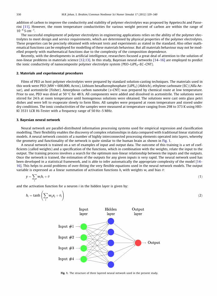
Neural network are parallel-distributed information processing systems used for empirical regression and classificationmodelling. Their flexibility enables the discovery of complex relationships in data compared with traditional linear statisticalmodels. A neural network consists of a number of highly interconnected processing elements operated into layers, wherebythe geometry and functionality of the network is quite similar to the human brain as shown in Fig. 1.

A neural network is trained on a set of examples of input and output data. The outcome of this training is a set of coef-ficients (called weights) and a specification of the functions, which in combination with the weights, relate the input to theoutput. The training process involves a search for the optimum non-linear relationship between the inputs and the outputs.Once the network is trained, the estimation of the outputs for any given inputs is very rapid. The neural network used hasbeen developed in a statistical framework, and is able to infer automatically the appropriate complexity of the model [14–16]. This helps to avoid problems of over-fitting the very flexible equations used in the neural network models. The outputvariable is expressed as a linear summation of activation functions hi with weights wi and bias h:

y ¼X

i

wihi þ h ð1Þ

and the activation function for a neuron i in the hidden layer is given by:

hi ¼ tanhX

j

wijxj þ hi

!ð2Þ

Fig. 1. The structure of three layered neural network used in the present study.

Table 1Conductivity values of different composition polymer electrolyte samples at elevated temperature.

PEO (wt.%) LiPF6 (wt.%) EC (wt.%) CNT (wt.%) Temp (K�1) Conductivity(S cm�1)

100 0 0 0 3.35402 �21.8472100 0 0 0 3.29870 �21.3619100 0 0 0 3.24517 �20.3656100 0 0 0 3.19336 �19.9035100 0 0 0 3.14317 �16.5504100 0 0 0 3.09454 �16.2984100 0 0 0 3.04739 �15.8950100 0 0 0 3.00165 �15.6734100 0 0 0 2.95727 �15.2018100 0 0 0 2.91418 �14.9211100 0 0 0 2.87233 �13.7957100 0 0 0 2.83166 �13.6085100 0 0 0 2.79213 �13.4302100 0 0 0 2.75368 �13.3027100 0 0 0 2.71628 �12.7967100 0 0 0 2.67989 �12.7717100 5 0 0 3.35402 �13.6310100 5 0 0 3.29870 �13.3716100 5 0 0 3.24517 �12.5725100 5 0 0 3.19336 �11.6943100 5 0 0 3.14317 �9.47620100 5 0 0 3.09454 �8.87486100 5 0 0 3.04739 �8.32398100 5 0 0 3.00165 �5.51057100 5 0 0 2.95727 �5.44313100 5 0 0 2.91418 �5.43535100 5 0 0 2.87233 �5.49597100 5 0 0 2.83166 �5.48116100 5 0 0 2.79213 �5.48859100 5 0 0 2.75368 �5.49597100 5 0 0 2.71628 �5.48859100 5 0 0 2.67989 �5.48116100 10 0 0 3.35402 �11.6154100 10 0 0 3.29870 �10.8729100 10 0 0 3.24517 �9.93411100 10 0 0 3.19336 �9.12474100 10 0 0 3.14317 �8.11720100 10 0 0 3.09454 �7.62530100 10 0 0 3.04739 �7.47011100 10 0 0 3.00165 �7.21983100 10 0 0 2.95727 �7.07010100 10 0 0 2.91418 �7.04993100 10 0 0 2.87233 �5.91742100 10 0 0 2.83166 �5.20805100 10 0 0 2.79213 �5.16630100 10 0 0 2.75368 �5.13286100 10 0 0 2.71628 �5.10347100 10 0 0 2.67989 �5.15405100 15 0 0 3.35402 �10.9114100 15 0 0 3.29870 �9.81122100 15 0 0 3.24517 �9.15581100 15 0 0 3.19336 �7.60044100 15 0 0 3.14317 �6.92684100 15 0 0 3.09454 �4.93584100 15 0 0 3.04739 �4.90384100 15 0 0 3.00165 �4.86741100 15 0 0 2.95727 �4.86234100 15 0 0 2.91418 �4.84352100 15 0 0 2.87233 �4.84352100 15 0 0 2.83166 �4.84179100 15 0 0 2.79213 �4.83658100 15 0 0 2.75368 �4.82257100 15 0 0 2.71628 �4.84179100 15 0 0 2.67989 �4.81727100 20 0 0 3.35402 �10.1023100 20 0 0 3.29870 �9.30859100 20 0 0 3.24517 �8.50518100 20 0 0 3.19336 �6.87561

(continued on next page)

M.R. Johan, S. Ibrahim / Commun Nonlinear Sci Numer Simulat 17 (2012) 329–340 331

Table 1 (continued)


100 20 0 0 3.14317 �5.10705100 20 0 0 3.09454 �5.06966100 20 0 0 3.04739 �5.06966100 20 0 0 3.00165 �5.05043100 20 0 0 2.95727 �5.05043100 20 0 0 2.91418 �5.05043100 20 0 0 2.87233 �5.06966100 20 0 0 2.83166 �5.06009100 20 0 0 2.79213 �5.06009100 20 0 0 2.75368 �5.09783100 20 0 0 2.71628 �5.09783100 20 0 0 2.67989 �5.16929100 20 5 0 3.35402 �9.73212100 20 5 0 3.29870 �9.07921100 20 5 0 3.24517 �8.18058100 20 5 0 3.19336 �7.84160100 20 5 0 3.14317 �7.57361100 20 5 0 3.09454 �7.40133100 20 5 0 3.04739 �7.22931100 20 5 0 3.00165 �7.16757100 20 5 0 2.95727 �7.11998100 20 5 0 2.91418 �7.11998100 20 5 0 2.87233 �7.11817100 20 5 0 2.83166 �7.21463100 20 5 0 2.79213 �7.28898100 20 5 0 2.75368 �7.20970100 20 5 0 2.71628 �7.10544100 20 5 0 2.67989 �7.00130100 20 10 0 3.35402 �8.85455100 20 10 0 3.29870 �8.08584100 20 10 0 3.24517 �7.53347100 20 10 0 3.19336 �7.30017100 20 10 0 3.14317 �6.97964100 20 10 0 3.09454 �5.56302100 20 10 0 3.04739 �5.36315100 20 10 0 3.00165 �5.33624100 20 10 0 2.95727 �5.37196100 20 10 0 2.91418 �5.36315100 20 10 0 2.87233 �5.35426100 20 10 0 2.83166 �5.36315100 20 10 0 2.79213 �5.35426100 20 10 0 2.75368 �5.37196100 20 10 0 2.71628 �5.36315100 20 10 0 2.67989 �5.40645100 20 15 0 3.35402 �8.48561100 20 15 0 3.29870 �7.96573100 20 15 0 3.24517 �7.76506100 20 15 0 3.19336 �7.57437100 20 15 0 3.14317 �7.39641100 20 15 0 3.09454 �7.30940100 20 15 0 3.04739 �7.23554100 20 15 0 3.00165 �7.17852100 20 15 0 2.95727 �7.13254100 20 15 0 2.91418 �7.09931100 20 15 0 2.87233 �6.95413100 20 15 0 2.83166 �6.91266100 20 15 0 2.79213 �6.89292100 20 15 0 2.75368 �6.79894100 20 15 0 2.71628 �6.75986100 20 15 0 2.67989 �6.67681100 20 15 1 3.35402 �8.42083100 20 15 1 3.29870 �7.69855100 20 15 1 3.24517 �7.38929100 20 15 1 3.19336 �7.19753100 20 15 1 3.14317 �7.04879100 20 15 1 3.09454 �7.00047100 20 15 1 3.04739 �6.93712100 20 15 1 3.00165 �6.85699100 20 15 1 2.95727 �6.72915


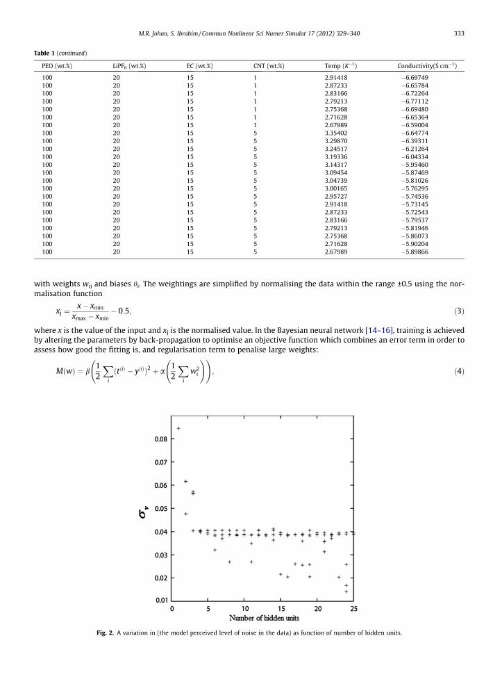
Table 1 (continued)


100 20 15 1 2.91418 �6.69749100 20 15 1 2.87233 �6.65784100 20 15 1 2.83166 �6.72264100 20 15 1 2.79213 �6.77112100 20 15 1 2.75368 �6.69480100 20 15 1 2.71628 �6.65364100 20 15 1 2.67989 �6.59004100 20 15 5 3.35402 �6.64774100 20 15 5 3.29870 �6.39311100 20 15 5 3.24517 �6.21264100 20 15 5 3.19336 �6.04334100 20 15 5 3.14317 �5.95460100 20 15 5 3.09454 �5.87469100 20 15 5 3.04739 �5.81026100 20 15 5 3.00165 �5.76295100 20 15 5 2.95727 �5.74536100 20 15 5 2.91418 �5.73145100 20 15 5 2.87233 �5.72543100 20 15 5 2.83166 �5.79537100 20 15 5 2.79213 �5.81946100 20 15 5 2.75368 �5.86073100 20 15 5 2.71628 �5.90204100 20 15 5 2.67989 �5.89866


with weights wij and biases hi. The weightings are simplified by normalising the data within the range ±0.5 using the nor-malisation function

xj ¼x� xmin

xmax � xmin� 0:5; ð3Þ

where x is the value of the input and xj is the normalised value. In the Bayesian neural network [14–16], training is achievedby altering the parameters by back-propagation to optimise an objective function which combines an error term in order toassess how good the fitting is, and regularisation term to penalise large weights:

MðwÞ ¼ b12

Xi

ðtðiÞ � yðiÞÞ2 þ a12

Xi

w2i

! !; ð4Þ

Fig. 2. A variation in (the model perceived level of noise in the data) as function of number of hidden units.


where b and a are complexity parameters which greatly influence the complexity of the model, t(i)and y( i)are the target andcorresponding output values for one example input from the training data x(i). The Bayesian framework for neural networkhas two further advantages. Firstly, the significance of the input variables is quantified automatically. Consequently, the sig-nificance perceived by the model of each input variable can be compared against existing theory. Secondly, the network’spredictions are accompanied by error bars which depend on the specific position in input space. These quantify the model’scertainty about its predictions.

4. Results and discussion

The database compiled from experimental data consists of 5 inputs including the chemical compositions and tempera-ture, as shown in Table 1.

Fig. 3. Test error as a function of the number of hidden units.

Fig. 4. Log predictive error as a function of the number of hidden units.


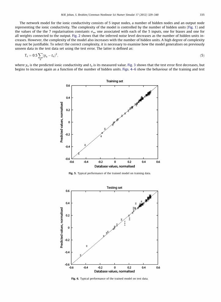
The network model for the ionic conductivity consists of 5 input nodes, a number of hidden nodes and an output noderepresenting the ionic conductivity. The complexity of the model is controlled by the number of hidden units (Fig. 1) andthe values of the the 7 regularisation constants rw, one associated with each of the 5 inputs, one for biases and one forall weights connected to the output. Fig. 2 shows that the inferred noise level decreases as the number of hidden units in-creases. However, the complexity of the model also increases with the number of hidden units. A high degree of complexitymay not be justifiable. To select the correct complexity, it is necessary to examine how the model generalises on previouslyunseen data in the test data set using the test error. The latter is defined as:

Te ¼ 0:5X

n

ðyn � tnÞ2; ð5Þ

where yn is the predicted ionic conductivity and tn is its measured value. Fig. 3 shows that the test error first decreases, butbegins to increase again as a function of the number of hidden units. Figs. 4–6 show the behaviour of the training and test

Fig. 5. Typical performance of the trained model on training data.

Fig. 6. Typical performance of the trained model on test data.


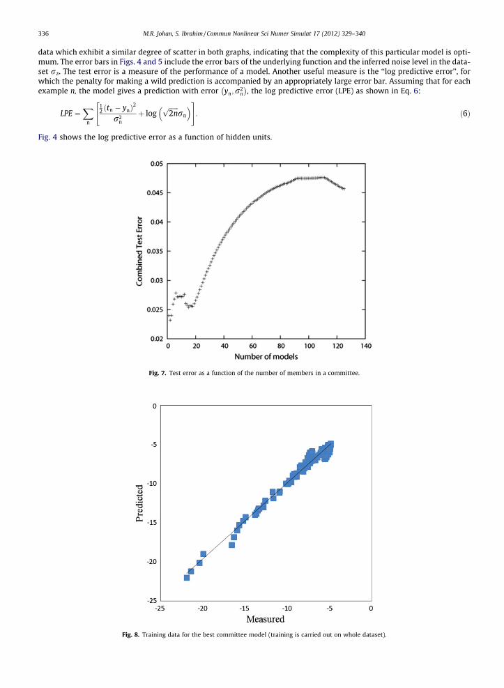
data which exhibit a similar degree of scatter in both graphs, indicating that the complexity of this particular model is opti-mum. The error bars in Figs. 4 and 5 include the error bars of the underlying function and the inferred noise level in the data-set rv. The test error is a measure of the performance of a model. Another useful measure is the ‘‘log predictive error’’, forwhich the penalty for making a wild prediction is accompanied by an appropriately large error bar. Assuming that for eachexample n, the model gives a prediction with error yn;r2

n

� �, the log predictive error (LPE) as shown in Eq. 6:

LPE ¼X

n

12 ðtn � ynÞ

2

r2n

þ logffiffiffiffiffiffi2np

rn

� �" #: ð6Þ

Fig. 4 shows the log predictive error as a function of hidden units.

Fig. 7. Test error as a function of the number of members in a committee.

Fig. 8. Training data for the best committee model (training is carried out on whole dataset).


When making predictions, MacKay [9–11] recommended the use of multiple good models instead of just one best model.This is called ‘forming a committee’. The committee prediction ~y is obtained using the expression:

~y ¼ 1L

Xi

yi; ð7Þ

where L is the size of the committee and yi is the estimate of a particular model i. The optimum size of the committee isdetermined from the validation error of the committee’s predictions using the test dataset. In the present analysis, a com-mittee of models is used to make more reliable predictions. The models are ranked according to their log predictive error.Committees are then formed by combining the predictions of best M models, where M gives the number of members in a

Fig. 9. Experimental and neural network curves of pure PEO conductivity according to temperature.

Fig. 10. Experimental and neural network curves of pure PEO–Salt conductivity according to temperature.


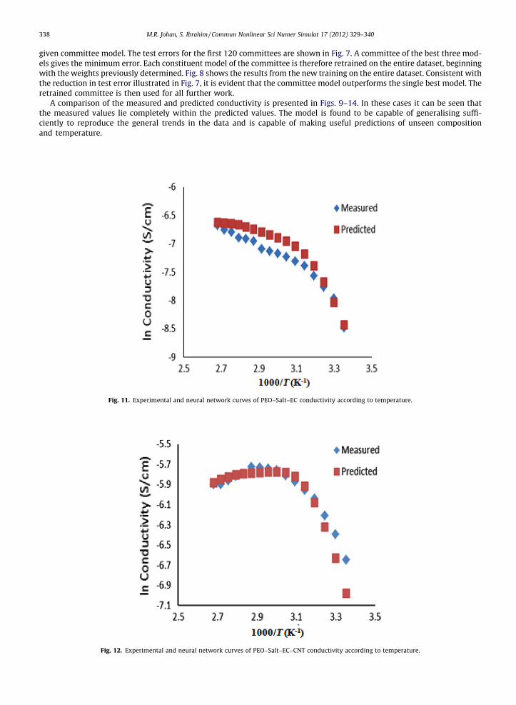
given committee model. The test errors for the first 120 committees are shown in Fig. 7. A committee of the best three mod-els gives the minimum error. Each constituent model of the committee is therefore retrained on the entire dataset, beginningwith the weights previously determined. Fig. 8 shows the results from the new training on the entire dataset. Consistent withthe reduction in test error illustrated in Fig. 7, it is evident that the committee model outperforms the single best model. Theretrained committee is then used for all further work.

A comparison of the measured and predicted conductivity is presented in Figs. 9–14. In these cases it can be seen thatthe measured values lie completely within the predicted values. The model is found to be capable of generalising suffi-ciently to reproduce the general trends in the data and is capable of making useful predictions of unseen compositionand temperature.

Fig. 11. Experimental and neural network curves of PEO–Salt–EC conductivity according to temperature.

Fig. 12. Experimental and neural network curves of PEO–Salt–EC–CNT conductivity according to temperature.

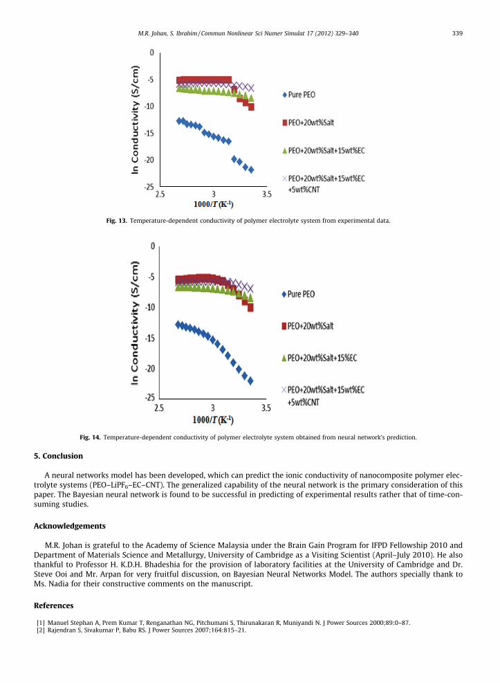
Fig. 13. Temperature-dependent conductivity of polymer electrolyte system from experimental data.

Fig. 14. Temperature-dependent conductivity of polymer electrolyte system obtained from neural network’s prediction.


5. Conclusion

A neural networks model has been developed, which can predict the ionic conductivity of nanocomposite polymer elec-trolyte systems (PEO–LiPF6–EC–CNT). The generalized capability of the neural network is the primary consideration of thispaper. The Bayesian neural network is found to be successful in predicting of experimental results rather that of time-con-suming studies.

Acknowledgements

M.R. Johan is grateful to the Academy of Science Malaysia under the Brain Gain Program for IFPD Fellowship 2010 andDepartment of Materials Science and Metallurgy, University of Cambridge as a Visiting Scientist (April–July 2010). He alsothankful to Professor H. K.D.H. Bhadeshia for the provision of laboratory facilities at the University of Cambridge and Dr.Steve Ooi and Mr. Arpan for very fruitful discussion, on Bayesian Neural Networks Model. The authors specially thank toMs. Nadia for their constructive comments on the manuscript.

References

[1] Manuel Stephan A, Prem Kumar T, Renganathan NG, Pitchumani S, Thirunakaran R, Muniyandi N. J Power Sources 2000;89:0–87.[2] Rajendran S, Sivakumar P, Babu RS. J Power Sources 2007;164:815–21.


[3] Rajendran S, Mahendran O, Kannan R. J Phys Chem Solids 2002;63:303–7.[4] Shanmukaraj D, Murugan R. J Power Sources 2005;149:90–5.[5] Ali AMMA, Yahya MZA, Bahron H, Subban RHY, Harun MK, Atan I. Mater Lett 2007;61:2026–9.[6] Appetecchi GB, Montanino M, Balducci A, Lux SF, Winterb M, Passerini S. J Power Sources 2009;192:599.[7] Saika D, Chen-Yang YM, Chen YT, Li YK, Lin SI. Desalin 2008;234:24–32.[8] Subban RHY, Arof AK. J Eur Polym 2004;40:1841–7.[9] Rupp B, Schmuck M, Balducci A, Winter M, Kern W. J Eur Polym 2008;44:2986–90.

[10] Ramesh S, Tai FY, Chia JS. Spectrochim Acta Part A 2008;69:670–5.[11] Appetecchi GB, Passerini S. Electrochim Act 2000;45:2139.[12] Bhadeshia HKDH. ISI J Int 1999;39(10):966–79.[13] Bhadeshia HKDH, Dimitriu RC, Forsik S, Park JH, Ryu JH. Mater Sci Technol 2009;25(4):04–510.[14] MacKay DJC. Neural Comput 1992;4:415–47.[15] MacKay DJC. Neural Comput 1992;4:448–72.[16] MacKay DJC. Network Comput Neural Syst 1995;6:469–505.

Optimization of neural network for ionic conductivity of nanocomposite solid polymer electrolyte...

Documents

Transcript of Optimization of neural network for ionic conductivity of nanocomposite solid polymer electrolyte...