Thermodynamic Modeling of Electrolyte Solutions
239
Thermodynamic Modeling of Electrolyte Solutions: Bridging Classical Macroscopic Models and Molecular Simulations by Sina Hassanjani Saravi A Dissertation In Chemical Engineering Submitted to the Graduate Faculty of Texas Tech University in Partial Fulfilment of the Requirements for the Degree of DOCTOR OF PHILOSOPHY Approved Dr. Chau-Chyun Chen Chair of Committee Dr. Rajesh Khare Dr. Fazle Hussain Dr. Sindee L. Simon Mark Sheridan Dean of the Graduate School August 2019
-
Upload
khangminh22 -
Category
Documents
-
view
0 -
download
0
Transcript of Thermodynamic Modeling of Electrolyte Solutions
Thermodynamic Modeling of Electrolyte Solutions: Bridging Classical Macroscopic
Models and Molecular Simulations
by
Sina Hassanjani Saravi
A Dissertation
In
Chemical Engineering
Submitted to the Graduate Faculty of Texas Tech University in
Partial Fulfilment of the Requirements for
the Degree of
DOCTOR OF PHILOSOPHY
Approved
Dr. Chau-Chyun Chen Chair of Committee
Dr. Rajesh Khare
Dr. Fazle Hussain
Dr. Sindee L. Simon
Mark Sheridan Dean of the Graduate School
August 2019

Copyright 2019, Sina Hassanjani Saravi

Mom, Dad, I dedicate this dissertation to you…
Thank you for giving me the ambition to believe that nothing is
impossible

Texas Tech University, Sina Hassanjani Saravi, August 2019
ii
ACKNOWLEDGEMENTS
“Be Concise!”, “Sometimes More is Less!”, and a magical yet simple one-word,
“Think!”, may not seem like life-changing mottos, but they are a few short examples of
countless impactful advice I have received from my advisor, Dr. Chau-Chyun Chen, during
my PhD. Dr. Chen, not only have you been the most hardworking person I’ve ever seen,
but you have also been the greatest mentor, teacher, and an impeccable role model. Without
your mentorship, I would not have become the person I am and the person I wish to
become. Forever, I will be grateful to you.
I’d like to express my sincerest gratitude to Dr. Rajesh Khare. You are a fantastic
teacher! I learned statistical mechanics and MD simulations from you and that opened for
me a whole new world of research which made me even more enthusiastic to pursue
science. Whether giving a lecture, reviewing manuscripts, or engaging in a scientific
discussion, you’ve shown what an amazingly professional and intellectual person you are.
I would also like to thank Dr. Fazle Hussain who gave me the motivation to look at
problems profoundly until I, as he would say, “Own them!”. I’d like to express my
appreciation to Dr. Simon who taught me ‘The Advanced Thermodynamics’ course in my
very first semester as a PhD student. Also, her invaluable comments and suggestions during
my qualifying exam helped me refine my work. I would also like to acknowledge the
financial support of the Jack Maddox Distinguished Engineering Chair Professorship in
Sustainable Energy, sponsored by the J.F Maddox Foundation, for making my PhD
possible.
I want to thank one of my best friends, colleagues, and lab mates, Dr. Ashwin
Ravichandran. He is unbelievably smart, humble, and sophisticated; or at least these are

Texas Tech University, Sina Hassanjani Saravi, August 2019
iii
what he says he is! Kidding aside, it’s been a great journey both in our friendship and in
working together. I wish him an amazing future, in personal life and science!
Islam, Harnoor, Nazir, Hla, Toni, Tanveer, Yuan, Matt, Pradeep, Yifan, Meng, Yue,
Rajasi, Samira, Sanjoy, and last but not least, my buddy Michael! Not only have you all
been my dearest lab mates and friends, you’ve been incredibly nice and supportive. What
an environment! What a great group of people! I will never forget you all. Also, a special
thanks goes to Dr. Md Islam for being such a selflessly helpful and supportive friend.
Words cannot describe the extent of my gratitude toward my small, but warm and
loving family: My mom, Homeyra Barimani, my dad, Ahmad Hassanjani Saravi, and my
only brother, Amirhossein Hassanjani Saravi. Mom! thanks for reading to me the fifth
grade’s science book as bedtime stories when I was five! You are the reason I pursued
science as a career. Dad! Thanks for teaching me math and motivating me to become an
engineer just like yourself! Amirhossein, thanks for being the best ‘Dadashi’ in the world.
Hanging out with you and talking about funny stuff for hours are among my favorite
“activities”.
Last, my wonderful wife, Soraya (and soon to be Dr. Soraya Honarparvar) whose love
and support have shaped me into the person I am. Year after year, it becomes clearer to me
what an unbelievably lucky person I am to have you in my life. For almost a decade, you’ve
been my best classmate, research collaborator, and critique, but beyond all, you’ve been
my best friend. Thank you for believing in me and making such a big deal out of my
achievements and acting like nothing happened in my failures!
Texas Tech University, Sina Hassanjani Saravi, August 2019
iv
TABLE OF CONTENTS
ACKNOWLEDGEMENTS ............................................................................................. ii
ABSTRACT ...................................................................................................................... ix
LIST OF TABLES .......................................................................................................... xii
LIST OF FIGURES ....................................................................................................... xiv
1. INTRODUCTION .....................................................................................................1
1.1. Background ...........................................................................................................1
1.2. Content of Dissertation .........................................................................................6
1.3. References ............................................................................................................8
2. THERMODYNAMIC MODELING OF AQUEOUS ELECTROLYTE SYSTEMS .................................................................................11
2.1. Abstract ...............................................................................................................11
2.2. Electrolyte Systems ............................................................................................12
2.3. Basic Thermodynamics of Electrolytes ..............................................................13
2.4. Thermodynamics of Vapor-Liquid Equilibrium ................................................16
2.5. Thermodynamics of Salt Precipitation ...............................................................18
2.6. Modeling Electrolyte Systems ............................................................................20
2.7. Thermodynamic Models for Electrolytes ...........................................................22
Texas Tech University, Sina Hassanjani Saravi, August 2019
v
2.8. Example 1. Modeling Aqueous Single Electrolytes: H2O-BaCl2 Binary Solution ...................................................................................................28
2.9. Example 2: Modeling BaSO4 (s) Precipitation in a Brine Solution .....................34
2.10. Looking Ahead .................................................................................................38
2.11. Acknowledgments ............................................................................................39
2.12. References ........................................................................................................40
3. THERMODYNAMIC MODELING OF HCl-H2O BINIARY SYSTEM WITH SYMMETRIC ELECTROLYTE NRTL MODEL ................43
3.1. Abstract ...............................................................................................................43
3.2. Introduction ........................................................................................................44
3.3. Thermodynamic Framework ..............................................................................49
Solution Chemistry and Hydration ............................................................. 49
Vapor-Liquid-Liquid Equilibrium .............................................................. 51
Symmetric Electrolyte NRTL Model.......................................................... 53
Calorimetric Properties ............................................................................... 55
3.4. The Modeling Approach .....................................................................................55
Model Parameters ....................................................................................... 55
Experimental Data ...................................................................................... 59
Data Treatment, Regression, and Optimization Method ............................ 67
3.5. Results and Discussion .......................................................................................69
3.6. Conclusions ........................................................................................................83
3.7. Acknowledgements ............................................................................................84
Texas Tech University, Sina Hassanjani Saravi, August 2019
vi
3.8. References ..........................................................................................................85
4. BRIDGING TWO-LIQUID THEORY WITH MOLECULAR SIMULATIONS FOR ELECTROLYTES: AN INVESTIGATION OF AQUOUES NaCl SOLUTION .........................................................................93
4.1. Abstract ...............................................................................................................93
4.2. Introduction ........................................................................................................94
4.3. Theoretical Background .....................................................................................97
Two-Liquid Theory for Electrolytes ........................................................... 97
The Cation-Centered Domain ................................................................... 100
The Anion-Centered Domain .................................................................... 102
The Molecule-Centered Domain............................................................... 103
4.4. Calculation Methodology .................................................................................104
4.5. Molecular Simulations ......................................................................................106
4.6. Binary Interaction Parameters from Regression ...............................................108
4.7. Results and Discussions ...................................................................................109
Regression of Experimental and Simulation Data .................................... 109
Interpretation of the Molecular Quantities in the Framework of eNRTL ....................................................................................................... 109
Prediction of Binary Interaction Parameters from MD Simulation and Validation of the eNRTL Assumptions .............................................. 116
Phase Equilibrium Predictions .................................................................. 119
4.8. Conclusions ......................................................................................................122
4.9. Acknowledgments ............................................................................................124
4.10. Supporting Information ..................................................................................125
Texas Tech University, Sina Hassanjani Saravi, August 2019
vii
Discussions Regarding the Nature of Interactions in the Ion- Centered Domains ..................................................................................... 131
4.11. References ......................................................................................................133
5. PRDICTING PHASE EQUILIBRIA PROPERTIES OF ELECTRLYTE SOLUTIONS BY COMBINING A CLASSICAL THERMODYNAMIC MODEL AND MOLECULAR SIMULATIONS: AQUOUES XCl2 SOLUTIONS, (X=Ba, Sr, Ca, Mg) ..........138
5.1. Abstract .............................................................................................................138
5.2. Introduction ......................................................................................................140
5.3. Theoretical Framework ....................................................................................144
Thermodynamics Background of the eNRTL Model ............................... 144
Relating the τ Parameters to Liquid Structure and Energetic Interaction Quantities ................................................................................ 148
The τ Parameter in a Cation-Centered Domain ........................................ 148
The τ Parameter in an Anion-Centered Domain ....................................... 151
The τ Parameters in a Molecule-Centered Domain .................................. 151
5.4. Quantification of the τ Parameters from Molecular Simulations .....................153
The Effective Molecular Diameters (σ) .................................................... 153
The First Neighbor Shell Radii (R) ........................................................... 153
The Energetic Interactions (ϵ) ................................................................... 154
The Nonrandomness Factor (α) ................................................................ 157
The Binary Interaction Parameters (τ) ...................................................... 158
5.5. Molecular Simulation Details ...........................................................................158
5.6. Results and Discussion .....................................................................................159
The Results of the Physical Quantities of the Aqueous Solutions from MD Simulations ................................................................................ 160
Calculating the Binary Interaction Parameters from MD Simulations ................................................................................................ 173
Texas Tech University, Sina Hassanjani Saravi, August 2019
viii
Defining Effective Binary Interaction Parameters from MD Simulations ................................................................................................ 174
Predicting Phase Equilibria Properties from τ Parameters Obtained via MD Simulations ................................................................... 181
5.7. Conclusions ......................................................................................................190
5.8. Acknowledgements ..........................................................................................191
5.9. Supplementary Information ..............................................................................192
5.10. References ......................................................................................................213
6. CONCLUSIONS AND FUTURE WORK ...........................................................217
Texas Tech University, Sina Hassanjani Saravi, August 2019
ix
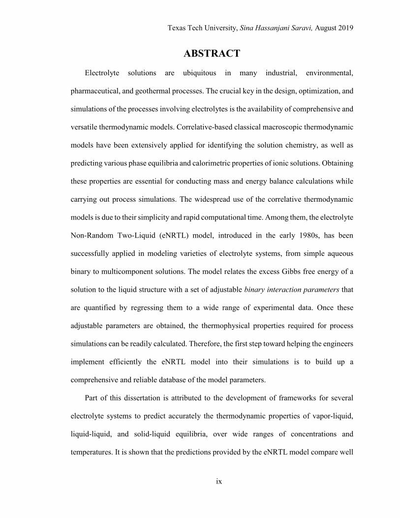
ABSTRACT Electrolyte solutions are ubiquitous in many industrial, environmental,
pharmaceutical, and geothermal processes. The crucial key in the design, optimization, and
simulations of the processes involving electrolytes is the availability of comprehensive and
versatile thermodynamic models. Correlative-based classical macroscopic thermodynamic
models have been extensively applied for identifying the solution chemistry, as well as
predicting various phase equilibria and calorimetric properties of ionic solutions. Obtaining
these properties are essential for conducting mass and energy balance calculations while
carrying out process simulations. The widespread use of the correlative thermodynamic
models is due to their simplicity and rapid computational time. Among them, the electrolyte
Non-Random Two-Liquid (eNRTL) model, introduced in the early 1980s, has been
successfully applied in modeling varieties of electrolyte systems, from simple aqueous
binary to multicomponent solutions. The model relates the excess Gibbs free energy of a
solution to the liquid structure with a set of adjustable binary interaction parameters that
are quantified by regressing them to a wide range of experimental data. Once these
adjustable parameters are obtained, the thermophysical properties required for process
simulations can be readily calculated. Therefore, the first step toward helping the engineers
implement efficiently the eNRTL model into their simulations is to build up a
comprehensive and reliable database of the model parameters.
Part of this dissertation is attributed to the development of frameworks for several
electrolyte systems to predict accurately the thermodynamic properties of vapor-liquid,
liquid-liquid, and solid-liquid equilibria, over wide ranges of concentrations and
temperatures. It is shown that the predictions provided by the eNRTL model compare well
Texas Tech University, Sina Hassanjani Saravi, August 2019
x
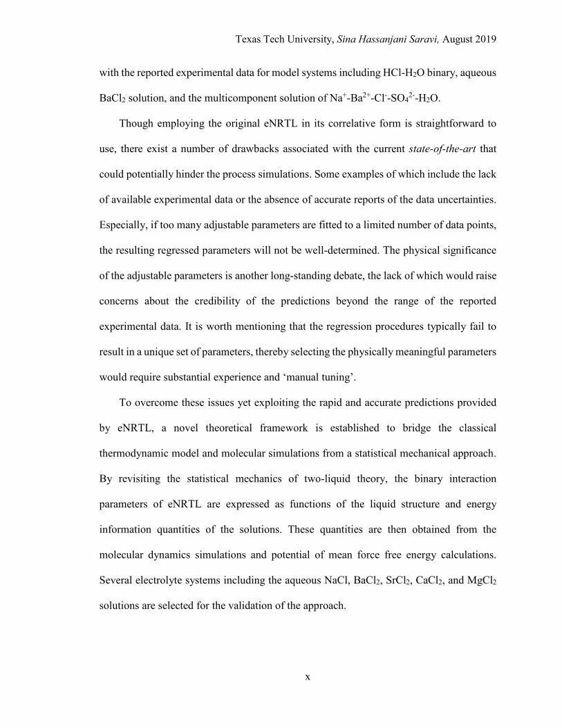
with the reported experimental data for model systems including HCl-H2O binary, aqueous
BaCl2 solution, and the multicomponent solution of Na+-Ba2+-Cl--SO42--H2O.
Though employing the original eNRTL in its correlative form is straightforward to
use, there exist a number of drawbacks associated with the current state-of-the-art that
could potentially hinder the process simulations. Some examples of which include the lack
of available experimental data or the absence of accurate reports of the data uncertainties.
Especially, if too many adjustable parameters are fitted to a limited number of data points,
the resulting regressed parameters will not be well-determined. The physical significance
of the adjustable parameters is another long-standing debate, the lack of which would raise
concerns about the credibility of the predictions beyond the range of the reported
experimental data. It is worth mentioning that the regression procedures typically fail to
result in a unique set of parameters, thereby selecting the physically meaningful parameters
would require substantial experience and ‘manual tuning’.
To overcome these issues yet exploiting the rapid and accurate predictions provided
by eNRTL, a novel theoretical framework is established to bridge the classical
thermodynamic model and molecular simulations from a statistical mechanical approach.
By revisiting the statistical mechanics of two-liquid theory, the binary interaction
parameters of eNRTL are expressed as functions of the liquid structure and energy
information quantities of the solutions. These quantities are then obtained from the
molecular dynamics simulations and potential of mean force free energy calculations.
Several electrolyte systems including the aqueous NaCl, BaCl2, SrCl2, CaCl2, and MgCl2
solutions are selected for the validation of the approach.
Texas Tech University, Sina Hassanjani Saravi, August 2019
xi
The results for the binary interaction parameters, together with the predictions of the
phase equilibria properties from the MD simulations are in satisfactory agreement with
those obtained from the regression. It is demonstrated, for the first time, that the eNRTL
model can be rendered completely predictive, circumventing the inherent shortcomings
associated with correlation. The established method, with further refinement and
improvement, can be broadly utilized for rapid predictions of the thermodynamic
properties in industrial process design.
Texas Tech University, Sina Hassanjani Saravi, August 2019
xii
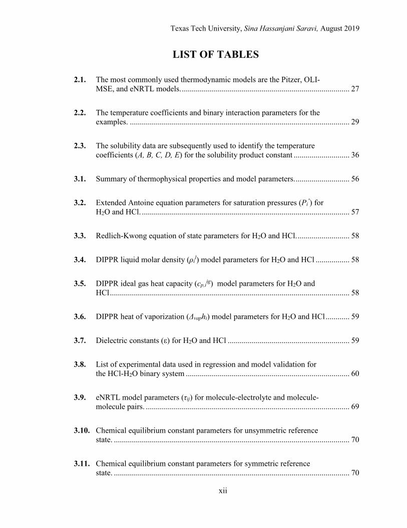
LIST OF TABLES
2.1. The most commonly used thermodynamic models are the Pitzer, OLI-MSE, and eNRTL models. .................................................................................... 27
2.2. The temperature coefficients and binary interaction parameters for the examples. .............................................................................................................. 29
2.3. The solubility data are subsequently used to identify the temperature coefficients (A, B, C, D, E) for the solubility product constant ............................ 36
3.1. Summary of thermophysical properties and model parameters. ........................... 56
3.2. Extended Antoine equation parameters for saturation pressures (Piº) for
H2O and HCl. ........................................................................................................ 57
3.3. Redlich-Kwong equation of state parameters for H2O and HCl. .......................... 58
3.4. DIPPR liquid molar density (ρil) model parameters for H2O and HCl ................. 58
3.5. DIPPR ideal gas heat capacity (cp,iig) model parameters for H2O and
HCl ........................................................................................................................ 58
3.6. DIPPR heat of vaporization (Δvaphi) model parameters for H2O and HCl ............ 59
3.7. Dielectric constants (ε) for H2O and HCl ............................................................. 59
3.8. List of experimental data used in regression and model validation for the HCl-H2O binary system .................................................................................. 60
3.9. eNRTL model parameters (τij) for molecule-electrolyte and molecule-molecule pairs. ...................................................................................................... 69
3.10. Chemical equilibrium constant parameters for unsymmetric reference state. ...................................................................................................................... 70
3.11. Chemical equilibrium constant parameters for symmetric reference state. ...................................................................................................................... 70
Texas Tech University, Sina Hassanjani Saravi, August 2019
xiii
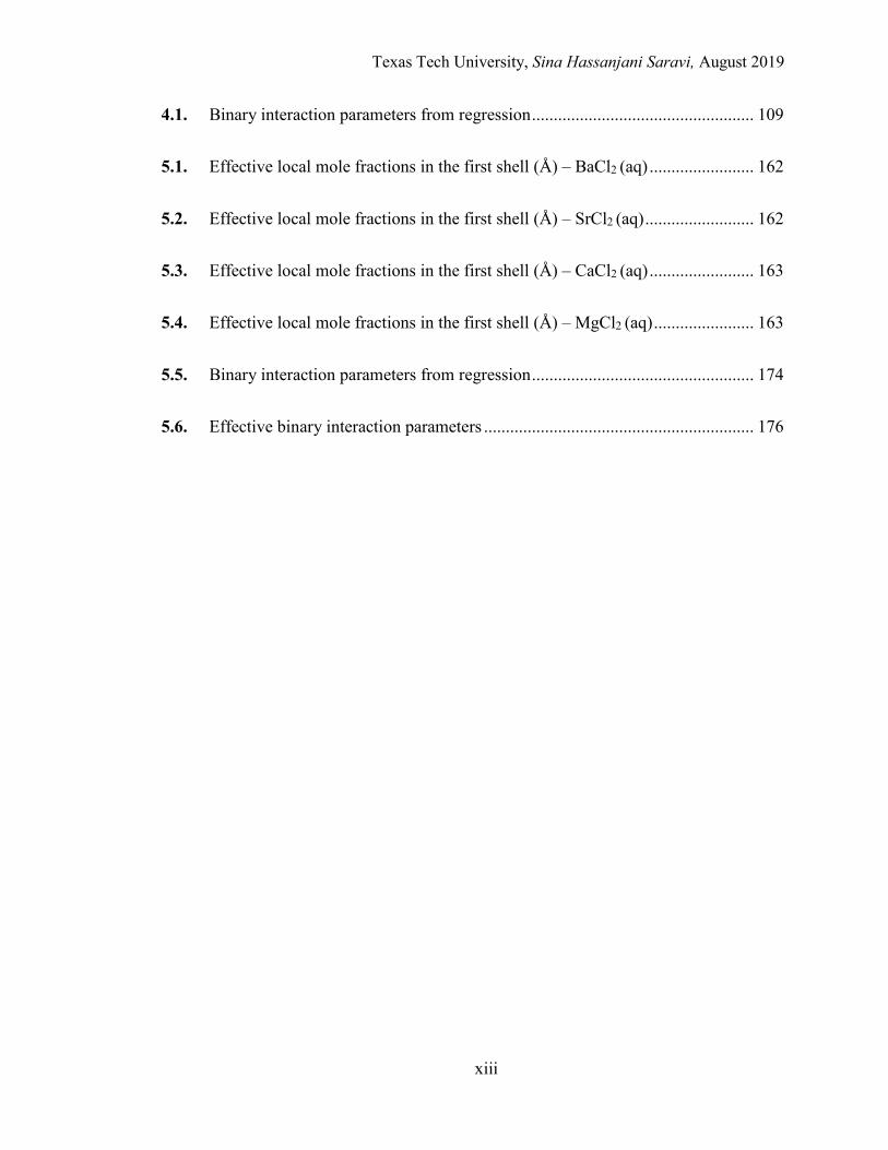
4.1. Binary interaction parameters from regression ................................................... 109
5.1. Effective local mole fractions in the first shell (Å) – BaCl2 (aq) ........................ 162
5.2. Effective local mole fractions in the first shell (Å) – SrCl2 (aq) ......................... 162
5.3. Effective local mole fractions in the first shell (Å) – CaCl2 (aq) ........................ 163
5.4. Effective local mole fractions in the first shell (Å) – MgCl2 (aq) ....................... 163
5.5. Binary interaction parameters from regression ................................................... 174
5.6. Effective binary interaction parameters .............................................................. 176
Texas Tech University, Sina Hassanjani Saravi, August 2019
xiv
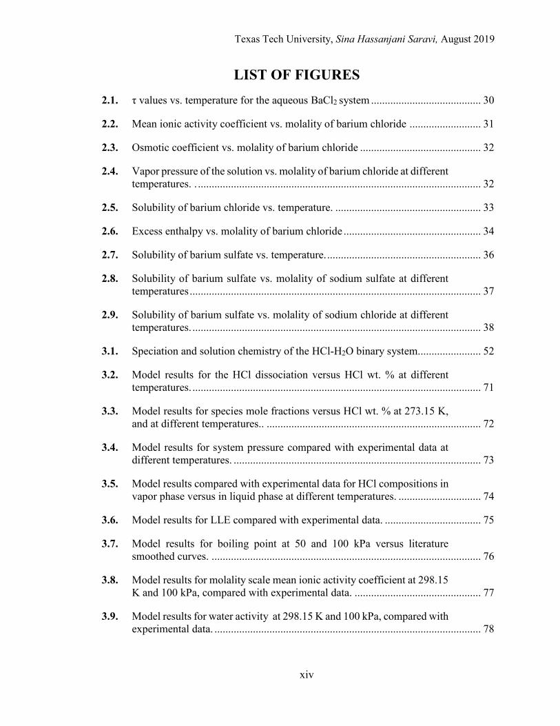
LIST OF FIGURES 2.1. τ values vs. temperature for the aqueous BaCl2 system ........................................ 30
2.2. Mean ionic activity coefficient vs. molality of barium chloride .......................... 31
2.3. Osmotic coefficient vs. molality of barium chloride ............................................ 32
2.4. Vapor pressure of the solution vs. molality of barium chloride at different temperatures. . ....................................................................................................... 32
2.5. Solubility of barium chloride vs. temperature. ..................................................... 33
2.6. Excess enthalpy vs. molality of barium chloride .................................................. 34
2.7. Solubility of barium sulfate vs. temperature. ........................................................ 36
2.8. Solubility of barium sulfate vs. molality of sodium sulfate at different temperatures .......................................................................................................... 37
2.9. Solubility of barium sulfate vs. molality of sodium chloride at different temperatures. ......................................................................................................... 38
3.1. Speciation and solution chemistry of the HCl-H2O binary system. ...................... 52
3.2. Model results for the HCl dissociation versus HCl wt. % at different temperatures. ......................................................................................................... 71
3.3. Model results for species mole fractions versus HCl wt. % at 273.15 K, and at different temperatures.. .............................................................................. 72
3.4. Model results for system pressure compared with experimental data at different temperatures. .......................................................................................... 73
3.5. Model results compared with experimental data for HCl compositions in vapor phase versus in liquid phase at different temperatures. .............................. 74
3.6. Model results for LLE compared with experimental data. ................................... 75
3.7. Model results for boiling point at 50 and 100 kPa versus literature smoothed curves. .................................................................................................. 76
3.8. Model results for molality scale mean ionic activity coefficient at 298.15 K and 100 kPa, compared with experimental data. .............................................. 77
3.9. Model results for water activity at 298.15 K and 100 kPa, compared with experimental data. ................................................................................................. 78
Texas Tech University, Sina Hassanjani Saravi, August 2019
xv
3.10. Model results for osmotic coefficient at 298.15 K and 100 kPa, compared with experimental data. ......................................................................................... 79
3.11. Model results for excess enthalpy (kJ/mol) with unsymmetric reference state at 298.15 K and 100 kPa, compared with experimental data. Also shown, the boiling-point limit and the extended trend for excess enthalpy. ................................................................................................................ 80
3.12. Model results for liquid molar heat capacity of dilute solutions (kJ/kmol.K) and experimental data at different temperatures. ............................. 81
3.13. Model results for liquid molar heat capacity (kJ/kmol.K) compared with experimental data and smoothed curves at different temperatures. ...................... 82
3.14. Merkel enthalpy-concentration chart (Btu/lb) and extended trend lines at different temperatures.. ......................................................................................... 83
4.1. Schematic describing the three possible local molecular domains considered by the eNRTL model ........................................................................ 100
4.2. The local mole fraction of different species in the three domains for the 4 mol/kg aqueous NaCl solution at 298.15 K. .................................................... 114
4.3. The local mole fraction of different species in the three domains for the 4 mol/kg aqueous NaCl solution at 298.15 K. .................................................... 115
4.4. The local mole fraction of different species in the three domains for the 4 mol/kg aqueous NaCl solution at 298.15 K. .................................................... 116
4.5. The binary interaction parameters for the aqueous NaCl solution at 298.15 K. ............................................................................................................. 118
4.6. Comparison of the mean ionic activity coefficients of aqueous NaCl solution phase behavior at 298.15 K between MD simulations and regression results. ................................................................................................ 121
4.7. Comparison of aqueous NaCl solution phase behavior (vapor pressure and excess Gibbs free energy) at 298.15 K between MD simulations and regression results. ................................................................................................ 122
5.1. Schematic configurations of the three local domains as hypothesized by the eNRTL model. .............................................................................................. 145
5.2. The effective mole fractions calculated from the MD simulations for the aqueous BaCl2 solution at 4 m — Cation-centered domain. .............................. 164
5.3. The effective mole fractions calculated from the MD simulations for the aqueous BaCl2 solution at 4 m — Anion-centered domain ................................ 165
Texas Tech University, Sina Hassanjani Saravi, August 2019
xvi
5.4. The effective mole fractions calculated from the MD simulations for the aqueous BaCl2 solution at 4 m — Molecule-centered domain ........................... 166
5.5. A schematic of the potential of mean force for the 4 m aqueous MgCl2 solution at 298.15 K. PMF of Mg2+ around a center Clˉ and water around a center water. ..................................................................................................... 167
5.6. A schematic of the potential of mean force for the 4 m aqueous MgCl2 solution at 298.15 K. PMF of Mg2+ around a center water and Clˉ around a center water. ..................................................................................................... 168
5.7. Potential of mean force of the Ba2+-Cl- pair in aqueous BaCl2 solution. The potential of mean force of the anion-cation pair at the concentration of 2 m from the local van der Waals, electrostatics, and the combination of both local and electrostatics contributions...................................................... 170
5.8. Potential of mean force of the Ba2+-Cl- pair in aqueous BaCl2 solution. The potential of mean force of the anion-cation pair at the concentration of 6 m from the local van der Waals, electrostatics, and the combination of both local and electrostatics contributions. ................................................... 171
5.9. Potential of mean force of the Ba2+-Cl- pair in aqueous BaCl2 solution. The potential of mean force attributed to the electrostatic forces calculated from the Debye-Hückel theory at different concentrations. .............. 172
5.10. The effective binary interaction parameters for the aqueous BaCl2 solution at 298.15 K. Regression vs. MD simulations. . ..................................... 177
5.11. The effective binary interaction parameters for the aqueous SrCl2 solution at 298.15 K. Regression vs. MD simulations. ....................................... 178
5.12. The effective binary interaction parameters for the aqueous CaCl2 solution at 298.15 K. Regression vs. MD simulations. ....................................... 179
5.13. The effective binary interaction parameters for the aqueous MgCl2 solution at 298.15 K. Regression vs. MD simulations. ....................................... 180
5.14. Mean ionic activity coefficients for the entire concentration range in the aqueous BaCl2 solution at 298.15 K. Experimental data, Regression, and MD simulations. ................................................................................................. 183
5.15. Mean ionic activity coefficients for the entire concentration range in the aqueous SrCl2 solution at 298.15 K. Experimental data, Regression, and MD simulations. ................................................................................................ 184
5.16. Mean ionic activity coefficients for the entire concentration range in the aqueous CaCl2 solution at 298.15 K. Experimental data, Regression, and MD simulations ................................................................................................... 185
Texas Tech University, Sina Hassanjani Saravi, August 2019
xvii
5.17. Mean ionic activity coefficients for the entire concentration range in the aqueous MgCl2 solution at 298.15 K. Experimental data, Regression, and MD simulations. .................................................................................................. 186
5.18. Vapor pressure and excess Gibbs free energy in the entire concentration range in the aqueous BaCl2 solution at 298.15 K. Regression vs. MD simulations. ......................................................................................................... 187
5.19. Vapor pressure and excess Gibbs free energy in the entire concentration range in the aqueous SrCl2 solution at 298.15 K. Regression vs. MD simulations. ......................................................................................................... 188
5.20. Vapor pressure and excess Gibbs free energy in the entire concentration range in the aqueous CaCl2 solution at 298.15 K. Regression vs. MD simulations. ......................................................................................................... 189
5.21. Vapor pressure and excess Gibbs free energy in the entire concentration range in the aqueous MgCl2 solution at 298.15 K. Regression vs. MD simulations. ......................................................................................................... 190
Texas Tech University, Sina Hassanjani Saravi, August 2019
1
CHAPTER 1. INTRODUCTION
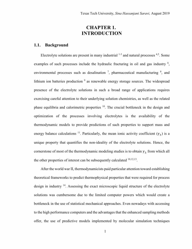
1.1. Background
Electrolyte solutions are present in many industrial 1-3 and natural processes 4,5. Some
examples of such processes include the hydraulic fracturing in oil and gas industry 6,
environmental processes such as desalination 7, pharmaceutical manufacturing 8, and
lithium ion batteries production 9 as renewable energy storage sources. The widespread
presence of the electrolyte solutions in such a broad range of applications requires
exercising careful attention to their underlying solution chemistries, as well as the related
phase equilibria and calorimetric properties 10. The crucial bottleneck in the design and
optimization of the processes involving electrolytes is the availability of the
thermodynamic models to provide predictions of such properties to support mass and
energy balance calculations 11. Particularly, the mean ionic activity coefficient (𝛾𝛾±) is a
unique property that quantifies the non-ideality of the electrolyte solutions. Hence, the
cornerstone of most of the thermodynamic modeling studies is to obtain 𝛾𝛾± from which all
the other properties of interest can be subsequently calculated 10,12,13.
After the world war II, thermodynamicists paid particular attention toward establishing
theoretical frameworks to predict thermophysical properties that were required for process
design in industry 14. Assessing the exact microscopic liquid structure of the electrolyte
solutions was cumbersome due to the limited computer powers which would create a
bottleneck in the use of statistical mechanical approaches. Even nowadays with accessing
to the high performance computers and the advantages that the enhanced sampling methods
offer, the use of predictive models implemented by molecular simulation techniques
Texas Tech University, Sina Hassanjani Saravi, August 2019
2
demands expensive computational time, making it inefficient to directly utilize them in
process simulations 15. That shifted the paradigm toward developing semi-empirical and
empirical correlative models for industrial process design to compensate for the ambiguous
structural characteristics of the ionic solutions 16. Most of these models are treated as
perturbation-like theories to express the excess Gibbs free energy of the electrolyte
solutions as a combination of the contributions of long-range electrostatic and short-range
van der Waals forces. Among the most widely used such models, Pitzer 17, OLI-MSE 18,
and the electrolyte Non-Random Two-Liquid (eNRTL) 12,19-21 models have been broadly
adopted and used by the industry due to their versatility and relatively inexpensive
computational procedures. A rather succinct description of these models is discussed in the
next chapter along with their advantages and disadvantages.
The eNRTL model introduced in 1982 by Chen et al. 19 has shown to provide the most
successful predictions considering the limited number of adjustable parameters, while
covering the widest ranges of ionic species, concentrations, and temperatures. The model
uses the local composition concept described by the original Non-Random Two-Liquid
theory of Brandani and Prausnitz 16 to account for the short-range interactions. The long-
range electrostatic forces, on the other hand, are expressed by a modified semi-empirical
version of the original Debye-Hückel 22 theory, i.e., Pitzer-Debye-Hückel 12,19-21.
Combining the two contributions, the excess Gibbs free energy of the electrolyte solutions
are obtained, from which the activity coefficients and consequently other thermophysical
properties can be acquired. Only two adjustable binary interaction parameters are needed
to account for the interactions between any pair of species, i.e., ion-ion, ion-molecule, or

Texas Tech University, Sina Hassanjani Saravi, August 2019
3
molecule-molecule, which renders the model considerably more applicable compared to
the other correlative models.
The limited number of parameters employed by the eNRTL model is a good indication
of not overestimating the physical significance of the model parameters and hence not
overfitting the experimental data. The concerns about using too many adjustable
parameters in macroscopic correlative models are twofold; first, the parameters will not be
well-determined if the number of the experimental data used for regression is insufficient
compared to the number of adjustable parameters. Second, though the interpolations could
be accurate, the extrapolations would not be reliable in a model where the adjustable
parameters are not physically well-defined. A recent molecular dynamics simulations study
of the aqueous NaCl solution by Hossain et al. 13 demonstrated that the mean ionic activity
coefficients predicted by the eNRTL model show an asymptotic behavior at supersaturated
solutions, compared to those predicted by the Pitzer model which show a rapid divergence
in high concentration regions. Such findings confirm the superiority of the extrapolations
predicted by the eNRTL model compared to those of Pitzer, while employing far fewer
number of adjustable parameters.
Despite the discussed advantages of the eNRTL model over the Pitzer model, lacking
a comprehensive library of the regressed binary interaction parameters has limited the
ability of broadly utilizing the eNRTL model in process simulations. Therefore, the first
goal of this dissertation, as part of building up a comprehensive database of the eNRTL
model parameters, is to establish thermodynamic frameworks for variety of ionic solutions
for providing accurate predictions of phase equilibria behavior, calorimetric, and speciation
properties. The electrolyte systems studied here cover from binary aqueous HCl solutions
Texas Tech University, Sina Hassanjani Saravi, August 2019
4
to binary and multicomponent solid-liquid equilibrium systems of, respectively, aqueous
BaCl2 and Na+-Ba2+-Cl--SO42--H2O solutions, which are covered in Chapters 2 and 3.
Furthermore, while not presented in this dissertation, several other multicomponent
systems have also been rigorously studied and reported in two publications to which the
reader is referred for further information 23,24.
Although the current state-of-the-art in quantifying the binary interaction parameters
through regression is straightforward and rapidly performed, there are a number of
limitations that need to be addressed. Lack of the available or reliable experimental data is
the foremost issue that one could encounter while performing regression. Even when data
are available, the inconsistency between the reported data points from different references,
the lack of reported uncertainties, and the inevitable arbitrary treatment of the data could
impose obstacles in carrying out an objective regression procedure. Furthermore, the
minimization functions employed in the regression seldom result in a unique set of
parameters. Thereby selecting the physically relevant parameters could be ambiguous and
requires manual tuning or arbitrary choosing from multiple solutions based on experience
or the quality of the yielded predictions.
Parallel to the classical correlative-based thermodynamic models, another path has
also been pursued by researchers to calculate the thermophysical properties of electrolyte
solutions from statistical mechanical approaches. Molecular dynamics (MD) and Monte
Carlo (MC) simulations have helped the researchers to study the liquid structure and free
energy profiles in electrolyte solutions. Many molecular simulation studies reported
predictions of the fundamental properties of electrolytes such as the chemical potential,
Gibbs free energy, and activity coefficients 25-31. Though valuable insight has been gained,
Texas Tech University, Sina Hassanjani Saravi, August 2019
5
due to the expensive computations required for implementing advanced simulation
techniques, the use of molecular simulations in process design has been limited.
In order to exploit the advantages of both correlative and predictive approaches while
circumventing the associated shortcomings discussed above, it is desired to develop a
hybrid methodology by which the adjustable parameters of the classical models can be
obtained from a completely predictive method. Such an approach has seldom been pursued
by researchers in the past. A few attempts for connecting the classical macroscopic models
to molecular simulations have been reported in the literature, however, for nonelectrolyte
components 15,32-34. A novel theoretical framework is thus established to bridge the classical
eNRTL model and molecular simulations for electrolyte solutions 11. By revisiting the
statistical mechanics of two-liquid theory, which is the basis of the eNRTL model, the
binary interaction parameters are, for the first time, formulated as functions of the local
microscopic structure of the liquid and energetic interaction quantities. All of these
physical quantities are then calculated from the MD simulations and potential of mean
force (PMF) free energy calculations. The comparison between the binary interaction
parameters obtained from the established predictive approach (which is covered in chapters
4 and 5), and those identified from the regression shows satisfactory agreement. The
established approach sheds light on the physical significance of the eNRTL model
parameters which previously assumed to be merely correlative and semi-empirical.
Overall, this dissertation illustrates that the classical macroscopic models, if developed
with solid physical foundation, could be supported from statistical mechanical theories and
molecular simulations, and hence should be confidently implemented in process
simulations, specifically, where data are scarce. Furthermore, the established hybrid
Texas Tech University, Sina Hassanjani Saravi, August 2019
6
framework can guide the regression-based methods to select physically relevant
parameters, thereby solving the problems associated with the multiple solutions of
minimization functions in regression procedures.
1.2. Content of Dissertation
The rest of this dissertation is organized as follows. In Chapter 2, a complete
description of the electrolyte solutions, their characteristics, chemistry and etc., are
discussed. Thermodynamic basics of the electrolytes are explained thoroughly, followed
by expanding on the current status of the widely used classical correlative thermodynamic
models. Various phase equilibria properties and equations including those of vapor-liquid
and solid-liquid (salt precipitation) equilibria are discussed. Strengths and weaknesses of
different models are explained and compared to one another. The chapter is then bringing
two examples on employing the eNRTL model to predict accurately the different properties
of VLE and SLE of a number of electrolyte systems, followed by conclusion and a direction
toward the future work.
Chapter 3 presents a comprehensive thermodynamic framework for the binary system
of HCl-H2O. By regressing abundant experimental data of phase equilibria and calorimetric
properties, the binary interaction parameters of the eNRTL and their temperature
dependence are quantified. Using the regressed parameters, the model is shown to provide
accurate predictions of a wide-ranging thermophysical properties over the entire
concentration range, which includes the phase separation into two liquids (LLE). The acid
is considered to be partially dissociated in the solution rather than following a simplistic
and unrealistic assumption of the complete dissociation. Thereby, the reported model is the
first ‘complete’ model for use in process design in industry.
Texas Tech University, Sina Hassanjani Saravi, August 2019
7
In Chapter 4 a new theoretical framework is established to render the classical
thermodynamic model—eNRTL— completely predictive. By revisiting the statistical
mechanics of two-liquid theory, the binary interaction parameters of the model are
expressed as functions of the liquid structure and interaction energy quantities. Such
quantities are then obtained from the MD simulations and potential of mean force free
energy calculations. Aqueous NaCl solution is selected as the model system to test the
validity of the developed methodology. The results demonstrate that the parameters and
property predictions from the MD simulations are aligned with those obtained from the
regression of the experimental data. Furthermore, the established framework provides the
physical interpretation of the adjustable, previously known to be semi-empirical,
parameters.
In Chapter 5, to extend the established theory to account for general electrolyte
solutions, the methodology (presented in Chapter 4) is extended and generalized for
multivalent electrolyte solutions. The formulations reported in Chapter 4 have thus been
revisited and refined. Several di-univalent ionic salt solutions are selected for the validation
of the technique. These model systems include aqueous BaCl2, SrCl2, CaCl2, and MgCl2
solutions. It is successfully illustrated that the established theoretical framework is
applicable to all classes of electrolyte solutions regardless of their valence numbers.
In Chapter 6, Conclusions and future work are discussed to help the reader capture
the essence and highlights of this dissertation, as well as demonstrating the possible future
paths that can and should be pursued toward making progress in modeling electrolyte
solutions by utilizing inexpensive molecular simulations in industry.

Texas Tech University, Sina Hassanjani Saravi, August 2019
8
1.3. References
1. Shaffer DL, Arias Chavez LH, Ben-Sasson M, Romero-Vargas Castrillón S, Yip NY, Elimelech M. Desalination and reuse of high-salinity shale gas produced water: drivers, technologies, and future directions. Environmental Science & Technology. 2013;47:9569-9583.
2. Newman SA, Barner HE, Klein M, Sandler SI. Thermodynamics of aqueous systems with industrial applications: ACS Publications, 1980.
3. Chen C-C. Toward development of activity coefficient models for process and product design of complex chemical systems. Fluid Phase Equilibria. 2006;241:103-112.
4. Sherman DM, Collings MD. Ion association in concentrated NaCl brines from ambient to supercritical conditions: results from classical molecular dynamics simulations. Geochemical Transactions. 2002;3:102-107.
5. Brodholt JP. Molecular dynamics simulations of aqueous NaCl solutions at high pressures and temperatures. Chemical Geology. 1998;151:11-19.
6. Reible DD, Honarparvar S, Chen C-C, Illangasekare TH, MacDonell M. Environmental impacts of hydraulic fracturing. In: Environmental technology in the oil industry. Springer; 2016:199-219.
7. Al-Ahmad M, Aleem FA. Scale formation and fouling problems effect on the performance of MSF and RO desalination plants in Saudi Arabia. Desalination. 1993;93:287-310.
8. Crison JR, Weiner ND, Amidon GL. Dissolution media for in vitro testing of water‐insoluble drugs: Effect of surfactant purity and electrolyte on in vitro dissolution of carbamazepine in aqueous solutions of sodium lauryl sulfate. Journal of Pharmaceutical Sciences. 1997;86:384-388.
9. Su C-C, He M, Amine R, et al. Solvating power series of electrolyte solvents for lithium batteries. Energy & Environmental Science. 2019.
10. Saravi SH, Honarparvar S, Chen C-C. Modeling aqueous electrolyte systems. Chemical Engineering Progress. 2015;111:65-75.
11. Saravi SH, Ravichandran A, Khare R, Chen C-C. Bridging Two-Liquid Theory with Molecular Simulations for Electrolytes: An Investigation of Aqueous NaCl Solution.
12. Song Y, Chen C-C. Symmetric electrolyte nonrandom two-liquid activity coefficient model. Industrial & Engineering Chemistry Research. 2009;48:7788-7797.
Texas Tech University, Sina Hassanjani Saravi, August 2019
9
13. Hossain N, Ravichandran A, Khare R, Chen C-C. Revisiting electrolyte thermodynamic models: Insights from molecular simulations. AIChE Journal. 2018;64:3728-3734.
14. May PM, Rowland D. Thermodynamic modeling of aqueous electrolyte systems: current status. Journal of Chemical & Engineering Data. 2017;62:2481-2495.
15. Ravichandran A, Khare R, Chen C-C. Predicting NRTL binary interaction parameters from molecular simulations. AIChE Journal. 2018;64:2758-2769.
16. Brandani V, Prausnitz J. Two-fluid theory and thermodynamic properties of liquid mixtures: General theory. Proceedings of the National Academy of Sciences. 1982;79:4506-4509.
17. Pitzer KS. Thermodynamics of electrolytes. I. Theoretical basis and general equations. The Journal of Physical Chemistry. 1973;77:268-277.
18. Wang P, Anderko A, Young RD. A speciation-based model for mixed-solvent electrolyte systems. Fluid Phase Equilibria. 2002;203:141-176.
19. Chen C-C, Britt HI, Boston J, Evans L. Local composition model for excess Gibbs energy of electrolyte systems. Part I: Single solvent, single completely dissociated electrolyte systems. AIChE Journal. 1982;28:588-596.
20. Chen C-C, Evans LB. A local composition model for the excess Gibbs energy of aqueous electrolyte systems. AIChE Journal. 1986;32:444-454.
21. Chen C-C, Song Y. Generalized electrolyte‐NRTL model for mixed‐solvent electrolyte systems. AIChE Journal. 2004;50:1928-1941.
22. Debye P, Hückel E. De la theorie des electrolytes. I. abaissement du point de congelation et phenomenes associes. Physikalische Zeitschrift. 1923;24:185-206.
23. Honarparvar S, Saravi SH, Reible D, Chen C-C. Comprehensive thermodynamic modeling of saline water with electrolyte NRTL model: A study on aqueous Ba2+-Na+-Cl−-SO4
2− quaternary system. Fluid Phase Equilibria. 2017;447:29-38.
24. Honarparvar S, Saravi SH, Reible D, Chen C-C. Comprehensive thermodynamic modeling of saline water with electrolyte NRTL model: A study of aqueous Sr2+-Na+-Cl−-SO4
2− quaternary system. Fluid Phase Equilibria. 2018;470:221-231.
25. Paluch AS, Jayaraman S, Shah JK, Maginn EJ. A method for computing the solubility limit of solids: Application to sodium chloride in water and alcohols. The Journal of Chemical Physics. 2010;133:124504.
26. Moucka F, Lísal M, Škvor Ji, Jirsák J, Nezbeda I, Smith WR. Molecular simulation of aqueous electrolyte solubility. 2. Osmotic ensemble Monte Carlo methodology
Texas Tech University, Sina Hassanjani Saravi, August 2019
10
for free energy and solubility calculations and application to NaCl. The Journal of Physical Chemistry B. 2011;115:7849-7861.
27. Aragones J, Sanz E, Vega C. Solubility of NaCl in water by molecular simulation revisited. The Journal of Chemical Physics. 2012;136:244508.
28. Mester Z, Panagiotopoulos AZ. Mean ionic activity coefficients in aqueous NaCl solutions from molecular dynamics simulations. The Journal of Chemical Physics. 2015;142:044507.
29. Mester Z, Panagiotopoulos AZ. Temperature-dependent solubilities and mean ionic activity coefficients of alkali halides in water from molecular dynamics simulations. The Journal of Chemical Physics. 2015;143:044505.
30. Orozco GA, Moultos OA, Jiang H, Economou IG, Panagiotopoulos AZ. Molecular simulation of thermodynamic and transport properties for the H2O + NaCl system. The Journal of Chemical Physics. 2014;141:234507.
31. Jiang H, Mester Z, Moultos OA, Economou IG, Panagiotopoulos AZ. Thermodynamic and transport properties of H2O + NaCl from polarizable force fields. Journal of Chemical Theory and Computation. 2015;11:3802-3810.
32. Neiman M, Cheng H, Parekh V, Peterson B, Klier K. A critical assessment on two predictive models of binary vapor–liquid equilibrium. Physical Chemistry Chemical Physics. 2004;6:3474-3483.
33. Jónsd SÓ, Rasmussen K, Fredenslund A. UNIQUAC parameters determined by molecular mechanics. Fluid Phase Equilibria. 1994;100:121-138.
34. Sum AK, Sandler SI. Use of ab initio methods to make phase equilibria predictions using activity coefficient models. Fluid Phase Equilibria. 1999;158:375-380.
Texas Tech University, Sina Hassanjani Saravi, August 2019
11
CHAPTER 2. THERMODYNAMIC MODELING OF AQUEOUS
ELECTROLYTE SYSTEMS1
2.1. Abstract
First-principles-based process simulation of electrolyte systems is a key enabling
technology for chemical engineers to design, debottleneck, and optimize chemical
processes with electrolytes. In the development of process simulation models for
electrolytes, a key challenge is the availability of accurate and rigorous thermodynamic
models.
This article introduces the fundamental thermodynamics of electrolyte systems, and
identifies critical thermodynamic parameters and the equations and relationships used to
determine them. It also outlines the steps to develop thermodynamic models of electrolyte
systems and provides two examples to illustrate these steps.
1 This chapter is reproduced from the paper published as: Saravi SH, Honarparvar S, Chen C-C. Modeling aqueous electrolyte systems. Chemical Engineering Progress. 2015, 111:65-75.
Texas Tech University, Sina Hassanjani Saravi, August 2019
12
2.2. Electrolyte Systems
Electrolyte systems are involved in a wide range of industrial processes, including
hydraulic fracturing, gas sweetening, oil and gas production, fluegas desulfurization, CO2
capture and sequestration, water desalination, nuclear waste processing, energy storage,
basic chemicals manufacturing, and pharmaceuticals manufacturing.
Electrolytes — substances that dissociate into pairs of charged ions and counter-
charged ions in a solution — are categorized based on their extent of dissociation. Strong
electrolytes (e.g., NaCl, KBr, CaCl2) dissociate completely in aqueous solutions, whereas
weak electrolytes (e.g., carbonates, phosphates, and carboxylates) only partially dissociate.
Although some compounds are considered strong electrolytes at high dilution, they may be
weak electrolytes at low dilution. For example, strong acids such as hydrochloric acid,
nitric acid, and sulfuric acid dissociate nearly completely at high dilution, but only partially
dissociate at high acid concentrations; thus, these acids should be considered weak
electrolytes or mixed-solvent electrolytes.
In addition to dissociation, other reactions, such as hydration, acid-base reactions, and
complex-ion formation, can occur in electrolyte systems. Therefore, solution chemistry is
the primary factor controlling the physical and chemical properties of electrolyte solutions
1. Also, regardless of whether electrolytes dissociate completely or partially,
electroneutrality is always maintained for electrolyte solutions.
The presence of ions is responsible for another unique characteristic of electrolyte
solutions — i.e. , the long-range ion-ion Coulombic electrostatic interaction. The short-
range ion-molecule interaction and molecule-molecule interaction also contribute to
solution nonideality.
Texas Tech University, Sina Hassanjani Saravi, August 2019
13
Data are available on the thermodynamic properties of electrolyte solutions, the most
common of which are mean ionic activity coefficient, osmotic coefficient, boiling point
elevation, freezing point depression, vapor pressure, enthalpy of solution or excess
enthalpy, partial molal heat capacity, solution pH, gas solubility, salt solubility, and true
species speciation. Solution pH and true species speciation data are particularly useful in
discerning the solution chemistry and the underlying thermodynamic constants 2,3.
Transport properties such as electrical conductivity could also help develop a proper
understanding on the nature of electrolyte solutions.
From a process simulation perspective, the most critical thermodynamic properties of
interest are the phase equilibrium properties, such as vapor pressure, gas solubility, and salt
solubility; calorimetric properties, such as liquid enthalpy and heat capacity; and speciation
such as pH and species concentrations. Accurate and consistent representation of these
thermodynamic properties is essential to support heat and mass balance calculations and
rate-based process simulation.
2.3. Basic Thermodynamics of Electrolytes
The fundamental thermodynamic property describing the behavior of component 𝑖𝑖 in
a multicomponent system is its chemical potential (𝜇𝜇𝑖𝑖). The chemical potential provides a
springboard to the properties needed for process simulation, as it can be put into molecular
thermodynamics models to calculate phase equilibrium, calorimetric, and speciation.
The chemical potential of component 𝑖𝑖 can be expressed in terms of a reference
chemical potential (𝜇𝜇𝑖𝑖0) and the component’s activity (𝑎𝑎𝑖𝑖):
𝜇𝜇𝑖𝑖 = 𝜇𝜇𝑖𝑖0 + 𝑅𝑅𝑇𝑇𝑙𝑙𝑙𝑙(𝑎𝑎𝑖𝑖) (2.1)
Texas Tech University, Sina Hassanjani Saravi, August 2019
14
The activity describes the concentration of species 𝑖𝑖. It can be expressed on several
different concentration scales (e.g., mole fraction, mole molality) in terms of the product
of either the mole fraction (𝑥𝑥𝑖𝑖) and the mole-fraction-scale activity coefficient (𝛾𝛾𝑖𝑖), or the
molality (𝑚𝑚𝑖𝑖) and the molality scale activity coefficient (𝛾𝛾𝑖𝑖(𝑚𝑚)):
𝑎𝑎𝑖𝑖 = 𝛾𝛾𝑖𝑖𝑥𝑥𝑖𝑖 (2.2)
𝑎𝑎𝑖𝑖 = 𝛾𝛾𝑖𝑖(𝑚𝑚)𝑚𝑚𝑖𝑖 (2.3)
Two different reference-state conditions are used with electrolyte systems. The
symmetric reference state, which assumes that the activity coefficient of a pure component
is unity, is typically used to describe the activity coefficient of the solvent (i.e., water) at
system temperature and pressure. In contrast, an unsymmetric reference state, which
assumes that the activity coefficients of a component at infinite dilution is unity, is often
chosen for electrolytes and molecular solutes, because the concentrations of these solutes
are low relative to that of the solvent water. The molality scale activity coefficient is often
used in the literature for aqueous dilute electrolyte solutions. However, the mole-fraction-
scale activity coefficient is a more practical choice for aqueous concentrated electrolytes
and mixed-solvent electrolyte systems.
As electrolytes undergo dissociation (complete or partial), the species are in chemical
equilibrium:
∑ 𝜈𝜈𝑖𝑖𝜇𝜇𝑖𝑖𝑖𝑖 = 0 (2.4)
where 𝜈𝜈𝑖𝑖 is the reaction stoichiometric coefficient for species 𝑖𝑖 involved in the electrolyte
reaction.
Consider an electrolyte in the form of 𝑀𝑀𝜈𝜈+𝑋𝑋𝜈𝜈− that dissociates into 𝜈𝜈+ cations of 𝑀𝑀
each with a charge of 𝑧𝑧+, and 𝜈𝜈− anions of 𝑋𝑋 each with a charge 𝑧𝑧− 4:
Texas Tech University, Sina Hassanjani Saravi, August 2019
15
𝑀𝑀𝜈𝜈+𝑋𝑋𝜈𝜈−(𝑎𝑎𝑎𝑎) ↔ 𝜈𝜈+𝑀𝑀𝑧𝑧+(𝑎𝑎𝑎𝑎) + 𝜈𝜈−𝑋𝑋𝑧𝑧−
(𝑎𝑎𝑎𝑎)
From Eq. 2.4, the chemical potential of the electrolyte is:
𝜇𝜇𝑀𝑀𝜈𝜈+𝑋𝑋𝜈𝜈− = 𝜈𝜈+𝜇𝜇𝑀𝑀𝑧𝑧+ + 𝜈𝜈−𝜇𝜇𝑋𝑋𝑧𝑧− (2.5)
By substituting Eq. 2.1 for the chemical potential of the ionic species in Eq. 2.5, the
chemical potential of the electrolytes can be calculated from:
𝜇𝜇𝑀𝑀𝜈𝜈+𝑋𝑋𝜈𝜈− = 𝜇𝜇𝑀𝑀𝜈𝜈+𝑋𝑋𝜈𝜈−0 + 𝜈𝜈+𝑅𝑅𝑇𝑇𝑙𝑙𝑙𝑙�𝛾𝛾𝑀𝑀𝑧𝑧+
(𝑚𝑚)𝑚𝑚𝑀𝑀𝑧𝑧+� +
𝜈𝜈−𝑅𝑅𝑇𝑇𝑙𝑙𝑙𝑙�𝛾𝛾𝑋𝑋𝑧𝑧−(𝑚𝑚)𝑚𝑚𝑋𝑋𝑧𝑧−�
(2.6)
where 𝛾𝛾𝑀𝑀𝑧𝑧+(𝑚𝑚) and 𝛾𝛾𝑋𝑋𝑧𝑧−
(𝑚𝑚) are the molality-scale ionic activity coefficients of 𝑀𝑀𝑧𝑧+ and 𝑋𝑋𝑧𝑧−,
respectively, which can be calculated with electrolyte activity coefficient models.
The following fundamental equations for stoichiometric number (Eq. 2.7), mean ionic
activity coefficient (Eq. 2.8), and the mean molality (Eq. 2.9) can be substituted into Eq.
2.6 to express the chemical potential of the electrolyte in terms of mean properties (Eq.
2.10).
𝜈𝜈 = 𝜈𝜈+ + 𝜈𝜈− (2.7)
𝛾𝛾±(𝑚𝑚) = (𝛾𝛾𝑀𝑀𝑧𝑧+
(𝑚𝑚)𝜈𝜈+𝛾𝛾𝑋𝑋𝑧𝑧−(𝑚𝑚)𝜈𝜈−)1 𝜈𝜈� (2.8)
𝑚𝑚± = (𝑚𝑚𝑀𝑀𝑧𝑧+𝜈𝜈+𝑚𝑚𝑋𝑋𝑧𝑧−𝜈𝜈−)1 𝜈𝜈� (2.9)
𝜇𝜇𝑀𝑀𝜈𝜈+𝑋𝑋𝜈𝜈− = 𝜇𝜇𝑀𝑀𝜈𝜈+𝑋𝑋𝜈𝜈−0 + 𝜈𝜈𝑅𝑅𝑇𝑇𝑙𝑙𝑙𝑙(𝛾𝛾±
(𝑚𝑚)𝑚𝑚±) (2.10)
Equations 2.3, 2.8, and 2.9 can be combined to express the mean activity (𝑎𝑎±) in terms
of mean properties:
𝑎𝑎± = (𝑎𝑎𝑀𝑀𝑧𝑧+𝜈𝜈+𝑎𝑎𝑋𝑋𝑧𝑧−𝜈𝜈−)1 𝜈𝜈� = 𝛾𝛾±(𝑚𝑚)𝑚𝑚± (2.11)
Texas Tech University, Sina Hassanjani Saravi, August 2019
16
To calculate the calorimetric properties in a form that is thermodynamically consistent
with the activity coefficients, molar liquid enthalpy (ℎ𝑙𝑙) and molar heat capacity (𝑐𝑐𝑝𝑝) of the
liquid solution are calculated by the following thermodynamic relationships:
ℎ𝑙𝑙 = 𝑥𝑥𝑤𝑤ℎ𝑤𝑤𝑜𝑜 + ∑ 𝑥𝑥𝑖𝑖ℎ𝑖𝑖∞,𝑎𝑎𝑎𝑎
𝑖𝑖 + ℎ∗,𝑒𝑒𝑒𝑒 (2.12)
𝑐𝑐𝑝𝑝 = �𝜕𝜕ℎ𝑙𝑙
𝜕𝜕𝜕𝜕�𝑝𝑝
(2.13)
where 𝑥𝑥𝑤𝑤 is the mole fraction of water, ℎ𝑤𝑤𝑜𝑜 is the molar liquid enthalpy of water at the
system temperature, ℎ𝑖𝑖∞,𝑎𝑎𝑎𝑎 is the aqueous-phase infinite-dilution reference state molar
enthalpy of the liquid mixture, which accounts for the nonideal behavior of the solution.
The enthalpy of solution 𝑖𝑖 in the aqueous phase at infinite dilution (ℎ𝑖𝑖∞,𝑎𝑎𝑎𝑎) can be
calculated by:
ℎ𝑖𝑖∞,𝑎𝑎𝑎𝑎 = ∆𝑓𝑓ℎ𝑖𝑖
∞,𝑎𝑎𝑎𝑎 + ∫ 𝑐𝑐𝑝𝑝,𝑖𝑖∞,𝑎𝑎𝑎𝑎𝜕𝜕
298.15 𝑑𝑑𝑇𝑇 (2.14)
where ∆𝑓𝑓ℎ𝑖𝑖∞,𝑎𝑎𝑎𝑎 is the enthalpy of formation in the aqueous phase at infinite dilution at
298.15 K, and 𝑐𝑐𝑝𝑝,𝑖𝑖∞,𝑎𝑎𝑎𝑎 is the heat capacity of solute 𝑖𝑖 in the aqueous phase at infinite dilution.
The molar excess enthalpy of the liquid mixture (ℎ∗,𝑒𝑒𝑒𝑒) is:
ℎ∗,𝑒𝑒𝑒𝑒 = −𝑅𝑅𝑇𝑇2 ∑ 𝑥𝑥𝑖𝑖𝜕𝜕𝑙𝑙𝜕𝜕𝛾𝛾𝑖𝑖𝜕𝜕𝜕𝜕𝑖𝑖 (2.15)
Molar liquid enthalpy and molar heat capacity are essential thermodynamic properties
used in heat balance and heat-duty calculations, and in heat exchanger rating and design,
among other applications, in process simulators.
2.4. Thermodynamics of Vapor-Liquid Equilibrium
Vapor-liquid equilibrium in electrolyte systems is important in a range of chemical
processes, and needs to be considered when modeling electrolyte systems.

Texas Tech University, Sina Hassanjani Saravi, August 2019
17
At equilibrium, the chemical potentials of component 𝑖𝑖 in the vapor and liquid phases
are equal:
𝜇𝜇𝑖𝑖𝑉𝑉 = 𝜇𝜇𝑖𝑖𝐿𝐿 (2.16)
Alternatively, the equilibrium condition can be expressed in terms of the fugacities, 𝑓𝑓𝑖𝑖.
𝑓𝑓𝑖𝑖𝑉𝑉 = 𝑓𝑓𝑖𝑖𝐿𝐿 (2.17)
The fugacity of component 𝑖𝑖 in the vapor phase is:
𝑓𝑓𝑖𝑖𝑉𝑉 = 𝜑𝜑𝑖𝑖𝑦𝑦𝑖𝑖𝑃𝑃 (2.18)
where 𝜑𝜑𝑖𝑖 is the vapor-phase fugacity coefficient of component 𝑖𝑖 (which can be calculated
by an equation of state), 𝑦𝑦𝑖𝑖 is the vapor-phase mole fraction, and 𝑃𝑃 is the system pressure.
The fugacity of component 𝑖𝑖 in the liquid phase is:
𝑓𝑓𝑖𝑖𝐿𝐿 = 𝛾𝛾𝑖𝑖𝑥𝑥𝑖𝑖𝑓𝑓𝑖𝑖0 (2.19)
where 𝛾𝛾𝑖𝑖 is the liquid-phase activity coefficient, 𝑥𝑥𝑖𝑖 is the liquid-phase mole fraction, and
𝑓𝑓𝑖𝑖0 is the liquid-phase reference fugacity.
The liquid-phase reference fugacity can be calculated from:
𝑓𝑓𝑖𝑖0 = 𝑝𝑝𝑖𝑖0𝜑𝜑𝑖𝑖0𝜃𝜃𝑖𝑖0 (2.20)
where 𝑝𝑝𝑖𝑖0 is the saturation vapor pressure of component 𝑖𝑖 at the system temperature; 𝜑𝜑𝑖𝑖0 is
the vapor-phase fugacity coefficient at the system temperature and 𝑝𝑝𝑖𝑖0; and 𝜑𝜑𝑖𝑖0 is the
Poynting pressure correction from 𝑝𝑝𝑖𝑖0 to the system pressure.
For volatile molecular solutes (e.g., nitrogen, methane, and carbon dioxide), Henry’s
law should be used to calculate the liquid-phase fugacity:
𝑓𝑓𝑖𝑖𝐿𝐿 = 𝐻𝐻𝑖𝑖𝛾𝛾𝑖𝑖∗𝑥𝑥𝑖𝑖 (2.21)
where 𝐻𝐻𝑖𝑖 is the Henry’s law constant for component 𝑖𝑖, and 𝛾𝛾𝑖𝑖∗ is the unsymmetric activity
coefficient of component 𝑖𝑖.
Texas Tech University, Sina Hassanjani Saravi, August 2019
18
The Henry’s law constant of component 𝑖𝑖 can be calculated from the Henry’s law
constant for solute 𝑖𝑖 in solvent 𝑗𝑗 (𝐻𝐻𝑖𝑖,𝑗𝑗) and a weighting factor (𝑤𝑤𝑖𝑖,𝑗𝑗):
𝐻𝐻𝑖𝑖 = ∑ 𝑤𝑤𝑖𝑖,𝑗𝑗𝐻𝐻𝑖𝑖,𝑗𝑗𝑗𝑗 (2.22)
The unsymmetric activity coefficient (𝛾𝛾𝑖𝑖∗) is the ratio of the liquid-phase activity
coefficient (𝛾𝛾𝑖𝑖) to the liquid-phase infinite dilution activity coefficient (𝛾𝛾𝑖𝑖∞):
𝛾𝛾𝑖𝑖∗ = 𝛾𝛾𝑖𝑖𝛾𝛾𝑖𝑖∞ (2.23)
These relationships (Eqs. 2.17-2.23) can be solved for vapor-liquid equilibrium and,
therefore, the distributions of volatile solvents and molecular solutes in the vapor phase
and the liquid phase.
2.5. Thermodynamics of Salt Precipitation
Salt precipitation is another phenomenon encountered in chemical processes. It is a key
separation technology commonly used in basic chemicals and pharmaceuticals
manufacturing. It can also be a concern in industrial processes; for example, the
precipitation of low-solubility salts, such as barium sulfate (BaSO4(s)), which is discussed
in Example 2, can cause scaling in pipes.
Salt precipitation is often treated as solid-liquid phase equilibrium 5, in which the solid
electrolyte (𝑀𝑀𝜈𝜈+𝑋𝑋𝜈𝜈−) is in equilibrium with the aqueous ions (𝑀𝑀𝑧𝑧+ and 𝑋𝑋𝑧𝑧−):
𝑀𝑀𝜈𝜈+𝑋𝑋𝜈𝜈−(𝑠𝑠) ⟷ 𝜈𝜈+𝑀𝑀𝑧𝑧+(𝑎𝑎𝑎𝑎) + 𝜈𝜈−𝑋𝑋𝑧𝑧−
(𝑎𝑎𝑎𝑎)
Combining the thermodynamic relationships discussed previously (Eqs. 2.1 and 2.11),
the chemical potentials of the electrolyte as a solid crystal and in the aqueous form at salt
saturation can be written as:

Texas Tech University, Sina Hassanjani Saravi, August 2019
19
𝜇𝜇𝑀𝑀𝜈𝜈+𝑋𝑋𝜈𝜈−(𝑠𝑠)= 𝜇𝜇𝑀𝑀𝜈𝜈+𝑋𝑋𝜈𝜈−(𝑎𝑎𝑎𝑎)
= 𝜇𝜇𝑀𝑀𝜈𝜈+𝑋𝑋𝜈𝜈−0 + 𝜈𝜈𝑅𝑅𝑇𝑇𝑙𝑙𝑙𝑙(𝛾𝛾±
(𝑚𝑚) ∙ 𝑚𝑚±) (2.24)
The equilibrium constant for salt precipitation is:
𝐾𝐾𝑒𝑒𝑎𝑎 =
�𝑎𝑎𝑀𝑀𝑧𝑧+�𝜈𝜈+�𝑎𝑎𝑋𝑋𝑧𝑧−�
𝜈𝜈−
𝑎𝑎𝑀𝑀𝜈𝜈+𝑋𝑋𝜈𝜈−(𝑠𝑠)=
�𝛾𝛾𝑀𝑀𝑧𝑧+(𝑚𝑚) 𝑚𝑚𝑀𝑀𝑧𝑧+�
𝜈𝜈+�𝛾𝛾𝑋𝑋𝑧𝑧−
(𝑚𝑚)𝑚𝑚𝑋𝑋𝑧𝑧−�𝜈𝜈−
𝑎𝑎𝑀𝑀𝜈𝜈+𝑋𝑋𝜈𝜈−(𝑠𝑠)=
(𝛾𝛾±(𝑚𝑚)∙𝑚𝑚±)𝜈𝜈
𝑎𝑎𝑀𝑀𝜈𝜈+𝑋𝑋𝜈𝜈−(𝑠𝑠)
(2.25)
By defining the solid pure crystal as its own reference state and therefore setting its
activity to unity, the solubility product constant (𝐾𝐾𝑠𝑠𝑝𝑝), which is the product of the activities
of the dissolved species that make up the solid crystal, becomes:
𝐾𝐾𝑒𝑒𝑎𝑎 (𝑎𝑎𝑀𝑀𝜈𝜈+𝑋𝑋𝜈𝜈−(𝑠𝑠)) = 𝐾𝐾𝑠𝑠𝑝𝑝 = �𝛾𝛾±(𝑚𝑚)𝑚𝑚±�
𝜈𝜈 (2.26)
The temperature and pressure dependency of 𝐾𝐾𝑠𝑠𝑝𝑝 is often expressed as 5:
𝑙𝑙𝑙𝑙𝐾𝐾𝑠𝑠𝑝𝑝 = 𝐴𝐴 + 𝐵𝐵𝜕𝜕
+ 𝐶𝐶𝑙𝑙𝑙𝑙𝑇𝑇 + 𝐷𝐷𝑇𝑇 + 𝐸𝐸 �𝑃𝑃−𝑃𝑃𝑟𝑟𝑟𝑟𝑟𝑟𝑃𝑃𝑟𝑟𝑟𝑟𝑟𝑟
� (2.27)
where A, B, C, D and E are determined by fitting Eq. 2.27 to experimental solubility data,
and 𝑃𝑃𝑟𝑟𝑒𝑒𝑓𝑓 is the reference pressure of 1 bar.
For cases in which salt hydrate crystals are formed, the chemical potential of hydrate
salts (e.g., 𝑀𝑀𝜈𝜈+𝑋𝑋𝜈𝜈− ∙ nH2O) is calculated from:
𝜇𝜇𝑀𝑀𝜈𝜈+𝑋𝑋𝜈𝜈−.𝜕𝜕𝐻𝐻2𝑂𝑂(𝑠𝑠) = 𝜇𝜇𝑀𝑀𝜈𝜈+𝑋𝑋𝜈𝜈−(𝑎𝑎𝑎𝑎)+ 𝑙𝑙𝐻𝐻2𝑂𝑂𝜇𝜇𝐻𝐻2𝑂𝑂 (2.28)
where the chemical potential of the water is:
𝜇𝜇𝐻𝐻2𝑂𝑂 = 𝜇𝜇𝐻𝐻2𝑂𝑂0 + 𝑅𝑅𝑇𝑇𝑙𝑙𝑙𝑙�𝑎𝑎𝐻𝐻2𝑂𝑂� (2.29)
Texas Tech University, Sina Hassanjani Saravi, August 2019
20
2.6. Modeling Electrolyte Systems
Electrolyte solution nonideality is, in general, dominated by the solution chemistry. A
qualitatively correct model for electrolyte systems can be readily developed if the solution
chemistry has been properly represented. Therefore, the first task in modeling electrolyte
systems is to accurately account for the solution chemistry, including complete and partial
dissociation, acid-base reactions, complex-ion formation, salt precipitation, and hydration.
A note of caution: Modelers will sometimes introduce hypothesized and
unsubstantiated reactions and speciation into the model to improve the fit of the model to
experimental data, at the cost of unduly expanding the model complexity and degrading
the model fundamentals. The addition of such hypothesized reactions and speciation that
cannot be supported by experimental evidence should be carefully scrutinized and avoided.
Mathematically, modeling the solution chemistry means solving the chemical
equilibrium problem for the various reactions involved in the aqueous phase. This
transforms the solution composition in terms of electrolytes (apparent component
composition) into the solution composition in terms of ionic species, molecular species,
and salt precipitates in chemical equilibrium (true species composition).
The apparent component composition and the true species composition for a given
electrolyte system are equivalent, as both represent the same system. While process
simulation of electrolyte systems can be performed in both ways, the apparent-component
approach is generally preferred, because it involves a smaller set of molecular species. This
is not always possible, however, since the process information may be available only in
true species compositions.

Texas Tech University, Sina Hassanjani Saravi, August 2019
21
Modeling the physical ion-ion, ion-molecule, and molecule-molecule interactions in
the aqueous solution with electrolyte thermodynamic models is the essential step to
upgrade a qualitative solution chemistry model to a robust, quantitative thermodynamic
model for electrolyte systems. Numerous electrolyte thermodynamic models have been
proposed to account for the solution nonideality resulting from such physical interactions.
Coupled with proper representation of solution chemistry, these models provide
comprehensive thermodynamic frameworks to correlate and calculate all thermodynamic
properties for electrolyte solutions.
All of the existing electrolyte thermodynamic models are correlative models designed
to provide a theoretical framework for data interpolation and extrapolation. They
incorporate adjustable binary and, in some cases, ternary interaction parameters to correlate
available experimental data and capture the solution nonideality as functions of solution
composition and temperature. The quality and usability of these models are best measured
by the ranges of concentrations for which the models are applicable, and the number and
type of adjustable parameters required to correlate experimental data within acceptable
accuracy.
To be used as a tool for process simulation, these models should provide robust
prediction capability for multicomponent electrolyte systems, involve only binary
interaction parameters, and cover the solution nonideality preferably up to high salt
concentrations (salt saturation or pure fused salts). furthermore, to support heat and mass
balance calculations, these models should account for the temperature dependence of the
solution nonideality and related calorimetric properties, and do so reliably with a
manageable number of temperature coefficients for the interaction parameters.

Texas Tech University, Sina Hassanjani Saravi, August 2019
22
Electrolyte systems are chemically complex and thus difficult to model. As mentioned
previously, avoid incorporating unsubstantiated reactions and speciation with the solution
chemistry. Equally important, recognize the uncertainty and potential low quality of
experimental measurements and avoid over-fitting experimental data with excessive
adjustable parameters. Simpler models with fewer parameters that properly represent the
general behavior of a system are far better engineering tools than complex equations that
seemingly duplicate experimental data with expanding lists of adjustable parameters of
diminishing physical significance.
For the vapor phase, depending on the system pressure, various equations of state can
be applied to calculate thermodynamic properties of solvents and volatile solutes.
2.7. Thermodynamic Models for Electrolytes
Due to long-range ion-ion Coulombic interactions, electrolyte solutions are nonideal
even at low electrolyte concentrations 4,5. Using well-established concepts from classical
electrostatics, Debye and Hückel derived the well-known limiting law for the activity
coefficients of ions:
𝑙𝑙𝑙𝑙𝛾𝛾±(𝑚𝑚) = −𝐴𝐴𝛾𝛾|𝑧𝑧+𝑧𝑧−|√𝐼𝐼 (2.30)
𝐼𝐼 = 12∑ 𝑚𝑚𝑖𝑖𝑖𝑖 𝑧𝑧𝑖𝑖2 (2.31)
where 𝐼𝐼 is the ionic strength and 𝐴𝐴𝛾𝛾 is the Debye-Hückel parameter. The equation properly
accounts for the fact that ions with higher valence numbers have a stronger effect on the
activity coefficients than those with smaller valence numbers.
For more concentrated electrolyte solutions, i.e., with ionic strength up to 1 molality,
various extended Debye-Hückel equations have been proposed. Two common ones are:
Texas Tech University, Sina Hassanjani Saravi, August 2019
23
𝑙𝑙𝑙𝑙𝛾𝛾±
(𝑚𝑚) = −𝐴𝐴𝛾𝛾|𝑍𝑍+𝑍𝑍−|√𝐼𝐼
1 + √𝐼𝐼 (2.32)
𝑙𝑙𝑙𝑙𝛾𝛾±
(𝑚𝑚) = −𝐴𝐴𝛾𝛾|𝑍𝑍+𝑍𝑍−|√𝐼𝐼
1 + √𝐼𝐼+ 𝑏𝑏𝐼𝐼 (2.33)
where 𝑏𝑏 is an adjustable parameter determined from experimental data.
Beyond the Debye-Hückel limiting law and extended Debye-Hückel equations, many
semi-empirical models have been proposed for electrolyte solutions. These semi-empirical
equations typically rely on the assumption that the molar excess Gibbs free energy (𝑔𝑔𝑒𝑒𝑒𝑒),
or excess Gibbs free energy (𝐺𝐺𝑒𝑒𝑒𝑒), of electrolyte solutions is the sum of two contributions,
one arising from long-range ion-ion electrostatic interactions (𝐺𝐺𝑒𝑒𝑒𝑒,𝐿𝐿𝐿𝐿) and the other from
short-range ion-ion, ion-molecular, and molecule-molecule interactions (𝐺𝐺𝑒𝑒𝑒𝑒,𝑆𝑆𝐿𝐿):
𝑔𝑔𝑒𝑒𝑒𝑒 = 𝑔𝑔𝑒𝑒𝑒𝑒,𝐿𝐿𝐿𝐿 + 𝑔𝑔𝑒𝑒𝑒𝑒,𝑆𝑆𝐿𝐿 (2.34)
𝑙𝑙𝑙𝑙𝛾𝛾± = 𝑙𝑙𝑙𝑙𝛾𝛾±𝐿𝐿𝐿𝐿 + 𝑙𝑙𝑙𝑙𝛾𝛾±
𝑆𝑆𝐿𝐿 (2.35)
where 𝐺𝐺𝑒𝑒𝑒𝑒,𝐿𝐿𝐿𝐿 is typically calculated by a Debye-Hückel type equation, and 𝐺𝐺𝑒𝑒𝑒𝑒,𝑆𝑆𝐿𝐿 can be
calculated using various proposed models.
Three thermodynamic modes (i.e., engineering expressions for 𝑔𝑔𝑒𝑒𝑒𝑒 or 𝐺𝐺𝑒𝑒𝑒𝑒) have been
extensively used in process simulators for modeling electrolyte systems: the Pitzer ion-
interaction model 6,7, the OLI mixed-solvent electrolytes (MSE) model 8, and the electrolyte
NRTL (eNRTL) model 9. Among these, the Pitzer model remains the most popular for the
thermodynamic treatment of aqueous electrolyte solutions in the academic community. In
industry, the eNRTL model is preferred if ample data are available to develop
comprehensive models, while the OLI-MSE model is used if a preliminary study is the
objective. Once, a thermodynamic model has been developed for an electrolyte system, the
excess Gibbs free energy (𝐺𝐺𝑒𝑒𝑒𝑒) can be used to calculate 𝛾𝛾𝑖𝑖:

Texas Tech University, Sina Hassanjani Saravi, August 2019
24
ln 𝛾𝛾𝑖𝑖 =
1𝑅𝑅𝑇𝑇
�𝜕𝜕𝐺𝐺𝑒𝑒𝑒𝑒
𝜕𝜕𝑙𝑙𝑖𝑖�𝜕𝜕,𝑃𝑃,𝑗𝑗≠𝑖𝑖
(2.36)
The activity coefficient (𝛾𝛾𝑖𝑖) can then be used to determine vapor-liquid equilibria,
enthalpy, heat capacity, and salt precipitation, among other thermodynamic properties.
The Pitzer model for an electrolyte solution is a virial expansion of ionic molalities:
𝐺𝐺𝑒𝑒𝑒𝑒∗
𝑅𝑅𝑇𝑇𝑤𝑤𝑠𝑠= 𝑓𝑓(𝐼𝐼) + ��𝑚𝑚𝑖𝑖𝑚𝑚𝑗𝑗𝜆𝜆𝑖𝑖𝑗𝑗(𝐼𝐼)
𝑗𝑗𝑖𝑖
+ ���𝑚𝑚𝑖𝑖𝑚𝑚𝑗𝑗𝑚𝑚𝑘𝑘Λ𝑖𝑖𝑗𝑗𝑘𝑘(𝐼𝐼) + ⋯𝑘𝑘𝑗𝑗𝑖𝑖
(2.37)
where 𝐺𝐺𝑒𝑒𝑒𝑒∗ is the aqueous-phase infinite-dilution reference state excess Gibbs free energy;
𝑤𝑤𝑠𝑠 is the amount of solvent; 𝑓𝑓(𝐼𝐼) is the Pitzer-Debye-Hückel formula for long-range
electrostatic interactions (which depends on the ionic strength, temperature, and solvent
properties); 𝑚𝑚𝑖𝑖, 𝑚𝑚𝑗𝑗, 𝑚𝑚𝑘𝑘, … are the molalities of ionic solute species 𝑖𝑖, 𝑗𝑗, 𝑘𝑘, … respectively.
𝜆𝜆𝑖𝑖𝑗𝑗(𝐼𝐼) accounts for the contribution of the two-body ion interaction; and Λ𝑖𝑖𝑗𝑗𝑘𝑘(𝐼𝐼) represents
the three-body ion interactions.
The Pitzer model further provides empirical expressions of ionic strength dependence
with binary and ternary interaction parameters suitable for describing the thermodynamic
properties of aqueous electrolyte solutions up to ionic strengths of approximately 6 to 10
molal. However, the Pitzer model falls short in process simulation applications due to the
very large number of adjustable binary and ternary interaction parameters required to
model multicomponent electrolyte systems. Furthermore, the interaction parameters of the
Pitzer model do not account for temperature dependence, so up to eight temperature
coefficients per interaction parameter may be required to cover temperatures from 0℃ to
200℃ 7,10.
Texas Tech University, Sina Hassanjani Saravi, August 2019
25
Additionally, the Pitzer model is only applicable to aqueous electrolyte solutions. It can
be cumbersome to extend this equation to model molecular solutes or nonaqueous solvents
in aqueous solutions or mixed-solvent electrolyte systems 10.
The OLI-MSE model 8 provides a semi-empirical expression for the molar excess Gibbs
free energy:
𝑔𝑔𝑒𝑒𝑒𝑒 = 𝑔𝑔𝑒𝑒𝑒𝑒,𝐿𝐿𝐿𝐿 + 𝑔𝑔𝑒𝑒𝑒𝑒,𝑆𝑆𝐿𝐿 + 𝑔𝑔𝑒𝑒𝑒𝑒,𝑀𝑀𝐿𝐿 (2.38)
where 𝑔𝑔𝑒𝑒𝑒𝑒,𝑀𝑀𝐿𝐿 is the middle-range contribution resulting from ion-ion and ion-molecule
interactions that are not accounted for by 𝑔𝑔𝑒𝑒𝑒𝑒,𝐿𝐿𝐿𝐿. For Eq. 2.38, 𝑔𝑔𝑒𝑒𝑒𝑒,𝐿𝐿𝐿𝐿 is calculated by a
Pitzer-Debye-Hückel formula, 𝑔𝑔𝑒𝑒𝑒𝑒,𝑆𝑆𝐿𝐿 is calculated by the UNIQUAC equation 11, and
𝑔𝑔𝑒𝑒𝑒𝑒,𝑀𝑀𝐿𝐿 is calculated with an ionic-strength-dependent, second-virial-coefficient-type
expression.
In the OLI-MSE model, a flexible yet inherently ambiguous formula is used to account
for ion-ion and ion-molecule interactions. Specifically, the short-range term and the
middle-range term provide two parallel sets of ion-ion and ion-molecule interaction
expressions and two parallel sets of binary interaction parameters that can be challenging
to uniquely identify from experimental data. A common way to address this challenge is to
use 𝑔𝑔𝑒𝑒𝑒𝑒,𝑀𝑀𝐿𝐿 primarily for ion-ion and ion-molecule interactions and 𝑔𝑔𝑒𝑒𝑒𝑒,𝑆𝑆𝐿𝐿 for molecule
interactions 12. However, it may be necessary to use both the short-range term and the
middle-range term for ion-ion interactions for a system as simple as NaCl in a solution of
water and methanol 8. Furthermore, the binary interaction parameters for the middle-range
term require up to five temperature coefficients per parameter.
The eNRTL model 9 is based on the assumption that the molar excess Gibbs free energy
is a sum of two terms — the long-range electrostatic interactions, and the local interaction
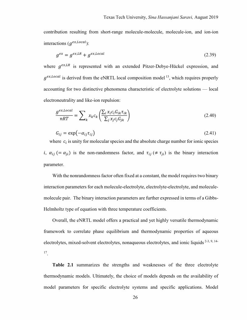
Texas Tech University, Sina Hassanjani Saravi, August 2019
26
contribution resulting from short-range molecule-molecule, molecule-ion, and ion-ion
interactions (𝑔𝑔𝑒𝑒𝑒𝑒,𝐿𝐿𝑜𝑜𝐿𝐿𝑎𝑎𝑙𝑙):
𝑔𝑔𝑒𝑒𝑒𝑒 = 𝑔𝑔𝑒𝑒𝑒𝑒,𝐿𝐿𝐿𝐿 + 𝑔𝑔𝑒𝑒𝑒𝑒,𝐿𝐿𝑜𝑜𝐿𝐿𝑎𝑎𝑙𝑙 (2.39)
where 𝑔𝑔𝑒𝑒𝑒𝑒,𝐿𝐿𝐿𝐿 is represented with an extended Pitzer-Debye-Hückel expression, and
𝑔𝑔𝑒𝑒𝑒𝑒,𝐿𝐿𝑜𝑜𝐿𝐿𝑎𝑎𝑙𝑙 is derived from the eNRTL local composition model 13, which requires properly
accounting for two distinctive phenomena characteristic of electrolyte solutions — local
electroneutrality and like-ion repulsion:
𝑔𝑔𝑒𝑒𝑒𝑒,𝐿𝐿𝑜𝑜𝐿𝐿𝑎𝑎𝑙𝑙
𝑙𝑙𝑅𝑅𝑇𝑇= � 𝑥𝑥𝑘𝑘𝑐𝑐𝑘𝑘 �
∑ 𝑥𝑥𝑖𝑖𝑐𝑐𝑖𝑖𝐺𝐺𝑖𝑖𝑘𝑘𝜏𝜏𝑖𝑖𝑘𝑘𝑖𝑖
∑ 𝑥𝑥𝑗𝑗𝑐𝑐𝑗𝑗𝐺𝐺𝑗𝑗𝑘𝑘𝑗𝑗�
𝑘𝑘 (2.40)
𝐺𝐺𝑖𝑖𝑗𝑗 = exp�−𝛼𝛼𝑖𝑖𝑗𝑗𝜏𝜏𝑖𝑖𝑗𝑗� (2.41)
where 𝑐𝑐𝑖𝑖 is unity for molecular species and the absolute charge number for ionic species
𝑖𝑖, 𝛼𝛼𝑖𝑖𝑗𝑗 (= 𝛼𝛼𝑗𝑗𝑖𝑖) is the non-randomness factor, and 𝜏𝜏𝑖𝑖𝑗𝑗 (≠ 𝜏𝜏𝑗𝑗𝑖𝑖) is the binary interaction
parameter.
With the nonrandomness factor often fixed at a constant, the model requires two binary
interaction parameters for each molecule-electrolyte, electrolyte-electrolyte, and molecule-
molecule pair. The binary interaction parameters are further expressed in terms of a Gibbs-
Helmholtz type of equation with three temperature coefficients.
Overall, the eNRTL model offers a practical and yet highly versatile thermodynamic
framework to correlate phase equilibrium and thermodynamic properties of aqueous
electrolytes, mixed-solvent electrolytes, nonaqueous electrolytes, and ionic liquids 2-3, 9, 14-
17.
Table 2.1 summarizes the strengths and weaknesses of the three electrolyte
thermodynamic models. Ultimately, the choice of models depends on the availability of
model parameters for specific electrolyte systems and specific applications. Model
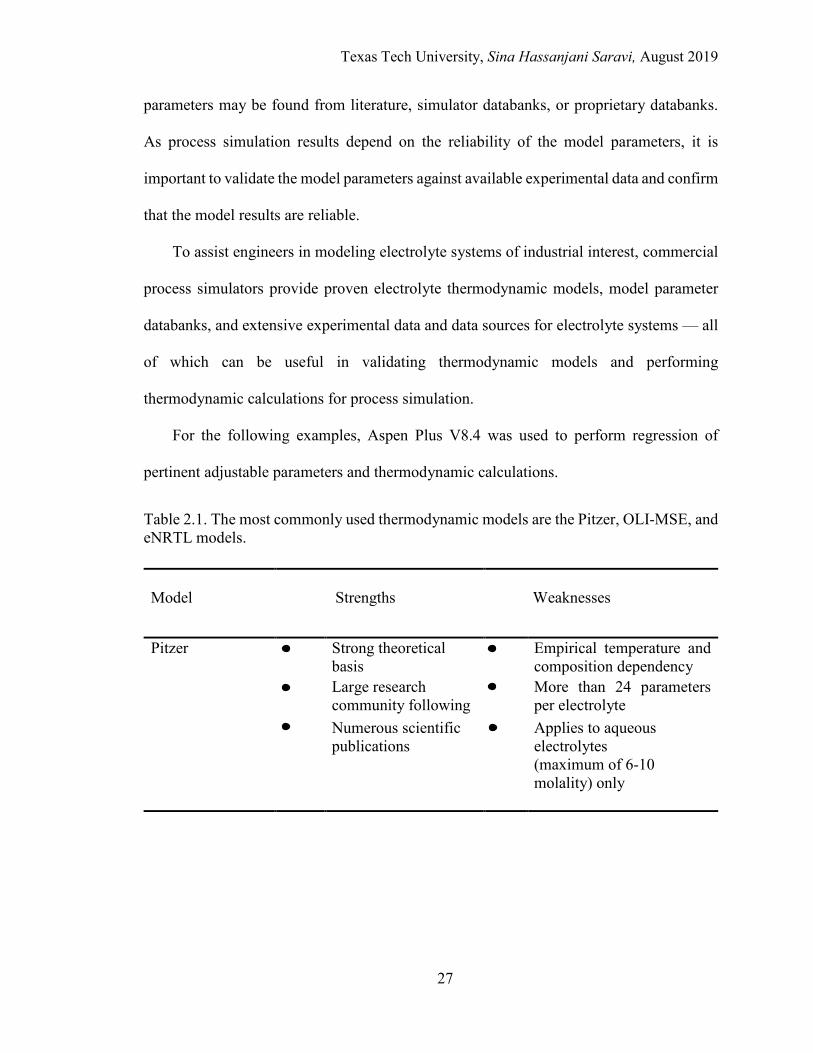
Texas Tech University, Sina Hassanjani Saravi, August 2019
27
parameters may be found from literature, simulator databanks, or proprietary databanks.
As process simulation results depend on the reliability of the model parameters, it is
important to validate the model parameters against available experimental data and confirm
that the model results are reliable.
To assist engineers in modeling electrolyte systems of industrial interest, commercial
process simulators provide proven electrolyte thermodynamic models, model parameter
databanks, and extensive experimental data and data sources for electrolyte systems — all
of which can be useful in validating thermodynamic models and performing
thermodynamic calculations for process simulation.
For the following examples, Aspen Plus V8.4 was used to perform regression of
pertinent adjustable parameters and thermodynamic calculations.
Table 2.1. The most commonly used thermodynamic models are the Pitzer, OLI-MSE, and eNRTL models.
Model
Strengths
Weaknesses
Pitzer
Strong theoretical basis
Empirical temperature and composition dependency
Large research community following
More than 24 parameters per electrolyte
Numerous scientific publications
Applies to aqueous electrolytes (maximum of 6-10 molality) only
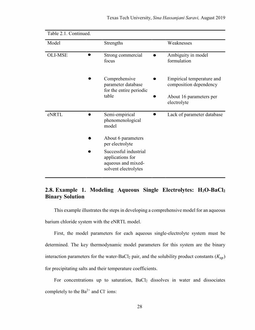
Texas Tech University, Sina Hassanjani Saravi, August 2019
28
Table 2.1. Continued.
Model Strengths
Weaknesses
OLI-MSE Strong commercial focus
Ambiguity in model formulation
Comprehensive parameter database for the entire periodic table
Empirical temperature and composition dependency
About 16 parameters per
electrolyte
eNRTL Semi-empirical phenomenological model
Lack of parameter database
About 6 parameters per electrolyte
Successful industrial applications for aqueous and mixed-solvent electrolytes
2.8. Example 1. Modeling Aqueous Single Electrolytes: H2O-BaCl2 Binary Solution
This example illustrates the steps in developing a comprehensive model for an aqueous
barium chloride system with the eNRTL model.
First, the model parameters for each aqueous single-electrolyte system must be
determined. The key thermodynamic model parameters for this system are the binary
interaction parameters for the water-BaCl2 pair, and the solubility product constants (𝐾𝐾𝑠𝑠𝑝𝑝)
for precipitating salts and their temperature coefficients.
For concentrations up to saturation, BaCl2 dissolves in water and dissociates
completely to the Ba2+ and Cl- ions:

Texas Tech University, Sina Hassanjani Saravi, August 2019
29
𝐵𝐵𝑎𝑎𝐶𝐶𝑙𝑙2(𝑎𝑎𝑎𝑎) → 𝐵𝐵𝑎𝑎2+(𝑎𝑎𝑎𝑎) + 2 𝐶𝐶𝑙𝑙−(𝑎𝑎𝑎𝑎)
For concentrations above saturation, Ba2+ and Cl- ions precipitate as BaCl2(s):
𝐵𝐵𝑎𝑎𝐶𝐶𝑙𝑙2(𝑠𝑠) ↔ 𝐵𝐵𝑎𝑎2+(𝑎𝑎𝑎𝑎) + 2 𝐶𝐶𝑙𝑙−(𝑎𝑎𝑎𝑎)
Thermodynamic data for aqueous BaCl2 solutions from various sources — mean ionic
activity coefficient 18-20, osmotic coeffcient 21-23, vapor pressure 24 , and excess Enthalpy 25
— are simultaneously fitted to the equation shown in Table 2.2 to calculate the temperature
coefficients for the eNRTL binary interaction parameters (𝜏𝜏𝑖𝑖𝑗𝑗). Figure 2.1 is a plot of 𝜏𝜏𝑖𝑖𝑗𝑗
as a function of temperature. Solubility data 26 are then used to calculate the temperature
coefficients (𝐴𝐴, 𝐵𝐵, 𝐶𝐶, 𝐷𝐷, 𝐸𝐸), which can then be substituted into Eq. 2.27 to calculate the
BaCl2(s) solubility product constant.
Table 2.2. The temperature coefficients and binary interaction parameters for the examples.
Component i Component j Cija Dij
a Eija 𝜏𝜏𝑖𝑖𝑗𝑗 at 98.15K
Example 1
H2O (Ba2+,Cl-) 5.106 834.460 0 7.904
(Ba2+,Cl-) H2O -3.249 -285.728 0 -4.207
Example 2
H2O (Na+, Cl-) 7.427b 429.0b -3.251b 8.865
(Na+, Cl-) H2O -4.350b -56.9b 3.110b -4.541
H2O (Na+, SO42-) 2.325b 1695.5b 12.020b 8.012
(Na+, SO42-) H2O -2.208b -505.5b -1.837b -3.903
(Na+, Cl-) (Na+, SO42-) -0.440b 370.7b 0b 0.804
(Na+, SO42-) (Na+, Cl-) -0.122b -152.7b 0b -0.634
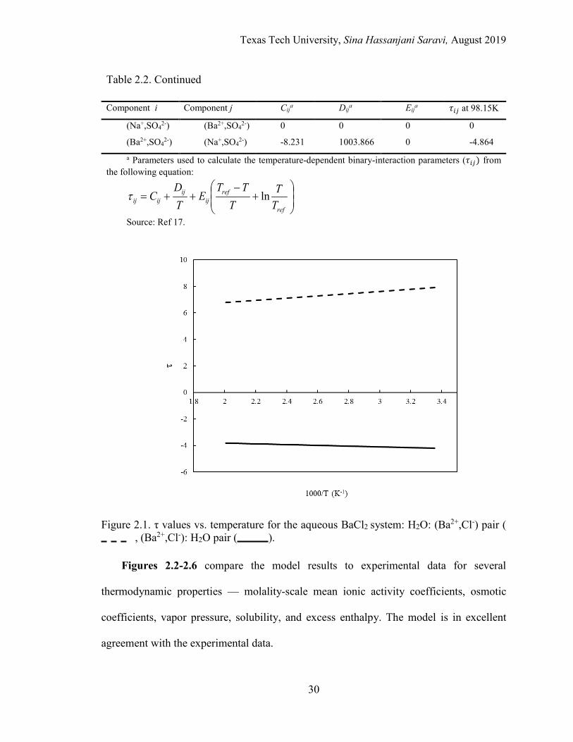
Texas Tech University, Sina Hassanjani Saravi, August 2019
30
Table 2.2. Continued
Component i Component j Cija Dij
a Eija 𝜏𝜏𝑖𝑖𝑗𝑗 at 98.15K
(Na+,SO42-) (Ba2+,SO4
2-) 0 0 0 0
(Ba2+,SO42-) (Na+,SO4
2-) -8.231 1003.866 0 -4.864 a Parameters used to calculate the temperature-dependent binary-interaction parameters (𝜏𝜏𝑖𝑖𝑗𝑗) from
the following equation:
+
−++=
ref
refij
ijijij T
TT
TTE
TD
C lnτ
Source: Ref 17.
Figure 2.1. τ values vs. temperature for the aqueous BaCl2 system: H2O: (Ba2+,Cl-) pair ( , (Ba2+,Cl-): H2O pair ( ).
Figures 2.2-2.6 compare the model results to experimental data for several
thermodynamic properties — molality-scale mean ionic activity coefficients, osmotic
coefficients, vapor pressure, solubility, and excess enthalpy. The model is in excellent
agreement with the experimental data.

Texas Tech University, Sina Hassanjani Saravi, August 2019
31
This example demonstrates that the thermodynamic model is capable of representing
a wide range of thermodynamic properties for the aqueous BaCl2 solution. Used in process
simulators, the model provides accurate and robust calculations for boiling point rise,
solution enthalpy, solution heat capacity, and salt solubility, which are essential for heat
and mass balance calculations. The model further provides a basis for modeling aqueous
multicomponent electrolyte systems in which BaCl2 is an electrolyte of the solution. More
examples on modeling aqueous single-electrolyte systems are available in the literature 14,
17.
Figure 2.2. Mean ionic activity coefficient vs. molality of barium chloride, model results (), experimental data ( ) 18, ( ) 19, ( ) 20.
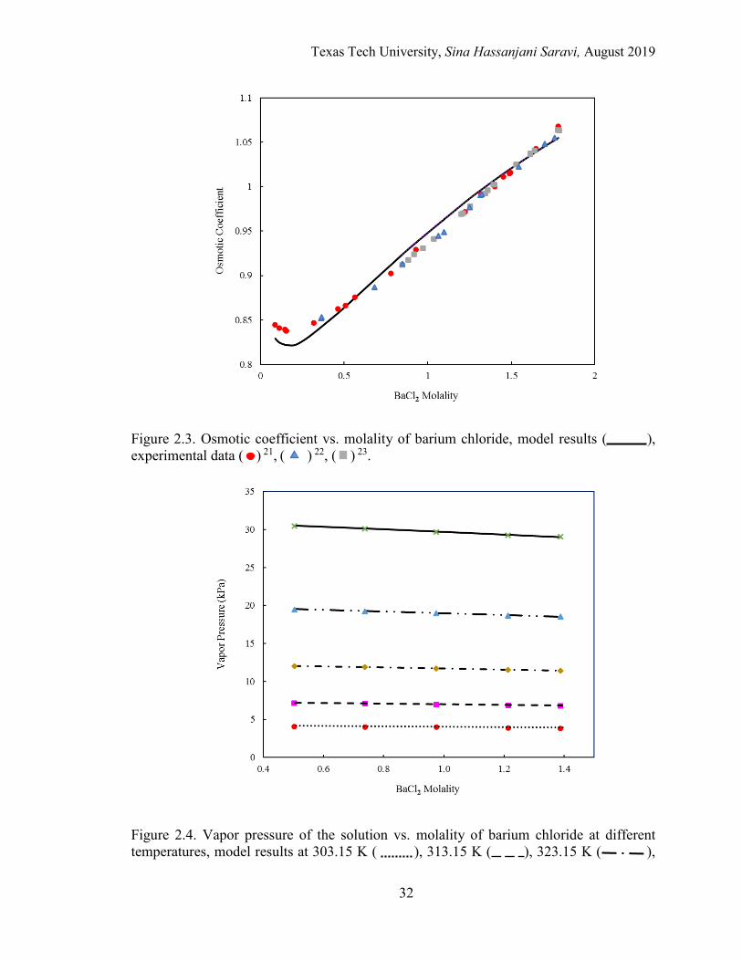
Texas Tech University, Sina Hassanjani Saravi, August 2019
32
Figure 2.3. Osmotic coefficient vs. molality of barium chloride, model results ( ), experimental data ( ) 21, ( ) 22, ( ) 23.
Figure 2.4. Vapor pressure of the solution vs. molality of barium chloride at different temperatures, model results at 303.15 K ( ), 313.15 K ( ), 323.15 K ( ),
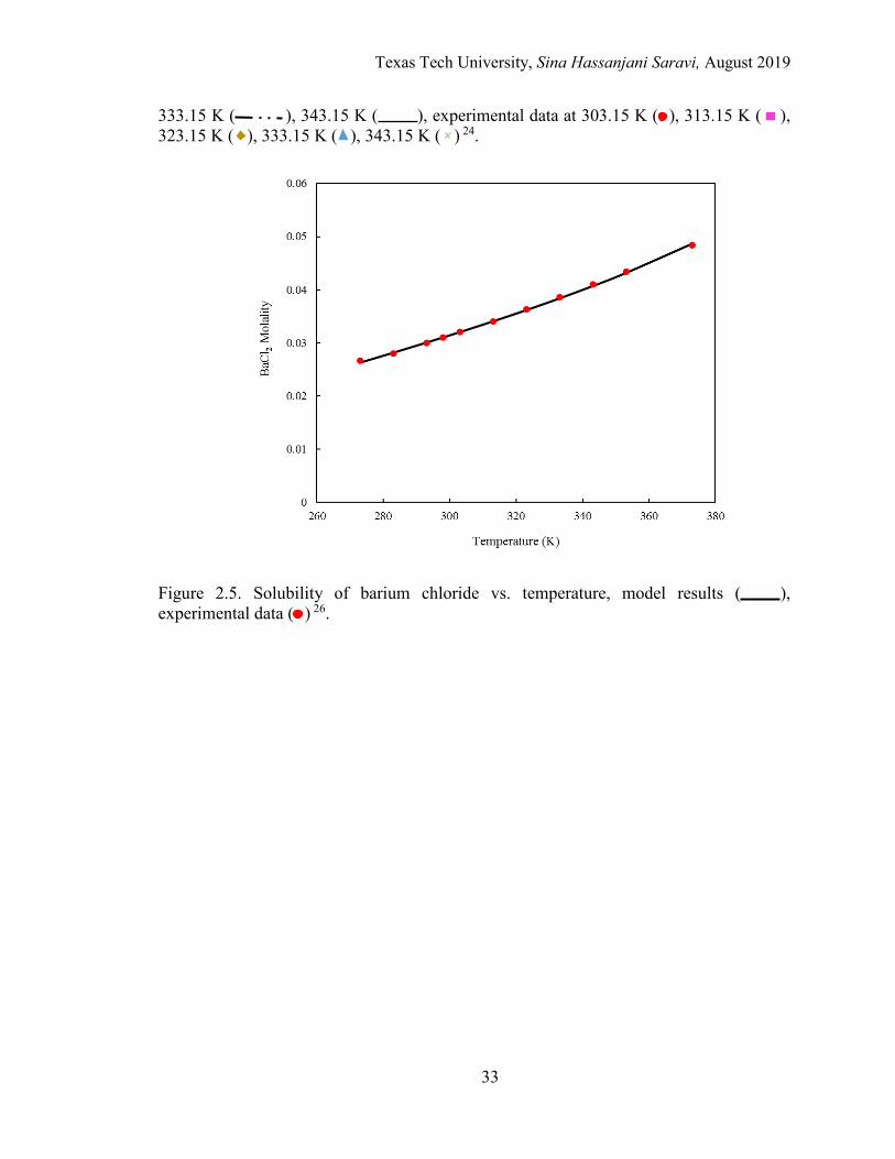
Texas Tech University, Sina Hassanjani Saravi, August 2019
33
333.15 K ( ), 343.15 K ( ), experimental data at 303.15 K ( ), 313.15 K ( ), 323.15 K ( ), 333.15 K ( ), 343.15 K ( ) 24.
Figure 2.5. Solubility of barium chloride vs. temperature, model results ( ), experimental data ( ) 26.
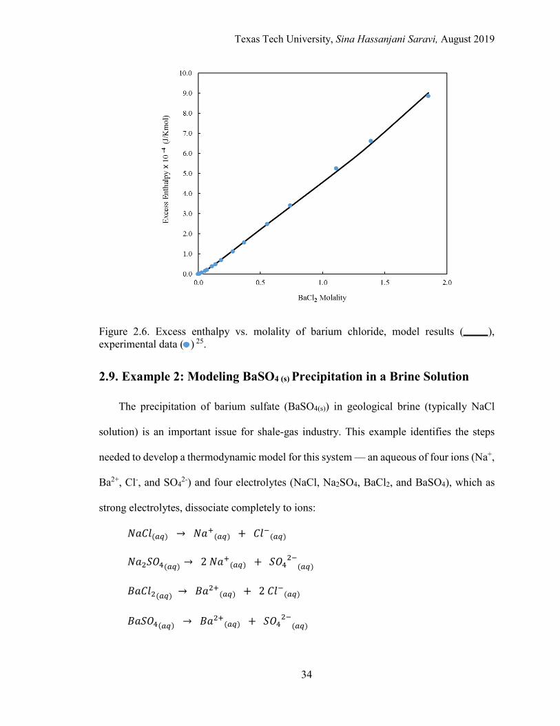
Texas Tech University, Sina Hassanjani Saravi, August 2019
34
Figure 2.6. Excess enthalpy vs. molality of barium chloride, model results ( ), experimental data ( ) 25.
2.9. Example 2: Modeling BaSO4 (s) Precipitation in a Brine Solution
The precipitation of barium sulfate (BaSO4(s)) in geological brine (typically NaCl
solution) is an important issue for shale-gas industry. This example identifies the steps
needed to develop a thermodynamic model for this system — an aqueous of four ions (Na+,
Ba2+, Cl-, and SO42-) and four electrolytes (NaCl, Na2SO4, BaCl2, and BaSO4), which as
strong electrolytes, dissociate completely to ions:
𝑁𝑁𝑎𝑎𝐶𝐶𝑙𝑙(𝑎𝑎𝑎𝑎) → 𝑁𝑁𝑎𝑎+(𝑎𝑎𝑎𝑎) + 𝐶𝐶𝑙𝑙−(𝑎𝑎𝑎𝑎)
𝑁𝑁𝑎𝑎2𝑆𝑆𝑆𝑆4(𝑎𝑎𝑎𝑎) → 2 𝑁𝑁𝑎𝑎+(𝑎𝑎𝑎𝑎) + 𝑆𝑆𝑆𝑆42−(𝑎𝑎𝑎𝑎)
𝐵𝐵𝑎𝑎𝐶𝐶𝑙𝑙2(𝑎𝑎𝑎𝑎) → 𝐵𝐵𝑎𝑎2+(𝑎𝑎𝑎𝑎) + 2 𝐶𝐶𝑙𝑙−(𝑎𝑎𝑎𝑎)
𝐵𝐵𝑎𝑎𝑆𝑆𝑆𝑆4(𝑎𝑎𝑎𝑎) → 𝐵𝐵𝑎𝑎2+(𝑎𝑎𝑎𝑎) + 𝑆𝑆𝑆𝑆42−(𝑎𝑎𝑎𝑎)
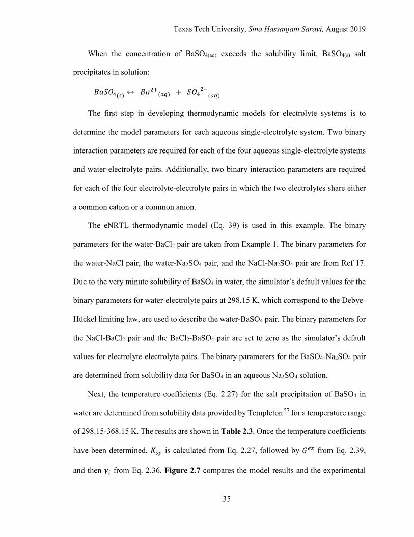
Texas Tech University, Sina Hassanjani Saravi, August 2019
35
When the concentration of BaSO4(aq) exceeds the solubility limit, BaSO4(s) salt
precipitates in solution:
𝐵𝐵𝑎𝑎𝑆𝑆𝑆𝑆4(𝑠𝑠) ↔ 𝐵𝐵𝑎𝑎2+(𝑎𝑎𝑎𝑎) + 𝑆𝑆𝑆𝑆42−(𝑎𝑎𝑎𝑎)
The first step in developing thermodynamic models for electrolyte systems is to
determine the model parameters for each aqueous single-electrolyte system. Two binary
interaction parameters are required for each of the four aqueous single-electrolyte systems
and water-electrolyte pairs. Additionally, two binary interaction parameters are required
for each of the four electrolyte-electrolyte pairs in which the two electrolytes share either
a common cation or a common anion.
The eNRTL thermodynamic model (Eq. 39) is used in this example. The binary
parameters for the water-BaCl2 pair are taken from Example 1. The binary parameters for
the water-NaCl pair, the water-Na2SO4 pair, and the NaCl-Na2SO4 pair are from Ref 17.
Due to the very minute solubility of BaSO4 in water, the simulator’s default values for the
binary parameters for water-electrolyte pairs at 298.15 K, which correspond to the Debye-
Hückel limiting law, are used to describe the water-BaSO4 pair. The binary parameters for
the NaCl-BaCl2 pair and the BaCl2-BaSO4 pair are set to zero as the simulator’s default
values for electrolyte-electrolyte pairs. The binary parameters for the BaSO4-Na2SO4 pair
are determined from solubility data for BaSO4 in an aqueous Na2SO4 solution.
Next, the temperature coefficients (Eq. 2.27) for the salt precipitation of BaSO4 in
water are determined from solubility data provided by Templeton 27 for a temperature range
of 298.15-368.15 K. The results are shown in Table 2.3. Once the temperature coefficients
have been determined, 𝐾𝐾𝑠𝑠𝑝𝑝 is calculated from Eq. 2.27, followed by 𝐺𝐺𝑒𝑒𝑒𝑒 from Eq. 2.39,
and then 𝛾𝛾𝑖𝑖 from Eq. 2.36. Figure 2.7 compares the model results and the experimental
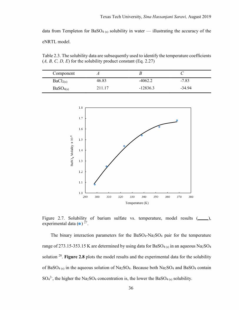
Texas Tech University, Sina Hassanjani Saravi, August 2019
36
data from Templeton for BaSO4 (s) solubility in water — illustrating the accuracy of the
eNRTL model.
Table 2.3. The solubility data are subsequently used to identify the temperature coefficients (A, B, C, D, E) for the solubility product constant (Eq. 2.27)
Component A B C
BaCl2(s) 46.83 -4062.2 -7.83
BaSO4(s) 211.17 -12836.3 -34.94
Figure 2.7. Solubility of barium sulfate vs. temperature, model results ( ), experimental data ( ) 27.
The binary interaction parameters for the BaSO4-Na2SO4 pair for the temperature
range of 273.15-353.15 K are determined by using data for BaSO4 (s) in an aqueous Na2SO4
solution 28. Figure 2.8 plots the model results and the experimental data for the solubility
of BaSO4 (s) in the aqueous solution of Na2SO4. Because both Na2SO4 and BaSO4 contain
SO42-, the higher the Na2SO4 concentration is, the lower the BaSO4 (s) solubility.
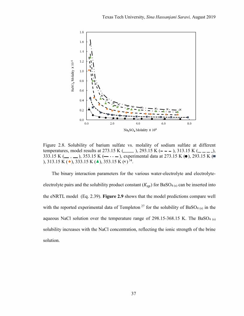
Texas Tech University, Sina Hassanjani Saravi, August 2019
37
Figure 2.8. Solubility of barium sulfate vs. molality of sodium sulfate at different temperatures, model results at 273.15 K ( ), 293.15 K ( ), 313.15 K ( ), 333.15 K ( ), 353.15 K ( ), experimental data at 273.15 K ( ), 293.15 K ( ), 313.15 K ( ), 333.15 K ( ), 353.15 K ( ) 34.
The binary interaction parameters for the various water-electrolyte and electrolyte-
electrolyte pairs and the solubility product constant (𝐾𝐾𝑠𝑠𝑝𝑝) for BaSO4 (s) can be inserted into
the eNRTL model (Eq. 2.39). Figure 2.9 shows that the model predictions compare well
with the reported experimental data of Templeton 27 for the solubility of BaSO4 (s) in the
aqueous NaCl solution over the temperature range of 298.15-368.15 K. The BaSO4 (s)
solubility increases with the NaCl concentration, reflecting the ionic strength of the brine
solution.
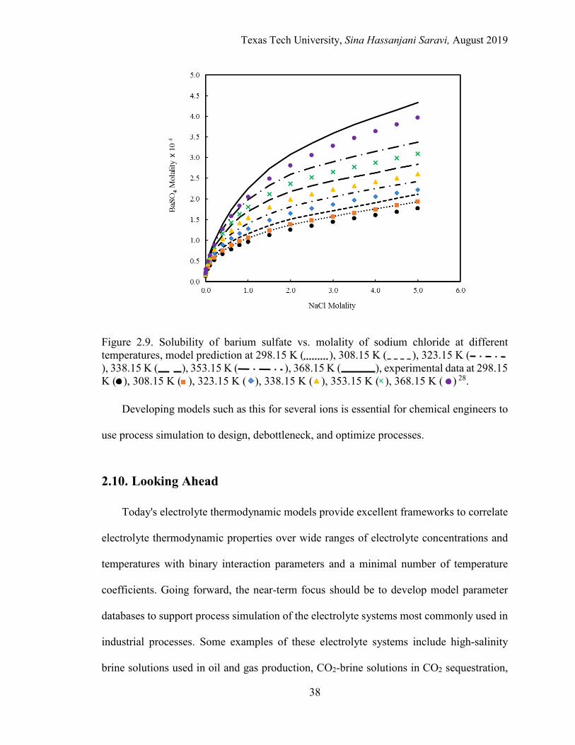
Texas Tech University, Sina Hassanjani Saravi, August 2019
38
Figure 2.9. Solubility of barium sulfate vs. molality of sodium chloride at different temperatures, model prediction at 298.15 K ( ), 308.15 K ( ), 323.15 K (), 338.15 K ( ), 353.15 K ( ), 368.15 K ( ), experimental data at 298.15 K ( ), 308.15 K ( ), 323.15 K ( ), 338.15 K ( ), 353.15 K ( ), 368.15 K ( ) 28.
Developing models such as this for several ions is essential for chemical engineers to
use process simulation to design, debottleneck, and optimize processes.
2.10. Looking Ahead
Today's electrolyte thermodynamic models provide excellent frameworks to correlate
electrolyte thermodynamic properties over wide ranges of electrolyte concentrations and
temperatures with binary interaction parameters and a minimal number of temperature
coefficients. Going forward, the near-term focus should be to develop model parameter
databases to support process simulation of the electrolyte systems most commonly used in
industrial processes. Some examples of these electrolyte systems include high-salinity
brine solutions used in oil and gas production, CO2-brine solutions in CO2 sequestration,
Texas Tech University, Sina Hassanjani Saravi, August 2019
39
nitric acid solutions in nuclear wastewater treatment, and hydrogen bromide solutions in
flow batteries.
In addition, research should be conducted to gain critical new insights essential for
continuing the development of predictive electrolyte thermodynamic models. furthermore,
engineering models, both correlative and predictive, are lacking for all transport properties
of electrolyte systems. Research and development of practical engineering models for
transport properties should be pursued.
Given the critical importance of electrolyte systems to modern chemical engineering,
it is hoped that real and substantive progress will be made in the not-too-distant future.
2.11. Acknowledgments
The authors gratefully acknowledge the financial support of the Jack Maddox
Distinguished Engineering Chair Professorship in Sustainable Energy sponsored by the J.
F. Maddox Foundation. The work is partially supported by a donation from the Apache
Corp. The authors thank Dr. Yuhua Song for his extensive editorial review of the article.
Texas Tech University, Sina Hassanjani Saravi, August 2019
40
2.12. References
1. Chen C-C., Mathias PM, Orbey H. Use of Hydration and Dissociation Chemistries with the Electrolyte NRTL Model. AIChE Journal., 45 (7), pp. 1576-1586 (1999)
2. Zhang Y, Chen C-C. Thermodynamic Modeling for CO2 Absorption in Aqueous MDEA Solution with Electrolyte NRTL Model. Industrial & Engineering Chemistry Research. 50 (1), pp. 163-175 (2011)
3. Que H, Chen C-C. Thermodynamic Modeling of the NH3-CO2-H2O System with Electrolyte NRTL Model. Industrial & Engineering Chemistry Research. 50 (19), pp. 11406-11421 (2011)
4. Prausnitz JM, Lichtenthaler RN, de Azevedo EG. Molecular Thermodynamics of Fluid-Phase Equilibria. 3rd Ed., Prentice Hall PTR, Upper Saddle River, New Jersey (1998)
5. Tanveer S, Hao YF, Chen C-C. Introduction to Solid-Fluid Equilibrium Modeling. Chemical Engineering Progress, 110 (9), pp. 37-47 (2014)
6. Pitzer KS. Thermodynamics of Electrolytes. I. Theoretical Basis and General Equations. The Journal of Physical Chemistry. 77 (2), pp. 268-277 (1973)
7. Rowland D, Kӧnigsberger E, Hefter G, May PM. Aqueous Electrolyte Solution Modelling: Some Limitations of the Pitzer Equations. Applied Geometry, (2014), http://dx.doi.org/10.1016/j.apgeochem.2014.09.021
8. Wang P, Anderko A, Young RD. A Speciation-Based Model for Mixed-Solvent Electrolyte Systems. Fluid Phase Equilibria. 203, pp. 141-176 (2002)
9. Song Y, Chen C-C. Symmetric Electrolyte Nonrandom Two-Liquid Activity Coefficient Model. Industrial & Engineering Chemistry Research. 48 (16), pp. 7788-7797 (2009)
10. Chen C-C. Toward Development of Activity Coefficient Models for Process and Product Design of Complex Chemical Systems. Fluid Phase Equilibria. 241, pp. 103–112 (2006)
11. Abrams DS, and Prausnitz JM. Statistical Thermodynamics of Liquid Mixtures. A New Expression for the Excess Gibbs Energy of Partly and Completely Miscible Systems. AIChE Journal. 21 (1), pp. 116-128 (1975)
12. Wang P, Anderko A, Springer RD, Young RD. Modeling Phase Equilibria and Speciation in Mixed-Solvent Electrolyte Systems: II. Liquid-Liquid Equilibria and Properties of Associating Electrolyte Solutions. Journal of Molecular Liquids. 125 (1), pp. 37-44 (2006)
Texas Tech University, Sina Hassanjani Saravi, August 2019
41
13. Renon H, Prausnitz JM. Local Compositions in Thermodynamic Excess Functions for Liquid Mixtures. AIChE Journal. 14 (1), pp. 135-144 (1968)
14. Bhattacharia SK, Chen C-C. Thermodynamic Modeling of KCl+H2O and KCl+NaCl+H2O Systems Using Symmetric Electrolyte NRTL Model. Fluid Phase Equilibria. 387, pp. 169-177 (2015).
15. Que H, Song Y, Chen C-C. Thermodynamic Modeling of the Sulfuric Acid-Water-Sulfur Trioxide System with the Symmetric Electrolyte NRTL Model. Journal of Chemical & Engineering Data. 56 (4), pp. 963-977 (2011)
16. Yan Y, Chen C-C. Thermodynamic Modeling of CO2 Solubility in Aqueous Solutions of NaCl and Na2SO4. The Journal of Supercritical Fluids. 55 (2), pp. 623-634 (2010)
17. Yan Y, Chen C-C. Thermodynamic Representation of the NaCl-Na2SO4-H2O System with Electrolyte NRTL Model. Fluid Phase Equilibria. 306, pp. 149-161 (2011)
18. Hamer WJ, Wu YC. Osmotic Coefficients and Mean Activity Coefficients of Uni‐univalent Electrolytes in Water at 25 °C. Journal of Physical and Chemical Reference Data. 1 (4), pp. 047-1100, (1972)
19. Lucasse WW. Activity Coefficients and Transference Numbers of the Alkaline Earth Chlorides. Journal of the American Chemical Society. 47 (3), pp. 743-754 (1925)
20. Tippetts EA, Newton RF. The Thermodynamics of Aqueous Barium Chloride Solutions from Electromotive Force Measurements. Journal of the American Chemical Society. 56 (8), pp. 1675-1680 (1934)
21. Robinson RA, The Osmotic and Activity Coefficient Data of Some Aqueous Salt Solutions from Vapor Pressure Measurement. Journal of the American Chemical Society. 59 (1), pp. 84-90 (1937)
22. Robinson RA. The Vapor Pressures of Solutions of Potassium Chloride and Sodium Chloride. Transactions of the Royal Society of New Zealand. 75 (2), pp. 203-217 (1945)
23. Robinson RA, Bower VE. Thermodynamics of the Ternary System: Water-Sodium Chloride-Barium Chloride at 25 °C. Journal of Research of the National Bureau of Standards. 69A (1), pp. 19-27 (1965)
24. Patil KR, Tripathi AD, Pathak G, Katti SS. Thermodynamic Properties of Aqueous Electrolyte Solution. 2. Vapor Pressure of Aqueous Solutions of NaBr, NaI, KCl, KBr, KI, RbCl, CsCl, CsBr, CsI, MgCl2, CaCl2, CaBr2, CaI2, SrCl2, SrBr2, SrI2, BaCl2, and BaBr2. Journal of Chemical Engineering Data. 36 (2), pp. 225-230, (1991)
Texas Tech University, Sina Hassanjani Saravi, August 2019
42
25. Wagman DD, Evans WH, Parker VB, Schumm RH, Halow I, Bailey SM, Churney KL, Nuttall RL. The NBS Tables of Chemical Thermodynamic Properties. Selected Values for Inorganic and C1 and C2 Organic Substances in SI Units. Journal of Physical and Chemical Reference Data. (1982), 11, Supplement No. 2
26. Seidell A. Solubilities of Inorganic and Organic Compounds, NYC, New York, D.Van Nostrand Company (1923)
27. Templeton CC. Solubility of Barium Sulfate in Sodium Chloride Solutions from 25 ℃ to 95 ℃. Journal of Chemical Engineering Data. 5 (4), pp. 514-516 (1960)
28. Jiang C. Solubility and Solubility Constant of Barium Sulfate in Aqueous Sodium Sulfate Solutions between 0 and 80 ℃. Journal of Solution Chemistry. 25 (1), pp. 105-111 (1996)

Texas Tech University, Sina Hassanjani Saravi, August 2019
43
CHAPTER 3. THERMODYNAMIC MODELING OF HCL-H2O BINIARY
SYSTEM WITH SYMMETRIC ELECTROLYTE NRTL MODEL2
3.1. Abstract
A comprehensive thermodynamic model is developed for the HCl-H2O binary system
based on the electrolyte nonrandom two-liquid activity coefficient model. Partial
dissociation of electrolyte HCl to hydronium cation and chloride anion is incorporated to
account for the true species in solution. Regressed from extensive thermodynamic data, the
model parameters include molecule-molecule and molecule-electrolyte binary interactions
parameters, as well as the chemical equilibrium constant parameters of the partial
dissociation solution chemistry. The model accurately calculates all phase equilibria and
thermodynamic properties including calorimetric properties with the concentration range
from pure water to pure HCl and temperatures from 273 up to about 400 K.
2 This chapter is reproduced from the paper published as: Saravi SH, Honarparvar S, Chen C-C. Thermodynamic Modeling of HCl-H2O Binary System with Symmetric Electrolyte NRTL Model. The Journal of Chemical Thermodynamics. 2018.

Texas Tech University, Sina Hassanjani Saravi, August 2019
44
3.2. Introduction
As a strong acid, aqueous hydrochloric acid is one of the most widely used electrolytes
in industry. It is commonly used in metals refining and ion exchangers regeneration, as
well as many environmental and geological processes 1-4. Furthermore, the study of
aqueous HCl solution at higher temperatures and pressures is of great importance in
hydrothermal processes, steam power generators, and bitumen recovery operations 5-7. The
highly non-ideal nature of this strong acid can be highlighted with the existence of
minimum-boiling azeotropic points 8, formation of two liquids at high pressures 9,
dissociation of HCl along with hydration of ions 8,10,11, etc.
The complex thermodynamic behavior of HCl-H2O binary system has attracted
numerous studies both experimentally and theoretically over the last century. As early as
1909, Rupert 9 carried out experiments to measure liquid-liquid equilibrium (LLE)
compositions of the HCl-H2O binary. Later, Zeisberg 12 reported a relatively thorough
compilation of partial pressure data for aqueous HCl solution from 2 to 46 wt. % and over
the temperature range of 273.15 to 383.15 K. These data were later included in Perry’s
Handbook 13. During the following decades, many researchers presented various
thermodynamic data for the aqueous HCl solution over wide ranges of temperature and
pressure 5,13-45. Among them are data for isothermal and isobaric vapor-liquid equilibrium
(VLE), LLE, molality scale mean ionic activity coefficient, osmotic coefficient, enthalpy
of formation, heat capacity, etc. Most of these data cover HCl concentrations up to the
commercial acid concentration practiced in the industry (~ 37 wt. % or 16 mol.kg-1 HCl).
A comprehensive review of these data is presented later.
Texas Tech University, Sina Hassanjani Saravi, August 2019
45
Parallel to the experimental studies, there have been many thermodynamic modeling
efforts for the HCl-H2O binary. These thermodynamic studies can be categorized either as
“equation of state-based” or “activity coefficient-based” models 8. Another dimension to
these thermodynamic studies is whether the electrolyte is treated either as “no
dissociation”, “complete dissociation”, or “partial dissociation” 46-49. While there are
several notable modeling efforts based on equations of state (EoS), most of the
thermodynamic modeling efforts fall into the category of “activity coefficient-based”
models due to their rigorous thermodynamic formulations and more reliable results.
Gibbon and Laughton 50 presented a modified Redlich-Kwong-Soave (RKS) EoS for
the HCl-H2O binary and showed qualitatively correct results for the azeotropic behavior of
the system and the heat of solution. Presenting a modified “alpha function” for cubic EoS,
Stryjek and Vera 51 proposed the Peng-Robinson-Stryjek-Vera EoS to describe VLE of the
HCl-H2O binary. With two temperature-dependent binary parameters adjusted, they
showed acceptable results of correlating the experimental VLE data specifically for
minimum-boiling azeotropic point. Later, applying a Patel and Teja cubic EoS 52 modified
by Panagiotopoulos and Reid 53, Delano 54 showed the EoS qualitatively predicts the
system pressure at bubble points.
There are many activity coefficient-based thermodynamic modeling efforts for the
HCl-H2O binary. Based on a modified Raoults’s law, the Clausius-Clapeyron equation for
pure component vapor pressures, and a simple two-suffix Margules equation for activity
coefficients, Brandes 8 obtained the “pseudo-vapor pressures” correlations for calculating
HCl and water partial pressures as functions of temperature and HCl composition. The
Texas Tech University, Sina Hassanjani Saravi, August 2019
46
model yielded satisfactory VLE predictions for temperatures up to 473 K and HCl
concentrations up to 55 wt %.
Using an extended Debye-Hückel theory, Greeley et al. 55 calculated mean ionic
activity coefficients, osmotic coefficients, and relative partial molal heat capacities for the
HCl-H2O binary for HCl concentrations up to 1.0 mol.kg-1 at the temperature range of
298.15 to 548.15 K. Based on a modified Debye-Hückel theory, Vega and Vera 22 applied
a semi-empirical activity coefficient correlation previously proposed by Correa and Vera
56, and showed satisfactory agreement with the experimental data of mean ionic activity
coefficient and VLE up to 373.15 K and 18.28 mol.kg-1 HCl. The reported deviations were
1 to 5 % for mean ionic activity coefficients, 10 to 20 % for water activity coefficients, and
less than 10 % for total system pressures.
By considering HCl partial dissociation and subsequent hydration of ions, Engels and
Bosen 57 applied the Wilson “local composition” activity coefficient equation 58 and
achieved satisfactory fits against VLE experimental data, including minimum-boiling
azeotropic point, up to 13.88 mol.kg-1 HCl at the temperature range of 298.15 to 373.15 K.
Liu and Grén 59 proposed an activity coefficient model based on a modified Debye-Hückel
theory for long-range interactions and a Wilson-type equation accounting for short-range
interactions. They successfully applied the model to characterize the HCl-H2O binary,
covering the temperature range of 273.15 to 383.15 K and the HCl concentration up to
21.55 mol.kg-1.
Hala et al. 60 presented their work on characterizing VLE of strong electrolytes in
concentrated solutions. They started with a mathematical definition of Gibbs free energy
in dilute solution, followed by a serial expansion leading to an explicit function of mole
Texas Tech University, Sina Hassanjani Saravi, August 2019
47
fraction-based mean ionic activity coefficient. They later applied the equations to the HCl-
H2O binary up to 12.18 mol.kg-1 HCl at 298.15 K 61,62. Applying Hala’s equation, Wozny
and Cremer 63 successfully calculated the azeotrope and activity coefficients of the aqueous
HCl system up to 14.90 mol.kg-1 HCl, with temperatures from 273.15 to 473.15 K and
pressures from 0.01 to 2 MPa. To properly capture the temperature dependence of the
system, they employed 19 coefficients and considered the azeotropic point as the reference
state.
Many models have been developed for the aqueous HCl solution 4,64-66 based on the
Pitzer activity coefficient equation 67,68. Among them, considering formation of a neutral
ion pair from the ions, Simonson et al. 65 calculated the excess thermodynamic properties
of the aqueous HCl solution in the temperature range of 298 to 648 K, pressures up to 40
MPa, and the HCl concentration up to 2 mol.kg-1. Using an extended Pitzer model
associated with Henry’s law as the HCl reference state, Brandani et al. 4 reported their
model results showing satisfactory match with the experimental VLE data and significant
improvement over those published by Engels and Bosen 57 for the temperature range of
298.15 to 383.15 K and the HCl concentration up to 16 mol.kg-1. Carslaw et al. 66 calculated
the activities and vapor pressures of a multicomponent system including the HCl-H2O
binary using a mole fraction-based Pitzer model 69,70. Mean ionic activity coefficients with
the concentration range of 0 to 20 mol.kg-1 HCl and the temperature range of 190 to 330 K
were investigated. The experimental data used for fitting the parameters included water
activity, osmotic coefficient, partial vapor pressure, and heat capacity.
Nichols and Taylor 71 presented their results for the HCl-H2O binary as part of a
sodium bearing waste treatment simulation study. Using both Pitzer and electrolyte
Texas Tech University, Sina Hassanjani Saravi, August 2019
48
nonrandom two-liquid (eNRTL) models 72,73, they compared the modeling results with the
experimental data of mean ionic activity coefficient from 0 to 16 mol.kg-1 HCl at 298.15
K. Despite claim on the superiority of Pitzer model over eNRTL, it seems that the presented
results of the latter model were not valid as they did not properly identify the eNRTL model
parameters from available experimental data. Incorporating the Debye-Hückel theory, the
classical Born theory, and an NRTL expression, Cruz and Renon 74 reported a model for
calculating activity coefficients of electrolytes including the HCl-H2O binary at 298.15 K
for the HCl concentration up to 18 mol.kg-1. They considered both complete and partial
dissociations of the electrolyte and achieved better results with the latter assumption.
Although they did not take into consideration hydration of the proton ion, their VLE
calculations showed good agreement with the data reported by Haase et al. 18 and Vega and
Vera 22.
Using an extended UNIQUAC model 75, Thomsen 76 reported thermodynamic
modeling of various aqueous electrolyte systems including the HCl-H2O binary. He was
able to depict the phase equilibria behavior and calorimetric properties up to 6 mol.kg-1
HCl and 383.15 K with excellent results. Wang et al. presented the OLI-MSE model 47, a
hybrid of the Pitzer model and the extended UNIQUAC model, and examined phase
equilibria behavior, enthalpy, heat capacity, and speciation for a number of electrolyte
systems including the HCl-H2O binary. They showed satisfactory agreements with the
VLE data in the temperature range of 273.15 to 343.15 K.
In summary, while much progress has been made in thermodynamic modeling of the
HCl-H2O binary, prior studies have been incomplete in terms of covering both VLE and
LLE over the entire HCl concentration range and addressing calorimetric properties such
Texas Tech University, Sina Hassanjani Saravi, August 2019
49
as liquid molar enthalpy and heat capacity. To address this deficiency and to support
process simulation of systems involving the HCl-H2O binary, this study aims to develop a
comprehensive thermodynamic model that accurately calculates all phase equilibria,
thermodynamic and calorimetric properties over the entire acid concentration range and
temperatures up to 400 K for the HCl-H2O binary. The proposed model is based on the
symmetric eNRTL activity coefficient equation 73 which has recently been successfully
applied to develop comprehensive thermodynamic models for a number of strong acid
systems including H2SO4-H2O binary and H2SO4-H2O-SO3 ternary 77, H2SO4-H2O-SO2
ternary 78, HNO3-H2O binary 79, and HNO3-H2SO4-H2O ternary 80.
The rest of this chapter starts with a section on the eNRTL model thermodynamic
framework which covers HCl dissociation solution chemistry, vapor-liquid-liquid
equilibria, eNRTL activity coefficient model, and calorimetric properties. It is then
followed by a summary of the model parameters and a comprehensive review of pertinent
experimental data for phase equilibria, thermodynamic properties, and calorimetric
properties. The data treatment, regression and optimization method are then presented,
followed by a discussion on the model results including comparisons with the experimental
data for model validation, and the conclusions.
3.3. Thermodynamic Framework
Solution Chemistry and Hydration To generate a reliable thermodynamic model for electrolyte systems, sound
understanding, and proper representation of the underlying solution chemistry are essential
as the predominant true species and their concentrations play crucial roles in all aspects of
the thermodynamic properties. Prior studies often either treated HCl as a nonelectrolyte or
Texas Tech University, Sina Hassanjani Saravi, August 2019
50
assumed complete dissociation of HCl to H+ and Clˉ ions. In reality, HCl is known to
undergo nearly complete dissociation in the dilute acid region while undissociated
molecular HCl becomes more prominent as the acid concentration increases. Triolo and
Narten 81 reported x-ray and neutron diffraction results on the HCl-H2O binary over a wide
range of concentrations and firmly established the existence of H3O+ and Clˉ ions. Ando
and Hynes 11 described the acid ionization of aqueous HCl using ab initio molecular orbital
methods combined with Monte Carlo simulations, resulting in similar outcomes. Later
study further confirmed proton ion hydrates with one water molecule to form hydronium
ion, an Eigen structure found to be the most probable proton complex 82.
Many prior thermodynamic modeling works for the HCl-H2O binary considered
partial dissociation of HCl in the solution 10,46,57,74,83-86. Among them, the work of Chen et
al. 86 is of particular interest as their study uniquely focused on coupling the partial
dissociation reaction with different hydration numbers to represent the nonideality of
electrolyte solutions. They reported that an optimal correlation of experimental VLE and
mean ionic activity coefficient data for the HCl-H2O binary was achieved by considering
the hydration of proton ions with three water molecules.
The present work is based on the partial dissociation of HCl and hydration of proton
ion (H+) with one water molecule to form hydronium ion (H3O+) as shown by reaction R1.
The model, while comprehensively representing the thermodynamic behavior of the
system, slightly deviates from the experimental data of mean ionic activity coefficient and
osmotic coefficient. To improve the results with lower deviation margins, this work further
presents a modified case by extending the model with the hydration of hydronium ion to
Zundel structure (H5O2+), shown by reaction (R2), to allow for more precise representation
Texas Tech University, Sina Hassanjani Saravi, August 2019
51
of the solution chemistry. Note that the existence of H5O2+ has been previously proven
experimentally 82,87 and it was also taken into account in the work of Que et al. 77 in
modeling the H2SO4-H2O binary system.
𝐻𝐻𝐶𝐶𝑙𝑙 + 𝐻𝐻2𝑆𝑆𝐾𝐾1↔ 𝐻𝐻3𝑆𝑆+ + 𝐶𝐶𝑙𝑙− (R1)
𝐻𝐻3𝑆𝑆+ + 𝐻𝐻2𝑆𝑆𝐾𝐾2↔ 𝐻𝐻5𝑆𝑆2+ (R2)
where 𝐾𝐾1 and 𝐾𝐾2 are the chemical equilibrium constants of reactions R1 and R2
respectively, and they are calculated from Eq. 3.1 80.
𝑙𝑙𝑙𝑙 𝐾𝐾𝑖𝑖 = 𝐴𝐴𝑖𝑖 +
𝐵𝐵𝑖𝑖𝑇𝑇
=−∆𝐺𝐺𝑟𝑟𝑒𝑒𝜕𝜕°
𝑅𝑅𝑇𝑇°+∆𝐻𝐻𝑟𝑟𝑒𝑒𝜕𝜕°
𝑅𝑅 �
1𝑇𝑇°−
1𝑇𝑇� , 𝑖𝑖 = 1, 2 (3.1)
where 𝐴𝐴𝑖𝑖 and 𝐵𝐵𝑖𝑖 are parameters of the chemical equilibrium constant obtained from
regression; ∆𝐺𝐺𝑟𝑟𝑒𝑒𝜕𝜕° and ∆𝐻𝐻𝑟𝑟𝑒𝑒𝜕𝜕° are the Gibbs free energy of formation and enthalpy of
formation of the reaction at standard temperature (𝑇𝑇° = 298.15 K) and standard pressure
(100 kPa).
Vapor-Liquid-Liquid Equilibrium The criterion for VLE is the equality of component fugacity in vapor and liquid phases:
𝑃𝑃𝑦𝑦𝑖𝑖𝜑𝜑𝑖𝑖 = 𝑥𝑥𝑖𝑖𝛾𝛾𝑖𝑖𝑓𝑓𝑖𝑖° (3.2)
where P is the total system pressure; 𝑦𝑦𝑖𝑖 is the mole fraction of species 𝑖𝑖 in the vapor phase;
𝜑𝜑i is the fugacity coefficient at the system pressure P; 𝑥𝑥𝑖𝑖 is the mole fraction in the liquid
phase; 𝛾𝛾𝑖𝑖 is the activity coefficient in the liquid phase; 𝑓𝑓𝑖𝑖° is the liquid phase reference
fugacity at the system temperature and the system pressure 79 shown in Eq. 3.3.
𝑓𝑓𝑖𝑖° = 𝑝𝑝𝑖𝑖°𝜑𝜑𝑖𝑖°𝜃𝜃𝑖𝑖° (3.3)
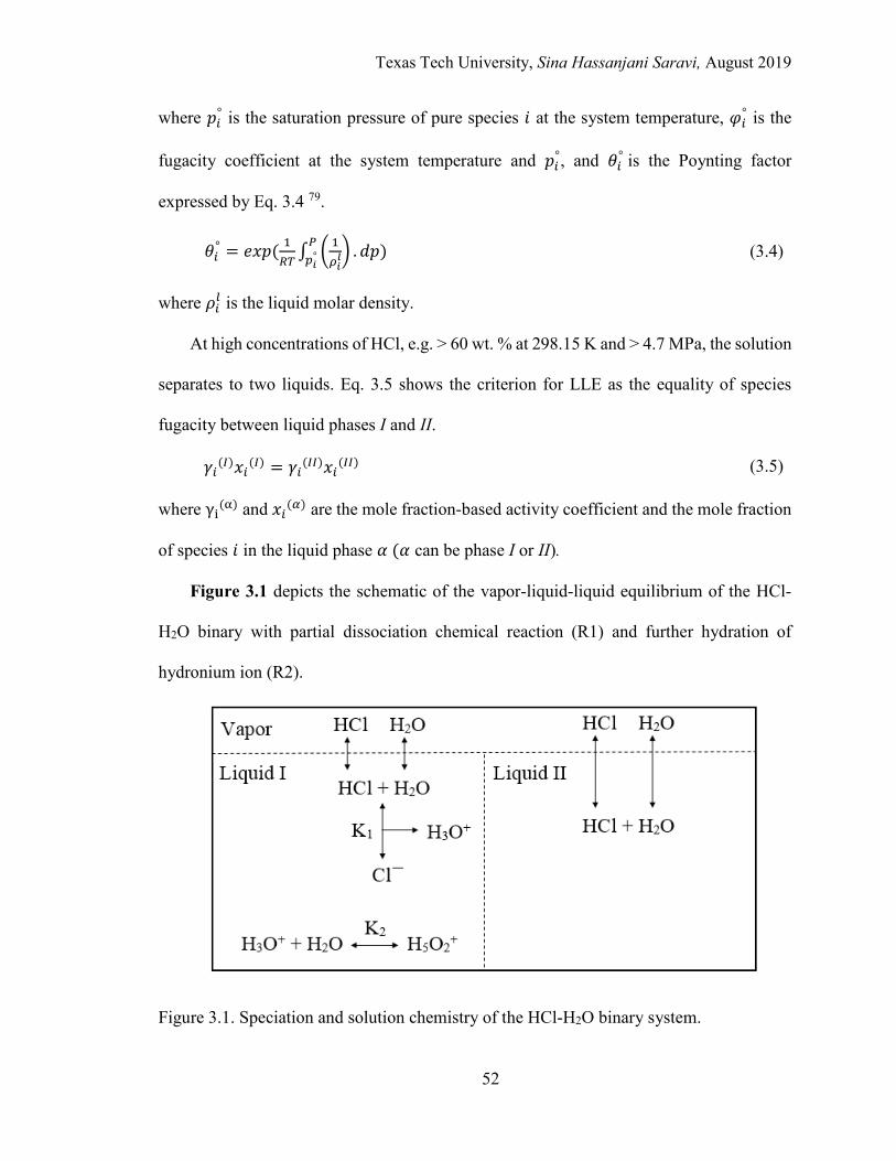
Texas Tech University, Sina Hassanjani Saravi, August 2019
52
where 𝑝𝑝𝑖𝑖° is the saturation pressure of pure species 𝑖𝑖 at the system temperature, 𝜑𝜑𝑖𝑖° is the
fugacity coefficient at the system temperature and 𝑝𝑝𝑖𝑖°, and 𝜃𝜃𝑖𝑖° is the Poynting factor
expressed by Eq. 3.4 79.
𝜃𝜃𝑖𝑖° = 𝑒𝑒𝑥𝑥𝑝𝑝 ( 1𝐿𝐿𝜕𝜕 ∫ � 1
𝜌𝜌𝑖𝑖𝑙𝑙� .𝑑𝑑𝑝𝑝𝑃𝑃
𝑝𝑝𝑖𝑖° ) (3.4)
where 𝜌𝜌𝑖𝑖𝑙𝑙 is the liquid molar density.
At high concentrations of HCl, e.g. > 60 wt. % at 298.15 K and > 4.7 MPa, the solution
separates to two liquids. Eq. 3.5 shows the criterion for LLE as the equality of species
fugacity between liquid phases I and II.
𝛾𝛾𝑖𝑖(𝐼𝐼)𝑥𝑥𝑖𝑖(𝐼𝐼) = 𝛾𝛾𝑖𝑖(𝐼𝐼𝐼𝐼)𝑥𝑥𝑖𝑖(𝐼𝐼𝐼𝐼) (3.5)
where γi(α) and 𝑥𝑥𝑖𝑖(𝛼𝛼) are the mole fraction-based activity coefficient and the mole fraction
of species 𝑖𝑖 in the liquid phase 𝛼𝛼 (𝛼𝛼 can be phase I or II).
Figure 3.1 depicts the schematic of the vapor-liquid-liquid equilibrium of the HCl-
H2O binary with partial dissociation chemical reaction (R1) and further hydration of
hydronium ion (R2).
Figure 3.1. Speciation and solution chemistry of the HCl-H2O binary system.
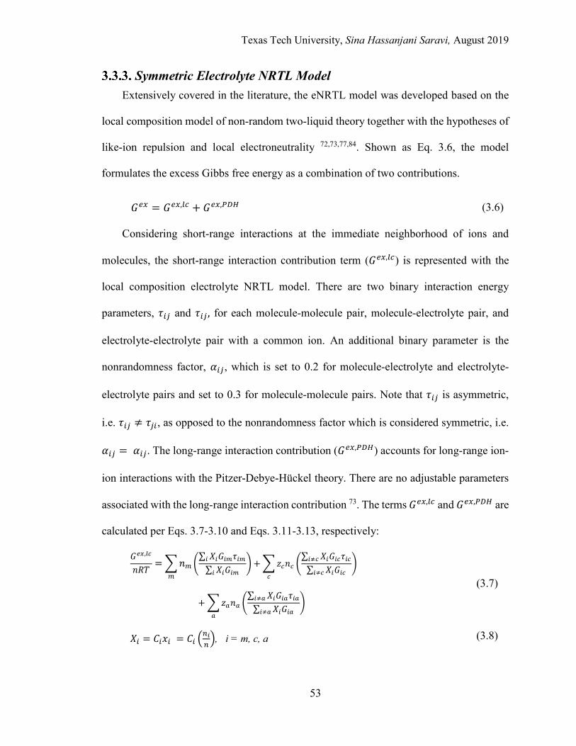
Texas Tech University, Sina Hassanjani Saravi, August 2019
53
Symmetric Electrolyte NRTL Model Extensively covered in the literature, the eNRTL model was developed based on the
local composition model of non-random two-liquid theory together with the hypotheses of
like-ion repulsion and local electroneutrality 72,73,77,84. Shown as Eq. 3.6, the model
formulates the excess Gibbs free energy as a combination of two contributions.
𝐺𝐺𝑒𝑒𝑒𝑒 = 𝐺𝐺𝑒𝑒𝑒𝑒,𝑙𝑙𝐿𝐿 + 𝐺𝐺𝑒𝑒𝑒𝑒,𝑃𝑃𝑃𝑃𝐻𝐻 (3.6)
Considering short-range interactions at the immediate neighborhood of ions and
molecules, the short-range interaction contribution term (𝐺𝐺𝑒𝑒𝑒𝑒,𝑙𝑙𝐿𝐿) is represented with the
local composition electrolyte NRTL model. There are two binary interaction energy
parameters, 𝜏𝜏𝑖𝑖𝑗𝑗 and 𝜏𝜏𝑖𝑖𝑗𝑗 , for each molecule-molecule pair, molecule-electrolyte pair, and
electrolyte-electrolyte pair with a common ion. An additional binary parameter is the
nonrandomness factor, 𝛼𝛼𝑖𝑖𝑗𝑗, which is set to 0.2 for molecule-electrolyte and electrolyte-
electrolyte pairs and set to 0.3 for molecule-molecule pairs. Note that 𝜏𝜏𝑖𝑖𝑗𝑗 is asymmetric,
i.e. 𝜏𝜏𝑖𝑖𝑗𝑗 ≠ 𝜏𝜏𝑗𝑗𝑖𝑖, as opposed to the nonrandomness factor which is considered symmetric, i.e.
𝛼𝛼𝑖𝑖𝑗𝑗 = 𝛼𝛼𝑖𝑖𝑗𝑗. The long-range interaction contribution (𝐺𝐺𝑒𝑒𝑒𝑒,𝑃𝑃𝑃𝑃𝐻𝐻) accounts for long-range ion-
ion interactions with the Pitzer-Debye-Hückel theory. There are no adjustable parameters
associated with the long-range interaction contribution 73. The terms 𝐺𝐺𝑒𝑒𝑒𝑒,𝑙𝑙𝐿𝐿 and 𝐺𝐺𝑒𝑒𝑒𝑒,𝑃𝑃𝑃𝑃𝐻𝐻 are
calculated per Eqs. 3.7-3.10 and Eqs. 3.11-3.13, respectively:
𝐺𝐺𝑒𝑒𝑒𝑒,𝑙𝑙𝐿𝐿
𝑙𝑙𝑅𝑅𝑇𝑇= �𝑙𝑙𝑚𝑚
𝑚𝑚�∑ 𝑋𝑋𝑖𝑖𝐺𝐺𝑖𝑖𝑚𝑚𝜏𝜏𝑖𝑖𝑚𝑚𝑖𝑖
∑ 𝑋𝑋𝑖𝑖𝐺𝐺𝑖𝑖𝑚𝑚𝑖𝑖�+ �𝑧𝑧𝐿𝐿𝑙𝑙𝐿𝐿
𝐿𝐿
�∑ 𝑋𝑋𝑖𝑖𝐺𝐺𝑖𝑖𝐿𝐿𝜏𝜏𝑖𝑖𝐿𝐿𝑖𝑖≠𝐿𝐿
∑ 𝑋𝑋𝑖𝑖𝐺𝐺𝑖𝑖𝐿𝐿𝑖𝑖≠𝐿𝐿�
+ �𝑧𝑧𝑎𝑎𝑙𝑙𝑎𝑎𝑎𝑎
�∑ 𝑋𝑋𝑖𝑖𝐺𝐺𝑖𝑖𝑎𝑎𝜏𝜏𝑖𝑖𝑎𝑎𝑖𝑖≠𝑎𝑎
∑ 𝑋𝑋𝑖𝑖𝐺𝐺𝑖𝑖𝑎𝑎𝑖𝑖≠𝑎𝑎�
(3.7)
𝑋𝑋𝑖𝑖 = 𝐶𝐶𝑖𝑖𝑥𝑥𝑖𝑖 = 𝐶𝐶𝑖𝑖 �𝜕𝜕𝑖𝑖𝜕𝜕�, i = m, c, a (3.8)
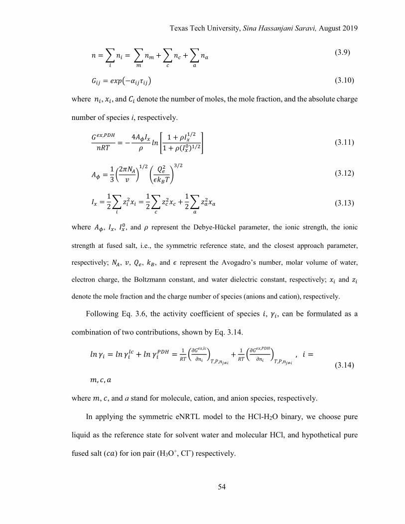
Texas Tech University, Sina Hassanjani Saravi, August 2019
54
𝑙𝑙 = �𝑙𝑙𝑖𝑖𝑖𝑖
= �𝑙𝑙𝑚𝑚𝑚𝑚
+ �𝑙𝑙𝐿𝐿𝐿𝐿
+ �𝑙𝑙𝑎𝑎𝑎𝑎
(3.9)
𝐺𝐺𝑖𝑖𝑗𝑗 = 𝑒𝑒𝑥𝑥𝑝𝑝�−𝛼𝛼𝑖𝑖𝑗𝑗𝜏𝜏𝑖𝑖𝑗𝑗� (3.10)
where 𝑙𝑙𝑖𝑖, 𝑥𝑥𝑖𝑖, and 𝐶𝐶𝑖𝑖 denote the number of moles, the mole fraction, and the absolute charge
number of species i, respectively.
𝐺𝐺𝑒𝑒𝑒𝑒,𝑃𝑃𝑃𝑃𝐻𝐻
𝑙𝑙𝑅𝑅𝑇𝑇= −
4𝐴𝐴𝜙𝜙𝐼𝐼𝑒𝑒𝜌𝜌
𝑙𝑙𝑙𝑙 �1 + 𝜌𝜌𝐼𝐼𝑒𝑒
1/2
1 + 𝜌𝜌(𝐼𝐼𝑒𝑒0)1/2� (3.11)
𝐴𝐴𝜙𝜙 =
13�
2𝜋𝜋𝑁𝑁𝐴𝐴𝑣𝑣
�1/2
�𝑄𝑄𝑒𝑒2
𝜖𝜖𝑘𝑘𝐵𝐵𝑇𝑇�3/2
(3.12)
𝐼𝐼𝑒𝑒 =12�𝑧𝑧𝑖𝑖2𝑥𝑥𝑖𝑖𝑖𝑖
=12�𝑧𝑧𝐿𝐿2𝑥𝑥𝐿𝐿𝐿𝐿
+12�𝑧𝑧𝑎𝑎2𝑥𝑥𝑎𝑎𝑎𝑎
(3.13)
where 𝐴𝐴𝜙𝜙, 𝐼𝐼𝑒𝑒, 𝐼𝐼𝑒𝑒0, and 𝜌𝜌 represent the Debye-Hückel parameter, the ionic strength, the ionic
strength at fused salt, i.e., the symmetric reference state, and the closest approach parameter,
respectively; 𝑁𝑁𝐴𝐴, 𝑣𝑣, 𝑄𝑄𝑒𝑒, 𝑘𝑘𝐵𝐵, and 𝜖𝜖 represent the Avogadro’s number, molar volume of water,
electron charge, the Boltzmann constant, and water dielectric constant, respectively; 𝑥𝑥𝑖𝑖 and 𝑧𝑧𝑖𝑖
denote the mole fraction and the charge number of species (anions and cation), respectively.
Following Eq. 3.6, the activity coefficient of species 𝑖𝑖, 𝛾𝛾𝑖𝑖, can be formulated as a
combination of two contributions, shown by Eq. 3.14.
𝑙𝑙𝑙𝑙 𝛾𝛾𝑖𝑖 = 𝑙𝑙𝑙𝑙 𝛾𝛾𝑖𝑖𝑙𝑙𝐿𝐿 + 𝑙𝑙𝑙𝑙 𝛾𝛾𝑖𝑖𝑃𝑃𝑃𝑃𝐻𝐻 = 1𝑅𝑅𝑇𝑇�𝜕𝜕𝐺𝐺
𝑒𝑒𝑥𝑥,𝑙𝑙𝑐𝑐
𝜕𝜕𝑙𝑙𝑖𝑖�𝑇𝑇,𝑃𝑃,𝑙𝑙𝑗𝑗≠𝑖𝑖
+ 1𝑅𝑅𝑇𝑇�𝜕𝜕𝐺𝐺
𝑒𝑒𝑥𝑥,𝑃𝑃𝐷𝐷𝐻𝐻
𝜕𝜕𝑙𝑙𝑖𝑖�𝑇𝑇,𝑃𝑃,𝑙𝑙𝑗𝑗≠𝑖𝑖
, 𝑖𝑖 =
𝑚𝑚, 𝑐𝑐,𝑎𝑎
(3.14)
where 𝑚𝑚, 𝑐𝑐, and a stand for molecule, cation, and anion species, respectively.
In applying the symmetric eNRTL model to the HCl-H2O binary, we choose pure
liquid as the reference state for solvent water and molecular HCl, and hypothetical pure
fused salt (𝑐𝑐𝑎𝑎) for ion pair (H3O+, Clˉ) respectively.
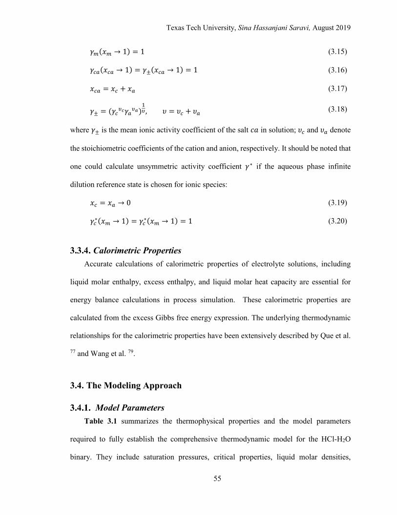
Texas Tech University, Sina Hassanjani Saravi, August 2019
55
𝛾𝛾𝑚𝑚(𝑥𝑥𝑚𝑚 → 1) = 1 (3.15)
𝛾𝛾𝐿𝐿𝑎𝑎(𝑥𝑥𝐿𝐿𝑎𝑎 → 1) = 𝛾𝛾±(𝑥𝑥𝐿𝐿𝑎𝑎 → 1) = 1 (3.16)
𝑥𝑥𝐿𝐿𝑎𝑎 = 𝑥𝑥𝐿𝐿 + 𝑥𝑥𝑎𝑎 (3.17)
𝛾𝛾± = (𝛾𝛾𝐿𝐿𝜐𝜐𝑐𝑐𝛾𝛾𝑎𝑎𝜐𝜐𝑎𝑎)1𝜐𝜐, 𝜐𝜐 = 𝜐𝜐𝐿𝐿 + 𝜐𝜐𝑎𝑎 (3.18)
where 𝛾𝛾± is the mean ionic activity coefficient of the salt 𝑐𝑐𝑎𝑎 in solution; 𝜐𝜐𝐿𝐿 and 𝜐𝜐𝑎𝑎 denote
the stoichiometric coefficients of the cation and anion, respectively. It should be noted that
one could calculate unsymmetric activity coefficient 𝛾𝛾∗ if the aqueous phase infinite
dilution reference state is chosen for ionic species:
𝑥𝑥𝐿𝐿 = 𝑥𝑥𝑎𝑎 → 0 (3.19)
𝛾𝛾𝐿𝐿∗(𝑥𝑥𝑚𝑚 → 1) = 𝛾𝛾𝐿𝐿∗(𝑥𝑥𝑚𝑚 → 1) = 1 (3.20)
Calorimetric Properties Accurate calculations of calorimetric properties of electrolyte solutions, including
liquid molar enthalpy, excess enthalpy, and liquid molar heat capacity are essential for
energy balance calculations in process simulation. These calorimetric properties are
calculated from the excess Gibbs free energy expression. The underlying thermodynamic
relationships for the calorimetric properties have been extensively described by Que et al.
77 and Wang et al. 79.
3.4. The Modeling Approach
Model Parameters Table 3.1 summarizes the thermophysical properties and the model parameters
required to fully establish the comprehensive thermodynamic model for the HCl-H2O
binary. They include saturation pressures, critical properties, liquid molar densities,
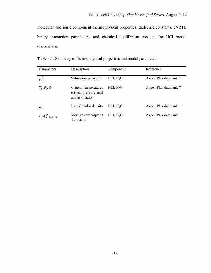
Texas Tech University, Sina Hassanjani Saravi, August 2019
56
molecular and ionic component thermophysical properties, dielectric constants, eNRTL
binary interaction parameters, and chemical equilibrium constant for HCl partial
dissociation.
Table 3.1. Summary of thermophysical properties and model parameters.
Parameters Description Component Reference
𝑝𝑝𝑖𝑖° Saturation pressure HCl, H2O Aspen Plus databank 88
𝑇𝑇𝐿𝐿 ,𝑃𝑃𝐿𝐿 ,𝛺𝛺 Critical temperature, critical pressure, and acentric factor
HCl, H2O Aspen Plus databank 88
𝜌𝜌𝑖𝑖𝑙𝑙 Liquid molar density HCl, H2O Aspen Plus databank 88
𝛥𝛥𝑓𝑓ℎ𝑚𝑚,298.15𝑖𝑖𝑖𝑖 Ideal gas enthalpy of
formation HCl, H2O Aspen Plus databank 88
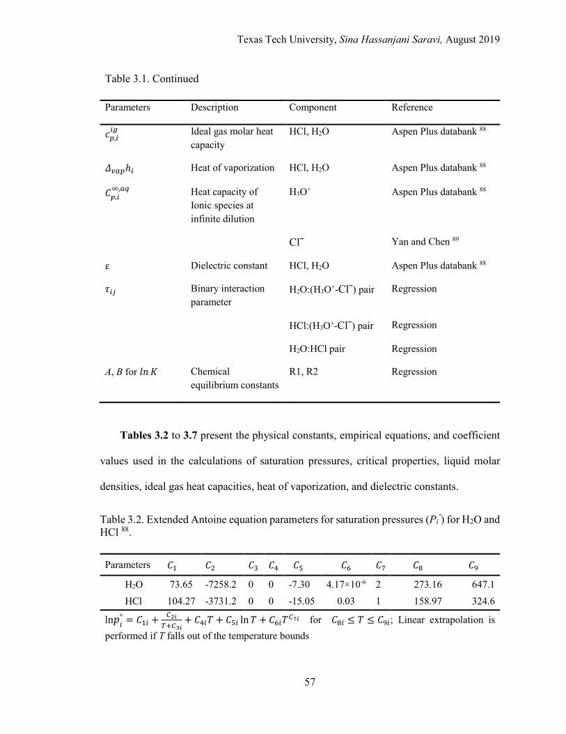
Texas Tech University, Sina Hassanjani Saravi, August 2019
57
Table 3.1. Continued
Parameters Description Component Reference
𝑐𝑐𝑝𝑝,𝑖𝑖𝑖𝑖𝑖𝑖 Ideal gas molar heat
capacity HCl, H2O Aspen Plus databank 88
𝛥𝛥𝑣𝑣𝑎𝑎𝑝𝑝ℎ𝑖𝑖 Heat of vaporization HCl, H2O Aspen Plus databank 88
𝐶𝐶𝑝𝑝,𝑖𝑖∞,𝑎𝑎𝑎𝑎 Heat capacity of
Ionic species at infinite dilution
H3O+ Aspen Plus databank 88
Clˉ Yan and Chen 89
ε Dielectric constant HCl, H2O Aspen Plus databank 88
𝜏𝜏𝑖𝑖𝑗𝑗 Binary interaction parameter
H2O:(H3O+-Clˉ) pair Regression
HCl:(H3O+-Clˉ) pair Regression
H2O:HCl pair Regression
A, B for 𝑙𝑙𝑙𝑙 𝐾𝐾 Chemical equilibrium constants
R1, R2 Regression
Tables 3.2 to 3.7 present the physical constants, empirical equations, and coefficient
values used in the calculations of saturation pressures, critical properties, liquid molar
densities, ideal gas heat capacities, heat of vaporization, and dielectric constants.
Table 3.2. Extended Antoine equation parameters for saturation pressures (Piº) for H2O and
HCl 88.
Parameters 𝐶𝐶1 𝐶𝐶2 𝐶𝐶3 𝐶𝐶4 𝐶𝐶5 𝐶𝐶6 𝐶𝐶7 𝐶𝐶8 𝐶𝐶9
H2O 73.65 -7258.2 0 0 -7.30 4.17×10⁻⁶ 2 273.16 647.1 HCl 104.27 -3731.2 0 0 -15.05 0.03 1 158.97 324.6
ln𝑝𝑝𝑖𝑖° = 𝐶𝐶1𝑖𝑖 + 𝐶𝐶2𝑖𝑖
𝜕𝜕+𝐶𝐶3𝑖𝑖+ 𝐶𝐶4𝑖𝑖𝑇𝑇 + 𝐶𝐶5𝑖𝑖 ln𝑇𝑇 + 𝐶𝐶6𝑖𝑖𝑇𝑇𝐶𝐶7𝑖𝑖 for 𝐶𝐶8𝑖𝑖 ≤ 𝑇𝑇 ≤ 𝐶𝐶9𝑖𝑖; Linear extrapolation is
performed if T falls out of the temperature bounds

Texas Tech University, Sina Hassanjani Saravi, August 2019
58
Table 3.3. Redlich-Kwong equation of state parameters for H2O and HCl 88.
Parameters 𝑇𝑇𝐶𝐶 (K) 𝑃𝑃𝐶𝐶 (MPa) Ω
H2O 647.10 22.29 0.345
HCl 324.65 8.42 0.131
Table 3.4. DIPPR liquid molar density (ρil) model parameters for H2O and HCl 88
Parameters 𝐶𝐶1 𝐶𝐶2 𝐶𝐶3 𝐶𝐶4 𝐶𝐶5 𝐶𝐶6 𝐶𝐶7
H2O 17.86 58.61 -95.37 213.89 -141.26 273.16 647.10
HCl 3.34 0.27 324.65 0.32 0.00 158.97 324.65
𝜌𝜌𝑖𝑖𝑙𝑙 = 𝐶𝐶1𝑖𝑖/𝐶𝐶2𝑖𝑖1+(1−𝜕𝜕/𝐶𝐶3𝑖𝑖)𝐶𝐶4𝑖𝑖 for 𝐶𝐶6𝑖𝑖 ≤ 𝑇𝑇 ≤ 𝐶𝐶7𝑖𝑖, for H2O
𝜌𝜌𝑖𝑖𝑙𝑙 = 𝐶𝐶1𝑖𝑖 + 𝐶𝐶2𝑖𝑖𝜏𝜏0.35 + 𝐶𝐶3𝑖𝑖𝜏𝜏2/3 + 𝐶𝐶4𝑖𝑖𝜏𝜏 + 𝐶𝐶5𝑖𝑖𝜏𝜏4/3 for 𝐶𝐶6𝑖𝑖 ≤ 𝑇𝑇 ≤ 𝐶𝐶7𝑖𝑖, for HCl
𝜏𝜏 = 1 − 𝜕𝜕𝜕𝜕𝑐𝑐
; 𝑣𝑣𝑖𝑖° is the liquid molar volume of species i; 𝑇𝑇𝐶𝐶 is the critical temperature of species
i; Linear extrapolation is performed if T falls out of the temperature bounds
Table 3.5. DIPPR ideal gas heat capacity (cp,iig) model parameters for H2O and HCl 88
Parameters 𝐶𝐶1 𝐶𝐶2 𝐶𝐶3 𝐶𝐶4 𝐶𝐶5 𝐶𝐶6 𝐶𝐶7
H2O 56.6 0.61204 -0.6258 0.3988 0 273.15 647.1
HCl 34.872 2.1553 -2.9128 1.2442 0 158.97 324.65
𝑐𝑐𝑝𝑝,𝑖𝑖𝑖𝑖𝑖𝑖 = 𝐶𝐶1𝑖𝑖 + 𝐶𝐶2𝑖𝑖 �
𝐶𝐶3𝑖𝑖𝜕𝜕�
𝑠𝑠𝑖𝑖𝜕𝜕ℎ(𝐶𝐶3𝑖𝑖 𝜕𝜕� )�2
+ 𝐶𝐶4𝑖𝑖 �𝐶𝐶5𝑖𝑖
𝜕𝜕�
𝑠𝑠𝑖𝑖𝜕𝜕ℎ(𝐶𝐶5𝑖𝑖 𝜕𝜕� )�2
for 𝐶𝐶6𝑖𝑖 ≤ 𝑇𝑇 ≤ 𝐶𝐶7𝑖𝑖
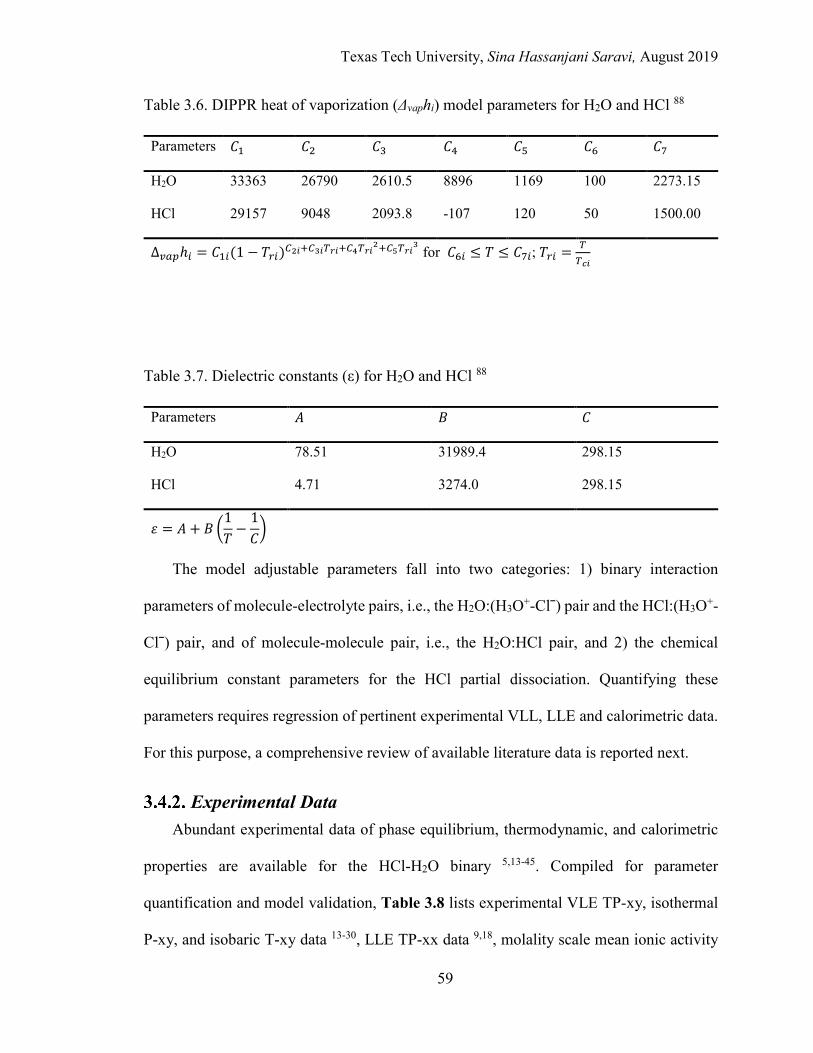
Texas Tech University, Sina Hassanjani Saravi, August 2019
59
Table 3.6. DIPPR heat of vaporization (Δvaphi) model parameters for H2O and HCl 88
Parameters 𝐶𝐶1 𝐶𝐶2 𝐶𝐶3 𝐶𝐶4 𝐶𝐶5 𝐶𝐶6 𝐶𝐶7
H2O 33363 26790 2610.5 8896 1169 100 2273.15
HCl 29157 9048 2093.8 -107 120 50 1500.00
∆𝑣𝑣𝑎𝑎𝑝𝑝ℎ𝑖𝑖 = 𝐶𝐶1𝑖𝑖(1 − 𝑇𝑇𝑟𝑟𝑖𝑖)𝐶𝐶2𝑖𝑖+𝐶𝐶3𝑖𝑖𝜕𝜕𝑟𝑟𝑖𝑖+𝐶𝐶4𝜕𝜕𝑟𝑟𝑖𝑖2+𝐶𝐶5𝜕𝜕𝑟𝑟𝑖𝑖3 for 𝐶𝐶6𝑖𝑖 ≤ 𝑇𝑇 ≤ 𝐶𝐶7𝑖𝑖; 𝑇𝑇𝑟𝑟𝑖𝑖 = 𝜕𝜕
𝜕𝜕𝑐𝑐𝑖𝑖
Table 3.7. Dielectric constants (ε) for H2O and HCl 88
Parameters 𝐴𝐴 𝐵𝐵 𝐶𝐶
H2O 78.51 31989.4 298.15
HCl 4.71 3274.0 298.15
𝜀𝜀 = 𝐴𝐴 + 𝐵𝐵 �1𝑇𝑇−
1𝐶𝐶�
The model adjustable parameters fall into two categories: 1) binary interaction
parameters of molecule-electrolyte pairs, i.e., the H2O:(H3O+-Clˉ) pair and the HCl:(H3O+-
Clˉ) pair, and of molecule-molecule pair, i.e., the H2O:HCl pair, and 2) the chemical
equilibrium constant parameters for the HCl partial dissociation. Quantifying these
parameters requires regression of pertinent experimental VLL, LLE and calorimetric data.
For this purpose, a comprehensive review of available literature data is reported next.
Experimental Data Abundant experimental data of phase equilibrium, thermodynamic, and calorimetric
properties are available for the HCl-H2O binary 5,13-45. Compiled for parameter
quantification and model validation, Table 3.8 lists experimental VLE TP-xy, isothermal
P-xy, and isobaric T-xy data 13-30, LLE TP-xx data 9,18, molality scale mean ionic activity
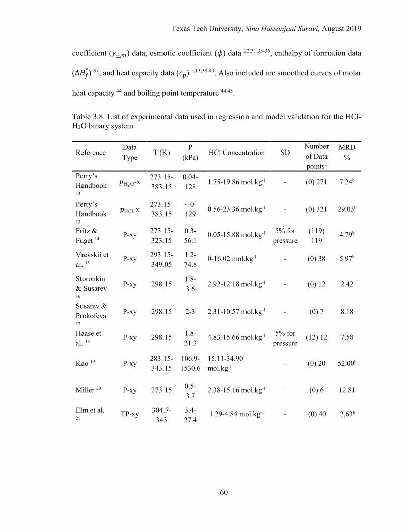
Texas Tech University, Sina Hassanjani Saravi, August 2019
60
coefficient (𝛾𝛾±,𝑚𝑚) data, osmotic coefficient (𝜙𝜙) data 22,31,33-36, enthalpy of formation data
(∆𝐻𝐻𝑓𝑓°) 37, and heat capacity data (𝑐𝑐𝑝𝑝) 5,13,38-43. Also included are smoothed curves of molar
heat capacity 44 and boiling point temperature 44,45.
Table 3.8. List of experimental data used in regression and model validation for the HCl-H2O binary system
Reference Data Type
T (K) P
(kPa) HCl Concentration SD
Number of Data pointsa
MRD %
Perry’s Handbook 13
𝑝𝑝H2O-x 273.15-383.15
0.04-128
1.75-19.86 mol.kg-1 - (0) 271 7.24b
Perry’s Handbook 13
𝑝𝑝HCl-x 273.15-383.15
~ 0-129
0.56-23.36 mol.kg-1 - (0) 321 29.03b
Fritz & Fuget 14
P-xy 273.15-323.15
0.3-56.1
0.05-15.88 mol.kg-1 5% for pressure
(119) 119
4.79b
Vrevskii et al. 15
P-xy 293.15-349.05
1.2-74.8
0-16.02 mol.kg-1 - (0) 38 5.97b
Storonkin & Susarev 16
P-xy 298.15 1.8-3.6
2.92-12.18 mol.kg-1 - (0) 12 2.42
Susarev & Prokofeva 17
P-xy 298.15 2-3 2.31-10.57 mol.kg-1 - (0) 7 8.18
Haase et al. 18
P-xy 298.15 1.8-21.3
4.83-15.66 mol.kg-1 5% for pressure
(12) 12 7.58
Kao 19 P-xy 283.15-343.15
106.9-1530.6
15.11-34.90 mol.kg-1
- (0) 20 52.00b
Miller 20 P-xy 273.15 0.5-3.7
2.38-15.16 mol.kg-1 -
(0) 6 12.81
Elm et al. 21
TP-xy 304.7-343
3.4-27.4
1.29-4.84 mol.kg-1 - (0) 40 2.63b
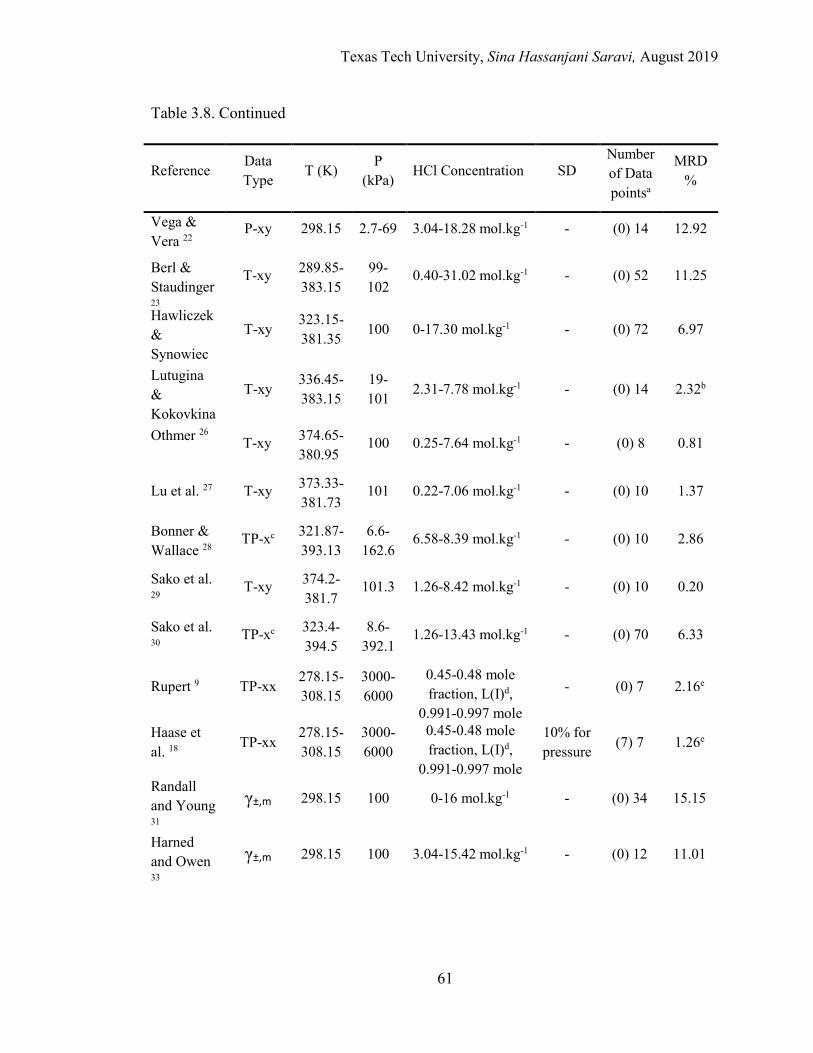
Texas Tech University, Sina Hassanjani Saravi, August 2019
61
Table 3.8. Continued
Reference Data Type
T (K) P
(kPa) HCl Concentration SD
Number of Data pointsa
MRD %
Vega & Vera 22
P-xy 298.15 2.7-69 3.04-18.28 mol.kg-1 - (0) 14 12.92
Berl & Staudinger 23
T-xy 289.85-383.15
99-102
0.40-31.02 mol.kg-1 - (0) 52 11.25
Hawliczek & Synowiec 24
T-xy 323.15-381.35
100 0-17.30 mol.kg-1 - (0) 72 6.97
Lutugina & Kokovkina 2
T-xy 336.45-383.15
19-101
2.31-7.78 mol.kg-1 - (0) 14 2.32b
Othmer 26
T-xy 374.65-380.95
100 0.25-7.64 mol.kg-1 - (0) 8 0.81
Lu et al. 27 T-xy 373.33-381.73
101 0.22-7.06 mol.kg-1 - (0) 10 1.37
Bonner & Wallace 28
TP-xc 321.87-393.13
6.6-162.6
6.58-8.39 mol.kg-1 - (0) 10 2.86
Sako et al. 29
T-xy 374.2-381.7
101.3 1.26-8.42 mol.kg-1 - (0) 10 0.20
Sako et al. 30
TP-xc 323.4-394.5
8.6-392.1
1.26-13.43 mol.kg-1 - (0) 70 6.33
Rupert 9 TP-xx 278.15-308.15
3000-6000
0.45-0.48 mole fraction, L(I)d,
0.991-0.997 mole
- (0) 7 2.16e
Haase et al. 18 TP-xx
278.15-308.15
3000-6000
0.45-0.48 mole fraction, L(I)d,
0.991-0.997 mole
10% for pressure (7) 7 1.26e
Randall and Young 31
γ±,m 298.15 100 0-16 mol.kg-1 - (0) 34 15.15
Harned and Owen 33
γ±,m 298.15 100 3.04-15.42 mol.kg-1 - (0) 12 11.01
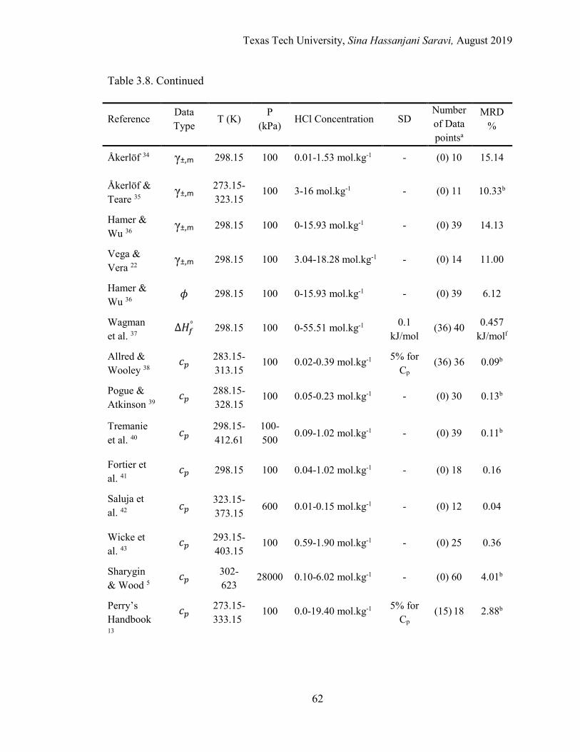
Texas Tech University, Sina Hassanjani Saravi, August 2019
62
Table 3.8. Continued
Reference Data Type T (K)
P (kPa)
HCl Concentration SD Number of Data pointsa
MRD %
Åkerlöf 34 γ±,m 298.15 100 0.01-1.53 mol.kg-1 - (0) 10 15.14
Åkerlöf & Teare 35
γ±,m 273.15-323.15
100 3-16 mol.kg-1 - (0) 11 10.33b
Hamer & Wu 36
γ±,m 298.15 100 0-15.93 mol.kg-1 - (0) 39 14.13
Vega & Vera 22
γ±,m 298.15 100 3.04-18.28 mol.kg-1 - (0) 14 11.00
Hamer & Wu 36
𝜙𝜙 298.15 100 0-15.93 mol.kg-1 - (0) 39 6.12
Wagman et al. 37
∆𝐻𝐻𝑓𝑓° 298.15 100 0-55.51 mol.kg-1 0.1 kJ/mol
(36) 40 0.457 kJ/molf
Allred & Wooley 38
𝑐𝑐𝑝𝑝 283.15-313.15
100 0.02-0.39 mol.kg-1 5% for Cp
(36) 36 0.09b
Pogue & Atkinson 39
𝑐𝑐𝑝𝑝 288.15-328.15
100 0.05-0.23 mol.kg-1 - (0) 30 0.13b
Tremanie et al. 40
𝑐𝑐𝑝𝑝 298.15-412.61
100-500
0.09-1.02 mol.kg-1 - (0) 39 0.11b
Fortier et al. 41
𝑐𝑐𝑝𝑝 298.15 100 0.04-1.02 mol.kg-1 - (0) 18 0.16
Saluja et al. 42
𝑐𝑐𝑝𝑝 323.15-373.15
600 0.01-0.15 mol.kg-1 - (0) 12 0.04
Wicke et al. 43
𝑐𝑐𝑝𝑝 293.15-403.15
100 0.59-1.90 mol.kg-1 - (0) 25 0.36
Sharygin & Wood 5
𝑐𝑐𝑝𝑝 302-623
28000 0.10-6.02 mol.kg-1 - (0) 60 4.01b
Perry’s Handbook 13
𝑐𝑐𝑝𝑝 273.15-333.15
100 0.0-19.40 mol.kg-1 5% for Cp
(15) 18 2.88b
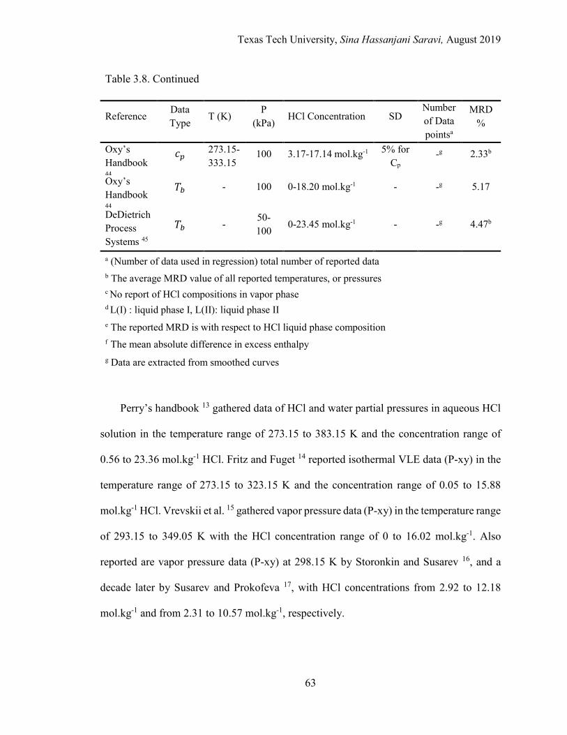
Texas Tech University, Sina Hassanjani Saravi, August 2019
63
Table 3.8. Continued
Reference Data Type T (K)
P (kPa)
HCl Concentration SD Number of Data pointsa
MRD %
Oxy’s Handbook 44
𝑐𝑐𝑝𝑝 273.15-333.15
100 3.17-17.14 mol.kg-1 5% for Cp
-g 2.33b
Oxy’s Handbook 44
𝑇𝑇𝑏𝑏 - 100 0-18.20 mol.kg-1 - -g 5.17
DeDietrich Process Systems 45
𝑇𝑇𝑏𝑏 - 50- 100
0-23.45 mol.kg-1 - -g 4.47b
a (Number of data used in regression) total number of reported data b The average MRD value of all reported temperatures, or pressures c No report of HCl compositions in vapor phase
d L(I) : liquid phase I, L(II): liquid phase II e The reported MRD is with respect to HCl liquid phase composition f The mean absolute difference in excess enthalpy g Data are extracted from smoothed curves
Perry’s handbook 13 gathered data of HCl and water partial pressures in aqueous HCl
solution in the temperature range of 273.15 to 383.15 K and the concentration range of
0.56 to 23.36 mol.kg-1 HCl. Fritz and Fuget 14 reported isothermal VLE data (P-xy) in the
temperature range of 273.15 to 323.15 K and the concentration range of 0.05 to 15.88
mol.kg-1 HCl. Vrevskii et al. 15 gathered vapor pressure data (P-xy) in the temperature range
of 293.15 to 349.05 K with the HCl concentration range of 0 to 16.02 mol.kg-1. Also
reported are vapor pressure data (P-xy) at 298.15 K by Storonkin and Susarev 16, and a
decade later by Susarev and Prokofeva 17, with HCl concentrations from 2.92 to 12.18
mol.kg-1 and from 2.31 to 10.57 mol.kg-1, respectively.
Texas Tech University, Sina Hassanjani Saravi, August 2019
64
Haase et al. 18 presented vapor pressure data (P-xy) at 298.15 K for the concentration
range of 4.83 to 15.66 mol.kg-1 HCl. Kao 19 measured vapor pressure data (P-xy) in the
temperature range of 263.15 to 343.15 K and the concentration range of 15.11 to 34.90
mol.kg-1 HCl. Also presented are the compiled vapor pressure data (P-xy) of Miller et al.
20 from 238.15 to 273.15 K with the concentration range of 2.38 to 15.16 mol.kg-1 HCl.
Elm et al. 21 presented TP-xy data in the temperature range of 304.7 to 343 K with the
concentration range of 1.29 to 4.84 mol.kg-1 HCl. Vega and Vera 22 reported P-xy data at
298.15 K in the concentration range of 3.04 to 18.28 mol.kg-1 HCl.
Berl and Staudinger 23 reported isobaric T-xy data with the temperature range of
289.85 to 383.15 K at around 99 to 102 kPa and HCl concentrations from 0.40 to 31.02
mol.kg-1. Hawliczek and Synowiec 24 presented T-xy data in the temperature range of
323.15 to 381.35 K at 100 kPa within the concentration range of 0 to 17.30 mol.kg-1 HCl.
Lutugina and Kokovkina 25 presented T-xy data with the temperature range of 336.45 to
383.15 K, the pressure range of 19 to 101 kPa, and the concentration range of 2.31 to 7.78
mol.kg-1 HCl. Othmer 26 reported T-xy data at 100 kPa with the temperature range of 374.65
to 380.95 K and the concentration range of 0.25 to 7.64 mol.kg-1 HCl. Lu et al. 27 reported
T-xy data from 373.33 to 381.73 K at 101 kPa with the concentration range of 0.22 to 7.06
mol.kg-1 HCl.
Bonner and Wallace 28 presented VLE data in the form of TP-x with temperatures from
321.87 to 393.13 K, pressures from 6.6 to 162.6 kPa, and HCl concentrations from 6.58 to
8.39 mol.kg-1. Sako et al. 29 reported T-xy data under atmospheric pressure. A year later,
Sako et al. 30 measured TP-x data with the temperature range of 323.4 to 394.5 K and the
concentrations from 1.26 to 13.43 mol.kg-1 HCl.
Texas Tech University, Sina Hassanjani Saravi, August 2019
65
Haase et al. 18 reported LLE data at temperatures from 278.15 to 308.15 K and
pressures from 3 to 6 MPa. However, their measurements were limited to those of the
primary liquid phase and there were no measurements for the species compositions in the
second liquid phase. However, they reported the measurements of Rupert 9 for the second
liquid phase containing mostly pure HCl. The HCl concentration ranges for the two liquid
phases are from 0.45 to 0.48 and 0.991 to 0.997 mole fractions, respectively.
Employing the electromotive force measurements (EMF), Randall and Young 31
computed molality scale mean ionic activity coefficients of HCl for the HCl-H2O binary at
298.15 K up to 16 mol.kg-1 HCl. Using the same technique, Harned and Ehlers 32 calculated
mean ionic activity coefficients, partial molar enthalpy, and partial molar heat capacity of
HCl in the aqueous binary solution at temperatures from 273.15 to 333.15 K and
concentrations up to 4 mol.kg-1 HCl. Years later, Harned and Owen 33 extended the data
range at 298.15 K up to 15.42 mol.kg-1 HCl for the mean ionic activity coefficient. Also,
by using EMF, Åkerlöf 34 reported mean ionic activity coefficients of dilute aqueous HCl
(up to 1.53 mol.kg-1) at 298.15 K, as a part of a study of different chloride solutions in
water-methanol mixtures. Åkerlöf and Teare 35 extended their experimental work on
concentrated aqueous HCl solution and reported the mean ionic activity coefficients to
cover HCl concentrations up to 16 mol.kg-1 at temperatures from 273.15 to 323.15 K.
Hamer and Wu 36 reported mean ionic activity coefficient and osmotic coefficient data at
298.15 K and pressure of 100 kPa for concentrations from 0 to 15.93 mol.kg-1 HCl. Vega
and Vera also reported mean ionic activity coefficient data up to 18.28 mol.kg-1 HCl at
298.15 K [19].

Texas Tech University, Sina Hassanjani Saravi, August 2019
66
Wagman et al. 37 presented enthalpy of formation data for the HCl-H2O binary from
very dilute HCl solution up to 55.51 mol.kg-1 HCl at 298.15 K and 100 kPa. These enthalpy
of formation data can be easily converted to and used as excess enthalpy data. Allred and
Woolley 38 gathered heat capacity data for the HCl-H2O binary with temperatures from
283.15 to 313.15 K at 100 kPa pressure for dilute HCl solutions from 0.02 to 0.39 mol.kg-
1 HCl. Pogue and Atkinson 39 also reported the heat capacity data for the temperature range
of 288.15 to 328.15 K at 100 kPa pressure with the concentration range of 0.05 to 0.23
mol.kg-1 HCl. Moreover, the heat capacity data from Tremanie et al. 40 covered the
temperature range of 298.15 to 412.61 K at pressures of 100 to 500 kPa and the
concentration range of 0.09 to 1.02 mol.kg-1 HCl. Fortier et al. 41 reported the heat capacity
data for the concentration range of 0.04 to 1.02 mol.kg-1 HCl at 298.15 K and 100 kPa.
Saluja et al 42 published the heat capacity data covering temperatures from 323.15 to 373.15
K at pressure of 600 kPa with the concentration range of 0.01 to 0.15 mol.kg-1 HCl. Also
presented the heat capacity data, Wicke et al 43 covered the temperature range of 293.15 to
403.15 K at 100 kPa for the HCl concentrations up to 1.90 mol.kg-1. Covering the more
concentrated HCl-H2O binary system, Perry’s handbook 13 reported the heat capacity data
with the temperature range of 273.15 to 333.15 K and the concentration range of 0 to 19.40
mol.kg-1 HCl at 100 kPa pressure. Measuring the heat capacity of aqueous HCl solution at
higher temperatures and pressures, Sharygin and Wood [5] covered temperatures from 302
to 623 K at a significant pressure of 28 MPa with the concentration range of 0.10 to 6.02
mol.kg-1 HCl. In addition, the smoothed heat capacity curves reported by Occidental
Petroleum’s hydrochloric acid handbook 44 cover the temperature range of 273.15 to
333.15 K and the concentration range of 3.17 to 17.14 mol.kg-1 at 100 kPa. The handbook
Texas Tech University, Sina Hassanjani Saravi, August 2019
67
also reports smoothed boiling temperature curves covering up to 18.21 mol.kg-1 HCl at 100
kPa 44. The De Dietrich Process Systems reported the smoothed boiling temperature curves
up to 23.45 mol.kg-1 HCl at 100 kPa, and up to 21.70 mol.kg-1 HCl at 50 kPa 45.
Data Treatment, Regression, and Optimization Method Quantification of the adjustable model parameters is carried out by simultaneous
regression of selected sets of experimental data including those of VLE 14,18, LLE 18, excess
enthalpy 37, and heat capacity 13,38,44. All the remaining data sets, although not included in
the data regression, are used for model validation. The simultaneous regression and
subsequent validation of the model with such wide varieties of experimental data help
ensure consistency of these data sets under one comprehensive thermodynamic framework.
The regression data sets are selected to cover the widest temperature and concentration
ranges possible, and with the best reliability and accuracy. The VLE data of Fritz and Fuget
14 is selected because it covers a wide concentration range from 0.05 to 15.88 mol.kg-1 HCl
and temperatures ranging from 273.15 up to 323.15 K with high data accuracy. Although
few other data sets also cover wide temperature and concentration ranges, they are
excluded from the regression. For example, the data of Zeisberg 12 reported in Perry’s
Handbook 13 have been shown to be inconsistent with the more recent measurements of
Fritz and Fuget 14. Also the uncertainty of several literature data sets 15,23,24 could not be
identified. Among the LLE data available 9,18, the more recent and accurate data set 18 is
included in the regression along with its corresponding VLE data. The mean ionic activity
coefficient data sets are not considered in the regression due to the intrinsic assumption of
complete HCl dissociation associated with mean ionic activity coefficient data. The
osmotic coefficient data are also excluded because they are inherently water vapor pressure

Texas Tech University, Sina Hassanjani Saravi, August 2019
68
data and carry larger standard deviations. To cover calorimetric properties, we include in
the regression the data for excess enthalpy 37 and the data 13,38 and smoothed curves 44 for
heat capacity.
Based on prior experiences in correlating these thermodynamic data, standard
deviations (SDs) are assigned depending on the type of experimental measurement.
Temperatures are treated as error-free for all data sets. The SDs of pressures are set to 5 %.
For VLE data, the SDs of compositions in mole fraction are set to zero for liquid phase and
0.01 for vapor phase with the exception of very dilute regions (< 0.01 mole fraction) where
the SDs are assigned to be 5 %. For LLE, the SDs of compositions in mole fraction are
fixed at 0.01. For liquid molar excess enthalpy and molar heat capacity, the SDs are set to
0.1 kJ/mol and 5 %, respectively.
The objective function in data regression, i.e., residual root mean square error
(RRMSE), is defined in Eq. 3.21:
𝑅𝑅𝑅𝑅𝑀𝑀𝑆𝑆𝐸𝐸 =�∑ ∑ [
𝑍𝑍𝑖𝑖𝑗𝑗 − 𝑍𝑍𝑀𝑀𝑖𝑖𝑗𝑗𝜎𝜎𝑖𝑖𝑗𝑗
]2𝑚𝑚𝑗𝑗=1
𝑘𝑘𝑖𝑖=1
𝑘𝑘 − 𝑙𝑙
(3.21)
where experimental data is represented by 𝑍𝑍𝑀𝑀𝑖𝑖𝑗𝑗; 𝑍𝑍𝑖𝑖𝑗𝑗 is the calculated value by the model,
𝜎𝜎 denotes the SDs for each set of data; 𝑖𝑖 represents the 𝑖𝑖𝑡𝑡ℎ data point; j is one of the
measured variables; k is the total number of data points; m is the total number of measured
variables; and n is the total number of adjustable parameters. Furthermore, mean relative
deviation (MRD), shown in Eq. 3.22, provides a quantitative measure for the deviation
between the experimental data and the model results.
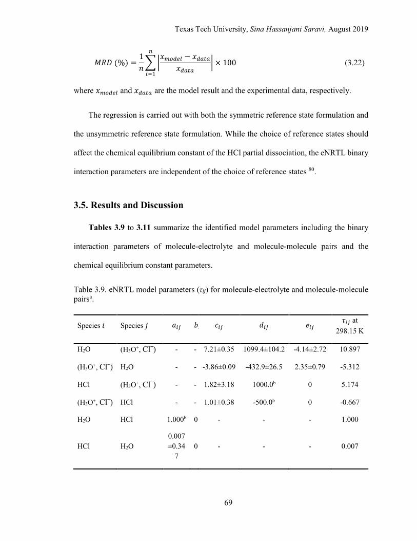
Texas Tech University, Sina Hassanjani Saravi, August 2019
69
𝑀𝑀𝑅𝑅𝐷𝐷 (%) =
1𝑙𝑙��
𝑥𝑥𝑚𝑚𝑜𝑜𝑚𝑚𝑒𝑒𝑙𝑙 − 𝑥𝑥𝑚𝑚𝑎𝑎𝑡𝑡𝑎𝑎𝑥𝑥𝑚𝑚𝑎𝑎𝑡𝑡𝑎𝑎
�𝜕𝜕
𝑖𝑖=1
× 100 (3.22)
where 𝑥𝑥𝑚𝑚𝑜𝑜𝑚𝑚𝑒𝑒𝑙𝑙 and 𝑥𝑥𝑚𝑚𝑎𝑎𝑡𝑡𝑎𝑎 are the model result and the experimental data, respectively.
The regression is carried out with both the symmetric reference state formulation and
the unsymmetric reference state formulation. While the choice of reference states should
affect the chemical equilibrium constant of the HCl partial dissociation, the eNRTL binary
interaction parameters are independent of the choice of reference states 80.
3.5. Results and Discussion
Tables 3.9 to 3.11 summarize the identified model parameters including the binary
interaction parameters of molecule-electrolyte and molecule-molecule pairs and the
chemical equilibrium constant parameters.
Table 3.9. eNRTL model parameters (τij) for molecule-electrolyte and molecule-molecule pairsa.
Species 𝑖𝑖 Species 𝑗𝑗 𝑎𝑎𝑖𝑖𝑗𝑗 𝑏𝑏𝑖𝑖 𝑐𝑐𝑖𝑖𝑗𝑗 𝑑𝑑𝑖𝑖𝑗𝑗 𝑒𝑒𝑖𝑖𝑗𝑗 𝜏𝜏𝑖𝑖𝑗𝑗 at
298.15 K
H2O (H3O+, Clˉ) - - 7.21±0.35 1099.4±104.2 -4.14±2.72 10.897
(H3O+, Clˉ) H2O - - -3.86±0.09 -432.9±26.5 2.35±0.79 -5.312
HCl (H3O+, Clˉ) - - 1.82±3.18 1000.0b 0 5.174
(H3O+, Clˉ) HCl - - 1.01±0.38 -500.0b 0 -0.667
H2O HCl 1.000b 0 - - - 1.000
HCl H2O 0.007±0.34
7 0 - - - 0.007
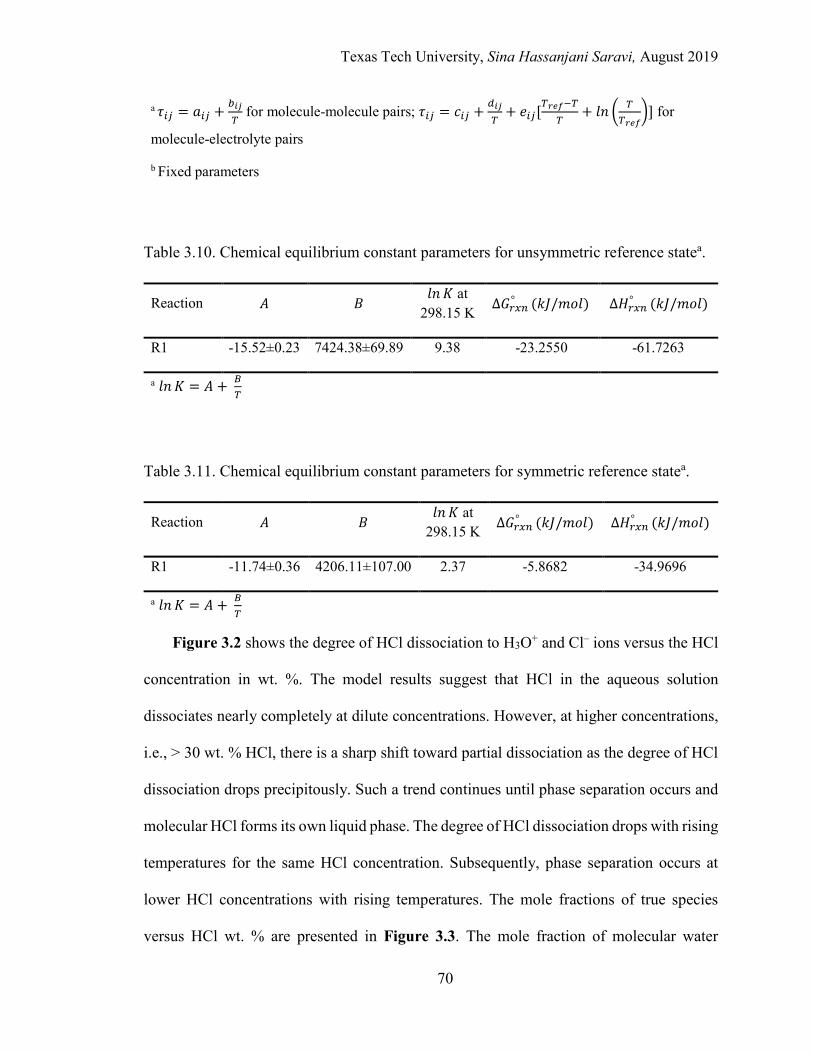
Texas Tech University, Sina Hassanjani Saravi, August 2019
70
a 𝜏𝜏𝑖𝑖𝑗𝑗 = 𝑎𝑎𝑖𝑖𝑗𝑗 + 𝑏𝑏𝑖𝑖𝑖𝑖𝜕𝜕
for molecule-molecule pairs; 𝜏𝜏𝑖𝑖𝑗𝑗 = 𝑐𝑐𝑖𝑖𝑗𝑗 + 𝑚𝑚𝑖𝑖𝑖𝑖𝜕𝜕
+ 𝑒𝑒𝑖𝑖𝑗𝑗[𝜕𝜕𝑟𝑟𝑟𝑟𝑟𝑟−𝜕𝜕𝜕𝜕
+ 𝑙𝑙𝑙𝑙 � 𝜕𝜕𝜕𝜕𝑟𝑟𝑟𝑟𝑟𝑟
�] for
molecule-electrolyte pairs
b Fixed parameters
Table 3.10. Chemical equilibrium constant parameters for unsymmetric reference statea.
Reaction 𝐴𝐴 𝐵𝐵 𝑙𝑙𝑙𝑙 𝐾𝐾 at
298.15 K ∆𝐺𝐺𝑟𝑟𝑒𝑒𝜕𝜕 ° (𝑘𝑘𝑘𝑘/𝑚𝑚𝑚𝑚𝑙𝑙) ∆𝐻𝐻𝑟𝑟𝑒𝑒𝜕𝜕
° (𝑘𝑘𝑘𝑘/𝑚𝑚𝑚𝑚𝑙𝑙)
R1 -15.52±0.23 7424.38±69.89 9.38 -23.2550 -61.7263
a 𝑙𝑙𝑙𝑙 𝐾𝐾 = 𝐴𝐴 + 𝐵𝐵𝜕𝜕
Table 3.11. Chemical equilibrium constant parameters for symmetric reference statea.
Reaction 𝐴𝐴 𝐵𝐵 𝑙𝑙𝑙𝑙 𝐾𝐾 at
298.15 K ∆𝐺𝐺𝑟𝑟𝑒𝑒𝜕𝜕 ° (𝑘𝑘𝑘𝑘/𝑚𝑚𝑚𝑚𝑙𝑙) ∆𝐻𝐻𝑟𝑟𝑒𝑒𝜕𝜕
° (𝑘𝑘𝑘𝑘/𝑚𝑚𝑚𝑚𝑙𝑙)
R1 -11.74±0.36 4206.11±107.00 2.37 -5.8682 -34.9696
a 𝑙𝑙𝑙𝑙 𝐾𝐾 = 𝐴𝐴 + 𝐵𝐵𝜕𝜕
Figure 3.2 shows the degree of HCl dissociation to H3O+ and Cl– ions versus the HCl
concentration in wt. %. The model results suggest that HCl in the aqueous solution
dissociates nearly completely at dilute concentrations. However, at higher concentrations,
i.e., > 30 wt. % HCl, there is a sharp shift toward partial dissociation as the degree of HCl
dissociation drops precipitously. Such a trend continues until phase separation occurs and
molecular HCl forms its own liquid phase. The degree of HCl dissociation drops with rising
temperatures for the same HCl concentration. Subsequently, phase separation occurs at
lower HCl concentrations with rising temperatures. The mole fractions of true species
versus HCl wt. % are presented in Figure 3.3. The mole fraction of molecular water
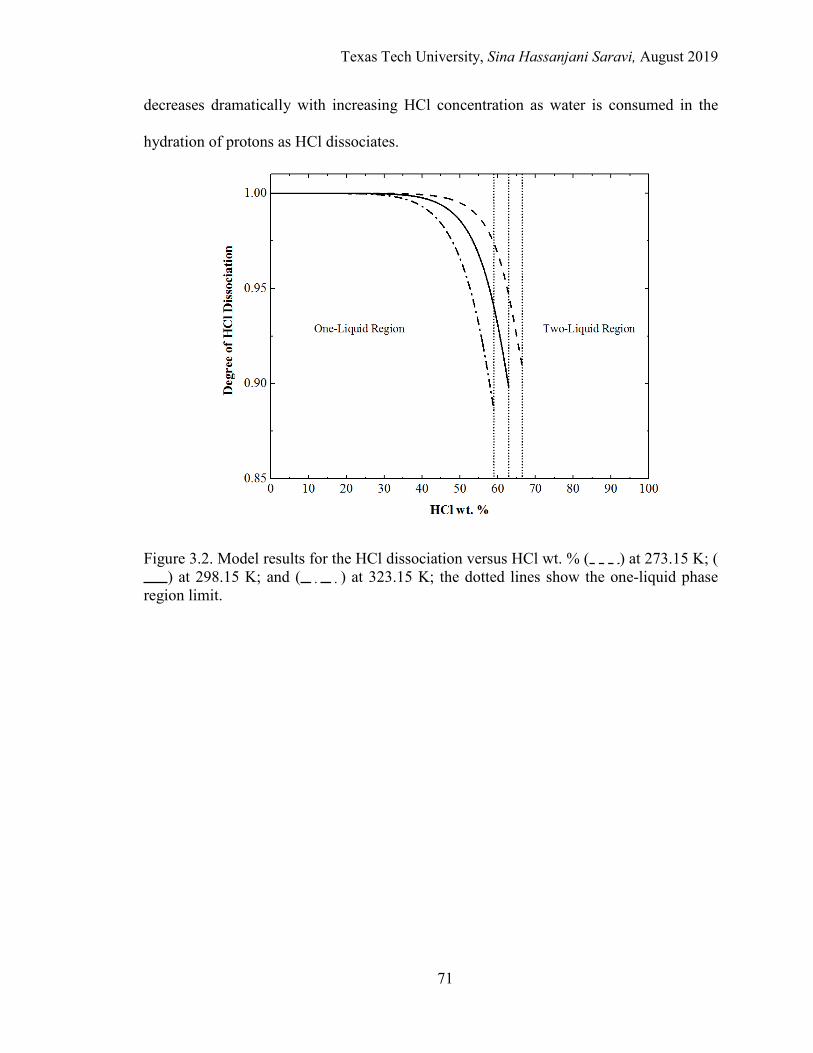
Texas Tech University, Sina Hassanjani Saravi, August 2019
71
decreases dramatically with increasing HCl concentration as water is consumed in the
hydration of protons as HCl dissociates.
Figure 3.2. Model results for the HCl dissociation versus HCl wt. % ( ) at 273.15 K; () at 298.15 K; and ( ) at 323.15 K; the dotted lines show the one-liquid phase
region limit.
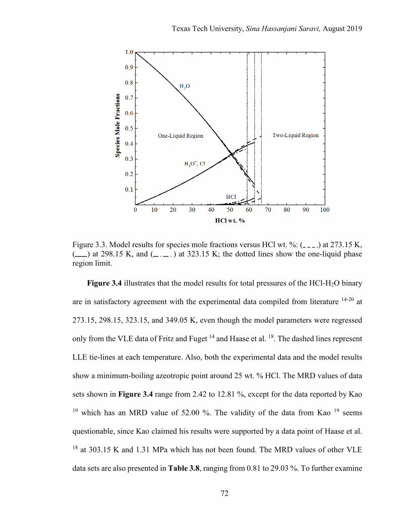
Texas Tech University, Sina Hassanjani Saravi, August 2019
72
Figure 3.3. Model results for species mole fractions versus HCl wt. %: ( ) at 273.15 K, ( ) at 298.15 K, and ( ) at 323.15 K; the dotted lines show the one-liquid phase region limit.
Figure 3.4 illustrates that the model results for total pressures of the HCl-H2O binary
are in satisfactory agreement with the experimental data compiled from literature 14-20 at
273.15, 298.15, 323.15, and 349.05 K, even though the model parameters were regressed
only from the VLE data of Fritz and Fuget 14 and Haase et al. 18. The dashed lines represent
LLE tie-lines at each temperature. Also, both the experimental data and the model results
show a minimum-boiling azeotropic point around 25 wt. % HCl. The MRD values of data
sets shown in Figure 3.4 range from 2.42 to 12.81 %, except for the data reported by Kao
19 which has an MRD value of 52.00 %. The validity of the data from Kao 19 seems
questionable, since Kao claimed his results were supported by a data point of Haase et al.
18 at 303.15 K and 1.31 MPa which has not been found. The MRD values of other VLE
data sets are also presented in Table 3.8, ranging from 0.81 to 29.03 %. To further examine
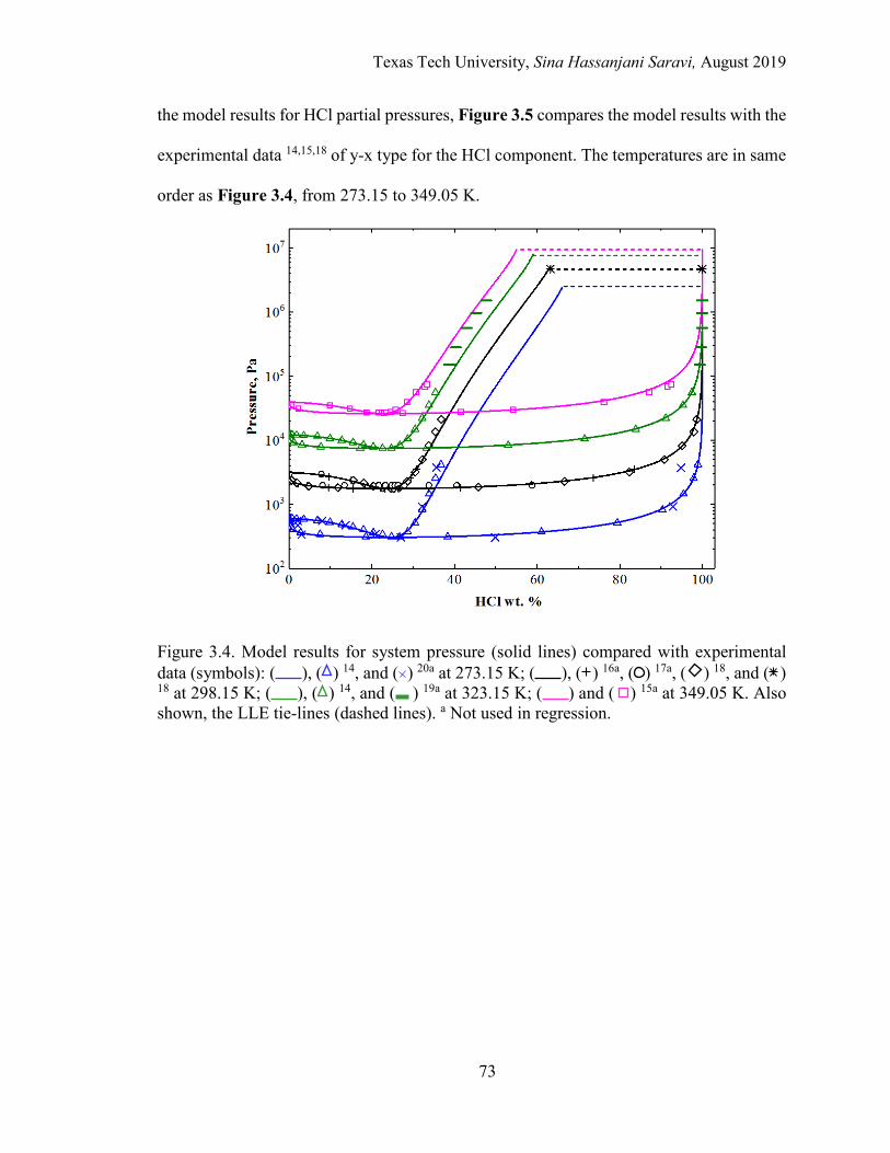
Texas Tech University, Sina Hassanjani Saravi, August 2019
73
the model results for HCl partial pressures, Figure 3.5 compares the model results with the
experimental data 14,15,18 of y-x type for the HCl component. The temperatures are in same
order as Figure 3.4, from 273.15 to 349.05 K.
Figure 3.4. Model results for system pressure (solid lines) compared with experimental data (symbols): ( ), ( ) 14, and ( ) 20a at 273.15 K; ( ), ( ) 16a, ( ) 17a, ( ) 18, and ( ) 18 at 298.15 K; ( ), ( ) 14, and ( ) 19a at 323.15 K; ( ) and ( ) 15a at 349.05 K. Also shown, the LLE tie-lines (dashed lines). a Not used in regression.
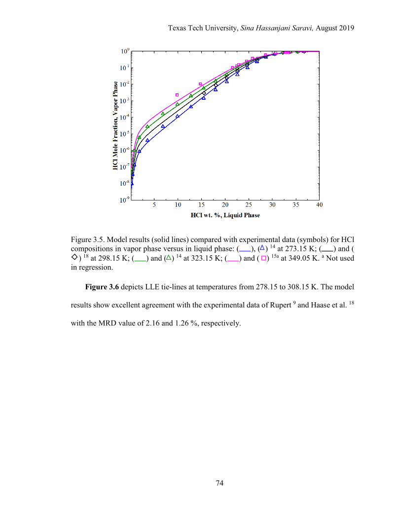
Texas Tech University, Sina Hassanjani Saravi, August 2019
74
Figure 3.5. Model results (solid lines) compared with experimental data (symbols) for HCl compositions in vapor phase versus in liquid phase: ( ), ( ) 14 at 273.15 K; ( ) and (
) 18 at 298.15 K; ( ) and ( ) 14 at 323.15 K; ( ) and ( ) 15a at 349.05 K. a Not used in regression.
Figure 3.6 depicts LLE tie-lines at temperatures from 278.15 to 308.15 K. The model
results show excellent agreement with the experimental data of Rupert 9 and Haase et al. 18
with the MRD value of 2.16 and 1.26 %, respectively.
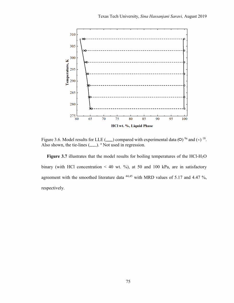
Texas Tech University, Sina Hassanjani Saravi, August 2019
75
Figure 3.6. Model results for LLE ( ) compared with experimental data ( ) 9a and ( ) 18. Also shown, the tie-lines ( ). a Not used in regression.
Figure 3.7 illustrates that the model results for boiling temperatures of the HCl-H2O
binary (with HCl concentration < 40 wt. %), at 50 and 100 kPa, are in satisfactory
agreement with the smoothed literature data 44,45 with MRD values of 5.17 and 4.47 %,
respectively.
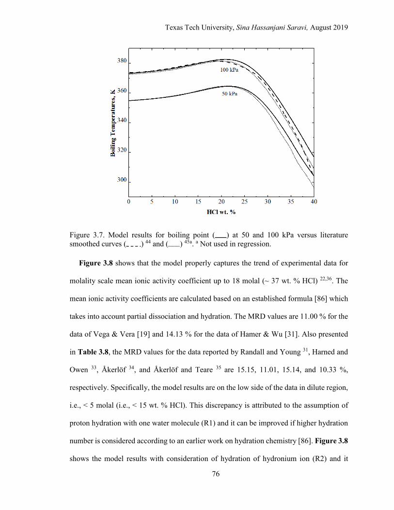
Texas Tech University, Sina Hassanjani Saravi, August 2019
76
Figure 3.7. Model results for boiling point ( ) at 50 and 100 kPa versus literature smoothed curves ( ) 44 and ( ) 45a. a Not used in regression.
Figure 3.8 shows that the model properly captures the trend of experimental data for
molality scale mean ionic activity coefficient up to 18 molal (~ 37 wt. % HCl) 22,36. The
mean ionic activity coefficients are calculated based on an established formula [86] which
takes into account partial dissociation and hydration. The MRD values are 11.00 % for the
data of Vega & Vera [19] and 14.13 % for the data of Hamer & Wu [31]. Also presented
in Table 3.8, the MRD values for the data reported by Randall and Young 31, Harned and
Owen 33, Åkerlöf 34, and Åkerlöf and Teare 35 are 15.15, 11.01, 15.14, and 10.33 %,
respectively. Specifically, the model results are on the low side of the data in dilute region,
i.e., < 5 molal (i.e., < 15 wt. % HCl). This discrepancy is attributed to the assumption of
proton hydration with one water molecule (R1) and it can be improved if higher hydration
number is considered according to an earlier work on hydration chemistry [86]. Figure 3.8
shows the model results with consideration of hydration of hydronium ion (R2) and it
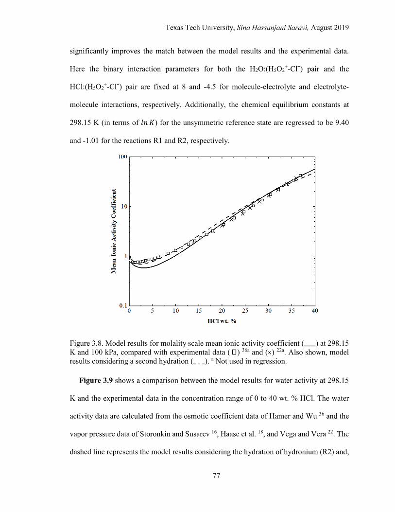
Texas Tech University, Sina Hassanjani Saravi, August 2019
77
significantly improves the match between the model results and the experimental data.
Here the binary interaction parameters for both the H2O:(H5O2+-Clˉ) pair and the
HCl:(H5O2+-Clˉ) pair are fixed at 8 and -4.5 for molecule-electrolyte and electrolyte-
molecule interactions, respectively. Additionally, the chemical equilibrium constants at
298.15 K (in terms of 𝑙𝑙𝑙𝑙 𝐾𝐾) for the unsymmetric reference state are regressed to be 9.40
and -1.01 for the reactions R1 and R2, respectively.
Figure 3.8. Model results for molality scale mean ionic activity coefficient ( ) at 298.15 K and 100 kPa, compared with experimental data ( ) 36a and ( ) 22a. Also shown, model results considering a second hydration ( ). a Not used in regression.
Figure 3.9 shows a comparison between the model results for water activity at 298.15
K and the experimental data in the concentration range of 0 to 40 wt. % HCl. The water
activity data are calculated from the osmotic coefficient data of Hamer and Wu 36 and the
vapor pressure data of Storonkin and Susarev 16, Haase et al. 18, and Vega and Vera 22. The
dashed line represents the model results considering the hydration of hydronium (R2) and,
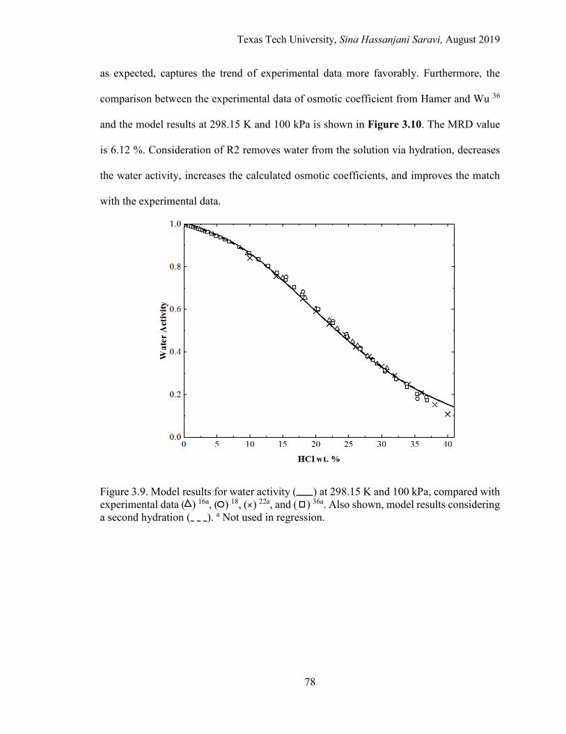
Texas Tech University, Sina Hassanjani Saravi, August 2019
78
as expected, captures the trend of experimental data more favorably. Furthermore, the
comparison between the experimental data of osmotic coefficient from Hamer and Wu 36
and the model results at 298.15 K and 100 kPa is shown in Figure 3.10. The MRD value
is 6.12 %. Consideration of R2 removes water from the solution via hydration, decreases
the water activity, increases the calculated osmotic coefficients, and improves the match
with the experimental data.
Figure 3.9. Model results for water activity ( ) at 298.15 K and 100 kPa, compared with experimental data ( ) 16a, ( ) 18, ( ) 22a, and ( ) 36a. Also shown, model results considering a second hydration ( ). a Not used in regression.
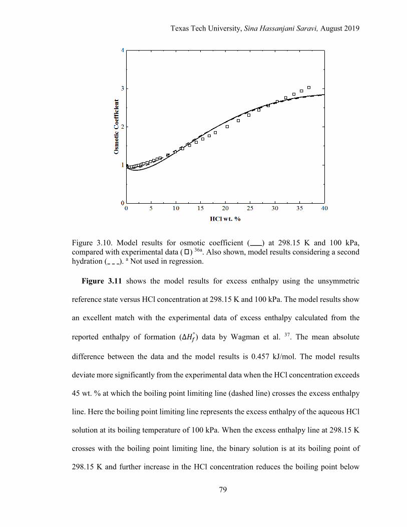
Texas Tech University, Sina Hassanjani Saravi, August 2019
79
Figure 3.10. Model results for osmotic coefficient ( ) at 298.15 K and 100 kPa, compared with experimental data ( ) 36a. Also shown, model results considering a second hydration ( ). a Not used in regression.
Figure 3.11 shows the model results for excess enthalpy using the unsymmetric
reference state versus HCl concentration at 298.15 K and 100 kPa. The model results show
an excellent match with the experimental data of excess enthalpy calculated from the
reported enthalpy of formation (∆𝐻𝐻𝑓𝑓°) data by Wagman et al. 37. The mean absolute
difference between the data and the model results is 0.457 kJ/mol. The model results
deviate more significantly from the experimental data when the HCl concentration exceeds
45 wt. % at which the boiling point limiting line (dashed line) crosses the excess enthalpy
line. Here the boiling point limiting line represents the excess enthalpy of the aqueous HCl
solution at its boiling temperature of 100 kPa. When the excess enthalpy line at 298.15 K
crosses with the boiling point limiting line, the binary solution is at its boiling point of
298.15 K and further increase in the HCl concentration reduces the boiling point below
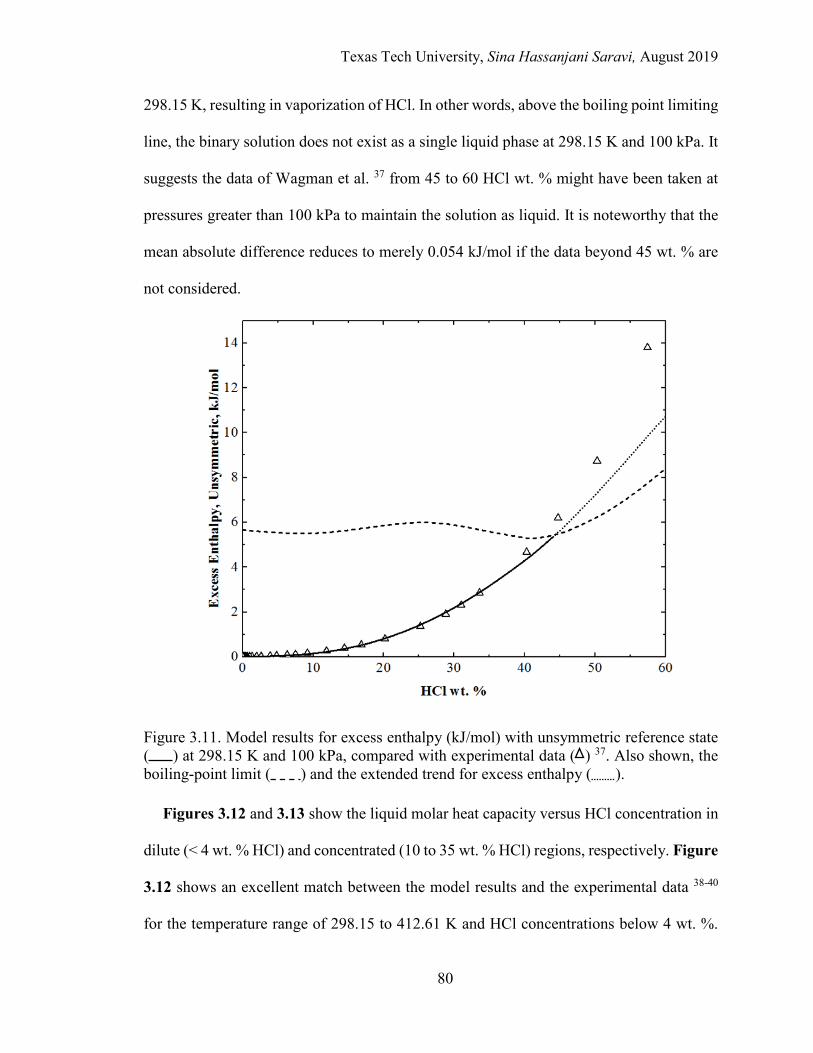
Texas Tech University, Sina Hassanjani Saravi, August 2019
80
298.15 K, resulting in vaporization of HCl. In other words, above the boiling point limiting
line, the binary solution does not exist as a single liquid phase at 298.15 K and 100 kPa. It
suggests the data of Wagman et al. 37 from 45 to 60 HCl wt. % might have been taken at
pressures greater than 100 kPa to maintain the solution as liquid. It is noteworthy that the
mean absolute difference reduces to merely 0.054 kJ/mol if the data beyond 45 wt. % are
not considered.
Figure 3.11. Model results for excess enthalpy (kJ/mol) with unsymmetric reference state ( ) at 298.15 K and 100 kPa, compared with experimental data ( ) 37. Also shown, the boiling-point limit ( ) and the extended trend for excess enthalpy ( ).
Figures 3.12 and 3.13 show the liquid molar heat capacity versus HCl concentration in
dilute (< 4 wt. % HCl) and concentrated (10 to 35 wt. % HCl) regions, respectively. Figure
3.12 shows an excellent match between the model results and the experimental data 38-40
for the temperature range of 298.15 to 412.61 K and HCl concentrations below 4 wt. %.
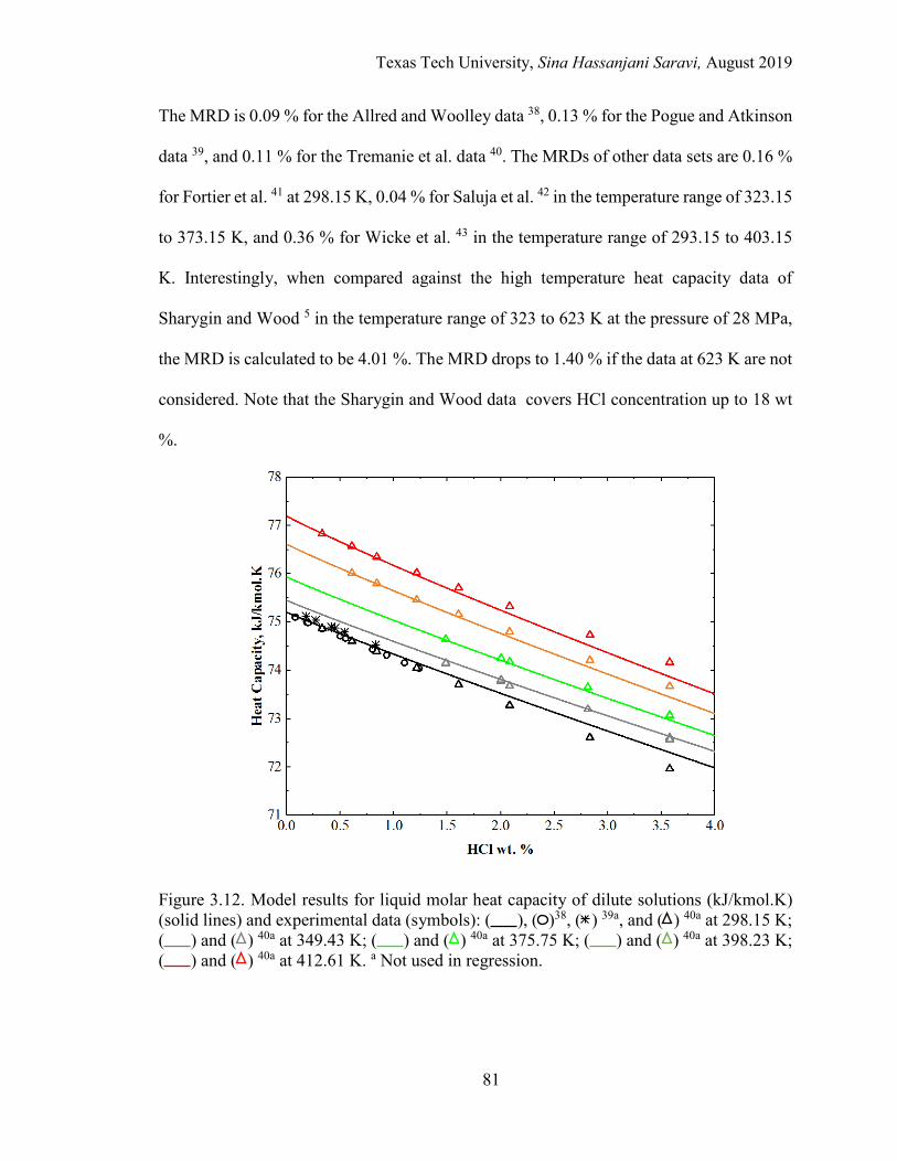
Texas Tech University, Sina Hassanjani Saravi, August 2019
81
The MRD is 0.09 % for the Allred and Woolley data 38, 0.13 % for the Pogue and Atkinson
data 39, and 0.11 % for the Tremanie et al. data 40. The MRDs of other data sets are 0.16 %
for Fortier et al. 41 at 298.15 K, 0.04 % for Saluja et al. 42 in the temperature range of 323.15
to 373.15 K, and 0.36 % for Wicke et al. 43 in the temperature range of 293.15 to 403.15
K. Interestingly, when compared against the high temperature heat capacity data of
Sharygin and Wood 5 in the temperature range of 323 to 623 K at the pressure of 28 MPa,
the MRD is calculated to be 4.01 %. The MRD drops to 1.40 % if the data at 623 K are not
considered. Note that the Sharygin and Wood data covers HCl concentration up to 18 wt
%.
Figure 3.12. Model results for liquid molar heat capacity of dilute solutions (kJ/kmol.K) (solid lines) and experimental data (symbols): ( ), ( )38, ( ) 39a, and ( ) 40a at 298.15 K; ( ) and ( ) 40a at 349.43 K; ( ) and ( ) 40a at 375.75 K; ( ) and ( ) 40a at 398.23 K; ( ) and ( ) 40a at 412.61 K. a Not used in regression.

Texas Tech University, Sina Hassanjani Saravi, August 2019
82
Figure 3.13. Model results for liquid molar heat capacity (kJ/kmol.K) (solid lines) compared with experimental data (symbols) 13 and smoothed curves (dashed lines) 44: (), ( ), and ( ) at 273.15 K; ( ), ( ), and ( ) at 293.15 K; ( ) and ( ) at 313.15 K; ( ), ( ), and ( ) at 333.15 K.
To further validate the model, the liquid molar heat capacity of the HCl-H2O binary is
generated for the concentrated region (10 to 35 wt. % HCl) for which the experimental data
are relatively scarce. Figure 3.13 shows a satisfactory match between the experimental
data of Perry’s Handbook 13 and the model results with an average MRD value of 2.88 %
at the four temperatures of 273.15, 293.15, 313.15 K, and 333.15 K. Furthermore, the
smoothed curves of heat capacity 44 are also compared satisfactorily with the model results
with an average MRD value of 2.33 % at the three temperatures of 273.15, 293.15, and
333.15 K.
Figure 3.14 shows the Merkel enthalpy-concentration chart for the HCl-H2O binary.
It is presented in English units, as is the convention for the Merkel chart. The reference
states for pure HCl and water are at 32 and 68 °F, respectively. The figure shows the model
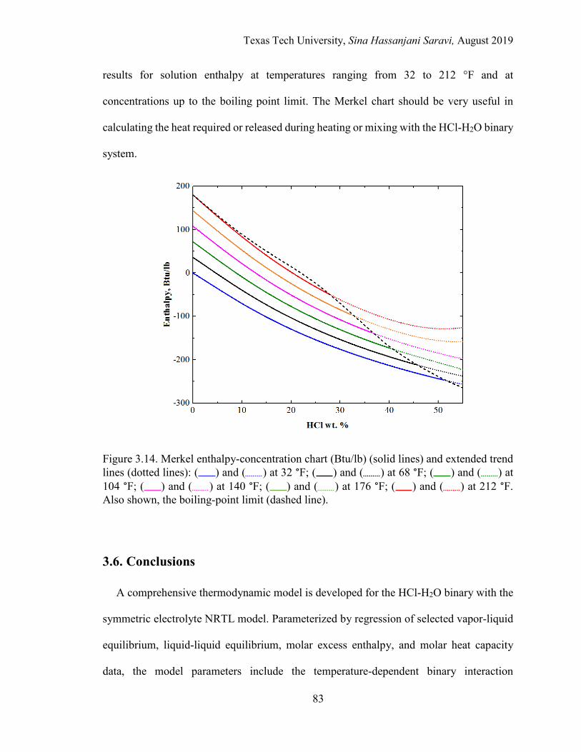
Texas Tech University, Sina Hassanjani Saravi, August 2019
83
results for solution enthalpy at temperatures ranging from 32 to 212 °F and at
concentrations up to the boiling point limit. The Merkel chart should be very useful in
calculating the heat required or released during heating or mixing with the HCl-H2O binary
system.
Figure 3.14. Merkel enthalpy-concentration chart (Btu/lb) (solid lines) and extended trend lines (dotted lines): ( ) and ( ) at 32 °F; ( ) and ( ) at 68 °F; ( ) and ( ) at 104 °F; ( ) and ( ) at 140 °F; ( ) and ( ) at 176 °F; ( ) and ( ) at 212 °F. Also shown, the boiling-point limit (dashed line).
3.6. Conclusions
A comprehensive thermodynamic model is developed for the HCl-H2O binary with the
symmetric electrolyte NRTL model. Parameterized by regression of selected vapor-liquid
equilibrium, liquid-liquid equilibrium, molar excess enthalpy, and molar heat capacity
data, the model parameters include the temperature-dependent binary interaction

Texas Tech University, Sina Hassanjani Saravi, August 2019
84
parameters of the H2O:(H3O+-Cl–), HCl:(H3O+-Cl–), and H2O:HCl pairs, as well as the
chemical equilibrium constant parameters for partial dissociation of HCl. The model
accurately calculates all phase equilibrium, thermodynamic, and calorimetric properties for
the HCl-H2O binary over the whole concentration range from pure H2O to pure HCl and at
temperatures from 273 to about 400 K. The model should be very useful in industrial
process simulations and heat and mass balance calculations involving the HCl-H2O binary.
The model can be further extended for mixed acids and mixed solvent electrolyte systems.
3.7. Acknowledgements
The authors gratefully acknowledge the financial support of the Jack Maddox
Distinguished Engineering Chair Professorship in Sustainable Energy sponsored by the J.F
Maddox Foundation.
Texas Tech University, Sina Hassanjani Saravi, August 2019
85
3.8. References
1. Acid H. Chemicals Economics Handbook. SRI International. 2001:733.4000.
2. Dabrowski A, Hubicki Z, Podkościelny P, Robens E. Selective removal of the heavy metal ions from waters and industrial wastewaters by ion-exchange method. Chemosphere. 2004;56:91-106.
3. Nelson F, Murase T, Kraus KA. Ion exchange procedures: I. Cation exchange in concentration HCl and HClO4 solutions. Journal of Chromatography A. 1964;13:503-535.
4. Brandani S, Brandani V, Di Giacomo G. Vapor-liquid equilibrium calculation of the system water-hydrogen chloride. Fluid phase equilibria. 1994;92:67-74.
5. Sharygin AV, Wood RH. Volumes and heat capacities of aqueous solutions of hydrochloric acid at temperatures from 298.15 K to 623 K and pressures to 28 MPa. The Journal of Chemical Thermodynamics. 1997;29:125-148.
6. Ho PC, Palmer DA, Gruszkiewicz MS. Conductivity measurements of dilute aqueous HCl solutions to high temperatures and pressures using a flow-through cell. The Journal of Physical Chemistry B. 2001;105:1260-1266.
7. Chialvo A, Ho P, Palmer D, Gruszkiewicz M, Cummings P, Simonson J. H3O+/Cl-
association in high-temperature aqueous solutions over a wide range of state conditions. A direct comparison between simulation and electrical conductance experiment. The Journal of Physical Chemistry B. 2002;106:2041-2046.
8. Brandes BT. Semiempirical Model of the Vapor − Liquid Phase Behavior of the Hydrogen Chloride − Water System. Industrial & engineering chemistry research. 2005;44:639-644.
9. Rupert FF. A Study Of The System Hydrogen Chloride And Water. Journal of the American Chemical Society. 1909;31:851-866.
10. Petković DM. Dissociation of strong acids in aqueous solutions. Journal of the Chemical Society, Dalton Transactions. 1982:2425-2427.
11. Ando K, Hynes JT. Molecular mechanism of HCl acid ionization in water: Ab initio potential energy surfaces and Monte Carlo simulations. The Journal of Physical Chemistry B. 1997;101:10464-10478.
12. Zeisberg F. Partial vapor pressures of aqueous HCl solutions. A consolidation of the reliable literature and criticism of Hurter’s formula for calculating partial pressures of HCl Chem Metall Eng. 1925;32:326-327.
Texas Tech University, Sina Hassanjani Saravi, August 2019
86
13. Perry RH, Green DW, Maloney J. Perry’s handbook of chemical engineering. Perry's Handbook of Chemical Engineering. 1997.
14. Fritz J, Fuget C. Vapor Pressure of Aqueous Hydrogen Chloride Solutions, 0° to 50° C. Industrial & Engineering Chemistry Chemical & Engineering Data Series. 1956;1:10-12.
15. Vrevskii MS, Zavaritskii NN, Sharlov LE. Determination of Vapor Pressure and Vapor Composition of Aqueous Solutions of Hydrogen Chloride and Hydrogen Bromide at Different Temperatures. Zhurnal Fizicheskoi Khimii. 1923;5:360-375.
16. Storonkin AV, Susarev MP. Investigation of the Total and Partial Vapor Pressures of the System Hydrogen Chloride-Sulfuric Acid-Water. Zhurnal Fizicheskoi Khimii. 1952;7:119-148.
17. Susarev M, Prokofeva R. Liquid-vapor Equilibrium In The System Water-hydrogen Chloride-ferric Chloride At 25-degrees-c. Zhurnal Fizicheskoi Khimii. 1963;37:2408-2412.
18. Haase R, Naas H, Thumm H. Experimental Investigations of the Thermodynamic Behavior of Concentrated Hydrogen Halide Acids. Zeitschrift für physikalische chemie. 1963;37:210-219.
19. Kao JT. Vapor-liquid equilibrium of water-hydrogen chloride system. Journal of Chemical and Engineering Data. 1970;15:362-367.
20. Miller E. Vapor-liquid equilibriums of water-hydrogen chloride solutions below 0. degree. C. Journal of Chemical and Engineering Data. 1983;28:363-367.
21. Elm N, Zipprian J, Schaber K. Vapour–liquid equilibria of binary and ternary aqueous systems with HCl, HBr and CaCl2 at highly diluted vapour phases. Fluid phase equilibria. 2001;189:163-178.
22. Vega R, Vera J. Phase equilibria of concentrated aqueous solutions containing volatile strong electrolytes. The Canadian Journal of Chemical Engineering. 1976;54:245-248.
23. Berl E, Staudinger H. Über die Bestimmung der Siedepunkts‐und Destillationskurve von Salzsäure‐Wasser‐Gemischen. Angewandte Chemie. 1930;43:1019-1022.
24. Hawliczek J, Synowiec J. Study of the Desorption of Hydrogen Chloride from Aqueous Solution. Chem Stosowana. 1962;3:369-387.
Texas Tech University, Sina Hassanjani Saravi, August 2019
87
25. Lutugina N, Kokovkina L. Liquid-vapor equilibrium in water-hydrogen chloride, water-hydrogen iodide, and water-hydrogen iodide-hydrogen chloride systems. J Appl Chem USSR. 1965;38:1487-1494.
26. Othmer D. Composition of Vapors from Boiling Binary Solutions1. Industrial & Engineering Chemistry. 1928;20:743-746.
27. Lu X, Wang Y, Shi J. Vapor equilibrium of hydrochloride-water binary system. J Chem Eng of China Universities. 1987;2:1-12.
28. Bonner WD, Wallace RE. The Boiling Points of Constant Boiling Hydrochloric Acids. Journal of the American Chemical Society. 1930;52:1747-1750.
29. Sako T, Hakuta T, Yoshitome H. Salt effects on vapor-liquid equilibria for volatile strong electrolyte-water systems. Journal of chemical engineering of Japan. 1984;17:381-388.
30. Sako T, Hakuta T, Yoshitome H. Vapor pressures of binary (water-hydrogen chloride,-magnesium chloride, and-calcium chloride) and ternary (water-magnesium chloride-calcium chloride) aqueous solutions. Journal of Chemical and Engineering Data. 1985;30:224-228.
31. Randall M, Young LE. The calomel and silver chloride electrodes in acid and neutral solutions. The activity coefficient of aqueous hydrochloric acid and the single potential of the deci-molal calomel electrode. Journal of the American Chemical Society. 1928;50:989-1004.
32. Harned HS, Ehlers RW. The thermodynamics of aqueous hydrochloric acid solutions from electromotive force measurements. Journal of the American Chemical Society. 1933;55:2179-2193.
33. Harned H, Owen B, Harned H, Owen B. Physical Chemistry of Electrolytic Solution Physical Chemistry of Electrolytic Solution (3rd Edn) Reinhold. New York. 1958:638.
34. Åkerlöf G. Activity coefficients of sodium, potassium and lithium chlorides and hydrochloric acid at infinite dilution in water-methyl alcohol mixtures. Journal of the American Chemical Society. 1930;52:2353-2368.
35. Åkerlöf G, Teare JW. Thermodynamics of concentrated aqueous solutions of hydrochloric acid. Journal of the American Chemical Society. 1937;59:1855-1868.
36. Hamer WJ, Wu YC. Osmotic coefficients and mean activity coefficients of uni‐univalent electrolytes in water at 25 °C. Journal of Physical and Chemical Reference Data. 1972;1:1047-1100.
Texas Tech University, Sina Hassanjani Saravi, August 2019
88
37. Wagman DD, Evans WH, Parker VB, Schumm RH, Halow I. The NBS tables of chemical thermodynamic properties. Selected values for inorganic and C1 and C2 organic substances in SI units. DTIC Document;1982.
38. Allred GC, Woolley EM. Heat capacities of aqueous HCI, NaOH, and NaCl at 283.15, 298.15 and 313.15 K: ΔC° p for ionization of water. The Journal of Chemical Thermodynamics. 1981;13:147-154.
39. Pogue R, Atkinson G. Apparent molal volumes and heat capacities of aqueous hydrogen chloride and perchloric acid at 15-55. degree. C. Journal of Chemical and Engineering Data. 1988;33:495-499.
40. Tremaine PR, Sway K, Barbero JA. The apparent molar heat capacity of aqueous hydrochloric acid from 10 to 140° C. Journal of solution chemistry. 1986;15:1-22.
41. Fortier J-L, Leduc P-A, Desnoyers J. Thermodynamic properties of alkali halides. II. Enthalpies of dilution and heat capacities in water at 25° C. Journal of Solution Chemistry. 1974;3:323-349.
42. Saluja PP, LeBlanc JC, Hume HB. Apparent molar heat capacities and volumes of aqueous solutions of several 1: 1 electrolytes at elevated temperatures. Canadian journal of chemistry. 1986;64:926-931.
43. Wicke E, Eigen M, Ackermann T. On the state of proton (hydronium-ion) in aqueous solution. Zeitschrift für Physikalische Chemie. 1954:5-6.
44. (Oxy) OPC. Hydrochloric Acid Handbook. 2013.
45. Systems DDP. Isothermal Absorption of Hydrogen Chloride. (http://wwwdedietrichcom/en/solutions-and-products/halide-treatment/hcl-treament/absorption-hcl, Accessed on May 1, 2017).
46. Cardoso MJEdM, Fredenslund A, Rasmussen P. Calculation of vapor liquid equilibria in hydrochloric acid water system. Internal Report Sept 8711, Instituttet for Kemiteknik, DTH, Lyngby, Denmark. 1987.
47. Wang P, Anderko A, Young RD. A speciation-based model for mixed-solvent electrolyte systems. Fluid Phase Equilibria. 2002;203:141-176.
48. Saravi SH, Honarparvar S, Chen C-C. Modeling aqueous electrolyte systems. Chemical Engineering Progress. 2015;111:65-75.
49. Anderko A, Wang P, Rafal M. Electrolyte solutions: from thermodynamic and transport property models to the simulation of industrial processes. Fluid Phase Equilibria. 2002;194:123-142.
Texas Tech University, Sina Hassanjani Saravi, August 2019
89
50. Gibbons RM, Laughton AP. An equation of state for polar and non-polar substances and mixtures. Journal of the Chemical Society, Faraday Transactions 2: Molecular and Chemical Physics. 1984;80:1019-1038.
51. Stryjek R, Vera J. Vapor—liquid equilibrium of hydrochloric acid solutions with the PRSV equation of state. Fluid Phase Equilibria. 1986;25:279-290.
52. Patel NC, Teja AS. A new cubic equation of state for fluids and fluid mixtures. Chemical Engineering Science. 1982;37:463-473.
53. Panagiotopoulos A, Reid R. New mixing rule for cubic equations of state for highly polar, asymmetric systems. In: ACS Publications; 1986.
54. Delano AD. Design analysis of the Einstein refrigeration cycle, Georgia Institute of Technology; 1998.
55. Greeley R, Smith Jr WT, Lietzke M, Stoughton R. Electromotive force measurements in aqueous solutions at elevated temperatures. ii. thermodynamic properties of hydrochloric acid1. The Journal of Physical Chemistry. 1960;64:1445-1448.
56. Correa H, Vera J. On the thermodynamics of concentrated strong electrolytes aqueous solutions the system NaNO3—NaCl—H2O. The Canadian Journal of Chemical Engineering. 1975;53:204-210.
57. Engels H, Bosen A. Description of the system HCl/H2O with a ‘local composition’ equation for the activity coefficient and a suitable dissociation model. Fluid phase equilibria. 1986;28:171-181.
58. Wilson GM. Vapor-liquid equilibrium. XI. A new expression for the excess free energy of mixing. Journal of the American Chemical Society. 1964;86:127-130.
59. Liu Y, Grén U. Description of vapor—liquid equilibrium of the HCl/H2O system using an activity-coefficient model. Fluid phase equilibria. 1991;63:49-63.
60. Hala E, Pick J, Fried V, Vilim O. Vapor-liquid Equilibrium, 2nd English Edition. In: Oxford-London-Edinburgh-New York-Toronto-Sydney-Paris-Braunschweig: Pergamon Press Ltd; 1967.
61. Hala E. Vapour-liquid equilibria in systems of electrolytic components. Paper presented at: I. Chem. E. Symp. Ser1969.
62. Hala E. Vapor—liquid equilibrium of strong electrolytes in chemical engineering application. Paper presented at: Proceedings of 6th Int. Conf. on Thermodynamics, Merseburg, Germany1980.
Texas Tech University, Sina Hassanjani Saravi, August 2019
90
63. Wozny G, Cremer H. Phase equilibria of strong electrolytes in aqueous solutions from total pressure measurements. Fluid Phase Equilibria. 1981;6:149-168.
64. Holmes H, Busey R, Simonson JM, Mesmer RE, Archer D, Wood R. The enthalpy of dilution of HCl (aq) to 648 K and 40 MPa thermodynamic properties. The Journal of Chemical Thermodynamics. 1987;19:863-890.
65. Simonson J, Holmes H, Busey R, Mesmer R, Archer D, Wood R. Modeling of the thermodynamics of electrolyte solutions to high temperatures including ion association. Application to hydrochloric acid. Journal of Physical Chemistry;(USA). 1990;94.
66. Carslaw KS, Clegg SL, Brimblecombe P. A Thermodynamic Model of the System HCl-HNO3-H2SO4-H2O, Including Solubilities of HBr, from < 200 to 328 K. Journal of Physical Chemistry. 1995;99:11557-11574.
67. Pitzer KS. Thermodynamics of electrolytes. I. Theoretical basis and general equations. The Journal of Physical Chemistry. 1973;77:268-277.
68. Pitzer K. Activity Coefficients in Electrolyte Solutions CRC. Ann Arbor. 1991.
69. Clegg SL, Pitzer KS, Brimblecombe P. Thermodynamics of multicomponent, miscible, ionic solutions. Mixtures including unsymmetrical electrolytes. The Journal of Physical Chemistry. 1992;96:9470-9479.
70. Clegg SL, Pitzer KS. Thermodynamics of multicomponent, miscible, ionic solutions: generalized equations for symmetrical electrolytes. The Journal of Physical Chemistry. 1992;96:3513-3520.
71. Nichols TT, Taylor DD. Thermodynamic Phase And Chemical Equilibrium At 0-110 C For The H+-K+-Na+-Cl--H2O System Up To 16 Molal And The HNO3-H2O System Up To 20 Molal Using An Association-Based Pitzer Model Compatible With ASPEN Plus. Idaho National Engineering and Environmental Laboratory, Idaho Falls, ID (US);2003.
72. Chen C-C, Britt HI, Boston J, Evans L. Local composition model for excess Gibbs energy of electrolyte systems. Part I: Single solvent, single completely dissociated electrolyte systems. AIChE Journal. 1982;28:588-596.
73. Song Y, Chen C-C. Symmetric nonrandom two-liquid segment activity coefficient model for electrolytes. Industrial & Engineering Chemistry Research. 2009;48:5522-5529.
74. Cruz JL, Renon H. A new thermodynamic representation of binary electrolyte solutions nonideality in the whole range of concentrations. AIChE Journal. 1978;24:817-830.
Texas Tech University, Sina Hassanjani Saravi, August 2019
91
75. Sander B, Fredenslund A, Rasmussen P. Calculation of vapour-liquid equilibria in mixed solvent/salt systems using an extended UNIQUAC equation. Chemical Engineering Science. 1986;41:1171-1183.
76. Thomsen K. Aqueous Electrolytes Model Parameters and Process Simulation, Technical University of DenmarkDanmarks Tekniske Universitet, CenterCenters, Center for Energy Resources EngineeringCenter for Energy Resources Engineering; 1997.
77. Que H, Song Y, Chen C-C. Thermodynamic modeling of the sulfuric acid− water− sulfur trioxide system with the symmetric electrolyte NRTL model. Journal of Chemical & Engineering Data. 2011;56:963-977.
78. Kaur H, Wang M, Gorensek MB, Chen C-C. Thermodynamic modeling of the hybrid sulfur (HyS) cycle for hydrogen production. Fluid Phase Equilibria. 2017.
79. Wang M, Gorensek MB, Chen C-C. Thermodynamic representation of aqueous sodium nitrate and nitric acid solution with electrolyte NRTL model. Fluid Phase Equilibria. 2016;407:105-116.
80. Wang M, Kaur H, Chen CC. Thermodynamic modeling of HNO3‐H2SO4‐H2O ternary system with symmetric electrolyte NRTL model. AIChE Journal. 2017.
81. Triolo R, Narten A. Diffraction pattern and structure of aqueous hydrochloric acid solutions at 20 C. The Journal of Chemical Physics. 1975;63:3624-3631.
82. Borman S. Revisiting the hydrated proton: Researchers probe previously inaccessible low-energy part of protonated water-cluster spectrum. Chemical & engineering news. 2005;83:26-27.
83. Chen C-C. Representation of solid-liquid equilibrium of aqueous electrolyte systems with the electrolyte NRTL model. Fluid Phase Equilibria. 1986;27:457-474.
84. Chen C-C, Evans LB. A local composition model for the excess Gibbs energy of aqueous electrolyte systems. AIChE Journal. 1986;32:444-454.
85. Luckas M, Eden DM. Improved representation of the vapor–liquid equilibrium of HCl‐H2O. AIChE Journal. 1995;41:1041-1043.
86. Chen C-C., Mathias PM, Orbey H. Use of hydration and dissociation chemistries with the electrolyte–NRTL model. AIChE Journal. 1999;45:1576-1586.
87. Headrick JM, Diken EG, Walters RS, et al. Spectral signatures of hydrated proton vibrations in water clusters. Science. 2005;308:1765-1769.

Texas Tech University, Sina Hassanjani Saravi, August 2019
92
88. Aspen Properties V8.8. Aspen Technology IB, MA, 2015.
89. Yan Y, Chen C-C. Thermodynamic representation of the NaCl + Na2SO4 + H2O system with electrolyte NRTL model. Fluid Phase Equilibria. 2011;306:149-161.
Texas Tech University, Sina Hassanjani Saravi, August 2019
93
CHAPTER 4. BRIDGING TWO-LIQUID THEORY WITH MOLECULAR
SIMULATIONS FOR ELECTROLYTES: AN INVESTIGATION OF AQUOUES NACL SOLUTION3
4.1. Abstract
We re-examine the theoretical framework of electrolyte Non-Random Two-Liquid
model and, based on the two-fluid theory, formulate the binary interaction parameters as
functions of species diameter (𝜎𝜎), effective interaction strength (𝜖𝜖), the domain radius
around the center species (𝑅𝑅), and the non-randomness factor (𝛼𝛼). We show that these
quantities can be directly obtained from molecular simulations using aqueous NaCl as the
model system. The binary interaction parameters determined from the simulations are
consistent with those obtained from regression of experimental data. Our work provides a
molecular interpretation of the classical thermodynamic model and shows a way to predict
from molecular simulations the binary interaction parameters for use in process industries.
3 This chapter is reproduced from the paper published as: Saravi SH, Ravichandran A, Khare R, Chen C-C. Bridging Two-Liquid Theory with Molecular Simulations for Electrolytes: An Investigation of Aqueous NaCl Solution, AIChE Journal. 2019;65.4:1315-1324
Texas Tech University, Sina Hassanjani Saravi, August 2019
94
4.2. Introduction
Aqueous electrolyte solutions are widely used in many industrial 1-3, environmental
4,5, geological 6,7, and pharmaceutical processes 8. The availability of reliable models for
phase equilibria calculations is the key challenge in design and optimization of these
processes 3,9. Extensive modeling efforts have been reported in the literature to calculate
phase equilibria and thermodynamic properties of aqueous electrolytes 10,11. Most of these
studies aim at quantifying the mean ionic activity coefficient (𝛾𝛾±), as it is the unique
thermodynamic property of aqueous electrolyte solutions 10,12,13.
Aqueous electrolyte solution models can be broadly categorized into correlative and
predictive models. Correlative models often relate the liquid structure to the excess Gibbs
energy of a system with a set of adjustable parameters as input. The adjustable parameters
are calculated by fitting the experimental data (including those of phase equilibria,
calorimetric properties, and speciation) to the model 10. The predictive models, on the other
hand, employ molecular simulation techniques to obtain the liquid structure and free
energy, without introducing any adjustable parameter. The quantities thus obtained are
used to predict the thermodynamic properties of the electrolyte solutions 14,15.
Correlative classical thermodynamic models are extensively used in the process
industry owing to their straightforward applicability covering a wide range of electrolyte
solutions and process conditions. Some examples of these models include, Pitzer 16,
eUNIQUAC 17, ePC-SAFT 18, and the electrolyte NRTL (eNRTL) models 12,19-21. Among
these, the Pitzer model and the eNRTL model are the two most widely applied
thermodynamic models due to their mathematical simplicity and application versatility.
The underlying concept behind these models is that the excess Gibbs free energy of an

Texas Tech University, Sina Hassanjani Saravi, August 2019
95
electrolyte solution can be expressed as a combination of two contributions: the long-range
electrostatic interactions and the short-range local interactions. These models depend on
experimental data to obtain the adjustable parameters that are further used to calculate the
excess Gibbs free energy and other derivative thermodynamic properties. Determination
of the interaction parameters of the models from regression is not always feasible due to
the limited availability of the experimental data, the need for substantial experience in data
treatment, and the necessity of properly defining the optimization problem.
On the other hand, molecular simulations circumvent the problems associated with the
classical thermodynamic models. Several of these models have previously been shown to
predict the chemical potential of aqueous electrolyte solutions 15,22-27. Though these models
have been shown to be predictive, they are often restricted by the necessity to implement
advanced simulation techniques to calculate the free energy of the system. Implementing
such techniques can be computationally expensive thereby creating a bottleneck in directly
applying molecular simulations to industrial process design. Hence it is desirable to
formulate a hybrid methodology that can utilize the predictive capability of molecular
simulations and the rapid applicability of the classical thermodynamic models. Developing
such a framework for electrolyte systems is the objective of this work.
The molecular interpretation of the classical thermodynamic models can be achieved
through the interaction parameters which quantify the strength and nature of intermolecular
forces. There have been a few attempts for finding the binary interaction parameters of
thermodynamic models for nonelectrolyte systems from molecular simulations 28-31.
Recently, a novel methodology was proposed for predicting the NRTL binary interaction
parameters from molecular dynamics (MD) simulations 29. This technique utilizes the
Texas Tech University, Sina Hassanjani Saravi, August 2019
96
framework of two-fluid theory 32 to relate the NRTL binary interaction parameters to
molecular size and interaction strength, both of which were obtained from simulations. It
was also shown that the binary interaction parameters obtained using this approach could
predict the phase equilibria behavior and the thermophysical properties of organic binary
mixtures. In this work, we extend the previously proposed technique 29 to aqueous uni-
univalent electrolyte solutions. Such an extension is non-trivial and requires the
interpretation of molecular parameters that is consistent with the theoretical framework of
the classical thermodynamic model.
We focus on the eNRTL model as it has been extensively applied to predict the phase
equilibria and thermodynamic properties of aqueous, non-aqueous, and mixed-solvent
electrolytes 12,19-21. The model’s sound theoretical background and mathematical
simplicity offers a versatile and comprehensive framework for application in process
modeling of electrolytes. Furthermore, it has been recently shown that the prediction of
mean ionic activity coefficient of aqueous NaCl solutions by the eNRTL model is
consistent with experimental data and MD simulations as opposed to the Pitzer model that
overestimates the mean ionic activity coefficient at higher salt concentrations 13. The
eNRTL model requires two adjustable binary interaction parameters per molecule-
electrolyte pair (𝜏𝜏𝐿𝐿𝑎𝑎,𝑚𝑚 and 𝜏𝜏𝑚𝑚,𝐿𝐿𝑎𝑎), that quantify the nature of the interaction between solvent
molecules and electrolyte species. The binary interaction parameters are commonly
determined from regression of experimental data. The model also includes an additional
parameter, the non-randomness factor, 𝛼𝛼, which is treated as an empirical constant
typically fixed at a value of 0.2.
Texas Tech University, Sina Hassanjani Saravi, August 2019
97
In this study, we re-examine the eNRTL model to quantify the binary interaction
parameters (𝜏𝜏𝐿𝐿𝑎𝑎,𝑚𝑚 and 𝜏𝜏𝑚𝑚,𝐿𝐿𝑎𝑎) by combining the statistical mechanics framework of two-
liquid theory for electrolytes with MD simulations. Furthermore, the non-randomness
factor, 𝛼𝛼, is directly obtained from simulations instead of treating it as an empirical
constant. The 𝜏𝜏 parameters are formulated as a function of species diameter (𝜎𝜎), effective
interaction strength (𝜖𝜖), and the radius of the neighbor domain (𝑅𝑅), all of which are
calculated from the MD simulations. Aqueous NaCl solution is selected as the model
system due to the availability of proven force field parameters [6] and its industrial
importance. Furthermore, we examine several inherent assumptions made by the model
regarding the nature of molecular interactions. These assumptions include the
concentration independence of the interaction parameters and equal magnitude of the
effective interaction between the cation-molecule and the anion-molecule pairs 19.
The rest of this chapter is organized as follows: Theoretical Background section covers
the fundamental concepts behind the two-liquid theory for electrolytes and the
development of our approach. Calculation Methodology and Molecular Simulations
sections detail the procedure followed to obtain the binary interaction parameters. The
significance of the approach and the interpretation of the results are provided in the Results
and Discussions section which is then followed by Conclusions.
4.3. Theoretical Background
Two-Liquid Theory for Electrolytes The short-range interactions in the eNRTL model are described using the non-random
two-liquid (NRTL) equation of Renon and Prausnitz 33, which is in turn based on the
original two-liquid theory of Scott 32. The long-range electrostatic interactions are

Texas Tech University, Sina Hassanjani Saravi, August 2019
98
described by the Pitzer–Debye–Hückel limiting law 16. While certain theoretical aspects
of the eNRTL model are described below, we refer the reader to the original literature for
an elaborate discussion 12,19-21.
Following the work of Chen et al. 19, the concept of local composition for electrolyte
solutions can be described as follows. For a binary electrolyte solution consisting of a
solvent molecule, 𝑚𝑚, and a completely dissociated solute, 𝑐𝑐𝑎𝑎, three types of molecular
domains are possible. When the solute dissociates to cation, 𝑐𝑐, and anion, 𝑎𝑎, the three
different types of domains will have 𝑐𝑐, 𝑎𝑎, and 𝑚𝑚 at the center, respectively, surrounded by
species in such a way that the two assumptions of the eNRTL model, i.e., local
electroneutrality and like-ion repulsion are satisfied. While the former ensures local
electroneutrality (i.e., the number of oppositely charged ions in a molecule-centered
domain are equal), the latter asserts that no like-ion species are present in the first neighbor
shell of an ion-centered domain. The schematic of the domains is shown in Figure 4.1.
The local compositions are then expressed as follows 19:
𝑥𝑥𝑗𝑗𝑖𝑖𝑥𝑥𝑘𝑘𝑖𝑖
= �𝑥𝑥𝑗𝑗𝑥𝑥𝑘𝑘� exp�−𝛼𝛼(𝑖𝑖)𝜏𝜏𝑗𝑗𝑖𝑖,𝑘𝑘𝑖𝑖� , 𝑖𝑖, 𝑗𝑗,𝑘𝑘 ∈ {𝑐𝑐, 𝑎𝑎,𝑚𝑚} (4.1)
𝜏𝜏𝑗𝑗𝑖𝑖,𝑘𝑘𝑖𝑖 = (𝑔𝑔𝑗𝑗𝑖𝑖 − 𝑔𝑔𝑘𝑘𝑖𝑖)/𝑅𝑅𝑇𝑇 (4.2)
where 𝑥𝑥𝑗𝑗𝑖𝑖 and 𝑥𝑥𝑘𝑘𝑖𝑖 are the local compositions of species 𝑗𝑗 and 𝑘𝑘 around the center
species 𝑖𝑖, respectively; 𝑥𝑥𝑗𝑗 and 𝑥𝑥𝑘𝑘 are the bulk mole fractions of j and k, respectively; 𝛼𝛼(𝑖𝑖)
is the non-randomness factor in an 𝑖𝑖-centered domain. 𝜏𝜏𝑗𝑗𝑖𝑖,𝑘𝑘𝑖𝑖 is the binary interaction
parameter of a domain with species 𝑗𝑗 and 𝑘𝑘 around 𝑖𝑖, representing the effective interaction
strength necessary for forming such a domain; 𝑔𝑔𝑗𝑗𝑖𝑖 and 𝑔𝑔𝑘𝑘𝑖𝑖 are the interaction energies
between species 𝑗𝑗 and 𝑖𝑖, and species 𝑘𝑘 and 𝑖𝑖, respectively. The summation of the local
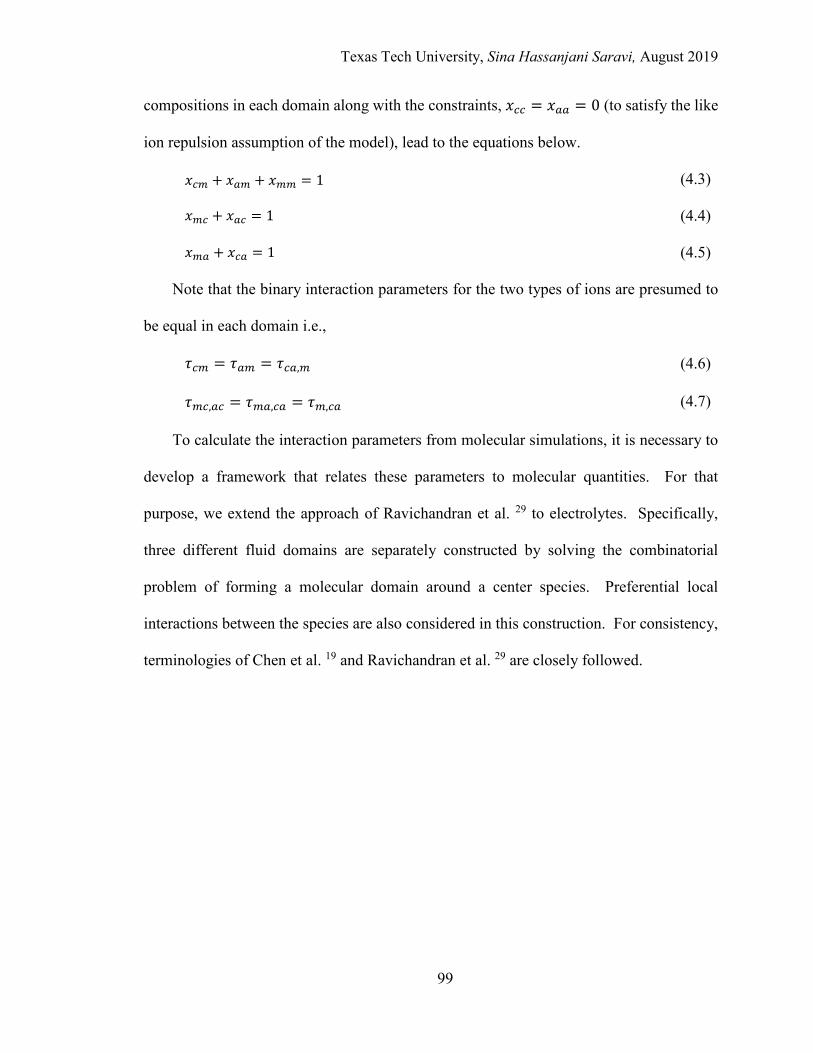
Texas Tech University, Sina Hassanjani Saravi, August 2019
99
compositions in each domain along with the constraints, 𝑥𝑥𝐿𝐿𝐿𝐿 = 𝑥𝑥𝑎𝑎𝑎𝑎 = 0 (to satisfy the like
ion repulsion assumption of the model), lead to the equations below.
𝑥𝑥𝐿𝐿𝑚𝑚 + 𝑥𝑥𝑎𝑎𝑚𝑚 + 𝑥𝑥𝑚𝑚𝑚𝑚 = 1 (4.3)
𝑥𝑥𝑚𝑚𝐿𝐿 + 𝑥𝑥𝑎𝑎𝐿𝐿 = 1 (4.4)
𝑥𝑥𝑚𝑚𝑎𝑎 + 𝑥𝑥𝐿𝐿𝑎𝑎 = 1 (4.5)
Note that the binary interaction parameters for the two types of ions are presumed to
be equal in each domain i.e.,
𝜏𝜏𝐿𝐿𝑚𝑚 = 𝜏𝜏𝑎𝑎𝑚𝑚 = 𝜏𝜏𝐿𝐿𝑎𝑎,𝑚𝑚 (4.6)
𝜏𝜏𝑚𝑚𝐿𝐿,𝑎𝑎𝐿𝐿 = 𝜏𝜏𝑚𝑚𝑎𝑎,𝐿𝐿𝑎𝑎 = 𝜏𝜏𝑚𝑚,𝐿𝐿𝑎𝑎 (4.7)
To calculate the interaction parameters from molecular simulations, it is necessary to
develop a framework that relates these parameters to molecular quantities. For that
purpose, we extend the approach of Ravichandran et al. 29 to electrolytes. Specifically,
three different fluid domains are separately constructed by solving the combinatorial
problem of forming a molecular domain around a center species. Preferential local
interactions between the species are also considered in this construction. For consistency,
terminologies of Chen et al. 19 and Ravichandran et al. 29 are closely followed.

Texas Tech University, Sina Hassanjani Saravi, August 2019
100
Figure 4.1. Schematic describing the three possible local molecular domains considered by the eNRTL model
The Cation-Centered Domain Consider the center cation locally coordinated by 𝑧𝑧(𝐿𝐿) number of species within the
first neighbor shell of radius 𝑅𝑅(𝐿𝐿), out of which 𝑙𝑙 is the number of anions and (𝑧𝑧(𝐿𝐿) − 𝑙𝑙) is
the number of molecules (solvent). In what follows, the total coordination number in any
domain with species 𝑖𝑖 as center (𝑧𝑧(𝑖𝑖)), is denoted as 𝑧𝑧 for the sake of simplicity in the text.
Following the like-ion repulsion assumption of the eNRTL model, we reiterate that the
cation-centered domain only includes anions and solvent molecules. The probability of
arranging 𝑙𝑙 anions and (𝑧𝑧 − 𝑙𝑙) molecules around a center cation (𝑓𝑓𝜕𝜕,𝑧𝑧𝐿𝐿 ) is as follows 29:
𝑓𝑓𝜕𝜕,𝑧𝑧𝐿𝐿 = 𝐶𝐶𝜕𝜕𝑧𝑧 𝑝𝑝𝑎𝑎
𝜕𝜕𝑝𝑝𝑚𝑚𝑧𝑧−𝜕𝜕 (4.8)
Here 𝐶𝐶𝜕𝜕𝑧𝑧 is the combinatorial factor; 𝑝𝑝𝑎𝑎 𝜕𝜕 is the probability of choosing 𝑙𝑙 number of
anions from an infinite pool of anions, cations, and molecules; and 𝑝𝑝𝑚𝑚𝑧𝑧−𝜕𝜕 is the
corresponding probability of choosing (𝑧𝑧 − 𝑙𝑙) number of molecules. Note that Eq. 4.8
represents the probability of forming a cation-centered domain without considering
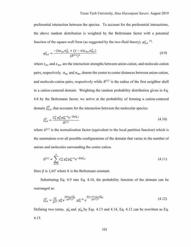
Texas Tech University, Sina Hassanjani Saravi, August 2019
101
preferential interaction between the species. To account for the preferential interactions,
the above random distribution is weighted by the Boltzmann factor with a potential
function of the square-well form (as suggested by the two-fluid theory), 𝜑𝜑𝜕𝜕,𝑧𝑧𝐿𝐿 34:
𝜑𝜑𝜕𝜕,𝑧𝑧𝐿𝐿 =
−(𝑙𝑙𝜖𝜖𝑎𝑎𝐿𝐿𝜎𝜎𝑎𝑎𝐿𝐿3 + (𝑧𝑧 − 𝑙𝑙)𝜖𝜖𝑚𝑚𝐿𝐿𝜎𝜎𝑚𝑚𝐿𝐿3 )
(𝑅𝑅(𝐿𝐿))3 (4.9)
where 𝜖𝜖𝑎𝑎𝐿𝐿 and 𝜖𝜖𝑚𝑚𝐿𝐿 are the interaction strengths between anion-cation, and molecule-cation
pairs, respectively. 𝜎𝜎𝑎𝑎𝐿𝐿 and 𝜎𝜎𝑚𝑚𝐿𝐿 denote the center to center distances between anion-cation,
and molecule-cation pairs, respectively while 𝑅𝑅(𝐿𝐿) is the radius of the first neighbor shell
in a cation-centered domain. Weighting the random probability distribution given in Eq.
4.8 by the Boltzmann factor, we arrive at the probability of forming a cation-centered
domain 𝑓𝑓𝜕𝜕,𝑧𝑧𝐿𝐿� , that accounts for the interaction between the molecular species:
𝑓𝑓𝜕𝜕,𝑧𝑧𝐿𝐿� =
𝐶𝐶𝜕𝜕𝑧𝑧 𝑝𝑝𝑎𝑎 𝜕𝜕𝑝𝑝𝑚𝑚𝑧𝑧−𝜕𝜕𝑒𝑒−𝛽𝛽𝜑𝜑𝑛𝑛,𝑧𝑧
𝑐𝑐
𝛺𝛺(𝐿𝐿) (4.10)
where 𝛺𝛺(𝐿𝐿) is the normalization factor (equivalent to the local partition function) which is
the summation over all possible configurations of the domain that varies in the number of
anions and molecules surrounding the center cation.
𝛺𝛺(𝐿𝐿) = �𝐶𝐶𝜕𝜕𝑧𝑧 𝑝𝑝𝑎𝑎
𝜕𝜕𝑝𝑝𝑚𝑚𝑧𝑧−𝜕𝜕𝑒𝑒−𝛽𝛽𝜑𝜑𝑛𝑛,𝑧𝑧𝑐𝑐
𝑧𝑧
𝜕𝜕=0
(4.11)
Here 𝛽𝛽 is 1/𝑘𝑘𝑇𝑇 where 𝑘𝑘 is the Boltzmann constant.
Substituting Eq. 4.9 into Eq. 4.10, the probability function of the domain can be
rearranged as:
𝑓𝑓𝜕𝜕,𝑧𝑧𝐿𝐿� = 𝐶𝐶𝑛𝑛𝑧𝑧
𝛺𝛺(𝑐𝑐) 𝑝𝑝𝑎𝑎 𝜕𝜕𝑒𝑒
𝛽𝛽𝑛𝑛𝜖𝜖𝑎𝑎𝑐𝑐𝜎𝜎𝑎𝑎𝑐𝑐3
(𝑅𝑅(𝑐𝑐))3 .𝑝𝑝𝑚𝑚𝑧𝑧−𝜕𝜕 𝑒𝑒𝛽𝛽(𝑧𝑧−𝑛𝑛) 𝜖𝜖𝑚𝑚𝑐𝑐𝜎𝜎𝑚𝑚𝑐𝑐
3
(𝑅𝑅(𝑐𝑐))3 (4.12)
Defining two terms, 𝑝𝑝𝑎𝑎 ′ and 𝑝𝑝𝑚𝑚
′ by Eqs. 4.13 and 4.14, Eq. 4.12 can be rewritten as Eq.
4.15.
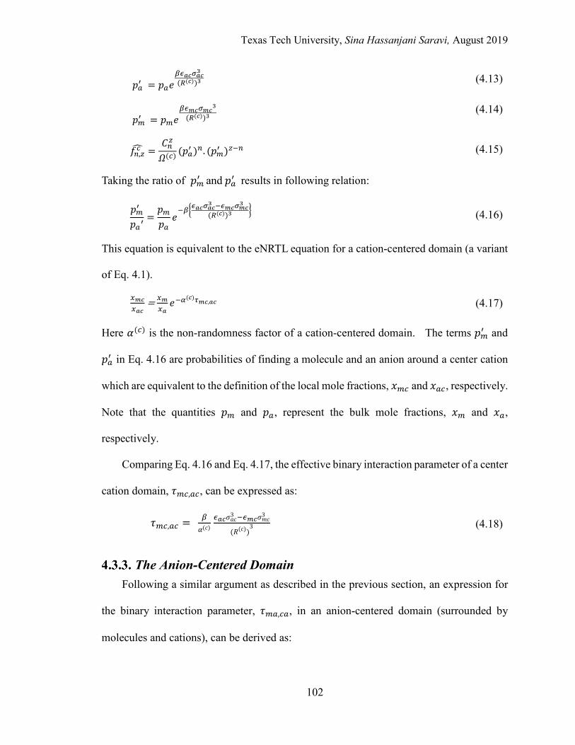
Texas Tech University, Sina Hassanjani Saravi, August 2019
102
𝑝𝑝𝑎𝑎 ′ = 𝑝𝑝𝑎𝑎𝑒𝑒
𝛽𝛽𝜖𝜖𝑎𝑎𝑐𝑐𝜎𝜎𝑎𝑎𝑐𝑐3(𝐿𝐿(𝑐𝑐))3 (4.13)
𝑝𝑝𝑚𝑚 ′ = 𝑝𝑝𝑚𝑚𝑒𝑒
𝛽𝛽𝜖𝜖𝑚𝑚𝑐𝑐𝜎𝜎𝑚𝑚𝑐𝑐3
(𝐿𝐿(𝑐𝑐))3 (4.14)
𝑓𝑓𝜕𝜕,𝑧𝑧𝐿𝐿� =
𝐶𝐶𝜕𝜕𝑧𝑧
𝛺𝛺(𝐿𝐿) (𝑝𝑝𝑎𝑎′ )𝜕𝜕. (𝑝𝑝𝑚𝑚′ )𝑧𝑧−𝜕𝜕 (4.15)
Taking the ratio of 𝑝𝑝𝑚𝑚 ′ and 𝑝𝑝𝑎𝑎
′ results in following relation:
𝑝𝑝𝑚𝑚′
𝑝𝑝𝑎𝑎′=𝑝𝑝𝑚𝑚𝑝𝑝𝑎𝑎
𝑒𝑒−𝛽𝛽�𝜖𝜖𝑎𝑎𝑐𝑐𝜎𝜎𝑎𝑎𝑐𝑐
3 −𝜖𝜖𝑚𝑚𝑐𝑐𝜎𝜎𝑚𝑚𝑐𝑐3
(𝐿𝐿(𝑐𝑐))3� (4.16)
This equation is equivalent to the eNRTL equation for a cation-centered domain (a variant
of Eq. 4.1).
𝑒𝑒𝑚𝑚𝑐𝑐𝑒𝑒𝑎𝑎𝑐𝑐
= 𝑒𝑒𝑚𝑚𝑒𝑒𝑎𝑎𝑒𝑒−𝛼𝛼(𝑐𝑐)𝜏𝜏𝑚𝑚𝑐𝑐,𝑎𝑎𝑐𝑐 (4.17)
Here 𝛼𝛼(𝐿𝐿) is the non-randomness factor of a cation-centered domain. The terms 𝑝𝑝𝑚𝑚′ and
𝑝𝑝𝑎𝑎′ in Eq. 4.16 are probabilities of finding a molecule and an anion around a center cation
which are equivalent to the definition of the local mole fractions, 𝑥𝑥𝑚𝑚𝐿𝐿 and 𝑥𝑥𝑎𝑎𝐿𝐿, respectively.
Note that the quantities 𝑝𝑝𝑚𝑚 and 𝑝𝑝𝑎𝑎, represent the bulk mole fractions, 𝑥𝑥𝑚𝑚 and 𝑥𝑥𝑎𝑎,
respectively.
Comparing Eq. 4.16 and Eq. 4.17, the effective binary interaction parameter of a center
cation domain, 𝜏𝜏𝑚𝑚𝐿𝐿,𝑎𝑎𝐿𝐿, can be expressed as:
𝜏𝜏𝑚𝑚𝐿𝐿,𝑎𝑎𝐿𝐿 = 𝛽𝛽𝛼𝛼(𝑐𝑐)
𝜖𝜖𝑎𝑎𝑐𝑐𝜎𝜎𝑎𝑎𝑐𝑐3 −𝜖𝜖𝑚𝑚𝑐𝑐𝜎𝜎𝑚𝑚𝑐𝑐3
(𝑅𝑅(𝑐𝑐))3 (4.18)
The Anion-Centered Domain Following a similar argument as described in the previous section, an expression for
the binary interaction parameter, 𝜏𝜏𝑚𝑚𝑎𝑎,𝐿𝐿𝑎𝑎, in an anion-centered domain (surrounded by
molecules and cations), can be derived as:
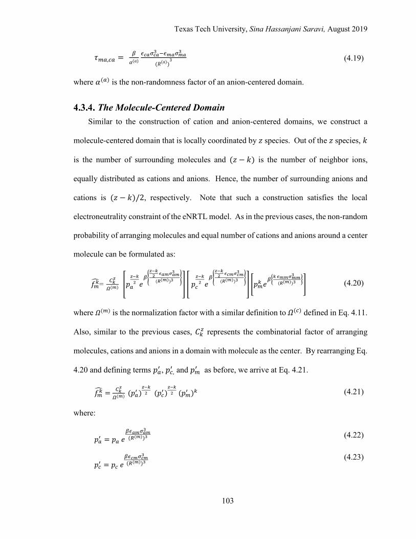
Texas Tech University, Sina Hassanjani Saravi, August 2019
103
𝜏𝜏𝑚𝑚𝑎𝑎,𝐿𝐿𝑎𝑎 = 𝛽𝛽𝛼𝛼(𝑎𝑎)
𝜖𝜖𝑐𝑐𝑎𝑎𝜎𝜎𝑐𝑐𝑎𝑎3 −𝜖𝜖𝑚𝑚𝑎𝑎𝜎𝜎𝑚𝑚𝑎𝑎3
(𝑅𝑅(𝑎𝑎))3 (4.19)
where 𝛼𝛼(𝑎𝑎) is the non-randomness factor of an anion-centered domain.
The Molecule-Centered Domain Similar to the construction of cation and anion-centered domains, we construct a
molecule-centered domain that is locally coordinated by 𝑧𝑧 species. Out of the 𝑧𝑧 species, 𝑘𝑘
is the number of surrounding molecules and (𝑧𝑧 − 𝑘𝑘) is the number of neighbor ions,
equally distributed as cations and anions. Hence, the number of surrounding anions and
cations is (𝑧𝑧 − 𝑘𝑘)/2, respectively. Note that such a construction satisfies the local
electroneutrality constraint of the eNRTL model. As in the previous cases, the non-random
probability of arranging molecules and equal number of cations and anions around a center
molecule can be formulated as:
𝑓𝑓𝑚𝑚𝑘𝑘�= 𝐶𝐶𝑘𝑘
𝑧𝑧
𝛺𝛺(𝑚𝑚) �𝑝𝑝𝑎𝑎𝑧𝑧−𝑘𝑘2 𝑒𝑒
𝛽𝛽�𝑧𝑧−𝑘𝑘2 𝜖𝜖𝑎𝑎𝑚𝑚𝜎𝜎𝑎𝑎𝑚𝑚
3
(𝑅𝑅(𝑚𝑚))3�� � 𝑝𝑝𝐿𝐿
𝑧𝑧−𝑘𝑘2 𝑒𝑒
𝛽𝛽�𝑧𝑧−𝑘𝑘2 𝜖𝜖𝑐𝑐𝑚𝑚𝜎𝜎𝑐𝑐𝑚𝑚
3
(𝑅𝑅(𝑚𝑚))3�� �𝑝𝑝𝑚𝑚𝑘𝑘 𝑒𝑒
𝛽𝛽�𝑘𝑘 𝜖𝜖𝑚𝑚𝑚𝑚𝜎𝜎𝑚𝑚𝑚𝑚3
(𝑅𝑅(𝑚𝑚))3�� (4.20)
where 𝛺𝛺(𝑚𝑚) is the normalization factor with a similar definition to 𝛺𝛺(𝐿𝐿) defined in Eq. 4.11.
Also, similar to the previous cases, 𝐶𝐶𝑘𝑘𝑧𝑧 represents the combinatorial factor of arranging
molecules, cations and anions in a domain with molecule as the center. By rearranging Eq.
4.20 and defining terms 𝑝𝑝𝑎𝑎′ , 𝑝𝑝𝐿𝐿,′ and 𝑝𝑝𝑚𝑚′ as before, we arrive at Eq. 4.21.
𝑓𝑓𝑚𝑚𝑘𝑘� = 𝐶𝐶𝑘𝑘𝑧𝑧
𝛺𝛺(𝑚𝑚) (𝑝𝑝𝑎𝑎′ )𝑧𝑧−𝑘𝑘2 (𝑝𝑝𝐿𝐿′)
𝑧𝑧−𝑘𝑘2 (𝑝𝑝𝑚𝑚′ )𝑘𝑘 (4.21)
where:
𝑝𝑝𝑎𝑎′ = 𝑝𝑝𝑎𝑎 𝑒𝑒
𝛽𝛽𝜖𝜖𝑎𝑎𝑚𝑚𝜎𝜎𝑎𝑎𝑚𝑚3(𝐿𝐿(𝑚𝑚))3 (4.22)
𝑝𝑝𝐿𝐿′ = 𝑝𝑝𝐿𝐿 𝑒𝑒
𝛽𝛽𝜖𝜖𝑐𝑐𝑚𝑚𝜎𝜎𝑐𝑐𝑚𝑚3(𝐿𝐿(𝑚𝑚))3
(4.23)
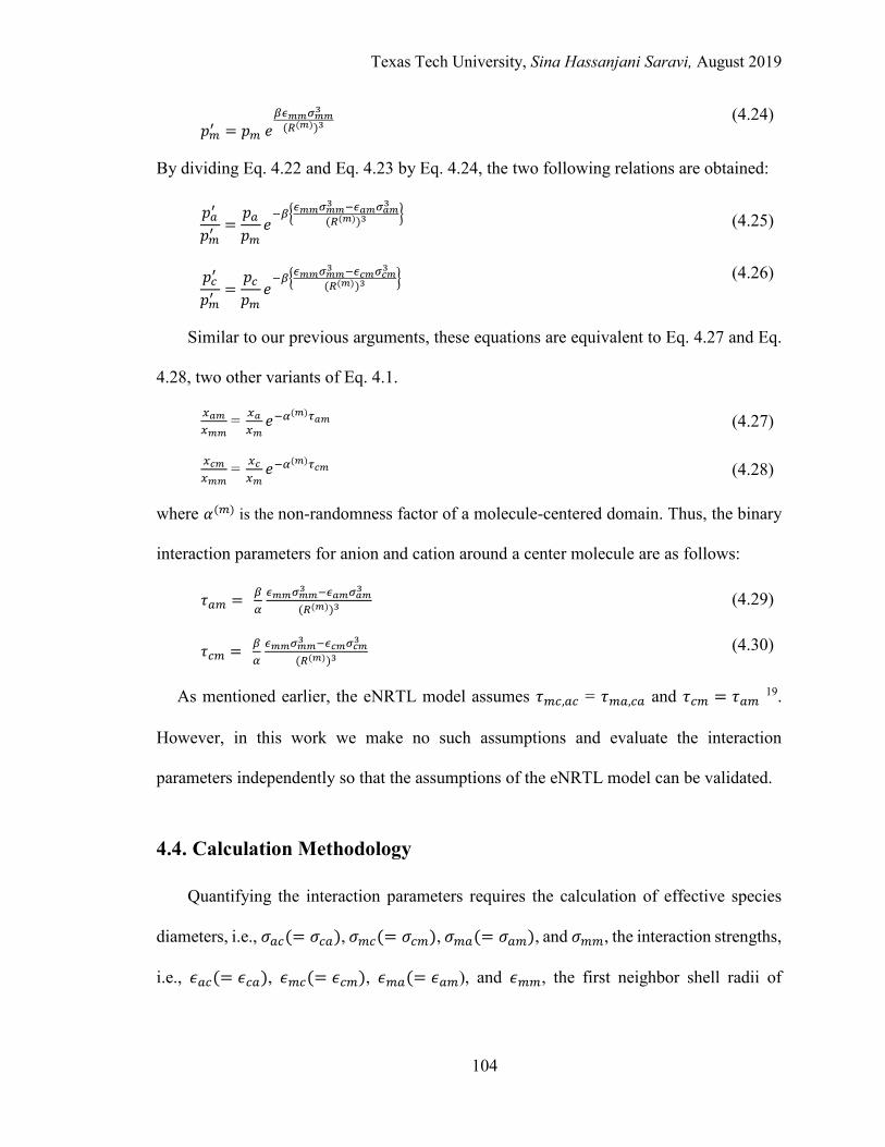
Texas Tech University, Sina Hassanjani Saravi, August 2019
104
𝑝𝑝𝑚𝑚′ = 𝑝𝑝𝑚𝑚 𝑒𝑒
𝛽𝛽𝜖𝜖𝑚𝑚𝑚𝑚𝜎𝜎𝑚𝑚𝑚𝑚3
(𝐿𝐿(𝑚𝑚))3 (4.24)
By dividing Eq. 4.22 and Eq. 4.23 by Eq. 4.24, the two following relations are obtained:
𝑝𝑝𝑎𝑎′
𝑝𝑝𝑚𝑚′=𝑝𝑝𝑎𝑎𝑝𝑝𝑚𝑚
𝑒𝑒−𝛽𝛽�𝜖𝜖𝑚𝑚𝑚𝑚𝜎𝜎𝑚𝑚𝑚𝑚
3 −𝜖𝜖𝑎𝑎𝑚𝑚𝜎𝜎𝑎𝑎𝑚𝑚3(𝐿𝐿(𝑚𝑚))3
� (4.25)
𝑝𝑝𝐿𝐿′
𝑝𝑝𝑚𝑚′=𝑝𝑝𝐿𝐿𝑝𝑝𝑚𝑚
𝑒𝑒−𝛽𝛽�𝜖𝜖𝑚𝑚𝑚𝑚𝜎𝜎𝑚𝑚𝑚𝑚
3 −𝜖𝜖𝑐𝑐𝑚𝑚𝜎𝜎𝑐𝑐𝑚𝑚3(𝐿𝐿(𝑚𝑚))3
�
(4.26)
Similar to our previous arguments, these equations are equivalent to Eq. 4.27 and Eq.
4.28, two other variants of Eq. 4.1.
𝑒𝑒𝑎𝑎𝑚𝑚𝑒𝑒𝑚𝑚𝑚𝑚
= 𝑒𝑒𝑎𝑎𝑒𝑒𝑚𝑚𝑒𝑒−𝛼𝛼(𝑚𝑚)𝜏𝜏𝑎𝑎𝑚𝑚 (4.27)
𝑒𝑒𝑐𝑐𝑚𝑚𝑒𝑒𝑚𝑚𝑚𝑚
= 𝑒𝑒𝑐𝑐𝑒𝑒𝑚𝑚𝑒𝑒−𝛼𝛼(𝑚𝑚)𝜏𝜏𝑐𝑐𝑚𝑚 (4.28)
where 𝛼𝛼(𝑚𝑚) is the non-randomness factor of a molecule-centered domain. Thus, the binary
interaction parameters for anion and cation around a center molecule are as follows:
𝜏𝜏𝑎𝑎𝑚𝑚 = 𝛽𝛽𝛼𝛼
𝜖𝜖𝑚𝑚𝑚𝑚𝜎𝜎𝑚𝑚𝑚𝑚3 −𝜖𝜖𝑎𝑎𝑚𝑚𝜎𝜎𝑎𝑎𝑚𝑚3
(𝐿𝐿(𝑚𝑚))3 (4.29)
𝜏𝜏𝐿𝐿𝑚𝑚 = 𝛽𝛽𝛼𝛼
𝜖𝜖𝑚𝑚𝑚𝑚𝜎𝜎𝑚𝑚𝑚𝑚3 −𝜖𝜖𝑐𝑐𝑚𝑚𝜎𝜎𝑐𝑐𝑚𝑚3
(𝐿𝐿(𝑚𝑚))3 (4.30)
As mentioned earlier, the eNRTL model assumes 𝜏𝜏𝑚𝑚𝐿𝐿,𝑎𝑎𝐿𝐿 = 𝜏𝜏𝑚𝑚𝑎𝑎,𝐿𝐿𝑎𝑎 and 𝜏𝜏𝐿𝐿𝑚𝑚 = 𝜏𝜏𝑎𝑎𝑚𝑚 19.
However, in this work we make no such assumptions and evaluate the interaction
parameters independently so that the assumptions of the eNRTL model can be validated.
4.4. Calculation Methodology
Quantifying the interaction parameters requires the calculation of effective species
diameters, i.e., 𝜎𝜎𝑎𝑎𝐿𝐿(= 𝜎𝜎𝐿𝐿𝑎𝑎), 𝜎𝜎𝑚𝑚𝐿𝐿(= 𝜎𝜎𝐿𝐿𝑚𝑚), 𝜎𝜎𝑚𝑚𝑎𝑎(= 𝜎𝜎𝑎𝑎𝑚𝑚), and 𝜎𝜎𝑚𝑚𝑚𝑚, the interaction strengths,
i.e., 𝜖𝜖𝑎𝑎𝐿𝐿(= 𝜖𝜖𝐿𝐿𝑎𝑎), 𝜖𝜖𝑚𝑚𝐿𝐿(= 𝜖𝜖𝐿𝐿𝑚𝑚), 𝜖𝜖𝑚𝑚𝑎𝑎(= 𝜖𝜖𝑎𝑎𝑚𝑚), and 𝜖𝜖𝑚𝑚𝑚𝑚, the first neighbor shell radii of
Texas Tech University, Sina Hassanjani Saravi, August 2019
105
different domains, i.e., 𝑅𝑅(𝐿𝐿), 𝑅𝑅(𝑎𝑎), and 𝑅𝑅(𝑚𝑚), and the non-randomness factors, 𝛼𝛼(𝐿𝐿), 𝛼𝛼(𝑎𝑎),
and 𝛼𝛼(𝑚𝑚). We obtain each of these quantities directly from MD simulations.
The 𝜎𝜎 parameters are obtained as the position of first peaks from the radial distribution
functions (RDFs) between the pairs of interest. The molecular and ionic interaction
strength, 𝜖𝜖, are obtained from the potential of mean force (PMF) between the pairs of
interest, i.e., depths of the first minima of the PMFs between cation-anion, molecule-cation,
molecule-anion, and molecule-molecule are taken as the interaction strengths, respectively.
Such calculations provide a better representation for the net interactions in the liquid phase
rather than considering the bare pair-wise interactions 29.
The size of the molecular domain 𝑅𝑅, is usually obtained as the size of first neighbor
shell from MD simulations. While this approach has been shown to be appropriate for
organic binary mixtures 29, such a definition is not consistent with the underlying
assumptions of the eNRTL model: local electroneutrality and like-ion repulsion. Hence,
to predict the interaction parameters of the eNRTL model, we propose a new approach to
define the size of the molecular domains such that the assumptions of the model are
satisfied. For this purpose, the local compositions in domains of different radii are obtained
by integrating the RDF of different pairs involving the center species. In a molecule-
centered domain, 𝑅𝑅(𝑚𝑚) is defined as the shortest distance from the solvent molecule at
which the local compositions of anions and cations are equal. The construction as the one
described above satisfies the local electroneutrality condition. On the other hand, in cation-
centered and anion-centered domains, the size of the domains, 𝑅𝑅(𝐿𝐿) and 𝑅𝑅(𝑎𝑎) are defined as
the longest distance from the center ionic species until which no other ion with the same
Texas Tech University, Sina Hassanjani Saravi, August 2019
106
charge as the center ion (i.e. like-ion) is present. Such a definition ensures consistency
with the like-ion repulsion assumption.
Finally, the non-randomness factor, 𝛼𝛼, is calculated from the knowledge of the local
coordination numbers. Renon and Prausnitz 33 pointed out that the non-randomness factor
is equivalent to the inverse of the coordination number (1/𝑧𝑧). This equivalency was
established by comparing the NRTL model relationship between local compositions and
bulk mole fractions with that of the Guggenheim’s quasichemical theory 35. We use this
interpretation to obtain 𝛼𝛼 directly from MD simulations. As the coordination number
around a center species can be different in cation-centered, anion-centered, and molecule-
centered domains due to the inherent differences in the local molecular structure, three
separate non-randomness factors, 𝛼𝛼(𝐿𝐿), 𝛼𝛼(𝑎𝑎), and 𝛼𝛼(𝑚𝑚) are obtained by integrating the
pertinent RDFs. Furthermore, we investigate the composition dependence of the 𝜏𝜏
parameters by performing simulations on aqueous solutions over a wide range of
concentrations. The molecular quantities of interest (described above) are obtained at each
concentration; these values are then used to examine the concentration dependence of the
binary interaction parameter.
4.5. Molecular Simulations
Simulations were carried out over wide range of concentrations from 0.5 to 16 molality
(mol/kg) of aqueous NaCl solution and at 298.15 K and 1 bar. Each simulation system
consisted of 1000 water molecules and varying number of ions as required to achieve the
desired concentration of the solution. Choosing simulations of small size facilitates rapid
prediction of the binary interaction parameters thereby enabling the use of our
Texas Tech University, Sina Hassanjani Saravi, August 2019
107
methodology for industrial process design. However, to investigate the effect of finite
simulation system size on our calculations, a larger system (with ten times the number of
water molecules than the smaller system) was also simulated at the concentration of 4
mol/kg.
The LAMMPS package was used to perform all of the simulations 36. Initial
equilibration of the system was carried out at constant number of particles, volume, and
temperature conditions (canonical ensemble) which was followed by 10 ns long
equilibration and 40 ns long production runs in the isothermal-isobaric ensemble using the
Nośe-Hoover thermostat and barostat 37 for the smaller systems. On the other hand, the
larger system was simulated for a duration of 25 ns. The Lennard-Jones and Coulombic
interactions were truncated at distance of 14 Å. The long-range electrostatic interactions
were calculated using the particle-particle particle-mesh (PPPM) 38 method and tail
corrections were applied to correct for the long-range part of the Lennard-Jones
interactions. The SPC/E model 39 and the Kirkwood-Buff force field (KBFF) parameters
40,41 were employed to represent the water molecules and ions, respectively. This choice
of the force field was made based on its ability to predict the mean ionic activity
coefficients, as described in previous studies 13,26. The 40 ns long production runs were
divided into 10 blocks of 4 ns length, each of which was used to obtain the desired
quantities and to estimate the error in those quantities. Similarly, for the larger system, the
first 10 ns of the trajectory were discarded, and the remaining 15 ns were divided into 5
blocks of 3 ns duration each. The PMF for different interactions were calculated from the
RDFs using Eq. 4.31 42. Given that the correlation times for water molecules (determined
from the orientation correlation of the water OH bond vector), even at high salt
Texas Tech University, Sina Hassanjani Saravi, August 2019
108
concentrations, are much shorter than 25 ps 13, our simulation trajectory includes many
such correlation times. Hence, our simulations sufficiently sample several configurations
of the aqueous system, enabling us to calculate the PMFs as per Eq. 4.31.
𝜙𝜙(𝑟𝑟) = −𝑅𝑅𝑇𝑇 ln𝑔𝑔(𝑟𝑟) (4.31)
4.6. Binary Interaction Parameters from Regression
The validity of the binary interaction parameters calculated from MD simulations is
tested by performing regression of experimental 43 and simulation 𝛾𝛾± data 13 (separately)
to independently determine the values of 𝜏𝜏𝑚𝑚,𝐿𝐿𝑎𝑎 and 𝜏𝜏𝐿𝐿𝑎𝑎,𝑚𝑚, and the associated uncertainties.
It is essential to quantify such uncertainties as the magnitude of the calculated mean ionic
activity coefficients is extremely sensitive to minor fluctuations in the 𝜏𝜏 values 12. First,
the experimental mean ionic activity coefficient data of Robinson and Stokes 44 at 298.15
K and 1 bar, in the concentration range of 0.1 to 6 mol/kg NaCl is correlated with the
eNRTL model by minimizing the residual root-mean-square error (RRMSE) as the
objective function. APSEN Properties package 45, version 8.8 was used for this purpose.
Furthermore, another set of values of the binary interaction parameters was also obtained
from the simulation determined 𝛾𝛾± data (calculated using the Kirkwood-Buff theory)
reported by Hossain et al. 13. Note that the simulation results of Hossain et al. employed
the same force field parameters as the present work. The 𝜏𝜏 parameters are identified using
the simulation data via regression using the same optimization technique as stated above.
Texas Tech University, Sina Hassanjani Saravi, August 2019
109
4.7. Results and Discussions
Regression of Experimental and Simulation Data The binary interaction parameters obtained from regression in this work for the
H2O:(Na+-Clˉ) pair at 298.15 K and 1 bar are listed in Table 4.1 along with those reported
by Yan and Chen 43. It can be seen that 𝜏𝜏 values calculated in this work are in agreement
with the binary interaction parameters reported by Yan and Chen 43. Also, Table 4.1 lists
the binary interaction parameters obtained from the KB simulation data for 𝛾𝛾± by Hossain
et al. 13, along with the uncertainties. These values will be used to validate the parameters
obtained from simulations in this work.
Table 4.1. Binary interaction parameters from regression
Parameters Yan and Chen 43 This work1 KB simulation2
𝜏𝜏𝑚𝑚,𝐿𝐿𝑎𝑎 8.86 8.89±0.06 7.23±0.18
𝜏𝜏𝐿𝐿𝑎𝑎,𝑚𝑚 -4.54 -4.55±0.02 -3.95±0.06
1 regressed from the data reported by Robinson and Stokes 44 2 regressed from the simulation data of Hossain et al. 13
Interpretation of the Molecular Quantities in the Framework of eNRTL
The binary interaction parameters are obtained from molecular simulations as
described in the previous sections. The effective species diameters are obtained from the
location of first peaks of the corresponding RDF. For instance, 𝜎𝜎𝑎𝑎𝐿𝐿 which represents the
effective diameter between Na+ and Clˉ interactions is considered as the location of the
first peak of the cation-anion RDF. All the 𝜎𝜎 parameters thus obtained are listed in Table
4.10.1 of the Supporting Information, at each concentration. We note that the
uncertainties in 𝜎𝜎 are negligible (less than 0.25%) and hence are not reported. Furthermore,
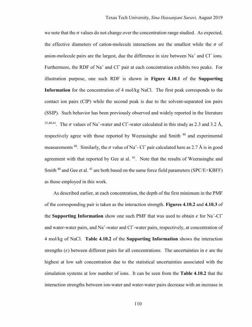
Texas Tech University, Sina Hassanjani Saravi, August 2019
110
we note that the 𝜎𝜎 values do not change over the concentration range studied. As expected,
the effective diameters of cation-molecule interactions are the smallest while the 𝜎𝜎 of
anion-molecule pairs are the largest, due the difference in size between Na+ and Clˉ ions.
Furthermore, the RDF of Na+ and Clˉ pair at each concentration exhibits two peaks. For
illustration purpose, one such RDF is shown in Figure 4.10.1 of the Supporting
Information for the concentration of 4 mol/kg NaCl. The first peak corresponds to the
contact ion pairs (CIP) while the second peak is due to the solvent-separated ion pairs
(SSIP). Such behavior has been previously observed and widely reported in the literature
25,40,41. The 𝜎𝜎 values of Na+-water and Clˉ-water calculated in this study as 2.3 and 3.2 Å,
respectively agree with those reported by Weerasinghe and Smith 40 and experimental
measurements 46. Similarly, the 𝜎𝜎 value of Na+- Clˉ pair calculated here as 2.7 Å is in good
agreement with that reported by Gee at al. 41. Note that the results of Weerasinghe and
Smith 40 and Gee et al. 41 are both based on the same force field parameters (SPC/E+KBFF)
as those employed in this work.
As described earlier, at each concentration, the depth of the first minimum in the PMF
of the corresponding pair is taken as the interaction strength. Figures 4.10.2 and 4.10.3 of
the Supporting Information show one such PMF that was used to obtain 𝜖𝜖 for Na+-Clˉ
and water-water pairs, and Na+-water and Clˉ-water pairs, respectively, at concentration of
4 mol/kg of NaCl. Table 4.10.2 of the Supporting Information shows the interaction
strengths (𝜖𝜖) between different pairs for all concentrations. The uncertainties in 𝜖𝜖 are the
highest at low salt concentration due to the statistical uncertainties associated with the
simulation systems at low number of ions. It can be seen from the Table 4.10.2 that the
interaction strengths between ion-water and water-water pairs decrease with an increase in
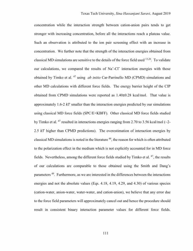
Texas Tech University, Sina Hassanjani Saravi, August 2019
111
concentration while the interaction strength between cation-anion pairs tends to get
stronger with increasing concentration, before all the interactions reach a plateau value.
Such an observation is attributed to the ion pair screening effect with an increase in
concentration. We further note that the strength of the interaction energies obtained from
classical MD simulations are sensitive to the details of the force field used 13,26. To validate
our calculations, we compared the results of Na+-Clˉ interaction energies with those
obtained by Timko et al. 47 using ab initio Car-Parrinello MD (CPMD) simulations and
other MD calculations with different force fields. The energy barrier height of the CIP
obtained from CPMD simulations were reported as 1.40±0.28 kcal/mol. That value is
approximately 1.6-2 𝑘𝑘𝑇𝑇 smaller than the interaction energies predicted by our simulations
using classical MD force fields (SPC/E+KBFF). Other classical MD force fields studied
by Timko et al. 47 resulted in interactions energies ranging from 2.70 to 3.56 kcal/mol (~2-
2.5 𝑘𝑘𝑇𝑇 higher than CPMD predictions). The overestimation of interaction energies by
classical MD simulations is noted in the literature 48, the reason for which is often attributed
to the polarization effect in the medium which is not explicitly accounted for in MD force
fields. Nevertheless, among the different force fields studied by Timko et al. 47, the results
of our calculations are comparable to those obtained using the Smith and Dang’s
parameters 49. Furthermore, as we are interested in the differences between the interactions
energies and not the absolute values (Eqs. 4.18, 4.19, 4.29, and 4.30) of various species
(cation-water, anion-water, water-water, and cation-anion), we believe that any error due
to the force field parameters will approximately cancel out and hence the procedure should
result in consistent binary interaction parameter values for different force fields.
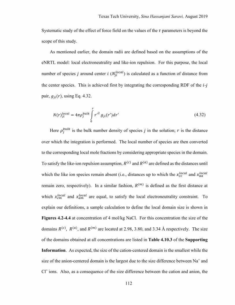
Texas Tech University, Sina Hassanjani Saravi, August 2019
112
Systematic study of the effect of force field on the values of the 𝜏𝜏 parameters is beyond the
scope of this study.
As mentioned earlier, the domain radii are defined based on the assumptions of the
eNRTL model: local electroneutrality and like-ion repulsion. For this purpose, the local
number of species 𝑗𝑗 around center 𝑖𝑖 (𝑁𝑁𝑗𝑗𝑖𝑖𝑙𝑙𝑜𝑜𝐿𝐿𝑎𝑎𝑙𝑙) is calculated as a function of distance from
the center species. This is achieved first by integrating the corresponding RDF of the 𝑖𝑖-𝑗𝑗
pair, 𝑔𝑔𝑗𝑗𝑖𝑖(𝑟𝑟), using Eq. 4.32.
𝑁𝑁(𝑟𝑟)𝑗𝑗𝑖𝑖𝑙𝑙𝑜𝑜𝐿𝐿𝑎𝑎𝑙𝑙 = 4𝜋𝜋𝜌𝜌𝑗𝑗𝑏𝑏𝑏𝑏𝑙𝑙𝑘𝑘 �𝑟𝑟′2
𝑟𝑟
0
𝑔𝑔𝑗𝑗𝑖𝑖(𝑟𝑟′)𝑑𝑑𝑟𝑟′ (4.32)
Here 𝜌𝜌𝑗𝑗𝑏𝑏𝑏𝑏𝑙𝑙𝑘𝑘 is the bulk number density of species 𝑗𝑗 in the solution; 𝑟𝑟 is the distance
over which the integration is performed. The local number of species are then converted
to the corresponding local mole fractions by considering appropriate species in the domain.
To satisfy the like-ion repulsion assumption, 𝑅𝑅(𝐿𝐿) and 𝑅𝑅(𝑎𝑎) are defined as the distances until
which the like ion species remain absent (i.e., distances up to which the 𝑥𝑥𝐿𝐿𝐿𝐿𝑙𝑙𝑜𝑜𝐿𝐿𝑎𝑎𝑙𝑙 and 𝑥𝑥𝑎𝑎𝑎𝑎𝑙𝑙𝑜𝑜𝐿𝐿𝑎𝑎𝑙𝑙
remain zero, respectively). In a similar fashion, 𝑅𝑅(𝑚𝑚) is defined as the first distance at
which 𝑥𝑥𝐿𝐿𝑚𝑚𝑙𝑙𝑜𝑜𝐿𝐿𝑎𝑎𝑙𝑙 and 𝑥𝑥𝑎𝑎𝑚𝑚𝑙𝑙𝑜𝑜𝐿𝐿𝑎𝑎𝑙𝑙 are equal, to satisfy the local electroneutrality constraint. To
explain our definitions, a sample calculation to define the local domain size is shown in
Figures 4.2-4.4 at concentration of 4 mol/kg NaCl. For this concentration the size of the
domains 𝑅𝑅(𝐿𝐿), 𝑅𝑅(𝑎𝑎), and 𝑅𝑅(𝑚𝑚) are located at 2.98, 3.80, and 3.34 Å respectively. The size
of the domains obtained at all concentrations are listed in Table 4.10.3 of the Supporting
Information. As expected, the size of the cation-centered domain is the smallest while the
size of the anion-centered domain is the largest due to the size difference between Na+ and
Clˉ ions. Also, as a consequence of the size difference between the cation and anion, the
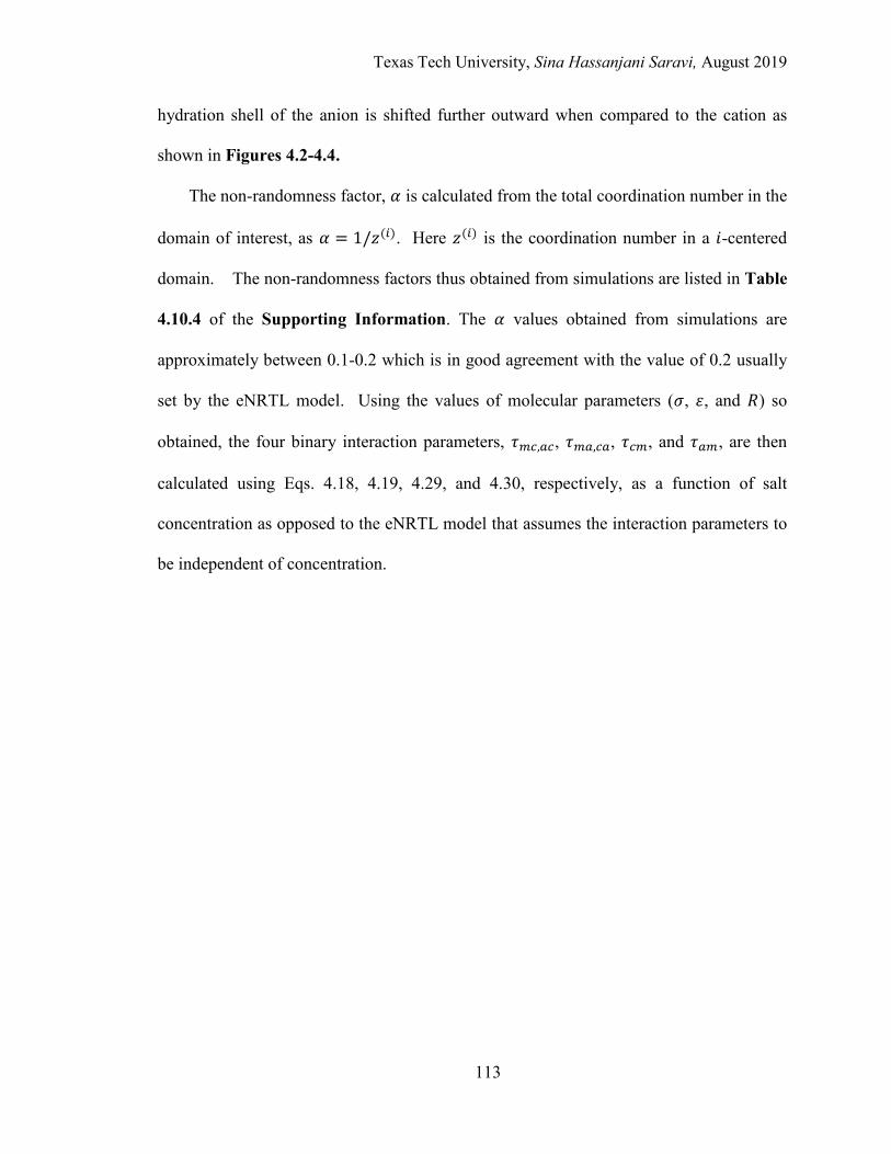
Texas Tech University, Sina Hassanjani Saravi, August 2019
113
hydration shell of the anion is shifted further outward when compared to the cation as
shown in Figures 4.2-4.4.
The non-randomness factor, 𝛼𝛼 is calculated from the total coordination number in the
domain of interest, as 𝛼𝛼 = 1/𝑧𝑧(𝑖𝑖). Here 𝑧𝑧(𝑖𝑖) is the coordination number in a 𝑖𝑖-centered
domain. The non-randomness factors thus obtained from simulations are listed in Table
4.10.4 of the Supporting Information. The 𝛼𝛼 values obtained from simulations are
approximately between 0.1-0.2 which is in good agreement with the value of 0.2 usually
set by the eNRTL model. Using the values of molecular parameters (𝜎𝜎, 𝜀𝜀, and 𝑅𝑅) so
obtained, the four binary interaction parameters, 𝜏𝜏𝑚𝑚𝐿𝐿,𝑎𝑎𝐿𝐿, 𝜏𝜏𝑚𝑚𝑎𝑎,𝐿𝐿𝑎𝑎, 𝜏𝜏𝐿𝐿𝑚𝑚, and 𝜏𝜏𝑎𝑎𝑚𝑚, are then
calculated using Eqs. 4.18, 4.19, 4.29, and 4.30, respectively, as a function of salt
concentration as opposed to the eNRTL model that assumes the interaction parameters to
be independent of concentration.
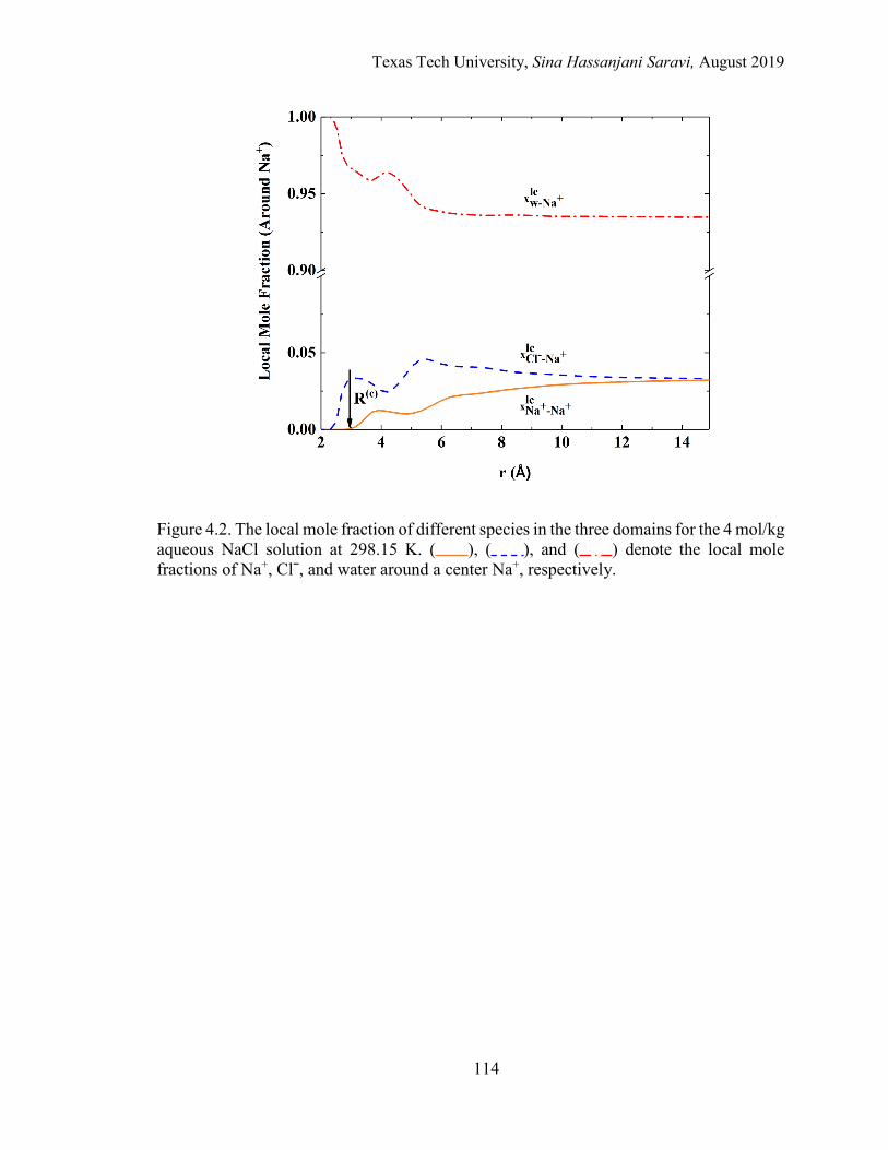
Texas Tech University, Sina Hassanjani Saravi, August 2019
114
Figure 4.2. The local mole fraction of different species in the three domains for the 4 mol/kg aqueous NaCl solution at 298.15 K. ( ), ( ), and ( ) denote the local mole fractions of Na+, Clˉ, and water around a center Na+, respectively.

Texas Tech University, Sina Hassanjani Saravi, August 2019
115
Figure 4.3. The local mole fraction of different species in the three domains for the 4 mol/kg aqueous NaCl solution at 298.15 K. ( ), ( ), and ( ) denote the local mole fractions of Na+, Clˉ, and water around a center Clˉ, respectively.
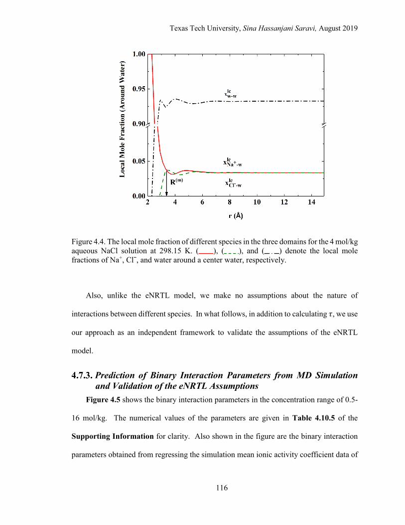
Texas Tech University, Sina Hassanjani Saravi, August 2019
116
Figure 4.4. The local mole fraction of different species in the three domains for the 4 mol/kg aqueous NaCl solution at 298.15 K. ( ), ( ), and ( ) denote the local mole fractions of Na+, Clˉ, and water around a center water, respectively.
Also, unlike the eNRTL model, we make no assumptions about the nature of
interactions between different species. In what follows, in addition to calculating 𝜏𝜏, we use
our approach as an independent framework to validate the assumptions of the eNRTL
model.
Prediction of Binary Interaction Parameters from MD Simulation and Validation of the eNRTL Assumptions
Figure 4.5 shows the binary interaction parameters in the concentration range of 0.5-
16 mol/kg. The numerical values of the parameters are given in Table 4.10.5 of the
Supporting Information for clarity. Also shown in the figure are the binary interaction
parameters obtained from regressing the simulation mean ionic activity coefficient data of
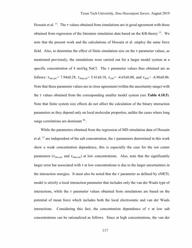
Texas Tech University, Sina Hassanjani Saravi, August 2019
117
Hossain et al. 13. The 𝜏𝜏 values obtained from simulations are in good agreement with those
obtained from regression of the literature simulation data based on the KB-theory 13. We
note that the present work and the calculations of Hossain et al. employ the same force
field. Also, to determine the effect of finite simulation size on the 𝜏𝜏 parameter values, as
mentioned previously, the simulations were carried out for a larger model system at a
specific concentration of 4 mol/kg NaCl. The 𝜏𝜏 parameter values thus obtained are as
follows: 𝜏𝜏𝑚𝑚𝐿𝐿,𝑎𝑎𝐿𝐿= 7.94±0.28, 𝜏𝜏𝑚𝑚𝑎𝑎,𝐿𝐿𝑎𝑎= 5.41±0.18, 𝜏𝜏𝐿𝐿𝑚𝑚= -4.65±0.08, and 𝜏𝜏𝑎𝑎𝑚𝑚= -4.96±0.06.
Note that these parameter values are in close agreement (within the uncertainty range) with
the 𝜏𝜏 values obtained from the corresponding smaller model system (see Table 4.10.5).
Note that finite system size effects do not affect the calculation of the binary interaction
parameters as they depend only on local molecular properties, unlike the cases where long
range correlations are dominant 50.
While the parameters obtained from the regression of MD simulation data of Hossain
et al. 13 are independent of the salt concentration, the 𝜏𝜏 parameters determined in this work
show a weak concentration dependence, this is especially the case for the ion center
parameters (𝜏𝜏𝑚𝑚𝐿𝐿,𝑎𝑎𝐿𝐿 and 𝜏𝜏𝑚𝑚𝑎𝑎,𝐿𝐿𝑎𝑎) at low concentrations. Also, note that the significantly
larger error bar associated with 𝜏𝜏 at low concentrations is due to the larger uncertainties in
the interaction energies. It must also be noted that the 𝜏𝜏 parameter as defined by eNRTL
model is strictly a local interaction parameter that includes only the van der Waals type of
interactions, while the 𝜏𝜏 parameter values obtained from simulations are based on the
potential of mean force which includes both the local electrostatic and van der Waals
interactions. Considering this fact, the concentration dependence of 𝜏𝜏 at low salt
concentrations can be rationalized as follows. Since at high concentrations, the van der
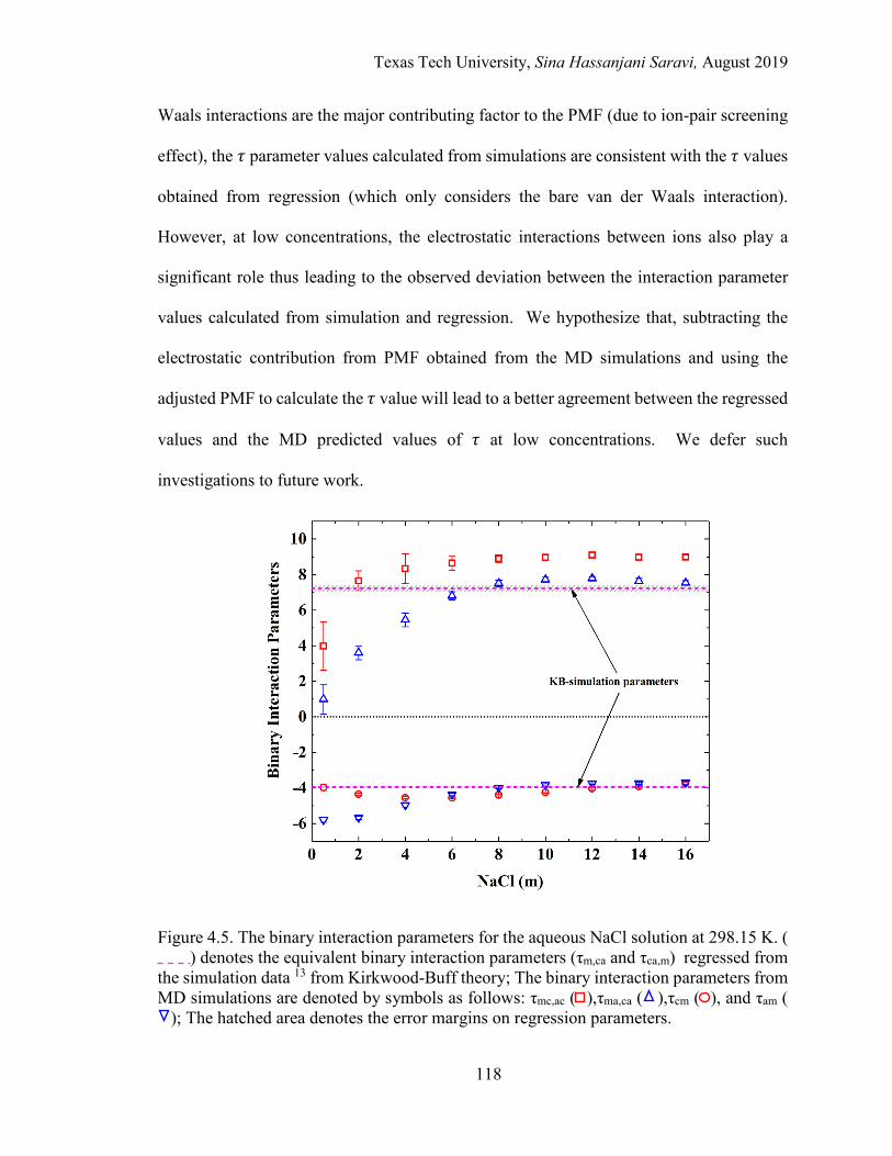
Texas Tech University, Sina Hassanjani Saravi, August 2019
118
Waals interactions are the major contributing factor to the PMF (due to ion-pair screening
effect), the 𝜏𝜏 parameter values calculated from simulations are consistent with the 𝜏𝜏 values
obtained from regression (which only considers the bare van der Waals interaction).
However, at low concentrations, the electrostatic interactions between ions also play a
significant role thus leading to the observed deviation between the interaction parameter
values calculated from simulation and regression. We hypothesize that, subtracting the
electrostatic contribution from PMF obtained from the MD simulations and using the
adjusted PMF to calculate the 𝜏𝜏 value will lead to a better agreement between the regressed
values and the MD predicted values of 𝜏𝜏 at low concentrations. We defer such
investigations to future work.
Figure 4.5. The binary interaction parameters for the aqueous NaCl solution at 298.15 K. () denotes the equivalent binary interaction parameters (τm,ca and τca,m) regressed from
the simulation data 13 from Kirkwood-Buff theory; The binary interaction parameters from MD simulations are denoted by symbols as follows: τmc,ac ( ),τma,ca ( ),τcm ( ), and τam (
); The hatched area denotes the error margins on regression parameters.
Texas Tech University, Sina Hassanjani Saravi, August 2019
119
The eNRTL model assumes that the strength of interaction between the cation-
molecule pair and the anion-molecule pair is equal. In terms of the two-liquid theory, this
assumption translates to the following expressions: 𝜏𝜏𝑚𝑚𝐿𝐿,𝑎𝑎𝐿𝐿 = 𝜏𝜏𝑚𝑚𝑎𝑎,𝐿𝐿𝑎𝑎 and 𝜏𝜏𝐿𝐿𝑚𝑚 = 𝜏𝜏𝑎𝑎𝑚𝑚. This
assumption can be seen to hold at high concentrations for 𝜏𝜏𝐿𝐿𝑚𝑚 and 𝜏𝜏𝑎𝑎𝑚𝑚 while at low
concentrations, significant deviations are observed (see Figure 4.5). Also, the assumption
of the eNRTL model regarding the nature of interactions in the cation and anion-centered
domains (𝜏𝜏𝑚𝑚𝐿𝐿,𝑎𝑎𝐿𝐿 and 𝜏𝜏𝑚𝑚𝑎𝑎,𝐿𝐿𝑎𝑎) is approximately true with 𝜏𝜏𝑚𝑚𝐿𝐿,𝑎𝑎𝐿𝐿 systematically higher than
𝜏𝜏𝑚𝑚𝑎𝑎,𝐿𝐿𝑎𝑎 throughout the entire concentration range. This observation is discussed further in
the Supporting Information (Figure 4.10.4). Furthermore, note that the abovementioned
assumption of the eNRTL theory reduces the number of adjustable parameters and renders
correlation of experimental data more feasible and hence has been widely adopted. The
results described above support that the 𝜏𝜏 parameters of the eNRTL model can be obtained
directly from the information of molecular structure and interactions in the condensed
phase system. Moreover, interpreting the model from statistical mechanics framework
allows for more rigorous validation of the underlying assumptions involved.
Phase Equilibrium Predictions As a further test of the parameter values, we compare the phase equilibrium properties
of the aqueous electrolyte solution obtained using the eNRTL model and the binary
interaction parameters calculated from MD simulations. The phase equilibrium predictions
from the eNRTL model considers both the local NRTL part and the long-range Pitzer-
Debye-Hückel formulation 12. For this purpose, the mean ionic activity coefficients
obtained from the eNRTL model using the 𝜏𝜏𝑚𝑚𝐿𝐿,𝑎𝑎𝐿𝐿 (= 8.34) and 𝜏𝜏𝐿𝐿𝑚𝑚 (= −4.54) parameters
and the corresponding 𝛼𝛼(𝐿𝐿) (= 0.18) and 𝛼𝛼(𝑚𝑚) (= 0.18) values determined in this work
Texas Tech University, Sina Hassanjani Saravi, August 2019
120
at the concentration of 4 mol/kg NaCl are shown in Figure 4.6. Further details on the
calculation of mean ionic activity coefficient using the eNRTL model and the
corresponding binary interaction parameters are presented in the literature where the
pertinent relations are derived 19. Figure 4.6 also shows the mean ionic activity coefficient
calculated from the regressed 𝜏𝜏 parameters 43, the predicted 𝛾𝛾± from MD simulations using
Kirkwood-Buff method 13, and the experimental data reported by Robinson and Stokes 44
along with the experimental data of Tang et al. 51. In addition, the uncertainties in 𝛾𝛾±
predicted by the eNRTL model (hatched area), due to the uncertainties associated with the
regressed 𝜏𝜏 parameters, are also shown. The 𝛾𝛾± values predicted from the binary
interaction parameters calculated using MD simulations in this work are in a reasonable
agreement with the KB theory-simulation results of Hossain et al. 13, despite the fact that
the techniques employed to obtain 𝛾𝛾± in both these calculations are different. As
mentioned before, we selected the 𝜏𝜏 values from the concentration 4 mol/kg NaCl as the
prediction of the 𝜏𝜏 parameter from MD simulations at high concentrations attains a plateau
value consistent with the eNRTL framework. Also, this choice of the 𝜏𝜏 parameter provided
the best prediction for 𝛾𝛾± compared with the results of Hossain et al. Accurate prediction
of 𝛾𝛾± using the MD determined 𝜏𝜏 parameters is challenging due to sensitivity of the
predicted 𝛾𝛾± to the values of the binary interaction parameters. Methodologies to further
improve the accuracy of the calculated 𝜏𝜏 parameters should be considered.
The vapor pressure (𝑃𝑃𝑠𝑠𝑎𝑎𝑡𝑡) and excess Gibbs free energy (𝐺𝐺𝑒𝑒𝑒𝑒) of the aqueous
electrolyte system are also calculated using the binary interaction parameters. Here the
excess Gibbs free energy was directly calculated from the activity coefficients, while the
vapor pressure was obtained from the flash calculation. Figure 4.7 shows that the

Texas Tech University, Sina Hassanjani Saravi, August 2019
121
predictions of vapor pressure and excess Gibbs free energy from the binary interaction
parameters of MD simulations are in excellent agreement with those obtained from
regression of MD simulation data of Hossain et al. 13, with the mean relative deviation
(MRD) of 1.04 % and 1.24 % for 𝑃𝑃𝑠𝑠𝑎𝑎𝑡𝑡 and 𝐺𝐺𝑒𝑒𝑒𝑒, respectively. We note that the predictions
of vapor pressure and excess Gibbs free energy are not as sensitive to the changes in 𝜏𝜏
parameters unlike 𝛾𝛾± which are very sensitive to the 𝜏𝜏 values.
Figure 4.6. Comparison of aqueous NaCl solution phase behavior at 298.15 K between MD simulations and regression results. ( ) denotes the mean ionic activity coefficients predicted from the binary interaction parameters of Yan and Chen 43, with the associated uncertainties shown as hatched area; ( ) presents the experimental data of Robinson and Stokes 44; ( ) denotes the experimental data of Tang et al. 51; the predicted mean ionic activity coefficient 13 by Kirkwood-Buff theory are presented by ( ); ( ) denotes the prediction of mean ionic activity coefficient using MD simulations results for binary interaction parameters of 4 mol/kg NaCl.

Texas Tech University, Sina Hassanjani Saravi, August 2019
122
Figure 4.7. Comparison of aqueous NaCl solution phase behavior at 298.15 K between MD simulations and regression results. ( ) and ( ) present the predictions of aqueous NaCl solution vapor pressure and excess Gibbs free energy at 298.15 K from binary interaction parameters of regression of the simulation data 13. ( ) and ( ) represent the vapor pressure and excess Gibbs free energy obtained from the binary interaction parameters calculated from the MD simulations (this work).
4.8. Conclusions
The eNRTL model is re-examined in terms of the two-fluid theory and a recent
framework for determining the binary interaction parameters from MD simulations.
Aqueous NaCl solution is chosen as the example system to investigate the validity of the
proposed approach. The binary parameters in the eNRTL model are expressed as functions
of species diameter (𝜎𝜎), effective interaction strength (𝜖𝜖), the domain radius around the
center species (𝑅𝑅), and the non-randomness factor (𝛼𝛼). Each of these quantities is directly
calculated from MD simulations while satisfying the two assumptions of eNRTL model,
i.e., local electroneutrality and like-ion repulsion.
Texas Tech University, Sina Hassanjani Saravi, August 2019
123
The binary interaction parameters calculated from MD simulations are in good
agreement with those obtained from data regression, especially, at moderate to high
concentrations. At low concentrations, these parameters exhibit concentration dependence
as they capture both the long-range electrostatic interactions and the short-range van der
Waals interaction. The binary interaction parameters calculated from MD at medium to
high concentrations are concentration independent, consistent with the eNRTL model and
hence the predictions from these concentrations should be used to calculate the phase
equilibrium properties.
This study provides a theoretical linkage between eNRTL, a classical thermodynamic
model for electrolytes, and molecular scale structure and interactions in the system. The
technique is useful for predicting the binary interaction parameters of the eNRTL model,
specifically in cases where the availability of experimental data is sparse to facilitate the
data regression procedure. The methodology can also guide data regression to predict
physically relevant parameters, thereby reducing the ambiguity in the parameter selection
process which otherwise requires significant manual tuning. On the other hand, challenges
remain in obtaining an accurate estimate for the phase equilibrium properties, especially
the mean ionic activity coefficient, using MD determined 𝜏𝜏 parameters. The predictions
of the binary interaction parameters obtained from our work can be refined by (1) fine-
tuning of the force fields/techniques (like CPMD) used to obtain the species interaction
energies and (2) including only the local van der Waals interaction energies between
components to calculate the 𝜏𝜏 parameters, (as discussed in the Results and Discussions
section). Our future work is aimed towards performing such calculations in addition to
extending and testing the current framework to multivalent electrolytes.
Texas Tech University, Sina Hassanjani Saravi, August 2019
124
4.9. Acknowledgments
The authors gratefully acknowledge the financial support of the Jack Maddox
Distinguished Engineering Chair Professorship in Sustainable Energy sponsored by the J.F
Maddox Foundation, United States. The authors also acknowledge the computational
resources provided by High Performance Computing Center (HPCC) at Texas Tech
University.

Texas Tech University, Sina Hassanjani Saravi, August 2019
125
4.10. Supporting Information
Table 4.10.1. Effective species diameters (Å)
NaCl concentration (m)
Parameters 0.5 2.0 4.0 6.0 8.0
𝜎𝜎𝑎𝑎𝐿𝐿 2.70 2.71 2.70 2.70 2.70
𝜎𝜎𝐿𝐿𝑚𝑚 2.31 2.31 2.31 2.31 2.31
𝜎𝜎𝑎𝑎𝑚𝑚 3.20 3.20 3.20 3.21 3.21
𝜎𝜎𝑚𝑚𝑚𝑚 2.75 2.76 2.77 2.77 2.79
Parameters 10.0 12.0 14.0 16.0
𝜎𝜎𝑎𝑎𝐿𝐿 2.70 2.70 2.70 2.70
𝜎𝜎𝐿𝐿𝑚𝑚 2.31 2.31 2.31 2.31
𝜎𝜎𝑎𝑎𝑚𝑚 3.22 3.22 3.23 3.23
𝜎𝜎𝑚𝑚𝑚𝑚 2.80 2.81 2.82 2.83
𝑎𝑎, 𝑐𝑐, and 𝑚𝑚 denote the anion, the cation, and the molecule

Texas Tech University, Sina Hassanjani Saravi, August 2019
126
Figure 4.10.1. Radial distribution function (RDF) of the Na+-Clˉ pair for the 4 mol/kg aqueous NaCl solution at 298.15 K.
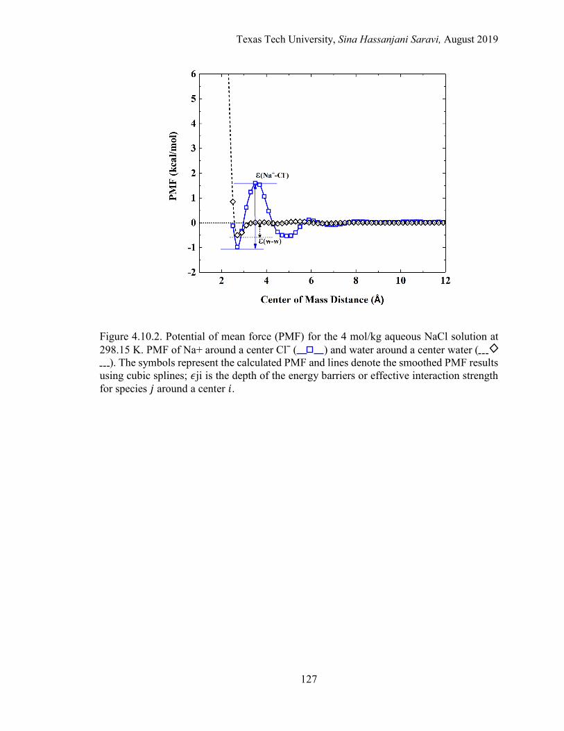
Texas Tech University, Sina Hassanjani Saravi, August 2019
127
Figure 4.10.2. Potential of mean force (PMF) for the 4 mol/kg aqueous NaCl solution at 298.15 K. PMF of Na+ around a center Clˉ ( ) and water around a center water (
). The symbols represent the calculated PMF and lines denote the smoothed PMF results using cubic splines; 𝜖𝜖ji is the depth of the energy barriers or effective interaction strength for species 𝑗𝑗 around a center 𝑖𝑖.
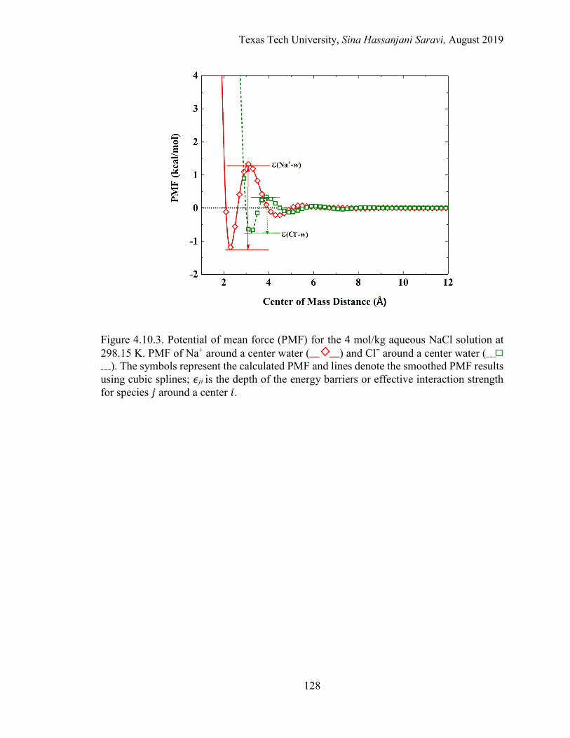
Texas Tech University, Sina Hassanjani Saravi, August 2019
128
Figure 4.10.3. Potential of mean force (PMF) for the 4 mol/kg aqueous NaCl solution at 298.15 K. PMF of Na+ around a center water ( ) and Clˉ around a center water (
). The symbols represent the calculated PMF and lines denote the smoothed PMF results using cubic splines; 𝜖𝜖ji is the depth of the energy barriers or effective interaction strength for species 𝑗𝑗 around a center 𝑖𝑖.
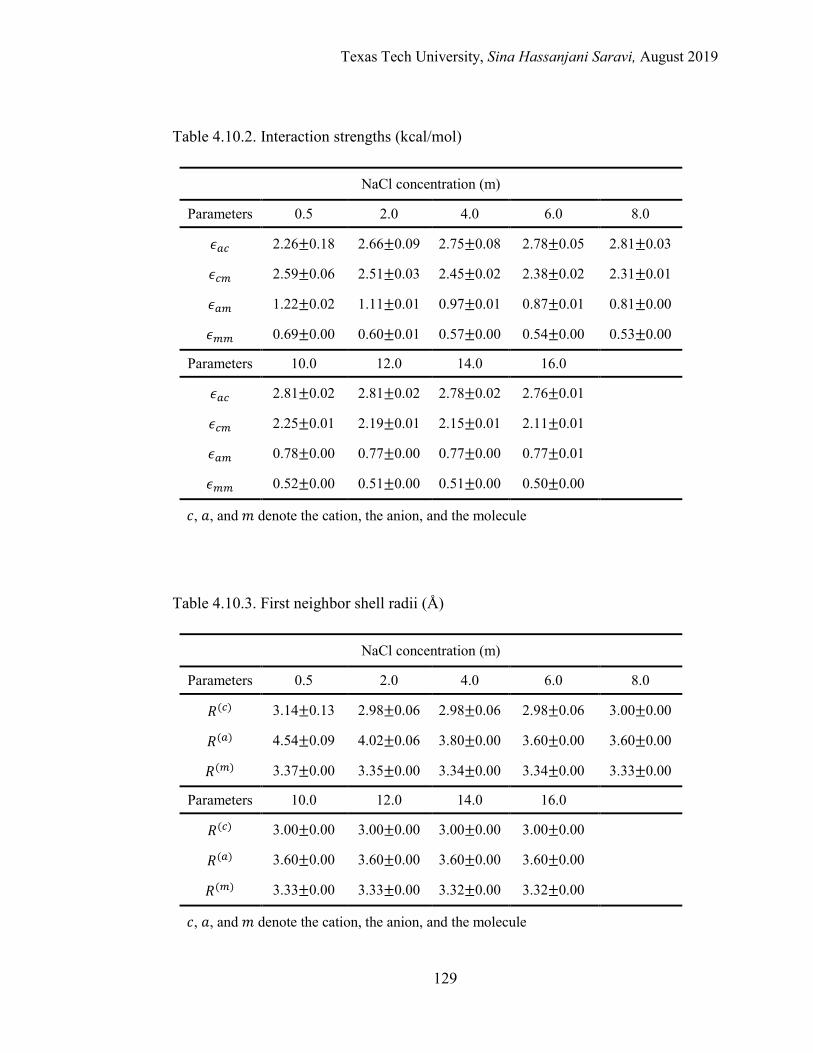
Texas Tech University, Sina Hassanjani Saravi, August 2019
129
Table 4.10.2. Interaction strengths (kcal/mol)
NaCl concentration (m)
Parameters 0.5 2.0 4.0 6.0 8.0
𝜖𝜖𝑎𝑎𝐿𝐿 2.26±0.18 2.66±0.09 2.75±0.08 2.78±0.05 2.81±0.03
𝜖𝜖𝐿𝐿𝑚𝑚 2.59±0.06 2.51±0.03 2.45±0.02 2.38±0.02 2.31±0.01
𝜖𝜖𝑎𝑎𝑚𝑚 1.22±0.02 1.11±0.01 0.97±0.01 0.87±0.01 0.81±0.00
𝜖𝜖𝑚𝑚𝑚𝑚 0.69±0.00 0.60±0.01 0.57±0.00 0.54±0.00 0.53±0.00
Parameters 10.0 12.0 14.0 16.0
𝜖𝜖𝑎𝑎𝐿𝐿 2.81±0.02 2.81±0.02 2.78±0.02 2.76±0.01
𝜖𝜖𝐿𝐿𝑚𝑚 2.25±0.01 2.19±0.01 2.15±0.01 2.11±0.01
𝜖𝜖𝑎𝑎𝑚𝑚 0.78±0.00 0.77±0.00 0.77±0.00 0.77±0.01
𝜖𝜖𝑚𝑚𝑚𝑚 0.52±0.00 0.51±0.00 0.51±0.00 0.50±0.00
𝑐𝑐, 𝑎𝑎, and 𝑚𝑚 denote the cation, the anion, and the molecule
Table 4.10.3. First neighbor shell radii (Å)
NaCl concentration (m)
Parameters 0.5 2.0 4.0 6.0 8.0
𝑅𝑅(𝐿𝐿) 3.14±0.13 2.98±0.06 2.98±0.06 2.98±0.06 3.00±0.00
𝑅𝑅(𝑎𝑎) 4.54±0.09 4.02±0.06 3.80±0.00 3.60±0.00 3.60±0.00
𝑅𝑅(𝑚𝑚) 3.37±0.00 3.35±0.00 3.34±0.00 3.34±0.00 3.33±0.00
Parameters 10.0 12.0 14.0 16.0
𝑅𝑅(𝐿𝐿) 3.00±0.00 3.00±0.00 3.00±0.00 3.00±0.00
𝑅𝑅(𝑎𝑎) 3.60±0.00 3.60±0.00 3.60±0.00 3.60±0.00
𝑅𝑅(𝑚𝑚) 3.33±0.00 3.33±0.00 3.32±0.00 3.32±0.00
𝑐𝑐, 𝑎𝑎, and 𝑚𝑚 denote the cation, the anion, and the molecule
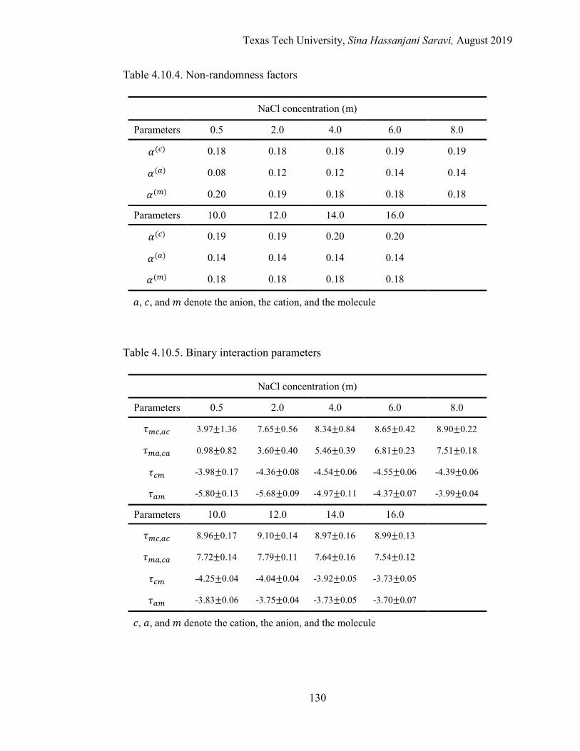
Texas Tech University, Sina Hassanjani Saravi, August 2019
130
Table 4.10.4. Non-randomness factors
NaCl concentration (m)
Parameters 0.5 2.0 4.0 6.0 8.0
𝛼𝛼(𝐿𝐿) 0.18 0.18 0.18 0.19 0.19
𝛼𝛼(𝑎𝑎) 0.08 0.12 0.12 0.14 0.14
𝛼𝛼(𝑚𝑚) 0.20 0.19 0.18 0.18 0.18
Parameters 10.0 12.0 14.0 16.0
𝛼𝛼(𝐿𝐿) 0.19 0.19 0.20 0.20
𝛼𝛼(𝑎𝑎) 0.14 0.14 0.14 0.14
𝛼𝛼(𝑚𝑚) 0.18 0.18 0.18 0.18
𝑎𝑎, 𝑐𝑐, and 𝑚𝑚 denote the anion, the cation, and the molecule
Table 4.10.5. Binary interaction parameters
NaCl concentration (m)
Parameters 0.5 2.0 4.0 6.0 8.0
𝜏𝜏𝑚𝑚𝐿𝐿,𝑎𝑎𝐿𝐿 3.97±1.36 7.65±0.56 8.34±0.84 8.65±0.42 8.90±0.22
𝜏𝜏𝑚𝑚𝑎𝑎,𝐿𝐿𝑎𝑎 0.98±0.82 3.60±0.40 5.46±0.39 6.81±0.23 7.51±0.18
𝜏𝜏𝐿𝐿𝑚𝑚 -3.98±0.17 -4.36±0.08 -4.54±0.06 -4.55±0.06 -4.39±0.06
𝜏𝜏𝑎𝑎𝑚𝑚 -5.80±0.13 -5.68±0.09 -4.97±0.11 -4.37±0.07 -3.99±0.04
Parameters 10.0 12.0 14.0 16.0
𝜏𝜏𝑚𝑚𝐿𝐿,𝑎𝑎𝐿𝐿 8.96±0.17 9.10±0.14 8.97±0.16 8.99±0.13
𝜏𝜏𝑚𝑚𝑎𝑎,𝐿𝐿𝑎𝑎 7.72±0.14 7.79±0.11 7.64±0.16 7.54±0.12
𝜏𝜏𝐿𝐿𝑚𝑚 -4.25±0.04 -4.04±0.04 -3.92±0.05 -3.73±0.05
𝜏𝜏𝑎𝑎𝑚𝑚 -3.83±0.06 -3.75±0.04 -3.73±0.05 -3.70±0.07
𝑐𝑐, 𝑎𝑎, and 𝑚𝑚 denote the cation, the anion, and the molecule
Texas Tech University, Sina Hassanjani Saravi, August 2019
131
Discussions Regarding the Nature of Interactions in the Ion-Centered Domains
The assumption of the eNRTL model that 𝜏𝜏𝑚𝑚𝐿𝐿,𝑎𝑎𝐿𝐿 = 𝜏𝜏𝑚𝑚𝑎𝑎,𝐿𝐿𝑎𝑎 and 𝜏𝜏𝐿𝐿𝑚𝑚 = 𝜏𝜏𝑎𝑎𝑚𝑚 (as
mentioned in the main text) is further elaborated in this section. Consider the difference in
the energies between the different species with respect to the species at the center of the
domain, i.e., 𝛿𝛿𝐸𝐸𝑚𝑚𝑎𝑎,𝐿𝐿𝑎𝑎 = 𝜖𝜖𝐿𝐿𝑎𝑎𝜎𝜎𝐿𝐿𝑎𝑎3 − 𝜖𝜖𝑚𝑚𝑎𝑎𝜎𝜎𝑚𝑚𝑎𝑎3 . These quantities are plotted in Figure 4.10.4.
Note that the contribution to 𝛿𝛿𝐸𝐸 in Figure 4.10.4 includes both van der Waals and
electrostatic interactions, unlike the consideration in the eNRTL model as explained in the
main text. The nature of interaction between the species at the center of the domain and
the surrounding is governed by both their size and the potential of mean force. At high
concentrations, these interactions are of similar magnitude while at low concentrations they
show deviation primarily due to the size difference between the cation and the anion.
Following these observations, we conclude that the assumption made by the eNRTL model
about the nature of these interactions are consistent with MD determined interaction
parameters at moderate to high salt concentrations.
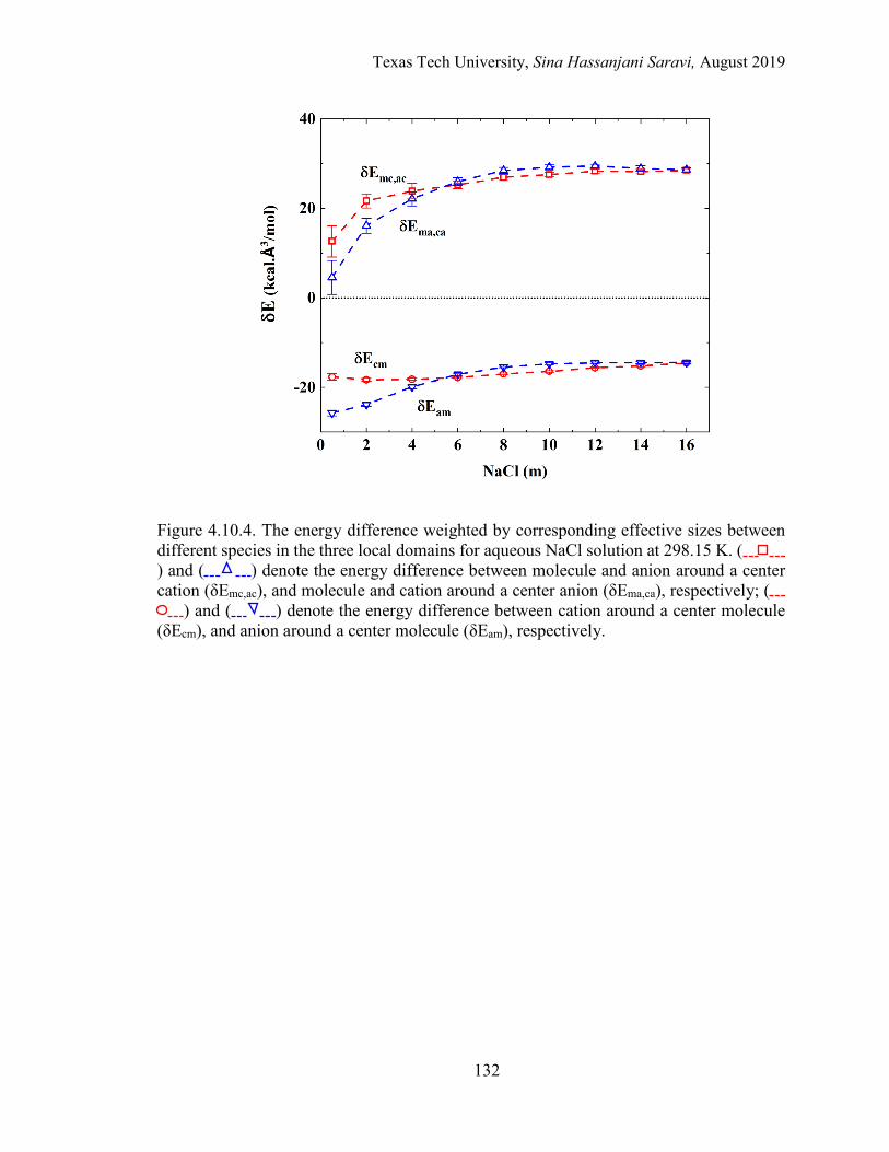
Texas Tech University, Sina Hassanjani Saravi, August 2019
132
Figure 4.10.4. The energy difference weighted by corresponding effective sizes between different species in the three local domains for aqueous NaCl solution at 298.15 K. () and ( ) denote the energy difference between molecule and anion around a center cation (δEmc,ac), and molecule and cation around a center anion (δEma,ca), respectively; (
) and ( ) denote the energy difference between cation around a center molecule (δEcm), and anion around a center molecule (δEam), respectively.

Texas Tech University, Sina Hassanjani Saravi, August 2019
133
4.11. References
1. Shaffer DL, Arias Chavez LH, Ben-Sasson M, Romero-Vargas Castrillón S, Yip NY, Elimelech M. Desalination and reuse of high-salinity shale gas produced water: drivers, technologies, and future directions. Environmental Science & Technology. 2013;47:9569-9583.
2. Newman SA, Barner HE, Klein M, Sandler SI. Thermodynamics of aqueous systems with industrial applications: ACS Publications, 1980.
3. Chen C-C. Toward development of activity coefficient models for process and product design of complex chemical systems. Fluid Phase Equilibria. 2006;241:103-112.
4. Honarparvar S, Saravi SH, Reible D, Chen C-C. Comprehensive thermodynamic modeling of saline water with electrolyte NRTL model: A study on aqueous Ba2+-Na+-Cl−-SO4
2− quaternary system. Fluid Phase Equilibria. 2017;447:29-38.
5. Honarparvar S, Saravi SH, Reible D, Chen C-C. Comprehensive thermodynamic modeling of saline water with electrolyte NRTL model: A study of aqueous Sr2+-Na+-Cl−-SO4
2− quaternary system. Fluid Phase Equilibria. 2018;470:221-231.
6. Sherman DM, Collings MD. Ion association in concentrated NaCl brines from ambient to supercritical conditions: results from classical molecular dynamics simulations. Geochemical Transactions. 2002;3:102-107.
7. Brodholt JP. Molecular dynamics simulations of aqueous NaCl solutions at high pressures and temperatures. Chemical Geology. 1998;151:11-19.
8. Crison JR, Weiner ND, Amidon GL. Dissolution media for in vitro testing of water‐insoluble drugs: Effect of surfactant purity and electrolyte on in vitro dissolution of carbamazepine in aqueous solutions of sodium lauryl sulfate. Journal of Pharmaceutical Sciences. 1997;86:384-388.
9. Chen C-C, Mathias PM. Applied thermodynamics for process modeling. AIChE Journal. 2002;48:194-200.
10. Saravi SH, Honarparvar S, Chen C-C. Modeling aqueous electrolyte systems. Chemical Engineering Progress. 2015;111:65-75.
11. Balbuena PB, Johnston KP, Rossky PJ. Molecular dynamics simulation of electrolyte solutions in ambient and supercritical water. 1. Ion solvation. The Journal of Physical Chemistry. 1996;100:2706-2715.
Texas Tech University, Sina Hassanjani Saravi, August 2019
134
12. Song Y, Chen C-C. Symmetric electrolyte nonrandom two-liquid activity coefficient model. Industrial & Engineering Chemistry Research. 2009;48:7788-7797.
13. Hossain N, Ravichandran A, Khare R, Chen C-C. Revisiting electrolyte thermodynamic models: Insights from molecular simulations. AIChE Journal. 2018;64:3728-3734.
14. Moučka F, Nezbeda I, Smith WR. Chemical potentials, activity coefficients, and solubility in aqueous NaCl solutions: Prediction by polarizable force fields. Journal of Chemical Theory and Computation. 2015;11:1756-1764.
15. Orozco GA, Moultos OA, Jiang H, Economou IG, Panagiotopoulos AZ. Molecular simulation of thermodynamic and transport properties for the H2O + NaCl system. The Journal of Chemical Physics. 2014;141:234507.
16. Pitzer KS. Thermodynamics of electrolytes. I. Theoretical basis and general equations. The Journal of Physical Chemistry. 1973;77:268-277.
17. Thomsen K, Rasmussen P, Gani R. Simulation and optimization of fractional crystallization processes. Chemical Engineering Science. 1998;53:1551-1564.
18. Cameretti LF, Sadowski G, Mollerup JM. Modeling of aqueous electrolyte solutions with perturbed-chain statistical associated fluid theory. Industrial & Engineering Chemistry Research. 2005;44:3355-3362.
19. Chen C-C, Britt HI, Boston J, Evans L. Local composition model for excess Gibbs energy of electrolyte systems. Part I: Single solvent, single completely dissociated electrolyte systems. AIChE Journal. 1982;28:588-596.
20. Chen C-C, Evans LB. A local composition model for the excess Gibbs energy of aqueous electrolyte systems. AIChE Journal. 1986;32:444-454.
21. Chen C-C, Song Y. Generalized electrolyte‐NRTL model for mixed‐solvent electrolyte systems. AIChE Journal. 2004;50:1928-1941.
22. Paluch AS, Jayaraman S, Shah JK, Maginn EJ. A method for computing the solubility limit of solids: Application to sodium chloride in water and alcohols. The Journal of Chemical Physics. 2010;133:124504.
23. Moucka F, Lísal M, Škvor Ji, Jirsák J, Nezbeda I, Smith WR. Molecular simulation of aqueous electrolyte solubility. 2. Osmotic ensemble Monte Carlo methodology for free energy and solubility calculations and application to NaCl. The Journal of Physical Chemistry B. 2011;115:7849-7861.
Texas Tech University, Sina Hassanjani Saravi, August 2019
135
24. Aragones J, Sanz E, Vega C. Solubility of NaCl in water by molecular simulation revisited. The Journal of Chemical Physics. 2012;136:244508.
25. Mester Z, Panagiotopoulos AZ. Mean ionic activity coefficients in aqueous NaCl solutions from molecular dynamics simulations. The Journal of Chemical Physics. 2015;142:044507.
26. Mester Z, Panagiotopoulos AZ. Temperature-dependent solubilities and mean ionic activity coefficients of alkali halides in water from molecular dynamics simulations. The Journal of Chemical Physics. 2015;143:044505.
27. Jiang H, Mester Z, Moultos OA, Economou IG, Panagiotopoulos AZ. Thermodynamic and transport properties of H2O + NaCl from polarizable force fields. Journal of Chemical Theory and Computation. 2015;11:3802-3810.
28. Neiman M, Cheng H, Parekh V, Peterson B, Klier K. A critical assessment on two predictive models of binary vapor–liquid equilibrium. Physical Chemistry Chemical Physics. 2004;6:3474-3483.
29. Ravichandran A, Khare R, Chen C-C. Predicting NRTL binary interaction parameters from molecular simulations. AIChE Journal. 2018;64:2758-2769.
30. Jónsd SÓ, Rasmussen K, Fredenslund A. UNIQUAC parameters determined by molecular mechanics. Fluid Phase Equilibria. 1994;100:121-138.
31. Sum AK, Sandler SI. Use of ab initio methods to make phase equilibria predictions using activity coefficient models. Fluid Phase Equilibria. 1999;158:375-380.
32. Scott RL. Corresponding states treatment of nonelectrolyte solutions. The Journal of Chemical Physics. 1956;25:193-205.
33. Renon H, Prausnitz JM. Local compositions in thermodynamic excess functions for liquid mixtures. AIChE journal. 1968;14:135-144.
34. Brandani V, Prausnitz J. Two-fluid theory and thermodynamic properties of liquid mixtures: General theory. Proceedings of the National Academy of Sciences. 1982;79:4506-4509.
35. Guggenheim EA. Mixtures: the theory of the equilibrium properties of some simple classes of mixtures, solutions and alloys: Clarendon Press, 1952.
36. Plimpton S. Fast parallel algorithms for short-range molecular dynamics. Journal of Computational Physics. 1995;117:1-19.
Texas Tech University, Sina Hassanjani Saravi, August 2019
136
37. Shinoda W, Shiga M, Mikami M. Rapid estimation of elastic constants by molecular dynamics simulation under constant stress. Physical Review B. 2004;69:134103.
38. Hockney R, Eastwood J. Computer Simulation Using Particles (Adam Hilger, New York). 1989.
39. Berendsen H, Grigera J, Straatsma T. The missing term in effective pair potentials. Journal of Physical Chemistry. 1987;91:6269-6271.
40. Weerasinghe S, Smith PE. A Kirkwood–Buff derived force field for sodium chloride in water. The Journal of Chemical Physics. 2003;119:11342-11349.
41. Gee MB, Cox NR, Jiao Y, Bentenitis N, Weerasinghe S, Smith PE. A Kirkwood-Buff derived force field for aqueous alkali halides. Journal of Chemical Theory and Computation. 2011;7:1369-1380.
42. Chandler D. Introduction to modern statistical mechanics. Introduction to Modern Statistical Mechanics, by David Chandler, pp 288 Foreword by David Chandler Oxford University Press, Sep 1987 ISBN-10: 0195042778 ISBN-13: 9780195042771. 1987:288.
43. Yan Y, Chen C-C. Thermodynamic representation of the NaCl + Na2SO4 + H2O system with electrolyte NRTL model. Fluid Phase Equilibria. 2011;306:149-161.
44. Robinson RA, Stokes RH. Electrolyte solutions: Courier Corporation, 2002.
45. Aspen Properties V8.8. Aspen Technology IB, MA, 2015.
46. Marcus Y. Ionic radii in aqueous solutions. Chemical Reviews. 1988;88:1475-1498.
47. Timko J, Bucher D, Kuyucak S. Dissociation of NaCl in water from ab initio molecular dynamics simulations. The Journal of Chemical Physics. 2010;132:114510.
48. Luo Y, Jiang W, Yu H, MacKerell AD, Roux B. Simulation study of ion pairing in concentrated aqueous salt solutions with a polarizable force field. Faraday Discussions. 2013;160:135-149.
49. Smith DE, Dang LX. Computer simulations of NaCl association in polarizable water. The Journal of Chemical Physics. 1994;100:3757-3766.
50. Ravichandran A, Chen C-C, Khare R. Prediction of χ parameter of polymer blends by combining molecular simulations and integral equation theory The Journal of Physical Chemistry B.122:9022-9031.

Texas Tech University, Sina Hassanjani Saravi, August 2019
137
51. Tang I, Munkelwitz H, Wang N. Water activity measurements with single suspended droplets: The NaCl-H2O and KCl-H2O systems. Journal of Colloid and Interface Science. 1986;114:409-415.
Texas Tech University, Sina Hassanjani Saravi, August 2019
138
CHAPTER 5. PRDICTING PHASE EQUILIBRIA PROPERTIES OF
ELECTRLYTE SOLUTIONS BY COMBINING A CLASSICAL THERMODYNAMIC MODEL AND MOLECULAR SIMULATIONS: AQUOUES XCL2
SOLUTIONS, (X=BA, SR, CA, MG)4
5.1. Abstract
Process design and simulations in industry rely on the availability of thermodynamic
models to provide accurate predictions of phase equilibria properties. As a widely used
classical thermodynamic model, the eNRTL model has shown to provide reliable
predictions for electrolyte solutions by employing the binary interaction parameters (𝜏𝜏). In
this study, we develop a predictive theoretical framework to calculate the 𝜏𝜏 parameters
directly from molecular dynamic (MD) simulations by revisiting the statistical mechanics
of two-liquid theory. The 𝜏𝜏 parameters are expressed as functions of the liquid structure
and local preferential interaction quantities, which in turn are obtained from the MD
simulations and free energy calculations. The aqueous BaCl2, SrCl2, CaCl2, and MgCl2
solutions are selected as model systems for the validation of our approach. The 𝜏𝜏
parameters obtained from the MD simulations are then used to predict the mean ionic
activity coefficient, vapor pressure, and excess Gibbs free energy of the model systems in
a wide concentration range from 0.5 to 12 mol/kg. The results from the MD simulations
are in satisfactory agreement with the predictions from regression of the experimental data.
4 This chapter is based on a manuscript under preparation as: Saravi SH, Khare R, and Chen C-C., Predicting Phase Equilibria Properties of Electrolyte Solutions by Combining a Classical Thermodynamic Model and Molecular Simulations: Aqueous XCl2 Solutions, (X = Ba, Sr, Ca, and Mg)

Texas Tech University, Sina Hassanjani Saravi, August 2019
139
The methodology can be broadly utilized for predicting the phase equilibria properties of
electrolytes, especially when data are scarce. Furthermore, the technique can provide
guidelines to select physically meaningful parameters in data regression procedures,
thereby enhancing the feasibility of using the classical thermodynamic models in industry.
Texas Tech University, Sina Hassanjani Saravi, August 2019
140
5.2. Introduction
The study of aqueous electrolyte solutions has attracted significant attention due to
their ubiquitous presence in industrial 1-3, pharmaceutical 4, and environmental processes
5. The Design and optimization of these processes rely heavily on the accurate predictions
of phase equilibria properties 6,7. Over the decades, numerous modeling studies have
reported predictions of the essential thermodynamic properties of electrolyte solutions,
such as the mean ionic activity coefficients (𝛾𝛾±), excess Gibbs free energy, and chemical
potential. Classical molecular thermodynamic models have been the primary tool to
provide such predictions for industrial use, owing to their versatility and inexpensive
computational procedures 7.
As a widely used classical thermodynamic model, the electrolyte non-random two-
liquid (eNRTL) model 8-11 has shown to provide accurate predictions of phase equilibria
properties for electrolyte solutions 7,12. The eNRTL’s consistent thermodynamics
framework and mathematical simplicity have led the model to be extensively applied for
predicting the phase equilibria properties of variety of electrolyte solutions; from simple
aqueous uni-univalent to mixed-solvent multivalent electrolyte systems 13-19. The model
relates the excess Gibbs free energy of an electrolyte solution to the microscopic local
structure of the liquid, with a set of concentration-independent binary interaction
parameters (𝜏𝜏). The parameters quantify the effective interaction strengths between
different species of the solution, namely, anions, cations, and molecules. The two inherent
assumptions made by the model, that is the electroneutrality and like-ion repulsion,
determine the configuration of the local structures, also known as the local domains. The
former assumption states that the net electric charge in the first solvation shell around a
Texas Tech University, Sina Hassanjani Saravi, August 2019
141
center molecule is zero, while the latter asserts that there are no like-charged ions within
the first shell around the ionic species.
The 𝜏𝜏 parameters are typically identified by regressing them to various experimental
data of phase equilibria, calorimetric, and speciation properties. Once the 𝜏𝜏 parameters are
quantified, the thermodynamic properties required for use in process simulations including
the activity coefficients can be readily calculated 8-11. Identifying the model parameters
from regression, however, could be hindered by the lack of available/reliable experimental
data. Furthermore, selecting physically relevant parameters could be ambiguous as the
minimization function employed in the regression procedure, often exhibits several local
minima and hence multiple solutions for the binary interaction parameters. Quantifying the
binary interaction parameters from first-principles-based theories, without the need for
introducing any adjustable parameters can help circumvent these drawbacks. There have
been a number of attempts for obtaining the binary interaction parameters of the classical
thermodynamic models, however only for nonelectrolytes, from predictive approaches by
utilizing molecular simulations 20-23. In particular, Ravichandran et al. 23 presented a novel
methodology to predict the 𝜏𝜏 parameters of the NRTL model from MD simulations for a
number of organic mixtures.
Extending the work of Ravichandran et al. 23, we have recently developed a theoretical
framework to identify the binary interaction parameters of the eNRTL model by bridging
the statistical mechanical framework of two-liquid theory for uni-univalent electrolytes
with molecular simulations 24. The 𝜏𝜏 parameters were expressed as functions of the liquid
structure and energetic interaction quantities of the solution, which themselves were
calculated directly from the MD simulations 24. The parameters calculated for aqueous
Texas Tech University, Sina Hassanjani Saravi, August 2019
142
NaCl solution, as a model system, were in satisfactory agreement with those obtained from
regression of the experimental data, specifically at moderate (~ 4 mol/kg) to supersaturated
(~ 16 mol/kg) concentrations. On the other hand, the parameters showed rather
considerable concentration dependence at lower salt concentrations (< ~ 2 mol/kg).
Furthermore, another assumption made by the model, that is the equality of the molecule-
cation and molecule-anion interactions was also shown to be somewhat reasonable by the
order of magnitude, however, with slight difference in quantities due to the species size
effects.
Overall, the results 24 were encouraging as a first-step toward directly utilizing the
molecular simulations in industrial process design to support phase equilibria predictions,
with relatively inexpensive computational time. Furthermore, our study provided insight
into the physical interpretation of the eNRTL binary interaction parameters, which were
previously assumed to be semi-empirical and merely correlative. The versatility of the
established methodology, on the other hand, requires further examination to assess its
generality to cover more complex systems including multivalent electrolyte solutions. Note
that the presence of the uni-univalent electrolytes was an intrinsic part of the theoretical
framework in our previous work 24.
The extension of the approach to the multivalent electrolyte solutions requires the
incorporation of the absolute charge numbers into the developed framework. In the original
eNRTL 9,11, such an extension was achieved by introducing a new concentration variable,
namely the effective mole fraction, for the treatment of the ionic species of higher valency
9. The effective mole fraction is defined as the product of the mole fraction and the absolute
charge number for the ionic species, and the mole fraction for molecular species, all of
Texas Tech University, Sina Hassanjani Saravi, August 2019
143
which are normalized such that their summation is unity. Employing such a variable has
shown to be useful for modeling the electrolyte systems with multivalent ions 9,25.
Similarly, the absolute charge number of the ionic species must be integrated into our
statistical mechanical framework so that the developed methodology 24 can be applied for
multivalent electrolyte solutions.
In this study, we revisit our proposed methodology 24 to establish a generalized
framework to identify the binary interaction parameters of multivalent electrolyte solutions
from the MD simulations. The binary interaction parameters are expressed as functions of
the effective molecular diameters (𝜎𝜎), the interaction strengths (𝜖𝜖), the first neighbor shell
radii (𝑅𝑅), and the nonrandomness factors (𝛼𝛼), all of which are obtained from the MD
simulations. Several di-univalent electrolyte systems, namely, aqueous BaCl2, SrCl2,
CaCl2, and MgCl2 solutions are selected for the validation of the framework. By gaining
insight into the structure of the local domains from the MD simulations, we assess the
validity of the electroneutrality and like-ion repulsion assumptions for each model systems,
throughout the concentration range studied. The preferential interactions in the local
domains are quantified from the potential of mean force calculations as described in our
previous work 24. However, a second case is also presented here where the contribution of
the short-range van der Waals forces is obtained by subtracting the contribution of the
Coulombic electrostatic forces from the total potential of mean force.
The rest of this chapter is organized as follows: Theoretical Framework section which
details the underlying concepts of the eNRTL model and our developed approach to
formulate the 𝜏𝜏 parameters. It is then followed by the Quantification of the 𝜏𝜏 Parameters
from Molecular Simulations. The Molecular Simulation Details are then reported in the

Texas Tech University, Sina Hassanjani Saravi, August 2019
144
next session. The binary interaction parameters obtained from the MD simulations, their
significance, and a comprehensive interpretation of the results are reported in the Results
and Discussion, followed by Conclusions.
5.3. Theoretical Framework
Thermodynamics Background of the eNRTL Model The eNRTL model 8-11 expresses the excess Gibbs free energy of the electrolyte
solutions as a combination of two contributions: the long-range electrostatic interactions
expressed by Pitzer-Debye-Hückel theory 26-28 and the short-range interactions, typically
of van der Waals-type, from the NRTL model developed by Renon and Prausnitz 29.
Consider the complete dissociation reaction of an electrolyte component (𝑐𝑐𝑎𝑎) to its
constituent cations (𝑐𝑐) and anions (𝑎𝑎), in the solvent molecules (𝑚𝑚). Eqs. 5.1 & 5.2 show
such a reaction and the corresponding stoichiometric relation between the species:
(𝑐𝑐𝑎𝑎) → 𝜈𝜈𝐿𝐿𝑐𝑐+𝑍𝑍𝑐𝑐 + 𝜈𝜈𝑎𝑎𝑎𝑎−𝑍𝑍𝑎𝑎 (5.1)
where
𝜐𝜐𝐿𝐿𝑍𝑍𝐿𝐿 = 𝜐𝜐𝑎𝑎𝑍𝑍𝑎𝑎 (5.2)
Here, 𝜈𝜈𝑖𝑖 and 𝑍𝑍𝑖𝑖 denote the stoichiometric coefficients and the absolute charge numbers of
ionic species, respectively. Upon the dissociation reaction of the electrolyte, it is assumed
that three local domains are formed with cation, anion, and molecule in turn at center. Each
of the center species is surrounded by solution components that are locally coordinated in
the first neighbor shell, such that the two assumptions of the model, i.e., electroneutrality
and like-ion repulsion are satisfied (see Figure 5.1).
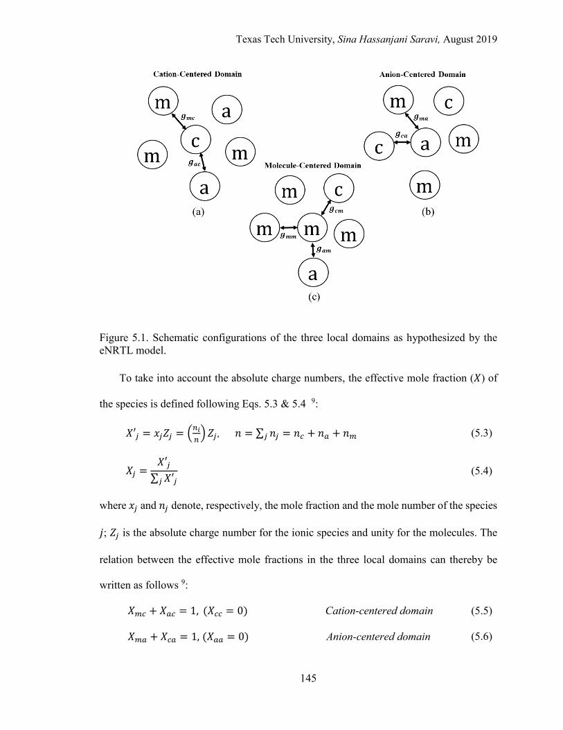
Texas Tech University, Sina Hassanjani Saravi, August 2019
145
Figure 5.1. Schematic configurations of the three local domains as hypothesized by the eNRTL model.
To take into account the absolute charge numbers, the effective mole fraction (𝑋𝑋) of
the species is defined following Eqs. 5.3 & 5.4 9:
𝑋𝑋′𝑗𝑗 = 𝑥𝑥𝑗𝑗𝑍𝑍𝑗𝑗 = �𝜕𝜕𝑖𝑖𝜕𝜕� 𝑍𝑍𝑗𝑗 , 𝑙𝑙 = ∑ 𝑙𝑙𝑗𝑗𝑗𝑗 = 𝑙𝑙𝐿𝐿 + 𝑙𝑙𝑎𝑎 + 𝑙𝑙𝑚𝑚 (5.3)
𝑋𝑋𝑗𝑗 =
𝑋𝑋′𝑗𝑗∑ 𝑋𝑋′𝑗𝑗𝑗𝑗
(5.4)
where 𝑥𝑥𝑗𝑗 and 𝑙𝑙𝑗𝑗 denote, respectively, the mole fraction and the mole number of the species
𝑗𝑗; 𝑍𝑍𝑗𝑗 is the absolute charge number for the ionic species and unity for the molecules. The
relation between the effective mole fractions in the three local domains can thereby be
written as follows 9:
𝑋𝑋𝑚𝑚𝐿𝐿 + 𝑋𝑋𝑎𝑎𝐿𝐿 = 1, (𝑋𝑋𝐿𝐿𝐿𝐿 = 0) Cation-centered domain (5.5)
𝑋𝑋𝑚𝑚𝑎𝑎 + 𝑋𝑋𝐿𝐿𝑎𝑎 = 1, (𝑋𝑋𝑎𝑎𝑎𝑎 = 0) Anion-centered domain (5.6)
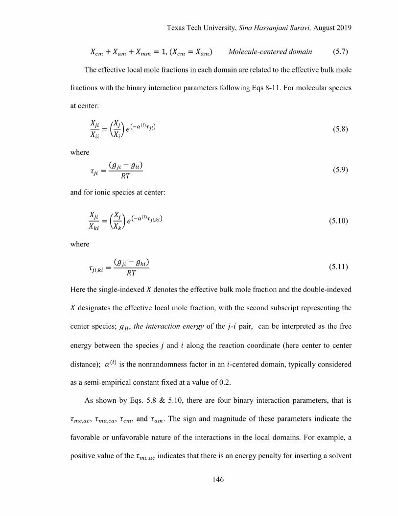
Texas Tech University, Sina Hassanjani Saravi, August 2019
146
𝑋𝑋𝐿𝐿𝑚𝑚 + 𝑋𝑋𝑎𝑎𝑚𝑚 + 𝑋𝑋𝑚𝑚𝑚𝑚 = 1, (𝑋𝑋𝐿𝐿𝑚𝑚 = 𝑋𝑋𝑎𝑎𝑚𝑚) Molecule-centered domain (5.7)
The effective local mole fractions in each domain are related to the effective bulk mole
fractions with the binary interaction parameters following Eqs 8-11. For molecular species
at center:
𝑋𝑋𝑗𝑗𝑖𝑖𝑋𝑋𝑖𝑖𝑖𝑖
= �𝑋𝑋𝑗𝑗𝑋𝑋𝑖𝑖� 𝑒𝑒�−𝛼𝛼(𝑖𝑖)𝜏𝜏𝑖𝑖𝑖𝑖� (5.8)
where
and for ionic species at center:
𝑋𝑋𝑗𝑗𝑖𝑖𝑋𝑋𝑘𝑘𝑖𝑖
= �𝑋𝑋𝑗𝑗𝑋𝑋𝑘𝑘� 𝑒𝑒�−𝛼𝛼(𝑖𝑖)𝜏𝜏𝑖𝑖𝑖𝑖,𝑘𝑘𝑖𝑖� (5.10)
where
𝜏𝜏𝑗𝑗𝑖𝑖,𝑘𝑘𝑖𝑖 =
(𝑔𝑔𝑗𝑗𝑖𝑖 − 𝑔𝑔𝑘𝑘𝑖𝑖)𝑅𝑅𝑇𝑇
(5.11)
Here the single-indexed 𝑋𝑋 denotes the effective bulk mole fraction and the double-indexed
𝑋𝑋 designates the effective local mole fraction, with the second subscript representing the
center species; 𝑔𝑔𝑗𝑗𝑖𝑖, the interaction energy of the 𝑗𝑗-𝑖𝑖 pair, can be interpreted as the free
energy between the species 𝑗𝑗 and 𝑖𝑖 along the reaction coordinate (here center to center
distance); 𝛼𝛼(𝑖𝑖) is the nonrandomness factor in an 𝑖𝑖-centered domain, typically considered
as a semi-empirical constant fixed at a value of 0.2.
As shown by Eqs. 5.8 & 5.10, there are four binary interaction parameters, that is
𝜏𝜏𝑚𝑚𝐿𝐿,𝑎𝑎𝐿𝐿, 𝜏𝜏𝑚𝑚𝑎𝑎,𝐿𝐿𝑎𝑎, 𝜏𝜏𝐿𝐿𝑚𝑚, and 𝜏𝜏𝑎𝑎𝑚𝑚. The sign and magnitude of these parameters indicate the
favorable or unfavorable nature of the interactions in the local domains. For example, a
positive value of the 𝜏𝜏𝑚𝑚𝐿𝐿,𝑎𝑎𝐿𝐿 indicates that there is an energy penalty for inserting a solvent
𝜏𝜏𝑗𝑗𝑖𝑖 =
(𝑔𝑔𝑗𝑗𝑖𝑖 − 𝑔𝑔𝑖𝑖𝑖𝑖)𝑅𝑅𝑇𝑇
(5.9)
Texas Tech University, Sina Hassanjani Saravi, August 2019
147
molecule in the first neighbor shell of a center cation, inside the lattice structure of a
hypothetical fused salt (𝑐𝑐𝑎𝑎). The model inherently assumes the effective interaction
strength of the molecule-anion pair is equal to that of the molecule-cation pair as noted
below:
𝜏𝜏𝑚𝑚𝐿𝐿,𝑎𝑎𝐿𝐿 = 𝜏𝜏𝑚𝑚𝑎𝑎,𝐿𝐿𝑎𝑎 = 𝜏𝜏𝑚𝑚,𝐿𝐿𝑎𝑎 (5.12)
𝜏𝜏𝐿𝐿𝑚𝑚 = 𝜏𝜏𝑎𝑎𝑚𝑚 = 𝜏𝜏𝐿𝐿𝑎𝑎,𝑚𝑚 (5.13)
Following such an assumption, only the two parameters 𝜏𝜏𝑚𝑚,𝐿𝐿𝑎𝑎 and 𝜏𝜏𝐿𝐿𝑎𝑎,𝑚𝑚 are sufficient
to represent, respectively, the interaction strength of the molecule-electrolyte and
electrolyte-molecule pairs. By obtaining 𝜏𝜏𝑚𝑚,𝐿𝐿𝑎𝑎 and 𝜏𝜏𝐿𝐿𝑎𝑎,𝑚𝑚 from regression, the activity
coefficients and therefore other thermophysical properties can be calculated. The
derivations of the thermodynamic properties from the 𝜏𝜏 parameters are presented in the
original series of articles on the eNRTL model development 8-11.
The eNRTL model further assumes 𝜏𝜏𝑚𝑚,𝐿𝐿𝑎𝑎 and 𝜏𝜏𝐿𝐿𝑎𝑎,𝑚𝑚 are concentration independent.
Such an assumption makes the applicability of the model significantly easier as only one
set of 𝜏𝜏 parameters can predict the activity coefficients for the entire concentration range.
This was rationalized as 𝜏𝜏 parameters are expressed as functions of the local interactions,
which in turn are considered to be strictly of short-range van der Waals nature. Short-range
interactions are known not to change with concentration change. Note that the,
hypothetically, concentration-independent 𝜏𝜏 parameters are obtained by fitting them to the
experimental data from the entire range of concentration, and hence are able to predict
reasonably the thermodynamics properties at any given concentration. This assumption
gives the theory a crucial advantage over the conventional MD simulation methods, where
obtaining the activity coefficients requires implementing advanced free energy calculation
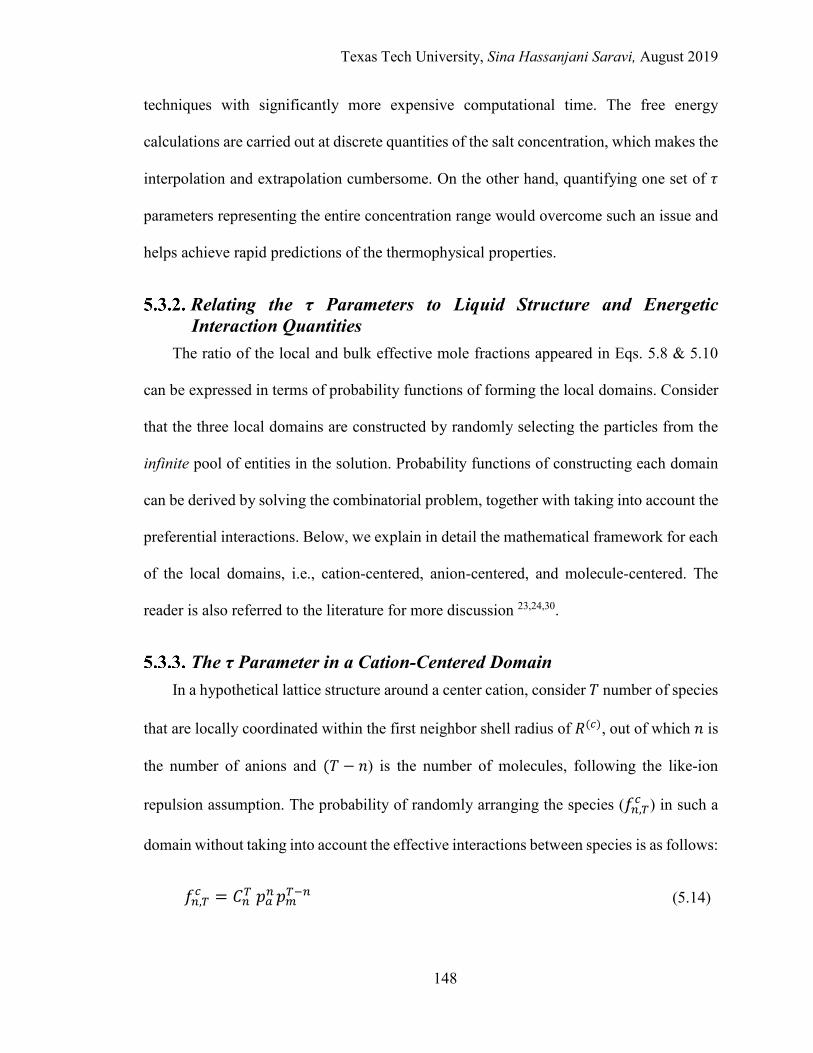
Texas Tech University, Sina Hassanjani Saravi, August 2019
148
techniques with significantly more expensive computational time. The free energy
calculations are carried out at discrete quantities of the salt concentration, which makes the
interpolation and extrapolation cumbersome. On the other hand, quantifying one set of 𝜏𝜏
parameters representing the entire concentration range would overcome such an issue and
helps achieve rapid predictions of the thermophysical properties.
Relating the τ Parameters to Liquid Structure and Energetic Interaction Quantities
The ratio of the local and bulk effective mole fractions appeared in Eqs. 5.8 & 5.10
can be expressed in terms of probability functions of forming the local domains. Consider
that the three local domains are constructed by randomly selecting the particles from the
infinite pool of entities in the solution. Probability functions of constructing each domain
can be derived by solving the combinatorial problem, together with taking into account the
preferential interactions. Below, we explain in detail the mathematical framework for each
of the local domains, i.e., cation-centered, anion-centered, and molecule-centered. The
reader is also referred to the literature for more discussion 23,24,30.
The τ Parameter in a Cation-Centered Domain In a hypothetical lattice structure around a center cation, consider 𝑇𝑇 number of species
that are locally coordinated within the first neighbor shell radius of 𝑅𝑅(𝐿𝐿), out of which 𝑙𝑙 is
the number of anions and (𝑇𝑇 − 𝑙𝑙) is the number of molecules, following the like-ion
repulsion assumption. The probability of randomly arranging the species (𝑓𝑓𝜕𝜕,𝜕𝜕𝐿𝐿 ) in such a
domain without taking into account the effective interactions between species is as follows:
𝑓𝑓𝜕𝜕,𝜕𝜕𝐿𝐿 = 𝐶𝐶𝜕𝜕𝜕𝜕 𝑝𝑝𝑎𝑎
𝜕𝜕𝑝𝑝𝑚𝑚𝜕𝜕−𝜕𝜕 (5.14)
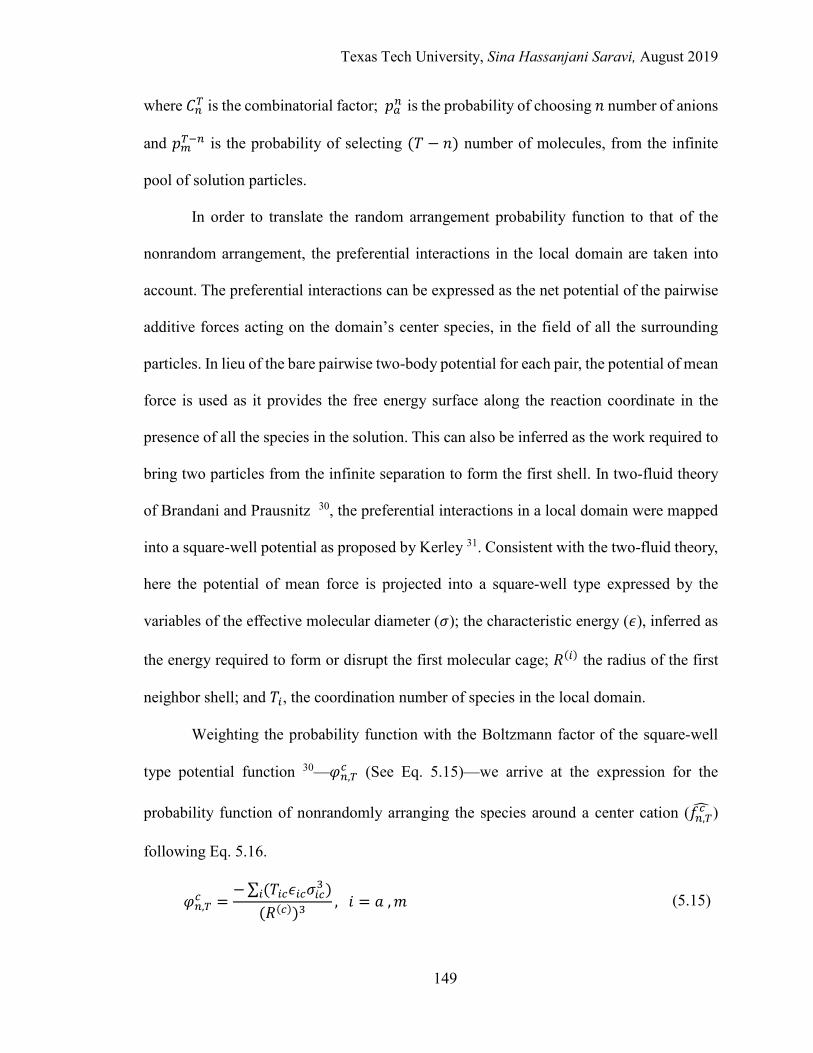
Texas Tech University, Sina Hassanjani Saravi, August 2019
149
where 𝐶𝐶𝜕𝜕𝜕𝜕 is the combinatorial factor; 𝑝𝑝𝑎𝑎 𝜕𝜕 is the probability of choosing 𝑙𝑙 number of anions
and 𝑝𝑝𝑚𝑚𝜕𝜕−𝜕𝜕 is the probability of selecting (𝑇𝑇 − 𝑙𝑙) number of molecules, from the infinite
pool of solution particles.
In order to translate the random arrangement probability function to that of the
nonrandom arrangement, the preferential interactions in the local domain are taken into
account. The preferential interactions can be expressed as the net potential of the pairwise
additive forces acting on the domain’s center species, in the field of all the surrounding
particles. In lieu of the bare pairwise two-body potential for each pair, the potential of mean
force is used as it provides the free energy surface along the reaction coordinate in the
presence of all the species in the solution. This can also be inferred as the work required to
bring two particles from the infinite separation to form the first shell. In two-fluid theory
of Brandani and Prausnitz 30, the preferential interactions in a local domain were mapped
into a square-well potential as proposed by Kerley 31. Consistent with the two-fluid theory,
here the potential of mean force is projected into a square-well type expressed by the
variables of the effective molecular diameter (𝜎𝜎); the characteristic energy (𝜖𝜖), inferred as
the energy required to form or disrupt the first molecular cage; 𝑅𝑅(𝑖𝑖) the radius of the first
neighbor shell; and 𝑇𝑇𝑖𝑖, the coordination number of species in the local domain.
Weighting the probability function with the Boltzmann factor of the square-well
type potential function 30—𝜑𝜑𝜕𝜕,𝜕𝜕𝐿𝐿 (See Eq. 5.15)—we arrive at the expression for the
probability function of nonrandomly arranging the species around a center cation (𝑓𝑓𝜕𝜕,𝜕𝜕𝐿𝐿� )
following Eq. 5.16.
𝜑𝜑𝜕𝜕,𝜕𝜕𝐿𝐿 =
−∑ (𝑇𝑇𝑖𝑖𝐿𝐿𝜖𝜖𝑖𝑖𝐿𝐿𝜎𝜎𝑖𝑖𝐿𝐿3 )𝑖𝑖
(𝑅𝑅(𝐿𝐿))3, 𝑖𝑖 = 𝑎𝑎 ,𝑚𝑚 (5.15)

Texas Tech University, Sina Hassanjani Saravi, August 2019
150
𝑓𝑓𝜕𝜕,𝜕𝜕𝐿𝐿� =
𝐶𝐶𝜕𝜕𝜕𝜕 ∏ (𝑝𝑝𝑖𝑖𝜕𝜕𝑖𝑖𝑐𝑐)𝑖𝑖 . 𝑒𝑒−𝛽𝛽𝜑𝜑𝑛𝑛,𝑇𝑇
𝑐𝑐
𝛺𝛺𝐿𝐿 , 𝑖𝑖 = 𝑎𝑎 ,𝑚𝑚 (5.16)
where 𝜑𝜑𝜕𝜕,𝜕𝜕𝐿𝐿 denotes the potential function in a cation-centered domain with 𝑙𝑙 number of
anions out of 𝑇𝑇 total coordination number; 𝑇𝑇𝑖𝑖𝐿𝐿, 𝜖𝜖𝑖𝑖𝐿𝐿, and 𝜎𝜎𝑖𝑖𝐿𝐿 denote, respectively, the
coordination number, interaction strength, and effective molecular diameter of species 𝑖𝑖
around the center cation; 𝑝𝑝𝑖𝑖 is the probability of selecting an 𝑖𝑖-type species from the infinite
pool; 𝛺𝛺𝐿𝐿 is the normalization factor as the summation over all possible configurations of
species in a cation-centered domain 24 (Equivalent to the local partition function); and 𝛽𝛽 is
the inverse of the thermal energy.
By expanding Eq. 5.16 and introducing the new terms (𝑝𝑝𝑖𝑖′), we arrive at Eq. 5.20,
following Eqs 17-19.
𝑓𝑓𝜕𝜕,𝜕𝜕𝐿𝐿� =
𝐶𝐶𝜕𝜕𝜕𝜕
𝛺𝛺𝐿𝐿�(𝑝𝑝𝑖𝑖𝜕𝜕𝑖𝑖𝑐𝑐
𝑖𝑖
. 𝑒𝑒𝛽𝛽𝜕𝜕𝑖𝑖𝑐𝑐𝜖𝜖𝑖𝑖𝑐𝑐𝜎𝜎𝑖𝑖𝑐𝑐
3
(𝐿𝐿(𝑐𝑐))3 ), 𝑖𝑖 = 𝑎𝑎 ,𝑚𝑚 (5.17)
𝑝𝑝𝑎𝑎 ′ = 𝑝𝑝𝑎𝑎𝑒𝑒
𝛽𝛽𝜖𝜖𝑎𝑎𝑐𝑐𝜎𝜎𝑎𝑎𝑐𝑐3
(𝐿𝐿(𝑐𝑐))3 (5.18)
𝑝𝑝𝑚𝑚 ′ = 𝑝𝑝𝑚𝑚𝑒𝑒
𝛽𝛽𝜖𝜖𝑚𝑚𝑐𝑐𝜎𝜎𝑚𝑚𝑐𝑐3
(𝐿𝐿(𝑐𝑐))3 (5.19)
𝑓𝑓𝜕𝜕,𝑧𝑧𝐿𝐿� =
𝐶𝐶𝜕𝜕𝜕𝜕
𝛺𝛺𝐿𝐿 (𝑝𝑝𝑎𝑎′ )𝜕𝜕. (𝑝𝑝𝑚𝑚′ )𝜕𝜕−𝜕𝜕 (5.20)
Dividing 𝑝𝑝𝑚𝑚 ′ by 𝑝𝑝𝑎𝑎
′ ,we arrive at Eq. 5.21:
𝑝𝑝𝑚𝑚′
𝑝𝑝𝑎𝑎′=𝑝𝑝𝑚𝑚𝑝𝑝𝑎𝑎
𝑒𝑒−𝛽𝛽�𝜖𝜖𝑎𝑎𝑐𝑐𝜎𝜎𝑎𝑎𝑐𝑐
3−𝜖𝜖𝑚𝑚𝑐𝑐𝜎𝜎𝑚𝑚𝑐𝑐3
(𝐿𝐿(𝑐𝑐))3� (5.21)
The terms 𝑝𝑝𝑚𝑚′
𝑝𝑝𝑎𝑎′ and 𝑝𝑝𝑚𝑚
𝑝𝑝𝑎𝑎 represent, respectively, the ratio of the probability of finding
molecules to anions in the local domain and in the bulk. Eq. 5.21 can then be expressed in
terms of the number of species in the local domain and in bulk as per Eq. 5.22.
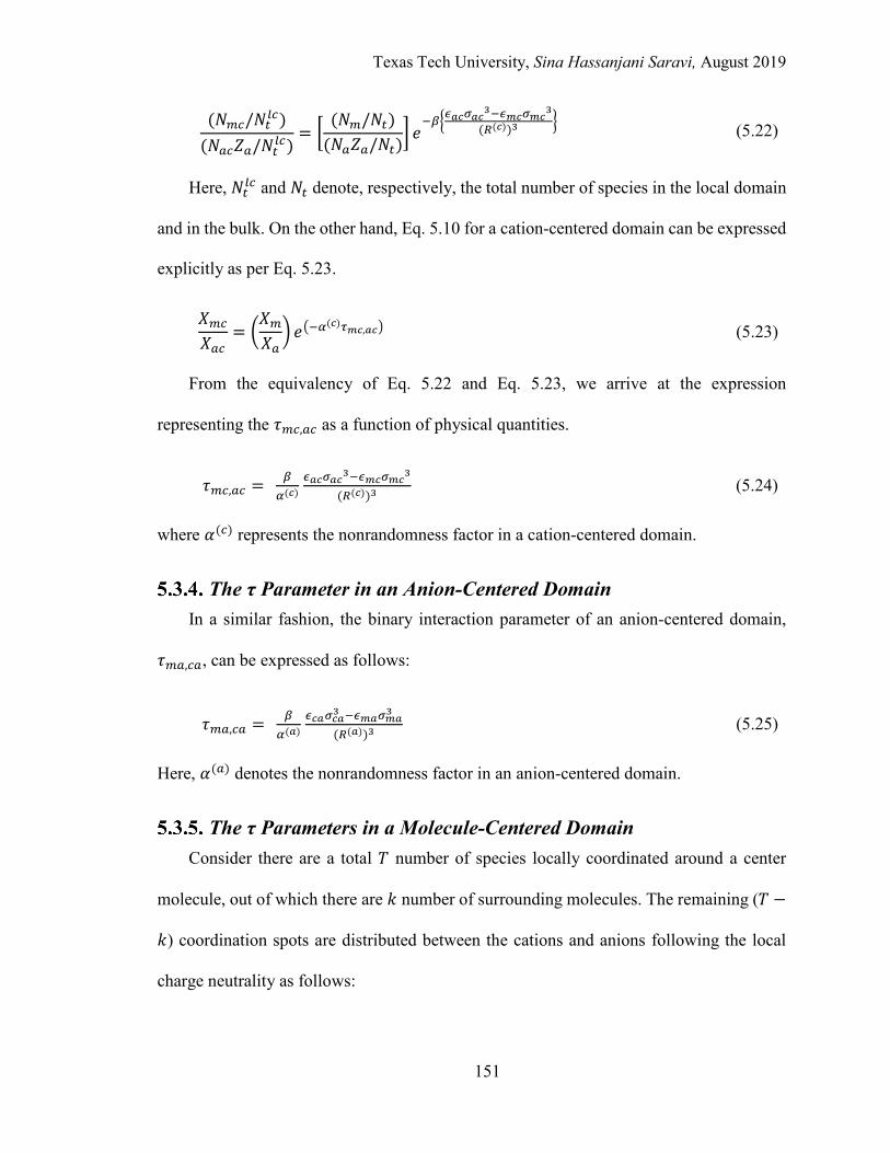
Texas Tech University, Sina Hassanjani Saravi, August 2019
151
(𝑁𝑁𝑚𝑚𝐿𝐿/𝑁𝑁𝑡𝑡𝑙𝑙𝐿𝐿)(𝑁𝑁𝑎𝑎𝐿𝐿𝑍𝑍𝑎𝑎/𝑁𝑁𝑡𝑡𝑙𝑙𝐿𝐿)
= �(𝑁𝑁𝑚𝑚/𝑁𝑁𝑡𝑡)
(𝑁𝑁𝑎𝑎𝑍𝑍𝑎𝑎/𝑁𝑁𝑡𝑡)� 𝑒𝑒
−𝛽𝛽�𝜖𝜖𝑎𝑎𝑐𝑐𝜎𝜎𝑎𝑎𝑐𝑐3−𝜖𝜖𝑚𝑚𝑐𝑐𝜎𝜎𝑚𝑚𝑐𝑐
3
(𝐿𝐿(𝑐𝑐))3� (5.22)
Here, 𝑁𝑁𝑡𝑡𝑙𝑙𝐿𝐿 and 𝑁𝑁𝑡𝑡 denote, respectively, the total number of species in the local domain
and in the bulk. On the other hand, Eq. 5.10 for a cation-centered domain can be expressed
explicitly as per Eq. 5.23.
𝑋𝑋𝑚𝑚𝐿𝐿𝑋𝑋𝑎𝑎𝐿𝐿
= �𝑋𝑋𝑚𝑚𝑋𝑋𝑎𝑎� 𝑒𝑒�−𝛼𝛼(𝑐𝑐)𝜏𝜏𝑚𝑚𝑐𝑐,𝑎𝑎𝑐𝑐� (5.23)
From the equivalency of Eq. 5.22 and Eq. 5.23, we arrive at the expression
representing the 𝜏𝜏𝑚𝑚𝐿𝐿,𝑎𝑎𝐿𝐿 as a function of physical quantities.
𝜏𝜏𝑚𝑚𝐿𝐿,𝑎𝑎𝐿𝐿 = 𝛽𝛽𝛼𝛼(𝑐𝑐)
𝜖𝜖𝑎𝑎𝑐𝑐𝜎𝜎𝑎𝑎𝑐𝑐3−𝜖𝜖𝑚𝑚𝑐𝑐𝜎𝜎𝑚𝑚𝑐𝑐3
(𝐿𝐿(𝑐𝑐))3 (5.24)
where 𝛼𝛼(𝐿𝐿) represents the nonrandomness factor in a cation-centered domain.
The τ Parameter in an Anion-Centered Domain In a similar fashion, the binary interaction parameter of an anion-centered domain,
𝜏𝜏𝑚𝑚𝑎𝑎,𝐿𝐿𝑎𝑎, can be expressed as follows:
𝜏𝜏𝑚𝑚𝑎𝑎,𝐿𝐿𝑎𝑎 = 𝛽𝛽𝛼𝛼(𝑎𝑎)
𝜖𝜖𝑐𝑐𝑎𝑎𝜎𝜎𝑐𝑐𝑎𝑎3 −𝜖𝜖𝑚𝑚𝑎𝑎𝜎𝜎𝑚𝑚𝑎𝑎3
(𝐿𝐿(𝑎𝑎))3 (5.25)
Here, 𝛼𝛼(𝑎𝑎) denotes the nonrandomness factor in an anion-centered domain.
The τ Parameters in a Molecule-Centered Domain Consider there are a total 𝑇𝑇 number of species locally coordinated around a center
molecule, out of which there are 𝑘𝑘 number of surrounding molecules. The remaining (𝑇𝑇 −
𝑘𝑘) coordination spots are distributed between the cations and anions following the local
charge neutrality as follows:
Texas Tech University, Sina Hassanjani Saravi, August 2019
152
𝑍𝑍𝐿𝐿𝑁𝑁𝐿𝐿𝑚𝑚 = 𝑍𝑍𝑎𝑎𝑁𝑁𝑎𝑎𝑚𝑚 (5.26)
The probability function of the non-random arrangement of the molecule-centered
domain is thus expressed as per Eq. 5.27.
𝑓𝑓𝑘𝑘,𝜕𝜕𝑚𝑚� =
𝐶𝐶𝑘𝑘𝜕𝜕
𝛺𝛺𝑚𝑚�(𝑝𝑝𝑖𝑖𝑁𝑁𝑖𝑖𝑚𝑚
𝑖𝑖
. 𝑒𝑒𝛽𝛽𝑁𝑁𝑖𝑖𝑚𝑚𝜖𝜖𝑖𝑖𝑚𝑚𝜎𝜎𝑖𝑖𝑚𝑚
3
(𝐿𝐿(𝑚𝑚))3 ), 𝑖𝑖 = 𝑐𝑐,𝑎𝑎 ,𝑚𝑚 (5.27)
where 𝑁𝑁𝑚𝑚𝑚𝑚 denotes the local number of molecules around the center molecule; 𝐶𝐶𝑘𝑘𝜕𝜕 is the
combinatorial factor; and 𝛺𝛺𝑚𝑚 is the normalization factor.
By introducing the 𝑝𝑝𝑖𝑖′ terms defined by Eq. 5.28 and rearranging the relations, we
arrive at Eq. 5.29 and Eq. 5.30
𝑝𝑝𝑖𝑖′ = 𝑝𝑝𝑖𝑖 𝑒𝑒
𝛽𝛽𝜖𝜖𝑖𝑖𝑚𝑚𝜎𝜎𝑖𝑖𝑚𝑚3
(𝐿𝐿(𝑚𝑚))3 , 𝑖𝑖 = 𝑐𝑐,𝑎𝑎,𝑚𝑚 (5.28)
𝑝𝑝𝑎𝑎′
𝑝𝑝𝑚𝑚′=𝑝𝑝𝑎𝑎𝑝𝑝𝑚𝑚
𝑒𝑒−𝛽𝛽�𝜖𝜖𝑚𝑚𝑚𝑚𝜎𝜎𝑚𝑚𝑚𝑚
3 −𝜖𝜖𝑎𝑎𝑚𝑚𝜎𝜎𝑎𝑎𝑚𝑚3
(𝐿𝐿(𝑚𝑚))3�
(5.29)
𝑝𝑝𝐿𝐿′
𝑝𝑝𝑚𝑚′=𝑝𝑝𝐿𝐿𝑝𝑝𝑚𝑚
𝑒𝑒−𝛽𝛽�𝜖𝜖𝑚𝑚𝑚𝑚𝜎𝜎𝑚𝑚𝑚𝑚
3 −𝜖𝜖𝑐𝑐𝑚𝑚𝜎𝜎𝑐𝑐𝑚𝑚3
(𝐿𝐿(𝑚𝑚))3�
(5.30)
Similar to the previous arguments for ion-centered domains, Eq. 5.29 and Eq. 5.30 are
equivalent to the following equations as variants of the Eq. 5.8 for, respectively, cations
and anions around the center domain molecule.
𝑋𝑋𝐿𝐿𝑚𝑚𝑋𝑋𝑚𝑚𝑚𝑚
= �𝑋𝑋𝐿𝐿𝑋𝑋𝑚𝑚
� exp�−𝛼𝛼(𝑚𝑚)𝜏𝜏𝐿𝐿𝑚𝑚� (5.31)
𝑋𝑋𝑎𝑎𝑚𝑚𝑋𝑋𝑚𝑚𝑚𝑚
= �𝑋𝑋𝑎𝑎𝑋𝑋𝑚𝑚
� exp�−𝛼𝛼(𝑚𝑚)𝜏𝜏𝑎𝑎𝑚𝑚� (5.32)
Hence, we arrive at the binary interaction parameters of cations and anions around a
center molecule as follows:
Texas Tech University, Sina Hassanjani Saravi, August 2019
153
𝜏𝜏𝐿𝐿𝑚𝑚 = 𝛽𝛽𝛼𝛼(𝑚𝑚)
𝜖𝜖𝑚𝑚𝑚𝑚𝜎𝜎𝑚𝑚𝑚𝑚3 −𝜖𝜖𝑐𝑐𝑚𝑚𝜎𝜎𝑐𝑐𝑚𝑚3
(𝐿𝐿(𝑚𝑚))3 (5.33)
𝜏𝜏𝑎𝑎𝑚𝑚 = 𝛽𝛽𝛼𝛼(𝑚𝑚)
𝜖𝜖𝑚𝑚𝑚𝑚𝜎𝜎𝑚𝑚𝑚𝑚3 −𝜖𝜖𝑎𝑎𝑚𝑚𝜎𝜎𝑎𝑎𝑚𝑚3
(𝐿𝐿(𝑚𝑚))3 (5.34)
5.4. Quantification of the τ Parameters from Molecular Simulations
In order to quantify the binary interaction parameters expressed by Eqs. 5.24 & 5.25
and Eqs. 5.33 & 5.34, the effective molecular diameters (𝜎𝜎𝑖𝑖𝑗𝑗), first neighbor shell radii of
each domain (𝑅𝑅(𝑖𝑖)), interaction strengths (𝜖𝜖𝑖𝑖𝑗𝑗), and the nonrandomness factors (𝛼𝛼(𝑖𝑖)) are
obtained from the MD simulations.
The Effective Molecular Diameters (σ) The effective molecular diameter of each pair of interest was taken as the position of
the first peak in the pertinent radial distribution function (RDF) 32, including that of the
cation-molecule (𝜎𝜎𝐿𝐿𝑚𝑚), anion-molecule (𝜎𝜎𝑎𝑎𝑚𝑚), anion-cation (𝜎𝜎𝑎𝑎𝐿𝐿), and molecule-molecule
(𝜎𝜎𝑚𝑚𝑚𝑚).
The First Neighbor Shell Radii (R) The location of the first minimum in the RDF of each pair of species, say the 𝑖𝑖 − 𝑗𝑗
pair, indicates the extent of the first neighbor shell of 𝑗𝑗-type around 𝑖𝑖 or 𝑖𝑖-type around 𝑗𝑗 23.
We designate such a distance as the 𝑅𝑅𝑓𝑓𝑚𝑚𝑖𝑖−𝑗𝑗 for the sake of simplicity. Thereby it may be
inferred that the radius of the first solvation shell around a cation-centered domain can be
taken as the larger of the two quantities, 𝑅𝑅𝑓𝑓𝑚𝑚𝑎𝑎−𝐿𝐿 and 𝑅𝑅𝑓𝑓𝑚𝑚𝑚𝑚−𝐿𝐿 (see Figure 5.1). Such a treatment,
though rationalized in molecular simulation studies 33, could potentially be in conflict with
the like-ion repulsion assumption of the eNRTL model. To overcome this issue in our
previous study 24, the like-ion repulsion assumption was strictly imposed to obtain the

Texas Tech University, Sina Hassanjani Saravi, August 2019
154
radius of the first solvation shell of the cation- and anion-centered domains as the longest
distance beyond which, the local mole numbers of the same-charged ions were nonzero.
On the other hand, enforcing the like-ion repulsion assumption can raise inconsistencies
for some model systems such as aqueous BaCl2 solutions where the acquired radius could
be smaller than the effective molecular diameters. In order to avoid conducting subjective
studies with different treatments for various aqueous solutions, the location of the first
minimum in the RDF of the pertinent pair is taken as the first shell radius. The like-ion
repulsion assumption for each model system is then evaluated to assess its validity
throughout the entire concentration range. A similar argument can be made for the
electroneutrality assumption where instead of imposing strictly, the first solvation shell
radius for calculating the 𝜏𝜏𝐿𝐿𝑚𝑚 and 𝜏𝜏𝑎𝑎𝑚𝑚 is taken, respectively, as the average between the
largest of the two quantities, (𝑅𝑅𝑓𝑓𝑚𝑚𝐿𝐿−𝑚𝑚 and 𝑅𝑅𝑓𝑓𝑚𝑚𝑚𝑚−𝑚𝑚) and (𝑅𝑅𝑓𝑓𝑚𝑚𝑎𝑎−𝑚𝑚 and 𝑅𝑅𝑓𝑓𝑚𝑚𝑚𝑚−𝑚𝑚). The
electroneutrality assumption is then evaluated in the entire range of concentration for the
four model systems.
The Energetic Interactions (ϵ) The energetic interaction strengths of an 𝑖𝑖 − 𝑗𝑗 pair, also known as the characteristic
energies (𝜖𝜖𝑖𝑖𝑗𝑗), were obtained from the PMF of the pertinent pair. The value of 𝜖𝜖𝑖𝑖𝑗𝑗 was taken
as the first barrier height in the free energy surface of the 𝑖𝑖 − 𝑗𝑗 pair, which is the difference
between the PMF at the shell radius, 𝑅𝑅(𝑖𝑖), and that at the contact distance, 𝜎𝜎𝑖𝑖𝑗𝑗. As mentioned
previously, this difference is attributed to the free energy required to form or disrupt the
first solvation shell, consistent with the definition of the characteristic energy discussed in
two-liquid theory 30.
Texas Tech University, Sina Hassanjani Saravi, August 2019
155
Using the total potential of mean force to determine the quantities of the characteristic
energies could raise concern about the inconsistency between the nature of the 𝜖𝜖𝑖𝑖𝑗𝑗 in the
theory, versus that in the MD simulations. The energetic interactions considered by the
eNRTL, shown in Figure 5.1, are considered to be strictly of van der Waals type, whereas
the potential of mean force from MD simulations are a combination of both electrostatics
and van der Waals contributions. In spite of this apparent discrepancy, using the total
potential of mean force is rationalized; the reason for which is two-fold. The configuration
of the local molecular domains hypothesized by the eNRTL theory depends on the structure
of the liquid, which is governed by both contributions. Second, due to the strong screening
effects predicted by the Debye-Hückel theory, the Lennard-Jones contribution in the local
structure of domains are anticipated to be predominant, even at low concentrations studied
here.
To verify such a rationale, a second case in presented here where the contribution of
the Coulombic electrostatic forces in the total PMF is approximated by solving the
Poisson’s equation. It is then subtracted from the total potential of mean force to obtain the
PMF governed only by the short-range van der Waals forces. While a brief description of
the approach is discussed here, we refer the reader to the literature for a detailed discussion
34. According to the Debye-Hückel’s first approximation, the potential of mean force of the
𝑗𝑗 − 𝑖𝑖 pair, 𝜑𝜑𝑗𝑗→𝑖𝑖(𝑟𝑟), where 𝑖𝑖 is the center species in any arbitrary domain, can be written by
the following equation:
𝜑𝜑𝑗𝑗→𝑖𝑖(𝑟𝑟) = 𝑞𝑞𝑗𝑗∅𝑖𝑖(𝑟𝑟) (5.35)
Texas Tech University, Sina Hassanjani Saravi, August 2019
156
Here, ∅𝑖𝑖(𝑟𝑟) is the average electrostatic potential acting upon the particle 𝑖𝑖 in the presence
of all the species in the solution, in a canonical ensemble; and 𝑞𝑞𝑗𝑗 is the charge of the species
𝑗𝑗. The term ∅𝑖𝑖(𝑟𝑟) itself satisfies the Poisson’s equation 34 as follows:
∇2∅𝑖𝑖(𝑟𝑟) =−4𝜋𝜋𝜀𝜀 �𝑐𝑐𝑗𝑗𝑞𝑞𝑗𝑗𝑒𝑒
−𝛽𝛽𝜑𝜑𝑗𝑗→𝑖𝑖(𝑟𝑟)
𝑗𝑗
(5.36)
where 𝑐𝑐𝑗𝑗 is the bulk number density of the 𝑗𝑗-type species; and 𝜀𝜀 is the dielectric constant.
Following the linearization approximation of the Debye-Hückel theory, the exponential
term can be expanded as follows:
�𝑐𝑐𝑗𝑗𝑞𝑞𝑗𝑗𝑒𝑒−𝛽𝛽𝜑𝜑𝑖𝑖→𝑖𝑖(𝑟𝑟� ≈�𝑐𝑐𝑗𝑗𝑞𝑞𝑗𝑗 − 𝛽𝛽𝑗𝑗𝑗𝑗
�𝑐𝑐𝑗𝑗𝑞𝑞𝑗𝑗2𝜑𝜑𝑗𝑗→𝑖𝑖(𝑟𝑟�𝑗𝑗
(5.37)
Note that the second term in the right-hand side is zero as per the electroneutrality in the
solution. Hence the Poisson’s equation can be summarized as below:
∇2∅𝑖𝑖(𝑟𝑟) = 𝜅𝜅2𝜑𝜑𝑗𝑗→𝑖𝑖(𝑟𝑟), 𝑟𝑟 > 𝑎𝑎
(5.38)
∇2∅𝑖𝑖(𝑟𝑟) = 0, 0 < 𝑟𝑟 ≤ 𝑎𝑎 (5.39)
where
𝜅𝜅 = �
4𝜋𝜋𝛽𝛽𝜀𝜀
�𝑞𝑞𝑗𝑗2𝑐𝑐𝑗𝑗𝑗𝑗
(5.40)
and 𝑎𝑎 is referred to as the distance of closest approach between ions. In the primitive model
34, where the ions are considered to be hard spheres, the quantity 𝑎𝑎 for a pair of species can
be regarded as the arithmetic mean of their molecular diameters. However, in order to
maintain the actual structure of the system governed by both electrostatics and van der
Waals forces, the distance of closest approach between ions are obtained from the structure
of the system given by the MD simulations. For this purpose, the exponential term in Eq.
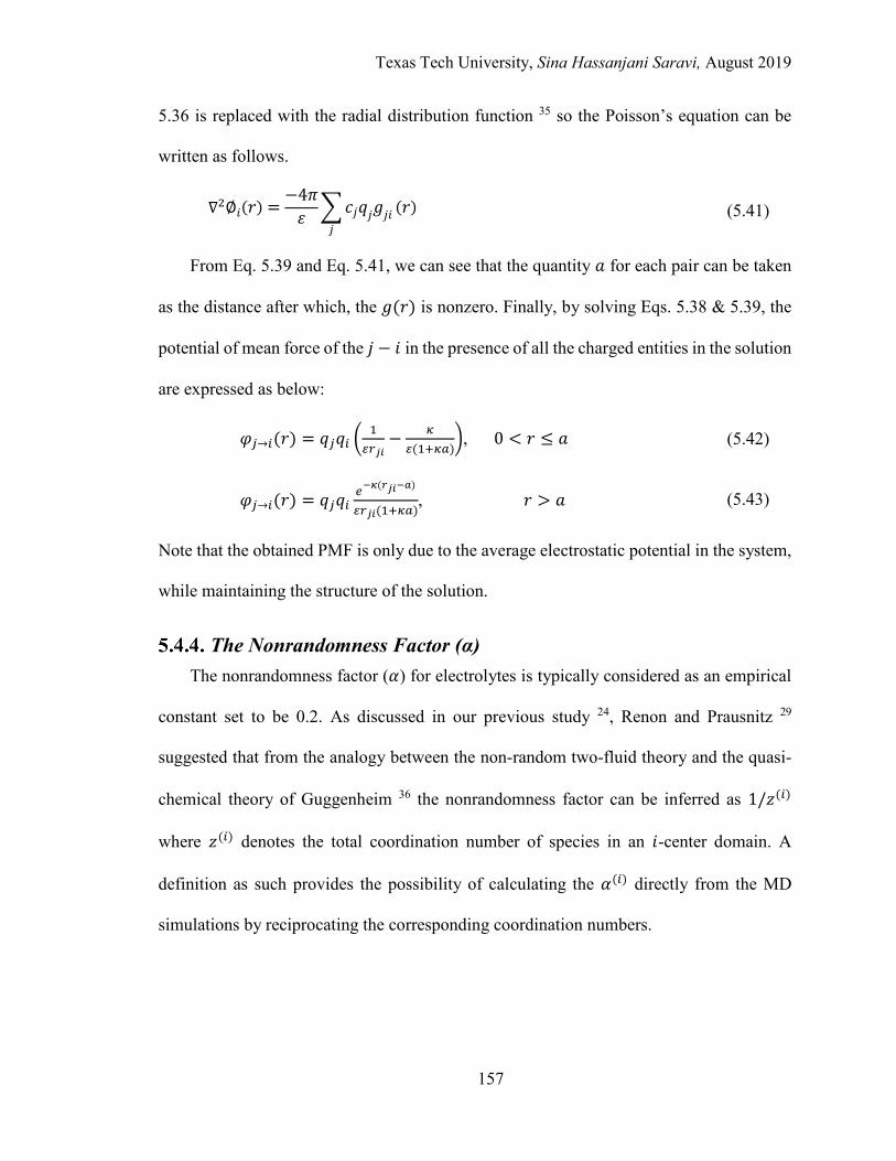
Texas Tech University, Sina Hassanjani Saravi, August 2019
157
5.36 is replaced with the radial distribution function 35 so the Poisson’s equation can be
written as follows.
∇2∅𝑖𝑖(𝑟𝑟) =−4𝜋𝜋𝜀𝜀 �𝑐𝑐𝑗𝑗𝑞𝑞𝑗𝑗𝑔𝑔𝑗𝑗𝑖𝑖
𝑗𝑗
(𝑟𝑟) (5.41)
From Eq. 5.39 and Eq. 5.41, we can see that the quantity 𝑎𝑎 for each pair can be taken
as the distance after which, the 𝑔𝑔(𝑟𝑟) is nonzero. Finally, by solving Eqs. 5.38 & 5.39, the
potential of mean force of the 𝑗𝑗 − 𝑖𝑖 in the presence of all the charged entities in the solution
are expressed as below:
𝜑𝜑𝑗𝑗→𝑖𝑖(𝑟𝑟) = 𝑞𝑞𝑗𝑗𝑞𝑞𝑖𝑖 �1𝜀𝜀𝑟𝑟𝑖𝑖𝑖𝑖
− 𝜅𝜅𝜀𝜀(1+𝜅𝜅𝑎𝑎)
�, 0 < 𝑟𝑟 ≤ 𝑎𝑎 (5.42)
𝜑𝜑𝑗𝑗→𝑖𝑖(𝑟𝑟) = 𝑞𝑞𝑗𝑗𝑞𝑞𝑖𝑖𝑒𝑒−𝜅𝜅(𝑟𝑟𝑖𝑖𝑖𝑖−𝑎𝑎)
𝜀𝜀𝑟𝑟𝑖𝑖𝑖𝑖(1+𝜅𝜅𝑎𝑎), 𝑟𝑟 > 𝑎𝑎 (5.43)
Note that the obtained PMF is only due to the average electrostatic potential in the system,
while maintaining the structure of the solution.
The Nonrandomness Factor (α) The nonrandomness factor (𝛼𝛼) for electrolytes is typically considered as an empirical
constant set to be 0.2. As discussed in our previous study 24, Renon and Prausnitz 29
suggested that from the analogy between the non-random two-fluid theory and the quasi-
chemical theory of Guggenheim 36 the nonrandomness factor can be inferred as 1/𝑧𝑧(𝑖𝑖)
where 𝑧𝑧(𝑖𝑖) denotes the total coordination number of species in an 𝑖𝑖-center domain. A
definition as such provides the possibility of calculating the 𝛼𝛼(𝑖𝑖) directly from the MD
simulations by reciprocating the corresponding coordination numbers.
Texas Tech University, Sina Hassanjani Saravi, August 2019
158
The Binary Interaction Parameters (τ) Finally, the binary interaction parameters were calculated using the quantities
discussed above using Eqs. 5.24 & 5.25 and Eqs. 5.33 & 5.34.
5.5. Molecular Simulation Details
The molecular simulations were performed separately for aqueous BaCl2, SrCl2,
CaCl2, and MgCl2 solutions using the LAMMPS package 37. For each system, the
simulations were carried out over a wide concentration range from 0.5 to 12 mol/kg at
298.15 K and 1 bar. Hereafter, we designate by 𝑚𝑚 the concentration of the salt solutions in
molality. To be consistent with our previous study for uni-univalent electrolytes 24 and
enabling rapid computations for practical industrial use, a relatively small system size
consisted of 1000 water molecules were considered for the simulations, with the number
of electrolytes varying as per the salt concentration. It was already shown 24 that the finite
size effect for calculating the binary interaction parameters are negligible.
Initial equilibration was carried out at a constant number of particles, volume, and
temperature (canonical ensemble) followed by an isothermal-isobaric (NPT) equilibration
of 10 ns long using Nośe-Hoover thermostat and barostat 38. The NPT production runs were
then carried out for the duration of 40 ns. The particle-particle particle-mesh (PPPM) 39
was used to calculate the long-range electrostatic interactions and tail corrections were used
for the long-range part of Lennard-Jones interactions. Lennard-Jones and Coulombic
interactions were truncated at the distance of 14 Å. The SPC/E 40 model was used to
represent the water molecules. For ionic species, the Kirkwood-Buff force field (KBFF)
parameters were employed from a recent study by Naleem et al. 41 reporting the KBFF of
several alkaline halide salts, including those selected as our model systems. KBFF
Texas Tech University, Sina Hassanjani Saravi, August 2019
159
parameters have been previously shown to predict successfully the mean ionic activity
coefficients of electrolyte solutions 12,24,42.
The trajectories of the 40 ns production run were divided into 10 blocks of 4 ns length
and the physical quantities required for identifying the 𝜏𝜏 parameters were then calculated
at each block. The quantity of each variable was calculated by averaging over the blocks
and the associated standard deviations were taken as the statistical uncertainties.
The potential of mean force of each pair of interest was obtained from the pertinent
RDF as per Eq. 5.44 43.
𝜙𝜙(𝑟𝑟) = −𝑅𝑅𝑇𝑇 ln𝑔𝑔(𝑟𝑟) (5.44)
Previously, Hossain et al. 12 reported that the correlation times for water molecules are
shorter than 25 ps. Since our simulations include sufficient number of correlations as
compared to those required for equilibration of water molecules, obtaining the PMF from
the RDF is rationalized and enables rapid free energy calculations, in lieu of employing
any types of enhanced sampling techniques.
5.6. Results and Discussion
Each of the liquid structure and energetic interaction quantities required for calculating
the 𝜏𝜏 parameters are obtained from the molecular simulations as explained previously.
These quantities include the effective molecular dimeter of the species (𝜎𝜎), the radius of
the first solvation shell of each local domain (𝑅𝑅), characteristic energies (𝜖𝜖), and the
nonrandomness factors (𝛼𝛼). The results and a comprehensive discussion on the physical
significance of the variables are reported herein, while more details are presented in the
Supplementary Information.
Texas Tech University, Sina Hassanjani Saravi, August 2019
160
The Results of the Physical Quantities of the Aqueous Solutions from MD Simulations
The effective molecular diameters—𝜎𝜎𝑎𝑎𝐿𝐿, 𝜎𝜎𝐿𝐿𝑚𝑚, 𝜎𝜎𝑎𝑎𝑚𝑚, and 𝜎𝜎𝑚𝑚𝑚𝑚—for aqueous BaCl2,
SrCl2, CaCl2, and MgCl2 solutions are reported in Tables 5.9.1-5.9.4, in the
Supplementary Information, obtained from the location of the first peak in the RDF of
each pair of interest. Furthermore, Figures 5.9.1-5.9.4 in the Supplementary
Information, as examples, illustrate one such RDF for each of the Ba2+-Clˉ, Sr2+-Clˉ, Ca2+-
Clˉ, and Mg2+-Clˉ pairs at the salt concentration of 4 m. As it can be observed from the
RDFs, the dominancy and sharpness of the first peaks, attributed to the contact ion pairs
(CIP), are reduced as the charge density of the cation increases. In the aqueous solution
with the smallest cationic size (Mg2+), there is only one prominent peak at the distance of
4.50 Å attributed to solvent-separated ion pair (SSIP). On the other hand, there exists no
peak corresponding to the contact ion pair (CIP). Such an observation has been confirmed
by both simulation 41,44,45 and experimental 46 studies. This can be rationalized due to the
high charge density of the Mg2+, which causes the cations to bound strongly to the water
molecules, forming fully hydrated complex ions. The CIP peak in the aqueous MgCl2
remains absent even at the highest concentration studied, i.e., 12 m salt.
With increasing the size of the cation, and hence a decrease in the charge density, the
anion is substituted with water molecules forming contact ion pairs. The CIP peak is thus
observed in the RDF of the cation-anion pair in the aqueous CaCl2 solution, however, not
significantly at lower concentrations. This explains the shift in the reported 𝜎𝜎 values from
4.94 Å (SSIP) to 2.90 Å (CIP) beyond the concentration of 4 m. In this study, the CIP peaks
with the 𝑔𝑔 (𝑟𝑟) values below unity are neglected in calculating the binary interaction
parameters and subsequently the SSIP peaks are used. In the aqueous SrCl2 solution, the
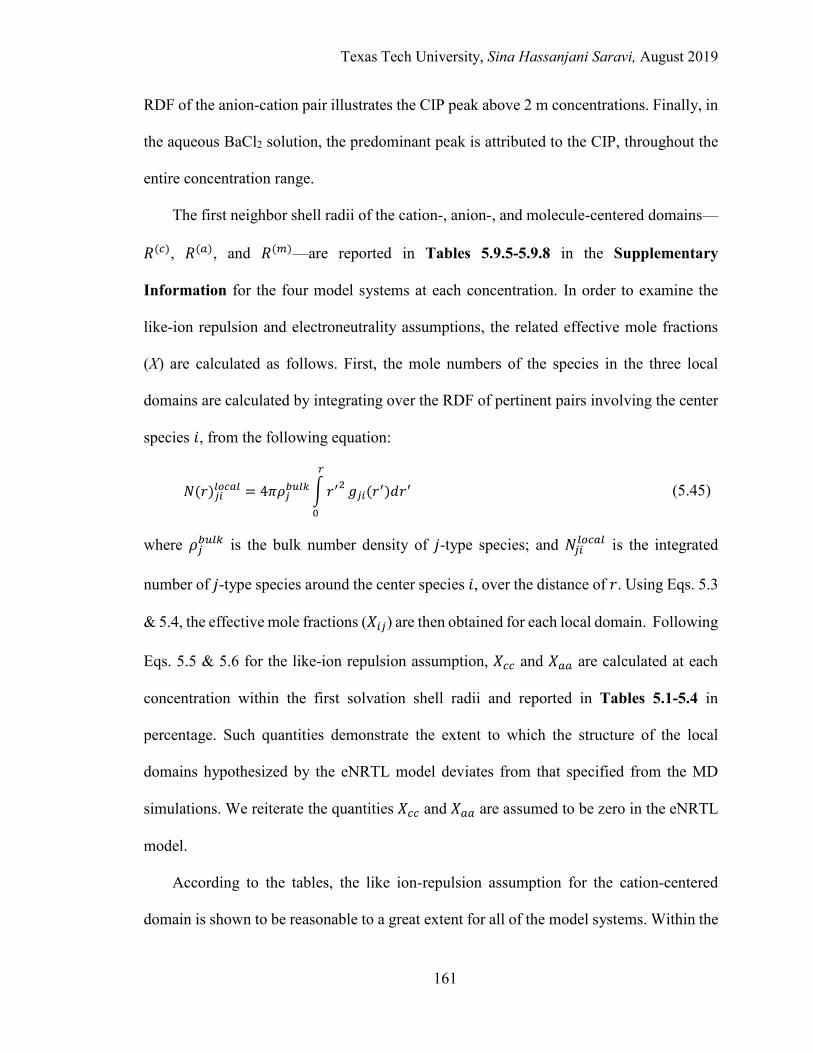
Texas Tech University, Sina Hassanjani Saravi, August 2019
161
RDF of the anion-cation pair illustrates the CIP peak above 2 m concentrations. Finally, in
the aqueous BaCl2 solution, the predominant peak is attributed to the CIP, throughout the
entire concentration range.
The first neighbor shell radii of the cation-, anion-, and molecule-centered domains—
𝑅𝑅(𝐿𝐿), 𝑅𝑅(𝑎𝑎), and 𝑅𝑅(𝑚𝑚)—are reported in Tables 5.9.5-5.9.8 in the Supplementary
Information for the four model systems at each concentration. In order to examine the
like-ion repulsion and electroneutrality assumptions, the related effective mole fractions
(X) are calculated as follows. First, the mole numbers of the species in the three local
domains are calculated by integrating over the RDF of pertinent pairs involving the center
species 𝑖𝑖, from the following equation:
𝑁𝑁(𝑟𝑟)𝑗𝑗𝑖𝑖𝑙𝑙𝑜𝑜𝐿𝐿𝑎𝑎𝑙𝑙 = 4𝜋𝜋𝜌𝜌𝑗𝑗𝑏𝑏𝑏𝑏𝑙𝑙𝑘𝑘 �𝑟𝑟′2
𝑟𝑟
0
𝑔𝑔𝑗𝑗𝑖𝑖(𝑟𝑟′)𝑑𝑑𝑟𝑟′ (5.45)
where 𝜌𝜌𝑗𝑗𝑏𝑏𝑏𝑏𝑙𝑙𝑘𝑘 is the bulk number density of 𝑗𝑗-type species; and 𝑁𝑁𝑗𝑗𝑖𝑖𝑙𝑙𝑜𝑜𝐿𝐿𝑎𝑎𝑙𝑙 is the integrated
number of 𝑗𝑗-type species around the center species 𝑖𝑖, over the distance of 𝑟𝑟. Using Eqs. 5.3
& 5.4, the effective mole fractions (𝑋𝑋𝑖𝑖𝑗𝑗) are then obtained for each local domain. Following
Eqs. 5.5 & 5.6 for the like-ion repulsion assumption, 𝑋𝑋𝐿𝐿𝐿𝐿 and 𝑋𝑋𝑎𝑎𝑎𝑎 are calculated at each
concentration within the first solvation shell radii and reported in Tables 5.1-5.4 in
percentage. Such quantities demonstrate the extent to which the structure of the local
domains hypothesized by the eNRTL model deviates from that specified from the MD
simulations. We reiterate the quantities 𝑋𝑋𝐿𝐿𝐿𝐿 and 𝑋𝑋𝑎𝑎𝑎𝑎 are assumed to be zero in the eNRTL
model.
According to the tables, the like ion-repulsion assumption for the cation-centered
domain is shown to be reasonable to a great extent for all of the model systems. Within the

Texas Tech University, Sina Hassanjani Saravi, August 2019
162
first solvation shell identified from the MD simulations, the 𝑋𝑋𝐿𝐿𝐿𝐿 % is shown to be zero for
aqueous BaCl2 and SrCl2 solutions in the entire concentration range studied. For aqueous
CaCl2 and MgCl2 solutions, the largest 𝑋𝑋𝐿𝐿𝐿𝐿 % is reported to be 2.4 and 4.4 %, respectively.
For the anion-centered domain, on the other hand, the like-ion repulsion assumption is only
qualitatively satisfied.
Table 5.1. Effective local mole fractions in the first shell (Å) – BaCl2 (aq)
Table 5.2. Effective local mole fractions in the first shell (Å) – SrCl2 (aq)
Concentration (m)
Parameters 0.5 2.0 4.0 6.0 8.0 10.0 12.0
% 𝑋𝑋𝐿𝐿𝐿𝐿 0.0 0.0 0.0 0.0 0.0 0.0 0.0
% 𝑋𝑋𝑎𝑎𝑎𝑎 0.0 31.8 31.9 32.0 31.3 31.8 32.5
% |𝑋𝑋𝑎𝑎𝑚𝑚 − 𝑋𝑋𝐿𝐿𝑚𝑚| 0.4 0.7 1.4 2.0 3.6 5.2 2.5
𝑎𝑎, 𝑐𝑐, and 𝑚𝑚 denote the anion, the cation, and the molecule
Concentration (m)
Parameters 0.5 2.0 4.0 6.0 8.0 10.0 12.0
% 𝑋𝑋𝐿𝐿𝐿𝐿 0.0 0.0 0.0 0.0 0.0 0.0 0.0
% 𝑋𝑋𝑎𝑎𝑎𝑎 0.8 0.0 0.1 2.8 13.3 15.5 20.5
% |𝑋𝑋𝑎𝑎𝑚𝑚 − 𝑋𝑋𝐿𝐿𝑚𝑚| 0.3 0.4 1.6 4.5 7.0 8.0 8.6
𝑎𝑎, 𝑐𝑐, and 𝑚𝑚 denote the anion, the cation, and the molecule
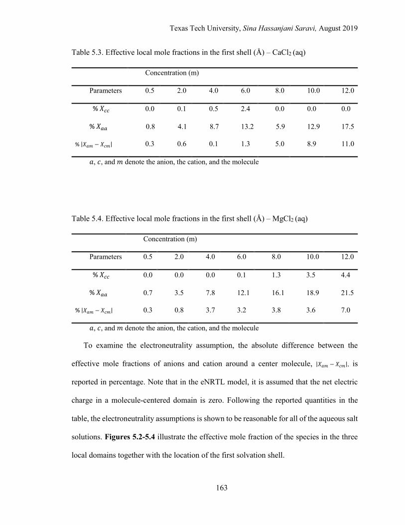
Texas Tech University, Sina Hassanjani Saravi, August 2019
163
Table 5.3. Effective local mole fractions in the first shell (Å) – CaCl2 (aq)
Table 5.4. Effective local mole fractions in the first shell (Å) – MgCl2 (aq)
To examine the electroneutrality assumption, the absolute difference between the
effective mole fractions of anions and cation around a center molecule, |𝑋𝑋𝑎𝑎𝑚𝑚 − 𝑋𝑋𝐿𝐿𝑚𝑚|, is
reported in percentage. Note that in the eNRTL model, it is assumed that the net electric
charge in a molecule-centered domain is zero. Following the reported quantities in the
table, the electroneutrality assumptions is shown to be reasonable for all of the aqueous salt
solutions. Figures 5.2-5.4 illustrate the effective mole fraction of the species in the three
local domains together with the location of the first solvation shell.
Concentration (m)
Parameters 0.5 2.0 4.0 6.0 8.0 10.0 12.0
% 𝑋𝑋𝐿𝐿𝐿𝐿 0.0 0.1 0.5 2.4 0.0 0.0 0.0
% 𝑋𝑋𝑎𝑎𝑎𝑎 0.8 4.1 8.7 13.2 5.9 12.9 17.5
% |𝑋𝑋𝑎𝑎𝑚𝑚 − 𝑋𝑋𝐿𝐿𝑚𝑚| 0.3 0.6 0.1 1.3 5.0 8.9 11.0
𝑎𝑎, 𝑐𝑐, and 𝑚𝑚 denote the anion, the cation, and the molecule
Concentration (m)
Parameters 0.5 2.0 4.0 6.0 8.0 10.0 12.0
% 𝑋𝑋𝐿𝐿𝐿𝐿 0.0 0.0 0.0 0.1 1.3 3.5 4.4
% 𝑋𝑋𝑎𝑎𝑎𝑎 0.7 3.5 7.8 12.1 16.1 18.9 21.5
% |𝑋𝑋𝑎𝑎𝑚𝑚 − 𝑋𝑋𝐿𝐿𝑚𝑚| 0.3 0.8 3.7 3.2 3.8 3.6 7.0
𝑎𝑎, 𝑐𝑐, and 𝑚𝑚 denote the anion, the cation, and the molecule
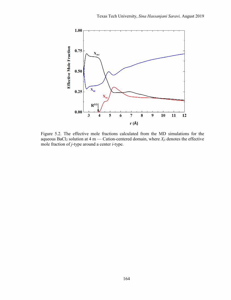
Texas Tech University, Sina Hassanjani Saravi, August 2019
164
Figure 5.2. The effective mole fractions calculated from the MD simulations for the aqueous BaCl2 solution at 4 m — Cation-centered domain, where Xji denotes the effective mole fraction of j-type around a center i-type.
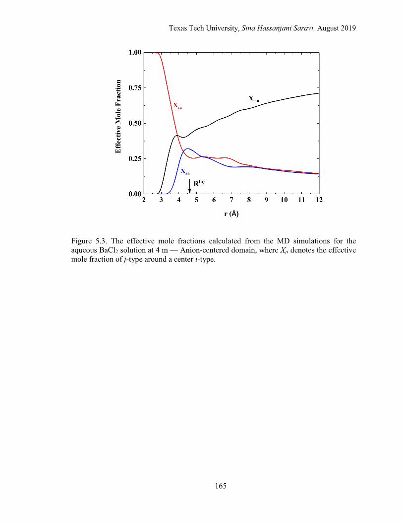
Texas Tech University, Sina Hassanjani Saravi, August 2019
165
Figure 5.3. The effective mole fractions calculated from the MD simulations for the aqueous BaCl2 solution at 4 m — Anion-centered domain, where Xji denotes the effective mole fraction of j-type around a center i-type.
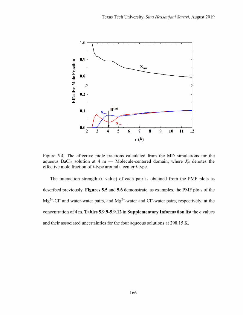
Texas Tech University, Sina Hassanjani Saravi, August 2019
166
Figure 5.4. The effective mole fractions calculated from the MD simulations for the aqueous BaCl2 solution at 4 m — Molecule-centered domain, where Xji denotes the effective mole fraction of j-type around a center i-type.
The interaction strength (𝜖𝜖 value) of each pair is obtained from the PMF plots as
described previously. Figures 5.5 and 5.6 demonstrate, as examples, the PMF plots of the
Mg2+-Clˉ and water-water pairs, and Mg2+-water and Clˉ-water pairs, respectively, at the
concentration of 4 m. Tables 5.9.9-5.9.12 in Supplementary Information list the 𝜖𝜖 values
and their associated uncertainties for the four aqueous solutions at 298.15 K.
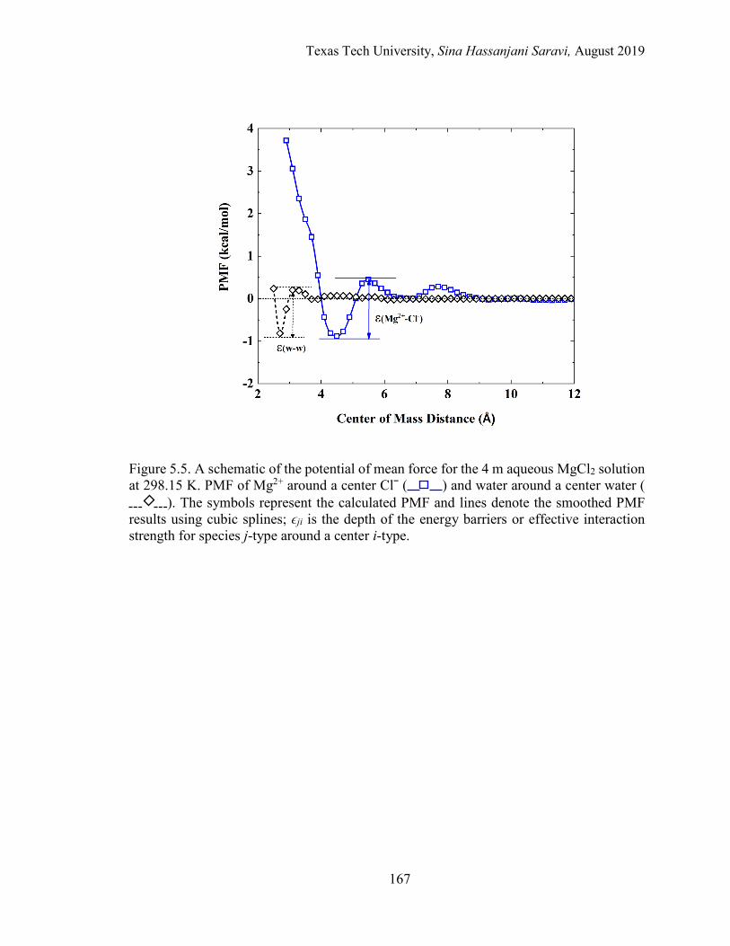
Texas Tech University, Sina Hassanjani Saravi, August 2019
167
Figure 5.5. A schematic of the potential of mean force for the 4 m aqueous MgCl2 solution at 298.15 K. PMF of Mg2+ around a center Clˉ ( ) and water around a center water (
). The symbols represent the calculated PMF and lines denote the smoothed PMF results using cubic splines; ϵji is the depth of the energy barriers or effective interaction strength for species j-type around a center i-type.
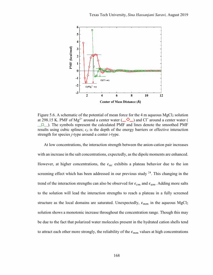
Texas Tech University, Sina Hassanjani Saravi, August 2019
168
Figure 5.6. A schematic of the potential of mean force for the 4 m aqueous MgCl2 solution at 298.15 K. PMF of Mg2+ around a center water ( ) and Clˉ around a center water (
). The symbols represent the calculated PMF and lines denote the smoothed PMF results using cubic splines; ϵji is the depth of the energy barriers or effective interaction strength for species j-type around a center i-type.
At low concentrations, the interaction strength between the anion-cation pair increases
with an increase in the salt concentrations, expectedly, as the dipole moments are enhanced.
However, at higher concentrations, the 𝜖𝜖𝑎𝑎𝐿𝐿 exhibits a plateau behavior due to the ion
screening effect which has been addressed in our previous study 24. This changing in the
trend of the interaction strengths can also be observed for 𝜖𝜖𝐿𝐿𝑚𝑚 and 𝜖𝜖𝑎𝑎𝑚𝑚. Adding more salts
to the solution will lead the interaction strengths to reach a plateau in a fully screened
structure as the local domains are saturated. Unexpectedly, 𝜖𝜖𝑚𝑚𝑚𝑚 in the aqueous MgCl2
solution shows a monotonic increase throughout the concentration range. Though this may
be due to the fact that polarized water molecules present in the hydrated cation shells tend
to attract each other more strongly, the reliability of the 𝜖𝜖𝑚𝑚𝑚𝑚 values at high concentrations
Texas Tech University, Sina Hassanjani Saravi, August 2019
169
is not ensured. We note that the force field parameters failed to capture the experimental
data for concentrations beyond 4 m 41.
Furthermore, the contribution of the local van der Waals forces in the total potential of
mean force is also calculated as explained previously. Figures 5.7 and 5.8 show the PMF
of the anion-cation pair as a function of center to center distance, in the aqueous BaCl2
solution at the concentration of 2 m and 6 m, respectively. Also shown in the figure are the
contributions of both electrostatic and local van der Waals forces in the total PMF. As
demonstrated, the depth of the free energy barrier of the short-range PMF is smaller than
that of the total PMF due the subtraction of the electrostatic forces. Also, by comparing
Figures 5.7 and 5.8, it is observed that by increasing the concentration from 2 m to 6 m,
the electrostatic forces are screened out significantly; thus, the local structure is governed
predominantly by the local short-range forces. That confirms our hypothesis that the
structure of the local domains is attributed to the short-range van der Waals forces. Figure
5.9 further demonstrates the effect of adding salts to the decrease of the electrostatic forces.
It can be observed that the so-called long-range interactions at high concentrations are
essentially diminished within the first solvation shell.
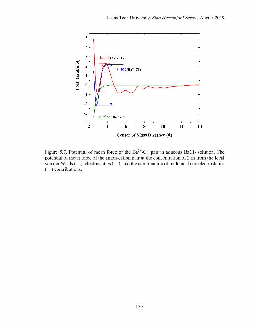
Texas Tech University, Sina Hassanjani Saravi, August 2019
170
Figure 5.7. Potential of mean force of the Ba2+-Cl- pair in aqueous BaCl2 solution. The potential of mean force of the anion-cation pair at the concentration of 2 m from the local van der Waals (—), electrostatics (—), and the combination of both local and electrostatics (—) contributions.
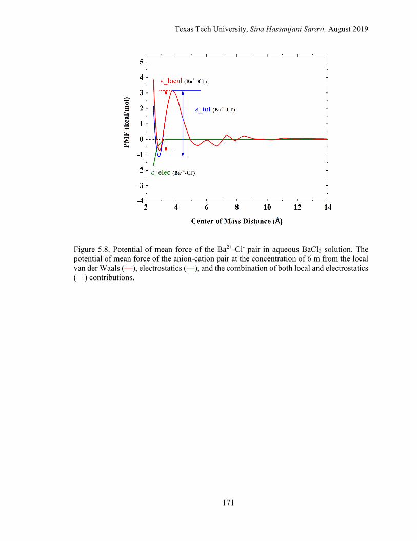
Texas Tech University, Sina Hassanjani Saravi, August 2019
171
Figure 5.8. Potential of mean force of the Ba2+-Cl- pair in aqueous BaCl2 solution. The potential of mean force of the anion-cation pair at the concentration of 6 m from the local van der Waals (—), electrostatics (—), and the combination of both local and electrostatics (—) contributions.
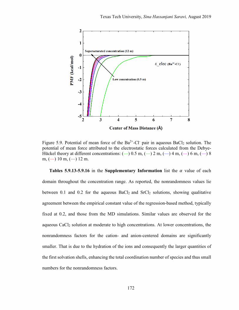
Texas Tech University, Sina Hassanjani Saravi, August 2019
172
Figure 5.9. Potential of mean force of the Ba2+-Cl- pair in aqueous BaCl2 solution. The potential of mean force attributed to the electrostatic forces calculated from the Debye-Hückel theory at different concentrations: (—) 0.5 m, (—) 2 m, (—) 4 m, (—) 6 m, (—) 8 m, (—) 10 m, (—) 12 m.
Tables 5.9.13-5.9.16 in the Supplementary Information list the 𝛼𝛼 value of each
domain throughout the concentration range. As reported, the nonrandomness values lie
between 0.1 and 0.2 for the aqueous BaCl2 and SrCl2 solutions, showing qualitative
agreement between the empirical constant value of the regression-based method, typically
fixed at 0.2, and those from the MD simulations. Similar values are observed for the
aqueous CaCl2 solution at moderate to high concentrations. At lower concentrations, the
nonrandomness factors for the cation- and anion-centered domains are significantly
smaller. That is due to the hydration of the ions and consequently the larger quantities of
the first solvation shells, enhancing the total coordination number of species and thus small
numbers for the nonrandomness factors.
Texas Tech University, Sina Hassanjani Saravi, August 2019
173
Calculating the Binary Interaction Parameters from MD Simulations The four binary interaction parameters, 𝜏𝜏𝑚𝑚𝐿𝐿,𝑎𝑎𝐿𝐿, 𝜏𝜏𝑚𝑚𝑎𝑎,𝐿𝐿𝑎𝑎, 𝜏𝜏𝐿𝐿𝑚𝑚, and 𝜏𝜏𝑎𝑎𝑚𝑚, are calculated
from the quantities thus obtained from the MD simulation results. By employing the Eqs.
5.24 & 5.25 and Eqs. 5.33 & 5.34, the binary parameters are calculated at each
concentration. In order to make a more meaningful comparison between the binary
interaction parameters from the MD simulations and those from regression, the value of
the nonrandomness factors were fixed at 0.2. Note that the product of 𝛼𝛼𝜏𝜏 determines the
structure of the local domains according to Eqs 8 & 10.
Tables 5.9.17-5.9.20 list the binary interaction parameters for the four aqueous salt
solutions at 298.15 K, over the entire concentration range. As it can be seen from the tables,
the sign of the 𝜏𝜏 parameters are as anticipated, i.e., positive for ion-centered domains and
negative for molecule-centered domains. The only exception is that while the 𝜏𝜏𝐿𝐿𝑚𝑚 and 𝜏𝜏𝑎𝑎𝑚𝑚
in aqueous MgCl2 exhibit negative values at lower concentrations, they eventually become
positive above 4 m concentration. That is due to the monotonic increase of the 𝜖𝜖𝑚𝑚𝑚𝑚
discussed previously. Figures 5.9.5-5.9.8 in Supplementary Information also show the
binary interaction parameters, together with those from regression of the experimental data.
The binary interaction parameters from regression (𝜏𝜏𝑚𝑚,𝐿𝐿𝑎𝑎 and 𝜏𝜏𝐿𝐿𝑎𝑎,𝑚𝑚) for the model systems
of our study are readily available in literature 13-16. Honarparvar et al., presented the 𝜏𝜏
values for the aqueous BaCl2 13 and SrCl2 14 solutions. Tanveer and coworkers have
reported the 𝜏𝜏 values for the aqueous CaCl2 and 15 MgCl2 16 solutions. Table 5.5 lists the
𝜏𝜏 values from regression for each aqueous solution at 298.15 K in the entire range of
concentration. These values are used for the validation of our results, as they have shown
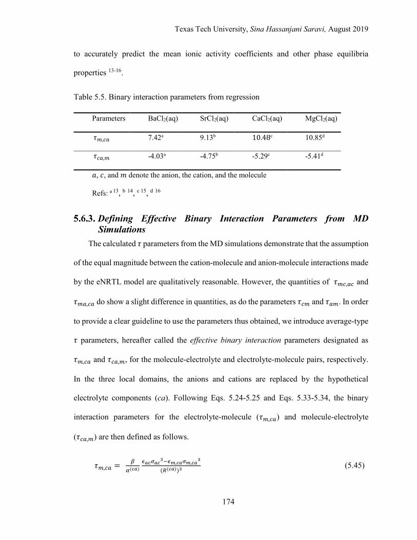
Texas Tech University, Sina Hassanjani Saravi, August 2019
174
to accurately predict the mean ionic activity coefficients and other phase equilibria
properties 13-16.
Table 5.5. Binary interaction parameters from regression
Parameters BaCl2(aq) SrCl2(aq) CaCl2(aq) MgCl2(aq)
𝜏𝜏𝑚𝑚,𝐿𝐿𝑎𝑎 7.42a 9.13b 10.48c 10.85d
𝜏𝜏𝐿𝐿𝑎𝑎,𝑚𝑚 -4.03a -4.75b -5.29c -5.41d
𝑎𝑎, 𝑐𝑐, and 𝑚𝑚 denote the anion, the cation, and the molecule
Refs: a 13, b 14, c 15, d 16
Defining Effective Binary Interaction Parameters from MD Simulations
The calculated 𝜏𝜏 parameters from the MD simulations demonstrate that the assumption
of the equal magnitude between the cation-molecule and anion-molecule interactions made
by the eNRTL model are qualitatively reasonable. However, the quantities of 𝜏𝜏𝑚𝑚𝐿𝐿,𝑎𝑎𝐿𝐿 and
𝜏𝜏𝑚𝑚𝑎𝑎,𝐿𝐿𝑎𝑎 do show a slight difference in quantities, as do the parameters 𝜏𝜏𝐿𝐿𝑚𝑚 and 𝜏𝜏𝑎𝑎𝑚𝑚. In order
to provide a clear guideline to use the parameters thus obtained, we introduce average-type
𝜏𝜏 parameters, hereafter called the effective binary interaction parameters designated as
𝜏𝜏𝑚𝑚,𝐿𝐿𝑎𝑎 and 𝜏𝜏𝐿𝐿𝑎𝑎,𝑚𝑚, for the molecule-electrolyte and electrolyte-molecule pairs, respectively.
In the three local domains, the anions and cations are replaced by the hypothetical
electrolyte components (ca). Following Eqs. 5.24-5.25 and Eqs. 5.33-5.34, the binary
interaction parameters for the electrolyte-molecule (𝜏𝜏𝑚𝑚,𝐿𝐿𝑎𝑎) and molecule-electrolyte
(𝜏𝜏𝐿𝐿𝑎𝑎,𝑚𝑚) are then defined as follows.
𝜏𝜏𝑚𝑚,𝐿𝐿𝑎𝑎 = 𝛽𝛽𝛼𝛼(𝑐𝑐𝑎𝑎)
𝜖𝜖𝑎𝑎𝑐𝑐𝜎𝜎𝑎𝑎𝑐𝑐3−𝜖𝜖𝑚𝑚,𝑐𝑐𝑎𝑎𝜎𝜎𝑚𝑚,𝑐𝑐𝑎𝑎3
(𝐿𝐿(𝑐𝑐𝑎𝑎))3 (5.45)
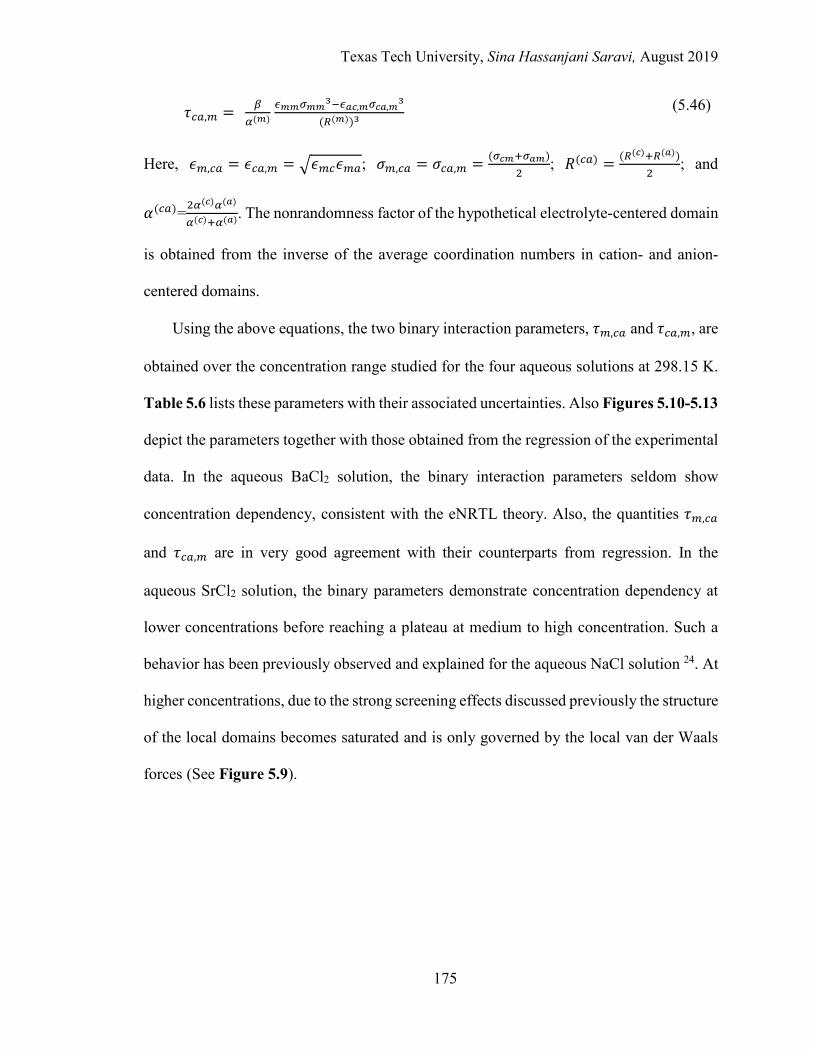
Texas Tech University, Sina Hassanjani Saravi, August 2019
175
𝜏𝜏𝐿𝐿𝑎𝑎,𝑚𝑚 = 𝛽𝛽𝛼𝛼(𝑚𝑚)
𝜖𝜖𝑚𝑚𝑚𝑚𝜎𝜎𝑚𝑚𝑚𝑚3−𝜖𝜖𝑎𝑎𝑐𝑐,𝑚𝑚𝜎𝜎𝑐𝑐𝑎𝑎,𝑚𝑚
3
(𝐿𝐿(𝑚𝑚))3 (5.46)
Here, 𝜖𝜖𝑚𝑚,𝐿𝐿𝑎𝑎 = 𝜖𝜖𝐿𝐿𝑎𝑎,𝑚𝑚 = �𝜖𝜖𝑚𝑚𝐿𝐿𝜖𝜖𝑚𝑚𝑎𝑎; 𝜎𝜎𝑚𝑚,𝐿𝐿𝑎𝑎 = 𝜎𝜎𝐿𝐿𝑎𝑎,𝑚𝑚 = (𝜎𝜎𝑐𝑐𝑚𝑚+𝜎𝜎𝑎𝑎𝑚𝑚)2
; 𝑅𝑅(𝐿𝐿𝑎𝑎) = (𝐿𝐿(𝑐𝑐)+𝐿𝐿(𝑎𝑎))2
; and
𝛼𝛼(𝐿𝐿𝑎𝑎)=2𝛼𝛼(𝑐𝑐)𝛼𝛼(𝑎𝑎)
𝛼𝛼(𝑐𝑐)+𝛼𝛼(𝑎𝑎). The nonrandomness factor of the hypothetical electrolyte-centered domain
is obtained from the inverse of the average coordination numbers in cation- and anion-
centered domains.
Using the above equations, the two binary interaction parameters, 𝜏𝜏𝑚𝑚,𝐿𝐿𝑎𝑎 and 𝜏𝜏𝐿𝐿𝑎𝑎,𝑚𝑚, are
obtained over the concentration range studied for the four aqueous solutions at 298.15 K.
Table 5.6 lists these parameters with their associated uncertainties. Also Figures 5.10-5.13
depict the parameters together with those obtained from the regression of the experimental
data. In the aqueous BaCl2 solution, the binary interaction parameters seldom show
concentration dependency, consistent with the eNRTL theory. Also, the quantities 𝜏𝜏𝑚𝑚,𝐿𝐿𝑎𝑎
and 𝜏𝜏𝐿𝐿𝑎𝑎,𝑚𝑚 are in very good agreement with their counterparts from regression. In the
aqueous SrCl2 solution, the binary parameters demonstrate concentration dependency at
lower concentrations before reaching a plateau at medium to high concentration. Such a
behavior has been previously observed and explained for the aqueous NaCl solution 24. At
higher concentrations, due to the strong screening effects discussed previously the structure
of the local domains becomes saturated and is only governed by the local van der Waals
forces (See Figure 5.9).
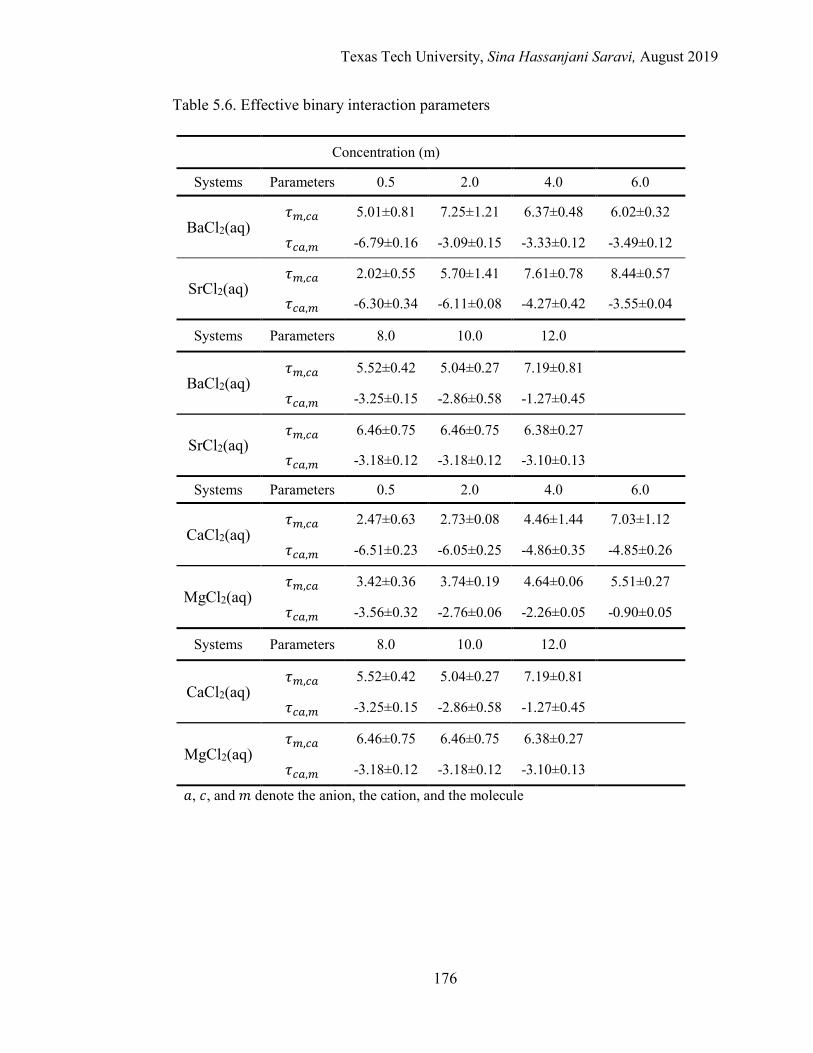
Texas Tech University, Sina Hassanjani Saravi, August 2019
176
Table 5.6. Effective binary interaction parameters
Concentration (m)
Systems Parameters 0.5 2.0 4.0 6.0
BaCl2(aq) 𝜏𝜏𝑚𝑚,𝐿𝐿𝑎𝑎 5.01±0.81 7.25±1.21 6.37±0.48 6.02±0.32
𝜏𝜏𝐿𝐿𝑎𝑎,𝑚𝑚 -6.79±0.16 -3.09±0.15 -3.33±0.12 -3.49±0.12
SrCl2(aq) 𝜏𝜏𝑚𝑚,𝐿𝐿𝑎𝑎 2.02±0.55 5.70±1.41 7.61±0.78 8.44±0.57
𝜏𝜏𝐿𝐿𝑎𝑎,𝑚𝑚 -6.30±0.34 -6.11±0.08 -4.27±0.42 -3.55±0.04
Systems Parameters 8.0 10.0 12.0
BaCl2(aq) 𝜏𝜏𝑚𝑚,𝐿𝐿𝑎𝑎 5.52±0.42 5.04±0.27 7.19±0.81
𝜏𝜏𝐿𝐿𝑎𝑎,𝑚𝑚 -3.25±0.15 -2.86±0.58 -1.27±0.45
SrCl2(aq) 𝜏𝜏𝑚𝑚,𝐿𝐿𝑎𝑎 6.46±0.75 6.46±0.75 6.38±0.27
𝜏𝜏𝐿𝐿𝑎𝑎,𝑚𝑚 -3.18±0.12 -3.18±0.12 -3.10±0.13
Systems Parameters 0.5 2.0 4.0 6.0
CaCl2(aq) 𝜏𝜏𝑚𝑚,𝐿𝐿𝑎𝑎 2.47±0.63 2.73±0.08 4.46±1.44 7.03±1.12
𝜏𝜏𝐿𝐿𝑎𝑎,𝑚𝑚 -6.51±0.23 -6.05±0.25 -4.86±0.35 -4.85±0.26
MgCl2(aq) 𝜏𝜏𝑚𝑚,𝐿𝐿𝑎𝑎 3.42±0.36 3.74±0.19 4.64±0.06 5.51±0.27
𝜏𝜏𝐿𝐿𝑎𝑎,𝑚𝑚 -3.56±0.32 -2.76±0.06 -2.26±0.05 -0.90±0.05
Systems Parameters 8.0 10.0 12.0
CaCl2(aq) 𝜏𝜏𝑚𝑚,𝐿𝐿𝑎𝑎 5.52±0.42 5.04±0.27 7.19±0.81
𝜏𝜏𝐿𝐿𝑎𝑎,𝑚𝑚 -3.25±0.15 -2.86±0.58 -1.27±0.45
MgCl2(aq) 𝜏𝜏𝑚𝑚,𝐿𝐿𝑎𝑎 6.46±0.75 6.46±0.75 6.38±0.27
𝜏𝜏𝐿𝐿𝑎𝑎,𝑚𝑚 -3.18±0.12 -3.18±0.12 -3.10±0.13
𝑎𝑎, 𝑐𝑐, and 𝑚𝑚 denote the anion, the cation, and the molecule
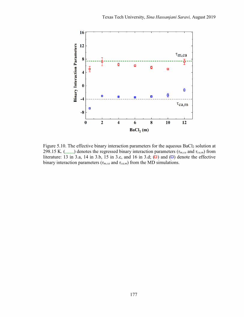
Texas Tech University, Sina Hassanjani Saravi, August 2019
177
Figure 5.10. The effective binary interaction parameters for the aqueous BaCl2 solution at 298.15 K. ( ) denotes the regressed binary interaction parameters (τm,ca and τca,m) from literature: 13 in 3.a, 14 in 3.b, 15 in 3.c, and 16 in 3.d; ( ) and ( ) denote the effective binary interaction parameters (τm,ca and τca,m) from the MD simulations.

Texas Tech University, Sina Hassanjani Saravi, August 2019
178
Figure 5.11. The effective binary interaction parameters for the aqueous SrCl2 solution at 298.15 K. ( ) denotes the regressed binary interaction parameters (τm,ca and τca,m) from literature: 13 in 3.a, 14 in 3.b, 15 in 3.c, and 16 in 3.d; ( ) and ( ) denote the effective binary interaction parameters (τm,ca and τca,m) from the MD simulations.
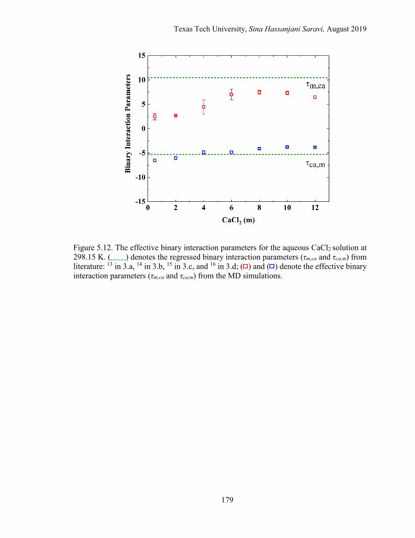
Texas Tech University, Sina Hassanjani Saravi, August 2019
179
Figure 5.12. The effective binary interaction parameters for the aqueous CaCl2 solution at 298.15 K. ( ) denotes the regressed binary interaction parameters (τm,ca and τca,m) from literature: 13 in 3.a, 14 in 3.b, 15 in 3.c, and 16 in 3.d; ( ) and ( ) denote the effective binary interaction parameters (τm,ca and τca,m) from the MD simulations.

Texas Tech University, Sina Hassanjani Saravi, August 2019
180
Figure 5.13. The effective binary interaction parameters for the aqueous MgCl2 solution at 298.15 K. ( ) denotes the regressed binary interaction parameters (τm,ca and τca,m) from literature: 13 in 3.a, 14 in 3.b, 15 in 3.c, and 16 in 3.d; ( ) and ( ) denote the effective binary interaction parameters (τm,ca and τca,m) from the MD simulations.
In the aqueous CaCl2 solution, 𝜏𝜏𝐿𝐿𝑎𝑎,𝑚𝑚 shows almost no concentration dependency and
demonstrates an excellent agreement with that reported from regression. 𝜏𝜏𝑚𝑚,𝐿𝐿𝑎𝑎 on the other
hand, displays a slight increase by adding salts at lower concentrations before reaching a
plateau. A systematic underestimation of the 𝜏𝜏𝑚𝑚,𝐿𝐿𝑎𝑎 is observed with respect to that reported
from regression. A similar behavior is shown for the aqueous MgCl2 solution in which
𝜏𝜏𝑚𝑚,𝐿𝐿𝑎𝑎, though demonstrating almost no concentration dependency, only agrees
qualitatively with that reported from regression. Such underestimations are expected to be
observed in electrolyte systems where the ionic species show the tendency toward forming
hydrated complex ions. In other word, the ionic species that form strong CIP peaks, such
as in aqueous BaCl2 solution and to some extent in aqueous SrCl2 solution, the results of
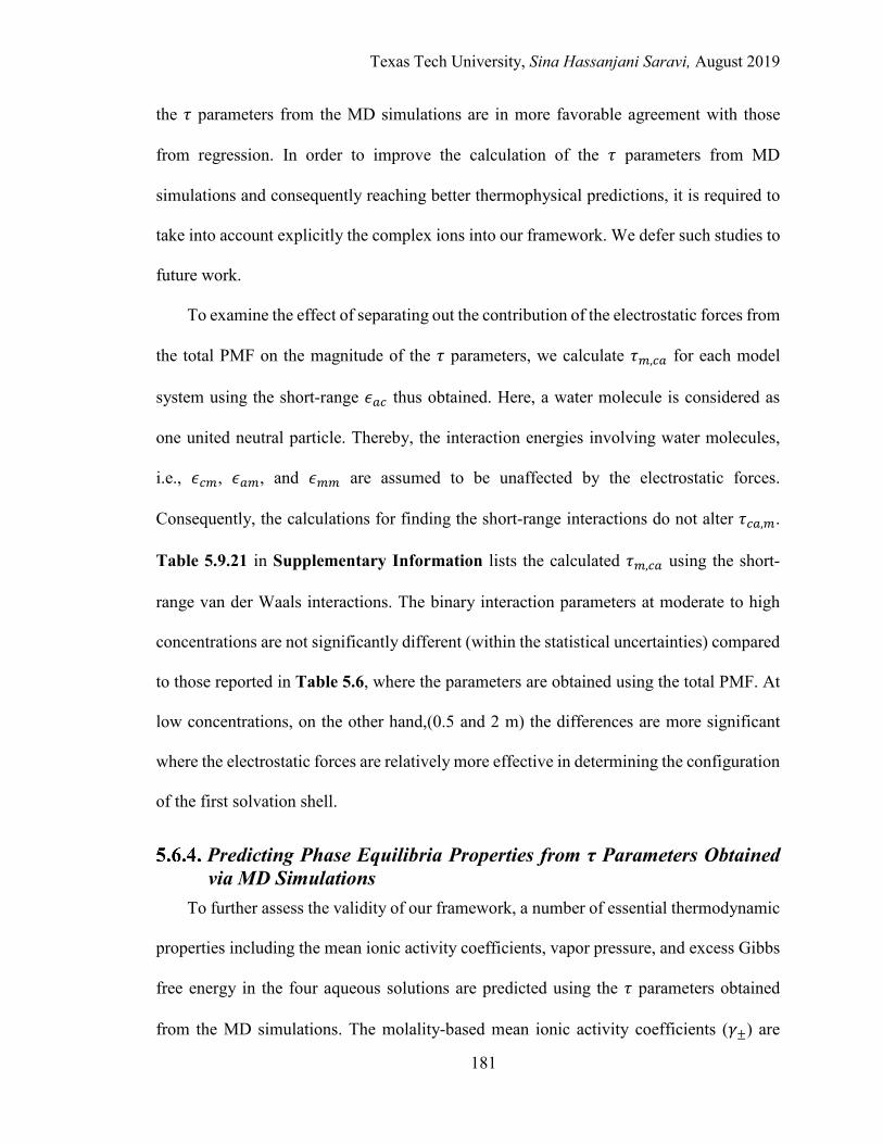
Texas Tech University, Sina Hassanjani Saravi, August 2019
181
the 𝜏𝜏 parameters from the MD simulations are in more favorable agreement with those
from regression. In order to improve the calculation of the 𝜏𝜏 parameters from MD
simulations and consequently reaching better thermophysical predictions, it is required to
take into account explicitly the complex ions into our framework. We defer such studies to
future work.
To examine the effect of separating out the contribution of the electrostatic forces from
the total PMF on the magnitude of the 𝜏𝜏 parameters, we calculate 𝜏𝜏𝑚𝑚,𝐿𝐿𝑎𝑎 for each model
system using the short-range 𝜖𝜖𝑎𝑎𝐿𝐿 thus obtained. Here, a water molecule is considered as
one united neutral particle. Thereby, the interaction energies involving water molecules,
i.e., 𝜖𝜖𝐿𝐿𝑚𝑚, 𝜖𝜖𝑎𝑎𝑚𝑚, and 𝜖𝜖𝑚𝑚𝑚𝑚 are assumed to be unaffected by the electrostatic forces.
Consequently, the calculations for finding the short-range interactions do not alter 𝜏𝜏𝐿𝐿𝑎𝑎,𝑚𝑚.
Table 5.9.21 in Supplementary Information lists the calculated 𝜏𝜏𝑚𝑚,𝐿𝐿𝑎𝑎 using the short-
range van der Waals interactions. The binary interaction parameters at moderate to high
concentrations are not significantly different (within the statistical uncertainties) compared
to those reported in Table 5.6, where the parameters are obtained using the total PMF. At
low concentrations, on the other hand,(0.5 and 2 m) the differences are more significant
where the electrostatic forces are relatively more effective in determining the configuration
of the first solvation shell.
Predicting Phase Equilibria Properties from τ Parameters Obtained via MD Simulations
To further assess the validity of our framework, a number of essential thermodynamic
properties including the mean ionic activity coefficients, vapor pressure, and excess Gibbs
free energy in the four aqueous solutions are predicted using the 𝜏𝜏 parameters obtained
from the MD simulations. The molality-based mean ionic activity coefficients (𝛾𝛾±) are
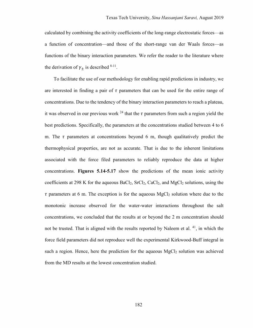
Texas Tech University, Sina Hassanjani Saravi, August 2019
182
calculated by combining the activity coefficients of the long-range electrostatic forces—as
a function of concentration—and those of the short-range van der Waals forces—as
functions of the binary interaction parameters. We refer the reader to the literature where
the derivation of 𝛾𝛾± is described 8-11.
To facilitate the use of our methodology for enabling rapid predictions in industry, we
are interested in finding a pair of 𝜏𝜏 parameters that can be used for the entire range of
concentrations. Due to the tendency of the binary interaction parameters to reach a plateau,
it was observed in our previous work 24 that the 𝜏𝜏 parameters from such a region yield the
best predictions. Specifically, the parameters at the concentrations studied between 4 to 6
m. The 𝜏𝜏 parameters at concentrations beyond 6 m, though qualitatively predict the
thermophysical properties, are not as accurate. That is due to the inherent limitations
associated with the force filed parameters to reliably reproduce the data at higher
concentrations. Figures 5.14-5.17 show the predictions of the mean ionic activity
coefficients at 298 K for the aqueous BaCl2, SrCl2, CaCl2, and MgCl2 solutions, using the
𝜏𝜏 parameters at 6 m. The exception is for the aqueous MgCl2 solution where due to the
monotonic increase observed for the water-water interactions throughout the salt
concentrations, we concluded that the results at or beyond the 2 m concentration should
not be trusted. That is aligned with the results reported by Naleem et al. 41, in which the
force field parameters did not reproduce well the experimental Kirkwood-Buff integral in
such a region. Hence, here the prediction for the aqueous MgCl2 solution was achieved
from the MD results at the lowest concentration studied.
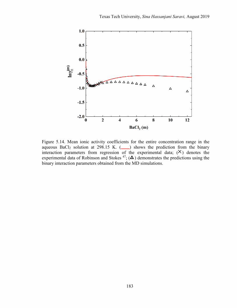
Texas Tech University, Sina Hassanjani Saravi, August 2019
183
Figure 5.14. Mean ionic activity coefficients for the entire concentration range in the aqueous BaCl2 solution at 298.15 K. ( ) shows the prediction from the binary interaction parameters from regression of the experimental data; ( ) denotes the experimental data of Robinson and Stokes 47; ( ) demonstrates the predictions using the binary interaction parameters obtained from the MD simulations.
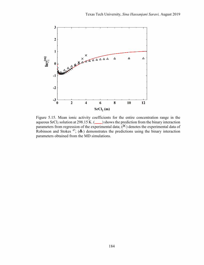
Texas Tech University, Sina Hassanjani Saravi, August 2019
184
Figure 5.15. Mean ionic activity coefficients for the entire concentration range in the aqueous SrCl2 solution at 298.15 K. ( ) shows the prediction from the binary interaction parameters from regression of the experimental data; ( ) denotes the experimental data of Robinson and Stokes 47; ( ) demonstrates the predictions using the binary interaction parameters obtained from the MD simulations.
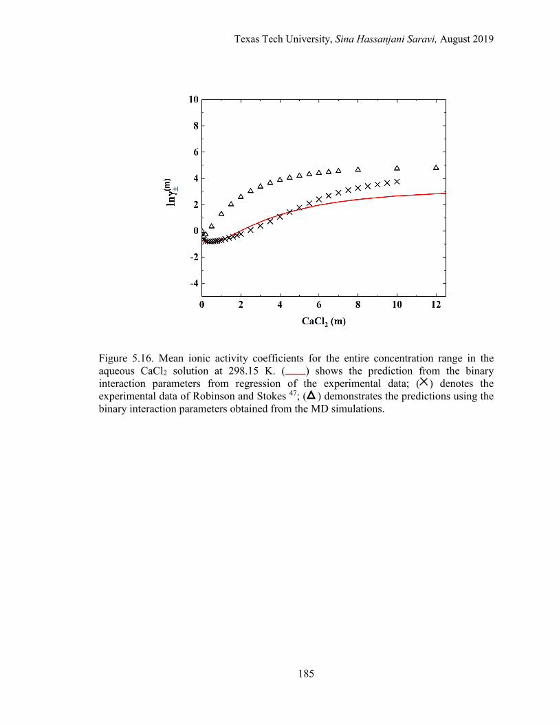
Texas Tech University, Sina Hassanjani Saravi, August 2019
185
Figure 5.16. Mean ionic activity coefficients for the entire concentration range in the aqueous CaCl2 solution at 298.15 K. ( ) shows the prediction from the binary interaction parameters from regression of the experimental data; ( ) denotes the experimental data of Robinson and Stokes 47; ( ) demonstrates the predictions using the binary interaction parameters obtained from the MD simulations.
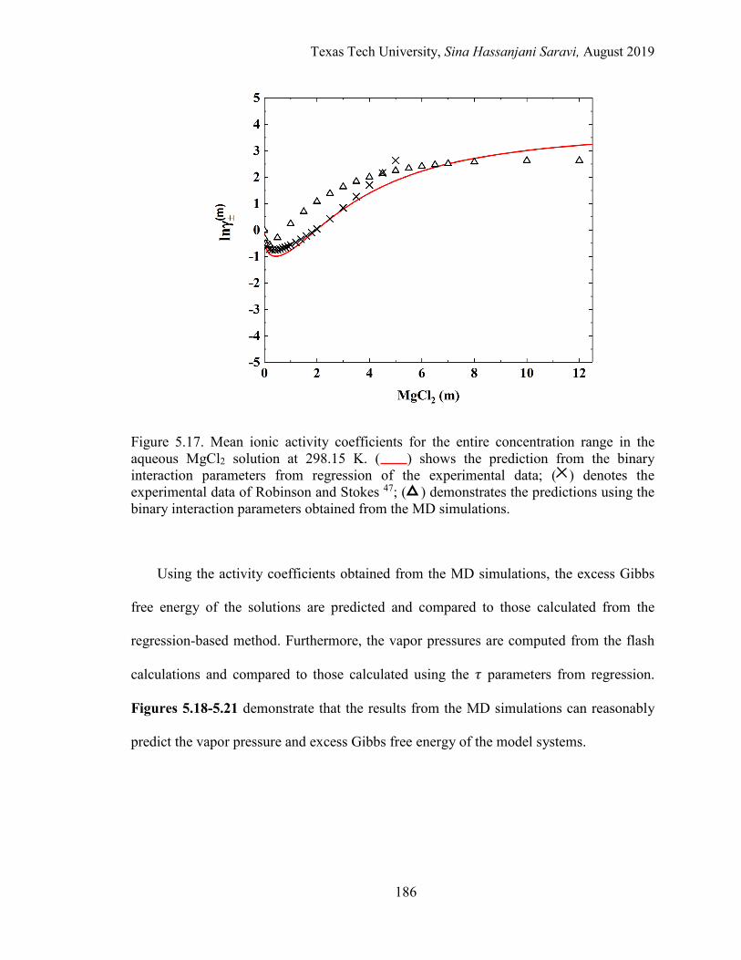
Texas Tech University, Sina Hassanjani Saravi, August 2019
186
Figure 5.17. Mean ionic activity coefficients for the entire concentration range in the aqueous MgCl2 solution at 298.15 K. ( ) shows the prediction from the binary interaction parameters from regression of the experimental data; ( ) denotes the experimental data of Robinson and Stokes 47; ( ) demonstrates the predictions using the binary interaction parameters obtained from the MD simulations.
Using the activity coefficients obtained from the MD simulations, the excess Gibbs
free energy of the solutions are predicted and compared to those calculated from the
regression-based method. Furthermore, the vapor pressures are computed from the flash
calculations and compared to those calculated using the 𝜏𝜏 parameters from regression.
Figures 5.18-5.21 demonstrate that the results from the MD simulations can reasonably
predict the vapor pressure and excess Gibbs free energy of the model systems.
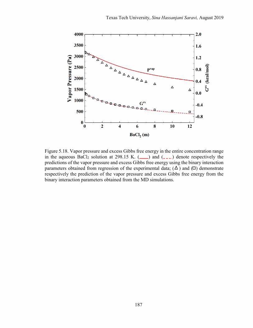
Texas Tech University, Sina Hassanjani Saravi, August 2019
187
Figure 5.18. Vapor pressure and excess Gibbs free energy in the entire concentration range in the aqueous BaCl2 solution at 298.15 K. ( ) and ( ) denote respectively the predictions of the vapor pressure and excess Gibbs free energy using the binary interaction parameters obtained from regression of the experimental data; ( ) and ( ) demonstrate respectively the prediction of the vapor pressure and excess Gibbs free energy from the binary interaction parameters obtained from the MD simulations.

Texas Tech University, Sina Hassanjani Saravi, August 2019
188
Figure 5.19. Vapor pressure and excess Gibbs free energy in the entire concentration range in the aqueous SrCl2 solution at 298.15 K. ( ) and ( ) denote respectively the predictions of the vapor pressure and excess Gibbs free energy using the binary interaction parameters obtained from regression of the experimental data; ( ) and ( ) demonstrate respectively the prediction of the vapor pressure and excess Gibbs free energy from the binary interaction parameters obtained from the MD simulations.
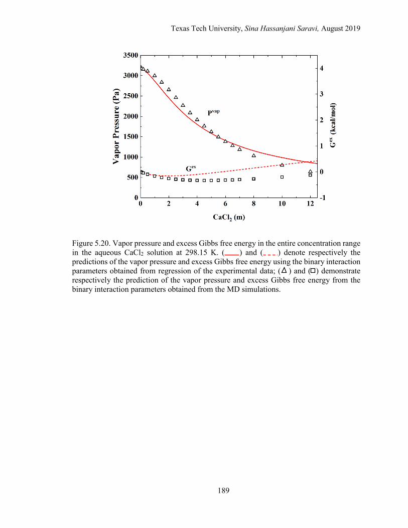
Texas Tech University, Sina Hassanjani Saravi, August 2019
189
Figure 5.20. Vapor pressure and excess Gibbs free energy in the entire concentration range in the aqueous CaCl2 solution at 298.15 K. ( ) and ( ) denote respectively the predictions of the vapor pressure and excess Gibbs free energy using the binary interaction parameters obtained from regression of the experimental data; ( ) and ( ) demonstrate respectively the prediction of the vapor pressure and excess Gibbs free energy from the binary interaction parameters obtained from the MD simulations.

Texas Tech University, Sina Hassanjani Saravi, August 2019
190
Figure 5.21. Vapor pressure and excess Gibbs free energy in the entire concentration range in the aqueous MgCl2 solution at 298.15 K. ( ) and ( ) denote respectively the predictions of the vapor pressure and excess Gibbs free energy using the binary interaction parameters obtained from regression of the experimental data; ( ) and ( ) demonstrate respectively the prediction of the vapor pressure and excess Gibbs free energy from the binary interaction parameters obtained from the MD simulations.
5.7. Conclusions
In this study, we established a theoretical framework to quantify the binary interaction
parameters (𝜏𝜏) of the eNRTL model for electrolytes from molecular dynamics (MD)
simulations. By revisiting the statistical mechanics of two-liquid theory, the 𝜏𝜏 parameters
were formulated as functions of the microscopic scale liquid structure and energetic
interaction quantities, which in turn were obtained from the MD simulations and free
energy calculations. The validity of the developed framework was assessed by examining
several di-univalent electrolyte solutions including BaCl2 (aq), SrCl2 (aq), CaCl2 (aq), and
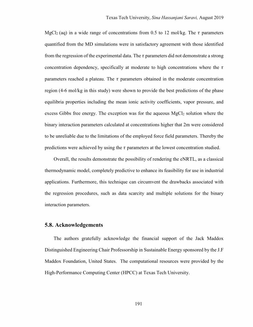
Texas Tech University, Sina Hassanjani Saravi, August 2019
191
MgCl2 (aq) in a wide range of concentrations from 0.5 to 12 mol/kg. The 𝜏𝜏 parameters
quantified from the MD simulations were in satisfactory agreement with those identified
from the regression of the experimental data. The 𝜏𝜏 parameters did not demonstrate a strong
concentration dependency, specifically at moderate to high concentrations where the 𝜏𝜏
parameters reached a plateau. The 𝜏𝜏 parameters obtained in the moderate concentration
region (4-6 mol/kg in this study) were shown to provide the best predictions of the phase
equilibria properties including the mean ionic activity coefficients, vapor pressure, and
excess Gibbs free energy. The exception was for the aqueous MgCl2 solution where the
binary interaction parameters calculated at concentrations higher that 2m were considered
to be unreliable due to the limitations of the employed force field parameters. Thereby the
predictions were achieved by using the 𝜏𝜏 parameters at the lowest concentration studied.
Overall, the results demonstrate the possibility of rendering the eNRTL, as a classical
thermodynamic model, completely predictive to enhance its feasibility for use in industrial
applications. Furthermore, this technique can circumvent the drawbacks associated with
the regression procedures, such as data scarcity and multiple solutions for the binary
interaction parameters.
5.8. Acknowledgements
The authors gratefully acknowledge the financial support of the Jack Maddox
Distinguished Engineering Chair Professorship in Sustainable Energy sponsored by the J.F
Maddox Foundation, United States. The computational resources were provided by the
High-Performance Computing Center (HPCC) at Texas Tech University.

Texas Tech University, Sina Hassanjani Saravi, August 2019
192
5.9. Supplementary Information
Figure 5.9.1. Radial distribution function (RDF) of the Ba2+-Clˉ pair in the aqueous BaCl2 at 4 m concentration and 298 K.
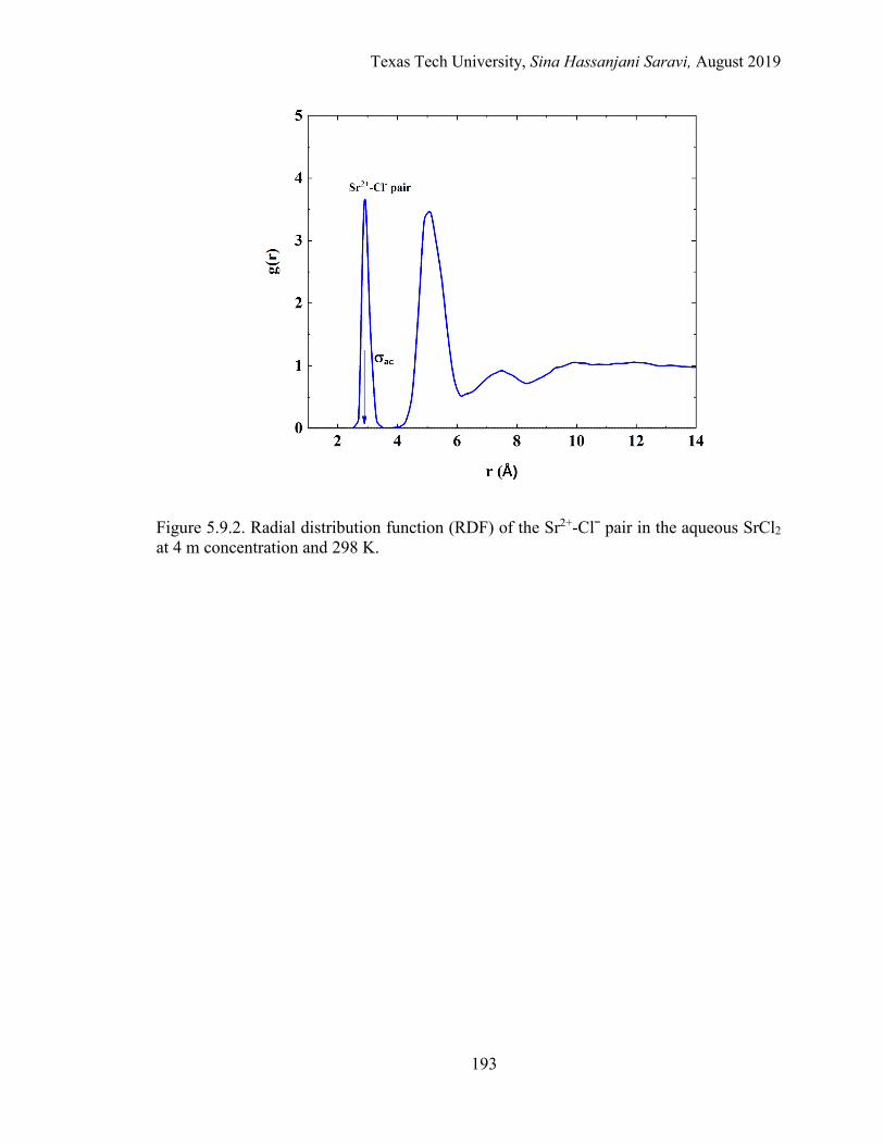
Texas Tech University, Sina Hassanjani Saravi, August 2019
193
Figure 5.9.2. Radial distribution function (RDF) of the Sr2+-Clˉ pair in the aqueous SrCl2 at 4 m concentration and 298 K.
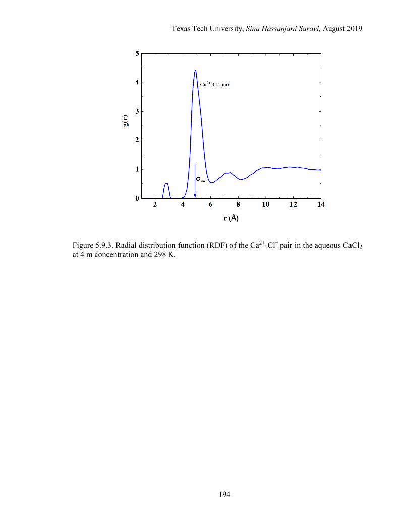
Texas Tech University, Sina Hassanjani Saravi, August 2019
194
Figure 5.9.3. Radial distribution function (RDF) of the Ca2+-Clˉ pair in the aqueous CaCl2 at 4 m concentration and 298 K.
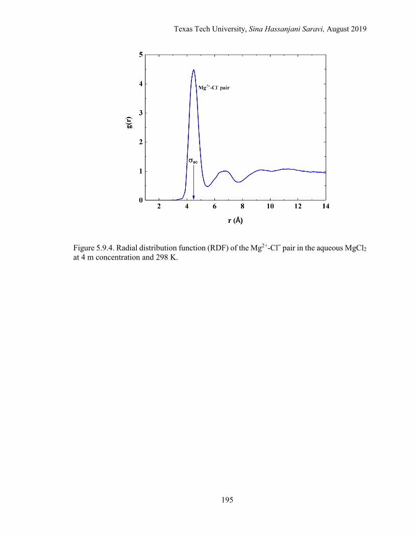
Texas Tech University, Sina Hassanjani Saravi, August 2019
195
Figure 5.9.4. Radial distribution function (RDF) of the Mg2+-Clˉ pair in the aqueous MgCl2 at 4 m concentration and 298 K.
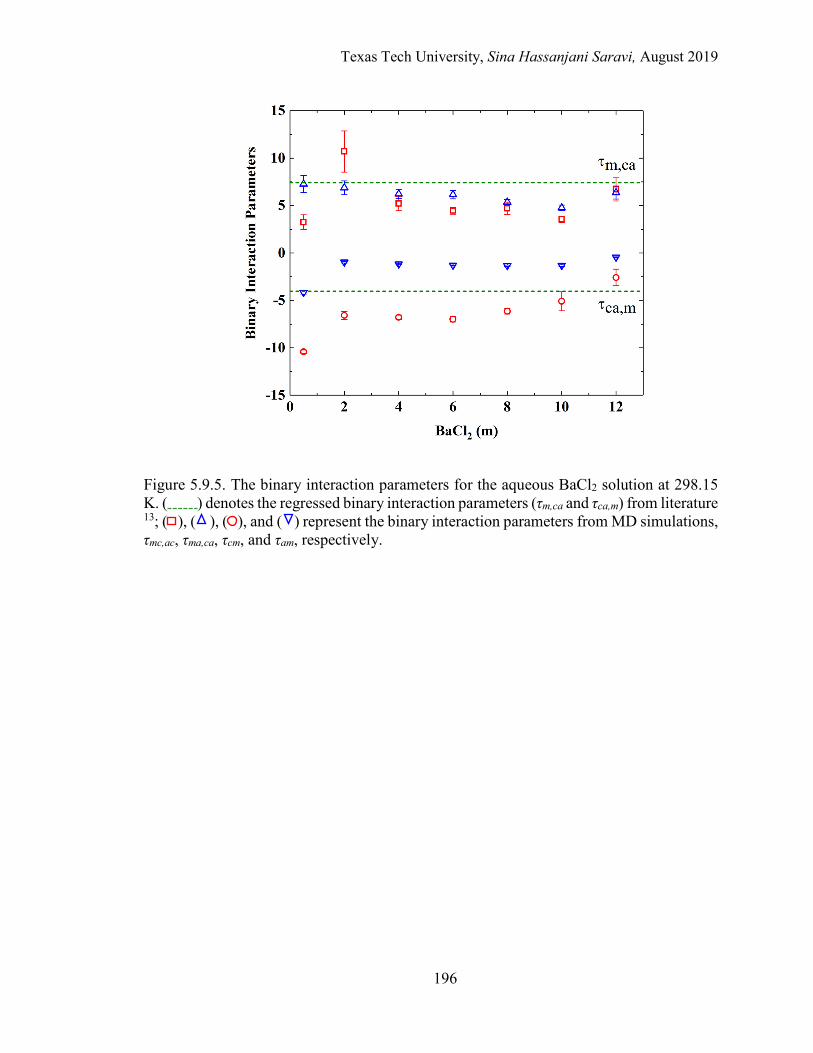
Texas Tech University, Sina Hassanjani Saravi, August 2019
196
Figure 5.9.5. The binary interaction parameters for the aqueous BaCl2 solution at 298.15 K. ( ) denotes the regressed binary interaction parameters (τm,ca and τca,m) from literature 13; ( ), ( ), ( ), and ( ) represent the binary interaction parameters from MD simulations, τmc,ac, τma,ca, τcm, and τam, respectively.
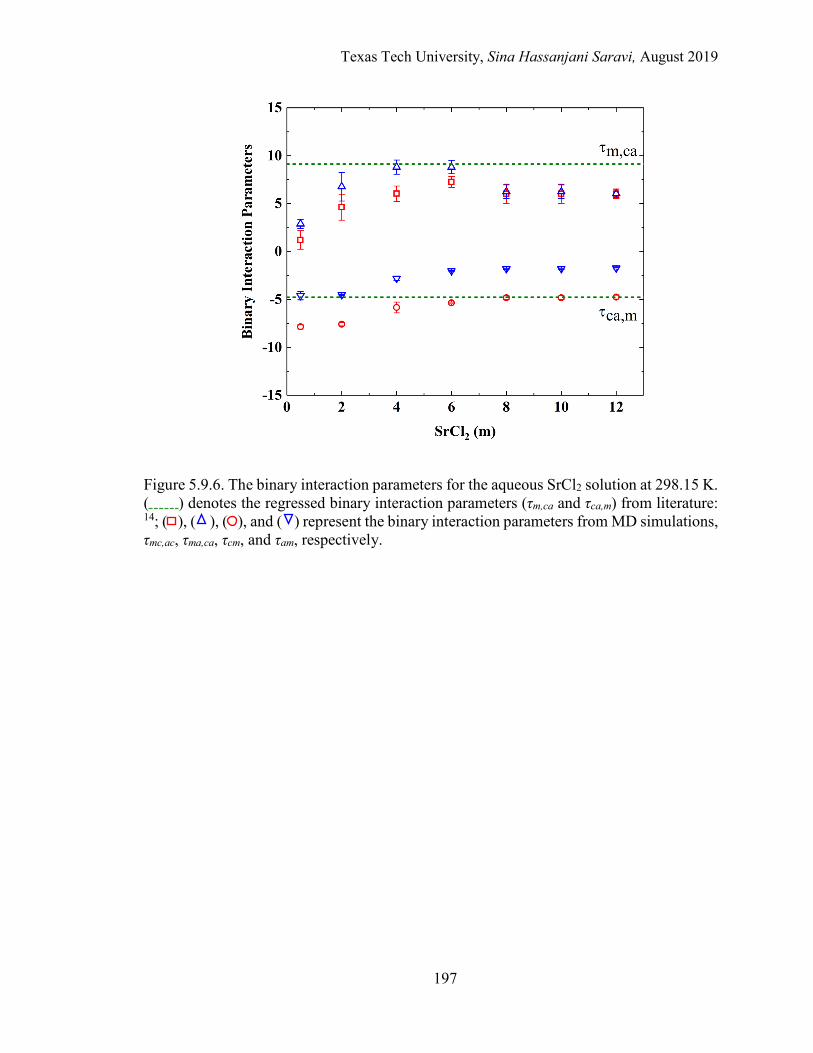
Texas Tech University, Sina Hassanjani Saravi, August 2019
197
Figure 5.9.6. The binary interaction parameters for the aqueous SrCl2 solution at 298.15 K. ( ) denotes the regressed binary interaction parameters (τm,ca and τca,m) from literature: 14; ( ), ( ), ( ), and ( ) represent the binary interaction parameters from MD simulations, τmc,ac, τma,ca, τcm, and τam, respectively.

Texas Tech University, Sina Hassanjani Saravi, August 2019
198
Figure 5.9.7. The binary interaction parameters for the aqueous CaCl2 solution at 298.15 K. ( ) denotes the regressed binary interaction parameters (τm,ca and τca,m) from literature: 15; ( ), ( ), ( ), and ( ) represent the binary interaction parameters from MD simulations, τmc,ac, τma,ca, τcm, and τam, respectively.
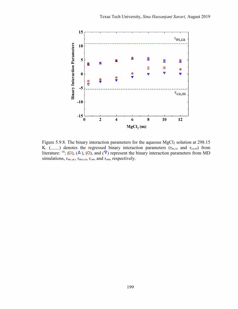
Texas Tech University, Sina Hassanjani Saravi, August 2019
199
Figure 5.9.8. The binary interaction parameters for the aqueous MgCl2 solution at 298.15 K. ( ) denotes the regressed binary interaction parameters (τm,ca and τca,m) from literature: 16; ( ), ( ), ( ), and ( ) represent the binary interaction parameters from MD simulations, τmc,ac, τma,ca, τcm, and τam, respectively.
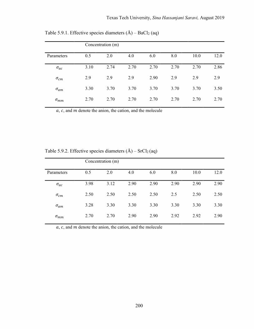
Texas Tech University, Sina Hassanjani Saravi, August 2019
200
Table 5.9.1. Effective species diameters (Å) – BaCl2 (aq)
Concentration (m)
Parameters 0.5 2.0 4.0 6.0 8.0 10.0 12.0
𝜎𝜎𝑎𝑎𝐿𝐿 3.10 2.74 2.70 2.70 2.70 2.70 2.86
𝜎𝜎𝐿𝐿𝑚𝑚 2.9 2.9 2.9 2.90 2.9 2.9 2.9
𝜎𝜎𝑎𝑎𝑚𝑚 3.30 3.70 3.70 3.70 3.70 3.70 3.50
𝜎𝜎𝑚𝑚𝑚𝑚 2.70 2.70 2.70 2.70 2.70 2.70 2.70
𝑎𝑎, 𝑐𝑐, and 𝑚𝑚 denote the anion, the cation, and the molecule
Table 5.9.2. Effective species diameters (Å) – SrCl2 (aq)
Concentration (m)
Parameters 0.5 2.0 4.0 6.0 8.0 10.0 12.0
𝜎𝜎𝑎𝑎𝐿𝐿 3.98 3.12 2.90 2.90 2.90 2.90 2.90
𝜎𝜎𝐿𝐿𝑚𝑚 2.50 2.50 2.50 2.50 2.5 2.50 2.50
𝜎𝜎𝑎𝑎𝑚𝑚 3.28 3.30 3.30 3.30 3.30 3.30 3.30
𝜎𝜎𝑚𝑚𝑚𝑚 2.70 2.70 2.90 2.90 2.92 2.92 2.90
𝑎𝑎, 𝑐𝑐, and 𝑚𝑚 denote the anion, the cation, and the molecule

Texas Tech University, Sina Hassanjani Saravi, August 2019
201
Table 5.9.3. Effective species diameters (Å) – CaCl2 (aq)
Concentration (m)
Parameters 0.5 2.0 4.0 6.0 8.0 10.0 12.0
𝜎𝜎𝑎𝑎𝐿𝐿 4.94 4.90 4.50 2.90 2.90 2.90 2.90
𝜎𝜎𝐿𝐿𝑚𝑚 2.50 2.50 2.50 2.50 2.34 2.30 2.30
𝜎𝜎𝑎𝑎𝑚𝑚 3.30 3.28 3.16 3.26 3.30 3.30 3.30
𝜎𝜎𝑚𝑚𝑚𝑚 2.70 2.90 2.90 2.90 2.90 2.90 2.90
𝑎𝑎, 𝑐𝑐, and 𝑚𝑚 denote the anion, the cation, and the molecule
Table 5.9.4. Effective species diameters (Å) – MgCl2 (aq)
Concentration (m)
Parameters 0.5 2.0 4.0 6.0 8.0 10.0 12.0
𝜎𝜎𝑎𝑎𝐿𝐿 4.50 4.50 4.50 4.50 4.48 4.30 4.30
𝜎𝜎𝐿𝐿𝑚𝑚 1.90 1.90 1.90 1.90 1.84 1.70 1.70
𝜎𝜎𝑎𝑎𝑚𝑚 3.14 3.10 3.10 3.10 3.10 3.10 3.10
𝜎𝜎𝑚𝑚𝑚𝑚 2.70 2.70 2.70 2.70 2.70 2.70 2.70
𝑎𝑎, 𝑐𝑐, and 𝑚𝑚 denote the anion, the cation, and the molecule
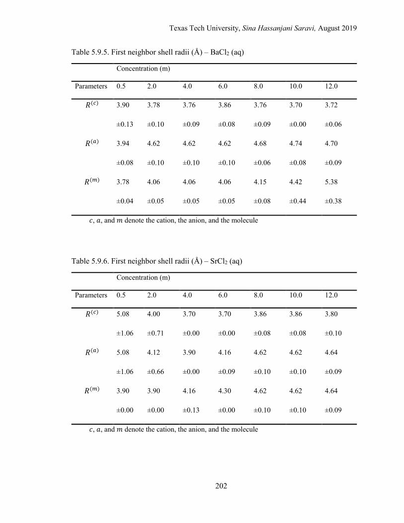
Texas Tech University, Sina Hassanjani Saravi, August 2019
202
Table 5.9.5. First neighbor shell radii (Å) – BaCl2 (aq)
Concentration (m)
Parameters 0.5 2.0 4.0 6.0 8.0 10.0 12.0
𝑅𝑅(𝐿𝐿) 3.90 3.78 3.76 3.86 3.76 3.70 3.72
±0.13 ±0.10 ±0.09 ±0.08 ±0.09 ±0.00 ±0.06
𝑅𝑅(𝑎𝑎) 3.94 4.62 4.62 4.62 4.68 4.74 4.70
±0.08 ±0.10 ±0.10 ±0.10 ±0.06 ±0.08 ±0.09
𝑅𝑅(𝑚𝑚) 3.78 4.06 4.06 4.06 4.15 4.42 5.38
±0.04 ±0.05 ±0.05 ±0.05 ±0.08 ±0.44 ±0.38
𝑐𝑐, 𝑎𝑎, and 𝑚𝑚 denote the cation, the anion, and the molecule
Table 5.9.6. First neighbor shell radii (Å) – SrCl2 (aq)
Concentration (m)
Parameters 0.5 2.0 4.0 6.0 8.0 10.0 12.0
𝑅𝑅(𝐿𝐿) 5.08 4.00 3.70 3.70 3.86 3.86 3.80
±1.06 ±0.71 ±0.00 ±0.00 ±0.08 ±0.08 ±0.10
𝑅𝑅(𝑎𝑎) 5.08 4.12 3.90 4.16 4.62 4.62 4.64
±1.06 ±0.66 ±0.00 ±0.09 ±0.10 ±0.10 ±0.09
𝑅𝑅(𝑚𝑚) 3.90 3.90 4.16 4.30 4.62 4.62 4.64
±0.00 ±0.00 ±0.13 ±0.00 ±0.10 ±0.10 ±0.09
𝑐𝑐, 𝑎𝑎, and 𝑚𝑚 denote the cation, the anion, and the molecule
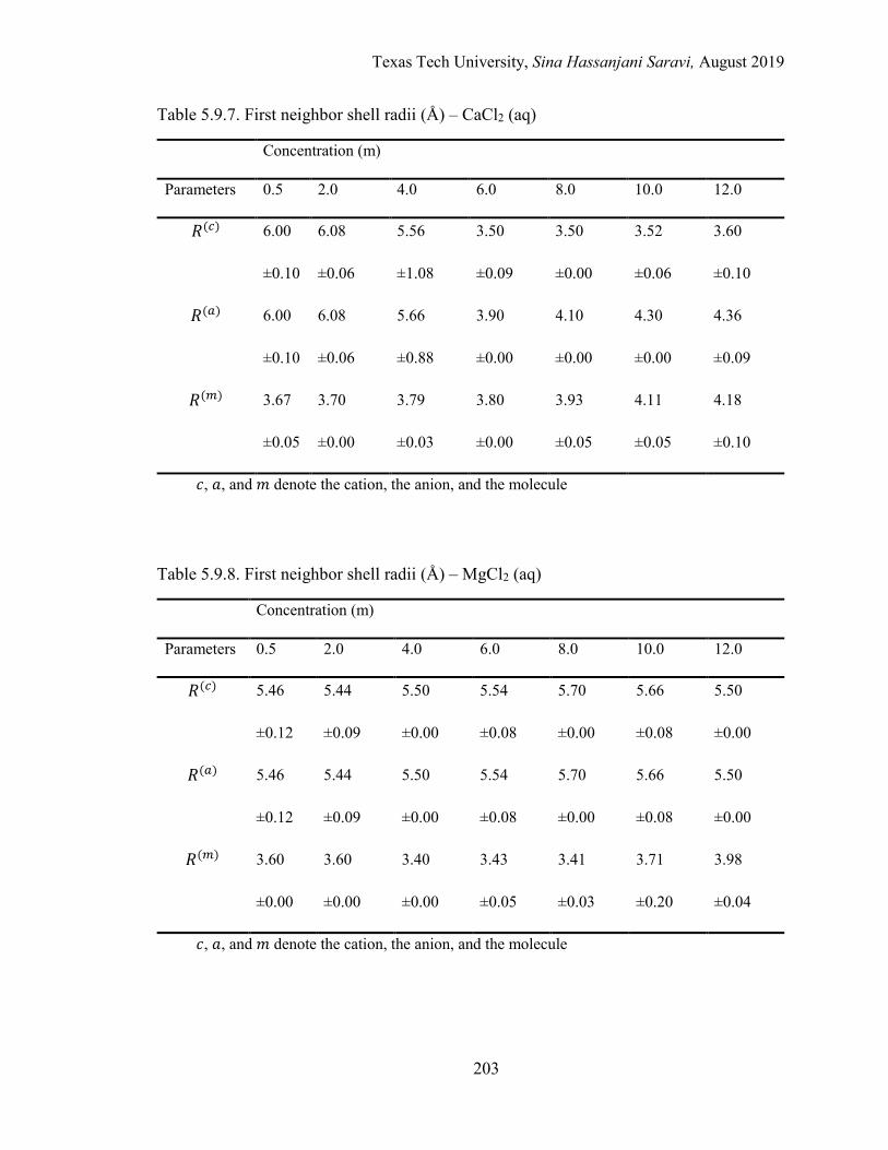
Texas Tech University, Sina Hassanjani Saravi, August 2019
203
Table 5.9.7. First neighbor shell radii (Å) – CaCl2 (aq)
Concentration (m)
Parameters 0.5 2.0 4.0 6.0 8.0 10.0 12.0
𝑅𝑅(𝐿𝐿) 6.00 6.08 5.56 3.50 3.50 3.52 3.60
±0.10 ±0.06 ±1.08 ±0.09 ±0.00 ±0.06 ±0.10
𝑅𝑅(𝑎𝑎) 6.00 6.08 5.66 3.90 4.10 4.30 4.36
±0.10 ±0.06 ±0.88 ±0.00 ±0.00 ±0.00 ±0.09
𝑅𝑅(𝑚𝑚) 3.67 3.70 3.79 3.80 3.93 4.11 4.18
±0.05 ±0.00 ±0.03 ±0.00 ±0.05 ±0.05 ±0.10
𝑐𝑐, 𝑎𝑎, and 𝑚𝑚 denote the cation, the anion, and the molecule
Table 5.9.8. First neighbor shell radii (Å) – MgCl2 (aq)
Concentration (m)
Parameters 0.5 2.0 4.0 6.0 8.0 10.0 12.0
𝑅𝑅(𝐿𝐿) 5.46 5.44 5.50 5.54 5.70 5.66 5.50
±0.12 ±0.09 ±0.00 ±0.08 ±0.00 ±0.08 ±0.00
𝑅𝑅(𝑎𝑎) 5.46 5.44 5.50 5.54 5.70 5.66 5.50
±0.12 ±0.09 ±0.00 ±0.08 ±0.00 ±0.08 ±0.00
𝑅𝑅(𝑚𝑚) 3.60 3.60 3.40 3.43 3.41 3.71 3.98
±0.00 ±0.00 ±0.00 ±0.05 ±0.03 ±0.20 ±0.04
𝑐𝑐, 𝑎𝑎, and 𝑚𝑚 denote the cation, the anion, and the molecule
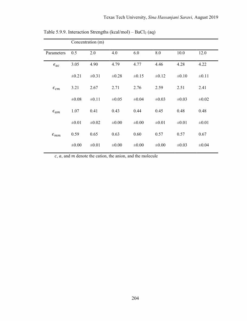
Texas Tech University, Sina Hassanjani Saravi, August 2019
204
Table 5.9.9. Interaction Strengths (kcal/mol) – BaCl2 (aq)
Concentration (m)
Parameters 0.5 2.0 4.0 6.0 8.0 10.0 12.0
𝜖𝜖𝑎𝑎𝐿𝐿 3.05 4.90 4.79 4.77 4.46 4.28 4.22
±0.21 ±0.31 ±0.28 ±0.15 ±0.12 ±0.10 ±0.11
𝜖𝜖𝐿𝐿𝑚𝑚 3.21 2.67 2.71 2.76 2.59 2.51 2.41
±0.08 ±0.11 ±0.05 ±0.04 ±0.03 ±0.03 ±0.02
𝜖𝜖𝑎𝑎𝑚𝑚 1.07 0.41 0.43 0.44 0.45 0.48 0.48
±0.01 ±0.02 ±0.00 ±0.00 ±0.01 ±0.01 ±0.01
𝜖𝜖𝑚𝑚𝑚𝑚 0.59 0.65 0.63 0.60 0.57 0.57 0.67
±0.00 ±0.01 ±0.00 ±0.00 ±0.00 ±0.03 ±0.04
𝑐𝑐, 𝑎𝑎, and 𝑚𝑚 denote the cation, the anion, and the molecule
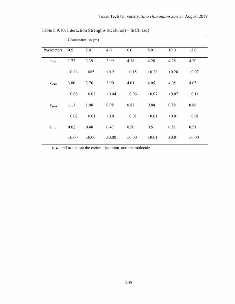
Texas Tech University, Sina Hassanjani Saravi, August 2019
205
Table 5.9.10. Interaction Strengths (kcal/mol) – SrCl2 (aq)
Concentration (m)
Parameters 0.5 2.0 4.0 6.0 8.0 10.0 12.0
𝜖𝜖𝑎𝑎𝐿𝐿 1.73 3.39 3.99 4.36 4.28 4.28 4.20
±0.86 ±085 ±0.21 ±0.15 ±0.28 ±0.28 ±0.07
𝜖𝜖𝐿𝐿𝑚𝑚 3.80 3.76 3.90 4.01 4.05 4.05 4.05
±0.08 ±0.07 ±0.04 ±0.06 ±0.07 ±0.07 ±0.11
𝜖𝜖𝑎𝑎𝑚𝑚 1.13 1.08 0.98 0.87 0.88 0.88 0.86
±0.02 ±0.01 ±0.01 ±0.01 ±0.01 ±0.01 ±0.01
𝜖𝜖𝑚𝑚𝑚𝑚 0.62 0.48 0.47 0.50 0.51 0.51 0.51
±0.00 ±0.00 ±0.00 ±0.00 ±0.01 ±0.01 ±0.00
𝑐𝑐, 𝑎𝑎, and 𝑚𝑚 denote the cation, the anion, and the molecule
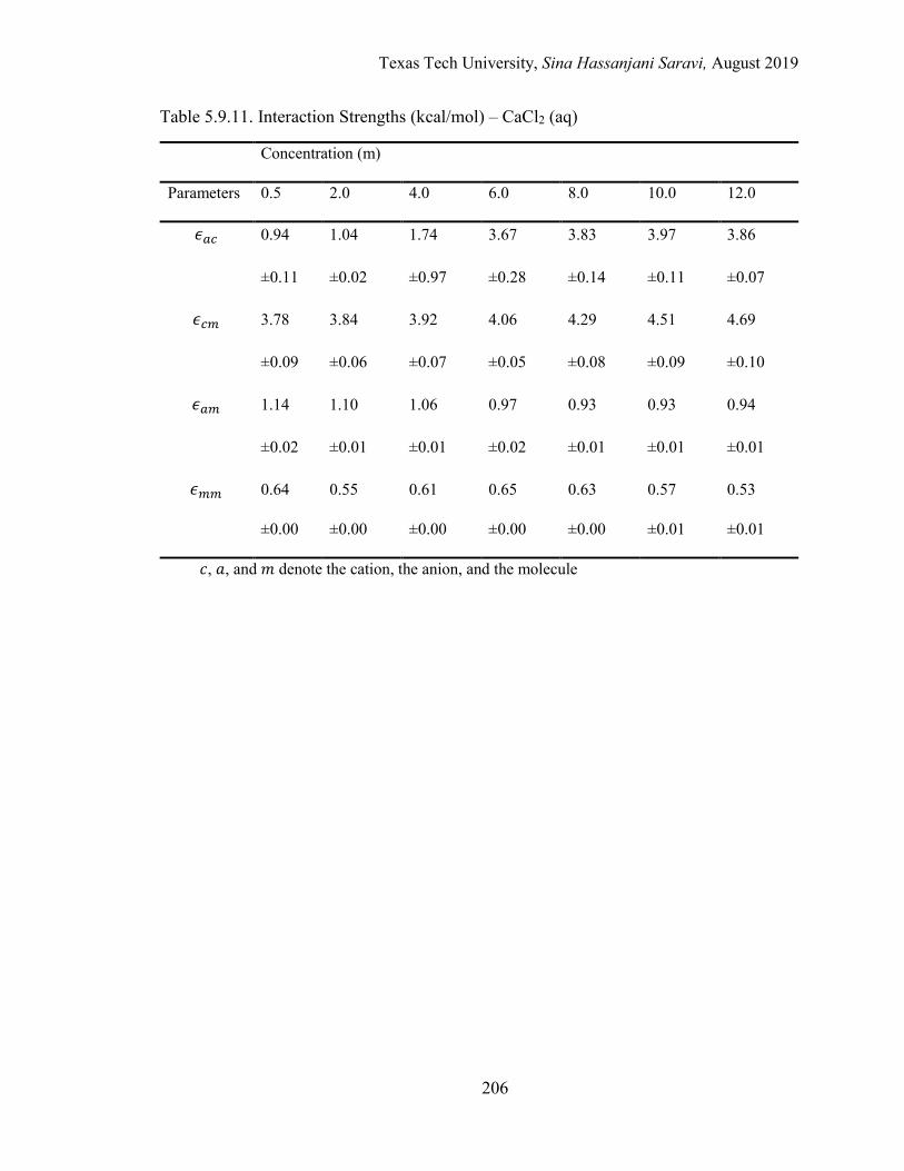
Texas Tech University, Sina Hassanjani Saravi, August 2019
206
Table 5.9.11. Interaction Strengths (kcal/mol) – CaCl2 (aq)
Concentration (m)
Parameters 0.5 2.0 4.0 6.0 8.0 10.0 12.0
𝜖𝜖𝑎𝑎𝐿𝐿 0.94 1.04 1.74 3.67 3.83 3.97 3.86
±0.11 ±0.02 ±0.97 ±0.28 ±0.14 ±0.11 ±0.07
𝜖𝜖𝐿𝐿𝑚𝑚 3.78 3.84 3.92 4.06 4.29 4.51 4.69
±0.09 ±0.06 ±0.07 ±0.05 ±0.08 ±0.09 ±0.10
𝜖𝜖𝑎𝑎𝑚𝑚 1.14 1.10 1.06 0.97 0.93 0.93 0.94
±0.02 ±0.01 ±0.01 ±0.02 ±0.01 ±0.01 ±0.01
𝜖𝜖𝑚𝑚𝑚𝑚 0.64 0.55 0.61 0.65 0.63 0.57 0.53
±0.00 ±0.00 ±0.00 ±0.00 ±0.00 ±0.01 ±0.01
𝑐𝑐, 𝑎𝑎, and 𝑚𝑚 denote the cation, the anion, and the molecule
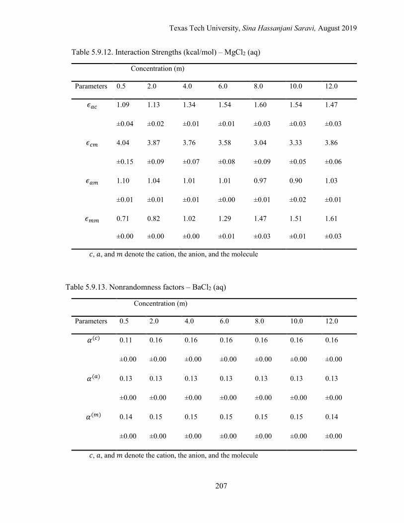
Texas Tech University, Sina Hassanjani Saravi, August 2019
207
Table 5.9.12. Interaction Strengths (kcal/mol) – MgCl2 (aq)
Concentration (m)
Parameters 0.5 2.0 4.0 6.0 8.0 10.0 12.0
𝜖𝜖𝑎𝑎𝐿𝐿 1.09 1.13 1.34 1.54 1.60 1.54 1.47
±0.04 ±0.02 ±0.01 ±0.01 ±0.03 ±0.03 ±0.03
𝜖𝜖𝐿𝐿𝑚𝑚 4.04 3.87 3.76 3.58 3.04 3.33 3.86
±0.15 ±0.09 ±0.07 ±0.08 ±0.09 ±0.05 ±0.06
𝜖𝜖𝑎𝑎𝑚𝑚 1.10 1.04 1.01 1.01 0.97 0.90 1.03
±0.01 ±0.01 ±0.01 ±0.00 ±0.01 ±0.02 ±0.01
𝜖𝜖𝑚𝑚𝑚𝑚 0.71 0.82 1.02 1.29 1.47 1.51 1.61
±0.00 ±0.00 ±0.00 ±0.01 ±0.03 ±0.01 ±0.03
𝑐𝑐, 𝑎𝑎, and 𝑚𝑚 denote the cation, the anion, and the molecule
Table 5.9.13. Nonrandomness factors – BaCl2 (aq)
Concentration (m)
Parameters 0.5 2.0 4.0 6.0 8.0 10.0 12.0
𝛼𝛼(𝐿𝐿) 0.11 0.16 0.16 0.16 0.16 0.16 0.16
±0.00 ±0.00 ±0.00 ±0.00 ±0.00 ±0.00 ±0.00
𝛼𝛼(𝑎𝑎) 0.13 0.13 0.13 0.13 0.13 0.13 0.13
±0.00 ±0.00 ±0.00 ±0.00 ±0.00 ±0.00 ±0.00
𝛼𝛼(𝑚𝑚) 0.14 0.15 0.15 0.15 0.15 0.15 0.14
±0.00 ±0.00 ±0.00 ±0.00 ±0.00 ±0.00 ±0.00
𝑐𝑐, 𝑎𝑎, and 𝑚𝑚 denote the cation, the anion, and the molecule

Texas Tech University, Sina Hassanjani Saravi, August 2019
208
Table 5.9.14. Nonrandomness factors – SrCl2 (aq)
Concentration (m)
Parameters 0.5 2.0 4.0 6.0 8.0 10.0 12.0
𝛼𝛼(𝐿𝐿) 0.08 0.11 0.13 0.13 0.15 0.14 0.15
±0.00 ±0.00 ±0.00 ±0.00 ±0.01 ±0.00 ±0.01
𝛼𝛼(𝑎𝑎) 0.08 0.12 0.12 0.11 0.12 0.11 0.12
±0.01 ±0.01 ±0.01 ±0.01 ±0.00 ±0.00 ±0.00
𝛼𝛼(𝑚𝑚) 0.14 0.13 0.13 0.13 0.14 0.13 0.13
±0.00 ±0.00 ±0.00 ±0.00 ±0.00 ±0.00 ±0.00
𝑐𝑐, 𝑎𝑎, and 𝑚𝑚 denote the cation, the anion, and the molecule
Table 5.9.15. Nonrandomness factors – CaCl2 (aq)
Concentration (m)
Parameters 0.5 2.0 4.0 6.0 8.0 10.0 12.0
𝛼𝛼(𝐿𝐿) 0.03 0.03 0.05 0.14 0.14 0.15 0.16
±0.00 ±0.00 ±0.04 ±0.00 ±0.00 ±0.00 ±0.00
𝛼𝛼(𝑎𝑎) 0.03 0.03 0.05 0.12 0.12 0.11 0.11
±0.00 ±0.00 ±0.04 ±0.00 ±0.00 ±0.00 ±0.00
𝛼𝛼(𝑚𝑚) 0.15 0.14 0.13 0.13 0.13 0.14 0.14
±0.00 ±0.00 ±0.00 ±0.00 ±0.00 ±0.00 ±0.00
𝑐𝑐, 𝑎𝑎, and 𝑚𝑚 denote the cation, the anion, and the molecule

Texas Tech University, Sina Hassanjani Saravi, August 2019
209
Table 5.9.16. Nonrandomness factors – MgCl2 (aq)
Concentration (m)
Parameters 0.5 2.0 4.0 6.0 8.0 10.0 12.0
𝛼𝛼(𝐿𝐿) 0.04 0.04 0.04 0.05 0.05 0.05 0.05
±0.00 ±0.00 ±0.00 ±0.00 ±0.00 ±0.00 ±0.00
𝛼𝛼(𝑎𝑎) 0.04 0.04 0.04 0.04 0.04 0.04 0.04
±0.00 ±0.00 ±0.00 ±0.00 ±0.00 ±0.00 ±0.00
𝛼𝛼(𝑚𝑚) 0.15 0.14 0.16 0.15 0.15 0.15 0.15
±0.00 ±0.00 ±0.00 ±0.00 ±0.00 ±0.00 ±0.00
𝑐𝑐, 𝑎𝑎, and 𝑚𝑚 denote the cation, the anion, and the molecule
Table 5.9.17. Binary interaction parameters – BaCl2 (aq)
Concentration (m)
Parameters 0.5 2.0 4.0 6.0 8.0 10.0 12.0
𝜏𝜏𝑚𝑚𝐿𝐿,𝑎𝑎𝐿𝐿 1.76 5.71 4.45 3.91 3.93 3.83 6.59
±0.78 ±2.17 ±0.74 ±0.37 ±0.65 ±0.33 ±1.23
𝜏𝜏𝑚𝑚𝑎𝑎,𝐿𝐿𝑎𝑎 7.27 6.88 6.22 6.15 5.36 4.76 6.37
±0.91 ±0.73 ±0.49 ±0.44 ±0.29 ±0.29 ±0.69
𝜏𝜏𝐿𝐿𝑚𝑚 -10.41 -6.58 -6.79 -6.99 -6.14 -5.09 -2.59
±0.20 ±0.44 ±0.23 ±0.28 ±0.32 ±1.01 ±0.87
𝜏𝜏𝑎𝑎𝑚𝑚 -4.16 -0.97 -1.18 -1.31 -1.35 -1.32 -0.44
±0.18 ±0.09 ±0.05 ±0.04 ±0.07 ±0.08 ±0.03
𝑐𝑐, 𝑎𝑎, and 𝑚𝑚 denote the cation, the anion, and the molecule
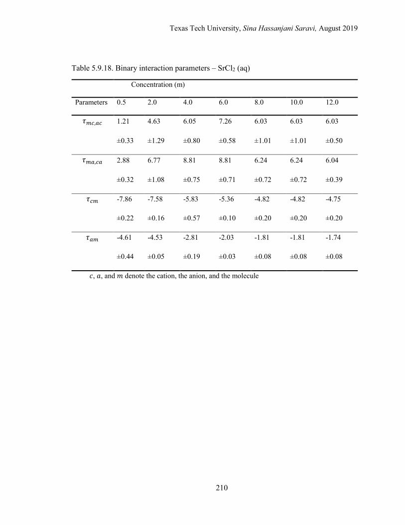
Texas Tech University, Sina Hassanjani Saravi, August 2019
210
Table 5.9.18. Binary interaction parameters – SrCl2 (aq)
Concentration (m)
Parameters 0.5 2.0 4.0 6.0 8.0 10.0 12.0
𝜏𝜏𝑚𝑚𝐿𝐿,𝑎𝑎𝐿𝐿 1.21 4.63 6.05 7.26 6.03 6.03 6.03
±0.33 ±1.29 ±0.80 ±0.58 ±1.01 ±1.01 ±0.50
𝜏𝜏𝑚𝑚𝑎𝑎,𝐿𝐿𝑎𝑎 2.88 6.77 8.81 8.81 6.24 6.24 6.04
±0.32 ±1.08 ±0.75 ±0.71 ±0.72 ±0.72 ±0.39
𝜏𝜏𝐿𝐿𝑚𝑚 -7.86 -7.58 -5.83 -5.36 -4.82 -4.82 -4.75
±0.22 ±0.16 ±0.57 ±0.10 ±0.20 ±0.20 ±0.20
𝜏𝜏𝑎𝑎𝑚𝑚 -4.61 -4.53 -2.81 -2.03 -1.81 -1.81 -1.74
±0.44 ±0.05 ±0.19 ±0.03 ±0.08 ±0.08 ±0.08
𝑐𝑐, 𝑎𝑎, and 𝑚𝑚 denote the cation, the anion, and the molecule
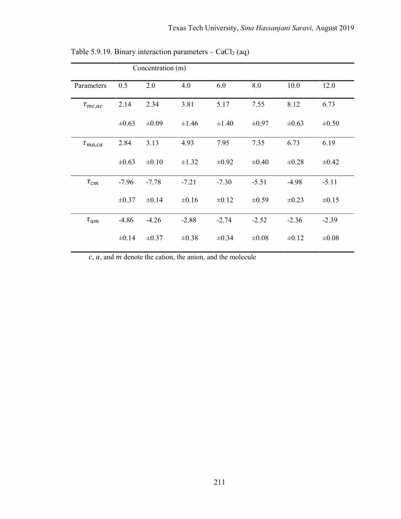
Texas Tech University, Sina Hassanjani Saravi, August 2019
211
Table 5.9.19. Binary interaction parameters – CaCl2 (aq)
Concentration (m)
Parameters 0.5 2.0 4.0 6.0 8.0 10.0 12.0
𝜏𝜏𝑚𝑚𝐿𝐿,𝑎𝑎𝐿𝐿 2.14 2.34 3.81 5.17 7.55 8.12 6.73
±0.63 ±0.09 ±1.46 ±1.40 ±0.97 ±0.63 ±0.50
𝜏𝜏𝑚𝑚𝑎𝑎,𝐿𝐿𝑎𝑎 2.84 3.13 4.93 7.95 7.35 6.73 6.19
±0.63 ±0.10 ±1.32 ±0.92 ±0.40 ±0.28 ±0.42
𝜏𝜏𝐿𝐿𝑚𝑚 -7.96 -7.78 -7.21 -7.30 -5.51 -4.98 -5.11
±0.37 ±0.14 ±0.16 ±0.12 ±0.59 ±0.23 ±0.15
𝜏𝜏𝑎𝑎𝑚𝑚 -4.86 -4.26 -2.88 -2.74 -2.52 -2.36 -2.39
±0.14 ±0.37 ±0.38 ±0.34 ±0.08 ±0.12 ±0.08
𝑐𝑐, 𝑎𝑎, and 𝑚𝑚 denote the cation, the anion, and the molecule
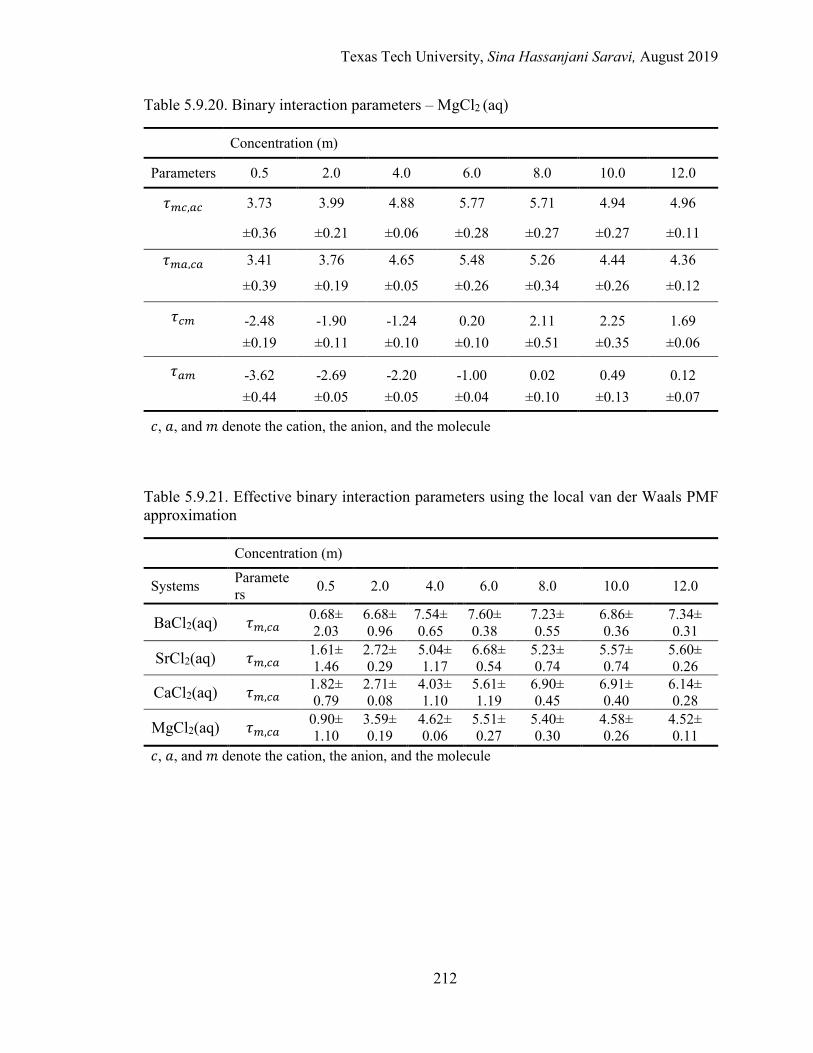
Texas Tech University, Sina Hassanjani Saravi, August 2019
212
Table 5.9.20. Binary interaction parameters – MgCl2 (aq)
Concentration (m)
Parameters 0.5 2.0 4.0 6.0 8.0 10.0 12.0
𝜏𝜏𝑚𝑚𝐿𝐿,𝑎𝑎𝐿𝐿 3.73 3.99 4.88 5.77 5.71 4.94 4.96
±0.36 ±0.21 ±0.06 ±0.28 ±0.27 ±0.27 ±0.11
𝜏𝜏𝑚𝑚𝑎𝑎,𝐿𝐿𝑎𝑎 3.41 3.76 4.65 5.48 5.26 4.44 4.36
±0.39 ±0.19 ±0.05 ±0.26 ±0.34 ±0.26 ±0.12
𝜏𝜏𝐿𝐿𝑚𝑚 -2.48 -1.90 -1.24 0.20 2.11 2.25 1.69 ±0.19 ±0.11 ±0.10 ±0.10 ±0.51 ±0.35 ±0.06
𝜏𝜏𝑎𝑎𝑚𝑚 -3.62 -2.69 -2.20 -1.00 0.02 0.49 0.12 ±0.44 ±0.05 ±0.05 ±0.04 ±0.10 ±0.13 ±0.07
𝑐𝑐, 𝑎𝑎, and 𝑚𝑚 denote the cation, the anion, and the molecule
Table 5.9.21. Effective binary interaction parameters using the local van der Waals PMF approximation
Concentration (m)
Systems Parameters 0.5 2.0 4.0 6.0 8.0 10.0 12.0
BaCl2(aq) 𝜏𝜏𝑚𝑚,𝐿𝐿𝑎𝑎 0.68± 2.03
6.68± 0.96
7.54± 0.65
7.60± 0.38
7.23± 0.55
6.86± 0.36
7.34± 0.31
SrCl2(aq) 𝜏𝜏𝑚𝑚,𝐿𝐿𝑎𝑎 1.61± 1.46
2.72± 0.29
5.04± 1.17
6.68± 0.54
5.23± 0.74
5.57± 0.74
5.60± 0.26
CaCl2(aq) 𝜏𝜏𝑚𝑚,𝐿𝐿𝑎𝑎 1.82± 0.79
2.71± 0.08
4.03± 1.10
5.61± 1.19
6.90± 0.45
6.91± 0.40
6.14± 0.28
MgCl2(aq) 𝜏𝜏𝑚𝑚,𝐿𝐿𝑎𝑎 0.90± 1.10
3.59± 0.19
4.62± 0.06
5.51± 0.27
5.40± 0.30
4.58± 0.26
4.52± 0.11
𝑐𝑐, 𝑎𝑎, and 𝑚𝑚 denote the cation, the anion, and the molecule
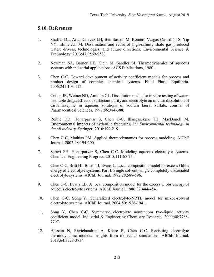
Texas Tech University, Sina Hassanjani Saravi, August 2019
213
5.10. References
1. Shaffer DL, Arias Chavez LH, Ben-Sasson M, Romero-Vargas Castrillón S, Yip NY, Elimelech M. Desalination and reuse of high-salinity shale gas produced water: drivers, technologies, and future directions. Environmental Science & Technology. 2013;47:9569-9583.
2. Newman SA, Barner HE, Klein M, Sandler SI. Thermodynamics of aqueous systems with industrial applications: ACS Publications, 1980.
3. Chen C-C. Toward development of activity coefficient models for process and product design of complex chemical systems. Fluid Phase Equilibria. 2006;241:103-112.
4. Crison JR, Weiner ND, Amidon GL. Dissolution media for in vitro testing of water‐insoluble drugs: Effect of surfactant purity and electrolyte on in vitro dissolution of carbamazepine in aqueous solutions of sodium lauryl sulfate. Journal of Pharmaceutical Sciences. 1997;86:384-388.
5. Reible DD, Honarparvar S, Chen C-C, Illangasekare TH, MacDonell M. Environmental impacts of hydraulic fracturing. In: Environmental technology in the oil industry. Springer; 2016:199-219.
6. Chen C-C, Mathias PM. Applied thermodynamics for process modeling. AIChE Journal. 2002;48:194-200.
7. Saravi SH, Honarparvar S, Chen C-C. Modeling aqueous electrolyte systems. Chemical Engineering Progress. 2015;111:65-75.
8. Chen C-C, Britt HI, Boston J, Evans L. Local composition model for excess Gibbs energy of electrolyte systems. Part I: Single solvent, single completely dissociated electrolyte systems. AIChE Journal. 1982;28:588-596.
9. Chen C-C, Evans LB. A local composition model for the excess Gibbs energy of aqueous electrolyte systems. AIChE Journal. 1986;32:444-454.
10. Chen C-C, Song Y. Generalized electrolyte‐NRTL model for mixed‐solvent electrolyte systems. AIChE Journal. 2004;50:1928-1941.
11. Song Y, Chen C-C. Symmetric electrolyte nonrandom two-liquid activity coefficient model. Industrial & Engineering Chemistry Research. 2009;48:7788-7797.
12. Hossain N, Ravichandran A, Khare R, Chen C-C. Revisiting electrolyte thermodynamic models: Insights from molecular simulations. AIChE Journal. 2018;64:3728-3734.
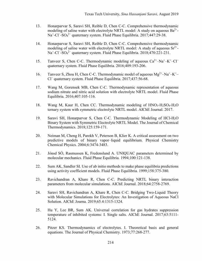
Texas Tech University, Sina Hassanjani Saravi, August 2019
214
13. Honarparvar S, Saravi SH, Reible D, Chen C-C. Comprehensive thermodynamic modeling of saline water with electrolyte NRTL model: A study on aqueous Ba2+-Na+-Cl−-SO4
2− quaternary system. Fluid Phase Equilibria. 2017;447:29-38.
14. Honarparvar S, Saravi SH, Reible D, Chen C-C. Comprehensive thermodynamic modeling of saline water with electrolyte NRTL model: A study of aqueous Sr2+-Na+-Cl−-SO4
2− quaternary system. Fluid Phase Equilibria. 2018;470:221-231.
15. Tanveer S, Chen C-C. Thermodynamic modeling of aqueous Ca2+–Na+–K+–Cl− quaternary system. Fluid Phase Equilibria. 2016;409:193-206.
16. Tanveer S, Zhou H, Chen C-C. Thermodynamic model of aqueous Mg2+–Na+–K+–Cl− quaternary system. Fluid Phase Equilibria. 2017;437:56-68.
17. Wang M, Gorensek MB, Chen C-C. Thermodynamic representation of aqueous sodium nitrate and nitric acid solution with electrolyte NRTL model. Fluid Phase Equilibria. 2016;407:105-116.
18. Wang M, Kaur H, Chen CC. Thermodynamic modeling of HNO3‐H2SO4‐H2O ternary system with symmetric electrolyte NRTL model. AIChE Journal. 2017.
19. Saravi SH, Honarparvar S, Chen C-C. Thermodynamic Modeling of HCl-H2O Binary System with Symmetric Electrolyte NRTL Model. The Journal of Chemical Thermodynamics. 2018;125:159-171.
20. Neiman M, Cheng H, Parekh V, Peterson B, Klier K. A critical assessment on two predictive models of binary vapor–liquid equilibrium. Physical Chemistry Chemical Physics. 2004;6:3474-3483.
21. Jónsd SÓ, Rasmussen K, Fredenslund A. UNIQUAC parameters determined by molecular mechanics. Fluid Phase Equilibria. 1994;100:121-138.
22. Sum AK, Sandler SI. Use of ab initio methods to make phase equilibria predictions using activity coefficient models. Fluid Phase Equilibria. 1999;158:375-380.
23. Ravichandran A, Khare R, Chen C-C. Predicting NRTL binary interaction parameters from molecular simulations. AIChE Journal. 2018;64:2758-2769.
24. Saravi SH, Ravichandran A, Khare R, Chen C-C. Bridging Two-Liquid Theory with Molecular Simulations for Electrolytes: An Investigation of Aqueous NaCl Solution. AIChE Journa. 2019;65.4:1315-1324.
25. Hu Y, Lee BR, Sum AK. Universal correlation for gas hydrates suppression temperature of inhibited systems: I. Single salts. AIChE Journal. 2017;63:5111-5124.
26. Pitzer KS. Thermodynamics of electrolytes. I. Theoretical basis and general equations. The Journal of Physical Chemistry. 1973;77:268-277.
Texas Tech University, Sina Hassanjani Saravi, August 2019
215
27. Pitzer KS, Mayorga G. Thermodynamics of electrolytes. II. Activity and osmotic coefficients for strong electrolytes with one or both ions univalent. The Journal of Physical Chemistry. 1973;77:2300-2308.
28. Pitzer KS. Electrolytes. From dilute solutions to fused salts. Journal of the American Chemical Society. 1980;102:2902-2906.
29. Renon H, Prausnitz JM. Local compositions in thermodynamic excess functions for liquid mixtures. AIChE journal. 1968;14:135-144.
30. Brandani V, Prausnitz J. Two-fluid theory and thermodynamic properties of liquid mixtures: General theory. Proceedings of the National Academy of Sciences. 1982;79:4506-4509.
31. Kerley GI. Perturbation theory and the thermodynamic properties of fluids. I. General theory. The Journal of Chemical Physics. 1980;73:469-477.
32. Perera A, Sokolić F, Zoranić L. Microstructure of neat alcohols. Physical Review E. 2007;75:060502.
33. Chowdhuri S, Chandra A. Hydration structure and diffusion of ions in supercooled water: Ion size effects. The Journal of chemical physics. 2003;118:9719-9725.
34. McQuarrie DA, McQuarrie DA, McQuarrie DA, McQuarrie DA. Statistical thermodynamics: Harper & Row New York, 1973.
35. Chandler D. Introduction to modern statistical mechanics. Introduction to Modern Statistical Mechanics, by David Chandler, pp 288 Foreword by David Chandler Oxford University Press, Sep 1987 ISBN-10: 0195042778 ISBN-13: 9780195042771. 1987:288.
36. Guggenheim EA. Mixtures: the theory of the equilibrium properties of some simple classes of mixtures, solutions and alloys: Clarendon Press, 1952.
37. Plimpton S. Fast parallel algorithms for short-range molecular dynamics. Journal of Computational Physics. 1995;117:1-19.
38. Shinoda W, Shiga M, Mikami M. Rapid estimation of elastic constants by molecular dynamics simulation under constant stress. Physical Review B. 2004;69:134103.
39. Hockney R, Eastwood J. Computer Simulation Using Particles (Adam Hilger, New York). 1989.
40. Berendsen H, Grigera J, Straatsma T. The missing term in effective pair potentials. Journal of Physical Chemistry. 1987;91:6269-6271.
Texas Tech University, Sina Hassanjani Saravi, August 2019
216
41. Naleem N, Bentenitis N, Smith PE. A Kirkwood-Buff derived force field for alkaline earth halide salts. The Journal of Chemical Physics. 2018;148:222828.
42. Mester Z, Panagiotopoulos AZ. Temperature-dependent solubilities and mean ionic activity coefficients of alkali halides in water from molecular dynamics simulations. The Journal of chemical physics. 2015;143:044505.
43. Timko J, Bucher D, Kuyucak S. Dissociation of NaCl in water from ab initio molecular dynamics simulations. The Journal of Chemical Physics. 2010;132:114510.
44. Gong Z, Sun H. A Coarse-Grained Force Field Parameterized for MgCl2 and CaCl2 Aqueous Solutions. Journal of chemical information and modeling. 2017;57:1599-1608.
45. Bruni F, Imberti S, Mancinelli R, Ricci M. Aqueous solutions of divalent chlorides: ions hydration shell and water structure. The Journal of chemical physics. 2012;136:064520.
46. Callahan KM, Casillas-Ituarte NN, Roeselová M, Allen HC, Tobias DJ. Solvation of magnesium dication: molecular dynamics simulation and vibrational spectroscopic study of magnesium chloride in aqueous solutions. The Journal of Physical Chemistry A. 2010;114:5141-5148.
47. Robinson RA, Stokes RH. Electrolyte solutions: Courier Corporation, 2002.

Texas Tech University, Sina Hassanjani Saravi, August 2019
217
CHAPTER 6. CONCLUSIONS AND FUTURE WORK
This dissertation presents an in-depth study of the thermodynamic modeling of
electrolyte solutions from both macroscopic classical models and statistical mechanical
approaches. Due to the ubiquitous presence of the electrolytes in many industrial and
environmental processes, it is essential for the engineers to have access to the reliable and
rigorous thermodynamic models. Such models enable rapid predictions of phase equilibria,
calorimetric, and speciation properties to support mass and energy balance calculations.
Predictive models based on various statistical mechanical theories, by employing
molecular simulations, provide insight into the liquid structure and free energy information
of the solution, from which the macroscopic thermophysical properties can be calculated.
Although molecular simulations make it possible to understand the underlying phenomena
taking place at the microscopic molecular level, the expensive computational time prevents
the rapid predictions of properties, thus creating a bottleneck in directly applying such
methods in process simulations for industrial applications. Correlative models, on the other
hand, have been widely applied in modeling the electrolytes in industry, owing to their
versatility and rapid computational procedures. In particular, the eNRTL model has shown
to be successful in predicting thermophysical properties of wide variety of electrolyte
solutions with only two adjustable ‘binary interaction parameters’ per pair of species. The
binary interaction parameters (𝜏𝜏) demonstrate the favorable or unfavorable nature of the
interactions between any pair of entities in the solution.
In the first part of this dissertation, the eNRTL model has been applied in several
electrolyte solutions and the adjustable 𝜏𝜏 parameters have been quantified from regression
Texas Tech University, Sina Hassanjani Saravi, August 2019
218
of various experimental data. A comprehensive thermodynamic framework is developed
for the HCl-H2O binary system which predicts accurately the VLE and LLE properties, as
well as the calorimetric properties such as excess enthalpy and heat capacity, within the
entire concentration range of acid and temperatures up to 400 K. The model has also been
applied to describe the aqueous BaCl2 solution and the aqueous quaternary solution of Na+-
Ba2+-Cl--SO42-, as part of the investigation of the scale precipitation phenomena in oil and
gas industry.
The binary interaction parameters of eNRTL have been conventionally identified from
regression of the experimental data. However, relaying merely on regression could
potentially cause a number of drawbacks, including the lack of available experimental data.
Also, selecting physically relevant parameters could be ambiguous as in most cases the
regression procedures fail to result in a unique set of parameters. To overcome these issues
and to expand the applicability of the model, a new statistical mechanical framework has
been established wherein the interaction parameters are described in terms of the size of
the species, the size of the local solvation shells, and the local interaction energies between
the particles. All of these physical quantities are obtained via MD simulations and potential
of mean force (PMF) free energy calculations. In order to test the validity of the proposed
approach, several electrolyte solutions including aqueous NaCl, BaCl2, SrCl2, CaCl2, and
MgCl2 solutions have been selected as model systems. The results for the binary interaction
parameters from the MD simulations are in good agreement with their counterpart from
regression. The model parameters from MD were then used in predicting a number of
essential thermodynamic properties such as mean ionic activity coefficient, excess Gibbs
Texas Tech University, Sina Hassanjani Saravi, August 2019
219
free energy, and vapor pressure, all of which demonstrated satisfactory agreement with
predictions from regression.
Overall, the results demonstrated that the eNRTL model can be rendered completely
predictive which enhances its feasibility for use in industry. Also, the established
methodology can help guide the regression procedure to select physically meaningful
parameters. This study lays the groundwork for connecting the classical macroscopic
models to their underlying statistical mechanics, and hence helps distinguish the correlative
models with strong physical background from the unsubstantiated empirical models.
Systematic studies have to be carried out to expand the applicability of the approach
toward building a comprehensive yet inexpensive theoretical framework and simulation
tool for chemical engineers. An example of the possible future research directions in this
area is studying the temperature dependence of the binary interaction parameters from
molecular simulations. Note that most of the classical force field parameters that are used
in molecular simulations are known to be valid up to only moderately higher temperatures
(~ 60 ºC). Furthermore, the challenges still exist to improve the predictions of mean ionic
activity coefficients which are highly sensitive to the slight changes in the quantity of the
𝜏𝜏 parameters. More accurate and exact PMF calculations could potentially improve the
results, especially if the free energy profile is taken explicitly into the formulations, in lieu
of the simplistic assumption of projecting the PMF onto a square-well type. Finally, the
hydration of the ionic species with high charge densities should be taken into account by
considering the hydrated complex ions formed in the aqueous solutions as united particles.
All of these possible improvements could significantly enhance the versatility of the

Texas Tech University, Sina Hassanjani Saravi, August 2019
220
established methodology, thus providing a new horizon to capture, explain, and model the
complex behavior of the electrolyte solutions.