THERMODYNAMIC PROPERTIES OF AQUEOUS SODIUM

CHLORIDE SOLUTIONS FROM 32 TO 350°F

By

JAMES CHIA-SAN CHOU ii

Bachelor of Science National Institute of Technology

Chungking, China 1941

Master of Science Georgia Institute of Technology

Atlanta, Georgia 1949

Submitted to the Faculty of the Graduate College of the Oklahoma State University

in partial fulfillment of the requirements for the Degree of

DOCTOR OF PHILOSOPHY July, 1968

THERMODYNAMIC PROPERTIES OF AQUEOUS.SODIUM

CHLORIDE.• SOLUTIONS FROM 32 TO· 350 °F

·Thesis Approved:

the Graduate College

·· ACKNOWLEDGMENTS

OKLAHOMA STATE UNiVERSITY LIBRAF~y

JAN ~81969

The writer wishes to express his gratitude to the Oklahoma Water

Resources Research·Institute for the .financial support of this study and

to the University of Hawaii.for granting him a year of sabbatical leave.

He ,is indebted to his thesis adviser, Dr. •. A. M. Rowe, Jr,, for his as-

sistance and encouratement throughout this study and to Professors A •. G •

. Comer, R. L. Robinson and J •. A.· Wiebelt of the advisory committee for

offering guidance.

Appreciation must also be ·extended to the writer's wife·Lillian,

who helped in many ways, and to·Mrs •. Nancy Wolfe for typing .the manu-

·script.

696103 iii

TABLE< OF -'CONTENTS

Chapter

·I. INTRO:QUCTION •

II. VAPOR'PRESSUR~ •

Ideal Solution. Experimental·Data and Graphical.Representations

'Activity of Water.and Osmotic Coefficient ..• Vapor ·Pressure ·Equations. • • • • • •••

. III. SPECIFIC HEAT. . • • . • • • •.• .•

:Page

1

4

4 • • 0 • 5 • • 0 0 7

0 16

32

Relation of Activity to Specific Heat • . • • • 32 Specific Heats of Water and Solid· Sodium Chloride .• 36 Specific Heat at 10.Atmospheres from Oto 175°C •.•.••• 41 Experiment a 1 Data. • • • • • . • . • . • • • 48

IV. . SPECIFIC VOLUME. . • • .•.•.• • . 0 " ••. •• 53

Specific Volume of Water from Oto 150°C. 53

Experimental Determination of the Derivative (}"1,x· .••. 57

Pressure-Volume-Temperature ... concentration Relation.1 • 82

V. ENTHALPY, ENTROPY AND HEAT OF VAPORIZATION .. Enthalpy at 25 °C and 1 Atmosphere • . • • • • . Enthalpy Table. • •••••• Entropy at 25°C and 1 Atmosphere •• Entropy Table • • • • Heat of Vaporization. • • . . .

IV. SUMMAR).'.' AND CONCLUSION •

··BIBLIOGRAPHY. . .

APPENDIX A - -- LI~T OF SYMBOLS . •

0 86

86 87

0 • 95 96 98

.108

• .113

0118

APPENDIX B·- FORTRAN ARITHMETIC FUNCTIONS FOR.VAPOR PRESSURE,_HEAT OF VAPORIZATION, SPECIFIC VOI,.UME, :F;NTHALPY·AND ENTROPY ••• 120

iv

LIST OF TABLES

Table ·Page

I. Vapor ·Pressure Lowering Ratio, (p~ - ·p1 ) /p1x2 6

II. Activities of Water at · 1 Atmosphere·. • • . fl . .•.. 12

III. Activities of Water at 10 Atmospheres 17

·IV. Activities of Water as Determined from Vapor·Pressure Data •. 24

v. Vapor Pressure of.Water ..•. , • II e ~ • 0 e O O 28

VI. Comparison of Experimental Data on Vapor Pressure with Calcctlated Values . . . . , • • . . 29

VII. Enthalpy of•Saturated Water • 37

VIII. Specific Heat of Water. . 39

IX. Concentration of.SodiumChloride in.Saturated $olution. . 44

· X. Constant-Pressure .. Specific Heat of· Solution at .. lQ. Atmospheres in Calories per Gram per Pegree Centigrade ... , •..... 46

XI. Comparison of Measured•Values of·Specific Heat with . Calculated· Values . . .

: XII. Specific ·VC?lullle of Water. .

XIII. Difference of Volume Change Between the Two Experimental

. 50

55

Conditions, t:N in Cubic Oentillleter .• , •• , .• 62

·xrv. Coefficients a and b of Equation (4-2). • 66

XV. Pilat ion of Vessel Subjected to Internal Pressure at 72 °F • · 68

XVI. Thermal Expansion of Vessel 70

'XVII. Specific Volume of Solution .. , .. , 72

· XVIII •. Values of ~)r,x in Cubic Centimeter per Gram per

.Atmosphere, Mctltiplied by .. 10,000 • . ..........•.• 75

v

Table ,Page

. XIX. Mean Compressibility per Atmosphere at O °C, .Multiplied by 10,000 • . • • • • . • • • • • 81

'XX. Enthalpy at 25 °C and 1. Atmosphere . • • • . • • 88

:.xxr. ~nthalpy in BTU per ·Pound • • • • 91

XJCII. Entropy at 25 °C and 1 Atmosphere. • • • 97

· XXIII. Entropy in· BTU per · Pound per Degree Rankine • • • • . 99

XXIV. Heat of Vaporization of Solution'Mfnus Latent Heat of Pure · Water in BTU per ·Pound. • • • • . • • . • • . . • . .106

vi

LIS! OF FIGURES

Figure Page

1. Logarithm of Activity of Water in Solution at 10 Atm., ,Calctilated from Osmotic Coefficient. . ..•...••.. 18

2. Logarithm of Activity of Water • • . 21

3. Logarithm of Activity of Water • 22

4.. · Logarithm .of Activity of Water • .23

5. Vapor Pressure-Lowering Obtained from:Equations (2-7) and (2-8). 31

6. Constant-Pressure Specific Heat at:10 Atmospheres ..• • 47

7. Comparison of Specific Heats at High Concentrations .. .49

8. Arrangement of Apparatus for DetE;!rmining Derivative ~v:)r ,x' . 58

9 .. Typical Measu·rements of Piston· Displacement for Compression r·est O O O 9 0 O O O O O O ' 0 61

10. Comparison of ~v:)r of Water . 0 • 76

11. Comparison of ~pv~ of Solution .. ,a 'fl,x 79

12. Specific Volume at 10 Atmospheres, . 85

13. ·Enthalpy at 10 Atmospheres . 0 94

14. Entropy at 10 Atmospheres. . .102

vii

CHAPTER --I

INTRODUCTION

As a result of the attention directed in recent years toward t:ne

use of evaporation processes for purifying uline water, knowledge of

the thermodynamic properties of brines at temperatures·in therange of

evaporator operation has become a matter of great interest. In ordinary

sea· l'later -sodium and chloride ions const-i,tute about 86 per cent of the

dissociated ions, and they are also frequently the principal cqntami­

nants in brackish water. The properties of .:sodium chloride. solutions

are often used as first approximations to those of sea water in design"".

ing desalinating evaporators. -It is desirable to have these properties

available in convenient forms.

-A great number of data have been collected on aqueous-sodium chlo:"'

ride solutions in the last century •. Many of the early e~:i;"iments were

-carried out meticulously with a high degree of precision, even by the

modern standards; however, the-experimental data are scattered in the

literature, usually limited to temperatures not over 100°C and recorded

in metric units. - In 1965 the M., W •. Kellogg Company PlL under a con­

tract with the Office of:Saline Water, compiled an engineering data book

which contains a few interesting charts covering some of the thermody­

namic properties of sodium chloride solutions in English units. In this

book one finds that the specific heats have been extrapolated from ap­

·proximately 165 to 250 °F without any justification and that the

·1

2

0 · densities are limited to a maximum temperature of 2l2 F at 1 atmosphere.

Evidently an expansion of such work is needed to encompass a broader re-

gion.

The objective of this study is to obtain formulae by correlating

the experimental data so that vapor pressures, specific volumes, enthal-

pies, entropies, and heats of vaporization can be readily computed for

the unsaturated solutions at temperatures from 32 to 350"F. This tern-

perature rang.e corresponds to the vapor pressure range of pure water

from 0.088 to 135 psia.

-Among the most basic data required for the calculations of thermo-

dynamic properties of solutions are the values of specific heats at

various conditions and pressure-volume-temperature-concentration (P-v-T-

x) relations .. Since an insufficient number of direct measurements of

specific heat 9 even below 75 °C,; has been. made, the values of specific

heats were calculated in this study with osmotic coefficient data, spec-

ific heat data for liquid water and solid salt, and concentration data

for saturated solutions. The detailed calculations and the comparison

of calculated :results with· experimental: data are shown in Chapter· III.

The results appear quite reasonable .

. As to the ·P-v-T-x relation, the data on specific volume in the lit-

erature are limited to solutions at one atmosphere or thevapor pres-

sures. In order to acount for the effect of pressure, solutions were

compressed isothermally up to 5,000 psig with a calibrated positive-dis-

placement pump, as reported in Chapter IV. Then, the experimental data

were fitted into an equation to represent specific volume explicitly in

terms of temperature, pressure, and concentration. This equation and

its derivatives enable one to determine the pressure dependencies of

3

specific heat, specific volume, enthalpy and entropy •

. Chapter V covers the calculations of enthalpy and entropy. The re­

ference state for the water in solution is the same as that of pur!;:l

·water in current steam tables; thus, the values obtained in this study

may be used in c·onjunction with the. steam tables for· heat balances .

. Heat of vapori.zation was computed from the activity of water in solu­

tion.

No equation can be found to represent the relations among the·pro­

perties in an absolutely co:t"rect manner without understanding the funda­

mental nature of the .. substances and their interactions. Roweyer, an

equation - even if.it is empirical - which adequately represents the

property relations can be used to interpolate the experimental data, to

facilitate calculations involving integration and differentiation, and

to provide a concise representation of a large mass of data. An effi­

cient evaluation of the properties is nearly impossible without interpo­

lation formulae, Some of th~ rather cumbersome equations developed in

this study would have been impractical in the pre-computer days, but

they present no difficulty today. The key·formulae in this paper can be

·easily programmed for computing the properties in the range.of interest.

-CHAPTER . II

VAPOR PRESSURE

Ideal Solution

From the viewpoint of the discrete nature of matter, the vapor

pressure -of a volatile component in solution reflect-s the probability

that a molecule will or can escape from the solution into the surround-

ings. Raoult's law gives the vapor pressure pi of a volatile co!llponent

in an ideal solution as

p = x.p~ i l. l.

where p~ is the vapor pressur-e of the pure liquid of that component at l.

the . same t·emperature and x. is the mole :fraction of the component in ].

solution. If each ion of a dissociated 1-1 electrolyte -in solution acts

independently as if it were a molecule to the escaping probability, the

vapor pressure lowering (p~ - p1 )/pi of the .solvent of an ideal binary

solution should be equal to two times the mole fraction :Ka of the elec-

trolyte; since

one has

4

5

This, expression furnishes a basis to roughly approximate the·vapor pres­

sure·of aqueous sodium chloride .solutions ·from the vapor pressure p~ of

pure water. The deviations of the actual values at a few selected tem­

peratures and concentrations are shown in Table·I. One notes that the

deviations vary nonuniformly and are·exceedingly large in some cases.

· Experimental Data and Graphical

Representations

Many experimental data on vapor pressµres of aqueous NaCl solutions

have been reported in literature, but most of them were taken at condi­

tions below the boiling-point temperature at one atmosphere. The re­

sults of early measurements from Oto l00°C from O to.25% weight of salt

have been compiled by Kracek as shown in International Critical Table

(51) and have been reviewed by Badger and Baker (3). Emden and Tam~

mann's data are recorded in Tabellen (28). Recently, Rabuss and Korosi

(7, 8) reported measurements with a modified isoteniscope over the tem­

perature range of 75 to 150°C at 0.1, 1,0, 2.0, and 3.0 moles salt per

1;000 grams water. Keevil (21) measured the vapor pressures of saturat-

ed solutions from 150 to 650°C, The experimental data from the various

sources are not in complete agreement among themselves. The values of

vapor pressures derived from data on osmotic coefficients, which will be

discussed later, are considered to be more precise than those reported

in literat,ure.

If the degree of accuracy is not critical, a graphical method may

facilitate the interpolation and extrapolation of experimental data.

· Othmer · (34) plotted ·the logarithms of the vapor pressures of several

aqueous·solutions against the logarithms of vapor pressures of water at

6

TABLE I

VAPOR PRESSURE LOWERING :RATIO, (p~ - P1)/p!xa

Temp., 9c Salt Weight 2 gm/100 gm Solution 1.0 2.0 s.o 10.0 15.0 20.0 .25.0

0 1.964 1.901 1.846 1.902 2.031 2.197 2.378 10 1.949 1.895 1.857 1.925 2.059 2.225 2.404

· · 20 1.934 1.889 1.865 1.944 2.082 2.247 . 2 .421 30 1.920 1.884 1.872 1. 960 2.099 2.261 2.432 40 1.907 1.878 1.878 1.972 2 .111 2 .271 2.435 so 1.894 1.872 1.883 1.982 2.120 2.275 2.433 60 1.882 1.867 1.886 1.989 2.125 2.275 2.427 70 1.871 1.861 1.888 1.993 2.127 ,2.271 2.416

.80 1.860 1. 856 1.890 1.996 ·2.126 2.264 2.401 90 1.850 1.851 1.891 1.997 2.122 2.253 2.382

100 1.841 1.846 1.890 1.997 2.117 Z,. 240 2 .361 110 1.831 1.841 1.890 1. 995 2.109 2.225 2.336 120 1.823 1.836 1.888 1. 991 2.099 2.207 2.309 130 1.814 · 1. 831 1.887 1. 987 2.088 2.187 2.280 140 1.860 1.826 1.884 L981 2.076 2.166 2.249 1§-0 1.798 1.821 1.882 1.975 2.062 2.143 2,216 160 1. 791 1.816 1.879 1. 967 2.047 2.118 2.182 170 1. 784 1.811 1.875 1.959 2.031 2.093 2.146 180 1. 777 · 1. 807 1.871 1.951 2.014 2.066 2.108

Note: ·Ratio of idea'l solution= 2.0

the same temperatures to show that the data points fell on a family of

· straight lines which were substantially parallel. Baker and Waite (4)

employed Duhring' s rule· (i.e., the ratios of the boiling points of two

similar liquids have approximately the same value at all pressures) to

plot the boiling points of aqueous solutions against the corresponding

boiling points of water; and the points so obtained formed a family of

approximately straight lines. Roehl (16) plotted the logarithms of the

vapor pressures of saturated aqueous solutions against the reciprocals

of absolute temperature and found the lines were also straight and par-

allel. Graphical approximations such as these mentioned may give

reasonable estimates for certain applications, but they can rarely be

.used for precise computation. To improve the precision, interpolation

formulae were developed in this study and are presented later in this

chapter.

Activity of Water and Osmotic Coefficient

The difference in the Gibbs free·energy of perfect gas, accompany-

ing an isothermal change between two states, is given by

RT ln P/P . 0

A Similar equation, originated by G. N. Lewis, may be arbitrarily writ-

ten for an imperfect gas at a constant temperature T:

RT ln f/f 0

where f and f are the fugacities at the pressures P and P . The defi-o O

nition of fugacity is completed by specifying the condition that f/P

7

8

approaches ·unity as P approaches zero.

When a liquid is in equilibrium with its vapor, the molal free en-

ergy of the liquid must be the same as that of vapor. It follows that

the fugacity of the liquid is equal to that of vapor with which it is in

equilibrium. The ratio of fugacity in a given state to fugacity in the

·reference state is called the activity and is here represented by the

' letter a. Activity is dimensionless, while fugacity has the dimension

.of pressure. In dealing with a solution, it is necessary to use the

partial molal free energy, or chemical potential, of each component.

The partial molal free energy g. of ith component in a solution is de­J.

fined as the rate of change of molal free energy of the solution with

.change in the number of moles' of .ith component, with the numbers of

moles of all other components being held constant at constant tempera-

ture and pressure. The activity a. of ith component is then related to J.

its partial molal. free energy by

·gi. - .-g0J.. = RT ln f. If~ = RT ln a .. 'J. J. J.

The reference state to which the partial molal free-energy of the sol-

vent in an electrolyte solution is r~ferred is invariably the pure sol-

vent at the same temperature and pressure of the solution.

For purely numerical reasons, another f~nction ~' called the prac-

tical osmotic coefficient, is defined by the relation

(2-2)

where~ refers to the number of ions in solution per molecule of dis-

sociated salt, m denotes the moles of salt per 1,000 grams of solvent,

a1 is the activity of solvent andM1 is the molecular weight of solvent.

9

The osmotic coefficients of aqueous sodium chloride solution from 60 to

• 100 C and from 0.05 to 4 m have been determined with boiling point data

by·Smith (45) •. He considers his measurements of boiling points are con-

0

sistent within-: 0.0002 C. Harned and Nims (14) determined the activity

coefficients of so~iium chloride from electromotive force measurements

over a temperature range from Oto 40°C. Smith and Hirtle (46) then

calculated the osmotic coefficients with Harned and Nims' data. Scat-

chard, Hamer, and Wood (40) determined the osmotic coefficients from.

isopiestic vapor p·ressure measurements at 25 °C for concentrations rang-

ing from 0.1 to 6.0 m; their results are in good agreement with Harned

. and Nims'. Recently,. Gardner,. Jones and Nordwall. (10) have designed a

capacitance ·pressure transducer to translate vapor pressure into dry

nitrogen pressure for the solution:and solvent separately; they extended

the osmotic coefficient data to 275°C at 1, 2, and 3 m from the measure-

ments of vapor pressures.

-The problem of using activities to calculate other properties is

best regarded as that of finding a correct expression which describes

activity as a function of composition, temperature, . or other relevant

variables. The Debye-H!ickel theory explains the behavior of strong

. electrolytes in very dilute solution. Their· limiting law. points out

that the ratio of activity of electrolytes to the square root of concen-

tration approaches linearity at high dilution .. Many papers have been

written to examine the range of validity of Debye-Hilckel equation, and

it is agreed that this equation will not fit the experimental data ac-

curately above 0.1 m .. Several modified versions of the equation have

been proposed for fitting the data.at higher concentrations, and as a

rule extra terms are added to the basic equation without theoretical

10

justification (37)~ The real nature of electrolyte solutions in regions

of high salt concentration:has yet to be discovered.

The activity a1 of solvent, the activity a1 of solute and the mole

fraction x of solute are related by the Gibbs""Duhem relation

(9 ln a 2) 1 - x , . ox . , T'

x

It follows that as x approaches zero, either

Guggenheim (13) points out that the first alternative applies to a non-

·electrolyte solution which is characterized by short-range forces be-

tween solute particles. In this case, if ln a1 is expressed in a series

of integral powers of x, say

ln a1 - A' xa + B '*1 + c 'x.4 + ....

where ·A', . BI' C' 0 • ~ <I are parameters which·depend on temperature and

pressure, there can be no term lower than the second power of ·x, How-

ever, for an electrolyte solution the deviation from ideality is due to

long range electrostatic interactions between·ions in addition to Short

range forces, so the second alternative is valid. The series represen-

n tation of ln a2 of electrolyte must ·include a term x where n is a frac-

tional number as

A"xn + B''x + C''x2 + , , ..

. Thus, the lowest power of x in the expression of ln a1 is less than

second power,

11

The logarithm of vapor pressure of a solution at a fixed concentra-

tion may be fitted into a three term polynomial, a + b/T + c · ln T, sat ..

isfactorily. Since ln a1 is approximately equal to the ratio of vapor

pressure of water· in solution to vapor pressure of pure ;:water at the

same temperature, the following :equation is expected to fit the experi-

mental values of ln a 1 at constant pressure:

. ln a1 = Ax + Bx1 ! 5 + . cxs + .(Dx + • Ex1 • e + Fx") /T

+ (Gx + .Hx1 ~ 6 + ·lxa) ln T (2-3)

where·x is the·mole fraction of salt andT is the temperature in degrees

Kelvin .. From the,osmotic coefficient data reported.in'literature, the

values of ln a1 have been calctilated with~Equation (2~2). The least

squares method was then used to determine the best values of the coef-

• ficients of Equation (2-3) at 1 atmosphere from Oto 100 c. The results

are:

A -0.072395368 B :;: -153.44684

c = -25.984373 D = ·-401. 49907

·E = 11212 .309 F = ·-9402. 7989

G := -0.1201684 H = 21.082685

I = 6.4225388.

. Equation· (2-3) is strictly an empirical equation, which does not de-

scribe the true nature of the relationship among the variables. How-

ever, it may be used as an interpolation formula. Table·!! shows the

comparison between activities of water as calculated from o.smotic coef-

ficient data and as given byEquation (2--3). The derivatives of ln a1

are related to other thermal properties, and these relations must be

12

TABLE·II

. ACTIVITIES OF WATER AT · 1 .. ATMOSPHERE

Molality Temp.,. oc Ln a1 (Data) Ln a1 . (Est~) Data-Est. Data

0.10 a.a -0.003351 (46) -0.003617 -0.0793 0.,20 a.a -0.006630 -0.007008 -0.0570 a.so a.a -0.016359 -0, 016774 -o .. 0254

· 1. 00 a.a -0.033005 -0.033027 . -0.0007 1.50 a.a -0,050373 -0.050121 0.0050 2.00 a.a -0.068605 -0.068463 0.0021 2.50 a.a -0.088098 -0.088237 -0.0016 3.00 a.a -0.109177 -0.109525 -0.0032 3.50 a.a -0.131913 -0.132360 -0.0034 0.10 20.0 -0.003351 -0.003542 -0.0571 0.20 20.0 -0.006644 -0.006924 -0.0421 0.50 20.0 -0.016539 -0.016837 -Q .. 0180 LOO · 20. a -0.033618 -0.033610 0.0002 1.50 20.0 -0.051562 -0.051360 0.0039

· 2.00 20.0 ,-0.070839 -0.070382 0,0064 2.50 20.0 -0.091251 -0.090802 0.0049 3.00 20.0 -0.113068 .. Q.112668 0.0035 3.50 20.0 -0.136453 .. o.135989 0.0034 0.10 25.0 -0.003358· (36) -0.003524 -0.0495 0.20 25.0 -0.006666 -0.006902 -0.0354 0.30 25.0 -0.009956 -0.010227 . -0.0272 0.50 25.0 -0.016611 -0.016839 -0.0137 o. 70 25.0 .-0. 023381 -0.023497 -0.0050 1.00 . 25. 0 -0.033798 -0.033708 0.0027

'l,50 25. a -0.051832 -0.051577 0.0049 2.00 25.0 -0.071055 -0.070719 0.0047

., 2. 50 25.0 -0.091611 . -0.091248 0.0040 3.00 25.0 -0.113501 -0.113202 0.0026 3.50 25.0 -0.136832 0 -Q, 136587 0,0018 4.00 25.0 -0.161712 -0.161385 0.0020 4.20 25.0 -0.171159 -0.171693 -0.0031 4.40 25.0 -0.181688 -0.182220 -0,0029 4.60 25.0 -0.192433 -0.192963 .-0.0028 4.80 25.0 -0.203393 -0.203919 -0.0026 5.00 25.0 -0.214751 -0.215086 -0,0016 5.20 25. a -0.226151 -0.226460 -0.0014 5.40 25.0 -0. 237963 -0.238040 -0.0003 5.60 25.0 -0.250005 -0.249820 0.0007 5.80 25,0 -0.262277 ... o.261800 0. 0018 6.00 25.0 -0.274780 -0.273974 0.0029 0.10 40.0 -0.003347 .-0.003472 -0. 0371 0,20 40.0 -0.006666 -0.006833 -0.0250 0.50 40.0 -0.016611 -0.016816 -0.0124 1.00 40.0 -0,033906 -0.033903 0.0001 1.50 40.0 -0.052156 -0.052042 0.0022

13

TABLE II - Continued

Molality Temp., ·c Ln a 1 (Data) Ln a 1 .(Est.) Data.-Est.

Data

2.00 40.0 -0.071704 -0.071444 0.0036 2.50 40.0 -0. 092512 -0.092188 0.0035 3.00 40.0 -0.114257 -0 .114296 -0.0003 3.50 40.0 -0.137462 -0.137760 -0.0022 0.05 50.0 -0.001694 -0.001740 -0.0274 0.10 50.0 -0.003340 -0.003437 -0.0291 0.14 50.0 -0.004666 -0.004781 -0.0247 0.20 50.0 -0.006637 .-0.006785 -0.0223 0.30 50.0 -0.009934 -0. 010111 -0.0178 0.40 50.0 -0.013274 -0.013439 -0.0124 0.50 50.0 -0.016629 -0.016781 -0.0092 0.60 50.0 -0.020041. -0.020148 -0.0054 0.70 50.0 . -0. 023482 -0.023546 -0.0027 0.80 50.0 -0.026952 -0.026978 -0.0010 1.00 50.0 . -0. 034014 -0.033962 0.0015 0.05 60.0 -0.001694 (45) -0.001720 -0.0154 0.10 60.0 -0.003347 -0.003404 -0.0169 0.20 60.0 -0.006637 -0.006736 -0.0150 0.30 60.0 -0.009934 -0.010056 -0.0123 0.40 60.0 -0,013274 -0.013385 ·-0.0083 o. 50 60.0 -0.016629 -0.016733 -0.0062

.0.60 60.0 -0.020041 -0.020108 -0.0033 o. 70 60.0 -0.023482 -0.023516 -0.0014 0.80 60.0 -0,026952 -0. 026960 · -0.0003 LOO 60.0 -0.034014 -0.033971 0.0013 1.50 60.0 -0.052318 -0.052292 0.0005 2.00 60.0 -0, 071992 -0.071840 0.0021 2.50 60,0 -0.092873 -0.092658 0.0023 3.00 60.0 -0.114690 . -0.114748 -0.0005 3.50 60.0 -0.137714 -0.138090 -0.0027 4.00 60.0 -0.162865 -0.162650 0. 0013 0.05 70.0 -0.001692 -0.001700 -0.0049 0.10 70.0 -0.003340 .-0.003371 -0.0092 0.20 70.0 -0.006623 -0.006687 .-0.0097 0.30 70.0 -0. 009912 -0.009998 -0.0087 0.40 70.0 -0. 013245 -0.013323 -0.0059 0.50 70.0 -0.016593 -0.016671 -0.0047. 0.60 70.0 -0.019998 . -0. 020049 -0.0026 0.70 70.0 -0.023406 -0.023462 -0.0024 .o. 80 70.0 -0.026923 -0.026912 0.0004 1.00 70.0 -0.033942 -0.033937 0.0002 1. 50 70.0 -0. 052318 -0.052286 0.0006 2.00 70.0 -0.071920 -0. 071834 0. 0012

·2.50 70.0 -0.092692 -0.092613 0.0009 3.00 70.0 -0.114474 -0 .114615 -0.0012 3.50 70.0 -0.137462 -0.137816 -0.0026 4.00 70.0 .-0.162432 -0.162180 0.0016

14

TABL:E II - Continued

Molality Temp., oc Ln a 1 • (Data) Ln a 1 (Est.) .· Data .. Est.

·. Data

0.05 80.0 -0.001690 -0.001681 0.0052 0.10 80.0 -0.003337 ... o.003339 -0.0007 0.20 80.0 -0.006615 -0.006637 .-0.0032 0.30 80.0 -0.009902 -0.009937 -0.0036 0.40 80.0 -0.013217 -0.013255 -0.0029 0.50 80.0 -0,016575 -0.016599 -0.0015 0,60 80.0 -0.019955 -0.019976 -0.0011 0.70 80.0 -0.023381 ,;;0,023388 -0.0003 0.80 80.0 -0. 026837 . -0.026838 -0.0001 1.00 80.0 . -o. 033870 -0.033863 0.0002 1. so 80.0 -0.052210 -0.052204 0.0001 2.00 80.0 -0.071704 -0.071713 -0.0001 2.50 80.0 -0.092422 -0,092410 0.0001 3.00 ·so. o -0.114257 . -0.114279 -0.0002 3 .• so 80.0 -0.136958 -0.137294 ·-0.0025 4.00 80.0 -0.161423 -0.161415 0.0001 0.05 100.0 -0.001684 -0.001645 0.0232 0.10 100.0 -0.003326 -0. 003277 0.0147 0.20 100.0 -0.006587 -0.006535 0.0078 0 . .30 100.0 -0.009848 -0.009806 0.0042 0.40 100.0 -0.013144 -0.013102 0.0032 0.50 100.0 -0.016485 -0.016428 0.0034 0.60 100.0 -0.019846 -0.019789 0.0029 0.70 100.0 -0.023230 -0.023186 0.0019 0.80 100.0 -0.026693 -0.026622' 0.0026 1.00 100.0 -0.033690 .-0.033616 0.0022 1. 50 100.0 -0.051886 -0.051848 0.0007 2.00 100.0 -0.071055 -0.071174 -0.0017

. 2. 50 100.0 -0.091521 -0.091595 -0.0008 3.00 100.0 -0.113285 -0.113085 0.0018 3.50 100.0 · -0. l.35.823 -0.135611 0. 0016 4.00 100.0 -0,159261 -0.159133 0.0008

Note: Data based on osmotic coefficients by Robinson et al. (36) and Smith et.al. (45,46).

15

taken into·consideration when determining the form of the interpolation

. formula for ln a 1 • . Equation (2-3) was adopted after having tried sever-

al other forms of formulae,

The rate of change-of the activity with pressure at a given temper-

ature may be evaluated from partial molal volumes. Differentiation of

ln a~ in Equation (2-1) gives·· l.

. (2-4)

If C;i ;:) is taken as a constant at its mean value over the g~ven

range of pressure, and if the activity at the·reference pressure P is 0 .

known, the value of activity at the·pressure ·P may be approximated by

the·equation

ln ai = ln ai(P) + ·o

-o V, - ·V.

l. l.

RT (P - B ) • 0

The activities of water at 10 atmospheres have been calculated from the

partial molal volume~ derived from:Equation (4-13) .. For ln a1 at 10

0

atmospheres from Oto 125 C the best coefficients of Equation (2~3) were

.found with multiple· regression to be:

A = ,-,2. 5509192 B ·= ,-99 .476802

c = .. 254.95580 D = -.. 294. 59634

E = 8729 .• 2130 F = 1316.7006

G ·- 0.25187398 H = 13.070179

I ·- 40.304140.

The largest error in fitting the data at 10 atmospheres occurs at ver;y

16

low salt concentrations; it appears similar to the result shown in Table

II for activities at 1 atmosphere .. As the value of activity a 1 ap-

· proaches unity, its logarithm becomes very sensitive to error; for exam-

ple, ln a1 = -0.0101 for a1 = 0.990 as compared to ln a1 = -0.0091 for

a1 = 0.991. An interpolation formula with more terms can lower the re-

lative errors, but the improved accuracy may not be warranted by the un-

certainty in the experimental data. Table III shows the estimated

( ) loo lie values of ln a1 by Equation 2-3 . for temperatures above are in

good agreement with the data derived from osmotic coefficients given by

Gardner, Jones and Nordwall (10). The effects of temperature and con-

centration on the negative values of ln a1 are Shown in Figure 1. The

slopes of the curves vary with temperature and concentration; after each

minimum point,. ln a1 increases monotonically with temperature ..

Vapor Pressure Equations

The fugacity of a solvent in equilibrium with its vapor is equal to

its vapor pressure if the solvent vapor behaves as a perfect gas .. Since

water vapor deviates from the ideal condition, one should consider it as

an imperfect gas for the calculation of fugacity. For convenience, the

difference in the volumes of vapor between real and perfect conditions

is defined as follows:

· RT OI - p - v.

The partial derivative of Gibbs free energy with respect to pressure at

constant temperature is equal to the volume. Then, from the definition

of fugacity, one may write

·17

TABLE III

ACTIVITIES OF WATER AT 10,A~MOSPHERES

0 .Molality -Ln a -Ln a Data-Est. t'. c . (Datal (Est.) Data

125 1.0 0,033081 0.03315~ -0.0022

150 1.0 0.032432 0.032578 -0.0045 ,.

175 1.0 0.031673 0.031908 -0.0074

·125 2.0 0.070061 0.070014 0.0007

150 2.0 0.068690 0,068467 0.0033

175 2.0 0.067025 0.066622 0.0060

125 3.0 0.110395 0.110558 -0.0015

150 3.0 0.107151 0.107389 -0.0022

175 3.0 0.103353 0.103680 -0.0032

Note: ))ata based on osmotic coefficients by Gardnet;' et al. (10).

.18 I I I I I I I I I

r -

--- - MOLAL I TY V" --~ ~m ,_ ~" -

"""

.16

.14

... -

. 12

3m ~- r--... --.............. ..............

JO

-Ln a 1 ... -

. 08

2m - -- -.06

- -

.04 lm

- -

.02

- -

I I I I I I I I I 0 0 60 120 180

TEMPERATURE, °F

Figure 1. Logarithm of Activity of Water in Solution at 10 atm., Calculated from Osmotic Coefficient

18

RT d ln f - vdP = RT ~ - QldP .

. Integration between virtually zero pressure to a given pressure,P1 ·gtves

. or

pl

ln f 1 = ln P1 - hf Cc'dP,

0

pl

£1 = 0P1 exp(- ~~ J Qc'dP).

0

. From the interpolation formula for P-v-T relat;i.on of water· vapor by

Keyes, .. Smith and Gerry (45), it follows that

where P1 is the pressure of water·vapor in atmospheres and.Tis the

temperature in degrees Kelvin. The values of the parameters are:

B0 1. 89 - 2641. 62 x 1080870/T:a /T,

G3 = 3. 635 x 10""'.4 - 6. 768 x 10a4 /'tiil4 •

(2-5)

. 20

When the· liquid phase of a solution is in equilibrium with its

vapor phase, the numerical value of the fugacity of any component in the

solution is equal to that in the vapor phase over the solution. Hence,

.the activity of water in solution may be determined from the vapor pres-

sure p1 of solution and the vapor pressure p~ of pure water by the rela-

tion

= ln ii.= ln 4 £° .. 1 Pi

P1

- iT I Qldp.

p~

(2-6)

The values of ln a 1 using the vapor pressure data given by Fabuss (7),

·Kracek (51) and Tammann (28) have been calculated with E:quations (2-5)

and (2-6). Figures 2,.3, and 4 show the comparisons of the ln a 1 as

calculated from vapor pressure data and as determined by Equation (2-3),

which is based on osmotic coefficient data. The vapor pressure data

from other sources (3, 28) have also been tried for the determination of

ln a 1 , but the results were even more inconsistent than those shown in

the graphs. Hence, it is believed that in general the osmotic coeffi-

cient data are more accurate than the vapor pressure data for determin-

ing activity.

The values of the second term on the right side of Equation (2-6)

are relatively unimportant as shown in Table·IV. This does not mean the

water vapor behaves as a perfect gas. The reason for th€--Second term

being negligible is that the correction factor for nonideality of water

vapor is practically the same for the solution as for pure water since

the vapor pressures of the solution and pure water vary approximately in

the same manner.

By making use of Equations (2-3) and (2-6), the values of ln p1 /p~,

.28 I I I ,'

I I I ' I I I I ' I I I I ' I·' I I I

,- -..... GRAMS SALT/ 100 GRAMS SOLUTION ...... 25 - ..... -........ .... _

(B) - -------- ............. -... ____ "'---..... _ --

- ....... ---·-· .24 ,- (A} -

- -( A} FROM VAPOR PRESSURE (51) - -( B} FROM OSMOTIC COEFFICIENTS

.20

- -...........

20 - ....... (B} -....... - ....

___ .. ____ -----.-.-- --------- ---------.16 (A}-

- -

-Ln a 1 - -

- -.12 15 \B)-

... ---- -------- ... _______ ---~-----------!! ~ -~

(A} - -

- ~

.08 (A} 10 - ------- ,---.:.. - -_.,,,,,., ... (Bl ,- -

... -

(A}~ 1~-... ........ 5 ..._ ___

-- --- ...... _ ·------------i..--------~-. 04

(B} 2.5 (8)

f- -...,_ --- -- -------------------..... ---------I-

(A} -

0 0

I I I I I

20 I I I I I

40 60 I I I I I I

80 100

TEMPERATURE I °C

Figure 2. . Logarithm of Activity of Water

21

.32 I I I I I I I I . I. . I I I I I I

""' -- -- -

GRAMS SALT I 100 GRAMS WATER .28 35

·- --·--· -.----- ...... (B ,---- -- -...... -(A) -· -

.24

- -30

(8) -~ --------.. - -· ·-....... __ -- -

(A) .20

- --Ln a.1 - 25 (8) --------.. ----~ ------ - .·

.16 (AL

- -.._

20 (Bl-: --- ---------- ~----- -

.12 (A) -

- -

i- 15 (Bl -----· ·-----------tll!II--- -

(A) .08

-'- -l A) FROM VAPOR PRESSURES (28)

: (B) FROi OSMOTIC OOEFFICIETS -

-I I I I ·' I I I I I I I I I I I .04

0 20 40 60 80 100

TEMPERATURE I °C

Figure· 3. · Logarithm of Activity of Water

. 2·2

23

.10 I I I I I .. I I I I I

MOLA LI TY - 2.5m --~........-- ____ , ·---· ---- - (A) ,,,,,-- ~ f=:....... ~)--

.08

.... 2.orn -............ .. _

(A) -,----,,,,,,,,-- - -::::........ ~) ' ,.. -

.06 (A) FROM VAPOR PRESSURES (7)

,.. ( 8) -ROM OSMOTIC-COEFFICIENTS -

-Ln 0.1

.. -

. 04 I.Om (A) .... lBr ~,-tlllll! ... _. ----...---

... -

. 02

- -

.... 0.lm (A) ( 8 >---- -----!

! ., ' I! I . I: :d I I I I I

:,1·0 · t-'i .. 60 ,J80

irf:HM_RE RlA!nWlR,E: ,' ~c

Figure 4. · Logarithm of. Activity of Water

Salt Wt., %

5.00 5.00 5.00 5.00 5.00 5.00 5.00 ·s.oo 5.00

10.00 · 10.00 10.00 10.00 10.00 io.oo 10.00 10.00 10.00 15.00 15.00 15.00 15.00 15.00

. 15. 00 15.00 15.00 15.00 20.00 20.00 20.00 20.00 20.00 20.00 20.00 20.00 20.00 25.00 25.00 25.00 25.00 25.00

TABLE·•IV

AC'.L'IVITIE;S OF WATER AS DETER.MINED.·FROM VAPOR.PRESSURE DATA

P1 D

-Ln ~) .. 1 I a t . c - RT . °' p . ' 0

P1

0.0 0.03987610 Q,00002183 10.0 0.03423858 0.00002946 20.0 0.03127062 0.00004078 30.0 0.02965304 0.00005675 40.0 0.03194690 0,00008709 50.0 0,03117022 0.00011811 60.0 0.03167531 0.00016290 80.0 0.03279920 0.00029178

100.0 0.03208832 0.00045906 o.o 0.06286561 0.00003402

10.0 0.06852764 0.00005798 20.0 0.06720263 0.00008609 30_.o 0.06590086 o. 00012389 40,'0 0.06803820 0.00018219 · so. 0 0.06865332 0.00025537 60.0 0.06753151 o. 00034121 80.0 0.06830589 0.00059714

·100.0 0.06805347 0.00095662 o.o 0.11049366 0.00005841

10.0 0.11615568 0.00009599 20.0 0.11082327 . o. 00013896 30.0 0.11050516 ·o. 00020323 40.0 0.11152330 o. 00029233

·so.a . 0.111Ql291 o. 00040513 60.0 0.11143030 0.00055103 80.0 0.11138947 0.00095351

100.0 0.11122563 0.00153102 0.0 0.18647957 0.00009500

10.0 0.17906952 0.00014352 20.0 0.16985679 0.00020694 30.0 0.17200735 0.00030700 40.0 0.17189544 0.00043753 50.0 0.16965091 0.00060069 60.0 0.17074689 0.00082038 80.0 0.16799311 0.00139918-

100.0 0.16717372 0.00223992 0.0 0,26871765 0.00013159

10.0 0.26019508 0.00020056 ,.20.0 0.25441414 0.00029758 30.0 0.25360600 0.00043522 40.0 0.25229586 0.00061782

24

-Ln a1 (~t l atm.)

0.03988292 0.03423339 0.03125053 0.02961407 0.03187524 0.03106560 0.03152421 0.03251544 0.03162978 0.06289102 0.06852003 0.06715948 o. 06581391 0,06788809 0.06842607 0.06721497 0.06772587 0.06709910 0.11052785 0.11613819 0.11075128 0.11035957 0.11128111 0.11085183 0.11091807 0.11046349 0.10970022 0.18651305 0.17903494 0.16974283 0.17178046 0.17152774 0.16911173 0.16998099 0.16663362

·0.16494518 0.26875345 o. 26013651 0,25423784 0.25327542 0.25176943

25

TABLE .IV - Continued

P1 Salt Wt., • -L~ ,~) -LI a-dp

-Ln a t,. c l io RT . (at 1 atm,)

p~

25.00 50.0 0.24820092 0.00084625 0.24743547 25.00 60.0 0.24656~71 0.00114230 0.24549538 25.00 80.0 0.24258?57 0.00194955 o. 24069215 25.00 100.0 0.23805684 0.00308357 0.23499366

Note: Vapor pressure data from;International Critical Tables (51).

26

based on osmotic coefficient data, were calculated and incorporated into

the· following interpolation formula for temperatures ranging from O to

ln ,Et= -l.227579lx + 15.026523:x:1 ' 9 - 574.51650:x/~ P1

- (331.63222x - 3322.7702:x:1 · 1 - 16390.844x~)1T

+ (0.040568938x - 3.8316690:x:1 ·; + 87.479492:xi)ln T

(2-7)

where xis the mole fraction of sodium chloride and Tis the temperature

in degrees Kelvin. It has the same form as the equation for ln a1 ; the

different coefficients were again determined by multiple regression.

The relative errors between actual and calculated values are about the

same as those for ln a1 •

. Regarding the vapor pressure of pure water p~, the Third Inter­

national Conference on Steam Tables (48) agreed upon a skeleton table

together with tolerances which constitute a criterion to judge the re-

liability of a steam table .. Many interpolation formulae have been de-

veloped for the vapor pressure of water and some of them are extremely

.complicated (33, 44). The true relation between vapor pressure and tern-

perature is still unknown so far. ·An equation which fits the data given

II

by the Third International.Conference on Steam Tables from Oto 175 C is

as follows:

ln p~ 71, 0571369 - 7381. 6477/T - 9. 0993037 ln T + 0. 0070831558T (2-8)

where p~ is the pressure in kilograms per square centimeter and T is the

temperature in degrees Kelvin .. If the first coefficient is changed to

71. 024449, the pressure unit becomes atmosphere. . The form of this c,

27

equation was originally suggested by Nernst, (32) from the fact that the

heat of vaporization may be expressed in the form of a power series.

, Table V. shows how well Equation, (2-8) fits the experimental data.

·Among many different empirical forms of equation for vapor pres-

sure,. another interesting one is the Antoine equation (49),

ln p~ . B

= A + C +,T ' (2-9)

This equation does not fit the data (Table VI) as accurately as the

Nernst equation, but it has the advantage of expressing temperature ex-

plicitly in terms Qf pressure .. In order to use a linear least-square

computer program to determine the coefficients, it is necessary to make

the following substitutions:

A= A', B =,-(A'C' +B'), C = --C'

so that

T ln P1 = B' +.A'T +.C'ln ~~

. where. the undetermined coefficients· are now in·· linear form. The best

values of the coefficients for fitting the vapor pressure data of water

from Oto 175~C are:

·A 11. 767794 .B = -3884.5791

C = -43.107355

where pressure is in atmospheres and temperature in degrees Kelvin.

Experience from curve fitting indicates that the vapor pressure of

solution may be expressed as a function of mole fraction x and vapor

28

TABLE V

VAPOR PRESSURE OF WATER

t' .. °C VaEor Pressure I kg/cm2

Difference '.Iolerance

(Data) (Est.) (+or-)

o.o 0.006228 0.006227 0.000001 0.000006

10.0 0.012513 0.012515 -0.000002 0.0000\1.0

20.0 0.023829 0.023837 -0.000008 0.000020

30.0 0.043254 0.043268 -0.000014 0.000030

40.0 0.075204 0.075224 -0.000020 0.000038

50.0 0.1.25780 0.125799 -0.000019 0.00006

60.0 0.203120 0.203126 -0.000006 0.00010

70.0 0.317750 0.317735 0.000015 0.00016

80.0 0.482920 ·0.482882 0.000038 0.00024

90.0 0. 714910 0. 714856 0.000054 0.00036

100.0 1.033230 1.033230 -0.000000 NIL

110.0 1.460900 1.461054 -0.000154 0.0010

120.0 2.024500 2.024989 -0.000489 0. 0013

130.0 2.754400 2.755366 -0.000966 o. 0016

140.0 3.684800 3.686188 -0.001388 0.0021

150.0 4.853500 4.855065 -0.001565 0.0032

160.0 6.302300 6.303094 -0.000794 0.0042

170. 0 8.076400 8.074694 0.001706 0.0053

:180.0 10.225000 10.217400 0.007600 0.007 Note: Data recommended by the Third ,International Conference on Steam

Tables (48).

Molality

0.1 0.1 0.1 0.1 0.1 0.1 1.0 1.0 1.0 1.0 1.0 1.0 2.0 2.0 2.0 2.0 2.0 2.0 2.5 2.5

. 2. 5 .· 2. 5 2.5 2.5

. TABLE VI

COMPARISON OF EXPERI~NTAL DATA ON,VAPOR PRESSURE WITH CALCULATED VALUES

. Temp., ·c ia12or·Ptessure 1

Data Eg; (2-9 ~ 10)

25.0 .23,70 23.75 50.0 92.20 92.48 75.0 288.20 288.22

100.0 757.50 756.13 .125.0 1734.80 1731. 77 1,50.0 3557,60 3556.58 .25.0 : 23. 00 23.08 .so.a 89.50 89.85 75.0 .280.00 279.94

100.0 734.60 734,27 125.0 1682.40 1681.39 150.0 3450.10 3452.58 25.0 22.10 22.23

·so.a 86.10 86.56 75.0 269.10 269.70

100.0 707.30 707.40 125.0 1619,90 1619.84 150,0 3322.00 3326.20 25.0 21. 70 21. 77 50.0 84 .• 40 84.76 75.0 263.80 264.10

100.0 693.40 692,76 125.0 1588,00 1586.40 150.0 3256.70 3257.66

Note: Data by Fabuss (7) .

. ..

29

mm Hg Eg. (2-7 .8)

.23.67 92.21

288.13 75i.48

i"'13.s. 63 •3559. 71

22.97 89.44

279.40 734.44

1682.8'3 3451. 63

22.13 86.12

268.93 706.94

1~20,26 3324.89

21,_ 68 84,34

263.37 692. 47

1.587. 71 3259.78

30

pressure p~ of pure water without directly specifying the temperature by

the following equation:

(2-10)

where ln p~ may be either in the form of Nernst equation or Antoine

equation, When the Antoine equation is used to represent ln p~, Equa-

tion (2-10) may be rearranged into the form

T = C(ln PJ - ex+ dx1 ,e - ex2 ) (AC+ B)(l +ax+ bx1 ~~)

A(l +ax+ bx1 ~6) +(ex+ dx1 ·e + ex:l - ln p1 ) (2-11)

which expresses temperature exp licitly. Thus, the boiling temperature

. of. solution. can be readily computed. Based on osmotic coefficient data,

the values of coefficients with·temperature in degrees Kelvin and pres-

sure in atmospheres were found to be:

a= -0,033204655 b = 0,13635246

c = -1,9203617 d = 3.2750375

e = -19.866438.

Comparisons of the experimental data on vapor pressure reported by

Fabuss (7) and the values calculated from Equations (2-7), (2-8), (2-9),

and (2-10) are shown in Table VI. Although the difference could hardly

be detected by ordinary vapor pressure gages, Equations (2-7) and (2-8)

are recommended for precise work, The development of Equation (2-7) is

based on osmotic coefficient data which appear more consistent and more

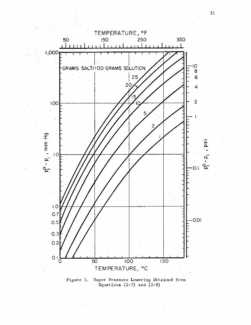
precise than vapor pressure data given in the literature, In Figure 5,

the variations of vapor pressure lowering with temperature and concen-

tration are illustrated,

O'I I

f= f= .. 10 0..--I

o_ p.

1.0

0.7

0.5

0.3

TEMPERATURE, °F 50 150 250 350 , I I I 11 I I I I I I I I I I I II I I I I I

. GRAMS SALT/100.GRAMS SOLUTION

I 25 20

50 100 150

TEMPERATURE I °C

·Figure·S. Vapor·Pressure·Lowering Obtained from 'Equations (2-7) and (2-8)

10 8 6

4

2

0.1

0.01

31

..... Cl)

p.

p. I

0-p.

CHAPTER.III

SPECIFIC.HEAT

· Relation of Activity to Specific .Heat

The specific heat of a solution may be related to the activi.ties of

the components through the concept of partial molal properties. For a

solution containing n1 moles of solvent and n2 moles of solute at pres­

sure·P and temperature T, the differential of any extensive property

Y(P, T, n1 , n2 ) may be written in the form

If the solution is at a constant temperature and pressure, this equation

reduces· to

dY = -y- dn + y-~dn l l · "" 2

(3-1)

where y1 - (oY/on1 )T p and Ya= (oY/dna)T p ; they are called par-' ,na , , nl ,

tial molal properties of the respective components. The nature of an

extensive property is .such that if the amounts of all the components are

changed in the.same proportion at constant T.and P, the value of the

dependent property changes in that proportion also, Letting dn1 = n1 dr,

and dn2 = n2 dr where dr is an infinitesimal proportioning factor, one

has dY = Ydr so that

32

33

.After cancelling out dr, this equation becomes

y

Therefore, an extensive property of a solution may be determined from

the numbers of moles and the partial molal properties of the components

at a given temperature and pressure .. Moreover, this relation is equally

valid if the unit of quantity is taken to be a unit of mass instead of

mole. Differentiation of Equation (3-2) gives

(3-3)

Combination of Equations· (3-1) and (3-3) leads to another equation valid

only at constant temperature and pressure,

(3-4)

which is a generalized form of the Gibbs-Duhem relation.

Since the partial molal properties are derived from extensive pro-

perties by differentiating with respect to one of the mole numbers, any

thermodynamic relation among extensive properties holds for the corre­

sponding partial molal properties, Differentiating the equation G = H -

TS with respect to n1 at constant temperature, pressure and number of

moles of the other component establishes the following relationship

among partial molal properties as

This equation may be transformed to the Gibbs-Helmholtz equation.by

34

applying the Maxwell relation,

. After dividing through both sides by Ta, the derivative may be rear=-

ranged to take the form

= -.-

Then, from Equation (2-1) one has

= - (3-5)

For an aqueous solution, ii.~ is equal to the molal enthalpy of pure water

at the temperature T since the reference state of water is the state of

an infinitely diluted solution. An equation analogous to Equation (3•5)

may be written for solute as

(3-6)

Substituting ii.1 and ii.3 from Equations (3-5) and (3-6) into Equation

(3-2), one may express the enthalpy pe:t:' · mole of solution as

where xis the mole fraction of solute .

. The definitions of fugacity and activity may be appl;i;ed to a pure

substance in the solid phase. If a is the activity of pure solid of s

solute in terms of the reference state identical to the one

35

con1entionally adopted for the solute in solution, it is possible to

write

RT ln a s

(3-8)

where g is the molal free energy of solid solute and i~ refers to the S . G

partial molal free energy of the solute in.solution at the same temper-

ature at infinite dilution. Following procedures applied to the deriva-

tion of Equation (3-5), one may obtain an expression to relate the deri­

vative<!~; a~ to molal enthalpy difference of the solute between the

solid state and the reference state, hs - h;,

= ·- (3-9)

The fugacity of the solid solute.in satutated solution is identical to

the fugacity of the solute dissolved in solution when the system is in

equilibrium. Consequently, the activity a in Equation (3-9) may be s

substituted by the activity a 2s of the dissolved solute in a saturated

solution since a common reference state has been assigned. Because the

value of an extensive property of electrolyte in solution depends on the

values of the properties of ions, the definition of mean ionic activity,

denoted by a ::I:' is introduced as a:a = a~ where \J is the number of ions

into which a formula unit of an electrolyte dissociates and a:a is the

activity of solute; for 1 ~ 1 strong electrolyte such as sodium chlo~~

ride, \J = 2 by assuming complete dissociation. Combining Equation (3-9)

and the definition of mean ionic activity, one may rewrite Equation

(3-7) as

36

h = (1 - ~) [fi~ - R12~. ~~ a,) ,,c] + x[ hs + 2RT:at 1:T ~:SJ,

- 2RTS~ ~; a:l::)i,,x]

(3-10)

where a:l::s denotes the mean ionic activity of solute in the saturated

solution. The constant-pressure specific heat cp may be derived from

Equation (3-10) by taking partial differentiation with respect to te,:n- ···

perature at constant ·p and x.

c (1 - x)[c - 2RT(!l 1n 81:'\ - RT~(oai ln881:'\ J P P , w , . oT )P , x \.. oT JP, x

· (3-11)

~.ln ~:I: . 9 ~ 2 ln a£\ J - 4RT~- oT )P, x ":' 2RT ,:- oT2 )P, x •

.This indicates the possibility of evaluating the specific heat of solu-

tion from the specific heat of pure water c , the specific heat of p,w

solid salt c and the derivatives of activities when the calorimetric p,s

measurements of c for a solution are not available. p

. Specific Heats of Water and Solid

Sodium Chloride

The values of enthalpy of saturated water from Oto 180°C in the

,Third.International Skeleton Steam Tables (48) were satisfactorily fit-

ted into the following interpolation formula, .as shown.in Table VII:

hf= -l.0031519T - 0.12638365 x 10-mTa + o.97645145 x 10~6 T3

where hf is the·enthalpy of saturated water in international steam-table

37

. TABLE ·vrr

~NTHALPY OF·SATURATED WATER

• · · Enthal1u:: 2 cal/gm Difference Tolerance ,Temp.,. c . (Data) (Est.) (+ or -)

0.0 o.oo o.oo· 0.00 0.00 10.0 10.04 10.02 0.02 0.01 20.0 20.03 20.02 0.01 0.02 30.0 30.00 30.01 -0.01 0.02 40.0 39.98 39.99 -0.01 0.02 50.0 49;95 49.96 -0.01 0.03 60.0 59.94 59.95 ·-0.01 0.03 70.0 69.93 69.94 -0.01 0.03 80.0 79.95 79.94 0.01 0.04 90.0 89.98 89.97 0.01 0.05

100.0 100.04 100.03 0.01 0.05 110.0 110 .12 110.12 0.00 0.06 120.0 120,25 120.25 0.00 0.06

'130.0 130.42 130.42 0.00 0.07 140.0 140.64 140,64 0.00 0.07 150,0 150.92 150.92 0.00 0.08 160.0 161. 25 161.27 -0.02 0.08

·110.0 171. 68 171.68 0.00 0.09 180.0 182.18 182. n 0.01 0.09

Note: Data recommended by the-Third.International Conference on Steam Tables (48).

38

calories per gram and Tis the temperature-in degrees·Kelvin. Differen-

tiating hf with respect to temperature gives the amount of heat required

per unit rise of temperature to heat water along the saturated·line

which is denoted here by subscript f •. To ?;elate the specific heat cf of

the saturated water with the constant-pressure specific heat c for p,w

the subcooled state, the temperature T and pressure P were selected as

the independent variables of entropy s so that

(3-13)

From the· Maxwell relation and the definitton of specific· heat, it fol~:

lows that

c ds = - ~')aP +·~ dT .

. To evaluate the specific heat along the saturation line, one may write

. (3-14)

Since the differentials in Equation (3-13) are exact, it follows that

(3-15)

· Thus, the variation of' specific heat with pressure may be determined

from an appropriate P-v-T relation .. In Table VIII are the constant-

pressure specific heats of water from Oto 1so•c at 10 atmospheres, as

calculated by the following equation:

···.'

39

TABLE VIII

SPECIFIC HEAT OF WATER

• Temp., ·c. S:eecific Heat 2 calLgm' C

cf c (1 atm) c. (10 atm) c (10 atm) p p p Eg •. (3-16) :e.g •. (3~17)

o.o 1.0039 1.0039 1. 0029 1. .0035 10.0 1. 0017 1,0017 1.0009 1. 0011 20.0 1.0000 1.0000 0.9994 0.9993 30.0 0.9990 0.9990 0.9984 · o. 99.82 40.0 0.9985 0.9986 0.9981 o. 9977 50.0 0.9986 0.9987 0.9983 O. 99 79 60.b 0.9993 0.9995 0.9991 0.9987 70.0 1.0006 1.0009 1.0005 1.0002 80.0 1. 0025 l.0029 1.0025 1.0023 90.0 1. 0049 1. 0056 1.0051 l,0050

100.0 1.0080 1.0088 1.0084 1,0084 110. 0 1. 0116 1.0123 1. 0125 120,0 1. 0158 1. 0168 1. 0172 130. 0 1. 0206 1. 0221 1.0225 140.0 1.0260 1.0281 1. 0285 150.0 1.0320 1.0348 1. 0351 160,0 1.0385 1.0422 1.0424 170.0 1.0457 1.0505 1.0503 180.0 1.0534 1. 0596 1.0589

40

10

[a{} ~;]£ -1 J T~)dP (3-16)

pf

where J is the Jotile's constant and Pf denotes the vapor pressure. The

data for the P-v-T relation were obtained from the Third International

Skeleton Steam Tables. To facilitate the calculations of specific heats

for solutions, the values of c at 10 atmospheres were fitted into the p,w

following. inte·rpolation formula by the least square method:

c p,w = 4.1986279 - 0.11428663 x 10-•t + 0.13498960 x 10~4 t;

(3-17)

where c is in joules per gram per degree and tis in degrees centi-p,w

grade,

The enthalpies of solid sodium chloride, h, from 298 to l,073°K s

have been determined by Kelly (24) from his spectroscopic observations.

The following equation fits the data within 1% accuracy:

... ; it, hs = hs(25 "C) + 10.98T + 1.95 x 10 T - 3.447.

From this equation one finds that the specific heat increases linearly

with temperature as follows:

c = 10.98 +3.90 x l0-3T p,s (3-18)

where c is in calories per mole per degree and Tis in degreesKel-p,s

vin. The coefficients of volume expansion of solid sodium chloride are

124.34 x 10 .. 8 at 100°c, 127.48 x 10""6 at 150°C and 130.58 x 10-s at

200 °C at atmospheric pressure according to Kaufmann' s compilation (19),

The available data on coefficients of expansion are insufficient for

41

meaningful evaluation of the pressure dependence of specific heats .

. However, the specific heat of a solid,, it is believed, is extremely in-

sensitive to pressure changes,. although the temperature dependence. is of

importance. . No allowance was made in this study. for the effect of pres-

sure on the specific heat of solid sodium chloride.

Specific Heat at 10 Atmospheres

from Oto 175°C

The evaluations of the partial derivatives of activities are neces-

sary in order to use Equation (3-11) to calculate the specific heats.

Equation (2-3) was proposed to represent the activities of water in so~

lution at a constant pressure; the values of the corresponding coeffi-

cients at 10 atmospheres were reported in Chapter II. From Equation

(2-3) the first and second derivatives of lri a 1 may be found in terms of

mole fraction of sodium chloride and absolute temperature as follows:

(!- ln a,) = oT ,x (3-19)

p~ ln al} = '- oT2 . ,x

The Gibbs~Duhem relation provides a means to determine the activi-

ties of solute from the known activities of solvent. Considering the

partial molal property in Equation (3-4) to be the partial molal Gibbs

free energy, one has an expression valid at a constant temperature and

pressure,

42

Afterdividing by dx and rearranging the terms, one finds that

= .- 1 - x (.q ln a,)r 2x '" . ox ,P'

(3-21)

Then, at a constant pressure, the change of ln a= between the two states

may be found by integration as

x" ln a; - ln a~ = ·~ J x ~ 1 {!, ~~ a,)r,Pdx + F(T). (3-,22) I

x'

When x diminishes, the activity coefficient.approaches unity regardless

of the value·of temperature. For this reason, every term in a ·series

representing.a:l: should be associated wit;h·x, and the function F(T) re­

sulting from integration must be equal to zero. The ·partial derivative

of ln· a1 with .respect to x .may be readily obtained from· Equation (2-3) .

. Upon .integt·ating from the mole .fraction of saturated solution, denoted

by subscript s, one has

·1n a - ln a ==\[Ax+ Bxl~~ + Cx2 +.(Dx + Ex1 ~1'j + Fx'a)/T ±: ·±S

(3-23)

+ (D ln x + 3Ex0 • 1 + 2Fx)/T + (G ln x + 3Hxc;i~a + 2Ix)ln T]x . x s

The mole fraction x for the saturated condition varies with temperature s

and pressure. Adams andHall (1) measured the electrical resistance of

solution and thus determined that the increase of dissolved sodium chlo-

ride due to changes in pressure· (1 to 2, 000 bars) was 1 gram per 100 r

grams of solution at 29.93°C. Evidently, the value of x is insensitive :S

43

to a small variation of pressure. The experimental data on solubility

at various temperatures are not in complete agreement. An interpolation

formula has been arbitrarily determined as follows to fit the data re-

ported by Sidell (42) and Schroeder, et al. (41) above l00°C, and by

Gillespie (51) below l00°C:

x = -0, 22195188 + 3. 5536043//'r + . 38955142 x 10".'GT s (3-24)

where x is the mole fraction of sodium chloride and Tis the tempera­s

ture in degrees Kelvin. The differences between the data and the calcu-

lated values using. Equation (3-24) are shown in Table.·IX.

Equation (3-24) gives the temperature dependence of mole fraction

at a saturated condition, by which one may evaluate the following deri-

vatives from Equation (3-23):

~ 1. n a.;i;;jp .- 0 ln a:;1:;s), 1 (- = -2T2 [-(Dx + Exl ,e + Fxa) , oT ,x oT .

+ (Dx + Ex115 + Fx2) + (D ln x + 3Fx0 .e + 2Fx) s s s

= (D ln x + 3Ex0 • 6 + 2Fx ) J + L [(Gx + Hx.1 • Iii + rxi) s s s 2T ·

- (Gx + Hx"' • 6 + Ix8 ) - (G ln x + 3Hx0 • e + 2Ix) s s s .

•

TABLE IX

CONCENTRATION OF SODIUM CHLORIDE IN SATURATED SOLUTION

44

Salt Weight 1 % Temp., c (Data) (Est,) Difference

0.0 26.34 (51) 26.38 -0.04 10.0 26.35 26.39 -0.04 20.0 26.43 26.45 -0.02 25,0 26.48 26.50 -0.02 30.0 26.56 26.55 0.01 40.0 26. 71 26. 68 0.03 50.0 26.89 26.84 0.05 60.0 27. 09 27.04 0.05 70.0 27.30 27.26 0.04 80.0 27.53 27.51 0.02 90.0 27.80 27.28 0.02

100.0 28.12 28.07 0.05 107.0 28.39 28.29 0.10 150.0 29.57 (42) 29.79 -0.22 173.0 30.36 30.69 -0.33 200.0 31. 60 31.81 -0.21 225.0 33.19 32.91 0.28 118.0 28.46 (41) 28.64 -0.18 140.0 29.62 29.41 0.21 160.0 30.36 30.17 0.19 180.0 30.98 30.97 0.01

Note: Data by Schroeder et al. (41) and Seidell (42), and from Inter­national Critical Tables (51).

45

+ .(Dx + Ex.1 • a + -F:k8 ) + -(D · ln 'x + 3E:x:'3 • 9 +. 2'C'x:) S . . S . '.S I'

.. {D ln x + -3Ex0 • 3 + 2Fx ) ] - 2T\ ((Gx + H:x1 '.Q + -Ix1) s s s ..

- (Gxs + H; • a + Ix!) - · (G · 1n x + 3Hx0 • a +. 2Ix)

+ (G ln x + 3Hi0 i 11 + 21x )] + ~Tx!"\·(1 - x') s s s ~ ~ s

[ - l... (i- + 1 5Ex-0 • 6 + 2F) + l (!L + 1 5Hx"l' 0 • 1 + .21) · T"' ' s · . . T ~ . ' s . . s ·-~

X ~ ~ ~X,li - _...§.J' ~ + O. 75Bx~ 1 : 1) .·~ -!);(1 - x ) T . . s T s . . s .. .

Substituting Equations (3~17), .(3-18), (3-19), (3-20), (3:25), and

(3-.26) into ·Equation· (3-11) yields the specific heat of the solution;

the results of calculations are presented in Table X and Figure 6 .. The

forms of interpolation formulae ·exercise a great influence on the final

results of the calculation; and the higher the concentration or the tern-

perature, the greater the influence, . This· shows that the probable error

resulting from using the· empirical formulae increases with the increase

of temperature or concentration. . Several otlier types of formulae have

been tried to test the validity of _the calculation procedures. Exper-

ience-indicates·that the fluctuations of the results are within-::: 1% of

Temp., ·c

0 10 20 30 40 50 60 70 80 90

100 110 120 130 140 ·150 160 170 180

-TABLE·X

CONSTANT-PR~SSURE·SPECIFIC HEAT OF SOLUTION AT 10 ATMOSPHERES IN CALORIES PER GRAM

PER DEGREE CENTIGRADE

Salt Weight 2 gmllOO gm Solution · 1.0 2.0 5.0 10.0 . 15. 0

.• 991 .979 ,946 .896 · .854 ,'. 988 • 977 .944 ·• 896 ,853 .987 .975 .943 .·895 .853 .986 .974 .• 942 .894 ·• 852 .985 .974 .941 .893 .851 .985 .974 .941 .892 .850 .986 .974 .941 .892 .849 .987 .975 .942 .891 .847 .989 .977 .942 .891 .846 .991 .979 .944 .891 .845 .995 .982 .946 .891 ,844 .998 .985 .948 .892 .842

l,003 .989 .951 .893 .842 1.008 .994 .954 .• 894 .841 1.013 .999 .958 .896 .840

· 1.019 1.004 .962 .898 .840 1.026 1.011 . 967 .9.00 .840 1.033 1.018 .973 .903 .841 1.041 1.025 . 979 .907 .841

46

20.0 25.0

.817 .• 787

.818 .788

.818 .789

.817 .788

.816 .. 787

.814 .785

.812 .782

.810 . 779

.807 • 775

.805 • 771

.802 .767

.799 . 762

.796 .758

.794 .753 • 791 .748 .788 .743 .786 .739 .784 .734 .782 • 729

1.04 ...

~ <!

. -o::: l .00 l9

w w 0::: l9 uJ 0

.96

'- .92 Ui w a: g .88

<! (.)

I­<! w I

(.)

LL

. 84

.80

~ .76 CL U)

-':" -...

-...

---

--....

-----... --

:72 0

I I I

GRAMS

I

20

I I I I I I I I I I I I I I I . I I I I I I I I I

-

--------~·

SALT I 100 GRAMS SOLUTION -2 ~ - - -

5 ---

--= 10 -

-

15 -

-20 -

25 .., ,

~

--- ------r-----...:.

·, ; I I I . I I I .I I I I I

40 60 80 100 120 140 160 180

TEMPERATURE 1 °C

Figure 6. . Constant-Pressure · Specific Heat at 10 Atmospheres .p­

"

48

c for concentrations up to 12% of sodium chloride and for temperatures p

less than 100°C for a combination of any reasonable formulae.

The method of multiple regression gives the following formula for

calculating th.e · values of specific heats in calories per gram per degree

as given in Table·X in terms of concentration in mole fraction and tern-

perature in degrees:Kelvin with maximum deviation of less than four

parts·per thousand:

c = 1.3165380 - 8.9594831x + 23.807251:x:9 - (0.20328368 x 10".'.'~ p

- 0.036271808x + 0.062168183x2 )T + .(0.32218320 x 10·".'" 3

- o. 61529617 x 10.,.4 x + 0.10557408 x 10".'"iaxa)'tg.

Experimental Data

Randall and Rossini (35) measured the specific heats at 25°C with

twin calorimeters. Lipsett, Johnson, and Maas (29) determined the spe~

cific heats at 20 and 25°C from heats of solution, using a rotating

calorimeter. . Some of the early exper;i.mental data are tabulated in the

-International Critical Tables (50,52). The highest temperature for the

experimental values recorded in literature is 75°C (39). Some discrep-

ancies among the measured data, illustrated in Figure 7, exist at high

concentrations. Table .XI shows the -measured- da.ta are in fair agreement

with the calculated values from Equation (3-2 7). All of these measure-

ments were taken at one atmosphere. The differences in specific heats

between 1 atmosphere and 10 atmospheres are considered to be negligible,

in this comparison .. It is· desirable to have ·experimental data at high

temperatures to verify the calculated values.

~ <! 0:: c...9

I

1.00

w .95 w 0:: c...9 w 0 ........

~ .90

0:: 0 _J

<! u

~ .85 I-<! w I

u Li.. .80 u w 0... Cf)

I I I I I I I I I I I I ' • I I I I I I

... -- MEASURED DATA TAKEN FROM

... REFERENCES (29), (39). AND (52)

'- VALUES DERIVED FROM ACTIVITIES

~

~ 7. 5 °/o ( 5 2) J. -----~c )-~-----o-------f.- o---~10°10 ... o---o ~

10% (29] ~

0--0 13. 95°/o l52) -· 12% (29) ----... -o-----· ---o--

o------0--0 16% (29)

- 20% (29) 0---0 24.49°/o l52) _ o===------o-------o----24% {29)

,_ 25% Cr---1i,. - ----- ---..-.-WEIGHT OF NaCl IN SOLUTION

...

' I I I ' I I I I I I I I I I I I ' ' I

I I I I I I I

6.8 I 0/o l~L----~ ---!I-------o

12.75 % (39) ;.----=t>------- ----6 ~-

----o

~ _,2_~0% (39) --- --,/\

I I I I I I I I I I .75 0 10 20 30 40 50 60 70

TEMPERATURE, °C

Figure 7. Comparison of Specific Heats at High Concentrations

I I

I I

----

----

--

-

----

----

80

~ I.O

so

TABLE<XI

COMPARISON OF MEASURED VALUES OF SPECIFIC HEAT WITij CALCULATED VALUES

c ' . cal/gm.· °C

. Data-Est. 0

t'' c Salt,% (Data) · (E~t.) . : Data

25 24.50 0.790 · (39) . o. 791 -0.0012 so 1.16 0.984 0.983 0.0006 so 2.84 0.965 0.965 -0.0008 so 6.81 0.924 0.924 -0.0005 so 12.75 0.871 0.868 0.0037 · so 24.50 0.787 0.786 0.0008 75 1.16 0.988 0.986 0.0018 75 .2.84 0.969 0,967 0.0013 75 6.81 0.936 0.925 0.0117 75 12.75 0.869 0.866 0.0040 75 24.50 0.780 o. 780 -0.0000

6 24.49 a.sos (52) 0.793 0.0148 6 17.78 0.826 0.833 ·-0. 0087 6 13.95 0.853 0.863 -0. 0114 6 7.50 0.910 0.922 -0.0132 6 5.13 0.934 0.946 -0.0125 6 3.88 0.948 0.959 -0.0111 6 3.14 0.958 0.966 ·-0.0086 6 2.11 0.968 0.977 -0.0092 6 1.59 0.978 0.983 -0.0054

20 24.49 0.807 o. 792 0.0196 20 17.78 0,828 0.831 .-0.0034 20 13. 95 0.858 0.861 -0.0031 20 '. 7, so 0.913 0.920 -0.0072 20 5.13 0.937 0.943 -0,0069 20 ·3.88 o. 951 0.956 -0.0057 20 3.14 0.960 0.964 -0.0037 20 2.11 0.970 0.975 -0.0046

·20 1.59 o. 978 0.980 -0.0028 20 1.07 0.983 0.986 -0.0034 20 0.80 0.989 0.989 0.0002 33 24.49 0.810 0.790 0.0248 33 17.78 0.829 0.829 -0.0001 33 ·13,95 0.861 0.859 0.0019 33 7.50 0.916 0.918 .-0.0025 :p 5.13 0.940 0.942 -0.0022 33 3.88 0.953 0.955 -0.0022 33 3.14 0.961 0.963 -0.0020

;33 2.11 0.972 0.973 -0.0017 /33 1.59 0.978 0.979 -0.0012 57 · 24 . .49 0.815 0.785 0.0365 57 17.78 0.841 0.826 0.0176 57 13.95 0.870 .0.857 0.0147

51

TABLE XI - Continued

c ' cal/gm ·c Data-Est. t, .. °C Salt,% .(Data) (Est.) Data

57 7.50 0.917 0.917 0.0004 20 0.20 0.997 (29) 0.995 0.0016 20 0.40 0.994 0.993 0.0010 20 0.60 0.991 0.991 0.0005 20 .0.80 0.989 0.989 0.0001 20 1.00 0.986 0.987 .-0.0003 20 1.20 0.984 0.985 -0.0006 20 1.40 0.981 0.982 -0.0009 20 · 2.00 0.974 0 •. 976 -0.0020

.20 3.00 0.962 0.965 -0.0030 ,20 4.00 ·0.951 0.955 -0.0044 .20 6.00 0.929 0.935 ,-0.0058 20 8.00 0.909. 0.915 ·-0.0061

· 20 10.00 0.891 0.896 -0.0058 20 1,2.00 0.873 0.878 -0.0050 20 14.00 0.857 0.861 -0.0039 20 16.00 0.842 0.845 -0.0028 20 ·18.00 0,828 ·0.830 -0.0017

. 20 20.00 0 .·816 0.816 ·-0.0004 .20· ·22.00 0.804 0.804 .-o. 0001 20 24.00 0.793 0.794 .-0.0009 20 26.00 0.783 o. 785 -0.0029 25 0.20 0.996 0.995 0.0016 25 0.40 0.994 0.993 O.OOl.2 25 0.60 0,991 o. 990 0.0008 25 0.80 0.989 0.988 0.0005 25 1.00 0.986 0.986 0.0004 25 1,20 0.984 0.984 0.0000 25 1.40 0.981 0.982 -0.0002 25 2.00 0,974 0.975 -0.0009 25 3.00 0.963 0.965 -0. 0019 25 4.00 0.952 0.954 .-o. 0029 25 6.00 0.930 0.934 -0.0038 25 ·8.oo 0.910 0.914 .-o. 0040 25 10.00 0.892 0.895 -0.0035 25 12. 00 0.875 0.877 -0.0026 25 ·14.00 0.859 0.860 -0.0014 25 16.00 0.843 0.844 -0.0006 25 18.00 0.829 0.829 -0.0003 25 20.00 0.817 0,816 0.0015 25 ·22.00 0.805 0.804 0.0015 25 ·24.00 0. 794 0.793 0.0005 25 26.00 o. 783 0.785 -0.0018

. 15 0.06 0.999 (15) 9.998 0.0018 25 0.06 0.997 . 0.996 0.0009

- 35 0.06 0.997 . 0.995 0.0012

52

TABLE XI - Continued

0 c. ' cal/gm '°C . Data-Est.

t' ', c Salt,,% (Data) (E:st.) Data

45 0,06 0. 997 0.995 -0.0021 15 0.29 0.996 0.99.5 o. 0011 25 0.29 0.994 0.994 0.0006

·35 0.29 0.994 o. 993 0.0008 45 0.29 0.995 0.993 0.0027 15 0.41 0.994 0.994 0.0005 25 0.41 0.993 0.992 · 0.0004

.35 0.41 0.992 0.992 0.0007 45 0.41 0.994 0.991 0.0022 15 0.58 0;992 0.992 0.0000

, 25 0.58 0.990 0.991 -0.0002 35 0.58 0.990 0.990 0.0002 45 0.58 0.992 0.990 0.0021 15 1. 72 0.977 0.980 -0.0032

. 25 1. 72 0,976 0.978 ·-0.0021 35 1. 72 0.976 0.977 -0.0011 45 1. 72 0.978 0.977 0.0008 15 4.00 0.949 0.956 -0.0068 25 4.00 0~950 0.954 -0.0044 35 4.00 0.951 0.953 -0.0023 45 4.00 0.952 0.9,53 -0.0012 15 5.69 0.930 0.938 -0.0091 25 5.69 0.932 0.937 .-0.0055 35 5.69 0.933 0;936 -0.0027 4.5 5.69 0,935 0.935 -0.0008

Note: Data by Hess et ,.al. (15),, Lip Sett et al. (29) and, Rutskov (39), and from:International.Critical Tables (52).

CHAPTER', IV

· SPECIFIC VOLUME

Specific Volume of Water from Oto 150°C

Liquids have neither the rigid geometrical structure of solids nor

the complete randomness of gases. The scientific understanding of the

liquid state has lagged behind the basic knowledge of both the solid and

gaseous states. The theory of the behavior of a liquid is not well de­

veloped because there is no clear-cut limiting cases, such as the crys­

talline phase at the absolute zero temperature for solid and the perfect

gas for the real gas .. Numerous equations of state have been developed

over the years, but most of them can be applied only to gases. To deal

with liquids, tables, graphs or power series are usually used in place

of an equation of state, .The behavior of water is further complicated

since it exhibits a peculiarity of thermal expansion in the low tempera-

ture region .. Of the many interpolation formulae that may be found in

·literature for the specific volume of water (6), none is simple even in

a small-range of temperature. Kell (22) recently used a seven-term

series for the precise representation of the specific volume from Oto .. 110 Cat 1 atmosphere .

. In-1893 Amagat (2) reported experimental values of densitiesand

compressibilities for water, which a~e considered precise even by modern

standards .. Since then, many experiments have been carrted out to a very

53

54

high degree of precision. Over the range Oto 40°C, values of densities

are often published to one part in· 10 million. . In this study the values

of specific volume of water are based on those recommended by the Third

.. International Conference on· Steam Tables (48) .. The following .mathemati-

cal expression was arbitrarily chosen to fit these data:

v = A(T) ~ P·B(T) - P9 •C(T) (4-1)

where vis in cubic centimeters per gram, Pin kilograms per square

centimeter and Tin degrees Kelvin. The three functions of temperature

0 for specific volumes in the region between Oto 180 C and up to 400

kilograms per square centimeter have been determined as follows:

:A(T) = 5.916365 - O.Olb357941T +.0.92700482 x 1o·irs

- 1127.5221/T + 100674.l/T$,

.B(T) = 0.52049144 x 10-s - 0.10482101 x l0~4 T + 0.83285321 x·l0-8 T1

- 1.1702939/T + 102.27831/T9 ,

C(T) = 0.11854697 x·10-, - 0.65991434 x 10~1~.

The values calculated from Equation (4-1) with the accepted values

are compared in Table XII. The deviations of the calculated values from

the data are within the tolerances accepted by the Third International

Conference on Steam Tables. The function A(T) may be interpreted as the

specific volume in a hypothetical .state of zero pressure. Since the

compressi]::,ilities of liquids are in the o+der of 10"" 6 per atmosphere,

A(T) is approximately equal to the specific volume at the vapor pressure

if the temperature is not over 1so 0 c.

55

TABLE-XII

SPECIFIC VOLUME OF WATER

0

p~ kg/cm.2 Se. Vol. 2 . c,r/P /gm Diff.

. Tolerance t' \ c (Data) ·(Est.) + or -

0 0.006 1. 00021 1.00021 -0.00000 0.00005 10 0.013 1.00035 . 1. 00036 -0.00001 0.0001 20 0.024 1.00184 1. 00183 O.OQOOl 0.0001 30 0.043 1.00442 1.00439 0.00003 0.0001 40 0.075 1.00789 1. 00787 0.00002 0.0001 50 0.126 1. 01210 1.01214 .-0.00004 0.0002 60 0.203 1.01710 1. 01712 -0.00002 0.0002 70 0.318 1.02280 1. 02276 0.00004 0.0002 80 0.483 1. 02900 1.02903 , -0. 00003 0.0002 90 0.715 1. 03590 1. 03592 -0.00002 0.0002

100 1.033 1. 04350 1. 04341 0.00009 0.0002 110 1.461 1.05150 1.05153 --0.00003 0.0004

· 120 2.025 1.06030 -1.06029 0:00001 0.0004 ·-13~ 2.754 ·1.06970 1. 06971 . -o.opoo1 0.0004 140 '3,685 1.07~80 1.07980 ·-0. 00000 0.0004

>150 . 4. 854 1.09060 -1.09061 : -01• 00001 0.0004 160 6.302 1.10210 ·1.10214 --0. 00004 0.0004

,' 170 8.076 1.11440 1.11443 -0.00003 0.0004 .',180 10.225 1.12750 1.12749 0.00001 0 •. 0004

0 1.000 1.00016 1.00016 ·-0. 00000 .0.00005 0 5.000 .. o. 99990 0.99996 -0.00006 0.0002 0 -10.000 0~99970 o. 99972 -0.00002 0.0002 0 .25.000 0.99890 .0.99898 - -0. 00008 ·0.0002 0 50.000 0 .. 99770 0.99775 -0.00005 0.0002 0 75.000 0.99650 0.99653 -0.00003 0.0002 0 100.000 0.99520 0.99532 -0.00012 0.0002 0 125.000 0.99400 0.99412 -0.00012 0.0002 0 150.000 0.99290 0.99292 -0.00002 0.0002 0 200.000 0.99050 0.99056 -0.00006 0.0002 0 250.000 0.98820 0.98822 -0.00002 0,0002 0 300.000 0.98590 0.98591 -0.00001 0.0002 0 350.000 0.98370 0.98364 0.00006 0.0002 0 400.000 0.98140 0.98139 0.00001 0.0002

50 1.000 l. 01210 1.01210 -0.00000 0.0002 50 5.000 1. 01190 1. 01192 -0.00002 0.0002 50 10.000 1.01170 1.01169 0.00001 0.0002 50 25.000 1. 01100 1. 01102 -o.o_ooo2 0.0002 50 50.000 1. 00990 1. 00991 -0.00001 0.0002 50 75.000 1.00880 1.00881 -0.09001 0.0002 50 100.000 1. 00770 1. 00772 -0.00002 0.0002 50 125. 000 · 1. 00670 1.00664 0,00006 0.0002 50 150.000 1.00560 1.00557 0.00003 0.0002 50 200.000 1.00350 1. 00347 0.00003 0.0002 50 250.000 1.00150 1.00142 0.00008 0.0002

56

TABLE' XII - ·Continued

• P~ kg/cm8 S;e. Vol.~ cm.la I gm Diff.

Tolerance t~· c (Data) (Est.) + or·-

/

50 . .300.000 o. 99950 0.99942 0.00008 0.0002 50 350.000 0.99750 0.99747 0.00003 0.0002 50 400.000 0.99560 0,99556 0.00004 0.0002

100 5.000 1. 04320 1. 04321 -0.00001 0.0002 100 10.000 1. 04310 1.04295 ·0.00015 0.0002 100 25.000 1.04220 1.04219 0.00001 0.0002 100 .50.000 1.04090 1.04092 -0.00002 0.0002 100 75.000 1. 03970 ·1.03968 0.00002 0.0002 100 100.000 1.03850 1.03845 0.00005 0.0002 100 1.25.000 1.03720 1. 03723 -0.00003 0.0002 1.00 ·1.so.000 1.03600 1.03603 -0.00003 0.0002 100 ·200.000 1.03370 1. 03368 0.00002 0.0002 100 250.000 1.03140 1. 03139 0.00001 0.0002 100 ,300.000 1.02910 1. 02917 . -0.00007 0.0002 100 350.000 1.02690 1. 02701 -0, 00011 0.0002 100 400.000 1.02470 ·1.02492 -0.00022 0.0002 150 5.000 1.09060 1.09060 ·0.00000 0.0002 150 10.000 1.. 09020 1.09027 -0.00007 0.0002 150 25.000 1. 08930 1. 08928 0.00002 0.0002 150 50.000 l. 08770 1. 08766 0.00004 0.0002 150 75.000 1. 08610 1.08605 0.00005 0,0002 150 100.000 1. 08450 1.08447 0.00003 0.0002 150 125.000 1.08290 1.08290 -0:00000 0.0002 150 150.000 1.08140 1.08136 0,00004 0.0002 150 200.000 1.07840 1. 07833 0.00007 0.0002 150 250.000 1.07550 1. 07538 o. 00012 0.0002 150 300.000 1.07260 1. 07251 0.00009 0.0002. 150 350.000 1.06980 1. 06972 0.00008 0.0002 150 400.000 1. 06700 1. 06701 -0.00001 0,0002 200 2.5.000 1.15560 1,15518 0.00042 0.0003 200 50.000 1.15320 1.15288 0.00032 0.0003 200 75.000 1.15080 1. 15061 0.00019 0.0003 200 100.000 1.14850 1.14837 0.00013 0.0003 200 125.000 1.14620 1.14614 0.00006 0.0003 200 150.000 1.14390 1.14394 -0.00004 0.0003 200 .200.000 1. 13950 1.13962 -0.00012 0.0003 200 2.50,000 1.13.530 1.13539 -0.00009 0.0003

,200 300.000 1.13120 1. 13126 -0.00006 0.0003 200 3.50.000 1.12720 1.12722 -0.00002 0.0003 200 400.000 1.12340 1.12329 0. 00011 0,0003

57

TABLE XII - Continued

Note: Data given by the Third·International Conference on.SteamTables · (48).

Experimental Determination of the Derivative~~ \coP)r,x

A survey of literature indicated the lack of experimental data on

• compressibility of sodium chloride solutions at temperatures above 40 C .

. Measurements were theref.ore made to obtain the derivative ~~ ,x for

temperatures ranging from Oto 180°C, for concentrations ranging from O

to 25% salt weight in solution, and for pressures up to 5,000 psig; .the

results were used to derive an appropriate·P·v-T-x relation. In this

investigation, the change in volume as a fupction of pressure for a con-

stant temperature was measured by utilizing a calibrated positive-dis-

·placement pump,

. The apparatus is shown· schematically in Figure 8 .. 'Xhe vessel which

.contains only the solution was made of stainless steel, surrounded by

three electrical heating coils of 650 watts each,. and insulated with a

layer of 1~" thick mineral wool. The electrical current through the

coil was controlled by a variable resistor in order to maintain the de-

sired temperature of solution in the vessel. To minimize the variation

of temperature of solution, 415 feet of 0.01" o.d. nickel chromium wire

was placed inside the vessel to distribute the heat uniformly throughout

the solution. The piston of the· pump, whd.ch was calibrated to O. 01

;..lex, +I

';ojrz, I'--

TEST VESSEL

0-RING SEAL

THERMOCOUPLE CONNECTION

RUSKA MODEL 2254 PUMP

0-5,000 PSI 14 IN. DIAL PRESSURE GAGE

1•n•J""l""I'

INDICATOR CALIBRATED TO 0.01 C. C. OF PISTON DISPLACEMENT

OIL RESERVOIR

Figure 8 •. Arrangement of Apparatus for Determining Derivative ~°")r,x

u, 00

59

cubic centimeter of piston displacement, could be advanced or retreated

at a uniform speed from Oto 100 cubic centimeters of displacement per

minute by means of a motor and gear box. A layer of light oil was

floating above the solution in the second vessel to separate the pump

and the pressure gage from the solution. The 14 11 dial bourdon pressure

gage was calibrated with a dead weight tester before and after the ex-

periment. Each division on the dial of the gage represented 5 psi, and

the gage could record a maximum pressure of 5,000 psig. The temperature

of the solution was measured by aConax 20,gage iron-constantan thermo-

couple together with a Leeds and Northrup millivolt potentiometer. The

thermocouple was placed. in the middle of the vessel.·. The readings from

the potentiometer were checked with a standard glass thermometer sus-

pended·in the vessel before the experiment, and the agreement was within

0 ,1 Fat the boiling point of water. The solutions were prepared from

distilled water and crystal sodium chloride of reagent grade with a

purity of 99.7%. To avoid possible contamination, the interior surface

.of the vessel was cleaned with dilute acid solution and thoroughly

rinsed with distilled water. After the vessel was filled with solution,

the entrained air was carefully driven out through the top of the ves-

sel.

The experimental procedure followed was first to raise the pressure

of the system· to 5,000 psig after the apparatus was assembled. The next

step was to adjust the electrical resistor and to wait for the attain-

ment of thermal equilibrium. Then, the pressure of the system was grad-

ually lowered by reversing t.he motion of the piston at a very slow

speed, and the·piston displacements were recorded at-intervals of 250

psi pressure. During this operation the temperature of the solution

60

dropped slightly; it was necessary to raise the current through the

heating coil for maintaining a constant temperature. To control the

variation of temperature within 0.2 °F throughout the test was not too

difficult. ·After the pressure was lowered to 185 psig, the valve under-

neath the vessel which contained only solution was closed to isolate the

solution in this vessel from the system. Next, the pressure was again

raised to 5,000 psig. The pressure was lowered, and the readings of

piston displacement were repeated for every 250 psi. These two sets of

data, first with the valve open and then with the valve closed, were

needed to account for the volume changes attributed to the vessel which

contained only solution, Under normal operation, the time required to

complete the test of a solution was about six hours for one temperature.

The fundamental measurements made in this experiment are the piston

displacements taken at every 250 psi pressure change for both the open

and closed valve positions. b

A series of measurements taken at 350 F and

25% .NaCl is shown in Figure 9. The difference between the two piston

displacements taken at the same pressure gives the change in volume of

test vessel and its contents. The·results of these measurements are

tabulated in Table. XIII. A very slight nonlinearity of the data is evi-

dent. For simplicity, the differences of the volume changes for the two

valve ·positions were assumed to be linear with the mean values of pres;-

sure, and the data were fitted by the least square method to the equa-

tion

t:N = a + bP. (4-2)

·In this equation 6.V is the difference of the volume change in cubic cen-

timeter and P is the pressure in psia •. The smoothed values of the

5000-4750'

4750-4500, L

4500 -42501- r L

4250-4000t .. ({'

4000-3750

3750-3500

3500-3250

(.!) 3250-3000 (/) CL 3000-2750'

W 2750-2500 c:: ::::, 250,0-2250, Cf)

Cf) 2250 -2000 w .~ 2000-1750

1750-1500

1500-1250'

1250 - IOOO

1000- 750

750:... 500

500- 2 50

0.7 08

6

0.9

l).V

TEMPERATURE = 350 .! 0.06°F CONCENTRATION = 25% Na. Cl

- 1.0 I.I 1.2

PISTON DISPLACEMENT, CM3

0

0

> 0

0

1.3 1.4

Figure 9. Typical Measurements of Piston Displacement for Compression Test

1.5

°' I-'

Pressure, .psig

(Temperature

-5000-4750 4750-4500 4500-4250 4250-4000 4000-3750 3750-3500 3500-3250 3250-3000 3000-2750 2750-2500 2500~2250 2250-2000 2000-1750 1750-1500 1500-1250 1250-1000 1000- 750

750- 500 500- 250

TABLE-XIII

DIFFERENC'E OF VOLUME CHANGE BETWEE:N ·THE. TWO · EXPERIMENTAL CONDITIONS, !:N :IN

CUBIC CENTIMETER

Salt Weight 2 gm/100 gm.Solution 0 ·5 10 ·15 20

= 72 F)

0.500 0.460 0.405 0.385 0.355 0.505 0.470 0.420 0.385 0.350 0.510 0.470 0.425 0.390 0.365 0.515 0.465 b.415 0.380 0.360 0.505 0.475 0.435 0.410 0.365 0.535 0.475 0.455 0.420 0.365 0.515 0.465 0.425 0.400 0.355 0.515 0.490 0.415 0.400 0.380 . 0.540 0.495 0.435 0 .. 410 0.365 0.485 0.465 0.450 0.405 0.365 0.490 0.480 0.410 0.400 0.385 0.570 0.495 0.450 0.415 0.395 0.495 0.485 0.445 0.415 0.365 0.565 0.495 0.370 0.405 0.385 0.530 0.490 0.440 0.425 0.395 0.545 0.505 0.455 0.430 0.390 0.540 0.525 0.535 0.440 0.415 0.540 0.505 0.515 0.455 0.430 0.560 0.495 0.455 0.445 0.395

· ('remperature = ·l.25 F)

5000-4750 0.485 0.450 0.410 0,385 0.360 4750-4500 0.505 0.460 0.410 0.390 0.360 4.500;;.4250 0.480 0.440 0.395 0.395 0.360 4250-4000 0.495 0.465 0.390 0.390 0.345 4000-3750 0.490 0.465 0.425 0.390 0.370

.. 3750-3500 0.535 0,485 0.425 0.390 0.380 3500-3250 0.490 0.475 0.420 0.395 0.360

'3250-3000 0.500 0.445 0.425 0.405 0.375 3000-2750 0.520 0.470 0.440 0.400 0.365 2750-2500 0.515 0.447 0.440 0.415 0.370 2500-2250 0.520 0.485 0,455 0.425 0.380

-2250-2000 0.495 0.480 0.430 0.400 0.390 2000-1750 0.490 0.470 0.420 0.410 0.385 1750-1500 0.510 0.475 0.440 0.425 0.380 1500-1250 0,530 0.500 0.440 0,415 0.405 1250-1000 0.545 0,490 0.470 0.420 0.410 1000- 750 0.535 0.480 0.480 0.430 0.410

62

25

0.325 0.340 0.345 0.340 0.340 0.310 0.350 0.330 0.350 0.340 0.345 0.350 0.335 0.360 0.370 0.380 0.370 0.380 0.400

0.315 0,340 0.345 0.335 0.350 0.350 0.365 0.375 0.355 0.345 0.370 0.360 0.365 0.355 0.365 0.365 0.360

63

·· TABLE XIII - Continued

.Pressure, .Salt·Weight 2 gm/100 gm'Solution psig 0 5 10 15 20 25

. _(Temperature·= 125 F)

750- 500 0.560 0.500 0.445 0.410 0.375 0.375 500- 250 0.550 0.515 0.480 0,420 0.415 0.375'

(Temperature= 180 F)

5000-4750 0.390 0.450 0.420 0.390 0.370 0.335 4750-4500 0.505 0.455 0.435 0,405 0.385 0.345 4500-4250 0.500 0,465 0.455 0.405 0.415 0.360 4.250-4000 0.525 0.475 0.430 0.410 0.385 0.350 4000-3750 0.510 0.460 0.465 0.420 0.405 0.355 3750 ... 3500 0.505 0.490 0.455 0.410 0.395 0.365

'3500-3250 0.535 0.475 0.445 0,430 0.375 0,360 .3250-3000 0,500 ·o.490 0.445 0.400 0.375 0.350 3000·2750 0.535 0.495 0.465 . 0.430 0.410 0.365 2750 .. 2500 0.525 0.485 · 0.560 0.405 0.385 0.380 2500-22.50 0.505 0.465 0.490 0.425 0.390 0.345 22.50-2000 0.51.5 0.490 0.470 0.405 0;385 0.385

-2000-1750 0.520 0.535 0.475 0.460 . 0.425 0.395 '1750-1500 O . .54.5 0.485 0.4.55 0.430 0.395 0.360 ·1500-1250 0.540 0.500 0.455 0.415 0.410 0.365 1250-1000 0.565 0.530 0.495 0.445 0.380 0.375

·1000- 750 0.575 0.465 · 0.470 0.450 0.430 0.390 750-.500 0 • .54.5 0.500 0.470 0.450 0.410 0.405

·500-·250 0 • .545 0.505 0.480 0.470 0.415 0.410

, (Temperature = -250 F)

5000-4750 0.560 0.490 0.450 0.405 0.390 0.350 4750-4500 0,550 0.495 0.455 0.415 0,420 0.375 4500-4250 0,525 0.515 0.455 0.415 0.400 0.380 4.250-4000 0.540 0,500 0.465 0.420 0.410 0.375 4000-3750 0.555 0.515 0.455 0.440 0.410 0.395 3750-3.500 0.540 o. 520 0.480 0.455 0,425 0.375 3500-3250 0.585 0.535 0.470 0.460 0.415 0.385 3250-3000 0.555 0,505 0.435 0.465 0.435 0.385

·3000-2750 0.585 0,495 0.490 0.440 0.445 0.395 2750-2500 0,585 0.530 0.475 0,460 0.420 0.390 2500-2250 0.565 0.540 0.485 0.470 0.430 0.410 2250-2000 0.555 0,525 0.500 0.445 0.445 0.400 2000-1750 0.600 0,540 0..505 0.465 0.435 0.380 1750-1500 0.570 0.555 0.500 0.465 0.420 0.410 1500-1250 0.580 0.535 0.535 0.455 0.460 0.445

·12so-1000 0.585 0.540 0.525 0,475 0.485 0.400 -1000-. 750 0.630 0.575 0.470 0.495 0.470 0.415

64

TABLE XIII - Continued

Pressure, Salt Weight 2 gm/100 gm Solution psig 0 5 10 15 20 25

. (Temperature = 250 F)

· 750- 500 0.615 0.560 0.555 0.460 0.415 0.395 SQQ .. 250 0.615 0.555 0.510 0.505 0.455 0.405

(Temperature = 300 F)

5000-4750 0.590 0.535 0.520 0.460 0.400 0.390 · 4750-4500 0.615 0.540 0.490 0.470 -0.445 0.410

4500-4250 0.595 0.550 0.495 0.465 0.430 0.400 4250-4000 0.615 0.545 0.510 0.470 0.425 0.415 4000-3750 0.640 . 0,550 0.485 0,470 0.445 0.390

- 3750-3500 0.600 0.560 0.500 0.485 0.460 0.435 3500-3250 0.620 0.565 0.490 0.460 0.455 0.430 3250 .. 3000 0.610 0.575 0.535 0.500 0.445 0.465 3000-2750 0.615 0.560 0.520 ·o.5oo 0.445 0.410 2750-2500 0.620 0,570 0.540 0.495 0.470 0.400

.2500-2250 0.630 0.605· 0.525 0.490 0.455 0.410 ·2250-2000 0.640 01625 0.510 0.495 0.445 0.425 2000-1750 0.655 0,565 0.535 0.510 0.470 0.415

·1750 .. 1500 0.615 0.590 0.555 0.495 0.455 0.420 1500 .. 1250 0.650 0.580 0.530 0.505 0.465 0.395 1250-1000 0.675 0.585 0,560 0.505 0.500 0.400 1000- .750 0.705 0,595 0.580 0.495 0.465 0.400

750- .500 0. 71.0 0.645 0.570 ·o.s30 0.460 0.445 500-.2.50 0.690 0.625 0.575 0.520 0.490 0.420

(Temperature= 350 F)

,5000-4750 0,595 0.595 0,500 0.505 0.450 0.405 4750-4500 o. 720 0.605 0.525 0.505 0.455 0.425 4500-4250 0,665 0.590 0,515 0.520 0.465 0.445 4250-4000 0.675 0.615 0.545' 0.520 0.475 0.425 4000-3750 0.700 o. 620 0.555 0.510 0.470 0.445 '3750-3500 0. 715 0.640 0-,560 0.505 0.480 0.425 3500-3250 0.740 0.635 0.545 0.525 0.480 0.450 3250-3000 0. 715 0.635 0,540 0.545 0,500 0.435 3000-2750 0.705 0.640 0.600 0.530 0,510 0.415 2750-2500 o. 710 0.650 0.575 0.565 0.490 0.440 2500-2250 o. 770 0.675 0.620 Q.545 0.460 0.455 2250-2000 0,745 0.620 0.585 0.575 0.495 0.495 2000-1750 0.745 0.660 0.590 0.545 0.515 0.475

·1750-1500 0,740 0.665 0.630 0.550 0.485 0.445 1500-1250 0.750 0.700 0.560 0,550 0.515 0.450 1250-1000 0.780 0. 695 0.605 0.545 0.510 0.480 1000- 750 o. 770 0.735 o. 610 . 0:575 0,505 0.480

65

·TABLEXIII - Continued

Pr·essure, Salt Weight 2 . gm/100 gm:Solution .psig 0 5, 10 ·15 20 25

(Temperature = -350 F)

750- 500 0.795 0.675 0.610 0.565 0.510 0.505 500- 250 0.835 o. 710 0.640 0.545 0.530 0.510

coefficients a and bare summarized in Table XIV.

The term t:N in Equation (4-2) represents the total volume change of

the isolated solution and of the vessel containing only solution with

the pressure change t::.P at a constant temperature. Since the derivative

~'1,x does not vary with pressure rapidly, its mean value over a small

pressure change t::.P is approximated by the equation

t:N - t::.V - ~'1,x ·!el! . Ml:::.P e (4-3)

where Mis the mass of solution isolated from the system after the clos-

ing of the valve and t:N e is the dilation of the vessel subjected to the

·internal pressure change 6,P. Let v1 be the specific volume of the iso­

lated solution, V0 the volume of the vessel at room temperature, and Vt

the increase of the volume of the vessel due to the thermal expansion of

metal at temperature t. Then, Equation (4-3) can be written as

(4-4)

66

. TABLE XIV

COEFFICIENTS a,AND b OF 'EQUATION • (4-2)

Salt,.% TemEerature 2 ·. °F

72 · 125 :180 .250 .· 300 350

(Coefficient a)

0 0.5567 . 0.5483 0.5671 0.6324 o. 7153 0.8293 5 0.5100 0.5065 0.5208 0.5734 0.6383 0. 7174

10 0.4704 0.4691 0.4843 0.5268 0.5758 0.6382 15 0.4370 0.4393 0.4537 .0.4885 0.5285 0.5776 20 0.4082 0.4137 0.4269 0.4552 0.4874 0.5266 25 0.3845 0.3927 0.4019 0.4263 0.4539 0.4852

(Coefficient b) x (-0.0001)

0 0.1232 0.1328 0.1534 \ 0.2041 0.2414 0.3239 5 0.1062 0.1112 0.1242 0.1519 0.1859 0.2364

10 0.1165 0.1178 0.1262 0.1438 0.1637 0.1903 15 0.1212 0.1224 0,1256 0.1337 o·.1438 0.1575 20 0.1273 0.1216 0.1197 0.1218 0,1269 0.1350 25 0.1289 0.1212 0.1166 o.114e 0.1171 0.1222

67

'The value of !}.V , . according to the usual. theory of elasticity (25), . e

.may be computed by the·equation

VAP[3(1 - 2cr)t~ + 2(1 + cr)t~] h · 1 0 ~v = -------------------------------------------e E(t2 • t'~)

· 0 1 (4-5)

where a is Poisson's ratio, Eis Young's modulus, r. is the inside radi­i

us, r 0 is :the outside radius, and Vis the internal volume of the ves-.

sel. For E = 30,000,000 psi and er= 0.3, which are the typical values

for stainless steel, the value of. tN is equal to 0.0304 cubic centi­e

meter for 250 psi of pressure change with the geometrical dimensions as

shown in Figure 8.

The increase.of volume with pressure as determined above was check-

ed experimentally by weighing the· overflow of water from the top of the

vessel in the.following manner .. The valve under the·vessel was closed

at a .desired, pressure, and the valve on the top was then op,ened- tcr drop

the·pressure to atmosphericpressure. The temperatures of water were

. o.bserved before and after the expansion .of water. From the ·P-v-T reU~

tion of water as given by Equation (4-1),. the volume increase b,V was e ..

computed .. The observed data at room temperature are given in Table XV,

and the results may be represented by the eq1,1ation

b,V = 0.05215 + 0.0001287P e (4-6)

where b,V is in cubic centimeter and P is in psig. The value of /J:,.V as e e

calculated by Equation (4-,,6) for 250 psi increment of pressure change is

O. 0322 cubic centimeter, which compares very closely to the value ob-

tained from:Equation·(4-5).

The moduli of elasticity of metals typically drop by about 0.03%

P, psig

5,020 4,510

· 4, 010 3,510 3,010 2,505 2,010 1,510

·1,015 . 505 253

where·· t::,Ve

Vl

v:a t

l t:a p

w 661.1 crr:P

TABLE XV

. D.ILATION OF VESSEL SUBJECTED TO 'INTERNAL . PRESSURE AT 72 °F

OF • •W, gm :t:l' 't:;p F

10. 726 73.13 72.13 9.658 72.92 72.02 8.635 72. 74 71.94

· 7 .590 72. 74 72.04 6.533 · 72.64 72!04 5.477 72.54 72.04 4-.406 72.50 72.10

:3.335 72.39 72;09 2.255 72.26 72.06 1.139 72.16 72.06 0.589 72.16 72.11

= dilation of vessel = v1 w + 661. l(v2 /v1 - 1) = .specific volume· -of water at t l and.:P = .Spe.cific volume· of water at ta and 1. atm = temperature .before .expansion = t-emperatur.e after ·expanston = internal pres·sure = ·overflow of mass from the t.op = volume of ·vessel at 72 °F and 1 atm.

68

I t::,V , -~ crrfi :.e,

0.7028 o. 6313 0.5717 0.5033 0.4315 0.3801 0.3033 0!2466 0.1799 0.1173 0.0919

69

per l °C temperature rise (30) •. The variation of Poisson's ratio with

temperature is. smaller than modulus of elasticity, and Equation (4-5) is

quite insensitive to the variation of Poisson's ratio. For this reason,

the value IJ.V at temperatures above the room temperature for pressure e

increment of 250 psi is taken to be

t:N "" 0.0322 -: (1.012 - o.000167t) e (4-7)

·where· AV is in cubic ce.ntimeter per 250 psi and t is in degrees Fahren­e

heit.

The measurement of the total volume V of solution in the vessel at 0

room temperature was carried out by drying·the-interiot surface and then

-measuring the amount of water required to fill the vessel. From repeat-

ed measurements, the value of V0 was ascertained to be 661.1-: 0,2 cubic

centimeters •

. The volume change Vt due to the thermal expansion of metal was de­

termined by recording the piston displacements ,at different temperatures

when the vessel contained pure water at 250 psig pressure. The data,

shown in Table XVI, were taken when the water and vessel reached the

conditions of thermal equilibrium. The values of Vt in cubic centi!'"

meters were then calculated from specific volumes given by Equation

(4-1). The results were fitted into the following,. int.~p,.Ql.a.t,J.:.Qn. •. £.or-

mula:

v + v ""661.741245 - o.0209182t + b.172507 x 1o~aea O t

where tis in degrees Fahrenheit •

(4-8)

. The data on densities in grams per cubic centimeter in the region

70

TABLE.XVI

THERMAL EXPANSION OF VESSEL

t, 'p v, crrP /gm 6.V pd' cm.3 Vt, err}

124.58 1.01198 6.180 182.37 1.03053 '16.600 240.67 1. 05572 30.250

·294.91 1.08535 45.920 343.25 1.11740 62. 720

where Vt= vessel expansion at temperature above 72°F =.661.13(v/v - 1) - t.V d

O p

0.76 2.58 5.57

·9.45 13.81

v = specific volume of water at temperature t and 250 psig v = specific volume of water at 72°F and 250 psig

0

.AVpd = piston displacement

. 661.13 cm3= vessel volume. at 72 °F and 250 psig.

71

from Oto l00°C and from 1 to 26 grams of salt per 100 grams of solution

at 1 atmosphere are given in International Critical Tables (51). From

these data and the,data obtained by Fabuss (7) at 100, 125, .150 and

175°C at 0.1, 1.0, 2.0 and 2.5 moles of salt per 1,000 grams of water at

pressures near· the vapor pressures,. an interpolation formula was est ab-

lished to r·epresent the specific volume of solution .at low pressures as

vi= A(T) + x·D(T) + ~a·E(T), (4-9)

where

D(T) = ·-2.573475 + 0.01153566T - 0.17617526 x 10~4 Ta,

. E(T) = 3.1262732 .. 0.017185204T + 0,25147256 x lO"''T2,

and the function A(T) is the same as that of Equation (4-1). The data

and the-estimated values from Equation (4-9) are shown in Table·XVII •

. Since the values of the derivative .©),x lie between 0.00008 to

0.00002 cubic centimeter per gram,.per atmosphere, the changes of v. with 1.

185 psi of pressure change are about 0.00101 to 0,00025 cubic centimeter

per gram. The error caused by using.· Equation· (4-9) to represent vi at

185 psi in'.Equation (4-4) may not be excessive in comparison with other

experimental unceftainties.

By using::Equation (4~4) together with Equations (4-2),.(4-7),

.(4-8), .(4-9) and (4-1), the values of the derivative {]Dr,x at O, 5,

10, 15, 20 and 25 grams salt per 100 grams solution were obtained and

tabulated.in TableXVIII. The comparison of the·experimental values ob-

tained in this work with those calculated from Smith and Keyes' formula

(43) and Equation· (4-1) is illustrated in Figure 10. The comparison is

for pure water only. . In considering the values derived from the

72

TABLE :XVII

SPECIFIC VOLUME OF·SOLUTION

• Salt, % Se .. Vol. 2 cm3 /gm Difference t'' c (Data) (Est.)

0 0.0100 0.9926 (51) 0.9929 · -0.0003 0 0.0200 0.9851 0.9856 -0.0005 0 0.0400 0.9705 0.9712 -0.0007 0 0.0600 0,9563 o. 9571 -0.0009 0 0.0800 0.9423 o. 9432 -0.0009 0 0.1000 0.9287 0.9296 ·-0. 0009 0 0.1200 0.9154 0.9162 -0.0008 0 0.1400 0.9023 0.9031 -0.0008 0 0.1600 0.8895 . o. 8902 -0.0007 0 0.1800 0.8770 0.8776 -0.0006 0 0,2000 0.8646 0.8652 -0.0006 0 0.2200 0.8524 0.8530 -cf: 0066 0 0,2400 0,8403 0.8411 -0.0008 0 0.2600 0.8284 0.8294 -0.0010

10 0.0100 0.9930 0.9932 -0.0002 10 0.0200 0.9858 0.9861 .-0.0003 10 0.0400 0. 9716 0.9720 -0.0004 10 0.0600 0.9578 0.9582 -0.0004 10 0.0800 0.9442 0.9446 -0.0003 10 0.1000 0.9309 0.9312 -0.0002 10 0.1200 0.9179 b.9180 -0.0001 10 0.1400 0.9051 0.9050 0.0000 10 0.1600 0.8924 0.8923 0.0001 10 0.1800 0.8799 0.8798 0.0002 10 0,2000 0.8676 0.8675 0.0002 10 0.2200 0.8555 0.8554 0.0001 10 0.2400 0.8435 0.8436 -0.0001 10 0,2600 0.8316 0.8319 -0.0004 20 0.0100 0.9947 0,9948 -0.0001 20 0.0200 0.9877 0,9878 -0.0001 20 0.0400 0.9739 0.9740 -0.0001 20 0.0600 0.9604 0.9604 -0.0000 20 0.0800 0.9471 0.9470 '0.0001 20 0.1000 0.9340 0.9338 0.0002 20 0.1200 o. 9211 0.9207 0.0004 20 0.1400 0.9084 0.9079 0.0005 20 · 0.1600 0.8959 o.8953 0.0006 20 0.1800 0.8835 0.8829 o.odo6 20 o. 2000 · 0.8712 0,8707 .0. 0006 20 0.2200 0.8591 0.8586 0.0005 20 0,2400 0.8472 0.8468 0.0004

>20 d,2600 0.8353 0.8352 0.0001 40 0.0100 1.0009 1. 0010 -0 .. 0001 40 0.0200 0,9941 0.9942 ·-0.0001

73

TABLE XVlI - Continued

0 Salt, % Se •. Vol. I cm.3 /gm :Oifference t.,. c

(Data) (Est•)

40 0.0400 0.9806 0.9807 -0 .. 0000 40 0.0600 0.9673 0.9673 0.0000 40 0.0800 0.9542 0,9541 0.0001 40 0.1000 0.9413 0.9411 0.0002 40 O.:J.200 0.9285 0.9283 0.0002 40 0.1400 0.9159 0.9156 ·0.0003 40 0.1600 0.9034 0.9031 0.0004 40 0.1800 0.8911 0.8907 0.0004 40 0.2000 0.8789 0.8786 0.0004 40 0.2200 0.8669 0.8666 0.0003 40 0.2400 0.8549 0.8547 0.0002 40 0,2600 0.8431 0.8431 0.0000 60 ·0.0100 1. 0101 1.0103 -0.0002 60 0. 0200, 1.0033 1.0035 -0.0002 60 0~0400 0.9898 0.9900 .-0;0002 60 0.0600 0.9765 0.9767 -0.0002

.. 60 0.0800 0.9633 0,9635 -0.0002 60 0.1000 0.9503 0.9505 ·-0.0002 60 0.1200 0.9375 0.9376 -0.0001 60 0.1400 0.9248 0.9249 -0.0001 60 0.1600 o. 9122 0.9123 -0.0001 60 0.1800 0.8998 0.8999 -0.0001 60 0.2000 0.8875 o. 8877 -0.0002 60 0.2200 0.8753 0.8756 -o·. 0003 60 0.2400 0.8633 0.8636 -0.0004 60 0,2600 0.8513 0.8518 .-0.0005 80 0.0100 1. 0220 1.0221 -0.0001 80 0.0200 1.0150 1. 0152 -0.0002 80 0.0400 1.0012 1. 0015 -0.0003 80 0.0600 o. 9877 0.9879 -0.0003 80 0.0800 0.9743 0.9745 -0.0003 80 0.1000 0.9611 0.9613 -0.0002 80 0.1200 0.9480 0.9482 -0.0003 80 0.1400 0.9351 0.9353 -0.0002 80 0.1600 0.9223 0.9225 -0.0002 80 0.1800 0.9097 0.9099 -0.0002 80 0,2000 0.8972 0.8974 -0.0002 80 0.2200 0.8847 0.8851 -0.0004 80 0.2400 0.8724 0.8730 -0.0006 80 0,2600 0.8601 0.8610 -0.0008

100 0.0100 1.0362 1.0363 -0.0001 100 0.0200 ·1.0289 1,0291 -0.0002 100 0.0400 1.0147 1.0149 -0.0002 100 0.0600 1.0006 1.0009 -0.0003 100 0.0800 0.9868 0.9871 -0.0003 100 0.1000 0.9731 0.9734: -0.0003

74

TABLE XVII - Continued

t . °C Salt, '7o SE, Vol. 2 . cm.a /gm Difference ' . (Data) (Est.)

.. 100 0.1200 0. 9597 0.9599 -0.0002 100 0.1400 0.9465 0.9466 -0.0001 100 0.1600 0.9334 0.9334 --0.0000 100 0.1800 0.9205 0.9205 0.0000 100 0.2000 0.9077 0.9077 0.0000 100 0.2200 0.8951 0.8950 0.0001 100 0,2400 0.8825 0.8826 -0.0000 100 0.2600 0.8702 0.8703 -0.0001

.25 0.0058 0,9989 (7) 0.9989 -0.0000 25 0.0552 0.9652 0. 9651 0.0001 25 0,1047 0.9327 0.9323 0.0004 25 0.1275 0.9181 0.9176 o·. 0005 45 0,0058 1..0059 1.0059 0.0000 45 0,0552 0.9728 0.9726 0. 00()1 45 0.1047 0.9406 0.9403 0.0003 45 0.1275 0.9260 0.9257 0.0003 65 o·. 0058 1.0157 1.0159 -0.0001 65 0.0552 0.9825 0.9825 0.0000 65 0.1047 0.9500 0.9500 -0.0000 65 0.1275 0.9353 0.9354 -0.0001 75 0.0058 1. 0216 1. 0218 -0.0003 75 0.0552 0.9878 0.9882 -0.0003 75 0.1047 0.9551 0.9554 .:.0.0003 75 0.1275 0.9405 0.9406 -0.0002

100 0.0058 1.0387 1.0393 -0.0005 100 0.0552 1.0037 1.0043 -0.0005 100 0.1047 0. 9696 0.9703 -0.0006 100 0.1275 0.9545 0,9549 -0.0004 125 0.0058 1.0598 1.0606 -0.0008 125 0.0552 1. 0224 ··1.0232 -0.0008 125 0.1047 0.9869 0.9871 -0.0002 125 0.1275 0.9710 0.9708 0.0001 150 0.0058 1.0845 1. 0860 -0.0015 150 0.0552. 1.0443 1. 0453 -0.0010 150 0.1047 1.0063 1.0062 0.0001 150 0.1275 o. 9896 0.9888 0.0008 175 0.0058 1.1137 1.1161 -0.0024 175 0.0552 1.0692 1. 0710 -0.0018 175 0.1047 1.0285 1. 0282 · 0.0003 175 0.1275 1.0106 1. 0092 0.0014

Note: Data by Fabuss et al. (7) and from International- Critical Tables (51.).

Salt, %

0 0 0 0 0 0 5 5 5 5 5 5

10 10

. 10 10 10 10 15

· 15 15 15 15 15 20 20 20 20 20 20 25 25 25 25 25 25

TABLE XVIII

VALUES OF (];)r,x :IN CUBIC CENTIMETER PER GRAM

PER ATMOSPHERE, MULTIPLIED BY ~10,000

0 Pressure atm t, c 10 100 200

22.22 0.4655 0.4510 0.4349 51. 67 0.4630 0.4470 0.4296 82.22 0.4890 0.4704 0.4497

121.11 0.5676 0.5419 0.5134 148.89 0.6666 0.6352 0.6004 176.67 0.8070 0.7633 0.7147 22.22 0.4098 0.3977 0.3843 51. 67 · 0.4117 0.3989 0.3847 82.22 0.4322 0.4176 0.4014

121.11 0.4944 0 . .4760 0.4554 148.89 0.5698 0.5465 0.5207 176 .. 67 0.6662 0.6356 0.6016 22,22 0.3627 0.3499 0.3356 51.. 67 0.3663 0.3532 0.3386 82.22 · o. 3863 0.3720 0.3560

121..11 0.4357 0.4188 0.4001 148.89 0.4917 0.4720 • ·o.4501 176.67 .0.5654 0.5417 0.5154

22.22 0.3234 0.3105 0.2962 51. 67 0.3297 0.3165 0.3019 82.22 0.3479 0.3341 " 0.3188

121.11 0.3877 0.3725 ,0.3557 148.89 0.4321 0.4154 0. 3969 176.67 0.4885 0.4697 0.4488 22,22 0.2899 0.2769 o. 2624 51. 67 0,2985 0.2858 0.2718 82.22 0,3146 0.3020 0,2878

121.11 0.3466 0.3334 0.3186 148.89 0.3816 0.3675 0.3517 176.67 0.4254 0.4099 0.3927 22.22 0,2623 0.2495 0.2353 51.67 o. 2725 0.2603 0.2467 82.22 0.2846 0.2727 0.2594

121.11 o. 3115 0.2994 0.2860 148.89 0.3405 0.3279 0.3139 176,67 0.3747 0.3612 0.3463

75

3-0e

0.4188 0.4120 0.4289 0.4848 0.5655 0.6662 0.3709 0.3704 0.3852 0.4349 0.4948 O .. 56:76 0.3214 0.3241 0.3401 0.3814 0.4282 0.4891 0.2819 0. 2873/ 0.3034 0.3389 0.3784 0.4279 0.2479 0.2577 0.2737 0,3038 0.3360 0.3755 0,2212 0,2332 0.2461 0.2726 0.2999 0.3313

~ I­<!

I

l9 .........

u u ID

0

x

I­->IQ_ ~~ ......__

so------,---,~-,--,--i---r---r"--,---,---,---,---r--r-r--r----i-~

70

o VALUES FROM THIS EXPERIMENT AT 100, 200, AND 300 ATM.

--- BY EQUATION (4-1)

-- BY SMITH AND KEYES' FORMULA (43)

60 I I I I I I I \ -M .....6 . / I I

I 00--------',

30.__--1~....i..~...:-~ ...... ~i.---..:.~-i----....i-~-'--~i.-..... ~---~....i-~ ...... ~i.----~------0 20 40 60 80 100 120 140 160 180

TEMPERATURE, °C

Figure 10. Comparison of(~~ of Water

-...J

°'

77

compressibilities of Kelly and Whalley' s recent investigation at one at-

mo.sphere (23), given below:

Temp., °C o.oo 10.00 20.00 40.00

-G;)r x 106 , cc/g-atm: 51. 67 48.49 46.58 45.25 .

. Smith and Keyes' values appear too low at temperatures below 30°C. On

the·other hand, the values obtained in this study may be too-low·at tern-

peratures above 100°c.

The velocities of sound through aqueous sodium chloride solutions

at atmospheric pressure have been measured by Freyer (9) and by Hubbard

and-Loomis ;(17). With Laplace's assumption that the changes taking

place in the medium traversed by the sound wave are·adiabatic, the velo­

city of sound u can be related to the derivatives (]Dr and (l;),. and

to temperature T, specific heat c and specific volume v by the relation p

(53),

~)r = \ + Tv r.g~· ·2 • ~p . u c \.oT p .

. (4.;.10)

The values of @¥-) and v at one atmosphere may be determined from Equa­

tion (4-9), .In Chapter·III, an·interpolation formula for cp was given,

-According to the-sound velocity measured by Freyer, the values of the

derivative (]Dr at 20°C and 1 atmosphet"e were calculated with.Equation

(4-10); the results are tabulated as follows:

x 1 6 10 16 20 24:

u 1497.0 1554.5 1600.6 1673.0 1722. 5 1771.5

45.24 39.41 35.38 30.00 26.83 23.97

. where x denotes the concentration in grams salt per 100 grams of

78

solution, u represents the sound velocity in meters per second and the

unit of the derivative is cubic centimeter per gram per atmosphere.

These values are plotted in Figure 11 and compared with the values at

~

72 F from this experiment. The disagreement between the two sets of

data increases with increasing salt concentration .. A careful review of

the testing procedures gave no reasonable·. explanation to account for

· such·large discrepancies at high-salt concentrations. Equation (4~10)

is based on the assumption that the velocity of wave transmission is

-solely dependent upon two physical properties of the medium, elasticity

and density. . A speculative opinion ii.s that the· electrostatic ·pressure

·due to the·electric field around the ions may also have.some effect on

the-velocity of sound through an electrolytic-solution •. The dectro-

. static forces that exist between ions ·in the crystal of a salt are weak-

ened by the presence of the water dipoles adjacent to the ions, .and thus

the crystal dissolves. These dissolved ions, being bharged, orient the

e.lectr·ical dipoles of the water around them, a positive ion pulling the

negatively charg.ed oxygen end of water molecule toward it, a negative

ion pulling the·positively charged hydrogen end. The field of ions

exercises large ·electrostatic pressure on the water dipoles to produce a

strong compression of the aqueous medium. Each ion is, therefore, sun·

rounded by a little sphere within which both the specific heat and the

·compressibility of water are reduced by pressure. This qualitative ex-

planation of the behavior of water in electrolytic.solution was first

pointed out by Tammann. Later, Gucker and.Rubin·(l2) determined from I

· the experimental data at 25 °C that the effect· of one gram NaCl per 100

grams of solution is analogous to a. rise of pressure to about 500 atmos-

pheres._

w 0:: w :::c a.. Cf)

0 ~ I­<!

0.: w a... ~ <! er: (.9

0::: w a...

(()

0 )(

79

so~~ ....... -----------,......,~-------...--.---~~---------

201--~~~--~~~~~~~~---~~~-+~~~---1

>< ,....,..t-'"101--~~~--~~~~,--~~~--~~~-+~~~---1 >10. rt) rt)

-.......:,_...,

I I. VALUES FROM THIS EXPERIMENT AT

22.22 °C AND 10 ATM.

II. VALUES AT 20°C AND l ATM, COMPUTED

FROM SOUND VELOCITY BY FREYER (9)

o~-------------'----i.......1-.i.---------'----------------... 0 5 10 15 20 25 GRAMS SALT PER 100 GRAMS SOLUTION

Figure 11. Comparison of a;),x of Solution

80

:Literature data are often reported in terms of mean isothermal com-

pressibility k, defined as .m

(4-11)

where· v1 and v are the specific volumes in cubic centimeters per gram p

at the same temperature but under the pressures 1 and P atmospheres, re-

spectively. Tait (47) has found that his experimental data at 0°C, for

pressures up to 450 atmospheres and for salt concentrations of 3.88 to

17.63 grams of NaCl per 100 grams of solution, can be represented by the

empirical expression

0.00186 km - (36 + .p + x)

where .k is the mean compressibility per atmosphere,. P is the pressure m

in long tons pe.r square inch, and x is the number of grams of salt per

100 grams of solution. .In order to compare the results of the present

experiment with Tait's, the mean compressibilities were computed from

values· of specific volumes given by ·Equation (4-13), .which fits· the ex-

·perimental results of this study. The disagreement between the values

by Tait's formula and by ·Equ_ations · (4-13) and (4-11) is less than 2%, as

shown· in Table XIX •

. Insufficient accuracy of the calibration of piston displacement and

inability of maintaining, thermal equilibrium exactly during a test are

thought to be the principal causes of experimental error. The other

sources of error include the static and dyna~ic errors of pressure gage

and thermocouple recordings, and the possible nonuniformity of the tern-

perature of solution in the vessel. The extent of each of these sources

TABLE XIX

0

MEAN COMPRESSIBILITY PER ATMOSPHERE; AT O c, MULTIPLIED BY 10,000

Salt Weight 2 gm/100 gm Solution _P, atm 5 10 15

(a) (b) (a) (b) (a) (b)

10 45.88 45.29 41.23 40.38 ,r 37 .24 36.42 100 45.30 44.65 40.68 39.87 36. 71 36.01 150 44.98 44.30 40.37 39.59 36.42 35.78 200 44.67 43.96 40.07 . 39.31 36.12 35.56 250 44.35 43.62 39.76 39.04 35.83 35.33 300 44.03 43,29 39.45 38. 77 ·35,53 35.11

Note: (a) By Equations (4,,, 11) and (4.,..13).

(b) By Tait's equation (47),

82

of error was not determined. However, many repeated tests were made,

and the deviation in results was less than one per cent of the average

value, of the derivative ~)r,x· The comparisons of results with data

on water from other sources show ~hat the probable errors of the deriva­

tives obtained from this experiment are within the limits of± 4.5% of

the true values.

Pressure-Volume-Temperature-Concentration

Relation

To fi.t the experimental data, a mathematical expression was arbi­

trarily chosen as

v = A(T) - P·B(T) - ps•C(T) + x·P(T) + Ka·E(T)

- xP·F(T) - x2 P·G(l') - \xP8 ,H(T). (4-13)

If the concentration x of salt in solution is zero, Equation (4-13) is

reduced to Equation (4-1), of which the functions A(T), B(T), and C(T)

have already been determi.ned. For a solution in a hypothetical state of

zero pressure, Equation (4-13) becomes

v =A(T) +x·D(T) +i;i·E(T). (4-14)

Since the data given in International Critical Tables (51) and by Fabuss

(7) are not at zero pressure, it was necessary to adjust these data to

zero pressure with the information on compression in the previous sec-

tion. The adjusted values were then fitted into Equation (4-14) for the

determination of the functions D(T) and E(T). For v in cubic centi-

meters per gram, Tin degrees Kelvin and x in grams salt per 100 grams

solutions, the functions D(T) and E(T) can be adequately represented by

83

the formulae,

D(T) ~2.5166005 + 0,011176552T - 0.17055209 x 10•4r',

E(T) = 2.8485101 - 0.015430471T + 0.22398153 x 10-4 T~.

Equation (4-14) fits the data accurately to three decimal places.

From Equation (4-13), it follows that

(.gv:'\ - f.QY..'\ - x·F(T) + x2 ·G(T) + xP•H(T). \..oP )r , x=O \.oP )r , x - (4-15)

The experimental values of the derivatives from the preceding section

were fitted to Eq1,1ation (4-15) with the quadratic forms of three temp~r-

ature functions, found by multiple regression as

F(T) = -0.0013949422 + 0.77922822 x 10-mT - 0,17736045 x 10-7T~,

G(T) = 0.0024223209 - 0.13698670 x 10·4 T + 0.20303356 x 10-1!~,

H(T) = 0.55541298 x 10-6 - 0.36241535 x 10•8T + 0.60444040 x 10•11T~.

with pressure pin kilograms per square centd.meter. The maximum differ-

ence between the data and the estimated values by Equation (4.15) is

2. 7%,of the value of (];)r,:x=O' Since the magnitude of the derivative

is in' the order of 10-5 , five percent of relative error .on the estimated

value of the derivative would induce an error of approximately 0.0004 to

0.0006 cubic centimeter per gram in the specific volume at 300 atmos-

pheres. The estimated maximum deviation of the experimental data on

specific volume from Equation (4-13) with the respective temperature

functions is less than 1.5 parts per thousand in the region from Oto

150°C for concentrations ranging from Oto 25% of salt weight in

84

solution and for pressures up to 300 atmospheres. The specific volumes

at 10 atmospheres are plotted in Figure 12.

:j u

1a5_.,._.._...._......_,....,...._ ......... .._..._.._...,_,....,...._ ......... ________ _.. ____ _

~~160l---l-~==~~~--::;~~~~b,..,l!!~~--h~::....,___;_1-,.,.~~--I 0

)(

w 1551---+-~~-::::a1...-,:=--~-+--:::i~--1f--.-~ ::, _J

~· 150~·~~=-~-+--,--,,...~~~~~~-::-___jh.....~~-l---:a,,,.e;.:........i

u LL, u 145~·--1f-.---c::,,.,,,,,.q.-~~--16,,,,l=-~-l---,.~~1--~_,,_~~~---I w Q. (/)

85 .

125 ....... ....._ .......... ...._ ...... __ ...... .....___. __ ...._ ...... _______ ............... __ ............... __..._, 50 150 250 350

TEMPERATURI;, °F

Figure 12 .. Specific Volume at 10.Atmospheres

/

.Cl4\PTER V

EN'rMLPY, ENTROPY AND HEAT OF VAPORIZATION

Enthalpy at 25°C and 1 Atmosphere

The enthalpy change accompanying the dilution of a solution at a

given temperature and pressure is called the heat of dilution. If a

solution which contains initially n1 moles of solvent and n; moles of

solute is diluted to an infinitely dilute solution by adding c~ - n1 )

moles of pure solvent, the heat transfer during the process is then as

follows:

where the· superscript O denotes infinite dilution, since the molal en-

thalpy of pure solvent is not different from the partial molal enthalpy

of solvent in the infinitely dilute solution. Dividing t:iH by n2 gives

the integral heat of dilution to infinite dilution per mole of solute,

(5-1)

If the infinite dilution is chosen as the reference state for the en-

thalpy of solute, 6; theri becomes zero. It follows that the enthalpy h

of solution can be related to the mole fraction of solute and the inte-

gral heat of dilution by the equation

86

87

h = (1 - x)h~ - xqd. (5-2)

The integral heat of dilution is also equal to the heat of forma-

tion of the solution in the final state minus that in the initial state.

The heats of formation at 25°C and 1 atmosphere for various concentra-

tions have been compiled by Rossini (38) .. The minimum value of heat of

formation is at 400 moles water per mole salt, so the heat of dilution

when diluting beyond this concentration is negative, i.e., heat is

evolved. In order to be consistent with the values in the steam tables,

-a the value of h1 is based on the convention of zero enthalpy for the

saturated water at 0°C and taken to be 25.015 calories per gram at 25°C

and 1 atmosphere. The values of enthalpy have been calculated from

Equation .(5-2) for the concentrations at which the integral heat of di-

lution can be obtained from the data on heat of formation. The results

are tabulated in Table XX and may be adequately represented by the in-

terpolation formula,

h 25.015(1 - x) + 30.805561 ~1 • 6 - 161.50632 ~~

+ 79.059598 x8 • 6 + 114,83149 Y!3, . (5-3)

in which the respective units are calories per gram and grams salt per

100 grams solution.

Enthalpy Table

For a homogeneous system of invariable composition, the differen-

tial of enthalpy may be expressed in terms of the two independent pro-

perties, temperature and pressure, as

88

TABLE XX

ENTHALPY AT. 25°C AND 1 ATMOSPHERE

Salt,.% Heat of Dilution . EnthalEia cal/gm Solution cal/gm Salt Eq. (5-2) Eq. (5-3)

28.8524 8.1782 15.44 15.42 26.4960 8.0756 16.25 16,24 24.4954 7.9729 16.93 16.97 17.7822 6.1593 19.47 19.47 13.9571. 4.6195 20.88 20.87 11.4863 3.4903 21. 74 21. 74 9.7588 2.6177 22.32 22.32 6.0931 0.6502 23.45 23.45 3.1423 -0.8897 24.26 24.26 1. 5962 -1.4714 24.64 24.64 0.804.5 -1. 5398 24.83 24.83 0.3234 -1.2661 24. 94 24. 94 0.1619 -1.0266 24. 98 24.98 0.0648 -0.7186 25.00 25.00 0.0324 -0.5304 25.01 25.01 0.0065 -0.2395 25.01 25.01 0.0032 -0.1711 25.01 25.01 0.0006 -0.0855 25.01 25.01

89

.This leads to the expression

T p

h h +J c dT + f[v - T &)]dP. 0 p (5-4)

T p 0 0

Using Equation (5-4) provides a means to evaluate the enthalpies of so-

lution at a fixed concentration if the values of specific heat and the

P-v-T relation are known .. In Chapter·III, an interpolation formula was

given for the constant-pressure specific heat at 10 atmospheres, and the

pressure dependency of c may be determined by the relation p

p

cp = c; - T J ~;~)i,dP. po

(5-5)

Equation (4-13) serves as the P-v-T-x relation of the solution at vari-

ous concentrations, For convenience, it is here rewritten with new no-

tations for the coefficients as

v = Avl +.Av2T + Av3Ts + Av4/T + Av5/Tg

- (Bvl + Bv2T + Bv3T2 + Bv4/T + Bv5/Tg)P

- (cvl + Cv2)P2 + (Dvl +.Dv2T + Dv3Ta)4

+ (E··v·l + Ev2T + E T2)x2 - (F + F T v3. vl v2

+ Fv3T2)Px - (Fvl + GvzT + Gv3T8)Px2

- 0.5(Hvl + Hv2T + Hv3Ta)P2x

(5-6)

so that the integrals in Equations• (5-4) and (5-5) may. be readily found.

p

J [ v - TG~J> Jap = :[Avl - Av3Ta + 2Av/T + 3Av5/Ts + (Dvl - Dv3T:a)x p

0

+ (Evl - Ev3Tlll)x2 ](P - Po) - O.S[Bvl - Bv3r9 .+ 2Bv4/T + 3Bv5/T~)

- (F. - F Tlll)x - (G. - G Tlll)x2 ](Pa - P0lll) - -31 [Cvl vl v3 . vl v3

(B + F x + G x2 ) - .!. (P3 - P03 )H x] - (1 - 1-)(2(P - P0 )A v3 v3 v3 6 v3 "-.T Tc,"' v4

- (P 2 - p0 a)B J - r1a - \.)[3(P - P0 )A . - 1.S(P9 - poa)B · J. v4 \.T T .. · vS · vS 0

By utilizing these equations, the values of enthalpy at tempera-

tu.res and p:t·essures other than 25 °C and 1 atmosphere may be· calculated

since the coefficients for specific heat and specific volume have al-

ready been determined. In Table XXI are the calculated values of en-

thalpy at the vapor pressures, and at 1,000, 2,000, 3,000, 4,000 and

90

5,000 psia. The variations of enthalpy with temperature and concentra-

tion at 10 atmospheres are illustrated in Figure 13. The enthalpies of

water in Keenan and Keyes' steam table (20) agree with the calculated

enthalpies at zero salt concentration to 1.5 parts per thousand. The

enthalpies of sodium chloride solutions-have also been calculated by

Jessup (18) and Kusunoki (27). However, the scope of Jessup's work is

limited to less than 60°F, and in his computation the enthalpies of the

hexahydrate and pure water have been taken as 200 BTU per pound each at

32°F. Kusunoki's work covers a wider range, from Oto 100°C at 1

91

TABLE•XXI

ENTHALPY IN BTU PER POUND

• Salt Weight 2 gm/100 gm Solution Temp, F 0 5 10 .·' 15 20 25

(At vapor pressure)

32 o.oo 0.13 -0,41 -1.58 -3.27 -5.40 35 3,00 2.98 2.29 0.99 -0.82 -3.03 40 8.01 7. 72 6.79 5.27 · 3. 28 o. 93 45 13.01. 12.46 11.28 9.54 7.37 4.88 50 18.01 17.19 15. 77 13.81 11.45 8.84 55 23.01 21.92 . 20.25 18.08 15.54 12.79 60 28.00 26.65 24. 74 22.34 1.9. 62 16.74 65 32.99 31.37 ·29.22 26.61 23.71 20.69 70 . 37 .98 36.10 33.70 30.87 27.79 24.64 75 · 42, 96 40.82 38.18 35.13 31.87 . 28. 58 80 47.95 45.54 42.65 39.39 35.94 32.52

- 'i. 85 52.93 50.26 47.12 · 43. 64 40.02 36.46 90 57.91 54.98 · 51. 60 47.90 44.01 40.40 95 62.89 59. 69 56.07 52.15 48.16 44.34

100 67.87 64.41 60.54 ·56.40 52.23 48.27 105 72.85 69.12 65.00 60.65 56.29 52,20 llO 77.83 73.83 69.47 64. 90 60.36 56.13 115 82.81 78.55 73.94 69.14 64.42 60.05 120 87.79 83,26 78.40 73.39 68.48 63.98 125 92. 77 87. 97 82.86 77. 63 72. 54 67.89 130 97.76 92.68 87.33 81.87 76.59 71. 81 135 102.74 97.39 91. 79 86.11 80.64 75. 72 140 107. 72 102 .11 96.25 90.35 84.69 79,63 145 112. 71 106.82 100. 71 94.58 88.74 83.54 150 117. 69 111. 54 105.17 98.82 92.78 87.44 155 122.68 116.25 109.63 103.05 96.82 91. 34 160 127.68 120.97 114. 09 107.28 100.86 95.23 165 132. 67 125.68 118.56 111. 51 104. 90 99.12 170 137.67 130.40 123.02 115. 74 108.93 103.01 175 142.67 135. 13 127.48 119. 97 112. 97 106.89 180 147.67 139. 85 131.94 124.20 116. 99 110. 77 185 152.68 144.57 136. 40 128.42 121.02 114. 64 190 157.69 149.30 140.86 132. 65 125.04 118. 51 195 162. 71 154.03 145.33 136. 87 129.06 122.37

. 200 167.73 158.76 149.79 141.09 133. 08 126.23 205 172.76 163.50 154.26 145.31 137.09 130. 09 210 177. 79 168.24 158. 72 149.54 · 141.10 133. 94 212 179. 80 170.13 160.51 151,22 142. 71 135.48 215 182.82 172. 98 163.19 153.76 145 .11 137. 78 220 187.87 177.72 167.66 157. 97 149.12 141. 62 225 192.91 1.82. 47 172.13 162.19 153.12 145.45 230 197. 97 187.23 176.60 166.41 157.12 149.28

92

TABLE XXI - Continued

• Salt Weight 2 gm/100 gm Solution Temp, F 0 5 10 15 20 25

· (At vapor pressure) 235 203.03 CJ:91. 98 181. 07 170.63 161.11 153.11 240 208.09 196.74 185.55 174.84 165 .11 156.92 245 213.17 201.51 190.02 179.06 169.10 160. 74 250 218.25 206. 28 194.50 183.27 173.08 164.54 255 223.33 211.05 198.98 187.48 177. 07 168.34 260 228.43 215.83 203.47 191. 70 181. 05 172 .14 265 233.53 220.62 207.95 195.91 185.02 175.92 270 238.64 225.41 212.44 200.12 188.99 179. 71 275 243.76 230.20 216.93 204.33 192.96 183.48 280 248.89 235.00 221.42 208.55 196.93 187.25 285 254.03 239.81 225.92 212.76 200.89 191. 01 290 259.18 .244.62 230.42 216.97 204.85 194. 77 295 264.33 249.44 234.92 221.18 208,81 198.52 300 269.50 254.27 . 239 .42 225.39 212. 76 202.26 305 274.67 259.10 243.93 229. 60 · 216. 71 205.99 310 279.86 263.94 248.44 233.81 220.65 209. 72 315 285.05 268,79 252. 96 238.02 224.59 213 .44 320 290.26 273.64 257.47 242.23 228.53 217.16 325 295.48 278.50 262.00 246.44 232.46 220 .. 86 330 300.70 283.36 266.52 250.65 236.39 224.56 335 305,94 288.24 271.05 254.85 240.32 228.25 340 311.19 293.12 275.58 259.06 244.24 231. 93 345 316.46 298.01 .280.12 2 63. 2 7 248.16 235.61 350 321.73 302.91 284.66 267.48 252.07 239.28

(Pressure = 1,000 PSIA)

50 20.89 19. 91 18.34 16.26 13.79 11.07 100 70.51 66.92 62.94 58. 70 54.43 50.39 150 120.14 113. 90 107.46 101. 03 94.93 89.52

· 200 169.98 160.98 .151. 97 143.23 135.18 128.29 250 ·2tW,26 208.31 196.54 185.30 175.11 166.55 300 271.22 . 256.05 241.26 227.26 214.65 204.16 350 323.08 304.37 . 286,22 269. 11 253 .. 75 240, 99 ,,r

(Pressure = 2,000 PSIA)

50 23.75 22.62 20.91 18.69 16.11 ?· 13.30 100 73.14 69.43 65.33 61.00 56.64 52.52 150 122.59 116. 2 7 109.75 103.25 97. 08 91. 61 200 172.26 '163.22 154.17 145.39 137.30 130.36 250 222,35 210.41 198,64 187.39 · 177 .18 ·168.60 300 273.08 257.97 243.22 229.25 216.66 206.17 350 324.68 . 306, 08 288.01 270.97 255.66 242~93

93

TABLE XXI - Continued

~ Salt Weight 2 gm/100 gm!Solution Temp, F 0 5 · 10 15 20 25

(Pressure = 3,000 PS.IA)

so 26.59 25.31 23.46 21.12 18.42 15.51 100 75.76 71.93 67.73 63.29 58.84 54.64 150 125.03 118. 63 112. 04 105.47 99.23 93.70 200 174.54 165.46 156,37 147.55 139.41 132.43 250 224.44 n2.s1 200.74 189.49 179.26 170.65 300 274.96 259.91 245.20 231. 25 218.~7 -208.18 350 326.30 307.81 289.83 272. 85 257.58 . 244.87

(Pressure = 4,0oo-PSIA)

50 29.41 27.98 25.99 23.53 20.73 17. 72 100 78.36 74.42 70.11 65.58 61.04 56.76 150 127.47 120.99 114. 33 107.69 101.38 95.78 200 176.82 167.70 158.57 149. 71 141. 53 134.51 250 226.55 214. 62 202.84 191. 58 181.33 172. 70 300 276.86 261.86 247.18 233.29 220.69 210.20 350 327.97 309.57 291. 66 274.75 259.52 246.83

(Pressure = 5,000 PSIA)

so 32.21 30.63 28.52 25.94 23.02 19.92 100 80.96 76.90 72.49 67.86 63.24 58.87 150 129. 91 123.35 116.61 109.90 103.53 97.87 200 179.10 169.94 160. 77 15i.87 143.65 136.58 250 228.67 216.73 204.95 193.68 183.41 174.76 300 278.78 263.83 249.18 235,28 222. 72 212.22 350 329.66 311. 35 293.52 276.66 261.47 248.80

.. >­a :...J <(

:c ..... 2

. l.u

94

0 . 4 8 12 16 20 24 28 32

GRAMS .SALT PER 100 GRAMS SOLUTION

Figure· 1;3. Enthalpy at 10 Atmospheres

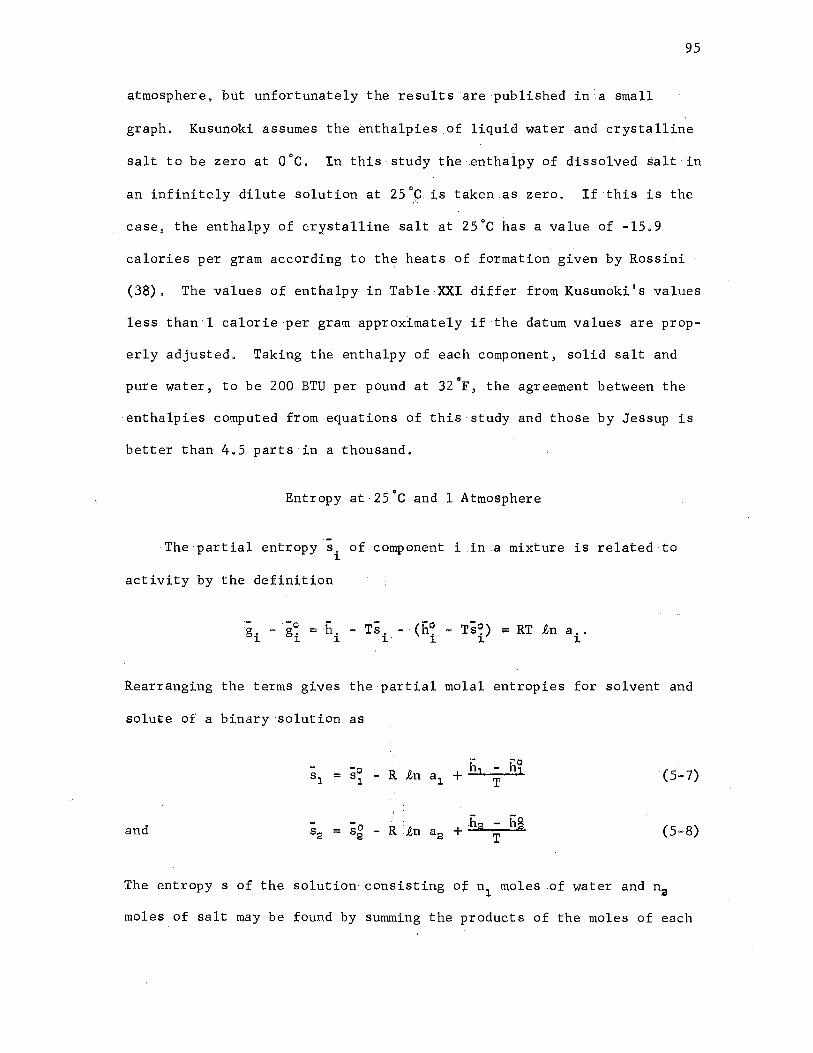
95

atmosphere, but unfortunately the results are published in a small

graph. Kusunoki assumes the ~nthalpies of liquid water and crystalline

salt to be zero at 0°C. In this study the enthalpy of dissolved Salt in

an infinitely dilute solution at 25°f is taken as zero .. If this is the

case, the enthalpy of crystalline salt at 25°C has a value of -15,9

calories per gram according to the heats of formation given by Rossini

(38), The values of enthalpy in Table XXI differ from Kusunoki' s values

less than 1 calorie per gram approximately if the datum values are prop-

erly adjusted. Taking the enthalpy of each component, solid salt and

• pure water, to be 200 BTU per pound at 32 F, the agreement between the

enthalpies computed from equations of this study and those by Jessup is

better than 4.5 parts in a thousand.

Entropy at 25°C and 1 Atmosphere

The partial entropy s. of component i in a mixture is related to l.

activity by the definition

g. - g~ = h. - Ts - (h0 - Ts~) = RT in a .. l. l. 1 i i l. l.

Rearranging the terms gives the partial molal entropies for solvent and

solute of a binary solution as

ii., -o -o R in - h1

sl = sl - al + T (5-7)

and sO R in h2 - h~ S:.3 - a2 + 2 T

. (5-8)

The entropy s of the solution consisting of n1 moles of water and n2

moles of salt may be found by summing the products of the moles of each

96

component times its partial molal entropy. Substitution of Equation

(5-1) for qd leads to

(5-9)

where~= denotes the mean activity •. Based on the ionic activity coef­

ficients determined by Robinson· (36), the heats of formation compiled by ,z_.

· Rossini (38) and the .tn a1 from Equation (2 ... 3), the values of entropy at

25°C and 1 atmosphere have been calculated and tabulated in Table·XXII.

In this calculation, the entropy of saturated water at o•c and the·en-

tropy of salt in the infinitely dilute solution at 25°C and 1 atmosphere

are taken to be zero. For the ease of later computations 1 the results

were fitted into an interpolation formula as follows:

s = 0.0876 + 0.067594387x - l.276743lx2 + 1.7277596~ (5-10)

wheres iS: in BTU per degree Rankine per pound and xis in grams salt

per 100 grams of solution.

Entropy Table

By.holding the composition of the solution constant, the entropy at

any temperature T and pressure·P may be related to the entropy in a

given state (T ·,.P) as follows: 0 0 .

s = .s 0

T P c

+ I -i2'- dT - .I ~~dP. (S-11)

T p 0 0

The values of entropy at the concentrations of 0 1 .5, 10, 15,.20 and 25

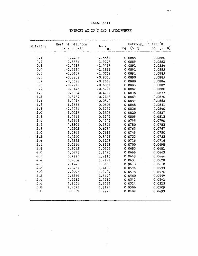
97

TABLE )CXII

ENTROPY·AT 25°C AND 1-Al'MOSPHERE

_Molality . He4t of Dilution Ln'a EntrOEI 2 Btu/lb' 1R cal/gm Salt ·%. Eq. (5-9) Eq. (5-10)

0.1 -1. 4487 -2.5531 0.0885 0.0880 0.2 -1.5587 -1.9178 0.0889 0.0882 0.3 -1. 4 737 -1. 5468 0.0891 0.0884 0.4 -1. 2994 --1.2833 0.0891 0.0885 0.5 -l.0759 -1.0772 0.0891 0.0885 0.6 -0.8232 -o·. 9073 0.0890 0.0885 0.7 -0,5528 · -0. 7619 0.0888 0.0884 0.8 -0. 2719 -0.6351 0.0885 0.0882 0.9 0.0146 -·0.5221 0.0882 0.0880 1.0 0.3034 --0.4202 0.0878 o. 0877 1.2 0.8789 -0.2418 0.0869 0.0870 1.4 1.4422 -0.0874 0.0859 0.0862 1. 6 1,9862 0.0505 0.0848 0.0851 1.8 . 2, 5071 0.1752 0.0836 0.0840 2.-0 .·. 3.0027 ·0.3305 0.0820 0.0827 2.2 · 3.4719 0.3949 0.0809 0.0813 2.4 3.9145 0.4942 0.0795 0.0798 2.6 -4.3305 0.5876 ·0.0180 0.0783 2.8 4. 7203 0.6764 0.0765 0.0767

. 3.0 5.0846 0.7613 0.0749 0.0750 3,2 5.4240 0.8426 0.0733 0.0733 .. ,, 3.4 5.7393 0. 92.08 0. 0716 0.0716 3.6 6.0314 o. 9968 0.0700 0.0698 3.8 6.3012 1.0707 0.0683 0.0681 4.0 6,5496 1.1420 0.0666 0.0663

. 4.2 6. 7773 1,2115 0.0648 0.0646 4.4 6.9854 1,2794 0.0631 0.0628 4.6 7.1745 l.3460 0.0613 0.0610 4,8 7.3457 l.4109 0.0596 0.0593 5.0 7.4995 1.4747 0.0578 0.0576 5.2 7.6369 1. 5374 0.0560 0.0559 5.4 7.7585 1.5989 0.0542 0.0542 5.6 7.8651 1. 6597 0.0524 0.0525 5.8 7.9573 1. 7194 0.0506 0.0509 6.0 8.0359 1. 7779 0.0489 0.0493

98

grams salt per 100 grams of solution have been determined by letting

T = 25°C and P = -1 atmosphere in order to use Equation (5-10) for s 0 0 0

The results of calculations are shown in Table XXIII and Figu'.!'.'e 14-.

Heat of Vaporization

- A molecule which leaves the surfaqe of a liquid must ~vercome the

forces of attraction of the other molecules in the liquid. The inter-

molecular forces of attraction are-relatively large because the mole-

cules are much closer together in the-liquid state than in the vapor

state •. In order to overcome these attractive forces, energy must be

suppli.ed to the liquid in the form of heat. The heat required to vapor-

ize a substance may be accurately computed from the S'lope of vapor pres-

. sure curve· and. the conesponding specific volumes of the liquid and

vapor phases. This relation was first discovered by the French engineer

Clapeyron before the formal formulation of the first law of thermodyriam-

ics (1834), but its deduction from the modern point of view was due to

Clausi.us.

The Clau.sius .. cl.apeyron relation appli.es only to a single component

system in equilibrium. For a binary solution, there is no such unique

relation between changes in pressure and temperature .. In the case of an

aqueous solution of nonvolatile salt, the vapor pressure has a definite

value only when the temperature and the concentration are held constant,

.and a modified version of the Clausius-Clapeyron relation is derived by

. Denbigh -(5) as follows:

ii -- ii ~"\ - 6 : .,?JT)x T'(v - v1)

g

TABLE· :XXIII

ENT~OPY 'IN BTU PER ,POUND 'PE.R DEGREE :AANKINE

. Temp.,. QF :: . 0 ,'

(At Vapor 'Pressure)

32 35 40 45 50 55 60 65 70 75 80 85 90 95

100 105 110

'115 ~20 125 130 135 140 145 150 155 160 165 170 175

·.180 185 190 195 200 205 210 212 215 220 225 230

0.0000 0.0061 0.0162 0.0262 Q.0361 0.0458 0.0555 0.0650 0.0745 0.0839 0.0932 0.1024 0.1115 0.1205 0.1294 0.1383 0.1471 0.1558 0,1644 0.1730 0.1815 0.1899 0;1982 0.2065 0.2147 0.2229 0.2310 0,2390 0.2470 0.2549 0.2628 0.2706 0.2783 o. 2860 0.2936 0.3012 0.3088 0.3118 0.3162 0.3237 0.3311 0.3384

Salt Weight, gm/100· gm Solution 5 . ~' 10 '· . 15 . 20

0.0051 0.0109 0.0204 0.0299 0,0392 0.0484 0,0576 o .. 0666 0.0756 0.0845 0.0933

·0.1020 0.1106 0.1192 0.1276 0.1360 0.1443 0.1526 0.1607 0.1688 0.1769 0.1848 0.1927 0,2005 0.2083 0.2160 0.2237 0.2312 0.2388 0.2462 0.2537 0.2610 0.2683 0.2756 0.2828 0.2899 0,2970 0.2999 0.3041 0.3111 0.3180 0.3250

·.: \

0.0047 0.0102 0.0192 0.0282 0.0370 0.0458 0.0545 0.0631 o. 0716 0.0800 0.0883

.0,0966 0.1048 0.1129 0.1209 0,1288 0.1367 0.1445 0.1523 0.1599 0,1675 0,1751 0.1825 0.1900 0.1973 0,2046 0.2118 0.2190 0.2261 0.2332 0.2402 0. 2471 0.2540 o. 2609 0.2677 0.2744 o. 2811 0.2838 o. 2877 0.2943 0.3009 0.3074

I' ..

0.0001 0.0053 0.0139 0.0224 0.0308 0.0391 0.0474 0.0556 0.0637 0.0717 0.0796 0.0875 0.0952 0.1029 0.1106 0, 1181 0.1256 0.1331 0.1404 0.1477 0.1549 0.1621 0.1692 0.1762 0.1832 0,1901 0.1970 0.2038 0,2105 0.2172 0.2238 0.2304 o .. 2370 0.2434 0.2499 0,2562 0.2626 0.2651 0.2688 0.2751 0,2812 0.2874

-0.0077 .. o.0027

0.0055 0.0136 0.0217 0.0297 0.0376 0.0454 0.0532 0.0608 0.0684 0.0759 0.0834 0.0908 0.0981 0.1053 0.1125 0.1196 0.1266 0.1336 0.1405 0.1473 0.1541 0.1609 0.1675 0.1741 0.1807 0.1872 0.1936 0.2000 0.2063 0.2126 0.2188 0.2249 o. 2311 o. 2371 0.2431 0,2455 0.2491 0.2550 0.2609 0,2667

99

. 25

-0.0175 -0.0127 -0,0048 0.0031 0.0109 0.0186 0.0263 0.0339 0.0413 0.0488 0.0561 0.0634 0.0706 0.0777 0.0848 0.0918 0.0987 0,1056 0.1124 0.1191 0.1258 0.1324 0.1389 0.1454 0.1518 0.1582 0.1645 0.1708 0.1770 0.1831 0.1892 0.1952 0.2012 0.2071 0.2130 0.2188 0,2246 0.2269 0.2303 0.236.0 0.2416 Oi2472

100

TABLE XXIII - Continued

.Temp.,. °F Salt Weight 2 gm/100 gm S6lution 0 5 10 15 20 25

(At Vapor Pressure)

235 0.3457 0.3318 0.3138 0.2935 0.2725 0.2527 240 0.3530 0.3387 0.3203. 0.2995 0.2782 0.2582 245 0.3602 0.3454 0.3266 0.3055 0.2839 0.2636 250 0.3674 0.3522 0.3330 0.3115 0.2895 0.2690 255 0.3745 0.3589 0.3392 0.3174 0.2951 0.2743 260 0.3816 0.3655 0.3455 0.3232 0.3006 0.2796 265 0.3887 0.3721 0.3517 0.3291 0.3061 0.2848 270 0 . .3957 0.3787 0.3579 0.3349 o. 3116 0.2900 27.5 0.4027 0.3853 0.3640 0.3406 0.3170 0.2952

· 280 0.4096 0.3918 0.3701 0.3463 0.3224 0.3003 285 0.4165 0.3982 0.3761 0.3520 0. 3277 0.3053 290 0.4234 0.4047 0.3821 0.3576 0,3330 0.3104 295 0.4303 o. 4110 0.3881 0.3632 . 0. 3382 0.3153 300 0.4371 · 0.4174. 0.3940 0.3687 0.3439- 0.3203 305 0.4438 0.4237 0.3999 0.3742 0.3486 0.3252 310 0.4506 0.4300 0.4058 0.3797 0.3537 0.3300 315 0.4573 0.4.363 · 0.4116 0.3851 0.3588 0.3348 320 0.4640 0.4425 0.4174 ·0,3905 0.3639 0,3396 325 0.4706 0.4487 ·0,4232 0.3959 0.3689 0,3443 330 0. 4772 0.4549 0.4289 0.4012 0.3739 0.3490 335 0.4838 0.4610 0.4346 0.4065 0.3788 0.3536 340 0.4904 0.4671 0.4403 0.4118 0.3837 0.3582 .345 0.4969 0.4731 0.4459 0.4170 0.3886 0.3628 350 0.5034 0.4792 0.4515 0.4222 0.3934 0.3673

(Pressure ~ 1,000 PSIA)

50 0.0359 0.0389 0.0367 0.0304 0.0212 0.0104 100 0.1288 0.1270 0.1202 0.1099 0.0974 0.0841 150 0.2138 0.2074 <0.1964 0.1824 0.1667 0.1511 200 0.2924 0.2817 .0.2667 0.2489 0, 2302 0.2123 250 0.3659 0.3509 0.3318 0.3105 0.2886 0.2682 300 0.4354 0.4159 0.3928 0.3676 0.3425 0.3194 350 0.5015 0.4776 p.4501 0.4210 0.3924 0.3664

(Pressure = 2,000 PSIA)

50 0.0357 0.0387 0.0363 0,0300 0.0208 0,0099 100 0.1282 0.1263 0.1195 0.1092 0.0967 0.0834 150 0.2129 0.2065 0.1956 0.1816 0.1659 0.1504 200 0.2912 0.2806 0.2657 0.2480 0.2294 o. 2115 250 0.3645 0.3496 0,3307 0.3094 o. 2877 0.2674 300 0.4336 0.4144 0. 3914 0.3665 0.3415 0.3186 350 · o. 4994 0.4758 0.4486 0.4197 0.3913 0.3655

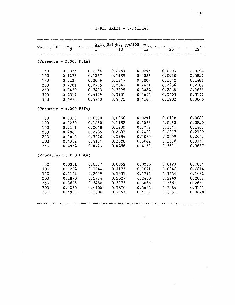
101

TABLE XXIII - ·· Continu~d

':pemp., ·. °F Salt Weight 2 gm/100 gm 0 5 10 '15 20 25

(Pressure= 3,000 PSIA)

50 0.0355 0.0384 0.0359 0.0295 ·0.0203 0.0094 100 0.1276 0.1257 0, 1189 0.1085 0.0960 0.0827

.· 150 0.2120 0.2056 0.1947 0.1807 0.1652 0.1496 200 0.2901 0.2795 0.2647 0.2471 0.2286 0.2107 250 0.3630 0.3483 0.3295 0.3084 0.2868 0.2666 300 0.4319 0.4129 0.3901 0.3654 0.3405 0.3177 350 0.4974 0.4740 0.4470 0 .. 4184 0.3902 0.3646

(Pressure· = 4,000':PSIA)

50 0.0353 0.0380 0,0356 0.0291 0.0198 0.0089 100 0.1270 0.1250 0.1182 0.1078 0.0953 0.0820 150 O, 2111 0.2048 0.1939 0.1799 0.1644 0.1489 200 0.2889 0.2785 0.2637 0.2462 0,2277 0.2100 250 0.3616 :0.3470 0.3284 0.3075 0.2859 0.2658 300 0.4302 0.4114 0.3888 0.3642 0.3396 0.3169 350 0.4954 0.4723 0.4456 0.4172 0.3891 0.3637

· (Pressure·= 5,000 :PSIA)

· 50 0 •. 0351 o. 0377 0.0352 0.0286 0.0193 0.0084 100 0.1264 0.1244 0.1175 0.1071 0.0946 0.0814

>150 o. 2102 0.2039 0.1931 0.1791 0.1636 0.1482 200 0.2878 0.2774 0.2627 0.2453 0,2269 0.2092 250 0.3603 0.3458 0.3273 0.3065 0.2851 0.2651 300 0.4285 0.4100 0.3876 0.3632 0.3386 0.3161 350 0.4934 0.4706 0.4441 0.4159 0.3881 0.3628

102

LL 0

en _J ....... :) I-en

~

>-a.. 0 0:: I-z w .16

-.040 4 8 I 2 16 20 24 2 8 32

GRAMS SALT PER 100 GRAMS SOLUTION

Figure 14. Entropy at 10 Atmospheres

·103

where the partial molal volume and partial molal enthalpy of water in

solution are denoted by the respective quantities with a subscript·l,

.and the molal volume and molal enthalpy in the vapor phase with a sub~

script g. . 'I'he difference between h and h1 is the heat being supplied g

from the surroundings to evaporate one mole of water from solution at

constant concentration. Obviously this is not the same as the heat of

vaporization of pure water.

By adding ·fi to both sides of Bquation (3-5). and rearranging terms, . g

the heat of vaporization of water for a given solution may be given in

terms of that for an infinitely dilute solution and the activity by the

equation

= h g (5-12)

The·last term of this equation may be interpreted as the difference be-

tween the heat of vaporization of water from·solution and the latent

heat of pure water at the same temperature. In accordance with the data

established by the Third·International·Conference on Steam Tables (48),

the latent heat of pure water in BTU per pound can be given by the fol-

lowing equation with a maximum deviation of two parts per ten thousand:

fi g

1093.3254 -~ o.57909483t + o.228937 x 1o~~ts

- 0.11130559 x 1o~ita (5-13)

where tis the temperature in degrees Fahrenheit .. In general, .en a1 is

a function .of temperature, pressure and concentration. The variation of

in a1 with T and x at constant pressure·is given by Equation (2-3). The

general expression for .en a1 , as discussed in Chapter·II, is

p

.1 I <­+RT . v1

·p 0

104

(5-14)

where .tn a11,p ·) is a function of T and x at the fixed pressure P ; v1 .• o ·o

and v~ are respectively the·partial volume at the concentration to which

the activity a1 refers and the ·partial volume at infinite dilution. . The

·partial volumes can be easily evaluated from the volume of solution by

the relation

Because the·partial quantities are derived from an extensive property by

simple differentiation, it is permisSible to choose ·either mass or mole

as unit of quantity. With the same notations as in Equation (5-6) for

the coefficients, the difference between the two partial volumes may be

written as

+ .Px(F.·vl + F 2'r + F 3T2 ) + .2P:x:iil(G ·1 + G 2T + G 3Tli) v .v · :v ·v v

+ -0.SP:iilx(H .1 +H 2T +·H 3r2). . v v v

Consequently,

·p 0 + ·[3x(-F + F T2 ) + 6x2 (-G + G t 2 )](P2 --p2\ vl v3 · ~v1 .v3 of

105

Thus, in a1 at any vapor pressure may be determined. The numerical

value of the last term in Equation. (5-14) is very small in c?mparison

with the value of in a1 at 10 atmospheres. Table XXIV shows the calcu­

lated differences between (6 - 6) and (6 - 6°) from Oto 350eF .. The g l g l

sum of the value in this table and the heat of vaporization of pure

water, which may be found i.n a steam table or calculated from Equation

(5-13), .is the heat required for the phase transition of water in solu-

tion from·li.qui.d to vapor at constant temperature and composition.

Temp., 6 F

32 35 40 45 50 55 60 65 70 75 80 85 90 95

100 105 llO 115 120 125 130 135 140 145 150 155 160 165 170 175 180 185 190 195 200 205 210 212 215 220

.· 225 230 235

TABLE·XXIV

.· HEAT OF VAPORIZATION OF. SOLUTION MINUS l,ATENT . HEAT OF 'PURE WATER 'IN BTU PER POUND

Salt Weight 2 gm/100 gm Solution 1 5 10 15 20

0.07 -0.40 -1.63 -3.10 -4.52 0.07 -0.39 -1.58 -3.01 -4.36 0.07 , -0.36 -1.51 -2.86 -4.10 0.08 -0.34 -1.44 -2.71 -3.84 0.08 -0.32 -1.37 -2.56 ,-3,58 0.08 -0.30 -1.30 -2.41 -3.32 0.08 -0.28 -1.23 -2.26 -3.06 0.08 ... Q.25 -1.16 -2.11 -2.80 0.08 -0.23 -1.08 -1.96 -2.54 0.09 -0.21 -1.01 -1.81 -2,28 0,09 -0.19 -0.94 -1. 66 c..2 .02 0.09 -0.17 -0.87 -1. 51 -1. 76 0.09 -0.15 -0.80 --1. 36 -1. 50 0.09 -0.12 -0.73 -1.21 -1.24 0.09 -0.10 -0.66 -1.06 -0.98 0.10 -0.08 -0.58 -0.91 --0. 72 0.10 -0.06 -0.51 -0,76 -0.46 0.10 -0.04 -0.44 -0,62 -0.20 0.10 -0.01 -0.37 -0.47 0.06 0.10 0.01 -0.30 -0.32 0.32 0.11 0.03 -0.23 -0.17 0.58 0.11 a.as -0.16 -0.02 0.84 0.11 0.07 .. o.09 0.13 1.10 0.11 0,09 -0.01 0.28 1.36 0.11 0.12 0.06 0.43 1. 62 0.11 0.14 0.13 0.58 1.88 0.12 0.16 0.20 0.73 2.14 0.12 0.18 0.27 0.88 2.40 0.12 0;20 0.34 1.03 2.66 0.12 0.23 0.41 1.18 2.92 0.12 0.25 0.49 1.33 3.18 0.12 0.,27 0,56 1.48 3.44 0.13 0,29 ·0.63 1. 63 3.70 0.13 0.31 0.70 l, 77 3.96 0.13 0.33 0. 77 1.92 4.22 0.13 0.36 0.84 2.07 4.48 0.13 0.38 0.91 2.22 4. 74 0.13 0.39 0.94 2.28 4.85 0.14 0.40 0.98 2.37 5.00 0.14 ·0.42 1.06 2.52 5.26 0.14 0.44 1.13 2.67 5.52 0.14 ·0.46 1.20 2.82 5.78 0.14 0.49 1. 27 2.97 6.04

106

25

-5,63 -5.38 -4.97 -4.56 -4.15 -3.74 -3.33 -2.92 -2.51 -2.10 -1.69 -1.28 -0.88 -0.47 -0.06

0.35 0.76 1.17 1. 58 1. 99 2.40

. 2. 81 3.22 3.63 4.04 4.45 4.86 5.27 5.68 6.08 6.49 6.90 7.31 7. 72 8.13 8.54 8.95 9.11 0.36 9. 77

10.18 10.59 11.00

107

TABLE .XXIV • Continued

Temp., "F Salt Weiaht 2 gm/100 gm Solution 1 5 10 15 20 25

240 0.14, o_.51 1 .. 34 · 3.12 6.30 11.40 245 0.15 0,53 1.41 3.27 6.56 11.81 250 0.15 0.55 1.48 3.42 6.82 12.22

. 255 0.15 0.57 1.55 3.57 7.08 ·12.63 260 0.15 0.60 1. 63 3.72 7.34 13.04 265 0.15 0.62 1. 70 3.87 7.60 13.45 270 0.15 0.64 1,77 4.02 7.86 13.86 275 0.16 0.66 1.84 4.16 8.12 14.27 280 0.16 0.68 1.91 4.31 8.39 14.68 285 0.16 o. 71 1.98 4.46 8.65 15.09 290 0.16 0.73 2.06 4.61 8.91 15.50 295 0.16 0.75 2.13 4. 76 9.17 15.91 300 0.17 o. 77 2.20 4,91 9.43 16.32 305 0.17 0.79 2.27 5,06 9.69 16.73 310 0.17 0.82 2.34 5.21 9.95 17.14 315 0,17 0.84 2.42 5.36 10.21 17.54 320 0.17 0.86 2,49 5.52 10.47 17.95 325 0.18 0.88 2.5(;i 5.67 10.73 18.36 330 0.18 0.91 2.63 5.82 10.99 18. 77 335 0.18 0.93 2. 71 5.97 11.25 19.18 340 0.18 0.95 2.78 6.12 11.52 19.60 345 0.18 0.98 2.85 6.27 11. 78 20.01 350 0.19 1.00 2.93 6.42 12.04 20.42

· CHAPTER VI

SUMMARY AND CONCLU~ION

An effort has been made to gather information on the thermodynamic

properties of aqueous·sodium chloride solution .. It is hoped that this

information may supplement the basic data for the desalination proces.:i.~

ses, Fortunately a sufficient amount of experimental data was found in

the literature to support this study .

. In Chapter.· II interpolation· formulae for vapor pressure and for

·1ogarithm of activity of water were developed from osmotic coefficients .

. The activity of water may be derived from either vapor pressure or os­

motic coefficient; however, the data on osmotic coefficient appear to be

more precise than vapor pressure, particularly in the region of low salt

concentration. In the early stage of this study, the data on vapor

pressure were used to compute the activity. . Consequently, the calculat­

ed values of specific heat did not agree very well with the·experimental

data. Some time ago Gastaldo (11) tried to calctilat~ the relative par­

tial molal enthalpy of sea water with·the activities which were based on

the vapor pressures by ordinary measurements. The results of his calcu­

lations also were very poor .. Undoubtedly the vapor pressures reported

in·literature are·generally not precise ·enough for the accurate determi­

nation of partial thermal properties. The data on osmotic coefficient,

used in Chapter II, come from very precise measurements of boiling :

point, vapor pressure, or electromotive force (10, 14, 45, 46). Based

108

109

on the osmotic coefficients, the logarithms of activity of water have

been calculated and fitted into an equation of nine constants, Equation

(2-3). The variation of logarithms of activity with pressure was proved

to be negligible for a pressure change of 10 atmospheres or less. Equa­

tion (2-7) is an interpolation formula for vapor pressures determined

from osmotic coefficients. Of the many different equations for vapor

pressure, the most popular one is perhaps the Antoine equation. This

equation does not represent the vapor pressures of water as accurately

as the Nernst equation, but it can be expressed explicitly in terms of

temperature. Equation (2-11), from which the qoiling temperature of

solution can be readily calculated, is an adaptation of the Antoine

equation that fits the vapor pressure of pure water.

The experimental data on specific heat are not only scarce but also

Slightly inconsistent, as shown in Figure 7, Therefore, in Chapter III

the specific heat was determined from activity of water, solubility,

specific heat of pure water and specific heat of· solid salt by following

the established rules of partial molal quantities. To make it easy for

the calculation of enthalpy and entropy, the results were fitted by a

simpler empirical formula, Equation (3-27), which gives the functional

relation among the specific heat, temperature and concentration at 10

atmospheres. The pressure dependency of specific heat is discussed in

Chapter IX.

In the middle portion of this study, an experimental program was

initiated to determine an equation that accurately represents the pres­

sure-volume-temperature-concentration data. For pure water, the data

adopted by the Third International Conference on Steam Tables (48) cover

the specific volumes of compressed water to 400 kg per sq cm; but for

110

the solution, the coverage of available data on density does not extend

to the high pressure region (7, Sl). Under this situation a decision

was made to measure the pressure effect on the specific volume of solu­

tion in order to have sufficient data for the equation of state, and the

experiment was carried out as described in Chapter·rv. By means of a

c.al.ib:r:ated positive-displacement pump, the change of volume with the

change of pressure at a fixed temperature was measured for solutions

under pressures up to 5,000 psia in the range of 70 to 350°F·and Oto 25

g;r.ams · salt per 100 grams solution. From the· experimental data so ob­

tained, the values of partial derivative of v with respect to P have

been determi.ned with probable error of about :l: 4. 5% of the true value.

Since the thermal properties of liquid are insensitive to the pressure

change, the e:r.·ro:r.· of this magnitude will not cause serious consequences

to the values of specific volume, enthalpy and entropy. The test re­

s~lts indicate that the larger the amount of salt added, the greater the

lowering of the va.lue of this derivative. . To fit the experimental data

regarding the specific volumes, Equation (4-13) was arbitrarily chosen

as a general exp'l'.·ession for the explicit representation of v .. In this

equation, the temperature functions A(T), B(T),. C(T), D(T) and E(T) were

determined with the data from literature, and the remaining three tem­

perature functions were obtained by curve~fitting the partial derivative

of v with respect to P.

The enthalpy and entropy at 25°C and 1 atmosphere were calculated

by taking the saturated water at 0°C and the salt in infinitely dilute

solution at 25 °C as the reference states for water and salt respective;

ly. In these calculations the heat of dilution was based on the heat of

formation by Rossini (38). Subsequently, the cogiputations of enthalpy

111

and entropy were extended to other temperatures and pressures by taking

advantage of the interpolation formulae, which have already been devel­

oped, for specific heat and specific volume. Finally, the heat of va­

porization was computed, and the difference of this between solution and

pure water is shown in Table XXIV •

. In conclusion, this study has yielded practical equations for com­

·puting the thermal properties of E!queous sodium chlo.ride solution in the

·32 to ,350°F temperature range, based on the data in harid. The method of

determining the specific heat and the development of theP-v-T-x rela­

tion are noticeably unconventional.

If the pressure is not over 10 atmospheres, the pressure dependen­

cies of specific volume, enthalpy and entropy may be neglected so that

the c·om.putations beeome simple. A short list of Fortran arithmetic

functions which may be called for the computations of vapor pressure,

.heat of vaporization, specific volume, enthalpy and entropy at a moder~

ate pressure is shown in Appendix B. . By adding a few terms to the ,

arithmetic function, the pressure dependency of specific volume can be

easily included. Simple expressions for the .. pressure effect on the

.values of enthalpy and entropy have not been devel9ped; however, the

estimate can be made by interpolating the values in Tables XXII and

.:XXIII.

Because of the unknown reliabilities of the data in the literature

and the complex nature of calculations, rigorous estimates of probable

·error have not been made for each ·property pr.esented; nevertheless, an

effort was made ·to compare the experimental data and the derived values

from the·various sources •. Although the agreement between the specific

·heats calctilated with the method in this study and the heat capacities

112

measured by calorimeters at temperatures below 80°C is gratifying, the

degree of accuracy of the calculated values at higher temperatures is

unknown ·due to the possible propagation of errors resulting from· the

mathematical maniptilat ion of the empirical formulae. The· recommend~-

tions of future work include the·error analysis for each property and I

the direct: measurements of specific heats in the high temperature re-

·gion.

(1)

(2)

(3)

. (4)

__ BIBLIOGBAPHY

Adams, L. H., and R. E. Hall. -"Solubility of Sodium Chloride." I

Journal of-~ Washington Academy ~ Sciences~ Vol. 21 (1931), p. 193.

Amagat, .M. E. H. ''Memoires sur l 'elasticite et la lilatation de.s fluides." Anna les _ de -Chimie -~ ~ Physique (France) , 6 seri~s, Vol. 29 (1893), p. 545.

Badger, W. L., and.E .• M._Baker. "Studies in Evaporator Design." Transactions of American Institute of Chemical Engineers, VoL 13 ( 1929), p. 151.

Baker, E._M,, and V. H. Waite. -"Boiling Point of Sa_lt·Solution Under Varying Pressures." Chemical .!!!.!!- Metallurgical Engi­

·neering, Vol. 25 (1921), p. 1139 •

. (5) Denbigh,. K. -~ Principle £!. Chemical Equili]?rium. London: Cam­bridge University Press, 1955, p. 218 •

. (6) Dorsey,_ N. E. _ Properties of Ordinary Water-Substance. New York: . Reinhold.Pul:ilishing. Corporation, 1940, p. 234.

(7) Fa buss,._ B. _ M. Thermodynamic _Properties of Saline Water. Progress Report 136, U.S. Office of:Saline Water, 1965,.pp. 30, 61.

_(8) Fa.buss, B. M., and A •. Korosi. ''Vapor ·pressure of Binary Aqueous -• Solutions of NaGl, KCl, _ Na2·so4 ·and 'MgS04 at·Co.ncentrations

and Temperatures of Interest in Desalination·Process." Desalination, Vol. l (1966), p. 139.

(9) Freyer,,E. B. '~onic Studies of the Physical Properties of Liq­uid.- The Velocity of Sound in Solution$ of Certain Alkali

-Halides and Their Compressibi,lities." Journal of American Chemical Society;~ Vol. 5~ (1931), p. 1313. -

. (10) Gardner, -E. R., .P. J. Jones, .and H. J,. de Nordwall. "Osmotic Co­efficients of Some Aqueous Sodium Chloride Solutions at High 'femperature." Transactions of Faraday ·Society (London),. Vol. 59 (1963), p. 1994.

- (11) -. Gastaldo, - C. "Determination of Coefficients for Thermodynamic Equations fo·r Determining the Properties of Sea Water, Parti­cularly Vapor ·Pressure." University of California in Los Angeles, .Report 61-80 (1962), p. 35.

113

. (12)

(13)

(14)

(15)

(16)

(17)

114

Gucker, F •. T., and. T. R •. Rubin. "The Apparent Molal Isochoric · . Heat· Capacity of Electrolytes. 11 · Journal of American: Chemical Societx, Vol. 57 (1935), p. 78.

Guggenheim,. E •. Q. Thermodynamics: .An Advanced Treatment for Chemists .!E!! PhY!,icists. t Amsterdam: 'North;;.;-Hollarid ':-P'iililisn:" ::-; ing. Company, 1957, p ... 393.

Harned, H. S., and L. F. Nims. -'~he Thermodynamic Properties of • Aqueous Sodium Chloride Solutions from O to 40 °. 11 .· Journal .2£. American Chemical Society, Vol. 54 (1932), p •. 423.

,Hess, c. B., and B. E •. Gramkee. ·"The Specific Heats of Some Aque­ous Sodium and Potassium Chloride Solutions at Several Tem­peratures," Journal .2£. Physical Chemistry, .Vol. 44 (1940), p. 483. .

Hirschler, · A. E. ''Vapor ·Pressures of Saturated. Solutions." Jour­B!l .2f American Chemical. Society, Vol. 38 (1946), p. 1.

Hubbard, J. C., and A. L. Loomis. ''Velocity of Sound in Liquids by the Sonic·Interferometer. 11 Philosophical Magazine and

. Journal of Science (London), 7th Series, Vol. 5 · (1928), p. 1.17'7.

(18) , Jes~up,. R. s. '~he Heat Content of Frozen. Sodium and Calcium Bri.nes. 11 ·. Refr·igerating. :Engineering, Vol. 22 (1931), p. 166.

(19) . Kaufmann, D. w. Sodium Chloride. New York: Reinhold. Publishing Corporation, 1960, .p. 603 .

. (20) .Keenan, .J. H., and F. G. Keyes. Thermodynamic Properties . .2! Steam. New York: · John Wiley and. Sons Company, 1936, ,pp~ 28-75 .

. (21) Keevil, .N. B. ''Vapor Pressure of· Aqueous· Solutions at High Tem­perature," Journal of American Chemical. Society, Vol. 64 (1942), p. 845.

(22) Kell, G,. S. ''Precise Representation of Volume Properties of Water at One Atmosphere." Journal of Chemical~ Engineering Da t a , Vo 1. 2 1 ( 19 6 7) , . p . 6 6 •

(23) Kell, G. S., and E. Whalley. -"The PVT 'Properties of Water·I. Liquid Water in the Temperature Range Oto 150°C and at Pres­.sure up to 1 kb." Philo.sophicaLTransactions of the Royal Societi (London), Series· A, Vol. 258 ( 1965), p. 565.

(24) ·Kelly, K. K •. '~ontributions to the Data on Theoretical Metal­lurgy." Bulletin 476, .U. s. Bureau of Mines, 1949. p. 166.

115

(25) Keyes, F. G. "Methods and Procedures Used in the Massachusetts Institute of Technology Program of Investigation of the Pres­sures and Volumes of Water to 460°C." Proceedings of Ameri­,m Academy of Arts and Sciences, Vol. 68 ( 1933), p. 505.

(26) Keyes, F. G., L.B. Smith, and H. T. Gerry. '~he Specific Volume of Steam in the Saturated and Superheated Condition Together with Derived Values of the Enthalpy, Entropy, Heat Capacity and Joule Thomson Coefficients." Proceedings of American Academy of Arts and Sciences~ Vol. 70 (1936), p. 329.

(27) Kusunoki,. K. "Construction of Enthalpy-Concentration Diagram for NaCl-H2 0 System." Kagaku Kogaku (Japan), V. 21 (1957), p. 775,

(28) Landolt, H., and R. Btfrnstein .. Physikalisch-Chemische Tabellen. Berlin: Julius Springer, 5 Auflage, 2 Band, 1923, pp. 1383, 1385.

(29) Lipsett, S. G., F •. M. G. Johnson, and 0 .. Maas. "A New Type of Rotating Adiabatic Calorimeter - The Surface Energy and Heat of Solution of Sodium Chloride." Journal of American Chemi­ill Society, Vol. 49 (1941), p. 1927 .

. (30) McLean, D. Mechanical Properties & Metals. New York: John Wiley and Sons Company, 1962, p. 8.

(31) M. W. Kellog Company. Saline Water Conversion Engi.neering -~ ~· U. s. Government 'Printing Office, 1965, pp. 12 •. 20, 12.30.

(32) Nernst, W. ~New-~ Theorem. New York: E. P •. Dutton and Company, 1.917, p. 123 •

. (33) Osborne, N. s., and C, H. Meyers. ·~ Formula and Tables for the Pressure of Saturated Water Vapor in the Range of Oto 374~C." Journal of Research of the National Bureau of Stand­args, Vol. 13 (1934), p. 1. ·- -

(34) Othmer, D, F. "Correlating Vapor Pressure and Latent Heat Data." Industrial and Engineering Chemistry, Vol. 32 (1940), p. 848.

(35) Randall, M., and F. D. Rossini. ''Heat Capacities in Aqueous Solu­tion." Journal of American Chemical Society, Vol. 51 (1929), p O 323.

(36) Robinson, R. A., and R.H. Stokes. Electrolyte Solutions. New York: Academic Press Inc,, 1955, pp. 461, 465.

(37) Robinson, .R. A., and H. S. Harned. ''Some Aspects of the Thermo­dynamics of Strong~lectrolytes from Electromotive Force and Vapor Pressure Measurements." Chemical Review, Vol. 28 (1941), p. 419.

116

(38) Rossini, F. D., et al. . "Selected Values of Chemical Thermodynamic Properties." Circular 500, . U. S. Bureau of Standards, 1952, p. 450 .

. (39) Rutskov, A. P. "Specific Heats of Aqueous· Solution of MgCl~, C8 Gl:,i, NaCl, KCl, KN03 , and NH3 N03 at 25°, 50°, and 75 c." Journal of Applied Chemistry (USSR), Vol. 21 (1948), .p. 820.

(40) Scatchard, G., W. J. Hamer, and S. K. Wood. "Isotonic Solutions I. The Chemical Potential of Water in Aqueous Solutions of Sodium Chloride, .Potassium Chloride, .. Sulfuric Acid,. Sucrose,

. Urea and 9lycerol at. 25 °." Journal of American Chemical Society, Vol. 60 (1938), p. 3061.

(41) Schroeder, W. C., A. Gabriel, and E. P, Partridge. "Solubility Equilibria of Sodium Sulfate at Temperature of 150 to. 350 •. 11

Journal of American Chemical Society, Vol. 57 (1935), p .. 1539.

(42)

(43)

(44)

(45)

(46)

Seidell, A. Solubilities of Inorganic and Organic Compounds. New York: D. Van Nostrand Company, 1919, p. 640.

Smith, L. B., and F. G. Keyes. "The Volumes of Unit Mass of Liq­uid Water and Their Correlation as a Function of Pressure and Temperature. 11 Proceedinga of American Academy .Qi~ . .fill£

· Sci~, Vol. 69 (1934), p, 285.

Smith, L.B.~ F. G. Keyes, and H. T. Gerry. '~he Vapor Pressure of Water," Proceedings of the American Academy of ~ and Sciences, Vol. 69 (1934), p. 137.

Smith, R. P, '~he Boiling Point Elevation II. Sodium Chloride 0.05 to l.OM and 60 to 100°." Journal of American Chemical Societ_y, Vol. 61 (1939), p. 500.

Smith, R. P., and D.S. Hirtle. '~he Boiling Point Elevation III. Sodium Chloride 1. 0 to 4. OM and 60 to 100 "." Journal of American Chemical Society, Vol. 61 (1939), p. 1123.

(47) Tait, P. G. Properties of Matter. London: Adam and Charles Black Company, 1907, p. 200.

(48) "The Third International Conference on Steam Tables." Mechanical Engineeril}g, Vol. 57 (1935), p. 710.

(49) Thomson, G. W. "The Antoine Equation for Vapor-Pressure Data." ChemicaLReviews, Vol. 38 (1946), p. 1.

(50) Washburn, E. W. International Critical Tables cif Numerical Data, .Physics, Chemistry~ Technology. Vol. 2. New York: McGraw-Hill Book Company, 1928, p. 328.

117

. (51) Washburn, .Eo Wo . International Critical. Tables of Numerical Data, Physics,· Chemistry and Technology. Vol. 3. New York: McGraw-Hill Book Company, 1928, pp. 79, 105, 370.

(52) Washburn,.· Ko W •. International Critical• Tables of Numerical Data 2

Physics,.-Chemistry and Technology. Vol. 5. New York: McGraw-Hill Book Company, 1928, p. 115.

(53) Wood, A. Bo ! Textbook of Sound. New York: Macmillan Company, 1955, pp. 261, 279.

APPENDIX A

LIST OF SYMBOLS

This li.st does not include symbols used only at a single point.

Occasionally 9 it i.s necessary to u.se the same. symbol for · different quan-

tities. For example, the principal use of G .is to represent Gibbs free

,energy 9 but it is also used to represent an empirical parameter in some

cases. To avoid confusion, all special uses of symbols are described

carefully wherever they occur.

.A, a 9 B, b,.C, c.

a

c

f

G, g

H, h

k

M

m

n

p

p

q

R

Empirical parameters

; Acti.vity

Specific heat, usually with a subscript to in­dicate conditions

Fugacity

Gibbs free energy

Enthalpy

Compressibility

Mass;.or molecular weight

Molality, moles salt per 1,000 grams sol,vent

Number of moles

Total normal pressure

Vapor pressure

Heat

Gas constant

118

s' s

.T

t

v, v

.X

Y'' y

Subscripts, superscripts

119

·Entropy

Absolute temperature·(Kelvin or Rankine scale)

·Temperature (centigrade ·or ·Fahrenheit scale)

Volume

Mole fraction; .or weight fraction of salt

·Any extensive ·property

Osmotic coefficient

Placed.above a letter to denote ·partial molal quantity

·used to designate conditions, states, or compo­nents.

APPENDIX B

FORTRAN ARITHMETIC FUNCTIONS FOR VAPOR PRESSURE,

HEAT OF VAPORIZATION, SPECIFIC VOLUME,

~NTHALPY AND ENTROPY

Since the liquid solution is only slightly compressible, the dif­

ference in thermal properties between a solution at its vapor pressure

and a compressed solution at the same temperature is negligible if the

pressure is only 100 psi or so higher than the vapor pressure. Acor­

rection of this order of magnitude is not warranted by the accuracy of

the experimental data. . In such a case the following arithmetic func- ·

tions may be inserted in a Fortran program to compute vapor pressure,

heat of vaporization, specific vo!ume, enthalpy and entropy at a given

temperature and salt concentration when they are called for.

120

FORTRAN ARITHMETIC FUNCTIONS

C T=TEMP. IN DEG. K., TF=TEMP. IN DEG. F., XN=MOLE FRACTION, XW=WT. C FRACTION, PCT,XW)=VAPOR PRESSURE IN PSIA, HV(TF,XW)=HEAT OF c VAPORIZATION IN eru PER LB., H(T,XW,XN)=ENTHALPY IN BT~ PER LB., C S<T,XW,XN)=ENTROPY IN BTU PER LB. PER DEG. F.,V(T,XW)=SPECIFIC C VOLUME IN CU. FT. PER LB.

T=(TF-32.)/1.8+273.16 XN=XW/(3.244227-2.244227*XW) P(T,XN>=l4.2233*(EXPl(.1E l-.33204655E-Ol*XN+el3635246E O*XN**

ll.5J*(•ll80G432E 2-.38845791E 4/CT-.43107355E 2)J+XN*(-.192036l 2E l+.32750375£ l*XN**0.5-.19866438£ 2*XN)J)

HV(TF,XWJ=.10933254E 4+TF*C-.57909483E O+TF*(e228937E-03-TF* l.lll30559E-05) )+XW*<-.732U9467E O+TF*C.52189427E-Ol-24795274E-04* 2TF)+XW*(-.24016695E 3+TF*(.73929343E Q+.40422239E-03*TFJ+XW*( 3e44575257E 3+TF*(.l4413009E- l-.12079358E-02*TF)l)l

Fl(XNJ=.13165380£ l+(-Q.88752969£ l+.23071563£ 2*XN)*XN F2(XN>=-0.20328368E-02+<.36271641E-Ol-0.62166018E-Ol*XN)*XN F3(XN)=.J2218320E-05+(-0.61529387E-04+.10557110E-03*XN>*XN H(T,XW,XN)=(25.0l5*(1.-XW)-30.80556l*XW**l•5+161•50632*XW*XW-

179.059598*XW**2•5-114.83149*XW**3+{Fl(XNl*<T-298.16)+0.5*F2(XN)*{ 2T*T-.88899384E 5J+F3<XN>*<T**3-.26506240E 8)/3.)J*l•B

SCT,XW,XN);.0876+XW*<•67594387E-Ol-(.12767431E l}*XW+.17277596E ll*XW*XW}+FlCXN)*(ALOGfTJ-.56976303E l>+F2<XN)*(T-289.16)+F3(XN}* 2e5*CT*T-.88899384E 5)

V<T,XW)=C0.59163651E l+(-0.10357941E-Ol+0.92700483E-05*T)*T+C 1-.11275221E 4+.10067411E 6/T)/T+XW*C-.25734754E l+C.11535660E-O 21-.17617526E-04*T>*T+XW*l.31262732E l+(-.17185204E-Ol+.25147256E-304*T>*T>>>*·l6018490E-Ol

f'-1' N I-'

VITA

James Chia-San Chou

Candidate for the Degree of

Doctor of Philosophy

Thesis: THERMODYNAMIC PROPERTIES OF AQUEOUS SODIUM CHLORIDE SOLUTIONS FROM 32 TO 350 °F

Major Field: Mechanical Engineering

Biographical:

Personal Data: .Born in Kiangsu, China on January 13, 1920, the son of Chen Yi and Yang Tze Chou; married to Lillian Tom on:March 3, 1948, father of Gregory K. and Thomas Q, Chou; naturalized on Maui, Hawaii.,,December 5, 1956,

Education: Graduated from National Institute of T€chnology (China) i.n 1941 with a Bachelor of Science degree; received the Master of.Science degree in:Mechanical Engineering from Georgia In­stitute of Technology in 1949; completed the requirements for the Doctor of Philosophy degree a~ Oklahoma State University in July, 1968.

Professi.onal.. Experience: Employed by Twenty-first Arsenal of National China as an assistant engineer from 1941 to 1943; served in Chinese Air Force as a maintenance engineering of~ ficer from 1943 to 1947; employed by Experimental Station of Georgia Institute of Technology as a research assistant in 1950; worked as a design engineer from 1951 to 1959 for Hawai­ian Commercial and Sugar Company, Daniel, Mann,. Johnson and Mendenhall Company, Honolulu Iron Works Company, T~paides Inc., and Zuckerman and Chou with responsibilities in the de­sign of steam power plant and processing equipment; taught varioris undergraduate courses in mechanical engineering BS a full-time member of the University of Hawaii faculty from 1960 to 1966.

Professional Organizations: . Member,. of American Society of Mechani­cal Engineers, American Society of Professional Engineers and American Society for Engineering Education.