J O U R N A L OF M A T E R I A L S SCIENCE 10 ( 1 9 7 5 ) 2 1 3 4 - 2 1 4 5

Prediction of thermodynamic properties of ternary liquid solutions including metal alloys

WITOLD BROSTOW Departement de Chimie, Universit# de Montreal, Montreal, Canada

JERZY S. SOCHANSKI Centre de Calcul, Universit# du Quebec, Trois-Rivieres, Canada

The free-volume theory of liquid solutions formulated by FIory and also by Patterson for binary systems, has been extended to ternary systems. Numerical calculations have been performed to test the validity of the approach, for a system of organic liquids, for a system of condensed gases, and also for a system of liquid metal alloys. Satisfactory results have been obtained in all cases. Thus, prediction of properties of ternary solutions from a limited number of data concerning pure components and binary mixtures was found possible.

1. Introduction In his classical work, Tonks [1] has obtained the exact partition function for a one-dimensional liquid of incompressible molecules. An approxi- mate generalization of the formula to the three- dimensional case has been proposed by Flory [2] for single liquids and also for binary mixtures. Patterson and Delmas [3] have demonstrated another way of arriving at the same result; they have taken a corresponding states theory of solutions elaborated by Prigogine and his col- leagues [4] and then they have made some specific assumptions concerning molecular interaction potentials. In the following we shall call the approach under consideration the Flory-Patterson theory; we hope to avoid confusion with an earlier theory described by Flory in his monograph [5] and widely used at the present time. Applications of the new theory - as reviewed by Flory [6] and also by Patterson [7] - show in many cases quantitative agreement with the experimental data, for pure components as well as for binary mixtures.

For many practical purposes it is necessary to predict properties of multicomponent liquid solutions from properties of pure components and

from data for binary systems. One can, therefore, find in the literature a relatively large number of correlations, describing ternary systems in partic- ular. Most of such correlations, however, have at least two drawbacks. First, they are empirical, unrelated to any description of structure and inter- actions in solutions on the molecular level. Secondly, they are aimed at a particular group of liquid mixtures; thus a formula is proposed, e.g. for high-pressure systems of liquified gases; it is not expected that the same formula could be used, for example, for liquid metals alloys.

Considerations such as outlined above have determined the object of the present work. We have extended the Flory-Patterson theory to ternary systems. Examples of calculations, per- formed to test the extension, include a system of organic liquids, a system of liquified gases, and also a metal alloy system.

2. Basic relations The three-dimensional partition function for the theory under consideration

Q = f2 [~eav*(v a / a - 1)3]Uree Nrsn/2vkT (1)

is in fact applicable to a mixture of any number of

21 34 �9 1975 Chapman and Hall Ltd. Printed in Great Britain.

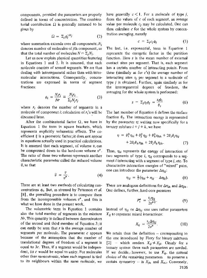
components, provided the parameters are properly defined in terms of concentration. The combina- torial contribution f~ is generally assumed to be given by

f2 = N]OSvJ (2)

where summation extends over all components; Nj denotes number of molecules of] th component, so that the total number of molecules N = 2 j N i.

Let us now explain physical quantities featuring in Equations 1 and 2. It is assumed, that each molecule consists of several segments. We are thus dealing with intersegmental rather than with inter- molecular interactions. Consequently, concen- trations are expressed in terms of segment fractions:

N i r i _ Niri ~ - ( 3 )

Nr ZjNjrj

where r i denotes the number of segments in a molecule of component i; calculation of r[s will be discussed later.

After the combinatorial factor f2, we have in Equation 1 the term in square brackets, which represents explicitly volumetric effects. The co- efficient ~ is a geometric factor; it does not appear in equations actually used in practical calculations. It is assumed that each segment, of volume v, can be compressed down to the hard-core volume v*. The ratio of these two volumes represents another characteristic parameter called the reduced volume g, so that

73 ~" - - - (4)

- - V*"

There are at least two methods of calculating con- centrations q~i. But, as stressed by Patterson et al. [8], the prevailing procedure is to compute them from the incompressible volumes 73*, and this is what we have done in the present work.

The volumetric term in Equation 1 contains also the total number of segments in the mixture Nr. This quantity is defined between denominators of the second and third member of Equation 3; it can easily be seen that r is the average number of segments per molecule. The parameter c appears because of the assumption that the number of translational degrees of freedom of a segment is equal to 3c. Thus, if a segment would be indepen- dent, its c would be equal to unity. For molecules other than monoatomic, when each segment is tied to its neighbours within the same molecule, we

have generally c < 1. For a molecule of type j, from the values of c of each segment, an average value per molecule c i may be calculated. One can then calculate c for the whole system by concen- tration averaging, namely

c = ~;cj~j (5)

The last, i.e. exponential, term in Equation 1 represents the energetic factor in the partition function. Here s is the mean number of external contact sites per segment. That is, each segment has a certain number of interacting points. From these (similarly as for c's) the average number of interacting sites sj per segment in a molecule of type ]" is obtained. Further, again similarly as for the intersegmental degrees of freedom, the averaging for the whole system is performed:

$iOi S = ~jSj~gj -- Oi ( 6 )

The last member of Equation 6 defines the surface fraction Oi. The interaction energy is represented by the parameter n; writing now specifically for a ternary mixture i + ] + k, we have

n = 0~nii + 0~r~yj + 0~nkk + 20i0j.rhj

+ 20iOkn~ + 20jOknjk. (7)

Thus, nil represents the energy of interaction of two segments of type i, no corresponds to a seg- ment i interacting with a segment of type ], etc. To characterize interaction energies of "mixed" pairs, one can introduce the parameter An/j:

n i j = 1 ( n i l -[- n# -- An/i)- (8)

There are analogous definitions for An~ and A~j k. One defines, further, hard-core pressures

sinii P~i = 2v.~. (9)

Instead of nij or A~i j one uses rather parameters Xij to represent mixed interactions:

S iA~iY (10) X O - 2v*

We retain thus the de f in i t ion- corresponding to the one introduced by Flory for binary mixtures [2] - which renders Xij 4:Xji. Clearly for a ternary system three such parameters are needed. If we decide,, however, to use Xii, the natural choice of the remaining parameters to preserve a certain symmetry - is Xjk and Xki. Conversely,

2135

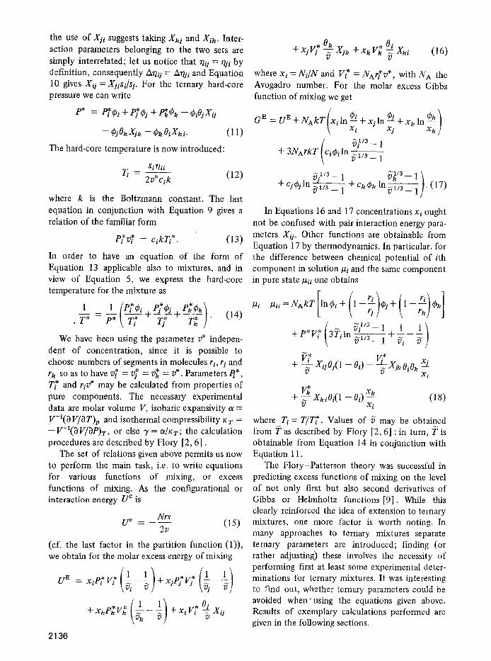
the use of Xji suggests taking Xkj and Xik . Inter- action parameters belonging to the two sets are simply interrelated; let us notice that ~ij -- *?ji by definition, consequently A~ij - A*2ji and Equation 10 gives Xi.i = X n s l / s j . For the ternary hard-core pressure we can write

P* = t~i~)i + PTC#y + t~kr - - ( ~ i O j X i j

-- r -- r O~Xk~. (11)

The hard-core temperature is now introduced:

$ i ~ i i

Ti = 2v *c i k (12)

where k is the Boltzmann constant. The last equation in conjunction with Equation 9 gives a relation of the familiar form

P?v~ = c ikTi* . (13)

In order to have an equation of the form of Equation 13 applicable also to mixtures, and in view of Equation 5, we express the hard-core temperature for the mixture as

1 1 [ . P * $ i , + . (14)

�9 r t * T;

We have been using the parameter 7)* indepen- dent of concentration, since it is possible to choose numbers of segments in molecules ri, rj and r k so as to have v* = v~ = v~ = v*. Parameters P/*, 7"* and riv* may be calculated from properties of pure components. The necessary experimental data are molar volume V, isobaric expansivity a = V - l ( t ) V / ~ T ) p and isothermal compressibility KT = - - V - t ( 3 V/3P)T , or else 3' = a/KT ; the calculation procedures are described by Flory [2, 6].

The set of relations given above permits us now to perform the main task, i.e. to write equations for various functions of mixing, or excess functions of mixing. As the configurational or interaction energy U c is

Mrs U ~ - ( l S )

2v

(cf. the last factor in the partition function (1)), we obtain for the molar excess energy of mixing

+ x ~ G G - + x~ V* ~ x u

2136

+ xj~* ok o~ - ~ X j k + x k V ~ -z Xki (16)

v

where x i = N d N and V* = NAr/*v* , with NA the Avogadro number. For the molar excess Gibbs function of mixing we get

~i 1/3 - 1 + 3 N A r k T c i~ i ln ~ l /a 1

~ j l / 3 - - 1 + ck ~bk ln~l (17) + cYq~J In ff~73-- 1 /3 -

In Equations 16 and 17 concentrations x i ought not be confused with pair interaction energy para- meters Xij . Other functions are obtainable from Equation 1 7 by thermodynamics. In particular, for the difference between chemical potential of ith component in solution gi and the same component in pure state I~ii one obtains

~ i - - 1 + ~ _ _ _ + P * V i * 3Tiln ~- i~- - 1 vi v

~* V,* + " ' X i j O j ( 1 - - O i ) - - ~ . x~ ~ X~k OiOk - -

x i

+ ~ - XkiOi(1 --Oi) x k (18) v x i

where Ti = T / T * . Values of ~ may be obtained from T as described by Flory [2, 6] ; in turn, T is obtainable from Equation 14 in conjunction with Equation 11.

The Flory-Patterson theory was successful in predicting excess functions of mixing on the level of not only first but also second derivatives of Gibbs or Helmholtz functions [9]. While this clearly reinforced the idea of extension to ternary mixtures, one more factor is worth noting. In many approaches to ternary mixtures separate ternary parameters are introduced; finding (or rather adjusting) these involves the necessity of performing first at least some experimental deter- minations for ternary mixtures. It was interesting to find out, whether ternary parameters could be avoided when" using the equations given above. Results of exemplary calculations performed are given in the following sections.

3. Ethanol + benzene + n-hexane The above system has been chosen because its components represent different classes of organic compounds; apart of an aliphatic and an aromatic we have here an associated component. The presence of an alcohol makes the test o f the theory more severe. Many theories of solutions fail completely for systems in which association O c c u r s .

Precise experimental measurements of heats of mixing H E for the system in question have been made by De Q. Jones and Lu [10]; they have studied the ternary system as well as all three respective binaries at 298.15K. The coverage of the ternary system was fairly extensive, so that De Q. Jones and Lu were able to draw isoenthalpic lines on the concentration triangle.

Our calculations were made using Equation 16; that is, in view of low pressure, the excess energy of mixing U E has been assumed to be equal to the excess enthalpy of mixing H E. Parameters for pure components have been calculated in the same way as in [11]. For binary mixtures also a procedure described earlier by one of us [11] has been followed; that is, rewriting Equation 6 as

Oi = = - (19) ~i + sj ~s

Si

one realizes that a description of a binary mixture involves characteristic (hard-core) parameters for pure components, plus two binary parameters: Xis and sj/sl. One can then solve for n experimental points (values of H E in the present case) a set of n equations in two unknowns. While an a priori prediction of the surface ratio sJsiis possible [12], the method does not seem accurate enough [11]. This is why we have obtained for each binary system the respective parameters Xii and si/si by computer fitting. For ternary mixtures we have used two methods. One was fitting ternary data using known parameters for pure components and finding the binary parameters Xij, Xsh and Ski as

well as the respective surface ratios. The second method consisted in predicing ternary heats of mixing basing entirely on binary data and on these for pure components.

Experimental data, for pure components necess- ary to calculate the characteristic parameters have been taken for ethanol from [13], for benzene from [14] and for n-hexane from [15]. The values obtained are given in Table I.

TAB LE I Characteristic parameters for pure components

Component T V* T* P* (K) (cm3mol -l) (K) (Jcm -a)

ethanol 298.2 46.41 5011 449.0 1.2645 benzene 298.2 69.21 4709 627.6 1.2917 n-hexane 298.2 99.56 4430 431.0 1.3227 N 2 100.0 26.18 1144 243.5 1.5457 Ar 100.0 22.17 1374 280.0 1.3706 O2 100.0 21.23 1347 373.0 1.3846 Zn 714.0 8.83 24604 5560.0 1.1025 Sn 714.0 16.23 37859 2342.0 1.0626 Cd 714.0 13.03 26640 3798.0 1.0933

Calculations for binary and ternary mixtures have been performed using a non-linear curve- fitting computer program of the type described by Cuthbert and Wood [16]. The program was devised to perform a least-squares estimation of p parameter values al,a2, ...,ap in an equation of the general form

y = y ( X l , X 2 .... Xm,a l ,a2 .... a v) (20)

representing a relation between a set of rn indepen- dent variables X1, ..., Xm and a dependent variable y. The experimental values of X's andy are taken as known from n experiments, with n > p . In our case, we have used Equations 16 and 18 as those of the general form Equation 20. For binary systems we had one independent variable xi and two unknown parameters Xis and si/sl. For ternary systems there were two independent variables xi and x~, and five unknown parameters Xij, Xsk, Xki, s~/sl and Sh/S i. TO apply the non4inear curve-fitting program, we have written a FORTRAN subroutine which calculated the y ' s of Equation 20 for the experimental concentrations (in the present case as given in [10]) and for a given set of parameter values. The main program then calculated the sum of squares of residuals, i.e. of differences between the y ' s resulting from the subroutine and the corresponding experimental values. The problem was thus reduced to finding a minimum of the sum of squares of residuals, and the parameter values giving the minimum were accepted as "true" values. For each of such true values, the program supplied the standard error, Student's t function, and 95% confidence limits. In Table II we list for brevity values of the parameters and 95% con- fidence limits (in parentheses) only. Indices E, B, and H refer to ethanol, benzene and n-hexane, respectively.

The first three columns in Table II contain parameters resulting from calculations for binary

2137

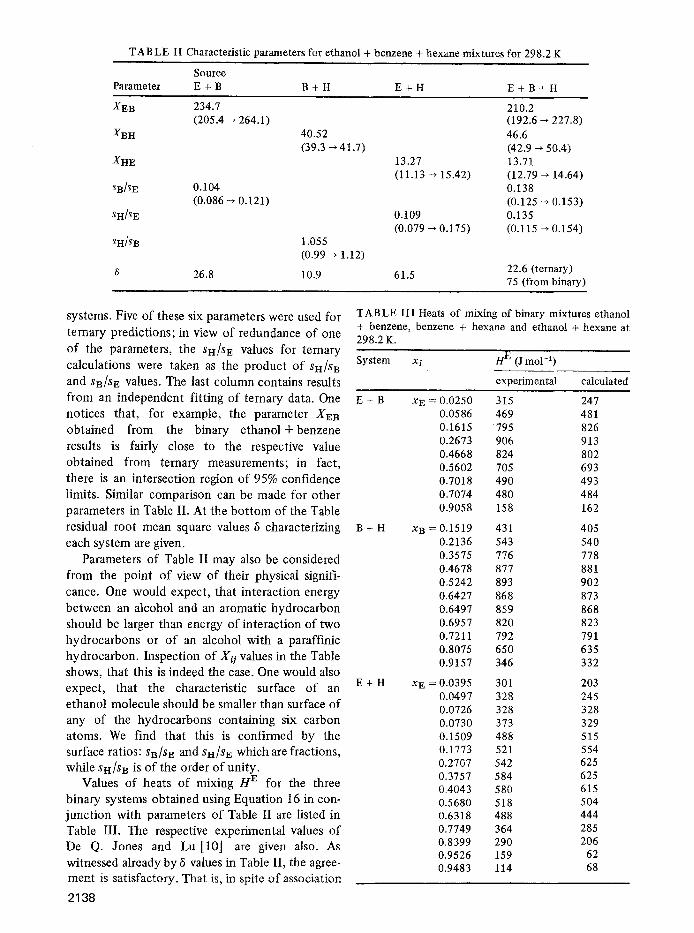
TAB LE II Characteristic parameters for ethanol + benzene + hexane mixtures for 298.2 K

Source

Parameter E + B B + H E + H E + B + H

XEB 234.7 210.2 (205.4 ~ 264.1) (192.6 --, 227.8)

XBH 40.52 46.6 (39.3 ~ 41.7) (42.9 ~ 50.4)

XHE 13.27 13.71 (11.13 ~ 15.42) (12.79 ~ 14.64)

SB/SE 0.104 0.138 (0.086 --' 0.121) (0.125 -~ 0.153)

SH/SE 0.109 0.135 (0.079 ~ 0.175) (0.115 --* 0.154)

SH/$ B 1 .055

(0.99 ~ 1.12) 22.6 (ternary) 26.8 10.9 61.5 75 (from binary)

systems. Five of these six parameters were used for

ternary predictions; in view of redundance of one

of the parameters, the SH/SE values for ternary calculations were taken as the product of SH/SB and SB/SE values. The last column contains results from an independent fitting of ternary data. One notices that, for example, the parameter XEB obtained from the binary ethanol + benzene results is fairly close to the respective value obtained from ternary measurements; in fact, there is an intersection region of 95% confidence limits. Similar comparison can be made for other parameters in Table II. At the bo t tom of the Table residual root mean square values 6 characterizing each system are given.

Parameters of Table II may also be considered from the point of view of their physical signifi-

cance. One would expect, that interact ion energy between an alcohol and an aromatic hydrocarbon should be larger than energy of interaction of two hydrocarbons or o f an alcohol with a paraffinic hydrocarbon. Inspection of Xii values in the Table shows, that this is indeed the case. One would also expect , that the characteristic surface of an ethanol molecule should be smaller than surface of any of the hydrocarbons containing six carbon atoms. We find that this is confirmed by the surface ratios: SB/S E and SH/SE which are fractions, while SI-I/SB is of the order of unity.

Values of heats of mixing H E for the three binary systems obtained using Equation 16 in con- junct ion with parameters o f Table II are listed in Table III. The respective experimental values of De Q. Jones and Lu [10] are given also. As witnessed already by 6 values in Table II, the agree- ment is satisfactory. That is, in spite o f association

2138

TABLE III Heats of mixing of bmary mixtures ethanol + benzene, benzene + hexane and ethanol + hexane at 298.2 K.

System xi H E (J mo1-1)

experimental calculated

E + B XE=

B + H x B -

E + H XE----

0.0250 315 247 0.0586 469 481 0.1615 795 826 0.2673 906 913 0.4668 824 802 0.5602 705 693 0.7018 490 493 0.7074 480 484 0.9058 158 162

0.1519 431 405 0.2136 543 540 0.3575 776 778 0.4678 877 881 0.5242 893 902 0.6427 868 873 0.6497 859 868 0.6957 820 823 0.7211 792 791 0.8075 650 635 0.9157 346 332

0.0395 301 203 0.0497 328 245 0.0726 328 328 0.0730 373 329 0.1509 488 515 0.1773 521 554 0.2707 542 625 0.3757 584 625 0.4043 580 615 0.5680 518 504 0.6318 488 444 0.7749 364 285 0.8399 290 206 0.9526 159 62 0.9483 114 68

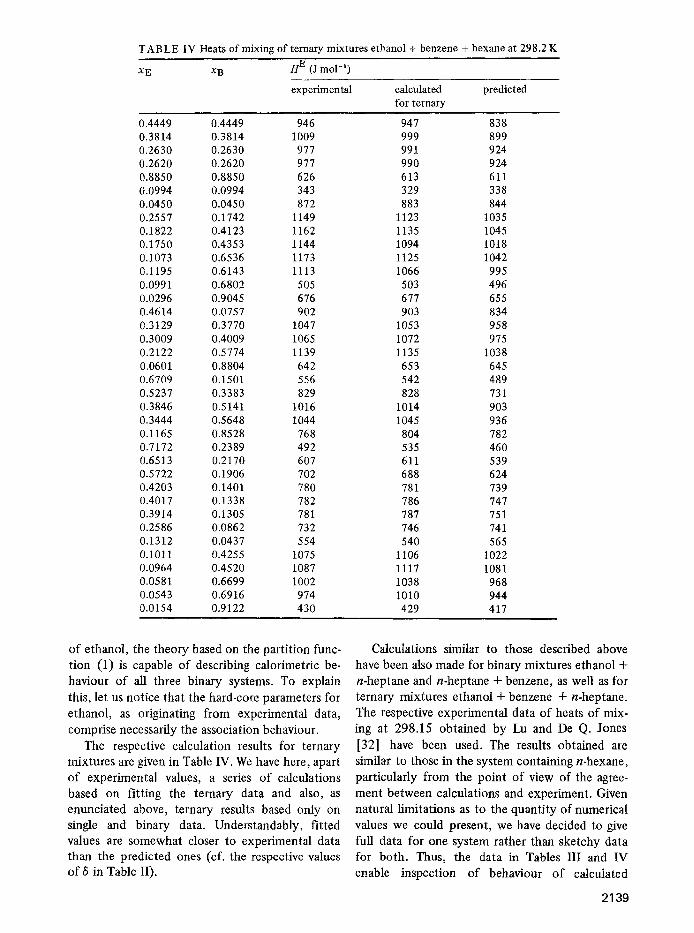
TAB LE IV Heats of mixing of ternary mixtures ethanol + benzene + hexane at 298.2 K

XE XB H E (J mol -~)

experimental calculated predicted for ternary

0.4449 0.4449 946 947 838 0.3814 0.3814 1009 999 899 0.2630 0.2630 977 991 924 0.2620 0.2620 977 990 924 0.8850 0.8850 626 613 611 0.0994 0.0994 343 329 338 0.0450 0.0450 872 883 844 0.2557 0.1742 1149 1123 1035 0.1822 0.4123 1162 1135 1045 0.1750 0.4353 1144 1094 1018 0.1073 0.6536 1173 1125 1042 0.1195 0.6143 1113 1066 995 0.0991 0.6802 505 503 496 0.0296 0.9045 676 677 655 0.4614 0.0757 902 903 834 0.3129 0.3770 1047 1053 958 0.3009 0.4009 1065 1072 975 0.2122 0.5774 1139 1135 1038 0.0601 0.8804 642 653 645 0.6709 0.1501 556 542 489 0.5237 0.3383 829 828 731 0.3846 0.5141 1016 1014 903 0.3444 0.5648 1044 1045 936 0.1165 0.8528 768 804 782 0.7172 0.2389 492 535 460 0.6513 0.2170 607 611 539 0.5722 0.1906 702 688 624 0.4203 0.1401 780 781 739 0.4017 0.1338 782 786 747 0.3914 0.1305 781 787 751 0.2586 0.0862 732 746 741 0.1312 0.0437 554 540 565 0.1011 0.4255 1075 1106 1022 0.0964 0.4520 1087 1117 1081 0.0581 0.6699 1002 1038 968 0.0543 0.6916 974 1010 944 0.0154 0.9122 430 429 417

of ethanol, the theory based on the part i t ion func- t ion (1) is capable of describing calorimetric be- haviour of all three binary systems. To explain this, let us notice that the hard-core parameters for ethanol, as originating from experimental data, comprise necessarily the association behaviour.

The respective calculation results for ternary mixtures are given in Table IV. We have here, apart of experimental values, a series of calculations based on fitting the ternary data and also, as enunciated above, ternary results based only on single and binary data. Understandably, fi t ted values are somewhat closer to experimental data than the predicted ones (cf. the respective values o f 6 in Table II).

Calculations similar to those described above have been also made for binary mixtures ethanol + n-heptane and n-heptane + benzene, as well as for ternary mixtures ethanol + benzene + n-heptane. The respective experimental data of heats of mix- ing at 298.15 obtained by Lu and De Q. Jones

[32] have been used. The results obtained are similar to those in the system containing n-hexane, particularly from the point of view of the agree- ment between calculations and experiment. Given natural l imitations as to the quant i ty of numerical values we could present, we have decided to give full data for one system rather than sketchy data for both. Thus, the data in Tables III and IV enable inspection of behaviour o f calculated

2139

functions in particular concentration regions (dilute solutions, solutions close to equimolar, and so on), for binary systems as well as for ternary mixtures.

On the basis of the calculations performed, we conclude - again association of alcohol notwith- standing - that single and binary data are suf- ficient for reasonable prediction of ternary heats of mixing. It is reasonable to infer that such pre- diction will be numerically better for organic systems which do not contain highly polar or associated components.

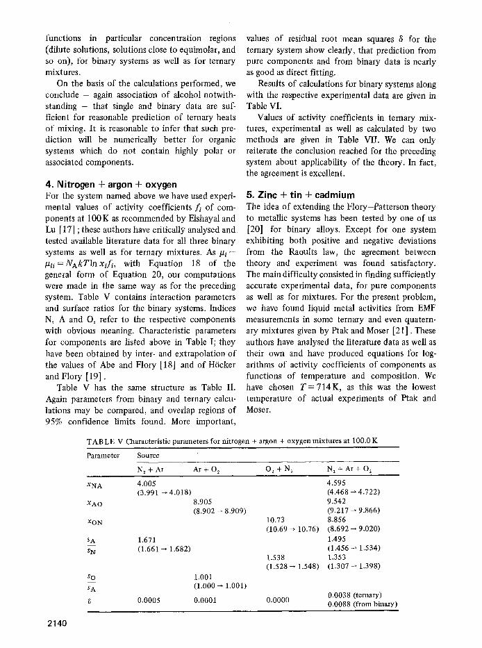
4. Nitrogen + argon + oxygen For the system named above we have used experi- mental values of activity coefficients fi of com- ponents at 100 K as recommended by Elshayal and Lu [17] ;these authors have critically analysed and tested available literature data for all three binary systems as well as for ternary mixtures. A s / ~ i - ~ii=NAkTlnxifl, with Equation 18 of the general form of Equation 20, our computations were made in the same way as for the preceding system. Table V contains interaction parameters and surface ratios for the binary systems. Indices N, A and O, refer to the respective components with obvious meaning. Characteristic parameters for components are listed above in Table I; they have been obtained by inter- and extrapolation of the values of Abe and Flory [18] and of H6cker and Flory [19].

Table V has the same structure as Table II. Again parameters from binary and ternary calcu- lations may be compared, and overlap regions of 95% confidence limits found. More important,

values of residual root mean squares 6 for the ternary system show clearly, that prediction from pure components and from binary data is nearly as good as direct fitting.

Results of calculations for binary systems along with the respective experimental data are given in Table VI.

Values of activity coefficients in ternary mix- tures, experimental as well as calculated by two methods are given in Table VII. We can only reiterate the conclusion reached for the preceding system about applicability of the theory. In fact, the agreement is excellent.

5. Zinc + tin + cadmium The idea of extending the Flory-Patterson theory to metallic systems has been tested by one of us [20] for binary alloys. Except for one system exhibiting both positive and negative deviations from the Raoults law, the agreement between theory and experiment was found satisfactory. The main difficulty consisted in finding sufficiently accurate experimental data, for pure components as well as for mixtures. For the present problem, we have found liquid metal activities from EMF measurements in some ternary and even quatern- ary mixtures given by Ptak and Moser [21]. These authors have analysed the literature data as well as their own and have produced equations for log- arithms of activity coefficients of components as functions of temperature and composition. We have chosen T = 714K, as this was the lowest temperature of actual experiments of Ptak and Moser.

TABLE V Characteristic parameters for nitrogen + argon + oxygen mixtures at 100.0 K

Parameter Source

N2+Ar Ar+O 2 O2+N~ N 2 + A r + O 2

XNA 4.005 4.595 (3.991 ~ 4.018) (4.468 ~ 4.722)

xAO 8.905 9.542 (8.902 ~ 8.909) (9.217 ~ 9.866)

XON 10.73 8.856 (10.69 ~ 10.76) (8.692 ~ 9.020)

SA 1.671 1.495 SN (1.661 -~ 1.682) (1.456 ~ 1.534)

1.538 1.353 (1.528 ~ 1.548) (1.307 ~ 1.398)

so 1.001 SA (1.000 ~ 1.001)

0.0038 (ternary) 6 0.0005 0.0001 0.0000 0.0088 (from binary)

2140

TABLE VI Activity coefficients of components in binary systems N2 + At, Ar + 02, O~ + N 2 at 100.0 K

System xi ~

experimental calculated experimental calculated

N 2 + A r X A = 0.0195 f N = 1.000 1.000 f A = 1.163 1.164 0.0480 1.001 1.000 1.152 1.152 0.0813 1.001 1.001 1.139 1.139 0.1400 1.004 1.004 1.118 1.117 0.1565 1.004 1.004 1.113 1.112 0.2222 1.009 1.009 1.093 1.092 0.3092 1.016 1.016 1.071 1.070 0.3618 1.022 1.022 1.059 1.058 0.4142 1.028 1.028 1.049 1.048 0.4421 1.032 1.032 1.044 1.043 0.5169 1.043 1.043 1.032 1.031 0.5703 1.051 1.051 1.025 1.024 0.6483 1.065 1.065 1.016 1.016 0.6597 1.067 1.067 1.015 1.015 0.7485 1.085 1.085 1.008 1.008 0.7691 1.089 1.089 1.007 1.007 0.7888 1.094 1.094 1.006 1.005 0.7982 1.096 1.096 1.005 1.005 0.8230 1.101 1.101 1.004 1.004 0.8514 1.108 1.107 1.003 1.003 0.8685 1.112 1.112 1.002 1.002 0.8903 1.117 1.118 1.002 1.001 0.9001 1.120 1.120 1.001 1.001 0.9444 1.131 1.131 1.001 1.000 0.9470 1.131 1.132 1.001 1.000

Ar + 02 x A = 0,0323 fA = 1.173 1,173 fo = 1.000 1.000 0.0855 1.153 1.153 1.001 1.001 0.1698 1.123 1,123 1.005 1.005 0.2519 1.099 1.098 1.001 1.011 0.3505 1.073 1.073 1.021 1.021 0.3942 1.063 1.063 1.027 1.027 0.4506 1,051 1.051 1.035 1,035 0.5684 1.031 1.031 1.056 1.056 0.6985 1.015 1.015 1.086 1.086 0.7736 1.008 1.009 1.106 1.105 0.8020 1.006 1.006 1.114 1.114 0.9048 1.002 1.001 1.146 1.146 0.9429 1.001 1.001 1.159 1.159 0.9604 1.000 1.000 1.165 1.166

02 + N~ x O = 0.0500 f N = 1.001 1.001 fo = 1.211 1.208 0.0701 1.001 1.001 1.200 1.196 0.0995 1.002 1.003 1.184 1.179 0.1360 1.005 1.005 1.166 1.159 0.1791 1.008 1.008 1.146 1.138 0.4248 1.040 1.039 1.064 1.056 0.4875 1.052 1.050 1.050 1.042 0.5897 1.075 1.071 1.031 1.025 0.6376 1.087 1.081 1.024 1.019 0.8056 1.135 1,121 1.007 1.005 0.9086 1.168 1.148 1.002 1.001

Characteristic parameters of pure components

have been obtained in the following way. Faber

[22] gives selected values of molar volumes, iso-

baric expansivities and isothermal compressibilities

of liquid metals close to their respective melting

points. For Zn and Cd we have accepted Faber's

values of volume and expansivity, assuming that

molar volume varies linearly with the temperature.

One thus obtains for cadmium Vcd ( 7 1 4 K ) =

14.25cm3mo1-1. Crawley [23] has measured

2141

TABLE VII Activity coefficients of components in ternary mixtures nitrogen + argon + oxygen at 100,0 K

xr~ xA fN fa fo

exp calc pred exp calc pred exp calc pred

0.8534 0.1073 1.002 1.003 1.003 1.120 1.128 1.120 1.158 1.164 1.189 0.7405 0.1666 1.008 1.009 1.010 1.099 1.101 1.092 1.134 1.136 1.153 0.6477 0.2627 1.014 1.018 1.019 1.078 1.076 1.068 1.126 1.127 1.140 0.6820 0.2315 1.012 1.014 1.015 1.085 1.085 1.076 1.130 1.131 1.146 0.3270 0.5019 1.058 1.062 1.063 1.032 1.028 1.024 1.097 1.098 1.100 0.2001 0.6869 1.093 1.093 1.089 1.013 1.011 1.009 1.118 1.118 1.118 0.1198 0.6757 1.108 1.105 1.103 1.014 1.012 1.010 1.100 1.100 1.097 0.0663 0.7654 1.130 1.122 1.117 1.007 1.006 1.115 1.115 1.115 1.110 0,4894 0.3020 1.030 1.035 1.038 1.062 1.059 1.051 1.093 1.091 1,097 0.3341 0,4601 1.055 1.059 1.061 1.037 1.033 1.028 1.090 1.089 1,092 0.5687 0.1417 1.023 1.027 1,031 1.098 1.091 1.079 1.084 1.080 1,086 0.5076 0.1598 1.031 1.034 1.040 1,084 1.086 1.074 1.072 1.068 1.073 0,4460 0.1681 1.040 1.044 1.050 1,082 1.084 1.072 1,061 1.056 1,059 0.3527 0.3368 1.051 1.055 1.059 1,053 1.051 1,043 1.069 1.067 1.070 0.2186 0.4806 1.077 1.079 1,082 1.034 1.031 1.027 1.071 1,072 1,072 0.0836 0.5414 1.112 1.107 1,110 1.030 1.028 1.025 1.063 1.064 1,061 0.0882 0,4617 1.111 1.106 1.111 1,042 1,040 1.037 1.048 1.049 1.047 0.1762 0.3672 1.089 1.088 1,095 1.053 1.051 1.046 1.044 1.044 1.043 0.3292 0.1234 1.068 1.070 1.079 1.094 1.100 1.088 1.034 1.030 1.031 0.1812 0.1224 1,111 1.107 1.118 1,109 1.115 1.105 1.015 1.013 1.013 0.1286 0.0955 1.114 1.126 1.138 1.125 1.132 1.122 1,008 1.007 1.007

pyconmetricaUy densities of liquid Cd. Using his type for metals was advocated by Grosse [27, 28].

density formula in [23], as well as using his The result obtained for 714K was virtually the

alternative formula from a review on liquid metals same as given by Kleppa for 594 K. As for para- [24] , one obtains 14.32 cm3mol-1; the agreement meters for Sn, we have used the same data as in an

is thus within 0.5%. Compressibility of Zn given earlier paper [20] ; density fromula of Schwaneke by Kleppa [25] for 693 K was accepted for 714 K. and Falke [29], a compressibility value of Kleppa

Compressibility of Cd given also by Kteppa [25] but for 594 K was accepted also. We have made an

independent calculation of compressibility of cad- mium using the formula of Egelstaff and Widom

[26] binding compressibility with surface tension and with temperature; the use of formulas of this

[25] , the Egelstaff and Widom formula [26], and an equation for surface tension dependence on

temperature also from Schwaneke and Falke [29].

The density equation we have used agrees again

reasonably well with the one given by Crawley

[24] , and based on Psn(T) measurements of

TABLE VIII Characteristic parameters for Zn + Sn + Cd alloys at 714,0 K

Parameter Source

Z,n + Sn Sn + Cd Cd + Zn Zn + Sn + Cd

Xznsn 244.5 261.8 (240 -+ 249) (260 ~ 264)

Xsncd 91.1 95.9 (85 ~ 98) (94 ~ 98)

XCdZn 409.8 408.5 (399 -+ 420) (406 ~ 412)

SSn 1.259 1.144 SZn (1.205 ~ 1.312) (1,121 ~ 1.168) SOd 0.897 0.881 s z n (0.858 ~ 0.936) (0.871 ~ 0.892)

SOd 0.768 ss n (0.748 ~ 0.789)

0.0030 (ternary) 6 0.0049 0.0011 0.0027 0.0085 (from binary)

2142

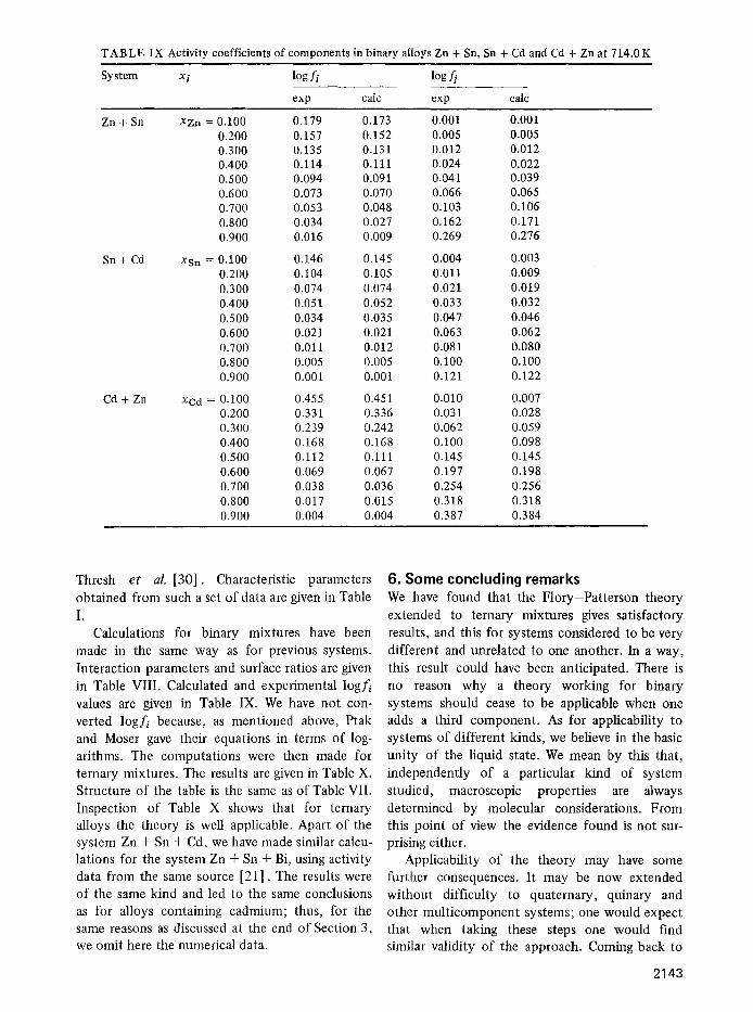
TABLE IX Activity coefficients of components in binary alloys Zn + Sn, Sn + Cd and Cd + Zn at 714.0 K

System x i log f i log J)

exp cNc exp cMc

Zn + Sn XZn = 0.100 0.179 0.173 0.001 0.001 0.200 0.157 0.152 0.005 0.005 0.300 0.135 0.131 0.012 0.012 0.400 0.114 0.111 0.024 0.022 0.500 0.094 0.091 0.041 0.039 0.600 0.073 0.070 0.066 0.065 0.700 0.053 0.048 0.103 0.106 0.800 0.034 0.027 0.162 0.171 0.900 0.016 0.009 0.269 0.276

Sn + Cd XSn = 0.100 0.146 0.145 0.004 0.003 0.200 0.104 0.105 0.011 0.009 0.300 0.074 0.074 0.021 0.019 0.400 0.051 0.052 0.033 0.032 0.500 0.034 0.035 0.047 0.046 0.600 0.021 0.021 0.063 0.062 0.700 0.011 0.012 0.081 0.080 0.800 0.005 0.005 0.100 0.100 0.900 0.001 0.001 0.121 0.122

Cd + Zn xCd = 0.100 0.455 0.451 0.010 0.007 0.200 0.331 0.336 0.031 0.028 0.300 0.239 0.242 0.062 0.059 0.400 0.168 0.168 0.100 0.098 0.500 0.112 0.111 0.145 0.145 0.600 0.069 0.067 0.197 0.198 0.700 0.038 0.036 0.254 0.256 0.800 0.017 0.015 0.318 0.318 0.900 0.004 0.004 0.387 0.384

Thresh e t al. [30] . Characteristic parameters

obtained from such a set of data are given in Table

I. Calculations for binary mixtures have been

made in the same way as for previous systems. Interaction parameters and surface ratios are given in Table VIII. Calculated and experimental logfl values are given in Table IX. We have not con- verted log f/ because, as mentioned above, Ptak and Moser gave their equations in terms of log- arithms. The computat ions were then made for ternary mixtures. The results are given in Table X. Structure of the table is the same as of Table VII. Inspection of Table X shows that for ternary alloys the theory is well applicable. Apart of the system Zn + Sn + Cd, we have made similar calcu- lations for the system Zn + Sn + Bi, using activity data from the same source [21] . The results were of the same kind and led to the same conclusions as for alloys containing cadmium; thus, for the same reasons as discussed at the end of Section 3, we omit here the numerical data.

6. Some concluding remarks We have found that the F lo ry -Pa t t e r son theory extended to ternary mixtures gives satisfactory results, and this for systems considered to be very different and unrelated to one another. In a way, this result could have been anticipated. There is no reason why a theory working for binary systems should cease to be applicable when one adds a third component . As for applicabili ty to systems of different kinds, we believe in the basic uni ty of the liquid state. We mean by this that, independently of a particular kind of system studied, macroscopic propert ies are always determined by molecular considerations. From this point of view the evidence found is not sur- prising either.

Applicabil i ty of the theory may have some further consequences. It may be now extended without difficulty to quaternary, quinary and other mul t icomponent systems; one would expect that when taking these steps one would find similar validity of the approach. Coming back to

2143

TAB LE X Activity coefficients of components in ternary mixtures Zn + Sn + Cd at 714.0 K

xz n XSn log f Zn log fSn log fCd

exp calc pred exp calc pred exp calc pred

0.100 0.133 0.330 0.330 0.322 0.094 0.097 0.085 0.016 0.015 0.015 0.100 0.222 0.301 0.299 0.289 0.067 0.070 0.060 0.026 0.026 0.026 0.100 0.311 0.277 0.273 0.262 0.047 0.049 0.042 0.038 0.039 0.038 0.100 0.400 0.257 0.250 0.239 0.032 0.034 0.028 0.052 0.053 0.051 0.100 0.489 0.238 0.232 0.220 0.020 0.022 0.018 0.068 0.068 0.065 0.100 0.578 0.222 0.217 0.204 0.011 0.013 0.011 0.084 0.085 0.079 0.100 0.667 0.208 0.205 0.192 0.006 0.007 0.006 0.103 0.103 0.095 0.100 0.756 0.195 0.196 0.182 0.002 0.004 0.003 0.122 0.122 0.112 0.200 0.131 0.272 0.273 0.268 0.067 0.067 0.054 0.033 0.033 0.032 0.200 0.219 0.248 0.247 0.241 0.047 0.047 0.036 0.046 0.046 0.046 0.200 0.306 0.228 0.226 0.219 0.032 0.032 0.024 0.061 0.061 0.060 0.200 0.394 0.210 0.208 0.200 0.020 0.022 0.016 0.078 0.078 0.074 0.200 0.481 0.195 0.193 0.185 0.012 0.014 0.010 0.095 0.095 0.090 0.200 0.569 0.182 0.181 0.172 0.007 0.017 0.007 0.115 0.112 0.105 0.200 0.656 0.171 0.172 0.162 0.005 0.007 0.005 0.135 0.131 0.122 0.300 0.129 0.218 0.219 0.216 0.051 0.048 0.033 0.059 0.058 0.057 0.300 0.214 0.198 0.199 0.196 0.036 0.034 0.023 0.074 0.074 0.072 0.300 0.300 0.182 0.182 0.178 0.025 0.025 0.016 0.091 0.091 0.088 0.300 0.386 0.169 0.168 0.164 0.017 0.019 0.012 0.110 0.109 0.104 0.300 0.471 0.157 0.157 0.152 0.013 0.015 0.010 0.130 0.127 0.120 0.300 0.557 0.148 0.148 0.142 0.011 0.013 0.010 0.151 0.145 0.136 0.400 0.125 0.168 0.170 0.169 0.046 0.042 0.026 0.093 0.093 0.091 0.400 0.208 0.154 0.154 0.153 0.035 0.033 0.021 0.111 0.110 0.107 0.400 0.292 0.142 0.142 0.141 0.028 0.028 0.018 0.130 0.128 0.124 0.400 0.375 0.132 0.132 0.130 0.024 0.025 0.018 0.150 0.147 0.140 0.400 0.458 0.124 0.124 0.122 0.022 0.025 0.019 0.171 0.165 0.156 0.500 0.120 0.124 0.125 0.125 0.053 0.050 0.034 0.137 0.138 0.135 0.500 0.200 0.114 0.114 0.115 0.046 0.045 0.032 0.156 0.156 0.151 0.500 0.280 0.106 0.106 0.106 0.041 0.043 0.032 0.175 0.174 0.167 0.500 0.360 0.100 0.099 0.099 0.039 0.043 0.034 0.196 0.192 0.183 0.600 0.112 0.087 0.085 0.086 0.076 0.075 0.059 0.192 0.195 0.190 0.600 0.188 0.081 0.079 0.080 0.070 0.072 0.059 0.210 0.212 0.205 0.600 0.262 0.077 0.074 0.076 0.067 0.072 0.060 0.228 0.229 0.219 0.700 0.100 0.056 0.051 0.053 0.117 0.120 0.106 0.258 0.265 0.259 0.700 0.167 0.054 0.049 0.051 0.111 0.117 0.105 0.272 0.279 0.270 0.800 0.075 0.031 0.025 0.027 0.185 0.189 0.179 0.337 0.350 0.343

ternary systems, for instance Hsu and Prausnitz

[31] have studied polymer compatibili ty in such

systems using the earlier theory [5]. It has been

found by one of us [11] when studying swelling

of natural rubber in organic solvents that the

F lory-Pa t te rson theory gives distinctly better

results than the earlier theory of polymer solutions

as described in [5]. Thus, using the new theory

instead of the old one should give more inform-

ation on the subject o f solubility of polymers. The same statement is expected to apply even more

to F lory-Pa t te rson theory versus empirical

approaches, not only to compactibility of poly-

mers but also to other problems involving ternary

liquid solutions.

2144

Acknowledgements The beginning of this work was preceded by some

discussions which one of us (W.B.) has had with

Professor Donald Patterson of Department of

Chemistry, McGilt University, Montreal. In the

course of our study we benefited from correspon-

dence with Dr Aristid V. Grosse of Germantown

Laboratories - Franklin Institute, Philadelphia.

Finally, we acknowledge with pleasure comments

on the manuscript by Professor Henry P. Schreiber

o f Department of Chemical Engineering, Ecole

Polytechnique, Montreal.

References 1. L. TONKS,Phys. Rev. 50 (1936) 955.

2. P .J . FLORY, Jr. Amer. Chem. Soc. 87 (1965) 1833. 3. D. PATTERSON and G. DELMAS, Discuss. Faraday

Soc. 49 (1970) 98. 4. I. PRIGOGINE, A. BELLEMANS and V. MATHOT,

"The Molecular Theory of Solutions" (North- Holland, Amsterdam, 1957).

5. P. J. FLORY, "Principles of Polymer Chemistry", (Cornell U.P., Ithaca, N.Y., 1953) Ch. XII.

6. P.J. FLORY,Diseuss. Faraday Soc. 49 (1970) 7. 7. D. PATTERSON, Pure Appl. Chem. 31 (1972) 133. 8. D. PATTERSON, Y. B. TEWARI and H. P.

SCHREIBER, Faraday Trans. H 68 (1972) 885. 9. S. V. SUBRAHMANYAM and K. RAGHUNATH,

Chem. Phys. Letters 2 (1968) 110; V. HYDER KAHN and S. V. SUBRAHMANYAM, Trans. Faraday Soc. 67 (1971) 2282.

10. H. K. DE Q. JONES and B. C.-Y. LU, J. Chem. Eng. Data 11 (1966)488.

11. W. BROSTOW, MacromoL 4 (1971) 742. 12. A. BONDI, J. Phys. Chem. 68 (1964) 441. 13. G. C. BENSON and H. D. PFLUG, Jr. Chem. Eng.

Data 15 (1970) 382. 14. B. E. EICHINGER and P. J. FLORY, Trans. Faraday

Soc. 64 (1968) 2035. 15. R. A. ORWOLL and P. J. FLORY, J. Amer. Chem.

Soc. 89 (1967) 6814. 16. D. CUTHBERT and F. S. WOOD, "Fitting Equations

to Data" (Wiley, New York, 1971). 17. I. M. ELSHAYAL and B. C.-Y. LU, J. Chem. Eng.

Data 16 (1971) 31.

18. A. ABE and P. J. FLORY, Jr. Amer. Chem. Soc. 87 (1965) 1838.

19. H. H(3CKER and P. J. FLORY, Trans. Faraday Soc. 64 (1968) 1188.

20. W. BROSTOW, High Temp. Sci. 6 (1974) 190. 21. W. PTAK and Z. MOSER, J. Electrochem. Soc. 119

(1972) 843. 22. T. E. FABER, "Introduction to the Theory of

Liquid Metals" (Cambridge University Press, 1972). 23. A. F. CRAWLEY, Trans. Met. Soc. AIME 242

(1968) 2237. 24. ldem, lnt. Met. Rev. 19 (1974) 32. 25. O.J. KLEPPA,J. Chem. Phys. 18 (1950) 1331. 26. P. A. EGELSTAFF and B. WlDOM, J. Chem. Phys.

53 (1970) 2667. 27. A.V. GROSSE, Report GL 1970-14, Germantown

Laboratories Inc., affiliated with the Franklin Institute, Philadelphia (1970).

28. A.V. GROSSE, Nature 232 (1971) 170. 29. A. E. SCHWANEKE and W. L. FALKE, Bur. Mines

Rep. Inv. 7372 (1970). 30. H.R. THRESH, A. F. CRAWLEY and W. G. WHITE,

Trans. Met. Soc. AIME 242 (1968) 819. 31. C. C. HSU and J. M. PRAUSNITZ, Macromol. 7

(1974) 32O. 32. B.C.-Y. LU and H. K. DE Q. JONES, Can. J. Chem.

Eng. 44 (1966) 251.

Received 31 December 1974 and accepted 8 May 1975.

2145