Optimization in a Simulation Setting: Use of Function Approximation in Debt Strategy Analysis
92
Working Paper/Document de travail 2007-13 Optimization in a Simulation Setting: Use of Function Approximation in Debt Strategy Analysis by David Jamieson Bolder and Tiago Rubin www.bankofcanada.ca
Transcript of Optimization in a Simulation Setting: Use of Function Approximation in Debt Strategy Analysis
Working Paper/Document de travail2007-13
Optimization in a Simulation Setting: Use of Function Approximation in Debt Strategy Analysis
by David Jamieson Bolder and Tiago Rubin
www.bankofcanada.ca
Bank of Canada Working Paper 2007-13
February 2007
Optimization in a Simulation Setting:Use of Function Approximation in
Debt Strategy Analysis
by
David Jamieson Bolder and Tiago Rubin
Financial Markets DepartmentBank of Canada
Ottawa, Ontario, Canada K1A [email protected]
Bank of Canada working papers are theoretical or empirical works-in-progress on subjects ineconomics and finance. The views expressed in this paper are those of the authors.
No responsibility for them should be attributed to the Bank of Canada.
ISSN 1701-9397 © 2007 Bank of Canada

ii
Acknowledgements
We would like to acknowledge Greg Bauer, Jeremy Rudin, Toni Gravelle, Scott Hendry,
Antonio Diez de los Rios, Jason Allen, and Fousseni Chabi-Yo of the Bank of Canada for useful
comments. We would also like to thank Jeremy Graveline from the University of Minnesota and
Mark Reesor from the University of Western Ontario for helpful discussions. All thanks are
without implication and we retain any and all responsibility for any remaining omissions or
errors.

iii
Abstract
The stochastic simulation model suggested by Bolder (2003) for the analysis of the federal
government’s debt-management strategy provides a wide variety of useful information. It does
not, however, assist in determining an optimal debt-management strategy for the government in its
current form. Including optimization in the debt-strategy model would be useful, since it could
substantially broaden the range of policy questions that can be addressed. Finding such an optimal
strategy is nonetheless complicated by two challenges. First, performing optimization with
traditional techniques in a simulation setting is computationally intractable. Second, it is
necessary to define precisely what one means by an “optimal” debt strategy. The authors detail a
possible approach for addressing these two challenges. They address the first challenge by
approximating the numerically computed objective function using a function-approximation
technique. They consider the use of ordinary least squares, kernel regression, multivariate
adaptive regression splines, and projection-pursuit regressions as approximation algorithms. The
second challenge is addressed by proposing a wide range of possible government objective
functions and examining them in the context of an illustrative example. The authors’ view is that
the approach permits debt and fiscal managers to address a number of policy questions that could
not be fully addressed with the current stochastic simulation engine.
JEL classification: C0, C14, C15, C51, C52, C61, C65, E6, G1, H63Bank classification: Debt management; Econometric and statistical methods; Fiscal policy;Financial markets

iv
Résumé
Le modèle de simulation stochastique proposé par Bolder (2003) aux fins de l’analyse de la
stratégie de gestion de la dette du gouvernement fédéral apporte un large éventail d’informations
précieuses. Toutefois, il n’est d’aucune aide, dans sa forme actuelle, pour déterminer la stratégie
optimale de gestion de la dette. L’inclusion d’un processus d’optimisation dans le modèle serait
utile puisqu’elle permettrait d’élargir grandement la gamme des enjeux pouvant être analysés. La
recherche d’une stratégie optimale se heurte néanmoins à deux obstacles majeurs. Premièrement,
les techniques traditionnelles d’optimisation dans un cadre de simulation nécessitent des calculs
excessivement lourds. Deuxièmement, il faut définir précisément ce que l’on entend par stratégie
« optimale ». Les auteurs présentent une approche afin de surmonter ces deux difficultés. Ils
s’attaquent à la première difficulté en faisant appel à une technique d’approximation de fonction
pour obtenir une estimation approchée de la véritable fonction objectif. À cet effet, ils évaluent
plusieurs algorithmes d’approximation : moindres carrés ordinaires, régression par la méthode du
noyau, régression multivariée par spline adaptative et régression par directions révélatrices
(projection-pursuit regression). Pour résoudre la deuxième difficulté, les auteurs examinent toute
une série de fonctions objectifs qu’ils illustrent par des exemples. D’après eux, l’approche
proposée rend possible l’analyse d’enjeux que les gestionnaires de la dette et les responsables de
la politique budgétaire ne peuvent étudier avec le modèle de simulation stochastique actuel.
Classification JEL : C0, C14, C15, C51, C52, C61, C65, E6, G1, H63Classification de la Banque : Gestion de la dette, Méthodes économétriques et statistiques;Politique budgétaire; Marchés financiers
Optimization in a Simulation Setting
1 Introduction
Debt strategy describes the funding decisions facing a government. In particular, it relates to the specific
choice of debt instruments selected by the government to refinance existing obligations and meet any new
borrowing requirements. In recent years, a significant amount of effort has been applied towards gaining a better
understanding of the debt-strategy problem. Most of the effort, however, has focused on the construction of
stochastic-simulation models. These models—described in Bolder (2003, [12]), Bolder (2006, [13, 14]), Bergstrom
and Holmlund (2000, [8]), Holmlund and Lindberg (2002, [26]), Pick and Anthony (2006, [33]), and OECD (2005,
[35]—are used to examine the distributional properties of the cost and risk associated with different possible
financing strategies that are available to the government.
Stochastic-simulation models provide substantial information on a given financing strategy. Indeed, they
permit the detailed comparison of two or more alternative financing strategies. The issue is that, in their
current form, they do not provide any insight into the optimal debt strategy that should be followed by the
government. This is not to say, however, that stochastic-simulation models are incapable of providing insight
into a government’s optimal debt strategy. Two substantial challenges must be overcome to use stochastic-
simulation models in this context. First, one must overcome the difficulties associated with optimizing in a
computationally expensive setting. Second, one must be precise about what exactly is meant by the idea of an
optimal debt strategy. This paper attempts to address both of these issues.
The first issue relates to the general computational expense associated with stochastic simulation. In the
stochastic-simulation model employed in the analysis of Canadian debt-strategy decisions, the evaluation of a
single financing strategy with 100,000 randomly generated outcomes can require several minutes of computation.1
This makes traditional non-linear optimization techniques unworkable. The reason is simple. Most non-linear
optimization algorithms require numerical computation of the gradient of the objective function, let’s call it f ,
with respect to the model parameters, x ∈ Rd. We can think of f as some function of the cost and risk of a
given strategy extracted from the stochastic-simulation engine and x as the proportion of issuance in the set of
available debt instruments. This gradient, or direction of steepest descent denoted ∇f(x), is used iteratively to
find an optimum value. Typically, for a central finite-difference approximation of ∇f(x), this will require 2d + 1
function evaluations.2 Even for relatively modest values of d, the computation of the gradient can take more1This may appear, at first glance, to be a very large number of simulations. To attain an acceptable degree of convergence,
however, it is necessary. Recall that simulations converge at approximately the rate at which 1√n
goes to zero, where n denotes the
number of simulations.2This is not to mention the computation associated with approximating the Hessian matrix used to determine optimality.
1
Optimization in a Simulation Setting
than an hour. As literally thousands of iterations on the gradient vector, ∇f(x) are required, the optimization
algorithm can take weeks to run.
If the exact form of the objective function was known with certainty, waiting a number of weeks for the
optimal debt-strategy associated with the model would not be so problematic. This brings us to the second
challenge addressed in this paper. The key challenge is that there is currently not complete clarity on the desired
form of a government’s debt-management objectives. The general consensus in the debt-strategy literature is
that it will depend on the moments of the debt-charge distribution; perhaps expected debt charges and their
attendant variability.3 The relative weight of each moment is rather less obvious. Notions of the government’s
utility function may be included. It may also be desirable to include fiscal-policy objectives into the government’s
criterion function. The bottom line is that there are a variety of alternative forms that one might consider for
the government’s objective function. One would, therefore, like to experiment with different possible forms and
understand the sensitivity of the optima to the model assumptions, the form of the objective function, and also
perhaps the set of available debt instruments. What is needed, therefore, is a fast and generally reliable approach
to determining the optimal debt strategy within the context of a stochastic-simulation algorithm.
Optimizing in a stochastic-simulation setting is basically a high-dimensional, non-linear, and computationally
expensive optimization problem. Solving this problem is essential to permitting us to move to the second problem
of understanding the government’s objective function. Indeed, if we can reasonably solve this problem, we rather
broadly widen the scope of what can be accomplished, from a policy-analysis perspective, with the stochastic-
simulation model. In other words, we can expand the range of questions that can be addressed by policy
makers. One common question, that cannot be addressed in the current modelling framework, for example, is
the implication of various constraints on the government’s debt strategy. The application of existing constraints
and the associated shadow prices can, however, provide interesting information about the relative costs of these
constraints.4 For a given objective function, one can also examine the sensitivity of the ensuing optimal debt
strategy to shocks in macroeconomic or financial outcomes. Questions such as “what if inflationary volatility
increases” or “what if short-term interest rates are expected to increase” can be addressed in this setting. Finally,
by the direct inclusion of fiscal-policy objectives in the government’s criterion function, one can effectively broaden
the scope of debt management.
How might we solve this problem? In this paper, we propose approximating our objective function, f(x), with
an approximating function, f(x). That is, we randomly select N different sets of portfolio weights xi, i = 1, ..N,3One might also look at order statistics or percentile measures of the distribution.4Clearly, this is only half of the story as one must still consider the relative benefits of these constraints. It does provide, however,
a useful starting point for further discussion.
2

Optimization in a Simulation Setting
yielding N corresponding values for our objective function, fi, i = 1, ..., N. This would require a fixed amount
of computational effort. A numerical algorithm is subsequently required to fit a function to this generated data
such that, for any set of portfolio weights x, we can approximate the true objective function, f . All of the policy
analysis, including determination of the optimal debt strategy, will therefore occur on f(x). To the extent that
the approximation, f(x), is a good fit to the true objective function, this approach will be successful.
In principle, therefore, the thesis of this paper is quite simple. We propose approximating our debt-strategy
objective function and performing optimization on this approximation. A complete analysis of this idea, in the
context of the debt-strategy problem, requires, at least, three separate steps. We summarize each step in the
form of the underlying three questions.
How to approximate? Our first step requires the identification and understanding of a set of possible function-
approximation techniques. We propose a number of choices ranging from simple to complex.
Do the approximations work? We need to convince ourselves that at least one of the previously suggested
approximation techniques can actually fit an arbitrary, noisy, high-dimensional, non-linear function with
a limited amount of data. This is complicated by the fact that, in the actual debt-strategy problem, the
true function is unknown by virtue of the fact it comes from a simulation algorithm. We will, therefore,
compare each of the function-approximation techniques in terms of their ability to fit a number of known,
albeit difficult, functions.
How can we apply this approach? The final step involves using the lessons learned in the previous steps to
apply our idea to the debt-strategy problem. Here we are faced with the second problem of determining
the government’s objective function. We do not propose to solve this problem, but rather consider several
alternatives in the context of a simplified illustrative example.
This is rather a tall order for one paper. Indeed, each one of these steps could easily become a separate paper
in its own right. This paper nevertheless attempts the daunting task of trying to address all three questions.
This implies that the organization of the paper is of paramount importance. In other words, the paper is
structured to reflect our three distinct, albeit related, objectives. We do this by essentially dividing the paper
into two fairly distinct chapters, wherein our three separate questions are addressed. The hope is that this will
allow the reader to focus on those sections of greatest interest. We have, therefore, constructed each section
so that they can each be read, more or less, independently of the others. In particular, Section 2 of the paper
is dedicated to addressing the first two questions. First, it provides a high-level discussion of four alternative
function-approximation algorithms, which is enhanced with the very mathematically detailed Appendix A. The
3

Optimization in a Simulation Setting
idea behind this appendix is to provide a generally self-contained description of the various approximation
algorithms; ample references are also provided to permit the reader to delve even deeper into these techniques.
The second component of Section 2 turns our attention towards testing the different approximation algorithms
on various known mathematical functions. We place a particular focus on how the algorithms perform as one
varies the degree of noise, the dimensionality, and the number of function evaluations provided. This is done with
known, difficult functions, because the true nature of the debt-strategy problem is, by construction, unknown
given it is computed numerically through simulation. The final component of the paper, in Section 3, aims
to examine alternative mathematical formulations of the government’s objective function, in the context of an
illustrative example, and discuss some of the additional analysis that one can perform using our technique. The
mathematical details behind each choice of objective function are relegated to Appendix B. It should also be
stressed that this section does not attempt to provide the last word on this issue. Indeed, this is a first attempt
and our objective is to provide an overview of what can be accomplished with our approach rather than a
definitive discussion of the government’s preference set with respect to debt management.
2 The Methodology
The objective of this section is to briefly introduce the four alternative function-approximation methodologies.
Detailed mathematical discussion of each of the approaches is found in Appendix A. This is particularly important
for two of the algorithms as they have not, to the authors knowledge, seen much application in either finance or
economics.
We consider four alternative function-approximation algorithms of varying degrees of complexity including
ordinary least squares (OLS), non-parametric kernel regression (NKR), multivariate adaptive regression splines
(MARS), and projection pursuit regression (PPR). The latter two techniques might be foreign to a reader with
a training in finance or economics. Each approach, however, is conceptually quite straightforward. Very briefly,
the specific algorithms have the following characteristics.
Ordinary least squares (OLS) This amounts to multiple linear regression models with quadratic and cu-
bic, as well as first- and second-order interaction terms. A brief background on the specific form of the
implementation for the OLS approach is found in Appendix A.2.
Non-parameteric kernel regressions (NKR) We employ a standard kernel regression with a Gaussian ker-
nel. This is essentially a slight generalization of the nearest-neigbour methods that represent the simplest
4
Optimization in a Simulation Setting
class of non-parametric models in the statistical literature. Some additional background on the mathemat-
ics behind kernel regressions is provided in Appendix A.3.
Multivariate adaptive regression splines (MARS) This model—which is fairly unknown in finance and
economics—is a generalization of the recursive-partitioning algorithm.5 The basic idea of the MARS
model is to define piecewise linear-spline functions on an overlapping partition of one’s parameter space.
A very detailed description of this algorithm is found in Appendix A.4.
Projection pursuit regression (PPR) This method essentially describes the objective function as a linear
combination of smoothed low-dimensional projections of the parameter space. The smoothing is performed
using a Gaussian kernel regression. One can think of this approach as a generalization of the well-known
principal-components algorithm. Again, the details of the PPR methodology are provided in Appendix A.5.
These four alternatives were not chosen in a random manner. The first two methods, OLS and NKR, were
essentially selected due to their simplicity. Our view was that we should use the simplest possible model to per-
form the function approximations. OLS is a simple parametric approach and NKR is a simple non-parametric
technique. If, for example, it turns out that OLS does a reasonable job in this setting, then we should, by virtue
of its extreme simplicity, use OLS. It is, however, reasonable to expect that simple models may not be able
to handle noise, high-dimensionality, and a limited number of function evalutions. We consequently considered
two additional approaches that involve a higher degree of complexity. MARS, in particular, is particularly well
suited for high-dimensional problems with moderate sample sizes. A priori, therefore, the MARS approach
seems to be tailored for our specific problem. The PPR algorithm is included in the analysis as it is a concep-
tually straightforward approach that generalizes the well-known, and often quite useful, principal-components
algorithm.
One well-known function approximation technique is absent from our roster; we have purposely excluded
neural-networks. The reason for its exclusion is the complexity involved in implementing such a model. We
did not have the time (or the inclination) to code our own neural-network algorithm and did not wish to use a
commerical software package and treat the model as a black box. The desire to avoid black-box solutions is one
of our primary selection criteria and it implies that we have written our own software routines for each of the
four function-approximation algorithms.6
5This is not entirely true. One exception of MARS in economics that came our attention—and there may, of course, be others—is
work on forecasting recessions and inflation from Sephton (2001, [36]) and (2005, [37]).6All of our code was written in Matlab.
5

Optimization in a Simulation Setting
Every function approximation algorithm has two principal aspects. The first component is how one trains
the model. Training, in this context, describes fitting the approximation function to the actual data. This is
not exactly equivalent to parametrization given some of the models under consideration are non-parametric.
Even non-parametric approaches require tuning or calibration that basically amounts to some form of training
algorithm. In the fitting stage, a key concern is the overfitting of the data. Given, in our final application, we will
be attempting to fit a function that is numerically computed using a stochastic simulation engine, we will be faced
with noisy observations. Overfitting to noisy data, however, can lead to dramatic deterioration of out-of-sample
performance for any approximation algorithm. As a consequence, we use a common statistical technique termed
generalized cross validation to minimize the extent to which our function approximation algorithms overfit. This
approach is described in Appendix A.1.
The second component of any function-approximation approach is prediction. This aspect describes how one,
using the trained model, predicts values of the fitted objective function that fall outside of the data used for
training. Both training and prediction are required for use of each function-approximation algorithm. One must
generate a training dataset and use this information to train the algorithm. Given a trained, or fitted, algorithm
one then uses the prediction component to actually optimize the approximated function. This is the objective of
the paper. The remainder of this section, therefore, is dedicated towards trying to understanding how well our
four different function-approximation techniques accomplish this task.
2.1 Comparing Function-Approximation Methods
The basic idea of this section is to provide confidence that our approximating functions can actually fit compli-
cated geometric forms. By examining how they approximate alternative mathematical functions we can better
understand the advantages and disadvantages of the different approaches. We also set the stage for the type of
analysis that can be performed with this methodology without being distracted by the debt-strategy problem.
Armed with an understanding of our function-approximation techniques, we proceed to compare and contrast
our models on a number of dimensions. To do this correctly, however, it is essential to determine what exactly
we are looking for in an approximating function. A list of model criteria, therefore, is the first order of business.
Reasonable properties for a function-approximation model include:
1. the ability to fit the data very closely both in- and out-of-sample for a given amount of noise, a given
dimensionality, and a fixed number of function evaluations;
2. relative ease and speed of implementation (i.e., training and prediction);
6

Optimization in a Simulation Setting
3. relative ease of interpretation (in other words, it should not be a black box);
4. sufficient smoothness to permit optimization;7
5. and, in the best of all worlds, should provide some insight into the underlying function;
Observe that the ability of the function to fit the data has a number of aspects that merit further dis-
cussion. First, we would like the function-approximation algorithm to be reasonably robust to noise in the
observation of the data.8 This is, to a certain extent, necessary in the debt-strategy setting as our true function
values—determined numerically through a stochastic-simulation model—are observed with simulation noise.9
Fortunately, we are in a position, through the number of simulations, to control the amount of noise in our
observations. This comes, however, at a computational price. To decrease the error by a factor of 10, for exam-
ple, one must increase the number of simulations by a factor of 100. The weak law of large numbers and the
central-limit theorem can be combined to show that the error of our simulation estimate decreases at the rate
of O(√
n), where n denotes the number of simulations.10 It is important, therefore, to understand roughly how
much noise a given function-approximation algorithm can bear to avoid undue computational effort with the
stochastic-simulation model.
The second point is that we require the function-approximation algorithm to be able to handle a reasonable
number of dimensions. Governments may issue debt in a wide range of maturity sectors; currently, for example,
the Canadian government regularly issues three separate Treasury bill maturities (i.e., three-, six-, and 12-month),
four nominal bond tenors (two-, five-, 10-, and 30-years), and one inflation index-linked bond (i.e., approximately
30-year term). This implies that the dimension of the issuance-weight vector in the Canadian setting is at least
eight (i.e., x ∈ R8).11 This is already a sufficiently large space for the curse of dimensionality to apply.12 It is
7The function approximation should be, at least, twice continuously differentiable in all of its arguments to permit the use of any
variation of the Gauss-Newton algorithm.8Noise, in this context, implies that the observed function evaluation (or signal) may deviate from the true function value by
some random amount. We often think of noise as arising from measurement error.9Computing derivatives in the presence of simulation noise can also be problematic; the reason is that the finite-difference
computation may actually assign differences arising strictly from noise to the gradient. This can lead to errors in the specification
of the direction of steepest descent and interrupt the convergence of the optimization algorithm.10O(
√n) means that the speed at which the error declines is proportional to the speed at which 1√
ngoes to zero.
11Other countries, particularly those that issue in multiple currencies, may have a much wider range of possible financing choices
and a consequently larger dimensionality.12The curse of dimensionality, a term coined by Bellman (1961, [7]), refers to the exponential growth of hypervolume as a function
of dimensionality. In other words, high-dimensional spaces are almost empty and require enormous computational effort to cover in
a uniform fashion.
7
Optimization in a Simulation Setting
also reasonable to expect that, in the course of our analysis, that we may wish to increase the dimensionality to
consider alternative tenors.
The final aspect relates to the number of function evaluations required for a meaningful approximation. In
principle, the fewer the required number of function evaluations, the better. If a given function-approximation
algorithm requires ten times the number of function evaluations to achieve the same degree of accuracy as
another approach, then one could reasonable conclude that the latter approach is superior. More importantly,
given the rather substantial cost associated with our debt-strategy stochastic simulation engine, we can only
afford to compute a fixed number of datapoints. It is, of course, true that some algorithms may perform better
given a greater number of function evaluations (i.e., data), but our goal is to keep the amount of computation
effort required under control. The number of function evaluations also has implications for the amount of time
required to determine the parameters of the approximating functions. For some of the algorithms considered in
this section, this is not a problem. For others, however, this can become an issue.
These three points, in particular, and the model-selection criteria, in general, will figure importantly in the
comparison of our four alternative function-approximation models. The idea behind the comparison is quite
simple. We consider three different known mathematical functions (i.e., fi(x), i = 1, ..., 3 for x ∈ D ⊂ Rd) with
a dimensionality that can be scaled up and down (i.e. d ∈ 1, ..., 10). We randomly select N different values of
x to generate a data sample,
fi(xj) + εij , (1)
for xj ∈ D ⊂ Rd, i = 1, .., 3, j = 1, ..., N , and where εij is a Gaussian noise term that is described by a
given signal-to-noise ratio.13 Using the data in equation (1), we train each of our four function-approximation
algorithms. Using these fitted models, we then proceed to compare the fit to the true known function (without
noise) in a number of different ways.
Recall that the principal criterion for the model evaluation is goodness of fit. We describe this in two distinct
ways. First, we attempt to describe how well the fitted function actually describes the true underlying function,
which we know without noise. We can compare the fit to the values used to train the function (i.e., in-sample
fit) or to a selection of points outside the dataset used in the training algorithm (i.e., out-of-sample fit). We opt
to focus on out-of-sample fit, given we are concerned about the overfitting of the algorithms in the presence of
noise. Examination of in-sample fit will not help us to understand the tendency of different algorithms to overfit.
Our second principal concern is the ability to optimize on the approximation function. Non-linear optimization13We could likely improve the performance by using low-discrepancy, or pseudo random sequences to select the data points in our
d-dimensional parameter space.
8
Optimization in a Simulation Setting
on the approximation function is essentially an out-of-sample prediction exercise. That is, if the approximation
algorithm adequately fits the underlying function, then the optimization algorithm should be able to successfully
find the associated optima. If not, it will not appropriately solve the optimization problem. In the course of our
model comparison, therefore, we consider functions whose minimum values are known. We exploit this knowledge
to compare the numerically obtained minimum function values of the approximation functions, f(x∗), to the true
minimum values, f(x∗)
To assess the accuracy of our four approximation approaches, we consider six alternative goodness-of-fit
measures. We can imagine that N + M data points are randomly sampled, with and without noise, from our
known functions.14 The first N points are used to train the approximation function. The remaining M points,
observed without noise, are used to assess the out-of-sample fit of each of the approximation algorithms.
The first two goodness-of-fit measures are classical notions of distance used frequently in mathematics and
statistics: mean-absolute and root-mean-squared error. Mean-absolute error (MAE)—which is essentially equiv-
alent to the `1-norm—has the following form,
MAEi =N+M∑
j=N+1
∣∣∣fi(xj)− fi(xj)∣∣∣
M, (2)
for mathematical functions, i = 1, .., 3. As the name suggests, it is essentially the average absolute distance
between the out-of-sample function approximation (i.e., fi(xj)) and the true function value observed without
noise (i.e., fi(xj)). Root-mean-squared error (RMSE)—again this is essentially equivalent to the `2-norm—is
described by the underlying expression,
RMSEi =
√√√√√ N+M∑j=N+1
(fi(xj)− fi(xj)
)2
M, (3)
for the functions, i = 1, ..., 3. One can see that this measure is basically the average squared distance between
the approximated and true functions; the square-root is subsequently applied to maintain the units.15
A third measure of goodness of fit that we consider is the out-of-sample correlation coefficient between the
approximated and true function values. This measure is computed as,
ρi =N+M∑
j=N+1
(fi(xj)− E
(fi(x)
))(fi(xj)− E (fi(x)))
(M − 2)√
var(fi(x)
)√var (fi(x))
, (4)
14You can imagine that the index j in equation (1) nows runs from j = 1, ..., N + M .15We can see that the RMSE will be more sensitive, by virtue of the quadratic form, to large devations between the approximated
and true functions.
9
Optimization in a Simulation Setting
for functions i = 1, ..., 3. One should be somewhat cautious in interpreting this measure. It is, for example,
possible to have a correlation coefficient of unity describing the approximated and true functions although the
distance between these two functions might be substantial. The correlation coefficient does, however, provide
a good sense of whether the approximating function captures the general shape of the true function. It is
particularly useful when used in conjunction with the other measures of goodness of fit.
The next measure of goodness of fit is a scaled MAE, which we will denote as sMAE. The idea behind this
measure was to normalize the notion of distance, between the approximated and true functions, by the magnitude
of the function. This is useful insofar as it provides an idea of the size of the error in percentage terms of the
function being approximated. The error might, for example, appear large in absolute terms, but it might be
quite small relative to the value of the function. We define this measure as a slight modification of equation (2)
as,
sMAEi =N+M∑
j=N+1
∣∣∣fi(xj)− fi(xj)∣∣∣
Mfi(xj), (5)
for i = 1, ..., 3. We can interpret the sMAE measure as a percentage. The smaller the value of sMAE, the tighter
the fit of the approximating function. A value of 0.05, for example, indicates that the magnitude of the MAE is
approximately 5% of the average value of the function used in the out-of-sample computations. Clearly, equation
(5) is not terribly well behaved as fi(xj) approaches zero from either direction. Nevertheless, we have found this
to be a stable and useful measure.
The final two measures are arguably the most important measures, because they relate to the optimization
problem. In particular, these measures examine the distance between the minimum found on the approximating
space and the actual known minimum value. We can think about this distance in two different ways. First,
we can examine the distance between the optimal arguments of f (i.e., x∗) and f (i.e., x∗). This is the typical
approach as x∗ is essentially the solution; or, in the debt-strategy setting, the set of optimal issuance weights in
the set of available debt instruments. The second perspective is to compare the true minimum function value
to the minimum arising from running the optimization algorithm on the approximating function. These two,
admittedly related, elements are the two measures that we use to compare the performance of our approximating
functions with respect to optimization.
The specific form of these two measures is related to the way that numerical optimization is performed. The
solution to the numerical optimization algorithm that is used to determine the minimum function value generally
depends on the starting values provided. For well-behaved functions, of course, the final minimum will not vary
by the choice of starting value. Given that we will be examining rather complex, high-dimensional functions
10
Optimization in a Simulation Setting
in the presence of substantial noise, this will not always be the case. The consequence is that we repeat the
numerical algorithm for κ different randomly selected starting values.16
The consequence, therefore, is κ different estimated minima for each different mathematical function. Our
measures, therefore, need to condense this information in a useful manner. The first measure, which measures
the distance in terms of the function argument, has the following form,
δ(x∗) = medk∈κ ‖x∗ik − x∗‖ , (6)
for i = 1, ..., 3. The idea behind the measure is fairly simple. First, we compute the Euclidean distance (i.e., ‖ ·‖)
between each estimated function minimum (i.e., x∗ik) and the true minimum (i.e., x∗) for each k = 1, ..., κ and
each function i = 1, .., 3. This generates a set of distances between the minima implied by our approximating
function, using κ different starting values for the numerical optimization algorithm, and the true minimum. We
then compute the median distance from the elements of this set and denote this measure as δ(x∗).
The final measure, therefore, is virtually identical although instead of focusing on the minima in terms of the
argument-vector, x, we consider the actual value of the function, f(x). It has the following form,
δ(f∗) = medk∈κ
∥∥∥f(x∗ik)− f(x∗)∥∥∥ , (7)
for i = 1, ..., 3. Why do we consider the median as opposed to the mean? The reason is that one of our comparison
functions is rather complex. Occasionally, one or two of the optimization attempts does not converge and tends
off to infinity. Computing the mean in this case does not provide sensible results. The median, with its relative
insensitivity to a small number of extreme observations, is a better choice.17
Having reviewed our comparison criteria, we can now turn our attention to focus on the actual comparison of
the models. The following sections detail the specific form of each of the functions to be approximated, provide
an overview of the previously discussed comparison criteria for each of our four approximation algorithms, and
examine the impact of dimensionality, noise, and the number of function evaluations on the results.
2.1.1 A parabolic function
The first mathematical function selected for examination is a d-dimensional parabola. We specifically selected
this function because of its simple form and well-defined minimum. A priori, the simple form of our test function
suggests that all models should perform quite well. The function-approximation literature, however, suggests16We rather arbitrarily set κ=10.17We could, of course, consider the minimum as opposed to the median. We felt that the use of the median would be a more
conservative measure of how well the approximating function permits us to find the global minimum of our target function.
11
Optimization in a Simulation Setting
that some approximation techniques have difficulty with rather simple mathematical functions. Moreover, we
will be adding complexity by considering the impact of noise, higher dimensions, and varying the size of the
training dataset.
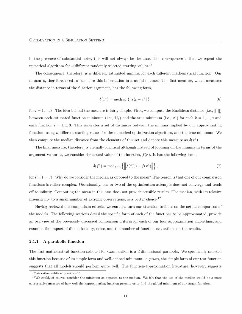
Figure 1: Parabolic Function: This figure displays the parabola function, with and without noise, used to com-pare our four function-approximation algorithms. This three-dimensional version of the parabola in equation 8 has thefunctional form, f1(x1, x2) = x2
1 + x22.
−10
−5
0
5
10
−10
−5
0
5
10
0
50
100
150
200
x1
x2
f(x1,x 2)
−10
−5
0
5
10
−10
−5
0
5
10
0
50
100
150
200
250
300
x1
x2
f(x1,x 2)
Given a parameter vector, x ∈ Rd, we describe the d-dimensional parabola function with the following
parsimonious form,
f1(x) = xT x. (8)
Figure 1 describes the form of this function for d = 2. Observe that in three dimensions, the parabola has a
cup-shaped form with a minimum at its vertex, which is the origin. Also observe the basic shape of the parabola
is preserved in the presence of Gaussian noise—we have used a signal-to-noise ratio of five. One can nevertheless
imagine that a function-approximation algorithm could easily become confused by assuming that a particularly
noisy function is, in fact, a true datapoint.
We now turn to see how our approximation functions fit our first function. Table 1 summarizes the six
comparison criteria for each of our four alternative approximation algorithms. This information is presented by
dimension; in particular, we examine d = 4, 8, and 12. All of the goodness-of-fit statistics are computed with a
12

Optimization in a Simulation Setting
Table 1: Fit to Parabola Function: This table describes the fit of the model to the parabola function–summarizedin equation 8—with a moderate degree of noise and a training dataset comprised of 1,000 randomly selected functionevaluations.
Models MAE RMSE ρ sMAE δ(x∗) δ(f∗)Dimension: d = 4
OLS 0.083 0.106 0.998 0.036 0.002 -0.002MARS 0.128 0.170 0.996 0.055 0.046 -0.046NKR 0.869 1.069 0.892 0.371 6.685 -6.694PPR 0.589 0.692 0.981 0.248 0.392 -0.932
Dimension: d = 8OLS 0.119 0.155 0.995 0.072 0.000 0.000MARS 0.198 0.269 0.986 0.120 0.059 -0.059NKR 1.323 1.432 0.618 0.798 8.216 -8.216PPR 0.922 1.142 0.746 0.559 1.249 -1.249
Dimension: d = 12OLS 0.043 0.056 0.998 0.034 0.063 -0.016MARS 0.179 0.241 0.981 0.142 0.169 -0.104NKR 1.034 1.172 0.368 0.821 8.684 -8.672PPR 0.909 1.141 0.350 0.770 5.767 -5.605
moderate amount of noise and a training dataset comprised of 1,000 randomly selected function evaluations.18 It
is important to note that there is some potential variability in the results. As the dataset is randomly selected,
different draws of the dataset will likely yield different results.19 It is, of course, possible to repeat the analysis
for a large number of independently generated 1,000 element datasets, but we opted not to do this during our
analysis. The primary reason is that some preliminary results revealed that the results do not change very much.
The first four columns of Table 1 include the four measures that describe how well the approximation fits the
true function. Recall that a good fit to the data is evidenced by small MAE, RMSE, and sMAE measures. We
would like to see a correlation coeficient as close as possible to one, and a good optimization fit, which involves
δ(x∗) and δ(f∗) values as close as possible to zero. The first thing to note is that the OLS approximation fits
18Gaussian noise is generated by letting the standard deviation of the innovation term be directly proportional to the variance of
the function. In particular, the noise term has the following distribution,
εij ∼ N(
0,var(fi(x))
ζ
), (9)
where the constant, ζ ∈ R, is the signal-to-noise ratio. We characterize low noise as ζ = ∞, moderate noise as ζ = 10, and a high
degree of noise as ζ = 5.19Selecting the points in a random fashion is probably not the best approach. One could presumably do a better job by using
pseudo-random, or low-discprepancy, sequences to select observations that better cover the space. This was not considered in this
study and we leave exploration of this point for further work.
13

Optimization in a Simulation Setting
Figure 2: Dimensionality and the Parabola Function: In this figure, we summarize the data provided in Table 1by examining the influence of dimensionality on the goodness-of-fit measures. All statistics are computed in the presenceof a moderate degree of noise and a training dataset comprised of 1,000 randomly selected function evaluations.
2 4 6 8 10 120
0.2
0.4
0.6
0.8
1
1.2
1.4MAE
Dimension2 4 6 8 10 12
0.2
0.4
0.6
0.8
1ρ
Dimension
2 4 6 8 10 120
1
2
3
4
5δ(x*)
Dimension2 4 6 8 10 12
−25
−20
−15
−10
−5
0
5δ(f*)
Dimension
OLS
MARS
NKR
PPR
the data extremely well. The correlation coefficient approaches unity, while the MAE and RMSE measures
indicate an almost perfect fit to the true underlying function. This should not be an enormous surprise given the
quadratic functional form. As we include quadratic terms in the construction of the OLS approximation, we are
able to fit the parabola function almost perfectly. The additional noise is not a problem given the OLS algorithm
is well known for its ability to abstract from noise. We also observe, however, that the MARS algorithm also
provides a close fit to the data. The correlation coefficient, across all three dimensions does not fall below 0.98.
Moreover, the MAE and RMSE measures are only about 1 12 to 2 times larger than those observed with the OLS
algorithm. Most importantly, the distance of the OLS and MARS minima from the true function are negligible.
Clearly, both of these approximation algorithms are quite capable of finding the minimum of the true function.
14

Optimization in a Simulation Setting
Figure 3: Noise and the Parabola Function: This figure examines the influence of noise on the goodness-of-fitmeasures. All statistics are computed with d = 8 and a training dataset comprised of 1,000 randomly selected functionevaluations for various degrees of noise.
Low Med High0
0.2
0.4
0.6
0.8
1
1.2
1.4MAE
Amount of noiseLow Med High
0.2
0.4
0.6
0.8
1ρ
Amount of noise
Low Med High0
1
2
3
4
5
6δ(x*)
Amount of noiseLow Med High
−30
−25
−20
−15
−10
−5
0δ(f*)
Amount of noise
OLS
MARS
NKR
PPR
What is rather surprising, however, is the performance of the NKR and PPR approaches. The NKR algo-
rithm’s goodness of fit—as measured by the MAE, RMSE and correlation coefficient—deteriorates dramatically
with increasing dimensionality. The correlation coefficient, for example, falls from almost 0.90 for d = 4 to less
than 0.4 for d = 12. A similar pattern is evident for the PPR technique. Clearly, these two approaches have
difficulty approximating the rather simple parabola function. The reason for the underperformance likely relates
to the fact that both of these approaches use Gaussian-based kernel approximations. Specifically, we suspect that
the local information used to estimate the shape of the function underestimates the exponential growth evident
in the parabola. This is also probably exacerbated by the presence of noise and increasing dimensionality in the
observation of the function values.
15

Optimization in a Simulation Setting
Figure 4: Number of Observations and the Parabola Function: This figure examines the influence of thenumber of observations on the goodness-of-fit measures. All statistics are computed with d = 8 and moderate amount ofnoise.
200 400 600 800 10000
0.5
1
1.5
2MAE
Function evaluations200 400 600 800 1000
0.2
0.4
0.6
0.8
1ρ
Function evaluations
200 400 600 800 1000−5
0
5
10δ(x*)
Function evaluations200 400 600 800 1000
−25
−20
−15
−10
−5
0
5
10δ(f*)
OLS
MARS
NKR
PPR
The strength of the performance of the OLS and MARS algorithms is supported by Figure 2 that graphically
summarizes four of the key goodness-of-fit criteria for each of the four approximation algorithms over the range
d = 1, .., 12. The correlation coefficient, MAE, and the two measures of optimization accuracy for the OLS and
MARS algorithms track one another closely. The dramatic deterioration of the performance of the NKR and
the PPR algorithms for the parabola function is also clearly evident in Figure 2. We do note that the optimiza-
tion performance of the PPR algorithm appears to be quite stable, although the distance of the approximated
minimum remains a substantial distance from the true minimum.
The next principal aspect that we wish to compare is the robustness of our algorithms to the presence of
noise in the dataset. This examination is performed in the context of three different noise settings: low, medium,
16
Optimization in a Simulation Setting
and high. Figure 3 outlines the impact these different levels of noise on the key goodness-of-fit measures. The
result is quite interesting. It does not appear, for the parabola function, that there is much difference in the
approximations for the OLS and MARS algorithms as one increases the noisiness of the observations. The NKR
and PPR approaches fare rather less well. A particular deterioration in the performance of the PPR algorithm is
evident as we increase the noise. It is difficult to judge the NKR algorithm in the presence of noise as it generally
fits the parabola function poorly at this dimensionality.
The final aspect of comparison among the models is how sensitive the results are to the size of the dataset.
This is important because there is a substantial computation expense associated with constructing a dataset for
the debt-strategy problem. Understanding how the approximation algorithms react to differently sized training
datasets, therefore, will help us understand the number of observations required from our stochastic-simulation
model.
Figure 4 outlines the impact of varying the number of observations from 200 to 1,000 in the presence of
a moderate amount of noise and holding the dimensionality fixed at d = 8. The MARS and OLS techniques
clearly improve as we increase the number of observations used to train and predict the data, but still perform
quite well even with 200 observations. This suggests that these two approaches, at least in the context of the
parabola function, are capable of approximating with a relatively sparse amount of information. Conversely,
the correlation coefficient and MAE measures steadily deteriorate as one decreases the amount of information
available for training the NKR and PPR algorithms. Interestingly, the PPR algorithm continues to approximate
the function minimum reasonably well. This, however, is not true for the NKR technique; the optimization
performance clearly improves as the number of observations is augmented.
To summarize, the MARS and OLS algorithms handle noise, dimensionality, and small number, of observa-
tions admirably well in the context of the simple parabola function. The NKR and PPR approaches, perhaps
surprisingly, demonstrate difficulty in fitting the parabola for even moderate dimensions, have trouble with noisy
observations, and their fit deteriorates steadily as one decreases the size of the dataset.
2.1.2 A conic-cosine function
The second mathematical function under consideration is a bit trickier than the previously examined parabola
function. It has a well-defined minimum, but it demonstrates an oscillatory structure that we suspected would
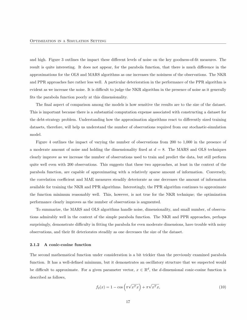
be difficult to approximate. For a given parameter vector, x ∈ Rd, the d-dimensional conic-cosine function is
described as follows,
f2(x) = 1− cos(π√
xT x)
+ π√
xT x, (10)
17
Optimization in a Simulation Setting
Figure 5 provides a three-dimensional view of the conic-cosine function. Note that it has a quadratic form, with
an obvious minimum at the origin, although through the presence of the cosine function it has a wavy shape.
In the presence of noise, this gives rise to a large number of local minima that can make optimization of this
function somewhat tricky.
Figure 5: Conic-Cosine Function: This figure displays the conic-cosine function used to compare our fourfunction-approximation algorithms. This three-dimensional version of the conic-cosine mapping has the functional form,
f2(x1, x2) = 1− cos(π√
x21 + x2
2
)+ π
√x2
1 + x22.
−10
−5
0
5
10
−10
−5
0
5
10
0
5
10
15
20
25
30
35
40
45
x1
x2
f(x1,x 2)
−10
−5
0
5
10
−10
−5
0
5
10
−10
0
10
20
30
40
50
x1
x2
f(x1,x 2)
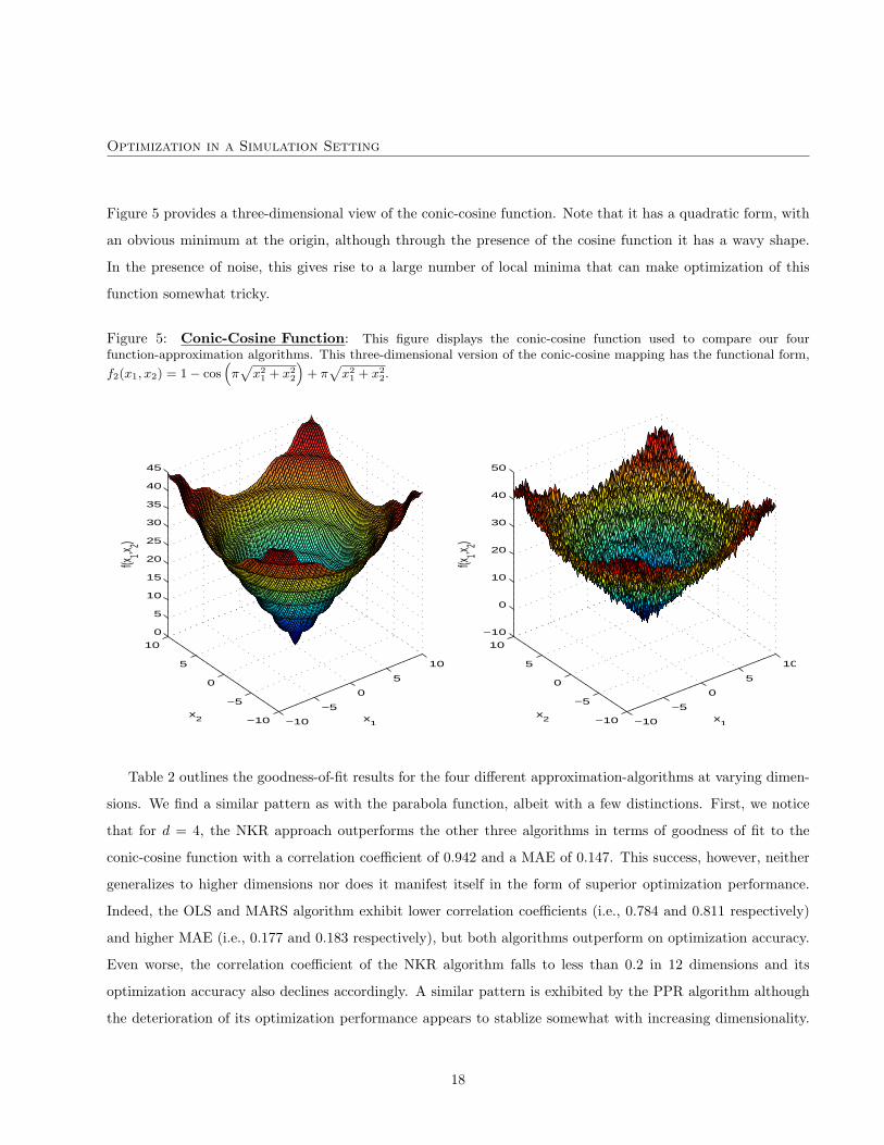
Table 2 outlines the goodness-of-fit results for the four different approximation-algorithms at varying dimen-
sions. We find a similar pattern as with the parabola function, albeit with a few distinctions. First, we notice
that for d = 4, the NKR approach outperforms the other three algorithms in terms of goodness of fit to the
conic-cosine function with a correlation coefficient of 0.942 and a MAE of 0.147. This success, however, neither
generalizes to higher dimensions nor does it manifest itself in the form of superior optimization performance.
Indeed, the OLS and MARS algorithm exhibit lower correlation coefficients (i.e., 0.784 and 0.811 respectively)
and higher MAE (i.e., 0.177 and 0.183 respectively), but both algorithms outperform on optimization accuracy.
Even worse, the correlation coefficient of the NKR algorithm falls to less than 0.2 in 12 dimensions and its
optimization accuracy also declines accordingly. A similar pattern is exhibited by the PPR algorithm although
the deterioration of its optimization performance appears to stablize somewhat with increasing dimensionality.
18

Optimization in a Simulation Setting
Table 2: Fit to Conic-Cosine Function: This table describes the fit of the model to the conic-cosine function–summarized in equation 10—with a moderate degree of noise and a training dataset comprised of 1,000 randomly selectedfunction evaluations.
Models MAE RMSE ρ sMAE δ(x∗) δ(f∗)Dimension: d = 4
OLS 0.177 0.346 0.784 0.322 0.000 0.000MARS 0.183 0.327 0.811 0.332 0.007 -0.307NKR 0.147 0.292 0.942 0.292 0.249 -0.156PPR 0.187 0.302 0.794 0.376 0.098 -1.430
Dimension: d = 8OLS 0.069 0.083 0.908 0.349 0.000 -0.050MARS 0.070 0.085 0.905 0.354 0.013 -0.428NKR 0.157 0.185 0.341 0.787 0.938 -4.921PPR 0.140 0.179 0.506 0.686 1.376 -5.541
Dimension: d = 12OLS 0.054 0.067 0.927 0.302 0.017 0.166MARS 0.066 0.082 0.887 0.367 0.289 -0.502NKR 0.153 0.172 0.167 0.854 3.576 -11.235PPR 0.159 0.195 0.297 0.863 1.998 -4.752
Nevertheless we can conclude, at least in the context of the conic-cosine function, that the NKR and PPR
algorithms are not robust to dimensionality.
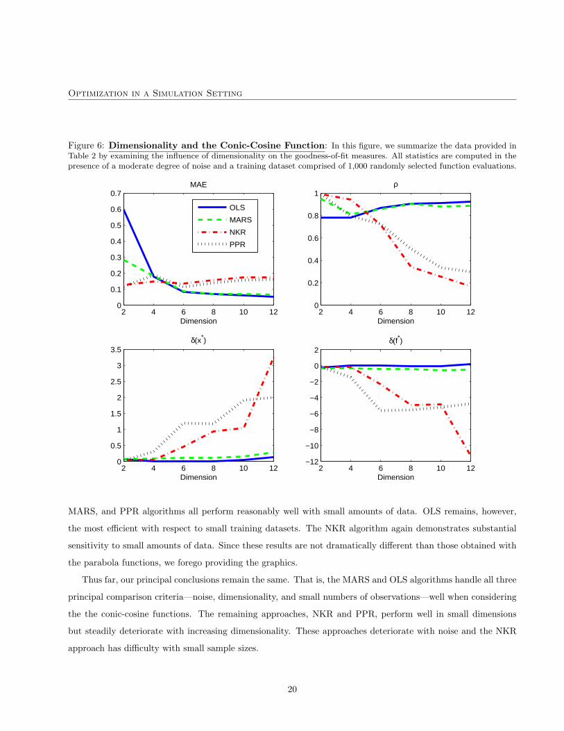
A second observation is that the goodness-of-fit performance of the OLS and MARS algorithms appears to
actually improve with increasing dimensionality. This trend is particularly obvious in Figure 6. Why exactly this
occurs is not clear, but perhaps it is related to the presence of noise. That is, in higher dimensions it might be
easier for these OLS and MARS to distinguish the signal from the noise. Optimization performance of the MARS
and OLS methods, however, actually decreases slightly as we increase the dimension, so perhaps we should not
be overly interested in the slight improvement in goodness of fit.
A third observation is that all of the algorithms seem to have more difficulty in approximating the conic-cosine
function, in terms of goodness of fit and optimization accuracy, relative to the d-dimensional parabola. This
suggests, rather unsurprisingly, that increasingly complex functional forms are more difficult to approximate.
We will revisit this point when examining the final comparison function in the next section.
An analysis of how these functions react to noise and different training set sizes, however, is not terribly
different from those results obtained with the parabola function. In particular, the OLS and MARS algorithm are
quite robust to noise with respect to goodness of fit and optimization accuracy. The NKR and PPR approaches
deteriorate in their approximation performance as we increase the amount of noise. Interestingly, the OLS,
19
Optimization in a Simulation Setting
Figure 6: Dimensionality and the Conic-Cosine Function: In this figure, we summarize the data provided inTable 2 by examining the influence of dimensionality on the goodness-of-fit measures. All statistics are computed in thepresence of a moderate degree of noise and a training dataset comprised of 1,000 randomly selected function evaluations.
2 4 6 8 10 120
0.1
0.2
0.3
0.4
0.5
0.6
0.7MAE
Dimension2 4 6 8 10 12
0
0.2
0.4
0.6
0.8
1ρ
Dimension
2 4 6 8 10 120
0.5
1
1.5
2
2.5
3
3.5δ(x*)
Dimension2 4 6 8 10 12
−12
−10
−8
−6
−4
−2
0
2δ(f*)
Dimension
OLS
MARS
NKR
PPR
MARS, and PPR algorithms all perform reasonably well with small amounts of data. OLS remains, however,
the most efficient with respect to small training datasets. The NKR algorithm again demonstrates substantial
sensitivity to small amounts of data. Since these results are not dramatically different than those obtained with
the parabola functions, we forego providing the graphics.
Thus far, our principal conclusions remain the same. That is, the MARS and OLS algorithms handle all three
principal comparison criteria—noise, dimensionality, and small numbers of observations—well when considering
the the conic-cosine functions. The remaining approaches, NKR and PPR, perform well in small dimensions
but steadily deteriorate with increasing dimensionality. These approaches deteriorate with noise and the NKR
approach has difficulty with small sample sizes.
20
Optimization in a Simulation Setting
2.1.3 The Rosenbrock banana function
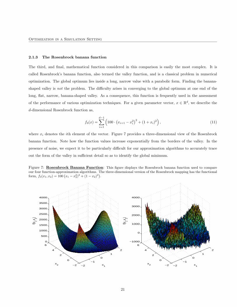
The third, and final, mathematical function considered in this comparison is easily the most complex. It is
called Rosenbrock’s banana function, also termed the valley function, and is a classical problem in numerical
optimization. The global optimum lies inside a long, narrow value with a parabolic form. Finding the banana-
shaped valley is not the problem. The difficulty arises in converging to the global optimum at one end of the
long, flat, narrow, banana-shaped valley. As a consequence, this function is frequently used in the assessment
of the performance of various optimization techniques. For a given parameter vector, x ∈ Rd, we describe the
d-dimensional Rosenbrock function as,
f3(x) =d−1∑i=1
(100 ·
(xi+1 − x2
i
)2+ (1 + xi)2
), (11)
where xi denotes the ith element of the vector. Figure 7 provides a three-dimensional view of the Rosenbrock
banana function. Note how the function values increase exponentially from the borders of the valley. In the
presence of noise, we expect it to be particularly difficult for our approximation algorithms to accurately trace
out the form of the valley in sufficient detail so as to identify the global minimum.
Figure 7: Rosenbrock Banana Function: This figure displays the Rosenbrock banana function used to compareour four function-approximation algorithms. The three-dimensional version of the Rosenbrock mapping has the functionalform, f3(x1, x2) = 100
(x1 − x2
2)2 + (1− x2)
2).
−2
−1
0
1
2
−2
0
2
4
6
0
500
1000
1500
2000
2500
3000
3500
4000
x1
x2
f(x1,x 2)
−2
−1
0
1
2
−2
0
2
4
6
−1000
0
1000
2000
3000
4000
x1
x2
f(x1,x 2)
21
Optimization in a Simulation Setting
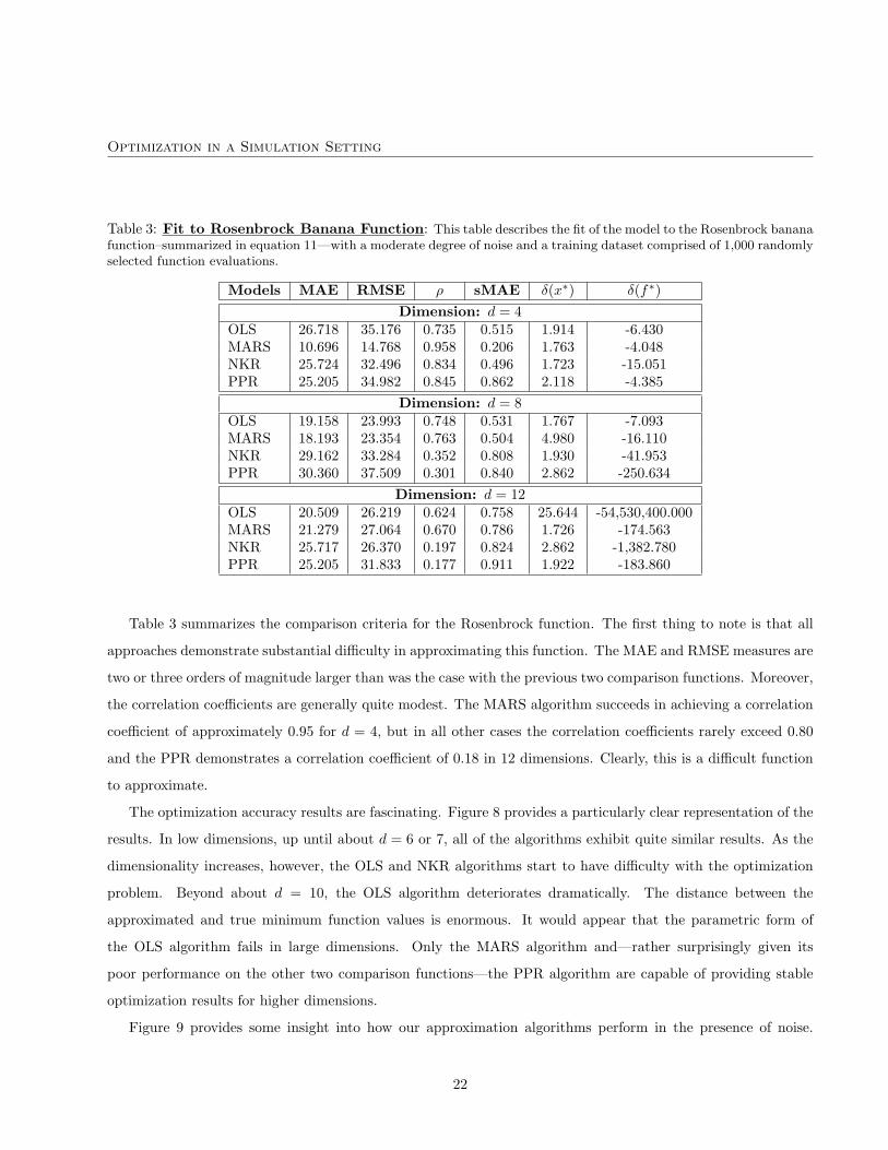
Table 3: Fit to Rosenbrock Banana Function: This table describes the fit of the model to the Rosenbrock bananafunction–summarized in equation 11—with a moderate degree of noise and a training dataset comprised of 1,000 randomlyselected function evaluations.
Models MAE RMSE ρ sMAE δ(x∗) δ(f∗)Dimension: d = 4
OLS 26.718 35.176 0.735 0.515 1.914 -6.430MARS 10.696 14.768 0.958 0.206 1.763 -4.048NKR 25.724 32.496 0.834 0.496 1.723 -15.051PPR 25.205 34.982 0.845 0.862 2.118 -4.385
Dimension: d = 8OLS 19.158 23.993 0.748 0.531 1.767 -7.093MARS 18.193 23.354 0.763 0.504 4.980 -16.110NKR 29.162 33.284 0.352 0.808 1.930 -41.953PPR 30.360 37.509 0.301 0.840 2.862 -250.634
Dimension: d = 12OLS 20.509 26.219 0.624 0.758 25.644 -54,530,400.000MARS 21.279 27.064 0.670 0.786 1.726 -174.563NKR 25.717 26.370 0.197 0.824 2.862 -1,382.780PPR 25.205 31.833 0.177 0.911 1.922 -183.860
Table 3 summarizes the comparison criteria for the Rosenbrock function. The first thing to note is that all
approaches demonstrate substantial difficulty in approximating this function. The MAE and RMSE measures are
two or three orders of magnitude larger than was the case with the previous two comparison functions. Moreover,
the correlation coefficients are generally quite modest. The MARS algorithm succeeds in achieving a correlation
coefficient of approximately 0.95 for d = 4, but in all other cases the correlation coefficients rarely exceed 0.80
and the PPR demonstrates a correlation coefficient of 0.18 in 12 dimensions. Clearly, this is a difficult function
to approximate.
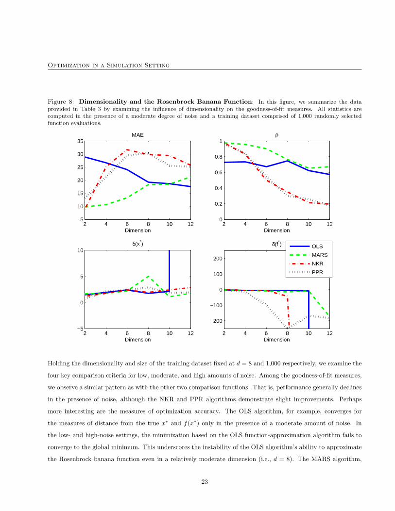
The optimization accuracy results are fascinating. Figure 8 provides a particularly clear representation of the
results. In low dimensions, up until about d = 6 or 7, all of the algorithms exhibit quite similar results. As the
dimensionality increases, however, the OLS and NKR algorithms start to have difficulty with the optimization
problem. Beyond about d = 10, the OLS algorithm deteriorates dramatically. The distance between the
approximated and true minimum function values is enormous. It would appear that the parametric form of
the OLS algorithm fails in large dimensions. Only the MARS algorithm and—rather surprisingly given its
poor performance on the other two comparison functions—the PPR algorithm are capable of providing stable
optimization results for higher dimensions.
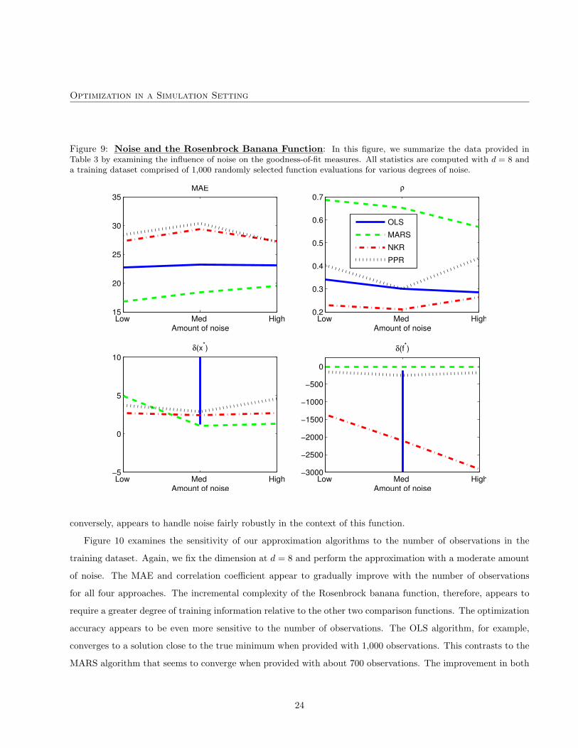
Figure 9 provides some insight into how our approximation algorithms perform in the presence of noise.
22
Optimization in a Simulation Setting
Figure 8: Dimensionality and the Rosenbrock Banana Function: In this figure, we summarize the dataprovided in Table 3 by examining the influence of dimensionality on the goodness-of-fit measures. All statistics arecomputed in the presence of a moderate degree of noise and a training dataset comprised of 1,000 randomly selectedfunction evaluations.
2 4 6 8 10 125
10
15
20
25
30
35MAE
Dimension2 4 6 8 10 12
0
0.2
0.4
0.6
0.8
1ρ
Dimension
2 4 6 8 10 12−5
0
5
10δ(x*)
Dimension2 4 6 8 10 12
−200
−100
0
100
200
δ(f*)
Dimension
OLS
MARS
NKR
PPR
Holding the dimensionality and size of the training dataset fixed at d = 8 and 1,000 respectively, we examine the
four key comparison criteria for low, moderate, and high amounts of noise. Among the goodness-of-fit measures,
we observe a similar pattern as with the other two comparison functions. That is, performance generally declines
in the presence of noise, although the NKR and PPR algorithms demonstrate slight improvements. Perhaps
more interesting are the measures of optimization accuracy. The OLS algorithm, for example, converges for
the measures of distance from the true x∗ and f(x∗) only in the presence of a moderate amount of noise. In
the low- and high-noise settings, the minimization based on the OLS function-approximation algorithm fails to
converge to the global minimum. This underscores the instability of the OLS algorithm’s ability to approximate
the Rosenbrock banana function even in a relatively moderate dimension (i.e., d = 8). The MARS algorithm,
23
Optimization in a Simulation Setting
Figure 9: Noise and the Rosenbrock Banana Function: In this figure, we summarize the data provided inTable 3 by examining the influence of noise on the goodness-of-fit measures. All statistics are computed with d = 8 anda training dataset comprised of 1,000 randomly selected function evaluations for various degrees of noise.
Low Med High15
20
25
30
35MAE
Amount of noiseLow Med High
0.2
0.3
0.4
0.5
0.6
0.7ρ
Amount of noise
Low Med High−5
0
5
10δ(x*)
Amount of noiseLow Med High
−3000
−2500
−2000
−1500
−1000
−500
0
δ(f*)
Amount of noise
OLS
MARS
NKR
PPR
conversely, appears to handle noise fairly robustly in the context of this function.
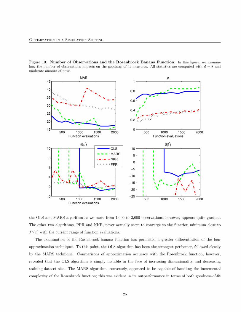
Figure 10 examines the sensitivity of our approximation algorithms to the number of observations in the
training dataset. Again, we fix the dimension at d = 8 and perform the approximation with a moderate amount
of noise. The MAE and correlation coefficient appear to gradually improve with the number of observations
for all four approaches. The incremental complexity of the Rosenbrock banana function, therefore, appears to
require a greater degree of training information relative to the other two comparison functions. The optimization
accuracy appears to be even more sensitive to the number of observations. The OLS algorithm, for example,
converges to a solution close to the true minimum when provided with 1,000 observations. This contrasts to the
MARS algorithm that seems to converge when provided with about 700 observations. The improvement in both
24
Optimization in a Simulation Setting
Figure 10: Number of Observations and the Rosenbrock Banana Function: In this figure, we examinehow the number of observations impacts on the goodness-of-fit measures. All statistics are computed with d = 8 andmoderate amount of noise.
500 1000 1500 200015
20
25
30
35
40
45MAE
Function evaluations500 1000 1500 2000
0
0.2
0.4
0.6
0.8
1ρ
Function evaluations
500 1000 1500 20000
2
4
6
8
10δ(x*)
Function evaluations500 1000 1500 2000
−25
−20
−15
−10
−5
0
5
10δ(f*)
OLS
MARS
NKR
PPR
the OLS and MARS algorithm as we move from 1,000 to 2,000 observations, however, appears quite gradual.
The other two algorithms, PPR and NKR, never actually seem to converge to the function minimum close to
f∗(x) with the current range of function evaluations.
The examination of the Rosenbrock banana function has permitted a greater differentiation of the four
approximation techniques. To this point, the OLS algorithm has been the strongest performer, followed closely
by the MARS technique. Comparisons of approximation accuracy with the Rosenbrock function, however,
revealed that the OLS algorithm is simply instable in the face of increasing dimensionality and decreasing
training-dataset size. The MARS algorithm, conversely, appeared to be capable of handling the incremental
complexity of the Rosenbrock function; this was evident in its outperformance in terms of both goodness-of-fit
25
Optimization in a Simulation Setting
and optimization accuracy. Finally, the PPR technique, despite its relative underperformance in the previous
two functions, seemed rather more capable of approximating the Rosenbrock banana function.
2.1.4 Summary of comparison
Among our list of approximation-model criteria, we required that a given algorithm have the ability to closely fit
the data for a given amount of noise, dimensionality, and number of function evaluations. In the preceding three
sections, we examined the ability of our four alternative methods to fit functions of increasing complexity. Simply
put, the OLS and MARS algorithms exhibited the most stability in terms of noise, dimensionality, and number
of observations for the first two comparison functions. The OLS approach, however, demonstrated significant
difficulty in handling dimensionality and noise in the context of the more complicated Rosenbrock function. For
this reason, we would suggest that the most appropriate approximation algorithm for use in the debt-strategy
analysis is the MARS technique.
This conclusion raises a natural question. In particular, do we expect our debt-strategy objective functions to
be as complex as the Rosenbrock banana function? No, but we want to ensure that by examining a wide range
of different functional forms, that our approximation algorithm has at least the potential to handle complex
objective functions. Part of the reason is that we do not know, as yet, the exact form of the government’s
objective function. As such, we require a substantial degree of flexibility.
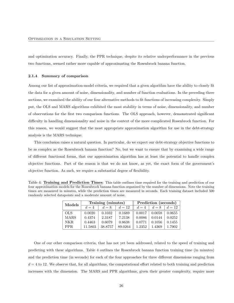
Table 4: Training and Prediction Times: This table outlines time required for the training and prediction of ourfour approximation models for the Rosenbrock banana function organized by the number of dimensions. Note the trainingtimes are measured in minutes, while the prediction times are measured in seconds. Each training dataset included 500randomly selected datapoints and a moderate amount of noise.
Training (minutes) Prediction (seconds)Modelsd = 4 d = 8 d = 12 d = 4 d = 8 d = 12
OLS 0.0020 0.1032 0.1689 0.0017 0.0058 0.0655MARS 0.4374 2.3187 7.2138 0.0086 0.0144 0.0252NKR 0.4463 0.6079 0.8638 0.0771 0.1056 0.1455PPR 11.5803 38.8757 89.0264 1.2352 1.4369 1.7902
One of our other comparison criteria, that has not yet been addressed, related to the speed of training and
predicting with these algorithms. Table 4 outlines the Rosenbrock banana function training time (in minutes)
and the prediction time (in seconds) for each of the four approaches for three different dimensions ranging from
d = 4 to 12. We observe that, for all algorithms, the computational effort related to both training and prediction
increases with the dimension. The MARS and PPR algorithms, given their greater complexity, require more
26
Optimization in a Simulation Setting
time for training. For d = 12 and 500 observations, the MARS algorithm required slightly more than seven
minutes for training while the PPR approach required almost 1.5 hours. The final point of interest relates to
the length of time required for prediction of f(x) for an arbitary vector, x ∈ Rd. The shorter this time period,
the faster the optimization procedure can be performed. The OLS and MARS algorithms are extremely fast,
while the NKR and PPR approaches are relatively slow. The PPR technique, in particular, requires almost two
seconds for prediction, which is far too slow to be useful in an optimization setting.20
3 The Application
In the previous section we established that, using the MARS algorithm, one can optimize in a reasonably high-
dimensional, non-linear setting, with a limited number of function evaluations and in the presence of noise.
Moreover, the optimization can be performed fairly quickly. In this section, therefore, we turn to examine how
this fact can be applied to the original debt-management problem. The principal task involved in this application
is a characterization of the government’s objective function with respect to its debt strategy. While we do not
claim to answer this problem, we will provide a number of possible alternatives. We then turn to apply the MARS
algorithm to these alternative objective functions and use a simplified setting to examine some illustrative results
that essentially demonstrate what can be accomplished with this method.
The first step in any optimization problem is to determine the form of one’s objective function. In this setting,
the answer is not immediately obvious. There are a number of alternatives, each with different implications for
the policy objectives of the government. To speak about an optimal debt strategy, therefore, it is necessary to
define rather precisely the conditions for optimality. Ultimately, this requires an understanding of the objectives
of the federal government with respect to its domestic debt portfolio. The stated objectives of the Canadian
government with respect to debt management are:
To raise stable and low-cost funding for the government and maintenance of a well-functioning market
in government of Canada securities.
While this is specific to Canada, most countries have a similar publically stated objectives.21 Most governments,
therefore, are looking for a financing strategy that provides stable and low-cost funding. This is a useful start,
20These two approaches are relatively slow as they both employ a Gaussian kernel. This implies that prediction of f(x) for an
arbitrary x ∈ D ⊂ Rd requires the calculation of the Gaussian probability density function for each point; even though this is
a closed-form expression, it must be repeated an enormous number of times. That is, although each individual computation is
extremely fast, when performed many times, it can create a computational burden.21See Bolder and Lee-Sing (2004, [18]) for a description of the debt-management objectives of a number of industrialized countries.
27
Optimization in a Simulation Setting
but one should note that a universal definition for financing cost and stability does not exist. As such, we will
examine a number of alternative formulations.
We begin by defining a financing strategy as θ. This is a fixed set of weights representing the issuance in
each of the d available financing instruments. The individual elements of θ cannot be negative (i.e., θi ≥ 0
for all i) and the elements must sum to unity (i.e.,∑d
i=1 θi = 1). We define the set of permissible financing
strategies that meet these two restrictions as Θ. As a final note, the weights are not permitted to vary through
time.22 Ultimately, therefore, the optimization problem is concerned with finding the vector, θ ∈ Θ ⊂ Rd. In
the notation of the previous two section, θ is the equivalent of the function parameters, x.
At time, t, there is a substantial amount of uncertainty about the future evolution of financial and macroeco-
nomic variables. Economic and financial uncertainty is summarized in a collection of state variables, Xt, t ∈ [0, T ],
where T denotes the terminal date.23 These state variables have stochastic dynamics defined on the probabil-
ity space, (Ω,F , P). A rather more detailed description of the derivation, parameter estimation, and empirical
performance of these stochastic models is found in Bolder (2006, [13, 14]).
How, therefore, do we propose to describe the government’s objective function? We propose a number of
possibilities, although they generally fall into two separate categories. The first category involves trying to write
the government’s objectives directly in terms of outputs stemming from the stochastic-simulation engine, such as
debt charges, volatility of debt charges, and the government’s fiscal situation. This approach is somewhat ad hoc,
although it has the benefit of being quite transparent. The second category involves indirectly incorporating the
outputs of the stochastic-simulation engine into a utility function that represents, in some comprehensive way,
the government’s risk preferences. This approach has the advantage of a sound theoretical foundation, although
it is perhaps somewhat less transparent.
In our illustrative analysis, we consider seven different possible objective functions. The form of each of these
objective functions and the associated mathematical structure of the constrained optimization problem is found
in Appendix B. In this section, however, we provide a high-level description of each possible specification.
Debt Charges This is perhaps the most obvious choice for an objective function. A government always has a22In a general stochastic optimal control setting, the financing strategy should be a function of the state variable and vary through
time. That is, θ ≡ θt, should itself be a random process. This adds an enormous amount of complexity and is not considered in this
work.23As a government is an infinitely lived organization, it may not seem reasonable to have a terminal date at all. From a practical
perspective, however, the further we move into the future, the less important the cashflows become from the current perspective.
Also, our ability to reasonably describe future economic and financial dynamics decreases dramatically as we move further into the
future. Typically, therefore, the fairly arbitrary value of ten years is selected for the terminal date.
28
Optimization in a Simulation Setting
strong interest in keeping the cost of their debt at a low level. We suggest, therefore, considering the stream
of expected government debt charges across the simulation horizon. If we have T years in the simulation,
therefore, we would have a stream of T expected annual debt charges. We propose merely considering
the simple average of this stream of debt charges. In other words, a government might wish to select the
financing strategy that minimizes the average expected annual debt charges over their simulation horizon.
More detail on this objective function is provided in Appendix B.1.
Discounted Debt Charges One of the problems with the previous approach is that it treats debt charges in
latter years of the stochastic simulation with the same degree of importance as debt charges occurring in
the first few years. This may be the case, but a government is probably more likely to want to discount
cashflows occurring further in the future. We propose, therefore, considering the minimization of the
average discounted expected annual debt charges over the simulation horizon. This objective function is
outlined in more detail in Appendix B.2.
Debt-Charge Stability The previous two approaches encompass the low-cost component of the government’s
stated objectives, but they do not consider the stability aspect. While we do not know exactly what
is meant by stability, one possible interpretation is to assume that we are concerned with the stability
of government debt charges. We subsequently suggest minimizing the previous objective function (i.e.,
average discounted expected annual debt charges over the simulation horizon) with a constraint on the
conditional volatility of the government’s annual debt charges. Greater detail on this objective function,
and our definition of conditional debt-charge volatility, are provided in Appendix B.3.
Fiscal-Policy Considerations Another possible notion of stability relates to the government’s fiscal situation.
A government, for example, may not be concerned about the instability of government debt charges, but
instead is more focused on the associated instability of their budgetary balance. We suggest, therefore,
two alternative choices. In the first, we place an additional constraint on the conditional volatility of
the government’s financial requirements. In the second, we contruct an objective function that is a linear
combination of average discounted expected annual debt charges and the probability of a budgetary deficit.
Both of these formulations are provided in Appendix B.4.
Utility (Loss) Functions Here we introduce the notion of a formal expected utility function. We consider
time-separable CARA and CRRA utility formulations, where utility is a function of the expected annual
debt charges. The logic behind the construction of these objective functions is found in Appendix B.5.
29
Optimization in a Simulation Setting
This is far from an exhaustive list of possible objective functions. One of the principal advantages of the
stochastic simulation approach is that it provides a rich description of the dynamics of the entire debt stock
over the simulation horizon. Not only does one have a characterization of the financial and macroeconomic
environment, but there is also detailed information on the composition of the domestic debt portfolio and the
government’s financial position. The objective functions provided thus far, therefore, are only a subset of the
possible components that can be incorporated into the analysis. One can easily imagine extending the objective
function to incorporate:
• an analysis of each of the preceding objective functions in real terms or as a proportion of real (or nominal)
GDP;
• a standardization of the expected debt charges by their standard deviation;24
• the terminal value of the debt stock in either nominal or real terms;
• the volatility of the market value of the debt stock;25
How specifically do we use the MARS algorithm to approximate these objective functions? It begins with the
construction of our data. We randomly select N government financing strategies, where N represents as much
computation as we can reasonably afford. For each financing strategy, we have a wide range of data on debt
charges, federal financing requirements, and the size of the debt stock. Each of the previously discussed objective
functions can be constructed from this data. This can, in some cases, require a bit of work. The utility function
approach, for example, requires us to compute the loss function for each year and each stochastic realization.
We then compute the expectation of the loss function across all realizations for each year and then sum across
the entire time horizon.26 For other objective functions, this is quite straightforward. When the objective
function is the sum of annual expected debt charges, we merely compute the required expectations from the
simulation-engine output and sum. The MARS algorithm is subsequently used to construct an approximation
of each objective function for an arbitrary financing strategy, not merely the N observations—corresponding to
N alternative financing strategies—that we have computed.
We now turn to provide some simple analysis of these alternative government objective functions. These
illustrative results are provided in the context of a simplified version of the debt-management problem. In24This would form a type of Sharpe ratio.25This is predicated on the idea that a large premium would indicate that the government should have waited to fund themselves,
while a large discount indicates that the government should have prefunded their borrowing requirements.26See equations (124) to (126) in Appendix B.5 for more detail.
30
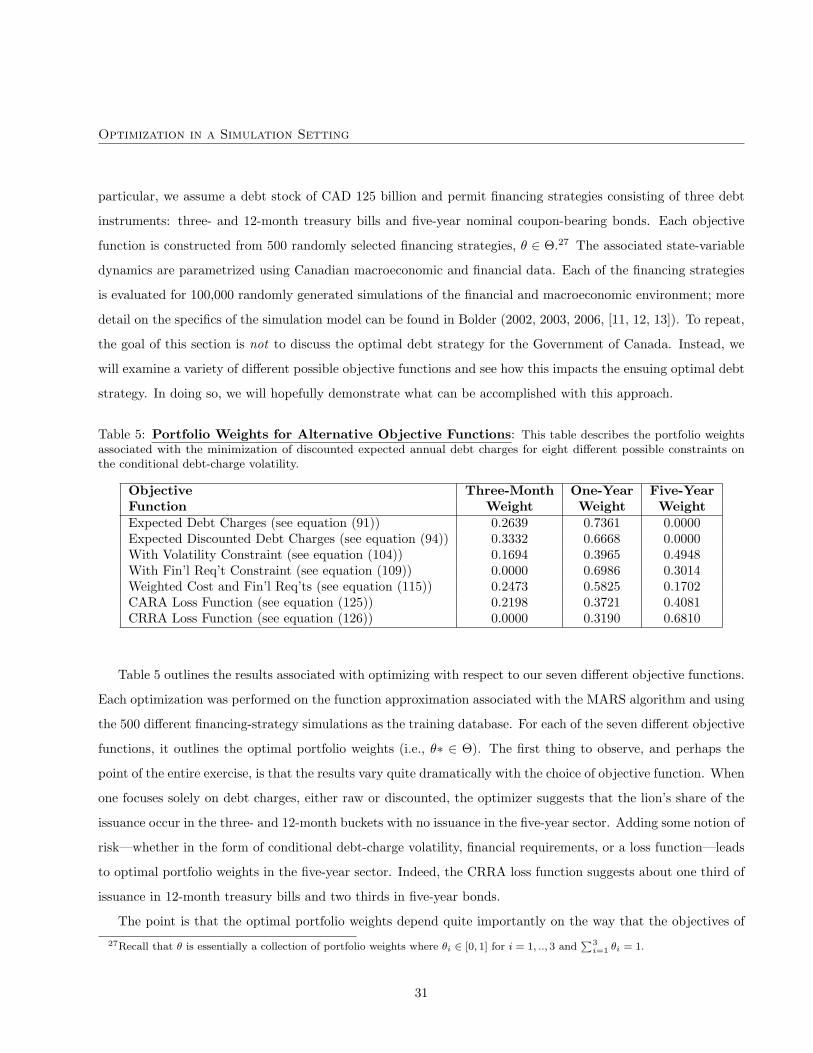
Optimization in a Simulation Setting
particular, we assume a debt stock of CAD 125 billion and permit financing strategies consisting of three debt
instruments: three- and 12-month treasury bills and five-year nominal coupon-bearing bonds. Each objective
function is constructed from 500 randomly selected financing strategies, θ ∈ Θ.27 The associated state-variable
dynamics are parametrized using Canadian macroeconomic and financial data. Each of the financing strategies
is evaluated for 100,000 randomly generated simulations of the financial and macroeconomic environment; more
detail on the specifics of the simulation model can be found in Bolder (2002, 2003, 2006, [11, 12, 13]). To repeat,
the goal of this section is not to discuss the optimal debt strategy for the Government of Canada. Instead, we
will examine a variety of different possible objective functions and see how this impacts the ensuing optimal debt
strategy. In doing so, we will hopefully demonstrate what can be accomplished with this approach.
Table 5: Portfolio Weights for Alternative Objective Functions: This table describes the portfolio weightsassociated with the minimization of discounted expected annual debt charges for eight different possible constraints onthe conditional debt-charge volatility.
Objective Three-Month One-Year Five-YearFunction Weight Weight WeightExpected Debt Charges (see equation (91)) 0.2639 0.7361 0.0000Expected Discounted Debt Charges (see equation (94)) 0.3332 0.6668 0.0000With Volatility Constraint (see equation (104)) 0.1694 0.3965 0.4948With Fin’l Req’t Constraint (see equation (109)) 0.0000 0.6986 0.3014Weighted Cost and Fin’l Req’ts (see equation (115)) 0.2473 0.5825 0.1702CARA Loss Function (see equation (125)) 0.2198 0.3721 0.4081CRRA Loss Function (see equation (126)) 0.0000 0.3190 0.6810
Table 5 outlines the results associated with optimizing with respect to our seven different objective functions.
Each optimization was performed on the function approximation associated with the MARS algorithm and using
the 500 different financing-strategy simulations as the training database. For each of the seven different objective
functions, it outlines the optimal portfolio weights (i.e., θ∗ ∈ Θ). The first thing to observe, and perhaps the
point of the entire exercise, is that the results vary quite dramatically with the choice of objective function. When
one focuses solely on debt charges, either raw or discounted, the optimizer suggests that the lion’s share of the
issuance occur in the three- and 12-month buckets with no issuance in the five-year sector. Adding some notion of
risk—whether in the form of conditional debt-charge volatility, financial requirements, or a loss function—leads
to optimal portfolio weights in the five-year sector. Indeed, the CRRA loss function suggests about one third of
issuance in 12-month treasury bills and two thirds in five-year bonds.
The point is that the optimal portfolio weights depend quite importantly on the way that the objectives of
27Recall that θ is essentially a collection of portfolio weights where θi ∈ [0, 1] for i = 1, .., 3 and∑3
i=1 θi = 1.
31
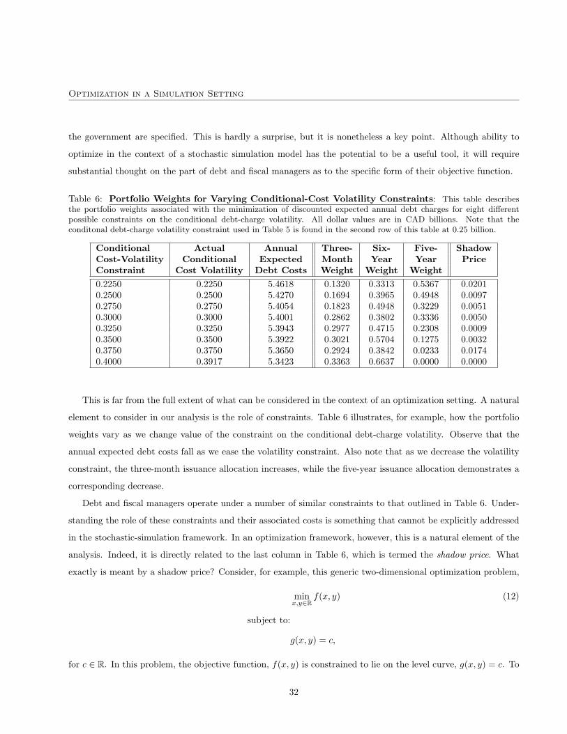
Optimization in a Simulation Setting
the government are specified. This is hardly a surprise, but it is nonetheless a key point. Although ability to
optimize in the context of a stochastic simulation model has the potential to be a useful tool, it will require
substantial thought on the part of debt and fiscal managers as to the specific form of their objective function.
Table 6: Portfolio Weights for Varying Conditional-Cost Volatility Constraints: This table describesthe portfolio weights associated with the minimization of discounted expected annual debt charges for eight differentpossible constraints on the conditional debt-charge volatility. All dollar values are in CAD billions. Note that theconditonal debt-charge volatility constraint used in Table 5 is found in the second row of this table at 0.25 billion.
Conditional Actual Annual Three- Six- Five- ShadowCost-Volatility Conditional Expected Month Year Year PriceConstraint Cost Volatility Debt Costs Weight Weight Weight0.2250 0.2250 5.4618 0.1320 0.3313 0.5367 0.02010.2500 0.2500 5.4270 0.1694 0.3965 0.4948 0.00970.2750 0.2750 5.4054 0.1823 0.4948 0.3229 0.00510.3000 0.3000 5.4001 0.2862 0.3802 0.3336 0.00500.3250 0.3250 5.3943 0.2977 0.4715 0.2308 0.00090.3500 0.3500 5.3922 0.3021 0.5704 0.1275 0.00320.3750 0.3750 5.3650 0.2924 0.3842 0.0233 0.01740.4000 0.3917 5.3423 0.3363 0.6637 0.0000 0.0000
This is far from the full extent of what can be considered in the context of an optimization setting. A natural
element to consider in our analysis is the role of constraints. Table 6 illustrates, for example, how the portfolio
weights vary as we change value of the constraint on the conditional debt-charge volatility. Observe that the
annual expected debt costs fall as we ease the volatility constraint. Also note that as we decrease the volatility
constraint, the three-month issuance allocation increases, while the five-year issuance allocation demonstrates a
corresponding decrease.
Debt and fiscal managers operate under a number of similar constraints to that outlined in Table 6. Under-
standing the role of these constraints and their associated costs is something that cannot be explicitly addressed
in the stochastic-simulation framework. In an optimization framework, however, this is a natural element of the
analysis. Indeed, it is directly related to the last column in Table 6, which is termed the shadow price. What
exactly is meant by a shadow price? Consider, for example, this generic two-dimensional optimization problem,
minx,y∈R
f(x, y) (12)
subject to:
g(x, y) = c,
for c ∈ R. In this problem, the objective function, f(x, y) is constrained to lie on the level curve, g(x, y) = c. To
32
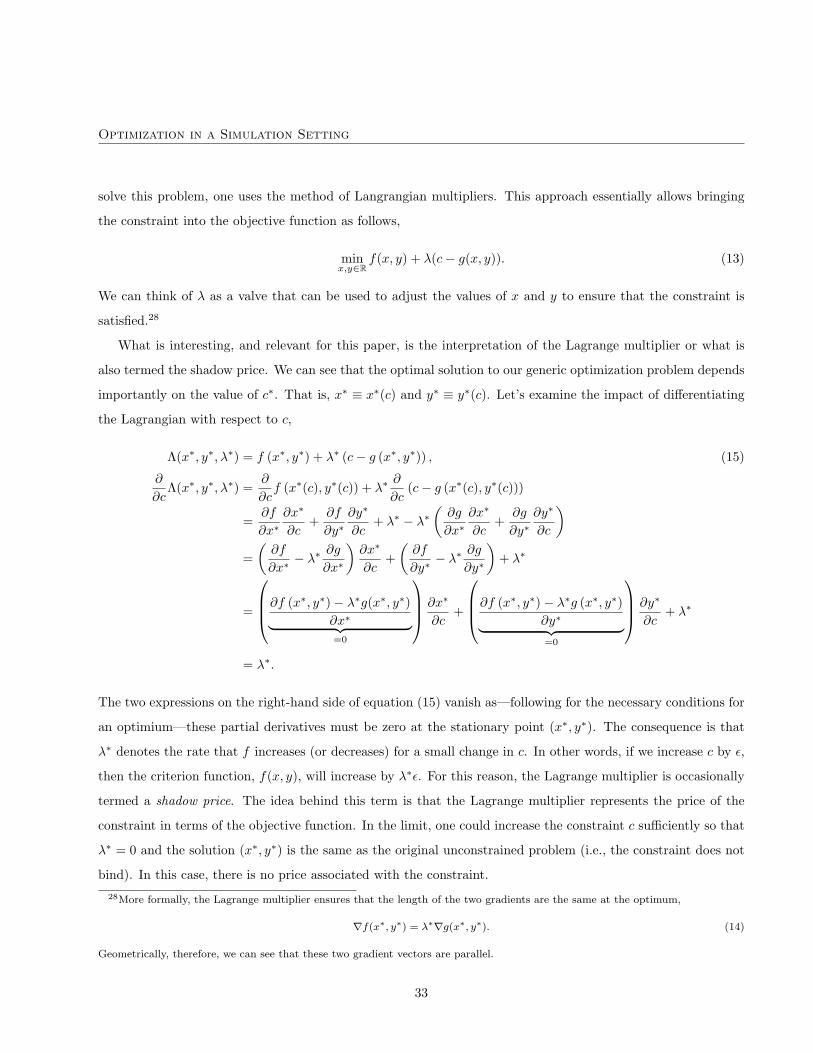
Optimization in a Simulation Setting
solve this problem, one uses the method of Langrangian multipliers. This approach essentially allows bringing
the constraint into the objective function as follows,
minx,y∈R
f(x, y) + λ(c− g(x, y)). (13)
We can think of λ as a valve that can be used to adjust the values of x and y to ensure that the constraint is
satisfied.28
What is interesting, and relevant for this paper, is the interpretation of the Lagrange multiplier or what is
also termed the shadow price. We can see that the optimal solution to our generic optimization problem depends
importantly on the value of c∗. That is, x∗ ≡ x∗(c) and y∗ ≡ y∗(c). Let’s examine the impact of differentiating
the Lagrangian with respect to c,
Λ(x∗, y∗, λ∗) = f (x∗, y∗) + λ∗ (c− g (x∗, y∗)) , (15)
∂
∂cΛ(x∗, y∗, λ∗) =
∂
∂cf (x∗(c), y∗(c)) + λ∗
∂
∂c(c− g (x∗(c), y∗(c)))
=∂f
∂x∗∂x∗
∂c+
∂f
∂y∗∂y∗
∂c+ λ∗ − λ∗
(∂g
∂x∗∂x∗
∂c+
∂g
∂y∗∂y∗
∂c
)=(
∂f
∂x∗− λ∗
∂g
∂x∗
)∂x∗
∂c+(
∂f
∂y∗− λ∗
∂g
∂y∗
)+ λ∗
=
∂f (x∗, y∗)− λ∗g(x∗, y∗)∂x∗︸ ︷︷ ︸=0
∂x∗
∂c+
∂f (x∗, y∗)− λ∗g (x∗, y∗)∂y∗︸ ︷︷ ︸=0
∂y∗
∂c+ λ∗
= λ∗.
The two expressions on the right-hand side of equation (15) vanish as—following for the necessary conditions for
an optimium—these partial derivatives must be zero at the stationary point (x∗, y∗). The consequence is that
λ∗ denotes the rate that f increases (or decreases) for a small change in c. In other words, if we increase c by ε,
then the criterion function, f(x, y), will increase by λ∗ε. For this reason, the Lagrange multiplier is occasionally
termed a shadow price. The idea behind this term is that the Lagrange multiplier represents the price of the
constraint in terms of the objective function. In the limit, one could increase the constraint c sufficiently so that
λ∗ = 0 and the solution (x∗, y∗) is the same as the original unconstrained problem (i.e., the constraint does not
bind). In this case, there is no price associated with the constraint.
28More formally, the Lagrange multiplier ensures that the length of the two gradients are the same at the optimum,
∇f(x∗, y∗) = λ∗∇g(x∗, y∗). (14)
Geometrically, therefore, we can see that these two gradient vectors are parallel.
33

Optimization in a Simulation Setting
We can now return to Table 6 and interpret the final column. One can interpret the shadow price as the
change in the objective function for a one unit change in the conditional debt-charge volatility constraint. Let’s
look at the first row. The annual expected debt charges are approximately CAD 5.46 billion with a conditional
debt-charge volatility of 22.5%. The shadow price of CAD 20 million tells us that a 1% decrease (increase) in the
level of the conditional volatility constraint should reduce (raise) annual expected debt charges by approximately
this amount.29
Table 7: Portfolio Weights for Alternative Three-Month Treasury-Bill Issuance Restrictions: Thistable describes the minimization of discounted expected annual debt charges for a variety of three-month treasury billportfolio weight constraints, a ≥ θ1 ≤ b, as described in equation (16).
Lower UpperShadow Shadowθ1 3-mth 1-yr 5-yrPrice Price
[0.00, 0.10] 0.100 0.642 0.258 0.000 0.005[0.10, 0.20] 0.200 0.712 0.089 0.000 0.004[0.20, 0.30] 0.300 0.700 0.000 0.000 0.004[0.30, 0.40] 0.333 0.667 0.000 0.000 0.000[0.40, 0.50] 0.400 0.600 0.000 0.013 0.000[0.50, 0.60] 0.500 0.500 0.000 0.041 0.000[0.60, 0.70] 0.600 0.400 0.000 0.083 0.000[0.70, 0.80] 0.700 0.300 0.000 0.134 0.000[0.80, 0.90] 0.800 0.200 0.000 0.205 0.000[0.90, 1.00] 0.900 0.100 0.000 0.286 0.000
The shadow price is a particularly useful mathematical object in the context of debt strategy analysis. As
previously mentioned, debt and fiscal managers operate under a number of different constraints. One common
constraint, for example, relates to the idea of well-functioning markets occurring in the Canadian debt managers
written objectives. In particular, debt managers often attempt to ensure that issuance in particular sectors of
the yield curve is sufficient to meet investor demand. This is done because there is evidence that insufficient
supply of government bonds at key maturities can have a negative impact on the ability of market participants
to issue and price their own securities, to hedge financial risks, and to speculate on current market conditions. A
reduced ability to perform these activities may, in turn, impinge on the well-functioning of fixed-income markets.
A natural question, however, is how do these issuance constraints impact the government’s other objectives.
Table 7 considers how we might answer this question in the context of our simple example. We use the sum of29We should stress that the shadow price only holds for small changes; considering that the actual debt-charge savings by relaxing
the constraint to 25% is 34.8 million, which compares favourably (although not perfectly) to the approximately 50 million (i.e., a
2.5% change in constraint times the 20 million Lagrange multiplier) suggested by the shadow price.
34
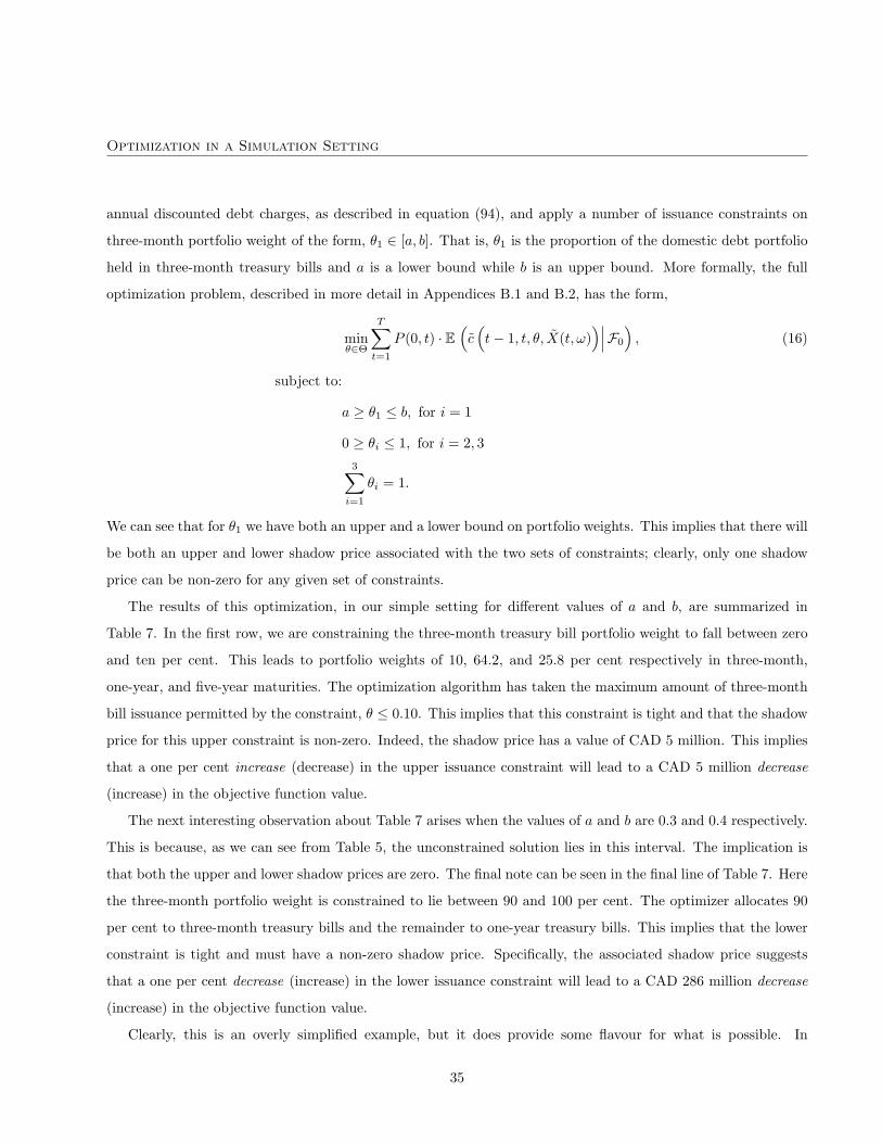
Optimization in a Simulation Setting
annual discounted debt charges, as described in equation (94), and apply a number of issuance constraints on
three-month portfolio weight of the form, θ1 ∈ [a, b]. That is, θ1 is the proportion of the domestic debt portfolio
held in three-month treasury bills and a is a lower bound while b is an upper bound. More formally, the full
optimization problem, described in more detail in Appendices B.1 and B.2, has the form,
minθ∈Θ
T∑t=1
P (0, t) · E(c(t− 1, t, θ, X(t, ω)
)∣∣∣F0
), (16)
subject to:
a ≥ θ1 ≤ b, for i = 1
0 ≥ θi ≤ 1, for i = 2, 33∑
i=1
θi = 1.
We can see that for θ1 we have both an upper and a lower bound on portfolio weights. This implies that there will
be both an upper and lower shadow price associated with the two sets of constraints; clearly, only one shadow
price can be non-zero for any given set of constraints.
The results of this optimization, in our simple setting for different values of a and b, are summarized in
Table 7. In the first row, we are constraining the three-month treasury bill portfolio weight to fall between zero
and ten per cent. This leads to portfolio weights of 10, 64.2, and 25.8 per cent respectively in three-month,
one-year, and five-year maturities. The optimization algorithm has taken the maximum amount of three-month
bill issuance permitted by the constraint, θ ≤ 0.10. This implies that this constraint is tight and that the shadow
price for this upper constraint is non-zero. Indeed, the shadow price has a value of CAD 5 million. This implies
that a one per cent increase (decrease) in the upper issuance constraint will lead to a CAD 5 million decrease
(increase) in the objective function value.
The next interesting observation about Table 7 arises when the values of a and b are 0.3 and 0.4 respectively.
This is because, as we can see from Table 5, the unconstrained solution lies in this interval. The implication is
that both the upper and lower shadow prices are zero. The final note can be seen in the final line of Table 7. Here
the three-month portfolio weight is constrained to lie between 90 and 100 per cent. The optimizer allocates 90
per cent to three-month treasury bills and the remainder to one-year treasury bills. This implies that the lower
constraint is tight and must have a non-zero shadow price. Specifically, the associated shadow price suggests
that a one per cent decrease (increase) in the lower issuance constraint will lead to a CAD 286 million decrease
(increase) in the objective function value.
Clearly, this is an overly simplified example, but it does provide some flavour for what is possible. In
35
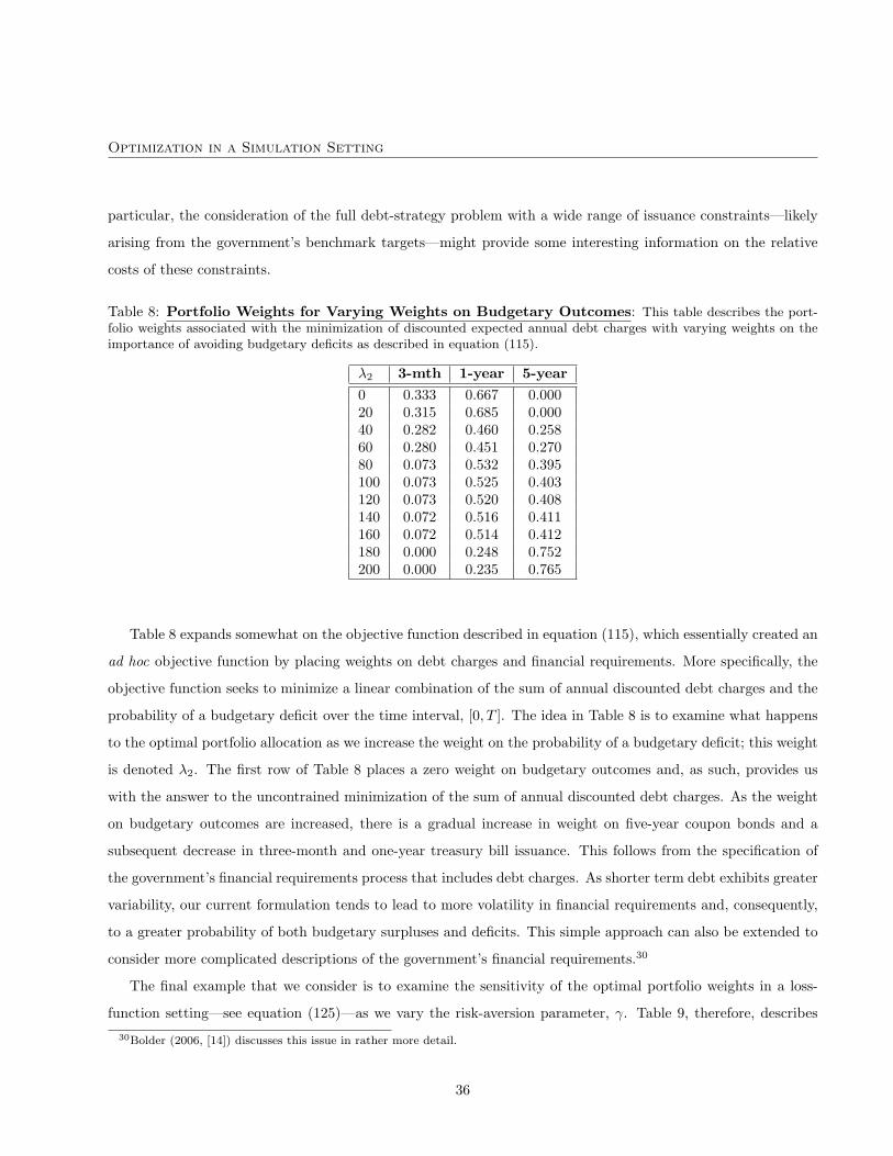
Optimization in a Simulation Setting
particular, the consideration of the full debt-strategy problem with a wide range of issuance constraints—likely
arising from the government’s benchmark targets—might provide some interesting information on the relative
costs of these constraints.
Table 8: Portfolio Weights for Varying Weights on Budgetary Outcomes: This table describes the port-folio weights associated with the minimization of discounted expected annual debt charges with varying weights on theimportance of avoiding budgetary deficits as described in equation (115).
λ2 3-mth 1-year 5-year0 0.333 0.667 0.00020 0.315 0.685 0.00040 0.282 0.460 0.25860 0.280 0.451 0.27080 0.073 0.532 0.395100 0.073 0.525 0.403120 0.073 0.520 0.408140 0.072 0.516 0.411160 0.072 0.514 0.412180 0.000 0.248 0.752200 0.000 0.235 0.765
Table 8 expands somewhat on the objective function described in equation (115), which essentially created an
ad hoc objective function by placing weights on debt charges and financial requirements. More specifically, the
objective function seeks to minimize a linear combination of the sum of annual discounted debt charges and the
probability of a budgetary deficit over the time interval, [0, T ]. The idea in Table 8 is to examine what happens
to the optimal portfolio allocation as we increase the weight on the probability of a budgetary deficit; this weight
is denoted λ2. The first row of Table 8 places a zero weight on budgetary outcomes and, as such, provides us
with the answer to the uncontrained minimization of the sum of annual discounted debt charges. As the weight
on budgetary outcomes are increased, there is a gradual increase in weight on five-year coupon bonds and a
subsequent decrease in three-month and one-year treasury bill issuance. This follows from the specification of
the government’s financial requirements process that includes debt charges. As shorter term debt exhibits greater
variability, our current formulation tends to lead to more volatility in financial requirements and, consequently,
to a greater probability of both budgetary surpluses and deficits. This simple approach can also be extended to
consider more complicated descriptions of the government’s financial requirements.30
The final example that we consider is to examine the sensitivity of the optimal portfolio weights in a loss-
function setting—see equation (125)—as we vary the risk-aversion parameter, γ. Table 9, therefore, describes
30Bolder (2006, [14]) discusses this issue in rather more detail.
36

Optimization in a Simulation Setting
Table 9: Portfolio Weights for Varying Risk-Aversion Parameters: This table describes the portfolioweights associated with the minimization of discounted expected annual debt charges with a CRRA loss function—asdescribed in equation (125)—for a variety of different risk-aversion parameters (i.e., γ ∈ [1.1, 6.5]).
γ 3-mth 1-year 5-year1.1000 0.268 0.732 0.0001.3000 0.277 0.301 0.4201.6000 0.234 0.283 0.4832.0000 0.181 0.313 0.5062.5000 0.000 0.304 0.6963.1000 0.000 0.385 0.6153.8000 0.043 0.239 0.7184.6000 0.000 0.218 0.7825.5000 0.502 0.000 0.4986.5000 0.042 0.000 0.958
the optimal portfolio weights for a CRRA loss function as we gradually increase the risk-aversion parameter. We
can see that for low risk aversion parameter levels (i.e., γ = 1.1), the optimal portfolio weights are quite close to
the unconstrained sum of annual discounted debt charges. That is, the lion’s share of the portfolio is comprised
of one-year treasury bills with the remainder in three-month treasury bills; in this setting, there is no five-year
coupon bond issuance. As we increase the risk-aversion parameter, however, we see a gradual migration away
from one-year treasury bills towards five-year coupon bonds.31
It is interesting, however, that for moderate risk-aversion settings (i.e., γ = 2.5 − 3) the portfolio weights
involve only one-year treasury bills and five-year coupon bonds. For quite large risk-aversion parameters (i.e.,
γ = 6.5) however, places almost all of the issuance in five-year coupon bonds with a small allocation in three-
month treasury bills. What is happening is that the larger the risk-aversion parameter, the greater the weight of
the loss function on the higher moments of the sum of annual discounted debt charges. The consequence is that
the greater volatilty associated with three-month treasury bills is replaced with the relative stability of five-year
coupon bonds as we increase the agent’s risk aversion.
In this section, we have, in the context of an illustrative analysis, considered what can be accomplished
with this technique. In particular, we can compare a government’s optimal debt strategy across a wide range
of alternative objective functions. The explicit inclusion of portfolio restrictions permits us to both observe
how the government’s optimal portfolio varies in the face of constraints and to examine the cost of these con-31Observe that the three-month weight appears to jump around somewhat as we increase the risk-aversion. While there is nothing
in the current set-up that ensures monotonicity in the portfolio weights as we vary the degree of risk aversion, this is still a bit odd.
We suspect it has to do with some some non-smoothness in the objective function for increasing levels of risk-aversion.
37
Optimization in a Simulation Setting
straints through the shadow prices. Finally, for those objective functions requiring weights or difficult-to-estimate
parameters, one can easily examine a wide range of optimal debt strategies conditional on different settings. Sen-
sitivity analysis of this form can be immensely useful for policy analysis. We can also examine how the portfolio
allocations react to different assumptions regarding the financial requirements process, the financial and macroe-
conomic state variables, and the set of available debt instruments. To repeat, this is not an exhaustive list of
what can be accomplished with the approximation-optimization technique, but we think it is a good start.
4 Conclusion
The objective of this paper was to address two related challenges in using a stochastic-simulation framework to de-
termine an optimal government debt-issuance strategy. The first challenge stems from handling the compuational
expense associated with applying an optimizer to a computationally expensive, high-dimensional, non-linear ob-
jective function. We addressed this issue by generating a fixed amount of data from our simulation engine and
then using the to data to fit the underlying function with a function-approximation technique. Optimization of
the objective function is then performed upon the approximated function.
To the extent the function approximation provides a good description of the underlying true function, this
approach will be useful. We assessed four different approximation algorithms on their ability to fit three different
known mathematical functions. We concluded that the MARS approach was the most reliable in its ability to
approximate in the context of a fixed amount of data, simulation noise, and increasing dimensionality. The OLS
algorithm also performed relatively well, but had difficulty in the context of highly non-linear functions with
large dimensionality. The general problem is that a large number of non-linear terms are required to fit such
functions, but these additional terms lead to a poor fit on the data boundary. The consequence is substantial
instability in optimization performance.
The second challenge relates to the specification of the government’s objective function with respect to its debt
strategy. Government debt-management publications provide some insight into the government’s preferences,
but there does remain a substantial degree of uncertainty in the definition of the goverment’s objectives. As
a consequence, we do not directly solve this challenge but rather offer a variety of alternative possibilities.
In particular, we focus on government debt charges, the volatility of these debt charges, the probability of a
budgetary deficit, and introduce notions of utility into a goverment loss function. Our objective is to provide an
illustrative rather than an exhaustive analysis. Clearly, a specific government’s choice of objective function must
be the result of extensive discussion amoung senior debt and fiscal management policymakers.
38

Optimization in a Simulation Setting
In the final section of this paper, we considered what can be accomplished with this technique. This was
performed in the context of a simplified government portfolio comprised of three possible debt instruments:
a three-month and one-year treasury bill as well as a five-year coupon-bearing bond. We demonstrated how
one can compare a government’s optimal debt strategy across a wide range of alternative objective functions.
Including portfolio restrictions allows one to observe how the government’s optimal portfolio varies in the face
of constraints and examine the cost of these constraints through the shadow prices. Finally, for those objective
functions requiring weights or difficult-to-estimate parameters, one can easily examine a wide range of optimal
debt strategies conditional on different settings. One can also examine how the portfolio allocations react
to different assumptions regarding the financial requirements process, the financial and macroeconomic state
variables, and the set of available debt instruments.
In conclusion, we feel that this technique has the potential to be a useful tool in debt-strategy analysis. It
permits debt and fiscal managers to introduce optimization techniques into their stochastic-simulation models.
By doing so, it forces the discipline of explicitly writing out the government’s objectives and constraints with
respect to debt strategy. This additional clarity can be quite useful insofar as it provides greater insight into the
government’s debt strategy. The technique also allows debt and fiscal managers to address a broader range of
questions regarding constraints, the range of debt instruments, and the impact of different modelling assumptions.
39
Optimization in a Simulation Setting
A Function-Approximation Techniques
This technical appendix provides a mathematical overview of the four function-approximation algorithms. An
extensive literature exists for each of these techniques and it would be a daunting, and perhaps undesirable, task
to provide a comprehensive description of each approach. Nevertheless, as many readers may not be familiar with
a few of these methodologies, we seek, in the following sections, to provide a brief introduction to the various
techniques considered in this paper. Moreover, it permits us to use this work as a stand-alone document.
To begin, let’s introduce some common notation. Imagine that there exists an unobservable mapping,
f : Rd → R. (17)
Although, we do not directly observe the form of f , we can perform N experiments to collect data describing
the relationship between f and its predictor variables. In particular, we assume the relationship that generates
the data has the form,
y = f(x) + ε, (18)
= f(x1, ..., xd) + ε,
for x ∈ Rd and y ∈ R. We can imagine ε—the difference between the true function, f , and the observed value
from the experiment—to be measurement or simulation error in our specific context.32 Moreover, we assume
that the values of x are defined on a given domain, D, where
x = x1, ..., xd ∈ D ⊂ Rd. (19)
The actual dataset is described as,
yi, xi,1, ..., xi,d : i = 1, ..., N . (20)
Our task is to consider four alternative approximations f(x) that reasonably capture the unknown function,
f(x), over the domain, D.
This technical appendix is organized in five parts. Appendix A.1 reviews a key measure used in the training
of each of the function-approximation algorithms: generalized cross validation. Appendices A.2 and A.3 provide
basic background details on the two simplest algorithms: OLS and NKR. We then turn in Appendix A.4 to
an extensive discussion of the MARS algorithm, which is necessary by virtue of its complexity and relatively
unknown status in the economics and finance literature. Finally, we provide a description of the PPR approach
in Appendix A.5.32In a more general setting, we think of ε as denoting the influence on y of other unobserved or uncontrolled variables.
40

Optimization in a Simulation Setting
A.1 Generalized cross validation
Cross-validation is a technique commonly used for assessing the performance of model-based function approx-
imation given noisy data. We introduce this notion at this point in the discussion since it is used in all four
approximation algorithms. A main concern associated with using non-parametric function approximations is the
danger of overfitting. The reason is that while non-parametric function approximation techniques offer versa-
tility, it is exactly this adaptivity that may create problems in the presence of noisy or sparse data. That is,
the algorithm may place too much weight on one or more noisy datapoints and dramatically underperform in
describing the global behaviour of the function. To control for overfitting we use the cross-validation technique
for estimating goodness-of-fit during the training of our four alternative approximation models.
Cross-validation, therefore, offers the possibility to consistently estimate the out-of-sample performance of
function approximations. It involves the creation of two sets of data: a training set and a testing set. The idea
is to train (i.e., fit) the approximation model on a subset of the data (i.e., the training set), and then estimate
goodness-of-fit statistics on the remaining set (i.e., the testing set). This essentially creates an out-of-sample
statistic. The training set usually contains more than 70% of the data, while the testing set typically comprises
less than then 30% of the data. There are many flavours of cross-validation. We use two approaches: leave-one-
out and K-fold cross-validation. Specifically, we use the leave-one-out cross-validation for testing of NKR and
PPR and utilize 15-fold cross-validation for OLS and MARS.
Leave-one-out cross-validation consists of training the function approximation on all but one of the data
points. The last remaining point is used for out-of-sample training-set performance estimation. This procedure
is repeated N times, omitting one observation each time, providing one out-of-training-set estimation for each
point in our dataset.33 Model selection using Akaike’s Information Criterion (AIC) is asymptotically equal to
leave-one-out cross-validation method.34
K-fold cross-validation consists of repeating the standard cross-validation procedure K times. At each of the
K iterations, the model is trained on (K−1)K elements of the dataset, while the remaining fraction 1
K is held as
the test set. In this way, each subset (and correspondingly each data point) appears once in the test set, and we
consequently have one out-of-sample training-set estimation for each point in our dataset. For appropriatetly
chosen K’s, model selection using K-fold cross-validation will give results that are asymptotically equal to the
Bayesian Information Criterion (BIC).35
There is usually, as one might imagine, a trade-off between efficiency and speed for cross validation. Leave-33This technique is also termed the jackknife procedure.34A detailed discussion of the equivalence of cross-validation and the AIC is found in Shao(1993, [38]) and Shao(1997, [39]).35Again, a detailed discussion of the equivalence of cross-validation and the BIC is found in Shao(1993, [38]) and Shao(1997, [39]).
41

Optimization in a Simulation Setting
one-out cross-validation is more efficient than K-fold since it employs all but a single data point. By excluding
more than a single point from the training set, K-fold cross-validation includes less information and cannot be as
accurate as the leave-one-out approach. On the other hand, K-fold cross-validation is usually computationally
less expensive, since it requires only K < N evaluations of the function approximation algorithm. In an attempt
to construct fast and reliable training algorithms, we used 15-fold cross-validation for model selection of OLS
and MARS function-approximation methodologies.
For the nearest-neighbor algorithms employed in the NKRs, cross-validation measures are constructed in such
a way that estimation at each point is independently computed. This implies that the leave-one-out technique
requires the same computation as K-fold cross-validation. For this reason, we used leave-one-out cross-validation
for NKR and PPR approximations since both use nearest-neighbour algorithms. Let’s now turn our attention
to discuss the specific function-approximation algorithms in turn.
42
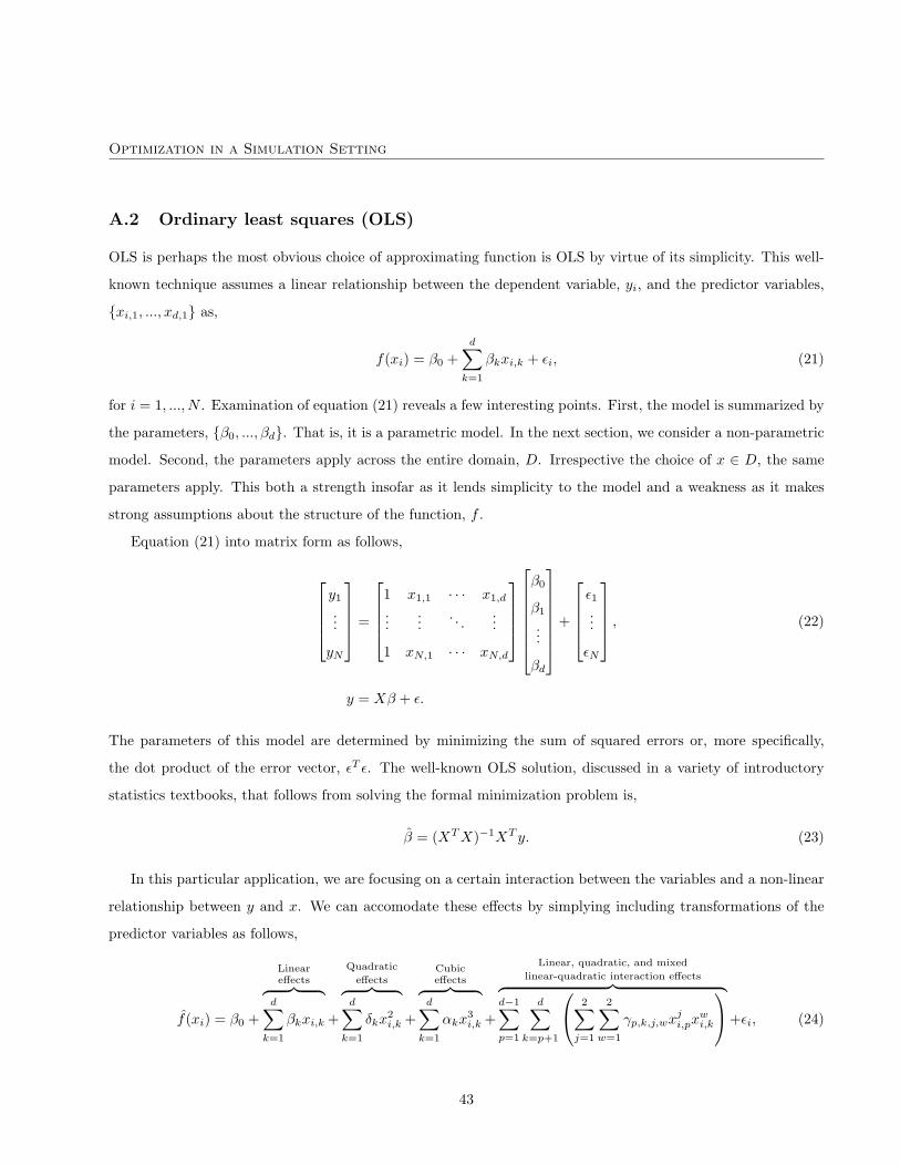
Optimization in a Simulation Setting
A.2 Ordinary least squares (OLS)
OLS is perhaps the most obvious choice of approximating function is OLS by virtue of its simplicity. This well-
known technique assumes a linear relationship between the dependent variable, yi, and the predictor variables,
xi,1, ..., xd,1 as,
f(xi) = β0 +d∑
k=1
βkxi,k + εi, (21)
for i = 1, ..., N . Examination of equation (21) reveals a few interesting points. First, the model is summarized by
the parameters, β0, ..., βd. That is, it is a parametric model. In the next section, we consider a non-parametric
model. Second, the parameters apply across the entire domain, D. Irrespective the choice of x ∈ D, the same
parameters apply. This both a strength insofar as it lends simplicity to the model and a weakness as it makes
strong assumptions about the structure of the function, f .
Equation (21) into matrix form as follows,
y1
...
yN
=
1 x1,1 · · · x1,d
......
. . ....
1 xN,1 · · · xN,d
β0
β1
...
βd
+
ε1...
εN
, (22)
y = Xβ + ε.
The parameters of this model are determined by minimizing the sum of squared errors or, more specifically,
the dot product of the error vector, εT ε. The well-known OLS solution, discussed in a variety of introductory
statistics textbooks, that follows from solving the formal minimization problem is,
β = (XT X)−1XT y. (23)
In this particular application, we are focusing on a certain interaction between the variables and a non-linear
relationship between y and x. We can accomodate these effects by simplying including transformations of the
predictor variables as follows,
f(xi) = β0 +
Lineareffects︷ ︸︸ ︷
d∑k=1
βkxi,k +
Quadratic
effects︷ ︸︸ ︷d∑
k=1
δkx2i,k +
Cubiceffects︷ ︸︸ ︷
d∑k=1
αkx3i,k +
Linear, quadratic, and mixed
linear-quadratic interaction effects︷ ︸︸ ︷d−1∑p=1
d∑k=p+1
2∑j=1
2∑w=1
γp,k,j,wxji,px
wi,k
+εi, (24)
43

Optimization in a Simulation Setting
which gives rise to a maximum of 2d2+d+1 regression coefficients. This formulation may appear to be excessive.
OLS, however, has a statistical structure that permits determination of the appropriate set of predictor variables.
In other words, one starts with the full model described in equation (24) and then eliminates predictor variables
that do not add—in a statistical sense—to the overall fit of the model to the dependent variable, y. As mentioned
in the previous seciton, this is performed with 15-fold cross-validation approach.
44

Optimization in a Simulation Setting
A.3 Non-parametric kernel regression (NKR)
Continuing from our previous set-up, we know that our approximation will be of the form,
y = f(x). (25)
Imagine that we would like our approximation to be the conditional expectation of the random variable, Y , given
that the predictor variable X = x, then it would have the following form,
f(x) = E(Y | X = x), (26)
=∫
D
yg(y | x)dy,
=∫
D
yg(x, y)g(x)︸ ︷︷ ︸
By Bayes
Theorem
dy,
where g(x|y), g(x, y), and g(x) denote the corresponding conditional, joint, and marginal densities, respectively.
The idea behind the non-parametric kernel regression is to approximate the corresponding joint and marginal
densities with a kernel estimator. The joint density approximation has the form,
g(x, y) =1n
n∑i=1
κh1(x− xi)κh2(y − yi), (27)
where κ(·) are the kernel-density estimators and h1 and h2 are the bandwidth parameters. The marginal density
for x has a similar form,
g(x) =1n
n∑i=1
κh(x− xi), (28)
where, again, h is the bandwidth parameter. There are a variety of possible choices of kernel-density estimator.
All of them share some common properties. In particular, they are generally symmetric and map a given x into a
relative-frequency based on the observed data. The basic idea is that the kernel function, κ, assigns a probability
value to the distance of x from a given xi—generally, one would expect a smaller weight for xi’s that are far from
x. The average of these probabilities are then computed for all xi. This represents the assigned probability value.
The bandwidth parameter essentially determines the importance of the local data in determining a density value
for a given x. There are three additional properties of interest. First, we can represent the role of the bandwidth
parameter alternatively as,
g(x) =1n
n∑i=1
κh(x− xi), (29)
=1
nh
n∑i=1
κ
(x− xi
h
),
45

Optimization in a Simulation Setting
In other words, we can directly place the bandwidth parameter into the kernel expression. Also, if the density
has compact support on Ω, then ∫Ω
κ(v)dv = 1, (30)
and, ∫Ω
vκ(v)dv = 0. (31)
These properties permit us to actually derive the non-parameteric kernel estimator.
To see how this works, we now substitute equations (27) and (28) into equation (26) and simplify to find our
kernel regression estimator of f(x). Specifically, we have
f(x) = E(Y | X = x), (32)
=∫
yg(x, y)g(x)
dy,
=∫
y1n
∑ni=1 κh1(x− xi)κh2(y − yi)
1n
∑ni=1 κh(x− xi)
dy,
=(
11n
∑ni=1 κh(x− xi)
)1n
n∑i=1
(∫yκh1(x− xi)κh2(y − yi)dy
),
=(
1g(x)
)1n
n∑i=1
κh1(x− xi)(∫
y
h2κ
(y − yi
h2
)dy
).
If we introduce the change of variables v = y−yi
h2, then dy = h2dv and y
h2= vh2+yi
h2. Plugging this back into
equation (32), we have
f(x) =(
1g(x)
)1n
n∑i=1
κh1(x− xi)(∫ (
vh2 + yi
h2
)κ (v) h2dv
), (33)
=(
1g(x)
)1n
n∑i=1
κh1(x− xi)(∫
(vh2 + yi)κ (v) dv
),
=(
1g(x)
)1n
n∑i=1
κh1(x− xi)
h2
∫vκvdv︸ ︷︷ ︸
Equation
(31)
+yi
∫κ (v) dv︸ ︷︷ ︸
Equation
(30)
,
=1n
∑ni=1 κh1(x− xi)
g(x)yi.
46
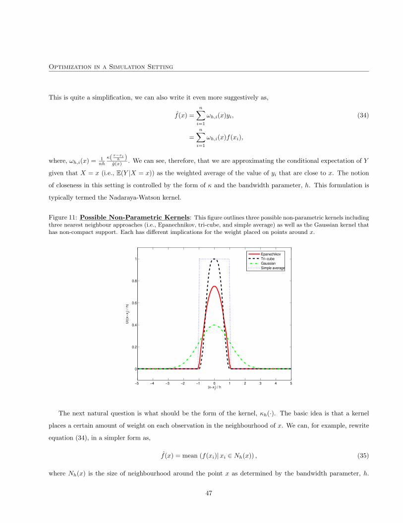
Optimization in a Simulation Setting
This is quite a simplification, we can also write it even more suggestively as,
f(x) =n∑
i=1
ωh,i(x)yi, (34)
=n∑
i=1
ωh,i(x)f(xi),
where, ωh,i(x) = 1nh
κ( x−xih )
g(x) . We can see, therefore, that we are approximating the conditional expectation of Y
given that X = x (i.e., E(Y |X = x)) as the weighted average of the value of yi that are close to x. The notion
of closeness in this setting is controlled by the form of κ and the bandwidth parameter, h. This formulation is
typically termed the Nadaraya-Watson kernel.
Figure 11: Possible Non-Parametric Kernels: This figure outlines three possible non-parametric kernels includingthree nearest neighbour approaches (i.e., Epanechnikov, tri-cube, and simple average) as well as the Gaussian kernel thathas non-compact support. Each has different implications for the weight placed on points around x.
−5 −4 −3 −2 −1 0 1 2 3 4 5
0
0.2
0.4
0.6
0.8
1
(x−xi) / h
D((
x−x i)
/ h)
EpanechikovTri−cubeGaussianSimple average
The next natural question is what should be the form of the kernel, κh(·). The basic idea is that a kernel
places a certain amount of weight on each observation in the neighbourhood of x. We can, for example, rewrite
equation (34), in a simpler form as,
f(x) = mean (f(xi)|xi ∈ Nh(x)) , (35)
where Nh(x) is the size of neighbourhood around the point x as determined by the bandwidth parameter, h.
47
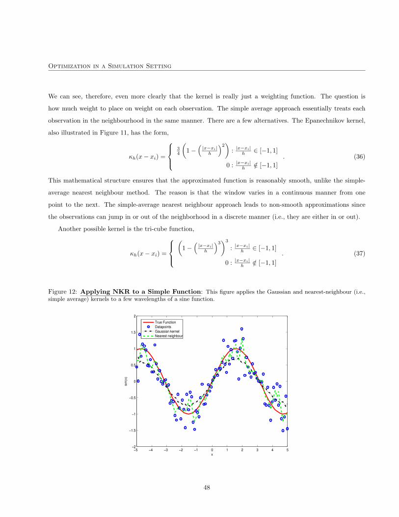
Optimization in a Simulation Setting
We can see, therefore, even more clearly that the kernel is really just a weighting function. The question is
how much weight to place on weight on each observation. The simple average approach essentially treats each
observation in the neighbourhood in the same manner. There are a few alternatives. The Epanechnikov kernel,
also illustrated in Figure 11, has the form,
κh(x− xi) =
34
(1−
(|x−xi|
h
)2)
: |x−xi|h ∈ [−1, 1]
0 : |x−xi|h /∈ [−1, 1]
. (36)
This mathematical structure ensures that the approximated function is reasonably smooth, unlike the simple-
average nearest neighbour method. The reason is that the window varies in a continuous manner from one
point to the next. The simple-average nearest neighbour approach leads to non-smooth approximations since
the observations can jump in or out of the neighborhood in a discrete manner (i.e., they are either in or out).
Another possible kernel is the tri-cube function,
κh(x− xi) =
(
1−(|x−xi|
h
)3)3
: |x−xi|h ∈ [−1, 1]
0 : |x−xi|h /∈ [−1, 1]
. (37)
Figure 12: Applying NKR to a Simple Function: This figure applies the Gaussian and nearest-neighbour (i.e.,simple average) kernels to a few wavelengths of a sine function.
−5 −4 −3 −2 −1 0 1 2 3 4 5−2
−1.5
−1
−0.5
0
0.5
1
1.5
2
x
sin(
x)
True FunctionDatapointsGaussian kernelNearest neighbour
48
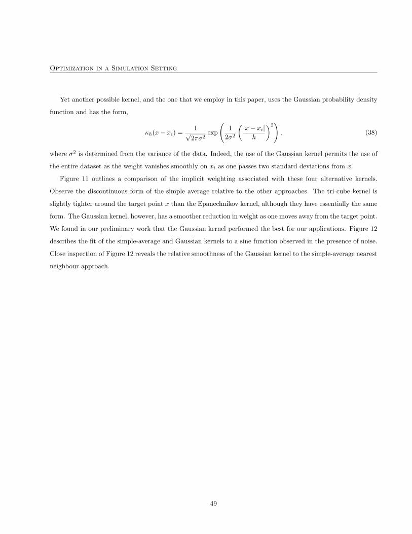
Optimization in a Simulation Setting
Yet another possible kernel, and the one that we employ in this paper, uses the Gaussian probability density
function and has the form,
κh(x− xi) =1√
2πσ2exp
(1
2σ2
(|x− xi|
h
)2)
, (38)
where σ2 is determined from the variance of the data. Indeed, the use of the Gaussian kernel permits the use of
the entire dataset as the weight vanishes smoothly on xi as one passes two standard deviations from x.
Figure 11 outlines a comparison of the implicit weighting associated with these four alternative kernels.
Observe the discontinuous form of the simple average relative to the other approaches. The tri-cube kernel is
slightly tighter around the target point x than the Epanechnikov kernel, although they have essentially the same
form. The Gaussian kernel, however, has a smoother reduction in weight as one moves away from the target point.
We found in our preliminary work that the Gaussian kernel performed the best for our applications. Figure 12
describes the fit of the simple-average and Gaussian kernels to a sine function observed in the presence of noise.
Close inspection of Figure 12 reveals the relative smoothness of the Gaussian kernel to the simple-average nearest
neighbour approach.
49

Optimization in a Simulation Setting
A.4 Multivariate adaptive regression splines (MARS)
Given the MARS approach is not well known in the economics and finance literature, we spend a substantial
amount of time reviewing it. MARS as a non-parameteric approach was first suggested by Friedman (1991, [22])
and is essentially a generalization of the recursive partitioning algorithm. Indeed, this is precisely how Friedman
(1991, [22]) motivates the MARS algorithm. We will, therefore, also begin with a brief discussion of the recursive
paritioning approach. The idea is quite simple. One partitions the space, D, into M disjoint subregions,
D =⋃
m∈1,...,M
Rm, (39)
where, ⋂m∈1,...,M
Rm = ∅. (40)
On each of these subregions, Rm,m = 1, ...,M, an approximation of the function is constructed. That is, if
x ∈ Rm, then the most common recursive-partitioning approximation has the form,
f(x|x ∈ Rm) = gm(x|x ∈ Rm), (41)
= am.
On each disjoint partition, the value of the function, f , is approximated by a constant. The function gm can,
of course, take any desired form, but simple functions appear to outperform more complex choices according to
Friedman (1991, [22]). Given that each paritition is disjoint, the constant am is, in fact, best chosen to be the
mean value of y = f(x) given that x ∈ Rm. To write this out in mathematical form, let’s define the set,
Ym = f(x) : x ∈ Rm. (42)
and then define the value of am, as
f(x) = am, (43)
=1
card(Ym)
∑i∈Ym
yi.
To recap, the recursive partioning algorithm breaks up the space into a number of disjoint subregions and
approximates the function with a constant on each subregion. The idea is that in small regions, the value of
the function, f , can be reasonably approximated by a constant. The principal task of this algorithm, therefore,
involves the selection of a good set of subregions, Rm,m = 1, ...,M, that captures the primary features of the
function, f .
50
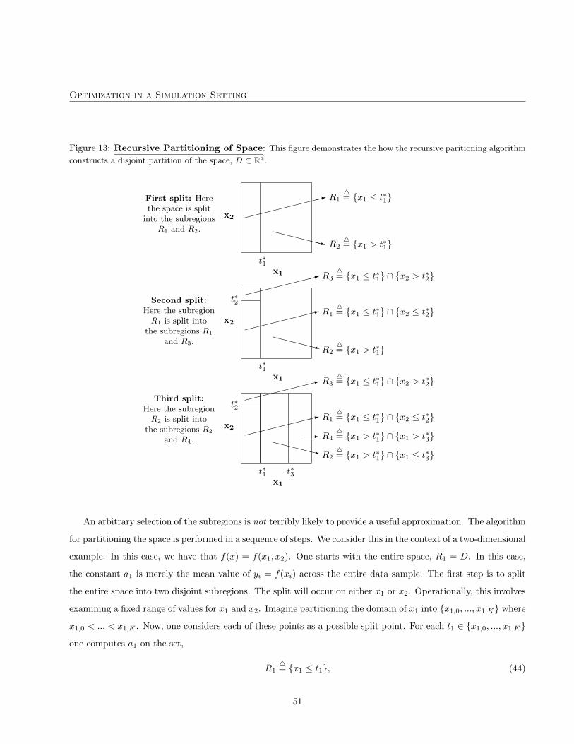
Optimization in a Simulation Setting
Figure 13: Recursive Partitioning of Space: This figure demonstrates the how the recursive paritioning algorithm
constructs a disjoint partition of the space, D ⊂ Rd.
First split: Herethe space is split
into the subregionsR1 and R2.
x2
x1
t∗1
XXXXXXz R24= x1 > t∗1
: R14= x1 ≤ t∗1
Second split:Here the subregion
R1 is split intothe subregions R1
and R3.
x2
x1
t∗1
t∗2: R3
4= x1 ≤ t∗1 ∩ x2 > t∗2
: R14= x1 ≤ t∗1 ∩ x2 ≤ t∗2
XXXXXz R24= x1 > t∗1
Third split:Here the subregion
R2 is split intothe subregions R2
and R4.
x2
x1
t∗1
t∗2
t∗3
: R34= x1 ≤ t∗1 ∩ x2 > t∗2
: R14= x1 ≤ t∗1 ∩ x2 ≤ t∗2
XXXXXz R24= x1 > t∗1 ∩ x1 ≤ t∗3
- R44= x1 > t∗1 ∩ x1 > t∗3
An arbitrary selection of the subregions is not terribly likely to provide a useful approximation. The algorithm
for partitioning the space is performed in a sequence of steps. We consider this in the context of a two-dimensional
example. In this case, we have that f(x) = f(x1, x2). One starts with the entire space, R1 = D. In this case,
the constant a1 is merely the mean value of yi = f(xi) across the entire data sample. The first step is to split
the entire space into two disjoint subregions. The split will occur on either x1 or x2. Operationally, this involves
examining a fixed range of values for x1 and x2. Imagine partitioning the domain of x1 into x1,0, ..., x1,K where
x1,0 < ... < x1,K . Now, one considers each of these points as a possible split point. For each t1 ∈ x1,0, ..., x1,K
one computes a1 on the set,
R14= x1 ≤ t1, (44)
51

Optimization in a Simulation Setting
and a2 on the set,
R24= x1 > t1. (45)
This is repeated for all of the possible choices of t1 ∈ x1,0, ..., x1,K to find a t∗1 such that a∗1 and a∗2 provide the
closest fit to the data. There are a variety of ways that one can measure the goodness of fit to the data, but for
the moment we can imagine a least-squares criterion such as root-mean squared error.
In Figure 13, we imagine that this point is t∗1 and demonstrate the form of R1 and R2. In particular, R1 is
defined as the entire space where x1 is less than or equal to t∗1 (i.e., R14= x1 ≤ t∗1) and R2 is the remainder
of the space where x1 is greater than t∗1 (i.e., R24= x1 > t∗1). One performs the same analysis on the second
argument of f(x1, x2). That is, we partition x2 into x2,0, ..., x2,K where x2,0 < ... < x2,K and consider point
each t2 ∈ x2,0, ..., x2,K as a possible split point. The best possible split point for x2, t∗2, is then compared to
the best possible split point for x1, t∗1. The split point that provides the superior fit to the data is selected as
the first split point.
The second split basically repeats the previous analysis, but isolates its attention to the separate subregions,
R1 and R2. Imagine that we attempted to further partition R1. In this case, we would examine values of x1
in the range x1,0, ..., t∗1, because this is the boundary of R1. At this point, as x2 has not yet been split, all of
the possible values of x2 in the original partition are available. In Figure 13, we assume that R1 is split at t∗2 to
create the set R1 and a new set R3. The definition of R1 is now revised as,
R14= x1 ≤ t∗1 ∩ x2 ≤ t∗2, (46)
so that it includes all points in the space, D, where x1 is less than or equal to t∗1 and x2 is less than or equal to
t∗2. The new set, R3, encompasses the part of the space where x1 is less than or equal to t∗1 and x2 is greater
than t∗2 or mathematically,
R34= x1 ≤ t∗1 ∩ x2 > t∗2. (47)
It is easy to see that the union of R1, R2, and R3 is equal to D and that the intersection of these three sets is
empty.
Figure 13 proceeds to perform a third split of R2 and provides the definitions of the revised set, R2 and the
new set, R4. In actuality, a large number of splits are performed in order to ensure a reasonable overall fit to
the data. One can imagine that the set definitions become progressively more complex. Indeed, the set notation
used so far, while quite intuitive, is not terribly convenient from a computational perspective. As a consequence,
52
Optimization in a Simulation Setting
the model described in equation (41) is typically written in a more useful form. In particular, one structures the
model as,
f(x) =M∑
m=1
amBm(x), (48)
=M∑
m=1
amIx∈Rm .
where Bm(x) is a basis function that is actually an indicator function of the form,
Bm(x) = Ix∈Rm=
0 : x /∈ Rm
1 : x ∈ Rm
. (49)
As the collection of sets,Rm,m = 1, ...,M is, by construction, disjoint, it follows that only one basis function,
Bm(x), is non-zero for each x ∈ D. To make these basis functions more precise, and practical, we introduce the
following definition,
H[γ] =
0 : γ ≤ 0
1 : γ > 0, (50)
which is also generally known as the Heaviside function.36 Figure 14 displays the form of the Heaviside basis
function described in equation (51) where the split occurs on x1 at the split point t∗1. The benefit of this
formulation becomes evident as we proceed to incorporate more subregions. Consider the set,
R14= x1 ≤ t∗1 ∩ x2 ≤ t∗2. (52)
We would like an indicator function that takes the values of unity should x ∈ R1 and zero otherwise. The
product of two appropriately structured Heaviside functions, as described in equation (51), has this property. In
particular,
B1(x) = Ix∈R1 , (53)
= Ix∈x1≤t∗1∩x2≤t∗2,
= H[−(x1 − t∗1)] ·H[−(x2 − t∗2)],
36One also sees definitions of the Heaviside function where,
H[γ] =
0 : γ < 0
12
: γ = 0
1 : γ > 0
. (51)
For our purposes, we will let H[0] = 0.
53
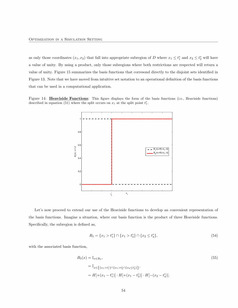
Optimization in a Simulation Setting
as only those coordinates (x1, x2) that fall into appropriate subregion of D where x1 ≤ t∗1 and x2 ≤ t∗2 will have
a value of unity. By using a product, only those subregions where both restrictions are respected will return a
value of unity. Figure 15 summarizes the basis functions that corresond directly to the disjoint sets identified in
Figure 13. Note that we have moved from intuitive set notation to an operational definition of the basis functions
that can be used in a computational application.
Figure 14: Heaviside Functions: This figure displays the form of the basis functions (i.e., Heaviside functions)described in equation (51) where the split occurs on x1 at the split point t∗1.
0
0.2
0.4
0.6
0.8
1
x1
Bi(x
), i=
1,2
t*1
B1(x)=H[−(x
1−t)]
B2(x)=H[+(x
1−t)]
Let’s now proceed to extend our use of the Heaviside functions to develop an convenient representation of
the basis functions. Imagine a situation, where our basis function is the product of three Heaviside functions.
Specifically, the subregion is defined as,
R5 = x1 > t∗1 ∩ x1 > t∗3 ∩ x2 ≤ t∗4, (54)
with the associated basis function,
B5(x) = Ix∈R5 , (55)
= Ix∈x1>t∗1∩x1>t∗3∩x2≤t∗4,
= H[+(x1 − t∗1)] ·H[+(x1 − t∗3)] ·H[−(x2 − t∗4)].
54
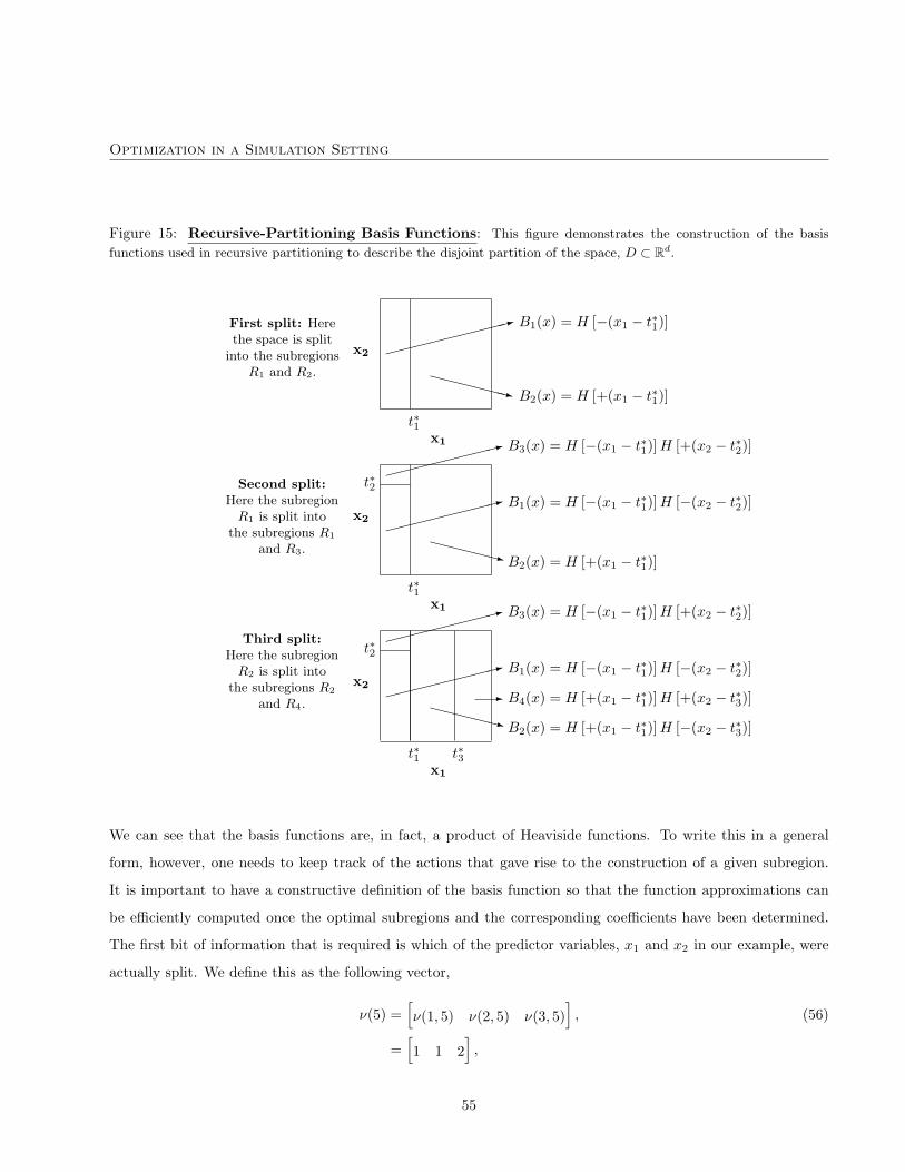
Optimization in a Simulation Setting
Figure 15: Recursive-Partitioning Basis Functions: This figure demonstrates the construction of the basis
functions used in recursive partitioning to describe the disjoint partition of the space, D ⊂ Rd.
First split: Herethe space is split
into the subregionsR1 and R2.
x2
x1
t∗1
XXXXXXz B2(x) = H [+(x1 − t∗1)]
: B1(x) = H [−(x1 − t∗1)]
Second split:Here the subregion
R1 is split intothe subregions R1
and R3.
x2
x1
t∗1
t∗2: B3(x) = H [−(x1 − t∗1)]H [+(x2 − t∗2)]
: B1(x) = H [−(x1 − t∗1)]H [−(x2 − t∗2)]
XXXXXz B2(x) = H [+(x1 − t∗1)]
Third split:Here the subregion
R2 is split intothe subregions R2
and R4.
x2
x1
t∗1
t∗2
t∗3
: B3(x) = H [−(x1 − t∗1)]H [+(x2 − t∗2)]
: B1(x) = H [−(x1 − t∗1)]H [−(x2 − t∗2)]
XXXXXz B2(x) = H [+(x1 − t∗1)]H [−(x2 − t∗3)]
- B4(x) = H [+(x1 − t∗1)]H [+(x2 − t∗3)]
We can see that the basis functions are, in fact, a product of Heaviside functions. To write this in a general
form, however, one needs to keep track of the actions that gave rise to the construction of a given subregion.
It is important to have a constructive definition of the basis function so that the function approximations can
be efficiently computed once the optimal subregions and the corresponding coefficients have been determined.
The first bit of information that is required is which of the predictor variables, x1 and x2 in our example, were
actually split. We define this as the following vector,
ν(5) =[ν(1, 5) ν(2, 5) ν(3, 5)
], (56)
=[1 1 2
],
55
Optimization in a Simulation Setting
that indicates that B5(x) in equation (55) arose through two consecutive splits to x1 and one split to x2. The
next piece of information that we require to reconstruct B5(x) is the location of the splits to the variables in
ν(5), which is summarized in the following vector,
t∗(5) =[t∗(1, 5) t∗(2, 5) t∗(3, 5)
], (57)
=[t∗1 t∗3 t∗4
].
We interpret the vector t∗ equation (57) as representing the location of the optimal split points for B5(x)
associated with the predictor-variable vector in equation (56). The final piece of information that we need to
know is what side of the split points described in equation (57) does the subregion R5 fall. This is summarized
in a final vector,
s(5) =[s(1, 5) s(2, 5) s(3, 5)
], (58)
=[+1 +1 −1
],
which basically keeps track of the sign associated with each split point. Collecting equations (56) to (58), we
can now write the basis function B5(x), described in equation (55) in more compact form as,
B5(x) = H[+(x1 − t∗1)] ·H[+(x1 − t∗3)] ·H[−(x2 − t∗4)], (59)
=3∏
k=1
H[s(k, 5)
(xν(k,5) − t∗(k, 5)
)].
This can, of course, be generalized for an arbitary basis function Bm(x) associated with subregion Rm. If we let
Km denote the number of splits that gave rise to Rm, then Bm(x) has the form,
Bm(x) =Km∏k=1
H[s(k,m)
(xν(k,m) − t∗(k,m)
)]. (60)
We will return to this expression shortly when we examine the generalization of the recursive partitioning
algorithm.
The recursive partitioning algorithm, despite its simplicity, is actually quite powerful. The principal advantage
of this approach is through its recursive approach to partitioning the space, D, it grows progressively more
local. This permits it to exploit the local importance of certain predictor variables in high-dimensional settings.
The forward recursion algorithm permits it to handle fairly complex interactions between predictor variables.
Recursive partitioning is also computationally fast and relatively easy to implement.
56

Optimization in a Simulation Setting
There are, nevertheless, two primary disadvantages of the recursive partitioning algorithm. First, the function
approximation associated with this model—described in equation (48)—is, by its very construction, discontinu-
ous at the subregion boundaries. This is a direct consequence of the basis functions and can be seen clearly in
Figure 16. This has implications for the accuracy of the approximation when the underlying function is contin-
uous. Moreover, it limits the ability of one to differentiate the function approximation, which may be desirable
should one wish, as we do, to perform an optimization on f(x).
Figure 16: MARS Partitioning: This figure demonstrates the construction of the basis functions used in the MARS
algorithm to describe the non-disjoint partition of the space, D ⊂ Rd. Observe that the base set, B0(x) can be splitrepeatedly in different ways and also that a given sequence of splits cannot involve more than one basis function with agiven predictor variable.
Base set: webegin with entirespace and then
partition.
x2
x19
XXXXXXXXz?
x2
x1t∗1
?
x2
x1t∗1
t∗2
First splits: Herethe algorithm
splits on x1 thenx2 and stops.
x2
x1t∗3
?
x2
x1 t∗3
t∗4
Second splits: Againthe algorithm
splits on x1 thenx2 and stops.
x2
x1
t∗5
?
x2
x1
t∗5
t∗6
Third splits: Herethe algorithm
splits on x2 thenx1 and stops.
A second issue with recursive partitioning is its inability to approximate certain fairly simple functions. In
57

Optimization in a Simulation Setting
particular, it has difficulty with linear or additive functions. This is because the forward partitioning approach
almost invariably creates lengthy interaction terms. That is, the basis function is almost always a product of
different predictor variables (i.e., axixj or axixjxk). As we saw previously, this is one of the strengthes of this
algorithm. It also represents something of a weakness. An additive or linear function requires all the terms
to be related to the same predictor variable. This can, of course, happen with recursive partitioning, but it
is highly improbable given that one requires a large number of partitions to adequately describe D. Recursive
paritioning also has difficulty where there are strong interaction effects, but they only involve a small number of
the predictor variables. Again, this occurs for the same reason. The basis functions are invariably functions of
all the predictor variables. If one requires a small number of interaction effects, then recursive partitioning will
generally fail. The basic issue with recursive partitioning is that there is not a sufficient number of low-order
(i.e., zero or first) interactions in the basis functions.
Given these drawbacks to the recursive partitioning algorithm, Friedman (1991, [22]) suggested a number of
modifications with the aim of improving the flexibility of the algorithm. He made two rather clever innovations
to recursive partitioning and added an additional restriction. This modified version of recursive partitioning is
termed multivariate adaptive regression splines or MARS. The two innovations involved,
1. not requiring the subregions to be disjoint;
2. and suggesting an alternative form for the basis function.
The idea of the first innovation is to permit the algorithm to approximate linear or additive functions. Recall
with the recursive partitioning algorithm, when a split occurs, the two new sibling subregions replace the parent
subregion. This is necessary to maintain the disjointness of the subregions. If one no longer requires disjoint
subregions, then both parent and sibling reqions may be further partitioned. Moreover, a given parent may yield
a large number of sibling subregions. This gives rise to a richer collection of subregions. A given parent may
have multiple subregions in different predictor variables or multiple subregions in the same predictor variable.
Either case will provide the algorithm with additional flexiblity to approximate the function. The point is that
this innovation permits a wide range of lower-order (i.e., zero or first) interaction effects thereby permitting the
approximation to better capture linear or additive functions.
The second innovation was introduced to deal with the inherent discontinuities in the recursive partitioning
algorithm caused by the use of the Heaviside function as the basic building block in the construction of the basis
functions. Friedman (1991, [22]) introduced what are termed two-sided truncated power basis functions. These
58
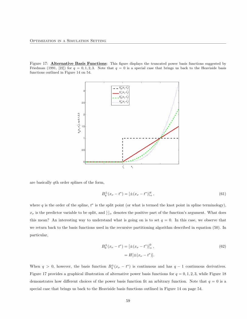
Optimization in a Simulation Setting
Figure 17: Alternative Basis Functions: This figure displays the truncated power basis functions suggested byFriedman (1991, [22]) for q = 0, 1, 2, 3. Note that q = 0 is a special case that brings us back to the Heaviside basisfunctions outlined in Figure 14 on 54.
0
0.5
1
1.5
2
2.5
3
x1
b q(x1=
t* 1), q
=0,1
,2,3
t*1
b0+1(x
1−t*
1)
b1+1(x
1−t*
1)
b2+1(x
1−t*
1)
b3+1(x
1−t*
1)
are basically qth order splines of the form,
B±q (xν − t∗) = [±(xν − t∗)]q+ , (61)
where q is the order of the spline, t∗ is the split point (or what is termed the knot point in spline terminology),
xν is the predictor variable to be split, and [·]+ denotes the positive part of the function’s argument. What does
this mean? An interesting way to understand what is going on is to set q = 0. In this case, we observe that
we return back to the basis functions used in the recursive partitioning algorithm described in equation (50). In
particular,
B±0 (xν − t∗) = [±(xν − t∗)]0+ , (62)
= H[±(xν − t∗)].
When q > 0, however, the basis function B±q (xν − t∗) is continuous and has q − 1 continuous derivatives.
Figure 17 provides a graphical illustration of alternative power basis functions for q = 0, 1, 2, 3, while Figure 18
demonstrates how different choices of the power basis function fit an arbitrary function. Note that q = 0 is a
special case that brings us back to the Heaviside basis functions outlined in Figure 14 on page 54.
59

Optimization in a Simulation Setting
The basis functions, for a qth order spline basis function, will have the form,
Bqm(x) =
Km∏k=1
[s(k,m)
(xν(k,m) − t∗(k,m)
)]q+
, (63)
as compared to the recursive partitioning basis functions described in equation (60).37 The usual approach when
using splines in a higher dimension setting is to limit the basis functions in equation (63) to products involving
polynomials of a lower order than q. In other words, the basis functions employed are tensor products of the
associated univariate spline functions for each of the predictor variables.
Maintaining this convenient tensor product form requires a restriction. In particular, Friedman (1991, [22])
suggests that one restrict each basis function to products of distinct predictor variables. Operationally, this
means that if for a given subregion, one has already split on x1, then one cannot split again on x1. This avoids
a quadratic term in the corresponding basis function in x1. Given that one no longer forces disjoint subregions,
one can always go back to the parent and split on x1 in a different way in the algorithm.
Friedman’s suggested restriction maintains that the tensor-product form of the basis functions that has a
substantial benefit in terms of the interpretation of the solution. The basic approximation equation for the
MARS model is given as,
f(x) = a0 B0(x)︸ ︷︷ ︸=1
+M∑
m=1
amBqm(x), (64)
= a0 +M∑
m=1
am
Km∏k=1
[s(k, m)
(xν(k,m) − t∗(k, m)
)]q+︸ ︷︷ ︸
Equation (63)
,
= a0 +M∑
m=1
am
Km∏k=1
[s(k, m)
(xν(k,m) − t∗(k, m)
)]+
for q = 1. In this form, there are not many insights to be made. What we would like to do, however, is to
decompose equation (64) into terms involving a single predictor variable, two predictor variables, three predictor
variables, and so on. Friedman (1991, [22]) shows us how this can be accomplished. If we recall equation (56) was
a vector that summarized the order in which the predictor variables where split to arrive at a given subregion.
Here we merely need to generalize this definition. Let ν(m) denote the collection of predictor variables that are
split for the mth basis function,
ν(m) = ν(k, m) : k = 1, ...,Km . (65)
37Equations (60) and (63) are, of course, identical when q = 0.
60

Optimization in a Simulation Setting
Figure 18: Comparing Spline Orders: This figure demonstrates the fit of the MARS algorithm to a simple two-dimensional function where the splines used in the basis function are of order q = 0, 1, and 2. The lower right-handquadrant demonstrates the first-order linear spline MARS basis function where the function is smoothed susequent to thefit to the data.
0 2 4 6 8 100
2
4
6
8
10
12
14
x
f(x)
Zero−order spline
0 2 4 6 8 100
2
4
6
8
10
12
14
x
f(x)
Linear spline
0 2 4 6 8 100
2
4
6
8
10
12
14
x
f(x)
Quadratic spline
0 2 4 6 8 100
2
4
6
8
10
12
14
x
f(x)
Smoothed Linear spline
Recall that as we no longer restrict the subregions to be disjoint and, at the same time, restrict the basis functions
to distinct predictor variables. This implies that there will be, in principle, some number of basis functions where
Km = 1. That is, these subregions include only a single split on a single predictor variable. If we examine all
such basis functions, then we are basically examining all the univariate spline approximations of the function, f .
We can define this as,
fi(xi) =∑
i∈ν(m):Km=1
amBm(xi), (66)
for i = 1, ..., d, which is basically a sum over all basis functions involving only a single predictor variable. We
can, of course, also examine those basis functions where Km = 2, where there are two splits on two distinct
61
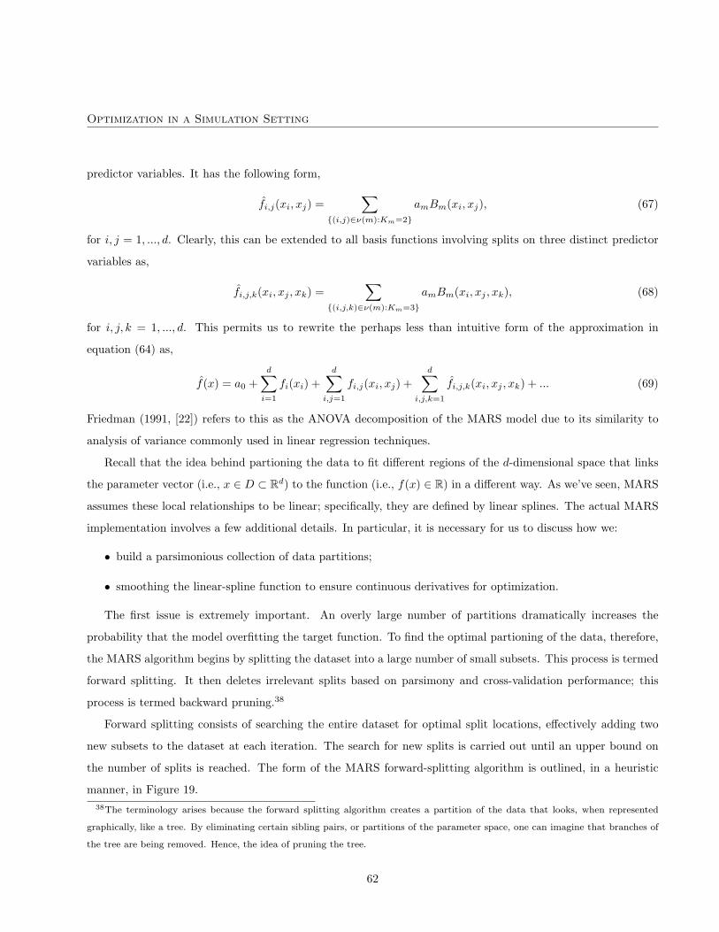
Optimization in a Simulation Setting
predictor variables. It has the following form,
fi,j(xi, xj) =∑
(i,j)∈ν(m):Km=2
amBm(xi, xj), (67)
for i, j = 1, ..., d. Clearly, this can be extended to all basis functions involving splits on three distinct predictor
variables as,
fi,j,k(xi, xj , xk) =∑
(i,j,k)∈ν(m):Km=3
amBm(xi, xj , xk), (68)
for i, j, k = 1, ..., d. This permits us to rewrite the perhaps less than intuitive form of the approximation in
equation (64) as,
f(x) = a0 +d∑
i=1
fi(xi) +d∑
i,j=1
fi,j(xi, xj) +d∑
i,j,k=1
fi,j,k(xi, xj , xk) + ... (69)
Friedman (1991, [22]) refers to this as the ANOVA decomposition of the MARS model due to its similarity to
analysis of variance commonly used in linear regression techniques.
Recall that the idea behind partioning the data to fit different regions of the d-dimensional space that links
the parameter vector (i.e., x ∈ D ⊂ Rd) to the function (i.e., f(x) ∈ R) in a different way. As we’ve seen, MARS
assumes these local relationships to be linear; specifically, they are defined by linear splines. The actual MARS
implementation involves a few additional details. In particular, it is necessary for us to discuss how we:
• build a parsimonious collection of data partitions;
• smoothing the linear-spline function to ensure continuous derivatives for optimization.
The first issue is extremely important. An overly large number of partitions dramatically increases the
probability that the model overfitting the target function. To find the optimal partioning of the data, therefore,
the MARS algorithm begins by splitting the dataset into a large number of small subsets. This process is termed
forward splitting. It then deletes irrelevant splits based on parsimony and cross-validation performance; this
process is termed backward pruning.38
Forward splitting consists of searching the entire dataset for optimal split locations, effectively adding two
new subsets to the dataset at each iteration. The search for new splits is carried out until an upper bound on
the number of splits is reached. The form of the MARS forward-splitting algorithm is outlined, in a heuristic
manner, in Figure 19.38The terminology arises because the forward splitting algorithm creates a partition of the data that looks, when represented
graphically, like a tree. By eliminating certain sibling pairs, or partitions of the parameter space, one can imagine that branches of
the tree are being removed. Hence, the idea of pruning the tree.
62
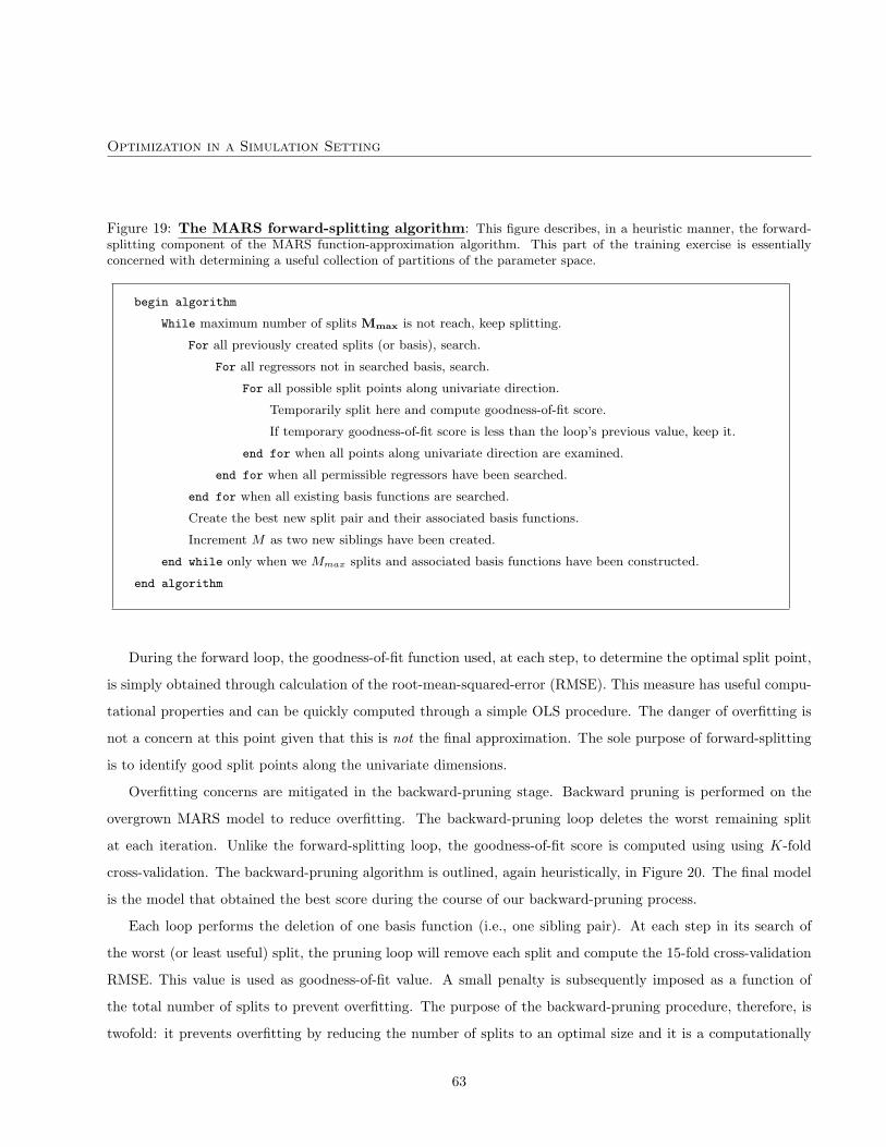
Optimization in a Simulation Setting
Figure 19: The MARS forward-splitting algorithm: This figure describes, in a heuristic manner, the forward-splitting component of the MARS function-approximation algorithm. This part of the training exercise is essentiallyconcerned with determining a useful collection of partitions of the parameter space.
begin algorithm
While maximum number of splits Mmax is not reach, keep splitting.
For all previously created splits (or basis), search.
For all regressors not in searched basis, search.
For all possible split points along univariate direction.
Temporarily split here and compute goodness-of-fit score.
If temporary goodness-of-fit score is less than the loop’s previous value, keep it.
end for when all points along univariate direction are examined.
end for when all permissible regressors have been searched.
end for when all existing basis functions are searched.
Create the best new split pair and their associated basis functions.
Increment M as two new siblings have been created.
end while only when we Mmax splits and associated basis functions have been constructed.
end algorithm
During the forward loop, the goodness-of-fit function used, at each step, to determine the optimal split point,
is simply obtained through calculation of the root-mean-squared-error (RMSE). This measure has useful compu-
tational properties and can be quickly computed through a simple OLS procedure. The danger of overfitting is
not a concern at this point given that this is not the final approximation. The sole purpose of forward-splitting
is to identify good split points along the univariate dimensions.
Overfitting concerns are mitigated in the backward-pruning stage. Backward pruning is performed on the
overgrown MARS model to reduce overfitting. The backward-pruning loop deletes the worst remaining split
at each iteration. Unlike the forward-splitting loop, the goodness-of-fit score is computed using using K-fold
cross-validation. The backward-pruning algorithm is outlined, again heuristically, in Figure 20. The final model
is the model that obtained the best score during the course of our backward-pruning process.
Each loop performs the deletion of one basis function (i.e., one sibling pair). At each step in its search of
the worst (or least useful) split, the pruning loop will remove each split and compute the 15-fold cross-validation
RMSE. This value is used as goodness-of-fit value. A small penalty is subsequently imposed as a function of
the total number of splits to prevent overfitting. The purpose of the backward-pruning procedure, therefore, is
twofold: it prevents overfitting by reducing the number of splits to an optimal size and it is a computationally
63
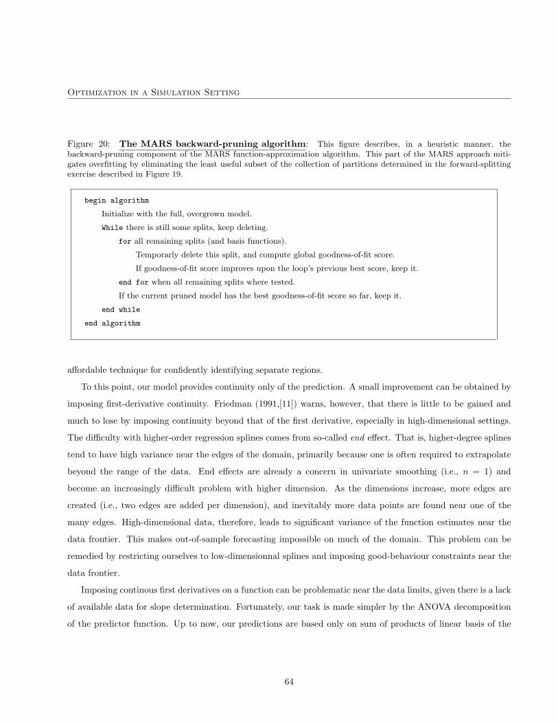
Optimization in a Simulation Setting
Figure 20: The MARS backward-pruning algorithm: This figure describes, in a heuristic manner, thebackward-pruning component of the MARS function-approximation algorithm. This part of the MARS approach miti-gates overfitting by eliminating the least useful subset of the collection of partitions determined in the forward-splittingexercise described in Figure 19.
begin algorithm
Initialize with the full, overgrown model.
While there is still some splits, keep deleting.
for all remaining splits (and basis functions).
Temporarly delete this split, and compute global goodness-of-fit score.
If goodness-of-fit score improves upon the loop’s previous best score, keep it.
end for when all remaining splits where tested.
If the current pruned model has the best goodness-of-fit score so far, keep it.
end while
end algorithm
affordable technique for confidently identifying separate regions.
To this point, our model provides continuity only of the prediction. A small improvement can be obtained by
imposing first-derivative continuity. Friedman (1991,[11]) warns, however, that there is little to be gained and
much to lose by imposing continuity beyond that of the first derivative, especially in high-dimensional settings.
The difficulty with higher-order regression splines comes from so-called end effect. That is, higher-degree splines
tend to have high variance near the edges of the domain, primarily because one is often required to extrapolate
beyond the range of the data. End effects are already a concern in univariate smoothing (i.e., n = 1) and
become an increasingly difficult problem with higher dimension. As the dimensions increase, more edges are
created (i.e., two edges are added per dimension), and inevitably more data points are found near one of the
many edges. High-dimensional data, therefore, leads to significant variance of the function estimates near the
data frontier. This makes out-of-sample forecasting impossible on much of the domain. This problem can be
remedied by restricting ourselves to low-dimensionnal splines and imposing good-behaviour constraints near the
data frontier.
Imposing continous first derivatives on a function can be problematic near the data limits, given there is a lack
of available data for slope determination. Fortunately, our task is made simpler by the ANOVA decomposition
of the predictor function. Up to now, our predictions are based only on sum of products of linear basis of the
64
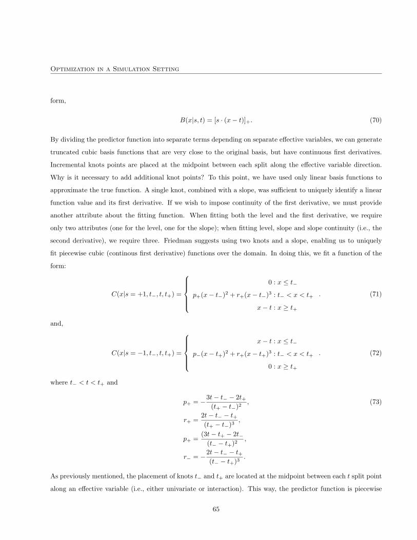
Optimization in a Simulation Setting
form,
B(x|s, t) = [s · (x− t)]+. (70)
By dividing the predictor function into separate terms depending on separate effective variables, we can generate
truncated cubic basis functions that are very close to the original basis, but have continuous first derivatives.
Incremental knots points are placed at the midpoint between each split along the effective variable direction.
Why is it necessary to add additional knot points? To this point, we have used only linear basis functions to
approximate the true function. A single knot, combined with a slope, was sufficient to uniquely identify a linear
function value and its first derivative. If we wish to impose continuity of the first derivative, we must provide
another attribute about the fitting function. When fitting both the level and the first derivative, we require
only two attributes (one for the level, one for the slope); when fitting level, slope and slope continuity (i.e., the
second derivative), we require three. Friedman suggests using two knots and a slope, enabling us to uniquely
fit piecewise cubic (continous first derivative) functions over the domain. In doing this, we fit a function of the
form:
C(x|s = +1, t−, t, t+) =
0 : x ≤ t−
p+(x− t−)2 + r+(x− t−)3 : t− < x < t+
x− t : x ≥ t+
. (71)
and,
C(x|s = −1, t−, t, t+) =
x− t : x ≤ t−
p−(x− t+)2 + r+(x− t+)3 : t− < x < t+
0 : x ≥ t+
. (72)
where t− < t < t+ and
p+ = −3t− t− − 2t+(t+ − t−)2
, (73)
r+ =2t− t− − t+(t+ − t−)3
,
p+ =(3t− t+ − 2t−
(t− − t+)2,
r− = −2t− t− − t+(t− − t+)3
.
As previously mentioned, the placement of knots t− and t+ are located at the midpoint between each t split point
along an effective variable (i.e., either univariate or interaction). This way, the predictor function is piecewise
65

Optimization in a Simulation Setting
cubic. The fitted basis function is, therefore, zero until it reaches t−, cubic and increasing up to t+ and linear
afterward.
Near the edges, knots are placed in such a way so as to ensure well-behaved derivatives. Knots are placed at the
midpoint between the most extreme data and first (or last) split point. Data limits are, therefore, characterized
by linear functions, permitting the possibility of safe interpolation and extrapolation near the edges.
Figure 21: Forward-Splitting and Backward-Pruning with a Simple Function : The first quadrant showsthe true function combined with the noise, the second quadrant outlines the fit after forward pruning, the third quadrantdescribes the fit after backward pruning, while the final quadrant is the ultimate smoothed MARS fit to the sine function.
0 0.1 0.2 0.3 0.4 0.5 0.6 0.7 0.8 0.9 1−2
−1.5
−1
−0.5
0
0.5
1
1.5
2
0 0.1 0.2 0.3 0.4 0.5 0.6 0.7 0.8 0.9 1−2
−1.5
−1
−0.5
0
0.5
1
1.5
2
0 0.1 0.2 0.3 0.4 0.5 0.6 0.7 0.8 0.9 1−2
−1.5
−1
−0.5
0
0.5
1
1.5
2
0 0.1 0.2 0.3 0.4 0.5 0.6 0.7 0.8 0.9 1−2
−1.5
−1
−0.5
0
0.5
1
1.5
2
Yet another smoothing parameter included in the MARS algorithm is the minimum distance between knots.
The MARS algorithm allows every data point to be available for splitting, offering the opportunity for the
creation of subregions of any size. This exploratory aspect of MARS implies that overfitting is an important
concern. There is, in particular, no way of distinguishing between a steep change in slope associated with the true
function and positive (or negative) deviation associated with noise. As such, one must assume the underlying
function is smoother than the noise. This assumption suggests the imposition of a smoothing parameter related
to the minimum distance between split points.39
We assume noise to be a random parameter ε ∼ N (0,Σ) with a symmetric distribution. The probability of
39This avoids, to a certain extent, the overweighting of particularly noisy observations.
66

Optimization in a Simulation Setting
having n consecutive positive/negative εi values is
P
⋂i∈1,...,n
εi > 0
= 21−n. (74)
By imposing a minimum distance between knots, it is therefore possible to further prevent overfitting. Based on
simple sign consideration for noise, we can estimate the risk of creating a domain containing only positive (or
negative) noise deviations.
Figure 21 illustrates the different steps of the MARS algorithm applied to one full period of a sine function
with a signal-to-noise variance-ratio of ten. After the forward splitting loop, some 20 subdomains were created.
Overfitting is observable around 0.7, were a particularly noisy observation was mapped. The backward pruning
loop eliminated overfitting by reducing the number of domains down to an easily interpretable five subdomains.
When first-derivative continuity is imposed, the MARS approximation yields a 0.9995 correlation coefficient with
the true underlying sine function.
67
Optimization in a Simulation Setting
A.5 Projection pursuit regression (PPR)
The final approximation algorithm that we will consider is termed projection-pursuit regression. This is a
particular implemenation of a more general approximation methodology termed projection pursuit that is well
documented in Huber (1985, [28]), Chen (1991, [20]), Hall (1989, [23]), Nason (1995, [32]), and Jones and
Sibson (1987, [29]). The basic idea of projection pursuit is dimension reduction. The algorithm seeks to find
interesting low-dimensional linear projections of the high-dimensional predictor variables, x ∈ Rd. The function
approximation, therefore, is merely the smoothed sum of these interesting low-dimensional projections. Why
do we consider low-dimensional projections? The reason is that working in high dimensions is difficult, while
we have a variety of efficient techniques that work quite well in low-dimensional settings.40 This may seem
somehow familiar to the basic intuition behind principal components analysis. Indeed, it can be demonstrated
that principal components analysis is, in fact, a special case of projection pursuit.
A few questions arise. First, what do we mean by low-dimensional projections? And, second, what do
we mean by interesting projections? We will address each of these important questions in turn. First, the
projections are typically one- or two-dimensional although Nason (1995, [32]) discusses a computationally efficient
implementation of a three-dimensional projection. For the purposes of this analysis, however, we will restrict our
attention to one-dimensional projections. Let’s make this notion somewhat more precise. Let a ∈ Rd×1 denote
an arbitrary d-dimensional vector. Recall that the argument of f(x) is also a d-dimensional column vector. As
a consequence, the dot product of a and x is described as,
aT x ∈ R, (75)
and takes a scalar value. In other words, the vector a is a linear projection, or transformation, of x from d
dimensions to a single dimension. If we let X ∈ Rd×N denote the entire data set, then the product of a and X
aT X ∈ R1×N , (76)
is an N -dimensional vector. Again, the vector a is a linear projection, or transformation, of the observed predictor
variables, X, into one-dimensional space. One can easily imagine generalizing a into a matrix A ∈ Rd×2 that
results in a projection of the data from d to two dimensions. We observe, therefore, that constructing low-
dimensional projections is a trivial exercise in matrix algebra.40Essentially, high-dimensional spaces are just too big. The amount of data to even cover a small portion of a high-dimensional
space is enormous. Typically, such a large data set is neither available nor actually desirable. This is often referred to as the curse
of dimensionality (see Bellman (1961).
68
Optimization in a Simulation Setting
This brings us to the more interesting second question. That is, how do we find interesting projections a? As
a is a vector, it is essentially a direction. In other words, what directions of our data are interesting? We could
look at those directions that the data is noisy, non-linear, or non-Gaussian. If we decide that the interesting
directions are those that are highly variable (i.e., noisy), then we will attempt to find the direction, a, that has
the maximum variance. We can write the variance of an arbitrary projection a onto the set of predictor variables
as,
var(aT X) = aT var(X)a. (77)
If we decide to select a such that it maximizes the sample variance of the projected data, then we need only
solve the following problem,
a∗ = arg maxa
aT var(X)a. (78)
If we add the construct that a has unit length, aT a = 1, then the solution to this problem is the first principal
component.41 We see, therefore, exactly how principal components can be cast in the context of projection
pursuit.
Projection pursuit, however, does not generally consider those projections that demonstrate large variance,
but rather those that are interesting. Providing a more precise definition of what is meant by interesting, however,
requires some additional structure. In the general projection pursuit setting, one constructs a projection index,
Q(·) that operates on aT X. The role of the projection index is to measure some aspect of the projected data.
In short, Q attempts to provide a measure of interestingness.
A more complete explanation of the projection index requires some additional statistical structure. If one
considers the set of predictor variables as a sample representation of a d-dimensional random vector with the
multivariate distribution function F , then aT X is a one-dimensional random variable with univariate distribution
function Fa. The projection index, Q, can therefore be considered as a functional on the space of one-dimensional
distributions.
Huber (1985, [28]) argues that those directions that are the most interesting are those projections that are the
most non-Gaussian. We can think of this as implying that determining what is interesting is difficult, but it is
rather easier to define what is uninteresting. In particular, the Gaussian distribution with its inherent symmetry
and complete description with two moments is uninteresting. A natural projection index for the measurement
of deviations of a given projection from Gaussianity would be some notion of entropy. Entropy, which can be41The first order conditions are aT var(X) = 0, which is the eigenvalue problem. The solution to the characteristic polynomial is
the eigenvector, a, associated with the largest eigenvalue of var(X).
69
Optimization in a Simulation Setting
operationalized in a number of different ways, is basically a notion of the distance between two distributions.
An entropy-based projection index that examines the distance of a given projection, aT X, versus the Gaussian
distribution would be a reasonable choice. It turns out that there are a wide range of different projection indices
that one can use for this purpose. In this paper, however, we take a slightly different approach.
The idea of projection pursuit regression abstracts somewhat from the projection index. Instead, the idea is
to find the collection of projections that best fit the observed data. Indeed, this approach will ultimately look
quite similar to the previously discussed non-parametric kernel regression approach. The idea is to postulate
that,
f(xi) = g1(aT1 xi), (79)
where g1 is a known arbitrary smooth function, that we will discuss shortly, and for i = 1, ..., N . We then proceed
to solve for the projection, a1, that best fits the dependent variable, y. We do this in the usual least-squares
manner as,
mina1
n∑i=1
(yi − g1(aT
1 xi))2
. (80)
The solution to this non-linear optimization problem, a∗1, represents the projection of the d-dimensional predictor-
variable vector, x, into a single dimension that best approximates the dependent variable, y. It is unlikely,
however, that a single projection onto x will be sufficient to adequately describe, f(x). Consequently, a second
direction is added. That is, our approximation has the form,
f(xi) = g1(aT1 xi) + g2(aT
2 xi), (81)
leading to the following non-linear optimization problem,
mina2
n∑i=1
(yi − g1(aT
1 xi)− g2(aT2 xi)
)2. (82)
The general form, therefore, is
f(xi) =K∑
k=1
gk(aTk xi), (83)
leading to the following non-linear optimization problem for the kth projection, aK ,
minaK
n∑i=1
(yi −
K∑k=1
gk(aTk xi)
)2
. (84)
The final aspect of the project-pursuit algorithm is the choice of the smoothing functions, gk, k = 1, ..., n.
We employ non-parametric kernel regressions of the form discussed in section A.3 with a Gaussian kernel. We
experimented with a number of different possible kernels, but found that this choice performed the best.
70
Optimization in a Simulation Setting
B Possible Government Objective Functions
The debt-strategy problem is, in its purest form, a stochastic optimal control problem. Bolder (2003, [12])
makes this observation and demonstrates how one might formally define the problem in this setting. This
appendix builds on this idea and extends the actual form of the government’s objective function with respect
to its debt-management strategy in a number of different directions. Appendices B.1 and B.2 illustrate how
one might consider only the government’s debt charges, while Appendix B.3 adds a constraint related to the
conditional volatility of these debt charges. Appendix B.4 introduces the government’s fiscal situation into
the government’s objectives in two alternative ways: through the volatility of the budgetary balance and the
probability of deficit. Finally, Appendix B.5 explores how we might the use of an expected utility framework to
capture the government’s risk preferences.
B.1 Debt charges
As one of the key criteria for the government is the cost of servicing the domestic debt portfolio, we require a
function that describes debt charges as a function of the state of the economy and the selected financing strategy.
We define this continuous function as,
c ≡ c (t, θ,X(t, ω)) . (85)
In other words, the debt-servicing costs depend on the current point in time, t, the selected financing strategy,
and the current state variables. Thus, we can define the cost associated with a given realization of the state
variables (ω ∈ Ω) over the interval [0, T ], and specific choice of financing strategy as,∫ T
0
c (t, θ,X(t, ω)) dt. (86)
This is useful, but we are more interested in understanding the expected debt charges across all possible realiza-
tions of the state variables. This is determined as,∫A∈Ft
∫ T
0
c (t, θ,X(t, ω)) dt dP = E
(∫ T
0
c (t, θ,Xt) dt
∣∣∣∣∣F0
). (87)
In actual fact, however, c is not a continuous function. We have had to perform a number of discretizations
during the implementation of these models. Moreover, we have a strong interest in examining the debt charges
on an annual basis. As such, we can define a discretized version of c as,
c ≡ c(0, t, θ, X(t, ω)
), (88)
71
Optimization in a Simulation Setting
where X denotes the discretized state variable vector. We interpret equation (88) as the debt-servicing charges
over the interval [0, t] for fixed θ ∈ Θ and ω ∈ Ω. If we partition our time interval into T periods, 1, ..., T, then
we can re-write the cost associated with a given realization of the state variables, (ω ∈ Ω), for a given financing
strategy as,
T∑t=1
c(t− 1, t, θ, X(t, ω)
). (89)
The expectation of equation (89) becomes,
E
(T∑
t=1
c(t− 1, t, θ, X(t, ω)
)∣∣∣∣∣F0
)=
T∑t=1
E(c(t− 1, t, θ, X(t, ω)
)∣∣∣F0
), (90)
given that the expectation of the sum is equal to the sum of the expectations.
This development suggests a straightforward objective function that seeks to minimize the expected debt
charges as,
minθ∈Θ
T∑t=1
E(c(t− 1, t, θ, X(t, ω)
)∣∣∣F0
). (91)
Let’s take a moment and relate this idea back to the central idea of this paper. We have proposed using an
function-approximation algorithm to describe the government’s objective function. We then proposed performing
any and all optimization on this approximation. In Sections 2 and 2.1 we worked towards identifying the MARS
algorithm as a useful function approximation algorithm. The question, therefore, is how exactly do we apply
MARS in this setting? For the objective function in equation (90), the true function is,
g(θ) =T∑
t=1
E(c(t− 1, t, θ, X(t, ω)
)∣∣∣F0
). (92)
We then randomly generate a range of possible portfolio weights, θi, i = 1, ..., N and compute the corresponding
function values, g(θi), i = 1, ..., N. Using this data, we then train the MARS algorithm to construct an
approximation, g(θ) for an arbitrary choice of θ. We then solve for the optimal strategy as,
θ∗ = arg minθ∈Θ
g(θ). (93)
72

Optimization in a Simulation Setting
B.2 Discounted debt charges
The formulation in equation (91) will lead to the financing strategy with the lowest expected cost over the
interval [0, T ], but it has a few flaws. First, it treats the debt charges in each period in exactly the same manner.
Simply put, the debt servicing costs in the first period are assumed to be equally important to those debt charges
occurring in the T th period.
Figure 22: Discounted Expected Annual Debt Charges: This figure outlines a plot of the sum of the discountedexpected annual debt charges over a ten-year time horizon. There are three possible debt instruments: three- and 12-monthtreasury bills and five-year nominal coupon-bearing bonds.
00.2
0.40.6
0.81
00.2
0.40.6
0.815
6
7
8
9
10
11
12
13
14
3−month weight1−year weight
CA
D b
illio
ns
It would seem reasonable, therefore, to apply some form of discounting to the cashflows. If we denote P (0, t)
as the discount factor prevailing from time 0 to time t, then we could modify equation (91) as follows,
minθ∈Θ
T∑t=1
P (0, t) · E(c(t− 1, t, θ, X(t, ω)
)∣∣∣F0
), (94)
which applies a fixed set of discount factors across all realizations of the state variables.42 An illustrative view
of the annual discounted expected debt charges, as described in equation (94), is outlined in Figure 22. One
could use the time 0 zero-coupon term structure to identify these factors. It might also make sense to use a
pre-determined set of discount factors that can be used consistently over time. The idea behind this suggestion is42It makes no difference if P (0, t) is inside or outside of the expectation operator as P (0, t) is an F0-measurable random variable.
73

Optimization in a Simulation Setting
the realization that the current zero-coupon term structure will change on a daily basis, while the government’s
view of future cashflows may remain fairly constant.
74
Optimization in a Simulation Setting
B.3 Debt-charge stability
A second flaw with the objective function in equation (91) is that it ignores the idea of stability. Stability can
be defined in a number of ways. A natural way to define stability relates to the variability of the debt-servicing
costs. This stems from the idea that high variable debt-service charges are undesirable as they have the potential
to complicate fiscal policy. We can write the variance of the debt-service charges as,
var(c(0, t, θ, Xt
)∣∣∣F0
), (95)
which describes the variance of the debt-service costs over the interval [0, t] associated with the financing strategy,
θ ∈ Θ, conditioning on the filtration at time 0, F0.
Dealing with the variance of the debt charges is somewhat more involved. It is clear that given the non-
linearity of variance that we cannot use the same trick as in equation (90) to describe the variance over the
interval [0, T ].43 We could, of course, constrain the objective function in equation (94) in the following manner,
minθ∈Θ
T∑t=1
P (0, t) · E(c(t− 1, t, θ, X(t, ω)
)∣∣∣F0
), (97)
subject to:
var(c(t− 1, t, θ, Xt
)∣∣∣F0
)≤ δt, for t ∈ 1, ..., T.
In other words, we can constrain the debt-charge variance in each of the periods in the time partition [0, ..., T ].
While this seems reasonable at first glance, a bit of reflection reveals that such an approach is difficult to
implement. The uncertainty about the state variable vector, Xt, will increase as we move forward in time. That
is, we expect to observe that
var(c(t− 1, t, θ, Xt
)∣∣∣F0
)≤ var
(c(t, t + 1, θ, Xt
)∣∣∣F0
), (98)
for all t ∈ 1, ..., T with equality occurring when the value of t becomes sufficiently large for the conditional
variance to converge to its unconditional value. This is not exactly a problem, but it raises a practical problem.
Specifically, it is relatively easy for the debt manager (and the fiscal policymaker for that matter) to write down
a constraint for the maximum desired debt-charge variability over the next year. To write down such a constraint
for the annual debt-service cost variability for a one-year period beginning in four years, however, is a rather43The variance of the sum is not equal to the sum of the variances. In particular, we have that
var
(T∑
t=1
c(t− 1, t, θ, Xt
)∣∣∣∣∣F0
)6=
T∑t=1
var(c(t− 1, t, θ, Xt
)∣∣∣F0
). (96)
75
Optimization in a Simulation Setting
different matter. The basic problem is that the state-variable dynamics are roughly equivalent to discretized
diffusion processes; this implies that their standard deviation grows at approximately the square-root of time.
The debt-charge volatility in four years time, therefore, will be about twice as large as the first year’s debt-charge
volatility simply because over longer periods there is much more uncertainty about the future evolution of the
state variables. This is a perfectly natural result, but it simply does not reflect how debt and fiscal managers
think about stability.
A potential solution arises from consideration of exactly how debt and fiscal managers think about stability.
In particular, their perspective is typically focused on a single period—generally speaking, a one-year period. If
a shock was experienced in the previous period, whether positive or negative, action is taken in that period and
attention is refocused on the upcoming period. Essentially, therefore, debt and fiscal managers are concerned
with a one-period conditional variance of the form,
var(c(t− 1, t, θ, Xt
)∣∣∣Ft−1
). (99)
The models used are, by and large, Gaussian in nature and, as such, we can state the transition density of c is
well characterized by its first two moments as follows,
f(c(t− 1, t, θ, Xt
)∣∣∣Ft−1
)∼ N
E(c(t− 1, t, θ, Xt
)∣∣∣Ft−1
)︸ ︷︷ ︸
Conditional mean
, var(c(t− 1, t, θ, Xt
)∣∣∣Ft−1
)︸ ︷︷ ︸
Conditional variance
. (100)
We are interested in the conditional variance from this transition density. We do not have a closed-form expression
for this quantity, but we do have an enormous amount of numerically generated information about the debt-
charge process from our stochastic-simulation engine. If we are willing to assume a particular parametric form
for the debt-charge process, then we can readily approximate the conditional variance. One reasonable choice is
an autoregressive formulation such as,
c(t− 1, t, θ, Xt
)= β0 +
p∑k=1
βk · c(t− 1− k, t− k, θ, Xt−k
)+ ξt. (101)
This provides the following form for the transition density of the debt-charge process in equation (100),
f(c(t− 1, t, θ, Xt
)∣∣∣Ft−1
)∼ N
β0 +p∑
k=1
βk · c(t− 1− k, t− k, θ, Xt−k
)︸ ︷︷ ︸
Conditional mean
,1
T − 1
T∑t=1
ξ2t︸ ︷︷ ︸
Conditionalvariance
. (102)
76
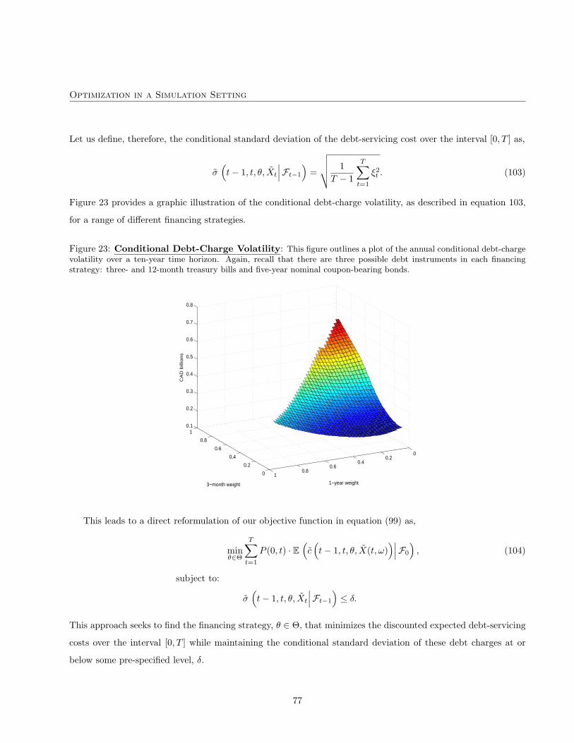
Optimization in a Simulation Setting
Let us define, therefore, the conditional standard deviation of the debt-servicing cost over the interval [0, T ] as,
σ(t− 1, t, θ, Xt
∣∣∣Ft−1
)=
√√√√ 1T − 1
T∑t=1
ξ2t . (103)
Figure 23 provides a graphic illustration of the conditional debt-charge volatility, as described in equation 103,
for a range of different financing strategies.
Figure 23: Conditional Debt-Charge Volatility: This figure outlines a plot of the annual conditional debt-chargevolatility over a ten-year time horizon. Again, recall that there are three possible debt instruments in each financingstrategy: three- and 12-month treasury bills and five-year nominal coupon-bearing bonds.
0
0.2
0.4
0.6
0.8
1
00.2
0.40.6
0.81
0.1
0.2
0.3
0.4
0.5
0.6
0.7
0.8
1−year weight3−month weight
CA
D b
illio
ns
This leads to a direct reformulation of our objective function in equation (99) as,
minθ∈Θ
T∑t=1
P (0, t) · E(c(t− 1, t, θ, X(t, ω)
)∣∣∣F0
), (104)
subject to:
σ(t− 1, t, θ, Xt
∣∣∣Ft−1
)≤ δ.
This approach seeks to find the financing strategy, θ ∈ Θ, that minimizes the discounted expected debt-servicing
costs over the interval [0, T ] while maintaining the conditional standard deviation of these debt charges at or
below some pre-specified level, δ.
77
Optimization in a Simulation Setting
B.4 Fiscal-policy considerations
The objective function in equation (104) essentially represents the traditional approach to debt management.
Traditionally, debt management has focused on attempting to find a trade-off between the level of debt charges
and debt-charge volatility. The generally upward sloping nature of the yield curve implies that, on average, short-
term debt is less expensive. As short-term interest rates are more volatile than their long-term counterparts,
one typically has to be prepared to accept higher uncertainty for lower expected debt charges. Understanding
this trade-off has been the focus of much of debt-management research in past years. This is consistent with
the historical fact that debt management has been conducted fairly independently of fiscal policy.44 Recently,
however, there has been an increasing appreciation that debt-charge volatilty is important only insofar as it
leads to an associated increase in budgetary volatility. We can, in a stylized manner, consider the government’s
budgetary position, F , to be the primary balance less debt charges,
F (t− 1, t, θ, Xt) = R(t− 1, t, Xt)− E(t− 1, t, Xt)︸ ︷︷ ︸Primary balance: Γ(t− 1, t, Xt)
−c(t− 1, t, θ, Xt), (105)
where the primary balance (i.e., Γ(t− 1, t, Xt))is government revenues (i.e., R(t− 1, t,Xt)) less non-debt charge
related expenditures (i.e., E(t − 1, t,Xt)). Observe that both revenue and expenditure depend on the time
interval [t − 1, t] and the value of the state variables.45 Budgetary volatilty, therefore, will depend, at least in
part, on the interaction between debt charges and the primary balance. In particular,
var(F (t− 1, t, θ, Xt)
)=var (Γ(t− 1, t,Xt)) + var (c(t− 1, t, θ, Xt)) (106)
− 2cov (Γ(t− 1, t,Xt), c(t− 1, t, θ, Xt)) ,
To the extent that the covariance between the primary balance and the debt charges is positive, the contribution
of debt-charge volatility towards budgetary volatility will be dampened. The sign, magnitude, and certainty of
this interaction, therefore, has a role to play in debt management decision. In other words, the sole consideration
of debt-charge volatility without reference to its relationship to the government’s financial requirements may be
misleading. The selection of a portfolio that minimizes budgetary volatility could potentially permit a greater
degree of flexibility in fiscal policy. That is, greater certainty would allow for a smoother tax profile and a larger
proportion of permanent, as opposed to temporary, expenditure initiatives.
There are a few possible ways to introduce budgetary volatility into our objective function. One possibility44This was not a deliberate choice, but rather a simplifying assumption.45Given that the state variables include information about output, inflation, and monetary conditions this seems quite reasonable.
78
Optimization in a Simulation Setting
is to use the same conditional standard deviation approach as suggested for the debt charge volatility. That is,
F(t− 1, t, θ, Xt
)= β0 +
p∑k=1
βk · F(t− 1− k, t− k, θ, Xt−k
)+ ζt. (107)
The associated transition density of the government’s budgetary position process is,
f(F(t− 1, t, θ, Xt
)∣∣∣Ft−1
)∼ N
β0 +p∑
k=1
βk · F(t− 1− k, t− k, θ, Xt−k
)︸ ︷︷ ︸
Conditional mean
,1
T − 1
T∑t=1
ζ2t︸ ︷︷ ︸
Conditionalvariance
. (108)
Thus, the conditional standard deviation of the government’s budgetary position over the interval [0, T ] is given
as,
η(t− 1, t, θ, Xt
∣∣∣Ft−1
)=
√√√√ 1T − 1
T∑t=1
ζ2t . (109)
This leads to a simple modification of our objective function in equation (104) as,
minθ∈Θ
T∑t=1
P (0, t) · E(c(t− 1, t, θ, X(t, ω)
)∣∣∣F0
), (110)
subject to:
η(t− 1, t, θ, Xt
∣∣∣Ft−1
)≤ α.
Analagous to equation (104), this formulation seeks to find the financing strategy, θ ∈ Θ, that minimizes the
discounted expected debt-servicing costs over the interval [0, T ] while maintaining the conditional standard
deviation of the government’s budgetary position at or below some pre-specified level, α. One could easily
envisage having both constraints on the conditional variance of the budgetary balance and the debt charges as,
minθ∈Θ
T∑t=1
P (0, t) · E(c(t− 1, t, θ, X(t, ω)
)∣∣∣F0
), (111)
subject to:
η(t− 1, t, θ, Xt
∣∣∣Ft−1
)≤ α,
σ(t− 1, t, θ, Xt
∣∣∣Ft−1
)≤ δ.
The reason for both constraints might be a general concern that an over-reliance on the conditional standard
deviation of the government’s budgetary position might expose the government to the time variation in the
79
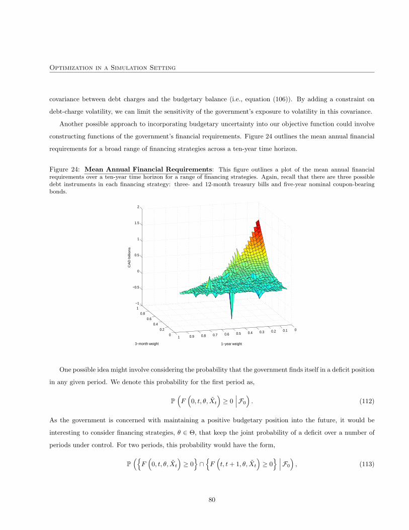
Optimization in a Simulation Setting
covariance between debt charges and the budgetary balance (i.e., equation (106)). By adding a constraint on
debt-charge volatility, we can limit the sensitivity of the government’s exposure to volatility in this covariance.
Another possible approach to incorporating budgetary uncertainty into our objective function could involve
constructing functions of the government’s financial requirements. Figure 24 outlines the mean annual financial
requirements for a broad range of financing strategies across a ten-year time horizon.
Figure 24: Mean Annual Financial Requirements: This figure outlines a plot of the mean annual financialrequirements over a ten-year time horizon for a range of financing strategies. Again, recall that there are three possibledebt instruments in each financing strategy: three- and 12-month treasury bills and five-year nominal coupon-bearingbonds.
00.2
0.40.6
0.81
00.10.20.30.40.50.60.70.80.91
−1
−0.5
0
0.5
1
1.5
2
1−year weight3−month weight
CA
D b
illio
ns
One possible idea might involve considering the probability that the government finds itself in a deficit position
in any given period. We denote this probability for the first period as,
P(F(0, t, θ, Xt
)≥ 0
∣∣∣F0
). (112)
As the government is concerned with maintaining a positive budgetary position into the future, it would be
interesting to consider financing strategies, θ ∈ Θ, that keep the joint probability of a deficit over a number of
periods under control. For two periods, this probability would have the form,
P(
F(0, t, θ, Xt
)≥ 0∩
F(t, t + 1, θ, Xt
)≥ 0 ∣∣∣F0
), (113)
80
Optimization in a Simulation Setting
while the joint probability of maintaining the government’s budgetary position in surplus territory would be,
P
⋂t∈1,..,T
F(t− 1, t, θ, Xt
)≥ 0 ∣∣∣∣∣∣F0
. (114)
This considers sample paths for the government’s budgetary position never falls below zero. How might we
introduce this into the objective function? One possibility is to assume that the government’s objective can be
summarized by a weighted sum of expected debt charges and the government’s budgetary position. This might
have the form,
minθ∈Θ
λ1 P
⋂t∈1,..,T
F(t− 1, t, θ, Xt
)≥ 0 ∣∣∣∣∣∣F0
︸ ︷︷ ︸
Contribution of budgetary position
+λ2
T∑t=1
P (0, t) · E(c(t− 1, t, θ, X(t, ω)
)∣∣∣F0
)︸ ︷︷ ︸
Contribution of debt charges
, (115)
where λ1, λ2 ∈ R.46 One could augment the criterion function in equation (115) to include constraints on
conditional debt-charge and financial requirement volatility as,
minθ∈Θ
λ1P
⋂t∈1,..,T
F(t− 1, t, θ, Xt
)≥ 0 ∣∣∣∣∣∣F0
+ λ2
T∑t=1
P (0, t) · E(c(t− 1, t, θ, X(t, ω)
)∣∣∣F0
), (116)
subject to:
η(t− 1, t, θ, Xt
∣∣∣Ft−1
)≤ α,
σ(t− 1, t, θ, Xt
∣∣∣Ft−1
)≤ δ.
46As a practical matter, we can probably expect some scaling problems given that the expected debt charges will be in units of
currency (probably in billions), while the probability of the budgetary position being in a deficit position will be bounded to the
unit interval, (0, 1). We can deal with this issue by appropriately scaling the values of λ1 and λ2.
81
Optimization in a Simulation Setting
B.5 Introducing utility functions
To this point, the objective functions that we have discussed are essentially risk neutral. Notions of risk have
been introduced, but not in a formal way. Formal consideration of the risk-aversion characteristics of the debt
manager can be introduced with the help of a loss function. A loss function can be motivated by the fact that all
losses are often not viewed with an equal level of concern by the debt manager. If one prefers greater losses than
the expected value of a gamble in order to avoid the risk inherent to the gamble, one is said to be risk averse.
Let all the possible outcomes be defined in the probability space (Ω,F , P). Then, provided some technical
conditions are satisfied, there exists a mathematical function representing a given preference relation.47 Greater
values of utility, U , correspond to outcomes preferred to those of smaller U values, and equal values to indifferent
outcomes.
Since utility is usually considered to be something positive, utility functions dealing with bad outcomes are
often termed loss functions. By definition, one tries to maximize utility, while one attempts to minimize loss. If,
facing an uncertain outcome, the overall utility of all possible outcomes is the expected utility of the uncertain
outcome, this utility is said to be a Von-Neuman-Morgenstein (VNM) utility function. To make this more
concrete, let the uncertain situation g with possible outcomes x1, x2, ..., xN and their respective probabilities
P(X = x1), P(X = x2), ..., P(X = xN ) be combined to form a gamble,
g = P(X = x1) x1, P(X = x2) x2, ..., P(X = xN ) xN . (117)
Then, the VNM-utility function associated with this gamble is,
U(g) = E(U(X)), (118)
=N∑
i=1
P(X = xi).U(xi)
In words, therefore, the overall VNM utility of a gamble is the probability weighted utility of each of the different
possible outcomes.
Risk aversion is present whenever the expected utility of outcomes is smaller than the utility of expected
outcome.
E(U(c)) < U(E(c)) (119)
47Existence of a utility function is granted if the preference relations on Ω are complete, reflexive, transitive, monotonic and
continous.
82
Optimization in a Simulation Setting
This is always the case if the utility is concave in gains and convex in losses. If the debt manager is risk
averse, than its objective function should include some kind of expected loss. Maximizing utility or equivalently
minimizing loss will therefore take into account not only the cost of debt, but also the relative risk of different
strategies.
The choice of a utility function for the debt manager’s preferences is a difficult and delicate task48. The
choices of possible loss functions are infinite and there is substantial debate regarding the validity of various
functional representations. Theoretical economics provide us with at least two types of utility functions that are
popular among researchers for their convenient computational properties. These utility specifications are termed
constant absolute risk aversion (CARA) and constant relative risk aversion (CRRA) utility. 49 We consider both
of these loss functions in the context of an arbitrary function of the government’s financing strategy, f(θ).50 For
loss functions L, therefore, CARA utility has the form,
L(f(θ)) = aeγf(θ)
γ+ b, (122)
while one form of the CRRA utility function is,
L(f(θ)) = af(θ)γ + b, (123)
for appropriate positive values of γ ∈ R and arbitrary constants a, b ∈ R.
Let’s actually see what the specific objective functions might look like under these two formulations of the
government’s loss functions. Assume that the debt manager is only concerned on the cost c of debt, regardless
of stability, then our problem can be restated as an optimal choice of the loss function L. If utility is assumed48One possible way to formulate our objective function is likely to be an interpolation of few certainty equivalent values provided
by the decision maker when presented uncertain outcomes.49The names CARA and CRRA relate to Arrow-Pratt’s absolute risk aversion,
rA(U , x) = −U”(x)
U ′(x), (120)
and relative risk aversion,
rR(U , x) = −xU ′′(x)
U ′(x), (121)
measures. These measures where essentially constructed to ensure that the notion of risk aversion was invariant under affine
transformations of the utility function.50We can think of f(θ), however, as the sum of the annual debt charges; it could also easily be extended to incorporate the
government’s budgetary balance.
83
Optimization in a Simulation Setting
to be time separable, which is generally the case, then our objective function becomes,
minθ∈Θ
E
(L
(T∑
t=0
c(t− 1, t, θ, X(t, ω)
)∣∣∣∣∣F0
)= min
θ∈ΘE
T∑
t=0
L(c(t− 1, t, θ, X(t, ω)
)︸ ︷︷ ︸
By time separability
∣∣∣∣∣∣∣∣∣∣F0
, (124)
= minθ∈Θ
T∑t=0
E(L(c(t− 1, t, θ, X(t, ω)
)∣∣∣F0
).
The application of the CARA loss function in equation (122) has the form,
minθ∈Θ
T∑t=0
E(a exp
γc(t− 1, t, θ, X(t, ω))
+ b
∣∣∣F0
), (125)
while the CRRA loss function from equation (123) can be described as,
minθ∈Θ
T∑t=0
E(ac(t− 1, t, θ, X(t, ω))γ + b
∣∣∣F0
). (126)
There are, at least, three interesting facts to note about these functions. First, positive affine transformations
do not affect the ordering represented by VNM-utility functions. This is important as one might wish to scale
the objective function through time or using other factors. Second, a CRRA loss function with γ set to unity is
equivalent to a risk-neutral setting. Finally, optimizing a CRRA function is equivalent to optimization of partial
moments of the c distribution. This essentially permits us to consider the higher moments of the debt-charge
distribution.
84

Optimization in a Simulation Setting
Bibliography
[1] Management of interest rate and refinancing risk: Cost-at-risk. Technical report, Working Party on Debt
Management: Organization for Economic Co-operation and Development, October 1998. Danish National-
bank.
[2] Central government debt management - proposed guidelines. Technical report, October 2001. Swedish
National Debt Office (Riksgalds Kontoret).
[3] Central government borrowing: Forecast and analysis. Technical report, February 2002. Swedish National
Debt Office (Riksgalds Kontoret).
[4] Danish government borrowing and debt. Technical report, February 2005. Danmarks Nationalbank.
[5] Debt and reserves management report 2006-07. Technical report, March 2006. HM Treasury (UK).
[6] Debt management strategy: 2006-2007. Technical report, Spring 2006. Department of Finance Canada.
[7] Richard Bellman. Adaptive Control Processes: A Guided Tour. Princeton University Press, 1961.
[8] Pal Bergstrom and Anders Holmlund. A simulation model framework for government debt analysis.
Riksgalds Kontoret: The Swedish National Debt Office, November 2000.
[9] Patrick Billingsley. Probability and Measure. Wiley, Third Avenue, New York, New York, third edition,
1995.
[10] David J. Bolder. Affine term-structure models: Theory and implementation. Bank of Canada: Working
Paper 2001-15, October 2001.
[11] David J. Bolder. Towards a more complete debt strategy simulation framework. Bank of Canada: Working
Paper 2002-13, May 2002.
[12] David J. Bolder. A proposed stochastic simulation framework for the government of canada’s debt strategy
problem. Bank of Canada: Working Paper 2003-10, April 2003.
[13] David J. Bolder. Modelling term-structure dynamics for portfolio analysis: A practitioner’s perspective.
Bank of Canada: Working Paper (forthcoming), 2006.
85

Optimization in a Simulation Setting
[14] David J. Bolder. Stochastic simulation for debt management: Comparing joint models of the canadian
macroeconomy and the term structure of interest rates. Bank of Canada: Working Paper (forthcoming),
2006.
[15] David J. Bolder and Scott Gusba. Exponentials, polynomials, and fourier series: More yield curve modelling
at the bank of canada. Bank of Canada: Working Paper 2002-29, 2002.
[16] David J. Bolder, Grahame Johnson, and Adam Metzler. An empirical analysis of the canadian term structure
of zero-coupon interest rates. Bank of Canada: Working Paper 2004-48, 2004.
[17] David J. Bolder and David Streliski. Yield-curve modelling at the bank of canada. Bank of Canada:
Technical Report No. 84, October 1999.
[18] David Jamieson Bolder and Clifton Lee-Sing. Is the debt war over? chapter How Should We Manage the
Debt? The Institute for Research on Public Policy, 2004.
[19] George Casella and Roger L. Berger. Statistical Inference. Duxbury Press, Belmont, California, 1990.
[20] Hung Chen. Estimation of a projection-pursuit type regression model. The Annals of Statistics, 19(1):142–
157, 1991.
[21] Rick Durrett. Probability: Theory and Examples. Duxbury Press, Belmont, California, second edition, 1996.
[22] Jerome H. Friedman. Multivariate adaptive regression splines. The Annals of Statistics, 19(1):1–67, 1991.
[23] Peter Hall. On projection pursuit. The Annals of Statistics, 19(1):142–157, 1989.
[24] James D. Hamilton. Time Series Analysis. Princeton University Press, Princeton, New Jersey, 1994. Chapter
22.
[25] Anders Holmlund. The debt office’s model for analyzing duration choice for the swedish kronor debt.
Riksgalds Kontoret: The Swedish National Debt Office, October 1999.
[26] Anders Holmlund and Sara Lindberg. The sndo’s simulation model for government debt analysis (preliminary
draft). Riksgalds Kontoret: The Swedish National Debt Office, January 2002.
[27] Lars Horngren. Methods for analyzing the structure of the central government debt. Riksgalds Kontoret:
The Swedish National Debt Office, June 1999.
[28] Peter J. Huber. Projection pursuit. The Annals of Statistics, 13(2):435–475, 1985.
86

Optimization in a Simulation Setting
[29] M. C. Jones and Robin Sibson. What is projection pursuit. Journal of the Royal Statistical Society,
150(1):1–36, 1987.
[30] Markus Leippold and Liuren Wu. Quadratic term-structure models. Swiss Institute of Banking and Finance
Working Paper, 2000.
[31] P. A. Lewis and J. G. Stevens. Nonlinear modelling of time series using multivariate adaptive regression
splines (mars). Journal of the American Statistical Association, 86(416):864–877, 1991.
[32] Guy Nason. Three-dimensional projection pursuit. Applied Statistics, 44(4):411–430, 1995.
[33] Andreas Pick and Myrvin Anthony. A simulation model for the analysis of the uk’s sovereign debt strategy.
Technical report, August 2006.
[34] William H. Press, Saul A. Teukolsky, William T. Vetterling, and Brian P. Flannery. Numerical Recipes in
C: The Art of Scientific Computing. Cambridge University Press, Trumpington Street, Cambridge, second
edition, 1992.
[35] Lars Riksbjerg and Anders Holmlund. Advances in risk management of government debt. chapter Analytical
Framework for Debt and Risk Management. OECD, Paris, France, 2005.
[36] Peter Sephton. Forecasting recessions: Can we do better on mars? Federal Reserve Bank of St. Louis
Review, pages 39–49, March/April 2001.
[37] Peter Sephton. Forecasting inflation using the term structure and mars. Applied Economic Letters, 12:199–
202, 2005.
[38] Jun Shao. Linear model selection by cross-validation. Journal of the American Statistical Association,
88:486–494, 1993.
[39] Jun Shao. An asymptotic theory for linear model selection. Statistica Sinica, 7:221–264, 1997.
87