arX

iv:1

312.

7815

v2 [

mat

h.O

C]

8 A

ug 2

014

1

Optimal polygonalL1 linearization andfast interpolation of nonlinear systems

Guillermo Gallego, Daniel Berjón and Narciso García

Abstract—The analysis of complex nonlinear systems is oftencarried out using simpler piecewise linear representations ofthem. A principled and practical technique is proposed tolinearize and evaluate arbitrary continuous nonlinear functionsusing polygonal (continuous piecewise linear) models under theL1 norm. A thorough error analysis is developed to guide anoptimal design of two kinds of polygonal approximations in theasymptotic case of a large budget of evaluation subintervals N.The method allows the user to obtain the level of linearization(N) for a target approximation error and vice versa. It issuitable for, but not limited to, an efficient implementation inmodern Graphics Processing Units (GPUs), allowing real-timeperformance of computationally demanding applications. Thequality and efficiency of the technique has been measured indetail on two nonlinear functions that are widely used in manyareas of scientific computing and are expensive to evaluate.

Index Terms—Piecewise linearization, numerical approxima-tion and analysis, least-first-power, optimization.

I. I NTRODUCTION

T HE approximation of complex nonlinear systems bysimpler piecewise linear representations is a recurrent

and attractive task in many applications since the resultingsimplified models have lower complexity, fit into well es-tablished tools for linear systems and are capable of rep-resenting arbitrary nonlinear mappings. Examples include,among others, complexity reduction for finding the inverse ofnonlinear functions [1], [2], distortion mitigation techniquessuch as predistorters for power amplifier linearization [3], [4],the approximation of nonlinear vector fields obtained fromstate equations [5], the obtainment of approximate solutionsin simulations with complex nonlinear systems [6], or thesearch for canonical piecewise linear representations in oneand multiple dimensions [7].

In the last decades, the main efforts in piecewise lin-earization have been devoted both to find approximations ofmultidimensional functions from a mathematical standpointand to define circuit architectures implementing them (see,forexample, [8] and references therein). In the one-dimensionalsetting, a simple and common linearization strategy consists inbuilding a linear interpolant between samples of the nonlinear

This work has been partially supported by the Ministerio de Economía yCompetitividad of the Spanish Government under project TEC2010-20412(Enhanced 3DTV). G. Gallego is supported by the Marie Curie -COFUNDProgramme of the EU (Seventh Framework Programme).

G. Gallego, D. Berjón and N. García are with Grupo de Tratamiento deImágenes (GTI), ETSI Telecomunicación, Universidad Politécnica de Madrid,Madrid, Spain, e-mail: ggb,dbd,narciso@gti.ssr.upm.es.

Copyright (c) 2014 IEEE. Personal use of this material is permitted.However, permission to use this material for any other purposes must beobtained from the IEEE.DOI: 10.1109/TCSI.2014.2327313

function over a uniform partition of its domain. Such apolygonal (i.e., continuous piecewise linear) interpolant maybe further optimized by choosing a better partition of thedomain according to the minimization of some error measure.This is a sensible strategy in problems where there is aconstraint on the budget of samples allowed in the partition.

Hence, in spite of the multiple benefits derived from mod-eling with piecewise linear representations, a proper selectionof the interval partitions and/or predefining the number ofpartitions is paramount for a satisfactory performance. Someresearchers [2] use cross-validation based approaches to selectsuch a number of pieces within a partition. In other applica-tions, the budget of pieces may be constrained by an internaldesign requirement (speed, memory or target error) of theapproximation algorithm or by some external condition.

Simplified models may be built using descent methods [9],dynamic programming [10] or heuristics such as genetic [1]and/or clustering [11] algorithms to optimize some targetapproximation error. In some cases, however, the resultingpiecewise representation may fail to preserve desirable prop-erties of the original nonlinear system such as continuity [1].

We consider the simplified model representation given bythe least-first-power or bestL1 approximation of a continuousnonlinear functionf by some polygonal function. The generictopic of least-first-power approximation has been previouslyconsidered in several references, e.g., [12], [13], [14], over aspan of many years and it is a recurrent topic and source ofinsightful results.

We develop a fast and practical method to compute asuboptimal partition of the interval where the polygonal inter-polant and the bestL1 polygonal approximation to a nonlinearfunction are to be computed. This technique allows to furtheroptimize theL1 polygonal approximation to a function amongall possible partitions having the same number of segments,or conversely, allow to achieve a target approximation errorwhile minimizing the budget of segments used to representthe nonlinear function. The resulting polygonal approximationis useful in applications where the evaluation of continuousmathematical functions constitutes a significant computationalburden, such as computer vision [15], [16] or signal process-ing [17], [18], [19].

Our work may be generalized to the linearization of multi-dimensional functions [7] and the incorporation of constraints,thus opening new perspectives also in the context of designingcircuit architectures for such piecewise linear approximations,as in [8]. However, these interesting generalizations will bethe topic of future work.

The paper is organized as follows: two polygonal approx-

2

f

πT f

f

|f − πT f | |f − f |

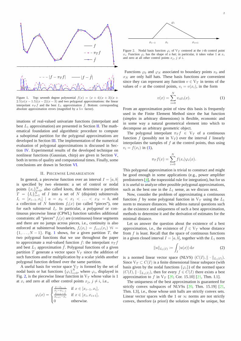
Figure 1. Top: seventh degree polynomialf(x) = (x + 4)(x + 3)(x +2.5)x(x− 1.5)(x− 2)(x− 3) and two polygonal approximations: the linearinterpolantπT f and the bestL1 approximationf . Bottom: correspondingabsolute approximation errors (magnified by a5× factor).

imations of real-valued univariate functions (interpolant andbestL1 approximation) are presented in SectionII . The math-ematical foundation and algorithmic procedure to computea suboptimal partition for the polygonal approximations aredeveloped in SectionIII . The implementation of the numericalevaluation of polygonal approximations is discussed in Sec-tion IV. Experimental results of the developed technique onnonlinear functions (Gaussian, chirp) are given in SectionV,both in terms of quality and computational times. Finally, someconclusions are drawn in SectionVI .

II. PIECEWISE L INEARIZATION

In general, a piecewise function over an intervalI = [a, b]is specified by two elements: a set of control or nodalpoints xiNi=0, also called knots, that determine a partitionT = IiNi=1 of I into a set ofN (disjoint) subintervalsIi = [xi−1, xi] | a = x0 < x1 < . . . < xN = b, anda collection ofN functions fi(x) (so called “pieces”), onefor each subintervalIi. In particular, apolygonal or con-tinuous piecewise linear (CPWL) function satisfies additionalconstraints: all “pieces”fi(x) are (continuous) linear segmentsand there are no jumps across pieces, i.e., continuity is alsoenforced at subinterval boundaries,fi(xi) = fi+1(xi) ∀i =1, . . . , N − 1. Fig. 1 shows, for a given partitionT, thetwo polygonal functions that we use throughout the paperto approximate a real-valued functionf : the interpolantπT fand bestL1 approximationf . Polygonal functions of a givenpartition T generate a vector spaceVT since the addition ofsuch functions and/or multiplication by a scalar yields anotherpolygonal function defined over the same partition.

A useful basis for vector spaceVT is formed by the set ofnodal basis or hat functionsϕiNi=0, whereϕi, displayed inFig. 2, is the piecewise linear function inVT whose value is 1at xi and zero at all other control pointsxj , j 6= i, i.e.,

ϕi(x) =

x−xi−1

xi−xi−1if x ∈ [xi−1, xi],

xi+1−xxi+1−xi

if x ∈ [xi, xi+1],

0 otherwise.

xi−1 xi xi+1

ϕi

Figure 2. Nodal basis functionϕi of VT centered at thei-th control pointxi. Functionϕi has the shape of ahat; in particular, it takes value 1 atxi

and zero at all other control pointsxj , j 6= i.

Functionsϕ0 andϕN associated to boundary pointsx0 andxN are only half hats. These basis functions are convenientsince they can represent any functionv ∈ VT in terms of thevalues ofv at the control points,vi = v(xi), in the form

v(x) =

N∑

i=0

viϕi(x). (1)

From an approximation point of view this basis is frequentlyused in the Finite Element Method since the hat function(simplex in arbitrary dimensions) is flexible, economic andin some way a natural geometrical element into which todecompose an arbitrary geometric object.

The polygonal interpolantπT f ∈ VT of a continuousfunction f (possibly not inVT ) over the intervalI linearlyinterpolates the samples off at the control points, thus usingvi = f(xi) in (1),

πT f(x) =

N∑

i=0

f(xi)ϕi(x).

This polygonal approximation is trivial to construct and mightbe good enough in some applications (e.g., power amplifierpredistorters [4], the trapezoidal rule for integration), but for usit is useful to analyze other possible polygonal approximations,such as the best one in theL1 sense, as we discuss next.

Now, consider the problem of approximating a continuousfunction f by some polygonal function inVT using theL1

norm to measure distances. We address natural questions suchas the existence and uniqueness of such a best approximation,methods to determine it and the derivation of estimates for theminimal distance.

Let us answer the question about the existence of a bestapproximation, i.e., the existence off ∈ VT whose distancefrom f is least. Recall that the space of continuous functionsin a given closed intervalI = [a, b], together with theL1 norm

‖u‖L1(I) :=

ˆ

I

|u(x)| dx (2)

is a normed linear vector space (NLVS)(C(I), ‖ · ‖L1(I)).SinceVT ⊂ C(I) is a finite dimensional linear subspace (withbasis given by the nodal functionsϕi) of the normed space(C(I), ‖ · ‖L1(I)), then for everyf ∈ C(I) there exists a bestapproximation tof in VT [20, Cor. 15.10] [21, Thm. I.1].

The uniqueness of the best approximation is guaranteed forstrictly convex subspaces of NLVSs [20, Thm. 15.19] [21,Thm. I.3], i.e., those whose unit balls are strictly convex sets.Linear vector spaces with the 1 or∞ norms are not strictlyconvex, therefore (a priori) the solution might be unique, but

3

it is not guaranteed. In these cases, the uniqueness questionrequires special consideration. Further insights about this topicare given in [22, ch. 4][21, ch. 3], which are general referencesfor L1 approximation (using polynomials or other functions)and in [23], which is a comprehensive and advanced referenceabout nonlinear approximation.

Next, we show how to compute such a bestL1 approxi-mation, and later we will carry out an error analysis. As iswell known [24, p. 130], generically, the analytic approach tooptimization problems using theL1 norm involves derivativesof the absolute value, which makes the search for an analyticalsolution significantly more difficult than other problems (e.g.,those using theL2 norm).

As already seen, a functionv ∈ VT can be written as (1).Let us explicitly note the dependence ofv with respect tothe coefficientsv = (v0, . . . , vN )⊤ by v(x) ≡ v(x;v). Theleast-first-power or bestL1 approximation tof ∈ C(I) is afunction f ∈ VT that minimizes‖f − f‖L1(I). Sincef ∈ VT ,it admits the expansion in terms of the basis functions ofVT ,i.e., lettingy = (y0, . . . , yN )⊤ we may write

f(x) ≡ f(x;y) =

N∑

i=0

yiϕi(x). (3)

By definition, the coefficientsy minimize the cost function

cost(v) := ‖f(x)− f(x;v)‖L1(I). (4)

Hence, they solve the necessary optimality conditions givenby the non-linear system ofN + 1 equations

g(v) :=∂

∂vcost(v) = 0, (5)

whereg = (g0, . . . , gN)⊤ is the gradient of (4), with entriesgj(v) =

∂∂vj

cost(v).Due to the partition of the intervalI into disjoint subinter-

vals Ii = [xi−1, xi], we may write (4) as

cost(v) =N∑

i=1

‖f(x)− f(x;v)‖L1(Ii)

=

N∑

i=1

ˆ

Ii

|f(x)− (vi−1ϕi−1(x) + viϕi(x))| dx,

therefore, if sign(x) = x/|x|, each gradient component is,

gj(v) =−ˆ

Ij

sign(

f(x)−j∑

n=j−1

vnϕn(x))

ϕj(x) dx

−ˆ

Ij+1

sign(

f(x)−j+1∑

n=j

vnϕn(x))

ϕj(x) dx.

Observe thatgj solely depends onvj−1, vj , vj+1 (except atextreme casesj = 0, N) due to the locality and adjacencyof the basis functionsϕi. In the case of theL2 norm, theoptimality conditions are linear and the previous observationleads to a tridiagonal (linear) system of equations.

A closed form solution of (5) may not be available, andso, to solve the system we use standard numerical iterativealgorithms of the formvk+1 = vk+sk to find an approximate

local solutiony = limk→∞ vk. Specifically, we use stepsk

in the Newton-Raphson iteration given by the solution of thelinear system H(vk) sk = −g(vk), where H= ∂g

∂v . Near thesolutiony, this iteration has quadratic convergence rate. Thisis also the step given by Newton’s optimization method whenapproximating (4) by its quadratic Taylor model. Due to thelocality of the basis functionsϕi, cost function (4) has theadvantage that its Hessian (H) is a tridiagonal matrix, sosk

is faster to compute than in the case of a full Hessian matrix.The search for the optimal coefficients may be initialized

by settingv0 equal to the values of the function at the nodalpoints, i.e.,v0 = (v00 , . . . , v

0N )⊤ with v0i = f(xi). A more

sensible initializationv0 to improve convergence toward theoptimal coefficients is given by the ordinatesv0 = c =(c0, . . . , cN )⊤ of the bestL2 approximation (i.e., orthogonalprojection off ontoVT ) PT f(x) =

∑Ni=0 ciϕi(x), which are

easily obtained by solving a linear system of equations usingthe Thomas algorithm,Mc = b with tridiagonal Gramianmatrix M = (mij), mij = 〈ϕi, ϕj〉, b = (b0, . . . , bN)⊤,bi = 〈f, ϕi〉 and inner product〈u, v〉 :=

´

I u(x)v(x)dx.From a numerical point of view, it is also a reasonable

choice to replace sign(x) by some smooth approximation,for example, sign(x) ≈ tanh(kx), with parameterk ≫ 1controlling the width of the transition aroundx = 0.

In summary, the coefficientsy that specify the bestL1

approximation (3) on a given partitionT are computed nu-merically via iterative local optimization techniques startingfrom an initial guessv0.

III. O PTIMIZING THE PARTITION

Given a vector spaceVT , we are endowed with a procedureto compute the least-first-power approximation of a functionf and the corresponding error,‖f − f‖L1(I). However, theapproximation error depends on the choice ofVT , which isspecified by the partitionT . Hence, the next problem thatnaturally arises is the optimization of the partitionT for agiven budget of control points, i.e., the search for the bestvector spaceVT to approximatef for a given partition size.This is a challenging non-linear optimization problem, evenin the simpler case (less degrees of freedom) of substitutingf by the polygonal interpolantπT f . Fortunately, a goodapproximation of the optimal partitionT ∗ can be easily foundusing an asymptotic analysis.

Next, we carry out a detailed error analysis for the polygonalinterpolantπT f and the polygonal least-first-power approxi-mation f . This will help us derive an approximation to theoptimal partition that is valid for bothπT f and f , because,as it will be shown, their approximation errors are roughlyproportional if a sufficiently large budget of control points,i.e., large number of subintervals, is available.

A. Error in a single interval: linear interpolant

First, let us analyze the error generated when approximatinga functionf , twice continuously differentiable, by its polyg-onal interpolantπT f in a single intervalIi = [xi−1, xi], oflength hi = xi − xi−1 . To this end, recall the followingtheorem on interpolation errors [25, sec. 4.2]: Letf be a

4

f

πT f

xi−1 xi

∆yi−1

∆yif

linei

xi−1 xi

Figure 3. Functionf and two linear approximations in intervalIi =[xi−1, xi]. Left: interpolant πT f defined in (7). Right: arbitrary linearsegmentlinei defined in (12), where∆yj is a signed vertical displacementwith respect tof(xj).

function in Cn+1(Ω), with Ω ⊂ R and closed, and letp bea polynomial of degreen or less that interpolatesf at n+ 1distinct pointsx0, . . . , xn ∈ Ω. Then, for eachx ∈ Ω thereexists a pointξx ∈ Ω for which

f(x)− p(x) =1

(n+ 1)!f (n+1)(ξx)

n∏

i=0

(x− xi). (6)

In the subintervalIi, letting δi(x) = (x − xi−1)/hi, thepolygonal interpolantπT f is written as

πT f(x) = f(xi−1)(

1− δi(x))

+ f(xi)δi(x). (7)

Since πT f interpolates the functionf at the endpoints ofIi, we can apply theorem (6) (with n = 1); hence, theapproximation error only depends onf ′′ and x, but not onf or f ′:

f(x)− πT f(x) = −1

2f ′′(ξx)(x − xi−1)(xi − x). (8)

Let us compute theL1 error over the subintervalIi byintegrating the magnitude of (8), according to (2):

‖f − πT f‖L1(Ii) =

ˆ

Ii

∣

∣

∣

∣

−1

2f ′′(ξx)(x− xi−1)(xi − x)

∣

∣

∣

∣

dx

=1

2

ˆ

Ii

|f ′′(ξx)| |(x− xi−1)(xi − x)| dx.

Next, recall the first mean value theorem for integration, whichstates that ifu : [A,B] → R is a continuous function andvis an integrable function that does not change sign on(A,B),then there exists a numberξ ∈ (A,B) such that

ˆ B

A

u(x)v(x) dx = u(ξ)

ˆ B

A

v(x) dx. (9)

Applying (9) to theL1 error and noting that(x− xi−1)(xi −x) ≥ 0 ∀x ∈ Ii gives

‖f − πT f‖L1(Ii)(9)=

1

2|f ′′(η)|

ˆ

Ii

(x− xi−1)(xi − x) dx

=h3i

12|f ′′(η)| , (10)

for η ∈ (xi−1, xi). Finally, if |f ′′i |max := maxη∈Ii |f ′′(η)|, a

direct derivation of theL1 error bound yields

‖f − πT f‖L1(Ii) ≤1

12|f ′′

i |maxh3i . (11)

Formula (11) states that the deviation off from beinglinear between endpoints ofIi is bounded by the maximumconcavity/convexity of the function inIi (e.g.,|f ′′

i |max limitsthe amount of bending) and the cubic power of the intervalsizehi, also known as the local density of control points.

B. Error in a single interval: best L1 linear approximation

To analyze the error due to the least-first-power approx-imation f and see how much it improves over that of theinterpolantπT f , let us first characterize the error incurredwhen approximating a functionf(x) by a linear segment notnecessarily passing through the endpoints ofIi,

linei(x; ∆yi−1,∆yi) =(

f(xi−1) + ∆yi−1

)(

1− δi(x))

+(

f(xi) + ∆yi)

δi(x), (12)

where∆yi−1 and ∆yi are extra parameters with respect toπT f that allow the linear segment to better fit the functionf in Ii. Letting (πT∆y)(x; ∆yi−1,∆yi) := ∆yi−1

(

1 −δi(x)

)

+∆yiδi(x) by analogy to (7), the corresponding errorǫ ≡ ǫ(x; ∆yi−1,∆yi) is

ǫ = f(x)− linei(x; ∆yi−1,∆yi), (13)

= f(x)− πT f(x)− (πT∆y)(x; ∆yi−1,∆yi),

(8)= −1

2f ′′(ξx)(x − xi−1)(xi − x)

− (πT∆y)(x; ∆yi−1,∆yi). (14)

1) Characterization of the optimal line segment: To findthe line segment that minimizes theL1 distance

‖ǫ‖L1(Ii) = ‖f − linei‖L1(Ii) =

ˆ

Ii

|ǫ(x; ∆yi−1,∆yi)| dx,

i.e., to specify the values of the optimal∆yi−1,∆yi in (12),we solve the necessary optimality conditions given by the non-linear system of equations

0 =∂‖ǫ‖L1(Ii)

∂∆yi−1=

ˆ

Ii

sign(

ǫ(x; ∆yi−1,∆yi))(

1− δi(x))

dx,

0 =∂‖ǫ‖L1(Ii)

∂∆yi=

ˆ

Ii

sign(

ǫ(x; ∆yi−1,∆yi))

δi(x) dx,

(15)where we used that, for a functiong(x),

∂

∂x|g(x)| = ∂

∂x

√

g2(x) = sign(

g(x)) ∂

∂xg(x).

Adding both optimality equations in (15) givesˆ

Ii

sign(

ǫ(x; ∆yi−1,∆yi))

dx = 0,

which implies thatǫ must be positive in half of the intervalIiand negative in the other half.

In fact, [26][21, Cor. 3.1.1] state that ifǫ has a finite numberof zeros (at whichǫ changes sign) inIi, thenlinei is a bestL1

approximation tof if and only if (15) is satisfied. To answerthe uniqueness question, [27][28][21, Thm 3.2] state that acontinuous function onIi has a unique bestL1 approximationout of the set of polynomials of degree≤ n. Hence, thesolution of (15) provides the bestL1 linear approximation.

5

Let us discuss the solution of (15). If ǫ changes sign onlyat one abscissax ∈ Ii, e.g., ǫ(x) = 0, ǫ(x < x) < 0and ǫ(x > x) > 0, the non-linear system of equations (15)cannot be satisfied since the first equation givesx = xi−1 +hi(1 − 1/

√2) while the second equation givesx = xi−1 +

hi/√2. However, in the next simplest case whereǫ changes

sign at two abscissasx1, x2 ∈ Ii, the non-linear system (15)does admit a solution. This is also intuitive to justify sinceit corresponds to the simplified casef ′′ = C constant inIi,where the sign change occurs ifǫ = 0, i.e., according to (14),12C (x − xi−1)(xi − x) + ∆yi−1

(

1 − δi(x))

+ ∆yiδi(x) =0, which is a quadratic equation inx. It is also intuitive bylooking at a plot of a candidate small error, as in Fig.3, right.

Next, we further analyze the aforementioned case ofǫchanging sign atx1, x2 ∈ Ii, with x2 > x1. Assume thatsign(ǫ) = −1 for x1 < x < x2 and sign(ǫ) = +1 inthe other half ofIi. If we apply the change of variablest = δi(x) = (x − xi−1)/hi, and lettj = δi(xj) for j = 1, 2,then (15) becomes

t22 − t21 − 2(t2 − t1) +1

2= 0,

t21 − t22 +1

2= 0.

Adding both equations gives, as we already mentioned,t2 −t1 = 1

2 , i.e., x2 − x1 = 12hi, stating thatǫ < 0 in half

of the interval. This equation can be used to simplify thesecond equation,(t2 + t1)(t2 − t1) =

12 , yielding t2 + t1 = 1.

Therefore (15) is equivalent to the linear systemt2 − t1 =12 , t2 + t1 = 1, whose solution ist1 = 1

4 , t2 = 34 , i.e.

x1 = xi−1 +14hi, x2 = xi−1 +

34hi.

This agrees with the particularization of a more general re-sult [21, Cor.3.4.1]: iff is adjoined to the set of (linear,n = 1)polynomials inIi, Pn(Ii), meaning thatf ∈ C(Ii) \ Pn(Ii)and f − p has at mostn + 1 distinct zeros inIi for everyp ∈ Pn(Ii), its bestL1 approximation out ofPn(Ii) is theuniqueℓ∗ ∈ Pn(Ii) which satisfies

ℓ∗ (xj) = f (xj)

for xj = xi−1 +(

1 + cos(jπ/(n + 2)))

hi/2 ∈ Ii, j =1, . . . , n + 1. The cosine term comes from the zeros of theChebyshev polynomial of the second kind.

In other words, the best approximation is constructed byinterpolatingf at thecanonical points xj (the points of signchange of sign(ǫ) in (15)), as expressed by [13][22] in anonlinear context. Hence, the values of∆yi−1,∆yi that sat-isfy (15) are chosen so that zero crossings ofǫ(x; ∆yi−1,∆yi)occur at canonical points14 and 3

4 length of the intervalIi,yielding the linear system of equations

ǫ(x1; ∆yi−1,∆yi) = 0ǫ(x2; ∆yi−1,∆yi) = 0

whose solution is, after substituting in (14),

∆yi−1 =3h2

i

64(f ′′(ξx2)− 3f ′′(ξx1)) ,

∆yi =3h2

i

64(−3f ′′(ξx2) + f ′′(ξx1)) .

(16)

The previous solution implies that the sum of the displace-ments has opposite sign to the convexity/concavity of thefunction f :

∆yi−1 +∆yi = −3h2i

16f ′′(η), (17)

wheref ′′(ξx1)+f ′′(ξx2) from (16) lies between the least andgreatest values of2f ′′ on Ii, and by the intermediate valuetheorem it is2f ′′(η) for someη ∈ (xi−1, xi). This agreeswith the intuition/graphical interpretation (see Fig.3, right).

2) Minimum error of the optimal line segment: Now thatthe optimal∆yi−1,∆yi have been specified, we may computethe minimum error. Lets = sign

(

ǫ(x; ∆yi−1,∆yi))

= ±1 forx1 < x < x2, then, since|a| = sign(a)a, we may expand

min ‖ǫ‖L1(Ii) =

(

−ˆ x1

xi−1

ǫ dx+

ˆ x2

x1

ǫ dx−ˆ xi

x2

ǫ dx

)

s.

(18)Next, since(x− xi−1)(xi − x) ≥ 0 for all x ∈ [p, q] ⊂ Ii,

use the first mean value theorem for integration (9) to simplifyˆ q

p

ǫ dx(14)(9)= −1

2f ′′(ηpq)

ˆ q

p

(x− xi−1)(xi − x) dx

−∆yi−1

ˆ q

p

(

1− δi(x))

dx−∆yi

ˆ q

p

δi(x) dx

= −1

2f ′′(ηpq)h

3i

[

δ2i (x)

2− δ3i (x)

3

]q

p

−∆yi−1hi

[

δi(x) −δ2i (x)

2

]q

p

−∆yi

[

δ2i (x)

2

]q

p

,

for someηpq ∈ (p, q). In particular, using the previous formulafor each term in (18) gives

−ˆ x1

xi−1

ǫ dx =1

2f ′′(η1)

5h3i

192+ ∆yi−1

7hi

32+ ∆yi

hi

32,

ˆ x2

x1

ǫ dx = −1

2f ′′(η2)

22h3i

192−∆yi−1

8hi

32−∆yi

8hi

32,

−ˆ xi

x2

ǫ dx =1

2f ′′(η3)

5h3i

192+ ∆yi−1

hi

32+ ∆yi

7hi

32,

for someη1, η2, η3 ∈ (xi−1, xi). Hence, (18) becomes

min ‖ǫ‖L1(Ii) = sh3i

384(5f ′′(η1)− 22f ′′(η2) + 5f ′′(η3)) .

The segments in the best polygonalL1 approximationfmay not strictly satisfy this becausef has additional continuityconstraints across segments. The jump discontinuity atx = xi

between adjacent independently-optimized pieces is

∣

∣∆y−i −∆y+i∣

∣ ≤ 3h2i

64|−3f ′′(ξx2,i) + f ′′(ξx1,i)|

+3h2

i+1

64|f ′′(ξx2,i+1)− 3f ′′(ξx1,i+1)| ,

where ∆y−i = (−3f ′′(ξx2,i) + f ′′(ξx1,i)) 3h2i /64 and

∆y+i = (f ′′(ξx2,i+1)− 3f ′′(ξx1,i+1)) 3h2i+1/64 are displace-

ments with respect tof(xi) of the optimized segments (16)at each side ofx = xi, and evaluation pointsξx1,j andξx2,j lie in Ij . In case of twice continuously differentiable

6

functions in a closed interval, the extreme value theoremstates that the absolute value terms in the previous equationare bounded. Accordingly, ifhi and hi+1 decrease due to afiner partitionT of the intervalI (i.e., a larger number ofsegmentsN in T ), the discontinuity jumps at the control pointsof the partition decrease, too. Therefore, the approximation‖f − f‖L1(Ii) ≈ min ‖f − linei‖2L1(Ii)

is valid for largeN .Finally, if Ii is sufficiently small so thatf ′′ is approximatelyconstant within it, sayf ′′

Ii, then

min ‖f − linei‖L1(Ii) ≈ h3i sf

′′Ii

(−12)

384=

h3i

32

∣

∣f ′′Ii

∣

∣ . (19)

In the last step we substituteds = −sign(f ′′Ii), which can be

proven by evaluation at the midpoint of intervalIi:

s = sign

(

ǫ

(

xi−1 + xi

2;∆yi−1,∆yi

))

(14)= sign

(

−f ′′Ii

h2i

4− (∆yi−1 +∆yi)

)

(17)= sign

(

−4h2i

16f ′′Ii +

3h2i

16f ′′Ii

)

= −sign(

f ′′Ii

)

.

In the same asymptotic situation, the error of the linearinterpolant (10) becomes

‖f − πT f‖L1(Ii) ≈h3i

12

∣

∣f ′′Ii

∣

∣ , (20)

which is larger than the bestL1 approximation error (19) bya factor of8/3 ≈ 2.67.

C. Approximation to the optimal partition

Once analyzed the errors of both interpolant and least-first-order approximation on a subintervalIi, let us use such resultsto propose a suboptimal partitionT ∗ of the intervalI in theasymptotic case of a large numberN of subintervals.

A suboptimal partition for a given budget of control points(N + 1) is one in which every subinterval has approximatelyequal contribution to the total approximation error [29], [30].Since such an error depends on the functionf being approx-imated, it is clear that such a dependence will be transferredto the suboptimal partition, i.e., the suboptimal partition istailored to f . Specifically, because the error is proportionalto the local amount of convexity/concavity of the function,a suboptimal partition places more controls points in regionsof f with larger convexity than in other regions so that errorequalization is achieved. AssumingN is large enough so thatf ′′ is approximately constant in each subinterval and thereforethe bound (11) is tight, we have

|f ′′i |maxh

3i ≈ C, (21)

for some constantC > 0, and the control points should bechosen so that the local knot spacing [30] is hi ∝ |f ′′

i |−1/3max ,

i.e., smaller intervals as|f ′′i |max increases. Hence, the local

knot distribution or density is

lkd(x) ∝ |f ′′(x)|1/3, (22)

|f ′′(x)| 13

0

1

F (x)

f(x)

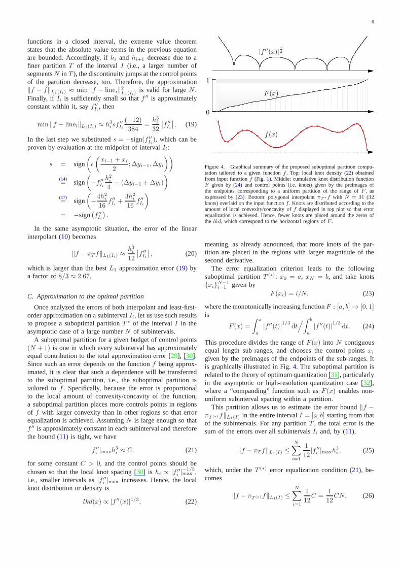
Figure 4. Graphical summary of the proposed suboptimal partition compu-tation tailored to a given functionf . Top: local knot density (22) obtainedfrom input functionf (Fig. 1). Middle: cumulative knot distribution functionF given by (24) and control points (i.e. knots) given by the preimages ofthe endpoints corresponding to a uniform partition of the range of F , asexpressed by (23). Bottom: polygonal interpolantπT∗f with N = 31 (32knots) overlaid on the input functionf . Knots are distributed according to theamount of local convexity/concavity off displayed in top plot so that errorequalization is achieved. Hence, fewer knots are placed around the zeros ofthe lkd, which correspond to the horizontal regions ofF .

meaning, as already announced, that more knots of the par-tition are placed in the regions with larger magnitude of thesecond derivative.

The error equalization criterion leads to the followingsuboptimal partitionT (∗): x0 = a, xN = b, and take knotsxiN−1

i=1 given byF (xi) = i/N, (23)

where the monotonically increasing functionF : [a, b] → [0, 1]is

F (x) =

ˆ x

a

|f ′′(t)|1/3 dt/

ˆ b

a

|f ′′(t)|1/3 dt. (24)

This procedure divides the range ofF (x) into N contiguousequal length sub-ranges, and chooses the control pointsxi

given by the preimages of the endpoints of the sub-ranges. Itis graphically illustrated in Fig.4. The suboptimal partition isrelated to the theory of optimum quantization [31], particularlyin the asymptotic or high-resolution quantization case [32],where a “companding” function such asF (x) enables non-uniform subinterval spacing within a partition.

This partition allows us to estimate the error bound‖f −πT (∗)f‖L1(I) in the entire intervalI = [a, b] starting from thatof the subintervals. For any partitionT , the total error is thesum of the errors over all subintervalsIi and, by (11),

‖f − πT f‖L1(I) ≤N∑

i=1

1

12|f ′′

i |maxh3i , (25)

which, under theT (∗) error equalization condition (21), be-comes

‖f − πT (∗)f‖L1(I) ≤N∑

i=1

1

12C =

1

12CN. (26)

7

To determineC, sum |f ′′i |

1/3maxhi ≈ C1/3 over all subintervals

Ii and approximate the result using the Riemann integral:

C1/3N ≈N∑

i=1

|f ′′i |1/3maxhi ≈

ˆ b

a

|f ′′(t)|1/3 dt, (27)

whose right hand side does not depend onN . Substituting (27)in (26) gives the approximate error bound for the polygonalinterpolant over the entire intervalI = [a, b]:

‖f − πT (∗)f‖L1(I) .1

12N2

(

ˆ b

a

|f ′′(t)|1/3 dt)3

. (28)

Finally, in the asymptotic case of largeN , the approxima-tion error off is roughly proportional to that ofπT f as shownin (19) and (20). Hence, the partition specified by (23) is also aremarkable approximation to the optimal partition forf asNincreases. This, together with (28) implies that both polygonalapproximations converge tof at a rate of at leastO(N−2).

Following a similar procedure, it is possible to estimatean error bound on the uniform partitionTU , which can becompared to that of the optimized one. ForTU , substitutehi = (b − a)/N in (25) and approximate the result usingthe Riemann integral,

‖f − πTUf‖L1(I) ≤

h2i

12

N∑

i=1

|f ′′i |maxhi

≈ (b− a)2

12N2‖f ′′‖L1(I). (29)

The quotient of (28) and (29) provides an estimate of the gainobtained by optimizing a partition.

D. Extension to vector valued functions

Let us point out, using a geometric approach, how theprevious method may be extended to handle vector valuednonlinear functions, i.e., functions with multiple valuesforthe samex. Let f(x) =

(

f1(x), . . . , fn(x))⊤ ∈ R

n consistof several functionsfj(x) defined over the same intervalI, and let ‖v‖1 =

∑nj=1 |vj | be the usual 1-norm inRn.

Without loss of generality, consider the casen = 2. The vectorvalued functionf(x) =

(

f1(x), f2(x))⊤

can be interpretedas the curveC : I ∋ x 7→ (f1(x), f2(x), x)

⊤ ⊂ R3.

Considering a partitionT of the intervalI into N subintervalsIi = [xi−1, xi], the linear interpolant between pointsC(xi−1)and C(xi) is the line joining them, i.e.,ri : Ii ∋ x 7→(πT f1(x), πT f2(x), x)

⊤ ⊂ R3. If, in each subintervalIi, we

measure the distance betweenC and the approximating lineri by the L1 distance of their canonical projections on thefirst n = 2 coordinate planes,‖f − πT f‖L1(Ii) =

∑nj=1 ‖fj −

πT fj‖L1(Ii), whereπT f(x) = (πT f1(x), πT f2(x))⊤, then the

total distance between the curveC and the polygonal lineapproximating it (consisting of linear segmentsriNi=1) is

‖f − πT f‖L1(I) =

N∑

i=1

‖f − πT f‖L1(Ii). (30)

In this framework, we may follow similar steps as those inSectionsIII-A throughIII-C, to conclude that now‖f ′′(x)‖1

plays the role of|f ′′(x)|. Hence (22) becomeslkd(x) ∝‖f ′′(x)‖1/31 and this may be used in the procedure (23)-(24) toobtain the suboptimal partition and approximate upper boundformulas (analogous to (28) and (29)) for (30). For largeN ,the 8/3 factor between the errors of the vector valued linearinterpolant and the bestL1 approximation still holds, i.e.,‖f − f‖L1(I) ≈ 3

8‖f − πT f‖L1(I) due to the independence ofthe optimizations in each coordinate plane given a partition T .

IV. COMPUTATIONAL COMPLEXITY

The evaluation ofv(x) for any polygonal functionv ∈ VT ,such as f and πT f previously discussed, is very simpleand consists of three steps: determination of the subintervalIi = [xi−1, xi) such thatxi−1 ≤ x < xi, computation ofthe fractional distanceδi(x) = (x − xi−1)/(xi − xi−1), andinterpolation of the resulting valuev(x) = (1− δi(x)) vi−1 +δi(x)vi. Regardless of the specific polygonal function underconsideration, the computational cost of its evaluation isdom-inated by the first step, which ultimately depends on whetheror not the partitionT is uniform. In the general case ofTnot being uniform, the first step of the evaluation impliessearchingT for the correct indexi; since T is an orderedset, we can employ a binary search to determinei, whichmeans that the computational complexity of the evaluation ofv(x) is O(logN) in the worst case. However, in the particularcase ofT being uniform, the first and second steps of thealgorithm greatly simplify:i ⇐ 1+⌊N (x− x0) / (xN − x0)⌋and δi(x) = 1 − i + N (x− x0) / (xN − x0); therefore, itsuffices to store the endpointsx0, xN and, most importantly,the computational complexity of the evaluation ofv(x) be-comesO(1).

Consequently, approximations based on uniform partitionsare expected to perform better, in terms of execution time,than those based on optimized partitions. However, ifx can bereasonably predicted (e.g., due to it being the next sample of awell-characterized input signal, such as in digital predistortersfor power amplifiers [3], [33]), other search algorithms withless mean computational complexity than binary search couldbe used to benefit from the reduced memory requirement ofoptimized partitions without incurring too great a computa-tional penalty.

The proposed algorithm is very simple to implement oneither CPUs or GPUs. However, the GPU case is speciallyrelevant because its texture filtering units are usually equippedwith dedicated circuitry that implements the interpolationstep of the algorithm in hardware [34], further acceleratingevaluation.

V. EXPERIMENTS

To assess the performance of the developed linearizationtechnique we have selected a nonlinear function that is usedin many applications in every field of science, the Gaussianfunction f(x) = exp(−x2/2)/

√2π. We approximate it using

a varying number of segments and a varying domain.Figure 5 showsL1 distances between the Gaussian func-

tion and the polygonal approximations described in previoussections, in the intervalx ∈ [0, 4]. The bestL1 polygonal

8

10−7

10−6

10−5

10−4

10−3

L1distance

15 31 63 127 255 511N

Actual πTUf

Approx. bound πTUf

Actual f on TU

Approx. bound f on TU

Actual πT (∗)f

Approx. bound πT (∗)f

Actual f on T (∗)

Approx. bound f on T (∗)

Figure 5. L1 distance for different polygonal approximations to the Gaussianfunction f(x) = exp(−x2/2)/

√2π in the intervalx ∈ [0, 4].

approximation was computed as explained in SectionII , usingthe Newton-Raphson iteration starting from the coefficients ofthe bestL2 approximation. The implementation relied in theMATLAB function lsqnonlin with tridiagonal Hessian andtolerances for stopping criteria:10−16 in parameter space and10−10 in destination space. Convergence was fast, requiringfew iterations (typically less than 25 function evaluations) ina process that is carried out once and off-line previous to theapplication of the linearized function.

The computation of the optimized partitionT ∗ requiredindependently solving equation (23) for each of theN − 1free knots ofT ∗. This solely relies in standard numericalintegration techniques, taking few seconds to complete, asopposed to recursive partitioning techniques such as [35],which take significantly longer.

The figure reports measured distances as well as the approx-imate upper bounds to the distances (28) and (29) using theRiemann integral to approximate the sums. The measuredL1

distances betweenπT f andf using the uniform and optimizedpartitions agree well with (29) and (28), respectively, whichhave aO(N−2) dependence rate that is also applicable to therest of the curves since they all have similar slopes. The fitis good even for modest values ofN (e.g.,N = 15). Also,the ratio between the distances corresponding tof andπT f isapproximately the value3/8 originating from (19) and (20).

Equations (28), (29) and/or the curves in Fig.5 can be usedto select the optimal value ofN solely based on distanceconsiderations. For example, in an application with a target L1

error tolerance‖ · ‖L1(I) ≤ 10−5, we obtainN ≥ ⌈253.9⌉ =254 for πTU

f (Eq. (29)), N ≥ ⌈212.2⌉ = 213 for πT∗f(Eq. (28)), N ≥ ⌈253.9

√

3/8⌉ = ⌈155.5⌉ = 156 for f onTU andN ≥ ⌈212.2

√

3/8⌉ = ⌈129.9⌉ = 130 for f on T ∗.Table I shows mean processing times per evaluation both

on a CPU (sequentially, one core only) and on a GPU. Allexecution time measurements have been taken in the samecomputer, equipped with an Intel Core i7-2600K processor, 16GiB RAM and an NVIDIA GTX 580 GPU. We compare thefastest option [36] for implementing the Gaussian function us-ing its definition against its approximation using the proposed

Table IMEAN PER-EVALUATION EXECUTION TIMES (IN PICOSECONDS).

VTU: POLYGONAL FUNCTIONS DEFINED ON A UNIFORM PARTITION.

VT∗ : POLYGONAL FUNCTIONS DEFINED ON AN OPTIMIZED PARTITION.

Number of points (N + 1) 32 64 128 256 512

CPUGaussian function 13710Function inVTU

1750 - 1780Function inVT∗ 8900 11230 13830 16910 20120

GPUGaussian function 14.2Function inVTU

7.8 - 7.9Function inVT∗ 122.7 142.9 163.2 188.3 211.1

10−7

10−6

10−5

10−4

10−3

10−2

L1distance

15 31 63 127 255 511N

Actual πTUf

Approx. bound πTUf

Actual f on TU

Approx. bound f on TU

Actual πT (∗)f

Approx. bound πT (∗)f

Actual f on T (∗)

Approx. bound f on T (∗)

Figure 6. L1 distance for different polygonal approximations to the Gaussianfunction f(x) = exp(−x2/2)/

√2π in the intervalx ∈ [0, 8].

algorithm. Note that the processing time of any polygonalfunctionv ∈ VT solely depends onT , as shown in SectionIV;as expected from the analysis, execution times are constantinthe case of a uniform partition and grow logarithmically withN in the case of an optimized partition. The proposed strategy,using a uniform partition, solidly outperforms conventionalevaluation of the nonlinear function.

The approximation errors inL1 distance over the intervalx ∈ [0, 8] were also measured. These measurements andthe corresponding approximate upper bounds are reported inFig. 6. Observe that, in this case, the curve‖f − fTU

‖L1([0,8])

is above‖f − πT (∗)f‖L1([0,8]), whereas in the interval[0, 4]the relation is the opposite (Fig.5). This issue is easilyexplained by our previous error analysis: the gap betweenthe approximation errors of the interpolant and the bestL1

approximation is constant ((20)/(19)≈ 8/3), whereas the gainobtained by optimizing a partition (‖f − πTU

f‖L1(I)/‖f −πT∗f‖L1(I) or ‖f − fTU

‖L1(I)/‖f − fT∗‖L1(I)) depends onthe approximation domainI. Fig. 7 shows both gains asfunctions of b in the intervalI = [a, b], with a = 0. Thehorizontal line at8/3 corresponds to the gain obtained byusing the bestL1 approximation instead of the interpolant,regardless of the partition. The blue solid line shows the gainobtained by optimizing a partition, (29)/(28). As b increases,it behaves asymptotically as the parabola (29)/(28) ≈ 0.077b2

(dashed line), which can readily be seen by taking the limitlimb→∞ ‖f ′′‖L1(I)/

(´ b

a |f ′′(t)|1/3 dt)3 ≈ 0.077. As b in-

creases, most of the gain is due to the approximation of the tail

9

2 3 4 5 6 7 80

0.5

1

1.5

2

2.5

3

3.5

4

4.5

5

b

Figure 7. Blue: gain obtained by optimizing a partition: (29)/(28) for theGaussian functionf(x) = exp(−x2/2)/

√2π, as a function ofb in the

interval I = [0, b]. Green: gain obtained by using the bestL1 approximationinstead of the interpolant.

|f ′′(x)| 13

f(x)

Figure 8. Suboptimal partition for the linear chirp function f(x) =sin(10πx2) in the interval x ∈ [0, 1]. Top: local knot density (lkd)corresponding tof . Bottom: polygonal interpolantπT∗f with N = 127(128 knots) overlaid on functionf .

of the Gaussian by few and large linear segments, which leavesmost of the budget of control points to better approximate thecentral part of the Gaussian. The point at which the gain (blueline) meets the horizontal line at8/3 indicates the value ofbwhere the‖f − fTU

‖L1([0,b]) and‖f −πT (∗)f‖L1([0,b]) curvesswap positions.

Chirp function

The performance of the linearization technique has alsobeen tested on a more challenging case: the chirp functionf(x) = sin(10πx2), which combines both nearly flat andhighly oscillatory parts (see Fig.8). Figure 9 reports theL1 distances between the chirp function and the polygonalapproximations described in previous sections, in the intervalx ∈ [0, 1]. ForN ≥ 63 the measured errors agree well with thepredicted approximate error bounds, whereas forN < 63 themeasured errors differ from the predicted ones (specifically inthe optimized partition) because in these cases the number oflinear segments is not enough to properly represent the highfrequency oscillations.

A sample optimized partition and the corresponding polygo-nal interpolantπT∗f is also represented in Fig.8. The knots ofthe partition are distributed according to the local knot density

10−5

10−4

10−3

10−2

10−1

L1distance

31 43 63 127 255 511N

Actual πTUf

Approx. bound πTUf

Actual f on TU

Approx. bound f on TU

Actual πT (∗)f

Approx. bound πT (∗)f

Actual f on T (∗)

Approx. bound f on T (∗)

Figure 9. L1 distance for different polygonal approximations to the chirpfunction f(x) = sin(10πx2) in the intervalx ∈ [0, 1].

(lkd) (see Fig.8, Top), whose envelope grows according tox2/3, and this trend is reflected in the accumulation of knotsin the regions of high oscillations (excluding the places aroundthe zeros of thelkd).

The evaluation times coincide with those of the Gaussianfunction (TableI) because the processing time of the polygonalapproximation does not depend on the function values.

VI. CONCLUSIONS

We have developed a practical method to linearize andnumerically evaluate arbitrary continuous real-valued func-tions in a given interval using simpler polygonal functionsand measuring errors according to theL1 distance. As a by-product, our technique allows fast (e.g., real-time) implemen-tation of computationally expensive applications that usesuchmathematical functions.

To this end, we analyzed the polygonal approximationsgiven by the linear interpolant and the least-first-power orbestL1 approximation of a function. A detailed error analysis in theL1 distance was carried out seeking a nearly optimal designof both approximations for a given budget of subintervalsN .In the practical asymptotic case of largeN , we used errorequalization to achieve a suboptimal design (partitionT )and derive a tight bound on the approximation error forthe linear interpolant, showingO(N−2) dependence rate thatwas confirmed experimentally. The bestL1 approximationimproves upon the results of the linear interpolant by a roughfactor of 8/3.

Combining both quality and computational cost criteria, weconclude from this investigation that, from an engineeringstandpoint, using the bestL1 polygonal approximation inuniform partitions is an excellent choice: it is simple, fastand its error performance is very close to the limit definedby optimal partitions. Possible paths to explore related toourtechnique are, among others, extension to multidimensionalfunctions and the incorporation of constraints in the lineariza-tion process (e.g., so that the bestL1 polygonal model alsosatisfies positivity or a target bounded range).

10

REFERENCES

[1] T. Hatanaka, K. Uosaki, and M. Koga, “Evolutionary computationapproach to Wiener model identification,” inProc. Congress on Evo-lutionary Computation. CEC ’02, vol. 1, 2002, pp. 914–919.

[2] R. Tanjad and S. Wongsa, “Model structure selection strategy for Wienermodel identification with piecewise linearisation,” inProc. Int. Conf.Electrical Engineering/Electronics, Computer, Telecommunications andInformation Technology (ECTI-CON), 2011, pp. 553–556.

[3] J. Cavers, “Optimum table spacing in predistorting amplifier linearizers,”IEEE Trans. Veh. Technol., vol. 48, no. 5, pp. 1699–1705, 1999.

[4] S.-N. Ba, K. Waheed, and G. Zhou, “Efficient spacing scheme fora linearly interpolated lookup table predistorter,” inIEEE Int. Symp.Circuits and Systems (ISCAS), 2008, pp. 1512–1515.

[5] F. Belkhouche, “Trajectory-based optimal linearization for nonlinearautonomous vector fields,”IEEE Trans. Circuits Syst. I, Reg. Papers,vol. 52, no. 1, pp. 127–138, 2005.

[6] M. Storace and O. De Feo, “Piecewise-linear approximation of nonlineardynamical systems,”IEEE Trans. Circuits Syst. I, Reg. Papers, vol. 51,no. 4, pp. 830–842, 2004.

[7] P. Julian, A. Desages, and O. Agamennoni, “High-level canonicalpiecewise linear representation using a simplicial partition,” IEEE Trans.Circuits Syst. I, Fundam. Theory Appl., vol. 46, no. 4, pp. 463–480, 1999.

[8] P. Brox, J. Castro-Ramirez, M. Martinez-Rodriguez, E. Tena,C. Jimenez, I. Baturone, and A. Acosta, “A Programmable and Con-figurable ASIC to Generate Piecewise-Affine Functions Defined OverGeneral Partitions,”IEEE Trans. Circuits Syst. I, Reg. Papers, vol. 60,no. 12, pp. 3182–3194, 2013.

[9] K. H. Usow, “On L1 Approximation I: Computation for ContinuousFunctions and Continuous Dependence,”SIAM J. Numerical Analysis,vol. 4, no. 1, pp. 70–88, 1967.

[10] R. Bellman and R. Roth, “Curve fitting by segmented straight lines,”Journal of the Amer. Stat. Assoc., vol. 64, no. 327, pp. 1079–1084,1969.

[11] S. Ghosh, A. Ray, D. Yadav, and B. M. Karan, “A Genetic AlgorithmBased Clustering Approach for Piecewise Linearization of NonlinearFunctions,” in Int. Conf. Devices and Communications (ICDeCom),2011, pp. 1–4.

[12] J. Rice, “On nonlinear L1 approximation,”Arch. Rational Mech. Anal.,vol. 17, pp. 61–66, 1964.

[13] ——, “On the computation of L1 approximations by exponentials,rationals, and other functions,”Math. Comp., vol. 18, pp. 390–396, 1964.

[14] A. Pinkus,On L1-Approximation, ser. Cambridge Tracts in Mathematics.Cambridge University Press, 1989.

[15] J. Gallego, M. Pardas, and J.-L. Landabaso, “Segmentation and trackingof static and moving objects in video surveillance scenarios,” in IEEEInt. Conf. Image Processing (ICIP), 2008, pp. 2716–2719.

[16] M. Guillaumin, T. Mensink, J. Verbeek, and C. Schmid, “Face recogni-tion from caption-based supervision,”Int. J. Comp. Vis., vol. 96, no. 1,pp. 64–82, 2012.

[17] Z. Xie and L. Guan, “Multimodal Information Fusion of Audio EmotionRecognition Based on Kernel Entropy Component Analysis,” in IEEEInt. Symp. on Multimedia, 2012, pp. 1–8.

[18] M. Sehili, D. Istrate, B. Dorizzi, and J. Boudy, “Daily sound recognitionusing a combination of GMM and SVM for home automation,” inProc.20th European Signal Proc. Conf., Bucharest, 2012, pp. 1673–1677.

[19] G. Gallego, C. Cuevas, R. Mohedano, and N. Garcia, “On the Maha-lanobis Distance Classification Criterion for Multidimensional NormalDistributions,”IEEE Trans. Signal Processing, vol. 61, no. 17, pp. 4387–4396, 2013.

[20] R. Plato, Concise Numerical Mathematics, ser. Graduate Studies inMathematics. Amer. Math. Soc., 2003, vol. 57.

[21] T. J. Rivlin, An Introduction to the Approximation of Functions. CourierDover Publications, 1981.

[22] J. Rice,The Approximation of Functions: Linear theory, ser. Addison-Wesley Series in Computer Science and Information Processing. Mass.,Addison-Wesley Publishing Company, 1964.

[23] R. A. DeVore, “Nonlinear approximation,”Acta Numerica, pp. 51–150,1998.

[24] T. K. Moon and W. C. Stirling,Mathematical Methods and Algorithmsfor Signal Processing. Prentice Hall, 2000.

[25] E. W. Cheney and D. R. Kincaid,Numerical Mathematics and Comput-ing, 7th ed. Cengage Learning, 2012.

[26] B. R. Kripke and T. J. Rivlin, “Approximation in the Metric ofL1(X,mu),” Trans. Amer. Math. Soc., vol. 119, no. 1, pp. 101–122, 1965.

[27] D. Jackson, “Note on a class of polynomials of approximation,” Trans.Amer. Math. Soc., vol. 22, no. 3, pp. 320–326, 1921.

[28] ——, The theory of approximation, Reprint of the 1930 original ed., ser.Amer. Math. Soc. Colloq. Pubs. Amer. Math. Soc., 1994, vol. 11.

[29] C. de Boor, “Piecewise linear approximation,” inA Practical Guide toSplines. Springer, 2001, ch. 3, pp. 31–37.

[30] M. Cox, P. Harris, and P. Kenward, “Fixed- and free-knotunivariateleast-square data approximation by polynomial splines,” in Proc. 4thInt. Symp. on Algorithms for Approximation, 2001, pp. 330–345.

[31] A. Gersho, “Principles of quantization,”IEEE Trans. Circuits Syst.,vol. 25, no. 7, pp. 427–436, 1978.

[32] T. Lookabaugh and R. Gray, “High-resolution quantization theory andthe vector quantizer advantage,”IEEE Trans. Inform. Theory, vol. 35,no. 5, pp. 1020–1033, 1989.

[33] K. Muhonen, M. Kavehrad, and R. Krishnamoorthy, “Look-up tabletechniques for adaptive digital predistortion,”IEEE Trans. Veh. Technol.,vol. 49, no. 5, pp. 1995–2002, 2000.

[34] M. Doggett, “Texture Caches,”IEEE Micro, vol. 32, no. 3, pp. 136–141,2012.

[35] J. T. Butler, C. Frenzen, N. Macaria, and T. Sasao, “A fast segmentationalgorithm for piecewise polynomial numeric function generators,” J.Computational and Appl. Math., vol. 235, no. 14, pp. 4076–4082, 2011.

[36] NVIDIA Corp., “CUDA C Programming Guide,” Tech. Rep., 2012.