Optimal edge detection and edge localization in complex SAR images with correlated speckle

2272 IEEE TRANSACTIONS ON GEOSCIENCE AND REMOTE SENSING, VOL. 37, NO. 5, SEPTEMBER 1999

Optimal Edge Detection and Edge Localization inComplex SAR Images with Correlated Speckle

Roger Fjørtoft, Armand Lopes, Jerome Bruniquel, and Philippe Marthon,Associate Member, IEEE

Abstract—We here develop optimal criteria for detection andlocalization of step edges in single look complex (SLC) syntheticaperture radar (SAR) images. By working on complex data ratherthan intensity images, we can easily take the speckle autocor-relation into account, obtain more accurate estimates of localmean reflectivities, and thus achieve better edge detection andedge localization than with operators known from the literature.Algorithms for the two-dimensional (2-D) implementation of themethods are proposed, and some segmentation results are shown.

Index Terms—Edge detection, edge localization, segmentation,single look complex (SLC), synthetic aperture radar (SAR) im-ages, speckle correlation.

I. INTRODUCTION

I N synthetic aperture radar (SAR) scenes with no texture,an edge can be defined as an abrupt change in the reflec-

tivity. The presence ofspeckle,which can be modeled as astrong, multiplicative noise, makes the usual differential edgedetectors inefficient. In particular, the false alarm rate varieswith the reflectivity. Several edge detectors with constantfalse alarm rate have therefore been developed specificallyfor SAR images, of which the normalized ratio (NR) [1],[2] and the generalized likelihood ratio (GLR) [3] operatorsare well-known examples. The latter can be considered as theoptimal solution, and is shown to yield better edge detectionperformance than other criteria that have been proposed. Bothoperators work on detected (intensity) data, and the speckle issupposed to be Gamma distributed and spatially uncorrelated.They rely on the maximum likelihood (ML) estimator of thelocal mean reflectivity, which is the arithmetic mean intensity(AMI) in this case. Oliver et al. [3] propose a two-stagealgorithm, which first detects step edges optimally using theGLR operator, and then determines the most probable edgepositions. In fact, the same radiometric criterion is used inboth stages, but the window configuration is different: ascanning-window central-edge (SWCE) configuration is used

Manuscript received August 31, 1998; revised June 1, 1999. This work wassupported by the French Space Agency CNES. The SARSO segmentationscheme was developed under Contract 833/CNES/94/1022/00 and R&TCNES OT/403*03.

R. Fjørtoft and A. Lopes are with the Centre d’Etudes Spatialesde la Biosphère (CESBIO), 31401 Toulouse, France (e-mail:[email protected]; [email protected]).

J. Bruniquel is with Alten Sud-Ouest, 31312 Labège, France, (e-mail:[email protected]).

P. Marthon is with the Laboratoire d’Informatique et de MathématiquesAppliquees (LIMA), Ecole Nationale Superieure d’Electrotechnique,d’Electronique, d’Informatique et d’Hydraulique de Toulouse (ENSEEIHT),Institut de Recherche en Informatique de Toulouse (IRIT), 31071 Toulouse,France (e-mail: [email protected]).

Publisher Item Identifier S 0196-2892(99)07191-0.

for detection, whereas a fixed-window scanning-edge (FWSE)configuration is used to improve the edge localization.

SAR data generally has correlated speckle, in which case anunderlying hypothesis of the NR and GLR criteria describedabove is violated. As a consequence, the statistics of theoperators will not be exact, and the performance becomessuboptimal. We here develop similar criteria for edge detectionand edge localization in single look complex (SLC) images,which give optimal results even when the speckle is spatiallycorrelated. Single look images offer the highest spatial resolu-tion, but the maximum strength of the fully developed specklemakes visual interpretation and automatic analysis of suchSAR images particularly difficult. The theoretical study is hererestricted to the monoedge case, which means that we supposethat there is never more than one edge within the analyzingwindow. The presence of multiple edges was considered in [4].A certain edge direction will also be assumed. The derivationof the optimal criteria is detailed in the first part of the article.We then address problems related to the two-dimensional (2-D)implementation and propose suitable algorithms. We finallypresent theoretical and empirical curves which illustrate thesupremacy of the new criteria, as well as some segmentationresults obtained on simulated and real SAR images.

II. EDGE DETECTION

A. Vectorial Probability Distributions

Let us consider a window centered on a given pixel in aSLC image. The window is split in two parts, containingand pixels, respectively. Let and be the complexsignal vectors corresponding to the two half windows, andlet be the signal vector containing the pixels of theentire window. If the speckle is fully developed, the probabilitydensity functions (PDF’s) of the different signal vectors arecircular complex Gaussian distributions [5]–[7]

(1)

where is the complex spatial covariance matrixcorresponding to signal vector , .

B. Neyman–Pearson Test

We want to test the hypothesis , saying that andare separated by an edge and cover homogeneous regions withdifferent reflectivities and , against the null hypothesis

, which says that corresponds to a zone of constant

0196–2892/99$10.00 1999 IEEE

FJØRTOFTet al.: COMPLEX SAR IMAGES WITH CORRELATED SPECKLE 2273

(a) (b)

Fig. 1. The 7� 7 (a) SWCE configuration and (b) FWSE configuration forvertical edges.

reflectivity . Hence the likelihood ratio (LR) for edgedetection is

(2)

The null hypothesis is rejected if is superior to athreshold .

Obviously, . If and areindependent, , and (2)becomes

(3)

As the speckle is correlated, and must be separatedspatially by a distance which is greater than the correlationlength, in order to be independent. For most sensors thespeckle correlation becomes insignificant for lags of more thanone or two pixels. Hence this requirement is not very restrictivein the case of edge detection with the SWCE approach, wherea window configuration like the one shown in Fig. 1(a) canbe used.

Substituting the probabilities in (1) into (3) and taking thelogarithm yields

(4)

where denotes the complex conjugate transpose of.

C. Complex Speckle Covariance

For each of the signal vectors , we suppose that theunderlying reflectivity is constant. If this is true, the mul-tiplicative speckle model allows us to express the covariancematrix of signal vector as

(5)

where represents the spatial covariance due to speckle.The spatial covariance matrix of the SLC speckle only

depends on sensor and SAR processor parameters. Principally,it should therefore be possible to obtain exact values from thedata provider. If is unknown, it can be estimated on anypart of the SLC image where the speckle is fully developedand where the mean reflectivity is not so low that the thermalnoise becomes dominant. The underlying reflectivity does notnecessarily need to be constant [8]. However, the correlations

are not exactly the same in near range and in far range. Thiscan be taken into account by using several different matriceswhen processing over the full swath. To produce the matrices

, , we simply rearrange the elements of inaccordance with the corresponding signal vectors. The specklevariance is one, so the elements of the covariance matrixare the correlation coefficients of the speckle, .

D. Spatial Whitening Filter

The reflectivities are in our case unknown and mustbe estimated. From (1) and (5) it can easily be shown thatthe ML estimator of reflectivity for SLC images is the spatialwhitening filter (SWF), which is given by

(6)

A whitening filter (WF) was used in [6] to obtain an intensityimage with minimal speckle variance from polarimetric data.A combined spatial and polarimetric WF was proposed in [7]for improved target detection. In [9], [10] it was shown thatthe WF is a ML estimator of texture.

Taking the AMI of pixels does not reduce the varianceby a factor , as in the case of uncorrelated speckle, butby a factor , and the computed mean values are onlyapproximately Gamma distributed [11]. However, if the data isavailable in SLC format, the optimal variance reduction factor

can be attained using the SWF. Moreover, the SWF outputis truly Gamma distributed.

Let us now assume that the covariance matrix in (6)is not perfectly known, so that we have to use an estimatedmatrix . The expectation of the estimated reflectivitycomputed by the SWF is then given by [10]

Tr (7)

which means that the SWF is an unbiased estimator only when. Hence any inaccuracy in will introduce a

bias on . In addition, the thermal noise causes a weak over-estimation of the reflectivities, which slightly reduces the edgecontrasts, but this phenomenon is not particular to the SWF.

The SWF performs well on correctly sampled complex SARimages, but as it involves a whitening process, it encountersproblems in terms of variance reduction and bias when appliedto images where a part of the spectrum is zero. Such zero-padding can easily be eliminated by resampling the image,without any loss of information. We have, however, noticedthat the SWF computed on a small window yields correctresults even if a fraction of the spectrum is zero [12].

The number of multiplications per pixel for the SWF isabout , so the computational cost becomes considerablefor very large windows. A practical solution is to calculatethe SWF on partially overlapping smaller windows within thebig window, and then average the results in intensity. Thecomputational complexity of this hybrid filter is only slightlyhigher than that of the SWF for the smaller window, and it isfar more robust to zero-padding in the spectral domain. Theperformance lies between that of the SWF and that of theAMI [12].


E. Likelihood Ratio Operator

If the pixels in the band which assures the independencebetween and are excluded from ,and it can easily be shown that . Using(5), and in particular the fact that ,we may rewrite (4) as

(8)

where is computed by the SWF (6). The LR is an optimaldetector, in the sense that it maximizes the probability ofdetection (PD) for a given probability of false alarm (PFA).The PFA is the probability of detecting an edge in a zone ofconstant reflectivity. However, we see from (8) thatdependson the reflectivities , which are unknown in our case. Hencethe LR is only of theoretical interest here, and it will not beanalyzed any further.

F. Generalized Likelihood Ratio Operator

If we replace the unknown reflectivities in the LR bythe ML estimations , we obtain the GLR. From (8) we seethat the GLR is given by

(9)

While the LR is optimal in the general case, the GLR can onlybe shown to be optimal in theminimax sense for Gaussianvariables [13]. This implies that the GLR given by (9) is anoptimal detector, at least for weak edge contrasts.

It is interesting to note that (9) is similar to the expressionderived by Oliveret al. for intensity images [3]. The onlydifference resides in the way the local mean reflectivities areestimated. As the SWF reduces to the AMI when the speckleis uncorrelated, the criterion presented in [3] is a special caseof (9). Also the GLR for intensity images can therefore beconsidered as an optimal detector, when the hypothesis ofuncorrelated speckle is verified.

The PDF of the GLR operator given by (9) has not beendeveloped analytically. In order to compute the theoreticalPFA corresponding to a threshold or vice versa, a simplesolution is to use the relation between the GLR and a SWF-based version of the double-sided ratio (DR) operator [1]

(10)

whose distribution is [1], [3]

(11)

For two thresholds and of the DR, whichare used when and when , respectively,

the PD is given by

(12)

which may be computed by numerical integration. However,it can be shown that [3], [14]

(13)

where is the hypergeometric function [15]. The computationof the PFA ( ) or the PD ( ) corresponding toa pair of thresholds and can be effectuated very efficientlythrough (13), as the hypergeometric function here reduces toa finite series.

The relation between and is found by rearranging theterms of (9)

(14)

In practice, we first fix the PFA that can be accepted. Thenext step is to find the appropriate thresholdfor the GLR,which will be used to decide whether or not an edge is present.We guess a first value for , solve (14) with respect to toobtain the two corresponding thresholdsand for the DR,and compute the PFA by introducing, , andinto (13). The threshold is adjusted and the procedure isrepeated until the computed PFA is sufficiently close to thedesired one. If we measure in a given pixel position,it indicates the presence of an edge with a risk of error equalto the specified PFA.

The normalized ratio (NR) proposed by Touziet al. [1] canalso be mapped to

(15)

Here, we consider a version of the NR operator whereand are computed by the SWF, so that problems due tospeckle correlation are eliminated. A given thresholdforthe NR corresponds to the thresholds andof the DR, which in general are different from the optimalthresholds and found through (14). For the SWCEconfiguration, however, where , it can easily beshown that , so that the GLR and NR performancescoincide.

The GLR given by (9) was developed under the hypothesisthat the half windows can be made independent by introducinga band of pixels between them. If the and cannot bemade independent, due to the correlation length or restrictions


on the window configuration, the true GLR can be computeddirectly from (2), by substituting estimated parameters into thePDF’s, similar to the edge localization method described inSection III-A. This approach is computationally complex, butwe have shown that (9) represents an excellent approximation,and that the speckle correlation between the half windowsactually improves the detector performance [16].

III. EDGE LOCALIZATION

Edge localization is an estimation problem rather than adetection problem. Assuming that an edge is present withinthe window, we want to determine the most probable edgeposition. Edge localization can therefore be considered asa refinement stage following the edge detection proceduredescribed above. The question is how to divide intoand .

A. ML Estimator

ML estimation of the edge position consists in maximizingthe probability density function given in (1) with respectto the edge position, or equivalently, by computing

(16)

where the energy function is given by

(17)

Using the FWSE configuration illustrated in Fig. 1(b), wecenter the window on the detected edge pixel and split thewindow in all possible edge positions. As the ML estimatormust use the same data set for all positions, we cannotintroduce any band of pixels separating the two parts of thewindow. The signal vectors and will consequently bedependent. For each pair of signal vectors the SWF definedin (6) is used to compute and . Let be a columnvector where the elements which correspond to are setto and the other elements are set to . We cannow write

(18)

where denotes the element-by-element product of twoequally sized matrices. To estimate the edge position using(16), the matrix , its determinant and its inverse mustbe computed for each new window position, and for allpossible edge positions within the window. If we denote thenumber of possible edge positions by, the total number ofmultiplications per edge pixel is about

.

B. Approximate ML Solution

If the window is big and the speckle correlation is relativelyweak, we may consider and as approximately indepen-dent. In this case . Asis constant for a fixed window position, is proportional

to in (3). Hence the most probable edge can be computedby (16) with the suboptimal energy function

(19)

Computing (16) with the new cost function requires aboutmultiplications per edge pixel, which is

far less than for the true ML estimator based on (17).

IV. TWO-DIMENSIONAL IMPLEMENTATION

The description so far is basically one-dimensional (1-D).The 2-D implementation poses some additional problems:First, the edge orientation is in general unknown, so that avariety of edge directions must be considered in the edgedetection stage. Moreover, the monoedge model is not alwaysverified. Depending on the scene type, several edges mayco-occur within the analyzing window, especially if a largewindow is used. Second, we must make sure that the edgesthat we extract are closed and skeleton if we want them todefine a segmentation of the image. Finally, it is essential thatthe edges remain connected and relatively regular in the edgelocalization stage.

A. Two-Dimensional Edge Detection

To detect edges with unknown orientation, a simple ap-proach consists in splitting the analyzing window in severaldifferent directions. We have chosen to compute the SWF-based GLR given by (9) across the vertical, horizontal, anddiagonal axes. The maximum value is retained as the edgestrength of the central pixel. However, the PD’s and PFA’s ofthe operator are not the same as in the unidirectional case. Ifthe GLR’s computed in the four directions were independent,the relation

(20)

could be used for the PFA. Theoretical relations are difficult toestablish when the GLR’s are correlated. In the case of squarewindows, where the half-windows for the different directionsare highly overlapping, the empirical relation

(21)

is a good approximation [1]. For long and narrow windows,which give a lower degree of overlap between the masks fordifferent directions, the observed PFA’s tend toward (20) [17].

On one hand, large windows should be used to reduce theinfluence of the speckle on the estimates of local reflectivities.On the other hand, smaller windows yield higher spatialresolution and the monoedge model is more easily verified.The window size constitutes a compromise between these tworequirements.

Rather than using a fixed size window, a statistical mul-tiresolution approach like the one described [18] can be used.Weak edges separating large regions can then be detected withlarge windows, while strong edges between small regions aredetected with small windows. The fact that GLR’s computedon different resolution levels have different statistical signifi-cance is taken into account: Thresholds corresponding to the


accepted PFA are first computed over the whole range ofrelevant window sizes. The maximum GLR on each level isthen divided by the appropriate threshold, and the maximumnormalized GLR across the resolution levels, which is thestrongest indication of the presence of an edge, is retainedas the edge strength of the pixel.

B. Two-Dimensional Edge Extraction

Plain thresholding of the edge strength map computed bythe multidirectional (multiresolution) GLR operator generallyproduces isolated edge segments that are several pixels wide.Closed, skeleton boundaries defining a segmentation of theimage can be obtained by applying the watershed algorithm[19] to the edge strength map. The watershed algorithm usuallyyields an over-segmented image. To reduce the number of falseor irrelevant edges to an acceptable level, we can threshold thebasin dynamics of the edge strength map [20]. The conceptof edge dynamics [21]–[23] permits a compact, hierarchicalrepresentation of the segmentations obtained by applyingdifferent thresholds to the basin dynamics. The user can thenchoose the best threshold for his application interactively.More details on the use of basin and edge dynamics in SARimage segmentation are given in [24].

Another way of reducing the over-segmentation is to mergeadjacent regions whose mean reflectivities are not significantlydifferent [4], [25].

C. Two-Dimensional Edge Localization

We shall now suppose that the actual contours have beenextracted with the methods described above, but that thedetected edge pixels not necessarily are in the correct positions.The segmentation is initially represented by an edge map, butwe also create a label image, in which every pixel carries thenumber of the region it belongs to. From a radiometric pointof view, the optimal edge position is the one that minimizes thecost function in (17). However, constraints on the regularityof the edges must be included in the energy function, as theradiometric criterion alone tends to create very irregular edgeswhich follow local speckle patterns. We have considered toways of introducing regularity constraints: a simple methodbased on Gibbs random fields, and a more sophisticated onebased on active contours (snakes).

1) Contextual Regularization Using Gibbs Random Fields:Gibbs random fields have been introduced in image process-ing to model regularity constraints in entire images [26].Potts model is a simple and frequently used model, whichhas constant and anisotropic potential functions. It permitsto model geometric regularity efficiently without having tospecify complicated local configurations.

Let the labels within a 3 3 window have indices asshown in Fig. 2(a). The energy term corresponding to Pottsmodel is then given by

(22)

where in our case is a negative constant which controls theweight given to the regularization constraint compared to the

(a) (b) (c)

Fig. 2. Illustration of Potts model (22). (a) The indicesi of the labels`iwithin a 3� 3 window. (b) A regular configuration of labels which yieldsV = 2�=T . (c) An irregular spatial configuration for whichV = �4�=T .

radiometric criterion. The parameterdiminish exponentiallyfrom the initial value during the global optimization stage,similar to the temperature in simulated annealing. The sumin (22) simply calculates the number of pixels in the eight-neighborhood which have the same label as the central pixel,minus the number of pixels which have a different label.

The energy function, including the regularization term,becomes

(23)

where the radiometric term is given by (17) or (19).We traverse the image several times and compute the mini-

mum of (23) with respect to the edge position for each detectededge pixel, similar to what is done in the iterated conditionalmodes (ICM) algorithm [27]. The role of the regularizationterm is to privilege regular shapes, which in most naturalscenes are more likely than very irregular structures.

2) Active Contours:The edge localization algorithm basedon active contours is preceded by a vectorization of the edges,as shown in Fig. 3. The edges are represented by nodes andarcs. We have to set the maximum distance that can beaccepted between an edge pixel and the corresponding arc.The higher the required precision is, the higher the numberof nodes will be. The refinement of the edge position consistsin traversing the list of nodes iteratively, and for each nodecalculate an energy function for a series of new node positionsin its neighborhood. When a new edge position is considered,we have to take the corresponding changes for the arcs and thelabel statistics into account to compute the energy function.If a position with a lower cost is found, the new positionis accepted and the concerned labels and label attributes areupdated before continuing.

The radiometric term in (17) or (19) can again be used. Ifwe use (19), the method is similar to the one proposed byRefregieret al. [28] for intensity images, but our approach isnot restricted to the edges of one single region. Nodes whereseveral regions meet need a special treatment: The energyfunction in (19) can easily be generalized to more than twoadjacent regions.

The fact that we work on vectorized edges constitutes aregularity constraint in itself. However, regularity constraintsbased on the angle between adjoining arcs, or shape parametersmeasuring the overall complexity of the boundary of a region,should be introduced.

V. EXPERIMENTAL RESULTS

The methods were tested on simulated complex specklewhose spatial covariance properties are close to those of the


(a) (b) (c) (d)

Fig. 3. (a) Initial contours, (b) vectorization process, (c) vectorized contours, and (d) modification of the node position to improve the edge localization.

TABLE ISPATIAL CORRELATION OF SIMULATED SLC SPECKLE

TABLE IISPATIAL CORRELATION OF RESAMPLED ERS SLC SPECKLE

speckle in a resampled ERS SLC image, where the spectralzero-padding has been eliminated [12]. The magnitudes of thecorrelation coefficients of the simulated speckle up to a lag oftwo pixels in each direction are shown in Table I, and thoseof the speckle in the resampled ERS SLC image are shownin Table II.

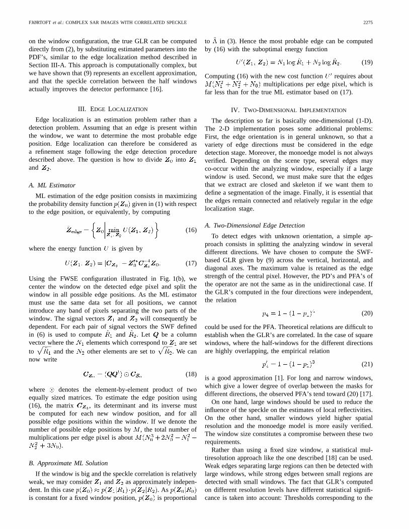
Fig. 4(a) illustrates the speckle reduction capacity of theSWF and the AMI in terms of the equivalent number ofindependent looks, which is equal to the square of estimatedreflectivity divided by its variance in a homogeneous zone.As predicted, the speckle variance is reduced by a factorwhen the SWF is computed on a sliding window coveringpixels of the simulated SLC image, whereas the AMI appliedto the corresponding single look intensity image reduces thespeckle variance by a factor , which is here about 35%lower than , due to the spatial speckle correlation. While theSWF becomes very time-consuming for large windows, hybridfilters are quite rapid. The performance loss of the hybrid filterbased on the SWF computed on a 33 window is about 20%.Starting from the result of the 7 7 SWF, we obtain a specklereduction factor that is only 10% below the optimum, and thecomputational complexity of the hybrid filter is still fair.

For the subsequent tests we used analyzing windows of size7 7. This window size yields a reasonable compromisebetween speckle reduction and spatial resolution for singlelook images, at least for high contrast edges.

We computed the threshold of the GLR operator withthe window configuration shown in Fig. 1(a) for a series

of PFA’s, as described in Section II-F. Experimental PFA’swere measured on the simulated speckle image for the SWF-based GLR in (9) and for the AMI-based GLR [3]. We alsotested a modified AMI-based GLR, where and in(9) and (13) were replaced by the equivalent numbers ofindependent pixels [4], and , to compensate for thespeckle correlation. Fig. 4(b) shows that the correspondencebetween theoretical and measured PFA is excellent for theSWF-based GLR, but that the error is considerable for theAMI-based GLR when no compensation is made for thespeckle correlation. At a theoretical PFA of 0.1%, for example,the measured PFA for the AMI-based GLR is more than fivetimes too high. A much better fit is obtained when usingthe equivalent number of pixels in each half window ratherthan the actual number of pixels. However, the measuredPFA of the correlation compensated AMI-based GLR deviatessomewhat from the theoretical value when it becomes verylow. This is probably due to the fact that the correlated speckleis not truly Gamma distributed. The difference from the truemultilook intensity distribution of SAR images with spatiallycorrelated speckle [11], [29] becomes visible when integratingnear the extremities of (11), which is derived from the Gammadistribution. It should be stressed that Fig. 4(b) only illustratesthe correspondence between predicted and measured PFA’s,and that this has no influence on the performance of thedetectors.

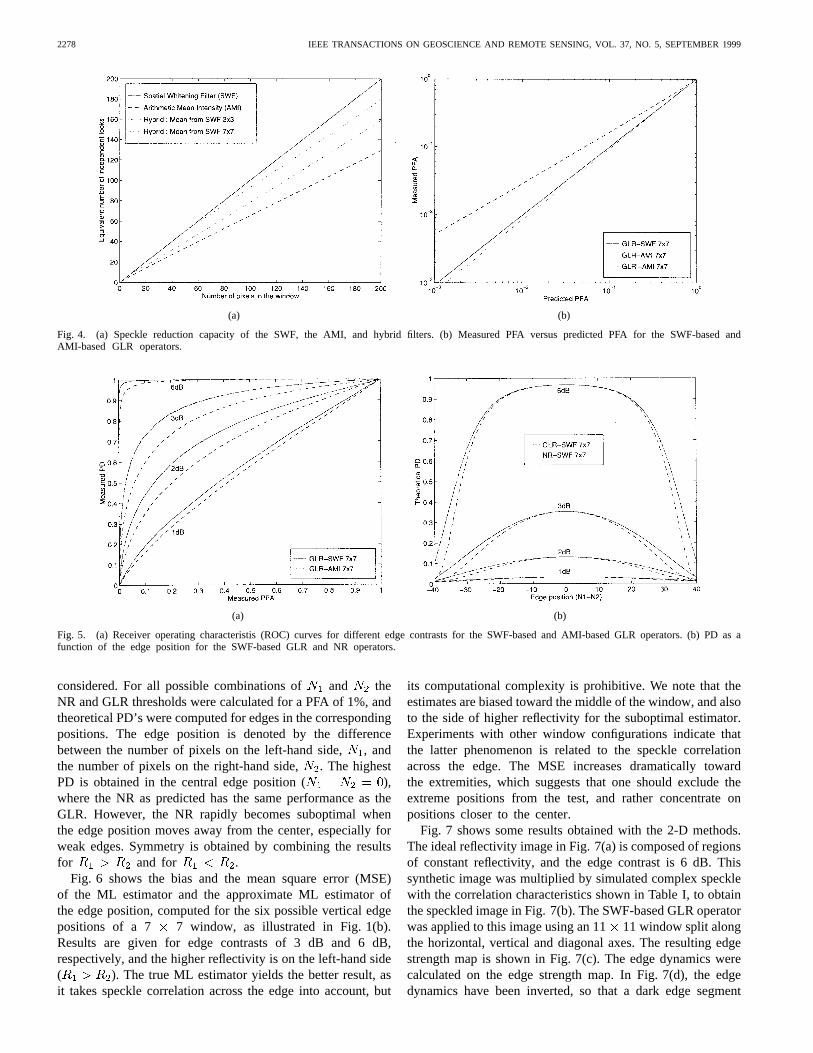
Fig. 5(a) shows the experimental receiver operating charac-teristics (ROC) of the two operators. All edges in the test imagewere vertical, and the window configuration in Fig. 1(a) wasused. The measured PD is plotted against the measured PFA,so that the problem with the fit of the PFA for the AMI-basedGLR has no impact on the results. The SWF-based GLR yieldsa substantially higher PD than the AMI-based GLR for a givenPFA, in particular for intermediate edge contrasts (3 dB). Forthe weakest contrast ratio (1 dB), the difference is modest,but this is an extreme case, where the PD is only slightlyhigher than the PFA. If we use thresholds corresponding to alow PFA (1%), only edges with very strong contrast (6 dB ormore) have a high PD when using a 77 window. A largerwindow must be used if we want to detect weaker edges whilekeeping a low PFA and a high PD.

The theoretical PD as a function of the edge position for theSWF-based versions of the GLR and NR operators is shownin Fig. 5(b). The total number of pixels was set to 42,like in Fig. 1(a), but other ways of splitting the window were


(a) (b)

Fig. 4. (a) Speckle reduction capacity of the SWF, the AMI, and hybrid filters. (b) Measured PFA versus predicted PFA for the SWF-based andAMI-based GLR operators.

(a) (b)

Fig. 5. (a) Receiver operating characteristis (ROC) curves for different edge contrasts for the SWF-based and AMI-based GLR operators. (b) PD as afunction of the edge position for the SWF-based GLR and NR operators.

considered. For all possible combinations of and theNR and GLR thresholds were calculated for a PFA of 1%, andtheoretical PD’s were computed for edges in the correspondingpositions. The edge position is denoted by the differencebetween the number of pixels on the left-hand side,, andthe number of pixels on the right-hand side,. The highestPD is obtained in the central edge position ( ),where the NR as predicted has the same performance as theGLR. However, the NR rapidly becomes suboptimal whenthe edge position moves away from the center, especially forweak edges. Symmetry is obtained by combining the resultsfor and for .

Fig. 6 shows the bias and the mean square error (MSE)of the ML estimator and the approximate ML estimator ofthe edge position, computed for the six possible vertical edgepositions of a 7 7 window, as illustrated in Fig. 1(b).Results are given for edge contrasts of 3 dB and 6 dB,respectively, and the higher reflectivity is on the left-hand side( ). The true ML estimator yields the better result, asit takes speckle correlation across the edge into account, but

its computational complexity is prohibitive. We note that theestimates are biased toward the middle of the window, and alsoto the side of higher reflectivity for the suboptimal estimator.Experiments with other window configurations indicate thatthe latter phenomenon is related to the speckle correlationacross the edge. The MSE increases dramatically towardthe extremities, which suggests that one should exclude theextreme positions from the test, and rather concentrate onpositions closer to the center.

Fig. 7 shows some results obtained with the 2-D methods.The ideal reflectivity image in Fig. 7(a) is composed of regionsof constant reflectivity, and the edge contrast is 6 dB. Thissynthetic image was multiplied by simulated complex specklewith the correlation characteristics shown in Table I, to obtainthe speckled image in Fig. 7(b). The SWF-based GLR operatorwas applied to this image using an 1111 window split alongthe horizontal, vertical and diagonal axes. The resulting edgestrength map is shown in Fig. 7(c). The edge dynamics werecalculated on the edge strength map. In Fig. 7(d), the edgedynamics have been inverted, so that a dark edge segment


(a) (b)

Fig. 6. (a) Bias and (b) mean square error (MSE) of the edge position estimates for edge contrasts of 3 dB and 6 dB.

(a) (b) (c) (d)

(e) (f) (g) (h)

Fig. 7. (a) Ideal reflectivity image with 6 dB edge contrast. (b) Corresponding image with single look correlated speckle. (c) Edge strength map obtainedwith the 11� 11 GLR operator. (d) Inverted edge dynamics. (e) Edges obtained by thresholding the edge dynamics superposed on the ideal image and (f)on the speckled image. (g) Edges after the localization refinement stage superposed on the ideal image, and (h) on the speckled image.

indicates a strong edge. Using an interactive visualizationtool, we observed the segmentation result for a wide range ofthresholds. With the most suitable one, all real edges and onlytwo false ones were detected. This is mainly due to the fact thatwe used a relatively big analyzing window when computingthe edge strength map. However, the edge localization is notalways perfect, as can be seen from Fig. 7(e), where thedetected edges have been superposed on the ideal image. Whenthe segmentation is superposed on the speckled image, asin Fig. 7(f), it is much more difficult to assess such smalldeviations from the correct edge positions by eye. The edge

localization was effectuated with the approximate ML criteriongiven by (16) and (19) and the contextual regularization termbased on Potts model. Several combinations of parameterswere used in (22). The most satisfactory result, obtained with

, , and five iterations, is shown in Fig. 7(g)and (h). The fit to the correct edge positions has generallybecome better, but the contours are slightly more irregular.Stronger regularization created problems at the extremities ofnarrow structures. A better preservation of fine structures canbe obtained with more complex image models, such as theChien model [30].


(a) (b) (c)

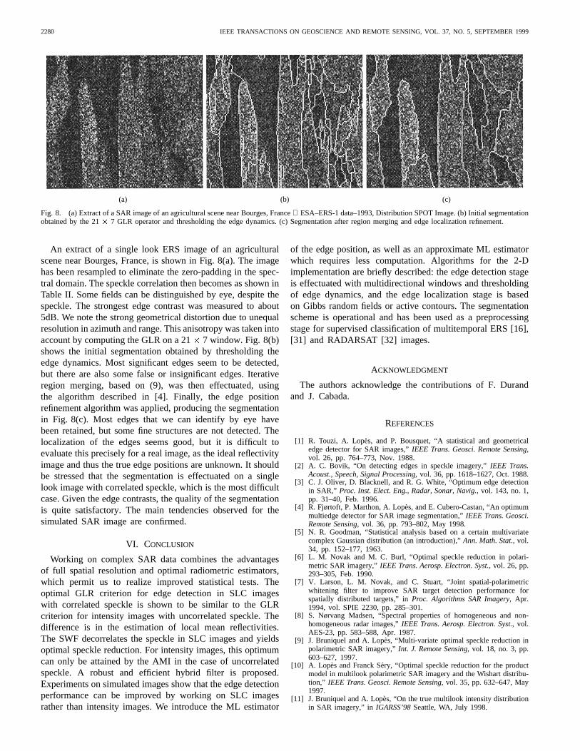
Fig. 8. (a) Extract of a SAR image of an agricultural scene near Bourges, France ESA–ERS-1 data–1993, Distribution SPOT Image. (b) Initial segmentationobtained by the 21� 7 GLR operator and thresholding the edge dynamics. (c) Segmentation after region merging and edge localization refinement.

An extract of a single look ERS image of an agriculturalscene near Bourges, France, is shown in Fig. 8(a). The imagehas been resampled to eliminate the zero-padding in the spec-tral domain. The speckle correlation then becomes as shown inTable II. Some fields can be distinguished by eye, despite thespeckle. The strongest edge contrast was measured to about5dB. We note the strong geometrical distortion due to unequalresolution in azimuth and range. This anisotropy was taken intoaccount by computing the GLR on a 217 window. Fig. 8(b)shows the initial segmentation obtained by thresholding theedge dynamics. Most significant edges seem to be detected,but there are also some false or insignificant edges. Iterativeregion merging, based on (9), was then effectuated, usingthe algorithm described in [4]. Finally, the edge positionrefinement algorithm was applied, producing the segmentationin Fig. 8(c). Most edges that we can identify by eye havebeen retained, but some fine structures are not detected. Thelocalization of the edges seems good, but it is difficult toevaluate this precisely for a real image, as the ideal reflectivityimage and thus the true edge positions are unknown. It shouldbe stressed that the segmentation is effectuated on a singlelook image with correlated speckle, which is the most difficultcase. Given the edge contrasts, the quality of the segmentationis quite satisfactory. The main tendencies observed for thesimulated SAR image are confirmed.

VI. CONCLUSION

Working on complex SAR data combines the advantagesof full spatial resolution and optimal radiometric estimators,which permit us to realize improved statistical tests. Theoptimal GLR criterion for edge detection in SLC imageswith correlated speckle is shown to be similar to the GLRcriterion for intensity images with uncorrelated speckle. Thedifference is in the estimation of local mean reflectivities.The SWF decorrelates the speckle in SLC images and yieldsoptimal speckle reduction. For intensity images, this optimumcan only be attained by the AMI in the case of uncorrelatedspeckle. A robust and efficient hybrid filter is proposed.Experiments on simulated images show that the edge detectionperformance can be improved by working on SLC imagesrather than intensity images. We introduce the ML estimator

of the edge position, as well as an approximate ML estimatorwhich requires less computation. Algorithms for the 2-Dimplementation are briefly described: the edge detection stageis effectuated with multidirectional windows and thresholdingof edge dynamics, and the edge localization stage is basedon Gibbs random fields or active contours. The segmentationscheme is operational and has been used as a preprocessingstage for supervised classification of multitemporal ERS [16],[31] and RADARSAT [32] images.

ACKNOWLEDGMENT

The authors acknowledge the contributions of F. Durandand J. Cabada.

REFERENCES

[1] R. Touzi, A. Lopes, and P. Bousquet, “A statistical and geometricaledge detector for SAR images,”IEEE Trans. Geosci. Remote Sensing,vol. 26, pp. 764–773, Nov. 1988.

[2] A. C. Bovik, “On detecting edges in speckle imagery,”IEEE Trans.Acoust., Speech, Signal Processing,vol. 36, pp. 1618–1627, Oct. 1988.

[3] C. J. Oliver, D. Blacknell, and R. G. White, “Optimum edge detectionin SAR,” Proc. Inst. Elect. Eng., Radar, Sonar, Navig.,vol. 143, no. 1,pp. 31–40, Feb. 1996.

[4] R. Fjørtoft, P. Marthon, A. Lopes, and E. Cubero-Castan, “An optimummultiedge detector for SAR image segmentation,”IEEE Trans. Geosci.Remote Sensing,vol. 36, pp. 793–802, May 1998.

[5] N. R. Goodman, “Statistical analysis based on a certain multivariatecomplex Gaussian distribution (an introduction),”Ann. Math. Stat.,vol.34, pp. 152–177, 1963.

[6] L. M. Novak and M. C. Burl, “Optimal speckle reduction in polari-metric SAR imagery,”IEEE Trans. Aerosp. Electron. Syst.,vol. 26, pp.293–305, Feb. 1990.

[7] V. Larson, L. M. Novak, and C. Stuart, “Joint spatial-polarimetricwhitening filter to improve SAR target detection performance forspatially distributed targets,” inProc. Algorithms SAR Imagery,Apr.1994, vol. SPIE 2230, pp. 285–301.

[8] S. Nørvang Madsen, “Spectral properties of homogeneous and non-homogeneous radar images,”IEEE Trans. Aerosp. Electron. Syst.,vol.AES-23, pp. 583–588, Apr. 1987.

[9] J. Bruniquel and A. Lop`es, “Multi-variate optimal speckle reduction inpolarimetric SAR imagery,”Int. J. Remote Sensing,vol. 18, no. 3, pp.603–627, 1997.

[10] A. Lopes and Franck Sery, “Optimal speckle reduction for the productmodel in multilook polarimetric SAR imagery and the Wishart distribu-tion,” IEEE Trans. Geosci. Remote Sensing,vol. 35, pp. 632–647, May1997.

[11] J. Bruniquel and A. Lop`es, “On the true multilook intensity distributionin SAR imagery,” inIGARSS’98Seattle, WA, July 1998.


[12] R. Fjørtoft and A. Lopès, “Comparison of estimators of the meanradar reflectivity from a finite number of correlated samples,” inProc.IGARSS’99,Hamburg, Germany, June 28–July 2, 1999, vol. 3, pp.1549–1551.

[13] M. Basseville and I. V. Nikiforov,Detection of Abrupt Changes: Theoryand Application. Englewood Cliffs, NJ: Prentice-Hall, 1993.

[14] R. Fjørtoft, J. C. Cabada, A. Lopes, and P. Marthon, “Optimal edgedetection and segmentation of SLC SAR images with spatially correlatedspeckle,” inProc. SAR Image Analysis, Modeling, and Techniques III,Barcelona, Spain, Sept. 21–24, 1998, vol. SPIE 3497, pp. 99–110.

[15] M. R. Spiegel,Mathematical Handbook of Formulas and Tables. NewYork: McGraw-Hill, 1974.

[16] R. Fjørtoft, Segmentation d’images radar par détection de contours,Ph.D. dissertation, CESBIO–LIMA/ENSEEIHT, Institut National Poly-technique de Toulouse, France, Mar. 1999.

[17] R. G. Caves, “Automatic matching of features in synthetic appertureradar data to digital map data, Ph.D. dissertation, Univ. Sheffield,Sheffield, U.K., June 1993.

[18] R. Fjørtoft, A. Lopes, P. Marthon, and E. Cubero-Castan, “Differentapproaches to multiedge detection in SAR images,” inProc. IGARSS’97,Singapore, Aug. 3–8, 1997, vol. 4, pp. 2060–2062.

[19] L. Vincent and P. Soille, “Watersheds in digital spaces: An efficientalgorithm based on immersion simulations,”IEEE Trans. Pattern Anal.Machine Intell.,vol. 13, pp. 583–598, May 1991.

[20] M. Grimaud, “A new measure of contrast: Dynamics,” inProc. ImageAlgebra and Morphological Processing,San Diego, CA, July 1992, vol.SPIE 1769, pp. 292–305.

[21] L. Najman and M. Schmitt, “Geodesic saliency of watershed contoursand hierarchical segmentation,”IEEE Trans. Pattern Anal. MachineIntell., vol. 18, pp. 1163–1173, Dec. 1996.

[22] C. Lemarechal, R. Fjørtoft, P. Marthon, and E. Cubero-Castan, “Com-ments on ‘Geodesic saliency of watershed contours and hierarchicalsegmentation’,”IEEE Trans. Pattern Anal. Machine Intell.,vol. 20, pp.762–763, July 1998.

[23] M. Schmitt, “Response to the comment on Geodesic saliency of wa-tershed contours and hierarchical segmentation,”IEEE Trans. PatternAnal. Machine Intell.,vol. 20, pp. 764–766, July 1998.

[24] C. Lemarchal, R. Fjørtoft, P. Marthon, A. Lopes, and E. Cubero-Castan,“SAR image segmentation by morphological methods,” inProc. SARImage Analysis, Modeling, and Techniques III,Barcelona, Spain, Sept.21–24, 1998, vol. SPIE 3497, pp. 111–121.

[25] R. Cook and I. McConnell, “MUM (merge using moments) segmentationfor SAR images,” inProc. SAR Data Processing for Remote Sensing,Rome, Italy, Sept. 26–30, 1994, vol. SPIE 2316, pp. 92–103.

[26] S. Geman and D. Geman, “Stochastic relaxation, Gibbs distributions andthe Bayesian restoration of images,”IEEE Trans. Pattern Anal. MachineIntell., vol. PAMI-6, pp. 721–741, Nov. 1984.

[27] J. Besag, “On the statistical analysis of dirty pictures,”J. R. Stat. Soc.B, vol. 48, pp. 259–302, 1986.

[28] P. Refregier, O. Germain, and T. Gaidon, “Optimal snake segmentationof target and background with independent Gamma density probabilities,application to speckled and preprocessed images,”Opt. Commun.,vol.137, pp. 382–388, May 1997.

[29] J. W. Goodman, “Statistical properties of laser speckle patterns,” inLaser Speckle and Related Phenomena,J. C. Dainty, Ed. New York:Springer-Verlag, 1975.

[30] X. Descombes, J.-F. Mangin, E. Pechersky, and M. Sigelle, “Finestructures preserving Markov model for image processing,” inProc.9th Scandinavian Conf. Image Analysis,Uppsala, Sweden, June 1995,pp. 349–356.

[31] A. Lopes, R. Fjørtoft, D. Ducrot, P. Marthon, and C. Lemaréchal,“Segmentation of SAR images in homogeneous regions,” inInformationProcessing for Remote Sensing,C. H. Chen, Ed. Singapore: WorldScientific, 1999.

[32] D. Ducrot and H. Sassier, “Contextual methods for multisource landcover classification with application to Radarsat and SPOT data,” inProc. Image and Signal Processing for Remote Sensing,Barcelona,Spain, Sept. 21–24, 1998, vol. SPIE 3500, pp. 225–236.

Roger Fjørtoft received the M.Sc. degree inelectronics from the Department of Telecom-munications, Norwegian Institute of Technology(NTH), Trondheim, Norway, in 1993, and theDEA and Ph.D. degrees in signal processing,image processing, and communications from theInstitut National Polytechnique de Toulouse (INPT),Toulouse, France, in 1995 and 1999, respectively.

Since 1995, he has been a Research Associate atthe Ecole Nationale Superieure d’Electrotechnique,d’Electronique, d’Informatique et d’Hydraulique de

Toulouse (ENSEEIHT), and at the Centre d’Etudes Spatiales de la Biosphere(CESBIO), Toulouse. His main research interests are detection and extractionof features in speckled images.

Armand Lop es received the engineering de-gree from the Ecole Nationale Superieure del’A eronautique et de l’Espace (Sup’Aéro), Toulouse,France, in 1977, and the Ph.D. degree from theUniversite Paul Sabatier (UPS), Toulouse, in 1983.

He is now Maıtre de Conferences at UPS,teaching physics. At the Centre d’Etude Spatiale desRayonnements (CESR) he studied the microwaveextinction and scattering by vegetation, the SARand scatterometer image processing. Since 1995,he has been at the Centre d’Etudes Spatiales de

la Biosphere (CESBIO), where his main activities concern SAR imagepost-processing.

Jerome Bruniquel received the engineering degreein electronics from the Ecole Nationale Superieured’Electrotechnique, d’Electronique, d’Informatiqueet d’Hydraulique de Toulouse (ENSEEIHT),Toulouse, France, in 1991, specializing in micro-waves in the last year. He joined the Centre d’EtudesSpatiales de la Biosphere (CESBIO) to preparehis Ph.D. thesis, entitled “Contribution of multi-temporal data to the radiometric enhancement andto the use of SAR images,” which he defended in1996.

Until 1998, he was a Research Associate at the CESBIO, working onstatistical estimation, filtering, and detection in the presence of multiplicativenoise. He is currently with Alten Sud-Ouest, Labege, France.

Philippe Marthon received the engineering degreeand the Ph.D. degree in computer science fromthe Ecole Nationale Superieure d’Electrotechnique,d’Electronique, d’Informatique et d’Hydraulique deToulouse (ENSEEIHT), Toulouse, France, in 1975and 1978, respectively, and the Doctorat d’Etatdegree from the Institut National Polytechnique deToulouse (INPT), in 1987.

He is currently Maˆıtre de Conferences at EN-SEEIHT and Research Scientist at the Institut deRecherche en Informatique de Toulouse (IRIT). His

research interests include image processing and computer vision.

Optimal edge detection and edge localization in complex SAR images with correlated speckle

Documents

Transcript of Optimal edge detection and edge localization in complex SAR images with correlated speckle