arX

iv:1

010.

3517

v1 [

astr

o-ph

.CO

] 1

8 O

ct 2

010

Optical Images and Source Catalog

of AKARI North Ecliptic Pole Wide Survey Field

Yiseul Jeon1,2, Myungshin Im1,2, Mansur Ibrahimov3, Hyung Mok Lee2, Induk Lee1,2,4, and

Myung Gyoon Lee2

ysjeon@astro.snu.ac.kr & mim@astro.snu.ac.kr

ABSTRACT

We present the source catalog and the properties of the B−, R−, and I−band

images obtained to support the AKARI North Ecliptic Pole Wide (NEP-Wide)

survey. The NEP-Wide is an AKARI infrared imaging survey of the north ecliptic

pole covering a 5.8 deg2 area over 2.5 – 6 µm wavelengths. The optical imaging

data were obtained at the Maidanak Observatory in Uzbekistan using the Seoul

National University 4k × 4k Camera on the 1.5m telescope. These images cover

4.9 deg2 where no deep optical imaging data are available. Our B−, R−, and

I−band data reach the depths of ∼23.4, ∼23.1, and ∼22.3 mag (AB) at 5σ,

respectively. The source catalog contains 96,460 objects in the R−band, and

the astrometric accuracy is about 0.15′′ at 1σ in each RA and Dec direction.

These photometric data will be useful for many studies including identification

of optical counterparts of the infrared sources detected by AKARI, analysis of

their spectral energy distributions from optical through infrared, and the selection

of interesting objects to understand the obscured galaxy evolution.

Subject headings: catalogs — galaxies: evolution — galaxies: photometry —

surveys

1Center for the Exploration of the Origin of the Universe (CEOU), Astronomy Program, Department

of Physics & Astronomy, Seoul National University, Shillim-Dong, Kwanak-Gu, Seoul 151-742, Republic of

Korea

2Astronomy Program, FPRD, Department of Physics & Astronomy, Seoul National University, Shillim-

Dong, Kwanak-Gu, Seoul 151-742, Republic of Korea

3Ulugh Beg Astronomical Institute, 33 Astronomicheskaya str., Tashkent, 100052, Uzbekistan

4Graduate Institute of Astronomy, National Central University, No.300 Jhongda Rd., Jhongli City,

Taoyuan County 320, Taiwan

– 2 –

1. INTRODUCTION

Recently, the observational study of the cosmic star formation history has been at the

center of our efforts to understand the evolution and the formation of galaxies. This is be-

cause the observational data play a key role in constraining physical processes governing the

evolutionary history of galaxies on which outcomes of the theoretical predictions are strongly

dependent. Many studies have been carried out to derive star formation rates in distant

galaxies (e.g., Goto et al. 2010; Le Borgne et al. 2009; Le Floc’h et al. 2009; Reddy et al.

2008; Shim et al. 2007; Im 2005), however, there is a major obstacle in such efforts - the

dust extinction of the light coming from star formation.

Since the discovery of ultra-luminous infrared galaxies (ULIRGs) and luminous infrared

galaxies (LIRGs) by the InfraRed Astronomical Satellite (IRAS), it has been recognized that

a significant portion of the light from the star formation is missing in the optical/ultraviolet

but emitted in infrared (IR). Therefore, statistical studies of infrared luminous galaxies to

reveal the hidden cosmic star formation activities were major themes of the more recent

infrared space telescope missions such as the Infrared Space Observatory (ISO), the Spitzer

Space Telescope, and the AKARI Space Telescope. Such studies found that the star for-

mation at higher redshifts (z ∼ 1) are more obscured than at z ∼ 0 (e.g., Le Floc’h et al.

2005; Bell et al. 2007; Goto et al. 2010) underlining the importance of infrared-based stud-

ies of galaxies. However, due to the lack of efficient coverage between 10 to 20 µm in the

Spitzer imaging, comparison of the same rest-frame mid-infrared (MIR) quantities over a

wide redshift range is not possible to further examine the usefulness of the MIR star forma-

tion indicators at various redshifts and the correlation between the star formation and the

relative strengths of MIR spectroscopic features made by molecules such as PolyAromatic

Hydrocarbon (PAH) and silicates. The additional MIR coverage at 10 to 20 µm is also

advantageous in studying the MIR-excess emission in early-type galaxies (Ko et al. 2009;

Shim et al. 2010), and the identification of Active Galactic Nuclei (AGN; e.g., Lee et al.

2007; Huang et al. 2009).

The AKARI satellite is an infrared space telescope launched in February 2006. By

offering a contiguous, wide-field imaging capability in the wavelength range between 2.5

and 26µm, AKARI complements the capability of the Spitzer space telescope, and provides

an unprecedented view of the universe, especially at 11 and 15µm. Because of the Sun-

synchronous orbit of AKARI, deep observations can be done only at the North and the

South ecliptic poles. Therefore, the North Ecliptic Pole (NEP) survey is one of the important

extragalactic surveys of AKARI. The NEP survey has two major programs, NEP-Wide and

NEP-Deep surveys. The NEP-Wide field covers 5.8 deg2 centered at NEP, whereas the NEP-

Deep field covers 0.38 deg2 with deeper exposures than the NEP-Wide. Due to the wide field,

– 3 –

the contiguous MIR wavelength coverage, and the low extinction value of E(B−V ) = 0.047

at the center of NEP (Schlegel et al. 1998), the NEP-Wide field is unique for the studies of

the extragalactic objects like infrared luminous galaxies and AGNs. For further information

about NEP surveys, the readers can refer to Matsuhara et al. (2006), Wada et al. (2007),

and Lee et al. (2007, 2009).

Optical imaging data can enhance the value of the unique AKARI NEP survey. Since

AKARI has a low spatial resolution (the full width at half maximum (FWHM) of the point

spread function (PSF) is about 6′′ at 15µm), the optical imaging with a higher resolution

can help improving the astrometric accuracy and help deblending confused objects. Also,

the optical bands are important to construct multi-wavelength spectral energy distributions

(SEDs) of infrared sources such as galaxies and AGNs to understand their properties. There

already exist deep optical data covering 2 deg2 of the central region of the NEP-Wide field,

obtained by the Canada-France-Hawaii Telescope (CFHT) with u∗, g′, r′, i′, and z′ filters

(Hwang et al. 2007). However, there is no deep optical data for the remaining NEP-Wide

area. The Digitized Sky Survey images are available, but neither their depths nor spatial

resolutions are sufficient (the depth is about 20 mag at R and the seeing is about 3′′ with

pixel scale of 1.0′′ at the NEP area) for identifying optical counterparts of many infrared

sources. Hence, we observed this remaining NEP-Wide area in optical B,R, and I filters.

The BRI filters were chosen because we needed a multiple color set at least three colors to

construct the optical part of the SED of galaxy; one blue part, one red part, and a middle

part between red and infrared bands. Also, those Bessell filters are wider than the Sloan

Digital Sky Survey (SDSS) filters, enabling us to achieve a higher signal to noise ratio (S/N)

per unit exposure time than the SDSS filters.

Throughout the paper, we use a cosmology with ΩM = 0.3,ΩΛ = 0.7, and H0 = 70 km

s−1Mpc−1 (e.g., Im et al. 1997). We also use the AB magnitude system.

2. OBSERVATION

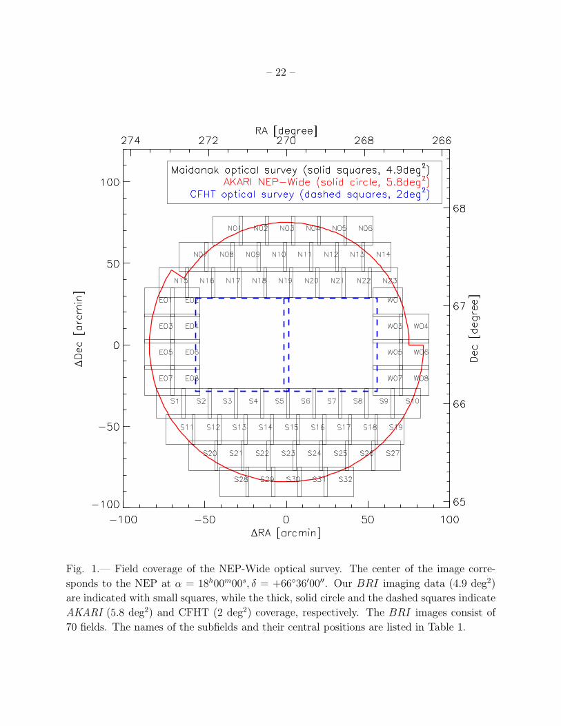
The AKARI NEP-Wide field is centered at α = 18h00m00s, δ = +6636′00′′ covering

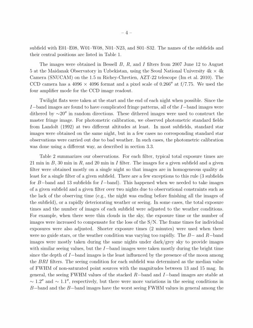
a circular area of 5.8 deg2. Our optical BRI imaging survey covers 4.9 deg2 outside the

central 2 deg2 area of the AKARI NEP-Wide. Figure 1 shows the field coverage of different

components of the NEP-Wide survey. The thick, solid circle indicates the AKARI NEP-

Wide (5.8 deg2) coverage. The dashed squares are the CFHT optical survey area. The small

squares show the Maidanak optical imaging area. It consists of 70 subfields, each of them

having an 18′×18′ field of view. These Maidanak fields are grouped into 4 different sections,

East (8 fields), West (7 fields), North (23 fields), and South (32 fields), and we name each

– 4 –

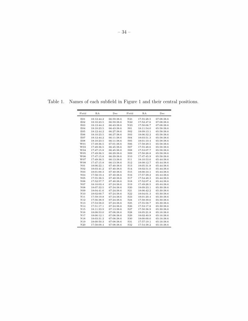
subfield with E01–E08, W01–W08, N01–N23, and S01–S32. The names of the subfields and

their central positions are listed in Table 1.

The images were obtained in Bessell B, R, and I filters from 2007 June 12 to August

5 at the Maidanak Observatory in Uzbekistan, using the Seoul National University 4k × 4k

Camera (SNUCAM) on the 1.5 m Richey-Chretien, AZT-22 telescope (Im et al. 2010). The

CCD camera has a 4096 × 4096 format and a pixel scale of 0.266′′ at f/7.75. We used the

four amplifier mode for the CCD image readout.

Twilight flats were taken at the start and the end of each night when possible. Since the

I−band images are found to have complicated fringe patterns, all of the I−band images were

dithered by ∼20′′ in random directions. These dithered images were used to construct the

master fringe image. For photometric calibration, we observed photometric standard fields

from Landolt (1992) at two different altitudes at least. In most subfields, standard star

images were obtained on the same night, but in a few cases no corresponding standard star

observations were carried out due to bad weather. In such cases, the photometric calibration

was done using a different way, as described in section 3.3.

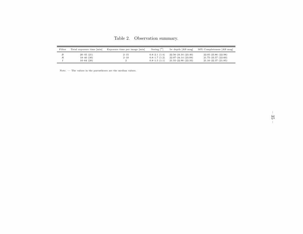
Table 2 summarizes our observations. For each filter, typical total exposure times are

21 min in B, 30 min in R, and 20 min in I filter. The images for a given subfield and a given

filter were obtained mostly on a single night so that images are in homogeneous quality at

least for a single filter of a given subfield. There are a few exceptions to this rule (3 subfields

for B−band and 13 subfields for I−band). This happened when we needed to take images

of a given subfield and a given filter over two nights due to observational constraints such as

the lack of the observing time (e.g., the night was ending before finishing all the images of

the subfield), or a rapidly deteriorating weather or seeing. In some cases, the total exposure

times and the number of images of each subfield were adjusted to the weather conditions.

For example, when there were thin clouds in the sky, the exposure time or the number of

images were increased to compensate for the loss of the S/N. The frame times for individual

exposures were also adjusted. Shorter exposure times (2 minutes) were used when there

were no guide stars, or the weather condition was varying too rapidly. The B− and R−band

images were mostly taken during the same nights under dark/grey sky to provide images

with similar seeing values, but the I−band images were taken mostly during the bright time

since the depth of I−band images is the least influenced by the presence of the moon among

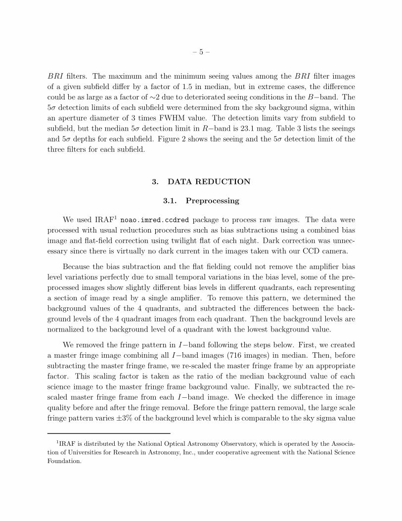
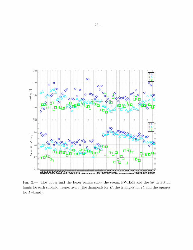
the BRI filters. The seeing condition for each subfield was determined as the median value

of FWHM of non-saturated point sources with the magnitudes between 13 and 15 mag. In

general, the seeing FWHM values of the stacked R−band and I−band images are stable at

∼ 1.2′′ and ∼ 1.1′′, respectively, but there were more variations in the seeing conditions in

B−band and the B−band images have the worst seeing FWHM values in general among the

– 5 –

BRI filters. The maximum and the minimum seeing values among the BRI filter images

of a given subfield differ by a factor of 1.5 in median, but in extreme cases, the difference

could be as large as a factor of ∼2 due to deteriorated seeing conditions in the B−band. The

5σ detection limits of each subfield were determined from the sky background sigma, within

an aperture diameter of 3 times FWHM value. The detection limits vary from subfield to

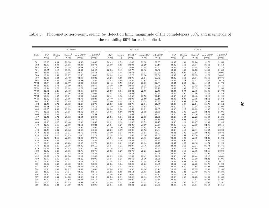
subfield, but the median 5σ detection limit in R−band is 23.1 mag. Table 3 lists the seeings

and 5σ depths for each subfield. Figure 2 shows the seeing and the 5σ detection limit of the

three filters for each subfield.

3. DATA REDUCTION

3.1. Preprocessing

We used IRAF1 noao.imred.ccdred package to process raw images. The data were

processed with usual reduction procedures such as bias subtractions using a combined bias

image and flat-field correction using twilight flat of each night. Dark correction was unnec-

essary since there is virtually no dark current in the images taken with our CCD camera.

Because the bias subtraction and the flat fielding could not remove the amplifier bias

level variations perfectly due to small temporal variations in the bias level, some of the pre-

processed images show slightly different bias levels in different quadrants, each representing

a section of image read by a single amplifier. To remove this pattern, we determined the

background values of the 4 quadrants, and subtracted the differences between the back-

ground levels of the 4 quadrant images from each quadrant. Then the background levels are

normalized to the background level of a quadrant with the lowest background value.

We removed the fringe pattern in I−band following the steps below. First, we created

a master fringe image combining all I−band images (716 images) in median. Then, before

subtracting the master fringe frame, we re-scaled the master fringe frame by an appropriate

factor. This scaling factor is taken as the ratio of the median background value of each

science image to the master fringe frame background value. Finally, we subtracted the re-

scaled master fringe frame from each I−band image. We checked the difference in image

quality before and after the fringe removal. Before the fringe pattern removal, the large scale

fringe pattern varies ±3% of the background level which is comparable to the sky sigma value

1IRAF is distributed by the National Optical Astronomy Observatory, which is operated by the Associa-

tion of Universities for Research in Astronomy, Inc., under cooperative agreement with the National Science

Foundation.

– 6 –

per pixel. After the fringe subtraction, the large scale variation is reduced to < 0.5% of the

background or more than 6 times less than the sky sigma value, showing that the fringe

pattern is removed successfully well below the sky sigma values.

After the fringe correction and the registration, all images were combined in median.

Cosmic rays are removed during the stacking of multiple images with a sigma clipping adopt-

ing +3-sigma for rejecting outlier pixels.

3.2. Astrometry

To derive astrometry solutions, we used a software named SCAMP which finds astrom-

etry solution by cross-matching automatically an input reference catalog containing a set of

accurate RA and Dec values of sources against a list of object positions obtained from an

input FITS image (Bertin 2006). In our case, we used USNO-B1 catalog (Monet et al. 2003)

as the reference catalog for the astrometry calibration. Astrometry solutions were derived

for all the stacked, subfield images in each filter separately. The degree of the polynomial for

distortion correction is adopted to be 4, since it gave the best solution among other options.

SCAMP can refine the astrometry solution by comparing positions of objects in overlapping

images, but the procedure does not apply to our case.

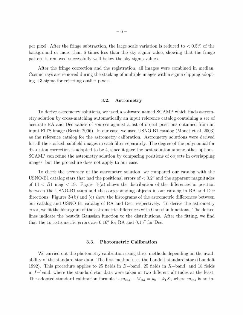
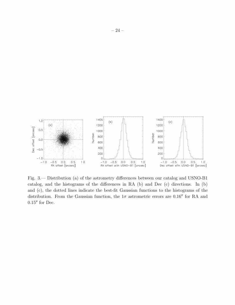
To check the accuracy of the astrometry solution, we compared our catalog with the

USNO-B1 catalog stars that had the positional errors of < 0.2′′ and the apparent magnitudes

of 14 < B1 mag < 19. Figure 3-(a) shows the distribution of the differences in position

between the USNO-B1 stars and the corresponding objects in our catalog in RA and Dec

directions. Figures 3-(b) and (c) show the histograms of the astrometric differences between

our catalog and USNO-B1 catalog of RA and Dec, respectively. To derive the astrometry

error, we fit the histogram of the astrometric differences with Gaussian functions. The dotted

lines indicate the best-fit Gaussian function to the distributions. After the fitting, we find

that the 1σ astrometric errors are 0.16′′ for RA and 0.15′′ for Dec.

3.3. Photometric Calibration

We carried out the photometry calibration using three methods depending on the avail-

ability of the standard star data. The first method uses the Landolt standard stars (Landolt

1992). This procedure applies to 25 fields in B−band, 25 fields in R−band, and 18 fields

in I−band, where the standard star data were taken at two different altitudes at the least.

The adopted standard calibration formula is mins −Mstd = k0 + k1X , where mins is an in-

– 7 –

strumental magnitude ( mins = 25−2.5 log (DN/sec) ), Mstd is a standard magnitude, k0 is

a zero point, k1 is an airmass coefficient, and X is an airmass. The instrumental magnitudes

were measured within an aperture of a 12′′ diameter on the standard stars. We checked with

growth curves that this aperture is large enough to contain virtually all photons from the star

irrespective of the seeing of our data. We chose the standard stars that have similar colors

for deriving the coefficients of the above formula. To confirm the effect of not including the

color terms, we checked the difference between the listed magnitudes of standard stars with

various colors (those not included in the derivation of the photometric zero-points) and the

magnitudes of these standard stars derived with our photometry solutions. We find that the

rms difference is less than 0.05 mag. That is, the magnitudes derived with our photometry

solutions are independent of the color terms well within the error 0.05 mag. This is consis-

tent with the expected variation in the photometric zero points due to neglecting the color

term, based on an observational campaign of photometry standards using the SNUCAM at

Maidanak (Lim et al. 2009). Therefore we decided to neglect the color term of the formula.

We found k0 and k1 values for each night and each filter, and derived the standard magni-

tudes of the objects using these values. The k0 has the values in the range of 1.67 ± 0.13 at

B−band, 1.70 ± 0.11 at R−band, and 2.07 ± 0.08 at I−band. Also, the k1 have the values

of 0.33 ± 0.05 at B−band, 0.10 ± 0.03 at R−band, and 0.04 ± 0.01 at I−band. These values

are consistent with values derived from a campaign observation of standard stars (Lim et al.

2009). The zero-point errors were estimated from the rms magnitude differences between

the known magnitudes of the standard stars and the magnitudes of the same standard stars

derived from our zero-point solution. The zero-point error is about 0.032 mag using this

method.

The second photometric calibration method is adopted for the data taken during the

nights which have only one altitude data for standard stars (34, 40, and 27 fields at B−, R−,

and I−band, respectively.). In such cases, we used other night’s k1 value since the night-to-

night variation in k1 is not significant. This produces an additional zero-point error of 0.028

mag, at most. Consequently, the total error associated with the zero-point determination of

the second photometric calibration method is less than 0.040 mag.

The third method of the photometric calibration is applied to the subfields without

associated standard star observations. For such fields (11, 5, and 25 fields in B−, R−, and

I−band, respectively.), we used photometry of sources in the overlapping area of a neighbor

subfield. The corresponding sources that have magnitudes between 12 and 16 mag were used

to measure the photometric zero-point. For this method, the zero-point error was derived

from the standard deviation of the magnitude offset between the sources in the field where

we want to determine the photometric zero-point and the matched sources in the neighbor

fields. In this case, the zero-point error is about 0.045 mag with respect to the photometry

– 8 –

of the neighbor field. Therefore, the total error in the zero-point for the third method is

about 0.032–0.045 mag, depending on the method used for the photometry calibration of

the neighbor field.

We checked the consistency of our photometric calibration using an overlap area between

two neighboring fields (those that were not used for the photometric calibration of the other

field). In the case of the first method, the mean photometry differences are −0.006± 0.028

mag in B (30 fields for overlaps), 0.002 ± 0.033 mag in R (23 fields for overlaps), and 0.001

± 0.017 mag in I magnitudes (17 fields for overlaps). In the case of the second method,

the mean photometry differences are about 0.002 ± 0.030 mag in B (37 fields for overlaps),

−0.006± 0.040 mag in R (44 fields for overlaps), and −0.022± 0.035 mag in I magnitudes

(20 fields for overlaps). Note that the consistency of our photometric calibration between

different nights are well below 0.05 mag for all filters which is expected from the zero-point

errors.

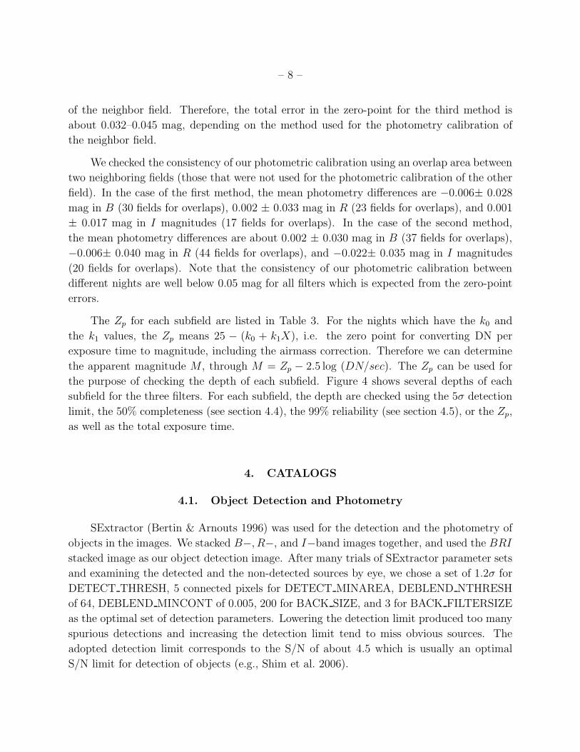
The Zp for each subfield are listed in Table 3. For the nights which have the k0 and

the k1 values, the Zp means 25 − (k0 + k1X), i.e. the zero point for converting DN per

exposure time to magnitude, including the airmass correction. Therefore we can determine

the apparent magnitude M , through M = Zp − 2.5 log (DN/sec). The Zp can be used for

the purpose of checking the depth of each subfield. Figure 4 shows several depths of each

subfield for the three filters. For each subfield, the depth are checked using the 5σ detection

limit, the 50% completeness (see section 4.4), the 99% reliability (see section 4.5), or the Zp,

as well as the total exposure time.

4. CATALOGS

4.1. Object Detection and Photometry

SExtractor (Bertin & Arnouts 1996) was used for the detection and the photometry of

objects in the images. We stacked B−, R−, and I−band images together, and used the BRI

stacked image as our object detection image. After many trials of SExtractor parameter sets

and examining the detected and the non-detected sources by eye, we chose a set of 1.2σ for

DETECT THRESH, 5 connected pixels for DETECT MINAREA, DEBLEND NTHRESH

of 64, DEBLEND MINCONT of 0.005, 200 for BACK SIZE, and 3 for BACK FILTERSIZE

as the optimal set of detection parameters. Lowering the detection limit produced too many

spurious detections and increasing the detection limit tend to miss obvious sources. The

adopted detection limit corresponds to the S/N of about 4.5 which is usually an optimal

S/N limit for detection of objects (e.g., Shim et al. 2006).

– 9 –

To cross-identify and perform the photometry of objects in each band, we used the

ASSOC parameter in SExtractor with a matching radius of 0.658′′, 3σ value of the astrometric

error. The above process may miss faint objects which are brighter in a particular filter than

the others. To supplement the above source detection, we also ran SExtractor on images

in each filter separately. This process reveals faint sources detected in a single filter image,

but not detected in the BRI stacked image. These sources detected in a single filter image

were also matched with detections in other single filter images with the matching radius

of 0.658′′. Adding these faint sources, we detected 63,333 for B, 96,460 for R and 70,492

sources for I filter over the reliability of 99% (see section 4.5). Among these objects, 16%

in B, 33% in R, and 15% in I are detected only in the single filter images. We derived

aperture magnitudes using an aperture of diameter of 3 times FWHM and auto magnitudes

with Kron-like elliptical apertures (Kron 1980) which are taken as the total magnitudes .

The aperture correction value is 0.10 ± 0.02 mag for all the filters and all the subfields.

The magnitude errors are computed by combining the standard SExtractor estimates

and the zero-point errors we estimated. The standard SExtractor error estimates are based

on the Poisson statistics, and could underestimate the noise values when the sky noises in

adjoining pixels are correlated due to the stacking of the dithered frames (Gawiser et al.

2006). Using a similar procedure described in Gawiser et al. (2006), we calculated how the

error within a square aperture of N × N pixels, σN , changes as a function of N . In the

case where each pixel noise is uncorrelated with each other, σN ∝ N . When the noise is

correlated, the exponent of N is greater than 1. In our data, we find σN ∝ N1.14. For a

magnitude measured within an aperture with 3.0′′ diameter (3 times a typical FWHM of our

image), there are about 110 pixels (or N ≃ 10). Therefore, the photometric errors of faint

objects (R & 22 mag) could be underestimated by as much as about a factor of 1.4. For the

brighter objects (R . 20 mag), the photometric errors are not affected by this effect, since

their errors are dominated by the object noise.

For the same object that exist on two or more fields in the overlapping areas, we chose

an object that had the smallest FLAGS value from SExtractor (the FLAGS has a nonzero

value if the object is blended, saturated, and/or truncated at an edge of a image) and the

smallest photometric error. Among the same objects, we only included the one with a better

S/N or image quality in the final catalog. The examples of such cases are objects on the

edge of an image or objects elongated due to astigmatism near the edge of the CCD in one

image, but do not suffer such a problem in the other. At the bright end, the photometry is

free from saturation and non-linearity above R ≃ 12 mag. We cut off the faint sources over

the magnitude of false detection rate 1% (see section 4.5).

We found spurious detections due to the reflection halos caused by the bright objects

– 10 –

and due to faint, uncorrected fringe patterns in R−band images. In case of the reflection

halos around bright stars, we divided the bright stars into three classes, and set a radius

to define the region where spurious detections lie within it (120′′ at 8 ≤ B mag < 10 , 80′′

at 10 ≤ B mag < 12 , 40′′ at 12 ≤ B mag < 14). We flag detections inside these radii as

‘near bright obj’, since they are likely to be spurious detections or their photometry are not

reliable. We also found many spurious detections in the outer regions of stacked R−band

images, thus we flag objects that are not matched with B− or I−band catalogs and exist

within 30′′ from the edge as ‘near edge’. We found 5,186 (5%) of ‘near bright obj’ at R−band

and 14,833 (15%)of ‘near edge’ sources, and checked those spurious sources by eyes. These

flags are included in the BRI merged catalog. Also we flag non-stellar sources as ‘galaxy’

(see, section 4.2). The flags are marked at the last column of the catalog (Table 4).

4.2. Star-Galaxy Separation

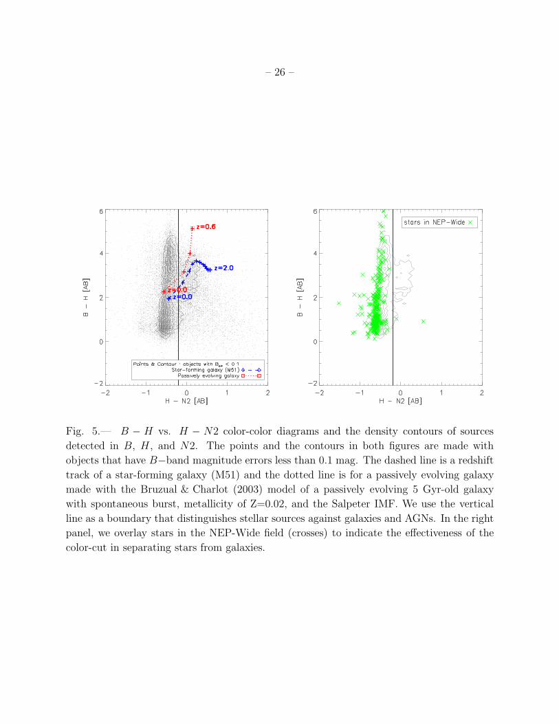
To distinguish stellar sources from other extragalactic sources, we used a B − H vs.

H −N2 color-color diagram and the SExtractor stellarity index. Here, the stellarity indices

measure the likelihood of a source being a point source or an extended source, with the

value of 1 for a perfect point source, and 0 for a diffuse, extended source. The stellarities

are measured from the single-filter stacked images. However, when we determine whether a

source is point-like or extended, we adopted the stellarity value measured in a stacked image

in the filter where the photometric error of the source is the smallest. Note that the stellarity

values are nearly identical among different filter images when an object is sufficiently bright

(R < 19 mag). We also note that the stellarity values are determined from the R−band

images for most of the objects, since the R−band images generally have the highest S/N

among the three filters.

The H−band magnitudes come from the catalog made from the J− and H−band

images of the NEP-Wide field which were took with FLAMINGOS on the 2.1m telescope

at Kitt Peak National Observatory (Jeon et al., in preparation), and the N2 magnitudes

come from the AKARI observation, of which the effective wavelength is 2.43µm (Lee et al.

2007). We matched the objects detected in H− and N2−band with the objects detected in

B−, R−, and I−band using a matching radius of 1.5′′ (for H−band) and 3′′ (for N2−band),

respectively.

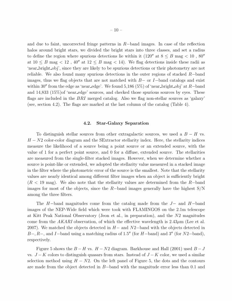
Figure 5 shows the B−H vs. H−N2 diagram. Barkhouse and Hall (2001) used B−J

vs. J −K colors to distinguish quasars from stars. Instead of J −K color, we used a similar

selection method using H − N2. On the left panel of Figure 5, the dots and the contours

are made from the object detected in B−band with the magnitude error less than 0.1 and

– 11 –

matched with H and N2 detections. We can notice that there is a stellar locus at H − N2

≃ −0.5 mag with 0 < B −H < 5. Because most of stars have similar slopes at wavelength

greater than 1µm on their SEDs, stars have H − N2 ∼ −0.5 mag. We checked the stellar

locus using stars (the crosses of the right panel of Figure 5) in NEP-Wide field which had

the stellarity greater than 0.8 and the magnitude of 10 < H < 13. Most of the stars are

located at the stellar locus with a few exceptions.

We also checked the location of galaxies using redshift tracks of galaxies. The dashed

line is for a star-forming galaxy, M51 (Silva et al. 1998) and the dotted line is for a pas-

sively evolving galaxy (see figure caption for the model used for this). We considered the

intergalactic medium (IGM) attenuation (Madau 1996) for all redshift tracks. Most of the

galaxy track lie in the area of H −N2 greater than −0.2 mag, but galaxies with z . 0.1 lie

at H−N2 < −0.2 mag. The PSF of galaxy at low redshift (z < 0.1) is in general larger than

that of star, so such sources can be identified as extended sources in the image. However,

if the low redshift galaxies are faint and small, they may get misclassified as stars with the

color cut.

Since the magnitude limit of the H and N2−band are different from those in the optical,

this method can be applied only to a relatively bright magnitude limit. Also, in order to

identify bright, extended sources (namely, low redshift galaxies) in the stellar region on the

color-color plot, we apply a stellarity cut where stellarity index has a value between 1 (point

sources) and 0 (extended sources).

In summary, we define stellar sources as the following:

Objects with H −N2 < −0.2 mag and the stellarity index > 0.2 or

Objects with H −N2 ≥ −0.2 mag and the stellarity index > 0.8 or

if there is no H −N2 color available, stellarity index > 0.8

The first condition weeds out extended objects at low redshift, while the second condition

allows us to select clear, point sources in the region of galaxies on the color-color magnitude.

The third criterion applies to a small number of objects near the detection limit of optical

images, since H and N2 images show detections of 98% and 77% of objects brighter than

the magnitude cut of the catalog at 50% completeness limit.

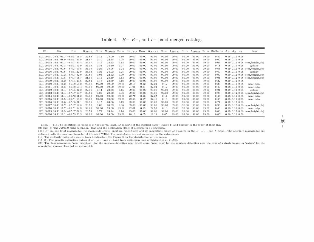
4.3. Catalog Format

The B−, R−, and I−band merged catalog is presented in Table 4. The catalog contains

objects that are deemed to be reliable above 99% confidence where the confidence values

– 12 –

are derived independently for each subfield in each filter (see section 4.5). Our catalog

contains each object’s identification number (ID), RA, Dec, the total magnitude and its

error in each band, the aperture magnitude within a circular aperture with a diameter of 3

times FWHM and its error in each band, the stellarity value from SExtractor, the galactic

extinction value from the extinction map of Schlegel et al. (1998) for each band, and the flags

described in section 4.1. Note that the listed magnitudes are not corrected for the galactic

extinction. The conversion formulas of Vega to AB magnitudes are B(Vega) = B(AB)+0.09,

R(Vega) = R(AB)− 0.22 and I(Vega) = I(AB)− 0.45. The offset values between Vega and

AB magnitude are computed from the Vega spectrum (Bohlin & Gilliland 2004) and B,

R, and I filter response functions (Bessell 1990) coupled with the CCD quantum efficiency

curve. The magnitude error is the square root of the quadratic summation of the photometric

measurement error and the zero-point error from the photometric calibration. We use a

dummy value of 99.00 for non-detection.

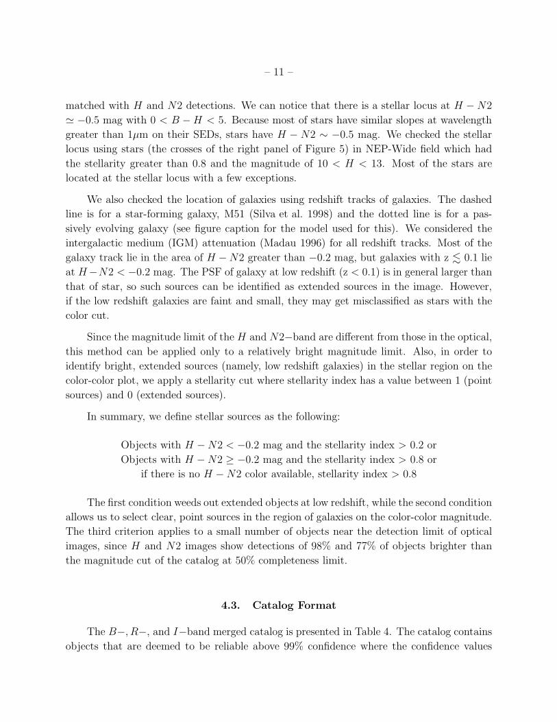
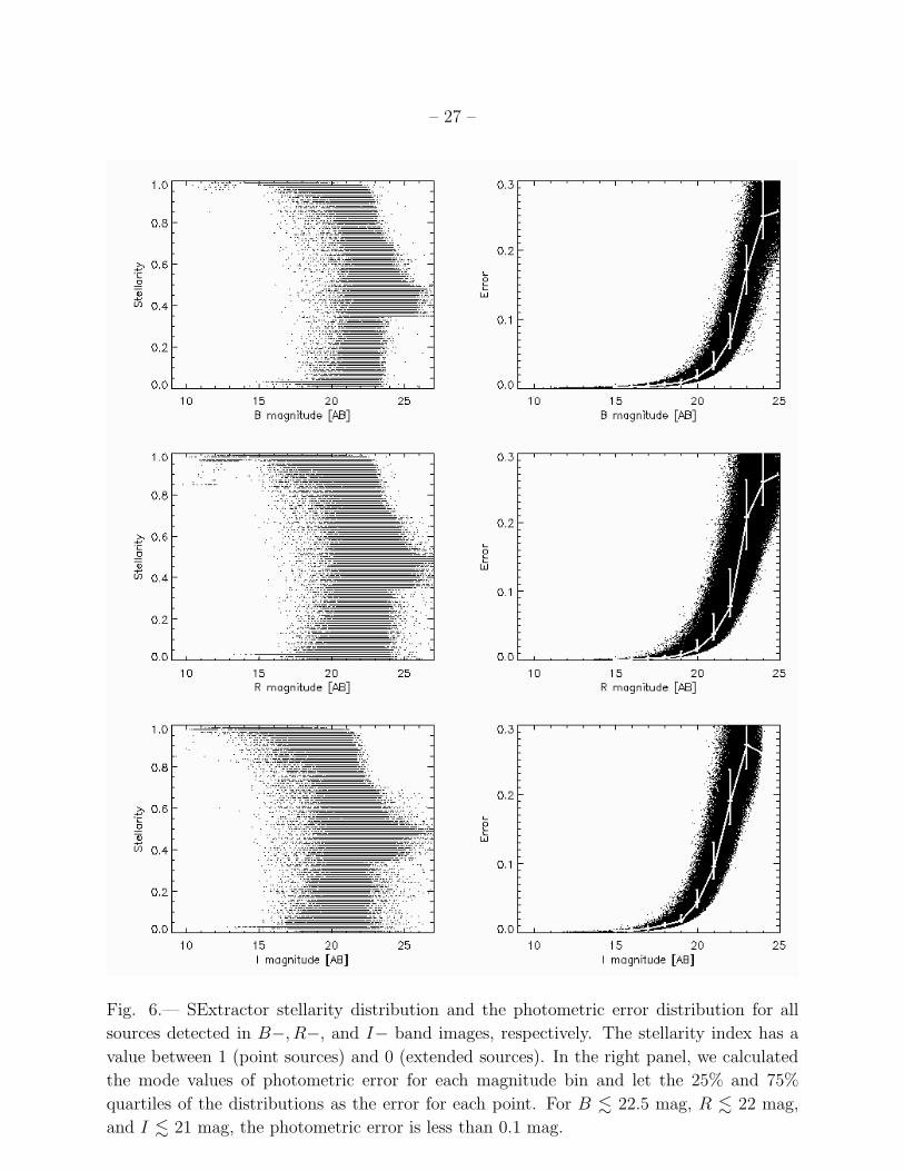
Figure 6 shows the stellarity distribution (the left three panels) and the photometric

error distribution (the right three panels) for all sources detected in B−, R−, and I− band

images. The white lines on the right panels show the mode values for each magnitude bins,

with the 25% and 75% quartiles indicated with error bars. The spread of the data points

in the magnitude versus error plots are caused mainly by varying depths of the data from

different subfields. On average, the photometric error is less than 0.1 mag at B . 22.5 mag,

R . 22 mag, and I . 21 mag.

4.4. Completeness

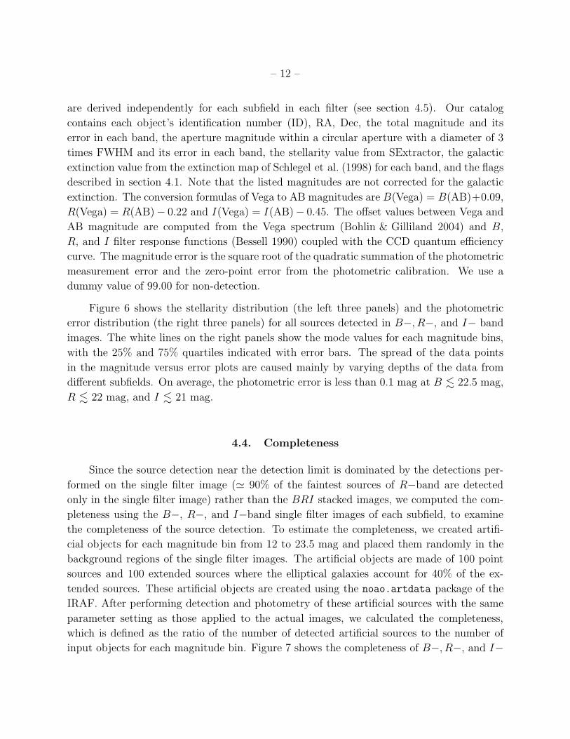
Since the source detection near the detection limit is dominated by the detections per-

formed on the single filter image (≃ 90% of the faintest sources of R−band are detected

only in the single filter image) rather than the BRI stacked images, we computed the com-

pleteness using the B−, R−, and I−band single filter images of each subfield, to examine

the completeness of the source detection. To estimate the completeness, we created artifi-

cial objects for each magnitude bin from 12 to 23.5 mag and placed them randomly in the

background regions of the single filter images. The artificial objects are made of 100 point

sources and 100 extended sources where the elliptical galaxies account for 40% of the ex-

tended sources. These artificial objects are created using the noao.artdata package of the

IRAF. After performing detection and photometry of these artificial sources with the same

parameter setting as those applied to the actual images, we calculated the completeness,

which is defined as the ratio of the number of detected artificial sources to the number of

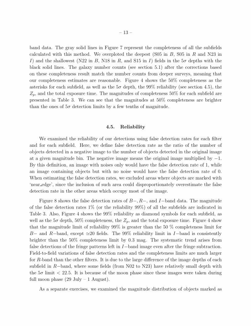
input objects for each magnitude bin. Figure 7 shows the completeness of B−, R−, and I−

– 13 –

band data. The gray solid lines in Figure 7 represent the completeness of all the subfields

calculated with this method. We overploted the deepest (S05 in B, S05 in R and N23 in

I) and the shallowest (N22 in B, N18 in R, and S15 in I) fields in the 5σ depths with the

black solid lines. The galaxy number counts (see section 5.1) after the corrections based

on these completeness result match the number counts from deeper surveys, meaning that

our completeness estimates are reasonable. Figure 4 shows the 50% completeness as the

asterisks for each subfield, as well as the 5σ depth, the 99% reliability (see section 4.5), the

Zp, and the total exposure time. The magnitudes of completeness 50% for each subfield are

presented in Table 3. We can see that the magnitudes at 50% completeness are brighter

than the ones of 5σ detection limits by a few tenths of magnitude.

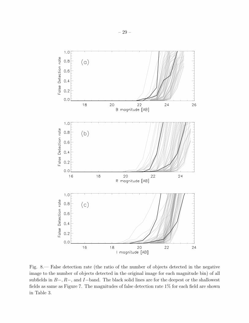
4.5. Reliability

We examined the reliability of our detections using false detection rates for each filter

and for each subfield. Here, we define false detection rate as the ratio of the number of

objects detected in a negative image to the number of objects detected in the original image

at a given magnitude bin. The negative image means the original image multiplied by −1.

By this definition, an image with noises only would have the false detection rate of 1, while

an image containing objects but with no noise would have the false detection rate of 0.

When estimating the false detection rates, we excluded areas where objects are marked with

‘near edge’, since the inclusion of such area could disproportionately overestimate the false

detection rate in the other areas which occupy most of the image.

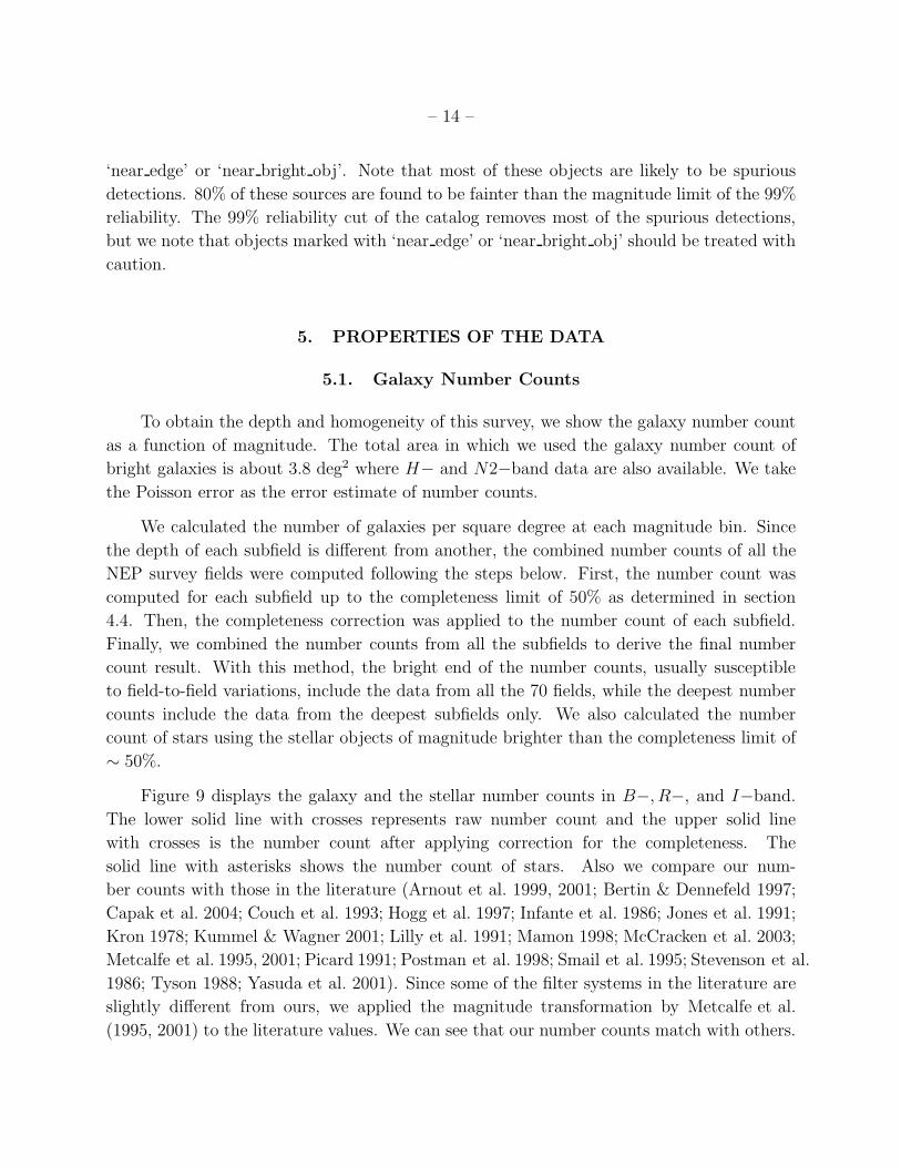
Figure 8 shows the false detection rates of B−, R−, and I−band data. The magnitude

of the false detection rates 1% (or the reliability 99%) of all the subfields are indicated in

Table 3. Also, Figure 4 shows the 99% reliability as diamond symbols for each subfield, as

well as the 5σ depth, 50% completeness, the Zp, and the total exposure time. Figure 4 show

that the magnitude limit of reliability 99% is greater than the 50 % completeness limit for

B− and R−band, except ≃20 fields. The 99% reliability limit in I−band is consistently

brighter than the 50% completeness limit by 0.3 mag. The systematic trend arises from

false detections of the fringe patterns left in I−band image even after the fringe subtraction.

Field-to-field variations of false detection rates and the completeness limits are much larger

for R-band than the other filters. It is due to the large difference of the image depths of each

subfield in R−band, where some fields (from N02 to N23) have relatively small depth with

the 5σ limit < 22.5. It is because of the moon phase since these images were taken during

full moon phase (29 July – 1 August).

As a separate exercises, we examined the magnitude distribution of objects marked as

– 14 –

‘near edge’ or ‘near bright obj’. Note that most of these objects are likely to be spurious

detections. 80% of these sources are found to be fainter than the magnitude limit of the 99%

reliability. The 99% reliability cut of the catalog removes most of the spurious detections,

but we note that objects marked with ‘near edge’ or ‘near bright obj’ should be treated with

caution.

5. PROPERTIES OF THE DATA

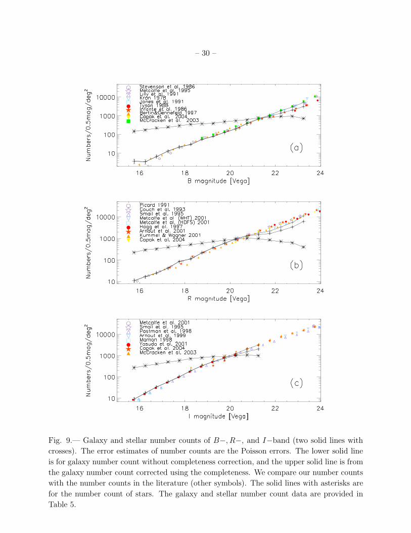
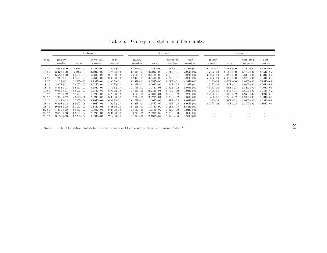
5.1. Galaxy Number Counts

To obtain the depth and homogeneity of this survey, we show the galaxy number count

as a function of magnitude. The total area in which we used the galaxy number count of

bright galaxies is about 3.8 deg2 where H− and N2−band data are also available. We take

the Poisson error as the error estimate of number counts.

We calculated the number of galaxies per square degree at each magnitude bin. Since

the depth of each subfield is different from another, the combined number counts of all the

NEP survey fields were computed following the steps below. First, the number count was

computed for each subfield up to the completeness limit of 50% as determined in section

4.4. Then, the completeness correction was applied to the number count of each subfield.

Finally, we combined the number counts from all the subfields to derive the final number

count result. With this method, the bright end of the number counts, usually susceptible

to field-to-field variations, include the data from all the 70 fields, while the deepest number

counts include the data from the deepest subfields only. We also calculated the number

count of stars using the stellar objects of magnitude brighter than the completeness limit of

∼ 50%.

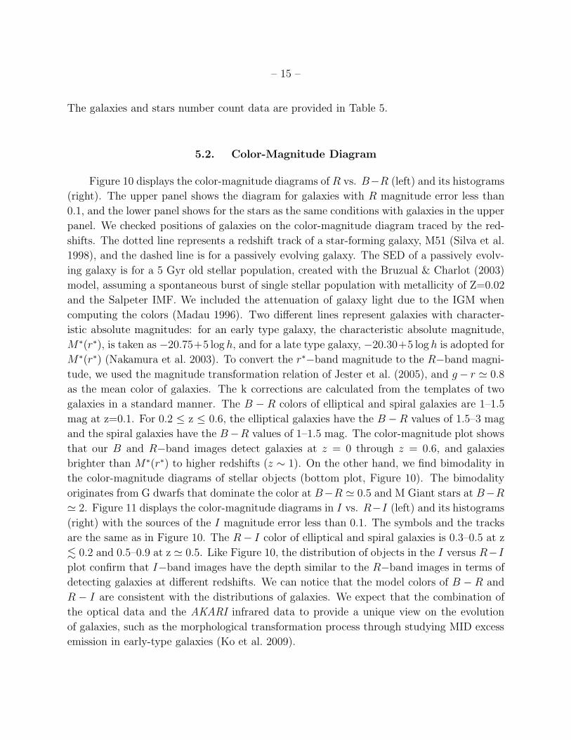
Figure 9 displays the galaxy and the stellar number counts in B−, R−, and I−band.

The lower solid line with crosses represents raw number count and the upper solid line

with crosses is the number count after applying correction for the completeness. The

solid line with asterisks shows the number count of stars. Also we compare our num-

ber counts with those in the literature (Arnout et al. 1999, 2001; Bertin & Dennefeld 1997;

Capak et al. 2004; Couch et al. 1993; Hogg et al. 1997; Infante et al. 1986; Jones et al. 1991;

Kron 1978; Kummel & Wagner 2001; Lilly et al. 1991; Mamon 1998; McCracken et al. 2003;

Metcalfe et al. 1995, 2001; Picard 1991; Postman et al. 1998; Smail et al. 1995; Stevenson et al.

1986; Tyson 1988; Yasuda et al. 2001). Since some of the filter systems in the literature are

slightly different from ours, we applied the magnitude transformation by Metcalfe et al.

(1995, 2001) to the literature values. We can see that our number counts match with others.

– 15 –

The galaxies and stars number count data are provided in Table 5.

5.2. Color-Magnitude Diagram

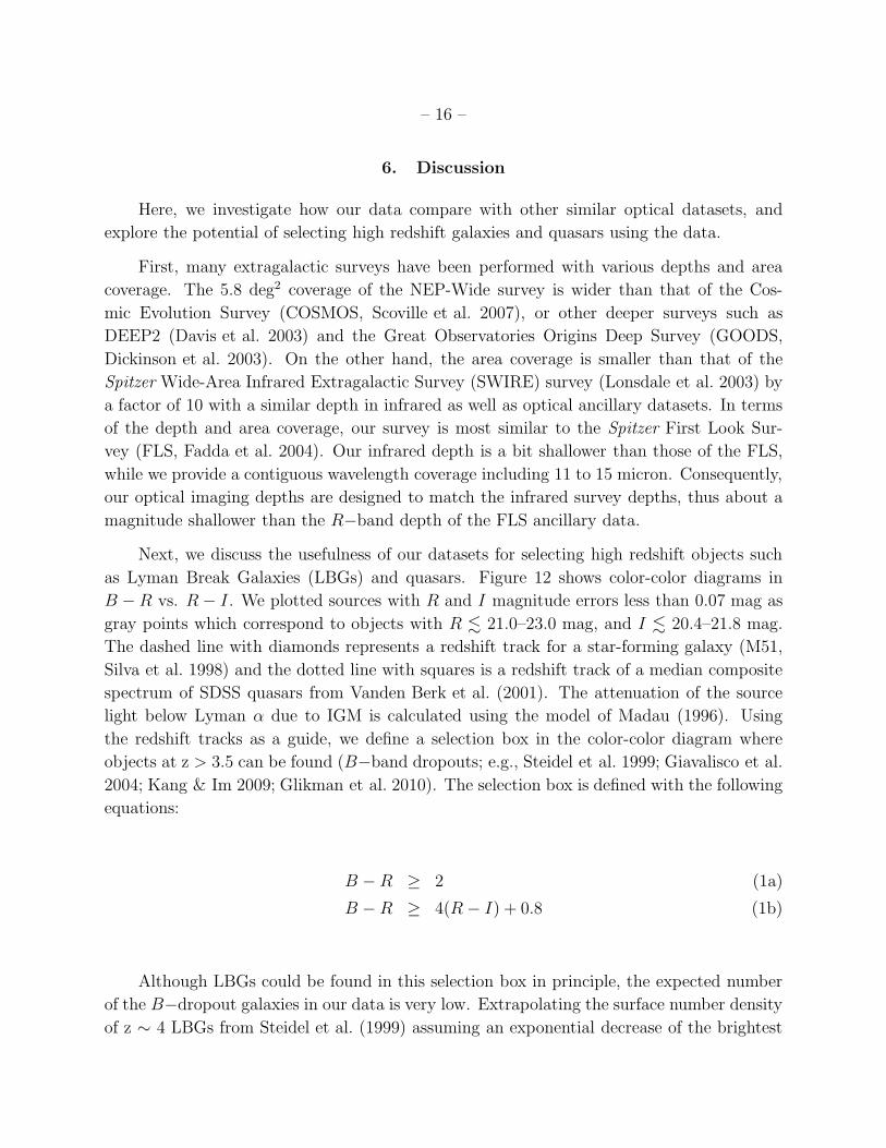
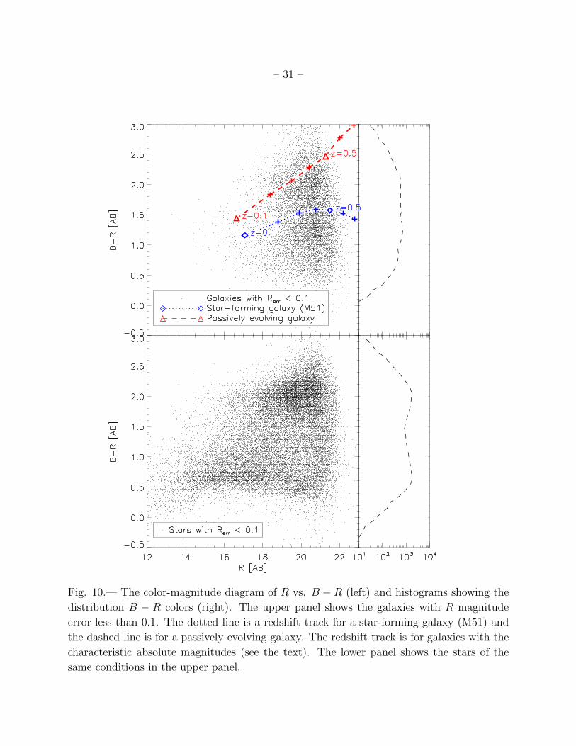
Figure 10 displays the color-magnitude diagrams of R vs. B−R (left) and its histograms

(right). The upper panel shows the diagram for galaxies with R magnitude error less than

0.1, and the lower panel shows for the stars as the same conditions with galaxies in the upper

panel. We checked positions of galaxies on the color-magnitude diagram traced by the red-

shifts. The dotted line represents a redshift track of a star-forming galaxy, M51 (Silva et al.

1998), and the dashed line is for a passively evolving galaxy. The SED of a passively evolv-

ing galaxy is for a 5 Gyr old stellar population, created with the Bruzual & Charlot (2003)

model, assuming a spontaneous burst of single stellar population with metallicity of Z=0.02

and the Salpeter IMF. We included the attenuation of galaxy light due to the IGM when

computing the colors (Madau 1996). Two different lines represent galaxies with character-

istic absolute magnitudes: for an early type galaxy, the characteristic absolute magnitude,

M∗(r∗), is taken as −20.75+5 log h, and for a late type galaxy, −20.30+5 log h is adopted for

M∗(r∗) (Nakamura et al. 2003). To convert the r∗−band magnitude to the R−band magni-

tude, we used the magnitude transformation relation of Jester et al. (2005), and g− r ≃ 0.8

as the mean color of galaxies. The k corrections are calculated from the templates of two

galaxies in a standard manner. The B − R colors of elliptical and spiral galaxies are 1–1.5

mag at z=0.1. For 0.2 ≤ z ≤ 0.6, the elliptical galaxies have the B −R values of 1.5–3 mag

and the spiral galaxies have the B−R values of 1–1.5 mag. The color-magnitude plot shows

that our B and R−band images detect galaxies at z = 0 through z = 0.6, and galaxies

brighter than M∗(r∗) to higher redshifts (z ∼ 1). On the other hand, we find bimodality in

the color-magnitude diagrams of stellar objects (bottom plot, Figure 10). The bimodality

originates from G dwarfs that dominate the color at B−R ≃ 0.5 and M Giant stars at B−R

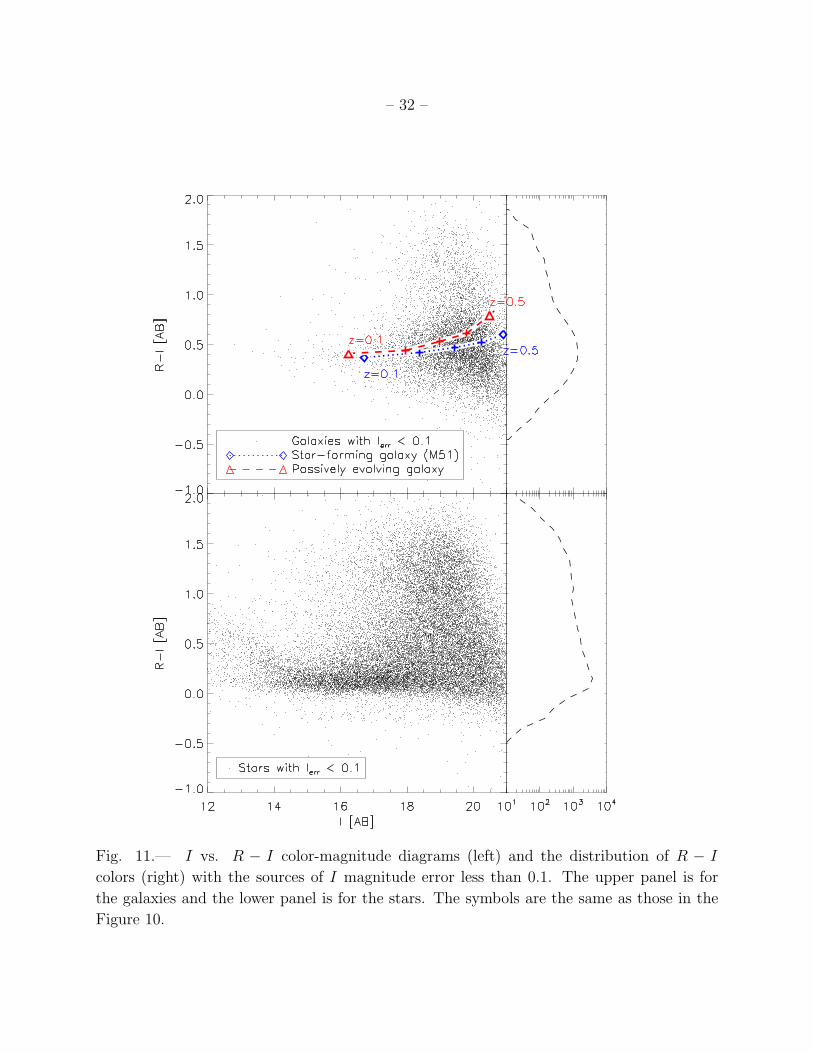
≃ 2. Figure 11 displays the color-magnitude diagrams in I vs. R−I (left) and its histograms

(right) with the sources of the I magnitude error less than 0.1. The symbols and the tracks

are the same as in Figure 10. The R− I color of elliptical and spiral galaxies is 0.3–0.5 at z

. 0.2 and 0.5–0.9 at z ≃ 0.5. Like Figure 10, the distribution of objects in the I versus R−I

plot confirm that I−band images have the depth similar to the R−band images in terms of

detecting galaxies at different redshifts. We can notice that the model colors of B − R and

R − I are consistent with the distributions of galaxies. We expect that the combination of

the optical data and the AKARI infrared data to provide a unique view on the evolution

of galaxies, such as the morphological transformation process through studying MID excess

emission in early-type galaxies (Ko et al. 2009).

– 16 –

6. Discussion

Here, we investigate how our data compare with other similar optical datasets, and

explore the potential of selecting high redshift galaxies and quasars using the data.

First, many extragalactic surveys have been performed with various depths and area

coverage. The 5.8 deg2 coverage of the NEP-Wide survey is wider than that of the Cos-

mic Evolution Survey (COSMOS, Scoville et al. 2007), or other deeper surveys such as

DEEP2 (Davis et al. 2003) and the Great Observatories Origins Deep Survey (GOODS,

Dickinson et al. 2003). On the other hand, the area coverage is smaller than that of the

Spitzer Wide-Area Infrared Extragalactic Survey (SWIRE) survey (Lonsdale et al. 2003) by

a factor of 10 with a similar depth in infrared as well as optical ancillary datasets. In terms

of the depth and area coverage, our survey is most similar to the Spitzer First Look Sur-

vey (FLS, Fadda et al. 2004). Our infrared depth is a bit shallower than those of the FLS,

while we provide a contiguous wavelength coverage including 11 to 15 micron. Consequently,

our optical imaging depths are designed to match the infrared survey depths, thus about a

magnitude shallower than the R−band depth of the FLS ancillary data.

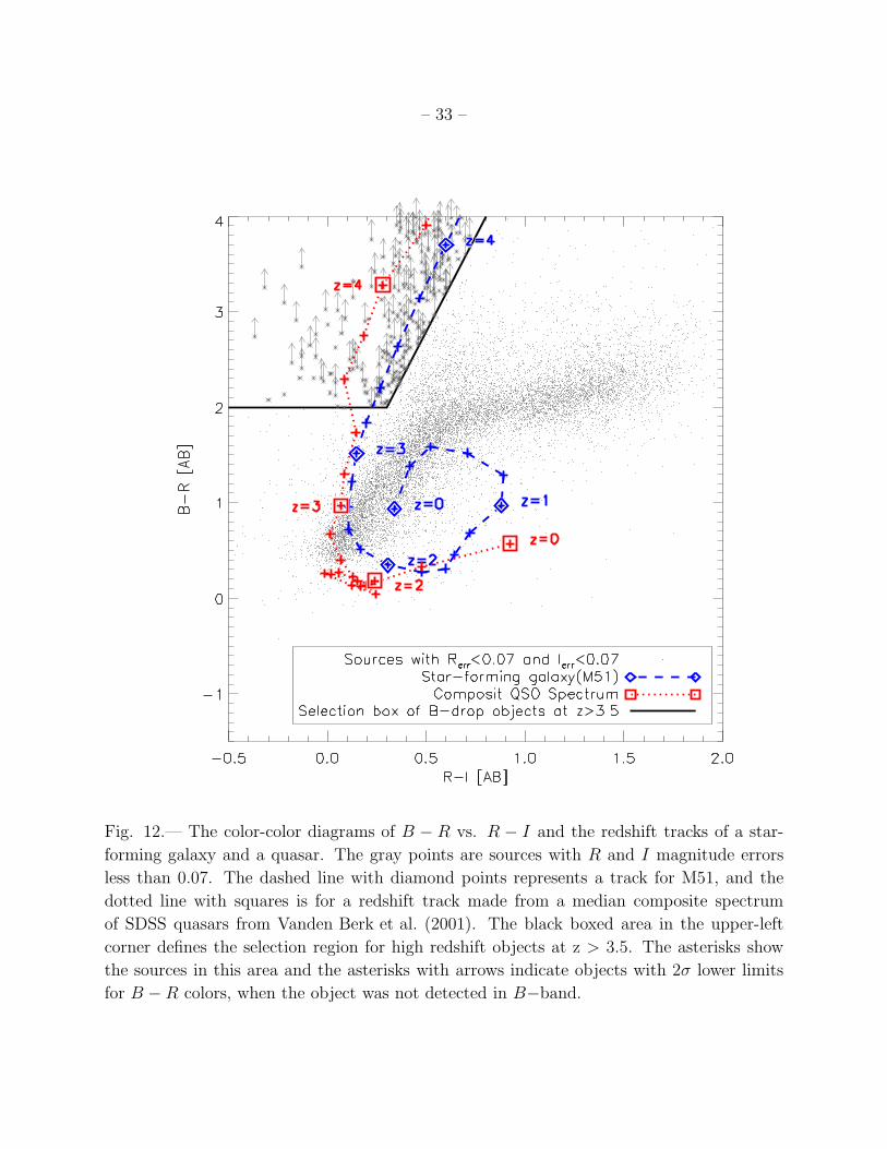
Next, we discuss the usefulness of our datasets for selecting high redshift objects such

as Lyman Break Galaxies (LBGs) and quasars. Figure 12 shows color-color diagrams in

B −R vs. R− I. We plotted sources with R and I magnitude errors less than 0.07 mag as

gray points which correspond to objects with R . 21.0–23.0 mag, and I . 20.4–21.8 mag.

The dashed line with diamonds represents a redshift track for a star-forming galaxy (M51,

Silva et al. 1998) and the dotted line with squares is a redshift track of a median composite

spectrum of SDSS quasars from Vanden Berk et al. (2001). The attenuation of the source

light below Lyman α due to IGM is calculated using the model of Madau (1996). Using

the redshift tracks as a guide, we define a selection box in the color-color diagram where

objects at z > 3.5 can be found (B−band dropouts; e.g., Steidel et al. 1999; Giavalisco et al.

2004; Kang & Im 2009; Glikman et al. 2010). The selection box is defined with the following

equations:

B − R ≥ 2 (1a)

B − R ≥ 4(R− I) + 0.8 (1b)

Although LBGs could be found in this selection box in principle, the expected number

of the B−dropout galaxies in our data is very low. Extrapolating the surface number density

of z ∼ 4 LBGs from Steidel et al. (1999) assuming an exponential decrease of the brightest

– 17 –

objects as in the Schechter function, we expect about one or less than oneB−dropout galaxies

at I < 21.5 mag. On the other hand, the number density could be higher by a factor of

10 or so, if the bright end of the luminosity function flattens due to AGN contribution as

seen in the luminosity functions of U−band dropout objects at z ∼ 3 (e.g., Hunt et al. 2004;

Shim et al. 2007). In our data, we identify ∼800 B−dropout candidates in the selection box,

but we believe that most of these are interlopers such as stars and low redshift galaxies due

to the large mismatch with the expected number.

The expected number of quasars over the 4.9 deg2 is . 10 at I < 20 mag (Richards et al.

2006), or 10 and 20 at R < 21.5 mag and 22.5 mag, respectively (Glikman et al. 2010). After

inspecting images of theB-dropout candidates visually and examining their multi-wavelength

SEDs from the optical through the MIR 11µm-band of AKARI, we identify at least several

objects that have the SED shapes consistent with those of high redshift quasars. Judging

from the shapes of the SEDs, most of the interlopers are low redshift galaxies or late-type

stars. The selection of quasar candidates at z > 3.5 is ongoing, and we expect that the

identification of z ∼ 4 quasars at these magnitude limits will be valuable for constraining

the faint-end slope of quasars at high redshift (e.g., Glikman et al. 2010).

7. SUMMARY

We have shown the characteristics of B−, R−, and I−band data at Maidanak Obser-

vatory from the follow-up imaging observation of the AKARI NEP-Wide field. Using the

SNUCAM on the 1.5m telescope, we covered 4.9 deg2 with the 5σ depth of ∼23.4, ∼23.1,

and ∼22.3 magnitudes (AB) at B−, R−, and I−band, respectively. We detected 63,333

sources in B−band, 96,460 objects in R−band, and 70,492 in I−band. These data are now

being used to identifying optical counterparts for accurate astrometry of infrared sources

and deblending of confused sources. Also, our data provide a multi-wavelength coverage

of the NEP-Wide field, enabling detailed SED analysis. Through these SEDs, we can get

key physical properties such as stellar mass and photometric redshifts, and select interesting

objects such as high redshift quasars. Spectroscopic follow-up surveys are being conducted

on infrared luminous objects using the information gathered from this imaging survey.

We would like to thank the observers in Maidanak Observatory who performed the

service observation over 2 months to obtain the data. This work was supported by the

Korea Science and Engineering Foundation (KOSEF) grant No. 2009-0063616, funded by

the Korea government (MEST), also in part by the Korea Research Foundation Grant funded

by the Korean Government (MOEHRD), grant number KRF-2007-611-C00003.

– 18 –

REFERENCES

Arnouts, S., et al. 2001, A&AS, 379, 740

Arnouts, A., DOdorico, S., Cristiani, S., Zaggia, S., Fontana, A., & Giallongo, E., 1999,

A&AS, 341, 641

Barkhouse, W. A. & Hall, P. B. 2001, AJ, 121, 2843

Bell, E. F., Zheng, X. Z., Papovich, C., Borch, A., Wolf, C., & Meisenheimer, K. 2007, ApJ,

663, 834

Bertin, E. 2006, Astronomical Data Analysis Software and Systems XV, 351, 112

Bertin, E. & Arnouts, S. 1996, A&AS, 117, 393B

Bertin, E. & Dennefeld, M., 1997, A&AS, 317, 43

Bessell, M. S. 1990, PASP, 102, 1181

Bohlin, R. C. & Gilliland, R. L. 2004, AJ, 127, 3508

Bruzual, G., & Charlot, S. 2003, MNRAS, 344, 1000

Capak, P., et al. 2004, AJ, 127, 180

Couch, W.J., Jurcevic, J., & Boyle, B.J., 1993, MNRAS, 260, 241

Davis, M., et al. 2003, Proc. SPIE, 4834, 161

Dickinson, M., & Giavalisco, M. 2003, The Mass of Galaxies at Low and High Redshift, ed.

R. Bender & A. Renzini (New York: Springer), 324

Fadda, D., Jannuzi, B. T., Ford, A., & Storrie-Lombardi, L. J. 2004, AJ, 128, 1

Gawiser, E., et al. 2006, ApJS, 162, 1

Giavalisco, M., et al. 2004, ApJ, 600, L93

Glikman, E., Bogosavljevic, M., Djorgovski, S. G., Stern, D., Dey, A., Jannuzi, B. T., &

Mahabal, A. 2010, ApJ, 710, 1498

Goto, T., et al. 2010, A&A, 514, A6

Hogg, D.W., Pahre, M.A., McCarthy, J.K., Cohen, J.G., Bland-ford, R., Smail, I., & Soifer,

B.T., 1997, MNRAS, 288, 404

– 19 –

Huang, J.-S., et al. 2009, ApJ, 700, 183

Hunt, M. P., Steidel, C. C., Adelberger, K. L., & Shapley, A. E. 2004, ApJ, 605, 625

Hwang, N. et al. 2007, ApJS, 172, 583

Im, M., Griffiths, R. E., & Ratnatunga, K. U. 1997, ApJ, 475, 457

Im, M. 2005, J. Korean Astron. Soc, 38, 135

Im, M., Ko, J., Cho, Y., Choi, C., Jeon, Y., Lee, I., & Ibrahimov, M. 2010, J. Korean Astron.

Soc, 43, 75

Infante, L., Pritchet, C., & Quintana, H., 1986, AJ, 91, 217

Jester, S. et al. 2005, AJ, 130, 873

Jones, L.R., Fong, R., Shanks, T., Ellis, R.S., & Peterson, B.A., 1991, MNRAS, 249, 481

Kang, E., & Im, M. 2009, ApJ, 691, L33

Ko, J., et al. 2009, ApJ, 695, L198

Kron, R. G. 1980, ApJS, 43, 305

Kron, R. G. 1978, PhD thesis, University of California at Berkeley.

Kummel, M. W. & Wagner, S. J., 2001, A&AS, 370, 384K

Landolt, A. U. 1992, AJ, 104, 340

Lee, H. M. et al. 2007, PASJ, 59S, 529

Lee, H. M. et al. 2009, PASJ, 61, 375

Le Floc’h, E., et al. 2005, ApJ, 632, 169

Le Floc’h, E., et al. 2009, ApJ, 703, 222

Le Borgne, D., Elbaz, D., Ocvirk, P., & Pichon, C. 2009, A&A, 504, 727

Lim, B. et al. 2009, JKAS, 42, 161

Lilly, S.J., Cowie, L.L., & Gardner, J.P., 1991, ApJ, 369, 79

Lonsdale, C. J., et al. 2003, PASP, 115, 897

– 20 –

Madau, P., Ferguson, H. C., Dickinson, M. E., Giavalisco, M., Steidel, C. C., & Fruchter, A.

1996, MNRAS, 283, 1388

Mamon, Gary A. 1998, in Wide Field Surveys in Cosmology, ed., S. Colombi, Y. Mellier, &

B. Raban (Gif-sur-Yvette : Editions Frontie‘res), 323

Matsuhara, H. et al. 2006, PASJ, 58, 673

McCracken, H. J. et al. , 2003, A&AS, 410, 17

Metcalfe, N., Shanks, T., Campos, A., McCracken, H. J., & Fong, R. 2001, MNRAS, 323,

795

Metcalfe, N., Shanks, T., Fong, R., & Roche, N. 1995, MNRAS, 273, 257

Monet, D. G. et al. 2003, AJ, 125, 984

Nakamura, O. et al. 2003, AJ, 125, 1682N

Picard, A., 1991, AJ, 102, 445

Postman, M., Lauer, T.R., Szapudi, I., & Oegerle, W., 1998, ApJ, 506, 33

Reddy, N. A., Steidel, C. C., Pettini, M., Adelberger, K. L., Shapley, A. E., Erb, D. K., &

Dickinson, M. 2008, ApJS, 175, 48

Richards, G. et al. 2006, AJ, 131, 2766

Schlegel, D. J., Finkbeiner, D. P., & Davis, M. 1998, ApJ, 500, 525

Scoville, N., et al. 2007, ApJS, 172, 1

Shim, H., Im, M., Pak, S., Choi, P., Fadda, D., Helou, G., & Storrie-Lombardi, L. 2006,

ApJS, 164, 435

Shim, H., Im, M., Choi, P., Yan, L., & Storrie-Lombardi, L. 2007, ApJ, 669, 749

Shim, H. et al. 2010, ApJ, submitted

Silva, L. et al. 1998, ApJ, 509, 103

Smail, I., Hogg, D.W., Yan, L., & Cohen, J.G., 1995, ApJ, 449, L105

Steidel, C. C., Adelberger, K. L., Giavalisco, M., Dickinson, M., & Pettini, M. 1999, ApJ,

519, 1

– 21 –

Stevenson P. R. F., Shanks T., & Fong R., 1986, in Chiosi C., Renzini A., eds, Spectral

Evolution of Galaxies. Reidel, Dordrecht p. 439

Tyson, J.A., 1988, AJ, 96, 1

Vanden Berk, D. E. 2001, AJ, 122, 549

Wada, T. et al. 2007, PASJ, 59S, 515

Yasuda, N. et al. 2001, AJ, 122, 1104

This preprint was prepared with the AAS LATEX macros v5.2.

– 22 –

Fig. 1.— Field coverage of the NEP-Wide optical survey. The center of the image corre-

sponds to the NEP at α = 18h00m00s, δ = +6636′00′′. Our BRI imaging data (4.9 deg2)

are indicated with small squares, while the thick, solid circle and the dashed squares indicate

AKARI (5.8 deg2) and CFHT (2 deg2) coverage, respectively. The BRI images consist of

70 fields. The names of the subfields and their central positions are listed in Table 1.

– 23 –

Fig. 2.— The upper and the lower panels show the seeing FWHMs and the 5σ detection

limits for each subfield, respectively (the diamonds for B, the triangles for R, and the squares

for I−band).

– 24 –

Fig. 3.— Distribution (a) of the astrometry differences between our catalog and USNO-B1

catalog, and the histograms of the differences in RA (b) and Dec (c) directions. In (b)

and (c), the dotted lines indicate the best-fit Gaussian functions to the histograms of the

distribution. From the Gaussian function, the 1σ astrometric errors are 0.16′′ for RA and

0.15′′ for Dec.

– 25 –

Fig. 4.— The figure shows several measures of the image quality and the depth of each

subfield, such as the 5σ depth (the cross symbols), the 50% completeness (the asterisks; see

section 4.4), the 99% reliability (the diamonds; see section 4.5), the photometric zero point,

Zp (the triangles), and the total exposure time (the squares).

– 26 –

Fig. 5.— B − H vs. H − N2 color-color diagrams and the density contours of sources

detected in B, H , and N2. The points and the contours in both figures are made with

objects that have B−band magnitude errors less than 0.1 mag. The dashed line is a redshift

track of a star-forming galaxy (M51) and the dotted line is for a passively evolving galaxy

made with the Bruzual & Charlot (2003) model of a passively evolving 5 Gyr-old galaxy

with spontaneous burst, metallicity of Z=0.02, and the Salpeter IMF. We use the vertical

line as a boundary that distinguishes stellar sources against galaxies and AGNs. In the right

panel, we overlay stars in the NEP-Wide field (crosses) to indicate the effectiveness of the

color-cut in separating stars from galaxies.

– 27 –

Fig. 6.— SExtractor stellarity distribution and the photometric error distribution for all

sources detected in B−, R−, and I− band images, respectively. The stellarity index has a

value between 1 (point sources) and 0 (extended sources). In the right panel, we calculated

the mode values of photometric error for each magnitude bin and let the 25% and 75%

quartiles of the distributions as the error for each point. For B . 22.5 mag, R . 22 mag,

and I . 21 mag, the photometric error is less than 0.1 mag.

– 28 –

Fig. 7.— Completeness for B−, R−, and I−band. The gray solid lines are the completeness

of all subfields from the simulation method, especially for the deepest fields (S05 for B, S05

for R, and N23 for I;the upper black solid lines) and the shallowest fields (N22 for B, N18

for R, and S15 for I;the lower black solid lines) in the 5σ depths. The horizontal dashed

line is for 50% completeness cut. The magnitudes of completeness 50% for each subfield are

shown in Table 3.

– 29 –

Fig. 8.— False detection rate (the ratio of the number of objects detected in the negative

image to the number of objects detected in the original image for each magnitude bin) of all

subfields in B−, R−, and I−band. The black solid lines are for the deepest or the shallowest

fields as same as Figure 7. The magnitudes of false detection rate 1% for each field are shown

in Table 3.

– 30 –

Fig. 9.— Galaxy and stellar number counts of B−, R−, and I−band (two solid lines with

crosses). The error estimates of number counts are the Poisson errors. The lower solid line

is for galaxy number count without completeness correction, and the upper solid line is from

the galaxy number count corrected using the completeness. We compare our number counts

with the number counts in the literature (other symbols). The solid lines with asterisks are

for the number count of stars. The galaxy and stellar number count data are provided in

Table 5.

– 31 –

Fig. 10.— The color-magnitude diagram of R vs. B − R (left) and histograms showing the

distribution B − R colors (right). The upper panel shows the galaxies with R magnitude

error less than 0.1. The dotted line is a redshift track for a star-forming galaxy (M51) and

the dashed line is for a passively evolving galaxy. The redshift track is for galaxies with the

characteristic absolute magnitudes (see the text). The lower panel shows the stars of the

same conditions in the upper panel.

– 32 –

Fig. 11.— I vs. R − I color-magnitude diagrams (left) and the distribution of R − I

colors (right) with the sources of I magnitude error less than 0.1. The upper panel is for

the galaxies and the lower panel is for the stars. The symbols are the same as those in the

Figure 10.

– 33 –

Fig. 12.— The color-color diagrams of B − R vs. R − I and the redshift tracks of a star-

forming galaxy and a quasar. The gray points are sources with R and I magnitude errors

less than 0.07. The dashed line with diamond points represents a track for M51, and the

dotted line with squares is for a redshift track made from a median composite spectrum

of SDSS quasars from Vanden Berk et al. (2001). The black boxed area in the upper-left

corner defines the selection region for high redshift objects at z > 3.5. The asterisks show

the sources in this area and the asterisks with arrows indicate objects with 2σ lower limits

for B − R colors, when the object was not detected in B−band.

– 34 –

Table 1. Names of each subfield in Figure 1 and their central positions.

Field RA Dec Field RA Dec

E01 18:12:44.2 66:59:38.6 N21 17:55:28.5 67:08:38.6

E02 18:10:23.5 66:59:38.6 N22 17:52:47.6 67:08:38.6

E03 18:12:44.2 66:43:38.6 N23 17:50:06.7 67:08:38.6

E04 18:10:23.5 66:43:38.6 S01 18:11:54.0 65:58:38.6

E05 18:12:44.2 66:27:38.6 S02 18:09:13.1 65:58:38.6

E06 18:10:23.5 66:27:38.6 S03 18:06:32.2 65:58:38.6

E07 18:12:44.2 66:11:38.6 S04 18:03:51.3 65:58:38.6

E08 18:10:23.5 66:11:38.6 S05 18:01:10.4 65:58:38.6

W01 17:49:36.5 67:01:38.6 S06 17:58:29.5 65:58:38.6

W03 17:49:36.5 66:45:38.6 S07 17:55:48.6 65:58:38.6

W04 17:47:15.8 66:45:38.6 S08 17:53:07.7 65:58:38.6

W05 17:49:36.5 66:29:38.6 S09 17:50:26.8 65:58:38.6

W06 17:47:15.8 66:29:38.6 S10 17:47:45.9 65:58:38.6

W07 17:49:36.5 66:13:38.6 S11 18:10:53.6 65:44:38.6

W08 17:47:15.8 66:13:38.6 S12 18:08:12.7 65:44:38.6

N01 18:06:22.1 67:40:38.6 S13 18:05:31.8 65:44:38.6

N02 18:03:41.2 67:40:38.6 S14 18:02:51.0 65:44:38.6

N03 18:01:00.3 67:40:38.6 S15 18:00:10.1 65:44:38.6

N04 17:58:19.4 67:40:38.6 S16 17:57:29.2 65:44:38.6

N05 17:55:38.5 67:40:38.6 S17 17:54:48.3 65:44:38.6

N06 17:52:57.7 67:40:38.6 S18 17:52:07.4 65:44:38.6

N07 18:10:03.4 67:24:38.6 S19 17:49:26.5 65:44:38.6

N08 18:07:22.5 67:24:38.6 S20 18:09:23.1 65:30:38.6

N09 18:04:41.6 67:24:38.6 S21 18:06:42.2 65:30:38.6

N10 18:02:00.7 67:24:38.6 S22 18:04:01.3 65:30:38.6

N11 17:59:19.8 67:24:38.6 S23 18:01:20.4 65:30:38.6

N12 17:56:38.9 67:24:38.6 S24 17:58:39.6 65:30:38.6

N13 17:53:58.0 67:24:38.6 S25 17:55:58.7 65:30:38.6

N14 17:51:17.1 67:24:38.6 S26 17:53:17.8 65:30:38.6

N15 18:11:33.9 67:13:38.6 S27 17:50:36.9 65:30:38.6

N16 18:08:53.0 67:08:38.6 S28 18:05:21.8 65:16:38.6

N17 18:06:12.1 67:08:38.6 S29 18:02:40.9 65:16:38.6

N18 18:03:31.2 67:08:38.6 S30 18:00:00.0 65:16:38.6

N19 18:00:50.3 67:08:38.6 S31 17:57:19.1 65:16:38.6

N20 17:58:09.4 67:08:38.6 S32 17:54:38.2 65:16:38.6

–35

–

Table 2. Observation summary.

Filter Total exposure time [min] Exposure time per image [min] Seeing [′′] 5σ depth [AB mag] 50% Completeness [AB mag]

B 20–45 (21) 2–15 0.8–2.1 (1.4) 22.56–24.34 (23.40) 22.05–23.86 (22.98)

R 18–40 (30) 2–10 0.8–1.7 (1.2) 22.07–24.14 (23.09) 21.75–23.57 (22.60)

I 16–64 (20) 2 0.8–1.5 (1.1) 21.55–22.90 (22.33) 21.16–22.37 (21.85)

Note. — The values in the parentheses are the median values.

–36

–

Table 3. Photometric zero-point, seeing, 5σ detection limit, magnitude of the completeness 50%, and magnitude of

the reliability 99% for each subfield.

B−band R−band I−band

Field Zpa Seeing Depthb comp50%c relia99%d Zp

a Seeing Depthb comp50%c relia99%d Zpa Seeing Depthb comp50%c relia99%d

[mag] [′′] [mag] [mag] [mag] [mag] [′′] [mag] [mag] [mag] [mag] [′′] [mag] [mag] [mag]

E01 22.88 0.84 23.95 23.63 23.62 23.42 1.59 22.83 22.25 22.87 23.32 1.01 22.16 21.79 21.53

E02 22.90 0.97 23.73 23.37 23.73 23.39 1.63 22.95 22.29 23.17 23.32 1.11 21.94 21.61 21.53

E03 22.90 0.94 23.75 23.38 23.71 23.21 1.13 23.01 22.48 22.67 23.32 1.11 21.98 21.69 21.12

E04 22.87 1.19 23.85 23.51 23.45 23.36 1.42 22.73 22.10 22.92 23.32 1.09 22.12 21.81 21.02

E05 22.85 1.49 23.18 22.80 23.54 23.32 1.48 22.74 22.31 22.70 23.32 0.97 22.11 21.66 20.91

E06 22.84 1.91 23.07 22.56 23.00 23.34 1.49 22.79 22.30 22.66 23.32 1.02 22.05 21.79 20.82

E07 22.86 1.44 23.40 22.88 23.22 23.28 1.68 22.79 22.04 22.82 23.32 1.15 21.84 21.16 20.78

E08 22.85 1.52 23.40 22.98 23.57 23.42 1.69 23.29 22.82 23.03 23.32 1.18 21.71 21.29 20.79

W01 22.88 1.97 22.97 22.41 22.89 23.40 1.72 22.58 22.02 22.31 23.37 0.92 22.44 21.97 21.72

W03 22.87 1.73 23.19 22.89 22.80 23.39 1.60 22.65 22.28 22.45 23.37 1.00 22.42 21.88 21.41

W04 22.84 1.73 23.14 22.77 22.81 23.39 1.32 23.09 22.57 22.78 23.37 1.02 22.33 21.84 21.55

W05 22.81 1.20 23.46 23.08 23.00 23.39 1.34 23.01 22.70 22.53 23.37 0.97 22.43 21.96 21.73

W06 22.78 1.42 23.16 22.81 23.01 23.41 1.42 22.63 22.23 22.74 23.36 1.00 22.36 21.75 21.48

W07 22.84 1.55 23.21 22.81 23.09 23.41 1.33 22.98 22.55 22.13 23.36 0.96 22.40 22.11 21.26

W08 22.82 1.47 23.06 22.75 22.28 23.40 1.43 22.95 22.60 22.16 23.36 0.95 22.38 22.11 21.54

N01 22.80 1.67 22.65 22.23 22.02 23.40 1.45 23.17 22.75 22.95 23.36 0.98 22.36 22.04 21.63

N02 22.76 1.71 23.00 22.48 22.79 23.39 1.03 22.78 22.34 21.87 23.36 1.08 22.14 21.79 21.52

N03 22.68 1.34 23.35 22.95 23.11 23.39 1.09 22.40 21.92 22.01 23.40 1.10 22.34 21.84 21.95

N04 22.65 0.99 23.29 23.06 22.41 23.38 1.03 22.68 22.02 21.35 23.40 1.17 22.29 21.83 21.79

N05 22.61 1.35 23.15 22.82 23.17 23.38 0.86 22.91 22.32 21.80 23.40 1.05 22.48 22.03 21.91

N06 22.57 1.32 23.23 22.91 22.58 23.37 1.02 22.62 22.31 21.37 23.40 1.03 22.56 22.23 21.98

N07 22.71 1.74 23.08 22.57 22.95 23.36 1.04 22.51 22.19 21.46 23.40 1.07 22.26 21.85 21.96

N08 22.69 1.44 23.22 22.79 22.72 23.32 1.36 22.28 21.81 21.19 23.40 0.98 22.34 21.82 22.08

N09 22.80 1.25 23.40 22.88 23.36 23.31 1.15 22.43 21.79 21.17 23.40 1.11 22.27 21.89 21.45

N10 22.78 1.69 22.98 22.51 23.24 23.31 1.26 22.38 21.89 20.77 23.38 1.18 22.60 22.09 22.11

N11 22.74 1.32 23.28 22.95 22.96 23.30 1.30 22.32 21.92 20.86 23.38 1.06 22.52 22.11 22.17

N12 22.70 1.32 23.36 23.03 22.99 23.29 1.17 22.26 21.78 20.34 23.38 1.13 22.31 21.87 22.22

N13 22.84 1.51 23.21 22.75 23.20 23.30 1.24 22.37 21.93 21.77 23.38 1.06 22.60 22.25 22.38

N14 22.80 2.13 22.83 22.30 22.71 23.34 1.19 22.65 22.26 22.00 23.38 1.04 22.50 22.00 21.84

N15 22.77 2.13 22.66 22.05 22.79 23.34 1.26 22.43 21.75 21.77 23.31 1.03 22.49 22.23 21.82

N16 22.85 1.52 23.32 22.84 23.29 23.33 1.19 22.53 22.15 21.34 23.31 0.96 22.33 22.02 21.26

N17 22.80 1.52 23.25 22.85 22.70 23.32 1.21 22.35 21.84 21.75 23.37 1.27 22.36 21.74 21.23

N18 22.81 1.49 23.38 23.05 23.15 23.31 1.14 22.07 21.76 21.46 23.34 1.18 22.34 21.74 21.71

N19 22.72 1.34 22.73 22.36 21.52 23.34 1.29 22.88 22.31 22.45 23.33 1.13 22.18 21.87 21.46

N20 22.72 1.43 23.06 22.76 22.70 23.33 1.27 22.73 22.25 22.40 23.37 1.13 22.33 22.10 20.99

N21 22.77 1.84 23.02 22.54 23.31 23.33 1.27 22.78 22.31 22.06 23.37 1.07 22.43 21.97 21.46

N22 22.77 1.71 22.56 22.17 22.43 23.32 1.23 22.82 22.42 21.90 23.36 1.06 22.44 22.13 20.61

N23 22.77 1.86 22.91 22.45 22.96 23.31 1.27 22.63 22.19 21.79 23.39 0.90 22.90 22.23 21.96

S01 22.96 1.58 23.72 23.18 23.76 23.54 1.07 23.89 23.48 23.16 23.42 0.88 22.84 22.37 20.77

S02 22.94 1.45 23.80 23.28 23.82 23.55 1.04 23.82 23.26 23.65 23.14 1.52 22.20 21.79 21.93

S03 23.10 1.23 24.10 23.43 24.18 23.55 1.01 23.80 23.04 23.61 23.43 0.80 22.85 21.94 19.94

S04 22.96 1.32 24.02 23.62 23.62 23.55 0.93 23.90 23.28 23.78 23.12 1.41 22.03 21.52 21.36

S05 23.09 1.19 24.34 23.86 23.10 23.56 0.88 24.14 23.53 23.19 23.42 1.23 22.40 21.78 21.39

S06 23.10 1.05 24.30 23.77 24.16 23.56 0.84 24.06 23.38 23.82 23.12 1.18 22.33 21.76 21.53

S07 23.10 1.44 24.00 23.56 24.12 23.56 0.91 23.86 23.14 23.85 23.06 1.40 22.23 21.81 21.60

S08 22.99 1.55 23.82 23.34 24.12 23.56 0.92 23.92 23.57 23.86 23.03 1.50 21.61 21.28 21.25

S09 23.00 1.35 23.93 23.44 24.18 23.55 1.01 23.91 23.37 23.72 23.14 1.06 22.37 22.09 21.97

S10 23.00 1.24 24.09 23.75 23.96 23.55 1.08 23.81 23.23 23.60 23.03 1.08 21.81 21.57 21.55

–37

–

Table 3—Continued

B−band R−band I−band

Field Zpa Seeing Depthb comp50%c relia99%d Zp

a Seeing Depthb comp50%c relia99%d Zpa Seeing Depthb comp50%c relia99%d

[mag] [′′] [mag] [mag] [mag] [mag] [′′] [mag] [mag] [mag] [mag] [′′] [mag] [mag] [mag]

S11 23.00 1.39 24.08 23.71 23.78 23.48 0.99 23.63 23.18 23.30 22.73 1.07 21.58 21.28 20.86

S12 23.00 1.36 24.00 23.36 24.03 23.48 0.92 23.80 23.27 23.70 22.68 1.10 22.06 21.78 20.73

S13 23.00 1.37 24.04 23.48 23.50 23.48 0.98 23.77 23.04 23.61 22.78 1.09 21.89 21.35 19.30

S14 23.00 1.41 23.97 23.62 23.96 23.45 1.08 23.67 23.25 23.17 23.29 1.04 22.51 22.08 21.58

S15 22.98 1.31 23.81 23.37 23.97 23.45 0.90 23.73 23.17 23.50 22.18 1.18 21.55 21.21 20.28

S16 22.97 1.36 23.91 23.44 23.61 23.45 0.84 23.82 23.37 23.50 23.28 1.09 22.60 22.24 21.77

S17 22.98 1.29 23.79 23.41 23.68 23.45 0.85 23.60 23.14 23.45 23.27 1.10 22.51 21.86 21.00

S18 22.98 1.53 23.63 23.19 23.98 23.45 0.92 23.75 23.23 23.11 23.21 1.11 22.40 22.00 21.51

S19 22.97 1.59 23.57 23.11 23.44 23.44 1.02 23.45 23.06 23.35 23.21 1.01 22.40 21.98 21.64

S20 22.97 1.45 23.71 23.30 23.55 23.38 0.95 23.60 23.01 23.24 23.16 1.32 21.87 21.36 21.40

S21 22.96 1.68 23.45 22.96 23.35 23.37 0.93 23.35 22.93 23.15 23.24 1.39 21.83 21.32 21.51

S22 23.05 1.49 23.72 23.26 23.72 23.37 0.91 23.41 22.94 22.91 23.33 1.34 21.93 21.51 21.82

S23 23.04 1.14 23.89 23.34 23.87 23.38 1.09 23.50 22.92 23.51 23.04 1.32 21.74 21.29 21.30

S24 22.91 1.15 23.66 23.26 23.98 23.38 1.13 23.55 23.22 23.18 23.35 1.05 22.29 21.75 21.55

S25 22.89 1.06 23.72 23.31 23.66 23.37 1.26 23.46 23.03 23.08 23.36 1.07 22.12 21.77 21.63

S26 22.62 1.58 23.29 22.87 23.01 23.38 1.17 23.24 22.82 22.74 23.36 1.07 22.24 21.94 21.23

S27 22.83 1.00 23.63 23.23 23.36 23.47 1.25 23.62 22.99 23.40 23.36 1.13 22.23 21.78 21.04

S28 22.82 0.96 23.64 23.28 23.50 23.33 1.46 23.21 22.59 23.19 23.36 1.08 22.25 21.95 21.39

S29 22.98 1.97 22.92 22.41 23.57 23.37 1.29 23.19 22.83 23.08 23.36 1.11 22.22 21.92 21.26

S30 22.52 1.88 23.02 22.42 23.07 23.48 1.48 23.25 22.76 23.47 23.35 1.03 22.24 21.93 21.40

S31 22.94 1.47 23.18 22.82 22.81 23.34 1.37 23.21 22.64 23.25 23.35 1.00 22.33 21.80 21.61

S32 22.92 1.49 23.24 22.87 22.42 23.42 1.32 23.11 22.65 22.85 23.35 1.03 22.27 21.95 21.58

aThe apparent magnitude is M = Zp − 2.5 log (DN/sec).

bThe 5σ detection limit for a circular aperture with diameter of 3 times FWHM

cThe magnitude corresponding to the completeness 50%

dThe magnitude corresponding to the reliability 99%

–38

–

Table 4. B−, R−, and I− band merged catalog.

ID RA Dec BAUTO Error BAPER Error RAUTO Error RAPER Error IAUTO Error IAPER Error Stellarity AB AR AI flags

E01 00001 18:11:06.3 +66:57:11.5 22.88 0.12 23.00 0.10 99.00 99.00 99.00 99.00 99.00 99.00 99.00 99.00 0.89 0.18 0.11 0.08

E01 00002 18:11:08.9 +66:51:35.9 21.67 0.10 22.35 0.08 99.00 99.00 99.00 99.00 99.00 99.00 99.00 99.00 0.00 0.18 0.11 0.08

E01 00003 18:11:09.3 +67:07:40.4 23.07 0.16 23.32 0.14 99.00 99.00 99.00 99.00 99.00 99.00 99.00 99.00 0.03 0.19 0.12 0.08 near bright obj

E01 00004 18:11:09.3 +66:51:19.9 23.59 0.33 24.10 0.27 99.00 99.00 99.00 99.00 99.00 99.00 99.00 99.00 0.18 0.18 0.11 0.08 galaxy

E01 00005 18:11:09.6 +67:07:54.8 23.39 0.25 23.96 0.24 99.00 99.00 99.00 99.00 99.00 99.00 99.00 99.00 0.64 0.19 0.12 0.08 near bright obj

E01 00006 18:11:09.6 +66:51:22.9 23.03 0.21 24.02 0.25 99.00 99.00 99.00 99.00 99.00 99.00 99.00 99.00 0.69 0.18 0.11 0.08 galaxy

E01 00007 18:11:10.2 +67:07:32.0 20.85 0.08 22.52 0.09 99.00 99.00 99.00 99.00 99.00 99.00 99.00 99.00 0.00 0.19 0.12 0.08 near bright obj

E01 00008 18:11:10.5 +67:07:51.7 21.90 0.11 23.19 0.13 99.00 99.00 99.00 99.00 99.00 99.00 99.00 99.00 0.01 0.19 0.12 0.08 near bright obj

E01 00009 18:11:11.2 +67:05:29.6 22.82 0.18 23.59 0.18 99.00 99.00 99.00 99.00 99.00 99.00 99.00 99.00 0.32 0.19 0.12 0.08

E01 00010 18:11:11.2 +66:50:56.2 99.00 99.00 99.00 99.00 22.15 0.12 22.21 0.12 99.00 99.00 99.00 99.00 0.36 0.18 0.11 0.08 near edge

E01 00011 18:11:11.3 +66:50:53.4 99.00 99.00 99.00 99.00 21.91 0.11 22.04 0.12 99.00 99.00 99.00 99.00 0.47 0.18 0.11 0.08 near edge

E01 00012 18:11:11.4 +67:05:27.2 22.35 0.14 23.33 0.15 99.00 99.00 99.00 99.00 99.00 99.00 99.00 99.00 0.21 0.19 0.12 0.08 galaxy

E01 00013 18:11:11.4 +67:07:10.7 20.55 0.06 20.60 0.06 99.00 99.00 99.00 99.00 99.00 99.00 99.00 99.00 0.98 0.19 0.12 0.08 near bright obj

E01 00014 18:11:11.4 +66:50:51.2 99.00 99.00 99.00 99.00 22.77 0.16 22.27 0.14 99.00 99.00 99.00 99.00 0.46 0.18 0.11 0.08 near edge

E01 00015 18:11:11.5 +66:51:19.2 99.00 99.00 99.00 99.00 22.69 0.17 22.46 0.16 99.00 99.00 99.00 99.00 0.43 0.18 0.11 0.08 near edge

E01 00016 18:11:11.6 +67:05:27.1 22.95 0.17 23.66 0.19 99.00 99.00 99.00 99.00 99.00 99.00 99.00 99.00 0.71 0.19 0.12 0.08

E01 00017 18:11:11.7 +67:07:12.8 20.50 0.06 20.62 0.06 99.00 99.00 99.00 99.00 99.00 99.00 99.00 99.00 0.96 0.19 0.12 0.08 near bright obj

E01 00018 18:11:11.7 +66:51:04.3 99.00 99.00 99.00 99.00 22.81 0.19 22.53 0.18 99.00 99.00 99.00 99.00 0.40 0.18 0.11 0.08 near edge

E01 00019 18:11:11.9 +67:07:22.9 23.59 0.79 23.24 0.14 99.00 99.00 99.00 99.00 99.00 99.00 99.00 99.00 0.00 0.19 0.12 0.08 near bright obj

E01 00020 18:11:12.1 +66:53:23.3 99.00 99.00 99.00 99.00 18.10 0.05 19.19 0.05 99.00 99.00 99.00 99.00 0.03 0.18 0.11 0.08

Note. — (1) The identification number of the source. Each ID consists of the subfield name (Figure 1) and number in the order of their RA.

(2) and (3) The J2000.0 right ascension (RA) and the declination (Dec) of a source in a sexigesimal.

(4)–(15) are the total magnitudes, its magnitude errors, aperture magnitudes and its magnitude errors of a source in the B−, R−, and I−band. The aperture magnitudes are

obtained with the aperture diameter of 3 times FWHM. The magnitudes are not corrected for the extinctions.

(16) The stellarity index of a source from SExtractor. See Figure 6 for the distribution of this index.

(17–19) The galactic extinction values of B−, R−, and I−band from extinction map of Schlegel et al. (1998).

(20) The flags parameter. ‘near bright obj’ for the spurious detection near bright stars, ‘near edge’ for the spurious detection near the edge of a single image, or ‘galaxy’ for the

non-stellar sources classified at section 4.2.

–39

–

Table 5. Galaxy and stellar number counts.

B−band R−band I−band

mag galaxy corrected star galaxy corrected star galaxy corrected star

number error number number number error number number number error number number

15.75 3.68E+00 9.85E-01 3.68E+00 1.46E+02 1.13E+01 1.73E+00 1.13E+01 2.24E+02 9.21E+00 1.56E+00 9.21E+00 2.72E+02

16.25 3.42E+00 9.49E-01 3.42E+00 1.74E+02 1.71E+01 2.12E+00 1.71E+01 2.96E+02 1.76E+01 2.15E+00 1.76E+01 3.35E+02

16.75 6.58E+00 1.32E+00 6.58E+00 2.19E+02 2.58E+01 2.61E+00 2.58E+01 3.27E+02 3.30E+01 4.28E+00 3.31E+01 4.03E+02

17.25 1.26E+01 1.82E+00 1.26E+01 2.49E+02 4.24E+01 3.34E+00 4.24E+01 3.91E+02 5.93E+01 5.91E+00 5.95E+01 5.04E+02

17.75 2.13E+01 2.37E+00 2.13E+01 2.92E+02 8.58E+01 4.75E+00 8.58E+01 4.58E+02 1.03E+02 9.62E+00 1.03E+02 5.84E+02

18.25 2.97E+01 2.80E+00 2.97E+01 3.42E+02 1.15E+02 8.29E+00 1.15E+02 5.25E+02 1.95E+02 1.42E+01 1.97E+02 7.06E+02

18.75 5.55E+01 3.82E+00 5.55E+01 3.73E+02 2.19E+02 1.27E+01 2.20E+02 5.99E+02 3.34E+02 3.08E+01 3.38E+02 7.96E+02

19.25 8.05E+01 4.60E+00 8.05E+01 3.91E+02 3.73E+02 2.81E+01 3.78E+02 7.24E+02 5.07E+02 7.27E+01 5.30E+02 8.81E+02

19.75 1.27E+02 5.77E+00 1.27E+02 4.78E+02 6.00E+02 5.98E+01 6.20E+02 8.28E+02 7.29E+02 1.02E+02 7.87E+02 9.12E+02

20.25 1.99E+02 2.62E+01 2.02E+02 5.38E+02 9.25E+02 9.37E+01 9.78E+02 9.36E+02 1.08E+03 1.24E+02 1.24E+03 9.83E+02

20.75 3.76E+02 5.74E+01 3.89E+02 6.09E+02 1.26E+03 1.20E+02 1.38E+03 1.02E+03 1.54E+03 1.49E+02 2.01E+03 1.05E+03

21.25 6.59E+02 8.96E+01 7.10E+02 7.69E+02 1.48E+03 1.38E+02 1.73E+03 1.00E+03 2.02E+03 1.70E+02 3.12E+03 9.80E+02

21.75 9.65E+02 1.12E+02 1.11E+03 8.38E+02 1.71E+03 1.47E+02 2.21E+03 8.55E+02 · · · · · · · · · · · ·

22.25 1.41E+03 1.35E+02 1.88E+03 9.24E+02 2.36E+03 1.71E+02 3.37E+03 7.24E+02 · · · · · · · · · · · ·

22.75 2.01E+03 1.58E+02 2.97E+03 9.31E+02 3.37E+03 2.02E+02 5.56E+03 6.31E+02 · · · · · · · · · · · ·

23.25 3.13E+03 1.95E+02 5.09E+03 7.14E+02 6.12E+03 2.73E+02 1.12E+04 3.98E+02 · · · · · · · · · · · ·

Note. — Units of the galaxy and stellar number densities and their errors are Numbers 0.5mag−1 deg−2.