International Journal of Forecasting 27 (2011) 512–528www.elsevier.com/locate/ijforecast

Open economy forecasting with a DSGE-VAR: Head to head withthe RBNZ published forecasts

Kirdan Leesa,∗, Troy Mathesonb, Christie Smitha,1

a Reserve Bank of New Zealand, 2 the Terrace, Wellington 6011, New Zealandb International Monetary Fund, 700 19th Street, N.W., Washington DC 20431, United States

Abstract

We construct a DSGE-VAR model for competing head to head with the long history of published forecasts of the ReserveBank of New Zealand. We also construct a Bayesian VAR model with a Minnesota prior for forecast comparison. The DSGE-VAR model combines a structural DSGE model with a statistical VAR model based on the in-sample fit over the majority ofNew Zealand’s inflation-targeting period. We evaluate the real-time out-of-sample forecasting performance of the DSGE-VARmodel, and show that the forecasts from the DSGE-VAR are competitive with the Reserve Bank of New Zealand’s published,judgmentally-adjusted forecasts. The Bayesian VAR model with a Minnesota prior also provides a competitive forecastingperformance, and generally, with a few exceptions, out-performs both the DSGE-VAR and the Reserve Bank’s own forecasts.c⃝ 2010 International Institute of Forecasters. Published by Elsevier B.V. All rights reserved.

Keywords: DSGE; Vector autoregression models; Macroeconomic forecasting; Open economy; Bayesian methods

s

1. Introduction

Combining models has been demonstrated to im-prove forecasts in a number of contexts (see for ex-ample Elliott & Timmermann, 2005; Goodwin, 2000;and Hall & Mitchell, 2007). Often this combinationhas been restricted to purely statistical models, ratherthan models developed from either microeconomic or

∗ Corresponding author. Tel.: +64 4 4713666.E-mail addresses: kirdan.lees@rbnz.govt.nz (K. Lees),

TMatheson@imf.org (T. Matheson), christie.smith@rbnz.govt.nz(C. Smith).

1 Tel.: +64 4 4713740.

0169-2070/$ - see front matter c⃝ 2010 International Institute of Forecadoi:10.1016/j.ijforecast.2010.01.008

macroeconomic theory. At the same time, policy-makers often want structural models to assess alter-native policies in the light of the Lucas critique, whichstresses the dependence of reduced form parameterson control parameters set by policymakers.

Del Negro and Schorfheide (2004) show how astructural Dynamic Stochastic General Equilibrium(DSGE) model can be combined with a vectorautoregression (VAR) to provide a hybrid, DSGE-VAR model that forecasts well and provides structurethat policymakers can use to evaluate alternativepolicies. While Bayesian VARs utilise time seriespriors to help improve the forecasting performances

ters. Published by Elsevier B.V. All rights reserved.

K. Lees et al. / International Journal of Forecasting 27 (2011) 512–528 513

of unrestricted VARs, the DSGE-VAR utilisesmacroeconomic theory to provide the priors. Equally,including the VAR component in the hybrid modelhelps to reduce the potential misspecification imposedon the data by the DSGE model.

In this paper we apply the DSGE-VAR methodol-ogy to New Zealand – a small, open economy withan inflation-targeting central bank. We estimate thefive-variable DSGE model developed by Lubik andSchorfheide (2007) over the majority of the infla-tion targeting history of the Reserve Bank of NewZealand, since New Zealand has the longest such his-tory of any explicit inflation targeter. The Lubik andSchorfheide (2007) DSGE model represents a mini-mal set of DSGE theory to apply to the data, and ourVAR, based on the set of observables implied by theDSGE model, acts to mitigate any potential misspeci-fication.

Since the Reserve Bank’s many published forecastsover time are predicated on endogenous policy, theyprovide a unique benchmark amongst explicit inflationtargeters against which to compare our DSGE-VARforecasts. Because these forecasts are free to conditionon any information set deemed relevant by the ReserveBank (such as high frequency financial data, surveydata, anecdotal evidence, institutional knowledge, orsimply policymaker beliefs), these forecasts shouldset a relatively high benchmark for the DSGE-VAR,compared to, say, a random-walk, or the simplesingle-equation forecasting models that are frequentlyused as points of comparison for macroeconomicforecasting.

The rest of the paper is organised as follows.Section 2 discusses the DSGE-VAR technology andoutlines the Del Negro-Schorfheide algorithm weadopt as our estimation procedure. Section 3 outlinesthe Lubik and Schorfheide model, our parameterestimates, and the impulse responses implied bythe model. Section 4 compares the out-of-sampleforecasts of the DSGE-VAR to the official forecastsof the Reserve Bank of New Zealand. Concludingcomments are made in Section 5.

2. DSGE-VARs

Wold (1938) demonstrated that covariance-stationaryprocesses have an infinite order moving average (MA)representation. If suitable restrictions prevail, infinite

order MA processes can be represented using ei-ther autoregressive moving average models (ARMAs)or autoregressions (ARs). Multivariate analogues forvector-valued stochastic processes parallel the univari-ate relationships between MAs, ARMAs, and ARs.

It has long been recognised that theoretical mod-els imply restricted forms for statistical models suchas vector autoregressions or vector autoregressivemoving average (VARMA) models. The correspon-dence between theoretical and statistical models hasprompted interest in using theoretical models as thesource of priors for their statistical counterparts. In-gram and Whiteman (1994) show that the prior froman RBC model can help to forecast key US macroe-conomic variables. DeJong, Ingram, and Whiteman(2000) emphasize that Bayesian methods can be usedto learn about the theoretical models.

Working in this vein, Del Negro and Schorfheide(2004) develop an estimation methodology that allowsresearchers to learn about theoretical models fromtheir statistical counterparts.2 Specifically, Del Negroand Schorfheide (2004) use a small dynamic stochas-tic general equilibrium (DSGE) model to provide pri-ors for a VAR. The DSGE model incorporates rational,forward-looking agents who maximise their welfaresubject to the constraints they face. By confronting theDSGE prior with the VAR, one can obtain a posteriordistribution for the parameters of the DSGE model.

Del Negro and Schorfheide’s approach can bethought of as generating artificial data by using theDSGE model to extend the sample of actual data.The VAR is then applied to this augmented datasample. The number of data observations generatedby the DSGE model determines the influence whichthe DSGE model will have on the VAR. If more dataare simulated from the DSGE model, it will have agreater influence on the parameter estimates obtainedfrom the VAR. A key hyperparameter λ determinesthe weight attached to the theoretical DSGE model.3

Del Negro and Schorfheide optimise this parameter tomaximise the marginal data density (see Del Negro &Schorfheide, 2004, for further details).

2 See Del Negro and Schorfheide (2003) for an overview of themethods and an application to US data. Gauss code is kindly madeavailable at http://www.econ.upenn.edu/schorf/research.htm.

3 For Bayesian VARs with a Minnesota prior, the correspondinghyperparameter is denoted by ι.

514 K. Lees et al. / International Journal of Forecasting 27 (2011) 512–528

As Del Negro and Schorfheide (2004) describe,one can envisage a hierarchical process that beginsby generating a prior for the DSGE parameter vector,denoted θ . Conditional on the DSGE prior, one formsa prior for the VAR parameters. The prior for the VARparameters can then be confronted with the data toform a posterior for the parameters of the VAR andthe DSGE model.

Suppose that we have the following VAR model:

yt = Φ0 + Φ1 yt−1 + · · · + Φp yt−p + ut , (1)

where yt is an n × 1 vector of variables at time t ,Φi are coefficients for i = 0, 1, . . . p, and ut ∼

N (0,Σu). Such a system can be represented moreparsimoniously as:

Y = XΦ + U, (2)

where y′t is the t th row of Y , [y′

t−1 · · · y′t−p] is the t th

row of X , Φ = [Φ′

0 · · ·Φ′p]

′, and u′t is the t th row of

U . Conditional on some initial values, the likelihoodfunction for this sample of data is:

Pr(Y |Φ,Σu) ∝ |Σu |−T/2

× exp

−12

trΣ−1

u (Y − XΦ)′(Y − XΦ), (3)

where tr [.] denotes the trace of a matrix.Suppose that λT artificial observations are gener-

ated, and let these artificial observations be denoted bythe superscript ∗. Del Negro and Schorfheide (2004)show that the likelihood of this artificial sample is:

Pr(Y (θ)∗|Φ,Σu) ∝ |Σu |−λT/2 exp

×

−

12

trΣ−1

u (Y ∗− X∗Φ)′(Y ∗

− X∗Φ). (4)

The joint likelihood of the samples of actual andartificial data is then:

Pr(Y ∗(θ), Y |Φ,Σu)

∝ Pr(Y |Φ,Σu)Pr(Y (θ)∗|Φ,Σu). (5)

The usual Bayesian approach is to specify a priorand update it with the likelihood of the data,using Bayes’ rule to obtain the posterior. Applyingsuch an interpretation to Eq. (5), one can regardPr(Y ∗(θ)|Φ,Σu) as representing Pr(Φ,Σu |θ), i.e., asa prior for Φ and Σu .

Del Negro and Schorfheide (2004) make aslight modification to this probability. Pr(Φ,Σu |θ) is

equated to

Pr(Y ∗(θ)|Φ,Σu)Pr(Φ,Σu). (6)

For analytical convenience, let Pr(Φ,Σu) ∝ |Σu |−(n+1)/2; this is an improper prior for θ and Σu . Theprobability Pr(Φ,Σu |θ) can then be calculated as:

Pr(Φ,Σu |θ) = c−1(θ)|Σu |−λT +n+1

2

× exp

−12

trλTΣ−1

u (Γ ∗yy(θ)− Φ′Γ ∗

xy

− Γ ∗yxΦ + Φ′Γ ∗

xx (θ)Φ)

, (7)

where Γ ∗yy , Γ ∗

xy , Γ ∗yx and Γ ∗

xx are the impliedpopulation moments from the DSGE model.

Given two conditions, the above process yields aproper prior for the VAR parameters after suitablenormalisation. Conditional on the vector of DSGEparameters (θ ), the VAR parameters have a conjugate,inverted-Wishart-normal prior. That is, the variancecovariance matrix Σu conditional on θ has an invertedWishart distribution, and Φ conditional on Σu andθ has a normal distribution. The conjugate priorreduces the computational burden of the algorithmsignificantly.

To specify this fully in Bayesian terms, the priorPr(Φ,Σu, θ) is formed hierarchically: one forms aprior for the DSGE model, and then conditional on thatprior one forms a prior view for the VAR parameters.For example,

Pr(Φ,Σu, θ) = Pr(Φ,Σu |θ)Pr(θ). (8)

In its entirety, we have:

Pr(Y,Φ,Σu, θ)

= Pr(Y |Φ,Σu, θ)Pr(Φ,Σu |θ)Pr(θ). (9)

However, Pr(Y |Φ,Σu, θ) is simply Pr(Y |Φ,Σu),and Pr(Φ,Σu |θ) is as in Eq. (7), which harks backto Eq. (4). The probability of the intersection of thedata and parameters is of course proportional to theposterior probability of the parameters given the data,that is:

Pr(Φ,Σu, θ |Y ) =Pr(Y,Φ,Σu, θ)

Pr(Y ). (10)

Thus, one can maximise the right hand side of Eq. (9)to find the parameters that maximise the posteriorprobability, since Pr(Y ) is a constant.

K. Lees et al. / International Journal of Forecasting 27 (2011) 512–528 515

The posterior distribution of the parameters isexplored using the following factorisation:

Pr(Φ,Σu, θ |Y ) = Pr(Φ,Σu |Y, θ)Pr(θ |Y ). (11)

Conditional on θ , the posterior distributions of Φ andΣu are once again conjugate inverted-Wishart-normal.

Rather than literally simulating the artificial data,the expected moments of the DSGE model are usedinstead of moments from simulated data, in orderto avoid sampling variation. The algorithm used toweight a VAR, together with a DSGE model, thusrests on appropriately weighting the moments of thetwo models, rather than on generating simulated datasamples.

Thus,

Pr(Y ∗(θ), Y (θ),Φ,Σu)

∝ Pr(Y |Φ,Σu)Pr(Y ∗|Φ,Σu)Pr(Φ,Σu). (12)

2.1. The Del Negro-Schorfheide algorithm

Thus far, the exposition implicitly conditions on thechoice of the hyperparameter λ. The hyperparameter λis chosen to maximise the marginal data density:

maxλ

Prλ(Y )

=

∫Pr(Y |Φ,Σu)Prλ(Φ,Σu |θ)Pr(θ)dθ. (13)

As Del Negro and Schorfheide (2004) note, it isconceptually possible to average results over the λhyperparameter; however, they (and we) concentrateinstead on the value of λ which maximises thefunction. As can be seen in Eq. (13), the marginal datadensity reflects both the likelihood and the prior, aswell as the choice of hyperparameter.

Here we briefly summarise the Del Negro-Schorfheide algorithm used to obtain the DSGE-VARresults.

1. The first step is to specify the prior for the DSGEmodel parameters. This involves determining theprior distributions of the DSGE parameters andthe key parameters of those distributions (such asmeasures of location and dispersion).

2. Once the DSGE prior has been specified, the modelneeds to be transformed into state space form,

thus linking the theoretical model to the observa-tion equations. Restrictions on the admissible pa-rameter space for the estimation also need to bespecified. Using the csminwel procedure of ChrisSims, one estimates the DSGE parameters with thehighest posterior probability. The rational expecta-tions solution from csminwel provides the (DSGE-restricted) reduced form for the rational expecta-tions model.

3. Once the posterior mode for the DSGE parametersis available, the Metropolis-Hastings algorithm canbe used to explore the posterior distribution of θ .Since the VAR parameters – conditional on both θand λ – are conjugate, it is straightforward to deter-mine the posterior distribution of the VAR parame-ters.4

4. The VAR parameters that maximise the posteriordistribution are a weighted function of the expectedmoments from the DSGE model and the momentsof the unrestricted VAR. The VAR parameters atthe posterior mode are thus readily obtainable fromthese DSGE and unrestricted VAR moments.

5. Searching over a grid of λ values, one can find theoptimal λ value that maximises the marginal datadensity Prλ(Y ). This step requires the integrationof the expression

Pr(Y |Φ,Σu)d(Φ,Σu). The in-

tegral can be approximated using the simulated ob-servations for Φ and Σu .

6. Once the optimal value of λ has been determined,one can examine the properties of the DSGE-VARmodel, including the impulse responses, variancedecompositions and other summary statistics.

7. The DSGE-VAR model can also be used to forecastfuture realisations of the variables of interest.

3. The model

We use the model of Lubik and Schorfheide(2007), for which the primary antecedent is Galiand Monacelli (2005). Both of these papers build onthe ‘new open economy macroeconomics’ (NOEM)

4 The joint posterior for θ , Φ, and Σu can be estimated byusing the Metropolis-Hastings algorithm to simulate a data samplefrom the posterior of θ , and then drawing from the conditionaldistributions for Σu and then Φ for each θ realisation. See Koop(2003) or Geweke (2005) for introductions to the Metropolis-Hastings algorithm.

516 K. Lees et al. / International Journal of Forecasting 27 (2011) 512–528

literature. The new Keynesian models in the NOEMliterature are natural points of reference for policyinstitutions, since the rigidities in these models meanthat there is a substantive stabilisation role for policy.Understanding how policy operates in such modelsand identifying good policies are natural objectives forcentral banks. The behaviour of actual and optimalpolicies in these models has been a key focus ofvarious papers, such as Benigno (2004), Del Negroand Schorfheide (2004), Gali and Monacelli (2005),Lubik and Schorfheide (2007), and many others.

The model has a continuum of countries with acontinuum of firms producing differentiated goods.Each firm operates in a monopolistically competitiveenvironment. Firms set prices according to Calvostaggered pricing. The production function is linearin labour, and abstracts from capital accumulationentirely. Technology is assumed to follow a unit rootprocess and is common to both the domestic and worldeconomies.

Consumers have constant relative risk aversionpreferences, and they aggregate consumption goodsusing Dixit-Stiglitz aggregation. Consumers alsoprefer home-produced goods.

Monetary policy is specified by a flexible Taylorrule, with the lagged interest rate, inflation, output, andthe change in the nominal exchange rate as argumentsin the policy rule.

International financial markets are assumed tobe perfect, enabling risk-sharing between domesticand foreign consumers. The world output reflectsproduction in both the international and domesticeconomies. The exchange rate is introduced into themodel via purchasing power parity (PPP). Terms oftrade effects also have an effect on output. The modeltreats the terms of trade, world output, and worldinflation as exogenous AR(1) processes.5

The linearised version of the model has a forward-looking IS curve (reflecting consumers’ intertemporaloptimisation), and a Phillips curve governing inflationbehaviour. The latter relates inflation to a notion of themarginal cost.

5 Treating the terms of trade as exogenous is clearly a short-cut.However, Del Negro and Schorfheide (2008) apply a similar modelto Chile, another small open economy with an inflation-targetingcentral bank, and find that the data support such an assumption.

The linearised equations are provided below.

yt = Et yt+1 − χ(Rt − Et πt+1)− ρz zt

−αχEt∆qt+1 + α(2 − α)1 − τ

τEt∆y∗

t+1 (14)

πt = βEt πt+1 + αβEt∆qt+1

−α∆qt +κ

χ(yt − ˜yt ) (15)

Rt = ρR Rt−1 + (1 − ρR)[ψπ πt

+ψy yt + ψ∆e∆et ] + εRt (16)

At = At−1 + ϵz,t (17)

∆qt = ρq∆qt−1 + ϵq,t (18)

y∗t = ρy∗ y∗

t−1 + ϵy∗t

(19)

π∗t = ρπ∗ π∗

t−1 + ϵπ∗t

(20)

∆et = πt − (1 − α)∆qt − π∗t (21)

where χ = [τ + α(2 − α)(1 − τ)]; ˜yt = −α(2 −

α) 1−ττ

y∗t ; and zt = ln At − ln At−1. Output is denoted

by yt ; inflation by πt ; the nominal interest rate byRt ; and technological growth by zt . Potential outputin the absence of nominal rigidities is yt ; et is thenominal exchange rate; and qt is the terms of trade.Tildes denote deviations from steady state values andasterisks denote foreign variables.

The policy parameters ψπ , ψy , ψ∆e, and ρRindicate the strength of the response to inflation,deviations of output from its steady-state, the changein the nominal exchange rate, and the lag of theinterest rate, respectively. α is the import shareof domestic consumption, β is the discount factor(although for estimation purposes we estimate ρ∗,where β = 1/(1 +

ρ∗

400 )), τ is the intertemporalelasticity of substitution, and κ gives the outputslope in the Phillips curve. The coefficients ρq , ρz ,ρy∗ and ρπ∗ define the AR(1) processes for theterms of trade, technology, foreign output and foreigninflation, respectively. The magnitudes of the shocksare parameterized by σR , σq , σz , σy∗ , and σπ∗ , thestandard deviations of the shocks to the interest rate,terms of trade, technology, foreign output, and foreigninflation, respectively.

The model is specified in terms of stationaryvariables, and the Kalman filter is used to computethe likelihood of the model. Since technology is theintegrated process that drives the trending behaviourof series such as output and consumption, the model is

K. Lees et al. / International Journal of Forecasting 27 (2011) 512–528 517

made stationary by taking the ratio of the key variablesto the level of technology.

The model variables can be broken down intoobservable and unobservable variables, parametersand shocks:

X t = [yt , πt , Rt ,∆et ,∆qt , zt , y∗t ,

π∗t , Et yt+1, Et πt+1]

′ (22)

Yt = [∆yt + zt , πt , Rt ,∆et ,∆qt ]′ (23)

θ =α, κ, ρ∗, ρq , ρz, ρy∗ , ρπ∗ , τ, σz,

σR, σq , σy∗ , σπ∗ , π , γ′ (24)

ψ =ψπ , ψy, ψ∆e, ρR

′ (25)

ϵt =ϵzt , ϵRt , ϵqt , ϵy∗

t, ϵπ∗

t

′ (26)

such that the state and measurement equations of theKalman filter are:

X t = AX t−1 + Bϵt (27)

Yt = C X t + D(θ), (28)

where X t is the state vector; ϵt is the vector of shocks;θ is the vector of non-policy parameters (with σidenoting the standard deviation of shock i); ψ isthe vector of policy coefficients;6 Yt is the vectorof observables, with C acting as a selection matrixfrom states to observables; and D(θ) is a vector ofconstants. More specifically, D(θ) = [γ , π , π + 4γ +

ρ∗, 0, 0], such that γ gives the steady-state growthrate of output, π gives the steady-state annual inflationrate, π+4γ+ρ∗ gives the steady-state nominal interestrate, and the steady-state growth rates for both thechange in the terms of trade and the exchange rateare set to zero.7 The foreign variables and the level oftechnology are not observed directly, but are inferredusing the Kalman filter.

3.1. Data

We use New Zealand quarterly data for real outputgrowth, inflation, the nominal interest rate, exchangerate changes, and terms of trade changes. The sample

6 In the description of the Bayesian estimation of the DSGEmodel, the DSGE parameter vector θ = [θ ′, ψ ′

]′.

7 The growth term appears in the interest rate calculation becauseagents are assumed to derive utility from consumption relative to thelevel of technology (see Lubik & Schorfheide, 2006).

40 50 60

% DSGE

70 80

–62

0–

615

mar

gin

al d

ata

den

sity

–62

5–

610

Fig. 1. Marginal data density as a function of the λ hyperparame-ters.

is from 1990Q1 to 2005Q4. Real output growth iscomputed as the log first difference in seasonally-adjusted (production) real gross domestic product, andis scaled by 100 to convert it into percentage changes.Inflation is defined as the log first difference in theconsumer price index, and is scaled by 400 to convertit into annualised percentage changes. The nominalinterest rate is the level of the 90-day bank bill yield.Exchange rate changes are defined to be 100 timesthe log first differences in the trade-weighted nominalexchange rate index (TWI), but inverted so that anincrease reflects a depreciation. The terms of trade is100 times the log first difference of the merchandiseterms of trade (export prices over import prices).

3.2. Estimated model

We iterate over a grid that contains the values of λ ∈

{0.6, 0.8, 1, 1.2, 1.4, 1.6, 1.8, 2.0, 2.5, 3.0, 5.0, 101},and find that the optimal λ is 1.0, implying a weight of50 percent on the DSGE model and 50 percent on theVAR(4). Fig. 1 shows that the marginal data density isrelatively flat in a region near the optimal lambda.

The parameter estimates based on the simulatedposterior are presented in Table 1.8 The policy pa-rameters are presented in the first four rows of the ta-ble. The data shifts the response to inflation to 3.719.To compare this with traditional empirical Taylor rulecoefficients, one needs to multiply 1 − ρR by ψπ ,

8 We present the parameter estimates from the DSGE-VAR,with parameter estimates from the DSGE being available fromthe authors on request. Details of the convergence tests areavailable in the discussion paper version of this paper, found athttp://www.rbnz.govt.nz/research/discusspapers.

518 K. Lees et al. / International Journal of Forecasting 27 (2011) 512–528

Table 1Prior and posterior distributions: New Zealand, 1990Q1–2005Q3.

Prior PosteriorPara. Dist. Mean Stdev ci(L) ci(H) Mean Stdev ci(L) ci(H)

ψπ G 1.500 0.5 0.784 2.396 3.719 0.597 2.792 4.729ψy G 0.250 0.125 0.087 0.485 0.189 0.074 0.081 0.323ψ∆e G 0.250 0.125 0.087 0.485 0.075 0.037 0.027 0.138ρR B 0.500 0.2 0.168 0.824 0.383 0.121 0.164 0.573α B 0.300 0.05 0.221 0.386 0.211 0.036 0.157 0.274ρ∗ G 0.500 0.25 0.171 0.968 0.670 0.322 0.231 1.262κ G 0.500 0.25 0.171 0.968 1.578 0.450 0.881 2.370τ B 0.500 0.2 0.178 0.826 0.531 0.088 0.387 0.679ρq B 0.500 0.2 0.175 0.825 0.203 0.099 0.064 0.386ρa B 0.200 0.1 0.061 0.382 0.312 0.059 0.220 0.413ρy∗ B 0.900 0.05 0.806 0.968 0.907 0.039 0.840 0.965ρπ∗ B 0.800 0.1 0.615 0.940 0.619 0.108 0.441 0.801π G 2.000 0.5 1.252 2.893 2.144 0.301 1.638 2.645γ N 0.500 0.2 0.172 0.827 0.781 0.096 0.616 0.936σq G−1 2.000 4 1.278 4.757 0.857 0.130 0.680 1.100σz G−1 2.000 4 1.286 4.620 1.647 0.206 1.346 2.019σr G−1 2.000 4 1.308 4.801 0.838 0.105 0.685 1.019σy∗ G−1 2.000 4 1.301 4.743 2.339 0.868 1.323 3.814σπ∗ G−1 2.000 4 1.285 4.796 2.376 0.302 1.904 2.900

B denotes the beta distribution, G denotes the gamma distribution, and G−1 denotes the inverse gamma distribution. Stdev is the standard

deviation. The inverse gamma priors are of the form p(σ |ν, s) ∝ σ−ν−1e−s/2σ2. For the inverse gamma priors, we report the parameters

s and ν. The priors are truncated at the boundary of the indeterminacy region of the parameter space. We report ρ∗ rather than β, whereβ = 1/(1 + ρ∗/400).

which yields 2.29. This estimate is somewhat higherthan the standard Taylor coefficient of 1.5, but is fairlycomparable to the estimate of Justiniano and Preston(2010). The response to the deviation of output fromsteady-state,ψy , falls slightly to 0.189, which is some-what below the parameter estimate of ψy = 0.25that Lubik and Schorfheide (2007) find over a longersample period, but close to the coefficient estimatedby Justiniano and Preston (2010), though Justinianoand Preston include output growth as an additional ar-gument in their policy rule. The posterior draws sug-gest a small coefficient on the response to the changein the nominal exchange rate, consistent with Lubikand Schorfheide’s conclusion that central banks do notrespond to changes in the nominal exchange rate.

In addition, the data shrink the dispersion onthe interest rate smoothing parameter, returning acoefficient of 0.383, which is lower than thecorresponding value 0.63 of Lubik and Schorfheide(2007), but similar to the coefficient 0.364 reportedby Santacreu (2005). In general, the empiricalliterature suggests a much lower level of interest rate

smoothing in New Zealand than in other countries,though Justiniano and Preston is an exception. For theUnited States, Lubik and Schorfheide (2004) report aparameter of 0.84 in post-1982 data, which is closeto the parameter of 0.91 that Dennis (2005) reports.In the euro area, Adolfson, Linde, and Villani (2007)report a value of 0.874 for the period 1994Q1 to2002Q4, while Lubik and Schorfheide (2007) reportcoefficients of 0.76 and 0.74 for Australia and theUnited Kingdom respectively.

With regard to the structural parameters, theimport share α falls from the prior 0.3 to theposterior 0.211. In contrast, the coefficient κ ondeviations of the output from its steady state increasesmarkedly, although the confidence intervals show widedispersion. The intertemporal elasticity of substitutionτ is relatively tightly estimated, with a mean of0.531, which is much higher than the value of0.31 which Lubik and Schorfheide (2007) report forCanadian data, for example. Finally, foreign outputappears to be particularly persistent, with 95% of thedraws from the posterior falling above 0.840. The

K. Lees et al. / International Journal of Forecasting 27 (2011) 512–528 519

data return a relatively tightly defined steady-stateannualised inflation rate of 2.144, and a steady-statequarter on quarter growth of 0.781. The steady-statereal interest rate r is 4× γ +ρ∗

= 4×0.781+0.670 =

3.794.9

To provide a cross-check on the system estimationmethods and on the importance of the priors ingenerating posterior results, Fukac, Pagan, and Pavlov(2006) suggest using single equation methods toestimate the model parameters, when such methodsare consistent with the assumptions of the model. Inthe Lubik and Schorfheide model, Fukac et al. (2006)note that it is possible to estimate α, ρπ∗ , and ρq insingle equations.

As for the UK results presented by Fukac et al.,our single equation estimate suggests that the growthrate of the NZ terms of trade is actually slightlynegatively correlated. This result contrasts with ourBayesian posterior, which implies that this correlationis positive (reflecting the beta prior, which placesa zero probability on negative values). Somewhatsimilarly, the persistence in foreign inflation from asingle equation regression is only about 0.29, andthus it is apparent that the prior mean of 0.8 usedin systems estimation has a fairly sizeable effect onthe posterior mode estimate of 0.619. Lastly, singleequation methods imply that α = 0.92, which is muchhigher than the posterior estimate from the Bayesianestimation. These single equation estimates suggest tous that the relationship between domestic and foreignprices in Lubik and Schorfheide’s model should berevisited in future work, to improve the match to thedata.

Fig. 2 shows the match of the model to key selectedmoments in the data. The first column of Fig. 2 showsthat the model matches the data mean of the growthrate of output, inflation, the change in the exchangerate, and the change in the terms of trade. However,the model understates the standard deviation of thenominal interest rate.

Nominal interest rates were in double digits for thefirst six quarters of the data sample, in part becauseinflation was 4%–5%, but the neutral real rate forNew Zealand may also have been higher at this pointin time (Basdevant, Bjorksten, & Karagedikli, 2004).

9 Real interest rates are much higher in New Zealand than in theUnited States.

Subsequent interest rates are lower: the 90-day interestrate averaged 7.5% in March 2006, with severalanalysts suggesting that the rates had reached the topof the cycle. The posterior appears – appropriately –to have difficulty in matching the volatility in interestrates that arises from the earliest quarters of the sampleperiod.

The second column of Fig. 2 shows the distri-butions of the population standard deviations of themodel variables relative to their respective samplecounterparts. The model concentrates most of the massof the distribution of the standard deviation of outputgrowth between 0.95 and 1.2, which is slightly higherthan the standard deviation of output growth in thedata. The model matches the standard deviation of in-flation, but underestimates the standard deviations forinterest rates, the change in the exchange rate, and theterms of trade.

The distribution of the first order autocorrelationstatistics for the model is displayed relative to thesample autocorrelations in the third column of thetable. The model matches the data autocorrelations,with the exception of the nominal interest rate. Thisis clearly associated with the surprisingly low degreeof interest rate smoothing (0.383) in the estimatedpolicy rule. Fukac and Pagan (2006) compare thecorrelations in the UK data to the correlations impliedby 20,000 draws from the posterior of parameterestimates from the Lubik and Schorfheide (2007)model. In marked contrast to our results, they reporttoo little autocorrelation in output growth and toomuch correlation in exchange rates.

3.3. The estimated structural IRFs

Following Del Negro and Schorfheide (2004), it isnatural to use the theoretical DSGE model to providethe prior information that enables the identificationof the model. One can think of the DSGE modelas providing information about the contemporaneousrelationships that exist between the model variables,which in turn allows us to orthogonalise the shocksthat affect the model dynamics.

Fig. 3 shows the impulse response functions fromthe estimated DSGE-VAR model with hyperparameterλ. The plot shows the DSGE impulse responses (solidlines) and the DSGE-VAR impulse responses (dashedlines), along with the corresponding 90% confidence

520 K. Lees et al. / International Journal of Forecasting 27 (2011) 512–528

0

0.5

11.5

00.5

11.5

00.20.40.6

0

1

2

0

0.5

1

0

0.2

0.4

0

0.2

0.4

0

1

2

0

1

2

0

1

2

00.20.40.60.8

0

1

2

3

0

0.5

1

1.5

0

0.5

1

1.5

0

1

2

0.5 10

Output Growth

1.5 1 20

Output Growth

Standard Deviation

3

1 20 3

1 20 3

1 20 3

1 20 3

-0.5 0.50

Output Growth

Autocorrelation

-1 1

-0.5 0.50

InflationInflation

-1 1

-0.5 0.50

Interest RateInterest Rate

-1 1

-0.5 0.50

Change in Exchange RateChange in Exchange Rate

-1 1

-0.5 0.50-1 1

Inflation

-2 20

Interest Rate

Change in Exchange Rate-4 4

-2 20-4 4

Mean

Change in Terms of TradeChange in Terms of TradeChange in Terms of Trade

5 764 8

1 320 4

Fig. 2. Matching selected moments: New Zealand, 1990Q1–2005Q3. Note: The distributions are the implied moment distributions from theDSGE-VAR; the vertical lines represent the moments in the data.

bands. Notice that the signs and magnitudes of theDSGE and DSGE-VAR impulse responses are quitesimilar. However, along some dimensions, such asthe impact of technology shocks on inflation, there issubstantial uncertainty about the initial impact of suchshocks and how they propagate through the system.

The impulse responses imply that a contraction inmonetary policy initially reduces output growth andappreciates the exchange rate, lowering inflation. Aterms of trade shock lowers inflation and increasesoutput via an appreciation of the currency. Sincetechnology is assumed to be difference stationary,productivity shocks increase output permanently. Thisleads to a fall in inflation and an easing in monetarypolicy. While an appreciation of the exchange rateis predicted by the model, this is subject to a

considerable amount of uncertainty according to theimpulse responses from the DSGE-VAR. A shock toforeign output leads to a fall in domestic potentialoutput. The subsequent excess demand is met byrising inflation and a contraction in monetary policy.Again, the overall impact on the exchange rate is quiteuncertain, according to the impulse responses from theDSGE-VAR.

4. Evaluating forecasting performance

Forecast accuracy is typically viewed as a metricfor assessing the credibility of both the models and thepolicy-makers who use them. Forecasting the macro-economy as accurately as possible is an important

K. Lees et al. / International Journal of Forecasting 27 (2011) 512–528 521

Fig. 3. Impulse responses, DSGE and DSGE-VAR (λ). Note: The figure shows the DSGE posterior mean (solid lines), DSGE-VAR posteriormean (dashed lines) and 90 percent probability bands (dotted lines).

policy task, since it helps to explain and justify currentpolicy actions.

Following Ingram and Whiteman (1994) and DelNegro and Schorfheide (2004), we test whether theforecasts from the DSGE-VAR are competitive withforecasts from either an unrestricted VAR or a VARwith a Minnesota prior (which shrinks the VARcoefficients toward a random walk).10 However, wealso provide two extensions to the previous literatureby comparing the forecasting performance of theDSGE-VAR with that of the real-time publishedforecasts of a central bank, and by considering the

10 The Minnesota prior is implemented in the same way as wasdone by Del Negro and Schorfheide (2004), where the prior meanfor the first lags of log GDP, log CPI, the log exchange rate andthe log terms of trade is one (implying that the prior mean forthe growth rates of these variables is zero). The prior mean forthe level of the interest rate is one. There is a hyperparameter ι(analogous to λ) which controls the weight of the Minnesota prior.This hyperparameter is chosen to maximise the log data density ex-ante, using a modification of the procedure used to determine λ.

DSGE-VAR in the context of a small open economy.The central bank forecasts are the forecasts givenin the Reserve Bank’s quarterly Monetary PolicyStatements (MPS).

To simulate the forecasting performances of ourmodels, we de-mean all data and estimate all equationsrecursively for 20 quarters from 1998Q4 to 2003Q3,increasing the sample length as more data becomeavailable. More parsimonious models may generatea better model fit when the sample sizes are small,because of parameter uncertainty.11 At the sametime, heavily parameterized models will fit the databetter than parsimonious models, in-sample. However,as Chatfield (1996) notes, parsimonious models oftenyield superior predictions out-of-sample. We use theAkaike Information Criterion to determine the optimalnumber of lags for the VAR in the shortest sample

11 For example, in a similar exercise Del Negro and Schorfheide(2008) show that using two lags of the VAR improves the fit of theDSGE-VAR.

522 K. Lees et al. / International Journal of Forecasting 27 (2011) 512–528

period, and fix the lags in the VAR thereafter. Thisprocedure suggests using four lags.

The out-of-sample forecasting performance of themodels is then evaluated at horizons h = 1, . . . 8quarters ahead using ex-post data. The forecast errorsare computed for the variables and are cumulated fromquarters 1 to h, except for interest rates, which areforecast errors for the levels.12

Our forecasting experiment uses the data whichwere actually available in real time, making theforecasts directly comparable. Effectively, we haveone data set for each quarter of our out-of-sampleperiod, where each data set has one more observationof revised historical data than the previous set. Whilefinancial data (exchange rates and interest rates) aretypically available every minute in real time, mostother data are only available at a monthly or quarterlyfrequency and are published with a lag which issometimes quite substantial. Thus, in order to estimatea model on a symmetric data set with, say, Tobservations on each of the variables, the overall sizeof the data set that can be used for estimation is limitedby the arrival of the least timely series. There may beT + 1 observations available for some series by thetime the T th observation arrives for the least timelyseries, so that the most up-to-date information mustbe discarded in order to achieve the same number ofobservations for all of the series.

The Reserve Bank forecasts each of the inputsto its macroeconomic model, the Forecasting andPolicy System (FPS), in order to fill the gaps causedby publication lags. For example, when the MPSforecasts are finalised each quarter (period T ), theReserve Bank has all but one month of financial data(two thirds of period T ), the CPI observation fromthe previous quarter (period T − 1), and GDP datafrom the quarter before that (period T −2). To balancethe data set, sectoral experts use indicator models andjudgement to forecast the key macroeconomic seriesup to period T , which serves as the starting point forthe FPS forecasts.13

12 The results are qualitatively similar when the errors on thegrowth rates are not cumulated.13 The near-term forecasts which are used to complete the data

set will not always be correct, meaning that there will be ‘startingpoint’ errors at the beginning of the forecast period. However, theReserve Bank has determined that the cost of these starting pointmeasurement errors is outweighed by the informational advantagethat can be gained by using all available information for forecasting.

Rather than truncate our data sets in real time, weuse the real-time Reserve Bank forecasts to fill in thegaps in our real-time data sets caused by publicationlags. We use exactly the same data as the ReserveBank used in real time up to period T . In this way,we ensure that our models have the same informationfor forecasting at horizons beyond period T , andmake the forecasting models conditional on the sameinformation.

We begin by documenting the way in which theperformance of the DSGE-VAR changes with λ.Fig. 4 displays the percentage improvement (or loss,if negative) in mean squared forecast errors (MSFE)from the DSGE-VAR relative to an unrestricted VAR.

The panel in the bottom right of the figure,marked ‘Multivariate’, shows the percentage gain inthe multivariate log-determinant statistic of the DSGE-VAR over the unrestricted VAR.14

The grid for λ ranges from 0 to ∞, where λ = ∞

means that there is a weight of 100% on the datasimulated from the DSGE and λ = 0 means that thereis no weight on the data simulated from the DSGE (themodel is an unrestricted VAR).

With the exception of some mixed results for infla-tion and the exchange rate, the DSGE-VAR producesforecasting gains over the unrestricted VAR. Thesegains are reflected in positive multivariate statistics forall horizons and λs considered. Interestingly, the re-sults for the multivariate statistic do not produce aninverted U-shape as pronounced as that documentedfor the United States by Del Negro and Schorfheide(2004). This could be due to the open economy di-mension of the DSGE model. Likewise, Del Negroand Schorfheide’s (2004) forecasting results for GDPgrowth and inflation are broadly mirrored in NewZealand, where we find forecasting gains with highervalues of λ at most horizons.

The gains for the DSGE-VAR model over theunrestricted VAR appear to be larger for New Zealandthan Del Negro and Schorfheide (2004) find for theUnited States. This is probably because the VARis estimated using fewer observations here than in

14 The log-determinant statistic is defined as the negative of thenatural logarithm of the determinant of the forecast error variancematrix, divided by 2 times the number of variables. The gain in thisstatistic can be thought of as the average gain over all variables beingforecast, after accounting for the cross-correlation in the errors.

K. Lees et al. / International Journal of Forecasting 27 (2011) 512–528 523

010

2030

40–1

050

Gai

n o

ver V

AR

(%

)

76

54

3

8

Horizon (quarters)2

Output

020

40

Weight on DSGE (%

)60

80100

–80

–40

0–1

2040

Gai

n o

ver V

AR

(%

)

76

54

3

8

Horizon (quarters)2

Inflation

020

40

Weight on DSGE (%

)60

80100

Gai

n o

ver V

AR

(%

)

76

54

3

8

Horizon (quarters)2

Interest rate

020

40

Weight on DSGE (%

)60

80100

Gai

n o

ver V

AR

(%

)

76

54

3

8

Horizon (quarters)2

Exchange rate

020

40

Weight on DSGE (%

)60

80100

Gai

n o

ver V

AR

(%

)

76

54

3

8

Horizon (quarters)2

Terms of trade

020

40

Weight on DSGE (%

)60

80100

1015

2025

305

35G

ain

ove

r VA

R (

%)

76

54

3

8

Horizon (quarters)2

Multivariate statistic

020

40

Weight on DSGE (%

)60

80100

3040

5060

7010

2080

05

1015

2025

–530

2030

4050

1060

Fig. 4. Percentage gain (loss) in MSFE for the DSGE-VAR over an unrestricted VAR.

524 K. Lees et al. / International Journal of Forecasting 27 (2011) 512–528

Del Negro and Schorfheide’s study.15 The samplingvariance of our estimates is reduced dramatically byincreasing the weight on the prior, and it is not until theweight on the prior is large that the variance reductionis dominated by an increased bias and the forecastaccuracy begins to deteriorate. This deterioration doesnot materialise in the terms of trade, where the DSGE-VAR improves on the unrestricted VAR regardless ofthe size of the artificial sample.

Del Negro and Schorfheide (2004) choose the ex-ante optimal value of λ to maximise the marginaldata density Prλ(Y ). Using this criterion, the optimalvalue of λ decreases over our out-of-sample period,beginning at around 3 in 1998Q4 and ending at around2 in 2003Q3. The decreasing weight on the prior overour sample is most likely to reflect the decreasedsampling variance of the VAR estimates as the VARis estimated using more data.

Table 2 details the percentage gain in MSFE overthe real-time forecasts of the Reserve Bank fromthe VAR with the Minnesota prior (MVAR), theunrestricted VAR (UNR), the DSGE-VAR (DVAR)and the pure DSGE model with no VAR correction.In each case, we test whether the gain in the MSFEover the Reserve Bank forecasts is significant usingthe Diebold and Mariano (1995) test.

The variance of the mean difference in squaredforecast errors is estimated using the Newey andWest (1987) heteroskedasticity and autocorrelationconsistent estimator, with a truncation lag of (h − 1).We compare the test statistic to a Student-t distributionwith (T − 1) degrees of freedom. Note that wecannot test the statistical significance of the relativemultivariate statistics using the Diebold and Mariano(1995) test, and thus these statistics should be viewedas descriptive only.

For GDP growth, the unrestricted VAR performspoorly relative to the published Monetary PolicyStatement growth forecasts. The one-quarter-aheadforecast from the unrestricted VAR is 33.7% lowerthan the MSFE from the published MPS, andin addition, the performance of the unrestrictedVAR deteriorates at longer horizons. The BayesianVAR with the Minnesota prior forecasts better than

15 Del Negro and Schorfheide (2004) estimate their VAR usinga rolling sample of 80 quarters. Our VAR is estimated recursively,beginning with 36 quarters of data and ending with 64 quarters.

the published growth forecasts across all horizons,and returns statistically significant improvements atforecast horizons of four, five and eight quarters ahead.

The DSGE-VAR also forecasts well relative to theMPS forecasts, returning forecasting gains at all butthe longer horizons. Interestingly, the basic DSGEmodel without the VAR correction also forecasts well,returning a statistically significant forecast improve-ment at five quarters ahead. However, this modelperforms poorly for forecasting inflation: forecast de-terioration is reported across all horizons. In con-trast, the DSGE-VAR returns forecast improvementsof 10%–15% at longer horizons, while the BVAR withthe Minnesota prior again returns a good performance.

While the unrestricted VAR returns inferiorforecasts relative to the Reserve Bank’s publishedforecasts, the other forecasting models all returnimprovements in the interest rate forecasts at longerhorizons. The DSGE-VAR forecasts are better than theMPS forecasts at horizons of three to eight quartersahead, while the DSGE model produces double-digitpercentage improvements, though these improvementsare not statistically significant.

Both the exchange rate and the terms of trade aremodelled as autoregressive processes in differencesunder the DSGE model. This approach returns a goodforecasting performance for the terms of trade.

The multivariate statistic sums the gains inforecasting performance across variables, but weightsthe forecasts according to the variance-covariancematrix of forecast errors, and allows for serialcorrelation in the forecast errors. The multivariatestatistics show that there are overall gains fromthe BVAR with the Minnesota prior, the DSGE-VAR and the DSGE. At longer horizons, the DSGEmodel returns gains in forecast accuracy of 10%–12%.The DSGE-VAR model performance is slightlyworse than that of the DSGE model. For this datasample, the out-of-sample forecasting performanceof the DSGE model is not improved by the VARcorrection. However, if the central bank placessignificant weight on forecasting inflation over otherkey macroeconomic variables, the VAR correctionmay well be appropriate.

Some additional insights into the relative forecast-ing performances of the alternative models can begained from viewing plots of the actual forecasts fromeach model as each quarter’s information becomes

K. Lees et al. / International Journal of Forecasting 27 (2011) 512–528 525

Table 2Percentage gain (loss) in MSFE over the real-time RBNZ forecasts.

GDP growth Inflationh UNR MVAR DVAR DSGE UNR MVAR DVAR DSGE

1 −33.7 5.6 19.6 6.4 −19.0 0.9 −10.0 −40.12 12.8 23.0 36.0 18.3 −49.2 −4.7 −26.3 −83.43 17.0 30.2 29.1 18.3 −43.1 4.0 −9.0 −75.04 8.5 42.5* 29.0 28.1 −17.2 15.5 2.1 −78.45 −10.3 43.2* 3.7 25.2*

−9.7 21.6* 10.1 −86.36 −22.2 42.2 −16.3 17.0 4.0 23.9* 13.8 −110.27 −27.4 47.6 −26.3 2.2 10.0 24.9 15.7 −106.88 −20.2 43.0*

−24.4 −20.5 12.5 22.9 13.3 −114.3

Interest rate Exchange rateh UNR MVAR DVAR DSGE UNR MVAR DVAR DSGE

1 −289.5 −74.9 −165.9 −144.7 −24.9 4.7 −10.0 −3.82 −274.2 −21.0 −47.1 −64.0 −32.9 −0.6 −22.0 −21.83 −119.0 5.7 13.2 −7.6 −14.8 1.4 −0.4 1.54 −31.1 33.8* 14.9 24.8 −14.4 0.7 4.6 15.95 −23.6 43.3** 23.5 26.0 −21.0 −9.9 −9.6 4.46 −47.4 39.6* 32.3 29.8 −21.8 −18.9 −24.2 −8.27 −86.8 33.8 33.6 17.7 −19.6 −26.7 −23.3 −6.78 −139.6 23.9 33.3 20.5 −22.6 −38.7 −30.3 −10.4

Terms of trade Multivariateh UNR MVAR DVAR DSGE UNR MVAR DVAR DSGE

1 −10.8 46.5** 37.4* 47.8**−19.2 −0.8 −4.9 −2.1

2 −19.8 47.8** 38.6** 49.5**−20.8 4.0 3.2 2.9

3 −22.3 32.1* 21.5 34.8*−16.9 3.3 2.5 3.7

4 −28.8 21.9 13.8 24.8 −11.9 10.8 8.8 10.25 −12.5 23.4 18.1 26.0 −11.3 11.4 8.4 12.96 −7.1 27.2 23.8 29.8 −12.8 10.9 5.9 12.37 −20.9 14.1 13.1 17.7 −18.6 7.5 3.1 11.18 −13.2 17.1 19.5* 20.5 −23.0 3.9 0.6 5.5

The numbers in the table reflect the percentage gain in MSFE over the real-time forecasts of the Reserve Bank: a positive number representsa gain and a negative number represents a loss. The models are Minnesota prior (MVAR); Unrestricted VAR (UNR); VAR with a DSGE prior(DVAR) based on ex ante optimal λ; and the DSGE model with no VAR correction (DSGE). The forecasts for the MVAR and DVAR are basedon the values of ι and λ that have the highest posterior probabilities in each quarter. The relative multivariate statistics are not tested for statisticalsignificance. All models are estimated recursively in simulated real-time for 20 quarters from 1998Q4 to 2003Q3, increasing the sample lengthas more data become available.

∗ Denotes significant gains at the 10% level.∗∗ Denotes significant gains at the 5% level.

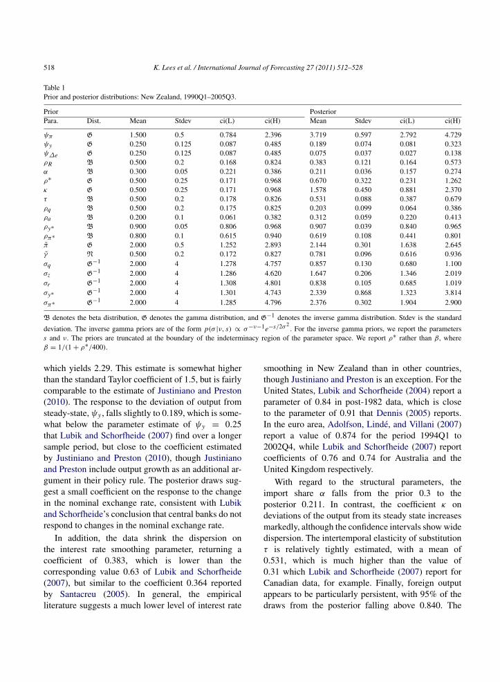
available. Fig. 5 shows forecasts from the DSGE-VAR and the Reserve Bank’s published MPS for an-nual inflation and the nominal 90-day interest rate atsix-monthly intervals (that is, omitting every secondforecast for display purposes) across the forecast eval-uation period.

Although the DSGE-VAR produces forecastswhich are competitive with the Reserve Bank’sforecasts, at times the forecasts are different. The

Reserve Bank’s interest rate forecasts are particularlysmooth, with the forecasts across 2000, and againin mid-2002, being too high relative to outturns, inhindsight. In contrast, the forecasts from the DSGE-VAR model show a considerable degree of short-run volatility (harming the MSFE performance, asis shown in Table 2), and more mean-reversion atlonger horizons. At least tentatively, the RBNZ’s MPS

526 K. Lees et al. / International Journal of Forecasting 27 (2011) 512–528

1998:1 1999:1 2000:1 2001:1 2002:1 2003:1 2004:1 2005:1

4

5

6

7

8

9

Interest rate

1998:1 1999:1 2000:1 2001:1 2002:1 2003:1 2004:1 2005:10.5

1

1.5

2

2.5

3

3.5

4

4.5Inflation

%

3

10

%

Fig. 5. Annual inflation and nominal interest rate forecasts: 1998Q4–2003Q3. Note: The dashed blue lines are the RBNZ’s published M P Sforecasts, the dotted red lines are the DSGE-VAR model forecasts and the solid black lines are the actual outturn. (For the interpretation of thereferences to colour in this figure legend, the reader is referred to the web version of this article.)

forecasts might be improved by placing some weighton the mean reversion property of the DSGE-VAR.

In terms of annual inflation, both the DSGE-VARand the RBNZ forecasts predict increasing inflationat the start of the forecast evaluation period, but bothmodels fail to predict the peak in annual inflation toalmost 4% at the end of 2000. Indeed, in general theforecasts from the two models are relatively similar,and it is not clear whether further forecasting gains

could be made by combining the DSGE-VAR and theRBNZ annual inflation forecasts.

5. Conclusion

This paper shows the benefits of utilizing DSGE-VAR models for forecasting in the open economy con-text. A VAR informed by Lubik and Schorfheide’s(2007) small open economy model produces forecasts

K. Lees et al. / International Journal of Forecasting 27 (2011) 512–528 527

which are comparable with, or, in the case of out-put growth, superior to, the Reserve Bank of NewZealand’s published judgement-adjusted forecasts. Inaddition, the forecasting performance of the DSGEmodel with no VAR correction is competitive. Atlonger horizons, where monetary policy is conven-tionally thought to have its greatest influence, boththe DSGE-VAR and the DSGE model outperform theforecasts given in the Reserve Bank of New Zealand’sMonetary Policy Statement.

The DSGE and DSGE-VAR models approach, butdo not attain, the performance of the Bayesian VARwith the Minnesota prior. However, the DSGE-VARis informative about the structure of the economy. TheDSGE structure should be robust to the Lucas critique;a policymaker who fears the Lucas critique can workwith a model which places a higher weight on theDSGE than is suggested by the data.

We believe that the DSGE-VAR is a usefulmodelling technology for central banks. In additionto the competitive forecasting performance reportedby Del Negro and Schorfheide (2004) for the U.S., theDSGE-VAR produces a good forecasting performancefor New Zealand, a small open economy with anexplicit inflation-targeting central bank. The ability toforecast well and yet obtain the economic structuresuggests that the DSGE-VAR may also be a usefulforecasting and policy analysis tool for other centralbanks.

Acknowledgements

We thank two anonymous referees, StephenBurnell, Todd Clark, Andrew Coleman, Marco DelNegro, Martin Fukac, Tim Kam, Thomas Lubik, EllisTallman, Shaun Vahey, and seminar participants atworkshops and seminars at the Reserve Bank ofNew Zealand, the Reserve Bank of Australia, LaTrobe University, the University of Melbourne, theAustralian National University and the New ZealandAssociation of Economists for comments. We aregrateful for Gauss code from Marco Del Negro andFrank Schorfheide, which we used in the paper.

References

Adolfson, M., Linde, J., & Villani, M. (2007). Forecastingperformance of an open economy dynamic stochastic generalequilibrium model. Econometric Reviews, 26(2–4), 289–328.

Basdevant, O., Bjorksten, N., & Karagedikli, O. (2004). Estimatinga time varying neutral real interest rate for New Zealand.Discussion Paper DP2004/01, Reserve Bank of New Zealand.

Benigno, P. (2004). Optimal monetary policy in a currency area.Journal of International Economics, 63(2), 293–320.

Chatfield, C. (1996). Model uncertainty and forecast accuracy.Journal of Forecasting, 14, 495–508.

DeJong, D. N., Ingram, B. F., & Whiteman, C. H. (2000). ABayesian approach to dynamic macroeconomics. Journal ofEconometrics, 98(2), 203–223.

Del Negro, M., & Schorfheide, F. (2003). Take your model bowling:Forecasting with general equilibrium models. Federal ReserveBank of Atlanta Economic Review, (Fourth quarter), 35–50.

Del Negro, M., & Schorfheide, F. (2004). Priors from generalequilibrium models for VARs. International Economic Review,45(2), 643–673.

Del Negro, M., & Schorfheide, F. (2008). Inflation dynamics ina small open-economy model under inflation targeting: Someevidence from Chile. Working Paper 329, Federal Reserve Bankof New York Staff Report..

Dennis, R. (2005). Specifying and estimating New Keynesian modelswith instrument rules and optimal monetary policies. FederalReserve Bank of San Francisco, Working Paper, 2004–17.

Diebold, F. X., & Mariano, R. S. (1995). Comparing predictiveaccuracy. Journal of Business and Economic Statistics, 13(3),253–263.

Elliott, G., & Timmermann, A. (2005). Optimal forecastcombination using under regime switching. InternationalEconomic Review, 46, 1081–1102.

Fukac, M., & Pagan, A. (2006). Issues in adopting DSGEmodels for use in the policy process. CAMA Working Paper10/2006, Australian National University, Centre for AppliedMacroeconomic Analysis.

Fukac, M., Pagan, A., & Pavlov, V. (2006). Econometric issuesarising from DSGE models. Mimeo. Paper presented atReserve Bank of New Zealand, ‘Macroeconomics and ModelUncertainty Conference’.

Gali, J., & Monacelli, T. (2005). Monetary policy and exchange ratevolatility in a small open economy. Review of Economic Studies,72(3), 707–734.

Geweke, J. (2005). Contemporary Bayesian econometrics andstatistics. Hoboken, New Jersey: John Wiley and Sons Ltd.

Goodwin, P. (2000). Correct or combine? Mechanically integratingjudgmental forecasts with statistical methods. InternationalJournal of Forecasting, 16, 261–275.

Hall, S. G., & Mitchell, J. (2007). Combining density forecasts.International Journal of Forecasting, 23(1), 1–13.

Ingram, B. F., & Whiteman, C. H. (1994). Supplanting the‘Minnesota’ prior: Forecasting macroeconomic time seriesusing real business cycle model priors. Journal of MonetaryEconomics, 34(3), 497–510.

Justiniano, A., & Preston, B. (2010). Monetary policy anduncertainty in an empirical small open economy model. Journalof Applied Econometrics, 25(1), 93–128.

Koop, G. (2003). Bayesian econometrics. Chichester, Sussex: JohnWiley and Sons Ltd.

528 K. Lees et al. / International Journal of Forecasting 27 (2011) 512–528

Lubik, T., & Schorfheide, F. (2004). Testing for indeterminacy:An application to U.S. monetary policy. American EconomicReview, 94(1), 190–217.

Lubik, T., & Schorfheide, F. (2006). A Bayesian look at new openeconomy. NBER Macroeconomics Annual 2006 (pp. 313–366).

Lubik, T., & Schorfheide, F. (2007). Do central banks respond toexchange rate movements? A structural investigation. Journalof Monetary Economics, 54(4), 1069–1087.

Newey, W. K., & West, K. (1987). A simple, positive semidefinite,heteroskedasticity and autocorrelation consistent covariancematrix. Econometrica, 55, 703–708.

Santacreu, A.M. (2005). Reaction functions in a small openeconomy: What role for non-traded inflation? Discussion PaperDP2005/04, Reserve Bank of New Zealand.

Wold, H. (1938). A study in the analysis of stationary time series.Uppsala: Almqvist and Wiksell.