Online Appendix to“Self-Ful�lling Debt Dilution”

By Mark Aguiar and Manuel Amador

Appendix A Closed-Form Expressions and DerivationsIn this appendix, we provide closed-form expressions for the solutions to the planning problemas well as equilibrium objects. We also include some notes on the underlying derivations.

A.1 �e E�cient Borrowing Allocation�e conjectured policy function for consumption in the borrowing allocation is given in (5). As+ is a stationary point, we immediately have:

%★� (+ ) =~ −�★(+ )A + _ .

Given this boundary condition and the consumption policy function, we solve the ODE (P) toobtain:

(i) For E ∈ [+ ,+ ]:

%★� (E) ≡1

A + _

[~ −� + (� + _+ − (d + _)E)

A+_d+_

(� + _+ − (d + _)+ )A−dd+_

].

(ii) For E ∈ (+ ,+<0G ]:

%★� (E) ≡1A

[~ −� + (� − ~ + A%★� (+ ))

(� − dE)Ad

(� − d+ )Ad

].

A.2 E�cient SavingFor the e�cient saving allocation, the conjecture is that the Safe Zone is an absorbing state. Inparticular, + is a stationary point, which pins down %★

((+ ) = (~ − d+ )/A . Given this boundary

condition and the policy function (9), we solve (P) for the Safe Zone to obtain:

%★( (E) ≡1A

[~ −� +

(� − d+

) d−Ad

(� − dE

) Ad

]for E ∈ [+ ,+<0G ] . (1)

For the saving region of the Crisis Zone, consumption is at its lower bound, � . Solving (P)for E ∈ [+ ,+ ), using %★

((+ ) from above as a boundary condition, we obtain the planner’s value

1

under saving:

% (E) ≡ 1A + _

~ −� + (� − ~ + (A + _)%★( (+ ))(� + _+ − (d + _)E

� − d+

) A+_d+_ . (2)

Per equation (12), %★((E) in the Crisis Zone is the maximum of % and %★

�. Straightforward di�er-

entiation indicate that % and %★�

cross at most once.

A.3 �e Borrowing Equilibrium

In the Crisis Zone (1�, 1�], @� (1) = @. Turning to the Safe Zone, recall that the conjectured

consumption policy function in the borrowing equilibrium is the same as the planner’s borrowingpolicy, (5). With this policy and the boundary @� (1�) = @, the solution to (20) is de�ned implicitlyby: (

1 − @� (1)1 − @

) AA+X

=� − ~ + A@� (1)1� − ~ + A@1

�

. (3)

For each 1 ∈ [0, 1�), there is a unique solution for @� (1) ∈ [@, 1]. Recall that for 1 < 0, we have

@� (1) = 1 regardless of the government’s policies.1�e government’s value in the borrowing equilibrium is obtained by inverting %★

�. Speci�-

cally:

+� (1) =

1d

(� − (� − d+ )

(�−~+A@� (1)1�−~+A@1�

) dA

)for 1 ∈ [−0, 1

�]

1d+_

©­«� + _+ −(�−~+(A+_)@1

) d+_A+_(

�−~+(A+_)@1�) d−AA+_

ª®¬ for 1 ∈ (1�, 1�],

(4)

where 0 ≡ (� − ~)/A is the maximal net in�ows that can be consumed by the government.

A.4 �e Saving Equilibrium�e saving equilibrium objects in the Safe Zone is straightforward: because it is an absorbingregion, there is no risk of default starting from 1 ≤ 1

(. Hence, the price is one, @( (1) = 1 and the

values and consumption are equivalent to their e�cient counterparts. �at is, inverting %★(

we

1 Note that there may be a discontinuity in @� at 1 = 0. Recall that at points of discontinuity, we impose that debtbuybacks occur at a price of one in the neighborhood around a discontinuity. �is restriction eliminates the technicalcomplication of the government a�empting to issue debt at one price and near-simultaneously repurchasing at alower price in an a�empt to exploit this discontinuity. �e restriction we impose ensures that the choice set is convexdespite the discontinuity in price, and hence the government has no motive to “mix” by moving consumption backand forth while keeping debt at the point of discontinuity.

2

obtain:

+( (1) = d−1 ©­«� − (� − d+ )(� − ~ + A1� − ~ + A1

(

) d

A ª®¬ for 1 ∈ [−0, 1(] (5)

where 1(≡ (~ − d+ )/A . �e consumption policy is � for 1 < 1

(, and d+ at 1

(.

Turning to the Crisis Zone, we begin with the saving region. Let {+ , C, @} denote the con-jectured equilibrium objects in the saving region of the Crisis Zone. In the saving region, wehave to deviate from the prescription of the e�cient allocation. �e reason is that the e�cientsavings policy, which sets consumption at its lower bound � , cannot be sustained in a competi-tive equilibrium. �at is, the e�cient savings rate is not privately optimal in an equilibrium withlong-term bonds.

We conjecture instead that the government saves by consuming at an interior optimum.2When consumption is interior, the linearity of the government’s objective function in (17) impliesthat it is indi�erent across alternative consumption choices, including the consumption level thatsets ¤1 = 0. Hence, the government must be indi�erent between the equilibrium consumptionstrategy and its associated stationary value:3

+ (1) ≡ ~ − [A + X (1 − @(1))]1 + _+d + _ . (6)

From the �rst-order condition in (17), interior consumption requires + ′(1) = −@(1). Usingthis, di�erentiating (6), and solving the resulting ODE with @(1

() = 1 as a boundary condition

yields

@(1) ≡A + X +

(11(

)− d+_+XX (_ + d − A )

d + _ + X . (7)

�e lenders’ break-even condition (19) requires @′(1) ¤1 = (A + X + _)@(1) − (A + X). Hence, we cansolve for the conjectured debt dynamics:

¤1 = −X1 ©­«@(1) − @

@(1) − @ + (d−A )@(1)A+X+_

ª®¬ ≡ 5 (1). (8)

Using (16), we obtain the associated consumption:

� (1) ≡ ~ − [A + X (1 − @(1))]1 + @(1) 5 (1). (9)

2�roughout the following analysis, we assume � is su�ciently low that an interior consumption choice is fea-sible.

3�e fact that the government’s value is equal to the stationary value while consumption is interior is discussedin Tourre (2017) and DeMarzo, He and Tourre (2018). �e authors give an interpretation of a durable monopolist inthe spirit of the Coase conjecture.

3

�e borrowing region of the Crisis Zone is also an absorbing state and corresponds to theequilibrium discussed in the previous subsection. Note that in this region, the price is @. Inthe Crisis Zone, +( (1) = max〈+ (1),+� (1)〉. As before, 1� is the intersection point of these twoalternatives. If no such 1� ∈ [1

(, 1�] exists, we set it to 1( . �e value of 1( is such that+( (1( ) = + ,

and we de�neB( ≡ [−0,1( ].4�e saving equilibrium value in the Crisis Zone is therefore:

+( (1) ≡{+ (1) for 1 ∈ (1

(, 1� ]

+� (1) for 1 ∈ (1� , 1( ];(10)

and the consumption policy is

C( (1) ≡{� (1) for 1 ∈ (1

(, 1� ]

C� (1) for 1 ∈ (1� , 1( ] .(11)

�e equilibrium price schedule is:

@( (1) ≡

1 for 1 ∈ [−0, 1

(]

@(1) for 1 ∈ [1(, 1� ]

@ for 1 ∈ (1� , 1( ];(12)

Appendix B Additional ResultsIn this appendix, we state state four results. �e �rst two allows us to provide a characterizationof a solution to the planner’s problem. �e next two are the same results for the government’sproblem in a competitive equilibrium.

�e value function %★(E) has the following standard properties:

Lemma B.1. �e solution to the planner’s problem, %★(E), is bounded and Lipschitz continuous.

Proof. �e proof is in Appendix C. �

Lemma B.1 states that %★ is bounded and Lipschitz continuous, and hence di�erentiable al-most everywhere. However, there may be isolated points of non-di�erentiability. At such points,%★ satis�es (P) in the viscosity sense. In particular:

Proposition B.1. Suppose a bounded, Lipschitz continuous function ? (E) with domain V has thefollowing properties:

(i) ? satis�es (P) at all points of di�erentiability;

4 If 1� < 1� , then @( is discontinuous at 1� , which is the case depicted in Figure 3. As previously discussed whenstating the government’s problem, and echoed in footnote 1, we rule out the government issuing at @( (1� ) and thenimmediately repurchasing at lim1′↓1� @( (1 ′) < @( (1� ) in an a�empt to set ¤1 = 0 by alternating between issuing andrepurchasing. Let us also note that the multiplicity result we obtain later on does not hinge on this particular issue:it is possible to obtain parameter values such that 1� = 1( and for which multiple equilibria coexist.

4

(ii) If limE↑+ ?

′(E) > limE↓+ ?

′(E) and limE↑+ ?

′(E) ≥ −1, then ? (+ ) = (~ − d+ )/A ;

(iii) At a point of non-di�erentiability E ≠ + , we have limE↑E ?′(E) < limE↓E ?

′(E);

(iv) If ?′(+ ) < −1, then ? (+ ) = (~ − d+ + _(+ −+ ))/(A + _);5 and

(v) ?′(+<0G ) ≤ −1;

then ? (E) = %★(E).

Proof. �e proof is in Appendix E. �

�e �rst condition of the proposition ensures that the candidate value function satis�es theHJB wherever it is smooth. �e second condition concerns the case when + is a locally stablestationary point; this will be relevant when we consider an e�cient “saving allocation” de�nedbelow. �e third condition states that any other point of non-di�erentiability has a “convex” kink.�e �nal two conditions are su�cient to ensure that E remains in V.

�e counterpart to Lemma B.1 for the equilibrium value function is:

Lemma B.2. In any competitive equilibrium such that @(1) ∈ [@, 1] for 1 ∈ B = [−0, 1], + isbounded, strictly decreasing, and Lipschitz continuous onB.

Proof. �e proof is in Appendix C. �

�e counterpart to Proposition B.1 for the government’s equilibrium problem (17) is:

Proposition B.2. Consider the government’s problem given a compact debt domainB and a priceschedule @ : B → [@, 1] that has a (bounded) derivative at almost all points in B. If a strictly

decreasing, Lipschitz continuous function E : B → [+ ,�/d] has the following properties:

(i) E satis�es (17) at all points of di�erentiability;

(ii) If lim1↑1 E′(1) > lim1↓1 E

′(1), then dE (1) = d+ = ~ − [A + X (1 − @(1))]1;

(iii) At a point of non-di�erentiability 1 ≠ 1, we have lim1↑1 E

′(1) < lim1↓1 E

′(1);

(iv) dE (−0) = � ; and

(v) (d + _)E (1) = ~ − [A + X (1 − @(1))]1 + _+ ;

then E (1) = + (1) is the government’s value function.

Proof. �e proof is in Appendix E. �

�e conditions listed in the proposition are similar to those from Proposition B.1. Namely,that the value function satis�es the HJB equation with equality wherever smooth; there may be alocal a�ractor that corresponds to 1 if the government saves; other points of non-di�erentiabilityhave convex kinks; and the endpoints of the domain deliver the value of holding debt constant.6

5For the endpoints of V, we interpret ? ′(+ ) ≡ limE↓+ ?′(E) and ? ′(+<0G ) ≡ limE↑+<0G ?

′(E).6Condition (v), at 1, is stronger than necessary, as the key requirement is that ¤1 ≤ 0 at the upper bound on debt;

however, in the equilibria described below, the stronger condition is always satis�ed.

5

Appendix C Proofs�is appendix contains all proofs except those for Propositions B.1 and B.2, which are presentedin the Online Appendix, along with a discussion of viscosity solutions more generally.

C.1 Proof of Lemma 1Proof. To generate a contradiction, suppose there is an e�cient allocation {c,) }, with ) < ∞.Note from (1) we have + (), c) = + . To see this, suppose instead that + (), c) > + ; that is,

+ (), c) = sup) ′≥C

∫ ) ′

)

4−(d+_) (B−) )2 (B)dB + 4−(d+_) () ′−) )+ + _∫ ) ′

)

4−(d+_) (B−) ) max〈+ (B, c),+ 〉dB

> + .

Hence, there exists a ) ′ > ) such that∫ ) ′

)

4−(d+_) (B−) )2 (B)dB + 4−(d+_) () ′−) )+ + _∫ ) ′

)

4−(d+_) (B−) ) max〈+ (B, c),+ 〉dB > + .

�is implies at time C < ) ,∫ )

C

4−(d+_) (B−C)2 (B)dB + 4−(d+_) ()−C)+ + _∫ )

C

4−(d+_) (B−C) max〈+ (B, c),+ 〉dB <∫ ) ′

C

4−(d+_) (B−C)2 (B)dB + 4−(d+_) () ′−C)+ + _∫ ) ′

C

4−(d+_) (B−C) max〈+ (B, c),+ 〉dB .

Hence, ) was never a sup of the original problem. �is establishes that + (), c) = + .Now consider an alternative allocation (c,∞). �e alternative consumption allocation equals

c for C < ) , but di�ers for C ≥ ) . We choose 2 (C) = (d + _)+ − _+ < ~ for C ≥ ) so that for allC ≥ ) :

+ (C, c) = 2 (C) + _+d + _

=(d + _)+ − _+ + _+

d + _= + .

�us, + (0; c) = + (0; c). Moreover, the alternative allocation delivers strictly more than zero tothe lender in expectation for C ≥ ) as 2 (C) < ~. As the government is indi�erent and the lenderreceives strictly more in expected present value, the original allocation is not e�cient. �

6

C.2 Proof of Lemma B.1Proof. Lemma 1 allows us to set ) = ∞ in the planning problem (3) to obtain

%★(E) = supc∈C,

∫ ∞

04−

∫ C0 A+1[E (B)<+ ]_3B [~ − 2 (C)]dC (13)

subject to

{E (0) = E

¤E (C) = −2 (C) + dE (C) − 1[E (C)<+ ]_[+ − E (C)

],

de�ned on the domain E ∈ V. %★ is bounded above by (~ −�)/A and below by (~ −�)/A . To seethat %★ is Lipschitz continuous in E , consider E1, E2 ∈ V, with E2 > E1. A feasible strategy startingfrom E (0) = E2 is to set consumption to � until E (C) = E1. Let Δ denote the time E (C) reaches E1.Suppose E (C) > + for C ∈ [0,Δ1) and E (C) < + for C ∈ (Δ1,Δ]. Let Δ2 = Δ − Δ1. If E2 < + , thenΔ1 = 0 and if E1 > + , then Δ2 = 0. �e dynamics of E (C) imply

4−dΔ1 =� − d max{E2,+ }� − d max{E1,+ }

4−(d+_)Δ2 =� + _+ − (d + _)min{E2,+ }� + _+ − (d + _)min{E1,+ }

.

Using this, one can show that

1 − 4−dΔ1−(d+_)Δ2 ≤ ! |E2 − E1 |, (14)

with ! ≡ (d + _)/(� − d+<0G ) ∈ (0,∞).As this is a feasible strategy for E2, integrating the objective function, we obtain

%★(E2) ≥ (~ −�)©­­«

1 − 4−AΔ1

A+4−AΔ1

(1 − 4−(A+_)Δ2

)A + _

ª®®¬ + 4−AΔ1−(A+_)Δ2%★(E1).

As ~ < � , we have

%★(E2) ≥ (~ −�)(1 − 4−AΔ1−(A+_)Δ2

A

)+ 4−AΔ1−(A+_)Δ2%★(E1),

which implies

%★(E1) − %★(E2) ≤(� − ~A+ %★(E1)

) (1 − 4−AΔ1−(A+_)Δ2

).

7

As %★(E1) ≤ (~ −�)/A , we have

%★(E1) − %★(E2) ≤(� −�A

) (1 − 4−AΔ1−(A+_)Δ2

).

As � > � and d ≥ A , this implies

%★(E1) − %★(E2) ≤(� −�A

) (1 − 4−dΔ1−(d+_)Δ2

)≤

(� −�A

)! |E2 − E1 |,

where the second line uses (14). As E1 < E2, and hence %★(E1) ≥ %★(E2) as %★ is the e�cientfrontier, we have

|%★(E1) − %★(E2) | ≤ |E2 − E1 |,

where

≡(� −�A

)! =

(� −�

� − d+<0G

) (d + _A

).

Hence, %★ is Lipschitz continuous with coe�cient ∈ (0,∞). �

C.3 Proof of Proposition 1Proof. We need to check the conditions of Proposition B.1. Note that %★

�is bounded, Lipschitz

continuous, and di�erentiable everywhere except + , where limE↑+ %

★′(E) < limE↓+ %

★′(E). �isinequality implies that condition (ii) in the proposition is irrelevant. Condition (iii) of PropositionB.1 is satis�ed trivially. Condition (iv) is satis�ed by construction.

At points of di�erentiability, the �rst-order condition for consumption requires %★′�(E) ≤ −1

for 2 = � to be optimal. Starting with E ∈ [+ ,+ ), di�erentiating the candidate function yields%★′�(E) ≤ −1. Hence � is optimal, and %★

�satis�es the HJB on this domain. Turning to E > + ,

note that %★�(E) is concave on this domain. �us, if lim

E↓+ %★′�(E) ≤ −1, then %★′

�(E) ≤ −1 for

E ∈ (+ ,+<0G ]. We have

limE↓+

%★′� (E) = −� − ~ + A%★

�(+ )

� − d+.

�is quantity is less than−1 when A%★�(+ ) ≥ ~−d+ . �is is the condition stated in the proposition.

�is condition is necessary and su�cient for %★�

to satisfy the HJB on (+ ,+<0G ). Moreover, it issu�cient to ensure that condition (v) of Proposition B.1 is satis�ed. �

8

C.4 Proof of Proposition 2Proof. �e proposed solution %★

(is di�erentiable everywhere save + and E � . At + we have

limE↑+ %

★′((E) ≥ −1 ≥ lim

E↓+ %★′(

. Hence, condition (ii) of Proposition B.1 is relevant and is satis-�ed by the candidate value function. %★

(satis�es condition (iii) at E � as it features a convex kink

by construction. Condition (iv) is also satis�ed by construction.On the domain E ∈ (+ ,+<0G ], we have %★′

((E) ≤ −1, and hence %★

(satis�es the HJB as well as

condition (v) of Proposition B.1.Turning to E < + , we now show that %★

((+ ) ≥ %★

�(+ ) is necessary and su�cient for %★

(to

satisfy the conditions of Proposition B.1.For su�ciency, suppose that %★

((+ ) ≥ %★

�(+ ). Let - ≡ {E ∈ [+ ,+ ) |%★

((E) ≥ %★

�(E)} =

[max{E � ,+ },+ ). On the domain - , %★((E) = % (E). One can show that % ′(E) ≥ −1 if and only if

% (E) ≥ (~ − (d + _)E + _+ )/(A + _). As the la�er term is the value associated with se�ing ¤E = 0,the inequality is satis�ed as % (E) ≥ %★

�(E) ≥ (~ − (d + _)E + _+ )/(A + _). Hence 2 = � is optimal

on - , and the HJB is satis�ed. If % (+ ) ≥ %★�(+ ), then - = [+ ,+ ), and hence the HJB is satis�ed

on the whole domain V. If instead there exists E � > + , then the HJB is satis�ed for E < E � fromProposition 1.

For necessity, suppose instead that %★((+ ) < %★

�(+ ). Comparison of the slopes implies that as

long as %★((E) < %★

�(E) for E ∈ [+ ,+ ), then %★′

((E) < %★′

�(E), and the two lines will never cross.

Moreover, %★′�(E) ≤ −1, and hence %★′

((E) < −1. �is implies that 2 = � is strictly sub-optimal

and the HJB is violated. �

C.5 Proof of Lemma B.2Proof. �e boundedness of + follows directly from �/d ≥ + (1) ≥ + for any 1 ∈ B.

To see that + is strictly decreasing, suppose 11 > 12 for 11, 12 ∈ B. If 12 = −0 ≡ (~ − �)/d ,then + (12) = �/d > + (11), where the la�er inequality follows from the budget set at 11 > 12.Now consider the following policy starting from 12 ∈ (−0, 11): Set 2 = � until 1 (C) = 11. As

¤1 (C) = 2 + (A + X)1 (C) − ~@(1 (C)) − X1,

and� > ~ − A1 ≥ ~ − [A + X (1−@(1))]1 for 1 ≥ 12, we have ¤1 (C) > 0. Let C ∈ (0,∞) denote when1 (C) = 11. As it is feasible for the government to follow this policy and not default while doingso, we have

+ (12) ≥∫ C

0�3C + 4−dC+ (11) =

(1 − 4dC

) �d+ 4−dC+ (11).

Subtracting + (11) from both sides yields:

+ (12) −+ (11) ≥(1 − 4dC

) (�

d−+ (11)

)> 0.

For continuity, we proceed in a similar fashion. Starting from11, consider the policy of se�ing

9

2 = � until 1 (C) = 12. Let C∗ denote the time where 1 (C) = 12. Given that � < ~ − (A + X)1 ≤~ − (A + X)1 (C) and @(1 (C)) ∈ [@, 1], C∗ < ∞. Moreover, the same statements imply that

12 − 11 ≥∫ C∗

0

(� + A1 (C) − ~

)3C ≥

∫ C∗

0

(� + A1 − ~

)3C =

(� + A1 − ~

)C∗,

where the �rst inequality follows from @(1) ≤ 1.

�e above implies that C∗ ≥ ! |11 − 12 |, with ! ≡(~ − A1 −�

)−1∈ (0,∞).

As this is a feasible strategy, we have

+ (11) ≥∫ C∗

04−dC�3C + 4−dC∗+ (12) = (1 − 4−dC

∗)�

d+ 4−dC∗+ (12),

where the inequality in the �rst line also re�ects that the right-hand side is the value assumingthe government never defaults, which is weakly below the optimal default policy. Subtracting+ (12) from both sides and rearranging, we have

+ (12) −+ (11) ≤ (1 − 4−dC∗)

(+ (12) −

�

d

).

Using the fact that �/d > + (1) ≥ + > �/d and 1 − 4−dC∗ ≤ C∗, we have

0 < + (12) −+ (11) ≤ C∗(+ (12) −

�

d

)≤ !

(� −�d

)|11 − 12 |.

Hence, |+ (12) −+ (11) | ≤ |12 − 11 | with ≡ !(� −�

)/d ∈ (0,∞). �

C.6 Proof of Proposition 3Proof. By construction, the price schedule @� is consistent with the lenders’ break-even condi-tion, given the conjectured government policy. �e remaining step is to verify if and when thegovernment’s policy is optimal given the conjectured @� . Hence, to prove the proposition, weneed to establish that +� satis�es the conditions of Proposition B.2 if and only if (22) holds.

For� to be optimal for all1 < 1� , the �rst-order condition for the HJB requires 1++ ′�(1)/@� (1) ≥

0 wherever + ′�(1) exists. �us, if + ′

�(1) ≥ −@� (1), then 2 = � is optimal. Recalling that +� was

constructed by assuming that the Hamiltonian is maximized at 2 = � , then + ′�(1) ≥ −@� (1) is

both necessary and su�cient to verify that the HJB is satis�ed at points of di�erentiability.We proceed to show that (22) is equivalent to + ′

�(1) ≥ −@� (1) at points of di�erentiability.

For 1 < 0, we have

d+� (1) = � − (� − d+� (0))(� + A1 − ~� − ~

) d

A

.

Note that +� is concave on this domain. For � to be optimal, it is therefore su�cient that

10

lim1↑0+′�(1) ≥ −1. �is will be true if and only if d+� (0) ≥ ~. Hence, the condition in equa-

tion (22) evaluated at 1 = 0 is necessary and su�cient for the HJB to hold for 1 ∈ (−0, 0). For1 = −0 = (~ −�)/d , we have +� (−0) = �/d , which is condition (iv) in Proposition B.2.

For 1 ∈ (0, 1�], from the lenders’ break-even condition, in the Safe Zone, we have (A +

X)@� (1) = @′� (1) ¤1 = @′�(1)

(� + [A + X (1 − @� (1))]1 − ~

). Di�erentiating +� in (4) and using this

expression to substitute for @′�(1), we have for 1 ∈ (0, 1

�]

+ ′� (1) = −@� (1)(

� − d+� (1)� − [A + X (1 − @� (1))]1 − ~

).

Hence, for 1 ∈ (0, 1�], the HJB is satis�ed if and only if d+� (1) ≥ ~ − [A + X (1 − @� (1))]1, which

is the condition in equation (22).For 1 ∈ (1

�, 1�], we have @� (1) = @ and

(d + _)+� (1) = � + _+ −(� + _+ − (d + _)+

) ©­«� − ~ + (A + _)@1

� − ~ + (A + _)@1�ª®¬d+_A+_

.

Note that +� (1) is concave in 1, hence we need to check the condition at 1 → 1� . We have for1 ∈ (1

�, 1�]

+ ′� (1) ≥ −� + _+ − (d + _)+� − ~ + (A + _)@1�

= −1,

where the �nal equality uses the de�nition of 1� ; hence, for this region the optimality conditionalways holds.

By construction, for 1 = 1� , condition (v) of Proposition B.1 is satis�ed.Note that as +� (1�) = + , the derivative of +� is continuous at 1

�. �e only point of non-

di�erentiability is 1 = 0. In particular, note that lim1↓0+′�(1) = − lim1↓0 @� (1) (� −d+� (0)) (� −~).

Hence, if lim1↓0 @� (1) < 1, then there is a convex kink at 1 = 0. �is is consistent with condition(iii) in Proposition B.2.

Hence, the conditions of Proposition B.2 hold if and only if (22) holds. �

C.7 Proof of Proposition 4Proof. �ere are three claims in the proposition:

Part (i). If a borrowing allocation is e�cient, it must dominate the stationary allocation, hence

A%★� (E) ≥ ~ − d+

11

for any + ≥ + . From the expressions for %★�

and +� , this implies that:

+� (1) ≥~ − A@� (1)1

d

=~ − A@� (1)

A+X (1−@� (1)) (A + X (1 − @� (1)))1d

≥ ~ − (A + X (1 − @� (1)))1d

for all 1 ∈ [0, 1�],

where the last inequality follows from A@� (1) ≤ A + X (1 − @� (1)) for all X ≥ 0, @� (1) ≤ 1 and1 ≥ 0. And thus condition (22) is satis�ed.

Part (ii). For 1 ∈ [0, 1�], Condition (22) becomes

d+� (1) − (~ − (A + X)1 + X@� (1)1) ≥ 0.

Now, from the price equation (3), we have(1 − @� (1)

1 − @

) AA+X

=� − ~ + A?� − ~ + A?

, (15)

where ? ≡ %★�(+ ) = @1

�. From this expression, we can de�ne @� (1) = � (X, ?), holding the other

parameters constant. Recall that condition (22) is restricted to 1 ∈ [0, 1�]; hence, the domain of

interest for ? is [0, ?], which is independent of X . We shall use the fact that

m� (X, ?)mX

=1 − � (X, ?)A + X

(@ + ln

( 1 − @1 − � (X, ?)

)), (16)

keeping in mind that @ = (A + X)/(A + X + _) and hence varies with X .Let +★

�denote the inverse of %★

�. Recall that +� (1) = +★

�(@� (1)1). Condition (22) can be

wri�en:

� (X, ?) ≡ d+★� (?) − ~ + (A + X)?/� (X, ?) − X? ≥ 0.

12

Taking the derivative with respect to X , we have that:

m� (X, ?)mX

=?

� (X, ?) − ? −(A + X)?� (X, ?)2

m� (X, ?)mX

=?

� (X, ?)

(1 − � (X, ?) − (A + X)

� (X, ?)m� (X, ?)mX

)=? (1 − � (X, ?))

� (X, ?)2

(� (X, ?) − (A + X)

(1 − � (X, ?))m� (X, ?)mX

)=? (1 − � (X, ?))

� (X, ?)2

(� (X, ?) − @ − ln

( 1 − @1 − � (X, ?)

)).

Note that m�/mX ≤ 0 if

� (X, ?) − @ − ln( 1 − @1 − � (X, ?)

)≤ 0.

For ? = ? , � (X, ?) = @, and this term is zero. Moreover, this expression is increasing in ? asm�/m? < 0. Hence, m� (X, ?)/mX ≤ 0 for ? ∈ [0, ?]. �us, if � (X0, ?) ≥ 0, then � (X, ?) ≥ 0 forX ∈ [0, X0].

Part (iii). �e fact that saving is e�cient implies

~ − d+A

> %★� (+ ) = @1�,

where the last equality follows from the de�nition of 1�. By continuity, there exists a +0 > +

such that

~ − d+0

A> %★� (+0) ≡ ?0 < ?,

where the last inequality follows from the fact that %★�

is strictly decreasing. As +0 = +★�(?0) by

de�nition of +★�

as the inverse of %★�

, this is equivalent to

d+★� (?0) < ~ − A?0.

Evaluated at ? = ?0, condition (22) is

� (X, ?0) = d+★� (?0) − ~ +

A?0

� (X, ?0)+ ?0X

(1

� (X, ?0)− 1

)≥ 0. (17)

Note that limX→∞ @ = 1, and hence � (X, ?) ≥ @ also converges to 1. Hence, d+★�(?0) − ~ +

A?0/� (X, ?0) → d+★�(?0) −~ + A?0 < 0. We now show that the last term in (17) converges to zero;

13

that is, X (1 − � (X, ?0)) → 0. From the de�nition of � in (15), we have

X (1 − � (X, ?0)) =_X

A + X + _

©­­­­­­«� − ~ + A?0

� − ~ + A?︸ ︷︷ ︸<1

ª®®®®®®¬

A+XA

.

As the ratio raised to the power (A + X)/A is strictly less than one as ?0 < ? , the right-hand sidegoes to zero as X → ∞. Hence, there exists a X1 such that for all X > X1, � (X, ?0) < 0, violatingthe condition for the borrowing equilibrium.

�

C.8 Proof of Proposition 5Proof. We proceed to show the necessity and su�ciency parts of the proposition independently.

�e “only if” part. Toward a contradiction, suppose that +( (1( ) < +� (1( ) (or equivalently1�> 1

(), and the conjectured saving equilibrium is indeed an equilibrium. First, note that @( (1) ∈

[@, 1], as the government defaults only with the arrival of + � = + .By construction, + (1

() = +( (1( ) = + . As +( is strictly decreasing, we have +( (1�) < + =

+� (1�). Hence, +( and +� do not intersect in [1(, 1�], and 1� > 1

(, and +( (1�) = + (1�).

We also have for 1 ≥ 1�: + ′(1) = −@( (1) ≤ −@ ≤ + ′� (1), where the la�er inequality uses a

property of the borrowing allocation value function (shown in the proof of Proposition 3). �isimplies that + (1) < +� (1) for all 1 ≥ 1

�, and there is no point of intersection to generate 1�

and +( = + for all 1 ∈ [1(, 1( ]. Now at 1( , we must have (as an equilibrium requirement) that

+ (1( ) = + < +� (1( ), where the la�er inequality follows from the fact that + < +� on this domain.�us, 1( < 1� . However, we have

(d + _)+ = ~ − [A + X (1 − @)]1� + _+

< ~ − [A + X (1 − @)]1( + _+

≤ ~ − [A + X (1 − @( (1( )]1( + _+= (d + _)+ (1( ) = (d + _)+ ,

where the �rst line uses the de�nition of1� ; the second line uses1� > 1( ; the third uses@( (1) ≥ @;and the �nal two equalities use the fact that + (1) is the stationary value at price @( and thede�nition of 1( , respectively. Hence, we have generated a contradiction.

�e “if” part. We �rst verify that +( satis�es the conditions of Proposition B.2 and establishthat @( is a valid equilibrium price schedule.

First, consider the government’s problem.

14

Condition (iv) and (v) of Proposition B.2 are satis�ed by construction. For 1 = 1(, condition

(ii) of Proposition B.2 applies and is satis�ed by construction.For 1 < 1

(, the conjectured value function is di�erentiable. For the HJB to hold with 2 = �

given that @( (1) = 1 in this region, we require + ′((1) ≥ −@( (1) = −1. On this domain, +( (1) =

+★((1), where the la�er is the inverse of the e�cient solution %★

(. As %★′

((E) ≤ −1, we have

+ ′((1) ≥ −1 = −@( (1). Hence, 2 = � is indeed optimal, and the HJB holds with equality.For 1 ∈ (1

(, 1� ),+( (1) = + (1), and thus+( is di�erentiable and satis�es the HJB with equality

by construction. Note that if @( (1) ≥ @ (something we check below), then ¤1 ≤ 0 in (1( , 1� ) byequation (16) (consistent with the equilibrium conjecture that the government is saving in thisregion). �is implies that �( (1) = � (1) ≤ � , and thus the conjectured policy function is a validone (recall that we are assuming that� is su�ciently low and can thus be ignored as a constraint).

For 1 ∈ (1� , 1( ), +( (1) = +� (1) and di�erentiability of +� implies that +( is di�erentiable. �eproof of Proposition 3 establishes that the HJB holds with equality in this domain, given that@( (1) = @.

�is con�rms that condition (i) of Proposition B.2 holds.If 1� ∈ (1

(, 1( ), +( (1� ) = +� (1� ), and there is a potential point of non-di�erentiability at 1� . If

@( (1� ) ≥ @ (something that we check below), we have that this kink is convex. �us, condition(iii) of Proposition B.2 holds.

Hence, given the conjectured @( , the value function is a viscosity solution to the government’sHJB equation.

Next, let us consider the price function. �e only thing le� to check is that @( (1) ∈ [@, 1] for1 ∈ (1

(, 1� ), where 1� ∈ (1

�, 1�). In this region, @( (1) ≤ 1 by equation (7). In addition,

(d + _)+( (1) = ~ −[A + X (1 − @( (1))

]1 + _+

≥ (d + _)+� (1)≥ ~ −

[A + X (1 − @)

]1 + _+ ,

where the �rst equality and second inequality follow from the equilibrium construction on 1 ∈(1(, 1� ). �e last inequality follows from the construction of +� (1) for 1 ∈ (1

�, 1�). Comparison

of the �rst and last lines establishes that @( (1) ≥ @. �

C.9 Proof of Proposition 6Proof. �e fact that the e�ciency of saving is a necessary condition for a saving equilibrium isestablished in the text. Turning to equation (25), multiply both sides of equation (24) by @ toobtain the following necessary and su�cient condition:

@%★( (+ ) ≥ @1� = %★� (+ ).

15

Using @ = (A + X)/(A + X + _) and the fact that %★((+ ) > %★

�(+ ), we solve for X to obtain

X ≥_%★

�(+ )

%★((+ ) − %★

�(+ )− A =

(A + _)%★�(+ ) − A%★

((+ )

%★((+ ) − %★

�(+ )

≥ 0,

where the last inequality is strict when d > A , as seen in the de�nition of %★�

. �us, this is anecessary and su�cient condition for the saving equilibrium, proving the proposition. �

C.10 Proof of Proposition 7Proof. Note that %★

�(E) is increasing in � . Hence,

%★� (+ ) ≤ lim�→∞

%★� (+ )

=~ − d+ + (d − A ) (+ −+ )

A + _

=A%★

((+ ) + (d − A ) (+ −+ )

A + _ .

�en a su�cient condition for saving to be strictly e�cient is

%★( (+ ) >A%★

((+ ) + (d − A ) (+ −+ )

A + _ ,

or

_

d − A >A (+ −+ )~ − d+

,

which is the last inequality in the proposition.Similarly,

%★( (+ ) − %★� (+ ) ≥

_%★((+ ) − (d − A ) (+ −+ )

A + _ ,

and

_%★�(+ )

%★((+ ) − %★

�(+ )− A ≤

_

(A%★

((+ ) + (d − A ) (+ −+ )

)_%★

((+ ) − (d − A ) (+ −+ )

− A

=(A + _) (d − A ) (+ −+ )

_%★((+ ) − (d − A ) (+ −+ )

≡ X.

From Proposition 6, a su�cient condition for a saving equilibrium, given that saving is e�cient,is that X is greater than X . Note that X is strictly positive and independent of � .

For the borrowing equilibrium, we need to show that the condition in equation (22) is satis�ed

16

as � becomes arbitrarily large. Speci�cally, �x any X = X > X . De�ne

�(1) ≡ d+� (1) − (~ − [A + X (1 − @� (1))]1),

where � implicitly depends on � and X . Note by condition (22) in Proposition 3 that if �(1) > 0on [0, 1�] ⊇ [0, 1�], then a borrowing equilibrium exists.

To establish the properties of �(1) as � → ∞, �rst note that 1� is independent of � . Inaddition,

lim�→∞

+� (1) = + + @(1� − 1),

where we use the fact that @� (1) → @ for 1 ∈ [0, 1�] as � → ∞. As the point-wise limit iscontinuous in 1, and by Lemma B.2 +� (1) is monotonic given � , the convergence is uniform onthe compact set [0, 1�] (see �eorem A of Buchanan and Hildebrandt (1908)).

Similarly, for 1 ∈ [0, 1�],

lim�→∞{~ − [A + X (1 − @� (1))]1} = ~ − [A + X (1 − @)]1 = ~ − (A + _)@1.

Again, the convergence is uniform by the same logic.Hence, �(1) converges uniformly on [0, 1�] to

�(1) ≡ lim�→∞

�(1) = d+ + d@(1� − 1) − (~ − (A + _)@1).

We now establish that �(1) > 0 for 1 ∈ [0, 1�]. �e linearity of �(1) in 1 implies that if theinequality holds for 1 = 0 and 1 = 1� , it is satis�ed for all intermediate points. For 1 = 0, we have

�(0) = d+ + d@1� − ~

=(d − A − _) (~ − d+ ) + d_(+ −+ )

A + _

=(d − A − _) (~ − d+ ) + (d − A )d (+ −+ )

A + _ > 0,

where the second line uses the de�nition of @1� and the �nal inequality uses the condition in theproposition. Similarly,

�(1�) = d+ − (~ − (A + _)@1)

= _(+ −+ ) > 0.

Hence, min1∈[0,1�] �(1) = min{�(0), �(1)} > 0.

As � → � uniformly on [0, 1�], for every n > 0, there exists an " such that for all � > " ,we have �(1) > �(1) − n for 1 ∈ [0, 1�]. Se�ing n < min

1∈[0,1�] �(1), we have �(1) > 0 for all

17

1 ∈ [0, 1�] and� > " . By Proposition 3, this is su�cient to establish the existence of a borrowingequilibrium for X = X when� > " . By part (ii) of Proposition 4, we have a borrowing equilibriumfor all X ∈ [0, X].

Combining results, there exists a non-empty interval Δ ≡ [X, X] and" such that for all� > "

and X ∈ Δ, both saving and borrowing equilibria coexist. �

C.11 Proof of Proposition 8Proof. We �rst sketch out the borrowing equilibrium under the assumed policy. Let {+ %

�, @%�}

denote the equilibrium policy and price functions. �e conjectured policy is for the governmentto borrow to 1� , which is the endogenous limit in the borrowing equilibrium absent the policy.From (27), it is optimal for the bondholders to sell their bonds at price @∗ > @ as soon as 1 = 1%

�,

where the la�er is de�ned by+ % (1%�) = + . �at is, bondholders sell their bonds to the third party

as soon as debt enters the Crisis Zone. We have

+ %� (1�) =~ − [A + X (1 − @∗)]1� + _+

d + _

= + +X (@∗ − @)1�

d + _ .

�e last term re�ects that the government rolls over debt at @∗ rather than @ once it reaches theborrowing limit. �e expression assumes that the government defaults upon the arrival of + . Tosee that this is optimal, note that the alternative of never defaulting yields the value

~ − [A + X (1 − @∗)]1�d

≤ ~ − A1�d

<~ − A1

(

d= + .

Facing @%�(1) = @∗ in the Crisis Zone, the government’s value can be obtained from the HJB, and

it is straightforward to verify that the �rst-order condition for 2 = � holds on this domain. As@∗ > @, 1%

�> 1

�, where the la�er is the benchmark borrowing equilibrium’s threshold for the

Safe Zone. Note as well that @∗ > @ implies that the third party takes a loss in expectation in theCrisis Zone.

For 1 ∈ [0, 1%], bondholders purchase debt at price @%

�(1) and collect A plus maturing principal

until 1 = 1%�, at which point they sell at @∗. �e equilibrium is recovered by solving the system of

di�erential equations:

d+ %� (1) = � ++%′� (1) ¤1

(A + X)@%� (1) = A + X + @%′� (1) ¤1

¤1 =� + (A + X)1 − ~

@%�(1)

− X1,

with the boundary conditions+ %�(1%�) = + and @%

�(1%�) = @∗. Note that these equations are identi-

cal to those in the benchmark borrowing equilibrium except that the boundary condition 1%�> 1

�

18

and @∗ > @.As is the case in the benchmark equilibrium, a necessary and su�cient condition for+ %

�to be

a solution to the government’s problem when facing @%�

is

+ %� (1) ≥~ − [A + X (1 − @%

�(1))]1

d,

for all 1 ∈ [0, 1�]. Following the same approach as in the proof of Proposition 7, we show that

this inequality holds as � →∞ uniformly over the full debt domain [0, 1�].As � →∞, we have for 1 ∈ [0, 1�],

lim�→∞

+ %� (1) = +%� (1�) + @

∗(1� − 1)

lim�→∞

~ − [A + X (1 − @%�(1))]1

d=~ − [A + X (1 − @∗)]1

d.

Recall from the proof of Proposition 7, that

�(1) = + + @(1� − 1) −~ − [A + X (1 − @)]1

d≥ 0

under the conditions of the proposition. Note that this implies

lim�→∞

(+ %� (1) −

~ − [A + X (1 − @%�(1))]1

d

)= �(1) +

X (@∗ − @)1�d + _ + (@∗ − @) (1� − 1) −

X (@∗ − @)d

1.

�is expression is linear in 1, and hence it is su�cient to verify the inequality at the endpoints1 = 0 and 1 = 1� . �e fact that �(0) > 0 and @∗ > @ implies that the limit is strictly positive at1 = 0. For 1 = 1� , we have

�(1�) −X (@∗ − @)1�

d + _ −X (@∗ − @)

d1�

=~ − [A + X (1 − @)]1� + _+

d + _ −~ − [A + X (1 − @)]1�

d+X (@∗ − @)1�

d + _ −X (@∗ − @)

d1�

=−_

d (d + _)

(~ − [A + X (1 − @∗)]1� − d+

)=

−_d (d + _)

(A (1

(− 1�) − X (1 − @∗)1�

)> 0,

where the last inequality uses 1� > 1(. �is completes the proof of part (i).

19

For part (ii), the saving equilibrium requires + %�(1() ≤ + . As � →∞,

+ %� (1( ) = +%� (1�) + @

∗(1� − 1( )

=~ − A1� + _+

d + _ + 1� − 1( − (1 − @∗) (1� − 1( ) −

X (1 − @∗)1�d + _

= + +(d + _ − A ) (1� − 1( )

d + _ − (1 − @∗)(1� − 1( +

X1�

d + _

).

As the second term is strictly positive, there exists a @ < 1 such that this expression exceeds +for @∗ > @, hence violating the necessary condition for a saving equilibrium.

�

C.12 Proof of Proposition 9Proof. For part (i), note that in the saving equilibrium undistorted by policy, @( (1) = 1 for 1 ≤ 1

(.

Hence, imposing a price �oor restricted to the Safe Zone does not alter the saving equilibrium,which exists by Proposition 7. Hence, the price �oor is irrelevant under the saving equilibrium.

Using the notation introduced in the proof of Proposition 8, a necessary condition for theborrowing equilibrium under the policy is for 1 ∈ [0, 1%

�]

+ %� (1) ≥~ − [A + X (1 − @%

�(1))]1

d≥ ~ − [A + X (1 − @

∗)]1d

.

Recall that in the construction of the borrowing equilibrium, 1�

is de�ned by solving the HJBassuming @� (1) = @. Hence, + %

�(1) = +� (1) for 1 > 1

(, as the policy is restricted to 1 ∈ [0, 1

(].

As +� (1( ) < + by the inequality of Proposition 7, we have 1%�< 1

(. For 1 = 1%

�, we have

+ %� (1%�) = + =

~ − A1(

d<~ − A1%

�

d,

where the �rst two equalities use the de�nitions of 1%�

and 1(, respectively. Hence, there exists a

@ < 1 such that

+ %� (1%�) <

~ − [A + X (1 − @∗)]1%�

d,

for @∗ > @, violating the necessary condition for a borrowing equilibrium. �is proves part (ii).�

Appendix D �e Hybrid EquilibriumIn this appendix, we present a third type of competitive equilibrium, which we label the “hybrid”equilibrium because it combines features of both borrowing and saving equilibria. In particular,

20

the government never saves, as in the borrowing equilibrium, but part of the Safe Zone is absorb-ing, as in the saving equilibrium. �e main purpose of introducing the hybrid equilibrium is toshow existence of a competitive equilibrium; in particular, we prove that if neither the borrowingnor the saving equilibrium exists, then a hybrid equilibrium exists. �e equilibrium objects aredepicted in Figure D.1 using the same parameters as in Figures 1 and 3.

More formally, given +� in (4), de�ne the threshold

+� (1� ) =~ − A1�

d, (18)

if such a threshold exists on the domain [0, 1�] ∩ [0, 1

(]. �e equilibrium conjecture is that for

1 ≤ 1� , the government borrows up to 1� and then remains there inde�nitely. �is behavior issimilar to the Safe Zone policy in the saving equilibrium, but the threshold 1� may be strictlybelow 1

(. At 1� , given that +� (1� ) = (~ − A1� )/d , the government is indi�erent to remaining

at 1� at risk-free prices versus borrowing to the debt limit at the borrowing equilibrium priceschedule. �e conjecture is that for 1 > 1� , the government borrows. In a hybrid equilibrium,therefore, 1� is a stationary point that is stable from the le� but not the right.

For 1 < 1� , we solve the government’s HJB assuming 2 = � to obtain a candidate +� onthis domain, using the boundary condition d+� (1� )~ − A1� . For 1 > 1� , the hybrid equilibriumcoincides with the borrowing equilibrium. Se�ing1� ≡ 1� , the hybrid equilibrium value functionis therefore

+� (1) =

�−(�+A1�−~)

(�+A1−~�+A1� −~

) dA

dfor 1 ≤ 1�

+� (1) for 1 ∈ (1� , 1� ] .(19)

�e associated price schedule is

@� (1) ={

1 for 1 ≤ 1�@� (1) for 1 ∈ (1� , 1� ] .

(20)

Finally, the policy function for consumption is

C� (1) =

� for 1 < 1�

~ − A1� for 1 = 1�

C� for 1 ∈ (1� , 1� ] .(21)

We state the following:

Proposition D.3. Suppose neither the borrowing equilibrium nor the saving equilibrium exists.Speci�cally, suppose that 1

(< 1

�and that there exists a 1 ∈ [0, 1

�] such that d+� (1) < ~ − [A +

X (1 − @� (1))]1. �en a hybrid equilibrium exists.

Proof. �e conjectured price schedule @� is consistent with the lenders’ break-even conditiongiven the assumed government policy. �us, to establish the conditions of an equilibrium, it issu�cient to prove that +� is a solution to the government’s HJB.

21

(i) For1 ∈ [1(, 1�]: By premise, 1

�> 1

(. �is implies that d+� (1( ) > + = ~−A1

(≥ ~−[A+X (1−

@� (1( ))]1( . For 1 > 1(, we have d+ > ~ − A1. As+� ≥ + for 1 ≤ 1

�, we have+� (1) ≥ ~ − A1

for 1 ∈ [1(, 1�]. From the proof of Proposition 3, this implies that+� (1) = +� (1) satis�es the

government’s HJB on this domain. �e proof of Proposition 3 extends this to 1 ∈ [1�, 1�] as

well.

(ii) For 1 ≤ 1(: Note that the premise implies there exists a 1 ∈ [0, 1

�] such that d+� (1) <

~ − [A +X (1−@� (1))]1 ≤ ~ − A1. �e above established that d+� (1) > ~ − A1 for 1 ∈ [1(, 1�].

Hence, 1 < 1(. By continuity, there exists a 1� ∈ (1, 1( ) such that d+� (1� ) = ~ − A1� . Note

as well that this implies + ′�(1� ) = lim1↓1� +

′�(1) ≥ −A/d . From the expression for +� , we

have lim1↑1� +� (1� ) = −1 ≤ −A/d . Hence, +� is either di�erentiable or has a convex kinkat 1� , satisfying the conditions for a solution to the government’s HJB at 1� . For 1 < 1� ,+ ′�(1) ≥ −1, implying that the HJB is satis�ed on this domain as well. Finally, +� (1) > +

for 1 ≤ 1� , rationalizing the government’s non-default on this domain.

�

�is establishes that at least one of the three types of equilibria always exists. We note thatthe hybrid may coexist with the other equilibria as well. In fact, as � → ∞, the condition formultiplicity presented in Proposition 7 also implies the existence of a hybrid equilibrium.

Appendix E Viscosity Solutions on Strati�ed Domains andthe Proofs of Propositions B.1 and B.2

In this appendix, we establish the equivalence between the sequence problems and the viscositysolutions of the Hamilton-Jacobi-Bellman (HJB) equations. �e two complications are that theobjective and/or the dynamics are not necessarily continuous in the state variables. We rely onthe results of Bressan and Hong (2007) (henceforth, BH) to establish the validity of the recursiveformulation. �is appendix introduces their environment and summarizes their core results. Rel-ative to BH, we make minor changes in notation and consider a maximization problem while theoriginal BH studies minimization. We then prove Propositions B.1 and B.2.

E.1 �e Environment of Bressan and Hong (2007)Let - ⊂ R# denote the state space. In the benchmark BH environment, - = R# ; however,they show how to restrict a�ention to an arbitrary subset by extending the dynamics and payo�functions to R# such that the subset is an absorbing region. Let U (C) ∈ A denote the controlfunction, where A is the set of admissible controls. Dynamics of the state vector G are given by¤G (C) = 5 (G (C), U (C)).

22

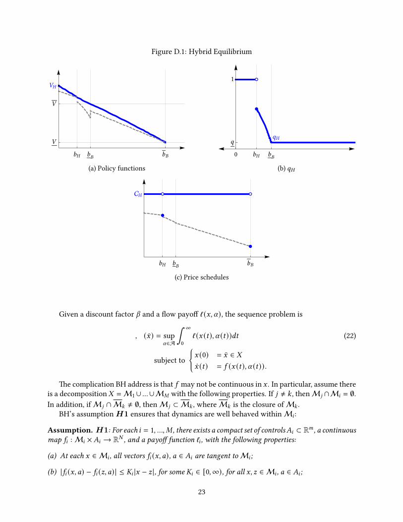
Figure D.1: Hybrid Equilibrium

(a) Policy functions (b) @�

(c) Price schedules

Given a discount factor V and a �ow payo� ℓ (G, U), the sequence problem is

, (G) = supU∈A

∫ ∞

0ℓ (G (C), U (C))3C (22)

subject to

{G (0) = G ∈ -¤G (C) = 5 (G (C), U (C)).

�e complication BH address is that 5 may not be continuous in G . In particular, assume thereis a decomposition- =M1∪ ...∪M" with the following properties. If 9 ≠ : , thenM 9 ∩M8 = ∅.In addition, ifM 9 ∩M: ≠ ∅, thenM 9 ⊂ M: , whereM: is the closure ofM: .

BH’s assumptionH1 ensures that dynamics are well behaved withinM8 :

Assumption. H1: For each 8 = 1, ..., " , there exists a compact set of controls�8 ⊂ R< , a continuousmap 58 :M8 ×�8 → R# , and a payo� function ℓ8 , with the following properties:

(a) At each G ∈ M8 , all vectors 58 (G, 0), 0 ∈ �8 are tangent toM8 ;

(b) |58 (G, 0) − 58 (I, 0) | ≤ 8 |G − I |, for some 8 ∈ [0,∞), for all G, I ∈ M8 , 0 ∈ �8 ;

23

(c) Each payo� function ℓ8 is non-positive and |ℓ8 (G, 0) − ℓ8 (I, 0) | ≤ !8 |G − I |, for some !8 ∈ [0,∞),for all G, I ∈ M8 , 0 ∈ �8 ;7

(d) We have 5 (G, 0) = 58 (G, 0) and ℓ (G, 0) = ℓ8 (G, 0) whenever G ∈ M8 , 8 = 1, ..., " .

�e key assumption is (1); namely, that dynamics are Lipschitz continuous when con�ned totangent trajectories. �is does not restrict how the dynamics change when crossing the bound-aries ofM8 .

Let TM8(G) denote the cone of trajectories tangent toM8 at G ∈ M8 :

T"8 (G) ≡{~ ∈ R#

����limℎ→0

infI∈M8|G + ℎ~ − I |ℎ

= 0}.

Part (a) ofH1 is equivalent to 58 (G, 0) ∈ TM8for all G ∈ M8, 0 ∈ �8 .

For G ∈ M8 , let � (G) ⊂ R#+1 denote the set of achievable dynamics and payo�s for the set ofcontrols �8 :

� (G) ≡ {( ¤G,D) | ¤G = 58 (G, 0), D ≤ ℓ8 (G, 0), 0 ∈ �8} , (23)

where 8 is such that G ∈ M8 . To handle discontinuous dynamics, BH use results from di�erentialinclusions. In particular, let � (G) denote an extended set of feasible trajectories and payo�s:

� (G) ≡ ∩n>02>{( ¤G,D) ∈ � (G′)

��|G − G′| < n} , (24)

where 2>( denotes the closed convex hull of a set ( .�e next key assumption is that� (G) does not contain additional trajectory-payo� pairs when

restricted to tangent trajectories:

Assumption. H2: For every G ∈ R# , we have

� (G) ={( ¤G,D) ∈ � (G) | ¤G ∈ TM8

}. (25)

BH de�ne the Hamiltonian using � (G) as the relevant choice set:

� (G, ?) ≡ sup( ¤G,D)∈� (G)

{D + ? ¤G}. (26)

�e corresponding HJB is

VF (G) = � (G, �F (G)), (27)

where � is the di�erential operator. BH de�ne the following concepts:

De�nition 1. A continuous functionF is a lower solution of (27) if the following holds: IfF − ihas a local maximum at G for some continuously di�erential i , then

VF (G) − � (G, �i (G)) ≤ 0. (28)7We strengthen part (c) to incorporate the Lipschitz continuity condition stated in BH equation (46).

24

De�nition 2. A continuous function F is an upper solution of (27) if the following holds: IfG ∈ M8 , and the restriction of F − i to M8 has a local minimum at G for some continuouslydi�erential i , then

VF (G) − sup( ¤G,D)∈� (G), ¤G∈)M8

{D + �i ¤G} ≥ 0. (29)

De�nition 3. A continuous function F , which is both an upper and a lower solution of (27), is aviscosity solution.

Note that the second de�nition di�ers from the �rst by restricting a�ention to M8 whendescribing the properties ofF−i , which relaxes the set ofi that satis�es the condition. However,the trajectories in the Hamiltonian are restricted to lie in the tangent set.8 �e added propertiesare the core distinction between the de�nition of viscosity solution used here versus the standardde�nition.9

With these de�nitions in hand, we summarize the core results of BH:

(i) (BH �eorem 1) IfH1 andH2 hold, and there exists at least one trajectory with �nite value,then the maximization problem admits an optimal solution.

(ii) (BH Proposition 1) Let assumptionsH1 andH2 hold. If the value function, is continuous,then it is a viscosity solution of (27).

(iii) (BH Corollary 1) Let assumptions H1 and H2 hold. If the value function , is boundedand Lipschitz continuous, then, is the unique non-positive viscosity solution to (27).10

E.2 �e Planner’s ProblemTo map problem (3) into BH, we make a few modi�cations and consider a generalized problem.First, we let the planner randomize when the government is indi�erent to default or not. �ishelps to convexify the choice set. In particular, let c (C) ∈ [0, 1] be an additional choice, wherec (C) is the probability the government defaults when + arises and the current value is + . It willalways be e�cient to set c (C) = 0 when E (C) = + , and so this does not alter the solution to theplanner’s problem. We denote the set of possible paths,π = {c (C) ∈ [0, 1]}C≥0, by �. �e controlsare α = (c,π) ∈ A ≡ C × �.

Recall that in (3) the objective is discounted by the probability of repayment, 4−_∫ C

0 1[E (B)<+ ]3B .Let us de�ne Γ(C) as follows:

Γ(C) ≡ Γ(0)4−_∫ C

0 (c (B)1[E (B)=+ ]+1[E (B)<+ ]3B

8�e fact that trajectories are restricted to)"8 in the de�nition of an upper solution was unintentionally omi�edin Bressan and Hong (2007) but is corrected in Bressan (2013).

9Note that we place the restriction on the upper solution while the original BH place it on the lower solution aswe consider a maximization problem.

10BH state a weaker continuity condition than Lipschitz continuity (BH H3) that is not necessary given ourenvironment.

25

for some Γ(0) ∈ (0, 1]. Note that Γ(C)/Γ(0) is the discount factor in the original problem with c =

0. By adding Γ(C) as an additional state variable, we will be able to keep track of the probabilityof survival in our recursive formulation.

Let - = V × (0, 1] denote the state space for G = (E, Γ). Let 5 (G, U) = ( ¤E, ¤Γ) given the controlU = (2, c):

5 (G, U) =¤E = −2 + dE − 1[E<+ ]_

[+ − E

]¤Γ = −_

[c1[E=+ ] + 1[E<+ ]

]Γ.

(30)

�e �ow value must be non-positive. We therefore subtract the constant (~ −�)/A from thevalue. To convert this into a �ow payo�, let

ℓ (G, 0) ≡ Γ(~ − 2) − (~ −�) ≤ 0,

where the inequality uses ~ > � and Γ ≤ 1. Note that ℓ is Lipschitz continuous in G .Hence, we consider the following problem, where G (C) ≡ (E (C), Γ(C)):

% (E, Γ) = supα∈A

∫ ∞

04−AC ℓ (G (C), U (C))dC (31)

subject to

{(E (0), Γ(0)) = (E, Γ)( ¤E (C), ¤Γ(C)) = 5 (G (C), U (C)) .

We then have a one-to-one mapping between % and %★:

% (E, Γ) = Γ%★(E) − (~ −�)/A . (32)

As %★ is bounded and Γ ∈ (0, 1], % is bounded. Similarly, % is Lipschitz continuous in the statevector (E, Γ).

We now verify the conditions of BH. De�ne �ve regions of the state space:

M1 ≡ {+ } × (0, 1]M2 ≡ (+ ,+ ) × (0, 1]M3 ≡ {+ } × (0, 1]M4 ≡ (+ ,+<0G ) × (0, 1]M5 ≡ {+<0G } × (0, 1] .

26

Let �8 denote the controls that produce trajectories that are tangent toM8 :11

�8 ≡ {(2, c) |2 ∈ [�,�], c ∈ [0, 1], ¤G ∈ T"8 }

=

{d+ − _(+ −+ )} × [0, 1] if 8 = 1{d+ } × [0, 1] if 8 = 3{d+<0G } × [0, 1] if 8 = 5[�,�] × [0, 1] otherwise.

(33)

Within eachM8 , the dynamics 5 are Lipschitz continuous in G for all 0 ∈ �8 . It is straightforwardto verify that we satisfy AssumptionH1.

Let us now verify AssumptionH2. �ere two cases:

Case 1: i ∈ {2,4}. In this case, � (G) = � (G), and BH Assumption H2 is straightforward toverify.

Case 2: i ∈ {1,3,5}. We show the 8 = 3 case (as the others are similar). We have12

� (G) ={( ¤G,D) | ¤E = 0, ¤Γ = −c_Γ, D ≤ ℓ (G, (d+ , c)), c ∈ [0, 1]

}(34)

=

{( ¤G,D) | ¤E = 0, ¤Γ ∈ [−_Γ, 0], D ≤ Γ(~ − d+ ) − (~ −�)

}= {0} × [−_Γ, 0] × (−∞, Γ(~ − d+ ) − (~ −�)] . (35)

Let G′ = (E′, Γ′) be in the neighborhood of G = (+ , Γ). We have

� (G′) ={( ¤G,D)

��¤E = −2 + dE′ − _1{E ′<+ } (+ − E

′),¤Γ ∈ [−_1{E ′<+ }Γ, 0],

D ≤ Γ(~ − 2) − (~ −�), 2 ∈ [�,�]}.

We have that

∪|G ′−G |≤n � (G′) ⊆ '(G, n) ≡{¤E = −2 + \,¤Γ = [−_(Γ + n), 0],D ≤ (Γ + n − 1)~ − (Γ − n)2 + 2,\ ∈ [d (+ − n) − _n, d (+ + n)]

2 ∈ [�,�]}.

11For 8 = 1, 3, 5, the tangent trajectories set ¤E = 0. Otherwise, they are the full set of trajectories.12Note this is the only case where the choice of c is relevant.

27

Note that '(G, n) is convex and � (G) = ∩n>0'(G, n). Also note that

� (G) = {( ¤G,D) ∈ � (G) | ¤G ∈ TM3},

where the equivalence uses the de�nitions of� , � , and the tangent trajectories TM3 . �is veri�esBHH2 forM3.

Similar steps hold for 8 = 1 and 5, verifying AssumptionH2 for all domains.13

As noted above, % is bounded and Lipschitz continuous. Hence, by BH Corollary 1, it is theunique viscosity solution with such properties for the HJB:

A % (E, Γ) = � ((E, Γ), (%+ , %Γ)) ≡ sup(2,c)∈[�,�]×[0,1]

{Γ(~ − 2) − (~ −�) + %E ¤E + %Γ ¤Γ

}, (36)

where ¤E and ¤Γ obey equation (30). Here, we have used the fact that � (G) contains the full setof trajectories generated by 2 ∈ [�,�] and c ∈ [0, 1]. Note that it is optimal to set c to 0, andthus we can ignore this choice in the Hamiltonian in what follows. We shall use the fact that �is convex in %E .

E.3 Proof of Proposition B.1Proof. Suppose that ? (E) satis�es the conditions in the proposition. We shall show that ? (E, Γ) ≡Γ? (E) − (~ − �)/A is a viscosity solution of (36). ? is di�erentiable in Γ at all points, and in Eat points where ? (E) is di�erentiable. We now check the conditions for a viscosity solution. Weproceed by checking on each domainM8 .

(i) (E, Γ) ∈ M2 ∪M4

As ? is di�erentiable on this part of the domain, by condition (i) of the proposition, we have

A? (E) = sup2∈[�,�]

{~ − 2 + ?′(E) ¤E + 1[E<+ ]? (E)

}= sup2∈[�,�]

{~ − 2 + Γ−1?E ¤E + Γ−1?Γ ¤Γ

},

where the second line uses ?E = Γ?′(E) and ?Γ ¤Γ/Γ = −_1[E<+ ]? . Multiplying through byΓ ∈ (0, 1] and subtracting (~ −�)/A from both sides yields

A? (E) = A (Γ? (E) − (~ −�)) = sup2∈[�,�]

{Γ(~ − 2) − (~ −�)/A + ?E ¤E + ?Γ ¤Γ

}= � ((E, Γ), (?E , ?Γ)) .

Hence, ? satis�es (36).Now consider a point of non-di�erentiability E . As (E, Γ) ∉ M3, E ≠ + , and hence con-dition (iii) of the proposition is applicable. Condition (iii) states that ?−

E≡ limE↑E ?

′(E) <13For E = + , we extend the dynamics to both sides of+ by se�ing ¤E = −2+dE−_(+ −E) in the neighborhood E < +

and ℓ arbitrarily low. �us, the dynamics are continuous at G = (+ , Γ). Similarly for E = +<0G , we set ¤E = −2 + dE .

28

limE↓E ?′(E) ≡ ?+

E). Hence, there is a convex kink. In this case, the lower solution does not

impose additional conditions, leaving the conditions for an upper solution to be veri�ed.Suppose i is di�erentiable and ? − i has a local minimum at (E, Γ). �en iE ∈ [?−E , ?

+E]. As

? is di�erentiable in Γ, we have iΓ = ?Γ . Note that

A? (E) = � ((E, Γ), (?−E , ?Γ)) = � ((E, Γ), (?+E , ?Γ)), (37)

as the HJB holds with equality at points of di�erentiability in the neighborhood of E , andusing the continuity of � .Note that there exists U ∈ [0, 1] such that iE = U?+E + (1 − U)?

−E

. �e convexity of � withrespect to iE implies that

� ((E, Γ), (iE , iΓ)) = � ((E, Γ), (U?+E + (1 − U)?−E , iΓ))

≤ U� ((E, Γ), (?+E , iΓ)) + (1 − U)� ((E, Γ), (?−E , iΓ))

= A? (E),

where the last equality uses (37) and iΓ = ?Γ . Hence, ? (E) satis�es the conditions of anupper solution.

(ii) (E, Γ) ∈ M3 = {+ } × (0, 1]Turning to E = + , we rede�ne ?+E ≡ lim

E↓+ ?′(E) and ?−E ≡ lim

E↑+ ?′(E). Given the continuity

of ? and the fact that it satis�es the HJB in the neighborhood of + with equality, we have

A? (+ ) = sup2∈[�,�]

{~ − 2 + ?+E ¤E} (38)

= sup2∈[�,�]

{~ − 2 + ?−E ¤E − _? (+ )},

where ¤E = −2 + d+ . As se�ing 2 = d+ is always feasible, this implies A? (+ ) ≥ (~ − d+ ) ≥ 0.To verify that ? is a viscosity solution to (26), note that if ? is di�erentiable, then it satis�esthe HJB with equality by condition (i) of the proposition.If it is not di�erentiable, we consider convex and concave kinks in turn.Suppose that ?−E < ?+E . �en the conditions for a lower solution do not impose any restric-tions. For an upper solution, consider a i such that ? − i has a local minimum at (+ , Γ).Again, iΓ = ?Γ = ? (+ ). Recall that for an upper solution, we need only consider trajectories

29

that are in TM3 , that is, ¤E = 0 and thus 2 = d+ . Hence:

A? (+ ) = AΓ? (+ ) − (~ −�)≥ Γ(~ − d+ ) − (~ −�)

= sup2=d+

Γ(~ − 2) − (~ −�) + iE(−2 + d+

)︸ ︷︷ ︸

¤E

= sup2=d+ ,c∈[0,1]

Γ(~ − 2) − (~ −�) + iE(−2 + d+

)︸ ︷︷ ︸

¤E

−? (+ ) × c_Γ︸ ︷︷ ︸iΓפΓ

,where the last equality uses ? (+ ) ≥ 0. Note that �nal term is the Hamiltonian maximizedalong tangent trajectories in TM3 . �us, the conditions of an upper solution are satis�ed.For the lower solution, we must consider the case in which ? − i has a local maximum at(+ , Γ). �is requires ?−E ≥ ?+E and iE ∈ [?+E , ?−E ]. Again, as ? is di�erentiable with respect toΓ, we have iΓ = ?Γ = ? (+ ).If ?+E ≤ −1, then condition (ii) in the proposition implies that

A? (+ ) = Γ(~ − d+ ) − (~ −�)

≤ sup2∈[�,�],c∈[0,1]

Γ(~ − 2) − (~ −�) + iE (−2 + d+ )︸ ︷︷ ︸¤E

+iΓ (−c_Γ)︸ ︷︷ ︸¤Γ

= � ((+ , Γ), (iE , iΓ)),

where the second to the last line follows from iΓ = ? (+ ) ≥ 0. Hence, ? (+ ) = Γ? (+ ) − (~ −�)/A satis�es the condition for a lower solution when ?+E ≤ −1.Alternatively, if ?+E > −1, then

A? (+ ) = sup2∈[�,�]

{~ − 2 + ?+E (−2 + d+ )}

= ~ −� + ?+E (d+ −�)≤ ~ −� + iE (d+ −�),

for iE ≥ ?+E as d+ > � . Hence,

A? (+ ) ≤ sup2∈[�,�],c∈[0,1]

Γ(~ − 2) − (~ −�) + iE (−2 + d+ )︸ ︷︷ ︸¤E

+iΓ (−c_Γ)︸ ︷︷ ︸¤Γ

30

for iE ∈ [?+E , ?−E ] and iΓ = ? (+ ), satisfying the condition for a lower solution.

(iii) (E, Γ) ∈ M1 = {+ } × (0, 1]For E = + , the condition for ? to be an upper solution is

A? (+ , Γ) ≥ Γ(~ − d+ + _(+ −+ )

)− (~ −�) − _? (+ )Γ,

where the right-hand side is the Hamiltonian evaluated at ¤E = 0. As ? satis�es the HJB withequality in the neighborhood of + , we have

? (+ , Γ) = limE↓+

A? (E, Γ) = limE↓+

� ((E, Γ), (Γ?′(E), ? (E)))

≥ limE↓+

{Γ

(~ − dE + _(+ − E)

)− (~ −�) − _? (E)Γ,

}= Γ

(~ − d+ + _(+ −+ )

)− (~ −�) − _? (+ )Γ.

Hence, ? is an upper solution.Turning to the lower solution, suppose ? − i has a local maximum at (+ , Γ). As + is at theboundary of the state space, this implies iE ≥ ?E (+ , Γ) and iΓ = ? (+ ). A lower solutionrequires

A? (+ , Γ) ≤ � ((+ , Γ), (iE , iΓ)) .

Suppose ?′(+ ) < −1. �en, condition (iv) of the proposition implies

A? (+ , Γ) = AΓ? (+ ) − (~ −�)

= AΓ

(~ − d+ + _(+ −+ )

A + _

)− (~ −�)

=

(1 − _

A + _

)Γ

(~ − d+ + _(+ −+ )

)− (~ −�)

≤ sup2∈[�,�]

Γ(~ − 2) − (~ −�) + iE (−2 + d+ − _(+ −+ ))︸ ︷︷ ︸¤E

+iΓ (−_Γ)︸︷︷︸¤Γ

= � ((+ , Γ), (iE , iΓ)),

where the inequality uses

−iΓ_Γ = −? (+ )_Γ

= −(~ − d+ + _(+ −+ )

) _

A + _ Γ.

�is veri�es that ? is a lower solution if ?′(+ ) < −1.

31

Turning to ?′(+ ) ≥ −1,

� ((+ , Γ),(iE , iΓ)) =

= sup2∈[�,�]

Γ(~ − 2) − (~ −�) + iE (−2 + d+ − _(+ −+ ))︸ ︷︷ ︸¤E

+iΓ (−_Γ)︸︷︷︸¤Γ

= Γ(~ −�) − (~ −�) + iE (−� + d+ − _(+ −+ ))︸ ︷︷ ︸

>0

+iΓ (−_Γ)

≥ Γ(~ −�) − (~ −�) + ?E (+ , Γ) (−� + d+ − _(+ −+ )) + iΓ (−_Γ)= � ((+ , Γ), (?E , ?Γ)) = A? (+ , Γ),

where the second equality uses the fact that � is optimal when iE ≥ Γ?′(E) ≥ −Γ; theinequality uses the fact that iE ≥ ?E and the term multiplying iE is positive; and the last lineuses the continuity of the Hamiltonian and the value function, and that � is optimal given?′(+ ) ≥ −1. �is veri�es that ? is a lower solution if ?′(+ ) ≥ −1.

(iv) (E, Γ) ∈ M5 = {+<0G } × (0, 1]For E = +<0G , the condition for ? to be an upper solution is

A? (+<0G , Γ) ≥ Γ (~ − d+<0G ) − (~ −�),

where the right-hand side is the Hamiltonian evaluated at ¤E = 0. As ? satis�es the HJB withequality in the neighborhood of +<0G , we have

A? (+<0G , Γ) = limE↑+<0G

A? (E, Γ) = limE↑+<0G

� ((E, Γ), (Γ?′(E), ? (E)))

≥ limE↑+<0G

{Γ (~ − dE) − (~ −�)

}= Γ (~ − d+<0G ) − (~ −�).

Hence, ? is an upper solution.For the lower solution, suppose ? − i has a local maximum at (+<0G , Γ). �is implies iE ≤?E = Γ?′(+<0G ) and iΓ = ? (+<0G ). �e condition for a lower solution is

A? (+<0G , Γ) ≤ sup2∈[�,�]

Γ(~ − 2) − (~ −�) + iE (−2 + d+<0G )︸ ︷︷ ︸¤E

= � ((+ , Γ), (iE , iΓ)) .

By condition (v) of the proposition, we have ?′(+<0G ) ≤ −1, implying that iE ≤ −Γ. Hence,

32

2 = � achieves the optimum in � ((+ , Γ), (iE , iΓ)). �at is,

� ((+ , Γ), (iE , iΓ)) = Γ(~ −�) − (~ −�) + iE (−� + d+<0G )︸ ︷︷ ︸¤E

≥ Γ(~ −�) − (~ −�) + ?E (−� + d+<0G )= A? (+<0G , Γ),

where the inequality uses iE ≥ ?E and � ≥ d+<0G ; and the �nal line uses continuity of �and ? . Hence, ? is a lower solution at (+<0G , Γ).

We have shown that ? implied by a ? satisfying the conditions of the proposition is a viscositysolution of the planner’s problem. �

E.4 �e Competitive Equilibrium�is section maps the government’s problem into the BH framework.

Let us �rst de�ne the following operator ) that takes as an input a candidate value function,+ (1), assumed to be bounded and Lipschitz continuous, and a debt dynamics function 5 (1, 2) thatembeds the price function, @(1):

)+ (1) =∫ ∞

04−(A+_)C

(2 (C) + _� (1 (C) |+ )

)(39)

subject to:¤1 (C) = 5 (1 (C), 2 (C))1 (0) = 1,

where

� (1 |+ ) ≡ 1[+ (1)<+ ] (+ − + (1)) .

�e government’s equilibrium value function is a �xed point of this operator. We shall mapthe right-hand side problem into the BH framework and use recursive techniques to solve theoptimization. Toward this goal, let

ℓ (1, 2) ≡ 2 + _� (1 |+ ).

Note that ℓ (1, 2) so de�ned is Lipschitz continuous and bounded. To be consistent with BH, wealso need a non-positive ℓ . �is can be achieved by subtracting the maximum value of ℓ . Ratherthan carrying this notation through, we proceed with the objects de�ned above, recognizing thatall �ow utilities and values can be appropriately translated (as we did explicitly in the planningproblem).

Turning to the dynamics, 5 (1, 2), suppose the government faces a closed, convex domain Band an equilibrium price schedule @ : B → [@, 1] that is di�erentiable almost everywhere with|@′(1) | < " < ∞.

33

Let 10 ≡ −0; 11, ..., 1# denote the # points of non-continuity in @; and 1#+1 ≡ 1. We considerequilibria in which lim sup1→1= @(1) = @(1=), as our tie-breaking rule is that the governmentchooses the action that maximizes the price when indi�erent.

To de�ne the domains, let M= ≡ (1=−1, 1=), = = 1, ..., # + 1, be the open sets on which @is di�erentiable. LetM#+1+= ≡ {1=}, = = 1, ..., # be the isolated points of non-di�erentiability.Finally, we have the endpoints of the domain: {−0} and {1}.

In the neighborhood of a discontinuity, we rule out repurchases at the “low price” (see foot-notes 1 and 4). We do this while ensuring the continuity of dynamics. Speci�cally, let Δ > 0be arbitrarily small; and in particular, Δ < inf= |1= − 1=−1 |/2. De�ne U (1) ≡ min{|1 − 1= |/Δ, 1},where 1= is the closest point of non-di�erentiability to 1. Note that U (1) ∈ [0, 1], and equals oneif |1 − 1= | ≥ Δ. Debt dynamics are given by

5 (1, 2) ={2−~+(A+X)1

@(1) − X1 if 2 ≥ ~ − (A + X)12−~+(A+X)1

U (1)@(1)+(1−U (1))@(1=) − X1 if 2 < ~ − (A + X)1.(40)

Note that 5 (1, 2) is Lipschitz continuous in 1 and 2 within the domainsM= .On the open setsM= , = = 1, ..., # + 1, any 2 ∈ �= ≡ [�,�] results in a tangent trajectory. For

= > # +1, 2 ∈ �= ≡ ~− [A +X (1−@(1=))]1= is the singleton set that generates a tangent trajectoryto the isolated pointM= . Hence, BH assumptionH1 is satis�ed.

Following BH, de�ne

� (1) ≡{( ¤1,D)

�� ¤1 = 5 (1, 2), D ≤ ℓ (1, 2), 2 ∈ �=}. (41)

If 1 = 1= for some =, we have

� (1=) = {0} × {D ≤ ℓ (1,~ − [A + X (1 − @(1=))]1=)}. (42)

Otherwise,

� (1) ={( ¤1,D)

�� ¤1 ∈ [5 (1,�), 5 (1,�)], D ≤ ℓ (1, @(1) ( ¤1 + X1) + ~ − (A + X)1)} . (43)

Finally, de�ne

� (1) ≡ ∩Y>0co{( ¤1,D) ∈ � (1′) such that |1′ − 1 | < Y

}. (44)

To characterize this set, if 1 ≠ 1= , then � (1) = � (1) as 5 is continuous within the open setM= ,= = 1, ..., # + 1, and the tangent trajectories are generated by 2 ∈ [�,�]. For 1 = 1= for some =,we have

� (1=) ={( ¤1,D) | ¤1 = 5 (1, 2), D ≤ ℓ (1, 2), 2 ∈ [�,�]

}.

For this case, restricting a�ention to 2 = ~−[A+X (1−@(1=))]1= yields � (1=). Hence BH assumptionH2 is satis�ed.

We use the assumption regarding repurchases around a point of discontinuity in @ to rule outthe following. Suppose that the following trajectory was feasible: ¤1 < −X1 and 2 = lim inf1→1= @(1=) ( ¤1−

34

X1) − (A + X)1 + ~ > @(1=) ( ¤1 − X1) − (A + X)1 + ~. �en, in the convexi�cation generating � (1=),a trajectory featuring ¤1 = 0 and 2 > ~ − [A + X (1 − @(1=))]1 would appear. �is new trajectorywould be generated by locating two trajectories featuring ¤1 < −X1 and ¤1 > −X1, such that theirconvex combination leads to ¤1 = 0. Because for the trajectory with ¤1 > −X1 we have that 2 = � ,the associated convex combination of the consumptions of these two trajectories would then bestrictly greater than the stationary consumption in � (1=), violatingH2.

BH Proposition 1 and Corollary 1 then imply that the solution to )+ is the unique bounded,Lipschitz continuous viscosity solution to

d ()+ ) (1) = sup2∈[�,�]

{2 + _� (1 |+ ) + ()+ )′(1) 5 (1, 2)

}.

As + is a �xed point of the operator, the government’s value + is a viscosity solution to

d+ (1) = � (1,+ ′(1)) ≡ sup2∈[�,�]

{2 + _1[+ (1)<+ ] (+ −+ (1)) ++

′(1) 5 (1, 2)}, (45)

where the term _1[+ (1)<+ ] (+ −+ (1)) is taken as a given function of 1 in verifying the viscosityconditions.

E.5 Proof of Proposition B.2Proof. We need to verify that if E satis�es the conditions of the proposition, it also satis�es theconditions for a viscosity solution. �e proof and details parallel that of the proof for PropositionB.1, and we omit some of the identical steps.

Lower solution conditions. In regard to the conditions for a lower solution, condition (i) inthe proposition ensures these are met wherever E is di�erentiable on the interior of B. At theboundaries, −0 and 1, conditions (iv) and (v) of the proposition state that E equals the stationaryvalue. Hence, dE (1) ≤ � (1, i′(1)), 1 ∈ {−0, 1}, for any i′(1), as ¤1 = 0 is always feasible.

For a non-di�erentiability at 1, the same argument as for % (+ ) in the proof of PropositionB.1 applies. �at is, if E has a concave kink, then condition (ii) imposes that value must be thestationary value, which is (weakly) less than � (1, i′(1)) for any i′(1). For a convex kink, thelower solution does not impose any restrictions.

At all other points of non-di�erentiability, condition (iii) states that E has a convex kink, andtherefore E − i cannot have a local maximum for a smooth function i . �us, the lower solutiondoes not impose any restrictions.

Upper solution conditions. For the upper solution, condition (i) of the proposition statesthat E satis�es the de�nition of an upper solution wherever it is di�erentiable. For points of non-di�erentiability at 1 ≠ 1, �rst suppose that @ is continuous at 1. Condition (iii) guarantees that Ehas a convex kink at 1, and as in the proof of Proposition B.1, then the convexity of � (1, i′(1))in i′(1) ensures the upper solution inequality is satis�ed. If @ is not continuous at 1, then the“tangent trajectories” are restricted to ¤1 = 0. Hence, we need to check that E is weakly greater

35

than the stationary value. �is is satis�ed by a continuity argument that parallels that in theproof of Proposition B.1.

�

ReferencesBressan, Alberto, “Errata Corrige,” Networks and Heterogeneous Media, 2013, 8 (2), 625–625.

and Yunho Hong, “Optimal Control Problems on Strati�ed Domains,” Networks and Hetero-geneous Media, 2007, 2 (2), 313–331.

36