S121

One-Dimensional Rabbit Sinoatrial Node Models:Benefits and Limitations

ALAN GARNY, M.SC., ENG., PETER KOHL, M.D., PH.D., PETER J. HUNTER, PH.D.,∗

MARK R. BOYETT, PH.D.,† and DENIS NOBLE, PH.D.

From the Department of Physiology, University of Oxford, Oxford, United Kingdom; ∗Bioengineering Institute,University of Auckland, Auckland, New Zealand; and †School of Biomedical Sciences,

University of Leeds, Leeds, United Kingdom

One-Dimensional Rabbit Sinoatrial Node Models. Introduction: Cardiac multicellular modelinghas traditionally focused on ventricular electromechanics. More recently, models of the atria have startedto emerge, and there is much interest in addressing sinoatrial node structure and function.

Methods and Results: We implemented a variety of one-dimensional sinoatrial models consisting of de-scriptions of central, transitional, and peripheral sinoatrial node cells, as well as rabbit or human atrial cells.These one-dimensional models were implemented using CMISS on an SGI� Origin� 2000 supercomputer.Intercellular coupling parameters recorded in experimental studies on sinoatrial node and atrial cell-pairsunder-represent the electrotonic interactions that any cardiomyocyte would have in a multidimensionalsetting. Unsurprisingly, cell-to-cell coupling had to be scaled-up (by a factor of 5) in order to obtain astable leading pacemaker site in the sinoatrial node center. Further critical parameters include the gradualincrease in intercellular coupling from sinoatrial node center to periphery, and the presence of electrotonicinteraction with atrial cells. Interestingly, the electrotonic effect of the atrium on sinoatrial node peripheryis best described as opposing depolarization, rather than necessarily hyperpolarizing, as often assumed.

Conclusion: Multicellular one-dimensional models of sinoatrial node and atrium can provide usefulinsight into the origin and spread of normal cardiac excitation. They require larger than “physiologic”intercellular conductivities in order to make up for a lack of “anatomical” spatial scaling. Multicellularmodels for more in-depth quantitative studies will require more realistic anatomico-physiologic properties.(J Cardiovasc Electrophysiol, Vol. 14, pp. S121-S132, October 2003, Suppl.)

atrium, cardiac excitation, computer model, conduction, electrotonic interaction junctions, pacemaking, rabbit,sinoatrial node

Introduction

Since the description of simple excitation-relaxation os-cillators by van der Pol and van der Mark,1 modeling of ex-citable cells of different types has been a continuing effort.Cardiac models, in particular, have gone all the way fromthe single cell to complex multicellular representations ofphysiologic structure and function. The most advanced mod-els now include details on the electrophysiology, passive andactive mechanics, tissue architecture, and cardiac anatomy,and are used to study the spread of excitation under different(patho) physiologic conditions.

The vast majority of multicellular models address ven-tricular activity; the atria and the sinoatrial node (SAN) havereceived much less attention. Cells in the SAN, the heart’s nat-ural pacemaker, generate spontaneous action potentials (AP).In contrast, atrial cells are excitable but quiescent unless stim-ulated. Spread of excitation is achieved via gap junctions thatconnect neighboring cells and allow ions, as well as smallmolecules, to diffuse between them. This process is passive

Supported by UK Biotechnology and Biological Sciences Research CouncilResearch Grant no. 43/E18561. A. Garny was supported by a Ph.D. schol-arship from the Boehringer Ingelheim Fonds. P. Kohl is a Royal SocietyResearch Fellow.

Address for correspondence: Alan Garny, M.Sc., Eng., Department of Phys-iology, University of Oxford, Parks Road, Oxford, OX1 3PT, UK. Fax: 44-01865 272-554; E-mail: alan.garny@physiol.ox.ac.uk

doi: 10.1046/j.1540.8167.90301.x

and allows electrotonic interaction of communicating cells.When an atrial cell is connected to a SAN cell, an electricalgradient is established, and the two cells affect each other’sbehavior. During atrial electrical diastole, changes in this gra-dient are dynamically determined by SAN cell activity. Thus,spontaneous depolarization in the SAN cell causes depolar-ization of the connected atrial cell due to intercellular gapjunction currents. If strong enough, this causes the atrial cellto reach its threshold for excitation (i.e., AP generation).

A number of multidimensional SAN-atrial models havebeen developed and used to determine the degree of cell-to-cell interaction required to achieve rhythm entrainment andspread of excitation from the SAN to the atria.2 Effects ofthe structure of the SAN on its function have also been as-sessed by models,3 as has atrial arrhythmogenesis.4,5 Giventhe computational demand of multidimensional models, onlya few of the above use detailed descriptions of the underlyingcellular electrophysiology. This has been achieved in a one-dimensional (1D) model by Zhang et al.,6 and we decided tobase our simulations on that study to assess the benefits andlimitations of 1D sinoatrial models for quantitative investi-gations into the origin and spread of cardiac excitation.

We conducted a thorough overhaul of the published SANcell model,6 implemented it in a CellML-based open reso-urce for public access (http://COR.physiol.ox.ac.uk/), and in-vestigated the effects of intercellular coupling on SAN-atrialfunction. We reconfirm that removal of SAN to atrial con-nections causes a pacemaker shift from SAN center to itsperiphery, and show that (1) low dimensional multicellularmodels such as 1D SAN-atrial cell strands require larger, than

S122 Journal of Cardiovascular Electrophysiology Vol. 14, No. 10, Supplement, October 2003

experimentally established, coupling between individual cellpairs (to compensate for the lack in anatomic 3D spatial con-nectivity); (2) the increase in cell coupling from the centerto the periphery of the SAN is a crucial feature for rhythmentrainment; and (3) the electrotonic effect of the atrium onSAN periphery is best described as opposing depolarizationrather than hyperpolarizing.

Thus, 1D models of the origin and spread of cardiac ex-citation, while limited by spatial parameter restrictions, canbe a valuable tool for theoretical assessment of cardiac SAN-atrial electrophysiology.

Methods

Single Cell Models

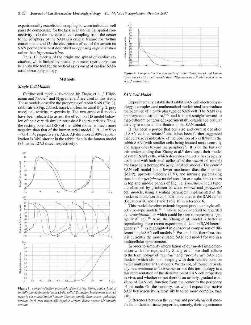
Cardiac cell models developed by Zhang et al.,6 Hilge-mann and Noble,7 and Nygren et al.8 are used in this study.These models describe the properties of rabbit SAN (Fig. 1),rabbit atrial (Fig. 2, black trace), and human atrial (Fig. 2, graytrace) cell activity, respectively. The two atrial cell modelshave been selected to assess the effect, on 1D model behav-ior, of their very dissimilar intrinsic AP characteristics. Thus,the resting potential (RP) of the rabbit model is much morenegative than that of the human atrial model (−91.1 mV vs−75.4 mV, respectively). Also, AP duration at 90% repolar-ization is 34% shorter in the rabbit than in the human model(84 ms vs 127.3 msec, respectively).

Figure 1. Computed action potentials of central (top panel) and peripheral(middle panel) sinoatrial node (SAN) cells.6 Transition between the two celltypes is via a distribution function (bottom panel). Gray traces: publishedversion. Dark gray traces: 0D-capable version. Black traces: 1D-capableversion.

Figure 2. Computed action potentials of rabbit (black trace) and human(gray trace) atrial cell models from Hilgemann and Noble7 and Nygrenet al.,8 respectively.

SAN Cell Model

Experimentally established rabbit SAN cell electrophysi-ology is complex, and mathematical models tend to reproducethe behavior of a particular type of SAN cell. The SAN is aheterogeneous structure,9-12 and it is not straightforward tomap different patterns of experimentally established cellularactivity to a spatial distribution in the SAN model.

It has been reported that cell size and current densitiesof SAN cells correlate,13 and it has been further suggestedthat cell size is indicative of the position of a cell within therabbit SAN (with smaller cells being located more centrallyand larger ones toward the periphery9). It is on the basis ofthis understanding that Zhang et al.6 developed their modelof rabbit SAN cells, which describes the activities typicallyassociated with both small cells (called the central cell model)and large cells (termed the peripheral cell model). The centralSAN cell model has a lower maximum diastolic potential(MDP), upstroke velocity (UV), and intrinsic pacemakingrate than the peripheral model (see, for example, black tracesin top and middle panels of Fig. 1). Transitional cell typesare obtained by gradation between central and peripheralcell models, using a scaling parameter implemented in themodel as a function of cell location relative to the SAN center(Equations 80 and 81 and Table 10 in reference 6).

This model therefore extends beyond previous single cell-activity–type models,14,15 whose behavior could be regardedas “transitional” or which could be seen to represent a “pe-ripheral” cell.16 Also, the Zhang et al. model is better atreproducing more recent experimental data on SAN hetero-geneity,17-21 as highlighted in our recent comparison of dif-ferent single SAN cell models.22 We conclude, therefore, thatit is currently the most suitable SAN cell model for use in amulticellular environment.

In order to simplify interrelation of our model implemen-tation with that reported by Zhang et al., we shall adhereto the terminology of “central” and “peripheral” SAN cellmodels (which also is in keeping with their relative positionin our multicellular 1D model). We do not, of course, provideany new evidence as to whether or not this terminology is afair representation of the distribution of SAN cell propertiesin vivo, and whether or not there is an orderly, gradual tran-sition of SAN cell function from the center to the peripheryof the node. On the contrary, we would expect that nativeSAN heterogeneity is most likely to be more complex thanthis.

Differences between the central and peripheral cell mod-els lie in their intrinsic properties, namely, their capacitance

Garny et al. One-Dimensional Rabbit Sinoatrial Node Models S123

and ionic conductances, simulating differences in currentdensities (Equation 80 and Table 10 in reference 6, respec-tively). Ionic conductances of transitional SAN cells are com-puted using a linear interpolation scheme (Equation 81 ofreference 6, a function of the cell’s capacitance, Equation80 of reference 6) between the values of the conductance inthe center and the periphery of the SAN (Table 10 of refer-ence 6). As cell capacitance is related, in the model, to thedistance from the SAN center, this provides a gradual transi-tion of parameters from center to periphery of the modeledSAN.

In the published model,6 Equation 80 assumes that theSAN region is always 3 mm long, which may be an unneces-sary constraint. We have rewritten the two equations (Equa-tions 80 and 81), with the view of using the model in morecomplex settings (i.e., variable length 1D, or 2D and 3D mod-els). Equation 80 now computes a scaling factor, FCell, whichis directly based on the location, dCell, of a cell relative to thecenter of the SAN, rather than linked through to a position viacapacitance (dCell = 0: center of the SAN, dCell = 1: peripheryof the SAN). FCell itself can follow any function of location.Its value (between 0 and 1) is used for linear interpolationbetween central and peripheral cell parameters in order todetermine transitional cell properties, such as capacitance orion current densities (Equation 81).

Other than the above, we systematically varied a greatnumber of parameters (Fig. 6 and Table 1–4) in order to obtaina stable version of a working 1D SAN-atrial model, and theseare explained below in detail.

Published, 0D-Capable and 1D-CapableVersions of the SAN Cell Model

The SAN cell model as published yields the activityillustrated by the gray traces in Figure 1, which is verydifferent from the corresponding AP shapes published inthe same paper.6 This raises the issue of typographical er-rors that needs to be addressed within the scientific com-munity. CellMLTM (http://www.cellml.org/)23 is a standardthat arose from this ever increasing concern and which al-lows, when implemented in a software program such asCOR (http://COR.physiol.ox.ac.uk/),24 to store and exchangecomputer-based biologic models, thus making publishedmodels free of typographical errors and directly useable.An alternative, or complementary, solution is to offer onlinedownloads of the models in the form of source codes.

The corrected version of the Zhang et al. model, given tous by the authors, faithfully reproduces the published singlecell activity. This model, which we refer to as the 0D-capableversion of the model, was implemented in our modeling en-vironment to reproduce central and peripheral cell activity(Fig. 1, dark gray traces). For further detail, see a listing of thedifferences in published and 0D-capable model parameters(Table 1) and underlying equations (Table 2).

Next, we tried to reproduce the published 1D behavior, asillustrated in Figure 13 of the Zhang et al. paper,6 by connect-ing the above 0D-capable cell models, using the conductivityvalues suggested in the paper. This failed, and we did notmanage to identify any set of secondary parameter variations(such as changes in distribution function or diffusion coef-ficients) that would have allowed us to reconcile publishedsingle cell and 1D strand activity.

A third version of the Zhang et al. SAN cell model wastherefore provided by the authors and used to generate Fig-ure 13 of their paper.6 We refer to this as the 1D-capableversion of the model. The single cell activity of 1D-capablecentral and peripheral cell models is illustrated by the blacktraces in Figure 1. These differ significantly from the singlecell activity published in the same paper (Table 1–3).

Tables 1 and 2 list the differences between the three ver-sions of SAN cell models. Some differences are minor, butthey are listed for completeness. Note the presence of a per-sistent Ca2+ current in the 1D-capable version of the model(bottom of Table 1, Equation 85 in Table 2). Major differencesbetween model versions are highlighted in gray.

Differences in electrophysiologic behavior of 0D-capableand 1D-capable models are summarized in Table 3 (percent-ages shown in Tables 1 and 3 refer to a comparison of 1D-capable model relative to control levels in the 0D-capableversion). Only the MDP of the central model is the samein the 0D- and 1D-capable models. The most pronouncedchanges are observed in UV. Thus, UV in the central ver-sion of the 1D-capable model is 62.5% higher than in theOD-capable model, reaching 3.9 V/s. This is, however, wellwithin the range of maximum UV of central SAN cells of upto 10 V/s, as identified by Kodama et al.21 Conversely, UV inthe peripheral version of the 1D-capable model is decreasedby 76.8%, compared to the 0D-capable version, from 61.7to 14.3 V/s. This appears necessary for implementation ofthe 1D model, but it is well outside the physiologic rangeidentified for peripheral SAN cells, where a value of at least40 V/s would be expected.21

Thus, in order to reproduce the published 1D behavior ina strand of SAN and atrial cells,6 one has to deviate from the0D-capable model (that is shaped on published experimentalsingle cell data) and use a very different 1D-capable model.The peripheral SAN cell model, in particular, is not as rep-resentative of experimentally described single cell behavioras the 0D-capable cell model implementation. Further testsare required to reassess the hitherto unpublished version ofthe Zhang et al. 1D-capable model for its physiologic rele-vance (e.g., compare their response to physiologic interven-tions with that observed experimentally).

Figure 1 summarizes computed AP parameters of cen-tral (top panel) and peripheral (middle panel) SAN cells,corresponding to (1) the published single cell model (pub-lished version, gray traces); (2) the corrected version of thepublished single cell model (0D-capable version, dark graytraces); and (3) the single cell model that was used to com-pute the published 1D simulation (1D-capable version, blacktraces). The corresponding parameter distribution functionsare shown in the bottom panel of the same figure, illus-trating published (gray trace) and 1D-capable (black trace)versions.

Leading Pacemaker Site Identification

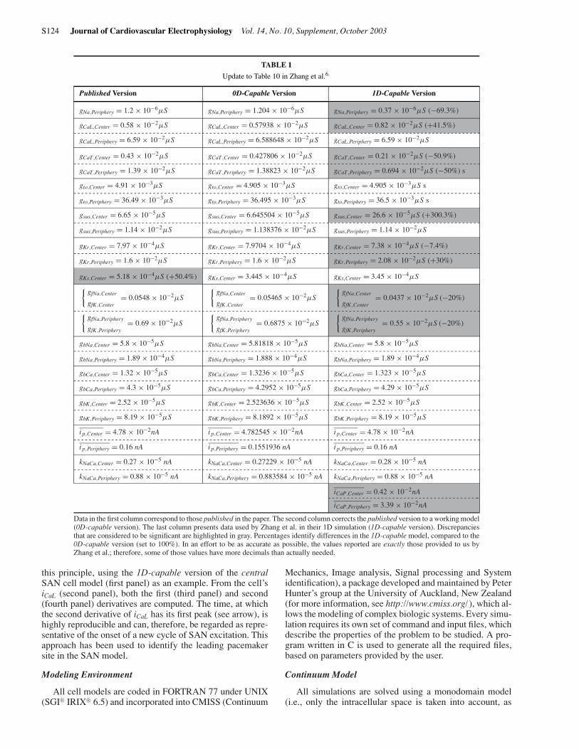
For the purpose of this study, we defined the location ofthe pacemaker site as the cell that first reaches its thresholdfor excitation. In SAN cells, the principal current responsiblefor AP upstroke is the L-type Ca2+ current, iCaL. This currentcan therefore be used to determine threshold crossing in aSAN cell model by identifying the first peak of the secondderivative of iCaL (Fig. 3, fourth panel), which correspondsto the time of maximum increase in iCaL. Figure 3 illustrates

S124 Journal of Cardiovascular Electrophysiology Vol. 14, No. 10, Supplement, October 2003

TABLE 1

Update to Table 10 in Zhang et al.6

Published Version 0D-Capable Version 1D-Capable Version

gNa,Periphery = 1.2 × 10−6µS gNa,Periphery = 1.204 × 10−6µS gNa,Periphery = 0.37 × 10−6µS (−69.3%)

gCaL,Center = 0.58 × 10−2µS gCaL,Center = 0.57938 × 10−2µS gCaL,Center = 0.82 × 10−2µS (+41.5%)- - - - - - - - - - - - - - - - - - - - - - - - - - - - - - - - - - - - - - - - - - - - - - - - - - - - - - - - - - - - - - - - - - - - - - - - - - - - - - - - - - - - - - - - - - - - - - - - - - - - - - - - - - - -

gCaL,Periphery = 6.59 × 10−2µS gCaL,Periphery = 6.588648 × 10−2µS gCaL,Periphery = 6.59 × 10−2µS

gCaT,Center = 0.43 × 10−2µS gCaT,Center = 0.427806 × 10−2µS gCaT,Center = 0.21 × 10−2µS (−50.9%)- - - - - - - - - - - - - - - - - - - - - - - - - - - - - - - - - - - - - - - - - - - - - - - - - - - - - - - - - - - - - - - - - - - - - - - - - - - - - - - - - - - - - - - - - - - - - - - - - - - - - - - - - - - -

gCaT,Periphery = 1.39 × 10−2µS gCaT,Periphery = 1.38823 × 10−2µS gCaT,Periphery = 0.694 × 10−2µS (−50%) s

gto,Center = 4.91 × 10−3µS gto,Center = 4.905 × 10−3µS gto,Center = 4.905 × 10−3µS s- - - - - - - - - - - - - - - - - - - - - - - - - - - - - - - - - - - - - - - - - - - - - - - - - - - - - - - - - - - - - - - - - - - - - - - - - - - - - - - - - - - - - - - - - - - - - - - - - - - - - - - - - - - -

gto,Periphery = 36.49 × 10−3µS gto,Periphery = 36.495 × 10−3µS gto,Periphery = 36.5 × 10−3µS s

gsus,Center = 6.65 × 10−5µS gsus,Center = 6.645504 × 10−5µS gsus,Center = 26.6 × 10−5µS (+300.3%)- - - - - - - - - - - - - - - - - - - - - - - - - - - - - - - - - - - - - - - - - - - - - - - - - - - - - - - - - - - - - - - - - - - - - - - - - - - - - - - - - - - - - - - - - - - - - - - - - - - - - - - - - - - -

gsus,Periphery = 1.14 × 10−2µS gsus,Periphery = 1.138376 × 10−2µS gsus,Periphery = 1.14 × 10−2µS

gKr,Center = 7.97 × 10−4µS gKr,Center = 7.9704 × 10−4µS gKr,Center = 7.38 × 10−4µS (−7.4%)- - - - - - - - - - - - - - - - - - - - - - - - - - - - - - - - - - - - - - - - - - - - - - - - - - - - - - - - - - - - - - - - - - - - - - - - - - - - - - - - - - - - - - - - - - - - - - - - - - - - - - - - - - - -

gKr,Periphery = 1.6 × 10−2µS gKr,Periphery = 1.6 × 10−2µS gKr,Periphery = 2.08 × 10−2µS (+30%)

gKs,Center = 5.18 × 10−4µS (+50.4%) gKs,Center = 3.445 × 10−4µS gKs,Center = 3.45 × 10−4µS{gfNa,Center

gfK,Center= 0.0548 × 10−2µS

{gfNa,Center

gfK,Center= 0.05465 × 10−2µS

{gfNa,Center

gfK,Center= 0.0437 × 10−2µS (−20%)

- - - - - - - - - - - - - - - - - - - - - - - - - - - - - - - - - - - - - - - - - - - - - - - - - - - - - - - - - - - - - - - - - - - - - - - - - - - - - - - - - - - - - - - - - - - - - - - - - - - - - - - - - - - -{gfNa,Periphery

gfK,Periphery= 0.69 × 10−2µS

{gfNa,Periphery

gfK,Periphery= 0.6875 × 10−2µS

{gfNa,Periphery

gfK,Periphery= 0.55 × 10−2µS (−20%)

gbNa,Center = 5.8 × 10−5µS gbNa,Center = 5.81818 × 10−5µS gbNa,Center = 5.8 × 10−5µS- - - - - - - - - - - - - - - - - - - - - - - - - - - - - - - - - - - - - - - - - - - - - - - - - - - - - - - - - - - - - - - - - - - - - - - - - - - - - - - - - - - - - - - - - - - - - - - - - - - - - - - - - - - -

gbNa,Periphery = 1.89 × 10−4µS gbNa,Periphery = 1.888 × 10−4µS gbNa,Periphery = 1.89 × 10−4µS

gbCa,Center = 1.32 × 10−5µS gbCa,Center = 1.3236 × 10−5µS gbCa,Center = 1.323 × 10−5µS- - - - - - - - - - - - - - - - - - - - - - - - - - - - - - - - - - - - - - - - - - - - - - - - - - - - - - - - - - - - - - - - - - - - - - - - - - - - - - - - - - - - - - - - - - - - - - - - - - - - - - - - - - - -

gbCa,Periphery = 4.3 × 10−5µS gbCa,Periphery = 4.2952 × 10−5µS gbCa,Periphery = 4.29 × 10−5µS

gbK,Center = 2.52 × 10−5µS gbK,Center = 2.523636 × 10−5µS gbK,Center = 2.52 × 10−5µS- - - - - - - - - - - - - - - - - - - - - - - - - - - - - - - - - - - - - - - - - - - - - - - - - - - - - - - - - - - - - - - - - - - - - - - - - - - - - - - - - - - - - - - - - - - - - - - - - - - - - - - - - - - -

gbK,Periphery = 8.19 × 10−5µS gbK,Periphery = 8.1892 × 10−5µS gbK,Periphery = 8.19 × 10−5µS

i p,Center = 4.78 × 10−2nA i p,Center = 4.782545 × 10−2nA i p,Center = 4.78 × 10−2nA- - - - - - - - - - - - - - - - - - - - - - - - - - - - - - - - - - - - - - - - - - - - - - - - - - - - - - - - - - - - - - - - - - - - - - - - - - - - - - - - - - - - - - - - - - - - - - - - - - - - - - - - - - - -

i p,Periphery = 0.16 nA i p,Periphery = 0.1551936 nA i p,Periphery = 0.16 nA

kNaCa,Center = 0.27 × 10−5 nA kNaCa,Center = 0.27229 × 10−5 nA kNaCa,Center = 0.28 × 10−5 nA- - - - - - - - - - - - - - - - - - - - - - - - - - - - - - - - - - - - - - - - - - - - - - - - - - - - - - - - - - - - - - - - - - - - - - - - - - - - - - - - - - - - - - - - - - - - - - - - - - - - - - - - - - - -

kNaCa,Periphery = 0.88 × 10−5 nA kNaCa,Periphery = 0.883584 × 10−5 nA kNaCa,Periphery = 0.88 × 10−5 nA

iCaP,Center = 0.42 × 10−2nA- - - - - - - - - - - - - - - - - - - - - - - - - - - - - - - - - - - - - - - --

iCaP,Periphery = 3.39 × 10−2nA

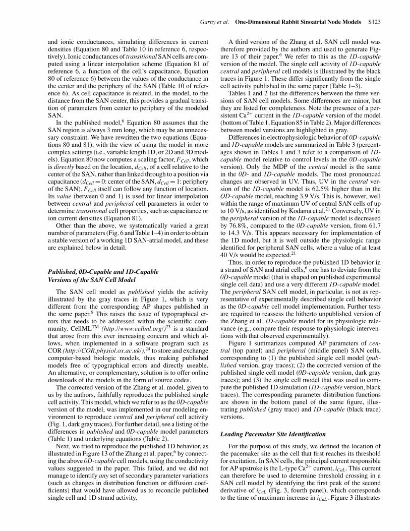
Data in the first column correspond to those published in the paper. The second column corrects the published version to a working model(0D-capable version). The last column presents data used by Zhang et al. in their 1D simulation (1D-capable version). Discrepanciesthat are considered to be significant are highlighted in gray. Percentages identify differences in the 1D-capable model, compared to the0D-capable version (set to 100%). In an effort to be as accurate as possible, the values reported are exactly those provided to us byZhang et al.; therefore, some of those values have more decimals than actually needed.

this principle, using the 1D-capable version of the centralSAN cell model (first panel) as an example. From the cell’siCaL (second panel), both the first (third panel) and second(fourth panel) derivatives are computed. The time, at whichthe second derivative of iCaL has its first peak (see arrow), ishighly reproducible and can, therefore, be regarded as repre-sentative of the onset of a new cycle of SAN excitation. Thisapproach has been used to identify the leading pacemakersite in the SAN model.

Modeling Environment

All cell models are coded in FORTRAN 77 under UNIX(SGI� IRIX� 6.5) and incorporated into CMISS (Continuum

Mechanics, Image analysis, Signal processing and Systemidentification), a package developed and maintained by PeterHunter’s group at the University of Auckland, New Zealand(for more information, see http://www.cmiss.org/ ), which al-lows the modeling of complex biologic systems. Every simu-lation requires its own set of command and input files, whichdescribe the properties of the problem to be studied. A pro-gram written in C is used to generate all the required files,based on parameters provided by the user.

Continuum Model

All simulations are solved using a monodomain model(i.e., only the intracellular space is taken into account, as

Garny et al. One-Dimensional Rabbit Sinoatrial Node Models S125

TA

BL

E2

Upd

ated

Equ

atio

nsfo

rth

eZ

hang

etal

.6Pa

per

Pub

lishe

dV

ersi

on0D

-Cap

able

Ver

sion

1D-C

apab

leV

ersi

on

FN

a=

9.52

×10−

2e−

6.3×

10−2

(V+3

4.4)

1+1.

66e−

0.22

5(V

+63.

7)+

8.69

×10

−2F

Na

=9.

518×

10−2

e−6.

306×

10−2

(V+3

4.4)

1+1.

662e

−0.2

251(

V+6

3.7)

+8.

693

×10

−2F

Na

=9.

518×

10−2

e−6.

306×

10−2

(V+3

4.4)

1+1.

662e

−0.2

251(

V+6

3.7)

+8.

693

×10

−2(8

)

m∞

=3√

1

1+e

−V 5.46

m∞

=3√

1

1+e−( V

+30.

325.

46

)m

∞=

3√1

1+e−( V

+30.

325.

46

)(9

)

τ m=

0.62

47×1

0−3

0.83

2e−0

.335

(V+5

6.7)

+0.6

27e0

.082

(V+6

5.01

)+

4×

10−5

τ m=

0.62

47×1

0−3

0.83

2216

6e−0

.335

66(V

+56.

7062

) +0.

6274

e0.0

823(

V+6

5.01

31)+

4.56

9×

10−5

τ m=

0.62

47×1

0−3

0.83

2216

6e−0

.335

66(V

+56.

7062

) +0.

6274

e0.0

823(

V+6

5.01

31)+

4.56

9×

10−5

(10)

αd L

=−1

4.19

(V+3

5)

e−( V+3

52.

5

) −1−

42.4

5Ve−

0.20

8V−1

αd L

=−1

4.19

5(V

+35)

e−( V+3

52.

5

) −1−

42.4

5Ve−

0.20

8V−1

αd L

=−1

4.2(

V+3

5)

e−( V+3

52.

5

) −1−

42.4

5Ve−

0.20

8V−1

(19)

βd L

=5.

71(V

−5)

e0.4

(V−5

) −1

βd L

=5.

715(

V−5

)e0

.4(V

−5) −

1β

d L=

5.71

(V−5

)e0

.4(V

−5) −

1(2

0)

d L∞

=1

1+e−( V

+23.

16

)d L

∞=

1

1+e−( V

+22.

3+0.

8F

Cel

l6

)d L

∞=

1

1+e−( V

+22.

26

)(2

2)

αf L

=3.

12(V

+28)

eV

+28

4−1

αf L

=3.

75(V

+28)

eV

+28

4−1

αf L

=3.

12(V

+28)

eV

+28

4−1

(24)

βf L

=25

1+e−( V

+28

4

)β

f L=

30

1+e−( V

+28

4

)β

f L=

25

1+e−( V

+28

4

)(2

5)

τf L

=1

αf L

+βf L

τf L

=1.

2−0.

2F

Cel

lα

f L+β

f Lτ

f L=

1α

f L+β

f L(2

6)

αf T

=15

.3e−( V

+71.

783

.3

)α

f T=

15.3

e−( V+7

1+0.

7F

Cel

l83

.3

)α

f T=

15.3

e−( V+7

1.7

83.3

)(3

5)

βf T

=15

eV

+71.

715

.38

βf T

=15

eV

+71

15.3

8β

f T=

15e

V+7

1.7

15.3

8(3

6)

τ q=

10.1

×10

−3τ q

=10

.103̄

×10

−3τ q

=10

.1×

10−3

(42)

+65

.17×

10−3

0.57

e−0.

08(V

+49)

+0.

24×

10−4

e0.1(

V+5

0.93

)+

65.1

6̄×10

−30.

5686

e−0.

0816

1(V

+39+

10F

Cel

l)+0

.717

4e(0

.271

9−0.

1719

FC

ell)

(V+4

0.93

+10

FC

ell)

+65

.17×

10−3

0.56

86e−

0.08

161(

V+3

9)+0

.717

4e0.

2719

(V+4

0.93

)

τ r=

2.98

×10

−3+

15.5

9×10

−31.

037e

0.09

(V+3

0.61

) +0.

369e

−0.1

2(V

+23.

84)

τ r=

2.97

75×

10−3

+19

.595

×10−

3

1.03

7e0.

0901

2(V

+30.

61) +

0.36

9e−0

.119

(V+2

3.84

)τ r

=2.

98×

10−3

+19

.59×

10−3

1.03

7e0.

0901

2(V

+30.

61) +

0.36

9e−0

.119

(V+2

3.84

)(4

5)

(con

tinu

ed)

S126 Journal of Cardiovascular Electrophysiology Vol. 14, No. 10, Supplement, October 2003

TA

BL

E2

(Con

tinue

d)

Pub

lishe

dV

ersi

on0D

-Cap

able

Ver

sion

1D-C

apab

leV

ersi

on

p a,

f ∞=

1

1+e− (

V+1

4.2

10.6

)p a

,f ∞

=1

1+e− (

V+1

4.2

10.6

)p a

,f ∞

=1

1+e− (

V+1

3.2

10.6

)(5

0)

τp a

,f=

1

37.2

eV

−915

.9+0

.96e

− (V

−922

.5)

τp a

,f=

1

37.2

eV

−915

.9+0

.96e

− (V

−922

.5)

τp a

,f=

1

37.2

eV

−10

15.9

+0.9

6e− (

V−1

022

.5)

(52)

τp a

,s=

1

4.2e

V−9 17

+0.1

5e− (

V−9

21.6

)τ

p a,s

=1

4.2e

V−9 17

+0.1

5e− (

V−9

21.6

)τ

p a,s

=1

4.2e

V−1

017

+0.1

5e− (

V−1

021

.6)

(53)

p i∞

=1

1+e

V+1

8.6

10.1

p i∞

=1

1+e

V+1

9.6

10.1

p i∞

=1

1+e

V+1

8.6

10.1

(56)

τpi

=0.

002

τpi

=0.

002

τpi

=0.

006

(57)

EK

s=

RT F

ln( [K

+] o

+0.1

2[N

a+] o

[K+

] i+0

.12[

Na+

] i

)E

Ks=

RT F

ln( [K

+] o

+0.0

3[N

a+] o

[K+

] i+0

.03[

Na+

] i

)E

Ks=

RT F

ln( [K

+] o

+0.0

3[N

a+] o

[K+

] i+0

.03[

Na+

] i

)(6

0)

i f,N

a=

gf,

Na

y(V

−E

Na)

i f,N

a=

gf,

Na

y(V

−E

Na)

i f,N

a=

gf,

Na

y(V

−77

.6)

(67)

i f,K

=g

f,K

y(V

−E

K)

i f,K

=g

f,K

y(V

−E

K)

i f,K

=g

f,K

y(V

+10

2)(6

8)

αy

=e− (

V+7

8.91

26.6

2)

αy

=e− (

V+7

8.91

26.6

3)

αy

=e− (

V+7

8.91

26.6

3)

(69)

i NaC

a=

k NaC

a[N

a+]3 i

[Ca2+

] oe0.

0374

3Vγ

NaC

a−[

Na+

]3 o[C

a2+] i

e0.03

74V(γ

NaC

a−1)

1+d N

aCa([

Na+

]3 i[C

a2+] o

+[N

a+]3 o

[Ca2+

] i)

i NaC

a=

k NaC

a[N

a+]3 i

[Ca2+

] oe0.

0374

3Vγ

NaC

a−[

Na+

]3 o[C

a2+] i

e0.03

743V

(γN

aCa−

1)

1+d N

aCa([

Na+

]3 i[C

a2+] o

+[N

a+]3 o

[Ca2+

] i)

i NaC

a=

k NaC

a[N

a+]3 i

[Ca2+

] oe0.

0374

3Vγ

NaC

a−[

Na+

]3 o[C

a2+] i

e0.03

743V

(γN

aCa−

1)

1+d N

aCa([

Na+

]3 i[C

a2+] o

+[N

a+]3 o

[Ca2+

] i)

(77)

Cs m

(x)=

20+

1.07

(x−0

.1)

Ls

( 1+0.

7745

e− (x−

2.05

0.29

5)) (6

5−

20)

FC

ell(

d Cel

l)=

1.07

3dC

ell−

0.1

3( 1+0.

7745

e−( 3dC

ell−

2.05

0.29

5

) )F

Cel

l(d C

ell)

=1.

072.

9dC

ell

3( 1+0.

7745

e−( 2.9d

Cel

l−2.

450.

195

) )(8

0)

gs (x)=

( 65−C

s m(x

)) g c+( C

S m(x

)−20

) gp

65−2

0X

(dC

ell)

=X

Cen

ter+

FC

ell(

d Cel

l)(X

Per

iph

ery−

XC

ente

r)

X(d

Cel

l)=

XC

ente

r+

FC

ell(

d Cel

l)(X

Per

iph

ery−

XC

ente

r)

(81)

i Ca

P=

i Ca

P[C

a2+] i

[Ca2+

] i+0

.000

4(8

5)

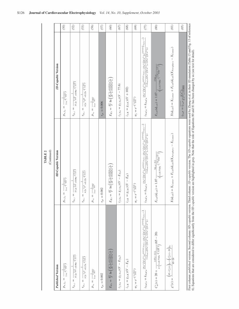
Firs

tcol

umn:

publ

ishe

dve

rsio

n.Se

cond

colu

mn:

0D-c

apab

leve

rsio

n.T

hird

colu

mn:

1D-c

apab

leve

rsio

n.T

he1D

-cap

able

equa

tions

wer

eus

edby

Zha

nget

al.i

nth

eir1

Dsi

mul

atio

n(T

able

13an

dFi

g.13

ofre

fere

nce

6).E

quat

ions

that

are

cons

ider

edto

diff

ersi

gnifi

cant

lyfr

omth

e0D

-cap

able

vers

ion

are

high

light

edin

gray

.Not

eth

atth

ero

leof

Equ

atio

ns80

and

81ha

sbe

ench

ange

dby

us(s

eete

xtfo

rde

tail)

.

Garny et al. One-Dimensional Rabbit Sinoatrial Node Models S127

TABLE 3

Electrophysiologic Characteristics Computed for the 0D-Capable and1D-Capable Versions of the Rabbit Sinoatrial Node Cell Model6

Model

Parameter 0D-Capable 1D-Capable

MDPCenter −56.2 mV −56.2 mV (0%)

MDPPeriphery −77.8 mV −80 mV (+2.8%)

MSPCenter 19.5 mV 21 mV (+7.7%)

MSPPeriphery 24.5 mV 21.1 mV (−13.9%)

APACenter 75.7 mV 77.2 mV (+2%)

APAPeriphery 102.3 mV 101.1 mV (−1.2%)

UVCenter 2.4V/s 3.9 V/s (+62.5%)

UVPeriphery 61.7V/s 14.3 V/s (−76.8%)

CLCenter 325 msec 333.4 msec (+2.6%)

CLPeriphery 160.4 msec 217.2 msec (+35.4%)

Discrepancies are highlighted in gray, together with the percentage bywhich the 1D-capable values differ from the 0D-capable model. MDP =maximum diastolic potential; MSP = maximum systolic potential; APA =action potential amplitude; UV = upstroke velocity; CL = cycle length.

opposed to a bidomain model, which also considers the ex-tracellular space). This approach requires knowledge of thesurface-to-volume ratio of the different cell types, as well asthe value of the conductivity tensor at each grid point. Theseare determined from cell dimensions and gap junction con-ductivity information (Table 4). We assumed all cells to becylindrical and adhered to the dimensions suggested by theauthors of the original models. A radius of 7.5 µm is usedfor all SAN cells, while their length increases from 50 µmfor central to 80 µm for peripheral SAN cell models.6 Di-mensions for atrial models are as follows: 10-µm radius and80-µm length for the rabbit atrial cell model,7 and 5.5-µmradius and 130-µm length for the human atrial cell model.8

This forms the basis for our continuum model, as opposed toa discrete model where dimensions would not be taken intoaccount.

Information on intercellular coupling is derived from pub-lished experimental data, obtained in pairs of rabbit SANcells, or atrial myocytes, using the double whole-cell patchclamp technique.25,26 The mean values reported in these stud-ies are 7.5 nS for SAN and 175 nS for atrial cell pairs. Theconductance between two neighboring cells, isolated from a3D tissue matrix, surely must under-represent the couplingthat any of these cells will have with surrounding cardiomy-ocytes in vitro. To address this issue, a scaling procedure forintercellular coupling was introduced, which allows one tovary the level of electrotonic interaction for the whole 1Dmodel.

Furthermore, immunohistochemical studies show that thedensity of gap junctions increases toward the periphery ofthe SAN.9 This increase is addressed in the model by as-suming a conductivity ratio of 1:10 between the center andthe periphery of the node. Default intercellular conductivi-ties are, therefore, portrayed to increase from 7.5 nS in theSAN center to 75 nS in its periphery, and 175 nS in theatrium.

Figure 3. Upstroke of SAN cell action potentials (first panel) is primarilycarried by the L-type Ca2+ current (iCaL, second panel), which can thereforebe used to determine the crossing of threshold for excitation. Both the first(third panel) and second (fourth panel) derivatives of iCaL are calculated. Thesecond derivative corresponds to the speed with which iCaL changes. Fastestchange in iCaL at the onset of an action potential occurs when threshold isreached. The time of threshold crossing is therefore identified by the firstpeak of the second derivative of the current (fourth panel, arrow).

Model Characteristics

In order to reproduce the simulations by Zhang et al.6

with matching spatial parameters, we modeled a 3 mm strandof rabbit SAN cells, electrotonically connected to 9.6 mmof rabbit7 or human8 atrial cell models (Fig. 4). The SANregion was simulated using either the 0D-capable or 1D-capable versions, and includes gradual changes in regionalcell properties, as described earlier (Equations 80 and 81).

Simulations initially assessed space steps (between 0.01and 1 mm) and yielded converging results for all grid spac-ings of 0.2 mm or less. Single cell models are solved usingan implicit Euler integrator with a time step of 0.01 msec,which is sufficient to ensure accuracy of results. Neumannboundary conditions are used, i.e., there is no flux at eitherend of the strand. Each problem consists of a 3.5-secondrun, of which 2.5 seconds are used to approach steady-statebehavior. Simulations are run on one processor of an SGI�

Origin� 2000 system at the Oxford Supercomputing Center(http://www.osc.ox.ac.uk/), using the optimized 32-bit ver-sion of the CMISS package. A typical 1D simulation takesslightly less than 10 minutes of computing time.

S128 Journal of Cardiovascular Electrophysiology Vol. 14, No. 10, Supplement, October 2003

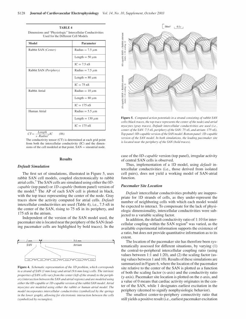
TABLE 4

Dimensions and “Physiologic” Intercellular ConductivitiesUsed for the Different Cell Models

Model Parameter

Rabbit SAN (Center) Radius = 7.5 µm

Length = 50 µm

IC = 7.5 nS

Rabbit SAN (Periphery) Radius = 7.5 µm

Length = 80 µm

IC = 75 nS

Rabbit Atrial Radius = 10 µm

Length = 80 µm

IC = 175 nS

Human Atrial Radius = 5.5 µm

Length = 130 µm

IC = 175 nS

CT= Lengthπ · Radius2 IC (86)

The conductivity tensor (CT) is determined at each grid pointfrom both the intercellular conductivity (IC) and the dimen-sions of the cell modeled at that point. SAN = sinoatrial node.

Results

Default Simulation

The first set of simulations, illustrated in Figure 5, usesrabbit SAN cell models, coupled electrotonically to rabbitatrial cells.7 The SAN cells are simulated using either the 0D-capable (top panel) or 1D-capable (bottom panel) version ofthe model.6 The AP of each SAN cell is plotted in black,with the top trace representing the center of the node. Graytraces show the activity computed for atrial cells. Defaultintercellular conductivities are used (Table 4), i.e., 7.5 nS inthe center of the SAN, rising to 75 nS in its periphery, and175 nS in the atrium.

Independent of the version of the SAN model used, thepacemaker site is located near the periphery of the SAN (lead-ing pacemaker cells are highlighted by bold traces). In the

3 mm 9.6 mm

SAN Atrium

Atrium Atrium Atrium SAN SAN SAN

Figure 4. Schematic representation of the 1D problem, which correspondsto a strand of SAN (3 mm long) and atrial (9.6 mm long) cells. The intrinsicproperties of SAN cells vary from the center (left of the strand) to the periph-ery (intersection between the SAN and atrial regions) and are modeled usingeither the 0D-capable or 1D-capable version of the rabbit SAN model. Atrialmyocytes are modeled using either the rabbit or human atrial model. Themodel incorporates intercellular conductivities (symbolized by the springsin the lower graph), allowing for electrotonic interaction between the cells(symbolized by rectangles).

Figure 5. Computed action potentials in a strand consisting of rabbit SANcells (black traces, the top trace represents the center of the node) and atrialmyocytes (gray traces). Default intercellular conductivities are used (i.e.,center of the SAN: 7.5 nS, periphery of the SAN: 75 nS, and atrium: 175 nS).Top panel: 0D-capable version of the SAN model. Bottom panel: 1D-capableversion of the SAN model. In both simulations, the leading pacemaker siteis located near the periphery of the SAN (bold traces).

case of the 0D-capable version (top panel), irregular activityof central SAN cells is observed.

Thus, implementation of a 1D model, using default in-tercellular conductivities (i.e., those derived from isolatedcell pairs), does not yield a working model of SAN-atrialfunction.

Pacemaker Site Location

Default intercellular conductivities probably are inappro-priate for 1D strands of cells, as they under-represent thenumber of neighboring cells with which each model wouldbe expected to interact. To compensate for the lack of physi-ologic dimensionality, intercellular conductivities were sub-jected to a variable scaling factor.

In addition, the default conductivity ratio of 1:10 for inter-cellular coupling within the SAN region9 was varied, as theavailable experimental information supports the existence ofa ratio, but does not provide quantitative information as to itsextent.

The location of the pacemaker site has therefore been sys-tematically assessed for different situations, by varying (1)the central-to-peripheral intercellular coupling ratio (usingvalues between 1:1 and 1:20), and (2) the scaling factor (us-ing values between 1 and 10). Results of these simulations aresummarized in Figure 6, where the location of the pacemakersite relative to the center of the SAN is plotted as a functionof both the scaling factor (x-axis) and the conductivity ratio(y-axis). Pacemaker site location is plotted on the z-axis, anda value of 0 means that cardiac activity originates in the cen-ter of the SAN, while 1 designates earliest excitation in theperiphery (deemed to signify nonphysiologic behavior).

The smallest center-to-periphery connectivity ratio thatstill yields a positive result (i.e., earliest pacemaker excitation

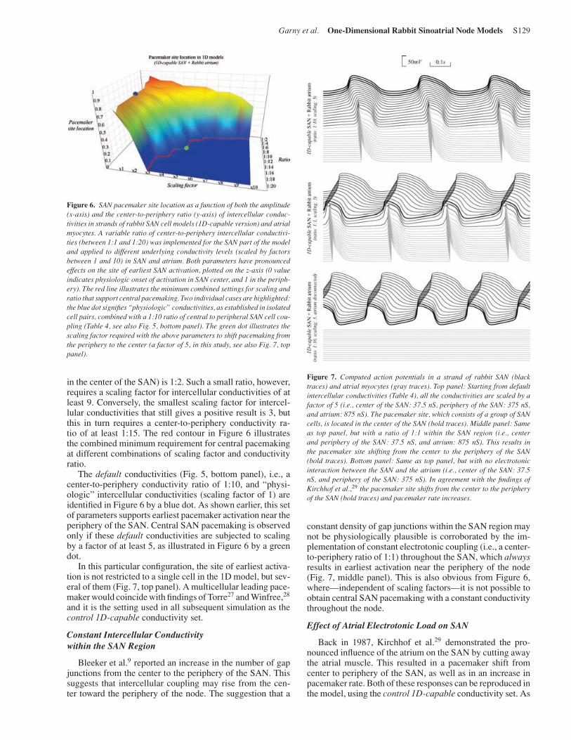
Garny et al. One-Dimensional Rabbit Sinoatrial Node Models S129

Figure 6. SAN pacemaker site location as a function of both the amplitude(x-axis) and the center-to-periphery ratio (y-axis) of intercellular conduc-tivities in strands of rabbit SAN cell models (1D-capable version) and atrialmyocytes. A variable ratio of center-to-periphery intercellular conductivi-ties (between 1:1 and 1:20) was implemented for the SAN part of the modeland applied to different underlying conductivity levels (scaled by factorsbetween 1 and 10) in SAN and atrium. Both parameters have pronouncedeffects on the site of earliest SAN activation, plotted on the z-axis (0 valueindicates physiologic onset of activation in SAN center, and 1 in the periph-ery). The red line illustrates the minimum combined settings for scaling andratio that support central pacemaking. Two individual cases are highlighted:the blue dot signifies “physiologic” conductivities, as established in isolatedcell pairs, combined with a 1:10 ratio of central to peripheral SAN cell cou-pling (Table 4, see also Fig. 5, bottom panel). The green dot illustrates thescaling factor required with the above parameters to shift pacemaking fromthe periphery to the center (a factor of 5, in this study, see also Fig. 7, toppanel).

in the center of the SAN) is 1:2. Such a small ratio, however,requires a scaling factor for intercellular conductivities of atleast 9. Conversely, the smallest scaling factor for intercel-lular conductivities that still gives a positive result is 3, butthis in turn requires a center-to-periphery conductivity ra-tio of at least 1:15. The red contour in Figure 6 illustratesthe combined minimum requirement for central pacemakingat different combinations of scaling factor and conductivityratio.

The default conductivities (Fig. 5, bottom panel), i.e., acenter-to-periphery conductivity ratio of 1:10, and “physi-ologic” intercellular conductivities (scaling factor of 1) areidentified in Figure 6 by a blue dot. As shown earlier, this setof parameters supports earliest pacemaker activation near theperiphery of the SAN. Central SAN pacemaking is observedonly if these default conductivities are subjected to scalingby a factor of at least 5, as illustrated in Figure 6 by a greendot.

In this particular configuration, the site of earliest activa-tion is not restricted to a single cell in the 1D model, but sev-eral of them (Fig. 7, top panel). A multicellular leading pace-maker would coincide with findings of Torre27 and Winfree,28

and it is the setting used in all subsequent simulation as thecontrol 1D-capable conductivity set.

Constant Intercellular Conductivitywithin the SAN Region

Bleeker et al.9 reported an increase in the number of gapjunctions from the center to the periphery of the SAN. Thissuggests that intercellular coupling may rise from the cen-ter toward the periphery of the node. The suggestion that a

Figure 7. Computed action potentials in a strand of rabbit SAN (blacktraces) and atrial myocytes (gray traces). Top panel: Starting from defaultintercellular conductivities (Table 4), all the conductivities are scaled by afactor of 5 (i.e., center of the SAN: 37.5 nS, periphery of the SAN: 375 nS,and atrium: 875 nS). The pacemaker site, which consists of a group of SANcells, is located in the center of the SAN (bold traces). Middle panel: Sameas top panel, but with a ratio of 1:1 within the SAN region (i.e., centerand periphery of the SAN: 37.5 nS, and atrium: 875 nS). This results inthe pacemaker site shifting from the center to the periphery of the SAN(bold traces). Bottom panel: Same as top panel, but with no electrotonicinteraction between the SAN and the atrium (i.e., center of the SAN: 37.5nS, and periphery of the SAN: 375 nS). In agreement with the findings ofKirchhof et al.,29 the pacemaker site shifts from the center to the peripheryof the SAN (bold traces) and pacemaker rate increases.

constant density of gap junctions within the SAN region maynot be physiologically plausible is corroborated by the im-plementation of constant electrotonic coupling (i.e., a center-to-periphery ratio of 1:1) throughout the SAN, which alwaysresults in earliest activation near the periphery of the node(Fig. 7, middle panel). This is also obvious from Figure 6,where—independent of scaling factors—it is not possible toobtain central SAN pacemaking with a constant conductivitythroughout the node.

Effect of Atrial Electrotonic Load on SAN

Back in 1987, Kirchhof et al.29 demonstrated the pro-nounced influence of the atrium on the SAN by cutting awaythe atrial muscle. This resulted in a pacemaker shift fromcenter to periphery of the SAN, as well as in an increase inpacemaker rate. Both of these responses can be reproduced inthe model, using the control 1D-capable conductivity set. As

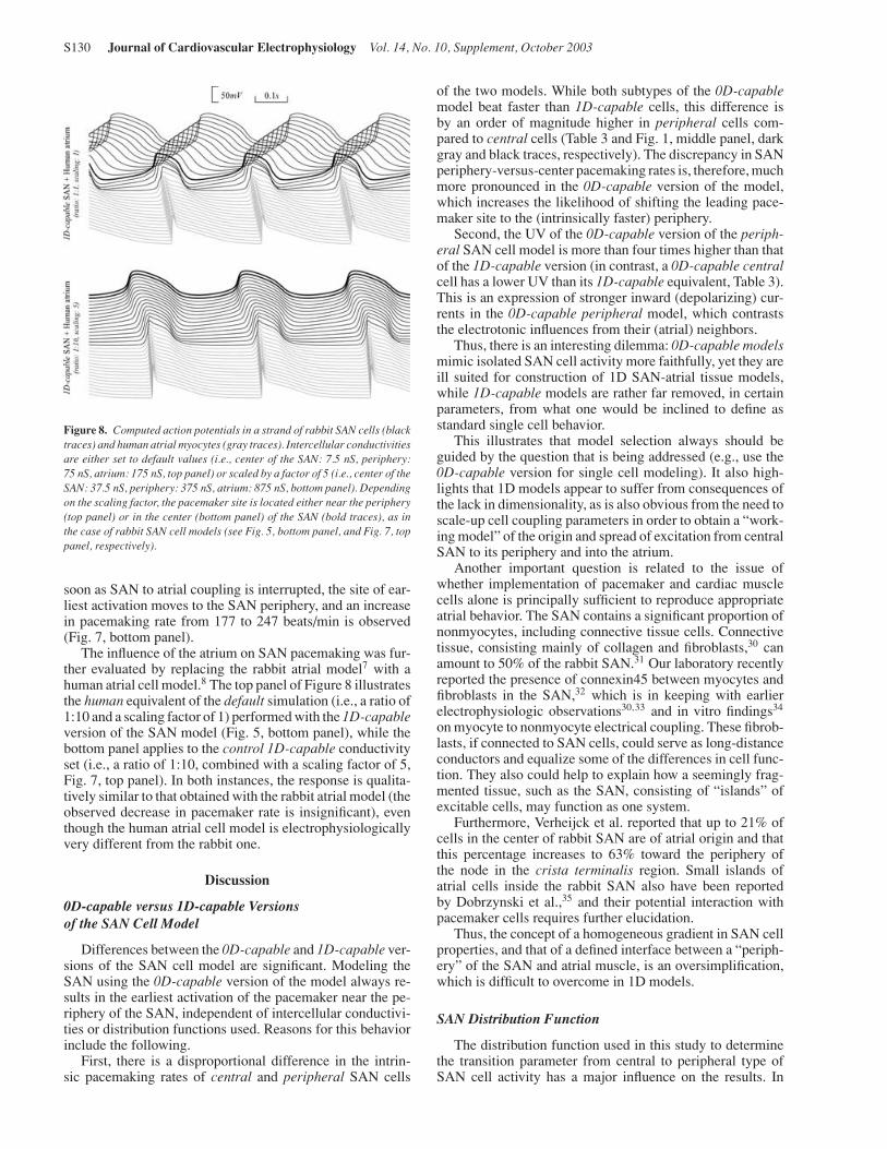
S130 Journal of Cardiovascular Electrophysiology Vol. 14, No. 10, Supplement, October 2003

Figure 8. Computed action potentials in a strand of rabbit SAN cells (blacktraces) and human atrial myocytes (gray traces). Intercellular conductivitiesare either set to default values (i.e., center of the SAN: 7.5 nS, periphery:75 nS, atrium: 175 nS, top panel) or scaled by a factor of 5 (i.e., center of theSAN: 37.5 nS, periphery: 375 nS, atrium: 875 nS, bottom panel). Dependingon the scaling factor, the pacemaker site is located either near the periphery(top panel) or in the center (bottom panel) of the SAN (bold traces), as inthe case of rabbit SAN cell models (see Fig. 5, bottom panel, and Fig. 7, toppanel, respectively).

soon as SAN to atrial coupling is interrupted, the site of ear-liest activation moves to the SAN periphery, and an increasein pacemaking rate from 177 to 247 beats/min is observed(Fig. 7, bottom panel).

The influence of the atrium on SAN pacemaking was fur-ther evaluated by replacing the rabbit atrial model7 with ahuman atrial cell model.8 The top panel of Figure 8 illustratesthe human equivalent of the default simulation (i.e., a ratio of1:10 and a scaling factor of 1) performed with the 1D-capableversion of the SAN model (Fig. 5, bottom panel), while thebottom panel applies to the control 1D-capable conductivityset (i.e., a ratio of 1:10, combined with a scaling factor of 5,Fig. 7, top panel). In both instances, the response is qualita-tively similar to that obtained with the rabbit atrial model (theobserved decrease in pacemaker rate is insignificant), eventhough the human atrial cell model is electrophysiologicallyvery different from the rabbit one.

Discussion

0D-capable versus 1D-capable Versionsof the SAN Cell Model

Differences between the 0D-capable and 1D-capable ver-sions of the SAN cell model are significant. Modeling theSAN using the 0D-capable version of the model always re-sults in the earliest activation of the pacemaker near the pe-riphery of the SAN, independent of intercellular conductivi-ties or distribution functions used. Reasons for this behaviorinclude the following.

First, there is a disproportional difference in the intrin-sic pacemaking rates of central and peripheral SAN cells

of the two models. While both subtypes of the 0D-capablemodel beat faster than 1D-capable cells, this difference isby an order of magnitude higher in peripheral cells com-pared to central cells (Table 3 and Fig. 1, middle panel, darkgray and black traces, respectively). The discrepancy in SANperiphery-versus-center pacemaking rates is, therefore, muchmore pronounced in the 0D-capable version of the model,which increases the likelihood of shifting the leading pace-maker site to the (intrinsically faster) periphery.

Second, the UV of the 0D-capable version of the periph-eral SAN cell model is more than four times higher than thatof the 1D-capable version (in contrast, a 0D-capable centralcell has a lower UV than its 1D-capable equivalent, Table 3).This is an expression of stronger inward (depolarizing) cur-rents in the 0D-capable peripheral model, which contraststhe electrotonic influences from their (atrial) neighbors.

Thus, there is an interesting dilemma: 0D-capable modelsmimic isolated SAN cell activity more faithfully, yet they areill suited for construction of 1D SAN-atrial tissue models,while 1D-capable models are rather far removed, in certainparameters, from what one would be inclined to define asstandard single cell behavior.

This illustrates that model selection always should beguided by the question that is being addressed (e.g., use the0D-capable version for single cell modeling). It also high-lights that 1D models appear to suffer from consequences ofthe lack in dimensionality, as is also obvious from the need toscale-up cell coupling parameters in order to obtain a “work-ing model” of the origin and spread of excitation from centralSAN to its periphery and into the atrium.

Another important question is related to the issue ofwhether implementation of pacemaker and cardiac musclecells alone is principally sufficient to reproduce appropriateatrial behavior. The SAN contains a significant proportion ofnonmyocytes, including connective tissue cells. Connectivetissue, consisting mainly of collagen and fibroblasts,30 canamount to 50% of the rabbit SAN.31 Our laboratory recentlyreported the presence of connexin45 between myocytes andfibroblasts in the SAN,32 which is in keeping with earlierelectrophysiologic observations30,33 and in vitro findings34

on myocyte to nonmyocyte electrical coupling. These fibrob-lasts, if connected to SAN cells, could serve as long-distanceconductors and equalize some of the differences in cell func-tion. They also could help to explain how a seemingly frag-mented tissue, such as the SAN, consisting of “islands” ofexcitable cells, may function as one system.

Furthermore, Verheijck et al. reported that up to 21% ofcells in the center of rabbit SAN are of atrial origin and thatthis percentage increases to 63% toward the periphery ofthe node in the crista terminalis region. Small islands ofatrial cells inside the rabbit SAN also have been reportedby Dobrzynski et al.,35 and their potential interaction withpacemaker cells requires further elucidation.

Thus, the concept of a homogeneous gradient in SAN cellproperties, and that of a defined interface between a “periph-ery” of the SAN and atrial muscle, is an oversimplification,which is difficult to overcome in 1D models.

SAN Distribution Function

The distribution function used in this study to determinethe transition parameter from central to peripheral type ofSAN cell activity has a major influence on the results. In

Garny et al. One-Dimensional Rabbit Sinoatrial Node Models S131

brief, the larger the proportion of central-like SAN cells, thehigher the likelihood that pacemaking originates in the cen-ter. This can be illustrated by implementing two differentdistribution functions. The published version (Fig. 1, bottompanel, gray trace) of the function yields peripheral pacemak-ing (not shown), while the 1D-capable distribution function(Fig. 1, bottom panel, black trace) causes earliest activationin the SAN center (Fig. 7, top panel).

Both the published and 1D-capable distribution functionsare, of course, purely empirical. Still, a recent report byDobrzynski et al.35 suggests that there may well be morecentral-like cells than peripheral ones in rabbit SAN. Part oftheir study was to delineate the different populations of cellsin the rabbit SAN region and atrial surrounding. The study,based on connexin distribution and neurofilament expression(a marker for SAN pacemaker cells), suggests that rabbit SANis mainly composed of central-like SAN cells. This supportsthe idea that the distribution function should contain only fewperipheral-like SAN cells. In contrast, peripheral cell-like ac-tivity is very common in isolated cell studies. Whether this isa true reflection of relative cell densities or possibly a conse-quence of cell-size dependent differences in the tolerance ofSAN myocytes to the isolation procedures (or even of a per-sonal bias by experimentalists toward investigating “larger”cells) is not known.

Gap Junction Information

Bleeker et al.9 reported an increase in gap junction den-sity from SAN center to the periphery. This was modeled byassuming a conductivity ratio of 1:10 between the center andthe periphery of the SAN. The ratio itself is, again, arbitrary.This does not undermine, however, our finding that existenceof a gradient in intercellular coupling is a prerequisite, inour model, for the central location of the site of earliest SANpacemaker activation (Fig. 7, middle panel).

The need for scaling-up experimentally established cell-pair conductivities probably is related to the lack of detailedanatomic information in the model, a characteristic inherentto its low spatial dimension. In vivo, cardiac cells communi-cate with more than one or two of their neighbors (estimatesfor ventricular cells are 6–8, while a good approximation ofSAN cell contact numbers is missing). With respect to thecomputational implementation, single SAN cells would have2, 4, or 6 neighbors in simple grid-structured 1D/2D/3D mod-els. It will be interesting to assess whether the need for con-nectivity scaling may be circumvented in higher dimensionmodels.

Role of the Atrium

As shown by Kirchhof et al.29 and reproduced in the model(Fig. 7, bottom panel), electrotonic interactions between theatrium and the SAN have a pronounced effect on normalsinus rhythm. In the model, the RP of rabbit atrial cells is sig-nificantly more negative than the MDP of rabbit SAN cells(−91.1 mV vs −80 mV, respectively). The atrium thereforehas a hyperpolarizing effect on the periphery of the SAN. Thisdelays diastolic depolarization and firing of AP in the periph-ery and allows the intrinsically slower central cells to leadpacemaking. The centrally generated excitation then propa-gates toward the SAN periphery, causing suprathreshold ex-citation there, and eventually leads to invasion of the atrialmuscle with a wave of excitation. Thus, despite the faster in-

trinsic pacemaking rate of peripheral SAN cells, electrotonicinteraction with atrial muscle shifts the earliest activation to-ward the center of the node. This can be illustrated by remov-ing the electrotonic connection between the SAN peripheryand the atrium, which causes a pacemaker shift toward theperiphery of the SAN.

Qualitatively the same results are observed using the hu-man atrial cell model, even though it has a RP that is lessnegative than the MDP of peripheral rabbit SAN cell mod-els (−75.4 mV vs −80 mV, respectively). This suggests thatthe periphery of the SAN does not need to be continuouslyhyperpolarized for the pacemaker site to be located in thecenter of the node. Suppression of peripheral pacemaking, inthis setting, is better described as an electrotonic influencefrom the atrium that opposes depolarization of the peripheralSAN cells. Although not verifiable using the present model,it is fair to assume that the atrial load on the center of theSAN is of hyperpolarizing nature, as shown experimentallyby Verheijck et al.36

The atrium therefore plays an important role in ensuringthat pacemaker activity originates in the center of the SAN.Strictly speaking, hyperpolarization of the SAN peripheryby atrial muscle may not be required, and it might be moreappropriate to think in terms of an electrotonic influence thatopposes depolarization.

Conclusion

Functional 1D models of SAN-atrial interaction requiremodification of single SAN cell model parameters that makethem less representative of experimentally determined singlecell activity. This probably is an indication of the limita-tions (dimensional restrictions) associated with 1D modelsof the origin and propagation of cardiac excitation. Othercontributing factors may include conceptual limitations im-posed by the gradual transition of cell properties from thecenter to the periphery of the SAN, or the reduction of themodel to include SAN pacemaker and atrial muscle cellsonly.

The logical next step is to reassess these limitations onmore realistic (higher spatial dimensionality) models of rab-bit SAN. Still, the current model has helped to highlight dif-ferences in single cell and 1D behavior, and identified that theinteractions between atrial muscle and SAN do not need to bebased on a maintained hyperpolarizing effect of the former onthe latter. It also shows that absolute intercellular conductancelevels and their variation across the SAN have crucial effectson the location of the site of earliest SAN activation. Finally,this study may serve as an illustration of the need to publishmathematical models in full and to make source code of sim-ulations available to the wider scientific community—eitherby providing downloads (e.g., http://COR.physiol.ox.ac.uk/for this study) or by using automated tools that minimize thelikelihood of errors in translation and transmission.

Appendix

List of Other Abbreviations

0D = zero-dimensional (here: single cell model); 1D =one-dimensional (here: strand of cells); 2D = two-dimensional (here: sheet of cells); 3D = three-dimensional(here: tissue block of cells); CellMLTM = Cell Markup

S132 Journal of Cardiovascular Electrophysiology Vol. 14, No. 10, Supplement, October 2003

Language (metalanguage for storing and exchangingcomputer-based biologic models); CMISS = Continuum Me-chanics, Image analysis, Signal processing and System iden-tification (modeling package); COR = Cellular Open Re-source (modeling package).

Acknowledgment: Simulations were run on an SGI� Origin� 2000 machineat the Oxford Supercomputing Center (http://www.osc.ox.ac.uk/).

References

1. van der Pol B, van der Mark J: The heartbeat considered as a relaxationoscillation, and an electrical model of the heart. Lond Edinburgh DublinPhysiol Magazine J Sci 1928;VI:763-775.

2. Noble D, Brown HF, Winslow RL: Propagation of pacemaker activity:Interaction between pacemaker cells and atrial tissue In Huizinga JD,eds: Pacemaker Activity and Intercellular Communication. Boca Raton,FL: CRC Press, 1995 pp. 73-92.

3. Noble D, Winslow RL: Reconstructing the heart: network models of SAnode-atrial interaction In Panfilov AV, Holden AV, eds: ComputationalBiology of the Heart. Chichester, UK: John Wiley & Sons Ltd., 1997,pp. 49-64.

4. Blanc O, Virag N, Vesin JM, Kappenberger L: A computer model ofhuman atria with reasonable computation load and realistic anatomicalproperties. IEEE Trans Biomed Eng 2001;48:1229-1237.

5. Harrild DM, Henriquez CS: A computer model of normal conductionin the human atria. Circ Res 2000;87:25e-36.

6. Zhang H, Holden AV, Kodama I, Honjo H, Lei M, Varghese T, BoyettMR: Mathematical models of action potentials in the periphery andcenter of the rabbit sinoatrial node. Am J Physiol 2000;279:H397-H421.

7. Hilgemann DW, Noble D: Excitation-contraction coupling and extracel-lular calcium transients in rabbit atrium: Reconstruction of basic cellularmechanisms. Proc R Soc Lond B 1987;230:163-205.

8. Nygren A, Fiset C, Firek L, Clark JW, Lindblad DS, Clark RB, GilesWR: Mathematical model of an adult human atrial cell: The role of K+currents in repolarization. Circ Res 1998;82:63-81.

9. Bleeker WK, Mackaay AJ, Masson-Pevet M, Bouman LN, Becker AE:Functional and morphological organization of the rabbit sinus node.Circ Res 1980;46:11-22.

10. Kodama I, Boyett MR: Regional differences in the electrical activity ofthe rabbit sinus node. Pflugers Arch 1985;404:214-226.

11. Masson-Pevet MA, Bleeker WK, Besselsen E, Treytel BW, Jongsma HJ,Bouman LN: Pacemaker cell types in the rabbit sinus node: A correl-ative ultrastructural and electrophysiological study. J Mol Cell Cardiol1984;16:53-63.

12. Oosthoek PW, Viragh S, Mayen AE, van Kempen MJ, Lamers WH,Moorman AF: Immunohistochemical delineation of the conduction sys-tem. I: The sinoatrial node. Circ Res 1993;73:473-481.

13. Honjo H, Boyett MR, Kodama I, Toyama J: Correlation between elec-trical activity and the size of rabbit sino-atrial node cells. J Physiol1996;496:795-808.

14. Demir SS, Clark JW, Murphey CR, Giles WR: A mathematical modelof a rabbit sinoatrial node cell. Am J Physiol 1994;266:C832-852.

15. Dokos S, Celler B, Lovell N: Ion currents underlying sinoatrial nodepacemaker activity: A new single cell mathematical model. J TheorBiol 1996;181:245-272.

16. Noble D, DiFrancesco D, Denyer JC: Ionic mechanisms in normal andabnormal cardiac pacemaker activity In Jacklet JW, eds: Cellular andNeuronal Oscillators. New York: Dekker, 1989, pp. 59-85.

17. Honjo H, Lei M, Boyett MR, Kodama I: Heterogeneity of 4-aminopyridine-sensitive current in rabbit sinoatrial node cells. Am JPhysiol 1999;276:H1295-H1304.

18. Kodama I, Boyett MR, Nikmaram MR, Yamamoto M, Honjo H, NiwaR: Regional differences in effects of E-4031 within the sinoatrial node.Am J Physiol 1999;276:H793-802.

19. Nikmaram MR: Regional differences in the regulation of the rabbitcardiac pacemaker. Ph.D. thesis, University of Leeds, 1996.

20. Kodama I, Boyett MR, Suzuki R, Honjo H, Toyama J: Regional dif-ferences in the response of the isolated sino-atrial node of the rabbit tovagal stimulation. J Physiol 1996;495:785-801.

21. Kodama I, Nikmaram MR, Boyett MR, Suzuki R, Honjo H, Owen JM:Regional differences in the role of the Ca2+ and Na+ currents in pace-maker activity in the sinoatrial node. Am J Physiol 1997;272:H2793-2806.

22. Garny A, Noble PJ, Kohl P, Noble D: Comparative study of rabbit sino-atrial node cell models. Chaos Solitons Fractals 2002;13:1623-1630.

23. Hedley WJ, Nelson MR, Bullivant DP, Nielsen PF: A short introductionto CellML. Phil Trans R Soc Lond A 2001;359:1073-1089.

24. Garny A, Kohl P, Noble D: Cellular Open Resource (COR): A pub-lic CellML based environment for modelling biological function. Int JBifurc Chaos 2003; (In press).

25. Verheule S, van Kempen MJA, Postma S, Rook MB, Jongsma HJ: Gapjunctions in the rabbit sinoatrial node. Am J Physiol 2001;280:H2103-H2115.

26. Verheule S, van Kempen MJA, Welscher PHJAt, Kwak BR, JongsmaHJ: Characterization of gap junction channels in adult rabbit atrial andventricular myocardium. Circ Res 1997;80:673-681.

27. Torre V: A theory of synchronization of heart pace-maker cells. J TheorBiol 1976;61:55-71.

28. Winfree AT: Biological rhythms and the behavior of populations ofcoupled oscillators. J Theor Biol 1967;16:15-42.

29. Kirchhof CJ, Bonke FI, Allessie MA, Lammers WJ: The influence ofthe atrial myocardium on impulse formation in the rabbit sinus node.Pflugers Arch 1987;410:198-203.

30. De Maziere AM, van Ginneken AC, Wilders R, Jongsma HJ, BoumanLN: Spatial and functional relationship between myocytes and fibrob-lasts in the rabbit sinoatrial node. J Mol Cell Cardiol 1992;24:567-578.

31. Opthof T: The mammalian sinoatrial node. Cardiovasc Drugs Ther1988;1:573-597.

32. Camelliti P, Kohl P, Green C: Gap junction coupling of cardiac fibrob-lasts in situ. Biophys J 2002;82:3089.

33. Kohl P, Kamkin AG, Kiseleva IS, Noble D: Mechanosensitive fibrob-lasts in the sino-atrial node region of rat heart: interaction with car-diomyocytes and possible role. Exp Physiol 1994;79:943-956.

34. Rook MB, van Ginneken AC, de Jonge B, el Aoumari A, GrosD, Jongsma HJ: Differences in gap junction channels between car-diac myocytes, fibroblasts, and heterologous pairs. Am J Physiol1992;263:C959-C977.

35. Dobrzynski H, Li J, Boyett MR: 3-D reconstruction of the complexanatomy of rabbit sinoatrial node. (Abstract) Biophys J 2003.

36. Verheijck EE, Wilders R, Bouman LN: Atrio-sinus interaction demon-strated by blockade of the rapid delayed rectifier current. Circulation2002;105:880-885.