On the Time-Domain Response of Havriliak-Negami Dielectrics

3182 IEEE TRANSACTIONS ON ANTENNAS AND PROPAGATION, VOL. 61, NO. 6, JUNE 2013

On the Time-Domain Response ofHavriliak-Negami Dielectrics

Matthew F. Causley and Peter G. Petropoulos

Abstract—We apply a combination of asymptotic and numer-ical methods to study electromagnetic pulse propagation in theHavriliak-Negami permittivity model of fractional relaxation.This dielectric model contains the Cole-Cole and Cole-Davidsonmodels as special cases. We analytically determine the impulseresponse at short and long distances behind the wavefront, andvalidate our results with numerical methods for performing in-verse Laplace transforms and for directly solving the time-domainMaxwell equations in such dielectrics. We find that the time-do-main response of Havriliak-Negami dielectrics is significantlydifferent from that obtained for Debye dielectrics. This makespossible using pulse propagation measurements in TDR setupsin order to determine the appropriate dielectric model, and itsparameters, for the actual dielectric whose properties are beingmeasured.

Index Terms—Debye dielectric model, dispersive dielectrics,fractional relaxation, Havriliak-Negami dielectric model, Maxwellequations, time-domain.

I. INTRODUCTION

P REVIOUS work [1]–[4] on the asymptotics of pulse prop-agation in the Debye model [5] of induced macroscopic

electric polarization has been shown [6] to agree with publishedlaboratory measurements [7] obtained using pulses and geome-tries typically found in the time-domain reflectometry (TDR)method for the determination of the frequency-dependent di-electric properties of materials. More recent work [8] indepen-dently verifies all the aforementioned theoretical and experi-mental results. Significantly, the large-depth time-domain re-sponse of a Debye dielectric satisfies an advection-diffusionequation and thus it is symmetric about its peak which is foundon a sub-characteristic ray whose speed is a fraction of the speedof light in such materials [1], [2].There is a large class of materials whosemicrostructure yields

an induced macroscopic electric polarization that is markedlydifferent from that of the Debye kind. A small sample of ma-terials in this class includes: amorphous polymers near glassyphase transition [9], [10]; heterogeneous soils [11]; and, perhapsmost importantly, the various complex biological tissues in thehuman body [12]–[14]. The experimentally-measured time-do-main responses in [15] indicate that in such materials it is non-

Manuscript received August 14, 2012; revised December 14, 2012; acceptedJanuary 22, 2013. Date of publication February 11, 2013; date of current versionMay 29, 2013.M. F. Causley is with the Department of Mathematics, Michigan State Uni-

versity, East Lansing, MI 48824 USA (e-mail: [email protected]).P. G. Petropoulos is with the Department of Mathematical Sciences, New

Jersey Institute of Technology, Newark, NJ 07102 USA (e-mail: [email protected]).Digital Object Identifier 10.1109/TAP.2013.2246536

symmetric responses, which are not characteristic of propaga-tion in a Debye dielectric, that are prevalent ([15, Section 4.4]).On the basis of our previous work [16], where we determinedthat the time-domain response of the Cole-Cole dielectric modelis non-symmetric about its peak value, it appears evident that forsuch materials a hierarchy of empirical models for the inducedmacroscopic electric polarization, which we will refer to as frac-tional relaxation models (FRMs), is more appropriate. Such em-pirical models have been developed over the last 70 years andinclude: the Cole-Cole (C-C) model [17], the Cole-Davidson(C-D) model [18], and the Havriliak-Negami (H-N) model [19].While FRMs have been introduced as purely empirical models,recent work [20] derives such models from first principles andinterprets the fractional relaxation they introduce as the interac-tion of different polarizable species with many different dielec-tric moments. Consequently, a distribution of relaxation timesthat peaks at some characteristic value is present, and it is theshape of this distribution function which gives rise to the variousFRMs. In the time domain, these FRMs introduce non-exponen-tial electric susceptibilities which are algebraically decaying intime and are singular as .Previously, we have examined the asymptotics of electro-

magnetic pulse propagation in the Cole-Cole dielectric model[16] and identified an open problem which we resolve in thepresent paper. Also, we have developed an algorithm to incor-porate the H-N model in the FDTD method [21] in a way thatallows the calculation of the time-dependent impulse responseof an H-N dielectric target with a preset error. In our asymp-totic and numerical FRM-related work we have determined thatpropagated pulses in such dielectric models evolve to non-sym-metric shapes which are distinct from the shapes obtained whendielectrics are represented with the Debye medium model. Thislends credence to the suggestion that FRMsmay be more appro-priate for representing the dielectric permittivity data obtainedexperimentally for complex media beyond water.The present work aims to complete our contributions to

the numerical and asymptotic study of pulse propagation inanomalously dispersive lossy dielectric models by presentingan asymptotic analysis of pulse propagation in the H-N model,which is the most general of the known FRMs. The fre-quency-dependent relative permittivity, which now involvestwo fractional parameters and , where , isgiven by

(1)

where is the complex frequency (below we will workwith the Laplace transform), and are respectively the zero-and infinite-frequency limits of the relative permittivity, isthe permittivity of vacuum, and is the relaxation time at which

0018-926X/$31.00 © 2013 IEEE

CAUSLEY AND PETROPOULOS: ON THE TIME-DOMAIN RESPONSE OF HAVRILIAK-NEGAMI DIELECTRICS 3183

the distribution of relaxation times achieves its peak. The Debyemodel is the special case , while the Cole-Cole modelis obtained when , and the Cole-Davidsonmodel is obtained when . We derive thetime-domain Green’s function for the H-N medium, and studyit with asymptotic methods valid for short and large depths. Ourmodel problem emulates a signaling problem in the TDR setupand is described in Section II, where the exact evaluation of themodel’s solution is also discussed. The asymptotic results forshort- and large-depth behavior are constructed and validated inSection III. In Section IV we investigate the possibility of usingour analytical/numerical results for model parameter estimationusing experimentally-obtained data (simulated herein with ourFDTD code [21]) on propagated pulses such as those encoun-tered during TDR measurements. Also, we connect our analysisto pulse propagation in lossless random media whose propertiesexhibit short- or long-range correlations thus creating the possi-bility of using TDR-measured responses to probe the statisticsof the microstructure of complex dielectrics.

II. MODEL EQUATIONS AND THEIR EXACT SOLUTION

We consider, with the geometry of TDR in mind, a pulsedplane-wave propagating through a one-dimensional non-mag-netic dielectric half-space whose permittivityis modeled with (1). The time-domain Maxwell’s equations re-duce to

(2)

where is the electric field, and is the in-duced electric polarization. Signaling data is prescribed at theboundary

(3)

and for . The induced electric polarization isdefined to be

(4)

where the time-domain susceptibility, , is obtained via theinverse Laplace transform from (1) as

(5)

Applying standard Laplace transform arguments reduces(2)–(5) to an ordinary differential equation for

(6)

with boundary data

Defining the frequency-dependent wave speed as

(7)

where , with

(8)

and requiring that is bounded as , we obtain theelectric field in the half-space on and behind the wavefront as

(9)

for . Setting in (9) we obtain the time-domain representation of the impulse response

(10)

where is an integration contour as in (9) or an allowable de-formation of it in the complex -domain.Equation (10) will be studied asymptotically, and numerically

by appropriate quadrature along . The region of analyticityof is independent of and .The square root in (8) produces a branch cut along the negativereal axis, and so the region of analyticity will be for which

. Thus, we can define to be any curve thatbegins at in the third quadrant, passes to the right ofany singularities of , and terminates at in the secondquadrant. Once a suitable contour is chosen, we constructquadrature points , where each is on the contour; wethen apply the mapping , so that (10) is approximated as

(11)

If is known, then (9) can be computed directly with thismethod, by replacing with . Otherwise, we canobtain , and convolve it in the time domain with thesignaling data, . The choice of contour will determine theaccuracy of the approximation and the number of pointsrequired to obtain a desired accuracy. Ideally, a steepest de-scent contour would be determined, which will pass through asaddle point, and along which the imaginary part of the phase

is constant. The saddle point satisfies, which yields

(12)

where the space-time parameter is defined as

(13)


Note that the saddle point depends on and only through. Unfortunately, this unwieldy expression (12) is a nonlinearequation that can be rationalized into a (degree 4) polynomial inonly when ; otherwise the equation is transcendental.

Instead of seeking a closed form solution, we find real thatsatisfies (12) using Newton’s method. In terms of , the saddlepoint moves along the real line, decreasing from , to

, where corresponds to thesubcharacteristic ray . The speed of this subcharacter-istic ray is . For , noreal-valued saddle point exists, and the steepest descent contourdevelops a cusp at the origin. This is illustrated in Fig. 1 for arepresentative set of parameters, with fixed and increasing.When the saddle point exists, the contour passes through it ver-tically . Although Fig. 1 is useful to ex-amine, it falls short of providing a parametric representationfrom which the steepest descent contour can be obtained. In-stead, we proceed to evaluate by choosing a hyper-bolic contour, as used in [22], to perform the numerical inverseLaplace transform. This contour, given by

(14)

provides a means to construct the weights and nodes .Specifically, we set

(15)

where , with an appropriate step size . As shownin [22], selection of the parameters and can be madeby asymptotic balancing of the error terms. There will be twosources of error in the approximation: the truncation error,which arises when the infinite limits aretruncated to ; and the discretization error, orquadrature error due to approximation of the integral with afinite sum. Unfortunately, it is not clear a priori what choice ofis required to ensure convergence with prescribed precision.

For a value of that is too large, evaluation of the impulseresponse over many values of will be time-consuming.Additionally, we have found in practice that it is helpful to scalethe quadrature nodes by either time , or by the delayedtime , where is the arrival time ofthe wavefront. The correct choice of both and the method ofscaling is ultimately determined by the size of and the timeinterval over which the solution is to be computed.This construction of the impulse response will be em-

ployed to validate the asymptotic behavior of the H-N mediumresponse at short and large depths in Section III. Solutions ob-tained using this hyperbolic contour have been validated bycomputing the impulse response with an alternative method thatfirst folds the Bromwich curve on the branch cut,

, and then discretizes the resulting integral withGauss-Legendre quadrature and an excessively large number ofnodes (3 to 4 times as many as those used in the hyperboliccontour) to ensure sufficient convergence. Also, we have em-ployed a numerical method of known accuracy [21] to validatethe numerical inverse Laplace transforms discussed above andthe asymptotic results obtained below.

Fig. 1. Numerically determined steepest descent contours for the H-N impulseresponse. The saddle point is at the intersection of each contour with the Real-axis. The contour and saddle point move to the left as the parameter increases,and the saddle point moves into the origin when (dotted line).For , the contour forms a cusp at the origin. (a) Zoom-out,(b) Zoom-in.

III. ASYMPTOTIC ANALYSIS

We now present an asymptotic investigation of the impulseresponse (10) for short and large depths into the H-N dielectrichalf-space. The results will be presented for the general (H-N)case, but are also valid for the limiting cases of the C-C andC-D models. Section III-B will also provide the resolution ofthe open problem identified in [16].

A. The Wavefront Region

We first examine the wavefront after propagation over a shortdepth into the H-N medium characterized by. We will also refer to this asymptotic regime in terms of theparameter (13) which satisfies near the wavefront. Ifin (10) we substitute and assume , we see thatthe phase of the wavefront behavior will be determined by theinfinite-frequency approximation

(16)

which is obtained by retaining the first two terms of the expan-sion of (8) for large . Inserting (16) into (10), the leadingorder behavior of the impulse response at the wavefront is thenobtained as , where

(17)

with . The integrand in (17) is written ina factored form in order to distinguish between two prominentfeatures of the early impulse response. The argument of the firstexponential factor is a hyperbolic term, which shows that thewavefront will propagate with the infinite-frequency speed .The second exponential factor will act as a smoothing operatoron the incoming pulse. Notice that the parameters and onlyappear as a product in this approximation; thus the behaviorof the electric field in the skin-depth cannot be distinctly dis-cerned as corresponding to a C-C, C-D, or H-N medium, unlessother considerations have determined that .To elaborate on the smoothing effects of the early impulse re-

sponse, we compute the early wavefront response for the elec-


Fig. 2. Validation of the infinite-frequency approximation of the Havriliak-Negami impulse response, at . The time is translated, so thatthe origin is at . (a) , (b) .

tric field due to an incident pulse by first taking the Laplacetransform

(18)

differentiating with respect to , and inverting the resulting ex-pression to produce the governing equation for the effectiveshort depth impulse response

(19)

where the right hand side is a fractional derivative, and acts as asmoothing operator for . Thus will be infinitelysmooth for since

(20)

for . This result was shown in [16] to hold for the C-Cmodel, and now it can be seen to generalize to the H-N andC-D models. In the limit , the behavior in a Debyemedium is recovered, and the solution of (19) will be

, which shows will not be infinitelysmooth at the wavefront and will now inherit any discontinuitiesin the signal .In contrast to the exact impulse response discussed in

Section II, the short-depth approximation can be success-fully computed using the method of steepest descents. Thisis due to the simpler expression for the phase, which can beused to obtain a closed form representation of the contour. Thesaddle point is now obtained by setting , where

is the phase of (17). Thisresults in

(21)

Notice that we have a moving saddle point, as it is inversely pro-portional to ; thus we first make the change of variables

Fig. 3. Time-domain response with rectangular-pulse signaling data,recorded at . The time is translated, so that the origin is at

. (a) , (b) .

in (17), where will be a large pos-itive parameter (recall that at the wavefront).This will ensure that the main contribution of the integral willremain localized near the saddle point, which is now given as

and is stationary. Makingthis change of variables in (17) produces

(22)

After substituting the second order approximation of the phaseabout

(23)

we integrate the resulting expression to obtain the leading orderterm of the asymptotic series

(24)

which is valid to . Fig. 2 shows the saddle point approx-imation for , and re-spectively, compared to the exact impulse response, obtainedusing the hyperbolic Bromwich contour (14) to evaluate (10).We also show the result of numerically evaluating (17) along thesteepest descent contour, computed as detailed below. Note thatthe relative amplitude of the impulse response depends stronglyon , and approaches infinity for ; this reflects thefact that for the Debye response. Ad-ditionally, note that the approximations show better agreementwith the exact response for smaller ; this is because willbe larger for smaller , which makes the saddle point approx-imation (24) more accurate. In Fig. 3 we show the result of con-volving (24) with signaling data consisting of a unit-amplituderectangular pulse of duration .In order to directly evaluate (17), as shown in Fig. 2, we first

find a parametric representation of the steepest descent contour.This is most easily accomplished in polar form. We first define

, and then note from (21) that both and willbe real, so that the steepest descent contour satisfies .This leads to

(25)


For the sake of simplicity, we define the function

(26)

so that , and . Thiscontour is shown in Fig. 4 for comparison to Fig. 1. The con-tours are only of interest for , since this is where the ap-proximation (17) is asymptotically valid. Using the parametricrepresentation and the expression (26), the short-depth approx-imation of the impulse response takes the form

(27)

Approximation of this integral can be accomplished using thetrapezoidal rule, which yields exponential convergence

(28)

where , and

B. The Large-Depth Behavior

We now examine the behavior of the propagating pulse atdepths satisfying . In this region, we will take

, or alternatively . This regime correspondsto the limit of (8); an asymptotic expansion yields

(29)

where . The leading order large-depth approxima-tion of the impulse response is , where

(30)

with .To accomplish the evaluation of , we again compute

the inverse Laplace transform along a steepest descent con-tour in the complex -domain. Now the phase is

and the saddle point will be

(31)

From this expression, we see that for the saddle pointwill be real which will make the phase real as well.We first makethe change of variables , with ; aftersubstituting the second order approximation of the phase about

we have

(32)

Fig. 4. Steepest descent contour for the phase of the short-depth approximationof the H-N impulse response (17). Contours are shown for , sincethe asymptotic regime corresponds to .

where , and thus

(33)

up to . Clearly, (33) loses validity as sinceand the asymptotic series diverges thus rendering the

leading order term useless for . This issue was identi-fied in [16] as an open problem and to resolve it we evaluate (30)by finding a parametric form of the steepest descent contour, asin the case of the shallow-depth response, and discretize the re-sulting integral. By setting , and setting the imaginarypart of the phase to zero, we obtain the parametric form

(34)

where the is again given by (26), and the interval istaken to ensure that the expression remains real for .Note that this expression satisfies . We note here thatthis calculation agrees with (33) in the time interval where it isvalid (see Fig. 7).At (30) can be evaluated analytically. Now, the

saddle point vanishes, and the expression (34) is no longer valid;the phase simplifies to , which can be made realalong the rays . The approximate impulseresponse is thus given by

(35)

where , and we have used the identity.

When , the saddle point vanishes, since it passes intothe branch cut on the negative real -axis; however the same


Fig. 5. Steepest descent contour of the large-depth approximation,with increasing values of . The separatrix (dotted line) is given by

, and corresponds to . (a) Zoom-out,(b) Zoom-in.

expression (34) will still define a steepest descent contour. It ismerely the domain that must be changed, which is instead com-prised of the disjoint intervals defined by .On these intervals, is negative, which in turnmakes negative; but this sign change is com-pensated by an additional change in the numerator of due to

, and therefore the parametric representation remainsreal. The two disjoint intervals in form a cusp at the origin inthe complex domain, which corresponds to . Thetwo regimes, namely that with the saddle point, and that with thecusp, are separated by the steepest descent contour along which

, as is shown in Fig. 5. This latter curve will be com-prised of the two rays , and must thereforebe treated separately. Note that this behavior in the steepest de-scent contours is similar to those of the exact impulse response,shown in Fig. 1.We can now express the approximate impulse response for

by replacing , and retaining the real partof the resulting integral; the imaginary part is odd with respectto the imaginary axis, and will therefore vanish. After some ma-nipulation, we obtain

(36)

where the endpoints are chosen depending on the sign of. This integral can be approximated with exponential accu-

racy using the trapezoidal rule

(37)

where

(38)

(39)

The approximate impulse response is compared in Fig. 6 for thesame parameters as Fig. 2 but for . Once again, thehyperbolic contour (14) is used to evaluate the exact impulseresponses . As illustrated in Fig. 6, the approximate impulseresponse clearly improves as increases, but in both cases thepeak of the exact impulse response is slightly underestimated.

Fig. 6. Validation of the large-depth approximation of the H-N Impulse Re-sponse at . (a) , (b) .

Fig. 7. Validation of (33) and (35) at . (a) ,(b) .

The saddle point approximation is not shown, since it does notprovide an accurate approximation for . However,Fig. 7 shows the correctness of (35), and the accuracy of (33)when it is valid. The splicing of (33), (35), and (37) provides theresolution of the open problem identified in [16].

IV. APPLICATIONS

A. Time-Domain Reflectometry

We now discuss the possible application of the results ob-tained in Section III to perform medium-model parameter esti-mation using recorded propagating pulses in TDR experiments.In [2], it was shown in the case of the Debye model that for largedepths the electric field satisfies an advection-diffusion equationwith the zero-frequency subcharacteristic speed . This resultsin a symmetric response, whose peak is located on the subchar-acteristic ray . But in the C-C model [16], the peak wasfound not to coincide with this ray; rather, it is the mean electricfield that does. When , the peak and mean electric fieldscoalesce. More importantly, we can compute the time at whichthe mean electric field occurs using the mean value theorem

Upon constructing this quantity, we find that is a linear func-tion of , with slope . The intercept can be computed bysetting , and doing so provides an alternate expression interms of the incident pulse

(40)


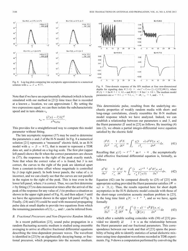
Fig. 8. Log-log plots comparing late asymptotic approximation to a numericalsolution with .

Note that if we have an experimentally obtained (which is hereinsimulated with our method in [21]) time trace that is recordedat a known location, we can approximate . By setting thetwo expressions equal, we can then isolate the subcharacteristicspeed and in turn obtain

This provides for a straightforward way to compute this modelparameter without fitting.The late asymptotic response (37) may be used to determine

the parameters and of the H-N model. In Fig. 8 a numericalsolution [21] represents a “measured” electric field, in an H-Nmodel with , that is meant to represent a TDRdata set, and is plotted on a log-log scale. The first plot (upperleft panel) shows the fit when the correct parameters are chosenin (37); the responses to the right of the peak exactly match.Note that when the correct value of is found, but is notcorrect, the curves to the right of the peak are identical apartfrom a constant-in-time offset whose magnitude is controlledby (top right panel). In both lower panels, the value of isincorrect, and we can clearly see that the curves are not parallelin the region to the right of the peak. This is true even in thelower left panel, where is correct. Thus, we can first determineby fitting (37) to data measured at times after the arrival of the

peak of the response for any value of (to produce a situation asshown in the upper right panel of Fig. 8), and then adjust untilwe have the agreement shown in the upper left panel of Fig. 8.Finally, (24) and (35) could be used with measured propagatingpulse data at small depths to provide two equations from whichthe remaining parameters of (1), and , can be inferred from.

B. Fractional Precursors and Non-Dispersive Random Media

In a recent publication [23], sound pulse propagation in arandom fluctuating acoustic medium is studied using ensembleaveraging to arrive at effective fractional differential equationsdescribing the time-dependent pressure waves. The wavefrontis identified in [23] by an algebraically decaying bump, or frac-tional precursor, which propagates into the acoustic medium.

Fig. 9. Time-domain response of the HN medium at four non-dimensionaldepths for signaling data , where

for and for . The medium modelparameters are , and .

This deterministic pulse, resulting from the underlying sto-chastic properties of weakly random media with short- andlong-range correlations, closely resembles the H-N mediummodel response which we have analyzed. Indeed, we canestablish a relationship between our parameters and , andthe Hurst parameter used in [23] as follows. By inserting (4)into (2), we obtain a partial integro-differential wave equationsatisfied by the electric field

(41)

Recalling that as , the asymptoticallyvalid effective fractional differential equation is, formally, asfollows:

(42)

Equation (42) can be compared directly to (25) of [23] withappropriate scaling provided theHurst parameter satisfies

. Thus, the results reported here for short depthasymptotics in the H-N dielectric model coincide with those ofthe short-range correlation acoustic medium problem in [23].In the long time limit , and so we have, againformally

(43)

which after a suitable scaling coincides with (30) of [23] pro-vided we identify as the relationship betweenthe Hurst parameter and our fractional parameters. This corre-spondence between our work and that of [23] opens the possi-bility of being able to identify statistics of actual dielectric mix-tures using time-dependent waveforms recorded in TDR experi-ments. Fig. 9 shows a computation performed by convolving the


signaling data described in the caption with a numerical evalu-ation of our (10), as described in Section II above, and suggeststhat the H-N model is the homogenization (in the sense of [23])of a lossless non-dispersive random medium that exhibits bothshort- and long-range correlations.

REFERENCES[1] P. Petropoulos, “The wave hierarchy for propagation in relaxing di-

electrics,” Wave Motion, vol. 21, no. 3, pp. 253–262, May 1995.[2] T. M. Roberts and P. G. Petropoulos, “Asymptotic and energy esti-

mates for electromagnetic pulses in dispersive media,” J. Opt. Soc. Am.A, vol. 13, no. 6, pp. 1204–1217, 1996.

[3] M. Kelbert and I. Sazonov, Pulses and Other Wave Processes inFluids. Dordrecht, The Netherlands: Kluwer Academic, 1996.

[4] T. M. Roberts and P. G. Petropoulos, “Asymptotics and energy esti-mates for electromagnetic pulses in dispersive media: Addendum,” J.Opt. Soc. Am. A, vol. 16, no. 11, pp. 2799–2800, 1999.

[5] P. Debye, Polar Molecules. New York, NY, USA: Dover, 1929.[6] T. M. Roberts, “Measured and predicted behavior of pulses in Debye-

and Lorentz-type materials,” IEEE Trans. Antennas Propag., vol. 52,no. 1, pp. 310–314, Jan. 2004.

[7] E. G. Farr and C. A. Frost, Impulse Propagation Measurements ofWater, Dry Sand, Moist Sand, and Concrete U.S. Air Force WeaponsLab., Tech. Rep. WL-TR-1997-7051, 1997.

[8] F. E. Stoudt, D. C. Peterkin, and B. J. Hankla, Transient RF and Mi-crowave Pulse Propagation in a Debye Medium (Water) Naval Sur-face Warfare Center, Interaction Note 622, 2011 [Online]. Available:www.ece.unm.edu/summa/notes/Interaction.html

[9] R. Hilfer, “H-function representations for stretched exponential relax-ation and non-Debye susceptibilities in glassy systems,” Phys. Rev. E,vol. 65, no. 6, pp. 061 510–061 514, Jun. 2002.

[10] A. Schönhals, F. Kremer, and E. Schlosser, “Scaling of the relaxationin low-molecular-weight glass-forming liquids and polymers,” Phys.Rev. Lett., vol. 67, no. 8, pp. 999–1002, Aug. 1991.

[11] T. Repo and S. Pulli, “Application of impedance spectroscopy for se-lecting frost hardy varieties of English ryegrass,” Ann. Botany, no. 78,pp. 605–609, 1996.

[12] P. Polk and E. Postow, Handbook of Biological Effects of Electromag-netics Fields. Boca Raton, FL, USA: CRC Press, 1995.

[13] T. Kim, J. Kim, and J. Pack, “Dispersive effect of UWB pulse on humanhead,” in Proc. 18th Int. Zurich Symp. Electromagnetic Compatibility,2007. EMC Zurich 2007, 2007, pp. 41–44.

[14] S. Gabriel, R. W. Lau, and C. Gabriel, “The dielectric properties ofbiological tissues: III. Parametric models for the dielectric spectrum oftissues,” Phys. Med. Biol., vol. 41, no. 11, pp. 2271–2293, 1996.

[15] W. S. Bigelow and E. G. Farr, Impulse Propagation Measurements ofthe Dielectric Properties of Several Polymer Resins. Albuquerque,NM: Farr Research Inc., 1999 [Online]. Available: www.farrresearch.com/Papers/mn55.pdf

[16] P. Petropoulos, “On the time-domain response of Cole-Cole di-electrics,” IEEE Trans. Antennas Propag., vol. 53, no. 11, pp.3741–3746, Nov. 2005.

[17] K. Cole and R. Cole, “Dispersion and absorption in dielectrics I. Al-ternating current characteristics,” J. Chem. Phys., vol. 9, pp. 341–52,1941.

[18] D. Davidson and R. Cole, “Dielectric relaxation in glycerol, propyleneglycol, and n-propanol,” J. Chem. Phys., vol. 19, pp. 1484–1490, 1951.

[19] S. Havriliak and S. Negami, “A complex plane representation of dielec-tric and mechanical relaxation processes in some polymers,” Polymer,vol. 8, no. 4, p. 161, 1967.

[20] Y. P. Kalmykov, W. T. Coffey, D. S. F. Crothers, and S. V. Titov,“Microscopic models for dielectric relaxation in disordered systems,”Phys. Rev. E, vol. 70, p. 041103, 2004.

[21] M. F. Causley, P. G. Petropoulos, and S. Jiang, “Incorporating theHavriliak-Negami dielectric model in the fd-td method,” J. Comput.Phys., pp. 3884–3899, 2011.

[22] J. A. C.Weideman and L. N. Trefethen, “Parabolic and hyperbolic con-tours for computing the Bromwich integral,” Math. Comput., vol. 76,no. 259, pp. 1341–1356, 2007.

[23] J. Garnier and K. Solna, “Fractional precursors in random media,”Waves Random Complex Media, vol. 20, no. 1, pp. 122–155, 2009.

Matthew F. Causley received the B.S. degree in applied mathematics (withHonors) from Kettering University, Flint, MI, in 2006 and the Ph.D. degree inmathematical sciences from the New Jersey Institute of Technology, Newark,NJ, USA, in 2011.He is currently a Postdoctoral Investigator with the Department of Math-

ematics, Michigan State University, East Lansing, MI, USA. His current re-search is on novel numerical methods for modeling plasmas. His research in-terests include computational electromagnetics, wave propagation in dispersivedielectrics, and fast convolution techniques.

Peter G. Petropoulos received the B.S.E.E. degree (with Highest Honors) fromRutgers University, New Brunswick, NJ, USA, in 1986 and the Ph.D. degreein applied mathematics from Northwestern University, Evanston, IL, USA, in1991.From 1991 to 1994, he was a Postdoctoral Fellow with the Directed Energy

Division, U.S.A.F. Armstrong Laboratory, Brooks AFB, TX, USA, and from1994 to 1998, he was an Assistant Professor with the Department of Mathe-matics, Southern Methodist University, Dallas, TX, USA. Since 1998, he hasbeen with the Department of Mathematical Sciences, New Jersey Institute ofTechnology, Newark, NJ, USA, where he is currently an Associate Professor.His research is in the areas of wave propagation, computational electromag-netics, and microscale electrohydrodynamics.

On the Time-Domain Response of Havriliak-Negami Dielectrics

Documents

Transcript of On the Time-Domain Response of Havriliak-Negami Dielectrics