INVESTIGATION OF ADVANCED GATE DIELECTRICS

FOR FUTURE COMPLEMENTARY METAL-OXIDE

SEMICONDUCTOR DEVICES

by

NARENDRA SINGH MEHTA, BE.

A THESIS

IN

ELECTRICAL ENGINEERING

Submitted to the Graduate Faculty

of Texas Tech University in Partial Fulfillment of the Requirements for

the Degree of

MASTER OF SCIENCE

IN

ELECTRICAL ENGINEERING

ACKNOWLEDGEMENTS

1 would like to thank my thesis advisors Dr. Shubhra Gangopadhyay and Dr.

Henryk Temkin, for their support, encouragement and guidance. Your guidance and

support has been extraordinary. 1 would also like to thank Dr. Tim Dallas for being on my

committee and helping me.

I would also like to thank my peers at Jack Maddox for helping me at times of

need. My friends also deserve special thanks for it is they who have helped me when I

have been bogged down by diflBculties, and their encouragement has made me go on for

higher goals in life. A special thanks to my fnend "The Bee" for being there at times of

need.

My parents have played a critical role in helping me achieve my goals and

dreams. They have and will always be the role models in my life. They have taught me

that the path to success is through hard work and vwthout them it is difficult to imagine

where I would be at the moment. Dear Mom and Dad, I dedicate this thesis to you.

TABLE OF CONTENTS

ACKNOWLEDGEMENTS ii

LIST OF TABLES v

LIST OF FIGURES vi

CHAPTER

1 INTRODUCTION 1

11 The Need to Scale Devices 1

1.2 The MOS Transistor 2

1.3 MOSFET Current Voltage Characterisitics 6

1.4 Scaling 7

1.5 Voltage Scaling 9

1.6 Delay Time Calculations 10

1.7 Delay Time Definitions 12

1.8 Calculation of Delay Times 12

2 THE MOS TRANSISTOR 19

2.1 Equilibrium in the MOS Capacitor 21

2.2 Analogy of the Field-induced Depletion Layer to a Metallurgical p-n Junction... 24

2.2.1 Solution of the Poisson Equation 24

2.2.2 Band Bending Approximation 25

2.2.3 The Poisson Equation 27

2.3 Calculation of the Field and Potential in Silicon and the Gate Dielectric 30

2.4 The MOS Capacitor at Low fi-equencies 31

2.5 MOS Capacitor at High Frequencies 39

2.6 Dit Extraction Using Conductance Method 42

2.7 The Single State Model 45

2.8 The Continuum Model 45

2.9 Terman'sCV Analysis for Dit Calculations 48

2.10 Metal-Semiconductor Workfimction Difference 50

2.11 Fixed Charge and Insulator Trapped Charge 51

iii

3 ANALYSIS OF MOS CAPACITORS 54

3 1 The Choice ofMaterials for High k Gate Dielectrics 54

3.2 Calibration ofthe 4275 a LCR Meter 54

3.3 Experimental Procedure 61

3.3.1 Substrate Cleaning 61

3.3.2 Deposition Technique 62

3.4 Surface Cleaning Experiment 63

3.5 Electrical Characterization of Hafnium Dioxide Samples 66

3.6 Leakage Current and Conduction Mechanism in Hf02 Films 76

3.7 Annealing in the Presence of Oxygen 78

3.8 Analysis of Nitrided Interfaces 80

3.9 Determination of Device Capacitance in a Leaky Dielectric 85

3.9.1 Experimental Results of Shunt Resistance Correction in AIN 87

3.10 Conclusion 90

REFERENCES 92

APPENDIX

A: MATLAB PROGRAMS FOR ANALYSIS 96

B: CALCULATION OF AREA OF MOS CAPACITORS 108

IV

LIST OF TABLES

1.1 Full scaling of the MOSFET dimensions potentials and doping densities 8

2 1 The effect of interface traps on CV measurements 47

3.1 Data set for device area 7,85* 10" at different points around the center ofthe wafer. 58

3.2 Variation of error with fi-equency for device of diameter 100|j,m 58

3.3 Error variation with capacitor size 60

3.4 Comparison of resuhs obtained using CVC program 61

LIST OF FIGURES

1.1: The MOS Transistor 3

12: Formation of depletion region in an n-channel enhancement type MOS 4

1.3 Pinch off point in the transistor 5

1.4 IV current voltage graphs using MATLAB 7

1.5 Cascade CMOS inverter with parasitic capacitances 11

1.6 Lumped load circuit of the inverter 11

1.7 Simplified inverter mask layout for delay analysis 15

2.1 The MOS capacitor 20

2.2 Calculated fi"ee carrier concentrations as fijnctions of normalized depth for p-type Si that has an acceptor density of lO'^ cm' and a surface charge density of 2*10' cm"^ 23

2.3 Band bending diagram for p type sample 26

2.4 Variation of Silicon surface charge density as a fianction of barrier height for p-type silicon having NA = 4*10'' cm'^ T = 300 °K, and <DB = 0.335 V 29

2.5 Electric field configuration in the dielectric and silicon surface 31

2.6 Cross Section of an MOS capacitor 31

2.7 Small signal a.c. Voltage superimposed on the gate bias, applied to the gate to measure the dynamic capacitance 32

2.8 Cross section of a MOS Capacitor with a small signal bias, showing the equivalent circuit 33

2.9 Low frequency dynamic capacitance as a function of gate voltage for a 1000 A thick oxide with a ptype substrate doping concentration of lO'' cm' 35

2.10 Low frequency dynamic capacitance as a fvinction of gate voltage for a 100 A thick oxide and a p-type substrate with doping concentration of 10'^ cm' 36

2.11 Low frequency dynamic capacitance as a fiinction of gate voltage for a 100 A thick oxide and a p-type substrate with doping concentration of 10'^ cm' 37

2.12 Band bending in MOSCAP as a fiinction of applied gate bias for a p-type substrate, indifferent regions of operation 38

2.13 High Frequency CV curves for 100 Angstroms oxide sample with different substrate doping concentrations 41

2.14 Normalized MOS Capacitance as a function of gate voltage plotted using ideal MOS CV equations developed by JR. Brews, for capacitors with same bulk oxide doping concentrations and different oxide thickness 42

vi

2.15 Equivalent circuit for a capacitor using (a) three-element model, (b) parallel

equivalent circuit, (c) series equivalent circuit for MOS capacitor 44

2.16 Equivalent circuits for conductance measurements; (a) MOS capacitor with interface trap time constant r„ = R,,C„; (b) Simplified circuit of (a),

(c) SimpHfied circuit of (c), (d) measured parameters 44

2.17 Equivalent Circuit of the MOS Capacitor for Terman's analysis 49

2 18 Energy band diagram for a non-ideal MOS capacitor. The metal semiconductor work function difference is relatively small 51

2.19 Locations of various charges within the oxide of an MOS capacitor 53

3.1 Experimental Setup ofthe CV measurement system 55

3.2 Comparison of data from standard LCR meter and system to be calibrated 56

3.3 CV curves on different size capacitors measured at 100 kHz on the machine to be calibrated 59

3 4 CV curves on different size capacitors measured at 100 kHz on the standard

machine 60

3.5 E-beam evaporation of Hf02 63

3.6 SC2 cleaned Hf02 sample, CV curves are of poor quality 64

3.7 CV curves of above sample using modified Shiraki clean 65 3.8 Unannealed as deposited 320 A Hf02M0S Capacitor CV curves 66

3.9 Illustration of movement of dipoles under electric field; (a) zero gate voltage, (b) positive gate voltage, (c) negative gate voltage 67

3.10 Plot of C-V and Gm-V for forward and reverse 1 MHz curves 68

3.11 Interface state density as calculated by Terman's method with respect to gate voltage 69

3.12 Forward CV curves for annealed and unannealed 320 AHf02film 70

3.13 Hysteresis in the H2 annealed 320 A Hf02 film 71

3.14 Corrected Gm/o) versus VG curves for the annealed MO S Capacitors 72

3.15 Gp/co matching with single state model at gate voltage of-0.92 V 73

3.16 Gp/o) matches with the continuum model at a gate bias of -1.52 V 74

3.17 Dit versus gate bias for the annealed 320 A annealed Hf02 sample 74

3.18 Time constant versus gate voltage for 320 A annealed Hf02 sample 75

3.19 JV curves for the annealed and unannealed sample 76

vu

3.20 J/E vs. E"^ for the 320 A Hf02 sample showing Frenkel-Poole Emission at higher electric fields 77

3 21 HfD2 as deposited sample 90 Angstroms thick (k ~ 18) 79

3.22 90 A Hf02 as deposited film annealed in the presence of O2 at 700 °C for 300 seconds (k~ 8) 80

3.23 Forward CV curves for 153 A AIN 111 sample with epitaxial Si grown 82

3 24 Clockwise hysteresis observed in the 153 A AIN sample 83

3.25 Corrected Gm/oo versus VG gate voltage for 153A AIN sample with epitaxial Si 83

3.26 Gp/o) versus Frequency for the 153 A sample at a gate voltage of-0.4 V 84

3 27 IV on the annealed sample 85

3.28 Small signal equivalent circuit models of a MIS capacitor (A) accurate model (B) series circuit model for low leakage devices (C) Parallel circuit model for low series resistance devices 86

3.29 The data was collected is frequencies 1 MHz and 100 kHz, 200 kHz and 400 kHz 88

3.30 The plot above shows the Corrected - frequency independent CV data for 1 MHz 200 kHz and 100 kHz measurement frequencies 89

3.31 Interface state density calculated using Terman's method 90

B, 1 High magnification image ofthe metal Unes in the reference wafer 108

B,2 Image ofthe metal dots on a SiC film 109

vui

CHAPTER 1

INTRODUCTION

1,1 The Need to Scale Devices

The semiconductor industry has undergone a phenomenal growth in the past few

years due to the rapid advances in the integration technologies and large-scale systems

design. The required computation and application power of devices used in

communications, high performance computing and consumer electronics has been

growing at a very fast pace. This fast pace growth and the demand of faster chips and

lower power devices has led to an increased use of complementary-metal-oxide-

semiconductor devices.

There is also an increased drive to shift to monolithic integration or SOC (system

on a chip) devices. The advantages of a system on a chip or monohthic integration

schemes are:

• Less area/volume hence compactness,

• Less power consumption,

• Less testing requirements at system level,

• Higher reliability, mainly due to on chip interconnects,

• Higher speeds due to significantly reduced interconnect length,

• Significant cost savings.

Today the most widely used logic family is the CMOS logic family. This provides

a designer vAth low standby power devices compared to other famiUes Uke TTL, RTL or

others. The MOS transistor is the most fundamental device used in this family.

Continuous scaling of the device is required to ensure future generations of faster

devices.

Over the last few decades, the minimum feature size of microelectronic devices

(MOS transistors) has been continuously reduced according to the famous Moor's law.

During this period the primary challenge has been lithographic patterning so that each

device generation has been identified by the minimum lithographic feature size.' The

1

Semiconductor Industry Association Roadmap suggests that 130 nm deep UV optical

lithography should be able to produce 0.1 pm devices. If the optical lithography limit is

surpassed, X-Ray and e-beam may be introduced into CMOS manufacturing. For the

present and the near fiiture it appears unlikely that lithography will limit the scaling of

devices. A fljndamental limit vnl\ more likely halt the fliture scahng of devices. This

dissertation tries to look at some of these fljndamental issues especially with regards to

gate dielectrics and the back end dielectrics. It does not however deal with scaling issues

like channel hot carrier degradation, boron penetration, etc.

A brief introduction of the MOS device operation and the need and types of

device scaling are discussed in this chapter. The fiiture chapters will deal increasingly

with the scaling of the oxide thickness - the use of high k materials for the gate dielectric,

detailed investigation of some novel gate dielectrics like hafriium dioxide and zirconium

dioxide, reduction of the RC delays in the MOS devices by the use of low k dielectric

materials for back end processing. A detailed analysis of the MOS capacitor is done, as

this is the most widely used device for the electrical characterization of thin films. Study

of the gate stack is also undertaken and the need for optimal surface cleaning methods

and control of the interlayer dielectric is also discussed. Copper is increasingly being

used as the interconnect metal in present day semiconductors because of the low

resistivity compared to aluminum which was the metal of choice till date. Some of the

problems encountered with the integration of copper are its increased diffiisivity in

silicon and silicon dioxide. The need for diffusion barriers can be hardly impressed. The

properties of the low k materials developed at the lab as effective diffiision barriers for

copper is also investigated.

1.2 The MOS Transistor

MOS transistor, unlike the bipolar junction transistor, is a voUage-controlled

device. Which means that the input output characteristics of the device are a fiinction of

voltage and not current (as is the case in BJT's).

The basic structure of an n-channel metal oxide semiconductor field effect

transistor is shovm in Fig. 1.1, This four-terminal device consists of a p-type substrate, in

which two-n+ diffusion regions, the drain and source are formed. The surface of the

substrate region between the drain and the source is covered with a thin dielectric

(generally oxide in current devices), and a metal (or polysilicon) gate is deposited on top

of the gate dielectric. The device structure is completely symmetrical with respect to the

drain and the source. The applied voltage and the direction of current flow is what

differentiates their roles.

Surface of Chip

' Qx>ss Section of Qiip

- Insulator

Fig. 1.1 The MOS Transistor.

A conducting channel will form between the source and the drain when the

applied gate voltage is suflBciently positive (for a n-MOS). The distance between the

drain and the source diffusion regions is the critical device dimension - the channel

length of the transistor L and the lateral extent of the channel is the channel width W.

Both the channel length and the width are important parameters, which can be used to

control some of the electrical properties of the device. The thickness of the oxide layer

covering the channel region tox is also an important parameter.

A MOS transistor having no conducting channel at zero gate bias is called an

enhancement-type MOSFET. if a conducting channel already exists at zero gate bias, the

device is called a depletion-type MOSFET.

The principle of operation of a MOSFET is to control the current conduction

between the source and the drain, using the electric field generated by the gate voltage as

a control variable.

The simplest bias condition that can be applied to a n channel MOS transistor is

shown in Fig. 1.2. The source drain and substrate terminals are connected to the ground.

A positive gate-to-source voltage VGS is then appUed to the gate in order to create the

conducting channel undemeath the gate. For small gate voltage levels, the majority

carriers holes are repelled back into the substrate, and the surface of the p-type substrate

is depleted. Since the surface is devoid of any mobile carriers current conduction between

the source and the drain is not possible.

r "^,-0 yae<^9 M»-0

QATE

OXIDE

l \ sounoE / T D R M N J T \ """ JJ

SUBSTRATE (p-SI) DEPLETION REQKX

T

1

yg-o

Fig. 1.2 Formation of depletion region in an n-channel enhancement type MOS.

Now if the gate to source voltage is fiirther increased as soon as the potential of

the channel region reaches -4)Fp surface inversion will be estabhshed, a conducting

channel between the source and the drain will be formed. The channel provides the

electrical connection between the source and the drain. The vohage at which surface

inversion takes place or the voltage at which the device turns on is very significant in

MOS operation.

The value of gate to source voltage required to create surface inversion is called

the threshold voltage Vro. Any gate-to-source voltage less than VTO is not sufficient to

establish inversion and hence no conduction can take place between the source and the

drain terminals. For any gate to source voltage VGS greater than Vjo a large number of

minority carriers (electrons in n channel) are attracted to the surface, which ultimately

contribute to channel current conduction.

The influence of the drain-to-source bias VDS and different modes of drain flow

are examined for a NMOS transistor with VDS > Vjo At VDS = 0, thermal equilibrium

exists in the inverted channel region, and the drain current ID is equal to zero. If a small

drain voltage VDS > 0 is applied, a drain current proportional to VDS wall flow from the

source to the drain through the conducting channel. The inversion layer forms a

continuous current path from the source to the drain. This operation mode is called the

linear mode or the linear region. Thus, in the linear region, the channel acts as a voltage-

controlled resistor. The electron velocity in this case is generally much lower than the

drift velocity limit.

As the drain voltage increases the inversion layer charge and the channel at the

drain end starts to decrease. For a vohage VDS = VDSAT the inversion charge at the drain is

reduced to zero. This is called the pinch-off" point as shown in Fig. 1.3.

v„>v,

Fig. 1.3 Pinch-oflf point in the transistor.

Beyond the pinch-off" point, a depleted surface region is formed adjacent to the

drain region. This depletion region grows towards the source with increasing drain-to-

source voltage. The operation of the MOSFET in this regime is called the saturation

region or mode. For a MOSFET operating in the saturation region, the effective channel

length of the device decreases with increasing drain-to-source voltage as the inversion

region near the drain vanishes. The pinched off" section ofthe channel absorbs most ofthe

voltage VDS - VDSAT and a high field region develops between the channel end and the

drain boundary. Electrons reaching the channel boundary are injected into this depleted

region and are accelerated by the electric field towards the drain at high velocity usually

reaching the velocity saturation limit. The pinch-off" event characterizes the saturation

operation ofthe MOSFET.

1.3 MOSFET Current Vohage Characteristics

Without going into the derivations of the current voltage equations of the

MOSFET, we have the following (IV) current voltage equations.

I^=OJor^V^,<V, 1.1

u C W

2 I^isat) = ^^^^y\v^s-VrY-{^^^Vos)for-^V^s^VT ^

2 L DS — ' GS ' T

Fig. 1.4 shows the IV curves for a MOS transistor computed using the above equations.

.6 10

^ 1 0 '

10-'

MOS IV Curves

— . .

_^,^-''^ "Z- ""

/^i^^-C^^C^^—^"^ -

If//

V I

'{

J i l l

1

:

1

•

0.5 1.5 Vds

2.5

Fig. 1.4 IV current vohage graphs using MATLAB

1.4 Scaling

There are two flindamental types of size reduction -scaling strategies: full scaling

(also called constant field scahng) and constant vohage scaling. Both types of scaling

have unique effects on device operating characteristics.

The proportional reduction in the devices resuUs in a total reduction in the silicon

area occupied by the circuit, thereby increasing the overall functional density of the chip.

A proportional scahng of the device by a factor S requires an increase in the doping

density by the corresponding value as shovsoi in the Table 1.1.

The flill scale or constant field scaling tries to preserve the magnitude of the

internal electric field in the MOSFET, while scahng the dimensions of the MOSFET. To

achieve this goal of a constant internal electrical field we must scale dovm all potentials

proportionately. This potential scahng also affects the threshold vohage VTO

Table 1.1 Full scaling ofthe MOSFET dimensions potentials and doping densities.

Quantity

Channel Length

Channel Width

Gate Oxide

thickness

Junction depth

Power Supply

Vohage

Threshold Vohage

Doping Density

Before Scaling

L

W

tox

Xj

VDD

VTO

NAorNo

After Scaling

L' =L/S

W' = w/s

tox ~ t o x ' ^

Xj' = Xj/S

VDD' = VDD/S

VTO' ~ VTO/S

NA/SorNo/S

The Poisson equations dictating the charge densities indicate that the charge

density must be increased by the same factor. Table 1.1 hsts scaling effects on all-

important MOS parameters, potentials, dimensions and dopmg densities.^ The gate oxide

capacitance due to fiiU scaling is changed as foUows:

P F 1.4

The aspect ratio W/L of the MOSFET remains unchanged under scaling.

Consequently, the transconductance factor kn will also be scaled by a factor of S. The

linear mode drain current ofthe scaled MOS now becomes

1.5 2 ^ - "" ' • '^" "" ' S

Similarly, the saturation mode drain current is also reduced by the same scaling factor

The power dissipation by the MOSFET can be found as

After full-scale reduction, the power dissipation ofthe MOSFET becomes

Hence, full-scale reduction reduces the power dissipation of the MOSFET by a factor of

S This significant reduction of power dissipation of the MOSFET is the most attractive

features of full scaling. The scaling of the device dimensions vsdil have a significant effect

on the charge up and charge down times of the device. It will also reduce the various

parasitic capacitances and resistances as weU contributing to an over all performance

improvement.

1.5 Voltage Scaling

The flill scaling dictates that the power supply vohage and the terminal vohages

all be scaled down proportionately, the scahng of vohages is not always practical. The

interface and peripheral circuitry may require certain vohage levels for all input and

output voltages, which would imply multiple power supply voltages and thus complicate

design. For these reasons, constant voltage scaling is usually preferred over flill scalmg.

In constant voltage scaling, aU device dunensions are scaled by a factor of S but

the power supply voltages and other voltages remain unchanged. The dopmg densities in

turn have to be mcreased by a factor of S in order to preserve charge field relations.

Under constant vohage scaling, the gate oxide capacitance per unit area is increased by a

factor of S. Hence, the transconductance parameter is also mcreased by S. Since the

terminal voltages remam unchanged the hnear mode drain current of the scaled device

can be written as

The saturation mode drain current too is increased by a factor of S after constant

voltage scaling. This implies that the drain current density is increased by a factor of S ,

this may cause serious reliability problems for the MOS transistor. The power dissipation

ofthe MOS transistor P' is

P'-fD'-^'os'=SIa-Vos=SP 1,10

To summarize constant vohage scaling may be preferred over full scahng in many

practical cases because of the external voltage constraints. Constant voltage scaling,

however, does introduce many problems because of the increased drain current density

and the power density by a factor of S This large increase in the current and the power

density may cause serious rehabihty problems for the scaled transistor, such as

electromigration, hot-carrier degradation, which degrades the oxide interface and thus

changes the IV characteristics of the device by increasing the interface traps, oxide

breakdown, and electrical over-stress. The simple gradual channel approximation also

does not reflect the correct current-vohage relationships and short channel effects have to

be considered.

1,6 Delay Time Calculations

The switching characteristics of digital circuits and in particular of inverter

circuits, essentially determine the overaU operating speed of digital systems. Fig. 1.5

shows a CMOS inverter with the parasitic capacitances associated with each MOSFET

illustrated individually.

The problem of analyzing the output voltage waveform is fairly comphcated even

for this sunple circuit shovsoi as a number of nonlinear, voltage-dependent capacitance are

involved. The problem can be simplified by combining the capacitances seen into an

equivalent lumped hnear capacitance connected between the output node of the inverter

and the ground. This combined capacitance at the output node is called the load

capacitance.

10

^load - ^ gd.n + ^gd.p + ^ dh.n + ^db.p + C ' ,„ , + F - C 1.11

V„ o-

.rx

ni )

- CS.D

-•D3/1

"SD.P

'"dec

- 'CIC T

t c_.. Hh ^^^ sb.ii

' o t i

c„

Fig. 1.5 Cascade CMOS inverter with parasitic capacitances.

With the lumped output load, the inverted circuit becomes that in Fig 1.6. The

delay tune estimated using lumped load might be a slight over estimate of the actual

inverter delay using the first approximation method.

^ ^

V c ,

Fig. 1.6 Lumped load circuh ofthe inverter.

11

1.7 Delay Time Definitions

The propagation delay times r ^^ andr^^^ determine the input-to-output signal

delay during the high to low and low to high transitions of the output, respectively. Tp^

is defined as the time delay between the V5o°/«-transition of the rising input vohage and

V5o»„- transition of the falling output voltage. Similariy, r^^ is defined as the time delay

between the V5o%-transition ofthe falling input vohage and V5o%- transition ofthe rising

output voltage. To simplify the calculations of the delay times the input waveform is

usually assumed to be an ideal step pulse with zero rise and fall times. Under this

assumption r ^ becomes the time required for the output voltage to fall from VQH to the

V5o°o level, and Zp^ becomes the time required for the output to rise from VOL to the

V5o»o level. The voltage level V5o% is defined as follows:

The average propagation tune is delay Zp ofthe inverter characterizes the average

tune requhed for the input signal to propagate through the inverter.

^p ^ ^PHL "*" ^PLH ] 1 3

2

Another parameter used to characterize delays is the rise and fall times r

andr, • fall

1.8 Calculation of Delay Times

The sunplest approach to fmd the delay tunes Tp^ andrp^ is by estunating the

average capacitance current during charge dovm and charge up.

C • AV '• PHL J

•' avg,HL

12

^ rui ^\oad-^yu,

1 1.15

cn-n.LH

An increase in the current drive and drain capabilities ofthe pMOS and nMOS transistors

respectively will reduce the propagation time delay constants.

The average current method shown about is relatively simple and requires

minimal calculations, however it neglects the variation of the capacitance current

between the beginning and the end of the points of the transition. An accurate value of

the propagation time delays can be found by solving the state equations of the output

node in the time domain. The differential equation associated with the output node is

C dV,

load dt - 1 'D.p 'D,n- 1.16

Solving this differential equation for the rising case and the falling case gives us

C load •PHL

k„ VDD ''^T.n )

2-K T.n

V -V '^ DD ' T,n

+ ln 1 DD

1.17

Similarly, for Tp^ we have

C. load • PLH

kn.loadY T,load\

2(v^D-rT \-V load ' OL

Fr hi

(2\V

load

load] VDD '' 50%)

V -V ' DD ' 50%

1.18

The above equations are using the simplifying assumption that the input signal

waveforms are an ideal step pulse waveforms wath zero rise and faU times. The input

vohage waveform is generally not an ideal step waveform, but has a finite rise and fall

tunes r and r^. The exact calculation of the output delay tunes under this assumption

becomes more complicated since both the nMOS and the pMOS transistors conduct

current under charge up and charge down events. To sunplify the estimation ofthe actual

propagation delay, we can utilize the propagation delays calculated under step-input

assumptions usmg the following empirical relationships,

13

^PHL (actual) = ATp„^^{step - input) + 1.19

^PLH {actual) = \ Tp^jj {step - input) + ^z ^

1.20

Another important issue is that the above delay times were calculated using the

simple current-voltage expressions originally developed for the long channel transistors.

The gradual channel approximation based equations used for the long channel transistors

can still be used for the sub-micron device with proper parameter adjustments hence the

approximation remains vahd. However, it should be noted that the current drive

capabihties of the sub micron transistors is significantly reduced because of velocity

saturation effects. An accurate model of propagation delay^ for sub micron devices can be

obtained using the current model by Sakurai-New^on.^

In the above discussion we have noted that the Cioad is dominated by its extrinsic

components. This assumption is not very accurate as Cioad is an increasing fiinction of

device dimensions Wnand Wp the Cioad expression becomes

Cioad =c,,,„(^„) + c ,, (fr^) + c^,„(^„) + c^,^(ir^)+c„. +c, . 1.21

The fan out capacitance C^ is also a fiinction ofthe device dimensions ofthe next

stage. Any effect to increase the channel wddth of the nMOS and the pMOS transistor in

order to reduce delay will lead to an increase in the intrinsic components of the load

capacitance. A simphfied inverter mask layout (Fig. 1,7) will be used to analyze the delay

problem.

14

' ! ? I ! i ! ! i = M ? I , rrr n" i - t - * - f - t -

•rn-!-T"T- T-Trrrt:i:lr ,.,j...I-i,.|...q,XlXi...u...!.4..I„u :n:^::i:rj:n:pff^.

4 ..\. u..u.:iM.;.-i. -:~r-t;.;t;.; I • i:l:l:»r • ••• I : l : t : » :

.i, i„|.

-T-

•T"

:;fe 3Si. :i.i >2i£33arf:t: _., ......i...i_!...iu..i_!...I...L..l..i.i.j_L.l..i..Li_.r..i_r...L.i..l_! !,

• • " • - • " • — • - - - • • • - • — • - -

...... - f .f. . • • . . . [—i. ,

H'"rf'

..!.4

rt :d::n:

uli.;t-Li..i.i.;i:i;:H::

"t-f-H"

^L. J.,.i..!.., ; t ] : I

i-t~7"ri-rtTH'"H" - - - _ - -.«._(—|.

- • - • » — ; " - • • » ' • * " - * • ; ; ; - ; ; ;

3

Fig. 1.7 Simphfied inverter mask layout for delay analysis.

The drain parasitic capacitances for the inverter above are described by

^ db,n — "n^dram^ jo.n^eq,n + 2{rr ^ + IJdrain ) ^ jsw,n^ eq.n 1.22

C,,,,=W^D,^^„C^^_^K^^„+2{W^ +/)...„ )C,^.,^, , , , 1.23

where C „ „ and C ^ ^ denote the zero-bias junction capacitance for n-type and p-type

diffusion regions, C^Q^ „ and Cj^^p denote the zero-bias sidewall junction capacitances,

and K^ „and K^ denote the vohage equivalence factors. The combined output load

capacitance becomes

Cioad = (^nCjo,„K,,,„ + W^C^,pK^^JD,,^„ + 2{W„ + D,,^„)C^^„K^^„

+ 2{W^ + D,_)C^^,, / : , , , , +c^+c^.

Thus, the total capacitive load ofthe inverter can now be expressed as

1.24

C,oad = «o + a„W„ + UpW^

where

1.25

15

" o -'2'I^dra,n(Cj,^„K^^„ + < ';.sw,;. <.<,,p ) + ^ mt +C^ 1,26

^n - ^cq.niC i,t„l^j,^,„ + 2C J 1,27

«.='^....(<^^o.p^..,„ + 2 (V^) . 1.28

Hence the propagation time delays for the falling and rising transitions can be written as

^a,+a„W„+apW^^ ^ 'PHL

w_ Mn^ox\'DD 'T.n) J

2r,

' DD I' T.n

f

In WDD-yT.n\

DD

1.29

(a,+a„W„+apW^^

PF„ ^^pC^{V^,-\^\^p\)

2fV, V - r '^ DD V T

hi

DD \' T,p\

^WDD-YT.^ ^ - 1

v DD

1.30

The channel lengths L^ and L^ are usually fixed and equal to each other. The ratio

of the channel widths Wp and Wn is defined as the aspect ratio R. The transition delays

can now be defined as

^PHL ^ n

fa,+{a„+Rap)W„^

W_ 1.31

16

^PLH ~ ' /.

^ (a ^ '•'

where r„ and f are defined as

.32

r. Mn+C^{V^^^V,J

2V ^'^ T.n

V -V ' DD " T.n

In WDD-VT.n) V, DD JJ

1.33

r.= A+(^«.(^DO-r.,„|).

21 r.p

V -\V ' DD \ T,p\

^WDD-tT.p\} hi

V V, DD JJ

1.34

From the above equations we find that there exists an inherent limitation to

switching speed in CMOS inverters, due to drain parasitic capacitances. Increasing W„

and Wp to reduce the propagation delay times will have a diminishing influence upon

delay beyond certain values, and the delay values will asymptotically reach the limit

value for large Wn and Wn. The delay values can be found as

limit r „ ( a „ + 7 ? a j 1.35

limit | - . ^PLH ~^ I. R "

1.36

The propagation delay times cannot be reduced beyond these hmits, which are dictated

by technology-related parameters such as doping density, minimum channel length and

minimum design layout rules. The need to scale devices is evident. The switching speed

17

limitation of modem submicron logic circuits mainly arises from the constraints imposed

by interconnect parasitics, rather than the intrinsic delay of individual gates. A reduction

in the feature size will also reduce the interconnect parasitics as the value of C, L and R

will also reduce because of smaller interconnects. It can be further reduced by the use of

lower dielectric constant materials for the back end processing and use of higher

conductivity materials for interconnects

18

CHAPTER 2

THE MOS TRANSISTOR

The MOS capacitor is the most fundamental of all devices used to characterize

semiconductor processes and devices. The MOS capacitor is a simple two terminal

device composed of a thin layer of dielectric (Si02) sandwiched between a silicon

substrate and a metallic field plate. The most common field plate material is alummum

and heavily doped polycrystalline silicon, A second metal layer at the back or bottom of

the semiconductor substrate provides an electrical contact to the silicon substrate. The

terminal connected to the dielectric is referred as the gate electrode, the dielectric surface

itself is referred to as the gate. The sihcon substrate contact itself is referred to as the

substrate contact or the back contact.

The ideal MOS structure has the foUowing expUch properties^:

1. The metallic gate is considered to be sufficiently thick so that it can be

considered as an equipotential region under a,c. as weU as d.c. biasing

conditions.

2. The oxide is a perfect msulator with zero current flowmg through the

oxide layer under all static biasing condhions,

3. There are no charge centers located m the oxide or at the oxide-

semiconductor interface

4. The semiconductor is uniformly doped

5. The substrate is sufficiently thick so that regardless of the applied bias

conditions a field free region "bulk" is encountered before reaching the

substrate back contact.

6. The substrate back contact is an ohmic contact

7. The MOS-C is a one-dimensional structure with all variables taken to be a

function only ofthe x-coordinate.

Most of the idealizations can be achieved in practice. For mstance the resistivity

of Si02 is lO'* ohm-cm, practicaUy the current through gate oxides (> 100 A) is

negligible.

19

The forbidden gap in Si02 and silicon for the MOS capacitor can be seen in the

Fig, 2,1 Position of Fermi level in the gate and in silicon is also shown. The forbidden

gap of silicon dioxide (Si02) is very large -8.8 eV. It is much smaller for Silicon (Si)

-1,12 eV The figure above also shows that the Fermi level for an aluminum gate. As

seen there exists an energy barrier between the silicon and the oxide and a large barrier

between the metal and the oxide. An energy of 3,2eV is required to get an electron from

the Fermi level ofthe metal EFM to the lowest unoccupied state in the oxide, and 4,3eV

would be needed to get an electron from the silicon valence band to the lowest

unoccupied states in the oxide.

SRJCON

OHMK CONTACT

E n •'•Hev

P-SUCOM

(k) DISTANCE

Fig 2.1 The MOS capacitor's (a) Cross section and (b) Energy band diagram.

These barriers prevent the free flow of carriers from the metal to the silicon or

vice versa. Thus the application of the bias across the MOS capacitor does not result in

current flow (apart from the transients related to the chargmg ofthe MOS capacitor). An

electric field is estabhshed in the oxide by the surface charge layers that form in the metal

and in the silicon. The surface charge in the metal responds mstantly to the applied ac

vohage (m the region of 0 - 10 MHz), hence no loss contribution is made by the metal to

MOS admittance. The surface charge layer m the metal is very thin (~ 1 A thick) as a

20

resuh ofthe large carrier density there. Therefore, the capacitive contribution of this layer

is undetectable in series with the oxide and silicon surface charge layer capacitances.

The substrate of the MOS capacitor is assumed to be p-type in the discussion

below. When a negative bias is applied on the gate, the negative gate attracts holes in the

silicon surface to form an accumulation layer. The thickness of such a layer is

comparable to a Debye length, typically 100-1000A thick, depending on bias and doping

density. As we increase the gate bias, negative charges are rapidly removed from the gate

leading in removal of holes from the accumulation layer. At a bias called the flatband

voltage the silicon will be neutral everywhere. As the gate is made more positive, the

holes are repeUed from the silicon surface. As the pn product must remain constant, the

electron density in the silicon surface increases. For the p-type sample, electron density is

neghgible for positive biases that are not too large. The poshive gate charge is balanced

by the negative acceptor ions in the silicon surface depletion layer. The sihcon depletion

layer varies from 0.1 -lOp deep depending on bias and dopmg density. For distances

greater than the depletion width, the sihcon is neutral.

If the positive bias on the gate is fiirther increased, electrons will appear on the

sihcon surface. The electrons are a result of thermal equihbrium. These electrons form a

thin inversion layer located very close to the Si-Si02 interface, in a region 30-300A thick,

dependmg on the bias and doping density. Below the inversion layer, the depletion layer

exists, and below the depletion layer, the neutral silicon. Once mversion occurs, any

fiirther mcrease in positive gate charge is balanced entirely by the addition of electrons to

the mversion layer. Consequently the depletion layer does not mcrease much in width.

A detailed mathematical explanation ofthe effect is discussed below.

2.1 Equihbrium in the MOS Capacitor

The Fermi level plays a crucial role m formulating equihbrium condhions when

two different systems of different allowable energies are brought into contact. The

combined system wiU be in thermal equihbrium only when EF is the same in both parts.

If Ep in each system - relative to a common datum level, is not mitially equal before

contact, then on contact there wiU be a flow of electrons from the system with higher

21

initial EF to the system with lower initial Ep. This kind of flow will continue until equality

of the system with lower initial Ep. This electron flow continues until equality of the

Fermi energies in the two systems is achieved.

When the electron transfer stops, the Fermi levels are equal, there is also an

energy balance: that is no energy is gained by the transfer of electrons. Otherwise

electrons would transfer to gain energy.

Let the work function in removing an electron from one material in isolation be pi

and the work fianction in removing an electron from another system be p2 The transfer of

electrons is also accompanied by the charging of the two materials. As a result the two

materials acquire potentials Ti and 4*2. The work done in the transfer of charge will be

zero provided that

Mx-q¥\=M2~W2 2,1

The application of a voltage to the system results m an electrochemical potential

difference vwthin the system. The difference between the Fermi levels in the system is

equal to the apphed voltage.

When a bias is apphed between the gate and the sihcon, the isolated system

consisting of the MOS capacitor connected to the bias source such as a battery still will

be in thermal equihbrium except for a brief initial transient phase during which the MOS

capacitor charges up to the battery vohage. After the initial transient, no current flows

through the system because current flow is stopped by the large energy barrier between

the oxide and each electrode. The free carrier concentration in the oxide is nearly

infinitesunal, that is the oxide is a near perfect insulator.*

As there is no DC current flow, no transport equations need to be solved. Because

there is no time dependence, the Poisson equation alone governs the potential. All that is

needed is the dependence on position of mobile carriers in the sihcon surface region.

' Si02 has a finite conductivity, which means that even with an oxide of resistivity 10'*-10^°Q-cm, there will be a very small finite current flowing through the oxide. In very thin oxides (<5nm), there will be a significant contribution to the gate leakage by the timneling current in the oxide. Hence thermal equilibrimn will be significantly disturbed in these oxides.

22

Figure 2.2 shows the thermal equilibrium hole and electron concentrations as a function

of distance in silicon.

IB to

«~1(J^ -

^ 1 0 "

fid'

o 10 010 oc ^ 9 «10

S . ujlO w E 7

10

10 -

10 -

10

-

^—^^*--— HOLES

X . — ELECTROH*

1 1__ 1 1 1 1 i^""~7—

- ^ ^

" x 0.1 0 2 03 04 OLS 0£ 0.7 OS 0.9 IJO

Fig. 2.2 Calculated free carrier concentrations as functions of normalized depth for p type Si that has an acceptor density of lO' cm"^ and a surface charge density of 2*10'^cm'^

This free carrier surface charge results from an electric field perpendicular to the

silicon surface plane pointmg into the sihcon and corresponds to a gate vohage of about

IV and an oxide thickness of 1000 A. This field repels holes from the silicon surface, and

attracts electrons. Therefore, hole density decreases from hs value equal to NA in the

neutral bulk to a lower value at the sihcon surface, and electron density increases from hs

value of UI^/NA hi the neutral bulk to a larger value at the silicon surface. Free carrier

charge pileup at the Si-Si02 interface is possible because no DC current can flow through

the oxide. As a resuh of these hole and electron gradients, ionized acceptors within the

23

region of these free carrier gradients will be uncompensated. Therefore, ionized

impurities also contribute to surface charge

2.2 Analogy ofthe Field-induced Depletion Layer to a Metallurgical p-n Junction

The field-induced depletion layer in the MOS capacitor is similar to half of a step

junction. The main difference is that the field-induced "junction" ofthe MOS capachor is

in thermal equilibrium, whereas the metallurgical p-n junction is in steady state under an

applied bias. Therefore, pn = n' everywhere in the field-induced junction, whereas in a

pn junction under bias, pn ^ n^ anywhere in the junction depletion layer, A polarity of

applied bias that produces accumulation in the field-induced junction forward biases the

p-n junction. After forward bias is applied to a field-induced junction, current will flow

until an accumulation layer builds up and thermal equihbrium is achieved. Accumulation

of majority carriers at the sihcon surface is one consequence of the condhion of thermal

equilibrium. In a p-n junction, flow of forward current does not allow an accumulation

layer to build up,*

A polarity of bias which produced depletion and inversion in the field-induced

junction reverse biases the p-n junction. Reverse bias generates current flows steady state

in the p-n junction but flows only until thermal equilibrium is achieved in the field-

induced junction. Buildup of an inversion layer is a consequence of this current fiow, the

dominant source of carriers for an mversion layer in sihcon at room temperature occurs

by an alternate emission of electrons and holes by traps that have energy levels near

midgap. Defects such as impurities mcorporated in the crystal can act as such traps.

2.2.1 Solution ofthe Poisson Equation

The Poisson equation is solved based on the following shnplifications:

1. The Poisson equation wall be solved in one dimension in the direction

perpendicular to the plane of the Si-Si02 interface. It is reasonable to treat

only one dimension because the field under the gate is uniform and

perpendicular to the silicon surface. The fringing field at the gate edge is

24

negligible, affecting an area only an oxide thickness from the periphery of the

gate

2 The impurity concentration in silicon is assumed to be uniform right up to the

surface

3, The Poisson equation is solved for the degenerate case. In the degenerate case,

equilibrium free carrier concentration in the silicon is described by degenerate

Fermi-Dirac statistics We use the degenerate or the Boltzmann approximation

ofthe Fermi Dirac statistics,

4 The Poisson equations will be solved using an approximate charge density.

The charge of the dopant ions is accounted for approximately by smearing out

the ion charge into a uniform background density. This smearing ignores the

discrete nature of theses ions as weU as statistical variations in their spatial

distribution. The charge of electrons and holes is treated as a self-consistent

field approximation. That is each electron or hole is treated as if it moved in

an average field. This average field is computed as the field due to the average

mobile charge density plus the smeared out dopant ion charge.

5, Surface quantization is neglected. Surface quantization has no effect on device

of MOS capachor characteristics under condhions of normal use except

through mobihty in the MOSFET at high gate biases.

2.2.2 Band Bending Approximation

Figure 2.2 indicates the band bending or the barrier height Hfs at the surface of p-

type silicon. The band bending approximation assumes that the denshy of states in the

valence and conduction bands is not changed by an electric field. The only effect ofthe

electric field is to shift the valence and conduction bands by a constant amount

determined by the potential at each given point in the silicon.

This assumption does not apply because it is known that thermal oxidation causes a redistribution ofthe impurity concentration at the silicon surface.

25

Electron Energy

q4's

- E,

- E,

Ev

Fig. 2.3 Band bending diagram for p type sample

As band bending is a function of distance, free carrier concentrations are also a

function of distance. The distance x is measured in the direction perpendicular to the

interfacial plane into the sihcon bulk. Hence

n{x)= ]M^{x)f„(E-Ep)dE. 2.2 Ecix)

Whh bias apphed the band bending *F(x) is poshive when the bands bend down, lowering

the electron energy. Therefore, the density of states is shifted to lower energies.

M^{x) = M^[E + qnx)\

Thus we find that

2.3

^(jif) = Np, exp qW{x)

kT

similarly the hole density in the valence band in the presence of an electric field is

2.4

p{x) = N^ exp kT

2.5

26

2 2.3 The Poisson Equation

The surface potential as a function of x in one dimension is given by Poisson

equation as

.2 = 2.6 dx e^

where p(x) is the charge density (coul/cm^) composed of immobile ionized donors and

acceptors and mobile holes and electrons and ES = 1.04*10"' F/cm is the dielectric

permittivity of silicon. As

p{x) = q[p{x)-n{x) + N^-N,\ 2.7

The Poisson equation becomes

2.8 d-(t>{x) ^ - q[p{x)- n{x) + Ni,-NJ

dx^ e^

The condhion of charge neutrahty must exist in the bulk, hence deep in the depletion

ND-NA=n(oo)-p(oo), 2,9

Expressing this in terms of dimensionless potentials u(x) and v(x) we have

ND-NA=ni[exp(uB)-exp(-UB)] where u(x) and v(x) are defined as

«(x) = ^ ^ kT

2,10

kT

As [exp(uB)-exp(-UB)] = sinh(uB)

andv(x) = ^ ^ ^ 2.11 kT

ND-NA=2nisinh(uB). 2.12

Hence the Poisson equation in the dimensionless form now becomes

27

d'u{x)

dx' /I, ^[sinh u{x) - sinh Ug ] 2.13

where X, is called as the intrinsic Debye length and is defined as^

I = 2q'n,

2.14

Integrating the Poisson equation and applying the boundary conditions, the resuh of the

integration is

kT /<; = Sgn{Ug -uj^2"^[{ug -ujsinhu

(cosh Ug - cosh u^))] 1/2

where Fs is the field at the surface ofthe device.

The field m the depletion layer can similarly be found as

kT Fs = Sgn{Ug -uJ—-F{u^,Ug)

qX,

where F(US,UB) is a dhnensionless electric field given by

2.15

2.16

F{u„Us) = 2"-[{Ug -Mjsinhwg -(coshM^ - c o s h u j

To get total charge per unit area we use Gauss's law

2.17

Q,=e,F,=Sgn{Ug-uXo ^kT^

vq J F{u„Us)

where Co=SsA4 is the effective semiconductor capacitance per unit area.

2.18

28

IKS

0.2 0.4 0.6 0 8 •,(VDLT>

Fig. 2.4 Variation of Sihcon surface charge density as a fiinction of barrier height for p type sihcon havmg NA = 4*10'^ cm"^ T = 300 °K, and OB = 0.335 V,

Depletion layer width increases with applied bias until the sihcon surface

becomes strongly inverted. Depletion layer width then increases only slowly with

increase in bias as the inverted layer shields the silicon from fiirther penetration of the

apphed field. Most of the electric lines of field now terminate on the surface inversion

layer field rather than on ionized impurities. The maximum depletion width is found out

to be

M'. = 2 - l „ ( - v , ) -

where Xa is the extrinsic Debye length.

Similarly for a p-type silicon, we have

2.19

>*'n^=2"^l (V,) 2.20

where vi is the Linder band bendmg and

29

T, ( /A ;V)

^'"^r^i— 2.21

kl I q

An adequate approximation is

r, 2 lOjv^+2,08, 2.22

Note that the inversion layer thickness is neglected in the depletion approximation

used to calculate the depletion layer width above. The inversion layer width is only a

small fraction ofthe Debye length hence this approximation can be made.

Hence we find that

( o .^ . . , V'^ max

28jiXI/^ ,whQiQ(p,={kTlq)v,. 2,23

The surface charge in the depletion layer is

Qs = ^sF, 2,24

Expressing this in terms of surface potential, we have

a=42f .^(A^.-A^DVJ'" 2.25

2,3 Calculation ofthe Field and Potential in Silicon and the Gate Dielectric

Assummg that there is no charge in the dielectric-silicon interface, the

displacement across the silicon-dielectric interface is continuous so that

€ E =eE 2.26 ox ox s s

where Sox is the dielectric permittivity of the dielectric and Eox is the field in the oxide. As

we have assumed that there are no charges m the oxide, the field in the oxide is a constant

and is equal to Vox/^ox. Where Vox is the vohage across the dielectric.

30

.V fM S

Fig. 2.5 Electric field configuration m the dielectric and silicon surface.

2.4 The MOS Capacitor at Low Frequencies

Fig. 2.6 shows a MOS capacitor used in the measurement of CV curves. The

metal in contact with Si provides an ohmic contact to the Si substrate. The dielectric is

either grown or deposhed on top ofthe cleaned Si surface as described later.

Gate

Dielectric

^ Interface

Silicon

Ohmic Contact

Fig. 2.6 Cross Section of an MOS capachor.

31

A metal contact of known area is deposited using e-beam evaporation of metal

and a mask with circular dots

The static capacitance for a MOS is defined as Q,^, ^Q^IV^, where QT is the

total charge density on the capacitor and Vg is the bias applied to h. The differential

capacitance is defined as C = dQp IdV^. As the charge stored in a MOS capacitor can

vary nonlinearly with voltage, these two capacitances are different

The small signal capacitance determines the rate of change of charge with voltage

and hence is very important in the analysis of MOS capacitors. To measure capacitance

as a fiinction of bias, a small signal a.c. vohage (typically a few mV) is superimposed on

the gate bias as in Fig. 2.7

25

20 V

15 (D

o >

10

5 -

10

Small Signal Voltage applied to Gate -> 1 1 1 1 1 1 r

^vA/^v^AAyVvV\

20 30 40 50 Time

60 70

V-/-r \ j

80 90 100

Fig. 2.7 Small signal a.c. Voltage superimposed on the gate bias, apphed to the gate to measure the dynamic capacitance.

32

The small signal voltage range must be such that the device produces a linear

response of a.c, current to ac voltage The interfacial charges and traps influence the

small signal range because they alter how rapidly the admittance of the MOS capachor

varies with gate bias

The total capachance ofthe MOS capacitor can be expressed as (Fig, 2,8)

+ - - w h e r e C ; ( ^ J = ^' c r,(^j r„ - - dyr

This is the same as two capacitances in series.

2.27

Vac

Vdc

i VI

r V2

%

: Cox

5 ; Cs

Fig. 2.8 Cross section of a MOS Capachor with a smaU signal bias, showing the equivalent circuit.

Assumptions made in the calculation of the MOS differential capachance in low

frequencies are

• Uniform doping concentration is assumed using the one dimensional

solution ofthe Poisson equation derived previously.

• The frequency is low enough for the minority carriers to respond to the

small signal.

The silicon surface charge obtained previously can be expressed m terms of the

dimensionless field in siliconF(w^,Mg) as

Qs Sgn{ug - M, )F{u^, MB ) and 2.28

33

F(u ,Ug) = 2^''[{Ug-^ujsinhug-coshu^ H-coshi/j"^ 2.29

differentiating Qs with respect to u, and simplifying we get the expression for silicon

capacitance as

Cs ^-Sgn{Ug~uJ

The gate voltage is found out to be

' ^ 'sinhw, -sinh u.

V ^ - / F{US,"B)

2.30

Qs kT 2.31

Using the expressions 2.27-2.31 for finding out the dynamic capachance as a fiinction of

gate voltage the following results are shown in Fig. 2.9.

34

0.9

0 8

0.7

0.6

O o 0,5

04

0.3

0.2

1 1 1 ^ ^ ^ ^ ^ _ ^ 1 1 1 1 1 _^-l 1

: ; ^ : 1 1 ^ 1 • 1 1 1 'i 1

-„...; i i i \ ]

Accumulation ; ^ ; ^

i ] i p H ; i --FUtf iajKl--^ ;

__

_—

T

1

\ I I • 1 I 'i • > 1 1 t \

i i ; i. :..--\.

; i* ; Depletion:

I I I : :

il i : ; ;l ; ; ; ; :^ Invieisioii: T •; "T ;

1 1 1 1 1 1 1

r ; ; ; lMA=1.0pOOO0eM]15/cih3 1 '"] \ '. \

1 i 1 1 1 i 1 1 1 .1 -1 n 1

V'G (Volts)

Fig. 2.9 Low frequency dynamic capacitance as a fiinction of gate voltage for a 1000 A thick oxide with a p type substrate doping concentration of lO'^ cm"

35

0,9 -

0.8

0.7

06

o 0,5 o

0.4

0.3

0.2

0,1

\ 1— 1 1 1 1 1 1 J —

1 1 1 _ 1 1 1 . - n ~ ~ * 1

1 1 1 I I 1 1 1 1

I 1 1 1 , 1 1 / 1 • 1

1 1 1 1 'i ( i|' 1 1 1

: ; ; : i ; ; ; : ;

1 1 1 ni ^ i » J • J. . | . j Hj J J. J.

i i i i 1 ; 1; i : i 1 J : • L i 1 • J • L r - - - -

-

; ; ; ; I

WA=1.0pOOOOeWD15/crti3

. .

.....|_.______ ______.

1 ! ! ! d 1 1 ! ! !

i i 1 1 i 1 1 i 1 -5 -1 0 1

VG(Volts)

Fig. 2.10 Low frequency dynamic capachance as a function of gate vohage for a thick oxide and a p-type substrate with doping concentration of 10 cm'

100 A

Compare the CV curves with the 100-A thick sample with dopmg lO'^ cm" m the

Fig 2.11. In Fig. 2.11 and 2.12, a MOS capachor with a p type substrate is subjected to a

negative gate bias, the first region ofthe C- F curve is called accumulatioa Negative gate

bias attracts holes to the silicon surface and the sihcon bands bend up. At very large

negative gate bias, hole density at the sihcon surface wiU greatly exceed hole density m

the bulk.

36

0.9

0,8

0,7

0.6

o 0.5 o

0.4

0.3

0.2

0.1

—— -I— 1 1 1 1

I I 1 ~ ~-._ 1 1 t < 1 '---I 1

1 1 i_ 1 —

, , - - - - ' | - - - 7 f l -, .- ,-• . ; t ; 1 ; ; ; ;

1 1 1 1 ; : ; : J ; L i : 1 J J L L

......J.....J.......L L-IJ-.IJ ^ ^ ^ i ' ' ' . i • J ' '

: ] i M i l ; "V""r""T"" ......A i i .l..M..l-i-- I \ \

j\iA=i.0po6oOei+Q13/ctfi3

1 1

J : _ _ J L _ _ ; _; [ [

: ; ; ; i ; J j j j j i 1 1 1 i-_ 1 1 1 1

-4 -1 0 1 VG(Volts)

Fig. 2.11 Low frequency dynamic capacitance as a fianction of gate voltage for a 100 A thick oxide and a p-type substrate with doping concentration of lO'^ cm'

The large hole charge density at the silicon surface v^ll contribute a large

differential capachance; that is, Cs will be large and Cs ~ Cox so that C = Cox. As gate

bias is made less negative, surface hole density will decrease, making Cs smaller. As a

resuh, C becomes less than Cox'. When gate bias decreases to zero, we are at the fiatband

point on the C-V curve. Fig. 2.12 (b) shows the energy-band diagram at the flatband'

point.

37

Vo<0 ^

^ I'v

MeUil tJxiJc ScniiconJuclo :lor

(a)

VG>0

r

^

Cc

1 .

tlH f:c

'I's

1 Jr q®|-

Mclal Oxide- Vmicoiuluclor

(c)

- ' E,.

Melal 0.xic]e Sem iconduolor

(b)

VG>0

w

\<

Wclal Oxiile SemiconilucLor

(d)

Fig. 2.12 Band bendmg in MOSCAP as a fiinction of apphed gate bias for a p-type substrate, m different regions of operation.

As gate bias is made positive, holes are repeUed from the sUicon surface, resulting

in the formation of a depletion layer of ionized acceptors. This bias range is caUed the

depletion region, and the bands bend down as shovm in Fig. 2.12(d). As gate bias is made

increasingly more positive, the depletion layer widens, making Cs smaller. Therefore, C

becomes smaUer. As gate bias is made more positive, surface hole density decreases

whereas surface electron density increases, keeping the pn product a constant at the

38

surface. When the Fermi level crosses the intrinsic Fermi level E,, surface hole and

electron densities are both equal to n, (p = n = ni). This point is called the onset of

inversion. As gate bias is made even more positive, surface electron density exceeds

surface hole density and an inversion layer of electrons is formed. Fig. 2.12(d) shows

band bending in inversion, inversion layer electron density exceeds bulk acceptor density

(i.e., n, 2: NA), the differential capacitance ofthe inversion layer becomes comparable to

and then exceeds Cox (i.e., C, »Cox) and C approaches Cox asymptotically. The

inversion regime is divided into two parts, the weak inversion part and the strong

inversion. Weak inversion starts at the onset of inversion when ns=ps = n, and ends when

minority carrier density equals ionized dopant impurity density,

2,5 MOS Capacitor at High Frequencies

High frequency measurements in MOS capacitor are defined as frequencies at

which the minority carriers stop responding, however the frequency is still lower than the

dielectric relaxation time(7//" <dielectric relaxation time = 10'^'^ order). The low and high

frequency CV curves are typicaUy identical in the accumulation, depletion and most of

weak inversion as the minority carrier concentration in the depletion regime is negligibly

small compared to the majority carriers. Hence, it is not important in this regime whether

the minority carriers respond to the a.c. voltage. The slight difference between low

frequency and high frequency C V curves caused by the response of the minority carriers

to the a.c. vohage can be barely detected by an admittance bridge. The major difference

between the high and low frequency CV curves occurs in the inversion regime, where

minority carrier concentration m the mversion regime becomes comparable to majority

carrier concentration. The minority carriers in the inversion region do not respond to the

fast a.c. smah signal and hence the inversion layer does not contribute any capachance in

the dynamic capachance of the MOS. To balance the increase/decrease in the charge at

the metal-oxide interface caused by the small signal voltage, the space charge region

responds to the change in the small signal gate vohage. Thus the net capachance seen by

the capacitance bridge is the oxide capacitance in series with the minimum space charge

capacitance as the depletion width has ah-eady reached hs maximum value. Hence an

39

increase in the gate voltage does not result in an increase in the measured capacitance like

the low frequency CV curves

In the determination ofthe high frequency CV characteristics of a MOS device, h

is important to note that the total numbers of minority carriers is fixed by the quiescent

gate bias and does not change in response to the a.c. signal. The second effect to consider

is that the minority carriers can move spatially at the silicon surface in response to the

high frequency gate voltage The inversion layer becomes wider and narrower during

each cycle of the a.c. gate voltage. Spatial rearrangement of the minority carriers

accounts for no more than 7% contribution in capacitance.

It is assumed that the net minority-carrier charge within the inversion layer is

determined by the DC bias. In the inversion layer h will be assumed that the distribution

of this minority-carrier charge is governed by Boltzmann statistics wdth a constant quasi-

Fermi level.

Without going into the derivation, using these assumptions and solvmg the

poisson equations^ we have for the high frequency the MOS capacitance as

r =2C

l-exp(-v^J + ^ « V

K^.y FBS

(exp(v , J - l ) -—- + 1 A + 1

F-\v^^,Ug) 2.32

where

A« exp(v,J-l

exp(v,)-exp(-vj-2v^

F\v^,Ug) - 1 2.33

Based on the above equations the foUowmg CV curves have been computed using

Matlab (See Appendix A). There are other solutions and models for the MOS Capachor

but they are ehher inaccurate or based on assumptions not apphcable to our devices.'°"

40

Fig. 2 13 shows how ideal CV curves vary for MIS Capachors whh oxide

thickness of 100 Angstroms and different doping concentrations Fig. 2.14 show ideal CV

curves with a constant substrate doping concentration of I el 7 and different oxide thick

nesses.

1

0,9

0,8

0.7

0.6

O o 0,5 o

0,4

0.3

0,2

0,1 -

1 1

1 1 1 1 1 1 1

' \ \ v \ : - ; ! ! 1 i ; ••.,•(.,•',. K I 1 ! 1 1

L . \ \ [

^ T 1

; 1 r—\\

.......L...J. i 1

L \ Jel5 /en

1

1 '., 1 1 I 1 1

i! \ 1 ! 1 ! !

l-X-\ \ \ \ 1 1 : .. ; : ; ; : i : ; : ; ; if-'r -i ^ V : rhrW/aii- -j

\ i i : i i

p \ i i i ; ;

i:', ;. ; i«i7/cni ' ; \ \ . • • - . 1 11, 1 1 1 1 1

1 1 1 •; r ;• 1

V i i i , : i 1;'. ; ; , , - ; ^ ; : 11 - - 1 1 1 e 1") lam \- 1 1 ! 1 1

- 2 - 1 0 1 VGCVolts)

Fig. 2.13 High Frequency CV curves for 100 Angstroms oxide sample with different substrate doping concentrations.

41

Fig. 2.14 Normalized MOS Capachance as a fiinction of gate vohage plotted usmg ideal MOS CV equations developed by JR. Brews, for capachors with same buUc oxide dopmg

concentrations and different oxide thickness.

2.6 Dii Extraction Using Conductance Method

Capachance-vohage data provide a rapid means of determining important gate-

stack and dielectric parameters. The classical theory of C-V was discussed m the previous

sections, an extension of this classical theory coupled with the SHR theory is the

conductance method to analyze interface traps. The conductance method was first

proposed by NicoUian and Goetzberger m 1967, and h is generally considered to be the

most sensitive method to determine Dit'^ It is also the most complete method, since it

yields Dh in the depletion and weak inversion portion of the bandgap, the capture cross-

section of the majority carriers, and information about surface potential fluctuations. In

the conductance method, mterface trap levels are detected through the loss resulting from

changes in their occupancy produced by small variations of gate vohage. A small ac, 42

voltage applied to the gate of an MOS capacitor alternately moves the band edges toward

or away from the Fermi level. Majority carriers are captured or emitted, changing the

occupancy of interface trap levels in a small energy interval, which is a few kT/q wide

and centered about the Fermi level. This capture and emission of majority carriers causes

an energy loss observed at all frequencies except the very lowest (to which interface traps

immediately respond) and the very highest (to which no interface trap response occurs).

The data extraction is based on the measurement of the equivalent parallel conductance,

Gp, of a MOS capacitor as a fiinction of bias vohage and frequency. The conductance,

representing the loss mechanism due to interface trap capture and emission of carriers, is

a measure ofthe interface trap density.

There are two steps in obtaining interface-trap-level density and capture

probability as fiinctions ofthe silicon bandgap energy:

1, Measuring capacitance and conductance as a function of gate bias to extract

silicon band bending as a fiinction of gate bias and

2, Measuring capacitance and conductance in the frequency domain at a different

gate bias to extract mterface-trap-level density and time constants as fiinctions of

gate bias. Series resistance is also an important source of small-signal energy loss

m the MOS

capachor. High-series resistance masks the loss due to mterface traps. To avoid this error,

series resistance needs to be measured to refine the measured conductance prior to Dit

extraction. Though leakage and series resistance are considered through G and rs factors

in Fig. 2.15, the three element model is an over shnphfied approximation when

considering interface traps.

43

1. I

.n, >

R.

ibi

Fig. 2.15 Equivalent circuh for a capachor using (a) three-element model, (b) parallel equivalent circuh, (c) series equivalent circuit for MOS capachor.

_LC,:

C.=P

T I"

i'' )

I < . in • ' ^ * _ '

IJI K' I id I

Fig. 2.16 Equivalent ch-cuits for conductance measurements; (a) MOS capachor v\dth mterface trap tune constant r„ = /?„C,,; (b) Simplified circuh of (a), (c) Simphfied circuh

of (c), (d) measured parameters.

The appropriate equivalent chcuit of a MOS capacitor for the conductance

method is shown above, h consists of the oxide capacitance. Cox, the semiconductor

capacitance, Cs, the interface trap capachance, Cit, and series resistance, rs,. The capture-

emission of carriers by Dit is a lossy process, represented by the resistance Rit. For

44

interface trap analysis, it is convenient to replace the circuh of Fig.2.16 (a) by that in Fig.

2 16 (b), and this circuit can be fiirther refined to the one shown in Fig.2.16 (c), while the

measured circuit is Fig. 2.16 (d).

To extract the interface trap information, Gm needs to be calculated from the

equivalent parallel capacitance and conductance, after series resistance corrections. Then

Gp/co can be extracted from the corrected Gm.

^P_ ^LGAGj+gj'C:) <o ^(IGIH^'CAC^^CJ-Glf

(. _ CAGi+co'-Cl)[co'C„{C^ -CJ-Gj] 235 " ^'ClGlHco'CJC^-CJ-Glf

A plot of Gp/(o versus co yields in a peak, if the frequency range is large enough.

The value of the peak and the poshion of the peak can be used to calculate the mterface

state density ofthe device,

2.7 The Single State Model

Experimental evidence suggests that only capture and emission of majority

carriers are important when measuring in the depletion region. If the capture and

emission of majority carriers in this regime is assumed to come from a single-level

interface trap, then the interface traps are said to behave according to the smgle state

model.

The paraUel conductance divided by ca for such traps is found out to be

C c —- - —^ also Gpfo) goes through a maximum when on =\. Hence a plot of (O \ + (0 z

the computed Gp/co can yield the characteristic tune and interface state density.

2.8 The Continuum Model

The interface states are assumed to be comprised of many levels so closely spaced

in energy that they carmot be distinguished as separate levels. They appear as a

45

continuum over the band gap of Si. For continuum of state at a finite absolute

temperature, capture and emission of majority carriers can occur by states located within

a few kT/q on either side ofthe Fermi level. This results in a time constant dispersion. It

is found that for the continuum of states,

^ = ^ l n ( l + ^ = r ^ , ) . 2.36 (0 2(m„

A plot of Gp/co versus co has a peak at o)z = 2.5. Thus from the analysis of Gp/co

of the device we can find the characteristic time and interface state density ofthe device.

After getting a particular value of the interface state density, to determine a fit, the

theoretical value of the G/co curves can be fitted to the experimental data to determine,

the exact model for the traps.

The mterface-trap-thne constant, lit, can be used to calculate capture probabihty

usmg the foUowing equations.

exp(- < v >) for electrons 2.37 c N

r„ = exp(- < v >) for holes 2.38

where Vs is band bending, < > denotes average over band-bendmg variations. No and NA

are substrate dopmg levels, and Cn and Cp are the electron and hole capture probabihties,

respectively. The tune constant is mversely proportional to the trap capture probabihty

and capture cross-section. Due to the exponential term m equations above, measured

capture probability is considerably less accurate than the interface-trap-level density.

However, a simple comparison of interface-trap time constants between similar

samples should be robust. To determine the effect of mterface traps on flatband, the type

of interface trap has to be identified. There are two types of mterface traps sitting in the

46

bandgap, the charge state can be positive, negative or neutral, depending on their types or

whether they are filled or empty.

Detailed information is given in Table 2.1. Interface trap characteristics of

thermal oxides are donor type in the upper half of the bandgap, no experiments on the

donor or acceptor nature of interface traps in the lower half of the bandgap have been

reported.

Dit = Dit (donor) + Dit (acceptor) may be accompanied by a +/- shift in the flatband

vohage. That is, elimination of donor interface traps reduces positive charge, whereas

elimination of acceptor interface traps reduces negative charge. Therefore, the mterface-

trap-charge density

Qit = Qit (donor) - Qit (acceptor) may shift ehher way, depending on the charge

balance of donor- and acceptor-type interface traps. Such a shift may mask any change in

the oxide-fixed-charge density. The major concern involved in this research is an

mterface-state-density extraction. No efforts have been made to extract the type of defect.

Table 2.1 The effect of interface traps on CV measurements.'^

Trap types

FUled by e

Empty

For p-substrate

Acceptor type

-ve charged

Neutral

Show more effect at depletion to inversion region when the traps at the upper half of the bandgap

change from empty to fiUed (neutral -^ -ve).

Donor type

Neutral

+ve charged

Show more effect at depletion to accumulation when the traps at the lower half of the bandgap change from filled to empty (

neutral -^ +ve).

For n-substrate Show effect at dep -^ Upper half bandgap

empty -^ fiUed (0 -^ -ve)

Show effect at dep —> Lower half bandgap

Filled to empty 0 -^ +ve)

47

2 9 Terman's CV Analvsis for Dj^Calculations.

The Terman's method is the high frequency method for determining interface trap

capacitance. In high frequency capacitance method the capacitance is measured as a

fiinction of gate bias with frequency fixed at a high enough value that the interface traps

do not respond. The term high frequency here refers to the fact that one can rule out

minority earner response. Generally minority carriers do not respond at a frequency

above 1 kHz in device grade silicon, where as interface traps will respond upto 100 MHz.

The interface traps do not follow the AC gate vohage in a high frequency C-V

measurement. They do follow very slow changes in the gate bias as the MOS capachor is

swept from accumulation to inversion. Because interface traps do not respond to the AC

gate voltage, they contribute no capachance to the high frequency C-V curve. However,

as mterface traps do foUow changes m the gate bias, they cause the high frequency C-V

curve to stretch out along the gate bias axis because mterface trap occupancy must be

changed in addition to changing depletion layer charge.

The stretchout does not produce a parallel shift m the C-V curve, as do oxide

fixed charge and work fianction differences. Interface traps produce a distortion in the

shape of the C-V curve. The distortion m the shape of the C-V curve wiU be observed

even if the interface trap levels are uniformly distributed in energy over the sihcon

bandgap. On the other hand, an mterface trap energy level with a minimal distribution

about a particular energy level vAll be reflected as a pronounced shape distortion of the

high frequency C-V curve around a bias where the corresponding Fermi level is sweepmg

past the interface trap level energy. For example, if the interface trap level density

increases abruptly somewhere in the sihcon bandgap, capachance wiU change much

slowly with the gate bias (flatten out) as the abrupt mcrease in the interface trap level

density is swept past the Fermi level at the sihcon surface of the gate bias. The

capacitance at high frequency is given by CHF,

This capachance corresponds to the equivalent ch-cuh shown m Fig, 2.17. The

circuit in the Fig. 2.17 does not contain interface traps exphcitly. Therefore, regardless of

the interface trap level density, the high frequency capachance of a MOS capachor wiU

be the same as that of an ideal one without interface traps, provided the Cs is the same,

48

However, Cs varies with band bending v|/s. Therefore the measured CHF will be the same

as the ideal if band bending is the same. However, the band bending when traps are

present is not identical to the bending in the ideal capacitor. Knowing the v|/s

corresponding to a given Cm. in the ideal MOS capacitor, one can construct a v)/s versus

VG curve for the capacitor with interface traps. The ideal capacitor v|/s versus VG curves

and the C-V curves can be constructed according to the model presented by Brews,'^ An

explanation of the ideal theoretical curves was made in the previous chapter on MOS

fundamentals.

Fig. 2.17 Equivalent Circuit ofthe MOS Capacitor for Terman's analysis.

Thus, after generation of the theoretical plot of CHF versus \\is, the plot can be

compared with the measured plot of CHF versus VQ. From this a comparison of V|/s versus

VG can be made.

Interface traps wiU cause a stretch-out ofthe \|/s versus VG curves. The stretch out

d¥s is a measure of the interface traps. The stretch-out in turn can be measured as —

Thus, the interface trap density can be determined by graphical or numerical

differentiation ofthe v|/s versus VG curves. Cit(V|/s)is determined as

49

( ; , (^ j=<: ,v ^ . N ' ^ '

y^^c, r . ,(TJ 2.39

Once Cit has been found, Dj, can be easily determined. It is found that Terman s

method is not the most accurate method to determine Dn for a device; hs sensitivity to

determining interface state density below lei I cm'^eV' is not high.'^'^

2.10 Metal-Semiconductor Workfijnction Difference

In a real MIS-C device the energy difference between the Fermi energy and the

vacuum level is unlikely to be the same in the isolated metal and semiconductor

components of the system'^; OM ^ OS = X + (Ec - EF)FB represents the band energy

diagram for such a MIS system (p-type) at VG = 0. The work fiinction difference modifies

the relation between the semiconductor surface potential and the applied gate vohage.

The metal-semiconductor work fiinction difference can be written as:

^Ms=-{^M -^s) = -[^M-X -{E, -Ep)p^\ where 2.40 q q

^M=^M-X, and x=X-X, 2.41

It is important to know how the above-mentioned nonideaUty wiU affect the

device characteristics. As can be seen from Fig. 2.18, VG < 0 should be apphed to achieve

flatband condhions. In other words a gate vohage VG = ^us (where ())MS < 0 for the given

device) must be apphed to achieve (|)s = 0. Since the ideal and the nonideal device wih

exhibit the same capachance under flatband condhions, we conclude the flatband pomt

for the nonideal device \A\\ be displaced laterally (|)MS vohs along the vohage axis. This

also means that one must always apply a gate bias of ^us wih have to be applied to

achieve same degree of band bending ((|)s) and hence observe the same capachance.

50

c|> M

«l>s

r

i — i;,

r f-v

Motjj O \ K I C SoimcoiKluctoi

Fig. 2.18 Energy band diagram for a non-ideal MOS capachor. The metal semiconductor work function difference is relatively smah.

As a resuh, the entire C-V characteristics will be lateraUy shifted to negative

voltages. A mathematical expression can be written as:

AV^={V^-V^) = <t>^ 2.42

where VG is the voltage applied to the nonideal device.

2 11 Fixed Charge and Insulator Trapped Charge

Fked charge is a property ofthe insulator, and is independent ofthe band bending

and surface potential. These are locahzed charges (Fig. 2.19) unable to change charge

state by exchange of mobile carriers with the silicon when gate bias is varied. Through

detail experimental investigation, it has been found that this charge is usually located

within a few angstroms of the insulator/sihcon interface and is due to unsatisfied sihcon

bonds in the insulator near the surface.

51

In general the expression for voltaye shift due to the charges present in the

insulator can be written as:

I f . . . 2.43 ^Vo = {^0 - Vo \sa.e,, ) = - T T - j ^ A ™ ( ^ V ^

where pins(x) is an assumed arbitrary charge distribution in the insulator, a

fiinction of distance in the insulator with x = 0 located at metal-insulator interface.

For the case of fixed charge pins(x) = QF5(d) where and 6(d) is a deha-flinction

positioned at the insulator-silicon interface and QF is the fixed oxide charge per unit area.

The flatband voltage shift, given by Eq. 2.28, can be written as:

AF^ ^ fixed \ Qp

2.43 C. ^c/jarge^

Fixed charge is independent of insulator thickness, semiconductor doping

concentration, and the semiconductor dopmg type (n or p). It varies as a fiinction Si

surface orientation being largest on {111} surfaces and smallest on {100} surfaces. It

also strongly depends upon the processing conditions particularly the temperature of the

ambient.

52

Mct;il/Poly

SiO,

Si

^I^HIHH^HI + Qo.

+ Or

V * €} tf) e?

1 1 1 - + +

1 Oi.

Na'

Q,n

e e + - - - t-

Fig. 2.19 Locations of various charges within the oxide of an MOS capacitor 1. Oxide trapped charge, Qot, is located m the oxide 2. Mobile charge, Qm, due to contaminants 3. Fixed charge, Qf, m the SiOx layer 4. Interface trapped charge, Qit, at the interface between the oxide and

the substrate

Insulator trapped charge (Qt), usuaUy is located ehher at the metal-insulator

mterface or at the msulator-Si mterface. It can be also distributed within the insulator

layer. It is usually lumped with the fixed oxide charge and so wiU not be discussed here

m details.

53

CHAPTER 3

ANALYSIS OF MOS CAPACITORS

With rapid shrinking of devices, the need for high k materials to replace Si02

as the current gate dielectric has been emphasized in the previous chapters. This

chapter deals with the experimental work done on MIS capacitors using gate

dielectrics as Aluminum Nitride (AI3N4) and Hafiiium Oxide (Hf02).

The choice of these materials for future CMOS devices, the experimental

work carried out and the resuhs obtained wdll be discussed in this chapter.

3.1 The Choice ofMaterials for High k Gate Dielectrics

There are many reasons that have narrowed down the research in high k gate

dielectrics to a select few."

• A dielectric constant > 10 is suggested for the immediate use in CMOS

devices, and a dielectric constant of greater than 20 for fiiture CMOS devices.

• The thermal stability of the dielectric on silicon is of prime interest since the

device will be subjected to temperatures around 1000° C for at least 10

seconds to activate the dopants^"

• Stability with gate electrode material is of importance

• The band gap ofthe material in consideration is of importance.

• Band alignment should not be undesirable.

• Leakage currents in the operating range ofthe device should be low.

• Channel mobihty should be high.

3.2 Calibration ofthe 4275 a LCR Meter

CV and IV analysis was carried out on gate dielectrics prepared using different

recipes and post deposhion conditions. A HP 4275 A LCR meter (Fig. 3.1) was used to

obtain the CV and GV curves for the devices at frequencies of 10 kHz, 20 kHz, 40 kHz,

100 kHz, 200 kHz and 400 kHz. ft is necessary to calibrate the meter for correct

grounding, correct subtraction of parashic capachances, and to ensure that the right CV

54

characteristics are obtained for the MOS device under study. It is also necessary to ensure

that the meter measures the CV and GV curves with a high degree of accuracy as is

demanded by conductance (Nicollian's method) and high frequency CV method

(Terman's method) to get an accurate estimate ofthe interface state density ofthe device.

Connections to the device are made using a Wentworth manual probe station. The probe

tip diameter can be varied. An optical microscope is used to aid in making contact with

the device. An open circuit correction eliminates the parasitic capacitances. The

limitation of this correction of parasitic capacitance is internal to the meter. Parashics up

to 1 pF can be corrected for. The probe station is set inside a light tight enclosure. This

enclosure also provides gaussian shielding to some extent.

COMPUTER GPIB INTERFACE

HP 4275 A

Q Q

Ground

Metal Dots

To Vacuum

Fig. 3.1 Experimental Setup ofthe CV measurement system.

A standard 200 mm patterned wafer with 2 nm ISSG oxide thickness was used in

this experiment. The wafer had capachors of various sizes. CV data across the wafer was

obtamed on a standard machme known to be operating correctly. Due to limited

translation capabihties of the probe station used, dots were measured around the center

region of the wafer in the system to be calibrated. The dots measured were of diameter

55

50, 100 and 200 microns. Three different frequencies 10 kHz, 100 kHz and 1 MHz, were

used for calibration.

1.2 X 10

0.8

o (D CI. (D O

0.6

0.4

0.2 -

Drift in Capacitance measurement

Experimental data Spline fitted data Ref. Data Error

-2.5 -1.5 -1 -0.5 Voltage

0,5 1,5

Fig. 3.2 Comparison of data from standard LCR meter and system to be calibrated.

The error analysis was carried out by subtractmg the experimental capacitance at

a bias from the capacitance observed m the standard machme, with the same dot diameter

and measurement frequency. Fig. 3.2 shows a comparison ofthe data obtamed usmg the

HP 4275A LCR meter to measure capachance and data obtained from the standard

system. The red line is the data from the LCR meter, the blue hne is the spline fitted data

and the magenta colored data is the data from the standard system. The cyan curve is the

error - the difference between the spline fitted curve and the data from the standard

system. Standard deviation was computed on the error curve to find the change in error

with vohage. An average of the error curve (cyan m color) was computed to find the

average error. As the value of the standard deviation obtained for this error curve was

very low (<10% the average value), h can be concluded that the error is fakly constant

56

and is like an offset in the capacitance values read. The parameters of the C-V

measurements in Fig. 3.2 are as follows:

• Dot Size 7.85*lO-5cm2

• Measurement frequency - 100 kHz

• Zeroing close to device

• Observed average error' -1.2pf

• Standard Deviation in error^ 0.1025pF

• Correlation coefficient^ 1 1

To check the consistency of the observed error, muhiple MOS structures of the

same size were considered. Table 3.1 shows the results obtained from calculating the

error for four dots ofthe same size around the center ofthe wafer (100 jim diameter, 100

kHz). The mean error in capacitance is calculated along with the standard deviation. We

see that the mean error in capachance is close to 1 pF for all dots, and the standard

deviation m this observed error is fah-|y constant. (The maximum accumulation region

capacitance here is 101.6 Pf) From this we can conclude that the error is fairly constant

for dots of size 100 pm. The observed percentage error is calculated as the error vAth

respect to the accumulation region capachance. However, as the observed capachance is

a constant offset (IpF), this error wUI increase in the depletion and the inversion regions.

We stih use the value of accumulation capachance to calculate the percent error because

when we measure other dots, this is the only value that remains constant (< 1%).

' The otKerved average error was calculated by finding the error in the capacitance as Voltage is varied from -3 to 1 Volts, between the data from Sematech and experimental data.

Observed Error =Average(C ot)served @ vi - C Standard data @ vi) as vi is varied from -3 to 1V

^ The Standard Deviation in error is a measure of the variance in error. A low value of standard deviation in the error (Around 10%) indicates that the error is independent ofthe voltage,

' The Correlation Coefficient is a measure of how closely the experimental data follows the data from the standard system, A Correlation coefficient of one indicates that the observed error is uniform and does not vary much with voltage.

57

Table 3.1 Data set for device area 7,85*10"' at different points around the center ofthe

wafer.

Serial

number

I

2

3

4

Dot size

(cm^'

7,85*10"'

7,85*10"'

7,85*10''

7,85*10"'

Mean error in

Capacitance (pF)

1,020

1,121

1,0823

1,174

Standard deviation in

error (pF)

0.1

0.1

0.1

0.1

%

Error*

< 1 %

Variation of error with respect to measurement frequency is seen in Table 3.2.

Dots of diameter 100pm were measured with different frequencies from lOkHz -IMHz,

and the result is compared with the data from the standard system. We can conclude that

even with frequency variation in consideration, the observed error is less than ±1% ofthe

accumulation region capacitance.

Table 3.2 Variation of error with frequency for device of diameter lOOpm.

Serial # 1 2 3

Frequency lOkHz 100 kHz 1 MHz

Mean Error (pF) -.41 1.08 -.513

Std. Dev. In error .1366 .1 .126

% Error <±1%

Different MOS sizes were considered to see whether there is an error variation

with respect to dot size (Table 3.2). It was found that the percent error is always less than

±1% of the accumulation region capachance. Another reason for considering

accumulation region capachance is that, as seen in Fig. 3.3, the mversion region

capacitance is as low as 26 pF, and the offset is 1 pF in the observed C value. We can not

conclude that the error for measuring a capachance of 26 pF is around 4% because if we

look at the data for the accumulation region capachance of the 50pm capachor we see

58

that the error is less than -0.11%, or less than .265 pF. Hence, we can only conclude that

the error is always less than 1% ofthe accumulation region capacitance ofthe MOS

device or it is 1% ofthe highest measured capacitance. We can only conclude that the

error is always less than 1% ofthe accumulation region capachance ofthe MOS device

or it is 1% ofthe highest measured capacitance. Hence we can only conclude that the

error is always less than 1% ofthe accumulation region capachance ofthe MOS device

or h is 1% ofthe highest measured capacitance.

The reason for the differences in capacitances ofthe larger and the smaller dots as

seen below is that the pad capacitance is an insignificant addition in the larger dots,

where as h becomes significant for the smaller dots. As can be seen, the dot sizes 50,

100, 500, 1000 pm are closer to the real C/Area curves in Fig. 3.3 and Fig. 3.4 in

ascending order, which is in accordance with the previously made conclusion.

xlO Capacitance/Area variation w.r.t dot size "T r

dSOO d50 d1000 d100

Fig. 3.3 CV curves on different size capachors measured at 100 kHz on the machine to be calibrated

59

Capacitance [F/cm''2] v. Voltage

OI < E o

w o c re

a. IV O

1.6E-06

1.4E-06

1.2E-06

1 .OE-06

8.0E-07

6.0E-07

4.0E-07 -

2,0E-07

O.OE+00

Note the almos I constant

f = •\Qn IrU-r

—•—A = 1.96E-5cm''2

—•—A = 7.85E-5cm*2

—A—A = 1.96E-3cm'^2

increase in C/A for the smallest unit. Ttiis is believed due to an error in the

zeroing ofthe pad capacitance.

-2,5 -1,5 -1 -0,5

Voltage [V]

0.5

Fig. 3.4 CV curves on different size capacitors measured at 100 kHz on the standard machine.

Table 3.3 Error variation with capachor size.

Serial # Dot Diameter (m pm) 1 50 2 100 3 500

Maximum Observed C % Error 26^4" -OAV

101.6 .99 2457 .297

The resuhant data taken in the system to be calibrated was analyzed using the

NCSU CVC program.^' The C-V data was run first on the average data from the standard

machine. The same parameters were used for data analysis m the data obtained from the

test system. Contacts from the center ofthe wafer were measured (7.85E-5 cm , 100 kHz)

60

and compared with respective data from the standard machine. Table 3.4 shows that the

average results from the standard data are the same.

Table 3.4 Comparison of resuhs obtained using CVC program.

Flatband V N surface (cm- ) Nbulk (cm" )

Thickness

Data from Standard system (Average data)

-1.035277 V 3.533E18

2,7768E18

2,25 nm

Resuhs from standard system (Average data) -1,04 V

3.61E18

2,77E18

2.25 nm

Data taken on system to be calibrated

-1.05 V

3.426E18

2,218E18

2.30 nm

Standard Data

(Center dots

data)

-1,031 V

3,26E18

2,525E18

2,33 nm

Corrected

Data

-1.047

3.206E18

2.013E18

2.33 nm

3.3 Experimental Procedure

Hafiiium dioxide has many mterestmg properties such as a good thermal

stabUity, ^ high bandgap of- 5.8,^ good band aUgnment with Si, high dielectric constant,

high free energy of reaction with Si (47.6 kCal/mole at 727 °C) and predicted

compatibUity with Si. E-beam evaporation was used to deposh Hf02 on cleaned Si wafers

and detailed electrical properties ofthe film were mvestigated.

3.3.1 Substrate Cleaning

p-type silicon wafers wdth (100) orientation were used for this study. Wafers used

were 3" in diameters. Various wet chemical cleanmg methodologies were used. It was

eventuaUy determmed that the modified Shiraki cleanmg technique provides us vsdth a

good hydrogen terminated surface with low surface state denshies.

61

The silicon wafers were cleaned using the Modified Shiraki method.^ This

cleaning method consists of the growth of a thick chemical silicon dioxide, foUowed by

several iterations of etching and thin silicon dioxide growth. The last step consists of

etching with 10-20% HF in ethyl alcohol, followed by drying the wafer whh compressed

nitrogen. There is no final deionized water rinse. This method produces an atomicaUy

flat, hydrogen-passivated surface. This method was found to yield hydrogen terminated

surface, which was stable for about a period of few hours. The hydrogen termination of

the bare Si surface prevented growth of native oxide. Growth of native oxide yields in a

higher EOT (Equivalent oxide thickness), which is undesirable. As wiU be discussed

later, hydrogen termination of the surface also provides us with a better interface as the

surface is well passivated to start v^th. This yields lower interface state density, which is

deshable m a MOS device. The presence of a well-passivated surface that prevents the

growth of native oxide precludes the need for UHV equipment.

3.3.2 Deposition Technique

MOS capacitors were prepared using e-beam evaporation of Hf02 on Si substrates

with a resistivity of -10 Q-cm. The samples were cleaned using wet chemical cleaning

techniques. Immediately after cleanmg within an hour, they were set in an e-beam

evaporator. Usmg a cryo pump, the pressure in the e-beam evaporator was reduced to le-

7 Torr. This provides us with an atmosphere free of moisture. Hafiiium Dioxide was kept

in pehet form in a graphite crucible in a water-cooled environment. Hf02 was deposited

on the wafer at a oxygen partial pressure of le-5. The deposhion rate was set to 1 A/sec.

Deposhion was controUed using a 6 MHz quartz crystal monitor.

Titanium metal dots 2000 A thick were deposhed on the oxide surface using a

mask. This provided the front contact ofthe MOS capachor. The dot diameters were 500,

250, 120, and 64 p. To make the back contact, a rough surface was prepared using a

diamond scribe to provide good ohmic contact. Ti metal 2000 A thick was then deposited

using e-beam evaporation on the back surface. To estimate the exact area of the dots an

optical microscope with a high-resolution digital camera was used, A calibration wafer,

which had metal grids of known thickness, was used to cahbrate the setup,

62

Fig. 3.5 E-beam evaporation of Hf02

The number of pixels for this known width of metal lines provided the scahng

factor. A picture ofthe metal dots of interest was then taken and the number of pixels in a

dot provided an accurate esthnate of the area of the dots. An optical microscope wdth a

screw gauge grid was also used to verify the area. The area estimate using the digital

camera image processmg technique provides a more accurate esthnate as h does not

assume that the dots are absolutely circular.

3,4 Surface Cleaning Experiment

Three p-type (100) wafers were subjected to wet chemical RCA, HF dip, and

modified Shiraki cleans. Hf02 was deposhed on these cleaned wafers using the e-beam

63

evaporator. Front metal dots and backside ohmic Ti contacts were also deposited using

the e-beam evaporator using the process mentioned above.

The RCA clean leaves the surface passivated by both dihydride and Si-F bonds.

The surface then becomes susceptible to the following reaction

Si-F + H2O > SiOH f HF

which results in defects that initiate oxidation, ^

3,1

(D O TO

" O (0 Q. (0 O

70-

60

50

40-

30

20-

10

0

- 1 — . I , I . i _

SC2 Cleaning

1 MHz R 10 KHzR

-3.0 -2.5 -2.0 -1.5 -1.0 -0.5

Voltage (V) 0.0

Fig. 3.6 SC2 cleaned Hfi32 sample, CV curves are of poor quality

The surface accumulates oxide and becomes rough. The defect density also is

high. In a modified Shiraki clean the replacement of H2O with ethanol leaves the surface

passivated with hydrogen. The surface is now hnmune to oxidation for several hours.

LEED experiments conducted show that the modified Shiraki cleaned sUicon wafers

show sharp (1x1) reconstruction compared to other cleans. CV measurements were

carried out on the MOS capachors.

64

The CV measurements carried out in the MOS capacitors prepared by the three

surface cleaning techniques, with similar Hf02 deposition conditions show that the

modified Shiraki cleaned sample has the least dispersion in the depletion region. The CV

curves of samples prepared using RCA and HF dip cleans show huge distortion around

the depletion region as seen in Fig. 3.6.

40

35

30

£r25 Q.

r 20 o :2 15

o

" 5

0

-5 -1.6 -1.2

100 kHz 20 kHz 1 MHz 200 kHz 10 kHz 400 kHz 40 kHz

-0.8

Voltage (V)

-0.4 0.0

Fig. 3.7 CV curves of above sample using modified Shiraki clean

A huge spread and distortion around the depletion region is indicative of a rough

mterface with a huge mterface state density. This is unsuhable for device grade

apphcations.

The results obtained using CV are m agreement with the LEED results, thus

clearly indicating that the modified Shiraki cleans produce an atomicaUy flat, high

hydrogen terminated surface with low surface state densities.

Hf02 capachors are prepared using modified Shiraki clean and e-beam deposhion.

Hft)2 was deposited in an oxygen partial pressure of 10"'Torr. The CV curves below

indicate an example of a 90 A thick as deposhed sample. The sample is subsequently

65

annealed in O2 at 700 °C for 5 minutes. It is found that the dielectric constant of this

oxygen annealed sample decreases from 15 to 8. Indicating a growth of an interfacial

layer Si02

3 5 Electrical Characterization of Hafnium Dioxide Samples

Hf02 was e-beam evaporated on a modified Shiraki cleaned p-type (100) 10 Q-

cm Si substrate in the presence of le-5 Torr partial pressure of O2. MOS capacitors were

fabricated by e-beam evaporation of Ti metal dots and ohmic contacts on the front and

the back surface of the wafer respectively. CV measurements were taken on this as-

deposited sample.

<D O

S O CD

a. CD

O

2 20E-011

2 00E-011

1 80E-011 -

1 60E-011

1 40E-011 -

1 20E-011 -

100E-011-

8.00E-012

6.00E-012

4 OOE-012

200E-012

OOOE+000

-2 OOE-012

Un-annealed 320 Angstrom Sample

1 MHz Reverse 10 kHz Forward 10 kHz Reverse 1 MHz Forward

—I 1 1 • 1 • 1 ' 1 1 1 ' I -3.0 -2 5 -2 0 -15 -10 -0.5 0 0

Voltage (V)

Fig. 3.8 Unannealed as deposited 320 A Hf02M0S Capacitor CV curves.

The unannealed CV curves as m Fig. 3.8, for the 320A ffi02 sample show

substantial frequency dispersion in the depletion region. A counter clockwise hysteresis is

also observed in this device. The counter clockwdse hysteresis is indicative of charge

trapping.^ The hysteresis effect is attributed to charge trappmg and not to dipole

polarization or mobUe charges because for a p-type substrate the presence of poshive

66

mobile charges would yield a clockwise hysteresis. Similariy, for a p-type substrate,

dipole polarization also yields in a clockwise hysteresis

Gate

electrode

0%

^ 1 ® ®

e

I® S^i^~^ Dielectric

e©

Fig. 3.9 Illustration of movement of dipoles under electric field; (a) zero gate vohage, (b) poshive gate vohage, (c) negative gate vohage. (Note substrate not shown.)

The clock wise hysteresis caused by a dipole polarization can be explamed by the

extra voltage required to reorient the dipoles as can be seen in the Fig. 3.9. For the 320 A

unannealed sample, we find that the hysteresis is of an anticlockwise nature. As stated

before this leads us to believe that there is charge trapping. As the substrate is p type,

electron injection takes place from the metal gate electrode. Thus charge trappmg takes

place in the bulk ofthe oxide. The amount of charge trapping can be found by calculating

the hysteresis shift at flat band

[N„] = {l/q){C,/A)AV^. 3.2

From above, we find that the equivalent charge gam in the film is m the order of

1.52* 10 ^ cm' This is a high value of charge trapping but is in agreement with the

resuhs reported by other researchers on high k dielectric materials. As the substrate is a p

type substrate, charge injection takes place from the gate electrode. Such trapping will

take place in the insulator bulk, if unsaturated bonds/vacancies are present. The trappmg

could also take place at the insulator/semiconductor interface by deep lying interface

states. The flat band vohage calculated using NCSU CVC analysis is -1.9 V 67

GV and CV plot

2 OOE-011

l j_1 50E-011

8 c S ^ 1 OOE-011 -a . (D

O

5aOE-012

OOOE+000:

1 MHz Reverse CV 1 MHz Forward CV 1 MHz Reverse Gm 1 MHz Forward Gm

Gate Voltage

2 5x10

2 0x10 '

1 0/10 '

_. 10

00 E

o

Fig. 3.10 Plot of C-V and Gm-V for forward and reverse 1 MHz curves.

A plot of CV curves with the GV curves superimposed as in the Fig. 3.10

indicates that the peak of GV occurs in the same place in the CV curve (both forward and

reverse). This as suggested by EH. NicoUian is an indicator ofthe fact that the GV peaks

are observed due to interface state densities in the device. Due to high leakage, the

intermediate frequencies were not measured by the LCR meter. Hence h is not possible to

use the Nicollians and Brews GV method to accurately determine the interface state

densities and the time constants for this as deposited sample. We use Terman's method to

resolve the interface state densities. As indicated earlier, Terman's method is inaccurate

for mterface state denshies less than le l l cm" eV"' The Terman's method uses the

stretchout in a high frequency CV curve as a measure of the interface state density, by

comparing the stretch to an ideal curve. It assumes that the measurement frequency is

high enough that the traps have stopped responding to this small signal. For analysis of

interface state density, we used the 1 MHz forward CV curve. The interface state density

-2.17-1 close to midgap is found out to be 3el 1 cm' eV" (Fig. 3.11)

68

xlO Dit vs VG graph

-2 -1.8 Gate Voltage

Fig. 3.11 Interface state density as calculated by Terman's method with respect to gate vohage.

The interface state density observed for the unannealed sample is high for the film

to be considered device grade, as suggested by the ITRS roadmap. As H2 anneahng has

been known to hnprove the interface properties and also passivate the bulk traps^*, the

samples are annealed in H2. H2 anneahng was carried out at 300 °C for 45 minutes at 1.5

Torr. To ensure proper annealing and avoid growth of interface, aU annealing

experiments were carried out in a very low O2 partial pressure.

69

CO

2 20E-011

2 00E-011

1 80E-011

1 60E-011

1 40E-011

1 20E-011

1 OOE-011

m 8 OOE-012 Q.

O 6 OOE-012-

4 OOE-012

2OOE-012-

0 OOE+000-

-2 OOE-012

HK090601-BA1 all frequencies from 10-IMHz kr ~= 20 EOT 60 Angstroms

10 kHz • 1 MHz -F CV arinealed sample • 10 kHz-FCV unannealed sample

— 1 • 1 ' 1 • 1 • 1 —

-30 -2 5 -2 0 -15 -10

Voltage (V)

— 1 —

-05 — I — 00

Fig. 3.12 Forward CV curves for annealed and unannealed 320 A Hf02film.

CV measurements were carried out on the annealed film. The armealed film

showed very little dispersion in the depletion and the accumulation region. This is

mdicative of a very good interface with low dielectric constant. H2 frequency dispersion

in the depletion region in reduced to 0.02 % per decade after annealing. The decrease m

frequency dispersion is due to passivation of danghng bonds at the msulator

semiconductor interface. ^ Charge leakage suggested by the sharp rise in the

accumulation capachance of the as-deposhed sample, not observable in the annealed

sample, is indicative of passivation of charge centers. A significant change is not

observed in the accumulation capacitance of the unannealed and the armealed sample.

This is indicative of the fact that significant changes have not taken place m the film

morphology nor has there been a growth of an interface at this annealing temperature. As

a growth of an mterfacial Si02 layer would decrease the over all film stack dielectric

constant. This also proves that under the annealing condhions, the metal (Ti)/oxide

system is stable. A flatband vohage of-1.96 V is observed in the annealed sample, which

is very similar to the unannealed case, this suggests that there has been no change in the

70

fixed charge in the oxide. A fixed charge density of 3.lei2 cm' is calculated for the

device. It is well known that H2 annealing does not reduce fixed charge in the film^"

There is slight frequency dispersion near the weak inversion, indicative of an unusual

response of the interface states. Hfi32 capacitors prepared using other methods, i.e. jet

vapor deposition and single layer sputtering^' also report a similar dispersion in

frequency near the weak inversion region. Hafnium Silicate films prepared using sputter

deposition and e-beam evaporation also report similar frequency dispersion around weak

inversion. The frequency dispersion in this bias region is caused by traps that cannot

respond to the high frequency small-signal gate vohage.

There is a slight decrease in the hysteresis observed for the annealed 320 A

sample. Like the unannealed sample, as seen in Fig. 3.13, the hysteresis after the first

sweep reduced in the subsequent sweep, and finaUy becomes constant after multiple

sweeps. A freezing of deep traps by fiUing the states with the injected charge is the cause

of the decrease in the hysteresis on subsequent forward and reverse cycles. The hysteresis

observed, as described for the unannealed sample, is due to charge injection from the gate

metal electrode to the bulk.

_- ^ LL

3 a> 0 c (0

* J

0 (0 a. 0

1 6

12

8

4

0

-

-

•

— 1 • 1 • 1 • 1 • 1

First sweep :;~-j,^^^^ Final sweep-

^^\r"*^\'^ "vs. \ "\

\\ \ "\\ \\ \ \\ \ ' \ \ ' \ ' \ \ ' \ \ \ \ 1 \ \ •

A \ \

'\ \ \

1 I 1 1 1 . 1 • 1

-3.0 -2.5 -2.0 -1.5 -1.0 -0.5 Bias (V)

Fig, 3,13 Hysteresis in the H2 annealed 320 A Hf02film,

71

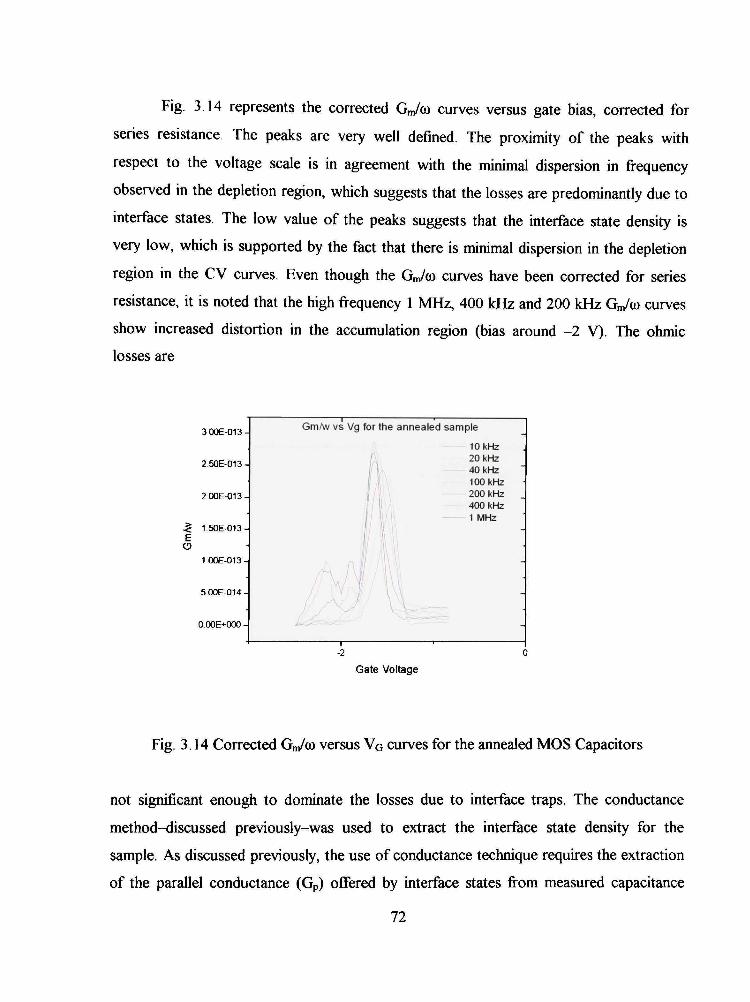
Fig, 3,14 represents the corrected Gm/co curves versus gate bias, corrected for

series resistance The peaks are very well defined. The proximity of the peaks with

respect to the voltage scale is in agreement with the minimal dispersion in frequency

observed in the depletion region, which suggests that the losses are predominantly due to

interface states. The low value of the peaks suggests that the interface state density is

very low, which is supported by the fact that there is minimal dispersion in the depletion

region in the CV curves. Even though the GJm curves have been corrected for series

resistance, it is noted that the high frequency 1 MHz, 400 kHz and 200 kHz GJm curves

show increased distortion in the accumulation region (bias around -2 V). The ohmic

losses are

3 00E-013

2 50E-013-

2 OOE-013

.§ 1.50E-013-E O

1 OOE-013

5 OOE-014

O.OOE+000 -

Gm/w vs Vg for the annealed sample

10 kHz 20 kHz 40 kHz 100 kHz 200 kHz 400 kHz 1 MHz

Gate Voltage

Fig. 3.14 Corrected Gm/co versus VG curves for the armealed MOS Capachors

not significant enough to dominate the losses due to interface traps. The conductance

method-discussed previously-was used to extract the mterface state density for the

sample. As discussed previously, the use of conductance technique requires the extraction

of the paraUel conductance (Gp) offered by interface states from measured capacitance

72

and conductance. The peak value of Gp/co is used to calculate Djt using either discrete or

continuum model. Fig. 3 15 and Fig, 3,16 show the matching of Gp/oo to single state and

continuum models at different gate voltages. It is found that Gp/o) matches the continuum

model only in a certain bias range, between -1,6 V to -1,46 V For all other gate vohages

(i,e , in inversion and in depletion), it matches perfectly whh the single state model. The

interface state density also immediately increases in the region close to weak inversion

where we observe frequency dispersion in the CV curves. The time constants for the bias

region close to weak inversion where frequency dispersion is observed in the CV curves

is high implying existence of slow traps, hence the apparent increase in frequency

dispersion in CV measurements. The fit of Gp/w to single state model in both depletion

and inversion impUes that the charges in the bulk of the oxide are minimal, it also imphes

that there are some deep level traps in the oxide - as explamed by the hysteresis.

1 20E-009

•Q. 4 00E-010

' • _ u J . . . . . • • • ! • • . . . • • • ! »

(^ntinuum Model Experimental Data Single State Model

Vg = -0.92 V

I nil 1—r-T I nn | 1—r T i i i i i | 1—r f i i ill] i—i i i i i i i | 10000 100000 1000000 1E7 1E8

Frequency

Fig. 3.15 Gp/(o matchmg whh single state model at gate voltage of-0.92 V

73

1 OOE-008

8 00E-009-

6 00E-009

a. y 4 OOE-009

2 00E-009-

0 OOE+000 -

10000

Single State Model — Continuum Model —•— Experimental data

Vg = -1 52

I I I l l | 1 1 • I I I M) 1 1 I I M l l | • 1 I I

100000 1000000 1E7 1E8

Frequency

Fig. 3.16 Gp/co matches whh the continuum model at a gate bias of -1.52 V

D. vs. Gate bias 2 00E+011

180E+011

1 60E+011

1 40E+011 -

1 20E+011-J) p 100E+011 (0

i 8.00E+010

"*" 6 00E+010.

4 OOE+010

2.00E+010.

O.OOE+000 •

3, fits Single State Model D. fits Continuum Model

—I • 1 > 1 ' 1 ' 1 ' — -18 -16 -14 -1.2 -10 -0 8

X Axis Title

Fig. 3.17 Dit versus gate bias for the annealed 320 A armealed Hf02 sample.

74

1x10'

10-

T VS Gate Bias

• • - « • • • — •

n ' 1 <-

t fits Single state Model T fits Continuum Model

— 1 — -1 8 -1 6 -14 -12

Gate Voltage

-1 0 -08

Fig. 3.18 Time constant versus gate vohage for 320 A annealed Hf02 sample.

Furthermore, it is clear that there are some slow traps, which are responsible for

the apparent frequency dispersion in CV curves around the weak inversion region. The

near perfect matching of the Gp/co curves with ehher single state or contmuum model in

all bias ranges of interest suggests that there are no statistical fluctuations in the surface

potential in the plane of the interface. This is apparent by a huge stretch out in the Gp/co

curves and there is no matching with either smgle state or continuum. This also supports

the presence of deep level traps.

The interface state density close to mid gap found using the conductance

technique is 1.2el0 cm" ev"' This is a very low interface state density. It suggests that H2

annealing at 300 °C, 1.5 Torr for 45 minutes greatly hnproves the interface state density.

It is also important to note that though hydrogen annealing reduces mterface state density,

however, hot carriers can break the Si-H bond and can drive the reaction backwards. '

75

1 6 Leakage Current and Conduction Mechanism in HfOo^Films

Current-Voltage measurements were carried out on the as-deposited and the

annealed films using Ti/Hfl32/Si structures. Fig. 3.19 is a plot ofthe JV measurements for

both unannealed and the annealed Hafiiia capacitors. Two orders of magnitude decrease

in current is observed for the annealed film compared to the unannealed. This suggests

that H2 annealing at 300 °C does not bring any phase change in the system. This is in

conformity with the observed phase changes in Hf02 whh temperature. ' ' ^

E

CO

c T3

o

10

1

01

001

1E-3

1E-4

1E-5

1E-6

1E-7

1E-8.g

1E-9.g

1E-10

HK 090601-BAl (Annealed) J = 1 5mA/cm' at E = 10' V/cm

HK090601-A (Unannealed) J = 26 7 mA/cm' @ 10* V/cm

Annealed

Unannealed

-6 -3 -2 -1 0

Voltage (V)

Fig, 3.19 JV curves for the armealed and unannealed sample.

It is known that grain boundaries in dielectric ceramics exhibh even higher

specific resistivities than do interior of the grains.^^ When a DC vohage is applied to a

thin dielectric film, a large portion of the applied voltage appears across the grain

boundaries. These large local electric fields lead to local dielectric breakdown or field-

assisted emission of trapped charges - the Poole-Frenkel Effect. Electron or hole currents

under these circumstances increases due to ionized donors or traps at grain surfaces, in

the buUc and also at the electrode. The ionization energy is inversely proportional to the

square of the permittivity. Thus, the Poole-Frenkel effect is far more dominant in high k

dielectrics compared to low k dielectrics.^ ' ^ 76

I • I . I . I

J/E experimental • Linear fit on J/E

k - 17 using Frenkel Poole method

Frenkel Poole Conduction mechanism

- 1 1 > 1 ' 1 1 1 ' 1 ' 1 1 1 ' 1 ' I

4k 5k 6k 7k 8k 9k 10k 11k 12k 13k

Fig. 3.20 J/E vs. E' '^ for the 320 A Hf02 sample shoving Frenkel-Poole Emission at higher electric fields.

The Poole-Frenkel effect can be used to describe the forward current-vohage

behavior of MOS structures.

J = CEexp{-q(p, /kT)exp{/m'''), 3.3

where E is the electric field, C is a constant related to the trap density, cpo is the barrier

height and

P = q"'l^7rc^c,kT

Rearrangmg equation above we have

3.4

In O^

v^y = h i (C) -^^+ / f f i : ' " . 3.5

77

Hence, a plot of In(J'E) versus E'^' is a straight line, with slope y5. yff can be used to

determine the effective dielectric constant ofthe film.

As is seen in the Fig. 3.20, for the 320 A annealed HfD2 film, at high electric field

as expected, there is a linear relationship between ln(J/E) and E'^^ However, there is a

deviation from the linear relationship at lower fields. The deviation from a straight line at

lower E can be explained by the presence of positive charges in the oxide, resuhing in a

naturally depleted surface at the substrate dielectric interface. Since the current increases

exponentially with the square root of the electric field, this suggests a bulk limited

conduction mechanism at room temperature. The calculated value of the relative

dielectric constant from the linear portion of the curve - which follows the Frenkel Poole

conduction mechanism - is close to 17, this is in good agreement with the C-V results. As

the substrates used in the experiment were of p type, current injection is taking place

from the metal gate electrode and not from the substrate because of deep depletion.

Current mjection from the metal is strongly dependent on the metal work fiinction. Thus

for the same fihn lower leakage currents can be obtained for metals with a higher work

fiinction than Ti.'"'""'"'

3.7 Aimealing m the Presence of Oxygen

Before armealing in hydrogen was carried out, a 90 A as-deposited Hf02 (Fig.

3.21) film was annealed in the presence of oxygen at 700 °C for five minutes. The

armealing, as expected reduced the charges in the bulk of the oxide and the deep level

traps - evident by the reduction in hysteresis m the annealed film as compared to the

unannealed film (Fig. 3.22). It was also found out that the dielectric constant reduced

from a value of-18 to 8, clearly indicatmg a formation of an mterfacial Si02 layer. The

presence of an interfacial Si02 layer was fiirther verified by FTIR analysis carried out on

a thick Hf02 film before and after anneahng in the presence of O2. This analysis showed

an increase m the Hf-0 peak and an mcrease in the Si-0 peak. It imphes the permeability

of HfiD2 films to oxygen [also reported by J.D. WiUc, J. Lee, etc.].

78

120

100

„ 80 U.

a.

^ 60.

o CO S- "0-1 o

20-

— I . 1 . 1 _

10 kHz

t MHz

1 MHz 10 KHz

\ .

-2 0 -15 -10 -0 5

Voltage (V)

0.0 05

Fig. 3.21 Hf02 as deposited sample 90 Angstroms thick (k ~ 18).

A development of an mterfacial layer is not helpfiil for high k materials for fiiture

CMOS devices as this increase the EOT (Fig. 3.22) and reduces the effective dielectric

constant of the film (~ 8) Hence, armealing in oxygen environment is not suggested for

Hafiiia films. Integration of Hf02 in the device flow for fiiture MOS devices will requke

a minimum of 1000 °C, 10-second thermal cycle in the presence of nitrogen and oxygen

for activation of dopants. This may substantiaUy increase the interfacial layer. It is

observed that the frequency dispersion in the depletion region of the annealed films is

much less compared to the unannealed films. Formation of a good Si-Si02 mterface

during armealing may reduce the interface traps and hence the frequency dispersion in the

depletion region in the CV curves. No further analysis was carried out on the films

annealed in O2.

79

70

6 0 -

50

S 30 o cn

10-

HfO^ Annealed at 700° C in O, (1 atm.)

-3 0 -2 5 -2 0 -15 -10 -0 5

Voltage (V)

00

Fig. 3.22 90 A UK>2 as deposhed fihn annealed in the presence of O2 at 700 °C for 300 seconds (k ~ 8).

3.8 Analysis of Nhrided Interfaces

Nhridation of the Si surface provides a interface impervious to oxygen and hence,

any subsequent thermal processing will avoid the build up of an oxide interface layer as

is seen in the case of Hf02 which reduces the dielectric constant ofthe stack and thus, the

EOT. AIN has a wide bandgap of 6.1, good thermal conductivity, high decomposhion

temperature, chemical stabihty and good dielectric properties."*^ Previous experiments

with Si/SisNVAlN/Gate structures have revealed poor electrical characteristics of this

stack 43

Wafers cleaned by the modified Shiraki method were first heated to 700° C to

release the hydrogen and produce clean silicon surfaces. The substrate was then exposed

to Sau. This generates an epitaxial Si layer. When the clean Si (111) surface is exposed

to ammonia at a beam equivalent pressure of 10" Torr, h mstantaneously produced Si3N4

surface reconstruction in RHEED measurements. The 8x8 reconstruction of Si3N4

80

gradually fades indicating growth of an amorphous layer. The RHEED image of the

wafers exposed to SiH, are indicative of a 2*2 surface reconstruction. The film thickness

was measured by grazing incidence X-ray diffraction (GIXRD), and SEM micrographs

were taken to determine the thickness ofthe films.

111 -orientation wafer was exposed to SiHj with substrate temperature of 640 °C

at a beam equivalent partial pressure of 10" Torr. This lead to growth of 111 ephaxial

silicon. Substrate temperature was increased to 830 °C with ammonia ambient and the

epitaxially grown Si was nitridated. Now, AIN is grown ephaxially at 600 °C. GIXRD

measurements found Si3N4 thickness to be 15 A and AIN thickness as 138 A, thus we

have a total dielectric stack thickness of 153 A. Aluminum metal dots were deposhed on

the sample using e-beam evaporation. CV measurements were taken on the sample.

The dielectric constant of this film was measured by findmg the capachance of

the MOS capachor in accumulation using a three-segment fit by NCSU's CVC program.

The dielectric constant found for this film is close to 9.1, which is in agreement with the

reported dielectric constant for AIN films, suggesting a stoichiometric fUm. The CV

measurement in the fihn was carried out at seven diff"erent frequencies. GV

measurements were also carrier out simuhaneously. Frequency dispersion of 7.5 % was

observed m accumulation (Fig. 3.23). This dispersion could be due to bulk behavior of

AIN, for an exact analysis, MIM structures should be fabricated and CV measurements

carried out.

81

5-111 153 Angstroms AIN sample

2 OOE-011 -

1 50E-011 ^

8 c 3 1 OOE-011-o CD Q. (0

O

5 OOE-012 -

OOOE+000-

•

1

100 kHz

10 kHz

1 MHz

200 kHz

20 kHz I I I 400 kHz //• / / / / 40 kHz 7 ' / / / / / • '

' 1

1

2 0

Voltage

Fig, 3,23 Forward CV curves for 153 A AIN 111 sample with ephaxial Si grown.

The flat band vohage -0.26 obtamed from the forward 10 kHz curve is close to the

metal semiconductor work fiinction of the device (-0.3), hence suggesting minimal fixed

charge in the oxide. The hysteresis observed for this sample is around 0.01 V. The

hysteresis is of clockwise nature. Clockwise hysteresis in a n-type sample is attributed to

trappmg of the majority carriers mjected from the semiconductor to the msulating film.

The amount of charge trapping as discussed before is found to be equal to 1.2el0 charges

cm' . Thus the charge trapping for the sample is minimal.

The plot of Gm/co versus gate vohage shows a high value ofthe conductance. This

is indicative of a high charge density. The frequency dispersion observed m the depletion

region also suggests the same for the MOS Capacitor. The clear peaks observed m the

corrected QJca plots show that the series resistance and ohmic losses have not dominated

the losses due to interface traps. The CV and GV curves have been corrected for series

resistance usmg the method proposed by NicoUian and Goetzburg. Thus the conductance

technique can be successfially used to extract the interface trap properties for the device.

82

18

16

14

12 iZ" a. 10 <i> " A (D ° O

2. 6 CD

" 4 -

2 -

0 -

10 KHz

Hysterisis ,01 V

- I I 1 i_ -1,2 -1,0 -0,8 -0,6 -0.4 -0.2 0.0 0,2 0,4 0.6

Voltage (V)

Fig. 3.24 Clockwise hysteresis observed m the 153 A AIN sample.

G /mvs. v .

4CI0E-012

O 2(X)E-012-

0 OOE+000

10 kHz 20 kHz 40 kHz 100 kHz 400 kHz 200 kHz 1 MHz

Fig. 3.25 Corrected GJco versus VG gate vohage for 153A AIN sample with ephaxial Si.

83

However when the conductance technique is used to calculate the interface state

densities, it is found that peaks corresponding to Gp/co could not be obtained. As is

illustrated in the Fig. 3.26.

2

1.B

1.6

1,4

i! 1 2 V)

mho

(§-0.8

0.6

0.4

0.2

0 IC

«io '

.

•

)'

The voltage is-O 4

^

\

\

\ . \

\

\

\

^ - ^ . . . _

10' 10" Frequency racJ/sec

-

-

""""-— 10'

Fig. 3.26 Gp/co versus Frequency for the 153 A sample at a gate vohage of-0.4 V

This suggests a need to measure the GV and CV curves below a frequency of 10

kHz, the minhnum frequency used for measurement for this sample. However CV and

GV measurements become extremely difficult to measure at very low frequencies for a

sample with significant gate leakage. Hence, the conductance technique cannot be used to

estimate the interface state density for this device.

The IV curves (Fig. 3.27) indicate a high leakage current for a 150A angstroms

sample. This could be due to poly mclusions in the dielectric.

84

1E-3

1E^

^ 1E-5

E o ^ 1E-6

->

1E-7

1E-8

1E-9

:

r

1 . 1 . 1 . 1 . 1

/

JvsV

1 1

- 3 - 2 - 1 0 1 2 3

Voltage (V)

Fig. 3.27 IV on the annealed sample

Because of the inadequacy of the Conductance technique to find the interface

state denshies, we used the method proposed by Kevin J Yang and Chenming Hu for

MOS capachance measurements for leaky dielectrics.""

3.9 Determination of Device Capachance in a Leaky Dielectric

Accurate determmation of the device capachance in a leaky sample is necessary

for the correct esthnation of the dielectric constant. Quantum mechanical tunneling

increases as the dielectric thickness reduces below 2nm (for Si02). In this reghne

Capacitance measurements are complicated by the leakage current. Accurate

measurement of device capacitance with a dielectric with huge leakage current is also

diflficuh.

The way to avoid the leakage problem may be to measure the capachance at very

high frequency, so that the capachive current is dominant. However, at very high

frequency, the series resistant becomes significant because of the low hnpedance of the

capachor.

85

One must account for the simultaneous presence of series and shunt parasitic

resistances in the CV measurement.

True device capacitance can be determined by measurements made at two

frequencies as demonstrated below

Fig. 3.28 SmaU signal equivalent chcuit models of a MIS capacitor (A) accurate model (B) series circuit model for low leakage devices (C) Parallel circuit model for low series

resistance devices.

Fig. 3.28 (A) shows the three-element ch-cuh model of a leaky MOS capachor. C

represents the actual frequency independent device capachance, Rp represents the

effective device resistance due to leakage, and Rs represents the series resistance of the

substrate and the gate. For devices with low leakage current series resistance dominates

the device. In this case, the device C may be found by a smgle measurement, ignoring the

shunt resistance, and determmmg the C usmg the model m Fig. 3.28 (B).

CV measurements of samples with large leakage currents must be performed

usmg the parallel ch-cuh model in Fig. 3.28 (C).

The hnpedance of the three-ch-cuh model shovm m Fig. 3.28 (A) is given by

Ra-jcoCR) Z = Rs +

\ + (o''C^Rp 3.6

Impedance ofthe parallel ch-cuh model in Fig 3.28 (C) is given by

86

Z= ^ 3.7 (oc\\ + iy)

where D = is the dissipation,/?' and Crefer to the measured values. Equating (oR C

the imaginary parts ofthe measured impedance and the true impedance one obtains

\ + a)'C^RA P - , . . 2 /^1 /1 , r»i2

CRp-= (o'C{\ + D"). 3.8

Measuring the capacitance and dissipation at two frequencies and substituting above and

solving for C we have

^_/rc;(i+Dr)-//c,(i+z);^) ^ f'-f2

which is the true device capacitance. The series resistance and the shunt resistance can

also be found in a simUar manner by equating the real parts ofthe impedance.

R = , = 3.10 •yJco^C'C{l + D'^)-co^C^

D' R„ R = '- 3.11

' coC'(l+ £>•') l + CD^C^Rl

3.9.1 Experimental Resuhs of Shunt Resistance Correction in AIN

AIN sample with dielectric thickness of 153A (physical thickness measured usmg

XRD) was used as a MIS capachor for the measurements. C and D' data was obtained

using the parallel circuit model given m Fig. 3.27 (C), usmg the HP 4275A LCR meter.

Data was analyzed and correction was applied on h to obtam the true capachance of the

device. The results are as below.

87

CV for AIN uncorrected

6 OOE-011

5 OOE-011

4 OOE-011

i T 3 OOE-011

o

2 OOE-011

1 OOE-011

0 OOE+000 -

100 kHz 1 MHz 200 kHz 400 kHz

Fig. 3.29 The data was collected is frequencies 1 MHz and 100 kHz, 200 kHz and 400 kHz.

Looking at the corrected data in Fig. 3.30, we find that even though there is a

huge frequency dispersion in the experimental data, the corrected data curves have very

httle dispersion with respect to frequency. This implies correction of the data for the

series and shunt resistances. Also, when the relative permittivity constant was calculated

for this MIS sample using the XRD resuhs thickness (153 A) we obtain a value of 9.1

that is close to the actual dielectric constant ofthe sample (AUSf). Note that the corrected

data matches weU with the 400 kHz frequency in the depletion region.

88

Corrected CV curves

7 OOE-011

6 OOE-011

5 OOE-011

4 OOE-011

(J 3 OOE-011

2OOE-011

1 OOE-011

0 OOE+000

100 kHz 1 MHz 200 kHz 400 kHz Cort lOOkHz-IMHz Corf 200kHz-1MHz

Fig. 3.30 The plot above shows the Corrected - frequency independent CV data for 1 MHz 200 kHz and 100 kHz measurement frequencies.

Hence, we conclude that the above method used is one that can be used to

calculate the frequency independent capacitance ofthe device.

We can now use the corrected data for calculating the mterface state denshies of

the device using Terman's analysis as seen in Fig. 3.30.

89

5

4.5

4

35

3

25

2

1.5

1

05

»io"

• 1 •

-

- 1 1 1 1 1 1 1

• 1

\

Dit vs VG graph

•1 •—1 1

-

-

-

-

-

/-

/ . \ DH 74e12 y ^

1 1 1 1 1 1 ;

-0.6 -04 -02 0 02 Gate Voltage

04 OB

Fig. 3.31 Interface state density calculated using Terman's method.

The mterface state density calculated for the AIN sample is 7.4el2 cm"^eV\ close

to mid-gap. This is a high value of Du, suggestmg that the films are not suhable for

device grade apphcations. Other films prepared using similar techniques, but without an

ephaxiaUy grown Si, showed very poor CV curves for both 111 and 100 substrates and

are not discussed fiirther.

3.10 Conclusion

Novel gate dielectrics were studied using MOS Capachors. Hf02 MOS Capachors

showed a low interface state density, low leakage currents but poor thermal stability in

the presence of oxygen. Growth of an interfacial layer is observed when annealing m O2.

This is not very supportive, as the device will be subjected to a thermal cycle of at least

1000 °C for 10 seconds. A solution to this problem would be capping ofthe dielectric or

engmeering the mterface to grow a layer of Si3N4 which wiU prevent transport of O2 to

the Si surface thus preventing growth of interfacial Si02. Nitridation experiments carried

out on 111 and 100 (not reported) wafers resuhed m samples with high interface state

90

denshies. However, finding a suhable annealing, deposition and cleaning regime may

solve this problem

91

2

REFERENCES

The National Technology Roadmap for Semiconductors, 3"* edition Semiconductors Industry Association, San Jose, CA, 1997.

Kang, Song-Mo and Y. Leblebici, CMOS Digital Integrated Circuhs Analysis and design, WCB McGraw Hill, New York, 1998.

Hirata, A, H. Onodera and K. Tamaru, "Estimation of Propagation Delay considering Short-Circuit Current for Static CMOS Gates," IEEE Trans, on Circuits and Systems

^ Sakurai, T and A.R. Newton, "A simple MOSFET model for circuit analysis," IEEE Trans. Electron. Devices, vol. 38, no. 4, pp. 887-893, Apr. 1991,

Pierret, R.F., Semiconductor Device Fundamentals, Addison Wesley Pubhshing Company, Recdenej, 1996 edt.

Garrett, C.G.B and W.H. Brattain, "Physical theory of semiconductor surfaces," Physical Review, vol. 99 no. 2, pp376-387, July 15 1955.

Shockley, W., "The theory of p-n junctions in semiconductors and p-n junction transistors," The Bell System Technical Journal, Vol. 28, 435,1949.

* Sah, C.T., Pierret, R.F and A.B. Tole, "Exact Analytical Solution of high frequency lossless MOS capacitance-voltage characteristics and validity of charge analysis," Solid State Electron, 1968, Vol. 12, pp 681-688.

^ NicoUian, EH. and Brews, JR., MOS (Metal Oxide Semiconductor) Physics and Technology, John Wiley and Sons, New York, 1982.

'° Lmder, R., "Semiconductor Surface Varactor," The Bell System Technical Journal, Vol. XLI, no. 3, May 1962.

" Temple, V. and Shewchun, J. "Exact frequency dependent complex admittance ofthe MOS diode mcluding surface state SHR impurity effects and low temperature dopant impurity response," Solid State Electron., 1973, Vol. 16, pp 93-113.

'^ Nicolhan, EH. and Goetzberger, A. "The Si-Si02 mterface - electrical properties as determined by metal insulator shicon conductance technique," The BeU System Technical Journal, Vol. XLVI, no. 6, July-August 1967,

92

\^ Heiman, F P and Warfield, G,, "The effects of oxide traps on the MOS Capacitance," IEEE Trans on Electron devices, April 1968, pp 167-178,

ferman, L M,, "An investigation of surface states at a silicon/silicon oxide interface employing MOS diodes," Solid State Electron, Vol, 5, pp 285-299,

15

16

Brews, J R,, "An improved high frequency MOS capacitance formula," Journal of Applied Physics, 45, 1276, 1974,

Sah, C,T,, Tole, A.B and Pierret, R,F, "Error analysis of surface state density determination using the MOS Capacitance method," Solid State Electron. 1969, pp 689-709.

'" Zaininger, K.H. and Warfield, G. "Limitations of the MOS Capacitance method for determination of semiconductor surface properties," IEEE Trans, on Electron Devices, April 1965, pp 179-192.

1 K

Schroder, D.K,, Semiconductor material and device characterization, Wiley-Interscience, New York, 1998,

' Wilk, G.D., Wallace, R.M. and Anthony, J.M., "High k gate dielectrics; Current status and material properties considerations," J. of Appl. Phys. Vol. 89, no. 10, 15 May 2001, pp 5243-5275.

Schlom, D.G. and Haeni, J.H., "A thermodynamic approach to selectmg alternative gate dielectrics," MRS BuUetm, March 2002, pp 198-204.

Housers, J.R. and Ahmed, K. "Characteristics of ultra-thin oxides using electrical C-V and I-V measurements," The American Institute of Physics, 1998, p 235.

^ Lee, B.H., Kang, L., Qi, W-J, Nieh, R., Jeon, Y., Onishi, K. and Le, J., "High quahty uhra thin CVD HfO/sub 2/ gate stack with poly-Si gate electrode," Tech. Dig. Int. Electron Devices Meet, pp 133, 2000

Robertson, J., "Band offsets of wide-band-gap oxides and implications for fiiture electronic devices," J. Vac. Sci. Technol. B 18(3), May/June 2000, pp 1785-1791

^'* A. Ishizaka, Y. Shiraki, "Low Temperature Surface Cleanmg of SUicon and Its AppUcationto Sihcon, "Journal ofElectrochem. Soc. 133, 666, 1986.

^' J Robertson, "Electronic structure and Band offsets of high dielectric constant gate oxides," MRS BuUetm, March 2002, pp 217-221

23

93

2<. Heiman, F P and Warfield, G., "The effect of oxide traps on the MOS capacitance,"

IEEE Trans on Electron, Devices, Ed, 12, 167, 1965,

Klofenstien, B , Rouzeyre, G and Durand, K,, "Interface studies and electrical properties of plasma sulfide layers," J, Appl, Physics, 63(1), 1 January 1998.

28

30

Deal, B E., "The current understanding of charges in the thermally oxidized silicon structure," J. Electrochem. Soc. 121, 198C, 1974.

Ebach, H and Rowe, J.E., "Hydrogen absorption and surface structures of Silicon," Surface Science, vol. 43, 1974, pp 481-492.

Zang, J.F., Zhao, C.Z., Groeseneken, G., Degraeve, R., EUis, J.N,, and Beech, CD., "Hydrogen induced positive charge generation in gate oxides," J. of App. phys. Vol. 90, no. 4, 15 August 2001, pp 1911-1919.

^' Qi, W. J , Lee, B.H., Nieh, R., Kang, L., Onishi, K., Jeon, Y. and Lee, J.C, SPIE conference on microelectronic device technology III, Santa Clara CA September 1999, SPIE Vol. 3881, pp 24-32.

Yoshi, I., Hama, K. and Hashimoto, K. " Role of Hydrogen at poly-Si/Si02 interface m trap generation by substrate hot-electron mjection," IEEE Electron. Devices, 1992, pp 136-140.

Brower, K.L., "Dissociation kinetics of hydrogen-passivated (111) Si-Si02 interface defects," Phys. Rev. B, Vol. 42, no. 6, 15 August 1990, pp 3444-3453.

Smith, R.C., Ma, T., HoUien, N., Tsung, L.Y., Bevan, M.J., Colombo, L., Roberts, J., Campbell, S.A. and Gladfeher, W.L., Adv. Mater. Opt. And Electron., Vol. 10, no. 105, 2000.

^ J.F. Conley, Y. Ono, D.J. Tweet, W. Zhuang, M. Khaiser and R. Solanki, 2001 IRW final report, pp 11-15.

Hench, LL. and West, J.K., Principles of Electronic ceramics, Wiley New York, 1990, p 163.

^ Herbert, J.M., Ceramic Dielectrics and Capachors, Gordon and Breach, New York, 1985, p. 23.

^ Shin, H., De Guire, MR. and Heuer, A. H., "Electrical properties of Ti02 films formed on self-assembled organic monolayers on sihcon," J. of App. Phys. Vol. 83, no. 6, 15 March 1998, pp 3311-3317.

94

36

^ Kwong, D L and White, J M,, Proceedings of the Sematech FEP PAG meeting, Austin, Texas Feb. 2000,

" Qi, W J , Nieh, R., Lee, H,, Onishi, K,, Kang, L,, Leon, Y,, Lee, J C , Kaushik, V,, Neuyen, BY., Prabhu, L, Eisenbeiser, K. and Finder, "Performance of MOSFETs with uhra thin ZrO/sub 2/ and Zr silicate gate dielectrics," J., 2000 symposium on VLSI technology, IEEE Electron devices Society Honlulu, June 2000, pi6.

Lee, B H., Kang, L., Qi, W.J. and Lee, J.C, "Thermal stability and electrical characteristics of ultrathin hafiiium oxide gate dielectric reoxidized with rapid thermal annealing,"Appl. Phys. Lett. 76, 1926(2000).

Morsanu, C , Stoica, T.A., Stoica, T.F., Necsoiu, D., and Popescu, M., "Optical, electrical and structural properties of AIN thin films," 1995 IEEE Electro. Device Lett, P 183,

'^^ Kaiser, S., Jakob, M., Zweek, J., Gebhardt, W., Ambacher, O., Dimitrov, R., Schremer, AT., Smart, J.A. and Shealy, JR., "Structural properties of AlGaN/CiaN hetrostructures on Si(lll) substrates suhable for high electron mobility transistors," J. Vacc. Sci. and Technol. B 18 (2000), 733.

'^ Yang, K.J., and Hu, C, "MOS capachance measurements for high leakage thin dielectrics," IEEE Trans, on Elect. Devices, vol. 46, no. 7, July 1999.

95

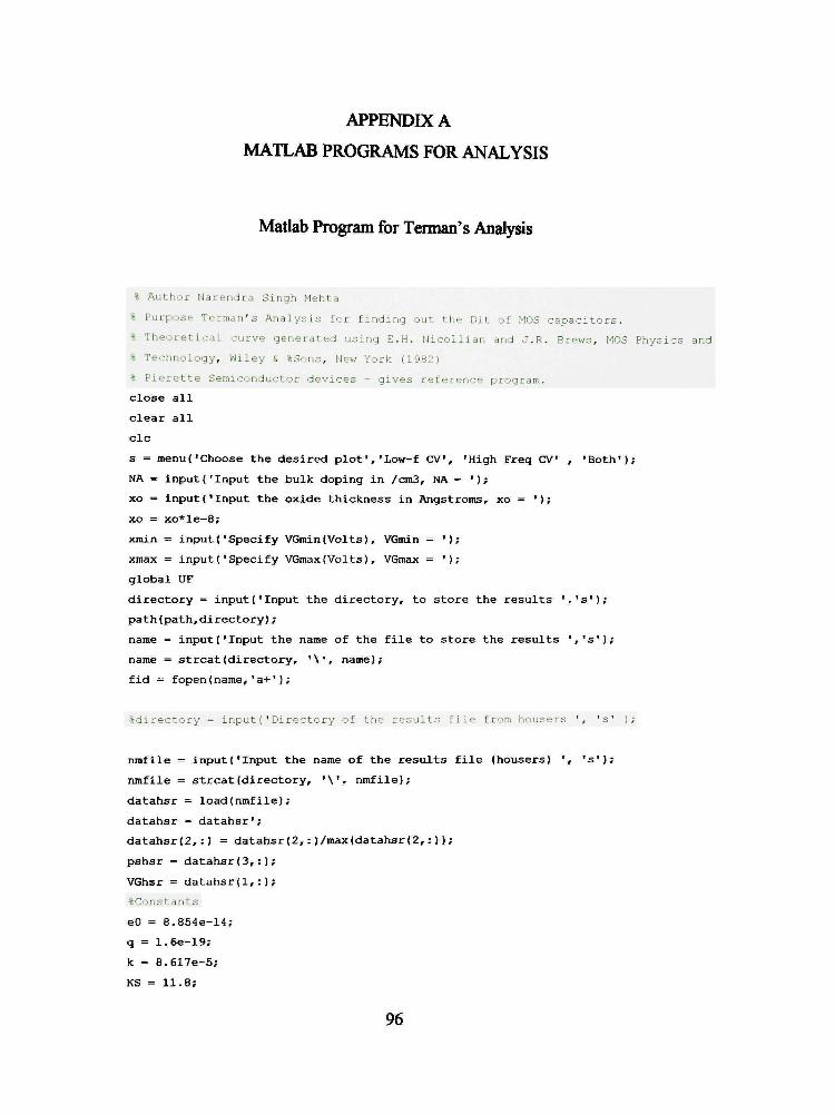
APPENDIX A

MATLAB PROGRAMS FOR ANALYSIS

Matlab Program for Tennan's Analysis

%

•*

%

*

%

Author Narendra Slnqh Mehta

Purpose Terman's Analysis for findin.3 out the Dit of MOS

Theoretical ..-urve generated usin g E.H. NicoUian and J.R.

Technology, Wiley S %Sons, New York (1962)

Pierette Semiconductor devices - gives reference program.

cap'acitors.

. Brews, MOS Physics and

close all

clear all

clc

s = menu('Choose the desired plot','Low-f CV', 'High Freq CV' , 'Both');

NA = input('Input the bulk doping in /cm3, NA = ' ) ;

xo = input("Input the oxide thickness in Angstroms, xo = ' ) ;

xo = xo*le-8;

xmin = input('Specify VGmin(Volts), VGmin = ' ) ;

xmax = input('Specify VGmax(Volts), VGmax = ' ) ;

global UF

directory = input('Input the directory, to store the results '.'s');

path(path,directory);

name = input('Input the name of the file to store the results ','s');

name = strcat(directory, '\', name);

fid = fopen(name,'a-H');

%directory = input('Directory of the results file from housers ', 's' );

nmfile = input('Input the name of the results file (housers) ', 's');

nmfile = strcat(directory, '\'. nmfile);

datahsr = load(nmfile);

datahsr = datahsr';

datahsr(2,:) = datahsr(2,:)/max(datahsr(2, :));

pshsr = datahsr(3,:);

VGhsr = datahsr(l,:);

%Constants

eO = 8.B54e-14;

q = 1.6e-19;

k = 8.617e-5;

KS = 11.8;

96

KO = 3.9;

ni = l.OelO;

T = 300;

kT = k*T;

* computed constants

UF = loq(NA/ni);

LD = sqrt((kT*KS*eO)/(2*q*ni));

% Gate voltage computations

%US - UF-L'5:0.5:UF + 25;

US = pshsr;

US = US/.0259;

F = sqrt(exp(UF).*(exp(-US) + US -1) + exp(-UF).*(exp(US)-US-l));

VG = kT*(US+(US./abs(US)).*(KS*xo)/(KO*LD).*F);

DENOML = exp(UF).*(l-exp(-US))+exp(-UF).*(exp(US)-l);

WL = (US./abs(US)).*LD.*(2*F)./DENOML;

cL= 1.0./(l-h(KO*WL)./(KS*xo));

% High frequency capacitance calculations

if s—1,

jj=length(US);

nn=0;

for ii=l:jj,

if US(ii)<3,

elseif nn ==0,

INTG=quad('CVintgrd',3,US(ii),le-18);

nn = 1;

else

INTG=INTG+quad{'CVintgrd',US(ii-1),US(ii),le-18);

end

if US(ii)<3,

cH(ii)=cL(ii);

else

d = (exp(US(ii))-US(ii)-l)./(F(ii).*exp(UF).*INTG);

DENOMH = exp(UF).*(l-exp(-US(ii)))+exp(-UF).*((exp(US(ii) )-l) ./(1-Hd) :

WH=LD.*(2*F(li))./DENOMH;

cH(ii)=1.0/{l-l-(KO*WH) ./(KS*xo));

end

end

else

end

figured)

97

*plottlnq the results

if s==l,

plot(VG,cL);

elseif s == 2,

plot(VG,cH);

else

plot(VG,cL, '~',VG,cH);

text(0.8*xmin,.17,' Low-f','color', [1,1,0]);

%text(0.8*xrain,.12,' High-f,'color', [1,0,1] );

end

axis([xmin,xmax,0,1]);

text(0.8*xmin,.27,[•NA=',num2str(NA),'/cm3']);

xlabel('VG(Volts)');

ylabel('C/CO');

grid

US = US*0.0259;

%datatotal = [VG;cH;cL;US];

% ANALYSIS OF THE RESULTS TERMANS ANALYSIS-

%figure

%plot(datahsr(1,:),datahsr(2,:));

%hold on

%plot(VG,cH,'g');

%title('Ch theoretical and practical vs VG');

%figure(3)

%plot(pshsr,VGhsr)

%hold on;

%plot(US,VG,'g')

delVG = VG-VGhsr;

diffVG = diff(delVG);

diffUS = diff(US);

dvgds = diffVG./diffUS;

Dit = abs({e0*KO/(q*xo))*dvgds);

%plot(US,VG-VGhsr)

%title('VG vs Diff VG');

figure

%plot(US(l:length(US)-l),dvgds);

zoom on;

plot(VGhsr(1:length(VGhsr)-1), Dit)

zoom on;

98

titleCDit vs VG graph')

Inth = length(Dit);

Dit(lnth+1) = Dit(Inth);

data = [VGhsr; cH; Dit];

Ditval = min(Dit)

fprintf(fid,'%3.6f %6.8f %12.12f\n',data);

fclose(fid)

Program for series resistance correction ^Program for series correction

clc

clear all

close all

% This command below is to read the directory v/here the file is stored

directory = input('Input the directory to read the CV Data ','s');

path(path,directory);

% The path command adds the directory name that we just entered into the matlab

search path

% This is required so that we can now access this directory

nm = dir(directory);

for counter =3:length(nm)

if nm(counter).name(length(nm(counter).name)-3:length(nm(counter) -name)) ==

'-txt'I nm(counter).name(length(nm(counter).name)-

3:length(nm(counter).name))=='.dat' |nm(counter).name(length(nm(counter).name)-

3:length{nm(counter).name))==•.DAT'| nm( counter).name (length(nm(counter).name)-

3:length(nm(counter).name))=='.TXT',

nm(counter).name

f = input('Input the frequency in kHz');

f =f*1000;

w = 2*pi*f;

fldata=load(nm(counter).name);

cap = fIdata(:,2) ;

gm= fIdata(:,3);

cox = max(fIdata(:, 2));

indexv = find(fldata(:,2)= cox);

indexv = min(indexv);

rs = gm(indexv)/(gm(indexv)'^2 + (w^2)*cap(indexv)*cap(indexv) );

a = gm-(gm.*gm-F(w'^2)*cap.*cap)*rs;

ccap = (gm.*gm + (w^2)*cap.*cap) .*cap./(a.*a+(vr*w*cap.*cap) ) ;

gmcap = ( (gm.*gm + (w'"2) *cap.*cap) .*a) ./(a.*a+(w'-2)*cap.*cap);

newnm = strcat(directory,'\cor',nm(counter).name);

99

fid = fopen(newnm,'w');

cordata = [ fIdata(:,1) ccap gmcap];

cordata = cordata' ;

fprintf(fid,'%3.20f \t %3.20f \t %3.20f \n ' ,cordata);

fclose(fid);

end

end

nm = dir(directory);

for counter =3:length(nm)

if nm(counter).name(length(nm(counter).name)-4:length(nm(counter).name)-3)

' f.'I nm(counter).name(length(nm(counter).name)-4:length(nm(counter).name)-3)=='F.',

if nm(counter).name(1) == 'c'

% Plotting all corrected forward data

f ldata=load (nm (counter) . name);

figured)

plot(fIdata(:,1),fIdata(:,2))

title('Corrected CV')

hold on

figure(2)

plot{fIdata(:,1),fIdata(:,3))

title('Corrected Gm')

else

figure(3)

% Plotting all uncorrected forward data

fldata=load(nm(counter).name);

plot(fIdata(:,1),fIdata(:,2))

title('Uncorrected CV')

hold on

figure(4)

plot(fIdata(:,1),fIdata(:,3))

title('Uncorrected GV')

end

end

end

Program to Calculate Interface State Density Using Conductance Technique

close all

clear all

clc

% This command below is to read the directory where the file is stored

100

directory = input('Input the directory to read the CV Data ','s');

path(path,directory);

* The patli conuiiand adds the directory name that we just entered into the matlab

search p ath

* This is required so that we can now access this directory

nm = dir(directory);

q = 1.6e-19;

intcount=l;

cox = input('Input the Cox in pf ')

area = input ('Input the area of the capacitor in cm' 2 ' );

cox = cox*le-12/area;

for counter =3:length(nm)

if nm(counter).name(length(nm(counter).name)-3:length(nm(counter)-name)) =

' .txt' I nm(counter) .name (length (nm(counter) .name)-3:length(nm(counter) .name) ) = ' .dat'

I nm(counter).name(length(nm(counter).name)-3:length(nm(counter).name))=='.DAT'I

nm(counter).name(length(nm(counter).name)-3:length(nm(counter).name) )==' .TXT',

nm(counter).name

f = input ('Input the frequency in kHz');

f =f*1000;

w = 2*pi*f;

freq(intcount)=w;

fldata=load(nm{counter).name);

cap(:,intcount) = fldata(:,2)/area;

gm(:,intcount)= fIdata(:,3)/area;

intcount = intcount-H;

vltg = fIdata(:,1);

end

end

figure

plot(vltg,cap)

title('Capacitance/area vs Voltage for different frequencies')

xlabeK'Volts');

ylabel {'Capacitance/area Farads/cm''2')

fiqure

plot(vltg,gm)

title('Gm/area vs Voltage for different frequencies')

xlabeK'Volts');

ylabel ('Conductance mho/cm'^2 Farads/cm^2')

for i = 1:length(freq),

101

for j = l:length{cap)

gpbywl(j,i)=

freq(i)*cox*cox*gm(j,i)*(gm(j,i)*gm(j,i)+freq(i)*freq(i)*cap(j,i)*cap(j,i))/(freq(i)*freq

(i)*cox*cox*gm(j,i)*gm(j,i) + (freq(i)*freq(i)*cap(j,i)*{cox-cap{j,i) )-gm( j , i) •gm( j ,i) )'"2);

end

end

gpbw2= gpbywl';

fr = freq';

data = [ fr, gpbw2];

d = sortrows(data,l);

d = sortrows(data,l);

f = cl(:,l);

f = f ;

gdata=d(:,2:length(d));

gdata =gdata';

% gdata is a y.by7 data representation of all the gpbyw at different frequencies.

figure

plot(vltg,gdata)

title('Gp by omega vs gate voltage for different frequencies')

XlabeK'Volts')

minbias = input('Input the bias ranges from which we want the Dit');

maxbias = input('Input the maximum bias till we want the Dit');

in= find(vltg<=maxbias & vltg>=minbias);

'If there is a peak enter the point of the peak by clicking the mouse or else

press Enter'

counttemp = 1 ;

ftenp = 20000:20000:100000000;

for i=l:size(in),

%xz = f(1):10000:f(7);

%yy = spline ( f,gdata ( in ( i) ,:),;••>;) ;

figure

%semi log;-: (y.y., yy, ' r ' )

%hold on

semilogx(f,gdata(in(i),:))

astr= strcat('The voltage is ', num2str(vltg(in(i))));

title(astr)

hold off

junkip = input('After you have interpolated the data, press any key ' ) ;

[x,y]=ginput(l);

if length(x) > 0,

%For single state model

102

strdt(counttemp)=in(i);

tss(counttemp) = 1/x;

ditss(counttemp)=y*2/q;

%temp.gpss = 2*y*ftemp*tss (counttemp) ./ (1 + ftemp,

*hold on

*For continuum of states

%semilog.x ( ftemp, tempgpss, 'r' )

. *ftemp*tss (counttemp) *-ts3 (counttemp) ) ;

;

ditcont(countterap)= y/(q*0.402);

tcont(counttemp)=1.98/x;

%tempgpcont=q*ditcont(counttemp).*(log(1+ftemp.*ftemp*tcont(counttemp)*tco

nt (counttemp) ) ) ./ (2*-ftemp*tcont (counttemp) ) ;

volts(counttemp) = vltg(in(i));

%semiloq:-: ( ftemp, tempgpcont, 'g ' ) ;

%hold off

counttemp=counttemp+l;

end

close

end

for counttemp=l:length(strdt),

figure

semilogx(f,gdata(strdt(counttemp),:),'-o')

%For single state model

terapgpss=ditss(counttenp)*q*ftemp*tss(countterrp). /(1+ftemp.*ftemp*tss(counttemp)*tss (coun

t t emp) ) ;

hold on

%For continuum of states

semilogx(ftemp,tempgpss, 'r' );

%ditcont(counttemp)= y/(q*0.402);

%tcont(counttemp)=1.98/x;

tempgpcont=q*ditcont (counttemp) .* (log(l+ftemp.*ftemp*tcont(counttemp)*tcont (counttemp))) .

/(2*ftemp*tcont(counttemp));

%volts(counttemp) = vltg(in(i));

semilogx(ftemp,tempgpcont,'g');

astr= strcat('The voltage is ', num2str(volts(counttemp)));

title(astr)

newnm = strcat(directory,'\gpfit'. num2str(volts(counttemp))) ;

103

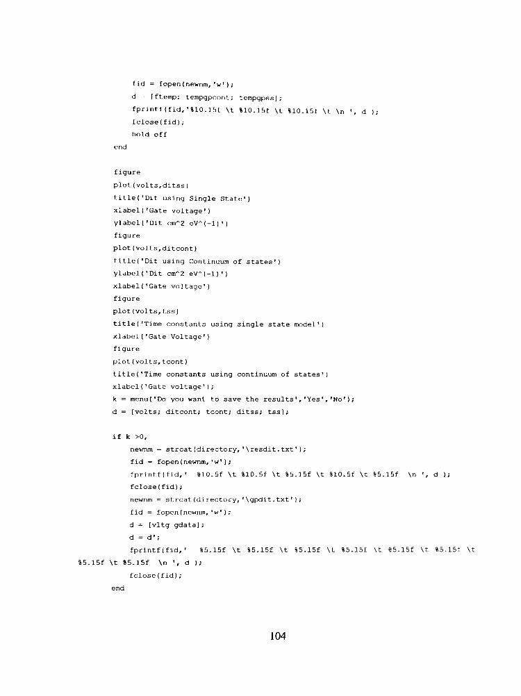
fid = fopen(newnm,'w');

d (ftemp; tempgpcont; tempgpss);

fprintt(fid,•%10.15f \t %10.15f \t %10.15f \t \n ', d );

fclose(fid);

hold off

end

figure

plot(volts,ditss)

title('Dit using Single State')

xlabeK'Gate voltage')

ylabel ('Dit cm'"2 eV^{-l)')

figure

plot(volts,ditcont)

title('Dit using Continuum of states')

ylabel ('Dit cm' 2 eV'-(-l)')

xlabel('Gate voltage')

figure

plot(volts,tss)

title('Time constants using single state model')

xlabel('Gate Voltage')

figure

plot(volts,tcont)

title('Time constants using continuum of states')

xlabel('Gate voltage');

k = menu('Do you want to save the results','Yes','No');

d = [volts; ditcont; tcont; ditss; tss];

if k >0,

newnm = strcat(directory,'\resdit.txt') ;

fid = fopen(newnm,'w');

fprintf(fid,' %10.5f \t %10.5f \t %5.15f \t %10.5f \t %5.15f \n ', d );

fclose(fid);

newnm = strcat(directory,'\gpdit.txt');

fid = fopen(newnm,'W);

d = [vltg gdata];

d = d';

fprintf(fid,' %5.15f \t %5.15f \t %5.15f \t %5.15f \t %5.15f \t %5.15f \t

%5.15f \t %5.15f \n ', d );

fclose(fid);

end

104

Program to develop the ideal curve of a MOS Capacitor •iName CVidoal f, .m

»Purp.ose Generation ni theoretical CV high frequency and low frequency curve

based on Brews piaper ow exact mode] of

*MOS cap'acit.M at hi jh arid 1 rjw Ireguencies.

fAuth'J'r Narendr.j S Mohta

Revioi'i'n date Oi/22/02

•*First version 10/01/01

%close all

* c1e a r all

*C1L-

s = menu('Choose the desired plot','Low-f CV', 'High Freq CV' , 'Both');

NA = input('Input the bulk doping in /cm3, NA = ' ) ;

xo = input('input the oxide thickness in Angstroms, xo = ' ) ;

xo = xo*le-8;

xmin = input('Specify VGmin(Volts), VGmin = ' ) ;

xmax = input('Specify VGmax(Volts), VGmax = ' ) ;

global UF

%name = input('Input the directory, file name to store the results ','s');

%fid = fopen ( name, 'W ) ;

%Constants

hold on

eO = 8.854e-14;

q = 1.6e-19;

k = 8.617e-5;

KS = 11.8;

KO = 3.9;

ni = l.OelO;

T = 300;

kT = k*T;

% computed constants

UF = log(NA/ni);

LD = sqrt((kT*KS*eO)/(2*q*ni));

% Gate v o l t a g e comp'Utat ions

US = UF-25:0 .5:UF+25;

F = s q r t ( e x p ( U F ) . * ( e x p ( - U S ) + US -1 ) + e x p ( - U F ) . * { e x p ( U S ) - U S - l ) ) ; VG = kT*(US-H(US./abs(US)) .*(KS*xo)/(KO*LD) . * F ) ;

105

DENOML = exp(UF).*d-exp(-US))-l-exp(-UF).*(exp(US)-l);

WL = (US./abs(US)).*LD.*(2*F)./DENOML;

cL= 1.0./d-^(KO*WL) ./(KS*xo) );

* High frequency capacitance calculations

if s-=l,

jj=length(US);

nn=0;

for ii=l:jj,

if US(ii)<3,

elseif nn = 0 ,

INTG=quadl ( ' CVintgrd', 3, US (ii), le-10);

nn = 1;

else

INTG=INTG+quadK'CVintgrd',US(ii-l),US(ii),le-10);

end

if US(ii)<3,

cH(ii)=cL(ii);

else

d = (exp(US(ii))-US(ii)-l)./(F(ii).*exp(UF).*INTG);

DENCMH = exp(UF) .* (l-exp(-US(ii) ) )+exp(-UF) .* ((exp(US(ii) )-l)./(l-Hd)

WH=LD.*(2*F(ii))./DENOMH;

cH(ii)=1.0/(1+(KO*WH)./(KS*xo));

end

end

else

end

figured)

^plotting the results

if s=l,

plot(VG,cL);

elseif s == 2,

plot{VG,cH);

else

plot(VG,cL,'—',VG,cH);

text(0.8*xmin,.17,• Low-f,'color', [1,1,0] );

%text (0.8*xmin, .12, ' High-f, 'color', [1,0,1] ) ;

end

axis([xmin,xmax,0,1]) ;

%text(0.8*xmin, .27, ['NA=',num2str(NA), '/cm3'] ) ;

x l a b e l ( ' V G ( V o l t s ) ' ) ;

y l abe l ( 'C /CO ' ) ;

g r i d

106

107

APPENDIX B

CALCULATION OF AREA OF MOS CAPACITORS

Accurate area ofthe MOS capacitor is very important for a number of parameters,

like calculation of dielectric constant, interface state density etc. Metal dots are deposited

using e-beam evaporation and a metal mask; photohthography of w afers covered with

blanket metal was also carried out to fabricate MOS Capachors of various areas. The area

of these dots carmot be accurately calculated by a optical microscope with a screw gauge

and digital counter, as the dots are often not chcular Fundamental image processing

techniques can be used to give an accurate estimate ofthe area.

A high-resolution, high magnification hnage of the reference is taken. The

reference used in our case was a wafer with metal lines of known wddths.

Fig. B. 1 High magnification hnage ofthe metal lines in the reference wafer.

Using basic image processing techniques (Thresholding and pixel count), the

number of pixels which fit in one line width, is calculated (muhiple hues and pictures are

used). From this computation, a conversion factor can be computed which relates each

pixel to a physical length at the magnification used by the microscope. Now, an image of

the metal dots m the desired film is taken, without changing the same magnification of

the microscope.

108

Fig. B.2 Image ofthe metal dots on a SiC film captured usmg the same magnification of microscope as used to capture Fig. B. 1.

After capture of the image with metal dots, basic image processing applications

like image cropping, edge detection etc can be used to compute the number of pixels m a

desired region, in our case the dots. The conversion factor can be successfiilly used to

calculate the actual area Irom this pixel count.

Attached Matlab programs show calibration and actual area calculation.

Program for Calibration

% Reads data files from the specified directory for calibration purpose, % The user selects the desired region of the image % The image is cropped to a smaller one for larger magnification % The user now selects the ROI which is left untouched and all the other % Regions in the image are made to value 0 % The user selects some points in the image to calculate the average pixel % value and then binarize this image for connected comp'Onent analysis % The user selects

109

clear all close all pause on

directory = input ('Di r ect ..r y of images ', 's' ); nmfile input('Th<. direoL.ry to ::L.,rf the results ', 's'); path(p,ii II,directory) ; list dir(directory); Inth = lenqthdist) fig =1; filel = inputCThe file to store the results ' , 's'); %fid = fopen(strcat(nmfile,'X','results.txt'), 'at'); fid = fopen(strcat (nmfile, 'X',filel), 'a-l '); tor universalcounter = l:ln,

for i = 3:length(list),

if ( (list(i) .name(length(list(i) .name) -3: length (list (i ) .name) ) )== '.tif ) , paused ) ;

%response = input('Opening the dat file Press any key to continue' , list(i).name);

list(i).name, nmfile = strcat(directory, '\', list{i).name), close all; %loading the data file figure(fig); %colormap(hot) fldata = imread(nmfile); imagesc(fldata); colormap gray; %gline(fig) %pause(5); [p,q] = getpts(fig); q = q raod(q,l);

for Icount = 1:length{fldata), fldata(q(l),lcount) = 255;

end close all figure(fig) imagesc{fldata); colormap gray [x,y] = getpts(fig); distance = sqrt((x(1)-x(2))"2 + (y(1)-y(2))^2); scale = input('input the value of the scale'); unit = scale/distance; X =0; y =0; %gline(fig); %pause(10); TEXT{10,10,'Please select the points on the edge of the film') {>"•,¥]= getpts(fig);

distance = sqrt ( (x (1)-x (2) )'-2 + (y (1)-y (2) ) "2); actdist = unit*distance; pixelsx = abs(xd)- x(2)) pixelsy = abs(y(1)-y(2))

fprintf(fid,'\n Name is %s average %3.8f\n unit %3.5f pixelsx %3.8f pixelsy %3.5f', list(i).name, actdist, unit, pixelsx, pixelsy);

X =0;

y =0;

110

fig = fig + 1; end,

end end

£close(fid); close all;

The program above can easily be modified to calculated the area ofthe dots once

the calibration factor is known.

I l l

PIRMISSiON TO COPY

In prescncuig this (hcsis in partial fuinilrru'ru oi the rf^quucnients for a master's

degree at Texas Tech Uiuversity oi lexa.s Tech University Health Sciences Center, I

agree that tlie Library and my major department shall make h freely available for

research purposes, i'ermission to copy this thesis for scholarly purposes may be

granted by tlie Director of tlie Library or my major professor. It is understood that

any copymg or publication of this thesis for fmancial gain shall not be aUowed

without my ftirther wntten permission and that any user may be liable for copyriglit

infrmgement.