Generalizing the Template Polyhedral Domain?

Michael A. Colon1 and Sriram Sankaranarayanan2

1. U.S. Naval Research Laboratory, Washington, DC. colon@itd.nrl.navy.mil2. University of Colorado, Boulder, CO. srirams@colorado.edu

Abstract. Template polyhedra generalize weakly relational domains byspecifying arbitrary fixed linear expressions on the left-hand sides of in-equalities and undetermined constants on the right. The domain opera-tions required for analysis over template polyhedra can be computed inpolynomial time using linear programming. In this paper, we introducethe generalized template polyhedral domain that extends template poly-hedra using fixed left-hand side expressions with bilinear forms involvingprogram variables and unknown parameters to the right. We prove thatthe domain operations over generalized templates can be defined as the“best possible abstractions” of the corresponding polyhedral domain op-erations. The resulting analysis can straddle the entire space of linearrelation analysis starting from the template domain to the full polyhe-dral domain.We show that analysis in the generalized template domain can be per-formed by dualizing the join, post-condition and widening operations.We also investigate the special case of template polyhedra wherein eachbilinear form has at most two parameters. For this domain, we use thespecial properties of two dimensional polyhedra and techniques from frac-tional linear programming to derive domain operations that can be imple-mented in polynomial time over the number of variables in the programand the size of the polyhedra. We present applications of generalizedtemplate polyhedra to strengthen previously obtained invariants by con-verting them into templates. We describe an experimental evaluation ofan implementation over several benchmark systems.

1 Introduction

In this paper, we present some generalizations of the template polyhedral do-main. Template polyhedral domains [34, 32] were introduced in our earlier workas a generalization of domains such as intervals [10], octagons [28], octahedra [7],pentagons [26] and logahedra [20]. The characteristic feature of these domains isthat assertions are restricted to a form that makes the analysis tractable. For in-stance, the assertions involved in the octagon domain are of the form ±x±y ≤ cfor each pair of program variables x and y, along with some unspecified constant? This material is based upon work supported by the National Science Foundation

(NSF) under Grant No. 0953941 and the Office of Naval Research (ONR). Anyopinions, findings, and conclusions or recommendations expressed in this materialare those of the author(s) and do not necessarily reflect the views of NSF or ONR.

c ∈ R. The goal of the program analysis is to discover a suitable set of constantsso that the resulting assertions are inductive, or equivalently, form a (post-) fixedpoint under the program’s semantics [11].

In this paper, we generalize template polyhedral domains to consider tem-plates with a linear expression on the left-hand side and a bilinear form on theright-hand side that specifies a parameterized linear expression. For instance,our analysis can handle template inequalities of the form x− y ≤ c1z+ c2w+ d,wherein x, y, z, w are program variables and c1, c2, d are unknown parameters forwhich values will be computed by the analysis so that the entire expression formsa program invariant. This generalization can straddle the space of numerical do-mains from weakly relational domains (bilinear form is an unknown constant)to the full polyhedral domain (bilinear form has all the program variables) [12,8]. The main contributions of this paper are as follows:

– We generalize template polyhedra to consider the case where each templatecan be of the form e ≤ f , wherein e is a linear expression over the pro-gram variables and f is a bilinear form over the program variables involvingunknown parameters that are to be instantiated by the analysis.

– We prove that the domain operations can be performed output sensitivelyin polynomial time for the special case of two unknown parameters in eachtemplate. Our technique uses fractional linear programming [5] to simulateJarvis’s march for two dimensional polyhedra [9, 23].

– We describe potential applications of our ideas to improve fixed points com-puted by other numerical domain analyses. These applications partially ad-dress the question of how to select generalized templates and use them in anumerical domain analysis framework.

We evaluate our approach against polyhedral analysis by using generalized tem-plates to improve the fixed points computed by polyhedral analysis on severalbenchmark programs taken from the literature [3, 34]. We find that the ideaspresented in this paper help to improve the fixed point in many of these bench-marks by discovering new relations not implied by the previously computed fixedpoints

2 Preliminaries

Throughout the paper, let R represent the set of real numbers. We fix a setof variables X = {x1, . . . , xn}, which often correspond to the variables of theprogram under study.Polyhedra: We recall some standard results on polyhedra. A linear expressione is of the form a1x1 + · · · + anxn + b, wherein each ai ∈ R and b ∈ R. Theexpression is said to be homogeneous if b = 0. For a linear expression e =a1x1 + · · ·+ anxn + b, let vars(e) = {xi|ai 6= 0}.

Definition 1 (Linear Assertions). A linear inequality is of the form a1x1 +· · ·+anxn+b ≤ 0. A linear assertion is a finite conjunction of linear inequalities.

Note that the linear inequality 0 ≤ 0 represents the assertion true, whereas theinequality 1 ≤ 0 represents false. An assertion can be written in matrix form asAx ≤ b, where A is an m×n matrix, while x = (x1, . . . , xn) and b = (b1, . . . , bm)are n- and m-dimensional vectors, respectively. The ith row of the matrix formis an inequality that will be written as Aix ≤ bi. Note that each equality isrepresented by a pair of inequalities. The set of points in Rn satisfying a linearassertion ϕ : Ax ≤ b is denoted JϕK : {x ∈ Rn | Ax ≤ b}. Such a set is calleda polyhedron. Given two linear assertions ϕ1 and ϕ2, we define the entailmentrelation ϕ1 |= ϕ2 iff Jϕ1K ⊆ Jϕ2K.

The representation of a polyhedron by a linear assertion is known as itsconstraint representation. Alternatively, a polyhedron can be represented explic-itly by a finite set of vertices and rays, known as its generator representation.There are several well-known algorithms for converting from one representationto the other. Highly engineered implementations of these algorithms such as theApron [24] and Parma Polyhedral (PPL) [2] libraries implement the conversionbetween constraint and genrator representations, which is a key primitive forimplementing the domain operations required to carry out abstract interpreta-tion over polyhedra [12]. Nevertheless, conversion between the constraint andthe generator representations still remains intractable for polyhedra involving alarge number of variables and constraints.

Linear Programming: We briefly describe the theory of linear programming.Details may be found in standard textbooks, such as Schrijver [35].

Definition 2 (Linear Programming). A canonical instance of the linear pro-gramming (LP) problem is of the form min. e s.t. ϕ, for a linear assertion ϕand a linear expression e, called the objective function.

The goal is to determine a solution of ϕ for which e is minimal. An LPproblem can have one of three results: (1) an optimal solution; (2) −∞, i.e, e isunbounded from below in ϕ; and (3) +∞, i.e, ϕ has no solutions.

It is well-known that an optimal solution, if it exists, is realized at a vertexof the polyhedron. Therefore, the optimal solution can be found by evaluatinge at each of the vertices. Enumerating all the vertices is very inefficient becausethe number of generators can be exponential in the number of constraints inthe worst-case. The popular simplex algorithm (due to Danzig [35]) employs asophisticated hill-climbing strategy that converges on an optimal vertex withoutnecessarily enumerating all vertices. In theory, simplex is worst-case exponen-tial. However, in practice, simplex is efficient for most problems. Interior pointmethods and ellipsoidal techniques are guaranteed to solve linear programs inpolynomial time [5].

Fractional Linear Programs: Fractional Linear Programs (FLPs) will forman important primitive for computing abstractions and transfer functions ofgeneralized template polyhedra. We describe the basic facts about these in thissection. More details about FLPs are available elsewhere [5].

Definition 3. A fractional linear program is an optimization problem of thefollowing form:

min.aT x + a0

cT x + c0s.t. Ax ≤ b, cT x + c0 > 0 . (1)

A fractional linear program can be solved by homogenizing it to an “equiva-lent” LP [5]:

min. aT x + a0z s.t. Ax ≤ bz ∧ cT x + c0z = 1 ∧ z ≥ 0 . (2)

If the LP (2) has an optimal solution (x∗, z∗) such that z∗ > 0 then 1z∗x∗ is

an optimal solution to the FLP (1). Furthermore, 1z∗x∗ is also a vertex of the

polyhedron Ax ≤ b. If, on the other hand, z∗ = 0, the optimal solution to (1)is an extreme ray of the polyhedron Ax ≤ b. Finally if LP (2) is infeasible thenthe FLP (1) is infeasible.

Transition Systems We will briefly define transition systems over real-valuedvariables as the model of computation used throughout this paper. It is possibleto abstract a given program written in a language such as C or Java with arrays,pointers and dynamic memory calls into abstract numerical models. Details ofthis translation, known as memory modeling, are available elsewhere [22, 6, 4].To ensure simplicity, our presentation here does not include techniques for han-dling function calls. Nevertheless, function calls can be handled using standardextensions of this approach.

Definition 4 (Transition System). A transition system Π is represented bya tuple 〈X,L, T , `0, Θ〉, where

– X = {x1, . . . , xn} is a set of variables. For each variable xi ∈ X, there isan associated primed variable x′i, and the set of primed variables is denotedby X ′. The variables of X are collectively denoted as a vector x;

– L is a finite set of locations;– T is a finite set of transitions. Each transition τ ∈ T consists of a tupleτ : 〈`,m, ρτ 〉 wherein `,m ∈ L are the pre- and the post-locations of thetransition, ρτ [X,X ′] is the transition relation that relates the current statevariables X and the next-state variables X ′;

– `0 ∈ L represents the initial location; and– Θ is the initial condition, specified as an assertion over X. It represents the

set of initial values of the program variables.

A transition system is linear iff the variables X range over the domain ofreal numbers, each transition τ ∈ T has a linear transition relation ρτ that isrepresented as a linear assertion over X ∪ X ′, and finally, the initial conditionΘ is a linear assertion over X. Further details on transition systems, includingtheir operational semantics and the definition of invariants, are available fromstandard references [27].

3 Generalized Templates

In this section, we introduce the generalized template domain. To begin with,we recall expression templates. A template T is a set of homogeneous linearexpressions {e1, . . . , em} over program variables X. The approach of templateexpressions was formalized in our previous work [34, 32]. Let X = {x1, . . . , xn}be the set of program variables and C = {c1, c2, . . . , d1, d2, . . .} denote a set ofunknown parameters.

Definition 5 (Bilinear Form). A bilinear form over X and C is given by anexpression of the form

f :

(∑i∈I

cixi

)+ d, wherein I ⊆ {1, . . . , n}

Given the bilinear form f above, let vars(f) : {xi | i ∈ I} and let pars(f) :{ci | i ∈ I} ∪ {d} denote the parameters involved in f .

Given a mapping µ : C → R, a bilinear form f : d+∑

i∈I cixi can be mappedto the linear expression f [µ] : µ(d) +

∑i∈I µ(ci)xi

Definition 6 (Generalized Templates). A generalized template G consistsof a set of entries: G = {(e1, f1), . . . , (em, fm)}, where for each i ∈ {1, . . . ,m},ei is a homogeneous linear expression over X, and fi is a bilinear form over Cand X. The entry (ej , fj) represents the linear inequality ej ≤ fj, where the left-hand side is a fixed linear expression and the right-hand side is a parameterizedlinear expression represented as a bilinear form.

We assume that two bilinear forms fi and fj, for i 6= j, cannot share commonparameters, i.e., pars(fi)∩pars(fj) = ∅. Finally, we assume that for each entry(ei, fi) in a generalized template G, vars(ei) ∩ vars(fi) = ∅, i.e, the left- andright-hand sides share no variables.

Example 1. Consider program variables X = {x1, x2, x3} and parameters C ={c1, c2, c3, c4, d1, d2, d3}. An example of a generalized template follows:

G :

(e1 : x1 , f1 : c1x2 + c2x3 + d1),(e2 : x2 , f2 : c3x3 + d2),(e3 : x3 − 2x1 , f3 : c4x2 + d3)

.

Notation: For a bilinear form fj , will use the variable dj to denote the constantcoefficient and cj,k to denote the parameter for the coefficient of the variable xk.

Generalized templates define an infinite family of convex polyhedra calledgeneralized template polyhedra.

Definition 7 (Generalized Template Polyhedron). Given a template G, apolyhedron ϕ :

∧i Aix ≤ bi is a generalized template polyhedron (GTP) iff ϕ

is the empty polyhedron, or each inequality ϕi : Aix ≤ bi in ϕ can be cast asthe instantiation of some entry (ej , fj) ∈ G in one of the following ways:

Vertex Instantiation: ϕi : ej ≤ fj [µij ] for some map µij : pars(fj) → Rthat instantiates the parameters in pars(fj) to some real values.

Ray Instantiation: ϕi : 0 ≤ fj [µij ] for some map µij : pars(fj) → R.

The rationale behind ray instantiation will be made clear presently. A confor-mance map γ between a GTP ϕ : Ax ≤ b and its generalized template G, mapsevery inequality ϕi : Aix ≤ bi to some entry γ(i) ∈ G so that ϕi may be viewedas a vertex or a ray instantiation of the template entry γ(i). If a conformancemap exists, then ϕ is said to conform to G.

If ϕ is a GTP that conforms to the template G, it is possible that (1) asingle inequality in ϕ can be expressed as instantiations of multiple entries in G,and (2) a single entry (ej , fj) can be instantiated as multiple inequalities (or noinequalities) in ϕ. In other words, conformance maps between ϕ and G, can bemany-to-one and non-surjective.

Example 2. Recalling the template G from Example 1, the polyhedron ϕ1 ∧· · · ∧ ϕ4, below, conforms to G:

ϕ1 x1 ≤ 1ϕ2 x1 ≤ x3 − 10

ϕ3 x2 ≤ 2x3 − 10ϕ4 x3 − 2x1 ≤ 3x2 + 1

The conformance map is given by

γ : 1 7→ (e1, f1), 2 7→ (e1, f1), 3 7→ (e2, f2), 4 7→ (e3, f3) .

On the other hand, the polyhedron x1 ≤ 1 ∧ x1 ≥ 5, does not conform to G,whose definition in this example does not permit lower bounds for the variablex1. �

We now describe the abstract domain of generalized templates, consisting ofall the generalized template polyhedra (GTP) that conform to the template G.We will denote the set of all GTPs given a templateG as ΨG and use the standardentailment amongst linear assertions as the ordering amongst GTPs. Theorem 2shows that the structure 〈ΨG, |=〉, induced by the generalized template G, is alattice.

Note 1. Using ray instantiations, the empty polyhedron false can be viewed as aGTP for any template G. We define the two polyhedra true and false to belongto ΨG for any G, including G = ∅.

Abstraction We now define the abstraction map αG that transforms a givenconvex polyhedron ϕ : Ax ≤ b into a GTP ψG : αG(ϕ). If ϕ is empty, then theabstraction αG(ϕ) is defined to be false. For the ensuing discussion, we assumethat ϕ is a non-empty polyhedron. Our abstraction map is the best possible,yielding the “smallest” GTP in ΨG through a process of dualization using Farkas’lemma [8]:

(1) For each (ej , fj) ∈ G, we wish to compute the set of all values of the unknownparameters in pars(fj) so that the entailment ϕ : Ax ≤ b |= ej ≤ fj holds.For convenience, we express ej ≤ fj as cT x ≤ d wherein c, d consist of linearexpressions over the unknowns in pars(fi).

(2) Applying Farkas’ lemma to the entailment above yields a dual polyhedronϕD

j , whose variables include the unknowns in pars(fj) and some vector ofmultipliers λ. This dual polyhedron is written as:

Ax ≤ b |= cT x ≤ d , holdsiff

ϕDj : (∃ λ ≥ 0) AT λ = c, bT λ ≤ d.

(3) We eliminate the multipliers λ from ϕDj to obtain ψj over variables pars(fj).

(4) If ψj is empty, then the abstraction is defined as the universal polyhedron.Otherwise, each vertex vi of ψj is instantiated to an inequality by vertexinstantiation: ej ≤ fj [pars(fj) 7→ vi] Similarly, each ray rk of ψj is instan-tiated to an inequality by ray instantiation: 0 ≤ fj [pars(fj) 7→ rk].

The overall result is the conjunction of all inequalities obtained by vertex and rayinstantiation for all the entries of G. In practice, this result has many redundantconstraints. These redundancies can be eliminated using LP solvers [32].

In the general case, the elimination of λ in step (3) may be computed exactlyusing the double description method [31] or Fourier-Motzkin elimination [35].However, in Section 4 we show techniques where the elimination can be per-formed in output-sensitive polynomial time when |pars(fj)| ≤ 2 (even when |λ|is arbitrary) using fractional linear programming. In Section 5, we show how theresult of the elimination can be approximated soundly using LP solvers.

Theorem 1. For any polyhedron ϕ and template G, let ψ : αG(ϕ) be the ab-straction computed using the procedure above. (A) ψ is a GTP conforming to G,i.e, ψ ∈ ΨG, (B) ϕ |= ψ and (C) ψ is the best abstraction of ϕ in the lattice:(∀ψ′ ∈ ΨG) ϕ |= ψ′ iff ψ |= ψ′.

Proofs of all the theorems will be provided in an extended version of thispaper. As a consequence, the existence of a best abstraction allows us to provethat 〈ΨG, |=〉 is itself a lattice.

Theorem 2. The structure 〈ΨG, |=〉 forms a lattice, and furthermore, the maps(αG, identity) form a Galois connection between this lattice and the lattice ofpolyhedra.

Example 3 (Abstraction). We illustrate the process of abstraction through anexample. Consider the polyhedron ϕ over two variables x, y:

ϕ : x ≤ 2 ∧ x ≥ 1 ∧ y ≤ 2 ∧ y ≥ 1 .

We wish to compute αG(ϕ) for the following template{

(e1 : x, f1 : c1y + d1)(e2 : y, f2 : c2x+ d2)

}.

We will now illustrate computing the polyhedron ψ1[c1, d1] corresponding to the

entry (e1 : x, f1 : c1y + d1). To do so, we wish to find values of c1, d1 thatsatisfy the entailment ϕ : (x ∈ [1, 2] ∧ y ∈ [1, 2]) |= x ≤ c1y + d1. Dualizing,using Farkas’ lemma, we obtain the following constraints

(∃λ1, λ2, λ3, λ4 ≥ 0)

λ1 − λ2 = 1λ3 − λ4 = −c1

2λ1 − λ2 + 2λ3 − λ4 ≤ d1

.Eliminating λ1,2,3,4 yields the polyhedron: ψ1 : c1 +d1 ≥ 2 ∧ 2c1 +d1 ≥ 2. Thepolyhedron ψ1 has a vertex v1 : (0, 2) and rays r1 : (1,−1) and r2 : (− 1

2 , 1).We obtain the inequality e1 ≤ f1[v1] : x ≤ 0y+2 by instantiating the vertex.

Similarly, instantiating using ray instantiation yields: 0 ≤ f1[r1] : 0 ≤ y − 1and 0 ≤ f1[r2] : 0 ≤ −1

2 y + 1. Considering the second entry (e2, f2) yields theinequality y ≤ 2 through a vertex instantiation and the inequalities x ≥ 1 andx ≤ 2 using ray instantiation. Conjoining the results from both entries, we obtainαG(ϕ), which is equivalent to ϕ. �

Why Ray Instantiation? We can now explain the rationale behind ray in-stantiation in our domain. If ray instantiation is not included then the best ab-straction clause in Theorem 1 will no longer hold (see proof in extended version).Example 4, below, serves as a counter-example. Further, 〈ΨG, |=〉 is no longer alattice since the least upper bound ΨG may no longer exist. This can compli-cate the construction of the abstract domain. Ray instantiations are necessaryto capture the rays of the dual polytope obtained in step (3) of the abstractionprocess. Let us assume that r is a ray of a dual polytope ψ[c] that contains allvalues of c so that the primal entailment ϕ |= ei ≤ fi[c] holds. In other words,for any c0 ∈ JψK, the inequality I : ei ≤ fi[c0] is entailed by ϕ. If ψ contains aray r then c0 +γr ∈ JψK for any γ ≥ 0. This models infinitely many inequalities,all of which are consequences of ϕ:

I(γ) : ei ≤ fi[c0 + γr] = ei ≤ fi[c0] + γfi[r] ,

for γ ≥ 0. Note that, in general, the inequality I(γ1) need not be a consequenceof I(γ2) for γ1 6= γ2. Including the ray instantiation I : 0 ≤ fi[r] allows us towrite each inequality I(γ) as a proper consequence of just two inequalities I, I,i.e, I(γ) : I + γI.

Example 4. If ray instantiation is disallowed, then the abstraction αG(ϕ) ob-tained for Example 3 will be x ≤ 2 ∧ y ≤ 2. However, this is no longer the best ab-straction possible. For example, each polyhedron x ≤ 2 ∧ y ≤ 2 ∧ x ≤ αy+2−α,for α ≥ 0, belongs to ΨG and is a better abstraction. However, larger values ofα yield strictly stronger abstractions without necessarily having a strongest ab-straction. Allowing ray instantiation lets us capture the inequality 0 ≤ y − 1 sothat there is once again a best abstraction. �

Post-Conditions: We now discuss the computation of post-conditions (trans-fer functions) across a transition τ : 〈`,m, ρτ [x,x′]〉.

Let ϕ be a GTP conforming to a template G. Our goal is to computepostG(ϕ, τ), given a transition τ . Since ρτ [x,x′] is a linear assertion, the bestpost-condition that we may hope for is given by the abstraction of the post-condition over the polyhedral domain: αG(postpoly(ϕ, τ)). We show that the post-condition postG(ϕ, τ) can be computed effectively, without computing postpoly ,by modifying the algorithm for computing αG.

1. Compute a convex polyhedron P [x,x′] : ϕ∧ ρτ [x,x′] whose variables rangeover both the current and the next state variables: x,x′. If P is empty, thenthe result of post-condition is empty.

2. For each entry (ej , fj) ∈ G, we consider the entailment P [x,x′] |= ej [x 7→x′] ≤ fj [x 7→ x′].

3. Dualizing, using Farkas’ lemma, we compute a polyhedron ψj over the pa-rameters in pars(fj).

4. If ψj is non-empty, instantiate the inequalities of the result using the verticesand rays of ψj . The result is the conjunction of all the vertex-instantiatedand ray-instantiated inequalities.

Theorem 3. postG(ϕ, τ) = αG(postpoly(ϕ, τ)).

For the case of transition relations that arise from assignments in basic blocksof programs, the post-condition computation can be optimized by substitutingthe next state variables x′ with expressions in terms of x before computing thedualization.

Example 5 (Post-Condition Computation). Recall the template G from Exam-ple 3. Let ϕ : x ∈ [1, 2], y ∈ [1, 2]. Consider the transition τ with transitionrelation ρτ :

ρτ [x, y, x′, y′] : x′ = x+ 1 ∧ y′ = y + 1 .

Our goal is to compute postG(ϕ, τ). To do so, we first compute P : ϕ ∧ ρτ :

P [x,x′] : 1 ≤ x ≤ 2 ∧ 1 ≤ y ≤ 2 ∧ x′ = x+ 1 ∧ y′ = y + 1 .

We consider the entailment P |= x′ ≤ c1y′ + d1 arising from the first entry of

the template. We may substitute x+ 1 for x′ and y + 1 for y′ in the entailmentyielding:

x ∈ [1, 2] ∧ y ∈ [1, 2] |= x+ 1 ≤ c1(y + 1) + d1 = x ≤ c1y + (d1 + c1 − 1) .

After dualizing and eliminating the multipliers, we obtain ψ1[c1, d1] : 2c1 + d1 ≥3 ∧ 3c1+d1 ≥ 3. This is generated by the vertex v1 : (3, 0) and rays r1 : ( 1

2 ,−1)and r2 : (−1

3 , 1), yielding inequalities x ≤ 3, y ≤ 3, and y ≥ 2 through vertexand ray instantiation. The overall post-condition is x ∈ [2, 3], y ∈ [2, 3]. �

For common program assignments of the form x := x + c, where c is aconstant, the post-condition computation can be optimized so that dualizationcan be avoided. Similar optimizations are possible for assignments of the form

x := c. The post-condition for non-linear transitions can be obtained by ab-stracting them as (interval) linear assignments or using non-linear programmingtechniques. We refer the reader to work by Mine for more details [29].

Join Join over the polyhedral domain is computed by the convex hull operation.For the case of GTPs, join is obtained by first computing the convex hull and thenabstracting it using αG. However, this can be more expensive than computing thepolyhedral convex hull. We provide an alternate and less expensive scheme thatis once again based on Farkas’ lemma. This join will be effectively computable inoutput-sensitive polynomial time when |pars(fj)| ≤ 2 for each template entry.

Let ϕ1 and ϕ2 be two GTPs conforming to a template G. We wish to computethe join ϕ1 tG ϕ2 that is the least upper bound of ϕ1 and ϕ2 in ΨG.

1. For each entry (ej , fj) ∈ G, we encode the entailments

ϕ1 |= ej ≤ fj and ϕ2 |= ej ≤ fj .

2. Let ψ1[pars(fj)] and ψ2[pars(fj)] be the polyhedra that result from encod-ing the entailments using Farkas’ lemma and eliminating the multipliers forϕ1 and ϕ2, respectively.

3. Let ψ : ψ1 ∧ ψ2 be the intersection. ψ captures all the linear inequalitiesthat (a) fit the template ej ≤ fj and (b) are entailed by ϕ1 as well as ϕ2.

4. If ψ is non-empty, compute the generators of ψ and instantiate by vertexand ray instantiation.

The conjunction of all the inequalities so obtained for all the entries in Gforms the resulting join.

Theorem 4. For GTPs ϕ1, ϕ2 corresponding to template G, ϕ : ϕ1 tG ϕ2 isthe least upper bound in ΨG of ϕ1 and ϕ2.

Widening Given ϕ1 and ϕ2, the standard widening ϕ1∇ϕ2 drops those in-equalities of ϕ1 that are not entailed by ϕ2. The result is naturally guaranteed tobe in ΨG provided ϕ1 and ϕ2 are. Furthermore, the entailment for each inequal-ity can be checked using linear programming [32]. Termination of this schemeis immediate since we drop constraints. Mutually redundant constraints used inthe standard polyhedral widening can also be considered for the widening [18].

Note 2. Care must be taken not to apply the abstraction operator on the resultϕ of the widening. It is possible to construct examples wherein widening maydrop a redundant constraint in ϕ1 that can be restored by the application of theαG operator [28].

Inclusion Checking Since our lattice uses the same ordering as polyhedra,inclusion checking can be performed in polynomial time using LP solvers.

Complexity Thus far, we have presented the GTP domain. The complexity ofvarious operations may vary depending on the representation chosen for GTPs.We assume that each GTP is represented as a set of constraints.

The abstraction of convex polyhedra, computation of join and computationof post-condition require the elimination of multipliers λ from the assertion ob-tained after dualization using Farkas’ lemma. The number of multipliers λ equalsthe number of constraints in the polyhedron being abstracted. This number isof the same order as the number of variables in the program plus the numberof constraints in the polyhedron. It still remains open if the elimination of theλ multipliers can be performed efficiently by avoiding the exponential blow-upthat is common for general polyhedra. We present two techniques to avoid thisproblem:

1. We present algorithms for the special case when each template entry has nomore than two parameters. In this case, our algorithms run in time that ispolynomial in the sizes of the inputs and the outputs.

2. The problem of sound approximations of the results of the elimination thatcan be computed in polynomial time will be tackled in Section 5.

4 Two Parameters Per Template Entry

In this section, we present efficient algorithms when each template entry has atmost two parameters. Following the discussion on complexity in the previoussection, we directly enumerate the generators of the projection of a dual formP [c, d,λ] onto c and d using repeated LP and FLP instances. The efficiency ofthe remaining operations over GTPs follow from the fact that they can all bereduced to computing αG.Abstraction: Our goal is to present an efficient algorithm for αG when eachentry of G has at most two unknown parameters. Specifically, let G be a templatewith entries of the form (ei, fi), wherein ei is an arbitrary linear expression overthe program variables and fi is of the form cixj + di, for some variable xj andunknown parameters ci, di.

Let ϕ[x1, . . . , xn] be a polyhedron over the program variables. If ϕ is empty,then the abstraction is empty. We assume for the remainder of this section thatϕ is a non-empty polyhedron. We compute αG(ϕ) by dualizing the entailmentbelow, for each entry (ei, fi):

ϕ[x1, . . . , xn] |= ei ≤ cixj + di . (3)

Using Farkas’ lemma, we obtain the dual form

ψi[ci, di] : (∃ λ ≥ 0) P [ci, di,λ] (4)

We present a technique that computes the vertices and rays of ψi using aseries of fractional linear programs without explicitly eliminating λ. We firstnote the following useful fact:

Lemma 1. The vector (0, 1) is a ray of ψi. Furthermore, since ϕ is non-empty,the vector (0,−1) cannot be a ray of ψi.

c

d

v0

v1 v2

v3

v4

r1r2

βα

vi

vi+1

tan α ≤ tan β

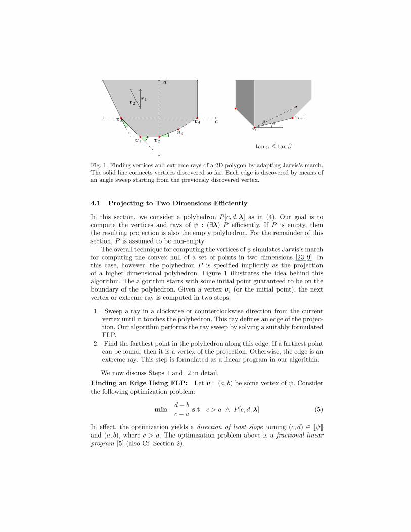
Fig. 1. Finding vertices and extreme rays of a 2D polygon by adapting Jarvis’s march.The solid line connects vertices discovered so far. Each edge is discovered by means ofan angle sweep starting from the previously discovered vertex.

4.1 Projecting to Two Dimensions Efficiently

In this section, we consider a polyhedron P [c, d,λ] as in (4). Our goal is tocompute the vertices and rays of ψ : (∃λ) P efficiently. If P is empty, thenthe resulting projection is also the empty polyhedron. For the remainder of thissection, P is assumed to be non-empty.

The overall technique for computing the vertices of ψ simulates Jarvis’s marchfor computing the convex hull of a set of points in two dimensions [23, 9]. Inthis case, however, the polyhedron P is specified implicitly as the projectionof a higher dimensional polyhedron. Figure 1 illustrates the idea behind thisalgorithm. The algorithm starts with some initial point guaranteed to be on theboundary of the polyhedron. Given a vertex vi (or the initial point), the nextvertex or extreme ray is computed in two steps:

1. Sweep a ray in a clockwise or counterclockwise direction from the currentvertex until it touches the polyhedron. This ray defines an edge of the projec-tion. Our algorithm performs the ray sweep by solving a suitably formulatedFLP.

2. Find the farthest point in the polyhedron along this edge. If a farthest pointcan be found, then it is a vertex of the projection. Otherwise, the edge is anextreme ray. This step is formulated as a linear program in our algorithm.

We now discuss Steps 1 and 2 in detail.

Finding an Edge Using FLP: Let v : (a, b) be some vertex of ψ. Considerthe following optimization problem:

min.d− b

c− as.t. c > a ∧ P [c, d,λ] (5)

In effect, the optimization yields a direction of least slope joining (c, d) ∈ JψKand (a, b), where c > a. The optimization problem above is a fractional linearprogram [5] (also Cf. Section 2).

Lemma 2. (a) If the FLP (5) is infeasible, then there is no point to the rightof (a, b) in JψK. (b) For non-empty ϕ, the FLP cannot be unbounded. (c) Anoptimal solution to the FLP yields the direction of least slope, as required byJarvis’s march.

Finding the Farthest Point Along an Edge: Once a direction with slope θis found starting from a vertex (a, b), we wish to find a vertex along this direction.This vertex can be found by solving the following LP:

max. c− a s.t. c− a ≥ 0 ∧ d = b+ θ(c− a) ∧ P [c, d,λ] (6)

In effect, we seek the maximum offset along the direction θ starting from (a, b)such that the end point (c, d) remains in ψ. The LP above cannot be infeasible(since (c, d) = (a, b) is a feasible point). If the LP above is unbounded then weobtain an extreme ray of ψ. Otherwise, we obtain an end-point that is a vertexof ψ. The overall algorithm is similar to Jarvis’s march as presented in standardtextbooks (Cf. Cormen, Leiserson and Rivest, Ch. 35.3 [9] or R.A. Jarvis’soriginal paper [23]). Rather than perform a “clockwise” and a “counterclockwise”march, we make use of the fact that (0, 1) is a ray of ψ and perform an equivalent“leftward” and a “rightward” march.

1. We start by finding some point on the boundary of ψ. Let (a, b,λ) be somefeasible point in P . We solve the problem min. d s.t. c = a ∧ P [c, d,λ].The point v0 can be treated as a starting point that is guaranteed to lie onthe boundary of ψ. Note, however, that v0 is not necessarilty a vertex of ψ.Since ϕ is assumed non-empty, the LP above cannot be unbounded.

2. We describe the rightward march. Each vertex vi+1 is discovered after com-puting v1, . . . ,vi. Let vi : (ai, bi) be the last vertex discovered.(a) Obtain least slope by solving the FLP problem in (5).(b) If the FLP is infeasible, then stop. vi is the right-most vertex and the

vector (0, 1) an extreme ray.(c) Solve the LP in (6). An optimal solution yields a vertex vi+1. Otherwise,

if the LP is unbounded, we obtain an extreme ray of ψ and vi is theright-most vertex.

3. The leftward march can be performed using the reflection T : c′ 7→ −c, d′ 7→d, carried out as a substitution in the polyhedron P . The resulting generatorsare reflected back.

Each generator discovered by our algorithm requires solving FLP and LPinstances. Furthermore, the initial point can itself be found by solving at mosttwo LP instances. Since LPs and FLPs can be solved efficiently, we have pre-sented an efficient, output-sensitive algorithm for performing the abstraction.This algorithm, in turn, can be used as a primitive to compute the join and thepost-condition efficiently, as well.

Note 3. It must be mentioned that an efficient (output-sensitive) algorithm foreach abstract domain operation does not necessarily imply that the overall analy-sis itself can also be performed efficiently in terms of program size and template

size. For instance, it is conceivable that the intermediate polyhedra and theircoefficients can grow arbitrarily large during the course of the analysis by re-peated applications of joins and post-conditions. This is a possibility for moststrongly-relational domains, including the two variables per inequality domainproposed by Simon et al. [37]. Nevertheless, in practice, we find that a carefulimplementation can control this blow-up effectively by means of widening.

5 Efficient Approximations

In Section 4, we discussed the special case in which each bilinear form in atemplate has at most two parameters. We presented an efficient algorithm forcomputing the abstraction operation. However, if |pars(fj)| > 2, we are forcedto resort to expensive elimination techniques using Fourier-Motzkin elimina-tion [35] or the double description method [31]. An alternative is to perform theelimination approximately to obtain ψ[c, d] such that

ψ[c, d] |= (∃ λ) P [c, d,λ] .

Note that, since we are working with the dual representation, we seek to under-approximate the result of the elimination.

We consider two methods for deriving an under-approximation of ψj by com-puting some of its generators. The under-approximations presented here are sim-ilar to those used in earlier work by Kanade et al. involving one of the authorsof this paper [25].Finding Vertices By Linear Programming: We simply solve k linearprograms, each yielding a vertex, by choosing some fixed or random objectivefi[c, d] and solving min. fi s.t. P [c, d,λ], λ ≥ 0. The solution yields a vertex(or a ray) of the feasible region (c, d,λ). By projecting λ out, we obtain a pointinside ψj or a ray of ψj , alternatively.Finding Vertices By Ray-Shooting: Choose a point (c0, d0) known to beinside ψj (using a linear programming). Let r be some direction. We seek a pointof the form (c0, d0) + γr for some γ ∈ R by solving the following LP:

max. γ s.t. ((c0, d0) + γr) ∈ JP [c, d,λ] ∧ λ ≥ 0K .

Any solution yields a point inside ψj by projection. If the LP is unbounded, weconclude that r is a ray of ψj .

We refer the reader to Kanade et al. [25] for more details on how under-approximation techniques described above can be used to control the size of thepolyhedral representation.

6 Applications

In this section, we present two applications of the ideas presented thus far. Indoing so, we seek to answer the following question: how do we derive interesting

templates without having the user of the analysis tool specify them? Note thatour previous work provides heuristics for guessing an initial set of templatesin a property directed manner and enriching this set based on pre-conditioncomputations [34].Improving Fixed-Points Template polyhedra can be used to improve post-fixed points that are computed using other known techniques for numerical do-mains. For instance, suppose we perform a polyhedral analysis for some pro-gram and compute invariants ϕ : e1 ≤ 0, . . . , em ≤ 0 for linear expressionse1, . . . , em. A local fixed point improvement template could specify entries of theform (ei, fi), wherein ei ≤ 0 is an inequality involved in the polyhedral invariantand fi is a bilinear form involving the program variables that do not appear inei. Improvement of fixed points can be attempted under more restrictive settingswhere the inequalities ei ≤ 0 are obtained from a less expensive analysis.Variable Packing Packing of variables is a commonly used tactic to tacklethe high complexity of domain operations in numerical domains [4, 22]. An al-ternative to packing would involve using generalized templates by specifyingexpressions of the form 0 ≤ c1x1 + · · · + ckxk as the template at a particularlocation where a variable pack of {x1, . . . , xk} is to be employed. This allowsus to seamlessly reason about multiple packs at different program locations andintegrate the reasoning about packs during the course of the analysis.

7 Implementation and Experiments

In this section, we describe our experimental evaluation of several of the ideaspresented in this paper on some benchmarks.Implementation The generalized template polyhedral domain presented inthis paper has been implemented using the Parma Polyhedral Library (PPL)for manipulating polyhedra [2]. Our implementation supports general templateswith arbitrarily many RHS parameters using generator enumeration capabilitiesof PPL. The special case of templates with at most two parameters has beenimplemented using the LP solver available in PPL. The analysis engine uses anaive iteration with delayed widening followed by the narrowing of post-fixedpoints, for a bounded number of iterations.

Note 4. In this paper, we have described an algorithm for performing abstractionusing polyhedral projection (elimination of multiplier variables for dualization).Our implementation uses a different technique based directly on generator enu-meration: to compute α(ϕ) we simply compute the generators of ϕ and derivethe dual constraints for each template entry from the generators of ϕ. Thishas been done since PPL has an efficiently engineered generator enumerationalgorithm. Therefore, our implementation performs a single vertex enumerationup-front and re-uses the result for each template entry, as opposed to eliminatingmultipliers for each template entry.Template Construction The overall template construction is based on apre-computed fixed point. For our experiments, we use the polyhedral domain

Table 1. Experimental evaluation of the GTP domain on some benchmark examplesusing various methods for forming templates. All timings are in seconds. #tpl: # oftemplates, #entries: average/min/max number of entries per template, # FP Impr: #of templates that improve the fixed point, Tpoly: polyhedral analysis time, Tflp: averagetime per template with FLP, Tve: average time per template with vertex enum.

M1Name #var #trs #tpl #entries #fp Tpoly Tflp Tve

avg (min,max) imp avg avg

lifo 8 10 42 1.0 1 , 1 6 0.02 0.02 0.00tick3i 8 9 78 1.0 1 , 1 0 0.03 0.02 0.01pool 9 6 64 1.1 1 , 2 8 0.01 0.03 0.01ttp 9 20 968 1.4 1 , 2 64 0.06 0.02 0.01cars2 10 7 149 1.1 1 , 2 4 13.5 0.06 0.01req-gr 11 8 81 1.3 1 , 2 25 0.01 0.06 0.02cprot 12 8 100 1.3 1 , 2 27 0.02 0.07 0.02CSM 13 8 131 1.4 1 , 2 27 0.02 0.06 0.02cprod 18 14 233 1.2 1 , 2 38 0.06 0.13 0.05incdec 32 28 854 1.1 1 , 2 103 1 0.41 0.23mesh2x2 32 32 940 1.1 1 , 2 212 1 0.51 0.29bigjava 45 37 1856 1.4 1 , 2 129 239 0.85 0.48

M2 M3Name #tpl #entries Tflp Tve #fp #entries T #fp

avg (min,max) avg avg impr avg (min,max) avg impr

lifo 7 6.0 6 , 6 0.6 0.0 6 1.0 1 , 1 0.0 0tick3i 14 5.6 3 , 7 0.1 0.0 0 1.0 1 , 1 0.0 0pool 10 7.1 4 , 8 0.5 0.0 8 1.2 1 , 2 0.0 3ttp 140 9.5 5 , 16 0.4 0.0 32 1.4 1 , 2 0.0 2cars2 18 9.3 7 , 18 1.4 0.2 3 1.1 1 , 2 0.1 1req-gr 9 11.3 10 , 16 1.5 0.2 9 1.3 1 , 2 0.0 8cprot 10 13.4 11 , 20 2.0 0.3 10 1.4 1 , 2 0.0 9CSM 12 15.3 7 , 22 2.5 0.5 12 1.4 1 , 2 0.0 7cprod 16 18.1 12 , 32 7.4 1.5 15 1.3 1 , 2 0.1 13incdec 29 32.7 16 , 60 43.6 87.8 29 1.1 1 , 2 1.1 7bigjava 44 60.4 34 , 86 67.1 50.4 42 1.4 1 , 2 1.7 8

to generate these fixed points. Next, using each inequality e ≤ 0 in the resultcomputed by the polyhedral domain, we compare three methods for forming tem-plates: (M1) Create multiple templates per invariant inequality, each templateconsisting of a single entry of the form e ≤ cjxj+dj , for each xj 6∈ vars(e), (M2)Create one template per inequality, each template consisting of multiple entriesof the form e ≤ cjxj + dj , for each xj 6∈ vars(e), and finally, (M3) Create onetemplate per inequality, consisting of a single entry of the form e ≤

∑j cjxj + d

for all variables xj 6∈ vars(e). For equalities e = 0, we consider entries of theform e ≤ cjxj+dj and e ≥ c′jxj+d′j , modifying the methods above appropriately.

Furthermore, for methods M1 and M2, we compare the implementationusing vertex enumeration against the fractional LP implementation for the keyprimitive of abstraction, which also underlies the implementation of the join

and post-condition operations. Since the fractional LP algorithm produces thesame result as the vertex enumeration, we did not observe any difference in thegenerated invariants. We compare the running times for these techniques.Results Table 1 reports on the time taken for the initial polyhedral analy-sis run, the number of templates, avg/min/max of the number of entries pertemplate and the number of analysis runs that discovered a stronger invariant.The benchmarks have been employed in our previous work [34] as well as othertools [3]. They range in size from small (≤ 10 program variables) to large (≥ 30program variables). The initial widening delay was set to 4 for each run of thepolyhedral analysis.

We note that our domain can be used to infer invariants that are not con-sequences of the polyhedral domain invariants. This validates the usefulness ofgeneralized templates for improving fixed points. The results using method M2show that analysis using generalized templates can be expensive when the num-ber of entries in each template is large. However, method M2 also provides afixed point improvement for almost all the templates that were run, whereas inmethod M1, roughly 10% of the runs resulted in a fixed point improvement.Even though method M3 does not allow us to use fractional linear program-ming, it presents a good tradeoff between running time and the possibility offixed point improvement.

The comparison between running times for the fractional LP approach andthe basic approach using vertex enumeration yields a surprising result: on mostlarger benchmarks, the fractional LP approach (which is polynomial time, intheory) is slower than the vertex enumeration. A closer investigation reveals thateach vertex enumeration pass yields very few (∼ 10) vertices and extreme rays.Therefore, the well-engineered generator enumeration implementation in PPLinvoked once, though exponential in worst-case, can outperform our techniquewhich requires repeated calls to LP solvers. On the other hand, the constraintsin the dual form P [c, d,λ] obtained by Farkas’ Lemma are common to all the LPand FLP solver invocations during a run of our algorithm. Incremental solversused in SMT solvers such as Z3 [13], could potentially be adapted to speed ouralgorithm up.

Finally, the comparison here has been carried out against invariants obtainedby polyhedral analysis. In the future, we wish to evaluate our domain againstother types of invariant generation tools such as VS3 [38] and InvGen [17].

8 Related Work

Polyhedral analysis was first introduced by Cousot & Halbwachs [12] using theabstract interpretation framework [11]. Further work has realized the usefulnessof domains based on convex polyhedra to the analysis of hybrid systems [19],control software [4], and systems software [36, 21, 22, 14]. However, these ad-vances have avoided the direct use of the original polyhedral domain due to thehigh cost of domain operations such as convex hulls and post-conditions [35].In spite of impressive advances made by polyhedra libraries such as PPL, the

combinatorial explosion in the number of generators cannot be overcome, ingeneral [2]. However, it is also well-known that these operations can be per-formed at a lower polynomial cost (in terms of the problem size and the outputsize) for two dimensional polyhedra [9, 35]. This fact has been used to designfast program analysis techniques to compute invariants that involve at most twoprogram variables [37]. Further restricting the coefficients to units (±1), yieldsthe weakly-relational octagon domain wherein the process of reasoning aboutthe constraints can be reduced to graph operations [28].

The restriction to at most two variables for each invariant and unit coefficientshas been observed to be quite useful for proving absence of runtime errors [21].On the other hand, current evidence suggests that invariants involving threeor more variables are often crucial for proving safety of string operations anduser-defined assertions [33].

Template polyhedral domains attempt to avoid the exponential complexityof polyhedral domain operations by fixing templates that represent the form ofthe desired invariants [34]. Recently, there have been many advances in our un-derstanding of template polyhedral domains. Techniques such as policy iterationand strategy iteration have exploited ideas from max-plus algebra to show thatthe least fixed point in weakly-relational domains is computable [15, 16]. Thesetechniques have been extended to handle templates with non-linear inequalitiesusing ideas from convex programming [1, 16]. The possibility that some of theseresults may generalize to the domain presented in this paper remains open.

The problem of modular template polyhedral analysis has been studied byMonniaux [30], wherein summaries for templates are derived by dualization usingFarkas’ lemma followed by quantifier elimination in the theory of linear arith-metic. This work has also extended the template domain to handle floating pointsemantics for control software. Srivastava and Gulwani [38] present a verificationtechnique using templates that can specify a richer class of templates involvingquantifiers and various Boolean combinations of predicates. However, their ap-proach for computing transformers works by restricting the coefficients to a finiteset and “bit blasting” using SAT solvers. The logahedron domain uses a similarrestriction [20]. Invariants with unit coefficients are quite useful for reasoningabout runtime properties of low-level code. However, it is as yet unclear if ver-ifying functional properties in domains such as control systems will necessitateinvariants with arbitrary coefficients.

9 Conclusion

We have presented a generalization of the template domain with arbitrary bilin-ear forms, along with efficient algorithms for computing the domain operationswhen the template has at most two parameters per entry. Our experimentalresults demonstrate that our techniques can be applied to strengthen the invari-ants computed by other numerical domains. In the future, we plan to investigatetechniques such as policy and strategy iteration for analysis over generalized

templates. Extensions to non-linear templates and the handling of floating pointsemantics are also of great interest.

References

1. A. Adje, S. Gaubert, and E. Goubault. Coupling policy iteration with semi-definiterelaxation to compute accurate numerical invariants in static analysis. In ESOP,volume 6012 of LNCS, pages 23–42. Springer, 2010.

2. R. Bagnara, E. Ricci, E. Zaffanella, and P. M. Hill. Possibly not closed convex poly-hedra and the Parma Polyhedra Library. In Static Analysis Symposium, volume2477 of LNCS, pages 213–229. Springer, 2002.

3. S. Bardin, A. Finkel, J. Leroux, and L. Petrucci. FAST: fast accelereation of sym-bolic transition systems. In CAV, volume 2725 of LNCS, pages 118–121. Springer,2003.

4. B. Blanchet, P. Cousot, R. Cousot, J. Feret, L. Mauborgne, A. Mine, D. Monniaux,and X. Rival. Design and implementation of a special-purpose static program an-alyzer for safety-critical real-time embedded software (invited chapter). In In TheEssence of Computation: Complexity, Analysis, Transformation. Essays Dedicatedto Neil D. Jones, volume 2566 of LNCS, pages 85–108. Springer, 2005.

5. S. Boyd and S. Vandenberghe. Convex Optimization. Cambridge University Press,2004. Online http://www.stanford.edu/ boyd/cvxbook.html.

6. S. Chatterjee, S. K. Lahiri, S. Qadeer, and Z. Rakamaric. A reachability predicatefor analyzing low-level software. In TACAS, volume 4424 of LNCS, pages 19–33.Springer, 2007.

7. R. Clariso and J. Cortadella. The octahedron abstract domain. Science of Com-puter Programming, 64(1):115–139, January 2007.

8. M. A. Colon. Deductive Techniques for Program Analysis. PhD thesis, StanfordUniversity, 2003.

9. T. Corman, C. F. Leiserson, and R. Rivest. Introduction to Algorithms. McGrawHill, 1990.

10. P. Cousot and R. Cousot. Static determination of dynamic properties of programs.In Proc. ISOP’76, pages 106–130. Dunod, Paris, France, 1976.

11. P. Cousot and R. Cousot. Abstract Interpretation: A unified lattice model for staticanalysis of programs by construction or approximation of fixpoints. In POPL, pages238–252, 1977.

12. P. Cousot and N. Halbwachs. Automatic discovery of linear restraints among thevariables of a program. In POPL’78, pages 84–97, Jan. 1978.

13. L. M. de Moura and N. Bjørner. Z3: An efficient SMT solver. In TACAS, volume4963 of LNCS, pages 337–340. Springer, 2008.

14. P. Ferrara, F. Logozzo, and M. Fahndrich. Safer unsafe code for .net. In OOPSLA,pages 329–346. ACM, 2008.

15. S. Gaubert, E. Goubault, A. Taly, and S. Zennou. Static analysis by policy iterationon relational domains. In ESOP, volume 4421 of LNCS, pages 237–252. Springer,2007.

16. T. Gawlitza and H. Seidl. Precise fixpoint computation through strategy iteration.In ESOP, volume 4421 of LNCS, pages 300–315. Springer, 2007.

17. A. Gupta and A. Rybalchenko. InvGen: An efficient invariant generator. In CAV,volume 5643 of LNCS, pages 634–640, 2009.

18. N. Halbwachs, Y.-E. Proy, and P. Roumanoff. Verification of real-time systemsusing linear relation analysis. Formal Methods in System Design, 11(2):157–185,1997.

19. T. A. Henzinger and P. Ho. HyTech: The Cornell hybrid technology tool. InHybrid Systems II, volume 999 of LNCS, pages 265–293. Springer, 1995.

20. J. Howe and A. King. Logahedra: A new weakly relational domain. In ATVA’09,volume 5799 of LNCS, pages 306–320. 2009.

21. F. Ivancic, S. Sankaranarayanan, I. Shlyakhter, and A. Gupta. Buffer overflowanalysis using environment refinement, 2009. Draft (2009).

22. F. Ivancic, I. Shlyakhter, A. Gupta, and M. K. Ganai. Model checking C programsusing F-SOFT. In ICCD, pages 297–308. IEEE Computer Society, 2005.

23. R. A. Jarvis. On the identification of the convex hull of a finite set of points in theplane. Information Processing Letters, 2(1):18 – 21, 1973.

24. B. Jeannet and A. Mine. Apron: A library of numerical abstract domains for staticanalysis. In CAV, volume 5643 of LNCS, pages 661–667. Springer, 2009.

25. A. Kanade, R. Alur, F. Ivancic, S. Ramesh, S. Sankaranarayanan, and K. Sashid-har. Generating and analyzing symbolic traces of Simulink/Stateflow models. InComputer-aided Verification (CAV), volume 5643 of LNCS, pages 430–445, 2009.

26. F. Logozzo and M. Fahndrich. Pentagons: A weakly relational abstract domain forthe efficient validation of array accesses. Sci. Comp. Prog., 75(9):796–807, 2010.

27. Z. Manna and A. Pnueli. Temporal Verification of Reactive Systems: Safety.Springer, New York, 1995.

28. A. Mine. A new numerical abstract domain based on difference-bound matrices.In PADO II, volume 2053 of LNCS, pages 155–172. Springer, May 2001.

29. A. Mine. Symbolic methods to enhance the precision of numerical abstract do-mains. In VMCAI’06, volume 3855 of LNCS, pages 348–363. Springer, 2006.

30. D. Monniaux. Automatic modular abstractions for template numerical constraints.Logical Methods in Computer Science, 6(3), 2010.

31. T. S. Motzkin, H. Raiffa, G. L. Thompson, and R. M. Thrall. The double de-scription method. In Contributions to the theory of games, volume 2 of Annals ofMathematics Studies, pages 51–73. Princeton University Press, 1953.

32. S. Sankaranarayanan, M. A. Colon, H. Sipma, and Z. Manna. Efficient stronglyrelational polyhedral analysis. In VMCAI’06, volume 3855/2006 of LNCS, pages111–125, 2006.

33. S. Sankaranarayanan, F. Ivancic, and A. Gupta. Program analysis using symbolicranges. In SAS, volume 4634 of LNCS, pages 366–383, 2007.

34. S. Sankaranarayanan, H. B. Sipma, and Z. Manna. Scalable analysis of linearsystems using mathematical programming. In VMCAI, volume 3385 of LNCS,January 2005.

35. A. Schrijver. Theory of Linear and Integer Programming. Wiley, 1986.36. A. Simon. Value-Range Analysis of C Programs: Towards Proving the Absence of

Buffer Overflow Vulnerabilities. Springer, 2008.37. A. Simon, A. King, and J. M. Howe. Two variables per linear inequality as an

abstract domain. In LOPSTR, volume 2664 of LNCS, pages 71–89. Springer, 2003.38. S. Srivastava and S. Gulwani. Program verification using templates over predicate

abstraction. In PLDI ’09, pages 223–234, New York, NY, USA, 2009. ACM.