J . Fluid Mech. (1989), vol. 205, p p . 421-451 Printed in Great Britain

42 1

On the structure of pressure fluctuations in simulated turbulent channel flow

By JOHN KIM NASA Ames Research Center, Moffett Field, CA 94035, USA

(Received 30 August 1988)

Pressure fluctuations in a turbulent channel flow are investigated by analysing a database obtained from a direct numerical simulation. Detailed statistics associated with the pressure fluctuations are presented. Characteristics associated with the rapid (linear) and slow (nonlinear) pressure are discussed. It is found that the slow pressure fluctuations are larger than the rapid pressure fluctuations throughout the channel except very near the wall, where they are about the same magnitude. This is contrary to the common belief that the nonlinear source terms are negligible compared with the linear source terms. Probability density distributions, power spectra, and two-point correlations are examined to reveal the characteristics of the pressure fluctuations. The global dependence of the pressure fluctuations and pressure-strain correlations are also examined by evaluating the integral associated with Green-function representations of them. I n the wall region where the pressure-strain terms are large, most contributions to the pressurestrain terms are from the wall region (i.e. local), whereas away from the wall where the pressure-strain terms are small, contributions are global. Structures of instantaneous pressure and pressure gradients a t the wall and the corresponding vorticity field are examined.

1. Introduction The pressure fluctuations in turbulent flows are of considerable interest in many

engineering applications. Pressure fluctuations on aerodynamic surfaces of airplanes and turbine blades, for example, contribute to noise generation and often lead to undesirable structural vibrations. Understanding the nature of the pressure fluctuations is essential to alleviate such problems. In addition, because pressure at a given point in turbulent flows is related to global information of the associated velocity field, it may be possible to obtain such information by examining local pressure fluctuations. The pressure fluctuations are also intimately related to vorticity fluctuations, although the governing equations for the evolution of the vorticity fluctuations do not explicitly contain pressure fluctuations. The gradients of surface-pressure fluctuations, for example, are equal to the flux of vorticity from the wall. A better understanding of the surface-pressure fluctuations could lead to a better understanding of the vorticity dynamics in the wall region. From a turbulence modelling point of view, the pressure-strain correlations that appear in the Reynolds-averaged Navier-Stokes equations are of significant interest because these terms are responsible for intercomponent energy transfer. In the Reynolds shear- stress budget equation, the pressure-strain term is, in fact, one of the two dominant terms. Existing models for the pressure-strain terms, however, are not satisfactory and are regarded as one of the major deficiencies in the Reynolds stress closure. Refer

422 J . Kim

to Mansour, Kim & Moin (1988) for a recent assessment of the existing turbulence models based on databases obtained from direct numerical simulations.

A great deal of experimental and theoretical work on pressure fluctuations has been performed during the past several decades. Willmarth (1975) provides a comprehensive review on the subject, and Eckelmann (1988) gives an updated review. In spite of the considerable efforts evidenced in the literature, progress in our understanding of the pressure fluctuations has been very slow because of inadequate measurements of pressure fields in turbulent flows. This is because we do not yet have a reliable measurement technique for turbulent pressure fluctuations within turbulent flow comparable to the modern measurement techniques for turbulent velocity fluctuations. Consequently, most measurements reported to date have been performed only on the surface using a surface-mounted pressure transducer. Furthermore, many of the earlier surface-pressure measurements suffered from inadequate spatial resolution because of the large size of pressure transducers employed in the experiments. The errors involved turned out to be significant (Blake 1970; Willmarth 1975; Schewe 1983). Bradshaw (1967) also cmphasized the importance of small-scale pressure fluctuations. He argued that the ‘active ’ universal velocity fluctuations in the wail region would lead to surface-pressure spectra containing a k-’ slope up to the wavenumber range inversely proportional to the sublayer thickness. Most pressure transducers used in the earlier works were an order of magnitude larger than the sublayer thickness. Schewe (1983) also reported the effect of inadequate spatial resolution of the pressure transducer on the measured power spectra. For example, he showed that the exponential decay exhibited in some of the measured power spectra was due to the inadequate spatial resolution.

Most theoretical works in which attempts were made to compute the pressure fluctuations and the power spectra-Kraichnan (1956), Lilley (1964), and Panton & Linebarger (1974), to name a few - also suffered from the lack of accurate information to guide their analyses. The analyses were based on the earlier measurements with the poor spatial resolution. Also, most of the theoretical work assumed that the contribution from the linear source term in the Poisson equation for pressure, representing the interaction of turbulence with the mean shear, is much larger than that from the nonlinear source terms representing interactions of the turbulence with itself. Corcos (1964), however, claimed that the nonlinear source terms should be of the same order of importance as the linear source term, after analysing the data of Willmarth & Wooldridge (1962). Willmarth (1975) later argued that Corcos’ conclusion may not necessarily be valid because the data used in the analysis did not satisfy the compatibility condition discussed by Phillips ( 1956).

The objective of this paper is to document detailed statistics arid turbulence structures associated with pressure fluctuations in a wall-bounded turbulent shear flow. The database used in the present work was obtained from a direct numerical simulation of turbulent channel flow by Kim, Moin & Moser (1987, hereinafter referred to as KMM). The physical realism and accuracy of the computed flow fields have been established by detailed comparison with existing experimental results. Many of the results presented in this paper include new information that cannot be validated directly by comparing it with experimental data, unlike most of the statistics and turbulence structures of the corresponding velocity field. However, the pressure fields considered in the present work are obtained from the same velocity fields whose validity has been thoroughly examined, and there is little doubt that the pressure information presented here is as valid as the velocity field. Also, although the Reynolds number considered is very low-Res x 3300 based on the centreline

Structure of pressure Jluctuations in turbulent channel Jlow 423

velocity and the channel half-width ~ because of the enormous amount of com- putational time necessary for high-Reynolds-number simulations, most of the computed statistics, as well as turbulence structures of the velocity fields, were essentially the same as those obtained in higher-Reynolds-number experiments. It is expected that the essential characteristics of the pressure field presented in this paper also would differ only slightly from those of higher-Reynolds-number flows, except for some features observable only for high-Reynolds-number flows such as the inertial subrange in the power spectra of the pressure fluctuations.

In $ 2 , a brief description of numerical procedures and splitting of pressure according to its source terms is presented. Detailed statistics of pressure fluctuations are discussed in $3. In $4, a Green-function representation for the pressure fluctuations is presented. In $5, the structure of instantaneous pressure fields and its association with the corresponding velocity and vorticity fields will be discussed. A brief summary is given in $6.

2. Numerical procedures and splitting of pressure A direct simulation of fully developed turbulent channel flow ~ turbulent flow

between two parallel plates - has been performed. The numerical algorithm and other details employed to generate the database can be found in KMM. The computation was carried out with about 2 x lo6 grid points (128 x 129 x 128, in x, y, and z , where x, y, z indicate streamwise, normal to the wall, and spanwise directions, respectively) for a Reynolds number of about 3300, based on the centreline velocity and channel half-width. The grid spacings in the streamwise and spanwise directions were Axf x 17, and Axf x 6 in wall units.? Non-uniform meshes were used in the normal direction. The first mesh point away from the wall was a t y+ x 0.05, and the maximum spacing (at the centreline of the channel) was 4.4 wall units. A spectral method -Fourier series in the streamwise and spanwise directions and Chebychev polynomial expansion in the normal direction -was used for the spatial derivatives. The time advancement was carried out by a semi-implicit second-order scheme.

The initial velocity field was obtained from a velocity field of a previous coarse computation (Moin & Kim 1982) by spectrally interpolating the coarse velocity field onto the present collocation points. This reduced the time required to reach a statistically steady state. Once the velocity field reached the steady state, about 100 instantaneous velocity fields (each contains about 8 x lo6 words) a t a regular time interval were stored on magnetic tapes for future analyses, from which the present results were obtained.

The turbulent pressure field for incompressible flows satisfies the following Poisson equation

where u,(i = 1,2 ,3) or u, u, w denote the three velocity components in the streamwise, normal to the wall, and spanwise directions, respectively, and p denotes the kinematic pressure. Here, all the flow variables are non-dimensionalized by the friction velocity, u,, and the channel half-width, 6. The Reynolds number is defined as Re = u,6/v, and y = f 1 corresponds to the upper and lower walls. Equation ( 1 ) is obtained by taking the divergence of the Navier-Stokes equations. The Neumann

t The superscript + indicates a non-dimensional quaiitit? scaled by the wall variables, e.g. y+ = yuJw, where w is the kinematic viscosity and u, = ( ~ , / p ) s is the wall shear velocity.

424 J . Kim

boundary condition is a result of evaluating the normal component equation a t the wall. One can use the Dirichlet boundary condition instead by evaluating the equations for horizontal components a t the wall, but it has been demonstrated that any compatible velocity field will produce the same result (Moin & Kim 1980 ; KMM). The Poisson equation for pressure is solved by the same method as described in KMM for the velocity field : that is, a FourierIChebychev-tau method is used to invert the elliptic operator, which involves the inversion of a tridiagonal matrix with one extra full row representing the boundary condition.

The pressure is sometimes split into rapid and slow parts by dividing the source terms in ( 1 ) into two parts, one containing the mean velocity gradient and the other without it. By decomposing the velocity field into mean and fluctuations as ui = Ui + u; and noting that the only non-zero mean velocity gradient for the present flow is dU/dy, ( 1 ) can be written as follows :

I dU av‘ apr V2pr=-2-- - ( * 1 ) = 0 , dy ax ay

aPs 1 a w v2ps=-u; , Ju j , i , - (* l ) =--, a Y Re ay2

where the subscripts rand s denote the rapid and slow parts, respectively. The terms ‘rapid’ and ‘slow’ are derived from the fact that only the rapid part responds immediately to a change imposed on the mean field, and the slow part will feel the change through nonlinear interactions. The slow part is sometimes referred to as the ‘return’ term because it is believed by many to be responsible for returning the Reynolds-stress tensor toward isotropy. Sometimes, the rapid and slow pressure are also referred to as linear and nonlinear pressure, respectively, because the corresponding source terms in ( 2 ) are linear in the fluctuating quantities for the rapid part and nonlinear for the slow part. The above treatment of the boundary conditions, i.e. the homogeneous condition for the rapid pressure and the inhomogeneous condition for the slow pressure, is somewhat arbitrary. Mansour et al. (1988) suggested that the effect of the boundary condition should be treated separately by splitting the pressure into three parts as follows:

I v2ps=-u; , iuj , i , - ( & l ) aPs = o , a Y

(3)

Re a2v’ ay2 I apst V2ps,=O, - (&l )=- - , aY

where p,, is called the Stokes pressure. The Stokes pressure is due solely to the inhomogeneous boundary condition and one can add the Stokes pressure either into the rapid part or into the slow part. The above triple splitting avoids the arbitrariness in treating the boundary condition, but it takes extra effort to carry the three terms (instead of two) separately in the analysis, and it may not be necessary to do so unless the Stokes pressure becomes significant.

Structure of pressure fluctuations in turbulent channel flow 425

3. Pressure statistics Throughout this paper, all quantities are non-dimensionalized by the watl-shear

velocity, u,, and the channel half-width, 6, unless otherwise stated. In some cases, the viscous lengthscale, v/u,, is used when it appears to be more appropriate. One could use the following global parameters to convert from one form of non- dimensionalization to others, if necessary :

u, 6 UC 6 Re, = - = 179, Rec = ~ = 3251, V V

uc = 18.2,) U ,

6" 0 6

= 0.141, - = 0.087, _- - 15.6, - u, 6

where U,, Urn, 6*, and 0 denote the centreline velocity, mass-averaged velocity, displacement thickness, and momentum thickness, respectively.

3.1. R.m.s. pressure fluctuation and probability density distribution The profiles of the root-mean-square (r.m.s.) fluctuation resulting from the triple splitting (equation (3)) across the channel are shown in figure 1. These results are obtained from a single realization (one pressure field) to examine the relative importance of each term. It is quite clear that the Stokes part is negligible compared with other two parts throughout the channel, including the near-wall region, where the Stokes part has its maximum. Thus, it would make little difference where we include the inhomogeneous boundary condition. For many practical purposes, one could use the homogeneous boundary condition for both the rapid and slow pressure and simply ignore the Stokes pressure as far as the r.m.s. fluctuations is concerned. It should be noted, however, that this does not imply that the presence of the wall is not affecting the pressure fluctuations. Rather, i t indicates that most of the influence from the presence of the wall is already built into the source terms through the no-slip boundary conditions (i.e. the source terms themselves are already affected by the no-slip boundary conditions on the velocities), and the explicit influence through the boundary condition to the Poisson equation is not significant. Because of the negligible contribution of the Stokes pressure to the total r.m.s. fluctuation, we use the conventional splitting (equation ( 2 ) ) in the present paper unless otherwise stated.

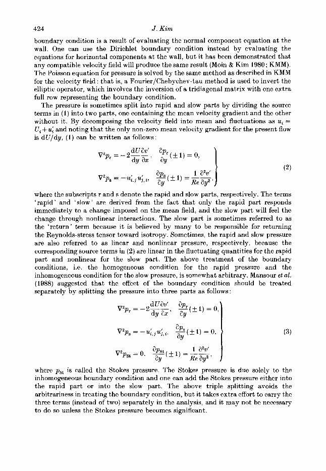
The profiles of the r.m.s. fluctuation of the rapid, slow, and total pressure obtained by averaging over five velocity fields are shown in figure 2. We note that the slow part is substantially larger than the rapid part except very close to the wall (y+ < 15 or y/S < O . l ) , contrary to the common belief that the rapid part would be the dominant one. Both the rapid and slow parts contribute approximately 75 % of the total r.m.s. pressure a t the wall (or about 55 % of the total mean-square fluctuation). The two are negatively correlated, with the correlation coefficient about -0.1 a t the wall. Throughout the channel, the correlation between the rapid and slow pressure is negligible; the magnitude of the correlation coefficient is less than 0.1. To investigate whether this particular behaviour is a characteristic peculiar to a low- Reynolds-number flow, pressure fluctuations from a higher-Reynolds-number flow - Re, x 400 or Re, x 7800 compared to Re, = 180 or Re, x 3300 of the present case- have been examined (J. Kim 1988, unpublished work), and i t showed basically the same trend (figure 3). For the high-Reynolds-number ease, the rapid and slow r.m.s. pressure contribute approximately 70% each to the total r.m.s. fluctuations a t the

426 J . Kim

- , 7A 0 ‘-1-7 ’ ’ ’ 1 ’ ‘ -1.0 -0.5 0 0.5 1 .o

Y I 6

FIGURE 1. Root-mean-square fluctuation for each pressure according to (3) :-, rapid; ----, slow; ---, Stokes.

-1.0 -0.5 0 0.5 1 .o Y / 6

FIGURE 2. Root-mean-square fluctuation for each pressure according to ( 2 ) : -, rapid; ----, slow; ---, total.

wall. The r.m.s. wall-pressure fluctuations reported here are smaller than previously reported values, but they are increasing with the Reynolds number - 1.4 for Re, = 180 and 1.9 for Re, = 400- which is consistent with the analyses by Bradshaw (1967) and Townsend (1976). From his numerical simulations of turbulent boundary layers, Spalart (1988) reported the same trend of the wall-pressure fluctuations.

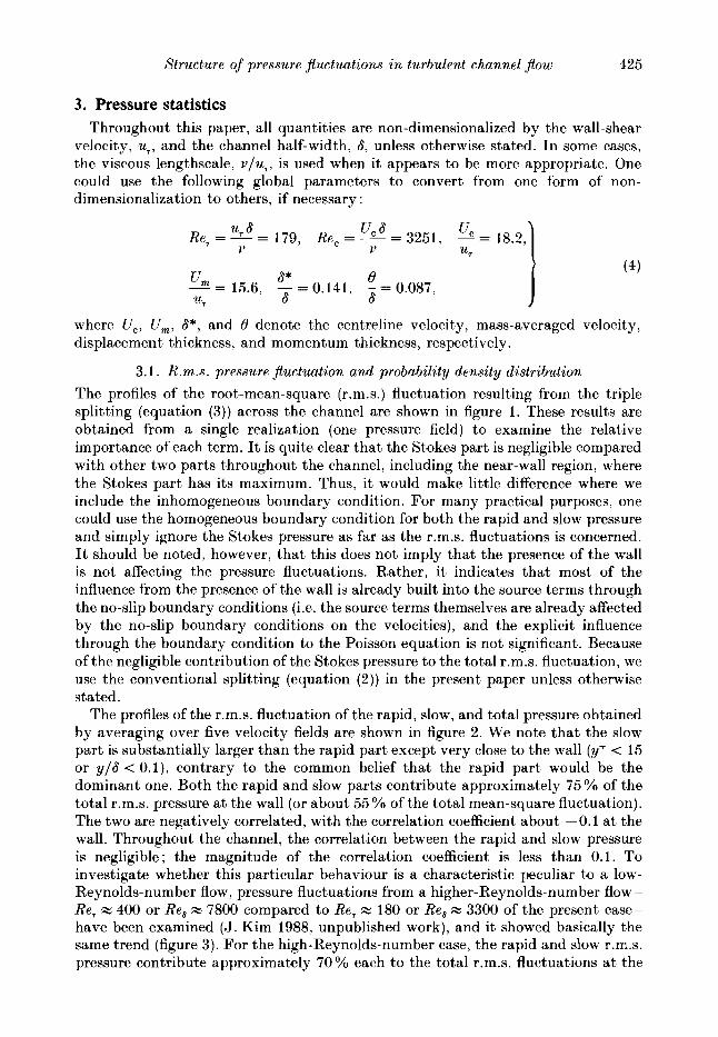
To obtain further insight into the pressure splitting, the source terms that appear in (2) are examined. The profiles of the mean-square linear, nonlinear, and total source terms are shown in figure 4. Figure 4 ( a ) shows that the nonlinear source term is much larger than the linear source term throughout the channel. This is because even though the mean shear is large in the wall region, aw’/ax is rather small (zero at the wall where the shear is the highest, and the mean shear drops significantly where aw‘/ax becomes finite away from the wall). Further breakdown of the nonlinear source terms - there are six different terms ~ is shown in figure 4 ( b ) , and i t is found that (aw’/az )(adlay) has the largest mean-square value. Note that the magnitude of ( a d / & ) (adlay) would be large a t the core of streamwise vortices, and indeed it has a local peak a t about y+ = 20, where the centres of streamwise vortices are located on the average (KMM). Note also that the locations of the maxima for each source

Structure of pressure jluctuations in turbulent channel jlow 427

- 1.0 -0.5 0 0.5 1 .o Y I 6

FIGURE 3. Root-mean-square fluctuation for Re, = 400: -, rapid; ----, slow; ---, total.

30 F

Y’ FIGURE 4. Profiles of the mean-square source terms. ( a ) -, linear; ----, nonlinear; ---, total. ( b ) Profiles of the mean-square nonlinear terms: - x--, (au‘/az)z, ----, (adlay) (aw’laz); ---, (au’/az) (aw’/az) ; . . . . . . , (aw’/ay)Z; -, (aw’/az) (aw’/ay); -.-, (aw’/az)z.

terms approximately coincide with the location of the maximum r.m.s. pressure fluctuation.

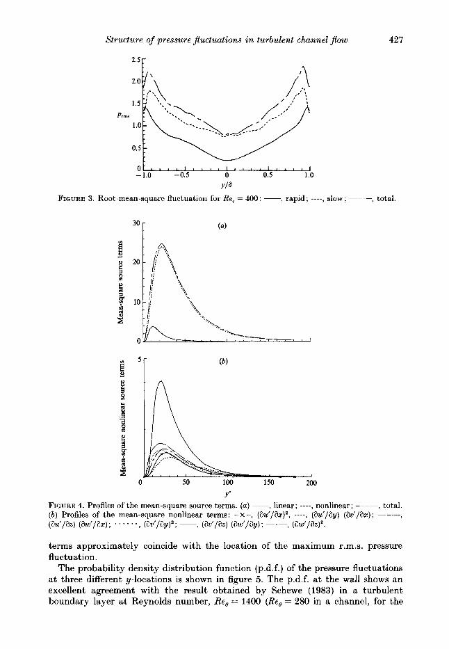
The probability density distribution function (p.d.f.) of the pressure fluctuations at three different y-locations is shown in figure 5. The p.d.f. a t the wall shows an excellent agreement with the result obtained by Schewe (1983) in a turbulent boundary layer at Reynolds number, R e , = 1400 (Re , = 280 in a channel, for the

428 J . Kim

I , , I

P'lP,,,

FIGURE 5. Probability density distribution of the total pressure fluctuations : -, computation ; ----, Gaussian distribution; 0, Schewe (1983). The abscissa is normalized by the local r.m.s. pressure fluctuations and the ordinate is normalized such tha t the area under the curve is equal t o one: ( a ) y+ = 0 ; ( b ) y' = 12; (c) y' = 100.

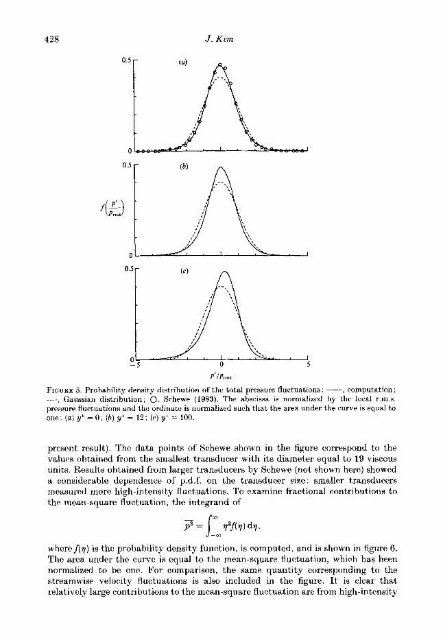
present result). The data points of Schewe shown in the figure correspond to the values obtained from the smallest transducer with its diameter equal t o 19 viscous units. Results obtained from larger transducers by Schewe (not shown here) showed a considerable dependence of p.d.f. on the transducer size : smaller transducers measured more high-intensity fluctuations. To examine fractional contributions to the mean-square fluctuation, the integrand of

wheref(7) is the probability density function, is computed, and is shown in figure 6. The area under the curve is equal to the mean-square fluctuation, which has been normalized to be one. For comparison, the same quantity corresponding to the streamwise velocity fluctuations is also included in the figure. It is clear that relatively large contributions to the mean-square fluctuation are from high-intensity

Structure of pressure jluctuations in turbulent channel jlow 429

~~I~nnW P’IP,,,

FIGURE 6. Fractional contributions to the mean-square fluctuation: -, u‘; ----, p‘. The abscissa is normalized by the corresponding local r.m.s. fluctuations and the ordinate is normalized such that the area under the curve is equal to one: ( a ) y+ = 0 for p and y+ = 5 for u; (6) y+ = 12; ( c ) y+ = 100.

fluctuations, especially from the negative fluctuations, compared to the streamwise velocity fluctuations. For instance, a t y+ = 12, only 1 % of the data points exceeds f 3 prms, but they contribute to about 42 YO of the total p,,,. The corresponding contribution to the streamwise velocity fluctuations, on the other hand, is negligible. While the mean-square streamwise velocity fluctuation takes larger contributions from the positive fluctuations (associated with the sweep-like events) near the wall (y’ < 15) and from the negative fluctuations away from the wall (y’ > 15), the mean- square pressure fluctuation takes about equal contributions from each side near the wall and more from the negative fluctuations away from the wall.

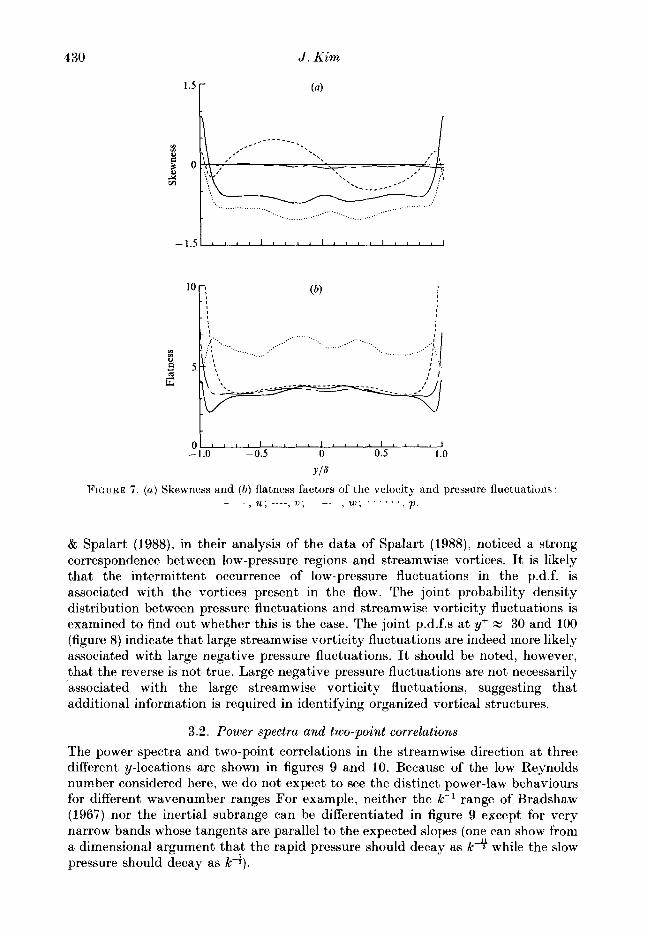
The skewness and flatness factors, p’3/(p’2)t and p’4/(p’2)2, respectively, computed from the p.d.f.s were presented in KMM and are shown in figure 7. The wall values of the skewness and flatness factors, -0.1 and 5.0, respectively, are comparable with Schewe’s results of -0.2 and 4.9. Moving away from the wall region, t,he p.d.f. becomes more negatively skewed with a higher flatness factor (more intermittsent) indicating the presence of localized and very low-pressure regions. Robinson, Kline

- _ _ _

430 J . Kim

'"F

-0.5 0 0.5 1 .O 01 ~ " ' ~ " " " " " " " '

Y / &

FIGURE 7 . ( a ) Skewness and ( b ) flatness factors of the velocity and pressure fluctuations

-1.0

. . , p . ~ @, '___. 2 , ' - _ _ W ' . . . . , , 1 , > ,

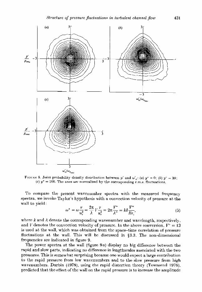
& Spalart (1988), in their analysis of the data of Spalart (1988), noticed a strong correspondence between low-pressure regions and streamwise vortices. It is likely that the intermittent occurrence of low-pressure fluctuations in the p.d.f. is associated with the vortices present in the flow. The joint probability density distribution between pressure fluctuations and streamwise vorticity fluctuations is examined to find out whether this is the case. The joint p.d.f.s a t y+ z 30 and 100 (figure 8) indicate that large streamwise vorticity fluctuations are indeed more likely associated with large negative pressure fluctuations. It should be noted, however, that the reverse is not true. Large negative pressure fluctuations are not necessarily associated with the large streamwise vorticity fluctuations, suggesting that additional information is required in identifying organized vortical structures.

3.2. Power spectra and two-point correlations The power spectra and two-point correlations in the streamwise direction at three different y-locations are shown in figures 9 and 10. Because of the low Reynolds number considered here, we do not expect to Bee the distinct power-law behaviours for different wavenumber ranges For example, neither the k-l range of Bradshaw (1967) nor the inertial subrange can be differentiated in figure 9 except for very narrow bands whose tangents are parallel to the expected slopes (one can show from a dimensional argument that the rapid pressure should decay as k d while the slow pressure should dccay as kf).

Structure of pressure fluctuations in turbulent channel $ow 43 1

P I

Prms _ - -3

I I

- 3

4 / W Z r m e

FIGUKE 8. Joint probability density distribution between p' and dz: ( a ) y+ = 0 . , ( b ) y+ = 30; (c) y+ = 100. The axes are normalized by the corresponding r.m.s. fluctuations.

To compare the present wavenumber spectra with the measured frequency spectra, we invoke Taylor's hypothesis with a convection velocity of pressure a t the

where k and h denote the corresponding wavenumber and wavelength, respectively, and V denotes the convection velocity of pressure. I n the above conversion, V+ = 13 is used at the wall, which was obtained from the space-time correlation of pressure fluctuations a t the wall. This will be discussed in $3.3. The non-dimensional frequencies are indicated in figure 9.

The power spectra a t the wall (figure 9 a ) display no big difference between the rapid and slow parts, indicating no difference in lengthscales associated with the two pressures. This is somewhat surprising because one would expect a large contribution to the rapid pressure from low wavenumbers and to the slow pressure from high wavenumbers. Durbin (1978), using the rapid distortion theory (Townsend 1976), predicted that the effect of the wall on the rapid pressure is to increase the amplitude

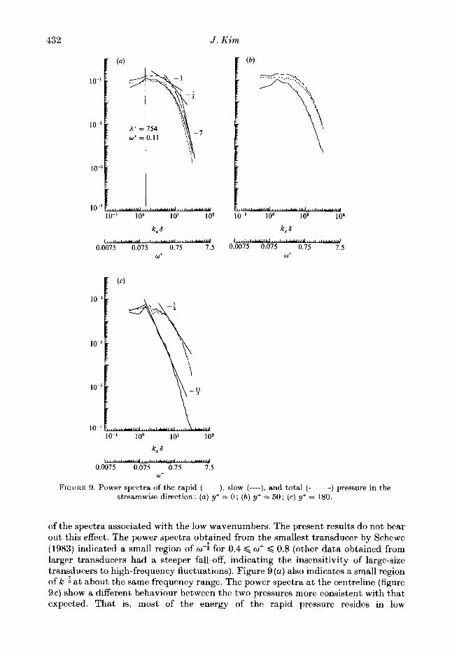
432 J . Kim -9 A' = 754 w+ = 0.11

s, - 7

lo-' 10-1 100 10' 1 O2

kz 8 P k A d d d U d

0.0075 0.075 0.75 7.5 Wf

10-1 100 10' 102

k, 8

0.0075 0.075 0.75 7.5 w+

10-1

10-3

10-7

k, 8

0.0075 0.075 0.75 1.5 &I+

FIGURE 9. Power spectra of the rapid (-), slow (----), and total (---) pressure in the streamwise direction: (a) y+ = 0 ; ( b ) y' = 50; (c) y+ = 180.

of the spectra associated with the low wavenumbers. The present results do not bear out this effect. The power spectra obtained from the smallest transducer by Schewe (1983) indicated a small region of O J - ~ for 0.4 < O+ < 0.8 (other data obtained from larger transducers had a steeper fall-off, indicating the insensitivity of large-size transducers to high-frequency fluctuations). Figure 9 ( a ) also indicates a small region of k-; a t about the same frequency range. The power spectra a t the centreline (figure 9c) show a different behaviour between the two pressures more consistent with that expected. That is, most of the energy of the rapid pressure resides in low

Structure of pressure fluctuations in turbulent channel flow 433

-0.5 ILLLLLLLLLLL-ILLLLLLLLLLLL--LL

-0.5 < 1 .o

0 1 2 3 4 5 6

X I 6

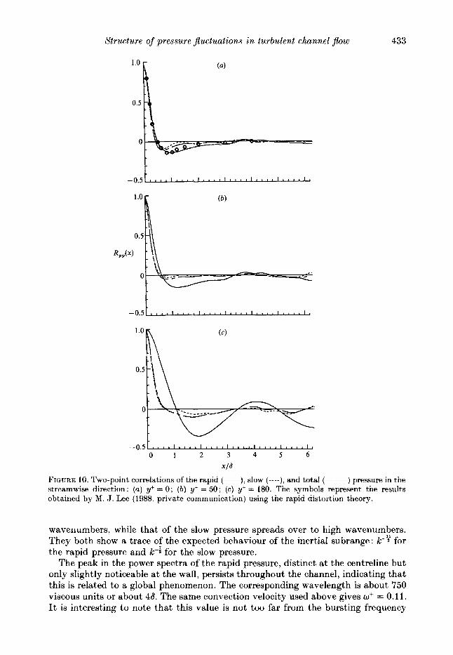
FIGURE 10. Two-point correlations of the rapid (-1, slow (----), and total (----) pressure in the streamwise direction: ( a ) y+ = 0 ; ( b ) y+ = 50; (c) y+ = 180. The symbols represent the results obtained by M. J. Lee (1988, private communication) using the rapid distortion theory.

wavenumbers, while that of the slow pressure spreads over to high wavenumbers. They both show a trace of the expected behaviour of the inertia1 subrange: k-y for the rapid pressure and kf for the slow pressure.

The peak in the power spectra of the rapid pressure, distinct at the centreline but only slightly noticeable a t the wall, persists throughout the channel, indicating that this is related to a global phenomenon. The corresponding wavelength is about 750 viscous units or about 46. The same convection velocity used above gives o+ = 0.1 1. It is interesting to note that this value is not too far from the bursting frequency

434 J . Kim

-400 -200 0 200 400

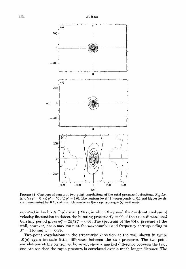
Ax+ FIGURE 1 I . Contours of constant two-point correlations of the total pressure fluctuations, R,,(Ax, Az): (a) y+ = 0 ; (6) y+ = 50; ( c ) y+ = 180. The contour level ‘ 1 ’ corresponds to 0.1 and higher levels are incremented by 0.1, and the tick marks in the axes represent 50 wall units.

reported in Luchik & Tiederman (1987), in which they used the quadrant analysis of velocity fluctuation to detect the bursting process : T l = 90 of their non-dimensional bursting period gives W: = 2x/T,+ = 0.07. The spectrum of the total pressure at the wall, however, has a maximum at the wavenumber and frequency corresponding to A+ = 330 and W+ = 0.26.

Two-point correlations in the streamwise direction at the wall shown in figure 10(a) again indicate little difference between the two pressures. The two-point correlations a t the centreline, however, show a marked difference between the two ; one can see that the rapid pressure is correlated over a much longer distance. The

Structure of pressure jluctuations in turbulent channel $ow 435

0

F " " " : I 7 - 1 <:-.. .......

................... .............. .... 200 6 ............. ............. < :.. ...................

.......... ... ,I.-. .......

....... I 4

: _,.-

-200 l L . - _

.......... '...+ .. ................

...... .......... :? 1 ....... ......... <..

.... p.. ............. :I.- ..........

I t ~ .............. I J-

0

-400 -200 0 200 400 Ax+

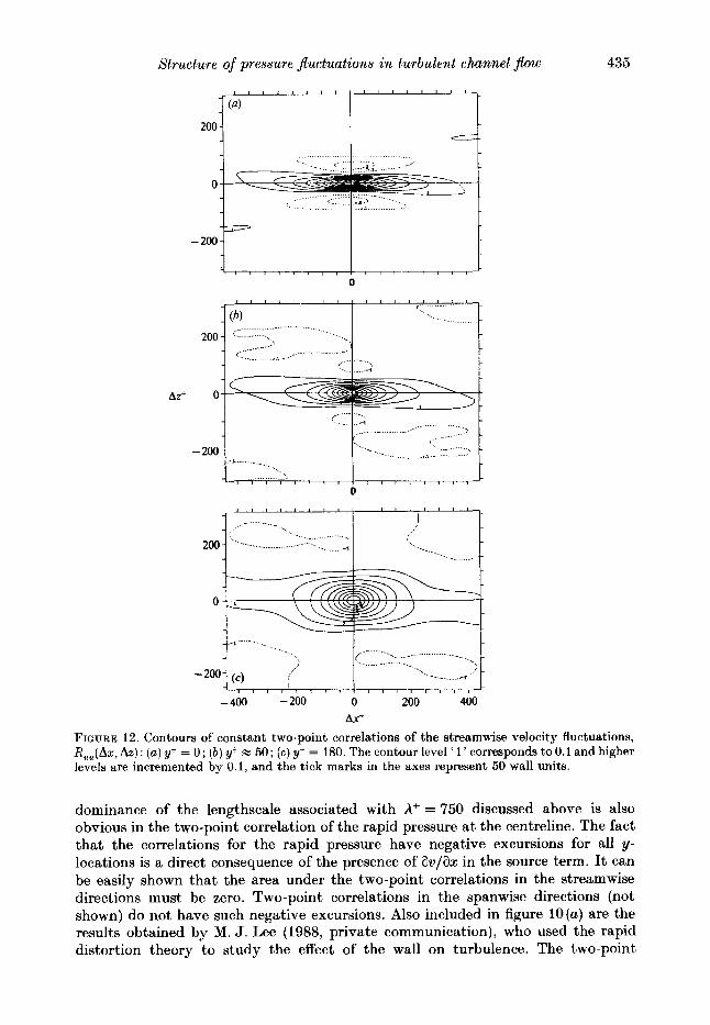
FIGURE 12. Contours of constant two-point correlations of the streamwise velocity fluctuations, Ruu(Ax, Az) : (a) y+ = 0; (5) y+ x 50; ( e ) y+ = 180. The contour level ' 1 ' corresponds to 0.1 and higher levels are incremented by 0.1, and the tick marks in the axes represent 50 wall units.

dominance of the lengthscale associated with A+ = 750 discussed above is also obvious in the two-point correlation of the rapid pressure at the centreline. The fact that the correlations for the rapid pressure have negative excursions for all y- locations is a direct consequence of the presence of av/ax in the source term. It can be easily shown that the area under the two-point correletions in the streamwise directions must be zero. Two-point correlations in the spanwise directions (not shown) do not have such negative excursions. Also included in figure 10(a) are the results obtained by M. J. Lee (1988, private communication), who used the rapid distortion theory to study the effect of the wall on turbulence. The two-point

436 J . Kim

1

0

AX+ = 50 - - 1 ! I I I I 1 ; I 0 1 I L

-200 -100 0 100 200

l - 4

Ax+

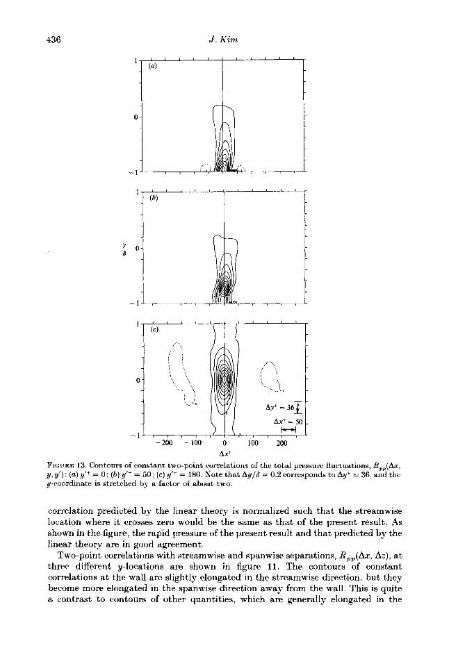
FIGURE 13. Contours of constant two-point correlations of the total pressure fluctuations, R,,(Ax, y, y’) : (a ) y’+ = 0 ; ( b ) y’+ = 50 ; ( c ) y’+ = 180. Note tha t Ay/6 = 0.2 corresponds t o Ay+ = 36, and the y-coordinate is stretched by a factor of about two.

correlation predicted by the linear theory is normalized such that the streamwise location where it crosses zero would be the same as that of the present result. As shown in the figure, the rapid pressure of the present result and that predicted by the linear theory are in good agreement.

Two-point correlations with streamwise and spanwise separations, R,,(Ax, Az), at three different y-locations are shown in figure 11. The contours of constant correlations at the wall are slightly elongated in the streamwise direction, but they become more elongated in the spanwise direction away from the wall. This is quite a contrast to contours of other quantities, which are generally elongated in the

Structure of pressure jluctuations in turbulent channel jlow 437

streamwise direction in the wall region and become less so away from the wall. For comparison, contours of constant two-point correlations of the streamwise velocity fluctuations are shown in figure 12. Two-point correlations of the streamwise velocity fluctuations near the wall (figure 12a) illustrate the presence of the familiar streaky structures elongated in the streamwise direction, alternating in the spanwise direction with the mean spanwise spacing - estimated by twice the distance of the negative peak - of about 100 wall units. The streamwise elongation becomes less pronounced away from the wall (figure 12 b, c ) . The two-point correlations of the wall pressure shown in figure 11 (a) are similar to those obtained by Bull (1967), but there are some differences. Bull’s results showed that contours for the high correlations were round, and become oval shapes at low correlations, but the present results do not show the oval shape at lower correlations. The contours a t the centreline of the present results (figure 11 c ) are more like Bull’s results at the wall.

Contours of constant two-point correlations of pressure as a function of streamwise and normal separations, R,,(Ax, y, y‘), a t three different y’ locations are shown in figure 13. For comparison, the same contours for the streamwise velocity fluctuations are also shown in figure 14. Note that in figures 13 and 14, the y-coordinate is stretched by a factor of about two and the domain extends to the other wall. Unlike the correlations of streamwise velocity fluctuations, the maximum correlation of the pressure fluctuations is approximately aligned along the normal direction to the wall. Note that contours of streamwise velocity fluctuations illustrate the presence of inclined structure, with the maximum correlation aligned along a line inclined about 20” to the wall (figure 14b). Two-point correlations along the normal direction with zero separations in the streamwise and spanwise directions are shown in figure 15, and indicate that the correlation length for the pressure along the normal direction is much larger than for the other quantities.

3.3. Space-time correlation and convection velocity

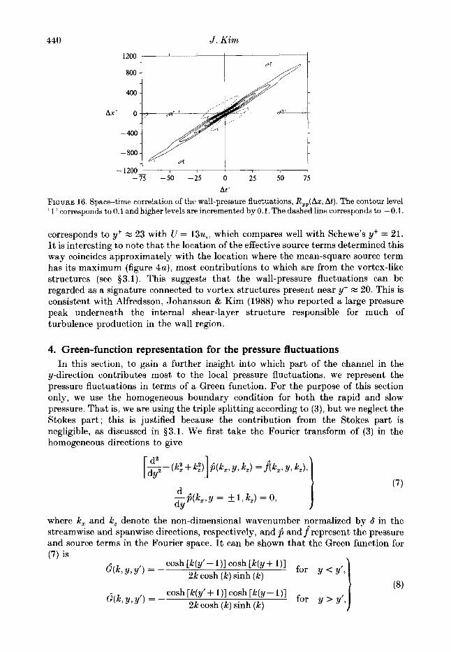
Space-time correlations of the total pressure as a function of streamwise separation and time delay, R,,(Ax, At), are computed from 50 consecutive pressure fields, which were obtained from 50 consecutive velocity fields stored a t an interval of At+ = 3. Figure 16 shows the space-time correlation a t the wall. It shows basically the same characteristics as measured by Willmarth & Wooldridge (1962) in a turbulent boundary layer. The maximum correlation is along the first (or third by the symmetry) quadrant in the (Ax, At)-plane, indicating that the pressure eddies are propagating downstream. They lose their correlations as they propagate down- stream, and there is a slight increase in the slope of dAxldAt, suggesting that the propagation speed of large eddies is higher than that of small eddies because only large eddies retain their coherence a t large time separations.

There are several ways to determine propagation velocityt using the space-time correlations (see Wills 1964, for example). In the present work, we used the propagation velocity determined by

Axmax is the streamwise separation where the space-time correlation, R,,(Ax, At), is maximum for a given At. V, determined this way will be a function of At used in (6), but their variation is rather small, as indicated in figure 16 where the ridge of the

t Strictly speaking, it is ‘propagation velocity’, but the term ‘convection velocity’ has been used in the literature. We use them interchangeably in the present paper.

438 J . Kim

0

1

0

- 1 -200 -100 0 100 200

AX+

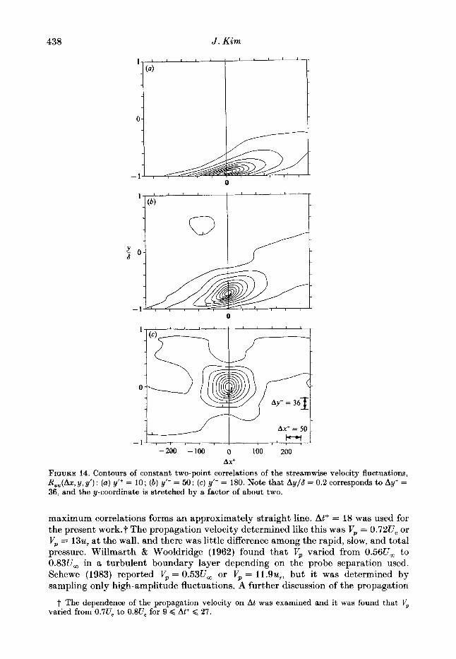
FIQURE 14. Contours of constant two-point correlations of the streamwise velocity fluctuations, R,,(Ax, y, y’) : (a) y’+ = 10; ( b ) y’+ = 50; (c) y’+ = 180. Note that Ay/S = 0.2 corresponds to Ay+ = 36, and the y-coordinate is stretched by a factor of about two.

maximum correlations forms an approximately straight line. At+ = 18 was used for the present w0rk.t The propagation velocity determined like this was V, = 0.72Uc or V, = 13u, at the wall, and there was little difference among the rapid, slow, and total pressure. Willmarth & Wooldridge (1962) found that V, varied from 0.56Um to 0.83Ua in a turbulent boundary layer depending on the probe separation used. Schewe (1983) reported V, = O.53Ua or V, = 11.9u,, but it was determined by sampling only high-amplitude fluctuations. A further discussion of the propagation

t The dependence of the propagation velocity on At was examined and it was found that varied from O.7Uc to O.8Uc for 9 < At+ < 27.

Structure of pressure jluctuations in turbulent channel jlow 439

t

-0.5 1 -1.0 -0.5 0 0.5 1 .o

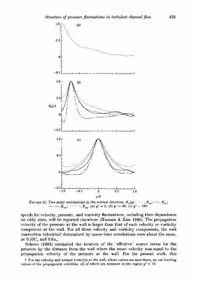
YI6 FIGURE 15. Two-point correlations in the normal direction, R,,(y): -, R,,,,; ----, R "" . I

, Rww; . . . . . . , Rpp . (a) y+=O; ( b ) y c = 5 0 ; (c) y'= 180.

speeds for velocity, pressu're, and vorticity fluctuations, including their dependence on eddy sizes, will be reported elsewhere (Hussain & Kim 1989). The propagation velocity of the pressure a t the wall is larger than that of each velocity or vorticity component a t the wall. For all three velocity and vorticity components, the wall convection velocitiesi determined by space-time correlations were about the same, a t O.53Uc and 9 . 6 ~ ~ .

Schewe (1983) estimated the location of the 'effective' source terms for the pressure by the distance from the wall where the mean velocity was equal to the propagation velocity of the pressure a t the wall. For the present work, this

t For the velocity and normal vorticity at the wall, whose values are zero there, we use limiting values of the propagation velocities, all of which are constant in the region y+ < 10.

440 J . Kim

-75 -50 -25 0 25 50 75

At+

FIGURE 16. Space-trme correlation of the wall-pressure fluctuations, Rpp(Az , At). The contour level ‘ 1 ’ corresponds to 0.1 and higher levels are incremented by 0.1. The dashed line corresponds to - 0.1.

corresponds to y+ x 23 with U = 13u,, which compares well with Schewe’s yf = 21. It is interesting to note that the location of the effective source terms determined this way coincides approximately with the location where the mean-square source term has its maximum (figure 4a), most contributions to which are from the vortex-like structures (see 53.1). This suggests that the wall-pressure fluctuations can be regarded as a signature connected to vortex structures present near y+ x 20. This is consistent with Alfredsson, Johansson & Kim (1988) who reported a large pressure peak underneath the internal shear-layer structure responsible for much of turbulence production in the wall region.

4. Green-function representation for the pressure fluctuations In this section, to gain a further insight into which part of the channel in the

y-direction contributes most to the local pressure fluctuations, we represent the pressure fluctuations in terms of a Green function. For the purpose of this section only, we use the homogeneous boundary condition for both the rapid and slow pressure. That is, we are using the triple splitting according to (3), but we neglect the Stokes part; this is justified because the contribution from the Stokes part is negligible, as discussed in 53.1. We first take the Fourier transform of (3) in the homogeneous directions to give

where k, and k, denote the non-dimensional wavenumber nlormalized by 6 in the streamwise and spanwise directions, respectively, and $ and f represent the pressure and source terms in the Fourier space. It can be shown that the Green function for (7) is

cash [k(y’- l)] cash [k(y+ l)] for y < y’, ‘(” ””) = -

‘(k’y’ ”) = -

2k cosh (k) sinh (k)

cash [k(y’+ l)] cash [k(y- I)] for y > y’,

2kcosh (k) sinh (k)

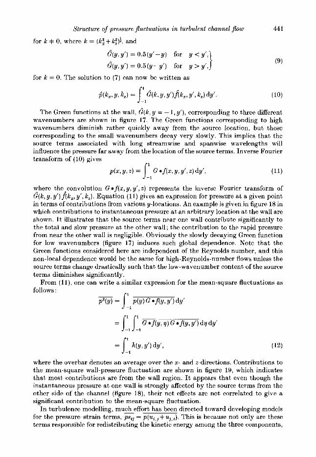
Structure of pressure fluctuations in turbulent channel flow 44 1

for k =+ 0, where k = ( k i + and

d(y, y’) = 0.5(y’- y) for y < y’,l

d(y, y’) = 0.5(y-y‘) for y > y’,j

for k = 0. The solution to (7) can now be written as

(9)

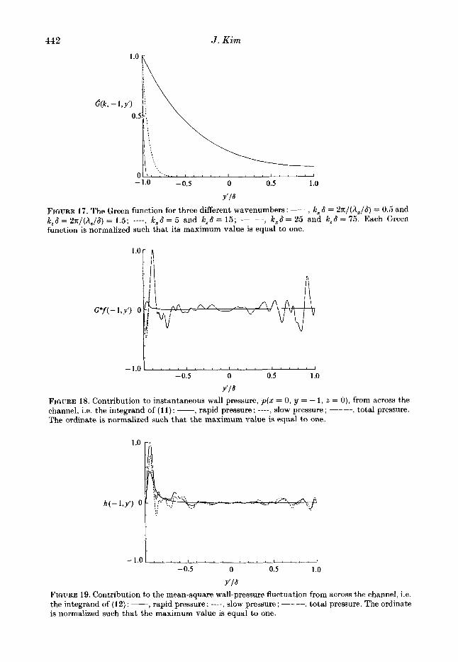
The Green functions a t the wall, d(k, y = - 1, y’), corresponding to three different wavenumbers are shown in figure 17. The Green functions corresponding to high wavenumbers diminish rather quickly away from the source location, but those corresponding to the small wavenumbers decay very slowly. This implies that the source terms associated with long streamwise and spanwise wavelengths will influence the pressure far away from the location of the source terms. Inverse Fourier transform of (10) gives

r i

where the convolution G * f(x, y, y’, z ) represents the inverse Fourier transform of d(k, y, y’)f(k,, y‘, kz). Equation (11) gives an expression for pressure at a given point in terms of contributions from various y-locations. An example is given in figure 18 in which contributions to instantaneous pressure at an arbitrary location at the wall are shown. It illustrates that the source terms near one wall contribute significantly to the total and slow pressure at the other wall; the contribution to the rapid pressure from near the other wall is negligible. Obviously the slowly decaying Green function for low wavenumbers (figure 17) induces such global dependence. Note that the Green functions considered here are independent of the Reynolds number, and this non-local dependence would be the same for high-Reynolds-number flows unless the source terms change drastically such that the low-wavenumber content of the source terms diminishes significantly.

From ( l l ) , one can write a similar expression for the mean-square fluctuations as follows :

where the overbar denotes an average over the x- and z-directions. Contributions to the mean-square wall-pressure fluctuation are shown in figure 19, which indicates that most contributions are from the wall region. It appears that even though the instantaneous pressure a t one wall is strongly affected by the source terms from the other side of the channel (figure 18), their net effects are not correlated to give a significant contribution to the mean-square fluctuation.

I n turbulence modelling, much effort has been directed toward developing models for the pressure-strain terms, = ~ ( U ~ , ~ + U , , ~ ) . This is because not only are these terms responsible for redistributing the kinetic energy among the three components,

442

1.0 F

J . Kim

0 , , I , , , , I , , , , I , , , , , - 1.0 -0.5 0 0.5 1 .o

Y’I6

FIQURE 17. The Green function for three different wavenumbers : -, k, S = 2n/(h,/S) = 0.5 and k,S = 2n/(A,/S) = 1.5; ----, k,S = 5 and k,S = 15; ---, k,S = 25 and k,S = 75 . Each Green function is normalized such that its maximum value is equal to one.

-0.5 0 0.5 1 .o Y’J6

FIQURE 18. Contribution to instantaneous wall pressure, p ( x = 0, y = - 1, 3 = 0 ) , from across the channel, i.e. the integrand of (1 1) : -, rapid pressure ; ----, slow pressure ; ---, total pressure. The ordinate is normalized such that the maximum value is equal to one.

-0.5 0 0.5 1.0

Y‘/6 FIGURE 19. Contribution to the mean-square wall-pressure fluctuation from across the channel, i.e. the integrand of (12) : -, rapid pressure; ----, slow pressure; ---, total pressure. The ordinate is normalized such that the maximum value is equal to one.

Structure of pressure Jluctuations in turbulent channel $ow 443

I

-1.olV. , , . 1 . , ' ' 8 ' ' ' '

-0.5 0 0.5' 1 .O

Y'l6 FIGURE 20(a-c). For caption see next page.

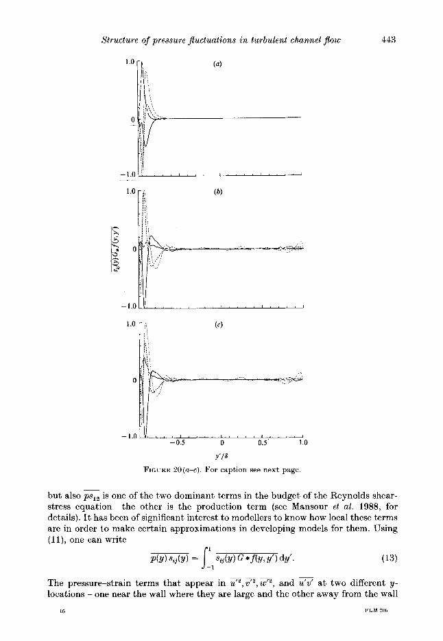
but also ps,, is one of the two dominant terms in the budget of the Reynolds shear- stress equation - the other is the production term (see Mansour et al. 1988, for details). It has been of significant interest to modellers to know how local these terms are in order to make certain approximations in developing models for them. Using ( l l ) , one can write

(13) 1

P ( Y ) S d Y ) = I, S d Y ) G * f ( Y > Y') dY'. - _ -

The pressure-strain terms that appear in u", d2, wr2, and a a t two different y- locations - one near the wall where they are large and the other away from the wall

15 FLM 205

444 J . Kim

- 1.0 >

-1.01 , , , ' , ' , ' , ' ' . ' ' ' * . ' . 1

1 .o

0

-1.0 -0.5 0 0.5 1 .o

Y'/6

FIGURE 20. Contributions to the pressurestrain correlations, i.e. the integrand of (13) : -, 2p(au /ax) ; ----, 2p(av/ay); ---, 2p(i3w/az) ; . . . . . . , p(au/ay+av/az). The ordinate is normalized such that the maximum value of the four terms is equal to one. ( a ) rapid, ( b ) slow, and (c) total pressure-strain at y+ x 10; ( d ) rapid, ( e ) slow, and (f) total pressurestrain a t y+ x 100.

where they are relatively small (Mansour et al. 1988) - are shown in figure 20. It is clear from the figures that the pressure-strain correlations in the wall region (figure 20 a-c) take their largest contributions ,from the wall region (contributions are local), but away from the wall the pressure-strain terms at a given y-location take their contributions from wide ranges of y-locations (global). This non-local character of the pressure-strain terms would make them hard to model in terms of local variables.

Structure of pressure Jluctuations in turbulent channel jlow 445

. . . . . . . . . . . . . . . . . . . . . . . .

(6)

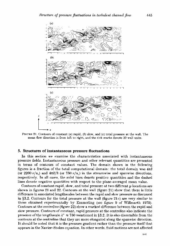
FIGURE 21. Contours of constant ( a ) rapid, (b ) slow, and (c) total pressure at the wall. The mean flow direction is from left to right, and the tick marks denote 50 wall units.

5. Structures of instantaneous pressure fluctuations In this section we examine the characteristics associated with instantaneous

pressure fields. Instantaneous pressure and other relevant quantities are presented in terms of contours of constant values. The domain shown in the following figures is a fraction of the total computational domain: the total domain was 4x8 (or 2260 vIu,) and 4x813 (or 750 vIu,) in the streamwise and spanwise directions, respectively. In all cases, the solid lines denote positive quantities and the dashed lines denote negative quantities with respect to the plane-averaged mean value.

Contours of constant rapid, slow, and total pressure a t two different y-locations are shown in figures 21 and 22. Contours at the wall (figure 21) show that there is little difference in associated lengthscales between the rapid and slow pressure as discussed in $3.2. Contours for the total pressure a t the wall (figure 21c) are very similar to those obtained experimentally by Emmerling (see figure 9 of Willmarth 1975). Contours a t the centreline (figure 22) show a marked difference between the rapid and slow pressure. Contours of constant, rapid pressure a t the centreline also indicate the presence of the lengthscale A+ x 750 mentioned in $3.2. It is also discernible from the contours a t the centreline that they are more elongated along the spanwise direction. It should be noted that it is the pressure gradient rather than the pressure itself that appears in the Navier-Stokes equation. In other words, fluid motions are not affected

15.2

446 J . Kim

LT " " " ' ! " ' " ' ' t " ' FIGURE 22. Contours of constant ( a ) rapid, ( b ) slow, and (c) total pressure a t the centreline. The

mean flow direction is from left to right, and the tick marks denote 50 wall units.

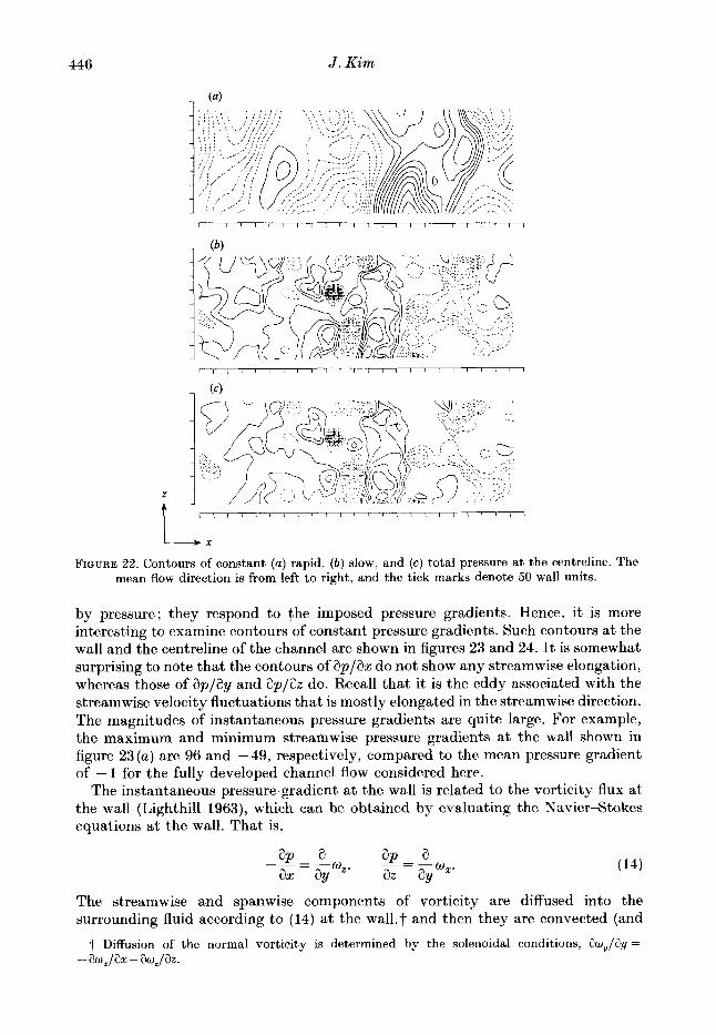
by pressure; they respond to the imposed pressure gradients. Hence, it is more interesting to examine contours of constant pressure gradients. Such contours at the wall and the centreline of the channel are shown in figures 23 and 24. It is somewhat surprising to note that the contours of ap/ax do not show any streamwise elongation, whereas those of splay and ap/ax do. Recall that it is the eddy associated with the streamwise velocity fluctuations that is mostly elongated in the streamwise direction. The magnitudes of instantaneous pressure gradients are quite large. For example, the maximum and minimum streamwise pressure gradients a t the wall shown in figure 23 ( a ) are 96 and - 49, respectively, compared to the mean pressure gradient of - 1 for the fully developed channel flow considered here.

The instantaneous pressure gradient at the wall is related to the vorticity flux a t the wall (Lighthill 1963), which can be obtained by evaluating the Navier-Stokes equations a t the wall. That is,

The streamwise and spanwise components of vorticity are diffused into the surrounding fluid according to (14) a t the wall,? and then they are convected (and

7 Diffusion of the normal vorticity is determined by the solenoidal conditions, awU/ay = - aw,/ax - bo,/az.

Structure of pressure Jluctuations in turbulent channel flow 447

FIGURE 23. Contours of constant (a) ap/ax, (6) ap/ay, and (c) applaz at the wall. The mean flow direction is from left to right, and the tick marks denote 50 wall units.

diffused) from the wall region. They will subsequently interact with (and modify) turbulence structures responsible for the source terms that created the pressure gradients at the wall. The new, modified source terms will create new pressure gradients at the wall, which in turn determine the flux of vorticity a t the wall, and so on. From (11) and figure 18, we also note that the vorticity flux at the wall is determined globally. Even the source term on the other side of the channel will influence the flux of vorticity a t one side of the channel by affecting the instantaneous pressure and, hence, the instantaneous pressure gradient. In some transitional flows, the pressure gradients at the wall and source terms away from the wall - usually located just above the critical layer -work together in phase to contribute to flow instability (M. V. Morkovin. 1988, private communication). Also, Kim (1983) and Alfredsson et al. (1988) showed a strong link between a turbulence structure responsible for intense turbulence production and a localized pressure peak at the surface. This suggests a possibility that one can modify the structure of turbulence by artificially modifying the pressure gradient a t the wall, and hence the turbulence production in the boundary layer.

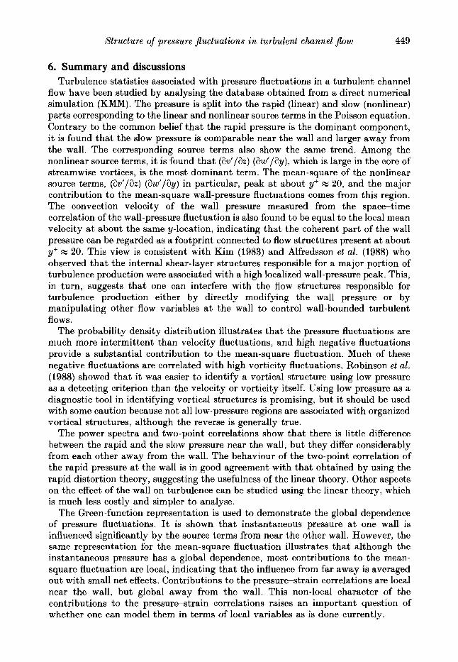
Contours of constant streamwise and spanwise vorticity a t the wall are shown in figure 25. A striking similarity exists between the spanwise pressure gradient at the wall (figure 23c) and the streamwise vorticity a t the wall (figure 25a) , but the correlation between the streamwise pressure gradient a t the wall (figure 23a) and spanwise vorticity (figure 25b) is not discernible at all. It is not clear what causes this difference.

448 J . Kim

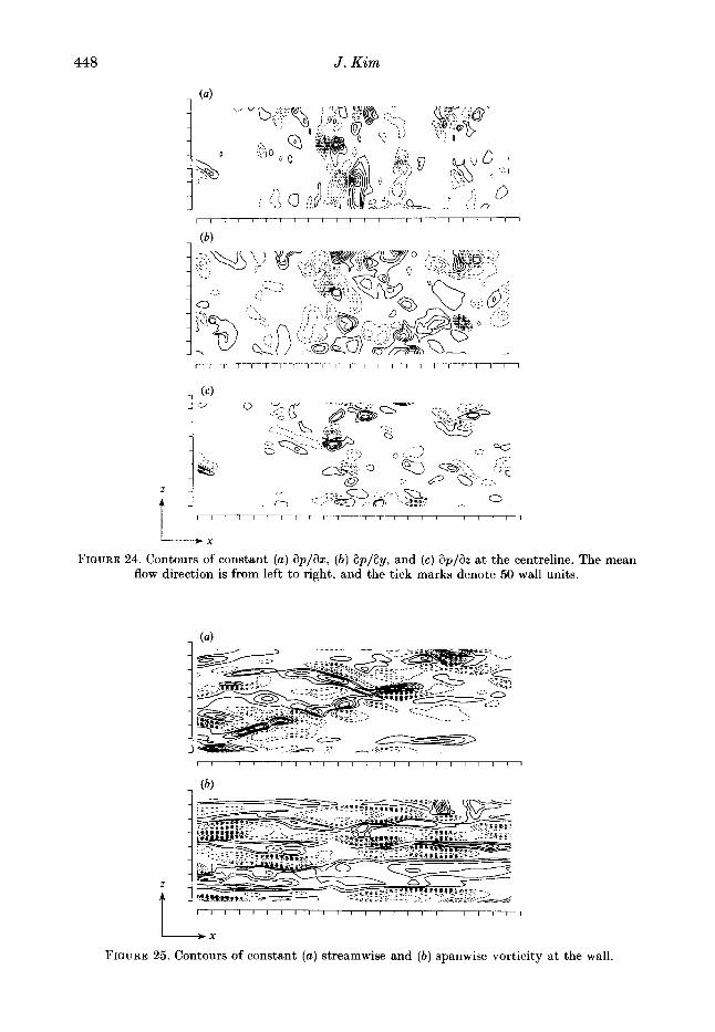
FIGURE 24. Contours of constant ( a ) applax, ( b ) applay, and ( c ) applaz at the centreline. The mean flow direction is from left t o right, and the tick marks denote 50 wall units.

1 1 1 1 1 1 1 1 1 1 1 1 1 1 1 1 1 1 1 1 1 1 1 1

L:. ' ' I ' I ' I ' I 1 I ' ' ' I I I ' ' I

FIGURE 25. Contours of constant ( a ) streamwise and ( b ) spanwise vorticity at the wall.

Structure of pressure fluctuations in turbulent channel $ow 449

6. Summary and discussions Turbulence statistics associated with pressure fluctuations in a turbulent channel

flow have been studied by analysing the database obtained from a direct numerical simulation (KMM). The pressure is split into the rapid (linear) and slow (nonlinear) parts corresponding to the linear and nonlinear source terms in the Poisson equation. Contrary to the common belief that the rapid pressure is the dominant component, i t is found that the slow pressure is comparable near the wall and larger away from the wall. The corresponding source terms also show the same trend. Among the nonlinear source terms, it is found that (av’laz) (aw’lay), which is large in the core of streamwise vortices, is the most dominant term. The mean-square of the nonlinear source terms, (ad lax ) (aw’lay) in particular, peak a t about y+ w 20, and the major contribution to the mean-square wall-pressure fluctuations comes from this region. The convection velocity of the wall pressure measured from the space-time correlation of the wall-pressure fluctuation is also found to be equal to the local mean velocity at about the same y-location, indicating that the coherent part of the wall pressure can be regarded as a footprint connected to flow structures present a t about y+ % 20. This view is consistent with Kim (1983) and Alfredsson et al. (1988) who observed that the internal shear-layer structures responsible for a major portion of turbulence production were associated with a high localized wall-pressure peak. This, in turn, suggests that one can interfere with the flow structures responsible for turbulence production either by directly modifying the wall pressure or by manipulating other flow variables a t the wall to control wall- bounded turbulent flows.

The probability density distribution illustrates that the pressure fluctuations are much more intermittent than velocity fluctuations, and high negative fluctuations provide a substantial contribution to the mean-square fluctuation. Much of these negative fluctuations are correlated with high vorticity fluctuations. Robinson et al. (1988) showed that it was easier to identify a vortical structure using low pressure as a detecting criterion than the velocity or vorticity itself. Using low pressure as a diagnostic tool in identifying vortical structures is promising, but it should be used with some caution because not all low-pressure regions are associated with organized vortical structures, although the reverse is generally true.

The power spectra and two-point correlations show that there is little difference between the rapid and the slow pressure near the wall, but they differ considerably from each other away from the wall. The behaviour of the two-point correlation of the rapid pressure a t the wall is in good agreement with that obtained by using the rapid distortion theory, suggesting the usefulness of the linear theory. Other aspects on the effect of the wall on turbulence can be studied using the linear theory, which is much less costly and simpler to analyse.

The Green-function representation is used to demonstrate the global dependence of pressure fluctuations. It is shown that instantaneous pressure at one wall is influenced significantly by the source terms from near the other wall. However, the same representation for the mean-square fluctuation illustrates that although the instantaneous pressure has a global dependence, most contributions to the mean- square fluctuation are local, indicating that the influence from far away is averaged out with small net effects. Contributions to the pressure-strain correlations are local near the wall, but global away from the wall. This non-local character of the contributions to the pressure-strain correlations raises an important question of whether one can model them in terms of local variables as is done currently.

450 J . Kim

Contours of constant pressure gradients show that those associated with ap,lay and ap/az are somewhat elongated in the streamwise direction, but not those associated with ap,lax. Examination of vorticity and pressure gradients a t the wall, which control the diffusion of vorticity from the wall, shows a strong correlation between w, and ap/az, but it shows no apparent correlation between w, and aplax. Further study is required to explain this interesting but puzzling observation.

I am grateful to Dr Nagi N. Mansour for many discussions during the course of this work, and to Professor P. Bradshaw and Drs Philippe R. Spalart and Sanjiva Lele for helpful comments on a draft of this manuscript.

R E F E R E N C E S

ALFREDSSON, P. H., JOHANSSON, A. V. & KIM, J . 1988 Turbulence production near walls: the role of flow structures with spanwise asymmetry. Proc. 1988 Summer School, CTR-S88. Center for Turbulence Research, NASA Ames Research Center.

BLAKE, W. K. 1970 Turbulent boundary layer wall-pressure fluctuations on smooth and rough walls. J . Fluid Mech. 44, 637.

BRADSHAW, P. 1967 Inactive motion and pressure fluctuations in turbulent boundary layers. J . Fluid Mech. 30, 241.

BULL, M. K. 1967 Wall pressure fluctuations associated with subsonic turbulent boundary layer flow. J . Fluid Mech. 28, 719.

CORCOS, G. M. 1964 The structure of the turbulent pressure field in boundary-layer flows. J . Fluid Mech. 18, 353.

DURBIN, P. A. 1978 Rapid distortion theory of turbulent flows. Ph.D. thesis, University of Cambridge.

ECKELMANN, H. 1988 A review of knowledge on pressure fluctuations. Proc. Zoran Zaric Memorial International Seminar on Near- Wall Turbulence, May 16-20, 1988. Dubrovnik, Yugoslavia.

HUSSAIN, A. K. M. F. & KIM, J. 1989 On the convection velocity of turbulent eddies. In preparation.

KIM, J. 1983 On the structure of wall-bounded turbulent flows. Phys. Fluids 26, 2088. KIM, J. , MOIN, P. & MOSER, R. D. 1987 Turbulence statistics in fully developed channel flow at

low Reynolds number. J . Fluid Mech. 177, 133 (referred to as KMM). KRAICHNAN, R. H. 1956 Pressure fluctuations in turbulent flow over a flat plate. J . Acoust. SOC.

A m . 28, 378. LIGHTHILL, M. J. 1963 Boundary layer theory. In Laminar Boundary Layers (ed. Rosenhead).

Oxford University Press. LILLEY, G. M. 1964 A review of pressure fluctuations in turbulent boundary layers at subsonic

and supersonic speeds. Arch. Mech. Stosow. 16, 301. LUCHIK, T. S. & TIEDERMAN, W. G. 1987 Timescale and structure of ejections and bursts in

turbulent channel flows. J . Fluid Mech. 174, 529. MANSOUR, IS. IS., KIM, J. & MOIN, P. 1988 Reynolds-stress and dissipation rate budgets in a

turbulent channel flow. J . Fluid Mech. 194, 15. MOIN, P. & KIM, J. 1980 On the numerical solution of time-dependent viscous incompressible fluid

flows involving solid boundaries. J . Comp. Phys. 35, 381. MOIN, P. & KIM, J. 1982 Kumerical investigation of turbulent channel flow. J . Fluid Mech. 118,

341. PANTON, R. & LINEBARGER, J. H. 1974 Wall pressure spectra calculations for equilibrium

boundary layers. J . Fluid Mech. 65, 261. PHILLIPS, 0. M. 1956 On the generation of waves by turbulent wind. J . Fluid Mech. 2, 417. ROBINSON, S. K., KLINE, S. J . & SPALART, P. R. 1988 Quasi-coherent structures in the turbulent

boundary layer : Part 11. Verification and new information from a numerically simulated flat- plate layer. Proc. Zoran Zaric Memorial International Seminar on Near- Wall Turbulence, May 16-20, 1988. Dubrovnik, Yugoslavia.

Structure of pressure fluctuations in turbulent channel flow 45 1

SCHEWE, G. 1983 On the structure and resolution of wall-pressure fluctuations associated with

SPALART, P. R. 1988 Direct simulation of a turbulent boundary layer up to Re, = 1410. J . Fluid

TOWNSEND, A. A. 1976 The Structure of Turbulent Shear Flozus, 2nd edn. Cambridge University

WILLMARTH, W. W. 1975 Pressure fluctuations beneath turbulent boundary layers. Ann. Rev.

WILLMARTH, W . W. & WOOLDRIDOE, C. E. 1962 Measurements of the fluctuating pressure at the

WILLS, J. A. B. 1964 On convection velocities in turbulent shear flows. J . Fluid Mech. 20, 417.

turbulent boundary-layer flow. J . Fluid Mech. 134, 31 1.

Mech. 187, 61.

Press.

Fluid Mech. 7, 13.

wall beneath a thick turbulent boundary layer. J . Fluid Mech. 14, 187.