On the effect of mantle conductivity on the super-rotating jets near the liquid core surface

A

M

efssctE4tttsI©

P

K

1

ti

f

0d

Physics of the Earth and Planetary Interiors 160 (2007) 245–268

On the effect of mantle conductivity on the super-rotatingjets near the liquid core surface

K.A. Mizerski∗, K. BajerWarsaw University, Institute of Geophysics, ul. Pasteura 7, 02-093 Warszawa, Poland

Received 14 August 2006; received in revised form 13 November 2006; accepted 15 November 2006

bstract

We consider hydromagnetic Couette flows in planar and spherical geometries with strong magnetic field (large Hartmann number,� 1). The highly conducting bottom boundary is in steady motion that drives the flow. The top boundary is stationary and is

ither a highly conducting thin shell or a weakly conducting thick mantle. The magnetic field, B0 + b, is a combination of the strong,orce-free background B0 and a perturbation b induced by the flow. This perturbation generates strong streamwise electromagnetictress inside the fluid which, in some regions, forms a jet moving faster than the driving boundary. The super-velocity, in thepherical geometry called super-rotation, is particularly prominent in the region where the ‘grazing’ line of B0 has a point of tangentontact with the top boundary and where the Hartmann layer is singular. This is a consequence of topological discontinuity acrosshat special field line. We explain why the magnitude of super-rotation already present when the top wall is insulating [Dormy,., Jault, D., Soward, A.M., 2002. A super-rotating shear layer in magnetohydrodynamic spherical Couette flow. J. Fluid Mech.52, 263–291], considerably increases when that wall is even slightly conducting. The asymptotic theory is valid when either thehickness of the top wall is small, δ ∼ M−1 and its conductivity is high, ε ∼ 1 or when δ ∼ 1 and ε ∼ M−1. The theory predictshe super-velocity enhancement of the order of δM3/4 in the first case and εM3/4 in the second case. We also numerically solvehe planar problem outside the asymptotic regime, for ε = 1 and δ = 1, and find that with the particular B0 that we chose the peakuper-velocity scales like M0.33. This scaling is different from M0.6 found in spherical geometry [Hollerbach, R., Skinner, S., 2001.nstabilities of magnetically induced shear layers and jets. Proc. R. Soc. Lond. A 457, 785–802].

2006 Elsevier B.V. All rights reserved.

ACS: 91.25.Za; 91.35.Lj; 91.25.Wb

le boun
eywords: Super-rotating jets; Electromagnetic coupling; Core–mant
. Introduction

The coupling between the top of the outer core and
he base of the mantle is an important factor influenc-ng both the dynamics of the mantle and the details of
∗ Corresponding author. Tel.: +48 22 55 46 889;ax: +48 22 55 46 882.

E-mail address: [email protected] (K.A. Mizerski).

031-9201/$ – see front matter © 2006 Elsevier B.V. All rights reserved.oi:10.1016/j.pepi.2006.11.006

dary; Hartmann layer; Topological discontinuity

the flow in the core. The effects are believed to be sig-nificant on a wide range of time scales, from decadesto millions of years (Zatman, 2001), and over differentspatial scales from the overall budget of the axial an-gular moment to the details of the equatorial westwarddrift. There are several plausible coupling mechanisms
but the conditions at the core–mantle boundary (CMB)are not sufficiently well known to go beyond basic esti-mates of their relative importance and contribution to thelength of day (LOD) variations that are the main effect
mailto:[email protected]

dx.doi.org/10.1016/j.pepi.2006.11.006

rth and
246 K.A. Mizerski, K. Bajer / Physics of the Ea
and therefore the signature of the core–mantle coupling.Besides frictional, topographic and gravitational interac-tions the electromagnetic coupling (Bullard et al., 1950;Munk and Revelle, 1952) plays a somewhat special rolefor two reasons. Firstly, the magnetic field interpolatedfrom the Earth’s surface down to the CMB serves, inspite of the fundamental as well as experimental diffi-culties, as a tool for mapping the core surface flow (Paisand Hulot, 2000). Secondly, the assumptions of the elec-tromagnetic coupling (EMC) theory can be indirectlyverified by checking their compatibility with the Earth’sdynamo models.

Current theories of the EMC are concerned mainlywith the electromagnetic torque at the base of the man-tle. The question whether the electromagnetic torque inthe solidus is large enough to make a significant contribu-tion to the total core–mantle coupling or play a dominantrole in the LOD variations is still open (Bloxham, 1998)with arguments for (Holme, 1998) and against (Jault andLeMouel, 1991; Love and Bloxham, 1994) being pre-sented. The verdict depends on the physical propertiesof the mantle base, i.e., on the radial profile of electri-cal conductivity. Two possibilities are often considered(Greff-Lefftz and Legros, 1999). One is slight electri-cal conductivity over a large part of the lower mantle(Alexandrescu et al., 1999), the other is a thin, highlyconducting layer at the mantle base (Holme, 1998). Thelatter gains support from the recent diamond anvil ex-periments (Dubrovinsky et al., 2003).

However, the electromagnetic stresses in the CMBregion can yield extra torque in a more subtle way thatcould appropriately be termed ‘indirect electromagneticcoupling’. Differential rotation in the core penetrated bypoloidal magnetic field gives rise to a Hartmann layer.Such layer is a site of strong electromagnetic force inthe region immediately adjacent to the CMB but in-side the fluid which, as a result, is super-rotating. Such asuper-rotating jet exerts extra torque on the fluid in theboundary layer which can then be relayed to the man-tle by topographic coupling, possibly enhanced by addi-tional small-scale electromagnetic stresses. The essenceof such indirect coupling is therefore the electromagneticeffect in the liquid not the Lorenz force acting directlyin the solid.

Dormy et al. (1998) computed the flow in a rapidlyrotating spherical annulus with slightly super-rotating,electrically conducting inner sphere, filled with equallyconducting fluid penetrated by initially potential dipo-
lar magnetic field. They found that in the region wherethe critical magnetic field line (C-line) grazes the outer,insulating sphere (has a point of tangent contact) thefluid is super-rotating, that is the angular velocity of
Planetary Interiors 160 (2007) 245–268

the fluid exceeds that of the inner sphere. Recentlyalso experimental evidence has been given for the ex-istence of super-rotating jet in a similar (spherical)configuration by Nataf et al. (2006). They also ar-gued that such a jet may be a cause of instability inthe equatorial region, namely radial oscillations in thevicinity of the outer sphere. This may mean that suchsuper-rotating jet at the core–mantle boundary couldalso influence the stability of the boundary layer atthe CMB.

Hollerbach (2000) carried out computations of thesame magnetic Couette flow but with the outer spherehaving the electrical conductivity equal to that of thefluid. He also calculated a somewhat simplified problemwith a stationary outer sphere without the extra compli-cation of the overall spin of the entire system and the as-sociated Coriolis force. He found that with a conductingouter sphere the super-rotating jet is much stronger andits velocity scales with the Hartmann number as M0.6.Later Dormy et al. (2002) provided a detailed theoreticalanalysis of this super-rotation in the case of stationary,insulating outer sphere.

In this paper we extend the theory of Dormy et al.(2002) to the case of a conducting top boundary. The con-ductivity profile of the lower mantle is still an open issue,so we consider two possible types of the outer boundary.One is a very thin shell of thickness δ � 1 (the lengthscale being the depth of the fluid) with electrical con-ductivity ε = 1 (the conductivity of the fluid is taken asthe unit). This would be appropriate if there existed, as isoften assumed, a thin highly conducting solid layer at thebase of the mantle. In order to derive within our asymp-totic theory an analytical formula for the enhancement ofsuper-rotation we need to take δ ∼ M−1. Even for suchan extremely thin conducting shell we find considerableenhancement of super-rotation of the order of δM3/4. Forthe Earth’s interior where M ∼ 106 this would mean thata conducting layer only several metres thick at the baseof the mantle would increase super-rotation by about3%. The influence of a thicker layer would be muchstronger.

The other type of outer boundary is a thick but weaklyconducting mantle, δ ∼ 1, ε ∼ M−1 � 1. The resultsare similar. Hence, the conductivity of the mantle, evenslight, either in extent or in magnitude, increases super-rotation and therefore makes the indirect electromag-netic coupling stronger.

Before engaging in the detailed calculations we shall
give a brief explanation of the mechanism by which atopological discontinuity leads to a current sheet and theassociated Lorenz force driving a jet and a sheet of liquidmoving unexpectedly fast.

rth and Planetary Interiors 160 (2007) 245–268 247

2m

tsdaodot(

t‘csibfto

2

bemPFp

P

FF

wtggbimgkcdo

Fig. 1. The magnetic Couette flow in: (a) spherical and (b) planar ge-ometry. The inner sphere (bottom boundary) is steadily rotating (mov-ing) while the outer sphere (top boundary) is stationary. The thicknessof the fluid layer is L and the electrical conductivity of the fluid andof the inner (bottom) boundary is σ = σbot. The thickness and con-ductivity of the outer (top) boundary relative to those of the fluid areδ and ε = σ /σ, respectively. The basic potential magnetic field B

K.A. Mizerski, K. Bajer / Physics of the Ea

. Topological discontinuity at a criticalagnetic field line

The flows that we are going to consider are models ofhe magnetohydrodynamic configuration occurring in apecial region of the interface between the highly con-ucting liquid core and the solid mantle. Both the liquidnd the solid are penetrated by the magnetic field B0f which we consider only the large scale axisymmetricipole component. The flow is driven by a steady rotationf the conducting inner sphere that transfers momentumo the fluid by both electromagnetic and viscous couplingFig. 1a). The outer sphere is stationary.

The essential feature of the magnetic configuration ishe existence of a critical field line, the C-line. This is agrazing’ line, the only one that has a point of tangentialontact with the outer shell. The C-line is special as iteparates the two families of field lines that differ in anmportant way. The ‘inner family’ are the lines that haveoth footpoints rooted in the inner sphere. The ‘outeramily’ are the lines that have one footpoint rooted inhe inner sphere and the other footpoint rooted in theuter sphere.

.1. Topological discontinuity

The magnetic field B0 naturally defines a mappingetween the inner boundary and the outer boundary. Forvery point P on the inner boundary there is exactly oneagnetic field line L(P) that crosses the boundary at. However, every field line has exactly two footpoints,1(L) andF2(L). For a given field B0 the footpoint map-ing is therefore defined as

−→ Fo(L(P)), where (2.1)

o(L(P)) = F2(L(P)) whenF1(L(P)) = Po(L(P)) = F1(L(P)) whenF2(L(P)) = P.

There are, clearly, two points on the inner spherehere this footpoint mapping is discontinuous. They are

he footpoints of the C-line, F1(C) and F2(C). The re-ion between them is mapped onto itself while the re-ion outside is mapped onto the outer sphere. It shoulde stressed that all the physical fields in this problem,n particular the magnetic field, the flow field and the

otion of the boundary points are continuous. The sin-ularity of the footpoint mapping is of rather special
ind that can appropriately be called topological dis-ontinuity. Still, it has rather dramatic consequences in-ucing very strong electric currents. The significancef this singularity was first noticed by Moffatt (1987)
top 0

is a pure co-axial dipole in the spherical case and a spatially periodicfield given by (3.2) in the planar case. The magnetic permeability isthe same everywhere.

in the context of the solar magnetic fields above thephotosphere.

In order to isolate the essential mechanism of thecurrent sheet formation due to topological discontinuitywe further simplify the problem by going from sphericalto planar geometry. Exact correspondence between
spherical and planar configuration could be made inthe so-called narrow gap limit. However, realising thesimplifications already built in the spherical problemstated here we do not aim at finding a rigorous planar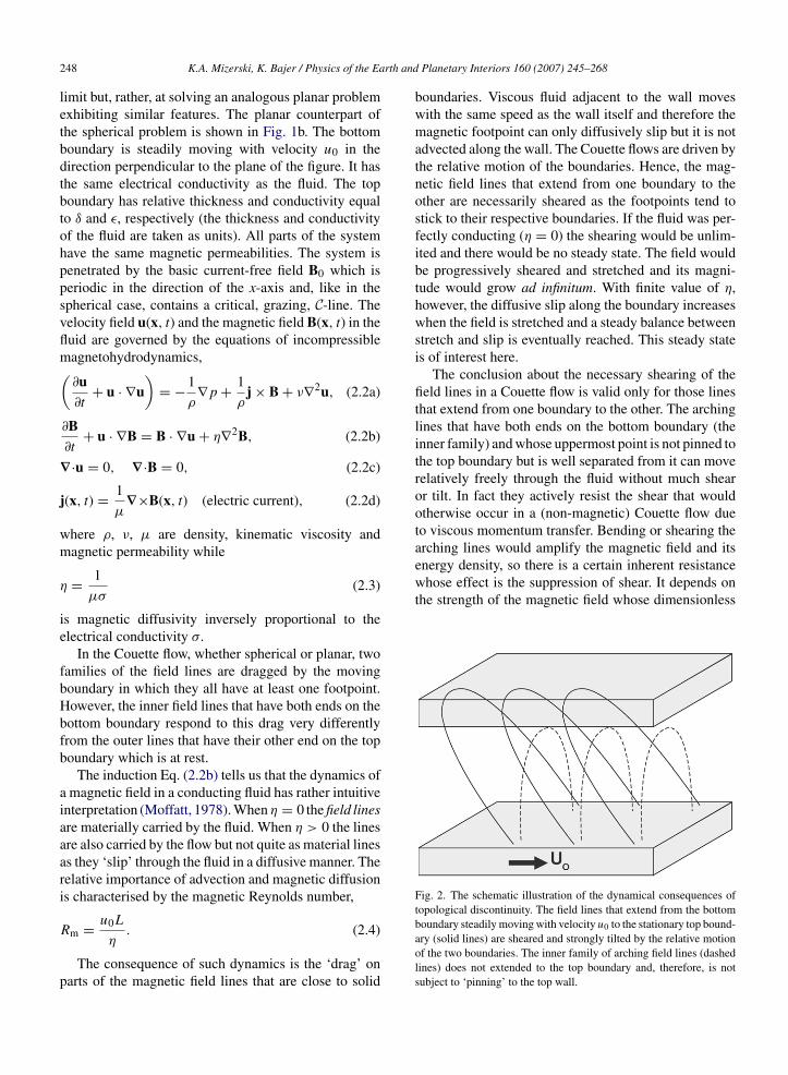

rth and Planetary Interiors 160 (2007) 245–268

boundaries. Viscous fluid adjacent to the wall moveswith the same speed as the wall itself and therefore themagnetic footpoint can only diffusively slip but it is notadvected along the wall. The Couette flows are driven bythe relative motion of the boundaries. Hence, the mag-netic field lines that extend from one boundary to theother are necessarily sheared as the footpoints tend tostick to their respective boundaries. If the fluid was per-fectly conducting (η = 0) the shearing would be unlim-ited and there would be no steady state. The field wouldbe progressively sheared and stretched and its magni-tude would grow ad infinitum. With finite value of η,however, the diffusive slip along the boundary increaseswhen the field is stretched and a steady balance betweenstretch and slip is eventually reached. This steady stateis of interest here.

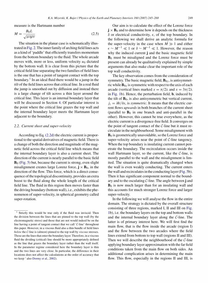
The conclusion about the necessary shearing of thefield lines in a Couette flow is valid only for those linesthat extend from one boundary to the other. The archinglines that have both ends on the bottom boundary (theinner family) and whose uppermost point is not pinned tothe top boundary but is well separated from it can moverelatively freely through the fluid without much shearor tilt. In fact they actively resist the shear that wouldotherwise occur in a (non-magnetic) Couette flow dueto viscous momentum transfer. Bending or shearing thearching lines would amplify the magnetic field and itsenergy density, so there is a certain inherent resistancewhose effect is the suppression of shear. It depends onthe strength of the magnetic field whose dimensionless

Fig. 2. The schematic illustration of the dynamical consequences oftopological discontinuity. The field lines that extend from the bottom


limit but, rather, at solving an analogous planar problemexhibiting similar features. The planar counterpart ofthe spherical problem is shown in Fig. 1b. The bottomboundary is steadily moving with velocity u0 in thedirection perpendicular to the plane of the figure. It hasthe same electrical conductivity as the fluid. The topboundary has relative thickness and conductivity equalto δ and ε, respectively (the thickness and conductivityof the fluid are taken as units). All parts of the systemhave the same magnetic permeabilities. The system ispenetrated by the basic current-free field B0 which isperiodic in the direction of the x-axis and, like in thespherical case, contains a critical, grazing, C-line. Thevelocity field u(x, t) and the magnetic field B(x, t) in thefluid are governed by the equations of incompressiblemagnetohydrodynamics,(

∂u∂t

+ u · ∇u)

= − 1

ρ∇p + 1

ρj × B + ν∇2u, (2.2a)

∂B∂t

+ u · ∇B = B · ∇u + η∇2B, (2.2b)

∇·u = 0, ∇·B = 0, (2.2c)

j(x, t) = 1

μ∇×B(x, t) (electric current), (2.2d)

where ρ, ν, μ are density, kinematic viscosity andmagnetic permeability while

η = 1

μσ(2.3)

is magnetic diffusivity inversely proportional to theelectrical conductivity σ.

In the Couette flow, whether spherical or planar, twofamilies of the field lines are dragged by the movingboundary in which they all have at least one footpoint.However, the inner field lines that have both ends on thebottom boundary respond to this drag very differentlyfrom the outer lines that have their other end on the topboundary which is at rest.

The induction Eq. (2.2b) tells us that the dynamics ofa magnetic field in a conducting fluid has rather intuitiveinterpretation (Moffatt, 1978). When η = 0 the field linesare materially carried by the fluid. When η > 0 the linesare also carried by the flow but not quite as material linesas they ‘slip’ through the fluid in a diffusive manner. Therelative importance of advection and magnetic diffusionis characterised by the magnetic Reynolds number,

Rm = u0L

η. (2.4)

The consequence of such dynamics is the ‘drag’ onparts of the magnetic field lines that are close to solid

boundary steadily moving with velocity u0 to the stationary top bound-ary (solid lines) are sheared and strongly tilted by the relative motionof the two boundaries. The inner family of arching field lines (dashedlines) does not extended to the top boundary and, therefore, is notsubject to ‘pinning’ to the top wall.

rth and

m

M

tafmbcibtticwtta

2

tantdBmdqbfitns

teltbTflaIalw


easure is the Hartmann number

= B0L√μηρν

(2.5)

The situation in the planar case is schematically illus-rated in Fig. 2. The inner family of arching field lines actss a kind of ‘paddle’ that efficiently transfers momentumrom the bottom boundary to the fluid. The whole arcadeoves with, more or less, uniform velocity u0 dictated

y the bottom wall. It is clear from this picture that theritical field line separating the two families of field liness the one that has a point of tangent contact with the topoundary.1 In an ideal fluid there would be a jump in theilt of the field lines across that critical line. In a real fluidhe jump is smoothed out by diffusion and instead theres a large change of tilt across a thin layer around theritical line. This layer is an internal boundary layer thatill be discussed in Section 4. Of particular interest is

he point where the critical line grazes the top wall andhe internal boundary layer meets the Hartmann layerdjacent to the boundary.

.2. Current sheet and super-velocity

According to Eq. (2.2d) the electric current is propor-ional to the spatial derivatives of magnetic field. There ischange of both the direction and magnitude of the mag-etic field across the critical field line which means thathe internal boundary layer is also a current sheet. Theirection of the current is nearly parallel to the basic field0 (Fig. 5) but, because the current is strong, even slightisalignment creates large Lorenz force, j × B0, in the

irection of the flow. This force, which is a direct conse-uence of the topological discontinuity, provides an extraoost to the fluid along the whole length of the criticaleld line. The fluid in this region then moves faster than

he driving boundary (bottom wall), i.e., exhibits the phe-omenon of super-velocity, in spherical geometry calleduper-rotation.

1 Strictly this would be true only if the fluid was inviscid. Thenhe division between the lines that are pinned to the top wall (by thelectromagnetic stress) and those that are not would indeed be on theine having a point of tangent contact that we call ‘C-line’ throughouthis paper. However, in a viscous fluid also a thin bundle of field lineselow the C-line is (almost) pinned to the top wall by viscous stresses.hose are the lines that enter the boundary layer. Therefore, in a viscousuid the dividing (critical) line should be more appropriately defineds the line that grazes the boundary layer rather than the wall itself.n the parameter regime considered here the boundary layer is thinnd the two lines are very close. In particular, the difference in theirocations does not affect the calculations at the order of accuracy thate keep ‘ also Dormy et al., 2002).

Planetary Interiors 160 (2007) 245–268 249

Our aim is to calculate the effect of the Lorenz forcej × B0 and to determine how it depends on the thicknessδ or electrical conductivity, ε, of the top boundary. Inthe following we shall derive an analytic formula forthe super-velocity in the case when M � 1 and eitherε ∼ M−1 � 1 or δ ∼ M−1 � 1. However, the reasonwhy the induced current j and the basic magnetic fieldB0 must be misaligned and the Lorenz force must bepresent can already be qualitatively explained by simplearguments that also make clear the important role of thetop wall conductivity.

The key observation comes from the consideration ofsymmetry. The basic magnetic field, B0z, is antisymmet-ric while B0x is symmetric with respect to the axis of eacharcade (vertical lines marked x = π/2λ and x = 3π/2λ

in Fig. 1b). Hence, the perturbation field, b, induced bythe tilt of B0, is also antisymmetric but vertical current,jz = ∂b/∂x, is symmetric. It means that the electric cur-rent flows upwards in both branches of the current sheet(parallel to B0 in one branch and anti-parallel in theother). However, this cannot be true everywhere, as theelectric current is a divergence-free field. It converges onthe point of tangent contact of the C-line but it must re-circulate in the neighbourhood. Some misalignment withB0 is geometrically unavoidable, so the Lorenz force andsuper-velocity arises near the point of C-line tangency.When the top boundary is insulating current cannot pen-etrate the boundary. The recirculation occurs inside thewall Hartmann layer, so the current, like the C-line, ismostly parallel to the wall and the misalignment is lim-ited. The situation is quite dramatically changed whenthe wall is even weakly conducting. The current entersthe wall and recirculates in the conducting layer (Fig. 5b).Then it has significant component normal to the bound-ary and to the osculating C-line. The angle between j andB0 is now much larger than for an insulating wall andthis accounts for much stronger Lorenz force and largersuper-velocity.

In the following we will analyse the flow in the entiredomain. The strategy is dictated by the overall structureconsisting of three regions, marked I, II and III on Fig.1b), i.e. the boundary layers on the top and bottom wallsand the internal boundary layer along the C-line. Thelatter is of primary interest here. We will first find themain flow, that is the flow inside the arcade (region I)and the flow between the two arcades where the fieldlines extend from bottom to top wall (regions II and III).Then we will describe the neighbourhood of the C-line
applying boundary layer approximation with the far fieldconditions taken from the main flow on both sides. Anadditional complication arises in determining the mainflow. This flow, especially in the regions II and III, is

rth and

everywhere in the fluid.2 This is clearly true in the topconducting shell, 1 < z < δ, where b1 → 0 in the limit


controlled by the wall boundary layers which must be re-solved. They determine the effective slip of the magneticfootpoints relative to the solid boundaries and thereforethe all-important tilt of the field lines in the regions II andIII. It should be stressed that the boundary layers in thisproblem are Hartmann layers, so the appropriate smallparameter in the singular perturbation theory is M−1.

3. The main flow

We seek a steady solution of Eq. (2.2) in the form ofa perturbed current-free field,

B(x) = B0(x, z) + b(x, z)

= B0(x, z) + Rmb(x, z)ey (3.1a)

u(x) = u(x, z)ey, p = p(x, z), (3.1b)

where b(x) is a perturbation generated from B0 by theflow. This perturbation has only the component in thedirection of the flow. We separated the factor Rm whichin a flow of this kind typically is the magnitude of theperturbation.

We take the following basic field

B0(x, z) = B0(e−λz sin λx, 0, e−λz cos λx

). (3.2)

This is a current-free magnetostatic equilibrium (motion-less solution of Eq. (2.2)) whose field lines are shown inFig. 1b). It can be expressed by both its flux functionA(x, z) and by its scalar potential Φ(x, z),

B0(x, z) = B0∇A × ey = B0∇Φ, (3.3a)

A(x, z) = λ−1 e−λz sin λx,

Φ(x, z) = −λ−1 e−λz cos λx. (3.3b)

The x and z components of (2.2b) are trivially satisfiedwhile those of (2.2a) determine the pressure distribution,

p(x, z) = p0 − R2m

2μb2(x, z). (3.4)

We non-dimensionalise the equations by taking L, B0,u0 and L−1 as units of length, magnetic field, velocityand λ respectively. From the y components of (2.2) weobtain

B0 · ∇u + ∇2b = 0 (3.5a)

B0 · ∇b + 1

M2 ∇2u = 0, for 0 < z < 1. (3.5b)

There is a marked difference, worth emphasizing at thispoint, between the planar and the spherical problem. Inthe planar case the advective term, (u · ∇)B, in the induc-tion Eq. (2.2b) vanishes identically while in the spherical


analog it does not. Therefore, the solution of the spher-ical problem, to be discussed in Section 7, like that ofDormy et al. (2002) is valid only for small values of Rmwhile our planar solution is valid for all values of Rmalthough it is most probably unstable for large Rm.

In the solid conductors the perturbation fields, de-noted b1(x, z) inside the top conducting layer andb2(x, z) inside the bottom wall, satisfy the Laplace’sequation

∇2b1 = 0 for 1 < z < 1 + δ, (3.6a)

∇2b2 = 0 for − δbot < z < 0. (3.6b)

We need to find a solution of (3.5) and (3.6) withmagnetic field and tangent electric field,

E = σ−1j − u × B, (3.7)

continuous across the interfaces between the liquid andsolid conductors, z = 0, z = 1, and vanishing magneticperturbation in the insulators. The complete set of bound-ary conditions then is

u(x, z = 0) = 1, u(x, z = 1) = 0, (3.8a)

b(x, z = 0) = b2(x, z = 0),

b(x, z = 1) = b1(x, z = 1), (3.8b)

∂b

∂z

∣∣∣∣z=0

= ∂b2

∂z

∣∣∣∣z=0

, ε∂b

∂z

∣∣∣∣z=1

= ∂b1

∂z

∣∣∣∣z=1

, (3.8c)

b2(x, z = −δbot) = 0, b1(x, z = 1 + δ) = 0, (3.8d)

where

ε = σtop

σ(3.9)

is the electrical conductivity of the top boundary relativeto that of the fluid.

3.1. Magnitude of the magnetic field perturbation

The bottom, moving wall has the same conductivityas the liquid, σbot = σ, while the top, stationary wall hasthe same magnetic permeability but its conductivity is,by assumption, much smaller,

ε ∼ M−1 � 1. (3.10)

The crucial consequence of this assumption is b � M−1

2 As we shall see later with the assumptions that we make here b ∼M−1 everywhere on the top boundary and in the regions II and IIIwhile b ∼ M−2 inside region I.

rth and

ε

ε

aaH

hM

mtpttot

qtbntw

b

dawM

B

B

ielis

u

b

wF

ostp

o


→ 0, so we can reasonably expect the scaling b1 ∼. The condition (3.8b) implies that this scaling holdscross the interface and according to (3.8c) it extendscross the boundary layer whose thickness, typically forartmann layers, is of the order O(M−1).The fact that b(x, z) is small when ε is small also

as a more intuitive physical explanation. With ε ∼−1 � 1 the electromagnetic wall–liquid coupling isuch stronger at the bottom and the fluid is ‘locked’ to

he lower boundary. The ‘drag’ on the magnetic foot-oints is strong at the bottom and weak at the top wherehey considerably ‘slip’ and form a Hartmann layer whilehere is no such layer at the bottom. The basic field B0 isnly weakly tilted by the relatively weak drag near theop, so the perturbation field b(x, z) is small.

This top–bottom asymmetry of the flow is a conse-uence of the large difference in the conductivity of thewo boundaries. For larger values of σtop, say ε ∼ 1, aoundary layer would form near the bottom, as well asear the top wall. The deformation of B0 by the flow withwo strong wall layers will no longer be small and thereill be b(x, z) ∼ 1.What is essential for our analysis is the scaling

(x, z) � M−1. The relation ε ∼ M−1 is a possible con-ition to ensure such scaling but not the only one. Byrguments similar to those above, one can show thatith ε ∼ 1 and δ ∼ M−1 one would also obtain b(x, z) ∼−1.Now we can write Eq. (3.5) in the form

0 · ∇u = 0 + O(M−1), (3.11a)

0 · ∇b = 0 + O(M−2). (3.11b)

In the zero-order approximation (in powers of M−1,.e., with vanishing right-hand sides) these become thequations for the main flow. This is a classical boundary-ayer-type problem as the leading-order approximationnvolves reducing the order of the equation when theecond term in Eq. (3.5b) is neglected.

Eq. (3.11) are satisfied by

(x, z) = F (A(x, z)) + O(M−1), (3.12a)

(x, z) = G(A(x, z)) + O(M−2), (3.12b)

here A(x, z) is the flux function given by (3.3b) and(·), G(·) are arbitrary functions. Hence, in the leadingrder approximation, the equations for the main flow are
atisfied by any b(x, z), u(x, z) which are constant alonghe lines of B0. Only the boundary conditions select onearticular solution from this large family.
We will now calculate these solutions in the interiorf the regions I, II and III.


3.2. Main flow inside the arcade (region I)

The main flow inside the region I is little affectedby the presence of the top wall and the influence of theinternal boundary layer is also weak. The only physicaleffect is steadily moving bottom boundary. In the frameof reference moving along with that boundary we have asteady situation without any driving forces, so there is noflow and the field is just B0. Going back to the originalframe of reference we obtain a rather simple solution forthe main flow in region I,

u = 1 + O(M−1), (3.13a)

b = 0 + O(M−2). (3.13b)

Two remarks are in order here. Firstly, the M−1 � 1situation is a singular perturbation problem but calculat-ing the main flow inside region I does not require anyboundary layer matching. This is because the field B0is strong and the influence of the top wall is small. Sec-ondly, at this stage the solution (3.13) is essentially aninspired guess. The consistency of the matched solu-tions in all regions must be checked later to validate thisguess and the underlying assumption of weak effect ofthe internal and top boundary layers on the main flow inregion I.

3.3. Main flow outside the arcade (regions II and III)

Outside the arcade we have an extra complication asthe main flow is affected by the presence of a Hartmannlayer on the top wall. We will first consider that layerand obtain an analytical solution inside it. The solution,expressed in terms of the rescaled vertical coordinatetypical for boundary layer calculations,

ξ = M(1 − z), (3.14)

will provide the far-field values of b(x, z) and u(x, z)which will then be taken as boundary conditions for themain flow in the regions II and III.

The symmetry of Eq. (3.5) suggests the use of theElsasser variables (Elsasser, 1950),

Z± = u ± Mb, (3.15)

which turn Eq. (3.5) into

B0 · ∇Z± ± 1

M∇2Z± = 0. (3.16)

In the spirit of a standard boundary layer approxi-
mation we now neglect the ∂/∂x and ∂2/∂x2 terms incomparison with ∂/∂z and ∂2/∂z2. We also approximateB0 across the boundary layer with its value at z = 1, i.e.,ξ = 0. This makes (3.5) a differential equation with one

rth and

two different flow regimes are possible. In practice suchpossibility is denied by the numerical results discussedin Section 6. They yield an apparently unique solution infull agreement with our theoretical results. Hence, evenif another solution co-exists it is probably unstable.


independent variable ξ and coefficients parametricallydepending on x,

B10z

∂Z±∂ξ

∓ ∂2Z±∂ξ2 = 0, (3.17)

where

B10z = B0z(ξ = 0) = e−λ cos λx, (3.18)

is the z-component of the basic field B0.The solutions are straightforward,

Z+ = C+(x) + D+(x) eB10z

ξ, (3.19a)

Z− = C−(x) + D−(x) e−B10z

ξ, (3.19b)

where C±, D± are functions of x alone. Since B10z(x) > 0

in region II, B10z(x) < 0 in region III and the boundary

layer solution far away from the wall must decay, weobtain

D+(x) = 0 for 0 < x <π

2λand

3π

2λ< x <

2π

λ

(region II), (3.20a)

D−(x) = 0 forπ

2λ< x <

3π

2λ(region III).

(3.20b)

Hence in both regions we have three unknown out offour functions C± and D± and three boundary condi-tions (3.8a)–(3.8c). From (3.19) the value of Z± andtheir derivatives on the wall and far away from it,

Z0± = Z±(ξ = 0), Zm

± = limξ→∞

Z±(ξ),

Z′0± = ∂Z±

∂ξ

∣∣∣∣ξ=0

(3.21)

can be expressed in terms of C± and D±.3 When thoseare eliminated we obtain the following relations betweenthe boundary conditions on both sides of the boundarylayer,

Zm+ = Z0

+, Zm+ = Z0

+ − 1

B10z

Z′0+ (region II)

(3.22a)

Zm− = Z0

− + 1

B10z

Z′0−, Zm

− = Z0− (region III).

(3.22b)

3 Here the superscript m stands for main flow.


We can now invert (3.15) and obtain the matching ofthe field and the flow across the boundary layer,

um(x) = ε−1

B10z

∂b1

∂z

∣∣∣∣z=1

,

bm(x) = b1|z=1 + M−1 ε−1

B10z

∂b1

∂z

∣∣∣∣z=1

(region II)

(3.23a)

um(x) = ε−1

B10z

∂b1

∂z

∣∣∣∣z=1

,

bm(x) = b1|z=1 − M−1 ε−1

B10z

∂b1

∂z

∣∣∣∣z=1

, (region III)

(3.23b)

The values um(x), bm(x) make boundary conditionsat z = 1 but they are still given in terms of b1 rather thanexplicitly.

This difficulty is resolved by our next ‘inspired guess’that (3.13a) holds in the regions II and III as well as inthe region I. In the case of ε = 0 it is easy to imagine thatthe influence of the top boundary on the main flow de-creases with M. As the basic field B0 becomes strongerit increasingly resists bending when the top ends of thefield lines are dragged by the fluid inside the boundarylayer on the top wall. For ε = 0 a plausible scaling of thisdecreasing influence is b = O(M−1) and, in fact, it holdsalso when ε ∼ M−1 which introduces an extra modifi-cation but of the same order of magnitude.4 The solution(3.13a) applied to the regions II and III is, for now, onlya proposition later to be supported by the consistence ofsolutions in all parts of the domain. It should be stressedthat such consistence, no matter how convincing, is nota rigorous proof of the adopted scalings and, in particu-lar, of the validity of (3.13a). The rigorous proof wouldbe outside the scope of this paper. It may even be im-possible as we cannot, on theoretical grounds, rule out apossibility that for the same set of physical parameters

4 The ratio of the electromagnetic and viscous stresses on the topboundary can be estimated as M2

(b/

∂u∂z

). With b = O(M−1) and

∂u∂z

∼ M (because of a presence of the Hartmann boundary layer) themagnetic stresses and viscous stresses are comparable both being ofthe order O(M). This means that the total stress at the top boundary isof the same order for ε ∼ M−1 as for ε = 0.

rth and

mdu

b

b

b

pIflcf

b

b

wa

C

is

s

b

u


We can now solve (3.6a) and obtain an explicit for-ula for b1(x, z) inside the top wall. The boundary con-

itions are (3.8d) and (3.23a) with (3.13a) substituted form, i.e.,

ε−1

B10z

∂b1

∂z

∣∣∣∣z=1

= 1 + O(M−1) . (3.24)

The leading order solution is

b1(x, z)

= εe−λ(2+δ)

2λ cosh(λδ)

(eλz − eλ(2+2δ−z)

)cos(λx). (3.25)

From (3.23b) and (3.25) we obtain explicit values ofm,

m(x) = −M−1 − ε tanh(λδ)e−λ

λcos(λx)

(region II) (3.26a)

m(x) = M−1 − ε tanh(λδ)e−λ

λcos(λx)

(region III). (3.26b)

According to (3.12) the leading order solution for theerturbation field b(x, z) in the interior of the regionsI and III is a function F (A(x, z)) of the unperturbedux function A(x, z) given by (3.3b). From the boundaryondition (3.26) we can easily obtain the form of theunction F (·),

= −M−1

⎡⎣1 + C

√1 −

(A

AC

)2⎤⎦ + O(M−2)

(region II), (3.27a)

= M−1

⎡⎣1 + C

√1 −

(A

AC

)2⎤⎦ + O(M−2)

(region III), (3.27b)

here AC = λ−1eλ is the value of A(x, z) on the C-linend

= εM tanh(λδ)AC (3.28)

s an O(1) constant. In the regions II and III |A| < |AC|,o the expression under the square root is positive.

For completeness we rewrite, in explicit form, theolutions for the main flow in all three regions,

= 0 + O(M−2) (region I) (3.29a)

= 1 + O(M−1) (region I) (3.29b)


b = −M−1(1 + εM tanh(λδ)λ−1

× e−λ√

1 − e2λ(1−z) sin2 λx) (region II) (3.30a)

u = 1 + O(M−1) (region II) (3.30b)

b = M−1(1 + εM tanh(λδ)λ−1

× e−λ√

1 − e2λ(1−z) sin2 λx) (region III) (3.31a)

u = 1 + O(M−1) (region III) (3.31b)

The above expression for the main flow reveals theessential features of the problem considered.

(1) The magnitude of the perturbation field b(x, z) isO(M−2) inside the arcade and O(M−1) outside it.Hence, there must be strong gradient of b, i.e. a cur-rent sheet, along the critical C-line which is the sep-aratrix between the two regions. Anticipating theresults of the next section we may assume the thick-ness of the sheet to be O(M−(1/2)). The jump of thefield is O(M−1), so the magnitude of the current inthe current sheet is O(M−(1/2)). This current flowsalong the C-line.

(2) On both branches of the C-line (0 < x < π/2λ

and π/2λ < x < π/λ) the current mentioned aboveflows upwards. Thus, conservation of electric chargeimplies that O(M−(1/2)) current must flow towardsthe top wall near x = π/2λ. Conversely, strong cur-rent flows out of the wall near x = 3π/2λ. Hence,in those two small regions (the size of the boundarylayer thickness) the strong current is necessarily per-pendicular to the lines of B0 and the Lorenz forcej × B0 is large. This force, aligned with the flow,is responsible for the super-velocity which will becalculated in the next section as part of the singularboundary layer analysis.

We should stress that this force is present evenwhen ε = 0. The top wall is then insulating and theelectric current cannot enter. It flows upwards alongthe C-line converging on the point of tangent con-tact and makes a sharp U-turn inside the boundarylayer flowing away along the wall (see Fig. 5a). Un-der such geometrical constraints current cannot flowalong the lines of B0 everywhere. Indeed it crossesthose lines near the top of the C-line thus generatingstrong Lorenz force parallel to b(x, z) and u(x, z).
This force is not compensated by the pressure gradi-ent which has no component in the y-direction andtherefore gives rise to super-velocity, that is a jetmoving faster than the ambient fluid. The effect is,

rth and
however, considerably weaker than in the case ofconducting wall.

(3) There is a singularity at the point where the walllayer and the C-line internal boundary layer merge.This could already be seen in the expression (3.26)which shows that the boundary condition bm(x) isdiscontinuous at the points where the regions II andIII meet (x = π/2λ and x = 3π/2λ). From this sin-gularity we could directly infer strong current nor-mal to the wall, without even invoking the overallcurrent flow along the C-line.

3.4. Thin but highly conducting top wall

With little extra effort we can extend the results of thissection to the case when ε ∼ 1 and δ ∼ M−1. Then, b1 ∼δ ∼ M−1 and the crucial assumption of our analysis ofthe main flow, namely b � M−1 everywhere in the fluid,still holds (see discussion after the relation 3.10). Thegeneral solutions (3.12) remain valid and so does thesolution (3.13) in the region I. The wall boundary layeranalysis is unaffected, the resulting matching conditions(3.23) are the same and the perturbation field b1(x, z)inside the top wall is also given by the formula (3.25). Inconsequence the main flow in the case of thin but highlyconducting top layer is given by (3.29)–(3.31). In orderto make the scaling of the perturbation field b(x, z) moreexplicit in the case when δ ∼ M−1 � 1 we approximateC given by (3.28)

C = εM tanh(λδ)AC ≈ εδMλAC = O(1). (3.32)

Hence, in this case, the constant C in (3.27) is alsoO(1) and all the conclusions of the scaling of the electriccurrent remain valid.

3.5. Flow near the bottom wall

The C-line to be analysed in the next section is rootedin the bottom wall. To analyse the neighbourhood of theC-line we will need the details of the flow near its foot-points. The method of calculation is similar as for thetop-wall boundary layer. The appropriate vertical coor-dinate is now (cf. Eq. (3.14))

ζ = Mz. (3.33)

Eq. (3.17) become

B00z

∂Z±∂ζ

± ∂2Z±∂ζ2 = 0, (3.34a)

B00z = B0z(x, z = 0) = cos λx. (3.34b)


Due to obvious symmetries it is enough to considerthe interval 0 < x < π/2λ. The solution analogous to(3.19) is

Z+ = C+(x) + D+(x) e−B00z

ζ, Z− = C−(x). (3.35)

At the bottom wall the matching analogous to(3.23) between the solution in the main flow, um

0 (x) =um(x, z = 0), bm

0 (x) = bm(x, z = 0) and in the solidb2(x, z = 0) takes form

um0 = 1 + 1

B00z

∂b2

∂z

∣∣∣∣z=0

,

bm0 = b2|z=0 + M−1

B00z

∂b2

∂z

∣∣∣∣z=0

. (3.36)

In the situations that we consider (either ε ∼ M−1

or δ ∼ M−1) the perturbation field b(x, z) = O(M−1)everywhere in the fluid, so we may expect b2(x, z) =O(M−1) in the solid too. There are no reasons for par-ticularly strong vertical gradients of b2 to develop inside

the bottom wall, so ∂b2∂z

∣∣∣z=0

= O(M−1) as well. Then,

the matching conditions (3.36) tell us that in the leadingorder both velocity and magnetic field are continuous atz = 0, so there is no boundary layer. There is a layer inwhich the increment of velocity is O(M−1) and of themagnetic field O(M−2), but this is a weak effect com-pared with the O(1) jump in u(x, z) near the top wall.

Analysing the flow near the bottom wall we fol-lowed the standard boundary layer analysis but the resultdemonstrates that, in fact, there is no boundary layer atz = 0. Still, the relations (3.36) that we obtained herewill be used later.

In this section we have calculated the main flow inthe entire domain, i.e., inside the arcade (region I) andoutside it (regions II and III). This required boundaryconditions on the top wall and for that we had to re-solve the Hartmann layer. The main flow solution re-vealed aO(M−1) discontinuity in the perturbationb(x, z)across the critical line (C-line) of the basic field B0.We shall now demonstrate that besides this relativelyweak discontinuity in b(x, z) on the C-line there is alsoa peak in velocity which considerably exceeds the ve-locity of the main flow which on both sides of the C-lineis u = 1 + O(M−1). This super-velocity is biggest nearthe top wall and it decreases as we follow the C-linedownwards.

4. The shear layer along the C-line

The occurrence of the super-velocity along the en-tire length of the C-line is a subtle effect. The jump

rth and Planetary Interiors 160 (2007) 245–268 255

oopitassilonobtt

tapfbbcTea

4

CCio

Aa

x

e

T(twma

Fig. 3. The double shear-layer along the critical magnetic field lineC. The point S is the point (x = π/2λ, z = 1) at which the C-line is


f b(x, z) across the C-line implies only a thin sheetf electric current but does not, in itself, explain theresence of strong shear. The associated Lorenz forcen a current sheet can, in principle, be balanced byhe pressure gradient and without a velocity incrementcross the sheet there is no obvious cause of viscoustress. The velocity profile across the C-line is not amoothed-out jump, i.e., one-signed shear as in a typ-cal internal boundary layer. It is rather a double shearayer, i.e., a strong peak in velocity with positive shearn one slope and negative on the other. This phe-omenon originates in the small region around the pointf tangent contact where the C-line enters the top-walloundary layer. As we have shown in the previous sec-ion, there is a fast jet in this region which is parallelo b(x, z).

We will now show that super-velocity is not confinedo the near-wall jet but it occurs in the entire current sheetlong the C-line, albeit it is strongest near the top androgressively weaker towards the bottom. This super-ast sheet is essentially a diffusive effect. It is sustainedy the combined driving effect of the jet near the topoundary and of the electric current ‘leaking’ from theurrent sheet, i.e., having small component normal to B0.his leakage causes streamwise Lorenz force along thentire length of the current sheet by the same mechanisms the near-wall jet is formed.

.1. Coordinates and equations

The coordinates appropriate for the analysis of the-layer are (l, n) where l is normalised length along the-line and n is distance in the direction perpendicular tot. Because of the symmetries it is enough to considernly the 0 < x < π/2λ branch.

First we change coordinates from (x, z) to A, τ, whereidentifies a field line and 0 < τ < 1 is a parameter

long it,

(τ) = λA(τ − 1) + π

2λ, (4.1a)

xp(λz(τ)) = 1

λAsin(λ2A(τ − 1) + π

2

). (4.1b)

In the region I the flux function is positive, A > AC.he points (A, τ = 1) are the summits of the field lines

their intersections with the line x = π/2λ) and, in par-
icular, (A = AC, τ = 1) is the point, marked S in Fig. 3,here the C-line is tangent to the top wall and the Hart-ann layer is singular. One possible measure of distance
long the lines of B0 (Dormy et al., 2002) is the scalar

tangent to the upper boundary; the point I is the intersection of thecritical line with the lower boundary.

potential Φ given by Eq. (3.3b),

γ(τ) = −∫SA

B0 · dr = −∫SA

dΦ

= e−λz(τ′)

λcos(λx(τ′))

∣∣∣∣∣τ

1

= −A tan(λ2A(τ − 1)). (4.2)

where SA is the point (A, τ = 1).We normalise it dividing by the distance between

the summit S of the C-line and its footpoint I (seeFig. 3),

Γ = γ(τI) =√

1 − e−2λ

λ, (4.3)

and obtain the coordinate along the C-line,

l = 1 − γ(τ) = 1 − e−λz

cos(λx), (4.4)
Γ λΓ
such that l = 0 at I and l = 1 at S. The widthof the C-layer is O(M−(1/2)) (Dormy et al., 1998;Starchenko, 1998a,b), so the appropriate normal

rth and
coordinate is

n = M1/2√

Γ (AC − A)

= M1/2√

Γ

(AC − e−λz

λsin(λx)

),

n = 0 on the C-line, n < 0 in region I,

n > 0 in region II. (4.5)

Eq. (3.16) can now be rewritten using the C-line coor-dinates (l, n). When the terms of the order O(M−1) andhigher are neglected the equations take the form

∂Z±∂l

± ∂2Z±∂n2 = 0. (4.6)

We shall now specify the conditions, at l = 0, 1 andn → ±∞.

4.2. Boundary conditions for n → ±∞

The main flow can be expressed in terms of the C-linecoordinates (l, n). From (3.27a) and (3.30b) we obtainthe solution for n > 0 (region II) and from (3.29) thatfor n < 0 (region I),

Zm± = 1 ∓ 1 ∓ Γ −(1/4)C M−(1/4)n1/2

×√

2

AC− M−(1/2)

A2C

n + O(M−1) for n > 0,

(4.7a)

Zm± = 1 + O(M−1) for n < 0, (4.7b)

where C is given by either (3.28) or (3.32) and AC isexpressed by Γ ,

AC = e−λ

λ=

√1 − λ2Γ 2

λ. (4.8)

We notice that due to the suitable choice of the C-line coordinates the main flow is, in fact, a function of nonly. However, the C-layer (the solution of the Eq. (4.6)to be derived) will depend on l. This l-dependence isforced solely by the non-uniform boundary conditionsat z = 0, 1 (to be derived), not by the main flow.

Typically for a boundary-layer calculation the far-field (n → ∞) boundary condition for the C-layer is themain flow taken at (AC − A) → 0. Expanding (4.7a) weobtain for the main flow close to the C-line

m −(1/4) 1/2 3/2 −(3/4)
Z± = 1 ∓ 1 ∓ Λ M n + O(n M )
for n → +∞, (4.9a)

Zm± = 1 + O(M−1) for n → −∞, (4.9b)


where

Λ = Γ −(1/4) C

√2

AC= O(1) (4.10)

is a constant proportional to ε and dependent on δ.The boundary layer Eq. (4.6) have the form of one-

dimensional diffusion equations with n being the spa-tial variable and l playing the role of time. The expres-sions (4.9) provide two boundary conditions for eachof those diffusion equations (at n → ±∞ respectively).For a unique solution we now need two more conditionsjust like two diffusion equations need two initial condi-tions. They will be given on z = 0 and z = 1. In the (l, n)space those are curves, not straight lines l = const, so theconditions imposed are not exactly analogous to the one-time initial conditions. Nevertheless, they are sufficientto determine the unique solution of (4.6).

4.3. Boundary conditions at l = 0

We first consider the condition at l = 0. From (3.36)and (3.8)c we obtain

(Z+ + Z−)|z=0 = 2 + 2

B0oz

∂b

∂z

∣∣∣∣z=0

. (4.11)

From this exact condition we can derive its approx-imate version. Keeping only the leading term we willobtain a valuable simplification with O(M−(1/2)) accu-racy. Firstly we write the equation for the surface z = 0in the (l, n) coordinates (see Eqs. (4.4) and (4.5))

l = 1− 1

λΓ

√1 − (λAC − λM−(1/2)Γ −(1/2)n)2. (4.12)

For finite n and large M this can be expanded in theTaylor series (cf. Eqs. (4.3) and (4.8))

l = 0 + O(M−(1/2)). (4.13)

This means that taking the condition (4.11) at l = 0 in-stead of z = 0 introduces errors of the order O(M−(1/2)).The gradient term in the condition (4.11) is, in fact, ofthe same order, so when we approximate z = 0 by l = 0we may as well neglect it. The ∂/∂z derivative is

∂

∂z= λ(1 − l)

∂

∂l

+λM1/2(AC − M−(1/2)Γ −(1/2)n)∂

∂n. (4.14)

−1
When applied to b(x, z) = O(M ) (see Eqs. (3.30a)and (3.31a)) indeed it yields
∂b

∂z

∣∣∣∣z=0

= O(M−(1/2)). (4.15)

rth and

b

4

TtttcfsaB

dmtit

tll

(

∣∣∣wHsmrt

ovEcse

h

O

tt


Therefore we obtain an approximate form of theoundary condition (4.11)

(Z+ + Z−)|l=0 = 2 + O(M−(1/4)). (4.16)

.4. Boundary condition at l = 1

The relations at l = 1 are somewhat more complex.he point of tangent contact between the C-line and the

op wall, (x = π/2λ, z = 1), is the point of singularity ofhe two coinciding shear layers, the Hartmann layer onhe top wall and the C-layer. This region requires separateareful analysis outlined by Roberts (1967). The needor special treatment is clear. The solution (3.19b) repre-ents a wall layer whose thickness scales like O(M−1) atny fixed value of x = π/2λ but grows without limit as10z → 0 when x → π/2λ. However, it turns out that theependence of the super-velocity on ε, which is our pri-ary interest here, is the leading order effect and the de-

ails of the singular layer are not necessary to determinet.5 All that is needed are a few general conclusions abouthe neighbourhood of the singularity (Roberts, 1967).

In the region where the C-line approaches the wallhere is a ‘bulge’ in the boundary layer. The Hartmannayer, whose thickness away from the singularity scalesike O(M−1), spreads to

1 − z) = O(M−(2/3)). (4.17)

The horizontal extent of this bulge is

π

2λ− x

∣∣∣ = O(M−(1/3)). (4.18)

The bulge overlaps with the region of super-velocityhose dependence on ε is our primary interest here.6

owever, it turns out that this dependence is a relativelytrong effect that can be determined from the globalatching of the solutions in different regions without

esolving the details of the singular layer which enterhe calculations only at higher orders.

We will assume the occurrence of super-velocityf yet unknown magnitude uS . This unknown super-elocity will enter the boundary condition for the C-layer
q. (4.6) and will then be fixed so as to obtain the overallonsistency. It should be stressed that the mathematicaltructure of this problem is such that uS is a param-ter in some kind of ‘internal’ condition that couples
5 The solution inside the singular Hartmann layer changes only atigher orders.6 The maximum of the super-velocity is located at a distance(M−2/3) from the wall. The singular Hartmann layer smoothes out

he velocity jump between the super-velocity maximum and the sta-ionary wall.


the two diffusion Eq. (4.6). Determining this parameteris part of the solution of the C-layer problem and doesnot involve matching across the singular (bulged) walllayer near the point S. The situation, although physi-cally completely different, is somewhat reminiscent ofthe problem of ordinary diffusion in presence of an inter-nal membrane. The membrane imposes an internal con-dition that fixes neither the concentration, nor the fluxbut a relation between the two. The unknown parameteris the permeability of the membrane which can be deter-mined from the outer conditions, e.g., measured flux andconcentration on distant walls, as a compatibility condi-tion on the matched solutions on the two sides of themembrane.

Once the uS is determined from the C-layer solutionit can be used, together with the conditions at the wall, todetermine the internal structure of the singular (bulged)Hartmann layer near the point S (Roberts, 1967; Dormyet al., 2002). However, this is not needed to determinethe leading order ε-dependence of uS and therefore willbe omitted.

In order to solve Eq. (4.6) we must consider theboundary conditions at l = 1 separately on the two sidesof the C-line, n � 0 and n < 0. The maximal super-velocity occurs at the point S (n = 0, but see footnote 1).At l = 1 (actually on the entire symmetry axis x =π/2λ) the perturbation field b vanishes due to symmetry,

u( π

2λ− x, z

)= u

( π

2λ+ x, z

),

b( π

2λ− α, z

)= −b

( π

2λ+ α, z

). (4.19)

Hence, we can write

Z+|l=1 = Z−|l=1 = 1 + uS(n), for n < 0. (4.20)

The unknown function uS(n) is the super-velocity atx = π/2λ. In order to calculate it we need one morecondition.

The condition at l = 1, n ≥ 0 is fairly straightfor-ward. We simply take the Hartmann jump condition(3.23) in region II near the point (x = π/2λ, z = 1). Onthis (outer) side of the C-line the singularity of the bound-ary layer (the bulge) does not affect the boundary condi-tion, at least to the accuracy we need. From the matchingcondition (3.23) we obtain

Z+|z=1 = Mb1|z=1, for n ≥ 0. (4.21)

In order to express this in the shear layer variables(n, l) we write the equation for the surface z = 1 as

rth and
(cf. (4.4) and (4.5)),

l = 1 − ACΓ

√1 − 1

A2C

(AC − Γ −(1/2)M−(1/2)n)2

= 1 − Γ −(5/4)√

2AC n1/2M−(1/4) + O(M−(3/4)).

(4.22)

The right-hand side of (4.21) becomes

M b1|z=1 = −Λn1/2M−(1/4) + O(M−(3/4)). (4.23)

We also expand the left-hand side of (4.21) and obtain

Z+|z=1 = Z+|l=1 − Γ −(5/4)√

2AC∂Z+∂l

∣∣∣∣l=1

× n1/2M−(1/4) + O(M−(3/4)). (4.24)

Finally we obtain the required boundary condition,

Z+|l=1 = −Λ n1/2 M−(1/4) + Γ −(5/4)√

2AC∂Z+∂l

∣∣∣∣l=1

× n1/2 M−(1/4) + O(M−(3/4)) for n � 0.

(4.25)

A word of comment is necessary here. The aboveboundary condition for n � 0 was obtained from (4.21)which is a correct matching condition across the non-singular wall layer away from the point S. In the leadingorder this condition remains valid also for the singularlayer but in this case the higher order corrections arelarger. This implies that the error in (4.25) is, in fact,larger than O(M−(3/4)). For a rigorous evaluation ofthis error we would need to resolve the singular layerbut a convincing estimate can be offered immediately.From (4.17)–(4.18) and (4.4)–(4.5) we notice that inthe coordinates (l, n) the span of the singular layeris |1 − l| = O(M−(1/3)) and n = O(M−(1/6)), respec-tively. Then, an estimate of the inaccuracy of the secondterm in (4.25) suggests that the corrections introducedby the singular Hartmann layer are O(M−(1/3)). This is
still smaller than the leading order corrections in (4.25)and in (4.9). The latter are of the order O(M−(1/4)) andonly those are included in further analysis.7
7 In fact the order of the right hand side of (4.25) is precisely M−(1/4)

since n is finite. However, the order of Λ M−(1/4)n1/2 in (4.9) asn → ∞ is not immediately clear. The match with the main flow is validin the region where M1/2(AC − A) ∼ n → ∞ and (AC − A) → 0. Theformer means that (AC − A) � M−(1/2) and the latter implies (AC −A) � M−(1/6) (the smallest term considered in the boundary condi-tions is of order of M−(1/4) while the terms proportional to (AC − A)3/2

in (4.9) have been neglected). The matching region is therefore de-


5. Super-velocity

In this section we shall derive an integral equa-tion (Eq. (5.15)) for the first-order correction to super-velocity that results from finite conductivity of the topwall. The asymptotics derived from this equation willlater be compared with the full numerical solutions ofour problem, i.e., of Eqs. (3.5) and (3.6).

In order to calculate the super-velocity uS(n) we mustsolve Eq. (4.6) together with the boundary conditions(4.9), (4.16), (4.25). We notice that the correct parameterof the perturbative expansion of Z± inside the C-layer isM−(1/4). The zero-order solution of (4.6) is not affectedby ε and is the same as in the case of insulating top wall(Dormy et al., 2002). The effect of the wall conductivityclearly shows in the first order correction term (see (4.9a)and (4.25)). This is the order of accuracy that we willkeep.

Gathering, for convenience, the equations and thecomplete set of the suitably truncated boundary condi-tions we have

∂Z+∂l

+ ∂2Z+∂n2 = 0,

∂Z−∂l

− ∂2Z−∂n2 = 0. (5.1)

Z+ = −Λ M−(1/4)n1/2, n → +∞, 0 < l < 1

(5.2a)Z− = 2 + Λ M−(1/4)n1/2, n → +∞, 0 < l < 1

(5.2b)

Z+ = 1, n → −∞, 0 < l < 1 (5.2c)

Z− = 1, n → −∞, 0 < l < 1 (5.2d)

Z+ + Z− = 2, l = 0 (5.3)

Z+ = −Λ n1/2 M−(1/4) + Γ −(5/4)√

2AC∂Z+∂l

× n1/2 M−(1/4), n � 0, l = 1 (5.4a)

Z+ = 1 + uS(n), n < 0, l = 1 (5.4b)

Z− = 1 + uS(n), n < 0, l = 1. (5.4c)

Following Dormy et al. (2002) we first solve the equa-tion for Z+. When the ‘time’ variable is changed from l
to 1 − l this becomes a diffusion equation on the inter-val 0 < 1 − l < 1. The solution is given by the Green’s
fined by M−(1/2) � (AC − A) � M−(1/5) and in terms of the shearlayer coordinates 1 � n � M1/3. This means that the order of the cor-rection in (4.9) as n → ∞ is M−(1/4) � Λ M−(1/4)n1/2 � M−(1/12).

rth and

f

Z

bw

i(rHdadfls

J

Z

t

Z

+J(l, n). The details of the straightforward calculations


ormula,

+ = 1√4(1 − l)π

∫ 0

−∞

[(1 + uS(n′))

× exp

(− (n−n′)2

4(1−l)

)]dn′+M−(1/4) 1√

4(1 − l)π

×∫ ∞

0

[(−Λ + Γ −(5/4)

√2AC

∂Z+∂l

∣∣∣∣l=1

)

×√

n′ exp

(− (n − n′)2

4(1 − l)

)]dn′. (5.5)

Here we have neglected the contributions from theoundary conditions (5.2) as they are exponentially smallhen M is large. We now focus on the term involving

∂Z+∂l

∣∣∣l=1

. This term reflects the curvature of the boundary

n the C-layer coordinates (l, n). The second integral in5.5) is multiplied by M−(1/4), so, for the required accu-acy, only the zero-order term of the integrand is needed.owever, at the leading order the ‘curvature term’ is in-ependent of ε, i.e. is the same for a conducting top walls for an insulating one. Therefore, the curvature termoes not play a role in our further analysis of the in-uence of the top wall conductivity and thereafter willimply be denoted by M−(1/4)J(l, n),

(l, n) = 1√4(1 − l)π

∫ ∞

0

[Γ −(5/4)

√2AC

∂Z+∂l

∣∣∣∣l=1

×√

n′ exp

(−(n − n′)2

4(1 − l)

)]dn′. (5.6)

Hence, we can write

+ = 1√4(1 − l)π

∫ 0

−∞

[(1 + uS(n′)

)× exp

(−(n−n′)2

4(1−l)

)]dn′−M−(1/4) Λ√

4(1−l)π

×∫ ∞

0

√n′ exp

(− (n − n′)2

4(1 − l)

)dn′

+M−(1/4)J(l, n). (5.7)

Similarly to Z+ we can also use the Green’s functiono calculate Z− from the initial condition given by (5.2)

− = 1 + 1erfc

(− n√

)− 1√

2 4(1 + l) 4(1 + l)π

×∫ 0

−∞uS(n′) exp

(− (n − n′)2

4(1 + l)

)dn′


+ M−(1/4) Λ√4(1 + l)π

∫ ∞

0

√n′

× exp

(− (n−n′)2

4(1+l)

)dn′−M−(1/4)J(l, n). (5.8)

The conditions (5.4b) and (5.4c) imply that

Z+(1, n) = Z−(1, n), for n < 0, (5.9)

so the combined Eqs. (5.7) and (5.8) yield an inte-gral equation for the super-velocity uS(n). If we expanduS(n),

uS(n) = u0S(n) + M−(1/4)u1

S(n) + · · · , (5.10)

then we obtain separate integral equations for each termof the expansion. The first and the second take the form

u0S(n) = 1

2erfc

(− n√

8

)− 1√

8π

∫ 0

−∞

[u0

S(n′)

exp

(− (n − n′)2

8

)]dn′ (5.11)

u1S(n) = − 1√

8π

∫ 0

−∞u1

S(n′) exp

(− (n − n′)2

8

)dn′

+ Λ√8π

∫ ∞

0

√n′ exp

(− (n − n′)2

8

)dn′

−J(1, n), (5.12)

As was mentioned before, the conductivity of the topwall does not enter the leading order calculation (thecoefficients in Eq. (5.11) do not depend on ε), but it doesaffect the first order term u1

S (the coefficient Λ in Eq.(5.12) depends on ε).

The important fact is that J(1, n) does not depend onε. To prove it we solve Eq. (5.11) which is of Fredholmtype and can be solved by successive iterations. We ob-tain a Neumann series in the form

u0S(n) = 1

2erfc

(− n√

8

)− 1

2√

8π

∫ 0

−∞

[erfc

(− n′

√8

)

× exp

(− (n − n′)2

8

)]dn′ + · · · . (5.13)

The term J(l, n) can, in principle, be evaluated in thefollowing way. First, we approximate uS(n) by u0

S(n)given above, then from (5.7) we calculate the leadingterm in Z (l, n) and, finally, from (5.6) we evaluate

are omitted because the only relevant conclusion, as wementioned before, is the fact thatJ(1, n) does not dependon ε.

rth and
Now, the crucial observation is that Eq. (5.12) is lin-ear in u1

S(n). Since J(1, n) does not depend on ε thefirst order correction to super-velocity, or super-velocityexcess, defined as

�u1S(n) = u1

S(n) − u1S,ε=0(n), (5.14)

where u1S,ε=0(n) is the value of u1

S(n) for insulating topwall (ε = 0), satisfies a simpler equation that no longerincludes the J(1, n) term.

�u1S(n)

= − 1√8π

∫ 0

−∞�u1

S(n′) exp

(−1

8(n − n′)2

)dn′

+ Λ√8π

∫ ∞

0

√n′ exp

(−1

8(n − n′)2

)dn′ (5.15)

The all-important second term in (5.15), that deter-mines the ε-dependence of �u1

S(n), can be written as

Λ√8π

∫ ∞

0

√n′ exp

(−1

8(n − n′)2

)dn′

= Λ1

2exp

(− 1

16n2)

D−(3/2)

(−1

2n

), (5.16)

where D−(3/2)(·) is the parabolic cylinder function(Gradshteyn and Ryzhik, 1994). This term is positive forall values of n < 0. The asymptotic behaviour as n →−∞ of the function D−(3/2)(·) is given by the formula

D−(3/2)

(−1

2n

)∼ exp

(− 1

16n2)(

−1

2n

)−(3/2)

×[1 − 15n−2 + · · ·

], (5.17)

so the term (5.16) exponentially decreases in the mainflow.

From (5.17) and (5.15) we obtain

�u1S(n) = − 1√

8π

∫ 0

−∞

[�u1

S(n′)

× exp

(−1

8(n − n′)2

)]dn′+εM tanh(λδ)C

× exp

(− 1

16n2)

D−(3/2)

(−1

2n

), (5.18a)

where

˜ √2 (−1/4) 2λ −(1/8) 1/2λ
C =
2λ (1 − e ) e , (5.18b)

and we have substituted Λ from (4.10) and (3.28). Thisintegral equation of Fredholm type describes the first or-der correction to super-velocity when the top wall is an


electrical conductor. Successive iterations yield a Neu-mann series which is an exact albeit impractical solutionand the formulae will not be given here. However, therecursive algebraic calculations show that

�u1S(n = 0) > 0. (5.19)

Hence, the super-velocity near the conducting top wallis larger than in the case of an insulator.

The first order perturbation analysis of the shear layerrevealed that for the top wall of either small conductivity(ε ∼ M−1, δ ∼ 1) or small thickness (δ ∼ M−1, ε ∼ 1)the super-velocity in the near-wall jet is enhanced by anadditional term M−(1/4)�u1

S(n = 0), where �u1S(n) is

the solution of (5.18). From (5.18a) we obtain that thissuper-velocity excess is proportional to εM3/4. Hence,in the parameter regime for which our theory is validtwo leading-order scalings can be observed. With theHartmann number M kept constant the super-velocityexcess �u should scale like O(ε1) but with εM tanh(λδ)kept constant we should observe �u ∼ M−(1/4). In thenext section we will describe numerical solutions of theoriginal problem, compare with the asymptotic valueobtained from Eq. (5.18a) and verify the two predictedscalings.

6. Numerical solutions

We have computed the solutions of Eqs. (3.5) and(3.6) with the boundary conditions (3.8), λ = 1 (hori-zontal period of the external field equal to the depth ofthe fluid) for a range of values of M and ε. In all calcu-lations the top and bottom walls had the same thicknessδ = δbot = 0.25. Because of the symmetries in the prob-lem it was enough to confine the numerical domain to0 � x � π/2. The equations were solved using a stan-dard finite difference scheme with the LU matrix decom-position applied to the resulting set of linear algebraicequations. For M � 103 the numerical results were allchecked with respect to the number of finite differencepoints used in each direction. All the computations weredone using the densest possible grid with 241 points inthe liquid and 15 points in each of the boundaries for thez-direction (uniformly spaced in each of the regions) and61 points in the x-direction (also uniformly spaced).

In Fig. 4 we show the surface plots of fluid velocityfor M = 103 comparing the cases of a weakly conduct-ing (ε = 0.01) and highly conducting (ε = 1) top wall.A sheet of fluid near the C-line is flowing with velocity
much greater than that of the bottom wall, u = 1, i.e.,there is a quasi-two-dimensional jet which is not planarbut lies on a surface bent in the shape of the C-line. Thevelocity in the jet is non-uniform having maximum near

K.A. Mizerski, K. Bajer / Physics of the Earth and Planetary Interiors 160 (2007) 245–268 261

Fig. 4. The velocity field obtained from the numerical solution of Eq.(two

tiε

notbwt

ε

tlti

b

Fig. 5. The velocity (gray scale map) and electric current (solid lines)obtained from the numerical solution (the same as in Fig. 4) of Eqs.(3.5) and (3.6) for M = 103, δ = 0.25 and two different values of thetop-wall-to-fluid conductivity ratio, ε = σtop/σ: (a) the weakly con-ducting top wall, ε = 0.01; (b) the high-conductivity top wall, ε = 1.

3.5) and (3.6) for M = 103 and two different values of the top-wall-o-fluid conductivity ratio, ε = σtop/σ: (a) the weakly conducting topall, ε = 0.01; (b) the high-conductivity top wall, ε = 1. The thicknessf the top wall is, in both cases, δ = 0.25.

he top wall and decreasing downward. When ε = 0.01t decreases practically to the wall velocity u = 1 but for= 1 we clearly see two small regions of super-velocityear the footpoints of the C-line. Those are the signaturesf the bottom wall boundary layer which forms whenhe electrical conductivity of the two walls is compara-le. This boundary layer did not feature in our analysis,hich applied when ε ∼ M−1, but it is conspicuous in

he numerical solutions with ε ∼ 1.The influence of the wall conductivity is striking, for

= 1 the peak super-velocity is over three time largerhan for ε = 0.01. In Fig. 5 we show again the fluid ve-ocity (the grey-scale map) with superposed isolines ofhe perturbation field b(x, z). These isolines are also the
ntegral lines of the electric current j(x, z), since
(x, z) = (0, b(x, z), 0), j(x, z) = ∇×b = ∇b × ey

=(

−∂b

∂z, 0,

∂b

∂x

)(6.1)

The solid curves are the lines b(x, z) = const with contour intervals:(a) 2.37 × 10−4; (b) 3.8 × 10−2. These lines are also the integral linesof j(x, z) along which the electric current is flowing.

and therefore j · ∇b = 0. Hence, the lines shown in Fig.5 are also the paths of the electric current. They are,clearly, almost parallel to the lines of B0. In the mainflow the misalignment is slight, of the order M−2 (see Eq.(3.11b)), while in the C-layer it is larger. The streamwiseLorenz force j × B0 in this region is big because currentis strong (the direction of the total field B0 + b jumpsacross the C-line, as shown in Fig. 2, so there is a currentsheet) and the alignment with B0 is worse than in the
main flow.
The labels indicate the value of b and from the di-rection of its gradient we clearly see that jz is symmet-ric while jx is antisymmetric with respect to the line

rth and Planetary Interiors 160 (2007) 245–268

Fig. 6. The dependence of super-velocity on the top-wall-to-fluid con-ductivity ratio, ε = σtop/σ. The figure shows the results of the numer-

The parameters equal εM = 1, λ = 1, δ = 0.25. In Eq.


x = π/2λ. This means that on both sides of the symme-try line x = π/2λ the electric current is flowing upwards,along B0, converging near the pointS. In the magnetohy-drodynamic approximation current is a solenoidal field(see Eq. (2.2d)), so the current flowing along the C-lineinto a neighbourhood of the point S must be dispersed.

In Fig. 5a we can see that for a weakly conducting topwall most of that dispersed current flows inside the Hart-mann layer very close to the wall. The figure also showsthe structure of the singular Hartmann layer discussedin Section 4. We notice the bulge near the point S. Theregion of calm fluid, i.e., the viscous layer (the light grey,almost white band adjacent to the wall) is clearly visible.The region of maximum super-velocity is marked by thedarkest colour. The thickness of the singular layer is ob-viously much bigger than that of the ordinary Hartmannlayer away from the S-point. resolved in the figure ofthis scale.

Another noticeable feature is the velocity profileacross the C-layer. We can see that between the maxi-mum super-velocity and the main flow in the regions IIand III (on the outside of the C-line) there is a band oflighter colour, i.e., a thin sheet of retarded fluid slowereven than the main flow. This makes the velocity gradientin the C-layer even stronger.

In Fig. 5b we see the effect of large top-wall con-ductivity. Strong electric current is flowing into the topwall. This accounts for the large increase of the electro-magnetic coupling between the fluid and the wall. The‘drag’ on the magnetic field lines is much stronger and,as a result, the perturbation field b(x, z) is roughly tentimes bigger.

The thickness of the C-layer depends only on M, soit is approximately the same as in Fig. 5a. Hence theelectric current is nearly one order of magnitude largerand we could expect a proportional increase of the super-velocity. In fact the maximum super-velocity, Umax, isonly about three times bigger than for ε = 0.01.

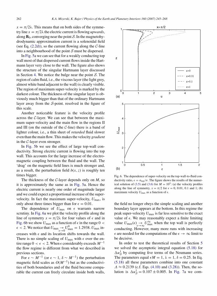
The dependence of Umax on ε warrants narrowscrutiny. In Fig. 6a we plot the velocity profile along theline of symmetry x = π/2λ for four values of ε and inFig. 6b we show Umax as a function of ε in the range 0 <

ε < 2. We notice that Umax →ε→0

U0max = 1.2938. Umax in-

creases with ε and its location shifts towards the wall.There is no simple scaling of Umax with ε over the en-tire range 0 < ε < 2. When ε considerably exceeds M−1

the flow regime is different from what we described inprevious sections.

−1 −1
For ε ∼ M (or ε ∼ 1, δ ∼ M ) the perturbationmagnetic field scales as O(M−1) but as the conductivi-ties of both boundaries and of the fluid become compa-rable the current can freely circulate inside both walls,
ical solution of (3.5) and (3.6) for M = 103: (a) the velocity profilesalong the line of symmetry, x = π/2 for ε = 0, 0.01, 0.1 and 1; (b)maximum velocity Umax as a function of ε.

the field no longer obeys the simple scaling and anotherboundary layer appears at the bottom. In this regime thepeak super-velocity Umax is far less sensitive to the exactvalue of ε. We may reasonably expect a finite limitingvalue Umax(ε) →

ε→∞U∞max when the top wall is perfectly

conducting. However, many more runs with increasingε are needed for the computations of the ε → ∞ limit tobe decisive.

In order to test the theoretical results of Section 5we solved the asymptotic integral equation (5.18) for�u1

S by computing five terms of the Neumann series.

(5.18) all these parameters combine into one constantΛ ≈ 0.2139 (c.f. Eqs. (4.10) and (3.28)). Then, the so-lution is �u1

S = 0.107 ± 0.005. In Fig. 7a we com-

K.A. Mizerski, K. Bajer / Physics of the Earth and

Fig. 7. The super-velocity enhancement due to the top-wall conduc-tivity as a function of the Hartmann number M and of the top-wall-to-fluid conductivity ratio, ε = σtop/σ. (a) The scaling with M forfixed εM = 1. The solution of the asymptotic Eq. (5.18a) for theexcess super-velocity M−(1/4) �u1

S is taken at n = 0 (dashed line)and compared with the numerical solutions of (3.5) and (3.6) for50 < M < 10,000 (solid line). Here �u is the computed differencebetween the maximum velocity in the fluid when the top wall is con-ducting and when it is insulating. (b) The scaling with ε for fixedMm0δ

pM

pt

tfia

. The comparison of the same asymptotic formula with the nu-erical solutions for three different values of M (broken lines) for.0001 < ε < 10. The thickness of both walls in all calculations is= δbot = 0.25.

are thus obtained asymptotic super-velocity excess,−(1/4)�u1

S, with the numerical solutions of the fullroblem (Eqs. (3.5) and (3.6)) for the range of values ofhe Hartmann number 50 < M < 10,000.

As the value of M increases the Hartmann layer andhe C-layer become very thin and the computational dif-culties are mounting, so it is difficult to attain a cleansymptotic regime M−(1/4) � 1. Nevertheless Fig. 7a


shows reasonable agreement and clear convergence be-tween the asymptotic formula and the computed super-velocity excess,

�u = Umax(ε = M−1) − Umax(ε = 0), (6.2)

obtained from the full numerical solutions. The asymp-totic formula is, in fact, somewhat better than we mightexpect. With M = 104 (left edge of Fig. 7) the discrep-ancy between �u and M−(1/4)�u1

S is about 0.01 (of theorder of M−(1/2)) while the theoretical accuracy of thelatter is O(M−(1/3)) ≈ 0.05 (see the discussion at the endof Section 4).

Another test of the asymptotic formula is the de-pendence of �u on ε at fixed M. Eq. (5.18) for aweakly conducting (or thin) wall predicts linear scaling.In Fig. 7b we show, on a logarithmic scale, the com-puted �u(ε, M = const) and the leading-order asymp-totic correction M−(1/4)�u1

S for M = 500, M = 1000and M = 2000 and with the conductivity ratio spanningthe range 10−4 < ε < 2 The linear dependence of thesuper-velocity excess, �u, on ε is evident and the agree-ment of the asymptotic formula with the numerical sim-ulations is very good.

We also compare the results of Hollerbach andSkinner (2001) for the scaling of the super-rotationwith the Hartmann number M in spherical geometrywith analogical scaling for planar geometry (for bothboundaries of finite thickness and having the sameconductivity as the fluid). We found that in our config-uration for 102 � M � 103 the super-velocity scaleslike M0.33 which differs significantly from the sphericalM0.6 scaling. Moreover, for values of M � 103, notconsidered by Hollerbach and Skinner (2001), thisscaling seems to change, namely the exponent decreases(see Fig. 8) indicating that for large M the asymptoticscaling may be different. The discrepancy between thescalings in the spherical and planar geometries suggestslack of universality. In both cases the power law seemsto exist for a certain range of Hartmann numbers andthat fact alone may indeed be universal. The value of theexponent seems to depend on the details of the magneticfield configuration and possibly on the curvature of theboundary in the vicinity of the singular point.

The computational results of this section thus confirmour analytical asymptotic predictions for the small butfinite top-wall conductivity. They also provide quantita-tive results beyond the asymptotic regime, i.e., for ε ∼ 1.The general conclusion of both the analysis and the nu-
merics on the mechanism of super-velocity generation istransparent. The acceleration of the fluid near the pointS = (x = π/2λ, z = 1) is due to the curvature of the ap-plied field B0 generating singularity at this point, and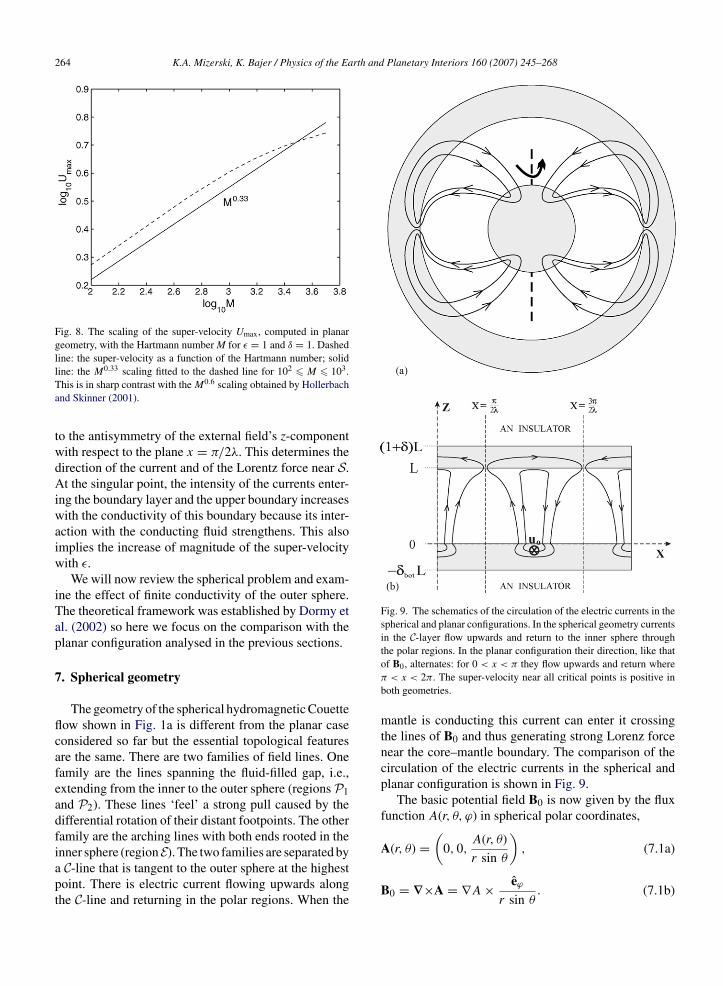

264 K.A. Mizerski, K. Bajer / Physics of the Earth and Planetary Interiors 160 (2007) 245–268

Fig. 8. The scaling of the super-velocity Umax, computed in planargeometry, with the Hartmann number M for ε = 1 and δ = 1. Dashedline: the super-velocity as a function of the Hartmann number; solid

Fig. 9. The schematics of the circulation of the electric currents in thespherical and planar configurations. In the spherical geometry currentsin the C-layer flow upwards and return to the inner sphere through

A(r, θ) = 0, 0, , (7.1a)

line: the M0.33 scaling fitted to the dashed line for 102 � M � 103.This is in sharp contrast with the M0.6 scaling obtained by Hollerbachand Skinner (2001).

to the antisymmetry of the external field’s z-componentwith respect to the plane x = π/2λ. This determines thedirection of the current and of the Lorentz force near S.At the singular point, the intensity of the currents enter-ing the boundary layer and the upper boundary increaseswith the conductivity of this boundary because its inter-action with the conducting fluid strengthens. This alsoimplies the increase of magnitude of the super-velocitywith ε.

We will now review the spherical problem and exam-ine the effect of finite conductivity of the outer sphere.The theoretical framework was established by Dormy etal. (2002) so here we focus on the comparison with theplanar configuration analysed in the previous sections.

7. Spherical geometry

The geometry of the spherical hydromagnetic Couetteflow shown in Fig. 1a is different from the planar caseconsidered so far but the essential topological featuresare the same. There are two families of field lines. Onefamily are the lines spanning the fluid-filled gap, i.e.,extending from the inner to the outer sphere (regions P1and P2). These lines ‘feel’ a strong pull caused by thedifferential rotation of their distant footpoints. The otherfamily are the arching lines with both ends rooted in the
inner sphere (regionE). The two families are separated bya C-line that is tangent to the outer sphere at the highestpoint. There is electric current flowing upwards alongthe C-line and returning in the polar regions. When the
the polar regions. In the planar configuration their direction, like thatof B0, alternates: for 0 < x < π they flow upwards and return whereπ < x < 2π. The super-velocity near all critical points is positive inboth geometries.

mantle is conducting this current can enter it crossingthe lines of B0 and thus generating strong Lorenz forcenear the core–mantle boundary. The comparison of thecirculation of the electric currents in the spherical andplanar configuration is shown in Fig. 9.

The basic potential field B0 is now given by the fluxfunction A(r, θ, ϕ) in spherical polar coordinates,(

A(r, θ))

r sin θ

B0 = ∇×A = ∇A × eϕ

r sin θ. (7.1b)

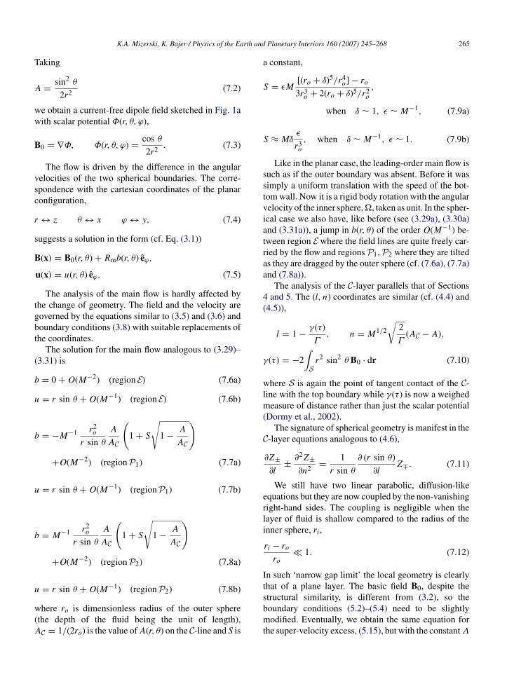
rth and

T

A

ww

B

vsc

r

s

B

tgbt

(

b

u

b

u

b

u

w(A


aking

= sin2 θ

2r2 (7.2)

e obtain a current-free dipole field sketched in Fig. 1aith scalar potential Φ(r, θ, ϕ),

0 = ∇Φ, Φ(r, θ, ϕ) = cos θ

2r2 . (7.3)

The flow is driven by the difference in the angularelocities of the two spherical boundaries. The corre-pondence with the cartesian coordinates of the planaronfiguration,

↔ z θ ↔ x ϕ ↔ y, (7.4)

uggests a solution in the form (cf. Eq. (3.1))

(x) = B0(r, θ) + Rmb(r, θ) eϕ,

u(x) = u(r, θ) eϕ. (7.5)

The analysis of the main flow is hardly affected byhe change of geometry. The field and the velocity areoverned by the equations similar to (3.5) and (3.6) andoundary conditions (3.8) with suitable replacements ofhe coordinates.

The solution for the main flow analogous to (3.29)–3.31) is

= 0 + O(M−2) (region E) (7.6a)

= r sin θ + O(M−1) (region E) (7.6b)

= −M−1 r2o

r sin θ

A

AC

(1 + S

√1 − A

AC

)+O(M−2) (regionP1) (7.7a)

= r sin θ + O(M−1) (regionP1) (7.7b)

= M−1 r2o A

(1 + S

√1 − A

)
r sin θ AC AC
+O(M−2) (regionP2) (7.8a)

= r sin θ + O(M−1) (regionP2) (7.8b)

here ro is dimensionless radius of the outer spherethe depth of the fluid being the unit of length),C = 1/(2ro) is the value of A(r, θ) on the C-line and S is


a constant,

S = εM[(ro + δ)5/r4

o] − ro

3r3o + 2(ro + δ)5/r2

o

,

when δ ∼ 1, ε ∼ M−1, (7.9a)

S ≈ Mδε

r3o

, when δ ∼ M−1, ε ∼ 1. (7.9b)

Like in the planar case, the leading-order main flow issuch as if the outer boundary was absent. Before it wassimply a uniform translation with the speed of the bot-tom wall. Now it is a rigid body rotation with the angularvelocity of the inner sphere, �, taken as unit. In the spher-ical case we also have, like before (see (3.29a), (3.30a)and (3.31a)), a jump in b(r, θ) of the order O(M−1) be-tween region E where the field lines are quite freely car-ried by the flow and regions P1, P2 where they are tiltedas they are dragged by the outer sphere (cf. (7.6a), (7.7a)and (7.8a)).

The analysis of the C-layer parallels that of Sections4 and 5. The (l, n) coordinates are similar (cf. (4.4) and(4.5)),

l = 1 − γ(τ)

Γ, n = M1/2

√2

Γ(AC − A),

γ(τ) = −2∫S

r2 sin2 θ B0 · dr (7.10)

where S is again the point of tangent contact of the C-line with the top boundary while γ(τ) is now a weighedmeasure of distance rather than just the scalar potential(Dormy et al., 2002).

The signature of spherical geometry is manifest in theC-layer equations analogous to (4.6),

∂Z±∂l

± ∂2Z±∂n2 = 1

r sin θ

∂ (r sin θ)

∂lZ∓. (7.11)

We still have two linear parabolic, diffusion-likeequations but they are now coupled by the non-vanishingright-hand sides. The coupling is negligible when thelayer of fluid is shallow compared to the radius of theinner sphere, ri,

ri − ro

ro� 1. (7.12)

In such ‘narrow gap limit’ the local geometry is clearlythat of a plane layer. The basic field B , despite the
0structural similarity, is different from (3.2), so theboundary conditions (5.2)–(5.4) need to be slightlymodified. Eventually, we obtain the same equation forthe super-velocity excess, (5.15), but with the constant Λ

rth and
replaced by

ΛS = Γ 1/423/4S√

AC, where

Γ =(

2 − ri

ro

) √1 − ri

ro, (7.13)

and S is given by (7.9). Hence, the equation for thesuper-velocity excess, analogous to (5.18), is

�u1S(n) = − 1√

8π

∫ 0

−∞

[�u1

S(n′)

× exp

(−1

8(n − n′)2

)]dn′

+ εM(1 + (δ/ro))5 − 1

(1 + (δ/ro))5 + (3/2)CS

× exp

(− 1

16n2)

D−(3/2)

(−1

2n

),

(7.14a)

where

CS =√

2(1 − (1/2)(ri/ro))1/4(1 − (ri/ro))1/8

r5/2o

.

(7.14b)

The equation differs little from (5.18). Hence, thescaling of the solution with M and with ε is the sameas in the planar case. In the narrow-gap limit the lo-cal geometry becomes nearly planar but there remainsa difference in B0 between the two cases. The similar-ity of Eqs. (5.18) and (7.14) shows, that the scaling ofthe super-velocity excess is robust. It does not dependon the details of B0, but on one essential feature, i.e.,topological discontinuity.8

The analysis can be extended beyond the narrow gaplimit, although considerable complications are mount-ing. When the effect of the coupling terms on the right-hand side of Eq. (7.11) is taken into account, the scalingwith ε found in the narrow-gap limit is unchanged.

There is one important difference between the planarconfiguration and the spherical one, even in the narrow-gap limit. In the planar case only the relative veloc-ity of the two walls is important while in the sphericalcase not only the differential rotation matters but also
the spin of the outer shell has influence that cannot beeliminated by changing the frame of reference. Whenboth boundaries rotate at different angular velocities, the
8 Presumably the scaling is the same whenever the point of tangentcontact between the C-line and the solid boundary is parabolic. It maybe different in the case of degenerate tangency, e.g., quartic.


Coriolis force substantially modifies the solution even inthe case of small differential rotation unless the flow isstrongly dominated by the magnetic forcing. The prob-lem of MHD Couette flow with Coriolis force was inves-tigated numerically by Hollerbach (1994) and Dormy etal. (1998) and analytically, for small Elsasser numbers,by Kleeorin et al. (1997).

Topological discontinuity is the key to another hy-dromagnetic flow problem that was studied numericallyby Hollerbach and Skinner (2001). They considered aspherical Couette flow with uniform basic magnetic fieldaligned with the axis of rotation. The outer sphere wasstationary and had the same electrical conductivity as theliquid while the rate of rotation and conductivity of theinner sphere were adjustable parameters. In that config-uration the topological discontinuity occurs across thefamily of field lines lying on the cylinder tangent to theinner sphere. The field lines inside that cylinder haveone footpoint rooted in the outer sphere and the otherrooted in the inner sphere. Those lines strongly ‘feel’the differential rotation and become twisted in a helicalshape, i.e., they acquire considerable azimuthal compo-nent b(r, θ)eϕ. The line outside the tangent cylinder haveboth ends rooted in the outer sphere and are far less af-fected by the rotation of the inner core. The dividing lineson the tangent cylinder have two footpoints on the outersphere and one point of tangent contact ‘dragged’ alongthe equator of the inner sphere. This configuration isamenable to asymptotic analysis of the kind we have pre-sented (M � 1, slow rotation and weak conductivity ofthe inner sphere) but the general conclusions can alreadybe drawn on the basis of topological considerations.

The main flow outside the tangent cylinder is dictatedby the highly conducing outer boundary, so it will sim-ply be the state of rest. There is a Hartmann layer on theinner sphere which is singular at the equator. However,in the neighbourhood of the singularity the Lorenz forceopposes the drag from the inner sphere, so we have aretarded rather than accelerated jet. This can be deducedfrom the symmetries of the problem. The perturbationfield b(r, θ) is antisymmetric with respect to the equa-torial plane θ = (1/2)π with b(r, θ) < 0 for θ < (1/2)πand b(r, θ) > 0 for θ > (1/2)π. Hence, the radial currentat the equator is positive, jr|θ=π/2 = 1/r(∂b/∂θ) > 0, soit flows out of the core into the fluid. Therefore, the az-imuthal component of the Lorenz force at the equator (ofthe inner core) is negative, opposite to the linear veloc-ity of the core surface, so instead of super-velocity we
have retarded fluid flowing much slower than the bound-ary. Relative to the inner core surface there is a strongcounter-rotating jet found by Hollerbach and Skinner(2001).

rth and

8

tet(wtolaToofiiavmc

hedcvbfttswssqctwpM

dg

mtolstbr


. Conclusions

The planar and spherical Couette flow with strong, ex-ernally applied magnetic field contains Hartmann lay-rs that locally, in the vicinity of the critical field lineangent to the rigid boundary, exhibit super-velocitiessuper-rotation), i.e. a strong streamwise jet in the near-all region where the speed of the fluid is much greater

han that of the distant boundary that drives the flow. Notnly the surface jet is moving with such ‘excessive’ ve-ocity but also, to a lesser extent, the entire sheet of fluidlong the whole length of the critical magnetic field line.he phenomenon is topological in nature, as the pointf tangent contact with the outer boundary is the locusf discontinuity in the end-to-end mapping of the basiceld B0. This special type of topological discontinuity

s responsible for the creation of a current sheet and thessociated electromagnetic stress that causes the super-elocities. The balance of the system and therefore theagnitude of the super-velocities is very sensitive to the

onductivity of the top wall.We have derived an asymptotic formula for the en-

ancement of the super-velocity when the top wall isither thin but highly conducting or thick but weakly con-ucting. This is a theoretical confirmation of the numeri-al result of Hollerbach (2000) who compared the super-elocities near an insulating boundary with those near theoundary that is both thick and highly conducting andound them much bigger in the latter case. Our asymp-otic formula, derived by means of a singular perturba-ion method building upon that of Dormy et al. (2002),hows that in the case of a highly conducting outer shellith (small) thickness δ ∼ M−1 the enhancement of

uper-velocity scales like δM3/4. For a thick mantle ofmall conductivity, ε ∼ M−1, it scales like εM3/4. Thisuantifies the trend revealed by Hollerbach (2000) butannot be directly extended to the ε ∼ 1, δ ∼ 1 regimehat he considered. The super-velocity in that regimee have calculated numerically and found that in thelanar case it scales with the basic field strength as

0.33. This is in sharp contrast with the M0.6 scalingetected by Hollerbach and Skinner (2001) in sphericaleometry.

Topological discontinuity at the liquid core surfaceay act as a powerful amplifier of any differential ro-

ation that may be present deeper down. The footpointsf the magnetic field lines in the vicinity of the criticaline tangent to the mantle may be dragged not just by the
lightly super-rotating inner core (Su et al., 1996), as inhe model by Dormy et al. (2002) but, more generally,y any layer in the liquidus differentially rotating withespect to the mantle. One possible cause of differential

rotation that might be amplified by singular Hartmannlayers are torsional oscillations.

The picture that we had in mind here is that of theEarth’s liquid core penetrated by the global poloidalforce-free field and we were concerned only with thesteady state. However, the super-rotation near the bound-ary, whether insulating or conducting, would feature ona range of spatial and temporal scales. Let us imag-ine a slightly buoyant, arched, magnetic flux tube risingthrough the rotating fluid and hitting the rigid ceiling. Asthe top of the arch enters the boundary layer a transientsurface jet is induced by the very mechanism describedhere. The ‘surface turbulence’ thus reflects, admittedlyin a rather indirect way, the spatio-temporal characteris-tics of the underlying magnetic field. This, clearly, is nosurprise but the fact that those characteristics are stronglyamplified by the mechanism of super-rotation could pos-sibly make them detectable.

Acknowldgments

One of us (KM) would like to thank EmmanuelDormy and Henri-Claude Nataf for suggesting the prob-lem of singularity of the Hartmann layer and super-rotation. We are also grateful to Lech Krysinski for valu-able discussions. The numerical calculations were per-formed at the Interdisciplinary Centre for Mathematicaland Computational Modelling (ICM), Warsaw Univer-sity (computational grant number G28-11). The supportfrom the Centre of Excellence in Small Scale Atmo-spheric Research CESSAR (EU Grant no. EVK2-CT-2002-80010) is gratefully acknowledged.

References

Alexandrescu, M., Gibert, D., Le Mouel, J.-L., Hulot, G., Saracco,G., 1999. An estimate of average lower mantle conductivity bywavelet analysis of geomagnetic jerks. J. Geophys. Res. 104 (B8),17735–17745.

Bloxham, J., 1998. Dynamics of angular momentum in the Earth’score. Annu. Rev. Earth Planet. Sci. 26, 501–517.

Bullard, E.C., Freedman, C., Gellman, H., Nixon, J., 1950. The west-ward drift of the Earths magnetic field. Phil. Trans. R. Soc. LondonA 243, 67–92.

Dormy, E., Cardin, P., Jault, D., 1998. MHD flow in a slightly differ-entially rotating spherical shell, with conducting inner core, in adipolar magnetic field. Earth Planet. Sci. Lett. 160, 15–30.

Dormy, E., Jault, D., Soward, A.M., 2002. A super-rotating shear layerin magnetohydrodynamic spherical Couette flow. J. Fluid Mech.
452, 263–291.
Dubrovinsky, L., Dubrovinskaia, N., Langenhorst, F., Dobson, D., Ru-bie, D., Geßmann, C., Abrikosov, I.A., Johansson, B., Baykov, V.I.,Vitos, L., Le Bihan, T., Crichton, W.A., Dmitriev, V., Weber, H.-P.,2003. Iron-silica interaction at extreme conditions and the electri-

rth and
cally conducting layer at the base of Earth’s mantle. Nature 422,58–61.

Elsasser, W.M., 1950. The hydromagnetic equations. Phys. Rev. 80,183.

Gradshteyn, I.S., Ryzhik, I.M., Jeffrey, A. (Eds.), 1994. Table of Inte-grals, Series, and Products, 5th ed., Academic Press.

Greff-Lefftz, M., Legros, H., 1999. Magnetic field and rotational fre-quencies. Phys. Earth Plane. Int. 112, 21–41.

Hollerbach, R., 1994. Magnetohydrodynamic Ekman and Stewartsonlayers in a rotating spherical shell. Proc. R. Soc. Lond. A 444,333–346.

Hollerbach, R., 2000. Magnetohydrodynamic flows in spherical shells.In: Egbers, C., Pfister, I.G. (Eds.). Physics of Rotating Fluids, Lec-ture Notes in Physics, vol. 549. Springer, pp. 295–316.

Hollerbach, R., Skinner, S., 2001. Instabilities of magnetically inducedshear layers and jets. Proc. R. Soc. Lond. A 457, 785–802.

Holme, R., 1998. Electromagnetic core–mantle coupling. I. Explainingdecadal changes in the length of day. Geophys. J. Int. 132, 167–180.

Jault, D., LeMouel, J.-L., 1991. Exchange of angular momentum be-tween the core and mantle. J. Geomagn. Geoelectr. 43, 111–129.

Kleeorin, N., Rogachevskii, L., Ruzmaikin, A., Soward, A.M.,Starchenko, S., 1997. Axisymetric flow between diferentially rotat-ing spheres in a dipole magnetic field. J. Fluid Mech. 344, 213–244.

Love, J.J., Bloxham, J., 1994. Electromagnetic coupling and the
toroidal magnetic field at the core–mantle boundary. Geophys. J.Int. 117, 235–256.
Moffatt, H.K., 1978. Magnetic Field Generation in ElectricallyConducting Fluids. Cambridge University Press. Available fromhttp://moffatt.tc.


Moffatt, H.K., 1987. Geophysical and astrophysical turbulence. In:Comte-Bellot, G., Mathieu, J. (Eds.). Advances in Turbulence.Springer, pp. 228–244. Available from http://moffatt.tc.

Munk, W.H., Revelle, R., 1952. On the geophysical interpretation ofirregularities in the rotation of the Earth. MNRAS Geophys. Suppl.6, 331–347.

Nataf, H.-C., Alboussicre, T., Brito, D., Cardin, P., Gagnicre, N., Jault,D., Masson, J.-P., Schmitt, D., 2006. Experimental study of super-rotation in a magnetostrophic spherical Couette flow. Geophys.Astrophys. Fluid Dyn. 100, 281–298.

Pais, A., Hulot, G., 2000. Length of day decade variations, torsionaloscillations and inner core super-rotation: evidence from recov-ered core surface zonal flows. Phys. Earth Planet. Int. 118, 291–316.

Roberts, P.H., 1967. Singularities of Hartmann layers. Proc. R. Soc.Lond. A 300, 94–107.

Starchenko, S.V., 1998. Magnetohydrodynamic flow between insulat-ing shells rotating in strong potential field. Phys. Fluids 10, 2412–2420.

Starchenko, S.V., 1998. Strong potential field influence on slightlydifferentially rotating spherical shells. Stud. Geophys. Geodyn. 42,314–319.

Su, W., Dziewonski, A.M., Jeanloz, R., 1996. Planet within aplanet: rotation of the inner core of Earth. Science 274, 1883–
1887.
Zatman, S., 2001. Phase relations for high frequency coremantle cou-pling and the Earths axial angular momentum budget. Phys. EarthPlanet. Int. 128, 163–178.

http://moffatt.tc.

http://moffatt.tc.

On the effect of mantle conductivity on the super-rotating jets near the liquid core surface

Documents

Transcript of On the effect of mantle conductivity on the super-rotating jets near the liquid core surface