On Balancing Energy Consumption in Wireless Sensor Networks 1 2

IEEE

Proo

f

IEEE TRANSACTIONS ON VEHICULAR TECHNOLOGY 1

On Balancing Energy Consumption inWireless Sensor Networks

1

2

Fatma Bouabdallah, Nizar Bouabdallah, and Raouf Boutaba3

Abstract—Wireless sensor networks (WSNs) require protocols4that make judicious use of the limited energy capacity of the5sensor nodes. In this paper, the potential performance improve-6ment gained by balancing the traffic throughout the WSN is7investigated. We show that sending the traffic generated by each8sensor node through multiple paths, instead of a single path, allows9significant energy conservation. A new analytical model for load-10balanced systems is complemented by simulation to quantitatively11evaluate the benefits of the proposed load-balancing technique.12Specifically, we derive the set of paths to be used by each sensor13node and the associated weights (i.e., the proportion of utilization)14that maximize the network lifetime.15

Index Terms—Energy conservation, load balancing, perfor-16mance analysis, routing, wireless sensor networks (WSNs).17

I. INTRODUCTION18

THE LIMITED energy capacity of sensor nodes dictates19

how communications must be performed inside wireless20

sensor networks (WSNs). WSN protocols must make judicious21

use of the finite-energy resources. Typically, sensor nodes avoid22

direct communication with a distant destination since a high23

transmission power is needed to achieve a reliable transmission24

[1], [2]. Instead, sensor nodes communicate by forming a25

multihop network to forward messages to the collector node,26

which is also called the sink node. In this regard, efficient27

routing in such multihop networks becomes crucial in achieving28

energy efficiency. In addition to using multihop communication29

for reducing the energy requirements for communication, an30

efficient routing protocol is needed to decrease the end-to-end31

energy consumption when reporting data to the sink node.32

To improve the network lifetime, extensive research on de-33

signing energy-efficient medium-access control (MAC) proto-34

cols has been conducted in the literature [3]–[5]. Accordingly,35

the sensor nodes turn off some hardware components when they36

are unused. As such, the wasted energy due to idle listening37

Manuscript received March 13, 2008; revised August 17, 2008 andSeptember 30, 2008. The review of this paper was coordinated byDr. W. Zhuang.

F. Bouabdallah is with the Institut National de Recherche en Informatique eten Automatique, 35042 Rennes, France (e-mail: [email protected]).

N. Bouabdallah is with the Institut National de Recherche en Informatiqueet en Automatique, 35042 Rennes, France, and also with the David R. CheritonSchool of Computer Science, University of Waterloo, Waterloo, ON N2L 3G1,Canada (e-mail: [email protected]).

R. Boutaba is with the School of Computer Science, University of Waterloo,Waterloo, ON N2L 3G1, Canada (e-mail: [email protected]).

Color versions of one or more of the figures in this paper are available onlineat http://ieeexplore.ieee.org.

Digital Object Identifier 10.1109/TVT.2008.2008715

to the medium is reduced. Indeed, a transceiver that constantly 38

senses the channel will quickly deplete the sensor node energy 39

and dramatically shorten the network lifetime. Thus, it is im- 40

perative that the idle sensor nodes enter sleep mode as often as 41

possible [11]. However, each sensor node must coordinate with 42

its neighbors to ensure communications when needed. To do so, 43

the works in [3]–[10] suggested wake-up scheduling schemes at 44

the MAC layer to activate sleeping nodes when needed. On the 45

other hand, the works in [12] and [13] addressed the problem at 46

the network layer by proposing new routing solutions that take 47

into account the sleep state of some network nodes. 48

To date, much of the work on WSNs has focused on the 49

energy minimization problem, taking into consideration the 50

individual sensor node performance, i.e., finding methods that 51

allow each sensor node to consume the minimum amount of en- 52

ergy subject to a given traffic load for handling. However, there 53

has been little focus on how traffic is balanced throughout mul- 54

tihop WSNs and how it impacts the overall network lifetime. 55

In this paper, the use of multiple paths between each sensor 56

node and the sink node is considered. It is shown that the 57

network lifetime can be improved by efficiently routing (i.e., 58

balancing) the traffic inside the WSN. 59

Assuming the network lifetime as the time for the first node 60

in the WSN to fail, a perfect routing protocol would slowly and 61

uniformly drain energy among nodes, leading to the death of 62

all nodes nearly at the same time. Typically, an ideal routing 63

protocol would avoid the fast drain of sensor nodes with high 64

energy consumption. To achieve this, we propose balancing the 65

energy consumption throughout the network by sending the 66

traffic generated by each sensor node through multiple paths, 67

instead of always forwarding through the same path. In fact, 68

always routing through the same path will quickly deplete the 69

energy of the sensor nodes contained therein. The problem 70

then consists of determining the set of routes to be used by 71

each sensor node and the associated weights (i.e., the routing 72

configuration) that maximize the network lifetime. 73

Using a classical contention-based access method to the data 74

channel and the most commonly used acknowledgment (ACK) 75

model to ensure reliable transmissions, a new analytical model 76

is developed for calculating the energy consumption at each 77

sensor node per unit of time, given a specific routing config- 78

uration. The energy consumed by a sensor node corresponds 79

to that used to transmit its own generated messages and to 80

relay the pass-through traffic of other sensor nodes. Moreover, 81

to better evaluate the real behavior of WSNs, we consider the 82

wasted energy due to retransmissions, overhearing, and idle 83

listening, which is not the case in many models developed in 84

the literature [13], [19]. Building on these results, we derive 85

0018-9545/$25.00 © 2009 IEEE

IEEE

Proo

f

2 IEEE TRANSACTIONS ON VEHICULAR TECHNOLOGY

the optimal routing configuration that maximizes the network86

lifetime. For the numerical results, a variety of network topolo-87

gies are considered, including regular and arbitrary meshed88

topologies and varying network sizes. As a main contribution89

of our paper, we show that, by efficiently balancing the traffic90

inside the network, significant energy savings of up to 15% can91

be achieved, compared to the basic routing protocols.92

Section II presents the state of the art related to the focus of93

this paper. Section III formulates the general problem statement94

and presents the system model to be studied. This model is95

then formally studied in Section IV. Specifically, we derive the96

energy consumed by each sensor node per unit of time, given97

a specific routing configuration. The results are provided in98

Section V, where we evaluate the performance of our proposal,99

using two well-known routing protocols as baseline examples.100

This paper concludes with a summary of our conclusions and101

contributions.102

II. RELATED WORK103

To minimize the energy consumption in WSNs, several104

energy-efficient MAC protocols [3]–[5] and energy-efficient105

routing protocols [12], [13] have been proposed in the literature.106

These schemes aim at decreasing the energy consumption by107

using sleep schedules [14]. The key idea behind this concept is108

completely turning off some parts of the sensor circuitry (e.g.,109

microprocessor, memory, and radio) when it does not receive110

or transmit data, instead of keeping the sensor node in the idle111

mode. This scheme simply attempts to reduce wasted energy112

due to idle listening, i.e., lost energy while listening to receive113

possible traffic that is not sent. To do so, the works in [3]–[10]114

suggest wake-up scheduling schemes at the MAC layer to115

activate sleeping nodes when needed. On the other hand, the116

works in [12] and [13] address the problem at the network layer117

by proposing new routing solutions that take into account the118

sleep state of some network nodes. Additional solutions for re-119

ducing energy consumption, based on congestion control, have120

also been proposed in [15] and [16]. These mechanisms aim121

at achieving further energy conservation by reducing the en-122

ergy wastage resulting from the frequently occurring collisions123

in WSNs.124

Although there is significant energy savings achieved by such125

schemes based on the sleep schedules, the WSN keeps sending126

redundant data. Typically, WSNs rely on the cooperative effort127

of the densely deployed sensor nodes to report detected events.128

As a result, multiple sensor nodes may report the same event.129

To further decrease energy consumption, we have proposed in130

[17] a MAC scheme that eliminates the transmission of useless131

redundant information by profiting from the spatial correlation132

between nodes, as in [18].133

While the previous approaches are quite useful, the energy134

efficiency of these protocols can considerably be affected if the135

traffic is far from being uniformly distributed in the network.136

Typically, these protocols aim at minimizing the energy con-137

sumed by each sensor node subject to a given traffic load for138

handling. However, there has been little focus on how traffic139

is balanced throughout multihop WSNs and how it impacts the140

network lifetime.141

In view of this, significant energy savings can be achieved 142

at the routing level when considering the multihop ability. Our 143

work is motivated by the results presented in [19], where the 144

authors investigated the problem of lifetime maximization in 145

WSNs under the constraint of end-to-end transmission suc- 146

cess probability. To do so, the authors adopted a cross-layer 147

strategy that considers the physical layer (i.e., power control), 148

the MAC layer (i.e., transmission control), and the network 149

layer (i.e., routing control). Specifically, regarding the network 150

layer, the authors formulated the problem of multihop routing 151

in the context of WSNs by considering the energy constraint 152

required for reliable end-to-end transmission. Building on this 153

formulation, the authors derived, for each sensor node, the path 154

with the minimum energy consumption, assuming collision- 155

free transmissions on the shared channel. This problem, which 156

is also well known as the minimum total energy (MTE) routing 157

problem, has extensively been addressed in the context of 158

ad-hoc networks [20]–[22]. The MTE problem consists of 159

finding the route that minimizes the total consumed energy 160

between any pair of source and destination nodes. 161

Nevertheless, using the MTE routing, i.e., always routing 162

through the path with the minimum energy consumption, will 163

quickly deplete the energy of the sensor nodes contained 164

therein. To address this issue, Kwon et al. [19] introduced the 165

concept of routing packets such that energy consumption is bal- 166

anced among multiple paths. However, in doing so, Kwon et al. 167

considered a simplistic scenario such as that when the medium 168

is slotted, i.e., for each transmission, all the network nodes are 169

supposed to be in sleep state, except for the sender and receiver 170

nodes. Thus, collision-free transmission is ensured. As such, 171

the typical energy wasted by the sensor nodes due to collisions, 172

overhearing, and idle listening was not considered. 173

In this paper, a general scenario with a conventional 174

contention-based access method to the wireless channel is 175

considered. We provide an in-depth analysis of load balancing 176

through multihop WSNs. Although this work takes inspiration 177

from [19], it differs in several ways. First, a more realistic sce- 178

nario with multiple-access nodes competing to access the com- 179

mon wireless channel is considered. This reveals some of the 180

major strengths of the WSN capabilities, e.g., the cooperative 181

effort of the densely deployed sensor nodes to report detected 182

events. It also allows for direct comparison with basic systems 183

(i.e., where traffic balancing is not considered), without any ad- 184

ditional assumptions, showing the clear benefit of load balanc- 185

ing. Our model indeed captures the real behavior of WSNs by 186

considering the wasted energy due to retransmissions, overhear- 187

ing, and idle listening. Second, this paper explores the impact of 188

collisions and the unreliability of links on the energy consump- 189

tion, considering the hidden-node problem that is typical in 190

multihop networks. This paper shows how collisions (i.e., con- 191

gestion) can be reduced through load balancing. In other words, 192

this paper illustrates how spatial reuse of the wireless channel 193

can be exploited to achieve additional energy conservation. 194

As an alternative to our multiple-path-routing approach for 195

achieving load balancing, the works in [23]–[26] proposed 196

instead the use of adaptive routing schemes, where the routing 197

decisions are made on the fly by considering the current residual 198

energy at the sensor nodes. These schemes balance between 199

IEEE

Proo

f

BOUABDALLAH et al.: ON BALANCING ENERGY CONSUMPTION IN WSNs 3

the MTE and the max-min residual energy routing [27], which200

selects the path whose minimum residual energy fraction after a201

packet delivery is the maximum. References [23]–[26] have the202

same design philosophy. They attempt to use the path with the203

minimum energy consumption while avoiding the nodes with204

small residual energy.205

In our study, we opt for the preconfigured static routing, in-206

stead of the adaptive on-the-fly routing for three main reasons:207

First, in our study, the sensor nodes are not mobile. Hence,208

the network topology is static, as opposed to typical ad-hoc209

networks, where on-the-fly routing is required to adapt to the210

frequent topological changes.211

The second reason behind using the preconfigured routing212

is the traffic pattern. In our study, we consider continuous-213

monitoring applications, where each node periodically reports214

its data to the sink node. The amount of information generated215

by each sensor node is therefore known a priori, as opposed216

to event-driven applications, where the generated information217

at each sensor node is not known a priori since it depends on218

the arbitrary occurrence of specific events. In such event-driven219

WSNs, it may be useful to make routing decisions on the fly for220

each occurring event by considering the current network state221

(i.e., the residual energy at each sensor node). However, this is222

not required in our targeted continuous-monitoring networks.223

To be more precise, it is not recommended for the third reason224

given here.225

Performing on-the-fly routing for each generated information226

induces considerable exchange of signaling messages. This227

routing scheme requires global and online information about228

the network state in making routing decisions. In computer229

networks where packets are large, the small control packets230

may impose little overhead. However, in WSNs where the231

packet size is small, they constitute a large overhead. This can232

extremely be costly since a large amount of energy has to be233

spent to route the control packets.234

In response to these challenges, we propose our preconfig-235

ured balanced routing scheme. From a performance evalua-236

tion perspective, we develop a model for energy consumption237

that captures the real behavior of WSNs, as opposed to pre-238

vious works, where many simplistic assumptions have been239

considered.240

III. MODEL AND PROBLEM DESCRIPTION241

A. Network Model242

We represent a WSN by directed graph G(V,E), which243

is called a connectivity graph. Each sensor node v ∈ V is244

characterized by a circular transmission range Rt(v) and a245

carrier-sensing range Rh(v) (which is also called the hearing246

range). In our study, we suppose that all the sensor nodes have247

the same transmission and carrier-sensing ranges denoted by248

Rt and Rh, respectively. During the transmission of node v,249

all the nodes inside its carrier-sensing range, which is denoted250

by H(v), sense the channel to be busy and cannot access251

the medium. Hereinafter, we denote by H+(v) = H(v) ∪ {v}252

and H−(v) the set of nodes that node v cannot hear, i.e.,253

H−(v) = V \H+(v).254

On the other hand, during the transmission of node v, all the 255

nodes residing in its transmission range and thus representing 256

its neighborhood denoted by Ne(v) receive the signal from 257

v with a power strength such that correct decoding is possi- 258

ble with high probability. A bidirectional wireless link exists 259

between v and every neighbor u ∈ Ne(v) and is represented 260

by the directed edges (u, v) and (v, u) ∈ E. Note that, the 261

proposed network model assumes the knowledge of sets H(v) 262

andNe(v) for each sensor node v ∈ V . To obtain such inputs in 263

practice, we assume that the cartography of the sensor network 264

is known in advance. 265

We represent the graph connectivity by a connectivity matrix. 266

The connectivity matrix of G(V,E) is a matrix whose rows and 267

columns are labeled by the graph vertices V , with a 1 or a 0 in 268

position (m,n), according to whether vm and vn are directly 269

connected or not. In other words, placing 1 in position (m,n) 270

means that vm and vn are within the transmission range of 271

each other (i.e., the two nodes can communicate). In our study, 272

all the sensor nodes periodically transmit their reports to the 273

sink node, which is denoted by S. Here, we target continuous- 274

monitoring applications, which represent an important class of 275

WSN applications. The average number of reports sent per 276

unit of time by each sensor node v is denoted by A(v). The 277

transmitted packet by v can follow one of the possible paths in 278

graph G(V,E) that connects v to sink node S. The set of paths 279

between vertex v and S is denoted by P (v). 280

In WSNs, the reporting sensor nodes compete to access 281

the common data channel to report their sensing data to the 282

sink nodes. In our study, access to the medium among the 283

competing nodes is arbitrated by the well-known IEEE 802.11- 284

like sensor network protocol [28], [29]. The IEEE 802.11 285

distributed coordination function access method is based on the 286

carrier-sense multiple-access/collision-avoidance (CSMA/CA) 287

technique. Thus, considering IEEE 802.11 in the context of 288

WSNs allows determining a general case study for all WSN 289

protocols based on the CSMA/CA technique. Note that SMAC AQ1290

[4] and TMAC [5] are WSN MAC protocols that rely on the 291

CSMA/CA technique to coordinate the access to the wireless 292

channel between all competing nodes. Thus, our study also 293

remains valid for those WSN MAC protocols. 294

According to the CSMA/CA technique, a host, wishing to 295

transmit a frame, first senses channel activity until an idle 296

period that is equal to distributed interframe space (DIFS) 297

is detected. Then, to avoid collisions, the station waits for a 298

random backoff interval before transmitting. The backoff time 299

counter is decremented in terms of time slots as long as the 300

channel is sensed to be free. The counter is suspended once 301

a transmission is detected on the channel. It resumes with the 302

old remaining backoff interval when the channel is sensed to 303

be idle again for a DIFS period. The station transmits its frame 304

when the backoff time becomes zero. If the frame is correctly 305

received, the receiving host sends an ACK frame after a short 306

interframe space (SIFS). If an ACK is not received by the sender 307

within an ACK timeout, the transmitted frame is supposed to be 308

lost (due to either collision or channel error). 309

In this case, the sending host attempts to send its frame 310

again when the channel is free for a DIFS period augmented 311

by the new backoff, which is sampled according to the binary 312

IEEE

Proo

f


exponential backoff (BEB) process. Specifically, for each new313

transmission attempt, the backoff interval is uniformly chosen314

from the range [0, CW ] in terms of time slots. At the first315

transmission attempt of a frame, CW is equal to the initial316

backoff window size CWmin. Following each unsuccessful317

transmission,CW is doubled until a maximum backoff window318

size value CWmax is reached. Once the frame is successfully319

transmitted, the CW value is reset to CWmin.320

In our analysis, we assume that there is no limit on theAQ2 321

number of retransmissions over a link. Hence, a packet is never322

discarded by a node and continues to be retransmitted until it is323

successfully delivered.324

The procedure previously described is referred to as the325

basic access mode. An optional request-to-send (RTS)/clear-326

to-send (CTS) mechanism can also be used to avoid collision327

among data packets due to the hidden terminal problem [30],328

[31]. Using the RTS/CTS mechanism, collisions still occur but329

among the small RTS frames, instead of the relatively large data330

packets. However, the actual payload of a data packet in WSNs331

is usually small. For instance, the CC2420 low-cost transceiver332

[32] has a transmit buffer of 128 B and a data packet payload333

of 30–50 B. For this reason, the RTS/CTS mechanism is usu-334

ally disabled in WSNs. Moreover, it was shown in [33] that335

RTS/CTS increases the overhead without really improving the336

network performance. In view of this, we consider the basic ac-337

cess mode, but the same study with slight modifications can eas-338

ily be adapted to the case where the RTS/CTS option is enabled.339

B. Problem Description340

In this paper, we approach the efficient routing of reports to341

the sink node by balancing the energy consumption throughout342

the network. By doing so, we aim at improving the WSN life-343

time. For each sensor node v, generated reports to the sink can344

follow one of the possible |P (v)| paths. We associate a weight345

w(p) to each path p ∈ P (v), such that∑

p∈P (v) w(p) = 1.346

Vector W (v) = (w(p))p∈P (v) represents the fraction of utiliza-347

tion of each path p ∈ P (v) used to send the traffic from node v348

to the sink node.349

The number of packets per unit of time that go through350

link (u, v) ∈ E is denoted by λ(u, v). It represents the rate of351

packets transmitted by node u to node v. These packets can be352

generated by either u or other sensor nodes and relayed by u to353

attain their final destination (i.e., the sink node). Rate λ(u, v)354

can simply be expressed as follows:355

λ(u, v) =∑k∈V

∑p∈P (k)

w(p) ×A(k) × 1∣∣(u,v)∈p(1)

where 1|(u,v)∈p is the indicator function of the condition that356

link (u, v) belongs to path p. Moreover, the packet rate trans-357

mitted by node u is given by358

λu =∑

n∈Ne(u)

λ(u, n). (2)

Note that (1) is derived by considering the system working359

in the unsaturated regime, which is more likely the case of360

real WSNs. WSNs indeed produce light traffic, compared with 361

traditional wireless networks. Unless explicitly notified, we 362

consider the WSN working under the unsaturated regime in the 363

reminder of this paper. 364

Let us consider a path p ∈ P (v). We denote the average 365

energy consumed by node u due to the successful delivery of a 366

packet transmitted by v to the sink node through path p.E(u, p) 367

includes only the energy consumed in transmission or reception 368

(i.e., it does not include the energy consumed by a sensor node 369

during the idle state). The average amount of energy consumed 370

by node u per unit of time due to the different transmissions 371

inside the WSN, which is denoted by E(u), can therefore be 372

expressed as follows: 373

E(u) = Eidle(u) +∑v∈V

∑p∈P (v)

w(p) ×A(v) × E(u, p) (3)

where Eidle(u) is the average amount of energy consumed by 374

node u per unit of time during its idle state. The lifetime of 375

sensor node u is then given by 376

T (u) =Einit

E(u)(4)

where Einit is the initial amount of energy provided to each 377

sensor node. 378

The network lifetime is defined as the time spent from the 379

deployment until the drain of the first sensor node. Hence, 380

to maximize the network lifetime, we have to maximize the 381

lifetime of the greediest node in the network in terms of energy 382

consumption. The problem then consists of minimizing the 383

following function: 384

maxW

T (u) = minW

(maxu∈V

E(u)). (5)

Indeed, to maximize the network lifetime, we have to avoid 385

the fast drain of sensor nodes with high energy consumption. 386

We therefore need to balance the energy consumption inside the 387

network by efficiently routing the data packets. This is achieved 388

by determining the optimal set of vectors (W (v))v∈V = W that 389

enables to minimize the energy consumption of the greediest 390

sensor nodes to maximize the network lifetime. 391

C. Motivating Balanced Routing Through an Example 392

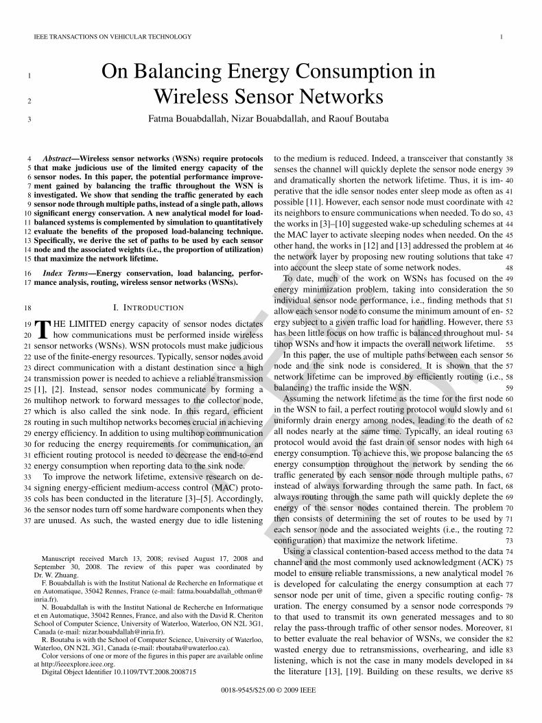
Consider the sample scenario shown in Fig. 1, where each 393

sensor node among A, B, and C transmits r reports per unit of 394

time to sink node S. Nodes B and C directly transmit their data 395

packets to S since S is within the B and C transmission ranges. 396

On the other hand, node A has to transmit through B or C to 397

reach S. 398

We denote by (1 − β(A,B)) the packet delivery success 399

probability from A to B. β(A,B) represents the quality of the 400

wireless link between nodes A and B. Assume that β(A,B) = 401

β(A,C) = β(B,S) = β(C,S). As such, paths p1 = [A,B,S] 402

IEEE

Proo

f


Fig. 1. Four-node example network.

and p2 = [A,C,S] are equivalent in terms of the quality of the403

wireless links.404

Assume that the routing layer chooses to use path p1 to405

deliver packets from A to S. As a result, node B transmits406

twice more packets than nodesA andC. Hence, node-B energy407

prematurely depletes, leading to a quick death of the network,408

although the remaining sensor nodes are still alive.409

Alternatively, using our balanced routing method, node A410

fairly shares its generated traffic between intermediate nodes B411

and C. Specifically, as paths p1 and p2 have equivalent prop-412

erties (i.e., same quality of the wireless links), node A sends413

exactly half of its traffic through each of the two possible414

paths. In doing so, the energy uniformly drains among nodes B415

and C, which improves the network lifetime, compared to the416

case where node A always transmits through the same path p1.417

It is worth noting that the proportions of utilization of con-418

current paths p1 and p2, which are denoted by w1 and w2,419

respectively, depend on the paths’ qualities. In the previous420

example, intermediate nodes B and C fairly share the traffic421

sent by node A (i.e., w1 = w2 = 0.5) since paths p1 and p2422

have the same quality and this routing configuration maximizes423

the network lifetime.424

Assume now that β(A,B) = β(A,C) and β(B,S) <425

β(C,S). This means that (B,S) is a better link than (C,S) and426

that transmitting through B helps reduce the total number of427

retransmissions. Typically, a packet sent by nodeA requires less428

energy to be correctly delivered to node S when it is transmitted429

through p1, instead of p2. However, always routing through the430

path with minimum energy will quickly deplete the capacity of431

node B. Again, the traffic needs to be balanced among paths p1432

and p2, and the tuple of weights (w1, w2) that maximizes the433

network lifetime depends on the quality of the wireless links434

(i.e., probability β).435

For an intuitive understanding of the aforementioned require-436

ments, we give this simple example. Suppose that β(B,S) =437

0.2, β(C,S) = 0.5, and β(A,B) = β(A,C). In average,438

node B needs to transmit a packet (1 + (β(B,S)/1 −439

β(B,S))) = 1.25 times to be correctly received by node S.440

In the same way, node C needs to transmit a packet twice, in441

average, to be correctly received by node S. To ensure a fair442

consumption of the energy at intermediate nodes B and C, w1443

and w2 are given by resolving the following system:444

{r × 1.25 × (w1 + 1) = r × 2 × (w2 + 1)w1 + w2 = 1

.

Hence, to maximize the WSN lifetime, w1 = 0.846 and 445

w2 = 0.154 of the traffic must be transmitted through paths p1 446

and p2, respectively. 447

IV. ANALYTICAL MODEL 448

In this section, we develop an analytical model for deriving 449

the energyE(u) consumed by each node u ∈ V per unit of time 450

due to the different network transmissions according to a given 451

routing set W (i.e., for a given set of vectors (W (v))v∈V ). Once 452

E(u) is obtained for each node u ∈ V , we can run a simple 453

algorithm to derive the optimal routing set W that achieves 454

objective function (5). As shown in (3), we need to calculate 455

elements Eidle(u) and E(u, p) to obtain E(u). 456

A. Calculation of E(u, p) 457

As explained before, E(u, p), with (u, v) ∈ (V \{S})2 and 458

p ∈ P (v), is the average amount of energy consumed by 459

node u in transmission and reception due to the successful 460

delivery of a packet from v to the sink node through path p. To 461

derive E(u, p), we distinguish between two cases, according to 462

whether node u belongs to path p or not. 463

Case 1: u ∈ p: In this case, node u is either the source or an 464

intermediate node on path p. The energy consumption at node 465

u when forwarding a packet transmitted through p to the sink 466

node is then the sum of the amounts of energy consumed in 467

reception and transmission. Hence, E(u, p) can be written as 468

follows: 469

E(u, p) = E(u, p)rec + E(u, p)trans. (6)

Energy consumed in reception: E(u, p)rec: This amount 470

of energy corresponds to three energy consumptions. 471

1) Energy consumed at node u (if u �= v, i.e., u is not the 472

source of p) to receive the data packet from the previous 473

node on path p, which is denoted hereinafter by #u− 1. 474

It corresponds to the energy consumed by u while re- 475

ceiving the different node #u− 1 transmission attempts 476

of the data packet. We recall that a transmission attempt 477

from #u− 1 to u may be unsuccessful due to either 478

collision or channel error. We denote by N c(#u− 1, u) 479

the average number of unsuccessful transmissions suf- 480

fered by a packet sent from #u− 1 to u before being 481

successfully transmitted. Hence, the energy consumed 482

by u in reception while trying to receive a successful 483

transmission of the data packet forwarded by #u− 1 is 484

given by 485(N c(#u− 1, u) + 1

)× Erec(data) × 1∣∣u�=v

where Erec(data) is the energy consumed by a sensor 486

node for the reception of a data packet. We note that, 487

in our study, we assume that all the data packets (i.e., 488

reports) sent by the different sensor nodes are of the 489

same size. Moreover, we assume that all the sensor nodes 490

transmit at the same bit rate. These assumptions are 491

typical of WSN applications. 492

IEEE

Proo

f


In turn, N c(#u− 1, u) can be calculated as follows:493

Let Nc(#u− 1, u) be a random variable representing494

the number of unsuccessful transmissions experienced495

by a packet before being successfully transmitted from496

#u− 1 to u. We denote by β(#u− 1, u) the probability497

that a transmission attempt from #u− 1 to u is unsuc-498

cessful. Nc(#u− 1, u) is a geometric random variable,499

and thus, we have500

E [Nc(#u−1, u)]=N c(#u−1, u) =β(#u−1, u)

1−β(#u−1, u). (7)

In the next section, we will show how to derive the501

probability β(#u− 1, u).502

2) The second amount of energy consumed by node u503

in reception is the energy consumed while overhear-504

ing unintended data transmissions. It corresponds to the505

data transmissions that are not intended for node u506

and performed by nodes inside its carrier-sensing range507

while relaying the packet transmitted on path p to508

its final destination. Such set of nodes is denoted by509

Z(u, p) = {k ∈ V/k ∈ H(u) ∩ p}. Each of the node k ∈510

(Z(u, p)\{#u− 1}) transmissions is overheard by node511

u and induces the following energy consumption at u:512 (N c(k,#k + 1) + 1

)× Erec(data)

where #k + 1 denotes the subsequent node to k on513

path p.514

3) The third amount of energy consumed by node u in515

reception is the energy spent while receiving an ACK516

frame from the next node (downstream node) on path p517

(i.e., from node #u+ 1) or overhearing unintended ACK518

frames sent by the other intermediate nodes on path p.519

Hence, the total amount of energy consumed by node u520

in reception during the delivery of a packet to the sink node521

through path p is given by522

E(u, p)rec =∑

k∈Z(u,p)

[ (N c(k,#k + 1) + 1

)

×Erec(data) + Erec(ACK) × 1∣∣k �=v

]. (8)

Note that, in our study, we assume that ACK frames are not523

subject to collision. To justify such assumption, let us first recall524

that following a correct transmission of a data packet through525

wireless link (u, v) (i.e., the data packet is correctly received526

by node v), the ACK message may not correctly be delivered to527

node u due to the reason given here.528

• A collision occurs at node u when receiving the ACK529

message, i.e., the ACK signal overlaps with other trans-530

missions at node u. This improbable event occurs when531

node v and a hidden node from v within the interfer-532

ence range of u (which is denoted hereinafter by n, n ∈533

H−(v) ∩H(u)) transmit at the same time. Note that such534

case happens if node n accesses the medium during the535

period of SIFS + tACK. In other words, if the backoff536

counter of node n expires during the SIFS + tACK period537

of time, then a collision on the ACK frame is perceived by 538

node u. Recall that, after the completion of u’s DATA 539

packet transmission, all the nodes in H−(v) ∩H(u) 540

will resume their access after DIFS + Backoff (see 541

Section III-A). Therefore, an ACK’s collision at u happens 542

only if DIFS + Backoff < SIFS + tACK. Considering the 543

scarcity of such event, we have neglected collisions on the 544

ACK frames. 545

Energy consumed in transmission: E(u, p)trans: This 546

amount of energy corresponds to two energy consumptions. 547

1) Energy consumed by node u during the different attempts 548

to successfully transmit the data packet to node #u+ 1. 549

It is simply given by 550(N c(u,#u+ 1) + 1

)× Etrans(data)

where Etrans(data) is the energy consumed by a sensor 551

node for the transmission of a data packet. 552

2) Energy consumed by node u (if u �= v, i.e., u is not the 553

source of p) to transmit an ACK frame to node #u− 1. 554

The total amount of energy consumed by node u in transmis- 555

sion is therefore given by 556

E(u, p)trans =(N c(u,#u+ 1) + 1

)× Etrans(data)

+ Etrans(ACK) × 1∣∣u�=v. (9)

Case 2: u /∈ p: In this case, we calculate the energy possibly 557

consumed by u due to the successful delivery of a packet 558

through path p, although u /∈ p. It is the energy that u may 559

consume due to the reception of signals that are not necessarily 560

intended for u, i.e., the signals transmitted by neighboring 561

nodes to u that participate in forwarding the data packet on p. 562

To calculate this amount of energy, let us consider again the set 563

Z(u, p) = {k ∈ V/k ∈ H(u) ∩ p}. This set of nodes simply 564

corresponds to nodes that jointly belong to path p and within 565

the node-u carrier-sensing range. These nodes, whose transmis- 566

sions are heard by node u, participate in the transmission of 567

the data packet through p. Specifically, each node k ∈ Z(u, p) 568

induces two energy consumptions at node u. 569

1) Energy consumed by node uwhile overhearing the differ- 570

ent transmission attempts of the data packet from node k 571

to node #k + 1 of path p. This amount of energy can be 572

expressed as follows: 573(N c(k,#k + 1) + 1

)× Erec(data).

2) Energy consumed by node u while listening to the ACK 574

frame sent by node k to node #k − 1 on path p, if k is 575

not the source of p. 576

Hence, the total amount of energy consumed by node u, 577

which does not belong to p, due to the transmission of a packet 578

through path p is given by 579

E(u, p) =∑

k∈Z(u,p)

[ (N c(k,#k + 1) + 1

)× Erec(data)

+ Erec(ACK) × 1∣∣k �=source(p)

]. (10)

IEEE

Proo

f


B. Calculation of Eidle(u)580

It is the energy consumed by node u in the idle state and the581

energy dissipated by node u when it is neither transmitting nor582

receiving (i.e., while listening to the idle channel). Eidle(u) can583

be expressed as follows:584

Eidle(u) = 1 −∑v∈V

∑p∈P (v)

w(p) ×A(v)

×[ ∑

k∈Z(u,p)

[N c(k,#k + 1)Tdata + TACK × 1|k �=v

]

+[N c(u,#u+ 1)Tdata + TACK × 1|u�=v

]× 1|u∈p

]

(11)

where Eidle is the amount of energy consumed per unit of585

time by a sensor node in the idle state, and Tdata and TACK586

are the transmission times of data reports and ACK messages,587

respectively. Note that (11) is always positive since we consider588

the unsaturated regime.589

Finally, by substituting (6), (10), and (11) into (3), we obtain590

the amount of energy E(u) consumed by each node u ∈ V591

per unit of time due to the different network transmissions592

according to a given routing set W . It is easy to see that the593

only unknown variable that remains to be calculated to obtain594

E(u) is β(k, n)∀(k, n) ∈ V 2.595

C. Calculation of β(u, v)596

Let us consider edge (u, v) ∈ E. As stated before, β(u, v) is597

defined as the probability of a transmission attempt from u to v598

to be unsuccessful due to either collision or channel error.599

In our study, the access to the medium is arbitrated by600

the well-known IEEE 802.11-like sensor network protocol. In601

the following, we derive probability β(u, v), considering the602

basic access mode case (i.e., Data/ACK). The same calculation603

methodology can simply be adapted to derive β(u, v) in the604

RTS/CTS-based access mode case.605

We note that various studies in the literature addressed the606

calculation of β(u, v), considering simplistic assumptions and607

particular network topologies [34]–[36]. Specifically, Bianchi608

[36] assumed that the network operates under saturation con-609

ditions, i.e., the transmission queue of each node is assumed610

to be always nonempty. In addition, Bianchi [36] assumed that611

all the nodes are within each others’ carrier-sensing range (i.e.,612

no hidden terminals). Medepalli and Tobagi [34] and Garetto613

[35] extended the calculation of β(u, v) for the multihop case614

with finite load. However, simplistic assumptions still need to615

be accounted for. For instance, the authors assumed that each616

node always transmits to the same neighbor, regardless of the617

packets’ source and destination nodes. As such, each sensor618

node transmits through a single fixed route to the sink node,619

and all the routes to the sink form a set of trees where the root620

is the sink node and the sensors are the leaf nodes.621

This assumption is impractical in WSNs, where routes622

change over time since the WSN topology changes, due to the623

drain of sensor nodes. In addition, the assumption considered624

in [34] is incompatible with the balanced routing philosophy,625

Fig. 2. Node n as a hidden node to node u.

which allows the traffic generated by each sensor node to 626

be bifurcated over different weighted routes to improve the 627

network lifetime. 628

To alleviate the aforementioned limitations, we recalculate 629

β(u, v), considering a general case by extending the works in 630

[34] and [36]. We follow the same philosophy used in [34] and 631

[36] since it yields very good results. This modeling approach 632

dictates the consideration of the different events arbitrating the 633

channel access for each node. The probabilities of these events 634

are then related in terms of each other through fixed-point 635

equations, which can be solved using numerical techniques. 636

Due to the complexity of solving such equations, we provide 637

hereinafter only the framework for deriving these equations. In 638

the performance evaluation section, we instead use simulations 639

to calculate β(u, v). 640

Let us consider Fig. 2. A transmission from node u is 641

unsuccessfully received by node v if one or more of four events 642

occur. 643

1) A: A packet error occurs during the transmission on 644

wireless link (u, v). 645

2) B: One or more sensor nodes, within both the carrier- 646

sensing ranges of u and v, transmit in the same backoff 647

slot as u. 648

3) C: Node u transmits while v is already busy with the 649

transmission of hidden nodes from u. For instance, as- 650

sume that node n is transmitting a packet to node v, as 651

shown in Fig. 2. Node n is outside the carrier-sensing 652

range of node u (i.e., n is a hidden node from u). As such, 653

node u still senses the channel to be idle and can transmit 654

a packet to v during node-n transmission. If this happens, 655

the newly arriving packet from u cannot be received by v 656

since it is already busy. Effectively, the packet from u to 657

v experiences a collision. 658

4) D: Node v receives transmissions from hidden nodes 659

from u, whereas the transmission of the latter is still 660

in progress. Typically, if, during the packet transmission 661

from u to v plus SIFS (also called the vulnerable period), 662

node n transmits a packet to any of its neighboring nodes, 663

the receiving node v will not return an ACK frame to u. 664

Node u therefore considers the packet as unsuccessfully 665

transmitted and schedules for a retransmission later. We 666

note that, in our analytical model, we do not consider the 667

signal capture property. 668

IEEE

Proo

f


Note that, according to events C and D, the collision per-669

ceived by node u results from the overlap of DATA packets670

emanating from u and one hidden node from u (denoted by n).671

However, focusing on each event separately allows us to iden-672

tify the differences between both events. In fact, considering673

event C, the transmitted packet by node u collides at node v674

with an in-progress transmission of a node n hidden from u.675

In other words, node u transmits to node v, which is already676

occupied by a transmission from a node n ∈ H−(u) such thatAQ3 677

v is within its interference range (i.e., n ∈ H−(u) ∩H(v)). On678

the other hand, according to event D, node u starts correctly679

transmitting to node v, but before the completion of the packet680

transmission, a collision occurs at node v due to the trans-681

mission of a node n ∈ H−(u) ∩H(v). Specifically, this event682

occurs if any node n ∈ H−(u) ∩H(v) accesses the medium683

during the vulnerable period TV (TV = (Tdata + SIFS)/Slot).684

We can see that such event is not considered in C.685

Based on the aforementioned analysis and assuming that the686

independence of the different events leads to failed transmis-687

sion, the probability that node u successfully transmits to v can688

be written as follows:689

1−β(u, v)=(1−Pr{A})(1−Pr{B})(1−Pr{C})(1−Pr{D})(12)

where Pr{A} = l(u, v), with l(u, v) being the packet error690

rate on link (u, v). In the following, we provide the details on691

computing the probabilities of events B, C, and D.692

1) Calculation of Pr{B}:693

Theorem 1: For every u ∈ V and v ∈ Ne(u), the proba-694

bility Pr{B} that one or more nodes inH(u) ∩H+(v) transmit695

in the same backoff slot used by u for transmission to v is696

given by697

Pr{B} = 1 −∏

k∈H(u)∩H+(v)

(1 − ΓkΨkρk) (13)

where698

Γk = Pr{node-k backoff timer expires in a given backoff

slot|node k is in backoff}Ψk = Pr{node k is in backoff

|k has a packet to transmit}

and ρk = max(1,∑

n∈Ne(k) λ(k, n) × E[T (k, n)]) indicates699

the server utilization of node k, with E[T (k, n)] being the aver-700

age service time of a packet transmitted by k to n.E[T (k, n)] is701

defined as the time spent by a packet since it reaches the head of702

line of the transmission queue of k until the end of its successful703

transmission to n.704

Proof 1:705

Pr{B} = 1 − Pr{no node in H(u) ∩H+(v)accesses the channel in a given backoff slot|node

u accesses the channel in that backoff slot}. (14)

Let us consider sensor node k ∈ H(u) ∩H+(v). For the sake706

of simplicity, we denote by X , Y , Z , and Q the following707

events: 708

X = {node k accesses the channel in a given backoff slot}Y = {node u accesses the channel in that backoff slot}Z = {k has a packet to transmit}Q = {nodek is in backoff}. (15)

Then, we have 709

Pr{X |Y} = Pr{X ,Z,Q|Y}= Pr{X |Q,Z,Y} × Pr{Q,Z|Y}= Pr{X |Q,Z,Y} × Pr{Q|Z,Y} × Pr{Z|Y}= Pr{X |Q} × Pr{Q|Z,Y} × Pr{Z}= Γk × Pr{Q|Z,Y} × ρk

� ΓkΨkρk. (16)

Note that event {Q|Z,Y} means that all the nodes in H(k) are 710

not transmitting. Moreover, since k ∈ H(u), event {Q|Z,Y} 711

only needs the nodes in H(k) ∩H−(u) not to be in the 712

transmission state. In (16), we assume that Pr{Q|Z,Y} � 713

Pr{Q|Z} = Ψk. Later, we will show how to derive Ψk. Sub- 714

stituting (16) into (15), we obtain (13), which concludes the 715

proof. � 716

We highlight that, to express the probability Γk that a sensor 717

node k transmits in a randomly chosen backoff slot, given that 718

k is in backoff, we use the well-known result of [36], which was 719

also used in [34], as follows: 720

Γk =2(1 − 2βk)

W (1 − 2βk) + βk(W + 1) (1 − (2βk)m)(17)

where m is the number of backoff stages (i.e., CWmax = 721

2mCWmin), and W = CWmin. Moreover, βk is the probability 722

that a transmission attempt of node k is unsuccessful and is 723

given by 724

βk =1λk

∑n∈Ne(k)

λ(k, n) × β(k, n). (18)

It is worth noting that (17) has been derived in [36] for the 725

case of a single-hop network. In [34], Medepalli and Tobagi 726

used (17) in the context of multihop networks and showed that 727

good results can still be obtained. 728

We also recall that, in our analysis, we assume that the 729

network is operating in the unsaturated regime since the traffic 730

load in WSNs is usually light, compared with that in classic 731

wireless networks. Typically 732

∑n∈Ne(k)

λ(k, n) × E [T (k, n)] < 1 ∀ k ∈ V.

Calculation of Pr{C}: The probability Pr{C} that 733

node v is already busy when it receives a transmission from 734

fbouabda

Barrer

IEEE

Proo

f


u can be written as follows:735

Pr{C} = Pr{node v is already busy|node u accesses

the channel to transmits to v}= Pr{node v is busy only due

to nodes hidden from u}= Pr{node v is busy only due to nodes hidden from

u | v is busy} × Pr{v is busy}. (19)

The first element of the expression of Pr{C} is typically the736

fraction of access attempts from only the nodes hidden from u737

to all the nodes in H+(v). Hence, we obtain738

Pr{node v is busy only due to

nodes hidden from u|v is busy}

=

[1−

∏k∈H−(u)∩H(v)

(1−αk)

] ∏k∈H+(u)∩H+(v)

(1−αk)

[1−

∏k∈H+(v)

(1−αk)

] (20)

where αk is the probability that node k transmits on the medium739

in a given slot. To derive αk, let us define the following events:740

X = {node k backoff timer expires in a given slot}Y = {node k is in backoff}Z = {k has a packet to transmit}.

Then, αk can be expressed as follows:741

αk = Pr{X |Y} × Pr{Y}= Pr{X |Y} × Pr{Y|Z} × Pr{Z}=ΓkΨkρk (21)

where Ψk = Pr{Y|Z} is the fraction of time that node k spends742

in backoff when attempting to successfully transmit a packet.743

Ψk is simply given by744

Ψk =bk

E[Tk](22)

where E[Tk] = (1/λk)∑

n∈Ne(k) λ(k, n) × E[T (k, n)] is the745

average service time of a packet successfully transmitted by746

node k. Moreover, bk = (1/λk)∑

n∈Ne(k) λ(k, n) × b(k, n) is747

the average total time spent by node k in backoff when at-748

tempting to successfully transmit a packet, where b(k, n) is the749

average total time spent by node k in backoff when attempting750

to transmit a packet to n.751

The second element of the expression of Pr{C} can be752

written as follows:753

Pr{v is busy} =1 − Pr{v is not busy}

=1 −∏

k∈H+(v)

δ(v, k) (23)

where δ(v, k) is the probability that v is not occupied by a 754

transmission from k. δ(v, k) is given by 755

δ(v, k) = 1 −∑

n∈Ne(k)

λ(k, n) ×(N c(k, n) + 1

)× Tdata −

∑n∈Ne(k)

λ(n, k) × TACK (24)

where Tdata and TACK are the transmission times of a data 756

packet and an ACK frame, respectively. 757

Finally, substituting (20) and (23) into (19), we obtain the 758

expression of Pr{C}. 759

Calculation of Pr{D}: We denote by TV = (Tdata + 760

SIFS)/Slot the vulnerable period of time, which is expressed 761

in terms of backoff slots, during which the transmission of a 762

hidden node from u and within the carrier-sensing range of 763

v prevents the success of the in-progress transmission from 764

u to v. Hence, the probability Pr{D} that node v receives 765

transmissions from hidden nodes from u while the transmission 766

of node u is still in progress can be derived as follows: 767

Pr{D} =1 − Pr{no node in H−(u) ∩H(v)transmits during TV slots}

=1 −∏

k∈H−(u)∩H(v)

(1 − αk)TV . (25)

Finally, substituting (13), (19), and (25) into (12), we obtain 768

the expression of β(u, v). We can see that the only remaining 769

unknown variable that needs to be calculated to be able to 770

compute β(u, v) is E[T (k, n)], i.e., the average time taken in 771

successfully transmitting a packet from node k to n. 772

D. Calculation of E[T (k, n)] 773

To derive E[T (k, n)], we extend the average cycle analysis 774

proposed in [34] to handle the case in which a node can transmit 775

to all its neighbors. Accordingly, E[T (k, n)] is expressed as 776

follows: 777

E [T (k, n)] = d(k, n) + b(k, n) + s(k, n) + c(k, n). (26)

Here, d(k, n) is the average time taken by a successful trans- 778

mission attempt of a packet from k to n. d(k, n) can simply be 779

given by 780

d(k, n) = d = DIFS + Tdata + SIFS + TACK. (27)

b(k, n) is the average total time spent by node k in backoff when 781

attempting to transmit a packet to n and can be expressed as 782

follows: 783

b(u,#u+ 1) =

[CWm

2× βm(u,#u+ 1)

+m−1∑i=0

CWi

2× βi(u,#u+ 1)

× (1 − β(u,#u+ 1))

]× Slot (28)

IEEE

Proo

f


Fig. 3. Markovian chain. (a) The state transition diagram. (b) The transitionprobability matrix.

where we recall that m is the number of backoff stages in the784

BEB, CWi = 2iCWmin (i.e., CWm = CWmax), and Slot is785

the duration of a backoff slot. Recall that, in (28), we assume,786

as in [36], that a packet is never discarded by a node and thus787

continues to be retransmitted until being successfully delivered788

(i.e., there is no retry limit). s(k, n) is the average time taken by789

the successful transmissions of other nodes in H(k) during the790

service of node k packet to node n. c(k, n) is the average time791

taken by the unsuccessful transmissions, regardless whether k is792

involved or not, which suspend the transmission of node k to n.793

To derive s(k, n) and c(k, n), let us consider the state transi-794

tion diagram of the Markov chain and its associated transition795

probability matrix shown in Fig. 3, where states E, F , and G796

are defined here.797

1) E :{A successful transmission is made by798

node k to n|X ,Y .799

2) F :{Unsuccessful transmission is made in H+(k)|X ,Y .800

3) G :{successful transmission is made by nodes other801

than k in H+(k)|X ,Y .802

Here, X and Y represent the following events:803

X = {at least one node in H+(k)has attempted to transmit}Y = {node k has a packet to transmit to n in its queue head}.

804

As shown in Fig. 3, Pi,j is the transition probability from805

states i to j, and Pi is the probability of remaining in the806

same state i, following a new transmission attempt by the nodes807

in H+(k). In our case, we have Pi,j = Pj∀i, j ∈ {E,F,G}808

since the probability of visiting state j, following the next809

transmission attempt by nodes in H+(k), does not depend of810

the current system state. We denote by NF the random variable811

representing the number of unsuccessful transmissions made812

before a successful transmission is achieved again by node k to813

node n. It is the number of times that state F is visited between814

two successive visits of state E. Hence, c(k, n) is given by815

c(k, n) = E[NF ] × d. (29)

In the same way, we obtain 816

s(k, n) = E[NG] × d (30)

where NG is the random variable representing the number 817

of times that state G is visited between two successive visits 818

of state E. In other words, E[NG] is the average number of 819

successful transmissions done by other nodes in H(k) during 820

the service of a packet from k to n. 821

Let Q denote the following event: 822

Q={state E is left between two successive visits of state E}.

Hence, based on [37], we have 823

Pr{NF = i|Q} ={

1 − rF , if i = 0rF × (hF )i−1 × (1 − hF ), otherwise

where rF and hF are given by 824

{rF = ηF + ηG(1 − PG)−1PG,F

hF = PF + PF,G(1 − PG)−1PG,F

with 825

ηF = Pr{The system leaves state E to F |the system has left state E}

=PF

1 − PE

ηG = 1 − ηF = Pr{The system leaves state E to G|the system has left state E}.

Hence, we obtain 826

E[NF |Q]=+∞∑i=1

i×rF ×(hF )i−1×(1−hF )=PF

PE(1−PE).

Then, we have 827

E[NF ]=E[NF |Q]×Pr{Q}=E[NF |Q]×(1−PE)=PF

PE.

(31)

In the same way, we also obtain 828

E[NG] =PG

PE. (32)

According to (31) and (32), we need to derive probabilities PE , 829

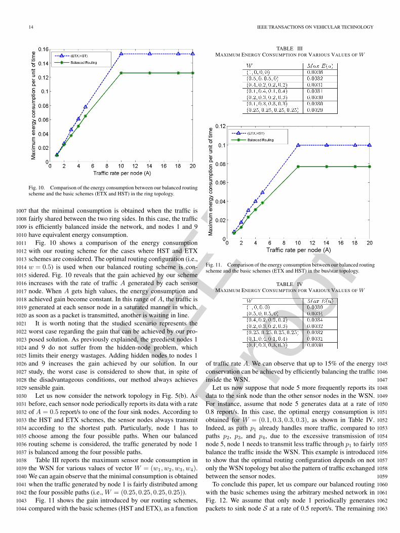
PF , and PG to derive E[NF ] and E[NG]. To achieve this, let us 830

define the probabilities θ(k, n) and θ(k) as follows: 831

θ(k, n) = Pr{node k successfully transmits in a given

slot to node n| k has a packet to transmit

to n in its queue head}= (1 − β(k, n)) × Γk × Ψ(k, n) (33)

IEEE

Proo

f


where832

Ψ(k, n) =b(k, n)

E [T (k, n)]. (34)

Moreover, θ(k) is defined as833

θ(k) = Pr{node k successfully transmits in a given slot|k has a packet to transmit}

=1λk

∑n∈Ne(k)

λ(k, n) × θ(k, n). (35)

Let us now derive the probability PF that an unsuccessful834

transmission is made in H+(k), given that at least one node in835

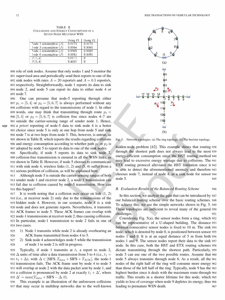
H+(k) has attempted to transmit and that node k has a packet836

to transmit to n in its queue head. Let Z denote the following837

event:838

Z ={

successful transmission is made in H+(k)}.

Hence, PF can be written as follows:839

PF =1 − Pr{Z,X|Y}Pr{X |Y}

=1 − Pr{X |Z,Y} × Pr{Z|Y}Pr{X |Y}

=1 − Pr{Z|Y}Pr{X |Y}

=1 −θ(k, n) +

∑m∈H(k)

θ(m) × ρm

1 −[Γk × Ψ(k, n) ×

∏m∈H(k)

(1 − αm)

] . (36)

In the same way, we obtain PG given by840

PG =

∑m∈H(H)

θ(m) × ρm

1 −[Γk × Ψ(k, n) ×

∏m∈H(k)(1 − αm)

] . (37)

Finally, PE is simply given by PE = 1 − PF − PG. Then,841

substituting (27)–(30) into (26), we obtain the expression of842

E[T (k, n)].843

V. PERFORMANCE EVALUATION844

In this section, we present the performance evaluation results.845

We first analyze the results regarding our balanced routing846

algorithms. We study the impact of traffic balancing on both847

the packet delivery success probability over the WSN links848

and on the energy consumption at each sensor node. Building849

on these results, we provide the optimal routing configuration850

that maximizes the network lifetime using simple illustration851

networks. The results are derived using both analytical and852

simulation approaches. A simulation model has been developed853

using ns-2 [38] to calculate the probability of unsuccessful854

transmission on each link (i.e., β) according to the routing con-855

TABLE IPARAMETER SETTING

Fig. 4. Simple seven-node multihop WSN.

figuration. Then, the analytical framework in Section IV-A-1. 856

is used to calculate the energy consumption at each sensor node. 857

In our study, we use the hop-based spanning trees (HSTs) 858

[39], [40] and expected transmission count (ETX)-based span- 859

ning trees (ETX) [41] as baselines to which the balanced 860

routing improvements can be compared. Both baselines take 861

advantage of the global information of the network state to 862

make routing decisions. Specifically, the HST protocol uses 863

flooding to select the shortest path in terms of the hop count. 864

This technique may lead to the use of slow and unreliable 865

links. The ETX protocol alleviates this issue since it takes 866

into account the quality of the wireless links in the routing 867

operation. Typically, each link in the network is assigned an 868

ETX cost metric to indicate its quality. 869

In our model, the sensor nodes achieve continuous moni- 870

toring of the supervised area. Each sensor node periodically 871

reports with rate A the local data to one of the existing sink 872

nodes over several hops. At each hop, the traffic originating 873

from the local sensor must be merged with route-through traffic. 874

The access to the data channel is arbitrated by the IEEE 802.11- 875

like sensor network protocol. The parameters setting in our 876

analysis are listed in Table I. 877

A. Impact of the Routing Decision on the Quality of the 878

Wireless Links and the Energy Consumption 879

In this section, we use a simple seven-node multihop WSN, 880

as shown in Fig. 4, to illustrate the impact of the traffic distribu- 881

tion inside the network on the packet delivery success probabil- 882

ity over the WSN links and on the energy efficiency. Recall that 883

the increase in the probability of a failed transmission β(u, v) 884

on a link (u, v) increases the number of retransmissions, which 885

amplifies the energy wastage. 886

In Fig. 4, the distance between consecutive nodes is fixed to 887

10 m, the transmission range of each sensor node is 12 m, and 888

the carrier-sensing range is 24 m. Nodes 2, 4, and 7 play the 889

IEEE

Proo

f


TABLE IICOLLISIONS AND ENERGY CONSUMPTION IN A

SEVEN-NODE MULTIHOP WSN

role of sink nodes. Assume that only nodes 1 and 5 monitor the890

supervised area and periodically send their reports to one of the891

sink nodes with rates A = 20 reports/s and A = 0.5 reports/s,892

respectively. Straightforwardly, node 1 reports its data to sink893

node 2, and node 5 can report its data to either node 4 or894

node 7.895

One can presume that node-5 reporting through either896

p1 = [5, 4] or p2 = [5, 6, 7] is always performed without any897

collisions with regard to the transmissions of node 1. In other898

words, one may think that transmitting through route p1 =899

[5, 4] or p2 = [5, 6, 7] is collision free since nodes 4–7 are900

outside the carrier-sensing range of sender node 1. Hence,901

a priori reporting of node-5 data to sink node 4 is a betterAQ4 902

choice since node 5 is only at one hop from node 5 and sink903

node 7 is at two hops from node 5. This, however, is untrue, as904

shown in Table II, which reports the results regarding collisions905

and energy consumption according to whether path p1 or p2 is906

adopted by node 5 to report its data to one of the sink nodes.907

Specifically, if node 5 reports its data to sink node 7,908

collision-free transmission is ensured in all the WSN links, as909

shown in Table II. However, if node 5 chooses to communicate910

with sink node 4, wireless links (1, 2) and (5, 4) suffer from a911

serious problem of collision, as will be explained here.912

Although node 5 is outside the carrier-sensing ranges of both913

sender node 1 and receiver node 2, a node-1 transmission can914

fail due to collision caused by node-5 transmission. How can915

this happen?916

It is worth noting that a collision may occur on link (1, 2)917

(i.e., at receiver node 2) only due to the transmissions of the918

hidden node 4. However, in our scenario, node 4 is a sink919

node and does not generate reports. Nevertheless, it transmits920

ACK frames to node 5. These ACK frames can overlap with921

node-1 transmissions at receiver node 2, thus causing collisions.922

In particular, node-1 transmission to node 2 fails in one of923

two cases.924

1) Node 1 transmits while node 2 is already overhearing an925

ACK frame transmitted from nodes 4 to 5.926

2) Sink node 4 acknowledges node 5 while the transmission927

of node 1 to node 2 is still in progress.928

Typically, if node 1 transmits at t1 a report to node 2,929

∆ units of time after a data transmission from 5 to 4 (i.e., t1 =930

t5 + ∆), with ∆ ∈ [SIFS, Tdata + SIFS + TACK], the node-1931

transmission fails. The ACK frame sent by node 4 to node 5932

will overlap at node 2 with the data packet sent by node 1, and933

a collision is pronounced by node 2 at exactly t1 + ∆′, where934

∆′ = max(Tdata + SIFS − ∆, 0).935

This example is an illustration of the unforeseen collisions936

that may occur in multihop networks due to the well-known937

Fig. 5. Network topologies. (a) The ring topology. (b) The bus/star topology.

hidden-node problem [42]. This example shows that routing 938

through the shortest path does not always lead to the most 939

energy-efficient consumption since the HST routing method 940

may lead to excessive energy wastage due to collisions. The 941

ETX routing protocol alleviates the HST limitation since it 942

is able to detect the aforementioned anomaly and therefore 943

chooses node 7, instead of node 4, as a sink node for sensor 944

node 5. 945

B. Evaluation Results of the Balanced Routing Scheme 946

In this section, we analyze the gain that can be introduced by 947

our balanced routing scheme over the basic routing schemes. 948

To achieve this, we use the simple networks shown in Fig. 5. 949

These topologies are sufficient to reveal many of the general 950

challenges. 951

Considering Fig. 5(a), the sensor nodes form a ring, which 952

can be representative of a U-shaped building. The distance 953

between consecutive sensor nodes is fixed to 10 m. The sink 954

node, which is denoted by node 0, is positioned between sensor 955

nodes 1 and 9. It is at an equal distance of 5 m from both 956

nodes 1 and 9. The sensor nodes report their data to the sink 957

node. In this case, both the HST and ETX routing schemes 958

dictate transmitting through the shortest path. Particularly, 959

node 5 can use one of the two possible routes. Assume that 960

node 5 always transmits through node 6. As a result, all the 961

nodes of the right half of the ring will consume more energy 962

than those of the left half of the ring. Typically, node 9 has the 963

highest burden since it deals with the maximum route-through 964

traffic. This results in a shorter lifetime for this node, which 965

yields to loss of coverage when node 9 depletes its energy, thus 966

leading to premature WSN death. 967

IEEE

Proo

f


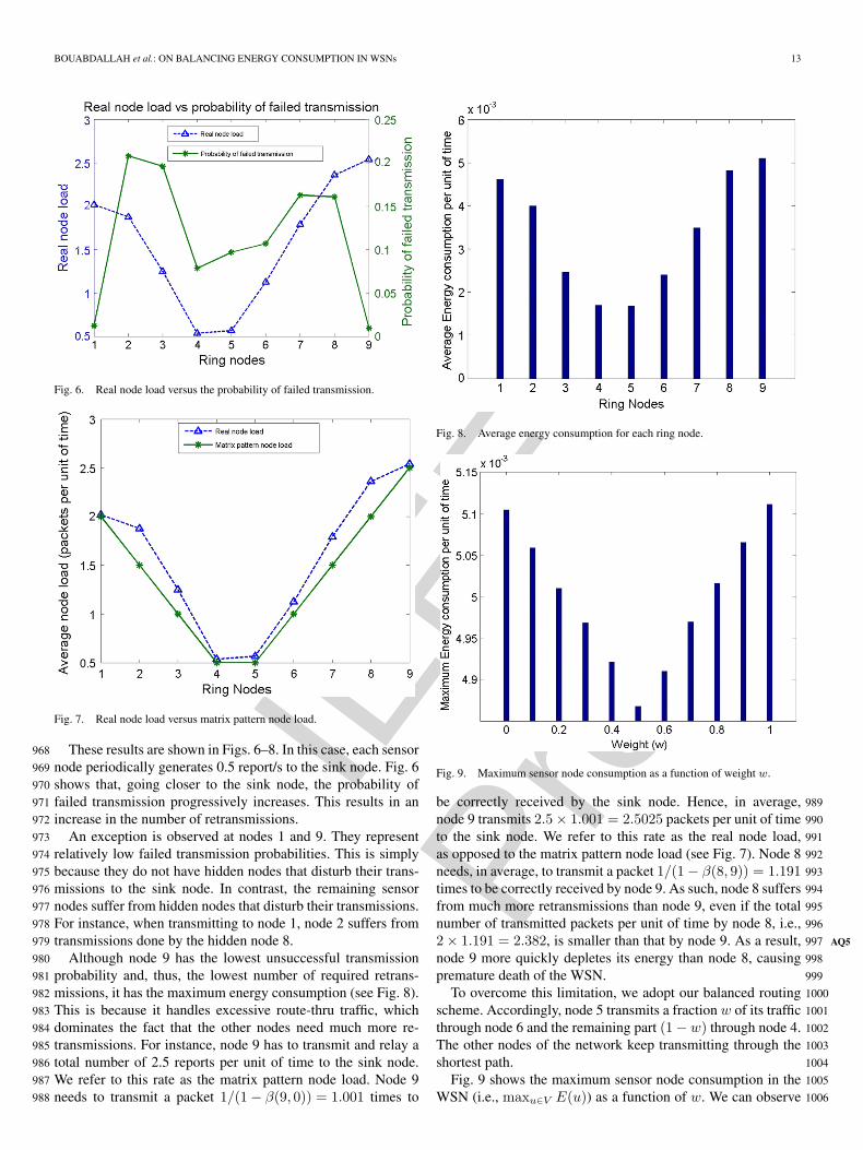
Fig. 6. Real node load versus the probability of failed transmission.

Fig. 7. Real node load versus matrix pattern node load.

These results are shown in Figs. 6–8. In this case, each sensor968

node periodically generates 0.5 report/s to the sink node. Fig. 6969

shows that, going closer to the sink node, the probability of970

failed transmission progressively increases. This results in an971

increase in the number of retransmissions.972

An exception is observed at nodes 1 and 9. They represent973

relatively low failed transmission probabilities. This is simply974

because they do not have hidden nodes that disturb their trans-975

missions to the sink node. In contrast, the remaining sensor976

nodes suffer from hidden nodes that disturb their transmissions.977

For instance, when transmitting to node 1, node 2 suffers from978

transmissions done by the hidden node 8.979

Although node 9 has the lowest unsuccessful transmission980

probability and, thus, the lowest number of required retrans-981

missions, it has the maximum energy consumption (see Fig. 8).982

This is because it handles excessive route-thru traffic, which983

dominates the fact that the other nodes need much more re-984

transmissions. For instance, node 9 has to transmit and relay a985

total number of 2.5 reports per unit of time to the sink node.986

We refer to this rate as the matrix pattern node load. Node 9987

needs to transmit a packet 1/(1 − β(9, 0)) = 1.001 times to988

Fig. 8. Average energy consumption for each ring node.

Fig. 9. Maximum sensor node consumption as a function of weight w.

be correctly received by the sink node. Hence, in average, 989

node 9 transmits 2.5 × 1.001 = 2.5025 packets per unit of time 990

to the sink node. We refer to this rate as the real node load, 991

as opposed to the matrix pattern node load (see Fig. 7). Node 8 992

needs, in average, to transmit a packet 1/(1 − β(8, 9)) = 1.191 993

times to be correctly received by node 9. As such, node 8 suffers 994

from much more retransmissions than node 9, even if the total 995

number of transmitted packets per unit of time by node 8, i.e., 996

2 × 1.191 = 2.382, is smaller than that by node 9. As a result, AQ5997

node 9 more quickly depletes its energy than node 8, causing 998

premature death of the WSN. 999

To overcome this limitation, we adopt our balanced routing 1000

scheme. Accordingly, node 5 transmits a fraction w of its traffic 1001

through node 6 and the remaining part (1 − w) through node 4. 1002

The other nodes of the network keep transmitting through the 1003

shortest path. 1004

Fig. 9 shows the maximum sensor node consumption in the 1005

WSN (i.e., maxu∈V E(u)) as a function of w. We can observe 1006

IEEE

Proo

f


Fig. 10. Comparison of the energy consumption between our balanced routingscheme and the basic schemes (ETX and HST) in the ring topology.

that the minimal consumption is obtained when the traffic is1007

fairly shared between the two ring sides. In this case, the traffic1008

is efficiently balanced inside the network, and nodes 1 and 91009

have equivalent energy consumption.1010

Fig. 10 shows a comparison of the energy consumption1011

with our routing scheme for the cases where HST and ETX1012

schemes are considered. The optimal routing configuration (i.e.,1013

w = 0.5) is used when our balanced routing scheme is con-1014

sidered. Fig. 10 reveals that the gain achieved by our scheme1015

increases with the rate of traffic A generated by each sensor1016

node. When A gets high values, the energy consumption and1017

achieved gain become constant. In this range of A, the traffic is1018

generated at each sensor node in a saturated manner in which,1019

as soon as a packet is transmitted, another is waiting in line.1020

It is worth noting that the studied scenario represents the1021

worst case regarding the gain that can be achieved by our pro-1022

posed solution. As previously explained, the greediest nodes 11023

and 9 do not suffer from the hidden-node problem, which1024

limits their energy wastages. Adding hidden nodes to nodes 11025

and 9 increases the gain achieved by our solution. In our1026

study, the worst case is considered to show that, in spite of1027

the disadvantageous conditions, our method always achieves1028

sensible gain.1029

Let us now consider the network topology in Fig. 5(b). As1030

before, each sensor node periodically reports its data with a rate1031

of A = 0.5 report/s to one of the four sink nodes. According to1032

the HST and ETX schemes, the sensor nodes always transmit1033

according to the shortest path. Particularly, node 1 has to1034

choose among the four possible paths. When our balanced1035

routing scheme is considered, the traffic generated by node 11036

is balanced among the four possible paths.1037

Table III reports the maximum sensor node consumption in1038

the WSN for various values of vector W = (w1, w2, w3, w4).1039

We can again observe that the minimal consumption is obtained1040

when the traffic generated by node 1 is fairly distributed among1041

the four possible paths (i.e., W = (0.25, 0.25, 0.25, 0.25)).1042

Fig. 11 shows the gain introduced by our routing schemes,1043

compared with the basic schemes (HST and ETX), as a function1044

TABLE IIIMAXIMUM ENERGY CONSUMPTION FOR VARIOUS VALUES OF W

Fig. 11. Comparison of the energy consumption between our balanced routingscheme and the basic schemes (ETX and HST) in the bus/star topology.

TABLE IVMAXIMUM ENERGY CONSUMPTION FOR VARIOUS VALUES OF W

of traffic rate A. We can observe that up to 15% of the energy 1045

conservation can be achieved by efficiently balancing the traffic 1046

inside the WSN. 1047

Let us now suppose that node 5 more frequently reports its 1048

data to the sink node than the other sensor nodes in the WSN. 1049

For instance, assume that node 5 generates data at a rate of 1050

0.8 report/s. In this case, the optimal energy consumption is 1051

obtained for W = (0.1, 0.3, 0.3, 0.3), as shown in Table IV. 1052

Indeed, as path p1 already handles more traffic, compared to 1053

paths p2, p3, and p4, due to the excessive transmission of 1054

node 5, node 1 needs to transmit less traffic through p1 to fairly 1055

balance the traffic inside the WSN. This example is introduced 1056

to show that the optimal routing configuration depends on not 1057

only the WSN topology but also the pattern of traffic exchanged 1058

between the sensor nodes. 1059

To conclude this paper, let us compare our balanced routing 1060

with the basic schemes using the arbitrary meshed network in 1061

Fig. 12. We assume that only node 1 periodically generates 1062

packets to sink node S at a rate of 0.5 report/s. The remaining 1063

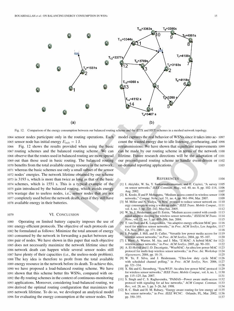
IEEE

Proo

f


Fig. 12. Comparison of the energy consumption between our balanced routing scheme and the (ETX and HST) schemes in a meshed network topology.

sensor nodes participate only in the routing operations. Each1064

sensor node has initial energy Einit = 1 J.1065

Fig. 12 shows the results provided when using the basic1066

routing schemes and the balanced routing scheme. We can1067

observe that the routes used in balanced routing are more spread1068

out than those used in basic routing. The balanced routing1069

benefits from the total available energy resource in the network,1070

whereas the basic schemes use only a small subset of the sensor1071

nodes’ energies. The network lifetime obtained by our scheme1072

is 3193 s, which is more than twice as long as that of the basic1073

schemes, which is 1551 s. This is a typical example of the1074

gain introduced by the balanced routing, which avoids energy1075

wastage due to useless nodes, i.e., sensor nodes that are not1076

completely used before the network death, even if they still have1077

available energy in their batteries.1078

VI. CONCLUSION1079

Operating on limited battery capacity imposes the use of1080

energy-efficient protocols. The objective of such protocols can1081

be formulated as follows: Minimize the total amount of energy1082

consumed by the network in forwarding a packet between any1083

pair of nodes. We have shown in this paper that such objective1084

does not necessarily maximize the network lifetime since the1085

network death can happen while several sensor nodes still1086

have plenty of their capacities (i.e., the useless-node problem).1087

The key idea is therefore to profit from the total available1088

energy resource in the network before its death. To achieve this,1089

we have proposed a load-balanced routing scheme. We have1090

shown that this scheme better fits WSNs, compared with on-1091

the-fly routing schemes in the context of continuous-monitoring1092

applications. Moreover, considering load-balanced routing, we1093

derived the optimal routing configuration that maximizes the1094

network lifetime. To do so, we developed an analytical model1095

for evaluating the energy consumption at the sensor nodes. The1096

model captures the real behavior of WSNs since it takes into ac- 1097

count the wasted energy due to idle listening, overhearing, and 1098

retransmissions. We have shown that significant improvements 1099

can be made by our routing scheme in terms of the network 1100

lifetime. Future research directions will be the adaptation of 1101

our preconfigured routing scheme to handle event-driven or 1102

on-demand reporting applications. 1103

REFERENCES 1104

[1] I. Akiyldiz, W. Su, Y. Sankarasubramaniam, and E. Cayirci, “A survey 1105on sensor networks,” IEEE Commun. Mag., vol. 40, no. 8, pp. 102–114, 1106Aug. 2002. 1107

[2] K. Kredo, II and P. Mohapatra, “Medium access control in wireless sensor 1108networks,” Comput. Netw., vol. 51, no. 4, pp. 961–994, Mar. 2007. 1109

[3] M. Miller and N. Vaidya, “A MAC protocol to reduce sensor network en- 1110ergy consumption using a wake-up radio,” IEEE Trans. Mobile Comput., 1111vol. 4, no. 3, pp. 228–242, May/Jun. 2005. 1112

[4] W. Ye, J. Heidemann, and D. Estrin, “Medium access control with coordi- 1113nated adaptive sleeping for wireless sensor networks,” IEEE/ACM Trans. 1114Netw., vol. 12, no. 3, pp. 493–506, Jun. 2004. 1115

[5] T. van Dam and K. Langendoen, “An adaptive energy-efficient MAC pro- 1116tocol for wireless sensor networks,” in Proc. ACM SenSys, Los Angeles, 1117CA, Nov. 2003, pp. 171–180. 1118

[6] J. Polastre, J. Hill, and D. Culler, “Versatile low power media access for 1119wireless sensor networks,” in Proc. ACM SenSys, 2004, pp. 95–107. 1120

[7] I. Rhee, A. Warrier, M. Aia, and J. Min, “Z-MAC: A hybrid MAC for 1121wireless sensor networks,” in Proc. ACM SenSys, 2005, pp. 90–101. 1122

[8] A. El-Hoiydi and J.-D. Decotignie, “WiseMAC: An ultra low power MAC 1123protocol for multi-hop wireless sensor networks,” in Proc. Int. Workshop 1124Algosensors, 2004, pp. 18–31. 1125

[9] W. Ye, F. Silva, and J. Heidemann, “Ultra-low duty cycle MAC 1126with scheduled channel polling,” in Proc. ACM SenSys, Nov. 2006, 1127pp. 321–334. 1128

[10] X. Shi and G. Stromberg, “SyncWUF: An ultra low-power MAC protocol 1129for wireless sensor networks,” IEEE Trans. Mobile Comput., vol. 6, no. 1, 1130pp. 115–125, Jan. 2007. 1131

[11] S. Singh and C. S. Raghavendra, “PAMAS—Power aware multi-access 1132protocol with signaling for ad hoc networks,” ACM Comput. Commun. 1133Rev., vol. 28, no. 3, pp. 5–26, Jul. 1998. 1134

[12] R. C. Shah and H. M. Rabaey, “Energy aware routing for low energy ad 1135hoc sensor networks,” in Proc. IEEE WCNC. Orlando, FL, Mar. 2002, 1136pp. 350–355. 1137

IEEE

Proo

f


[13] J. Chang and L. Tassiulas, “Maximum lifetime routing in wireless sensor1138networks,” IEEE/ACM Trans. Netw., vol. 12, no. 4, pp. 609–619, Aug. 15,11392004.1140

[14] C. F. Chiasserini and M. Garetto, “An analytical model for wireless sensor1141networks with sleeping nodes,” IEEE Trans. Mobile Comput., vol. 5,1142no. 12, pp. 1706–1718, Dec. 2006.1143

[15] S. Tilak, N. B. Abu-Ghazaleh, and W. Heinzelman, “Infrastructure trade-1144offs for sensor networks,” in Proc. ACM WSNA, Atlanta, GA, Sep. 2002,1145pp. 49–58.1146

[16] O. B. Akan and I. F. Akyildiz, “Event-to-sink reliable transport for wire-1147less sensor networks,” IEEE/ACM Trans. Netw., vol. 13, no. 5, pp. 1003–11481016, Oct. 2005.1149

[17] F. Bouabdallah, N. Bouabdallah, and R. Boutaba, “Towards reliable and1150efficient reporting in wireless sensor networks,” IEEE Trans. Mobile1151Comput., vol. 7, no. 8, pp. 978–994, Aug. 2008.1152

[18] M. C. Vuran and I. F. Akyildiz, “Spatial correlation-based collaborative1153medium access control in wireless sensor networks,” IEEE/ACM Trans.1154Netw., vol. 14, no. 2, pp. 316–329, Apr. 2006.1155

[19] H. Kwon, T. H. Kim, S. Choi, and B. G. Lee, “A cross-layer strategy1156for energy-efficient reliable delivery in wireless sensor networks,” IEEE1157Trans. Wireless Commun., vol. 5, no. 12, pp. 3689–3699, Dec. 2006.1158

[20] D. J. Baker and A. Ephremides, “The architectural organization of a1159mobile radio network via a distributed algorithm,” IEEE Trans. Commun.,1160vol. COM-29, no. 11, pp. 1694–1701, Nov. 1981.1161

[21] A. Ephremides, J. E. Wieselthier, and D. J. Baker, “A design concept for1162reliable mobile radio networks with frequency hopping signaling,” Proc.1163IEEE, vol. 75, no. 1, pp. 56–73, Jan. 1987.1164

[22] V. Rodoplu and T. H. Meng, “Minimum energy mobile wireless1165networks,” in Proc. IEEE ICC, Atlanta, GA, Jun. 1998, vol. 31166pp. 1633–1639.1167

[23] C. K. Toh, “Maximum battery life routing to support ubiquitous mobile1168computing in wireless ad hoc networks,” IEEE Commun. Mag., vol. 39,1169no. 6, pp. 138–147, Jun. 2001.1170

[24] Q. Li, J. Aslam, and D. Rus, “Online power-aware routing in wireless1171ad hoc networks,” in Proc. ACM MobiCom, Rome, Italy, Jul. 2001,1172pp. 97–107.1173

[25] I. Stojmenovic and X. Lin, “Power-aware localized routing in wireless1174networks,” IEEE Trans. Parallel Distrib. Syst., vol. 12, no. 11, pp. 1122–11751133, Nov. 2001.1176

[26] J. H. Chang and L. Tassiulas, “Maximum lifetime routing in wireless1177sensor networks,” IEEE/ACM Trans. Netw., vol. 12, no. 4, pp. 609–619,1178Aug. 2004.1179

[27] J. H. Chang and L. Tassiulas, “Maximum lifetime routing in wireless1180sensor networks,” in Proc. ATIRP Conf., Mar. 2000, pp. 609–619.1181

[28] Wireless LAN Medium Access Control (MAC) and Physical Layer (PHY)1182Specifications, 1999. Available: ISO/IEC IEEE 802.11 Standard.1183

[29] C. P. Chan and S. C. Liew, “Data-collection capacity of IEEE 802.11-1184like sensor networks,” in Proc. IEEE ICC, Istanbul, Turkey, Jun. 2006,1185pp. 3339–3346.1186

[30] F. A. Tobagi and L. Kleinrock, “Packet switching in radio channels—1187Part II: The hidden terminal problem in carrier sense multiple-access and1188the busy-tone solution,” IEEE Trans. Commun., vol. COM-23, no. 12,1189pp. 1417–1433, Dec. 1975.1190

[31] K. Jain, J. Padhye, V. Padmanabhan, and L. Qiu, “Impact of interference1191on multi-hop wireless network performance,” in Proc. ACM MobiCom,1192San Diego, CA, Sep. 2003, pp. 66–80.1193

[32] Chipcon, CC2420 Data Sheet. [Online]. Available: http://www.1194chipcon.com/1195

[33] J. Bicket, D. Aguayo, S. Biswas, and R. Morris, “Architecture and evalu-1196ation of an unplanned 802.11b mesh network,” in Proc. ACM MobiCom,1197Cologne, Germany, Sep. 2005, pp. 31–42.1198

[34] K. Medepalli and F. A. Tobagi, “Towards performance modeling of IEEE1199802.11 based wireless networks: A unified framework and its applica-1200tions,” in Proc. IEEE INFOCOM, Barcelona, Spain, Apr. 2006, pp. 1–12.1201

[35] M. Garetto, T. Salonidis, and E. Knightly, “Modeling per-flow throughput1202and capturing starvation in CSMA multi-hop wireless networks,” in Proc.1203IEEE INFOCOM, Barcelona, Spain, Apr. 2006, pp. 1–13.1204

[36] G. Bianchi, “Performance analysis of the IEEE 802.11 distributed coordi-1205nation function,” IEEE J. Sel. Areas Commun., vol. 18, no. 3, pp. 535–547,1206Mar. 2000.1207

[37] B. Sericola, “Closed form solution for the distribution of the total time1208spent in a subset of states of a Markov process during a finite observation1209period,” J. Appl. Probab., vol. 27, pp. 713–719, 1990.1210

[38] The Network Simulator—NS-2. [Online]. Available: http://www.isi.edu/1211nsnam/ns1212

[39] D. B. Johnson, D. A. Maltz, and J. Broch, “DSR: The dynamic source1213routing protocol for multihop wireless ad hoc networks,” in Ad Hoc1214

Networking, C. E. Perkins, Ed. Reading, MA: Addison-Wesley, 2001, 1215ch. 5, pp. 139–172. 1216

[40] C. E. Perkins and E. M. Royer, “Ad-hoc on demand distance vector 1217routing,” in Proc. WMCSA, 1999, pp. 90–100. 1218

[41] D. Couto, D. Aguayo, J. Bicket, and R. Morris, “A high-throughput path 1219metric for multi-hop wireless routing,” in Proc. ACM MOBICOM, 2003, 1220pp. 134–146. 1221

[42] M. Garetto, J. Shi, and E. Knightly, “Modeling media access in embed- 1222ded two-flow topologies of multi-hop wireless networks,” in Proc. ACM 1223MobiCom, Cologne, Germany, Aug. 2005, pp. 200–214. 1224

Fatma Bouabdallah received the B.S. degree in computer engineering from the AQ61225Ecole Nationale des Sciences de l’Informatique, Tunis, Tunisia, in 2005 and the 1226M.S. degree in network and computer science from the University of Paris VI, 1227Paris, France, in 2006. She is currently working toward the Ph.D. degree with 1228the Institut National de Recherche en Informatique et en Automatique. Rennes, 1229France. 1230

Her research interests include wireless sensor networks, cross-layer design, 1231and modeling and performance evaluation of computer networks. 1232

Nizar Bouabdallah received the B.S. degree in 1233telecommunications engineering from the Ecole 1234Superieur des Communications (Sup’Com), Tunis, 1235Tunisia, in 2001 and the M.S. and Ph.D. degrees 1236in network and computer science from the Univer- 1237sity of Paris VI, Paris, France, in 2002 and 2004, 1238respectively. 1239

In 2002, he joined Alcatel Research Laboratories, 1240Marcoussis, France. In 2005, he was with North 1241Carolina State University, Raleigh, as a Postdoctoral 1242Fellow. He is currently a Researcher with the In- 1243

stitut National de Recherche en Informatique et en Automatique, Rennes, 1244France. Since February 2007, he has been a Visitor Researcher with the 1245David R. Cheriton School of Computer Science, University of Waterloo, 1246Waterloo, ON, Canada. His research interests include optical networking, 1247wireless and sensor networks, performance evaluation, and network planning 1248and modeling. 1249

Raouf Boutaba received the M.Sc. and Ph.D. de- 1250grees in computer science from the University Pierre 1251& Marie Curie, Paris, France, in 1990 and 1994, 1252respectively. 1253

He is currently a Professor of computer science 1254with the School of Computer Science, University 1255of Waterloo, Waterloo, ON, Canada. His research 1256interests include network, resource, and service man- 1257agement in wired and wireless networks. 1258

Dr. Boutaba is currently a Distinguished Lecturer 1259of the IEEE Communications Society the Chairman 1260

of the IEEE Technical Committee on Information Infrastructure, and the 1261Director of the ComSoc Related Societies Board. He is the Founder and 1262Editor-in-Chief of the IEEE TRANSACTIONS ON NETWORK AND SERVICE 1263MANAGEMENT and is currently serving on the editorial boards of several 1264other journals. He was the recipient of several best paper awards and other 1265recognitions, such as the Premier’s Research Excellence Award. 1266

On Balancing Energy Consumption in Wireless Sensor Networks 1 2

Documents

Transcript of On Balancing Energy Consumption in Wireless Sensor Networks 1 2