ON A MULTILEVEL KRYLOV METHOD FOR THE HELMHOLTZ EQUATION PRECONDITIONED BY SHIFTED LAPLACIAN

Electronic Transactions on Numerical Analysis.Volume 31, pp. 403-424, 2008.Copyright 2008, Kent State University.ISSN 1068-9613.

ETNAKent State University

http://etna.math.kent.edu

ON A MULTILEVEL KRYLOV METHOD FOR THE HELMHOLTZ EQUATIONPRECONDITIONED BY SHIFTED LAPLACIAN ∗

YOGI A. ERLANGGA† AND REINHARD NABBEN‡

Abstract. In Erlangga and Nabben [SIAM J. Sci. Comput., 30 (2008), pp. 1572–1595], a multilevel Krylovmethod is proposed to solve linear systems with symmetric and nonsymmetric matrices of coefficients. This mul-tilevel method is based on an operator which shifts some small eigenvalues to the largest eigenvalue, leading toa spectrum which is favorable for convergence accelerationof a Krylov subspace method. This shift technique in-volves a subspace or coarse-grid solve. The multilevel Krylov method is obtained via a recursive application ofthe shift operator on the coarse-grid system. This method has been applied successfully to 2D convection-diffusionproblems for which a standard multigrid method fails to converge.

In this paper, we extend this multilevel Krylov method to indefinite linear systems arising from a discretization ofthe Helmholtz equation, preconditioned by shifted Laplacian as introduced by Erlangga, Oosterlee and Vuik [SIAMJ. Sci. Comput. 27 (2006), pp. 1471–1492]. Within the Krylov iteration and the multilevel steps, for each coarse-gridsolve a multigrid iteration is used to approximately invert the shifted Laplacian preconditioner. Hence, a multilevelKrylov-multigrid (MKMG) method results.

Numerical results are given for high wavenumbers and show the effectiveness of the method for solving Helm-holtz problems. Not only can the convergence be made almost independent of grid sizeh, but also linearly dependenton the wavenumberk, with a smaller proportional constant than for the multigrid preconditioned version, presentedin the aforementioned paper.

Key words. multilevel Krylov method, GMRES, multigrid, Helmholtz equation, shifted-Laplace precondi-tioner.

AMS subject classifications.65F10, 65F50, 65N22, 65N55.

1. Introduction. Nowadays Krylov subspace methods are the methods of choice forsolving large, sparse linear systems of equations

Au = b, A ∈ Cn×n. (1.1)

If A is Hermitian positive definite, (1.1) is typically solved by the conjugate gradient method(CG). The convergence rate of CG can be bounded in terms of thecondition number ofA,κ(A) [18], which in this case is the ratio of the largest eigenvalue tothe smallest one. For anill-conditioned system, this convergence rate is often toosmall, so that a preconditioner hasto be incorporated.

For general matrices, convergence bounds are somewhat moredifficult to establish anddo not express a direct connection with the condition numberof A. It is, however, a commonbelief that eigenvalues clustering around a value far from zero improve the convergence.Therefore, without specifically referring to the conditionnumber, it is often sufficient to saythat a nonsingular matrixM is a good preconditioner if the eigenvalues ofM−1A are moreclustered and farther from zero than those ofA.

A class of preconditioners which exploits the detail of the spectrum ofA can be basedon projection methods. These methods accelerate the convergence by removing the compo-nents of the residuals corresponding to the smallest eigenvalues during the iteration. One wayto achieve this is by deflating a number of the smallest eigenvalues to zero. Nicolaides [16]

∗Received October 9, 2007. Accepted June 8, 2009. Published online on September 30, 2009. Recommended byOliver Ernst.

†TU Berlin, Institut fur Mathematik, MA 3-3, Strasse des 17. Juni 136, D-10623 Berlin, Germany. Currently atThe University of British Columbia, Department of Earth and Ocean Sciences, 6339 Stores Road, Vancouver, BCV6T 1Z4, Canada ([email protected]).

‡TU Berlin, Institut fur Mathematik, MA 3-3, Strasse des 17. Juni 136, D-10623 Berlin, Germany([email protected]).

403



404 Y. A. ERLANGGA AND R. NABBEN

showed that by adding eigenvectors related to some small eigenvalues, the convergence of CGmay be improved. For GMRES, Morgan [14] also shows that by augmenting the Krylov sub-space by eigenvectors related to some small eigenvalues, these eigenvectors no longer havecomponents in the residuals, and the convergence bound of GMRES can be made smaller;thus, a faster convergence may be expected; see also a unifieddiscussion on this subject byEiermann et al. in [3].

A similar approach is proposed in [13], where a matrix resembling deflation of somesmall eigenvalues is used as a preconditioner. Suppose thatther smallest eigenvalues are tobe deflated to zero, and define the deflation matrix as

PD = I − AZE−1Y T , E = Y T AZ, (1.2)

where the columns of the full rank matricesZ, Y ∈ Cn×r form the basis of the deflation

subspaces. The matrixE ∈ Cr×r can generally be considered as theGalerkin (or more

correctly thePetrov-Galerkin) matrix associated withA. It can be proved [7, 13, 15] that fora nonsingularA and any full rankZ, Y , the spectrum ofPDA containsr zero eigenvalues.Since the components of the residuals corresponding to the zero eigenvalues do not enter theiteration, the convergence rate is now bounded in terms of the effectivecondition numberof PDA, which for a Hermitian positive definite matrixA andY = Z is the ratio betweenthe largest eigenvalue and the smallest nonzero eigenvalueof PDA. Furthermore, it can beshown that a largerr leads to a smallereffectivecondition number [15]. Hence, with a largedeflation subspace, convergence can be improved considerably.

A large deflation subspace implies that the matrixE in (1.2) is large. It is then possiblethat the inversion ofE with direct methods becomes impractical, and therefore onehas toresort to iterative methods. Related to the computation ofE−1, it is shown in [15] that theconvergence of CG withPD deteriorates ifE−1 is computed inaccurately. We say in this casethatPD is sensitive to an inaccurate computation ofE−1. This means that to retain its fastconvergence, an iterative method can only be applied to the Galerkin system (i.e., the linearsystem associated with the Galerkin matrix) with a sufficiently tight termination criterion.Reference [20] discusses this aspect of deflation in detail with extensivenumerical tests.

As an alternative to the deflation preconditioner (1.2), another projection-type precondi-tioner is proposed by the authors in [8]. In this new projection preconditioner, small eigenval-ues are shiftednot towards zero,but towards the largest eigenvalue (in magnitude), instead.This leads to eigenvalue clustering in a location far from zero. To discuss this method, weintroduce a more general linear system which is equivalent to (1.1), namely

Au = b, (1.3)

whereA = M−11 AM−1

2 , u = M2u, and b = M−11 b. Here,M1 andM2 are any nonsin-

gular preconditioning matrices. The projection associated with a shift towards the largesteigenvalue ofA is done via the action of the matrix

PN = I − AZE−1Y T + λnZE−1Y T , E = Y T AZ, (1.4)

on the general system (1.3). Here,λn is the maximum eigenvalue (in magnitude) ofA.We prefer to use the notation (1.3), because this allows us to consider a more general class ofproblems involving preconditioners. As discussed in [8], for some problems (e.g., the Poissonand convection-diffusion equation discretized on uniformgrids) the preconditionersM1,M2

are not actually needed, i.e., it suffices to setM1 = M2 = I. The role ofM1 andM2 maybecome important if, e.g., a nonuniform grid is employed, and in this case the choiceM1 = I



MULTILEVEL KRYLOV METHOD FOR HELMHOLTZ EQUATION 405

andM2 = diag(A) is already sufficient. With (1.4), we then solve the left preconditionedsystem

PN Au = PN b

with a Krylov method. Even though its derivation is motivated by projection methods,PN isnot a projection operator, asP 2

N6= PN . In this paper we shall callPN the shift operator or

matrix, instead.The right preconditioned version of (1.5) can also be defined using the shift matrix

QN = I − ZE−1Y T A + λnZE−1Y T . (1.5)

Given (1.5), we then solve the preconditioned system

AQN u = b, u = QN u, (1.6)

with a Krylov method.One advantage of (1.4) over (1.2) is thatPN is insensitive to an inexact inversion ofE.

This property allows us to use a large deflation subspace to shift as many small eigenvaluesas possible. To obtain an optimal overall computational complexity, the associated Galerkinsystem is solved by a (inner) Krylov method with a less tight termination criterion. Theconvergence rate of this inner iteration can be significantly improved if a shift operator similarto (1.4) is also applied to the Galerkin system. The action of this shift operator will requireanother solve of another Galerkin system, which will be carried out by a Krylov method. Ifthis process is done recursively, a multilevel Krylov method (MK) results. The potential ofthis multilevel Krylov method is demonstrated in [8].

In this paper we extend the application of the multilevel Krylov method to indefinite lin-ear systems. In particular, we shall focus on the Helmholtz equation. With this application,this paper can be considered as a continuation of our discussion on the multilevel Krylovmethod, which was presented in [8]. Therefore, for more theoretical results on the method,the readers should consult [8]. Before applying the multilevel Krylov method, the Helmholtzequation is first preconditioned by the shifted Laplacian preconditioner [10]. Since this pre-conditioner is inverted implicitly by one multigrid iteration, we never have the Galerkin sys-tem in an explicit form. We shall demonstrate that with an appropriate approximation to theGalerkin matrix, multigrid-based preconditioners can also be incorporated into the multilevelKrylov framework. We call the resultant method the multilevel Krylov-multigrid (MKMG)method.

In the context of solving the Helmholtz equation, Elman et al. also used Krylov itera-tions (in their case, GMRES [19]) in a multilevel fashion [4]. However, their approach isbasically a multigrid concept specially adapted to the Helmholtz equation. While at the finestand coarsest level, standard smoothers still have good smoothing properties, at the interme-diate levels GMRES is employed in place of standard smoothers. Since GMRES does nothave a smoothing property, it plays a role in reducing the errors butnot in smoothing them.A substantial number of GMRES iterations at the intermediate levels, however, is required toachieve a significant reduction of errors.

It is worth mentioning that even though the multilevel Krylov method uses a hierarchy oflinear systems similar to multigrid, the way it treats each system and establishes a connectionbetween systems differs from multigrid [9, 8]. In fact, the multilevel Krylov method is not bydefinition an instance of a multigrid method. With regard to the work in [4], we shall shownumerically that the multilevel Krylov method can handle linear systems at the intermediatelevels efficiently; i.e., a fast multilevel Krylov convergence can be achieved with only a fewKrylov iterations at the intermediate levels.




We organize the paper as follows. In Section2, we first revisit the Helmholtz equationand our preconditioner of choice, theshifted Laplace preconditioner. In Section3, somerelevant theoretical results concerning our multilevel Krylov method are discussed. Somepractical implementations are explained in Section4. Numerical results from 2D Helmholtzproblems are presented in Section5. Finally, in Section6, we draw some conclusions.

2. The Helmholtz equation and the shifted Laplace preconditioner. The 2D Helm-holtz equation for heterogeneous media can be written as

Au := −(

∂2

∂x2+

∂2

∂y2+ k2(x, y)

)u(x, y) = g(x, y), in Ω = (0, 1)2, (2.1)

wherek(x, y) is the wavenumber, andg is the source term. Dirichlet, Neumann, or Som-merfeld (non-reflecting) conditions can be applied at the boundariesΓ ≡ ∂Ω; see, e.g., [5].If a discretization is applied to (2.1) and the boundary conditions, and if the wavenumberis high (as usually encountered in realistic applications), the resultant linear system is largebut sparse, and symmetric but indefinite. In most cases, an application of Krylov subspacemethods to iteratively solve the linear system results in slow convergence. Standard precon-ditioners, e.g., ILU-type preconditioners, do not effectively improve the convergence [12].

In [10, 11], for the Helmholtz equation, the shifted Laplacian operator

M := − ∂2

∂x2− ∂2

∂y2− (α − jβ)k2(x, y), j =

√−1, α, β ∈ R, (2.2)

is proposed to accelerate the convergence of a Krylov subspace method. The preconditioningmatrix M is obtained from discretization of (2.2), with the sameboundary conditions asfor (2.1). The solutionu is computed from the (right) preconditioned system

AM−1u = b, u = M−1u, (2.3)

whereA andM are the Helmholtz and shifted Laplacian matrices respectively.If (α, β) are well chosen, the eigenvalues ofAM−1 can be clustered around one. In this

paper we shall only consider the pair(α, β) = (1, 0.5), which in [10] is shown to lead toan efficient and robust preconditioning operator. Since theconvergence of Krylov methods isclosely related to the spectrum of the given matrix, we shallgive some insight on the spectrumof the preconditioned Helmholtz system (2.3) in the remainder of this section.

The following theorem is a special case of Theorem 3.5 in [22], and holds for thed-dimensional Helmholtz equation.

THEOREM 2.1 ([22]). Let A = L + jC − K and M = L + jC − (α − βj)Kbe the discretization matrices of(2.1) and (2.2), respectively, withL, C, andK the nega-tive Laplacian, the boundary conditions, and the Helmholtz(k2) term, respectively. Choose(α, β) = (1, 0.5).

(i) For Dirichlet boundary conditions,C = 0 and the eigenvalues ofM−1A lie on thecircle in the complex plane with centerc = (1

2 , 0) and radiusR = 12 .

(ii) For Sommerfeld boundary conditions,C 6= 0 and the eigenvalues ofM−1A areenclosed by the circle with centerc = (1

2 , 0) and radiusR = 12 .

Proof. The proof for arbitrary(α, β) can be found in [22].Sinceσ(M−1A) = σ(AM−1), Theorem2.1 holds also forAM−1. For the Helmholtz

equation with Dirichlet boundary conditions some detailedinformation about the spectrum,e.g., the largest and smallest eigenvalues, can also be derived. We shall follow the approachused in [11], which was based on a continuous formulation of the problem. The results, how-ever, also hold for the discrete formulation as indicated in[11]. For simplicity, we considerthe 1D Helmholtz equation.




At the continuous level, the eigenvalue problem of the preconditioned system can bewritten as

−(

d2

dx2− k2

)u = λ

(− d2

dx2− (1 − 0.5j)k2

)u, (2.4)

with λ the eigenvalue andu now the eigenfunction. By using the ansatzu = sin(iπx), i ∈ N,from (2.4) we find that

λi =i2π2 − k2

i2π2 − (1 − 0.5j)k2,

with

Re(λi) =(i2π2 − k2)2

(i2π2 − k2)2 + 0.25k4, Im(λi) = − 0.5(i2π2 − k2)k2

(i2π2 − k2)2 + 0.25k4.

From the above relations, observe that0 < Re(λi) < 1, and therefore

limi→∞

Re(λi) = limk→∞

Re(λi) = 1.

The real parts are close to zero ifi2π2 are close tok2. The sign of the imaginary parts dependson the modei. Also, limk→∞ Im(λi) = 0.5 andlimi→∞ Im(λi) = −0.5. By eliminatingi2π2 in (2.5), we have

(Re(λi) − 0.5)2 + Im(λi)2 = 0.25.

Thus,λi lie on the circle with centerc = (12 , 0) and radiusR = 1

2 , as suggested by Theo-rem2.1(i). The largest possible|λi| is approached asi → ∞, where, in this case,Re(λi) → 1andIm(λi) → 0. Thus,limi→∞ |λi| = 1. This result is true for any choice ofk.

Suppose now that for somei, i2π2 − k2 = ǫ. For ǫ ≪ k, Re(λi) = 4ǫ2/k4 andIm(λi) = −2ǫ/k2, and hence

|λi| = Re(λi)2 + Im(λi)

2 =

(4ǫ2

k4

)2

+

(2ǫ

k2

)2

≈ 4ǫ2

k4.

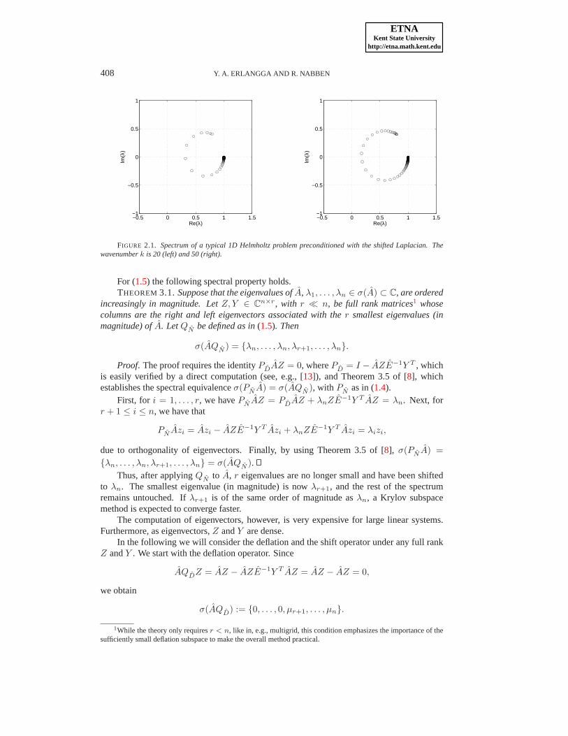
Therefore, while the spectrum ofM−1A is more clustered than the spectrum ofA, someeigenvalues lie at a distance of orderO(ǫ/k2) from zero. Figure2.1 illustrates this spectralproperty for a 1D Helmholtz problem withk = 20 and50. Clearly, the largest eigenvalue forbothk’s is essentially the same and close to one, but the smallest eigenvalue moves towardszero ask increases.

Since small eigenvalues may cause problems to a Krylov method, we discuss in the nextsection the multilevel Krylov method, used to handle small eigenvalues.

3. Multilevel Krylov method. Consider again the linear system (1.3), where, for ourHelmholtz equation,A = AM−1 andb = b. Our objective is to shift some small eigenvaluesin the spectrum ofA to a fixed point, such that the new linear system has some more favorablespectrum for convergence acceleration.

As explained in Section1, one way to achieve this is by using some deflation techniques,in which some small eigenvalues are shifted to zero. Using the multilevel Krylov method,however, we shift these small eigenvalues to the largest eigenvalue, and this shift is done byeither (1.4) or (1.5). Note that if we setλn = 0 in (1.4) or (1.5) we recover the deflationpreconditioner.




−0.5 0 0.5 1 1.5−1

−0.5

0

0.5

1

Re(λ)

Im(λ

)

−0.5 0 0.5 1 1.5−1

−0.5

0

0.5

1

Re(λ)

Im(λ

)

FIGURE 2.1. Spectrum of a typical 1D Helmholtz problem preconditioned with the shifted Laplacian. Thewavenumberk is 20 (left) and 50 (right).

For (1.5) the following spectral property holds.THEOREM3.1. Suppose that the eigenvalues ofA, λ1, . . . , λn ∈ σ(A) ⊂ C, are ordered

increasingly in magnitude. LetZ, Y ∈ Cn×r, with r ≪ n, be full rank matrices1 whose

columns are the right and left eigenvectors associated withthe r smallest eigenvalues (inmagnitude) ofA. LetQN be defined as in(1.5). Then

σ(AQN ) = λn, . . . , λn, λr+1, . . . , λn.

Proof. The proof requires the identityPDAZ = 0, wherePD = I − AZE−1Y T , whichis easily verified by a direct computation (see, e.g., [13]), and Theorem 3.5 of [8], whichestablishes the spectral equivalenceσ(PN A) = σ(AQN ), with PN as in (1.4).

First, for i = 1, . . . , r, we havePN AZ = PDAZ + λnZE−1Y T AZ = λn. Next, forr + 1 ≤ i ≤ n, we have that

PN Azi = Azi − AZE−1Y T Azi + λnZE−1Y T Azi = λizi,

due to orthogonality of eigenvectors. Finally, by using Theorem 3.5 of [8], σ(PN A) =

λn, . . . , λn, λr+1, . . . , λn = σ(AQN ).Thus, after applyingQN to A, r eigenvalues are no longer small and have been shifted

to λn. The smallest eigenvalue (in magnitude) is nowλr+1, and the rest of the spectrumremains untouched. Ifλr+1 is of the same order of magnitude asλn, a Krylov subspacemethod is expected to converge faster.

The computation of eigenvectors, however, is very expensive for large linear systems.Furthermore, as eigenvectors,Z andY are dense.

In the following we will consider the deflation and the shift operator under any full rankZ andY . We start with the deflation operator. Since

AQDZ = AZ − AZE−1Y T AZ = AZ − AZ = 0,

we obtain

σ(AQD) := 0, . . . , 0, µr+1, . . . , µn.

1While the theory only requiresr < n, like in, e.g., multigrid, this condition emphasizes the importance of thesufficiently small deflation subspace to make the overall methodpractical.




Thus,AQD hasr zero eigenvalues for arbitrary matricesZ andY . In contrast to Theorem3.1,the remaining eigenvaluesµr+1, . . . , µn are not, in general, eigenvalues ofA. Thus, some ofthe eigenvalues ofA are shifted to zero, some of them are shifted to theµi.

The following theorem establishes a spectral relationshipbetween deflation and the shiftoperator with any full rankZ andY .

THEOREM 3.2. Let Z, Y ∈ Cn×r be of rankr, A be nonsingular, and letQD =

I − ZE−1Y T A. If QN is defined as in(1.5), andZ, Y are such that

σ(AQD) := 0, . . . , 0, µr+1, . . . , µn,

then

σ(AQN ) = λn, . . . , λn, µr+1, . . . , µn.

Proof. Combine Theorems 3.4 and 3.5 in [8]. Note, that the columns ofZ are the lefteigenvectors ofAQD corresponding to the eigenvalue equal to zero. Then, we obtain

AQNZ = λnZ.

Theorem 3.5 in [8] gives

σ(AQN ) = σ(PN A).

Now, if

AQDxi = µixi,

for r + 1 ≤ i ≤ n and some eigenvectorsxi, we easily obtain

PN A(QDxi) = µi(QDxi).

In the above theorem,QD is the right preconditioning version of the deflation precon-ditioner. The action ofQD on A shifts r eigenvalues ofA to zero. WithQN , these zeroeigenvalues in the spectrum ofAQD becomeλn in the spectrum ofAQN . Under the arbi-trariness ofZ andY , the rest of the eigenvalues is also shifted toµi, i = r + 1, . . . , n, butthese eigenvalues are the same for bothAQD andAQN . Their exact values depend on thechoice ofZ andY . In particular,µn 6= λn. However, for anyµn andλn, there exists a con-stantω ∈ C such thatµn = ωλn. The constantω is called theshift scaling factor. A shiftcorrection can be incorporated in (1.5) by replacingλn with ωλn. With this scaling, thespectrum ofAQD andAQN differ only in the multiple eigenvalue zero and inλn. If the con-vergence is only measured by the ratio of the largest and smallest nonzero eigenvalues, whichcan be true in the case of symmetric positive definite matrices, a very similar convergence forboth methods can be expected.

To constructQN , we need two components: the largest eigenvalueλn and the rectangularmatricesZ andY .

For λn, we note that in general its computation is expensive. As advocated in [8], itis sufficient to use an approximation toλn. For example, Gerschgorin’s theorem [23] canprovide a good approximation toλn. For our Helmholtz problems, however, we shall useresults in Section2, i.e., for AM−1, Re(λn(AM−1)) = |λn(AM−1)| = 1. Thus, we setλn = 1 in QN .

For Z andY , we require that these matrices are sparse to avoid excessive memory re-quirements. Next, we note thatZ : C

r 7→ Cn, andY T : C

n 7→ Cr, r ≪ n, are linear




1 1 1 1 1 1 1 1 1 11/2 1/2 1/2 1/2 1/21/2

FIGURE 3.1. Interpolation in 1D: piece-wise interpolation (left) and linear interpolation (right).

maps similar to prolongation and restriction operators in multigrid. In multigrid, the matrixE = Y T AZ is called the Galerkin coarse-grid approximation ofA. Since they are sparse,these multigrid intergrid transfer operators are good candidates for the deflation matrices.In [8], we used the piece-wise constant (zeroth-order) interpolation for Z and setY = Z.This choice is not common in multigrid, but leads to an efficient multilevel Krylov method.Since at the present time we do not have detailed theoreticalcriteria for the choice ofZ andY ,we investigate these two possible options by looking at spectral properties and numerical ex-periments based on a simple 1D problem. In this case, all eigenvalues can be computed easilyand the matricesM andE can be inverted exactly. In a 1D finite difference setting, the piece-wise constant interpolation and multigrid prolongation (in this case, linear interpolation) areillustrated in Figure3.1.

We first consider the spectra ofAM−1QN , with Z the piece-wise constant interpolationmatrix andY = Z. Following the aforementioned discussion, we setλn = 1. Furthermore,we setω = 1. The spectra are shown in Figure3.2. Compared to Figure2.1, Figure3.2clearly shows that small eigenvalues near the origin are no longer present. The action ofQN ,however, changes the whole spectrum; i.e.,λi, i = r+1, . . . , n, are also shifted. Nevertheless,this eigenvalue distribution is more favorable for a Krylovmethod as it is now clustered farfrom the origin. Figure3.2 also indicates that increasing the deflation vectors (increasingr)improves the clustering. Fork = 20 andr = n/2 = 50, the eigenvalues ofAM−1QN arenow clustered compactly around one; cf. Figure3.2(c). Fork = 50, a very similar eigenvalueclustering withk = 20 is observed if we setr = n/2; in this case,r = 125.

Next, we consider the spectra ofAQN with Z representing thelinear interpolation. Sim-ilarly, we setY = Z, λn = 1, andω = 1. The spectra fork = 20 and50 are shown inFigure3.3 for r = n/2. Compared to Figure3.2(c) and (d), the spectra are clustered aroundone as well. Thus, either the piece-wise constant interpolation or the linear interpolation leadto spectrally similar systems, and hence we can expect very similar convergence property forboth choices.

To see how the spectral properties translate to the convergence of a Krylov method, weperform numerical experiments based on the 1D Helmholtz problem with constant wavenum-ber. Again,M andE are inverted exactly. We apply GMRES to (1.6) and measure the numberof iterations needed to reduce the relative residual by six orders of magnitude. Convergenceresults are shown in Table3.1, with Z ∈ C

n×r based on either piece-wise constant interpo-lation or linear interpolation, and withY = Z. In all cases,r = n/2, wheren = 1/h andhis the mesh size. The mesh sizeh decreases when the wavenumberk increases, so that thesolutions are solved on grids equivalent to 30, 15, and 8 gridpoints per wavelength2.

For the case without a “two-level” Krylov step (withoutQN ), denoted by “standard”, weobserve convergence, which depends linearly on the wavenumber k. The convergence be-comes less dependent onk if QN is incorporated. In particular, ifZ is the linear interpolation

2 The use of 8 gridpoints per wavelength on the finest grid is, however, too coarse for a second-order finite-difference scheme used in this experiment, as the pollution error becomes dominant, see, e.g., [2, 1]. For a second-order scheme, the rule of thumb is to use at least 12 gridpoints per wavelength. For this reason, this is the onlyexample where 8 gridpoints per wavelength are used.




−0.5 0 0.5 1 1.5−1

−0.5

0

0.5

1

Re(λ)

Im(λ

)

(a)k = 20, r = 5

−0.5 0 0.5 1 1.5−1

−0.5

0

0.5

1

Re(λ)

Im(λ

)

(b) k = 20, r = 20

−0.5 0 0.5 1 1.5−1

−0.5

0

0.5

1

Re(λ)

Im(λ

)

(c) k = 20, r = n/2 = 50

−0.5 0 0.5 1 1.5−1

−0.5

0

0.5

1

Re(λ)

Im(λ

)

(d) k = 50, r = n/2 = 125

FIGURE 3.2. Spectra of a preconditioned 1D Helmholtz problem,k = 20 and50. The number of grid pointsfor eachk is n = 100 and250, respectively.Z is obtained from the piece-wise constant interpolation.

matrix, the convergence can be made almost independent ofk, unless the grid is too coarse.The convergence deterioration is worse in the case of the piece-wise constant interpolation.

TABLE 3.1Number of preconditioned GMRES iterations for a 1D Helmholtz problem. Equidistant grids equivalent to

30/15/8 gridpoints per wavelength are used, andr = n/2. The relative residual is reduced by six orders of magni-tude.

k = 20 k = 50 k = 100 k = 200 k = 500

Standard 14/15/15 24/25/26 39/40/42 65/68/78 142/146/157QN , piece-wise constant 4/5/7 4/6/10 5/7/14 6/10/20 7/15/37QN , linear interpolation 3/4/5 3/4/7 3/4/8 3/5/10 3/5/12

4. Multilevel Krylov method with approximate Galerkin systems. In Section3 wesaw that the convergence of GMRES preconditioned byM andQN can be made indepen-dent ofk, provided thatM andE are explicitly inverted. In higher dimensions (2D or 3D)this approach is no longer practical. Particular to our preconditioner, the inverse ofM isapproximately computed by one multigrid iteration. Hence,M−1 is not explicitly available.




−0.5 0 0.5 1 1.5−1

−0.5

0

0.5

1

Re(λ)

Im(λ

)

(a)k = 20, r = n/2 = 50

−0.5 0 0.5 1 1.5−1

−0.5

0

0.5

1

Re(λ)

Im(λ

)

(b) k = 50, r = n/2 = 125

FIGURE 3.3. Spectra of a preconditioned 1D Helmholtz problem,k = 20 and50. The number of grid pointsfor eachk is n = 100 and250, respectively.Z is obtained from the linear interpolation.

First consider thetwo-levelKrylov method. With any full rankY,Z ∈ Cn×r, the (right)

preconditioning step of a Krylov method can be written as

w = M−1QNv = M−1(I − ZE−1Y T AM−1 + ωλnZE−1Y T )v

= M−1(v − ZE−1Y T v′), (4.1)

where

v′ = (AM−1 − ωλnI)v and E = Y T AZ. (4.2)

In GMRES, the vectorv is the Arnoldi vector, which in turn givesv′ via (4.2). The vectorv′ ∈ C

n is then restricted toCr by Y T as in (4.1), namely

v′

R := Y T v′. (4.3)

With v′

R, the Galerkin problem in (4.1) now reads

vR := E−1v′

R ⇐⇒ v′

R = EvR. (4.4)

It is important to note here that the operatorQN remains effective for convergence accel-eration under inexact inversion ofE; see [8]. Therefore, a Krylov method can be used to ap-proximately solve (4.4). In general, the accuracy of the solution produced by a Krylov methoddepends on the termination criteria. For ill-conditionedE it is possible that many Krylov it-erations are needed for a substantial reduction of residuals/errors. To obtain a large reductionof residuals/errors within a small number of Krylov iterations, shifting similar to (1.5) canalso be applied to the Galerkin system. This shift will require solving another but smallerGalerkin system. A recursive application of shifting and iterative Galerkin solution leads tothe multilevel Krylov method. An algorithm of the multilevel Krylov method is presentedin [8].

With respect to the Galerkin solution, one immediate complication arises. SinceM−1 isonly available implicitly (via one multigrid iteration), the Galerkin matrixE is not explicitlyavailable. Aside from computational complexity to do inversion, formingE explicitly is alsonot advisable because ofM−1, which implies thatE is dense. To set up a Galerkin system




which is conducive to the multilevel Krylov method, we propose the following approxima-tion. We approximate the inverseM−1 by Z(Y T MZ)−1Y T . This leads to

E := Y T AZ = Y T AM−1Z

≈ Y T AZ(Y T MZ)−1Y T Z = AHM−1H BH =: AH , (4.5)

where the productsAH := Y T AZ, MH := Y T MZ, andBH := Y T Z are the Galerkinmatrices associated withA, M , andI respectively.

With the approximation (4.5), the Galerkin system (4.4) can now be written as

v′

R = AHM−1H BHvR, (4.6)

where the solution vectorvR is obtained by using a Krylov subspace method. A fast conver-gence of a Krylov method for (4.6) can be obtained by applying a projection on (4.6). Thisimmediately defines our multilevel Krylov method.

To construct a multilevel Krylov algorithm, we shall use notations which incorporatelevel identification. For example, for the two-level Krylovmethod discussed above,A, MandZ are now denoted byA(1), M (1) andZ(1,2), respectively. With these notations, we have

A(2) = A(2)M (2)−1

B(2),

whereA(2) = Y (1,2)T

A(1)Z(1,2), M (2) = Y (1,2)T

M (1)Z(1,2), andB(2) = Y (1,2)T

I(1)Z(1,2).The matrixA(2) is the second level(j = 2) Galerkin matrix associated withA(1) =

A(1)M (1)−1

, etc. If A(2) is small enough, the Galerkin system

A(2)M (2)−1

B(2)v(2)R = (v′

R)(2)

can be solved exactly. Otherwise, we shall use a Krylov method to approximately solve it.For the latter, we define the shift operator

Q(2)

N= I − Z(2,3)A(3)−1

Y (2,3)T

A(2) + ω(2)λ(2)n Z(2,3)A(3)−1

Y (2,3)T

,

with A(3) = Y (2,3)T

A(2)Z(2,3), and solve the linear system

A(2)M (2)−1

B(2)Q(2)

Nv(2)R = (v′

R)(2),

wherev(2)R = Q

(2)

Nv(2)R , by a Krylov subspace method. In this case, the shift operator QN

makes the system better conditioned, improves the convergence on the second level, andhence reduces iterations needed to solve the Galerkin system. The multilevel Krylov methodis obtained if the same argument is applied toA(3).

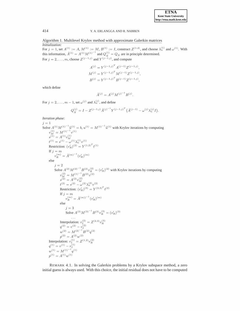
Suppose thatm levels are used, where at levelm − 1 the associated Galerkin problemis sufficiently small to be solved exactly. The multilevel Krylov method can be written in analgorithm as follows.




Algorithm 1. Multilevel Krylov method with approximate Galerkin matricesInitialization:For j = 1, setA(1) := A, M (1) := M , B(1) := I, constructZ(1,2), and chooseλ(1)

n andω(1). Withthis information,A(1) = A(1)M (1)−1

andQ(1)

N= QN are in principle determined.

For j = 2, . . . , m, chooseZ(j−1,j) andY (j−1,j), and compute

A(j) = Y

(j−1,j)T

A(j−1)

Z(j−1,j)

,

M(j) = Y

(j−1,j)T

M(j−1)

Z(j−1,j)

,

B(j) = Y

(j−1,j)T

B(j−1)

Z(j−1,j)

,

which define

A(j) = A

(j)M

(j)−1

B(j)

.

For j = 2, . . . , m − 1, setω(j) andλ(j)n , and define

Q(j)

N= I − Z

(j−1,j)A

(j)−1

Y(j−1,j)T `

A(j−1)

− ω(j)

λ(j)n I

´.

Iteration phase:j = 1

SolveA(1)M (1)−1 eu(1) = b, u(1) = M (1)−1 eu(1) with Krylov iterations by computingv(1)M = M (1)−1

v(1)

s(1) = A(1)v(1)M

t(1) = s(1)− ω(1)λ

(1)n v(1)

Restriction:(v′R)(2) = Y (1,2)T

t(1)

If j = m

v(m)R = A(m)−1

(v′R)(m)

elsej = 2

SolveA(2)M (2)−1

B(2)v(2)R = (v′

R)(2) with Krylov iterations by computing

v(2)M = M (1)−1

B(2)v(2)

s(2) = A(2)v(2)M

t(2) = s(2)− ω(2)λ

(2)n v(2)

Restriction:(v′R)(3) = Y (2,3)T

t(2)

If j = m

v(m)R = A(m))−1

(v′R)(m)

elsej = 3

SolveA(3)M (3)−1

B(3)v(3)R = (v′

R)(3)

. . .

Interpolation:v(2)I = Z(2,3)v

(3)R

q(2) = v(2)− v

(2)I

w(2) = M (2)−1

B(2)q(2)

p(2) = A(2)w(2)

Interpolation:v(1)I = Z(1,2)v

(2)R

q(1) = v(1)− v

(1)I

w(1) = M (1)−1

q(1)

p(1) = A(1)w(1)

REMARK 4.1. In solving the Galerkin problems by a Krylov subspace method, a zeroinitial guess is always used. With this choice, the initial residual does not have to be computed




explicitly because it is equal to the right-hand side vectorof the Galerkin system. Hence, wecan save one vector multiplication withA(j)M (j)−1

B(j).

REMARK 4.2. At every levelj, we require an estimate toλ(j)n . Our numerical results

reveal that withω(j) = 1, j = 1, . . . , n − 1, takingλ(j)n = 1 leads to a good method.

5. Multilevel Krylov-multigrid method. In Algorithm 1, at each level two precondi-tioner solutions related toM (j) are required to computev(j)

M andw(j). At the levelj = 1,this solution is approximately determined by one multigriditeration. Even though the re-sultant error reduction factorρ is not that of the typical text-book multigrid convergence (inthis case,ρ = 0.6), this choice leads to an effective preconditioner for convergence acceler-ation of Krylov subspace methods for the Helmholtz equation[12]. Since the size ofM (j),1 < j < m, may also be large, we shall use one multigrid iteration to approximately com-puteM (j)−1

.A multigrid method consists of a recursive application of presmoothing, restriction,

coarse-grid correction, interpolation and defect correction, and postsmoothing. Both pre-and postsmoothing are carried out by basic iterative methods, e.g., damped Jacobi or Gauss-Seidel, which smooth the error. The smooth errors are then restricted to the coarse-gridsubspace, where a coarse-grid system is solved to further correct the errors. This correctionis then added to the error in the fine-grid subspace, after an interpolation process. For furtherreading on multigrid, we refer to, e.g, [21]. What is important to us is the multigrid restrictionand interpolation process, and the coarse-grid correctionstep.

Assume that a sequence of fine and coarse gridsΩj , j = 1, . . . ,m, Ω1 ⊃ Ω2 · · · ⊃ Ωm

are given. The multigrid transfer operators between two gridsΩj andΩj+1, denoted by

Ij+1j : G(Ωj) 7→ G(Ωj+1), Ij

j+1 : G(Ωj+1) 7→ G(Ωj), (5.1)

are associated with the restriction and interpolation (or prolongation) process, respectively,and are given as well. For the Galerkin coarse-grid correction, the coarse-grid system isassociated with the Galerkin coarse-grid matrix defined as

M(j)MG = Ij+1

j M(j+1)MG Ij

j+1. (5.2)

The processes (5.1) are algebraically the same as whatZ andY T , respectively, do in themultilevel Krylov method, and (5.2) is similar toE. In multigrid, however, the matricesIj+1

j

andIjj+1 should represent a sufficiently accurate interpolation and, respectively, restriction

of smooth functions. Since the multilevel Krylov method does not necessarily require thiscriterion, the matricesIj+1

j andIjj+1 are in general not the same asZ andY T , respectively.

This implies that, in general,M (j) 6= M(j)MG, j > 1. But it is not a problem for the multilevel

Krylov method to haveZ = Ij+1j andY T = Ij

j+1, as the conditions in Theorem3.2are met.

In this case,M (j) = M(j)MG.

We comment on the choiceZ = Ij+1j andY T = Ij

j+1. First, as shown for the 1Dexample in Section3, with Z based on multigrid linear interpolation the convergence ofthetwo-level Krylov method is faster than with the piece-wise constant interpolation. We canexpect that this convergence property also holds for themulti-level Krylov method. Secondly,since nowM (j) = M

(j)MG, both the multilevel Krylov method and the multigrid steps for the

preconditioner solves use the same components. This avoidsadditional storage for multigridcomponents. Furthermore, all coarse-grid information used by the multilevel Krylov andmultigrid parts are computed only once during the initialization phase of the multilevel Krylovmethod. This will save the cost of the initialization phase.




A multigrid algorithm for solving, e.g.,v(j)M = M (j)−1

v(j)B in Algorithm 1, withv

(j)B =

B(j)v(j), can be written as follows.

Algorithm 2. Multigrid with (j − m + 1) levels

Givenv(j)M,ℓ

Presmoothing:v(j)M,ℓ+1/3 = smooth(M (j), v

(j)M,ℓ, v

(j)B )

r(j) = v(j)B − M (j)v

(j)M,ℓ+1/3

Restriction:r(j+1) = Y (j,j+1)T

r(j)

Coarse-grid problem:if j = m solvee(m) = M (m)−1

r(m)

else. . .

endifProlongation:d(j) = Z(j,j+1)e(j+1)

Defect correction:v(j)M,ℓ+2/3 = v

(j)M,ℓ+1/3 + d(j)

Post-smoothing:v(j)M,ℓ+1 = smooth(M (j), v

(j)M,ℓ+2/3, v

(j)B )

Incorporating Algorithm 2 in Algorithm 1, the multilevel Krylov-multigrid method (MKMG)results. Note that in Algorithm 2, the finest multigrid levelis always the same as the currentlevel in the multilevel Krylov step. Hence, for the action ofQ

(j)

Ndone at levelj = J < m,

multigrid with J − m grid levels is used to approximate the action of preconditionerM (J).Figure5.1 illustrates one MKMG cycle withm = 5 levels. The white circles indicate

the pre- and postsmoothing process in multigrid applied toM , while the black circles cor-respond to the multilevel steps. In this figure, the multigrid step is shown with V-cycle, butthis can in principle be replaced by other multigrid cycles.At the levelj of the multilevelKrylov method, multigrid withm − j levels is called to approximately invertM (j) with thecorresponding coarse-grid matricesM (j+1), . . . ,M (m). Once the multilevel Krylov methodreaches the levelj = m − 1, the Galerkin problem at levelj = m is solved exactly.

1

2

3

4

5

IT+1IT

FIGURE 5.1. Multilevel Krylov-multigrid cycle withm = 5. “ •”: multilevel Krylov step; “”: multigrid step.

6. Numerical experiments. In this section we present convergence results for the 1Dand 2D Helmholtz equation. We compare performance of the multilevel Krylov-multigridmethod (denoted by MKMG) with that of Krylov preconditionedby shifted Laplacian (de-




noted by MG). For both methods, we employ one multigrid iteration to invert the shiftedLaplacian, with F-cycle and one pre- and postsmoothing. Following [10], Jacobi with un-derrelaxation (ωR = 0.5) is used as a smoother. This value was found via the Local FourierAnalysis (LFA), and appeared to be optimal for problems considered there for a wide rangeof wavenumbers. The coarsest level for both MKMG and MG consists of only one interiorgrid point.

At each levelj > 1 of MKMG, GMRES [17] is applied to the preconditioned Galerkinsystem. Since in this case the preconditioners are not fixed,a flexible version of GMRES,called FGMRES, is employed. Forj = 1, the finest level, FGMRES is used for MKMG andMG. Convergence for MKMG and MG is declared if the initial relative residual is reducedby six orders of magnitude.

In principle it is not necessary to use the same number of FGMRES iterations at eachlevel. The notation MKMG(6,2,2), for instance, indicates that 6 FGMRES iterations areemployed at levelj = 2, 2 at levelj = 3 and 2 at levelj = 4, . . . ,m − 1. At level j = mthe coarse-grid problem is solved exactly. As observed in [8], it is the accuracy of solving theGalerkin system at the second level which is of importance.

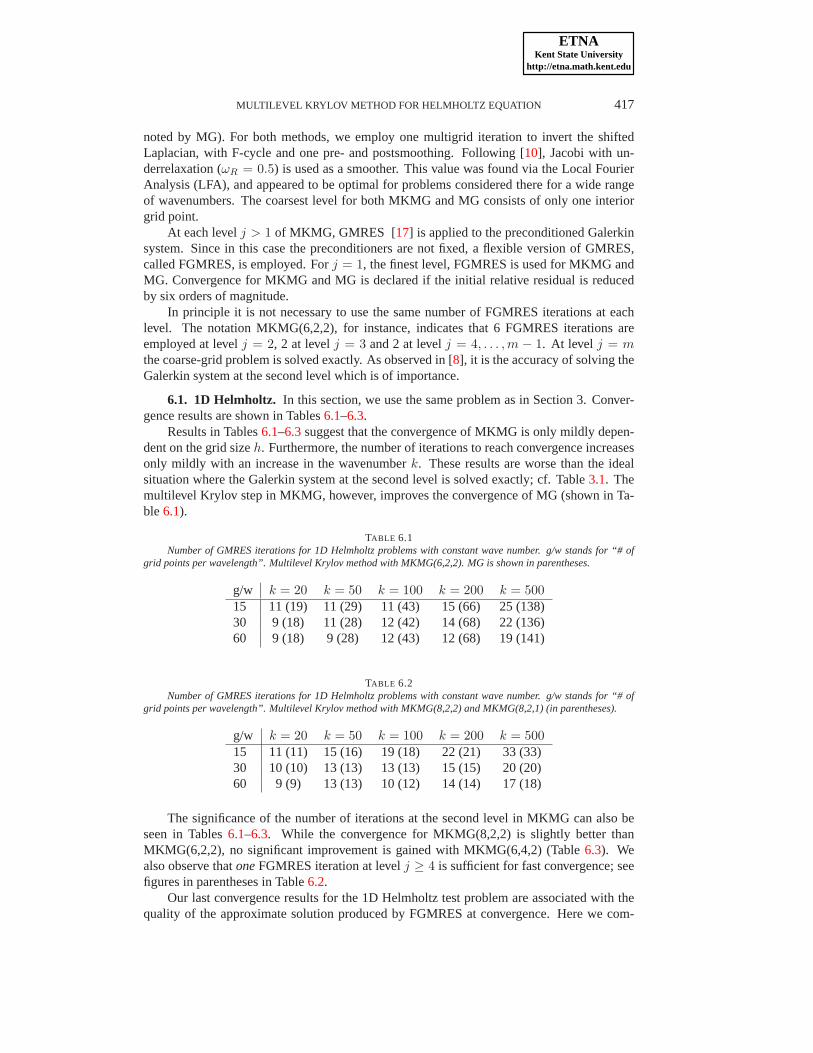
6.1. 1D Helmholtz. In this section, we use the same problem as in Section 3. Conver-gence results are shown in Tables6.1–6.3.

Results in Tables6.1–6.3suggest that the convergence of MKMG is only mildly depen-dent on the grid sizeh. Furthermore, the number of iterations to reach convergence increasesonly mildly with an increase in the wavenumberk. These results are worse than the idealsituation where the Galerkin system at the second level is solved exactly; cf. Table3.1. Themultilevel Krylov step in MKMG, however, improves the convergence of MG (shown in Ta-ble6.1).

TABLE 6.1Number of GMRES iterations for 1D Helmholtz problems with constant wave number. g/w stands for “# of

grid points per wavelength”. Multilevel Krylov method withMKMG(6,2,2). MG is shown in parentheses.

g/w k = 20 k = 50 k = 100 k = 200 k = 50015 11 (19) 11 (29) 11 (43) 15 (66) 25 (138)30 9 (18) 11 (28) 12 (42) 14 (68) 22 (136)60 9 (18) 9 (28) 12 (43) 12 (68) 19 (141)


grid points per wavelength”. Multilevel Krylov method withMKMG(8,2,2) and MKMG(8,2,1) (in parentheses).

g/w k = 20 k = 50 k = 100 k = 200 k = 50015 11 (11) 15 (16) 19 (18) 22 (21) 33 (33)30 10 (10) 13 (13) 13 (13) 15 (15) 20 (20)60 9 (9) 13 (13) 10 (12) 14 (14) 17 (18)

The significance of the number of iterations at the second level in MKMG can also beseen in Tables6.1–6.3. While the convergence for MKMG(8,2,2) is slightly better thanMKMG(6,2,2), no significant improvement is gained with MKMG(6,4,2) (Table6.3). Wealso observe thatoneFGMRES iteration at levelj ≥ 4 is sufficient for fast convergence; seefigures in parentheses in Table6.2.

Our last convergence results for the 1D Helmholtz test problem are associated with thequality of the approximate solution produced by FGMRES at convergence. Here we com-





grid points per wavelength”. Multilevel Krylov method withMKMG(6,4,2). Theℓ2 norm of errors are shown inparentheses.

g/w k = 20 k = 50 k = 100 k = 200 k = 50015 11 (2.42E–8) 15 (6.87E–8) 20 (6.68E–8) 23 (1.29E–7) 36 (4.80E–8)30 10 (6.35E–8) 13 (4.83E–8) 13 (3.39E–8) 14 (1.02E–7) 19 (1.27E–7)60 9 (1.17E–7) 16 (1.24E–7) 12 (6.78E–8) 16 (1.16E–6) 19 (4.39E–7)

pute the error between the approximate solution of MKMG at convergence and the solutionobtained from a sparse direct method. Theℓ2 norms of the error are shown in parentheses inTable6.3. For all cases, theℓ2 norms of the error fall below10−5.

6.2. 2D Helmholtz. In this section, 2D Helmholtz problems in a square domain withconstant wavenumbers are presented. At the boundaries, thefirst-order approximation tothe Sommerfeld (non-reflecting) condition due to Engquist and Majda [6] is imposed. Weconsider problems where a source is generated in the middle of the domain.

Following the 1D case, the deflation subspaceZ is chosen to be the same as the in-terpolation matrix in multigrid. For 2D cases, however, care is needed in constructing theinterpolation matrixZ. Consider a set of fine grid points defined by

Ωh := (x, y) | x = xix= ixh, y = yiy

= iyh, ix = 1, . . . , Nx,h, iy = 1, . . . , Ny,h,

associated with the grid points on levelj = 1. The set of grid pointsΩH corresponding to thecoarse-grid levelj = 2 is determined as follows. We assume that(x1, y1) ∈ ΩH coincideswith (x1, y1) ∈ Ωh, as illustrated in Figure6.1 (left). Starting from this point, the completeset of coarse-grid points is then selected according to the standard multigrid coarsening, i.e.,by doubling the mesh size. This results in the coarse grid, for H = 2h,

ΩH := (x, y) | x = xix= (2ix − 1)h, y = yiy

= (2iy − 1)h,

ix = 1, . . . , Nx,H , iy = 1, . . . , Ny,H.

As shown in [12], this coarsening strategy leads to a good multigrid methodfor the shiftedLaplacian preconditioner. Moreover, from a multilevel Krylov method point of view, thiscoarsening strategy results in larger projection subspaces than if, e.g.,(x1, y1) ∈ ΩH coin-cides with(x2, y2) ∈ Ωh; see Figure6.1 (right). As shown in Figure6.1, for example, with7 × 7 grid points at the finest level, the latter coarsening approach leads to only 9 deflationvectors, i.e.,r = 9. In contrast, the earlier approach results in 16 deflation vectors (r = 16),which eventually shift 16 small eigenvalues.

Both approaches, however, produce the same number of deflation vectors if an evennumber of grid points is used in each direction.

Having defined the coarse-grid points according to Figure6.1(left), the deflation vectorsare determined by using the bilinear interpolation processof coarse-grid value into the finegrid as follows [21], for level 2 to level 1 (see Figure6.3(a) for the meaning of the symbols):

IhHv(1)(x, y) =

v(2)(x, y), for •,12 [v(2)(x, y − h) + v(2)(x, y + h)], for ,12 [v(2)(x − h, y) + v(2)(x + h, y)], for ,14 [v(2)(x − h, y − h) + v(2)(x − h, y + h)

+ v(2)(x + h, y − h) + v(2)(x + h, y + h)], for .




1 2 3 41

2

3

4

1 3 4 5 6

1

2

2

3

4

5

6

7

7 1 2 3 4 5 6 7

1

2

3

4

5

6

7

1 2 3

1

2

3

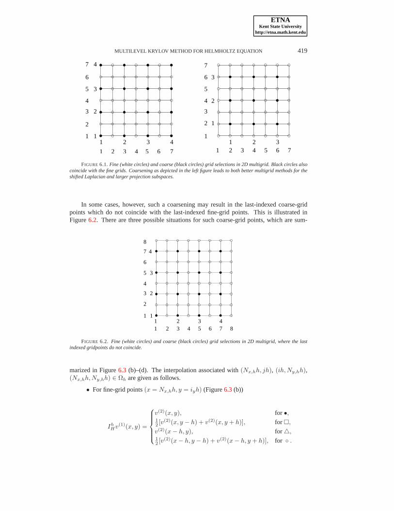
FIGURE 6.1. Fine (white circles) and coarse (black circles) grid selections in 2D multigrid. Black circles alsocoincide with the fine grids. Coarsening as depicted in the left figure leads to both better multigrid methods for theshifted Laplacian and larger projection subspaces.

In some cases, however, such a coarsening may result in the last-indexed coarse-gridpoints which do not coincide with the last-indexed fine-gridpoints. This is illustrated inFigure6.2. There are three possible situations for such coarse-grid points, which are sum-

1 2 3 4 5 6 7 81 2 3 4

1

2

3

4

1

2

3

4

5

6

7

8

FIGURE 6.2. Fine (white circles) and coarse (black circles) grid selections in 2D multigrid, where the lastindexed gridpoints do not coincide.

marized in Figure6.3 (b)–(d). The interpolation associated with(Nx,hh, jh), (ih,Ny,hh),(Nx,hh,Ny,hh) ∈ Ωh are given as follows.

• For fine-grid points(x = Nx,hh, y = iyh) (Figure6.3(b))

IhHv(1)(x, y) =

v(2)(x, y), for •,12 [v(2)(x, y − h) + v(2)(x, y + h)], for ,

v(2)(x − h, y), for ,12 [v(2)(x − h, y − h) + v(2)(x − h, y + h)], for .




• For fine-grid points(x = ixh, y = Ny,hh) (Figure6.3(c))

IhHv(1)(x, y) =

v(2)(x, y), for •,v(2)(x, y − h), for ,12 [v(2)(x − h, y) + v(2)(x + h, y)], for ,12 [v(2)(x − h, y − h) + v(2)(x + h, y − h)], for .

• For fine-grid points(x = Nx,hh, y = Ny,hh) (Figure6.3(d))

IhHv(1)(x, y) =

v(2)(x, y), for •,v(2)(x, y − h), for ,

v(2)(x − h, y), for ,

v(2)(x − h, y − h), for .

Based on the interpolation matrixIhH , we setZ(1,2) = Z(h,H) = Ih

H andRHh = (Ih

H)T .

x,H Nx,HiNy,H Ny,H

x,HNi

(a) (b) (c) (d)

y,Hi +1 i +1y,H

iy,H iy,Hi +1x,H x,H x,Hi +1

FIGURE 6.3. Fine (white colored) and coarse (black colored) grid selection indicating the bilinear interpola-tion in 2D multigrid. Black circles (•) coincide with the fine grids.

Convergence results are shown in Tables6.4–6.8 for various wavenumbers. From thesetables, for low grid resolutions (e.g., 15 grid points per wavelength) we observe convergenceof MKMG which is mildly dependent on the wavenumberk. The convergence becomesless dependent onk if the grid sizeh is smaller; see also Figures6.4–6.6 for comparisonswith MG.


grid points per wavelength”. Multilevel Krylov method withMKMG(4,2,1).

g/w k = 20 k = 40 k = 60 k = 80 k = 100 k = 120 k = 200 k = 30015 11 14 15 17 20 22 39 6420 12 13 15 16 18 21 30 4530 11 12 12 13 13 15 24 39

From Tables6.4–6.8, it is apparent that MKMG(8,2,1) is the most efficient method, sofar, in terms of the number of iterations; it converges faster for all k andh used. If one ismore concerned with the number of MKMG iterations to reach convergence, one can usemore iterations at the levelj = 3 (e.g., MKMG(8,3,1), not shown), but this setting does notlead to a further reduction in CPU time.






g/w k = 20 k = 40 k = 60 k = 80 k = 100 k = 120 k = 200 k = 30015 11 14 15 18 19 21 31 5220 12 13 15 15 16 18 25 3730 11 12 12 13 13 14 18 28



g/w k = 20 k = 40 k = 60 k = 80 k = 100 k = 120 k = 200 k = 30015 11 14 14 18 18 20 28 4720 12 13 15 15 16 17 25 3630 11 12 12 13 13 14 16 25

TABLE 6.7Number of GMRES iterations for 2D Helmholtz problems with constant wave number. g/w stands for “#grid

points per wavelength”. Multilevel Krylov method with MKMG(8,2,1).

g/w k = 20 k = 40 k = 60 k = 80 k = 100 k = 120 k = 200 k = 30015 11 14 14 17 18 21 27 3920 12 13 15 14 15 16 20 2830 11 12 12 12 13 14 15 19

TABLE 6.8Number of GMRES iterations for 2D Helmholtz problems with constant wave number. g/w stands fostands for

“#grid points per wavelength”. Multilevel Krylov method with MKMG(4,3,1).

g/w k = 20 k = 40 k = 60 k = 80 k = 100 k = 120 k = 200 k = 30015 11 14 15 18 20 22 40 6620 12 14 15 16 17 20 29 3930 11 12 12 14 14 15 23 35

In order to gain insight onto the total arithmetic operations needed by MKMG, in Fig-ures6.4–6.6, we compare CPU time needed by MKMG and MG to reach convergence. Wemeasure the elapsed time on a Pentium 4 machine for the initialization and iteration phasewith the MATLAB commandstic/toc. Since thefor loop is used in most parts of theinitialization phase, the measured time is too pessimistic.

From Figures6.4–6.6we observe that, for low wavenumbers, MG is still faster thananyMKMG methods. MKMG only outperforms MG when the wavenumber becomes sufficientlylarge. For instance, MKMG(8,2,1) is faster than MG fork > 150, in terms of number ofiterations and CPU time.

For k = 300, we were unable to run MG until convergence because of the excessivememory used to keep all Arnoldi vectors. With 30 gridpoints per wavelength, the solutionvector alone has2.25 × 106 complex-valued entries. In this case, restarting GMRES doesnot help. With full GMRES, we have to terminate the iterationafter 86 iterations with the




computed residual only6.55 × 10−4, and with about 2.3×104 seconds of CPU time. Eventhough for MKMG the initialization phase also consists of computing coarse-grid informationassociated with matricesA(j) andB(j), and not onlyM (j) as in MG, the extra computationdoes not significantly contribute to the total initialization time, as shown in the lower part ofFigures6.4–6.6(right). With nearly wavenumber-independent convergence, MKMG requiresfar less memory than MG for high wavenumbers.

0 50 100 150 200 250 300 3500

50

100

150

200

250

Wavenumber, k

# Ite

ratio

n

MG−MK(4,2,1)

MG−MK(6,2,1)

MG−MK(8,2,1)

MG

0 50 100 150 200 250 300 35010

−1

100

101

102

103

Wavenumber, k

Tim

e, S

ec

Multigrid/MultilevelSetup Time

Iteration Time

FIGURE 6.4. Number of iterations and CPU time for GMRES with multigrid applied to the shifted Laplacianpreconditioner (MG) and multigrid-multilevel Krylov method (MKMG). 15 grid points per wavelength.

0 50 100 150 200 250 300 3500

20

40

60

80

100

120

140

160

Wavenumber, k

# Ite

ratio

n

MG−MK(4,2,1)

MG−MK(6,2,1)

MG−MK(8,2,1)

MG

0 50 100 150 200 250 300 35010

−1

100

101

102

103

104

Wavenumber, k

Tim

e, S

ec


Iteration Time

FIGURE 6.5. Number of iterations and CPU time for GMRES with multigrid applied to the shifted Laplacianpreconditioner (MG) and the multigrid-multilevel Krylov method (MKMG). 20 grid points per wavelength.

7. Conclusions. In this paper, we have discussed a new multilevel Krylov method forsolving the 2D Helmholtz equation. This MKMG method is basedon a multilevel Krylovmethod applied to the Helmholtz equation preconditioned bythe shifted Laplacian. With thismethod, small eigenvalues of the original preconditioned system and the associated Galerkin(coarse-grid) systems are shifted to one, leading to favorable spectra for the convergence ofKrylov subspace methods. At every level in the MKMG method, afew Krylov iterations areused to solve the projected Galerkin (coarse-grid) preconditioned problems. The precondi-tioner solves are done by one multigrid iteration, whose maximum level is reduced accordingto the projection level.




0 50 100 150 200 250 300 3500

20

40

60

80

100

120

140

160

Wavenumber, k

# Ite

ratio

n

MG−MK(4,2,1)

MG−MK(6,2,1)

MG−MK(8,2,1)

MG

0 50 100 150 200 250 300 35010

−1

100

101

102

103

104

Wavenumber, k

Tim

e, S

ec


Iteration Time

FIGURE 6.6. Number of iterations and CPU time for GMRES with multigrid applied to the shifted Laplacianpreconditioner (MG) and multigrid-multilevel Krylov method (MKMG). 30 grid points per wavelength.

Numerical experiments have been performed on the 1D and 2D Helmholtz equationwith constant wavenumber. The MKMG method leads to only mildly h-dependent andk-dependent convergence. This considerable improvement in the convergence rate leads toa speed up in CPU time when compared to Krylov methods with multigrid-based precondi-tioner alone.

Finally, this multilevel Krylov method consists of severalingredients: a preconditionerfor Krylov iterations, restriction and prolongation operators, an approximation of the maxi-mum eigenvalue, and an approximation to the Galerkin matrix. In this paper, we have chosena specific choice of all these ingredients, some of which are the same as and have been theintegral parts of a multigrid-based preconditioning method for the Helmholtz equation. Nev-ertheless, other choices or new developments in those methods can be easily implemented inour multilevel Krylov framework to obtain an even faster convergence.

Acknowledgment. We thank two anonymous referees for their constructive commentsand remarks, which improve significantly the manuscript, and Gavin Menzel-Jones for hisEnglish-related suggestions.

REFERENCES

[1] I. BABUSKA , F. IHLENBURG, T. STROUBOULIS, AND S. K. GANGARAJ, A posteriori error estimation forfinite element solutions of Helmholtz’s equation. Part II: Estimation of the pollution error, Internat. J.Numer. Methods Engrg., 40 (1997), pp. 3883–3900.

[2] A. BAYLISS, C. I. GOLDSTEIN, AND E. TURKEL, On accuracy conditions for the numerical computation ofwaves, J. Comput. Phys., 59 (1985), pp. 396–404.

[3] M. E IERMANN , O. G. ERNST, AND O. SCHNEIDER, Analysis of acceleration strategies for restarted minimalresidual methods, J. Comput. Appl. Math., 123 (2000), pp. 261–292.

[4] H. C. ELMAN , O. G. ERNST, AND D. P. O’LEARY, A multigrid method enhanced by Krylov subspaceiteration for discrete Helmholtz equations, SIAM J. Sci. Comput., 22 (2001), pp. 1291–1315.

[5] B. ENGQUIST AND A. M AJDA, Absorbing boundary conditions for the numerical simulation of waves, Math.Comp., 31 (1977), pp. 629–651.

[6] , Absorbing boundary conditions for the numerical simulation of waves, Math. Comp., 31 (1977),pp. 629–651.

[7] Y. A. ERLANGGA AND R. NABBEN, Deflation and balancing preconditioners for Krylov subspace methodsapplied to nonsymmetric matrices, SIAM J. Matrix Anal. Appl., 30 (2008), pp. 684–699.

[8] , Multilevel projection-based nested Krylov iteration for boundary value problems, SIAM J. Sci. Com-put., 30 (2008), pp. 1572–1595.




[9] , Algebraic multilevel Krylov methods, SIAM J. Sci. Comput., 31 (2009), pp. 3417–3437.[10] Y. A. ERLANGGA, C. W. OOSTERLEE, AND C. VUIK , A novel multigrid-based preconditioner for the het-

erogeneous Helmholtz equation, SIAM J. Sci. Comput., 27 (2006), pp. 1471–1492.[11] Y. A. ERLANGGA, C. VUIK , AND C. W. OOSTERLEE, On a class of preconditioners for solving the Helm-

holtz equation, Appl. Numer. Math., 50 (2004), pp. 409–425.[12] , Comparison of multigrid and incomplete LU shifted-Laplacepreconditioners for the inhomogeneous

Helmholtz equation, Appl. Numer. Math., 56 (2006), pp. 648–666.[13] J. FRANK AND C. VUIK , On the construction of deflation-based preconditioners, SIAM J. Sci. Comput., 23

(2001), pp. 442–462.[14] R. B. MORGAN, A restarted GMRES method augmented with eigenvectors, SIAM J. Matrix Anal. Appl., 16

(1995), pp. 1154–1171.[15] R. NABBEN AND C. VUIK , A comparison of deflation and the balancing preconditioner, SIAM J. Sci. Com-

put., 27 (2006), pp. 1742–1759.[16] R. A. NICOLAIDES, Deflation of conjugate gradients with applications to boundary value problems, SIAM

J. Numer. Anal., 24 (1987), pp. 355–365.[17] Y. SAAD , A flexible inner-outer preconditioned GMRES algorithm, SIAM J. Sci. Comput., 14 (1993),

pp. 461–469.[18] , Iterative Methods for Sparse Linear Systems, SIAM, Philadelphia, 2003.[19] Y. SAAD AND M. H. SCHULTZ, GMRES: a generalized minimal residual algorithm for solving nonsymmetric

linear systems, SIAM J. Sci. Stat. Comput., 7 (1986), pp. 856–869.[20] J. TANG, R. NABBEN, K. VUIK , AND Y. A. ERLANGGA, Theoretical and numerical comparison of projec-

tion methods derived from deflation, J. Sci. Comput., 39 (2009), pp. 340–370.[21] U. TROTTENBERG, C. OOSTERLEE, AND A. SCHULLER, Multigrid, Academic Press, New York, 2001.[22] M. B. VAN GIJZEN, Y. A. ERLANGGA, AND C. VUIK , Spectral analysis of the discrete Helmholtz operator

preconditioned with a shifted Laplacian, SIAM J. Sci. Comput., 29 (2006), pp. 1942–1952.[23] R. S. VARGA, Gerschgorin and His Circles, Springer, Berlin-Heidelberg, 2004.

ON A MULTILEVEL KRYLOV METHOD FOR THE HELMHOLTZ EQUATION PRECONDITIONED BY SHIFTED LAPLACIAN

Documents

Transcript of ON A MULTILEVEL KRYLOV METHOD FOR THE HELMHOLTZ EQUATION PRECONDITIONED BY SHIFTED LAPLACIAN