X-ray properties of the microquasar GRS 1915+105 during a variability class transition
Upload
khangminh22Category
view
3download
0
INSTITUT DE FISICAD’ALTES ENERGIES
UNIVERSITAT AUTONOMADE BARCELONA
Observation of the Crab pulsar wind nebula and microquasarcandidates with MAGIC
Ph.D. DissertationUniversitat Autonoma de Barcelona
speciality: Astrophysics
Roberta ZaninIFAE
Edifici Cn, UAB08193 Bellaterra (Barcelona), Spain
supervised by:
Juan Cortina BlancoIFAE
Edifici Cn, UAB08193 Bellaterra (Barcelona), Spain
Enrique Fernandez SanchezIFAE
IFAE & UABEdifici Cn, UAB
08193 Bellaterra (Barcelona), [email protected]

To Florian Goebel
irreplaceable friendand dearest collegue
Vorrei sapere a che cosa e servitovivere, amare e soffrire
spendere tutti i tuoi giorni passatise presto hai dovuto partire,se presto hai dovuto partirevoglio pero ricordarti com'eri
pensare che ancora vivivoglio pensare che ancora mi ascolti
e che come allora sorridi,e che come allora sorridi

Contents
Acronyms V
Unit definition XI
Introduction 1
1 The non-thermal universe 31.1 Cosmic rays . . . . . . . . . . . . . . . . . . . . . . . . . . . . . . . . . . . . . 4
1.1.1 Galactic cosmic rays . . . . . . . . . . . . . . . . . . . . . . . . . . . . 51.1.2 Extra-galactic cosmic rays . . . . . . . . . . . . . . . . . . . . . . . . . 7
1.2 -ray astrophysics . . . . . . . . . . . . . . . . . . . . . . . . . . . . . . . . . 71.3 Neutrino astrophysics . . . . . . . . . . . . . . . . . . . . . . . . . . . . . . . 121.4 Astrophysical sources . . . . . . . . . . . . . . . . . . . . . . . . . . . . . . . . 12
PART I. THE MAGIC DETECTOR and DATA ANALYSIS 17
2 The MAGIC Telescopes 192.1 Introduction . . . . . . . . . . . . . . . . . . . . . . . . . . . . . . . . . . . . . 192.2 Telescope subsystems . . . . . . . . . . . . . . . . . . . . . . . . . . . . . . . . 21
2.2.1 Frame and drive system . . . . . . . . . . . . . . . . . . . . . . . . . . 232.2.2 Starguider system . . . . . . . . . . . . . . . . . . . . . . . . . . . . . 252.2.3 Reflector . . . . . . . . . . . . . . . . . . . . . . . . . . . . . . . . . . . 262.2.4 Camera . . . . . . . . . . . . . . . . . . . . . . . . . . . . . . . . . . . 312.2.5 Calibration system . . . . . . . . . . . . . . . . . . . . . . . . . . . . . 342.2.6 Readout and data acquisition systems . . . . . . . . . . . . . . . . . . 342.2.7 Trigger . . . . . . . . . . . . . . . . . . . . . . . . . . . . . . . . . . . . 382.2.8 Sumtrigger . . . . . . . . . . . . . . . . . . . . . . . . . . . . . . . . . 392.2.9 Pyrometer . . . . . . . . . . . . . . . . . . . . . . . . . . . . . . . . . . 392.2.10 GRB monitoring alert system . . . . . . . . . . . . . . . . . . . . . . . 392.2.11 Clocks . . . . . . . . . . . . . . . . . . . . . . . . . . . . . . . . . . . . 402.2.12 Weather station . . . . . . . . . . . . . . . . . . . . . . . . . . . . . . . 40
2.3 Operation of the telescopes . . . . . . . . . . . . . . . . . . . . . . . . . . . . 402.3.1 Scheduling of sources . . . . . . . . . . . . . . . . . . . . . . . . . . . . 402.3.2 Regular and ToO observations . . . . . . . . . . . . . . . . . . . . . . 412.3.3 Source pointing modes . . . . . . . . . . . . . . . . . . . . . . . . . . . 412.3.4 Calibration and data runs . . . . . . . . . . . . . . . . . . . . . . . . . 42
2.4 Central control . . . . . . . . . . . . . . . . . . . . . . . . . . . . . . . . . . . 42
I

II CONTENTS
2.4.1 Communication with telescope subsystems . . . . . . . . . . . . . . . . 432.4.2 Program structure . . . . . . . . . . . . . . . . . . . . . . . . . . . . . 432.4.3 Status of the subsystems: graphical user interface . . . . . . . . . . . . 452.4.4 Central control functions . . . . . . . . . . . . . . . . . . . . . . . . . . 502.4.5 Error/event logging . . . . . . . . . . . . . . . . . . . . . . . . . . . . . 55
2.5 Online analysis . . . . . . . . . . . . . . . . . . . . . . . . . . . . . . . . . . . 56
3 The MAGIC standard analysis chain 593.1 Monte Carlo simulations . . . . . . . . . . . . . . . . . . . . . . . . . . . . . . 613.2 Conversion into ROOT format and merging of control data stream . . . . . . 623.3 Signal reconstruction and calibration . . . . . . . . . . . . . . . . . . . . . . . 623.4 Image cleaning . . . . . . . . . . . . . . . . . . . . . . . . . . . . . . . . . . . 63
3.4.1 Standard timing image cleaning . . . . . . . . . . . . . . . . . . . . . . 633.4.2 Sum image cleaning . . . . . . . . . . . . . . . . . . . . . . . . . . . . 66
3.5 Parameter reconstruction . . . . . . . . . . . . . . . . . . . . . . . . . . . . . 673.5.1 Stereo parameter reconstruction . . . . . . . . . . . . . . . . . . . . . . 69
3.6 Data quality checks . . . . . . . . . . . . . . . . . . . . . . . . . . . . . . . . . 713.7 /hadron separation . . . . . . . . . . . . . . . . . . . . . . . . . . . . . . . . 723.8 Determination of the arrival direction: the Disp method . . . . . . . . . . . . 743.9 Signal detection . . . . . . . . . . . . . . . . . . . . . . . . . . . . . . . . . . . 77
3.9.1 Sensitivity . . . . . . . . . . . . . . . . . . . . . . . . . . . . . . . . . . 793.9.2 Cut optimization . . . . . . . . . . . . . . . . . . . . . . . . . . . . . . 79
3.10 Sky maps . . . . . . . . . . . . . . . . . . . . . . . . . . . . . . . . . . . . . . 793.10.1 Angular resolution . . . . . . . . . . . . . . . . . . . . . . . . . . . . . 80
3.11 Energy estimation . . . . . . . . . . . . . . . . . . . . . . . . . . . . . . . . . 813.11.1 Energy resolution . . . . . . . . . . . . . . . . . . . . . . . . . . . . . . 81
3.12 Spectrum calculation . . . . . . . . . . . . . . . . . . . . . . . . . . . . . . . . 823.13 Spectral unfolding . . . . . . . . . . . . . . . . . . . . . . . . . . . . . . . . . 843.14 Light curves . . . . . . . . . . . . . . . . . . . . . . . . . . . . . . . . . . . . . 853.15 Upper limits . . . . . . . . . . . . . . . . . . . . . . . . . . . . . . . . . . . . . 863.16 Systematic uncertainties . . . . . . . . . . . . . . . . . . . . . . . . . . . . . . 87
PART II. CRAB NEBULA 91
4 Introduction to Pulsar Wind Nebulae 934.1 Pulsars . . . . . . . . . . . . . . . . . . . . . . . . . . . . . . . . . . . . . . . . 94
4.1.1 Neutron stars . . . . . . . . . . . . . . . . . . . . . . . . . . . . . . . . 954.1.2 Neutron star magnetosphere . . . . . . . . . . . . . . . . . . . . . . . . 964.1.3 -ray emission from pulsars . . . . . . . . . . . . . . . . . . . . . . . . 99
4.2 Supernova Remnants . . . . . . . . . . . . . . . . . . . . . . . . . . . . . . . . 1004.3 Pulsar wind nebulae . . . . . . . . . . . . . . . . . . . . . . . . . . . . . . . . 101
4.3.1 Inner structure . . . . . . . . . . . . . . . . . . . . . . . . . . . . . . . 1024.3.2 Evolution of pulsar wind nebulae . . . . . . . . . . . . . . . . . . . . . 1024.3.3 Pulsar wind nebula spectra . . . . . . . . . . . . . . . . . . . . . . . . 104
4.4 The Crab Nebula . . . . . . . . . . . . . . . . . . . . . . . . . . . . . . . . . . 1074.4.1 The Crab Pulsar . . . . . . . . . . . . . . . . . . . . . . . . . . . . . . 1074.4.2 The Crab Pulsar Wind Nebula . . . . . . . . . . . . . . . . . . . . . . 108
CONTENTS III
4.4.3 The broad-band spectrum of the Crab Nebula . . . . . . . . . . . . . . 1114.4.4 The Crab Nebula at very high energies . . . . . . . . . . . . . . . . . . 1124.4.5 Theoretical models for the IC emission from Crab Nebula . . . . . . . 1144.4.6 The Crab Nebula variability . . . . . . . . . . . . . . . . . . . . . . . . 115
5 Spectrum and ux variability of the Crab Nebula 1195.1 Data sample . . . . . . . . . . . . . . . . . . . . . . . . . . . . . . . . . . . . . 1205.2 Description of the analysis . . . . . . . . . . . . . . . . . . . . . . . . . . . . . 123
5.2.1 Sum versus standard image cleaning . . . . . . . . . . . . . . . . . . . 1245.2.2 Energy resolution and bias . . . . . . . . . . . . . . . . . . . . . . . . . 1265.2.3 Signal clipping . . . . . . . . . . . . . . . . . . . . . . . . . . . . . . . 129
5.3 Differential energy spectrum . . . . . . . . . . . . . . . . . . . . . . . . . . . . 1315.3.1 Unfolded spectrum . . . . . . . . . . . . . . . . . . . . . . . . . . . . . 1325.3.2 Systematic uncertainties . . . . . . . . . . . . . . . . . . . . . . . . . . 137
5.4 Estimation of the Inverse Compton peak . . . . . . . . . . . . . . . . . . . . . 1435.5 Theoretical picture . . . . . . . . . . . . . . . . . . . . . . . . . . . . . . . . . 1455.6 Flux variability . . . . . . . . . . . . . . . . . . . . . . . . . . . . . . . . . . . 146
PART III. MICROQUASARS 151
6 Introduction to microquasars 1536.1 Binary systems . . . . . . . . . . . . . . . . . . . . . . . . . . . . . . . . . . . 153
6.1.1 Microquasars . . . . . . . . . . . . . . . . . . . . . . . . . . . . . . . . 1546.2 The main components of microquasars . . . . . . . . . . . . . . . . . . . . . . 157
6.2.1 The compact object . . . . . . . . . . . . . . . . . . . . . . . . . . . . 1576.2.2 Companion star . . . . . . . . . . . . . . . . . . . . . . . . . . . . . . . 1586.2.3 Accretion disk . . . . . . . . . . . . . . . . . . . . . . . . . . . . . . . . 1596.2.4 The corona . . . . . . . . . . . . . . . . . . . . . . . . . . . . . . . . . 1606.2.5 Jets . . . . . . . . . . . . . . . . . . . . . . . . . . . . . . . . . . . . . 160
6.3 Disk-jet connection . . . . . . . . . . . . . . . . . . . . . . . . . . . . . . . . . 1616.4 Black hole X-ray binaries . . . . . . . . . . . . . . . . . . . . . . . . . . . . . 1626.5 Neutron star X-ray binaries . . . . . . . . . . . . . . . . . . . . . . . . . . . . 1656.6 VHE emission from microquasars . . . . . . . . . . . . . . . . . . . . . . . . . 166
6.6.1 Leptonic models . . . . . . . . . . . . . . . . . . . . . . . . . . . . . . 1676.6.2 Hadronic models . . . . . . . . . . . . . . . . . . . . . . . . . . . . . . 1676.6.3 Microquasar in -rays: observations . . . . . . . . . . . . . . . . . . . 168
7 Cygnus X-3 1697.1 MAGIC observations . . . . . . . . . . . . . . . . . . . . . . . . . . . . . . . . 172
7.1.1 Data analysis . . . . . . . . . . . . . . . . . . . . . . . . . . . . . . . . 1757.2 Results . . . . . . . . . . . . . . . . . . . . . . . . . . . . . . . . . . . . . . . . 176
7.2.1 Results during high-energy -ray emission . . . . . . . . . . . . . . . . 1797.2.2 Results during the soft state . . . . . . . . . . . . . . . . . . . . . . . . 1827.2.3 Results during the hard state . . . . . . . . . . . . . . . . . . . . . . . 1837.2.4 Results during X-ray/radio states . . . . . . . . . . . . . . . . . . . . . 184
7.3 Discussion . . . . . . . . . . . . . . . . . . . . . . . . . . . . . . . . . . . . . . 186

IV CONTENTS
8 Scorpius X-1 1898.1 MAGIC observations . . . . . . . . . . . . . . . . . . . . . . . . . . . . . . . . 1918.2 X-ray results . . . . . . . . . . . . . . . . . . . . . . . . . . . . . . . . . . . . 1928.3 MAGIC results . . . . . . . . . . . . . . . . . . . . . . . . . . . . . . . . . . . 1928.4 Discussion . . . . . . . . . . . . . . . . . . . . . . . . . . . . . . . . . . . . . . 194
9 Conclusions and outlook 197
APPENDIXES i
A Acceleration mechanisms and photon-matter interactions iA.1 Acceleration mechanisms . . . . . . . . . . . . . . . . . . . . . . . . . . . . . . i
A.1.1 Fermi acceleration . . . . . . . . . . . . . . . . . . . . . . . . . . . . . iA.2 Interaction with photon fields . . . . . . . . . . . . . . . . . . . . . . . . . . . ii
A.2.1 Inverse Compton radiation . . . . . . . . . . . . . . . . . . . . . . . . . iiA.2.2 Pair production . . . . . . . . . . . . . . . . . . . . . . . . . . . . . . . ii
A.3 Interaction in matter . . . . . . . . . . . . . . . . . . . . . . . . . . . . . . . . iiiA.3.1 Bremsstrahlung . . . . . . . . . . . . . . . . . . . . . . . . . . . . . . . iiiA.3.2 ν0 decay . . . . . . . . . . . . . . . . . . . . . . . . . . . . . . . . . . . iiiA.3.3 Electron-positron annihilation . . . . . . . . . . . . . . . . . . . . . . . iv
A.4 Interaction with magnetic fields . . . . . . . . . . . . . . . . . . . . . . . . . . ivA.4.1 Synchrotron radiation . . . . . . . . . . . . . . . . . . . . . . . . . . . iv
B Astrophysical detectors viiB.1 Air shower arrays . . . . . . . . . . . . . . . . . . . . . . . . . . . . . . . . . . viiB.2 Imaging Atmospheric Cherenkov telescopes . . . . . . . . . . . . . . . . . . . ixB.3 Neutrino telescopes . . . . . . . . . . . . . . . . . . . . . . . . . . . . . . . . . x

Acronyms
asl above sea level
ADAF Advection Dominated Accretion Flow
ADC Analogical to Digital Converter
AGASA Akeno Giant Air Shower Array
AGILE Astro-rivelatore Gamma a Immagini LEggero
AGN Active Galactic Nucleus
AMANDA Antarctic Muon And Neutrino Detector Array
AMC Active Mirror Control
AMI Arcminute Microkelvin Imager
ANTARES Astronomy with a Neutrino Telescope and Abyss environmental RESarch
ARGO-YBJ Astrophysical Radiation with Ground-based Observatory at YangBaJing
ASCII American Standard Code for Information Interchange
ASM All-Sky Monitor
ATel Astronomical Telegram
BAT Burst Alert Telescope
BATSE Burst And Transient Source Experiment
BH Black Hole
CANGAROO Collaboration of Australia and Nippon for a GAmma-Ray Observatory inthe Outback
CASA-MIA Chicago Air Shower Array-Michigan Muon Array
CAT Cherenkov Atmospheric Telescope
CC Central Control
CCD Charge-Coupled Device
CCNN Close Compact Next Neighbor
CD Color-color Diagram
V

VI CONTENTS
CE Common Era
CGRO Compton Gamma-Ray Observatory
CGS Cm Gr Second
CH Counting House
CL Confidence Level
CMB Cosmic Microwave Background
CoG Center of Gravity
CPU Central Processing Unit
CR Cosmic Ray
CTA Cherenkov Telescope Array
DAQ Data AcQuisition
DC Direct Current
DoF Degree of Freedom
DRS2 Domino Ring Sampler 2
DT Discriminator Threshold
EAS Extensive Atmospheric Shower
EAS-TOP Extensive Atmospheric Shower-TOP
EGRET Energetic Gamma-Ray Experiment Telescope
EHE Extra High Energy
ESA European Space Agency
FB Flaring Branch
FADC Flash Analogical to Digital Converter
FIFO First In, First Out
FIR Far InfraRed
FoV Field of View
GBI Green Bank Interferometer
GCN Gamma-ray burst Coordinate Network
GLAST Gamma-ray Large Area Space Telescope
GBM GLAST Burst Monitor

CONTENTS VII
GPS Global Positioning System
GRB Gamma Ray Burst
GUI Graphical User Interface
GZK Greisen-Zatsepin-Kuzmin
HB Horizontal Branch
HE High-Energy
HEGRA High Energy Gamma Ray Astronomy
HESS High Energy Stereoscopic System
HiRES High Resolution fly’s eye
HMXB High-Mass X-ray Binaries
HST Hubble Space Telescope
HTML HyperText Markup Language
HV High Voltage
IACT Imaging Atmospheric Cherenkov Telescope
IC Inverse Compton
IFAE Institut de Fısica d’Altes Energies
IGM InterGalactic Magnetic
INAF Istituto Nazionale AstroFisica
INFN Istituto Nazionale Fisica Nucleare
IP Internet Protocol
IPR Individual Pixel Rate
IR InfraRed
ISM InterStellar Medium
KASCADE KArlsruhe Shower Core and Array DEtector
LAT Large Array Telescope
LED Light Emitting Diode
LMXB Low-Mass X-ray Binarie
LUT Look-Up Table
LVDS Low Voltage Differential Signal

VIII CONTENTS
LV Low Voltage
MAGIC Major Atmospheric Gamma-ray Imaging Cherenkov
MARS MAGIC Analysis and Reconstruction Software
MC Monte Carlo
MHD MagnetoHydro Dynamic
MIR MAGIC Integrated Readout
MJD Modified Julian Date
MPI Max-Planck Institute for physics
MQ MicroQuasar
MSP MilliSecond Pulsar
MUX Multiplexing readout system
NASA National Aeronautics and Space Administration
NB Normal Branch
NEMO NEutrino Mediterranean Observatory
NESTOR Neutrino Extended Submarine Telescope with Oceanographic Research
NIM Nuclear Instrumentation Module
NS Neutron Star
NSB Night Sky Background
NT-200 Neutrino Telescope-200
OA Online Analysis
OVRO Owens Valley Radio Observatory
PC Personal Computer
PCA Proportional Counter Array
PCI Peripheral Component Interconnect
PDF Probability Density Function
PI Principal Investigator
PLC Programmable Logical Controller
PULSAR PULSer And Recorder
PMT Photo Multiplier Tube

CONTENTS IX
PSF Point Spread Function
PWN Pulsar Wind Nebula
PWNe Pulsar Wind Nebulae
QE Quantum Efficiency
RF Random Forest
RMS Root Mean Square
RXTE Rossi X-ray Timing Explorer
RT Ryle Telescope
SBIG Santa Barbara Instrument Group
SCCP Slow Control Cluster Processor
SDM Standard Disk Model
SED Spectral Energy Distribution
SI Systeme International d’unites, i.e. international system of units
SN SuperNova
SNe SuperNovae
SNR SuperNova Remnant
SSC Synchrotron Self Compton
ST Sum Trigger
TAC Time Allocation Committee
TCP/IP Transmission Control Protocol/Internet Protocol
ToO Target of Opportunity
UHE Ultra High Energy
US United States
UL Upper Limit
UTC Universal Time Coordinated
UV Ultra Violet
VCSEL Vertical-Cavity Surface-Emitting Laser
VERITAS Very Energetic Radiation Imaging Telescope Array System
VHE Very High Energy

X CONTENTS
VI Virtual Instrument
VME Virtual Mobile Engine
XRB X-Ray Binarie
ZA Zenith Angle
Unit definition
• Electronvolt (eV) is a unit of energy equal to ≡ 1:6 1019 J. It is the amount ofenergy gained by one unbound electron moving in an electric potential of 1 Volt.
• Erg (erg) is a unit of energy in the Cm Gr Second (CGS) unit system. It correspondsto 107 J which is about 1 TeV.
• Jansky (Jy) is a unit of spectral flux density often used in radio astronomy. 1 Jycorresponds to 1026 W
m2 _Hzin the Systeme International d’unites, i.e. international
system of units (SI).
• Gauss (G) is a unit of magetic field. In the SI 1 G = 104 T.
• Light year (ly) is a unit of distance which is common in astrophysics. 1 ly is thedistance that light travels in a vacuum in one year. In the SI 1 ly = 9.4607 1015 m.
• Parsec (pc) unit of distance equal to 3.26 ly. A parsec is the distance from the Sun toan astrophysical object which has a parallax angle of one arcsecond.
• Modified Julian Date (MJD) consists in a dating method based on continuing daycounts. The MJD provides the number of days which have ellapsed since midnight ofWedenesday November 17, 1858.
XI

Introduction
The history of the -ray astronomy in the past twenty years is marked by the success ofthe Imaging Atmospheric Cherenkov Telescope (IACT) in the exploration of the Very HighEnergy (VHE) band. The last generation of IACTs, with the High Energy StereoscopicSystem (HESS), Very Energetic Radiation Imaging Telescope Array System (VERITAS),and Major Atmospheric Gamma-ray Imaging Cherenkov (MAGIC) telescopes, have beencapable to increase the total number of known VHE emitting sources from a few to almost onehundred in just seven years of operation. This population comprises galactic and extragalacticobjects. IACTs have proved to be very effective in both the discovery of new emitters, aswell as in the fine analysis of the physics properties of well established sources. Amongthem, the Crab Pulsar Wind Nebula is probably the best studied astrophysical object andthe archetypal Pulsar Wind Nebula (PWN). Due to its brightness at almost all wavelenghts,it is considered as an astrophysical candle. Despite the Crab Nebula broad-band spectrumhas been thoroughly studied across twenty orders of magnitudes, from radio frequencies toVHEs, further effort is needed to resolve the contradictions in the combination of all themultiwavelenght results. With the commissioning of the second MAGIC telescope in 2009and the beginning of the operations in stereoscopic mode, the performance of the instrumentimproved dramatically, allowing MAGIC to reach the lowest ever energy threshold among allthe existing IACTs, and describe the Crab Nebula spectrum with unprecedented precisiondown to 50 GeV. This achievement is of crucial importance for the VHE -ray astrophysicsin the pre-CTA era, since it can cast new light on some of the unsolved mysteries of one ofits most established sources.
On the other hand, MAGIC made a strong impact in the discovery of new VHE sourcesand, with the improved sensitivity of the stereoscopic mode, this will be even more so inthe future. Among the galactic objects, MicroQuasars (MQs) constitute some of the bestcandidates for VHE emission, but despite several well accepted models predict such signal,it has not been detected. There are, in fact, evidences that the three binary systems whichhave been unambiguously detected at energies above few hundreds of GeV are binary pulsarsrather than accreting microquasars. Nevertheless, the recent detection of the microquasarCygnus X-3 above 100 MeV by both Astro-rivelatore Gamma a Immagini LEggero (AGILE)and Fermi satellites, and the claim of short one-day flares from Cygnus X-1 reported byAGILE confirmed that microquasars remain interesting targets for VHE telescopes. MAGICmade a strong effort in searching for VHE signals from microquasars, but found only a non-significant evidence of signal from Cygnus X-1 in 80 minutes of observation on September 24,2006. MAGIC tried to detect similar flares in the following four years but the subsequenthundred more hours of observations were unsuccessful. Besides Cygnus X-1, MAGIC pointedat two other microquasar candidates, whose results are presented in this thesis: Cygnus X-3and Scorpius X-1. The most constraining Upper Limits (ULs) to the integral flux of thesesources at the energy above few hundred GeV are provided. Further investigations are beingplanned to discover these sources at VHE in the next years.
After short introduction to astroparticle physics and VHE astrophysics, this thesis is di-
1
2 CONTENTS
vided in three parts.The first part is dedicated to the MAGIC telescopes (Chapter 2) and the standard analysischain (Chapter 3). It describes the technical contributions the author made during her thesiswork. In particular, the chapter about the MAGIC provides a detail description of the instru-ment in the context of its control system and an overview of the observation strategies andthe online procedures. The author was the main responsible for the extension of the centralcontrol program to the system of two telescopes and for the online analysis.
The second part is devoted to PWNe. After a short introduction to the topic (Chapter 4),it presents the main topic of this part of the thesis, the Crab Pulsar Wind Nebula. Chapter5 describes the observations of the Crab Nebula with the MAGIC stereoscopic systems andthe resulting high-precision measurements of its differential energy spectrum and light curve.The last part of the thesis is dedicated to microquasars. It starts with a short introductionon this class of astrophysical source from both a phenomenological and theoretical point ofview (Chapter 6). Finally the analyses and corresponding results of the MAGIC observationsof Cygnus X-3 (Chapter 7) and Scorpius X-1 (Chapter 8) are presented. Particular attentionis drawn on trigger strategy used in the observational campaigns of these transient sources.This is an issue of key importance for planning future observations.
1The non-thermal universe
Cosmic rays are energetic charged particles originating from outer space, both in ourGalaxy and in some extragalactic objects. By interacting with radiation and magneticfields at the site of their production, they emit non-thermal radiation which spans fromradio frequencies up to ultra-high-energies. This chapter provides a short descriptionof the non-thermal Universe and the techniques which can be used to observe it. Par-ticular attention is paid to the -ray astronomy and its main observational targets.
Much of classical astronomy and astrophysics deals with thermal radiation emitted by hotand warm objects such as stars, planets, and dust. However, at the beginning of the 20th
century higher energy phenomena were observed suggesting the existence of non-thermal ra-diation from the Universe. In 1912, Victor Hess discovered the Cosmic Rays (CRs) and in1938 Pierre Auger proved the existence of Extensive Atmospheric Showers (EASs), cascadesof particles initiated by primary CRs with energies above 1015 eV. Modern instruments revealthat the CR spectrum extends up to 1020 eV and beyond (§ 1.1). Such high energies cannotbe produced in thermal processes unless they trace back to the very early stage of the BigBang. Their production must be explained through other mechanisms.In mid 20th century the detection of radio-waves from the galactic plane (Staelin, D. H. &Reifenstein, III, E. C., 1968) and X-ray radiation from outside the solar system (Giacconi,R. et al., 1962), led to the identification of non-thermal mechanisms producing synchrotronradiation. The latter is emitted when high-energy electrons are deflected in magnetic fields(§ A.4.1). Other common non-thermal mechanisms are the Inverse Compton (IC) scatteringof energetic electrons on seed photons (§ A.2.1) and the interaction of VHE protons (CRs)with ambient matter to produce hadronic showers.
The interest on the non-thermal phenomena increased when their important role to un-derstand the evolution of the Universe was recognized. Non-thermal and thermal radiationsprovide similar contributions to the total energy balance of the Universe. In addition, sinceCRs carry the highest known energies, they offer the possibility of exploring fundamental
3
4 1. THE NON-THERMAL UNIVERSE
physics beyond the reach of terrestrial accelerators.Non-thermal radiation can thus be studied either by observing CRs or electromagnetic
radiation over wide ranges of the electromagnetic spectrum (from radio to γ-rays). However,since the charged particles of the CRs are deflected by randomly oriented component of thegalactic magnetic field, they lose their directional information and impinge upon the Earthnearly uniformly from all directions. Therefore, the information they provide is only relatedto their energy spectrum and chemical composition, except for the highest energies (above1020 eV) for which the charged particles are no longer bended by the magnetic fields. Apartfrom these extreme energies, astronomy can be carried out only by looking at neutral particles,i.e. γ-rays and neutrinos, which travel on straight paths. The production of these neutralmessengers is always associated to the presence of accelerated charged particles which interactwith radiation and magnetic fields. Thus, they can be used to study the sources of the CRs.
1.1 Cosmic rays
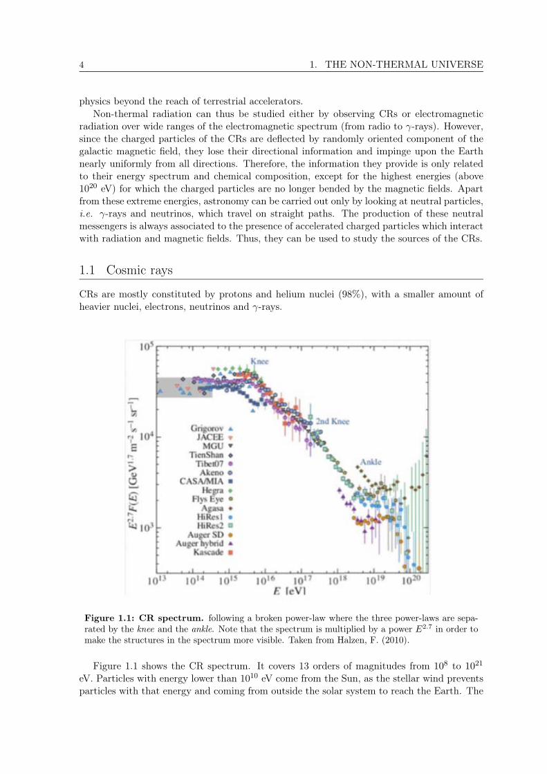
CRs are mostly constituted by protons and helium nuclei (98%), with a smaller amount ofheavier nuclei, electrons, neutrinos and γ-rays.
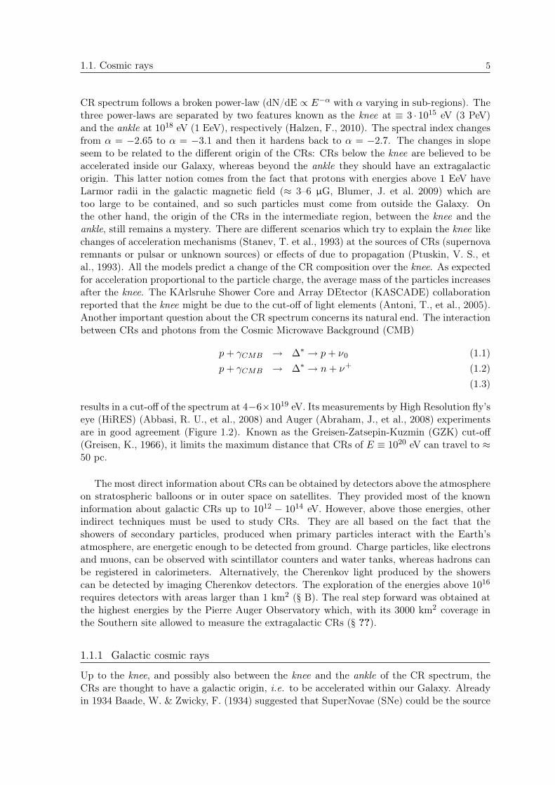
Figure 1.1: CR spectrum. following a broken power-law where the three power-laws are sepa-rated by the knee and the ankle. Note that the spectrum is multiplied by a power E2.7 in order tomake the structures in the spectrum more visible. Taken from Halzen, F. (2010).
Figure 1.1 shows the CR spectrum. It covers 13 orders of magnitudes from 108 to 1021
eV. Particles with energy lower than 1010 eV come from the Sun, as the stellar wind preventsparticles with that energy and coming from outside the solar system to reach the Earth. The
1.1. Cosmic rays 5
CR spectrum follows a broken power-law (dN/dE / E with varying in sub-regions). Thethree power-laws are separated by two features known as the knee at ≡ 3 · 1015 eV (3 PeV)and the ankle at 1018 eV (1 EeV), respectively (Halzen, F., 2010). The spectral index changesfrom = 2:65 to = 3:1 and then it hardens back to = 2:7. The changes in slopeseem to be related to the different origin of the CRs: CRs below the knee are believed to beaccelerated inside our Galaxy, whereas beyond the ankle they should have an extragalacticorigin. This latter notion comes from the fact that protons with energies above 1 EeV haveLarmor radii in the galactic magnetic field (≈ 3–6 µG, Blumer, J. et al. 2009) which aretoo large to be contained, and so such particles must come from outside the Galaxy. Onthe other hand, the origin of the CRs in the intermediate region, between the knee and theankle, still remains a mystery. There are different scenarios which try to explain the knee likechanges of acceleration mechanisms (Stanev, T. et al., 1993) at the sources of CRs (supernovaremnants or pulsar or unknown sources) or effects of due to propagation (Ptuskin, V. S., etal., 1993). All the models predict a change of the CR composition over the knee. As expectedfor acceleration proportional to the particle charge, the average mass of the particles increasesafter the knee. The KArlsruhe Shower Core and Array DEtector (KASCADE) collaborationreported that the knee might be due to the cut-off of light elements (Antoni, T., et al., 2005).Another important question about the CR spectrum concerns its natural end. The interactionbetween CRs and photons from the Cosmic Microwave Background (CMB)
p+ CMB ! ! p+ ν0 (1.1)p+ CMB ! ! n+ ν+ (1.2)
(1.3)
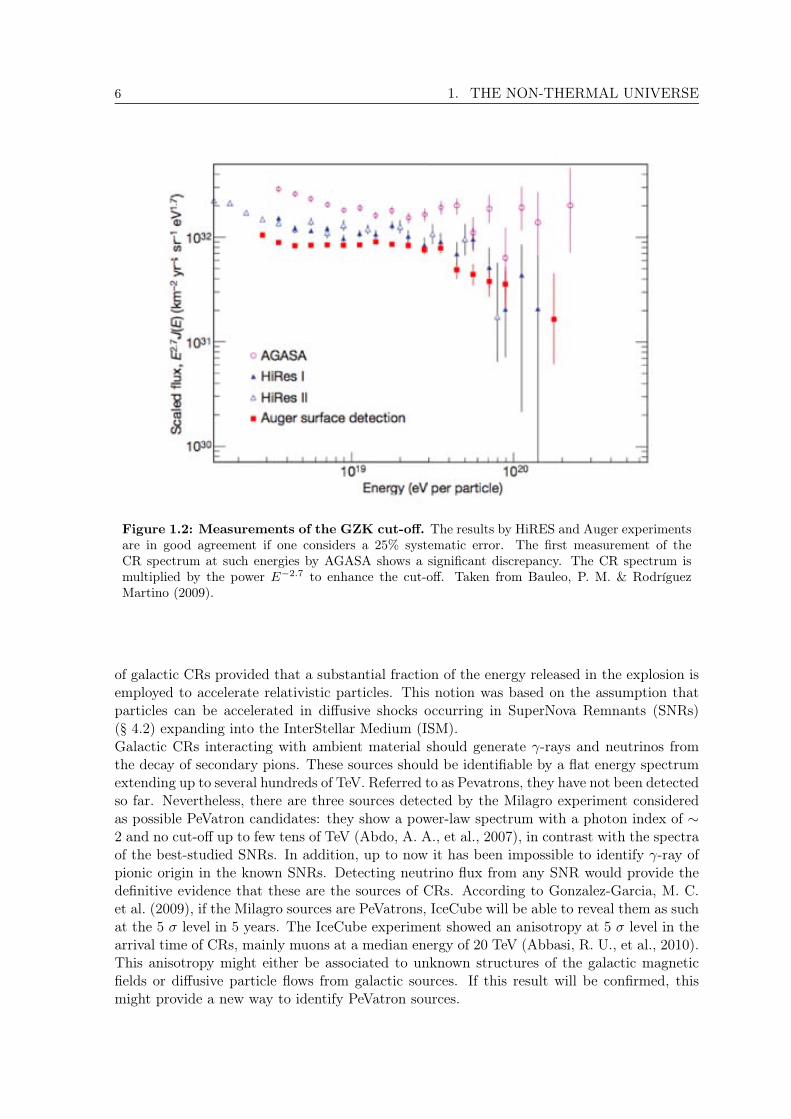
results in a cut-off of the spectrum at 461019 eV. Its measurements by High Resolution fly’seye (HiRES) (Abbasi, R. U., et al., 2008) and Auger (Abraham, J., et al., 2008) experimentsare in good agreement (Figure 1.2). Known as the Greisen-Zatsepin-Kuzmin (GZK) cut-off(Greisen, K., 1966), it limits the maximum distance that CRs of E ≡ 1020 eV can travel to ≈50 pc.
The most direct information about CRs can be obtained by detectors above the atmosphereon stratospheric balloons or in outer space on satellites. They provided most of the knowninformation about galactic CRs up to 1012 1014 eV. However, above those energies, otherindirect techniques must be used to study CRs. They are all based on the fact that theshowers of secondary particles, produced when primary particles interact with the Earth’satmosphere, are energetic enough to be detected from ground. Charge particles, like electronsand muons, can be observed with scintillator counters and water tanks, whereas hadrons canbe registered in calorimeters. Alternatively, the Cherenkov light produced by the showerscan be detected by imaging Cherenkov detectors. The exploration of the energies above 1016
requires detectors with areas larger than 1 km2 (§ B). The real step forward was obtained atthe highest energies by the Pierre Auger Observatory which, with its 3000 km2 coverage inthe Southern site allowed to measure the extragalactic CRs (§ ??).
1.1.1 Galactic cosmic rays
Up to the knee, and possibly also between the knee and the ankle of the CR spectrum, theCRs are thought to have a galactic origin, i.e. to be accelerated within our Galaxy. Alreadyin 1934 Baade, W. & Zwicky, F. (1934) suggested that SuperNovae (SNe) could be the source
6 1. THE NON-THERMAL UNIVERSE
Figure 1.2: Measurements of the GZK cut-off. The results by HiRES and Auger experimentsare in good agreement if one considers a 25% systematic error. The first measurement of theCR spectrum at such energies by AGASA shows a significant discrepancy. The CR spectrum ismultiplied by the power E − 2.7 to enhance the cut-off. Taken from Bauleo, P. M. & RodrıguezMartino (2009).
of galactic CRs provided that a substantial fraction of the energy released in the explosion isemployed to accelerate relativistic particles. This notion was based on the assumption thatparticles can be accelerated in diffusive shocks occurring in SuperNova Remnants (SNRs)(§ 4.2) expanding into the InterStellar Medium (ISM).Galactic CRs interacting with ambient material should generate γ-rays and neutrinos fromthe decay of secondary pions. These sources should be identifiable by a flat energy spectrumextending up to several hundreds of TeV. Referred to as Pevatrons, they have not been detectedso far. Nevertheless, there are three sources detected by the Milagro experiment consideredas possible PeVatron candidates: they show a power-law spectrum with a photon index of ∼2 and no cut-off up to few tens of TeV (Abdo, A. A., et al., 2007), in contrast with the spectraof the best-studied SNRs. In addition, up to now it has been impossible to identify γ-ray ofpionic origin in the known SNRs. Detecting neutrino flux from any SNR would provide thedefinitive evidence that these are the sources of CRs. According to Gonzalez-Garcia, M. C.et al. (2009), if the Milagro sources are PeVatrons, IceCube will be able to reveal them as suchat the 5 σ level in 5 years. The IceCube experiment showed an anisotropy at 5 σ level in thearrival time of CRs, mainly muons at a median energy of 20 TeV (Abbasi, R. U., et al., 2010).This anisotropy might either be associated to unknown structures of the galactic magneticfields or diffusive particle flows from galactic sources. If this result will be confirmed, thismight provide a new way to identify PeVatron sources.
1.2. γ-ray astrophysics 7
1.1.2 Extra-galactic cosmic rays
There is no clear separation between the spectra of the galactic and extragalactic CRs, eventhough the ankle is considered as the partition marker. The mechanisms responsible for theacceleration of particles up to 1018 eV are still unknown. However, as CRs above these ener-gies are no longer confined by the galactic magnetic field, it is natural to think that they areproduced by extragalactic sources.
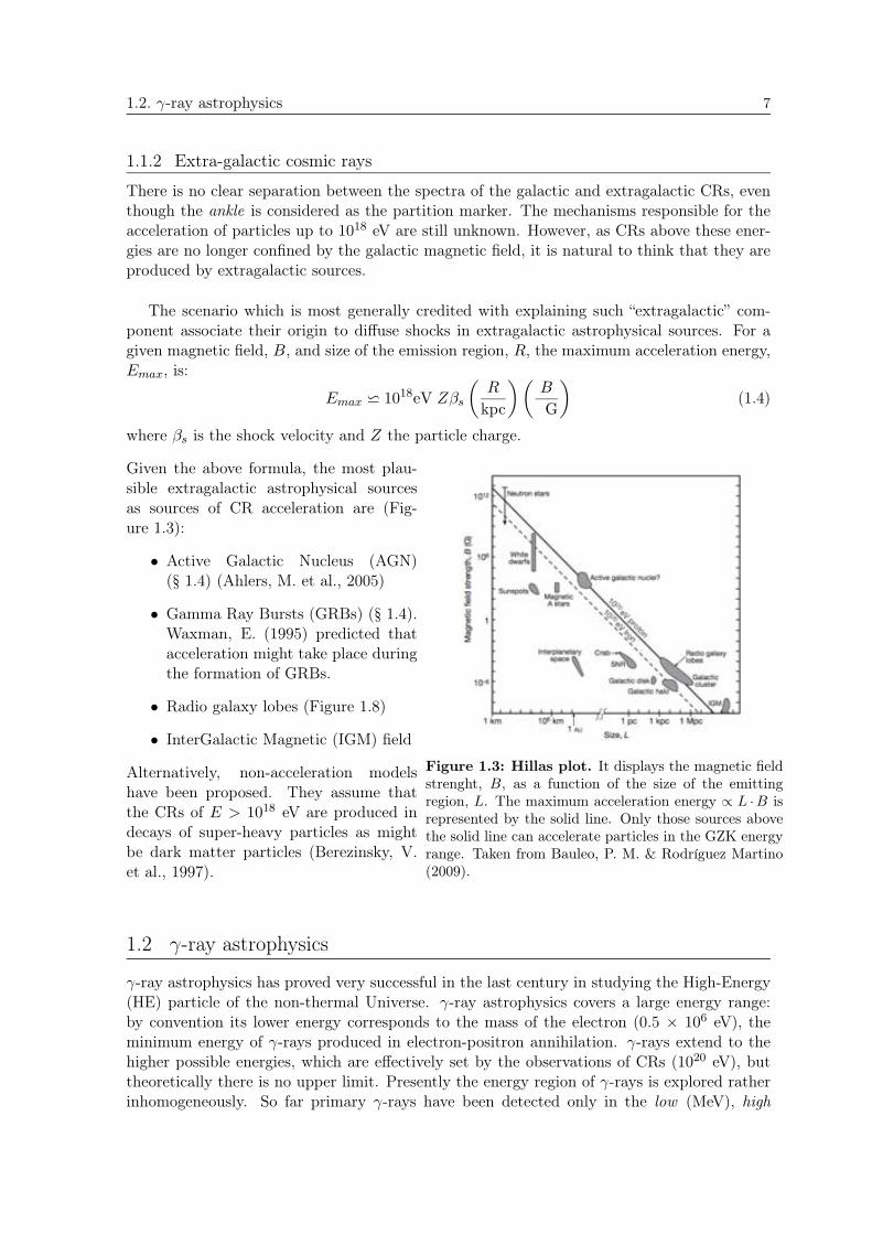
The scenario which is most generally credited with explaining such “extragalactic” com-ponent associate their origin to diffuse shocks in extragalactic astrophysical sources. For agiven magnetic field, B, and size of the emission region, R, the maximum acceleration energy,Emax, is:
Emax 1018eV Zβs
(R
kpc
)(B
µ G
)(1.4)
where βs is the shock velocity and Z the particle charge.
Given the above formula, the most plau-sible extragalactic astrophysical sourcesas sources of CR acceleration are (Fig-ure 1.3):
• Active Galactic Nucleus (AGN)(§ 1.4) (Ahlers, M. et al., 2005)
• Gamma Ray Bursts (GRBs) (§ 1.4).Waxman, E. (1995) predicted thatacceleration might take place duringthe formation of GRBs.
• Radio galaxy lobes (Figure 1.8)
• InterGalactic Magnetic (IGM) field
Alternatively, non-acceleration modelshave been proposed. They assume thatthe CRs of E > 1018 eV are produced indecays of super-heavy particles as mightbe dark matter particles (Berezinsky, V.et al., 1997).
Figure 1.3: Hillas plot. It displays the magnetic fieldstrenght, B, as a function of the size of the emittingregion, L. The maximum acceleration energy ∝ L ·B isrepresented by the solid line. Only those sources abovethe solid line can accelerate particles in the GZK energyrange. Taken from Bauleo, P. M. & Rodrıguez Martino(2009).
1.2 γ -ray astrophysics
γ-ray astrophysics has proved very successful in the last century in studying the High-Energy(HE) particle of the non-thermal Universe. γ-ray astrophysics covers a large energy range:by convention its lower energy corresponds to the mass of the electron (0.5 × 10⁶ eV), theminimum energy of γ-rays produced in electron-positron annihilation. γ-rays extend to thehigher possible energies, which are effectively set by the observations of CRs (1020 eV), buttheoretically there is no upper limit. Presently the energy region of γ-rays is explored ratherinhomogeneously. So far primary γ-rays have been detected only in the low (MeV), high
8 1. THE NON-THERMAL UNIVERSE
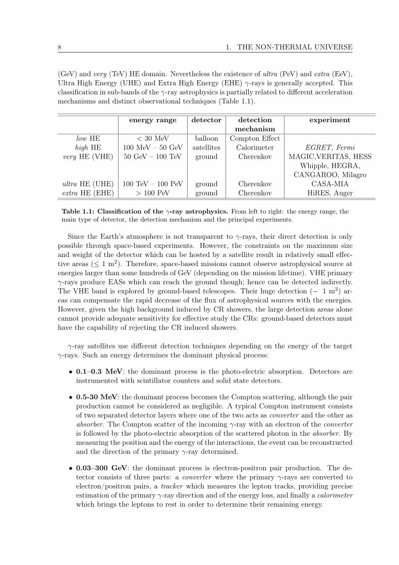
(GeV) and very (TeV) HE domain. Nevertheless the existence of ultra (PeV) and extra (EeV),Ultra High Energy (UHE) and Extra High Energy (EHE) -rays is generally accepted. Thisclassification in sub-bands of the -ray astrophysics is partially related to different accelerationmechanisms and distinct observational techniques (Table 1.1).
energy range detector detection experimentmechanism
low HE < 30 MeV balloon Compton Effecthigh HE 100 MeV – 50 GeV satellites Calorimeter EGRET, Fermi
very HE (VHE) 50 GeV – 100 TeV ground Cherenkov MAGIC,VERITAS, HESSWhipple, HEGRA,
CANGAROO, Milagroultra HE (UHE) 100 TeV – 100 PeV ground Cherenkov CASA-MIAextra HE (EHE) > 100 PeV ground Cherenkov HiRES, Auger
Table 1.1: Classification of the -ray astrophysics. From left to right: the energy range, themain type of detector, the detection mechanism and the principal experiments.
Since the Earth’s atmosphere is not transparent to -rays, their direct detection is onlypossible through space-based experiments. However, the constraints on the maximum sizeand weight of the detector which can be hosted by a satellite result in relatively small effec-tive areas ( 1 m2). Therefore, space-based missions cannot observe astrophysical source atenergies larger than some hundreds of GeV (depending on the mission lifetime). VHE primary -rays produce EASs which can reach the ground though; hence can be detected indirectly.The VHE band is explored by ground-based telescopes. Their huge detection (− 1 m2) ar-eas can compensate the rapid decrease of the flux of astrophysical sources with the energies.However, given the high background induced by CR showers, the large detection areas alonecannot provide adequate sensitivity for effective study the CRs: ground-based detectors musthave the capability of rejecting the CR induced showers.
-ray satellites use different detection techniques depending on the energy of the target -rays. Such an energy determines the dominant physical process:
• 0.1–0.3 MeV: the dominant process is the photo-electric absorption. Detectors areinstrumented with scintillator counters and solid state detectors.
• 0.5-30 MeV: the dominant process becomes the Compton scattering, although the pairproduction cannot be considered as negligible. A typical Compton instrument consistsof two separated detector layers where one of the two acts as converter and the other asabsorber. The Compton scatter of the incoming -ray with an electron of the converteris followed by the photo-electric absorption of the scattered photon in the absorber. Bymeasuring the position and the energy of the interactions, the event can be reconstructedand the direction of the primary -ray determined.
• 0.03–300 GeV: the dominant process is electron-positron pair production. The de-tector consists of three parts: a converter where the primary -rays are converted toelectron/positron pairs, a tracker which measures the lepton tracks, providing preciseestimation of the primary -ray direction and of the energy loss, and finally a calorimeterwhich brings the leptons to rest in order to determine their remaining energy.
1.2. -ray astrophysics 9
The -ray satellites usually have a very good background (CRs) rejection thanks to an anti-coincidence system which suppresses the charged particles which isotropically hit the detector.
The first -ray satellite, Explorer 11, was launched in 1961, but only the European SpaceAgency (ESA) mission COS-B (1975–1982) and the National Aeronautics and Space Adminis-tration (NASA) one SAS-2 provided the first detailed views of the -ray Universe (1972–1973).The first milestone of the -ray astrophysics was set by the Energetic Gamma-Ray ExperimentTelescope (EGRET) experiment on board of the Compton Gamma-Ray Observatory (CGRO)(1991–2000). It revealed more than 270 galactic and extragalactic objects between 0.1 and10 GeV. A step further in HE astrophysics was signed by the innovative Fermi satellite (for-merly called GLAST), launched in June 2008. Fermi hosts two instruments: the Large ArrayTelescope (LAT) and the complementary GLAST Burst Monitor (GBM). Fermi/LAT is animaging, wide Field of View (FoV), high-energy -ray telescope covering the energy rangebetween 100 MeV to about 300 GeV (Atwood, W. B., et al., 2009), whereas the Fermi/GBMconsists of 12 detectors sensitive to the range from 8 keV to 30 MeV. These 12 detectors areoriented in different positions of the sky providing nearly the full sky coverage. They are usedto detect GRBs (§ 1.4).
There are two main types of VHE ground-based telescopes which have proved successfulup to now. The principal ground-based -ray experiments are shortly presented in § B.1 and§ B.2.
• Air shower arrays. They are arrays of detectors capable of detecting the particles inEASs. By measuring the arrival time of the shower front at the individual stations, thedirection of the primary CRs can be estimated. In order to estimate the energy of theprimary particle, the shower must be entirely contained within the complete detector.This leads to building big arrays in excess of 104 m2. There are different techniqueswhich allow for the EAS detection. The most direct one uses plastic scintillators coupledwith muon detectors (air shower particle arrays). A more indirect technique is basedon the detection of the Cherenkov light produced by the shower charged particles eithertravelling through the atmosphere (atmospheric Cherenkov arrays) or inside water tanks(water Cherenkov arrays). Other air shower arrays detect the air fluorescence producedby the EASs in the atmosphere (air fluorescence arrays).
The first generation of air shower arrays mainly comprises air shower particles arrays.They are very inefficient detectors of -rays, as they can only sample the tail of the EASat ground level and have hardly any handle to separate -rays from background CR. Inaddition, the sparse sampling leads to very high energy thresholds (> 50 TeV). None ofthis first generation of EAS arrays detected any -ray emitter. The substantial progressin lowering the energy threshold, achieved by the second generation, was obtained eitherby increasing the sensitive detector area or building the detector at much higher altitude.The first approach was followed by the Milagro collaboration, whereas the second bythe Tibet AS array located at 4300 m above sea level (asl).
• Atmospheric Cherenkov telescopes (IACTs). An energetic -ray on hitting theEarth atmosphere, initiates an EAS, with a typical shower maximum around 8–12 kmasl. The shower charged particles, mostly electrons and positrons, emit Cherenkov lightwhen their speed exceeds that of the light in the atmosphere. This light, beamed alongthe direction of the incident -ray, illuminates nearly uniformly a dish of ≡ 120 m radiuson the ground. If a telescope is located within the Cherenkov light pool, it can collectpart of this light and focus it onto a ≡ 3–5 FoV camera composed of Photo Multiplier

10 1. THE NON-THERMAL UNIVERSE
Tubes (PMTs). These photon detectors are capable of resolving the images of theshowers which have a typical angular extension of ∼ 0.5 . An image reconstructionalgorithm allows the determination of the main parameters of the primary particles,such as energy and incoming direction.The exploration of this technique occurred in the 90s, when the pioneering Whippletelescope, with a 10 m diameter reflector, reported the detection of the Crab Nebula asthe first VHE astrophysical source (Weekes, T. C., et al., 1989). In the following years,other experiments, High Energy Gamma Ray Astronomy (HEGRA) (Aharonian, F. A.,et al., 2000), Collaboration of Australia and Nippon for a GAmma-Ray Observatory inthe Outback (CANGAROO) (Tanimori, T., et al., 1998) and Cherenkov AtmosphericTelescope (CAT) (Barrau, A., et al., 1997), confirmed the success of the techniquediscovering a ten of VHE sources, mainly nearby AGNs. The second generation ofIACTs offered an order of magnitude improvement in flux sensitivity and a significantreduction of the energy threshold down to some tens of GeV. In the last seven years, withthe HESS, MAGIC and VERITAS telescopes in operation, the number of VHE sourcesreached 100, and they represent different galactic and extragalactic source populations(§ 1.4).
Figure 1.4: Sketch of detection techniques in VHE γ-ray astrophysics. On the left: theatmospheric Cherenkov technique; On the right: the scheme of the EAS arrays.
Each of the above-mentioned types of ground-based telescopes has advantages and disadvan-tages. IACTs have better angular and energy resolutions than air shower arrays. On the otherhand, they are optical instruments which operate only during dark time or under moderatemoonlight conditions and have a small FoV, whereas air shower arrays continuously scan the“entire” sky. These complementary features define different roles for the two category of de-tectors. IACTs are perfect instruments for morphological and spectral studies of TeV sourceswith a limited extension. While air shower arrays can monitor the whole sky for strong tran-sients.
Despite the results obtained by the current instruments are already impressive, an orderof magnitude improvement in the entire VHE domain can lead to the discovery of many otherTeV-emitter, and above all to deeper studies of spectra and morphologies of the known sources.This is the goal for the next generation ground-based γ-ray detectors and it yielded theconstruction design of the world-wide project, Cherenkov Telescope Array (CTA): an array
1.2. -ray astrophysics 11
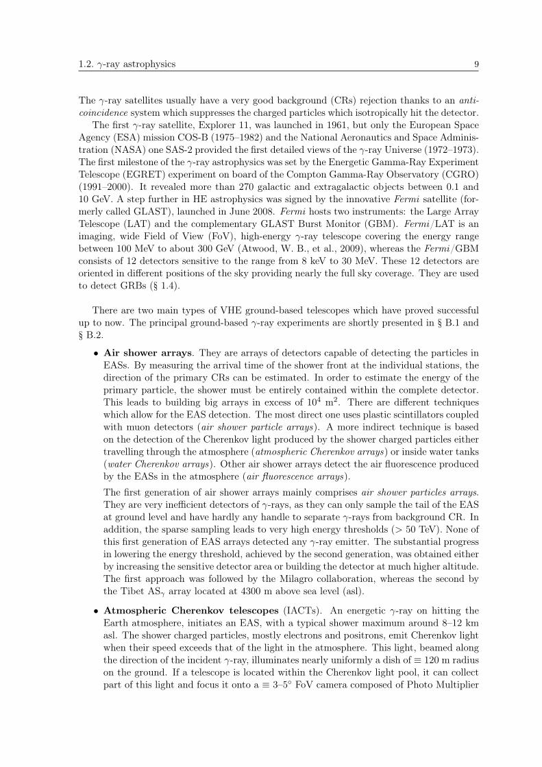
of tens of telescopes. The design scenario foresees three types of telescopes with differentmirror sizes in order to cover the entire energy range from 10 GeV up to 100 TeV (CTAConsortium, 2010). Figure 1.5 shows the sensitivity for the current IACTs compared withthe one expected for CTA.
Figure 1.5: The differential sensitivity expected for CTA. The black lines show the sensi-tivity of the design concept for different observation times. Colorful lines illustrate the sensitivityobtained with different analysis methods. Taken from CTA Consortium (2010).
12 1. THE NON-THERMAL UNIVERSE
1.3 Neutrino astrophysics
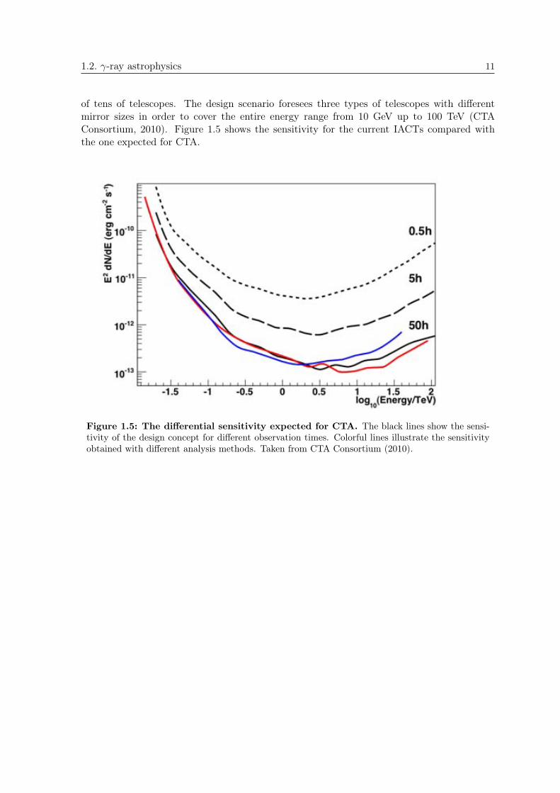
Neutrino astrophysics in the energy range of MeV iswell established. It has led to the observation of solarneutrinos and neutrinos from the supernova SN1987A(Hirata, K. et al., 1987). On the other hand, higher-energy neutrinos, GeV-neutrinos, have not been de-tected so far. Given their very weak signals, thesources of background, mainly muons and neutrinosproduced by CRs in the Earth’s atmosphere, must bereduced as much as possible. For this reason, neutrinodetectors are built deep underground or underwater.However, since underground detectors have turned tobe too small to detect the expected neutrino fluxes, thenew frontier of the high-energy neutrino astrophysicsis led by much larger arrays built in open water andice. These instruments consist of PMTs detecting theCherenkov light from charged particles produced byneutrino interactions (Figure 1.6).
Figure 1.6: Sketch of neutrinotelescopes.
Since the Cherenkov radiation produces a strong signal in water and ice, the energy thresh-old of these detectors is as low as some tens of GeV. This low energy threshold and the factthat the Sun and nearby SNe produce very high fluxes of neutrinos lead to the detection ofa large amount of atmospheric neutrinos. These atmospheric neutrinos constitute an impor-tant source of background, but, on the other hand, they allow for signal calibrations. Thenew generation of neutrino telescopes can reach energies as high as 1013−1014 eV. With theinaugurations of the 1 km3 IceCube array in the South Pole on April 28, 2011, a new era forthe neutrino astrophysics has begun (§ B.3).
1.4 Astrophysical sources
Established TeV γ-ray emitters are:
• Pulsars, rapidly rotating and highly magnetized Neutron Stars (NSs). The acceleratedparticles near the pulsar are beamed out the magnetosphere along the magnetic axis.Since the rotation and magnetic axes of the pulsar are not aligned, the observer seethe pulsar’s emission only when the beam crosses his line of sight. Pulsars can produceγ-ray emission. Many of them have been detected below few GeV (Abdo, A. A., et al.,2010b). The mechanisms of such radiation are still poorly understood. Only recentlyVHE radiation from the Crab Pulsar has been detected (Aliu, E., et al., 2008; Otte, N.,2011) establishing the pulsar as another class of VHE source population. They will bediscussed in detail in § 4.1.
• SNRs. A SNR is the leftover of a SuperNova (SN) explosion. The remnant consistsof the material ejected by the explosion and the ISM it sweeps up along the way. Ininteractions with the lower density ISM, the remnant creates shock waves. Particlesare accelerated in these shocks through the Fermi acceleration mechanism (§ A.1). Theultra-relativistic particles produced in the shock emit synchrotron radiation up to several
1.4. Astrophysical sources 13
hundreds of MeV, and higher-energy emission by IC scattering. Prominent detectedSNRs emitting VHE are: Cas A (Aharonian, F. A., et al., 2001; Albert, J., et al.,2007b), IC 433 (Albert, J., et al., 2007a), RX J1713.7–3946 (Aharonian, F. A., et al.,2006c), Vela X (Aharonian, F. A., et al., 2006d).
• Pulsar Wind Nebulae (PWNe). A PWN is a bubble of relativistic particles andmagnetic fields created when the relativistic pulsar wind interacts with the ambientmedium, either the SNR or the ISM. In this interaction particles are accelerated up toultra-relativistic energies. These particles, mainly electrons, are an efficient source ofVHE -rays by IC scattering with ambient photons. The archetypal PWN is the CrabNebula, which is the brightest VHE steady VHE source in the Northern sky. PWNe arethe main topic of Chapter 4.
• -ray binary systems. They are galactic binary systems whose dominant emission isin the -ray energy band. They consist of a compact object, either a NS or a BlackHole (BH) orbiting around a massive star. Two main scenarios can explain the observedVHE emission: either wind/wind interactions in the pulsar binary scenario or accretionin the microquasar scenario. In a pulsar binary system, the compact object is a rotatingNS and the pulsar winds interacting with the stellar wind can originate shocks whereparticles are accelerated. These ultra-relativistic particles IC scattering with the stellarphotons produce the observed VHE radiation. In the microquasar scenario, the compactobject accretes matter from the companion star creating an accretion disk. The latterejects relativistic jets containing ultra-relativistic particles which can produce VHE -rays. These systems will be discussed in detail in Chapter 6.
• Galactic center. The center of our Galaxy was established as a steady VHE photonemitter (Aharonian, F. A., et al., 2006a; Albert, J., et al., 2006a). It is a very crowedregion, possibly containing SNRs, PWNe and/or BHs (like Sgr A). The origin of theVHE emission might be related to one or more of these source populations.
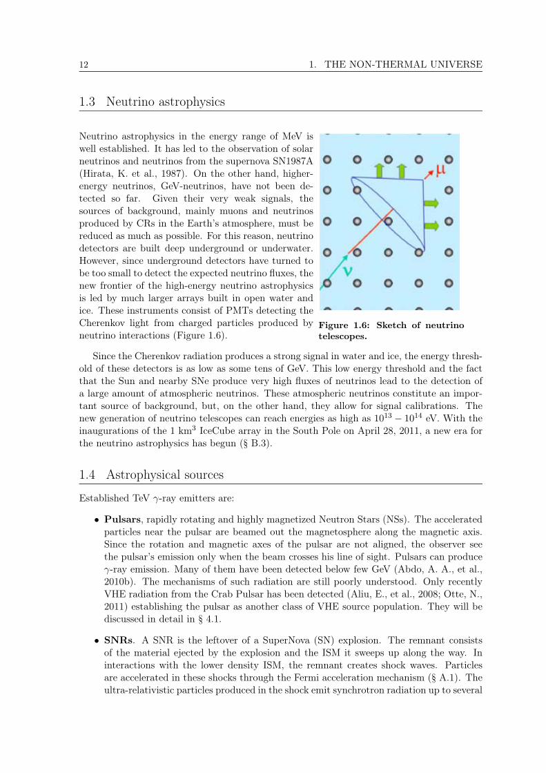
• AGNs. An AGN is a galaxy hosting a super-massive BH ( 106 M) in its center.
According to the unified AGN model (Urry, C. M. &Padovani, P., 1995) the BH is surrounded by an accre-tion disk and fast moving clouds which emit Doppler-broadened lines. In around 10% of the AGNs, thein-falling matter turns into powerful collimated rela-tivistic jets orthogonal to the galaxy plane. Figure 1.7shows a sketch of an AGN.The observed properties of the AGNs mainly dependon the viewing angle of the observer, the accretion rateand the mass of the BH. AGNs are classified using op-tical and radio observations (Figure 1.8). AGNs whichhave low optical luminosity are called Seyfert galaxiesand radio galaxies. The more powerful AGNs in theoptical and are the radio quasars and BL Lac. Whenthe jet of this loud optical AGNs is aligned with theline of sight of the observer, they are called blazars. Amore detailed classification can be found in Figure 1.8.
Figure 1.7: Sketch of an AGN.

14 1. THE NON-THERMAL UNIVERSE
Figure 1.8: Classification scheme for AGNs. Taken from Mazin, D. (2007).
• starburst galaxies. A starburst galaxy is a galaxy with an exceptionally high rate ofstar formation. As a result, the rate of SN explosions in these galaxies is much higherthan usual: ∼ 1/year. This guarantees both the mechanism of acceleration of particlesat SNR shocks and a large amount of seed photons for IC scattering and consequentproduction of VHE γ-rays. The prototypes of the starburst galaxies are M82 which hasbeen detected by VERITAS above 700 GeV (Acciari, V. A., et al., 2009), and NGC 253discovered by HESS (Acero, F., et al., 2009a).
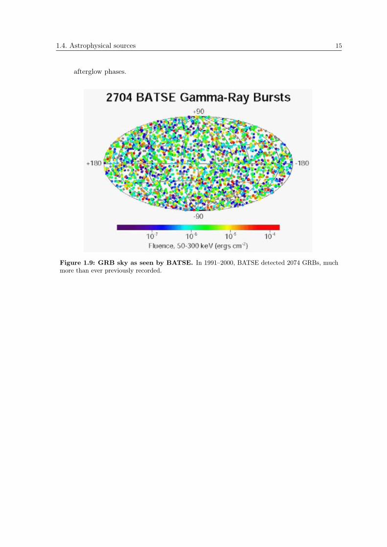
• GRBs. A GRB is a sudden very short and intense γ-ray outburst of extragalactic origin(average z = 2.3–2.7). GRBs, observed at a typical rate of one per day, are isotropicallydistributed in the sky (Figure 1.9). Up to now the origin of GRBs is still unknown andthey are believed to be originated from two possible different progenitors:
– the sudden catastrophic collapse of rapidly rotating very massive stars (M > 100M)
– the merger of two compact objects
Two different origins are considered because there are two distinct families of GRBs: along duration (> 2 s) one, possibly related to the first class of progenitors with lowerenergies, and a short duration (< 2 s) one, related to the latter class. A GRB is typicallycharacterized by a prompt emission mainly emitting in the soft γ-rays followed by a so-called afterglow emission. The latter is observed at all wavelengths from X-rays to radiofrequencies and it can last from hours to weeks. The prompt emission is usually sointense that almost over-shine the entire sky in γ-rays. It is interpreted as the resultof the growth of huge relativistic jets. No GRBs have been detected in the VHE bandso far. Nevertheless, they are still considered as interesting targets for this branch ofastrophysics because many models predict VHE emission during the prompt and the
1.4. Astrophysical sources 15
afterglow phases.
Figure 1.9: GRB sky as seen by BATSE. In 1991–2000, BATSE detected 2074 GRBs, muchmore than ever previously recorded.


PART ONE
THE MAGIC DETECTORand
DATA ANALYSIS

18 1. THE NON-THERMAL UNIVERSE
.

2The MAGIC Telescopes
The two MAGIC imaging atmospheric Cherenkov telescopes, designed for thedetection of very high energy -rays, are operating in stereoscopic mode since Autumn2009 after the commissioning of the second telescope. Located in the Canary island ofLa Palma, they both consist of a 17 parabolic reflector dish focusing the collectedCherenkov light onto a pixelized camera. The very large reflective surface permits tolower the detector energy threshold, as well as the use of an ultra-fast 2GSample/sreadout system. The main technical characteristics of the MAGIC telescopes aredescribed in this chapter with a particular stress on the upgraded version of theMAGIC I clone, called MAGIC II. The chapter follows the logic of the control systemwhich breaks the telescopes up in autonomous functional units, called subsystems. Itends with the description of the central control program, which allows to control andmonitor all the subsystems, and a short description of the main online procedures.
The author has been responsible for the central control program since the end of 2007.She followed the commissioning of the second telescope in Summer 2008 during whichshe was in charge of adapting the existing control program to the stereoscopic system(Zanin, R. & Cortina, J., 2009; Cortina, J., et al., 2010). The stereo data taking isdetailed described in the data operation manual (Cortina, J. & Zanin, R., 2011). Theauthor has been responsible also for the online analysis of MAGIC I mono data (Zanin,R. et al., 2008).
2.1 Introduction
The MAGIC telescopes are two 17 m diameter imaging atmospheric Cherenkov telescopes(IACTs). They are located in the Canary island of La Palma (28 45’ N, 17 54’ W, 2225 mabove sea level) at the Roque de los Muchachos observatory. The first telescope MAGIC Istarted operations in stand-alone mode in 2004. MAGIC became a stereoscopic system inAutumn 2009 when the second telescope, MAGIC II, completed the commissioning phase.
The MAGIC telescopes make use of the imaging Cherenkov technique (§ 1.2) to detectVHE -rays. They were designed to decrease the energy threshold of the previous generationof IACTs allowing the exploration of the lowest region of the VHE band between 30 and100 GeV. In the three years of operation before the advent of the Fermi satellite, in June2008, MAGIC I was the only instrument capable of studying such energy range (Albert, J.,
19
20 2. THE MAGIC TELESCOPES
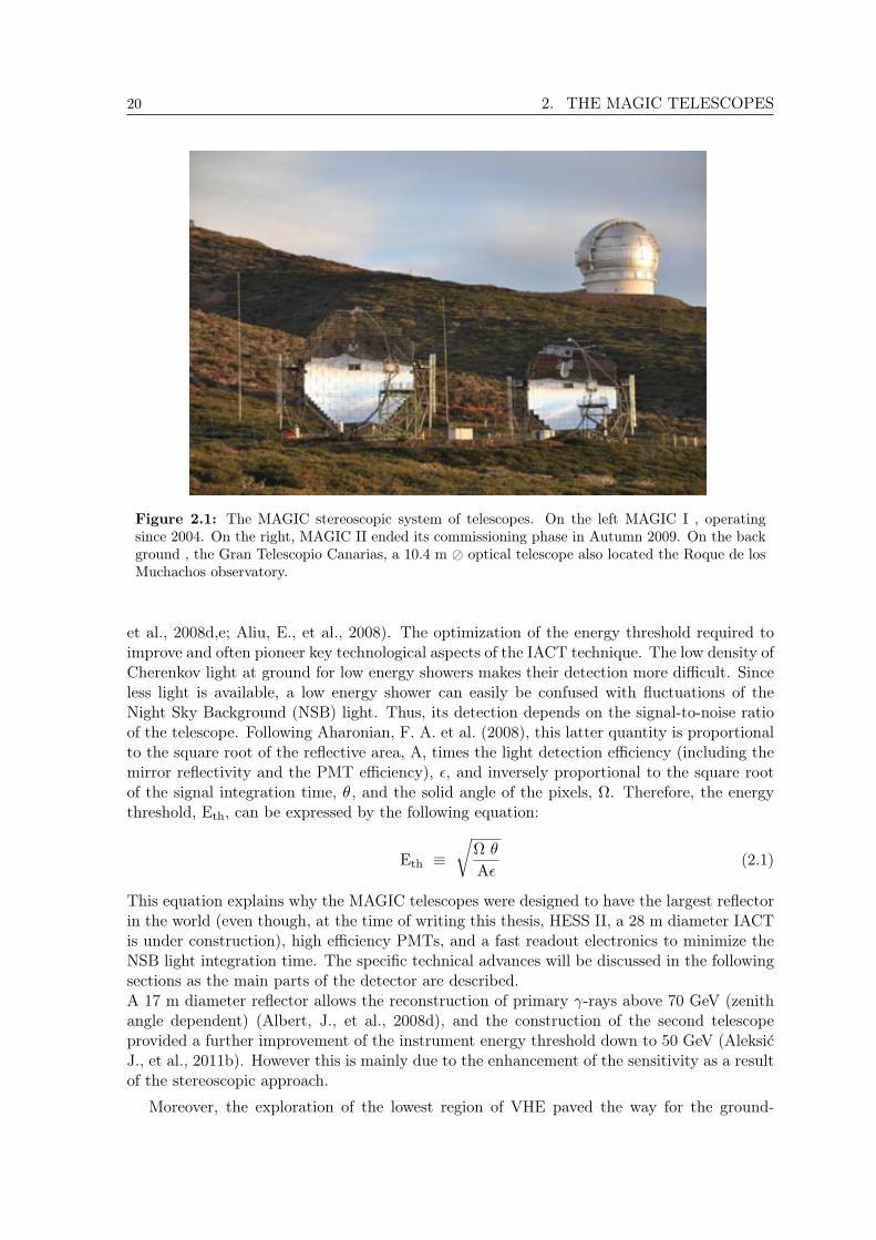
Figure 2.1: The MAGIC stereoscopic system of telescopes. On the left MAGIC I , operatingsince 2004. On the right, MAGIC II ended its commissioning phase in Autumn 2009. On the background , the Gran Telescopio Canarias, a 10.4 m optical telescope also located the Roque de losMuchachos observatory.
et al., 2008d,e; Aliu, E., et al., 2008). The optimization of the energy threshold required toimprove and often pioneer key technological aspects of the IACT technique. The low density ofCherenkov light at ground for low energy showers makes their detection more difficult. Sinceless light is available, a low energy shower can easily be confused with fluctuations of theNight Sky Background (NSB) light. Thus, its detection depends on the signal-to-noise ratioof the telescope. Following Aharonian, F. A. et al. (2008), this latter quantity is proportionalto the square root of the reflective area, A, times the light detection efficiency (including themirror reflectivity and the PMT efficiency), , and inversely proportional to the square rootof the signal integration time, θ , and the solid angle of the pixels, . Therefore, the energythreshold, Eth, can be expressed by the following equation:
Eth ≡r
θ
A(2.1)
This equation explains why the MAGIC telescopes were designed to have the largest reflectorin the world (even though, at the time of writing this thesis, HESS II, a 28 m diameter IACTis under construction), high efficiency PMTs, and a fast readout electronics to minimize theNSB light integration time. The specific technical advances will be discussed in the followingsections as the main parts of the detector are described.A 17 m diameter reflector allows the reconstruction of primary -rays above 70 GeV (zenithangle dependent) (Albert, J., et al., 2008d), and the construction of the second telescopeprovided a further improvement of the instrument energy threshold down to 50 GeV (AleksicJ., et al., 2011b). However this is mainly due to the enhancement of the sensitivity as a resultof the stereoscopic approach.
Moreover, the exploration of the lowest region of VHE paved the way for the ground-
2.2. Telescope subsystems 21
based detection of -ray sources at large cosmological distances. This is because the pairattenuation of -rays, which can inhibit their propagation, is less efficient in this energyrange. Subsequently the improved prospects of detecting GRB, extremely energetic and shortlived explosions occurring mostly at large redshifts, made this search one of key MAGICscience goals. Since the life time of a GRB is estimated to span between 10 s and 100 s(Paciesas, W. S., et al., 1999) following-up GRB alerts, coming from satellites, implies thatthe telescope should be repositioned within some tens of seconds. Therefore, a powerful drivesystem together with a light structure became important requirements in the telescope design,which led to the use of an innovative light-weight, high-rigidity material for the telescope frameconstruction.
MAGIC II, thought of as a clone of the first telescope, was constructed to improve theinstrument’s sensitivity. The stereoscopic approach permits to reconstruct more precisely theimage parameters which disentangle a gamma shower from a background one, enhancing thebackground suppression. Being built when MAGIC I operation was already well understood,the design of MAGIC II was modified in many aspects in order to improve its performance.
2.2 Telescope subsystems
Each telescope can be broken up in different functional units, called subsystems. The listbelow shows all the possible tasks of an IACT with the involved hardware/mechanical elementsand the corresponding subsystems (according to MAGIC naming).
• The telescope movements are handled by the drive system operating the telescopeframe.
• The light collection requires a reflective surface (reflector) made up of mirror tiles which,in the particular case of MAGIC, can be re-oriented depending on the telescope’s el-evation angle. This mirror adjustment is performed by the active mirror controlsubsystem.
• Cherenkov photons are detected using PMTs which are hosted inside the camera.
• The calibration of the instrument which allows the computation of the conversion factorbetween digital signals and physical quantities. The calibration system makes use ofa set of Light Emitting Diodes (LEDs).
• The data are digitized in a set of electronic boards which convert the PMT analog signalsinto digital ones and prepare them for the final data storage. This is the function of thereadout subsystem.
• The on-line event selection is electronically performed by the trigger system whichdiscriminates between events from EAS and NSB light. Thus, it indicates if it is worthor not to record a detected event.
• The data storage is done by the data acquisition system which records the acquireddata to disk in order to be analyzed oine.
Moreover, there are the so-called common subsystems which do not constitute anyfunctional part of the telescope, but simply collect information useful for the data taking,such as weather conditions (by the weather station, and the pyrometer), GRB alerts (bythe GRB alert program), etc.

22 2. THE MAGIC TELESCOPES
Figure 2.2: Outline of the central control scheme. The CC program interacts with eachsubsystem control program coordinating the data taking and providing the user a friendly interfaceto operate the telescopes.
2.2. Telescope subsystems 23
Each subsystem is controlled via software by a control program installed in a PersonalComputer (PC) in the counting house. Each control program can be run by the operator instand-alone mode, or remotely by the CC program. The latter, communicating via Ethernetwith all the subsystem programs, can coordinate their actions, thus automatizing the datataking procedure and providing the user with a graphical interface for instrument operation.Figure 2.2 shows the outline of the MAGIC control system.
In the following, the different subsystems will be described in detail, emphasizing, for eachof them, the differences between MAGIC I and MAGIC II .
2.2.1 Frame and drive system
The telescope frame satisfies three main requirements: 1) it is large, 2) it is light-weight, 3)it is stiff. The first requirement is meant to guarantee a low energy threshold, the secondone a fast repositioning, and the third a good image quality since it avoids deformations ofthe reflector. The space frame is a three-layer structure made of low-weight carbon fiber-epoxy tubes joined by aluminium knots (Figure 2.3), with a total weight of 5.5 tons (lessthan a third of an equivalent steel structure). According to the specifications the maximumdeformation of the structure, for any orientation of the telescope, is below 3.5 mm, confirmingthe high rigidity of the chosen material (Bretz, T. et al., 2009). The carbon fiber-epoxy isalso especially resistant to the harsh atmospheric conditions of the MAGIC site1.The camera PMTs, located at the focal distance of ≡17 m, is carried by a single tubulararch (Figure 2.3), and stabilized by thin steel cables anchored to the main dish structure.Nevertheless, small bendings of the structure, due the weight of the camera (≡ half a ton),are unavoidable during the telescope tracking, but can be corrected by an automatic systemof mirror re-orientation (§ 2.2.3).
The telescope mount makes use of the alt-azimuth drive to track sources during largeexposures, like most of the optical telescopes. The allowed motion in azimuth spans from-90 to +318 and the range in elevation spans from -70 to +90. The drive mechanism hastwo drive chains controlled by synchronous motors with gears which are linked to the chainsprocket wheels (Figure 2.4). The azimuthal drive chain is fixed on a circular railway railof 20 m diameter, and it is moved by two motors. The elevation drive chain with just onemotor is mounted on a slightly oval ring below the mirror dish which forms integral part ofthe camera support must structure. For safety reasons this chain is equipped with an extrabrake, operating as holding brake. The azimuth and elevational movements are regulated byindividual programmable micro controllers dedicated to analog motion control, called MACS.
The pointing of the system is constantly cross-checked by a feedback pointing system whichconsists in three shaft-encoders (one on the azimuth axis and two at the opposite sides of theelevation axis) evaluating the angular telescope position with a 14-bit precision/360. Thesemeasurements compared with the positions readout by the motors themselves can be usedto estimate the intrinsic mechanical accuracy of the pointing system. Bretz, T. et al. (2009)showed that this accuracy for the 80% of the time is much better than 1’ on the sky (a fifthof a pixel diameter).
In MAGIC I , the control program of the drive system communicates with both the encoders
1Temperatures below 0 C are typical at the MAGIC site in Winter, whereas the frame suers under strongsolar irradiation in Summer.

24 2. THE MAGIC TELESCOPES
Figure 2.3: The telescope mount. On the left: two pictures of the carbon fiber-epoxy tubesand an Aluminium knot junction. On the right: a picture of MAGIC II where the frame structureand the mast holding the camera are visible (before the complete mirror installation).
and the MACS through a CANbus protocol. During MAGIC II construction many mechanicalparts of the drive system were replaced by better performing ones, especially for what regardsthe communication protocols. The main upgrades are:
• The two MACS were replaced by a single professional Programmable Logical Controller(PLC) which communicates with the software control program via Ethernet.
• Absolute 13-bit shaft-encoders with a better resolution were installed. They are readout by an Ethernet interface.
The use of the PLCs, instead of MACS makes the hardware and software maintenance mucheasier. This was the main reason for which MAGIC I drive system was also upgraded in May2009. Now the two drive systems are exactly two clones.
Pointing models
In order to account for the constant deformations of the mechanical structures, the trackingsoftware employs analytical pointing models, which are updated every few months. Thesemodels, also called bending models, are based on the TPointTM telescope modeling software2:
2http://www.tpsoft.demon.co.uk/ by Wallace, P. M.
2.2. Telescope subsystems 25
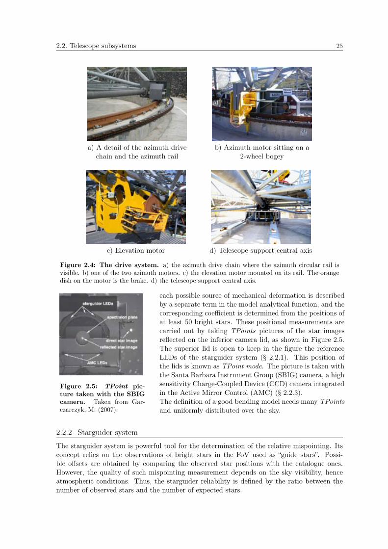
a) A detail of the azimuth drivechain and the azimuth rail
b) Azimuth motor sitting on a2-wheel bogey
c) Elevation motor d) Telescope support central axis
Figure 2.4: The drive system. a) the azimuth drive chain where the azimuth circular rail isvisible. b) one of the two azimuth motors. c) the elevation motor mounted on its rail. The orangedish on the motor is the brake. d) the telescope support central axis.
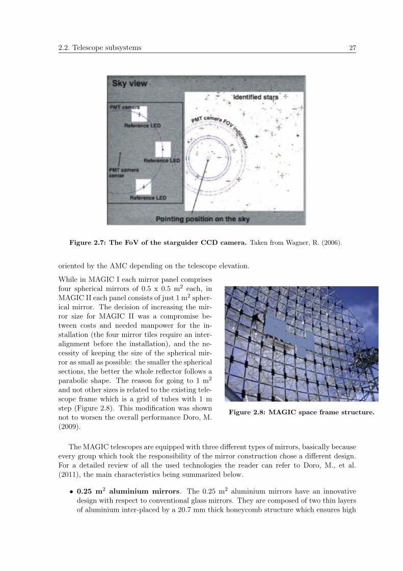
Figure 2.5: TPoint pic-ture taken with the SBIGcamera. Taken from Gar-czarczyk, M. (2007).
each possible source of mechanical deformation is describedby a separate term in the model analytical function, and thecorresponding coefficient is determined from the positions ofat least 50 bright stars. These positional measurements arecarried out by taking TPoints pictures of the star imagesreflected on the inferior camera lid, as shown in Figure 2.5.The superior lid is open to keep in the figure the referenceLEDs of the starguider system (§ 2.2.1). This position ofthe lids is known as TPoint mode. The picture is taken withthe Santa Barbara Instrument Group (SBIG) camera, a highsensitivity Charge-Coupled Device (CCD) camera integratedin the Active Mirror Control (AMC) (§ 2.2.3).The definition of a good bending model needs many TPointsand uniformly distributed over the sky.
2.2.2 Starguider system
The starguider system is powerful tool for the determination of the relative mispointing. Itsconcept relies on the observations of bright stars in the FoV used as “guide stars”. Possi-ble offsets are obtained by comparing the observed star positions with the catalogue ones.However, the quality of such mispointing measurement depends on the sky visibility, henceatmospheric conditions. Thus, the starguider reliability is defined by the ratio between thenumber of observed stars and the number of expected stars.

26 2. THE MAGIC TELESCOPES
The starguider system uses a high sensitivity CCD camera equipped with a Schneider-Kreuznach Xenoplan 1.9/35mm wide-field lens (more information in Wagner, R. (2006)).This camera is read out at a rate of 25 frames per second using a frame grabber connectedto the PC of the drive system. Since the drawback for the high sensitivity is the high noiselevel, good quality images can be obtained only by averaging many (typically 125) single shots(Figure 2.6). The software in charge of the picture managing is implemented into the drivesystem control program.
Figure 2.6: Pictures taken with the starguider CCD camera. On the left: a single shotpicture showing the high noise level; On the right: picture obtained averaging 125 single shots.
The CCD camera is mounted in the center of the reflector dish. Given its 6.2 FoV, itsimultaneously observes part of the PMT camera and the sky position the telescope is pointingat (Figure 2.7). In addition the starguider system includes a set of dim LEDs installed onthe PMT camera. They provide a reference frame which is necessary for the mispointingdetermination.
2.2.3 Reflector
The 17 m diameter reflector follows a parabolic profile which allows to preserve the temporalstructure of the shower light flashes. This information is important to reduce the number ofaccidental triggers due to NSB light, and thus to improve the signal to noise ratio, as demon-strated in Aliu, E., et al. (2009). For such a large reflector, the time spread between photonshitting the center and photons hitting the edges of the mirror surface is non-negligible. There-fore, the solutions used by the other IACTs, such as a Davies and Cotton mounting sphericalreflector (Davies & Cotton, 1957), which performs even better than a parabolic reflectorfor small size telescopes (Lewis, 1990), would never work for a large diameter telescope likeMAGIC. For example, a spherical reflector of 17 m diameter would introduce a time delay oftens of ns which is much more than the duration of a Cherenkov pulse would spoil the showertime structure.
The parabolic reflectors of both MAGIC telescopes are tessellated in 247 individuallymovable 1 m2 mirror panels covering a total surface of 234 m23. These panels can be re-
3The mirror panels at the edges of the surface are smaller than 1 m2.
2.2. Telescope subsystems 27
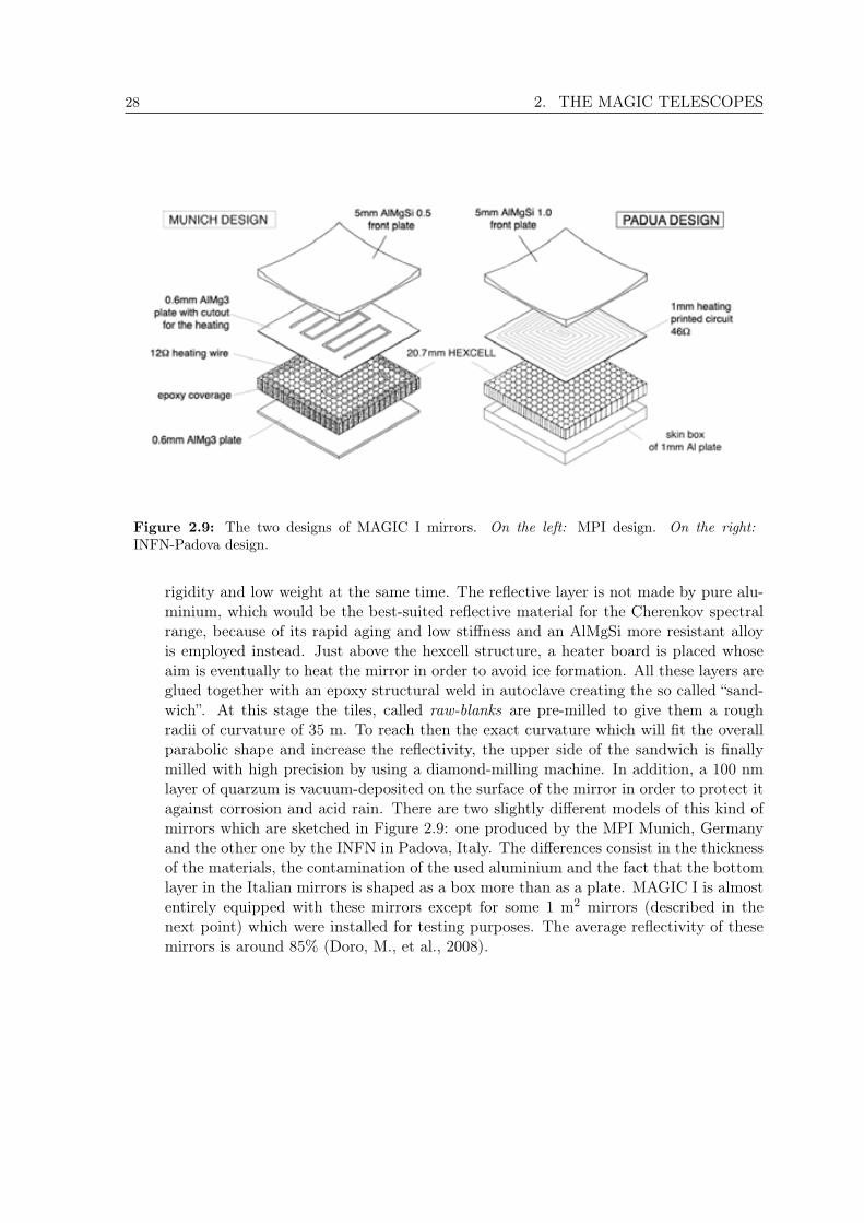
Figure 2.7: The FoV of the starguider CCD camera. Taken from Wagner, R. (2006).
oriented by the AMC depending on the telescope elevation.
While in MAGIC I each mirror panel comprisesfour spherical mirrors of 0.5 x 0.5 m2 each, inMAGIC II each panel consists of just 1 m2 spher-ical mirror. The decision of increasing the mir-ror size for MAGIC II was a compromise be-tween costs and needed manpower for the in-stallation (the four mirror tiles require an inter-alignment before the installation), and the ne-cessity of keeping the size of the spherical mir-ror as small as possible: the smaller the sphericalsections, the better the whole reflector follows aparabolic shape. The reason for going to 1 m2
and not other sizes is related to the existing tele-scope frame which is a grid of tubes with 1 mstep (Figure 2.8). This modification was shownnot to worsen the overall performance Doro, M.(2009).
Figure 2.8: MAGIC space frame structure.
The MAGIC telescopes are equipped with three different types of mirrors, basically becauseevery group which took the responsibility of the mirror construction chose a different design.For a detailed review of all the used technologies the reader can refer to Doro, M., et al.(2011), the main characteristics being summarized below.
• 0.25 m2 aluminium mirrors. The 0.25 m2 aluminium mirrors have an innovativedesign with respect to conventional glass mirrors. They are composed of two thin layersof aluminium inter-placed by a 20.7 mm thick honeycomb structure which ensures high
28 2. THE MAGIC TELESCOPES
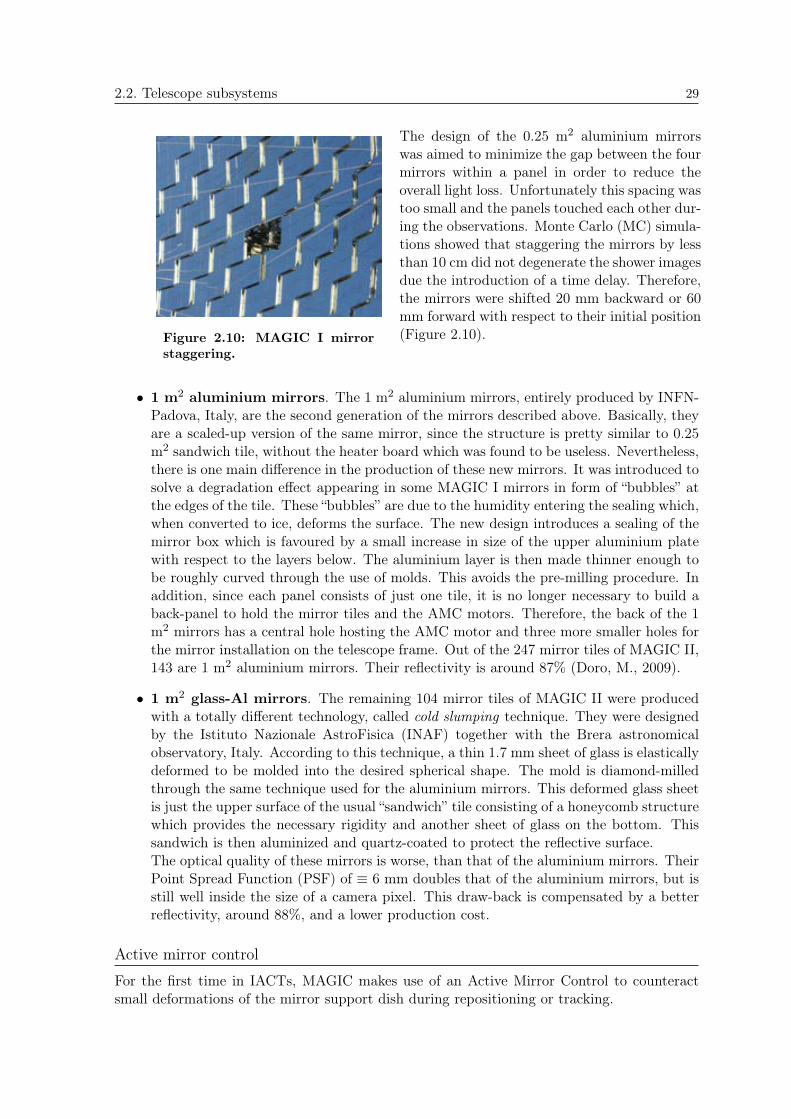
Figure 2.9: The two designs of MAGIC I mirrors. On the left: MPI design. On the right:INFN-Padova design.
rigidity and low weight at the same time. The reflective layer is not made by pure alu-minium, which would be the best-suited reflective material for the Cherenkov spectralrange, because of its rapid aging and low stiffness and an AlMgSi more resistant alloyis employed instead. Just above the hexcell structure, a heater board is placed whoseaim is eventually to heat the mirror in order to avoid ice formation. All these layers areglued together with an epoxy structural weld in autoclave creating the so called “sand-wich”. At this stage the tiles, called raw-blanks are pre-milled to give them a roughradii of curvature of 35 m. To reach then the exact curvature which will fit the overallparabolic shape and increase the reflectivity, the upper side of the sandwich is finallymilled with high precision by using a diamond-milling machine. In addition, a 100 nmlayer of quarzum is vacuum-deposited on the surface of the mirror in order to protect itagainst corrosion and acid rain. There are two slightly different models of this kind ofmirrors which are sketched in Figure 2.9: one produced by the MPI Munich, Germanyand the other one by the INFN in Padova, Italy. The differences consist in the thicknessof the materials, the contamination of the used aluminium and the fact that the bottomlayer in the Italian mirrors is shaped as a box more than as a plate. MAGIC I is almostentirely equipped with these mirrors except for some 1 m2 mirrors (described in thenext point) which were installed for testing purposes. The average reflectivity of thesemirrors is around 85% (Doro, M., et al., 2008).
2.2. Telescope subsystems 29
Figure 2.10: MAGIC I mirrorstaggering.
The design of the 0.25 m2 aluminium mirrorswas aimed to minimize the gap between the fourmirrors within a panel in order to reduce theoverall light loss. Unfortunately this spacing wastoo small and the panels touched each other dur-ing the observations. Monte Carlo (MC) simula-tions showed that staggering the mirrors by lessthan 10 cm did not degenerate the shower imagesdue the introduction of a time delay. Therefore,the mirrors were shifted 20 mm backward or 60mm forward with respect to their initial position(Figure 2.10).
• 1 m2 aluminium mirrors. The 1 m2 aluminium mirrors, entirely produced by INFN-Padova, Italy, are the second generation of the mirrors described above. Basically, theyare a scaled-up version of the same mirror, since the structure is pretty similar to 0.25m2 sandwich tile, without the heater board which was found to be useless. Nevertheless,there is one main difference in the production of these new mirrors. It was introduced tosolve a degradation effect appearing in some MAGIC I mirrors in form of “bubbles” atthe edges of the tile. These “bubbles” are due to the humidity entering the sealing which,when converted to ice, deforms the surface. The new design introduces a sealing of themirror box which is favoured by a small increase in size of the upper aluminium platewith respect to the layers below. The aluminium layer is then made thinner enough tobe roughly curved through the use of molds. This avoids the pre-milling procedure. Inaddition, since each panel consists of just one tile, it is no longer necessary to build aback-panel to hold the mirror tiles and the AMC motors. Therefore, the back of the 1m2 mirrors has a central hole hosting the AMC motor and three more smaller holes forthe mirror installation on the telescope frame. Out of the 247 mirror tiles of MAGIC II,143 are 1 m2 aluminium mirrors. Their reflectivity is around 87% (Doro, M., 2009).
• 1 m2 glass-Al mirrors. The remaining 104 mirror tiles of MAGIC II were producedwith a totally different technology, called cold slumping technique. They were designedby the Istituto Nazionale AstroFisica (INAF) together with the Brera astronomicalobservatory, Italy. According to this technique, a thin 1.7 mm sheet of glass is elasticallydeformed to be molded into the desired spherical shape. The mold is diamond-milledthrough the same technique used for the aluminium mirrors. This deformed glass sheetis just the upper surface of the usual “sandwich” tile consisting of a honeycomb structurewhich provides the necessary rigidity and another sheet of glass on the bottom. Thissandwich is then aluminized and quartz-coated to protect the reflective surface.The optical quality of these mirrors is worse, than that of the aluminium mirrors. TheirPoint Spread Function (PSF) of ≡ 6 mm doubles that of the aluminium mirrors, but isstill well inside the size of a camera pixel. This draw-back is compensated by a betterreflectivity, around 88%, and a lower production cost.
Active mirror control
For the first time in IACTs, MAGIC makes use of an Active Mirror Control to counteractsmall deformations of the mirror support dish during repositioning or tracking.
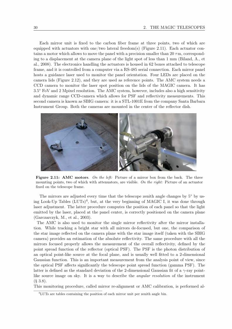
30 2. THE MAGIC TELESCOPES
Each mirror unit is fixed to the carbon fiber frame at three points, two of which areequipped with actuators with one/two lateral freedom(s) (Figure 2.11). Each actuator con-tains a motor which allows to move the panel with a precision smaller than 20 τm, correspond-ing to a displacement at the camera plane of the light spot of less than 1 mm (Biland, A., etal., 2008). The electronics handling the actuators is housed in 62 boxes attached to telescopeframe, and it is controlled from a computer via a RS-485 serial connection. Each mirror panelhosts a guidance laser used to monitor the panel orientation. Four LEDs are placed on thecamera lids (Figure 2.12), and they are used as reference points. The AMC system needs aCCD camera to monitor the laser spot position on the lids of the MAGIC camera. It has3.5 FoV and 2 Mpixel resolution. The AMC system, however, includes also a high sensitivityand dynamic range CCD-camera which allows for PSF and reflectivity measurements. Thissecond camera is known as SBIG camera: it is a STL-1001E from the company Santa BarbaraInstrument Group. Both the cameras are mounted in the center of the reflector dish.
Figure 2.11: AMC motors. On the left: Picture of a mirror box from the back. The threemounting points, two of which with attenuators, are visible. On the right: Picture of an actuatorfixed on the telescope frame.
The mirrors are adjusted every time that the telescope zenith angle changes by 5 by us-ing Look-Up Tables (LUTs)4, but, at the very beginning of MAGIC I, it was done throughlaser adjustment. The latter procedure computes the position of each panel so that the lightemitted by the laser, placed at the panel center, is correctly positioned on the camera plane(Garczarczyk, M., et al., 2003).The AMC is also used to monitor the single mirror reflectivity after the mirror installa-
tion. While tracking a bright star with all mirrors de-focused, but one, the comparison ofthe star image reflected on the camera plane with the star image itself (taken with the SBIGcamera) provides an estimation of the absolute reflectivity. The same procedure with all themirrors focused properly allows the measurement of the overall reflectivity, defined by thepoint spread function of the reflector (optical PSF). The PSF is the photon distribution ofan optical point-like source at the focal plane, and is usually well fitted to a 2-dimensionalGaussian function. This is an important measurement from the analysis point of view, sincethe optical PSF affects significantly the telescope point spread function (gamma PSF). Thelatter is defined as the standard deviation of the 2-dimensional Gaussian fit of a -ray point-like source image on sky. It is a way to describe the angular resolution of the instrument(§ 3.8).This monitoring procedure, called mirror re-alignment or AMC calibration, is performed al-
4LUTs are tables containing the position of each mirror unit per zenith angle bin.
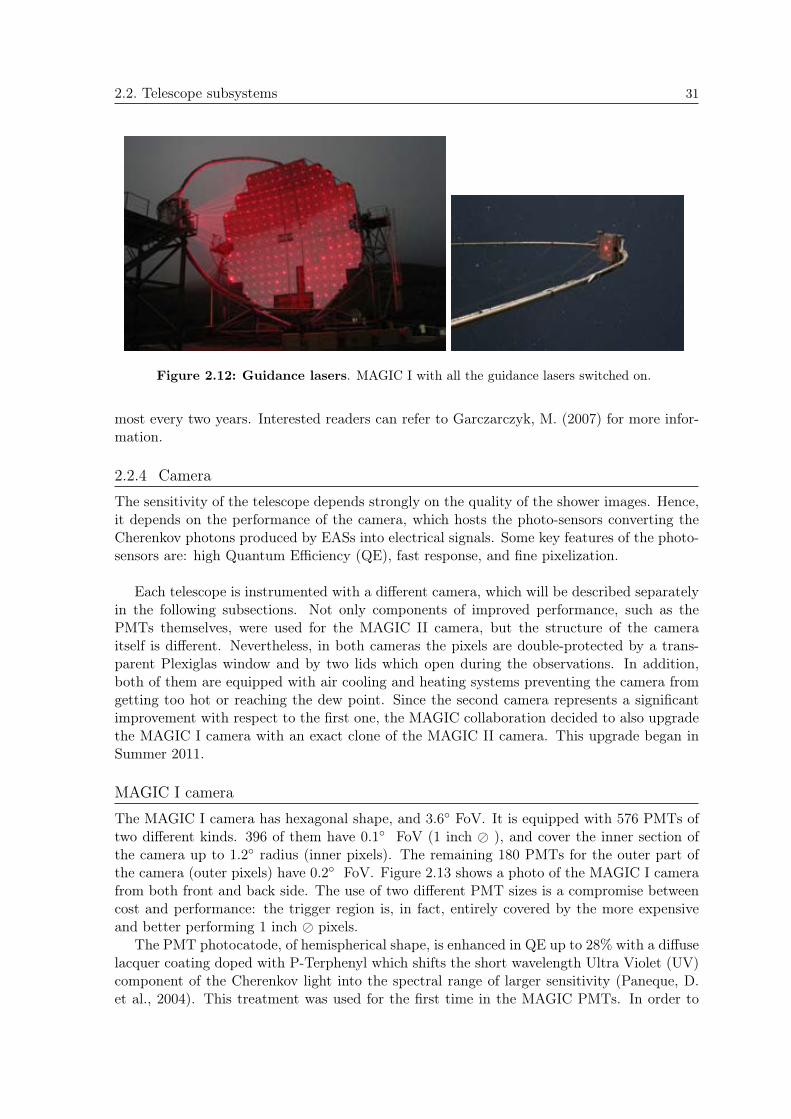
2.2. Telescope subsystems 31
Figure 2.12: Guidance lasers. MAGIC I with all the guidance lasers switched on.
most every two years. Interested readers can refer to Garczarczyk, M. (2007) for more infor-mation.
2.2.4 Camera
The sensitivity of the telescope depends strongly on the quality of the shower images. Hence,it depends on the performance of the camera, which hosts the photo-sensors converting theCherenkov photons produced by EASs into electrical signals. Some key features of the photo-sensors are: high Quantum Efficiency (QE), fast response, and fine pixelization.
Each telescope is instrumented with a different camera, which will be described separatelyin the following subsections. Not only components of improved performance, such as thePMTs themselves, were used for the MAGIC II camera, but the structure of the cameraitself is different. Nevertheless, in both cameras the pixels are double-protected by a trans-parent Plexiglas window and by two lids which open during the observations. In addition,both of them are equipped with air cooling and heating systems preventing the camera fromgetting too hot or reaching the dew point. Since the second camera represents a significantimprovement with respect to the first one, the MAGIC collaboration decided to also upgradethe MAGIC I camera with an exact clone of the MAGIC II camera. This upgrade began inSummer 2011.
MAGIC I camera
The MAGIC I camera has hexagonal shape, and 3.6 FoV. It is equipped with 576 PMTs oftwo different kinds. 396 of them have 0.1 FoV (1 inch ), and cover the inner section ofthe camera up to 1.2 radius (inner pixels). The remaining 180 PMTs for the outer part ofthe camera (outer pixels) have 0.2 FoV. Figure 2.13 shows a photo of the MAGIC I camerafrom both front and back side. The use of two different PMT sizes is a compromise betweencost and performance: the trigger region is, in fact, entirely covered by the more expensiveand better performing 1 inch pixels.
The PMT photocatode, of hemispherical shape, is enhanced in QE up to 28% with a diffuselacquer coating doped with P-Terphenyl which shifts the short wavelength Ultra Violet (UV)component of the Cherenkov light into the spectral range of larger sensitivity (Paneque, D.et al., 2004). This treatment was used for the first time in the MAGIC PMTs. In order to

32 2. THE MAGIC TELESCOPES
minimize the losses into the dead space between the round PMTs, hex-to-round light guideswere used. The light concentrators, consisting of a thin aluminium tube, channel the incominglight into the PMT with an incident angle of approximately 40. The total QE of the entiresystem (mirrors, effective PMT QE, light guides) is ≡ 15% between 300 and 600 nm.
Figure 2.13: MAGIC I camera. On the left: photo of the front of the camera where the twotype of PMTs are visible. On the right: picture of rear of the camera.
The PMTs have only 6-dynodes and run at a relatively low gain of 20000–40000 to preventhigh anode currents during moonlight observation from damaging the devices. This needsto be compensated with fast, high gain amplifiers at the base of the PMTs. Each pixel isconnected to a High Voltage (HV) regulator. The applied HV can be monitored with a 12-bitAnalogical to Digital Converter (ADC).
The control program of this subsystem is developed into two different layers: one involvesthe communication with the hardware and is written in C/C++ programming languages, anda second layer for the operation is written in the visual programming language of LabVIEW(Cortina, J., et al., 2003). The communication with the hardware is mainly performed throughtwo CANbus lines of 200 m length to control and monitor the PMT HV. CANbus is alsoused to control devices with a serial port access by using CANbus to RS-232 converter. Inaddition, the camera cooling, and the power of the camera electronics are controlled by twoPLCs which are accessible using Modbus protocol via RS-485 lines.
MAGIC II camera
The camera of MAGIC II is instead of circular shape with a FoV of 3.5 similar to theMAGIC I camera. It has a modular design (Figure 2.15) which simplifies the access to thephoto-sensors, making either the maintenance of the actual system or a possible upgrade withimproved photo-sensors easier. The camera is uniformly equipped with 1039 0.1 FoV PMTsgrouped into 169 clusters (Borla Tridon, D., et al., 2009). The trigger region comprises only91 clusters covering a circle of 2.5 diameter (≡ 5% larger than trigger region of MAGIC I ).
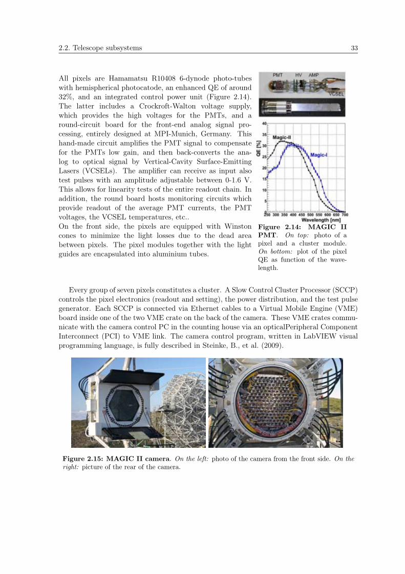
2.2. Telescope subsystems 33
All pixels are Hamamatsu R10408 6-dynode photo-tubeswith hemispherical photocatode, an enhanced QE of around32%, and an integrated control power unit (Figure 2.14).The latter includes a Crockroft-Walton voltage supply,which provides the high voltages for the PMTs, and around-circuit board for the front-end analog signal pro-cessing, entirely designed at MPI-Munich, Germany. Thishand-made circuit amplifies the PMT signal to compensatefor the PMTs low gain, and then back-converts the ana-log to optical signal by Vertical-Cavity Surface-EmittingLasers (VCSELs). The amplifier can receive as input alsotest pulses with an amplitude adjustable between 0-1.6 V.This allows for linearity tests of the entire readout chain. Inaddition, the round board hosts monitoring circuits whichprovide readout of the average PMT currents, the PMTvoltages, the VCSEL temperatures, etc..On the front side, the pixels are equipped with Winstoncones to minimize the light losses due to the dead areabetween pixels. The pixel modules together with the lightguides are encapsulated into aluminium tubes.
Figure 2.14: MAGIC IIPMT. On top: photo of apixel and a cluster module.On bottom: plot of the pixelQE as function of the wave-length.
Every group of seven pixels constitutes a cluster. A Slow Control Cluster Processor (SCCP)controls the pixel electronics (readout and setting), the power distribution, and the test pulsegenerator. Each SCCP is connected via Ethernet cables to a Virtual Mobile Engine (VME)board inside one of the two VME crate on the back of the camera. These VME crates commu-nicate with the camera control PC in the counting house via an opticalPeripheral ComponentInterconnect (PCI) to VME link. The camera control program, written in LabVIEW visualprogramming language, is fully described in Steinke, B., et al. (2009).
Figure 2.15: MAGIC II camera. On the left: photo of the camera from the front side. On theright: picture of the rear of the camera.
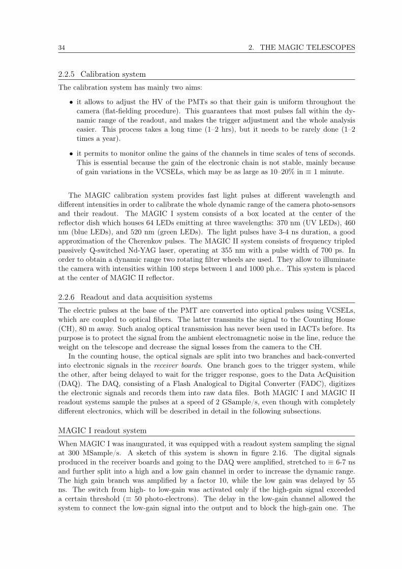
34 2. THE MAGIC TELESCOPES
2.2.5 Calibration system
The calibration system has mainly two aims:
• it allows to adjust the HV of the PMTs so that their gain is uniform throughout thecamera (flat-fielding procedure). This guarantees that most pulses fall within the dy-namic range of the readout, and makes the trigger adjustment and the whole analysiseasier. This process takes a long time (1–2 hrs), but it needs to be rarely done (1–2times a year).
• it permits to monitor online the gains of the channels in time scales of tens of seconds.This is essential because the gain of the electronic chain is not stable, mainly becauseof gain variations in the VCSELs, which may be as large as 10–20% in ≡ 1 minute.
The MAGIC calibration system provides fast light pulses at different wavelength anddifferent intensities in order to calibrate the whole dynamic range of the camera photo-sensorsand their readout. The MAGIC I system consists of a box located at the center of thereflector dish which houses 64 LEDs emitting at three wavelengths: 370 nm (UV LEDs), 460nm (blue LEDs), and 520 nm (green LEDs). The light pulses have 3-4 ns duration, a goodapproximation of the Cherenkov pulses. The MAGIC II system consists of frequency tripledpassively Q-switched Nd-YAG laser, operating at 355 nm with a pulse width of 700 ps. Inorder to obtain a dynamic range two rotating filter wheels are used. They allow to illuminatethe camera with intensities within 100 steps between 1 and 1000 ph.e.. This system is placedat the center of MAGIC II reflector.
2.2.6 Readout and data acquisition systems
The electric pulses at the base of the PMT are converted into optical pulses using VCSELs,which are coupled to optical fibers. The latter transmits the signal to the Counting House(CH), 80 m away. Such analog optical transmission has never been used in IACTs before. Itspurpose is to protect the signal from the ambient electromagnetic noise in the line, reduce theweight on the telescope and decrease the signal losses from the camera to the CH.
In the counting house, the optical signals are split into two branches and back-convertedinto electronic signals in the receiver boards. One branch goes to the trigger system, whilethe other, after being delayed to wait for the trigger response, goes to the Data AcQuisition(DAQ). The DAQ, consisting of a Flash Analogical to Digital Converter (FADC), digitizesthe electronic signals and records them into raw data files. Both MAGIC I and MAGIC IIreadout systems sample the pulses at a speed of 2 GSample/s, even though with completelydifferent electronics, which will be described in detail in the following subsections.
MAGIC I readout system
When MAGIC I was inaugurated, it was equipped with a readout system sampling the signalat 300 MSample/s. A sketch of this system is shown in figure 2.16. The digital signalsproduced in the receiver boards and going to the DAQ were amplified, stretched to ≡ 6-7 nsand further split into a high and a low gain channel in order to increase the dynamic range.The high gain branch was amplified by a factor 10, while the low gain was delayed by 55ns. The switch from high- to low-gain was activated only if the high-gain signal exceededa certain threshold (≡ 50 photo-electrons). The delay in the low-gain channel allowed thesystem to connect the low-gain signal into the output and to block the high-gain one. The

2.2. Telescope subsystems 35
output was sent to long ring buffers where it waited for the trigger decision. If passed, it wasreadout with FADC modules and stored in First In, First Out (FIFO) buffers. The dead timewas around 1 µ s. A multi-thread readout program, written in the C++ environment, readthe data from the FIFO buffer and wrote to the raw files (Goebel, F., et al., 2003).
Figure 2.16: Sketches of the two MAGIC I readout systems. On the left: 300 MSample/sreadout system in operation between 2003 and February 2007. On the right: the current MAGIC Ireadout system sampling at 2 GSample/s and making use of the multiplexing technique.
The system was upgraded to an ultra fast FADC of 2 GHz sampling rate which makes useof a novel fiber-optic multiplexing technique5. Multiplexing is possible as the signal duration(few ns) and the trigger frequency (∼ 1 kHz) result in a low duty cycle for the digitizers. Thefiber-optic Multiplexing readout system (MUX) uses commercial FADC modules (producedby the company Acqiris) to digitize 16 channels consecutively. The concept is shown in figure2.16.
In preparation for the MUX installation, fiber optic splitters were installed already in April2006. Afterwards, half of the split signal is sent directly to the receiver boards, so digitizedand sent to the trigger system, and the other half is delayed by using optical fibers beforeback-converting it into digital signal. Within group of 16 channels, each channel is delayedof 40 ns with respect to the previous one. The maximum delay is of 1160 ns to account forthe 40 ns for the 16 channels and 560 ns needed to wait for the trigger decision. On themultiplexer boards the optical signals are converted back to electronic signals by using PINdiodes. Fast high bandwidth MOSFET-switched open for 40 ns channel by channel. Finallythe signals are summed in two active summation stages and digitized by the Acqiris boards.The reader interested on this commercial device can refer to Goebel, F., et al. (2008). Thesedigitized data are stored on five on-boards with a dead time (before the next event can berecorded) of 2.5 µ s. Each on-board is subdivided into three segments, with a capacity of 50events each, which is read out asynchronously by a rank-mounted PC controlled by the MUXcontrol program. The MuxDaq program combines the data coming from the five PCs andtransmitted via Ethernet, and stores them in a buffer ring. Once the data integrity is checked,it performs a quick signal reconstruction for the on-line data quality monitor and consequentlystores the data into raw files. All these tasks are performed in parallel as independent threadsof the MuxDaq program. Figure 2.17 shows a scheme of this program.
5The multiplexing technique combined multiple analog signals in one optical fiber.
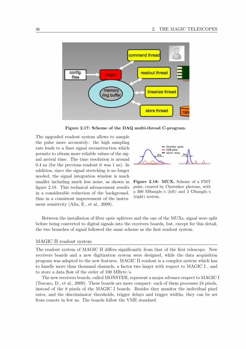
36 2. THE MAGIC TELESCOPES
Figure 2.17: Scheme of the DAQ multi-thread C-program.
The upgraded readout system allows to samplethe pulse more accurately: the high samplingrate leads to a finer signal reconstruction whichpermits to obtain more reliable values of the sig-nal arrival time. The time resolution is around0.4 ns (for the previous readout it was 1 ns). Inaddition, since the signal stretching is no longerneeded, the signal integration window is muchsmaller including much less noise, as shown infigure 2.18. This technical advancement resultsin a considerable reduction of the background,thus in a consistent improvement of the instru-ment sensitivity (Aliu, E., et al., 2009).
Figure 2.18: MUX. Scheme of a PMTpulse, created by Cherenkov photons, witha 300 MSample/s (left) and 2 GSample/s(right) system.
Between the installation of fiber optic splitters and the one of the MUXs, signal were splitbefore being converted to digital signals into the receivers boards, but, except for this detail,the two branches of signal followed the same scheme as the first readout system.
MAGIC II readout system
The readout system of MAGIC II differs significantly from that of the first telescope. Newreceivers boards and a new digitization system were designed, while the data acquisitionprogram was adapted to the new features. MAGIC II readout is a complex system which hasto handle more than thousand channels, a factor two larger with respect to MAGIC I , andto store a data flow of the order of 100 MByte/s.
The new receivers boards, called MONSTER, represent a major advance respect to MAGIC I(Tescaro, D., et al., 2009). These boards are more compact: each of them processes 24 pixels,instead of the 8 pixels of the MAGIC I boards. Besides they monitor the individual pixelrates, and the discriminator thresholds, trigger delays and trigger widths, they can be setfrom remote in few ns. The boards follow the VME standard.
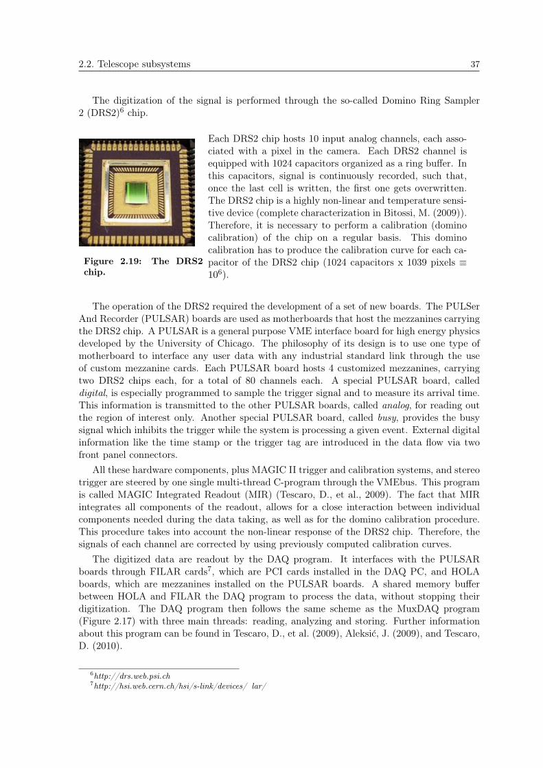
2.2. Telescope subsystems 37
The digitization of the signal is performed through the so-called Domino Ring Sampler2 (DRS2)6 chip.
Figure 2.19: The DRS2chip.
Each DRS2 chip hosts 10 input analog channels, each asso-ciated with a pixel in the camera. Each DRS2 channel isequipped with 1024 capacitors organized as a ring buffer. Inthis capacitors, signal is continuously recorded, such that,once the last cell is written, the first one gets overwritten.The DRS2 chip is a highly non-linear and temperature sensi-tive device (complete characterization in Bitossi, M. (2009)).Therefore, it is necessary to perform a calibration (dominocalibration) of the chip on a regular basis. This dominocalibration has to produce the calibration curve for each ca-pacitor of the DRS2 chip (1024 capacitors x 1039 pixels ≡106).
The operation of the DRS2 required the development of a set of new boards. The PULSerAnd Recorder (PULSAR) boards are used as motherboards that host the mezzanines carryingthe DRS2 chip. A PULSAR is a general purpose VME interface board for high energy physicsdeveloped by the University of Chicago. The philosophy of its design is to use one type ofmotherboard to interface any user data with any industrial standard link through the useof custom mezzanine cards. Each PULSAR board hosts 4 customized mezzanines, carryingtwo DRS2 chips each, for a total of 80 channels each. A special PULSAR board, calleddigital, is especially programmed to sample the trigger signal and to measure its arrival time.This information is transmitted to the other PULSAR boards, called analog, for reading outthe region of interest only. Another special PULSAR board, called busy, provides the busysignal which inhibits the trigger while the system is processing a given event. External digitalinformation like the time stamp or the trigger tag are introduced in the data flow via twofront panel connectors.
All these hardware components, plus MAGIC II trigger and calibration systems, and stereotrigger are steered by one single multi-thread C-program through the VMEbus. This programis called MAGIC Integrated Readout (MIR) (Tescaro, D., et al., 2009). The fact that MIRintegrates all components of the readout, allows for a close interaction between individualcomponents needed during the data taking, as well as for the domino calibration procedure.This procedure takes into account the non-linear response of the DRS2 chip. Therefore, thesignals of each channel are corrected by using previously computed calibration curves.
The digitized data are readout by the DAQ program. It interfaces with the PULSARboards through FILAR cards7, which are PCI cards installed in the DAQ PC, and HOLAboards, which are mezzanines installed on the PULSAR boards. A shared memory bufferbetween HOLA and FILAR the DAQ program to process the data, without stopping theirdigitization. The DAQ program then follows the same scheme as the MuxDAQ program(Figure 2.17) with three main threads: reading, analyzing and storing. Further informationabout this program can be found in Tescaro, D., et al. (2009), Aleksic, J. (2009), and Tescaro,D. (2010).
6http://drs.web.psi.ch7http://hsi.web.cern.ch/hsi/s-link/devices/lar/
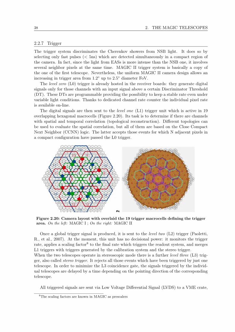
38 2. THE MAGIC TELESCOPES
2.2.7 Trigger
The trigger system discriminates the Cherenkov showers from NSB light. It does so byselecting only fast pulses (< 5ns) which are detected simultaneously in a compact region ofthe camera. In fact, since the light from EASs is more intense than the NSB one, it involvesseveral neighbor pixels at the same time. MAGIC II trigger system is basically a copy ofthe one of the first telescope. Nevertheless, the uniform MAGIC II camera design allows anincreasing in trigger area from 1.2up to 2.5diameter FoV.
The level zero (L0) trigger is already hosted in the receiver boards: they generate digitalsignals only for those channels with an input signal above a certain Discriminator Threshold(DT). These DTs are programmable providing the possibility to keep a stable rate even undervariable light conditions. Thanks to dedicated channel rate counter the individual pixel rateis available on-line.
The digital signals are then sent to the level one (L1) trigger unit which is active in 19overlapping hexagonal macrocells (Figure 2.20). Its task is to determine if there are channelswith spatial and temporal correlation (topological reconstruction). Different topologies canbe used to evaluate the spatial correlation, but all of them are based on the Close CompactNext Neighbor (CCNN) logic. The latter accepts those events for which N adjacent pixels ina compact configuration have passed the L0 trigger.
Figure 2.20: Camera layout with overlaid the 19 trigger macrocells defining the triggerarea. On the left: MAGIC I ; On the right: MAGIC II
Once a global trigger signal is produced, it is sent to the level two (L2) trigger (Paoletti,R., et al., 2007). At the moment, this unit has no decisional power: it monitors the triggerrate, applies a scaling factor8 to the final rate which triggers the readout system, and mergesL1 triggers with triggers generated by the calibration system and the stereo trigger.When the two telescopes operate in stereoscopic mode there is a further level three (L3) trig-ger, also called stereo trigger. It rejects all those events which have been triggered by just onetelescope. In order to minimize the L3 coincidence gate, the signals triggered by the individ-ual telescopes are delayed by a time depending on the pointing direction of the correspondingtelescope.
All triggered signals are sent via Low Voltage Differential Signal (LVDS) to a VME crate,
8The scaling factors are known in MAGIC as prescalers
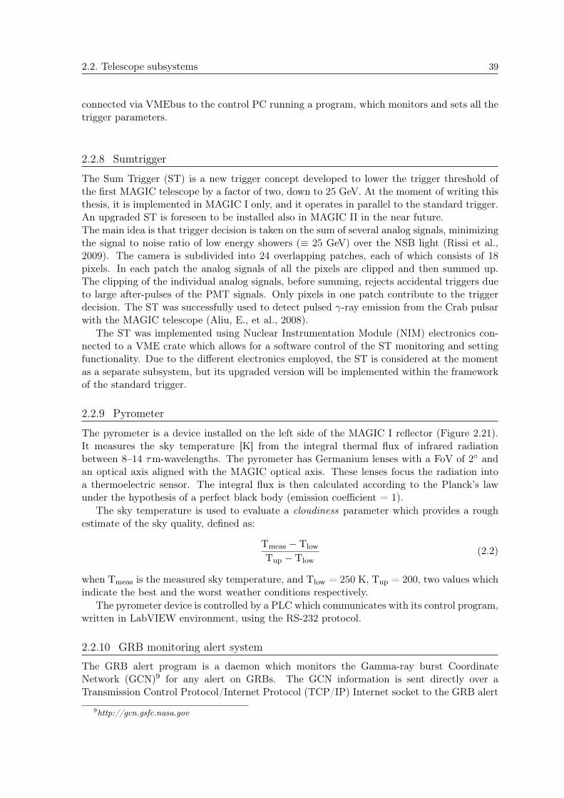
2.2. Telescope subsystems 39
connected via VMEbus to the control PC running a program, which monitors and sets all thetrigger parameters.
2.2.8 Sumtrigger
The Sum Trigger (ST) is a new trigger concept developed to lower the trigger threshold ofthe first MAGIC telescope by a factor of two, down to 25 GeV. At the moment of writing thisthesis, it is implemented in MAGIC I only, and it operates in parallel to the standard trigger.An upgraded ST is foreseen to be installed also in MAGIC II in the near future.The main idea is that trigger decision is taken on the sum of several analog signals, minimizingthe signal to noise ratio of low energy showers (≡ 25 GeV) over the NSB light (Rissi et al.,2009). The camera is subdivided into 24 overlapping patches, each of which consists of 18pixels. In each patch the analog signals of all the pixels are clipped and then summed up.The clipping of the individual analog signals, before summing, rejects accidental triggers dueto large after-pulses of the PMT signals. Only pixels in one patch contribute to the triggerdecision. The ST was successfully used to detect pulsed -ray emission from the Crab pulsarwith the MAGIC telescope (Aliu, E., et al., 2008).
The ST was implemented using Nuclear Instrumentation Module (NIM) electronics con-nected to a VME crate which allows for a software control of the ST monitoring and settingfunctionality. Due to the different electronics employed, the ST is considered at the momentas a separate subsystem, but its upgraded version will be implemented within the frameworkof the standard trigger.
2.2.9 Pyrometer
The pyrometer is a device installed on the left side of the MAGIC I reflector (Figure 2.21).It measures the sky temperature [K] from the integral thermal flux of infrared radiationbetween 8–14 τm-wavelengths. The pyrometer has Germanium lenses with a FoV of 2 andan optical axis aligned with the MAGIC optical axis. These lenses focus the radiation intoa thermoelectric sensor. The integral flux is then calculated according to the Planck’s lawunder the hypothesis of a perfect black body (emission coefficient = 1).
The sky temperature is used to evaluate a cloudiness parameter which provides a roughestimate of the sky quality, defined as:
Tmeas Tlow
Tup Tlow(2.2)
when Tmeas is the measured sky temperature, and Tlow = 250 K, Tup = 200, two values whichindicate the best and the worst weather conditions respectively.
The pyrometer device is controlled by a PLC which communicates with its control program,written in LabVIEW environment, using the RS-232 protocol.
2.2.10 GRB monitoring alert system
The GRB alert program is a daemon which monitors the Gamma-ray burst CoordinateNetwork (GCN)9 for any alert on GRBs. The GCN information is sent directly over aTransmission Control Protocol/Internet Protocol (TCP/IP) Internet socket to the GRB alert
9http://gcn.gsfc.nasa.gov
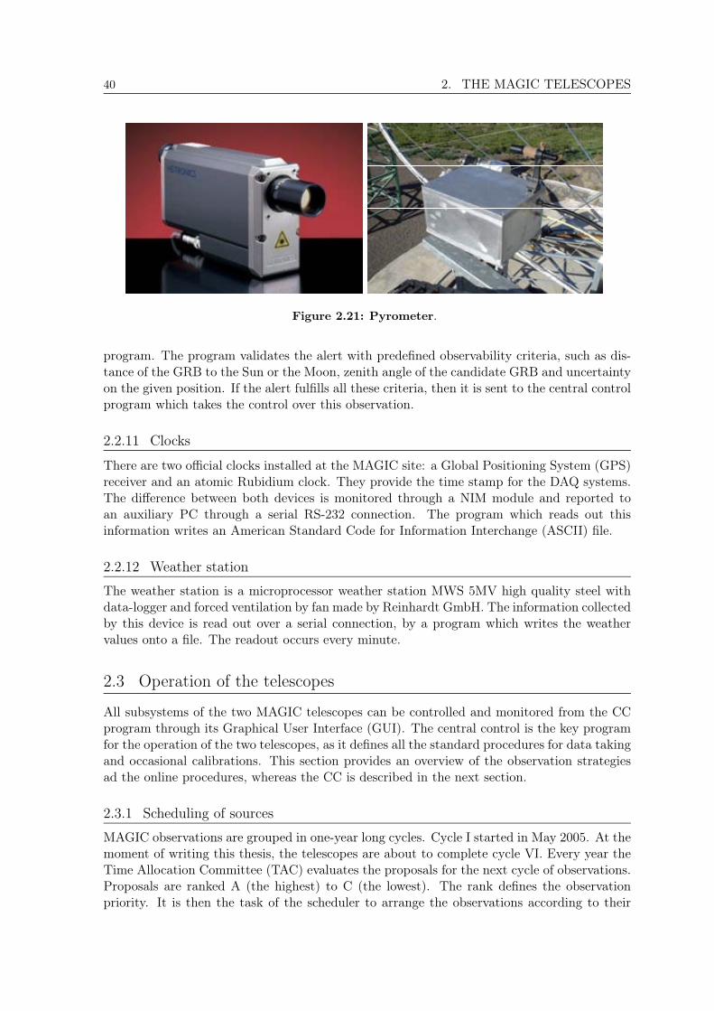
40 2. THE MAGIC TELESCOPES
Figure 2.21: Pyrometer.
program. The program validates the alert with predefined observability criteria, such as dis-tance of the GRB to the Sun or the Moon, zenith angle of the candidate GRB and uncertaintyon the given position. If the alert fulfills all these criteria, then it is sent to the central controlprogram which takes the control over this observation.
2.2.11 Clocks
There are two official clocks installed at the MAGIC site: a Global Positioning System (GPS)receiver and an atomic Rubidium clock. They provide the time stamp for the DAQ systems.The difference between both devices is monitored through a NIM module and reported toan auxiliary PC through a serial RS-232 connection. The program which reads out thisinformation writes an American Standard Code for Information Interchange (ASCII) file.
2.2.12 Weather station
The weather station is a microprocessor weather station MWS 5MV high quality steel withdata-logger and forced ventilation by fan made by Reinhardt GmbH. The information collectedby this device is read out over a serial connection, by a program which writes the weathervalues onto a file. The readout occurs every minute.
2.3 Operation of the telescopes
All subsystems of the two MAGIC telescopes can be controlled and monitored from the CCprogram through its Graphical User Interface (GUI). The central control is the key programfor the operation of the two telescopes, as it defines all the standard procedures for data takingand occasional calibrations. This section provides an overview of the observation strategiesad the online procedures, whereas the CC is described in the next section.
2.3.1 Scheduling of sources
MAGIC observations are grouped in one-year long cycles. Cycle I started in May 2005. At themoment of writing this thesis, the telescopes are about to complete cycle VI. Every year theTime Allocation Committee (TAC) evaluates the proposals for the next cycle of observations.Proposals are ranked A (the highest) to C (the lowest). The rank defines the observationpriority. It is then the task of the scheduler to arrange the observations according to their
2.3. Operation of the telescopes 41
obtained grade. A “tentative” observation schedule is produced every sidereal month. Theschedule defines the observation time slot for every object, along with the observation mode,the moonlight conditions, and the zenith angle. The schedule can be modified if, in themeanwhile, any observation trigger activates (§ 2.3.2).
2.3.2 Regular and ToO observations
MAGIC observations can be carried out either as Target of Opportunity (ToO) observations,or regular observations.
Regular observations are arranged whenever the source is visible in La Palma, for a numberof hours which depend on the expected/known brightness of the source. These campaigns aremeant for the study of objects with a stable and constant flux.
ToO observations instead, are activated by trigger alerts which makes use of multi-wavelength,and multi-experiment information. Most of their targets are variable sources showing suddenflux enhancements, called “flares”, which are to a large extent unpredictable. Nevertheless,since the VHE radiation is often correlated to the emission in other energy bands, a fluxenhancement in another wavelength can be used to trigger MAGIC. Trigger strategies whichrely on the status of the X-ray emission take advantage from public data released by monitor-ing detectors, such as All-Sky Monitor (ASM) or Burst Alert Telescope (BAT), on board ofthe RXTE and Swift satellites respectively. Since August 2009, new soft -ray data recordedby Fermi/LAT are made publicly available every six hours. Trigger alerts based on optical,infrared or radio frequencies generally require previous agreements with the correspondingexperiments. Although they can be replaced by the use of Astronomical Telegrams (ATels)10
which provide an internationally recognized, but not refereed, system for the notification oftransient astronomical phenomena. ATels are released almost on real time to allow for multi-wavelength observation coverage of the objects.Trigger alerts for MAGIC can come also from other IACTs. Such alerts normally relate tosources which are well known VHE emitters for which there is no more competition betweenexperiments. All of them organize monitoring programs and observe variable sources con-stantly along their period of visibility, hoping to catch some flares. For this reason, an OnlineAnalysis (OA) tool which provides results in real time is necessary (§ 2.5). On the other hand,the VERITAS collaboration still operates the Whipple telescope with this purpose.
2.3.3 Source pointing modes
MAGIC observations are carried out either in tracking or in wobble mode. The observationmode determines the background estimation procedure.
In the tracking, or on/off, mode the telescope tracks directly the source, and, therefore,the source position is always located at the camera center. These observations are called onpointings. In this observation mode, additional data are needed for the background estimation.Off pointings are carried out observing a region of the sky with no known -ray source inthe FoV, and in the same observational conditions (background light, presence of stars, andzenith angle) as on pointings.
Most of the MAGIC observations are carried out in wobble mode, or more properly false-source tracking mode, (Fomin, V. P., et al., 1994). The telescope tracks alternatively twoopposite directions in the sky located at a defined offset (default 0.4) from the source position.The wobble position is swapped, generally, every 20 minutes. This is the favoured observation
10http://www.astronomerstelegram.org/. It is responsibility of the International Astronomic Union.

42 2. THE MAGIC TELESCOPES
mode because it does not require any additional off data. Since the source position does notcoincide with the camera center, there are regions of the camera where -ray events are notexpected, and can be used to define the off data sample (§ 3.9). In this way no observationtime is lost pointing at dark regions of the sky. Moreover, the background estimation ismuch more reliable, as it is derived from the same data sample of the source observation.However, this observation mode has two main drawbacks: a loss in -ray efficiency, estimatedof the order of 15-20%, due to the smaller effective trigger region around the source, and apossible bias introduced by the off-center source position which mainly depends on the camerainhomogeneities. The wobbling of the observation positions is meant to take into account thiseffect: for every source pointing, the background is estimated from the same physical regionof the camera taken from the symmetric wobble position.
2.3.4 Calibration and data runs
The expression data taking includes the entire online procedure of observing the scheduledsources, from the source pointing to the data storage. It can be completely performed throughthe CC program, subject of the next section. In fact, by communicating with all the subsys-tems (§ 2.2), the CC program can coordinate every single operation of the telescopes.
MAGIC data are classified according to the kind of events they record. Mainly there are:
• calibration runs contain trigger generated by the calibration system. They are usedfor the data calibration (§ 3.3).
• pedestal runs contain random triggers with a null probability of recording atmosphericshower events. They are used to define the electronic noise of the electronic chain.
• data runs all the cosmic events which trigger the telescopes. These runs can includealso pedestal and calibration events, interleaved with cosmic events at a rate of 25 Hzrespectively (hereafter interleaved events). These additional calibration events allowsfor a constant update of the calibration factors (§ 3.3) in the recorded data.
Each source observation requires at least one pedestal and one calibration run, usually takenbefore the data runs.
Each telescope records stereo events independently. The event correspondence is done(§ 3.5.1), later on, oine, by using the trigger number which is delivered by the L3 trigger(§ 2.2.7). In order to ease up the file management in the oine analysis, data runs aregrouped into data sequences with a run number which is common for both telescopes (givenby the CC program). Files in the data sequence (whose number is different from telescope totelescope) have a second number, called subrun number which is given by the correspondingDAQ system. In standard data taking, a data sequence lasts for 20 minutes. Whereas, eachdata subrun usually contains a couple of minutes of observations, even though this dependson the trigger rate.
2.4 Central control
The central control program allows an operator to configure all subsystems of the telescopesand take data. It also permits to monitor the most relevant parameters of the subsystemsthrough a graphical user interface. The program is called SuperArehucas.
2.4. Central control 43
The implementation of the standard procedures for stereo data taking inside the CC leadsto a level of automatization which permits to avoid oversights, and possible misuse of theinstrument. Nevertheless, the CC confers the full control over the telescope to the operators.For example, they can configure the various components of the detector, according to the ob-servational conditions. They can also stop any automatic procedure in case of extraordinaryproblems during data taking.
The CC program is written in LabVIEW 8.5 in order to take advantage of the built-incontrol utilities and the graphical capabilities of this platform. SuperArehucas includes 756subroutines, which in LabVIEW are called Virtual Instruments (VIs).
2.4.1 Communication with telescope subsystems
Communication between CC and every subsystem is performed through C-coded TCP/IPsockets. Sockets are endpoints of inter-process communication based on a combination ofInternet Protocol (IP) addresses and port numbers. When two of these endpoints, setupby two unrelated processes (also residing in two different machines) connect, they create areliable byte stream which can be read or written. Thus, in the general socket communicationscheme, a server program listens in a socket connected to a port number. A client programcan connect its own socket to the server’s socket which it writes to. In the meanwhile, theserver socket reads the data sent in.
The control system of the MAGIC telescopes expects each subsystem to open both a serverand a client socket: one is used to receive instructions/data from the CC, and the other oneto send to the CC all its relevant information. Analogously, SuperArehucas has two socketsfor each subsystem.
In order to establish a connection with each subsystem, at start up, the CC starts pollingsubsystem by subsystem for availability, and this fact is displayed to the user. Every subsystemsends a ASCII report to the CC every second describing its state, time stamp, and all relevantoperational parameters. The state variable is used to define the action of the subsystem. Ifthe CC does not receive any report from a subsystem for more than 10 s, it defines thecorresponding subsystem state as “unavailable”. The central control sends a CC-report every10 s to each subsystem which, in this way, can know when the CC is available. Moreover,reading the CC-report is the only mean a subsystem has to be aware of the running parametersof the other subsystems. Commands from CC are sent through the same thread of the CC-report. They are executed by the subsystem as if the user had input them directly at thecorresponding console.
2.4.2 Program structure
The logic of the central control program is based on several decisional loops implemented asindividual threads (Figure 2.22), and an extensive use of global variables:
• The report thread takes care of the report system: it sends every 10 s the CC-reportto all subsystems, and reads out every second the reports that the subsystems send it.The information contained in the received reports is then processed and saved into a setof global variables (“subsystems global variables”).
• The GUI control thread monitors controls, i.e. buttons and menus. Whenever oneof them is clicked, the loop activates the global variable which identifies the function(“function global variables”) the operator requests.

44 2. THE MAGIC TELESCOPES
• The action thread starts the functions requested by means of the controls: it constantlychecks if one the “function global variables” has been activated, and acts consequentlyby calling the corresponding VI.
• The subsystem panel thread displays on the GUI (§ 2.4.3) all the information receivedfrom the subsystems reports. It makes use of the “subsystem global variables”.
• The camera display thread displays the status of all relevant parameters in all indi-vidual pixels (§ 2.4.3).
• The GRB thread activates the GRB automatic procedure whenever a GRB alert isreceived through the report sent by the GRB monitor program (§ 2.2.10).
The fact that the procedures the CC performs are executed in subroutines which run in back-ground, guarantees the operator a full control over them. In fact, the operator can alwaysintervene by means of the controls in the GUI. Nevertheless, there is the exception given bythe automatic GRB procedure.
Figure 2.22: Scheme of the main loop of the central control program. Rectangles identifythreads.
Safety checks
All the specific actions are executed by sending fixed commands, in the ASCII format, tothe involved subsystems (§ 2.4.1). However, before sending the commands the CC programperforms additional decisional loops to check if the addressee is correctly configured to be ableto execute the required action. These checks prevent possible mistakes which can deterioratethe data quality and avoid that the command will be unsuccessful.
2.4. Central control 45
Moreover, the subsystem parameters are constantly compared to safety limits or standardvalues and warning or safety reactions result when the parameters seem to show problematicstates. For example, if the external humidity measured by the weather station, exceeds acertain value, the electronic inside the camera can be damaged. Therefore, the CC programimmediately closes the lids which protect the camera. If the sun is still present, the systemdoes not allow the operator to rump the HVs up in order not to ruin the PMTs. If the windspeed is too high, this can destroy the telescope frame or the lids if opened: in this case theCC closes the lids and parks the telescope. If, for any reason, the drive system changes actionunexpectedly during data taking, the CC automatically stops the data acquisition and informsthe shifters. Warning messages are issued through colorful pop-up windows and sounds.
2.4.3 Status of the subsystems: graphical user interface
SuperArehucas graphical user interface is shown in Figure 2.23. It contains all the informationwhich are needed to monitor the data taking procedure and determine the overall performanceof the detector.
Status of individual pixels: pixel displays
On the left side of the GUI, there are three pixel displays for each telescope (in Figure 2.23MAGIC I above and MAGIC II below). Each of these displays can show the following infor-mation for each of the pixels:
• charge of the last event processed by the DAQ system in FADC counts. Thisinformation comes from the rough signal extraction performed online by the DAQ system(§ 2.2.6). The charge is pedestal-subtracted only if the DAQ has taken at least a pedestalrun before.
• PMT anode Direct Currents (DCs) in µA allow to monitor the intensity of thelight background. During normal operation they must be under 7 µA. Stars in the FoVare visible through a DC increase.
• PMT HV readout in Volt. This display is useful to identify dead pixels.
• PMT HV settings in Volt. They should be equal to the HV readout values withina 10% . If they are systematically different for all the pixels, it means that the HVramping up procedure has failed. If they differ only for some pixels, it is due to achecking routine of the camera program which reduces the HV of those pixels with toohigh DCs.
• Individual Pixel Rate in Hz monitors accidental triggers in individual pixels due tonoise. During stereo data taking it should be around 500 kHz.
• DTs in arbitrary units (higher DT indicates a more restrictive trigger level). They areadjusted in real time during data taking by the so-called “Individual Pixel Rate (IPR)control” routine.
• trigger delay times in arbitrary units. They should be fixed to their optimal valuesand hardly modified.
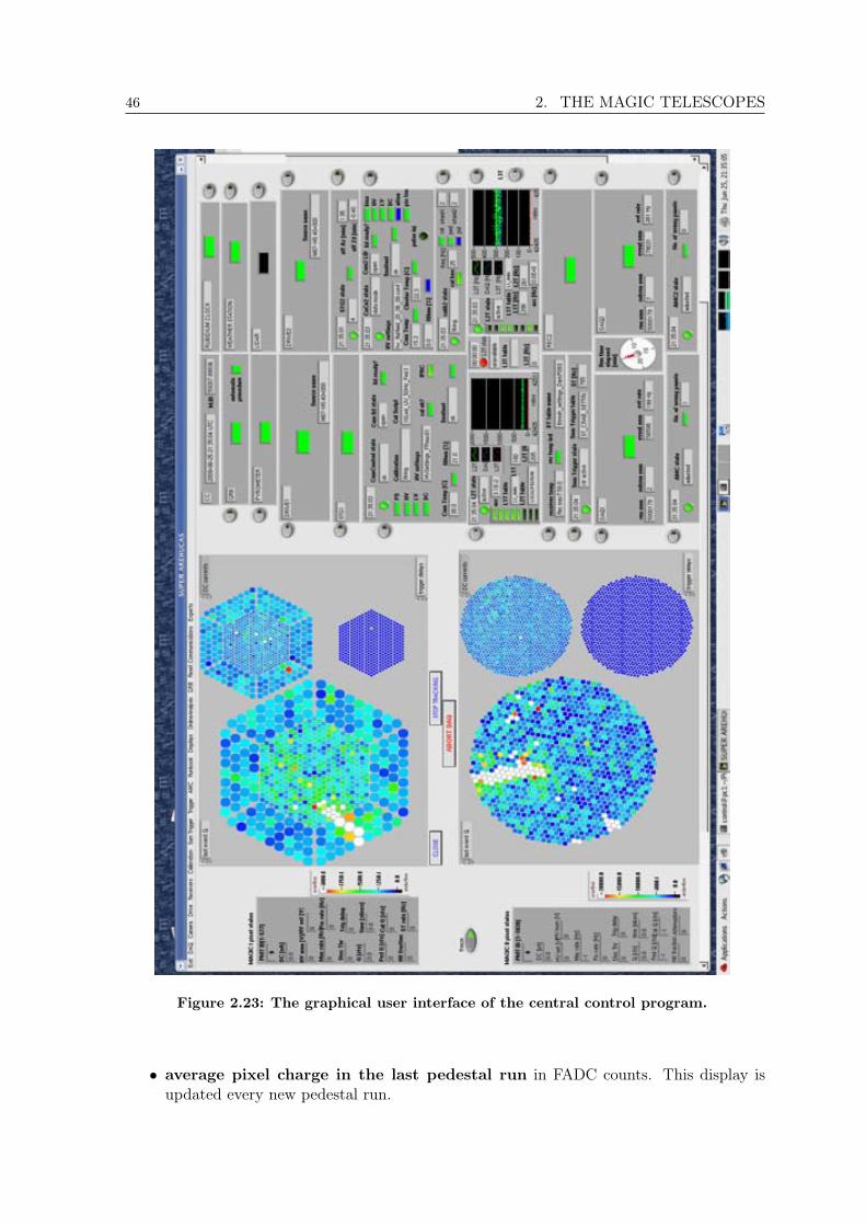
46 2. THE MAGIC TELESCOPES
Figure 2.23: The graphical user interface of the central control program.
• average pixel charge in the last pedestal run in FADC counts. This display isupdated every new pedestal run.

2.4. Central control 47
• average pixel charge in the last calibration run in FADC counts. This display isupdated every new calibration run.
• trigger rate in the 19 macro-cells in Hz. This is the only display which does notinclude pixel information. It shows only 19 values. Each of which corresponds to onetrigger macro-cell (§ 2.2.7).
The color scale of all the displays goes from blue (lowest) to red (highest). Black indicatesunderflow, and white overflow. The color scale can be changed by the operator through thecorresponding function in the menu. Running the mouse over the largest displays, the oper-ator can check the values of all the above described parameters, and the pixel numbers. Thelatter are shown in the two panels on the left side of the camera displays.
Status of the subsystem elements: subsystem panel
The right side of the GUI shows a panel built-up of 23 windows, one for each subsystem (§ 2.2).These windows are grouped in such a way that they form three sub-panels: the top centralone for the “common subsystems”, the bottom left for MAGIC I , and the bottom right forMAGIC II subsystems. Each window contains the main information that the correspondingsubsystem sends to the CC every second through its reports (§ 2.4.1). As a result, thevariables inside the window are updated with the same frequency. Nevertheless, each windowhas two possible states: one which includes all the subsystem information needed to identify aproblem (“full state”), and a more compact one which shows a LED, whose color indicates thesubsystem behavior (green: everything is fine, yellow: alarm state, red: there is a problem),and just information indispensable for data taking (“LED state”). In case of green light,the operator can choose which state of the window to visualize by using the button on theexternal side of the window. If any problem appears, the window will immediately switch onthe “full state”, and it cannot be changed until the problem is solved. The “full state” windowsalways contain: a round LED indicating the status of the TCP communication between theCC and the corresponding subsystem, the state of the subsystem, and a clock showing thetime of the last report received by the CC (large time differences with respect to the timeof the CC computer, shown in the first top left window, indicate that the communication ismalfunctioning). The additional information for each subsystem is listed below.
• pyrometer:
cloudiness (Ÿ 2.2.9)
status of the sky quality
• GRB monitor:
status of the automatic GRB procedure
status of the GRB observations
GRB coordinates (only if any)
• weather station:
external temperature
external humidity
wind speed [km/h]
48 2. THE MAGIC TELESCOPES
wind direction
• clocks:
time difference between the GPS receiver and the rubidium clock (Ÿ 2.2.11) [µs]
• lidar: not yet available.
• MAGIC I and MAGIC II drive:
name of observed source requested position [RA, DEC] requested position [az, zd] observed position [RA, Dec] observed position [az, zd]
• MAGIC I and MAGIC II starguider:
azimuth mispointing [] zenith mispointing [] status of the mispointing
• MAGIC I camera:
status of the electronic power Low Voltages (LVs) status of the pixel HVs status of the electronics power supplies status of the DCs state of the lids HV settings file-name temperature inside the camera [C] humidity inside the camera [%] status of the IPR control state of the sentinel. The sentinel indicates the response of the safety routines of the
camera control program. MAGIC I calibration state. The calibration system for MAGIC I is setup through a script
launched by the MAGIC I camera control program. That is the reason for which thissubsystem has been merged with the MAGIC I camera program.
name of the calibration script
• MAGIC II camera:
status of the HVs, LVs, biases, DCs, attenuators, pixel temperature lid state HV settings file-name temperature inside the camera [C] humidity inside the camera [%] mean temperature of the clusters [C] sentinel state status of the pulse injector

2.4. Central control 49
• MAGIC II calibration:
interleaved ped/cal frequency [Hz]
status of the calibration box
filter wheel settings
status of the calibration switches
• MAGIC I and MAGIC II trigger
L1T rate [Hz]
L2T rate [Hz]
L1T table name
L2T table name
accidental events rate [Hz]
status of the prescaling factors
graph showing the rate behavior as function of time. Both DAQ and trigger rates aredisplayed.
• MAGIC I sum trigger:
sum trigger table name
sum trigger rate
• MAGIC I receivers:
receiver temperature [C]
DT table name
ˆ the MAGIC II receiver:
state of the PULSAR boards
temperature of the electronics racks [C]
DT table name
status of the IPR control
state of the cooling system for the electronics racks
communication status of the cooling system control program
• MAGIC I and MAGIC II DAQ
run number
run sub-number
event number
event rate [Hz]
free available disk space [MBytes]
elapsed time since last wobbling
• MAGIC I and MAGIC II AMC:
number of de-focused mirror panels
status of de-focused mirror problem
50 2. THE MAGIC TELESCOPES
2.4.4 Central control functions
The functions available in the CC program can be called through either buttons in the GUIor menus.
Buttons control the functions which are used more often during the operation of the tele-scopes. They are related to the telescopes positioning, the camera lids, and the data taking(Figure 2.23). The buttons are visible only when the relevant subsystems are available. Theyusually start pop-up menus which guide the operator through the operation he/she wants toperform. The following buttons are available:
• POSITION . When the telescope is stopped and the drive system is available, thebutton “POSITION” allows the operator to move the telescope. When it is clicked, apop-up window offers three possibilities:
– “positioning and tracking” which allows the operator either to select the source fromany of the available catalogues11 or to type in the desired coordinates. The firstoption guarantees the definition of the correct source name. After having selectedthe position, the operator is asked about the observation mode (§ 2.3.3). In caseof wobble observations, the CC takes care of computing the wobbling positionsdepending on the requested offset, and rotation angle. Only at this point thetelescope starts slewing, and, when reached the position, tracking.
– “park position” will move the telescope to the park position
– “special fixed position” where the operator can input a fixed position in azimuthand zenith coordinates.
• STOP TRACKING . It stops the telescope.
• OPEN LIDS and CLOSE LIDS control the movements of the camera lids.
• START DAQ . It starts the data taking procedure. It is visible only when the mainsubsystems involved in the data taking procedure (readout systems, DAQs, triggers,and cameras) are available. When pressed, the CC warns the operator about possibleproblems with any of the subsystems. In such a case, the operator decides if keepingon and starting the data taking. A pop-up window gives the operator the possibilityto select the calibration and pedestal setup (both for pedestal/calibration runs andinterleaved events), and the prescaling factors. The data taking procedure comprisestwo loops: the external one which scans the data sequences, and an internal one whichrecords the data sequence. The first loop takes care of:
– setting the correct run number for the data sequence
– taking calibration and pedestal runs (usually they are taken just once per sourceobservation, before first corresponding data sequence).
– computing and changing wobble position every data sequence
– performing mirror adjustment (§ 2.2.3) every data sequence
– notifying the operator through a loud sound the end of the data sequence
11SuperArehucas uses catalogues in Xephem format. Xephem is a free astronomical software package.

2.4. Central control 51
The internal loop, which is in charge of recording the data, saves also the subsystemsreports, received during data run, into specific files called report files (“.rep”). Later on,the content of these report files is added to data in the oine analysis (§ 3.2).
• ABORT DAQ . It stops the data sequence main loop.
All the other functions which the CC can perform are accessible through the menus ontop of the GUI. These functions include the settings of the various subsystems, occasionalprocedures and some basic operations. The latter are usually performed within more complexsubroutines which define complex procedures. Below, the reader can find the list of all theavailable functions, with a short description. In general, the setting functions of pixel-relatedparameters always gives the possibility to set the values pixel-by-pixel or for the whole cameratogether by uploading a file containing the predefined settings. Whereas, the “save to file”function saves the current settings in a file with the appropriate format so that it can be usedby the setting function.
• Exit
– quit SuperArehucas
• DAQ
– go to daq test :“daq test” defines a state of the DAQ systems in which data arerecorded, but not stored to disk. This state allows the operator to monitor therate and get a feeling of how events look like.
– go to standby : “standby” defines another state of the DAQ systems are stopped(no data recording).
– pedestal run
– calibration run
– linearity run: it takes a linearity run which contains pedestal and calibrationevents in bunches of different intensities. They are meant to check the linearity ofthe electronic chain during the observation night.
– dominocalibration run [only MAGIC II ]: it performs the domino calibration(§ 2.2.6). It feeds the channels of the DRS2 chip with known increasing chargelevels for a fixed number of events. For each level the response is determined.
– abort dominocalibration run: it allows to interrupt the the dominocalibrationrun which takes more than 5 minutes to finish.
– input source name: it allows to change the default source name which is givenby the CC itself.
– power on/off MAGIC II readout + trigger electronics: it can be done fromremote only for the more modern MAGIC II electronics.
– data with pulse injector [only MAGIC II ]: it starts the data taking procedureusing the pulse injector as pulse generator. These data are important to study theresponse of the electronic chain after the PMTs.
– enable/disable drive check: this check controls that the state of the drive systemdoes not change unexpectedly. It is an important check since it allows to find out ifone telescope stops during the data taking because of some mechanical or softwarefailures.
52 2. THE MAGIC TELESCOPES
– enable/disable humidity check: this check controls that the humidity does notexceed the safety limits. In such a case, the CC activates automatically the safetyprocedure to prevent possible damages to the electronics.
• Camera
– switch on/off LV [only MAGIC II ]: the LVs of the camera can be switchedon from remote only for the MAGIC II telescope camera.
– set HVs the HV settings can be done either pixel by pixel or for the full cameraby uploading a file with the predefined settings.
– save HVs to file: it saves the current HV settings in a file with the appropriateformat so that it can be used by the above function.
– set biases [only MAGIC II ]: the bias settings can be done either pixel by pixelor for the full camera by uploading a file with the predefined settings.
– set attenuators [only MAGIC II ]
– enable/disable pulse injector [only MAGIC II ] (§ 2.2.4)
– starguider LEDs on/off: it activates the dim references LEDs of the starguidersystem. (§ 2.2.2)
– open TPoint lid (§ 2.2.1)
• Drive
– arm/disarm cosy it activates a safety procedure which foresees that if someoneenters one of the two fences around the telescopes, the corresponding drive systemimmediately stops the telescope movements. Cosy is the name of the drive systemcontrol program.
– enable/disable starguider mode: it actives/disactivates the starguider control.
– choose the star: it is the only subroutine written in C++ language within theMARS environment (Chapter 3). It select the convenient star for the next TPoint,taking into account the sky distribution of the already taken TPoints (§ 2.2.1).
– take a TPoint (§ 2.2.1)
• Receivers
– enable/disable IPR control: the IPR control keeps the IPR below a referencevalue. Thus, it increases or decreases the DTs of a given pixels if its IPR isrespectively too high or too low12.
– set DTs
– save DTs to file12In more detail, the IPR control operates as follows:∗ when enabled, it saves the current DTs as the minimum possible DT.∗ if a pixel has a too high IPR, it increases the DT by one step, and it iterates until the pixel IPR is low
enough.∗ if a pixel has a too low IPR, and its DT has been increased with respect to the initial minimum value,
it tries to reset the DT to its minimum value. After resetting it, it checks if the IPR is low enough,otherwise it increases it again.
2.4. Central control 53
– set trigger delays
– save trigger delays to file
– set pulse width
– MAGIC I IPRC setup: it allows to set up the parameters used by the IPRcontrol algorithm. For MAGIC I the IPR control is implemented in SuperArehucas.In fact, the receivers of MAGIC I communicate directly with the CC via serial port,without any control program.
– MAGIC II IPRC setup: it allows to set the parameters of the MAGIC II IPRcontrol which is implemented into the MIR program (§ 2.2.6). This is much faster(no communication between subsystem in between) than the MAGIC I one.
– rec2 full/reduced report: the report of the MAGIC II receiver subsystem isso long (it contains many information for each pixel, for a total amount of 1039pixels), that the CC needs more than 1 sec to read it out, and this can causea loss of information from overlapping with subsequent reports. For this reason,by default, the MAGIC II receiver report does not send pixel-by-pixel informationabout the trigger delays and pulse widths (these setting should never change duringthe data taking).
– set one receiver channel
– read all trigger delays [only MAGIC I ]: this function kind of substitutes themonitoring tasks of the report system.
– read all DTs [only MAGIC I ]: see above
• Calibration
– start calib. script [only MAGIC I ]
– stop calibration: it stops the calibration triggers.
– switch on/off calibration box [only MAGIC II ]
– calibration laser on/off [only MAGIC II ]
– check laser: it is a procedure to check the status of the laser, which, for hardwarereasons, cannot be monitored other than trying to fire.
– setup calibration [only MAGIC II ]: it allows to set the filter wheels of theMAGIC II calibration system (§ 2.2.5).
• Sum Trigger
– enable/disable ST control
– change ST control parameters
– set ST DTs: ST DTs are the discriminator thresholds of the sum trigger. Theyare expressed in mVolt. They can be set patch-by-patch or for all the patches byuploading a predefined file (§ 2.2.8).
– modify ST DTs: it allows to monitor the rates o the single sum trigger patches,and in case they are not constant, to change the ST thresholds of the necessarypatches.
– save ST DTs to file

54 2. THE MAGIC TELESCOPES
• Trigger
– load trigger table
– define prescaling factors (§ 2.2.6).
– start/stop triggers
– rate report on/off: it activate/disactivate the sending of the trigger reports tothe CC. It is used only for testing purposes.
• AMC
– laser adjust (§ 2.2.3)
– enable/disable TPoint mode [only MAGIC II ]
– take SBIG picture [only MAGIC II ]: at the moment, pictures with the AMCCCD camera (§ 2.2.3) can be taken from the CC only for MAGIC II . The MAGIC ISBIG camera control program is not integrated in the AMC program. Thereforeit does not communicate with the CC.
• GRB
– enable/disable automatic procedure
– testing GRB procedure from SuperArehucas: a special subroutine sends aGRB alert. Thus, only the GRB data taking procedure can be tested.
– activate/disactivate telescopes movements for test
• Runbook
– add comment to runbook (§ 2.4.5)
• Online analysis
– start OA: it is only needed in special cases when the automatic launch of the OAfails (§ 2.5).
• Display
– set colors: it set the color scale of the camera displays described in § 2.4.3.
• Reset communications. This menu provides a “reset communication function” forevery opened socket (§ 2.4.1). Generally the CC program opens two sockets for eachsubsystem (the server and the client). In all these cases the “reset communicationfunction” resets both of them. Nevertheless, there is the exception of the subsystemscontrolled by the MIR program (§ 2.2.6): for them SuperArehucas uses a unique clientsocket, and different server sockets. For this reason, in the case of the MIR subsystems,the “reset communication function” specifies the socket it resets. The socket resettingis performed through shell-BASH scripts.
reset camera1
reset DAQ1
reset drive113
13Since the starguider subsystem is controlled by the drive control program, the starguider1 reports aresent/read through the same sockets as the drive.
2.4. Central control 55
reset AMC1
reset trigger1
reset sum trigger1
reset receivers1
reset pyrometer
reset GRB
reset camera2
reset drive2
reset AMC2
reset DAQ2
reset cooling
reset read from trigger2
reset read from receivers2
reset read from calibration2
reset read from stereo trigger
reset read from pulsars
reset write to calib2/L3/pulsar/rec2/trigger2
• Experts These functions should be used by observers.
– send command: it allows the operator to send arbitrary commands to the desiredsubsystem.
– atfield (§ 2.2.5).
– ADA stands for automatic delay adjustment. It calls a subroutine whose algorithmlooks for the optimal trigger delays and save the results in a file.
2.4.5 Error/event logging
SuperArehucas keeps errors and general event information in a number of ASCII files:
• the debug file (“.dbg”) contains detailed debug information of the program operation.
• the runbook file (“.rbk”) logs the operator names and all their comments.
• the run summary file (”.run” in plain ASCII and “.run.html” in HyperText MarkupLanguage (HTML)) contains information about each subrun. There is one file for eachtelescope. These “run files” are used to fill the MAGIC database.
• the CC report files (“.rep”), one for each telescope, contain the reports of the cor-responding subsystems, plus the common ones. These files can be converted into theROOT format (§ 3.2) to study the evolution of the subsystems during the session.
56 2. THE MAGIC TELESCOPES
2.5 Online analysis
The OA is a program which performs a simplified data analysis during data taking. It iswritten in C++ programming language within the standard MAGIC software environment,MARS, (Chapter 3).
The main purpose of the OA is to extend observations in case a flare is detected in realtime. It generates alpha plots (§ 3.9), which allow to estimate the level of the source activity.The sensitivity (§ 3.9.1) of the online analysis is rather worse than that of the standard oineanalysis: it is sensitive to flares at the level of 40% of the Crab Nebula flux in 20 minutesof observation (typical observation time for monitoring purposes). This reduced sensitivity isdue to the fast processing time needed for the analysis: it has to be at least as fast as the datataking. Nevertheless, the performance of the OA can still be improved, also because it hasnot been adapted to the stereo analysis yet. In addition, the OA can help the operators tomonitor the quality of the observations since it allows to monitor the camera inhomogeneitiesand the relative gain of the pixels.
The OA consists of four main steps. First, it reconstructs and calibrates the signals dig-itized by the 2 GSample/s FADC of MAGIC I . Afterwards, an image cleaning algorithmrejects all those signals which are the result of fluctuations of the NSB light. The remainingpixels make up the shower image which is then parametrized. The third analysis step sepa-rates -ray candidate events from cosmic-ray events among the recorded images. Finally, itperforms the search for a -ray signal from the observed source by statistically evaluating thenumber of -ray candidate events over the estimated background events (those which survivedto the gamma/hadron separation).
From the image parametrization on, the OA makes use of the MAGIC standard analysistools, which are described in detail in Chapter 3, the first steps of the analysis are performedby simplified algorithms:
• Recorded signals are sampled by MAGIC I MUX DAQ in 80 FADC slices, out of whichonly 50 are stored to disk (from 16 to 64, the others contain only “switching noise”).For each pixel, the signal reconstruction procedure looks for the FADC slice with thehighest value, the signal peak. The average baseline is calculated in ten slices far fromthe peak. The integral of the signal calculated over 15 slices around the peak, after thepedestal subtraction, provides the signal charge in FADC counts. Figure 2.24 illustratesthe procedure.
• The goal of the calibration is converting the integrated signal from FADC counts tonumber of ph.e. in the PMTs. First, it performs a flat-field of the camera in orderto guarantee that all the pixels have an equal response to light (relative calibration).Then the signal is multiplied by a fixed factor to convert the FADC counts into unitsdefined as the average number of ph.e. in an inner pixel (absolute calibration). Inparticular, the OA calibration procedure, for each new data file, loops over the first 300interleaved calibration events whose signal is extracted as described above. Afterwards,it obtains the relative conversion factors by comparing the average signal of each pixelto the average charge of all the pixels. The absolute conversion factor is fixed at 0.018ph.e. per FADC count and it is applied to both inner and outer pixels (§ 2.2.4).
• The OA image cleaning algorithm selects only those pixels with a signal charge largerthan 8 ph.e., as long as they have at least one neighbor pixel with at least 8 ph.e..
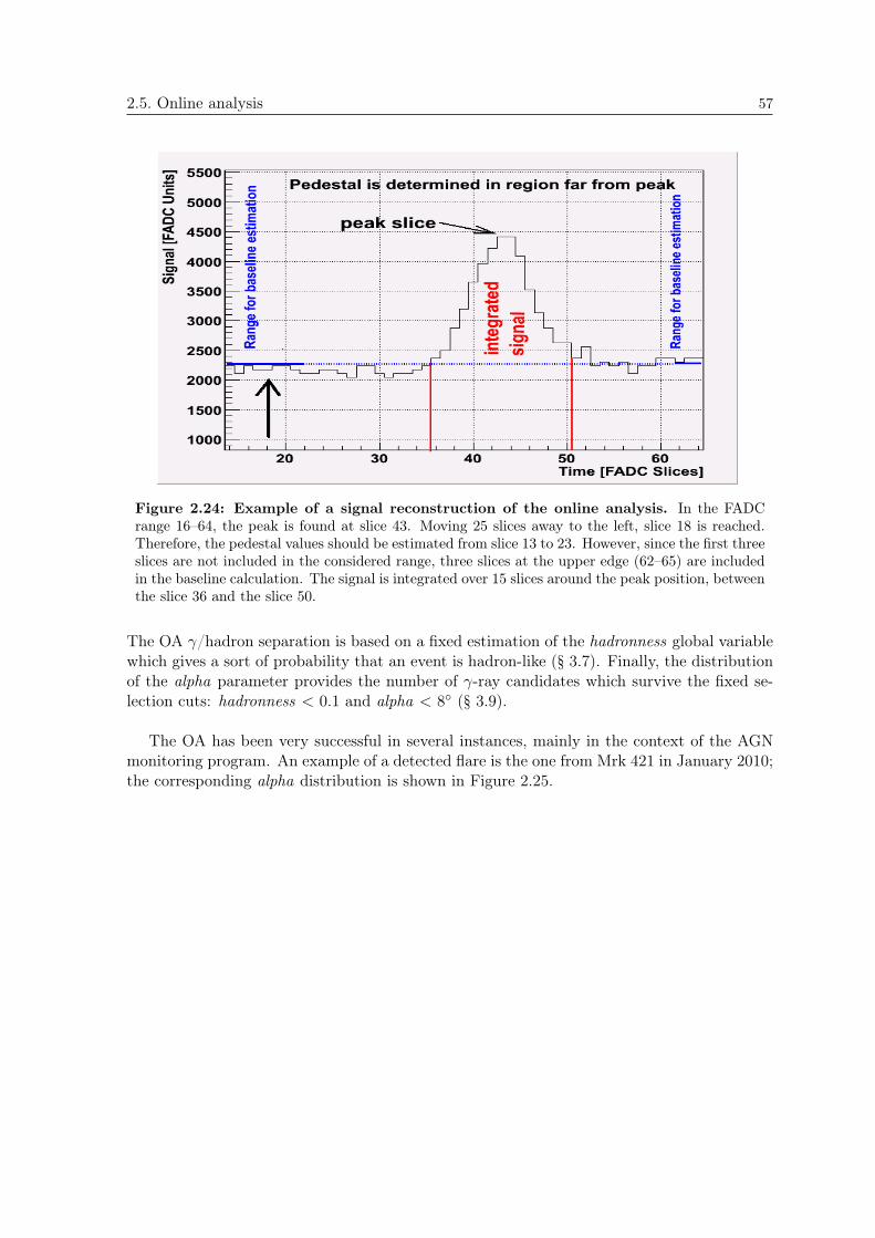
2.5. Online analysis 57
Figure 2.24: Example of a signal reconstruction of the online analysis. In the FADCrange 16–64, the peak is found at slice 43. Moving 25 slices away to the left, slice 18 is reached.Therefore, the pedestal values should be estimated from slice 13 to 23. However, since the first threeslices are not included in the considered range, three slices at the upper edge (62–65) are includedin the baseline calculation. The signal is integrated over 15 slices around the peak position, betweenthe slice 36 and the slice 50.
The OA /hadron separation is based on a fixed estimation of the hadronness global variablewhich gives a sort of probability that an event is hadron-like (§ 3.7). Finally, the distributionof the alpha parameter provides the number of -ray candidates which survive the fixed se-lection cuts: hadronness < 0.1 and alpha < 8 (§ 3.9).
The OA has been very successful in several instances, mainly in the context of the AGNmonitoring program. An example of a detected flare is the one from Mrk 421 in January 2010;the corresponding alpha distribution is shown in Figure 2.25.

58 2. THE MAGIC TELESCOPES
Figure 2.25: Example of an alpha distribution produced by the online analysis. It showsa flare of the AGN Mrk 421 occurred in January 2010.

3The MAGIC standard analysis chain
The software for the standard MAGIC data analysis, MARS, is programmed in theROOT environment. Several executables take care for the various analysis steps, fromsignal reconstruction and calibration to identification, and the spatial, spectral andtemporal characterization of -ray sources. This chapter will describe the standardanalysis chain for the analysis of both mono and stereo data with a special emphasison their differences.The author contributed in the development of the software for the stereoscopicanalysis. Part of this work is described in Carmona, E., et al. 2011.
The software of the MAGIC collaboration is named MARS, acronym of MAGIC Analysisand Reconstruction Software (Moralejo, A., et al., 2009). It is a collection of object-orientedprograms written in C++ programming language. They make use of classes and libraries ofthe ROOT1 software framework.
Several consecutive steps form the standard analysis chain. They are represented in theflow diagram shown in Figure 3.1:
• Reconstruction of the Cherenkov pulses in each PMT of the camera, and theircalibration into number of photo-electrons (ph.e.). The corresponding program iscalled callisto.
• Image cleaning removing pixels which contain noise, and calculation of image pa-rameters. The corresponding program is called star.
• Merging the data streams from two telescopes and calculation of the stereo param-eters. The corresponding program is called superstar.
• Training for /hadron separation, and energy estimation, and production of thecorresponding matrices. The program, called coach, needs a sample of simulated MC -ray events and a sample of background events taken from real data.
1ROOT is a software framework developed at CERN and originally designed for particle physics analysis.It is available at http://root.cern.ch.
59

60 3. THE MAGIC STANDARD ANALYSIS CHAIN
Figure 3.1: Flow diagram of the MAGIC standard analysis chain.
• Application of the γ/hadron separation and energy estimation matrices tosignal data, background data and a test sample of simulated MC γ-ray events. Thecorresponding program is called melibea.
• Determination of the statistical significance of the γ-ray signal. The corre-sponding program is called odie.
• Computation of the differential energy spectrum and light curve. The corre-sponding program is called fluxlc.
• Unfolding of the energy spectrum in order to correct for the finite energy resolutionof the instrument. The program is called unfolding.

3.1. Monte Carlo simulations 61
3.1 Monte Carlo simulations
The MAGIC analysis chain relies on MC simulation of -ray events. Since the backgroundrate in real data is 104 times larger than the -ray rate in a typical TeV source, real data areessentially made up of background events. Simulated -ray images are compared to imagesproduced by real cosmic rays in order to discriminate among them which ones are -ray can-didates. Nevertheless, also protons and He++ ions events can be simulated, and are used forspecific purposes, such as performance studies (Aleksic J., et al., 2011b).
The MC software used in MAGIC is divided into three stages:
• Shower simulation. The CORSIKA 6.019 program (Heck, D. et al., 1998) simulatesEAS initiated by VHE -rays or hadrons. In particular, it uses the EGS4 code forelectromagnetic shower generation and QGSJET-II and FLUKA for respectively high-and low-energy hadronic shower generation. The Cherenkov photons produced in thesimulated showers and reaching the ground in the vicinity of the telescope are savedinto disk. The CORSIKA program models the atmosphere using the so-called UnitedStates (US) standard atmosphere.
• Simulation of photon absorption and reection in the telescope reectingsurface. This stage accounts for the Cherenkov light absorption and scattering inthe atmosphere. The standard US atmospheric model is considered to account for theRayleigh scattering. The effect of Mie scattering losses is calculated using the Eltermanmodel (Elterman, 1964) for the distribution of aerosols and ozone. This second stagealso simulates the reflection of the Cherenkov photons on the reflector dish to obtaintheir arrival directions and times on the camera plane. One of the input of the programis the mirror reflectivity discussed in § 2.2.3.
• Simulation of the telescope photo-detectors and electronics. The incomingdirections of the Cherenkov photons are smeared out according to the optical PSF(§ 2.2.3). This task clearly belongs to the previous stage, but it is performed here tomake the simulation more flexible. Finally the simulation of the response of the PMTs,trigger and data acquisition electronics allows to produce the final Cherenkov images.It considers noise levels (electronic noise and night sky background light) as measuredin real data.
Further details about MC simulations can be found in Majumdar, P. et al. (2005).Theoutput files have the same format of the raw data files. Thus, they can be analyzed accordingto the standard analysis chain in the MARS framework.
The standard MC production simulates -ray events coming from a point-like source witha power-law spectrum. Nevertheless, there are specific MC productions for diffuse -rayemission. The latter is necessary for the study of extended sources.
In this thesis work, different MC samples for point-like sources are used. They accountfor the varying performance of the instrument over the years (due both to hardware upgradesand aging effects), and the different observation modes (§ 2.3.3).

62 3. THE MAGIC STANDARD ANALYSIS CHAIN
3.2 Conversion into ROOT format and merging of control data stream
The first step of the analysis chain converts raw data files to ROOT files which can betreated within the MARS and ROOT frameworks. At the same time, the report files (2.4)are synchronized and merged with the data events. From this point on, all the informationthat the subsystems send to the CC program during data-taking (§ 2.2) can be easily accessedfrom the data files.
3.3 Signal reconstruction and calibration
Data contain the sampling of the triggered pulses which are digitized by ultra-fast 2GSample/sFADC. The recorded signals are sampled in 80 FADC time slices, but MAGIC I MUX DAQstores only 50 samples, since the others contain only “switching noise”. The analysis of thesesamples, called signal extraction, provides the signal arrival time, its amplitude and intensityin FADC counts. Afterwards, a calibration procedure converts the arbitrary units, FADCcounts, to equivalent ph.e. which are proportional to the Cherenkov photons. MAGIC IIdata are first corrected for the non-linear response of the DRS2 chip (§ 2.2.6).
Several algorithms were studied within the MAGIC collaboration to optimize the signalextraction (Albert, J., et al., 2008b), but only the standard ones are used in this thesis work:the “digital filter” for MAGIC I pre-MUX data (digitized by FADC at 300 MSample/s, referto § 2.2.6 for more detailed information), the “cubic spline extractor” for MAGIC I MUX data,and the “sliding window” for MAGIC II data (digitized at 2 GSample/s).
• Digital filter: it performs a fit of the Cherenkov digitized pulse to a standard pre-defined pulse form. This procedure outputs a signal amplitude, a signal integral, anda signal arrival time. This method works properly only if the signal shape is constant.This explains why this algorithm was dropped after the upgrade of MAGIC I readoutto the MUX system, which no longer requires artificial shaping and stretching of digitalsignals (§ 2.2.6).
• Cubic spline extractor: it interpolates the pedestal subtracted samples with a cubic-spline curve. Afterwards, it looks for the maximum of the interpolation function repre-senting the signal amplitude. The signal intensity in FADC counts is obtained as thespline integral in a window of fixed size with variable integration limits which dependon the maximum position. The signal arrival time is defined as the position of the halfmaximum at the rising edge of the pulse.
• Sliding window extractor: it searches for the maximum integral content of a numberof consecutive FADC slices inside a defined time range (global window). The signalarrival time is the average of the FADC slices time, weighted over the FADC slicecontents.
Once the signal is reconstructed, the charge, in FADC counts, is converted into the number ofph.e. arriving at the first dynode of the PMT. This conversion is performed through the F-factor method (Mirzoyan, R., 1997) which uses calibration events to estimate the proportionalrelation between ph.e. and FADC counts. Calibration events are generated by short lightpulses (≡ 2 ns) with an intensity which is comparable to real Cherenkov pulses. The F-factor method assumes that the number of ph.e. per calibration event in every pixel follows
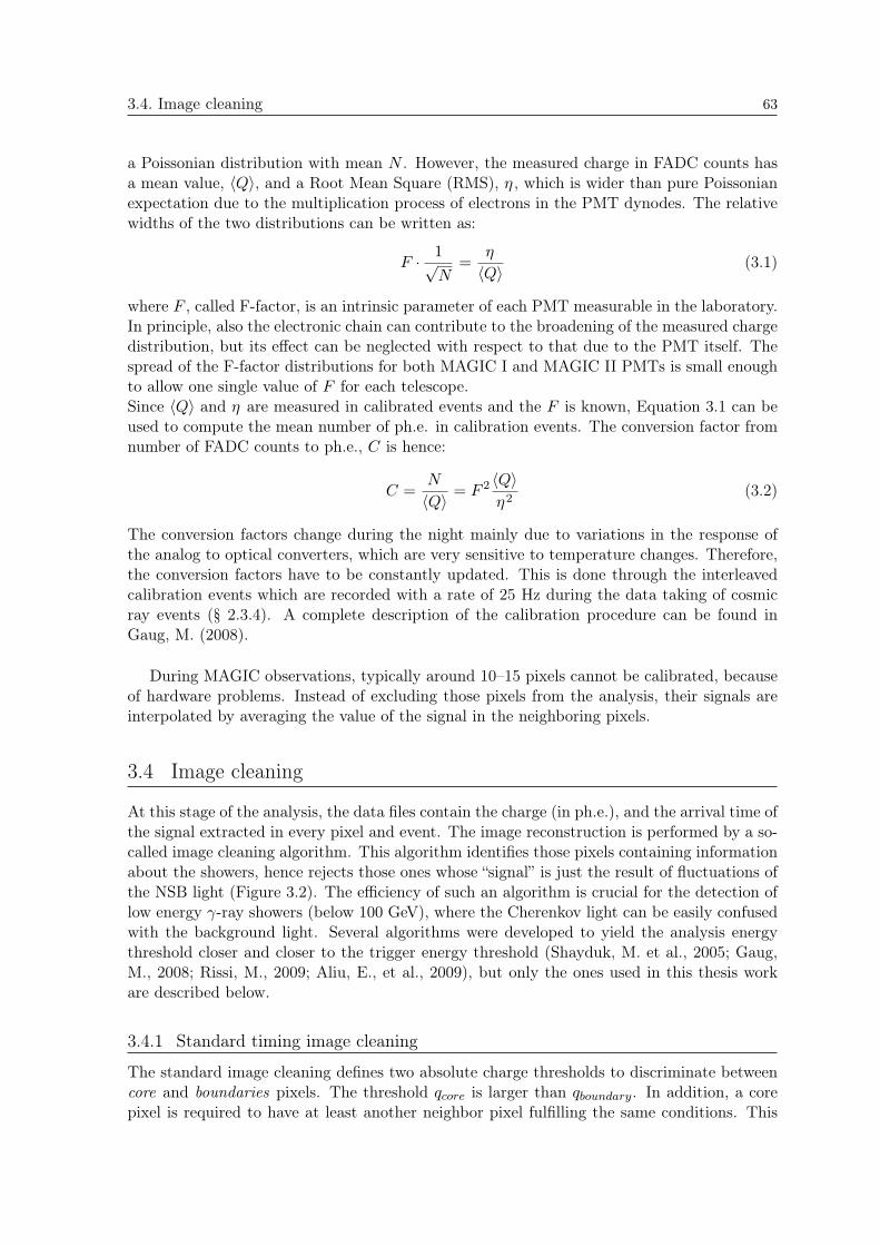
3.4. Image cleaning 63
a Poissonian distribution with mean N . However, the measured charge in FADC counts hasa mean value, hQi, and a Root Mean Square (RMS), η, which is wider than pure Poissonianexpectation due to the multiplication process of electrons in the PMT dynodes. The relativewidths of the two distributions can be written as:
F ·1pN
=η
hQi(3.1)
where F , called F-factor, is an intrinsic parameter of each PMT measurable in the laboratory.In principle, also the electronic chain can contribute to the broadening of the measured chargedistribution, but its effect can be neglected with respect to that due to the PMT itself. Thespread of the F-factor distributions for both MAGIC I and MAGIC II PMTs is small enoughto allow one single value of F for each telescope.Since hQi and η are measured in calibrated events and the F is known, Equation 3.1 can beused to compute the mean number of ph.e. in calibration events. The conversion factor fromnumber of FADC counts to ph.e., C is hence:
C =N
hQi= F 2 hQi
η2(3.2)
The conversion factors change during the night mainly due to variations in the response ofthe analog to optical converters, which are very sensitive to temperature changes. Therefore,the conversion factors have to be constantly updated. This is done through the interleavedcalibration events which are recorded with a rate of 25 Hz during the data taking of cosmicray events (§ 2.3.4). A complete description of the calibration procedure can be found inGaug, M. (2008).
During MAGIC observations, typically around 10–15 pixels cannot be calibrated, becauseof hardware problems. Instead of excluding those pixels from the analysis, their signals areinterpolated by averaging the value of the signal in the neighboring pixels.
3.4 Image cleaning
At this stage of the analysis, the data files contain the charge (in ph.e.), and the arrival time ofthe signal extracted in every pixel and event. The image reconstruction is performed by a so-called image cleaning algorithm. This algorithm identifies those pixels containing informationabout the showers, hence rejects those ones whose “signal” is just the result of fluctuations ofthe NSB light (Figure 3.2). The efficiency of such an algorithm is crucial for the detection oflow energy -ray showers (below 100 GeV), where the Cherenkov light can be easily confusedwith the background light. Several algorithms were developed to yield the analysis energythreshold closer and closer to the trigger energy threshold (Shayduk, M. et al., 2005; Gaug,M., 2008; Rissi, M., 2009; Aliu, E., et al., 2009), but only the ones used in this thesis workare described below.
3.4.1 Standard timing image cleaning
The standard image cleaning defines two absolute charge thresholds to discriminate betweencore and boundaries pixels. The threshold qcore is larger than qboundary. In addition, a corepixel is required to have at least another neighbor pixel fulfilling the same conditions. This

64 3. THE MAGIC STANDARD ANALYSIS CHAIN
a) raw image b) arrival time
c) cleaned image (15:9 No Timing) d) cleaned image (9:4.5 No Timing)
e) cleaned image (9:4.5 Timing)
Figure 3.2: Real event recorded with MAGIC II . a) event charge and b) arrival time beforeimage cleaning. The following panels show the reconstructed image c) with a high threshold imagecleaning 15:9 without timing constraints, d) with standard image cleaning levels 9:4.5 withouttiming information, and e) with standard thresholds and timing constraints.
second requirement avoids that pixels unrelated to the image, but with large charge due to
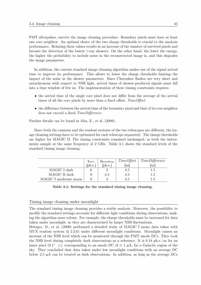
3.4. Image cleaning 65
PMT afterpulses, survive the image cleaning procedure. Boundary pixels must have at leastone core neighbor. An optimal choice of the two charge thresholds is crucial to the analysisperformance. Relaxing these values results in an increase of the number of survived pixels andfavours the detection of the lowest -ray showers. On the other hand, the lower the energy,the higher the probability to include noise in the reconstructed image is, and this degradesthe image parameters.
In addition, the current standard image cleaning algorithm makes use of the signal arrivaltime to improve its performance. This allows to lower the charge thresholds limiting theimpact of the noise in the shower parameters. Since Cherenkov flashes are very short andasynchronous with respect to NSB light, arrival times of shower-produced signals must fallinto a time window of few ns. The implementation of these timing constraints requires:
• the arrival time of the single core pixel does not differ from the average of the arrivaltimes of all the core pixels by more than a fixed offset, TimeOffset
• the difference between the arrival time of the boundary pixel and that of its core neighbordoes not exceed a fixed TimeDifference.
Further details can be found in Aliu, E., et al. (2009).
Since both the cameras and the readout systems of the two telescopes are different, the im-age cleaning settings have to be optimized for each telescope separately. The charge thresholdsare higher for MAGIC II. The timing constraints remained unchanged, as both the instru-ments sample at the same frequency of 2 GHz. Table 3.1 shows the standard levels of thestandard timing image cleaning.
qcore qboundary TimeOffset TimeDifference[ph.e.] [ph.e.] [ns] [ns]
MAGIC I dark 6 3 4.5 1.5MAGIC II dark 9 4.5 4.5 1.5
MAGIC I moderate moon 8 4 4.5 1.5
Table 3.1: Settings for the standard timing image cleaning.
Timing image cleaning under moonlight
The standard timing image cleaning provides a stable analysis. Moreover, the possibility tomodify the standard settings accounts for different light conditions during observations, mak-ing the algorithm more robust. For example, the charge thresholds must be increased for datataken under moonlight, as they are characterized by larger NSB fluctuations.Britzger, D., et al. (2009) performed a detailed study of MAGIC I mono data taken withMUX readout system (§ 2.2.6) under different moonlight conditions. Moonlight causes anincrease of the NSB level which can be monitored through the PMT anode DCs. They tookthe NSB level during completely dark observations as a reference. It is 0.18 ph.e./ns for aninner pixel (0.1 ), corresponding to an anode DC of ≡ 1 µA, for a Galactic region of thesky. They concluded that data taken under low moonlight conditions with an average DCbelow 2.5 µA can be treated as dark observations. In addition, as long as the average DCs

66 3. THE MAGIC STANDARD ANALYSIS CHAIN
does not exceed 4 µA, the standard timing image cleaning, with higher charge thresholds forcore and boundary pixels, allows to use the standard MC, and no correction in the MC isneeded. The charge thresholds they suggested for this moderate moonlight conditions are 8and 4 for core and boundary pixels respectively.
A similar study on stereoscopic observations is ongoing at the moment of writing thisthesis. The description of these preliminary results goes, however, beyond the purpose of thissection, since none of the stereo analyses presented in this thesis work is characterized bymoon light conditions.
3.4.2 Sum image cleaning
The sum image cleaning is based on the definition of core and boundary pixels depending ontheir charge levels (qcore > qboundary) as the standard timing image cleaning does. However,it introduces more constraints taking advantage from the compactness in time and extensionof the Cherenkov images. These additional constraints allow to lower the charge thresholds.A core pixel has to lie within a compact group of x next neighbor (x-NN) pixels, where x isequal to 2, 3 or 4, and the total clipped charge of the x-NN group of pixels has to exceed thethreshold of the corresponding group, QxNN
th . This so-called “clipping” procedure2 is applied inorder to prevent large accidental signals (essentially PMT afterpulses) to dominate the chargein an x-NN group. Both clipping levels and summed thresholds are defined in terms of qcore:
QxNNth = SxNN
th ·x · qcore (3.3)
QclipxNN = CxNN ·QxNNth
x(3.4)
In this way the optimization of the setting parameters SxNNth and CxNN is independent from
the noise level (both electronic and NSB light), hence it is independent from the telescope. Inaddition, the arrival time of a core pixel has to fall within a time window, txNN (different foreach multiplicity), from the mean arrival time of the corresponding x-NN group. Boundarypixels are defined like in the standard timing image cleaning. Table 3.2 shows the values ofthe parameters used in this thesis work.
xNN qcore qboundary CxNN SxNNth txNN tboundary
[ ph.e.] [ ph.e.] [ns] [ns]2NN 2.20 1.8 0.9
MAGIC I 3NN 4 3 1.05 1.3 1.2 1.54NN 1.05 0.7 1.92NN 2.20 1.8 0.9
MAGIC II 3NN 7 4 1.05 1.3 1.2 1.53NN 1.05 0.7 1.9
Table 3.2: Settings for the sum image cleaning.
Generally the sum image cleaning recovers more pixels than the standard one. This is animportant aspect in the reconstruction of low energy -ray images which contain only fewpixels. In fact, this algorithm below 100 GeV is more efficient than the standard timing imagecleaning (§ 5.2.1).
2Signal clipping means limiting the signal amplitude below a certain level.

3.5. Parameter reconstruction 67
3.5 Parameter reconstruction
The pixels which survived to the image cleaning procedure form the reconstructed showerimage, i.e. the Cherenkov light distribution on the camera plane. For further analysis, everyimage is now parametrized by a set of parameters describing its shape, orientation and alsotiming properties. Image parameters are classified according to their function:
• Hillas parameters, computed as image moments up to the second order (Hillas, A. M.,1985) are strictly related to physics of EASs. Figure 3.3 gives a graphical idea of someparameters described below.
– Size: total charge, in ph.e., contained inthe image. It is related to the energy of theprimary γ-ray initiating the shower (Fig-ure 3.4).
– Width: the RMS spread of the light alongthe minor axis of the ellipse image. Itrelated to the lateral distribution of theshower.
– Length: the RMS spread of the lightalong the major axis of the ellipse image.It related to the projection of the showerlongitudinal development.
Figure 3.3: Sketch showing the def-inition of some image parameters.Taken from Albert, J., et al. 2008d.
– Conc(N): fraction of the image charge which is contained in the N brightestpixels. The image compactness which tends to be larger for γ-induced showers.From now on, conc will stand for conc(2), which is the one generally used.
Figure 3.4: Correlation between the size and the energy image parameters.
• Source dependent parameters still have a physical interpretation, but they are separatedfrom the previous class because of their dependence from the expected source position.
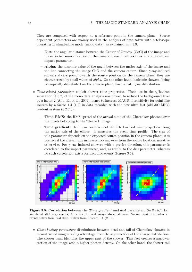
68 3. THE MAGIC STANDARD ANALYSIS CHAIN
They are computed with respect to a reference point in the camera plane. Sourcedependent parameters are mainly used in the analysis of data taken with a telescopeoperating in stand-alone mode (mono data), as explained in § 3.9.
– Dist: the angular distance between the Center of Gravity (CoG) of the image andthe expected source position in the camera plane. It allows to estimate the showerimpact parameter.
– Alpha: the absolute value of the angle between the major axis of the image andthe line connecting the image CoG and the camera center. Since γ-ray-inducedshowers always point towards the source position on the camera plane, they arecharacterized by small values of alpha. On the other hand, hadronic showers, beingisotropically distributed on the camera plane, have a flat alpha distribution.
• Time-related parameters exploit shower time properties. Their use in the γ/hadronseparation (§ 3.7) of the mono data analysis was proved to reduce the background levelby a factor 2 (Aliu, E., et al., 2009), hence to increase MAGIC I sensitivity for point-likesources by a factor 1.4 (1.2) in data recorded with the new ultra fast (old 300 MHz)readout system (§ 2.2.6).
– Time RMS: the RMS spread of the arrival time of the Cherenkov photons overthe pixels belonging to the “cleaned” image.
– Time gradient: the linear coefficient of the fitted arrival time projection alongthe major axis of the ellipse. It measures the event time profile. The sign ofthis parameter depends on the expected source position in the camera plane: it ispositive if the arrival time increases moving away from the source location, negativeotherwise. For γ-ray induced showers with a precise direction, this parameter iscorrelated to the impact parameter, and, as result, to the dist parameter, whereasno such correlation exists for hadronic events (Figure 3.5).
Figure 3.5: Correlation between the Time gradient and dist parameter. On the left: forsimulated MC γ-ray events; At center: for real γ-ray-induced showers; On the right: for hadronicevents taken from real data. Taken from Tescaro, D. (2010).
• Ghost-busting parameters discriminate between head and tail of Cherenkov showers inreconstructed images taking advantage from the asymmetries of the charge distribution.The shower head identifies the upper part of the shower. This fact creates a narrowersection of the image with a higher photon density. On the other hand, the shower tail

3.5. Parameter reconstruction 69
generates a broader and sparser image section which follows the increase of the showerlateral development.
– Asymmetry: the signed distance between the image CoG and the pixel with thehighest content. It is positive when the shower head is closer to the camera centerthan the cascade tail.
– M3Long: the third moment of the image along its major axis. The sign of thisparameter follows the same convention as the asymmetry one.
• Image quality parameters allow an estimation of the image reconstruction accuracy.
– LeakageN : the fraction of the shower light con-tained in the N outermost rings of pixels in thecamera. Unless explicitly specified, only leakage1will be considered. Images with large leakage arelikely to be truncated, and this fact has to betaken into account during the estimation of theenergy of the primary -ray.
– Number of islands: the number of separatedgroups of pixels which survive the image cleaningprocedure (Figure 3.6).
Figure 3.6: Example of athree islands event.
3.5.1 Stereo parameter reconstruction
Up to this section the described analysis code runs over the data of each telescope separately.At this point, there are two sets of data containing the same events from two different pointsof view. The task of the next analysis step consists of combining in one data set the matchingpairs of events. At the same time, stereoscopic parameters, giving a 3-dimensional event de-scription, are computed. Refer to Kohnle, A., et al. (1996) for a detailed description of theseparameters.
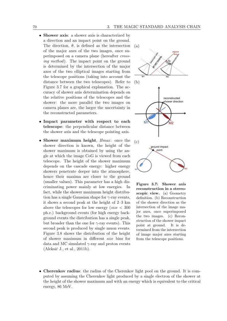
70 3. THE MAGIC STANDARD ANALYSIS CHAIN
• Shower axis: a shower axis is characterized bya direction and an impact point on the ground.The direction, θ, is defined as the intersectionof the major axes of the two images, once su-perimposed on a camera plane (hereafter cross-ing method). The impact point on the groundis determined by the intersection of the majoraxes of the two elliptical images starting fromthe telescope positions (taking into account thedistance between the two telescopes). Refer toFigure 3.7 for a graphical explanation. The ac-curacy of shower axis determination depends onthe relative positions of the telescopes and theshower: the more parallel the two images oncamera planes are, the larger the uncertainty inthe reconstructed parameters.
• Impact parameter with respect to eachtelescope: the perpendicular distance betweenthe shower axis and the telescope pointing axis.
• Shower maximum height, Hmax : once theshower direction is known, the height of theshower maximum is obtained by using the an-gle at which the image CoG is viewed from eachtelescope. The height of the shower maximumdepends on the cascade energy: higher energyshowers penetrate deeper into the atmosphere,hence their maxima are closer to the ground(smaller values). This parameter has a high dis-criminating power mainly at low energies. Infact, while the shower maximum height distribu-tion has a single Gaussian shape for γ-ray events,it shows a second peak at the height of 2–3 kmabove the telescopes for low energy (size < 300ph.e.) background events (for high energy back-ground events the distribution has a single peak,but broader than the one for γ-ray events). Thissecond peak is produced by single muon events.Figure 3.8 shows the distribution of the heightof shower maximum in different size bins fordata and MC simulated γ-ray and proton events(Aleksic J., et al., 2011b).
(a)
(b)
(c)
Figure 3.7: Shower axisreconstruction in a stereo-scopic view. (a) Geometrydefinition. (b) Reconstructionof the shower direction as theintersection of the image ma-jor axes, once superimposedthe two images. (c) Recon-struction of the shower impactpoint at ground. It is de-termined from the intersectionof image major axes startingfrom the telescope positions.
• Cherenkov radius: the radius of the Cherenkov light pool on the ground. It is com-puted by assuming the Cherenkov light produced by a single electron of the shower atthe height of the shower maximum and with an energy which is equivalent to the criticalenergy, 86 MeV.

3.6. Data quality checks 71
• Cherenkov photon density: the photon density on the ground. It is evaluated underthe same assumptions done for the previous parameter.
Figure 3.8: Shower maximum height distributions for different size bins for MC rays(dotted line), MC protons (full circles), and real data (solid line). size is expressed in ph.e.. Takenfrom Aleksic J., et al. (2011b).
3.6 Data quality checks
At this stage, the data files contain all the image parameters needed for the following analysissteps which lead to the signal detection and flux estimation. In order to guarantee stable andsolid results, it is important to perform some checks on the data quality, and eventually reject“bad” data. The data quality can be affected by weather, hardware failures, and cars passingat the MAGIC site (car lights produce a rapid increase of the trigger rate for few seconds).
Most of the bad quality data are due to the atmospheric conditions during data taking. Infact, the transparency of the atmosphere to Cherenkov light is inversely proportional to thequantity of aerosols and aqueous vapors in the sky depending on the presence of clouds orcalima3: the higher the density, the lower the rate of cosmic-ray events detected at ground.
Despite the fact that, for safety reasons, -ray ground-based telescopes do not observewhen the weather is bad, the range of allowed atmospheric conditions is wide. This obliges usto define oine data selection criteria which guarantee a data sample with good and constantquality. These criteria are mainly based on Cloudiness (§ 2.2.9) and rate of analyzed events(“analysis rate”, after the image cleaning) scaled with the Zenith Angle (ZA). These twovariables are not directly correlated because the automatic IPR control (§ 2.4.4) changes theDT levels in order to keep the trigger rate as much constant as possible (§ 2.4.4), and thisaffects the telescope’s trigger threshold. In order to compute the correct data quality cuts,it is important to scale the rate dependence on the ZA. The trigger rate, and the analysisrate, decrease with increasing ZA for the following reason. The larger the ZA, the thickerthe atmosphere along the path of the shower so the shower develops further away from thetelescope and the area illuminated on the ground is larger. On one hand, this implies a largerdetection area; on the other hand, it means that the density of the light which reaches thetelescope reflector is lower. The empirical rate-ZA relation follows (Figure 3.9):
rate = rate0 ·p
cosZA; (3.5)
3Calima is the high-altitude, ultra-thin Saharan dust transported by the wind from Africa.

72 3. THE MAGIC STANDARD ANALYSIS CHAIN
where rate0 is the rate at zenith.Generally, the data selection criteria are:
• cloudiness < 50%
• analysis rate within 20% of the mean value. This condition is first applied to databelonging to the same observation night in order to discard sporadic rate changes, dueto cars or fast moving clouds. Later it is used for night-by-night observations in orderto keep the rate of the entire data sample constant.
The range of the allowed parameters may depend on the goal of the analysis. For instance, astudy of the flux variability of a new discovered source requires more stringent data selectioncuts in order to prevent changing atmospheric conditions to induce fake variations of thesource flux.
Figure 3.9: Empirical relation between rate and zenith angle.
The use of meteorological instruments (pyrometers, lidars...) during the γ-ray observationsmay help to quantify the effect of the atmospheric conditions on the data, and, as a result,to correct for it. At the moment, the only instrument available for the controlling of theatmosphere is a pyrometer. It provides a rough estimation of the sky quality evaluating thecloudiness parameter. While this information is sufficient to perform a data quality check, itcannot be used for the data correction and, for this reason, an elastic lidar is currently beingcommissioned at the MAGIC site.
3.7 γ /hadron separation
An IACT triggers on three different kinds of events:
• accidental triggers, mainly fluctuations of the signal due to background light, such asthe NSB light, Moon light, or cars driving near the telescopes.
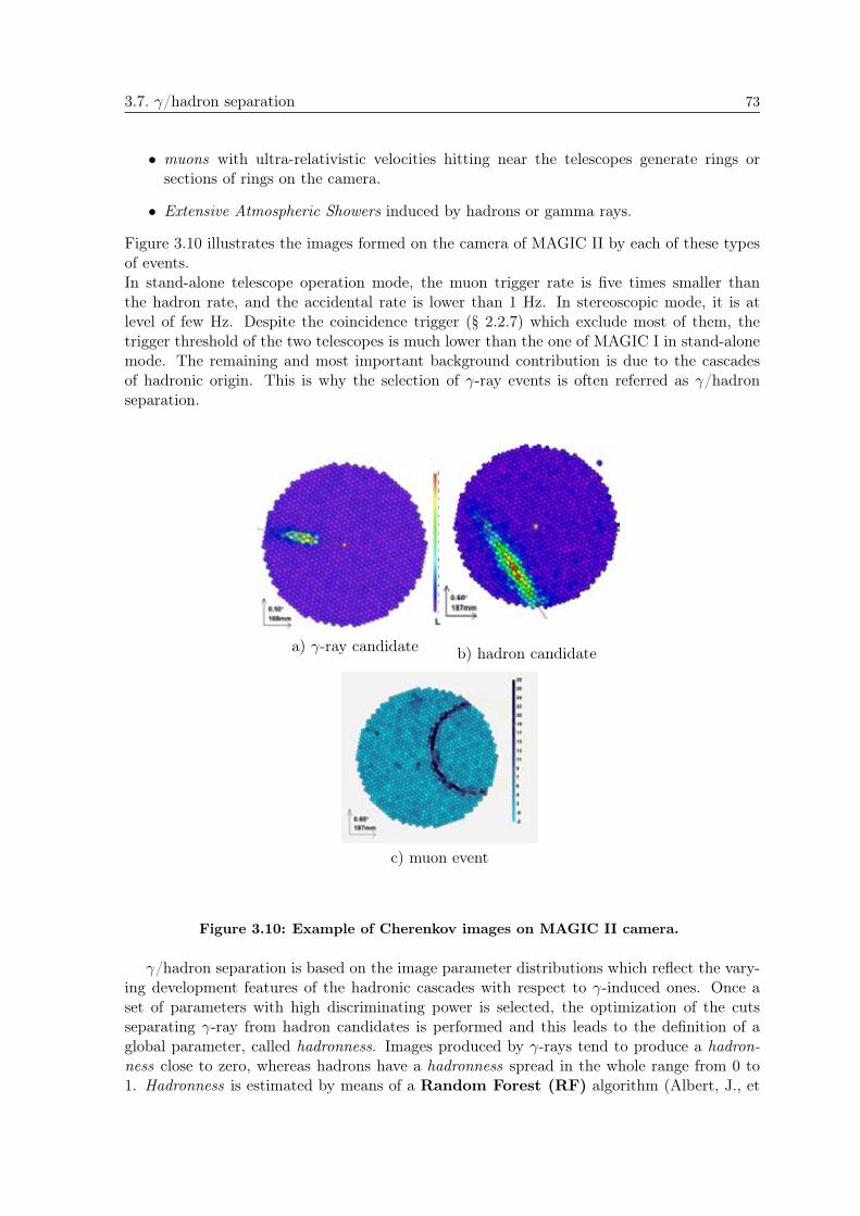
3.7. γ/hadron separation 73
• muons with ultra-relativistic velocities hitting near the telescopes generate rings orsections of rings on the camera.
• Extensive Atmospheric Showers induced by hadrons or gamma rays.
Figure 3.10 illustrates the images formed on the camera of MAGIC II by each of these typesof events.In stand-alone telescope operation mode, the muon trigger rate is five times smaller thanthe hadron rate, and the accidental rate is lower than 1 Hz. In stereoscopic mode, it is atlevel of few Hz. Despite the coincidence trigger (§ 2.2.7) which exclude most of them, thetrigger threshold of the two telescopes is much lower than the one of MAGIC I in stand-alonemode. The remaining and most important background contribution is due to the cascadesof hadronic origin. This is why the selection of γ-ray events is often referred as γ/hadronseparation.
a) γ-ray candidate b) hadron candidate
c) muon event
Figure 3.10: Example of Cherenkov images on MAGIC II camera.
γ/hadron separation is based on the image parameter distributions which reflect the vary-ing development features of the hadronic cascades with respect to γ-induced ones. Once aset of parameters with high discriminating power is selected, the optimization of the cutsseparating γ-ray from hadron candidates is performed and this leads to the definition of aglobal parameter, called hadronness. Images produced by γ-rays tend to produce a hadron-ness close to zero, whereas hadrons have a hadronness spread in the whole range from 0 to1. Hadronness is estimated by means of a Random Forest (RF) algorithm (Albert, J., et

74 3. THE MAGIC STANDARD ANALYSIS CHAIN
al., 2008c), a multi-dimensional classification system based on the construction of decisionaltrees. This is the most commonly used procedure for /hadron separation within the MAGICcollaboration, and also the most effective one according to Bock, R. K., et al. (2004).
The RF is first trained with events of known nature, i.e. MC simulated -ray eventsand hadron events extracted randomly from off data (§ 2.3.3). In order to avoid artifactsin the training, events in the hadron sample are selected in such a way that the shape oftheir size and ZA distributions matches that of the MC sample. RF uses a set of N highdiscriminating parameters to construct a large number (default 100) of decisional trees. Ifevery parameter is considered as 1-dimensional vector, all the events are contained in anN-dimensional hypercube. A decisional tree grows as follows: once a starting point in thehypercube, and a starting parameter are selected at random, RF finds out the cut of theparameter which better separates both samples. The N-dimensional space is divided intotwo parts, called branches. The procedure is then repeated iteratively (another parameteris chosen, the corresponding optimized cut is selected, and the subsample split) so that thenumber of branches increases. The algorithm stops when a subsample composed only by oneof the two initial categories of events (gammas or hadrons) is found; thus, the ending leaf ofthe tree is reached and it is labeled as 0 or 1 depending if it contains gamma or hadron events.The cut optimization is obtained by minimizing the Gini index (Gini, C., 1921). This indexis expressed in terms of number of gammas, N , number of hadronic events, Nbg, and totalnumber of events, N , in the tree:
QGini = 4 ·N
N·Nbg
N(3.6)
Minimizing the Gini index corresponds to minimize the variance of the populations of -rayand hadronic events.
The application of the RF trees to the data sample to be analyzed constitutes the effective /hadron separation. Each real event has to pass through all the separating trees. For eachtree the event is assigned with a value, 0 or 1, according to its characteristic parameter valuesand subsequently to the reached ending leaf. The average of all the obtained values overthe N trained trees defines the hadronness. A hadronness distribution for background, andsimulated MC -ray events is illustrated in Figure 3.11.
This -ray efficiency, , is defined as the fraction of simulated MC -ray events betweenthe number of events surviving all the analysis cuts, N aftercuts , and the total number ofproduced events, N total :
=N aftercuts
N total
(3.7)
The harder the cut, the better the background rejection, and the lower the gamma efficiency.Hard cuts are used for the search for signals where the gamma efficiency is not important.
3.8 Determination of the arrival direction: the Disp method
The arrival direction of the primary gamma ray can be determined in a rather straight-forwardway in case of arrays of IACTs (§ 3.5.1), but requires a complex method based on MC simula-tions in case of stand-alone IACTs. It is the so-called Disp method, proposed by Fomin, V. P.,
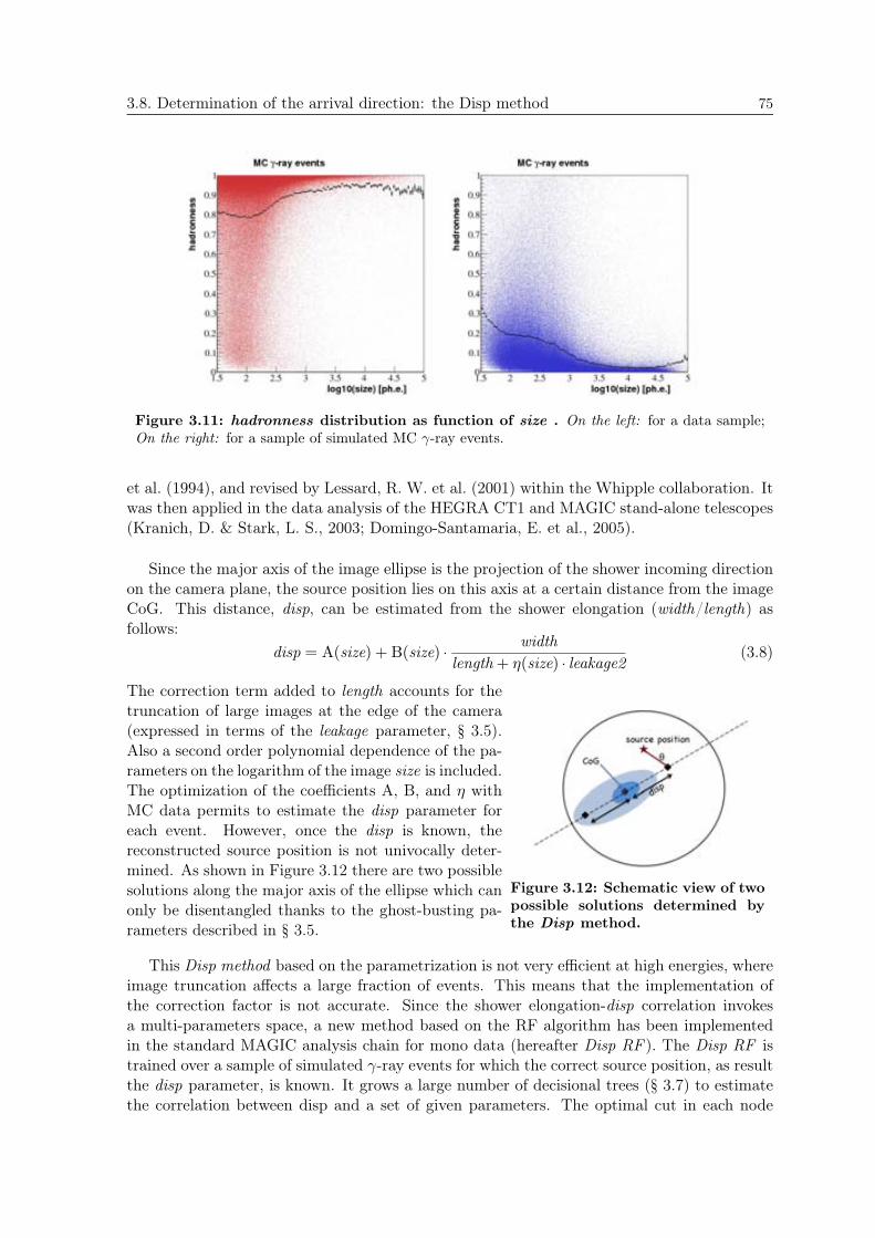
3.8. Determination of the arrival direction: the Disp method 75
Figure 3.11: hadronness distribution as function of size . On the left: for a data sample;On the right: for a sample of simulated MC γ-ray events.
et al. (1994), and revised by Lessard, R. W. et al. (2001) within the Whipple collaboration. Itwas then applied in the data analysis of the HEGRA CT1 and MAGIC stand-alone telescopes(Kranich, D. & Stark, L. S., 2003; Domingo-Santamaria, E. et al., 2005).
Since the major axis of the image ellipse is the projection of the shower incoming directionon the camera plane, the source position lies on this axis at a certain distance from the imageCoG. This distance, disp, can be estimated from the shower elongation (width/length) asfollows:
disp = A(size) + B(size) ·width
length + η(size) · leakage2(3.8)
The correction term added to length accounts for thetruncation of large images at the edge of the camera(expressed in terms of the leakage parameter, § 3.5).Also a second order polynomial dependence of the pa-rameters on the logarithm of the image size is included.The optimization of the coefficients A, B, and η withMC data permits to estimate the disp parameter foreach event. However, once the disp is known, thereconstructed source position is not univocally deter-mined. As shown in Figure 3.12 there are two possiblesolutions along the major axis of the ellipse which canonly be disentangled thanks to the ghost-busting pa-rameters described in § 3.5.
Figure 3.12: Schematic view of twopossible solutions determined bythe Disp method.
This Disp method based on the parametrization is not very efficient at high energies, whereimage truncation affects a large fraction of events. This means that the implementation ofthe correction factor is not accurate. Since the shower elongation-disp correlation invokesa multi-parameters space, a new method based on the RF algorithm has been implementedin the standard MAGIC analysis chain for mono data (hereafter Disp RF ). The Disp RF istrained over a sample of simulated γ-ray events for which the correct source position, as resultthe disp parameter, is known. It grows a large number of decisional trees (§ 3.7) to estimatethe correlation between disp and a set of given parameters. The optimal cut in each node
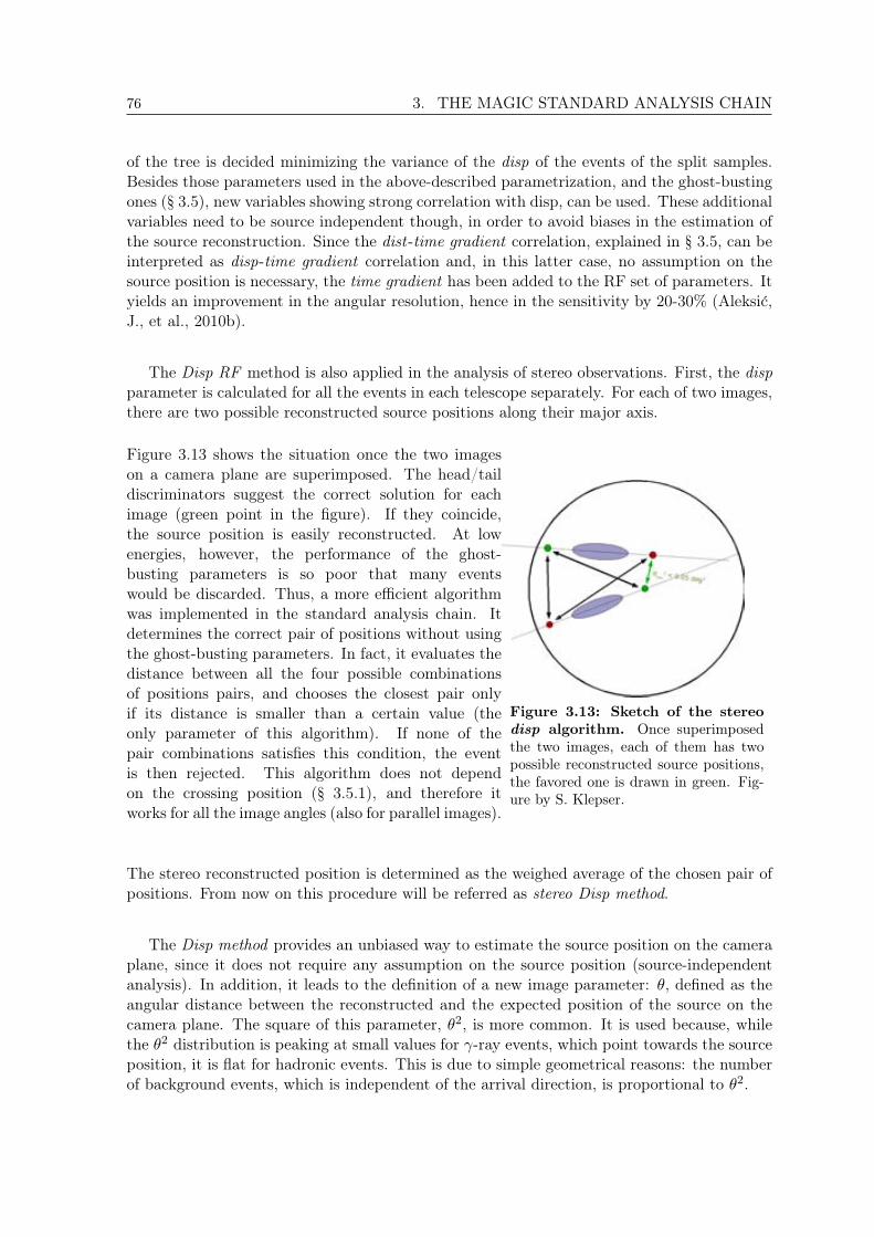
76 3. THE MAGIC STANDARD ANALYSIS CHAIN
of the tree is decided minimizing the variance of the disp of the events of the split samples.Besides those parameters used in the above-described parametrization, and the ghost-bustingones (§ 3.5), new variables showing strong correlation with disp, can be used. These additionalvariables need to be source independent though, in order to avoid biases in the estimation ofthe source reconstruction. Since the dist-time gradient correlation, explained in § 3.5, can beinterpreted as disp-time gradient correlation and, in this latter case, no assumption on thesource position is necessary, the time gradient has been added to the RF set of parameters. Ityields an improvement in the angular resolution, hence in the sensitivity by 20-30% (Aleksic,J., et al., 2010b).
The Disp RF method is also applied in the analysis of stereo observations. First, the dispparameter is calculated for all the events in each telescope separately. For each of two images,there are two possible reconstructed source positions along their major axis.
Figure 3.13 shows the situation once the two imageson a camera plane are superimposed. The head/taildiscriminators suggest the correct solution for eachimage (green point in the figure). If they coincide,the source position is easily reconstructed. At lowenergies, however, the performance of the ghost-busting parameters is so poor that many eventswould be discarded. Thus, a more efficient algorithmwas implemented in the standard analysis chain. Itdetermines the correct pair of positions without usingthe ghost-busting parameters. In fact, it evaluates thedistance between all the four possible combinationsof positions pairs, and chooses the closest pair onlyif its distance is smaller than a certain value (theonly parameter of this algorithm). If none of thepair combinations satisfies this condition, the eventis then rejected. This algorithm does not dependon the crossing position (§ 3.5.1), and therefore itworks for all the image angles (also for parallel images).
Figure 3.13: Sketch of the stereodisp algorithm. Once superimposedthe two images, each of them has twopossible reconstructed source positions,the favored one is drawn in green. Fig-ure by S. Klepser.
The stereo reconstructed position is determined as the weighed average of the chosen pair ofpositions. From now on this procedure will be referred as stereo Disp method.
The Disp method provides an unbiased way to estimate the source position on the cameraplane, since it does not require any assumption on the source position (source-independentanalysis). In addition, it leads to the definition of a new image parameter: , defined as theangular distance between the reconstructed and the expected position of the source on thecamera plane. The square of this parameter, 2, is more common. It is used because, whilethe 2 distribution is peaking at small values for -ray events, which point towards the sourceposition, it is flat for hadronic events. This is due to simple geometrical reasons: the numberof background events, which is independent of the arrival direction, is proportional to 2.

3.9. Signal detection 77
3.9 Signal detection
The distributions of the image parameters alpha and 2 (called alpha plot, § 3.5, and 2 plot,§ 3.8, respectively) peak at small values for the -ray events, and flatten up for hadrons. Forthis reason, they define the geometrical space where to search for a -ray signal, defining theso-called signal region.
Choosing alpha rather than 2 depends on the kind of analysis that one wants to perform.A source-independent analysis is normally based on the 2 distribution, and employs imageparameters whose definition does not depend on an a priori known source position. The 2
is reconstructed through the unbiased Disp method (§ 3.8). Also the RF for the /hadronseparation is trained only with source-independent parameters. A source-dependent analysis,also known as alpha analysis, relies on an a priori assumption on the source position on thecamera plane, which is needed for the calculation of the alpha parameter itself. This assump-tion permits to exploit source-dependent parameters, mainly dist, as additional discriminatingvariables in the RF for the /hadron separation. In addition, the introduction of the time pa-rameters, such as the time gradient which is so strongly correlated with dist (§ 3.5), yields toa significant improvement of the analysis performance (Aliu, E., et al., 2009). Therefore, thealpha analysis is more performing than the 2 one in case of point-like sources with knownpositions and observed with a stand-alone telescope (mono data analysis). This does notapply to the stereo data analysis, which takes advantage from the powerful discriminating,source-independent stereoscopic parameters.
In searching for a -ray signal in a data sample (on data), the gamma selection cuts(mainly the hadronness cut) are applied, and the number of events within the signal region,Non, counted. Among these -ray candidate events there some with a hadronic origin. In orderto estimate the amount of these hadrons which survive all the selection cuts, an independentdata sample with no expected signal (off sample) is used. The same analysis chain and sameselection cuts as for the on data are applied to the off sample. In this way the number ofbackground events, No , in the signal region is obtained. The number of -ray events, “excessevents” Nex, is defined as the difference between Non and the scaled No :
Nex = Non · No (3.9)
where is the normalization factor between the on and the off samples. is defined asthe fraction of on events over off events in a region far away from the signal region and thedistribution tails4. To test the null hypothesis (i.e. that all the observed excess events, Nex,are compatible with background fluctuations) the Equation number 7 in Li, T.P. & Ma, Y.Q.(1983) is used. It defines the significance N:
N =p
2
Non · ln
1 +
Non
Non No
+ No · ln
(1 + )
No
Non No
1=2
(3.10)
Figure 3.14 shows an example of the strong signal coming from the Crab Nebula (detectedwith two different data samples) by using the alpha distribution and the 2 distribution.
The off data sample depends on the observation mode (§ 2.3.3). If the on data are takenin tracking mode, the off sample consists of a completely independent data sample which
4The normalization region in the alpha plot spans from 2080 , whereas in the θ2 plot from 0.10.3 .
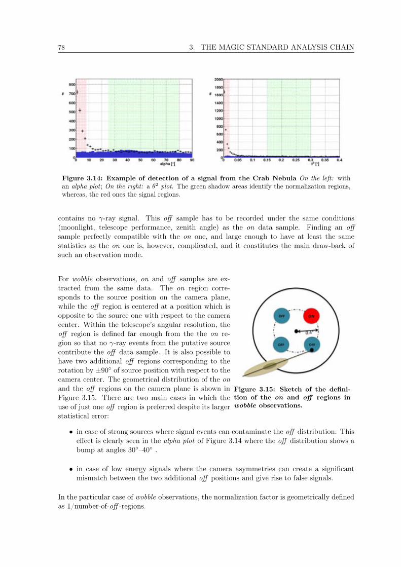
78 3. THE MAGIC STANDARD ANALYSIS CHAIN
Figure 3.14: Example of detection of a signal from the Crab Nebula On the left: withan alpha plot ; On the right: a θ2 plot. The green shadow areas identify the normalization regions,whereas, the red ones the signal regions.
contains no γ-ray signal. This off sample has to be recorded under the same conditions(moonlight, telescope performance, zenith angle) as the on data sample. Finding an offsample perfectly compatible with the on one, and large enough to have at least the samestatistics as the on one is, however, complicated, and it constitutes the main draw-back ofsuch an observation mode.
For wobble observations, on and off samples are ex-tracted from the same data. The on region corre-sponds to the source position on the camera plane,while the off region is centered at a position which isopposite to the source one with respect to the cameracenter. Within the telescope’s angular resolution, theoff region is defined far enough from the the on re-gion so that no γ-ray events from the putative sourcecontribute the off data sample. It is also possible tohave two additional off regions corresponding to therotation by ± 90of source position with respect to thecamera center. The geometrical distribution of the onand the off regions on the camera plane is shown inFigure 3.15. There are two main cases in which theuse of just one off region is preferred despite its largerstatistical error:
Figure 3.15: Sketch of the defini-tion of the on and off regions inwobble observations.
• in case of strong sources where signal events can contaminate the off distribution. Thiseffect is clearly seen in the alpha plot of Figure 3.14 where the off distribution shows abump at angles 30–40 .
• in case of low energy signals where the camera asymmetries can create a significantmismatch between the two additional off positions and give rise to false signals.
In the particular case of wobble observations, the normalization factor is geometrically definedas 1/number-of-off -regions.
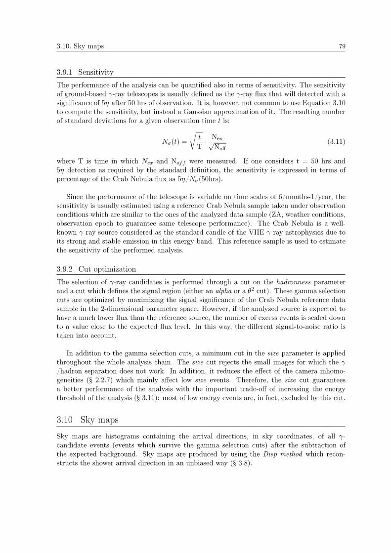
3.10. Sky maps 79
3.9.1 Sensitivity
The performance of the analysis can be quantified also in terms of sensitivity. The sensitivityof ground-based -ray telescopes is usually defined as the -ray flux that will detected with asignificance of 5η after 50 hrs of observation. It is, however, not common to use Equation 3.10to compute the sensitivity, but instead a Gaussian approximation of it. The resulting numberof standard deviations for a given observation time t is:
N(t) =
rt
T·
NexpNo
(3.11)
where T is time in which Nex and Noff were measured. If one considers t = 50 hrs and5η detection as required by the standard definition, the sensitivity is expressed in terms ofpercentage of the Crab Nebula flux as 5η/N(50hrs).
Since the performance of the telescope is variable on time scales of 6/months-1/year, thesensitivity is usually estimated using a reference Crab Nebula sample taken under observationconditions which are similar to the ones of the analyzed data sample (ZA, weather conditions,observation epoch to guarantee same telescope performance). The Crab Nebula is a well-known -ray source considered as the standard candle of the VHE -ray astrophysics due toits strong and stable emission in this energy band. This reference sample is used to estimatethe sensitivity of the performed analysis.
3.9.2 Cut optimization
The selection of -ray candidates is performed through a cut on the hadronness parameterand a cut which defines the signal region (either an alpha or a 2 cut). These gamma selectioncuts are optimized by maximizing the signal significance of the Crab Nebula reference datasample in the 2-dimensional parameter space. However, if the analyzed source is expected tohave a much lower flux than the reference source, the number of excess events is scaled downto a value close to the expected flux level. In this way, the different signal-to-noise ratio istaken into account.
In addition to the gamma selection cuts, a minimum cut in the size parameter is appliedthroughout the whole analysis chain. The size cut rejects the small images for which the /hadron separation does not work. In addition, it reduces the effect of the camera inhomo-geneities (§ 2.2.7) which mainly affect low size events. Therefore, the size cut guaranteesa better performance of the analysis with the important trade-off of increasing the energythreshold of the analysis (§ 3.11): most of low energy events are, in fact, excluded by this cut.
3.10 Sky maps
Sky maps are histograms containing the arrival directions, in sky coordinates, of all -candidate events (events which survive the gamma selection cuts) after the subtraction ofthe expected background. Sky maps are produced by using the Disp method which recon-structs the shower arrival direction in an unbiased way (§ 3.8).
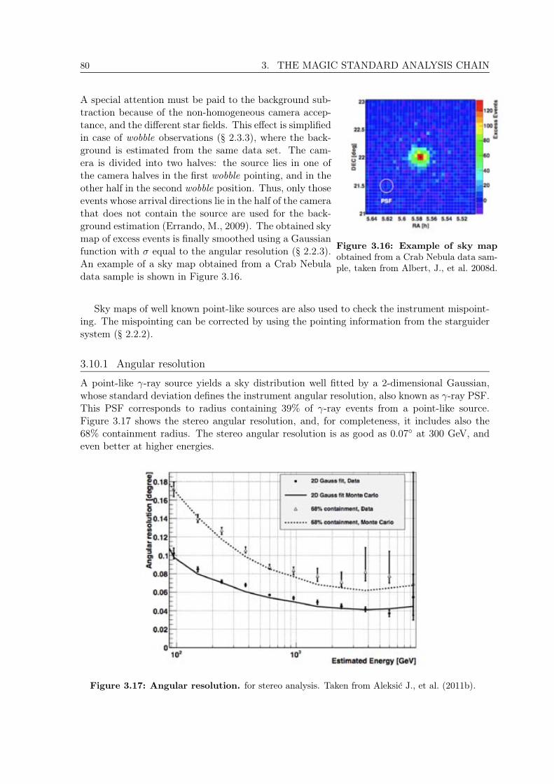
80 3. THE MAGIC STANDARD ANALYSIS CHAIN
A special attention must be paid to the background sub-traction because of the non-homogeneous camera accep-tance, and the different star fields. This effect is simplifiedin case of wobble observations (§ 2.3.3), where the back-ground is estimated from the same data set. The cam-era is divided into two halves: the source lies in one ofthe camera halves in the first wobble pointing, and in theother half in the second wobble position. Thus, only thoseevents whose arrival directions lie in the half of the camerathat does not contain the source are used for the back-ground estimation (Errando, M., 2009). The obtained skymap of excess events is finally smoothed using a Gaussianfunction with σ equal to the angular resolution (§ 2.2.3).An example of a sky map obtained from a Crab Nebuladata sample is shown in Figure 3.16.
Figure 3.16: Example of sky mapobtained from a Crab Nebula data sam-ple, taken from Albert, J., et al. 2008d.
Sky maps of well known point-like sources are also used to check the instrument mispoint-ing. The mispointing can be corrected by using the pointing information from the starguidersystem (§ 2.2.2).
3.10.1 Angular resolution
A point-like γ-ray source yields a sky distribution well fitted by a 2-dimensional Gaussian,whose standard deviation defines the instrument angular resolution, also known as γ-ray PSF.This PSF corresponds to radius containing 39% of γ-ray events from a point-like source.Figure 3.17 shows the stereo angular resolution, and, for completeness, it includes also the68% containment radius. The stereo angular resolution is as good as 0.07 at 300 GeV, andeven better at higher energies.
Figure 3.17: Angular resolution. for stereo analysis. Taken from Aleksic J., et al. (2011b).

3.11. Energy estimation 81
3.11 Energy estimation
The energy estimation in the standard MAGIC analysis chain can be performed either bymeans of a RF or by using LUTs. The second method was introduced for the stereoscopicanalysis and it became the standard option for such an analysis thanks to its faster processingtime. The RF, however, can still be applied and provides a useful cross-checking tool. In thefollowing, both methods will be described, since the first one was used for the analyses ofmono data and the latter for stereo analyses.
The RF for the energy estimation is trained over a sample of MC -ray events whoseenergy, Etrue, is known. The parameters considered in the RF are mainly size, zenith angle,and conc. Shower maximum height and impact parameter can be added in case of stereo ob-servations. Also leakage is included to account for the image truncation at high energies. Thedecisional trees of the RF algorithm are built as described in § 3.7 with the only difference onhow the optimal cut in each tree node is chosen. It is the cut which minimizes the varianceof the Etrue of the events in the split samples.
The energy LUTs are based on a simple model describing the distribution of the Cherenkovphotons on the ground. This model relies on the Cherenkov radius, rC , and Cherenkov density,αC , (refer to § 3.5.1 for the parameter definition). The LUTs are built, independently for eachtelescope, by dividing a sample of simulated MC gammas, with known Etrue, in bins of size,and impact/rC . Since the energy of the primary -ray is proportional to size/αC , each of thetable bins contains the mean value of the distribution of Etrue · αC/size with an error whichis given by the RMS of the distribution. The final energy estimation, Eest, is the weightedaverage value obtained from both telescopes, where the weight is given by the uncertaintyassociated to the corresponding bin. Eest is then corrected for the ZA: the empirical correctionfactor is 0.4 · cos(ZA).
3.11.1 Energy resolution
The energy resolution is defined as the η of a Gaussian fit to the peak of (Eest-Etrue)/Etruedistribution. This value provides an estimation of the goodness of the energy reconstructionfor the bulk of events excluding all the outliers. The difference from zero of the peak of the(Eest-Etrue)/Etrue distribution gives the mean energy bias. The energy reconstruction is asgood as it is close to the zero value. MAGIC I mono analysis has a resolution around 25%between 200 GeV and 1 TeV. On the other hand, for stereo analysis it is as good as 15%in the same energy range. The estimated energy of low-energy primary gammas is typicallyoverestimated (positive energy bias) at low energies (below 200 GeV), and at very high energies(above some TeV). Figure 3.18 illustrates the energy resolution and bias as function of Etruefor the stereo analysis.
The energy threshold of the analysis is defined as the peak of the Etrue distribution eitherbefore or after applying the gamma selection cuts (§ 3.9).
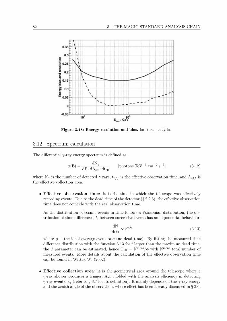
82 3. THE MAGIC STANDARD ANALYSIS CHAIN
Figure 3.18: Energy resolution and bias. for stereo analysis.
3.12 Spectrum calculation
The differential -ray energy spectrum is defined as:
σ(E) =dN
dE · dAe · dte[photons TeV1 cm2 s1] (3.12)
where N is the number of detected rays, teff is the effective observation time, and Aeff isthe effective collection area.
• Effective observation time: it is the time in which the telescope was effectivelyrecording events. Due to the dead time of the detector (§ 2.2.6), the effective observationtime does not coincide with the real observation time.
As the distribution of cosmic events in time follows a Poissonian distribution, the dis-tribution of time differences, t, between successive events has an exponential behaviour:
dNd(t)
/ et (3.13)
where φ is the ideal average event rate (no dead time). By fitting the measured timedifference distribution with the function 3.13 for t larger than the maximum dead time,the φ parameter can be estimated, hence Te = Nmeas/φ with Nmeas total number ofmeasured events. More details about the calculation of the effective observation timecan be found in Wittek W. (2002).
• Effective collection area: it is the geometrical area around the telescope where a -ray shower produces a trigger, Asim, folded with the analysis efficiency in detecting -ray events, (refer to § 3.7 for its definition). It mainly depends on the -ray energyand the zenith angle of the observation, whose effect has been already discussed in § 3.6.

3.12. Spectrum calculation 83
The effective collection area Aeff , defined as:
Ae(E;ZA) = Asim · = Asim ·N aftercuts
N total[m2] (3.14)
is computed by using MC -ray events and their original energy, Etrue. In Figure 3.19the typical effective collection area for MAGIC stereoscopic observations is displayed.The trigger probability increases very fast at low energies until all showers within thelight pool generate enough light to trigger the telescope, and then the effective collectionarea remains almost constant.
Figure 3.19: Typical effective collection area for stereoscopic observations at low zenith angles(ZA < 30).
• Number of excess events: it is computed, for each energy bin, through either thealpha or the 2 distribution according to the kind of performed analysis (§ 3.9). The /hadron separation cuts, mainly hadronness, and alpha/2 cuts, are determined sep-arately bin-by-bin in order to obtain a constant cut efficiency around 70-80%. Sucha large cut efficiency leads to the definition of much looser cuts with respect to theones optimized for the signal extraction (§ 3.9). The main reason for this choice isthat it guarantees a better agreement between MC and data, hence provides a correctestimation of the effective area.
The maximum number of energy bins used to determine a spectrum depends on the energyresolution which defines the minimum size bin, but also on the flux strenght of the sourcewhich determines the number of excess events for each energy bin. When fitting the spectrum,in fact, the significance of each spectral point is required to be at least 1.5η. Therefore, whilefor strong sources, like the Crab Nebula , the first condition on the energy resolution is themost constraining one, it is exactly the opposite for weak sources (10% of the Crab Nebulaflux).
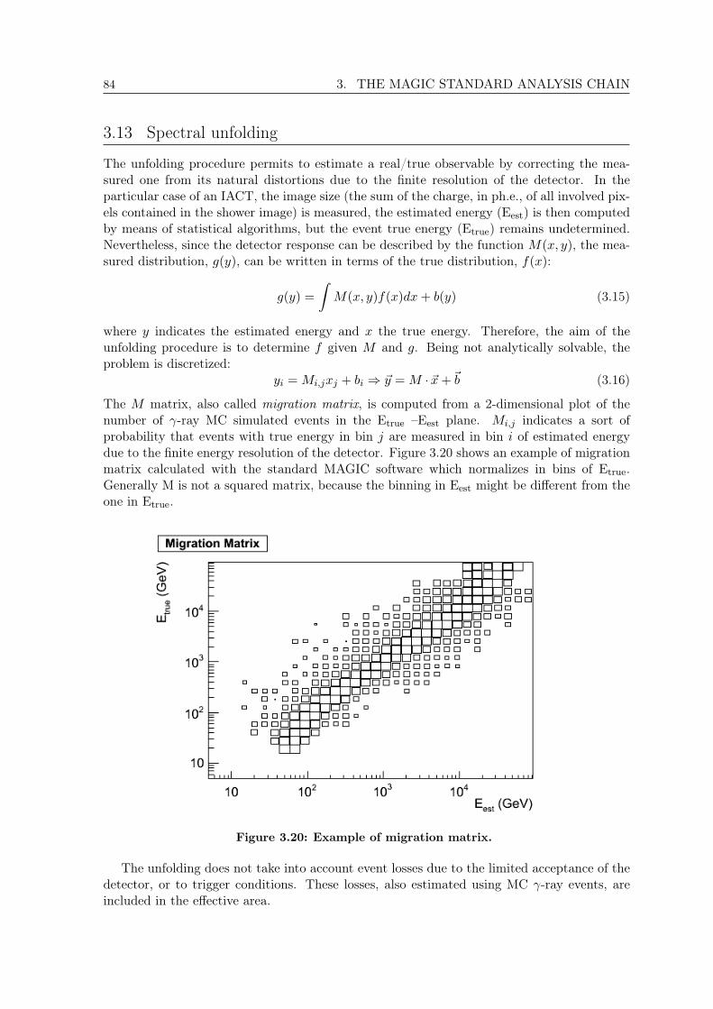
84 3. THE MAGIC STANDARD ANALYSIS CHAIN
3.13 Spectral unfolding
The unfolding procedure permits to estimate a real/true observable by correcting the mea-sured one from its natural distortions due to the finite resolution of the detector. In theparticular case of an IACT, the image size (the sum of the charge, in ph.e., of all involved pix-els contained in the shower image) is measured, the estimated energy (Eest) is then computedby means of statistical algorithms, but the event true energy (Etrue) remains undetermined.Nevertheless, since the detector response can be described by the function M(x; y), the mea-sured distribution, g(y), can be written in terms of the true distribution, f(x):
g(y) =ZM(x; y)f(x)dx+ b(y) (3.15)
where y indicates the estimated energy and x the true energy. Therefore, the aim of theunfolding procedure is to determine f given M and g. Being not analytically solvable, theproblem is discretized:
yi = Mi;jxj + bi ) ~y = M · ~x+~b (3.16)
The M matrix, also called migration matrix, is computed from a 2-dimensional plot of thenumber of -ray MC simulated events in the Etrue –Eest plane. Mi;j indicates a sort ofprobability that events with true energy in bin j are measured in bin i of estimated energydue to the finite energy resolution of the detector. Figure 3.20 shows an example of migrationmatrix calculated with the standard MAGIC software which normalizes in bins of Etrue.Generally M is not a squared matrix, because the binning in Eest might be different from theone in Etrue.
Figure 3.20: Example of migration matrix.
The unfolding does not take into account event losses due to the limited acceptance of thedetector, or to trigger conditions. These losses, also estimated using MC -ray events, areincluded in the effective area.

3.14. Light curves 85
There are different approaches to find the solution for ~x (Albert, J., et al., 2007c):
• Unfolding with regularization. It is based on the inversion of the migration matrix,which, however, is often not invertible. In this latter case, minimization methods, i.e.least square method, can provide the wanted solutions, as those ~x which, after foldingwith M, are most compatible with ~y. Although technically correct, the solution usuallyleads to large fluctuations making the distribution of the Etrue differ from the physicalone, hence useless. The remedy to this problem is regularization: adding a regularizationterm to the least square expression (γ2
0) allows to smoothly suppress those insignificantcoefficients5 of the solution which are the cause of the large fluctuations (Anykeyevet al., 1991).
γ2 = γ20 +
θ
2Reg (3.17)
Large values of θ , corresponding to no regularization, often produce noisy spectra whichperfectly fit the data. On the other hand, small values of θ , indicating high level of reg-ularization, yield to smooth unfolded distribution which can strongly deviate from thedata. Thus, selecting the appropriate value for θ is very important.In MAGIC, there are several unfolding methods which differ for the way the regular-ization is implemented. The most used ones are Tikonov, A.N. & Arsenin, V.J. (1979),Schmelling, M. (1998), and Bertero, M. (1989). The agreement within these methods isrequired to be confident on the results.
• Forward unfolding. It consists of parametrizing ~x as an analytic function which isa priori assumed (the assumed energy spectrum, in the treated particular case) andminimizing γ2
0 with respect to these parameters. The minimization is generally solvedanalytically forcing the solution to be continuous. The parametrization can be inter-preted as a regularization, leading to a suppression of the noise component of ~x, but noexplicit regularization is done. It is not a real unfolding because its result is just thebest fit, with corresponding errors, obtained using a priori assumed parametrization.Thus, the forward unfolding should only be used to check the results obtained withother unfolding methods.
3.14 Light curves
Light curves show integral -ray fluxes, in a considered energy range [E0;E1], as a functionof time. The integral fluxes in the time intervals [Ti;Tj ] are computed from Eq. 3.12:
(E) =Z Ti
Tj
Z E1
E0
σ(E) dE dt [photons cm2 s1] (3.18)
and they can be negative in case of a negative statistical fluctuation of the number of excessevents. In this case ULs to the integral flux are provided instead of flux points (§ 3.15).
The number of time bins is mainly determined by the statistics of the signal. Once thetime bins are defined, the light curve is obtained by calculating, for each time bin, the numberof excess events in the considered energy range. The effective collection area is computed foreach time bin separately by using MC -ray events having a zenith angle distribution whichresembles the one of the data in the considered time bin.
5Mainly the eigenvalues of the covariance matrix of ~y (after having been transformed to a diagonal matrix).

86 3. THE MAGIC STANDARD ANALYSIS CHAIN
Since no real unfolding is applied to light curves, the effect of the finite energy resolution ofthe detector (i.e. the mismatch between the estimated energy, Eest, and the true one, Etrue)are taken into account by expressing the effective collection area in terms of Eest. Using thesame notation as for Eq. 3.19, it is calculated as follows. The geometrical area, Asim, remainsexpressed in terms of Etrue, as well as the total number of simulated γ-ray events, Nγtotal,in the considered energy range. The number of γ-ray events surviving the gamma selectioncuts in the given energy range is computed by using the estimated energy and it has to beweighted with the spectral shape.
Aeff(Eest) = Asim(Etrue) ·Nγaftercuts(Eest)
Nγtotal(Etrue)(3.19)
The choice of the lower energy limit is fundamental. On one hand, the effective collectionarea is very sensitive to small fluctuations in the energy reconstruction (mismatches betweentrue and reconstructed energy) at low energies. On the other hand, due to the falling power-law spectra, the low energy events dominate the emission in the considered energy range. Alower energy limit at the beginning of the collection area plateau is normally safe.
3.15 Upper limits
Whenever no significant signal is found, ULs to the integral or differential flux of the sourcecan be derived with a certain Confidence Level (CL).
From the measured quantities: number of excess events, Nex, which, in this case, can bealso negative, and number of background events, Nbg, one can estimate the UL on the numberof excess event, NUL
ex . This calculation is performed in two steps. First, under the hypothesison the mean number of excess events µ ex and background events µ bg, the Probability DensityFunction (PDF) for Nex is constructed: P(Nex | µ Ex; µ bg). The confidence interval [Nlow
ex , Nupex ]
is defined as the range out of which would lie the result Nex of only a percentage α ofmeasurements (carried out under the same conditions):
P(Nex ∈[Nlowex ; Nup
ex ] | µ ex; µ bg) = 1−α (3.20)
The limit µ upEx can be directly interpreted as upper limit on NEx at the CL=100(1-α ). In fact
Later, this PDF has to inverted in order to find the PDFfor µ Ex given NEx and Nbg: P(µ Ex | Nex; Nbg). The let-ter problem can be solved either through a Bayesian (He-lene, O., 1983) or a frequentist approach which is the oneadopted within the MAGIC collaboration. It is based onFeldman, G. J. & Cousins, R. D. (1998) which proposesthe construction of a confidence belt: for each µ Ex a con-fidence interval is derived, (Figure 3.21). Given a valueof NEx, the confidence interval can then be inverted toobtain limits [µ low
Ex , µupEx] satisfying:
P(µ Ex ∈[µ lowEx , µupEx] | NEx; Nbg) = α (3.21)
at the CL=100(1- ). In fact
Figure 3.21: Confidence belt.Taken from Neyman, J (1937).
in (1-α ) of the cases the µ Ex will fall within the found range.Rolke et al. generalized Feldman’s method including a probability model for the background(Rolke, W. A. & Lopez, A. M., 2001) and for the overall efficiency (Rolke, W. A. et al., 2005).
3.16. Systematic uncertainties 87
The latter work is used as reference in MAGIC for the UL calculation.The chosen CL is 95% and the assumed systematic uncertainty is 30% . The latter includes
also systematic errors on the analysis methods, such as changes in the efficiency. Therefore,the efficiency is assumed to be constant and equal to 1. Any deviation from these settings areexplicitly stated in this thesis work.
The estimation of the ULs to the differential flux at the mean energy E0 requires someassumptions. In fact, if no signal is detected, nothing else is known about the source itself.Therefore,
• the energy differential spectrum is assumed as σ(E) = K · S(E). Usually it is given bya power-law spectrum with a photon index =2.6 (Crab-like spectrum):
σ(E) = K ·
EE0
(3.22)
• the time evolution of the possible emission is assumed to be constant over the period ofobservation.
Under the above-mentioned assumptions, the integral flux can be expressed as:
KZ 1
E0
S(E) dE =
R1E0
dN R1E0
R Tobs
0 A(E) dE dt(3.23)
where Tobs is the effective observation time. Thus, the UL to integral flux is given by:
KUL <NUL
Ex
Tobs ·R1E0
S(E) A(E) dE[photons TeV1 cm2 s1] (3.24)
The integral over the effective area is the weigthed effective area average < Ae >.
3.16 Systematic uncertainties
In addition to the statistical errors, the measurements of -ray differential energy spectra, andlight curves are affected by systematic errors. The systematic uncertainties can be dependingon which observable they affect: the energy scale, the flux normalization or the spectral slope.All the uncertainty estimations provided in the following were taken from Aleksic J., et al.(2011b), unless differently stated. They are summarized in Table 3.3.
• Sources of systematic uncertainty on the energy scale:
– MC atmospheric simulations. MC simulations use a fixed atmosphere model(§ 3.1) which does not match the atmosphere at the Roque de los MuchachosObservatory perfectly. This can produce an effect as large as 3% (Albert, J., et al.,2008d). In addition, the model does not take into account seasonal variations. Theaverage atmospheric values between Summer and Winter change by about 15% thetransmission of the atmosphere though (Bernlohr, K., 2000).
– Atmospheric transmission losses. Changes in the atmospheric transmissiondue to Mie scattering introduce an additional uncertainty in the energy scale.
88 3. THE MAGIC STANDARD ANALYSIS CHAIN
After tight data quality (§ 3.6) cuts, this uncertainty is estimated of the order of5%.
– Light losses. Light losses can be due to a worsening of the mirror reflectivity, ora degradation of the camera entrance window and the Winston cone light guides.Both of them can be caused by dust deposit. Light losses can be adjusted in theMC simulations. Nevertheless, due to malfunctioning of the AMC (§ 2.2.3), thelight losses can vary from one night to another, and this introduces a systematicuncertainty on the energy scale of about 8%. This value was estimated by usingreflected star images and the analysis of the muon images.
– Signal extraction. The method used for the signal extraction (§ 3.3) both inMAGIC I and MAGIC II produces an uncertainty in the number of ph.e. lowerthan 3%. This number was estimated by varying different windows of the signalextractor.
– F-factor. The F-factor method (§ 3.3) used for the signal calibration introducesa 10% effect on the energy scale.
– Temperature dependence of the gain. This produces a 2% effect on the energyscale.
– PMT performance. There are calibration uncertainties in the QE measurementsof the PMTs (≡ 4%), in the estimation of the electron collection efficiency of thefirst dynode (≡ 5%) and in the evaluation of the light collected in the Winstoncone (4%).
– Flat-fielding of the camera. The fact that the flat-fielding (§ 2.2.5) is done onlyat one wavelength and that it can be influenced by temperature drifts produces a6–8% systematic effect on the energy scale at low energies and a smaller 2% effectat high energies (above ≡ 300 GeV).
• Sources of systematic uncertainty on the absolute ux:
– Background subtraction. Dead pixels, stars in the FoV, as well as triggerinefficiencies make the camera highly inhomogeneous. On top of it, the stereotrigger produces a natural inhomogeneity. The stereo FoV can be treated as theoverlapping region between two cones (not a circular area) originating from bothtelescopes. This results in an enhanced amount of triggered events in the directiongiven by the position of the second telescope and can lead to a 10–15% variation onthe background estimation. However, this effect is reduced down to 1% uncertaintyby wobbling the source position (§ 2.3.3) and estimating the background from thecorresponding anti-source position (§ 3.9). This uncertainty depends on the ratiobetween excess and background. Therefore, it plays a different role dependingeither on strenght of the source flux or on the energy: the lower the energy, thehigher this systematic error.
– MC-data agreement. Differences between simulated and real -ray showers maylead to an error in the calculation of the gamma efficiency (§ 3.7), and, subsequently,in the estimation of the effective collection area. The overall uncertainty, estimatedby applying different cuts in the analysis, is about 10%.
– Mispointing. Relative pointing differences between MAGIC I and MAGIC IIspoil the reconstruction of the stereo parameters (§ 3.8). The typical mispointing

3.16. Systematic uncertainties 89
systematic effect class uncertainty night-to-nightMC atmospheric simulations ES 3% 0%
atmospheric transmission losses ES 5% 5%light losses ES 8% 8%
signal extraction ES 3% 0F-factor ES 10% 0
temperature dependence of the gain ES 2% 2%PMT QE ES 4% 0
PMT electron collection efficiency ES 5% 0light collection in Winston cone ES 5% 0
flat-fielding ES 2–8% 2%background subtraction FN 1–8% 1%MC-data disagreement FN 10% 8%
mispointing FN 1–4% 1–4%NSB FN 1–4% 0
non-linearity readout SS 0.04 0analysis SS 0.1 0
Table 3.3: Uncertainty of the main sources of systematic effects. From left to right:the systematic effect, the class of the effect defines if it affect the energy scale (ES), the fluxnormalization (FN) or the spectral slope (SS), the overall value of the uncertainty and the value ofuncertainty which can vary from night-to-night at energies above 300 GeV.
is smaller than 0.02 (Aleksic, J., et al., 2010b), and it causes a systematic erroron the gamma efficiency 4%.
– Different NSB levels. Each FoV is characterized by its own NSB level. Thelatter can vary significantly in Galactic FoVs or in presence of star/moon light.Higher NSB means higher fluctuations which might spoil the image parametercalculation, hence decrease the efficiency in detecting -ray events. Dedicated MCstudies estimated this effect to be 1–4%.
• Sources of systematic uncertainty on the spectral slope:
– Non-linearity of the readout chain. Non-linearities in the analog signal chainand the small residual non-linearities of the DRS2 (§ 2.2.6) produce a systematicuncertainty of about 0.04 in the slope of a power-law differential energy spectrum.
– Analysis. This uncertainty takes into account the effect of different unfoldingmethods (§ 3.13), different efficiencies of the gamma selection cuts (§ ??), anddifferent zenith angle ranges. This systematic error produces for a typical power-law spectrum a spread in photon index of 0.1. An independent estimation of thissystematic uncertainty will be treated in detail in § 5.3.2.
The overall systematic uncertainty depends on the energy. The error on the flux normal-ization is estimated to be 11% at medium energies, above 300 GeV, and up to 19% at lowenergies (below 100 GeV). The energy scale of the MAGIC telescopes can be determined witha precision of 17% at low energies and of 15% at higher energies. The slope of the differentialenergy spectra is affected by a systematic uncertainty around 0.015.

90 3. THE MAGIC STANDARD ANALYSIS CHAIN
Just some of the considered sources of systematic effect can produce variations in the fluxfrom night-to-night. An estimation of the values for the night-to-night systematic uncertain-ties is given in Table 3.3.

PART TWO
CRAB PULSAR WIND NEBULA
Van Gogh - “Crab on its back”


4Introduction to Pulsar Wind Nebulae
PWNe are bubbles of relativistic particles and magnetized fields created when theultra-relativistic wind from a pulsar interacts with the ambient medium. Theyproduce a broad-band spectrum of non thermal radiation from radio frequencies toTeV energies. The radiation is of synchrotron origin up to hard X-rays/soft -rays,while, at higher energies it results from Inverse Compton scattering on backgroundradiation. PWNe can be used to improve our understanding of relativistic shocks andparticle acceleration because they are nearby (hundreds to thousands of pc), theirspectrum expands over many decades of energy, and many models for the radiationproduction have been developed. This chapter provides a short review on the state ofthe art of the current knowledge of the PWNe, and, in particular, of the Crab Nebula,the archetypal of the PWNe.
It is a summary extracted from literature.
PWNe are a class of cosmic sources which contain magnetized relativistic wind radiat-ing non-thermal (synchrotron and IC) emission across the electromagnetic spectrum. Thesewinds are constantly powered by rotating NSs, the so-called pulsars, usually located at theircenter. Pulsars release a third of their total rotational energy (≡ 1049 erg) into their sur-rounding nebulae. Since pulsars, as well as their nebulae, originate in SN explosions, they arecontained within the shell of the SNRs. The SNRs are the leftover of the material ejected inthe explosion an interacting with the ISM.
The best studied PWN is the Crab Nebula , considered as prototype of this class of object.Over the past decades 40–50 PWNe have been identified either in our own Galaxy or in theMagellanic Clouds. Because PWNe have a well-defined central energy source and are closeenough to be spatially resolved, they act as a testing ground for studying both relativisticflows and shocks resulting from the interaction of relativistic winds with the ambient medium.
In the following, a summary of the current understanding of pulsars and PWNe is pre-sented. The chapter includes a short description of the SNRs. The latter does not pretend tobe exhaustive, but rather to introduce the concepts used in the other sections.
93

94 4. INTRODUCTION TO PULSAR WIND NEBULAE
4.1 Pulsars
Pulsars are rapidly rotating, highly-magnetized NSs formed during the SN explosions of mas-sive (≤ 5–10 MJ) stars (§ 4.1.1).
In 1967 Pacini suggested that a rotating magnetized NS could be a possible energy sourceof the continuum emission from the Crab Nebula (Pacini, F., 1967). Around the same time,a source of pulsed radio emission with a period of 1.337 s was detected by chance in anotherportion of the sky (Hewish et al., 1968). This was the first instance of a new class of objectscalled pulsars, whose name derives from “pulsating stars”. Their association with the rotatingmagnetized NSs was soon proposed by Gold, T. (1968) and Pacini, F. (1968) in the context ofthe magnetic dipole model. The latter foresaw losses of rotational energy through magneticdipole radiation causing a gradual slowdown of the pulsar, hence, an increase of the pulseperiod, P . These predictions could be confirmed with the detection of a pulsar with a periodP = 33 ms in the Crab Nebula (Staelin, D. H. & Reifenstein, III, E. C., 1968; Comella, J. M.et al., 1969), and the observation that its period increases of 36.5 ns per day (Richards, D. W.& Comella, J. M., 1969).
Pulsars can be classified through the measurements of its period, and its period derivativeP . The P -P diagram in Figure 4.1 shows two main populations of pulsars: “normal” pulsarswith a period of ∼ 0.5 s which increases at rates P ∼ 10−15 s/s, and MilliSecond Pulsars(MSPs) with a period which spans from 1.5 ms to 30 ms, and a time derivative of 10−19 s/s.These two measured quantities permit to infer the pulsar age, the surface magnetic field, and
Figure 4.1: Pulsars P -P diagram. Taken from Lorimer, D. R. (2005).
the rate at which the pulsar rotational energy is dissipated. The latter, known as spin-down
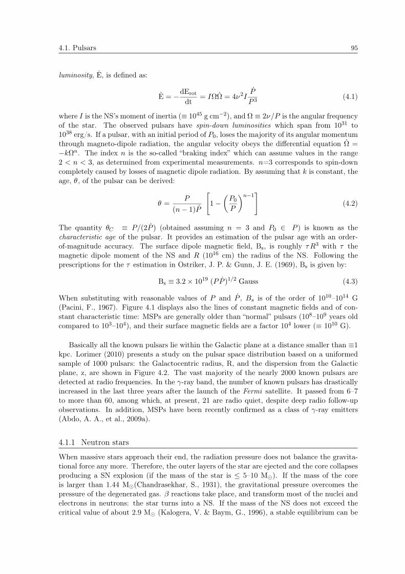
4.1. Pulsars 95
luminosity, _E, is defined as:
_E = dErot
dt= I _ = 4ν2I
_PP 3
(4.1)
where I is the NS’s moment of inertia (≡ 1045 g cm2), and 2ν=P is the angular frequencyof the star. The observed pulsars have spin-down luminosities which span from 1031 to1038 erg/s. If a pulsar, with an initial period of P0, loses the majority of its angular momentumthrough magneto-dipole radiation, the angular velocity obeys the differential equation _ =kn. The index n is the so-called “braking index” which can assume values in the range2 < n < 3, as determined from experimental measurements. n=3 corresponds to spin-downcompletely caused by losses of magnetic dipole radiation. By assuming that k is constant, theage, θ , of the pulsar can be derived:
θ =P
(n 1) _P
"1
P0
P
n1#
(4.2)
The quantity θC P=(2 _P ) (obtained assuming n = 3 and P0 ∈ P ) is known as thecharacteristic age of the pulsar. It provides an estimation of the pulsar age with an order-of-magnitude accuracy. The surface dipole magnetic field, Bs, is roughly τR3 with τ themagnetic dipole moment of the NS and R (1016 cm) the radius of the NS. Following theprescriptions for the τ estimation in Ostriker, J. P. & Gunn, J. E. (1969), Bs is given by:
Bs ≡ 3:2 1019 (P _P )1=2 Gauss (4.3)
When substituting with reasonable values of P and _P , Bs is of the order of 1010–1014 G(Pacini, F., 1967). Figure 4.1 displays also the lines of constant magnetic fields and of con-stant characteristic time: MSPs are generally older than “normal” pulsars (108–109 years oldcompared to 103–104), and their surface magnetic fields are a factor 104 lower (≡ 1010 G).
Basically all the known pulsars lie within the Galactic plane at a distance smaller than ≡1kpc. Lorimer (2010) presents a study on the pulsar space distribution based on a uniformedsample of 1000 pulsars: the Galactocentric radius, R, and the dispersion from the Galacticplane, z, are shown in Figure 4.2. The vast majority of the nearly 2000 known pulsars aredetected at radio frequencies. In the -ray band, the number of known pulsars has drasticallyincreased in the last three years after the launch of the Fermi satellite. It passed from 6–7to more than 60, among which, at present, 21 are radio quiet, despite deep radio follow-upobservations. In addition, MSPs have been recently confirmed as a class of -ray emitters(Abdo, A. A., et al., 2009a).
4.1.1 Neutron stars
When massive stars approach their end, the radiation pressure does not balance the gravita-tional force any more. Therefore, the outer layers of the star are ejected and the core collapsesproducing a SN explosion (if the mass of the star is 5–10 M). If the mass of the coreis larger than 1.44 M(Chandrasekhar, S., 1931), the gravitational pressure overcomes thepressure of the degenerated gas. reactions take place, and transform most of the nuclei andelectrons in neutrons: the star turns into a NS. If the mass of the NS does not exceed thecritical value of about 2.9 M (Kalogera, V. & Baym, G., 1996), a stable equilibrium can be
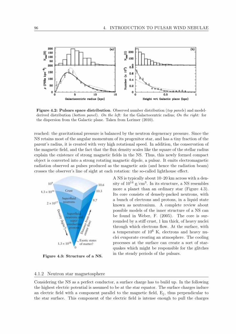
96 4. INTRODUCTION TO PULSAR WIND NEBULAE
Figure 4.2: Pulsars space distribution. Observed number distribution (top panels) and model-derived distribution (bottom panel). On the left: for the Galactocentric radius; On the right: forthe dispersion from the Galactic plane. Taken from Lorimer (2010).
reached: the gravitational pressure is balanced by the neutron degeneracy pressure. Since theNS retains most of the angular momentum of its progenitor star, and has a tiny fraction of theparent’s radius, it is created with very high rotational speed. In addition, the conservation ofthe magnetic field, and the fact that the flux density scales like the square of the stellar radiusexplain the existence of strong magnetic fields in the NS. Thus, this newly formed compactobject is converted into a strong rotating magnetic dipole, a pulsar. It emits electromagneticradiation observed as pulses produced as the magnetic axis (and hence the radiation beam)crosses the observer’s line of sight at each rotation: the so-called lighthouse effect.
Figure 4.3: Structure of a NS.
A NS is typically about 10–20 km across with a den-sity of 1014 g/cm3. In its structure, a NS resemblesmore a planet than an ordinary star (Figure 4.3).Its core consists of densely-packed neutrons, witha bunch of electrons and protons, in a liquid stateknown as neutronium. A complete review aboutpossible models of the inner structure of a NS canbe found in Weber, F. (2005). The core is sur-rounded by a stiff crust, 1 km thick, of heavy nucleithrough which electrons flow. At the surface, witha temperature of 106 K, electrons and heavy nu-clei evaporate creating an atmosphere. The coolingprocesses at the surface can create a sort of star-quakes which might be responsible for the glitchesin the steady periods of the pulsars.
4.1.2 Neutron star magnetosphere
Considering the NS as a perfect conductor, a surface charge has to build up. In the followingthe highest electric potential is assumed to be at the star equator. The surface charges inducean electric field with a component parallel to the magnetic field, E‖, thus perpendicular tothe star surface. This component of the electric field is intense enough to pull the charges

4.1. Pulsars 97
out against the gravitational forces. If the charges are not trapped in the surface by bindingforces (meaning the surface is not solid), they move perpendicularly to the surface as to shortout the Ek component. The space surrounding the NS, called magnetosphere, is thereforepopulated with free-force plasma and electromagnetic fields.
The only available analytical description of the NS magnetosphere is that of Goldreich,P. & Julian, W. H. (1969). These authors assumed the simplest case where the magneticfield is that of a dipole aligned with the rotation axis (aligned rotator). In the realistic case,instead, magnetic dipoles are arbitrarily tilted with respect to the rotation axis (oblique rota-tors). In fact, even if the two axes coincided in the pre-supernova star, the mass loss duringthe explosion is unlikely to be symmetric especially in the presence of strong magnetic field.In the last decade, this realistic case has been treated using numerical methods: Contopou-los, I. et al. (1999) proposed solutions for a time-independent magnetosphere. Whereas, onlyrecently, Spitkovsky, A. (2006) used new numerical methods to account for the time evolution.
A plausible picture of the pulsar magnetosphere distinguishes two separate zones: theinner magnetosphere where the pulsed emission comes from, and the wind zone populated bya relativistic magnetized wind.
• The inner magnetosphere is contained within the light cylinder. This is the cylinderaround the NS where the velocity of the magnetosphere reaches the speed of light, c.Its radius, RLC, is defined as:
RLC c
(4.4)
and it has typical value of ≡100 km. The charged particles extracted from the starsurface by the strong electric field move along the closed, and electric equipotentiallines of the magnetic field. Therefore, they corotate with the NS, and their chargedensity is given by:
αGJ ≡! ·!B=(2νc) (4.5)
which is known as the Goldreich-Julian charged density. The corotation breaks downat large distances, at some point close to the light cylinder. Therefore, those particlesbound to the lines closing outside the light cylinder can escape the rigid corotation. Inparticular, if the critical line is the magnetic field line with the same electric potential asthe interstellar medium, electrons stream out along higher-latitude lines, whereas pro-tons along lower-latitude lines (Figure 4.4). The corotation defines two separate zoneswithin the inner magnetosphere: the closed magnetosphere, a region limited by the lastfield line that closes within the light cylinder, and the complementary open magneto-sphere. In the open magnetosphere, the outflowing of charges reduce the charge density,thus a strong Ek develops. Consequently, particle acceleration can occur along the openmagnetic lines. In presence of the strong magnetic field, the accelerated particles losetheir energy via synchrotron radiation. The resulting photons create electron-positronpairs which start an electromagnetic cascade. These pairs short-out the parallel com-ponent of the electric field, self-limiting the acceleration. The produced primary andsecondary photons constitute the observable pulsed emission from radio frequencies upto -rays. The energy contained in the pulsed emission makes up only a 10% of thespin-down luminosity. Most of it, in fact, leaves the magnetosphere in form of magne-tized wind.
In the inner magnetosphere, only a small fraction (104–105) of the NS spin-down

98 4. INTRODUCTION TO PULSAR WIND NEBULAE
Figure 4.4: Sketch of the inner magnetosphere and wind zone in the particular case of analigned rotator. The NS is bottom left. Taken from Goldreich, P. & Julian, W. H. (1969).
luminosity is converted into kinetic particle energy (Arons, J., 1979; Michel, F. C.,1982). In other words, all the energy flux is most likely Poynting flux dominated. Thisis quantified by the ratio of the Poynting flux, LP = νB2/4π , to particle kinetic energyflux, LE = nνΓmc2, the so-called magnetization parameter σ (Kennel, C. F. & Coroniti,F. V., 1984a):
σ =B2
4π nΓmc2(4.6)
At the light cylinder, σ ∼ 104 (Arons, J., 1979).
• The wind zone is the region included between the light cylinder, and the terminationshock, at a distance rs. The particles which have escaped the inner magnetosphere forma highly relativistic, and magnetized wind with a Lorentz factor as large as Γ∼ 106
(unshocked pulsar wind). This wind carries most of the spin-down energy of the NSin the form of electromagnetic, and particle energy density. The energy flux, which isPoynting dominating at the light cylinder, becomes a kinetic dominated flux before thetermination shock, i.e. σ < 1. This energy transfer is a matter of debate (known as the σproblem). A dissipative transition cannot be the responsible process, as no intense X-rayradiation from this region has been observed: it is underluminous instead. Contopoulos,I. & Kazanas, D. (2002) derived a possible solution by using the conservation laws ofthe associated MagnetoHydro Dynamic (MHD) flow. The X-ray underluminosity is dueto the fact the relativistic unshocked winds move with the magnetic field; thus, they donot emit synchrotron radiation. This statement does not exclude that this wind can bedirectly observed through its IC radiation (Bogovalov, S. V. & Aharonian, F. A., 2000).
The relativistic wind slows down to match the boundary condition imposed by the more-slowly-expanding material at the nebula radius. Thus, when the ram pressure of thewind is balanced by the pressure of the PWN, a termination shock forms. Its distance

4.1. Pulsars 99
from the pulsar has the following dependence:
rs ∝
√E
PPWN. (4.7)
where PPWN is the total pressure in the shocked pulsar nebula (Gaensler, B. M. &Slane, P. O., 2006). Reasonable values of the nebula pression and E yield terminationshock radii in the order of 0.1 pc.
4.1.3 γ -ray emission from pulsars
In all models about the high-energy pulsar emission, charged particles are accelerated in theopen magnetosphere (§ 4.1.2) by the component of the induced electric field which is parallelto the magnetic field. These accelerated particles emit curvature emission up to γ-rays.Moreover, the resulting photons create electron-positron pairs in the strong magnetic field.These pairs radiate synchrotron photons (their momenta have a component perpendicular tothe magnetic field), many of which are able to produce a second generation of pairs. Thiselectromagnetic cascade process stops when the synchrotron photons are no longer energeticenough to pair-produce. Finally, γ-rays can be emitted also by IC scattering of low energysynchrotron photons (SSC).
The open magnetosphere includes two presumable acceleration sites: above the magneticpoles of the NS, and in the vacuum gaps of the the open magnetosphere (Figure 4.5). Differentassumptions on the acceleration site leads to different models for the γ-ray emission. The mostpopular ones are:
• the polar cap model (Sturrock, P. A., 1971;Arons, J. & Scharlemann, E. T., 1979; Daugh-erty, J. K. & Harding, A. K., 1982). It predictsthat particle acceleration takes place near theNS surface close to its magnetic poles. This re-gion extends for 0.5–1 stellar radii. The γ-raysare emitted by curvature radiation and IC up-scattering A distinct feature of the polar capmodel is a sharp “super-exponential” cut-off inthe energy spectrum which is caused by the effi-cient pair production attenuation at the pair es-cape energy (Harding, A. K. et al., 1997), wherethe pair escape energy is the highest energy forwhich the photon can escape the magnetospherewithout being subject to pair production. Thiscut-off shows an energy dependence which is in-versely proportional to the surface of the mag-netic field strength. The trade-off of this modelis the fact that it predicts too small beam size toproduce the observed wide pulse profiles.
Figure 4.5: Sketch of the pul-sar inner magnetosphere cross-section. It indicates the possiblesites of particle acceleration. Takenfrom Hirotani (2008).
• the slot gap model. Scharlemann, E. T. et al. (1978) found that in the polar capscenario the potential gap above the pole increases when approaching the last closed

100 4. INTRODUCTION TO PULSAR WIND NEBULAE
field line. Based on these findings, Arons, J. (1983) pointed out the possibility of alow-latitude acceleration region, the “slot gap”: a narrow bundle of field lines borderingthe closed magnetosphere (Figure 4.5). The electromagnetic cascades in this region havehigher pair multiplicity than in the polar cap because the primary electrons accelerateand produce over a larger distance. The radiation from the slot gap model naturallyproduces a wider cone of emission, solving the problem of the too narrow predicted binsizes (Harding, A. & Muslimov, A., 2005).
• the outer gap model. Cheng, K. S. et al. (1986b,a) showed that a charge depletedvolume (due to the charges streaming out along the field open lines) can form in themagnetosphere also at low-latitude. This gap is contained within the last closed fieldline, the null surface (defined as
−→Ω ·−→B = 0), the light cylinder, and an open magnetic
field line which is limited by pair creation (Figure 4.5). The high-energy photons pro-duced in the outer gaps are affected by a much less efficient pair production than inthe polar caps because of orders of magnitude lower magnetic fields. The maximumγ-ray energy is determined by the maximum energy of the accelerated electrons, whichis limited by radiation reaction losses. Therefore, the shape of the cut-off is expected tofall more gradually than in the polar cap models (exponential cut-off). Some outer gapmodels predict VHE pulsed emission due to IC scattering (Hirotani, K., 2006).
4.2 Supernova Remnants
Figure 4.6: Sketch of a composed pulsar-PWN-SNR system. Taken from Gaensler, B. M. & Slane,P. O. (2006).
The material ejected during the SN in-teracts with the surrounding ISM, and itforms a SNR. The resulting shock (for-ward shock) wave have an initial speed of103 km s−1, and it constantly slows downas it sweeps up the surrounding material.The expansion can occur over tens of thou-sands of years until the shock speed fallsbelow a few 102 km s−1. At the forwardshock the ambient gas is compressed andheated. After having swept up roughlyits own mass from the surrounding ambi-ent, the hot plasma starts to decelerate,and a reverse shock forms. It moves in-ward towards the pulsars, and the PWN.With the formation of this second shockthe SNR enters into the so-called Sedovphase which is strongly affected by theISM. Figure 4.6 shows a sketch of a com-posite pulsar-PWN-SNR system.
For a detailed review on SNRs, the reader is referred to Reynolds, S. P. (2008).
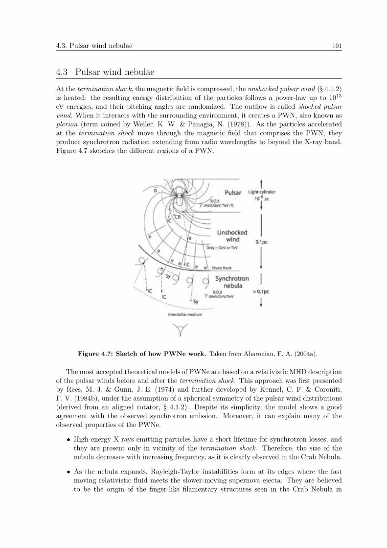
4.3. Pulsar wind nebulae 101
4.3 Pulsar wind nebulae
At the termination shock, the magnetic field is compressed, the unshocked pulsar wind (§ 4.1.2)is heated: the resulting energy distribution of the particles follows a power-law up to 1015
eV energies, and their pitching angles are randomized. The outflow is called shocked pulsarwind. When it interacts with the surrounding environment, it creates a PWN, also known asplerion (term coined by Weiler, K. W. & Panagia, N. (1978)). As the particles acceleratedat the termination shock move through the magnetic field that comprises the PWN, theyproduce synchrotron radiation extending from radio wavelengths to beyond the X-ray band.Figure 4.7 sketches the different regions of a PWN.
Figure 4.7: Sketch of how PWNe work. Taken from Aharonian, F. A. (2004a).
The most accepted theoretical models of PWNe are based on a relativistic MHD descriptionof the pulsar winds before and after the termination shock. This approach was first presentedby Rees, M. J. & Gunn, J. E. (1974) and further developed by Kennel, C. F. & Coroniti,F. V. (1984b), under the assumption of a spherical symmetry of the pulsar wind distributions(derived from an aligned rotator, § 4.1.2). Despite its simplicity, the model shows a goodagreement with the observed synchrotron emission. Moreover, it can explain many of theobserved properties of the PWNe.
• High-energy X rays emitting particles have a short lifetime for synchrotron losses, andthey are present only in vicinity of the termination shock. Therefore, the size of thenebula decreases with increasing frequency, as it is clearly observed in the Crab Nebula.
• As the nebula expands, Rayleigh-Taylor instabilities form at its edges where the fastmoving relativistic fluid meets the slower-moving supernova ejecta. They are believedto be the origin of the finger-like filamentary structures seen in the Crab Nebula in

102 4. INTRODUCTION TO PULSAR WIND NEBULAE
the optical, and UV bands. Simulations indicate that 60–75% of the swept up mass isconcentrated into these filaments (Bucciantini, N. et al., 2004).
• The higher the synchrotron losses, the steeper the resulting spectrum. This explainswhy the spectrum flattens out when the distance to the pulsar increases.
4.3.1 Inner structure
Recent observations showed that the inner region ofPWNe is characterized by complex structures, gener-ally referred as jet-torus structures. A main emissiontorus corresponding to the pulsar equatorial plane, andtwo jets of material that flow along the toroidal axisare clearly visible (Figure 4.8). Usually one of the twojets is fainter than the other as result of the Dopplerbeaming of the material whereby the intensity varieswith the viewing angle (Pelling, R. M., et al., 1987). Inaddition, multiple arcs and rings are present togetherwith a central knot, and the luminosity around thetorus is not constant.
Figure 4.8: X-ray image of the PWN3C 58. where the jet-torus structure is vis-ible.
Such structure cannot be explained under the assumption of an isotropic energy flux of theunshocked pulsar winds proposed by Kennel, C. F. & Coroniti, F. V. (1984b). On the otherhand, an equatorial flux, with a strong latitude dependence (∝ sin ψ , with ψ the angle from therotation axis), can describe it, as recently confirmed by numerical simulations (Bucciantini,N. et al., 2006). An equatorial flux, in fact, naturally produces an oblate termination shock.Subsequently, the speed of the outflow is not constant over the pulsar latitude (larger athigher latitudes). This explains the difference in the luminosity of distinct torus positions.Moreover, given a magnetic field distribution dependent on the pulsar latitude (∝ sin ψ ), thisframework can also derive the jet collimation (Khangoulian, D. V. & Bogovalov, S. V., 2003).The modification of the unshocked pulsar wind energy flux distribution can be associated withthe numerical solution found for the pulsar magnetosphere in case of oblique rotator (§ 4.1.2).These are the so-called stripped wind models (Spitkovsky, A., 2006).
4.3.2 Evolution of pulsar wind nebulae
Pulsars and PWNe are, at least initially, surrounded by a SNR. They constitute compositesystems, and the SNR provides boundary conditions for the pulsar winds. Since the energyin the SNR (∼ 1051 erg) is much larger than the total energy ejected by the pulsar during itslifetime (∼ 1049 erg), the PWN cannot significantly affect the SNR. On the other hand, theevolution of the SNR has an important influence on the PWN morphology and its emissionproperties. Recent studies of the PWN-SNR system distinguish three main phases in thePWN evolution (Bucciantini, N., 2008):
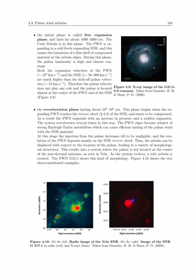
4.3. Pulsar wind nebulae 103
• the initial phase is called free expansionphase, and lasts for about 1000–3000 yrs. TheCrab Nebula is in this phase. The PWN is ex-panding in a cold freely expanding SNR, and thiscauses the formation of a thin shell of compressedmaterial at the nebula edges. During this phase,the pulsar luminosity is high and almost con-stant.Both the expansion velocities of the PWN(∼ 103 km s−1) and the SNR ((∼ 50–300 km s−1)are much higher than the kick-off pulsar veloci-ties (∼ 10 km s−1). Therefore the pulsar velocitydoes not play any role and the pulsar is locatedalmost at the center of the PWN and of the SNR(Figure 4.9).
Figure 4.9: X-ray image of the G21.5-0.9 remnant. Taken from Gaensler, B. M.& Slane, P. O. (2006).
• the reverberation phase lasting about 104–105 yrs. This phase begins when the ex-panding PWN reaches the reverse shock (§ 4.2) of the SNR, and starts to be compressed.As a result the PWN responds with an increase in pressure and a sudden expansion.The system reverberates several times in this way. The PWN edges become subject ofstrong Rayleigh-Taylor instabilities which can cause efficient mixing of the pulsar windwith the SNR material.At this stage the injection from the pulsar decreases till to be negligible, and the evo-lution of the PWN depends mainly on the SNR reverse shock. Thus, the nebula can bedisplaced with respect to the location of the pulsar, leading to a variety of morphologi-cal structures. This results into a system where the pulsar is not located at the centerof the non-thermal emission, as seen in Vela. As the system evolves, a relic nebula iscreated. The PWN G24.5 shows this kind of morphology. Figure 4.10 shows the twoabove-mentioned examples.
Figure 4.10: On the left: Radio image of the Vela SNR. On the right: Image of the SNRG 317.1 in radio (red) and X-rays (blue). Taken from Gaensler, B. M. & Slane, P. O. (2006).
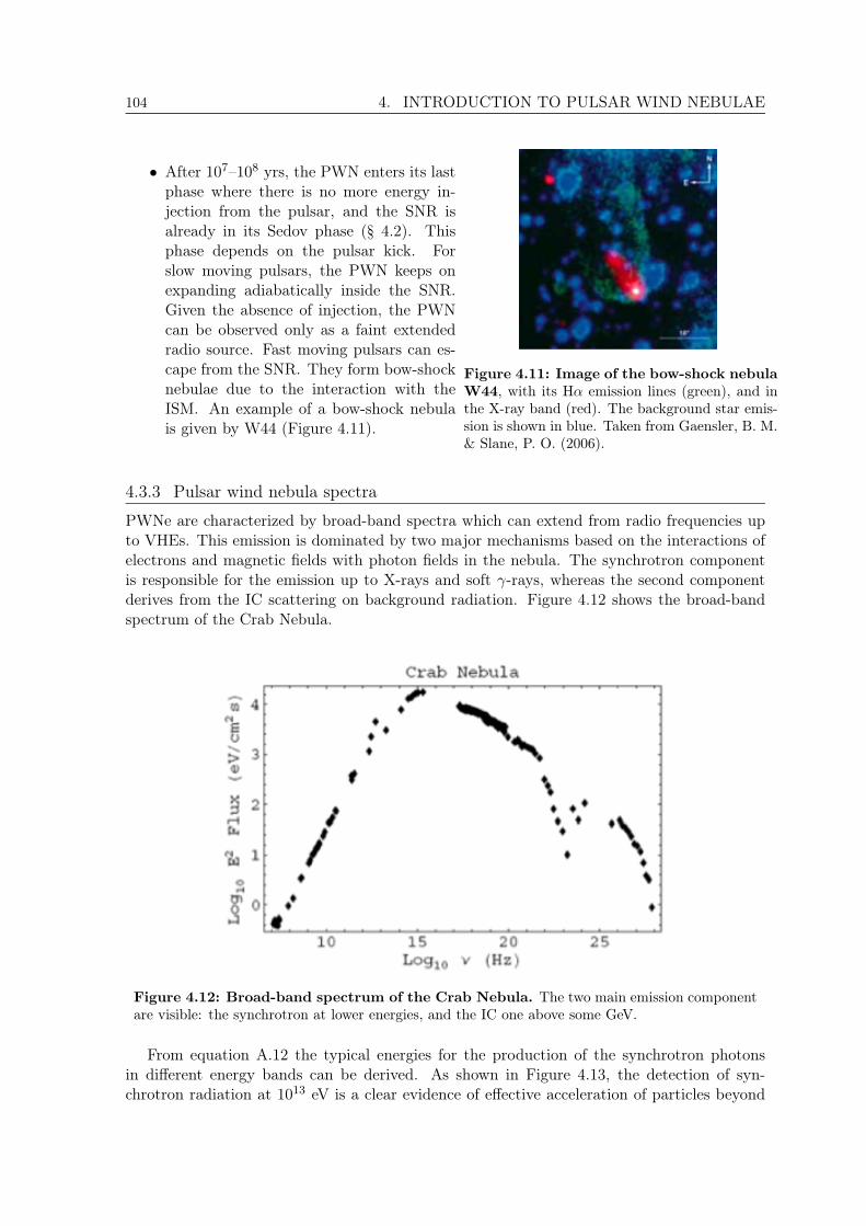
104 4. INTRODUCTION TO PULSAR WIND NEBULAE
• After 107–108 yrs, the PWN enters its lastphase where there is no more energy in-jection from the pulsar, and the SNR isalready in its Sedov phase (§ 4.2). Thisphase depends on the pulsar kick. Forslow moving pulsars, the PWN keeps onexpanding adiabatically inside the SNR.Given the absence of injection, the PWNcan be observed only as a faint extendedradio source. Fast moving pulsars can es-cape from the SNR. They form bow-shocknebulae due to the interaction with theISM. An example of a bow-shock nebulais given by W44 (Figure 4.11).
Figure 4.11: Image of the bow-shock nebulaW44, with its Hα emission lines (green), and inthe X-ray band (red). The background star emis-sion is shown in blue. Taken from Gaensler, B. M.& Slane, P. O. (2006).
4.3.3 Pulsar wind nebula spectra
PWNe are characterized by broad-band spectra which can extend from radio frequencies upto VHEs. This emission is dominated by two major mechanisms based on the interactions ofelectrons and magnetic fields with photon fields in the nebula. The synchrotron componentis responsible for the emission up to X-rays and soft γ-rays, whereas the second componentderives from the IC scattering on background radiation. Figure 4.12 shows the broad-bandspectrum of the Crab Nebula.
Figure 4.12: Broad-band spectrum of the Crab Nebula. The two main emission componentare visible: the synchrotron at lower energies, and the IC one above some GeV.
From equation A.12 the typical energies for the production of the synchrotron photonsin different energy bands can be derived. As shown in Figure 4.13, the detection of syn-chrotron radiation at 1013 eV is a clear evidence of effective acceleration of particles beyond
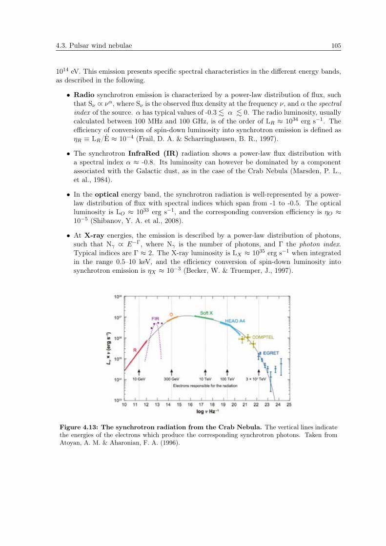
4.3. Pulsar wind nebulae 105
1014 eV. This emission presents specific spectral characteristics in the different energy bands,as described in the following.
• Radio synchrotron emission is characterized by a power-law distribution of flux, suchthat Sν ∝ να , where Sν is the observed flux density at the frequency ν, and α the spectralindex of the source. α has typical values of -0.3 α 0. The radio luminosity, usuallycalculated between 100 MHz and 100 GHz, is of the order of LR ≈ 1034 erg s−1. Theefficiency of conversion of spin-down luminosity into synchrotron emission is defined asηR ≡ LR/E ≈ 10−4 (Frail, D. A. & Scharringhausen, B. R., 1997).
• The synchrotron InfraRed (IR) radiation shows a power-law flux distribution witha spectral index α ≈ -0.8. Its luminosity can however be dominated by a componentassociated with the Galactic dust, as in the case of the Crab Nebula (Marsden, P. L.,et al., 1984).
• In the optical energy band, the synchrotron radiation is well-represented by a power-law distribution of flux with spectral indices which span from -1 to -0.5. The opticalluminosity is LO ≈ 1033 erg s−1, and the corresponding conversion efficiency is ηO ≈10−5 (Shibanov, Y. A. et al., 2008).
• At X-ray energies, the emission is described by a power-law distribution of photons,such that Nγ ∝ E−Γ, where Nγ is the number of photons, and Γthe photon index.Typical indices are Γ≈ 2. The X-ray luminosity is LX ≈ 1035 erg s−1 when integratedin the range 0.5–10 keV, and the efficiency conversion of spin-down luminosity intosynchrotron emission is ηX ≈ 10−3 (Becker, W. & Truemper, J., 1997).
Figure 4.13: The synchrotron radiation from the Crab Nebula. The vertical lines indicatethe energies of the electrons which produce the corresponding synchrotron photons. Taken fromAtoyan, A. M. & Aharonian, F. A. (1996).
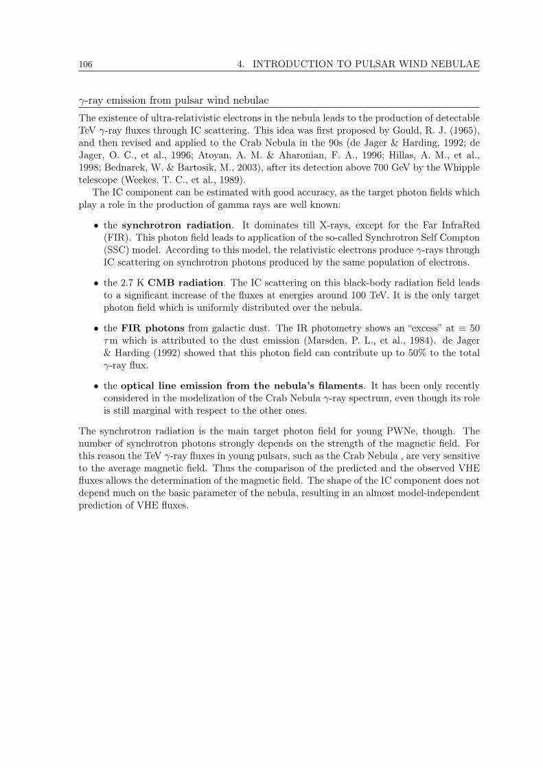
106 4. INTRODUCTION TO PULSAR WIND NEBULAE
-ray emission from pulsar wind nebulae
The existence of ultra-relativistic electrons in the nebula leads to the production of detectableTeV -ray fluxes through IC scattering. This idea was first proposed by Gould, R. J. (1965),and then revised and applied to the Crab Nebula in the 90s (de Jager & Harding, 1992; deJager, O. C., et al., 1996; Atoyan, A. M. & Aharonian, F. A., 1996; Hillas, A. M., et al.,1998; Bednarek, W. & Bartosik, M., 2003), after its detection above 700 GeV by the Whippletelescope (Weekes, T. C., et al., 1989).
The IC component can be estimated with good accuracy, as the target photon fields whichplay a role in the production of gamma rays are well known:
• the synchrotron radiation. It dominates till X-rays, except for the Far InfraRed(FIR). This photon field leads to application of the so-called Synchrotron Self Compton(SSC) model. According to this model, the relativistic electrons produce -rays throughIC scattering on synchrotron photons produced by the same population of electrons.
• the 2.7 K CMB radiation. The IC scattering on this black-body radiation field leadsto a significant increase of the fluxes at energies around 100 TeV. It is the only targetphoton field which is uniformly distributed over the nebula.
• the FIR photons from galactic dust. The IR photometry shows an “excess” at ≡ 50τm which is attributed to the dust emission (Marsden, P. L., et al., 1984). de Jager& Harding (1992) showed that this photon field can contribute up to 50% to the total -ray flux.
• the optical line emission from the nebula's filaments. It has been only recentlyconsidered in the modelization of the Crab Nebula -ray spectrum, even though its roleis still marginal with respect to the other ones.
The synchrotron radiation is the main target photon field for young PWNe, though. Thenumber of synchrotron photons strongly depends on the strength of the magnetic field. Forthis reason the TeV -ray fluxes in young pulsars, such as the Crab Nebula , are very sensitiveto the average magnetic field. Thus the comparison of the predicted and the observed VHEfluxes allows the determination of the magnetic field. The shape of the IC component does notdepend much on the basic parameter of the nebula, resulting in an almost model-independentprediction of VHE fluxes.

4.4. The Crab Nebula 107
4.4 The Crab Nebula
The Crab Nebula is almost certainly associated with a SN ex-plosion observed in 1054 CE (Lundmark, K., 1921; Stephen-son, F. R. & Green, D. A., 2002). The explosion of a 8–10 M star (Kitaura, F. S. et al., 2006) was noted by thecourt astronomers of the Song emperor as a powerful tran-sient phenomenon: the “guest star” remained visible duringthe daytime for three weeks, and was visible at night for 22months. The Crab Nebula was discovered in 1731 by theEnglish astronomer John Bevis. Few years later it was ob-served by Charles Messier and became the first object in hisfamous catalog of nebulous non-cometary objects. In fact,the Crab Nebula is also known as M1. In 1844, Lord Rossenamed the nebula “the Crab” because of its resemblance toa crab which lives in rivers, as seen by a 72-inch reflectingtelescope in the 19th century (Figure 4.14).The Crab Nebula is located in the Taurus constellation, closeto -Tauri. It is mainly observable from the northern hemi-sphere, but, being placed in the galactic plane, it is accessi-ble also from the southern hemisphere at high zenith angles.The Crab Nebula lies at a distance of ≡ 2 kpc (Trimble, V.,1968).
Figure 4.14: Lord Rosse's draw-ing of the Crab Nebula . Thiswork gave the name to the nebulabecause of its resemblance to a crab’sclaw.
The Crab Nebula is one of the best nonstellar objects in the sky ever studied. Due toits bright glow at almost all wavelengths, its observations exhibits a spatial and temporalresolution which allow to constrain relevant physics. The importance of the Crab Nebulato astrophysics does come from the high quality of its observations: a more complete anddetailed comparison between theory and observations than it is possible with any other non-stellar astrophysical object.
Because of its apparent overall flux steadiness, the Crab Nebula has been considered asstandard candle at almost all the wavelengths. It has been used to cross-calibrate X-ray and -ray telescopes, to check the instrument performance over time, and to provide units for theemission of other astrophysical objects. This notion changed dramatically in September 2010,when Tavani, M., et al. (2011) observed a strong -ray flare in which the radiation of the CrabNebula above 100 MeV almost doubled within just few days. This surprising observation wasimmediately confirmed by the Fermi/LAT team (Abdo, A. A., et al., 2011). Such unexpecteddiscovery raised a new interest of the astrophysical community on the Crab Nebula . It offers,in fact, a unique opportunity to test the mechanism of particle acceleration and high-energyemission in shocks (§ 4.4.6).
4.4.1 The Crab Pulsar
At the center of the Crab Nebula lies the Crab Pulsar, also known as PSR B0531+21. It is oneof the most energetic pulsars in our Galaxy, with a spin-down luminosity of ≡= 5 1038 erg s1.With a period of 33 ms, its characteristic age has been estimated to 1240 yrs which is closeto the observational value. The main characteristics of the Crab Pulsar are summarized
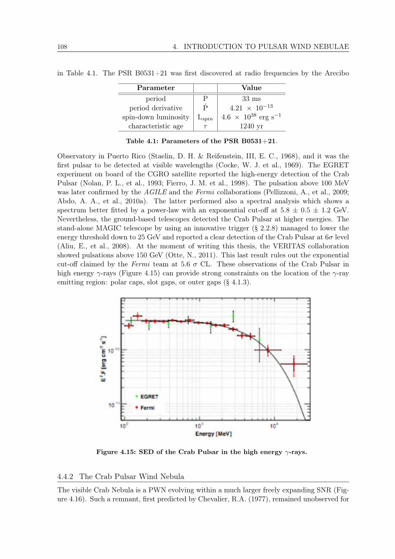
108 4. INTRODUCTION TO PULSAR WIND NEBULAE
in Table 4.1. The PSR B0531+21 was first discovered at radio frequencies by the Arecibo
Parameter Valueperiod P 33 ms
period derivative P 4.21 × 10⁻¹³
spin-down luminosity Lspin 4.6 × 1038 erg s−1
characteristic age τ 1240 yr
Table 4.1: Parameters of the PSR B0531+21.
Observatory in Puerto Rico (Staelin, D. H. & Reifenstein, III, E. C., 1968), and it was thefirst pulsar to be detected at visible wavelengths (Cocke, W. J. et al., 1969). The EGRETexperiment on board of the CGRO satellite reported the high-energy detection of the CrabPulsar (Nolan, P. L., et al., 1993; Fierro, J. M. et al., 1998). The pulsation above 100 MeVwas later confirmed by the AGILE and the Fermi collaborations (Pellizzoni, A., et al., 2009;Abdo, A. A., et al., 2010a). The latter performed also a spectral analysis which shows aspectrum better fitted by a power-law with an exponential cut-off at 5.8 ± 0.5 ± 1.2 GeV.Nevertheless, the ground-based telescopes detected the Crab Pulsar at higher energies. Thestand-alone MAGIC telescope by using an innovative trigger (§ 2.2.8) managed to lower theenergy threshold down to 25 GeV and reported a clear detection of the Crab Pulsar at 6σ level(Aliu, E., et al., 2008). At the moment of writing this thesis, the VERITAS collaborationshowed pulsations above 150 GeV (Otte, N., 2011). This last result rules out the exponentialcut-off claimed by the Fermi team at 5.6 σ CL. These observations of the Crab Pulsar inhigh energy γ-rays (Figure 4.15) can provide strong constraints on the location of the γ-rayemitting region: polar caps, slot gaps, or outer gaps (§ 4.1.3).
Figure 4.15: SED of the Crab Pulsar in the high energy γ-rays.
4.4.2 The Crab Pulsar Wind Nebula
The visible Crab Nebula is a PWN evolving within a much larger freely expanding SNR (Fig-ure 4.16). Such a remnant, first predicted by Chevalier, R.A. (1977), remained unobserved for
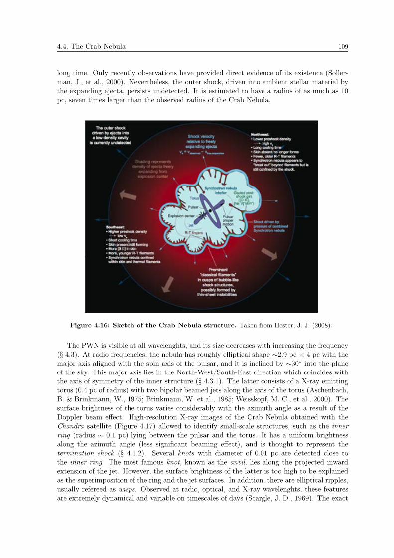
4.4. The Crab Nebula 109
long time. Only recently observations have provided direct evidence of its existence (Soller-man, J., et al., 2000). Nevertheless, the outer shock, driven into ambient stellar material bythe expanding ejecta, persists undetected. It is estimated to have a radius of as much as 10pc, seven times larger than the observed radius of the Crab Nebula.
Figure 4.16: Sketch of the Crab Nebula structure. Taken from Hester, J. J. (2008).
The PWN is visible at all wavelenghts, and its size decreases with increasing the frequency(§ 4.3). At radio frequencies, the nebula has roughly elliptical shape ∼2.9 pc × 4 pc with themajor axis aligned with the spin axis of the pulsar, and it is inclined by ∼30 into the planeof the sky. This major axis lies in the North-West/South-East direction which coincides withthe axis of symmetry of the inner structure (§ 4.3.1). The latter consists of a X-ray emittingtorus (0.4 pc of radius) with two bipolar beamed jets along the axis of the torus (Aschenbach,B. & Brinkmann, W., 1975; Brinkmann, W. et al., 1985; Weisskopf, M. C., et al., 2000). Thesurface brightness of the torus varies considerably with the azimuth angle as a result of theDoppler beam effect. High-resolution X-ray images of the Crab Nebula obtained with theChandra satellite (Figure 4.17) allowed to identify small-scale structures, such as the innerring (radius ∼ 0.1 pc) lying between the pulsar and the torus. It has a uniform brightnessalong the azimuth angle (less significant beaming effect), and is thought to represent thetermination shock (§ 4.1.2). Several knots with diameter of 0.01 pc are detected close tothe inner ring. The most famous knot, known as the anvil, lies along the projected inwardextension of the jet. However, the surface brightness of the latter is too high to be explainedas the superimposition of the ring and the jet surfaces. In addition, there are elliptical ripples,usually refereed as wisps. Observed at radio, optical, and X-ray wavelenghts, these featuresare extremely dynamical and variable on timescales of days (Scargle, J. D., 1969). The exact
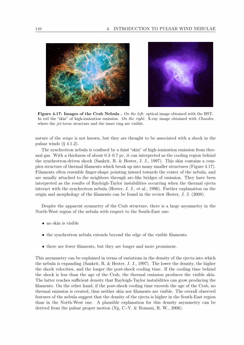
110 4. INTRODUCTION TO PULSAR WIND NEBULAE
Figure 4.17: Images of the Crab Nebula . On the left: optical image obtained with the HST.In red the “skin” of high-ionization emission. On the right: X-ray image obtained with Chandrawhere the jet-torus structure and the inner ring are visible.
nature of the wisps is not known, but they are thought to be associated with a shock in thepulsar winds (§ 4.1.2).
The synchrotron nebula is confined by a faint “skin” of high-ionization emission from ther-mal gas. With a thickness of about 0.3–0.7 pc, it can interpreted as the cooling region behindthe synchrotron-driven shock (Sankrit, R. & Hester, J. J., 1997). This skin contains a com-plex structure of thermal filaments which break up into many smaller structures (Figure 4.17).Filaments often resemble finger-shape pointing inward towards the center of the nebula, andare usually attached to the neighbors through arc-like bridges of emission. They have beeninterpreted as the results of Rayleigh-Taylor instabilities occurring when the thermal ejectainteract with the synchrotron nebula (Hester, J. J., et al., 1996). Further explanation on theorigin and morphology of the filaments can be found in the review Hester, J. J. (2008).
Despite the apparent symmetry of the Crab structure, there is a large asymmetry in theNorth-West region of the nebula with respect to the South-East one:
• no skin is visible
• the synchrotron nebula extends beyond the edge of the visible filaments.
• there are fewer filaments, but they are longer and more prominent.
This asymmetry can be explained in terms of variations in the density of the ejecta into whichthe nebula is expanding (Sankrit, R. & Hester, J. J., 1997). The lower the density, the higherthe shock velocities, and the longer the post-shock cooling time. If the cooling time behindthe shock is less than the age of the Crab, the thermal emission produces the visible skin.The latter reaches sufficient density that Rayleigh-Taylor instabilities can grow producing thefilaments. On the other hand, if the post-shock cooling time exceeds the age of the Crab, nothermal emission is created, thus neither skin nor filaments are visible. The overall observedfeatures of the nebula suggest that the density of the ejecta is higher in the South-East regionthan in the North-West one. A plausible explanation for this density asymmetry can bederived from the pulsar proper motion (Ng, C.-Y. & Romani, R. W., 2006).
4.4. The Crab Nebula 111
4.4.3 The broad-band spectrum of the Crab Nebula
The overall spectrum of the Crab Nebula extends over 20 orders of magnitudes in energy fromradio frequencies up to VHEs. It is composed of two non-thermal broad components:
• a low-energy component dominates the overall output and extends from radio to -ray frequencies. This emission is thought to be synchrotron radiation, associated withthe emission from electrons between a few GeV up to a few tens of TeV (Figure 4.7).It is confirmed through polarization measurements (Dean, A. J., et al., 2008). TheCrab Nebula is remarkably efficient at converting the energy of the pulsar wind intosynchrotron radiation, almost 26% of the entire energy injected by the pulsar in thenebula.The synchrotron emission peaks between optical and soft X-ray frequencies and comesprimarily from the torus. The bump in the FIR is the result of the thermal emissionfrom dust in the nebula. This dust is condensated from material ejected in the SNexplosion.Assuming an average magnetic field of 2–3 104 G (Marsden, P. L., et al., 1984), thesynchrotron losses in 1000 yrs (almost the age of the nebula) can account for the coolingof relativistic electrons only down to Ecr ≡ 200 GeV (Equation A.13). This simpleconsideration implies that two different populations of relativistic electrons should bedistinguished in the Crab Nebula: the wind electrons freshly accelerated at the shockwith energies E Ecr (Ecr corresponds to synchrotron radiation in the near-IR/opticalband), and the radio electrons at lower energies responsible for the radio emission. Thissecond population of electrons is considered a leftover from an early phase of evolution ofthe pulsar, during which it was injected in different parts of the nebula (Atoyan, A. M.,1999). An experimental proof for this argument of the two electron populations is givenby the fact that the single power-law synchrotron spectrum steepens significantly in thenear-IR/optical band (Marsden, P. L., et al., 1984) becoming inconsistent with the windshock acceleration model for the Crab Nebula.
• the high-energy component dominates above 426 35 MeV (Abdo, A. A., et al., 2011)and derives from IC scattering of high-energy electrons from the pulsars on mainlysynchrotron photons (SSC, § 4.3.3). It peaks between some tens and some hundredsof GeV, but its position has not been clearly determined yet. The models for thishigh-energy component will be discussed in detail in § 4.4.5.
In the Crab Nebula the synchrotron emission reaches the soft -rays up to 1 GeV. Thisis a clear indication that electrons are accelerated at UHEs in the termination shock. Sincesuch energetic electrons have short radiative lifetimes, they necessarily radiate close to theacceleration zone, hence identifying the site of the injection.
The soft -ray emission was first detected by the -ray satellites. In particular, the COS-Bsatellite showed a differential energy spectrum from 70 MeV up to 1 GeV which is well-fittedby a single power-law with photon index 2.7 0.3 (Clear, J., et al., 1987). The EGRETexperiment on board of the CGRO satellite extended the Crab Nebula spectrum up to 5GeV, and the fitted single power-law had a photon index of 2.93 0.15 (Nolan, P. L., etal., 1993). However, above 1 GeV the observed data points appeared to be significantlyabove the fitted model. A broken power-law, in fact, seemed to better fit the data, but notconclusively, due to the lack of statistics at the highest energies. This claimed hardening ofthe Crab Nebula spectrum provided the first indication of the transition energy where the
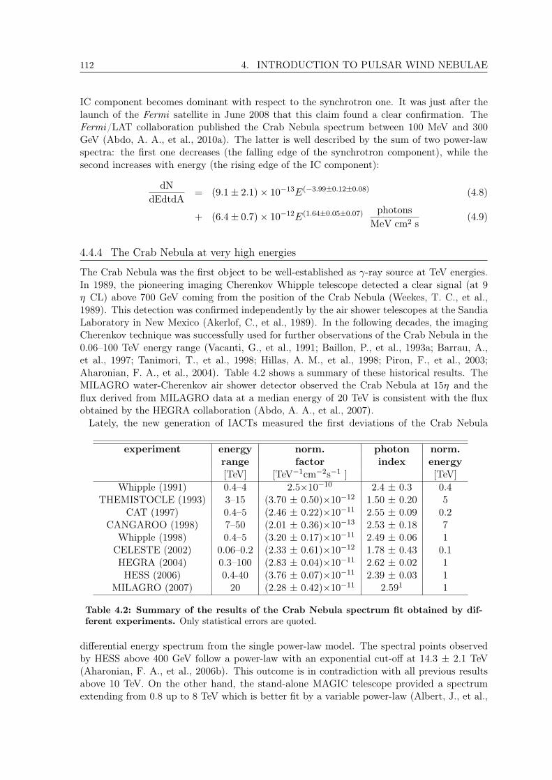
112 4. INTRODUCTION TO PULSAR WIND NEBULAE
IC component becomes dominant with respect to the synchrotron one. It was just after thelaunch of the Fermi satellite in June 2008 that this claim found a clear confirmation. TheFermi/LAT collaboration published the Crab Nebula spectrum between 100 MeV and 300GeV (Abdo, A. A., et al., 2010a). The latter is well described by the sum of two power-lawspectra: the first one decreases (the falling edge of the synchrotron component), while thesecond increases with energy (the rising edge of the IC component):
dNdEdtdA
= (9:1 2:1) 1013E(3:990:120:08) (4.8)
+ (6:4 0:7) 1012E(1:640:050:07) photonsMeV cm2 s
(4.9)
4.4.4 The Crab Nebula at very high energies
The Crab Nebula was the first object to be well-established as -ray source at TeV energies.In 1989, the pioneering imaging Cherenkov Whipple telescope detected a clear signal (at 9η CL) above 700 GeV coming from the position of the Crab Nebula (Weekes, T. C., et al.,1989). This detection was confirmed independently by the air shower telescopes at the SandiaLaboratory in New Mexico (Akerlof, C., et al., 1989). In the following decades, the imagingCherenkov technique was successfully used for further observations of the Crab Nebula in the0.06–100 TeV energy range (Vacanti, G., et al., 1991; Baillon, P., et al., 1993a; Barrau, A.,et al., 1997; Tanimori, T., et al., 1998; Hillas, A. M., et al., 1998; Piron, F., et al., 2003;Aharonian, F. A., et al., 2004). Table 4.2 shows a summary of these historical results. TheMILAGRO water-Cherenkov air shower detector observed the Crab Nebula at 15η and theflux derived from MILAGRO data at a median energy of 20 TeV is consistent with the fluxobtained by the HEGRA collaboration (Abdo, A. A., et al., 2007).Lately, the new generation of IACTs measured the first deviations of the Crab Nebula
experiment energy norm. photon norm.range factor index energy[TeV] [TeV1cm2s1 ] [TeV]
Whipple (1991) 0.4–4 2.51010 2.4 0.3 0.4THEMISTOCLE (1993) 3–15 (3.70 0.50)1012 1.50 0.20 5
CAT (1997) 0.4–5 (2.46 0.22)1011 2.55 0.09 0.2CANGAROO (1998) 7–50 (2.01 0.36)1013 2.53 0.18 7
Whipple (1998) 0.4–5 (3.20 0.17)1011 2.49 0.06 1CELESTE (2002) 0.06–0.2 (2.33 0.61)1012 1.78 0.43 0.1HEGRA (2004) 0.3–100 (2.83 0.04)1011 2.62 0.02 1HESS (2006) 0.4-40 (3.76 0.07)1011 2.39 0.03 1
MILAGRO (2007) 20 (2.28 0.42)1011 2.591 1
Table 4.2: Summary of the results of the Crab Nebula spectrum fit obtained by dif-ferent experiments. Only statistical errors are quoted.
differential energy spectrum from the single power-law model. The spectral points observedby HESS above 400 GeV follow a power-law with an exponential cut-off at 14.3 2.1 TeV(Aharonian, F. A., et al., 2006b). This outcome is in contradiction with all previous resultsabove 10 TeV. On the other hand, the stand-alone MAGIC telescope provided a spectrumextending from 0.8 up to 8 TeV which is better fit by a variable power-law (Albert, J., et al.,

4.4. The Crab Nebula 113
2008d):
dNdEdAdt
= (6.0 ± 0.2) × 10−10 (4.10)
·(
E
300GeV
)(−2.31± 0.06)−(0.26± 0.07)log10( E300GeV ) photons
TeV cm2 s(4.11)
The hardening of the spectrum at energies below few hundreds of GeV indicates that the peakof the IC component is approaching. The fit to the MAGIC data points allowed an estimationof the peak at 77 ± 35 GeV.
Figure 4.18 illustrates the Spectral Energy Distribution (SED) of the Crab Nebula in theγ-ray energy domain. It includes the main experimental results obtained up to now. Theoverlap between satellites and ground-based telescopes measurements has become possibleonly in the last few years. If at low γ-ray energies, the innovative Fermi satellite filled thegap between few and a hundred of GeV, the construction of IACTs with larger reflectorsallowed to lower the energy threshold of the ground-based telescopes down to 50 GeV.
Figure 4.18: The SED of the Crab Nebula in the γ-ray energy domain.
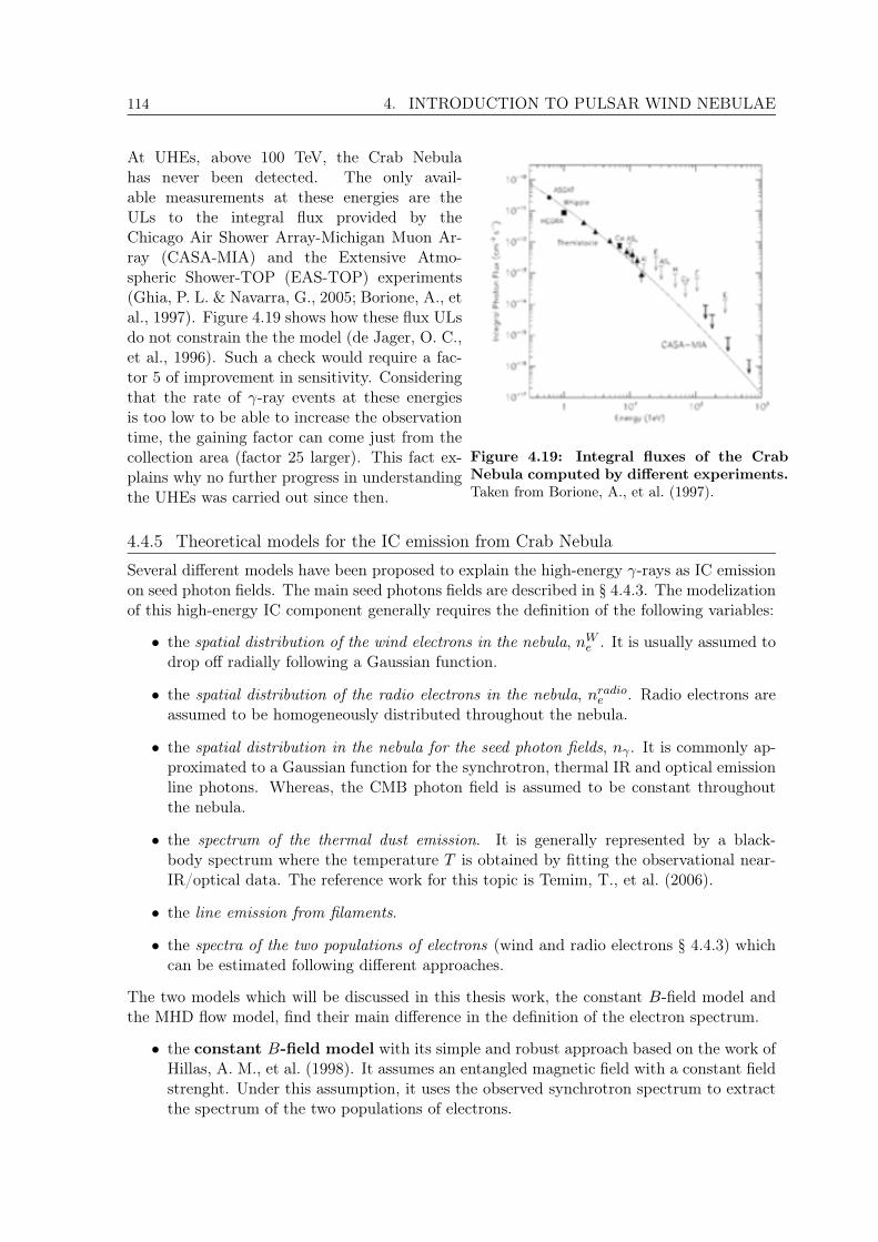
114 4. INTRODUCTION TO PULSAR WIND NEBULAE
At UHEs, above 100 TeV, the Crab Nebulahas never been detected. The only avail-able measurements at these energies are theULs to the integral flux provided by theChicago Air Shower Array-Michigan Muon Ar-ray (CASA-MIA) and the Extensive Atmo-spheric Shower-TOP (EAS-TOP) experiments(Ghia, P. L. & Navarra, G., 2005; Borione, A., etal., 1997). Figure 4.19 shows how these flux ULsdo not constrain the the model (de Jager, O. C.,et al., 1996). Such a check would require a fac-tor 5 of improvement in sensitivity. Consideringthat the rate of γ-ray events at these energiesis too low to be able to increase the observationtime, the gaining factor can come just from thecollection area (factor 25 larger). This fact ex-plains why no further progress in understandingthe UHEs was carried out since then.
Figure 4.19: Integral fluxes of the CrabNebula computed by different experiments.Taken from Borione, A., et al. (1997).
4.4.5 Theoretical models for the IC emission from Crab Nebula
Several different models have been proposed to explain the high-energy γ-rays as IC emissionon seed photon fields. The main seed photons fields are described in § 4.4.3. The modelizationof this high-energy IC component generally requires the definition of the following variables:
• the spatial distribution of the wind electrons in the nebula, nWe . It is usually assumed todrop off radially following a Gaussian function.
• the spatial distribution of the radio electrons in the nebula, nradioe . Radio electrons areassumed to be homogeneously distributed throughout the nebula.
• the spatial distribution in the nebula for the seed photon fields, nγ. It is commonly ap-proximated to a Gaussian function for the synchrotron, thermal IR and optical emissionline photons. Whereas, the CMB photon field is assumed to be constant throughoutthe nebula.
• the spectrum of the thermal dust emission. It is generally represented by a black-body spectrum where the temperature T is obtained by fitting the observational near-IR/optical data. The reference work for this topic is Temim, T., et al. (2006).
• the line emission from filaments.
• the spectra of the two populations of electrons (wind and radio electrons § 4.4.3) whichcan be estimated following different approaches.
The two models which will be discussed in this thesis work, the constant B-field model andthe MHD flow model, find their main difference in the definition of the electron spectrum.
• the constant B-field model with its simple and robust approach based on the work ofHillas, A. M., et al. (1998). It assumes an entangled magnetic field with a constant fieldstrenght. Under this assumption, it uses the observed synchrotron spectrum to extractthe spectrum of the two populations of electrons.
4.4. The Crab Nebula 115
• the application of the MHD ow model to the IC component (Atoyan, A. M. &Aharonian, F. A., 1996). The MHD model by Kennel, C. F. & Coroniti, F. V. (1984b)requires few a priori assumptions to describe the evolution of the injected particles, i.e.the electron propagation model:
– spherical symmetry of the nebula. The latter is approximated to a sphere withradius of 1.8 pc.
– the radius of the termination shock, rS . The canonical value has been for long time0.10 pc (Rees, M. J. & Gunn, J. E., 1974). Recently, the termination shock wasidentified with the inner ring observed in X-ray by Chandra (Weisskopf, M. C., etal., 2000), and estimated at 0:14 0:01 pc.
– the magnetization parameter, η. Recently, Mori, K., et al. (2004) determined avalue of η between 0.01 and 0.03, more likely close to 0.05.
– the power-law spectrum of the injected electrons.
By fitting the resulting synchrotron spectrum with the observation data, the free pa-rameters of the electron spectrum can be estimated.
Figure 4.20 illustrates the Crab Nebula SED for the constant B-field and the MHD modelsas presented in Meyer, M. et al. (2010). These authors revised both models including morerecent observational measurements. The best match of the free model parameters (average B-field and magnetization parameter for the constant B-field and the MHD model respectively)to the measured SED were obtained using a rather weak field of B = (124 6)τG or a valueη = 0:0045 0:0003.
Both the models are in good agreement with the Fermi part of the spectrum, even thoughthe shape of the synchrotron cut-off is harder than the measured spectrum for the MHDflow model. At energies beyond the position of the peak in the IC part of the SED, theMHD model does not provide a satisfactory description of the available data: the spectraare considerably harder than the VHE measurements. This discrepancy is directly relatedto the mismatch visible in the X-ray part of the spectrum. Nevertheless, a re-definition ofthe standard assumptions might lead to better results. A straight-forward modification is theintroduction of an anisotropic wind with variations of η when moving out of the equatorialplane towards the polar regions of the outflow (Volpi, D. et al., 2008). The simpler approachof the constant B-field model yields a better agreement with the VHE observational data.
4.4.6 The Crab Nebula variability
The variability of the Crab Nebula is known almost since its discovery. Scargle, J. D. (1969)claimed the existence of optical features in the nebula, whose brightness varies on differenttimescales. Wisps and knots were observed to brighten and fade over weeks and months atdifferent wavelengths (Hester, J. J., et al., 2002; Bietenholz, M. F. et al., 2004). Despitethe varying intensity of these compact features, the large-scale integrated emission from thenebula was expected to be steady within a few percent.
In September 2010, for the first time, a flare of the integrated emission from the CrabNebula at energies above 100 MeV was reported. It lasted few days, between September 18and 23 (Tavani, M., et al., 2011; Abdo, A. A., et al., 2011). Spectral analysis, as well asthe short timescale variability, indicate that this enhanced emission has a synchrotron origin.The integral flux corresponds to an increase by a factor 5.5 0.8 with respect to the average
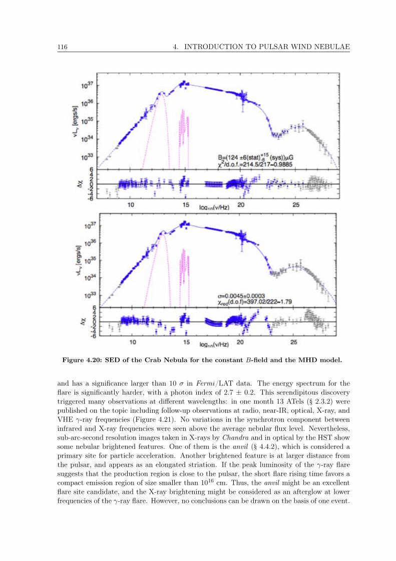
116 4. INTRODUCTION TO PULSAR WIND NEBULAE
Figure 4.20: SED of the Crab Nebula for the constant B-field and the MHD model.
and has a significance larger than 10 σ in Fermi/LAT data. The energy spectrum for theflare is significantly harder, with a photon index of 2.7 ± 0.2. This serendipitous discoverytriggered many observations at different wavelengths: in one month 13 ATels (§ 2.3.2) werepublished on the topic including follow-up observations at radio, near-IR, optical, X-ray, andVHE γ-ray frequencies (Figure 4.21). No variations in the synchrotron component betweeninfrared and X-ray frequencies were seen above the average nebular flux level. Nevertheless,sub-arc-second resolution images taken in X-rays by Chandra and in optical by the HST showsome nebular brightened features. One of them is the anvil (§ 4.4.2), which is considered aprimary site for particle acceleration. Another brightened feature is at larger distance fromthe pulsar, and appears as an elongated striation. If the peak luminosity of the γ-ray flaresuggests that the production region is close to the pulsar, the short flare rising time favors acompact emission region of size smaller than 1016 cm. Thus, the anvil might be an excellentflare site candidate, and the X-ray brightening might be considered as an afterglow at lowerfrequencies of the γ-ray flare. However, no conclusions can be drawn on the basis of one event.
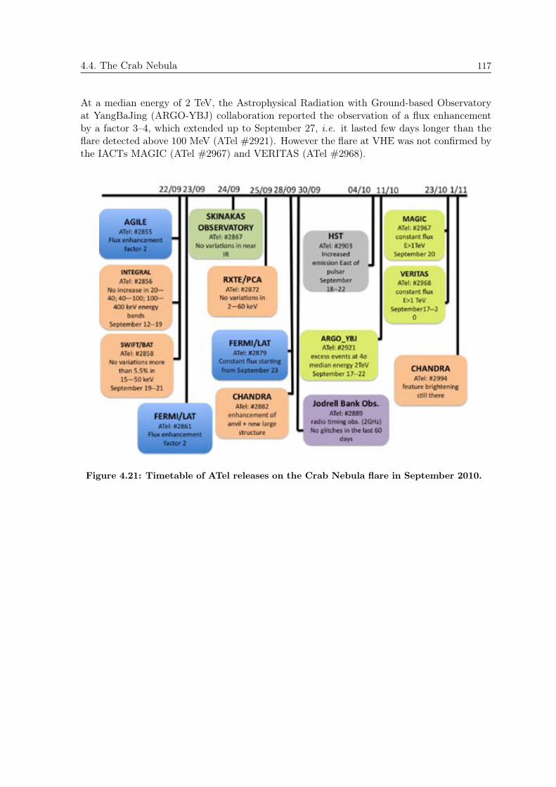
4.4. The Crab Nebula 117
At a median energy of 2 TeV, the Astrophysical Radiation with Ground-based Observatoryat YangBaJing (ARGO-YBJ) collaboration reported the observation of a flux enhancementby a factor 3–4, which extended up to September 27, i.e. it lasted few days longer than theflare detected above 100 MeV (ATel #2921). However the flare at VHE was not confirmed bythe IACTs MAGIC (ATel #2967) and VERITAS (ATel #2968).
Figure 4.21: Timetable of ATel releases on the Crab Nebula flare in September 2010.

118 4. INTRODUCTION TO PULSAR WIND NEBULAE
There are other three γ-ray flares from theCrab Nebula reported so far. The AGILEteam detected a γ-ray flare above 100MeV in October 2007 (before the launchof the Fermi satellite). This flare lastedfor two weeks and was almost at the samelevel of the September 2010 flare (Tavani,M., et al., 2011). Fermi/LAT collabo-ration detected its first γ-ray flare fromthe Crab Nebula in February 2009. Thisflare was not observed by AGILE becausethe instrument was pointing at a differentpart of the sky. It had a duration of 16days, and an increase in flux by a factor3.8 ± 0.5. The significance of such an in-crease was at the level of 8 σ. A study ofthe spectral variations revealed a soften-ing of the spectrum (Figure 4.22) with aphoton index of 4.3 ± 0.3 (Abdo, A. A.,et al., 2011).
Figure 4.22: SED of the Crab Nebula in the high-energy band measured by Fermi/LAT. Black opencircles indicate the average spectrum computed over 25months of observations. Red circles indicate the CrabNebula spectrum during the February 2009 flare, andblue open squares indicate the spectrum during the flareof September 2010. Taken from Abdo, A. A., et al.(2011).
The last flux enhancement from the Crab Nebula was observed by AGILE and Fermi inApril 2011 (ATels #3279 #3282 #3284 #3286). The integrated flux above 100 MeV startedincreasing on April 9, 2011, and reached its peak with an increase by a factor 5 on April 14,2011. Chandra followed up observations revealed a new bright knot, which is not aligned withthe jet (ATel #3283).
Vittorini, V., et al. (2011) explained the γ-ray flares from the Crab Nebula in termsof a fast-rising-synchrotron-cooling model. They assumed a fresh population of impulsivelyaccelerated electrons and positrons which is produced on short timescales (short with respectto the cooling timescales). The acceleration would occur in nebular sites subjected to plasmainstabilities and/or substantial pulsar wind particle density enhancements. This assumptionfollows from the short observed flaring rising time. To fit the synchrotron cooling timescaleswith the flare observations (for a Lorentz factor γ ∼ 5 × 10⁻⁹ of electrons irradiating in theGeV range) they estimated a local magnetic field as small as 10−3 G (5 times larger than thenebular average).
5Spectrum and flux variability of the Crab Nebula
The MAGIC stereoscopic system observed the Crab Nebula for 50 hours betweenOctober 2009 and March 2011. This large data sample allowed to perform ahigh-precision study on the IC -ray emission from the Crab Nebula. It re-sulted in an unpercented differential energy spectrum which spans eight ordersof magnitude in flux and three orders of magnitude in energy between 50 GeVand 45 TeV. The spectrum can be described by a variable power-law f0 (E/1TeV)α+bLog(E/1TeV ) with = 2:40 0:01stat 0:1sys, b = 0:15 0:01stat 0:05systand f0 = 3:27 0:03stat 0:48syst. This work presents the most precise estimation ofthe peak of the IC component of the Crab Nebula spectrum is set at 59 6 GeV. Theintegral flux above both 300 and 700 GeV is constant on daily time scales within thesystematic uncertainty. No flux enhancement is observed simultaneously to the GeVflares reported by AGILE and Fermi.
The author is the main responsible of the paper: “The measurement of Crab Nebulaspectrum over three orders of magnitude” which is in preparation and will be submittedin Autumn 2011. Part of this work is already published in Zanin, R., et al. (2011).
Measurements of IC -ray emission in the region between few GeV and hundred GeV arecharacterized by large statistical uncertainties. At higher energies, there are some discrepan-cies between the measurements of the HEGRA and the HESS collaborations. The first claimeda single power-law spectrum from 400 GeV up to 100 TeV, whereas the second reported anexponential cut-off at much lower energies, around 14 TeV. The new MAGIC stereoscopicsystem with an energy threshold as low as 80 GeV and a flux sensitivity twice better than theprevious stand-alone MAGIC I telescope is ideally suited to produce a more precise differentialenergy spectrum of the Crab Nebula from few tens of GeV up to some tens of TeV. On theother hand, MAGIC has a smaller collection area than the above mentioned experiments atenergies above 10 TeV, but this draw-back can be compensated by observing the Crab Nebulalonger.
Moreover, the recent discovery of flux variability in the soft- -ray band (Tavani, M., et al.,2011; Abdo, A. A., et al., 2011) casts doubts on the notion that the Crab Nebula is a constant
119
120 5. SPECTRUM AND FLUX VARIABILITY OF THE CRAB NEBULA
source in the VHE band (§ 4.4.6). Therefore, checking the flux stability in this energy rangewith precise and more sensitive measurements has become a topic of primary importance.A possible variability of the IC flux component might have the same origin of the soft- -rayflares, hence show itself on timescales of days; but it might also have larger variations (monthsor years) as those detected in the X-rays (Wilson-Hodge, C. A., et al., 2011). In the first caseit should be visible at energies above few TeV.
For these reasons, the MAGIC collaboration collected 50 hours of Crab Nebula data sincethe beginning of its stereoscopic operation. The analysis of these 50 hours is the subject ofthis chapter which has mainly four goals:
• reconstruction of the IC -ray emission spectrum from energies which overlap the satel-lite measurements up to the VHEs above 10 TeV.
• more precise measurement of the position of IC peak. Right now the most accuratemeasurement is 77 35 GeV by Albert, J., et al. (2008d).
• disentangling the discrepancies between HESS and HEGRA results above few TeV
• check the flux stability at different energy thresholds
5.1 Data sample
The data sample considered in this analysis includes stereoscopic observations of the CrabNebula carried out in the last two observation cycles (§ 2.3.1), between October 2009 andMarch 2011. These observations were performed in wobble mode (§ 2.3.3), and at differentzenith angles (4 < ZA < 50). No moonlight was present during the observations. The dataset corresponds to about 50 hrs of exposure time.
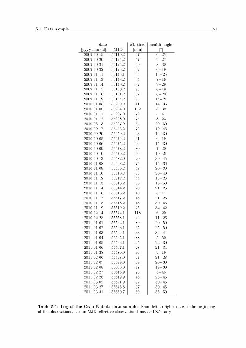
5.1. Data sample 121
date eff. time zenith angle[yyyy mm dd] [MJD] [min] []2009 10 15 55119.2 47 6252009 10 20 55124.2 57 9272009 10 21 55125.2 99 8302009 10 22 55126.2 62 6192009 11 11 55146.1 35 15252009 11 13 55148.2 54 7162009 11 14 55149.2 82 9292009 11 15 55150.2 73 6192009 11 16 55151.2 87 6202009 11 19 55154.2 25 14212010 01 05 55200.9 41 14362010 01 08 55204.0 152 8322010 01 11 55207.0 72 5412010 01 12 55208.0 75 8232010 03 13 55267.9 54 20302010 09 17 55456.2 72 19452010 09 20 55459.2 43 14302010 10 05 55474.2 61 6192010 10 06 55475.2 46 15302010 10 09 55478.2 80 7202010 10 10 55479.2 66 10212010 10 13 55482.0 20 39452010 11 08 55508.2 75 14362010 11 09 55509.2 47 20392010 11 10 55510.3 33 30402010 11 12 55512.2 44 15262010 11 13 55513.2 36 16502010 11 14 55514.2 20 21262010 11 16 55516.2 10 8112010 11 17 55517.2 18 21262010 11 18 55518.2 18 30452010 11 19 55519.2 25 34422010 12 14 55544.1 118 6202010 12 28 55558.1 42 11262011 01 01 55562.1 89 20502011 01 02 55563.1 65 25502011 01 03 55564.1 33 34442011 01 04 55565.1 88 5502011 01 05 55566.1 25 22302011 01 06 55567.1 28 21342011 01 28 55589.0 36 9192011 02 06 55598.0 27 21282011 02 07 55599.0 39 20302011 02 08 55600.0 47 19302011 02 27 55618.9 73 5452011 02 28 55619.9 46 28452011 03 02 55621.9 92 30452011 03 27 55646.8 97 30452011 03 31 55650.7 69 3550
Table 5.1: Log of the Crab Nebula data sample. From left to right: date of the beginningof the observations, also in MJD, effective observation time, and ZA range.
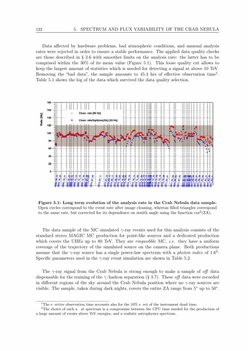
122 5. SPECTRUM AND FLUX VARIABILITY OF THE CRAB NEBULA
Data affected by hardware problems, bad atmospheric conditions, and unusual analysisrates were rejected in order to ensure a stable performance. The applied data quality checksare those described in § 3.6 with smoother limits on the analysis rate: the latter has to becomprised within the 30% of its mean value (Figure 5.1). This loose quality cut allows tokeep the largest amount of statistics which is needed for detecting a signal at above 10 TeV.Removing the “bad data”, the sample amounts to 45.4 hrs of effective observation time1.Table 5.1 shows the log of the data which survived the data quality selection.
Figure 5.1: Long term evolution of the analysis rate in the Crab Nebula data sample.Open circles correspond to the event rate after image cleaning, whereas filled triangles correspondto the same rate, but corrected for its dependence on zenith angle using the function cos2(ZA).
The data sample of the MC simulated -ray events used for this analysis consists of thestandard stereo MAGIC MC production for point-like sources and a dedicated productionwhich covers the UHEs up to 80 TeV. They are ringwobble MC, i.e. they have a uniformcoverage of the trajectory of the simulated source on the camera plane. Both productionsassume that the -ray source has a single power-law spectrum with a photon index of 1.62.Specific parameters used in the -ray event simulation are shown in Table 5.2.
The -ray signal from the Crab Nebula is strong enough to make a sample of off datadispensable for the training of the /hadron separation (§ 3.7). These off data were recordedin different regions of the sky around the Crab Nebula position where no -ray sources arevisible. The sample, taken during dark nights, covers the entire ZA range from 5 up to 50.
1The eective observation time accounts also for the 10% eect of the instrument dead time.2The choice of such a at spectrum is a compromise between the CPU time needed for the production of
a large amount of events above TeV energies, and a realistic astrophysics spectrum.
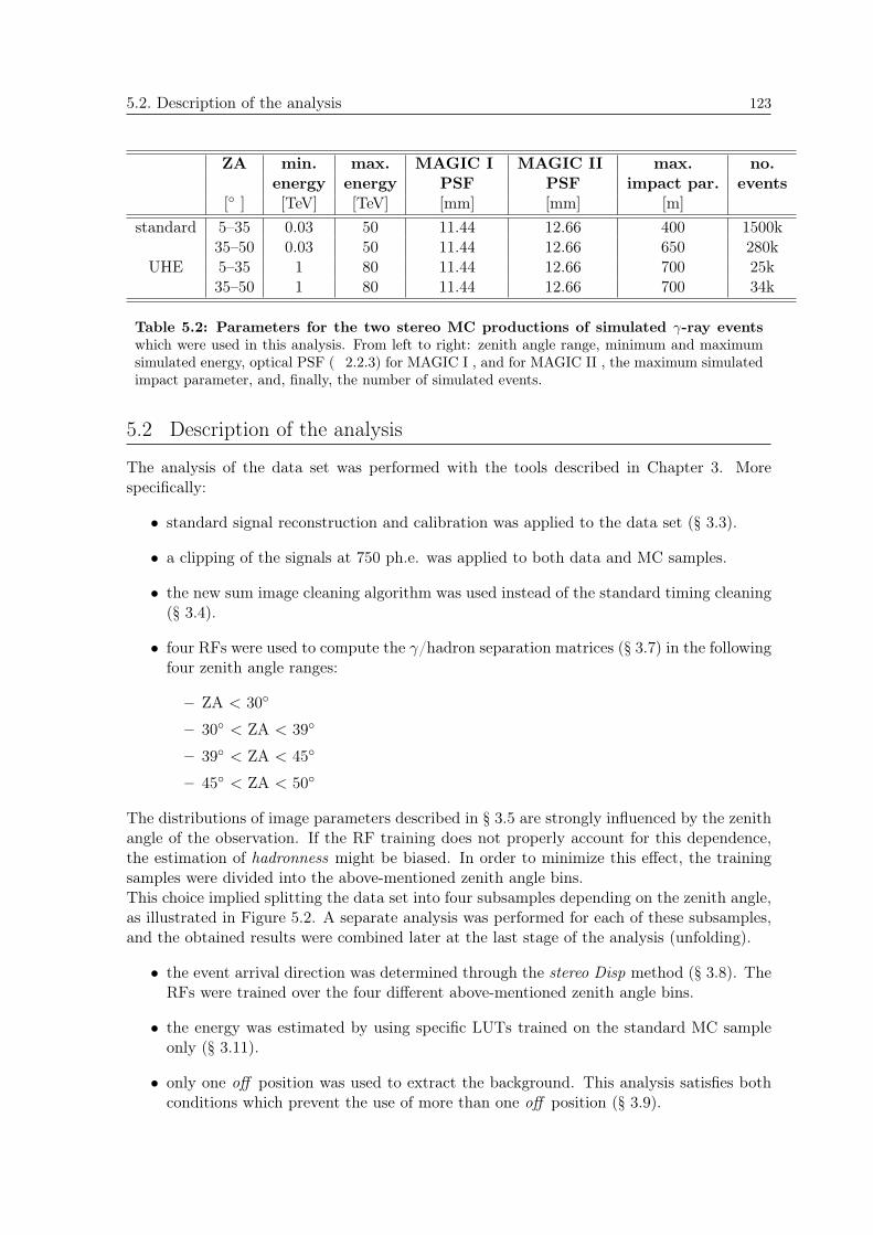
5.2. Description of the analysis 123
ZA min. max. MAGIC I MAGIC II max. no.energy energy PSF PSF impact par. events
[ ] [TeV] [TeV] [mm] [mm] [m]standard 5–35 0.03 50 11.44 12.66 400 1500k
35–50 0.03 50 11.44 12.66 650 280kUHE 5–35 1 80 11.44 12.66 700 25k
35–50 1 80 11.44 12.66 700 34k
Table 5.2: Parameters for the two stereo MC productions of simulated -ray eventswhich were used in this analysis. From left to right: zenith angle range, minimum and maximumsimulated energy, optical PSF (Ÿ 2.2.3) for MAGIC I , and for MAGIC II , the maximum simulatedimpact parameter, and, finally, the number of simulated events.
5.2 Description of the analysis
The analysis of the data set was performed with the tools described in Chapter 3. Morespecifically:
• standard signal reconstruction and calibration was applied to the data set (§ 3.3).
• a clipping of the signals at 750 ph.e. was applied to both data and MC samples.
• the new sum image cleaning algorithm was used instead of the standard timing cleaning(§ 3.4).
• four RFs were used to compute the /hadron separation matrices (§ 3.7) in the followingfour zenith angle ranges:
– ZA < 30
– 30 < ZA < 39
– 39 < ZA < 45
– 45 < ZA < 50
The distributions of image parameters described in § 3.5 are strongly influenced by the zenithangle of the observation. If the RF training does not properly account for this dependence,the estimation of hadronness might be biased. In order to minimize this effect, the trainingsamples were divided into the above-mentioned zenith angle bins.This choice implied splitting the data set into four subsamples depending on the zenith angle,as illustrated in Figure 5.2. A separate analysis was performed for each of these subsamples,and the obtained results were combined later at the last stage of the analysis (unfolding).
• the event arrival direction was determined through the stereo Disp method (§ 3.8). TheRFs were trained over the four different above-mentioned zenith angle bins.
• the energy was estimated by using specific LUTs trained on the standard MC sampleonly (§ 3.11).
• only one off position was used to extract the background. This analysis satisfies bothconditions which prevent the use of more than one off position (§ 3.9).

124 5. SPECTRUM AND FLUX VARIABILITY OF THE CRAB NEBULA
• a minimum cut in the size parameter at 30 ph.e. was applied throughout the entireanalysis. Such a low size cut aims at keeping the largest possible fraction of low-energyevents.
Figure 5.2: ZA distribution of the data set. The colors illustrate the data sample subdivision.A completely independent analysis was applied to each of these data subsamples.
5.2.1 Sum versus standard image cleaning
The performance of the new sum image cleaning algorithm was studied in comparison withthe standard cleaning. For this purpose, only data taken at small zenith angles (ZA < 30)were used in order to ensure a uniform low trigger energy threshold (≡ 34 hrs of observa-tions). Two completely independent analyses were performed on this data sample startingfrom the image cleaning stage. The analysis with the standard cleaning will be referred toas reference analysis. A common size cut at 30 ph.e. was applied to both of them. Differentenergy ranges were considered in order to better explore the behaviour of this new cleaning.In the reference analysis, for each energy range the gamma selection cuts were optimized asdescribed in § 3.9.2. On the other hand, in the “new” analysis, the 2 cut was fixed at thesame value as the one for the reference analysis, and the hadronness cuts were chosen suchthat the same number of excess events was obtained. In this way, the number of backgroundevents are comparable and show the different ability in rejecting the background of the twoanalyses. Results are shown in Table 5.3.
The sum image cleaning shows a significant improvement in rejecting the background atlow energies, and consequently in the analysis sensitivity (§ 3.9.1). The improvement is moresignificant at low energies, below 100 GeV (Table 5.3). The use of this image cleaning allowsto find a much clearer hint of signal below 60 GeV (Figure 5.3). Note that the gammaselection cuts used for this analysis had not been optimized. Therefore, the signal could beeven stronger. Figure 5.4 shows the comparison of the 2 distributions for energies smallerthan 70 GeV where the -ray signal is detected at more than 5η level. At high energies thebackground rejection is similar for the two analyses as well as their integral sensitivity. For

5.2. Description of the analysis 125
energy analysis had.cut 2cut bg exc signif. sens.[GeV] [] [η] [% Crab flux]> 250 reference 0.20 0.011 309 9607 101 106.8 0.75 0.02
sum 0.22 0.011 333 9673 102 106.7 0.77 0.02> 1000 reference 0.22 0.010 35 2354 49 54.7 1.03 0.09
sum 0.21 0.010 41 2318 49 53.9 1.13 0.09< 150 reference 0.40 0.032 13243 10109 191 53.2 4.7 0.1
sum 0.33 0.032 11431 10040 181 55.8 4.37 0.09< 100 reference 0.50 0.032 11582 4328 166 26.2 10.2 0.4
sum 0.4 0.032 9687 4337 154 28.2 9.3 0.4< 80 reference 0.65 0.032 10202 1729 148 11.65 24.0 2.1
sum 0.41 0.032 5821 1741 116 15.07 18.0 1.3< 70 reference 0.65 0.032 6477 755 117 6.45 43.9 7.0
sum 0.41 0.032 3109 771 84 9.23 29.7 3.4< 60 reference 0.65 0.032 3006 134 78 1.71 168.4 99.6
sum 0.37 0.032 737 138 41 3.44 80.7 24.5
Table 5.3: Statistics of the 2 distributions obtained for different low energy rangesin the case of the two analyses: the reference one using the standard timing imagecleaning, and the new one with the sum image cleaning. From left to right: energy range,analysis type, hadronness cut, 2 cut, number of background events in the signal region, numberof excess events, LiMa significance, and corresponding sensitivity.
energies larger than 250 GeV the analysis sensitivity is (0.75 0.02)% of the Crab Nebulaflux, in perfect agreement with the value presented in Aleksic J., et al. (2011b).
Figure 5.3: 2 distribution below 60 GeV. On the left: for the standard timing image cleaninganalysis. On the right: for the sum image cleaning.
In the specific case of this work, the use of the sum image cleaning allowed to reconstructthe first spectral point in the energy bin between 43 and 58 GeV. This effect is illustrated inFigure 5.5: it shows the distributions of the number of excess events and of the significanceper spectral point. The significance was computed by using Li & Ma formula 17.
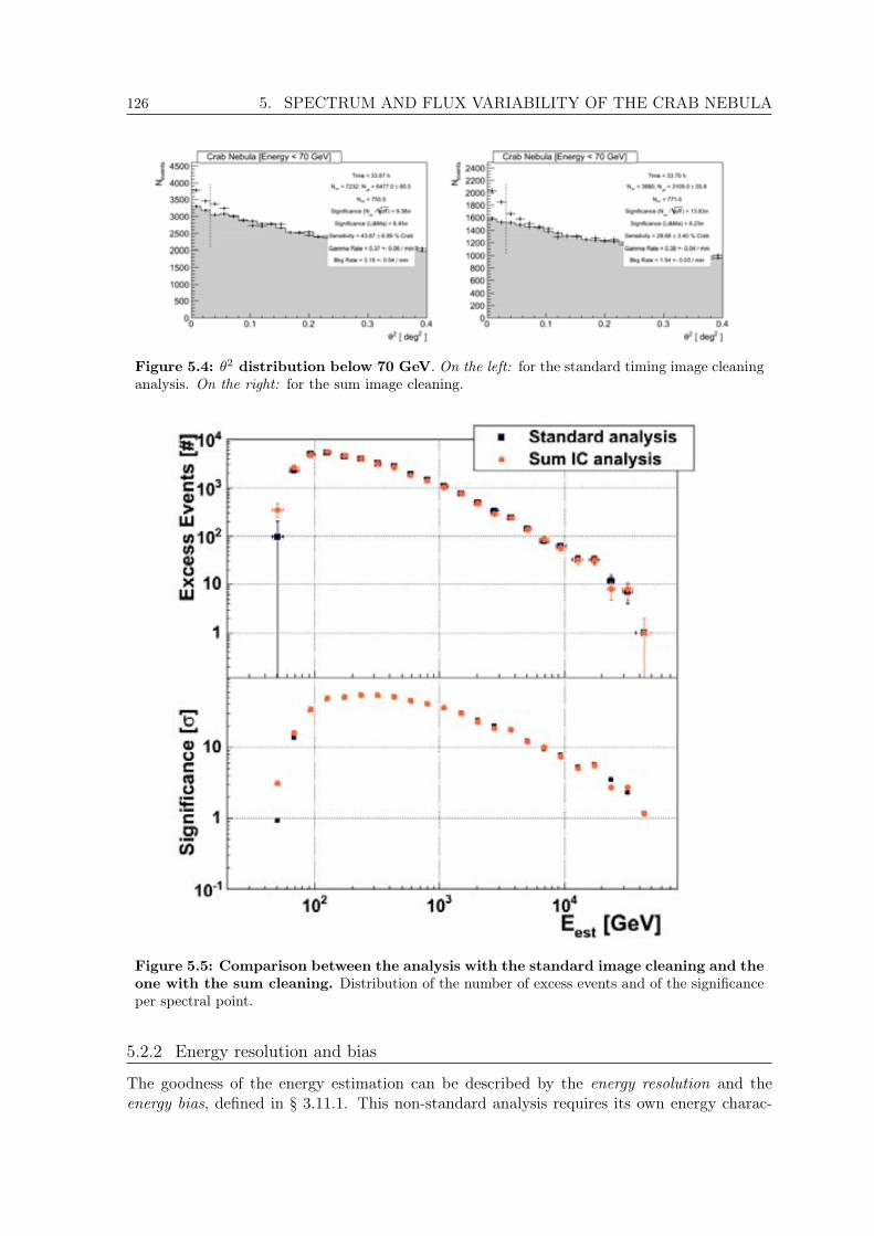
126 5. SPECTRUM AND FLUX VARIABILITY OF THE CRAB NEBULA
Figure 5.4: 2 distribution below 70 GeV. On the left: for the standard timing image cleaninganalysis. On the right: for the sum image cleaning.
Figure 5.5: Comparison between the analysis with the standard image cleaning and theone with the sum cleaning. Distribution of the number of excess events and of the significanceper spectral point.
5.2.2 Energy resolution and bias
The goodness of the energy estimation can be described by the energy resolution and theenergy bias, defined in § 3.11.1. This non-standard analysis requires its own energy charac-
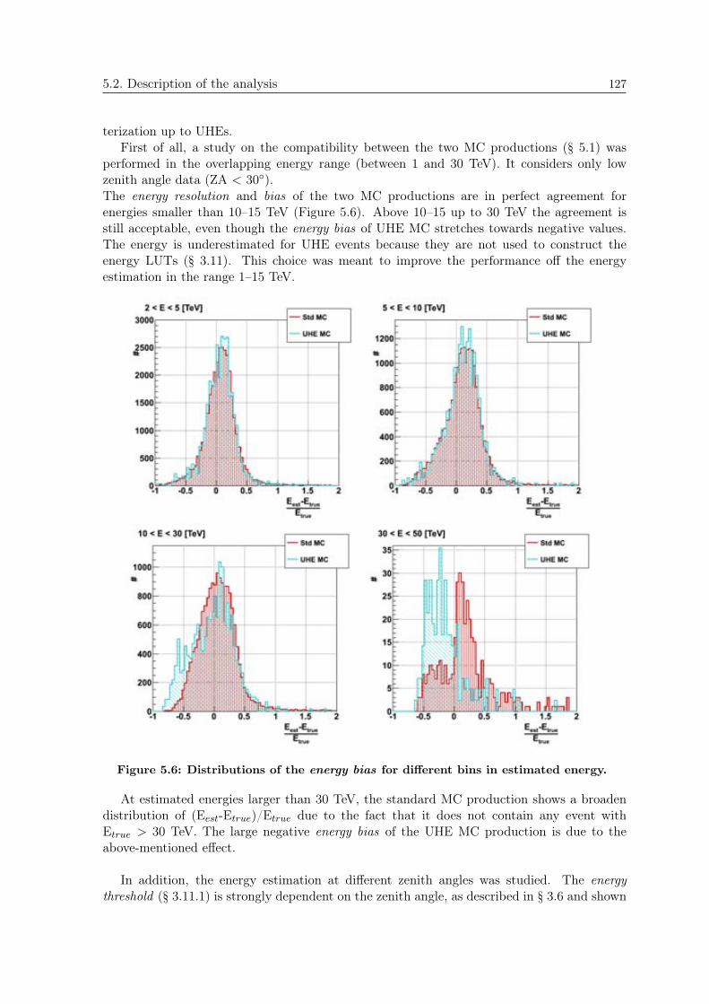
5.2. Description of the analysis 127
terization up to UHEs.First of all, a study on the compatibility between the two MC productions (§ 5.1) was
performed in the overlapping energy range (between 1 and 30 TeV). It considers only lowzenith angle data (ZA < 30).The energy resolution and bias of the two MC productions are in perfect agreement forenergies smaller than 10–15 TeV (Figure 5.6). Above 10–15 up to 30 TeV the agreement isstill acceptable, even though the energy bias of UHE MC stretches towards negative values.The energy is underestimated for UHE events because they are not used to construct theenergy LUTs (§ 3.11). This choice was meant to improve the performance off the energyestimation in the range 1–15 TeV.
Figure 5.6: Distributions of the energy bias for different bins in estimated energy.
At estimated energies larger than 30 TeV, the standard MC production shows a broadendistribution of (Eest-Etrue)/Etrue due to the fact that it does not contain any event withEtrue > 30 TeV. The large negative energy bias of the UHE MC production is due to theabove-mentioned effect.
In addition, the energy estimation at different zenith angles was studied. The energythreshold (§ 3.11.1) is strongly dependent on the zenith angle, as described in § 3.6 and shown

128 5. SPECTRUM AND FLUX VARIABILITY OF THE CRAB NEBULA
Figure 5.7: Energy bias as a function of the energy. On the left: : of the estimated energy.On the right: : of the true energy.
in Figure 5.8.This figure illustrates also how the energy threshold changes if one applies different set of
cuts. In particular, loose cuts indicate cuts which allow 85% of the -ray events to survive(spectrum-like selection cuts, § 3.12), while tight cuts keep only 70% of -ray events (signal-search-like selection cuts § 3.9.2).
Figure 5.8: Energy threshold as a function of the zenith angle for different sets of cuts.Loose cuts guarantee 85% gamma eciency, tight cuts only 70%.

5.2. Description of the analysis 129
The energy resolution and the energy bias were studied for low zenith angles (ZA < 30)and for data in the ZA bin between 39 and 45(Figure 5.9). The differential energy resolutionis illustrated in Figure 5.10, and the results obtained for the low zenith angles are in perfectagreement with the values in Aleksic J., et al. (2011b) which are also presented in Figure 3.18.The energy bias as a function of both estimated and true energy is displayed in Figure 5.11.
5.2.3 Signal clipping
The current implementation of the pulse saturation in the MC simulation is very simple.The pulses are simply truncated at a given height (900 ph.e.). The saturation in the data isdifferent because the pulses are truncated and broadened. Therefore, there might be somesystematic difference between MC and data for the highest energies. This effect can bequantified by applying a truncation on the charge of individual pixels on both data and MC,a so-called “clipping”. Two different clipping levels were chosen for this purpose: 750 and500 ph.e.. The two resulting analyses were compared to the reference analysis (no clipping)in terms of integral sensitivity for energies larger than 1, 5 and 10 TeV. The comparisonwas performed following the same procedure used for the different image cleaning algorithms(§ 5.2.1), and the results are displayed in Table 5.4. This study proved that the “non optimal”
energy analysis had.cut 2cut bg exc signif. sens.[TeV] [] [η] [% Crab flux]> 1 reference 0.22 0.010 35 2354 49 54.7 1.03 0.09
clip 750 ph.e. 0.21 0.010 41 2318 49 53.9 1.13 0.09clip 500 ph.e. 0.22 0.010 37 2329 49 54.3 1.08 0.09
> 5 reference 0.22 0.016 4 201 14 15.8 4.1 1.1clip 750 ph.e. 0.19 0.016 4 202 15 15.8 4.1 1.1clip 500 ph.e. 0.18 0.016 3 202 14 16.0 3.5 1.1
> 10 reference 0.38 0.016 3 72 9 9.1 9.9 3.3clip 750 ph.e. 0.32 0.016 3 72 9 9.1 9.9 3.3clip 500 ph.e. 0.20 0.016 3 72 9 9.1 9.9 3.3
Table 5.4: Comparison between analyses with different clipping levels.
pulse saturation in our simulations and the consequent mismatch between data and MC doesnot affect the reconstruction of the high-energy events. The integral sensitivity above 1, 5and 10 TeV is clipping-independent: all three analyses have the same power in rejecting thebackground.
Another way to evaluate the impact of the clipping on the analysis is to check for theeffect of the larger efficiency in -ray selection on the effective collection areas (§ 3.12). Asillustrated in Figure 5.12, this is not the case though. The clipping at 750 ph.e. and thereference analyses present collection areas which are comparable within the statistical errors.On the other hand, the clipping at 500 ph.e. analysis shows a 5–10% decrease of the collectionarea above few TeV.
The forthcoming analysis was performed with a clipping at 750 ph.e., but this choice hasno effect on the final results.
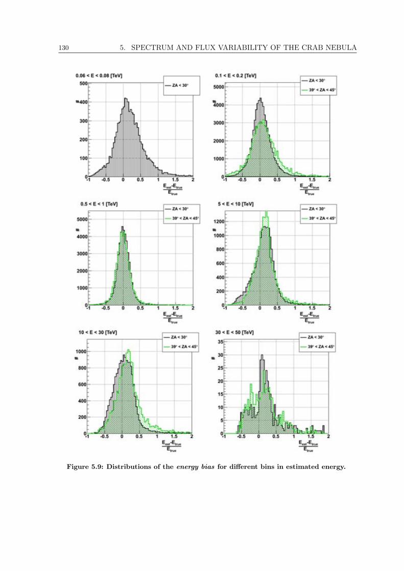
130 5. SPECTRUM AND FLUX VARIABILITY OF THE CRAB NEBULA
Figure 5.9: Distributions of the energy bias for different bins in estimated energy.

5.3. Differential energy spectrum 131
Figure 5.10: Energy resolution as a function of estimated energy.
Figure 5.11: Energy bias as a function of energy. On the left: : dependence on the estimatedenergy; On the right: : dependence on true energy.
5.3 Dierential energy spectrum
The data sample was divided into four subsamples depending on the zenith angle. An in-dependent analysis was run over each of the subsamples, whose effective observation timeamounts to:
• 33.7 hrs for ZA < 30 :
• 6.8 hrs for 30 < ZA < 39
• 3.5 hrs for 39 < ZA < 45
• 1.4 hrs for 45 < ZA < 50

132 5. SPECTRUM AND FLUX VARIABILITY OF THE CRAB NEBULA
Figure 5.12: Collection area for different clipping levels.
The computation of the differential energy spectrum requires the measurement of the numberof excess events in each energy bin (§ 3.12). The gamma selection cuts were optimized on MCto obtain a large gamma efficiency (Equation 3.7). In particular, it was guaranteed that 80%of -ray events survived the selection cuts below 5 TeV, and 95% of them at higher energies.At high energies the discrepancies between data and MC are larger than in the other energyrange. Keeping such loose cuts reduces systematic effects (§ 3.12).
Results obtained for the data subsamples in the four zenith angle ranges are illustratedbelow. Figure 5.13 shows the distributions of the effective collection area and the number ofexcess events as function of the estimated energy. The resulting differential energy spectraare displayed in Figure 5.14 as function of the estimated energy. The correction for theknown finite resolution and bias in the energy estimation was applied to these differentialenergy spectra through the unfolding procedure (§ 3.13). This results in the conversion ofthe estimated energy in true energy. From now on, unless explicitly stated, “energy”, E, willstands for true energy, Etrue.
5.3.1 Unfolded spectrum
The differential energy spectra obtained for the data subsamples in the four zenith angleranges were combined at the level of the unfolding (§ 3.13). The result is an unprecedenteddifferential energy spectrum of the Crab Nebula which spans eight orders of magnitude influx and three orders of magnitude in energy, between 50 GeV and 45 TeV. It is shown inFigure 5.15. The differential flux for each spectral point is quoted in Table 5.5. The differentialenergy spectrum in Figure 5.15 is unfolded with Bertero’s method (Bertero, M., 1989).
This result represents a high-precision measurement with six spectral points per energydecades and statistical errors which are as low as 5% below 100 GeV. This is the first time thatsuch a level of precision has been reached at these energies. Nevertheless, at all energies, theoverall uncertainty is dominated by systematic uncertainties rather than statistical ones. Thesystematic uncertainties, displayed in Figure 5.15 as a yellow-shadowed area, will be discussed
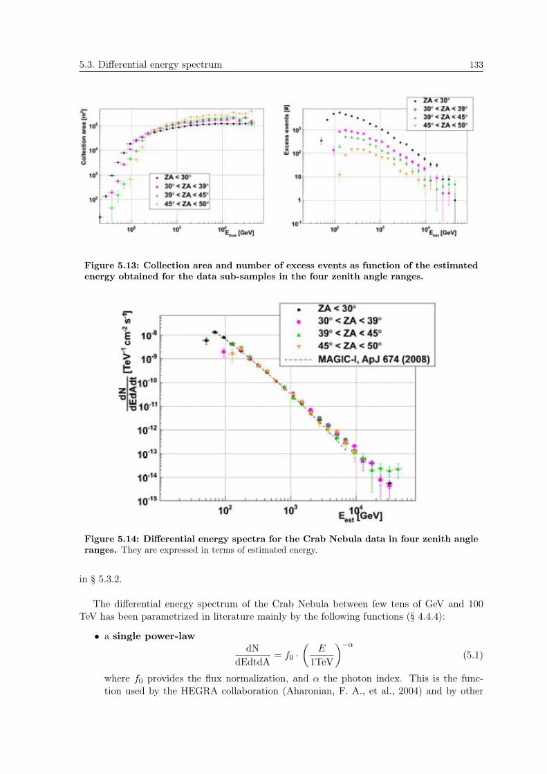
5.3. Differential energy spectrum 133
Figure 5.13: Collection area and number of excess events as function of the estimatedenergy obtained for the data sub-samples in the four zenith angle ranges.
Figure 5.14: Differential energy spectra for the Crab Nebula data in four zenith angleranges. They are expressed in terms of estimated energy.
in § 5.3.2.
The differential energy spectrum of the Crab Nebula between few tens of GeV and 100TeV has been parametrized in literature mainly by the following functions (§ 4.4.4):
• a single power-lawdN
dEdtdA= f0 ·
E
1TeV
(5.1)
where f0 provides the flux normalization, and the photon index. This is the func-tion used by the HEGRA collaboration (Aharonian, F. A., et al., 2004) and by other

134 5. SPECTRUM AND FLUX VARIABILITY OF THE CRAB NEBULA
Figure 5.15: Differential energy spectrum for the Crab Nebula between 50 GeV and45 TeV. It is unfolded with the Bertero’s method. The top panel shows in addition to the unfoldeddata points also results of a variable power-law fit and the systematic uncertainties. The bottompanel shows the relative residuals between the fit results and the data points.
experiments previous to HEGRA.
• a variable/curved power-law function
dNdEdtdA
= f0 ·
E
1TeV
+bLog10( E1TeV )
(5.2)
where b gives the curvature of the function. The first stand-alone MAGIC telescopeshowed a hardening of the Crab Nebula spectrum for energies lower than few hun-dreds GeV (Albert, J., et al., 2008d). A variable power-law fit seems to better describeMAGIC I data.
• a single power-law with an exponential cut-off
dNdEdtdA
= f0 ·
E
1TeV
· exp
EEc
(5.3)
where Ec identifies the energy of the cut-off. This is the fit function suggested by theHESS experiment. They claimed a cut-off energy of (14.3 2.1) TeV (Aharonian, F. A.,et al., 2006b).
The obtained differential energy spectrum was fitted to all these three functions. The fittakes into account the correlations between the spectral points, which were introduced by the

5.3. Differential energy spectrum 135
mean energy differential flux[GeV] [TeV cm2s1]58.4 (1.95 0.11) 108
85.2 (8.87 0.30) 109
124.3 (3.73 0.10) 109
181.4 (1.41 0.03) 109
264.7 (6.81 0.16) 1010
386.3 (3.36 0.07) 1010
563.6 (1.30 0.03) 1010
822.3 (5.04 0.16) 1011
1199.7 (2.17 0.08) 1011
1750.3 (8.23 0.39) 1012
2553.7 (2.73 0.19) 1012
3727.2 (1.45 0.10) 1012
5437.8 (4.92 0.49) 1013
7933.6 (1.62 0.24) 1013
11574.9 (4.64 1.24) 1014
16887.4 (2.69 0.66) 1014
24647.6 (9.90 2.29) 1015
35960.1 (3.05 2.48) 1015
Table 5.5: Mean energy and differential flux of the spectral points shown in Figure 5.15.
unfolding procedure. No systematic errors were included in the fit. Results are displayed interms of SED in order to enhance any spectral feature (Figure 5.16). The relative residualsbetween the spectral points and the fit results are also shown in the bottom panel, samefigure.
A correlated fit of a single power-law provides a flux normalization f0 = (3.03 0.03)1011 TeV1 cm2 s1, and a photon index =(2.33 0.01). The γ2 of the fit is 270 for16 Degree of Freedom (DoF). The variable power-law fit results in a flux normalization f0
of (3.27 0.03) 1011 TeV1 cm2 s1, a photon index of 2.40 0.01 and a curvature bof -0.15 0.01. This fit has a γ2 of 72 for 15 DoF. Finally a fit of a single power-law withan exponential cut-off gives a flux normalization of (3.66 0.08) 1011 TeV1 cm2 s1, aphoton index of -2.22 0.01, and an exponential cut-off at 9.4 1.1. It has a γ2 of 104 for15 DoF.
All these fits present too high values of the γ2/DoF. This is due to the fact that the resid-uals to the fit function shows deviations which are statistically significant, mainly around 200GeV and 2.5 TeV. These spectral features, so-called wiggles, can be explained by systematiceffects and will be treated in detail in § 5.3.2. Nevertheless, since the γ2/DoF for the singlepower-law fit is 30 larger than the one obtained for the other two fits, this suggests that thepower-law behaviour is disfavored. Moreover, at energies above 5 TeV the residuals show asystematic negative trend. On the other hand, the variable power-law and the power-law withcut-off remain equally valid. Note the estimated energy cut-off is compatible with the onereported by HESS (Aharonian, F. A., et al., 2006b). For sake of simplicity from now on, onlyfits of variable power-laws will be performed.
Three other unfolding methods (Schmelling’s, Tikonov’s and forward unfoldings) were con-sidered and all of them gave consistent results: both the spectral points and the fit parameters
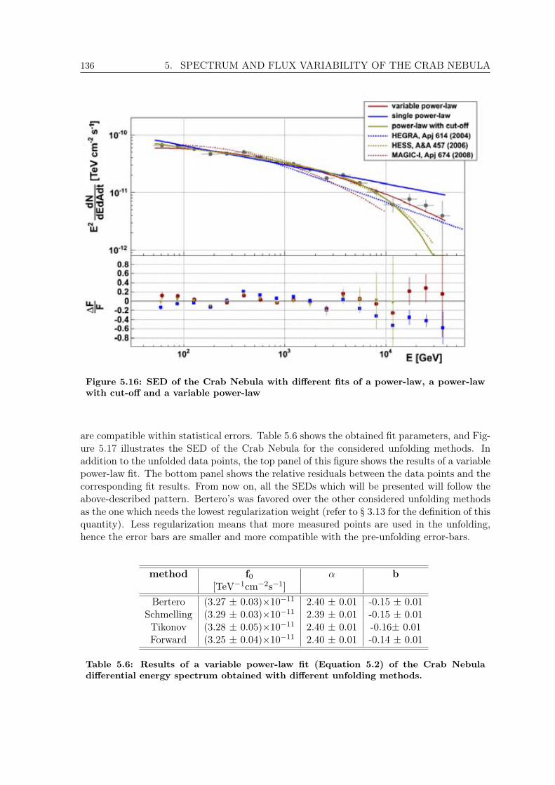
136 5. SPECTRUM AND FLUX VARIABILITY OF THE CRAB NEBULA
Figure 5.16: SED of the Crab Nebula with different fits of a power-law, a power-lawwith cut-off and a variable power-law
are compatible within statistical errors. Table 5.6 shows the obtained fit parameters, and Fig-ure 5.17 illustrates the SED of the Crab Nebula for the considered unfolding methods. Inaddition to the unfolded data points, the top panel of this figure shows the results of a variablepower-law fit. The bottom panel shows the relative residuals between the data points and thecorresponding fit results. From now on, all the SEDs which will be presented will follow theabove-described pattern. Bertero’s was favored over the other considered unfolding methodsas the one which needs the lowest regularization weight (refer to § 3.13 for the definition of thisquantity). Less regularization means that more measured points are used in the unfolding,hence the error bars are smaller and more compatible with the pre-unfolding error-bars.
method f0 b[TeV1cm2s1]
Bertero (3.27 0.03)1011 2.40 0.01 -0.15 0.01Schmelling (3.29 0.03)1011 2.39 0.01 -0.15 0.01Tikonov (3.28 0.05)1011 2.40 0.01 -0.16 0.01Forward (3.25 0.04)1011 2.40 0.01 -0.14 0.01
Table 5.6: Results of a variable power-law fit (Equation 5.2) of the Crab Nebuladifferential energy spectrum obtained with different unfolding methods.
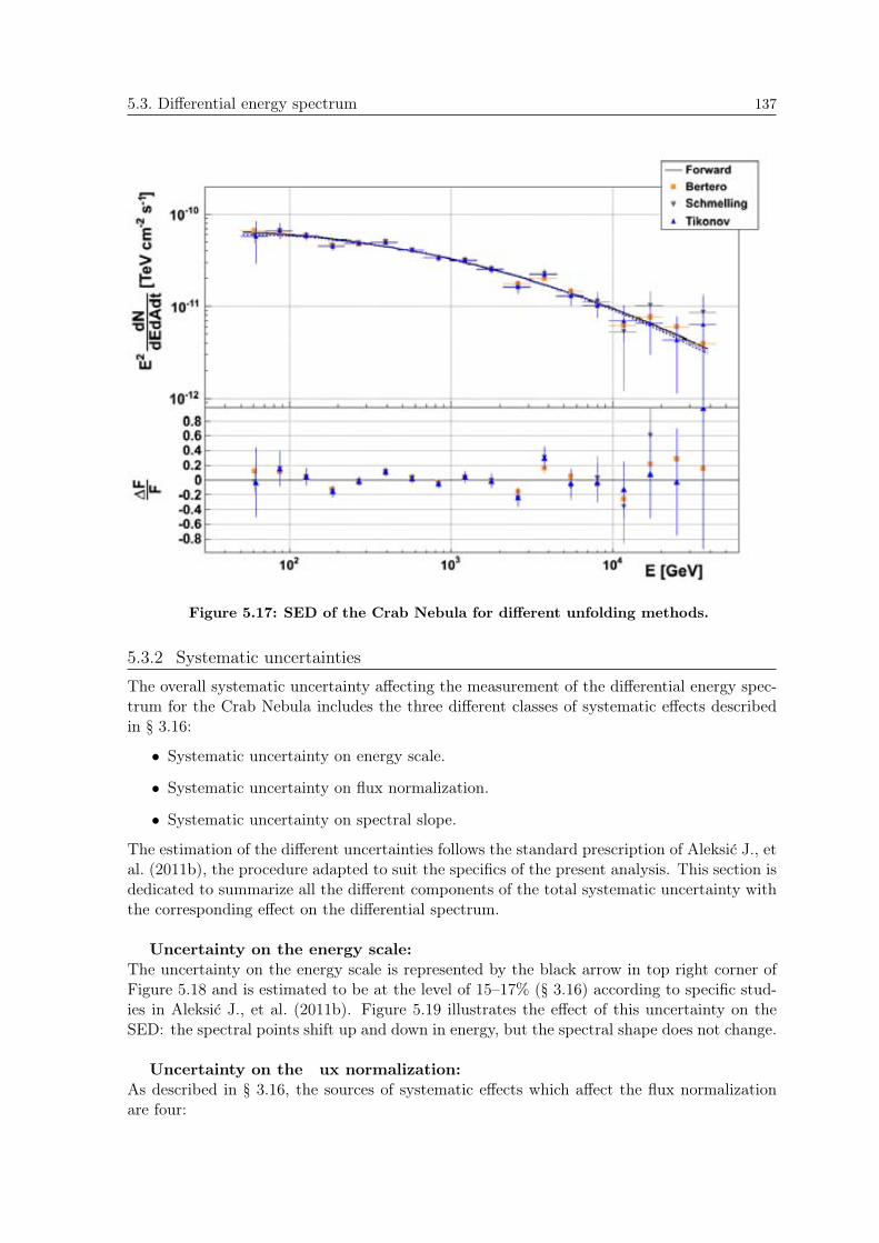
5.3. Differential energy spectrum 137
Figure 5.17: SED of the Crab Nebula for different unfolding methods.
5.3.2 Systematic uncertainties
The overall systematic uncertainty affecting the measurement of the differential energy spec-trum for the Crab Nebula includes the three different classes of systematic effects describedin § 3.16:
• Systematic uncertainty on energy scale.
• Systematic uncertainty on flux normalization.
• Systematic uncertainty on spectral slope.
The estimation of the different uncertainties follows the standard prescription of Aleksic J., etal. (2011b), the procedure adapted to suit the specifics of the present analysis. This section isdedicated to summarize all the different components of the total systematic uncertainty withthe corresponding effect on the differential spectrum.
Uncertainty on the energy scale:The uncertainty on the energy scale is represented by the black arrow in top right corner ofFigure 5.18 and is estimated to be at the level of 15–17% (§ 3.16) according to specific stud-ies in Aleksic J., et al. (2011b). Figure 5.19 illustrates the effect of this uncertainty on theSED: the spectral points shift up and down in energy, but the spectral shape does not change.
Uncertainty on the ux normalization:As described in § 3.16, the sources of systematic effects which affect the flux normalizationare four:
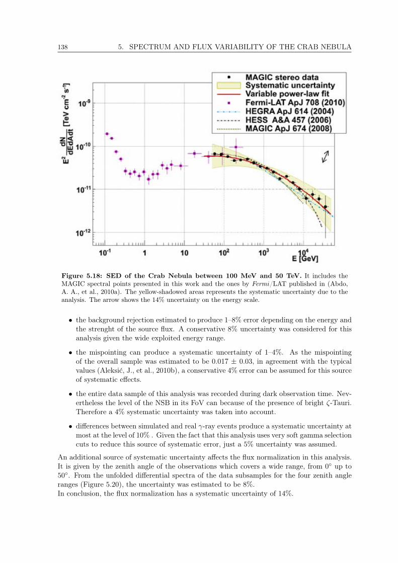
138 5. SPECTRUM AND FLUX VARIABILITY OF THE CRAB NEBULA
Figure 5.18: SED of the Crab Nebula between 100 MeV and 50 TeV. It includes theMAGIC spectral points presented in this work and the ones by Fermi/LAT published in (Abdo,A. A., et al., 2010a). The yellow-shadowed areas represents the systematic uncertainty due to theanalysis. The arrow shows the 14% uncertainty on the energy scale.
• the background rejection estimated to produce 1–8% error depending on the energy andthe strenght of the source flux. A conservative 8% uncertainty was considered for thisanalysis given the wide exploited energy range.
• the mispointing can produce a systematic uncertainty of 1–4%. As the mispointingof the overall sample was estimated to be 0.017 0.03, in agreement with the typicalvalues (Aleksic, J., et al., 2010b), a conservative 4% error can be assumed for this sourceof systematic effects.
• the entire data sample of this analysis was recorded during dark observation time. Nev-ertheless the level of the NSB in its FoV can because of the presence of bright -Tauri.Therefore a 4% systematic uncertainty was taken into account.
• differences between simulated and real -ray events produce a systematic uncertainty atmost at the level of 10% . Given the fact that this analysis uses very soft gamma selectioncuts to reduce this source of systematic error, just a 5% uncertainty was assumed.
An additional source of systematic uncertainty affects the flux normalization in this analysis.It is given by the zenith angle of the observations which covers a wide range, from 0 up to50. From the unfolded differential spectra of the data subsamples for the four zenith angleranges (Figure 5.20), the uncertainty was estimated to be 8%.In conclusion, the flux normalization has a systematic uncertainty of 14%.
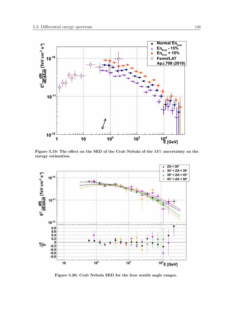
5.3. Differential energy spectrum 139
Figure 5.19: The effect on the SED of the Crab Nebula of the 15% uncertainty on theenergy estimation.
Figure 5.20: Crab Nebula SED for the four zenith angle ranges.
140 5. SPECTRUM AND FLUX VARIABILITY OF THE CRAB NEBULA
Uncertainty on the spectral slope:Since the differential energy spectrum is well-fitted by a variable power-law, the systematicuncertainty on the spectral slope is split between the uncertainties of the photon index, ,and the curvature parameter, b. Besides the 0.04 error on the photon index due to the non-linearity of the analog signal chain (§ 3.16), there is another dominant source belonging to thisclass of systematics: the analysis methods. The latter was evaluated by estimating the effectof the RF, the image cleaning, the zenith angle of the observations, the unfolding methodsand the efficiency of the gamma selection cuts (always above the 70% in order to reduce thediscrepancy between MC and data). It results in a systematic uncertainty on of 0.06 and onb of 0.05. The obtained values are in agreement with the overall uncertainty on the spectralslope quoted in Aleksic J., et al. (2011b).
The last two categories of systematics, the uncertainty on the flux normalization and theuncertainty on the spectral slope, are expressed in terms of systematic errors of the fit pa-rameters. The total effect is indicated by the yellow-shadowed bands around the differentialspectrum in Figure 5.15 and around the corresponding SED between 100 MeV and 50 TeV inFigure 5.18.
Summarizing the fit parameters are:f0 = (3.27 0:03stat 0:46syst) 1011 photons cm2 s1. = 2.40 0:01stat 0:1systb = -0.15 0:01stat 0:05syst
In the estimation of the systematic uncertainty of the analysis, the effect of the tails inthe migration matrix was also checked (Figure 5.21 top left). The original migration matrixwas then truncated in such a way that only bins with a relative error of at least 10% survive(Figure 5.21 top right). The bottom panel of Figure 5.21 shows the SEDs obtained with thetwo different matrices. All the points compatible are within the statistical errors. Therefore,the degradation of the migration matrix does not add any source of systematic uncertainty.

5.3. Differential energy spectrum 141
Figure 5.21: Study of the effect of the tails in the migration matrix. On top left : theoriginal migration matrix. On top right : the truncated migration matrix which considers only binswith at least 10% statistical error. On bottom: the SED obtained with the two above-describedmigration matrices.
Spectral Features
As explained in § 5.3.1, the Crab Nebula differential energy spectrum presents some statisti-cally significant discrepancies from the fitted variable power-law. Though the total systematicuncertainty described in the previous section is wide enough to cover the disagreement, it mustbe noticed that such uncertainty, influencing the global fit parameters, cannot explain alonethe local features of the spectrum. In other words, a strictly energy dependent treatmentof the systematics is needed to assign an uncorrelated uncertainty to each energy bin of theunfolded spectrum, and a dedicated effort is ongoing to put into practice this new approach.
The possible source of this energy-dependent effect is under-investigation. It might berelated to discrepancy between MC and data, to some hidden features of the atmosphericCherenkov technique, or even to some yet-to-be-discovered physics effect. In fact, some ofthese systematic effects maybe only be ruled out by ways of simultaneous observations with
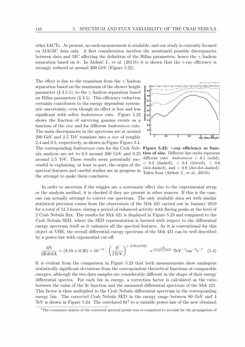
142 5. SPECTRUM AND FLUX VARIABILITY OF THE CRAB NEBULA
other IACTs. At present, no such measurement is available, and our study is currently focusedon MAGIC data only. A first consideration involves the mentioned possible discrepanciesbetween data and MC affecting the definition of the Hillas parameters, hence the γ/hadronseparation based on it. In Aleksic J., et al. (2011b) it is shown that the γ-ray efficiency isstrongly reduced at around 300 GeV (Figure 5.22).
The effect is due to the transition from the γ/hadronseparation based on the maximum of the shower heightparameter (§ 3.5.1), to the γ/hadron separation basedon Hillas parameters (§ 3.5). This efficiency reductioncertainly contributes to the energy dependent system-atic uncertainty, even though its effect is less and lesssignificant with softer hadronness cuts. Figure 5.22shows the fraction of surviving gamma events as afunction of the size and for different hadronness cuts.The main discrepancies in the spectrum are at around200 GeV and 2.5 TeV translate into a size of roughly2.4 and 3.5, respectively, as shown in Figure Figure 3.4.The corresponding hadronness cuts for the Crab Neb-ula analysis are set to 0.3 around 200 GeV and 0.25around 2.5 TeV. These results seem potentially suc-cessful in explaining, at least in part, the origin of thespectral features and careful studies are in progress inthe attempt to make them conclusive.
Figure 5.22: γ-ray efficiency as func-tion of size. Different line styles representdifferent cuts: hadronness < 0.1 (solid),< 0.2 (dashed), < 0.4 (dotted), < 0.6(dot-dashed), and < 0.9 (dot-dot-dashed).Taken from (Aleksic J., et al., 2011b).
In order to ascertain if the wiggles are a systematic effect due to the experimental setupor the analysis method, it is checked if they are present in other sources. If this is the case,one can actually attempt to correct our spectrum. The only available data set with similarstatistical precision comes from the observation of the Mrk 421 carried out in January 2010for a total of 12.3 hours, during a period of enhanced activity with flaring peaks at the level of2 Crab Nebula flux. The results for Mrk 421 is displayed in Figure 5.23 and compared to theCrab Nebula SED, where the SED representation is favored with respect to the differentialenergy spectrum itself as it enhances all the spectral features. As it is conventional for thisobject at VHE, the overall differential energy spectrum of the Mrk 421 can be well describedby a power-law with exponential cut-off:
dNdEdtdA
= (9.18 ± 0.30) × 10−11 ·(
E
1TeV
)(−2.05± 0.02)
· e− E
(3.5± 0.3)TeV TeV−1cm−2s−1 (5.4)
It is evident from the comparison in Figure 5.23 that both measurements show analogousstatistically significant deviations from the correspondent theoretical functions at comparableenergies, although the two data samples are considerably different in the shape of their energydifferential spectra. For each bin in energy, a correction factor is calculated as the ratiobetween the value of the fit function and the measured differential spectrum of the Mrk 421.This factor is then multiplied to the Crab Nebula differential spectrum in the correspondingenergy bin. The corrected Crab Nebula SED in the energy range between 80 GeV and 4TeV is shown in Figure 5.24. The correlated fit3 to a variable power-law of the new obtained
3The covariance matrix of the corrected spectral points was re-computed to account for the propagation of
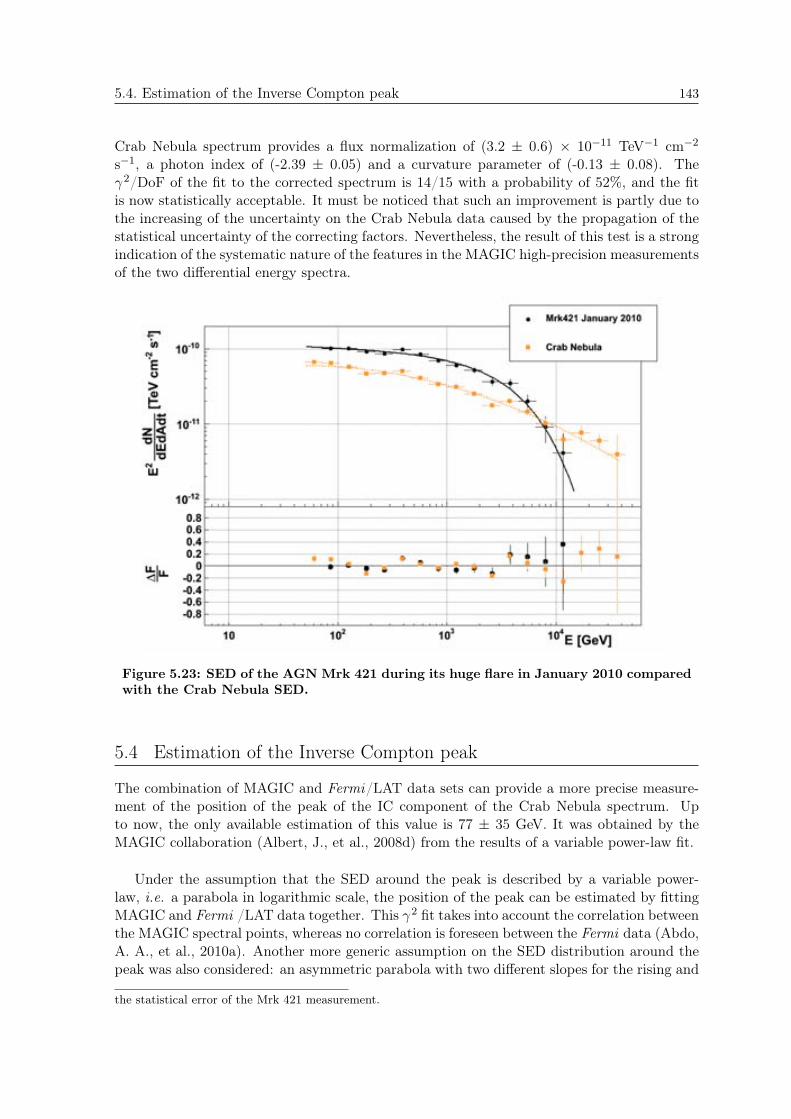
5.4. Estimation of the Inverse Compton peak 143
Crab Nebula spectrum provides a flux normalization of (3.2 0.6) 1011 TeV1 cm2
s1, a photon index of (-2.39 0.05) and a curvature parameter of (-0.13 0.08). Theγ2/DoF of the fit to the corrected spectrum is 14/15 with a probability of 52%, and the fitis now statistically acceptable. It must be noticed that such an improvement is partly due tothe increasing of the uncertainty on the Crab Nebula data caused by the propagation of thestatistical uncertainty of the correcting factors. Nevertheless, the result of this test is a strongindication of the systematic nature of the features in the MAGIC high-precision measurementsof the two differential energy spectra.
Figure 5.23: SED of the AGN Mrk 421 during its huge flare in January 2010 comparedwith the Crab Nebula SED.
5.4 Estimation of the Inverse Compton peak
The combination of MAGIC and Fermi/LAT data sets can provide a more precise measure-ment of the position of the peak of the IC component of the Crab Nebula spectrum. Upto now, the only available estimation of this value is 77 35 GeV. It was obtained by theMAGIC collaboration (Albert, J., et al., 2008d) from the results of a variable power-law fit.
Under the assumption that the SED around the peak is described by a variable power-law, i.e. a parabola in logarithmic scale, the position of the peak can be estimated by fittingMAGIC and Fermi /LAT data together. This γ2 fit takes into account the correlation betweenthe MAGIC spectral points, whereas no correlation is foreseen between the Fermi data (Abdo,A. A., et al., 2010a). Another more generic assumption on the SED distribution around thepeak was also considered: an asymmetric parabola with two different slopes for the rising and
the statistical error of the Mrk 421 measurement.

144 5. SPECTRUM AND FLUX VARIABILITY OF THE CRAB NEBULA
Figure 5.24: The Crab Nebula differential energy spectrum corrected for the Mrk 421spectrum. Details in the text.
falling edges. Results are summarized in Table 5.7. For completeness, results obtained byfitting only MAGIC data are also reported. Their only aim is to check that the statisticalprecision improves increasing the considered data set.
Both the fits of a parabola and an asymmetric parabola have γ2/DoF ≡ 3. The high-valueof the γ2 is due to the significant deviations from the fit function in the MAGIC data. Whatis really relevant in this context is that the two fits have the same probability. In addition, astudy of the correlation between fit parameters have been performed. Figure 5.25 illustratesthe contours of the γ2 fit error as a function of the slope and the position of the IC peak.These parameters are strongly correlated: the larger the slope, the higher the energy of thepeak. Also the two slopes of the asymmetric parabola are correlated.
fit function data slope1 peak normalization slope2[GeV]
parabola M -0.15+0:010:01 47.9+10:2
9:6 -10.22+0:010:01
parabola M+F 0.16+0:010:01 58.6+6:2
5:7 -10.24+0:010:01
asym. parabola M+F -0.15+0:010:01 49.4+9:6
8:7 -10.23+0:010:01 -0.21+0:04
0:06
Table 5.7: Results for three different fits to the SED around the position of the ICpeak. From left to right, the assumed fit function, the considered data set only MAGIC (M) pointsor MAGIC plus Fermi/LAT points (M+F), and the results for the fit parameters.
Depending on the assumption on the spectral shape of the IC component around its peakposition, the peak is estimated to be between 50 and 59 GeV with a statistical error at thelevel of 10–20% . This is a much more precise measurement with respect to the previous onewhich have a 50% uncertainty.

5.5. Theoretical picture 145
Figure 5.25: Contours of the γ2 fit error as function of different parameters of theasymmetric parabola fit to the IC peak. On the left: the slope and the energy of the IC peakOn the right: the two slopes. The contours correspond to 1,2 and 3η significances. The dashed linecorresponds to an identical value of the slope1 and slope2.
5.5 Theoretical picture
The broad-band SED of the Crab Nebula was matched with two different model calculationsthat are based on the model first suggested by Hillas, A. M., et al. (1998) assuming a constantB-field as well as a solution of the ideal radial MHD flow (Kennel, C. F. & Coroniti, F. V.,1984b). More specifically the differential energy spectrum has been interpreted using themodels in Meyer, M. et al. (2010), described in § 4.4.5. Both model calculations are shownin Figure 5.26 together with the archival data as well as the new measurement presented inthis work. The spectral measurement obtained with the MAGIC telescopes covers for thefirst time the crucial energy range at the peak of the IC component. None of the two modelsprovides a satisfactory match to the data within the statistical errors.
The dip (i.e. wiggle) in the differential energy spectrum at 200–300 GeV falls just on topof the expected position of the IC peak. This spectral feature at this specific position is hardto understand: theoreticians may need to postulate the existence of an additional structurein the B-field downstream of the shock. Hence it is of crucial importance to understand theorigin of the systematic effect which causes the above-mentioned wiggle and, if possible, tocorrect for it.
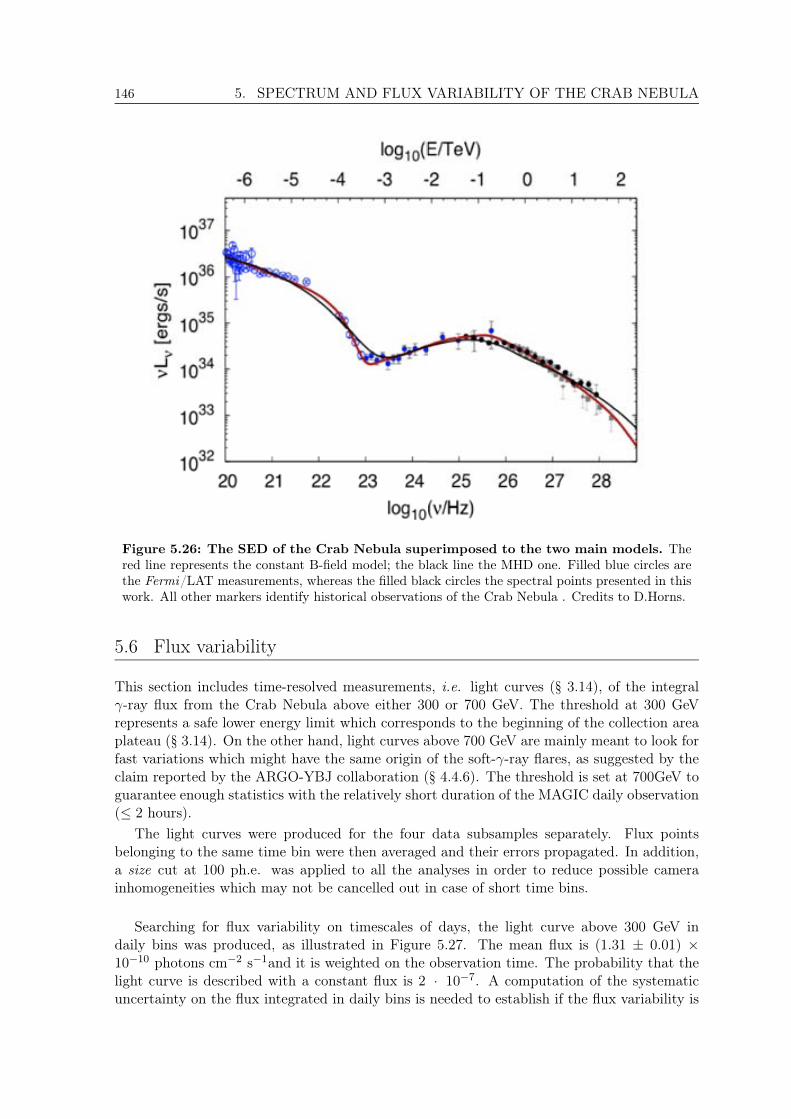
146 5. SPECTRUM AND FLUX VARIABILITY OF THE CRAB NEBULA
Figure 5.26: The SED of the Crab Nebula superimposed to the two main models. Thered line represents the constant B-field model; the black line the MHD one. Filled blue circles arethe Fermi/LAT measurements, whereas the filled black circles the spectral points presented in thiswork. All other markers identify historical observations of the Crab Nebula . Credits to D.Horns.
5.6 Flux variability
This section includes time-resolved measurements, i.e. light curves (§ 3.14), of the integralγ-ray flux from the Crab Nebula above either 300 or 700 GeV. The threshold at 300 GeVrepresents a safe lower energy limit which corresponds to the beginning of the collection areaplateau (§ 3.14). On the other hand, light curves above 700 GeV are mainly meant to look forfast variations which might have the same origin of the soft-γ-ray flares, as suggested by theclaim reported by the ARGO-YBJ collaboration (§ 4.4.6). The threshold is set at 700GeV toguarantee enough statistics with the relatively short duration of the MAGIC daily observation(≤ 2 hours).
The light curves were produced for the four data subsamples separately. Flux pointsbelonging to the same time bin were then averaged and their errors propagated. In addition,a size cut at 100 ph.e. was applied to all the analyses in order to reduce possible camerainhomogeneities which may not be cancelled out in case of short time bins.
Searching for flux variability on timescales of days, the light curve above 300 GeV indaily bins was produced, as illustrated in Figure 5.27. The mean flux is (1.31 ± 0.01) ×10−10 photons cm−2 s−1and it is weighted on the observation time. The probability that thelight curve is described with a constant flux is 2 · 10−7. A computation of the systematicuncertainty on the flux integrated in daily bins is needed to establish if the flux variability is
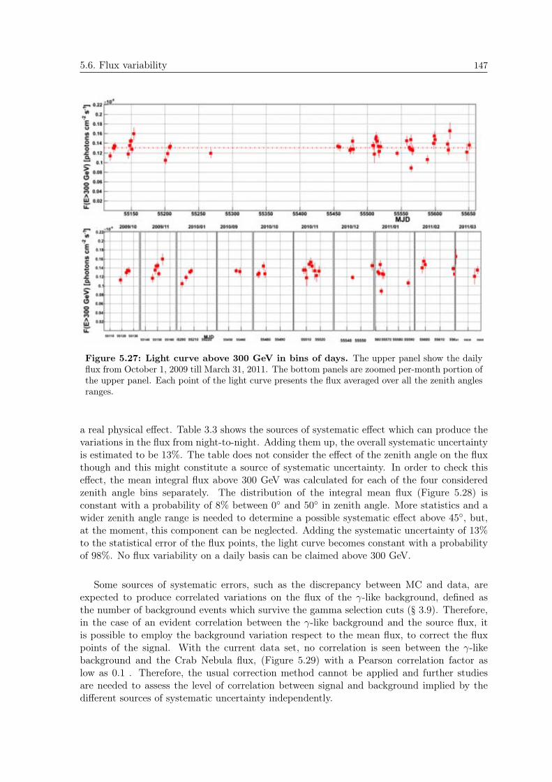
5.6. Flux variability 147
Figure 5.27: Light curve above 300 GeV in bins of days. The upper panel show the dailyflux from October 1, 2009 till March 31, 2011. The bottom panels are zoomed per-month portion ofthe upper panel. Each point of the light curve presents the flux averaged over all the zenith anglesranges.
a real physical effect. Table 3.3 shows the sources of systematic effect which can produce thevariations in the flux from night-to-night. Adding them up, the overall systematic uncertaintyis estimated to be 13%. The table does not consider the effect of the zenith angle on the fluxthough and this might constitute a source of systematic uncertainty. In order to check thiseffect, the mean integral flux above 300 GeV was calculated for each of the four consideredzenith angle bins separately. The distribution of the integral mean flux (Figure 5.28) isconstant with a probability of 8% between 0 and 50 in zenith angle. More statistics and awider zenith angle range is needed to determine a possible systematic effect above 45, but,at the moment, this component can be neglected. Adding the systematic uncertainty of 13%to the statistical error of the flux points, the light curve becomes constant with a probabilityof 98%. No flux variability on a daily basis can be claimed above 300 GeV.
Some sources of systematic errors, such as the discrepancy between MC and data, areexpected to produce correlated variations on the flux of the -like background, defined asthe number of background events which survive the gamma selection cuts (§ 3.9). Therefore,in the case of an evident correlation between the -like background and the source flux, itis possible to employ the background variation respect to the mean flux, to correct the fluxpoints of the signal. With the current data set, no correlation is seen between the -likebackground and the Crab Nebula flux, (Figure 5.29) with a Pearson correlation factor aslow as 0.1 . Therefore, the usual correction method cannot be applied and further studiesare needed to assess the level of correlation between signal and background implied by thedifferent sources of systematic uncertainty independently.

148 5. SPECTRUM AND FLUX VARIABILITY OF THE CRAB NEBULA
Figure 5.28: Distribution of the mean integral flux above 300 GeV as a function of thezenith angle.
Figure 5.29: Integral flux above 300 GeV of the Crab Nebula versus the integral fluxof the -like background in the same energy range. The correlation factor is 0.01.
Let us finalize the search for the flux variability at the highest energies, where ARGO-YBJclaimed a flare simultaneous with Fermi/LAT. Figure 5.30 shows the light curve above 700

5.6. Flux variability 149
GeV with a time bin of one day. The mean integral flux above 700 GeV is (4.00 0.06) 1011 photons cm2 s1with a probability of being constant of 3 · 106. Including the above-mentioned 13% systematic uncertainty, the flux is constant with a probability of 52%. Thered band in Figure 5.30 shows the 3-days period corresponding to the Crab Nebula flare above100 MeV detected by both AGILE and Fermi/LAT in September 2010. MAGIC recorded onehour of data simultaneous to this flare and no flux enhancement is seen either above 300 GeVor above 700 GeV.
Figure 5.30: Daily light curve above 700 GeV. The upper panel show the daily flux fromOctober 1, 2009 till March 31, 2011. The bottom panels are zoomed per-month portion of theupper panel. Red-shadowed area identifies the period of the flux enhancement in the the soft- -rayband.


PART THREE
MICROQUASARS AT VHE
Salvador Dalı - “Swans reflecting elephants”

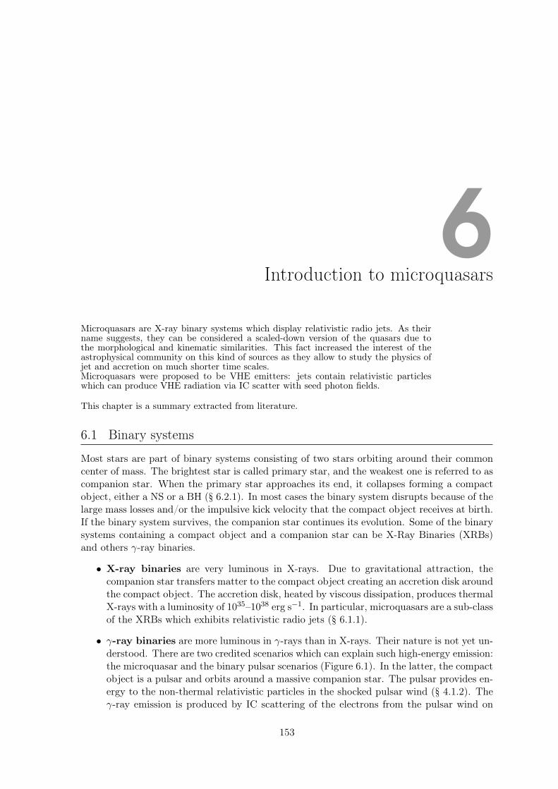
6Introduction to microquasars
Microquasars are X-ray binary systems which display relativistic radio jets. As theirname suggests, they can be considered a scaled-down version of the quasars due tothe morphological and kinematic similarities. This fact increased the interest of theastrophysical community on this kind of sources as they allow to study the physics ofjet and accretion on much shorter time scales.Microquasars were proposed to be VHE emitters: jets contain relativistic particleswhich can produce VHE radiation via IC scatter with seed photon fields.
This chapter is a summary extracted from literature.
6.1 Binary systems
Most stars are part of binary systems consisting of two stars orbiting around their commoncenter of mass. The brightest star is called primary star, and the weakest one is referred to ascompanion star. When the primary star approaches its end, it collapses forming a compactobject, either a NS or a BH (§ 6.2.1). In most cases the binary system disrupts because of thelarge mass losses and/or the impulsive kick velocity that the compact object receives at birth.If the binary system survives, the companion star continues its evolution. Some of the binarysystems containing a compact object and a companion star can be X-Ray Binaries (XRBs)and others -ray binaries.
• X-ray binaries are very luminous in X-rays. Due to gravitational attraction, thecompanion star transfers matter to the compact object creating an accretion disk aroundthe compact object. The accretion disk, heated by viscous dissipation, produces thermalX-rays with a luminosity of 1035–1038 erg s1. In particular, microquasars are a sub-classof the XRBs which exhibits relativistic radio jets (§ 6.1.1).
• -ray binaries are more luminous in -rays than in X-rays. Their nature is not yet un-derstood. There are two credited scenarios which can explain such high-energy emission:the microquasar and the binary pulsar scenarios (Figure 6.1). In the latter, the compactobject is a pulsar and orbits around a massive companion star. The pulsar provides en-ergy to the non-thermal relativistic particles in the shocked pulsar wind (§ 4.1.2). The -ray emission is produced by IC scattering of the electrons from the pulsar wind on
153
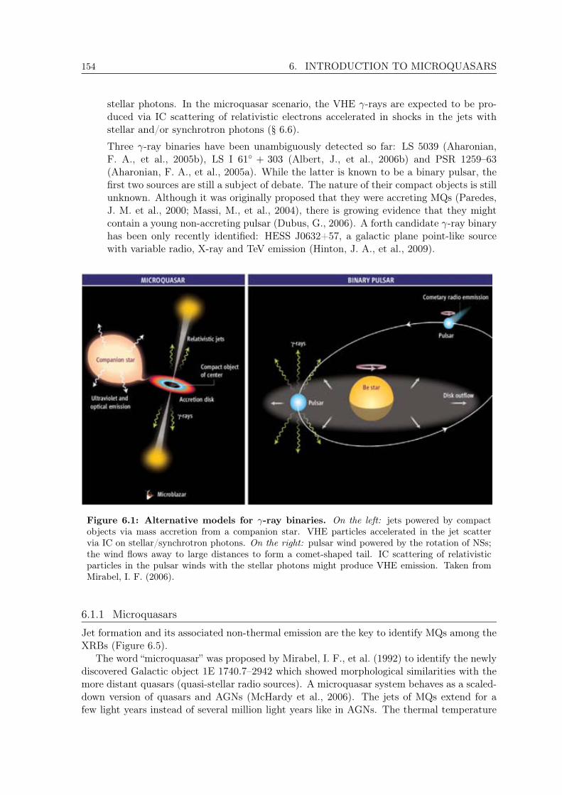
154 6. INTRODUCTION TO MICROQUASARS
stellar photons. In the microquasar scenario, the VHE γ-rays are expected to be pro-duced via IC scattering of relativistic electrons accelerated in shocks in the jets withstellar and/or synchrotron photons (§ 6.6).
Three γ-ray binaries have been unambiguously detected so far: LS 5039 (Aharonian,F. A., et al., 2005b), LS I 61+ 303 (Albert, J., et al., 2006b) and PSR 1259–63(Aharonian, F. A., et al., 2005a). While the latter is known to be a binary pulsar, thefirst two sources are still a subject of debate. The nature of their compact objects is stillunknown. Although it was originally proposed that they were accreting MQs (Paredes,J. M. et al., 2000; Massi, M., et al., 2004), there is growing evidence that they mightcontain a young non-accreting pulsar (Dubus, G., 2006). A forth candidate γ-ray binaryhas been only recently identified: HESS J0632+57, a galactic plane point-like sourcewith variable radio, X-ray and TeV emission (Hinton, J. A., et al., 2009).
Figure 6.1: Alternative models for γ-ray binaries. On the left: jets powered by compactobjects via mass accretion from a companion star. VHE particles accelerated in the jet scattervia IC on stellar/synchrotron photons. On the right: pulsar wind powered by the rotation of NSs;the wind flows away to large distances to form a comet-shaped tail. IC scattering of relativisticparticles in the pulsar winds with the stellar photons might produce VHE emission. Taken fromMirabel, I. F. (2006).
6.1.1 Microquasars
Jet formation and its associated non-thermal emission are the key to identify MQs among theXRBs (Figure 6.5).
The word “microquasar” was proposed by Mirabel, I. F., et al. (1992) to identify the newlydiscovered Galactic object 1E 1740.7–2942 which showed morphological similarities with themore distant quasars (quasi-stellar radio sources). A microquasar system behaves as a scaled-down version of quasars and AGNs (McHardy et al., 2006). The jets of MQs extend for afew light years instead of several million light years like in AGNs. The thermal temperature
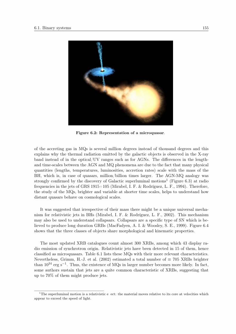
6.1. Binary systems 155
Figure 6.2: Representation of a microquasar.
of the accreting gas in MQs is several million degrees instead of thousand degrees and thisexplains why the thermal radiation emitted by the galactic objects is observed in the X-rayband instead of in the optical/UV ranges such as for AGNs. The differences in the length-and time-scales between the AGN and MQ phenomena are due to the fact that many physicalquantities (lengths, temperatures, luminosities, accretion rates) scale with the mass of theBH, which is, in case of quasars, million/billion times larger. The AGN-MQ analogy wasstrongly confirmed by the discovery of Galactic superluminal motions1 (Figure 6.3) at radiofrequencies in the jets of GRS 1915+105 (Mirabel, I. F. & Rodrıguez, L. F., 1994). Therefore,the study of the MQs, brighter and variable at shorter time scales, helps to understand howdistant quasars behave on cosmological scales.
It was suggested that irrespective of their mass there might be a unique universal mecha-nism for relativistic jets in BHs (Mirabel, I. F. & Rodrıguez, L. F., 2002). This mechanismmay also be used to understand collapsars. Collapsars are a specific type of SN which is be-lieved to produce long duration GRBs (MacFadyen, A. I. & Woosley, S. E., 1999). Figure 6.4shows that the three classes of objects share morphological and kinematic properties.
The most updated XRB catalogues count almost 300 XRBs, among which 43 display ra-dio emission of synchrotron origin. Relativistic jets have been detected in 15 of them, henceclassified as microquasars. Table 6.1 lists these MQs with their more relevant characteristics.Nevertheless, Grimm, H.-J. et al. (2002) estimated a total number of ≡ 705 XRBs brighterthan 1034 erg s1. Thus, the existence of MQs in larger number becomes more likely. In fact,some authors sustain that jets are a quite common characteristic of XRBs, suggesting thatup to 70% of them might produce jets.
1The superluminal motion is a relativistic eect: the material moves relative to its core at velocities whichappear to exceed the speed of light.
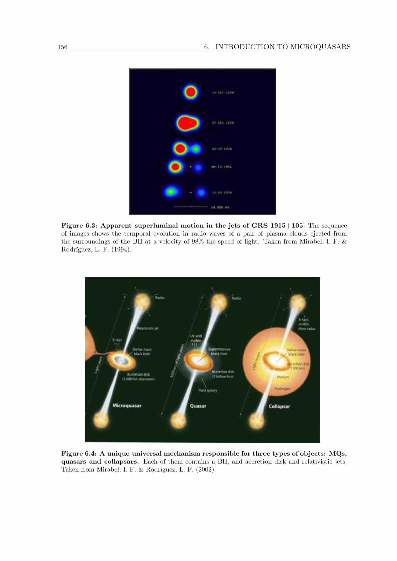
156 6. INTRODUCTION TO MICROQUASARS
Figure 6.3: Apparent superluminal motion in the jets of GRS 1915+105. The sequenceof images shows the temporal evolution in radio waves of a pair of plasma clouds ejected fromthe surroundings of the BH at a velocity of 98% the speed of light. Taken from Mirabel, I. F. &Rodrıguez, L. F. (1994).
Figure 6.4: A unique universal mechanism responsible for three types of objects: MQs,quasars and collapsars. Each of them contains a BH, and accretion disk and relativistic jets.Taken from Mirabel, I. F. & Rodrıguez, L. F. (2002).

6.2. The main components of microquasars 157
source name compact companion distance periodobject star [kpc]High-mass X-ray binaries
Cygnus X-1 BH O9.7 Iab 2 5.6dCygnus X-3 n.a. Wolf-Rayet 3.4–9.8 4.8hr
SS 433 BH A 5.5 13.1dV4641 Sgr BH B 3–8 2.8d
Low-mass X-ray binariesCircinus X-1 NS n.a. 7.8–10.5 16.65 dGX 339-4 BH sub-giant > 6 1.7 d
GRO J1655-40 BH sub-giant F <1.7 2.6 dGRS 1758-258 BH K 8.5 18.4 dGRS 1915+105 BH K,M 11.2 33 dXTE J1550-564 BH sub-giant 5.3 37 hrXTE J1748-288 BH > 8Scorpius X-1 NS M 2.8 18.9 h1E 140.7-2942 BH 7 12.73d4U 0614+091 NS white dwarf 3.2 0.85 hrH1743-322 BH n.a. n.a. n.a.
Table 6.1: Established MQ with their main characteristics. From left to right, sourcename, compact object, type of companion star, distance, and orbital period.
6.2 The main components of microquasars
This section describes the main components of a MQ which are also sketched in the represen-tation in Figure 6.5.
6.2.1 The compact object
A MQ harbors either a NS or a BH. Both of them correspond to the final stages of the starevolution. As described in § 4.1.1, NSs are produced in SN explosions which occur in thecollapse of stars with a mass 5–10 M. If the newly created NS is too massive (> 2.9 M)to reach a stable equilibrium, it evolves into a BH. Besides this possible delayed formation,BHs can be formed directly through the collapse of more massive stars with mass 10 M(Fryer, C. L., et al., 2002). The question on the explosive or implosive BH formation canbe addressed through kinematic studies of BH binaries. They suggest that some stellar BHsform associated with SN explosions: the SN imparts the center of mass of the system with arunaway velocity. In some cases, the kinematic evidence is reinforced by chemical compositionof the companion star, when it contains elements produced in the explosion. It was found thatthe BH microquasar GRO J1665-40 was ejected far from its birth place by an energetic SN(Israelian, G. et al., 1999). Kinematical studies on Cygnus X-1 (Mirabel, I. F. & Rodrigues,I., 2003) and GRS 1915+105(Dhawan, V. et al., 2007) suggest that the BH formation is notrelated to any SN explosion. Cygnus X-1 moves together with the massive star associationCygnus OB3. Its velocity relative to the association is 9 2 km s1, which is typical foran expanding association. Since no kick velocity was received by the microquasar, it seemsto have formed in situ (Figure 6.6). Another way to understand the BH formation can beprovided by observations of nearby GRBs of long duration (§ 1.4). This type of GRBs is
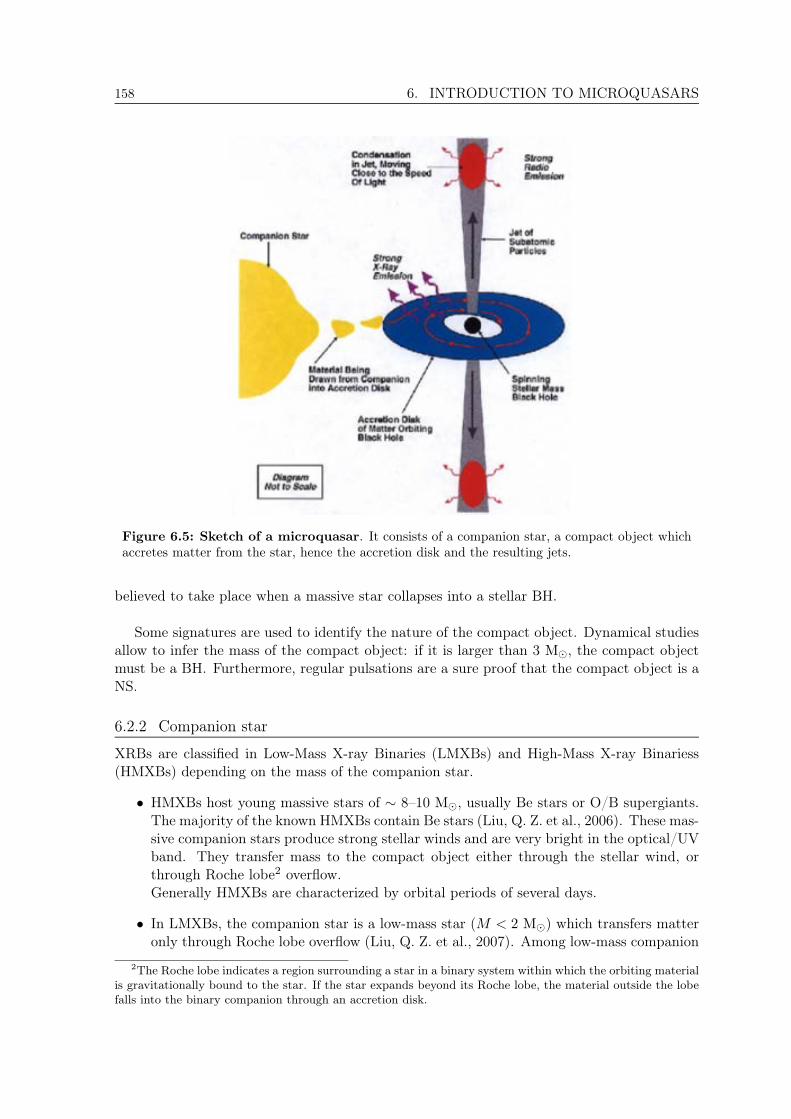
158 6. INTRODUCTION TO MICROQUASARS
Figure 6.5: Sketch of a microquasar. It consists of a companion star, a compact object whichaccretes matter from the star, hence the accretion disk and the resulting jets.
believed to take place when a massive star collapses into a stellar BH.
Some signatures are used to identify the nature of the compact object. Dynamical studiesallow to infer the mass of the compact object: if it is larger than 3 M, the compact objectmust be a BH. Furthermore, regular pulsations are a sure proof that the compact object is aNS.
6.2.2 Companion star
XRBs are classified in Low-Mass X-ray Binaries (LMXBs) and High-Mass X-ray Binariess(HMXBs) depending on the mass of the companion star.
• HMXBs host young massive stars of ∼ 8–10 M, usually Be stars or O/B supergiants.The majority of the known HMXBs contain Be stars (Liu, Q. Z. et al., 2006). These mas-sive companion stars produce strong stellar winds and are very bright in the optical/UVband. They transfer mass to the compact object either through the stellar wind, orthrough Roche lobe2 overflow.Generally HMXBs are characterized by orbital periods of several days.
• In LMXBs, the companion star is a low-mass star (M < 2 M) which transfers matteronly through Roche lobe overflow (Liu, Q. Z. et al., 2007). Among low-mass companion
2The Roche lobe indicates a region surrounding a star in a binary system within which the orbiting materialis gravitationally bound to the star. If the star expands beyond its Roche lobe, the material outside the lobefalls into the binary companion through an accretion disk.
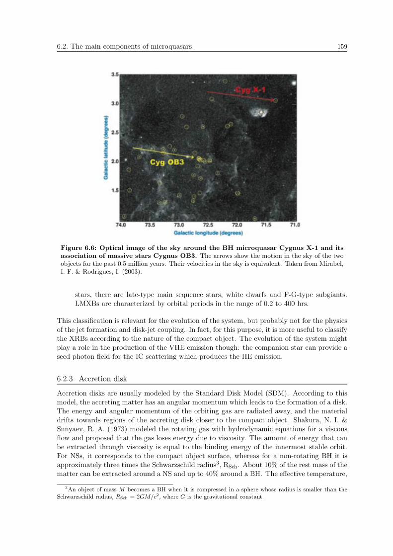
6.2. The main components of microquasars 159
Figure 6.6: Optical image of the sky around the BH microquasar Cygnus X-1 and itsassociation of massive stars Cygnus OB3. The arrows show the motion in the sky of the twoobjects for the past 0.5 million years. Their velocities in the sky is equivalent. Taken from Mirabel,I. F. & Rodrigues, I. (2003).
stars, there are late-type main sequence stars, white dwarfs and F-G-type subgiants.LMXBs are characterized by orbital periods in the range of 0.2 to 400 hrs.
This classification is relevant for the evolution of the system, but probably not for the physicsof the jet formation and disk-jet coupling. In fact, for this purpose, it is more useful to classifythe XRBs according to the nature of the compact object. The evolution of the system mightplay a role in the production of the VHE emission though: the companion star can provide aseed photon field for the IC scattering which produces the HE emission.
6.2.3 Accretion disk
Accretion disks are usually modeled by the Standard Disk Model (SDM). According to thismodel, the accreting matter has an angular momentum which leads to the formation of a disk.The energy and angular momentum of the orbiting gas are radiated away, and the materialdrifts towards regions of the accreting disk closer to the compact object. Shakura, N. I. &Sunyaev, R. A. (1973) modeled the rotating gas with hydrodynamic equations for a viscousflow and proposed that the gas loses energy due to viscosity. The amount of energy that canbe extracted through viscosity is equal to the binding energy of the innermost stable orbit.For NSs, it corresponds to the compact object surface, whereas for a non-rotating BH it isapproximately three times the Schwarzschild radius3, RSch. About 10% of the rest mass of thematter can be extracted around a NS and up to 40% around a BH. The effective temperature,
3An object of mass M becomes a BH when it is compressed in a sphere whose radius is smaller than theSchwarzschild radius, RSch = 2GM/c2, where G is the gravitational constant.
160 6. INTRODUCTION TO MICROQUASARS
Te , of the gas depends on the mass, M , of the compact object: Te / M1=4 _M1=4. Theaccretion disk of compact objects with a mass of some tens of M radiates X-rays.
Nevertheless, some sources exhibit hard X-rays which are difficult to explain with the SDM.This is the case for Cygnus X-1, for instance, where temperatures as high as 109 K are neededto match the observations, which, therefore, can not be fully explained within the SDM.New models have been proposed to explain such emission based on the advection dominatedaccretion flows (Narayan & Yi, 1994). The Advection Dominated Accretion Flow (ADAF)model assumes a low density accreting gas. This assumption implies that the gas is unable tocool efficiently through viscosity within the accreting time. Most of the released gravitationalenergy of the gas in the accretion flow is converted into internal energy of the gas. The disk ishot and thick. Only a small fraction of the released energy in ADAFs is radiated away. Theradiation efficiency is therefore significantly lower than that for standard thin disks.
6.2.4 The corona
In order to explain the hard X-ray emission, some models have introduced a new component tothe SDM, called “corona”. In these models, the low density gas is not able to cool efficiently theinnermost part of the disk. Consequently, the temperature increases and the disk inflates. Thisinflated disk is called corona and can explain the hard X-ray emission through the scatteringof electrons on seed photons. The transition between the corona (inefficient cooling) and thedisk (efficient cooling) takes place at a radius of ≡ 100 RSch .
6.2.5 Jets
Jets are collimated ejecta with an opening angle 15 (Bridle, A. H. & Perley, 1984). Theyseem to be systematically associated with the presence of an accretion disk around a compactobject. Since the main difference between NSs and BHs is the presence of a surface or anevent horizon respectively, it seems likely that the formation of the jets does not depend onthe nature of the compact object itself, but on the accretion flow process.
The most credited scenario for the explanation of the jet formation is based on MHD. Astrong electromagnetic field in the compact object, coupled with differential rotation, con-verts the rotational energy stored in the disk into the kinetic energy in the ejecta. Plasmatrapped in the magnetic field lines is subjected to the Lorentz force which, under conditionsof high conductivity (this is the MHD assumption), splits into two vector components: amagnetic pressure gradient and a magnetic tension. The magnetic pressure gradient alongthe rotation axis accelerates plasma out of the system, whereas the magnetic tension colli-mates the outflow of material which escapes the gravitational potential well and forms the jet.
Jets in MQs emit non-thermal radiation which has been observed from radio frequenciesto optical/UV (Russell, D. M. & Fender, R. P., 2010), and up to X-rays (Corbel, S., et al.,2002) at large scales. This emission is a clear evidence for the presence of relativistic particlesinside the jet. It is generally accepted that particle acceleration takes place in shock wavesthrough the Fermi acceleration mechanism (§ A.1). There are different models which explainthe creation of shock waves in the microquasar environment:
• continuous jet and internal shocks. Jets are considered as a continuous flow andthe emission is produced through internal shocks (Kaiser, C. R. et al., 2000). Theseinternal shocks are due to the collision between small regions of the jets characterizedby different densities and/or velocities.
6.3. Disk-jet connection 161
• discrete jets and internal shocks. Jets consist of discrete material ejected in form ofblobs (van der Laan, H., 1966). The collision between blobs with different velocities canmimic internal shocks (Jamil, O. et al., 2010). This mechanism leads to the productionof a quasi-steady emission with fluctuations connected to the variation scale of theinjected blobs.
• external shocks. Aside from the composition of the jets, external shock could be pro-duced as a result of the interaction between the jet and dense material from the stellarwind (Perucho, M. & Bosch-Ramon, V., 2008) or the surrounding medium (Bordas, P.et al., 2009). In such a scenario, the emission may be observable both as a transient anda quasi-stationary phenomenon. Since there is a considerable evidence that the stellarwinds are clumpy, these clumps might produce transient emission by interacting withthe jets (Araudo, A. T. et al., 2009).
Mirabel, I. F. & Rodrıguez, L. F. (1999) proposed that MQs with jet axis that form angles 10 with the line of sight should appear as microblazars (analogously to blazars). Due torelativistic beaming, in microblazars the brightness of outbursts is enhanced by a factor 8 3, where is the Lorentz factor. In addition, also the time interval of the phenomena isreduced by factors 0.5 2. Then, microblazars should appear as intense sources of HEphotons with very fast variations of flux. Due to the difficulty to find and follow them and tothe relatively low statistical probability of small angles between the jet axis and the line ofsight, the most of the so far observed MQs exhibit angles larger than 30.
6.3 Disk-jet connection
MQs allow to gain an insight into the connection between the accretion disk and the jet. Dur-ing simultaneous multi-wavelength observations of the frequent outbursts from GRS 1915+105,the X-ray flux was monitored simultaneously with the emission of the jet at different frequen-cies (Mirabel, I. F., et al., 1998). Figure 6.7 shows the complete temporal sequence of a flarefrom GRS 1915+105 which lasted less than one hour. A sudden drop in X-ray luminosity wasfollowed by the ejection of jets, first observed in IR, then at radio frequencies. The drop canbe interpreted as the disappearance of the warmer inner part of the accretion disk beyond theBH horizon. Few minutes later, fresh matter coming from the companion star feeds again theaccretion disk, which has evacuated part of its kinetic energy under the form of bipolar jets.Moving away, the plasma becomes transparent first in IR and then at radio frequencies. Thetime delay between the IR and the radio peaks is consistent with the model of adiabaticallyexpanding clouds (§ 6.2.5). However, according to this model, the IR emission should beobserved 103 s after the ejection, but it occurred more than 200 s after the drop in X-rayflux. In this observation the ejection of the plasma clouds takes place during the subsequentreplenishment of the inner accretion disk, well after the disappearance of the soft componentand it can last up to tens minutes.
After this observation of an event involving the accretion disk and the jet of a MQ, asimilar event happened for the quasar 3C 120 (Marscher, A. P., et al., 2002), but in scales ofyears rather than minutes. The ratio of time scales is comparable to the ratio of the massesof the super-massive BH in 3C 120 and the stellar one in GRS 1915+105, as expected in thecontext of the unified BH model.
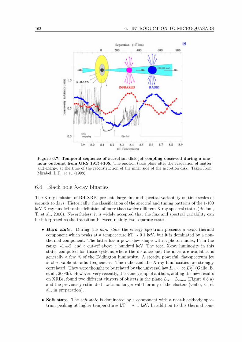
162 6. INTRODUCTION TO MICROQUASARS
Figure 6.7: Temporal sequence of accretion disk-jet coupling observed during a one-hour outburst from GRS 1915+105. The ejection takes place after the evacuation of matterand energy, at the time of the reconstruction of the inner side of the accretion disk. Taken fromMirabel, I. F., et al. (1998).
6.4 Black hole X-ray binaries
The X-ray emission of BH XRBs presents large flux and spectral variability on time scales ofseconds to days. Historically, the classification of the spectral and timing patterns of the 1-100keV X-ray flux led to the definition of more than twelve different X-ray spectral states (Belloni,T. et al., 2000). Nevertheless, it is widely accepted that the flux and spectral variability canbe interpreted as the transition between mainly two separate states:
• Hard state . During the hard state the energy spectrum presents a weak thermalcomponent which peaks at a temperature kT ∼ 0.1 keV, but it is dominated by a non-thermal component. The latter has a power-law shape with a photon index, Γ, in therange ∼1.4-2, and a cut-off above a hundred keV. The total X-ray luminosity in thisstate, computed for those systems where the distance and the mass are available, isgenerally a few % of the Eddington luminosity. A steady, powerful, flat-spectrum jetis observable at radio frequencies. The radio and the X-ray luminosities are stronglycorrelated. They were thought to be related by the universal law Lradio ∝ L0.7
X (Gallo, E.et al., 2003b). However, very recently, the same group of authors, adding the new resultson XRBs, found two different clusters of objects in the plane LX−Lradio (Figure 6.8 a)and the previously estimated law is no longer valid for any of the clusters (Gallo, E., etal., in preparation).
• Soft state. The soft state is dominated by a component with a near-blackbody spec-trum peaking at higher temperatures kT = ∼ 1 keV. In addition to this thermal com-
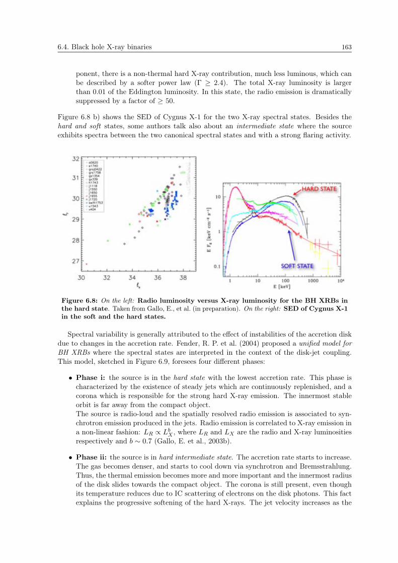
6.4. Black hole X-ray binaries 163
ponent, there is a non-thermal hard X-ray contribution, much less luminous, which canbe described by a softer power law (Γ≥ 2.4). The total X-ray luminosity is largerthan 0.01 of the Eddington luminosity. In this state, the radio emission is dramaticallysuppressed by a factor of ≥ 50.
Figure 6.8 b) shows the SED of Cygnus X-1 for the two X-ray spectral states. Besides thehard and soft states, some authors talk also about an intermediate state where the sourceexhibits spectra between the two canonical spectral states and with a strong flaring activity.
Figure 6.8: On the left: Radio luminosity versus X-ray luminosity for the BH XRBs inthe hard state. Taken from Gallo, E., et al. (in preparation). On the right: SED of Cygnus X-1in the soft and the hard states.
Spectral variability is generally attributed to the effect of instabilities of the accretion diskdue to changes in the accretion rate. Fender, R. P. et al. (2004) proposed a unified model forBH XRBs where the spectral states are interpreted in the context of the disk-jet coupling.This model, sketched in Figure 6.9, foresees four different phases:
• Phase i: the source is in the hard state with the lowest accretion rate. This phase ischaracterized by the existence of steady jets which are continuously replenished, and acorona which is responsible for the strong hard X-ray emission. The innermost stableorbit is far away from the compact object.The source is radio-loud and the spatially resolved radio emission is associated to syn-chrotron emission produced in the jets. Radio emission is correlated to X-ray emission ina non-linear fashion: LR ∝ LbX , where LR and LX are the radio and X-ray luminositiesrespectively and b ∼ 0.7 (Gallo, E. et al., 2003b).
• Phase ii: the source is in hard intermediate state. The accretion rate starts to increase.The gas becomes denser, and starts to cool down via synchrotron and Bremsstrahlung.Thus, the thermal emission becomes more and more important and the innermost radiusof the disk slides towards the compact object. The corona is still present, even thoughits temperature reduces due to IC scattering of electrons on the disk photons. This factexplains the progressive softening of the hard X-rays. The jet velocity increases as the

164 6. INTRODUCTION TO MICROQUASARS
Figure 6.9: A schematic view of the unified model for BH XRBs. It is a hardness-intensity diagram, where the soft, the hard and the hard/soft intermediate states are representedby the corresponding four phases. For each of these phases the accretion disk-jet behaviour issketched outside the diagram. The lower panel indicates the variation of the inner disk radius andthe bulk Lorentz factor of the outflow as function of the hardness. Adapted from Fender, R. P.et al. (2004).
accretion disk moves closer and closer to the compact object. This may be due to thefact that matter needs a higher velocity to escape from the disk.
• Phase iii: the source moves to a soft intermediate state. The processes explained in theprevious phase lead to a maximum softening of the hard X-rays, after which the thermalemission from the disk becomes dominant. Around the time when the source crossesthe line between jet-free and jet-producing states, the velocity of the jet increases veryrapidly. This increase produces a shock in the pre-existing jet which manifests itself asa flare, seen also at radio frequencies.
• Phase iv: the source is in soft state when the accretion rate is at its highest. Theaccretion disk is stable and extends to the last stable orbit. No jet is present; thusthe spectrum is dominated by the thermal emission of the accretion disk. When theaccretion rate starts to decrease, the corona is produced, new jets are ejected, and thesystem moves to a hard state.The origin of the hard X-ray emission in this phase is rather controversial. Some authorspropose a residual corona where the magnetic field plays an important role acceleratingelectrons which produce non-thermal emission. The radio emission is quenched, proba-bly due to physical suppression of the jets (Fender, R. P., et al., 1999).
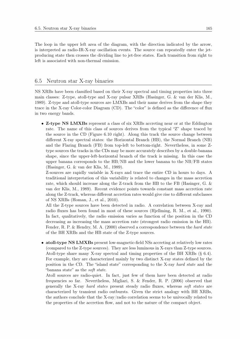
6.5. Neutron star X-ray binaries 165
The loop in the upper left area of the diagram, with the direction indicated by the arrow,is interpreted as radio-IR-X-ray oscillation events. The source can repeatedly enter the jet-producing state then crosses the dividing line to jet-free states. Each transition from right toleft is associated with non-thermal emission.
6.5 Neutron star X-ray binaries
NS XRBs have been classified based on their X-ray spectral and timing properties into threemain classes: Z-type, atoll-type and X-ray pulsar XRBs (Hasinger, G. & van der Klis, M.,1989). Z-type and atoll-type sources are LMXBs and their name derives from the shape theytrace in the X-ray Color-color Diagram (CD). The “color” is defined as the difference of fluxin two energy bands.
• Z-type NS LMXBs represent a class of six XRBs accreting near or at the Eddingtonrate. The name of this class of sources derives from the typical “Z” shape traced bythe source in the CD (Figure 6.10 right). Along this track the source change betweendifferent X-ray spectral states: the Horizontal Branch (HB), the Normal Branch (NB)and the Flaring Branch (FB) from top-left to bottom-right. Nevertheless, in some Z-type sources the tracks in the CDs may be more accurately describes by a double-bananashape, since the upper-left-horizontal branch of the track is missing. In this case theupper banana corresponds to the HB/NB and the lower banana to the NB/FB states(Hasinger, G. & van der Klis, M., 1989).Z-sources are rapidly variable in X-rays and trace the entire CD in hours to days. Atraditional interpretation of this variability is related to changes in the mass accretionrate, which should increase along the Z-track from the HB to the FB (Hasinger, G. &van der Klis, M., 1989). Recent evidence points towards constant mass accretion ratealong the Z-track, whereas different accretion rates would give rise to different subclassesof NS XRBs (Homan, J., et al., 2010).All the Z-type sources have been detected in radio. A correlation between X-ray andradio fluxes has been found in most of these sources (Hjellming, R. M., et al., 1990).In fact, qualitatively, the radio emission varies as function of the position in the CDdecreasing as increasing the mass accretion rate (strongest radio emission in the HB).Fender, R. P. & Hendry, M. A. (2000) observed a correspondence between the hard stateof the BH XRBs and the HB state of the Z-type sources.
• atoll-type NS LMXBs present low-magnetic-field NSs accreting at relatively low rates(compared to the Z-type sources). They are less luminous in X-rays than Z-type sources.Atoll-type share many X-ray spectral and timing properties of the BH XRBs (§ 6.4).For example, they are characterized mainly by two distinct X-ray states defined by theposition in the CD. The “island state” corresponding to the X-ray hard state and the“banana state” as the soft state.Atoll sources are radio-quiet. In fact, just few of them have been detected at radiofrequencies so far. Nevertheless, Migliari, S. & Fender, R. P. (2006) observed thatgenerally the X-ray hard states present steady radio fluxes, whereas soft states arecharacterized by transient radio outbursts. Given the strict analogy with BH XRBs,the authors conclude that the X-ray/radio correlation seems to be univocally related tothe properties of the accretion flow, and not to the nature of the compact object.
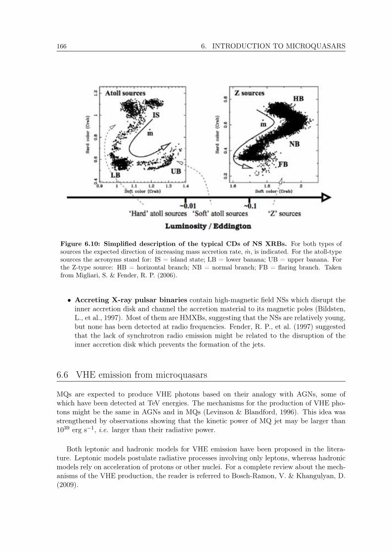
166 6. INTRODUCTION TO MICROQUASARS
Figure 6.10: Simplified description of the typical CDs of NS XRBs. For both types ofsources the expected direction of increasing mass accretion rate, m, is indicated. For the atoll-typesources the acronyms stand for: IS = island state; LB = lower banana; UB = upper banana. Forthe Z-type source: HB = horizontal branch; NB = normal branch; FB = flaring branch. Takenfrom Migliari, S. & Fender, R. P. (2006).
• Accreting X-ray pulsar binaries contain high-magnetic field NSs which disrupt theinner accretion disk and channel the accretion material to its magnetic poles (Bildsten,L., et al., 1997). Most of them are HMXBs, suggesting that the NSs are relatively young,but none has been detected at radio frequencies. Fender, R. P., et al. (1997) suggestedthat the lack of synchrotron radio emission might be related to the disruption of theinner accretion disk which prevents the formation of the jets.
6.6 VHE emission from microquasars
MQs are expected to produce VHE photons based on their analogy with AGNs, some ofwhich have been detected at TeV energies. The mechanisms for the production of VHE pho-tons might be the same in AGNs and in MQs (Levinson & Blandford, 1996). This idea wasstrengthened by observations showing that the kinetic power of MQ jet may be larger than1039 erg s−1, i.e. larger than their radiative power.
Both leptonic and hadronic models for VHE emission have been proposed in the litera-ture. Leptonic models postulate radiative processes involving only leptons, whereas hadronicmodels rely on acceleration of protons or other nuclei. For a complete review about the mech-anisms of the VHE production, the reader is referred to Bosch-Ramon, V. & Khangulyan, D.(2009).

6.6. VHE emission from microquasars 167
6.6.1 Leptonic models
The leptonic models extend the energy of leptons from synchrotron radio emitting energies upto γ-rays. The most accredited models predict that HE photons come from the IC scatteringof relativistic electron with low-energy photons (Atoyan, A. M. & Aharonian, F. A., 1999;Markoff, S. et al., 2001; Georganopoulos, M. et al., 2002; Bosch-Ramon, V. et al., 2006).Figure 6.11 shows the main features considered by the leptonic models listed in their associatedregions.
Figure 6.11: Sketch of the microquasar leptonicscenario. The main features considered by the model arelisted in their associated regions. The plot, not to scale, istaken from Bosch-Ramon, V. et al. (2006).
Depending on the nature of theseed photons, mainly two scenarioshave been proposed: the SSC modelwhere synchrotron photons are ICup-scattered by the same populationof electrons which produce them,and the external IC model whichforesees that a denser populationof photons produced outside the jet(corona/disk photons or from thestellar wind) is the dominant photonfield target for the Compton scatter-ing of the electrons. The IC scat-tering on stellar photons is ineffi-cient in LMXBs, where the stellarluminosity is negligible, as well as inHMXBs at high energies because ofthe large distance between the com-panion star and the jet shock. Itmust be mentioned, however, thatrecently Bednarek, W. & Pabich,J. (2010) proposed efficient stellarIC scattering also for very compactLMXBs. The low-mass star can beheated by the X-ray source producedto accretion of matter.
As a result, there are parts of the stellar surface which can reach temperature as high asthose of the high-mass stars, hence producing enough soft photons to make the IC efficient.
6.6.2 Hadronic models
In hadronic models hadrons are responsible for GeV-TeV γ-rays, whereas electrons are signif-icant emitters at lower energies. The main radiative processes are: the collision of relativisticprotons with ions (pp) in the jet or the stellar wind (Romero, G. E. et al., 2003), and theinteraction between jet relativistic protons and X-ray photons (pγ) from the disk, the coronaor the jet itself (synchrotron emission) (Romero, G. E., 2008). These proton collisions produceneutral pions (π 0) that decay into γ-rays, and charged pions (π ± ) that decay into muons andneutrinos, the former decaying then to electron-positron pairs and neutrinos. The leptonsoriginated from the secondary pairs can produce low-energy emission via synchrotron, IC and
168 6. INTRODUCTION TO MICROQUASARS
Bremsstrahlung (Orellana, M. et al., 2007).
There are other models which take into account the possibility that a significant amountof protons, accelerated in the region where the jet ends, are released and interact further awayin a high density region of the ISM (Bosch-Ramon, V. et al., 2005). Proton-proton collisionswithin the cloud lead to the creation of neutral and charged pions, and consequently to thecreation of -rays and e pairs. Due to propagation effects, the outcomes of these interactionscan differ strongly depending on the age, the nature of the accelerator, and its distance to thecloud.
6.6.3 Microquasar in -rays: observations
Although MQs were proposed to emit -ray more than one decade ago (Atoyan, A. M. &Aharonian, F. A., 1999), only recently this could be proved thanks to the new generation of -ray satellites. The microquasar Cygnus X-3 was detected in 2009 by both Fermi/LAT andAGILE at energies above 100 MeV (Abdo, A. A., et al., 2009b; Tavani, M., et al., 2009). Inaddition, AGILE reported the detection of several 1-day flares from the well known BH MQ,Cygnus X-1, above 100 MeV (Sabatini, S., et al. 2010; ATels #2512 #2715). This could notbe confirmed by Fermi/LAT, though.
At higher energies, above few tens of TeV, no emission has been established so far. In the80’s, the first generation of ground-based telescopes reported many claims on the detectionof PeV-TeV signals coming from microquasars, mainly Cygnus X-3 (Danaher, S. et al., 1981;Lamb, R. C. et al., 1982; Bhat, C. L. et al., 1986). However, the fact that most sensitiveexperiments could not confirm such claims, raised many doubts on their validity. Recently,Albert, J., et al. (2007d) published a non-significant evidence of signal, at the post-trial level of4.1η, from Cygnus X-1 during a short (less than 1 day) flare on September 24, 2006. MAGICtried to catch a similar flare in the following three cycles of observations (2007–2009), but thesubsequent hundred more hours of observations were unsuccessful.
Nowadays, IACTs are making a strong effort to catch a VHE signal from a well-establishedmicroquasar. MAGIC pointed towards several interesting candidates; besides Cygnus X-1,MAGIC observed SS 433, GRS 1915+105, Cygnus X-3, and Scorpius X-1. In the third partof this thesis work, the results of the observations of Cygnus X-3 and Scorpius X-1 will bepresented.
7Cygnus X-3
Cygnus X-3 is a peculiar MQ where a compact object orbits around a Wolf-Rayetcompanion star with a short orbital period of only 4.8 hrs. It has been detected atradio frequencies and up to HE -rays. However, many models also predict VHEemission when the source displays relativistic persistent jets or relativistic transientejections.The first stand-alone MAGIC telescope observed Cygnus X-3 for 70 hrs betweenMarch 2006 and August 2009 in different X-ray/radio spectral states and also duringa period of enhanced -ray emission. This allows us to search for VHE emission fromCygnus X-3 in the different cases for which this radiation is predicted. MAGIC foundno evidence for a VHE signal from the direction of the MQ. An upper limit to theintegral flux for energies higher than 250 GeV has been set to 2.2 1012 photonscm2 s1 (95% CL). This is the best limit so far to the VHE emission from this source.
The results presented in this chapter are published in Aleksic, J., et al. (2010a). Theauthor was the Principal Investigator (PI) of the Cygnus X-3 observations and themain analyzer of the resulting data set.
Cygnus X-3 is a bright and persistent X-ray binary, discovered in 1967 (Giacconi, R. et al.,1967), but the HE processes occurring in the source are still poorly understood. It lies closeto the Galactic plane at a distance between 3.4 and 9.8 kpc, probably at 7 kpc depending ondifferent distance estimates to the Cygnus OB2 association (Ling, Z. et al., 2009).
The nature and the mass of the compact object are still a subject of debate. The historicaldetection in -rays of a 12.6 MSP coincident with Cygnus X-3 position (Chadwick, P. M.et al., 1985) would provide an evidence that the compact object is a NS. However, there isno independent confirmation for this pulsar signal. Published results suggest either a NS of1.4 M (Stark & Saia, 2003) or a BH of less than 10 M (Hanson, M. M. et al., 2000). Theidentification of its donor star (§ 6.2.2) as a Wolf-Rayet star (van Kerkwijk, M. H., et al., 1992)makes Cygnus X-3 a rather special XRBs since only two other objects of this class, both extra-galactic, host such a companion star type (Prestwich, A. H., et al., 2007; Carpano, S., et al.,2007). In both cases, there is evidence that the compact object is a BH. The presence of themassive Wolf-Rayet star classifies Cygnus X-3 as a HMXB. Nevertheless, Cygnus X-3 shows a
169
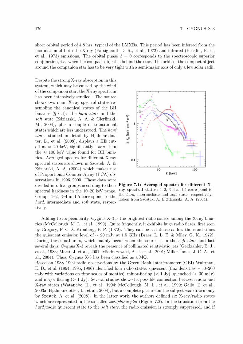
170 7. CYGNUS X-3
short orbital period of 4.8 hrs, typical of the LMXBs. This period has been inferred from themodulation of both the X-ray (Parsignault, D. R., et al., 1972) and infrared (Becklin, E. E.,et al., 1973) emissions. The orbital phase φ = 0 corresponds to the spectroscopic superiorconjunction, i.e. when the compact object is behind the star. The orbit of the compact objectaround the companion star has to be very tight with a semi-major axis of only a few solar radii.
Despite the strong X-ray absorption in thissystem, which may be caused by the windof the companion star, the X-ray spectrumhas been intensively studied. The sourceshows two main X-ray spectral states re-sembling the canonical states of the BHbinaries (§ 6.4): the hard state and thesoft state (Zdziarski, A. A. & Gierlinski,M., 2004), plus a couple of transitionalstates which are less understood. The hardstate, studied in detail by Hjalmarsdot-ter, L., et al. (2008), displays a HE cut-off at ≈ 20 keV, significantly lower thanthe ≈ 100 keV value found for BH bina-ries. Averaged spectra for different X-rayspectral states are shown in Szostek, A. &Zdziarski, A. A. (2004) which makes useof Proportional Counter Array (PCA) ob-servations in 1996–2000. These data weredivided into five groups according to theirspectral hardness in the 10–20 keV range.Groups 1–2, 3–4 and 5 correspond to thehard, intermediate and soft state, respec-tively.
Figure 7.1: Averaged spectra for different X-ray spectral states: 1–2, 3–4 and 5 correspond tothe hard, intermediate and soft state, respectively.Taken from Szostek, A. & Zdziarski, A. A. (2004).
Adding to its peculiarity, Cygnus X-3 is the brightest radio source among the X-ray bina-ries (McCollough, M. L., et al., 1999). Quite frequently, it exhibits huge radio flares, first seenby Gregory, P. C. & Kronberg, P. P. (1972). They can be as intense as few thousand timesthe quiescent emission level of ∼ 20 mJy at 1.5 GHz (Braes, L. L. E. & Miley, G. K., 1972).During these outbursts, which mainly occur when the source is in the soft state and lastseveral days, Cygnus X-3 reveals the presence of collimated relativistic jets (Geldzahler, B. J.,et al., 1983; Martı, J. et al., 2001; Mioduszewski, A. J. et al., 2001; Miller-Jones, J. C. A., etal., 2004). Thus, Cygnus X-3 has been classified as a MQ.Based on 1988–1992 radio observations by the Green Bank Interferometer (GBI) Waltman,E. B., et al. (1994, 1995, 1996) identified four radio states: quiescent (flux densities ∼ 50–200mJy with variations on time scales of months), minor-flaring (< 1 Jy), quenched (< 30 mJy)and major flaring (> 1 Jy). Several studies showed a possible connection between radio andX-ray states (Watanabe, H., et al., 1994; McCollough, M. L., et al., 1999; Gallo, E. et al.,2003a; Hjalmarsdotter, L., et al., 2008), but a complete picture on the subject was drawn onlyby Szostek, A. et al. (2008). In the latter work, the authors defined six X-ray/radio stateswhich are represented in the so-called saxophone plot (Figure 7.2). In the transition from thehard/radio quiescent state to the soft state, the radio emission is strongly suppressed, and if

Cygnus X-3 171
Figure 7.2: Saxophone plot . Schematic representation of the evolution of Cygnus X-3 throughits radio and X-ray states. The dotted lines represent the transition levels. Adapted from Szostek,A. et al. (2008).
it reaches the quenched level, the source usually produces a major radio flare.
Cygnus X-3 has also historically drawn a great deal of attention due to numerous claims ofdetection at TeV and PeV γ-rays, using early detectors in these energy ranges (Vladimirsky,B. M. et al., 1973; Danaher, S. et al., 1981; Lamb, R. C. et al., 1982; Dowthwaite, J. C., etal., 1983; Samorski, M. & Stamm, W., 1983; Cawley, M. F., et al., 1985; Bhat, C. L. et al.,1986). However, a critical analysis of these observations raised doubts about their validity(Chardin, G. & Gerbier, G., 1989), and in recent years more sensitive instruments have notconfirmed those claims for energies above 500 GeV (Schilling, M. et al., 2001; Albert, J., etal., 2008a). Nevertheless, MQs are believed to produce VHE emission inside the jets (§ 6.6):high density photon and magnetic fields by the accretion disk and the companion star mightcreate favorable conditions for effective production of γ-rays. This radiation can have:
• an episodic nature due to the ejection of strong radio emitting blobs (Atoyan, A. M.& Aharonian, F. A., 1999), mainly occurring in the soft state in the case of BH XRBs
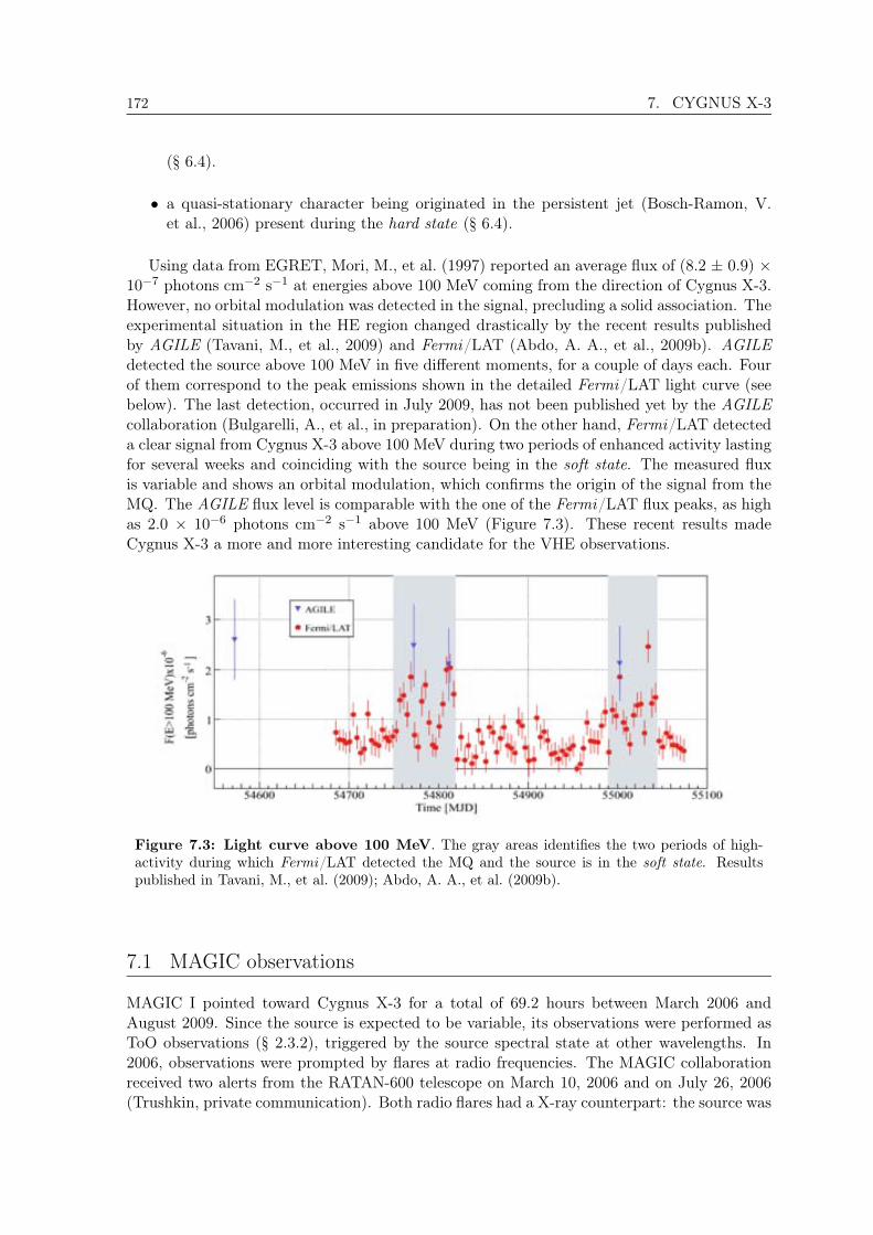
172 7. CYGNUS X-3
(§ 6.4).
• a quasi-stationary character being originated in the persistent jet (Bosch-Ramon, V.et al., 2006) present during the hard state (§ 6.4).
Using data from EGRET, Mori, M., et al. (1997) reported an average flux of (8.2 ± 0.9) ×10−7 photons cm−2 s−1 at energies above 100 MeV coming from the direction of Cygnus X-3.However, no orbital modulation was detected in the signal, precluding a solid association. Theexperimental situation in the HE region changed drastically by the recent results publishedby AGILE (Tavani, M., et al., 2009) and Fermi/LAT (Abdo, A. A., et al., 2009b). AGILEdetected the source above 100 MeV in five different moments, for a couple of days each. Fourof them correspond to the peak emissions shown in the detailed Fermi/LAT light curve (seebelow). The last detection, occurred in July 2009, has not been published yet by the AGILEcollaboration (Bulgarelli, A., et al., in preparation). On the other hand, Fermi/LAT detecteda clear signal from Cygnus X-3 above 100 MeV during two periods of enhanced activity lastingfor several weeks and coinciding with the source being in the soft state. The measured fluxis variable and shows an orbital modulation, which confirms the origin of the signal from theMQ. The AGILE flux level is comparable with the one of the Fermi/LAT flux peaks, as highas 2.0 × 10⁻⁶ photons cm−2 s−1 above 100 MeV (Figure 7.3). These recent results madeCygnus X-3 a more and more interesting candidate for the VHE observations.
Figure 7.3: Light curve above 100 MeV. The gray areas identifies the two periods of high-activity during which Fermi/LAT detected the MQ and the source is in the soft state. Resultspublished in Tavani, M., et al. (2009); Abdo, A. A., et al. (2009b).
7.1 MAGIC observations
MAGIC I pointed toward Cygnus X-3 for a total of 69.2 hours between March 2006 andAugust 2009. Since the source is expected to be variable, its observations were performed asToO observations (§ 2.3.2), triggered by the source spectral state at other wavelengths. In2006, observations were prompted by flares at radio frequencies. The MAGIC collaborationreceived two alerts from the RATAN-600 telescope on March 10, 2006 and on July 26, 2006(Trushkin, private communication). Both radio flares had a X-ray counterpart: the source was
7.1. MAGIC observations 173
in the soft state according to Rossi X-ray Timing Explorer (RXTE)/ASM1 and Swift/BAT2
measurements. In 2007, the observations were triggered using public RXTE/ASM (1.5–12keV) and Swift/BAT (15–50 keV) data, as follows: a) Swift/BAT daily flux larger than 0.05counts cm2 s1 and b) ratio between RXTE/ASM and Swift/BAT count rates lower than200. These criteria guarantee the source to be in the hard state. During 2008 and 2009,MAGIC observed Cygnus X-3 following HE -ray alerts issued by the AGILE satellite. Thefirst of these alerts arrived on April 18, 2008, the second one on July 18, 2009 (Tavani, privatecommunication). These last two campaigns occurred when the source was in the soft state.All these triggered observations were lasting at most two hours per night depending on thesource visibility, its zenith angle and, above all, the competition with other scheduled sources.Nevertheless, if the OA (§ 2.5) had shown a signal larger than 3η, the observation shouldhave been followed up as long as possible with absolute priority with respect to any otherscheduled and ToO source.
At La Palma, Cygnus X-3 culminates at a zenith angle of 12. The observations werecarried out with the first stand-alone MAGIC telescope at zenith angles between 12 and 50.They were performed partially in on/off mode (just the first campaign) and in wobble mode(§ 2.3.3). The entire Cygnus X-3 data set recorded by MAGIC amounts to 69.2 hours, out ofwhich 12.5 hours3 were rejected from further analysis because of their anomalous event rates.It led to a total amount of 56.7 hours of useful data distributed in 39 nights of observation.The details of the observations are quoted in Table 7.1.
The recorded Cygnus X-3 data set extends over five different cycles of observation (§ 2.3.1),which are characterized by varying hardware configurations and performances of the telescope:
• during the first campaign (cycle I) MAGIC I was equipped with the old readout systemat 300 MSample/s (§ 2.2.6).
• the second campaign (cycle II) was carried out with fiber optic splitters (§ 2.2.6), butstill the 300 MHz readout system. The performance of the instrument did not changemuch with respect to the previous observational cycle, but a new MC production wasneeded for such analysis.
• from the third campaign on (cycle III, IV, and V), MAGIC I was provided with the up-graded readout system (§ 2.2.6) characterized by a 2 GHz sampling rate. This hardwareupgrade together with the development of new analysis methods which make use of thetiming parameters of the shower images yielded to an improvement of the instrumentperformance by a factor 1.4 (Aliu, E., et al., 2009).
• during the third campaign (cycle III) the telescope was characterized by two differentperformances due to a mirror re-alignment (§ 2.2.3) which led to a significant improve-ment of the mirror reflectivity. The optical PSF, in fact, passed from 12–14 mm to9–10 mm. Since the mirror re-alignment was performed on July 30-31, 2007, data fromthe third campaign were divided into July and August data samples. They were thenanalyzed separately with two different MC productions accounting for the correct opticalPSF of the telescope (§ 3.1).
1Based on quick-look results provided by the RXTE/ASM team.2Swift/BAT transient monitor results provided by the Swift/BAT team.39.6 hours were rejected due to calima (Ÿ 3.6).
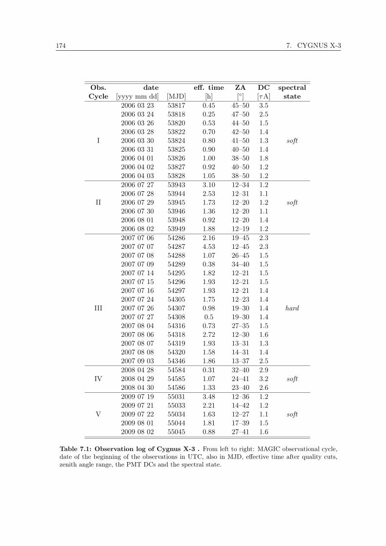
174 7. CYGNUS X-3
Obs. date eff. time ZA DC spectralCycle [yyyy mm dd] [MJD] [h] [] [τA] state
2006 03 23 53817 0.45 45–50 3.52006 03 24 53818 0.25 47–50 2.52006 03 26 53820 0.53 44–50 1.52006 03 28 53822 0.70 42–50 1.4
I 2006 03 30 53824 0.80 41–50 1.3 soft2006 03 31 53825 0.90 40–50 1.42006 04 01 53826 1.00 38–50 1.82006 04 02 53827 0.92 40–50 1.22006 04 03 53828 1.05 38–50 1.22006 07 27 53943 3.10 12–34 1.22006 07 28 53944 2.53 12–31 1.1
II 2006 07 29 53945 1.73 12–20 1.2 soft2006 07 30 53946 1.36 12–20 1.12006 08 01 53948 0.92 12–20 1.42006 08 02 53949 1.88 12–19 1.22007 07 06 54286 2.16 19–45 2.32007 07 07 54287 4.53 12–45 2.32007 07 08 54288 1.07 26–45 1.52007 07 09 54289 0.38 34–40 1.52007 07 14 54295 1.82 12–21 1.52007 07 15 54296 1.93 12–21 1.52007 07 16 54297 1.93 12–21 1.42007 07 24 54305 1.75 12–23 1.4
III 2007 07 26 54307 0.98 19–30 1.4 hard2007 07 27 54308 0.5 19–30 1.42007 08 04 54316 0.73 27–35 1.52007 08 06 54318 2.72 12–30 1.62007 08 07 54319 1.93 13–31 1.32007 08 08 54320 1.58 14–31 1.42007 09 03 54346 1.86 13–37 2.52008 04 28 54584 0.31 32–40 2.9
IV 2008 04 29 54585 1.07 24–41 3.2 soft2008 04 30 54586 1.33 23–40 2.62009 07 19 55031 3.48 12–36 1.22009 07 21 55033 2.21 14–42 1.2
V 2009 07 22 55034 1.63 12–27 1.1 soft2009 08 01 55044 1.81 17–39 1.52009 08 02 55045 0.88 27–41 1.6
Table 7.1: Observation log of Cygnus X-3 . From left to right: MAGIC observational cycle,date of the beginning of the observations in UTC, also in MJD, effective time after quality cuts,zenith angle range, the PMT DCs and the spectral state.

7.1. MAGIC observations 175
• data from the forth campaign (cycle IV) were recorded under moderate moonlight con-ditions, as shown by the anode PMT DCs in Table 7.1. Therefore, they required specificimage cleaning levels to account for the larger noise, as described in § 3.4.1.
• 0.7 hours of data recorded during cycle I, on March 23–24, 2006 are characterized bymoonlight conditions.
7.1.1 Data analysis
Data analysis was carried out using the standard MAGIC calibration and analysis softwaredescribed in Chapter 3.
• standard calibration (§ 3.3). The signal extractor used in this analysis is the digitalfilter for the first two observational campaigns (300 MHz FADC) and the cubic-splineextractor for the other data samples.
• standard timing image cleaning (§ 3.4.1) for all campaigns, but the forth for which theimage cleaning levels were increased due to the moonlight conditions (§ 3.4.1). The 0.7hours of moon data in cycle I were analyzed with the standard image cleaning in orderto have a uniform sample of cycle I data. This results in ≡ 20% underestimation of theeffective area for those 0.7 hours of observation (Rico, J., et al., 2008).
• use of the timing parameters (§ 3.5) also for data of the first and second campaigns takenwith the 300 MHz readout. The use of these parameters became part of the standardanalysis only after the upgrade of the MAGIC I readout system (§ 2.2.6). Nevertheless,it has been proved that they lead to an improvement in sensitivity (even if lower inmagnitude) for data recorded with the old FADC (§ 3.5).
• low quality data rejected according to the criteria in § 3.6.
• minimum size cut at 200 ph.e. in order to homogenize the different data and MCsamples and achieve a common stable energy threshold of all the analyses.
• search for VHE signal performed by using the distribution of alpha angle (§ 3.5).
• the evaluation of the background depended on the data taking mode (§ 3.9). In par-ticular, for the observations carried out in wobble mode, the background was extractedfrom 3 off regions. While, for the on/off data, the used off data sample included offdata taken during dark night within March 2006 at zenith angles between 38 and 50.
• the computation of the ULs to the integral flux at 95% CL was performed by using theRolke’s method assuming a 30% systematic uncertainty (§ 3.15). The source spectrumwas assumed to a power-law with a photon index 2.6 which is the one used in the MCproduction. However, a 30% change in the photon index yields a variation of less than1% in the ULs.
Given the substantial differences between data from various cycles of observations, eachcycle of data was analyzed separately using a matching sample of MC simulated -ray events.The gamma selection cuts for each cycle of data were optimized on a corresponding CrabNebula sample according to the criteria described in § 3.9. The energy threshold common toall the analyses was defined as the highest energy threshold among the single analyses ones.It was set at 250 GeV.
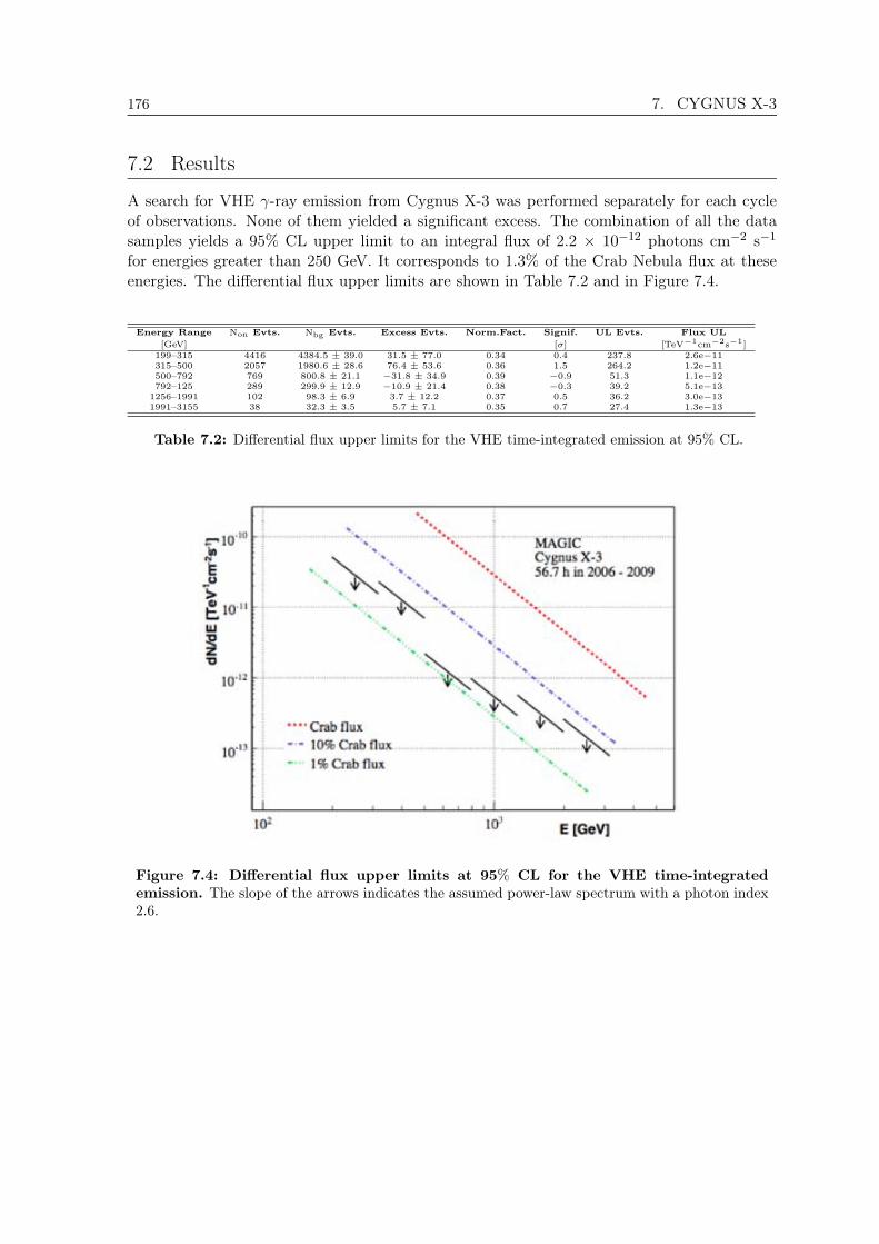
176 7. CYGNUS X-3
7.2 Results
A search for VHE γ-ray emission from Cygnus X-3 was performed separately for each cycleof observations. None of them yielded a significant excess. The combination of all the datasamples yields a 95% CL upper limit to an integral flux of 2.2 × 10⁻¹² photons cm−2 s−1
for energies greater than 250 GeV. It corresponds to 1.3% of the Crab Nebula flux at theseenergies. The differential flux upper limits are shown in Table 7.2 and in Figure 7.4.
Energy Range Non Evts. Nbg Evts. Excess Evts. Norm.Fact. Signif. UL Evts. Flux UL[GeV] [σ] [TeV − 1cm− 2s− 1]
199–315 4416 4384.5 ± 39.0 31.5 ± 77.0 0.34 0.4 237.8 2.6e− 11315–500 2057 1980.6 ± 28.6 76.4 ± 53.6 0.36 1.5 264.2 1.2e− 11500–792 769 800.8 ± 21.1 − 31.8 ± 34.9 0.39 − 0.9 51.3 1.1e− 12792–125 289 299.9 ± 12.9 − 10.9 ± 21.4 0.38 − 0.3 39.2 5.1e− 13
1256–1991 102 98.3 ± 6.9 3.7 ± 12.2 0.37 0.5 36.2 3.0e− 131991–3155 38 32.3 ± 3.5 5.7 ± 7.1 0.35 0.7 27.4 1.3e− 13
Table 7.2: Differential flux upper limits for the VHE time-integrated emission at 95% CL.
Figure 7.4: Differential flux upper limits at 95% CL for the VHE time-integratedemission. The slope of the arrows indicates the assumed power-law spectrum with a photon index2.6.
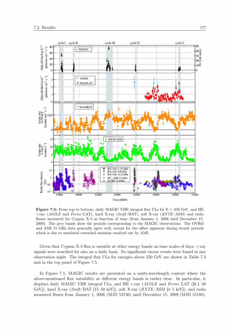
7.2. Results 177
Figure 7.5: From top to bottom: daily MAGIC VHE integral flux ULs for E > 250 GeV, and HEγ-ray (AGILE and Fermi/LAT), hard X-ray (Swift/BAT), soft X-ray (RXTE/ASM) and radiofluxes measured for Cygnus X-3 as function of time (from January 1, 2006 until December 15,2009). The grey bands show the periods corresponding to the MAGIC observations. The OVROand AMI 15 GHz data generally agree well, except for the offset apparent during steady periodswhich is due to unrelated extended emission resolved out by AMI.
Given that Cygnus X-3 flux is variable at other energy bands on time scales of days, γ-raysignals were searched for also on a daily basis. No significant excess events were found in anyobservation night. The integral flux ULs for energies above 250 GeV are shown in Table 7.3and in the top panel of Figure 7.5.
In Figure 7.5, MAGIC results are presented on a multi-wavelength context where theabove-mentioned flux variability at different energy bands is rather clear. In particular, itdisplays daily MAGIC VHE integral ULs, and HE γ-ray (AGILE and Fermi/LAT ([0.1–30GeV]), hard X-ray (Swift/BAT [15–50 keV]), soft X-ray (RXTE/ASM [3–5 keV]), and radiomeasured fluxes from January 1, 2006 (MJD 53736) until December 15, 2009 (MJD 55180).
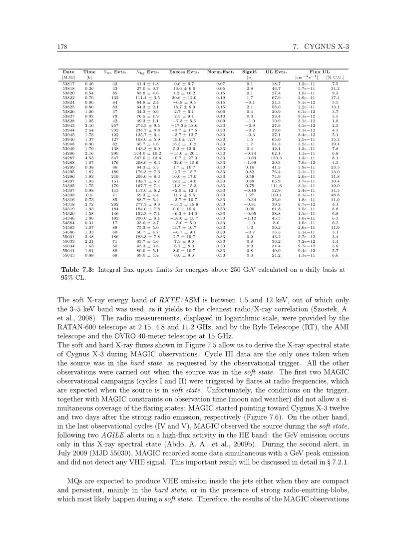
178 7. CYGNUS X-3
Date Time Non Evts. Nbg Evts. Excess Evts. Norm.Fact. Signif. UL Evts. Flux UL[MJD] [h] [] [cm2s1] [% C.U.]
53817 0.46 42 41.4 1.8 0.6 6.7 0.07 0.1 18.7 1.2e11 7.553818 0.26 43 27.0 0.7 16.0 6.6 0.05 2.8 46.7 5.7e11 34.253820 0.54 85 83.8 4.6 1.2 10.2 0.15 0.1 27.4 1.5e11 9.353822 0.70 132 111.4 3.5 20.6 12.0 0.19 1.7 67.9 2.9e11 17.453824 0.80 84 84.8 2.4 0.8 9.5 0.15 0.1 24.3 9.1e12 5.553825 0.80 83 64.3 2.1 18.7 9.3 0.15 2.1 58.0 2.2e11 13.153826 1.00 37 34.3 0.6 2.7 6.1 0.06 0.4 20.9 6.1e12 3.753827 0.92 79 76.5 1.9 2.5 9.1 0.13 0.3 28.4 9.1e12 5.553828 1.05 42 49.3 1.1 7.3 6.6 0.09 1.0 10.9 3.1e12 1.853943 3.10 257 274.3 9.5 17.3 18.6 0.33 0.9 27.9 4.1e12 2.553944 2.54 232 235.7 8.8 3.7 17.6 0.33 0.2 38.6 7.1e12 4.353945 1.73 122 125.7 6.4 3.7 12.7 0.33 0.3 27.1 8.4e12 5.153946 1.37 127 108.0 5.9 19.0 12.7 0.33 1.5 65.0 2.5e11 15.353948 0.90 82 65.7 4.6 16.3 10.2 0.33 1.7 54.3 3.2e11 19.453949 1.79 138 143.3 6.9 5.3 13.6 0.33 0.4 42.1 1.3e11 7.854286 2.16 299 314.0 10.2 15.0 20.1 0.33 0.74 62.1 1.1e11 6.854287 4.53 547 547.0 13.4 0.7 27.0 0.33 0.03 150.3 1.3e11 8.154288 1.07 176 208.0 8.3 32.0 15.6 0.33 1.99 20.3 7.0e12 4.354289 0.38 86 84.3 5.3 1.7 10.7 0.33 0.16 41.3 3.9e11 23.554295 1.82 189 176.3 7.6 12.7 15.7 0.33 0.82 76.4 2.1e11 13.054296 1.93 219 209.0 8.3 10.0 17.0 0.33 0.59 74.9 2.0e11 11.854297 1.93 151 138.7 6.7 12.3 14.0 0.33 0.89 65.9 1.7e11 10.454305 1.75 179 167.7 7.4 11.3 15.3 0.33 0.75 111.6 3.1e11 19.054307 0.98 115 117.0 6.2 2.0 12.4 0.33 0.16 52.9 2.4e11 14.554308 0.5 71 59.3 4.4 11.7 9.5 0.33 1.27 100.1 8.1e11 48.854316 0.73 85 88.7 5.4 3.7 10.7 0.33 0.34 33.0 1.8e11 11.054318 2.72 262 277.3 9.6 15.3 18.8 0.33 0.81 39.2 6.7e12 4.154319 1.93 184 184.0 7.8 0.0 15.6 0.33 0.00 61.8 1.5e11 8.854320 1.58 146 152.3 7.1 6.3 14.0 0.33 0.95 38.8 1.1e11 6.854346 1.86 182 200.0 8.1 18.0 15.7 0.33 1.12 45.3 1.0e11 6.354584 0.31 17 23.0 2.7 5.0 5.0 0.33 1.0 8.0 1.0e11 6.254585 1.07 89 75.3 5.0 13.7 10.7 0.33 1.3 50.2 2.0e11 11.954586 1.33 60 66.7 4.7 6.7 9.1 0.33 0.7 15.5 5.1e11 3.155031 3.48 186 183.3 7.8 2.7 15.7 0.33 0.2 43.2 5.7e12 3.455033 2.21 71 63.7 4.6 7.3 9.6 0.33 0.8 36.2 7.2e12 4.455034 1.63 50 43.3 3.8 6.7 8.0 0.33 0.9 31.4 9.7e12 5.855044 1.81 88 80.0 5.1 8.0 10.7 0.33 0.8 40.0 9.4e12 5.755045 0.88 69 69.0 4.8 0.0 9.6 0.33 0.0 24.2 1.1e11 6.6
Table 7.3: Integral flux upper limits for energies above 250 GeV calculated on a daily basis at95% CL.
The soft X-ray energy band of RXTE/ASM is between 1.5 and 12 keV, out of which onlythe 3–5 keV band was used, as it yields to the cleanest radio/X-ray correlation (Szostek, A.et al., 2008). The radio measurements, displayed in logarithmic scale, were provided by theRATAN-600 telescope at 2.15, 4.8 and 11.2 GHz, and by the Ryle Telescope (RT), the AMItelescope and the OVRO 40-meter telescope at 15 GHz.The soft and hard X-ray fluxes shown in Figure 7.5 allow us to derive the X-ray spectral stateof Cygnus X-3 during MAGIC observations. Cycle III data are the only ones taken whenthe source was in the hard state, as requested by the observational trigger. All the otherobservations were carried out when the source was in the soft state. The first two MAGICobservational campaigns (cycles I and II) were triggered by flares at radio frequencies, whichare expected when the source is in soft state. Unfortunately, the conditions on the trigger,together with MAGIC constraints on observation time (moon and weather) did not allow a si-multaneous coverage of the flaring states: MAGIC started pointing toward Cygnus X-3 twelveand two days after the strong radio emission, respectively (Figure 7.6). On the other hand,in the last observational cycles (IV and V), MAGIC observed the source during the soft state,following two AGILE alerts on a high-flux activity in the HE band: the GeV emission occursonly in this X-ray spectral state (Abdo, A. A., et al., 2009b). During the second alert, inJuly 2009 (MJD 55030), MAGIC recorded some data simultaneous with a GeV peak emissionand did not detect any VHE signal. This important result will be discussed in detail in § 7.2.1.
MQs are expected to produce VHE emission inside the jets either when they are compactand persistent, mainly in the hard state, or in the presence of strong radio-emitting-blobs,which most likely happen during a soft state. Therefore, the results of the MAGIC observations
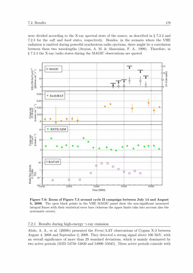
7.2. Results 179
were divided according to the X-ray spectral state of the source, as described in § 7.2.2 and7.2.3 for the soft and hard states, respectively. Besides, in the scenario where the VHEradiation is emitted during powerful synchrotron radio ejections, there might be a correlationbetween these two wavelengths (Atoyan, A. M. & Aharonian, F. A., 1999). Therefore, in§ 7.2.4 the X-ray/radio states during the MAGIC observations are quoted.
Figure 7.6: Zoom of Figure 7.5 around cycle II campaign between July 14 and August5, 2006. The open black points in the VHE MAGIC panel show the non-significant measuredintegral fluxes with their statistical error bars (whereas the upper limits take into account also thesystematic errors).
7.2.1 Results during high-energy -ray emission
Abdo, A. A., et al. (2009b) presented the Fermi/LAT observations of Cygnus X-3 betweenAugust 4, 2008 and September 2, 2009. They detected a strong signal above 100 MeV, withan overall significance of more than 29 standard deviations, which is mainly dominated bytwo active periods (MJD 54750–54820 and 54990–55045). These active periods coincide with

180 7. CYGNUS X-3
Figure 7.7: Zoom of Figure 7.5 around cycle V campaign between May 29 and August17, 2009. The open black points in the VHE MAGIC panel show the non-significant measuredintegral fluxes with their statistical error bars (whereas the ULs take into account also the systematicerrors).
the X-ray soft state of the source, indicating that Cygnus X-3 emits HE γ-rays during thisspectral state, with an average flux of 1.2 × 10⁻⁶ photons cm−2 s−1 and a photon index2.70 ± 0.05stat ± 0.20sys (under the assumption of a power-law spectrum). They also esti-mated that the peak flux can be as high as 2 × 10⁻⁶ photons cm−2 s−1 without providingany photon index.The five AGILE detections between 100 MeV and 3 GeV (Tavani, M., et al., 2009; Bulgar-
elli, A., et al., in preparation) coincide with the strongest HE outbursts, which can be seenoverlapping them with the Fermi/LAT light curve. The AGILE integral flux averaged overthe first four detections is estimated of 1.9 × 10⁻⁶ photons cm−2 s−1 with a correspondingphoton index of 1.8 ± 0.2.
In cycle V, MAGIC pointed at Cygnus X-3 during the second period of HE enhanced ac-

7.2. Results 181
tivity detected by Fermi/LAT, as shown in the Figure 7.7. In particular, MAGIC carried outobservations simultaneous with a GeV emission peak on July 21 and 22, 2009 (MJD 55033–55034), and it did not detect any VHE emission. The corresponding MAGIC integral fluxULs above 250 GeV are lower than 6% of the Crab Nebula flux.
Figure 7.8 shows the SED of Cygnus X-3 between 100 MeV and 5 TeV including MAGIC95% CL ULs at VHE, and the power-law spectrum in the HE range reported by both AGILEand Fermi/LAT. The spectra take into account the error on the photon index and the oneon the integral flux, which is 30% and 40% for Fermi/LAT and AGILE, respectively. TheSED for the average soft state was obtained considering the average Fermi/LAT flux andMAGIC results of the soft state data set. On the other hand, to obtain the SED during aHE emission peak, the MAGIC measurements simultaneous with the GeV emission peak andboth Fermi/LAT and AGILE spectral power-law fits were used. The Fermi/LAT photonindex during the peak was assumed to be the same as the one for the soft state averageflux. Being the latter dominated by the brightest phases of the γ-ray outburst, it can beconsidered representative also of the flaring activity. Both MAGIC ULs are consistent withthe extrapolation of the Fermi/LAT spectra up to VHE, but not with the extrapolation ofthe harder AGILE spectrum, which would suggest a cut-off between some tens and 250 GeV.
Figure 7.8: Cygnus X-3 spectral energy distribution in the HE and VHE bands. Thelines indicate the power-law spectra derived from Fermi/LAT and AGILE integral fluxes andphoton indeces, where the corresponding errors were taken into account and are shown in shadowedareas. The arrows display the 95% CLMAGIC differential flux upper limits and their slope indicatesthe assumed power-law spectrum with a photon index 2.6. The black indicators show the SEDduring the period of enhanced GeV activity coinciding with the soft state, whereas, the red andblue ones during the HE peak emission (MJD 55031–55034).
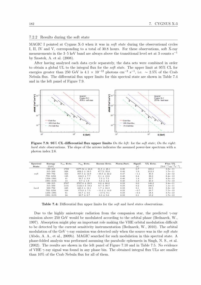
182 7. CYGNUS X-3
7.2.2 Results during the soft state
MAGIC I pointed at Cygnus X-3 when it was in soft state during the observational cyclesI, II, IV and V, corresponding to a total of 30.8 hours. For these observations, soft X-raymeasurements in the 3–5 keV band are always above the transitional level set at 3 counts s−1
by Szostek, A. et al. (2008).After having analyzed each data cycle separately, the data sets were combined in order
to obtain a global UL to the integral flux for the soft state. The upper limit at 95% CL forenergies greater than 250 GeV is 4.1 × 10⁻¹² photons cm−2 s−1, i.e. ∼ 2.5% of the CrabNebula flux. The differential flux upper limits for this spectral state are shown in Table 7.4and in the left panel of Figure 7.9.
Figure 7.9: 95% CL differential flux upper limits On the left: for the soft state; On the right:hard state observations. The slope of the arrows indicates the assumed power-law spectrum with aphoton index 2.6.
Spectral Energy Non Evts. Nbg Evts. Excess Evts. Norm.Fact. Signif. UL Evts. Flux ULState [GeV] [σ] [TeV − 1cm− 2s− 1]
199–315 1709 1677.54 ± 24.6 31.5 ± 48.1 0.36 0.7 169.2 3.5e− 11315–500 926 858.3 ± 18.5 67.7± 35.6 0.40 1.9 212.3 1.7e− 11
soft 500–792 324 357.5 ± 12.9 − 33.5 ± 22.2 0.47 − 1.1 30.3 1.2e− 12792–1256 125 124.9 ± 7.7 0.1 ± 13.6 0.48 0.4 38.0 8.4e− 131256–1991 41 33.7 ± 3.9 7.3 ± 7.5 0.46 1.4 32.7 4.5e− 131991–3155 14 8.7 ± 1.8 5.3 ± 4.2 0.40 1.3 20.3 1.7e− 13199–315 2707 2707.0 ± 29.9 0.0 ± 60.0 0.33 0.0 146.2 3.4e− 11315–500 1131 1122.3 ± 19.2 8.7 ± 38.7 0.33 0.2 108.5 1.1e− 11
hard 500–792 445 443.3 ± 12.1 1.7 ± 24.3 0.33 0.1 62.5 3.3e− 12792–1256 164 175.0 ± 7.5 − 11.0 ± 14.9 0.33 − 0.7 24.7 7.7e− 131256–1991 61 64.7 ± 4.6 − 3.7± 9.1 0.33 − 0.4 18.4 3.7e− 131991–3155 24 23.7 ± 2.7 0.3 ± 5.6 0.33 0.1 15.2 1.7e− 13
Table 7.4: Differential flux upper limits for the soft and hard states observations.
Due to the highly anisotropic radiation from the companion star, the predicted γ-rayemission above 250 GeV would be modulated according to the orbital phase (Bednarek, W.,1997). Absorption might play an important role making the VHE orbital modulation difficultto be detected by the current sensitivity instrumentation (Bednarek, W., 2010). The orbitalmodulation of the GeV γ-ray emission was detected only when the source was in the soft state(Abdo, A. A., et al., 2009b). MAGIC searched for such modulation in this spectral state. Aphase-folded analysis was performed assuming the parabolic ephemeris in Singh, N. S., et al.(2002). The results are shown in the left panel of Figure 7.10 and in Table 7.5. No evidenceof VHE γ-ray signal was found in any phase bin. The obtained integral flux ULs are smallerthan 10% of the Crab Nebula flux for all of them.

7.2. Results 183
7.2.3 Results during the hard state
The 25.9 hours of MAGIC cycle III data sample were obtained when Cygnus X-3 was inhard state. Swift/BAT count rates during this cycle are rather high, greater than 0.05counts cm−2 s−1, whereas the soft X-ray fluxes in the 3–5 keV band are below 2 counts s−1.
For this spectral state, the integral flux upper limit for energies greater than 250 GeV is1.1% of the Crab Nebula flux (1.8 × 10⁻¹² photons cm−2 s−1). The differential flux ULs arequoted in Table 7.4 and plotted in the right panel of Figure 7.9.
The performed phase-folded analysis for this spectral state did not yield any significantdetection. The computed upper limits to the integral flux are, on average, at the level of 5%of the Crab Nebula flux (see right panel in Figure 7.10 and Table 7.5).
Figure 7.10: Phase-wise integral flux upper limits for E > 250 GeV On the left: for thesoft state; On the right: for the hard state. The effective observation time (in hours) and the signalsignificance for each phase bin are written on top of each arrow. The grey arrow indicates theintegral flux UL on the VHE time-integrated emission.
X-ray Phase Time Non Nbg Excess Norm. Signif. UL Flux ULstate [h] Evts. Evts. Evts. Fact. [σ] Evts. [cm− 2s− 1] [% C.U.]
0.0–0.1 1.34 64 68.0 ± 4.7 − 4.3 ± 9.3 0.33 − 0.5 18.2 6.7e− 12 4.00.1–0.2 1.40 75 67.3 ± 4.7 8.3 ± 9.8 0.33 0.9 38.6 1.5e− 11 8.90.2–0.3 1.63 108 107.0 ± 5.9 1.3 ± 12.0 0.33 0.1 32.1 9.2e− 12 5.60.3–0.4 2.05 162 162.0 ± 7.3 0.3 ± 14.6 0.33 0.0 37.1 7.7e− 12 4.70.4–0.5 2.11 113 106.0 ± 5.9 7.3 ± 12.1 0.33 0.6 42.3 9.6e− 12 5.8
soft 0.5–0.6 3.40 231 222.3 ± 8.5 8.7 ± 17.5 0.33 0.5 57.1 8.5e− 12 5.10.6–0.7 4.93 370 361.3± 10.2 9.1 ± 21.8 0.29 0.4 68.3 5.7e− 12 3.40.7–0.8 7.13 649 600.7 ± 17.1 49.4 ± 30.7 0.49 1.6 163.9 8.1e− 12 4.90.8–0.9 4.69 331 310.0 ± 8.4 21.2 ± 20.0 0.23 1.1 86.4 8.3e− 12 5.10.9–1.0 2.05 109 116.0 ± 6.2 − 7.0 ± 12.1 0.33 − 0.6 22.1 5.5e− 12 3.30–1 30.78 2216 2120.3 ± 29.5 96.3 ± 55.5 0.41 1.8 311.6 4.1e− 12 2.5
0.0–0.1 2.89 511 509.7 ± 12.9 1.3 ± 26.1 0.33 0.0 102.5 8.6e− 12 5.20.1–0.2 3.23 477 501.3 ± 12.8 − 24.3 ± 25.3 0.33 − 0.9 52.5 4.6e− 12 2.70.2–0.3 2.53 281 308.0 ± 10.1 − 27.0 ± 19.5 0.33 − 1.4 33.6 4.1e− 12 2.50.3–0.4 2.53 266 230.0 ± 8.7 36.0 ± 18.5 0.33 2.0 218.1 2.1e− 11 12.40.4–0.5 2.79 248 261.0 ± 9.2 − 13.0 ± 18.3 0.33 − 0.7 43.2 5.4e− 12 3.3
hard 0.5–0.6 2.27 210 205.3 ± 8.2 4.7 ± 16.6 0.33 0.3 73.1 1.1e− 11 6.80.6–0.7 2.99 242 243.0 ± 8.9 − 1.0 ± 17.9 0.33 − 0.1 65.8 7.1e− 12 4.30.7–0.8 2.63 234 222.7 ± 8.6 11.3 ± 17.5 0.33 0.6 116.3 1.1e− 11 6.80.8–0.9 1.95 199 189.7 ± 7.9 9.3 ± 16.2 0.33 0.6 118.5 1.3e− 11 7.80.9–1.0 2.13 235 261.3 ± 9.3 − 26.3 ± 17.9 0.33 − 1.4 33.8 3.9e− 12 2.40–1 25.9 2903 2932.0 ± 31.1 − 29.0 ± 62.2 0.33 − 0.5 191.0 1.8e− 12 1.1
Table 7.5: Integral flux upper limits for energies above 250 GeV for the phase-folded analyses ofthe observations in the soft and hard states.
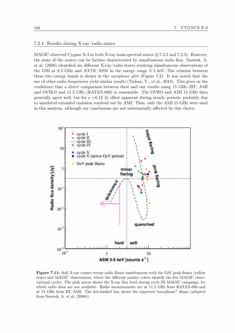
184 7. CYGNUS X-3
7.2.4 Results during X-ray/radio states
MAGIC observed Cygnus X-3 in both X-ray main spectral states (§ 7.2.2 and 7.2.3). However,the state of the source can be further characterized by simultaneous radio flux. Szostek, A.et al. (2008) identified six different X-ray/radio states studying simultaneous observations ofthe GBI at 8.3 GHz and RXTE/ASM in the energy range 3–5 keV. The relation betweenthese two energy bands is shown in the saxophone plot (Figure 7.2). It was noted that theuse of other radio frequencies yield similar results (Tudose, V., et al., 2010). This gives us theconfidence that a direct comparison between their and our results using 15 GHz (RT, AMIand OVRO) and 11.2 GHz (RATAN-600) is reasonable. The OVRO and AMI 15 GHz datagenerally agree well, but for a ∼0.12 Jy offset apparent during steady periods, probably dueto unrelated extended emission resolved out by AMI. Thus, only the AMI 15 GHz were usedin this analysis, although our conclusions are not substantially affected by this choice.
Figure 7.11: Soft X-ray counts versus radio fluxes simultaneous with the GeV peak fluxes (yellowstars) and MAGIC observations, where the different marker colors identify the five MAGIC obser-vational cycles. The pink arrow shows the X-ray flux level during cycle III MAGIC campaign, forwhich radio data are not available. Radio measurements are at 11.2 GHz from RATAN-600 andat 15 GHz from RT/AMI. The dot-dashed line shows the expected “saxophone" shape (adaptedfrom Szostek, A. et al. (2008)).

7.2. Results 185
Figure 7.11 shows the soft X-ray [3–5 keV] RXTE/ASM count rates versus radio fluxdensities corresponding either to the nights of MAGIC observations for the five observationalcycles, or to the AGILE flux peaks (only the last four AGILE detections were considered,since no simultaneous radio data were available for the first one). Unfortunately, no radio datasimultaneous with cycle III and cycle IV MAGIC observations were available. Nevertheless,in case of cycle III data, this does not prevent us from pointing out that Cygnus X-3 wasin a quiescent state, just by using the soft X-ray measurements. For cycle IV data, quasisimultaneous radio observations (one day before MAGIC observations) were used. This latterchoice does not affect our qualitative result, since the source had already entered a post-flaringstate. As shown in Figure 7.12, in April 2008, AGILE detected Cygnus X-3 (MJD 54572–54573) one day before a major radio flare (Trushkin, S. A. et al., 2008) lasting a few days,but MAGIC started pointing at the MQ ten days after the peak radio emission.
Figure 7.12: Zoom of Figure 7.5 around cycle IV campaign between April 9 and May2, 2008. The open black points in the VHE MAGIC panel show the non-significant measuredintegral fluxes with their statistical error bars (whereas the upper limits take into account also thesystematic errors).
186 7. CYGNUS X-3
All the HE flux peaks were detected in the right branch of the saxophone, before, after orduring a flaring state. Although Abdo, A. A., et al. (2009b) quoted a time lag between theradio and the -ray peaks of 57 days, the correlation between the two energy bands is notyet clear. On the other hand, MAGIC observed Cygnus X-3 in its soft state some days afterthe radio flare occurred, although for the first nights of cycle V observations, the radio fluxdensities are rather high and oscillating between two small flares (Figure 7.7).
7.3 Discussion
MAGIC observations of Cygnus X-3 cover all X-ray spectral states of the source in whichVHE emission is thought to be likely produced, either from a persistent jet in the hard state,or during powerful ejections in the soft state. However, no significant excess events were foundin any of the inspected samples.
VHE -rays have been predicted from microquasar jets (Atoyan, A. M. & Aharonian,F. A., 1999; Romero, G. E. et al., 2003; Bosch-Ramon, V. et al., 2006). A robust predictionof modeling is that photon-photon absorption cannot be neglected if the -rays are producedclose to a massive star (Bednarek, W., 1997; Orellana, M. et al., 2007). In particular forCygnus X-3, the presence of a Wolf-Rayet companion, with temperature T ≈ 105 K and radiusR ≈ 1011 cm, leads to an optical depth θ 1 for VHE -rays for an emitter located at severalorbital radii from the star (Bednarek, W., 2010). Even under very efficient electromagneticcascading, i.e. a radiation to magnetic energy density ratio 8ν u=B2 − 1, the expected VHEfluxes are below the sensitivity of the present instruments (Bednarek, W., 2010). Therefore,in order to detect VHE photons the emitter should be located far from the binary system.
Fermi/LAT detected Cygnus X-3 when it was in the soft state, and found orbital modu-lation for the radiation above 100 MeV with a photon index 2.7 for the periods of enhanced-activity (Abdo, A. A., et al., 2009b). For the epochs outside these high-activity periods, theGeV flux decreases significantly (Figure 7.5 in Abdo, A. A., et al. (2009b)) and no modula-tion is found. The GeV orbital light curve of Cygnus X-3 in the HE active periods can beexplained in the context of anisotropic IC scattering with the stellar photons (Abdo, A. A., etal., 2009b; Bosch-Ramon & Khangulyan, 2009; Dubus et al., 2010), which is also energeticallymore efficient than hadronic mechanisms such as pp interactions or photomeson production.Since very bright X-ray emission is produced in the inner accretion disk or at the base ofthe jets in Cygnus X-3, the GeV radiation would be absorbed unless it is originated beyond≡ 1010 cm above the compact object. This implies that the GeV radiation is produced inthe jet of Cygnus X-3 rather than in the inner accretion disk/corona region. On the otherhand, the GeV emitter cannot be too high in the jet, since otherwise there would not bestrong orbital modulation (Abdo, A. A., et al., 2009b). Therefore, the observed GeV and thepredicted detectable VHE emission cannot be explained by one particular population becausethe former should be produced in/close to the system and the latter farther from it. Thelocation of a hypothetical VHE emitter could coincide with the innermost region of the radioemitting jet, which, to avoid synchrotron self-absorption, should start relatively far from thebinary system. This is consistent with the fact that MAGIC did not detect Cygnus X-3 dur-ing the high-activity GeV period, even though the flux upper limits are close to a power-lawextrapolation of the Fermi/LAT spectrum to energies greater than 100 GeV and well belowan extrapolation of the AGILE spectrum.
During the periods of GeV high-activity of the source, as by the synchrotron self Comptonscenario (Atoyan, A. M. & Aharonian, F. A., 1999), a detectable TeV signal could arise dur-ing the first hours of a radio outburst. Unfortunately, MAGIC has never observed the source
7.3. Discussion 187
during this phase of the flare, but always some days before or after the maximum radio flux.This radiation would not be strongly modulated, due to its origin far from the system. Thetwo times more sensitive MAGIC stereoscopic arrangement may indeed detect Cygnus X-3 ifit observes the source for longer time at the very maximum of a GeV flare, which might beeven earlier than the onset of the radio outburst (Abdo, A. A., et al., 2009b).
In the hard state, the VHE emission is expected to be produced inside the compact andpersistent jets, whose total luminosity is estimated to be at least 1037 erg s1 (Martı, J. et al.,2005). The MAGIC VHE -ray upper limit set at 1.1 1012 erg cm2 s1 is equivalent toa VHE luminosity of ' 7 1033 erg s1 at 7 kpc. Thus, the maximum conversion efficiencyof the jet power into VHE -rays is 0.07% which is similar to that of Cygnus X-1 for the ULon the VHE steady emission, but one order of magnitude greater than that of GRS 1915+105(Albert, J., et al., 2007d; Acero, F., et al., 2009b). These ULs are in good agreement with thetheoretical expectations which generally predict a VHE steady luminosity of ' 1032 erg s1.Persistent galactic jets do not seem to be good candidate sources to be detected at VHEsby the current sensitivity instrumentation. Only ten times more sensitive future instruments,such as CTA, may have a chance to detect such VHE emission. This would provide a newhandle on the emission mechanisms of compact jets.

8Scorpius X-1
Scorpius X-1 is a Z-type LMXB which has been classified as microquasar because ofthe detected discrete radio emission far away from the core source. Its X-ray emissionshows a power-law component of non-thermal origin which is more significant whenthe source is in the X-ray horizontal branch state. These observational results suggestthat this NS LMXB might be a VHE -ray emitter especially in the horizontalbranch state. The MAGIC telescope pointed at Scorpius X-1 in May 2010 in amulti-wavelength campaign which included RXTE /PCA observations. The X-raydata were needed to define the X-ray spectral state during the MAGIC observations.MAGIC found no significant VHE signal from Scorpius X-1 and the resulting upperlimits to the integral flux above 300 GeV are at the level of 3% of the Crab Nebula flux.
The results of this chapter are published in Aleksic, J., et al. (2011a) where the authorcontributed in the analysis and interpretation of the MAGIC data.
Scorpius X-1 is a Z-type LMXB (§ 6.5) that contains a low-magnetic-field NS and a M-typestar with a mass of 0.4 M (Steeghs & Casares, 2002). The matter accretion occurs throughRoche lobe outflow. Located at a distance of 2.8 0.3 kpc (Bradshaw, C. F. et al., 1999), ithas a circular orbit (radius = 1:5 1011 cm) with an inclination of 44 6 (Fomalont, E. B.et al., 2001). The orbital period is of 0.787 days (Gottlieb, E. W. et al., 1975).
Scorpius X-1 is the brightest and persistent X-ray source in the sky with an X-ray lumi-nosity LX = 4 12 1037 erg s1 (Hasinger, G. & van der Klis, M., 1989). It displays thetypical X-ray spectral states of the Z-type sources (§ 6.5) whose definition is based on thesource position in double-banana track of the CD (Figure 8.1). Scorpius X-1 covers the wholetrack of the CD in few hours, but spends most of its time in the HB state. The hard X-rayemission (above 30 keV) from Scorpius X-1 is dominated by a power-law component with aphoton index between 2 and 3.4 (Di Salvo, T., et al., 2006; D’Aı, A., et al., 2007). This hardX-ray flux decreases as the source moves toward higher accretion rate (stronger in the HBstate) becoming not significantly detectable in the FB state (inset Figure 8.1). The fact thatno evidence of high-energy cut-off is observed in this power-law component up to 100–200 keV
189
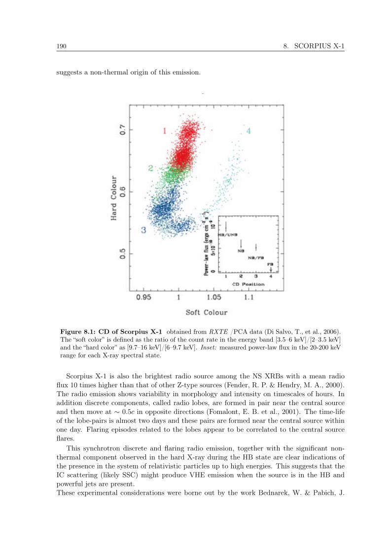
190 8. SCORPIUS X-1
suggests a non-thermal origin of this emission.
Figure 8.1: CD of Scorpius X-1 obtained from RXTE /PCA data (Di Salvo, T., et al., 2006).The “soft color” is defined as the ratio of the count rate in the energy band [3.5–6 keV]/[2–3.5 keV]and the “hard color” as [9.7–16 keV]/[6–9.7 keV]. Inset: measured power-law flux in the 20-200 keVrange for each X-ray spectral state.
Scorpius X-1 is also the brightest radio source among the NS XRBs with a mean radioflux 10 times higher than that of other Z-type sources (Fender, R. P. & Hendry, M. A., 2000).The radio emission shows variability in morphology and intensity on timescales of hours. Inaddition discrete components, called radio lobes, are formed in pair near the central sourceand then move at ∼ 0.5c in opposite directions (Fomalont, E. B. et al., 2001). The time-lifeof the lobe-pairs is almost two days and these pairs are formed near the central source withinone day. Flaring episodes related to the lobes appear to be correlated to the central sourceflares.
This synchrotron discrete and flaring radio emission, together with the significant non-thermal component observed in the hard X-ray during the HB state are clear indications ofthe presence in the system of relativistic particles up to high energies. This suggests that theIC scattering (likely SSC) might produce VHE emission when the source is in the HB andpowerful jets are present.These experimental considerations were borne out by the work Bednarek, W. & Pabich, J.
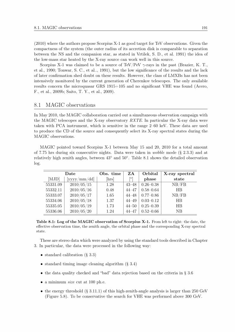
8.1. MAGIC observations 191
(2010) where the authors propose Scorpius X-1 as good target for TeV observations. Given thecompactness of the system (the outer radius of its accretion disk is comparable to separationbetween the NS and the companion star, as stated in Vrtilek, S. D., et al. 1991) the idea ofthe low-mass star heated by the X-ray source can work well in this source.
Scorpius X-1 was claimed to be a source of TeV/PeV -rays in the past (Brazier, K. T.,et al., 1990; Tonwar, S. C., et al.., 1991), but the low significance of the results and the lackof later confirmation shed doubt on these results. However, the class of LMXBs has not beenintensively monitored by the current generation of Cherenkov telescopes. The only availableresults concern the microquasar GRS 1915+105 and no significant VHE was found (Acero,F., et al., 2009b; Saito, T. Y., et al., 2009).
8.1 MAGIC observations
In May 2010, the MAGIC collaboration carried out a simultaneous observation campaign withthe MAGIC telescopes and the X-ray observatory RXTE. In particular the X-ray data weretaken with PCA instrument, which is sensitive in the range 2–60 keV. These data are usedto produce the CD of the source and consequently select its X-ray spectral states during theMAGIC observations.
MAGIC pointed toward Scorpius X-1 between May 15 and 20, 2010 for a total amountof 7.75 hrs during six consecutive nights. Data were taken in wobble mode (§ 2.3.3) and atrelatively high zenith angles, between 43 and 50. Table 8.1 shows the detailed observationlog.
Date Obs. time ZA Orbital X-ray spectral[MJD] [yyyy/mm/dd] [hrs] [] phase state
55331.09 2010/05/15 1.28 43–48 0.26–0.38 NB/FB55332.11 2010/05/16 0.48 44–47 0.58–0.64 HB55333.07 2010/05/17 1.65 44–48 0.77–0.86 NB/FB55334.06 2010/05/18 1.37 44–49 0.03–0.12 HB55335.05 2010/05/19 1.73 44–50 0.25–0.39 HB55336.06 2010/05/20 1.24 44–47 0.52–0.66 NB
Table 8.1: Log of the MAGIC observation of Scorpius X-1. From left to right: the date, theeffective observation time, the zenith angle, the orbital phase and the corresponding X-ray spectralstate.
These are stereo data which were analyzed by using the standard tools described in Chapter3. In particular, the data were processed in the following way:
• standard calibration (§ 3.3)
• standard timing image cleaning algorithm (§ 3.4)
• the data quality checked and “bad” data rejection based on the criteria in § 3.6
• a minimum size cut at 100 ph.e.
• the energy threshold (§ 3.11.1) of this high-zenith-angle analysis is larger than 250 GeV(Figure 5.8). To be conservative the search for VHE was performed above 300 GeV.

192 8. SCORPIUS X-1
• the gamma selection cuts were optimized on a data sample of Crab Nebula recorded inthe same zenith angle range using the criteria described in § 3.9
• the computation of the ULs to the integral flux at 95% CL was performed by usingRolke’s method including a 30% systematic uncertainty (§ 3.15). The source spectrumwas assumed to be a power-law with a photon index = 3. This photon index wastaken to account for the possibility that the spectrum of Scorpius X-1 is steeper thanthe Crab Nebula one, as it would be for some plausible scenarios (§ 8.4). However, a30% change in the photon index yields a variation of less than 1% in the flux ULs atthese energies.
The sensitivity (§ 3.9.1) of this high zenith angle analysis is 1.1% of the Crab Nebula flux forenergies above 300 GeV in 50 hrs.
8.2 X-ray results
The CD of Scorpius X-1 during the MAGIC observations was obtained by using the definitionsof the hard and soft colors in D’Aı, A., et al. (2007). In this way the selection of the different X-ray spectral states can be supported by these historical results. In particular, the “soft color”is defined as the ratio between the count rate in the energy bands [4.08–6.18 keV]/[1.94–4.05 keV], whereas the “hard color” as [8.32–16.26 keV]/[6.18–8.32 keV]. The obtained resultis shown in Figure 8.2 (Aleksic, J., et al., 2011a). During the six nights of observations thesource covered the full double-banana-shaped track. The top part of the upper-banana wasselected as corresponding to the HB (gray box in Figure 8.2). The different symbols and colorsof the figure indicate the different observation days. This day-folded analysis shows that thesource did not move extensively along the CD track during the single observation nights.
8.3 MAGIC results
The results of the X-ray data show that during three of the six observation nights the sourcewas in the HB state (MJD 55332, 55334, 55335), as indicated also in Table 8.1. Therefore,the source was in the HB during almost half of time (3.58 hrs) that MAGIC pointed at it.
The total Li & Ma significance (Li & Ma, formula 7) of the -ray signal coming fromScorpius X-1 for the complete data set of MAGIC observations is 0.52η. The resulting fluxUL (§ 3.15) is 2:4 1012 cm2 s1 above 300 GeV. The search for a VHE signal for thoseperiods when the source was in HB state, where such an emission should be expected. Nosignificant signal was found either in this sub-sample. The integral flux UL is 3:4 1012
cm2 s1 above 300 GeV. No -ray emission was found either in the complementary sub-sample when the source was in the NB/FB states. A summary of the X-ray-state-selectedresults is presented in Table 8.2. The differential flux ULs computed for the HB and the wholedata sample are shown in Figure 8.3, as a constraint for future theoretical modeling of VHEemission from Scorpius X-1. Differential flux UL can be used to derive also energy flux ULs.Taking = 3, the energy flux ULs are 3.6, 5.5, and 5.4 1012 erg cm2 s1 above 300 GeVfor the whole data set, the HB and the NB/FB respectively.
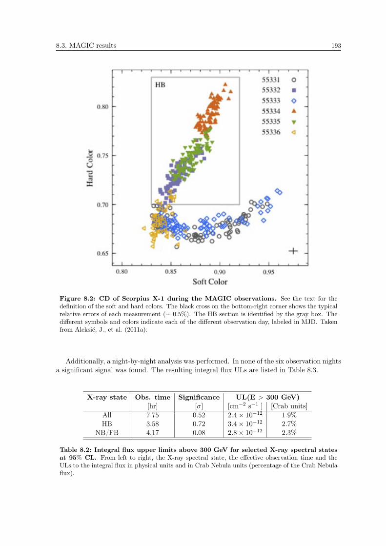
8.3. MAGIC results 193
Figure 8.2: CD of Scorpius X-1 during the MAGIC observations. See the text for thedefinition of the soft and hard colors. The black cross on the bottom-right corner shows the typicalrelative errors of each measurement (∼ 0.5%). The HB section is identified by the gray box. Thedifferent symbols and colors indicate each of the different observation day, labeled in MJD. Takenfrom Aleksic, J., et al. (2011a).
Additionally, a night-by-night analysis was performed. In none of the six observation nightsa significant signal was found. The resulting integral flux ULs are listed in Table 8.3.
X-ray state Obs. time Significance UL(E > 300 GeV)[hr] [σ] [cm−2 s−1 ] [Crab units]
All 7.75 0.52 2.4 × 10⁻¹² 1.9%HB 3.58 0.72 3.4 × 10⁻¹² 2.7%
NB/FB 4.17 0.08 2.8 × 10⁻¹² 2.3%
Table 8.2: Integral flux upper limits above 300 GeV for selected X-ray spectral statesat 95% CL. From left to right, the X-ray spectral state, the effective observation time and theULs to the integral flux in physical units and in Crab Nebula units (percentage of the Crab Nebulaflux).

194 8. SCORPIUS X-1
Figure 8.3: Differential flux upper limits above 300 GeV for all the observations (black-dashed) and for the HB state (red). The slope of the bars indicates the power-lawphoton index assumed in the UL calculation. The Crab Nebula spectrum (Albert, J.,et al., 2008d) is shown for comparison, as well as its 10% (dashed) and 1% (dotted)fractions.
Date Obs. Time UL(E > 300 GeV)[MJD] [hrs] [cm−2 s−1 ] [Crab units]
55331.09 1.28 7.9 × 10⁻¹² 6.4%55332.11 0.48 5.2 × 10⁻¹² 4.2%55333.07 1.65 3.5 × 10⁻¹² 2.8%55334.06 1.37 5.1 × 10⁻¹² 4.2%55335.05 1.73 5.3 × 10⁻¹² 4.3%55336.06 1.24 2.0 × 10⁻¹² 1.6%
Table 8.3: Integral flux upper limits above 300 GeV for day-by-day analysis at 95%CL. From left to right: the date, the corresponding effective observation time, and the ULs to theintegral flux in physical and Crab units.
8.4 Discussion
To put in the context the MAGIC results and understand the potentialities of Scorpius X-1 toproduce VHE emission, in this section possible emission scenarios are presented. The energyavailable from the relativistic jet and the processes that could give rise to the VHE emissioneither as its base or further away from the compact object. Finally, Scorpius X-1 will becompared with other MQs and the detected γ-ray binaries.
The properties of a possible γ-ray emitter will be mostly constrained by the jet power,which dictates the maximum energy budget available, and the emitter size and location. Thejet luminosity Lj can be fixed by assuming that the power-law hard X-rays come from the
8.4. Discussion 195
jet, and assuming an X-ray luminosity to total jet power ratio of 0.01–0.1. Given that thepower-law luminosity is LntX ≡ 1035 1036 erg s1, a value of Lj ≡ 1039 erg s1 seemsreasonable, and is also high enough to account for the radio emission of the source (Foma-lont, E. B. et al., 2001). The VHE luminosity ULs in the HB show that Scorpius X-1 hasa maximum VHE luminosity to jet power ratio of LV HE=Lj 103. This value is slightlybelow the ratio inferred for the Cygnus X-1 flare (Albert, J., et al., 2007d), and similar tothe UL of Cygnus X-3 (Aleksic, J., et al., 2010a), but an order of magnitude above the ULof GRS 1915+105 (Acero, F., et al., 2009b). However, given the transient nature of thesesources, the orbital coverage and the total length of the observational campaign play a role intheir eventual detection. Since the campaign presented here is relatively short and does notprovide a complete orbital coverage, it does not rule out the possibility of VHE flares fromScorpius X-1.
Assuming that the jets of Scorpius X-1 can indeed accelerate particles efficiently, there areseveral possible reasons to explain MAGIC non-detection:
• If particles were accelerated in the jet base and the power-law hard X-rayswere emitted there, it might be difficult to accelerate particles beyond 100 MeV atthis location because of strong radiative cooling. The emitted spectrum is likely to bevery soft because of the dominant synchrotron cooling. In addition, the radiation from10 GeV to 1 TeV would likely to be absorbed through pair creation by the intense ra-diation field from the accretion disk. At this location even lower energy GeV photonswould be absorbed. However, if the magnetic field is low enough and the electromagneticcascading efficient, absorption at the jet base due to the disk photon field might not beso relevant (Aharonian, F. A. & Vardanian, V. V., 1985). Another source of absorptionis the stellar photon field, enhanced through accretion X-ray irradiance of the stellarsurface, and could be optically thick to VHE photons in certain orbital phases. Note,however, that MAGIC did not detect the source even for those orbital phases in whichthis source of -ray absorption should be negligible: on MJD 55334 the source was inthe HB and the orbital phase range of the observation was σ= 0.03–0.12, for whichthe expected -ray opacity is θ ≡ 0.1 (Bednarek, W. & Pabich, J., 2010). Concludingthis scenario, the combined effect of a steep -ray spectrum and pair creation absorp-tion would diminish the chances of a VHE detection, particularly for high zenith angleobservations and correspondingly high energy threshold as in this study.
• If the radiation at VHE were produced further from the compact object, atdistances larger than 108 cm, it could be eventually detected. The SSC channel,efficient for intermediate values of the magnetic field, would yield a less steep spectrumand may occur in regions where the emitter and the environment are optically thinto VHE photons. IC with the X-ray enhanced stellar photon field could also yieldsignificant and less-steep VHE radiation and would be most efficient for optical depthsof order to units. According to the calculations of Bednarek, W. & Pabich, J. (2010),this would take place around orbital phases close to 0.3 and 0.7, but we did not detectedsuch an emission on MJD 55335 at orbital phases 0.25–0.39. At these high altitudes inthe jet, GeV photons could easily escape the system and produce detectable high-energy -ray emission. The eventual detection of Scorpius X-1 by Fermi or AGILE , plus anon-detection with low-enough ULs at VHE, would likely favor the scenario where -rayradiation is emitted from a location far away from the NS but with a spectrum too steepfor a VHE detection. Synchrotron cooling dominance could explain the steep spectrum

196 8. SCORPIUS X-1
and would mean that the power-law hard X-rays have a synchrotron origin.
In a leptonic scenario, such as the SSC and external IC, it can be assumed that X-ray emis-sion has a synchrotron origin and VHE -rays have an IC origin. The VHE to non-thermalX-ray luminosity ratio is then a sensitive indicator of the importance of synchrotron coolingand ultimately of the magnetic field of the emitter. Considering only the hard X-ray power-law as non-thermal X-ray emission, this ratio has a maximum value LV HE=LntX ≡< 0:02 forthe HB state. This ratio is much higher for the detected gamma-ray binary. For the case ofLS I 61+303 , for example, the VHE to X-ray ratio is between 0.5 and 1 during the X-ray andVHE peak at phases σ = 0:60:7 (Anderhub, H., et al., 2009). However, as mentioned abovefor the comparison with other MQs, the short total length of the observational campaign pre-sented here prevents us from making absolute comparisons because of the possible transientnature of the source. On the other hand, if there is no such flaring behavior, the differencein the VHE to X-ray luminosity ratios indicates that the underlying physics is significantlydifferent than for LS I 61 + 303 or LS 5039.
In conclusion, these results place the first ULs on the VHE -ray emission from Scor-pius X-1 in all of the X-ray spectral states of the source. If Scorpius X-1 is indeed capableof producing TeV emission, either a longer observational campaign, with better coverage (toprobe phase-dependent effects such as absorption, cascading..), or an instrument with a sig-nificant increase in sensitivity, such as the future CTA, might be required to detect it. TheseULs also indicate that the underlying VHE emission physics may be inherently different inthe case of Scorpius X-1 and the detected gamma-ray binaries.
9Conclusions and outlook
The work described in this thesis embraces multiple facets of the VHE -ray astrophysics,from the technical aspects of instrument commissioning to the details of data taking andanalysis, and the interpretation of physics results.
The author was strongly involved in the commissioning of the second MAGIC telescopeas responsible of the central control, and contributed significantly to develop the software forstereo data analysis. With the stereoscopic mode, in operation since 2009, the performance ofthe instrument improved significantly both in sensitivity (0.8% of the Crab Nebula flux in 50hours of observation above 250 GeV) and angular resolution (0.06 above 250 GeV). This up-grade constituted a milestone for the MAGIC experiment, and the successful implementationof the central control for the two telescopes was of crucial importance.
From the point of view of the data analysis, this thesis reports on the observations of threegalactic sources, the Crab Pulsar Wind Nebula, and two microquasar candidates, Cygnus X-3and Scorpius X-1. The results of the Crab Nebula observations are based on a total of 50hours of data collected between October 2009 and March 2011 and take full advantage of theimproved sensitivity and the lower energy threshold of the stereoscopic mode. The obtaineddifferential energy spectrum is of unprecedented precision, spans eight orders of magnitude influx and three orders of magnitude in energy, between 50 GeV and 45 TeV. It represents anextremely accurate measurement, with six spectral points per energy decades and statisticalerrors as low as 5% below 100 GeV. The spectral data are well described by a variable power-law f0 (E/1 TeV)+bLog(E=1TeV ) with = 2:400:01stat0:1sys, b = 0:150:01stat0:05systand f0 = 3:27 0:03stat 0:48syst. With this model, the analysis provides the most preciseestimation of the peak of the IC component of the Crab Nebula spectrum set at 59 6 GeV.The differential energy spectrum has been interpreted in the context of both the constantB-field and the MHD model, but none of two models provides a satisfactory match to thedata within the statistical errors. Finally, the Crab Nebula flux above 300 GeV calculatedon a daily basis across the full data set is found to be constant within the 13% systematicuncertainty. In particular, no enhancement of the flux is observed in correspondence with theSeptember 2010 flare reported by AGILE and Fermi at energies above 100 MeV. This resultdoes not confirm the claim of a flaring evidence above few TeV by ARGO-YBJ.
In the case of the microquasar candidates to VHE emission, the observations of Scorpius X-
197
198 9. CONCLUSIONS AND OUTLOOK
1 are entirely carried out in stereo mode, while the analysis of Cygnus X-3 employs onlymono data. Results from the two sources provide the most constraining ULs to date to theirintegral flux above 250/300 GeV, at the level of 1–3% of the Crab Nebula flux (95% CL).In particular, for Cygnus X-3, the combination of all data samples yields a 95% CL upperlimit to the integral flux of 2.2 1012 photons cm2 s1 for energies greater than 250 GeV,corresponding to 1.3% of the Crab Nebula flux at these energies. A -ray signal from thissource is also searched for on a daily basis and no significant excess events are found in anyobservation night. Data are then grouped according to the source X-ray spectral state whichis related to the corresponding VHE emission model. When the source is an X-ray soft state(flaring branch), it is characterized by strong relativistic ejections which might be the sourceof particle acceleration. On the other hand, the X-ray hard state (normal branch) showspersistent relativistic jets which are good candidates for the production of VHE radiation.The upper limits resulting from this study are the first of their kind. For the X-ray soft state,an UL of 4.1 1012 photons cm2 s1 is set at 95% CL for energies greater than 250 GeV,corresponding to ≡ 2.5% of the Crab Nebula flux. The upper limit for the hard state atthe same energy range is 1.8 1012 photons cm2 s1, i.e. 1.1% of the Crab Nebula flux.Finally, in July 2009, MAGIC recorded for the first time some data simultaneously with a GeVflare reported by both AGILE and Fermi. No VHE signal was detected, with correspondingintegral flux ULs above 250 GeV lower than 6% of the Crab Nebula flux. In the case ofScorpius X-1, the upper limit on the total flux UL (§ 3.15) is 2:4 1012 cm2 s1 above 300GeV. Results are also extracted according to their state, with no emission detected in eitherthe HB state or the complementary NB/FB states. In particular for the HB state, where aVHE signal is expected, the upper limit on the integral flux is 3:4 1012 cm2 s1 above300 GeV. These results place the first ULs on the VHE -ray emission from Scorpius X-1 inall of the X-ray spectral states of the source.
The study of the Crab Nebula , as well as the hunt for microquasar TeV emission, willcertainly profit form a longer observation campaign with the stereo MAGIC system, especiallyin the case of Cygnus X-3 whose available data are taken with only one telescope. Furthermore,the advent of CTA will represent a new major step in understanding the mechanisms behindthe VHE emission of PWNe and, hopefully, establish microquasars as a new population ofVHE emitters.
AAcceleration mechanisms and photon-matter
interactions
This appendix describes the principal mechanisms of CR acceleration and the mainprocesses for the production and absorption of -rays.
A.1 Acceleration mechanisms
Acceleration of charged particles can be a direct effect of very large magnetic and electricfields, but it can also occur via statistical diffuse shock acceleration mechanisms. The lattertheory was formulated by Enrico Fermi who gave the name to the two main mechanisms. Theinterested reader can find a copious literature on this topic (Malkov, M. A. & O’C Drury, L.,2001; Kirk, J. G. & Duffy, P., 1999; Aharonian, F. A., 2004b).
A.1.1 Fermi acceleration
The diffuse shock acceleration, also known as Fermi acceleration, can differentiate within firstorder and second order depending on the characteristics of the moving plasma.
• The second order Fermi mechanism describes the acceleration of a charged particleinteracting with a moving, magnetized cloud of material. The mean energy gain of theparticle per interaction is hE=Ei / 2, with = vcloud=c. Thus, for typical valuesof = 105, the energy gain is 1010E1 per crossing, with E1 as the energy of thecharged particle before being accelerated. The acceleration efficiency is therefore quitelow. The resulting energy spectrum is strongly dependent on magnetic cloud propertiesand is quite unpredictable, which is in contrast with the observed featureless power-lawspectrum of the CRs.
• The first order Fermi mechanism occurs when the moving material hosts shockwaves. A shock identifies a blob of material moving with a velocity which is higher thanthe speed of the sound in the medium. Every time a particle passes through a shockwave, it is accelerated and its acceleration is proportional to : hE=Ei / / V=cwhere V is the relative velocity between the particle and the cloud. The greater the
i

relative difference, the larger the energy gain of the particle per shock; the larger themagnetic field strength, the higher the particle crossing frequency.The first order Fermi acceleration is more efficient than the second order one and it isbelieved to be the most diffuse mechanism of acceleration at the TeV, PeV scales.
A.2 Interaction with photon elds
During their travel, CRs and -rays interact with dense low-energy photon fields, which arepresent in many astrophysical environments.
A.2.1 Inverse Compton radiation
IC scattering happens whenever a HE electron interacts with low-energy photons and thephoton acquires a large amount of the electron momentum and is re-emitted at much higherenergies. This process is one of the main responsible for the acceleration of soft ambientphotons to VHE.
The IC scattering process happens in two distinct regimes, defined by the parameter b =4Ehψ0=(mec
2)2, where E is the electron energy and hψ0 is the energy of the initial photon.
• in the Thompson regime, corresponding to b ∈ 1, the cross-section of the IC scat-tering is constant. In case of power-law distributed electrons with a photon index e,the spectra of the up-scattered photons are described by a hard power-law with photonindex = (e + 1)=2. The efficiency of the IC scattering in the Thompson regime isproportional to the energy density of the target photons.
• in the Klein-Nishina regime (b − 1) the cross-section decreases with energy (/ln b=b). In case the electrons have a power-law distribution, the up-scattered photonspresent steep power-law spectra with photon index = (e + 1). The efficiency of theIC scattering process in the Klein-Nishina regime is proportional to the number densityof target photons. This implies that low-frequencies photons can contribute significantlyto the production of VHE -rays.
A.2.2 Pair production
Pair production is the mechanism which leads to the production of an electron/positron pairthrough the annihilation of a high-energy photon with a low-energy photon.The pair production can be divided into two families of processes:
• Classical pair production. A high-energy -ray interacts with the electric field of anatomic nucleus and produces the pair. The second photon is a virtual photon of theelectric field.
( )! e+ + e (A.1)
• Photon-photon pair production. In this case the soft photons are available in the envi-ronment, as stellar of inter-stellar radiation:
! e+ + e (A.2)
ii
The reaction is allowed provided there is enough energy to create the pair, at least the totalrest-mass-energy of the two particles. The cross-section for this process peaks when:
E 1E 2(1 cos ) ≡ 2(mec2)2 (A.3)
where is the collision angle. Thus, for photons of energy near 100 MeV, the highest cross-section occurs for the head-on collision with X-ray photons of ≡ 5 keV.
The former process prevents high-energy -rays to cross the Earth atmosphere, whereasthe second one is responsible for the absorption of -rays during their travel through ISM andIGM.
A.3 Interaction in matter
While propagating, CRs interact with ambient gas or dust. These interactions produce -rays.
A.3.1 Bremsstrahlung
Bremsstrahlung is a process involving charge particles, mainly electrons, when crossing amedium. They can be accelerated by the electric field produced by nuclei of heavy atoms,hence produce radiation. The energy loss as function of the path length follows the Bethe &Heither formula:
dEdx
rad
= E
X0(A.4)
1X0
/ Z2
Aα cm1 (A.5)
where X0 is the radiation length which corresponds to the path length that gives an energyfraction loss of 1/e. It depends on the material atomic number, Z, and its density, α. There-fore, low density materials have a larger radiation length, hence CRs are more penetrating.
Bremsstrahlung becomes dominant with respect to ionization when the energy of the in-coming particle is larger than a critical energy, E0. The critical energy identifies the energyat which the energy loss by ionization equals the energy loss for Bremsstrahlung. It dependsmainly on the atomic number of the medium:
Ec '1600 ·mec
2
Z(A.6)
Since the energy loss through Bremsstrahlung is proportional to the particle energy, theemitted photons follow the same spectral distribution of the ch-raged particles. All chargedparticles can emit Bremsstrahlung radiation, but electrons by far the most efficient ones. Infact, the total radiate powers goes as m4.
A.3.2 0 decay
Relativistic protons and nuclei interact with ambient gas through inelastic collisions. Theinteractions with larger cross-section are those ones which involve the production of pions,
iii
such as:pp! ppν+νν0 (A.7)
Positive, negative and neutral charged pions are produced with equal probability. The decayof charged pions is accompanied by the production of neutrinos ψe; ψ:
ν+ ! τ+ψ; τ+ ! e+ψ ψe (A.8)ν ! τ ψ; τ ! eψe ψe (A.9)
These neutrinos have a spectral shape which resembles the one for accelerated particles.
Neutral pions annihilate into two energetic photons (ν0 ! ). The energy of the emittedphotons by a ν0 at rest is half of the ν0 mass: E = m0c
2=2 ≡ 67:5 MeV. If the ν0 is movingwith a velocity v = c, the energy of the photon in the laboratory frame is:
E = ·m(1 + cos ) ≡ ·m (A.10)
where is the angle between the photon direction with respect to the pion one. The spec-trum of such emission is well-fitted by a power-law with a photon index of sim 2.5.
-ray produced by pions are the so-called -rays of hadronic origin. They are distinguish-able from those of electromagnetic origin because of their spectral features, lack of correlationwith other wavelengths (like X-rays in the SSC scenario), and presence of molecular clouds.In addition, their emission coexists with a neutrino flux coming from the charged pion decays.
A.3.3 Electron-positron annihilation
High-energy electrons interact with positrons and annihilate into two energetic photons:
e+e ! (A.11)
Seed positrons are found as secondary products of spallation of CRs with matter. Conversely,positrons can interact with cold thermal electrons in ambient gas or plasma. The -rayspectrum is steeper than the positron spectrum: = p 1, at least if the electrons are nottoo much relativistic.
A.4 Interaction with magnetic elds
A.4.1 Synchrotron radiation
Charged particles in magnetic fields emit radiation. In the classical approximation, due tothe effect of the Lorentz force, the charged particle spirals around the magnetic field lineswith a frequency wL = qB=2m, called Larmor frequency, where m and q are the mass and thecharge of the particle, and B the magnetic field component perpendicular to the plane of theparticles’ trajectory. The radiation has the shape of a dipole radiation with frequency wL.
In case of relativistic charged particles, the emitted radiation is beamed in a cone centeredon the particle and with an angular spread inversely proportional to velocity. In addition, itis a broad-band emission.The spectrum of synchrotron radiation of mono-energetic electrons is a continuum that peaks
iv

at:
E w 1:5 · 105 ·B
G
Ee
TeV
2
(A.12)
where Ee is the energy of the electron population.The lifetime of a relativistic electron with respect to the synchrotron energy losses, i.e.
the synchrotron cooling time is:
θsynch ≈ 1:2 103
B
104G
2
Ee
TeV
1
yr (A.13)
The characteristic frequency of synchrotron radiation is about ψsynch ≡ ψB 2 whereψB = wL sin =2ν is the cyclotron frequency of a electron moving at a pitch angle to themagnetic field. For isotropic pitching angles:
ψsynch ≈ 1:8 1015
B
3 104G
Ee
TeV
2
Hz (A.14)
v

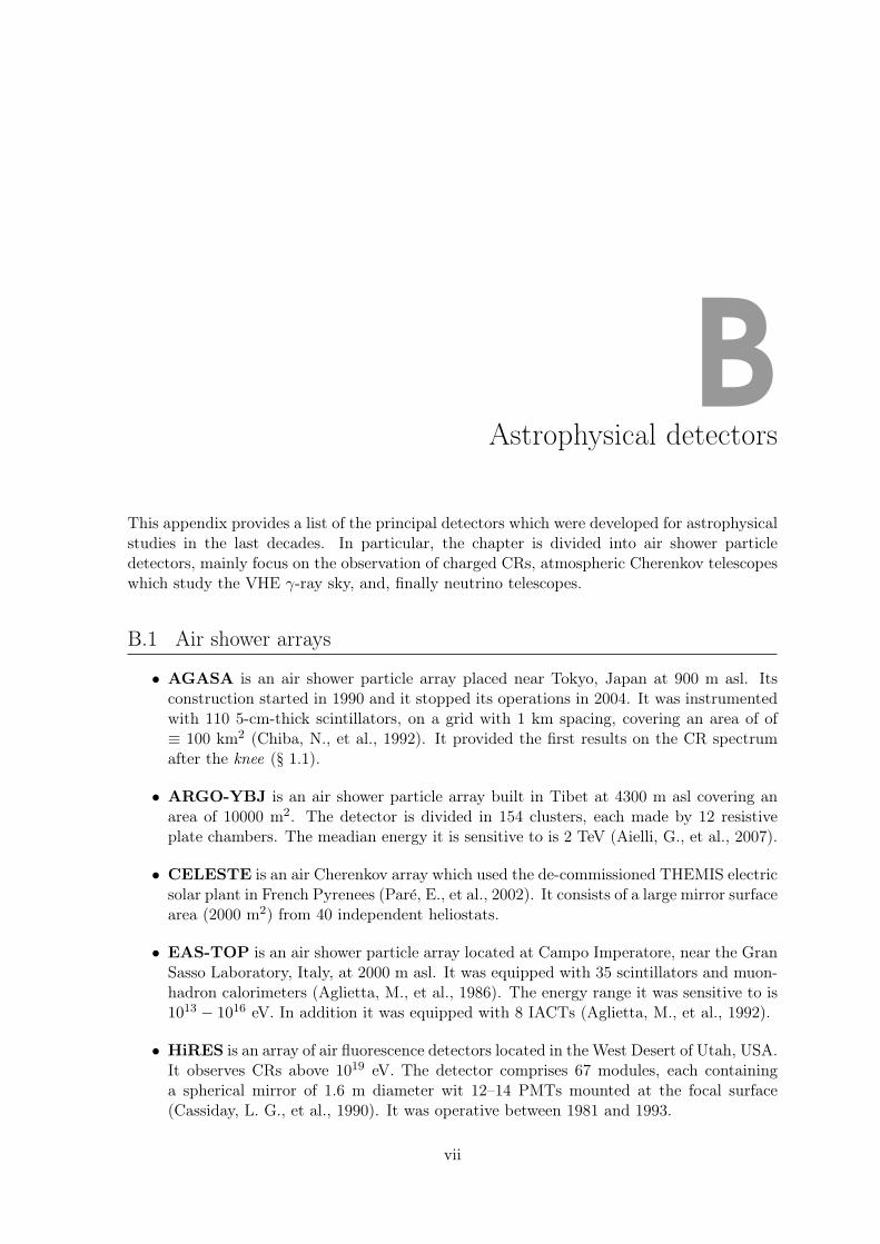
BAstrophysical detectors
This appendix provides a list of the principal detectors which were developed for astrophysicalstudies in the last decades. In particular, the chapter is divided into air shower particledetectors, mainly focus on the observation of charged CRs, atmospheric Cherenkov telescopeswhich study the VHE -ray sky, and, finally neutrino telescopes.
B.1 Air shower arrays
• AGASA is an air shower particle array placed near Tokyo, Japan at 900 m asl. Itsconstruction started in 1990 and it stopped its operations in 2004. It was instrumentedwith 110 5-cm-thick scintillators, on a grid with 1 km spacing, covering an area of of≡ 100 km2 (Chiba, N., et al., 1992). It provided the first results on the CR spectrumafter the knee (§ 1.1).
• ARGO-YBJ is an air shower particle array built in Tibet at 4300 m asl covering anarea of 10000 m2. The detector is divided in 154 clusters, each made by 12 resistiveplate chambers. The meadian energy it is sensitive to is 2 TeV (Aielli, G., et al., 2007).
• CELESTE is an air Cherenkov array which used the de-commissioned THEMIS electricsolar plant in French Pyrenees (Pare, E., et al., 2002). It consists of a large mirror surfacearea (2000 m2) from 40 independent heliostats.
• EAS-TOP is an air shower particle array located at Campo Imperatore, near the GranSasso Laboratory, Italy, at 2000 m asl. It was equipped with 35 scintillators and muon-hadron calorimeters (Aglietta, M., et al., 1986). The energy range it was sensitive to is1013 1016 eV. In addition it was equipped with 8 IACTs (Aglietta, M., et al., 1992).
• HiRES is an array of air fluorescence detectors located in the West Desert of Utah, USA.It observes CRs above 1019 eV. The detector comprises 67 modules, each containinga spherical mirror of 1.6 m diameter wit 12–14 PMTs mounted at the focal surface(Cassiday, L. G., et al., 1990). It was operative between 1981 and 1993.
vii
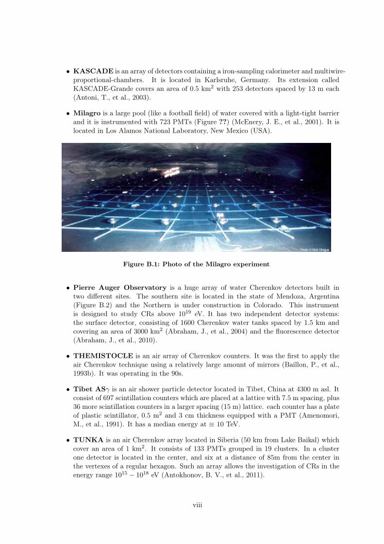
• KASCADE is an array of detectors containing a iron-sampling calorimeter and multiwire-proportional-chambers. It is located in Karlsruhe, Germany. Its extension calledKASCADE-Grande covers an area of 0.5 km2 with 253 detectors spaced by 13 m each(Antoni, T., et al., 2003).
• Milagro is a large pool (like a football field) of water covered with a light-tight barrierand it is instrumented with 723 PMTs (Figure ??) (McEnery, J. E., et al., 2001). It islocated in Los Alamos National Laboratory, New Mexico (USA).
Figure B.1: Photo of the Milagro experiment
• Pierre Auger Observatory is a huge array of water Cherenkov detectors built intwo different sites. The southern site is located in the state of Mendoza, Argentina(Figure B.2) and the Northern is under construction in Colorado. This instrumentis designed to study CRs above 1019 eV. It has two independent detector systems:the surface detector, consisting of 1600 Cherenkov water tanks spaced by 1.5 km andcovering an area of 3000 km2 (Abraham, J., et al., 2004) and the fluorescence detector(Abraham, J., et al., 2010).
• THEMISTOCLE is an air array of Cherenkov counters. It was the first to apply theair Cherenkov technique using a relatively large amount of mirrors (Baillon, P., et al.,1993b). It was operating in the 90s.
• Tibet AS is an air shower particle detector located in Tibet, China at 4300 m asl. Itconsist of 697 scintillation counters which are placed at a lattice with 7.5 m spacing, plus36 more scintillation counters in a larger spacing (15 m) lattice. each counter has a plateof plastic scintillator, 0.5 m2 and 3 cm thickness equipped with a PMT (Amenomori,M., et al., 1991). It has a median energy at ≡ 10 TeV.
• TUNKA is an air Cherenkov array located in Siberia (50 km from Lake Baikal) whichcover an area of 1 km2. It consists of 133 PMTs grouped in 19 clusters. In a clusterone detector is located in the center, and six at a distance of 85m from the center inthe vertexes of a regular hexagon. Such an array allows the investigation of CRs in theenergy range 1015 1018 eV (Antokhonov, B. V., et al., 2011).
viii
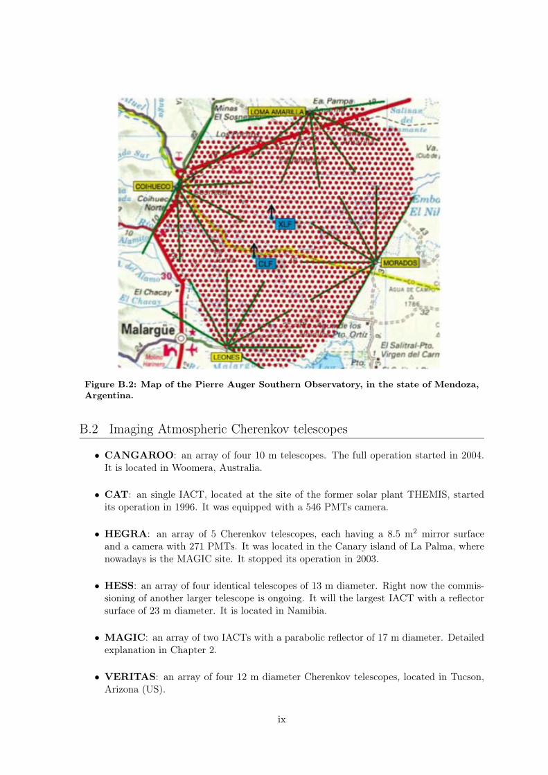
Figure B.2: Map of the Pierre Auger Southern Observatory, in the state of Mendoza,Argentina.
B.2 Imaging Atmospheric Cherenkov telescopes
• CANGAROO: an array of four 10 m telescopes. The full operation started in 2004.It is located in Woomera, Australia.
• CAT: an single IACT, located at the site of the former solar plant THEMIS, startedits operation in 1996. It was equipped with a 546 PMTs camera.
• HEGRA: an array of 5 Cherenkov telescopes, each having a 8.5 m2 mirror surfaceand a camera with 271 PMTs. It was located in the Canary island of La Palma, wherenowadays is the MAGIC site. It stopped its operation in 2003.
• HESS: an array of four identical telescopes of 13 m diameter. Right now the commis-sioning of another larger telescope is ongoing. It will the largest IACT with a reflectorsurface of 23 m diameter. It is located in Namibia.
• MAGIC: an array of two IACTs with a parabolic reflector of 17 m diameter. Detailedexplanation in Chapter 2.
• VERITAS: an array of four 12 m diameter Cherenkov telescopes, located in Tucson,Arizona (US).
ix

x B. ASTROPHYSICAL DETECTORS
B.3 Neutrino telescopes
• Antarctic Muon And Neutrino Detector Array (AMANDA): an array of 677PMTs in 19 strings located under the ice in the South Pole. Its construction started in1996 and ends in 2000. It effective area of 20000 m2 was one order of magnitude belowthe size suggested by the theoretical models. It looks for high-energy neutrino from theNorthern sky.
• Astronomy with a Neutrino Telescope and Abyss environmental RESarch(ANTARES): located in the Mediterranean sea close to Toulouse, France, it consistsof 12 strings, with 75 PMTs each, anchored at the sea bed at 2.5 km. The full detectoris in operation since 2007. It observes the Southern sky.
• IceCube: 1 km3 array of ice Cherenkov detectors built as extension of the AMANDAdetector in the South Pole. Its construction was completed at the beginning of 2011. Itconsists of 4800 PMTs arranged in 80 strings.
• IceTop: 1 km array of ice Cherenkov detectors at the surface.
• NEutrino Mediterranean Observatory (NEMO): located in the Mediterraneansea at 3.3 km depth near the East coast of Sicily. It consists of a mechanical structure,consisting of 20 m long rigid arms connected by each other by ropes. Inside the armsthe PMTs are set. It observes the Southern sky.
• Neutrino Extended Submarine Telescope with Oceanographic Research (NESTOR):located near the West Coast of the Peloponnese at 4 km depth. Its design is based onrigid hexagonal structures with 32 m diameter, each of them carrying 6 pairs of PMTs.These rigid structures are the basic blocks of the “towers” of 300 m height. It observesthe Southern sky.
• Neutrino Telescope-200 (NT-200): the pioneering neutrino detector built in theLake Baikal, Russia in 1993. It consists of ≡ 200 PMTs at 8 strings. It was expandedin 2005, nut now it is dismissed.
Bibliography
Abbasi, R. U., et al. (2008). First observation of the Greisen-Zatsepin-Kuzmin suppression.Physical Review Letters, 100 (10), 101101–101105.
Abbasi, R. U., et al. (2010). Measurement of the anisotropy of cosmic-ray arrival directionswith IceCube. Astrophys. Journal Letters, 718 , L194–198.
Abdo, A. A., et al. (2007). TeV gamma-ray sources from a survey of the galactic plane withMILAGRO. Astrophys. Journal Letters, 664 , L91–94.
Abdo, A. A., et al. (2009a). A population of -ray millisecond pulsars seen with the FermiLarge Area Telescope. Science, 325 , 848–852.
Abdo, A. A., et al. (2009b). Modulated high-energy -ray emission from the microquasarCygnus X-3. Science, 326 , 1512–1516.
Abdo, A. A., et al. (2010a). Fermi Large Area Telescope observations of the Crab Pulsar andNebula. Astrophys. Journal , 708 , 1254–1267.
Abdo, A. A., et al. (2010b). The First Fermi Large Area Telescope catalog of gamma-raypulsars. Boh, 187 , 460–494.
Abdo, A. A., et al. (2011). -ray flares from the Crab Nebula. Science, 331 , 739–742.
Abraham, J., et al. (2004). Properties and performance of the prototype instrument for thePierre Auger Observatory. Nuclear Instruments and Methods in Physics Research A, 523 ,50–95.
Abraham, J., et al. (2008). Observation of the suppression of the flux of cosmic rays above4 1019eV. Physical Review Letters, 101 (6), 061101–061105.
Abraham, J., et al. (2010). The fluorescence detector of the Pierre Auger Observatory. NuclearInstruments and Methods in Physics Research A, 620 , 227–251.
Acciari, V. A., et al. (2009). A connection between star formation activity and cosmic raysin the starburst galaxy M82. Nature, 462 , 770–772.
Acero, F., et al. (2009a). Detection of gamma rays from a starburst galaxy. Science, 326 ,1080–1082.
Acero, F., et al. (2009b). HESS upper limits on very high energy -ray emission from themicroquasar GRS 1915+105. Astronomy & Astrophysics, 508 , 1135–1140.
Aglietta, M., et al. (1986). High-energy cosmic-ray physics with an EAS array on the top ofthe Gran Sasso Laboratory. Nuovo Cimento C Geophysics Space Physics C , 9 , 262–270.
xi

xii BIBLIOGRAPHY
Aglietta, M., et al. (1992). Imaging of atmospheric EAS Cherenkov light at EAS-TOP. NuovoCimento C Geophysics Space Physics C , 15 , 357–363.
Aharonian, F. A. (2004a). Very high energy cosmic gamma radiation. World Scientific Print-ers.
Aharonian, F. A. (2004b). Very high energy cosmic gamma radiation : a crucial window onthe extreme Universe.
Aharonian, F. A., Buckley, J., Kifune, T., & Sinnis, G. (2008). High energy astrophysics withground-based gamma ray detectors. Reports on Progress in Physics, 71 (9), 56pp.
Aharonian, F. A., & Vardanian, V. V. (1985). On the origin of soft gamma-rays fromCygnus X-1. Astrophysics and space science, 115 , 31–37.
Aharonian, F. A., et al. (2000). The energy spectrum of TeV -rays from the Crab Nebula asmeasured by the HEGRA system of Imaging Air Cerenkov Telescopes. Astrophys. Journal ,539 , 317–324.
Aharonian, F. A., et al. (2001). Evidence for TeV gamma ray emission from Cassiopeia A.Astronomy & Astrophysics, 370 , 112–120.
Aharonian, F. A., et al. (2004). The Crab Nebula and pulsar between 500 GeV and 80 TeV:observations with the HEGRA stereoscopic air Cerenkov telescopes. Astrophys. Journal ,614 , 897–913.
Aharonian, F. A., et al. (2005a). Discovery of the binary pulsar PSR B1259-63 in very-high-energy gamma rays around periastron with HESS. Astronomy & Astrophysics, 442 ,1–10.
Aharonian, F. A., et al. (2005b). Discovery of very high energy -rays associated with anX-ray binary. Science, 309 , 746–749.
Aharonian, F. A., et al. (2006a). Discovery of very-high-energy -rays from the GalacticCentre ridge. Nature, 439 , 695–698.
Aharonian, F. A., et al. (2006b). Observations of the Crab Nebula with HESS. Astronomy &Astrophysics, 457 , 899–915.
Aharonian, F. A., et al. (2006c). A detailed spectral and morphological study of the gamma-ray supernova remnant RX J1713.7-3946 with HESS. Astronomy & Astrophysics, 449 ,223–242.
Aharonian, F. A., et al. (2006d). First detection of a VHE gamma-ray spectral maximumfrom a cosmic source: HESS discovery of the Vela X nebula. Astronomy & Astrophysics,448 , L43–47.
Ahlers, M., Ringwald, A., & Tu, H. (2005). Strongly interacting neutrinos as the highestenergy cosmic rays: a quantitative analysis. ArXiv Astrophysics e-prints.
Aielli, G., et al. (2007). The status of the ARGO experiment at YBJ. Nuclear Physics BProceedings Supplements, 166 , 96–102.

BIBLIOGRAPHY xiii
Akerlof, C., et al. (1989). Detection of very high energy gamma-rays from the Crab nebula.Proceedings of the at the Gamma Ray Observatory Science Workshop, (pp. 10–12).
Albert, J., et al. (2006a). Observation of gamma rays from the Galactic Center with theMAGIC Telescope. Astrophys. Journal Letters, 638 , L101–104.
Albert, J., et al. (2006b). Variable very-high-energy -ray emission from the microquasarLS I 61 + 303. Science, 312 , 1771–1773.
Albert, J., et al. (2007a). Discovery of very high energy gamma radiation from IC 443 withthe MAGIC telescope. Astrophys. Journal Letters, 664 , L87–90.
Albert, J., et al. (2007b). Observation of VHE -rays from Cassiopeia A with the MAGICtelescope. Astronomy & Astrophysics, 474 , 937–940.
Albert, J., et al. (2007c). Unfolding of differential energy spectra in the MAGIC experiment.Nuclear Instruments and Methods in Physics Research A, 583 , 494–506.
Albert, J., et al. (2007d). Very high energy -ray radiation from the stellar mass black holebinary Cygnus X-1. Astrophys. Journal Letters, 665 , L51–54.
Albert, J., et al. (2008a). MAGIC observations of the unidentified -ray source TeVJ2032+4130. Astrophys. Journal Letters, 675 , L25–28.
Albert, J., et al. (2008b). FADC signal reconstruction for the MAGIC telescope. NuclearInstruments and Methods in Physics Research A, 594 , 407–419.
Albert, J., et al. (2008c). Implementation of the Random Forest method for the imagingatmospheric Cherenkov telescope MAGIC. Nuclear Instruments and Methods in PhysicsResearch A, 588 , 424–432.
Albert, J., et al. (2008d). VHE -ray observation of the Crab Nebula and its pulsar with theMAGIC Telescope. Astrophys. Journal , 674 , 1037–1055.
Albert, J., et al. (2008e). Very-high-energy -rays from a distant quasar: how transparent isthe universe? Science, 320 , 1752–.
Aleksic, J. (2009). Characterization of the MAGIC II data acquisition read-out system. Master Thesis at Institut de Fisica d'Altes Energies. Available athttp://wwwmagic.mppmu.mpg.de/pubblications/theses/index.html .
Aleksic, J., et al. (2010a). MAGIC constraints on -ray emission from Cygnus X-3. Astrophys.Journal , 721 , 843–855.
Aleksic, J., et al. (2010b). Search for an extended VHE -ray emission from Mrk 421 andMrk 501 with the MAGIC Telescope. Astronomy & Astrophysics, 524 , A77(9pp).
Aleksic, J., et al. (2011a). A search for very high energy -ray emission from Scorpius X-1with the MAGIC Telescopes. Astrophys. Journal Letters, 735 , L5–11.
Aleksic J., et al. (2011b). Performance of the MAGIC stereo system obtained with the CrabNebula data. submitted to Asptroparticle Physics.
Aliu, E., et al. (2008). Observation of pulsed -rays above 25 GeV from the Crab pulsar withMAGIC. Science, 322 , 1221–1224.
xiv BIBLIOGRAPHY
Aliu, E., et al. (2009). Improving the performance of the single-dish Cherenkov telescopeMAGIC through the use of signal timing. Astroparticle Physics, 30 , 293–305.
Amenomori, M., et al. (1991). Status and performance of the AS array of the Tibet AS exper-iment. In J. Matthews (Ed.) High Energy Gamma Ray Astronomy , vol. 220 of AmericanInstitute of Physics Conference Series, (pp. 257–264).
Anderhub, H., et al. (2009). Correlated X-ray and very high energy emission in the -raybinary LS I 61 + 303. Astrophys. Journal Letters, 706 , L27–32.
Antokhonov, B. V., et al. (2011). The new Tunka-133 EAS Cherenkov array: status of 2009.Nuclear Instruments and Methods in Physics Research A, 628 , 124–127.
Antoni, T., et al. (2003). The cosmic-ray experiment KASCADE. Nuclear Instruments andMethods in Physics Research A, 513 , 490–510.
Antoni, T., et al. (2005). KASCADE measurements of energy spectra for elemental groupsof cosmic rays: Results and open problems. Astroparticle Physics, 24 , 1–25.
Anykeyev, V. B., Spiridonov, A. A., & Zhigunov, V. P. (1991). Comparative investigation ofunfolding methods. Nuclear Instruments and Methods in Physics Research A, 303 , 350–369.
Araudo, A. T., Bosch-Ramon, V., & Romero, G. E. (2009). High-energy emission from jet-clump interactions in microquasars. Astronomy & Astrophysics, 503 , 673–681.
Arons, J. (1979). Some problems of pulsar physics. Space Science Review , 24 , 437–510.
Arons, J. (1983). Pair creation above pulsar polar caps - Geometrical structure and energeticsof slot gaps. Astrophys. Journal , 266 , 215–241.
Arons, J., & Scharlemann, E. T. (1979). Pair formation above pulsar polar caps - Structureof the low altitude acceleration zone. Astrophys. Journal , 231 , 854–879.
Aschenbach, B., & Brinkmann, W. (1975). A model of the X-ray structure of the Crab Nebula.Astronomy & Astrophysics, 41 , 147–151.
Atoyan, A. M. (1999). Radio spectrum of the Crab Nebula as an evidence for fast initial spinof its pulsar. Astronomy & Astrophysics, 346 , L49–52.
Atoyan, A. M., & Aharonian, F. A. (1996). On the mechanisms of gamma radiation in theCrab Nebula. Monthly Notices of the Royal Astronomical Society , 278 , 525–541.
Atoyan, A. M., & Aharonian, F. A. (1999). Modelling of the non-thermal flares in the Galacticmicroquasar GRS 1915+105. Monthly Notices of the Royal Astronomical Society , 302 , 253–276.
Atwood, W. B., et al. (2009). The Large Area Telescope on the Fermi gamma-ray spacetelescope mission. Astrophys. Journal , 697 , 1071–1102.
Baade, W., & Zwicky, F. (1934). Cosmic rays from super-novae. Proceedings of the NationalAcademy of Science, 20 , 259–263.
Baillon, P., et al. (1993a). Energy spectrum of the Crab Nebula in the multi-TeV region.International Cosmic Ray Conference, 1 , 271–273.

BIBLIOGRAPHY xv
Baillon, P., et al. (1993b). Status report on THEMISTOCLE experiment. In R. C. Lamb (Ed.)Towards a Major Atmospheric Cherenkov Detector II for TeV Astro/Particle Physics, (pp.121–125).
Barrau, A., et al. (1997). Performances of the CAT imaging telescope and some preliminaryresults on Mkn 180 and the Crab. ArXiv Astrophysics e-prints.
Bauleo, P. M., & Rodrıguez Martino, J. (2009). The dawn of the particle astronomy era inultra-high-energy cosmic rays. Nature, 458 , 847–851.
Becker, W., & Truemper, J. (1997). The X-ray luminosity of rotation-powered neutron stars.Astronomy & Astrophysics, 326 , 682–691.
Becklin, E. E., et al. (1973). Infrared and X-ray variability of Cygnus X-3. Nature, 245 ,302–304.
Bednarek, W. (1997). Cascade initiated by VHE -rays in the radiation field of a close massivecompanion. Astronomy & Astrophysics, 322 , 523–532.
Bednarek, W. (2010). On the possibility of sub-TeV-ray emission from Cygnus X-3. MonthlyNotices of the Royal Astronomical Society , 406 , 689–700.
Bednarek, W., & Bartosik, M. (2003). Gamma-rays from the pulsar wind nebulae. Astronomy& Astrophysics, 405 , 689–702.
Bednarek, W., & Pabich, J. (2010). Optical depths for gamma-rays in the radiation fieldof a star heated by an external X-ray source in LMXBs. Application to Hercules X-1 andScorpius X-1. Astronomy & Astrophysics, 514 , A61–71.
Belloni, T., Klein-Wolt, M., Mendez, M., van der Klis, M., & van Paradijs, J. (2000). A model-independent analysis of the variability of GRS 1915+105. Astronomy & Astrophysics, 355 ,271–290.
Berezinsky, V., Kachelrie, M., & Vilenkin, A. (1997). Ultrahigh energy cosmic rays withoutGreisen-Zatsepin-Kuzmin cutoff. Physical Review Letters, 79 , 4302–4305.
Bernlohr, K. (2000). Impact of atmospheric parameters on the atmospheric Cherenkov tech-nique. Astroparticle Physics, 12 , 255–268.
Bertero, M. (1989). Linear inverse and ill-posed problems. Advances in eectronics and electronphysics, (pp. 1–120).
Bhat, C. L., Sapru, M. L., & Razdan, H. (1986). Estimate from Gulmarg of PeV photon fluxfrom Cygnus X-3 and its relevance. Astrophys. Journal , 306 , 587–598.
Bietenholz, M. F., Hester, J. J., Frail, D. A., & Bartel, N. (2004). The Crab Nebula’s wispsin radio and optical. Astrophys. Journal , 615 , 794–804.
Biland, A., et al. (2008). The active mirror control of the MAGIC telescopes. Proceedings ofthe 30th International Cosmic Ray Conference, 3 , 1353–1356.
Bildsten, L., et al. (1997). Thermonuclear burning on the accreting X-ray pulsar GRO J1744-28. Astrophys. Journal , 113 , 367–408.
xvi BIBLIOGRAPHY
Bitossi, M. (2009). Ultra-fast sampling and readout for the MAGIC II telescope data ac-quisition system. PhD Thesis at the Universita degli Studi di Pisa, Italy. Available athttp://wwwmagic.mppmu.mpg.de/pubblications/theses/index.html .
Blumer, J., Engel, R., & Horandel, J. R. (2009). Cosmic rays from the knee to the highestenergies. Progress in Particle and Nuclear Physics, 63 , 293–338.
Bock, R. K., et al. (2004). Methods for multidimensional event classification: a case studyusing images from a Cherenkov gamma-ray telescope. Nuclear Instruments and Methods inPhysics Research A, 516 , 511–528.
Bogovalov, S. V., & Aharonian, F. A. (2000). Very-high-energy gamma radiation associatedwith the unshocked wind of the Crab pulsar. Monthly Notices of the Royal AstronomicalSociety , 313 , 504–514.
Bordas, P., Bosch-Ramon, V., Paredes, J. M., & Perucho, M. (2009). Non-thermal emissionfrom microquasar/ISM interaction. Astronomy & Astrophysics, 497 , 325–334.
Borione, A., et al. (1997). A search for ultra-high-energy -ray emission from the Crab Nebulaand Pulsar. Astrophys. Journal , 481 , 313–326.
Borla Tridon, D., et al. (2009). Performance of the camera of the MAGIC II telescope.Proceedings of the 31st International Cosmic Ray Conference.
Bosch-Ramon, V., & Khangulyan, D. (2009). Understanding the very-high emission frommicroquasars. International Journal of Modern Physics D , 18 , 347–387.
Bosch-Ramon, V., Aharonian, F. A., & Paredes, J. M. (2005). Electromagnetic radiationinitiated by hadronic jets from microquasars in the ISM. Astronomy & Astrophysics, 432 ,609–618.
Bosch-Ramon, V., & Khangulyan, D. (2009). Understanding the very-high emission frommicroquasars. International Journal of Modern Physics D , 18 , 347–387.
Bosch-Ramon, V., Romero, G. E., & Paredes, J. M. (2006). A broadband leptonic model for -ray emitting microquasars. Astronomy & Astrophysics, 447 , 263–276.
Bradshaw, C. F., Fomalont, E. B., & Geldzahler, B. J. (1999). High-resolution parallaxmeasurements of Scorpius X-1. Astrophys. Journal Letters, 512 , L121–124.
Braes, L. L. E., & Miley, G. K. (1972). Radio detection of Cygnus X-3. Nature, 237 , 506.
Brazier, K. T., et al. (1990). Scorpius X-1: a source of 300 GeV -rays. Nuclear Physics BProceedings Supplements, 14 , 191–195.
Bretz, T., Dorner, D., Wagner, R. M., & Sawallisch, P. (2009). The drive system of the majoratmospheric -ray imaging Cherenkov telescope. Astroparticle Physics, 31 , 92–101.
Bridle, A. H., & Perley, R. A. (1984). Extragalactic radio jets. Annual Review of Astronomyand Astrophysics, 22 , 319–358.
Brinkmann, W., Aschenbach, B., & Langmeier, A. (1985). X-ray morphology of the Crabnebula. Nature, 313 , 662–664.

BIBLIOGRAPHY xvii
Britzger, D., et al. (2009). Studies of the influence of moonlight on observations with theMAGIC telescope. Proceedings of the of 29th International Cosmic Ray Conference.
Bucciantini, N. (2008). Theory of pulsar wind nebulae. Proceedings of the of the "40 Yearsof Pulsars: Millisecond Pulsars, Magnetars and More" conference, 983 , 186–194.
Bucciantini, N., Amato, E., Bandiera, R., Blondin, J. M., & Del Zanna, L. (2004). MagneticRayleigh-Taylor instability for pulsar wind nebulae in expanding supernova remnants. As-tronomy & Astrophysics, 423 , 253–265.
Bucciantini, N., Thompson, T. A., Arons, J., Quataert, E., & Del Zanna, L. (2006). Rela-tivistic magnetohydrodynamics winds from rotating neutron stars. Monthly Notices of theRoyal Astronomical Society , 368 , 1717–1734.
Bulgarelli, A., et al. (in preparation).
Carmona, E., et al. (2011). Performance of the MAGIC stero system. Proceedings of the ofthe 33th International Cosmic Ray Conference.
Carpano, S., et al. (2007). A 33 hour period for the Wolf-Rayet/black hole X-ray binarycandidate NGC 300 X-1. Astronomy & Astrophysics, 466 , L17–20.
Cassiday, L. G., et al. (1990). The HIRES fly’s eye project. Proceedings of the of the Inter-national Cosmic Ray Conference, 10 , 244–246.
Cawley, M. F., et al. (1985). Variability in the light curve of very high energy gamma raysfrom Cygnus X-3. Astrophys. Journal , 296 , 185–189.
Chadwick, P. M., Dipper, N. A., Dowthwaite, J. C., Gibson, A. I., & Harrison, A. B. (1985).A 12.6-ms pulsar in Cygnus X-3. Nature, 318 , 642–644.
Chandrasekhar, S. (1931). The maximum mass of ideal white dwarfs. Astrophys. Journal ,74 , 81–82.
Chardin, G., & Gerbier, G. (1989). Cygnus X-3 at high energies - A critical analysis ofobservational results. Astronomy & Astrophysics, 210 , 52–65.
Cheng, K. S., Ho, C., & Ruderman, M. (1986a). Energetic radiation from rapidly spinningpulsars. I - Outer magnetosphere gaps. II - VELA and Crab. Astrophys. Journal , 300 ,500–539.
Cheng, K. S., Ho, C., & Ruderman, M. (1986b). Energetic radiation from rapidly spinningpulsars. II. VELA and Crab. Astrophys. Journal , 300 , 522–539.
Chevalier, R.A. (1977). In supernovae. 66 , 202.
Chiba, N., et al. (1992). Akeno Giant Air Shower Array (AGASA) covering 100 km2 area.Nuclear Instruments and Methods in Physics Research A, 311 , 338–349.
Clear, J., et al. (1987). A detailed analysis of the high energy -ray emission from the Crabpulsar and nebula. Astronomy & Astrophysics, 174 , 85–94.
Cocke, W. J., Disney, M. J., & Taylor, D. J. (1969). Discovery of optical signals from pulsarNP 0532. Nature, 221 , 525–527.
xviii BIBLIOGRAPHY
Comella, J. M., Craft, H. D., Lovelace, R. V. E., & Sutton, J. M. (1969). Crab Nebula pulsarNP 0532. Nature, 221 , 453–454.
Contopoulos, I., Kazanas, D., & Fendt, C. (1999). The axisymmetric pulsar magnetosphere.Astrophys. Journal , 511 , 351–358.
Contopoulos, I., & Kazanas, D. (2002). Toward resolving the Crab η-problem: a linearaccelerator? Astrophys. Journal , 566 , 336–342.
Corbel, S., et al. (2002). Large-scale, decelerating, relativistic X-ray jets from the microquasarXTE J1550-564. Science, 298 , 196–199.
Cortina, J., & Zanin, R. (2011). Data operational manual for the magic telescopes. MAGIC-TDAS. Private use at http://www.magic.mppmu.mpg.de.
Cortina, J., et al. (2003). Camera and central control of the magic telescope. Proceedings ofthe 28th International Cosmic Ray Conference.
Cortina, J., et al. (2010). The control system of the magic telescopes. MAGIC-TDAS. Privateuse at http://www.magic.mppmu.mpg.de.
CTA Consortium (2010). Design Concepts for the Cherenkov Telescope Array. ArXiv e-prints.
D’Aı, A., et al. (2007). Broadband spectral evolution of Scorpius X-1 along its color-colordiagram. Astrophys. Journal , 667 , 411–426.
Danaher, S., Fegan, D. J., Porter, N. A., & Weekes, T. C. (1981). Gamma-ray observationsof Cygnus X-3 at energies of 10 to the 12th eV. Nature, 289 , 568–569.
Daugherty, J. K., & Harding, A. K. (1982). Electromagnetic cascades in pulsars. Astrophys.Journal , 252 , 337–347.
Davies, J., & Cotton, E. (1957). Journal Solar Energy Sci. and Eng., (pp. 1–16).
de Jager, O. C., & Harding, A. K. (1992). The expected high-energy to ultra-high-energy -ray spectrum of the Crab Nebula. Astrophys. Journal , 396 , 161–172.
de Jager, O. C., et al. (1996). -ray observations of the Crab Nebula: a study of the synchro-Compton spectrum. Astrophys. Journal , 457 , 253–266.
Dean, A. J., et al. (2008). Polarized -ray emission from the Crab. Science, 321 , 1183–1185.
Dhawan, V., Mirabel, I. F., Ribo, M., & Rodrigues, I. (2007). Kinematics of black hole X-raybinary GRS 1915+105. Astrophys. Journal , 668 , 430–434.
Di Salvo, T., et al. (2006). A hard X-ray view of Scorpius X-1 with INTEGRAL: nonthermalemission? Astrophys. Journal Letters, 649 , L91–94.
Domingo-Santamaria, E., Flix, J., Rico, J., Scalzotto, V., & Wittek, W. (2005). The DISPanalysis method for point-like or extended gamma source searches/studies with the MAGICTelescope. Proceedings of the 29th International Cosmic Ray Conference, 5 , 363–+.
Doro, M. (2009). Novel reflective elements and indirect dark matter searches for MAGIC IIand future IACTs. PhD Thesis at Universita degli Studi di Padova, Italy. Available athttp://wwwmagic.mppmu.mpg.de/pubblications/theses/index.html .
BIBLIOGRAPHY xix
Doro, M., et al. (2008). The reflective surface of the MAGIC telescope. Nuclear Instrumentsand Methods in Physics Research A, 595 , 200–203.
Doro, M., et al. (2011). The reflector of the imagining cherenkov telescopes MAGIC I andMAGIC II . Journal of instrumentation.
Dowthwaite, J. C., et al. (1983). Ultra high energy gamma rays from Cygnus X3. Astronomy& Astrophysics, 126 , 1–6.
Dubus, G., Cerutti, B., & Henri, G. (2010). The relativistic jet of Cygnus X-3 in gamma rays.Monthly Notices of the Royal Astronomical Society , 404 , L55–59.
Dubus, G. (2006). Gamma-ray binaries: pulsars in disguise? Astronomy & Astrophysics,456 , 801–817.
Elterman, L. (1964). Parameters for attenuation in the atmospheric windows for fifteenwavelengths. Applied Optics IP , 3 , 745.
Errando, M. (2009). Discovery of very high energy gamma-ray emission from 3c 279 and 3c 66a/b with the magic telescope. PhD Thesis at Institut de Fisica d'Altes Energies, Barcelona,Spain. Available at http://wwwmagic.mppmu.mpg.de/pubblications/theses/index.html .
Feldman, G. J., & Cousins, R. D. (1998). Unified approach to the classical statistical analysisof small signals. Phyicasl Review D , 57 , 3873–3889.
Fender, R. P., Belloni, T. M., & Gallo, E. (2004). Towards a unified model for black holeX-ray binary jets. Monthly Notices of the Royal Astronomical Society , 355 , 1105–1118.
Fender, R. P., & Hendry, M. A. (2000). The radio luminosity of persistent X-ray binaries.Monthly Notices of the Royal Astronomical Society , 317 , 1–8.
Fender, R. P., et al. (1997). A deep search for radio emission from three X-ray pulsars: areradio emission and X-ray pulsations anti-correlated? In C. Winkler, T. J.-L. Courvoisier,& P. Durouchoux (Ed.) "The Transparent Universe" conference, vol. 382 of ESA SpecialPublication, (pp. 303–306).
Fender, R. P., et al. (1999). Quenching of the radio jet during the X-ray high state of GX339-4. Astrophys. Journal Letters, 519 , L165–168.
Fierro, J. M., Michelson, P. F., Nolan, P. L., & Thompson, D. J. (1998). Phase-resolvedstudies of the high-energy -ray emission from the Crab, Geminga, and VELA pulsars.Astrophys. Journal , 494 , 734–746.
Fomalont, E. B., Geldzahler, B. J., & Bradshaw, C. F. (2001). Scorpius X-1: the evolutionand nature of the twin compact radio lobes. Astrophys. Journal , 558 , 283–301.
Fomin, V. P., et al. (1994). New methods of atmospheric Cherenkov imaging for gamma-rayastronomy. I. The false source method. Astroparticle Physics, 2 , 137–150.
Frail, D. A., & Scharringhausen, B. R. (1997). A radio survey for pulsar wind nebulae.Astrophys. Journal , 480 , 364–370.
Fryer, C. L., et al. (2002). The limiting stellar initial mass for black hole formation in closebinary systems. Astrophys. Journal , 578 , 335–347.

xx BIBLIOGRAPHY
Gaensler, B. M., & Slane, P. O. (2006). The evolution and structure of pulsar wind nebulae.Annual Review of Astronomy and Astrophysics, 44 , 17–47.
Gallo, E., Fender, R. P., & Pooley, G. G. (2003a). A universal radio-X-ray correlation inlow/hard state black hole binaries. Monthly Notices of the Royal Astronomical Society ,344 , 60–72.
Gallo, E., Fender, R. P., & Pooley, G. G. (2003b). A universal radio-X-ray correlation inlow/hard state black hole binaries. Monthly Notices of the Royal Astronomical Society ,344 , 60–72.
Gallo, E., et al. (in preparation).
Garczarczyk, M. (2007). First observations of the grb prompt and early afterglow emis-sion phase at ≡ 100 gev energy regime with the 17 m diameter magic telescope.PhD Thesis at Max-Planck Institute fuer Physik, Muenchen, Germany. Available athttp://wwwmagic.mppmu.mpg.de/pubblications/theses/index.html .
Garczarczyk, M., et al. (2003). The active mirror control of the magic telescope. Proceedingsof the 28th International Cosmic Ray Conference.
Gaug, M. (2008). Calibration of the magic telescope and observation of gamma-raybursts. PhD Thesis at Institut de Fisica d'Altes Energies, Barcelona, Spain. Availableat http://wwwmagic.mppmu.mpg.de/pubblications/theses/index.html .
Geldzahler, B. J., et al. (1983). The 1982 September radio outburst of Cygnus X-3 - evidencefor jetlike emission expanding at not less than about 0.35 C. Astrophys. Journal Letters,273 , L65–69.
Georganopoulos, M., Aharonian, F. A., & Kirk, J. G. (2002). External Compton emissionfrom relativistic jets in Galactic black hole candidates and ultraluminous X-ray sources.Astronomy & Astrophysics, 388 , L25–28.
Ghia, P. L., & Navarra, G. (2005). The experimental data on the high energy Galactic cosmicrays from Eas-Top. International Journal of Modern Physics A, 20 , 6817–6820.
Giacconi, R., Gorenstein, P., Gursky, H., & Waters, J. R. (1967). An X-ray survey of theCygnus region. Astrophys. Journal Letters, 148 , L119.
Giacconi, R., Gursky, H., Paolini, F. R., & Rossi, B. B. (1962). Evidence for X-rays fromsources outside the solar system. Physical Review Letters, 9 , 439–443.
Gini, C. (1921). Measurement of inequality of income. Economic Journal , 31 , 22–43.
Goebel, F., et al. (2003). The data acquisition of the MAGIC telescope. Proceedings of the28th International Cosmic Ray Conference.
Goebel, F., et al. (2008). Upgrade of the MAGIC telescope with a multiplexed fiber-optic2GSamples/s FADC data acquisition system. Proceedings of the 30th International CosmicRay Conference, 3 , 1481–1484.
Gold, T. (1968). Rotating neutron stars as the origin of the pulsating radio sources. Nature,218 , 731–732.

BIBLIOGRAPHY xxi
Goldreich, P., & Julian, W. H. (1969). Pulsar electrodynamics. Astrophys. Journal , 157 ,869–880.
Gonzalez-Garcia, M. C., Halzen, F., & Mohapatra, S. (2009). Identifying Galactic PeVatronswith neutrinos. Astroparticle Physics, 31 , 437–444.
Gottlieb, E. W., Wright, E. L., & Liller, W. (1975). Optical studies of UHURU sources. XI. Aprobable period for Scorpius X-1 = V818 Scorpii. Astrophys. Journal Letters, 195 , L33–35.
Gould, R. J. (1965). High-energy photons from the Compton-synchrotron process in the CrabNebula . Physical Review Letters, 15 , 577–579.
Gregory, P. C., & Kronberg, P. P. (1972). Discovery of giant radio outburst from Cygnus X-3.Nature, 239 , 440–443.
Greisen, K. (1966). End to the cosmic-ray spectrum? Physical Review Letters, 16 , 748–750.
Grimm, H.-J., Gilfanov, M., & Sunyaev, R. (2002). The Milky Way in X-rays for an outsideobserver. Log(N)-Log(S) and luminosity function of X-ray binaries from RXTE/ASM data.Astronomy & Astrophysics, 391 , 923–944.
Halzen, F. (2010). The search for the sources of the cosmic rays one century after theirdiscovery. Proceedings of the of the XVI International Symposium on Very High EnergyCosmic Ray Interactions.
Hanson, M. M., Still, M. D., & Fender, R. P. (2000). Orbital dynamics of Cygnus X-3.Astrophys. Journal , 541 , 308–318.
Harding, A., & Muslimov, A. (2005). Pulsar slot gaps and unidentified Egret sources. Astro-physics and Space Science, 297 , 63–70.
Harding, A. K., Baring, M. G., & Gonthier, P. L. (1997). Photon-splitting cascades in -raypulsars and the spectrum of PSR 1509-58. Astrophys. Journal , 476 , 246–261.
Hasinger, G., & van der Klis, M. (1989). Two patterns of correlated X-ray timing and spectralbehaviour in low-mass X-ray binaries. Astronomy & Astrophysics, 225 , 79–96.
Heck, D., Knapp, J., Capdevielle, J. N., Schatz, G., & Thouw, T. (1998). CORSIKA: a MonteCarlo code to simulate extensive air showers..
Helene, O. (1983). Upper limit of peak area. Nuclear Instruments and Methods in PhysicsResearch, 212 , 319–322.
Hester, J. J. (2008). The Crab Nebula: an astrophysical chimera. Annual Review of Astronomyand Astrophysics, 46 , 127–155.
Hester, J. J., et al. (1996). WFPC2 Studies of the Crab Nebula. III. Magnetic Rayleigh-TaylorInstabilities and the Origin of the Filaments. Astrophys. Journal , 456 , 225–233.
Hester, J. J., et al. (2002). Hubble space telescope and Chandra monitoring of the Crabsynchrotron Nebula. Astrophys. Journal Letters, 577 , L49–52.
Hewish, A., Bell, S. J., Pilkington, J. D. H., Scott, P. F., & Collins, R. A. (1968). Observationof a rapidly pulsating radio source. Nature, 217 , 709–713.
xxii BIBLIOGRAPHY
Hillas, A. M. (1985). Cerenkov light images of EAS produced by primary gamma. InternationalCosmic Ray Conference, 3 , 445–448.
Hillas, A. M., et al. (1998). The spectrum of TeV -rays from the Crab Nebula. Astrophys.Journal , 503 , 744–759.
Hinton, J. A., et al. (2009). HESS J0632+057: a new -ray binary? Astrophys. JournalLetters, 690 , L101–104.
Hirata, K., Kajita, T., Koshiba, M., Nakahata, M., & Oyama, Y. (1987). Observation of aneutrino burst from the supernova SN1987A. Physical Review Letters, 58 , 1490–1493.
Hirotani, K. (2008). High-energy emission from rotation-powered pulsars: outer-gap vs. slot-gap models. ArXiv e-prints.
Hirotani, K. (2006). Particle accelerator in pulsar magnetospheres: super-Goldreich-Juliancurrent with ion emission from the neutron star surface. Astrophys. Journal , 652 , 1475–1493.
Hjalmarsdotter, L., et al. (2008). The nature of the hard state of Cygnus X-3. Monthly Noticesof the Royal Astronomical Society , 384 , 278–290.
Hjellming, R. M., et al. (1990). Radio observations of the X-ray binary Cygnus X-2. Astronomy& Astrophysics, 235 , 147–155.
Homan, J., et al. (2010). XTE J1701-462 and its implications for the nature of subclasses inlow-magnetic-field neutron star low-mass X-ray binaries. Astrophys. Journal , 719 , 201–212.
Israelian, G., Rebolo, R., Basri, G., Casares, J., & Martın, E. L. (1999). Evidence of asupernova origin for the black hole in the system GRO J1655 - 40. Nature, 401 , 142–144.
Jamil, O., Fender, R. P., & Kaiser, C. R. (2010). Shocks: X-ray binary jets with an internalshocks model. Monthly Notices of the Royal Astronomical Society , 401 , 394–404.
Kaiser, C. R., Sunyaev, R., & Spruit, H. C. (2000). Internal shock model for microquasars.Astronomy & Astrophysics, 356 , 975–988.
Kalogera, V., & Baym, G. (1996). The maximum mass of a neutron star. Astrophys. Jour-nalLetter , 470 , L61+.
Kennel, C. F., & Coroniti, F. V. (1984a). Confinement of the Crab pulsar’s wind by itssupernova remnant. Astrophys. Journal , 283 , 694–709.
Kennel, C. F., & Coroniti, F. V. (1984b). Magnetohydrodynamic model of Crab Nebularadiation. Astrophys. Journal , 283 , 710–730.
Khangoulian, D. V., & Bogovalov, S. V. (2003). The role of a magnetic field in the formationof jet-like features in the Crab nebula. Astronomy Letters, 29 , 495–501.
Kirk, J. G., & Duffy, P. (1999). Particle acceleration and relativistic shocks. Journal ofPhysics G Nuclear Physics, 25 , 163–206.
Kitaura, F. S., Janka, H.-T., & Hillebrandt, W. (2006). Explosions of O-Ne-Mg cores, theCrab supernova, and subluminous type II-P supernovae. Astronomy & Astrophysics, 450 ,345–350.
BIBLIOGRAPHY xxiii
Kohnle, A., et al. (1996). Stereoscopic imaging of air showers with the first two HEGRACherenkov telescopes. Astroparticle Physics, 5 , 119–131.
Kranich, D., & Stark, L. S. (2003). An new method to determine the arrival direction ofindividual air showers with a single air Cherenkov telescope. Proceedings of the of the28thInternational Cosmic Ray Conference, 5 , 3023–+.
Lamb, R. C., Godfrey, C. P., Wheaton, W. A., & Tumer, T. (1982). Cygnus X-3 observed atphoton energies above 500 GeV. Nature, 296 , 543–544.
Lessard, R. W., Buckley, J. H., Connaughton, V., & Le Bohec, S. (2001). A new analysismethod for reconstructing the arrival direction of TeV gamma rays using a single imagingatmospheric Cherenkov telescope. Astroparticle Physics, 15 , 1–18.
Levinson, A., & Blandford, R. (1996). On the jets associated with Galactic superluminalsources. Astrophys. Journal Letters, 456 , L29–32.
Lewis, D. (1990). Optical characteristics of the whipple observatory tev -ray imaging tele-scope. Experimental Astronomy , 1 .
Li, T.P., & Ma, Y.Q. (1983). Analysis methods for results in -ray astronomy. Astrophys.Journal , 271 .
Ling, Z., Zhang, S. N., & Tang, S. (2009). Determining the distance of Cygnus X-3 with itsX-Ray dust scattering halo. Astrophys. Journal , 695 , 1111–1120.
Liu, Q. Z., van Paradijs, J., & van den Heuvel, E. P. J. (2006). Catalogue of high-mass X-raybinaries in the Galaxy (4th edition). Astronomy & Astrophysics, 455 , 1165–1168.
Liu, Q. Z., van Paradijs, J., & van den Heuvel, E. P. J. (2007). A catalogue of low-mass X-raybinaries in the Galaxy, LMC, and SMC (Fourth edition). Astronomy & Astrophysics, 469 ,807–810.
Lorimer, D. R. (2010). Radio pulsar populations. ArXiv e-prints.
Lorimer, D. R. (2005). Binary and millisecond pulsars. Living Reviews in Relativity , 8 , 7–77.
Lundmark, K. (1921). Suspected new stars recorded in old chronicles and among recentmeridian observations. Publ.Astronom.Soc.Pac., 33 , 225–238.
MacFadyen, A. I., & Woosley, S. E. (1999). Collapsars: gamma-ray bursts and explosions in“failed supernovae”. Astrophys. Journal , 524 , 262–289.
Majumdar, P., Moralejo, A., Bigongiari, C., Blanch, O., & Sobczynska, D. (2005). MonteCarlo simulation for the MAGIC telescope. Proceedings of the of the 29th InternationalCosmic Ray Conference, 5 , 203–+.
Malkov, M. A., & O’C Drury, L. (2001). Nonlinear theory of diffusive acceleration of particlesby shock waves. Reports on Progress in Physics, 64 , 429–481.
Markoff, S., Falcke, H., & Fender, R. (2001). A jet model for the broadband spectrum of XTEJ1118+480. Synchrotron emission from radio to X-rays in the Low/Hard spectral state.Astronomy & Astrophysics, 372 , L25–28.

xxiv BIBLIOGRAPHY
Marscher, A. P., et al. (2002). Observational evidence for the accretion-disk origin for a radiojet in an active galaxy. Nature, 417 , 625–627.
Marsden, P. L., et al. (1984). Far-infrared observations of the Crab Nebula. Astrophys. JournalLetters, 278 , L29–32.
Martı, J., Paredes, J. M., & Peracaula, M. (2001). Development of a two-sided relativistic jetin Cygnus X-3. Astronomy & Astrophysics, 375 , 476–484.
Martı, J., Perez-Ramırez, D., Garrido, J. L., Luque-Escamilla, P., & Paredes, J. M. (2005).Possible hot spots excited by the relativistic jets of Cygnus X-3. Astronomy & Astrophysics,439 , 279–285.
Massi, M., et al. (2004). Hints for a fast precessing relativistic radio jet in LS I 61 + 303.Astronomy & Astrophysics, 414 , L1–4.
Mazin, D. (2007). A study of very high energy -ray emission from AGNsand contraints on the extragalactic background light. PhD Thesis atthe Max-Planck Institute fuer Physik, Muenchen, Germany. Available athttp://wwwmagic.mppmu.mpg.de/pubblications/theses/index.html .
McCollough, M. L., et al. (1999). Discovery of correlated behavior between the hard X-rayand the radio bands in Cygnus X-3. Astrophys. Journal , 517 , 951–955.
McEnery, J. E., et al. (2001). The Milagro gamma-ray observatory. In F. A. Aharonian &H. J. Volk (Ed.) American Institute of Physics Conference Series, vol. 558 of AmericanInstitute of Physics Conference Series, (pp. 549–552).
McHardy, I. M., Koerding, E., Knigge, C., Uttley, P., & Fender, R. P. (2006). Active galacticnuclei as scaled-up Galactic black holes. Nature, 444 , 730–732.
Meyer, M., Horns, D., & Zechlin, H.-S. (2010). The Crab Nebula as a standard candle in veryhigh-energy astrophysics. Astronomy & Astrophysics, 523 , A2.
Michel, F. C. (1982). Theory of pulsar magnetospheres. Reviews of Modern Physics, 54 ,1–66.
Migliari, S., & Fender, R. P. (2006). Jets in neutron star X-ray binaries: a comparison withblack holes. Monthly Notices of the Royal Astronomical Society , 366 , 79–91.
Miller-Jones, J. C. A., et al. (2004). Time-sequenced Multi-Radio Frequency Observations ofCygnus X-3 in Flare. Astrophys. Journal , 600 , 368–389.
Mioduszewski, A. J., Rupen, M. P., Hjellming, R. M., Pooley, G. G., & Waltman, E. B.(2001). A one-sided highly relativistic jet from Cygnus X-3. Astrophys. Journal , 553 ,766–775.
Mirabel, I. F. (2006). Very energetic gamma-rays from microquasars and binary pulsars.Science, 312 , 1759–1760.
Mirabel, I. F., & Rodrigues, I. (2003). Formation of a black hole in the dark. Science, 300 ,1119–1121.
BIBLIOGRAPHY xxv
Mirabel, I. F., & Rodrıguez, L. F. (1994). A superluminal source in the galaxy. Nature, 371 ,46–48.
Mirabel, I. F., & Rodrıguez, L. F. (1999). Sources of relativistic jets in the Galaxy. AnnualReview of Astronomy and Astrophysics, 37 , 409–443.
Mirabel, I. F., & Rodrıguez, L. F. (2002). Microquasars in the Milky Way. Sky & Telescope,103 (5), 32.
Mirabel, I. F., et al. (1992). A double-sided radio jet from the compact galactic centerannihilator 1E1740.7-2942. Nature, 204 , 981–982.
Mirabel, I. F., et al. (1998). Accretion instabilities and jet formation in GRS 1915+105.Astronomy & Astrophysics, 330 , L9–12.
Mirzoyan, R. (1997). On the calibration accuracy of light sensors in atmospheric Cherenkovfluorescence and neutrino experiments. Proceedings of the of the 25th International CosmicRay Conference, 7 , 265–+.
Moralejo, A., et al. (2009). MARS, the MAGIC Analysis and Reconstruction Software. ArXive-prints.
Mori, K., et al. (2004). Spatial variation of the X-ray spectrum of the Crab Nebula. Astrophys.Journal , 609 , 186–193.
Mori, M., et al. (1997). Cygnus X-3 and EGRET gamma-ray observations. Astrophys. Journal ,476 , 842–846.
Narayan, R., & Yi, I. (1994). Advection-dominated accretion: a self-similar solution. Astro-phys. Journal Letters, 428 , L13–16.
Neyman, J (1937). Phil. Trans. Royal Socienty London, 236 .
Ng, C.-Y., & Romani, R. W. (2006). Proper motion of the Crab Pulsar revisited. Astrophys.Journal , 644 , 445–450.
Nolan, P. L., et al. (1993). Observations of the Crab pulsar and nebula by the EGRETtelescope on the Compton Gamma-Ray Observatory. Astrophys. Journal , 409 , 697–704.
Orellana, M., Bordas, P., Bosch-Ramon, V., Romero, G. E., & Paredes, J. M. (2007). Leptonicsecondary emission in a hadronic microquasar model. Astronomy & Astrophysics, 476 , 9–15.
Ostriker, J. P., & Gunn, J. E. (1969). On the nature of pulsars. I. Theory. Astrophys. Journal ,157 , 1395–1417.
Otte, N. (2011). . Proceedings of the of the Third Fermi Symposium.
Paciesas, W. S., et al. (1999). The fourth BATSE gamma-ray burst catalog (Revised). As-trophys. Journal , 122 , 465–495.
Pacini, F. (1967). Energy emission from a neutron star. Nature, 216 , 567–568.
Pacini, F. (1968). Rotating neutron stars, pulsars and supernova remnants. Nature, 219 ,145–146.
xxvi BIBLIOGRAPHY
Paneque, D., Gebauer, H. J., Lorenz, E., & Mirzoyan, R. (2004). A method to enhance thesensitivity of photomultipliers for Air Cherenkov Telescopes by applying a lacquer thatscatters light. Nuclear Instruments and Methods in Physics Research A, 518 , 619–621.
Paoletti, R., et al. (2007). The trigger system of the MAGIC Telescope. IEEE Transactionson Nuclear Science, 54 , 404–409.
Pare, E., et al. (2002). CELESTE: an atmospheric Cherenkov telescope for high energy gammaastrophysics. Nuclear Instruments and Methods in Physics Research A, 490 , 71–89.
Paredes, J. M., Martı, J., Ribo, M., & Massi, M. (2000). Discovery of a high-energy -ray-emitting persistent microquasar. Science, 288 , 2340–2342.
Parsignault, D. R., et al. (1972). No X-ray flare seen by Uhuru. Nature, 239 , 123–126.
Pelling, R. M., et al. (1987). A scanning modulation collimator observation of the high-energyX-ray source in the Crab Nebula. Astrophys. Journal , 319 , 416–425.
Pellizzoni, A., et al. (2009). Discovery of new -ray pulsars with AGILE. Astrophys. JournalLetters, 695 , L115–119.
Perucho, M., & Bosch-Ramon, V. (2008). On the interaction of microquasar jets with stellarwinds. Astronomy & Astrophysics, 482 , 917–927.
Piron, F., et al. (2003). CELESTE observations of the Crab Nebula and Mkn 421 in 1999-2000and 2000-2001. International Cosmic Ray Conference, 5 , 2607–2610.
Prestwich, A. H., et al. (2007). The orbital period of the Wolf-Rayet binary IC 10 X-1:dynamic evidence that the compact object is a black hole. Astrophys. Journal Letters, 669 ,L21–24.
Ptuskin, V. S., et al. (1993). Diffusion and drift of very high energy cosmic rays in galacticmagnetic fields. Astronomy & Astrophysics, 268 , 726–735.
Rees, M. J., & Gunn, J. E. (1974). The origin of the magnetic field and relativistic particlesin the Crab Nebula. Monthly Notices of the Royal Astronomical Society , 167 , 1–12.
Reynolds, S. P. (2008). Supernova remnants at high energy. Annual Review of Astronomyand Astrophysics, 46 , 89–126.
Richards, D. W., & Comella, J. M. (1969). The period of pulsar NP 0532. Nature, 222 ,551–552.
Rico, J., et al. (2008). Observations of very high energy gamma-rays during moonlight andtwilight with the MAGIC telescope. In International Cosmic Ray Conference, vol. 3 ofInternational Cosmic Ray Conference, (pp. 1365–1368).
Rissi, M., Otte, N., Schweizer, T., & Shayduk, M. (2009). A new sum trigger to provide alower energy threshold for the MAGIC telescope. IEEE Transactions on Nuclear Science,56 , 3840–3843.
Rissi, M. (2009). Detection of pulsed very-high-energy rays from thecrab pulsar with the magic telescope using an analog sum trigger. PhDThesis at Swiss Federal Institute of Technology Zurigh. Available athttp://wwwmagic.mppmu.mpg.de/pubblications/theses/index.html .

BIBLIOGRAPHY xxvii
Rolke, W. A., Lopez, A. M., & Conrad, J. (2005). Limits and confidence intervals in thepresence of nuisance parameters. Nuclear Instruments and Methods in Physics Research A,551 , 493–503.
Rolke, W. A., & Lopez, A. M. (2001). Confidence intervals and upper bounds for small signalsin the presence of background noise. Nuclear Instruments and Methods in Physics ResearchA, 458 , 745–758.
Romero, G. E. (2008). Hadronic models of high-energy radiation from microquasars: recentdevelopments. In Microquasars and Beyond .
Romero, G. E., Torres, D. F., Kaufman Bernado, M. M., & Mirabel, I. F. (2003). Hadronicgamma-ray emission from windy microquasars. Astronomy & Astrophysics, 410 , L1–4.
Russell, D. M., & Fender, R. P. (2010). Powerful jets from accreting black holes: evidencefrom the optical and infrared. ArXiv e-prints.
Sabatini, S., et al. (2010). Episodic transient gamma-ray emission from the microquasarCygnus X-1 . Astrophys. Journal , 712 , L10–15.
Saito, T. Y., et al. (2009). Microquasar observations with the MAGIC telescope. ArXive-prints.
Samorski, M., & Stamm, W. (1983). Detection of 2 X 10 to the 15th to 2 X 10 to the 16theV gamma-rays from Cygnus X-3. Astrophys. Journal Letters, 268 , L17–21.
Sankrit, R., & Hester, J. J. (1997). The shock and extended remnant around the Crab Nebula.Astrophys. Journal , 491 , 796–807.
Scargle, J. D. (1969). Activity in the Crab Nebula. Astrophys. Journal , 156 , 401–426.
Scharlemann, E. T., Arons, J., & Fawley, W. M. (1978). Potential drops above pulsar polarcaps - Ultrarelativistic particle acceleration along the curved magnetic field. Astrophys.Journal , 222 , 297–316.
Schilling, M., Mang, O., & Siems, M. (2001). Recent HEGRA observations of Cygnus X-3.In International Cosmic Ray Conference, vol. 6 of International Cosmic Ray Conference,(pp. 2521–2525).
Schmelling, M. (1998). Numerische methoden der datenanalyses. MPIK, Heidelberg .
Shakura, N. I., & Sunyaev, R. A. (1973). Black holes in binary systems. Observationalappearance. Astronomy & Astrophysics, 24 , 337–355.
Shayduk, M., Hengstebeck, T., Kalekin, O., Pavel, N. A., & Schweizer, T. (2005). A new imagecleaning method for the MAGIC Telescope. Proceedings of the of the 29th InternationalCosmic Ray Conference, 5 , 223–+.
Shibanov, Y. A., Lundqvist, N., Lundqvist, P., Sollerman, J., & Zyuzin, D. (2008). Opticalidentification of the 3C 58 pulsar wind nebula. Astronomy & Astrophysics, 486 , 273–282.
Singh, N. S., et al. (2002). New measurements of orbital period change in Cygnus X-3.Astronomy & Astrophysics, 392 , 161–167.

xxviii BIBLIOGRAPHY
Sollerman, J., et al. (2000). Observations of the Crab Nebula and its Pulsar in the far-ultraviolet and in the optical. Astrophys. Journal , 537 , 861–874.
Spitkovsky, A. (2006). Time-dependent force-free pulsar magnetospheres: axisymmetric andoblique Rotators. Astrophys. Journal Letters, 648 , L51–54.
Staelin, D. H., & Reifenstein, III, E. C. (1968). Pulsating radio sources near the Crab Nebula.Science, 162 , 1481–1483.
Stanev, T., Biermann, P. L., & Gaisser, T. K. (1993). Cosmic rays. IV. The spectrum andchemical composition above 10’ GeV. Astronomy & Astrophysics, 274 , 902–908.
Stark, M. J., & Saia, M. (2003). Doppler modulation of X-ray lines in Cygnus X-3. Astrophys.Journal Letters, 587 , L101–104.
Steeghs, D., & Casares, J. (2002). The mass donor of Scorpius X-1 revealed. Astrophys.Journal , 568 , 273–278.
Steinke, B., et al. (2009). MAGIC-II camera slow control software. Proceedings of the 31stInternational Cosmic Ray Conference.
Stephenson, F. R., & Green, D. A. (2002). Historical supernovae and their remnants. Historicalsupernovae and their remnants, by F. Richard Stephenson and David A. Green. Interna-tional series in astronomy and astrophysics, vol. 5. Oxford: Clarendon Press, 2002, ISBN0198507666 , 5 .
Sturrock, P. A. (1971). A model of pulsars. Astrophys. Journal , 164 , 529–556.
Szostek, A., & Zdziarski, A. A. (2004). A study of RXTE and BeppoSAX observations ofCygnus X-3. ArXiv Astrophysics e-prints.
Szostek, A., Zdziarski, A. A., & McCollough, M. L. (2008). A classification of the X-ray andradio states of Cygnus X-3 and their long-term correlations. Monthly Notices of the RoyalAstronomical Society , 388 , 1001–1010.
Tanimori, T., et al. (1998). Detection of -rays of up to 50 TeV from the Crab Nebula.Astrophys. Journal Letters, 492 , L33–36.
Tavani, M., et al. (2009). Extreme particle acceleration in the microquasar CygnusX-3. Na-ture, 462 , 620–623.
Tavani, M., et al. (2011). Discovery of powerful -ray flares from the Crab Nebula. Science,331 , 736–739.
Temim, T., et al. (2006). Spitzer Space Telescope Infrared Imaging and Spectroscopy of theCrab Nebula. Astronomical Journal , 132 , 1610–1623.
Tescaro, D. (2010). Tev -ray observations of nearby active galactic nucleiwith the magic telescope: exploring the high energy region of the multiwave-length picture. PhD Thesis at Institut de Fisica d'Altes Energies. Available athttp://wwwmagic.mppmu.mpg.de/pubblications/theses/index.html .
Tescaro, D., et al. (2009). The readout system of the MAGIC II Cherenkov Telescope. Pro-ceedings of the 31st International Cosmic Ray Conference.

BIBLIOGRAPHY xxix
Tikonov, A.N., & Arsenin, V.J. (1979). Methods of solution of ill-posed problems.
Tonwar, S. C., et al.. (1991). Detection of ultrahigh-energy radiation from Scorpius X-1: Ootyobservations during 1984 - 1987. Phys. Rev. Lett., 67 , 2248–2251.
Trimble, V. (1968). Motions and structure of the filamentary envelope of the Crab Nebula .Astronomical Journal , 73 , 535–547.
Trushkin, S. A., Nizhelskij, N. A., & Bursov, N. N. (2008). Longterm multi-frequency moni-toring of microquasars. Proceedings of the of Microquasars and Beyond .
Tudose, V., et al. (2010). Probing the behaviour of the X-ray binary Cygnus X-3 with verylong baseline radio interferometry. Monthly Notices of the Royal Astronomical Society , 401 ,890–900.
Urry, C. M., & Padovani, P. (1995). Unified schemes for radio-loud active galactic nuclei.Publ. of the Astronomical Society of the Pacific, 107 , 803–845.
Vacanti, G., et al. (1991). Gamma-ray observations of the Crab Nebula at TeV energies.Astrophys. Journal , 377 , 467–479.
van der Laan, H. (1966). A model for variable extragalactic radio sources. Nature, 211 ,1131–1133.
van Kerkwijk, M. H., et al. (1992). Infrared helium emission lines from Cygnus X-3 suggestinga Wolf-Rayet star companion. Nature, 355 , 703–705.
Vittorini, V., et al. (2011). Spectral evolution of the 2010 September -ray flare from theCrab Nebula. Astrophys. Journal Letters, 732 , L22(5pp).
Vladimirsky, B. M., Stepanian, A. A., & Fomin, V. P. (1973). High-energy gamma-ray out-burst in the direction of the X-ray source Cygnus X-3. In International Cosmic Ray Con-ference, vol. 1 of International Cosmic Ray Conference, (pp. 456–460).
Volpi, D., Del Zanna, L., Amato, E., & Bucciantini, N. (2008). Non-thermal emission fromrelativistic MHD simulations of pulsar wind nebulae: from synchrotron to inverse Compton.Astronomy & Astrophysics, 485 , 337–349.
Vrtilek, S. D., et al. (1991). Observations of Scorpius X-1 with IUE - Ultraviolet results froma multiwavelength campaign. Astrophys. Journal , 376 , 278–288.
Wagner, R. (2006). Measurement of vhe -ray emission from four blazarsusing the magic telescope and a comparative blazar study. PhD Thesisat the Max-Planck Institute fuer Physik, Muenchen, Germany. Available athttp://wwwmagic.mppmu.mpg.de/pubblications/theses/index.html .
Waltman, E. B., et al. (1994). The quiescent level of Cygnus X-3 at 2.25 and 8.3 GHz:1988-1992. The Astronomical Journal , 108 , 179–187.
Waltman, E. B., et al. (1995). The evolution of outbursts in Cygnus X-3 at 2.25 and 8.3 GHz.The Astronomical Journal , 110 , 290–299.
Waltman, E. B., et al. (1996). Quenched radio emission in Cygnus X-3. The AstronomicalJournal , 112 , 2690–2698.
xxx BIBLIOGRAPHY
Watanabe, H., et al. (1994). Correlation between X-ray intensity and radio outbursts ofCygnus X-3. Astrophys. Journal , 433 , 350–356.
Waxman, E. (1995). Cosmological gamma-ray bursts and the highest energy cosmic rays.Physical Review Letters, 75 , 386–389.
Weber, F. (2005). Strange quark matter and compact stars. Progress in Particle and NuclearPhysics, 54 , 193–288.
Weekes, T. C., et al. (1989). Observation of TeV -rays from the Crab Nebula using theatmospheric Cerenkov imaging technique. Astrophys. Journal , 342 , 379–395.
Weiler, K. W., & Panagia, N. (1978). Are Crab-type supernova remnants (Plerions) short-lived? Astronomy & Astrophysics, 70 , 419–422.
Weisskopf, M. C., et al. (2000). Discovery of spatial and spectral structure in the X-rayemission from the Crab Nebula. Astrophys. Journal Letters, 536 , L81–84.
Wilson-Hodge, C. A., et al. (2011). When a standard candle flickers. Astrophys. JournalLetters, 727 , L40(6pp).
Wittek W. (2002). Determination of the effective observation time. MAGIC-TDAS. Privateuse at http://www.magic.mppmu.mpg.de.
Zanin, R., & Cortina, J. (2009). The central control of the MAGIC telescopes. Proceedingsof the 31st International Cosmic Ray Conference.
Zanin, R., Moralejo, A., & Hsu, C. C. (2008). Online analysis. MAGIC-TDAS. Private useat http://www.magic.mppmu.mpg.de.
Zanin, R., et al. (2011). Measurement of the Crab Nebula spectrum over three orders ofmagnitude. Proceedings of the of 32th International Cosmic Ray Conference.
Zdziarski, A. A., & Gierlinski, M. (2004). Radiative Processes, Spectral States and Variabilityof Black-Hole Binaries. Progress of Theoretical Physics Supplement , 155 , 99–119.
List of Figures
1.1 Cosmic ray spectrum. . . . . . . . . . . . . . . . . . . . . . . . . . . . . . . . 41.2 Measurements of the GZK cut-off. . . . . . . . . . . . . . . . . . . . . . . . . 61.3 Hillas plot. . . . . . . . . . . . . . . . . . . . . . . . . . . . . . . . . . . . . . 71.4 Sketch of detection techniques in VHE -ray astrophysics. . . . . . . . . . . . 101.5 Differential sensitivity expected for CTA. . . . . . . . . . . . . . . . . . . . . . 111.6 Sketch of neutrino telescopes. . . . . . . . . . . . . . . . . . . . . . . . . . . . 121.7 Sketch of an AGN. . . . . . . . . . . . . . . . . . . . . . . . . . . . . . . . . . 131.8 Classification scheme for AGNs. . . . . . . . . . . . . . . . . . . . . . . . . . . 141.9 GRB sky as seen by BATSE. . . . . . . . . . . . . . . . . . . . . . . . . . . . 15
2.1 The MAGIC telescopes. . . . . . . . . . . . . . . . . . . . . . . . . . . . . . . 202.2 Outline of the central control scheme. . . . . . . . . . . . . . . . . . . . . . . 222.3 The telescope mount. . . . . . . . . . . . . . . . . . . . . . . . . . . . . . . . . 242.4 The drive system . . . . . . . . . . . . . . . . . . . . . . . . . . . . . . . . . . 252.5 TPoint picture. . . . . . . . . . . . . . . . . . . . . . . . . . . . . . . . . . . . 252.6 Pictures taken with the starguider CCD camera. . . . . . . . . . . . . . . . . 262.7 The FoV of the starguider CCD camera. . . . . . . . . . . . . . . . . . . . . . 272.8 MAGIC space frame structure. . . . . . . . . . . . . . . . . . . . . . . . . . . 272.9 The design of MAGIC I mirrors. . . . . . . . . . . . . . . . . . . . . . . . . . 282.10 MAGIC I mirror staggering. . . . . . . . . . . . . . . . . . . . . . . . . . . . . 292.11 Motors of the active mirror control. . . . . . . . . . . . . . . . . . . . . . . . . 302.12 MAGIC I guidance lasers . . . . . . . . . . . . . . . . . . . . . . . . . . . . . 312.13 MAGIC I camera. . . . . . . . . . . . . . . . . . . . . . . . . . . . . . . . . . 322.14 MAGIC II PMT module. . . . . . . . . . . . . . . . . . . . . . . . . . . . . . 332.15 MAGIC II camera . . . . . . . . . . . . . . . . . . . . . . . . . . . . . . . . . 332.16 Sketches of the two MAGIC I readout systems. . . . . . . . . . . . . . . . . . 352.17 Scheme of the DAQ program. . . . . . . . . . . . . . . . . . . . . . . . . . . . 362.18 Scheme of the MUX read-out system. . . . . . . . . . . . . . . . . . . . . . . . 362.19 The domino ring sampler 2 chip. . . . . . . . . . . . . . . . . . . . . . . . . . 372.20 Camera layout with the trigger macrocells overlaid. . . . . . . . . . . . . . . . 382.21 Pyrometer. . . . . . . . . . . . . . . . . . . . . . . . . . . . . . . . . . . . . . 402.22 Scheme of the main loop of the central control program. . . . . . . . . . . . . 442.23 Graphical user interface of the central control program. . . . . . . . . . . . . . 462.24 Example of a signal reconstruction in the online analysis. . . . . . . . . . . . . 572.25 Example of an alpha distribution produced by the online analysis. . . . . . . . 58
3.1 Flow diagram of the MAGIC standard analysis chain. . . . . . . . . . . . . . 603.2 Example of an event before and after the image cleaning procedure. . . . . . . 643.3 Sketch of image parameters. . . . . . . . . . . . . . . . . . . . . . . . . . . . . 67
xxxi

xxxii LIST OF FIGURES
3.4 Correlation between the size and the energy image parameters. . . . . . . . . 673.5 Correlation between the Time gradient and the dist parameter. . . . . . . . . 683.6 Example of a three island event. . . . . . . . . . . . . . . . . . . . . . . . . . 693.7 Shower axis reconstruction in stereoscopic view. . . . . . . . . . . . . . . . . . 703.8 Shower maximum height distributions. . . . . . . . . . . . . . . . . . . . . . . 713.9 Empirical relation between rate and zenith angle. . . . . . . . . . . . . . . . . 723.10 Example of Cherenkov images. . . . . . . . . . . . . . . . . . . . . . . . . . . 733.11 hadronness distribution of data, and simulated MC -ray events. . . . . . . . 753.12 Schematic view of two possible solutions determined by the Disp method. . . 753.13 Sketch of the stereo disp algorithm. . . . . . . . . . . . . . . . . . . . . . . . . 763.14 Example of alpha and 2 plots. . . . . . . . . . . . . . . . . . . . . . . . . . . 783.15 Sketch of on and off regions in wobble observations. . . . . . . . . . . . . . . 783.16 Example of sky map. . . . . . . . . . . . . . . . . . . . . . . . . . . . . . . . . 803.17 Angular resolution. . . . . . . . . . . . . . . . . . . . . . . . . . . . . . . . . . 803.18 Energy resolution and bias. . . . . . . . . . . . . . . . . . . . . . . . . . . . . 823.19 Typical effective collection area for stereoscopic observations. . . . . . . . . . 833.20 Example of migration matrix. . . . . . . . . . . . . . . . . . . . . . . . . . . . 843.21 Confidence belt. . . . . . . . . . . . . . . . . . . . . . . . . . . . . . . . . . . . 86
4.1 Pulsars P - _P diagram. . . . . . . . . . . . . . . . . . . . . . . . . . . . . . . . 944.2 Pulsar space distribution. . . . . . . . . . . . . . . . . . . . . . . . . . . . . . 964.3 Neutron star structure. . . . . . . . . . . . . . . . . . . . . . . . . . . . . . . . 964.4 Sketch of the inner magnetosphere and wind zone. . . . . . . . . . . . . . . . 984.5 Sketch of the pulsar inner magnetosphere cross-section . . . . . . . . . . . . . 994.6 Sketch of a PWN-SNR system. . . . . . . . . . . . . . . . . . . . . . . . . . . 1004.7 Sketch of how pulsar wind nebulae work. . . . . . . . . . . . . . . . . . . . . . 1014.8 X-ray image of the PWN 3C 58. . . . . . . . . . . . . . . . . . . . . . . . . . 1024.9 Image of the G21.5-0.9 remnant. . . . . . . . . . . . . . . . . . . . . . . . . . 1034.10 Images of the Vela SNR and SNR G 317.1. . . . . . . . . . . . . . . . . . . . . 1034.11 Image of W44 . . . . . . . . . . . . . . . . . . . . . . . . . . . . . . . . . . . . 1044.12 Broad-band spectrum of the Crab Nebula . . . . . . . . . . . . . . . . . . . . 1044.13 The Crab Nebula synchrotron spectrum. . . . . . . . . . . . . . . . . . . . . . 1054.14 Lord Rosse’s drawing of the Crab Nebula . . . . . . . . . . . . . . . . . . . . . 1074.15 SED of the Crab Pulsar . . . . . . . . . . . . . . . . . . . . . . . . . . . . . . 1084.16 Sketch of the Crab Nebula structure. . . . . . . . . . . . . . . . . . . . . . . . 1094.17 Optical and X-ray image of the Crab Nebula . . . . . . . . . . . . . . . . . . . 1104.18 The SED of the Crab Nebula in the -ray energy domain. . . . . . . . . . . . 1134.19 Integral fluxes of the Crab Nebula computed by different experiments. . . . . 1144.20 SED of the Crab Nebula for the constant B-field and the MHD model. . . . . 1164.21 Timetable of astronomical telegram releases on the Crab Nebula flare occurred
in September 2010. . . . . . . . . . . . . . . . . . . . . . . . . . . . . . . . . . 1174.22 SED of the Crab Nebula in the high-energy band measured by Fermi/LAT. . 118
5.1 Analysis rate for the Crab Nebula data sample. . . . . . . . . . . . . . . . . . 1225.2 Distribution of the zenith angle . . . . . . . . . . . . . . . . . . . . . . . . . . 1245.3 2 distribution below 60 GeV for the Crab Nebula data sample. . . . . . . . . 1255.4 2 distribution below 70 GeV for the Crab Nebula data sample. . . . . . . . . 126

LIST OF FIGURES xxxiii
5.5 Comparison between the analysis with the standard image cleaning and theone with the sum cleaning. . . . . . . . . . . . . . . . . . . . . . . . . . . . . . 126
5.6 Distributions of the energy bias for different bins in estimated energy. . . . . . 1275.7 Energy bias as function of the energy. . . . . . . . . . . . . . . . . . . . . . . 1285.8 Energy threshold as function of the zenith angle. . . . . . . . . . . . . . . . . 1285.9 Distributions of the energy bias for different bins in estimated energy. . . . . . 1305.10 Energy resolution as function of the estimated energy. . . . . . . . . . . . . . 1315.11 Energy bias as function of the energy. . . . . . . . . . . . . . . . . . . . . . . 1315.12 Collection area for different clipping levels. . . . . . . . . . . . . . . . . . . . . 1325.13 Collection area . . . . . . . . . . . . . . . . . . . . . . . . . . . . . . . . . . . 1335.14 Pre-unfolded differential energy spectra for the Crab Nebula data in four zenith
angle ranges. . . . . . . . . . . . . . . . . . . . . . . . . . . . . . . . . . . . . 1335.15 Unfolded differential energy spectrum of the Crab Nebula. . . . . . . . . . . . 1345.16 SED of the Crab Nebula with different fit functions overlaid. . . . . . . . . . . 1365.17 SED of the Crab Nebula for different unfolding methods. . . . . . . . . . . . . 1375.18 Crab Nebula SED between 100 MeV and 50 TeV. . . . . . . . . . . . . . . . . 1385.19 The effect on the SED of the Crab Nebula of the 15% uncertainty on the energy
estimation. . . . . . . . . . . . . . . . . . . . . . . . . . . . . . . . . . . . . . 1395.20 Crab Nebula SED for the four zenith angle ranges. . . . . . . . . . . . . . . . 1395.21 Unfolded spectrum of the Crab Nebula . . . . . . . . . . . . . . . . . . . . . . 1415.22 -ray efficiency as function of size. . . . . . . . . . . . . . . . . . . . . . . . . 1425.23 SED of the AGN Mrk 421 during its huge flare in January 2010 compared with
the Crab Nebula SED. . . . . . . . . . . . . . . . . . . . . . . . . . . . . . . . 1435.24 The Crab Nebula differential energy spectrum corrected for the Mrk 421 spec-
trum. . . . . . . . . . . . . . . . . . . . . . . . . . . . . . . . . . . . . . . . . . 1445.25 Contours of the γ2 fit error as function of parameters of the fit to the IC. . . 1455.26 The SED of the Crab Nebula superimposed to the two main models. . . . . . 1465.27 Daily light curve of the Crab Nebula above 300 GeV. . . . . . . . . . . . . . . 1475.28 Distribution of the mean integral flux above 300 GeV as a function of the zenith
angle. . . . . . . . . . . . . . . . . . . . . . . . . . . . . . . . . . . . . . . . . 1485.29 Integral flux above 300 GeV of the Crab Nebula versus the integral flux of the
-like background in the same energy range. . . . . . . . . . . . . . . . . . . . 1485.30 Daily light curve of the Crab Nebula above 700 GeV. . . . . . . . . . . . . . . 149
6.1 Alternative models for -ray binaries. . . . . . . . . . . . . . . . . . . . . . . . 1546.2 Representation of a microquasar . . . . . . . . . . . . . . . . . . . . . . . . . 1556.3 Superluminal motion in the jets of GRS 1915+105. . . . . . . . . . . . . . . . 1566.4 A unique universal mechanism responsible for three types of objects: micro-
quasars, quasars and collapsars. . . . . . . . . . . . . . . . . . . . . . . . . . . 1566.5 Sketch of a microquasar. . . . . . . . . . . . . . . . . . . . . . . . . . . . . . . 1586.6 Optical image of the sky around the BH microquasar Cygnus X-1 and its as-
sociation of massive stars Cygnus OB3. . . . . . . . . . . . . . . . . . . . . . . 1596.7 Temporal sequence of accretion disk-jet coupling. . . . . . . . . . . . . . . . . 1626.8 Radio luminosity versus X-ray luminosity for the black hole X-ray binaries in
the hard state and SED of Cygnus X-1 in the soft and the hard states. . . . . 1636.9 A schematic view of the unified model for black hole X-ray binaries. . . . . . 1646.10 Simplified description of the typical color-color diagram of neutron star X-ray
binaries. . . . . . . . . . . . . . . . . . . . . . . . . . . . . . . . . . . . . . . . 166

xxxiv LIST OF FIGURES
6.11 Sketch of the leptonic microquasar scenario. . . . . . . . . . . . . . . . . . . . 167
7.1 Cygnus X-3 averaged spectra for different X-ray spectral states. . . . . . . . . 1707.2 Saxophone plot for Cygnus X-3. . . . . . . . . . . . . . . . . . . . . . . . . . . 1717.3 Cygnus X-3 light curve above 100 MeV by Fermi/LAT and AGILE . . . . . . 1727.4 Differential flux upper limits at 95% CL for the VHE time-integrated emission
of Cygnus X-3. . . . . . . . . . . . . . . . . . . . . . . . . . . . . . . . . . . . 1767.5 Light curve of Cygnus X-3 from January 1, 2006 and December 15, 2009 at
different energy band. . . . . . . . . . . . . . . . . . . . . . . . . . . . . . . . 1777.6 Zoom of Figure 7.5 around cycle II campaign between July 14 and August 5,
2006. . . . . . . . . . . . . . . . . . . . . . . . . . . . . . . . . . . . . . . . . . 1797.7 Zoom of Figure 7.5 around cycle V campaign between May 29 and August 17,
2009. . . . . . . . . . . . . . . . . . . . . . . . . . . . . . . . . . . . . . . . . . 1807.8 Cygnus X-3 spectral energy distribution in the HE and VHE bands. . . . . . 1817.9 95% CL differential flux upper limits for Cygnus X-3 . . . . . . . . . . . . . . 1827.10 Phase-wise integral flux upper limits for E > 250 GeV for Cygnus X-3 . . . . 1837.11 MAGIC measurements of Cygnus X-3 overlaid to the saxophone plot. . . . . . 1847.12 Zoom of Figure 7.5 around cycle IV campaign between April 9 and May 2, 2008.185
8.1 Color-color diagram of Scorpius X-1. . . . . . . . . . . . . . . . . . . . . . . . 1908.2 Color-color diagram of Scorpius X-1 during the MAGIC observations. . . . . . 1938.3 Differential flux upper limits above 300 GeV for Scorpius X-1. . . . . . . . . . 194
B.1 Photo of the Milagro experiment . . . . . . . . . . . . . . . . . . . . . . . . . viiiB.2 Pierre Auger Southern Observatory . . . . . . . . . . . . . . . . . . . . . . . . ix

List of Tables
1.1 Classification of the -ray astrophysics. . . . . . . . . . . . . . . . . . . . . . . 8
3.1 Image cleaning settings. . . . . . . . . . . . . . . . . . . . . . . . . . . . . . . 653.2 Sum image cleaning settings. . . . . . . . . . . . . . . . . . . . . . . . . . . . 663.3 Uncertainty of the main sources of systematic effects. . . . . . . . . . . . . . . 89
4.1 Parameters of the PSR B0531+21. . . . . . . . . . . . . . . . . . . . . . . . . 1084.2 Summary of the results of the Crab Nebula spectrum fit obtained by different
experiments. . . . . . . . . . . . . . . . . . . . . . . . . . . . . . . . . . . . . . 112
5.1 Log of the Crab Nebula data sample. . . . . . . . . . . . . . . . . . . . . . . . 1215.2 Parameters for the stereo MC production. . . . . . . . . . . . . . . . . . . . . 1235.3 Comparison results between the standard reference analysis, and the new one
which uses the sum image cleaning. . . . . . . . . . . . . . . . . . . . . . . . . 1255.4 Comparison between analyses with different clipping levels. . . . . . . . . . . 1295.5 Mean energy and differential flux of the spectral points shown in Figure 5.15. 1355.6 Fit results of the Crab Nebula differential energy spectrum for different unfold-
ing methods. . . . . . . . . . . . . . . . . . . . . . . . . . . . . . . . . . . . . 1365.7 Results for three different fits to the SED around the position of the IC peak. 144
6.1 List of the established MQ with their main characteristics. . . . . . . . . . . . 157
7.1 Observation log of Cygnus X-3 . . . . . . . . . . . . . . . . . . . . . . . . . . . 1747.2 Differential flux upper limits for the VHE time-integrated emission from Cygnus X-
3. . . . . . . . . . . . . . . . . . . . . . . . . . . . . . . . . . . . . . . . . . . . 1767.3 Integral flux upper limits for energies above 250 GeV calculated on a daily basis
for Cygnus X-3 . . . . . . . . . . . . . . . . . . . . . . . . . . . . . . . . . . . 1787.4 Differential flux upper limits for the soft and hard states observations of Cygnus X-
3 . . . . . . . . . . . . . . . . . . . . . . . . . . . . . . . . . . . . . . . . . . . 1827.5 Integral flux upper limits for energies above 250 GeV for the phase-folded anal-
yses of the observations of Cygnus X-3 in the soft and hard states. . . . . . . 183
8.1 Log of the observations of Scorpius X-1 with the MAGIC telescopes. . . . . . 1918.2 Integral flux upper limits above 300 GeV for selected X-ray spectral states of
Scorpius X-1. . . . . . . . . . . . . . . . . . . . . . . . . . . . . . . . . . . . . 1938.3 Integral flux upper limits above 300 GeV for day-by-day analysis of Scorpius X-
1 data. . . . . . . . . . . . . . . . . . . . . . . . . . . . . . . . . . . . . . . . . 194
xxxv

Acknowledgments
This PhD gave me the opportunity to meet, share ideas, and work with many beautiful peoplein the VHE -ray community. With some, I also developed a long lasting friendship in thenumerous weeks spent together up there, at the Roque de los Muchachos observatory: I willalways be thankful to all these friends of mine for teaching me what doing physics is all about.
Among them, my first thought goes to Florian Goebel. All his courage, his enthusiasm,his optimism are with me now, together with the indelible memory of his smile, and the grimreality of my tears for not having him within us anymore.
I am particularly grateful to five more people who strongly contributed to the work ofmy PhD and my scientific formation in general. Juan Cortina, my supervisor, a tough anddirect boss, who has always supported my projects and from whom I always managed tosteal a smile, even in the most difficult moments. Daniel Mazin, invaluable guide in the CrabNebula analysis and great colleague when it comes the moment of taking key decisions. He hasalways encouraged me to broaden my horizons and seek collaboration. Oscar Blanch, who hasunfailingly found the time to give me his priceless advices for any problem I faced, and whoseonly fault was to arrive in our group too late to start a project together. Abelardo Moralejo,the guru of the MAGIC analysis, the man you know you can count on when you need tounravel the knottiest problem. Nepomuk Otte, ex-magician and now successful member ofthe VERITAS collaboration. We met at the University of California Santa Cruz where we laidthe foundation of a three years long collaboration that is now coming to a fruitful conclusion.It is hard to overestimate the importance for my work and my career of those three monthsspent with him and his team.
Many other people played an important role in the making of this thesis. A special thanksgoes to all the students and ex-students I met at Institut de Fısica d’Altes Energies (IFAE).Diego Tescaro, the third "compagno" of the adventures in La Palma, who shared with me andFlorian all the happy and sad moments of those days. And then Manel Errando, GianlucaGiavitto, Ignasi Reichardt, Jelena Aleksic, Alicia Lopez: with all of them I have, soon orlater, shared office, laugh, and drinks. A warm thank you to Roger Firpo, once my officemateand now the administrator of our computing farm, for the patience and the time he dedicatedto the thousands of technical problems we faced. How not to mention the IFAE engineers,with whom I shared many days and nights in La Palma for the commissioning of the secondtelescope: Miquel, Pepe, Alex, thanks for what you taught me, and even more so for the foodand the fun. A word of acknowledgement for Manel Martınez, Enrique Fernandez and MatteoCavalli-Sforza who gave me the opportunity to be an IFAE member, and take my PhD in thisprestigious research center.
I would like to acknowledge the team of the Universitat de Barcelona, Josep Maria Pare-des, Marc Ribo, Vıctor Zabalza, Valentı Bosch-Ramon, and Pol Bordas who helped me inthe interpretation and analysis of the microquasar observations. Emiliano Carmona, StefanKlepser and Julian Sitarek as valuable collaborators in the problem-solving of the analysis,Elisa Bernardini and Javier Rico for their precious advices in the refereeing processes.
Let me also thank the other people who worked with me during the commissioning:
xxxvii

Riccardo Paoletti, Thomas Schweizer, Markus Garczarczyk, Markus Gaug, Tobias Jogler,Francesco Dazzi and the team of the mirror installation: Michele Doro, Mose Mariotti, LuigiLessio, Massimo Rebeschini, Cornelia Schultz, and Marco Scarcioffolo.
Finally, the honour of the last huge grazie to my mum and dad, Margherita and Pino, andto Gianluca, who shared with me every single moment of this PhD: without your love andsupport, I know I could not have made it through.
Copyright © 2022 FDOKUMEN