arX

iv:a

stro

-ph/

0506

735v

1 2

9 Ju

n 20

05

Hadronic high-energy gamma-ray emission from the microquasar

LS I +61 303

Gustavo E. Romero1

Instituto Argentino de Radioastronomıa (IAR), C.C. 5, 1894 Villa Elisa, Argentina.

romero@irma.iar.unlp.edu.ar

Hugo R. Christiansen

State Univesity of Ceara, Physics Dept., Av. Paranjana 1700, 60740-000 Fortaleza - CE,

Brazil

hugo@uece.br

and

Mariana Orellana2

Instituto Argentino de Radioastronomıa (IAR), C.C. 5, 1894 Villa Elisa, Argentina.

morellana@irma.iar.unlp.edu.ar

ABSTRACT

We present a hadronic model for gamma-ray production in the microquasar

LS I +61 303. The system is formed by a neutron star that accretes matter from

the dense and slow equatorial wind of the Be primary star. We calculate the

gamma-ray emission originated in pp interactions between relativistic protons in

the jet and cold protons from the wind. After taking into account opacity effects

on the gamma-rays introduced by the different photons fields, we present high-

energy spectral predictions that can be tested with the new generation Cherenkov

telescope MAGIC.

Subject headings: gamma-rays: observations — gamma-rays: theory — X-ray:

binaries — stars: individual (LS I +61 303)

1Member of CONICET, Argentina

2Fellow of CONICET, Argentina

– 2 –

1. Introduction

LS I +61 303 is a Be/X-ray binary that presents unusually strong and variable radio

emission (Gregory & Taylor 1978). The X-ray emission is weaker than in other objects of the

same class (e.g. Greiner & Rau 2001) and shows a modulation with the radio period (Paredes

et al. 1997). The most recent determination of the orbital parameters (Casares et al. 2005)

indicates that the eccentricity of the system is 0.72± 0.15 and that the orbital inclination is

∼ 30◦±20◦. The best determination of the orbital period (P = 26.4960±0.0028) comes from

radio data (Gregory 2002). The primary star is a B0 V with a dense equatorial wind. Its

distance is ∼ 2 kpc. The X-ray/radio ourtbursts are triggered 2.5-4 days after the periastron

passage of the compact object, usually thought to be a neutron star. These outbursts can

last until well beyond the apastron passage.

Recently, Massi et al. (2001) have detected the existence of relativistic radio jets in

LS I +61 303, which makes of it a member of the microquasar class. Microquasars are

thought to be potential gamma-ray sources (Paredes et al. 2000, Kaufman Bernado et

al. 2002, Bosch-Ramon et al. 2005a) and, in fact, LS I +61 303 has long been associated

with a gamma-ray source. First with the COS-B source CG135+01, and later on with 3EG

J0241+6103 (Gregory & Taylor 1978, Kniffen et al 1997). The gamma-ray emission is clearly

variable (Tavani et al. 1998) and has been recently shown that the peak of the gamma-ray

lightcurve is consistent with the periastron passage (Massi 2004), contrary to what happens

with the radio/X-ray emission, which peaks after the passage.

The matter content of microquasars jets is unknown, although in the case of SS 433

iron X-ray line observations have proved the presence of ions in the jets (Kotani et al. 1994,

1996; Migliari et al. 2002). In the present paper we will assume that relativistic protons

are part of the content of the observed jets in LS I +61 303 and we will develop a simple

model for the high-energy gamma-ray production in this system, with specific predictions for

Cherenkov telescopes like MAGIC. We emphasize that our model is not opposed, but rather

complementary to pure leptonic models as those presented by Bosch-Ramon & Paredes

(2004) and Bosch-Ramon et al. (2005a), since the leptonic contribution might dominate

at lower gamma-ray energies and after the periastron passage. In the next section we will

describe the basic features of the model, and then we will present the calculations and results.

2. General picture

A hadronic model for the gamma-ray emission in microquasars with early-type compan-

ions has been already developed by Romero et al. (2003). This model, however, is limited to

– 3 –

the simple case of a massive star with a spherically symmetric wind and a compact object in

a circular orbit. Here we will consider a B-type primary with a wind that forms a circumstel-

lar outflowing disk of density ρw(r) = ρ0(r/R∗)−n (Gregory & Neish, 2002). The continuity

equation implies a wind velocity of the type vw = v0(r/R∗)n−2. We will consider that the

wind remains mainly near to the equatorial plane, confined in a disk with half-opening angle

φ = 15◦, with n = 3.2, ρ0 = 10−11 g cm−3, and v0 = 5 km s−1 (Martı and Paredes 1995).

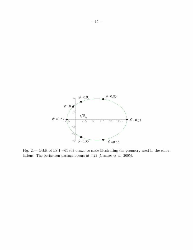
The modeled properties of the system will be expressed in terms of the orbital phase

ψ (ψ = 0.23 at the periastron passage according to the latest determination by Casares et

al. 2005) which is related to the separation between the stars by r(ψ) = a(1 − e2)/[1 −e cos(2π(ψ + 0.73))], where a is the semi-major axis of the orbit and e the eccentricity. The

wind accretion rate onto the compact object of mass Mc can be estimated as:

Mc =4π(GMc)

2ρw(r)

v3rel

, (1)

where vrel is the relative velocity between the neutron star (moving in a Keplerian orbit) and

the circumstellar wind, assumed to be flowing radially on the equatorial plane.

Following the basic assumption of the jet-disk symbiosis model (Falcke & Biermann

1995) we will assume that the accretion rate is coupled to the kinetic jet power by:

Qj = qjMcc2, (2)

where qj ∼ 0.1 is the coupling constant. Most of this power will consist of cool protons that

are ejected with a macroscopic Lorentz factor Γ ∼ 1.25 (Massi et al. 2001). Only a small

fraction qrelj ∼ 10−3 is in the form of relativistic hadrons. The relativistic jet is confined by

the pressure of the cold particles (Pcold > Prel), which expand laterally at the local sound

speed.

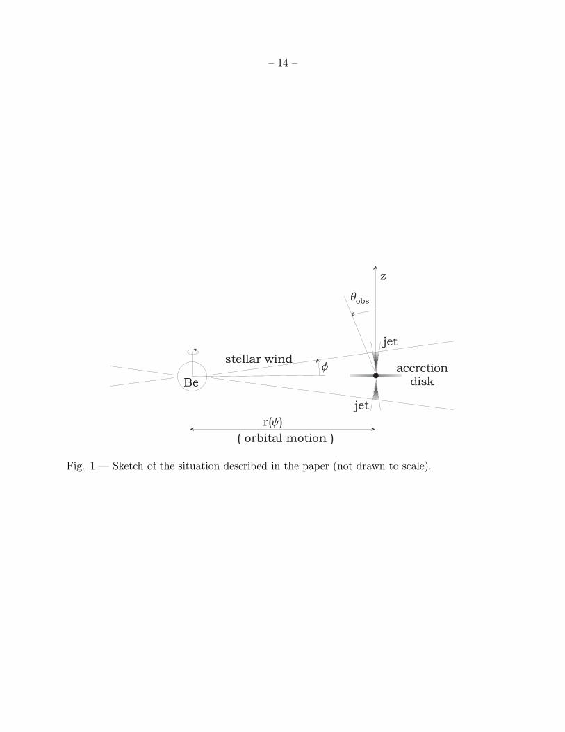
The jet axis, z, will be assumed normal to the orbital plane. The jet will be conical,

with a radius Rj(z) = z(R0/z0), where z0 is the injection point and R0 is the initial radius

of the jet. We will adopt z0 = 107 cm and R0 = z0/10 as reasonable values (see Romero

et al. 2003 and Bosch-Ramon et al. 2005a, who deals with similar jets for additional

details). The relativistic proton spectrum will be a power law N ′p(E

′p) = Kp E

′−αp , valid for

E ′pmin ≤ E ′

p ≤ E ′pmax (in the jet frame). The corresponding relativistic proton flux will be

J ′p(E

′p) = (c/4π)N ′

p(E′p). Since the jet expands in a conical way, the proton flux evolves with

z as:

J ′p(E

′p) =

c

4πK0

(z0z

)2

E ′p−α, (3)

where it is implicit the assumption of the conservation of the number of particles (see Ghis-

ellini et al. 1985), and a prime refers to the jet frame. Using relativistic invariants, it can

– 4 –

be shown that the proton flux, in the lab (observer) frame, becomes (e.g. Purmohammad &

Samimi 2001):

Jp(Ep, θ) =cK0

4π

(z0z

)2 Γ−α+1(

Ep − βb

√

E2p −m2

pc4 cos θ

)−α

[

sin2 θ + Γ2

(

cos θ − βbEp√E2

p−m2

pc4

)2]1/2

. (4)

In this expression, Γ is the jet Lorentz factor, θ is the angle subtended by the proton velocity

direction (which will be roughly the same as that of the emerging photon) and the jet

axis (notice that then θ ≈ θobs), and βb is the bulk velocity in units of c. We will make

all calculations in the lab frame, where the cross sections for pp interactions have suitable

parametrizations.

The number density n0′ of particles flowing in the jet at R0, and the normalization

constant K0 can be determined as in Romero et al. (2003). In the numerical calculations

of the next section we have considered E ′maxp = 100 TeV, E ′min

p = 1 GeV, Γ = 1.25, and,

α = 2.2 (see the list of the assumed parameters in Table 1). The assumed maximum energy

is consistent with the jet size and shock acceleration with an efficiency ∼ 0.01 − 0.1.

The matter from the wind can penetrate the jet from the side, diffusing into it as long

as the particle gyro-radius is smaller than the radius of the jet. This imposes a constraint

onto the value of the magnetic field in the jet: Bjet ≥ Ek/(eR0), where Ek = mp v2rel/2. For

the periastron passage (Ek maximum) results Bjet ≥ 2.8 10−6 G, which is surely satisfied.

However, some effects, like shock formation on the boundary layers, could prevent some

particles from entering into the jet. Given our ignorance of the microphysics involved, we

adopt a parameter fp that takes into account particle rejection from the boundary in a

phenomenological way. In a conservative approach, we will adopt fp ∼ 0.1 .

Some of the particles entering the jet flow would be immediately accelerated to the jet

velocity (by Coloumb interactions or wave-particle interactions). As a consequence, the jet

should be slowed down during its motion through the equatorial wind. However, it is a fact

that the jet survives this interaction since it is seen at radio wavelengths far beyond the

wind region, up to distances of ∼ 400 AU (Massi et al. 2001, 2004). Since the bulk velocity

seems not to be very high (Massi et al. 2001) and hence its change does not affect seriously

the calculations of the gamma-ray emissivity, we will neglect, in what follows, the effects of

a macroscopic deceleration. The reader interested in the case of the hadronic gamma-ray

emission of a jet slowed down to rest by the effects of the wind and the resulting standing

shock wave as the major source of radiation is referred to the recent treatment presented by

Romero & Orellana (2005).

– 5 –

In Figure 1 we show a sketch of the general situation and in Figure 2 we show the orbit

of the system and the corresponding phases.

3. Gamma-ray emission

Relativistic protons in the jet will interact with target protons in the wind through

the reaction channel p + p → p + p + ξπ0π0 + ξπ±(π+ + π−), where ξπ is the corresponding

multiplicity. Then pion decay chains will lead to gamma-ray and neutrino emission. The

differential gamma-ray emissivity from π0-decays can be expressed as (e.g. Aharonian &

Atoyan 1996):

qγ(Eγ , θ) = 4πσpp(Ep)2Z

(α)

p→π0

αJp(Eγ , θ) ηA, (5)

where Z(α)

p→π0 is the so-called spectrum-weighted moment of the inclusive cross-section (see,

for instance, Gaisser 1990). Jp(Eγ) is the proton flux distribution (4) evaluated at E = Eγ .

The cross section σpp(Ep) for inelastic p − p interactions at energy Ep ≈ 6ξπ0Eγ/K, where

K ∼ 0.5 is the inelasticity coefficient and ξπ0 = 1.1(Ep/GeV)1/4, can be represented for

Ep ≥ 1 GeV by

σpp(Ep) ≈ 30 × [0.95 + 0.06 log (Ep/GeV)] (mb).

Finally, the parameter ηA takes into account the contribution from different nuclei in the wind

and in the jet (for standard composition of cosmic rays and interstellar medium ηA ∼ 1.4).

The spectral energy distribution is:

Lγ(Eγ, θ) = E2γ

∫

V

n(~r′) qγ(Eγ, θ) d3~r′, (6)

where V is the interaction volume between the jet and the circumstellar disk. The particle

density of the wind that penetrates the jet is n(r) ≈ fpρw(r)/mp.

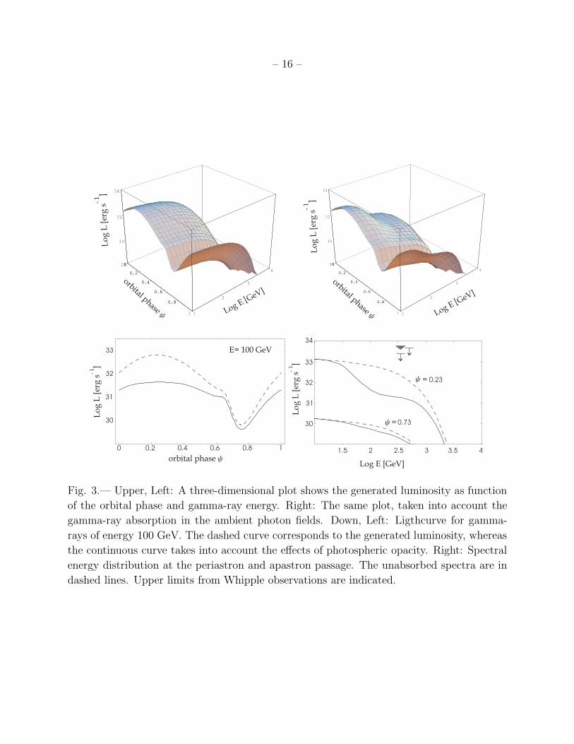
In our calculations, we adopt a viewing angle of θ = 30◦ in accordance with the average

value given by Casares et al. (2005). In Figure 3 we show a 3-D plot that shows the evolution

of the gamma-ray spectral energy distribution as a function of the orbital phase. Other

two plots in this figure show cuts at both the periastron and apastron, and the luminosity

evolution with the orbital phase at 100 GeV. In both cases we show the unabsorbed (dashed

lines) and the absorbed (continuum lines) curves. This absorption is discussed in the next

section.

At the periastron passage the unattenuated luminosity is ∼ 1033 erg s−1. We can make

a simple order-of-magnitude estimate of this value. The accretion rate at the periastron

– 6 –

is ∼ 3 × 1017 g s−1. This means that the total power in relativistic protons should be

Qrelj = 10−3Mcc

2 ∼ 2.8 × 1035 erg s−1. The density of the stellar wind at the injection point

of the jet is n ∼ 4×1011 cm−2 and the cross section for protons of Ep ∼ 1 TeV, σpp ∼ 34 mb.

Hence, the mean free path of the protons results λpp ∼ 8.3 × 1013 cm. The thickness of the

region of the disk traversed by the jet is ∆z ∼ rperias tan 15◦ ∼ 4.4× 1011 cm. Consequently,

we can approximate the gamma-ray luminosity by:

Lγ = 2fπQrelj

(

1 − e−∆z/λpp

)

, (7)

where fπ ∼ 0.2 is the fraction of the energy of the leading proton that goes into neutral pions

and hence into gamma-rays. With a simple substitution into Eq. (7) we get Lγ ∼ 6.6× 1032

erg s−1, in good agreement with the detailed numerical calculations presented in Fig. 3.

4. Opacity

The optical depth for a photon with energy Eγ, which in this case depends upon the

direction observed, can be estimated as

τ(ρ, Eγ) =

∫

∞

Emin(Eγ)

∫

∞

ρ

nph(Eph, ρ′)σe−e+(Eph, Eγ)dρ

′ dEph, (8)

where Eph is the energy of the ambient photons, nph(Eph, ρ) is their density at a distance ρ

from the neutron star, and σe−e+(Eph, Eγ) is the photon-photon pair creation cross section

given by:

σe+e−(Eph, Eγ) =πr2

0

2(1 − ξ2)

[

2ξ(ξ2 − 2) + (3 − ξ4) ln

(

1 + ξ

1 − ξ

)]

, (9)

where r0 is the classical radius of the electron and

ξ =

[

1 −(mec

2)2

EphEγ

]1/2

. (10)

In Eq. (8), Emin is the threshold energy for pair creation in the ambient photon field. This

field can be considered as formed by two components, one from the Be star and the other

from the hot accreting matter impacting onto the neutron star: nph = nph,1 + nph,2. Here,

nph,1(Eph, ρ) =

(

πB(Eph)

hcEph

)

R2⋆

ρ2 + r2 − 2ρr sin θ, (11)

– 7 –

is the black body emission from the star, with

B(Eph) =2E3

ph

(hc)2 (eEph/kTeff − 1)(12)

and Teff = 22500 K (Martı & Paredes 1995). The separation r between the stars is again

variable with the phase angle ψ.

The emission from the heated matter can be approximated by a Bremsstrahlung spec-

trum:

nph,2(Eph, ρ) =LX E

−2ph

4πc ρ2 eEph/Ecut−offfor Eph ≥ 1 keV, (13)

where LX is the total luminosity in hard X-rays and Ecut−off ∼ 100 keV. The photon index

of the hard X-rays is taken to be within the range published by Greiner & Rau (2001), which

was observationally determined. LX is also constrained by observations, being LX ∼ 1034

erg s−1 (Paredes et al. 1997). Notice that no bump due to a putative accretion disk has

been observed at X-rays, so we neglect this contribution.

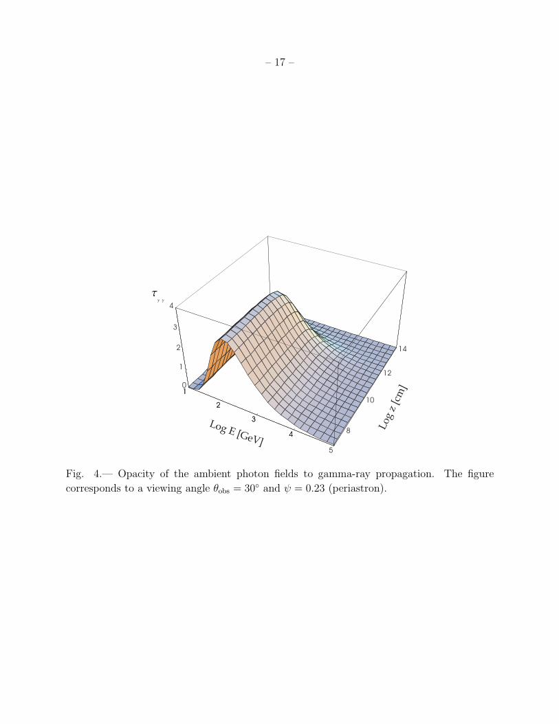
As an example, Figure 4 shows the dependence of the optical depth τ with the energy

of the γ-rays and its variation along the z axis for the observer at θobs = 30◦. From detailed

versions of this plot, we find that for photons of Eγ = 100 GeV significant absorption occurs

mostly between ψ = 0.1 and ψ = 0.5. The optical depth remains well below the unity along

the whole orbit for photons of energies Eγ . 30 GeV and Eγ & 2 TeV.

5. Secondary electron-positron pairs and synchrotron emission

Secondary pairs are produced by the decays of charged pions and muons, as well as by

photon-photon interactions. The main reactions that lead to charged pions are:

p+ p → p+ p+ ξπ0π0 + ξπ±(π+ + π−) (14)

p+ p → p+ n+ π+ +X (15)

p+ p → 2n+ 2π+ +X (16)

where n is a neutron, X stands for anything (neutral) else, and the charged pion multiplicity

is ξπ± ≈ 2(Ep/GeV)1/4. The neutrons have a proper lifetime of 886 ± 1 s and since they

move at ultrarelativistic speed can escape from the source, decaying at considerable distances

(Eichler & Wiita 1978). On the contrary, pions decay into the jet trough π± → µ± + ν and

µ± → e± + ν + ν. For an injection proton spectrum given by Eq. (3) with α = 2.2, we have

that the pion spectrum (in the jet’s system) will be a power-law J ′

π±(E ′

π±) = Kπ± E ′−απ

π± , with

– 8 –

απ ∼ 2.3. The electron-positron distribution mimics this power law (Ginzburg & Syrovatskii

1964, Dermer 1986):

J ′e±(E ′

e±) = Kπ→e±E′−α±

e± , (17)

with

Kπ→e± =

(

mµ

me

)α±−12(α± + 5)

α±(α± + 2)(α± + 3)Kπ± , (18)

and α± = απ.

The energy density of pion-generated pairs along the jet at the periastron passage can

be calculated as:

wπ→e± =

∫

(4π/c)E ′e±J

′e±(E ′

e±)dE ′e±, (19)

where J ′e±(E ′

e±) takes into account all the contributions from z0 to zmax. Integrating we get

wπ→e± ≈ 3 × 109 erg cm−3.

We can compare the energy density of pairs from the charged pion decays with that of

the pairs produced by direct gamma-ray absorption. The total luminosity of these pairs is:

Le± = L0γ(1 − e−τ ). (20)

Then, using the opacity calculated in the previous section, the pair energy density results

wγγ→e± ∼Le±

4πR20c. (21)

At the periastron passage, we get wγγ→e± ≈ 3.7 × 109 erg cm−3. Hence, the pair injection

from the photon-photon annihilation is similar to that of pion decay. In what follows we will

evaluate the spectrum of these particles using the approximation derived by Aharonian et

al. (1983), which is in excellent agreement with the more detailed calculations (exact to 2nd

order QED) presented by Bottcher & Schlickeiser (1997).

The differential pair injection rate is given by (Bottcher & Schlickeiser 1997):

ne±(γ) =3

32cσ

T

∫

∞

γ

dǫγNγ(ǫγ)

ǫ3γ

∫

∞

ǫγ

4γ(ǫγ−γ)

dǫphnph(ǫph)

ǫ2ph

×

[4ǫ2γ

γ(ǫγ − γ)ln

(

4ǫphγ(ǫγ − γ)

ǫγ

)

− 8ǫγǫph +2(2ǫγǫph − 1)ǫ2γγ(ǫγ − γ)

−(

1 −1

ǫγǫph

)

ǫ4γγ2(ǫγ − γ)2

], (22)

– 9 –

where γ = Ee±/mec2, ǫγ = Eγ/mec

2, and ǫph = Eph/mec2. A numerical integration yields

a pair spectrum that can be well fitted by a power law Ne± ∝ E−1.9e± . The proportionality

constant Kγγ→e± can be obtained from the absorbed gamma-ray luminosity.

The presence of a magnetic field in the jet will imply that all these secondary pairs

will produce synchrotron emission. Following Bosch-Ramon et al. (2005b) we assume that

the magnetic field is entangled to cold protons in such a way it has random directions and

hence the synchrotron emission is isotropic in the jet’s frame. To calculate the synchrotron

luminosity we estimate the specific emission (jǫ(z)) and absorption (kǫ(z)) coefficients from

the secondary particle distribution (see Pacholczyk 1970 for the detailed formulae), in such

a way that:

dLǫ(z)

dz= 2πRj

jǫ(z)

kǫ(z)× [1 − exp(−ljkǫ(z))], (23)

where to simplify the notation we are not using now primes to indicate that the calculation

is in the jet’s frame. In Eq. (23) lj ∼ Rj is the typical size of the synchrotron emitting

plasma and ǫ is the photon energy in units of mec2. Integrating over the jet length we get

the spectral energy distribution as:

Lobssyn = ǫ

∫ zmax

z0

δ2dLǫ

dzdz, (24)

where δ is the Doppler boosting factor defined as:

δ =1

Γ(1 − βb cos θobs). (25)

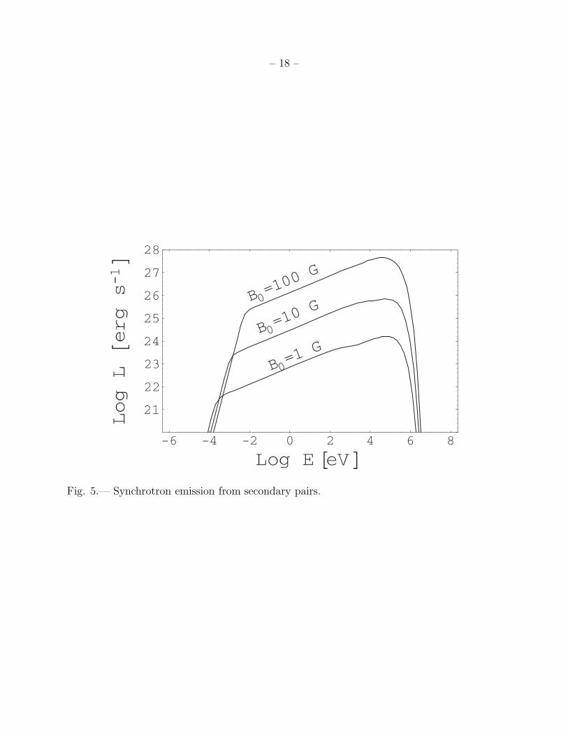
To calculate the specific emission jǫ(z) we adopt different values of the magnetic field

at z0: B0 = 1, 10, and 100 Gauss (Bosch-Ramon & Paredes 2004). In Figure 5 we show

the spectral energy distribution of the synchrotron radiation of all secondary pairs for the 3

different values of B0. The radio emission is quite negligible in comparison to the observed

values, which at the minimum imply a luminosity of ∼ 1031 erg s−1 (e.g. Ribo et al. 2005).

6. Discussion

The predicted gamma-ray luminosity is clearly at its maximum during the periastron

passage, when the neutron star travels through the densest parts of the wind. This is in

accordance with the fact noticed by Massi (2004) that the peaks of the EGRET flux are

coincident with the periastron and not with the radio maxima. The radio outbursts are

– 10 –

the result of particle injection in the jet that occurs after some relaxation time from the

periastron passage, when the accretion rate is increased (Paredes et al. 1991). Any purely

leptonic model for the gamma-ray emission would have to explain why the radio and gamma-

ray peaks are not observed in similar orbital phases.

Other specific feature of the gamma-ray emission predicted by our model is the presence

of a local, secondary maximum at ψ ∼ 0.65 when the accretion rate, given by (1), has also

a local maximum due to the fact that the wind velocity is roughly parallel to the neutron

star orbital velocity, hence reducing vrel and increasing Mc, as noticed by Martı & Paredes

(1995).

The effects of the opacity of the ambient photon fields to gamma-ray propagation pro-

duces a “valley” in the spectral energy distribution, between a few tens of GeV and a few

TeV, with a local minimum at around 100 GeV, during the periastron passage. The pre-

dicted luminosity is within the detection possibilities of an instrument like MAGIC, which,

integrating over several periastron passages, could build up a SED which can be compared

with that presented in Fig. 3. Upper limits obtained with the Whipple telescope (Hall et

al. 2003, Fegan et al. 2005) are indicated in the figure. The source is too weak for the

sensitivity of this instrument according to our model.

7. Concluding remarks

We have presented a hadronic model for the high-energy gamma-ray production in the

microquasar LS I +61 303. The model is based on the interaction of a mildly relativistic jet

with a small content of relativistic hadrons with the dense equatorial disk of the companion

B0 V star. Gamma-rays are the result of the decay of neutral pions produced by pp collisions.

Charged pion decay will lead to neutrino production, that will be discussed elsewhere. The

model takes into account the opacity of the ambient photon fields to the propagation of the

gamma-rays. The predictions include a peak of gamma-ray flux in the periastron passage,

with a secondary maximum at phase ψ ∼ 0.65. The spectral energy distribution presents a

minimum around 100 GeV due to absorption. The spectral features should be detectable by

an instrument like MAGIC through exposures ∼ 50 hr, integrated along different periastron

passages.

– 11 –

Acknowledgments

We thank J.M. Paredes and V. Bosch-Ramon for careful readings of the manuscript

and comments. The latter gave us useful support on calculations for the secondary emis-

sion. We also thank constructive suggestions by an anonymous referee. This work has been

supported by the Argentinian agencies CONICET and ANPCyT (PICT 03-13291). HRC

thanks support from FUNCAP and CNPq (Brazil).

REFERENCES

Aharonian, F.A., Atoyan, A.M., & Nagapetyan, A.M. 1983, Astrophysics, 19, 187

Aharonian, F. A., & Atoyan, A. M. 1996, A&A, 309, 917

Bosch-Ramon, V., & Paredes, J.M. 2004, A&A, 425, 1069

Bosch-Ramon, V., Romero, G.E., & Paredes, J.M. 2005a, A&A, 429, 267

Bosch-Ramon, V., Romero, G.E., & Paredes, J.M. 2005b, A&A, submitted

Bottcher, M. & Schlickeiser, R. 1997, A&A, 325, 866

Casares, J., Ribas, I., Paredes, J.M., et al. 2005, MNRAS, in press

Dermer, C.D. 1986, ApJ, 307, 47

Eichler, D. & Wiita, P.J. 1978, Nature 274, 38

Falcke, H. & Biermann, P. L. 1995, A&A, 293, 665

Fegan, S., et al. 2005, ApJ, in press

Gaisser, T.K. 1990, Cosmic Rays and Particle Physics, Cambridge University Press, Cam-

bridge

Ghisellini, G., Maraschi, L., & Treves, A. 1985, A&A, 146, 204

Ginzburg, V.L. & Syrovatskii, S.I. 1964, Sov. Astron. 8, 342

Gregory, P.C, & Taylor, A.R. 1978, Nature, 272, 704

Gregory, P.C., & Neish, C. 2002, ApJ, 580, 1133

Gregory, P.C. 2002, ApJ, 575, 427

– 12 –

Greiner, J. & Rau, A. 2001, A&A, 375, 145

Hall, T.A., Bond, I.H., Bradbury, S.M., et al. 2003, ApJ, 583, 853

Kaufman Bernado, M. M., Romero, G. E., & Mirabel, I. F. 2002, A&A, 385, L10

Kotani, T., Kawai, N., Aoki, T., et al. 1994, PASJ, 46, L147

Kotani, T., Kawai, N., Matsuoka, M., & Brinkmann, W. 1996, PASJ, 48, 619

Kniffen, D.A., Alberts, W.C.K., Berstch, D.L., et al. 1997, ApJ, 486, 126

Marti, J., & Paredes, J.M. 1995, A&A, 298, 151

Massi, M., Ribo, M., Paredes, J.M., et al. 2001, A&A, 376, 217

Massi, M., Ribo, M., Paredes, J.M., et al. 2004, A&A, 414, L1

Massi, M. 2004, A&A, 422, 267

Migliari, S., Fender, R. & Mendez, M. 2002, Science, 297, 1673

Pacholczyk, A. G., 1970, Radio Astrophysics, Freeman, San Francisco

Paredes, J.M., Martı, J., Estalella, R., & Sarrate, J. 1991, A&A, 248, 124

Paredes, J.M., Martı, J., Peracaula, M, & Ribo, M. 1997, A&A, 320, L25

Paredes, J. M., Martı, J., Ribo, M., & Massi, M. 2000, Science, 288, 2340

Purmohammad, D. & Samimi, J. 2001, A&A 371, 61

Ribo, M., Combi, J.A., & Mirabel, I.F. 2005, Ap&SS 297, 143

Romero, G.E., Torres, D.F., Kaufman Bernado, M.M. & Mirabel, I.F. 2003, A&A, 410, L1

Romero, G.E. & Orellana, M. 2005, A&A, in press (astro-ph/0505287)

Tavani, M., Kniffen, D.A., Mattox, J.R., et al. 1998, ApJ, 497, L89

This preprint was prepared with the AAS LATEX macros v5.2.

– 13 –

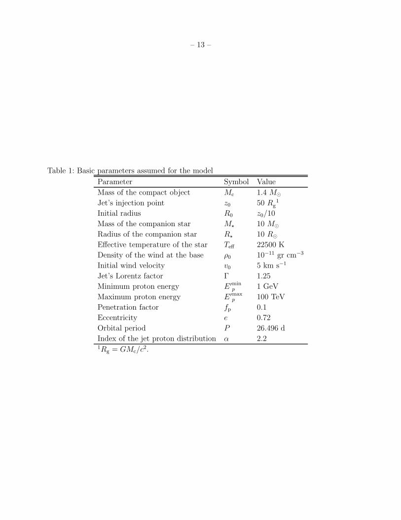
Table 1: Basic parameters assumed for the model

Parameter Symbol Value

Mass of the compact object Mc 1.4 M⊙

Jet’s injection point z0 50 R 1g

Initial radius R0 z0/10

Mass of the companion star M⋆ 10 M⊙

Radius of the companion star R⋆ 10 R⊙

Effective temperature of the star Teff 22500 K

Density of the wind at the base ρ0 10−11 gr cm−3

Initial wind velocity v0 5 km s−1

Jet’s Lorentz factor Γ 1.25

Minimum proton energy E ′minp 1 GeV

Maximum proton energy E ′maxp 100 TeV

Penetration factor fp 0.1

Eccentricity e 0.72

Orbital period P 26.496 d

Index of the jet proton distribution α 2.21Rg = GMc/c

2.

– 14 –

Fig. 1.— Sketch of the situation described in the paper (not drawn to scale).

– 15 –

Fig. 2.— Orbit of LS I +61 303 drawn to scale illustrating the geometry used in the calcu-

lations. The periastron passage occurs at 0.23 (Casares et al. 2005).

– 16 –

Fig. 3.— Upper, Left: A three-dimensional plot shows the generated luminosity as function

of the orbital phase and gamma-ray energy. Right: The same plot, taken into account the

gamma-ray absorption in the ambient photon fields. Down, Left: Ligthcurve for gamma-

rays of energy 100 GeV. The dashed curve corresponds to the generated luminosity, whereas

the continuous curve takes into account the effects of photospheric opacity. Right: Spectral

energy distribution at the periastron and apastron passage. The unabsorbed spectra are in

dashed lines. Upper limits from Whipple observations are indicated.

– 17 –

Fig. 4.— Opacity of the ambient photon fields to gamma-ray propagation. The figure

corresponds to a viewing angle θobs = 30◦ and ψ = 0.23 (periastron).

– 18 –

Fig. 5.— Synchrotron emission from secondary pairs.