arX

iv:h

ep-p

h/01

0124

3v1

22

Jan

2001 Correlations in e+e−

→ W +W − hadronic decays

E.A. De Wolf

EP Division, CERN, European Organisation for Nuclear Research,

CH-1211 Geneva 23, Switzerland

and

Department of Physics, Universitaire Instelling Antwerpen,

Universiteitsplein 1, B-2610 Antwerpen, Belgium.

Abstract

A mathematical formalism for the analysis of correlations in multi-source eventssuch as W+W− production in e+e− annihilations is presented. Various measuresused in experimental searches for inter-W correlations are reviewed.

1 Introduction

The problem of possible inter-W dynamical correlations continues to attract muchexperimental attention at LEP-II [1]. The importance of these in a precision measure-ment of the W -mass [2–4] is by far the main reason for the flurry of present activities.However, this should not be the sole motivation for careful experimental work in thissubfield. For example, the possible absence of Bose-Einstein correlations (BEC) be-tween pions originating from different W ’s raises interesting general and basic questionsregarding the coherent versus incoherent nature of particle emission. Also the questionof possible color- or string-reconnection effects may be of considerable importance forour understanding of the vacuum properties of Quantumchromodynamics.

As repeatedly emphasized by the Lund group [5, 6], Bose-Einstein correlations ofa coherent type, for which we suggest the name “String Symmetrization Correlations(SSC)”, are present in any string model of hadron production. Moreover, the SSCdepend essentially only on local properties of the string and should thus be indepen-dent of the environment in which the string is fragmenting. This basic property isnot in contradiction with experimental results on Bose-Einstein correlations in e+e−

annihilations and lepton-nucleon scattering.However, in systems comprising several strings, a second type of Bose-Einstein cor-

relations may exist if the different strings behave independently so that they act asincoherent sources of particle emission. This second-order intensity correlation effect,or HBT effect, since first discovered by Hanbury Brown and Twiss [7], is expectedto reflect the “geometry” of the collision process and, in particular, to be sensitiveto the size of the “freeze-out” volume where the hadrons are formed. This volumecould have an extension of many fermi’s and can thus be significantly larger than thetypical “radii” of less than a fermi, commonly measured e.g. in BEC studies of e+e−

annihilations. As a result, correlation functions of identical bosons may well show anadditional enhancement at substantially smaller values of their momentum differencethan for SSC correlations.

The reaction e+e− → W+W− → q1q2q3q4 → hadrons is a prototypical example ofa system of which the hadronisation proceeds via the fragmentation of two color-fieldsor strings. Barring possible reconnection effects at an early stage of the evolution ofthe system, these strings are thought to fragment independently. Thus, SSC withinsingle W ’s and inter-W HBT correlations could coexist in this system, but manifestthemselves in different ranges of e.g. the commonly used variable Q2, the square ofthe difference of the four-momenta of the identical pions. No dedicated searches inthis direction have been made so far. Moreover, if the HBT correlations are of muchshorter range than naively expected, the influence on W -mass measurements is likelyto be much weaker than present studies suggest.

Limited statistics as well as limited experimental sensitivity at very small Q mayprevent the HBT-type of correlation effect to be clearly observed in e+e− → W+W− →

1

4q events. However, as yet unexplored alternative reactions exist. Much larger statisticsis available in e.g. e+e− → qq + g → three-jet events. For these, due to the emission ofa hard gluon, two color-disconnected strings are stretched, one between the quark andthe gluon, another between the gluon and the antiquark. Depending on the origin ofthe identical pions studied, SSC as well as HBT correlations should contribute1 to thecorrelations among identical bosons.

In hadron-hadron, hadron-nucleus and nucleus-nucleus collisions, hadroproductionis also believed to result from the break-up of several to very many strings. Since the su-perposition of many independent particle “sources” weakens the measured strength ofcorrelations of the SSC type, HBT correlations may well dominate the Bose-Einsteincorrelations measured in these processes. This could also explain the observed pos-itive correlation between particle density (or multiplicity) and the measured BECradii. Finally, due to the “inside-outside” character of hadron production, wherebylow-momentum particles “freeze out” first (in any reference frame), one may expect acorrelation between the width of the Bose-Einstein enhancement and particle momentaif the HBT correlations are the dominant effect.

Returning to correlations in the WW system, experimental study of such effectsshould start from a well-defined mathematical framework. Since, in general, inter-Wdynamics introduces genuine correlations between the decay products of the W ’s, wegeneralize the formalism presented in an earlier paper on the subject [8] where observ-ables relevant for the case of stochastic independence and fully overlapping decays ofthe W ’s were proposed. We consider the general case of stochastic dependence and theseparation of the W hadronic decay products in momentum space. We concentrate onsecond-order (two-particle) inclusive densities and correlation functions but the resultscan be generalized to higher orders.

In the mathematical treatment of the problem, a general inter-W correlation func-tion is introduced, representing an arbitrary stochastic correlation between hadronsfrom different W ’s which could arise from color reconnection effects, Bose-Einsteincorrelations or others. Although most of the examples treated in this paper relate toBose-Einstein studies involving identical particles, the formalism is general and can beused, where needed with a suitable change of kinematic variables, in other contexts aswell.

2 Multivariate distributions and moments

Before discussing the problem of correlations among particles originating from W ’sdecaying into fully hadronic, so-called four-jet configurations, e+e− → q1q2q3q4 →hadrons, we first consider a more general problem.

Assume that a system (e.g. an event) comprising in total n (observed) particles,

1I thank B. Andersson and G. Gustafson for discussions of this point.

2

can be subdivided into S possibly stochastically correlated groups or “sources” Ωi

(i = 1, . . . , S). We take the n particles to be of identical type and assume that thegroups are mutually exclusive i.e. every particle can be assigned to one and one grouponly2: Ωi ∩Ωj = 0, ∀i, j and i 6= j. No assumptions are made, however, about possibleoverlap in momentum space of particles from different groups.

Let n be the total number of particles counted in the union of the S groups,

n =S∑

m=1

nm . (1)

Consider further the multivariate multiplicity distribution PS(n1, . . . , nS) giving thejoint probability for the simultaneous occurrence of n1 particles in class Ω1, . . . , nS

particles in class ΩS . The probability distribution of n is then given by

P (n) =n∑

n1=0

· · ·n∑

nS=0

PS(n1, . . . , nS)δn,n1+···+nS. (2)

We further define the single-variate factorial moment generating function of P (n)

G(z) =∞∑

n=0

(1 + z)n P (n) . (3)

By expanding (1 + z)n, (3) can be rewritten as

G(z) = 1 +∞∑

q=1

zq

q!

∞∑

n=0

n!

(n − q)!P (n), (4)

= 1 +∞∑

q=1

zq

q!

⟨

n!

(n − q)!

⟩

, (5)

G(z) = 1 +∞∑

q=1

zq

q!Fq; (6)

where in the last line we introduce the symbol Fq for the (unnormalized) factorial (orbinomial) moment of the probability distribution P (n). The brackets in Eq. (5) denotea statistical average.

Fq = 〈n(n − 1) . . . (n − q + 1)〉 ,

=∫

∆dy1 . . .

∫

∆dyq ρq(y1, . . . , yq). (7)

2Such a subdivision can be based on a “natural” partition of the n particles in S groups accordingto the underlying dynamics. It could also be based on an experimentally dictated partition of thephase space in S distinct (non-overlapping) regions e.g. as the result of jet clustering.

3

The last equation expresses that, for identical particles, the factorial moment Fq isequal to the integral over q-dimensional phase space (here for simplicity of notationrepresented by the variables yi) of the q-particle inclusive density ρq(y1, . . . , yq) overthe same phase space volume ∆ [9]. The q-particle inclusive density ρq(y1, . . . , yq) isdefined as

ρq(y1, . . . , yq) =1

σ

dqσ

dy1 . . . dyq

, (8)

with σ the total cross section of the considered reaction. Experimentally, this quantityis approximated by

ρq(y1, . . . , yq) =1

Nevt

dNq-tuples

dy1 . . . dyq

, (9)

with dNq-tuples the number of q-tuples of particles, counted in a phase space domain(y1 + dy1, . . . , yq + dyq); Nevt is the number of events in the sample.

Factorial cumulants are formally defined as the coefficients of zq/q! in the Taylorexpansion of the function log G(z):

log G(z) = 〈n〉 z +∞∑

q=2

zq

q!Kq. (10)

The (unnormalized) factorial cumulants of order q, Kq, also known as Muellermoments [10], are equal to the q-fold phase space integral of the q-particle inclusive (so-called “connected” or “genuine”) factorial cumulant correlation function Cq(y1, . . . , yq)

Kq =∫

∆dy1 . . .

∫

∆dyq Cq(y1, . . . , yq). (11)

The correlation functions Cq(y1, . . . , yq) are, as in the cluster expansion in statisticalmechanics, defined via the sequence

ρ1(1) = C1(1),

ρ2(1, 2) = C1(1)C1(2) + C2(1, 2),

ρ3(1, 2, 3) = C1(1)C1(2)C1(3) + C1(1)C2(2, 3) + C1(2)C2(1, 3) +

+ C1(3)C2(1, 2) + C3(1, 2, 3), (12)

etc. (13)

These relations can be inverted yielding

C2(1, 2) = ρ2(1, 2) − ρ1(1)ρ1(2) ,

C3(1, 2, 3) = ρ3(1, 2, 3) −∑

(3)

ρ1(1)ρ2(2, 3) + 2ρ1(1)ρ1(2)ρ1(3) ,

C4(1, 2, 3, 4) = ρ4(1, 2, 3, 4) −∑

(4)

ρ1(1)ρ3(1, 2, 3) −∑

(3)

ρ2(1, 2)ρ2(3, 4)

4

+ 2∑

(6)

ρ1(1)ρ1(2)ρ2(3, 4) − 6ρ1(1)ρ1(2)ρ1(3)ρ1(4), (14)

etc. (15)

In the above relations we have abbreviated ρq(y1, . . . , yq) to ρq(1, 2, . . . , q) etc.; thesummations indicate that all possible permutations have to be taken (the numberunder the summation sign indicates the number of terms).

The factorial moments Fq and factorial cumulants Kq are easily found if G(z) isknown

Fq =dqG(z)

dzq

∣

∣

∣

∣

∣

z=0

, (16)

Kq =dq log G(z)

dzq

∣

∣

∣

∣

∣

z=0

. (17)

The counting distribution P (n) is likewise determined by G(z)

P (n) =1

n!

dnG(z)

dzn

∣

∣

∣

∣

∣

z=−1

. (18)

Let us now introduce the multidimensional S-variate generating function

GS(z1, . . . , zS) =∞∑

n1=0

∞∑

n2=0

· · ·∞∑

nS=0

(1 + z1)n1 · · · (1 + zS)nS PS(n1, . . . , nS), (19)

from which the S-variate factorial moments are easily obtained by differentiation:

Fq1...qS=⟨

n[q1]1 . . . n

[qS]S

⟩

=

(

∂

∂z1

)q1

· · ·(

∂

∂zS

)qS

GS(z1, . . . , zS)

∣

∣

∣

∣

∣

z1=···zS=0

. (20)

Likewise, S-variate factorial cumulants are obtained by differentiation of log GS(z1, . . . , zS).Returning to the function G(z) (3), it is not difficult to see that it can be written

in terms of the multivariate generating function (19) as

G(z) = GS(z1, . . . , zS)|z1=z2=···=zS=z . (21)

Equation (21) therefore allows to express the factorial moments of n in terms of themultivariate factorial moments of n1, . . . , nS.

Application of the Leibnitz rule

(

d

dz

)q

f(z) =∑

aj

q!

a1 !a2 ! . . . aS!

(

d

dz

)a1

f1(z) · · ·(

d

dz

)aS

fS(z)

5

to the functionf(z) = f1(z) · · · fS(z)

and using (21) leads immediately to the relation

Fq =∑

aj

F (S)a1...aS

q!

a1! . . . aS!. (22)

The summation is over all sets aj of non-negative integers such that

S∑

j=1

aj = q.

Formula (22) is a generalization for factorial moments of the usual multinomial theorem.Likewise, taking the natural logarithm of both sides of (21), one obtains an identical

relation as (22) among single-variate and multivariate factorial cumulants.As an example, for two groups (S = 2) one finds from (22)

F2 = F(2)02 + 2F

(2)11 + F

(2)20 , (23)

F3 = F(2)03 + 3(F

(2)12 + F

(2)21 ) + F

(2)30 , (24)

F4 = F(2)04 + 6F

(2)22 + 4(F

(2)13 + F

(2)31 ) + F

(2)40 . (25)

The factorial moments F0i, Fi0, are determined from the counting distribution in asingle group. The univariate factorial moments Fq are obtained from the sum of counts

in the two groups. The “mixed” factorial moments F(2)ij (i, j 6= 0) express inter-group

stochastic dependences. The relations (23)-(25) are trivially extended to more thantwo groups.

3 W +W − correlations

3.1 Integral moments and cumulants

We now apply the general results from the previous section to the case of interest: theproduction of W+W− in e+e− annihilation, and their subsequent decay to four jets:W+W− → 4q → hadrons. Here, the number of “sources” S is equal to two.

Eq. (23) is of particular interest. In a less formal way, it can be written as:

F2 ≡ 〈n(n − 1)〉 = 〈n1(n1 − 1)〉 + 〈n2(n2 − 1)〉 + 2 〈n1n2〉 , (26)

where n1 and n2 are the number of particles from the decay of W+ and W−, respectively.This equation could also be derived directly by noting that n = n1 + n2 and workingout the expression for 〈n(n − 1)〉. To derive relations for S > 2 or between factorial

6

moments of higher order, it is evidently less cumbersome to make use of the generatingfunctions and Eq.(22).

In absence of inter-W correlations of whatever origin, kinematical, dynamical, dueto experimental selections and cuts, . . . , one has

〈n1n2〉 = 〈n1〉 〈n2〉 . (27)

Exhibiting explicitly the presence of inter-W correlations we write (26) as

F2 ≡ 〈n(n − 1)〉 = 〈n1(n1 − 1)〉 + 〈n2(n2 − 1)〉 + 2 〈n1〉 〈n2〉 (1 + δI), (28)

withδI ≡ 〈n1n2〉 / 〈n1〉 〈n2〉 − 1 6= 0, (29)

a measure of positive or negative inter-W correlations. Similarly, the factorial cumulantK2 can be written as

K2 = K20 + K02 + 2 〈n1〉 〈n2〉 δI . (30)

This equation expresses the correlation function, integrated over full phase space, ofthe whole system in terms of the integrated correlation functions of each componentseparately, and of the integrated inter-W correlation.

3.1.1 Interlude

The quantity δI is related to the variances D2W± of the single-W±, W± → qq, and

W+W− → 4q multiplicity distributions via the relation

D2WW =

⟨

(n − 〈n〉)2⟩

=⟨

[(n1 − 〈n1〉) + (n2 − 〈n2〉)]2⟩

(31)

= D2W+ + D2

W− + 2 〈n1n2〉 − 2 〈n1〉 〈n2〉 (32)

giving

δI =D2

WW − D2W+ − D2

W−

2 〈n1〉 〈n2〉. (33)

3.2 Differential distributions

In section 3.1, general relations were obtained relating factorial moments and cumu-lants of the multiplicity distributions of a W+W− system to those of its W+ andW− components. Since q-th order factorial moments are integrals over phase spaceof q-particle inclusive densities, we now turn to relations among the fully differentialparticle densities and correlation functions of a W+W− system and those of its com-posing parts, considering explicitly possible statistical dependences. We restrict thediscussion to second-order densities and correlations.

7

For two stochastically independent systems, we derived in an earlier paper [8] therelations

Cww2 (1, 2) = Cw+

2 (1, 2) + Cw−

2 (1, 2), (34)

ρww2 (1, 2) = ρw+

2 (1, 2) + ρw−

2 (1, 2) + ρw+

1 (1)ρw−

1 (2) + ρw+

1 (2)ρw−

1 (1), (35)

and furtherρww

1 (1) = ρw+

1 (1) + ρw−

1 (1). (36)

Here Cww2 (1, 2) and CW±

2 (1, 2) are the two-particle correlation functions for W+W− →4q events and W± → 2q events, respectively; ρww

1 (1), ρw1 (1) are the corresponding

single-particle inclusive densities.Inspection of (30) suggest to write a general expression for Cww

2 (1, 2) as

Cww2 (1, 2) = Cw+

2 (1, 2) + Cw−

2 (1, 2) + δI(1, 2)

ρw+

1 (1) ρw−

1 (2) + ρw+

1 (2) ρw−

1 (1)

.

(37)The function δI(1, 2) describes correlations among different W ’s.

For δI(1, 2) = 0 (independent W ’s), (37) expresses the additivity3 of the facto-rial cumulant correlation functions, a necessary and sufficient condition for stochasticindependence [8].

The factors ρw+

1 (1) ρw−

1 (2), ρw+

1 (2) ρw−

1 (1) are introduced for normalization andexplicitly account for differences in the single-particle densities of the two W ’s, as isthe case when the momentum spectra of the decay products from different W ’s are notidentical i.e. do not fully overlap4.

With the definitions

ρww2 (1, 2) = Cww

2 (1, 2) + ρww1 (1) ρww

1 (2) (38)

ρw2 (1, 2) = Cw

2 (1, 2) + ρw1 (1) ρw

1 (2) (39)

and using (36) we can write a general form for ρww2 (1, 2)

ρww2 (1, 2) = Cw+

2 (1, 2) + Cw−

2 (1, 2) +

ρw+

1 (1) ρw−

1 (2) + ρw+

1 (2) ρw−

1 (1)

δI(1, 2)

+

ρw+

1 (1) + ρw−

1 (1)

ρw+

1 (2) + ρw−

1 (2)

. (40)

Note that, in general, and in fully differential form, the terms ρw+

1 (1) ρw−

1 (2) andρw+

1 (2) ρw−

1 (1) are not equal. ρww2 (1, 2), however, must be symmetric in its arguments

3For independent “sources”, additivity is valid for all orders of the cumulant correlation functions.4In [8] it was implicitly assumed that ρw+

1 (1) ρw−

1 (2) = ρw+

1 (2) ρw−

1 (1) ≡ ρw1 (1) ρw

1 (2), where

ρw1 (1) is the single-particle inclusive density of one W and with the further assumption that ρw+

1 (1) =

ρw−

1 (1) ≡ ρw1 (1). Ignoring possible charge-dependence, these equations are valid if the W+ and W−

hadronic decay products overlap completely in momentum space.

8

for identical particles. Equation (40), together with (39) takes the form

ρww2 (1, 2) = ρw+

2 (1, 2) + ρw−

2 (1, 2)

+ 1 + δI(1, 2)

ρw+

1 (1) ρw−

1 (2) + ρw+

1 (2) ρw−

1 (1)

(41)

Defining the experimentally often studied normalized two-particle density

Rww2 (1, 2) =

ρww2 (1, 2)

ρww1 (1) ρww

1 (2), (42)

one finds

Rww2 (1, 2) =

ρw+

2 (1, 2) + ρw−

2 (1, 2) +

ρw+

1 (1) ρw−

1 (2) + ρw+

1 (2) ρw−

1 (1)

1 + δI(1, 2)ρw+

1 (1) ρw+

1 (2) + ρw−

1 (1) ρw−

1 (2) + ρw+

1 (1) ρw−

1 (2) + ρw+

1 (2) ρw−

1 (1).

(43)

3.3 Correlations in the variable Q

The previous sections dealt exclusively with fully differential quantities. In practice,these are impossible to measure and a projection on a lower-dimensional space isneeded. We here consider, for illustration, the kinematical variable Q2 = −(p1 − p2)

2,the negative square of the difference in 4-momenta of particles 1 and 2. We use thenotation ρw+ ⊗ ρw−

(Q) for integrals of the type∫ ∫

d3p1d3p2 ρw+

(1) ρw−

(2) δ(

Q2 + (p1 − p2)2)

. (44)

In practical applications, such integrals are calculated using an event and track-mixingtechnique.

We assume from now on that δI(1, 2) in (37) is a function of Q only: δI(Q). Thissimplifies the calculations but may not be fully realistic. At least for Bose-Einsteinstudies, it is known that the correlation function of like-sign pairs is not isotropic infour-momentum space. To simplify further we also assume that

ρw+

1 ⊗ ρw+

1 (Q) = ρw−

1 ⊗ ρw−

1 (Q) ≡ ρw1 ⊗ ρw

1 (Q).

The expressions in the previous sections take the following form

ρww2 (Q) = ρw+

2 (Q) + ρw−

2 (Q) + 2 1 + δI(Q) ρw+

1 ⊗ ρw−

1 (Q), (45)

Cww2 (Q) = Cw+

2 (Q) + Cw−

2 (Q) + 2δI(Q)

ρw+

1 ⊗ ρw−

1 (Q)

. (46)

Integrating these expressions over all Q, we have

δI =1

〈nW+〉 〈nW−〉∫

dQ δI(Q)

ρw+

1 ⊗ ρw−

1 (Q)

. (47)

9

Further

Rww2 (Q) =

ρw+

2 (Q) + ρw−

2 (Q) + 2 1 + δI(Q)

ρw+

1 ⊗ ρw−

1 (Q)

2

ρw1 ⊗ ρw

1 (Q) + ρw+

1 ⊗ ρw−

1 (Q) . (48)

Introducing the “overlap function”

g(Q) =ρw+

1 ⊗ ρw−

1 (Q)

ρw1 ⊗ ρw

1 (Q), (49)

we can rewrite (45)-(46) as

ρww2 (Q) = ρw+

2 (Q) + ρw−

2 (Q) + 2 1 + δI(Q) g(Q) ρw1 ⊗ ρw

1 (Q), (50)

Cww2 (Q) = Cw+

2 (Q) + Cw−

2 (Q) + 2δI(Q) g(Q) ρw1 ⊗ ρw

1 (Q). (51)

Likewise

Rww2 (Q) =

ρw+

2 (Q) + ρw−

2 (Q) + 2 1 + δI(Q) g(Q) ρw1 ⊗ ρw

1 (Q)

2ρw1 ⊗ ρw

1 (Q) 1 + g(Q) , (52)

=1

2

Rw+

2 (Q)

1 + g(Q)+

1

2

Rw−

2 (Q)

1 + g(Q)+ 1 + δI(Q) g(Q)

1 + g(Q). (53)

Here Rw2 (Q) is the normalized two-particle density for a single W

Rw2 (Q) =

ρw2 (Q)

ρw1 ⊗ ρw

1 (Q)= 1 + Kw

2 (Q), (54)

with Kw2 (Q) the normalized two-particle cumulant density.

The meaning of the various terms in (50) is the following: a term such as ρw+

2 (Q)“counts” the number of like-sign pairs within a single W+. Integrated over all Q, itequals 〈nw+(nw+ − 1)〉; the term 2 1 + δI(Q) g(Q)ρw

1 ⊗ρw1 (Q), “counts” the number

of pairs (i, j) with particle i belonging to W+ and particle j belonging to W−. Itsintegral over all Q is equal to 2 〈nw+nw−〉; the term 2g(Q)ρw

1 ⊗ ρw1 (Q) ≡ ρw+

1 ⊗ρw−

1 (Q) “counts” the number of pairs (i, j) in uncorrelated W ’s. Its integral equals2 〈nw+〉 〈nw−〉. These relations can serve as a check of any experimental method usedto calculate the so-called “mixing” terms ρw

1 ⊗ ρw1 (Q), ρw+

1 ⊗ ρw−

1 (Q).To simplify further the expressions, but without essential loss of generality, we shall

from now on assume that

ρw+

2 (Q) = ρw−

2 (Q) ≡ ρw2 (Q). (55)

We obtain from (53)

Rww2 (Q) =

Rw2 (Q)

1 + g(Q)+ 1 + δI(Q) g(Q)

1 + g(Q)= 1 +

Kw2 (Q) + g(Q)δI(Q)

1 + g(Q), (56)

Kww2 (Q) =

Kw2 (Q)

1 + g(Q)+ δI(Q)

g(Q)

1 + g(Q). (57)

10

where Kww2 (Q) = Rww

2 (Q)−1, is the normalized cumulant density of the WW system.Both Kww

2 (Q) and Kw2 (Q) are often parameterized with Gaussians. However, from

Eqs. (56)-(57), it is seen that neither Rww2 (Q) nor Kww

2 (Q) will, in general, have thesame functional Q-dependence as Kw

2 (Q) unless Kw2 (Q) ∼ δI(Q) and g(Q) is constant.

Consider next the following limiting forms of the previous expressions.

• Fully overlapping and uncorrelated W -decays: δI(Q) = 0.

Here, all factors ρ1⊗ρ1(Q) are equal so that g(Q) = 1. Equations (56-57) become

Rww2 (Q) =

1

2

1 + Rw2 (Q)

, (58)

Kww2 (Q) =

1

2KW

2 (Q). (59)

For this special case, the cumulant correlation function for W+W− → 4q eventsis only half that of a single W , corresponding to W+W− → 2q events. This resultwas first derived in [8]. Its validity basically rests on the additivity of factorialcumulants for sums of independent random variables5.

• Decreasing overlap, arbitrary δI(Q). Above production threshold, and withincreasing center-of-mass energy,

√s, the decay products of the two W ’s will show

a decreasing overlap in momentum space. The factor ρw+

1 ⊗ ρw−

1 (Q) which is ameasure of this overlap, will tend to zero for any fixed value of Q when s → ∞.For g(Q) → 0 one obtains

Rww2 (Q) → ρw

2 (Q)

ρw1 ⊗ ρw

1 (Q)= Rw

2 (Q), (61)

Kww2 (Q) → KW

2 (Q). (62)

This result is intuitively clear. The diminishing overlap of the W+ and W− decayproducts decreases the contribution from pairs of particles which originate fromdifferent W ’s. For any fixed Q, Rww

2 (Q) increasingly receives contributions frompairs belonging to the same W only.

5In general, for S fully overlapping identical and independent “sources” it follows from the additivityof cumulants that

K(S)q

〈n〉q =K

(1)q

Sq−1, (60)

with K(S)q the unnormalized integrated factorial cumulant of a system composed of S sources, 〈n〉

its average multiplicity and K(1)q the integrated factorial cumulant of a single source [11]. We note

that, besides the assumptions mentioned, no further approximations are involved in deriving (60) incontrast to the derivation in [12] where (60) is only obtained under (unnecessary) further conditions.

11

Equations (56-57) show that, as a consequence of not fully overlapping “sources”,genuine inter-source correlations, represented by δI(Q), are “diluted” in the actualmeasurement of Rww

2 (Q) or Kww2 (Q) since g(Q)/(1 + g(Q)) may become quite small

in practical situations.This has further implications. In experimental conditions where one is attempting

to avoid the effect of inter-source correlations (such as in W -mass measurements),methods should be devised to render the overlap function as small as possible e.g. bysuitably chosen cuts.

On the opposite, when the main interest is focussed on establishing inter-sourcecorrelations, one could try to devise methods that maximize g(Q)/(1+ g(Q)) and thusincrease the experimental sensitivity to δI(Q).

With respect to searches for inter-W correlations at LEP, it remains to be inves-tigated how much the presently adopted cuts and algorithms used to select with highefficiency WW events, affect the shape of the overlap fuction and contribute to weaken(possible) genuine WW correlation effects in the analyzed data. The same holds forstudies of possible color-reconnection effects.

With the formalism described above, it is now straightforward to obtain expressionsfor a variety of observables used in experimental studies of inter-W correlations. Someof these are reviewed in the following. Others are easily constructed using the resultsof this section.

4 Examples

4.1 The L3 test-statistics D and D′

The L3 collaboration, in a search for inter-W (BE) correlations, discussed in a recentpaper [13] the distributions (“test-statistics”)

∆ρ(Q) = ρww2 (Q) − 2ρw

2 (Q) − 2ρmix2 (Q), (63)

D(Q) =ρww

2 (Q)

2ρw2 (Q) + 2ρmix

2 (Q), (64)

D′(Q) =D(Q)

DMC, no BEC(Q); (65)

where ρmix2 (Q) is identical to ρw+

1 ⊗ ρw−

1 (Q). The ratio D′(Q) is obtained by divid-ing D(Q) by the same derived from a Monte Carlo calculation without Bose-Einsteincorrelations. As very similar quantity was studied by ALEPH [14].

These distributions can be rewritten as

∆ρ(Q) = 2g(Q) δI(Q) ρw1 ⊗ ρw

1 (Q), (66)

12

D(Q) = 1 + δI(Q)g(Q)

Rw2 (Q) + g(Q)

, (67)

D′(Q) = 1 + δI(Q)g(Q)

Rw2 (Q) + g(Q)

. (68)

Observe that (67) and (68) are formally, but not necessarily experimentally, identical6.These expressions show that none of the studied observables isolates completely the

genuine inter-W correlation function δI(Q). It can be measured most directly via theunnormalized function ∆ρ(Q), as seen from (66), once the mixing term ρw+

1 ⊗ ρw−

1 (Q)is determined. This equation therefore (strongly) suggests to study the ratio

∆ρ(Q)

2ρmix2 (Q)

= δI(Q). (69)

It can be determined directly from data only.

4.2 The fraction of pairs from different W ’s

This distribution was used by L3 [15] and DELPHI [16]. The fraction of like sign pairsfrom different W ’s is, in our notation, defined as

F (Q) =2 1 + δI(Q) ρw+

1 ⊗ ρw−

1 (Q)

ρww2 (Q)

, (70)

or

F (Q) =g(Q) 1 + δI(Q)

Rw2 (Q) + g(Q) 1 + δI(Q) . (71)

The equation can be solved for g(Q) with the result

g(Q) = Rw2 (Q)

F (Q)

1 − F (Q)

1

1 + δI(Q). (72)

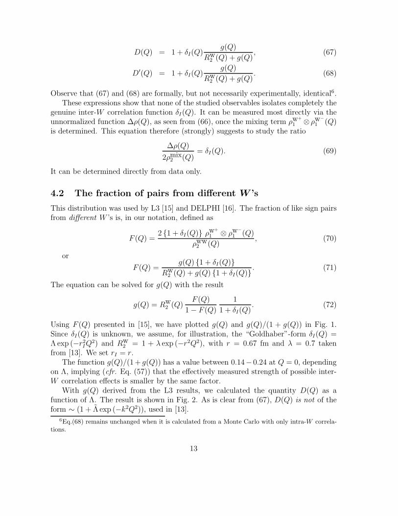
Using F (Q) presented in [15], we have plotted g(Q) and g(Q)/(1 + g(Q)) in Fig. 1.Since δI(Q) is unknown, we assume, for illustration, the “Goldhaber”-form δI(Q) =Λ exp (−r2

IQ2) and Rw

2 = 1 + λ exp (−r2Q2), with r = 0.67 fm and λ = 0.7 takenfrom [13]. We set rI = r.

The function g(Q)/(1+ g(Q)) has a value between 0.14− 0.24 at Q = 0, dependingon Λ, implying (cfr. Eq. (57)) that the effectively measured strength of possible inter-W correlation effects is smaller by the same factor.

With g(Q) derived from the L3 results, we calculated the quantity D(Q) as afunction of Λ. The result is shown in Fig. 2. As is clear from (67), D(Q) is not of theform ∼ (1 + Λ exp (−k2Q2)), used in [13].

6Eq.(68) remains unchanged when it is calculated from a Monte Carlo with only intra-W correla-tions.

13

To test for inter-W correlations, a density function, Rww2 (Q)BES, is defined in [15]

which is supposed to coincide with the data distribution Rww2,L3(Q) (defined below)

if inter-W correlations are absent. This function is stated to describe the data onRww

2,L3(Q), thus adding extra support to the claimed absence of inter-W BEC.The quantity Rww

2,L3(Q) is defined as the ratio of the like-sign two-particle densityin the data to the same obtained from a Monte Carlo model without Bose-Einsteincorrelations. Assuming that the model reproduces perfectly Rw

2 (Q), this quantity isgiven by

Rww2,L3(Q) =

Rw2 + g(Q) 1 + δI(Q)

1 + g(Q)= 1 +

Kw2 + g(Q)δI(Q)

1 + g(Q). (73)

The “test” function Rww2 (Q)BES is taken to be

Rww2 (Q)BES = 1 + 1 − F (Q) Kw

2 (Q), (74)

with F (Q) given by (71) and setting δI(Q) = 0. Equation (74) can then be written as

Rww2 (Q)BES = 1 +

1 + Kw2 (Q)

1 + Kw2 (Q) + g(Q)

Kw2 (Q). (75)

With δI(Q) = 0 in (73) for no inter-W correlations, it is seen that this distributionand that of Eq. (75) are different, unless Kw

2 (Q) = 0 or g(Q) = 0. We conclude that(74) is not suitable to test for the “null hypothesis” δI(Q) = 0. An analogous test-distribution, used by the DELPHI Collaboration for similar purposes (see below), hasthe same defect.

4.3 The DELPHI observables

In the DELPHI analysis of Bose-Einstein correlations in WW events [16], the followingratio is studied

Rdata4q =

ρww2 (Q)

ρww2,MC, no BE(Q)

, (76)

where the denominator is calculated from a Monte Carlo without Bose-Einstein effects.This can be rewritten using (50) as

Rdata4q (Q) =

Rw2 (Q)

1 + g(Q)+ 1 + δI(Q) g(Q)

1 + g(Q)= 1 +

Kw2 (Q) + g(Q)δI(Q)

1 + g(Q), (77)

which coincides with the general expression (56). We have assumed that, in the MonteCarlo, identical particle pairs are uncorrelated, i.e. ρw

2 (Q) = ρw1 ⊗ ρw

1 (Q).The function (77) is plotted in Fig. 3, together with Rw

2 (denoted by R2q in [16])measured in the DELPHI analysis and used here as input. From the above expression,

14

and from the figure, it is clear that this distribution remains sensitive to inter-Wcorrelations. However, it cannot, in general, be described by the same parameterizationas used for Rw

2 (Q), even for δI(Q) = 0. Fig.3 also shows, for illustration, the samefunction using a Gaussian parameterization of δI(Q) with a “radius-parameter” of3 fm. The latter might be typical for the range of second-order interference (HBT)correlations associated with incoherent strings. In this case, the Q-region affected byBEC is restricted to values below ∼ 100 MeV and will decrease even further for stilllarger “radii”.

In Fig. 4 we show the intercept, Rdata4q (Q) at Q = 0, and that of Rw

2 (Q), as a

function of Λ. It is seen that the intercept for the WW → 4q channel remains belowthat of Rw

2 (Q) for Λ < λ. It is, of course, independent of the values of the parametersr and rI .

4.3.1 R4q(Q)(mixing)

DELPHI also studied a “test” distribution, R4q(Q)(mixing), constructed from mixedindependent (WW → 2q) events and defined as

R4q(Q)(mixing) =

[

ρw2 (Q) + ρmix

2 (Q)]

data[

ρw2 (Q) + ρmix

2 (Q)]

MoCa, No Be

(78)

with ρmix2 (Q) = ρw+

1 ⊗ ρw−

1 . The above expression is equal to

R4q(Q)(mixing) = 1 +Kw

2 (Q)

1 + g(Q). (79)

This expression indeed coincides with (77) for δI(Q) = 0 and can thus be used to testfor inter-W correlations. It is plotted in Fig. 3 and depends here (weakly) on δI(Q)which enters the definition of g(Q). We remark again that R4q(Q)(mixing) cannot, in

general, be described by the same parameterization as used for Rw2 (Q).

Defining ∆λ(mixing) as the difference in intercepts at Q = 0 of R4q(Q)(mixing) and

Rdata4q we find

∆λ(mixing) = Λg(0)

1 + g(0), (80)

with Λ = δI(0).

4.3.2 R4q(Q)(linear)

A further quantity studied by DELPHI is R4q(Q)(linear), defined in Eq. (25) of ref. [16].

It is constructed to supposedly coincide with Rww2 (Q) if inter-W correlations are ab-

15

sent. With our notation it is given by

R4q(Q)(linear) = Rw2 (Q) +

1 − Rw2 (Q)

g(Q)

Rw2 (Q) + g(Q)

. (81)

This function is plotted in Fig. 5. The distribution differs from Rdata4q even for δI(Q) = 0

(or Λ = 0) and, therefore, has not the intended properties. Nevertheless, from Fig. 3and Fig. 5 it can be seen that R4q(Q)(linear) and R4q(Q)(mixing) are numerically quiteclose. The weak dependence on Λ is again due to the apriori unknown dependence ofg(Q) on δI(Q).

5 Summary

In this paper we described a mathematical formalism which should allow a systematicstudy and improved understanding of particle correlations in a physical system whichis composed of S possibly stochastically correlated parts. Most emphasis was put ontwo-particle inclusive densities and correlation functions for S = 2, but the formalismcan be extended to arbitrary orders and arbitrary S.

Taking the reaction e+e− → W+W− → q1q2q3q4 → hadrons as a prime example,it was shown how to relate the measurement of correlations within one hadronicallydecaying W to those measured in the full WW → 4q system.

For the observables used in present studies, correlations in fully hadronic WWdecay’s can be expressed in terms of the correlation function of a single W , an inter-Wcorrelation δI and a function, g, which quantifies the degree of overlap in momentumspace of the decay products from different W ’s.

On several examples, we have shown that some of the presently used techniques tosearch for inter-W correlations are not optimal. In some cases, experimental quanti-ties have been used which lack the correct mathematical properties and are based onintuition rather than on sound mathematics.

The determination of the overlap function allows to assess quantitatively the sen-sitivity of a particular distribution to inter-W correlations. Moreover, the influence ofexperimental and methodological cuts can be systematically investigated .

An estimate of g(Q), presented here, indicates that the fully hadronic, four-jet decaychannel of the reaction e+e− → W+W− may not be optimal to search for inter-W Bose-Einstein effects. The usual event selections, requiring four well-isolated jets in the finalstate, weaken the sensitivity to possible inter-W correlations. Better results may wellbe obtained in analyses using less stringent cuts, or which include e.g. three-jet eventswith suitably chosen topology so as to keep the QCD background at a tolerable level.

Our survey of some of the test-distributions used so far indicates that the observable∆ρ(Q), defined in Eq. (63), proposed in [8] and measured by L3 [13], provides a direct

16

measure of possible inter-W correlations. It suggests itself as suitable observable well-adapted for a global LEP-wide combination of WW data.

References

[1] For a recent review see: W. Kittel, Interconnection Effects and W+W− decays,Proc. XXXIVth Rencontres de Moriond, QCD and High Energy Interactions, LesArcs (France), Nijmegen preprint HEN-420, 1999; hep-ph/9905394 .

[2] L. Lonnblad and T. Sjostrand, Phys. Lett. B 351 (1995) 293.

[3] V.A.Khoze and T. Sjostrand, Eur. Phys. J. C6 (1999) 271.

[4] Z. Kunszt et al., in “Physics at LEP2”, eds. G. Altarelli, T. Sjostrand and F.Zwirner, CERN Report 96-01, Vol.1, p.141 (1996).

[5] B. Andersson, The Lund Model , Cambridge University Press, Cambridge, 1998.

[6] B. Andersson and M. Ringner, Nucl. Phys. B 513 (1998) 627; Phys. Lett. B 421(1998) 283; J. Hakkinen and M. Ringer, Eur. Phys. J. C5 (1998) 275.

[7] R. Hanbury Brown and R.Q. Twiss, Nature 178 (1956) 1046.

[8] S.V. Chekanov, E.A. De Wolf and W. Kittel, Eur. Phys. J. C6 (1999) 403.

[9] E.A.De Wolf, I.M. Dremin and W. Kittel, Phys. Reports 270 (1996) 1.

[10] A.H. Mueller, Phys. Rev. D4 (1971) 150.

[11] B. Buschbeck and P. Lipa, Phys. Lett. B223 (1989) 465.

[12] G. Alexander and E. Sarkisyan, Phys. Lett. B 487 (2000) 215.

[13] L3 Collaboration, M. Acciarri et al., Phys. Lett. B493 (2000) 23.

[14] ALEPH Collaboration, R. Barate et al. Phys. Lett. B 478 (2000) 50; ibidem,Further studies on Bose-Einstein correlations in W -pair decays, submitted toICHEP2000, Abstract 283.

[15] J.A. van Dalen, Bose-Einstein correlations in W -pair production at LEP: Results

from L3 and OPAL, preprint HEN-435, Nijmegen, 2000, to be published in Proc.IX Int. Workshop on Multiparticle Production “New frontiers in soft physics andcorrelations on the threshold of the third millennium”, Torino, Italy, June 12-172000; and private communication.

[16] DELPHI Collaboration, P. Abreu et al., Correlations between particles in e+e− →W+W− events , DELPHI 2000-115 CONF 414, submitted to ICHEP2000.

17

0

0.1

0.2

0.3

0.4

0.5

0.6

0.7

0.8

0.9

1

0 0.1 0.2 0.3 0.4 0.5 0.6 0.7 0.8 0.9 1Q (GeV)

g(Q)

g(Q)/(1+g(Q))

Figure 1: L3: the functions g(Q) and g(Q)/(1 + g(Q)); g(Q) is calculated assumingthe form δI(Q) = Λ exp (−r2

IQ2), rI = 0.67 fm, with Λ varying in the range 0.0 − 1.0,

in steps of 0.2.

18

0.8

1

1.2

1.4

1.6

1.8

2

0 0.1 0.2 0.3 0.4 0.5 0.6 0.7 0.8 0.9 1

Λ= 0

Λ= 1

D(Q)

R2q

Q (GeV)

D(Q

)

Figure 2: The test-statistic D(Q) used by L3, Eq.(67). Also shown is the L3 parame-terization of R2q(Q) ≡ Rw

2 (Q).

19

1

1.1

1.2

1.3

1.4

1.5

1.6

0 0.1 0.2 0.3 0.4 0.5 0.6 0.7 0.8 0.9 1

Λ= 0

Λ= 1 R4q

R4q rI=3 fm

R4qmix

R2q

Q (GeV)

Figure 3: DELPHI: The normalized densities R4q(Q) = Rww2 (Q), Eq.(77) in the

text, using as input the DELPHI parameterization of R2q(Q) ≡ Rw2 (Q) and assuming

δI(Q) = Λ exp (−r2Q2); Λ varies in the range 0.0 − 1.0, in steps of 0.2 The dashedcurves show the same with r = 3 fm. Also shown (dot-dashed) is the distribution,Eq.(79), corresponding to mixed independent WW → 2q events. It depends implicitlyon δI(Q) through the function g(Q).

20

1

1.1

1.2

1.3

1.4

1.5

1.6

0 0.2 0.4 0.6 0.8 1 1.2 1.4

R2q(Q=0)

R4q(Q=0)

Λ

Inte

rcep

ts

δI(Q)= Λ . exp(-r2Q2)

R2q(Q)=1 + λ . exp(-r2Q2)

Figure 4: DELPHI: The value of the normalized density R4q(Q) ≡ Rww2 (Q), Eq.(77)

in the text, and of R2q(Q) ≡ Rw2 (Q), at Q = 0, as a function of the parameter Λ in

δI(Q) = Λ exp (−r2Q2).

21

1

1.1

1.2

1.3

1.4

1.5

1.6

0 0.1 0.2 0.3 0.4 0.5 0.6 0.7 0.8 0.9 1

R4q

R4qlinear

R2q

Q (GeV)

Figure 5: DELPHI: The normalized density R4q(Q) ≡ Rww2 (Q), Eq.(77) in the text,

using as input the DELPHI parameterization of R2q(Q) ≡ Rw2 (Q) and with δI(Q) =

Λ exp (−r2Q2); Λ varies in the range 0.0 − 1.0 in steps of 0.2. Also shown is thedistribution corresponding to the so-called Linear Scenario in ref. [16].

22