CERN-TH.7011/93DTP/93/74

On Colour Rearrangement

in Hadronic W+W− Events

Torbjorn SjostrandTheory Division, CERN

CH-1211 Geneva 23, Switzerland

and

Valery A. KhozeDepartment of Physics, University of Durham

Durham DH1 3LE, England

Abstract

We discuss the possibility of colour rearrangement in e+e− →W+W− → q1q2q3q4 events,i.e. that the original colour singlets q1q2 and q3q4 may be transmuted, for instance, intonew singlets q1q4 and q3q2. The effects on event properties could be quite large if sucha rearrangement would occur instantaneously, so that gluon emission would be restrictedto each of the new singlets separately. We argue that such a scenario is unlikely for tworeasons. Firstly, the W+ and W− usually decay at separate times after the W+W− pro-duction, which leads to large relative phases for energetic radiation off the two constituentsof a rearranged system, and a corresponding dampening of the QCD cascades. Secondly,within the perturbative scenario the colour transmutation appears only in order α2

s andis colour-suppressed. Colour reconnection at longer time scales is quite feasible, however,and may affect the fragmentation phase. If so, the nature of non-perturbative QCD canbe probed in a new way. We formulate several alternative toy models and use these toestimate the colour reconnection probability as a function of the event kinematics. Pos-sible consequences for LEP 2 events are illustrated, with special attention to systematicerrors in W mass determinations.

CERN-TH.7011/93October 1993

1 Introduction

Consider the production of several colour singlet particles, which decay to coloured partonsclose to each other in space and time. A topical example, which will be used as a basisfor the continued discussion, is

e+e− →W+W− → q1q2 q3q4 (1)

at LEP 2. The outgoing partons first undergo a perturbative phase, in which showersof additional partons develop, and subsequently a non-perturbative phase, in which thepartons fragment into a hadronic final state. In this paper we will study the extent towhich the showering and fragmentation of one singlet can ‘interfere’ with that of the other,in such a way that observable event properties are affected. This is a topic about whichlittle is known today, but which has the potential to provide new insights, as we shall tryto show.

Since perturbative QCD is reasonably well understood, it is possible to predict withsome confidence what to expect on the partonic level. We will here demonstrate thatwithin the purely perturbative scenario these interference effects should be negligiblysmall. However, non-perturbative QCD is not yet well understood, and there is no obviousreason why interference effects should be small in the fragmentation process. It is thereforein this area that process (1) can be a very useful probe. We will develop and compare thepredictions of two main alternative models, which correspond to two different hypotheseson the structure of the QCD vacuum and of the confinement mechanism. With a lot ofhard work and some luck, LEP 2 could be in a position to provide some discrimination.

To illustrate what we mean by ‘interference’, consider process (1) above. The standardpoint of view is to assume the W+ and W− decays to be independent of each other. Apartfrom some spin-related correlations in the angular distribution of the W-decay products,each W system can then shower and fragment without any reference to what is happeningto the other. In particular, the perturbative parton emission is initiated by two separatecolour dipoles, q1q2 and q3q4. This picture should be valid if the W’s are long-lived, sothat the two W decays occur at well-separated points. In the other extreme, the W’s areassumed to decay ‘instantaneously’, so that the process really involves the production ofa q1q2q3q4 state in a single point. This state forms one single colour quadrupole, and itis the quadrupole as a whole that can emit additional partons and eventually fragment tohadrons. No trace is left of the individual identities of the W+ and W− decay products.

It is very difficult to obtain a complete description along the latter lines — all thestandard methods of dealing with the showering and fragmentation processes would beof little use. (The matrix element calculation approach would still be valid, but moredifficult to apply.) However, our experience with perturbative QCD in qqg events hastaught us that a colour quadrupole can be well approximated by the sum of two separatecolour dipoles, each of which is a net colour singlet. (There may also be contributionsfrom non-singlet dipoles, see below.) The new aspect is that we here have two sets of suchpotential dipoles, the original one, i.e. q1q2 and q3q4, and a colour rearranged set, q1q4and q3q2.

The possibility of having events with rearranged colour dipoles was first studied byGustafson, Pettersson and Zerwas (GPZ) [1]. Since they assume that the dipole mass setsthe scale for the amount of energetic gluon radiation and multiple soft particle productionto be expected, event properties may change a lot if the original dipoles are replaced bythe rearranged ones. The original dipoles each have the W mass, while the rearranged

1

ones may have much lower masses, if the kinematics is selected suitably. GPZ couldtherefore present large differences in the total multiplicity, the energy flow, the rapiditydistribution, and so on.

Unfortunately, this is not a very likely scenario. As we will show, the separationbetween the W+ and W− decay vertices is large enough that energetic QCD radiation willoccur independently within each original dipole, to a good first approximation. However,the fragmentation process is extending much further in space and time, and thus colourreconnection in this phase is a possibility. Observable event properties are less affectedby a reconnection that comes only after the perturbative phase [2], but this does notnecessarily mean that effects are negligibly small. Detailed studies of event shapes shouldhelp reveal the nature and size of colour rearrangement phenomena.

While interference effects are interesting in their own right, if there, they may alsoprovide a serious source of uncertainty. One of the main objectives of LEP 2 will be todetermine the W mass. This could either be done by a threshold scan of the cross section,or by a reconstruction of W masses event by event for some fixed energy above the W+W−

threshold. Currently the latter approach is the favoured one [3]. Fully hadronic decays,i.e. process (1), would seem to be preferable: jet energies need not be so well measuredin the calorimeters, since already a knowledge of the four jet directions would be enoughto constrain the kinematics and therefore the W masses. Electroweak effects, includinginitial state radiation, and effects of semileptonic c decays would be under control. Bycontrast, purely leptonic or mixed leptonic–hadronic decays suffer from a large missingmomentum vector given by the neutrino(s).

The main problem is that the assignment of hadrons to either of the two W’s is notunique. If only an experimental issue, the smearing could be estimated and corrected for.However, to this we now add an uncertainty in the colour structure of the event. So longas the original q1q2 and q3q4 dipoles shower and fragment independently of each other,the invariant masses of the hadrons belonging to these two systems, if separated correctly,add up to give the original W+ and W− masses, respectively. But if a reconnection occurs,e.g. to the alternative colour singlets q1q4 and q3q2 (or even more complicated systems),there is no concept of a conserved W mass in the fragmentation. This introduces anadditional element of smearing and, more dangerously, the potentiality for a systematicbias in the W mass determination. Clearly, such effects must be studied and understood,in order to be corrected for.

The possibility of colour rearrangements is not restricted to e+e− → W+W− events.Other examples could have been found: pp/pp →W+W−, e+e− → Z0Z0, e+e− → Z0H0,pp/pp→W±H0, H0 →W+W−, tt→ bW+bW−, etc. One could also add processes thatinvolve a single colour singlet particle interfering with the beam jets of a pp event, such aspp→W±, or even interactions among beam jets themselves, such as in multiple parton–parton interaction events or in heavy ion collisions. The problem with the latter processesis that there are so many other uncertainties that any chance of systematic studies wouldbe excluded. By contrast, in e+e− → W+W− events, the decay of a non-interfering Wpair is very well understood, thanks to our experience with Z0 decays at LEP 1.

The hadronic decay of a B meson is another typical example of a colour quadrupolestructure. J/ψ production in such decays is the one place where colour reconnectionhas already been observed (see discussion and additional references in ref. [1]): in ab→ c + W− → c + c + s decay the c and c belong to separate colour singlets, but appearalmost simultaneously and can therefore coherently form a colour singlet state such asthe J/ψ. Of course, the number of colours not being infinite, there is a finite chance

2

of 1/N2C = 1/9 that the c and c are in a colour singlet configuration. However, this

kind of accidental colour ambiguities is not what we imply by colour rearrangement —after all, had the W been a long-lived particle, so that the c and c were produced faraway, the question of whether they are in a relative octet or singlet state would havebeen moot. (Accidental ambiguities do not spoil the original colour singlet combinations,such as c + s, but only add more.) Further, while difficult to estimate, it seems that thecolour reconnection probability in B decay is more like 20%, i.e. higher than the abovemaximum. In this paper we will therefore concentrate on dynamical models for colourrearrangement, and leave aside the accidental possibility. Anyway, one should not use thedetails of B→ J/ψ phenomenology to provide any specific input for W+W− production,since the space–time evolution and the capability to radiate energetic gluons are ratherdifferent in the two processes.

To summarize, there are two main reasons to study the phenomenon of colour rear-rangement:

1. In its own right, since it provides a laboratory for a better understanding of thespace–time structure of perturbative and non-perturbative QCD.

2. As a potential source of error to W mass determinations and other measurements.(In the end, the precision of the theoretical predictions has to match the experimen-tal accuracy, or even exceed it.)

We cannot today predict what will come out of experimental studies at LEP 2, butwant to provide here some comments on what one could plausibly expect under somesimplified alternative scenarios. This might form a reasonable starting point for morerefined theoretical and experimental studies in the future.

The plan of the paper is therefore as follows. In section 2 we show what maximal effectscould be expected if colour rearrangement always took place, either ‘instantaneously’ oronly later, between the parton shower and the fragmentation phases. These ‘worst case’or ‘best case’ scenarios, depending on the point of view, are subsequently rejected infavour of more realistic ones. In Section 3 we show why one would not expect sizeableeffects on the perturbative level, based on the time separation between the W+ and W−

decays, and on colour algebra. The subsequent discussion is therefore concentrated oneffects in the fragmentation process: in Section 4 we describe different ways of estimatingthe colour rearrangement probability as a function of event topology, and in Section 5some experimental consequences are discussed. Finally, Section 6 contains a summaryand outlook.

2 Maximal effects of colour reconnection

The objective of this section is purely didactic: to familiarize readers with possible exper-imental consequences of colour rearrangements. Our ‘best bet’ estimates of such effectswill be presented in Section 5. The current section is here mainly because it is neededto appreciate the significance of Sections 3 and 4. The naıve scenarios we introduce hereshould be taken for what they are: extremely simple recipes for colour reconnection, inwhich a number of known complications are swept under the carpet. In particular, theW+ and W− are assumed to decay instantaneously, so that there is no space or timeseparation between the two decay vertices.

In order to stay as close as possible to the studies of GPZ, we first consider two Wbosons produced at rest, each with the nominal mass mW = 80 GeV, decaying into the

3

final state ud + du, with an opening angle of 30 between u and u, Fig. 1a. To firstapproximation, one may then entertain three alternatives:

1. In the no-reconnection scenario, the ud and du systems shower and fragment inde-pendently of each other, Fig. 1b. The event therefore looks like two overlayed e+e−

annihilation events at rest, each with 80 GeV c.m. energy. This scenario is justwhat one expects from an extreme perturbative point of view.

2. In the GPZ ‘instantaneous’ reconnection scenario, two colour singlets uu and ddare immediately formed, each then having an invariant mass of 20.7 GeV and anet motion away from the origin. These systems subsequently shower and fragmentindependently of each other, Fig. 1c. There is only little radiation, since the maxi-mum scale for that radiation is 20 GeV rather than 80 GeV. The final event lookslike two strongly boosted 20 GeV e+e− annihilation events. We do not know of anyphysics mechanism that would lead to this scenario (except maybe as a rare fluc-tuation), but include it since it was advocated by GPZ and since it gives maximaleffects.

3. In the intermediate reconnection scenario, a reconnection occurs between the showerand fragmentation steps. Therefore the original ud and du colour singlet systemsshower, each with maximum virtuality 80 GeV, just as in the no-reconnection sce-nario. Stricty speaking, the gluons emitted in the ud system are not uniquely associ-ated to either the u or the d. However, in practice, the shower algorithm used [4] doesallow a pragmatic subdivision of the radiation into two subsets, essentially (but notquite) by hemisphere. For instance, if partons are ordered in colour/string/dipoleorder, a W+ (W−) branching to ug+

1 g+2 g+

3 d (dg−1 g−2 g−3 g−4 u) may be split into twosubsets ug+

1 and g+2 g+

3 d (dg−1 g−2 g−3 and g−4 u). After the showers, the partons cantherefore be reconnected into two new colour singlets, ug+

1 g−4 u and dg−1 g−2 g−3 g+2 g+

3 d.Each of these systems then fragments separately, Fig. 1d. In the limit αs → 0, i.e.when energetic QCD radiation is switched off, this coincides with the instantaneousscenario. In practice, however, QCD radiation is profuse, and the masses of the twofragmenting systems is substantially above the 20 GeV nominal value.

Fragmentation is assumed to be given according to the Lund string model [5] (see alsoSection 4.1). Events are generated with the Jetset 7.3 program [6], which is known towell describe the e+e− → qq events in the 10–100 GeV mass range.

Some simple results are presented in Fig. 2. The event axis (with respect to whiche.g. rapidity is defined) is here the theoretical one, i.e. intermediate between the original uand u directions. The total multiplicity is about a factor of 2 lower for the instantaneousreconnection scenario: 〈nch〉 = 21.8 versus 40.0 for no reconnection and 37.8 for theintermediate one. The first number reflects the lower invariant mass of the colour singletsystems. The instantaneous scenario contains two strongly boosted systems with nothingin between; therefore the rapidity distribution has a very strong dip in the middle, Fig. 2b,which is reflected in the multiplicity distribution for the central rapidity region, |y| < 1,Fig. 2c. It is also visible in the charged particle flow in the event plane, Fig. 2d, whereparticle production at around 90 to the event axis is suppressed. It is maybe a bit moresurprising that the instantaneous scenario does not have more particle production thanthe no-reconnection one at 0; after all, this is the region where a string connects the u(d) and u (d) partons of the instantaneous events, while no such string is present in theno-reconnection ones. Our interpretation is that this shows how large the effects of QCDradiation are, i.e. that radiation with an 80 GeV maximum virtuality scale leads to anoverwhelmingly large broadening of jet profiles.

4

In all the distributions, the intermediate scenario deviates much less from the standardone than does the instantaneous. This means that the particle flow is to a large extentdominated by the perturbative gluon emission phase, at least when this phase is assumedto be valid down to a cut-off scale of Q0 ≈ 1 GeV and gluon emission is therefore profuse.However, the effects of the intermediate scenario seem puny only when compared withthe instantaneous one: the differences between the no- and intermediate-reconnectiondistributions of Fig. 2b (e.g.) would be easily distinguishable experimentally.

The problem is that the kinematics we have considered so far is totally unrealistic.While effects are largest when the two W’s are produced at rest, this is the point wherethe phase space for production is vanishing. Next we therefore have to introduce somesemi-realistic experimental conditions.

In order to generate complete e+e− → W+W− → q1q2q3q4 events, we use thePythia 5.6 event generator [7]. The W+W− pair is here distributed according to theproduct of three terms: a Breit-Wigner for each W, and a basic e+e− →W+W− matrixelement (which is a function of the actual W± masses) [8]. Subsequently each W decays toa qq pair, ud, us, cd, cs or their charge conjugates. The decay angles are properly corre-lated [9]. This is followed by perturbative parton shower evolution and non-perturbativefragmentation, as above. Initial state photon radiation can and should also be includedfor detailed experimental studies, but is omitted for most of the studies below.

To illustrate the size of the effects, consider a c.m. energy of 170 GeV, i.e. some dis-tance above the threshold. The nominal input W mass is 80 GeV; the average generatedmW is somewhat lower, predominantly because of phase-space effects.The charged mul-tiplicity distribution is shown in Fig. 3a for the scenarios 1–3 above. Clearly differencesare nowhere as drastic as in Fig. 2a: the average values are 36.6 without recoupling, 36.2with intermediate, and 33.7 with instantaneous recoupling. In part this is related to anaveraging over various event topologies in Fig. 3, where Fig. 2 was only for one particu-larly favourable configuration. In part one also expects smaller differences further awayabove threshold, since the difference in mass between original and reconnected colour sys-tems is reduced. The latter effect is particularly easy to understand if one considers theregion far above threshold, where the two W’s and their respective decay products arestrongly boosted away from each other, and a reconnection between the two widely sepa-rated systems in fact leads to an increase in system masses, i.e. opposite to the thresholdbehaviour.

The charged rapidity distribution with respect to the thrust axis, Fig. 3b, and thenumber of charged particles in |y| < 1, Fig. 3c, also show much lesser differences thanthose observed in Figs. 2b and 2c. In particular, the change in kinematics leads to a muchnarrower central rapidity dip. Qualitatively, however, differences are still there. This isparticularly obvious in the low-multiplicity part of Fig. 3c. Differences can be enhancedby various cuts, e.g. by requiring a large thrust value.

As a final exercise, we study the task of W mass determination. This is an importanttopic in itself [3], and it is not our intention here to optimize an algorithm so as tominimize statistical errors. Rather, the objective is to find whether any systematic effectsarise from reconnections.

The details of our W mass reconstruction algorithm will be presented in Section 5.3.For the moment, suffice it to say that four jets are reconstructed per event (events withouta clear four-jet structure are rejected), assuming that particle four-momenta are fullyknown. The jets are paired to give two W masses, which are then averaged to give onemW = (mW+ + mW−)/2 number per event. The difference between the reconstructed

5

and the generated mW is shown in Fig. 3d. By the procedure adopted, the distributionsthus do not contain any spread from the intrinsic Breit-Wigner shape of the W’s or fromdetector imperfections. Any spread comes from misassignments of particles to jets. Largedeviations may occur when entire subjets are incorrectly clustered.

If one considers the range ±10 GeV of difference between reconstructed and generatedmasses, the average and spread is −0.28 ± 1.57 GeV for the no-reconnection scenario,−0.14 ± 1.60 GeV for the intermediate one, and 0.30 ± 1.55 GeV for the instantaneousone. The fraction of W’s with deviations larger than ±10 GeV is 1.5%, 1.5% and 1.7%, re-spectively. Compared with the no-reconnection scenario, the intermediate (instantaneous)one gives a systematic shift of over 100 (500) MeV. The aimed-for statistical error on theW mass is roughly 50 MeV. It is therefore of importance to understand whether thesecolour reconnection numbers above have to be included as a systematical uncertainty, orwhether reconnection effects are only a small fraction of this.

3 The perturbative picture of colour rearrangement

In this section we want to discuss the colour dynamics of particle flow in W+W− eventsfrom a purely perturbative point of view. The non-perturbative standpoint will follow inSection 4.

3.1 Introduction to the perturbative approach

During the last years experiments, especially at the Z0 pole, have provided an exceed-ingly rich source of information on the jet structure of final states in hard processes (seee.g. ref. [10]). These data have shown that, at high energies, the main characteristics ofmultihadronic events are determined by the perturbative stage of the process evolution.Analytical perturbation theory — the perturbative approach [11] — provides a quanti-tative description of inclusive particle production in jets. In the perturbative approachthe resummation of the perturbative series is performed, and the terms of relative or-der√αs are taken into account in a systematic way — the modified leading logarithmic

approximation (MLLA). Under the key assumption that the non-perturbative hadroniza-tion process is local in the configuration space of partons, the infrared singularities can befactorized out of hadron distributions. If so, the asymptotic shapes of these distributionsare fully predicted — the hypothesis of local parton–hadron duality (LPHD). Data agreeremarkably well with the predictions of the MLLA–LPHD framework [12].

Until now, the perturbative approach was applied only to systems of partons producedalmost simultaneously, with a short time scale

tprod ∼1E 1

µ, (2)

where E is the hard scale of the production process and µ−1 ≈ 1 fm is the character-istic strong interaction time scale. The radiation accompanying such a system can berepresented as a superposition of gauge invariant terms, in which each external quarkline is uniquely connected to an external antiquark line of the same colour. The de-scription of gluons is straightforward: remember that a gluon has both a quark and anantiquark colour index. The system is thus decomposed into a set of colourless qq an-tennae (dipoles). One of the simplest examples is the celebrated qqg system, which (to

6

leading order in 1/N2C) is well approximated by the sum of two separate antennae/dipoles.

The perturbative treatment of the qq antennae is based on the following key ideas:1. The principal source of multiple hadroproduction is gluon bremsstrahlung caused by

conserved colour currents. Therefore the flow of colour quantum numbers, reflectingthe dynamics at short distances, controls the particle distributions in the final state.

2. The evolution of a quark jet is viewed as a sequence of coherent parton branchings.In the final state, an original quark jet is enshrouded by secondary partons resultingfrom radiation of quasi-collinear and/or soft gluons with momenta k and transversemomenta k⊥ in the range

µ . k⊥ k E . (3)

It is the large probability for such emissions,

W ∼ αsπ

ln2E ∼ 1 (4)

that leads to the well-known double logarithmic phenomena in jet development.In this approach, the particle multiplicity is obtained as the convolution of the probabilityof primary gluon bremstrahlung off the parent quarks with the multiplicity initiated bysuch a gluon [11].

Any restriction on the primary gluon energy to be well below E

k . kmax E (5)

drastically reduces the perturbatively induced multiplicity and makes the qq antennapractically inactive [11, 13]. As we shall see, this is of relevance for colour rearrangedsystems in W+W− events.

3.2 W-pair decays in the perturbative approach

Encouraged by the successes of the perturbative approach, one could be tempted to applythe same quark–gluon dynamics to the description of the final state in process (1). Inparticular, each individual W± decay corresponds to a parton shower at almost the samescale as the well-studied Z0 → qq case.

As we shall show, the emission of a single primary gluon (which subsequently initiatesa coherent parton shower) corresponds to the no-reconnection scenario. Within the per-turbative approach, colour transmutations can result only from the interferences betweengluons (virtual as well as real) radiated in the two decays. Rearrangements of the colourflows should lead to a dependence of the structure of final particle distributions on therelative angles between the jets originating from the different W’s (on top of what maybe there from trivial kinematics).

It is the goal of this section to demonstrate why the colour reconnection effects, viewedperturbatively, are strongly suppressed. Our argumentation below is based on two mainreasons, which are deeply rooted in the basic structure of QCD:

1. Because of the group structure of QCD, at least two gluons should be emitted togenerate the colour rearrangement. Moreover the interference piece proves to besuppressed by 1/N2

C as compared to the O(α2s) no-reconnection emissions.

2. The effects of the W width ΓW strongly restrict the energy range of primary gluonsgenerated by the alternative systems of type q1q4 and q3q2. Not so far from theW+W− threshold one expects

k . kreconmax ∼ ΓW . (6)

7

Therefore the would-be parton showers initiated by such systems are terminatedat a virtuality scale of O(ΓW), and can hardly lead to sizeable fluctuations in thestructure of the hadronic final state.

3.3 Single-gluon emission in W pair decays

Let us first consider the emission of a single primary soft gluon of four-momentumk, see Fig. 4. The momenta of the final state quarks are labelled by e+e− →q1(p1) q2(p2) q3(p3) q4(p4), with Q1 = p1 + p2 and Q2 = p3 + p4. Denote by M (0) thenon-radiative Feynman amplitude with the W propagators removed and introduce theconserved currents Jµ(k), J ′µ(k) generated by the individual W decays. In the limitk pi the amplitude M (1) for gluon radiation accompanying process (1) is then

M (1) ≡ (M (1))injm = gs M(0)[(T a)ij δ

nm (J(k) · ελ) + δij (T a)nm (J ′(k) · ελ)

], (7)

where gs is related to the strong coupling constant by αs = g2s/4π, ελ is the gluon polar-

ization vector, T a are the SU(3) colour matrices, and a = 1, . . . , 8 and i, j,m, n = 1, 2, 3are colour labels.

The W± propagator functions D are absorbed into the definition of the currents Jµ(k),J ′µ(k) [14]

Jµ(k) = jµ(k)D(Q1 + k)D(Q2) ,J ′µ(k) = j′µ(k)D(Q1)D(Q2 + k) , (8)

where

jµ(k) =pµ1p1 · k

− pµ2p2 · k

,

j′µ(k) =pµ3p3 · k

− pµ4p4 · k

(9)

describe the gauge-invariant soft gluon emission from two colour charges of momenta p1, p2

(p3, p4). The expression for the propagator function is

D(Q) =1

Q2 −m2W + imWΓW

. (10)

To emphasize that the emission is generated primarily by the conserved currents jµ, j′µ

we have introduced the ‘radiative blobs’ in Fig. 4 and in what follows.In order to obtain the differential distribution for gluon emission we have to square the

matrix element, sum over colours and spins, and integrate over the Q21 and Q2

2 virtualities.We find (see also [13, 14])

1σ(0) dσ(1) =

d3k

ω

CF αs4π2 F

(1) , (11)

F (1) =(mWΓW

π

)2 ∫dQ2

1 dQ22

[−J · J † − J ′ · J ′†

], (12)

where ω = k0 is the gluon energy and CF = (N2C − 1)/2NC = 4/3.

8

In the massless quark limit the radiation pattern F (1) is given by

F (1) = 2 (12 + 34) , (13)

where the qq ‘antennae’ are defined by [11]

ij =(pi · pj)

(pi · k)(pj · k). (14)

Near threshold, where the decay products of a W are almost back-to-back,

F (1) =2ω2

(1− cos θ12

(1− cos θ1)(1− cos θ2)+

1− cos θ34

(1− cos θ3)(1− cos θ4)

)

≈ 4ω2

( 1sin2 θ1

+1

sin2 θ3

), (15)

where θi is the angle between parton i and the gluon, and θij the angle between partonsi and j.

Let us emphasize that on the level of single gluon emission, real as well as virtual, thetwo antennae q1q2 and q3q4 do not interact and the colour flows are not rearranged. Theabsence of such an interaction is easily seen from the diagram of Fig. 5, which representsthe decay–decay radiative interference contribution to the cross section of process (1). Atthe position of the vertical dashed line, both the q1q2 and the q3q4 subsystems have tobe in colour singlet states (in order to couple to the W’s), so the gluon octet charge isuncompensated.

3.4 Double-gluon interference effects in W-pair decays

At least two primary gluons, real or virtual, should be emitted to generate a colour flowrearrangement, see Figs. 6–8. Note that the diagrams of Figs. 6a and 6b do not interferewith each other, and that the diagrams of Fig. 7 could interfere with those of Fig. 4,thus inducing a colour transmutation. The infrared divergences in the virtual pieces arecancelled by the corresponding real emissions. For the case of decay–decay radiativeinterference the soft emissions are cancelled in the inclusive cross section up to at leastO(ΓW/mW) (see [15, 16] and below).

The main qualitative results for the reconnection effects appearing in O(α2s) are not

much different for various decay–decay interference samples. We shall examine below oneexample corresponding to the diagrams of Fig. 6a. In the limit k1, k2 pi the matrixelement can be written as

M (2)a = g2

s M(0)

[(T a)ij (T b)nm (j(k1) · ε(1)

λ ) (j′(k2) · ε(2)λ′ )D(Q1 + k1)D(Q2 + k2)

+a↔ b, k1 ↔ k2, ε

(1)λ ↔ ε(2)

λ′

], (16)

where k1,2 are the momenta of the soft gluons and ε(1)λ , ε(2)

λ′ are their polarization vectors.After summing over colours and spins, the interference term may be presented in the

form

1σ0

dσinta '

d3k1

ω1

d3k2

ω2

(CF αs4π2

)2 1N2C − 1

12F inta , (17)

F inta = 2χ12 (j(k1) · j′(k1)) (j(k2) · j′(k2)) , (18)

9

with− (j(k) · j′(k)) = 14 + 23− 13− 24 . (19)

Here χ12 is the so-called profile function [13, 14], which controls the decay–decay interfer-ences:

χ12 =(mWΓW

π

)2

<∫

dQ21 dQ2

2D(Q1 + k1)D∗(Q1 + k2)D(Q2 + k2)D∗(Q2 + k1) , (20)

where D∗ is the complex conjugate of D and < represents the real part. The profilefunction has the formal property that χ12 → 0 as ΓW → 0 and χ12 → 1 as Γ→∞.

The interference is suppressed by 1/(N2C − 1) = 1/8 as compared to the total rate of

double primary gluon emissions (related to the square of diagrams of the type of Fig. 6),see eq. (17). This is a result of the ratio of the corresponding colour traces,

Tr(T aT b) · Tr(T aT b)Tr(T aT a) · Tr(T bT b)

=(CF NC)/2(CF NC)2 =

1N2C − 1

. (21)

Such a suppression takes place for any decay–decay radiative interference piece, real aswell as virtual, as is clear from Fig. 8.

Near threshold and in the limit of massless quarks the interference contribution to theradiation pattern is

F inta =

2χ12

ω21 ω

22

16 cosφ13 cos φ13

sin θ1 sin θ3 sin θ1 sin θ3, (22)

where θi (θi) is the angle between the qi and the gluon k1 (k2), and φ13 (φ13) is therelative azimuth between q1 and q3 around the direction of the k1 (k2). The expression ineq. (22) evidently contains a dependence on the relative orientation of the decay productsof the two W’s. (The interference is maximal when all the partons lie in the same plane,φ13 = φ13 = 0, cf. eqs. (15) and (22).) Therefore one might expect that the decay–decayinterferences would induce some colour-suppressed reconnection effects in the structure offinal states in process (1).

3.5 W width effects

It is the profile function χ12 that cuts down the phase space available for gluon emissionsby the alternative quark pairs (or by any accidental colour singlets) and thus eliminatesthe very possibility for the reconnected systems to develop QCD cascades. That the Wwidth does control the radiative interferences can be easily understood by considering theextreme cases.

If the W-boson lifetime could be considered as very short, 1/ΓW → 0, both the q1q2and q3q4 pairs appear almost instantaneously, and they radiate coherently, as thoughproduced at the same vertex. In the other extreme, ΓW → 0, the q1q2 and q3q4 pairsappear at very different times t1, t2 after the W+W− production,

tprod ∼1mW ∆t = |t1 − t2| ∼

1ΓW

. (23)

The two dipoles therefore radiate gluons and produce hadrons according to the no-reconnection scenario.

The crucial point is the proper choice of the scale the W width should be comparedwith. That scale is set by the energies of primary emissions, real or virtual [13, 14, 15]. Let

10

us clarify this supposing, for simplicity, that we are in the W+W− threshold region. Therelative phases of radiation accompanying two W decays are then given by the quantity

ωi ∆t ∼ωiΓW

. (24)

When ωi/ΓW 1 the phases fluctuate wildly and the interference terms vanish. This is adirect consequence of the radiophysics of the colour flows [11] reflecting the wave dynamicsof QCD. The argumentation remains valid for energies above the W+W− threshold as well.Suppression of the interference in the case of radiation with ωi ΓW can be demonstratedalso in a more formal way.

One can perform the integration over dQ21 and dQ2

2 in eq. (20) by taking the residuesof the poles in the propagators. This gives

χ12 =m2

WΓ2W (κ1κ2 +m2

WΓ2W)

(κ21 +m2

WΓ2W) (κ2

2 +m2WΓ2

W), (25)

withκ1,2 = Q1,2 · (k1 − k2) . (26)

For the interference between the diagrams of Fig. 6b, the corresponding profile functionis given by the same formula with k2 → −k2. Near the W+W− pair threshold eq. (25) isreduced to

χ12 =Γ2

W

Γ2W + (ω1 − ω2)2 . (27)

From eq. (27) it is clear that only primary emissions with ω1,2 . ΓW can inducesignificant rearrangement effects: the radiation of energetic gluons (real or virtual) withω1,2 ΓW pushes the W propagators far off their non-radiative resonant positions, sothat the propagator functions D(Q1 + k1) and D(Q1 + k2) (D(Q2 + k1) and D(Q2 + k2))corresponding to the same W practically do not overlap. We can neglect the contribu-tion to the inclusive cross section from kinematical configurations with ω1, ω2 ΓW,|ω1 − ω2| . ΓW since the corresponding phase-space volume is negligibly small.

Equation (25) clearly shows that χ12 vanishes if any of the scalar products Qi ·kj (i, j =1, 2) well exceedsmWΓW. Again accidental kinematics with κ1, κ2 mWΓW is suppressedbecause of phase space reasons. Hence all our arguments concerning cutting down theQCD cascades induced by the alternative systems remain valid above the threshold aswell. The smallness of the decay–decay radiative interference for energetic emission in theproduction of a heavy unstable particle pair, at the threshold and far above it, proves tobe of a general nature. For the case of e+e− → bW+bW− this was explicitly demonstratedin ref. [14].

At very high energies E mW the energy scale of the would-be QCD showers gener-ated by the alternative systems is restricted more strongly,

kreconmax ∼

ΓW mW

EW. (28)

Within the framework of a perturbative analysis such a restriction makes sense only if

η = µEW

mW ΓW. 1 . (29)

11

Remembering that the lifetime of a W in the laboratory frame is

tdec ∼EW

mW

1ΓW

(30)

one can easily see that as long as η < 1, the requirement of perturbative soft gluons ω > µautomatically implies that a W decays before the formation of the first light hadrons fromthe QCD cascades.

In the extreme ultrarelativistic limit, when η = µ tdec 1, the energy of primaryperturbative gluons becomes limited from below, ω > µη. This restriction arises fromthe relationship between tdec and the gluon hadronization time,

tdec < thad ∼ω

µ2 . (31)

The profile function χ12 in such an extreme case decreases with increasing energy and thedecay–decay radiative interference is strongly suppressed. For instance,

χ12 ∼(µ

ω

)2 1η2 <

1η4 for µη < ω < ΓW ,

χ12 <m2

W

E2W

for ω > ΓW . (32)

Therefore, in addition to the α2s and 1/N2

C suppression effects noted above, any re-connected quark system (including accidental colour singlets) proves to be practicallyinactive. The bulk of radiation (and thus of multihadron production) in the final state ofprocess (1) is governed by the original q1q2 and q3q4 antennae, which radiate the primarygluons with ω ΓW that initiate coherent showers. The corresponding hard scale forthe non-reconnected parton showers is mW. Also accounting for cascade multiplication,the yield of the reconnection-sensitive particles can be quantified as the multiplicity at ahard scale of O(ΓW).

All the argumentation based on the effects of a phase difference between the radiationsaccompanying two W decays remain valid also in the case when one of the W bosons ispractically real and the other is far off the mass shell, i.e. t1 ∼ 1/ΓW and t2 ∼ 1/mW.This case could be of interest for the intermediate mass Higgs decay [2]. The effects ofthe profile function χ12 are the same for t2 t1 ∼ 1/ΓW as when t1, t2 ∼ 1/ΓW.

3.6 Structure of inclusive particle flow in W-pair events

Let us discuss the general topology of events corresponding to process (1). The single-inclusive particle flow (antenna–dipole pattern) may be written as (see ref. [11] for details)

8π dNdΩn

= 2 [(12) + (34)] N ′q(mW

2

)+R [(14) + (23) − (13)− (24)] N ′q (krecon

max ) . (33)

The distribution (ij) describes the angular radiation pattern of the ij antenna,

(ij) ≡ ω2 (ij) =aijai aj

=1− ninj

(1− nin)(1− njn), (34)

where the ni,j denote the directions of the q/q momenta and n the direction of the regis-tered flow. The factors

N ′q(Ejet) =d

d lnEjetNq(Ejet) , (35)

12

with Nq(Ejet) the multiplicity inside a QCD jet of energy/hardness Ejet, take into accountthe cascade particle multiplication. Approximately [11],

N ′qNq'√

2NCαsπ

(1 +O(√αs)) . (36)

The factor R describes the rearrangement strength. In principle, it could be computedwithin the perturbative scenario. However, for the purposes of this paper we shall herepresent only some order-of-magnitude estimates. Each squared diagram of Figs. 4, 6and 7 (as well as the set of corresponding higher-order diagrams) contribute to the no-recoupling first term in eq. (33). Interferences between the diagrams of Fig. 6a and Fig.6b and between the diagrams of Fig. 7 and Fig. 4 exemplify the lowest-order contributionto the reconnecting interference piece.

It follows from the discussion in the previous subsections that the rearrangementcoefficient is expected to be

R . O(αsN2C

). (37)

Moreover, the suppression of energetic radiation accompanying the reconnected systemsmakes the corresponding cascades practically sterile, so the rearrangement affects only afew particles,

Nq(kreconmax )

Nq(mW/2)∼ O(10−1) . (38)

Because of both these factors, the magnitude of the reconnection effects in the perturbativescenario is expected to be numerically small, O(10−2) or less. This gives the factor bywhich the maximal perturbative effects shown in Section 2 should be scaled down for arealistic estimate of perturbative reconnection effects.

One can derive the antenna pattern corresponding to colour transmutation (the secondterm in eq. 33), for instance by examining the interference between the diagrams ofFig. 7 with those of Fig. 4. The same structure appears for the interference contributionscorresponding to the diagrams of Fig. 6a and Fig. 6b after integration over the momentumof one of the emitted gluons. The infrared divergences corresponding to the unobservedgluon are cancelled when both real and virtual emission contributions are taken intoaccount.

From the antenna patterns given by eqs. (19) and (33) one immediately sees that, inaddition to the two rearranged dipoles q1q4 and q3q2 present in the GPZ string picture, twoother terms q1q3 and q2q4 appear. As was mentioned before, these terms are intimatelyconnected with the conservation of colour currents. Moreover, the 13 and 24 antennaecome in with a negative sign. In general, QCD radiophysics predicts both attractiveand repulsive forces between quarks and antiquarks, see refs. [11, 17, 18]. Normally therepulsion effects are quite small, but in the case of colour-suppressed phenomena theymay play an important role.

One can easily understand the physical origin of the attraction and repulsion effectswith the help of the ‘QED’ model of ref. [18], where quarks are replaced by leptons. Forillustration, the photonic interference pattern in

γγ → Z0Z0 → e+e−µ+µ− (39)

could be examined. In addition to the attractive forces between opposite electrical charges([e−µ+ and [e+µ− QED-antennae) there is a negative-sign contribution ([e−µ− and [e+µ+

13

QED-antennae) corresponding to the repulsive forces between two same-sign charges. InQED there is no equivalent to the colour suppression factor, so in the limit ΓZ →∞ (i.e.χ12 → 1) the dipole radiation structure is simply given by the expression

[e−e+ +\µ−µ+ +([e−µ+ +[e+µ− −[e−µ− −[e+µ+

). (40)

For instance, near the Z0Z0 threshold, the total interference is maximal and constructive(destructive) when e− is collinear with µ− (µ+); for ΓZ → ∞ the radiation pattern isequivalent to that induced by a charge −2 (charge 0) particle.

By contrast to the perturbative QCD description, only the positive-sign dipoles appearin the Lund string model. This is because each string corresponds to a colour singlet,while the negative-sign qq/qq dipoles correspond to non-singlets (antitriplets/sextets).There need not be a physics conflict between the two pictures: one should rememberthat the perturbative approach describes short-distance phenomena, where partons maybe considered free to first approximation, while the Lund string picture is a model forthe long-distance behaviour of QCD, where confinement effects should lead to a subdivi-sion of the full system into colour singlet subsystems (ultimately hadrons) with screenedinteractions between these subsystems.

Also the role of colour quantum numbers may differ, as follows. Reconnection issuppressed by a factor 1/(N2

C − 1) in the perturbative description. The same suppressionwould appear in the non-perturbative string model if only endpoint quark colours wereconsidered. For instance, in the W+W− → q1q2q3q4 process, with perturbative gluonemission neglected for the moment, the q1q4 system would have to be in a colour singletstate for a reconnection to be possible. However, in a realistic picture, the string itself ismade up of a multitude (an infinity) of coloured confinement gluons. Therefore all coloursare well represented in the local neighbourhood of any potential string reconnection point.The local gluons can then always be rearranged in such a way that colour neutrality ismaintained for the reconnected systems. Although some suppression of the reconnectionprobability might well remain, as a first guess we will assume that there is no suchsuppression in the non-perturbative phase.

Let us come now to the issue of observability of the reconnection effects in a real-lifeexperiment. Analogously to the string [19] / drag [17] effect, colour rearrangement couldgenerate azimuthal anisotropies in the distributions of the particle flow. That is, in therest frame of one W the particle distribution relative to the daughter-quark directioncould become azimuthally asymmetric (on top of the trivial kinematical effects causedby the overlap with the decay products of the other W). Such an asymmetry should bestrongly dependent on the overall topology of the 4-jet q1q2q3q4 system. It is instructiveto note that the negative-sign (13) and (24) dipoles of eq. (33) in fact act to increase themagnitude of the string-like anisotropy effects of the (14) and (23) dipoles.

It should be emphasized that, analogously to the other colour-suppressed interferencephenomena (see refs. [11, 17, 20]), the rearrangement phenomenon can be viewed only on acompletely inclusive basis, when all the antennae–dipoles are simultaneously active in theparticle production. The very fact that the reconnection pieces are not positive-definitereflects their wave interference nature. Therefore the effects of recoupled sterile cascadesshould appear on top of a background generated by the ordinary-looking no-reconnectiondipoles.

Again there is an important difference between the perturbative QCD radiophysicspicture and the non-perturbative string model. The latter not only allows but even

14

requires a completely exclusive description: in the end the q1q2q3q4 system must besubdivided into and fragment as two separate colour singlets, either q1q2 and q3q4 orq1q4 and q3q2. (Neglecting the fact that the recoupling and fragmentation will involveadditional partons emitted in the preceding perturbative phase, see below.) The stringmodel therefore predicts effects that should be searched for on an event-by-event basis.Normally (such as in the e+e− → qqg process) the two pictures work in quite peacefulcoexistence; differences only become drastic when dealing with the small colour-suppressedeffects.

Summing up the above discussion, it can be concluded that colour rearrangement af-fects only a few low energy particles. Not so far from the W+W− threshold the magnitudeof the reconnection-induced anisotropy effects in the particle-flow distribution is expectedto be

∆N recon

Nno−recon .αs(ΓW)N2C

N ′q(kreconmax )

N ′q(mW/2). O(10−2) . (41)

In the integral inclusive cross section for e+e− → W+W− → q1q2q3q4, at and abovethe W+W− threshold, the reconnection effects are expected to be negligibly small,

∆σrecon

σ.

(CF αs)2

N2C

ΓW

mW, (42)

where we would expect that the running coupling constant should be evaluated at a scaleof O(ΓW). Numerically, then, σrecon/σ 10−3.

Let us clarify the origin of the factor ΓW/mW in eq. (42) (for details see ref. [15]).Because of the exact cancellation between the real and virtual soft (|k0| mW) gluonemissions, the interference rearrangement effects can manifest themselves only in termsof the order of |k0|/mW. But the radiated energy in the reconnected systems is restrictedto be in the |k0| . ΓW domain, and so the magnitude of the rearrangement phenomenashould include the factor ΓW/mW. Note that the soft gluon cancellation argument is basedon an integration over all gluon momenta; it does not apply for the registered particleflow, which is a more exclusive distribution.

Using the analogy with the QED radiation in reaction (39), the anisotropy of particleflow in QCD can be put in correspondence with that of photon emission in (39). Therearrangement effects in the integrated QCD process cross section would correspond tothe interference radiative corrections to the cross section of process (39). The essentialdifference between the radiative phenomena in the two processes (1) and (39) is that inthe QED case the interference terms contribute to the photon angular distribution (forω . ΓZ) with the same strength as the independent emission terms of each Z0 decay. Onlyin the QCD case does the decay–decay recoupling interference acquire a small weightingfactor, see eq. (37).

4 Non-perturbative models for topology dependence

Having demonstrated that perturbative colour rearrangement effects are negligibly small,in the rest of the paper we consider exclusively the possibility of reconnection occurringas a part of the non-perturbative fragmentation phase. Since fragmentation is not under-stood from first principles, this requires model building rather than exact calculations.We will use the standard Lund string fragmentation model [5] as a starting point, assummarized in Section 4.1. The colour reconnection phenomenon is therefore equated

15

with the possibility that the string drawing given by the preceding hard process and par-ton shower activity is subsequently modified. We expect the reconnection probability todepend on the detailed string topology, i.e. to vary as a function of c.m. energy, actual Wmasses, the amount of parton shower activity and the angles between outgoing partons.

Throughout this section, the discussion is entirely on the probabilistic level, i.e. anynegative-sign interference effects are absent. This means that the original colour singletsq1q2 and q3q4 may transmute to new singlets q1q4 and q3q2, but that any effects e.g. ofthe q1q3 and q2q4 dipoles (cf. eq. (19)) are absent. In this respect, the non-perturbativediscussion is more limited in outlook than the perturbative one above.

The imagined time sequence is the following (for details see Section 4.2). The W+ andW− fly apart from their common production vertex and decay at some distance. Aroundeach of these decay vertices, a perturbative parton shower evolves from an original qq pair.The typical distance that a virtual parton (of mass m ∼ 10 GeV) travels before branchingis comparable with the typical W+W− separation, but shorter than the fragmentationtime. Each W can therefore effectively be viewed as instantaneously decaying into a stringspanned between the partons. These strings expand, both transversely and longitudinally,at a speed limited by that of light. They eventually fragment into hadrons and disappear.Before that time, however, the string from the W+ and the one from the W− may overlap.If so, there is some probability for a colour reconnection to occur in the overlap region.The fragmentation process is then modified.

The standard string model does not constrain the nature of the string fully. At oneextreme, the string may be viewed as an elongated bag, i.e. as a flux tube without anypronounced internal structure. At the other extreme, the string contains a very thin core,a vortex line, which carries all the topological information, while the energy is distributedover a larger surrounding region. The latter alternative is the chromoelectric analogueto the magnetic flux lines in a type II superconductor, whereas the former one is moreakin to the structure of a type I superconductor. We use them as starting points fortwo contrasting approaches, with nomenclature inspired by the superconductor analogy.In scenario I, the reconnection probability is proportional to the space–time volume overwhich the W+ and W− strings overlap, with strings assumed to have transverse dimensionsof hadronic size. In scenario II, reconnections take place when the cores of two stringscross. These two alternatives are presented in Sections 4.4 and 4.5 respectively. As awarm-up exercise, Section 4.3 contains a discussion of a simplified variant of scenario I,here called scenario 0, where strings are replaced by simple spherical volumes.

4.1 Relevant features of string fragmentation

The string is the simplest Lorentz-invariant description of a linear confinement potential.The mathematical one-dimensional string can be thought of as parametrizing the positionof the axis of a cylindrically symmetric flux tube or vortex line. The transverse extentof a physical string around this axis is unspecified. A string tension of κ ≈ 1 GeV/fmcombined with a bag constant of (0.23 GeV)4 implies a radius of roughly 0.7 fm, i.e.comparable to the proton radius.

In the decay of a W, W± → qq, a string is stretched from the q end to the q one. Ifa number of gluons are emitted during the perturbative phase, the string is stretched viathese gluons, i.e. from the q to the first gluon, from there to the second one, . . . , andfrom the last gluon to the q end, Fig. 9 [19]. The string can therefore be described in adual way, either as a sequence of partons connected by string pieces, or as a sequence of

16

string pieces joined at gluon corners. The gluons play the role of energy and momentumcarrying kinks on the string. Since a gluon is attached to two string pieces, the forceacting on it is twice that acting on a quark, which always sits at the end of a string.This ratio may be compared with the standard QCD ratio of colour Casimir factors,NC/CF = 2/(1 − 1/N2

C) = 9/4. In this, as in other respects, the string model can beviewed as a variant of QCD where the number of colours NC is not 3 but infinite [17, 11].Note that the factor of 2 above does not depend on the kinematical configuration: asmaller opening angle between two partons corresponds to a smaller string length drawnout per unit time, but also to an increased transverse velocity of the string piece, whichgives an exactly compensating boost factor in the energy density per unit string length.

The ordering of the gluons along the string is ambiguous, but in practice the partonshower picture, used to generate the parton configurations, does keep track of the colourflow and should provide a reasonable first approximation. The string is preferentiallystretched so as to minimize the total length, i.e. partons that are nearby in momentumspace are also likely to be closely related in colour flow. In addition to the dominantbranchings q → q + g and g → g + g, the shower formalism also allows branchingsg → q + q. These latter split the string into two. They will not be much covered in thispaper, but are included in the results we present.

Let us now turn to the fragmentation process, and start by considering a qq eventwithout any energetic gluons. As the q and q move apart, the potential energy stored inthe string increases, and the string may break by the production of a new q′q′ pair, sothat the system splits into two colour-singlet systems qq′ and q′q. If the invariant mass ofeither of these string pieces is large enough, further breaks may occur. The string break-upprocess proceeds until only on-the-mass-shell hadrons remain, each hadron correspondingto a small piece of string with a quark at one end and an antiquark at the other.

If transverse momenta are neglected, each break-up vertex is characterized by twocoordinates, e.g. (t, z) for a string aligned along the z axis. Adjacent string breaks arerelated by the requirement that the intermediate string piece should have the right mass toform a hadron. Each break-up therefore effectively corresponds to one degree of freedom.Break-ups are acausally separated, i.e. (∆t)2 − (∆z)2 < 0, which means that there isno unique ordering of them. They may thus be considered in any convenient order, e.g.from the quark end inwards. It is therefore useful to formulate an iterative scheme for thefragmentation, wherein hadrons are produced one after the other in sequence, startingat the q end. In each step the hadron carries away a fraction of the available light-conemomentum (E + pz for a quark travelling in the +z direction), so that the remainingmomentum of the string is gradually reduced. If m⊥ denotes the transverse mass ofthe produced hadron and z the fraction of remaining light-cone momentum taken by thehadron, then the z probability distribution is given by the ‘Lund symmetric fragmentationfunction’,

f(z) ∝ 1z

(1− z)a exp(−bm2⊥/z) . (43)

The two parameters a and b are to be determined from experiment. When complementedby additional aspects, such as the generation of transverse momenta, the appearance ofdifferent flavours and hadron multiplets, and so on, a complete picture of the fragmenta-tion process is obtained [5].

In this classical (1 + 1)-dimensional picture, the hadron formed by two string breaksat (t1, z1) and (t2, z2) (with z1 > z2 by convention) has E = κ(z1−z2) and pz = κ(t1− t2).Starting from the endpoint of the string, the momenta of hadrons may then be used to

17

recursively define the space–time points of string breaks. The proper time τ of stringbreaks therefore has an inclusive distribution, which reflects the shape of f(z):

P(Γfrag) ∝ (Γfrag)a exp(−bΓfrag) , where Γfrag = (κτ )2 . (44)

Subsequent formulae become especially simple for a ≡ 0. Since the best experimentalvalues are not far away from that, we will henceforth use a = 0, b ≈ 0.4 GeV−2. (Thisansatz is only needed for the inclusive proper time distribution; it is still possible to use adifferent set of a and b values in eq. (43), to obtain the momenta of hadrons.) This set givesa 〈Γfrag〉 = (1+a)/b in agreement with data, but somewhat larger fluctuations around thisaverage than the best experimental estimate. Introducing τfrag = 1/κb1/2 ≈ 1.5µ ≈ 1.5 fm(with c = 1) (cf. eq. (2)), eq. (44) then becomes

Pfrag(τ ) dτ = exp(−τ 2/τ 2frag) 2τdτ/τ 2

frag , (45)

where Pfrag(τ ) is the differential probability that the string will fragment at a time τ . Thespace–time area swept out by the string grows like τ 2; therefore an exponential decay inτ 2 (rather than in τ ) is to be expected when the probability for the string to break is aconstant per unit of time and length [21].

When the string contains several gluon kinks, the fragmentation process is much morecomplicated, but can still be described in a similar language [22]. The string is breakingalong its full length, according to the same probability distribution in τ as above. Eachstring piece by itself fragments into hadrons, much like a simple qq string, except ataround the gluon kinks. There a hadron will straddle the kink, i.e. contain parts oftwo adjacent string pieces. Again an iterative scheme can be formulated to describe thefragmentation from the quark ends inwards. The simple picture becomes considerablymore complicated when the invariant mass between two adjacent partons becomes small,i.e. for soft or collinear emission. For instance, a gluon loses its energy to the two stringpieces it pulls out in a time tE = Eg/2κ; therefore a soft gluon with energy below roughlyEg ≈ 2κτfrag ≈ 3 GeV will lose its energy on a time scale shorter than the fragmentationone. After the time tE the string motion is considerably more complicated. We have ascheme for the momentum–energy fragmentation process also in this case [22], but havenot tried to include the same subtleties in the space–time picture.

Clearly, the emphasis in the traditional description of string fragmentation is on themomentum–energy picture, as in eq. (43). A space–time equivalent may be derived, as aby-product, but is not to be trusted more than allowed by the uncertainty relations. Forthe current paper it would have been an advantage to turn this around, and start outfrom a ‘micro description’ of the space–time evolution. Specifically, one would have likedto trace the motion of the string pieces and the breaking of strings by qq pair creation intime order, thereafter to translate this space–time picture into an momentum–energy one.Our continued discussion could then have been made more precise, in that the state of thesystem would be fully specified at any potential space–time point of colour reconnection.

The main problem with allowing string breaks in strict time order is that it is thenmore difficult to simultaneously fulfil the requirements of an overall Lorentz-invariantdescription and of correct masses for hadrons. One way out is to relax the mass constraint,by having the string break into variable-mass clusters rather than fixed-mass hadrons.This is the approach taken in the CALTECH-II model [23]. However, it was never possibleto achieve a good agreement with data for CALTECH-II. In addition, there is no clearspace–time picture for the subsequent decay of clusters into hadrons, as would be requiredin a complete description.

18

In this paper, we therefore rely on a slightly more primitive approach, which westill think will be enough to give a good first approximation to the more complicatedfull picture. The key simplification is to divide the full process into two steps, whichare addressed in sequence rather than in parallel. In the first step, potential colourreconnections are considered. Here the inclusive decay distribution of eq. (45) is usedto give the probability that the string did not yet fragment by the time of a potentialrecoupling, i.e.

Pno−frag(τ ) =∫ ∞τPfrag(τ ′) dτ ′ = exp(−τ 2/τ 2

frag) . (46)

No other aspects of the fragmentation process are used here. Only in the second step,after the (possibly reconnected) string topology has been fixed, is the full machinery of themomentum–energy picture used to fragment the strings into an exclusive set of hadrons.

4.2 The general space–time picture

Consider the production of a W+W− pair in the rest frame of the process. In general,the two masses m± = m(W±) are unequal and differ from the nominal mass mW. Bymomentum conservation, the absolute values of the three-momenta agree, p∗ = |p+| =|p−|, but the energies E± are different, E± = (s± ((m+)2− (m−)2))/2

√s, where s = E2

cmis the squared c.m. energy. Also the boost factors, β± = p±/E± and γ± = E±/m±,therefore differ.

In a complete description of the production process, there is a competition between thephase space and the W± Breit–Wigners. (Also the form of the matrix element (includingCoulomb final state interactions) plays a role, although we may neglect that for qualitativeconsiderations.) For Ecm = 2mW this results in a 〈p∗〉 ≈ 22 GeV, rather than the naıvep∗ = 0. The 〈p∗〉 does change with c.m. energy, but less rapidly than in the naıvepicture, Fig. 10a. Above 2mW the competition gradually becomes less important; forEcm = 200 GeV the 〈p∗〉 is just what one would expect for W’s on the mass shell. Ifinstead the c.m. energy is decreased below 2mW, at least one W can no longer benefitfrom the Breit–Wigner peak enhancement. Since the Breit–Wigner varies less rapidlyin the tails, the phase space factor becomes more important, proportionally speaking.Therefore 〈p∗〉 is also increased at lower Ecm.

The average proper lifetime of a W depends on its mass m according to

〈τ〉 = τdec(m) =~m√

(m2 −m2W)2 + (ΓWm2/mW)2

, (47)

where 1 = ~ ≈ 0.197 GeV·fm. For a W on the mass shell this reduces to the standardexperession τdec(mW) = ~/ΓW ≈ 0.1 fm. However, with a standard Breit–Wigner distri-bution of masses, typically the W lifetime is only about two thirds as long as the naıveexpectation, Fig. 10b. The W width ΓW ≈ 2.1 GeV has been defined for m = mW; thevariation of the width as a function of mass has been included as an explicit factor m/mW

in eq. (47).The actual proper lifetime of a W± is thus distributed according to

P(τ±) dτ± = exp(−τ±/τdec(m±)) dτ±/τdec(m±) . (48)

If the W+W− pair is created at the origin, (x00, t

00) = (0, 0), the W± decay vertices are

given by (x±0 , t±0 ) = (γ±β±τ±, γ±τ±). The average separations |t+0 − t−0 | and |x+

0 − x−0 | as

19

a function of the c.m. energy are shown in Fig. 10b. At typical LEP 2 energies the timeseparation is about 0.08 fm and the spatial separation 0.05 fm.

Each W decays to a qq pair. The quarks normally are off the mass shell and thereforebranch further, q → q + g. The daughter partons may branch in their turn, and so on.A parton shower thus develops, to leading order made up out of the three branchingsq → q + g, g → g + g and g → q + q. The branchings are ordered in mass, by trivialkinematical constraints, i.e. daughter partons have to be less virtual than the motherparton. In current parton shower algorithms, the evolution is stopped at some lowercut-off scale, typically m0 ≈ 1 GeV. Branchings may well occur at lower scales, but canno longer be described in perturbative terms; they are instead effectively included in thefragmentation description. The branching process is ambiguous, in the sense that onegiven partonic final state may be arrived at by a host of intermediate branching histories.However, coherence effects impose a further ordering in terms of decreasing emissionangles [11], which limits this ambiguity. Several shower algorithms have been proposed,which differ in technical details, but agree in most of their predictions. (An exception isprompt photon production, which may offer an opportunity to learn more about showerevolution [24].) In the following, we use the one of ref. [4].

It is not unreasonable to neglect on-shell quark masses, since the heaviest quark pro-duced with any significant rate is the c one (W− → bc decays are negligible). The averagelifetime of a parton in a shower is then given by its off-shell mass m and energy E:

〈tpart〉 = γ 〈τpart〉 =E

m

~

m=~E

m2 . (49)

A parton with a mass close to the lower cut-off, m ≈ m0 ≈ 1 GeV, and a maximal energy,E ≈ mW/2 ≈ 40 GeV, would thus have time to travel about 8 fm before branching to thefinal partons. This is a distance much larger than the separation between the W+ andW− decays, and so it is to be feared that it is important to keep track of the space–timeevolution of the shower. However, branchings at such low mass scales do not give riseto separate jets, but only to some additional transverse momentum smearing inside thehadron fragments of a jet. At LEP 1, the limit for meaningful jet resolution is typicallym ≈ 10 GeV (yij = m2

ij/E2cm > ycut ≈ 0.01), which corresponds to 〈tpart〉 ≈ 0.1 fm. The

overall event structure is thus determined on a scale comparable to the separation betweenthe W+ and W− decays, and at a time much shorter than typical fragmentation scales.For the subsequent discussion of string motion we will thus assume that all partons of aW decay have a common origin. The effects of the low-mass branchings will be studiedby cutting off the shower at different m0 scales.

As the partons move apart they pull out a string, made up of straight string piecesbetween adjacent partons. The most general case we need to consider is a string piececreated at a point (x0, t0), with the two endpoints of the string moving out with velocitiesv1 = p1/E1 and v2 = p2/E2. Usually we will neglect the possibility that the endpointpartons are off the mass shell, i.e. assume that |v1| = |v2| = 1. The string position canthen be described as

xstring(t) = x0 + (v1 + α(v2 − v1)) (t− t0) , 0 ≤ α ≤ 1 , (50)

with the centre of the string at α = 1/2. Therefore the overall motion of the string isgiven by β = (v1 + v2)/2 and a unit vector along the string direction by u = (v2 −v1)/|v2 − v1|. One obtains |β| =

√(1 + cos θ12)/2 = cos(θ12/2) and γ = 1/ sin(θ12/2),

20

where θ12 is the angle between the two partons. The γ factor gives the time dilatation forthe fragmentation process in the middle of the string, i.e. 〈tfrag〉 = γτfrag. The regions ofthe string closer to the endpoints of the string obviously fragment later, on the average.

We saw above that high-virtuality partons decay in times much shorter than typicalfragmentation times. Low-mass partons, on the other hand, can travel distances largerthan τfrag, and so it is of some interest to study the importance of boost effects on thefragmentation process. Consider a quark or gluon with an energy E and mass m, wherethe two daughters take energy fractions z and 1 − z, respectively. The new string pieceproduced by the parton branching is spanned between these two daughters. The openingangle θ12 can be approximated by

θ12 = θ1 + θ2 ≈p⊥zE

+p⊥

(1− z)E=

p⊥z(1− z)E

≈ m√z(1− z)E

, (51)

where θi is the angle of either daughter and p⊥ is their common transverse momentumwith respect to the mother direction. Therefore

〈tfrag〉 = γτfrag =τfrag

sin(θ12/2)≈ 2τfrag

θ12≈ 2

√z(1− z)

E

mτfrag , (52)

and

〈tfrag〉〈tpart〉

≈2√z(1− z)Eτfrag/m

~E/m2 =2~

√z(1− z)mτfrag ≈ (15 GeV−1)

√z(1− z)m . (53)

It is easy to convince oneself that this ratio is comfortably bigger than unity in thewhole physical region. In the extreme case of m = m0 ≈ 1 GeV and z = E1/E =(m0/2)/(mW/2) ≈ 1/100, one obtains 〈tfrag〉/〈tpart〉 ≈ 1.5.

The difference between the correct string drawing and the one obtained by settingtpart = 0 is shown in Fig. 11 for a very simple example. The W decays to a q∗q pairat point A. The q∗ is virtual, and subsequently branches, q∗ → q + g, at point B. Thecorrect string topology at some later time is shown by Fig. 11a. Closest to the q end isa string piece pulled out by the q∗ and the q before the q∗ branched, and this piece istherefore aligned along the original q∗q event axis. Next comes the string piece pulledout by the q and the g after the latter was produced. The kink (C) that joins these twostring pieces does not carry any energy, unlike an ordinary gluon kink. It was formed atthe q∗ decay vertex and is travelling in the q direction with the speed of light. Finally,there is the string piece between the g and the q, expanding from point B. Figure 11bshows the same picture in the approximation that point B coincides with A, so that thereis no string piece pulled out between q∗ and q.

4.3 Scenario 0: spherical volumes

Strings are assumed to have a well-defined longitudinal direction. However, if the mainjets of the W+ and the W− are well separated, the strings only overlap in the middle.To first approximation, it is therefore useful to consider the case of a string being acompletely spherical colour source. The probability for a reconnection to occur is takento be proportional to the overlap of the W+ colour source with the W− one, with detailsto be specified in the following.

21

The result is a very simple model for colour reconnection, which gives some feelingfor the energy dependence of the reconnection probability, and where several results canbe obtained without recourse to a complete event generator. This toy model is thus notof comparable scope with the two other scenarios we will develop below. Clearly, anyinformation on the angular distributions of the W± decays is lost. In particular, if onejet from the W+ and one from the W− move out in the same general direction the stringswill overlap for longer, and the spherical approximation is likely to break down.

The colour field strength Ω0 of a spherically symmetric colour source at rest at theorigin can be approximated by

Ω0(x, t) = exp(−x2/2r2had) θ(t− |x|) exp(−t2/τ 2

frag) . (54)

The first factor corresponds to a Gaussian fall-off of the field strength. Alternativescould certainly be considered, with a more or less sharp edge, but would not affect thequalitative picture. We have seen above that the typical transverse size of a string isrcyl ≈ 0.7 fm when the string is described as a cylinder with a sharp edge. If this isreplaced by a Gaussian fall-off in two transverse dimensions, an appropriate choice ofwidth in each dimension is rhad ≈ rcyl/

√2 ≈ 0.5 fm. The subsequent step function

θ(t−|x|) ensures that information on the decay of the W, assumed to take place at t = 0,spreads outwards at the speed of light (c = 1). The final factor is the probability that astring remains at time t, i.e. has not yet fragmented, eq. (46). The typical proper lifetimeis τfrag ≈ 1.5 fm ≈ 3rhad. Some time-retardation could be included also here, but then itwould be necessary to first specify the spatial point of fragmentation, which would meantaking the model more seriously than it warrants.

In a second step, we generalize to a moving colour source, again created at the originbut moving away with a speed β. The evaluation of Ω(x, t) is most conveniently done byperforming a boost −β back to the rest frame of the source:

Ω(x, t;β) = Ω0(x′, t′) , (55)

x′ = x + γ

(γβx1 + γ

− t)β , (56)

t′ = γ(t− βx) (57)

(remember that the volume element d3x dt = d3x′ dt′ is boost-invariant). Finally, if thesource is not created at the origin but at a point (x0, t0), the distribution is

Ω(x, t; x0, t0;β) = Ω(x− x0, t− t0;β) = Ω0((x− x0)′, (t− t0)′) . (58)

Now consider the production of a W+W− pair at the origin, moving out back-to-back. In this simple toy study we assume both W’s to have the same nominal massm = mW = 80 GeV. The common velocity is therefore β = |β| =

√1− 4m2

W/s. Theproper lifetime of each W is distributed according to eq. (48) with τdec = τdec(mW). Theoverlap of the two sources, averaged over the W± lifetime spectra, is then given by

I(β) =∫P(τ+) dτ+

∫P(τ−) dτ−

∫d3x dt Ω(x, t; γτ+β, γτ+) Ω(x, t;−γτ−β, γτ−) .

(59)Since the absolute normalization of I(β) is irrelevant, results are conveniently nor-

malized to I(0), which is the maximum value. This ratio I(β)/I(0) is shown in Fig. 12.There are a few comments to be made. Firstly, the variation of I(β) with c.m. energy

22

is rather slow. In other words, the ‘threshold region’ of potentially large reconnectionprobabilities covers the whole LEP 2 range, with a variation in I(β) of a factor 3–4. Sec-ondly, the curves show that this variation is shared between three contributing factors:the motion of the sources, the time retardation factor, and the decay of W± away fromthe origin. Of these, the last one is the least important, in spite of us having used the longlifetime of on-the-mass-shell W’s. With a realistic W mass spectrum, the displacement ofthe W decay vertices is therefore even less significant.

We may assume the probability for string recoupling to be proportional to I(β), withsome unknown constant of proportionality. However, should the probability become large,saturation must set in. In the current scenario only two configurations are possible,q1q2 + q3q4 and q1q4 + q3q2, so each recoupling corresponds to flipping between thesetwo. The probability for the latter configuration should therefore exponentially approacha saturation value of 1/2 , i.e.

Precon = P(q1q4 + q3q2) =12

(1− exp

(−k0I(β)I(0)

)). (60)

Depending on the k0 value chosen one may obtain widely different results for Precon, seeFig. 13. Obviously, the energy variation of Precon is never faster than that of I(β).

To the list of uncertainties already mentioned, one should add the possibility of amodified velocity dependence in eq. (59). As it stands, this equation only gauges thegeometrical overlap of two colour sources, but does not specify the mechanism wherebythe colour reconnection occurs. Rapidly moving colour sources might interact differentlythan ones at rest, presumably more intensely, such that the net variation of reconnectionprobability with c.m. energy could be even slower than shown in Fig. 13.

In summary, the main lesson of this simple exercise is that the colour reconnectionphenomenon is likely to have a very extended threshold region. An increase of LEP 2energy could not be used to make an ‘undesirable’ phenomenon ‘go away’. Let us recallthat, also in the perturbative scenario, the magnitude of the reconnection effects (albeitsmall) is expected to be comparable at the threshold and reasonably far above it (EW ∼O(mW)).

4.4 Scenario I: elongated bags

In this scenario strings are assumed to be (time-retarded) cylindrical bags, and the re-coupling probability to be proportional to the integrated overlap between such cylinders.The formalism has many similarities with the preceding one, but is intended to be morerealistic, in a number of respects.

If a string, viewed in its rest frame, is expanding along the direction ±u, |u| = 1, thecolour field strength Ω0 may be written as

Ω0(x, t; u) = exp−(x2 − (ux)2)/2r2

had

θ(t− |x|) exp

−(t2 − (ux)2)/τ 2

frag

. (61)

As for eq. (54), the first term gives a Gaussian fall-off, but now only in the transversedirections (if u = (0, 0, 1) then x2 − (ux)2 = r2 − z2 = x2 + y2). The time retardationfactor θ(t− |x|) is unchanged. The last factor, the probability that the string has not yetfragmented, now depends on the proper time along the string axis (τ 2 = t2−(ux)2 = t2−z2

for a string along the z axis).Now consider a moving string piece, created at a point (x0, t0), with the string position

described as in eq. (50). The transverse motion direction of the string piece is given by β

23

and a unit vector along the string direction by u. The colour field strength in an arbitrarypoint (x, t) is then

Ω(x, t; x0, t0;β; u) = Ω(x− x0, t− t0;β; u) = Ω0((x− x0)′, (t− t0)′; u) , (62)

where boosted coordinates x′ and t′ are given by eqs. (56) and (57). Note that u isunchanged by the boost, u′ = u, since β and u are orthogonal and u is a pure space-likevector (vi = (vi, 1)⇒ u = (u, 0)).

Had perturbative QCD effects been neglected, each W would have decayed to a qqpair, i.e. one single string piece, with the two endpoint vectors vi given by the q and q.In the full description, however, the perturbative parton shower produces a number ofgluons, and the string is therefore stretched from the q via these gluons to the q. A stringwith n partons, labelled q1 g2 g3 · · · gn−1 qn, has n − 1 separate string pieces. Each ofthese gives a colour source Ω(x, t; x0, t0;βi; ui), where (x0, t0) is the common decay vertexof the W, while the βi and ui are defined by the direction vectors vi and vi+1 of the twoadjacent partons along the string.

Normally at most one of the many pieces of a string should contribute to the colourfield in any specific space–time point. However, with the simple ansatz of eq. (61), thereis no cut-off to stop the overlapping of several colour fields. Such overlaps are especiallylikely to happen close to a gluon corner, where two pieces meet, but also occur because oursimple transverse Gaussians in principle extend all the way to infinity. Where overlaps dooccur, normally one field is much more important than the rest. As a simple solution, thecolour field strength of the decay products of a W is therefore defined as the maximumof all possible contributions,

Ωmax(x, t; x0, t0) = maxi=1,n−1

Ω(x, t; x0, t0;βi; ui) . (63)

In a W+W− event, the overlap between the colour fields of the W+ decay products,on the one hand, and the W− ones, on the other, is thus given by

I+− =∫

d3x dt Ω+max(x, t; x+

0 , t+0 ) Ω−max(x, t; x−0 , t

−0 )

=∫

d3x dt Ω+max(x, t; γ+τ+β+, γ+τ+) Ω−max(x, t; γ−τ−β−, γ−τ−) . (64)

The integral I+− is too complicated to allow any analytical short-cuts, and has to beevaluated numerically for each individual event, since it explicitly depends on the specificparton configuration. This would be very time-consuming if good accuracy is strived for.Fortunately it is possible to take a numerical shortcut. If a Monte Carlo method is usedto estimate the integral, then, to first approximation, the estimated I+− value need notbe the right one for each separate event, as long as the average is correct for an imaginedinfinite ensemble of identical events. It could be argued that, to second approximation,an error is made, since the reconnection probability Precon should saturate and thereforenot be quite proportional to I+−, cf. eq. (60). However, in scenario 0 there was onlyone possible colour reconnection, while there is here a multitude of them, depending onwhich string pieces are involved. Saturation should therefore be related more to the localoverlap of Ω+

max and Ω−max than to the overlap integral over the full space–time. Further,the simple classical colour field configurations that we have introduced should be seenas smoothed-out averages of a more ‘grainy’ structure. Therefore we can make virtue

24

of necessity, and use the Monte Carlo approach as a way to introduce a more realisticinterpretation of the colour field.

In this spirit, the integral is approximated by

I+− =∫

d3x dt Ω+max(x, t; x+

0 , t+0 ) Ω−max(x, t; x−0 , t

−0 )

=∫

Ωtrial(x, t) d3x dtΩ+

max(x, t; x+0 , t

+0 ) Ω−max(x, t; x−0 , t

−0 )

Ωtrial(x, t)

∝⟨

Ω+maxΩ−max

Ωtrial(x, t; x+

0 , t+0 ; x−0 , t

−0 )⟩

≈ 1100

100∑i=1

Ω+maxΩ−max

Ωtrial(xi, ti; x+

0 , t+0 ; x−0 , t

−0 ) ≡ I+−

Σ . (65)

In the last two lines it is to be understood that the points (xi, ti) are to be selected atrandom according to the trial distribution Ωtrial, which has been taken as

Ωtrial(x, t) = exp(−x2/f2r r

2had) exp(−2(t− t+−)2/f2

t τ2frag) θ(t− t+−) , (66)

with t+− = max(γ+τ+, γ−τ−). The limit fr, ft →∞ corresponds to a ‘correct’ samplingof the full space–time, with vanishing probability to sample an interesting point. Thevalues fr = 2.5 and ft = 2 give a compromise, which allows reasonable efficiency withoutintroducing too much bias of saturation effects (see below). Results are not sensitive tothis choice.

Out of the 100 space–time points selected for each event, only about 30 give a non-vanishing contribution; the others are outside the forward light-cone either of the W+

string or of the W− one. The sum of weights in eq. (65) is used to determine whethera recoupling should occur or not. In case of recoupling, one of the possible points isselected, with a probability proportional to the weight of this point. The selected pointis associated with the overlap of a specific string piece from the W+ with another fromthe W−, any potential ambiguities having been resolved by the recipe of eq. (63). Thusit is possible also to select where on the two strings the reconnection occurs.

With reconnection possible in several different string pieces, it is not obvious at whatvalue the reconnection probability should be forced to saturate, since two reconnectionsdo not have to cancel each other. To see this, consider two strings q+g+q+ and q−g−q−

from the W± decays. A first reconnection between the q+g+ and g−q− string pieces wouldgive the two new strings q+q− and q−g−g+q+. A second reconnection between the q−g−

and g+q+ pieces would not give back the original configuration, but rather lead to a stateconsisting of three strings, q+q−, q−q+ and g+g−. (Multiple string reconnections couldbe an interesting source of pure gluonium states. Also a single string, e.g. in Z0 decay,could fold back on itself in such a way that a gluon loop could be split off. This could bea production mechanism, e.g. for J/ψ and Υ states.)

For simplicity, we have chosen to allow at most one reconnection per event, but to setsaturation at unit reconnection probability, i.e.

Precon = 1− exp(−kI f

3r ft I+−

Σ

). (67)

Note that I+−Σ is somewhere in between a local and a global quantity, and therefore

represents a pragmatic compromise between the conflicting demands. When all weightsin the sum are of moderate size, saturation is no problem, and the naıve behaviour is

25

recovered, i.e. the reconnection probability in a point is given by the overlap Ω+maxΩ−max

in that point. If one weight is very large, the averaging procedure with the other weightssomewhat smoothens fluctuations in Precon. Once the decision has been taken to allow areconnection, however, the large weight does have its full impact on the choice of wherethis reconnection occurs. The above procedure contains one obvious error, namely thatthe saturation introduces an artificial dependence on the choice of Ωtrial. This tends toreduce the importance of recouplings at large distances and times, but not enough toprovide a serious distortion of results.

A priori, the constant kI in eq. (67) is unknown. Unlike the spherical case, there is noI(0) to normalize to, so we only explicitly separate out the dependence on the choice ofΩtrial. Instead kI will later be determined by comparison with scenario II below.

4.5 Scenario II: vortex lines

In scenario II it is assumed that strings are like vortex lines in type II superconductors.Then all the topological information is given by the small core region, even if most of theenergy is stored in the region surrounding the core. Reconnections can only take placewhen the core regions of two string pieces cross each other. This means that the transverseextent of strings can be neglected, which leads to considerable simplifications comparedwith the previous scenario. It is every bit as well founded physically as scenario I.

Consider string piece i spanned between partons i and i + 1 of the W+ string, andstring piece j spanned between partons j and j + 1 of the W− string. By analogy witheq. (50), the position of the two string pieces may be described as

x+i (t, α+) = x+

0 + (vi + α+(vi+1 − vi)) (t− t+0 ) , 0 ≤ α+ ≤ 1 ,x−j (t, α−) = x−0 + (vj + α−(vj+1 − vj)) (t− t−0 ) , 0 ≤ α− ≤ 1 . (68)

To find whether the two string pieces cross, one could step through the string evolutionas a function of time. However, it is more convenient to solve

x+i (t, α+) = x−j (t, α−) . (69)

This is a system of three equations — x, y and z — with three unknowns — t, α+ andα−. If the values of the unknowns are not constrained, the system always has exactly onesolution, except for trivial pathologies such as two strings completely at rest or exactlyparallel to each other. The uniqueness of the solution is easy to understand, by simplegeometrical considerations for two moving, infinitely long strings. To find out if two stringpieces actually do cross each other, it is therefore only necessary to check whether thesolution is in the physical domain t > max(t+0 , t

−0 ), 0 ≤ α+ ≤ 1, and 0 ≤ α− ≤ 1.

To the above requirements comes the additional constraint that neither string piecemust have had time to fragment before the time of crossing. In agreement with our earlierassumption, this is taken to be given by a Gaussian fall-off in the proper time of eachstring piece at the point of crossing,

Pno−frag = exp(−(t− t+0 )2 − (x+

i (t, α+)− x+0 )2

τ 2frag

)exp

(−

(t− t−0 )2 − (x−j (t, α−)− x−0 )2

τ 2frag

).

(70)If a string crossing occurs, according to the above criteria, then a reconnection is

assumed to take place with unit probability.

26

This scenario does not have any free parameters at all, except for τfrag, of course,which may be considered as a known constant. It is therefore much more constrainedand predictive than the ones encountered above. However, it would be wrong to leave theimpression that everything is understood. Below we give a list of some uncertainties thatone should be aware of, and also of some potential variations from the basic model.• Occasionally an event may allow several string crossings, which could then, for

instance, give rise to closed gluon loops, as discussed before. In the current study,at most one reconnection has been allowed, namely the one (among the potentialones) that occurs first in time. We do not expect the inclusion of some additionalreconnections to have any influence on the studies presented in this paper.• The gain in string length by a reconnection depends on the topology of the event, as

illustrated in Fig. 14. (For string pieces spanned between gluons, a g is representedby a q or a q, depending on the direction of the colour flow along the string.) In aconfiguration like the one in Fig. 14a, the change in string topology is drastic, so areconnection would almost certainly occur. If the configuration is more like Fig. 14b,where the two q (and/or q) ends are close together, a reconnection does not implya major change. If quantum mechanical fluctuations are introduced around theclassical limit, one might then expect the reconnection probability to be close to1/2. It is also possible to have crossings where the string length would be increasedby a reconnection, such as Fig. 14c, and the reconnection probability consequentlycould be smaller than 1/2. Crossings which give a large increase in string lengthare not favoured geometrically, but some 20% of all crossings correspond to anincrease rather than a decrease (at 170 GeV). Additional parameters would beneeded to model a smooth change in the reconnection probability with topology,without necessarily adding new insights. Therefore we have not pursued it, except tostudy an option where recouplings are allowed only if they reduce the string length.For two q1q2 and q3q4 (or equivalents with gluons) string pieces, this translates intothe requirement that m14m23 < m12m34, where mij is the invariant mass of partonsi and j. We call this scenario II′.• It could be argued that strings with different endpoint colours could pass through

each other without interacting, so that the interaction probability would be furtherreduced. Based on the discussion in section 3.6 we choose to neglect this possibility.(The same argument could be raised for scenarios 0 and I, although colour is moresmeared-out in those two, so that the reduction is more likely to be in the parametersk0, kI than in Precon itself. Thus nothing new is introduced, given that k0, kI areunknown anyway.)• The more gluon emission is occurring in the parton shower evolution, the more a

string will twist around in space, and the more likely it is that the strings fromthe two W’s intersect. Results are therefore sensitive to the amount of soft-gluonemission, i.e. to the m0 cut-off in the parton shower. This sensitivity will be studiedlater on. Also scenario I has a dependence on the partonic state, but not to thesame extent: a tube around a string core is a smoother object than the core itself.• The approach of letting all string regions expand away from the W vertex, as we do,

is not correct. Low-virtuality partons travel out a long distance before they branch.This means that some string regions will not be formed until after the system hasspread outwards enough for string crossings to be rare. However, such string piecesgenerally subtend small angles, and are therefore not likely to be the ones that cross

27

in the first place. Further, before the parton branched, it is not that a given angularregion was empty of strings; that region was still filled, only by a string with oneless kink. This uncertainty is therefore intimately related to the soft-gluon issueabove.

5 Non-perturbative model predictions

In this section we present results based on a complete simulation of the non-perturbativescenarios I and II described in Section 4.

5.1 Reconnection probability

The reconnection probability Precon is predicted in scenario II without any adjustable pa-rameters, although with uncertainties as already noted. Scenario I contains a completelyfree strength parameter kI, which could be adjusted to give any desired Precon. To easecomparisons between the two alternatives, we have chosen kI = 0.6, such that the ratesof reconnected events agree at Ecm ≈ 170 GeV.

The resulting energy dependence of Precon is shown in Fig. 15a. The main message isthat the variation is very slow: the reconnection probability varies by at most a factor of2 over the c.m. energy range 150–200 GeV. This is much slower than in scenario 0, seeFig. 13. The key difference is that scenario 0 did not include any Breit–Wigners for theW masses, so that the two W’s were produced at rest for Ecm = 2mW. In scenarios I andII, on the other hand, the effects of Breit–Wigners are included. As shown in Fig. 10a,this leads to a less rapid variation of 〈p∗〉. A larger 〈p∗〉 gives W+ and W− decay pointsthat are more separated, Fig. 10b, and W decay products that are faster moving awayfrom each other. The variation of the reconnection probability is thus directly relatedto that of the 〈p∗〉. Below 2mW the picture is of one low-mass W, which decays veryrapidly, but with decay products swiftly moving away from the central region, while theheavier W is essentially on the mass shell and therefore decays later. The decrease inPrecon below 160 GeV thus reflects that the lighter W has fewer decay products, and thatthose products are faster boosted away from the origin.

The variation of Precon with c.m. energy is a bit more pronounced in scenario II than inscenario I. This is fully understandable, in the sense that a faster motion of the W’s awayfrom each other implies that the W+ and W− decay products are better separated. Theprobability for a head-on crossing of two string cores, as required in scenario II, thereforedies away faster with increasing p∗ and β than the probability for the Gaussian tails ofthe strings to overlap, as is sufficient in scenario I.

The difference between the two scenarios is even more marked in Fig. 15b, wherethe dependence of Precon on the parton shower cut-off scale is shown for a fixed energyEcm = 170 GeV. The kI = 0.6 choice is made such that the two curves agree for thenominal cut-off m0 = 1 GeV. In the other limit, when m0 ≥ mW/2, there is no partonshower evolution, i.e. each W gives a simple qq system.

When each W only decays to one string piece, the solution to eq. (69) in scenario II ist = 0, α+ = α− = 0.5, i.e. in the unphysical region before the W’s have decayed. In otherwords, if there is no parton shower evolution, the two string pieces are moving away fromeach other and cannot cross. The reconnection probability thus has to vanish in the largem0 limit. Conversely, the more string pieces there are, the larger is the probability that

28

two of these pieces will cross. However, the overall string drawing is mainly determinedby the energetic gluons emitted at large virtualities, while low-virtuality branchings onlyadd smaller wrinkles to this. Precon therefore does not increase as fast as the product ofthe numbers of W+ and W− string pieces.

By contrast, scenario I only shows a small dependence on the parton shower cut-offscale: the ∼ 0.5 fm thick strings produced ∼ 0.1 fm apart can overlap even if no gluonsat all are emitted, and introducing further structure to these strings can go both ways,with only a small net increase in overlap. To understand this, compare a qq and a qqgdecay of a W at rest. In the former, the string is expanding out on two sides but alwayspasses through the origin. In the latter, both string pieces (qg and gq) are boosted awayfrom the origin. Two W’s that decay to multijets will therefore usually have a smalleroverlap close to the middle of the event than would two W’s decaying to qq, which partlycompensates for the gain in overlap away from the middle.

In Section 4.2 we argued that shower evolution at scales above 10 GeV occur atdistances smaller than the separation between W+ and W− decays. However, also aparton with a virtuality below 10 GeV would often have time to branch and produce anew string piece which could interact — the W+–W− separation only sets a lower limitfor how soon strings meeting head-on can collide. Further, because of the way the showeralgorithm is constructed, the usage of an m0 = 10 GeV cut-off in fact also removes somebranching configurations that would be allowed for an m = 10 GeV parton in a showerwith m0 = 1 GeV. While it may be that a shower with m0 = 1 GeV gives a string withmore wrinkles than is realistically resolved at the time of overlap, the above argumentsindicate that an m0 = 10 GeV scenario is too far in the other extreme. A realistic rangeof uncertainty for Precon would probably correspond to the variation between m0 = 1 GeVand m0 = 2–3 GeV, i.e. at most a factor of 2 for scenario II and negligibly little forscenario I.

Even for c.m. energy, m0 cut-off and other parameters fixed, the reconnection prob-ability varies from one event to the next as a function of the partonic configurationgenerated on the perturbative level. Generally speaking, events with large partonic ac-tivity also have a large Precon. Fig. 16a shows the dependence of Precon on the numberof reconstructed jets (using LUCLUS with the default djoin = 2.5 GeV [6]). The reconnec-tion probability varies by about a factor of 2 between small and large jet multiplicities.As explained in the previous paragraphs, results in scenario II are more sensitive to thenumber of partons, and therefore show a larger variation of Precon with njet. Since a largernumber of jets also translates into a larger charged multiplicity, Precon varies almost asmuch with nch as with njet, Fig. 16b. Again differences between scenarios I and II areobvious. Among simpler measures, the charged multiplicity seems to be the one that givesthe largest variation in Precon. By contrast, global event measures such as thrust mainlyreflect the topology of the q1q2q3q4 configuration (before parton showers) and Precon istherefore rather insensitive to them. The T4, i.e. the thrust minimized with respect tofour different jet directions, is of about comparable quality with nch.

5.2 Event properties

In Fig. 2 we showed how large the effects of reconnections can be in the case of a par-ticularly favourable event topology and instantaneous reconnections. It is now time tosee how much of that survives. We have already demonstrated that the instantaneousreconnection scenario is incompatible with perturbative QCD calculations. Furthermore,

29

phase space is vanishing for the topology of Fig. 2, i.e. with the W+ and W− at rest.While some selection might still be made based on event topology, to first approximationit is more realistic to integrate over all configurations at a fixed c.m. energy. The interme-diate reconnection scenario shown in Fig. 3 is therefore a more reliable guide to how largeare the effects to be expected. With the exception of the W mass plot, differences to theno-reconnection baseline scenario are small. The results of Fig. 3 were still for 100% re-connected events. A realistic scenario with ∼30% reconnection, as obtained above, wouldtherefore be expected to show even smaller differences to the no-reconnection scenario.The reduction would not have to be exactly by a factor of 0.3, since our scenarios I andII allow reconnections to take place between any two string pieces, while the intermediatescenario assumes all reconnections to occur in the middle of the event.

As expected, the charged multiplicity distribution comes out very similar with andwithout reconnection, Fig. 17a. The averages are 〈nch〉 = 36.63, 36.31 and 36.45 forno reconnection, scenario I and scenario II, respectively. These numbers are based on aMonte Carlo sample of 40,000 events, so with a width of the multiplicity distributions ofabout 7.9 this gives a statistical error of 0.04. The differences between the models thus arestatistically significant, but are at a level well below experimental observability: LEP 2will have to face lower statistics, a large background from other processes, QED radiationfrom the initial and final state, and a need to construct the expected no-reconnectionmultiplicity by extrapolation from Z0 data at LEP 1. On top of that, essentially all themultiplicity difference is appearing in the low-momentum region, |p| < 1 GeV, wheredetector efficiency may be limited.

Unfortunately, effects seem to be very small also for the other simple event propertieswe have studied, such as the rapidity distribution dnch/dy, the number of charged particlesin |y| < 1, the thrust and T4 distributions, and the number of jets. Also trivial correlations,such as the average charged multiplicity as a function of the number of jets, show nosignificant effects.

It will therefore be necessary to devise more specific measures, which are intended toprobe in detail the regions of phase space where differences are expected. This will bea delicate task, and we have no good proposal at the moment. As an example, whichagain does not show sufficiently large effects to be interesting in itself, consider Fig. 17b.Exactly four jets are found in each event with LUCLUS, and all particles are assigned toone of these jets. The azimuthal distribution of particles around the jet axis is plotted forparticles belonging to the jet, with ϕ = 0 defined by the nearest other jet. No attemptis made to specify an orientation around the jet axis to distinguish −ϕ from +ϕ, so therange is 0 ≤ ϕ ≤ π. For the plot in Fig. 17b we have additionally required that theopening angle to the nearest jet should be at least 1 radian, and only considered particleswith a transverse momentum relative to the jet axis in the range 0.3 GeV < p⊥ < 0.8 GeV.These cuts slightly enhance the dynamical effects discussed below, but are not essential.

To zeroth approximation one would expect a flat distribution dn/dϕ. To first approx-imation, the particle density should be suppressed close to ϕ = 0, since particles whichemerge in that direction can easily be assigned to the nearest other jet instead. Thereshould also be a somewhat smaller suppression close to ϕ = π, around the next-to-nearestother jet — remember that the event topology is essentially that of two back-to-back jetpairs, one pair from each W, so the nearest and next-to-nearest jets should be close toopposite in azimuth. On top of this now comes potential dynamical string effects. Theoriginal string stretchings are between almost back-to-back jets, and therefore are notexpected to give large azimuthal anisotropies. In addition, with our choice of ϕ = 0,

30

the azimuthal angle of the almost back-to-back jet is fairly isotropically distributed. If areconnection occurs, it will therefore show up as a string stretched either to the nearestor to the next-to-nearest other jet, i.e. lead to more particle production close to ϕ = 0 orϕ = π and less at around ϕ = π/2. Unfortunately, it seems that effects in scenarios I andII are too small to be detectable, although the results for the (unphysical) instantaneousscenario confirm that the distribution is in principle sensitive to effects.

A more ambitious goal would be to search for phenomena that would be impossiblewithout reconnections. However, the ones we have been able to think of are all flawed.Consider e.g. the production of particles at large x = 2E/Ecm. The kinematical limit isx ≤ 1 in an e+e− → γ∗/Z0 → qq event, but less in an e+e− → W+W− → q1q2q3q4 one,because the energy is shared between more primary partons. For instance, for the twoW’s at rest and with equal masses the limit is x ≤ 1/2. So an excess at large x would be asignal that particles are allowed to pick up energy from both the W+ and W− during thefragmentation stage, i.e. evidence for reconnections. However, the string topology has tobe very special for large-x production to be possible at all, with e.g. the q1 and q4 closelyparallel. Therefore we do not observe a large-x excess in the reconnection scenarios. Evenif we had done so, the excess would have had to be very large to be able to competeagainst the background of e+e− → γ∗/Z0 → qqg events with the same topology, wherelarge-x production is not suppressed.

String reconnection would also allow a new way of producing J/ψ mesons: in aW+W− → cs sc event the c and c may be reconnected into a colour singlet, which ‘col-lapses’ into one single J/ψ particle. (If the cc invariant mass is too large, the system willfragment into a pair of D mesons plus further hadrons, a final state which is indistin-guishable from no-reconnection D meson production.) In a sample of 50,000 scenario IIhadronic W+W− events we found one such occurrence. This is overwhelmed by a tentimes larger background from c → c g → c cc → J/ψ c, i.e. parton shower branchingsfollowed by a ‘collapse’ of a low-mass colour singlet cc system, and W+ → cb decays andg → bb shower branchings with a B hadron decaying to J/ψ. In an experiment withseveral hundred times the expected LEP 2 statistics, one could presumably also requirea large x to enhance the signal, but the background from processes such as γ∗/Z0 → bbgwould almost certainly be overwhelming.

We close this subsection with an indirect investigation of string reconnection effects,viewed as a function of the position of the string piece where the reconnection is occurring.In our approach it is not meaningful to try to define position better than this, i.e. to aspecific point along the string piece, since the whole piece is affected by a reconnection. Ifpartons are ordered along the (original) string from one end to the other, and partons onthe two sides of the affected string piece have total energies E1 and E2 in the rest frameof the W, then the reconnection position can be defined by

drec =|E1 −E2|E1 + E2

, (71)

where the denominator is nothing but the mass of the W. A drec ≈ 0 corresponds to areconnection close to the middle of the string, while a drec ≈ 1 is a reconnection close tothe string endpoint. Each reconnection is characterized by one drec for the W+ and onefor the W−; below we only consider the average drec = (d−rec + d+

rec)/2. The distributionof drec values is shown in Fig. 18a. The mean is 〈drec〉 ≈ 0.18. However, this numbercomes from the convolution of two effects, the one quoted above and the parton showerevolution. The latter allows the two jets to have different masses and thus E1 6= E2. In

31

the intermediate scenario, where naıvely reconnections occur at drec ≡ 0, parton showersactually give a 〈drec〉 ≈ 0.06.

One would like to study how a reconnection changes e.g. the multiplicity of an event,as a function of drec. However, effects are too small to be studied well that way, giventhat fluctuations in the fragmentation process are non-negligible. Instead we use theλ-measure of string length [25], which is roughly proportional to the expected hadronicmultiplicity but does not contain the fragmentation fluctuations. The complete formulaefor λ are quite complicated, but it is here enough to use the simpler form

λ =∑i

ln(

1 +m2i

m2ρ

). (72)

The sum runs over all string pieces i in the event, with mi the string piece invariant mass(calculated from the momenta of the partons that span the string, with gluon momentasplit equally between the two adjacent pieces), while mρ sets a suitable hadronic massscale. A reconnection means that two terms in the sum have to be replaced by two newterms. The change induced by a reconnection is defined as ∆λ = λnew − λold.

Fig. 18b shows how 〈∆λ〉 varies as a function of drec. To set the scale, 〈λ〉 ≈ 20. Infact, not much variation is observed in scenario I. In scenario II there is a clear trendthat reconnections at larger drec give a smaller change ∆λ. In part, this is related to alarger admixture of reconnections with a topology like the one shown in Fig. 14c. Inscenario II′, where events with an increased string length are removed, almost the samebehaviour is recovered as in scenario I. (The cut in scenario II′ is in terms of the criterionm14m23 > m12m34, which is essentially equivalent to ∆λ > 0.) This does not fully explainwhy the curves are so flat for scenario I, since also this scenario contains reconnectionswith ∆λ < 0, although fewer, and these were not removed.

In principle, the drec and ∆λ quantities could be related to experimental observables,such as the event topology and multiplicities in different regions of the event. Unfor-tunately, the results above then indicate that it may be difficult to distinguish betweenscenarios I and II experimentally, given that minor variations of scenario II may give aspread in observables as big as the one between scenarios I and II in the first place. Furtherstudies are therefore needed to understand the implications of reconnections as a functionof event topology and reconnection scenario, and to invent more sensitive experimentalobservables.

5.3 W mass determinations

The most critical single observable for LEP 2 physics is the W mass. Experimentally, mW

depends on all particle momenta of an event in a non-trivial fashion.If there are no interference effects between the W+ and W− decays, each final state

particle uniquely comes from one of the decays. Given a correct separation of particlesinto these two classes, the W± four-momenta can be reconstructed and squared to givethe W± masses. In practice, several complications have to be faced:

1. the purely statistical error is ∼ ΓW/√n for n observed W’s, from the fluctuations

in the mass of produced W’s;2. the average W mass at LEP 2 is not the fundamental W mass parameter of the

theory, since it is offset because of phase-space and (Born-level) matrix-elementdistortions, and of higher-order QED and weak corrections;

32

3. background events may be mistaken for signal ones;4. particle four-momentum determinations have experimental errors;5. some particles are not observed at all, e.g. neutrinos from charm decays and particles

at low angles to the beam direction;6. initial state photons may go unobserved or may (mistakenly) be assigned to either

W;7. a particle coming from the W+ decay may be assigned to the W−, and vice versa;

and, finally,8. QCD interference effects, perturbative or non-perturbative, may efface the separate

identities of the W+ and W− systems.It is not our intention to cover points 1–6 here; for a study of those aspects see ref. [3].

The first two points are sidestepped by comparing, event by event, the actually generatedW masses with the reconstructed ones. (For an 80 GeV input mass the actually generatedaverage mass is 79.2 GeV at our standard energy of 170 GeV. The 0.8 GeV difference,or whatever a more detailed formalism gives, can always be compensated analytically atthe end of the day.) Background processes are not at all studied; presumably they canbe controlled by fairly standard cuts. Points 4–6 would experimentally be addressed bya variety of techniques, including making use of energy–momentum constraints, based onthe known beam energy. We, however, will assume that all particles are perfectly wellmeasured.

If a particle or a collection of particles (of reasonably small total energy) are misas-signed between the W+ and W−, it is easy to see that the W+ and W− mass estimateswill be shifted in opposite directions. The shifts do not have to have the same size, but asignificant cancellation of errors is obtained if the average mW = (m+

W + m−W)/2 is usedrather than the individual W masses. The cancellation more than compensates for thestatistics loss of having only one W mass number from each event rather than two. Ex-perimentally, the assumption that the two W masses of the events are the same is evenmore useful: if the beam energy is known and initial state QED radiation is neglectedthen only one number need be determined, namely p∗ = |p+| = |p−|. This number mainlydepends on the (acollinearity) angles between jets, which presumably can be measuredwell, while less well measured jet energies can be constrained by kinematics.

To study the effects of point 8, and those of point 7 that survive the W mass averaging,the following procedure is adopted. The LUCLUS algorithm [6] is used to reconstruct fouror more jets, with the jet distance parameter djoin = 8 GeV. This gives almost 25% ofevents with five or more jets. These events are eliminated from the subsequent analysis,since events which contain hard gluon radiation give much worse W mass resolution —a whole jet may be misassigned. Further, it is required that each jet has an energy ofat least 20 GeV and that the distance between any two jets is larger than 0.5 radians —misassignment of particles is much more likely if two jets are nearby. In total about 60%of the events survive all the cuts (the number goes up to about 64% for the instantaneousscenario, owing to a reduced amount of QCD radiation). The cuts have not been opti-mized, but should constitute a sensible first approximation. For the surviving events, thejet–jet invariant masses are calculated.

The four jets may be paired in three different ways, so that each event yields threepossible mW values. Very often one combination stands out as the most likely one, butambiguities are not so infrequent. It is quite feasible to histogram all three combinationsand treat the wrong ones as a background to the peak. We have instead tried a few

33

different criteria to pick one of the three combinations.1. In a Monte Carlo one has the advantage of knowing the original q1q2q3q4 configu-

ration, before parton showers and fragmentation. The reconstructed jets are thusmatched one-to-one to the original partons; this is done by picking the matching thatminimizes the product of the invariant masses between each jet and its associatedparton. The subdivision into W+ and W− jets is thereafter automatic.

2. Since we already know that the W mass is close to 80 GeV, one may pick thecombination that minimizes |mW − 80|.

3. It could be argued that the above recipe would accept false combinations, whereone mass is too small and the other too large, so alternatively one could insteadminimize |m(1)

W − 80| + |m(2)W − 80|, where m(1,2)

W are the two reconstructed jet–jetmasses.

4. Close to threshold the jets from the same W should be almost back-to-back. Onecan therefore maximize the sum of opening angles between jets from the same pair.

By and large, these procedures give comparable results. In particular, the use ofparton-level information in the first procedure does not offer significant gains — ambigui-ties in events mainly arise because of hard QCD radiation, and then the original q1q2q3q4configuration is not too reliable a guide.

The results presented in Section 2 and Fig. 3d are based on the first method. Corre-sponding results for scenarios I and II are shown in Fig. 19a, while Figs. 19b–19d showresults for methods 2, 3 and 4. Considering the no-reconnection events, method num-ber 2 is the one that gives the smallest systematic offset, 〈∆mW〉 = 〈(mW)reconstructed−(mW)generated〉, see Table 1. Method number 1 gives the narrowest distribution, definedin terms of the width of the ∆mW distribution in the range ±10 GeV. Since this methodmakes use of knowledge hidden in real life, unlike the others, it is surprising that theadvantage is not bigger than it is. Method number 4, which makes no assumption aboutthe W mass value, is the least successful one. The tails of the ∆mW distributions are verybroad and act to push up the width. To the spreads σ(mW) of Table 1 should be addedthe effect of the far wings, when |∆mW| is larger than 10 GeV. Typically 2%–4% are foundin these regions; predominantly ∆mW < 10 GeV for methods 1 and 3 and ∆mW > 10GeV for methods 2 and 4. The importance of the wings should not be overstated; anyactual fitting program for the W mass would be mostly sensitive to events in the regionclose to the peak.

The systematic mass shifts obtained for the no-reconnection scenario are not so critical:they can be calculated by standard Monte Carlo methods and corrected for. Any methodthat performs well in other respects can therefore be adopted, even when it is known toinduce a non-negligible systematic shift. Worse is any additional shift appearing whenreconnection effects are considered. Such shifts may have to be included among thesystematic errors of an experimental W mass determination. Also other aspects of thedistributions could be of some importance, such as the differences in peak height visiblein Fig. 19.

The systematic mass shifts of scenarios I and II are shown in Table 1. Numbers are alsogiven for the intermediate and instantaneous scenarios: although we know these latter twoto be unphysical, they are somewhat easier to study because of the larger size of the shifts.If shifts are suitably scaled down, the instantaneous scenario may also give some feel forthe size of potential perturbative effects. Rather surprisingly, the sign of the mass shiftsneed not be the same. Specifically, while the reconstructed mW always is shifted upwards

34

in the intermediate and instantaneous scenarios, compared to the no-reconnection one,the shifts are very small and of uncertain sign for scenario I and large and negative forscenario II.

We have no detailed understanding of these mass shifts, but a few general commentscan be made. One way of viewing the W mass determination is to consider the anglesbetween the four jets. If those jets appear as two back-to-back pairs then the event isreconstructed as two W’s at rest, with a mass sum equal to the c.m. energy. The furtheraway from 180 the angle between the two jets of a W gets to be, the lower is its mass,other things being the same. Now consider the two original massless partons from one ofthe W decays, where the W is not at rest. The W mass is then given by

m2 = (p1 + p2)2 = 2E1E2(1− cos θ12) . (73)

The fragmentation products are boosted in the W direction of motion, and thus soft parti-cles are shifted into the angular range between partons 1 and 2 (the familiar string/dipoleresult). This leads to a systematic shift inwards of reconstructed jet directions [26], i.e.a reduction of θ12. Were eq. (73) to be used, this would lead to an underestimate of m.However, the fragmentation also implies that the two reconstructed jets acquire massesm1,2, so that the correct formula to use is

m2 = m21 +m2

2 + 2E1E2 − 2√E2

1 −m21

√E2

2 −m22 cos θ12 . (74)

The introduction of jet masses exactly compensates the reduction in θ12.Let us now assume that a reconnection occurs before the fragmentation. Depending on

how the new strings are stretched, i.e. how soft particles are distributed between jets, thereconstructed θ12 may be shifted in different directions. As a first approximation, imaginethat this shift is completely at random, i.e. that the new colour partner is isotropicallydistributed in azimuth with respect to the old partner. On the average, θ12 then remainsunchanged in the fragmentation stage, rather than being reduced. If eq. (74) is still used,the mass terms will then lead to m being overestimated. This is likely to be what is goingon in the intermediate and instantaneous reconnection scenarios.

In scenarios I and II, reconnections do not necessarily occur close to the middle ofevents, i.e. close to the original W+W− production and decay volume. Many low-momentum particles will therefore be distributed along the naıve string direction, asif no reconnection had occurred. The mass shift then also comes from other regions of theevent, which are less transparent to analyse. Branchings at the end of the parton showers(which occur late and therefore should maybe not be included in the reconnection descrip-tion) do not seem to play any particular role: results with m0 = 2 GeV are consistentwith the default m0 = 1 GeV ones. Also note that the results for scenario II′ are veryclose to those of scenario II, i.e. here reconnections that increase the string length do notseem to have any special significance, unlike the results of Fig. 18b. It is tempting tospeculate that the observed difference could be related to the fact that string crossingshave to be ‘head-on’ in scenarios II and II′ while they need only be grazing in scenario I,and that this translates into different sets of events for which reconnections occur awayfrom the middle.

The numbers in Table 1 are based on a total statistics of 160,000 events for each ofthe scenarios considered, whereof n ≈ 100, 000 survive the cuts. (The statistical error onthe W mass will be limited by the number of LEP 2 events. Here we are considering thestatistical error on an evaluation of a systematic error, and for this purpose Monte Carlo

35

statistics well in excess of the experimental sample is not inappropriate.) This gives atypical error of σ(mW)/

√n ≈ 2 GeV/102.5 ≈ 6 MeV for each 〈∆mW〉 determination in a

specific scenario and a factor of√

2 larger than that for the systematic mass shift betweenscenarios. While systematic effects in the intermediate and instantaneous scenarios arethus established beyond doubt, the size of effects in scenarios I, II and II′ remains illdefined. From Table 1, one could assume that non-perturbative effects are bounded by30 MeV, say. Admittedly, some numbers for scenarios II and II′ are slightly larger thanthis, but optimized methods are likely to do somewhat better. Although we primarily baseourselves on scenarios I and II, the 30 MeV number is also consistent with the intermediatescenario scaled down by Precon ≈ 1/3. We have argued that perturbative effects arestrongly suppressed, by at least a factor of 10−2 compared with the instantaneous scenario,so any perturbative systematic effects should at most be at the 5 MeV level. There couldalso be an interplay between the perturbative and non-perturbative phases (see belowin the summary). We have no way of estimating the size of such effects, but would notexpect them to be larger than the ones we already studied. So assume it to be another 5MeV, with numbers to be added linearly since they are not unrelated.

In total, our best estimate of the systematic uncertainty on the W mass would thusbe a number roughly like 40 MeV from the reconnection phenomenon alone. In viewof the limit set by LEP 2 statistics, this number is manageable, but not negligible. Itmay well be the largest individual source of systematic error for W mass determinationsin doubly hadronic W+W− decays [3]. However, note that our W mass reconstructionmethods are not the experimental ones. Other methods may be more or less sensitive tothe differences between the scenarios: today we do not know. It is therefore importantthat each experimental mW reconstruction method is checked against the scenarios in thispaper. For instance, the importance given to the wings of the mass peak could quite likelybe tuned to reduce the uncertainty by some amount. It is also important that the data arechecked for any trace of reconnection effects. So far we did not find the good variable(s),but if the W mass is shifted by reconnection effects, this must mean that some particlessomewhere in the event are affected. Detailed experimental studies, based on a deepenedunderstanding of the reconnection phenomenon, should therefore allow a self-screening ofthe data to be carried out, with the possibility to apply systematic mass corrections as afunction of the observed deviations from the no-reconnection scenario.

6 Summary and Outlook

It should by now be clear that the phenomenon of colour reconnection — which has to bethere, at some level (remember B→ J/ψ) — is not totally understood. In this paper wehave shown why perturbative colour rearrangements are strongly suppressed, while non-perturbative recouplings may be quite frequent. However, we are aware that the papermay raise more new questions than it answers old ones.

The main points of the pertubative description of the W+W− → q1q2q3q4 productionnot far from threshold are the following:• Any reconnection effects come with a factor α2

s/(N2C − 1), i.e. they cannot appear

in first but only in second order, and are colour-suppressed.• The difference between the W+ and W− decay times implies a relative phase between

the radiation accompanying the W± decays. This leads to a suppression of theinterference terms for gluon energies ω & ΓW. Interference effects are thus limited

36

to a few low-momentum hadrons.• In a W+W− → q1q2q3q4 decay the original dipole structure is 12 + 34, while

colour transmutation corresponds to an admixture of the further dipole combination14 + 23− 13− 24. The appearance of negative-sign dipoles can only be understoodin an inclusive sense, i.e. the complete dipole combination is active in the productionof particles in each hadronic event.• In the total cross section, the cancellation between real and virtual soft gluon emis-

sion leads to the interference terms being suppressed by at least a factor of ΓW/mW,in addition to the overall factor α2

s/(N2C − 1) noted above.

Of course, the degree of suppression of interference terms needs to be analysed for eachspecific observable. The suppression need not always be large. Generically, the higher thedegree of inclusiveness, the stronger the suppression.

In order to address non-perturbative colour reconnection effects, we have developedseveral alternative models for the space–time structure of the string fragmentation process.To the best of our knowledge, nothing similar has ever been attempted before. Our twomain scenarios are called I and II, by analogy with type I and type II superconductors,respectively. The type II superconductor is often used as a toy model for confinementin QCD, while scenario I is closely related to the bag model approach to QCD wavefunctions, so both have some credibility. Nature could well correspond to somethingin between these extremes, however, or even to something altogether different. Unlikethe (amplitude-level-based) perturbative description, the (probabilistic) non-perturbativestring always corresponds to a well-defined colour topology of the event: you either havestrings q1q2 and q3q4 or strings q1q4 and q3q2, not both at the same time. And you donot have the negative-sign dipoles q1q3 and q2q4.

To make any progress at all, we have had to rely on models that are far from perfect.The uncertainty comes in many forms:

1. As a positive asset: the fact that different models for the colour string give differentpredictions means that it may be possible to learn about the structure of the QCDvacuum. It is here essential that the colour rearrangement is almost exclusivelya non-perturbative phenomenon. Had perturbative aspects dominated, the wholetopic would just have been one of testing our calculational skills, without any chanceto learn something fundamentally new.

2. Because of ‘laziness’: we have introduced various approximations in the descriptionof the string motion and the fragmentation process. With a lot of hard work, butwithout the need for any truly new ideas, it would be possible to improve on theseaspects. The amount of work would be out of proportion with the potential gainsin precision, however, so long as there is no possibility to receive any experimentalfeedback.

3. As a true limit in our current physics understanding: one example is the question ofan interplay between the perturbative and non-perturbative phases, see discussionbelow.

To begin with, consider the production of two W’s at rest. One of the two will decayfirst. The partons of this decay, both the original qq ones and additional bremsstrahlunggluons (and q′q′ pairs), will spread outwards from the origin with the speed of light. Thepartonic activity is therefore concentrated in an outward-moving shell of roughly 1/mW

thickness, if one just considers the W decay process. The production of massive partonsin the shower evolution increases the width of the shell by some amount, but does not

37

change the overall picture. This shell is not equally populated, but contains ‘hot spots’around the directions of the outgoing q and q, while most of the shell is empty. Insidethe expanding shell there are no perturbative partons, but only the softer confinementgluons.

When the second W decays, there is no possibility for its perturbative partons tointeract directly with the pertubative partons of the first W: the first shell is alwaysspreading ahead of the second one. However, the perturbative partons of the second Wmay directly interact with the left-behind confinement partons (i.e. the strings or colourflux tubes) of the first. This phenomenon is what we mean by an interplay between theperturbative and non-perturbative phases. Maybe it could one day be addressed as ‘Wdecay and parton shower evolution in a heat bath’, with techniques similar to those beingdeveloped in heavy-ion physics. For now, it is completely neglected. All colour rearrange-ments are therefore attributed to the interactions between the confinement gluons of thetwo W decays.

One can obtain very large reconnection effects with optimistic physics assumptionsapplied to idealized experimental conditions, cf. the GPZ study. However, if we considera realistic physics model in a real-life situation, like W+W− decay at LEP 2, all studiedeffects turn out to be very small. The most spectacular one is the implied 40 MeVsystematic uncertainty on the W mass. The reader may well wonder: how come it isso difficult to find other variables that show large effects, when we already have one?Well, in fact, the W mass shifts we discuss here are not large, it is only that we are setto measure mW with the highest possible accuracy. A 40 MeV uncertainty correspondsto a relative error on mW of half a per mille. We already noted that the total chargedmultiplicity shows effects a factor of 10 bigger than this — but also concluded that variousuncertainties will make 〈nch〉 useless as a probe of reconnection effects. Maybe the bestwe can hope for is a probe that gives differences, if only at the per cent level, but wherethe no-reconnection prediction is very well understood. In the long run, we believe suchmeasures will be constructed.

One interesting cross-check on models could potentially be provided by Bose–Einsteineffects. The typical separation of W+ and W− decay vertices is smaller than the observedBose–Einstein radius, so naıvely all hadrons could be viewed as produced from a singlesource. However, if the strings from the W+ and W− decays keep their separate identities,i.e. act as independent sources, the observable magnitude of Bose–Einstein effects will besmaller in W+W− events than in Z0 ones. A behaviour of this kind may already have beenseen in the UA1 data [27]. It would be particularly exciting if the size of Bose–Einsteineffects at LEP 2 varied as a function of event topology in a way related to the reconnectionprobability.

Our current 40 MeV estimate for systematic uncertainties on the W mass is the sum of30 MeV from non-perturbative reconnections, 5 MeV from perturbative ones and (out ofthin air) 5 MeV from the interplay of the perturbative and non-perturbative phases. The30 MeV number depends sensitively on the assumed reconnection probability, which is acompletely free parameter in scenario I and has a non-negligible uncertainty in scenario II.(Most notably, maybe strings can only reconnect the third of the time when the endpointcolours match.) However, the reconnection probability cannot be too low, or one wouldnot observe J/ψ in B decay. Even if, arbitrarily, one were to reduce the non-pertubativecontribution by a factor of 2, the net uncertainty would still be 25 MeV, which is notquite negligible. The issue therefore has to be studied further, e.g. for the choice of thebest experimental algorithm to use.

38

Despite its evident shortcomings (large missing momentum) the mixed leptonic–hadronic channel is free from the potential reconnection-induced ambiguities. Also QED-induced interference effects would be under control [13, 14, 15]. The relative importanceto be assigned to results from different W+W− decay channels therefore has to be assessedcarefully.

A high-statistics run above the Z0Z0 threshold would allow an unambiguous determi-nation of any systematic mass shift, given that the Z0 mass is already known from LEP 1[28]. Such a shift could then be used to correct the W mass. If the various potentialsources of systematic error could be disentangled, it could also imply a direct observationof reconnection effects. More generally, Z0 events from LEP 1 can be used to predict anumber of properties for Z0Z0 events, such as the charged multiplicity distribution. Anysign of deviations would provide important information on the reconnection issue.

Perturbative and non-perturbative calculations alike show only a very slow variation ofeffects with c.m. energy: there is no essential variation over the range of W+W− energiesthat can be probed by LEP 2. If we want to call colour reconnection a threshold effect,we have to acknowledge that the threshold region is very extended.

In some sense, the effects studied here could be considered as only the tip of an iceberg.Colour reconnection can occur in any process which involves the simultaneous presenceof more than one colour singlet, such as tt events, decays of colour singlet resonancesproduced in hadron colliders, and so on. Many of the techniques developed for W+W−

could be directly applied to these problems. Additional aspects may have to be addresses,such as the presence of colour in the initial state for hadron colliders.

A related set of phenomena can occur in reactions with only one colour singlet, andhence without the possibility of a colour rearrangement in the sense of this paper. Specif-ically, we have in mind a simple process such as e+e− → tt→ bW+ bW− → b`+ν` b`−ν`.If the top mass is sufficiently large (mt & 120 GeV) and one is not too far from threshold,the t and t quarks do not have time to hadronize before they decay [29]. The b and btherefore form part of one colour singlet. However, because of the time difference betweenthe t and t decays, emission of energetic gluons occurs independently from the b quark(the tb dipole) and from the b one (the tb dipole). The bb dipole is sterile in the samesense as discussed in section 3.5, i.e. it can only radiate gluons with ω . Γt. Thereforethe connection between the b and the b (each with accompanying hard gluons) is mainlyprovided by the long-distance fragmentation mechanism.

In addition to the observables we have considered, such as the W mass, quite a fewother interesting phenomena could be affected as well. Among them are (see also [15]):

1. The possibility to discriminate between the co-called 1-string and 3-string scenarios[30] in the process e+e− → tt→ bW+bW−.

2. The ‘b-quark attraction effect’, namely the possible enhancement of the amplitudeof the b-quarks near the origin in the field of t-quarks produced in the thresholdregion of the same process as above [31].

3. Effects of the tb, tb and bb interactions on the forward–backward asymmetry ine+e− → tt [32].

4. The azimuthal asymmetry of b-jets in tt events.We therefore expect colour transmutation phenomena to be of topical interest over theyears to come.

39

Acknowledgements

This work was supported in part by the UK Science and Engineering Research Council.The authors are grateful to Yu.L. Dokshitzer and V.S. Fadin for useful discussions.

References

[1] G. Gustafson, U. Pettersson and P. Zerwas, Phys. Lett. B209 (1988) 90

[2] T. Sjostrand, in ‘e+e− Collisions at 500 GeV: The Physics Potential’, ed. P.M. Zerwas,DESY 92-123A, p. 453

[3] LEP 2 workshop presentation by L. Camilleri at the LEPC open meeting, CERN,November 1992

[4] M. Bengtsson and T. Sjostrand, Nucl. Phys. B289 (1987) 810

[5] B. Andersson, G. Gustafson, G. Ingelman and T. Sjostrand, Phys. Rep. 97 (1983)31

[6] T. Sjostrand, Comput. Phys. Commun. 39 (1986) 347;T. Sjostrand and M. Bengtsson, Comput. Phys. Commun. 43 (1987) 367

[7] H.-U. Bengtsson and T. Sjostrand, Comput. Phys. Commun. 46 (1987) 43;T. Sjostrand, CERN-TH.6488/92

[8] R.W. Brown and K.O. Mikaelian, Phys. Rev. D19 (1979) 922;T. Muta, R. Najima and S. Wakaizumi, Mod. Phys. Lett. A1 (1986) 203

[9] J.F. Gunion and Z. Kunszt, Phys. Rev. D33 (1986) 665

[10] T. Hebbeker, Phys. Rep. 217 (1992) 69;S. Bethke, in Proceedings of the XXVI International Conference on High EnergyPhysics, Dallas, Texas, 1992, ed. J.R. Sanford, AIP conference proceedings, vol. 1,p. 81

[11] Yu.L. Dokshitzer, V.A. Khoze, A.H. Mueller and S.I. Troyan, ‘Basics of PerturbativeQCD’, ed. J. Tran Thanh Van (Editions Frontieres, Gif-sur-Yvette, 1991)

[12] Yu.L. Dokshitzer, V.A. Khoze and S.I. Troyan, Z. Phys. C55 (1992) 107

[13] Yu.L. Dokshitzer, V.A. Khoze, L.H. Orr and W.J. Stirling, Nucl. Phys. B403 (1993)65

[14] V.A. Khoze, L.H. Orr and W.J. Stirling, Nucl. Phys. B378 (1992) 413

[15] V.S. Fadin, V.A. Khoze and A.D. Martin, Durham preprints DTP/93/18 andDTP/93/64

[16] V.S. Fadin, V.A. Khoze and A.D. Martin, Phys. Lett B311 (1993) 311

[17] Ya.I. Azimov, Yu.L. Dokshitzer, V.A. Khoze and S.I. Troyan, Phys. Lett. 165B(1985) 147

40

[18] Yu.L. Dokshitzer, V.A. Khoze, A.H. Mueller and S.I. Troyan, Rev. Mod. Phys. 60(1988) 373

[19] B. Andersson, G. Gustafson and T. Sjostrand, Phys. Lett. 94B (1980) 211

[20] Yu.L. Dokshitzer, V.A. Khoze and S.I. Troyan, Sov. J. Nucl. Phys. 50 (1990) 505

[21] X. Artru and G. Mennessier, Nucl. Phys. B70 (1974) 93

[22] T. Sjostrand, Nucl. Phys. B248 (1984) 469

[23] T.D. Gottschalk and D.A. Morris, Nucl. Phys. B288 (1987) 729

[24] See Proc. Workshop on photon radiation from quarks, ed. S. Cartwright, CERN92-04 (Geneva, 1992)

[25] B. Andersson, P. Dahlqvist and G. Gustafson, Z. Phys. C44 (1989) 455

[26] JADE Collaboration, W. Bartel et al., Phys. Lett. 157B (1985) 340

[27] UA1 Collaboration, C. Albajar et al., Phys. Lett. B226 (1989) 410

[28] We thank V. Innocente for reminding us of this possibility

[29] J.H. Kuhn, Acta Phys. Aust. Suppl. 24 (1982) 203;I.I. Bigi, Yu.L. Dokshitzer, V.A. Khoze, J.H. Kuhn and P.M. Zerwas, Phys. Lett.B181 (1986) 157

[30] T. Sjostrand and P. Zerwas, in ‘e+e− Collisions at 500 GeV: The Physics Potential’,ed. P.M. Zerwas, DESY 92-123A, p. 463

[31] M. Jezabek, J.H. Kuhn and T. Teubner, Z. Phys. C56 (1992) 653

[32] H. Murayama and Y. Sumino, Phys. Rev. D47 (1992) 82

41

Table

Table 1: Systematic mass shifts for W mass determinations at 170 GeV. Results arefor the four methods described in the text. The 〈∆mW〉 and σ(∆mW) numbers arethe average and spread of the difference between the reconstructed and the generatedmW = (m+

W+m−W)/2 mass of an event, defined for the no-reconnection scenario. Thefurther columns give the additional systematic mass shift obtained when reconnec-tions are allowed, 〈δmW〉 = 〈∆mW〉recon−〈∆mW〉no−recon = 〈mW〉recon−〈mW〉no−recon.(The results for scenario II with m0 = 2 GeV are relative to no-reconnection num-bers with the same cut-off, not shown. This makes about 5 MeV difference, whichwould likely vanish if fragmentation parameters are properly retuned for the higherm0 scale.) All numbers are in MeV. The statistical error on 〈∆mW〉 is about 6 MeVand on each 〈δmW〉 about 10 MeV.

Method 〈∆mW〉 σ(∆mW) 〈δmW〉 (MeV)(MeV) (MeV) I II II II′ Inter- Instan-

(m0 = 2) mediate taneous1 −276 1570 +14 −21 −23 −17 +136 +5762 +158 2060 −10 −34 −33 −28 +62 +2863 −355 2050 +14 −34 −31 −27 +88 +4964 +471 2210 +1 −27 −28 −31 +74 +275

42

Figure Captions

Fig. 1 Schematic pictures of the toy alternatives of Section 2 (see text). In (b) to (d)the ‘+’ sign separates (colour singlet) parton systems that fragment indepen-dently of each other.a) Original parton configuration.b) No reconnection.c) Instantaneous reconnection, with reduced showering activity.d) Intermediate reconnection, with same showering as in the no-reconnectioncase, but different fragmentation.

Fig. 2 Event properties when the two W’s are at rest with a relative decay angle of30, see text.a) Charged multiplicity.b) Rapidity distribution of charged particles.c) Charged multiplicity in the rapidity range |y| < 1.d) Charged multiplicity flow in the first quadrant of the event planes (the otherquadrants may be obtained by symmetry).Full histograms for no reconnection, dashed for intermediate, and dash-dottedfor instantaneous reconnection.

Fig. 3 Event properties at 170 GeV, for a mixture of W+W− events.a) Charged multiplicity.b) Rapidity distribution of charged particles.c) Charged multiplicity in the rapidity range |y| < 1.d) Difference between reconstructed and generated average W mass of an event.Full histograms for no reconnection, dashed for intermediate, and dash-dottedfor instantaneous reconnection.

Fig. 4 Diagrams for single primary gluon emission in e+e− → W+W− → q1q2q3q4.Here and in what follows the ‘radiative blobs’ are intended to reflect that theemission is caused by the conserved-colour quark currents.

Fig. 5 An example of a single-gluon decay–decay interference contribution to thecross section for e+e− → W+W− → q1q2q3q4. The gluons are real or virtualdepending on the position of the vertical dashed line.

Fig. 6 Diagrams for double primary gluon emission in e+e− →W+W− → q1q2q3q4.

Fig. 7 Diagrams for radiatively corrected single gluon emission in e+e− →W+W− →q1q2q3q4. Colour rearrangement could arise as a result of interference betweenthe diagrams of Fig. 4 and Fig. 7.

Fig. 8 An example of the double-gluon decay–decay interference contribution to thecross section for e+e− → W+W− → q1q2q3q4. Each gluon could be real orvirtual depending on the position of the vertical dashed line.

Fig. 9 A W decaying to qg1g2g3q, with a schematic representation of the motionof the partons (arrows) and the strings (thick lines) drawn out between thepartons.

43

Fig. 10 a) Average kinematical variables in W+W− events as a function of c.m. energy.Full the common momentum p∗, dashed (dash-dotted) the minimum (maxi-mum) of the W+ and W− masses. For comparison, the dotted curve gives thenaıve behaviour p∗ =

√(Ecm/2)2 −m2

W.b) Average proper time of W± decays (full curve), and time (dashed) andspace (dash-dotted) separation (in fm) between the W+ and W− decays, as afunction of c.m. energy.

Fig. 11 Comparison of string topology with the lifetime of the parton taken into ac-count (a) and not (b). See text for details. Dashed lines show past motionof partons, arrows indicate direction vectors of motion, and thick full linesrepresent the string.

Fig. 12 I(β)/I(0), i.e. the overlap of two spherical colour sources normalized to thevalue at threshold. Full curve is for the full expression of eq. (59), dashedwhen W± are assumed to decay instantaneously, P(τ±) = δ(τ±), and dash-dotted when W± are assumed to decay instantaneously and additionally thetime retardation factor θ(t− |x|) in eq. (54) is neglected.

Fig. 13 Probability for colour reconnection, Precon according to eq. (60); full curve fork0 = 1, dashed for k0 = 5, and dash-dotted for k0 = 0.2.

Fig. 14 Schematic illustration of string topologies, where any gluon has been repre-sented by either a q or a q in such a way as to maintain the correct colourtopology. Blobs represent positions of W decays, thin dashed lines and arrowsindicate motion of string endpoints, thick dashed and full lines show stringsbefore and after the reconnection. Figures (a), (b) and (c) are for differenttopologies, see text.

Fig. 15 Probability that a reconnection will occur as a function of (a) c.m. energy Ecm

and (b) parton shower cut-off m0. Full lines for scenario II and dashed onesfor scenario I.

Fig. 16 Probability that a reconnection will occur as a function of (a) the number ofjets in the event and (b) the charged multiplicity. Full lines for scenario IIand dashed ones for scenario I. Kindly note that statistical fluctuations arenot quite negligible in the few first and last bins.

Fig. 17 Event properties at 170 GeV, for a mixture of W+W− events.a) Charged multiplicity.b) Particle-multiplicity distribution around jet axis; see text for details.Full lines for scenario II, dashed ones for scenario I, dash-dotted ones for no-reconnection and (in (b)) dotted ones for the instantaneous scenario.

Fig. 18 a) Distribution in drec, the position of string reconnection, for 170 GeV W+W−

events.b) Average change in string length, 〈∆λ〉, as a function of drec.Full lines for scenario II, dashed ones for scenario I, and dotted ones for sce-nario II′.

44

Fig. 19 Difference between the reconstructed and generated average W mass of anevent. Figures (a)–(d) correspond to methods 1–4 of Section 5.3 for pickingthe right pairing of jets. Full histogram for scenario II, dashed one for scenarioI, dash-dotted for no-reconnection and dotted for the instantaneous scenario.

45

u

u

d

d

(a)

ug+1

dg+

2

g+3

+d

g−1g−2

g−3

u

g−4

(b)

d

dg +

u

ug

(c)

dg−1

g−2

g−3

dg+

2

g+3

+ug+

1

u

g−4

(d)

Fig. 1

46

P(nch)

nch(a)

dnch/dy

y(b)

Fig. 2

47

P(nch in |y| < 1)

nch(c)

dnch/dθ

θ [](d)

Fig. 2

48

P(nch)

nch(a)

dnch/dy

y(b)

Fig. 3

49

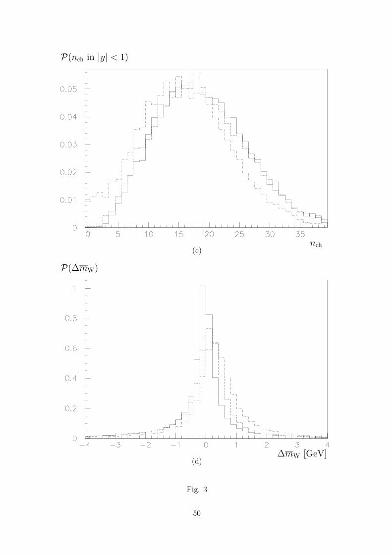
P(nch in |y| < 1)

nch(c)

P(∆mW)

∆mW [GeV](d)

Fig. 3

50

e−

e+ W+

W−

q1

q2

q3

q4

k

+

e−

e+ W+

W−

q1

q2

q3

q4

k

Fig. 4

e−

e+ W+

W−

= 0

Fig. 5

51

e−

e+ W+

W−

q1

q2

q3

q4

k1

k2

+

e−

e+ W+

W−

q1

q2

q3

q4

k2

k1

(a)

e−

e+ W+

W−

q1

q2

q3

q4

k1

k2

+

e−

e+ W+

W−

q1

q2

q3

q4

k1

k2

(b)

Fig. 6

52

e−

e+ W+

W−

q1

q2

q3

q4

k

+

e−

e+ W+

W−

q1

q2

q3

q4

k

Fig. 7

e−

e+ W+

W−

Fig. 8

q

g1

g2

g3

q

Fig. 9

53

[GeV]

Ecm[GeV]

p∗ naıve

〈p∗〉

〈min(m+W,m

−W)〉

〈max(m+W,m

−W)〉

(a)

[fm]

Ecm[GeV]

〈τ〉

〈|∆t0|〉

〈|∆x0|〉

(b)

Fig. 10

54

q

g

qA BC

(a)

q

g

qA

(b)

Fig. 11

55

I(β)/I(0)

Ecm [GeV]

Fig. 12

Precon

Ecm [GeV]

Fig. 13

56

q1

q2

q3

q4

(a)

q1

q2 q3

q4

(b)

q1

q2q3

q4

(c)

Fig. 14

57

Precon

Ecm [GeV](a)

Precon

m0 [GeV](b)

Fig. 15

58

Precon

njet(a)

Precon

nch(b)

Fig. 16

59

P(nch)

nch(a)

dn/dϕ

ϕ(b)

Fig. 17

60

P(drec)

drec(a)

〈∆λ〉

drec(b)

Fig. 18

61

P(∆mW)

∆mW [GeV](a)

P(∆mW)

∆mW [GeV](b)

Fig. 19

62

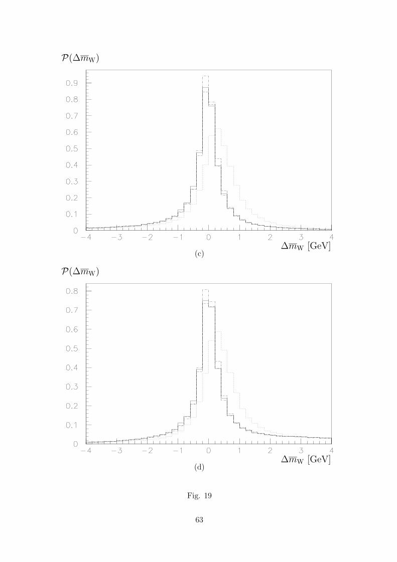
P(∆mW)

∆mW [GeV](c)

P(∆mW)

∆mW [GeV](d)

Fig. 19

63