NUMERICAL MODELING OF PULSATILE FLOW OF BLOOD THROUGH A STENOSED TAPERED ARTERY UNDER PERIODIC BODY...

June 29, 2010 7:35 WSPC/S0219-5194/170-JMMB 00339

Journal of Mechanics in Medicine and BiologyVol. 10, No. 2 (2010) 251–272c© World Scientific Publishing CompanyDOI: 10.1142/S0219519410003393

NUMERICAL MODELING OF PULSATILE FLOW OF BLOODTHROUGH A STENOSED TAPERED ARTERY UNDER

PERIODIC BODY ACCELERATION

GAURAV VARSHNEY∗ and V. K. KATIYAR†

Department of MathematicsIndian Institute of Technology, Roorkee–247667, India

∗[email protected]†[email protected]

SUSHIL KUMAR

University Institute of Engineering and TechnologyCSJM University, Kanpur–208001, India

[email protected]

Received 24 August 2008Revised 4 July 2009

Accepted 5 August 2009

A mathematical model is developed for the pulsatile flow of blood through a stenosedtapered artery under the influence of externally imposed body acceleration. The arteryis assumed as a cylindrical tube with time-dependent radius having mild stenosis andthe non-Newtonian behavior of blood is characterized by generalized Power-law model.The governing equations are transformed by using a radial transformation and solvednumerically by a suitable finite difference scheme in order to obtain the velocity, fluidacceleration, wall shear stress, and flow rate. The effect of stenosis severity, tapering,and externally imposed body acceleration on the blood flow in artery is discussed withthe help of graph. It is found that all flow characteristics are affected by the stenosisseverity, tapering, and periodic acceleration applied on the body.

Keywords: Blood flow; body acceleration; stenosis; tapering; finite difference method.

1. Introduction

Arterial stenosis is one of the most serious forms of arterial disease. The presence ofa stenosis restricts blood flow in the artery and makes an artery work in the direc-tion that is opposite to the direction of a healthy one. Atherosclerosis, a diseasein which plaque builds up on the inside of the arteries, is strongly related to thecharacteristic of the blood flow in arteries. Hemodynamics i.e. fluid dynamic-relatedphenomena play an important role in the initiation and progression of atheroscle-rosis. Atherosclerotic lesions are found preferentially at specific sites in the arterial

∗Corresponding author.

251

http://dx.doi.org/10.1142/S0219519410003393

June 29, 2010 7:35 WSPC/S0219-5194/170-JMMB 00339

252 G. Varshney, V. K. Katiyar & S. Kumar

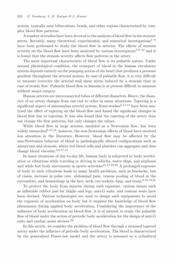
system, typically near bifurcations, bends, and other regions characterized by com-plex blood flow patterns.

A number of studies have been devoted to the analysis of blood flow in the stenoticartery. Recently, many theoretical, experimental, and numerical investigations1–8

have been performed to study the blood flow in arteries. The effects of stenosisseverity on the blood flow have been analyzed by various investigators7,9–12 and itis found that the stenosis severity affects flow patterns in the artery.

The most important characteristic of blood flow is its pulsatile nature. Undernormal physiological condition, the transport of blood in the human circulatorysystem depends entirely on the pumping action of the heart that produces a pressuregradient throughout the arterial system. In case of pulsatile flow, it is very difficultto measure correctly the arterial wall shear stress induced by a stenosis than incase of steady flow. Pulsatile blood flow in humans is at present difficult to measurewithout major surgery.

Human arteries are interconnected tubes of different diameters. Hence, the diam-eter of an artery changes from one end to other in many situations. Tapering is asignificant aspect of mammalian arterial system. Some studies6,13,14 have been ana-lyzed the effect of tapering on the blood flow and found the significant changes inblood flow due to tapering. It was also found that the tapering of the artery doesnot change the flow patterns, but only changes the values.

While blood flow in large arteries, modeled as a Newtonian flow, has beenwidely researched8,15,16; however, the non-Newtonian effects of blood have receivedless attention in the literature. However, blood flow may be affected by thenon-Newtonian behavior of blood in pathologically altered configurations such asaneurysms and stenosis, where red blood cells and platelets can aggregate and thuschange blood viscosity.3,6,17,18

In many situations of day-to-day life, human body is subjected to body acceler-ation or vibrations while traveling or driving in vehicles, water ships, and airplanesand while fast body movements in sports activities15,17,19,20 A prolonged exposureof body to such vibrations leads to many health problems, such as headache, lossof vision, increase in pulse rate, abdominal pain, venous pooling of blood in theextremities, and hemorrhage in the face, neck, eye sockets, lung, and brain.8,16,18,21

To protect the body from injuries during such exposure, various means suchas inflatable rubber pad for thighs and legs, anti-G suits, and contour seats havebeen devised. Various technologies are used to design such equipments to avoidthe exposure of acceleration on body but it requires the knowledge of blood flowphenomena during applied body acceleration. Considering the importance of theinfluence of body acceleration on blood flow, it is of interest to study the pulsatileflow of blood under the action of periodic body acceleration for the design of anti-Gsuits and cardiac assist devices.22

In this article, we consider the problem of blood flow through a stenosed taperedartery under the influence of periodic body acceleration. The blood is characterizedby the generalized Power-law model and the artery is assumed as a cylindrical

June 29, 2010 7:35 WSPC/S0219-5194/170-JMMB 00339

Numerical Modeling of Pulsatile Flow of Blood 253

tube having mild stenosis. A finite difference scheme is used to solve the governingequations. A comparison of the velocity profile, wall shear stress together withthe flow rate, and fluid acceleration are discussed for different values of tapering,stenosis severity, and body acceleration.

2. Formulation of the Problem

2.1. Mathematical model

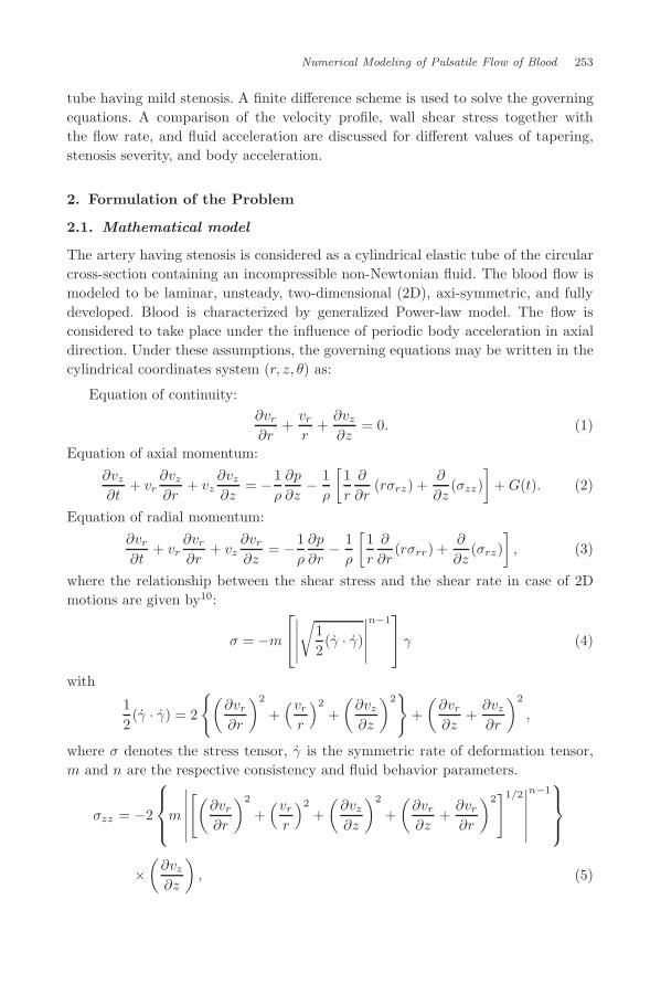
The artery having stenosis is considered as a cylindrical elastic tube of the circularcross-section containing an incompressible non-Newtonian fluid. The blood flow ismodeled to be laminar, unsteady, two-dimensional (2D), axi-symmetric, and fullydeveloped. Blood is characterized by generalized Power-law model. The flow isconsidered to take place under the influence of periodic body acceleration in axialdirection. Under these assumptions, the governing equations may be written in thecylindrical coordinates system (r, z, θ) as:

Equation of continuity:∂vr

∂r+

vr

r+

∂vz

∂z= 0. (1)

Equation of axial momentum:∂vz

∂t+ vr

∂vz

∂r+ vz

∂vz

∂z= −1

ρ

∂p

∂z− 1

ρ

[1r

∂

∂r(rσrz) +

∂

∂z(σzz)

]+ G(t). (2)

Equation of radial momentum:∂vr

∂t+ vr

∂vr

∂r+ vz

∂vr

∂z= −1

ρ

∂p

∂r− 1

ρ

[1r

∂

∂r(rσrr) +

∂

∂z(σrz)

], (3)

where the relationship between the shear stress and the shear rate in case of 2Dmotions are given by10:

σ = −m

∣∣∣∣∣√

12(γ̇ · γ̇)

∣∣∣∣∣n−1 γ (4)

with

12(γ̇ · γ̇) = 2

{(∂vr

∂r

)2

+(vr

r

)2

+(

∂vz

∂z

)2}

+(

∂vr

∂z+

∂vz

∂r

)2

,

where σ denotes the stress tensor, γ̇ is the symmetric rate of deformation tensor,m and n are the respective consistency and fluid behavior parameters.

σzz = −2

m

∣∣∣∣∣∣[(

∂vr

∂r

)2

+(vr

r

)2

+(

∂vz

∂z

)2

+(

∂vr

∂z+

∂vr

∂r

)2]1/2

∣∣∣∣∣∣n−1

×(

∂vz

∂z

), (5)

June 29, 2010 7:35 WSPC/S0219-5194/170-JMMB 00339


σrz = −

m

∣∣∣∣∣∣[(

∂vr

∂r

)2

+(vr

r

)2

+(

∂vz

∂z

)2

+(

∂vr

∂z+

∂vz

∂r

)2]1/2

∣∣∣∣∣∣n−1

×(

∂vz

∂r+

∂vr

∂z

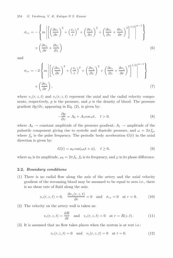
)(6)

and

σrr = −2

m

∣∣∣∣∣∣[(

∂vr

∂r

)2

+(vr

r

)2

+(

∂vz

∂z

)2

+(

∂vr

∂z+

∂vz

∂r

)2]1/2

∣∣∣∣∣∣n−1

×(

∂vr

∂r

), (7)

where vz(r, z, t) and vr(r, z, t) represent the axial and the radial velocity compo-nents, respectively, p is the pressure, and ρ is the density of blood. The pressuregradient ∂p/∂z, appearing in Eq. (2), is given by:

−∂p

∂z= A0 + A1cosωt, t > 0, (8)

where A0 → constant amplitude of the pressure gradient; A1 → amplitude of thepulsatile component giving rise to systolic and diastolic pressure, and ω = 2πfp,where fp is the pulse frequency. The periodic body acceleration G(t) in the axialdirection is given by:

G(t) = a0 cos(ωbt + φ), t ≥ 0, (9)

where a0 is its amplitude, ωb = 2πfb, fb is its frequency, and ϕ is its phase difference.

2.2. Boundary conditions

(1) There is no radial flow along the axis of the artery and the axial velocitygradient of the streaming blood may be assumed to be equal to zero i.e., thereis no shear rate of fluid along the axis.

vr(r, z, t) = 0,∂vz(r, z, t)

∂r= 0 and σrz = 0 at r = 0. (10)

(2) The velocity on the artery wall is taken as:

vr(r, z, t) =∂R

∂tand vz(r, z, t) = 0 at r = R(z, t). (11)

(3) It is assumed that no flow takes places when the system is at rest i.e.:

vr(r, z, t) = 0 and vz(r, z, t) = 0 at t = 0. (12)

June 29, 2010 7:35 WSPC/S0219-5194/170-JMMB 00339


2.3. Geometry of stenosed artery

The geometry of the time-variant mild stenosis arterial segment for different taperangle is mathematically given by:

R(z, t) =

[mz + a − 4τmsecϕ(z − d)

l2(l − (z − d))

]a1(t), d ≤ z ≤ d + l

(mz + a)a1(t), otherwise

(13)

where m(tan φ) represents the slope of the tapered vessel, a is the unconstrictedradius of stenosed artery, τm is the maximum height of stenosis, d is the locationof stenosis, and l is the length of the stenosis.

The time variant parameter a1(t) = 1 − b cos(ωt − 1)e−bωt; ω = 2πfp. φ < 0 isthe converging tapering, φ = 0 is non-tapered artery, and φ > 0 is the divergingtapering.

3. Solution Procedure

3.1. Transformation of the governing equations

Let us introduce a radial coordinate transformation [x = (r/R(z, t))], which hasthe effect of immobilizing the vessel wall in the transformed coordinate x.17 Usingthis transformation, Eqs. (1)–(7) together with boundary conditions (10–12) takethe following form:

1r

∂vr

∂x+

vr

xR+

∂vz

∂z− x

R

∂vz

∂x

∂R

∂z= 0 (14)

∂vz

∂t=[

x

R

∂R

∂t− vr

R+ vz

x

R

∂R

∂z

]∂vz

∂x− vz

∂vz

∂z− 1

ρ

∂p

∂z

− 1ρ

[1

xRσxz +

1R

∂σxz

∂x+

∂σzz

∂z− x

R

∂σxz

∂x

∂R

∂z

]+ G(t). (15)

Normal stress:

σzz = −2

m

∣∣∣∣∣∣∣[(

1R

∂vr

∂x

)2

+( vr

xR

)2

+(

∂vz

∂z− x

R

∂R

∂z

∂vz

∂x

)2

+(

∂vr

∂z− x

R

∂R

∂z

∂vr

∂x+

1r

∂vz

∂x

)2]1/2

∣∣∣∣∣∣n−1

×(

∂vz

∂z− x

R

∂R

∂z

∂vz

∂x

). (16)

June 29, 2010 7:35 WSPC/S0219-5194/170-JMMB 00339


Shear stress:

σxz = −

m

∣∣∣∣∣∣∣[(

1R

∂vr

∂x

)2

+( vr

xR

)2

+(

∂vz

∂z− x

R

∂R

∂z

∂vz

∂x

)2

+(

∂vr

∂z− x

R

∂R

∂z

∂vr

∂x+

1r

∂vz

∂x

)2]1/2

∣∣∣∣∣∣n−1

×(

1R

∂vz

∂z+

∂vr

∂z− x

R

∂R

∂z

∂vz

∂x

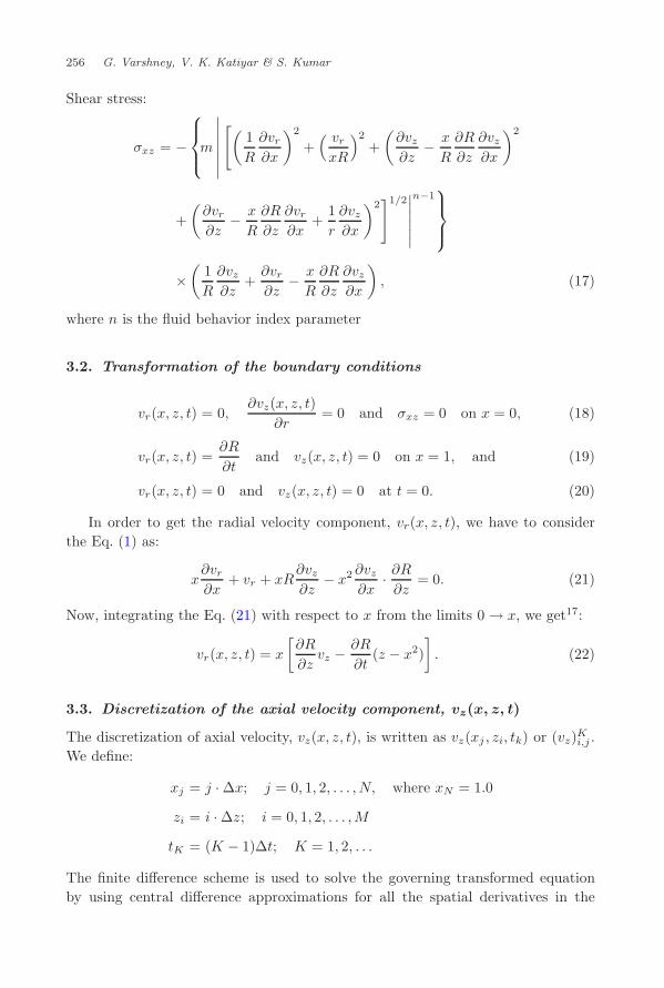
), (17)

where n is the fluid behavior index parameter

3.2. Transformation of the boundary conditions

vr(x, z, t) = 0,∂vz(x, z, t)

∂r= 0 and σxz = 0 on x = 0, (18)

vr(x, z, t) =∂R

∂tand vz(x, z, t) = 0 on x = 1, and (19)

vr(x, z, t) = 0 and vz(x, z, t) = 0 at t = 0. (20)

In order to get the radial velocity component, vr(x, z, t), we have to considerthe Eq. (1) as:

x∂vr

∂x+ vr + xR

∂vz

∂z− x2 ∂vz

∂x· ∂R

∂z= 0. (21)

Now, integrating the Eq. (21) with respect to x from the limits 0 → x, we get17:

vr(x, z, t) = x

[∂R

∂zvz − ∂R

∂t(z − x2)

]. (22)

3.3. Discretization of the axial velocity component, vz(x, z, t)

The discretization of axial velocity, vz(x, z, t), is written as vz(xj , zi, tk) or (vz)Ki,j .

We define:

xj = j · ∆x; j = 0, 1, 2, . . . , N, where xN = 1.0

zi = i · ∆z; i = 0, 1, 2, . . . , M

tK = (K − 1)∆t; K = 1, 2, . . .

The finite difference scheme is used to solve the governing transformed equationby using central difference approximations for all the spatial derivatives in the

June 29, 2010 7:35 WSPC/S0219-5194/170-JMMB 00339


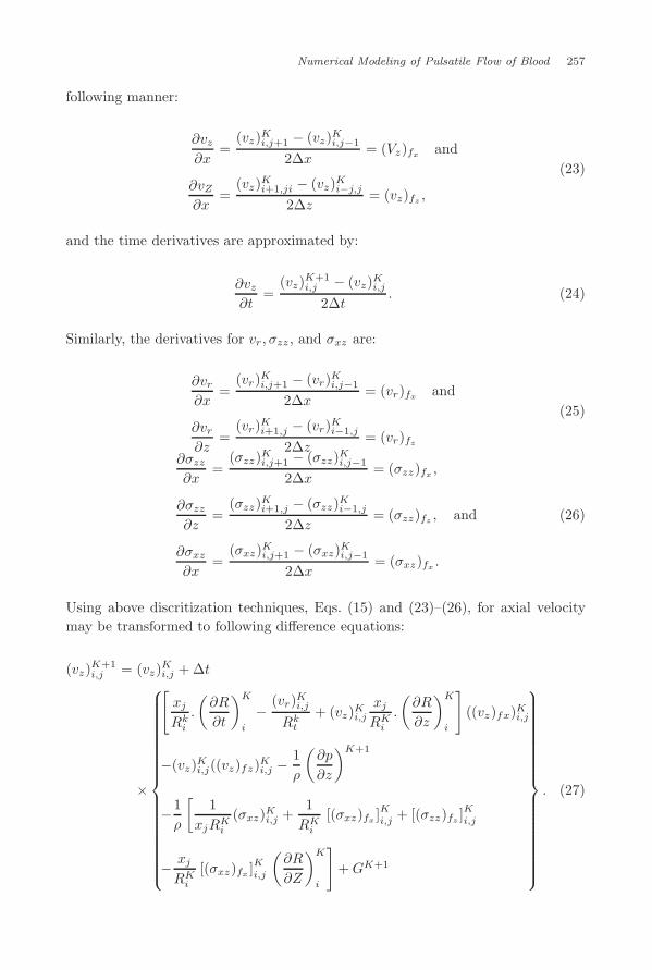
following manner:

∂vz

∂x=

(vz)Ki,j+1 − (vz)K

i,j−1

2∆x= (Vz)fx and

∂vZ

∂x=

(vz)Ki+1,ji − (vz)K

i−j,j

2∆z= (vz)fz ,

(23)

and the time derivatives are approximated by:

∂vz

∂t=

(vz)K+1i,j − (vz)K

i,j

2∆t. (24)

Similarly, the derivatives for vr, σzz , and σxz are:

∂vr

∂x=

(vr)Ki,j+1 − (vr)K

i,j−1

2∆x= (vr)fx and

∂vr

∂z=

(vr)Ki+1,j − (vr)K

i−1,j

2∆z= (vr)fz

(25)

∂σzz

∂x=

(σzz)Ki,j+1 − (σzz)K

i,j−1

2∆x= (σzz)fx ,

∂σzz

∂z=

(σzz)Ki+1,j − (σzz)K

i−1,j

2∆z= (σzz)fz , and (26)

∂σxz

∂x=

(σxz)Ki,j+1 − (σxz)K

i,j−1

2∆x= (σxz)fx .

Using above discritization techniques, Eqs. (15) and (23)–(26), for axial velocitymay be transformed to following difference equations:

(vz)K+1i,j = (vz)K

i,j + ∆t

×

[xj

Rki

.

(∂R

∂t

)K

i

− (vr)Ki,j

Rkt

+ (vz)Ki,j

xj

RKi

.

(∂R

∂z

)K

i

]((vz)fx)K

i,j

−(vz)Ki,j((vz)fz)K

i,j −1ρ

(∂p

∂z

)K+1

−1ρ

[1

xjRKi

(σxz)Ki,j +

1RK

i

[(σxz)fx ]Ki,j + [(σzz)fz ]Ki,j

− xj

RKi

[(σxz)fx ]Ki,j

(∂R

∂Z

)K

i

]+ GK+1

. (27)

June 29, 2010 7:35 WSPC/S0219-5194/170-JMMB 00339


The Eqs. (16) and (17) have their discritized form as:

(σzz)Ki,j = 2

m

∣∣∣∣∣∣∣( 1

RKi

((vr)fx)Ki,j

)2

+

((vr)K

i,j

xjRKi

)

+

(((vz)fz )K

i,j −xj

RKi

(∂R

∂z

)K

i

((vz)fx)Ki,j

)2

+

(((vr)fz )K

i,j −xj

RKi

(∂R

∂z

)K

i

((vz)fx)Ki,j +

1Rk

j

((Vz)fx)Ki,j

)2

1/2

n−1

×(

((vz)fz )Ki,j −

xj

RKi

(∂R

∂Z

)K

i

((vz)fz )Ki,j

)

and

(σxz)Ki,j = −2

m

( 1

Rki

((vr)fx)Ki,j

)2

+

((vr)K

i,j

xjRki

)2

+

(((vz)fz )K

i,j −xj

RKi

(∂R

∂z

)K

i

((vz)fx)Ki,j

)2

+

(((vx)fz )K

i,j −xj

RKi

(∂R

∂z

)K

i

)((vr)fx)K

ijj +1

RKi

((vz)fx)Ki,j

)2

1/2∣∣∣∣∣∣∣n−1

×(

((vr)fz )Ki,j −

xj

RKj

(∂R

∂z

)K

i

((vx)fx)Ki,j +

1RK

i

((vz)fx)Ki,j

). (28)

The boundary conditions in discretized form are as follows:

(vr)Ki,j =0, (vz)K

i,1 =(vz)Ki,2, (σxz)K

i,1 =0, (vz)Ki,N+1 =0, (vr)K

i,N+1 =(

∂R

∂t

)K

i

and

(vr)1i,j = 0, (vz)1i,j = 0. (29)

The radial velocity can be calculated from the Eq. (22) and its discretized form is:

(vr)K+1i,j = xj

[(∂R

∂z

)K

i

(vz)K+1i,j −

(∂R

∂t

)K

i

[2 − x2j ]

]. (30)

June 29, 2010 7:35 WSPC/S0219-5194/170-JMMB 00339


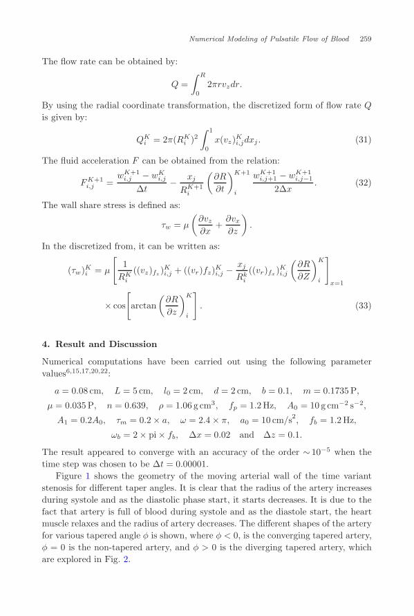
The flow rate can be obtained by:

Q =∫ R

0

2πrvzdr.

By using the radial coordinate transformation, the discretized form of flow rate Q

is given by:

QKi = 2π(RK

i )2∫ 1

0

x(vz)Ki,jdxj . (31)

The fluid acceleration F can be obtained from the relation:

FK+1i,j =

wK+1i,j − wK

i,j

∆t− xj

RK+1i

(∂R

∂t

)K+1

i

wK+1i,j+1 − wK+1

i,j−1

2∆x. (32)

The wall share stress is defined as:

τw = µ

(∂vz

∂x+

∂vx

∂z

).

In the discretized from, it can be written as:

(τw)Ki = µ

[1

RKi

((vz)fz )Ki,j + ((vr)fz)K

i,j −xj

Rki

((vr)fx)Ki,j

(∂R

∂Z

)K

i

]x=1

× cos

[arctan

(∂R

∂z

)K

i

]. (33)

4. Result and Discussion

Numerical computations have been carried out using the following parametervalues6,15,17,20,22:

a = 0.08 cm, L = 5 cm, l0 = 2 cm, d = 2 cm, b = 0.1, m = 0.1735 P,

µ = 0.035 P, n = 0.639, ρ = 1.06 g cm3, fp = 1.2 Hz, A0 = 10 g cm−2 s−2,

A1 = 0.2A0, τm = 0.2 × a, ω = 2.4 × π, a0 = 10 cm/s2, fb = 1.2 Hz,

ωb = 2 × pi × fb, ∆x = 0.02 and ∆z = 0.1.

The result appeared to converge with an accuracy of the order ∼ 10−5 when thetime step was chosen to be ∆t = 0.00001.

Figure 1 shows the geometry of the moving arterial wall of the time variantstenosis for different taper angles. It is clear that the radius of the artery increasesduring systole and as the diastolic phase start, it starts decreases. It is due to thefact that artery is full of blood during systole and as the diastole start, the heartmuscle relaxes and the radius of artery decreases. The different shapes of the arteryfor various tapered angle φ is shown, where φ < 0, is the converging tapered artery,φ = 0 is the non-tapered artery, and φ > 0 is the diverging tapered artery, whichare explored in Fig. 2.

June 29, 2010 7:35 WSPC/S0219-5194/170-JMMB 00339


Fig. 1. Radius of constricted artery at different time for φ = −0.1◦.

Fig. 2. Radius of constricted artery for different tapered angle.

June 29, 2010 7:35 WSPC/S0219-5194/170-JMMB 00339


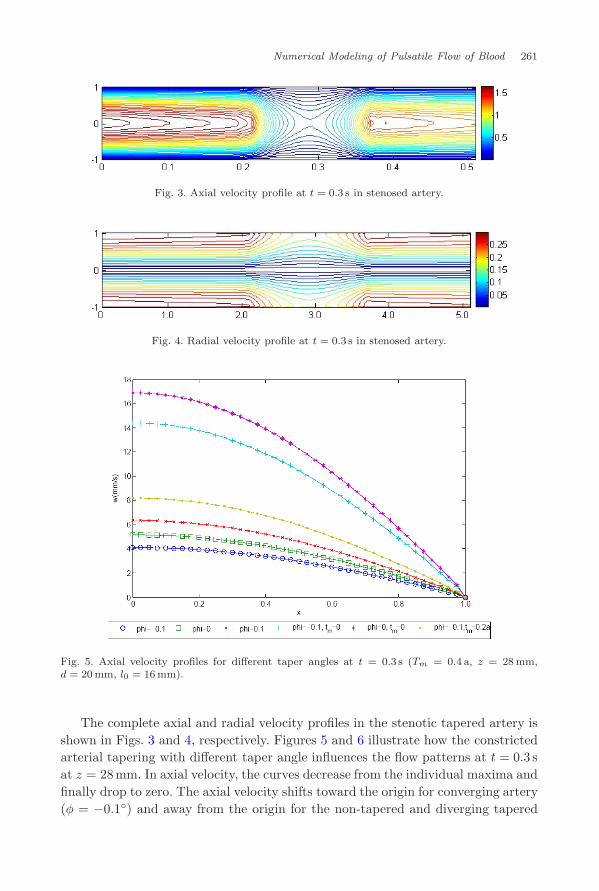
Fig. 3. Axial velocity profile at t = 0.3 s in stenosed artery.

Fig. 4. Radial velocity profile at t = 0.3 s in stenosed artery.

Fig. 5. Axial velocity profiles for different taper angles at t = 0.3 s (Tm = 0.4 a, z = 28 mm,d = 20 mm, l0 = 16 mm).

The complete axial and radial velocity profiles in the stenotic tapered artery isshown in Figs. 3 and 4, respectively. Figures 5 and 6 illustrate how the constrictedarterial tapering with different taper angle influences the flow patterns at t = 0.3 sat z = 28mm. In axial velocity, the curves decrease from the individual maxima andfinally drop to zero. The axial velocity shifts toward the origin for converging artery(φ = −0.1◦) and away from the origin for the non-tapered and diverging tapered

June 29, 2010 7:35 WSPC/S0219-5194/170-JMMB 00339


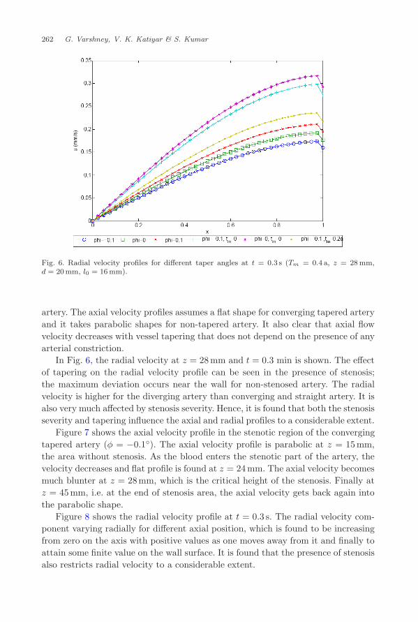
Fig. 6. Radial velocity profiles for different taper angles at t = 0.3 s (Tm = 0.4 a, z = 28 mm,d = 20mm, l0 = 16 mm).

artery. The axial velocity profiles assumes a flat shape for converging tapered arteryand it takes parabolic shapes for non-tapered artery. It also clear that axial flowvelocity decreases with vessel tapering that does not depend on the presence of anyarterial constriction.

In Fig. 6, the radial velocity at z = 28mm and t = 0.3 min is shown. The effectof tapering on the radial velocity profile can be seen in the presence of stenosis;the maximum deviation occurs near the wall for non-stenosed artery. The radialvelocity is higher for the diverging artery than converging and straight artery. It isalso very much affected by stenosis severity. Hence, it is found that both the stenosisseverity and tapering influence the axial and radial profiles to a considerable extent.

Figure 7 shows the axial velocity profile in the stenotic region of the convergingtapered artery (φ = −0.1◦). The axial velocity profile is parabolic at z = 15mm,the area without stenosis. As the blood enters the stenotic part of the artery, thevelocity decreases and flat profile is found at z = 24mm. The axial velocity becomesmuch blunter at z = 28mm, which is the critical height of the stenosis. Finally atz = 45mm, i.e. at the end of stenosis area, the axial velocity gets back again intothe parabolic shape.

Figure 8 shows the radial velocity profile at t = 0.3 s. The radial velocity com-ponent varying radially for different axial position, which is found to be increasingfrom zero on the axis with positive values as one moves away from it and finally toattain some finite value on the wall surface. It is found that the presence of stenosisalso restricts radial velocity to a considerable extent.

June 29, 2010 7:35 WSPC/S0219-5194/170-JMMB 00339


Fig. 7. Axial velocity profiles for different axial positions at t = 0.3 s (Tm = 0.4 a, φ = −0.1◦,d = 20 mm, l0 = 16 mm).

Fig. 8. Radial velocity profiles for different axial positions at t = 0.3 s (Tm = 0.4 a, φ = −0.1◦,d = 20 mm, l0 = 16 mm).

June 29, 2010 7:35 WSPC/S0219-5194/170-JMMB 00339


Fig. 9. Axial velocity profiles for different times at z = 28mm (Tm = 0.4 a, φ = −0.1◦, d = 20 mm,l0 = 16mm).

Figure 9 shows the variation of the axial velocity profile at z = 28mm fordifferent periods. The flow profiles are directly responsible for the pulsatile pressuregradient produced by the pumping action of the heart. When the time increasesfrom 0.1 s to 0.3 s, the curve shifts toward the origin. At t = 0.6 s again the axialvelocity increases because of the diastole. It is also clear that the streaming bloodis much higher for Newtonian than the non-Newtonian values. It is because of thefact that if flowing blood is treated as Newtonian, it has a high shear rate flow,which increases the axial velocity profile. Thus, the non-Newtonian characteristicsof the flowing blood affect the axial velocity profile. The result agrees qualitativelywith the research of Chaturani and Palanisamy15 and Sud and Sekhon16 on stenoticblood flow treated as Newtonian fluid.

In Fig. 10, the radial velocity profile at different period is shown. The radialvelocity profile assume a positive value during systole i.e. at t = 0.1 s and 0.3 s. andnegative during diastole i.e. at t = 0.6 s and 0.75 s. This clarifies that in systolicphase, the heart muscle has fully contracted and blood is squeezed out and duringdiastole, their the heart relaxes and becomes full of blood.

The variation of fluid acceleration F at time t = 0.6 s at the location z = 28mm,where the artery gets maximum narrowing is shown in Fig. 11. The accelerationis maximum on the axis and attains some finite value on the wall. By increasing

June 29, 2010 7:35 WSPC/S0219-5194/170-JMMB 00339


Fig. 10. Radial velocity profiles for different times at z = 28mm (Tm = 0.4 a, φ = −0.1◦,d = 20 mm, l0 = 16 mm).

Fig. 11. Radial variation of fluid acceleration at t = 0.6 s. (A0 = 100 kg m−2 s−2, a0 = 100 mm/s2

z = 28mm, Tm = 0.4 a, d = 20 mm, l0 = 16 mm).

June 29, 2010 7:35 WSPC/S0219-5194/170-JMMB 00339


the constant amplitude of the pressure gradient A0, the fluid is accelerated. Whenthe amplitude of body acceleration a0 is increases, the flow is accelerated morenear the wall followed by a negative value. It is clear that blood is acceleratedmore for diverging tapered artery than converging and straight artery. Blood isalso accelerated more by applying acceleration of high magnitude.

The variation of flow rate at the location z = 28mm over a period of nearly fourcardiac cycle for various tapered angle is illustrated in Fig. 12. The pulsatile natureof the flow rate has been found in all cases thoughout the time scale. One may notethe flow rate for a non-tapered artery having higher in magnitude than the flowrate for converging tapered artery and the flow rate for diverging tapered artery isevery time higher than those of non-tapered and converging tapered arteries. Theflow rate is high for the corresponding Newtonian model. It is concluded that thepresence of stenosis, the taper angle and non-Newtonian rheology of the flowingblood affect the flow rate to considerable extent. Such behavior is found to be ingood agreement with those of Mandal et al.17

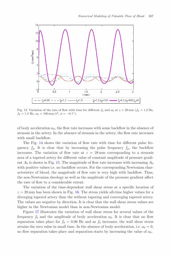
Figure 13 illustrates the variations of the flow rate Q with time t for differentvalues of the frequency and amplitude of body acceleration along with the effectof stenosis severity. It can be observed that if the value of the body accelerationis 0.06Hz, the flow rate remains positive and for fb = 1.2Hz. The backflow occurswith the formulation of several flow separation zones. By increasing the amplitude

Fig. 12. Variation of the rate of flow with time at z = 28mm (Tm = 0.4 a, d = 20mm, l0 = 16 mm,φ = −0.1◦).

June 29, 2010 7:35 WSPC/S0219-5194/170-JMMB 00339


Fig. 13. Variation of the rate of flow with time for different fb and a0 at z = 28mm (fp = 1.2 Hz,fb = 1.2 Hz, a0 = 100mm/s2, φ = −0.1◦).

of body acceleration a0, the flow rate increases with some backflow in the absence ofstenosis in the artery. In the absence of stenosis in the artery, the flow rate increaseswith small backflow.

The Fig. 14 shows the variation of flow rate with time for different pulse fre-quency fp. It is clear that by increasing the pulse frequency fp, the backflowincreases. The variation of flow rate at z = 28mm corresponding to a stenosisarea of a tapered artery for different value of constant amplitude of pressure gradi-ent A0 is shown in Fig. 15. The magnitude of flow rate increases with increasing A0

with positive values i.e. no backflow occurs. For the corresponding Newtonian char-acteristics of blood, the magnitude of flow rate is very high with backflow. Thus,the non-Newtonian rheology as well as the amplitude of the pressure gradient affectthe rate of flow to a considerable extent.

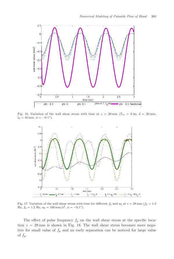
The variation of the time-dependent wall shear stress at a specific location ofz = 28mm has been shown in Fig. 16. The stress yields all-time higher values for adiverging tapered artery than the without tapering and converging tapered artery.The values are negative by direction. It is clear that the wall shear stress values arehigher in the Newtonian model than in non-Newtonian model.

Figure 17 illustrates the variation of wall shear stress for several values of thefrequency fb and the amplitude of body acceleration a0. It is clear that no flowseparation takes place for fb = 0.06 Hz and as fb increases, the wall shear stressattains the zero value in small time. In the absence of body acceleration, i.e. a0 = 0,no flow separation takes place and separation starts by increasing the value of a0.

June 29, 2010 7:35 WSPC/S0219-5194/170-JMMB 00339


Fig. 14. Variation of the rate of flow with time for different fp at z = 28mm (fb = 1.2 Hz,a0 = 100 mm/s2, φ = −0.1◦).

Fig. 15. Variation of the rate of flow with time for different A0 at z = 28mm (fp = 1.2 Hz,fb = 1.2 Hz, a0 = 100mm/s2, φ = −0.1◦).

June 29, 2010 7:35 WSPC/S0219-5194/170-JMMB 00339


Fig. 16. Variation of the wall shear stress with time at z = 28mm (Tm = 0.4a, d = 20 mm,l0 = 16mm, φ = −0.1◦).

Fig. 17. Variation of the wall shear stress with time for different fb and a0 at z = 28mm (fp = 1.2Hz, fb = 1.2 Hz, a0 = 100 mm/s2, φ = −0.1◦).

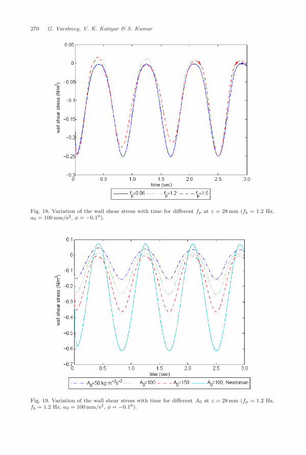
The effect of pulse frequency fp on the wall shear stress at the specific loca-tion z = 28mm is shown in Fig. 18. The wall shear stress becomes more nega-tive for small value of fp and an early separation can be noticed for large valueof fp.

June 29, 2010 7:35 WSPC/S0219-5194/170-JMMB 00339


Fig. 18. Variation of the wall shear stress with time for different fp at z = 28mm (fb = 1.2 Hz,a0 = 100 mm/s2, φ = −0.10).

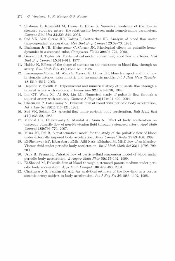
Fig. 19. Variation of the wall shear stress with time for different A0 at z = 28mm (fp = 1.2 Hz,fb = 1.2 Hz, a0 = 100mm/s2, φ = −0.10).

June 29, 2010 7:35 WSPC/S0219-5194/170-JMMB 00339


Finally, the variation of wall shear stress for various values of pressure gradientamplitude A0 and non-Newtonian rheology of the flowing blood is shown in Fig. 19.The wall shear stress is pulsatile in nature for all cases. The wall shear stressdecreases by increasing the value of A0. The non-Newtonian rheology of the bloodaffects the wall shear stress very small in comparison to the amplitude of pressuregradient.

Hence, it is found that tapering, amplitude of pressure gradient, stenosis severityand amplitude, and frequency of body acceleration change wall shear stress andproduce the formation of early separation zone, which is responsible for the arterialblockage.

5. Conclusion

This analysis presented numerical results for an unsteady blood flow in a taperedartery with mild stenosis, using the generalized Power-law model of blood viscosityunder the influence of periodic body acceleration. In this article, we used the time-dependent radius of the artery and tapering in the artery, which is an importantfactor considered for analyzing blood flow in stenotic artery. From the numericalresults, it is concluded that all the flow characteristics e.g. velocity, flow rate, fluidacceleration, and wall shear stress are affected by tapering, stenosis severity, pres-sure gradient, and periodic body acceleration. It is found that the non-Newtonianbehavior is an important factor and should not be neglected in the study of bloodflow in artery. The present study would be helpful to analyze the complexity ofblood flow in stenotic tapered artery and to design the anti-G suits and to driverseats of industrial vehicles.

Acknowledgment

One of the authors Gaurav Varshney is thankful to Council of Scientific and Indus-trial Research, India for providing Senior Research Fellowship during this work.

References

1. Chakravarty S, Datta A, Pulsatile blood flow in a porous stenotic artery, Math ComputModel 16(2):35–54, 1992.

2. Chakravarty S, Mandal PK, Mathematical modeling of blood flow through an over-lapping arterial stenosis, Math Comput Model 19(1):59–70, 1994.

3. Hernan A, Gonzalez R, Numerical implementation of viscoelastic blood flow in asimplified arterial geometry, Med Eng Phys 29:491–496, 2007.

4. Khanafer KM, Gadhoke P, Berguer R, Bull JL, Modeling pulsatile flow in aorticaneurysms, Biorheology 43:661–679, 2006.

5. Liepsch D, An introduction to biofluid mechanics — basic models and applications,J Biomechan 35:415–435, 2002.

6. Mandal PK, An unsteady analysis of non-Newtonian blood flow through taperedarteries with a stenosis, Int J Non-Linear Mechanics 40:151–164, 2005.

June 29, 2010 7:35 WSPC/S0219-5194/170-JMMB 00339


7. Shalman E, Rosenfeld M, Dgany E, Einav S, Numerical modeling of the flow instenosed coronary artery: the relationship between main hemodynamic parameters,Comput Biol Med 32:329–344, 2002.

8. Sud VK, Von Gierke HE, Kaleps I, Oestreicher HL, Analysis of blood flow undertime-dependent acceleration, Med Biol Engi Comput 23:69–73, 1985.

9. Buchanan Jr JR, Kleinstreuer C, Corner JK, Rheological effects on pulsatile hemo-dynamics in a stenosed tube, Computers Fluids 29:695–724, 2000.

10. Gerrard JH, Taylor LA, Mathematical model representing blood flow in arteries, MedBiol Eng Comput 15:611–617, 1977.

11. Haldar K, Effects of the shape of stenosis on the resistance to blood flow through anartery, Bull Math Biol 47(4):545–550, 1985.

12. Kaazempur-Mofrad M, Wada S, Myers JG, Ethier CR, Mass transport and fluid flowin stenotic arteries: axisymmetric and asymmetric models, Int J Heat Mass Transfer48:4510–4517, 2005.

13. Deplano V, Siouffi M, Experimental and numerical study of pulsatile flow through atapered artery with stenosis, J Biomechan 32:1081–1090, 1999.

14. Liu GT, Wang XJ, Ai BQ, Liu LG, Numerical study of pulsatile flow through atapered artery with stenosis, Chinese J Phys 42(4-I):401–409, 2004.

15. Chaturani P, Palanisamy V, Pulsatile flow of blood with periodic body acceleration,Int J Eng Sci 29(1):113–121, 1991.

16. Sud VK, Sekhon GS, Arterial flow under periodic body acceleration, Bull Math Biol47(1):35–52, 1985.

17. Mandal PK, Chakravarty S, Mandal A, Amin N, Effect of body acceleration onunsteady pulsatile flow of non-Newtonian fluid through a stenosed artery, Appl MathComput 189:766–779, 2007.

18. Misra JC, Pal B, A mathematical model for the study of the pulsatile flow of bloodunder externally imposed body acceleration, Math Comput Model 29:89–106, 1999.

19. El-Shehawey EF, Elbarabary EME, Afifi NAS, Elshahed M, MHD flow of an Elastico-Viscous fluid under periodic body acceleration, Int J Math Math Sci 23(11):795–799,2000.

20. Usha R, Prema K, Pulsatile flow of particle–fluid suspension model of blood underperiodic body acceleration, Z Angew Math Phys 50:175–192, 1999.

21. El-Shahed M, Pulsatile flow of blood through a stenosed porous medium under peri-odic body acceleration, Appl Math Comput 138:479–488, 2003.

22. Chakravarty S, Sannigrahi AK, An analytical estimate of the flow-field in a porousstenotic artery subject to body acceleration, Int J Eng Sci 36:1083–1102, 1998.

NUMERICAL MODELING OF PULSATILE FLOW OF BLOOD THROUGH A STENOSED TAPERED ARTERY UNDER PERIODIC BODY...

Documents

Transcript of NUMERICAL MODELING OF PULSATILE FLOW OF BLOOD THROUGH A STENOSED TAPERED ARTERY UNDER PERIODIC BODY...