Direct Numerical Simulations of Transitional Flow in Turbomachinery

Wissink, 02.02.2006 1

DIRECT NUMERICAL SIMULATIONS OF TRANSITIONAL FLOW IN

TURBOMACHINERY

J.G. Wissink, W. Rodi

Institute for Hydromechanics, University of Karlsruhe

Kaiserstrasse 12, D-76128 Karlsruhe, Germany.

e-mail: wissink@ifh.uni-karlsruhe.de, rodi@ifh.uni-karlsruhe.de

An overview is provided of various Direct Numerical Simulations (DNS) of transitional flows in turbine-related

geometries. Two flow cases are considered: the first case concerns separating flow over a flat plate and the

second case flows in turbine cascades.

In the first case, in which Re=60000, either an oscillating oncoming flow (1) or a uniform flow with and without

oncoming turbulent free-stream fluctuations (2) is prescribed at the inlet. In both subcases (1) and (2), separation

is induced by a contoured upper wall. In (1), the separated boundary layer is found to roll-up due to a Kelvin-

Helmholtz (KH) instability. This rolled-up shear layer is subject to spanwise instability and disintegrates rapidly

into turbulent fluctuations. In (2) a massive separation bubble is obtained in the simulation without oncoming

free-stream fluctuations. A KH instability is eventually triggered by numerical round-off error and followed

again by a rapid transition. With oncoming turbulent fluctuations, this KH instability is triggered much earlier

and transition is enhanced, which leads to a drastic reduction in size of the separation bubble.

The second case, concerning flow in turbine cascades, includes (1) flow in the T106 turbine cascade with

periodically oncoming wakes at Re=51800 and (2) flow and heat transfer in a MTU cascade with oncoming

wakes and background turbulence at Re=72000. In the simulation of flow in the T106 cascade with oncoming

wakes, the boundary layer along the downstream half of the suction side is found to separate intermittently and

subsequently rolls up due to a KH instability leading to separation-induced transition. At times when the wakes

impinge separation is suppressed. In the simulations of flow around a MTU turbine blade, evidence of by-pass

transition in the suction side boundary layer flow is observed while the pressure-side boundary layer remains

laminar in spite of significant fluctuations present. In agreement with the experiments, the impinging wakes

cause the heat transfer coefficient to increase significantly in the transitional suction-side region close to the

trailing edge and by about 30% on the pressure side. The large increase in heat transfer in the pre-transitional

Direct Numerical Simulations of Transitional Flow in Turbomachinery

Wissink, 02.02.2006 2

suction-side region observed in the experiments could not be reproduced. The discrepancy is explained by

differences in spectral contents of the turbulence in the oncoming wakes.

1. Introduction

Periodic unsteadiness, caused by rotor-stator interaction, and relatively low Reynolds numbers are

characteristic for flow in certain turbomachinery components. Both phenomena directly affect blade boundary

layer transition, the tendency to separation, heat transfer and flow losses. While industrial CFD procedures are

able to predict fairly accurately inviscid flow, the models in use for transition and turbulence, which are based on

the Reynolds averaged Navier-Stokes (RANS) equations, are still not sufficiently reliable and universal for

coping with the complex phenomena cited above. The models need to be improved, and for this both an

understanding of the underlying physical mechanisms and availability of high-quality data for testing the models

are required. Direct Numerical Simulations (DNS) are now possible for idealized situations and can provide a

wealth of information, but it is clear that this calculation method cannot be used in the design process which will

have to rely on RANS-based methods for a long time to come. In turbomachinery cascades, the focus is on flow

periodicity caused by oncoming wakes of upstream rotor or stator blade rows which travel through the cascade,

generating a very complex flow which is difficult to predict. These phenomena were investigated in the joint

German Research Foundation (DFG) research programme: “Periodic Unsteady Flows in Turbomachinery” [1].

In this programme both experimental and numerical research was performed of flow in turbine-related

geometries. In one subproject of the DFG research programme several Direct Numerical Simulations (DNS) of

transitional flow in turbine-related geometries have been performed, and the present paper summarizes this

work. Basically, two sets of DNS can be distinguished.

In the first set, boundary layer separation flow was studied as a model for the flow along the suction side of

a turbine blade. A contoured upper wall was used to induce an adverse streamwise pressure gradient along a flat

plate mounted at the bottom, causing the boundary layer to separate. The effects of disturbances, added at the

inlet to a uniform flow field, were studied. In the second set, a study was made of flows around turbine blades

with and without periodically oncoming wakes. In one of the cases, the focus was on the interaction of wakes

with a periodically separating boundary layer, while in the other case the aim was to elucidate the physical

mechanisms that play a role in wake-induced by-pass transition and heat transfer.

More detailed background information on both sets of DNS and an overview of some of the literature can

be found below.

Direct Numerical Simulations of Transitional Flow in Turbomachinery

Wissink, 02.02.2006 3

2. Flat Plate Boundary Layer Separation

In the first set of simulations, a flow over a flat plate with transition in a Laminar Separation Bubble (LSB)

was studied. In the presence of a strong enough adverse pressure gradient the laminar boundary layer over a flat

plate separates and forms a LSB. The separated boundary layer is very unstable and usually undergoes a fast

transition to turbulence. Farther downstream, the turbulent wake-like flow may re-attach and slowly evolve into

a turbulent boundary layer. Previously, DNS of LSB flow with steady inflow has been performed by Alam and

Sandham [2], Maucher et al. [3] and Spalart and Strelets [4]. To generate an adverse pressure gradient, required

for the formation of a separation bubble, Alam and Sandham as well as Spalart and Strelets used suction through

the upper boundary while Maucher et al. applied a special boundary condition for the free-stream velocity. In the

simulation with steady inflow of Wissink and Rodi [5], the adverse pressure gradient was generated by the

special shape of the upper wall (see Fig. 1). As in the simulation of Wissink and Rodi [5], Spalart and Strelets

relied on small numerical round-off errors present in any LSB simulation to trigger natural modes. They detected

a Kelvin-Helmholtz (KH) instability and found evidence of a low-frequency wavering mode in the separated

boundary layer. Wissink and Rodi performed further LSB flow simulations in which they introduced oscillations

and fluctuations to the oncoming flow [6-8]. In the present paper we aim to provide an overview and

comparative study of these LSB simulations.

2.1 Flow configuration and computational aspects. The computational geometry was chosen in

accordance with experiments performed in a companion project at the Technical University of Berlin [9]. A

direct comparison to the experiments is not possible because instantaneous velocity profiles at the inlet are not

exactly known and because of the relatively high Reynolds numbers employed in the experiments. The special

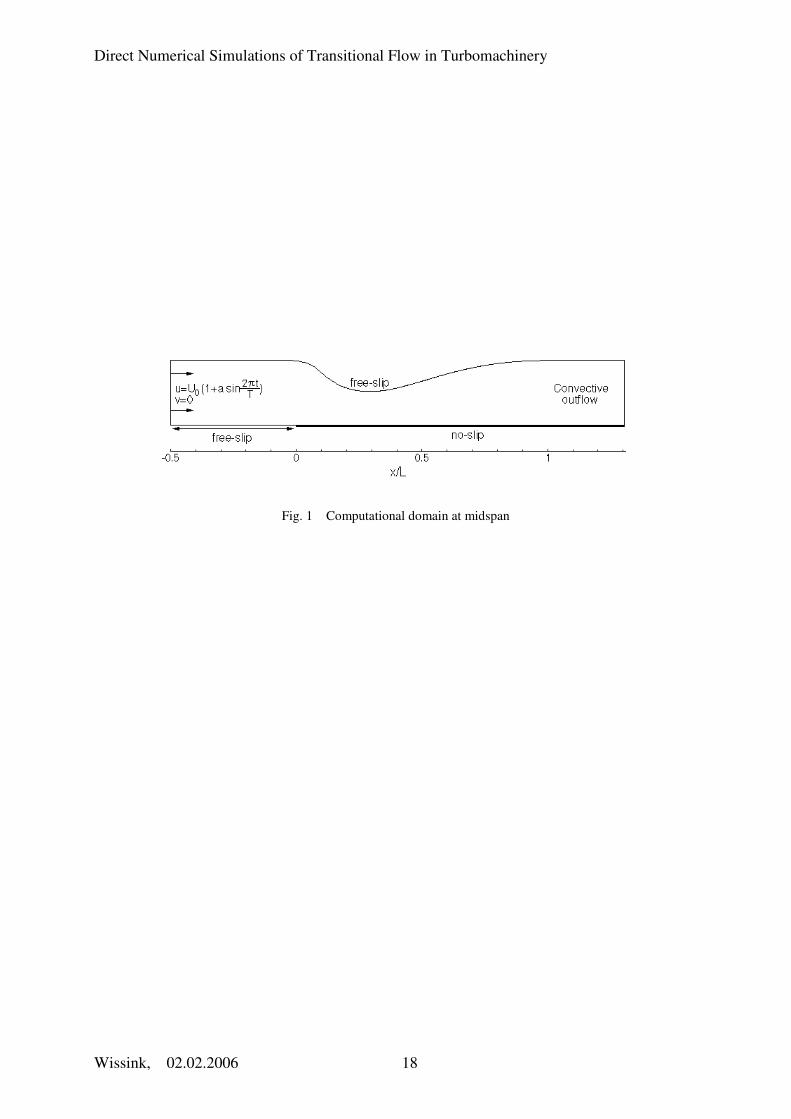
shape of the upper wall, illustrated in Fig. 1, generates a strongly adverse streamwise pressure gradient along the

flat plate, due to which the boundary layer separates. By employing a free-slip boundary condition, separation

along the upper wall was avoided. Along the lower wall, for x < 0 free-slip boundary conditions were employed

while for x > 0 no-slip boundary conditions were used. At the outlet a convective outflow boundary condition

was used, while in the spanwise direction periodic boundary conditions were employed. The Reynolds number,

Re=60000, is based on the mean inflow velocity U0 and the length of the plate in the experiment L. The precise

inflow boundary condition used depends on the situation simulated. Fig. 1 shows the inlet boundary conditions

employed in the simulations with oscillating external flow. At the inflow boundary of these simulations an

Direct Numerical Simulations of Transitional Flow in Turbomachinery

Wissink, 02.02.2006 4

oscillating flow field (u,v,w) = U0 (1+a sin2πt/T,0,0) was prescribed, where a is the amplitude and T is the

period.

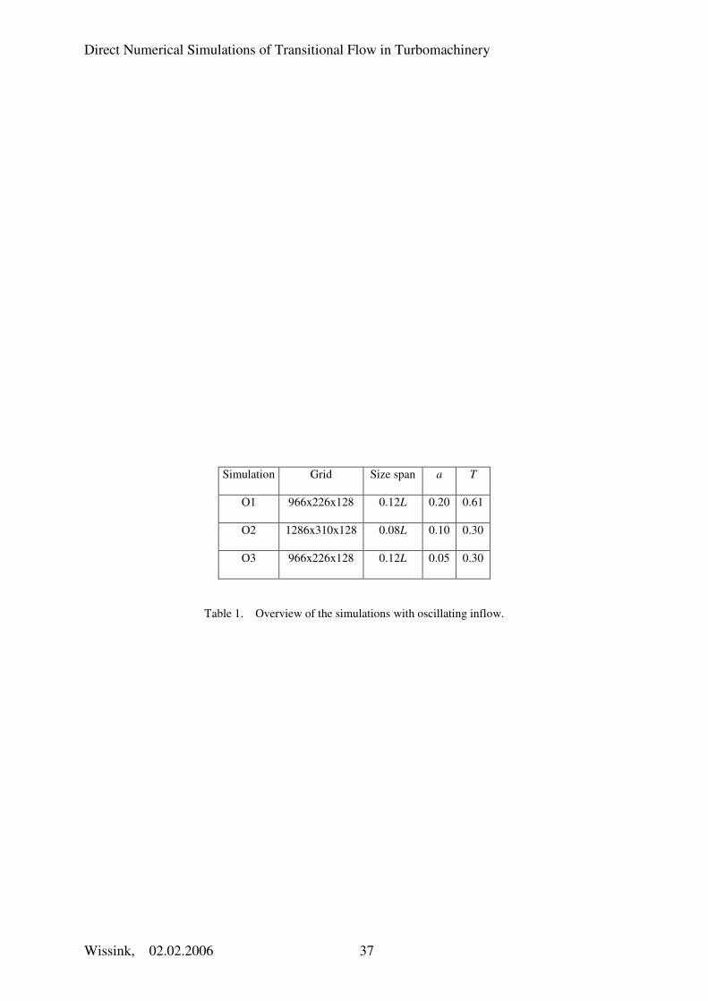
An overview of the simulations performed is provided in Table 1. After an initial period of approximately

∆T=6L/U0, in which the flow was allowed to develop, phase-averaged statistics were gathered for at least 10

further periods of simulation. For the phase-averaging procedure, the period T was divided into 256 equal

phases, φ=0,1/256,…,255/256. For Simulations O1 and O2 a grid-refinement study has been performed which shows

a very good qualitative agreement of the simulations on various meshes and also a good quantitative agreement

with respect to the most important phase-averaged quantities such as the location of separation, the maximum

reverse flow, the fluctuating kinetic energy etc. The present paper reports on the best resolved simulations.

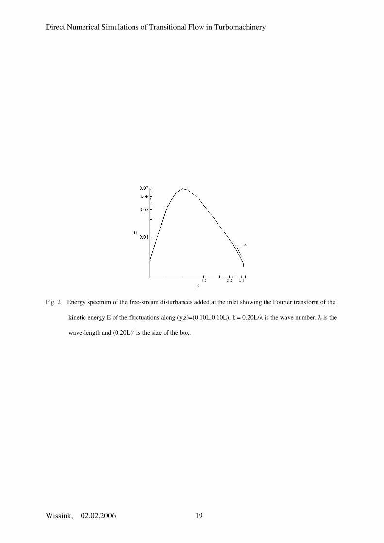
In the simulations with free-stream disturbances the inflow boundary conditions read: (u,v,w) = U0 (1,0,0) +

(u’,v’,w’). The free-stream disturbances (u’,v’,w’) were obtained by interpolation from a snapshot of a separate

Large-Eddy Simulation (LES) of isotropic turbulence in a box and were kindly made available by Dr. Jochen

Fröhlich of the University of Karlsruhe. Fig. 2 shows a log-log plot of the energy spectrum of the free-stream

disturbances added at the inlet. More information about the evolution of the disturbances as they travel through

the inflow domain can be found in [8]. The integral length-scale associated with the free-stream disturbances is

Λ=0.019L. An overview of the simulations with steady inflow and with free-stream disturbances is provided in

Table 2. To allow the separated boundary layer to reattach and assume typical characteristics of a turbulent

boundary layer, the length of the flat plate, lx, was chosen relatively large in Simulations F2 and F3.

Both the simulations with oscillating inflow and with steady inflow were performed on the IBM SP-SMP of

the Computing Center in Karlsruhe using up to 128 processors. The simulations with free-stream fluctuations

were run on the Hitachi SR8000-F1 at LRZ (Leibniz Rechenzentrum) in Munich using 256 processors. The

computational domain was subdivided in a number of equal-sized sub-domains. To each of the sub-domains one

processor was assigned. This way a near-optimal load-balancing was achieved. Communication between

processors was performed using the standard Message Passing Interface (MPI) protocol. Typical runtimes for the

simulations performed varied between one and three months of clock time.

2.2 Results

Boundary layer separation with oscillating inflow. In the presence of streamwise oscillating flow, the

adverse streamwise pressure gradient, generated by the special shape of the upper wall, is alternately weakened

Direct Numerical Simulations of Transitional Flow in Turbomachinery

Wissink, 02.02.2006 5

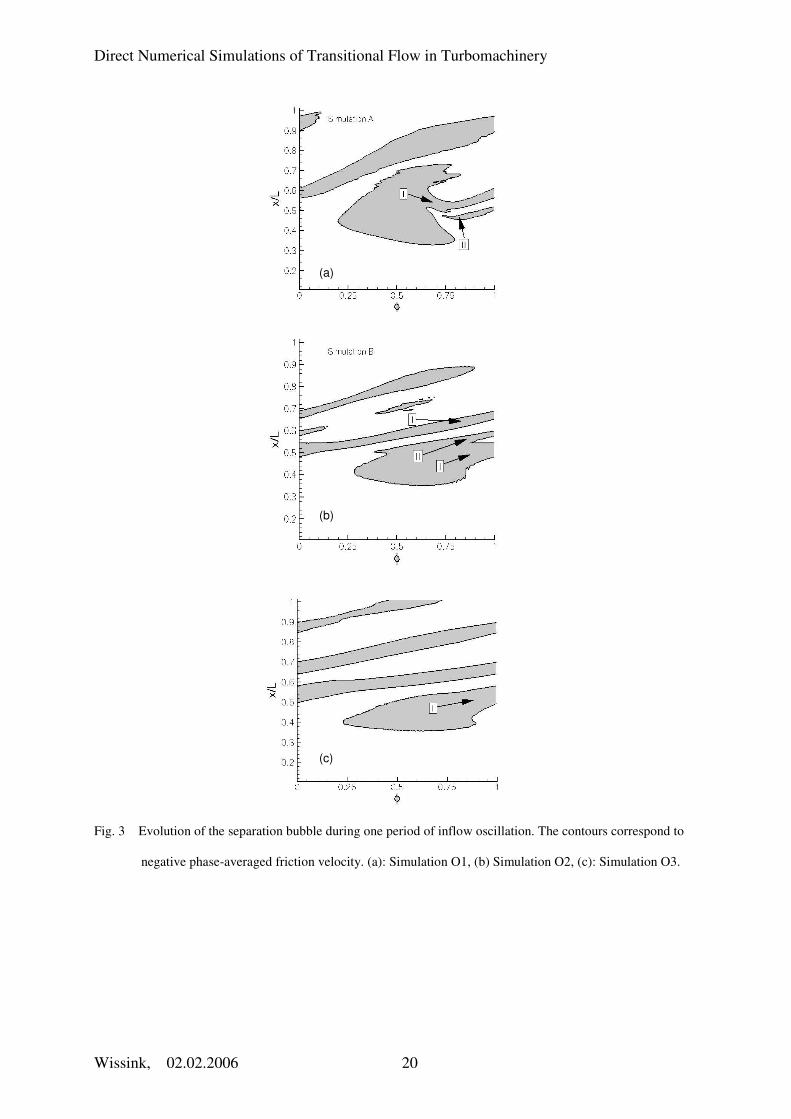
and enhanced. As a result, the locations of separation and transition move back and forth. In Fig. 3, the location

of the separation bubble is identified by contours of the negative phase-averaged friction velocity. The figure

shows the evolution of the separation bubbles for the three simulations with oscillating external flow listed in

Table 1. Owing to the large oscillation-amplitude and period in Simulation O1, compared to Simulations O2 and

O3, the maximum streamwise extent of the separation bubble is much larger. In all three simulations a large roll

of re-circulating, turbulent flow (labeled “I”) is shed as the oncoming flow decelerates (see also Figs. 4,5). In

Fig. 3ab, the remainder of the separation bubble is labeled “II”. In Simulation O2, Region II intermittently

merges with the newly formed separation bubble of the next period. In Simulation O3, however, it was

impossible to define Region II. This is explained by the small inflow-amplitude which only mildly triggers the

KH instability which is responsible for the roll-up of the shear layer and the formation of Regions I and II.

Hence, while Region II was already quite small in Simulation O2, in Simulation O3 it is even smaller and may

completely merge with the newly formed bubble of the next period. In none of the three simulations, however,

was Region I found to merge with the remainder of a bubble formed during another period. Along the flat plate,

the number of separation bubble-remains – separated by patches of laminar flow - increases with decreasing

inflow-oscillation period. For instance, at φ = 0.5 two such remains are observed for Simulation O1, three for

Simulation O2 and four for Simulation O3.

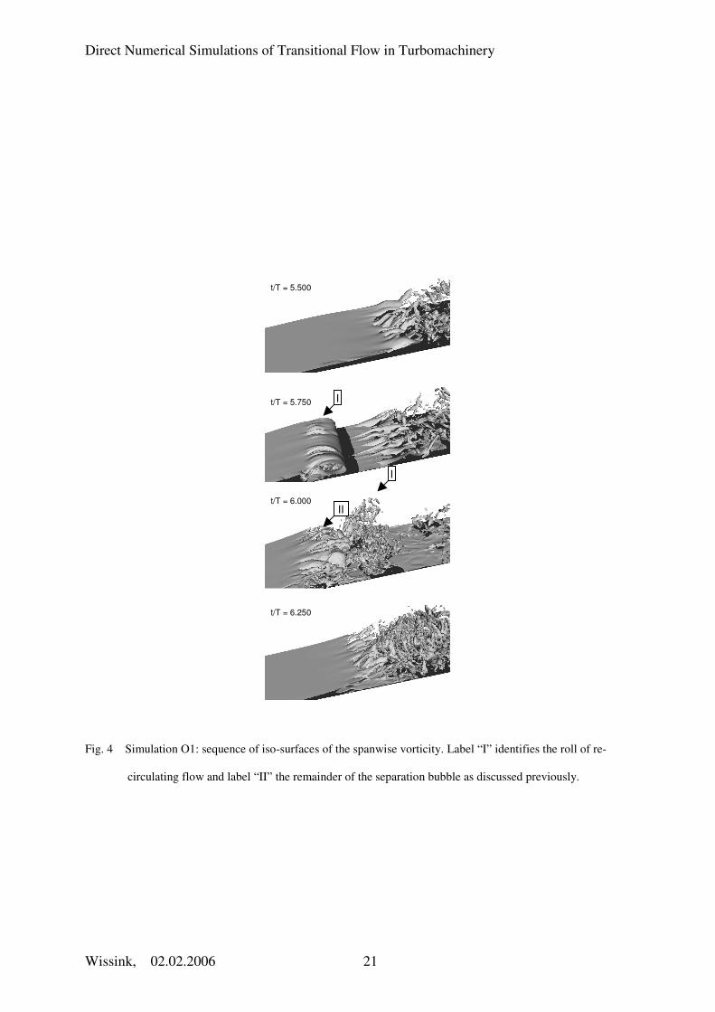
Figs. 4,5 show a series of snapshots of the spanwise vorticity from Simulations O1 and O3 which allow the

illustration and comparison of the dynamics of the boundary layers during one period of inflow oscillation.

Owing to the large period of T=0.61L/U0 employed in Simulation O1, in between the remains of two

subsequently formed separation bubbles, a clearly visible patch of laminar boundary layer flow can be observed.

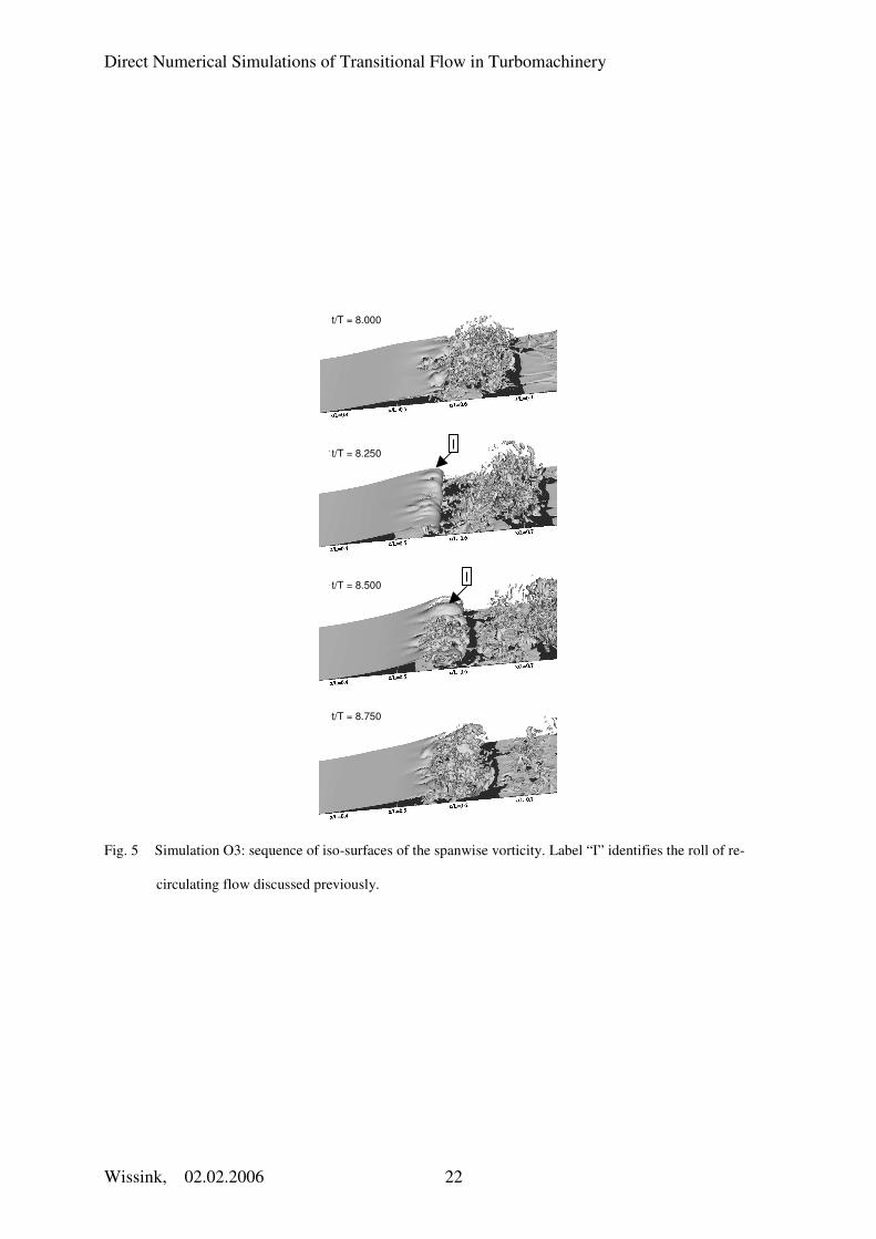
The much smaller period of T=0.30L/U0 in Simulations O2 and O3 allows only a relatively small patch of

laminar boundary layer flow to emerge, though at no time are subsequently formed separation bubbles observed

to merge. In both simulations, the separated shear layer is found to roll up owing to a KH-instability. The roll of

re-circulating flow (visible at t/T=5.750 in Simulation O1 and at t/T=8.500 in Simulation O3) is shed and

subsequently very quickly becomes turbulent. As discussed in Wissink and Rodi [6], at least two types of elliptic

instabilities – which may occur when two-dimensional flow with elliptical streamlines is subjected to three-

dimensional disturbances - contribute to this very fast transition to turbulence of the re-circulating flow.

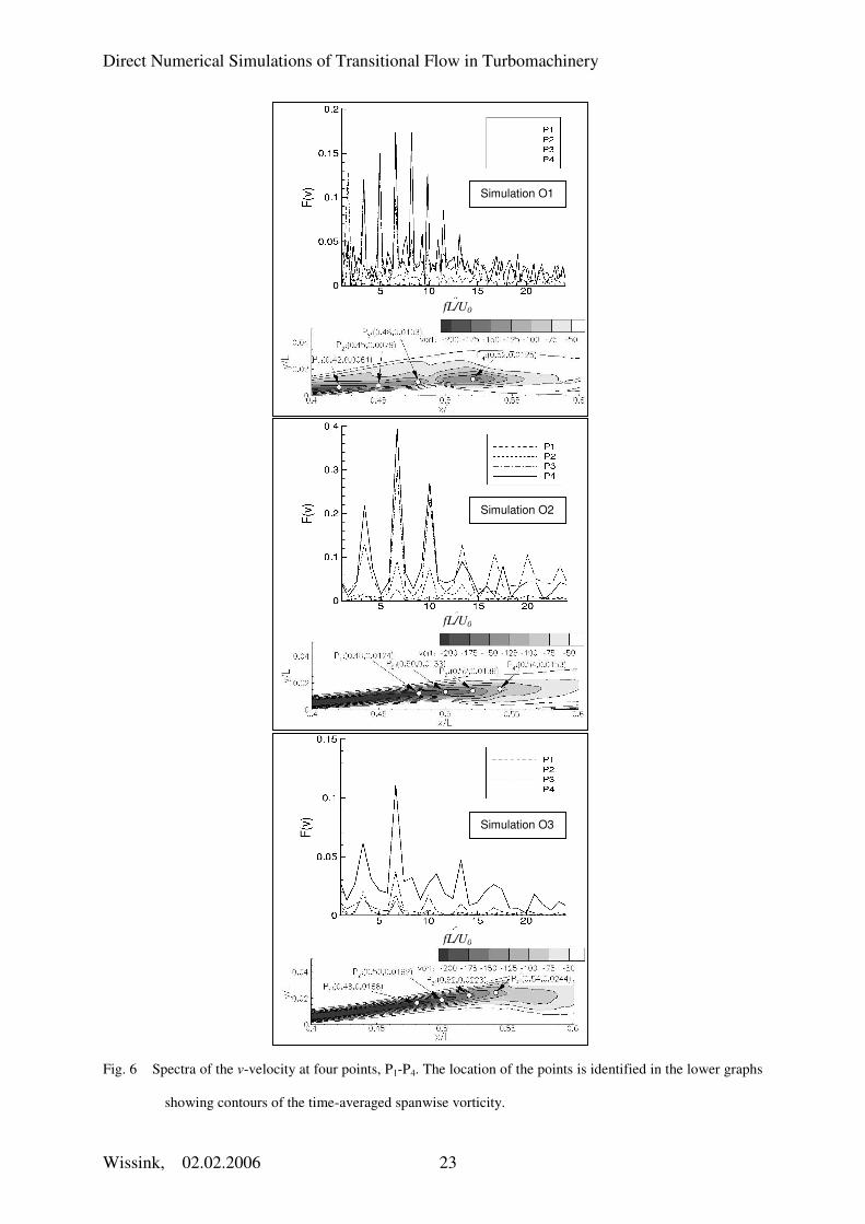
In Fig. 6, a comparison is made of spectra of the v-velocity component gathered at various locations P1,…,P4

in the time-averaged separated boundary layer. The points P1,…,P4 are identified in the lower graphs, showing

contours of the time-averaged spanwise vorticity. In all graphs, the peaks correspond to the oscillation-frequency

(left-most peak) of the inflow and its higher harmonics. For each simulation, the maximum amplitude in each of

Direct Numerical Simulations of Transitional Flow in Turbomachinery

Wissink, 02.02.2006 6

the points P4, located farthest away from the location of separation, is reached at a frequency of f ≈ 6.7U0 /L,

indicating that the most unstable modes of all three KH-instabilities coincide. This is not surprising since in all

simulations the thickness and strength of the shear layer is comparable. In Simulations O1 and O3, at point P2 the

most unstable mode is reached at the smaller frequency of f ≈ 3.3U0 /L. Apparently, the most unstable frequency

becomes smaller as the location of the point where the time-signal is recorded is nearer to the location of

separation.

Boundary-layer separation with free-stream fluctuations. The simulations with and without free-

stream fluctuations stemming from a separate LES of isotropic turbulence in a box (see Fig. 2) are listed in Table

2. In Simulation F1, without explicitly added fluctuations at the inlet, a KH instability is triggered by numerical

round-off errors. The addition of free-stream fluctuations, 5% in Simulation F2 and 7% in Simulation F3, leads

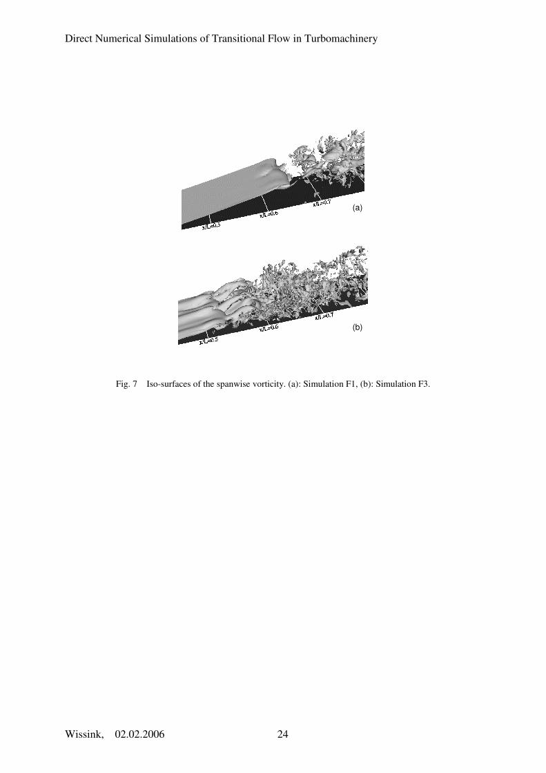
to a drastic reduction in size of the separation bubble compared to the one obtained in Simulation F1. In Fig. 7, a

comparison is made between Simulation F1 and Simulation F3. The figure shows snapshots of the instantaneous

spanwise vorticity illustrating the presence of a KH instability in both simulations. In all simulations, the

boundary layer separates near x/L=0.37. While in Simulation F1 the shear layer rolls up at x/L=0.63, in

Simulation F3 the shear layer is found to roll up farther upstream, at x/L=0.52, corresponding to a much smaller

separation bubble. Both figures illustrate that once the shear layer has rolled up, the transition to turbulence is

almost instantaneous.

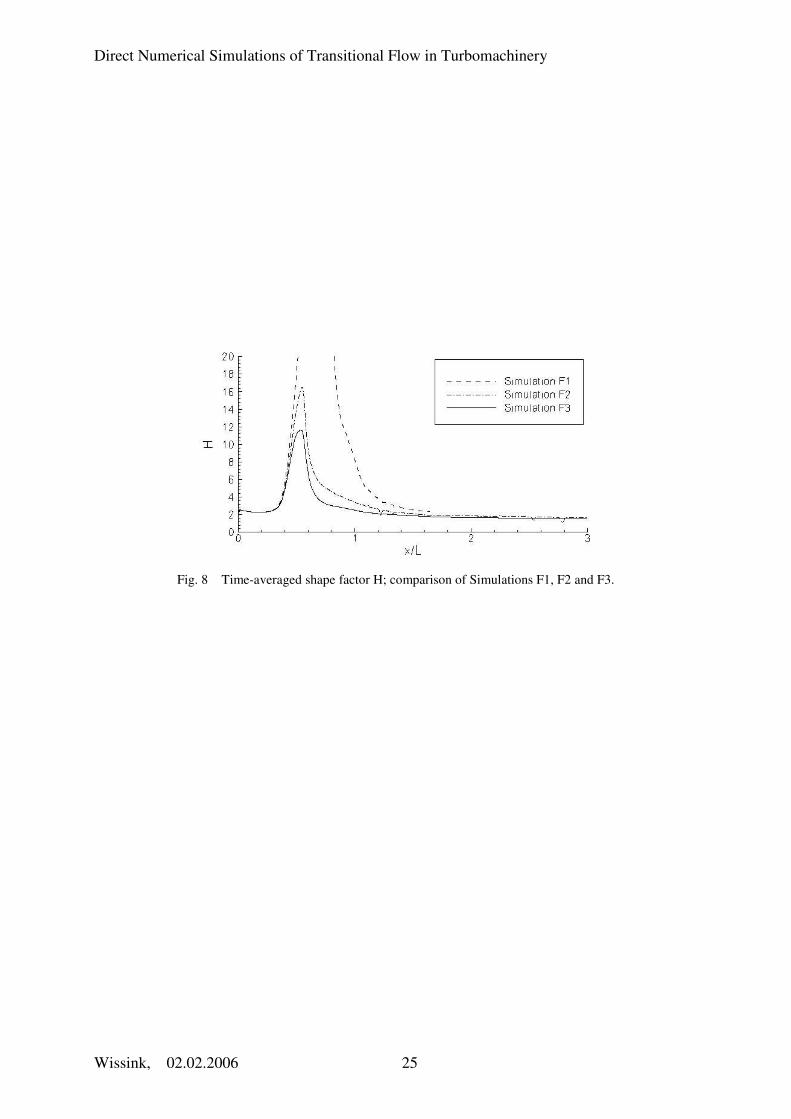
In Fig. 8, a comparison is shown of the time-averaged boundary-layer shape factor H obtained in the

Simulations F1, F2 and F3. It gives further evidence that the size of the separation bubble is quite sensitive to the

amount of inflow fluctuations (see also Table 2, which provides the approximate location of re-attachment xre).

The difference in separation bubble size is reflected by the shape factor showing a peak of H =16.4 in Simulation

F2 as compared to a peak of H=11.8 in Simulation F3. Upstream of the separation bubble, the shape factor takes

on values around H=2.4, which are characteristic for a laminar boundary layer. Downstream of the separation

bubble, the redeveloping turbulent boundary layer only very slowly assumes values around H=1.7 which are

characteristic for a turbulent boundary layer. This reflects the effect of the wall-adjacent wake-like turbulent

flow on the redeveloping boundary layer flow downstream of the separation bubble. Compared to both

Simulations F2 and F3, the shape factor of Simulation F1 – without free-stream disturbances - is much larger,

assuming a peak value of H=77.3.

Direct Numerical Simulations of Transitional Flow in Turbomachinery

Wissink, 02.02.2006 7

3. Flow Around Turbine Blades

In the second set of DNS, flow around Low-Pressure Turbine (LPT) blades with periodically incoming

wakes was studied. Generally, flows in turbine cascades are very complex and call for powerful computational

tools and models. The aerodynamic performance of a turbine blade is affected strongly by disturbances carried

by oncoming wakes generated by the preceding row of blades. Because of advances in computational power,

recently LES and DNS of flow in LPT cascades with oncoming wakes has become feasible [10,11,12,13,14].

Compared to a DNS, an LES is computationally less demanding and therefore appears to be an attractive

alternative. Unfortunately, LES is found to be less accurate in predicting the details of boundary layer transition

including the location in the presence of impinging disturbances. This is partly due to the fact that in an LES

only the resolved part of the free-stream fluctuations physically impinges on the boundary layer resulting in a

weaker triggering of boundary layer instabilities [12]. A previous DNS of flow in a T106A LPT cascade has

been performed by Wu & Durbin [13]. Their Reynolds number, based on the axial chord length and inflow

conditions, was Re=148000. They were the first to identify longitudinal vortical structures generated along the

pressure side of the blade by impinging wakes. In the passage between two turbine blades they discovered

production of fluctuating kinetic energy at the apex of the strained wake as predicted by Rogers [15]. In our DNS

we mostly focus on the study of boundary layer development. Especially along the suction side the presence of

boundary layer separation - inducing boundary layer transition – or wake-induced by-pass transition has a major

impact on heat transfer and losses.

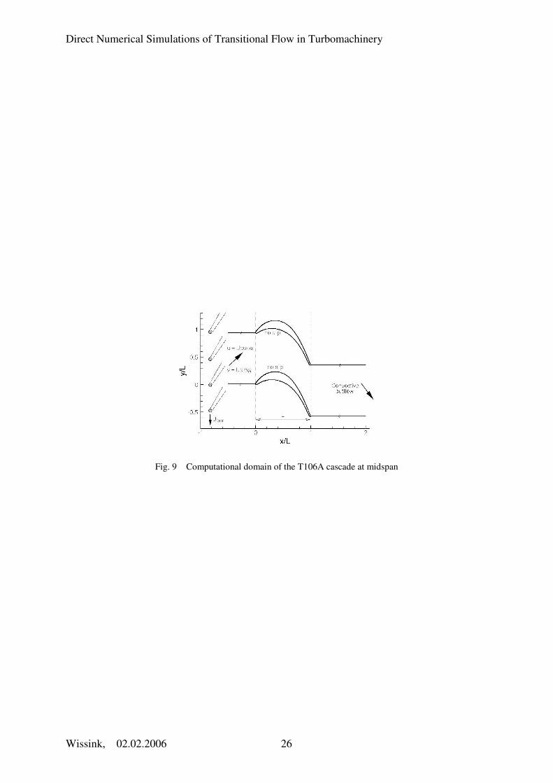
3.1 Flow configuration and computational aspects. The computational geometries were chosen in

accordance with experiments performed in a companion project performed at the University of the Armed Forces

in Munich [16] (T106A blades) and experiments performed earlier by Liu and Rodi [17,18] at the University of

Karlsruhe (MTU blades), the latter focused on heat transfer. The numerical simulations were performed for a

section of mid-span which is approximately two-dimensional (see for example Fig. 9). In the y-direction, both

upstream and downstream of the blades, periodic boundary conditions were applied. At the surface of the blades

a no-slip boundary condition was employed. In the spanwise direction periodic boundary conditions were used

while at the outlet a convective outflow boundary condition was employed. Artificial wakes were introduced at

the inlet, superposed on the mean flow (u,v,w)=U(cosα,sinα,0), where α is the angle of attack (see Tables 3 and

4). The data used for the wakes stem from a separate simulation by Wu and Durbin of Stanford University [19]

who performed LES of flow with a far-wake behavior.

Direct Numerical Simulations of Transitional Flow in Turbomachinery

Wissink, 02.02.2006 8

The main parameters of the DNS performed of flow in the T106A LPT cascade with and without wakes are

listed in Table 3. The Reynolds number – based on the inflow velocity and axial chord – is Re=51800. In the

simulation with wakes, the vertical distance between wakes is ½P, where P=0.9306L is the pitch between blades

and L is the axial chord-length. The angle of attack for this flow problem is α=45.5°. The period of the flow,

T=1.138L/U, is equal to the time needed by the wakes to perform a vertical sweep through the inlet plane over a

distance ½P.

The simulations of flow around and heat transfer from a model MTU turbine blade at Re=72000 – based on

inflow velocity and axial chord - are summarized in Table 4. In Simulation M1 no wakes were at the inlet, which

corresponds to Case A of the experiments, while in Simulation M2 wakes were introduced corresponding to

Case C of the experiments with a wake-passing-frequency of f=2.4U/L. The angle of attack in both simulations

was α=0°. To reflect the set-up in the experiments of Liu and Rodi [17,18], at the inflow the temperature θ of

the oncoming flow was set to θ0 = 0.7 θb, while the temperature at the surface of the blades was assumed to

remain constant at θ = θb. In the DNS the heat transfer and its increase due to impinging wakes was studied. The

local Nusselt number Nu defined by

( )( )

θθθ

κ θ θ

∂∂= = − −

− ∂ ∂=

0

10

3b

nLb

hL LNu

n� �� � ,

with h being the heat-transfer coefficient and κ the thermal conductivity, was chosen as a non-dimensional

measure of heat transfer from the surface of the model turbine blade to the outer flow. To reflect the presence of

background disturbances in the experiment with oncoming wakes, free-stream fluctuations of intensity Tu=4%

were added to the inflow of the DNS. To be able to employ periodic boundary conditions in the y-direction of

the DNS, it is necessary that the vertical distance between wakes is an integer divider of the pitch P=L between

blades. For this reason, the vertical distance between wakes in Simulation M2 was chosen to be ½P, which is

only an approximation of the distance of 0.567L in the experiments. As a result, the period of the flow in the

DNS is T=0.3676L/U.

The computations of flow in turbine cascades were all performed on the Hitachi SR8000-F1 at LRZ in

Munich using up to 256 processors.

3.2 Results

Results from the simulations of the flow in the two different turbine cascades with oncoming wakes will

Direct Numerical Simulations of Transitional Flow in Turbomachinery

Wissink, 02.02.2006 9

now be discussed. The first case concerns the flow in the T106A cascade. The combination of low Reynolds

number and a relatively high angle of attack of the inflow causes the flow around the T106A blades to separate

along the suction side near the trailing edge resulting in separation induced transition. The separation is,

however, periodically suppressed by impinging wakes. As in the flat plate simulations, the separated boundary

layer exhibits a KH instability. The second case concerns flow and heat transfer in a MTU cascade. Here,

incomplete by-pass transition of the boundary layer flow along the downstream half of the suction side is found

to occur and an increase in laminar heat transfer from the pressure side is found to be promoted by longitudinal

vortical structures.

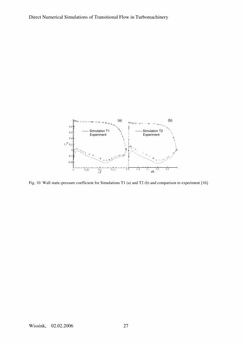
Flow in the T106 turbine cascade with incoming wakes. Fig. 10 shows the time-averaged wall-static

pressure coefficient, Cp, of (a) Simulation T1 without wakes and (b) Simulation T2 with wakes. Compared to

experiment, in Simulation T1 Cp is reasonably well captured. Certain differences on the suction side can be

attributed to discrepancies in the angle of attack, which was only approximately known in the experiment, and

some minor compressibility effects. The difference between Simulation T2 and experiment, shown in Fig. 10b, is

somewhat larger, which indicates that the physical presence of wake-generating cylinders in the experimental

inlet region partly blocks the inflow thereby reducing the mass flux through the passage. Consequently, the

effective Reynolds number in the experiment also slightly reduces. The marked “kink” present along the suction

side at x/L=0.93 (Fig. 10a) indicates that there is massive separation in the simulation without periodically

impinging wakes. The much smaller kink at x/L=0.88 in Fig. 10b points to a much reduced average separation

in Simulation T2 which occurs only intermittently along the downstream half of the suction side.

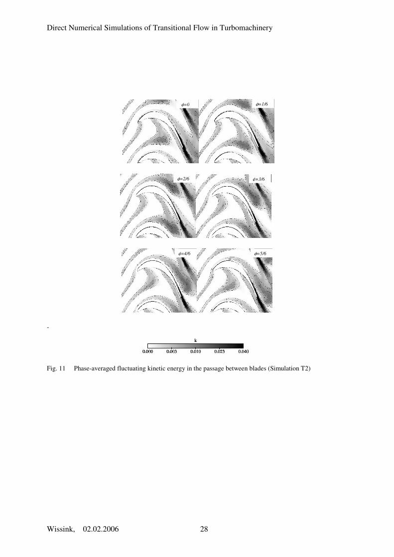
The series of snapshots of the phase-averaged fluctuating kinetic energy shown in Fig. 11 illustrates the

stretching and straining of the wakes and the production of fluctuating kinetic energy k in the passage between

blades. For each phase φ, the location of the wakes is well-defined by an increased level of k. Production of

fluctuating kinetic energy is concentrated at the apex of the strained wake and in the boundary layer along the

downstream half of the suction side. As the wake approaches the leading edge of the blade, it begins to wrap

around it. Especially near the suction side, immediately downstream of the leading edge, the wake is severely

stretched while its axis aligns with the surface of the suction side. As a consequence, in this region the wake

impinges at virtually zero angle of attack. As the wake is stretched, the fluctuations carried by the wake are

damped. Along the pressure side, near the leading edge the wake impinges at a relatively large angle of attack,

which becomes increasingly smaller as the wake approaches the trailing edge of the blade. At the trailing edge

itself, the angle between the wake-axis and the surface of the blade is virtually zero. As a result of the wakes

Direct Numerical Simulations of Transitional Flow in Turbomachinery

Wissink, 02.02.2006 10

impinging at the pressure side, longitudinal vortical structures are obtained (also observed for the MTU blade in

Fig. 18).

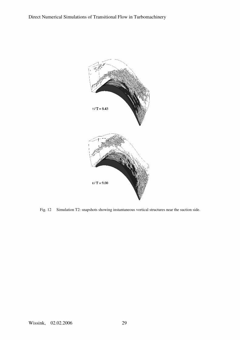
Fig. 12 shows two snapshots of vortical structures present in part of the passage between blades near the

suction side. The vortical structures have been made visible using the λ2 criterion of Jeong and Hussain [20],

showing a negative isosurface of the second largest eigenvalue of the sum of the squares of the symmetric and

anti-symmetric part of the velocity gradient tensor. The figure clearly shows the presence of relatively large-

scale vortical structures carried by the periodically oncoming wakes. As already observed in Fig. 11, the wake

impinges on the upstream half of the suction side at virtually zero angle of attack. While the wake is stretched,

its vortical structures become elongated and very thin, thereby lessening its effect as it impinges on the suction

side boundary layer. The production of fluctuations in the passage between blades gives rise to an increase in

vortical structures, visible for instance at t/T=8.43, adjacent to the upper boundary of the plotted section. In both

snapshots, small scale vortical structures were present immediately upstream of the trailing edge, which indicates

that the local boundary layer flow is no longer laminar.

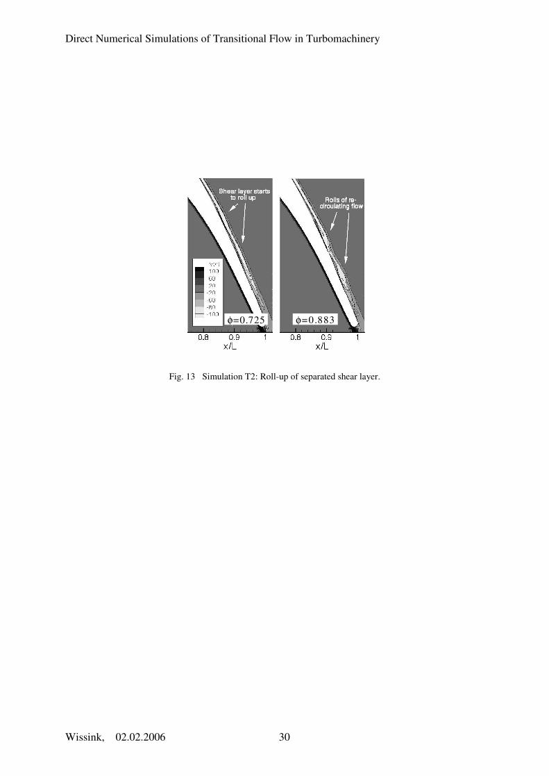
In Fig. 13, two snapshots are shown providing a close-up of the separated shear-layer along the downstream

half of the suction side. The shear layer has been made visible using the phase-averaged spanwise vorticity. The

figure clearly illustrates the roll-up of the separated shear layer owing to a KH instability triggered by an

impinging wake, giving rise to the appearance of two re-circulation zones. Inside the rolled-up shear layer,

significant amounts of fluctuating kinetic energy are produced, causing separation induced transition.

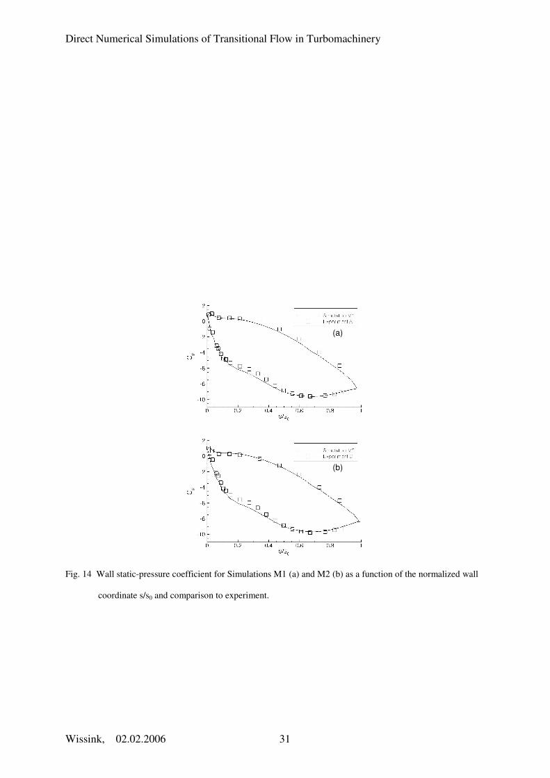
Flow and heat transfer in the MTU cascade. In Fig. 14, the time-averaged wall-static pressure

coefficient, Cp =(p-pref) / ½u2ref, of Simulations M1 and M2 is compared to experiments A and C [17,18],

respectively. The results obtained in both Simulations compare well with the experiments. Compared with the

T106 blade (Fig. 10) the favorable streamwise pressure gradient along the upstream half of the suction side is

considerably stronger. As a consequence, the streamwise acceleration of the flow along the suction side of the

MTU blade is relatively large. Though a small adverse pressure gradient region is present immediately upstream

of the trailing edge on the suction side, it is not strong enough to induce boundary layer separation.

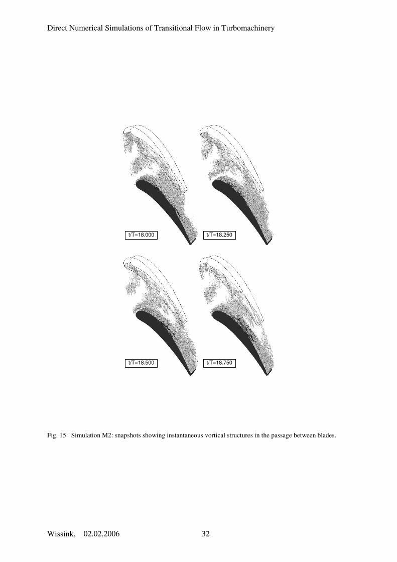
Fig. 15 shows snapshots of instantaneous vortical structures in the passage between the blades. As in Fig.

11, these structures have been made visible using the λ2-criterion of Jeong and Hussain. Compared to the

vortical structures carried by the wakes in Simulation T2 of the T106 cascade, the vortical structures inside the

wakes of Simulation M2 are of a smaller scale. This is a direct consequence of the action of background

disturbances, added at the inlet, on the coherent structures carried by the wakes, resulting in their partial

Direct Numerical Simulations of Transitional Flow in Turbomachinery

Wissink, 02.02.2006 11

destruction. As in Simulation T2, an increase in vortical structures present in the middle of the cascade is

observed, which is a consequence of fluctuating kinetic energy production at the apex of the wake.

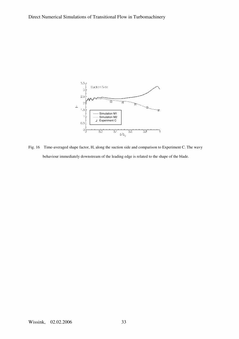
In Fig. 16, the time-averaged shape factor, H, along the suction side is shown for Simulations M1 and M2.

The shape factor obtained in Simulation M2 – with wakes - is in very good agreement with experiment.

Upstream of s/s0=0.65, where the streamwise pressure gradient is favorable, it assumes values larger than two,

which are characteristic for a laminar boundary layer. Farther downstream, in the neighbourhood of the trailing

edge, the values fall below two, indicating that the flow is at least intermittently turbulent in this region. In

Simulation M1, without oncoming wakes and background fluctuations, the shape factor rises significantly in the

region where the streamwise pressure gradient turns adverse. This indicates a tendency towards separation, but

separation was in fact never observed. Along the pressure side –not illustrated here- there is hardly any

difference in the shape factors found in Simulations M1 and M2. In both simulations, downstream of s/s0=0.25, a

constant value of H=2.35 was obtained, indicating that the pressure-side boundary layer remains laminar.

Fig. 17 shows the time-averaged local Nusselt number along the suction and pressure sides of the MTU

blade. Along the suction side, the Nusselt number obtained in Simulation M1 –without wakes- is in good

agreement with experiment A. The Nusselt number obtained in Simulation M2 –with wakes-, is underestimated,

especially in the laminar region, though the shape of the profile, which is related to the increase of Nu in the

region were the boundary layer becomes intermittently turbulent, is reasonably well predicted. The

underestimation of Nu is possibly explained by the spectrum of scales present in the disturbances added at the

inflow. While small scale structures in the outer flow are found not to be able to notably penetrate/disturb the

suction side boundary layer in the presence of a strongly favourable pressure gradient, large scale disturbances

might be more effective and are probably present in the experiment, leading to the observed increase in the heat

transfer coefficient. There is evidence of the existence of a preferred free-stream fluctuation length-scale which

is particularly effective in promoting laminar heat transfer in the presence of an accelerating streamwise flow

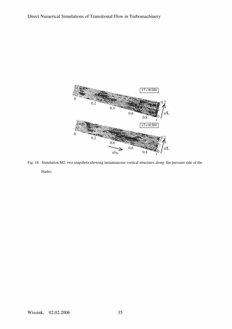
[21]. Along the pressure side, the Nusselt number obtained in Simulations M1 and M2, respectively, is in good

agreement with experiment. The moderate increase in Nu from Experiment A without wakes to Experiment C

with wakes and background turbulence is quite well captured in the numerical simulations. The reason for this

increase in Nu is most likely the increased transport of heat from the wall promoted by the wake-induced,

streamwise vortical structures present along the pressure side. These structures can be seen in the two snapshots

shown in Fig. 18. The snapshots illustrate the evolution of the wake-induced structures along the pressure side of

the blade (see also Wu and Durbin [10] and Wissink [11]) during one wake-passing period T.

Direct Numerical Simulations of Transitional Flow in Turbomachinery

Wissink, 02.02.2006 12

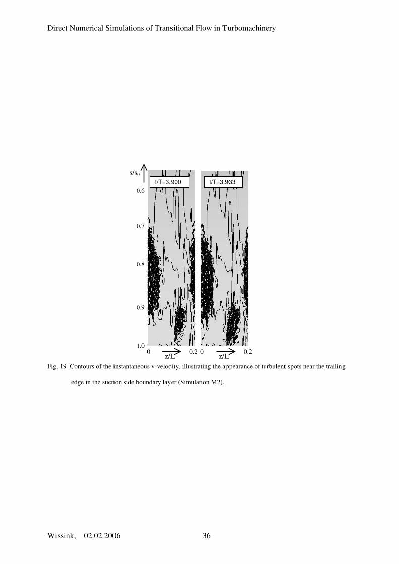
Fig. 19 illustrates the appearance of turbulent spots along the suction side, immediately upstream of the

trailing edge. It shows two snapshots of instantaneous contours of the velocity component in the y-direction (see

Fig. 9). Two separate turbulent spots are clearly visible, one lying on the periodic spanwise boundary and the

other one a bit farther downstream. Though the snapshots are relatively close to one another, they do illustrate

the travelling downstream of the turbulent spots and provide proof of incomplete by-pass transition of the

boundary layer flow along the suction side boundary layer of the MTU blade as opposed to separation-induced

transition of the boundary layer flow along the suction side of the T106 blade.

4. Conclusions

The recent increase in computational power has made it possible to employ DNS for the study of transitional

flow in turbine-related geometries. The application of DNS is still limited to flow with moderate Reynolds

numbers and simplified geometries such as a two-dimensional geometry representing a model of the flow along

the suction side of a turbine blade (discussed in Section 2) or a section at mid span of one single turbine blade

(see Section 3). To accurately describe the instantaneous flow in a 2D section of a LP turbine passage using

realistic operating conditions, approximately 100 million. grid points were found to be needed, combined with a

time-step in the order of 10-5L/U. On average, it took several months of clock time to run one single simulation

on a modern, massively parallel computer. Periodicity of the inflow signal, for instance induced by prescribed

inflow-oscillations or by periodically impinging wakes, was used to gather phase-averaged statistics. Because, as

observed above, the DNS were very expensive, only a moderate (but largely sufficient) number of periods was

affordable during which phase-averaged statistics were gathered.

Though the computational power is not yet sufficient to tackle with DNS fully three-dimensional flow

problems occurring in a real turbine, the simulations performed in two-dimensional geometries provide valuable

data for the further development and improvement of models for transition to turbulence to be employed in

Reynolds Averaged Navier Stokes (RANS) simulations and allow the examination of physical mechanisms

involved in boundary layer transition. The DNS results of separating flow with oncoming disturbances, for

instance, show that a Kelvin-Helmholtz instability plays a very important role in the early transition to

turbulence, after which secondary instabilities take over. The same Kelvin-Helmholtz instabilities were observed

to be triggered in the separated flow along the downstream half of the suction side in the T106A simulation with

periodically oncoming wakes. On the other hand, in the MTU-blade simulation with oncoming wakes by-pass-

transition processes were found to play a very important role in the incomplete transition of the suction side

Direct Numerical Simulations of Transitional Flow in Turbomachinery

Wissink, 02.02.2006 13

boundary layer. Compared to the background fluctuations, the small-scale fluctuations carried by the periodically

impinging wakes are relatively intense and cause the location of transition to alternately move up- and

downstream. The streamwise vortical structures observed along the pressure side explain the increase in heat

transfer from the model blade towards the outer flow. However, compared with experiment, the increase in

laminar heat transfer caused by the wakes with small-scale fluctuations was partly underpredicted. In the near

future, we will perform a further DNS of flow around the MTU blade to study the effect on the heat transfer of

more realistic incoming wakes having larger-scale fluctuations.

Further DNS of turbomachinery flows are under way, and simulations of flow in a compressor cascade with

incoming disturbances have already been carried out [22]. The expected further increase in computational power

will make it possible to perform simulations at higher Reynolds numbers, to significantly increase the number of

periods used for phase-averaging, to perform simulations using more than one turbine passage and to calculate

simulations with more complex three-dimensional geometries. Hence, the importance of DNS will grow with

increasing computational power and, though it is highly unlikely that in the foreseeable future it will replace

RANS as a standard tool for industrial applications, it is already an important tool in transition studies.

Unfortunately, DNS results are sensitively dependent on the boundary conditions used. Hence, to obtain an

accurate prediction of the flow one would need to be able to prescribe the often very complex instantaneous

boundary conditions with a high degree of accuracy. The main strength of DNS lies in its capability of accurately

describing complex transitional and turbulent flow phenomena by resolving all relevant scales of motion, thereby

allowing the extraction and study of all details of the flow.

Acknowledgments

The authors would like to thank the German Research Foundation (DFG) for funding this project, the

steering committee of the Supercomputing Facilities in Bavaria (HLRB) for granting computing time on the

Hitachi SR8000-F1 at Leibniz Computing Center (LRZ) in Munich and the Computing Center of the University

of Karlsruhe for granting access to the IBM SP-SMP supercomputer.

Direct Numerical Simulations of Transitional Flow in Turbomachinery

Wissink, 02.02.2006 14

Nomenclature

a = amplitude of oscillating inflow

Cp = pressure coefficient

E = kinetic energy

f = non-dimensional frequency of Kelvin-Helmholtz mode

F(v) = amplitude of Fourier mode of v-spectrum

h = heat transfer coefficient

H = shape factor

k = fluctuating kinetic energy

L = length of plate / axial chord length blade

n = distance from turbine blade

Nu = local Nusselt number

p = pressure

P = pitch

Re = Reynolds number

S = distance from leading edge measured along the surface

S0 = distance from leading edge to trailing edge measured along the surface

St = Strouhal number

T = period

Tu = turbulence level

U0 = magnitude of time-averaged inlet velocity

u = velocity component in x-direction

v = velocity component in y-direction

w = velocity component in z-direction

x = x-coordinate

Direct Numerical Simulations of Transitional Flow in Turbomachinery

Wissink, 02.02.2006 15

y = y-coordinate

Greek symbols

α = angle of inflow with positive x-axis

φ = phase

κ = thermal conductivity of air at 300K

θ = temperature

θ0 = temperature of turbine blade

ν = kinematic viscosity

Subscripts

ref = reference

re = re-attachment

0 = inflow

b = blade

c = chord

w = wall

References

[1] Hourmouziadis, J., 2000, “Das DFG Verbundvorhaben instationäre Strömung in Turbomaschinen,” In:

Deutscher Luft- und Raumfahrtkongress, Leipzig, Germany, September 18-21, DGLR-JT2000-030

[2] Alam, M. and Sandham, N.D., 2000, “Direct Numerical Simulation of ´short´ laminar separation bubbles

with turbulent reattachment,” J. Fluid Mech., 410, pp. 1-28.

[3] Maucher, U. Rist, U, Kloker, M, and Wagner, S., 2000, “DNS of laminar-turbulent transition in separation

bubbles. In: High-performance Computing in Science and Engineering, Eds. E. Krause and W. Jäger,

Publisher Springer, Berlin, Heidelberg.

Direct Numerical Simulations of Transitional Flow in Turbomachinery

Wissink, 02.02.2006 16

[4] Spalart, P.R. and Strelets, M.Kh., 2000, ”Mechanisms of Transition and heat transfer in a separation bubble,”

J. Fluid Mech., 403, pp. 329-349.

[5] Wissink, J.G. and Rodi, W., 2002, ”DNS of transition in a laminar separation bubble,” in: Advances in

Turbulence IX, (I.P. Castro, P.E. Hancock and T.G. Thomas eds.).

[6] Wissink, J.G. and Rodi, W., 2003, ”DNS of a laminar separation bubble in the presence of oscillating flow,”

Flow, Turbulence and Combustion, 71, pp. 311-331.

[7] Wissink, J.G., Michelassi, V. and Rodi, W., 2003, ”Heat transfer in a laminar separation bubble affected by

oscillating external flow,” in: Turbulence, Heat and Mass Transfer-4, (K. Hanjalic, Y. Nagano and M.J.

Tummers eds.).

[8] Wissink, J.G. and Rodi, W., 2004, ”DNS of a laminar separation bubble affected by free-stream

disturbances,” in: Direct and Large-Eddy Simulation V, (R. Friedrich, B.J. Geurts and O. Métais eds.).

[9] Lou, W. and Hourmouziadis, J., 2000, “Separation bubbles under steady and periodic-unsteady main flow

conditions,” In: Proceedings of the 45th ASME International Gas Turbine & Aeroengine Technical

Congress, Munich Germany May 8-11.

[10] Wu, X. and Durbin, P.A., 2001, “Evidence of longitudinal vortices evolved from distorted wakes in a

turbine passage,” J. Fluid Mech., 446, pp. 199-228.

[11] Wissink, J.G., 2003, ”DNS of separating, low Reynolds number flow in a turbine cascade with incoming

wakes,” Int. J. of Heat and Fluid Flow, 24, pp. 626-635.

[12] Michelassi, V., Wissink, J.G. and Rodi, W., 2002, ”Analysis of DNS and LES of flow in a low pressure

turbine cascade with incoming wakes,” Flow, Turbulence and Combustion 69, pp. 295-329.

[13] Kalitzin, G., Wu, X. and Durbin, P.A., 2002, “DNS of fully turbulent flow in a LPT passage,” In:

Engineering Turbulence Modelling and Experiments 5, Eds. W. Rodi and N. Fueyo, Elsevier.

[14] Raverdy, B., Mary, I., Sagaut, P. and Liamis, N., 2003, “High-resolution large-eddy simulation of flow

around low-pressure turbine blade,” AIAA J. 41(3), pp 390-397.

[15] Rogers, M.M., 2002, “The evolution of strained turbulent plane wakes,” J. Fluid Mech. 463, pp. 53-120.

[16] Stadtmüller, P. and Fottner, L., 2001, “A test case for the numerical investigation of wake passing effects on

a highly loaded LP turbine cascade blade,” ASME Paper 2001-GT-311.

[17 ]Liu, X. and Rodi, W., 1994, “Velocity measurements in wake-induced unsteady flow in a linear turbine

Direct Numerical Simulations of Transitional Flow in Turbomachinery

Wissink, 02.02.2006 17

cascade,” Exp. in Fluids 17, pp. 45-58.

[18] Liu, X. and Rodi, W., 1994, “Surface pressure and heat transfer measurements in a turbine cascade with

unsteady oncoming wakes,” Exp. in Fluids 17, pp. 171-178.

[19] Wu, X., Jacobs, R.G., Hunt, J.C.R., Durbin, P.A., 1999, ”Simulation of boundary layer transition induced by

periodically impinging wakes,” J. Fluid Mech. 398, pp. 109-153.

[20] Jeong, J. and Hussain, F., 1995, “On the identification of a vortex,” J. Fluid Mech. 285, pp. 69-94.

[21] Dullenkopf, K. and Mayle, R.E. 1995, "An Account of Free-Stream-Turbulence Length Scale on Laminar

Heat Transfer", ASME J. Turbomachinery Vol. 117, pp. 401-406.

[22] Zaki, T.A., Durbin, P.A., Wissink, J.G., Rodi, W., 2006, “Direct Numerical Simulation of by-pass and

separation-induced transition in a linear compressor cascade”, ASME-paper GT2006-90885.

Direct Numerical Simulations of Transitional Flow in Turbomachinery

Wissink, 02.02.2006 18

Fig. 1 Computational domain at midspan

Direct Numerical Simulations of Transitional Flow in Turbomachinery

Wissink, 02.02.2006 19

Fig. 2 Energy spectrum of the free-stream disturbances added at the inlet showing the Fourier transform of the

kinetic energy E of the fluctuations along (y,z)=(0.10L,0.10L), k = 0.20L/λ is the wave number, λ is the

wave-length and (0.20L)3 is the size of the box.

Direct Numerical Simulations of Transitional Flow in Turbomachinery

Wissink, 02.02.2006 20

Fig. 3 Evolution of the separation bubble during one period of inflow oscillation. The contours correspond to

negative phase-averaged friction velocity. (a): Simulation O1, (b) Simulation O2, (c): Simulation O3.

(a)

(c)

(b)

Direct Numerical Simulations of Transitional Flow in Turbomachinery

Wissink, 02.02.2006 21

Fig. 4 Simulation O1: sequence of iso-surfaces of the spanwise vorticity. Label “I” identifies the roll of re-

circulating flow and label “II” the remainder of the separation bubble as discussed previously.

t/T = 5.500

t/T = 5.750

t/T = 6.000

t/T = 6.250

I

II

I

Direct Numerical Simulations of Transitional Flow in Turbomachinery

Wissink, 02.02.2006 22

Fig. 5 Simulation O3: sequence of iso-surfaces of the spanwise vorticity. Label “I” identifies the roll of re-

circulating flow discussed previously.

t/T = 8.000

t/T = 8.250

t/T = 8.500

t/T = 8.750

I

I

Direct Numerical Simulations of Transitional Flow in Turbomachinery

Wissink, 02.02.2006 23

Fig. 6 Spectra of the v-velocity at four points, P1-P4. The location of the points is identified in the lower graphs

showing contours of the time-averaged spanwise vorticity.

Simulation O1

Simulation O3

Simulation O2

fL/U0

fL/U0

fL/U0

Direct Numerical Simulations of Transitional Flow in Turbomachinery

Wissink, 02.02.2006 24

Fig. 7 Iso-surfaces of the spanwise vorticity. (a): Simulation F1, (b): Simulation F3.

(a)

(b)

Direct Numerical Simulations of Transitional Flow in Turbomachinery

Wissink, 02.02.2006 25

Fig. 8 Time-averaged shape factor H; comparison of Simulations F1, F2 and F3.

Direct Numerical Simulations of Transitional Flow in Turbomachinery

Wissink, 02.02.2006 26

Fig. 9 Computational domain of the T106A cascade at midspan

Direct Numerical Simulations of Transitional Flow in Turbomachinery

Wissink, 02.02.2006 27

Fig. 10 Wall static-pressure coefficient for Simulations T1 (a) and T2 (b) and comparison to experiment [16].

Simulation T1 � Experiment

Simulation T2 � Experiment

(b) (a)

Direct Numerical Simulations of Transitional Flow in Turbomachinery

Wissink, 02.02.2006 28

φ=0 φ=1/6

φ=2/6 φ=3/6

φ=4/6 φ=5/6

-

Fig. 11 Phase-averaged fluctuating kinetic energy in the passage between blades (Simulation T2)

Direct Numerical Simulations of Transitional Flow in Turbomachinery

Wissink, 02.02.2006 29

Fig. 12 Simulation T2: snapshots showing instantaneous vortical structures near the suction side.

Direct Numerical Simulations of Transitional Flow in Turbomachinery

Wissink, 02.02.2006 30

φ=0.725 φ=0.883

Fig. 13 Simulation T2: Roll-up of separated shear layer.

Direct Numerical Simulations of Transitional Flow in Turbomachinery

Wissink, 02.02.2006 31

Fig. 14 Wall static-pressure coefficient for Simulations M1 (a) and M2 (b) as a function of the normalized wall

coordinate s/s0 and comparison to experiment.

(a)

(b)

Direct Numerical Simulations of Transitional Flow in Turbomachinery

Wissink, 02.02.2006 32

Fig. 15 Simulation M2: snapshots showing instantaneous vortical structures in the passage between blades.

t/T=18.000

t/T=18.750 t/T=18.500

t/T=18.250

Direct Numerical Simulations of Transitional Flow in Turbomachinery

Wissink, 02.02.2006 33

Fig. 16 Time-averaged shape factor, H, along the suction side and comparison to Experiment C. The wavy

behaviour immediately downstream of the leading edge is related to the shape of the blade.

Simulation M1 ⋅⋅⋅⋅⋅⋅⋅⋅ Simulation M2 � Experiment C

Direct Numerical Simulations of Transitional Flow in Turbomachinery

Wissink, 02.02.2006 34

Fig. 17 Simulations I & II: time-averaged Nusselt number, Nu, as a function of the normalized wall-coordinate;

comparison to experiments.

Simulation M1 ⋅⋅⋅⋅⋅⋅⋅⋅ Simulation M2 � Experiment A � Experiment C

Direct Numerical Simulations of Transitional Flow in Turbomachinery

Wissink, 02.02.2006 35

Fig. 18 Simulation M2: two snapshots showing instantaneous vortical structures along the pressure side of the

blades.

t/T=18.000

t/T=18.500 1

1

0.8

0.8

0.6 0.4

0.6 0.4

0.2

0.2

0

0

s/s0

0

0

0.2

0.2

z/L

z/L

Direct Numerical Simulations of Transitional Flow in Turbomachinery

Wissink, 02.02.2006 36

Fig. 19 Contours of the instantaneous v-velocity, illustrating the appearance of turbulent spots near the trailing

edge in the suction side boundary layer (Simulation M2).

t/T=3.900 t/T=3.933

1.0

0.9

0.8

0.6

0.7

s/s0

0 0 0.2 0.2 z/L z/L

Direct Numerical Simulations of Transitional Flow in Turbomachinery

Wissink, 02.02.2006 37

Simulation Grid Size span a T

O1 966x226x128 0.12L 0.20 0.61

O2 1286x310x128 0.08L 0.10 0.30

O3 966x226x128 0.12L 0.05 0.30

Table 1. Overview of the simulations with oscillating inflow.

Direct Numerical Simulations of Transitional Flow in Turbomachinery

Wissink, 02.02.2006 38

Simulation Grid Size span lx xre Tu (%)

F1 1038x226x128 0.08L 1.6L 1.28L 0

F2 1926x230x128 0.08L 3.0L 1.00L 5

F3 1926x230x128 0.08L 3.0L 0.77L 7

Table 2. Overview of the simulations with and without free-stream fluctuations, lx is the actual length of the flat

plate used in the simulation, xre is the approximate location of re-attachment and Tu is the turbulence

level at the inlet.

Direct Numerical Simulations of Transitional Flow in Turbomachinery

Wissink, 02.02.2006 39

Sim Grid Span WD WHW

T1 771x256x128 0.25L - -

T2 1014x260x64 0.20L 25% 0.03L

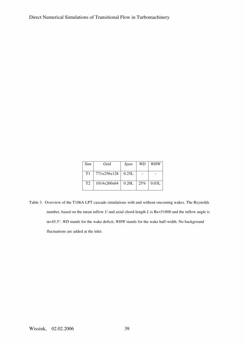
Table 3. Overview of the T106A LPT cascade simulations with and without oncoming wakes. The Reynolds

number, based on the mean inflow U and axial chord-length L is Re=51800 and the inflow angle is

α=45.5°. WD stands for the wake deficit, WHW stands for the wake half-width. No background

fluctuations are added at the inlet.

Direct Numerical Simulations of Transitional Flow in Turbomachinery

Wissink, 02.02.2006 40

Sim Grid WD WHW Tu Exp.

M1 1254x582x128 - - 0% A

M2 1254x582x128 30% 0.045L 2.8% C

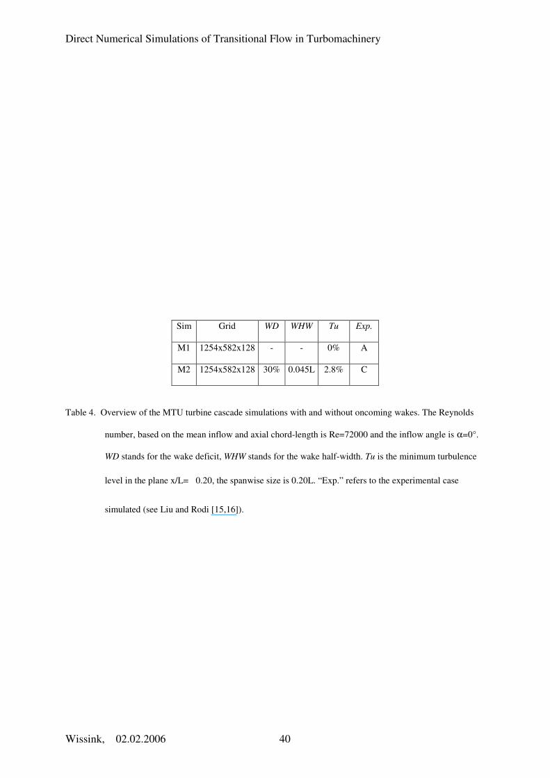
Table 4. Overview of the MTU turbine cascade simulations with and without oncoming wakes. The Reynolds

number, based on the mean inflow and axial chord-length is Re=72000 and the inflow angle is α=0°.

WD stands for the wake deficit, WHW stands for the wake half-width. Tu is the minimum turbulence

level in the plane x/L= � 0.20, the spanwise size is 0.20L. “Exp.” refers to the experimental case

simulated (see Liu and Rodi [15,16]).

Direct Numerical Simulations of Transitional Flow in Turbomachinery

Wissink, 02.02.2006 41

Fig. 1 Computational domain at midspan

Fig. 2 Energy spectrum of the free-stream disturbances added at the inlet

Fig. 3 Evolution of the separation bubble during one period of inflow oscillation. The contours correspond to

negative phase-averaged friction velocity. (a): Simulation O1, (b) Simulation O2, (c): Simulation O3.

Fig. 4 Simulation O1: sequence of iso-surfaces of the spanwise vorticity. Label “I” identifies the roll of re-

circulating flow and label “II” the remainder of the separation bubble as discussed previously.

Fig. 5 Simulation O3: sequence of iso-surfaces of the spanwise vorticity. Label “I” identifies the roll of re-

circulating flow discussed previously.

Fig. 6 Spectra of the v-velocity at four points, P1-P4. The location of the points is identified in the lower graphs

showing contours of the time-averaged spanwise vorticity.

Fig. 7 Iso-surfaces of the spanwise vorticity. (a): Simulation F1, (b): Simulation F3.

Fig. 8 Time-averaged shape factor H; comparison of Simulations F1, F2 and F3.

Fig. 9 Computational domain of the T106A cascade at midspan.

Fig. 10 Wall static-pressure coefficient for Simulations T1 (a) and T2 (b) and comparison to experiment [16].

Fig. 11 Phase-averaged fluctuating kinetic energy in the passage between blades (Simulation T2).

Fig. 12 Simulation T2: snapshots showing instantaneous vortical structures near the suction side.

Direct Numerical Simulations of Transitional Flow in Turbomachinery

Wissink, 02.02.2006 42

Fig. 13 Simulation T2: Roll-up of separated shear layer.

Fig. 14 Wall static-pressure coefficient for Simulations M1 (a) and M2 (b) as a function of the normalized wall

coordinate s/s0 and comparison to experiment.

Fig. 15 Simulation M2: snapshots showing instantaneous vortical structures in the passage between blades.

Fig. 16 Time-averaged shape factor, H, along the suction side and comparison to Experiment C.

Fig. 17 Simulations I & II: time-averaged Nusselt number, Nu, as a function of the normalized wall-coordinate;

comparison to experiments.

Fig. 18 Simulation M2: two snapshots showing instantaneous vortical structures along the pressure side of the

blades.

Fig. 19 Contours of the instantaneous v-velocity, illustrating the appearance of turbulent spots near the trailing

edge in the suction side boundary layer (Simulation M2).

Direct Numerical Simulations of Transitional Flow in Turbomachinery

Wissink, 02.02.2006 43

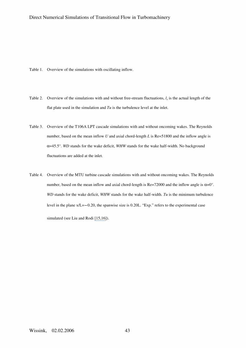
Table 1. Overview of the simulations with oscillating inflow.

Table 2. Overview of the simulations with and without free-stream fluctuations, lx is the actual length of the

flat plate used in the simulation and Tu is the turbulence level at the inlet.

Table 3. Overview of the T106A LPT cascade simulations with and without oncoming wakes. The Reynolds

number, based on the mean inflow U and axial chord-length L is Re=51800 and the inflow angle is

α=45.5°. WD stands for the wake deficit, WHW stands for the wake half-width. No background

fluctuations are added at the inlet.

Table 4. Overview of the MTU turbine cascade simulations with and without oncoming wakes. The Reynolds

number, based on the mean inflow and axial chord-length is Re=72000 and the inflow angle is α=0°.

WD stands for the wake deficit, WHW stands for the wake half-width. Tu is the minimum turbulence

level in the plane x/L= � 0.20, the spanwise size is 0.20L. “Exp.” refers to the experimental case

simulated (see Liu and Rodi [15,16]).