1

Analyzing the Transitional Region in Low PowerWireless Links

Marco Zuniga and Bhaskar KrishnamachariDepartment of Electrical Engineering - Systems

University of Southern California, Los Angeles, CA 90089-0781marcozun@usc.edu, bkrishna@usc.edu

Abstract— The wireless sensor networks community, has nowan increased understanding of the need for realistic link layermodels. Recent experimental studies have shown that real deploy-ments have a “transitional region” with highly unreliable links,and that therefore the idealized perfect-reception-within-rangemodels used in common network simulation tools can be verymisleading. In this paper, we use mathematical techniques fromcommunication theory to model and analyze low power wirelesslinks. The primary contribution of this work is the identificationof the causes of the transitional region, and a quantification oftheir influence. Specifically, we derive expressions for the packetreception rate as a function of distance, and for the width ofthe transitional region. These expressions incorporate importantchannel and radio parameters such as the path loss exponentand shadowing variance of the channel; and the modulation andencoding of the radio. A key finding is that for radios usingnarrow-band modulation, the transitional region is not an artifactof the radio non-ideality, as it would exist even with perfect-threshold receivers because of multi-path fading. However, wehypothesize that radios with mechanisms to combat multi-patheffects, such as spread-spectrum and diversity techniques, canreduce the transitional region.

I. I NTRODUCTION

Wireless sensor network protocols are often evaluatedthrough simulations that make simplifying assumptions aboutthe link layer, such as the binary perfect-reception-within-range model. Several recent empirical studies [1] [2] [3] havequestioned the validity of these assumptions. These studieshave revealed the existence of three distinct reception regionsin a wireless link: connected, transitional, and disconnected.The transitional region is often quite significant in size, and isgenerally characterized by high-variance in reception rates andasymmetric connectivity. Particularly, in dense deploymentssuch as those envisioned for sensor networks, a large numberof the links in the network (even higher than 50%) can beunreliable due to the transitional region.

Because of its inherent unreliability and extent, the transi-tional region can have a major impact on the performanceof upper-layer protocols. In [1] it is shown that the dy-namics of even the simplest flooding mechanism and thetopology of data gathering trees constructed in dense sensornetworks can be significantly affected due to the asymmetricand occasional long-distance links caused by nodes presentin the transitional region. In [6] also, it is argued that the

This work was supported in part by NSF under grant number 0347621, andby a gift grant from Ember Corporation.

routing structures formed taking into account unreliable linkscan be very different from the structures formed based ona simplistic model. Similarly, the authors of [7] report thatsuch unreliable links can have a significant impact on routingprotocols, particularly geographic forwarding schemes. On theother hand, other works have proposed mechanisms to takeadvantage of nodes in the transitional region. For instance,[5] found that protocols using the traditional minimum hop-count metric perform poorly in terms of throughput, and thata new metric called ETX (expected number of transmissions),which uses nodes in the transitional region, has the bestperformance. On the same line of work, by evaluating linkestimator and neighborhood table management, the authors in[3] found that cost-based routing using aminimum expectedtransmissionmetric has a good performance. Therefore, due tothe significant impact that nodes in the transitional region haveon upper-layer protocols, there is an increased understandingof the need for realistic link layer models for wireless sensornetworks.

In order to address this need, some recent works [3] [7] [8]have proposed new link models based on empirical data. Whilethese empirical models do play an invaluable role in improvingthe realism of protocol evaluation, they suffer from somesignificant shortcomings. They do not provide fundamentalinsight into the root causes of the observed phenomena. Andthey do not provide a systematic way to generalize the models(i.e., extend their validity and accuracy) beyond the specificradio and environment conditions of the experiments fromwhich the models are derived.

On the other hand, there exists a rich literature on wire-less communications, particularly in the context of cellulartelecommunication networks1, that provides a set of modelsand tools for analyzing the physical layer. In this study,we make use of these analytical tools to derive expressionsfor the packet reception rate as a function of distance fordifferent settings, and to determine the width of the transitionalregion. These expressions do not consider node mobility nordynamic objects in the environment; thus, while different linksexperience different levels of fading, the fading for each linkis assumed to be constant over time.

The analysis done in this work provides some importantcontributions. First, it allows us to delimit the influence of

1In cellular systems the transitional region is not of interest (except formodelling inter-cell interference) as cells are designed to fit only the connectedregion.

the wireless environment and the radio on the transitionalregion; furthermore, the derived expressions show how thetransitional region is impacted by important radio parameterssuch as modulation, encoding, output power, frame size andreceiver noise, as well as important environmental parameters,namely, the path loss exponent and the log-normal shadowvariance. Second, we are able to conclude that, for radios usingnarrow-band modulation, the transitional region is present evenwith perfect-threshold radios (i.e., that it is not an artifactof radio non-ideality alone) due to shadowing effects; hence,radios with mechanisms to combat multi-path may reduce thetransitional region. And third, we bring to the notice of thecommunity simple analytical models for the link layer thatcan be used to enhance simulations.

The rest of the paper is organized as follows. Section IIpositions our work in the current literature. The basic frame-work of the model is derived in section III, it shows how thechannel and radio influence the transitional region. In sectionIV, the model is extended for different environments, encodingschemes, and frames size. This section also introduces thetransitional region coefficientΓ as a mean to measure thequality of the link by taking into account the width of thedifferent regions. Section V shows empirical experiments usedto validate and enhance the correctness of the model, andprovides theoretical models for several scenarios. Finally, wepresent our conclusions and future work in section VI.

II. RELATED WORK

Recent experimental studies [1] [2] [3] identify the existenceof three distinct reception regions in the wireless link: con-nected, transitional, and disconnected. This behavior deviateto a large extend from the idealized disc-shape model used inmost published results. In [6], Kotzet al. provide data demon-strating the unrealistic nature of some common assumptionsused in MANET research. In real scenarios, packet losses leadto different connectivity graphs, and coverage ranges that areneither circular nor convex, and are often noncontiguous.

Several researchers have pointed out that the use of simpleradio models may lead to wrong simulation results in upper-layers. In one of the earliest works, Ganesanet al. [1]presented empirical results from flooding in a dense sensornetwork and study different effects at the link, MAC, andapplication layers. They found that the flooding tree exhibitsa high clustering behavior, in contrast to the more uniformlydistributed tree obtained with a disc shape model.

Zhao et al. [2] report measurements of packet delivery fora sixty-node test-bed in different indoor and outdoor environ-ments. They study the impact of the wireless link in packetdelivery at the physical and MAC layers by testing differentencoding schemes (physical layer) and different traffic loads(MAC layer).

In [5], De Coutoet al.present measurements for DSDV andDSR, over a 29 node 802.11b test-bed and show that whenthe real channel characteristics are not taken into account,the minimum hop-count metric has poor performance. Byincorporating the effects of link loss ratios, asymmetry, andinterference, they present theexpected transmission count

metric which finds high throughput paths. On the same lineof work, Woo et al. [3] study the effect of link connectivityon distance-vector based routing in sensor networks. By eval-uating link estimator, neighborhood table management, andreliable routing protocols techniques, they found that cost-based routing using aminimum expected transmissionmetricshows good performance.

Recently, Zhouet al. [7] reported that radio irregularity hasa significant impact on routing protocols, but a relatively smallimpact on MAC protocols. They found that location-basedrouting protocols, such as geographic routing perform worsein the presence of radio irregularity than on-demand protocols,such as AODV and DSR.

Through empirical studies, the previous works bring to lightthe impact that the channel behavior has on protocol perfor-mance at different layers. However, for large-scale networks,on-site testing may be unfeasible and models for simulatorswill be needed. In order to help overcoming this problem sometools and models have been recently proposed.

In [3], the authors derive a packet loss model based onaggregate statistical measures such as mean and standarddeviation of packet reception rate (PRR). The model assumes agaussian distribution of the PRR for given transmitter-receiverdistance, which is not accurate.

Using the SCALE tool [4], Cerpaet al. [8] identify otherfactors for link modelling. They capture features of groupsof links associated with a particular receiver, a particulartransmitter, a particular radio, and links associated with agroup of radios that are geographically close. Using severalstatistical techniques, they provide a spectrum of models ofincreasing complexity and increasing accuracy.

A most recent model, called the Radio Irregularity Model(RIM), was proposed in [7]. Based on experimental data,RIM takes into account both the non-isotropic properties ofthe propagation media and the heterogeneous properties ofdevices.

While these models are important steps towards a realisticchannel model, their main drawback is that they are valid onlyfor the parameters used in the deployment; among those wehave: modulation, encoding, packet size, environment char-acteristics, noise floor and output power. If these parametersare modified the empirical model is either not valid or notaccurate.

On the other hand, years of research in wireless commu-nications, particularly cellular networks, provide a rich set ofmodels and tools for analyzing the physical layer [13]. Twoof these tools are of significant importance to understand thetransitional region, the log-normal shadowing path loss model(to model the environment) and the bit-error performance ofvarious modulation and encoding schemes with respect to thesignal to noise ratio (to model the radio).

The research done so far has identified the channel mod-elling problem and its impact on upper-layer protocols, italso has proposed some realistic channel models. However,what is missing is a clear understanding of the causes ofthe link behavior. Our work presents an in-depth analysis ofthe transitional region and provides theoretical models forthe link layer showing how PRRs vary with distance for

0 5 10 15 20 25 30 35 40

−110

−100

−90

−80

−70

−60

−50

distance (m)

Pr (

dBm

)Analytical Channel Model

Fig. 1. Channel Model,n = 4, σ = 4, Pt = 0 dBm

different radios and environments. The model presented inthis work does not consider interference, which is part of ourfuture work. Nevertheless, in scenarios where the traffic andcontention are relatively light; a very reasonable assumptionfor many classes of data-centric sensor networks, our modelprovides an accurate estimate of the links’ quality.

III. D ELIMITING RESPONSIBILITIES: THE CHANNEL AND

THE RADIO

The transitional region is the result of placing specific de-vices, for example MICA2 motes, in an specific environment,like the aisle of a building. With the intend of analyzinghowthe channel and the radio determine the transitional region;first, we define models for both elements, to subsequentlystudy their interaction.

A. The Wireless Channel

When an electromagnetic signal propagates, it may bediffracted, reflected and scattered. These effects have twoimportant consequences on the signal strength. First, thesignal strength decays exponentially with respect to distance.And second, for a given distanced, the signal strength israndom and log-normally distributed about the mean distance-dependent value.

Due to the unique characteristics of each environment, mostradio propagation models use a combination of analyticaland empirical methods. One of the most common radiopropagation models is the log-normal shadowing path lossmodel [13]2. This model can be used for large and small[11] coverage systems; furthermore, empirical studies [12]have shown the the log-normal shadowing model providesmore accurate multi-path channel models than Nakagami andRayleigh for indoor environments. The model is given by:

PL(d) = PL(d0) + 10nlog10(d

d0) + Xσ (1)

2The model is valid only for the transmission frequency and environmentwhere the data was gathered.

0 5 10 15 200

0.1

0.2

0.3

0.4

0.5

0.6

0.7

0.8

0.9

1

SNR (dB)

PR

R

Analytical Radio Model

Zero Packet Reception

Perfect Packet Reception

Fig. 2. Radio Model: Non-Coherent FSK, NRZ radio,f = 50 bytes

Whered is the transmitter-receiver distance,d0 a referencedistance,n the path loss exponent (rate at which signaldecays), andXσ a zero-mean Gaussian RV (in dB) withstandard deviationσ (shadowing effects)3. In the most generalcase,Xσ is a random process that is a function of time, but,since we are not assuming dynamic environments, we modelit as a constant random variable over time for a particular link.

The received signal strength (Pr) at a distanced is theoutput power of the transmitter minusPL(d). Figure 1 showsan analytical propagation model forn = 4, σ = 4, PL(d0) =55 dB and an output power of0 dBm.

B. The Radio

To facilitate the explanation of the radio model, this sub-section assumes NRZ encoding. Section IV provides modelsfor other encoding schemes.

The steps followed to derive the radio model are similarto the ones in [9]. LetPi be a Bernoulli random variable,wherePi is 1 if the packet is received and 0 otherwise. Then,for r transmissions, the packet reception rate is defined by1r

∑ri=1 Pi. SincePis are i.i.d. random variables, by the weak

law of large numbers PRR can be approximated byE[Pi],where E[Pi] is the probability of successfully receiving apacket.

If NRZ is used and 1 Baud = 1 bit, the probabilityp ofsuccessfully receiving a packet is:

p = (1− Pe)8`(1− Pe)8(f−`)

= (1− Pe)8f (2)

Where f is the frame size4, ` is the preamble (both inbytes), andPe is the probability of bit error.Pe depends on themodulation scheme, for non-coherent FSK (modulation usedin MICA2 motes),Pe is given by:

Pe =12

exp−α2 (3)

3n andσ are obtained through curve fitting of empirical data;PL(d0) canbe obtained empirically or analytically.

4A frame consists of: preamble, network payload (packet) and CRC

0 5 10 15 20 25 30 35 40

−110

−100

−90

−80

−70

−60

−50

distance (m)

Pr (

dBm

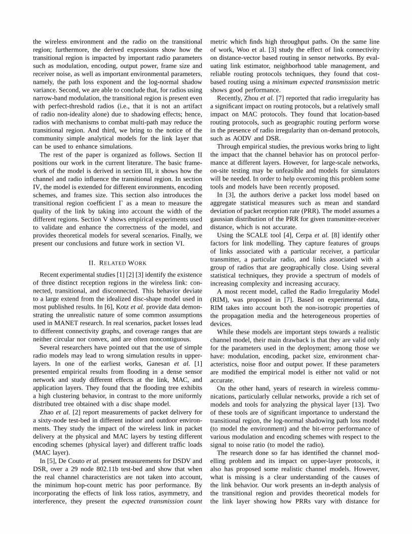
)Analytical Method to Determine Regions in Wireless Links

µ µ+2σ µ−2σ

noise floor (Pn)

Pn + γ

U

Pn + γ

L

Beginning of Transitional Region

End of Transitional Region

Fig. 3. Analytical Observation of the Transitional Region

Whereα is the Eb

N0ratio. Hence, the PRRp is defined as:

p = (1− 12

exp−α2 )8f (4)

Nevertheless, most commercial radios do not provide theEb

N0metric, but the RSSI (Received Signal Strength Indicator)

of the received signal. The RSSI measurements can be usedto determine the SNR (Signal-to-Noise ratio); henceforth, inthis work, the expression based onEb

N0are converted to SNR.

The relation between SNR andEb

N0is given by:

SNR =Eb

N0

R

BN(5)

Where R is the data rate in bits, andBN is the noisebandwidth. For MICA2 motes,R = 19.2 kbps andBN = 30kHz. Finally, the PRRp in terms of the SNR (γ) is given by:

p = (1− 12

exp−γ2

10.64 )8f (6)

The curve in figure 2 shows equation 6 (receiver response)for a frame size of 50 bytes. As we shall see later, this curveplays an important role in determining the different regions.

C. The Noise Floor

Another important element that determines the transitionalregion is the noise floor, which depends on both, the radioand the environment. The temperature of the environment in-fluences the thermal noise generated by the radio components(noise figure), the environment can further influence the noisefloor due to interfering signals. When the receiver and theantenna have the same ambient temperature the noise floor isgiven by [13]:

Pn = (F + 1)kT0B (7)

WhereF is the noise figure,k the Boltzmann’s constant,T0 the ambient temperature andB the equivalent bandwidth.MICA2s use the Chipcon CC1000 radio [14], which has anoise figure of 13 dB and a system noise bandwidth of 30

0 5 10 15 20 25 30 35 400

0.1

0.2

0.3

0.4

0.5

0.6

0.7

0.8

0.9

1

distance (m)

PR

R

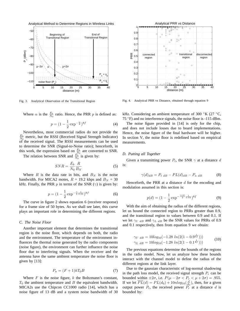
Analytical PRR vs Distance

connected region

transitional region

disconnected region

Fig. 4. Analytical PRR vs Distance, obtained through equation 9

kHz. Considering an ambient temperature of 300◦K (27 ◦C,75 ◦F) and no interference signals, the noise floor is -115 dBm.

The noise figure provided in [14] is only for the chip,and does not include losses due to board implementations.Hence, the noise figure of the final hardware will be higher.In section V, the noise floor is redefined based on empiricalmeasurements.

D. Putting all Together

Given a transmitting powerPt, the SNRγ at a distancedis:

γ(d)dB = Pt dB − PL(d)dB − Pn dB (8)

Henceforth, the PRR at a distanced for the encoding andmodulation assumed in this section is:

p(d) = (1− 12

exp−γ(d)

21

0.64 )8f (9)

With the aim of obtaining the radius of the different regions,let us bound the connected region to PRRs greater than 0.9,and the transitional region to values between 0.9 and 0.1. Ifwe let γU dB andγL dB be the SNR values for PRRs of 0.9and 0.1 respectively, then from equation 9 we obtain:

γU dB = 10log10(−1.28 ln(2(1− 0.918f )))

γL dB = 10log10(−1.28 ln(2(1− 0.118f )))

(10)

The previous equations determine the bounds of the regionsin the radio model. Now, let us analyze how these boundsinteract with the channel model to define the radius of thedifferent regions at the link layer.

Due to the gaussian characteristic of log-normal shadowingin the path loss model, the received signal strengthPr can bebounded within±2σ, i.e. P (µ− 2σ < Pr < µ + 2σ) = .955.If we let PL(d) = PL(d0) + 10nlog10( d

d0), then, for a given

output powerPt, the received powerPr at a distanced isbounded by:

2 4 6 8 10 1210

−1

100

101

102

103

σ

TR

TR Coefficient for Different Environments

η = 2η = 4η = 6η = 8

0 5 10 15 20 25 30 35 40

−110

−100

−90

−80

−70

−60

−50

distance (m)

Pr (

dBm

)

Impact of σ in the Transitional Region

radio bounds

σ = 4

σ = 2

σ = 1

0 5 10 15 20 25 30 35 40

−110

−100

−90

−80

−70

−60

−50

distance (m)

Pr (

dBm

)

Impact of η in the Transitional Region

η = 6

η = 5

η = 4

radio bounds

(a) (b) (c)

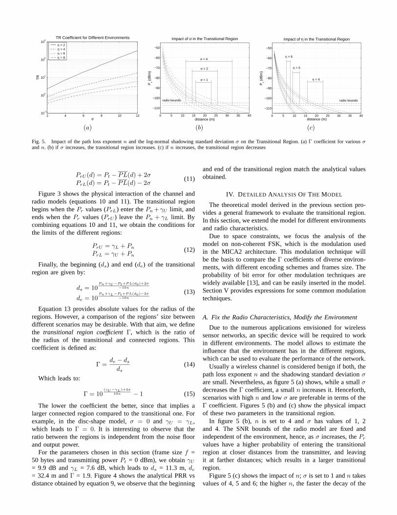
Fig. 5. Impact of the path loss exponentn and the log-normal shadowing standard deviationσ on the Transitional Region. (a)Γ coefficient for variousσandn. (b) if σ increases, the transitional region increases. (c) ifn increases, the transitional region decreases

PrU (d) = Pt − PL(d) + 2σPrL(d) = Pt − PL(d)− 2σ

(11)

Figure 3 shows the physical interaction of the channel andradio models (equations 10 and 11). The transitional regionbegins when thePr values (PrL) enter thePn +γU limit, andends when thePr values (PrU ) leave thePn + γL limit. Bycombining equations 10 and 11, we obtain the conditions forthe limits of the different regions:

PrU = γL + Pn

PrL = γU + Pn(12)

Finally, the beginning (ds) and end (de) of the transitionalregion are given by:

ds = 10Pn+γU−Pt+P L(d0)+2σ

−10n

de = 10Pn+γL−Pt+P L(d0)−2σ

−10n

(13)

Equation 13 provides absolute values for the radius of theregions. However, a comparison of the regions’ size betweendifferent scenarios may be desirable. With that aim, we definethe transitional region coefficientΓ, which is the ratio ofthe radius of the transitional and connected regions. Thiscoefficient is defined as:

Γ =de − ds

ds(14)

Which leads to:

Γ = 10(γU−γL)+4σ

10n − 1 (15)

The lower the coefficient the better, since that implies alarger connected region compared to the transitional one. Forexample, in the disc-shape model,σ = 0 and γU = γL,which leads toΓ = 0. It is interesting to observe that theratio between the regions is independent from the noise floorand output power.

For the parameters chosen in this section (frame sizef =50 bytes and transmitting powerPt = 0 dBm), we obtainγU

= 9.9 dB andγL = 7.6 dB, which leads tods = 11.3 m,de

= 32.4 m andΓ = 1.9. Figure 4 shows the analytical PRR vsdistance obtained by equation 9, we observe that the beginning

and end of the transitional region match the analytical valuesobtained.

IV. D ETAILED ANALYSIS OF THE MODEL

The theoretical model derived in the previous section pro-vides a general framework to evaluate the transitional region.In this section, we extend the model for different environmentsand radio characteristics.

Due to space constraints, we focus the analysis of themodel on non-coherent FSK, which is the modulation usedin the MICA2 architecture. This modulation technique willbe the basis to compare theΓ coefficients of diverse environ-ments, with different encoding schemes and frames size. Theprobability of bit error for other modulation techniques arewidely available [13], and can be easily inserted in the model.Section V provides expressions for some common modulationtechniques.

A. Fix the Radio Characteristics, Modify the Environment

Due to the numerous applications envisioned for wirelesssensor networks, an specific device will be required to workin different environments. The model allows to estimate theinfluence that the environment has in the different regions,which can be used to evaluate the performance of the network.

Usually a wireless channel is considered benign if both, thepath loss exponentn and the shadowing standard deviationσare small. Nevertheless, as figure 5 (a) shows, while a smallσdecreases theΓ coefficient, a smalln increases it. Henceforth,scenarios with highn and lowσ are preferable in terms of theΓ coefficient. Figures 5 (b) and (c) show the physical impactof these two parameters in the transitional region.

In figure 5 (b), n is set to 4 andσ has values of 1, 2and 4. The SNR bounds of the radio model are fixed andindependent of the environment, hence, asσ increases, thePr

values have a higher probability of entering the transitionalregion at closer distances from the transmitter, and leavingit at farther distances; which results in a larger transitionalregion.

Figure 5 (c) shows the impact ofn; σ is set to 1 andn takesvalues of 4, 5 and 6; the highern, the faster the decay of the

5 6 7 8 9 10 11 120

0.1

0.2

0.3

0.4

0.5

0.6

0.7

0.8

0.9

1

SNR (dB)

PR

R

Analytical PRR vs SNR for NRZ

50 bytes100 bytes150 bytes

5 6 7 8 9 10 11 120

0.1

0.2

0.3

0.4

0.5

0.6

0.7

0.8

0.9

1

SNR (dB)

PR

R

Analytical PRR vs SNR for 4B5B

50 bytes100 bytes150 bytes

5 6 7 8 9 10 11 120

0.1

0.2

0.3

0.4

0.5

0.6

0.7

0.8

0.9

1

SNR (dB)

PR

R

Analytical PRR vs SNR for Manchester

50 bytes100 bytes150 bytes

5 6 7 8 9 10 11 120

0.1

0.2

0.3

0.4

0.5

0.6

0.7

0.8

0.9

1

SNR (dB)

PR

R

Analytical PRR vs SNR for SECDED

50 bytes100 bytes150 bytes

(a) (b) (c) (d)

Fig. 6. Receiver Response for Different Encoding Schemes and Frames Size: (a) NRZ, (b) 4B5B, (c) Manchester, (d) SECDED

0 5 10 15 20 25 30 35 400

0.1

0.2

0.3

0.4

0.5

0.6

0.7

0.8

0.9

1

distance (m)

PR

R

PRR vs Distance, Ideal Environment − Ideal Receiver

equivalent todisc−shape model

0 5 10 15 20 25 30 35 400

0.1

0.2

0.3

0.4

0.5

0.6

0.7

0.8

0.9

1

distance (m)

PR

R

PRR vs Distance, Ideal Environment − Real Receiver

0 5 10 15 20 25 30 35 400

0.1

0.2

0.3

0.4

0.5

0.6

0.7

0.8

0.9

1

distance (m)

PR

R

PRR vs Distance, Real Environment − Ideal Receiver

connected region

transitional region

disconnected region

0 5 10 15 20 25 30 35 400

0.1

0.2

0.3

0.4

0.5

0.6

0.7

0.8

0.9

1

distance (m)

PR

R

PRR vs Distance, Real Environment − Real Receiver

connected region

transitional region

disconnected region

(a) (b) (c) (d)

Fig. 7. PRR vs Distance for Ideal and Real Scenarios.

signal strength and the thinner the width of the transitionalregion.

Finally, it is important to mention that even though figure 5(a) shows the curves of a radio using NRZ and frames of 50bytes, similar trends are observed for other encoding schemesand frames size.

B. Fix the Environment, Modify the Radio Characteristics

Some WSN applications will require the optimization ofthe radio for a specific environment. In these cases, it will beimportant to explore different encoding schemes and observethe influence of the frame size.

Figure 6 shows the radio model (PRR vs SNR) for differentencoding schemes5 (NRZ, 4B5B, Manchester and SECDED6),and various frames size.

For any encoding scheme, as the frame size increases,the SNR bounds increase (curves shift right) which leads tosmaller connected regions. On the other hand, for the sameframe size, the SNR bounds required by SECDED are thesmallest (largest connected region), followed by NRZ, 4B:5Band Manchester. This result is due to the error correction

5The plots represent frames with a preamble length of 2 bytes for allencoding schemes.

6SECDED encodes each byte into 24 bits

encoding 50 bytes 100 bytes 150 bytesNRZ 2.2785 2.0347 1.91514B5B 2.1938 1.9671 1.8551

Manchester 2.0347 1.8384 1.7404SECDED 2.5677 2.2180 2.0489

TABLE I

SNR RANGE γU − γL FOR A NON-COHERENTFSK, NRZ RADIO

capabilities of SECDED, which comes at a cost of energyefficiency (encoding ratio 1:3). NRZ, 4B5B, and Manchesterdoes not provide error correction. Nevertheless, for the samepacket size, the encoding ratios are 1:1, 1:1.25 and 1:2respectively; resulting in higher SNRs required, which leadto smaller regions.

Though done for ASK modulation, empirical results fordifferent encoding schemes [2] agree with the expected the-oretical behavior, i.e. for the same environment, SECDEDshows a larger connected region than Manchester encoding.

Even though the absolute radius of the regions are ofinterest in protocol evaluation, and their length can be obtainedthrough equation 13; in the design of the radio, the main goal –with regards to the regions– is to increase the connected regionwithout increasing the transitional one. Henceforth, rather thancomparing absolute distances, theΓ coefficient will be used.

Table I shows theγU − γL for the different encodingsand frames size. The lower theγU − γL the thinner thetransitional region, SECDED shows the highest value amongthe encoding schemes; and, for a given encoding, as the framesize increases,γU − γL decreases.

Finally, table II shows theΓ coefficient of different radiosin a environment withn = 4 andσ = 4. As we observe, theencoding or frame size do not have a significant impact on the

encoding 50 bytes 100 bytes 150 bytesNRZ 1.8639 1.8240 1.80464B5B 1.8500 1.8130 1.7950

Manchester 1.8240 1.7923 1.7766SECDED 1.9120 1.8540 1.8263

TABLE II

Γ COEFFICIENT FOR ANON-COHERENTFSK, NRZ RADIO

0 5 10 15 20 25 30 35 40

−110

−100

−90

−80

−70

−60

−50

distance (m)

Pr (

dBm

)Regions in Wireless Links for a Perfect−Threshold Receiver

perfect−threshold receiver

transitional region

Fig. 8. Transitional Region for a Perfect-Threshold Receiver.

Γ coefficient. No significant impacts were observed for othervalues ofn andσ either.

C. Can the transitional region be removed with a perfect-threshold radio?

The previous section shows that modifying the encodingor packet size does not reduce significantly theΓ coefficient,this result leads to an interesting question:Can the transitionalregion be removed with a perfect-threshold receiver (i.e.γU =γL)?. Figure 7 shows analytical PRR vs distance plots whereperfect-threshold and real receivers are placed in ideal andreal environments, by an ideal environment we refer to onewith no shadowing effects (σ = 0); the real receiver and realenvironment follow the models derived in section III.

Figure 7 (a) shows the PRR vs distance for a perfect-threshold receiver in an ideal environment, this curve is thedisc-shape model commonly used in many simulators. Figure 7(b) shows a real receiver in an ideal environment, this scenarioresults in a small and deterministic transitional region, wherethe PRR decreases monotonically with respect to distance.Figure 7 (c) is the most interesting plot, it shows aperfect-threshold receiver in a real environment; in this scenarioγU = γL, which leads to binary links (0 or 1). Nevertheless,even in this ideal scenario the binary perfect-reception-within-range model does not capture the behavior of the link, sincethere exist a region where a link can randomly take values of0 or 1. Finally, figure 7d) shows the real behavior of the link.

Figure 8 shows the analytical behavior of a perfect-thresholdreceiver. We can observe that for a perfect-threshold receiver,the transitional region would be caused by the shadowingvariance of the environment. Given that the shadowing vari-ance is caused by multi-path effects, we hypothesize that,to have a significant impact in decreasing the transitionalregion, receivers should use mechanisms that combat multi-path effects, such as spread spectrum and diversity techniques.

This subsection provides some important conclusions. First,a perfect-threshold receiver would not solve the transitionalregion problem due to multi-path effects. Second, in realscenarios, the radio is the cause of obtaining continuous values

0 1000 2000 3000 4000 5000 6000 7000 8000−120

−115

−110

−105

−100

−95

−90Empirical Noise Floor

sample number

Noi

se F

loor

(dB

m)

Analytical Noise Floor (−115 dBm)

indoorenvironment

outdoorenvironment

Fig. 9. Empirical Measurements of the Noise Floor.

of PRR, and not ’0/1’ links; and the environment is thecause of the random (non-monotonically) decreasing trend.And third, given that multi-path effects play a significant rolein determining the transitional region, receivers able to combatthese effects may improve significantly the quality of the link.

V. EMPIRICAL VALIDATION OF THE MODEL

In order to enhance and validate the theoretical modeldeveloped, MICA2 motes were used to perform empiricalevaluation. First, we describe the methodology used. Then,we redefine the noise floor; after that, the channel parameters,n andσ, are obtained; and the radio model is compared withthe empirical results. Finally, we evaluate the accuracy of theanalytical link layer model derived (PRR vs distance).

A. Methodology

Two different environments were tested, an indoor envi-ronment (aisle of a building), and an outdoor environment(football field). For each environment, a chain topology of 21MICA2 motes was deployed with nodes spaced every meter.The frame size was 50 bytes and Manchester encoding wasused with a preamble of 28 bytes. A simple TDMA protocolwas implemented to avoid collisions. Upon reception of apacket the sequence number and the received signal strength(Pr) were stored; simultaneously, the noise floor was measuredby taking samples of the idle channel. For both environments;various power levels were tested (from -20dBm to 5dBm insteps of 1dBm), due to space constraints we present resultsfor medium (-7 dBm) and high (5 dBm) powers. For eachpower level, each node transmitted 100 packets, at a rate of 5packets/sec. After all nodes transmitted their 100 packets, theaveragePr (RSSI) and PRR were measured for all the linksin the network.

B. The Noise Floor

Figure 9 shows samples of the noise floor for both environ-ments. The average noise floor is approximately -105 dBm7,

7The noise floor difference in both environments is due to slightly differenttemperatures, and sensitivity inaccuracies (±6dB [14]).

0 5 10 15 20

−110

−100

−90

−80

−70

−60

−50

distance (m)

Indoor Channel, Pout

= 5dBmP

r (dB

m)

0 5 10 15 20

−110

−100

−90

−80

−70

−60

−50

distance (m)

Pr (

dBm

)

Outdoor Channel, Pout

= 5 dBm

−105 −100 −95 −90 −850

10

20

30

40

50

60

70

80

90

100Radio Response, Indoor Environment

Pr (dBm)

PR

R (

%)

begmidendanalytical

−105 −100 −95 −90 −850

10

20

30

40

50

60

70

80

90

100Radio Response, Outdoor Environment

Pr (dBm)

PR

R (

%)

begmidendanalytical

(a) (b) (c) (d)

Fig. 10. Empirical Validation of Channel and Radio Models. (a) Indoor Channel (b) Outdoor Channel (c) Indoor Radios (d) Outdoor Radios

0 5 10 15 200

10

20

30

40

50

60

70

80

90

100

distance (m)

PR

R (

%)

Outdoor, PRR vs. Distance, Pout

= 5dBm

0 5 10 15 200

10

20

30

40

50

60

70

80

90

100

distance (m)

PR

R (

%)

Outdoor, PRR vs. Distance, Pout

= −7dBm

(a) (b)

0 5 10 15 200

0.1

0.2

0.3

0.4

0.5

0.6

0.7

0.8

0.9

1

distance (m)

PR

R

Outdoor, Analytical PRR vs Distance, Pout

= 5dBm

0 5 10 15 200

0.1

0.2

0.3

0.4

0.5

0.6

0.7

0.8

0.9

1

distance (m)

PR

R

Outdoor, Analytical PRR vs Distance, Pout

= −7dBm

(c) (d)

Fig. 11. Validation of the Model for Outdoor Channel. (a) and (b) are theempirical measurements; (c) and (d) the analytical counterparts

which has a 10 dBm difference with respect to the specifiedvalue obtained in section III-C. This difference is mainly dueto the fact that in the initial calculation we did not considerthe losses from the output of the chip to the antenna. Theselosses depend on the board implementation and are beyondthe scope of this work. Hence, for the model, let us redefinethe noise floor to an average value of -105 dBm.

C. The Channel and Radio Models

The channel parameters (n and σ) were obtained fromfigures 10 (a) and 10 (b). However, there was a small compli-cation to obtain them in the outdoor environment – figure 10(b). Due to the noise floor,Pr values below -100 dBm werenot detected (values were recorded only for received packets).For this reason, only the closest distances (1m∼6m) wereconsidered in the curve-fitting. Table III shows the parametersfor both environments.

Figures 10 (c) and 10 (d) show the radio model and thePRR vsPr of three different receivers for both environments;the receivers were located at the beginning, middle and end ofthe chain. The radio model was obtained from the parametersused in the deployment. Since the model is based on SNRs, it

0 5 10 15 200

10

20

30

40

50

60

70

80

90

100

distance (m)

PR

R (

%)

Indoor, PRR vs. Distance, Pout

= 5dBm

0 5 10 15 200

10

20

30

40

50

60

70

80

90

100

distance (m)

PR

R (

%)

Indoor, PRR vs. Distance, Pout

= −7dBm

(a) (b)

0 5 10 15 200

0.1

0.2

0.3

0.4

0.5

0.6

0.7

0.8

0.9

1

distance (m)

PR

RIndoor, Analytical PRR vs Distance, P

out = 5dBm

0 5 10 15 200

0.1

0.2

0.3

0.4

0.5

0.6

0.7

0.8

0.9

1

distance (m)

PR

R

Indoor, Analytical PRR vs Distance, Pout

= −7dBm

(c) (d)

Fig. 12. Validation of the Model for Indoor Channel. (a) and (b) are theempirical measurements; (c) and (d) the analytical counterparts

was shifted according to the average noise floor (-105 dBm).An analogous trend is observed on the empirical responseof the receivers and the radio model; furthermore, the radioresponse is independent of the environment due to the similartemperatures in both scenarios.

D. The Link Layer Model

For the parameters used in the experiments, table IV showsthe expected radius of the different regions. Figures 11 and12 show the empirical and analytical results of the link layerabstraction (PRR vs distance) for the outdoor and indoorenvironments, respectively.

Figures 11 (a), 11 (b), 12 (a) and 12 (b) correspond to theempirical results; and figures 11 (c), 11 (d), 12 (c) and 12(d) are their analytical counterparts. The radius obtained in

environment n (95% conf. bounds) σ (95% conf. bounds)outdoor 4.7 (4.30 - 5.10) 4.6 (2.80 - 6.40)indoor 3.0 (2.67 - 3.23) 3.8 (2.60 - 5.00)

TABLE III

CHANNEL PARAMETERS

0~10 10~20 20~30 30~40 40~50 50~60 60~70 70~80 80~90 90~1000

0.1

0.2

0.3

0.4

0.5

0.6

0.7

0.8

0.9

1

PRR (%)

prob

abili

tyProbability Mass Function of PRR for Various Distances

d = 02 m − connected regiond = 12 m − transitional regiond = 20 m − disconnected region

0 5 10 15 200

0.1

0.2

0.3

0.4

0.5

0.6

0.7

0.8

0.9

1

SNR (dB)

PR

R

Analysis of PRR Distribution

SNR disconnected regionSNR transitional regionSNR connected regionradio model

γL γ

U

0~10 10~20 20~30 30~40 40~50 50~60 60~70 70~80 80~90 90~1000

0.1

0.2

0.3

0.4

0.5

0.6

0.7

0.8

0.9

1

PRR (%)

prob

abili

ty

Analytical Prob. Mass Function of PRR for Various Distances

d = 02 m − connected regiond = 10 m − transitional regiond = 20 m − disconnected region

(a) (b) (c)

Fig. 13. PRR Distribution for Different Transmitter-Receiver Distances. (a) empirical distribution of the high-power-outdoor environment, (b) analyticalobservation of the distribution, (c) analytical distribution of the high-power-outdoor environment

table IV fairly approximate the real behavior. Also, by simpleinspection a similar distribution of the PRRs is observed.However, in order to verify the correctness of the model, letus compare the empirical and analytical distributions of thePRR as a function of the transmitter-receiver distance. Forexample, a link in the connected region is expected to have,with high probability, a PRR above 90%; while a link in thetransitional region, depending on whether the node is at thebeginning, middle or end of this region, will have differentPRR distributions. Notice that the distributions depend on thetransmitter-receiver distance for the given channel and radioparameters, and are constant in time due to the focus on staticenvironments of this work.

In figure 13 (a), each curve shows the PRR distribution oftransmitter-receiver distances between 2 and 20 m (in stepsof 1 m) for the outdoor-high-power scenario. Three curvesare specially highlighted, one on each region. As expected,curves in the connected and disconnected regions show a highprobability (∼ 1) of having high (90%<) and low (<10%)PRRs, respectively. However, the curve in the transitionalregion –all curves in general– show a strong bias to eitherhigh or low PRRs, with a small probability of being between10% and 90%. This behavior can be explained in light of themodel derived in this work.

Figure 13 (b) shows the radio model and three SNR distri-butions of tentative receivers. The left-most curve represents anode in the disconnected region, where low SNR values resultin low PRRs. The right-most curve represents a node in theconnected region, which contrary to the previous curve resultsin high PRRs. And, the middle curve represents a node in thetransitional region.

For the curve in the transitional region, the probability that

scenario ds (m) de (m)outdoor-high-power 5.7 15.5outdoor-medium-power 3.2 8.6indoor-high-power 17.4 65.1indoor-medium-power 6.9 25.9

TABLE IV

ANALYTICAL RADIUS OF TRANSITIONAL REGION

an SNR value falls within theγU−γL region is low comparedto the probability of falling either in the high or low regions.It is important to remark -and can be easily observed- thatindependently of where the SNR distribution is centered, SNRvalues have a low probability of falling within theγU − γL

region. Figure 13 (c) is the analytical counterpart of figure 13(a) for the high-power-outdoor environment. Similar trends areobtained for other scenarios.

Finally, one of the goals of this work is to provide a realisticlink layer model for low power devices. With that aim, tableV presents a comprehensive list of equations for differentmodulation and encoding techniques8.

VI. CONCLUSIONS ANDFUTURE WORK

The impact that the channel behavior has on the perfor-mance of upper-layer protocols in wireless sensor networksrequires a clear understanding of the different regions of lowpower wireless links. We have presented a detailed study ofthe transitional region. Some of the key contributions andconclusions of this work are:• Mathematical link layer models are presented for the

statistical variation of packet reception rates with respectto distance (for different environment and radio character-istics). This analysis yields the boundaries of the differentregions — connected, transitional, and disconnected. Themethodology presented can be easily extended to other ra-dios that use different modulation and encoding schemes.

• The study shows the influence that the modulation, en-coding, output power, frame size, noise floor, and channelparameters have on the transitional region.

• The Γ (transitional region) coefficient is introduced as ameans to compare thequality of the link for differentenvironments. The smaller the coefficient, the better thelink. Environments with a high path loss exponentn anda small shadowing standard deviationσ, decrease theΓ coefficient. Also, while the frame size and encodingscheme influences the radius of the regions, their ratio (Γcoefficient) is not significantly affected.

8The model assumes that the preamble is not encoded, and hence is thesame for all encoding schemes. Other radio designs may lead to slightlydifferent expressions.

STEP 1 : Channel Obtain parameters of the channel and use them in next step

PL(d0), n, σ Can be obtained through own empirical measurements, or from some published results [10]STEP 2 : SNR Obtain SNRγ as a function of distanced. For MICA2: −20 dBm < Pt < 5 dBm, Pn = −105dBm

γdB(d) Pt − PL(d0)− 10nlog10(dd0

)−N(0, σ)− Pn

STEP 3 : Modulation ChoosePe according to the modulation used, insertγ(d) not in dB, i.e.10γdB(d)

10 , and convert fromEbN0

to RSSI

by inserting the appropriate bit data rateR and noise bandwidthBN

ASK noncoherent:12[exp−

γ(d)2

BNR +Q(

√γ(d)BN

R)] coherent:Q(

√γ(d)

2BNR

)

FSK noncoherent:12

exp−γ(d)

2BNR coherent:Q(

√γ(d)BN

R)

PSK binary: Q(

√2γ(d)BN

R) differential: 1

2exp−γ(d)

BNR

STEP 4 : Encoding Choose packet reception ratep(d) according to the encoding scheme, frame and preamble lengths

NRZ (1− Pe)8`(1− Pe)8(f−`)

4B5B (1− Pe)8`(1− Pe)8(f−`)1.25

Manchester (1− Pe)8`(1− Pe)8(f−`)2.0

SECDED (1− Pe)8`((1− Pe)8 + 8Pe(1− Pe)7)(f−`)3.0

TABLE V

THEORETICAL MODELS FOR THEL INK LAYER

• Even with a perfect-threshold radio, the transitional re-gion still exists so long as there are multi-path effects.However, we hypothesize that radios with mechanisms tocombat multi-path effects, such as spread-spectrum anddiversity techniques, can reduce the transitional region.

Even though interference was not studied, the channelmodel can be used to considerPr signals of non-intended re-ceivers as noise. For scenarios where the traffic and contentionare relatively light; a very reasonable assumption for manyclasses of data-centric sensor networks, the presented modelprovides an accurate estimate of the links’ quality. However,a more detailed study is needed to accurately quantify theimpact of interference in the different regions for high-trafficnetworks.

Our work focused on the spatial variation of the link andwe did not consider the time domain. We believe that in staticenvironments (i.e. static nodes, and no dynamic objects aroundthem) time variations are mainly due to fluctuations in thethermal noise of the radios. Then, the time variations couldbe modelled by a gaussian distribution of the thermal noise,and use these samples as the noise floor for each packet,instead of the deterministic value assumed in this work. Formore challenging dynamic environments, richer time-varyingfading models will be required; for example, developing goodmodels for the correlated temporal variations of theXσ termin the log-normal shadowing model. We would also like toextend our modelling and analysis to more sophisticated radiosthat implement techniques such as spread spectrum and multi-antenna diversity to combat fading effects.

ACKNOWLEDGEMENT

We would like to acknowledge assistance from and useful conver-sations with Alec Woo, Dr. Jerry Zhao, Prof. John Heidemann, Dr.Robert Poor, and Prof. Scott Shenker.

REFERENCES

[1] D. Ganesan, B. Krishnamachari, A. Woo, D. Culler, D. Estrin andS. Wicker.“Complex Behavior at Scale: An Experimental Study of

Low-Power Wireless Sensor Networks”. UCLA CS Technical ReportUCLA/CSD-TR 02-0013, 2002.

[2] J. Zhao and R. Govindan. “Understanding Packet Delivery Performancein Dense Wireless Sensor Networks”. Sensys ’03.

[3] A. Woo, T. Tong, and D. Culler. “Taming the Underlying Issues forReliable Multhop Routing in Sensor Networks”. SenSys ’03.

[4] A. Cerpa, N. Busek, and D. Estrin. “SCALE: A tool for SimpleConnectivity Assessment in Lossy Environments”. CENS TechnicalReport, September 2003.

[5] D. S. J. De Couto, D. Aguayo, J. Bicket, and R. Morris. “A High-Throughput Path Metric for Multi-Hop Wireless Routing”. ACM Mobi-Com, September 2003.

[6] D. Kotz, C. Newport and C. Elliott. “The mistaken axioms of wireless-network research”. Technical Report TR2003-467, Dept. of ComputerScience, Dartmouth College, July 2003.

[7] G. Zhou, T. He, S. Krishnamurthy, and J. Stankovic. “Im- pact of radioirregularity on wireless sensor networks”. MobiSys ’04.

[8] A. Cerpa, J. L. Wong, L. Kuang, M. Potkonjak and D. Estrin. “StatisticalModel of Lossy Links in Wireless Sensor Networks”. CENS TechnicalReport 0041, April 2004.

[9] D. Lal, A. Manjeshwar, F. Herrmann, E. Uysal-Biyikoglu, A. Ke-shavarzian. “Measurement and Characterization of Link Quality Metricsin Energy Constrained Wireless Sensor Networks”. Globecom 2003.

[10] K. Sohrabi, B. Manriquez, and G. Pottie. “Near Ground Wideband Chan-nel Measurement”. Vehicular Technology Conference IEEE, volume 1,pages 571-574, 1999.

[11] S. Y. Seidel and T. S. Rapport. “914 MHz Path Loss Prediction Model forIndoor Wireless Communication in Multi floored Buildings”. In IEEETransactions on Antennas and Propagation, volume 40(2), pages 207-217, February 1992.

[12] H. Nikookar and H. Hashemi. “Statistical modeling of signal amplitudefading of indoor radio propagation channels”. 2nd International Confer-ence on Universal Personal Communications, 1993. Vol 1, Pages:84-88.

[13] Theodore S. Rappapport. “Wireless Communications: Principles andPractice”. Prentice Hall.

[14] Chipcon. CC1000 low power radio transceiver, http://www.chipcon.com.