ORIGINAL ARTICLE

Numerical modeling of pollutant load accumulation in the Musaestuary, Persian Gulf

Alireza Payandeh • Nasser Hadjizadeh Zaker •

Mohammad Hossien Niksokhan

Received: 20 October 2013 / Accepted: 30 May 2014

� Springer-Verlag Berlin Heidelberg 2014

Abstract Musa estuary is a predominantly tide-driven

embayment located in the northwestern part of the Persian

Gulf. This estuary is bordered by dense population and

industrial development that add significantly to the water’s

pollution load. The eastern part of the estuary opens into

the small estuaries which are not similar in terms of pol-

lutant load accumulation. The present study investigates

the relationships between pollutant load accumulation and

some physical and hydrodynamic characteristics of the

Musa estuary. Tidal regime, bottom topography, persis-

tency of currents and pollutant sources were analyzed

numerically in relation to pollutant load accumulation.

Residence time was calculated using the MIKE 3 model

and this concept was used as a metric of pollutant load

accumulation. It was found that the assimilative capacity of

Musa estuary is not the same during the month so that the

capacity to absorb pollution in spring tide is more than at

any other time. Based on the results, the present study

suggests that in all estuarine ecosystems, the persistency of

currents can be used as an indicator of areas which are

faced with pollutant load accumulation.

Keywords Musa estuary � Residence time � Pollutant

load accumulation � Persistency of current � Tidal regime

Introduction

In recent decades, considerable amounts of pollutants are

entering into the estuarine environment due to large

deployment of utilities, industrial and port activities. Wo-

lanski (2007) noted some of the risks that threaten such

environments such as marine eutrophication because of

additional concentrations of nutrients in wastewater, heavy

metal pollution, polychlorinated biphenyls, radionuclide

and hydrocarbons. Proportional to the acceleration of

industrialization and urban development in coastal areas,

the environmental research should address the influence of

the developmental activities on environment in order to

mitigate the adverse environmental effects. Numerical

modeling is a useful way to study water environment and

has long been used to study estuaries (e.g. Chen et al. 2013;

Sentenac et al. 2013; Shi et al. 2010; Liu et al. 2012; Nouri

et al. 2010).

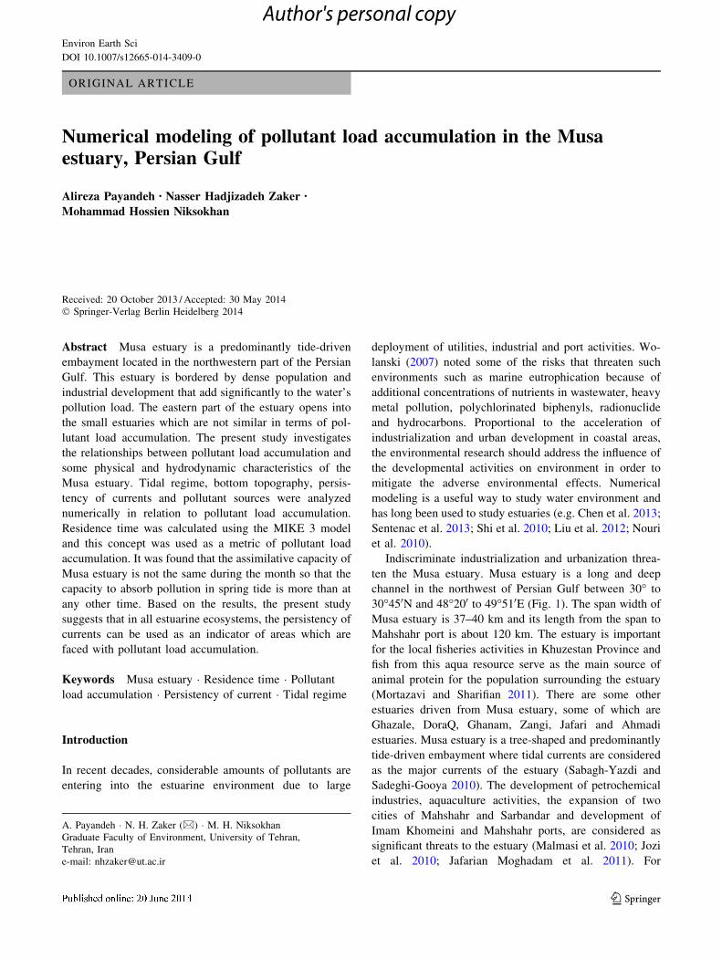
Indiscriminate industrialization and urbanization threa-

ten the Musa estuary. Musa estuary is a long and deep

channel in the northwest of Persian Gulf between 30� to

30�450N and 48�200 to 49�510E (Fig. 1). The span width of

Musa estuary is 37–40 km and its length from the span to

Mahshahr port is about 120 km. The estuary is important

for the local fisheries activities in Khuzestan Province and

fish from this aqua resource serve as the main source of

animal protein for the population surrounding the estuary

(Mortazavi and Sharifian 2011). There are some other

estuaries driven from Musa estuary, some of which are

Ghazale, DoraQ, Ghanam, Zangi, Jafari and Ahmadi

estuaries. Musa estuary is a tree-shaped and predominantly

tide-driven embayment where tidal currents are considered

as the major currents of the estuary (Sabagh-Yazdi and

Sadeghi-Gooya 2010). The development of petrochemical

industries, aquaculture activities, the expansion of two

cities of Mahshahr and Sarbandar and development of

Imam Khomeini and Mahshahr ports, are considered as

significant threats to the estuary (Malmasi et al. 2010; Jozi

et al. 2010; Jafarian Moghadam et al. 2011). For

A. Payandeh � N. H. Zaker (&) � M. H. Niksokhan

Graduate Faculty of Environment, University of Tehran,

Tehran, Iran

e-mail: nhzaker@ut.ac.ir

123

Environ Earth Sci

DOI 10.1007/s12665-014-3409-0

Author's personal copy

environmental management of this region and to reduce the

possible effects of expanding industries, it is necessary to

exactly identify the vulnerability of the estuary against

pollution load accumulation.

Different water time scales, such as residence time and

water age, are criteria that link the physical and biological

features of water and are appropriate indicators to compare

the behavior of each part of estuary in dealing with pol-

lution. Estuaries with a short residence time will export

pollutants from upstream sources more rapidly then estu-

aries with longer residence time The development of pri-

mary definitions of water residence time and water age can

be viewed in works of researchers such as Bolin and Rhode

(1973), Zimmerman (1976), Takeoka (1984). Also, using

the concept of residence time, Brooks et al. (1999) inves-

tigated the condition of dispersion and flushing of Cobs-

cook Bay which is a macrotidal estuary near the entrance to

Bay of Fundy. They attempted a three-dimensional mod-

eling of water circulation which is affected by semi-diurnal

tide and runoff from rivers. Using a two-dimensional par-

ticle tracking modeling, Patgaonkar et al. (2012) calculated

the residence time of pollutant discharge in Kachchh bay

which is in northeast coast of the Arabian Sea and

concluded that tidal currents have a strong component in

the east–west direction that prevents the transmission of

pollutants between its north and south. Longer residence

time of anthropogenic nutrients has been reported as the

main cause of eutrophication and hypoxia conditions in

Chesapeake Bay (Cerco and Cole 1993).

The most important point in previous studies about

residence time in estuaries especially the Musa estuary is

lack of a comprehensive study on the factors that increase

or decrease the residence time. In the present study, the

residence time in Musa estuary is studied as an effect and

attempt to provide a comprehensive study on relationships

between residence time and tidal regime, persistency of

currents and bottom topography. In addition to these fac-

tors, pollutant sources has strong effect on the amount of

pollution, therefore another part of the research deals with

effects of pollutant sources position on the pollutant load

accumulations in various estuaries of Musa. Results of the

current study can be used in Environmental management of

the study area. Also they can be used for identifying the

suitable locations for sewer outlets, suitable sites for

aquaculture activities, finding locations of spawning areas

used by marine fishes and calculations related to TMDL

(total maximum daily load).

Materials and methods

Model setup

MIKE 3 FM hydrodynamic model was used to calculate

the residence time. MIKE 3 FM is based on the numerical

solution of the three-dimensional incompressible Rey-

nolds-averaged Navier–Stokes equations, subject to the

assumption of Boussinesq and of hydrostatic pressure. The

spatial discretization of the primitive equations is per-

formed using finite volume method. In the horizontal plane

an unstructured grid is used while in the vertical domain a

structured discretization is used (DHI 2007). Model grids

were generated by MIKE Mesh Generator, which uses

hydrography data and user defined grid limits. Hydrogra-

phy of the region was carried out by Iranian Port and

Maritime Organization (PMO) in 2004. Recorded surface

elevations of tide gauge located at 30�120900N and

48�5705900E employed to provide the boundary condition of

the hydrodynamic model. Analysis of wind data in Mah-

shahr synoptic station (30�330E, 40�490N) for 5 years

showed that the prevailing wind in the area is Shamal wind.

This result agrees with previous studies (e.g. Thoppil and

Hoganb 2010) indicating that Shamal wind is a north-

westerly wind blowing over Iraq and the Persian Gulf

states including Saudi Arabia and Kuwait, often strong

during the day, but decreasing at night. Measured wind at

Fig. 1 Landsat TM image showing the tree-shaped study area and

geographic features cited in text. The inset map (upper right) shows

the Khor-Musa (in the red quadrangle) along the NW Persian Gulf

margin

Environ Earth Sci

123

Author's personal copy

Mahshahr synoptic station was uniformly applied over the

entire domain. Table 1 contains parameters specified in the

MIKE 3 FM model. As the model is located in an area

where flooding and drying occur, we have specified a

drying water depth, a flooding water depth and a wetting

depth. When the water depth is less than the wetting depth

the problem is reformulated and only if the water depth is

less than the drying depth the element/cell is removed from

the simulation. The flooding depth is used to determine

when an element is flooded (i.e. reentered into the calcu-

lation). The reformulation is made by setting the

momentum fluxes to zero and only taking the mass fluxes

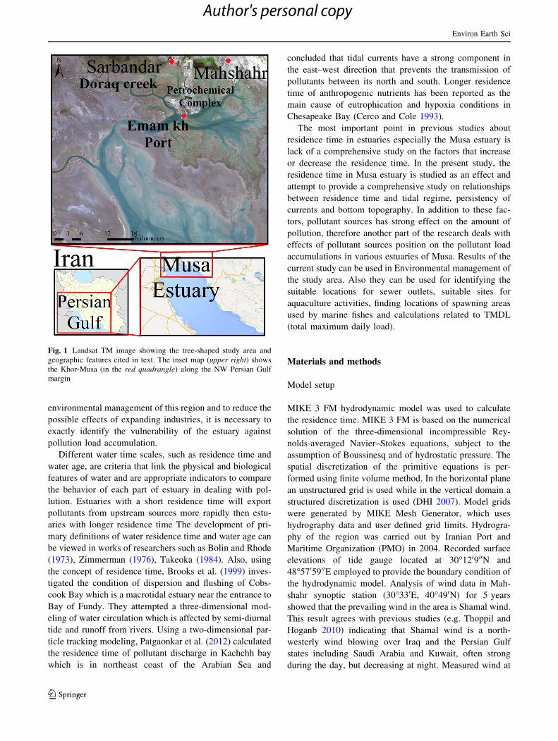
into consideration. Figure 2 shows all permanent water

areas and areas that can become dry in low tides.

Sensitivity analysis and calibration

Various sensitivity tests were carried out to analyze the

effect of variations of different model parameters on the

results including bed resistance, mesh resolution, eddy

viscosity, and boundary conditions. This analysis revealed

that the modeling was sensitive to some parameters. Model

outputs were sensitive to mesh resolution. After increasing

the resolution a few times, the outputs became insensitive

to mesh resolution. Sensitivity analysis indicated that the

modelling is very sensitive to bed resistance. It can be

calculated either through the roughness height or quadratic

roughness coefficient. Examining the roughness heights

between 0.001 and 0.3 m, a value of 0.01 m was chosen.

Eddy viscosity coefficient is another important parameter

defining the turbulence mixing in the water. Turbulence

mixing is generally larger in places where the velocity

gradient is large. There are two available options provided

in MIKE 3 FM model for eddy viscosity, i.e. constant eddy

viscosity and Smagorinsky eddy viscosity, which is a

function of velocity gradients. The Smagorinsky eddy

viscosity (Smagorinsky 1963) with the coefficient of 0.28

was adopted for the simulation. Figure 3 shows the com-

parisons of measured and simulated tidal elevations and

current velocity time series at a point with coordinates of

30�2504000N and 49�405900E. It is observed that the pre-

dicted tidal elevations show a very good agreement with

field measurements. Similar good agreements were

observed in current speed.

Fig. 2 Permanent water areas

(yellow areas) and areas that

can become dry at low tides (red

areas)

Table 1 Overview of parameters specified in the MIKE 3 model

Parameters Values

Time step interval 7 s

Time integration Higher order

Critical CFL number 1

Drying depth 0.005 m

Flooding depth 0.05 m

Wetting depth 0.1 m

Interpolation method Natural neighbour

Number of scatter points 80,976

Number of elements 6,453

Mesh nodes 4,728

Eddy viscosity Smagorinsky eddy viscosity

with the coefficient of 0.28

Bed resistance Roughness height = 0.01 m

Wind Mahshahr synoptic station data

with a time step of 15 min

Boundary condition The recorded surface elevations

of tide gauge Located at

30�120900N and 48�5705900E

Environ Earth Sci

123

Author's personal copy

Calculation of residence time

Several definitions and methods have been proposed to

calculate the residence time which most of them are dif-

ferent from each other in terms of concept and calculation

methods and procedures (Bolin and Rhode 1973; Zimmer-

man 1976; Dettmann 2001; Monsen et al. 2002; Delhez

et al. 2004; Sandery and Kampf 2005; Patgaonkar et al.

2012). For example, Zimmerman (1976) and Shen and Haas

(2004) have used flushing time, Monsen et al. (2002) has

used the residence time and some other researchers (Dett-

mann 2001; Delhez et al. 2004) have used e-folding time.

In the present study, two concepts of point residence

time and regional residence time have been used to which

are developed based on Thomann and Mueller (1987).

According to Thomann and Mueller (1987) definition, if a

certain amount of a substance in time of t0 and initial

concentration of c0 which is released in homogeneous mass

of water and no further amount of the substance is added to

the water and the density of water and fluxes in boundaries

remain constant, the concentration of water in time of t is:

Cðt�t0Þ ¼ C0e�Q=V � ðt � t0Þ ¼ C0eð�ðt � t0Þ=h ð1Þ

where Q is the flux of substance, V is the density of control

volume, t stands for time and O– is the residence time.

Residence time is the e-folding time, i.e., the time

required to reduce the total mass of the tracer in the estu-

ary, or a segment of it, to a factor of e-1 of its original

Fig. 3 Comparisons between

the calculated and measured

time series at 30�250400 0N and

49�40590 0E. a and b water

surface elevations for 10 and

15 days, c current velocities for

6 days

Environ Earth Sci

123

Author's personal copy

value. This time scale has been termed residence time

(Thomann and Mueller 1987). For example if the initial

mass of the tracer is X and after a time T the current value

is observed Y = X/e then T is the residence time.

This definition is selected as a measure of control vol-

ume and cannot be an index of point to point comparison.

Therefore, in the present study the following definitions are

developed.

Point residence time: Point residence time is the required

time for the absolute reduction of grid mesh concentration by

a factor of 1/e. Considering that the concentration time series

has the minimum and maximum points on different time-

scales, our understanding of the term ‘‘absolute’’ is the first

time that the concentration drops to 1/e & 0.37 and after that

the concentrations don’t increase from this value. Point

Residence Time makes it possible to show the distribution of

residence time in area with enough resolution.

Regional residence time: Regional residence time can be

calculated for any desired area. In this case, the average

concentration of all the elements within each time step is

calculated and the time required for absolute reduction of

average concentration by a factor of 1/e of its initial con-

centration is considered Regional Residence Time. This

index can be used to compare different areas with each

other or the same area in different conditions.

Calculation of pollution age and pollution influx rate

Residence time can be used as an indicator of pollutant load

accumulation in different parts of the Musa estuary, but this

concept does not consider pollutant sources effect. As

defined in previous section, uniform concentration of the

tracer was used to calculate the residence time. Therefore

pollutant sources effect is eliminated deliberately in order to

study other factors. In the present study, two concepts of

pollution age and pollution influx rate were developed for

assessing the sensitivity of different parts to pollutant sour-

ces. Pollution age index was defined based on the concept of

age. Zimmerman (1988) defined age as the time which a

water parcel has elapsed since its entrance to the estuary from

one of its boundaries. Delhez et al. (1999) used another

definition which is: the time elapsed since the parcel under

consideration left the region where its age is assumed to be

zero (Fig. 4a). Delhez et al. (2003) developed a method to

calculate the age of water using two tracers: one conservative

and one decaying with decay constant k. If these two tracers

release with the same concentration and the same rate then

water age could be calculated as below:

T ¼ �k�1 lnðCdecay=CconservativeÞ ð2Þ

Here, T is the age of water particle (day), K is the decay

coefficient (1/day), Cdecay is the Concentration of the

decaying tracer (kg/m3), and Cconservative is the concentra-

tion of the conservative tracer (kg/m3). Water age in Del-

hez et al. (2003) definition is always dependent on the

discharge point of the tracers.

The present study is looking for an index which shows

time travel of pollutant to reach to different parts of the

estuary. To achieve this goal, the discharge point of the two

tracers is replaced with existing pollutant sources (Fig. 4b).

Calculating age under this condition represents the time

travel of pollutants to different parts. Therfore in the

present study pollution age is used instead of water age.

Pollution influx rate was defined as bellow:

Pollution Influx Rateg

ðm3 dayÞ

� �

¼Cdecay

gm3

� �� �ðpollution age ð30 daysÞ½day])

ð3Þ

This index represents the arrival rate of the pollution in an

individual point. This index was used to compare sensitivity

of different parts of the estuary to existing pollutant sources.

Calculation of persistency

Persistency is a concept that expresses the stability of cur-

rent vectors (Witting 1912; Palmen 1930). When the current

is unidirectional in time, the persistency is 100 % and the

more variable the direction, leads to smaller persistency.

Witting (1912) and Palmen (1930) defined the persistency

as the ratio between vector and scalar mean speeds:

R ¼

ffiffiffiffiffiffiffiffiffiffiffiffiffiffiffiffiffiffiffiffiffiffiffiffiffiffiffiffiffiffiffiffiffiffiffiffiffiffiffiffiffiffiffiffiffiffiffiffiffiffiffiffiffiffiffiffiffi1=N

Pn un

� �2þ 1=NP

n v2n

� �q1=N

Pn

ffiffiffiffiffiffiffiffiffiffiffiffiffiffiffiu2

n þ v2n

p ð4Þ

where R is the persistency and is given as a percentage,

N is the number of time steps, un is the velocity in

x direction and vn is the speed in y direction.

Results and discussion

Results are categorized and presented in individual

sections.

Hydrodynamic results

Hydrodynamic modeling was conducted for a period of

4 months between August and November 2000. This is the

time period that current velocity and sea surface elevation

data were measured in the study area. Figure 5 shows two

snapshots of surface velocity vectors at rising tide (flood)

and lowering tide (ebb), respectively.

The results of simulations showed no significant dif-

ferences in the pattern of currents in the study area during

Environ Earth Sci

123

Author's personal copy

different months. The results also indicated that tides are

the major forcing factor in the Musa estuary and wind

forcing does not have significant effect on the current. The

simulations showed that tidal range increases from 3 m

near the mouth of the Musa estuary to a maximum of 6 m

at the head of the creek. The magnification of the tidal

range can be attributed to the geometrical shape of the

creek. The maximum current velocity ranged between 1.25

and 2.5 ms-1 with the highest velocities at the western end

of the main channel. Currents were mainly in the long-

shore direction with little cross-shore component. Hydro-

dynamic results are in line with previous studies (Sabagh-

Yazdi and Sadeghi-Gooya 2010).

Tidal regime and residence time

Musa estuary has a mixed semidiurnal tidal cycle as it

experiences two unequal high tides and two unequal low

Fig. 4 a The concept of water

age based on Delhez et al.

(1999) definition, b the concept

of pollution age

Fig. 5 Velocity-magnitude

vectors of the flow field at

a rising tide (flood), b lowering

tide (ebb). Black arrows

indicate the direction of current

vectors

Environ Earth Sci

123

Author's personal copy

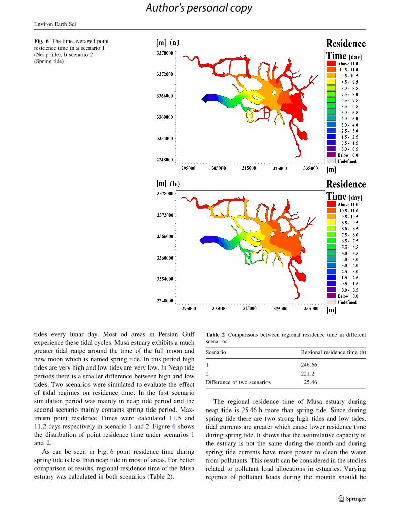
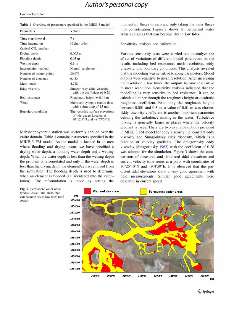
tides every lunar day. Most od areas in Persian Gulf

experience these tidal cycles. Musa estuary exhibits a much

greater tidal range around the time of the full moon and

new moon which is named spring tide. In this period high

tides are very high and low tides are very low. In Neap tide

periods there is a smaller difference between high and low

tides. Two scenarios were simulated to evaluate the effect

of tidal regimes on residence time. In the first scenario

simulation period was mainly in neap tide period and the

second scenario mainly contains spring tide period. Max-

imum point residence Times were calculated 11.5 and

11.2 days respectively in scenario 1 and 2. Figure 6 shows

the distribution of point residence time under scenarios 1

and 2.

As can be seen in Fig. 6 point residence time during

spring tide is less than neap tide in most of areas. For better

comparison of results, regional residence time of the Musa

estuary was calculated in both scenarios (Table 2).

The regional residence time of Musa estuary during

neap tide is 25.46 h more than spring tide. Since during

spring tide there are two strong high tides and low tides,

tidal currents are greater which cause lower residence time

during spring tide. It shows that the assimilative capacity of

the estuary is not the same during the month and during

spring tide currents have more power to clean the water

from pollutants. This result can be considered in the studies

related to pollutant load allocations in estuaries. Varying

regimes of pollutant loads during the mounth should be

Fig. 6 The time averaged point

residence time in a scenario 1

(Neap tide), b scenario 2

(Spring tide)

Table 2 Comparisons between regional residence time in different

scenarios

Scenario Regional residence time (h)

1 246.66

2 221.2

Difference of two scenarios 25.46

Environ Earth Sci

123

Author's personal copy

allocated in order to use full assimilative capacity of Musa

estury.

Residence time of deeper parts especially the main

channel are more affected by tidal regimes. It was found

that the difference between point residence time in neap

tide and spring tide is 36 h in some deep areas. Shallow

areas of Musa estuary are mostly located at the end of

estuary and are less affected by main tidal currents therfore

their residence time is less sensitive to monthly tidal

regimes.

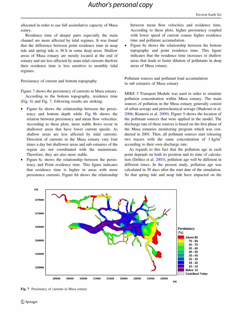
Persistency of current and bottom topography

Figure 7 shows the persistency of currents in Musa estuary.

According to the bottom topography, residence time

(Fig. 6) and Fig. 7, following results are striking:

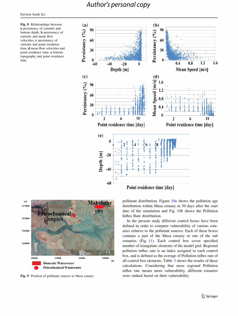
• Figure 8a shows the relationship between the persis-

tency and bottom depth while Fig. 8b shows the

relation between persistency and mean flow velocities.

According to these plots, more stable flows occur in

shallower areas that have lower current speeds. As

shallow areas are less affected by tidal currents.

Direction of currents in the Musa estuary vary four

times a day but shallower areas and sub estuaries of the

region are not coordinated with the mainstream.

Therefore, they are also more stable.

• Figure 8c shows the relationship between the persis-

tency and Point residence time. This figure indicates

that residence time is higher in areas with more

persistence currents. Figure 8d shows the relationship

between mean flow velocities and residence time.

According to these plots, higher persistency coupled

with lower speed of current coause higher residence

time and pollutant accumulation.

• Figure 8e shows the relationship between the bottom

topography and point residence time. This figure

indicates that the residence time increases in shallow

areas that leads to faster dilution of pollutants in deep

areas of Musa estuary.

Pollutant sources and pollutant load accumulation

in sub estuaries of Musa estuary

MIKE 3 Transport Module was used in order to simulate

pollution concentration within Musa estuary. The main

sources of pollution in the Musa estuary generally consist

of urban sewage and petrochemical sewage (Shakouri et al.

2006; Kianersi et al. 2009). Figure 9 shows the location of

the pollutant sources that were applied in the model. The

discharge rate of these sources is based on the first phase of

the Musa estuaries monitoring program which was con-

ducted in 2001. Thus, all pollutant sources start releasing

two tracers with the same concentration of 1 kg/m3

according to their own discharge rate.

As regards to this fact that the pollution age in each

point depends on both its position and its time of calcula-

tion (Delhez et al. 2003), pollution age will be different in

different times. In the present study, pollution age was

calculated in 30 days after the start date of the simulation.

So that spring tide and neap tide have impacted on the

Fig. 7 Persistency of currents in Musa estuary

Environ Earth Sci

123

Author's personal copy

pollutant distribution. Figure 10a shows the pollution age

distribution within Musa estuary in 30 days after the start

date of the simulation and Fig. 10b shows the Pollution

Influx Rate distribution.

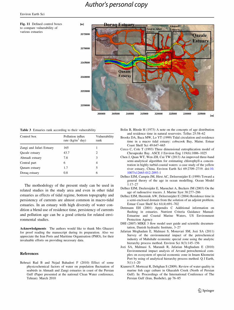
In the present study different control boxes have been

defined in order to compare vulnerability of various estu-

aries relative to the pollutant sources. Each of these boxes

contains a part of the Musa estuary or one of the sub

estuaries (Fig. 11). Each control box cover specified

number of triangulate elements of the model grid. Regional

pollution influx rate is an index assigned to each control

box, and is defined as the average of Pollution influx rate of

all control box elements. Table 3 shows the results of these

calculations. Considering that more regional Pollution

influx rate means more vulnerability, different estuaries

were ranked based on their vulnerability.

Fig. 8 Relationships between

a persistency of currents and

bottom depth, b persistency of

currents and mean flow

velocities, c persistency of

currents and point residence

time, d mean flow velocities and

point residence time, e bottom

topography and point residence

time

Fig. 9 Position of pollutant sources in Musa estuary

Environ Earth Sci

123

Author's personal copy

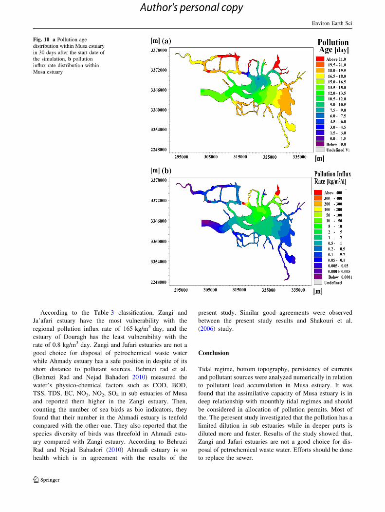
According to the Table 3 classification, Zangi and

Ja’afari estuary have the most vulnerability with the

regional pollution influx rate of 165 kg/m3 day, and the

estuary of Douragh has the least vulnerability with the

rate of 0.8 kg/m3 day. Zangi and Jafari estuaries are not a

good choice for disposal of petrochemical waste water

while Ahmady estuary has a safe position in despite of its

short distance to pollutant sources. Behruzi rad et al.

(Behruzi Rad and Nejad Bahadori 2010) measured the

water’s physico-chemical factors such as COD, BOD,

TSS, TDS, EC, NO3, NO2, SO4 in sub estuaries of Musa

and reported them higher in the Zangi estuary. Then,

counting the number of sea birds as bio indicators, they

found that their number in the Ahmadi estuary is tenfold

compared with the other one. They also reported that the

species diversity of birds was threefold in Ahmadi estu-

ary compared with Zangi estuary. According to Behruzi

Rad and Nejad Bahadori (2010) Ahmadi estuary is so

health which is in agreement with the results of the

present study. Similar good agreements were observed

between the present study results and Shakouri et al.

(2006) study.

Conclusion

Tidal regime, bottom topography, persistency of currents

and pollutant sources were analyzed numerically in relation

to pollutant load accumulation in Musa estuary. It was

found that the assimilative capacity of Musa estuary is in

deep relationship with mounthly tidal regimes and should

be considered in allocation of pollution permits. Most of

the. The peresent study investigated that the pollution has a

limited dilution in sub estuaries while in deeper parts is

diluted more and faster. Results of the study showed that,

Zangi and Jafari estuaries are not a good choice for dis-

posal of petrochemical waste water. Efforts should be done

to replace the sewer.

Fig. 10 a Pollution age

distribution within Musa estuary

in 30 days after the start date of

the simulation, b pollution

influx rate distribution within

Musa estuary

Environ Earth Sci

123

Author's personal copy

The mothodology of the present study can be used in

related studies in the study area and even in other tidal

estuaries as effects of tidal regime, bottom topography and

persistency of currents are almost common in macro-tidal

estuaries. In an estuary with high diversity of water con-

dition a blend use of residence time, persistency of currents

and pollution age can be a good criteria for related envi-

ronmental studies.

Acknowledgments The authors would like to thank Mrs Ghazavi

for proof reading the manuscript during its preparation. Also we

appreciate the Iran Ports and Maritime Organisation (PMO), for their

invaluable efforts on providing necessary data.

References

Behruzi Rad B and Nejad Bahadori F (2010) Effect of some

physicochemical factors of water on population fluctuation of

seabirds in Ahmadi and Zangi estuaries in coast of the Persian

Gulf (Paper presented at the national Clean Water conference,

Tehran). March 2010

Bolin B, Rhode H (1973) A note on the concepts of age distribution

and residence time in natural reservoirs. Tellus 25:58–62

Brooks DA, Baca MW, Lo YT (1999) Tidal circulation and residence

time in a macro tidal estuary: cobscook Bay, Maine. Estuar

Coast Shelf Sci 49:647–665

Cerco C, Cole T (1993) Three dimensional eutrophication model of

Chesapeake Bay. ASCE J Environ Eng 119(6):1006–1025

Chen J, Quan WT, Wen ZH, Cui TW (2013) An improved three-band

semi-analytical algorithm for estimating chlorophyll-a concen-

tration in highly turbid coastal waters: a case study of the yellow

river estuary, China. Environ Earth Sci 69:2709–2719. doi:10.

1007/s12665-012-2093-1

Delhez EJM, Campin JM, Hirst AC, Deleersnijder E (1999) Toward a

general theory of the age in ocean modelling. Ocean Model

1:17–27

Delhez EJM, Deelersijder E, Maouchet A, Beckers JM (2003) On the

age of radioactive tracers. J. Marine Syst 38:277–286

Delhez EJM, Heemink AW, Deleersnijder E (2004) Residence time in

a semi-enclosed domain from the solution of an adjoint problem.

Estuar Coast Shelf Sci 61(4):691–702

Dettmann EH (2001) Appendix C Additional information on

flushing in estuaries. Nutrient Criteria Guidance Manual-

Estuarine and Coastal Marine Waters, US Environment

Protection Agency

DHI (2007) MIKE 3 flow model user guide and scientific documen-

tation, Danish hydraulic Institute, 3–27

Jafarian Moghadam E, Malmasi S, Monavari SM, Jozi SA (2011)

Survey of the environmental impact of the petrochemical

industry of Mahshahr economic special zone using the analytic

hierarchy process method. Environ Sci 8(3):145–156

Jozi SA, Malmasi S, Marandi R, Jafarian Moghadam E (2010)

Environmental impact analysis of Arvand petrochemical com-

plex on ecosystem of special economic zone in Imam Khomeini

Port by using of analytical hierarchy process method. Q J Earth,

5(1):1–20

Kianersi F, Mortezai R, Dehghan S (2009). Review of water quality in

marine fish cage culture in Ghazaleh Creek (North of Persian

Gulf). In: Proceedings of the International Conference of The

Persian Gulf (Iran, Bushehr), pp 76–85

Fig. 11 Defined control boxes

to compare vulnerability of

various estuaries

Table 3 Estuaries rank according to their vulnerability

Control box Pollution influx

rate (kg/m3 day)

Vulnerability

rank

Zangi and Jafari Estuary 165 1

Qazale estuary 43.7 2

Ahmadi estuary 7.8 3

Central part 6 4

Qanam estuary 1.7 5

Doraq estuary 0.8 6

Environ Earth Sci

123

Author's personal copy

Liu WC, Chen WB, Chang YP (2012) Modeling the transport and

distribution of lead in tidal Keelung River estuary. Environ Earth

Sci 65:39–47. doi:10.1007/s12665-011-1063-3

Malmasi S, Jozi SA, Monavari SM, Jafarian ME (2010) Ecological

impact analysis on Mahshahr petrochemical industries using

analytic hierarchy process method. Int J Environ Res

4(4):725–734

Monsen NE, Cloern JE, Lucas LV (2002) A comment on the use of

flushing time, residence time, and age as transport time scales.

Limnol Oceanogr 47(5):1545–1553

Mortazavi MS, Sharifian S (2011) Mercury bioaccumulation in some

commercially valuable marine organisms from Mosa Bay,

Persian Gulf. Int J Env Res 5(3):757–762

Nouri J, Mirbagheri SA, Farrokhian F, Jaafarzadeh N, Alesheikh AA

(2010) Water quality variability and eutrophic state in wet and

dry years in wetlands of the semiarid and arid regions. Environ

Earth Sci 59:1397–1407. doi:10.1007/s12665-009-0126-1

Palmen E (1930) Studies about the omungen in the surrounding seas

Finland, societas scientiarum fennica. Comm Phys-Math

12:1–94

Patgaonkar RS, Vethamony P, Lokesh KS, Babu MT (2012)

Residence time of pollutants discharged in the Gulf of Kachchh,

northwestern Arabian Sea. Mar Pollut Bull 64:1659–1666

Sabagh-Yazdi SR, Sadeghi-Gooya A (2010) Modeling Khowr-e Musa

multi-branch estuary currents due to the Persian Gulf tides using

NASIR depth average flow solver. J Persian Gulf 6:45–50

Sandery PA, Kampf J (2005) Winter-Spring flushing of Bass Strait,

South-Eastern Australia: a numerical modeling study. Estuarine,

Coastal and Shelf Science, pp 6323–6331

Sentenac P, Jones G, Zielinski M, Tarantino A (2013) An approach

for the geophysical assessment of fissuring of estuary and river

flood embankments: validation against two case studies in

England and Scotland. Environ Earth Sci 69:1939–1949. doi:10.

1007/s12665-012-2026-z

Shakouri A, Savari A, Yavari V, Nabavi MB (2006) Study on

diversity indices and their correlation with environmental factors

in polychaetes on four creeks of Mahshahr region. Pajouhesh

Sazandegi 81:136–148

Shen J, Haas L (2004) Calculating age and residence time in the tidal

York River using three-dimensional model experiments. Estuar

Coast Shelf Sci 61:449–461

Shi JZ, Zhou HQ, Liu H, Zhang YG (2010) Two-dimensional

horizontal modeling of fine-sediment transport at the South

Channel-North Passage of the partially mixed Changjiang River

estuary. China Environ Earth Sci 61:1691–1702. doi:10.1007/

s12665-010-0482-x

Smagorinsky J (1963) General circulation experiment with the

primitive equations. Mon Weather Rev 91(3):99–164

Takeoka H (1984) Fundamental concepts of exchange and transport

timescales in a coastal sea. Cont Shelf Res 3:311–326

Thomann RV, Mueller JA (1987) Principles of surface water quality

modelling and control. Harper Collins, New York

Thoppil PG, Hoganb PJ (2010) Persian Gulf response to a wintertime

shamal wind event. Deep-Sea Research I 57:946–955

Witting R (1912) Summary Overview of the hydrography of Bothnia

and Gulf of Finland and the Baltic ordlichen N, Finland.

Hydrogr-biol. Unters. No. 7

Wolanski E (2007) Estuarine Ecohydrology. Elsevier, Amsterdam.

ISBN 978-0-444-53066-0

Zimmerman JTF (1976) Mixing and flushing of tidal embayments in

the western duch Wadden sea.Part I. Distribution of salinity and

calculation of mixing time scales. Neth J Sea Res 10:149–191

Zimmerman JTF (1988) Estuarine residence times. In: Kjerfve B (ed),

Hydrodynamics of estuaries. V. 1. CRC Press. pp 75–84

Environ Earth Sci

123

Author's personal copy