Engineering Fracture Mechanics 108 (2013) 19–36

Contents lists available at SciVerse ScienceDirect

Engineering Fracture Mechanics

journal homepage: www.elsevier .com/locate /engfracmech

Numerical fracture growth modeling using smooth surfacegeometric deformation

0013-7944/$ - see front matter � 2013 Elsevier Ltd. All rights reserved.http://dx.doi.org/10.1016/j.engfracmech.2013.04.012

⇑ Corresponding author. Tel.: +44 20 759 47 435; fax: +44 20 7594 7444.E-mail address: apaluszn@imperial.ac.uk (A. Paluszny).

Adriana Paluszny ⇑, Robert W. ZimmermanDepartment of Earth Science and Engineering, Imperial College, London SW7 2AZ, United Kingdom

a r t i c l e i n f o a b s t r a c t

Keywords:Fracture propagation

Smooth surfaceFinite elementDeformationCoons

Numerical methods for fracture propagation model fracture growth as a geometricresponse to deformation. In contrast to the widely used faceted representations, a smoothsurface can be used to represent the fracture domain. Its benefits include low cost, resolu-tion-independent storage, swift generation of local tip coordinate systems, and a paramet-ric representation. In the present work, an interaction-free deformation-informed surfacemodification algorithm of the fracture is presented, with localized stress intensity factorcomputations, and automatic resolution adjustment, which allows for geometric evolutionwithout the need of appending or re-approximating the fracture surface. The method isbased on the movement of surface control points, and on the systematic editing of weightsand knots; it does not require trimming, and is able to shift fracture shape and capture itspath evolution efficiently. Throughout growth, the number of points required for fracturerepresentation increases only as a function of curvature, but not area, and the discretiza-tion of the parametric surface is achieved in constant time. The proposed algorithm canbe incorporated into any fracture propagation code that keeps track of fracture geometryand updates it as a function of deformation. Use of the algorithm is demonstrated for a dis-crete finite element-based fracture propagation method.

� 2013 Elsevier Ltd. All rights reserved.

1. Introduction

Fractures in rocks are usually created by tectonically driven events, by weathering, or are caused by human factors suchas those triggered by explosives or hydraulic fracturing. Their creation and effects are modeled by a range of simulators. Mul-ti-physics flow simulators usually rely on an initial, geologically based fracture representation of the medium to reproducereservoir conditions. These usually originate from analogue field mappings, or are stochastically generated based on site-spe-cific criteria. In this context, mechanical simulators focus on modeling the formation and growth of fractures in response togeomechanical deformation. Whereas flow codes require accurate, resolution-independent fracture representation [1,2],mechanical growth codes have the additional requirement of capturing geometric change as a function of fracturepropagation.

The simulation of crack propagation using the finite element method has been shown to be well suited to reproduce frac-ture propagation in three dimensions (e.g. [3–5]). Fractures can be defined as entities within the mesh to avoid re-meshing(e.g. smeared crack and anisotropic damage model). In general, methods that rely on fixed meshes require these meshes tobe sufficiently refined to capture stress singularities that may ensue during the simulation. Other methods aim to reducecomplexity by representing only the boundaries of the bodies, but are less suited to capture heterogeneity in the matrix

Nomenclature

b boundary curveS surfaceRi,j rational basis functionwi,j weightPi,j control point(i, j) control point indices(u,v) parametric coordinateNi,j shape functionr stressDe linear elastic stiffness matrixe strainJ J-IntegralAc increased surface areau displacementW strain energy densityG strain energy release rateE elasticity modulusm Poisson’s ratioK stress intensity factorlmax maximum advance lengthladv advance lengtha propagation exponentuo perpendicular deflection anglewo tangent deflection angle~p propagation vectorTo tip pointTF tip point after growthM parametric constraintbM space constraintf(i, j) localization constraintCðÞ closest boundary point on surfaceeBij modified rational basis functiondk distance-based weighted absolute deformation error

20 A. Paluszny, R.W. Zimmerman / Engineering Fracture Mechanics 108 (2013) 19–36

(e.g. the boundary element method). Mesh-free methods [6,7] bypass meshing completely, and define domains as sets ofpoints, which introduces difficulties such as domain interface blurring, and costly computational operations. The ExtendedFinite Element (XFEM) avoids re-meshing by defining enrichment functions to represent discrete fractures at a sub-grid le-vel. XFEM has been applied to grow [8] and intersect [9] fractures in 2D and 3D [10], including the modeling of intra-fracturefriction [11]. XFEM has difficulties representing intra-element fracture intersection, multiple fractures in one element, andrequires special approaches to handle fracture tips within elements. The cracking particle method is a numerical methodspecific to the simulation of crack propagation, in which crack surfaces are represented by a set of point-based enriched func-tions [12], with no explicit definition of fracture surfaces. Geomechanical growth relying on this method usually requires re-interpretation of fracture geometry during growth. Finite element-based fracture propagation has been limited in the past bythe technology of controlling geometry and mesh generation, but is now facilitated by smooth surface geometric represen-tation and mature mesh generation technology (cf. [13–16]). Smooth surfaces are represented in a generic manner usingNon-Uniform Rational B-Splines (NURBS), a compact mathematical representation of a free-form surface described by aset of knots, control points, and weights. Although NURBS representation of fractures is already widely accepted [17], mainlydue to its elegance and resolution-independent storage, the problem of geometric evolution specific to fracture growth israrely discussed. Approaches to capture propagation using smooth surfaces include constrained parametric-based extension,cumbersome lofting and stitching of new surface regions, and costly re-approximation of the surface.

In many fracture propagation methods, fractures are defined by the mesh; in some cases, as in most FEM approaches, thefracture is defined by set of triangles ‘‘cut’’ into the mesh [4]. Alternatively, XFEM defines cracks as a set of level-set functionsthat correspond to specific elements in the mesh, and thus, albeit somewhat independent of its form, the definition of thecrack is a function of the mesh. Mesh-free methods keep track of a set of nodes that constitute the fracture, and anisotropicdamage models track elements in which the fracture develops. Most of these rely on faceted descriptions of the fracture dur-ing growth.

Fig. 1. Fracture geometry evolves as a function of propagation vectors, which result of evaluating propagation and failure laws based on stress intensityfactors, approximated at the fracture tips. Frenet frames are computed at the tip locations to determine the local coordinate system of the fracture.

A. Paluszny, R.W. Zimmerman / Engineering Fracture Mechanics 108 (2013) 19–36 21

Deformation of NURBS is usually assumed in the context of user-driven direct manipulation [18,19]. The two mainapproaches for direct NURBS manipulation are geometric and physically-based constraint methods. Piegl [18] describesgeometric deformation of curves and surfaces in terms of movement of control points and modification of their weights.Constraint-based methods for surface deformation rely on the movement of control points to satisfy externally imposedconstraints [19,20]. These are costly, as they compute geometric change by solving the finite element-based deformationof the surface. Linear constraints and global energy minimization functions can also be used to solve for deformation[21,22]. The previous are all best suited for interaction-driven deformation in which constraints are typically appliedto the body of the shape to sculpt or model a shape. In the specific case of fracture propagation, NURBS shape modifi-cation is based on the arbitrary extension of a surface boundary in response to a physical event. These constraints arethe result of fracture growth, coalescence, and arrest, and involve honoring multiple constraints in a non-conventionalmanner.

In the present work, a discrete fracture growth method is used, which represents fracture geometry explicitly usingNURBS surfaces, and for which the mesh is only an instrument to enable finite element-based computation of stress intensityfactors. This results in the non-interactive evolution of fracture geometry, expressed at the fracture boundaries. A constraint-based geometric surface growth method is presented, which is suitable for the modeling of fracture propagation. Fig. 1 illus-trates the proposed approach.

2. Fracture geometry

Fracture growth is defined as a function of deformation, whereby for each tip locality, length advance and propagationangle jointly define the fracture geometric extension (see Section 3). This results in an evolving geometry that is an emergentproperty of growth (see Section 5). After each growth step, the geometry is updated and the mesh is regenerated to discretizethe new geometry.

2.1. Initial geometric state

Seeds for fracture growth are defined as sets of elliptical or circular discs, for which the two radii have a normal distri-bution, and positions have a continuous uniform distribution. It is assumed that the initial description of the fracture can bedescribed by four boundary NURBS curves (see Fig. 2),

bðu;0Þ; bðu;1Þ; bð0;vÞ; bð1; vÞ ð1Þ

where the domain of the parametric surface b(u,v) is the unit square, and u,v 2 [0,1]. These are interpolated using a bi-linearblended Coons patch, which approximates the fracture surface using a blending function that defines the space betweenthem [23] as

Scðu;vÞ ¼ ð1� uÞbð0;vÞ þ ubð1; vÞ þ ð1� vÞbðu; 0Þ þ vbðu;1Þ �1� u

u

� �T bð0;0Þ bð0;1Þbð1;0Þ bð1;1Þ

� �1� v

v

� �ð2Þ

As opposed to a bilinear interpolation, which only uses the intersection corner points as input, the Coons patch takesinto account the four boundary curves. Thus, there are four initial curves, which jointly represent the tip boundary.These are Bézier curves which in turn can be expressed as splines, i.e. NURBS. The Coons patch provides an initialdescription of the fracture surface, which does not rely on trimming. Therefore, the surface can be manipulated withoutthe concern that topological changes might disturb the trimming function, and deviate from the underlying trimmedpatch.

Fig. 2. NURBS representation.

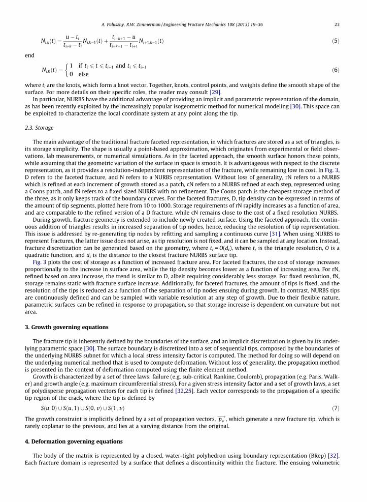
Fig. 3. Cost of storage as a function of increased area, in which: D refers to the faceted fracture; N refers to a NURBS representation: rN is refined at eachincrement of growth and stored as a patch, cN is refined at each step and stored as a Coons patch, and fN is a fixed sized NURBS; hri is the average fractureradius; and n refers to the number of required storage points.

22 A. Paluszny, R.W. Zimmerman / Engineering Fracture Mechanics 108 (2013) 19–36

It follows that a Coons patch can also be expressed as a NURBS surface by creating the internal control points of the patch[24].

2.2. NURBS representation

A NURBS-based parametric representation provides a framework for the representation and growth of fractures that isindependent from the utilized numerical method. For mesh-driven FEM growth algorithms, where fracture geometry is keptindependent of the mesh [25], NURBS are an appropriate solid modeling approach [17]. NURBS have been suggested as theideal candidate for geometric housekeeping of fracture growth in the context of mesh-free modeling [26] and have recentlybeen used in the context of crack propagation for XFEM [27].

Their representation is economical and, for cubic splines, C2 continuous-two important factors that allow the geometry toevolve with a strong resolution gradient (more geometric detail at the tips and folds, coarse elsewhere). As the resolution ofthe NURBS surface is fixed, the storage required to represent it does not increase as a function of fracture surface area (seeFig. 3). Therefore, there is no resolution attached to the representation of the fracture, and it can be discretized as a functionof local density and proximity to other features. Resolution independence is key to capture stress singularities, which changelocation during growth.

The geometry of the fracture is stored in three dimensions as a NURBS surface, and can be expressed as a tensor product oftwo NURBS curves, of polynomial orders n and m [28]:

Sðu; vÞ ¼Xn

i¼1

Xm

j¼1

Pi;jRi;jðu;vÞ ð3Þ

where S(u,v) is a point on the surface as a function of parameters u and v, Pi is the vector of control points, and

Ri;jðu;vÞ ¼wi;jNi;nðuÞNj;mðvÞPk

p¼1

Plq¼1wp;qNp;nðuÞNq;mðvÞ

ð4Þ

where Ni,k are the normalized B-Spline basis functions of k-degree, w are the weights, and the basis function is defined recur-sively as

A. Paluszny, R.W. Zimmerman / Engineering Fracture Mechanics 108 (2013) 19–36 23

Ni;kðtÞ ¼u� ti

tiþk � tiNi;k�1ðtÞ þ

tiþkþ1 � utiþkþ1 � tiþ1

Niþ1;k�1ðtÞ ð5Þ

end

Ni;0ðtÞ ¼1 if ti 6 t 6 tiþ1 and ti 6 tiþ1

0 else

�ð6Þ

where ti are the knots, which form a knot vector. Together, knots, control points, and weights define the smooth shape of thesurface. For more details on their specific roles, the reader may consult [29].

In particular, NURBS have the additional advantage of providing an implicit and parametric representation of the domain,as has been recently exploited by the increasingly popular isogeometric method for numerical modeling [30]. This space canbe exploited to characterize the local coordinate system at any point along the tip.

2.3. Storage

The main advantage of the traditional fracture faceted representation, in which fractures are stored as a set of triangles, isits storage simplicity. The shape is usually a point-based approximation, which originates from experimental or field obser-vations, lab measurements, or numerical simulations. As in the faceted approach, the smooth surface honors these points,while assuming that the geometric variation of the surface in space is smooth. It is advantageous with respect to the discreterepresentation, as it provides a resolution-independent representation of the fracture, while remaining low in cost. In Fig. 3,D refers to the faceted fracture, and N refers to a NURBS representation. Without loss of generality, rN refers to a NURBSwhich is refined at each increment of growth stored as a patch, cN refers to a NURBS refined at each step, represented usinga Coons patch, and fN refers to a fixed sized NURBS with no refinement. The Coons patch is the cheapest storage method ofthe three, as it only keeps track of the boundary curves. For the faceted fractures, D, tip density can be expressed in terms ofthe amount of tip segments, plotted here from 10 to 1000. Storage requirements of rN rapidly increases as a function of area,and are comparable to the refined version of a D fracture, while cN remains close to the cost of a fixed resolution NURBS.

During growth, fracture geometry is extended to include newly created surface. Using the faceted approach, the contin-uous addition of triangles results in increased separation of tip nodes, hence, reducing the resolution of tip representation.This issue is addressed by re-generating tip nodes by refitting and sampling a continuous curve [31]. When using NURBS torepresent fractures, the latter issue does not arise, as tip resolution is not fixed, and it can be sampled at any location. Instead,fracture discretization can be generated based on the geometry, where tr = O(dt), where tr is the triangle resolution, O is aquadratic function, and dt is the distance to the closest fracture NURBS surface tip.

Fig. 3 plots the cost of storage as a function of increased fracture area. For faceted fractures, the cost of storage increasesproportionally to the increase in surface area, while the tip density becomes lower as a function of increasing area. For rN,refined based on area increase, the trend is similar to D, albeit requiring considerably less storage. For fixed resolution, fN,storage remains static with fracture surface increase. Additionally, for faceted fractures, the amount of tips is fixed, and theresolution of the tips is reduced as a function of the separation of tip nodes ensuing during growth. In contrast, NURBS tipsare continuously defined and can be sampled with variable resolution at any step of growth. Due to their flexible nature,parametric surfaces can be refined in response to propagation, so that storage increase is dependent on curvature but notarea.

3. Growth governing equations

The fracture tip is inherently defined by the boundaries of the surface, and an implicit discretization is given by its under-lying parametric space [30]. The surface boundary is discretized into a set of sequential tips, composed by the boundaries ofthe underlying NURBS subnet for which a local stress intensity factor is computed. The method for doing so will depend onthe underlying numerical method that is used to compute deformation. Without loss of generality, the propagation methodis presented in the context of deformation computed using the finite element method.

Growth is characterized by a set of three laws: failure (e.g. sub-critical, Rankine, Coulomb), propagation (e.g. Paris, Walk-er) and growth angle (e.g. maximum circumferential stress). For a given stress intensity factor and a set of growth laws, a setof polydisperse propagation vectors for each tip is defined [32,25]. Each vector corresponds to the propagation of a specifictip region of the crack, where the tip is defined by

Sðu;0Þ [ Sðu;1Þ [ Sð0;vÞ [ Sð1;vÞ ð7Þ

The growth constraint is implicitly defined by a set of propagation vectors, pv�!, which generate a new fracture tip, which is

rarely coplanar to the previous, and lies at a varying distance from the original.

4. Deformation governing equations

The body of the matrix is represented by a closed, water-tight polyhedron using boundary representation (BRep) [32].Each fracture domain is represented by a surface that defines a discontinuity within the fracture. The ensuing volumetric

24 A. Paluszny, R.W. Zimmerman / Engineering Fracture Mechanics 108 (2013) 19–36

domain is deformed by solving the equations of linear elastic deformation, assuming an homogeneous, isotropic, linear elas-tic medium [33]:

r ¼ Deðe� e0Þ þ r0 ð8Þ

where r and e are the strain and stress vectors, r0 and e0 are the initial strain and stress, and De is a linear elastic stiffnessmatrix. For a static system:

@rþ F ¼ 0 ð9Þ

where @ is the divergence operator and F represents the external body forces, i.e. gravity, dilatation, and acceleration.The domain is discretized using an arbitrary three-dimensional mesh composed of a set of isoparametric quadratic bars,

triangles and tetrahedra. Elements around the crack tip are quarter-point tetrahedra, which better capture the singularitiesat the fracture tips, and improve the accuracy in stress intensity factor calculations [34,35]. The ensuing system is solvedusing the finite element method (FEM), for which displacements are the solution variable defined at the nodes, and materialproperties are defined at the element Gaussian integration points at which stresses and strains are computed.

The insides of the fractures are not meshed. The fractures exist in the mesh as negative volumes surrounded by matrixelements. The geometry of the mesh is stored independently from the mesh, which is discarded and re-generated at eachgrowth step.

4.1. Stress intensity factor

Three main failure criteria can be used to determine growth [36]: the maximum circumferential stress criterion [37] forwhich the implementation is straightforward, accurate, and dependent on mesh refinement; the minimum strain energydensity criterion [38], which is less accurate and also mesh-dependent; and the maximum strain energy release rate crite-rion, which requires complex implementation of stress intensity factor measurements at the fracture tips, but the accuracyof which is mesh-independent. An energy-based approach is used in the present approach, in order to remain discretization-independent; this requires the computation of stress intensity factors around the tip.

The stress intensity factor is a measure of the energy concentrated around the crack tip. For linear elastic, brittle mate-rials, J = G, where G is the strain energy release rate, and the J Integral [39,40], characterizes the amplitude of the singularfield around a sharp fracture tip. The J Integral, defined as a volume integral in local space, expresses the energy releasedby a unit fracture extension in the direction of the fracture plane, as follows:

Jv ¼1Ac

ZV

rij@uj

@xk�Wdik

� �@qk

@xidv ð10Þ

where W denotes the strain energy density, Ac is the increased crack surface area, d is the Kronecker delta, and q is an arbi-trary weighting vector function representing the virtual crack extension. It follows that J = G = K2Eeff, and [41]

Eeff ¼ E1

1þ m2 þm

mþ 1

� �ez

ex þ ey

� �ð11Þ

where E is the elastic modulus, m is Poisson’s ratio, and ex, ey, and ez are the local principal strains.The stress intensity factor values (SIF) are approximated at the center of each fracture tip segment. Most methods, such as

the stiffness derivative [42], and the displacement correlation technique, rely on a symmetric brick-like mesh around the tip.Thus, the tip curve is discretized by symmetric prism and hexahedral elements arranged in an annular manner. In the pres-ent approach, mesh optimization is based on geometry, and is thus arbitrarily generated to optimize the number and qualityof mesh elements. Therefore, a specific mesh structure around the tip cannot be guaranteed. More flexible integration tech-niques are implemented to obtain accurate SIF values: specifically, the reduced virtual integration technique [25], based onthe integration of J over a virtual cylinder extracted from an arbitrarily-defined mesh [43]. This allows SIFs to be computedaccurately, independently of the mesh layout.

4.2. Failure criterion

A failure criterion, such as the sub-critical failure criterion (e.g. [44]), determines whether or not local fracture propaga-tion will occur. It follows that

KIC P KI P K�I ð12Þ

where KIC is the critical stress intensity factor, or toughness, K�I is the sub-critical stress intensity factor, usually defined as afraction of KIC, and KI is the mode I component of the local stress intensity factor. The propagation angle is determined by themaximum circumferential stress method [37]. Specifically, the 3D angle criterion for multi-axial loading is used [45], whichpresents a solution incorporating KIII.

A. Paluszny, R.W. Zimmerman / Engineering Fracture Mechanics 108 (2013) 19–36 25

4.3. Propagation criterion

The propagation criterion describes the magnitude of propagation. An empirical Paris-based approach [46] is used, whichrelies on power law growth depending on the SIF and two experimentally measured properties. It follows that

ladv ¼ lmaxðG=GmaxÞa ð13Þ

where G is the strain energy release rate, which is a function of the stress intensity factor, Gmax is the fracture’s maximum G,ladv is the advance distance at a single point at the crack tip, lmax is the maximum crack advance, and the propagation expo-nent, a, is generally defined as a function of material and in situ conditions. Propagation and failure criteria are both materialand in situ condition dependent, and should be adjusted as part of the experimental setup of the deformation experiments.

4.4. Angle criterion

The propagation angle is determined by a 3D angle criterion for multi-axial loading [47], which is a modified maximumcircumferential stress method [37] that takes into account KI, KII, and KIII. The criterion considers growth in terms of twodeflection angles uo and wo which are perpendicular and tangent to the crack tip, respectively, as a function of maximumprincipal stress ro and the stress components r/, rz, s/z in the reference cylindrical coordinates (/,z) defined around thetip. It follows that the deflection angle uo is computed as

@ro

@u

����u¼uo

¼ 0 and@2ro

@u2

�����u¼uo

< 0 ð14Þ

the deflection angle wo is defined by the orientation of ro as

wo ¼12

arctan2suzðuoÞ

ruðuoÞ � rzðuoÞ

� �ð15Þ

and the component of the local stress intensity factor in the direction of propagation, Kv is defined as

Kv ¼12

cosðuo=2Þ Kcs þffiffiffiffiffiffiffiffiffiffiffiffiffiffiffiffiffiffiffiffiffiffiK2

cs þ 4K2III

q� ð16Þ

where Kcs = KIcos (uo/2)2 � 3/2KIIsin (uo). uo is computed numerically a priori, as a function of the normalized modal Kni ,

where

Kni ¼

Ki

KI þ jKIIj þ jKIIIj: ð17Þ

where i = {I, II, III}, and KI P 0. It follows that

� for pure mode I, uo = 0� ^ wo = 0�;� for pure mode II, max(uo) = 70.5� ^ wo = 0�;� for pure mode III, uo = 0� ^max (wo) = 45�.

In areas where the discretization error is high, e.g. in the case of proximal objects ready to intersect, the propagation angleis assumed to be zero.

4.5. Computation of growth vector

The growth vector is computed in the local, orthogonal coordinate system, x1\x2\x3, for the propagation angle uo

puo

�! ¼ ladv ½cosðuoÞ sinðuoÞ 0�T ð18Þ

and the propagation angle wo

qwo

�! ¼ ladd½0 sinðwoÞ cosðwoÞ�T ð19Þ

where ladv is the local propagation extent, and ladd is the extent of the tip region, which can be approximated as the half-dis-tance to the next tip center along the surface boundary.

The local to global rotation matrix, Q, which transforms vectors from the local circle coordinate system to the global coor-dinate system, is defined as

Q ¼x1½x� x1½y� x1½z�x2½x� x2½y� x2½z�x3½x� x3½y� x3½z�

0B@

1CA

T

ð20Þ

Fig. 4. Growth vectors incorporate the two deflection angles uo and wo which are perpendicular and tangent, respectively, to the crack tip To.

26 A. Paluszny, R.W. Zimmerman / Engineering Fracture Mechanics 108 (2013) 19–36

where x1 is the forward-pointing axis, x2 is normal to the fracture surface, and x3 = x1 � x2 is tangent to the tip.Propagation vectors in global space are defined as

Fig. 5.Ti. The

pv�! ¼ puo

�!Q ð21Þqv�! ¼ qwo

�!Q ð22Þ

At the center, propagation is defined by pv�!. However, away from the center, propagation is a function of both uo and wo. For

wo – 0, two additional off-center tip locations are defined:

T 0o ¼ qv�!þ To ð23Þ

T 00o ¼ � qv�!þ To ð24Þ

where T�o ¼ To; T0o; T

00o

� �capture the twist in the propagation front, and the final tip is described by three new locations,

TF ¼ pv�!þ To ð25Þ

T 0F ¼ T 0o þ pv�! ð26Þ

T 00F ¼ T 00o þ pv�! ð27Þ

where T�F ¼ TF ; T0F ; T

00F

� �are points along the new tip front. The fracture is assumed to propagate in a continuous fashion, and

possible discrete breaks in continuity given by large values of wo are smoothed into the fracture geometry. The deformationof the fracture surface is controlled by the twisting constraints T�o, and the extension constraints T�F . Propagation vectors areillustrated in Fig. 4.

4.6. Growth correction due to intersection

The growth vector is corrected if it intersects any vicinal surface, bS, which represents a secondary fracture or a matrixboundary.

Given that

I T�oT�F��!

; bS �¼ fTig ð28Þ

where Iðs; SÞ gives the set of points which are the intersection between a segment s, and a surface S, if {Ti} – £, then

T�F ¼ Ti ð29Þ

where Ti is the closest intersection to the original extension constraints. In order to expedite this computation, and avoidperforming costly segment-surface intersections, an alternative is to measure the shortest distance, li, between each T�oand a set of proximal secondary surfaces, fbSg, and adjust ladv = min(li). Fig. 5 illustrates how the intersection is handled.

Fracture intersection. The primary surface, S, grows towards the secondary fracture, bS. Growth is corrected by replacing TF with the intersection pointinsert shows the effect of correcting the growth vectors (left) as compared to arresting growth after penetration (right).

A. Paluszny, R.W. Zimmerman / Engineering Fracture Mechanics 108 (2013) 19–36 27

5. Geometric fracture growth

Faceted fractures can be extended by adding triangles to the fracture representation (e.g. [48]). In contrast, whenusing a NURBS representation, the surface must be refitted, extended by lofting, or modified. Refitting requires thecostly re-interpolation of the surface. The addition of lofted surface extensions requires stitching operations to main-tain surface continuity. The modification of existing surfaces [18] provides the advantage of retaining a single geo-metric entity to represent each fracture, avoiding expense and possible domain inconsistencies due to stitching orrefitting.

5.1. Modified LaGreca growth algorithm

The extension of the fracture NURBS representation is subdivided into definition of point constraints, knot insertion atsurface boundary to enhance local level of detail, and control point movement based on mid-range Gaussian influence ofthe applied constraints [49]. For each tip location, To, a point constraint is described by space constraint, bM , a parametricconstraint, M = S(u,v), and localization constraint, f(i, j), depicted in Fig. 6.

5.2. Space constraint

A set of propagation vectors, defined in Section 4.5, pairs each original tip center with a new tip position T�o; T�F

� �� �. Space

constraints are defined as the set of new tip locations which constrain the new shape of the fracture surface T�F� �

, from nowon referenced as f bMg. Fig. 7 illustrates the sequential and iterative approaches for the resolution of the set of spaceconstraints.

5.3. Parametric constraint

The parametric constraint refers, for each space constraint, T⁄, to its closest NURBS subnet boundary point:

Fig. 6.Points Mline rep

8 bM9MjM ¼ CðS;MÞ ð30Þ

where bM is the spatial constraint, M ¼ CðS; bMÞ is the boundary point, closest to bM , on surface S. This definition differs fromthe original definition in [49] in that S(�) is defined on the boundary of S, and not at any location. Thus, deformation is fo-cused on extending the surface at its edges, as opposed to deforming its shape. The specific procedure to identify space-local-ization constraint pairs, fhM; bMig, is described in Algorithm 1.

Fracture growth. A growth constraint is described by space constraint, bM , a parametric constraint, M = S(u,v), and a localization constraint, f(i, j).0 and M00 are surface boundary neighbors at each side of M. Deformation is expressed in terms of movement m! at each control point (i, j). The strong

resents the tip, S is the fracture surface.

28 A. Paluszny, R.W. Zimmerman / Engineering Fracture Mechanics 108 (2013) 19–36

Algorithm 1. ConstraintPairs (): Identification of space-localization constraint pairs

Require: Set of surface tips, Tio

n oRequire: Set of propagation vectors, pi

v�!�

Require: 8i; eid < et ! bMi ¼ Ti

o þ piv

1: Define a set of growth pairs fGg ¼ fhM; bMig2: for each Ti

o do

3: get closest boundary point Mi ¼ Cðf bMigÞ

4: if Mi is in growth area and j bMiMi���!

j 6 lmax then

5: fGg ¼ fGg [ hMi; bMii6: end if7: end for8: Define a set of original growth pairs {G}o = {G}9: for each surface boundary point, M do10: get neighbor constraints11: if M R {G} then12: get its surface boundary point

neighbors, (n1,n2)13: if 9fn1; n̂1g ^ fn2; n̂2g 2 fGgo then14: Its between two known constraints15: fGg ¼ fGg [ ðM; ðn̂1 þ n̂2Þ=2:Þ16: else if 9fni; n̂ig 2 fGgo then17: It neighbors a known constraints18: fGg ¼ fGg [ hM; n̂ii19: end if20: end if21: end for

5.4. Localization constraint

A function, f(i, j) is used to define the influence of the growth constraint on the rest of the surface. It follows that

f ¼ ½0;n� 1� � ½0;m� 1� ! Rþ ð31Þ

such that for

9ði; jÞ 2 ½0;n� 1� � ½0;m� 1� ð32Þ

where n, m is the number of control points (i, j), and

Ri;jðu;vÞf ði; jÞ – 0: ð33Þ

For, f(i, j) = Ri,j(u,v), deformation depends on the degree of the surface. f(i, j) models the ‘‘natural influence’’ of the constrainton its vicinity, i.e. the influence given by the interpolating functions of the surface. For degree-independent influence,f ði; jÞ ¼ eBijðu;vÞ, a filtered set of coefficients defined as

eBijðu;vÞ ¼Xn

k¼�n̂

Xn

m¼�n̂

hðn̂þ k; n̂þmÞREðiþkÞ;EðjþmÞðu;vÞ ð34Þ

where, in the original formulation, h is a convolution mask having radius of influence n, and E(i) are the neighbor controlpoints enclosed by the mask. A distance-based influence function distributes deformation evenly over a radial area of thesurface, increasing competition between constraints during growth and penalizing efficiency.

For fracture specific NURBS deformation, the localization constraint is proposed to be based on tip topology, whereby

eBijðu;vÞ ¼ Ri;jðu;vÞ þXn

k;l

dkRk;lðu;vÞ ð35Þ

where d is a distance based weight, and (k, l) are n neighbor control points, sampled along the boundary at a parametricdistance dn of (i, j), as shown in Fig. 6.

A. Paluszny, R.W. Zimmerman / Engineering Fracture Mechanics 108 (2013) 19–36 29

5.5. Control point movement

The deformation procedure is summarized in Algorithm 2. It follows that the point constraints are applied using asequential iterative algorithm to obtain a set of displacement vectors, which are then applied to the control points, definedas [50]

mði; jÞ����!

¼ f ði; jÞPn�1k

Pm�1l Rk;lðu; vÞf ðk; lÞ

pv�! ð36Þ

5.6. Multiple constraints

The absolute deformation error ed is quantified by adding the distances between the deformed surface and each spatialconstraint:

ed ¼Xc¼T�jCðS; bMÞ; bM�������!

j ð37Þ

where c 2 T⁄ is a constraint, and CðS; bMÞ is the closest point to bM on surface S.

Algorithm 2. Growth algorithm

Require: N is the amount of constraint pairsRequire: TopologicalNeighbors (): identify topological neighbors of M for a given localization constraint1: Get ConstraintPairs ()2: Compute ed

3: while ed > eth do4: Create map m, of constraint pair to basis function

hM0;M00i ! eBijðu;vÞ5: for each pair hM; bMi in ConstraintPairs () do6: Get surface boundary neighbors of M,

TopologicalNeighbors (M) = hM0,M00i7: Assuming that w0 = 1, w00 = 1, and nn = 28: Accumulate basis,eBijðuhM;bMi;v hM;bMiÞ ¼ RMðu;vÞ þ RM0 ðu;vÞ þ RM00 ðu;vÞð Þ=3

9: Add pair to m10: end for11: for each control point (i, j) of S do12: Initialize movement vector m(i, j) = (0,0,0)

13: for each pair hM; bMi in ConstraintPairs () do14: Get basis value from map,

d ¼ m½hM; bMi� ¼ eBijðuhM;bMi;v hM;bMiÞ15: Accumulate movement vector:

mði; jÞ ¼ mði; jÞ þ dðM bM��!Þ16: end for17: Normalize movement, m(i, j) = m(i, j)/N18: Move control point (i, j)

19: for each pair hM; bMi in ConstraintPairs () do20: Update location of M21: end for22: end for23: Compute ed

24: end while

For multiple constraints, each constraint, weighted by a factor dN, is applied in a sequential manner to reduce e, asfollows:

mtði; jÞ����!

¼ 1N

XN�1

j¼0

M bM��! dN ð38Þ

Fig. 7. Fracture growth: multiple constraints.

30 A. Paluszny, R.W. Zimmerman / Engineering Fracture Mechanics 108 (2013) 19–36

where N is the number of space constraints, M and bM are the spatial and parametric constraints, and

dN ¼eBijðu; vÞeBTðu; vÞ

¼eBijðu;vÞP

i

PjeBijðu;vÞ

: ð39Þ

Note that eBTðu;vÞ must be pre-computed for each constraint projection bM ¼ Sðu;vÞ, to avoid computational penalties.As the surface grows, the parametric space is deformed to satisfy f bMg. The FEM mesh is generated at every time step, and

its quality is driven by the current state of the geometry, as opposed to being history-dependent.

5.7. Refinement

The surface is deformed to capture changes in surface area, and captures extension as a function of propagation angle. Forin-plane growth and low curvature, the surface copes well with the initial parameterization. For larger curvatures, and non-uniform growth, the parametric space must be refined, in order for it to capture evolving geometry with sufficient detail.

The new surface region encloses a subset of the parametric space of which the density does not soar with growth, espe-cially if growth occurs only at a portion of the surface boundary. Thus, for larger curvatures, the parametric space must berefined. There are two approaches. The first is to elevate the degree of the surface orthogonal to the growing surface bound-ary, resulting in an overall increase of degrees of freedom. The second involves inserting knots at parametric locations toincrease local degree of refinement (see Fig. 8).

In the context of fracture propagation, a generic refinement approach increases control points as a function of new frac-ture area. Instead, the refinement should be performed as a function of increased curvature, which, due to the nature of prop-agation, ensues as a function of increased growth angle. In the presented method, for a NURBS of k-th degree, k knots areinserted at

u0 ¼ fub � ðub � ub�1Þ=kr ;uo þ ðuo � u1Þ=krg ð40Þv 0 ¼ fvb � ðvb � vb�1Þ=kr ;vo þ ðvo � v1Þ=krg ð41Þ

Fig. 8. Internal structure of NURBS does not constrain the generated mesh, it only provides the detail to capture local changes in the geometry.

Fig. 9. Fracture refinement. k knots are inserted at the same parametric locations, u0 and v0 , to ensure that the strong discontinuity can be locally captured.

Fig. 10. Experimental setup: (a) side view of the initial mesh of a single tilted fracture embedded in a slab subjected to uniaxial tension. Top view of theinitial mesh of (b) 30 and (c) 100 randomly located fractures in a slab. Fractures are layer restricted and their orientation is perpendicular to the beddingplane.

A. Paluszny, R.W. Zimmerman / Engineering Fracture Mechanics 108 (2013) 19–36 31

where u0 and v0 are the inserted knots, kr is a partitioning number (taken here as 10), ub and vb are the maximum, and uo andvo minimum knot values, and the �b�1 and �1 are their corresponding non-equal consecutive knots (Fig. 9).

The above procedure sets the grounds for the implementation of NURBS-based shape functions for elements at andaround the tips, and improves quality by allowing integration and interpolation to be computed directly on the geometry.This is in line with the novel Isogeometry developments in the FEM field [30].

6. Numerical results

The methodology is demonstrated with two growth examples, depicted in Fig. 10: a tilted fracture embedded in a slabsubjected to tension, and a set of low and high density fractures embedded in a slab subjected to tension. The first exampleillustrates the ability of the method to represent crack paths accurately, and the second shows its performance in the contextof multiple simultaneously propagating fractures.

32 A. Paluszny, R.W. Zimmerman / Engineering Fracture Mechanics 108 (2013) 19–36

6.1. Tilted fracture

A center, throughgoing, 24 � 10�3 m length fracture is embedded in a 48 � 96 � 12 � 10�3 m rectangular specimen asshown in Fig. 10a. The bottom and top boundaries are displaced in tension by 1 � 10�5 m. The slab is assumed to have a Pois-son’s ratio of 0.25, Young’s modulus of 20 GPa, a Kic of 1.5 � 106 Pa m0.5, a propagation coefficient a of 0.35, and lmax of 5. Thedeformation results in growth which is represented by a set of polydisperse vectors, shown in Fig. 11.

Fracture growth is captured using three different approaches: (a) traditional faceted/triangulated fracture growth, (b)generic NURBS representation, and (c) angle-refined NURBS representation. In the latter, knots are inserted at the boundaryvicinity when the propagation angle is above a minimum threshold, here defined as 20�. Fig. 12 shows the control point con-nectivity, which implicitly defines the NURBS parametric coordinate system for (a) a consecutively refined NURBS fracturerepresentation, and (b) a low-cost angle-refined NURBS representation.

Fig. 11. Top view of the growth vectors of a tilted fracture embedded in a slab subjected to uniaxial tension. Segments represent growth vectors at multipleiterations. Dots represent path corrections due to boundary intersection.

Fig. 12. NURBS growth detail. The curves connect the location of the NURBS control points and illustrate the internal structure of the parametric space. In(a), the NURBS is refined at each step of growth, which causes storage requirements to soar as a function of fracture surface area (see Fig. 13). In (b), thesurface is deformed without refinement. Notice how control points redistribute to cover the additional surface area.

Fig. 13. Stored points as compared to fracture surface area.

Fig. 14. Propagation of a tilted fracture embedded in a slab, front and side view of three geometric methods for fracture representation of growth of a tiltedcrack under tension: (a) triangle-based fracture representation, (b) NURBS representation with no refinement, and (c) NURBS refined by average growthangle. (a) and (c) are in good agreement with experiments reported in [52] while (b) tends to overpredict curvature at the onset of growth due to lack ofresolution of the underlying smooth surface, in the locality of the kink.

A. Paluszny, R.W. Zimmerman / Engineering Fracture Mechanics 108 (2013) 19–36 33

In the faceted fracture description, the discretization is fixed to honor the initial fracture representation. In the smoothfracture description, the discretization is independent of the internal structure of the geometric entity, as shown in Fig. 8,and is adaptively refined to the shape of the surface. Fig. 13 plots the storage requirements for each method: triangle-basedrepresentation requires most storage and increases linearly as a function of added surface area, NURBS with overall refine-ment require increased storage as compared to the growth-based refinement alternative, and storage for NURBS with norefinement remains constant throughout growth.

The deformation results in mixed mode growth of the fracture, at an angle aligned with the top boundary. All cases yield agood approximation of the expected result. A front and isometric view of the growth is shown in Fig. 14. The path of theunrefined NURBS tends to exhibit artificial curving, resulting from the lack of refinement at the sharp bend (see Fig. 14b).For the case where the NURBS is refined by knot insertion for a mean propagation angle above 20� (Fig. 14c), the resultingpattern is improved. Numerical results are in good agreement with published 3D numerical experiments [51,52].

6.2. Layer-restricted growth

Fracture patterns that form in stratigraphic layers are often parallel or semi-parallel. They represent an important crackgrowth example, as they combine the complexity inherent in fracture interaction and coalescence, with the growth domainrestriction imposed by the bounds of the layer. Two cases are presented. The first is a 20 � 20 � 2 m slab with 30 initial frac-tures, with initial length of 1 m, and a = 1 (see Fig. 10b). The second, is a 100 � 100 � 2 m slab with 100 initial fractures, withinitial length of 1 m, and a = 10, yielding an uneven growth of the fractures (see Fig. 10c). Fig. 15 shows the ensuing fracturepatterns for both cases. Refinement is applied as a function of propagation angle. The resulting patterns ressemble layer re-stricted fracture sets found in the field. Layered restricted patterns presented in this section are in good agreement with fieldobservations reported in the literature [53,54].

6.3. Implementation details

The simulator is developed as an object-oriented finite-element based API specialized in the simulation of fracture andfragmentation mechanics. The code for the FEM deformation and fracture propagation is developed using the C++program-ming language. Elastic deformation equations are solved using the CSMP++ kernel [55]. The FEM inversion of the matrix is

Fig. 15. Layer-restricted multiple fracture growth in response to uniaxial tension. Two brittle layers containing (a) 30 and (b) 100 fractures are depicted,after eight growth iterations, for a = 1 and lmax = 0.5. White lines highlight the control net. For each case the mesh top view, geometry top view andgeometry perspective view are shown.

34 A. Paluszny, R.W. Zimmerman / Engineering Fracture Mechanics 108 (2013) 19–36

performed by an external engine, the Fraunhofer SAMG Solver [56], which solves for vectorial fields using the multi-gridmethod. Details of the implementation and validation of the three-dimensional fracture propagation are discussed in [25].

7. Conclusions

A method has been presented to grow NURBS fracture surfaces using a set of stress-intensity factor-dependent con-straints. The presented algorithm is tailored for fracture growth, which follows the constrained extension of fractures alongsurface edges, with a variation of angles, and with increasing level of detail gained of adding curvature to the growing frac-ture surface. The shape is directly modified as a function of growth, by using an iterative control point movement algorithmfor stable geometric-based modification.

Using a NURBS surface to represent the surface of a fracture considerably simplifies the representation of that surface.Problems that originally pertained to discrete fracture representation, such as node separation due to growth-resulting fromever increasing tip segment sizes, which in turn require re-fitting of the fracture tip, and restricted node and edge locationsin meshers which over-constrain the domain to be discretized, are no longer present using the proposed approach.

A. Paluszny, R.W. Zimmerman / Engineering Fracture Mechanics 108 (2013) 19–36 35

Acknowledgements

The authors thank Rio Tinto for supporting this work, through the Rio Tinto Centre for Advanced Mineral Recovery atImperial College London.

References

[1] Chew LP, Vavasis SA, Gopalsamy S, Yu T, Soni BK. A concise representation of geometry suitable for mesh generation. In: Proceedings, 11thinternational meshing roundtable. Springer-Verlag; 2002. p. 275–84.

[2] Paluszny A, Matthai SK, Hohmeyer M. Hybrid finite element-finite volume discretization of complex geologic structures and a new simulationworkflow demonstrated on fractured rocks. Geofluids 2007;7:186–208.

[3] Schollmann M, Fulland M, Richard H. Development of a new software for adaptive crack growth simulations in 3d structures. Engng Fract Mech2003;70(2):249–68.

[4] Bremberg D, Dhondt G. Automatic crack-insertion for arbitrary crack growth. Engng Fract Mech 2008;75(3–4):404–16.[5] Gurses E, Miehe C. A computational framework of three-dimensional configurational-force-driven brittle crack propagation. Comput Meth Appl Mech

Engng 2009;198(15–16):1413–28.[6] Bordas S, Rabczuk T, Zi G. Three-dimensional crack initiation, propagation, branching and junction in non-linear materials by an extended mesh-free

method without asymptotic enrichment. Engng Fract Mech 2008;75:943–60.[7] Belytschko T, Tabbara M. Dynamic fracture using element-free Galerkin methods. Int J Numer Meth Engng 1996;39:923–38.[8] Moes N, Dolbow J, Belytschko T. A finite element method for crack growth without remeshing. Int J Numer Methods Engng 1999;46:131–50.[9] Daux C, Moes N, Dolbow J, Sukumar N, Belytschko T. Arbitrary branched and intersecting cracks with the extended finite element method. Int J Numer

Methods Engng 2000;48:1741–60.[10] Sukumar N, Moes N, Moran B, Belytschko T. Extended finite element method for three-dimensional crack modelling. Int J Numer Methods Engng

2000;48:1549–70.[11] Dolbow J, Moes N, Belytschko T. An extended finite element method for modelling crack growth with frictional contact. Comput Meth Appl Mech

Engng 2001;190:6825–46.[12] Rabczuk T, Belytschko T. Cracking particles: a simplified mesh-free method for arbitrary evolving cracks. Int J Numer Methods Engng

2004;61:2316–43.[13] Owen SJ. A survey of unstructured mesh generation technology. In: 7th International meshing roundtable. Sandia National Laboratories; 1998. p.

239–67.[14] Klingner BM, Shewchuk JR. Aggressive tetrahedral mesh improvement. In: Proceedings of the 16th international meshing roundtable, Seattle,

Washington; 2007. p. 3–23.[15] Labelle F, Shewchuk JR. Isosurface stuffing: fast tetrahedral meshes with good dihedral angles. ACM Trans Graph 2007;26(3):57.1–57.10.[16] Si H. Constrained Delaunay tetrahedral mesh generation and refinement. Finite Elem Anal Des 2010;46(1-2):33–46.[17] Martha LF, Wawrzynek PA, Ingraffea AR. Arbitrary crack representation using solid modeling. Engng Comput 1993;9:63–82.[18] Piegl L. Modifying the shape of rational B-Splines. part 2: surfaces. Comput Aided D 1989;21(9):538–46.[19] Hu S-M, Li Y-F, Ju T, Zhu X. Modifying the shape of NURBS surfaces with geometric constraints. Comput Aided D 2001;33(12):903–12.[20] Pourazady M, Xu X. Direct manipulations of NURBS surfaces subjected to geometric constraints. Comput Graph 2006;30(4):598–609.[21] Celniker G, Welch W. Linear constraints for deformable non-uniform B-Spline surfaces. In: Proceedings of the 1992 symposium on interactive 3D

graphics, I3D ’92. New York (NY, USA): ACM; 1992. p. 165–70.[22] Welch W, Witkin A. Variational surface modeling. Comput Graph 1992;26(2):157–66.[23] Farin G, Hansford D. Discrete coons patches. Comput Aided Geom D 1999;16:691–700.[24] Qian X, Sigmund O. Isogeometric shape optimization of photonic crystals via Coons patches. Comput Meth Appl Mech Engng 2011;200(25–

28):2237–55.[25] Paluszny A, Zimmerman R. Numerical simulation of multiple 3d fracture propagation using arbitrary meshes. Comput Meth Appl Mech Engng

2011;200:953–66.[26] Rabczuk T, Bordas S, Zi G. A three-dimensional meshfree method for continuous multiple-crack initiation, propagation and junction in statics and

dynamics. Comput Mech 2007;40:473–95.[27] De Luycker E, Benson DJ, Belytschko T, Bazilevs Y, Hsu MC. X-fem in isogeometric analysis for linear fracture mechanics. Int J Numer Methods Engng

2011;87(6):541–65.[28] Prautzsch H, Boehm W, Paluszny M. Bézier and B-Spline techniques. Springer; 2002.[29] Farin G. Curves and surfaces for computer aided geometric design. 5th ed. Morgan Kaufman; 2002.[30] Hughes T, Cottrell J, Bazilevs Y. Isogeometric analysis: CAD, finite elements, NURBS, exact geometry and mesh refinement. Comput Meth Appl Mech

Engng 2005;194(39–41):4135–95.[31] Rosetti A, Zerres P, Vormwald M. A procedure for evaluating the crack propagation taking into account the material’s plastic behaviour. In: Proceedings

of the 4th crack path conference; 2012.[32] Paluszny A, Matthai SK. Numerical modeling of discrete multi-crack growth applied to pattern formation in geological brittle media. Int J Solids Struct

2009;46:3383–97.[33] Jaeger JC, Cook NGW, Zimmerman RW. Fundamentals of rock mechanics. Blackwell Publishing; 2007.[34] Banks-Sills L. Application of the finite element method to linear elastic fracture mechanics. Appl Mech Rev 1991;44(10):447–61.[35] Banks-Sills L, Sherman D. Comparison of methods for calculating stress intensity factors with quarter-point elements. Int J Fract 1986;32:127–40.[36] Bouchard P, Bay F, Chastel Y. Numerical modelling of crack propagation: automatic remeshing and comparison of different criteria. Comput Meth Appl

Mech Engng 2003;192:3887–908.[37] Erdogan F, Sih G. On the crack extension in plates under plane loading and transverse shear. J Basic Engng 1963;85:519–27.[38] Sih G, Macdonald B. Fracture mechanics applied to engineering problems-strain energy density fracture criterion. Engng Fract Mech

1974;6(2):361–86.[39] Cherepanov G. The propagation of cracks in a continuous media. J Appl Math Mech 1967;31:503–12.[40] Rice JR. A path independent integral and the approximate analysis of strain concentration by notches and cracks. J Appl Mech 1968;35:379–86.[41] Nikishkov GP, Atluri SN. Calculation of fracture mechanics parameters for an arbitrary three-dimensional crack, by the equivalent domain integral

method. Int J Numer Methods Engng 1987;24(9):1801–21.[42] Parks DM. A stiffness derivative finite element technique for determination of crack tip stress intensity factors. Int J Fract 1974;10:487–502.[43] Cervenka J, Saouma V. Numerical evaluation of 3-d SIF for arbitrary finite element meshes. Engng Fract Mech 1997;57:541–63.[44] Segall P. Rate-dependent extensional deformation resulting from crack growth in rock. J Geophys J Impact Engng 1984;89:4185–95.[45] Schöllmann M, Richard HA, Kullmer G, Fulland M. A new criterion for the prediction of crack development in multiaxially loaded structures. Int J Fract

2002;117:129–41.[46] Charles R. Static fatigue of glass. J Appl Phys 1958;29:1549–60.

36 A. Paluszny, R.W. Zimmerman / Engineering Fracture Mechanics 108 (2013) 19–36

[47] Schöllmann M, Richard HA, Kullmer G, Fulland M. A new criterion for the prediction of crack development in multiaxially loaded structures. Int J Fract2002;117:129–41.

[48] Dhondt G, Schrade M. Mode-II and mode-III effects of cyclic crack propagation in specimens. In: Proceedings of the 4th crack path conference; 2012.[49] La Greca R, Daniel M, Bac A. Controlled local deformation of NURBS surfaces to satisfy several punctual constraints. In: Curves and surfaces, avignon,

France; 2006.[50] La Greca R, Daniel M, Bac A. Local deformation of NURBS curves. In: Daehlen KMM, Schumaker LL, editors. Mathematical methods for curves and

surfaces: Tromso 2004. Brentwood (TN): Nashboro Press; 2005. p. 243–52.[51] Dhondt G, Chergui A, Buhholz F-G. Computational fracture analysis of different specimens regarding 3d and mode coupling effects. Engng Fract Mech

2001;68:383–401.[52] Dhondt G, Bremberg D. Propagation of cracks in selected specimens subject to mixed-mode. Strct Dur Health Monit 2010;6(4):305–28.[53] Engelder T, Peacock DCP. Joint development normal to regional compression during flexural-flow folding: the Lilstock buttress anticline, Somerset,

England. J Struct Geol 2001;23(2):259–77.[54] Belayneh M, Cosgrove JW. Fracture-pattern variations around a major fold and their implications regarding fracture prediction using limited data: an

example from the bristol channel basin. Geol Soc Spec Pub 2004;231(1):89–102.[55] Matthai SK, Geiger S, Roberts SG. The complex systems platform csp3d3.0: User-s guide. Tech. rep. ETH Zürich Research Reports; 2001.[56] Stüben K. A review of algebraic multigrid. J Comput Appl Math 2001;281–309:128.