Nonlinear Geometric and Differential Geometric Guidance of UAVs for Reactive Collision Avoidance

Technical Report

IISc/SID/AE/LINCGODS/AOARD/2009/01

Nonlinear Geometric and Differential Geometric Guidance

of UAVs for Reactive Collision Avoidance

Anusha Mujumdar Radhakant Padhi

Project Assistant Assistant Professor

Department of Aerospace Engineering

Indian Institute of Science

Bangalore, India.

Report Documentation Page Form ApprovedOMB No. 0704-0188

Public reporting burden for the collection of information is estimated to average 1 hour per response, including the time for reviewing instructions, searching existing data sources, gathering andmaintaining the data needed, and completing and reviewing the collection of information. Send comments regarding this burden estimate or any other aspect of this collection of information,including suggestions for reducing this burden, to Washington Headquarters Services, Directorate for Information Operations and Reports, 1215 Jefferson Davis Highway, Suite 1204, ArlingtonVA 22202-4302. Respondents should be aware that notwithstanding any other provision of law, no person shall be subject to a penalty for failing to comply with a collection of information if itdoes not display a currently valid OMB control number.

1. REPORT DATE 07 JUL 2009

2. REPORT TYPE FInal

3. DATES COVERED 01-07-2008 to 30-06-2009

4. TITLE AND SUBTITLE Reconfigurable Co-operative Flying of UAVs at Low Altitude in Urban Environment

5a. CONTRACT NUMBER FA23860914076

5b. GRANT NUMBER

5c. PROGRAM ELEMENT NUMBER

6. AUTHOR(S) Radhakant Padhi

5d. PROJECT NUMBER

5e. TASK NUMBER

5f. WORK UNIT NUMBER

7. PERFORMING ORGANIZATION NAME(S) AND ADDRESS(ES) Indian Institute of Science,Indian Institute of Science,Bangalore560-012,India,IN,560 012

8. PERFORMING ORGANIZATIONREPORT NUMBER N/A

9. SPONSORING/MONITORING AGENCY NAME(S) AND ADDRESS(ES) AOARD, UNIT 45002, APO, AP, 96337-5002

10. SPONSOR/MONITOR’S ACRONYM(S) AOARD

11. SPONSOR/MONITOR’S REPORT NUMBER(S) AOARD-094076

12. DISTRIBUTION/AVAILABILITY STATEMENT Approved for public release; distribution unlimited

13. SUPPLEMENTARY NOTES

14. ABSTRACT Local collision avoidance for safe autonomous Unmanned Aerial Vehicles in an urban environment hasbeen investigated. A nonlinear differential geometric guidance law based on ?collision cone approach? and?dynamic inversion? was developed and successfully simulated. Both linear ?aiming point guidance?(APG) and nonlinear APG algorithms have been developed and validated from 3-D simulation studies.Finally a first-order autopilot was incorporated to provide satisfactory guidance with up to 0.2 second delay.

15. SUBJECT TERMS Aircraft Control, Flight Control, UAV

16. SECURITY CLASSIFICATION OF: 17. LIMITATION OF ABSTRACT Same as

Report (SAR)

18. NUMBEROF PAGES

68

19a. NAME OFRESPONSIBLE PERSON

a. REPORT unclassified

b. ABSTRACT unclassified

c. THIS PAGE unclassified

Standard Form 298 (Rev. 8-98) Prescribed by ANSI Std Z39-18

Table of Contents

Table of Contents i

List of Figures iii

1 Introduction 1

2 Literature survey 42.1 Global Path Planning Algorithms with Local Collision Avoidance . . . . . . 4

2.1.1 Graph Search Algorithms . . . . . . . . . . . . . . . . . . . . . . . . 42.1.2 Rapidly-exploring Random Tree . . . . . . . . . . . . . . . . . . . . . 62.1.3 Potential Field Method . . . . . . . . . . . . . . . . . . . . . . . . . . 102.1.4 Minimum Effort Guidance . . . . . . . . . . . . . . . . . . . . . . . . 14

2.2 Local Collision Avoidance Algorithms . . . . . . . . . . . . . . . . . . . . . . 212.2.1 Nonlinear Model Predictive Control Approach . . . . . . . . . . . . . 212.2.2 Vision-based Neural Network Approach . . . . . . . . . . . . . . . . . 232.2.3 Conflict Detection and Resolution . . . . . . . . . . . . . . . . . . . . 26

2.3 Conclusions . . . . . . . . . . . . . . . . . . . . . . . . . . . . . . . . . . . . 29

3 Problem Formulation 313.1 Modeling . . . . . . . . . . . . . . . . . . . . . . . . . . . . . . . . . . . . . . 313.2 Detecting and Avoiding Collision . . . . . . . . . . . . . . . . . . . . . . . . 32

4 Differential Geometric Guidance for Collision Avoidance 34

5 Geometric Guidance for Collision Avoidance 385.1 Linear Geometric Guidance . . . . . . . . . . . . . . . . . . . . . . . . . . . 395.2 Nonlinear Geometric Guidance . . . . . . . . . . . . . . . . . . . . . . . . . . 39

6 Correlation between Differential Geometric Guidance and Geometric Guid-ance 416.1 Case I . . . . . . . . . . . . . . . . . . . . . . . . . . . . . . . . . . . . . . . 426.2 Case II . . . . . . . . . . . . . . . . . . . . . . . . . . . . . . . . . . . . . . . 44

i

7 Extension of Differential Geometric and Geometric guidance to 3D Sce-nario 46

8 Numerical Experiments 498.1 DGG, LGG and NGG in two dimensions . . . . . . . . . . . . . . . . . . . . 49

8.1.1 Case I: No obstacles critical . . . . . . . . . . . . . . . . . . . . . . . 498.1.2 Case II: One obstacle critical . . . . . . . . . . . . . . . . . . . . . . . 508.1.3 Case III: Two obstacles critical . . . . . . . . . . . . . . . . . . . . . 51

8.2 Testing the DGG, LGG and NGG algorithms in 2D for performance in thepresence of autopilot lags . . . . . . . . . . . . . . . . . . . . . . . . . . . . . 528.2.1 Case I: Autopilot lag: 0.1 seconds . . . . . . . . . . . . . . . . . . . . 528.2.2 Case II: Autopilot lag: 0.2 seconds . . . . . . . . . . . . . . . . . . . 528.2.3 Higher autopilot lags . . . . . . . . . . . . . . . . . . . . . . . . . . . 53

8.3 DGG, LGG and NGG in three dimensions . . . . . . . . . . . . . . . . . . . 55

9 Conclusions and Future Work 58

Bibliography 59

ii

List of Figures

2.1 The local planner finding the best path among pre-computed motion primitives 6

2.2 Growing an RRT . . . . . . . . . . . . . . . . . . . . . . . . . . . . . . . . . 7

2.3 Path found by RRT in a space with 25 obstacles. . . . . . . . . . . . . . . . 8

2.4 Path found by RRT in a space with 50 obstacles. . . . . . . . . . . . . . . . 9

2.5 Potential field vector diagram . . . . . . . . . . . . . . . . . . . . . . . . . . 11

2.6 Reaching the goal and avoiding an obstacle using MEG . . . . . . . . . . . . 15

2.7 Path found by Sequential PN in 3 dimensions . . . . . . . . . . . . . . . . . 17

2.8 Control for Sequential PN in Y-direction . . . . . . . . . . . . . . . . . . . . 18

2.9 Control for Sequential PN in Z-direction . . . . . . . . . . . . . . . . . . . . 19

2.10 Path found by MEG in 3 dimensions . . . . . . . . . . . . . . . . . . . . . . 19

2.11 Control for MEG in Y-direction . . . . . . . . . . . . . . . . . . . . . . . . . 20

2.12 Control for MEG in Z-direction . . . . . . . . . . . . . . . . . . . . . . . . . 20

2.13 Trajectory tracking and re-planning using MPC . . . . . . . . . . . . . . . . 22

2.14 Danger Mode operation using visibility graph and GNNs . . . . . . . . . . . 25

2.15 Conflict detection using PCA . . . . . . . . . . . . . . . . . . . . . . . . . . 27

2.16 Vector sharing resolution to resolve the conflict . . . . . . . . . . . . . . . . 28

3.1 UAV velocities in the body frame . . . . . . . . . . . . . . . . . . . . . . . . . 32

3.2 Construction and analysis of the collision cone . . . . . . . . . . . . . . . . . . . 32

4.1 Velocity vector representation of the collision avoidance problem in two dimensions 34

4.2 Variation of kv with time-to-go . . . . . . . . . . . . . . . . . . . . . . . . . . . 36

5.1 Aiming angle representation of collision avoidance problem in two dimensions . . . 38

6.1 The collision avoidance problem in two dimensions . . . . . . . . . . . . . . . . 41

iii

6.2 Variation of kv with the time-to-go . . . . . . . . . . . . . . . . . . . . . . . . . 45

6.3 Variation of kv with the time-to-go . . . . . . . . . . . . . . . . . . . . . . . . . 45

7.1 Representation of the collision avoidance problem in three dimensions . . . . . . . 46

8.1 Path found by DGG, LGG and NGG when no obstacle is critical . . . . . . . . . 50

8.2 Control plots for DGG, LGG and NGG when no obstacle is critical . . . . . . . . 50

8.3 Path found by DGG, LGG and NGG when one obstacle is critical . . . . . . . . 50

8.4 Control plots for DGG, LGG and NGG when one obstacle is critical . . . . . . . 50

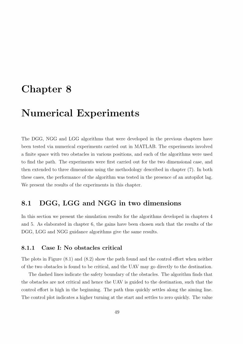
8.5 Path found by DGG, LGG and NGG when both obstacles are critical . . . . . . . 51

8.6 Control plots for DGG, LGG and NGG when both obstacles are critical . . . . . 51

8.7 Path found by DGG with and without autopilot lag; lag=0.1 seconds . . . . . . . 53

8.8 Control plot for DGG with and without autopilot lag; lag=0.1 seconds . . . . . . 53







8.15 Path found by DGG, LGG and NGG in three dimensions . . . . . . . . . . . . . 56

8.16 XY view of the path found by DGG, LGG and NGG in three dimensions . . . . . 57

8.17 XZ view of the path found by DGG, LGG and NGG in three dimensions . . . . . 57

8.18 Control for DGG, LGG and NGG in Y-direction for 3D case . . . . . . . . . . . 57

8.19 Control for DGG, LGG and NGG in Z-direction for 3D case . . . . . . . . . . . 57

iv

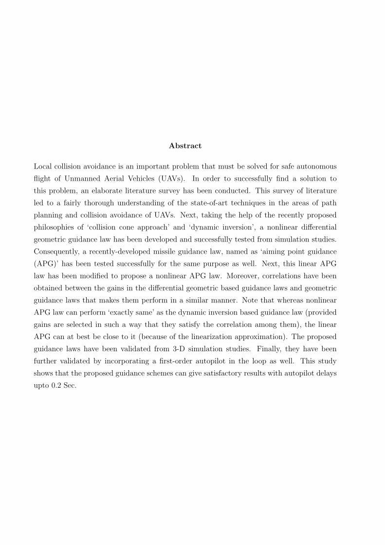
Abstract

Local collision avoidance is an important problem that must be solved for safe autonomous

flight of Unmanned Aerial Vehicles (UAVs). In order to successfully find a solution to

this problem, an elaborate literature survey has been conducted. This survey of literature

led to a fairly thorough understanding of the state-of-art techniques in the areas of path

planning and collision avoidance of UAVs. Next, taking the help of the recently proposed

philosophies of ‘collision cone approach’ and ‘dynamic inversion’, a nonlinear differential

geometric guidance law has been developed and successfully tested from simulation studies.

Consequently, a recently-developed missile guidance law, named as ‘aiming point guidance

(APG)’ has been tested successfully for the same purpose as well. Next, this linear APG

law has been modified to propose a nonlinear APG law. Moreover, correlations have been

obtained between the gains in the differential geometric based guidance laws and geometric

guidance laws that makes them perform in a similar manner. Note that whereas nonlinear

APG law can perform ‘exactly same’ as the dynamic inversion based guidance law (provided

gains are selected in such a way that they satisfy the correlation among them), the linear

APG can at best be close to it (because of the linearization approximation). The proposed

guidance laws have been validated from 3-D simulation studies. Finally, they have been

further validated by incorporating a first-order autopilot in the loop as well. This study

shows that the proposed guidance schemes can give satisfactory results with autopilot delays

upto 0.2 Sec.

Chapter 1

Introduction

Unmanned aerial vehicles (UAVs) are expected to be ubiquitous in the near future, au-

tonomously performing complex military and civilian missions such as reconnaissance, en-

vironmental monitoring, border patrol, search and rescue operations, disaster relief, traffic

monitoring etc [DeGarmo & Nelson(2004)]. Many of these applications require the UAV to

fly at low altitudes in proximity with man made and natural structures. A collision with

a stationary structure or another UAV could prove to be potentially fatal, and might even

result in mission failure. Therefore, it is required that the UAV must be able to successfully

sense and avoid obstacles and at the same time look ahead to pursue its goal. This requires

robust and computationally feasible collision avoidance algorithms to be implemented on-

board the UAV.

UAVs however have limited resources. Several implications exist for any algorithm to be

implemented onboard:

1. Size of the onboard processor is limited. The processing speed and memory available to

the algorithm are limited. Therefore, the algorithm must be computationally efficient.

2. The algorithm must respond quickly, so that it can be implemented in an online navi-

gation system.

3. The payload of UAVs is extremely limited. Therefore the sensor used to gain infor-

mation from the surroundings must be lightweight. The sensors used must also be

economical and energy efficient.

1

4. In addition, UAVs may need to avoid detection for certain stealthy missions like enemy

reconnaissance. Active sensors, which send out energy into the environment are thus

not suitable, since they can be detected.

In view of (3) and (4), vision based navigation is a suitable option, since it is lightweight,

economical as well as covert. The collision avoidance algorithms should therefore be able to

perform well with vision data, which is usually noisy and inaccurate. Collision avoidance

algorithms must satisfy the above requirements.

UAV collision avoidance approaches can be classified into deliberative global path plan-

ning and reactive local collision avoidance algorithms. Global path planning algorithms

assume complete knowledge of the environment beforehand and find an obstacle-free tra-

jectory to the goal point. These methods take into account the dynamics of the UAV, and

avoid known obstacles like buildings, trees etc. Additionally, the UAV constraints such as

turn radius and kinodynamic constraints are also taken into account. They also attempt

to find optimal paths. These methods are usually computationally expensive and cannot

be executed online. Additionally, global planning methods are unsuitable for avoiding colli-

sions with pop-up and moving obstacles. Local methods are reactive, i.e. an onboard sensor

detects the possibility of collision and then an alternative route is planned online. These

consist of computationally efficient algorithms and are able to react quickly to changes in the

environment. However these methods cannot guarantee optimality. Local navigation meth-

ods do not retain global information and continually react to changing environments. It is

essential that local planning methods are fast, since the speed of the UAV is limited by them.

Recent collision avoidance approaches implement multi-layer architectures. A global

planning layer first finds a dynamically feasible obstacle-free optimal path to the goal, and

then a local collision avoidance layer reacts to changes in the environment and computes

an alternate, collision-free path online. This scheme reduces the computation resources re-

quired since the amount of online computation carried out is less. Optimality of the path

may also be guaranteed, except for brief periods when the UAV maneuvers away from the

planned trajectory to avoid a local obstacle. This paper reviews some recently evolving ideas

of collision avoidance algorithms. A literature survey of recently evolving philosophies on

obstacle and collision avoidance of UAVs is presented in Chapter 2.

2

Collision avoidance is often considered as another side of the target interception problem

[Chakravarthy & Ghose(1998)]. This is because once a potential collision is detected, an

alternate point may be found which results in avoiding collision. After this, the problem

reduces to one of finding a path which satisfies terminal conditions. This constitutes a guid-

ance problem.

We solve this problem by formulating a “Differential Geometric” guidance law using a

nonlinear control philosophy called Dynamic Inversion, used popularly in output tracking.

Based on this we also formulate two geometric guidance laws called the Linear Geometric

Guidance and the Nonlinear Geometric Guidance. These guidance laws hold promise for not

only solving the collision avoidance problem, but the target interception problem as well.

The collision avoidance algorithms developed in the study are sense-and-avoid algorithms,

but with a global element, since the destination point is also taken into account.

3

Chapter 2

Literature survey

This chapter presents a literature survey on recently evolving ideas for obstacle and collision

avoidance for UAVs. Although both global path planning and local collision avoidance

methods are covered, the emphasis is on online collision avoidance in both.

2.1 Global Path Planning Algorithms with Local Col-

lision Avoidance

Conventionally, a basic motion planning problem consists of producing a continuous motion

that connects a start configuration and a goal configuration, while avoiding collision with

known obstacles [Lavalle(2006)]. The algorithms discussed in this section retain global infor-

mation, i.e. the algorithm first plans a path to the goal avoiding the obstacles known apriori.

If a collision is predicted to occur, the path is re-planned so that the obstacle is avoided.

However the objective is to always move towards the goal point and thus the re-planned path

must also reach the goal point after collision is avoided. Hence these algorithms are consid-

ered to be global path planning algorithms with local collision avoidance features imbedded

into it.

2.1.1 Graph Search Algorithms

Graph search methods search for a feasible path in a given environment. Examples of graph

search algorithms are deterministic graph search techniques such as A∗ search algorithm

4

[Ferbach(1998)] or Voronoi graph search [Bortoff(2000)] and probabilistic sampling based

planners such as Probabilistic Roadmap Method (PRM) [Pettersson & Doherty(2006)]. Al-

though these algorithms are mainly used for global path planning, reactive planners have

been achieved by modifying the algorithms in order to reduce the computation time. An

example of search algorithms used for both global and local UAV path planning is the work

of [Hwangbo et al.(2007)]. An A∗ search algorithm is used for global planning, while for

local obstacle avoidance, a best first search [Lavalle(2006)] is performed. Both kinematics

and dynamics of the UAV are taken into consideration. First, the global planner plans a

path taking into account the kinematics of the vehicle (e.g., kinematic constraints such as

minimum radius of curvature or maximum climb angle). This generates a set of way-points

for the UAV to follow. These way-points may be tracked by a way-point controller (such

as a PD controller) in the absence of obstacles. When new obstacles are sensed the local

planner is activated, which plans a path to avoid obstacles and go to the sub-goal (which

is in this case the waypoint provided by the global planner). The local planner takes into

account the dynamics of the vehicle (e.g. constraints on velocity and acceleration).

The global planner performs planning in 3D discretized grids using the A∗ search algo-

rithm. The A∗ search algorithm finds the optimal path among the defined nodes. The UAV

kinematics is taken into account for defining the grid cell size as well as the node intercon-

nections, and thus the optimal path found by A∗ algorithm is always kinematically feasible.

At this stage obstacles smaller than the grid size or moving obstacles are neglected.

The local planner performs a finer level of planning between two way-points defined by

the global planner. Here the changes in environment are updated continuously, and moving

and pop-up obstacles or obstacles smaller than the grid size are taken into account while

planning the path. Aggressive maneuvers beyond the kinematics of the vehicle are allowed

at this stage in order to avoid the obstacles. A sampling based motion planner under differ-

ential constraints is used for local planning. For this a set motion primitives is used. Motion

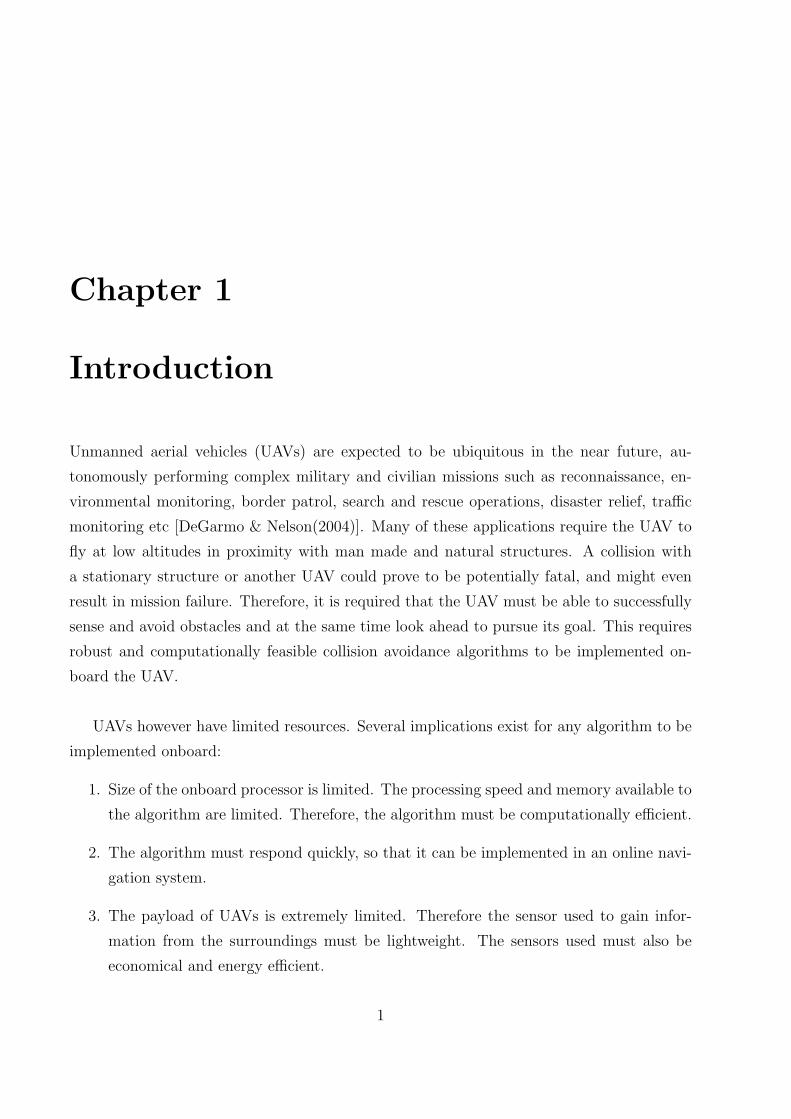
primitives are calculated at every state by finding all dynamically feasible motions from that

state (Figure 2.1). These are pre-computed and saved in a look-up table for efficiency.

Then, a best first search is done, in which nodes closer to the sub-goal are connected first.

5

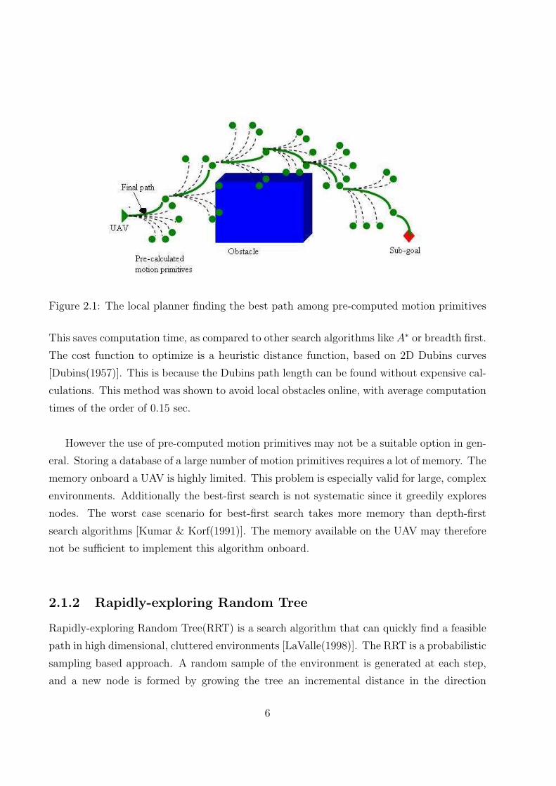
Figure 2.1: The local planner finding the best path among pre-computed motion primitives

This saves computation time, as compared to other search algorithms like A∗ or breadth first.

The cost function to optimize is a heuristic distance function, based on 2D Dubins curves

[Dubins(1957)]. This is because the Dubins path length can be found without expensive cal-

culations. This method was shown to avoid local obstacles online, with average computation

times of the order of 0.15 sec.

However the use of pre-computed motion primitives may not be a suitable option in gen-

eral. Storing a database of a large number of motion primitives requires a lot of memory. The

memory onboard a UAV is highly limited. This problem is especially valid for large, complex

environments. Additionally the best-first search is not systematic since it greedily explores

nodes. The worst case scenario for best-first search takes more memory than depth-first

search algorithms [Kumar & Korf(1991)]. The memory available on the UAV may therefore

not be sufficient to implement this algorithm onboard.

2.1.2 Rapidly-exploring Random Tree

Rapidly-exploring Random Tree(RRT) is a search algorithm that can quickly find a feasible

path in high dimensional, cluttered environments [LaValle(1998)]. The RRT is a probabilistic

sampling based approach. A random sample of the environment is generated at each step,

and a new node is formed by growing the tree an incremental distance in the direction

6

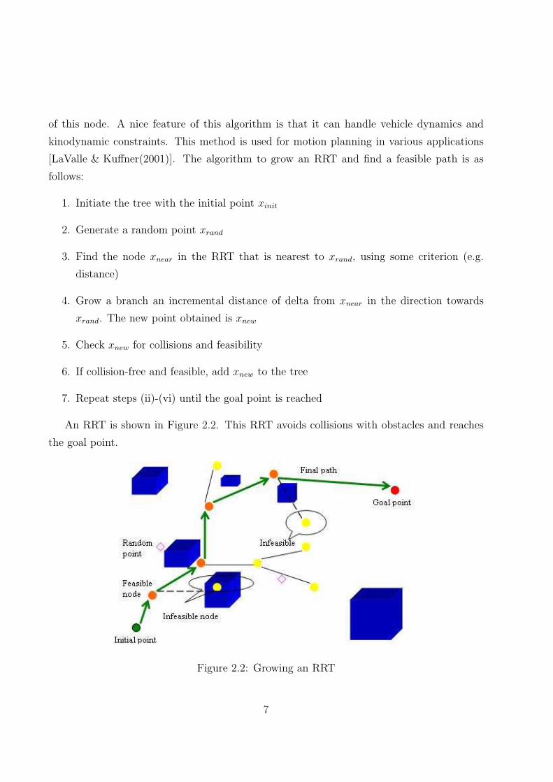
of this node. A nice feature of this algorithm is that it can handle vehicle dynamics and

kinodynamic constraints. This method is used for motion planning in various applications

[LaValle & Kuffner(2001)]. The algorithm to grow an RRT and find a feasible path is as

follows:

1. Initiate the tree with the initial point xinit

2. Generate a random point xrand

3. Find the node xnear in the RRT that is nearest to xrand, using some criterion (e.g.

distance)

4. Grow a branch an incremental distance of delta from xnear in the direction towards

xrand. The new point obtained is xnew

5. Check xnew for collisions and feasibility

6. If collision-free and feasible, add xnew to the tree

7. Repeat steps (ii)-(vi) until the goal point is reached

An RRT is shown in Figure 2.2. This RRT avoids collisions with obstacles and reaches

the goal point.

Figure 2.2: Growing an RRT

7

We conducted numerical experiments in a 100 m by 100 m cluttered space. Figure 2.3

shows the path found by the RRT with 25 obstacles, while 2.4 shows the path with 50

obstacles.

0 20 40 60 80 1000

10

20

30

40

50

60

70

80

90

100

1

2

3

4

5

6

789

1011

12

13

14

15

16

17

18

19

20

21

22

23

2425

26

27

28

29

30

31

32

33

3435

36

37

Figure 2.3: Path found by RRT in a space with 25 obstacles.

As can be seen, there are some extraneous branches in the tree that are not a part of the

final path. This is due to the random nature of space exploration in the method.

The RRT is used as a global path planner in [Griffiths et al.(2006)]. With appropriate

modifications [Amin et al.(2006)], RRT can be used to plan a global, dynamically feasible

and optimal path to the goal, as well as perform re-planning when obstacles are detected

by the sensor onboard. Since collision checking is an expensive process in RRT, an effi-

cient method of obstacle representation called Quadtrees [Frisken & Perry(2003)] is used.

Quadtrees are a data structure used to represent the environment efficiently. Quadtrees

divide the environment into quadrants. This division is carried out until a quadrant is filled

by the obstacle and becomes a leaf node. It must be noted that this results in an unequal

spatial division, which is more efficient than using uniform grids.

8

0 20 40 60 80 1000

10

20

30

40

50

60

70

80

90

100

1

2 3 45

6

7

89

10

11 12

13

14

15

16

17

18

19

20

21

22

23

24

25

26

27

28

29

30

31

32

33

34

35

36

3738

39

40

41

42

43

44 45

46 47 48

49

50

51

Figure 2.4: Path found by RRT in a space with 50 obstacles.

The RRT finds feasible paths to the goal by avoiding obstacles. But the path found

is usually far from optimal. Therefore, at the global level of planning the path found by

RRT is passed through the Dijkstra’s algorithm, which is a search method that finds short-

est distance paths. The path found by RRT is usually far from optimal and needs to be

pruned. The Dijkstra’s search algorithm [Lavalle(2006)] is used for this, which first finds

the reachability of every point and then sorts these points according to a cost function (an

approximate distance function in this case). Another pass through this step re-samples the

points to shorter distances and then finds the optimal path again. The number of passes of

the Dijkstra’s algorithm depends on the computation resources available and requirement of

optimality.

To reduce computation time, a dual RRT concept is used, in order to speed up computa-

tion [Kuffner & LaValle(2000)]. Both trees are grown simultaneously from the start and goal

point at each iteration, and at every step a “connect” operation is performed, which tries to

connect both the trees. Perhaps a natural extension of this idea would be to grow multiple

trees from fixed points in the search space and then perform multiple connect operations at

9

every step. Another modification is made to reduce the cost for finding the nearest point

in the tree to add a new node. An approximate distance function is used for this, which

uses an absolute value function and eliminates the necessity for square root operation. The

deviation from true Euclidean distance is claimed to be around 6%, which is not significant.

For 3D implementation, penalty for change in altitude is made high. This is because

change in altitude is not a desired behavior for many applications (e.g. surveillance). Only

when a path cannot be found at the same altitude, a change in altitude is allowed. The

RRT is thus implemented both as a global and a local planner with suitable modifications as

discussed. An optimal global path is first calculated offline, and then when the sensor detects

obstacles the path is modified. Simulation results in [Amin et al.(2006)] demonstrate that

this scheme offers a good global planner as well as a reactive algorithm for online collision

avoidance. An important disadvantage of RRT is that it is an open loop method, and thus

is sensitive to modeling inaccuracies and external noise such as wind. Additionally, avoiding

collision with moving obstacles may not be possible, because of the random nature of the

algorithm.

2.1.3 Potential Field Method

The potential field approach [Khatib(1985)] has found widespread use as a navigation method

for ground robots and more recently in UAVs. In this method the UAV is modeled as mov-

ing under the influence of a potential field. The artificial potential field function may be

designed according to the problem, and is determined by the goal and the set of obstacles.

The idea is to reach the goal point, along with avoiding collisions with any obstacles along

the way.

The potential function consists of an “attraction field”, which pulls the UAV towards the

goal, and a “repulsive field”, which ensures that the UAV does not collide with obstacles.

The resultant field defines the direction of motion. This method is fast and efficient.It is also

easy to add new obstacles to the function. A formation of UAVs has also been accomplished

using the potential field approach[Paul et al.(2008)]. The total potential field experienced

by each UAV is a combination of the potential field due to the formation, collision avoidance

10

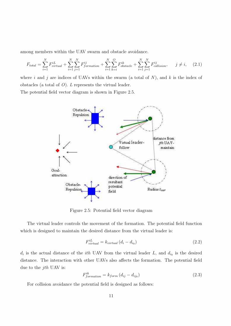
among members within the UAV swarm and obstacle avoidance.

Ftotal =N∑

i=1

F iLvirtual +

N∑

i=1

N∑

j=1

F ijformation +

N∑

i=1

O∑

k=i

F ikobstacle +

N∑

i=1

N∑

j=1

F ijcollision, j 6= i, (2.1)

where i and j are indices of UAVs within the swarm (a total of N ), and k is the index of

obstacles (a total of O). L represents the virtual leader.

The potential field vector diagram is shown in Figure 2.5.

Figure 2.5: Potential field vector diagram

The virtual leader controls the movement of the formation. The potential field function

which is designed to maintain the desired distance from the virtual leader is:

F iLvirtual = kvirtual (di − di0) (2.2)

di is the actual distance of the ith UAV from the virtual leader L, and di0 is the desired

distance. The interaction with other UAVs also affects the formation. The potential field

due to the jth UAV is:

F ikformation = kform (dij − dij0) (2.3)

For collision avoidance the potential field is designed as follows:

11

F ijcollision =

(Kcollrsav

||dji|| −Kcoll

)dji

||dji|| for ||dji|| < rsav (2.4)

A safety sphere of radius rsav is assumed around the UAV. dij is the distance between

UAVs i and j. If another UAV enters the sphere this factor increases, and converges to

infinity at the centre of the sphere.

Similarly, for obstacle avoidance the field is modeled as follows:

F ikobstacle =

(Kobst

||dki|| −Kobst

rsav

)dki

||dki|| for ||dki|| < rsav

0 otherwise(2.5)

dki is the distance between UAV i and the k -th obstacle. Kcoll and Kobstare gains that need

to be tuned.

The resultant magnitude and direction of the potential field is obtained by summing

the individual potential fields. Here the magnitude of the field is restricted to a maximum

quantity, while the direction is kept the same. This is done to limit the speed of the UAV.

A trajectory is then generated using this resultant potential field. The potential field de-

signed here is continuous, and simulation results demonstrate that this method successfully

achieves formation flight along with collision and obstacle avoidance. The UAVs avoid a

local minimum and head towards their goal, which is a stable minimum.

In [Scherer et al.(2008)] a framework for flying an unmanned helicopter close to the

ground is described, avoiding even small obstacles such as wires. It consists of a slow global

path planner, a high frequency local reactive obstacle avoidance algorithm and a low level

speed controller. The sensor used is a ladar that can sense small obstacles from ranges

of 100m. Information about the environment is given to the algorithm through Evidence

Grids, which are a map of the environment that can be updated after every sensor scan

[Martin & Moravec(1996)]. A layered architecture with deliberate path planning running at

low frequency and reactive obstacle avoidance running at high frequency is used. The lowest

layer is the speed controller which accelerates or decelerates the vehicle based on how close

the obstacle is.

The reactive local obstacle avoidance algorithm uses the potential field approach. The

control law consists of an attraction factor towards the goal and a repulsion factor from

12

the obstacles. These factors are calculated based on the distance and angle measures. The

attraction to the goal is directly proportional to the angle to the goal, and inversely pro-

portional to the exponential of the distance from the goal. The repulsion from obstacles is

inversely proportional to the exponentials of both the distance and the angle to the obstacle:

attract (goal) = kgψg

(e−c1dg + c2

)(2.6)

repulse (obstacle) = koψo

(e−c3do

) (e−c4|ψo|

)(2.7)

where ψg and dg are the angle and distance to the goal, respectively, and ψo and do are

the angle and distance to the obstacle. kg, ko, c1, c2, c3, c4 are parameters to be found.

These parameters are found by training the system against a human pilot and then tuned

[Hamner et al.(2006)].

An angular acceleration command is formulated by summing these factors and then

damping it with the current angular velocity as follows:

φ = −bφ− attract (g) +∑

o∈O

repulse (o) (2.8)

Also, the algorithm maneuvers in both horizontal and vertical planes before one of them

becomes clear of obstacles and then the UAV chooses that plane to travel in. This algorithm

has been extended to the 3D case. The obstacles considered by the algorithm are limited

by a box shape constraint to maintain computation tractability. The algorithm was imple-

mented in an unmanned helicopter. It was found that obstacle avoidance was successful even

when the helicopter flew at low altitudes (8m) and at high speeds (3m/s to 10 m/s). The

helicopter avoided even thin wires. However, this method does not explicitly avoid moving

obstacles.

However the potential field method has some inherent limitations [Koren & Borenstein(1991)].

A major drawback of this method is that it is possible for the UAV to get caught in a local

minimum i.e. the UAV gets caught among obstacles before reaching the goal. It is also

difficult for this method to find paths through narrow passages. Additionally, the potential

function needs to be designed heuristically for every problem, and finding it becomes difficult

for large obstacle-laden spaces with many motion constraints.

13

2.1.4 Minimum Effort Guidance

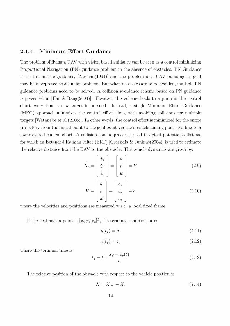
The problem of flying a UAV with vision based guidance can be seen as a control minimizing

Proportional Navigation (PN) guidance problem in the absence of obstacles. PN Guidance

is used in missile guidance, [Zarchan(1994)] and the problem of a UAV pursuing its goal

may be interpreted as a similar problem. But when obstacles are to be avoided, multiple PN

guidance problems need to be solved. A collision avoidance scheme based on PN guidance

is presented in [Han & Bang(2004)]. However, this scheme leads to a jump in the control

effort every time a new target is pursued. Instead, a single Minimum Effort Guidance

(MEG) approach minimizes the control effort along with avoiding collisions for multiple

targets [Watanabe et al.(2006)]. In other words, the control effort is minimized for the entire

trajectory from the initial point to the goal point via the obstacle aiming point, leading to a

lower overall control effort. A collision cone approach is used to detect potential collisions,

for which an Extended Kalman Filter (EKF) [Crassidis & Junkins(2004)] is used to estimate

the relative distance from the UAV to the obstacle. The vehicle dynamics are given by:

Xv =

xv

yv

zv

=

u

v

w

= V (2.9)

V =

u

v

w

=

ax

ay

az

= a (2.10)

where the velocities and positions are measured w.r.t. a local fixed frame.

If the destination point is [xd yd zd]T , the terminal conditions are:

y(tf ) = yd (2.11)

z(tf ) = zd (2.12)

where the terminal time is

tf = t +xd − xv(t)

u(2.13)

The relative position of the obstacle with respect to the vehicle position is

X = Xobs −Xv (2.14)

14

Figure 2.6: Reaching the goal and avoiding an obstacle using MEG

Also, for stationary obstacles

X = −V (2.15)

where V is the vehicle velocity. The collision safety boundary is a sphere of radius d meters

around the obstacle.

A collision cone [Chakravarthy & Ghose(1998)] in two dimensional space is formed by a

set of tangents from the UAV to the safety boundary of the obstacle, as shown in Figure

2.6. If the velocity vector is contained within the collision cone, the obstacle is said to be

critical, and an alternate maneuver is to be calculated. The aiming point Xap is a point

that the UAV must maneuver to so that the minimum safety distance is maintained. This

may be found using the Collision Cone Approach. Time-to-go to the aiming point tgo is also

found. Additional time-to-go criteria are specified, which point out that collision must only

be avoided if time-to-go is within certain range:

tgo − t < T (2.16)

0 < tgo < tf (2.17)

where time T should be small enough so that collision avoidance is done only when there is

urgency.

15

The PN guidance law is derived by solving the following optimization problem for control

minimization for each aiming point obtained:

min Joa =1

2

tgo∫

t0

aT (t)a(t)dt =1

2

tgo∫

t0

(a2y(t) + a2

z(t))dt (2.18)

subject to vehicle dynamics with terminal conditions

yv(tgo) = yap, zv(tgo) = zap (2.19)

The resulting optimal guidance law is

aoa(t) = −3

1

(tgo−to)2

0

yv (t0)− yap

zv (t0)− zap

+ 1

tgo−t0

0

v (t0)

w (t0)

(2.20)

The problem of reaching destination is handled in another PN guidance problem with the

terminal conditions:

y(tf ) = yd, z(tf ) = zd (2.21)

The optimal control obtained from the PN Guidance method is only piecewise continuous,

with a jump between targets.

MEG handles all the terminal conditions within one problem [Ben-Asher(1993)]. The op-

timal control is continuous and piecewise linear. This method, therefore, yields a lower cost.

The optimization problem remains the same and all the terminal conditions are considered

in the problem. The control law is found by cubic interpolation of the single condition case.

The resulting optimal control law is

16

a (t0) = aoa (t)− 3

3(tgo − to

)+ 4

(tf − tgo

)

0

v (t0)

w (t0)

+ 3

(tgo−to)

0

yv (t0)− yap

zv (t0)− zap

− 2

(tf−tgo)

0

yap − yd

zap − zd

(2.22)

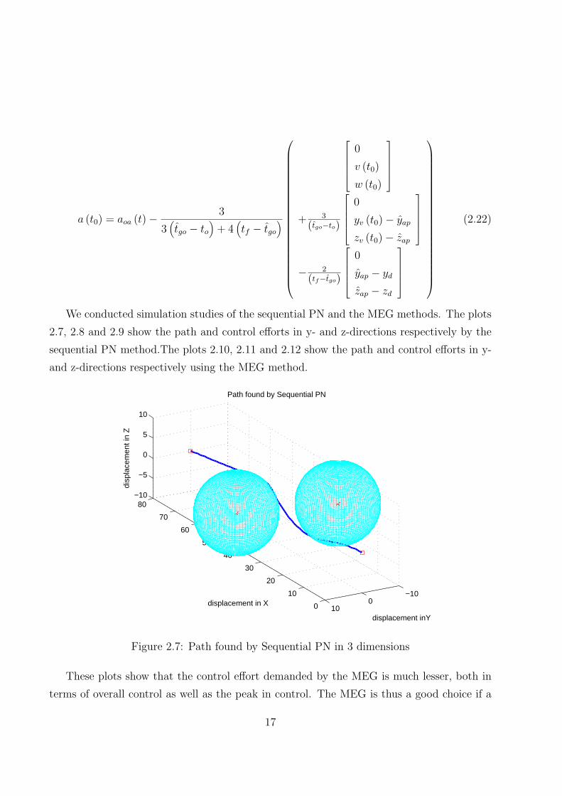
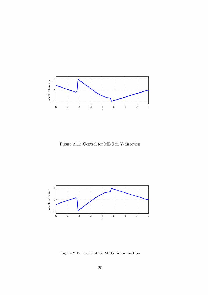
We conducted simulation studies of the sequential PN and the MEG methods. The plots

2.7, 2.8 and 2.9 show the path and control efforts in y- and z-directions respectively by the

sequential PN method.The plots 2.10, 2.11 and 2.12 show the path and control efforts in y-

and z-directions respectively using the MEG method.

0

10

20

30

40

50

60

70

80

−100

10

−10

−5

0

5

10

displacement inY

Path found by Sequential PN

displacement in X

disp

lace

men

t in

Z

Figure 2.7: Path found by Sequential PN in 3 dimensions

These plots show that the control effort demanded by the MEG is much lesser, both in

terms of overall control as well as the peak in control. The MEG is thus a good choice if a

17

0 1 2 3 4 5 6 7 8

−5

0

5

t

acce

lera

tion

in y

Figure 2.8: Control for Sequential PN in Y-direction

minimum effort collision avoidance path is desired.

In [Watanabe et al.(2006)], both PN Guidance and Minimum Effort Guidance are used to

solve the same problem. The cost is found to be lower in MEG. Therefore, MEG is found to

be a better method in terms of the control minimization achieved. However, an assumption

made in this method is that the obstacles are stationary. Therefore, this method needs to

be extended for avoiding collisions with moving obstacles.

18

0 1 2 3 4 5 6 7 8

−5

0

5

t

acce

lera

tion

in z

Figure 2.9: Control for Sequential PN in Z-direction

0

10

20

30

40

50

60

70

80

−100

10

−10

−5

0

5

10

Y

Path found by MEG

X

Z

Figure 2.10: Path found by MEG in 3 dimensions

19

0 1 2 3 4 5 6 7 8

−5

0

5

t

acce

lera

tion

in y

Figure 2.11: Control for MEG in Y-direction

0 1 2 3 4 5 6 7 8

−5

0

5

t

acce

lera

tion

in z

Figure 2.12: Control for MEG in Z-direction

20

2.2 Local Collision Avoidance Algorithms

Local collision avoidance algorithms deal only with the problem of avoiding collisions with

obstacles as and when they are detected. These algorithms do not retain global information,

that is they do not require knowledge of the entire environment, or the initial and goal

points. The information about the immediate environment, and nearby obstacles (fixed and

moving) are provided to the algorithm by onboard sensors/cameras. This information is

often sufficient to compute an avoidance maneuver for the UAV. It must be emphasized

that these algorithms can be imbedded into any global path planning algorithms, under the

assumption that after avoiding the obstacle, the UAV comes back to the global path as soon

as possible.

2.2.1 Nonlinear Model Predictive Control Approach

Model Predictive Control (MPC) [Camacho & Bordons(1999)] has gained popularity in re-

cent years as a control approach for nonlinear dynamical systems. This approach handles

realistic system constraints such as input saturation and state constraints and is found to

be suitable for path-planning problems in complex environments [Leung et al.(2006)]. An

MPC scheme is implemented by [Shim et al.(2006)] to achieve online collision avoidance in

UAVs. Since MPC performs online optimization over a finite receding horizon, it can ac-

count for future environment changes. Collision avoidance is built into the optimization

problem, which performs reference trajectory tracking and obstacle avoidance in a single

module. When a collision is predicted to occur, a safe trajectory that avoids the impending

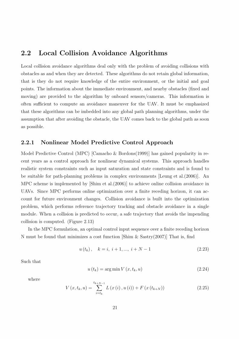
collision is computed. (Figure 2.13)

In the MPC formulation, an optimal control input sequence over a finite receding horizon

N must be found that minimizes a cost function [Shim & Sastry(2007)] That is, find

u (tk) , k = i, i + 1, ..., i + N − 1 (2.23)

Such that

u (tk) = arg min V (x, tk, u) (2.24)

where

V (x, tk, u) =tk+N−1∑

i=tk

L (x (i) , u (i)) + F (x (tk+N)) (2.25)

21

Figure 2.13: Trajectory tracking and re-planning using MPC

Lis a positive definite cost function and F is the terminal cost. The cost function L is chosen

as:

L (x, u) =1

2(xr − x)T Q (xr − x) +

1

2uT

r Rur + S (x) +O∑

l=1

P (xv, ηl) (2.26)

The first term in the cost function ensures that any deviation from the reference state

results in a large value of cost, and therefore is penalized. Similarly the second term penalizes

high control inputs. The term S(x) penalizes states that are outside the allowable range.

The last term is a potential function term to be included for obstacle avoidance. It is chosen

as follows:

P (xv, ηl) =1

(xv − ηl)T G (xv − ηl) + ε

(2.27)

where xv ∈ R3 is the position of the UAV, and ηl is the position of the l -th obstacle out

of O obstacles. This penalty function increases as ‖xv − ηl‖ decreases. G is positive definite

and ε is a quantity that is kept positive to prevent P from being singular when ‖xv−ηl‖ → 0.

The potential function term may be chosen to be enabled only when ‖xv − ηl‖ < σmin, a

minimum safety distance to be maintained. A new trajectory is then planned. Including

collision avoidance into the optimization step reduces the risk of the UAV falling into a local

minimum, since MPC looks ahead and optimizes over a finite horizon.

22

The obstacles’ predicted position after k+N-1 steps is required (N is the horizon) in

order to avoid the obstacle. If the current position and velocity vl of the obstacle may be

estimated, the position of the obstacle after Np steps (prediction horizon) may be found at

the kth step:

ηl (tk+i) = ηl (tk) + ∆tvl (tk) (ti−1) (2.28)

Control saturation is taken into account during the online optimization process. Addition-

ally a tracking feedback controller in the loop will track the reference without any error in

the presence of modeling uncertainties.

A dual mode strategy is followed in order to track a reference trajectory, as well as avoid

collisions. In normal flight, parameters are chosen so as to achieve tracking performance and

good stability. In the emergency evasive maneuver case, the parameters are chosen so as to

generate a trajectory that will avoid collision at all cost. During evasion, large control effort

and large deviations from reference are allowed.

Results of simulations in [Shim & Sastry(2007)] indicate that this method is capable of

avoiding hostile obstacles flying at high speeds ( 100 kmph) and with different heading an-

gles. This method was implemented successfully in unmanned helicopters. A disadvantage

of this method is that MPC is quite computation intensive, and may not be suitable for

online implementation on small UAVs. An extension of this approach can be towards col-

lision avoidance with maneuevering obstacles. This would require an estimator and some

knowledge of the dynamics of the obstacle.

2.2.2 Vision-based Neural Network Approach

A vision based Grossberg Neural Network (GNN) [Grossberg(1988)] scheme is used for local

collision avoidance[Wang et al.(2007)]. GNNs are nonlinear competitive neural networks.

These are able to explain the working of human vision, and have been used in a variety of

vision based applications, especially in pattern recognition [Carpenter & Grossberg(1991)].

GNNs may be used for UAV vision based navigation. A combination of Visibility Graphs

and GNNs is used to achieve online collision avoidance.

23

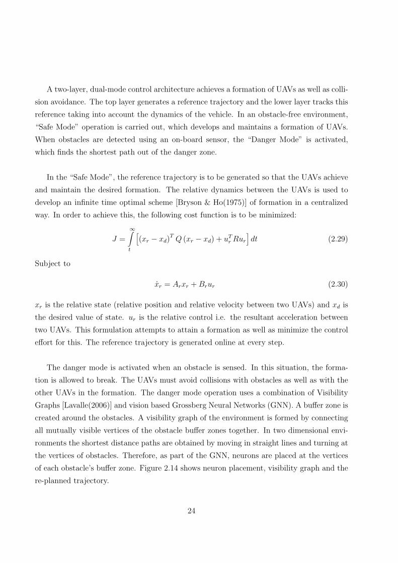
A two-layer, dual-mode control architecture achieves a formation of UAVs as well as colli-

sion avoidance. The top layer generates a reference trajectory and the lower layer tracks this

reference taking into account the dynamics of the vehicle. In an obstacle-free environment,

“Safe Mode” operation is carried out, which develops and maintains a formation of UAVs.

When obstacles are detected using an on-board sensor, the “Danger Mode” is activated,

which finds the shortest path out of the danger zone.

In the “Safe Mode”, the reference trajectory is to be generated so that the UAVs achieve

and maintain the desired formation. The relative dynamics between the UAVs is used to

develop an infinite time optimal scheme [Bryson & Ho(1975)] of formation in a centralized

way. In order to achieve this, the following cost function is to be minimized:

J =

∞∫

t

[(xr − xd)

T Q (xr − xd) + uTr Rur

]dt (2.29)

Subject to

xr = Arxr + Brur (2.30)

xr is the relative state (relative position and relative velocity between two UAVs) and xd is

the desired value of state. ur is the relative control i.e. the resultant acceleration between

two UAVs. This formulation attempts to attain a formation as well as minimize the control

effort for this. The reference trajectory is generated online at every step.

The danger mode is activated when an obstacle is sensed. In this situation, the forma-

tion is allowed to break. The UAVs must avoid collisions with obstacles as well as with the

other UAVs in the formation. The danger mode operation uses a combination of Visibility

Graphs [Lavalle(2006)] and vision based Grossberg Neural Networks (GNN). A buffer zone is

created around the obstacles. A visibility graph of the environment is formed by connecting

all mutually visible vertices of the obstacle buffer zones together. In two dimensional envi-

ronments the shortest distance paths are obtained by moving in straight lines and turning at

the vertices of obstacles. Therefore, as part of the GNN, neurons are placed at the vertices

of each obstacle’s buffer zone. Figure 2.14 shows neuron placement, visibility graph and the

re-planned trajectory.

24

Figure 2.14: Danger Mode operation using visibility graph and GNNs

The activity of each neuron depends upon excitation received from other neurons as well

as excitation from the goal point. The activity is calculated from a shunting equation:

dxi

dt= −axi + (b− xi)

E +

k∑

j=1

wijxj

(2.31)

where

E = E1 + E2 (2.32)

E1 =α

dp

(2.33)

E2 =

100, if the neuron is on destination

0, otherwise(2.34)

xi is the activity of the ith neuron, wijxij is excitation due to neighboring neuron, where

wij = (µ/dij). dij is the distance between UAVS i and j. dp is the perpendicular distance

of the vertex from the line joining the UAV and the target. E is the excitation composed

of two parts. E1 is the excitation due to closeness of the vertex from the present path. α

and µ are weights that must be tuned correctly so that the deviation from current path and

closeness to goal are weighed correctly. The neurons nearest to the goal and nearest to the

current path have the highest values of activity. Thus, by following the vertices with highest

activities, the UAV is able to get out of the danger mode. The path followed will be the

shortest distance path. Collision avoidance with other UAVs is achieved in the following

way. When a potential collision is sensed, the UAV with lower index creates a buffer zone

25

around the UAV with higher index and attempts to avoid it.

In the lower layer, tracking the reference generated by both the Safe Mode and the Danger

Mode is done using a Model Predictive Controller (MPC) [Camacho & Bordons(1999)]. This

method consists of finding the optimal control input sequence to minimize a cost function

at every step. The cost function here is formulated such that the actual output tracks the

reference output, along with control minimization. This method also takes into account

practical vehicle constraints. The cost function to be minimized at the kth step is:

Jk = [y (tk)− yd (tk)]T Qk [y (tk)− yd (tk)] + ∆U (tk) Rk∆U (tk) (2.35)

y is the actual output, yd is the desired output and ∆U is the control history. Qk and Rk

are weighting matrices to be chosen appropriately.

Simulation results in [Wang et al.(2007)] show that the UAVs developed a desired forma-

tion and successfully re-planned trajectories to avoid obstacles along the way. Cooperative

collision avoidance among UAVs is also achieved. A possible extension of this method is the

case of non-cooperative collision avoidance. This can be implemented with an estimator to

find the hostile obstacles’ velocity and position.

2.2.3 Conflict Detection and Resolution

UAV collision avoidance may be percieved as a Conflict Detection and Resolution (CD&R)

problem. CD&R methods are used widely for Air Traffic Control [Kuchar & Yang(2000)].

These methods predict the possibility of a conflict between two aircraft, and compute a ma-

neuver strategy for the UAV such that conflict is avoided. One approach [Park et al.(2008)] is

to perform conflict detection by the Point of Closest Approach (PCA) [Krozel & Peters(1997)]

method. For conflict resolution, a vector sharing resolution method is used. Conflict is de-

fined as “a predicted violation of a separation assurance standard”. It is assumed that every

UAV has information about every other UAV. A protection zone is defined as a sphere of

a specified distance. If the protection zone is violated, the UAVs must maneuver such that

conflict is avoided.

The UAVs are modeled as point masses flying with constant velocities. The point mass

26

UAV equations are:

V =√

V 2H + V 2

V (2.36)

x

y

z

=

VH

VH

V

cos γ

sin γ

sin θ

(2.37)

γ =g tan φ

VH

(2.38)

where θ is the UAV’s pitch angle, γ is heading angle and φ is the bank angle. Pitch angle

and heading angles are commanded as follows, where N and M are time constants in φ

θ

=

1N1M

φcom − φ

θcom − θ

(2.39)

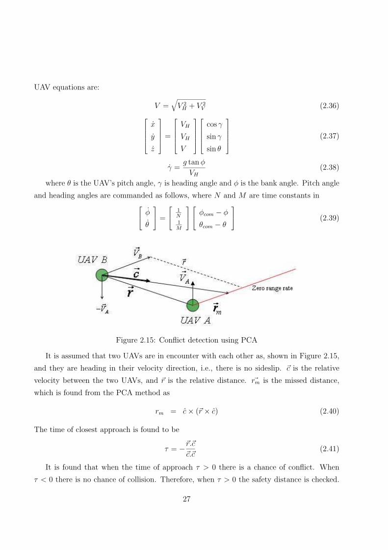
Figure 2.15: Conflict detection using PCA

It is assumed that two UAVs are in encounter with each other as, shown in Figure 2.15,

and they are heading in their velocity direction, i.e., there is no sideslip. ~c is the relative

velocity between the two UAVs, and ~r is the relative distance. ~rm is the missed distance,

which is found from the PCA method as

rm = c× (~r × c) (2.40)

The time of closest approach is found to be

τ = −~r.~c

~c.~c(2.41)

It is found that when the time of approach τ > 0 there is a chance of conflict. When

τ < 0 there is no chance of collision. Therefore, when τ > 0 the safety distance is checked.

27

If the magnitude of the missed distance vector is less than the safety measure (rm < rsafe),

there is a conflict, which must be resolved.

For conflict resolution, a resolution maneuver must be computed, which lies along the

missed distance vector, as shown in Figure 2.16. ~VA and ~VB are the actual velocity directions

of UAV A and UAV B respectively. ~UA and ~UB are the velocity directions the UAV must go

along so that the distance between the UAVs is rsafe. rV SA and rV SB are the vectors of each

UAV along the missed distance vector such that |rsafe| = |rV SA|+ |rV SB|+ |rm|. The slower

UAV takes more sharing.

Figure 2.16: Vector sharing resolution to resolve the conflict

It is proposed by [Merz(1991)] that the optimal maneuver to resolve the conflict consists

of an acceleration along the missed distance vector . The commands to the UAV are decided

based on the range of the LOS angle and the required pitch angle. The LOS angle is

calculated as:

γ = sig(~VH × ~UH

)cos−1

~VH .~UH

|~VH |

(2.42)

Depending on the range of the LOS angle, the bank angle command is given suitably. The

time constant N is set as 1 second.

The required pitch angle is:

θreq = tan−1

~UV

|~UH |

(2.43)

Depending on its range the time constant M is set. Simulations done in a non-cooperative

scenario in [Park et al.(2008)] show that the UAV successfully detects conflict and maneuvers

28

such that conflict is avoided. However, this algorithm assumes perfect information between

the UAVs, which is not a realistic assumption. Communication links used at the present

time to relay information among UAVs cannot guarantee perfect information transfer. In

addition, this algorithm will be difficult to implement for a maneuvering obstacle, since the

algorithm is developed for an obstacle moving with constant velocity. Moreover, the velocity

of the UAV itself is assumed to be constant, which limits the possibilities of this method.

2.3 Conclusions

Much of the benefits of deploying UAVs can be derived from autonomous missions. Path

planning with collision avoidance is an important problem which needs to be addressed to

ensure safety of such vehicles in autonomous missions. An attempt has been made in this

review paper to present a brief overview of a few promising and evolving ideas such as graph

search, RRT, potential field, model predictive control, vision based algorithms, minimum

effort guidance etc. Note that there are several requirements that an algorithm must satisfy

in order to solve the online collision avoidance problem completely. A few key issues that

need to be addressed in a good collision avoidance algorithms include:

• Collision avoidance with fixed and moving obstacles- both in cooperative and non-

cooperative flying

• Solution of the problem taking the vehicle dynamics into account, including state and

input constraints (many of the current algorithms are based on only kinematics)

• Development of fast algorithms, which can be implemented online with limited onboard

processor capability

• Capability to sense and avoid even small obstacles (such as electric power lines, small

birds etc.)

• Robustness for issues such as limited information of the environment, partial loss of

information etc.

In addition to the above issues, there are many other issues for successful deployment

of UAVs, such as requirement for light weight equipments, power efficiency (for high en-

durance), stealthiness etc. Although an attempt has been made in this paper to give an

29

overview of some of the recently proposed techniques which partially address some of these

issues, promising algorithms satisfying many of these requirements simultaneously is yet to

be developed. Additionally, some of the assumptions behind the proposed algorithms (such

as non-maneuvering constant speed flying objects, appearance of one obstacle at a time, per-

fect information about the environment etc.) are not realistic and hence need to be relaxed.

A lot of research is being carried out worldwide to design collision avoidance systems that

address many of these important concerns.

30

Chapter 3

Problem Formulation

In Chapter 2 we discussed various methodologies used to achieve collision avoidance in UAVs.

In this chapter we formulate the collision avoidance problem for the UAV.

3.1 Modeling

The motion of the UAV is modeled via simple kinematics i.e.,

x

y

z

=

u

v

w

(3.1)

u

v

w

=

0

ay

az

(3.2)

All of these are measured w.r.t. the body frame as shown in Figure 3.1

The controls are ay and az . Note that the acceleration in x-direction is an engine control

and therefore is sluggish. Hence we assume that the guidance loop has no control over the

UAV’s motion in the body x-axis.

31

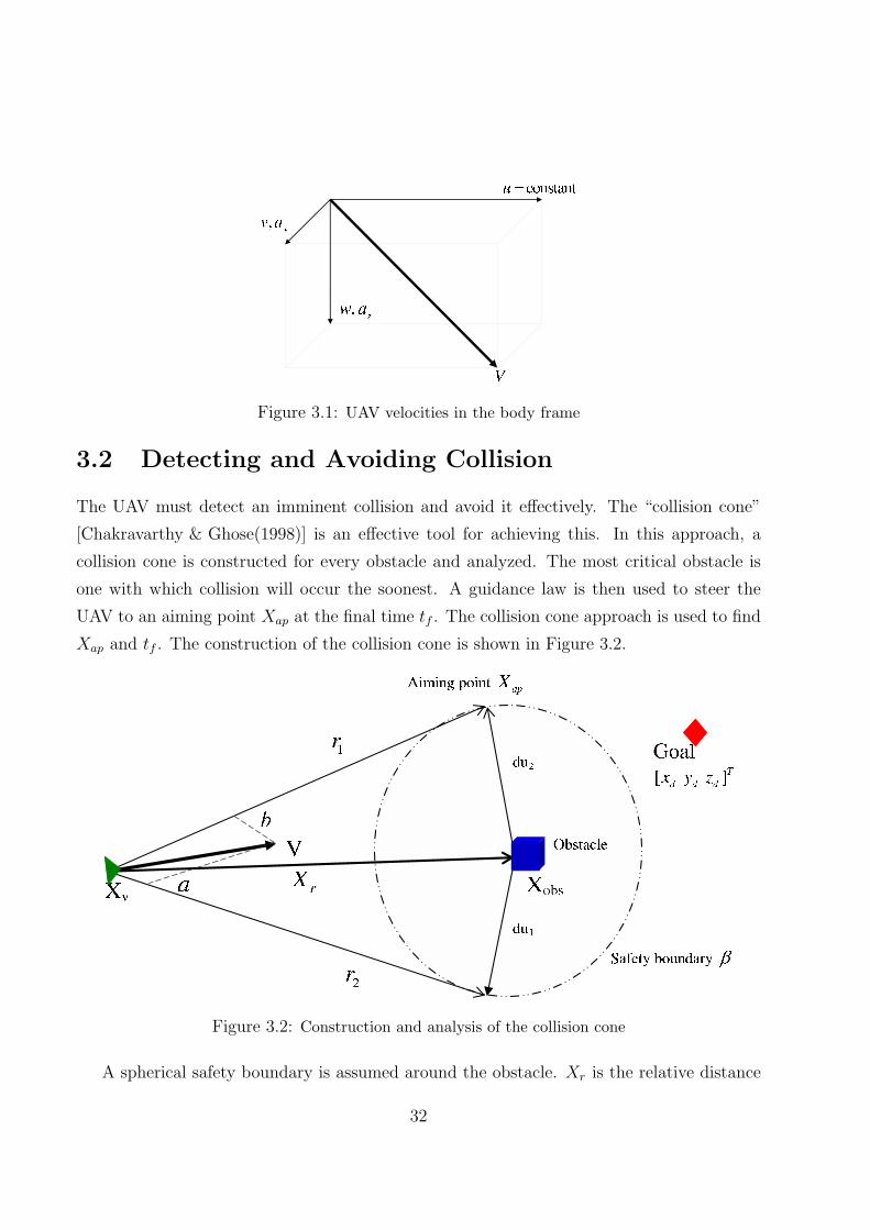
Figure 3.1: UAV velocities in the body frame

3.2 Detecting and Avoiding Collision

The UAV must detect an imminent collision and avoid it effectively. The “collision cone”

[Chakravarthy & Ghose(1998)] is an effective tool for achieving this. In this approach, a

collision cone is constructed for every obstacle and analyzed. The most critical obstacle is

one with which collision will occur the soonest. A guidance law is then used to steer the

UAV to an aiming point Xap at the final time tf . The collision cone approach is used to find

Xap and tf . The construction of the collision cone is shown in Figure 3.2.

Figure 3.2: Construction and analysis of the collision cone

A spherical safety boundary is assumed around the obstacle. Xr is the relative distance

32

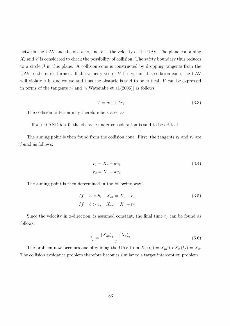
between the UAV and the obstacle, and V is the velocity of the UAV. The plane containing

Xr and V is considered to check the possibility of collision. The safety boundary thus reduces

to a circle β in this plane. A collision cone is constructed by dropping tangents from the

UAV to the circle formed. If the velocity vector V lies within this collision cone, the UAV

will violate β in due course and thus the obstacle is said to be critical. V can be expressed

in terms of the tangents r1 and r2[Watanabe et al.(2006)] as follows:

V = ar1 + br2 (3.3)

The collision criterion may therefore be stated as:

If a > 0 AND b > 0, the obstacle under consideration is said to be critical

The aiming point is then found from the collision cone. First, the tangents r1 and r2 are

found as follows:

r1 = Xr + du1 (3.4)

r2 = Xr + du2

The aiming point is then determined in the following way:

If a > b, Xap = Xv + r1 (3.5)

If b > a, Xap = Xv + r2

Since the velocity in x-direction, is assumed constant, the final time tf can be found as

follows:

tf =(Xap)x − (Xv)x

u(3.6)

The problem now becomes one of guiding the UAV from Xv (t0) = Xin to Xv (tf ) = Xd.

The collision avoidance problem therefore becomes similar to a target interception problem.

33

Chapter 4

Differential Geometric Guidance for

Collision Avoidance

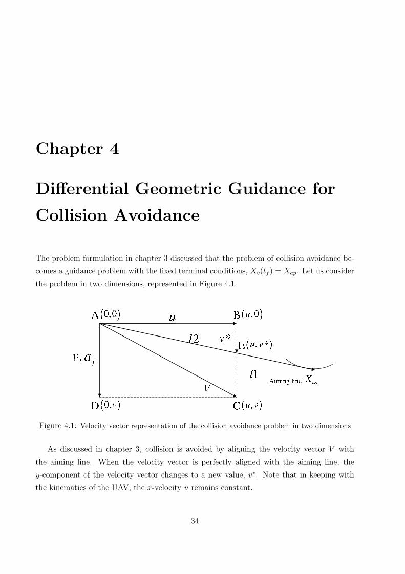
The problem formulation in chapter 3 discussed that the problem of collision avoidance be-

comes a guidance problem with the fixed terminal conditions, Xv(tf ) = Xap. Let us consider

the problem in two dimensions, represented in Figure 4.1.

Figure 4.1: Velocity vector representation of the collision avoidance problem in two dimensions

As discussed in chapter 3, collision is avoided by aligning the velocity vector V with

the aiming line. When the velocity vector is perfectly aligned with the aiming line, the

y-component of the velocity vector changes to a new value, v∗. Note that in keeping with

the kinematics of the UAV, the x-velocity u remains constant.

34

v∗ is found as follows: The points B (u, 0), E (u, v∗) and C (u, v) lie on the line

l1 : x = u (4.1)

The points A (0, 0), E (u, v∗) and Xap (xap, yap) lie on the line l2. The equation of l2 using

the two-point form of equation of the line is:

l2 :y

yap

=x

xap

(4.2)

The point E is the intersection of the lines l1 and l2. Substituting (4.1) into (4.2):

v∗ =

(yap

xap

)u (4.3)

The point Xap is found from the collision cone described in chapter 3, and u is a constant

velocity. Hence v∗ is easily found, and is a constant.

The objective is, therefore, to find a guidance law that will take the y-velocity v to the

desired value v∗ in the time tgo = (tf − t) . Keeping this in mind we design a guidance law

based on Dynamic Inversion (DI), a control strategy used for output tracking of nonlinear

systems. The principle of dynamic inversion is to drive a stabilizing error dynamics (chosen

by the designer) to zero. The main advantage of DI is that it essentially guarantees global

asymptotic stability w.r.t. the tracking error.

We now describe the DI guidance design. Let the error be

E = v − v∗ (4.4)

Imposing the first order error dynamics

E + KE = 0 (4.5)

i.e.

(v − v∗) + K (v − v∗) = 0 (4.6)

Since v∗ is a constant, and v = ay from the system dynamics, the DI based guidance law

is derived to be:

ay = −kv (v − v∗) (4.7)

35

We call (4.7) the ”Dynamic Inversion Guidance law”, or the ”Differential Geometric

Guidance” (DGG) law, since the law is derived based on the derivative of the error. We

design the constant kv such that the settling time (i.e. the time taken to align the velocity

vector with the aiming line) is inversely proportional to the time-to-go, i.e.

kv =1

τv

(4.8)

Such that settling time

Ts = 4τv (4.9)

Where

Ts = α (tf − t) , 0 < α < 1 (4.10)

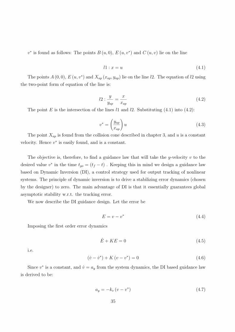
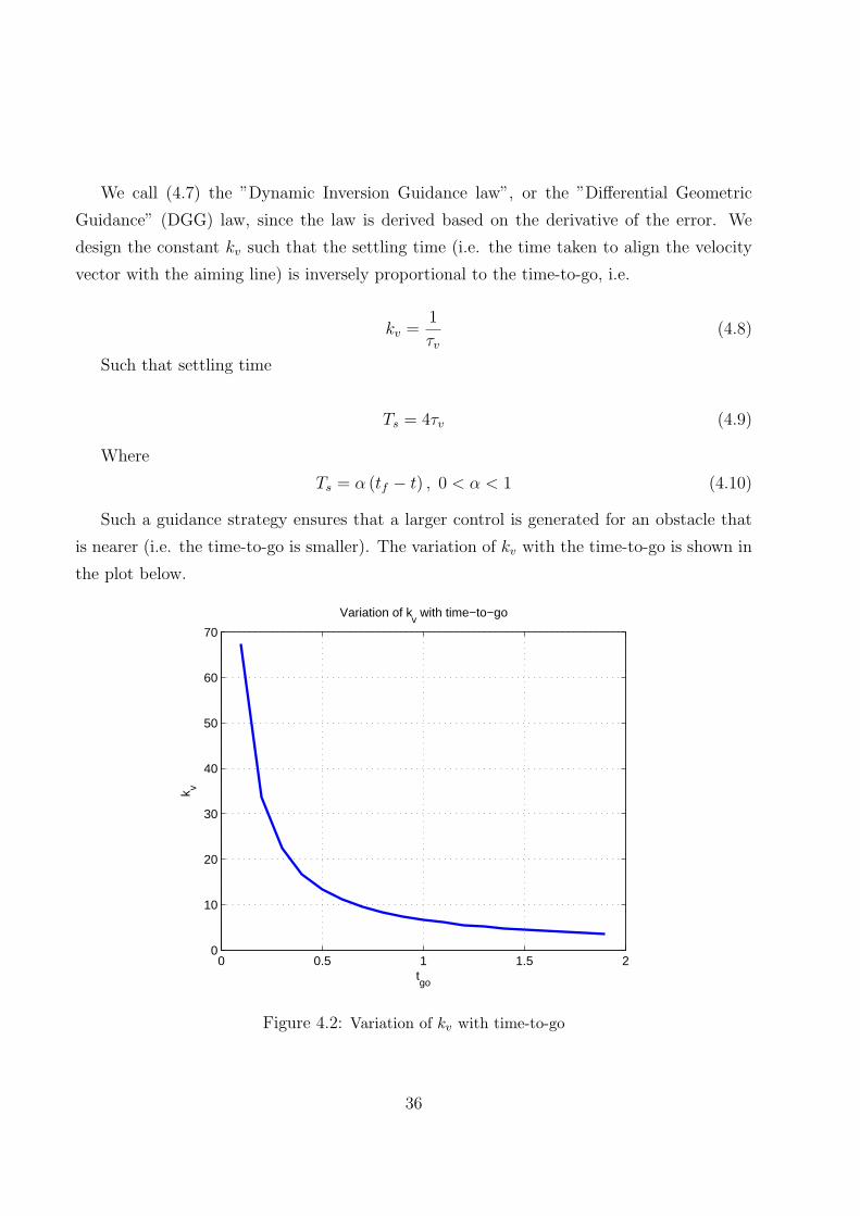
Such a guidance strategy ensures that a larger control is generated for an obstacle that

is nearer (i.e. the time-to-go is smaller). The variation of kv with the time-to-go is shown in

the plot below.

0 0.5 1 1.5 20

10

20

30

40

50

60

70

tgo

k v

Variation of kv with time−to−go

Figure 4.2: Variation of kv with time-to-go

36

The guidance strategy (4.7) is proportional to the error in the y-velocity, and thus pro-

duces a large control input at the beginning which effects quick settlement along the aiming

line. Since the control ay is a function of both the time-to-go and the error in velocity, if the

x-coordinates of the aiming point are very close (i.e. the time-to-go is small), the peak in

the control required to effect the alignment is higher. Another factor influencing the control

is the choice of α, which determines how fast the trajectory aligns along the aiming line. If

the value of α is close to 1, the settling is slow and the peak in control is low. However if

fast settling is desired, a high value of α will effect this but with a higher peak in control.

If the time-to-go is small, as well as the value of α is low, the peak in control may become

quite large. Therefore, the value of α must be chosen judiciously based on the requirement

of speed of alignment.

37

Chapter 5

Geometric Guidance for Collision

Avoidance

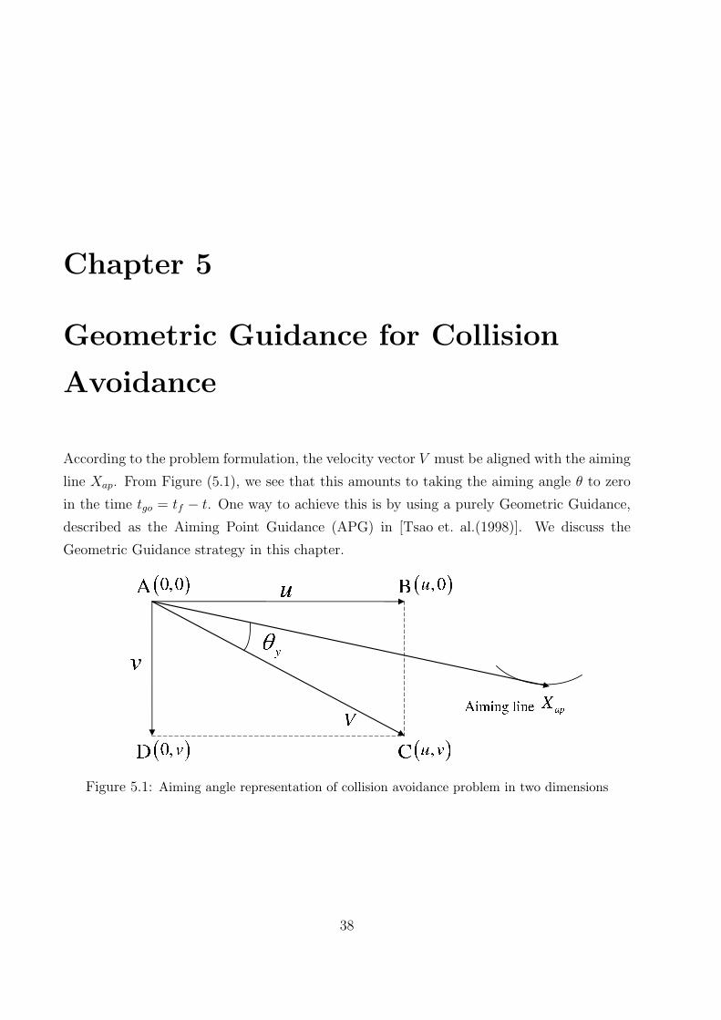
According to the problem formulation, the velocity vector V must be aligned with the aiming

line Xap. From Figure (5.1), we see that this amounts to taking the aiming angle θ to zero

in the time tgo = tf − t. One way to achieve this is by using a purely Geometric Guidance,

described as the Aiming Point Guidance (APG) in [Tsao et. al.(1998)]. We discuss the

Geometric Guidance strategy in this chapter.

Figure 5.1: Aiming angle representation of collision avoidance problem in two dimensions

38

5.1 Linear Geometric Guidance

The Aiming Point Guidance (APG) Law in [Tsao et. al.(1998)] aims to achieve a zero aiming

angle by explicitly designing the turning rate to be linearly dependent upon it. We accord-

ingly design the guidance law such that the acceleration is linearly proportional to the angle

θ, with proper dimensions for kv.

ay = kvθ (5.1)

(5.1) is called the Linear Aiming Point (LAP) Guidance, or Linear Geometric Guidance

(LGG) law, since the control is linearly dependent on the aiming angle θ. Such a guidance

law results in a high turning rate at the beginning (when the target is first encountered)

and quickly settles along the aiming line, instead of maneuvering all the way to impact.

Such a maneuver is an advantage when compared to a conventional Proportional Navigation

Guidance (PNG) law. The PNG law aims to minimize the line-of-sight rate, and aligns itself

to the aiming line at the very last time instant. Thus, any perturbation or target maneuver

could result in a large miss distance or control saturation near the final time.

As discussed in [Tsao et. al.(1998)], the APG law works very well when accurate predic-

tions of the final time Xf and aiming point Xap are possible. Since in our system the velocity

along the x-direction is assumed to be a constant, Xap and tf are found accurately using the

Collision Cone approach (section 3.2). Additionally, since the target is assumed to be station-

ary, the time-to-go prediction is accurate. It is possible to extend these to moving obstacles

via simple prediction algorithms. Only in the case of a highly maneuverable target a high

precision prediction algorithm is needed to find the terminal conditions. However since UAV

flight occurs in urban terrain, the targets (obstacles) are in general not highly maneuverable.

5.2 Nonlinear Geometric Guidance

We propose a new Nonlinear Geometric Guidance (NGG) law as follows:

ay = kv sin θ (5.2)

39

The control is thus a nonlinear function of the aiming angle θ. An advantage that im-

mediately presents itself is that the range of the sine function is [−1, 1] whereas the range of

θ is [−∞,∞]. This means that the acceleration in NGG is always bounded, provided kv is

bounded. Even if we bound θ to a realistic range of [−π, π], the NGG control will be only

one third as high as the LGG control for the same value of kv. We also expect the NGG

law to give a better performance in the presence of autopilot delays. The NGG may also be

called as the Nonlinear Aiming Point (NAP) guidance.

These advantages are due to the nonlinear dependence of control on θ. We will prove in

Chapter 6 that the LGG is in fact an approximation of the NGG.

40

Chapter 6

Correlation between Differential

Geometric Guidance and Geometric

Guidance

After independently discussing the differential geometric guidance, linear geometric guidance

and nonlinear geometric guidance, we attempt to find a correlation between these three

guidance laws. This is valid because the objective in all the three cases is the same, i.e. to

kill the aiming angle θ and align quickly along the aiming line. Let us once again consider

the figure representing the collision avoidance problem.

Figure 6.1: The collision avoidance problem in two dimensions

Let us first consider the DGG and LGG laws. The DGG law is

41

ay = −kv (v − v∗) (6.1)

The LGG guidance law is

ay = −kvθ (6.2)

In order to make the correlation, we assume that the value of control is the same in both

the cases. We then wish to find out a relationship between kv and kv.

Dividing (6.1) by (6.2) we get:

kv

kv

=v − v∗

θ(6.3)

We know that the angle φ between two lines ~a and ~b in two dimensions is given by:

φ = cos−1

~a ·~b‖~a‖

∥∥∥~b∥∥∥

(6.4)

Therefore, referring to Figure (6.1), θ can be found as follows:

θ = cos−1

(AC · AE

‖AC‖ ‖AE‖

)(6.5)

i.e.,

cos θ =

⟨ u

v

·

u

v∗

⟩

∥∥∥∥∥∥

u

v

∥∥∥∥∥∥

∥∥∥∥∥∥

u

v∗

∥∥∥∥∥∥

(6.6)

This gives us

cos θ =u2 + vv∗√

u2 + v2√

u2 + v∗2(6.7)

6.1 Case I

The Taylor series approximation for cosθ is cos θ = 1− θ2

2!+ θ4

4!− . . .

Neglecting powers of θ greater than and equal to 4 we have:

42

cos θ = 1− θ2

2=

u2 + vv∗√u2 + v2

√u2 + v∗2

(6.8)

Therefore,

θ =√

2

(1− u2 + vv∗√

u2 + v2√

u2 + v∗2

) 12

(6.9)

i.e.

θ =√

2

u2

√1 + v2

u2

√1 + v∗2

u2 − (u2 + vv∗)√u2 + v2

√u2 + v∗2

12

(6.10)

Using the binomial approximation√

1 + x = 1 + x2,

θ =√

2

u2

(1 + v2

2u2

) (1 + v∗2

2u2

)− (u2 + vv∗)√

u2 + v2√

u2 + v∗2

12

(6.11)

Neglecting the term v2v∗24u4 , we get:

θ =√

2

u2

(1 + v2

2u2 + v∗22u2

)− (u2 + vv∗)√

u2 + v2√

u2 + v∗2

12

(6.12)

i.e.

θ =1√2

(v2 + v∗2 − 2vv∗√u2 + v2

√u2 + v∗2

) 12

(6.13)

Therefore

θ =1√2

(v − v∗)

4

√(u2 + v2) (u2 + v∗2)

(6.14)

Substituting this in the LGG guidance law (6.2):

ay = −kvθ =−kv√

2

(v − v∗)

4

√(u2 + v2) (u2 + v∗2)

(6.15)

Equating (6.15) with (6.1):

−kv (v − v∗) =−kv√

2

(v − v∗)

4

√(u2 + v2) (u2 + v∗2)

(6.16)

We arrive at the following relationship between kv and kv:

43

kv =√

2kv

(4

√(u2 + v2) (u2 + v∗2)

)(6.17)

6.2 Case II

We have the relation sin θ =√

1− cos2 θ. From (6.7) we have:

sin θ =

√√√√1−(

u2 + vv∗√u2 + v2

√u2 + v∗2

)2

(6.18)

i.e.,

sin θ =

(u√

u2 + v2√

u2 + v∗2

)(v − v∗) (6.19)

If sin θ ≈ θ we get

θ =

(u√

u2 + v2√

u2 + v∗2

)(v − v∗) (6.20)

Substituting this in the LGG law (6.2) we get

ay = −kv

(u√

u2 + v2√

u2 + v∗2

)(v − v∗) (6.21)

Equating (6.21) with the DGG law (6.1) we get the following correlation between kv and

hatkv:

kv = kv

(√u2 + v2

√u2 + v∗2

u

)(6.22)

This gives us a relationship between the LGG and the DGG laws. Note that in case I of

the LGG there are two extra approximations i.e., the binomial approximation in (6.11) and

neglecting fourth powers of u in (6.12). Therefore case II is a closer approximation to the

DGG law. However, instead of approximating the sine of the angle, the guidance law can be

directly formulated as

ay = kv sin θ (6.23)

This is the Nonlinear Geometric Guidance law discussed in chapter 5. Thus the NGG

is directly correlated to the DGG and the LGG is an approximation of the DGG, when the

44

gains are selected appropriately. The NGG will therefore possess the advantages of DGG as

discussed in chapter 4. Additionally, the LGG approximations in both Case I and Case II

hold true only while |θ| << 1. If |θ| exceeds 1, the approximation no longer holds true and

the NGG gives precise values, while the control in LGG will be higher.

Figures 6.2 and 6.3 below show the variation of kv with time-to-go, and kv with time-to-

go.

0 0.5 1 1.5 20

10

20

30

40

50

60

70

tgo

k v

Variation of kv with time−to−go

Figure 6.2: Variation of kv with the time-to-go

0 0.5 1 1.5 20

100

200

300

400

500

600

700

tgo

k vhat

Plot of kv vs. time−to−go for LAP

Figure 6.3: Variation of kv with the time-to-go

45

Chapter 7

Extension of Differential Geometric

and Geometric guidance to 3D

Scenario

With the 2D collision avoidance problem satisfactorily solved, we look for a solution to the

more realistic 3D collision avoidance problem. The aiming point Xap and the time-to-go tgo

are found from the collision cone as discussed in Chapter 3. The velocity vector must be

aligned with the aiming line in the time tgo. This problem is represented in 3D in Figure 7.1.

Figure 7.1: Representation of the collision avoidance problem in three dimensions

46

The angle θ now needs to be killed in three dimensions. The solution is based on the

principle that if we kill the projections of the angles in two perpendicular planes XY and

XZ, the alignment occurs in three dimensions. This is valid because the x-velocity is a

constant. Therefore the controls ay in the XY plane and az in the XZ plane are found in

the same way as in the 2D case i.e.

ay = −kv (v − v∗) (7.1)

and

az = −kw (w − w∗) (7.2)

The factors kv and kv are designed in the same way as described in Chapter 4, i.e.,

kv =1

τv

(7.3)

Such that settling time,

Ts1 = 4τv (7.4)

Where

Ts1 = α (tf − t) , 0 < α < 1 (7.5)

Similarly,

kw =1

τw

And

Ts2 = 4τw (7.6)

Where

Ts2 = β (tf − t) , 0 < β < 1 (7.7)

The equations (7.1) and (7.2) are the DGG laws in 3D. Similar to the 2D case, the LGG

and NGG laws are formulated as follows:

LGG Laws:

47

ay = −kvθy (7.8)

And

az = −kwθz (7.9)

Where

kv = kv

(√u2 + v2

√u2 + v∗2

u

)(7.10)

and

kw = kw

(√u2 + w2

√u2 + w∗2

u

)(7.11)

With the same expressions for the gains kv and kv the NGG guidance laws in 3D are:

ay = −kv sin θy (7.12)

The validity of this extension to 3D has been tested successfully via numerical experi-

ments, the results of which are presented in Chapter (8).

48

Chapter 8

Numerical Experiments

The DGG, NGG and LGG algorithms that were developed in the previous chapters have

been tested via numerical experiments carried out in MATLAB. The experiments involved

a finite space with two obstacles in various positions, and each of the algorithms were used

to find the path. The experiments were first carried out for the two dimensional case, and

then extended to three dimensions using the methodology described in chapter (7). In both

these cases, the performance of the algorithm was tested in the presence of an autopilot lag.

We present the results of the experiments in this chapter.

8.1 DGG, LGG and NGG in two dimensions

In this section we present the simulation results for the algorithms developed in chapters 4

and 5. As elaborated in chapter 6, the gains have been chosen such that the results of the

DGG, LGG and NGG guidance algorithms give the same results.

8.1.1 Case I: No obstacles critical

The plots in Figure (8.1) and (8.2) show the path found and the control effort when neither

of the two obstacles is found to be critical, and the UAV may go directly to the destination.

The dashed lines indicate the safety boundary of the obstacles. The algorithm finds that

the obstacles are not critical and hence the UAV is guided to the destination, such that the

control effort is high in the beginning. The path thus quickly settles along the aiming line.

The control plot indicates a higher turning at the start and settles to zero quickly. The value

49

−20 −10 0 10 20 30 40 50 60−60

−50

−40

−30

−20

−10

0

10

20

30

displacement along X

disp

lace

men

t alo

ng Y

Path found by DI, LAP and NAP guidance when no obstacle is critical

Linear APGDI GuidanceNonlinear APG

Initial point: (−20,0)Obstacle1:(0,20)Obstacle2:(10,−30)Destination:(60,−50)

Figure 8.1: Path found by DGG, LGG and NGGwhen no obstacle is critical

0 1 2 3 4 5 6 7 8−6

−5

−4

−3

−2

−1

0

1

time

Con

trol

: acc

eler

atio

n al

ong

Y

Control plots for DI, LAP and NAP guidance when no obstacle is critical


Figure 8.2: Control plots for DGG, LGG andNGG when no obstacle is critical

of the factor α that decides the rate of settling is fixed at 0.6. It is clear that the correlation

established in chapter 6 is valid, since the plots in all three cases show the same results.

8.1.2 Case II: One obstacle critical

Next, we look at the case when only one of the two obstacles is found to be critical. The

plots (8.5) and (8.6) show the path and control plots in such a condition.

80 100 120 140 160 180 200−10

−5

0

5

10

15

20

25

30

35

40


disp

lace

men

t alo

ng Y

Path found by DI, LAP and NAP guidance when 1 obstacle is critical


Initial point: (80,40)Obstacle1:(100,20)Obstacle2:(160,0)Destination: (200,−10)

Figure 8.3: Path found by DGG, LGG and NGGwhen one obstacle is critical

0 2 4 6 8 10 12−2.5

−2

−1.5

−1

−0.5

0

0.5

time

Con

trol

: acc

eler

atio

n al

ong

Y

Control plots for DI, LAP and NAP guidance when 1 obstacle is critical


Figure 8.4: Control plots for DGG, LGG andNGG when one obstacle is critical

50

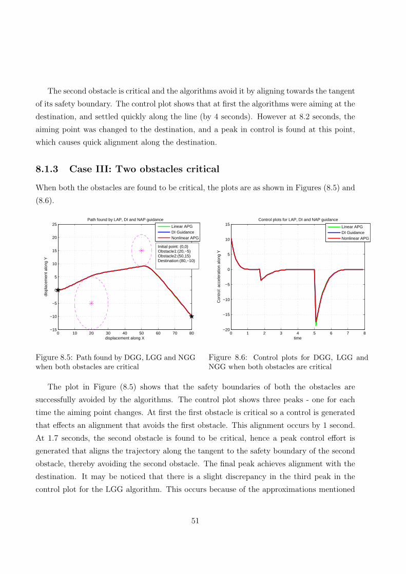
The second obstacle is critical and the algorithms avoid it by aligning towards the tangent

of its safety boundary. The control plot shows that at first the algorithms were aiming at the

destination, and settled quickly along the line (by 4 seconds). However at 8.2 seconds, the

aiming point was changed to the destination, and a peak in control is found at this point,

which causes quick alignment along the destination.

8.1.3 Case III: Two obstacles critical

When both the obstacles are found to be critical, the plots are as shown in Figures (8.5) and

(8.6).

0 10 20 30 40 50 60 70 80−15

−10

−5

0

5

10

15

20

25


disp

lace

men

t alo

ng Y

Path found by LAP, DI and NAP guidance


Initial point: (0,0)Obstacle1:(20,−5)Obstacle2:(50,15)Destination:(80,−10)

Figure 8.5: Path found by DGG, LGG and NGGwhen both obstacles are critical

0 1 2 3 4 5 6 7 8−20

−15

−10

−5

0

5

10

15

time

Con

trol

: acc

eler

atio

n al

ong

YControl plots for LAP, DI and NAP guidance


Figure 8.6: Control plots for DGG, LGG andNGG when both obstacles are critical

The plot in Figure (8.5) shows that the safety boundaries of both the obstacles are

successfully avoided by the algorithms. The control plot shows three peaks - one for each

time the aiming point changes. At first the first obstacle is critical so a control is generated

that effects an alignment that avoids the first obstacle. This alignment occurs by 1 second.

At 1.7 seconds, the second obstacle is found to be critical, hence a peak control effort is

generated that aligns the trajectory along the tangent to the safety boundary of the second

obstacle, thereby avoiding the second obstacle. The final peak achieves alignment with the

destination. It may be noticed that there is a slight discrepancy in the third peak in the

control plot for the LGG algorithm. This occurs because of the approximations mentioned

51

in chapter 6. The NGG is thus exactly analogous to the DGG guidance algorithm, whereas

the LGG guidance law is an approximation of the DGG algorithm.

8.2 Testing the DGG, LGG and NGG algorithms in

2D for performance in the presence of autopilot

lags

Every UAV has an autopilot lag which includes the lag in several components of the UAV.

In order to test the performance of the DGG, LGG and NGG algorithms in the presence of

autopilot lags, we modeled the autopilot lag as a first order response system as follows:

ay =ay − a∗y

τ(8.1)

Where a∗y represents the commanded value of control, i.e. the control calculated by the

DGG, LGG and NGG algorithms. ay represents the output of the autopilot lag system, and

τ is the autopilot lag. In order to incorporate the lag into the system, we augmented the

autopilot output ay into the state equations (3.1).

8.2.1 Case I: Autopilot lag: 0.1 seconds

We tested the DGG guidance algorithm in presence of an autopilot lag of 0.1 second. The

resulting path and control plots are shown in Figures (8.7) and (8.8).

The plot in Figure (8.7) indicates that for an autopilot lag of 0.1 second, the path found is

not very different from a path found without any autopilot delay. The control plot indicates

that an autopilot lag changes the control plot significantly. This is because the autopilot has

been incorporated into a closed loop system, and the DGG algorithm attempts to achieve

an alignment before the settling time. This leads to oscillations in the control.

8.2.2 Case II: Autopilot lag: 0.2 seconds

The autopilot lag is now increased to 0.2 seconds. The resulting plots are shown in Figures

8.9 and 8.10.

52

0 10 20 30 40 50 60 70 80−10

−5

0

5

10

15

20

25

30


disp

lace

men

t alo

ng Y

Path found by DI guidance with and without autopilot

DI GuidanceDI Guidance with autopilot

Autopilot lag: 0.1 second

max deviation= 1.0704 m

Figure 8.7: Path found by DGG with and with-out autopilot lag; lag=0.1 seconds

0 1 2 3 4 5 6 7 8−20

−15

−10

−5

0

5

10

15

20

25

time

Con

trol

: acc

eler

atio

n al

ong

Y

Control plot for DI with and without autopilot


Autopilot lag: 0.1 second

Figure 8.8: Control plot for DGG with and with-out autopilot lag; lag=0.1 seconds

The deviation from the original path is thus not significant, although the control plot

shows oscillations, which are discussed in Case I above.

8.2.3 Higher autopilot lags

When autopilot lags greater than 0.2 seconds are incorporated, there occur significant devi-

ations from the original path. With the same obstacle positions as in Case II, if an autopilot

lag of 0.3 seconds is incorporated, the control plot is as shown in Figure 8.12. This plot

shows the performance of the DGG and LGG guidance laws.

Figure 8.12 shows that both the DGG and the LGG guidance laws show significant

deviations from the original control effort. However the deviation is extremely high in the

case of LGG, with the result that the control demanded by the LGG algorithm reaches

unrealistic values. Thus it is clear that the DGG guidance law is preferable in the presence

of autopilot lags. Figure shows the path found by LGG and the DGG guidance in presence

of the autopilot lag of 0.3 seconds.

The Figures 8.13 and 8.14 show the path found and the control plots for the DGG and

LGG guidance in the presence of an autopilot lag of 0.4 seconds.

The control plots 8.14 show that both the DGG and the LGG guidance laws lead to

oscillations in the control. However the highest control demand in DGG guidance is only

38 m/s2, whereas the highest control demand in the LGG guidance is an infeasible value of

53

0 10 20 30 40 50 60 70 80−15

−10

−5

0

5

10

15

20

25


disp

lace

men

t alo

ng Y

Path found by DI with and without autopilot


autopilot lag: 0.2 sec

max deviation: 0.537 m


0 1 2 3 4 5 6 7 8−15

−10

−5

0

5

10

15

time

Con

trol

: acc

eler

atio

n al

ong

Y

Control plot for DI guidance with and without autopilot


Figure 8.10: Control plot for DGG with andwithout autopilot lag; lag=0.2 seconds

-151.3 m/s2. Additionally the paths shown in Figure 8.13 shows that the path found by the

LGG guidance law violates the safety boundary of the second obstacle. This is a significant

disadvantage.

0 10 20 30 40 50 60 70 80−15

−10

−5

0

5

10

15

20

25

30

35


disp

lace

men

t alo

ng Y

Path found by DI and LAP guidance with autopilot

LAP Guidance with autopilotDI Guidance with autopilot

autopilot lag: 0.3 seconds


0 1 2 3 4 5 6 7 8−150

−100

−50

0

50

100

150

200

time

Con

trol

: acc

eler

atio

n al

ong

Y

Control for DI and LAP guidance with autopilot lag




54

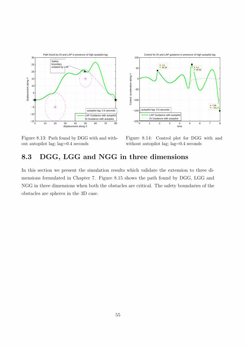
0 10 20 30 40 50 60 70 80−15

−10

−5

0

5

10

15

20

25

30


disp

lace

men

t alo

ng Y

Path found by DI and LAP in presence of high autopilot lag


Safetyboundaryviolated by LAP



0 1 2 3 4 5 6 7 8−200

−150

−100

−50

0

50

100

X: 1.8Y: 38.38

time

Con

trol

: acc

eler

atio

n al

ong

Y

Control for DI and LAP guidance in presence of high autopilot lag

X: 5.2Y: 66.86

X: 7.98Y: −151.3




8.3 DGG, LGG and NGG in three dimensions

In this section we present the simulation results which validate the extension to three di-

mensions formulated in Chapter 7. Figure 8.15 shows the path found by DGG, LGG and

NGG in three dimensions when both the obstacles are critical. The safety boundaries of the

obstacles are spheres in the 3D case.

55

0

10

20

30

40

50

60

−100

1020

−15

−10

−5

0

5

10

displacement along Y

Path found by LAP, DI and NAP


disp

lace

men

t alo

ng Z


Initial point:(2,3,0)Obstacle1:(20,5,−5)Obstacle2:(46,10,5)Destination: (60,10,2)

Figure 8.15: Path found by DGG, LGG and NGG in three dimensions

56

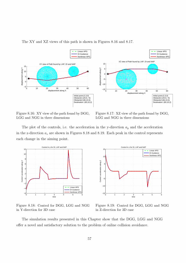
The XY and XZ views of this path is shown in Figures 8.16 and 8.17.

0 10 20 30 40 50 60−5

0

5

10

15 XY view of Path found by LAP, DI and NAP


disp

lace

men

t alo

ng Y



Figure 8.16: XY view of the path found by DGG,LGG and NGG in three dimensions

0 10 20 30 40 50 60−15

−10

−5

0

5

10 XZ view of Path found by LAP, DI and NAP


disp

lace

men

t alo

ng Z



Figure 8.17: XZ view of the path found by DGG,LGG and NGG in three dimensions

The plot of the controls, i.e. the acceleration in the y-direction ay and the acceleration

in the z-direction az are shown in Figures 8.18 and 8.19. Each peak in the control represents

each change in the aiming point.

0 1 2 3 4 5 6−6

−4

−2

0

2

4

6

8

10

12

time

Con

trol

: acc

eler

atio

n al

ong

Y

Control in y for DI, LAP and NAP


Figure 8.18: Control for DGG, LGG and NGGin Y-direction for 3D case

0 1 2 3 4 5 6−15

−10

−5

0

5

10

15

time

Con

trol

: acc

eler

atio

n al

ong

Z

Control in z for DI, LAP and NAP


Figure 8.19: Control for DGG, LGG and NGGin Z-direction for 3D case

The simulation results presented in this Chapter show that the DGG, LGG and NGG

offer a novel and satisfactory solution to the problem of online collision avoidance.

57

Chapter 9

Conclusions and Future Work

In this study, a new Dynamic Inversion based Differential Geometric Guidance law and

consequently the Linear Geometric Guidance and Nonlinear Geometric Guidance laws are

proposed, and a correlation formulated between them. These guidance laws have been used

to solve the online collision avoidance problem in a unique way. The path found by these

laws settle along the desired line quickly, instead of maneuvering until the final time. These

algorithms are developed in two dimensions, and extended successfully to three dimensions.

Current work includes:

1. developing an algorithm for avoiding collision with moving obstacles (both benign and

maneuvering

2. exploring the use of these guidance laws in avoiding collision between UAVs within a

team

3. incorporating a more realistic point-mass model of the UAV

The scope of the three guidance laws DGG, LGG and NGG developed in this study are

however not limited to collision avoidance. Since alignment occurs quickly, the guidance laws

hold promise for target interception problems as well (such as ballistic missiles).

This study has thus been successful in developing algorithms that are successful in solving

the online obstacle avoidance problem satisfactorily.

58

Bibliography

[Amin et al.(2006)] Amin J. N. , Boskovic J.D. & Mehra R.K. (2006). A Fast and Efficient

Approach to Path Planning for Unmanned Vehicles. AIAA Guidance, Navigation, and

Control Conference and Exhibit, Aug 2006.

[Ben-Asher(1993)] Ben-Asher J.Z. (1993). Minimum-Effort Interception of Multiple Targets.

Journal of Guidance, 16 (3), 600-602.

[Bortoff(2000)] Bortoff, S.A.(2000). Path planning for UAVs. Proceedings of the American

Control Conference, 1 (6), 364-368.

[Camacho & Bordons(1999)] Camacho E.F. & Bordons C. (1999). Model Predictive Control.

New York: Springer.

[Bryson & Ho(1975)] Bryson A. E. & Ho Y.C. (1975). Applied Optimal Control: Optimiza-

tion, Estimation, and Control. New York: Taylor & Francis

[Carpenter & Grossberg(1991)] Carpenter G.A. & Grossberg S. (1991) Pattern Recognition

By Self-Organizing Neural Networks. The MIT Press.

[Chakravarthy & Ghose(1998)] Chakravarthy A. & Ghose D. (1998). Obstacle Avoidance in

a Dynamic Environment: A Collision Cone Approach. IEEE Transactions on Systems,

Man and Cybernetics-Part A: Systems and Humans, 28 (5), 562-574.

[Crassidis & Junkins(2004)] Crassidis J. L. & Junkins J. L. (2004). Optimal Estimation of

Dynamic Systems. CRC Press.

[DeGarmo & Nelson(2004)] DeGarmo M. & Nelson G. M. (2004). Prospective Unmanned

Aerial Vehicle Operations in the Future National Airspace System. AIAA 4th Aviation

59

Technology, Integration and Operations (ATIO) Forum, Chicago, Illinois, Sep. 20-22,

2004.

[Dubins(1957)] Dubins L. E. (1957). On curves of minimal length with a constraint on aver-

age curvature, and with prescribed initial and terminal positions and tangents. American

Journal of Mathematics, 79 (3), 497-516.

[Ferbach(1998)] Ferbach P. (1998). A Method of Progressive Constraints for Nonholonomic

Motion Planning. IEEE Transactions on Robotics and Automation, 14 (1), 172-179.

[Frisken & Perry(2003)] Frisken S. & Perry R. (2003). Simple and Efficient Traversal Meth-

ods for Quadtrees and Octrees. Journal of Graphics Tools, 7 (3), 1-11.

[Griffiths et al.(2006)] Griffiths S., Saunders J., Curtis A., Barber B., Mclain T. & Beard R.

(2006). Maximizing Miniature Aerial Vehicles. IEEE Robotics & Automation Magazine,

13 (3), 34-43.

[Grossberg(1988)] Grossberg S. (1988). Nonlinear neural networks: Principles, mechanisms,

architecture. Neural Networks, 1, 17-61.

[Hamner et al.(2006)] Hamner B., Singh, S. & Scherer, S. (2006). Learning obstacle avoid-

ance parameters from operator behavior. Journal of Field Robotics, 23 (11), 1037 - 1058.

[Han & Bang(2004)] Han S.C. & Bang H. (2004). Proportional Navigation-Based Optimal

Collision Avoidance for UAVs. Proceedings of 2nd International Conference on Au-

tonomous Robots and Agents, December 13-15, 2004, Palmerston North, New Zealand.

[Hwangbo et al.(2007)] Hwangbo M, Kuffner J & Kanade T (2007). Efficient Two-phase

3D Motion Planning for Small Fixed-wing UAVs. IEEE International Conference on

Robotics and Automation, Roma, Italy, 10-14 April 2007.

[Khatib(1985)] Khatib O. (1985). Real Time Obstacle Avoidance for Manipulators and Mo-

bile Robots. Proceedings IEEE International Conference on Robotics and Automation,

2, 500-505.

[Koren & Borenstein(1991)] Koren Y. & Borenstein J. (1991). Potential Field Methods and

Their Inherent Limitations for Mobile Robot Navigation. Proceedings of the IEEE Con-

ference on Robotics and Automation, 2, 1398-1404.

60

[Krozel & Peters(1997)] Krozel J. & Peters M. (1997). Strategic Conflict Detection and Res-

olution for Free Flight. Seagull technology, Inc.

[Kuchar & Yang(2000)] Kuchar J. & Yang, L. (2000). Review of Conflict Detection and Res-

olution Modeling Methods. IEEE Transactions on Intelligent Transportation Systems,

1 (4), 179-189.

[Kumar & Korf(1991)] Kumar N. R. V. V. & Korf R. (1991). Depth-first vs. Breadth-first

search. AAAI-91 Proceedings.

[Kuffner & LaValle(2000)] Kuffner J.J. & LaValle S.M. (2000). RRT-Connect An Efficient

Approach to Single-Query Path Planning. Proceedings of IEEE International Conference

on Robotics and Automation, 2, 995-1001.

[Lavalle(2006)] LaValle S.M. (2006). Planning Algorithms. Cambridge University Press.

[LaValle(1998)] LaValle S. M. (1998). Rapidly-exploring random trees: A new tool for path

planning. TR 98-11, Computer Science Dept., Iowa State University

[LaValle & Kuffner(2001)] LaValle S. M. & Kuffner J.J. (2001). Rapidly-exploring random

trees: Progress and prospects. Algorithmic and Computational Robotics: New Direc-

tions. A K Peters.

[Leung et al.(2006)] Leung C., Huang S., Kwok N. & Dissanayake G.(2006). Planning un-

der uncertainty using model predictive control for information gathering. Robotics and

Autonomous Systems, 54, 898910.

[Merz(1991)] Merz A.W.(1991). Maximum-Miss Aircraft Collision Avoidance. Dynamics and

Control, 1 (1), 25-34.

[Martin & Moravec(1996)] Martin M. C. & Moravec, H. (1996). Robot evidence grids. Tech-

nical Report CMU-RI-TR-96-06, Robotics Institute. Carnegie Mellon University, Pitts-

burgh.

[Paul et al.(2008)] Paul T., Krogstad T.R. & Gravdahl J.T. (2008). Modeling of UAV for-

mation flight using 3D potential field. Simulation Modeling Practice and Theory, 16 (9),

1453-1462

61

[Park et al.(2008)] Park J.W.,Oh H.D. & Tahk M.J. (2008). UAV Collision Avoidance Based

on Geometric Approach. SICE Annual Conference, 2122-2126.

[Pettersson & Doherty(2006)] Pettersson P.O. & Doherty P.(2006).Probabilistic roadmap

based path planning for an autonomous unmanned helicopter. Journal of Intelligent

and Fuzzy Systems, 17 (4), 395-405.

[Scherer et al.(2008)] Scherer S., Singh S., Chamberlain L. & Elgersma M. (2008). Flying

Fast and Low Among Obstacles: Methodology and Experiments. The International

Journal of Robotics Research, 27 (5), 549574.

[Shim et al.(2006)] Shim D. H., Chung H. & Sastry S. (2006). Autonomous Exploration

in Unknown Urban Environments for Unmanned Aerial Vehicles. IEEE Robotics and

Automation Magazine, 13 (3), 27-33.

[Shim & Sastry(2007)] Shim D.H. & Sastry S. (2007). An Evasive Maneuvering Algorithm

for UAVs in See-and-Avoid Situations. Proceedings of the American Control Conference,

3886-3891.

[Tsao et. al.(1998)] Lu-Ping Tsao, Ching-Lain Chou, Chuen-Ming Chen & Chi-Teh Chen

(1998). Aiming Point Guidance Law for Air-to-Air Missiles. emphInternational Journal

of Systems Science,29 (2), 95-102.

[Wang et al.(2007)] Wang X., Yadav V., & Balakrishnan S.N. (2007). Cooperative UAV

Formation Flying With Obstacle/Collision Avoidance. IEEE Transactions on Control

Systems Technology, 15 (4), 672-679.

[Watanabe et al.(2006)] Watanabe Y., Calise A.J & Johnson E.N. (2006). Minimum Effort

Guidance for Vision-Based Collision Avoidance. AIAA Atmospheric Flight Mechanics

Conference and Exhibit, Keystone, Colorado, 21 - 24 August 2006.

[Zarchan(1994)] Zarchan P. (1994). Tactical and Strategic Missile Guidance. AIAA.

62

Nonlinear Geometric and Differential Geometric Guidance of UAVs for Reactive Collision Avoidance

Documents

Transcript of Nonlinear Geometric and Differential Geometric Guidance of UAVs for Reactive Collision Avoidance