Nuclear magnetic resonance spectroscopy interpretation for ...

Master ThesisComputer Science

Nuclear magnetic resonancespectroscopy interpretation for

protein modeling using computervision and probabilistic graphical

models

Piotr Jakub Klukowski

School of Computing

Blekinge Institute of Technology

SE-371 79 Karlskrona

Sweden

This thesis is submitted to the School of Computing at Blekinge Institute of Technology

in partial fulfillment of the requirements for the degree of Master of Science in Computer

Science. The thesis is equivalent to XX weeks of full time studies.

Contact Information:Author: Piotr Klukowski 890804-P117E-mail: [email protected]

University advisor(s):Dr Marie PerssonSchool of Computing

School of ComputingBlekinge Institute of Technology Internet : www.bth.se/comSE-371 79 Karlskrona Phone : +46 455 38 50 00Sweden Fax : +46 455 38 50 57

Abstract

Context. Dynamic development of Nuclear Magnetic Res-onance spectroscopy (NMR) allowed fast acquisition of ex-perimental data which determine structure and dynamics ofmacromolecules. Nevertheless, speed of experimental datacollection exceeds human ability of their interpretation. Nowa-days, NMR spectra are analyzed manually what takes weeksor years depending on protein complexity. Potential solutionof this problem will allow to calculate a structure of proteinfrom NMR spectrum automatically what significantly reducestime of structure solving. Therefore it can open new avenuesin drug discovery, structural genomics, and increase our abil-ities of analyzing organization of living organisms.Objectives. In presented work, a new approach to protein3D NMR spectra analysis is presented. It is based on com-puter vision which has not been ever applied in that contextin 20 years history of research in the area.Methods. Accuracy of proposed method was evaluated inempirical studies. At first 365.000-elements benchmark datasetwas established and used to calculate standard classificationmetrics (Precision, Recall, F-measure). Secondly, proposedmethod was used to solve the structure of the “Upstream of N-ras” protein. Resulting structure was compared with the one,which was calculated using traditional (manual) approach.Results. Quality of proposed approach is up to 0.9583 F-measure on benchmark dataset, depending on protein com-plexity. Comparison of automatically calculated model withreference structure from protein databank (1WFQ) reveals nosignificant differences, what has proven that proposed methodcan be used in practice in NMR laboratories.Conclusions. Proposed solution constitute the first exampleof application computer vision in automated protein NMRanalysis. Empirical studies have proven that algorithm canbe successfully applied to protein structure prediction.

Keywords: NMR spectroscopy, peak picking problem, com-puter vision, protein structure prediction

i

List of Figures

1.1 Spectral image recorded using NMR spectroscopy . . . . . . . . . 21.2 Differences between current and desired situations in NMR spectra

processing . . . . . . . . . . . . . . . . . . . . . . . . . . . . . . . 2

2.1 Architecture and organization of NMR spectrometer . . . . . . . . 92.2 Atoms interactions detectable in NOESY experiment . . . . . . . 102.3 Manifestation of Nuclear Overhauser Effect in NOESY spectrum . 112.4 Scalar magnetization transfer in HNCACB spectrum . . . . . . . 122.5 Manifestation of scalar magnetization transfer in HNCACB spectrum 122.6 The rule of four peaks in line . . . . . . . . . . . . . . . . . . . . 132.7 Connectivity rule - illustration I . . . . . . . . . . . . . . . . . . . 142.8 Connectivity rule - illustration II . . . . . . . . . . . . . . . . . . 152.9 Connectivity rule - illustration III . . . . . . . . . . . . . . . . . . 162.10 Distribution of peak carbon coordinates in NMR spectrum . . . . 172.11 Columns and diagonal in NOESY spectrum . . . . . . . . . . . . 182.12 Columns in HNCA spectrum . . . . . . . . . . . . . . . . . . . . . 18

3.1 Coordinate systems in HNCACB, HNCA and NOESY experiments 20

4.1 Organization of proposed peak picking method . . . . . . . . . . . 224.2 Distribution of peak intensities in not normalized NMR spectrum

layer . . . . . . . . . . . . . . . . . . . . . . . . . . . . . . . . . . 254.3 Imperfections of NMR spectrum . . . . . . . . . . . . . . . . . . . 264.4 Estimation of peak volumes in layer of NMR spectrum . . . . . . 304.5 Estimation of peak areas in layer of HNCACB spectrum . . . . . 314.6 Visualization of vertical scanning line used to conduct high-level

inference . . . . . . . . . . . . . . . . . . . . . . . . . . . . . . . . 354.7 Architecture of Bayesian network . . . . . . . . . . . . . . . . . . 36

5.1 Learning curve of HNCACB classifier . . . . . . . . . . . . . . . . 405.2 Learning curve of NOESY classifier . . . . . . . . . . . . . . . . . 415.3 Peak intensity vs maximum deviation from extremum - separation

of the learning set . . . . . . . . . . . . . . . . . . . . . . . . . . . 43

ii

5.4 Normalized peak volume vs normalized peak area - separation ofthe learning set . . . . . . . . . . . . . . . . . . . . . . . . . . . . 43

5.5 Normalized peak width vs normalized peak height - separation ofthe learning set . . . . . . . . . . . . . . . . . . . . . . . . . . . . 44

5.6 Width to height ratio vs minimum deviation from extremum - sep-aration of the learning set . . . . . . . . . . . . . . . . . . . . . . 44

5.7 Impact of the feature groups I, II and III on the classification quality 455.8 Impact of the feature groups II and III on the classification quality 465.9 Impact of the feature groups I and II on the classification quality 465.10 Impact of the feature groups I and III on the classification quality 475.11 Impact of the feature groups I and IV on the classification quality 475.12 Visualization of the learning set in 3D space using PCA - perspec-

tive I . . . . . . . . . . . . . . . . . . . . . . . . . . . . . . . . . . 485.13 Visualization of the learning set in 3D space using PCA - perspec-

tive II . . . . . . . . . . . . . . . . . . . . . . . . . . . . . . . . . 485.14 Exemplary layer form benchmark dataset . . . . . . . . . . . . . . 495.15 Case study of HNCA spectra - illustration I . . . . . . . . . . . . 515.16 Case study of HNCA spectra - illustration II . . . . . . . . . . . . 535.17 Case study of HNCA spectra - illustration III . . . . . . . . . . . 535.18 Case study of TOCSY spectrum . . . . . . . . . . . . . . . . . . . 545.19 Case study of NOESY spectrum . . . . . . . . . . . . . . . . . . . 545.20 Superimposed structures of the upstream of N-Ras . . . . . . . . 56

A.1 F-measure of SVM with Gaussian kernel for different values of σand soft margin . . . . . . . . . . . . . . . . . . . . . . . . . . . . 60

A.2 F-measure of SVM with polynomial kernel function for differentvalues of polynomial order and soft margin . . . . . . . . . . . . . 61

C.1 User interface of developed software . . . . . . . . . . . . . . . . . 65

iii

List of Tables

2.1 Impact of subatomic particles on value of nuclear spin number (I) 82.2 Carbon atoms in HNCACB spectrum . . . . . . . . . . . . . . . . 13

4.1 Features evaluated in the context of peak detection . . . . . . . . 304.2 Variables and their dependencies identified in analysis of the labo-

ratory practice related to the peak picking process of HNCA spectrum 334.3 Variables and their dependencies identified in analysis of the lab-

oratory practice related to the peak picking process of HNCACBspectrum . . . . . . . . . . . . . . . . . . . . . . . . . . . . . . . . 34

4.4 Variables and their dependencies identified in analysis of the lab-oratory practice related to the peak picking process of NOESYspectrum . . . . . . . . . . . . . . . . . . . . . . . . . . . . . . . . 34

5.1 Correlation between feature values and classes . . . . . . . . . . . 425.2 Impact of feature selection on classification quality . . . . . . . . 455.3 Properties of benchmark dataset . . . . . . . . . . . . . . . . . . . 505.4 Properties of benchmark dataset . . . . . . . . . . . . . . . . . . . 505.5 Results of automatic peak picking of benchmark datasets . . . . . 505.6 NMR spectra used to model UNR protein structure . . . . . . . . 555.7 Number of peaks found in automated peak picking of UNR spectra 55

B.1 Average time needed to scan NMR spectrum using proposed ap-proach to the peak picking . . . . . . . . . . . . . . . . . . . . . . 62

iv

Contents

Abstract i

Mathematical notation vi

1 Introduction 1

1.1 A general introduction to the problem and research area . . . . . 1

1.2 Motivation, aim and contribution of the work . . . . . . . . . . . 3

1.3 Related work . . . . . . . . . . . . . . . . . . . . . . . . . . . . . 3

1.4 Organization of the thesis . . . . . . . . . . . . . . . . . . . . . . 6

2 Practical knowledge about peak picking 8

2.1 Introduction to NMR spectroscopy . . . . . . . . . . . . . . . . . 8

2.2 Spectra types . . . . . . . . . . . . . . . . . . . . . . . . . . . . . 10

2.3 Common rules in manual peak picking . . . . . . . . . . . . . . . 12

3 Peak picking problem statement 20

4 Proposed method 22

4.1 A general concept . . . . . . . . . . . . . . . . . . . . . . . . . . . 22

4.2 Peak detection . . . . . . . . . . . . . . . . . . . . . . . . . . . . 244.2.1 Preprocessing method . . . . . . . . . . . . . . . . . . . . 244.2.2 Features . . . . . . . . . . . . . . . . . . . . . . . . . . . . 264.2.3 Classification . . . . . . . . . . . . . . . . . . . . . . . . . 31

4.3 High-level inference . . . . . . . . . . . . . . . . . . . . . . . . . . 324.3.1 Practical knowledge extraction . . . . . . . . . . . . . . . . 324.3.2 Bayesian network structure . . . . . . . . . . . . . . . . . 354.3.3 Inference process . . . . . . . . . . . . . . . . . . . . . . . 384.3.4 Post-processing and final output . . . . . . . . . . . . . . . 39

5 Empirical studies 40

5.1 Model learning and parameters tuning . . . . . . . . . . . . . . . 40

5.2 Peak picking accuracy . . . . . . . . . . . . . . . . . . . . . . . . 49

5.3 Generating 3D protein structure . . . . . . . . . . . . . . . . . . . 55

6 Conclusion and final remarks 57

A Parameter calibration 60

B Performance tests 62

C Description of software interface 64

Bibliography 67

References 68

v

Mathematical notation

NMR spectroscopy

S NMR spectrum

Sn n-th layer of NMR spectrum

Sn,c,h element of NMR spectrum which possesses coordinates (n, c, h)measured in ID units

Sn,c,h element of NMR spectrum which possesses coordinates (n, c, h)measured in ppm units

Cα,n alpha carbon of n-th amino acid in protein

Cβ,n beta carbon of n-th amino acid in protein

FS set of all artifacts in spectrum S

P peak in NMR spectrum

Pn,c,h peak which has extremum in (n, c, h)

WS set of all peaks in spectrum S

ZS set of all true peaks in spectrum S

Peak detection

µS mean value of intensities in NMR spectrum S

µSn mean value of intensities in n-th layer of NMR spectrum S

ψ(Pn,c,h) response generated by classifier in classification of Pn,c,h

σS standard deviation of intensities in NMR spectrum S

σSn standard deviation of intensities in n-th layer of NMR spec-trum S

σsvm sigma parameter of radial based kernel of SVM classifier

c soft margin of SVM classifier

fn n-th feature descriptor

fn(Pn,c,h) value calculated by n-th feature descriptor for given peakPn,c,h

vi

h(c,h)x horizontal gradient of the pixel (c, h)

h(c,h)y vertical gradient of the pixel (c, h)

High-level inference

A random variable representing violation of peak position con-straints

C random variable representing sign of peak P

E random variable representing type of the NMR experiment(e.g. NOESY, HNCACB)

M random variable indicating peak P position in local extrema

O random variable representing peak P connectivity

S random vector representing sequence of peaks

T random variable representing appearance of P twin peak

U random variable representing appearance of peak P

X random variable representing position of peak P

ϕi(X1, X2, . . . , Xn) i-th factor in the Bayesian network over the variablesX1, X2, . . . , Xn

p(X1, X2, . . . , Xn) probability distribution over variables X1, X2, . . . , Xn

vii

Chapter 1

Introduction

1.1 A general introduction to the problem and

research area

In the past three decades, structural biology has emerged as one of the mostpowerful techniques allowing researchers to understand many aspects of biologyand is the only tool to date that could mechanistically explain biochemical reac-tions at atomic level.

Information carried in three-dimensional structures of macromolecules such asproteins, nucleic acids or carbohydrates allow to understand functions of livingorganism at a very high level of precision and fidelity. As a result, such knowl-edge could facilitate drug discovery and allow to answer basic questions abouthuman nature such as “Which biochemical reactions are responsible for genesisof cancer?”, “How to stop the ageing process?” or “How cell is organized?”. Inspite of the fact that mentioned questions may remain unanswered for a long timethey constitute a strong and straightforward motivation for research in structuralbiology.

Because of the fact that mentioned discipline copes with molecules at atomiclevel, special research techniques are required. Two most popular are X-ray crys-tallography and Nuclear Magnetic Resonance (NMR) spectroscopy [48, 37]. Thelatter one is of special importance to this research project. This particular methodis the only one which allows to investigate three-dimensional structure of macro-molecules, their dynamics and chemical kinetics simultaneously [48]. Due tomentioned properties, NMR is emerging as one of the most popular and powerfultechniques in nowadays structural biology. The importance of this method wasemphasized by two Noble Prizes for Richard R. Ernst and Kurt Wurtrich in 1991and 2002, respectively.

In spite of unquestionable advantages, NMR has its shortcomings, too. Theoutput of NMR experiment is composed of few hundreds or few thousands ofinterconnected images which are nowadays analyzed manually by researchers.Manual analysis is particularly tedious and time consuming. Depending on pro-tein complexity interpretation of the spectral images can take up to few years.

This process is called peak picking and is perceived as one of the biggest

1

Chapter 1. Introduction 2

bottlenecks in protein structure solution using NMR spectroscopy [34, 32]. Fullautomation of this process is extremely desired and could open new avenues inmany research areas, such as drug discovery or structural genomics.

In the peak picking problem, the researcher is obliged to select manuallythose elements in pictures (result of NMR experiment) which correspond to nucleiappropriately to the experiment type e.g. carbon nuclei in protein backbone(Figure 1.1). Afterwards, coordinates of mentioned elements are manually (orsemi-manually) assigned to particular chemical shift resonances and subsequentlythree-dimensional structure might be calculated with specific software (Flya [34],CS-Rosetta [29], Cyana [16]). Therefore, the peak picking is the only stage instructure solution by NMR which remains non-automated and is fully dependenton human being (Figure 1.2). Scientific society has been struggling to solve thisproblem for over 20 years without satisfactory solution.

Figure 1.1: Spectral image recorded using NMR spectroscopy. Such picture undergoesmanual peak picking.

Figure 1.2: Differences between current and desired situations in NMR spectra pro-cessing. Stages marked in red are not automated. Reaching desired situation is mainaim of the thesis.


1.2 Motivation, aim and contribution of the work

Automation of the peak picking problem is an essential step which may sig-nificantly reduce human involvement in the process of protein structure solutionby NMR. Nowadays, a researcher needs months or years to conduct peak pickingof single protein. Therefore, if we succeed with automation of this process itwill possible to calculate three-dimensional protein models by NMR much fasterthan it is possible today (Figure 1.2). Then, calculated models could be ana-lyzed computationally for practical and pure-scientific purposes, e.g. by virtualscreening against inhibitors, allosteric regulators or binding partners [6]. In con-sequence, automation of the peak picking problem may contribute to accelerationof drug discovery, shed light at structural genomics and increase our capabilitiesof investigating biochemical reactions in living organisms at atomic level.

Although possibilities of the peak picking automation have been studied over20 years no satisfactory solution exists. Surprisingly, throughout the whole historyof research in the area, nobody have ever tried to apply computer vision methodsto analyze spectroscopic images. It constitute a gap in the current knowledge,which is filled in presented research project. The contributions of this work arethree-fold:

• To propose a new approach to the automated peak picking problem. Espe-cially, we concentrate on the following NMR experiments: NOESY, HNCAand HNCACB.

• To evaluate the accuracy of the proposed method in the empirical studiesusing standard classification metrics and to prove effectiveness by solvingautomatically three-dimensional structure of upstream of N-Ras protein

• To deliver an implementation of the proposed peak picking method in theform of standalone software.

We expect that presented solution is good enough to automate process ofstructure determination for some classes of proteins. Moreover, we hope thatour research will shed light at automated NMR spectra analysis and indicateon computer vision methods as a novel approach to solve problems in NMRspectroscopy.

1.3 Related work

In early nineties development of multidimensional NMR experiments (over2D) was in its beginning but even then demand for automation was already large.In next few years Bax and co-workers developed three dimensional through-bondexperiments what escalated need for automation dramatically [38]. Therefore we


may presume that nowadays, solution of the peak picking problem is even moredesired.

The very first method of automated peak picking was published by Cieslaret al. in 1988 [9]. It was based on the peak intensities and threshold basedclassification. Nonetheless, this type of methods has one primary disadvantage[13]. In NMR spectrum, a certain number of true peaks possesses low intensitywhich is comparable with intensities of noise. Usually, user selects a peak basedon its shape, position and intensity. In order to select all true peaks based onintensity only (as proposed in the software), a low value of threshold has tobe chosen. As a result, the outcome encompasses number of inappropriatelyidentified resonances which correspond to noise or artifacts.

In the next three years after Cieslar’s publication several new approaches wereproposed [7, 25]. Most of them were based on peak symmetry detection or shapeestimation by either Gaussian function or ellipses. This approaches outperformmethods which are based on intensity only because they utilize more informationcarried in NMR spectra. Nevertheless, such approaches are still not good enoughto replace human in NMR spectrum interpretation.

In 1990 Garrett et al. proposed a method called STELLA [13]. In thatapproach the user is obliged to label manually a few examples of true peaksat currently analyzed spectrum. After that, a distribution of intensities aroundexemplary peaks is calculated. Finally, STELLA searches peaks which are similarto the examples. The main shortcoming of the solution is that the user is obligedto provide examples for each analyzed spectrum. In general, the quality of finalsolution is strongly dependent on quality of provided examples.

The next method called CAPP was proposed in 1991 [25]. In that approach asingle peak is modeled as a set of ellipses. The authors of mentioned method claimthat CAPP is similar to the manual peak picking because set of ellipses creates agood approximation of a contour diagram which is used by researchers in spectraanalysis. The CAP method is composed of a three main steps: (a) generation ofthe contour diagram, (b) calculation of the ellipses that best fit the contours and(c) searching for real peaks from the ellipses. This approach has accuracy of peakpicking up to 82%. The evaluation test was caried out using 690 examples fromHNCA, HNCO, HN(CO)CA, HCACO, HCA(CO)N spectra. The evaluation ofCAPP method shows that the method is more likely to generate false negativesthat false positives. A final structure of the protein is affected stronger by falsenegatives than false positives in HNCACB and HNCA experiments. Therefore,it is worse to omit a true peak than select peaks more than necessary.

In 90s, peak picking was a subject of intensive investigations. Many newmethods for automated peak picking were proposed [13, 10, 14, 36, 42, 22, 5, 49,47].

At the same time machine learning approaches were tested. For examplein 1993 Carrara et al. evaluated artificial neural networks in the context ofpeak picking [7]. In that approach inputs of the neural network were created


by: (a) 11x11 square of spectrum intensities around local extremum, and (b) 16inputs representing average signal intensity in analyzed area. The output layerof mentioned neural network was composed of one neuron which generated a realnumber from 0 to 1 ( [0; 0.5] for artifacts and [0.5;1] for real peaks). This approachreached accuracy about 75%. The authors claim that their classifier has problemswith generalization what is typical in the area of NMR spectroscopy. Usually theNMR spectra are characterized by relatively high variations in appearance. Whatis worth mentioning, a neural network sometimes has problems with shifts androtation of a picture if a raw picture is put as an input.

In 1994 Antz et al. proposed approach to peak picking of 2D spectrum whichis based on Bayesian Theorem and Multivariate Discriminate Analysis [2]. Theauthors selected 4 features which describe peak: (a) absolute intensity, (b) theratio of peak volume to peak intensity, (c) the relative volume of the tail of a peak,and (d) the relative volume of the top of the peak. For all these features (a-d), aprobability distribution conditioned on peak class was calculated. Finally, Bayes’theorem was used to calculate posterior distribution which constitute the finalsolution. The output of the program is an assignment of probability that a givenelement of a spectrum is true peak.

The next method was proposed by Koradi et al. in 1998 [26]. The approachcalled AUTOPSY bases on following stages: (a) determination of noise level,(b) segmentation of a spectrum using Flood-Fill algorithm, (c) identification ofseparated peaks, (d) separation of overlapped peaks, and (e) generation of finalpeak list using results of detection and elements of expert knowledge. In orderto evaluate quality of solution generated by AUTOPSY, Koradi and co-workersperformed a case study using a 2D NOESY spectrum of the toxin from Williopsismrakii. They analyzed spectrum using automated and manual method. Afterthat, a 3D structure of a toxin was modeled and RMSD between mean manualand automated structures was calculated. Koradi and co-workers concluded thatmentioned protein was modeled with reasonable precision. However, there is noinformation how method deals with wider range of spectra and proteins.

In 2002, the ATNOS method was proposed. It is designed for NOESY spectraonly and uses an iterative peak picking approach. The method requires aminoacid sequence, list of chemical shifts from sequence-specific resonance assignmentand H-H NOESY spectra for analysis. Based on mentioned input initial solutionis proposed. After that, the solution is processed by DYANA and Candid softwarewhich conduct NOE assignment. Finally, the output of the DYANA software isused by ATNOS as an input for the second iteration of the peak picking.

In 2009, Alipanahi et al. proposed SVD based approach to the peak pick-ing problem [1]. The authors provide very reliable information about methodefficiency, quality of final solution and conduct case study on protein TM1112.According to quality of the solution, the method was tested on a benchmark dataset which consist of 32 spectra (1H, 15N)-HSQC, HNCO, HNCA, CBCA(CO)NHand HNCACB. The results of peak classification reveal average recall 88% and


precision 74%. What is worth mentioning, it takes only 15.7 seconds per spectrumto identify peaks. Case study conducted on set of TM1112 spectra demonstratesthat output of this method can be subsequently used for structure determina-tion. Nevertheless, it is difficult to estimate how the method tackles with morecomplex cases. TM proteins comes from bacteria Thermatoga maritima and arecharacterized by great stability and high peak dispersion.

One of the newest methods proposed in 2011 by Krone et al.. It bases oninterpretation of NMR spectra as a sample drawn from Mixture of BivariateGaussians with unknown number of components and unknown parameters [28].Such decomposition allows determination of peak centers. The authors conductedqualitative case study of protein HET-s from organism Fusarium graminearum.Results published by Krone et al. show decomposition, however, no quantitativeanalysis of huge data set is provided.

In 2012 the newest approach was proposed proposed [32]. In that approachthe author used a wavelet transform to preprocess NMR spectrum. At furtherstage, heuristic which estimates peak volume is proposed. This results in gen-eration of rating of the peaks based on their volumes. Main drawback of theWavPeak approach lies in necessity of definition of number of expected peaks. Asa consequence, resulting output peaklist consists of the same amount of entriesas predefined expected number of peaks. Thus, considerable number of artifactsis assigned as real peaks.

1.4 Organization of the thesis

In the second chapter practical knowledge about manual peak picking is pre-sented. It creates foundations for development of automated approach proposedin the thesis. Practical knowledge about peak picking is mainly related to typesof NMR experiments and common rules supporting manual peak peaking.

In the third chapter, the problem of automated peak picking is stated. Thissection contains formal definitions of peak, true peak, NMR spectrum, peak pick-ing, solution of the peak picking problem and a few others concepts. Moreoverinput and output data structures are presented. Finally mathematical notationsrelated to spectra processing are introduced.

Chapter four presents proposed solution of the peak picking problem. In foursections issues related to: preprocessing, peak detection, high-level inference andpostptocessing are discussed.

In chapter five, empirical studies are presented. First section contains resultsof simulations related to model calibration. Second section presents informationabout performance of the final solution which is measured using both qualita-tive and quantitative methods. The quantitative analyse is conducted with theuse of a benchmark dataset whereas the qualitative one is carried out by casestudy of a few randomly selected fragments of NMR spectra. Finally, the last


section presents three-dimensional model of upstream of N-Ras protein which wascalculated using proposed computer vision approach to peak picking.

The sixth chapter presents conclusions from the thesis and final remarks. Theemphasis is put on evaluation of empirical studies results against research objec-tives. Discussion explains to what extend thesis aims and objectives were reached.Moreover, chapter identifies a few gaps in current knowledge and presents howcomputer vision approach can be improved in the future.

Chapter 2

Practical knowledge about peak picking

Through the years of research the NMR researchers established number of dif-ferent NMR experiments enabling discovery of three-dimensional structures ofproteins. Each NMR experiment possesses unique properties which simplify peakpicking. Because of that a practical knowledge about NMR spectroscopy mightbe used as a priori knowledge in construction of the peak picking method.

Nonetheless, many books about NMR spectroscopy explain thoroughly phys-ical and theoretical foundations of this method ignoring the practical aspects ofNMR spectrum interpretation (e.g. peak picking) [45]. Documentation of avail-able peak picking software packages provide detailed information about softwareinterface and architecture, assuming user familiarity with practical aspects re-lated to spectrum interpretation. Therefore there is a gap in the literature onthis subject. To address this issue, practical knowledge related to the peak pickingis presented in this chapter.

2.1 Introduction to NMR spectroscopy

In the presence of the magnetic field atom possesses a property called the nuclearspin momentum. Its value is represented by a spin number I and depends onnumber of protons and neutrons in atom nuclei (Table 2.1).

Condition Spin number (I)

Number of neutrons is even and number of protons is even 0Number of neutrons plus number of protons is odd 1

2 ,32 ,

52 , . . .

Number of neutrons is odd and number of protons is odd 1,2,3, . . .

Table 2.1: Impact of subatomic particles on value of nuclear spin number (I)

According to the quantum mechanics, atom with spin number I possessesexactly 2I + 1 energy levels in its nucleus. For example atom with spin number12

possesses 2 energy levels (m = −12

and m = 12). It is worth mentioning that

the bigger magnetic field is, the bigger energy gap between levels exists. Thisrelationship is of great importance in NMR spectroscopy. This is why in spec-

8

Chapter 2. Practical knowledge about peak picking 9

trometers powerful magnet is mounted which generates magnetic field of about1 to 20T what is significant in comparison to magnetic field of Earth (10−4T ).

The important property of nuclei is that they can switch energy levels in tran-sition process. This effect might by achieved by delivering a portion of energy tonucleus which is equal to the gap between energy levels. The transition energy isrelatively low, so the atoms might be excited using radio waves. The key equationin that process is the Larmor equation: ω = γB. It states that the absorptionfrequency of a transition (ω) is equal to gyromagnetic ratio (γ) multiplied by thestrength of the static magnetic field at the nucleus (B) [48].

Summing up if we generate a wave which is perpendicular to constant magneticfield generated by spectrometer we excite nucleus to higher energy level m = −1

2.

After that, the nuclei will generate an oscillating magnetic fields which inducecurrent in the receiver coil - so called Free Induction Decay (FID). Finally, theFID is transformed (among the others by Fourier Transform) what creates thefinal spectrum. Figure 2.1 illustrates organization of NMR spectrometer.

Figure 2.1: Architecture and organization of NMR spectrometer [48]. Figure presentsmost important elements of NMR spectrometer in X-Y-Z coordinate system. B0 corre-sponds to static magnetic field which is used to orient magnetic dipoles. B1 is a pulseof magnetic field which excites nucleus to higher energy level. Receiver coil is used todetect FID signal.

NMR experiment is conducted in few stages:

1. Sample of interest is put into magnet


2. Generation of constant magnetic field B0 along Z axis orients magneticdipoles

3. Generation of radiofrequency pulse (rf pulse) B1 excites nuclei

4. Observation of current induced in the coil (FID)

5. Processing of FID signal

2.2 Spectra types

In this work we focus on three-dimensional NOESY, HNCA and HNCACB ex-periments. This scope of the research project was chosen because mentionedexperiments are most frequently used in modern NMR spectroscopy and are suf-ficient for 3D protein structure solution.

NOESY

The NOESY is an acronym that stands for Nuclear Overhauser Effect Spectroscopy.This type of NMR experiment uses Nuclear Overhauser Effect (NOE) whichmight be explained in simplified manner as interaction between two nuclei whereinteraction occurs through space rather than through chemical covalent bond.Approximately, the strength of NOE is proportional to r−6, where r is a distancebetween the nuclei. Practically, this effect is observable for the atoms which arelocated closer to each other than 5 A (5 · 10−10 meters).

Figure 2.2: Atoms interactions (red arrows) detectable in NOESY experiment

The NOESY spectrum allows a researcher to get constraints related to theprotein structure by specifying pairs of atoms which are closely to each other in


space. The exemplary interactions which might be detected by NOESY experi-ment between three subsequent amino acids in protein, are presented in the figure2.2. NOE peaks arise in NMR spectrum in a form of peaks arranged in columns(Figure 2.3).

Figure 2.3: Manifestation of Nuclear Overhauser Effect in NOESY spectrum

HNCACB and HNCA

When properly prepared protein is put into a spectrometer, constant magneticfield enforces its nuclear spin orientation. In consequence, each atom in theprotein generates its own magnetic field. By emitting radiowave pulse atomicmagnetic fields are taken out of equilibrium state. The process of restoring themto equilibrium state (so-called relaxation) induces current in the receiver coil(FID).

In some cases it is possible to emit radiofrequency pulses which mix two mag-netic fields of neighbouring atoms through chemical bond between them. Thisprocess, called scalar magnetization transfer, creates the foundations of HNCAand HNCACB experiments and allows to interpret peaks visible on the spectrum.Magnetic transfer between atoms in subsequent amino acids is presented in Figure2.4. In Figure 2.5 it is shown as four peaks.

The last type of spectra which is considered in this research project is HNCA.Its foundations are analogous to HNCACB. The only exception is that in HNCAwe purposely do not detect Cβ carbon. It increases readability of the spectrumand greatly reduces time of NMR experiment when huge proteins are being ana-lyzed.


Figure 2.4: Scalar magnetization transfer (red arrows) in HNCACB spectrum

Figure 2.5: Manifestation of scalar magnetization transfer in HNCACB spectrum

2.3 Common rules in manual peak picking

Due to NOE effect and scalar magnetization transfer each type of NMR spectrumpossesses unique properties which support manual peak picking. Most of themare discussed in this section.


The rule of four peaks in line

The rule is applicable to HNCACB spectra. In this type of experiment, realpeaks that carry information about specific amino acid residues appear at singlehydrogen frequency (in literature also denoted as proton frequency). At specificproton frequency (e.g. A or B in Figure 2.6) there are 4 peaks: P1, P2, P3 and P4.Two of them (P1, P2) have negative signs of intensities and two of them (P3, P4)positive ones. What is important in the peak picking process among the red peaksone is significantly more intensive than another. Negative peaks bear the samefeature. A single line analysis is summarized in the Table 2.2.

Figure 2.6: Fragment of HNCACB spectrum which illustrates the rule of four peaksin line

Peak sign Intensity ConclusionPositive the highest α carbon of successor amino acid (Cα,n)Positive not the highest α carbon of predecessor amino acid (Cα,n−1)Negative the lowest β carbon of successor amino acid (Cβ,n)Negative not the lowest β carbon of predecessor amino acid (Cβ,n−1)

Table 2.2: Carbon atoms in HNCACB spectrum

What is worth mentioning, it is possible that due to insensitivity of HNCACBexperiment some peaks may not be visible. Similarly, there are some exceptionsto the rules stated above. For example glycine does not possess Cβ carbon.As a result, this amino acid is represented by just one peak in NMR spectrum.Nonetheless, in the ideal case each amino acid is represented by two peaks (glycine


by one) and since each line represents two amino acids (one amino acid and itspredecessor) there are usually four peaks in line.

Connectivity rule

Connectivity rule claims that all columns of HNCACB spectrum are intercon-nected and create a chain of relationships. It is derived from the fact that eachamino acid appears two times in NMR spectrum - once as successor and once aspredecessor. To explain laboratory practices related to identification of mentionedchain of relationships a case study of HNCACB spectrum is presented.

Figure 2.7: Left figure: layer N=117.4 ppm of HNCACB spectrum. Peaks P1 to P4

correspond to carbons Cβ,n−1, Cα,n−1, Cα,n and Cβ,n, accordingly. Right figure: layerN=117.4 ppm of CBCACONH spectrum. Peaks P ′1 and P ′2 confirm Cβ,n−1 and Cα,n−1in P1 and P2.

As a starting point we select a layer N=117.4 ppm (Figure 2.7). In the figure,six peaks are presented. Four of them are in HNCACB spectrum (P1, P2, P3 andP4) and the last two (P ′1 and P ′2) in CBCACONH spectrum. The latter spectrum


can be used (its not obligatory) to support peak picking of HNCACB. ThusCBCACONH experiments cannot be interpreted independently.

Peaks P1 and P2 possess corresponding twin peaks P ′1 and P ′2 on CBCACONHspectrum. Because of that P1 and P2 are called weak peaks and represent Cβ,n−1and Cα,n−1 carbons. On the contrary, peaks P3 and P4 do not possess any twinpeaks on CBCACONH, they appear as strong peaks and correspond to Cα,n andCβ,n carbons.

Based on this singular layer, we have information about two amino acids: asuccessor represented by Cα,n, Cβ,n, and its predecessor which is represented byCα,n−1, Cβ,n−1. Third amino acid which is a predecessor of Cα,n−1, Cβ,n−1 has tobe found. Thus, our goal is to find layer N which possess strong peaks Cα andCβ on levels E and F (Figure 2.8).

Figure 2.8: Left figure: layer N=117.4 ppm of HNCACB spectrum. Peaks P1 toP4 correspond to carbons Cβ,n−1, Cα,n−1, Cα,n and Cβ,n, accordingly. Frequencies atwhich carbons Cβ,n−1 and Cα,n−1 are located are marked by dotted lines, E and F.Right figure: layer N=117.4 ppm of CBCACONH spectrum. Peaks P ′1 and P ′2 confirmCβ,n−1 and Cα,n−1 in P1 and P2.


In the layer N=126.3 ppm two peaks are found in dotted lines E and F (Figure2.9). They do not have any twin peaks in CBCACONH spectrum, so they are astrong peaks which correspond to Cα,n, Cβ,n in this line. Since peaks are locatedexactly in lines E and F we have a match: P1 = P5 and P3 = P8. In the layerN=117.4 this amino acid is presented as predecessor, on N=126.3 the same aminoacid is presented as successor. Moreover, on currently analyzed layer (N=126.3ppm), peaks P6 and P8 represent predecessors. Basing on the analysis presentedabove, the following chain might be identified: (P2, P4)→ (P1, P3)→ (P6, P7).

Figure 2.9: Left figure: layer N=126.3 ppm of HNCACB spectrum. Peaks P5 to P8

correspond to carbons Cβ,n, Cβ,n−1, Cα,n−1 and Cα,n, accordingly. Proton frequenciesat which carbons Cα,n−1 and Cβ,n−1 are located are marked by dotted lines, E and F.Right figure: layer N=117.4 ppm of CBCACONH spectrum. Peaks P ′6 and P ′7 confirmCβ,n−1 and Cα,n−1 in P6 and P7.

By repeating steps described above entire backbone of protein may be con-nected. In general, almost all peaks in the spectrum have to be interconnected.However, there are several exceptions to this rule, e.g. when peaks are locatednearby the spectrum border, or when proline is investigated. Mentioned amino


acid does not possess amide proton, thus HNCA/HNCACB/CBCACONH exper-iments do not show this residue.

Peaks position constraints

In HNCACB and HNCA experiments peaks coordinates (N,C,H) are expressedusing one of three different units: Hz, ID or ppm. The first and the last coordinateare not constrained. On the contrary, carbon coordinate (C) has limited domain.The constraints related to this axis (in ppm units) are presented in Figure 2.10.

Figure 2.10: Distribution of carbon coordinates (C) in NMR spectrum [48]. Solidlines indicate deviation ±3σ from the mean value which is marked by solid circle. α,β corresponds to carbons Cα and Cβ detectable in HNCACB spectrum. γ, δ and ε aredetected in extended CBCACONH experiment, so-called HCCCONH-TOCS. Three-letter identifiers (e.g. ALA, ARG, ASP, . . . ) represent amino acid type.


NOESY spectra

Picking peaks of NOESY spectra involves less amount of expert knowledge, incomparison to HNCACB/HNCA. In NOESY spectra, peaks usually appear inany number in columns. This effect is shown in Figure 2.11, line A and B.

The second important rule is that line C is a diagonal of the spectrum andhas to be excluded from the analysis.

Figure 2.11: Columns (A,B) and diagonal (C) in NOESY spectrum.

Figure 2.12: Exemplary layer of the HNCA spectrum. Each line marked in the figure,A and B, corresponds to two amino acids and their carbons Cα,n, Cα,n−1. Sometimes,due to imperfection of NMR spectrum one peak might disappear or two peaks canoverlap (line A).


Issues related to HNCA experiment

Rules applied for HNCACB analysis find their application in the analysis ofHNCA experiments although minor alterations need to be introduced. The onlydifference is that in HNCA spectra carbons Cβ,n and Cβ,n−1 are not visible. Thus,each line is composed of two peaks: Cα,n and Cα,n−1. Taking into considerationthis difference we can use chain rule and restrictions from Figure 2.10 to analyzeHNCA spectra. The exemplary layer taken from HNCA spectrum is presented inFigure 2.12.

Chapter 3

Peak picking problem statement

For the peak picking purposes, the NMR spectrum is provided in *.ucsf formatwhich is widely acceptable and supported by most popular NMR software pack-ages. From formal point of view, the NMR spectrum is a 3D tensor. Each elementof the tensor contains information about intensity measured in a discrete pointin 3D coordinate system. The intensity is an abstract value which is derivedfrom FID signal induced in the coil during the NMR experiment. However, be-fore the spectrum is generated, FID signal is subjected to multistage processingwhich includes Fourier transform so dependencies between intensity and FID isnot straightforward.

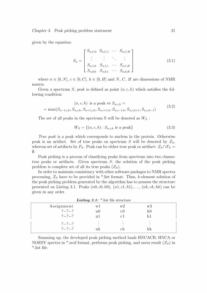
Depending on the type of the experiment, a few different coordinate systemsare used (Figure 3.1). The most popular are: N − C − H, C − H1 − H2 andN −H1 −H2. The first one corresponds to HNCA and HNCACB experiments,whereas the other ones to NOESY.

Figure 3.1: Coordinate systems in HNCACB, HNCA and NOESY experiments

In further part of the thesis, the spectrum tensor is denoted as S, and itselement (n, c, h) as Sn,c,h.

When NMR spectrum is analyzed, the researcher divides three-dimensionalspectrum into layers and then analyzes them independently. Although this pro-cess is not vital, the proposed method of automated peak picking is taking ad-vantage from this approach. Thus, the layer Sn of a spectrum S is a 2D matrix

20

Chapter 3. Peak picking problem statement 21

given by the equation:

Sn =

Sn,C,0 Sn,C,1 · · · Sn,C,H...

.... . .

...

Sn,1,0 Sn,1,1 · · · Sn,1,HSn,0,0 Sn,0,1 · · · Sn,0,H

(3.1)

where n ∈ [0, N ], c ∈ [0, C], h ∈ [0, H] and N , C, H are dimensions of NMRmatrix.

Given a spectrum S, peak is defined as point (n, c, h) which satisfies the fol-lowing condition:

(n, c, h) is a peak⇔ Sn,c,h =

= max(Sn−1,c,h, Sn,c,h, Sn+1,c,h, Sn,c+1,h, Sn,c−1,h, Sn,c,h+1, Sn,c,h−1)(3.2)

The set of all peaks in the spectrum S will be denoted as WS :

WS = {(n, c, h) : Sn,c,h is a peak} (3.3)

True peak is a peak which corresponds to nucleus in the protein. Otherwisepeak is an artifact. Set of true peaks on spectrum S will be denoted by ZS,whereas set of artifacts by FS. Peak can be either true peak or artifact: ZS∩FS =∅.

Peak picking is a process of classifying peaks from spectrum into two classes:true peaks or artifacts. Given spectrum S, the solution of the peak pickingproblem is complete set of all its true peaks (ZS).

In order to maintain consistency with other software packages to NMR spectraprocessing, ZS have to be provided in *.list format. Thus, k-element solution ofthe peak picking problem generated by the algorithm has to possess the structurepresented on Listing 3.1. Peaks (n0, c0, h0), (n1, c1, h1),. . . , (nk, ck, hk) can begiven in any order.

Listing 3.1: *.list file structure

Assignment w1 w2 w3?−?−? n0 c0 h0?−?−? n1 c1 h1

?−?−?...

......

?−?−? nk ck hk

Summing up, the developed peak picking method loads HNCACB, HNCA orNOESY spectra in *.ucsf format, performs peak picking, and saves result (ZS) in*.list file.

Chapter 4

Proposed method

4.1 A general concept

To deal with the automation of the peak picking, two-stage spectra processingmethod is proposed. Its organization is illustrated in Figure 4.1. During thefirst stage, preprocessing and object detection are performed. It allows to findimportant objects in NMR spectrum and estimate how it is probable that theyare true peaks.

Figure 4.1: Organization of proposed peak picking method

22

Chapter 4. Proposed method 23

The second stage of processing is based on inference process which is im-plemented using Bayesian network. In case of triple-resonance spectra (HNCA,HNCACB) there are many logical dependencies among peaks which are used inlaboratory practice to conduct reliable peak picking. That is why implementa-tion of such rules in inference engine might reduce number of false-positives andfalse-negatives in classification results.

Technically, during the first stage of processing, NMR spectrum in Sparkyformat (*.ucsf) is loaded and normalized. Each spectrum has intensity normallydistributed however, σ and µ are almost unique for each NMR experiment. Be-cause of huge discrepancy in these parameter values it is difficult to analyze a rawspectrum. This is why we decided to transform spectra intensities distributionsto N (0, 1).

This approach allows the classifier to generalize more accurately on bigger datasets. What is worth mentioning, the values of σS and µS are calculated globallyfor the entire spectrum. We also tried to normalize each layer independently whatis typical for computer vision image analysis, however the results of this approachwere not promising.

After normalization a weak Gaussian blur is applied. This approach has bothadvantages and disadvantages. The positive aspect of Gaussian blur applica-tion is that it decreases noise and smoothens peaks what increase performanceof computer vision approach. On the other hand, intensive Gaussian blur ham-pers detection of overlapped peaks. After concerning mentioned arguments, wedecided to apply very weak Gaussian blur σ=0.5 which slightly increases theclassification accuracy.

Having a preprocessed spectrum, the method analyzes it layer-by-layer. Eachlayer is loaded individually and object detection is performed on it. At first, alllocal extrema are identified. Usually, a single layer of NMR spectrum containsa several thousands of extrema. Approximately 99% of them represent noise.Careful analysis of all extrema is pointless due to the computational complexity.

To address the problem mentioned above we used a heuristic which quicklyestimates peak volume [32]. Basing on peak volumes, a ranking is created. Top500 peaks from each layer are taken for further analysis. It is worth mentioning,that this number of peaks is significantly higher than the number of true peakswhich is usually less than 50 per layer.

Top 500 peaks selected in the previous step are scanned using a scanningwindow in the scale space. The image inside the scanning window is stored intwo independent copies. One of them is made symmetrical in order to removeinformation about peak neighborhood and emphasize peaks shape. Problem ofoverlapping peaks is partially solved here. The second copy represents the originalspectrum image - peak and its closest surrounding. In order to obtain a featurerepresentation of mentioned two copies of spectrum fragment, for both of themthe Histogram of Oriented Gradients (HOG) is calculated [11, 35]. The resultingfeature vector consists of about 200 elements.


Each scanning window is evaluated by the Support Vector Machine (SVM)classifier which has been trained using 2700 manually selected examples. Becauseit is impossible to judge, whether a peak is an artifact basing just on its appear-ance, the result of classification is a real number instead of identifier of the class.The classifier response is proportional to the distance between classified exampleand separating hyperplane which usually varies from −3 for huge true peaks to+3 for smallest artifacts.

The classification results (500 peaks classifications × number of layers) arestored in 3D sparse tensor M which has the same size as NMR spectrum S (NMRspectrum is 3D tensor of intensities). The Mn,c,h element of the tensor representsSVM response for a peak, which possesses extremum in the point (n, c, h).

The tensor M is used in the second stage of processing to conduct the inferenceprocess of triple-resonance spectra. We decided to use Bayesian network in thatcontext because it is the simplest framework enabling implementation of all ruleswhich are used by NMR researcher to conduct peak picking (e.g. connectivity ruleor four peaks in line rule). The Bayesian network scans entire sparse tensor Mtaking advantage of non-local information which cannot be used by the classifier.The architecture of Bayesian network is presented in Figure 4.7. It is composedof 8 variables which represent: type of the experiment, peak sequence in column,peak position constraints, peak sign, peak position, peak appearance, and finallythe true peak. All factors in the Bayesian network were estimated in a way whichmaximize Bayesian network performance on the validation set which is composedof 400 manually labeled peaks. The output of the Bayesian network constitutethe solution of the peak picking problem. In order to use it in other NMR softwarepackages the postprocessing must be performed.

Since an NMR spectrum is the tensor with intensities in the discrete coordinatesystem, it is necessary to perform interpolation of results in the postprocessingphase. To address this problem, method implemented in Sparky was used [15].Given a solution in point Sn,c,h, a seven points are used in the interpolationprocess: Sn,c,h−1, Sn,c,h+1, Sn,c−1,h, Sn,c+1,h, Sn−1,c,h, Sn+1,c,h, and Sn,c,h. Theyrepresent the close neighborhood of the solution at each axis: N,C and H. Theinterpolation is made by fitting a second order polynomial into three points alongeach axis (e.g. Sn,c,h−1, Sn,c,h, Sn,c,h+1). The final solution is the maximum pointon each fitted curve, i.e. on each axis. The final output is converted from id toppm units and saved in the form of *.list file (Sparky format).

4.2 Peak detection

4.2.1 Preprocessing method

NMR spectra are characterized by huge variations of intensities, resolution, signal-to-noise ratio and other properties. Due to mentioned reasons, it is troublesome


for computational method to analyze spectroscopic data without preprocessing.In preprocessing stage, NMR spectra are normalized toN (0, 1). Usually, these

types of data adopt Gaussian distribution (Figure 4.2), so changing mean valueto zero and sigma to one, simplifies the process of analyzing different spectrawithout disturbing data distribution significantly.

According to the results, our method achieves the best performance when eachlayer is normalized using the following formula:

S∗n =Sn,c,h − µS

σS(4.1)

where (µS) and (σS) are mean and standard deviation calculated for entirespectrum.

This approach outperforms the method in which mean and standard deviationare calculated for currently analyzed picture what is more typical for computervision:

S∗n =Sn,c,h − µSn

σSn

(4.2)

The normalization method formulated in the equation (4.1) has one mainadvantage - it does not disturb balance of a picture which contains artifacts only.In the same case, a layer-based normalization - equation (4.2) fails, and thus itresults in significant amount of false positives in the final solution.

The second stage of preprocessing uses Gaussian blur (σ = 0.5). It improvesclassifier performance by slight reduction of noise and imperfections in the NMRspectrum such as those presented in Figure 4.3. Additionally, it makes the prob-lem of overlapping peaks more difficult to solve.

Figure 4.2: Distribution of peak intensities in not normalized NMR spectrum layer


Figure 4.3: Imperfections of NMR spectrum which can be reduced by Gaussian blur.Appliaction of the filter makes peak more smooth what reduces number of unnecessaryextrema.

4.2.2 Features

Histogram of Oriented Gradients

Due to plenty of available approaches to feature extration in computer vision[41, 18, 51, 33], literature reviews [31], available evaluations and comparisons[8, 40, 39], we decided to focus on one promising approach to address the peakpicking problem. The main attention is paid to Histogram of Oriented Gradients(HOG) [11]. It was primarily proposed by Dalal and Triggs for human detectionproblem. Since then the HOG has been widely applied to many computer visionproblems [50, 52, 30].

Histogram of Oriented Gradients was chosen to address the problem of peakpicking because of the following reasons:

1. It is a robust shape descriptor what is beneficial feature in peak detectionproblem since true peaks are selected mainly based on their shape.


2. HOG can robustly represent objects which are partially occluded what mayfind application in overlapping peak detection

3. HOG was tested on the two data sets: MIT pedestrian database [44] andINRIA [21]. According to the results, HOG method outperformed waveletsand SIFT [33]. As it was previously mentioned in Chapter 1.3, waveletswere tested in the context of peak picking and resulted in reasonable out-put. Thus presumably HOG method might be successfully applied to peakrecognition in the NMR spectra.

In the HOG method an image is normalized and centered gradients are cal-culated for each pixel using the masks: [−1 0 1] and [−1 0 1]T . After that, givenhorizontal hx and vertical hy gradients, an orientation in each pixel at (x, y) iscalculated using formula:

φ = arctan

(hyhx

)(4.3)

In the next step, image is divided into cells which have a size 8 × 8 pixels.For each cell histogram is calculated. The histogram is composed of N binswhich correspond to certain range of pixel orientations. The ni bin representsorientation φi = 2π

Ni and its neighbourhood. During feature calculation voting is

conducted. At first weights are calculated: w1 =∣∣∣ φi−φφj−φi

∣∣∣ and w2 =∣∣∣ φj−φφj−φi

∣∣∣ where

i and j are indices of histogram bins which represent neighboring orientations ofφ. Finally, values stored in bins are increased: ni := ni + w1

√(hx + hy)2 and

nj := nj + w2

√(hx + hy)2.

After histograms for all cells are constructed the cells are grouped in blocks.One block is K × K grid of cells. Each block is normalized using one of thefew possible metrics which are presented in [11]. Finally, normalized histogramscomprise descriptors which are used in classification process.

In the proposed solution to the peak picking problem, Histogram of OrientedGradients is calculated twice, using two different images. The first one is the frag-ment of the original NMR spectrum which presents peak and its closest neigh-bourhood. The second picture presents peak after symmetrization. For eachimage HOG (11 bins, 3 × 3 cells) is calculated what gives 198 element featurevector in total (99 per image).

Peak symetrization reduces information about peak neighbourhood what al-lows HOG to describe shape of the peak only. Symmetrized image can be com-putated using following formula:

da,b =

{max(0,min(da,b, d−a,−b)) if d0,0 > 0

min(0,max(da,b, d−a,−b)) if d0,0 ≤ 0(4.4)

where d0,0 is equal to Sn,c,h for the peak which possesses extremum in (n, c, h).


Other features

Apart from HOG features extraction, 13 other features were tested (Table 4.1).

Feature DescriptionNormalizedpeak area

Given a peak with maximum in (n0, c0, h0), its shape is ap-proximated using Gaussian function:

g(c, h, σc, σh) = Aexp

(−(c− c0)2

2σ2x

− (h− h0)2

2σ2h

)(4.5)

by minimizing of the error function:

f(σc, σh) =∑c

∑h

(g(c0 + c, h0 + h, σc, σh)− Sn0,c0+c,h0+h)2

(4.6)where c and h belongs to the neighborhood of (n0, c0, h0).The parameters σx and σy approximate width and height ofa peak, respectively. Finally, the area G can be presented as:

G = 36πσxσy (4.7)

After the area of peaks in layer is estimated, standard devia-tion σG and mean µG are calculated. These statistics are usedto normalize feature:

G =G− µGσG

(4.8)

A layer of the HNCA spectrum which demonstrates peak areaestimation is presented in Figure 4.5.

Peaksymmetry

Given peak with extremum in (n0 c0 h0), let cL and cR bethe neighbour extrema such that cL < c0 < cR. The peaksymmetry LC on axis C is given by:

LC =|c0 − cL||cR − c0|

(4.9)

Analogously, peak symmetry along H axis can be calculatedusing formula:

LH =|h0 − hL||hR − h0|

(4.10)


Feature DescriptionPeak

intensitySn,c,h for a peak having extremum in (n, c, h)

Normalizedpeak widthand height

Width and height of the peak are approximated by 6σx and6σy.

Inaccuracy ofgaussian ap-proximation

Minimal value of function (4.6)

Normalizedvolume

Volume of a peak calculated using method described in [32]:

1. Let us define a set E = {(c, h) :(c, h) is a local extremum}

2. For each element (c, h) ∈ E calculate volume:

v =∑

a∈[−1;1]

∑b∈[−1;1]

Sn,c+a,h+b (4.11)

3. Select K elements which have the highest volume

4. Calculate intensity difference (ik, jk) between selectedelements ek and their direct neighbours:ik = Sn,ck,hk − Sn,ck−1,hk ; jk = Sn,ck,hk − Sn,ck,hk−1

5. Calculate mean value of ik and jk: m1 =∑K

k=1 ikK

and

m2 =∑K

k=1 jkK

6. Calculate parameters: Rh = max(m1,m2)m1

, Rc =max(m1,m2)

m2.

7. For each element ek, a final value of volume is calculated,using formula:

vk =∑

a∈[−Rh;Rh]

∑b∈[−Rc;Rc]

Sn,c+a,h+b (4.12)

8. Normalize distribution of vk

Estimation of peak volumes on HNCA spectrum is presentedin Figure 4.4.


Feature DescriptionWidth andheight ratio

(W)

Calculated using formula:

W =σxσy

(4.13)

Intensity towidth (Iw)and height(Ih) ratio

Given by:

Iw =Sn,c,hσx

(4.14)

Ih =Sn,c,hσy

(4.15)

Maximumand minimum

deviationfrom peak

center

Maximum and minimum deviation (Dmin, Dmax) are given by:

Dmin = mink1,k2

(Sn,c+k1,h+k2) (4.16)

Dmax = maxk1,k2

(Sn,c+k1,h+k2) (4.17)

where: k1 ∈ [−2; 2], k2 ∈ [−2; 2]

Table 4.1: Features evaluated in the context of peak detection

Figure 4.4: Estimation of peak volumes in layer of NMR spectrum. Figure presents15 peaks which have the highest volume according to equation (4.12)


Figure 4.5: Estimation of peak areas in layer of HNCACB spectrum. Red ellipsesrepresent peak area which was calculated automatically using equation (4.6)

4.2.3 Classification

The SVM classifier was trained using 2700 manually labeled examples of peakswhich had been gathered from almost 300 layers located in 3 different NMRHNCACB/HNCA spectra. The learning set was composed of 700 examples oftrue peaks and 2000 examples of artifacts.

The parameters of the classifier were calibrated on validation set which con-tains 400 examples of peaks. In total, 130 of them were true peaks and 270were artifacts. Results show that SVM achieves best performance when Gaussiankernel function is used with σ = 10 and soft margin equal to 5.

In proposed approach, on each layer the classifier classifies 500 peaks whichwere selected heuristically. The heuristic selects peaks which have highest volumecalculated using equation (4.11). This approach allows to reduce computationaltime significantly because it excludes thousands of artifacts which are character-ized by peak volume close to zero.

After top 500 peaks on each layer are classified, the results are stored in 3Dsparse tensor M . This data structure has the same resolution as NMR spectrum- N × C × H. Element Mn,c,h corresponds to SVM classifier response for peakin NMR spectrum which has extremum in (n, c, h). In case where peak (n, c, h)was not selected by heuristic the value of Mn,c,h is zero. The sparse tensor Mn,c,h

constitutes an input for high-level inference by Bayesian network.


4.3 High-level inference

The classifier is a reasonable mechanism to detect interesting objects in the NMRspectra where only local information about peak is used. However, it is trouble-some to train classifier in a way that allows to analyze relationships between ob-jects in spectrum and interfere about their meaning. Because of that, we proposeinference engine in the peak picking approach. It looks globally at classificationresults and utilizes non-local information about detected peaks.

We decided to use Bayesian network to address this problem since it is simplestframework to implement all the rules derived from experts knowledge. The rulesused by researcher to conduct peak picking are presented in Section 4.3.1.

4.3.1 Practical knowledge extraction

Systematic analysis of laboratory practices related to the peak picking (Chapter2.3) allowed to establish a set of formal rules which are useful in the context ofautomatic inference. All of them were implemented in Bayesian network and arepresented in the Tables 4.2 (HNCA spectrum), 4.3 (HNCACB), and 4.4 (NOESY).

hcolorrgb0.9,0.9,0.9

ID Name Possible values Dependentvariables (ID)

Hidden

1 Number of peaksin one column

1 or 2 9 Yes

2 Peak position All positions of Cα,n, Cα,n−1carbons defined in the Table2.10

8 No

3 Peak appearance Response of SVM classifier 8 No4 Sequence of peaks

in column+ or + + 9 Yes

5 Confirmationin HN(CO)CAspectrum

True or False

If peak is confirmed inHN(CO)CA, then it in-creases probability that itis true peak, if we find noinformation about peak onHN(CO)CA, then it doesnot affect probability in anyway.

8 No



Hidden

6 Layer context 1,2,3

True peaks are usuallybig enough to be visibleon a few neighbourhoodlayers. If peak is visiblejust on one layer, then itgives no information aboutpeak class - it could byeither artifact or true peak.On the other hand, peakvisibility on two or morelayers is a strong indicator,that peaks represent trueresonance.

8 No

7 Connectivity rule Real number

Connectivity rule canbe modeled as a maximumresponse of the classifier forthe peak which is poten-tially connected with theanalyzed one.

8 No

8 Class of the peak 0 (artifact) or 1 (true peak) None Yes9 NMR layer ap-

pearance2D matrix of intensities None No

Table 4.2: Variables and their dependencies identified in analysis of the laboratorypractice related to the peak picking process of HNCA spectrum


Hidden


2, 3 or 4 9 Yes

2 Peak position All positions of Cα,n, Cα,n−1,Cβ,n and Cβ,n−1 carbons de-fined in the table 2.10

8 No

3 Peak appearance Response of SVM classifier 8 No



Hidden

4 Sequence of peaksin column

++,−++,+−+,+−−,−−++,− + −+,+ − −+,+ +−−,−+ +− or +−+−

9 Yes

5 Confirmation onCBCA(CO)NHspectrum

True or False 8 No

6 Layer context 1,2,3 8 No7 Connectivity rule Real number 8 No8 Class of the peak 0 (artifact) or 1 (true peak) None Yes9 NMR layer ap-


Table 4.3: Variables and their dependencies identified in analysis of the laboratorypractice related to the peak picking process of HNCACB spectrum


Hidden


Any number 9 Yes

2 Peak position Any positions

Peaks are usually groupedin columns

8 No

3 Peak appearance Response returned by SVMclassifier

8 No

4 Sequence of peaksin column

Any sequence of positivepeaks:+ + . . .+

9 Yes

5 Confirmation onCBCA(CO)NHspectrum

No confirmation 8 No

6 Layer context 1,2 or 3

Weak layer context

8 No

7 Connectivity rule Not applicable 8 No8 Class of the peak 0 (artifact) or 1 (true peak) None Yes9 NMR layer ap-


Table 4.4: Variables and their dependencies identified in analysis of the laboratorypractice related to the peak picking process of NOESY spectrum


4.3.2 Bayesian network structure

In order to conduct the inference process, layer of NMR spectrum is scanned usinga vertical scanning line (Figure 4.6). In general, for each position of the scanningline the Bayesian network analyzes 8 peaks located in a line (P1, P2, . . . , P8) whichgenerate the strongest responses of SVM classifier. In practice, the inference isconducted when at least one of the peaks is classified as true peak.

Figure 4.6: Visualization of vertical scanning line used to conduct high-level inference

The architecture of Bayesian network mentioned above is presented in Figure 4.7.It is composed of the following variables:

1. E (experiment, observed) - type of the experiment e.g. HNCA or HNCACB.

2. S (peak sequence, unobserved) - sequence of peaks which appears in onevertical line in NMR spectrum. For example if two positive and one negativepeaks are located on the scanning line S = + +−.

3. A (acceptable position, unobserved) - determines if position of all peaks insequence S is acceptable according to the Table 2.10.

4. Pi (true peak, unobserved) - determines if the i-th peak (out of 8 analysedpeaks in line) is an artifact or true peak.

5. Ci (peak sign, observed) - sign of peak Pi. Peaks which have positive inten-sity are represented by Ci = 1, negative peaks by Ci = 0.

6. Xi (peak position, observed) - position of peak Pi in (C,H) coordinatesystem.


7. Ui (peak appearance, observed) - response of the SVM classifier for peakPi.

8. Oi (peak connectivity, unobserved) - determines if analyzed peak satisfiesconnectivity rule.

9. Ti (twin peak, observed) - determines if peak Pi is confirmed on spectrumCBCA(CO)NH/HN(CO)CA .

10. Mi (monotonicity, observed) - determines if peak Pi is located in local ex-tremum of three layers N − 1, N , N + 1.

Figure 4.7: Architecture of Bayesian network

Apart from variables, factors must be formally defined in order to conductinference process. One of the most important factors is φ1:

φ1(S, P1, . . . , P8, C1, . . . , C8) (4.18)

It determines, if given combination of peaks (Pi) and their signs (Ci) can berepresented by a sequence S. For example:

φ1(“ + +−−”, P1 = 1, P2 = 0, P3 = 1, P4 = 1, P5 = 1, P6 = 0, P7 = 0, P8 = 0,

C1 = 1, C2 = 1, C3 = 1, C4 = 0, C5 = 0, C6 = 1, C7 = 0, C8 = 0) = 1

(4.19)


According to the equation (4.19), we select peaks number P1, P3, P4 and P5

in scanning line. First two of them are positive: C1 = 1 and C3 = 1, whereasthird and fourth peaks are negative: C4 = 0, C5 = 0. Because of that sequenceS = “ + +−−“ is a representation of mentioned combination of peak and theirsigns, therefore value of factor is equal to 1. Sequence S = “ + + − −” can bealso represented by peaks P1, P6, P7 and P8:

φ1(“ + +−−”, P1 = 1, P2 = 0, P3 = 0, P4 = 0, P5 = 0, P6 = 1, P7 = 1, P8 = 1,

C1 = 1, C2 = 1, C3 = 1, C4 = 0, C5 = 0, C6 = 1, C7 = 0, C8 = 0) = 1

(4.20)

On the contrary, the combination:

φ1(“ + +−−”, P1 = 1, P2 = 1, P3 = 1, P4 = 1, P5 = 0, P6 = 0, P7 = 0, P8 = 0,

C1 = 1, C2 = 1, C3 = 1, C4 = 0, C5 = 0, C6 = 1, C7 = 0, C8 = 0) = 0

(4.21)

represents “ + + +−” so it cannot be represented by “ + +−−”. As a result thevalue of the factor φ1 is equal to zero.

The second factor has the following structure:

φ2(S,E) (4.22)

It represents probability that the sequence S occurs in experiment E. Possiblevalues for HNCA spectrum are “ + ” and “ + +”, since this type of spectrumpossesses one or two positive peaks in vertical line. In case of HNCACB spectrumthere are more possibilities: “++”, “−++”, “+−+”, “++−”, “++−−”, “+−−+”, “−−++”, “+−+−” and “−+−+”. NOESY spectra do not possess anypeak sequences. That is one of the reasons why Bayesian network is constructedfor HNCA/HNCACB only.

The third factor has the following structure:

φ3(A,P1, .., P8) (4.23)

It informs if combination of peaks P1, P2, . . . , P8 is possible according to the con-straints presented in the Table 2.10. Value of the factor is modelled using thefollowing equations:

φ3(A = 1, P1, .., P8) =8∏i=1

allowed(Pi) (4.24)

φ3(A = 0, P1, .., P8) = 1− φ(A = 1, P1, .., P8) (4.25)


Thus, the combination of peaks is possible if none of them breaks the constraints.Additionally, the structure of Bayesian network is modelled by two conditionalprobability distributions. The first one have the following structure:

pi(Pi|Ui, Oi,Mi) (4.26)

It models how probable it is that given peak Pi represents carbon atom in proteinsequence of given appearance (Ui), connectivity (Oi), and monotonicity Mi. Ithas the following form:

p(Pi = 1|Ui, Oi,Mi) = Mi · (ασ(Ui) + (1− α)Oi)) (4.27)

p(Pi = 0|Ui, Oi,Mi) = 1− (Pi = 1|Ui, Oi,Mi) (4.28)

where α is a parameter which has to be calibrated in empirical studies, and σ(·)- logistic sigmoid function.

The last probability distribution p2 has the following structure:

p(Oi|Ti, E) (4.29)

It informs whether a given peak satisfies connectivity rule. It is given by equation:

p(Oi = 1|Ti, E) =

{φ(Oi, Ti) if E satisfies connectivity rule

0 otherwise(4.30)

4.3.3 Inference process

In order to conduct inference process, the probability distribution conditioned onobservable variables is calculated:

p(P1, P2, . . . , P8, O1, O2, . . . , O8, A, S|“observable variables”) =

p(A|P1, . . . , P8, X1, . . . , X8)× p(S|E,P1, . . . , P8, C1, . . . , C8)×8∏i=1

p(Pi|Ui, Oi,Mi)p(Oi|Ti, E)

(4.31)

Equation (4.31) is marginalized in order to obtain probability distribution depen-dent on P1, P2, . . . , P8 only:

p(P1, . . . , PN |“observable variables”) =∑O1,O2,...,O8

∑A

∑S

p(P1, P2, . . . , P8, O1, O2, . . . , O8, A, S|“observable variables”)

(4.32)


Finally, values P1, P2, . . . , P8 are chosen using maximum a posteriori estimation:

(P ∗1 , P∗2 , . . . , P

∗N) = arg max

P1,P2,...,P8

p(P1, P2, . . . , P8|“observable variables”) (4.33)

4.3.4 Post-processing and final output

As it was previously mentioned, the NMR spectrum is a 3D tensor which containsintensities measured in discrete points (n, c, h). Naturally, positions of atoms inprotein are represented by real number. Thus interpolation of peaks coordinatesneeds to be carried out.

To address this issue an algorithm from Sparky software was implemented[15]. Let Sn,c,h be a point marked by Bayesian network as true peak. In order tomake the interpolation, six neighbouring points are analyzed:

• Sn−1,c,h, Sn,c,h, Sn+1,c,h - to interpolate on N axis

• Sn,c−1,h, Sn,c,h, Sn,c+1,h - to interpolate on C axis

• Sn,c,h−1, Sn,c,h, Sn,c,h−1 - to interpolate on H axis

Each time peak coordinates are interpolated, three points on a given axis arechosen and a second order polynomial y = ax2 + bc + c is fitted. The maximalargument of fitted curve (−b

2a) constitute the final interpolated solution to the

problem.After interpolation the final solution is converted to the *.list format which is

consistent with Sparky [15].

Chapter 5

Empirical studies

5.1 Model learning and parameters tuning

Learning curve

The aim of the first simulation was to evaluate if the number of examples in thelearning set is sufficient to train SVM classifier. In order to address this problemlearning curves were plotted for HNCACB and NOESY classifiers independently.

The first simulation was composed of 48 iterations. In each of them, theclassifier was trained using different number of samples from learning set (form20 in the first iteration, to the 2420 in the last one). Afterwards, in each iteration300-elements validation set (about 33% of positives examples) was classified andmachine learning metrics (accuracy, precision, recall, F-measure) were calculated.We have investigated how size of the learning set affects classification quality.

Figure 5.1: Learning curve of HNCACB classifier

The results of simulation are presented in Figure 5.1. They show, that the clas-

40

Chapter 5. Empirical studies 41

sifier reaches its maximal performance when is trained using 2420 examples. It isprobable that adding new samples will increase classification quality. Nonetheless,such approach was impossible due to the limitations of the available spectroscopicdata. In the Figure 5.1, there are two iterations in which precision is higher thanrecall. It is caused by adding new examples which are significantly different fromthe others. Their introduction to the learning set affected the position of separat-ing hyperplane in SVM classifier. As a result, proportions of false-positives andfalse-negatives have changed. What is worth mentioning, the F-measure remainsunaffected by this event.

The simulation with NOESY spectra was performed in the similar manner.The only difference was that other datasets were used. The last iteration had2010 samples. The validation set, as previously, had 300 examples, 33% of whichwere true peaks.

According to the results (Figure 5.2), the classifier reached maximum perfor-mance when 1910 examples were used for training purpose. Studying the shapeof learning curve may suggest that introducing any new elements to the learningset will not increase classification quality.

Figure 5.2: Learning curve of NOESY classifier

Features

During the development of proposed approach, the following features were con-sidered: (1) Histogram of Oriented Gradients on normalized spectrum, (2) His-togram of Oriented Gradients on normalized and symmetrized spectrum, (3) Peakintensity, (4) Normalized peak volume, (5) Normalized peak area, (6) Normalizedpeak width, (7) Normalized peak height, (8) Width to height ratio, (9) Inaccuracy


of Gaussian approximation, (10) Intensity to height ratio, (11) Intensity to widthratio, (12) Peak symmetry on horizontal axis, (13) Peak symmetry on verticalaxis, (14) Minimum deviation from peak center, (15) Maximum deviation frompeak center.

The quality of features mentioned above was evaluated using three differentapproaches:

1. Calculation of the correlation between feature and class.

2. Visualization of features in order to decide how they separate the data.

3. Analysis, how changes in the feature vector affect F-measure of the classifierin 5-fold cross-validation experiment on 2700-element dataset.

At first, the correlation between features no. 3-15 and class were calculatedusing data stored in the learning set. HOG was excluded from correlation analysisbecause the single numerical feature is just a part of histogram and cannot beanalyzed independently. The results of correlation analysis are presented in theTable 5.1.

Feature name Feature ID CorrelationPeak intensity 3 0.4312

Normalized peak volume 4 0.3507Normalized peak area 5 0.2230

Normalized peak width 6 0.1507Normalized peak height 7 0.2519Width to height ratio 8 -0.0670

Inaccuracy of Gaussian approximation 9 0.2274Intensity to height ratio 10 0.1348Intensity to width ratio 11 0.2102

Peak symmetry on horizontal axis 12 0.1965Peak symmetry on vertical axis 13 0.1317

Minimum deviation from peak center 14 0.0066Maximum deviation from peak center 15 0.4031

Table 5.1: Correlation between feature values and classes calculated using data storedin 2700-elements learning set

Few selected numerical features were visualized in 2D plain in order to showhow they separate examples from the learning set. The results are presented inFigures 5.3 - 5.6.

The first plane shows, how two best numerical features separate data. Peakintensity has correlation of 0.4312 whereas maximum deviation from extremumis 0.4031.


Figure 5.3: Peak intensity vs maximum deviation from extremum - separation of thelearning set

The second visualization presents how peak volume and area separate learningset:

Figure 5.4: Normalized peak volume vs normalized peak area - separation of thelearning set


The third plane presents how peak width and height separate learning set:

Figure 5.5: Normalized peak width vs normalized peak height - separation of thelearning set

The fourth plane visualizes how the learning set is separated by two featureswhich possess the worst correlation according to Table 5.1:

Figure 5.6: Width to height ratio vs minimum deviation from extremum - separationof the learning set

Comparison of Figures 5.3 and 5.6 shows clearly what are the differencesbetween good and bad features. Naturally, the features which separate learningset similarly to 5.6 are not selected to the final solution. Nonetheless, in orderto decide which features are profitable their impact on classification quality wasmeasured. In order to do so, the features were assigned into four groups:

I. Histogram of Oriented Gradients in normalized spectrum

II. Histogram of Oriented Gradients in normalized and symmetrized spectrum


III. All numerical features (3-15)

IV. Best numerical features (peak intensity and maximum deviation from ex-tremum)

We evaluated how each group of features affects the quality of classificationon validation set. The results of simulations are presented in the Table 5.2.

Simulation ID Feature groups Maximum F-measure1 I, II, III 0.901002 II, III 0.865593 I, II 0.925334 I, III 0.819415 I, IV 0.81941

Table 5.2: Impact of feature selection on classification quality

In each simulation, the quality of the feature vector was calculated in 5-foldcross-validation experiment on 2700-elements dataset. A cross-validation experi-ments were carried out for different values of SVM parameters σ and soft marginwhat allowed to exclude classifier bias from the experiment. The detailed resultsare presented in Figures 5.7-5.11. Each figure corresponds to one selection offeature groups and presents results of 72 cross-validations which were carried outfor different assignments of σ and soft margin.

Figure 5.7: Impact of the feature groups I, II and III on the classification quality(F-measure)


Figure 5.8: Impact of the feature groups II and III on the classification quality (F-measure)

Figure 5.9: Impact of the feature groups I and II on the classification quality (F-measure)

The feature vector based on HOG (Figure 5.9) achieves the best performance.In general, the numerical features are not reliable. Even the introduction of thetwo best numerical features (peak intensity and maximum deviation from ex-tremum) slightly decreases performance in comparison to the approach whereHOG was used exclusively. Presumably, such features as intensity (even normal-ized) works weakly in generalization process. The NMR spectra are very differentin appearance. The two peaks of equal intensities may have a different meaning


on two different spectra. That is why a flexible descriptor is necessary. The HOGcan cope with some shape deformations or overlapping objects. Because of thatHOG provides the best quality of classification in the performed experiments.

Figure 5.10: Impact of the feature groups I and III on the classification quality(F-measure)

Figure 5.11: Impact of the feature groups I and IV on the classification quality(F-measure)

Visualization of the learning set using PCA

After the best feature vector was identified subsequent validation was carriedout. A final feature vector (198 elements) was visualized in the 3D space using


Principal Component Analysis (PCA) (Figures 5.12 and 5.13). Such visualizationallows to observe how the examples separate the dataset.

According to the results, we may observe that peaks can be easily separatedusing radial based function. HOG descriptors provide almost perfect distributionof the data in hyperspace. Data projection proves a potential of HOG features insolving the peak picking problem.

Figure 5.12: Visualization of the learning set in 3D space using PCA - perspective I

Figure 5.13: Visualization of the learning set in 3D space using PCA - perspective II


5.2 Peak picking accuracy

In order to evaluate the quality of proposed solution using classification metrics(precision, recall, F-measure) a benchmark dataset was created. It is composedof 6 different 3D NMR spectra, which were recorded using 5 different proteinsand 6 different experiments. For each benchmark spectrum (*.ucsf) the followingfiles were generated:

1. List of true peaks in *.csv format which were found during manual analysisof consistent block of layers (between 5 and 40 subsequent layers in eachspectrum). The blocks were selected in a way which provides variety ofpeak examples. There are layers with different: amount of peaks (someof them contains no true peaks), levels of peaks overlapping, and signal tonoise ratio. Detailed information about benchmark is provided in Table 5.4.

2. Matlab object (*.mat) describing spectrum properties. It contains infor-mation about spectrum type (e.g. NOESY, HNCACB) and specifies whichfragment of the spectrum has to be excluded from the analysis. In general,a small fragment of spectrum represents water, and carries no informationabout protein structure. This fragment can be easily specified by researcherbefore either automated or manual peak picking (Figure 5.15).

Figure 5.14: Exemplary layer form benchmark dataset. For each benchmark spec-trum, fragment which should be excluded from analysis is provided. Fragment markedby black contour represent water, thus it carries no information about protein structure.

In order to evaluate performance of proposed approach to the automatic peakpicking problem, all benchmark spectra (99 layers from 6 blocks) were scanned


using our method. Results are presented in Table 5.5.

SpectrumName Type Resolution

Spectrum 1 HNCA 128N×128C×1024HSpectrum 2 HNCA 256N×128C×832HSpectrum 3 HNCA 64N×256C×512HSpectrum 4 TOCSY 128C×128C×1216HSpectrum 5 NOESY 256C×512H×608HSpectrum 6 HNCACB 256N×256C×416H

Table 5.3: Properties of benchmark dataset

BenchmarkName No. layers No. peaks No. true peaks

Spectrum 1 10 (30-40) 58463 23Spectrum 2 39 (30-69) 50383 33Spectrum 3 5 (20-25) 25458 71Spectrum 4 20 (10-30) 126096 85Spectrum 5 13 (80-93) 71271 103Spectrum 6 22 (30-52) 33700 42

Sum 99 layers 365371 357

Table 5.4: Properties of benchmark dataset

Name No. peaks Precision Recall F-measureSpectrum 1 58463 0.9200 1.0000 0.9583Spectrum 2 50383 0.9117 0.9687 0.9393Spectrum 3 25458 0.6235 0.7571 0.6838Spectrum 4 126096 0.7708 0.8809 0.8222Spectrum 5 71271 0.6178 0.9509 0.7490Spectrum 6 33700 0.9268 0.9047 0.9156

Mean - 0.7951 0.9103 0.8447

Table 5.5: Results of automatic peak picking of benchmark datasets

Considering results, the method achieves best performance with HNCA andHNCACB spectra which have huge signal to noise ratio (0.9156-0.9583 F-measure).On the contrary, results on spectrum 3 are the worst. However, this spectrummight be perceived as the most difficult in the whole benchmark. This spectrumwas recorded using a difficult membrane protein. It possesses plenty of overlap-ping peaks, significant amount of artifacts and small signal to noise ratio.


In spite of the fact that our method was not developed for TOCSY spectraanalyze, we decided to include one TOCSY spectrum in the benchmark dataset.Since this type of spectrum possesses peaks which are very similar to the peaksof HNCA/HNCACB spectra. During the manual analysis of TOCSY spectrano logical rules are used to support peak picking. Because of that, we disabledBayesian network and scan TOCSY spectrum using HNCA/HNCACB classifieronly. The results were promising. Our method achieved F-measure equal to0.8222. Qualitative analysis of classified layers revealed that quality of classifi-cation is sufficient to use TOCSY spectra in protein modelling. Hence, we haveproven that our method possess capabilities for generalization.

It is worth discussing why F-measure=0.8222 is sufficient. First of all, peakpicking is ambiguous. If we give two copies of the same spectrum to two ex-perienced researcher and ask them to conduct peak picking independently eachof them may provide different list of selected true peaks. Naturally, their listsof peaks may be identical in over 95%, but still not the same. Sometimes it isdifficult even for experienced researcher to judge if a given peak is true peak orartifact.

Figure 5.15: Visualization of automated peak picking of layer 34 in spectrum 1. Inthe picture red dots represent distribution of peaks and the blue dots show coordinatesof true peaks selected by proposed peak picking method. Note that not every extremumin presented layer is a peak. It sometimes happens that true peaks are visible in a fewsubsequent layers, however they must be selected in one layer where conditions posedin definition of peak are satisfied (Chapter 3). In the picture provided above all peaksare selected correctly.

Secondly, it is reasonable to discuss what F-measure=0.8222, recall 0.8809and precision=0.7708 mean in practice. Approximately in every 1 000 peaks in


NMR spectrum one is a true peak. Recall about 0.9 implies that in every 10000 peaks we missed one true peak. Precision about 0.8 means that in every 10000 peaks we selected two peaks which are artifacts in reality. Summing up, wemade only three mistakes per 10 000 peaks. The statements posed above alsoexplains why we did not use accuracy to measure performance of our method.This metric reaches about 99.9% for all classification results. Mostly because truepeaks appear rarely in NMR spectrum.

Based on results obtained from scanning NOESY spectrum, our method achievedF-measure 0.7490. Analysis of recall and precision reveals that proposed computervision approach to the peak picking selected almost all true peaks (recall 0.9509).However, significant amount of artifacts were included to the final solution as well(precision 0.6178). In NOESY spectra false positives are undesirable because theyput additional constraints on distance between hydrogen atoms in the protein 3Dstructure. This accuracy of the automated peak picking was sufficient to model3D structure of upstream of N-ras, however it may fail on more complex proteins.That is why peak picking of NOESY spectra will be improved in the future.

Apart of quantitative analysis of benchmark data we evaluated results of au-tomated peak picking in qualitative manner. Each layer from benchmark wasvisualized together with its classification results. Qualitative analysis allowed usto judge what are the most frequent reasons for automated peak picking failure.The results of qualitative analysis are provided in Figures 5.16-5.19. To simplifyinterpretation, the following notation is used:

1. All peaks in the pictures are marked by small red dots. If element of aspectrum is not marked by red dot it should not be analyzed. Note thateach visualization shows one layer of 3D image. Often true peaks are bigenough to be visible in few consecutive layers. Nonetheless, they possessexactly one extremum at one specific layer and have to be selected just once(not at all subsequent layers). If element of NMR spectrum looks like truepeak and it is not marked by red point it means that this particular peakhave to be analyzed in neighbouring layer.

2. All peaks selected by the proposed method are marked by blue dots


Figure 5.16: Visualization of automated peak picking of layer 37 in spectrum 1.In the picture an artifact located on the right-hand side of the lowest true peak wasassigned to wrong class. Such type of artifacts are called truncation artifacts and appearwhen highly dynamic protein structures are investigated. Proposed method sometimesclassify this type of artifacts as true peak what is a source of false positives.

Figure 5.17: Visualization of automated peak picking of layer 21 in spectrum 3. Thisspectrum is probably the most difficult in the entire benchmark dataset. Here, highlyoverlay fragment is presented. This particular problem was perfectly solved by proposedpeak picking method. Note that some peaks are almost invisible - only analysis of shapeof contour lines allows to determine position of true peaks with the use of HOG shapedescriptor.


Figure 5.18: Visualization of automated peak picking of layer 25 in spectrum 4.Selection of all true peaks, blue dots, results in perfect analysis of this layer. Furtherinvestigations of TOCSY peak picking results reveal that classification errors comemostly from peaks ambiguity.

Figure 5.19: Visualization of the automated peak picking of layer 83 in spectrum 5.In this layer only one column of true peaks has to be selected (blue dots). In generalproposed method selects too many peaks in the other layers of NOESY spectrum.


5.3 Generating 3D protein structure

In order to provide evaluation of proposed approach to the peak picking problem,upstream of N-Ras (UNR) protein was analysed.

At first, six NMR experiments (1×HNCA, 3×NOESY, 2×TCOSY) were mea-sured. Measured NMR spectra differ in resolution and recording frequencies.Information about their features is provided in Table 5.6.

ID Type of experiment Recording frequency Spectrum resolution Solvent1 HNCA 600 MHz 128N×128C×1024H H2O2 NOESY 700 MHz 128C×512H×336H D2O3 NOESY 900 MHz 256C×512H×600H H2O4 NOESY 900 MHz 128N×256H×240H H2O5 TOCSY 600 MHz 128C×128C×1216H D2O6 TOCSY 600 MHz 128C×160H×1216H D2O

Table 5.6: NMR spectra used to model UNR protein structure

Each spectrum was analyzed automatically using proposed approach to thepeak picking, what takes approximately 1.5 hour per spectrum. As an output,the method returned list of true peaks in each spectrum (Table 5.7).

Spectrum ID 1 2 3 4 5 6 SumNumber of peaks 273 615 2485 1533 1855 1348 8109

Table 5.7: Number of peaks found in automated peak picking of UNR spectra

Output of automated analysis was loaded into FLYA software for 3D structurecalculation [34]. Generated model was compared with reference structure (no.1WFQ) from Protein Data Bank [46]. The result of comparison is presented inFigure 5.20.

Further analysis of protein models presented in Figure 5.20 revealed that con-tent and range of the secondary structure elements, here β-sheets, in these struc-tures are the same. Flexible loops, N and C termini of both structures are poorlydefined due to lack of Nuclear Overhauser Effect (NOE) restraints and thereforethey adopt multiple conformations. Although structural model generated withFLYA did not undergo refinement e.g. simulated annealing it is virtually identicalthe structure determined in the traditional manner.


Figure 5.20: Overlay of structures of UNR protein determined in fully automatedmode with program FLYA (blue) and UNR structure obtained from the Protein DataBank, www.pdb.org (ID number: 1WFQ, red).

Chapter 6

Conclusion and final remarks

Overall results obtained during the research project are rewarding. We managedto achieve all aims of the thesis, which were:

• To propose a new approach to the automated peak picking problem. Es-pecially, we concentrated on the following NMR spectra: NOESY, HNCAand HNCACB.

• To evaluate the accuracy of the proposed method in the empirical studiesusing standard classification metrics and to prove effectiveness by solvingautomatically three-dimensional structure of upstream of N-Ras protein.

• To deliver an implementation of the proposed peak picking method in theform of standalone software.

According to the first aim of the thesis, proposed approach to the peak pickingproblem was thoroughly described in Chapter 4. We used computer vision andmachine learning techniques to utilize local information about peaks: appearanceand closest neighbourhood. The output of this local analysis was used as aninput for Bayesian network which conducts high-level inference taking advantageof global information e.g. peak positions and rules which are used by NMR expertto conduct peak picking. Surprisingly, in spite of over 20 years of investigationsin this field, computer vision approach has not been ever evaluated. Therefore, aproposed approach is unprecedented in the area of automated 3D NMR spectraanalysis.

According to the second aim of the thesis, the benchmark dataset was devel-oped in order to conduct reliable evaluation of proposed method. It was estab-lished in cooperation with NMR expert. Currently no benchmark data for thepeak picking is publicly available what is a significant gap in comparison to othercomputer science problems such as human detection which has huge and reliabledatasets available in the Internet [44, 21]. Therefore development of benchmarkdataset (365371 peaks, 6 spectra) may be perceived as another contribution ofthis research project.

Proposed method of the peak picking guarantees F-measure between 0.9583on high quality spectra to 0.7490 on spectra of poor quality. This results come

57

Chapter 6. Conclusion and final remarks 58

from analysis which was conducted using mentioned benchmark data. In liter-ature, many methods were proposed which possess accuracy between 85% and90%. Nonetheless, this numerical evaluation is difficult to assess because of hugediscrepancy in NMR spectra appearance. Results of NMR experiments havedifferent resolutions, sizes, signal-to-noise ratios, number of artifacts, types of ar-tifact and many other. In order to provide more reliable measure of peak pickingquality a case study of the protein Upstream of N-Ras (UNR) was conducted.According to results presented in Chapter 5.3, the difference between proteinmodels created manually and automatically was negligible. It means, that giventwo models of the same protein, it is impossible to judge which was modeledmanually and which using automated approach proposed in this thesis. Theseresults prove that our method has practical applications in NMR laboratories.

According to the third aim of the thesis, proposed solution to the peak pickingproblem was implemented in the form of standalone software working in Matlabruntime environment. Implementation was published as an Open Source Project.Description of the most important functionalities of a system is available in Ap-pendix A. Among the others, software allows to load NMR spectrum from themost popular format (*.ucsf), scan it and save the results of peak picking to*.list file (Sparky format) which is widely used by structure calculation software.Because of that, out implementation might be easily used in practice, withoutchanging software packages.

As it was mentioned above, all three aims of the thesis were achieved and re-sults are promising. Nonetheless, it is worth mentioning, that proposed solutionhas some shortcomings. Our computer vision approach was tested on 6 spectra,which were obtained during the studies of 5 different proteins. Moreover, spectrawere generated using 3 different frequencies: 600, 700 and 900 MHz. Althoughspectra, which were used in testing process were different in appearance, we sup-pose that proposed method may have a problems with generalization, if we scanthe spectrum which is significantly different from examples in the learning set.We leave this problem for further investigations.

In the future, the proposed method of peak picking can be extended by addi-tion of new NMR experiments which should be analyzed. Moreover, the methodwill be extended in a way which allows to analyze wider range of macromolecules.Currently, only proteins are investigated. In the future we would like to auto-matically analyze spectra of nucleic acids and carbohydrates as well. Finally,the computer science method will be updated. Currently the proposed solutionbehaves like a human being. It divides spectrum into layers, visualize them,evaluate using computer vision and conduct the reasoning using the Bayesiannetwork. We suspect that this approach can be improved. The human being hasinability to analyze highly-dimensional data. How to visualize 4D or 5D spacewhich contains 4GB of float numbers in a way which allows to conduct peakpicking by researcher? From the computer perspective, number of dimensionsdoes not matter. Naturally, it increases computational complexity but taking

Chapter 6. Conclusion and final remarks 59

into consideration size of spectra and algorithmic complexity of this classificationproblem, we are able to analyze the utter spectrum with good personal computerin short time (Appendix B). New method of the peak picking will scan spectrain all dimensions simultaneously without partitioning spectrum into layers.

Moreover, we are going to establish an open source testing environment forautomated peak picking purposes. It will allow other computer scientists to proto-type their solutions fast. Thus, we hope that our work will contribute to popular-ization of this important problem. As it is mentioned in Chapter 1.2 automationof the peak picking can open new avenues in structural genomics and drug design.

All things considered, the results obtained during this research project aredefinitely promising. Main contributions to science are following:

1. For the first time in history computer vision method for 3D NMR spectraanalysis was proposed and evaluated in empirical studies.

2. Benchmark data for automated peak picking purposes was developed andpublished.

3. 3D model of the protein Upstream of N-Ras was calculated in a fully auto-mated way using proposed approach to automated NMR spectra analysis.Resulting model was consistent with reference structure from protein data-bank.

4. Proposed approach to the automated peak picking of 3D NMR spectrawas implemented as a standalone software and is publically available uponrequest

In the following months developed software will be introduced in NMR labora-tory in ETH Zurich in Switzerland. We will focus on improvements and extensionsof benchmark datasets.

Appendix A

Parameter calibration

Kernel functions

One of the most important issues which affects classification results is assignmentof classifier’s parameters.

In this section three kernel functions and their parameters are evaluated: lin-ear (soft margin), polynomial (soft margin, polynomial order) and rbf (soft mar-gin, sigma). For each kernel function and parameter values, 5-fold cross-validationexperiment on 2700-elements dataset (33% of true peaks) was performed.

In the first experiment, Gaussian kernel was investigated. The results pre-sented in Figure A.1 correspond to 72 5-fold cross-validations which were per-formed for each assignment of parameters (σ from 5 to 200 and soft margin from0.1 to 200)

Figure A.1: F-measure of SVM with Gaussian kernel for different values of σ andsoft margin

In the second experiment polynomial kernel was evaluated. In Figure A.2

60

Appendix A. Parameter calibration 61

results of 120 5-fold cross-validation simulations are presented. For polynomialorder they spread from 3 to 12 and for soft margin from 0.1 to 200.

Figure A.2: F-measure of SVM with polynomial kernel function for different valuesof polynomial order and soft margin

Considering results, each kernel function performed very well for its optimalparameters. The selection of parameters is a crucial step which makes classifierperformance varied from 50% to 92%. The overall results was slightly better inthe case where Gaussian kernel were used. The result is surprising since Dalaland co-workers prove that in case of human detection the linear kernel is the bestchoice [11].

Appendix B

Performance tests

During the NMR spectrum processing, the efficiency of scanning is not of a pri-mary importance. The most attention is paid to the quality of final solution.Nowadays, the researchers need weeks or even years to process spectrum, so timeof automated scanning which is about a few hours is fully acceptable.

Nonetheless, in order to maintain completeness of the evaluation, the efficiencyof scanning was measured. In order to do that, a few NMR spectra which areof different resolutions were gathered and scanned using the proposed approach.The experiment was conducted on a personal computer with the processor AMDX8 FX-8120. In the simulations only one core of the processor was used. Finallythe average time of scanning one layer was measured using the Matlab profiler.The spectra used in this experiment together with results are presented in theTable B.1.

ID NMR type Spectrumresolution

Time of scanning thewhole spectrum on oneCPU core

Average timeof scanningone layer

1 HNCACB 256x1024x1024 8690.70 s = 144.84 min 33.948 s2 HNCACBB 256x256x416 9407.65 s = 156.9 min 36.749 s

3 HNCA 128x128x1024 3751.04 s = 62.5 min 29.305 s4 NOESY 128x512x336 3370.02 s = 56.2 min 26.328 s5 NOESY 256x512x608 7015.29 s = 116.9 min 27.403 s

Table B.1: Average time needed to scan NMR spectrum using proposed approach tothe peak picking

Based on results, it is possible to observe that scanning time is not dependedon layer resolution. It comes from the fact, that always only 500 best peaks arescanned in each layer.

In case of HNCACB experiments the scanning time was between 29 and 34seconds per layer. It is a few seconds more in comparison to NOESY spectra.The difference comes from the fact, that NOESY spectra have no logical rulesimplemented in the Bayesian network framework.

62

Appendix B. Performance tests 63

All in all, the time of scanning NMR spectrum which is about 30 seconds perlayer is short in comparison to the time of manual peak picking which might beabout hours or days.

Appendix C

Description of software interface

Proposed method of the peak picking together with testing environment wasimplemented using the MatLab. Developed software possesses functionalitieswhich support implementation and evaluation of new peak picking approaches.Among the others, the software:

1. Possesses modules which solve most popular technical problems related tocomputational 3D NMR spectra processing

(a) Loads NMR spectra from *.ucsf files

(b) Saves pick picking results to Sparky *.list file

(c) Visualizes 3D NMR spectra

2. Supports development of other machine learning solutions in the context ofpeak picking problem

(a) Supports gathering the examples to the learning set from NMR spec-trum

(b) Extracts features in the scale space

(c) Trains classifier and analyze its performance using different parameterconfigurations

(d) Draws learning curve and run many others machine learning simula-tions

(e) Allows to modify NMR spectrum using custom preprocessing method

3. Supports implementation of Bayesian networks as an inference method

All modules was implemented using Matlab in convenient way which allows forextensions and replacement. In order to develop a new approach to the peak pick-ing problem, it is necessary to update some modules only, without implementingthe whole solution from scratch. Such approach allows to develop a prototype ofa peak picking method relatively fast. Moreover, usage of developed environmentguarantee compatibility with other NMR software packages - like Sparky. The

64

Appendix C. Description of software interface 65

potential contributor is not occupied with strictly technical issues - like NMRspectrum loading, classifier training, generating Sparky file, building learning setetc. That is why this environment can be used in the future for development newapproaches to the peak picking faster, than it is possible nowadays.

Figure C.1: User interface of developed software. Image presents visualization of thelayer from NOESY spectrum. Most of the figures in this thesis was generated usingthis program.

Because of graphical user interface C.1, usage of developed environment isstraightforward. Nevertheless, a few most important features are presented inthis appendix. The file menu has the following functions:

1. Open Main Spectra - loads new spectrum from *.ucsf (Sparky file formatfor NMR)

2. Next layer - visualizes layer of loaded NMR spectrum in the form of thecontour plot

3. Save figure as. . . - saves current contour plot as graphical file

4. Exit - closes the program

In the properties menu:

1. Specify neglected region - allows to exclude part of the spectrum fromanalyze


2. Set scanning window size - specifies minimal size of the scanning window.Has huge impact on the results of scanning. This function is particularlyimportant for the software users. It allows to adjust a scanning algorithmto a particular spectrum.

The “View”, “Filers”, “Actions” and “Peaks” menus contain many options whichare responsible for visualization, filtering spectrum and feature extraction. Prob-ably the most important feature is “View-¿Collect samples to the learning set”,which simplify the process of creating benchmarks and learning sets. In the “Ma-chine Learning” menu:

1. Create learning set - builds learning set based on *.dat file which de-scribes peak coordinates and spectra files.

2. Load learning set - loads learning set to the program and train SVMclassifier based on loaded data.

3. Scan current layer - scans current layer of NMR spectrum using proposedapproach.

4. Analyze SVM parameters - runs the simulation which trains SVM clas-sifier using different assignments of parameters (e.g. soft margin) and clas-sify validation set. The results of the simulation are provided in visual formwhich allow user to decide which SVM parameter is optimal.

5. Learning curve - draws a learning curve using default learning and vali-dation sets provided by user

6. Scale space histograms - a simulation which allows to distinguish whichscale space is the best for given SVM classifier and NMR spectrum

7. Cross validation - runs a cross validation experiment on a learning set

The latter menus are following:

1. Dimensionality reduction - allows to visualize learning set using a di-mensionality reduction methods - like PCA

2. Bayesian network - runs a simulation which evaluates precision, accuracy,recall and F-measure of Bayesian network

3. Test - presents textual report about NMR objects stored in the memory

The environment presented above allows user to take advantage of the peakpicking method proposed in the thesis. Nonetheless, by changing content ofmodules, we can modify the method, or develop a completely new one. Themost important changes to the program might be introduced by modifying thefollowing files:


1. getFeatureVector.m - calculates a feature vector for a given scale andpeak coordinates in NMR spectrum. Modification allows to test new localfeature descriptors.

2. postProcessingBayesian.m - allows for modifications of the inferenceprocess and postprocessing

3. preprocessingX.m - allows to change preprocessing method

4. trainClassifier.m - allows to change issues related to training classifier.

References

[1] Alipanahi B., Gao X., Karakoc E., Donaldson L., and Li M., PICKY: anovel SVD-based NMR spectra peak picking method. Bioinformatics, vol. 25,pp. 268275, 2009.

[2] Antz C., Neidig K.P., and Kalbitzer H.R., A general Bayesian method foran automated signal class recognition in 2D NMR spectra combined with amultivariate discriminant analysis. Journal of biomolecular NMR, vol. 5, pp.287296, 1995.

[3] Bartels C., Gntert P., Billeter M., and Wthrich K., GARANT-a generalalgorithm for resonance assignment of multidimensional nuclear magneticresonance spectra. Journal of Computational Chemistry, vol. 18, pp. 139149,1997.

[4] Bishop C. M., Pattern Recognition and Machine Learning. Springer, 2006.

[5] Brown J. W., Huestis W. H., Quantification of two-dimensional NOE spectravia a combined linear and nonlinear least-squares fit. Journal of BiomolecularNMR, vol. 4, pp. 645652, 1994.

[6] Bujnicki J. M., Practical Bioinformatics. Springer, 2007.

[7] Carrara E.A., Pagliari F., Nicolini C., Neural Networks for the Peak-Picking of Nuclear Magnetic Resonance Spectra. Neural Networks, vol. 6,pp. 10231032, 1993.

[8] Chandrasekhar V., Chen D. M., Lin A., Takacs G., Tsai S. S., Cheung N.,Reznik Y., Grzeszczuk R., Girod B., Comparison of Local Feature Descrip-tors for Mobile Visual Search. 17th IEEE International Conference on ImageProcessing (ICIP), 2010

[9] Cieslar C., Clore G.M., Gronenborn A.M., Computer aided sequential as-signment of protein 1H-NMR spectra. Journal of Magnetic Resonance, vol.80, 1988.

[10] Corne S.A., Johnson A.P., and Fisher J., An artificial neural network forclassifying cross peaks in two-dimensional NMR spectra. Journal of MagneticResonance vol. 100, issue 2, pp. 256266, 1969.

68

References 69

[11] Dalal N., Triggs B., Histograms of oriented gradients for human detection.IEEE Computer Society Conference on Computer Vision and Pattern Recog-nition, 2005

[12] Dancea F., Gnther U., Automated Protein NMR Structure DeterminationUsing Wavelet De-noised NOESY Spectra. Journal of Biomolecular NMR,vol. 33, pp. 139152, 2005.

[13] Garrett D.S., Powers R., Gronenborn A.M., and Clore M. G., A commonsense approach to peak picking in two-, three-, and four-dimensional spectrausing automatic computer analysis of contour diagrams. Journal of MagneticResonance vol. 95, pp. 214220, 1991.

[14] Glaser S., and Kalbitzer H., Automated recognition and assessment of crosspeaks in two-dimensional NMR spectra of macromolecules. Journal of Mag-netic Resonance, vol. 74, pp. 450463, 1987.

[15] Goddard T. D., Kneller D. G., SPARKY 3, University of California, SanFrancisco

[16] Gntert P., Automated NMR structure calculation with CYANA. Methods inMolecular Biology, vol. 278, pp. 353378, 2004.

[17] Gntert P., Automated structure determination from NMR spectra. Europeanbiophysics journal: EBJ, vol. 38, pp. 129143, 2009.

[18] Harris C., Stephens M., A combined corner and edge detector. Alvey VisionConference, 1988.

[19] Herrmann T., Gntert P., and Wthrich K., Protein NMR structure determina-tion with automated NOE-identification in the NOESY spectra using the newsoftware ATNOS. J. Biomol. NMR, vol. 24, issue 3, pp. 171189, November2002.

[20] Human Genome Project, http://www.ornl.gov/sci/techresources/HumanGenome/home.shtml, accessed 06 May 2013

[21] INRIA Person Dataset, http://pascal.inrialpes.fr/data/human/, accessed 06May 2013

[22] Jeannerat D., and Bodenhausen G., Separation of overlapping multipletsand contraction of substructures within multiplets using symmetry proper-ties. Journal of Magnetic Resonance, vol. 119, issue 1, pp. 139-144, 1996.

[23] Johnson B.A., Using NMRView to Visualize and Analyze the NMR Spectraof Macromolecules. In Protein NMR Techniques. Humana Press, New Jersey.

References 70

[24] Jung Y.-S., and Zweckstetter M., Mars - robust automatic backbone assign-ment of proteins. Journal of Biomolecular NMR vol. 30, issue 1, pp. 11-23,2004.

[25] Kleywegt G. J., Boelens R., Kaptein R., A versatile approach toward thepartially automatic recognition of cross peaks in 2D 1H NMR spectra. Journalof Magnetic Resonance, vol. 94, 1991.

[26] Koradi R., Billeter M., Engeli M., Guntert P., and Wuthrich K., AutomatedPeak Picking and Peak Integration in Macromolecular NMR Spectra UsingAUTOPSY. Journal of Magnetic Resonance, vol. 135, pp.288-297, 1998.

[27] Korzhneva D.M., Ibraghimov I.V., Billeter M., and Orekhov V.Y., MUNIN:application of three-way decomposition to the analysis of heteronuclear NMRrelaxation data. Journal of biomolecular NMR vol. 21, issue 3, pp. 263268,2001.

[28] Krone M., Klawonn F., Lhrs T., and Ritter C., Identification of nuclearmagnetic resonance signals via gaussian mixture decomposition. Proceedingsof the 10th international conference on Advances in intelligent data analysisX, Springer-Verlag, 2011.

[29] Lange O., Determination of solution structures of proteins up to 40 kDa usingCS-Rosetta with sparse NMR data from deuterated samples. Proceedings ofthe National Academy of Sciences of the United States of America, vol. 109,2012.

[30] Lee J.E., Kim J.H., Kim S.J., Kim Y.G., Lee J.H., and Park G.T., Hu-man and Robot Localization Using Histogram of Oriented Gradients (HOG)Feature for an Active Information Display in Intelligent Space. AdvancedScience Letters, vol. 9, pp. 99106, 2012.

[31] Li J., Allinson N. M., A comprehensive review of current local features forcomputer vision, Neurocomputing, vol. 71, pp. 1771-1787, 2008.

[32] Liu Z., Abbas A., Jing B.Y., and Gao X., WaVPeak: picking NMR peaksthrough wavelet-based smoothing and volume-based filtering. Bioinformaticsvol. 28, pp. 914920, 2012.

[33] Lowe D. G., Object recognition from local scale-invariant features. The Pro-ceedings of the 7th IEEE International Conference on Computer Vision, vol.2, pp. 1150-1157, 1999.

[34] Lpez-Mndez B., and Gntert, P., Automated protein structure determinationfrom NMR spectra. Journal of the American Chemical Society vol. 128, pp.1311213122, 2006.

References 71

[35] Ludwig O. , Delgado D. , Goncalves V. , and Nunes U., Trainable Classifier-Fusion Schemes: An Application To Pedestrian Detection. 12th InternationalIEEE Conference On Intelligent Transportation Systems, vol. 1, pp 432-437,2009.

[36] Meier B. U., Bodenhausen G., and Ernst R. R., Pattern recognition intwo-dimensional NMR spectra. Journal of Magnetic Resonance, vol. 60, pp.161163, 1984.

[37] Messerschmidt D. A., X-Ray Crystallography of Biomacromolecules: A Prac-tical Guide. 2007.

[38] Marion D., Driscoll P. C., Kay L. E., Wingfield P. T., Bax A., GronenbornA. M., i Clore G. M., Overcoming the overlap problem in the assignment ofproton NMR spectra of larger proteins by use of three-dimensional heteronu-clear proton-nitrogen-15 Hartmann-Hahn-multiple quantum coherence andnuclear Overhauser-multiple quantum coherence spectroscopy: application tointerleukin 1.beta.. Biochemistry, vol. 28, issue 15, pp. 61506156, 1989.

[39] Mikolajczyk K., and Schmid C., A performance evaluation of local descrip-tors, IEEE Transactions on Pattern Analysis and Machine Intelligence. vol.27, issue 10, pp. 16151630, 2005.

[40] Miksik O., and Mikolajczyk K., Evaluation of local detectors and descriptorsfor fast feature matching. 21st International Conference on Pattern Recog-nition (ICPR), 2012.

[41] Moravec H., Towards automatic visual obstacle avoidance. Proceedings of theInternational Joint Conference on Artificial Intelligence, 1977.

[42] Neidig K. P., Saffrich R., Lorenz M., and Kalbitzer H. R., Cluster analysisand multiplet pattern recognition in two-dimensional NMR spectra. Journalof Mangeric Resonance, vol. 89, pp. 543552, 1990.

[43] Orekhov V.Y., Ibraghimov I.V., and Billeter M., MUNIN: a new approachto multi-dimensional NMR spectra interpretation. Journal of biomolecularNMR, vol. 20, pp. 4960, 2001.

[44] Pedestrian dataset, http://cbcl.mit.edu/software-datasets/PedestrianData.html, accessed 06 May 2013

[45] Practical guide to protein NMR, http://www.protein-nmr.org.uk/, accessed06 May 2013

[46] Protein Data Bank, http://www.pdb.org/pdb/explore/remediatedSequence.do?structureId=1WFQ, accessed 06 May 2013

References 72

[47] Rouh A., Louis-Joseph A., and Lallemand J.Y., Bayesian signal extractionfrom noisy FT NMR spectra. Journal of biomolecular NMR. vol. 4, pp. 505-518, 1994.

[48] Rule G. S., and Hitchens T. K., Fundamentals of Protein NMR Spectroscopy.Springer, 2006.

[49] Sze K.H., Barsukov I. L., and Roberts C. K., Quantitative evalua-tion ofcross-peak volumes in multidimensional spectra by nonlinear-least-squarescurve fitting. Journal of Magnetic Resonance, vol.113, 185195, 1995.

[50] Tang C. i Chen Q., Zenithal people counting using histogram of oriented gra-dients. 5th International Congress on Image and Signal Processing (CISP),ss. 946951, 2012.

[51] Trajkovic M. , Hedley M., Fast corner detection. Image Vis. Comput., vol.16, pp. 75-87, 1998.

[52] Yang X., Zhang C., and Tian Y., Recognizing actions using depth motionmaps-based histograms of oriented gradients. Proceedings of the 20th ACMinternational conference on Multimedia, pp. 10571060, 2012.

Nuclear magnetic resonance spectroscopy interpretation for ...

Documents

Transcript of Nuclear magnetic resonance spectroscopy interpretation for ...